Lead Sheet Generation with Deep Learning Stephanie Van Laere

Stephanie Van Laere

Lead Sheet Generation with Deep Learning

Academic year 2017-2018Faculty of Engineering and ArchitectureChair: Prof. dr. ir. Bart DhoedtDepartment of Information Technology

Master of Science in Computer Science Engineering Master's dissertation submitted in order to obtain the academic degree of

Counsellors: Ir. Cedric De Boom, Dr. ir. Tim VerbelenSupervisor: Prof. dr. ir. Bart Dhoedt

Stephanie Van Laere





Permission of use

The author gives permission to make this master dissertation available for con-sultation and to copy parts of this master dissertation for personal use. In thecase of any other use, the copyright terms have to be respected, in particular withregard to the obligation to state expressly the source when quoting results fromthis master dissertation.

Stephanie Van LaereGhent, May 2018

I

AcknowledgementsWhen I stumbled on this project, I immediately thought this would be the perfectfit for me. Being a musician and a composer myself, I saw this as the bestopportunity to combine two passions of mine: computer science and music. Atthe final stages of one of the biggest projects of my life, I am overwhelmed bygratefulness to all the people that have helped me through this project.

Firstly, I would like to thank my counselors, dr. ir. Cedric De Boom and dr.ir. Tim Verbelen, for your enormous support. Through the hours of feedbacksessions, this master dissertation wouldn’t be what it is now without you. I wouldalso like to thank my supervisor, prof. dr. ir. Bart Dhoedt, that I was able towork on this project. I truly couldn’t have imagined a better subject than thisone.

I would like to thank all my friends from BEST, who provided me great laugh-ter through moments I truly needed it. I would especially like to thank Karim,Margot and Alexander, for guidance and occasional distraction that was invalu-able to me. I would also like to thank Esti for our little thesis working momentsand our friendship throughout these past six years. Laurence, thank you for thecoffee and Skype dates and of course, our 11-year long friendship. Janneken,thank you for singing every song I ever wrote and making my love for music groweven stronger. Lars, for helping and supporting me. Finally, I would like to thankeverybody who filled in the survey and sent it to their friends. I never expected177 responses in such a short amount of time and it helped immensely.

I would like to thank my parents for introducing me to the piano and all typesof music throughout my youth. You have always supported me through thickand thin, with some advice, a great meal, a hug or a joke. My brother, for yourinnovative, creative mind and confidence. My sister, for your generous and altru-istic heart. My grandparents, whom I’ve never seen without the biggest smiles.Finally, my great-grandmother, for your inspiration. I will always remember youplaying ‘La tartine de beurre’ on the piano in our living room.

Stephanie Van Laere

II


Stephanie Van Laere

Supervisor: Prof. dr. ir. Bart DhoedtCounsellors: Ir. Cedric De Boom, Dr. ir. Tim Verbelen

Master’s dissertation submitted in order to obtain the academic degreeof Master of Science in Computer Science Engineering

Department of Information TechnologyChair: Prof. dr. ir. Bart DhoedtFaculty of Engineering and Architecture – Ghent UniversityAcademic year 2017-2018

AbstractThe Turing test of music, the idea that a computer creates music where it be-

comes indistinguishable from a human-composed music piece, has been fascinatingresearches for decades now. Most explorations on music generation has focusedon classical music, but some research has also been done regarding modern music,partially about lead sheet music. A lead sheet is a format of music representa-tion that is especially popular in jazz and pop music. The main elements aremelody notes, chords and optional lyrics. In the field of lead sheet generation,Markov models have been mostly explored, whilst a lot of the research in theclassical field incorporates Recurrent Neural Networks (RNNs). We would like touse these RNNs to generate modern-age lead sheet music by using the Wikifoniadataset. Specifically, we use a model with two components. The first componentgenerates the chord scheme, the backbone of a lead sheet, together with the du-ration of the melody notes. The second component generates the pitches on thischord scheme. We evaluated this model through a survey with 177 participants.

Keywords: music generation, recurrent neural networks, deep learning, leadsheet generation

III

Lead Sheet Generation with Deep Learning Stephanie Van Laere

Supervisor(s): Bart Dhoedt, Cedric De Boom, Tim Verbelen

Abstract— The Turing test of music, the idea that a computer

creates music where it becomes indistinguishable from a human-composed music piece, has been fascinating researches for decades now. Most explorations on music generation has focused on classical music, but some research has also been done regarding modern music, partially about lead sheet music. A lead sheet is a format of music representation that is especially popular in jazz and pop music. The main elements are melody notes, chords and optional lyrics. In the field of lead sheet generation, Markov models have been mostly explored, whilst a lot of the research in the classical field incorporates Recurrent Neural Networks (RNNs). We would like to use these RNNs to generate modern-age lead sheet music by using the Wikifonia dataset. Specifically, we use a model with two components. The first component generates the chord scheme, the backbone of a lead sheet, together with the duration of the melody notes. The second component generates the pitches on this chord scheme. We evaluated this model through a survey with 177 participants. Keywords— music generation, recurrent neural networks, deep

learning, lead sheet generation

I. INTRODUCTION What is art? That is a question that can be thoroughly

discussed for hours by any art lover. Can the name ‘art’ only be used when it is made by humans, or is it also art if a human doesn’t recognize computer generated ‘art’? We want to focus on research that makes this question so enticing: improving computer-generated music that resembles the work of humans.

Specifically, we want to focus on lead sheet generation by using Recurrent Neural Networks (RNNs). A lead sheet is a format of music representation that is especially popular in jazz and pop music. The main elements are melody notes, chords and optional lyrics. An example can be found in Figure 1.

Figure 1 A (partial) example of a lead sheet.

We divided the problem in two components. The first component generated the chords together with the rhythm or duration of the melody notes. The second component generated the pitches of the melody notes, based on the chords and the rhythm. We evaluated our model through a survey with 177 participants.

1 http://www.synthzone.com/files/Wikifonia/Wikifonia.zip 2 https://developers.google.com/protocol-buffers/docs/proto

II. RELATED WORKS Music can be represented in two ways: (i) a signal or audio

representation, which uses raw audio or waveforms, or (ii) a symbolic representation, which will note music through discrete events, such as notes, chord or rhythms. We will focus on symbolic music generation.

Researchers have been working on music generation

problems for decades now. From the works of Bharucha and Todd in 1989 using neural networks (NNs) [1] to working with more complex models such as the convolutional generative adversarial network (GAN) from Yang et al. in 2017 [2], the topic clearly still has a lot left to explore.

Research specifically for lead sheet generation has also been conducted. FlowComposer [3] is part of the FlowMachines [4] project and generates lead sheets in the style of the corpus selected by the user. The user can enter a partial lead, which is then completed by the model. If needed, the model can also generate from scratch. Some meter-constrained Markov chains represent the lead sheets. Pachet et al. have also conducted some other research within the FlowMachines project regarding lead sheets. In [5], they use the Mongeau & Sankoff similarity measure in order to generate similar melody themes to the imposed theme. This is definitely relevant in any type of music, since a lot of melody themes are repeated multiple times during pieces. Ramona, Cabral and Pachet have also created the ReChord Player, which generates musical accompaniments for any song [6]. Even though most research on modern lead sheet generation makes use of Markov models, we want to focus on using Recurrent Neural Networks (RNNs) for lead sheet generation using the Wikifonia dataset1.

III. WIKIFONIA DATA PREPROCESSING AND AUGMENTATION The pieces from the Wikifonia dataset were all in MusicXML

(MXL) format [7]. To make it easier to process, we transformed the pieces into a Protocol Buffer format2, inspired by Google's Magenta [8].

Some preprocessing steps were taken. Polyphonic notes, which means that multiple notes are played at the same time, are deleted until only the highest notes, the melody notes, remain. Anacruses, which are sequences of notes that precede the downbeat of the first measure, are omitted. Ornaments, which are decorative notes that are played rapidly in front of the central note, are also left out.

In order for the model to know which measures need to be played after which measures, repeat signs need to be eliminated. The piece needs to be fed to the model as it would be played. That's why we need to unfold the piece. Figure 2 shows this process.

In the original dataset there were 42 different rhythm types,

including more complex rhythm types that were not frequent. We removed the pieces which held these less occurring rhythm types. Of the 6394 scores, 184 were removed and only 12 rhythm types remained. Since we wanted to model lead sheets, we removed 375 scores which did not have any chords.

Figure 2 The process of unfolding for a lead sheet.

There were flats♭, sharps ♯ and double flats in the chords of the scores. We adapted all the chords’ roots and alters to only have twelve options: A, A♯, B, C, C♯, D, D♯, E, F, F♯, G and G♯. The modes of the chords were also reduced from 47 options to four: major, minor, augmented and diminished.

For data augmentation, the scores were transformed in all 12

keys. The reason why this can be beneficial to our model, is because this will give the model more data to rely on to make the decisions. It also prevents the model from learning a bias that a subset of the dataset might have towards a specific key.

IV. A NEW WAY OF LEAD SHEET GENERATION

A. Methodology When approaching the problem of how to generate lead

sheets, we wanted to first build the backbone of a lead sheet, the chord scheme, before handling the melody and the lyrics. There were two possibilities of modeling this that we have considered.

The first option is to generate a new chord scheme, just as in the training data. Once a chord scheme is generated, then we can generate the melody on this generated chord scheme. There are two difficulties that rise up when using this as a model. Firstly, many melody notes are usually played on the same chord. Therefore, if we want to generate melody notes on the generated chord scheme, we don’t really know how many melody notes we should generate per chord. Should it be a dense or fast piece, or should we only play one note on the chord? The second difficulty is to make sure that the duration of the different melody notes from the same chord sum up to the duration of the chord. If, for example, the model decides that four quarter notes should be played on a half note chord, this is a problem.

In light of these two difficulties, we have opted for option two: combining the duration of the notes with the chords. As can be seen by Figure 3, we repeat the chord for each note where it should be played, so the duration of the chord becomes the duration of the note.

To generate the chord scheme, we predict the next chord

based on the previous time_steps chords:

𝑝 𝑐ℎ𝑜𝑟𝑑( 𝑐ℎ𝑜𝑟𝑑()*, 𝑐ℎ𝑜𝑟𝑑(),, … , 𝑐ℎ𝑜𝑟𝑑().(/0_2.032)(1)

In turn, we use the entire chord scheme and time_steps previous melody notes to predict the next note:

𝑝 𝑛𝑜𝑡𝑒( 𝑛𝑜𝑡𝑒()*, 𝑛𝑜𝑡𝑒(),, … , 𝑛𝑜𝑡𝑒().(/0_2.032, 𝑐ℎ𝑜𝑟𝑑𝑠)(2)

Figure 3 The chord is repeated for each note so the duration of the chord becomes the duration of the note.

B. Data representation For the chord generation, we form two one-hot encoders that

we concatenate to form one big vector. The first one represents the chord itself. There are [A, A♯, B, C, C♯, D, D♯, E, F, F♯, G and G♯] x [Maj, Min, Dim, Aug] or 48 possibilities. The measure bar, to represent the end of a measure, can also be added, which is optional. The second one-hot encoder represents the rhythm of the chord and is of size 13. The first element represents a measure bar, which is again optional. The other 12 elements are the 12 different rhythm types. Figure 4 visually represent the chord representation.

Figure 4 Two one-hot vectors representing the chord itself and the duration of the chord concatenated in the chord generation problem.

Measure bars representations are included.

For the melody generation, the first one-hot encoded vector representing the pitch of the note is of size 131. The first 128 elements of the vector represent the (potential) pitch of the note. This pitch is determined through the MIDI standard. The 129th element is only set to one if it is a rest (or no melody note is played). The 130th element represents a measure bar, which can be included or excluded. Figure 5 clarifies.

Figure 5 Representation of the melody note, where the measure bar is included. The start token kickstarts the generation process.

C. Architecture The architecture can be found in Figure 6. In this Figure,

measure bars are included in the sizing. The first component is the chord scheme generation component. This consists of an input layer which will read the chords with their duration. This is followed by a number of LSTM layers, which is set to two in the figure. In this figure, the LSTM size is set to 512, but this

can be adapted. The fully connected (FC) layer outputs the chord predictions of the chord generation part of the model.

The chord scheme is used as an input for the bidirectional LSTM encoder in the melody generation part of the model. A bidirectional RNN uses information about both the past and the future to generate an output. When we replace the RNN cell by a LSTM cell, we get a bidirectional LSTM. By using this as an encoder, we get information about the previous, current and future chords. This information can be used together with the previous melody notes when we generate a note, so the prediction looks ahead at how the chord scheme is going to progress and look back at both the chord scheme and the melody. Again, 512 is used as a dimension for the LSTMs but this can be adapted. Multiple layers of LSTMs in both directions are possible.

Figure 6 The architecture of the model, split into a chord scheme generating component and a melody generating component.

D. Loss functions For the chord generating component, we have two loss functions, one for the chord itself and one for the duration, that we’ll add up. The model outputs the softmax for each of those elements. Afterwards, we perform cross entropy on the targets and the predictions.

(3)

where index 𝑖 represents the time step at which we are calculating the loss and index 𝑗is the jth element of the vector. The total loss is a combination of the two (𝛼 ∈ [0,1]):

(4)

The mean is taken for all time steps:

(5)

The melody generating component has one loss function.

(6)

Again, the mean is taken for all time steps:

(7)

E. Training and generation details The chord generating component is trained using an input

sequence of size time_steps and a target sequence of size time_steps. The subsequent note of each note in the input sequence is the target for that note. These sequences are selected from random scores in the training set each time and also batched together.

The melody generating component is trained by giving a set of chords of size time_steps (𝑐ℎ𝑜𝑟𝑑(, 𝑐ℎ𝑜𝑟𝑑()*, … , 𝑐ℎ𝑜𝑟𝑑().(/0_2.032, batched together) to the encoder. The forward and backward bi-directional LSTM outputs are concatenated to form a matrix of size (batch_size, time_steps, 2.LSTM_size). Then, the previous melody notes (𝑛𝑜𝑡𝑒()*, 𝑛𝑜𝑡𝑒(),, … , 𝑛𝑜𝑡𝑒().(/0_2.032)*) are added to form a matrix of size (batch_size, time_steps, 2.LSTM_size+note_size). This is used as the input for the decoder. The target sequences, also batched together, are the melody notes corresponding to the chords (𝑛𝑜𝑡𝑒(, 𝑛𝑜𝑡𝑒()*, … , 𝑛𝑜𝑡𝑒().(/0_2.032). Again, all these sequences are randomly selected from a random score in the training set.

For the generation of the chord scheme, we use an initial seed

with a chosen length to kickstart the generation. In this case, we use a seed length of time_steps. A forward pass will predict the next note and is added each time, shifting out the oldest note. We will sample the next chord and its rhythm.

The generation process of the melody generating component runs the entire selected chord scheme through the encoder first. We will take the start token and concatenate the corresponding encoder output and put this through the decoder. We sample the next note and add this to the input note sequence, after the start token. Again, we will shift out the oldest note. This continues until each chord has a corresponding melody note.

V. EXPERIMENTS AND RESULTS All files generated for this paper used the default

hyperparameter values that are shown in Table 1.

Table 1 The hyperparameter values used for the generation of pieces.

A. Measure bars We found that, during the generation, measure bars didn't

really fall in the places they were expected. Sometimes we had only one quarter note in between measure bars and sometimes 4 quarter notes filled the measure completely. Sometimes, the pitch part indicated the measure bar, sometimes the rhythm part, sometimes the chord and all in between. We can clearly see that this way of modeling the measure wasn't successful. We therefore dropped the measure bar completely during the notation of the music piece in MIDI and excluded them for the generation. Further research needs to be done on how to model measures efficiently.

B. Survey A survey was conducted in order to see how our computer-

generated pieces compare to real human-composed pieces. This was done by asking the participant a set of questions for each

Hyperparameter Default Value Time Steps 50 Size of LSTM layers 256 Number of LSTM layers 2 Inclusion measure bar No

piece in Google Form format. There were 177 participants for this particular online survey.

The pieces were exported to mp3 in MuseScore, in order to eliminate any human nuances that could hint to the real nature of the piece. To make it easier on the ears, some chords were tied together, since the output of the model repeats each chord for each note. Then, for each piece, a fragment of 30 seconds was chosen. In the survey, there were three categories of music pieces: human-composed pieces, completely computer-generated pieces and pieces where the melody was generated on an actual human-composed chord scheme. Three audio fragments were included for each.

We asked the participants about their music experience,

where they could choose between experienced musician, amateur musician or listener. For each audio fragment, there were three questions:

1. Do you recognize this audio fragment? (yes or no) 2. How do you like this audio fragment? (scale from 1 to 5) 3. Is this audio fragment made by a computer or a human?

(scale from 1 to 5)

We’ve found that in general, there was a significant correlation between the mean likeability of a piece and the mean of how much the participants thought it was made by a computer or a human. We also concluded that the computer-generated pieces were perceived at least as human as the human pieces and outperforming them even. This was significant with 𝑝 =8.10)D. The experienced or amateur musicians didn’t outperform the listeners.

C. Subjective evaluation We also evaluated the pieces ourselves, including the bad

examples. In general, we have found that the claim of Waite in [9] that the music made by RNNs lacks a sense of direction and become boring is true in our case. Even though the model produces musically coherent fragments sometimes, a lot of the time you couldn't recognize that two melodies chosen from the same piece are in fact from the same piece.

Also, even though our pieces have some good fragments, they usually have at least one portion which doesn't sound musical at all once we start generating longer pieces. This was confirmed by the examples above. This could possibly be fixed with a larger dataset, by training longer or letting an expert in music filter out these fragments.

VI. CONCLUSION AND FUTURE WORKS This paper focused on generating lead sheets, specifically

melody combined with chords, in the style of the Wikifonia dataset. The model discussed first used a number of LSTM layers and a fully connected layer to generate a chord scheme, which included the chord itself and also the rhythm of the melody note. After that, we used a Bi-LSTM encoder to gain some information about the entire chord scheme we want to generate the melody pitches on. This chord scheme information and the information about previous melody notes was used in the decoder (again a number of LSTM layers and a fully connected layer). This second part generates the melody pitches on the rhythm that was already established in the chord scheme.

The survey results are very positive. The participants couldn't really distinguish the computer-generated pieces from the human-composed pieces. Self-proclaimed expert musicians and amateur musicians didn't perform better than regular music

listeners. In general, we found a significant correlation between the mean likeability of a piece and the mean of how much the participants think it is human-composed.

Even though this result is promising, more research needs to be done to determine a sense of direction of the pieces and to eliminate the bad fragments inside pieces.

Three main areas of further research have been discussed.

The first one is adding lyrics to the lead sheets. This can be done by working on a syllable level for the training dataset and adding a third component to the melody on chord model, which generates the lyrics on the melody notes. We believe the information of the chords can be left out in this stage, since the melody guides the words, but further research needs to be done. The second part of further research is to add more structure to the lead sheets. Usually a lead sheet consists of some sort of structure, such as verse - chorus – verse - chorus - bridge - chorus. This could be established by adding for example a similarity factor to the models discussed, such as in [10]. Thirdly, ways to represent measures could still be researched further. Perhaps adding a metric to see how many notes we still need to fill up the measure could be an option.

EXAMPLES GENERATED MUSIC The files that were used in the survey can be found in

https://tinyurl.com/y8qpvu92. Good and bad examples that are taken from the same file can be found in https://tinyurl.com/y7tmnnah. The MIDI files can have strange notations sometimes,because the MIDI pitches were converted to standard music format by MuseScore.

ACKNOWLEDGEMENTS I would like to express my deepest gratitude to Cedric De

Boom and Tim Verbelen for guiding me through this project and to Bart Dhoedt for letting me work on this subject.

REFERENCES

[1] J. J. Bharucha and P. M. Todd, “Modeling the perception of tonal structure with neural nets,” Computer Music Journal, vol. 13, no. 4, pp. 44–53, 1989.

[2] L.-C. Yang, S.-Y. Chou, and Y.-H. Yang, “Midinet: A convolutional generative adversarial network for symbolic-domain music generation,” in Proceedings of the 18th International Society for Music Information Retrieval Conference (ISMIR’2017), Suzhou, China, 2017.

[3] A. Papadopoulos, P. Roy, and F. Pachet, “Assisted lead sheet composition using flowcomposer,” in International Conference on Principles and Practice of Constraint Programming, pp. 769–785, Springer, 2016.

[4] “Flowmachines project.” [Online]. Available: http://www.flow-machines.com/ [Accessed:20-May-2018].

[5] F. Pachet, A. Papadopoulos, and P. Roy, “Sampling variations of sequences for structured music generation,” in Proceedings of the 18th International Society for Music Information Retrieval Conference (ISMIR’2017), Suzhou, China, pp. 167–173, 2017.

[6] M. Ramona, G. Cabral, and F. Pachet, “Capturing a musician’s groove: Generation of realistic accompaniments from single song recordings.,” in IJCAI, pp. 4140–4142, 2015.

[7] M. Good et al., “Musicxml: An internet-friendly format for sheet music,” in XML Conference and Expo, pp. 03–04, 2001.

[8] “Google magenta: Make music and art using machine learning.” [Online]. Available: https://magenta.tensorflow.org/ [Accessed:3-Dec-2017].

[9] E. Waite, “Generating long-term structure in songs and stories,” 2016. [Online]. Available: https://magenta.tensorflow.org/2016/07/15/ lookback-rnn-attention-rnn [Accessed:25-May-2018].

[10] S. Lattner, M. Grachten, and G. Widmer, “Imposing higher-level structure in polyphonic music generation using convolutional restricted boltzmann machines and constraints,” arXiv preprint arXiv:1612.04742, 2016.

Contents

Permission of use I

Acknowledgements II

Abstract III

Extended Abstract IV

Contents VIII

Listing of figures XII

List of Tables XV

List of Abbreviations XVII

List of Symbols XIX

1 Introduction 1

2 Music Theory 42.1 Standard music notation . . . . . . . . . . . . . . . . . . . . . . . 4

2.1.1 Clef . . . . . . . . . . . . . . . . . . . . . . . . . . . . . . 52.1.2 Notes and rests . . . . . . . . . . . . . . . . . . . . . . . . 52.1.3 Key . . . . . . . . . . . . . . . . . . . . . . . . . . . . . . 82.1.4 Meter . . . . . . . . . . . . . . . . . . . . . . . . . . . . . 92.1.5 Chord . . . . . . . . . . . . . . . . . . . . . . . . . . . . . 92.1.6 Measure . . . . . . . . . . . . . . . . . . . . . . . . . . . . 10

2.2 Scales . . . . . . . . . . . . . . . . . . . . . . . . . . . . . . . . . 102.2.1 Major Scale . . . . . . . . . . . . . . . . . . . . . . . . . . 10

VIII

2.2.2 Minor Scale . . . . . . . . . . . . . . . . . . . . . . . . . . 112.3 Transposition . . . . . . . . . . . . . . . . . . . . . . . . . . . . . 112.4 Circle of Fifths . . . . . . . . . . . . . . . . . . . . . . . . . . . . 122.5 Structure of a musical piece . . . . . . . . . . . . . . . . . . . . . 12

3 Sequence Generation with Deep Learning 133.1 Deep Learning . . . . . . . . . . . . . . . . . . . . . . . . . . . . 143.2 Sequence Generating Models . . . . . . . . . . . . . . . . . . . . . 20

3.2.1 Recurrent Neural Network (RNN) . . . . . . . . . . . . . . 213.2.2 Long Short-Term Memory (LSTM) . . . . . . . . . . . . . 213.2.3 Encoder-Decoder . . . . . . . . . . . . . . . . . . . . . . . 22

4 State of the Art in Music Generation 244.1 Music Representation . . . . . . . . . . . . . . . . . . . . . . . . . 24

4.1.1 Signal or Audio Representation . . . . . . . . . . . . . . . 244.1.2 Symbolic Representations . . . . . . . . . . . . . . . . . . 25

A Musical Instrument Digital Interface (MIDI) Pro-tocol . . . . . . . . . . . . . . . . . . . . . . . . 26

B MusicXML (MXL) . . . . . . . . . . . . . . . . . 27C Piano Roll . . . . . . . . . . . . . . . . . . . . . 29D ABC Notation . . . . . . . . . . . . . . . . . . . 30E Lead Sheet . . . . . . . . . . . . . . . . . . . . . 32

4.2 Music Generation . . . . . . . . . . . . . . . . . . . . . . . . . . . 334.2.1 Preprocessing and data augmentation . . . . . . . . . . . 334.2.2 Music Generation . . . . . . . . . . . . . . . . . . . . . . . 344.2.3 Evaluation . . . . . . . . . . . . . . . . . . . . . . . . . . 41

5 Data Analysis of the Dataset Wikifonia 435.1 Internal Representation . . . . . . . . . . . . . . . . . . . . . . . 435.2 Preprocessing . . . . . . . . . . . . . . . . . . . . . . . . . . . . . 45

5.2.1 Deletion of polyphonic notes . . . . . . . . . . . . . . . . . 455.2.2 Deletion of anacruses . . . . . . . . . . . . . . . . . . . . . 465.2.3 Deletion of ornaments . . . . . . . . . . . . . . . . . . . . 465.2.4 Unfold piece . . . . . . . . . . . . . . . . . . . . . . . . . . 475.2.5 Rhythm . . . . . . . . . . . . . . . . . . . . . . . . . . . . 475.2.6 Chord . . . . . . . . . . . . . . . . . . . . . . . . . . . . . 49

A Root . . . . . . . . . . . . . . . . . . . . . . . . 49B Alter . . . . . . . . . . . . . . . . . . . . . . . . 50C Mode . . . . . . . . . . . . . . . . . . . . . . . . 51

IX

5.3 Data Augmentation . . . . . . . . . . . . . . . . . . . . . . . . . . 515.3.1 Transposition . . . . . . . . . . . . . . . . . . . . . . . . . 51

5.4 Histograms of the dataset . . . . . . . . . . . . . . . . . . . . . . 535.4.1 Chords . . . . . . . . . . . . . . . . . . . . . . . . . . . . 535.4.2 Melody Notes . . . . . . . . . . . . . . . . . . . . . . . . . 54

5.5 Split of the dataset . . . . . . . . . . . . . . . . . . . . . . . . . . 55

6 A new approach to Lead Sheet Generation 566.1 Melody generation . . . . . . . . . . . . . . . . . . . . . . . . . . 56

6.1.1 Machine Learning Details . . . . . . . . . . . . . . . . . . 586.2 Melody on Chord generation . . . . . . . . . . . . . . . . . . . . . 61

A Chords, with note duration . . . . . . . . . . . . 63B Melody pitches . . . . . . . . . . . . . . . . . . . 65

6.2.1 Machine Learning Details . . . . . . . . . . . . . . . . . . 66

7 Implementation and Results 737.1 Experiment Details . . . . . . . . . . . . . . . . . . . . . . . . . . 737.2 Melody Generation . . . . . . . . . . . . . . . . . . . . . . . . . . 74

7.2.1 Training and generation details . . . . . . . . . . . . . . . 747.2.2 Subjective comparison and Loss curves of MIDI output files 75

A Temperature . . . . . . . . . . . . . . . . . . . . 75B Comparison underfitting, early stopping and over-

fitting . . . . . . . . . . . . . . . . . . . . . . . . 76C Time Steps . . . . . . . . . . . . . . . . . . . . . 78D Inclusion of Measure bars . . . . . . . . . . . . . 81E Data augmentation . . . . . . . . . . . . . . . . 82F LSTM size . . . . . . . . . . . . . . . . . . . . . 83G Number of LSTM Layers . . . . . . . . . . . . . 84

7.2.3 Conclusion . . . . . . . . . . . . . . . . . . . . . . . . . . 847.3 Melody on Chord Generation . . . . . . . . . . . . . . . . . . . . 85

7.3.1 Training and generation details . . . . . . . . . . . . . . . 857.3.2 Subjective comparison of MIDI files . . . . . . . . . . . . . 86

A Comparison underfitting, early stopping and over-fitting . . . . . . . . . . . . . . . . . . . . . . . . 86

B Examples and intermediate conclusions . . . . . 887.3.3 Survey . . . . . . . . . . . . . . . . . . . . . . . . . . . . . 897.3.4 Conclusion . . . . . . . . . . . . . . . . . . . . . . . . . . 100

X

8 Conclusion 1018.1 Further work . . . . . . . . . . . . . . . . . . . . . . . . . . . . . 102

Appendix A Chords 104

References 106

Index 115

XI

Listing of figures

2.1 Standard musical notation: Itsy-bitsy spider. The elements are asfollowed: orange (1) is the clef, red (2) is the key (signature), blue(3) is the time signature or meter, green (4) is the notation for thechords and the purple boxes (5) are the measure bars. . . . . . . . 5

2.2 Different Clefs [11] . . . . . . . . . . . . . . . . . . . . . . . . . . 62.3 Rhythmic notation of notes. Each line splits the duration in half. 62.4 The do-re-mi syntax and ABC syntax of notes [12] . . . . . . . . 72.5 Rhythmic notation of rests. Each line splits the duration in half. . 72.6 Rhythm notes with dots . . . . . . . . . . . . . . . . . . . . . . . 72.7 Accidentals of notes. The accidentals in this picture are respec-

tively a flat, a natural, a sharp, a double sharp, a double flat . . . 82.8 Octave of C . . . . . . . . . . . . . . . . . . . . . . . . . . . . . . 82.9 Repeat signs used in a musical piece. The instructions are depicted

in the figure. . . . . . . . . . . . . . . . . . . . . . . . . . . . . . 102.10 A repeat sign with first and second ending. The instructions are

depicted in the figure. . . . . . . . . . . . . . . . . . . . . . . . . 102.11 D major scale . . . . . . . . . . . . . . . . . . . . . . . . . . . . . 112.12 D minor scale . . . . . . . . . . . . . . . . . . . . . . . . . . . . . 112.13 Transpostion of a C major piece of ‘Twinkle twinkle little star’ into

an F major piece [14] . . . . . . . . . . . . . . . . . . . . . . . . . 112.14 The Circle of Fifths [15] shows the relationship between the differ-

ent key signatures and their major and minor keys. . . . . . . . . 12

3.1 Graphical representation of a NN . . . . . . . . . . . . . . . . . . 15

3.2 Activation functions . . . . . . . . . . . . . . . . . . . . . . . . . 163.3 Example of feedforward (a) and recurrent (b) network . . . . . . . 183.4 Early stopping: stop training when the validation error reaches a

minimum. Otherwise, it is overfitting [36]. . . . . . . . . . . . . . 19

XII

3.5 Sequence generation model: input and output . . . . . . . . . . . 20

3.6 A LSTM memory block . . . . . . . . . . . . . . . . . . . . . . . 223.7 Encoder-Decoder architecture, inspired by [47] . . . . . . . . . . . 23

4.1 Visual representation of raw audio and its fourier transformed spec-trum [49] . . . . . . . . . . . . . . . . . . . . . . . . . . . . . . . 25

4.2 MIDI extract [17] . . . . . . . . . . . . . . . . . . . . . . . . . . . 274.3 MusicXML example [54] . . . . . . . . . . . . . . . . . . . . . . . 284.4 Pianola: the self-playing piano . . . . . . . . . . . . . . . . . . . . 294.5 Piano Roll representation . . . . . . . . . . . . . . . . . . . . . . 294.6 ABC notation: Speed the Plough [59] . . . . . . . . . . . . . . . . 304.7 ABC notation: four octaves . . . . . . . . . . . . . . . . . . . . . 314.8 Lead Sheet Example . . . . . . . . . . . . . . . . . . . . . . . . . 324.9 Soprano prediction, DeepBach’s neural network architecture . . . 374.10 Reinforcement learning with audience feedback [78] . . . . . . . . 39

5.1 Example of an anacrusis . . . . . . . . . . . . . . . . . . . . . . . 465.2 Example of an ornament . . . . . . . . . . . . . . . . . . . . . . . 465.3 Preprocessing step: unfolding the piece by eliminating the repeat

signs . . . . . . . . . . . . . . . . . . . . . . . . . . . . . . . . . . 475.4 Distribution of roots of chords in dataset without data augmentation 535.5 Distribution of modes of chords in dataset without data augmentation 545.6 Distribution of the melody pitches . . . . . . . . . . . . . . . . . 54

6.1 Two one hot encoders concatenated of a note representing the pitchand the rhythm in the melody generation problem. Measure barsare included in this figure. . . . . . . . . . . . . . . . . . . . . . . 57

6.2 Architecture of the first simple melody generation model with twoLSTM layers. Measure bars are included in this specific example . 59

6.3 Training procedure of the first simple melody generation model . 606.4 Generation procedure of the first simple melody generation model

with seed length equal to 4 . . . . . . . . . . . . . . . . . . . . . . 626.5 Some Old Blues - John Coltrane: the original and adapted chord

structure . . . . . . . . . . . . . . . . . . . . . . . . . . . . . . . . 646.6 Two one-hot encoder vectors representing the chord itself and the

duration of the chord concatenated in the chord generation prob-lem. Measure bars representations are included in this figure. . . . 66

XIII

6.7 Melody on chord generation: representation of a note where themeasure bar is included . . . . . . . . . . . . . . . . . . . . . . . 67

6.8 Architecture of the melody on chord generation model where mea-sure bars are included . . . . . . . . . . . . . . . . . . . . . . . . 68

6.9 Bidirection RNN [94] . . . . . . . . . . . . . . . . . . . . . . . . 696.10 Melody on chord generation: our Encoder-Decoder architecture . 70

7.1 The conversion of MIDI pitches to standard music notation byMuseScore . . . . . . . . . . . . . . . . . . . . . . . . . . . . . . . 77

7.2 Comparison Training and Validation Loss for all default values forthe melody model . . . . . . . . . . . . . . . . . . . . . . . . . . . 78

7.3 Training loss curves for different time_steps values for the melodymodel . . . . . . . . . . . . . . . . . . . . . . . . . . . . . . . . . 80

7.4 Training loss curves: inclusion of the measure bars or not for themelody model . . . . . . . . . . . . . . . . . . . . . . . . . . . . . 81

7.5 Training loss curves using data augmentation or not . . . . . . . . 827.6 Training loss curves for different LSTM size values for the melody

model . . . . . . . . . . . . . . . . . . . . . . . . . . . . . . . . . 837.7 Training loss curves: compare number of LSTM layers for the

melody model . . . . . . . . . . . . . . . . . . . . . . . . . . . . . 847.8 Comparison Training and Validation Loss for all default values . . 877.9 A step in preparing the MIDI files for the survey . . . . . . . . . 907.10 Survey responses: correlation between mean likeability and how

much the participants of the survey think it is computer generated 957.11 Survey responses: number of correct answers out of six per music

experience category . . . . . . . . . . . . . . . . . . . . . . . . . . 98

A.1 Different representations for chords . . . . . . . . . . . . . . . . . 105

XIV

List of Tables

3.1 One-hot encoding example . . . . . . . . . . . . . . . . . . . . . . 17

4.1 MIDI velocity table [52] . . . . . . . . . . . . . . . . . . . . . . . 264.2 MIDI ascii [17] . . . . . . . . . . . . . . . . . . . . . . . . . . . . 274.3 Reinforcement Learning: Miles Davis - Little Blue Frog in Musical

Acts by [80] . . . . . . . . . . . . . . . . . . . . . . . . . . . . . . 40

5.1 Original Statistics Dataset Wikifonia . . . . . . . . . . . . . . . . 445.2 Statistics Dataset Wikifonia after deletion of scores with rare rhythm

types . . . . . . . . . . . . . . . . . . . . . . . . . . . . . . . . . . 485.3 The twelve final rhythm types and their count in the dataset . . . 495.4 Statistics Dataset Wikifonia after deletion of scores with rare rhythm

types and scores with no chords . . . . . . . . . . . . . . . . . . . 505.5 Roots of chords and how much they appear in the scores without

transposition . . . . . . . . . . . . . . . . . . . . . . . . . . . . . 505.6 Alters of chords and how much they appear in the scores without

transposition . . . . . . . . . . . . . . . . . . . . . . . . . . . . . 515.7 Modes of chords, how much they appear and their replacement in

the scores without transposition . . . . . . . . . . . . . . . . . . . 52

6.1 The options for root, alter, mode and rhythm in a chord . . . . . 646.2 Chord generation: snippet of table for the index where the chord

one hot vector is one depending on the root, alter and mode of thechord . . . . . . . . . . . . . . . . . . . . . . . . . . . . . . . . . . 65

7.1 Default and possible values for parameters in the melody genera-tion model . . . . . . . . . . . . . . . . . . . . . . . . . . . . . . . 74

7.2 The longest common subsequent melody sequence for five gener-ated MIDI files using the default hyperparameter values. One timeusing only pitch, the other using both pitch and duration. . . . . 79

XV

7.3 Default and possible values for parameters in the melody genera-tion component for the melody on chord generation model . . . . 85

7.4 The pieces that were included in the survey, with their categoryand potential origin . . . . . . . . . . . . . . . . . . . . . . . . . . 92

7.5 The Longest Common Subsequent Sequence (LCSS) for (partially)generated MIDI files in the survey. One time using only pitch andone time using only chords. A full copy is expected for the ‘onlychord’ one for files 3.mid, 6.mid and 8.mid. . . . . . . . . . . . . . 93

7.6 The percentage of participants of the survey who responded thatthey recognized the audio fragment . . . . . . . . . . . . . . . . . 94

7.7 How much the participants responded they liked or disliked a piecet 967.8 The participants’ answer to the question if the fragment was computer-

generated or human-composed . . . . . . . . . . . . . . . . . . . . 977.9 Survey responses: average number of correct answers (out of six)

per music experience category . . . . . . . . . . . . . . . . . . . . 99

XVI

List of Abbreviations

AI Artificial Intelligence

BPTT Backpropagation Through Time

DL Deep Learning

DRL Deep Reinforcement Learning

DNN Deep Neural Network

FC Fully Connected (Layer)

FFNN Feed-forward Neural Network

GAN Generative Adversarial Network

GRU Gated Recurrent Unit

HMM Hidden Markov Model

LCSS Longest Common Subsequent Subsequence

LM Language Modeling

LSTM Long Short-Term Memory

MIDI Musical Instrument Digital Interface

ML Machine Learning

MXL MusicXML

XVII

NLG Natural Language Generation

NN Neural Network

RBM Restricted Boltzmann Machine

ReLU Rectified Linear Unit

RL Reinforcement Learning

RNN Recurrent Neural Network

RNN-LM Recurrent Neural Network Language Model

VAE Variational Auto-Encoder

VRASH Variational Recurrent Autoencoder Supported by History

XVIII

List of Symbols

♭ Flat

♮ Natural

♯ Sharp

5 Double sharp

♭♭ Double flat

ˇ “*32th note

ˇ “* ‰

32th note dotted

ˇ “) 16th note3

ˇ “

== One note of a triplet

ˇ “( 8th note

3

ˇ “

Two notes of a tripletlinked

ˇ “( ‰8th note dotted

ˇ “ Quarter noteˇ “‰ Quarter note dotted˘ “ Half note˘ “‰ Half note dotted¯ Whole note

XIX

“Talking about music is like dancing about archi-tecture.”

Unknown

1Introduction

What is art? That is a question that can be thoroughly discussed for hours byany art lover. Can the name ‘art’ only be used when it is made by humans, or isit also art if a human doesn’t recognize computer generated ‘art’? Any form ofart generation that tries to pass the Turing test of art puts a new nuance to thisquestion. No matter what your specific answer to the question ‘What is art?’ is,the research to mimic the human creative mind remains fascinating.

Researchers have been working on music generation problems for decades now.From the works of Bharucha and Todd in 1989 using neural networks (NNs)[1] to working with more complex models such as the convolutional generativeadversarial network (GAN) from Yang et al. in 2017 [2], the topic clearly still hasa lot left to explore.

1

A lead sheet is a format of music representation that is especially popular injazz and pop music. The main elements are melody notes, chords and optionallyrics. Research specifically for lead sheet generation has also been conducted.FlowComposer [3] is part of the FlowMachines project [4] and generates lead sheetsin the style of the corpus selected by the user. The user can enter a partial lead,which is then completed by the model. If needed, the model can also generate fromscratch. Some meter-constrained Markov chains represent the lead sheets. Pachetet al. have also conducted some other research within the FlowMachines projectregarding lead sheets. In [5], they use the Mongeau & Sankoff similarity measure inorder to generate similar melody themes to the imposed theme. This is definitelyrelevant in any type of music, since a lot of melody themes are repeated multipletimes during pieces. Ramona, Cabral en Pachat have also created the ReChordPlayer, which generates musical accompaniments for any song [6]. Even thoughmost research on modern lead sheet generation makes use of Markov models, wewant to focus on using Recurrent Neural Networks (RNNs).

There are two main forms of music representation: signal representations,which use raw audio or an audio spectrum, and symbolic representations. Anexample of the signal representation can be found in WaveNet [7], which is adeep neural network that uses raw audio in order to generate music. This masterdissertation focuses on the other form of music representation: symbolic repre-sentation. Symbolic representations will note music through discrete events, suchas notes, chord or rhythms. Specifically in this master dissertation, we will use aMusicXML (MXL) dataset called Wikifonia. This dataset mostly contains mostlymodern jazz/pop music. In this master dissertation, we want to model the leadsheets found in the Wikifonia dataset and generate similar types of music.

All types of sequence generating models have been used in the past to generatemusic: from Recurrent Neural Networks (RNNs) [8] to even Reinforcement learn-ing algorithms [9]. In this master dissertation, we will discuss two models: a simplemelody generating model and a more complex melody on chord generating model.Both will use RNNs, specifically Long Short-Term Memory networks (LSTMs).

2

The more complex model first generates a chord scheme with the rhythm or du-ration of the melody notes. This chord scheme will be used to generate the pitchof the melody notes in the second part. We will evaluate the models in threeways: (i) by comparing the training loss curves, (ii) by analyzing the pieces sub-jectively ourselves and (iii) by making a survey with 9 audio fragments. These 9fragments had three categories: human-composed pieces, pieces where the chordschemes were human-composed but the melody was generated and fully generatedcomputer pieces. This survey was filled in by 177 participants.

In Chapter 2, a short introduction on music theory is given. This will givethem a basic understanding of the musical concepts that will be used in this masterdissertation. This is quickly followed by a chapter that discusses deep learningand some sequence generating models that will be used in our model (Chapter3). Chapter 4 will discuss the state of the art in music representation and musicgeneration. The Wikifonia dataset will be completely analyzed in Chapter 5,as well as all the preprocessing and data augmentation steps that were taken.Afterwards, the models and the results will be discussed in Chapters 6 and 7respectively. We will end with a conclusion and a discussion on potential futurework in Chapter 8.

3

”Music is a moral law. It gives soul to the uni-verse, wings to the mind, flight to the imagina-tion, and charm and gaiety to life and to every-thing.”

Plato

2Music Theory

First, we will introduce the basic elements of music theory that will be usedthroughout the remainder of this master dissertation. Readers familiar with mu-sic theory can skip this chapter and move to Chapter 3. For a more elaboratediscussion on music theory, the interested reader can refer to [10].

2.1 Standard music notation

In order to look at the different elements of standard music notation, the song‘Itsy-Bitsy Spider’ is included in Figure 2.1 as an example. This standard musicnotation is composed of several elements: a clef, a key, a meter or time signa-ture, notes and rests, chords and measures. These elements will be individuallydiscussed in the following sections.

4

Figure 2.1: Standard musical notation: Itsy-bitsy spider. The elements are as followed: or-ange (1) is the clef, red (2) is the key (signature), blue (3) is the time signature or meter,green (4) is the notation for the chords and the purple boxes (5) are the measure bars.

2.1.1 Clef

The first highlighted piece of Figure 2.1 (the orange box or the box indicated witha ‘1’) is the clef of the piece. The clef is a reference in the sense that it indicateshow to read the notes. For example, in this figure, a G-clef or Treble clef is used.This means that the first note in this piece is an A. For an F-clef or Bass clef thesame note would be an E. Figure 2.2 depicts some of the possible clefs and theirrespective interpretation of notes [11].

2.1.2 Notes and rests

Notes are put on a staff, indicated by five parallel lines. Notes have two importantelements: pitch and duration or rhythm. The pitch is the frequency the note isplayed on. A note will sound higher or lower depending on its placement of thenote on the staff and the clef (see Section 2.1.1). The rhythm depends on the way

5

Figure 2.2: Different Clefs [11]

the note is drawn. Figure 2.3 shows the duration of the notes and their names,dividing the duration by two with each line.

Figure 2.3: Rhythmic notation of notes. Each line splits the duration in half.

Notes can also be represented in a textual format. Figure 2.4 shows both thedo-re-mi as the ABC syntax of the notes. Do-re-mi is usually used for singing.

Of course, notes aren’t the only important element in a musical piece. Rests

6

Figure 2.4: The do-re-mi syntax and ABC syntax of notes [12]

are also crucial. Rests are recorded when no note is being played at the moment.Figure 2.5 shows the same division as Figure 2.3 but for rests.

Dots can be added to both notes and rests to increase the duration of the noteor rest by half (see Figure 2.6).

Figure 2.5: Rhythmic notation of rests. Each line splits the duration in half.

Figure 2.6: Rhythm notes with dots

7

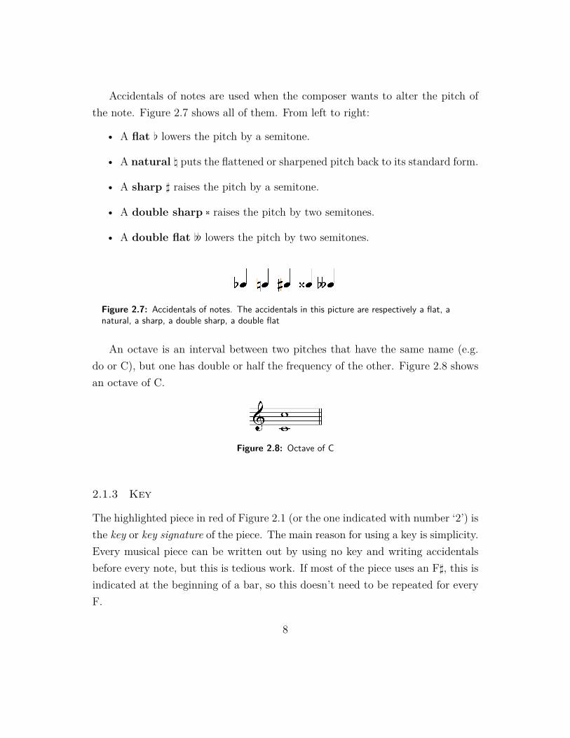
Accidentals of notes are used when the composer wants to alter the pitch ofthe note. Figure 2.7 shows all of them. From left to right:

• A flat ♭ lowers the pitch by a semitone.

• A natural ♮ puts the flattened or sharpened pitch back to its standard form.

• A sharp ♯ raises the pitch by a semitone.

• A double sharp 5 raises the pitch by two semitones.

• A double flat ♭♭ lowers the pitch by two semitones.

Figure 2.7: Accidentals of notes. The accidentals in this picture are respectively a flat, anatural, a sharp, a double sharp, a double flat

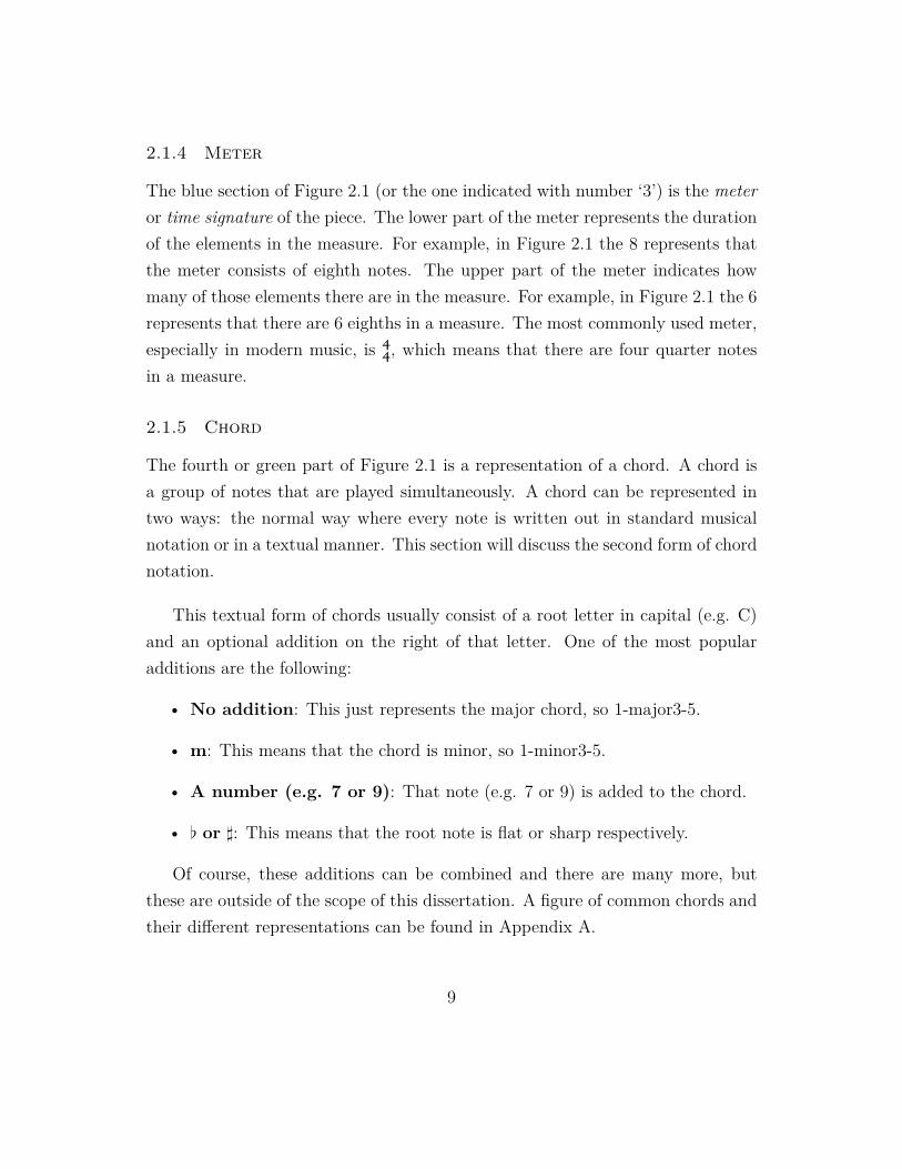
An octave is an interval between two pitches that have the same name (e.g.do or C), but one has double or half the frequency of the other. Figure 2.8 showsan octave of C.

Figure 2.8: Octave of C

2.1.3 Key

The highlighted piece in red of Figure 2.1 (or the one indicated with number ‘2’) isthe key or key signature of the piece. The main reason for using a key is simplicity.Every musical piece can be written out by using no key and writing accidentalsbefore every note, but this is tedious work. If most of the piece uses an F♯, this isindicated at the beginning of a bar, so this doesn’t need to be repeated for everyF.

8

2.1.4 Meter

The blue section of Figure 2.1 (or the one indicated with number ‘3’) is the meteror time signature of the piece. The lower part of the meter represents the durationof the elements in the measure. For example, in Figure 2.1 the 8 represents thatthe meter consists of eighth notes. The upper part of the meter indicates howmany of those elements there are in the measure. For example, in Figure 2.1 the 6represents that there are 6 eighths in a measure. The most commonly used meter,especially in modern music, is 4

4, which means that there are four quarter notesin a measure.

2.1.5 Chord

The fourth or green part of Figure 2.1 is a representation of a chord. A chord isa group of notes that are played simultaneously. A chord can be represented intwo ways: the normal way where every note is written out in standard musicalnotation or in a textual manner. This section will discuss the second form of chordnotation.

This textual form of chords usually consist of a root letter in capital (e.g. C)and an optional addition on the right of that letter. One of the most popularadditions are the following:

• No addition: This just represents the major chord, so 1-major3-5.

• m: This means that the chord is minor, so 1-minor3-5.

• A number (e.g. 7 or 9): That note (e.g. 7 or 9) is added to the chord.

• ♭ or ♯: This means that the root note is flat or sharp respectively.

Of course, these additions can be combined and there are many more, butthese are outside of the scope of this dissertation. A figure of common chords andtheir different representations can be found in Appendix A.

9

2.1.6 Measure

The fifth and final (purple) highlighted pieces of Figure 2.1 are certain barriersfor the piece. The single vertical lines divide the piece into measures. The doublevertical lines at the end of the piece indicate the ending of a piece. Other possiblebarriers and how to play them are depicted in Figures 2.9 and 2.10 [13].

Figure 2.9: Repeat signs used in a musical piece. The instructions are depicted in the figure.

Figure 2.10: A repeat sign with first and second ending. The instructions are depicted in thefigure.

2.2 Scales

This section will only discuss the most important scales for this master disserta-tion: the major and the minor scales.

2.2.1 Major Scale

There are two types of steps one can make in a musical piece: a whole tone (w) ora semitone (s). The major scale consists of seven steps in the following succession:w-w-s-w-w-w-s. An example of a major scale (D major) is given in Figure 2.11.

10

Figure 2.11: D major scale

2.2.2 Minor Scale

The minor scale has the following succession: w-s-w-w-s-w-w. An example of aminor scale (D minor) is given in Figure 2.12.

Figure 2.12: D minor scale

2.3 Transposition

Transposing a piece basically means that we move the piece up or down by a setinterval. In essence, the piece doesn’t change, the piece is just played in a higheror lower key. The most common reason pieces for transposing pieces, is to matchthe range of the singer. As an example, Figure 2.13 shows the transposition of‘Twinkle twinkle little star’ from a C major key to an F major key [14].

Figure 2.13: Transpostion of a C major piece of ‘Twinkle twinkle little star’ into an F majorpiece [14]

11

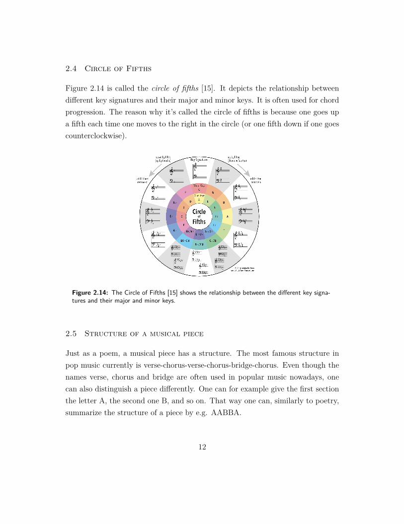
2.4 Circle of Fifths

Figure 2.14 is called the circle of fifths [15]. It depicts the relationship betweendifferent key signatures and their major and minor keys. It is often used for chordprogression. The reason why it’s called the circle of fifths is because one goes upa fifth each time one moves to the right in the circle (or one fifth down if one goescounterclockwise).

Figure 2.14: The Circle of Fifths [15] shows the relationship between the different key signa-tures and their major and minor keys.

2.5 Structure of a musical piece

Just as a poem, a musical piece has a structure. The most famous structure inpop music currently is verse-chorus-verse-chorus-bridge-chorus. Even though thenames verse, chorus and bridge are often used in popular music nowadays, onecan also distinguish a piece differently. One can for example give the first sectionthe letter A, the second one B, and so on. That way one can, similarly to poetry,summarize the structure of a piece by e.g. AABBA.

12

“I visualize a time when we will be to robots whatdogs are to humans, and I’m rooting for the ma-chines.”

Claude Shannon

3Sequence Generation with Deep Learning

Even though the term Artificial Intelligence (AI) has only been around since themid-1950s, where John McCarthy coined the term [16], the intrigue of makingmachines that think on their own has been around at least since ancient Greece[17]. This desire mostly manifested in stories like the bronze warrior Talos inArgonautica of Apollonius of Rhodes [17, 18].

John McCarthy, often referred to as the ‘father’ of AI, defined AI as ‘the scienceand engineering of making intelligent machines, especially intelligent computerprograms’ [19]. Currently, AI not only has a wide range of topics for research [17],but it is also gaining fast momentum in the corporate industry [20].

Nowadays, the most prominent technique for A.I. systems is deep learning,which has recently showed state of the art results in the domains of object recogni-tion [21], sequence generation [22], image analyzing [23] and many other domains.

13

Therefore, this chapter will give an overview of what deep learning is and howit works, after which models that can be used for sequence generation will bediscussed.

3.1 Deep Learning

Deep Learning (DL) is a subfield of Machine Learning (ML), which has gainedpopularity in the last decade [24]. There are three types of learning: supervised,unsupervised or partially supervised [25]. Supervised means that the trainingdata includes both the input and the aimed result. Unsupervised means it onlyincludes the input, but not the expected results. Partially supervised is some-where in between. Deep hierarchical models have the goal to form higher levels ofabstractions through multiple layers that combine lower level features [26]. SinceDeep Neural Networks (DNNs) are the most prominent form of DL models, thiswill be focused upon from now on [27]. In the second part of this chapter, othermodels are also discussed.

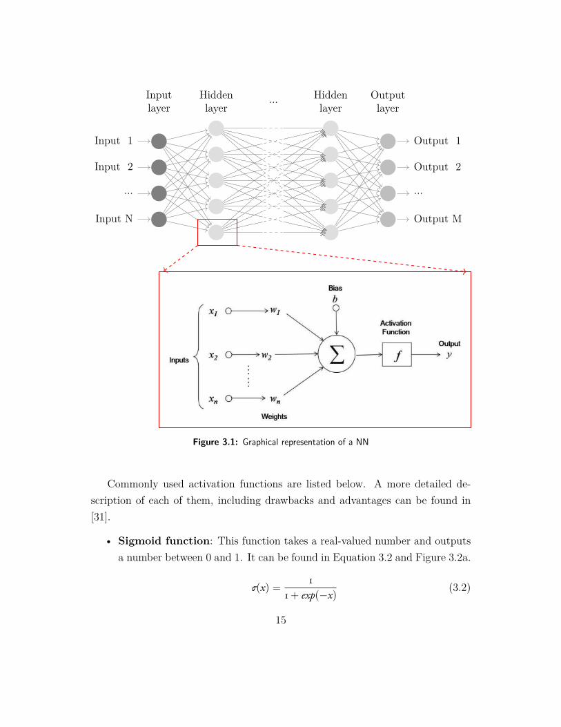
Firstly, traditional Neural Networks (NNs) will be discussed. A NN is made upof many processors called neurons that are interconnected [28]. Figure 3.1 showsthe direct graph of a NN with certain weights wij on the edges. A more in-depthrepresentation of a node can be found in the red box [29]. The activation functionis usually a non-linear function.

Mathematically, the output of each node i can be described as seen in equation3.1, where fi is the activation function of node i, yi is the output of the node, xj isthe jth input of the node, wij is the weight on the edge between the two nodes andθi is the bias of the node [30].

yi = fi(n∑j=1

wij · xj − θi) (3.1)

14

Input 1

Input 2

...

Input N

Output 1

Output 2

...

Output M

Hiddenlayer

Hiddenlayer

Inputlayer

Outputlayer

...

Figure 3.1: Graphical representation of a NN

Commonly used activation functions are listed below. A more detailed de-scription of each of them, including drawbacks and advantages can be found in[31].

• Sigmoid function: This function takes a real-valued number and outputsa number between 0 and 1. It can be found in Equation 3.2 and Figure 3.2a.

σ(x) = 11+ exp(−x) (3.2)

15

−6 −4 −2 0 2 4 6

0.5

1

y = 11+exp(−x)

(a) Sigmoid function

y = tanh x

−2 −1 1 2

−1

1

x

y

(b) Tanh Function−4 −2 0 2 4

1

2

3

4

(c) ReLU Function

Figure 3.2: Activation functions

• Tanh: This function takes a real-valued number and outputs a numberbetween -1 and 1 (see Figure 3.2b).

• Rectified Linear Unit (ReLU): This function is defined as:

f(x) = max(0, x) (3.3)

The function is displayed in Figure 3.2c. The ReLU is the de-facto standardcurrently in deep learning [32].

• Leaky ReLU: This function solves the dying ReLU problem (more infocan be found in [31]) through a small constant α.

f(x) =

αx x<0

x x>=0

• Maxout: This function computes k linear mixes of the input with itsweights and biases, where-after it selects the maximum. If k = 2, thenthe equation is as follows:

max(wT1 x+ b1,wT

2 x+ b2) (3.4)

• Softmax: This function puts the largest weight on the most likely out-

16

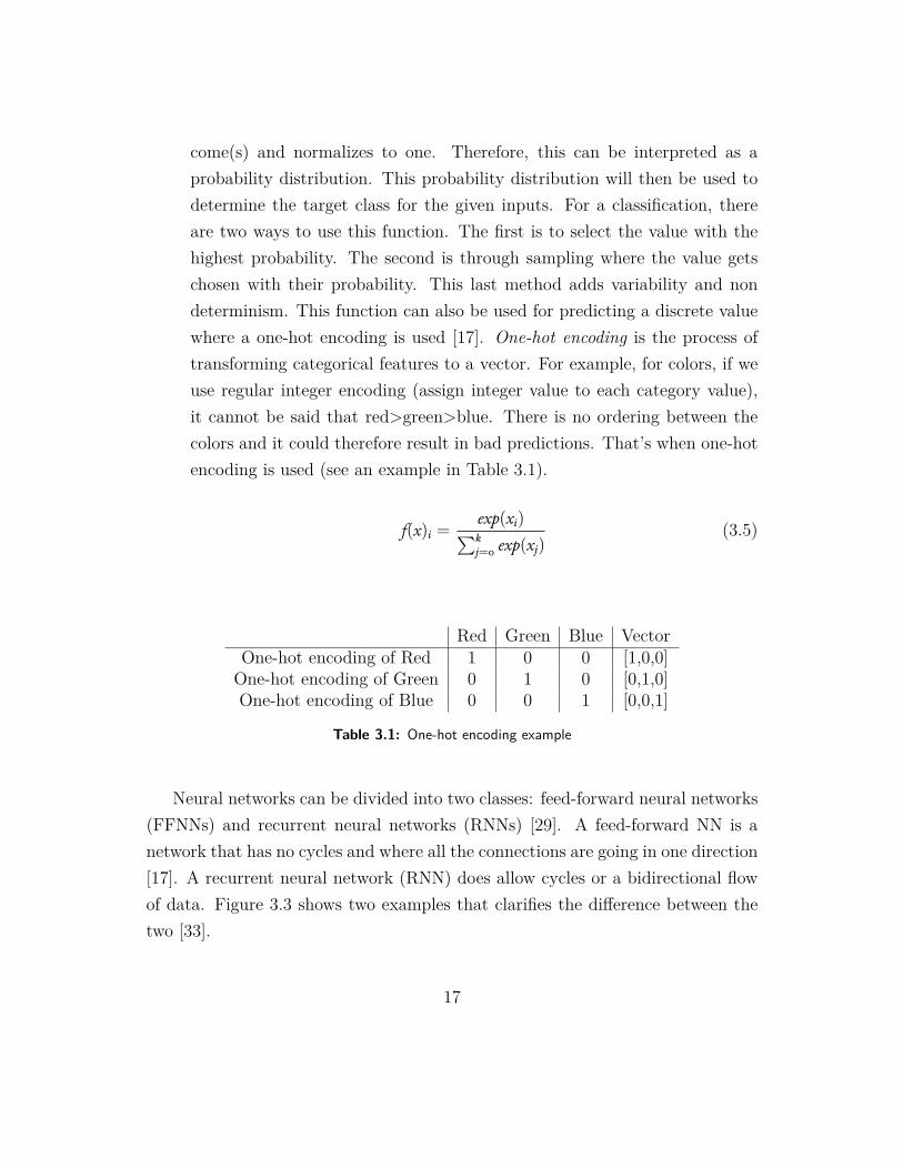
come(s) and normalizes to one. Therefore, this can be interpreted as aprobability distribution. This probability distribution will then be used todetermine the target class for the given inputs. For a classification, thereare two ways to use this function. The first is to select the value with thehighest probability. The second is through sampling where the value getschosen with their probability. This last method adds variability and nondeterminism. This function can also be used for predicting a discrete valuewhere a one-hot encoding is used [17]. One-hot encoding is the process oftransforming categorical features to a vector. For example, for colors, if weuse regular integer encoding (assign integer value to each category value),it cannot be said that red>green>blue. There is no ordering between thecolors and it could therefore result in bad predictions. That’s when one-hotencoding is used (see an example in Table 3.1).

f(x)i =exp(xi)∑kj=0 exp(xj)

(3.5)

Red Green Blue VectorOne-hot encoding of Red 1 0 0 [1,0,0]

One-hot encoding of Green 0 1 0 [0,1,0]One-hot encoding of Blue 0 0 1 [0,0,1]

Table 3.1: One-hot encoding example

Neural networks can be divided into two classes: feed-forward neural networks(FFNNs) and recurrent neural networks (RNNs) [29]. A feed-forward NN is anetwork that has no cycles and where all the connections are going in one direction[17]. A recurrent neural network (RNN) does allow cycles or a bidirectional flowof data. Figure 3.3 shows two examples that clarifies the difference between thetwo [33].

17

Figure 3.3: Example of feedforward (a) and recurrent (b) network

Machine Learning algorithms depend heavily on data. Therefore, we will needthree disjoint datasets: a training set, a validation set and a test set. The trainingset is used to train the model, whilst the validation set selects the best performingmodel on data that was not used during training. The test set is used after thetraining and validating, and is used to see how well the model generalizes on datathat is completely new. These three sets are all derived from one large dataset.

In supervised learning, the model has to know what a good output is. Theloss function or cost function will determine the quality of the output. The lossfunction calculates an error between the labeled data and the output of the model.An ideal model should generate low values for the cost function. This is alsoimportant for the test set loss, since this will be an indicator on how well themodel generalizes. An example for a cost function in supervised learning is themean-squared error (see equation 3.6), which minimizes the difference betweenthe desired output and the one given by the model [34].

MSE =1N

n∑i=1

(ŷi − yi)2 (3.6)

Once the cost function is defined, we need a method to minimize this costfunction with respect to the weights. A minimum can be found if the gradientof this loss function with respect to the weights ∇L(w) is zero. This minimumcan be found by iteratively going in the direction of the negative gradient. This

18

algorithm is called Gradient Descent. To calculate this gradient, backpropagationcan be used. This algorithm has two steps: a forward step and backward step. Theforward step will let data go through the network to generate a specific output.Then the error can be generated by comparing the desired output with the outputfrom the model. In the backward step, the error is propagated throughout thenetwork so each neuron can see how much they have contributed to the error.After that, the weights can be adjusted to optimize the model [35].

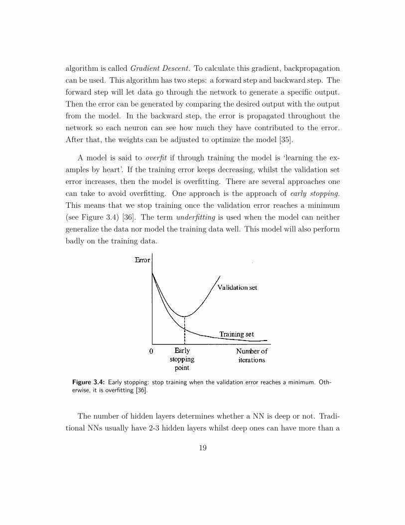
A model is said to overfit if through training the model is ‘learning the ex-amples by heart’. If the training error keeps decreasing, whilst the validation seterror increases, then the model is overfitting. There are several approaches onecan take to avoid overfitting. One approach is the approach of early stopping.This means that we stop training once the validation error reaches a minimum(see Figure 3.4) [36]. The term underfitting is used when the model can neithergeneralize the data nor model the training data well. This model will also performbadly on the training data.

Figure 3.4: Early stopping: stop training when the validation error reaches a minimum. Oth-erwise, it is overfitting [36].

The number of hidden layers determines whether a NN is deep or not. Tradi-tional NNs usually have 2-3 hidden layers whilst deep ones can have more than a

19

hundred [27].

This was a very short overview of how deep learning works. More informationabout the specifics mentioned in this section, can be found in dedicated literature[17, 29, 37].

3.2 Sequence Generating Models

Sequence generation is necessary for this master dissertation since a melody oreven more broadly a music piece, can be seen as a sequence of notes. In our casewith lead sheets, this can be seen as a sequence of syllables, notes and chords.Sequence generation essentially attempts to predict the next element(s) given theprevious elements of the sequence [38]. Figure 3.5 shows the input and output ofsuch a prediction model [39].

SequencePrediction

Model

s1, s2, ..., sj sj+1, ..., sk

Figure 3.5: Sequence generation model: input and output

The next element from the sequence is usually generated by sampling froma probability distribution that shows how likely each element is given the inputsequence. This probability distribution is formed through the training of the data.Mathematically, for generative RNNs, this can be formulated as follows, where fand g are modeled by the RNN, sn are the input/output sequences and hn are thehidden states:

sn+1 = f(hn, sn) (3.7)

20

hn1 = g(hn, sn) (3.8)

In this section, different networks that were used in this master dissertationto generate sequences are discussed in detail. Other sequence generating models,that will also be mentioned in the state of the art, will not be discussed here.They can be found in literature.

3.2.1 Recurrent Neural Network (RNN)

As briefly discussed before, RNNs are networks with cycles, which means that theoutputs of a hidden layer are also used as an additional input to compute the nextvalue. This cycle represents a temporal aspect of the network. The networks canform short term memory elements through these cycles [40].

The training process of a RNN is similar to that of a traditional NN [41]. Thebackprogragation algorithm is used yet again, but the parameters are shared byevery timestep in the network. The gradient therefore depends not only on thecurrent time step, but also past time steps. Therefore, it is called BackpropagationThrough Time (BPTT).Usually, it is trained by giving a sequence as input and it predicts the next elementin the sequence [42]. Therefore, it can be used for music generation.

3.2.2 Long Short-Term Memory (LSTM)

In RNNs with conventional backpropagation through time (BPTT), a problem hasarisen called the vanishing or exploding gradients problem. This problem occurswhen the norm of the gradient either makes the long term components go to zero(vanishing) or to very high numbers (exploding) [43]. Long Short-Term Memory(LSTM) is designed to resolve this problem [44].

The LSTM contains memory blocks in the recurrent hidden layer that storethe temporal state of the network. Figure 3.6 depicts a LSTM memory block,where xt represents the memory cell input and yt represents the output [45]. The

21

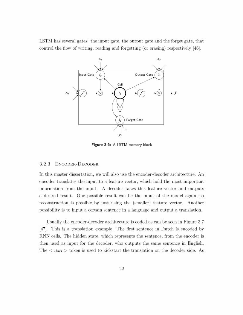
LSTM has several gates: the input gate, the output gate and the forget gate, thatcontrol the flow of writing, reading and forgetting (or erasing) respectively [46].

ct

Cell

× yt×

×

ft Forget Gate

itInput Gate otOutput Gate

xt

xt xt

xt

Figure 3.6: A LSTM memory block

3.2.3 Encoder-Decoder

In this master dissertation, we will also use the encoder-decoder architecture. Anencoder translates the input to a feature vector, which hold the most importantinformation from the input. A decoder takes this feature vector and outputsa desired result. One possible result can be the input of the model again, soreconstruction is possible by just using the (smaller) feature vector. Anotherpossibility is to input a certain sentence in a language and output a translation.

Usually the encoder-decoder architecture is coded as can be seen in Figure 3.7[47]. This is a translation example. The first sentence in Dutch is encoded byRNN cells. The hidden state, which represents the sentence, from the encoder isthen used as input for the decoder, who outputs the same sentence in English.The < start > token is used to kickstart the translation on the decoder side. As

22

can be clearly seen by the figure, the sentence in Dutch has five words, whilst thesentence in English only has three.

Figure 3.7: Encoder-Decoder architecture, inspired by [47]

23

”Basic research is like shooting an arrow into theair and, where it lands, painting a target.”

Homer Burton Adkins

4State of the Art in Music Generation

This chapter first discusses different music representations that can be used formachine learning, and presents the state of the art in music generation.

4.1 Music Representation

Music can be represented in many ways, ranging from MIDI format to audioformat. There are two main forms of music representation: signal representationsand symbolic representations. In the next sections we will discuss both in moredetail.

4.1.1 Signal or Audio Representation

The most basic type of music representation is an audio signal. This can be bothraw audio or an audio spectrum, calculated using a Fourier transformation [17].

24

The significance of using this format as input can not only be found in musicgeneration, but also in music recommendation systems, since software such asSpotify or Apple Music have increased in popularity the past couple of years [48].Figure 4.1 shows a visual representation of a raw audio file and its correspondingaudio spectrum [49].

Since this master dissertation will focus on symbolic representations, from nowon only symbolic representations are mentioned and used. Examples of musicgeneration from an audio format can be found in [50, 51].

Figure 4.1: Visual representation of raw audio and its fourier transformed spectrum [49]

4.1.2 Symbolic Representations

Most of the research in music generation focuses on symbolic representations ofmusic. Symbolic representations will note music through discrete events, suchas notes, chord or rhythms. This section will discuss the most popular ways torepresent music.

25

A Musical Instrument Digital Interface (MIDI) Protocol

Music Instrument Digital Interface (MIDI) Protocol is a music protocol that de-fines two types of messages: event messages, for information such as pitch, nota-tion and velocity, and control messages, for information such as volume, vibratoor audio panning. The main note messages are:

• NOTE ON This message is sent when a note is being played. Informationsuch as the pitch and the velocity are also included.

• NOTE OFF This message is sent when a note has stopped. The sameinformation can be included in the message.

The note’s pitch is an integer in the interval [0,127], where the number 60represents middle C on a piano. The note’s velocity is an integer in the interval[1,127], where Table 4.1 shows the different nuances [52]. pppp means that thenotes are played very softly and ffff means it is played loudly.

Music notation Velocity Music Notation Velocitypppp 8 mf 64ppp 20 f 80pp 31 ff 96p 42 fff 112

mp 53 ffff 127

Table 4.1: MIDI velocity table [52]

Other important parameters are the channel number and number of ticks:

• Channel Number is the number of the MIDI channel and is an integerin the interval [0,15]. Channel number 9 is exclusively used for percussioninstruments.

• Ticks represents the number of ticks for a quarter note ˇ “.

26

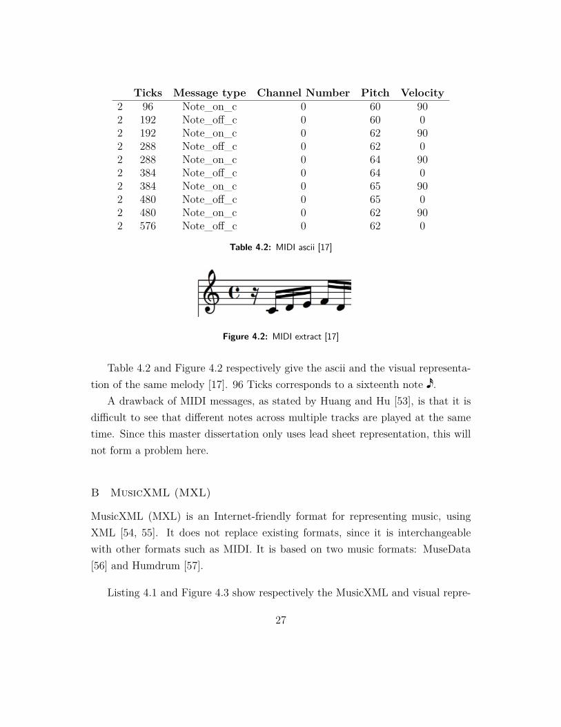
Ticks Message type Channel Number Pitch Velocity2 96 Note_on_c 0 60 902 192 Note_off_c 0 60 02 192 Note_on_c 0 62 902 288 Note_off_c 0 62 02 288 Note_on_c 0 64 902 384 Note_off_c 0 64 02 384 Note_on_c 0 65 902 480 Note_off_c 0 65 02 480 Note_on_c 0 62 902 576 Note_off_c 0 62 0

Table 4.2: MIDI ascii [17]

Figure 4.2: MIDI extract [17]

Table 4.2 and Figure 4.2 respectively give the ascii and the visual representa-tion of the same melody [17]. 96 Ticks corresponds to a sixteenth note ˇ “) .

A drawback of MIDI messages, as stated by Huang and Hu [53], is that it isdifficult to see that different notes across multiple tracks are played at the sametime. Since this master dissertation only uses lead sheet representation, this willnot form a problem here.

B MusicXML (MXL)

MusicXML (MXL) is an Internet-friendly format for representing music, usingXML [54, 55]. It does not replace existing formats, since it is interchangeablewith other formats such as MIDI. It is based on two music formats: MuseData[56] and Humdrum [57].

Listing 4.1 and Figure 4.3 show respectively the MusicXML and visual repre-

27

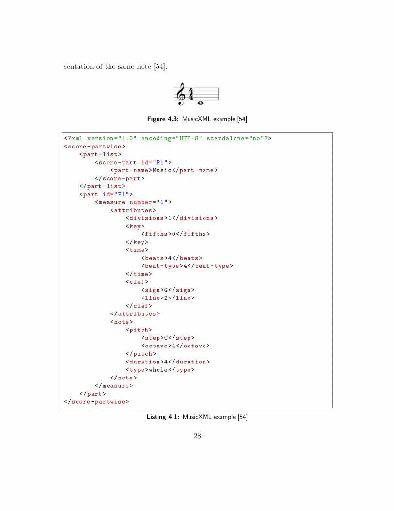
sentation of the same note [54].

Figure 4.3: MusicXML example [54]

<?xml version="1.0" encoding="UTF -8" standalone="no"?><score -partwise>

<part-list><score -part id="P1">

<part-name>Music</part-name></score -part>

</part-list><part id="P1">

<measure number="1"><attributes>

<divisions>1</divisions><key>

<fifths>0</fifths></key><time>

<beats>4</beats><beat-type>4</beat-type>

</time><clef>

<sign>G</sign><line>2</line>

</clef></attributes><note>

<pitch><step>C</step><octave>4</octave>

</pitch><duration>4</duration><type>whole</type>

</note></measure>

</part></score -partwise>

Listing 4.1: MusicXML example [54]

28

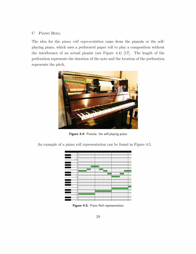
C Piano Roll

The idea for the piano roll representation came from the pianola or the self-playing piano, which uses a perforated paper roll to play a composition withoutthe interference of an actual pianist (see Figure 4.4) [17]. The length of theperforation represents the duration of the note and the location of the perforationrepresents the pitch.

Figure 4.4: Pianola: the self-playing piano

An example of a piano roll representation can be found in Figure 4.5.

Figure 4.5: Piano Roll representation

29

A major drawback of the piano roll representation is that the NOTE OFFevent that does exist in MIDI, doesn’t exist [58]. According to a piano roll repre-sentation, there is no difference between two short notes and one long note.

D ABC Notation

Listing 4.2 and Figure 4.6 give respectively the ABC notation and the visualrepresentation of the same piece [59]. The first five lines are the header of themusical piece. The notes themselves are contained in the following four lines.

X:1T:Speed the PloughM:4/4C:Trad.K:G|:GABc dedB|dedB dedB|c2ec B2dB|c2A2 A2BA|GABc dedB|dedB dedB|c2ec B2dB|A2F2 G4:||:g2gf gdBd|g2f2 e2d2|c2ec B2dB|c2A2 A2df|g2gf g2Bd|g2f2 e2d2|c2ec B2dB|A2F2 G4:|

Listing 4.2: ABC notation: Speed the Plough [59]

Figure 4.6: ABC notation: Speed the Plough [59]

30

The components of the header are as follows:

• X: A reference number that was useful when it was first introduced forselecting specific tunes from a file. Nowadays, software doesn’t need thisanymore.

• T: This field represents the title of the piece. In this case, T is ‘Speed thePlough’.

• M: Also known as meter of a piece. A standard 44 is used for this piece.

• C: This field represents the composer of the piece. In this piece, C is ‘Trad’.

• K: The key of the piece is G Major.

Each note is represented by a letter, but the octave and duration depends onthe formatting of the letter. Listing 4.3 and Figure 4.7 show four octaves of notes,in ABC notation and standard notation respectively.

C, D, E, F,|G, A, B, C|D E F G|A B c d|e f g a|b c' d' e'|f' g' a' b'|

Listing 4.3: Four octaves in abc notation [59]

Figure 4.7: ABC notation: four octaves

If there is a field L present (e.g. L: 1/16 ˇ “) ), then this is used as the defaultlength of notes. If it is not specified, an eighth note ˇ “( is assumed. Then thelength of the note can be adapted through numbers. For example c2 in case of thedefault length of an eighth note ˇ “( is a quarter note ˇ “, since 2 · 1

8 =14 . A sixteenth

note ˇ “) is therefore represented by c/2.

31

E Lead Sheet

A lead sheet is a format of music representation that is especially popular in jazzand pop music. Figure 4.8 shows an example of a jazz standard in lead sheetformat. As clearly can be seen from the example, there are a few elements to thelead sheet:

Figure 4.8: Lead Sheet Example

• Melody: The melody is presented in standard musical format. This is

32

usually the melody that the singer sings.

• Chord: The chords are placed above the melody in a textual format.

• Lyrics: The lyrics are placed under the melody, with each syllable corre-sponding to a specific note.

• Other: Other information such as the title, composer and performanceparameters can also be added to the lead sheet.

4.2 Music Generation

This section is divided in three parts. First, preprocessing and data augmentationideas are discussed. Afterwards, relevant works considering actual music genera-tion will be discussed. Some possible evaluation methods are touched upon at theend.

4.2.1 Preprocessing and data augmentation

Before the data is used, two (potential) steps can be taken: preprocessing anddata augmentation. Not all datasets have the ideal format for machine learningalgorithms. The data still needs to be cleaned, transformed or ‘preprocessed’. Thedata could for example be scaled or missing data points can be amended. Thisstep is called preprocessing. Data augmentation on the other hand increases theamount of data points in our dataset. The dataset may be smaller or more limitedthan we want, since they are taken in a set of conditions. Collecting more datais costly, therefore we want to opt for data augmentation. In object recognitionfor example, the object can be rotated and added to the dataset. In music, thepieces could be transposed.

Some preprocessing and data augmentation ideas are discussed in this section.

Preprocessing

For practical reasons, lead sheets are often written in condensed formats, usingrepeat signs (see Section 2.1.6) and using multiple lines for lyrics. However, it

33

is best that for machine learning purposes they are “unfolded”, so there is noambiguity in which measure needs to be played after which one [60].

Duplicates or overlapping notes in the same MIDI channel don’t have any pur-pose so these can be removed as well [61]. Certain channels can also be removed:channels where only a few (e.g. two) note events occur or percussion channelswhich don’t serve any melodic purpose [61]. Transposing to a common tonality,e.g. C major, can be also used to eliminate affinity to certain keys [62].

In some datasets there are data duplicates, e.g. the same piece written by differentpeople. When splitting the data into training, test and validation sets, the sta-tistical dependences need to be reduced. A possible solution, provided by Walder[61], has three steps:

1. Compute the normalized histogram of the midi pitches of the file. Do thesame for the quantized durations. Concatenate the two vectors to form asignature vector for each file.

2. Perform hierarchical clustering on these vectors. Order the files by traversingthe resulting hierarchy in a depth first fashion.

3. Given the ordening, split the dataset.

Data Augmentation

The data can be augmented by transposing into all possible keys (so within thevocal range) [63]. Any affinity that a composer has for a certain key is eliminatedthis way [64].

4.2.2 Music Generation

Recurrent Neural Networks have a dominant role in the field of Music Generation,since RNNs have had successes in many fields concerning generation, for examplein text [65], handwriting [66] or image generation [67]. The reason feed-forward

34

networks (FFNN) are less popular in the case of generation, is through their totalinability of storing past information. In the music generation field, this translatesto the lack of knowing the position in the song [68]. An example of FFNN beingused in music generation is Hadjeres and Briot’s MiniBach Chorale GenerationSystem [42]. Even though the result was acceptable, it was less favorable thanusing more complex RNN networks.

General RNNs lack the ability of modeling a more global structure. Thesenetworks usually predict on a note-by-note basis. Examples of this can be foundin [1, 69]. In context of his note-by-note attempt to music generation throughRNNs, Mozer stated in [8] that it still lacked thematic structure and that thepieces were not musically coherent. The reason stated was the “architecture andtraining procedure do not scale well as the length of the pieces grow and as theamount of higher-order structure increases.” Eck et al. linked this to the prob-lem of vanishing gradients [68] and suggested that structure needs to be inducedat multiple levels. They introduced a RNN architecture using LSTMs. Theyperformed two experiments, using a 12-bar blues format: the first one being thegeneration of chord sequences and the second one being the combined generationof melody and chords. Both melody and chords were presented to the system asone-hot encodings and they strictly constrained the notes to 13 possible valuesand the chords to 12 possible chords. Each input vector represents a slice of time,which means that no distinction can be made between two short notes of the samepitch and one long note (see piano-roll drawback in Section C). Two possible so-lutions to this piano-roll problem were suggested. The first one is to the slice oftime and marking the end of note with a zero. The second one is to model specialunits in the network to indicate the beginning of the note, inspired by the workof Todd [69]. Even though the generation is deterministic and even though theconstraints on the possible notes and chords is strict, they did capture a globaland local structure.

In the field of classical music, we’ll discuss to ways of generating music. Thefirst is a rule-based expert system, and the second is a deep learning solution. An

35

example of a rule-based expert system was introduced by Ebcioglu et al. [70].Considering Bach fully integrated thorough bass, counterpoint and harmony inhis compositions, a lot of rules can be formulated in order to make music in thestyle of Bach [71]. Experts formulated more than 300 rules, which generatedexcellent results, however, these results did not always sound like Bach. The maindrawback of this method is the large effort needed from experts to make such arule-based expert system.Therefore, a deep learning model is usually used for music generation, since it alsodoesn’t require any prior knowledge. The work of Boulanger-Lewandowski et al.[62] works with an RNN-RBM to model polyphonic classical music. The mainrestriction in this type of generation is that generation can only be performedfrom left to right. DeepBach, introduced by Hadjeres et al. [63], shows moreflexibility without plagiarism. In DeepBach, a MIDI representation is used anda hold symbol “_ _” is used to code whether the previous note is held. Togenerate steerable and strong results, LSTMs are used in both directions. Figure4.9 shows the architecture of DeepBach. The first four lines of the input dataare the four voices, whereas the other two model metadata. Generation is donethrough pseudo-Gibbs sampling. The authors of the article state:

“These choices of architecture somehow match real compositional prac-tice on Bach chorales. Indeed, when reharmonizing a given melody, itis often simpler to start from the cadence and write music backwards.”

Compared to BachBot, which made use of a 3-layer stacked LSTM in order togenerate new chorales in the style of Bach, the DeepBach model was more generaland more flexible [72]. An important remark from the BachBot authors is thatthe number of layers or the depth truly makes a large difference. Increasing thenumber of layers can decrease the validation loss up to 9%.

For more modern music, jazz and pop, some research has also been conducted.In the world of Jazz, Takeshi et al. have made an offline jazz piano trio synthesizing

36

Figure 4.9: Soprano prediction, DeepBach’s neural network architecture

system [73]. The system uses hidden Markov models (HMMs) and DNNs togenerate a bass and drum accompaniment for the piano MIDI input. In popmusic, Chu et al. were inspired by a Song of Pi video1, where the music is createdfrom the digits of π [74]. Their hierarchical RNN model, using MIDI input andgenerating melody, chords and drums, even outperformed Google’s Magenta [75] ina subjective evaluation with 27 human participants. There has also been researchregarding GANs to generate multi-track pop/rock music [2, 22, 76].

Research specifically for lead sheet generation has also been conducted. Flow-Composer [3] is part of the FlowMachines [4] project and generates lead sheets (amelody with chords) in the style of the corpus selected by the user. The user canenter a partial lead, which is then completed by the model. If needed, the modelcan also generate from scratch. Some meter-constrained Markov chains represent

1https://www.youtube.com/watch?v=OMq9he-5HUU&feature=youtu.be

37

the lead sheets. Pachet et al. have also conducted some other research withinthe FlowMachines project regarding lead sheets. In [5], they use the Mongeau &Sankoff similarity measure in order to generate similar melody themes to the im-posed theme. This is definitely relevant in any type of music, since a lot of melodythemes are repeated multiple times during pieces. Ramona, Cabral and Pachethave also created the ReChord Player, which generates musical accompanimentsfor any song [6]. All these examples within the FlowMachines project, use theFlowMachines Lead Sheet Data Base1, which requires a login to access it.

An important limitation is that current techniques learn only during training,but do not adapt when the generation happens [42]. The first solution of thiscould be to add the generated musical piece to the training data and to retrain.However, this could lead to overfitting and doesn’t necessarily produce betterresults.

Another approach is through reinforcement learning. Murray-Rust et al. [9]have identified three types of feedback rewards that can be used in reinforcementlearning for music generation:

1. How well the generated piece satisfies the predefined internal goals. Thesecan be defined by the composer or can be defined during the performance.

2. Direct feedback (like or dislike) from human participants/audience members.

3. The incorporation of ideas the musical agent suggests, which results in in-teractive feedback.

An example of the first reward system was used in [77]. They used some basicjazz improvisation rules in order to make the system improvise. Examples of theserules were: (i) using a note from the scale associated with the chord is fine and(ii) a note shouldn’t be longer than a quarter note.An example of the second possibiblity (the direct feedback from audience mem-bers) can be found in [78]. Figure 4.10 shows the three main components of the

1http://lsdb.flow-machines.com/

38

system: the listener, the reinforcement agent and the musical system. Musicaltension was used as a reward function, since the authors correlate the tension tothe rise of emotions in an audience. The biggest problem, as stated by [79], is thatthe interaction of the audience may disrupt the performance entirely. Thereforethey suggested tracking emotions through facial recognition as a less disruptivefeedback loop. However, this has not been explored further.

Figure 4.10: Reinforcement learning with audience feedback [78]

An example of the interactive feedback system from other agents can be foundin [9]. The interactions between agents is modeled through Musical Acts [80],which were inspired by Speech Acts that are used in common agent communicationlanguages. An example of these Musical Act, as stated in [80] for the song LittleBlue Frog by Miles Davis, can be found in Table 4.3.

A very important remark was made by Bretan et al. [64] concerning the simi-larity between two musical passages. There can be a strong relationship betweentwo chords or two musical passages even without using the same structure harmon-ically, rhythmically or melodically. Especially in chord prediction, an interesting

39

Time(s) Instrument Performative Description

2:00 - 2:13 Trumpet INFORM A spiky, stabbing phrase,based on scale 2

Clarinet

CONFIRM(an agent A informs adifferent agent B, and

the agent B ishappy with this)

briefly seems to agreewith the trumpet.

Bass clarinet CONFIRM Confirms scale 3

2:13 - 2:29 TrumpetDISCONFIRM

(same as confirm, butB is not content)

Ignores bass clarinet,and continues with stabs

Clarinet DISCONFIRMIgnores bass clarinet,and continues withlyricism in scale 2

2:29 - 2:43

TrumpetClarinet

BassClarinet

ARGUE(occurs when multiple

agents presentconflicting ideas)

All play lyrically, withclarinet on scale 2,

trumpet on 1and Bass Clarinet in 3

2:43 - 3:08 TrumpetPROPOSE

(an agent proposesa new idea)

proposes a resolution,by playing stabs which

fit with any of the scales

3:03 - 3:08 E-PianoVibes CONFIRM supports the trumpet’s

resolution

Table 4.3: Reinforcement Learning: Miles Davis - Little Blue Frog in Musical Acts by [80]

approach has been suggested in order to model these strong relationships. InChordRipple, Huang et al. used chords that are played together often in a nearvector space [81], inspired by the word2vec model introduced by Mikolov et al.[82]. In this model, the major and minor chords are arranged according to thecircle of fifths (see Figure 2.14) [15]. Chords were represented into attributes, suchas the root, the chord type, the inversion, bass, extensions and alterations.

40

Similarly to the chord2vec model in ChordRipple, Madjiheurem et al. also intro-duced a chord2vec model inspired by the word2vec model [83]. In the sequence-to-sequence model they suggested, chords were represented as an ordered sequenceof notes. A special symbol ε is added to mark the end of a chord. In order topredict neighboring chords a RNN Encoder-Decoder is used.

Even though naïve sequence modeling approaches can perform well in musicgeneration, these approaches miss important musical characteristics. For examplea sense of coherence is needed by repeating motifs, phrases or melodies, unless themusical material is restricted or simplified. Lattner et al. [84] have solved this byusing a self-similarity matrix to model the repetition structure. Other constraintson the tonality and the meter were also added. The same trade-off between aglobal structure and locally interesting melodies was noticed by Tikhonov et al.[85]. They suggested a Variational Recurrent Autoencoder Supported by History(VRASH). VRASH combines a LSTM Language Model, which does not capturethe global structure, with a Variational Auto-Encoder (VAE).

Even though most research that has been conducted use piano rolls or MIDIformats, some research can also be found using the ABC notation [86, 87, 88].

4.2.3 Evaluation

There are many ways for evaluation a musically generated piece. Possible evalu-ation ideas are the following:

• In many evaluation methods [62, 83], a baseline is used to compare the newmethod to. This can be an older method that has some similarity to the onethe author wants to evaluate or a simple one, such as a Gaussian density.

• An online Turing test with human evaluators can also be used [63, 72].Subjects first have to rate their level of expertise, after which they vote“Human” or “Computer” on different pieces.

• Finding objective metrics is quite difficult in the field of music generation.Dong et al. [76] defined some objective metrics that could be used:

41

1. EB: ratio of empty bars (in %)

2. UPC: Number of used pitch classes, which are the classes of notes (e.g.C, C#, ...), per bar (can be 1-12).

3. QN: ratio of qualified notes (in %). If the note has a small duration(less than three time steps, or 32th note), it is considered as noise.

4. NIS: ratio of notes in the C scale (in %)

5. TD: tonal distance. The larger TD is, the weaker hamornicity is be-tween a pair of tracks.

Furthermore, they tracked these metrics for the training data and comparedthose to the generated data.

42

“Data matures like wine, applications like fish.”

James Governor

5Data Analysis of the Dataset Wikifonia

The dataset used in this master dissertation is the Wikifonia dataset. Even thoughit is not available anymore due to copyrighted issues, there was a download linkavailable1. It is a dataset with 6394 MusicXML scores in lead sheet format.Lyrics and chords are included in most scores. Table 5.1 shows some statistics ofthe dataset.

5.1 Internal Representation

Even though the piece is in MusicXML format, this can be hard to work with.We had to find a way to store the same information in a more readable and easilyadaptable way. Inspired by Google’s Magenta [75], the MusicXML file was parsedto a Protocol Buffer [89]. Protocol Buffers are buffers that structure and encode

1http://www.synthzone.com/files/Wikifonia/Wikifonia.zip

43

Type of statistic NumberScores 6394

Scores with lyrics 5220Syllables in lyrics 730192

Unique syllables in lyrics 12922Scores with multiple simultaneous notes 300

Pieces with more than one repeat 3443Pieces with meter 4

4 4408Pieces with meter 3

4 816Pieces with meter 22 749Pieces with meter 24 212

Pieces with meter 68 147




Pieces with meter 64 6Pieces with meter 3




4 1Different rhythm types of notes in scores 42

Table 5.1: Original Statistics Dataset Wikifonia

the data in an efficient way. A part of the “music_representation.proto”-file canbe found in Listing 5.1. The definitions of TimeSignature, KeySignature, Tempo,Note and Chord are all defined further in the file.

message MusicRepresentation {// Unique idstring id = 1;// the path of the filestring filepath = 2;

// Lacking a time signature , 4/4 is assumed per MIDI standard.repeated TimeSignature time_signatures = 4;// Lacking a key signature , C Major is assumed per MIDI standard.

44

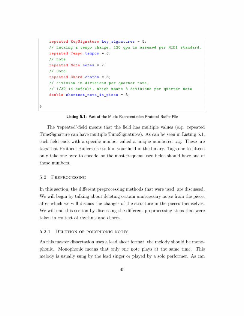
repeated KeySignature key_signatures = 5;// Lacking a tempo change , 120 qpm is assumed per MIDI standard.repeated Tempo tempos = 6;// noterepeated Note notes = 7;// Cordrepeated Chord chords = 8;// division in divisions per quarter note,// 1/32 is default , which means 8 divisions per quarter notedouble shortest_note_in_piece = 3;

}

Listing 5.1: Part of the Music Representation Protocol Buffer File

The ‘repeated’-field means that the field has multiple values (e.g. repeatedTimeSignature can have multiple TimeSignatures). As can be seen in Listing 5.1,each field ends with a specific number called a unique numbered tag. These aretags that Protocol Buffers use to find your field in the binary. Tags one to fifteenonly take one byte to encode, so the most frequent used fields should have one ofthose numbers.

5.2 Preprocessing

In this section, the different preprocessing methods that were used, are discussed.We will begin by talking about deleting certain unnecessary notes from the piece,after which we will discuss the changes of the structure in the pieces themselves.We will end this section by discussing the different preprocessing steps that weretaken in context of rhythms and chords.

5.2.1 Deletion of polyphonic notes

As this master dissertation uses a lead sheet format, the melody should be mono-phonic. Monophonic means that only one note plays at the same time. Thismelody is usually sung by the lead singer or played by a solo performer. As can

45

be seen in Table 5.1, there were 300 scores that had polyphonic fragments in it.These were mostly scores of a more classical nature. In order to make the dataconsistent, we had to make sure that all melodies were monophonic. Therefore, allpolyphonic notes were removed until only the top note, the melody note, remainedin the piece.

5.2.2 Deletion of anacruses

An anacrusis is a sequence of notes that precedes the downbeat of the first measure.Figure 5.1 shows an example, where the first measure that can be seen is theanacrusis. These measures were deleted as a preprocessing step.

Figure 5.1: Example of an anacrusis

5.2.3 Deletion of ornaments

Ornaments or embellishments are decorative notes that are played rapidly in frontof the central note [90]. Figure 5.2 shows a smaller ornament note before a mainquarter note.

Figure 5.2: Example of an ornament

46

In some pieces, ornament notes were present. In a MusicXML file, these arethe notes that have no duration. These notes were removed from the piece, sincethey don’t serve any true melodic purpose. They just serve to add a variety.

5.2.4 Unfold piece

In order for the model to know which measures need to be played subsequently,repeat signs need to be eliminated. The piece needs to be fed to the model asit would be played. That’s why we need to unfold the piece. An example ofsuch unfolding can be found in Figures 5.3a and 5.3b, which respectively showthe original and unfolded piece. As can be seen, the yellow part is added again inbetween the green and the blue part in order to make sure the piece is given tothe model as was intended by the composer.

(a) The original piece

(b) The piece after the algorithm

Figure 5.3: Preprocessing step: unfolding the piece by eliminating the repeat signs

5.2.5 Rhythm

In order to make sure that most pieces have similar formats, we had to analyzethe different rhythms of notes in each piece. As can be seen from the original

47

statistics of the dataset (see Table 5.1), there were 42 different rhythm types inthe original dataset. Since we want to encode the rhythms as a one-hot vector,and make this as efficient as possible, we want to eliminate the less frequently usedrhythm types. We wanted to delete pieces that had less occurring rhythm types,in order to make sure the dataset is as conform as possible. Namely, these rarerhythm types indicated that the piece was more complex than or simply differentfrom others in the dataset. Therefore, these 184 pieces were removed. In the end,only 12 rhythm types remained. The new statistics of the dataset can be foundin Table 5.2. Table 5.3 shows the twelve final rhythm types and how many timesthey occur in the dataset.
















Table 5.2: Statistics Dataset Wikifonia after deletion of scores with rare rhythm types

48

Note ImageOccurrence of rhythm type inthe scores

32th note ˇ “* 67232th note dotted ˇ “* ‰ 1435

16th note ˇ “) 60745

One note of a triplet3

ˇ “

==

226168th note ˇ “( 389947

Two notes of a triplet linked3

ˇ “ 148268th note dotted ˇ “( ‰ 18646

quarter note ˇ “ 301286quarter note dotted ˇ “

‰ 34549half note ˘ “ 82011

half note dotted ˘ “‰ 30441

whole note ¯ 29602

Table 5.3: The twelve final rhythm types and their count in the dataset

5.2.6 Chord

Chords are one of the main elements of lead sheets that we would like to model.Therefore, we first wanted to delete all scores that didn’t have chords in them. Intotal, these were 375 scores. The updated statistics table can be found in Table5.4.

A chord has three elements: a root, an accidental or alter and a mode. Weanalyzed all three in the following subsections.

A Root

There are seven different potential roots for a chord: A, B, C, D, E, F and G.Table 5.5 shows these roots and how much they appear in the scores withouttransposition.

49
















Table 5.4: Statistics Dataset Wikifonia after deletion of scores with rare rhythm types andscores with no chords

Root NumberA 29892B 29074C 46931D 34226E 29441F 39304G 43804

Table 5.5: Roots of chords and how much they appear in the scores without transposition

B Alter

There are four alters that appeared in the scores: ♭♭, ♭, ♮ and ♯. Table 5.6 showsthese alters and how much they appear in the scores without transposition.

50

Alter Number♭♭ 7♮ 197845♭ 49214♯ 5606

Table 5.6: Alters of chords and how much they appear in the scores without transposition

However, we wanted for each chord that had the same harmonious content tohave the exact same representation. For example, A♯, B♭ and C♭♭ have the sameharmonic structure, yet a different name. Therefore, all chords were adapted tofit one of the following twelve combination of roots and alters: A, A♯, B, C, C♯,D, D♯, E, F, F♯, G and G♯.

C Mode

There are 47 different modes that appear in the score. They can be found in Table5.7 with their count. The last column of the table represents the new mode thatwe replace the original mode with, so we only end up with four different modes:major, minor, diminished and augmented. The reason these four were chosen,was because they represent the structure of the basis of the chord (the first threenotes, separated by a third each). More information on this can be found in musictheory books.

5.3 Data Augmentation

In this section, the data augmentation of the dataset is discussed. The only dataaugmentation technique used was transposition.

5.3.1 Transposition

We already explained what transposition means in Section 2. In order to augmentthe dataset, we can transpose the original pieces in all possible keys. We did this

51

Mode Howmany Replace

major 88621 Majdominant 59365 Maj

minor 29577 Minminor-seventh 25292 Minmajor-seventh 7645 Maj

dominant-ninth 5536 Majmajor-sixth 5324 Maj

4957 Majdiminished 3850 Dimminor-sixth 2616 Min

min 2440 Min7 2382 Maj

suspended-fourth 1999 Majhalf-diminished 1988 Dim

diminished-seventh 1651 Dimaugmented-seventh 1605 Aug

augmented 1344 Augdominant-13th 972 Maj

dominant-seventh 935 Majmaj7 835 Maj

minor-ninth 833 Minmin7 793 Min

major-ninth 510 Majdominant-11th 224 Maj

Mode Howmany Replace

power 217 Majminor-11th 200 Min

suspended-second 160 Majminor-major 130 Min

dim 127 Dimaugmented-ninth 87 Maj

9 77 Maj6 62 Maj

major-minor 56 Majmin9 46 Minsus47 40 Majaug 31 Aug

major-13th 24 Majm7b5 23 Dimmaj9 22 Majmin6 20 Minmaj69 18 Majdim7 11 Dim

minor-13th 4 Mindim7 2 Dim/A 1 Maj

minMaj7 1 Minmin/G 1 Min

Table 5.7: Modes of chords, how much they appear and their replacement in the scores with-out transposition

by incrementing the piece each time with a semitone, until we have reached theoctave. This means that the size of our dataset will be multiplied by twelve. Thereason why this can be beneficial to our model, is because this will give the modelmore data to rely on to make the decisions. It also prevents the model fromlearning a bias that a large subset of the dataset might have towards a specifickey.

52

An alternative approach that wasn’t used in this master dissertation, was totranspose all the pieces in a common key (e.g. C major). This has been advocatedby Boulanger-Lewandowski et al. as a preprocessing step in order to improveresults [62].

5.4 Histograms of the dataset

We wanted to plot the distribution of certain elements of the chords and the notesin order to gain a better understanding about the dataset. This was done in thetwo following subsections.

5.4.1 Chords

As can be clearly seen in Figure 5.4, C and G are the most common chords,followed by F and D in the dataset that wasn’t augmented. This is expected sincethese are chords that musicians use more often than other chords.

Figure 5.4: Distribution of roots of chords in dataset without data augmentation

It is also expected that the major and modes are used more often than theaugmented or diminished modes. That’s what we have found in Figure 5.5.

53

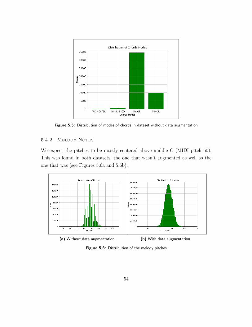
Figure 5.5: Distribution of modes of chords in dataset without data augmentation

5.4.2 Melody Notes

We expect the pitches to be mostly centered above middle C (MIDI pitch 60).This was found in both datasets, the one that wasn’t augmented as well as theone that was (see Figures 5.6a and 5.6b).

(a) Without data augmentation (b) With data augmentation

Figure 5.6: Distribution of the melody pitches

54

5.5 Split of the dataset

Of course, the dataset was split into a training set and a test set. The trainingpart of the split was data augmented, whilst the other one was not.

55

”Not until a machine can write a sonnet or com-pose a concerto because of thoughts and emotionsfelt, and not by the chance fall of symbols, couldwe agree that machine equals brain-that is, notonly write it but know that it had written it.”

Professor Jefferson Lister

6A new approach to Lead Sheet

Generation

This chapter discusses the methodology details of two models: one simple melodygenerating model and a lead sheet generating model we’ll call the melody on chordgenerating model. The second one uses some knowledge obtained from the firstmodel.

6.1 Melody generation

First, we train a baseline model that only generates the melody of the lead sheet.The goal is to construct a model that predicts the next note conditioned on theprevious time_steps notes. These previous notes represent the ‘background’ of the

56

music piece. Mathematically, this is written as follows:

p(notei|notei−1, notei−2, ..., notei−time_steps) (6.1)

A note of a melody has two elements:

1. a rhythm or duration

2. a pitch (or no pitch if it is a rest)

We model a note by concatenating two one-hot encoded vectors, as depictedon Figure 6.1. This representation contains both the pitch and rhythm, as wellas additional elements for modeling measure bars.

Figure 6.1: Two one hot encoders concatenated of a note representing the pitch and therhythm in the melody generation problem. Measure bars are included in this figure.

The first one-hot encoded vector representing the pitch of the note is of size130. The first 128 elements of the vector represent the (potential) pitch of thenote. This pitch is determined through the MIDI standard, as was discussed inSection 4.1.2A. The 129th element is only set to one if it is a rest. The 130th ele-ment represents a measure bar (or the end of a measure), which can be includedor excluded.

57

The second one-hot encoder represents the rhythm of the note and is of size13. The first element represents a measure bar, which is again optional. The other12 are the ones that were discussed in Section 5.2.5.

The reason why the measure bar is modeled twice, is because two loss functionswill be applied separately on the two elements of the note. If the measure barisn’t represented once in each element, we will give the model a zero-vector astarget, which results in the model not training properly. The reason why will beelaborated on in Section 6.1.1, after the part of the loss functions. Including thesemeasure bars is optional.

6.1.1 Machine Learning Details

As baseline model, we used a stacked LSTM with n LSTM layers (n = 2..4) anda fully connected (FC) output layer. Figure 6.2 shows the architecture. The tworecurrent LSTM layers have a dimension of 512 in this figure, but this dimensioncan be adapted. All different possible values for the hyperparameters will bediscussed in Section 7.

As stated above, we have two elements of a note: the pitch and the rhythmor duration. We will have to model two loss functions, one for each element,after which we will combine the two to find the loss function of the model. Bothproblems are classification problems, and we will use the same loss function forboth. Therefore, the model outputs the softmax, which is performed separatelyfor the pitch and the rhythm section. After the softmax, we will perform a crossentropy on the targets and the predictions, again for the pitch and the rhythmsection separately. If y is the target and y is the prediction of the model, we canmathematically write:

LCE,pitch(yi, yi) = −129∑j=0

y(j)i,0:129 · log(y(j)i,0:129) (6.2)

LCE,rhythm(yi, yi) = −12∑j=0

y(j)i,130:142 · log(y(j)i,130:142) (6.3)

58

Figure 6.2: Architecture of the first simple melody generation model with two LSTM layers.Measure bars are included in this specific example

where the index i represents the time step at which we are calculating the lossand the index j is the jth element of the vector. The total loss is a combination ofthe two (α ∈ [0, 1]):

L(yi, yi) = α · LCE,pitch(yi, yi) + (1− α) · LCE,rhythm(yi, yi) (6.4)


L(y, y) =∑time_steps−1

i=0 L(yi, yi)time_steps (6.5)

Given the formulas above, we can further explain the reason why the measurebar is modeled in both elements of the note. If a zero-vector target would begiven (which is the case if it is only modeled once), the loss of that element wouldalways be zero. This is of course not a favorable outcome.

The model is trained by using two sequences, both of size time_steps that can

59

be defined in the model. For each note of the first or input sequence, the nextnote is the target in the second or target sequence. Figure 6.3 explains this allmore in-depth.

Figure 6.3: Training procedure of the first simple melody generation model

Of course, these sequences are batched together in a batch of batch size k forone training iteration [91]. For each element of the batch, the input and targetsequence are generated from a randomly selected score in the training dataset.

In order to generate music, we need an initial seed to kickstart the generationprocess. Usually this seed is taken from the test dataset, but sequences from thetrain and validation set can also be used. The length of the seed sequence can bechosen, but usually the training sequence length time_steps is used.

60

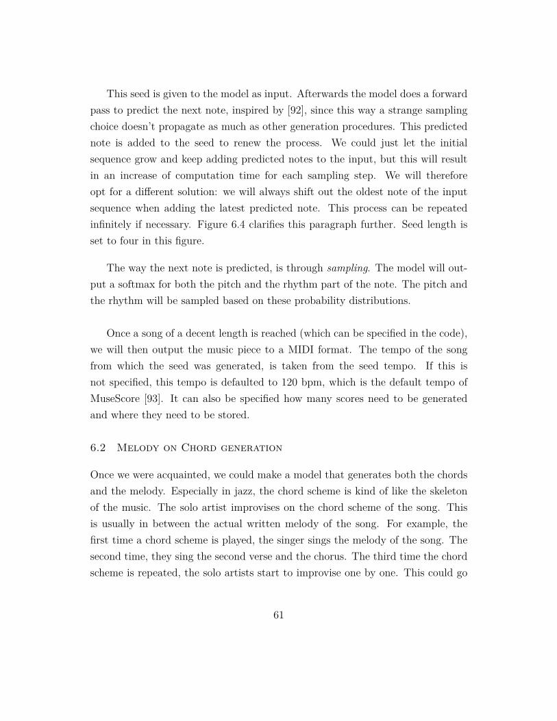
This seed is given to the model as input. Afterwards the model does a forwardpass to predict the next note, inspired by [92], since this way a strange samplingchoice doesn’t propagate as much as other generation procedures. This predictednote is added to the seed to renew the process. We could just let the initialsequence grow and keep adding predicted notes to the input, but this will resultin an increase of computation time for each sampling step. We will thereforeopt for a different solution: we will always shift out the oldest note of the inputsequence when adding the latest predicted note. This process can be repeatedinfinitely if necessary. Figure 6.4 clarifies this paragraph further. Seed length isset to four in this figure.

The way the next note is predicted, is through sampling. The model will out-put a softmax for both the pitch and the rhythm part of the note. The pitch andthe rhythm will be sampled based on these probability distributions.

Once a song of a decent length is reached (which can be specified in the code),we will then output the music piece to a MIDI format. The tempo of the songfrom which the seed was generated, is taken from the seed tempo. If this isnot specified, this tempo is defaulted to 120 bpm, which is the default tempo ofMuseScore [93]. It can also be specified how many scores need to be generatedand where they need to be stored.

6.2 Melody on Chord generation

Once we were acquainted, we could make a model that generates both the chordsand the melody. Especially in jazz, the chord scheme is kind of like the skeletonof the music. The solo artist improvises on the chord scheme of the song. Thisis usually in between the actual written melody of the song. For example, thefirst time a chord scheme is played, the singer sings the melody of the song. Thesecond time, they sing the second verse and the chorus. The third time the chordscheme is repeated, the solo artists start to improvise one by one. This could go

61

Figure 6.4: Generation procedure of the first simple melody generation model with seedlength equal to 4

on for as many chord schemes as they want. They usually end by repeating theinitial melody.

In pop music, this is less the case, but even then, chords usually have a repeatedstructure.

When approaching this problem, we wanted to first build this backbone, beforehandling the melody and the lyrics. In this master dissertation, there were twopossibilities of modeling this that we have considered.

The first option is to generate a new chord scheme, just as in the training data.

62

A chord, similarly to a note in the simple melody generation model in Section 6.1,has a pitch and a duration. This pitch consists of a root letter (A,B,C,D,E,F orG), an alter (e.g. ♯) and a mode (e.g. Major, Minor). Similarly to the simplemelody model in 6.1, we could generate a chord scheme. Once a chord schemeis generated, then we can generate the melody on this generated chord scheme.There are two difficulties that arise when using this as a model.

Firstly, many melody notes are usually played on the same chord. Therefore,if we want to generate melody notes on the generated chord scheme, we don’treally know how many melody notes we should generate per chord. Should it bea dense or fast piece, or should we only play one note on the chord?

The second difficulty is to make sure that the duration of the different melodynotes from the same chord sum up to the duration of the chord. If, for example,the model decides that four quarter notes should be played on a half note chord,this is a problem.

In light of these two difficulties, we have opted for option two: combining theduration of the notes with the chords. As can be seen by Figures 6.5a and 6.5b,we repeat the chord for each note where it should be played, so the duration ofthe chord becomes the duration of the note.

If we generate a chord scheme where the duration of the chord is equal to theduration of the melody note, we know that each chord needs to have exactly onemelody note. This solves the two difficulties mentioned above.

With this in mind, we actually divide our problem into two subproblems:

1. The generation of chords, combined with the rhythm of the melody notes.

2. The generation of melody pitches on a provided chord scheme.

In Section 6.2A and 6.2B, these two problems are further explained.

A Chords, with note duration

As described previously in Section 5.2.6, a chord has a root, an alter, a mode anda rhythm or duration. We limit the options for those four elements, as seen in

63

(a) Original chord scheme

(b) Repeated chord structure. The chord is repeated for each note so the duration of the chordbecomes the duration of the note

Figure 6.5: Some Old Blues - John Coltrane: the original and adapted chord structure

Table 6.1.

Root [A, B, C, D, E, F, G] 7 elements, no changes

Alter [♮ or 0, ♯ or 1] 2 elements, change ♭♭ and ♭to one of the two

Mode [Maj, Min, Dim and Aug]4 elements, the 43 othermodes were replaced by oneof these four

Rhythm [ ˇ “* , ˇ “* ‰ , ˇ “) ,3

ˇ “

==

, ˇ “( ,3

ˇ “ , ˇ “( ‰ ,ˇ “, ˇ “‰ , ˘ “, ˘ “‰ , ¯ ]

12 elements, scores withless occurring rhythm typeswere deleted

Table 6.1: The options for root, alter, mode and rhythm in a chord

Since we match the duration of the chord to the duration of the note in anotherpreprocessing step, we can model the prediction of the next chord similarly to thesimple melody generation problem in Section 6.1. The next chord is based on theprevious time_steps chords:

64

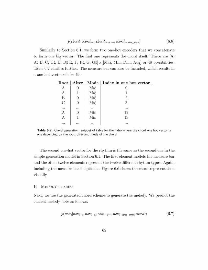
p(chordi|chordi−1, chordi−2, ..., chordi−time_steps) (6.6)

Similarly to Section 6.1, we form two one-hot encoders that we concatenateto form one big vector. The first one represents the chord itself. There are [A,A♯ B, C, C♯, D, D♯ E, F, F♯, G, G♯] x [Maj, Min, Dim, Aug] or 48 possibilities.Table 6.2 clarifies further. The measure bar can also be included, which results ina one-hot vector of size 49.

Root Alter Mode Index in one hot vectorA 0 Maj 0A 1 Maj 1B 0 Maj 2C 0 Maj 3... ... ... ...A 0 Min 12A 1 Min 13... ... ... ...

Table 6.2: Chord generation: snippet of table for the index where the chord one hot vector isone depending on the root, alter and mode of the chord

The second one-hot vector for the rhythm is the same as the second one in thesimple generation model in Section 6.1. The first element models the measure barand the other twelve elements represent the twelve different rhythm types. Again,including the measure bar is optional. Figure 6.6 shows the chord representationvisually.

B Melody pitches

Next, we use the generated chord scheme to generate the melody. We predict thecurrent melody note as follows:

p(notei|notei−1, notei−2, notei−3..., notei−time_steps, chords) (6.7)

65

Figure 6.6: Two one-hot encoder vectors representing the chord itself and the duration ofthe chord concatenated in the chord generation problem. Measure bars representations areincluded in this figure.

So we predict the following notes based on time_steps previous notes and allthe chords of the music piece, or all the chords of the previously generated chordscheme.

The representation of the note looks similar to the one previously discussed.The only addition is the start token. The use of this will be further explained inSection 6.2.1. Figure 6.7 shows the current representation.

6.2.1 Machine Learning Details

The research on lead sheet generation of modern music have been mostly limitedto Markov models. We wanted to use RNNs in this master dissertation to gaina new perspective on lead sheet generation. Figure 6.8 shows the architecture ofthis model. In this figure, measure bars are included in the sizing. As explained inSection 6.2, we have two big components: a chord scheme generating componentand a melody generating component, based on this generated chord scheme. Theseindividual components will be further explained in the following paragraphs.

66

Figure 6.7: Melody on chord generation: representation of a note where the measure bar isincluded

The first component is the chord scheme generating component. This consistsof an input layer which will read the chords with their duration. This is followedby a number of LSTM layers, which is set to two in the figure. In this figure, theLSTM size is set to 512, but this can be adapted. The fully connected (FC) layeroutputs the chord predictions of the chord generation part of the model.

The chord scheme is used as an input for the bidirectional LSTM encoder inthe melody generation part of the model. A bidirectional RNN uses informationabout both the past and the future to generate an output. Figure 6.9 shows aBidirection RNN network, where

←−h and−→h are the hidden states of the backward

and forward RNN layer [94]. If Wx,y represent the weight matrices, then the outputgets computed as such:

−→h t = sigmoid(Wx,−→h · xt +W−→h ,−→h ·−→h t+1 + b−→h ) (6.8)

←−h t = sigmoid(Wx,←−h · xt +W←−h ,←−h ·←−h t+1 + b←−h ) (6.9)

67

Figure 6.8: Architecture of the melody on chord generation model where measure bars areincluded

yt = W−→h ,y ·−→h t +W←−h ,y ·

←−h t + by (6.10)

When we replace the RNN cell by a LSTM cell, we get a bidirectional LSTM.By using this as an encoder, we get information about the previous, current andfuture chords. This information can be used together with the previous melodynotes when we generate a note, so the prediction looks ahead at how the chordscheme is going to progress and looks back at both the chord scheme and themelody.

Again, 512 is used as a dimension for the LSTMs but this can be adapted.Multiple layers of LSTMs in both directions are possible.

In our architecture, there is exactly one melody note per chord. Therefore wecan adapt the regular encoder-decoder architecture (see Section 3.2.3) to Figure6.10. The encoder is a Bi-LSTM so there are arrows in both ways, which resultsin each hidden state having information about the entire chord scheme. Then the

68

Figure 6.9: Bidirection RNN [94]

< start > token is concatenated to the first chord, which is given to the decoderas input. This < start > token is used to kickstart the melody generation process.This is inspired on the start token often used in sequence-to-sequence models, suchas translation [47]. The following process is similar to the one above. The decoderitself is composed of a number of LSTM layers, followed by a fully connected layerthat predicts the note. Therefore we predict the note based on information aboutthe entire chord scheme and the previous notes.

Again, since there are two components of the model, there are also two lossfunctions. For the first component, the chord scheme generating component,we have very similar loss functions to the melody generation model in Section6.1. Again, there is a loss function for both components: the chord itself andthe rhythm. The model outputs the softmax for each element. Afterwards, weperform cross entropy on the targets and the predictions.

69

Figure 6.10: Melody on chord generation: our Encoder-Decoder architecture

LCE,chord(ychord,i, ychord,i) = −48∑j=0

y(j)chord,i,0:48 · log(y(j)chord,i,0:48) (6.11)

LCE,rhythm(ychord,i, ychord,i) = −12∑j=0

y(j)chord,i,49:61 · log(y(j)chord,i,48:61) (6.12)

where i represents the time step at which we are calculating the loss and (j) isthe jth of the vector. The total loss is a combination of the two (α ∈ [0, 1]):

L(ychord,i, ychord,i) = α ·LCE,chord(ychord,i, ychord,i)+ (1− α) ·LCE,rhythm(ychord,i, ychord,i) (6.13)


70

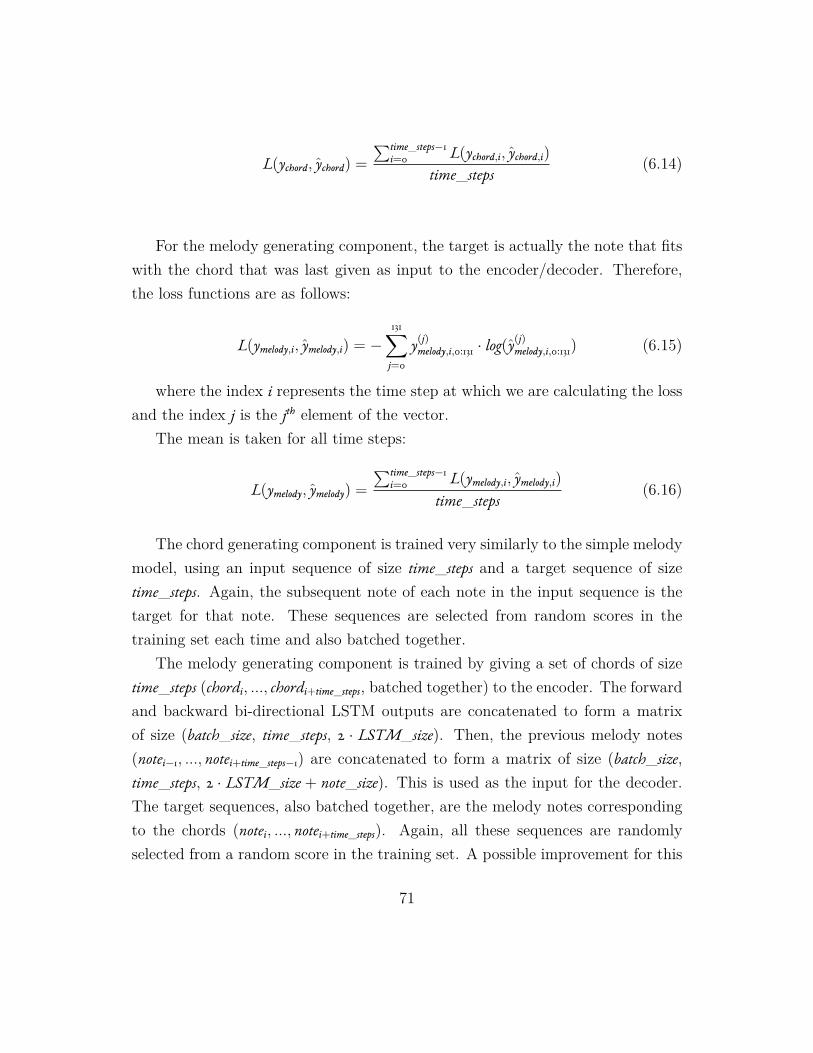
L(ychord, ychord) =∑time_steps−1

i=0 L(ychord,i, ychord,i)time_steps (6.14)

For the melody generating component, the target is actually the note that fitswith the chord that was last given as input to the encoder/decoder. Therefore,the loss functions are as follows:

L(ymelody,i, ymelody,i) = −131∑j=0

y(j)melody,i,0:131 · log(y(j)melody,i,0:131) (6.15)

where the index i represents the time step at which we are calculating the lossand the index j is the jth element of the vector.


L(ymelody, ymelody) =

∑time_steps−1i=0 L(ymelody,i, ymelody,i)

time_steps (6.16)

The chord generating component is trained very similarly to the simple melodymodel, using an input sequence of size time_steps and a target sequence of sizetime_steps. Again, the subsequent note of each note in the input sequence is thetarget for that note. These sequences are selected from random scores in thetraining set each time and also batched together.

The melody generating component is trained by giving a set of chords of sizetime_steps (chordi, ..., chordi+time_steps, batched together) to the encoder. The forwardand backward bi-directional LSTM outputs are concatenated to form a matrixof size (batch_size, time_steps, 2 · LSTM_size). Then, the previous melody notes(notei−1, ..., notei+time_steps−1) are concatenated to form a matrix of size (batch_size,time_steps, 2 · LSTM_size + note_size). This is used as the input for the decoder.The target sequences, also batched together, are the melody notes correspondingto the chords (notei, ..., notei+time_steps). Again, all these sequences are randomlyselected from a random score in the training set. A possible improvement for this

71

is to actually use the entire chord scheme in training as well. This wasn’t testeddue to timing constraints.

The generation of the chord generating component is very similar to the simplemelody model. We use an initial seed with a chosen length to kickstart thegeneration. In this case, we use a seed length of time_steps. A forward pass willpredict the next note and is added each time, shifting out the oldest note. Wewill also sample the next chord and its rhythm.

The generation process of the melody generating component runs the entirechord scheme through the encoder first. This chord scheme can be selected bythe user. We will take the start token and concatenate the corresponding encoderoutput and put this through the decoder. We sample the next note and add thisto the input note sequence, after the start token. Once the input note sequencereaches size time_steps, we will keep shifting out the oldest note, in order to reducecomputation time. This continues until each chord has a corresponding melodynote.

72

“I’m not frightened by the advent of intelligentmachines. It’s the sarcastic ones I worry about.”

Quentin R. Bufogle

7Implementation and Results

7.1 Experiment Details

To implement the models that were described in Section 6, we use the open-sourcelibrary TensorFlow [95]. More specifically, Python 3.6 was used with TensorFlow1.4.0. TensorFlow lets the programmer run computations on both CPU and GPU.The number of GPUs or CPUs used can also be specified. TensorBoard, a visual-ization tool for data, is included in TensorFlow [96] and is also used in this masterdissertation to represent the training and validation losses.

Two music tools were used in this master dissertation: MidiUtil and Mus-eScore. MidiUtil is a Python library that makes it easier to write MIDI files fromwithin a Python program [97]. This was used to write the generated music piecesto MIDI files that will be discussed in the following sections.

MuseScore is a free music notation program which we used to visualize the

73

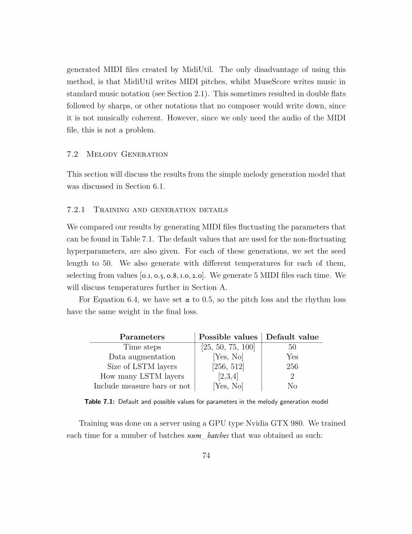
generated MIDI files created by MidiUtil. The only disadvantage of using thismethod, is that MidiUtil writes MIDI pitches, whilst MuseScore writes music instandard music notation (see Section 2.1). This sometimes resulted in double flatsfollowed by sharps, or other notations that no composer would write down, sinceit is not musically coherent. However, since we only need the audio of the MIDIfile, this is not a problem.

7.2 Melody Generation

This section will discuss the results from the simple melody generation model thatwas discussed in Section 6.1.

7.2.1 Training and generation details

We compared our results by generating MIDI files fluctuating the parameters thatcan be found in Table 7.1. The default values that are used for the non-fluctuatinghyperparameters, are also given. For each of these generations, we set the seedlength to 50. We also generate with different temperatures for each of them,selecting from values [0.1, 0.5, 0.8, 1.0, 2.0]. We generate 5 MIDI files each time. Wewill discuss temperatures further in Section A.

For Equation 6.4, we have set α to 0.5, so the pitch loss and the rhythm losshave the same weight in the final loss.

Parameters Possible values Default valueTime steps [25, 50, 75, 100] 50

Data augmentation [Yes, No] YesSize of LSTM layers [256, 512] 256

How many LSTM layers [2,3,4] 2Include measure bars or not [Yes, No] No

Table 7.1: Default and possible values for parameters in the melody generation model

Training was done on a server using a GPU type Nvidia GTX 980. We trainedeach time for a number of batches num_batches that was obtained as such:

74

1. First, we see how many sequences of length time_steps there are in each score

2. We add all these numbers up to find how many sequences of length time_stepsthere are in all the scores

3. We divide that number by the batch_size

Training lasted about 7 hours for each combination of parameters, except forthe one where the training dataset wasn’t augmented. Then it only lasted about35 min. We only had 9 unique combinations of the parameters, because we useddefaults that were already present in the values that we were testing. Thereforethe whole training time was about:

Training_time = 8 · 7h+ 1 · 35min = 56h35min (7.1)

Generation lasts about 1h30min for each combination of parameters, includingthe temperatures. So the total generation time was about:

Generation_time = 9 · 1h30min = 13h30min (7.2)

7.2.2 Subjective comparison and Loss curves of MIDI output files

In this section, we will compare the different hyperparameter values that werediscussed previously for the simple melody generation model. We will discusstheir loss curves and also give a subjective listening comparison.

A Temperature

The softmax from Equation 3.5 can be redefined by including temperature τ asfollows:

f(x)i =exp(xi/τ)∑kj=0 exp(xj/τ)

(7.3)

75

This temperature can tweak the desire for randomness in the generated musicpiece, whilst still holding on to some certainty in the piece. With lower temper-atures (close to zero), the pitch with the highest confidence will almost alwaysbe picked. The higher the temperature, the more room exists for freedom andrandomness in the piece. Therefore, it can be interesting to see how the musicpieces evolve when the temperature is changed.

These statements can also be seen from the results that were generated. Theexamples below use the default values of the parameters listen in Table 7.1, exceptthat the temperature was changed. These were also generated when the validationloss value was at its minimum. The recordings for each temperature can be foundon https://tinyurl.com/ycgqmzs9 with filenames temp_«insert the tempera-ture here».mp3. The seed size was set to the same value as the time steps (50),so the actual generation only starts after about 30 seconds. The same seed wasused for each of the examples, so the comparison was easier to make. The seedwas taken from one of the files that were not included in the training set. It canbe clearly seen from e.g. temp_0.1.mp3 that it only generates a melody note G,whilst temp_5.mp3 generates very randomly. Temperature 0.9 or 1 are preferred.From now on, we will use temperature 1 to generate the examples.

The MIDI files were also included with filenames temp_«insert the temperaturehere».mid. If you open these with MuseScore, it can occur that a weird notationis used (see Figure 7.1). Flats suddenly followed by sharps isn’t easily readablefor composers or musicians. MuseScore just takes the MIDI pitch of the note andconverts it to a notation (flat, neutral or sharp) it chooses. It should be cleanedby a professional musician in order to make it readable for musicians.

B Comparison underfitting, early stopping and overfitting

To find the best results, we have to know when we should stop training the model.It is said that for a lot of classification problems the lowest validation loss givesa stopping point so the model can generalize better. But is it truly useful to stop

76

https://tinyurl.com/ycgqmzs9

Figure 7.1: The conversion of MIDI pitches to standard music notation by MuseScore

at a lowest validation loss in this case? For example, if three notes are a possiblelogical successor to the sequence of notes we already have, it doesn’t make a lot ofsense to generalize which one of the three to choose. A lower training loss modelsthe training set better, but a low validation loss doesn’t necessarily say that wepredict music better in general. Of course, we have to keep in mind that theoverfit model doesn’t copy and paste examples from the training set, so furtherresearch is required.

Figure 7.2 show the train and loss curves for the model trained with all thedefault hyperparameter values from Table 7.1. The model was trained for about151500 batches (num_batches calculated as described in Section 7.2.1). We can seethat the lowest validation loss is already achieved quite early, at batch number8900.

The listening examples can be found in https://tinyurl.com/ycp6sxza.Again the first 50 notes are the seed, which is about 30 seconds or so. After that,the generated pieces start. The underfitting example (filename underfitting.mp3or underfitting.mid) is very random and is not coherent at all. The early stopping(filename early_stopping.mp3 or early_stopping.mid) can still be very randombut has some better parts. The overfitting example (filename overfitting.mp3 oroverfitting.mid) is the best example of all three.

To know for sure if training for num_batches doesn’t just copy examples fromthe dataset, we want to find the longest common subsequent melody sequence be-tween the training files and the generated file. This was checked for five generatedexamples using the default hyperparameter values. It was checked in two ways:

77

https://tinyurl.com/ycp6sxza

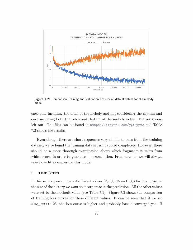
Figure 7.2: Comparison Training and Validation Loss for all default values for the melodymodel

once only including the pitch of the melody and not considering the rhythm andonce including both the pitch and rhythm of the melody notes. The rests wereleft out. The files can be found in https://tinyurl.com/y9f8yptc and Table7.2 shows the results.

Even though there are short sequences very similar to ones from the trainingdataset, we’ve found the training data set isn’t copied completely. However, thereshould be a more thorough examination about which fragments it takes fromwhich scores in order to guarantee our conclusion. From now on, we will alwaysselect overfit examples for this model.

C Time Steps

In this section, we compare 4 different values (25, 50, 75 and 100) for time_steps, orthe size of the history we want to incorporate in the prediction. All the other valueswere set to their default value (see Table 7.1). Figure 7.3 shows the comparisonof training loss curves for these different values. It can be seen that if we settime_steps to 25, the loss curve is higher and probably hasn’t converged yet. If

78

https://tinyurl.com/y9f8yptc

Method Generatedfile

Longestcommonsubse-quentse-quence(LCSS)

Original trainingfile

RatioLC-SS/lengthgener-atedscore

Onlypitch

0.mid 13 David & Max Sapp -There is a River

131020 = 0.01274

1.mid 48 Jimmy McHugh -Let’s Get Lost

48963 = 0.0498

2.mid 13

Charles Fox, Nor-man Gimbel - ReadyTo Take A ChanceAgain

13938 = 0.0138

3.mid 14Marc Bolan - Chil-dren Of The Revolu-tion

14995 = 0.01407

4.mid 14 Hurricane Smith -Oh Babe

141005 = 0.01393

Pitchanddura-tion

0.mid 10Irving Berlin- Count YourBlessings

101020 = 0.0098

1.mid 35 Jimmy McHugh -Let’s Get Lost

35963 = 0.0363

2.mid 12Robert Freeman -Do You Want ToDance

12938 = 0.0128

3.mid 8Sergio Eulogio Gon-zalez Siaba - ElCuarto de Tula

8995 = 0.00804

4.mid 12 Enrique Francini -Azabache

121005 = 0.01194

Table 7.2: The longest common subsequent melody sequence for five generated MIDI filesusing the default hyperparameter values. One time using only pitch, the other using bothpitch and duration. 79

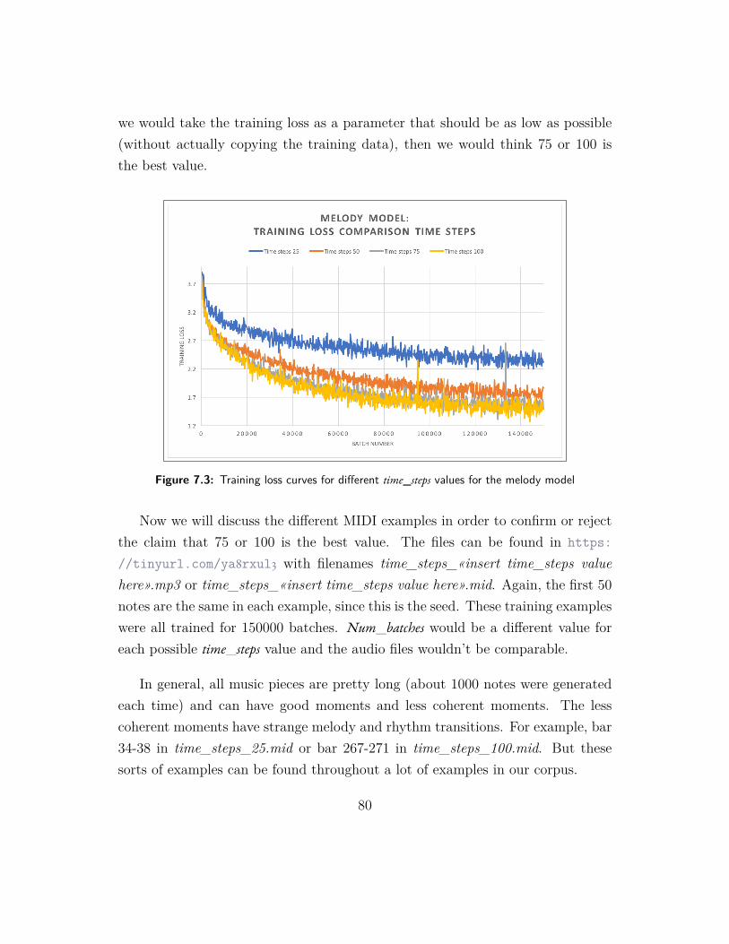
we would take the training loss as a parameter that should be as low as possible(without actually copying the training data), then we would think 75 or 100 isthe best value.

Figure 7.3: Training loss curves for different time_steps values for the melody model

Now we will discuss the different MIDI examples in order to confirm or rejectthe claim that 75 or 100 is the best value. The files can be found in https://tinyurl.com/ya8rxul3 with filenames time_steps_«insert time_steps valuehere».mp3 or time_steps_«insert time_steps value here».mid. Again, the first 50notes are the same in each example, since this is the seed. These training exampleswere all trained for 150000 batches. Num_batches would be a different value foreach possible time_steps value and the audio files wouldn’t be comparable.

In general, all music pieces are pretty long (about 1000 notes were generatedeach time) and can have good moments and less coherent moments. The lesscoherent moments have strange melody and rhythm transitions. For example, bar34-38 in time_steps_25.mid or bar 267-271 in time_steps_100.mid. But thesesorts of examples can be found throughout a lot of examples in our corpus.

80

https://tinyurl.com/ya8rxul3

https://tinyurl.com/ya8rxul3

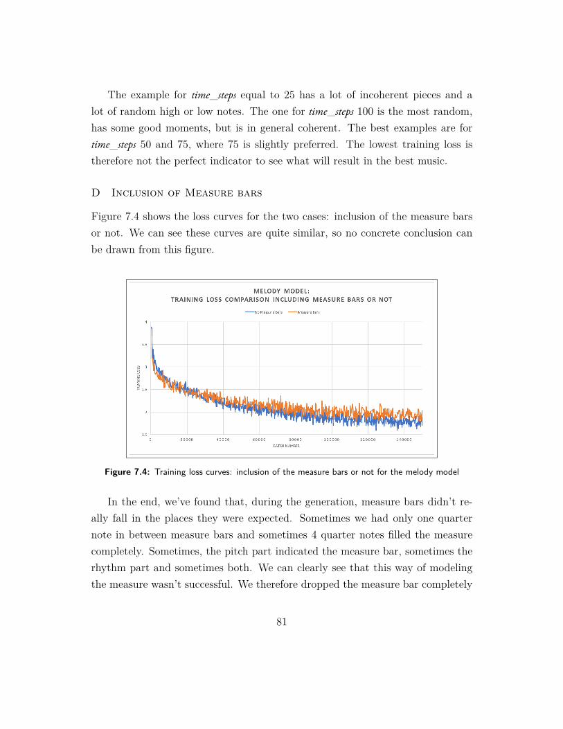
The example for time_steps equal to 25 has a lot of incoherent pieces and alot of random high or low notes. The one for time_steps 100 is the most random,has some good moments, but is in general coherent. The best examples are fortime_steps 50 and 75, where 75 is slightly preferred. The lowest training loss istherefore not the perfect indicator to see what will result in the best music.

D Inclusion of Measure bars

Figure 7.4 shows the loss curves for the two cases: inclusion of the measure barsor not. We can see these curves are quite similar, so no concrete conclusion canbe drawn from this figure.

Figure 7.4: Training loss curves: inclusion of the measure bars or not for the melody model

In the end, we’ve found that, during the generation, measure bars didn’t re-ally fall in the places they were expected. Sometimes we had only one quarternote in between measure bars and sometimes 4 quarter notes filled the measurecompletely. Sometimes, the pitch part indicated the measure bar, sometimes therhythm part and sometimes both. We can clearly see that this way of modelingthe measure wasn’t successful. We therefore dropped the measure bar completely

81

during the notation of the music piece in MIDI and excluded them for generation.Further research needs to be done on how to model measures efficiently.

E Data augmentation

In a lot of research papers, as was seen in Section 4.2, the training data is aug-mented in order to expand the music pieces to all possible keys. The same wasdone for this master dissertation. Figure 7.5 shows the training loss curves whiledata augmenting the training data or not. It can be seen that without data aug-mentation the training loss converges more quickly, as was expected, since lessdata is available.

Figure 7.5: Training loss curves using data augmentation or not

The files can be found in https://tinyurl.com/yca4krn3. The files withfilenames data_aug.mid/mp3 and no_data_aug.mid/mp3 are trained for the samenumber of batches, namely the num_batches for the data augmentation model. Asa reminder, the procedure to find num_batches can be found in Section 7.2.1.

Since we train the models for the same number of batches and without dataaugmentation there is a lot less training data available, that means it is also more

82

https://tinyurl.com/yca4krn3

likely for the example without data augmentation to be stealing examples fromthe training data set. This is, of course, not favorable.

Therefore we want to compare it to an example for which the model withoutdata augmentation was only trained for its own num_batches. This example canbe found in no_data_aug_stop_at_lowest_validation_loss.mid/mp3. This pieceis a lot more random than the data augmentation one. Only if the dataset couldbe expanded with a lot more files in a lot of different scales, the model withoutdata augmentation could be favorable. In our case, the data augmented versionis favored.

F LSTM size

Figure 7.6 shows the training loss curves for different LSTM size values. We canclearly see that an LSTM size of 512 generates a much lower training loss. Wecould state that this is better, but this would be a premature conclusion. Wewould have to compare generated examples.

Figure 7.6: Training loss curves for different LSTM size values for the melody model

The files can be found in https://tinyurl.com/y9tkrp8d with filenameslstm_size_«insert lstm size value here».mp3 or lstm_size_«insert lstm size value

83

https://tinyurl.com/y9tkrp8d

here».mid. Even though it is very hard to hear a distinct difference between thetwo sizes, we do prefer the size 512 since the melody is a bit more coherent anddynamic. However, the model with LSTM size 256 also generates a good melody.

G Number of LSTM Layers

Figure 7.7 shows the training loss curves where the number of LSTM layers wasadapted. The lowest training losses can be found with four LSTM layers, closelyfollowed by three LSTM layers. Two LSTM layers generate a higher loss curve.

Figure 7.7: Training loss curves: compare number of LSTM layers for the melody model

The files can be found in https://tinyurl.com/yaam5479 with filenameslstm_layers_«insert number of lstm layers here».mp3 or lstm_layers_«insertnumber of lstm layers here».mid. Even though it wasn’t expected, the exampleswith four LSTM layers generate more random rhythms (this was noticed over fivefiles with five different seeds). Two or three LSTM layers were quite similar.

7.2.3 Conclusion

This simple model gave us a basic understanding of the problem ahead, and alsoprovided us with good examples and inspiration.

84

https://tinyurl.com/yaam5479

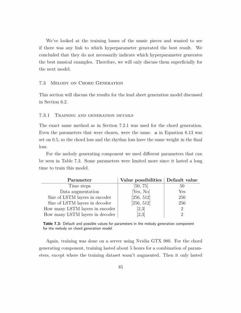
We’ve looked at the training losses of the music pieces and wanted to seeif there was any link to which hyperparameter generated the best result. Weconcluded that they do not necessarily indicate which hyperparameter generatesthe best musical examples. Therefore, we will only discuss them superficially forthe next model.

7.3 Melody on Chord Generation

This section will discuss the results for the lead sheet generation model discussedin Section 6.2.

7.3.1 Training and generation details

The exact same method as in Section 7.2.1 was used for the chord generation.Even the parameters that were chosen, were the same. α in Equation 6.13 wasset on 0.5, so the chord loss and the rhythm loss have the same weight in the finalloss.

For the melody generating component we used different parameters that canbe seen in Table 7.3. Some parameters were limited more since it lasted a longtime to train this model.

Parameter Value possibilities Default valueTime steps [50, 75] 50

Data augmentation [Yes, No] YesSize of LSTM layers in encoder [256, 512] 256Size of LSTM layers in decoder [256, 512] 256

How many LSTM layers in encoder [2,3] 2How many LSTM layers in decoder [2,3] 2

Table 7.3: Default and possible values for parameters in the melody generation componentfor the melody on chord generation model

Again, training was done on a server using Nvidia GTX 980. For the chordgenerating component, training lasted about 5 hours for a combination of param-eters, except where the training dataset wasn’t augmented. Then it only lasted

85

about 25 minutes. For the melody generating component, training lasted about16h30min for each combination of parameters with data augmentation. Withoutdata augmentation, training was about 1h20min.

Training_time(chord) = 8 · 5h+ 1 · 25min = 40h25min (7.4)

Training_time(melody) = 6 · 16h30+ 1 · 1h20min = 100h20min (7.5)

These two components could be trained in parallel.

7.3.2 Subjective comparison of MIDI files

Since we’ve seen in the melody model that it was very hard to compare the piecesbased on the hyperparameter, we will only compare certain aspects this time. Wewill still compare the lowest validation model to the overfitting one, since thiscould be relevant to see if we would copy certain aspects of the training datasetif we use the overfitted examples. We will not discuss the loss curves of the otherhyperparameters however. We will provide both good and bad examples from thedataset and give some intermediate conclusions.

A Comparison underfitting, early stopping and overfitting

First of all, even though the chord generating component has very similar ar-chitecture to the melody generating component, the loss curves do look ratherdifferent (see Figures 7.8a and 7.8b). The chord generating component’s valida-tion curve still keeps going down, long after the simple melody model’s validationcurve does. No direct conclusion from this can be made, since we don’t know if alower validation loss actually makes the generation any better. More examinationneeds to be made.

The files can be found in https://tinyurl.com/y9wk7r7t. Two examples aregiven for both overfitting and lowest validation, all with the same seed. Because ofthis seed, the MIDI and mp3 files differ only after about 30 seconds. Overfittingis preferred again, similarly to the melody model. However, we’ve found that

86

https://tinyurl.com/y9wk7r7t

(a) Simple melody generationmodel

(b) Chord generating componentof melody on chord model

(c) Melody generating componentof melody on chord model

Figure 7.8: Comparison Training and Validation Loss for all default values

87

there was more copying of the training dataset in the overfitting parts, and thatthe lowest validation also generated good results. We will therefore continue withexamples where the model was trained until the point of lowest validation, forboth the chord generating component and the melody generating component.

B Examples and intermediate conclusions

To give a more well-rounded discussion about the generated pieces, we wanted todiscuss the best and worst examples. They can be found in https://tinyurl.com/y7tmnnah. We generated long pieces where both the chord scheme andmelody models were trained until their lowest validation point. We took thebest and worst examples of five pieces, tied the chords and sometimes playedthe chords an octave lower in order to hear the melody better. We named thembest_«i».mid/mp3 and worst_«i».mid/mp3. If the index i is the same, that meansit came from the same piece. The files original_«i».mid/mp3 show the originalfiles they were taken from. These files were grouped together in folders Piece «i».

For the best parts, we found in a lot of pieces at least one fragment of 20or 30 seconds that was considered ‘good’. To find longer fragments, we had tosearch more, since usually one bad harmonic move made the fragment audiblygenerated. However, the parts we’ve found were melodically coherent. Most ofthe good examples are of a slow nature, except for the one from piece 5. In thisexample, you can also hear best that there is no real sense of measure in (mostof) the generated pieces. More on the good outputs and their promising resultscan be found in the survey (Section 7.3.3).

For the worst parts, some were amelodic in the melody (such as the worstexample from piece 1), some were mostly bad in terms of rhythm (such as theworst example from piece 3) and some were both (such as the worst example frompiece 2). For most pieces, it was easier to find the worst fragments, except forpiece 4. This was probably mostly because there was a better ‘base’, the chordscheme.

In general, we have confirmed the claim of Waite in [98] that the music made

88

https://tinyurl.com/y7tmnnah

https://tinyurl.com/y7tmnnah

by RNNs lacks a sense of direction and become boring. Even though the modelproduces musically coherent fragments sometimes, a lot of the time you couldn’trecognize that two melodies chosen from the same piece are in fact from the samepiece.

Also, even though our pieces have some good fragments, they usually haveat least one portion which doesn’t sound musical at all once we start generatinglonger pieces. This was confirmed by the examples above. This could possibly befixed with a larger dataset, by training longer or letting an expert in music filterout these fragments.

7.3.3 Survey

A survey was conducted in order to see how our computer-generated pieces com-pare to real human-composed pieces. This was done by asking the participant aset of questions for each piece in Google Form format. There were 177 participantsfor this particular online survey. For each chord in a piece, it was played in itsroot position1. To make it easier on the ears, some chords were tied together, sincethe output of the model repeats each chord for each note. Figure 7.9 clarifies.

The pieces were exported to mp3 in MuseScore, in order to eliminate anyhuman nuances that could hint to the real nature of the piece. Then, for eachpiece, a fragment of 30 seconds was chosen.

We wanted to establish what background the participant of the survey hadin music. When asked about their music experience, where they could choosebetween experienced musician, amateur musician or listener. This was followedby three questions for each audio fragment:

1. Do you recognize this audio fragment?Answers: yes or no

2. How do you like this audio fragment?Answer: They could answer on a scale from 1 to 5 where 1 represented

1https://en.wikipedia.org/wiki/Inversion_(music)

89

(a) The initial MIDI file with no ties

(b) The MIDI file after the notes were tied together

Figure 7.9: A step in preparing the MIDI files for the survey

complete dislike and 5 represented love

3. Is this audio fragment made by a computer or a human? Beware: the musicis played by a computer. We only want to know if you think the music itselfis composed by a human or a computer.Answer: They could answer on a scale from 1 to 5 where 1 represented’definitely a human’ and 5 represented ’definitely a computer’

In the survey, there were three categories of music pieces: human-composedpieces, completely computer-generated pieces and pieces where the melody wasgenerated on an actual human-composed chord scheme. For each of these cat-egories, three audio fragments were included in the survey. For the human-composed pieces, we tried to select audio fragments that weren’t too popular

90

with the public, so not like e.g. Village People - Y.M.C.A. For the generatedpieces, we selected fragments that were completely generated, which means thatwe only started listening after the seed of 50 notes in the chord scheme. The gen-erated pieces were taken from the default value hyperparameters, only traininguntil lowest validation.

The files that were used in the survey can be found in https://tinyurl.com/y8qpvu92 and Table 7.4 shows their (potential) origin and category. The pieces andthe answers can also be found in https://youtu.be/Qayllb1EZKU. The origin forthe partially generated files is the chord scheme on which the melody was based.The human-composed scores show as origin the original name of the song in theWikifonia dataset.

In order to make sure that these files weren’t copied, we wanted to see if amelody or chord scheme was copied at all from the training dataset. This is againdone by finding the Longest Common Subsequent Sequence (LCSS). Of course,we expect full copies for the chord scheme for the files 3.mid, 6.mid and 8.midsince they use that chord scheme. The results can be found in Table 7.5. TheLCSSs for the chords are longer than the melodies since it is much more likely forexample to have many of the same chords (e.g. C major) after each other thanmelody notes. For example, 7.mid’s LCSS for only chord has 111 times the samechord (F# Major), followed by four B major chords.

For each piece, at least 2.3% of the participants noted that they recognized thefragment, with a record of 12.4% for 3.mid. Table 7.6 shows all the percentages.The reason this could be a high percentage for 3.mid is because the chord schemecould be more recognizable, since Elton John is quite a popular artist. However,the melody is not taken from the dataset (see Table 7.5).

In general, there was some sort of correlation in how much a person liked theaudio piece and how much they think it is composed by a human if we disregardthe neutral answers. If the highest percentage of people didn’t like an audiofragment, they were more likely to give it a ‘computer’ stamp, even if it was made

91

https://tinyurl.com/y8qpvu92

https://tinyurl.com/y8qpvu92

https://youtu.be/Qayllb1EZKU

File CategoryIf (partially) human, realname of chord scheme orpiece

1.mid Human-composed piecesBurton Lane, Ralph Freed - HowAbout You (Arr: Wim Alderd-ing)

2.mid Generated pieces N/A

3.mid Generated melody,human chord scheme

Bernie Taupin, Elton John -Crocodile Rock

4.mid Human-composed pieces Marr Morrissey - How soon is now

5.mid Human-composed pieces Maud Nugent - Sweet RosieO’Grady

6.mid Generated melody,human chord scheme Diane Warren - There You’ll Be


8.mid Generated melody,human chord scheme Frank Mills - The Happy Song


Table 7.4: The pieces that were included in the survey, with their category and potentialorigin

92

MethodGeneratedfile LCSS Original training

file

RatioLC-SS/lengthgener-atedscore

Onlymelodypitch

2.mid 14 Coldplay - Cemeteriesof London

141050 = 0.01333

3.mid 19 Neil Diamond - Iam....I said

19550 = 0.03454

6.mid 14Maria Grever, StanleyAdams - What a Dif-ference a Day Makes

14454 = 0.03083

7.mid 21 Street, Morrissey -SUEDEHEAD

211050 = 0.02

8.mid 14 Giosy Cento - ViaggioNella Vita

14409 = 0.0342

9.mid 29 Bobby Timmons, JonHendricks - Moanin’

291050 = 0.0276

Onlychord

2.mid 63 Peter Gabriel - Steam 631050 = 0.06

3.mid 550 Bernie Taupin, EltonJohn - Crocodile Rock

550550 = 1

6.mid 454 Diane Warren - ThereYou’ll Be

454454 =1

7.mid 115 Paul Peterson - SheCan’t Find Her Keys

1151050 = 0.1095

8.mid 409 Frank Mills - TheHappy Song

409409 = 1

9.mid 54 Jerry Leiber, MikeStoller - Lucky lips

541050 = 0.05142

Table 7.5: The Longest Common Subsequent Sequence (LCSS) for (partially) generatedMIDI files in the survey. One time using only pitch and one time using only chords. A fullcopy is expected for the ‘only chord’ one for files 3.mid, 6.mid and 8.mid.

93

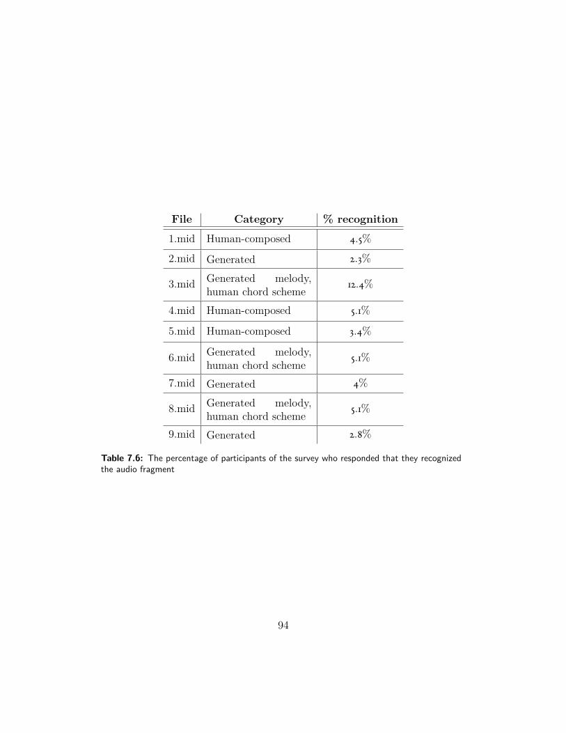
File Category % recognition1.mid Human-composed 4.5%

2.mid Generated 2.3%

3.mid Generated melody,human chord scheme 12.4%

4.mid Human-composed 5.1%

5.mid Human-composed 3.4%


7.mid Generated 4%


9.mid Generated 2.8%

Table 7.6: The percentage of participants of the survey who responded that they recognizedthe audio fragment

94

by a human. This can also be seen in Tables 7.7 and 7.8. Only 6.mid was anexception to this observation. This observation makes sense, since most peopleassociate human-composed music to be more easy on the ears, whilst assumingcomputer-generated music to be more random and ‘unlikeable’. This correlationcan also be seen in Figure 7.10. In this figure, the mean likeability (values fromone to five) and the mean of how much the people think the piece is computergenerated (values from one to five) was taken and plotted against each other. Acorrelation with r2 = 0.82051 was found. We now want to test the significance ofthis correlation. We want to do this through a hypothesis test [99, 100]. Theseare our hypotheses:

Figure 7.10: Survey responses: correlation between mean likeability and how much the par-ticipants of the survey think it is computer generated

1. Null Hypothesis H0: The correlation coefficient is not significantly dif-ferent from zero. There is not a significant linear relationship (correlation)between the mean likeability and the mean perception of the piece is beingcomputer generated.

2. Alternate Hypothesis Ha: The population correlation coefficient is signif-

95

icantly different from zero. There is a significant linear relationship (corre-lation) between the mean likeability and the mean perception of computer-generated content.

Our degrees of freedom are n− 2 = 9− 2 = 7, where 9 is the number of piecesn. We set the level of significance to 0.05. We know our r2 = 0.82051 so our r is0.90582. We perform a one-tailed test, so we find the critical t value to be 1.895from the one-tail t-distribution table2. We observe:

t = r√

n− 21− r2 = 5.6568 (7.6)

This t value is larger than our critical t value so our Null Hypothesis can berejected. There is therefore a significant relationship between the mean likeabilityand the mean perception of computer-generated content.

File Category % dislike % neutral % like1.mid Human-composed 39.5% 39.5% 20.9%

2.mid Generated 20.9% 32.2% 46.8%

3.mid Generated melody,human chord scheme 14.1% 28.2% 57.6%

4.mid Human-composed 17.5% 27.1% 55.3%



7.mid Generated 28.2% 38.9% 32.7%


9.mid Generated 50.8% 35.0% 14.1%

Table 7.7: How much the participants responded they liked or disliked a piecet

2http://www.statisticshowto.com/tables/t-distribution-table/

96

File Category % human % neutral % computer1.mid Human-composed 20.3% 12.4% 67.2%

2.mid Generated 38.9% 28.2% 32.7%





7.mid Generated 48.5% 20.9% 30.5%


9.mid Generated 20.9% 19.7% 59.3%

Table 7.8: The participants’ answer to the question if the fragment was computer-generatedor human-composed

97

We will perform a bootstrap hypothesis in order to determine if the com-puter generated pieces were perceived as more human than the real pieces. Weconcluded that the computer-generated pieces were perceived at least as humanas the human pieces and outperforming them even. This was significant withp = 8 · 10−6. We have considered the fact that perhaps the first example, whichwas human, influenced the answers. This could be the case since the pieces wereplayed by MuseScore, which sounded more computer generated. The listenersperhaps needed to adapt to the sound first. We performed a bootstrap hypothesistest, comparing the first example and the second example, and the second exam-ple was perceived more human than the first with p = 0.0. We therefore wantedto repeat the first bootstrap test, without the first human example. Even then,our results were significant, with p = 0.0026. We could therefore conclude thatthe computer generated pieces were perceived to be as human or more than thereal human pieces. The partially computer-generated examples outperformed thecomputer-generated pieces (p = 1.2 · 10−5).

Figure 7.11: Survey responses: number of correct answers out of six per music experiencecategory

We now wanted to see if the experienced or amateur musicians estimate better

98

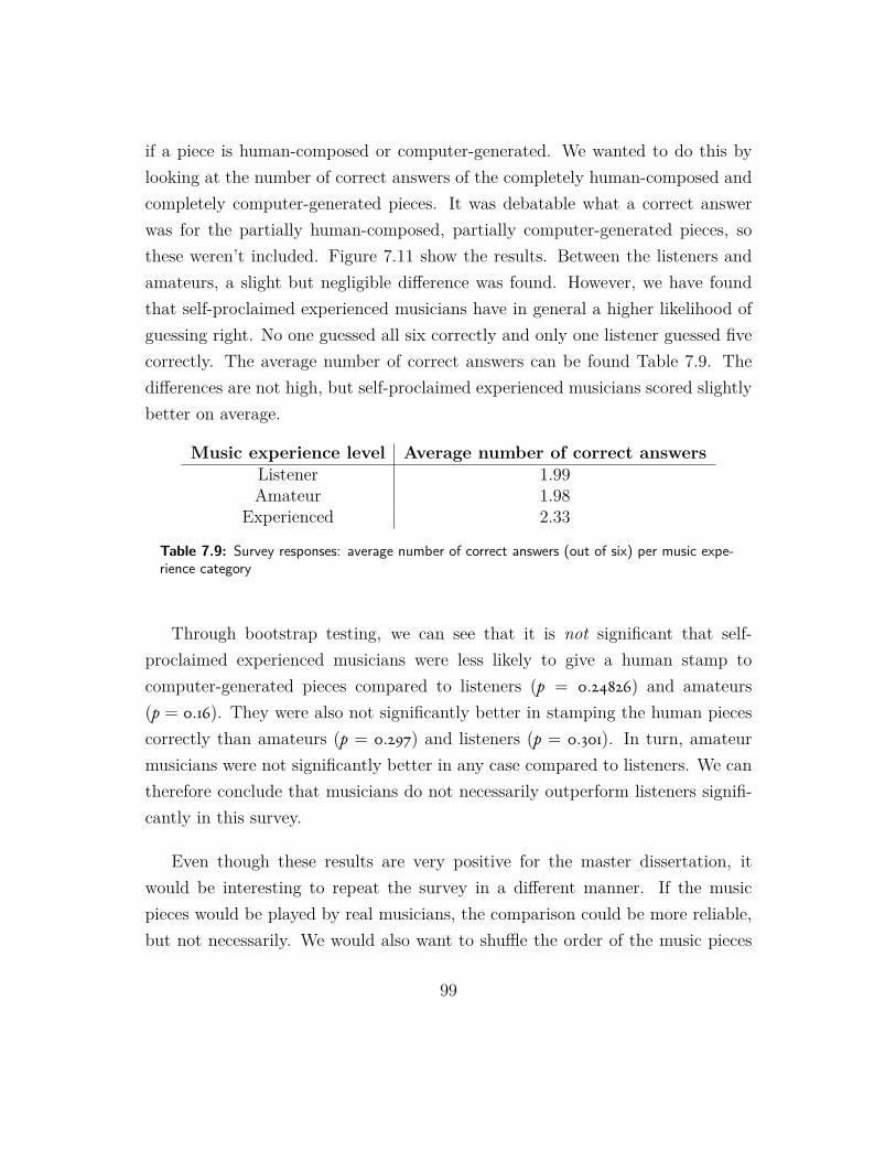
if a piece is human-composed or computer-generated. We wanted to do this bylooking at the number of correct answers of the completely human-composed andcompletely computer-generated pieces. It was debatable what a correct answerwas for the partially human-composed, partially computer-generated pieces, sothese weren’t included. Figure 7.11 show the results. Between the listeners andamateurs, a slight but negligible difference was found. However, we have foundthat self-proclaimed experienced musicians have in general a higher likelihood ofguessing right. No one guessed all six correctly and only one listener guessed fivecorrectly. The average number of correct answers can be found Table 7.9. Thedifferences are not high, but self-proclaimed experienced musicians scored slightlybetter on average.

Music experience level Average number of correct answersListener 1.99Amateur 1.98

Experienced 2.33

Table 7.9: Survey responses: average number of correct answers (out of six) per music expe-rience category

Through bootstrap testing, we can see that it is not significant that self-proclaimed experienced musicians were less likely to give a human stamp tocomputer-generated pieces compared to listeners (p = 0.24826) and amateurs(p = 0.16). They were also not significantly better in stamping the human piecescorrectly than amateurs (p = 0.297) and listeners (p = 0.301). In turn, amateurmusicians were not significantly better in any case compared to listeners. We cantherefore conclude that musicians do not necessarily outperform listeners signifi-cantly in this survey.

Even though these results are very positive for the master dissertation, itwould be interesting to repeat the survey in a different manner. If the musicpieces would be played by real musicians, the comparison could be more reliable,but not necessarily. We would also want to shuffle the order of the music pieces

99

for each participant in order to guarantee that the adaption period is filteredout. Unfortunately, this was not possible with Google Forms. An extra formfield to put comments in for each piece could give us more insights in why theuser responded in a certain way. We could also include ‘bad’ computer-generatedexamples in order to see the influence it could have on the results.

7.3.4 Conclusion

The survey results are very positive. The participants couldn’t really distinguishthe computer-generated pieces from the human-composed pieces. Self-proclaimedexpert musicians and amateur musicians didn’t perform better than listeners tomusic. In general, we found a significant correlation between the mean likeabilityof a piece and the mean of how much the participants think it is human-composed.

As was said before, the pieces can still lacks a sense of direction and becomea bit boring to listen to after a while, especially if listened to in the softwareprogram MuseScore. Long-term coherence is also missing. Melodies taken fromthe same piece cannot always be linked to each other.

Even though our pieces have some good fragments, they usually have at leastone portion which doesn’t sound musical at all once we start generating longerpieces. This was confirmed by the examples above. This could possibly be fixedwith a larger dataset, by training longer or letting an expert in music filter outthese fragments. So, even though not a lot of effort was put in choosing the 30seconds fragments for the survey, it would have taken a lot longer if more extensivefragments needed to be chosen for the survey.

All pieces don’t have a sense of measure yet. This still needs to be furtherresearched.

100

“Everything in the universe has a rhythm, every-thing dances.”

Maya Angelou

8Conclusion

This master dissertation focused on generating lead sheets, specifically melodycombined with chords, in the style of the Wikifonia dataset. We’ve found that alot of lead sheet generation focused on Markov models. We therefore wanted toadapt the information of RNNs in the classical world to more modern music.

Two models were discussed: a simple melody generating model and a melodyon chord generating model. The second model first used a number of LSTMlayers and a fully connected layer to generate a chord scheme, which includedthe chord itself and also the rhythm of the melody note. After that, we used aBi-LSTM encoder to gain some information about the entire chord scheme wewant to generate the melody pitches on. This chord scheme information and theinformation about previous melody notes was used in the decoder (again a numberof LSTM layers and a fully connected layer). This second part generates the

101

melody pitches on the rhythm that was already established in the chord scheme.

In general, we have confirmed the claim of Waite in [98] that the music madeby RNNs lacks a sense of direction and become boring. Even though the modelproduces musically coherent pieces sometimes, a lot of the time you couldn’trecognize that two melodies chosen from the same piece are in fact from the samepiece.

Also, our pieces have some good fragments, but once we start generating longerpieces, they usually have at least one portion which doesn’t sound musical at all.This could possibly be fixed with a larger dataset, possible by training longer orletting an expert in music filter out these fragments.

All pieces don’t have a sense of measure yet. This still needs to be furtherresearched.

The survey results are very positive. The participants couldn’t really dis-tinguish the computer-generated pieces from the human-composed pieces. Self-proclaimed expert musicians and amateur musicians didn’t perform better thanlisteners to music. In general, we found a significant correlation between themean likeability of a piece and the mean of how much the participants think it ishuman-composed.

8.1 Further work

Three main areas of further research have been discussed. The first one is addinglyrics to the lead sheets. This can be done by working on a syllable level for thetraining dataset and adding a third component to the melody on chord model,which generates the lyrics on the melody notes. We believe the information ofthe chords can be left out in this stage, since the melody guides the words, butfurther research needs to be done.

The second part of further research is to add more structure to the lead sheets.Usually a lead sheet consists of some sort of structure, such as verse - chorus - verse

102

- chorus - bridge - chorus, as was seen in Section 2.5. This could be establishedby adding for example a similarity factor to the models discussed, such as in [84].

Thirdly, ways to represent measures could still be researched further. We havetried one way to represent measures in this master dissertation, through repre-senting measure bars, which was unsuccessful since some measures for examplewere more than full and others empty. Perhaps adding some sort of metric to seehow many notes we still need to fill up the measure could be an option.

Smaller areas of improvements can also be found:Experimentation within the melody on chord model could still be done. For

example, training the melody on chord component using the entire chord schemeinstead of only one part could improve its results. Adding lead sheets to thedataset could also lead to significant improvements. Using a GRU instead ofan LSTM could also be worth investigating, since it has been shown to outper-form the LSTM in some cases in terms of CPU time and parameter updates andgeneralization [101].

Even though these results are very positive for the survey, it would be inter-esting to repeat it differently to gain more insight. If the music pieces would beplayed by real musicians, the comparison could be more reliable, but not nec-essarily. We would also want to shuffle the order of the music pieces for eachparticipant in order to guarantee that the adaption period is filtered out. Anextra form field to put comments in for each piece could give us more insights inwhy the user responded in a certain way. We could also include ‘bad’ computer-generated examples in order to see the influence it could have on the results.

103

AChords

Figure A.1 gives both the textual as musical representation of common chords.

104

Figure A.1: Different representations for chords105

References

[1] J. J. Bharucha and P. M. Todd, “Modeling the perception of tonal structurewith neural nets,” Computer Music Journal, vol. 13, no. 4, pp. 44–53, 1989.

[2] L.-C. Yang, S.-Y. Chou, and Y.-H. Yang, “Midinet: A convolutional gen-erative adversarial network for symbolic-domain music generation,” in Pro-ceedings of the 18th International Society for Music Information RetrievalConference (ISMIR’2017), Suzhou, China, 2017.

[3] A. Papadopoulos, P. Roy, and F. Pachet, “Assisted lead sheet compositionusing flowcomposer,” in International Conference on Principles and Practiceof Constraint Programming, pp. 769–785, Springer, 2016.

[4] “Flowmachines project.” [Online]. Available: http://www.flow-machines.com/ [Accessed:20-May-2018].

[5] F. Pachet, A. Papadopoulos, and P. Roy, “Sampling variations of sequencesfor structured music generation,” in Proceedings of the 18th InternationalSociety for Music Information Retrieval Conference (ISMIR’2017), Suzhou,China, pp. 167–173, 2017.

[6] M. Ramona, G. Cabral, and F. Pachet, “Capturing a musician’s groove:Generation of realistic accompaniments from single song recordings.,” inIJCAI, pp. 4140–4142, 2015.

[7] A. Van Den Oord, S. Dieleman, H. Zen, K. Simonyan, O. Vinyals, A. Graves,N. Kalchbrenner, A. Senior, and K. Kavukcuoglu, “Wavenet: A generativemodel for raw audio,” arXiv preprint arXiv:1609.03499, 2016.

[8] M. C. Mozer, “Neural network music composition by prediction: Explor-ing the benefits of psychoacoustic constraints and multi-scale processing,”Connection Science, vol. 6, no. 2-3, pp. 247–280, 1994.

106

http://www.flow-machines.com/

http://www.flow-machines.com/

[9] D. Murray-Rust, A. Smaill, and M. Edwards, “Mama: An architecture forinteractive musical agents,” Frontiers in Artificial Intelligence and Applica-tions, vol. 141, p. 36, 2006.

[10] K. Shaffer, B. Hughes, and B. Moseley, “Open music theory.” [Online].Available: http://openmusictheory.com/ [Accessed:4-Dec-2017].

[11] “Some clefs.” [Online]. Available: http://www2.sunysuffolk.edu/prentil/webnastics2015/zen_my-final-site/Musical_Staff.html[Accessed:4-Dec-2017].

[12] “Teaching the basic music notes, what are the symbols?,” 2016. [On-line]. Available: https://music.stackexchange.com/questions/41452/teaching-the-basic-music-notes-what-are-the-symbols[Accessed:16-Dec-2017].

[13] “Repeats, codas, and endings.” [Online]. Available: http://totalguitarist.com/lessons/reading/notation/guide/repeats/[Accessed:4-Dec-2017].

[14] “Transposition.” [Online]. Available: https://www.clementstheory.com/study/transposition/ [Accessed:13-Apr-2018].

[15] S. M. Wood, “Circle of fifths,” 2016. [Online]. Available: http://www.musiccrashcourses.com/lessons/key_relationships.html[Accessed:2-Dec-2017].

[16] J. McCarthy, M. Minsky, and N. Rochester, “A proposal for the dartmouthsummer research project on artificial intelligence,” 1955.

[17] I. Goodfellow, Y. Bengio, and A. Courville, Deep Learning. MIT Press,2016. http://www.deeplearningbook.org.

[18] A. of Rhodes, Argonautica. Digireads.com Publishing, 1606.

[19] J. McCarthy, “What is artificial intelligence,” 2007.

[20] E. Brynjolfsson and A. Mcafee, “The business of artificial intelligence,” Har-vard Business Review, 2017.

[21] S. Ren, K. He, R. Girshick, and J. Sun, “Faster r-cnn: towards real-time ob-ject detection with region proposal networks,” IEEE transactions on patternanalysis and machine intelligence, vol. 39, no. 6, pp. 1137–1149, 2017.

107

http://openmusictheory.com/

http://www2.sunysuffolk.edu/prentil/webnastics2015/zen_my-final-site/Musical_Staff.html

http://www2.sunysuffolk.edu/prentil/webnastics2015/zen_my-final-site/Musical_Staff.html

https://music.stackexchange.com/questions/41452/teaching-the-basic-music-notes-what-are-the-symbols

https://music.stackexchange.com/questions/41452/teaching-the-basic-music-notes-what-are-the-symbols

http://totalguitarist.com/lessons/reading/notation/guide/repeats/

http://totalguitarist.com/lessons/reading/notation/guide/repeats/

https://www.clementstheory.com/study/transposition/

https://www.clementstheory.com/study/transposition/

http://www.musiccrashcourses.com/lessons/key_relationships.html

http://www.musiccrashcourses.com/lessons/key_relationships.html

http://www.deeplearningbook.org

[22] L. Yu, W. Zhang, J. Wang, and Y. Yu, “Seqgan: Sequence generative ad-versarial nets with policy gradient.,” in AAAI, pp. 2852–2858, 2017.

[23] G. Litjens, T. Kooi, B. E. Bejnordi, A. A. A. Setio, F. Ciompi, M. Ghafoo-rian, J. A. van der Laak, B. van Ginneken, and C. I. Sánchez, “A survey ondeep learning in medical image analysis,” Medical image analysis, vol. 42,pp. 60–88, 2017.

[24] L. Deng, D. Yu, et al., “Deep learning: methods and applications,” Foun-dations and Trends® in Signal Processing, vol. 7, no. 3–4, pp. 197–387,2014.

[25] C. Donalek, “Supervised and unsupervised learning,” in Astronomy Collo-quia. USA, 2011.

[26] D. Erhan, Y. Bengio, A. Courville, P.-A. Manzagol, P. Vincent, and S. Ben-gio, “Why does unsupervised pre-training help deep learning?,” Journal ofMachine Learning Research, vol. 11, no. Feb, pp. 625–660, 2010.

[27] “What is deep learning? how it works, techniques and applications,” 2017.

[28] J. Schmidhuber, “Deep learning in neural networks: An overview,” Neuralnetworks, vol. 61, pp. 85–117, 2015.

[29] S. J. Russell and P. Norvig, “Artificial intelligence: a modern approach(third edition),” 2010.

[30] X. Yao, “Evolving artificial neural networks,” Proceedings of the IEEE,vol. 87, no. 9, pp. 1423–1447, 1999.

[31] F.-F. Li, “Stanford lectures: Convolutional neural networks for visual recog-nition - activation functions,” 2017. [Online]. Available: http://cs231n.github.io/neural-networks-1/#actfun [Accessed: 13-Nov-2017].

[32] S. Sonoda and N. Murata, “Neural network with unbounded activationfunctions is universal approximator,” Applied and Computational HarmonicAnalysis, 2015.

[33] S. Li, C. Wu, H. Li, B. Li, Y. Wang, and Q. Qiu, “Fpga acceleration ofrecurrent neural network based language model,” 2015.

[34] R. Hecht-Nielsen et al., “Theory of the backpropagation neural network.,”Neural Networks, vol. 1, no. Supplement-1, pp. 445–448, 1988.

108

http://cs231n.github.io/neural-networks-1/#actfun

http://cs231n.github.io/neural-networks-1/#actfun

[35] M. Nielsen, “How the backpropagation algorithm works,” 2017.

[36] “Early stopping.” [Online]. Available: http://neuron.csie.ntust.edu.tw/homework/94/neuron/Homework3/M9409204/discuss.htm[Accessed:18-Dec-2017].

[37] F.-F. Li, “Stanford lectures: Convolutional neural networks for visualrecognition,” 2017. [Online]. Available: http://cs231n.stanford.edu/[Accessed:31-Oct-2017].

[38] R. Sun and C. L. Giles, “Sequence learning: from recognition and predictionto sequential decision making,” IEEE Intelligent Systems, vol. 16, no. 4,pp. 67–70, 2001.

[39] J. Brownlee, “Making predictions with sequences,” 2017. [Online]. Avail-able: https://machinelearningmastery.com/sequence-prediction/[Accessed:12-Mar-2018].

[40] T. Mikolov, M. Karafiát, L. Burget, J. Cernockỳ, and S. Khudanpur, “Re-current neural network based language model.,” in Interspeech, vol. 2, p. 3,2010.

[41] D. Britz, “Recurrent neural networks tutorial, part 1 – introductionto rnns,” 2015. [Online]. Available: http://www.wildml.com/2015/09/recurrent-neural-networks-tutorial-part-1-introduction-to-rnns/[Accessed:12-Mar-2018].

[42] J.-P. Briot, G. Hadjeres, and F. Pachet, “Deep learning techniques for musicgeneration-a survey,” arXiv preprint arXiv:1709.01620, 2017.

[43] R. Pascanu, T. Mikolov, and Y. Bengio, “On the difficulty of training recur-rent neural networks,” in International Conference on Machine Learning,pp. 1310–1318, 2013.

[44] S. Hochreiter and J. Schmidhuber, “Long short-term memory,” Neural com-putation, vol. 9, no. 8, pp. 1735–1780, 1997.

[45] “The lstm memory cell figure,” 2016.

[46] H. Sak, A. Senior, and F. Beaufays, “Long short-term memory recurrentneural network architectures for large scale acoustic modeling,” in FifteenthAnnual Conference of the International Speech Communication Association,2014.

109

http://neuron.csie.ntust.edu.tw/homework/94/neuron/Homework3/M9409204/discuss.htm

http://neuron.csie.ntust.edu.tw/homework/94/neuron/Homework3/M9409204/discuss.htm

http://cs231n.stanford.edu/

https://machinelearningmastery.com/sequence-prediction/

http://www.wildml.com/2015/09/recurrent-neural-networks-tutorial-part-1-introduction-to-rnns/

http://www.wildml.com/2015/09/recurrent-neural-networks-tutorial-part-1-introduction-to-rnns/

[47] “Encoder decoder architecture.” [Online]. Available: https://smerity.com/articles/2016/google_nmt_arch.html [Accessed:11-May-2018].

[48] A. Van den Oord, S. Dieleman, and B. Schrauwen, “Deep content-based mu-sic recommendation,” in Advances in neural information processing systems,pp. 2643–2651, 2013.

[49] E. Cheever, “A fourier approach to audio signals,” 2015. [Online].Available: http://lpsa.swarthmore.edu/Fourier/Series/WhyFS.html[Accessed:27-Nov-2017].

[50] A. M. Sarroff and M. A. Casey, “Musical audio synthesis using autoencodingneural nets,” in ICMC, 2014.

[51] G. Parascandolo, H. Huttunen, and T. Virtanen, “Recurrent neural net-works for polyphonic sound event detection in real life recordings,” in Acous-tics, Speech and Signal Processing (ICASSP), 2016 IEEE International Con-ference on, pp. 6440–6444, IEEE, 2016.

[52] D. Vandenneucker, “Midi tutorial,” 2012. [Online]. Available:http://www.music-software-development.com/midi-tutorial.html[Accessed:27-Nov-2017].

[53] A. Huang and R. Wu, “Deep learning for music,” arXiv preprintarXiv:1606.04930, 2016.

[54] M. Good et al., “Musicxml: An internet-friendly format for sheet music,”in XML Conference and Expo, pp. 03–04, 2001.

[55] “Musicxml,” 2017. [Online]. Available: http://www.musicxml.com/[Accessed:27-Nov-2017].

[56] “Musedata.” [Online]. Available: http://www.musedata.org/ [Accessed:27-Nov-2017].

[57] “The humdrum toolkit: Software for music research.” [Online]. Available:http://www.humdrum.org/ [Accessed:27-Nov-2017].

[58] C. Walder, “Modelling symbolic music: Beyond the piano roll,” in AsianConference on Machine Learning, pp. 174–189, 2016.

[59] “abc notation.” [Online]. Available: http://www.humdrum.org/[Accessed:27-Nov-2017].

110

https://smerity.com/articles/2016/google_nmt_arch.html

https://smerity.com/articles/2016/google_nmt_arch.html

http://lpsa.swarthmore.edu/Fourier/Series/WhyFS.html

http://www.music-software-development.com/midi-tutorial.html

http://www.musicxml.com/

http://www.musedata.org/

http://www.humdrum.org/

http://www.humdrum.org/

[60] F. Pachet, J. Suzda, and D. Martinez, “A comprehensive online database ofmachine-readable lead-sheets for jazz standards.,” in ISMIR, pp. 275–280,2013.

[61] C. Walder, “Symbolic music data version 1.0,” arXiv preprintarXiv:1606.02542, 2016.

[62] N. Boulanger-Lewandowski, Y. Bengio, and P. Vincent, “Modeling tempo-ral dependencies in high-dimensional sequences: Application to polyphonicmusic generation and transcription,” arXiv preprint arXiv:1206.6392, 2012.

[63] G. Hadjeres and F. Pachet, “Deepbach: a steerable model for bach choralesgeneration,” arXiv preprint arXiv:1612.01010, 2016.

[64] M. Bretan, S. Oore, D. Eck, and L. Heck, “Learning and evaluating musicalfeatures with deep autoencoders,” arXiv preprint arXiv:1706.04486, 2017.

[65] I. Sutskever, J. Martens, and G. E. Hinton, “Generating text with recurrentneural networks,” in Proceedings of the 28th International Conference onMachine Learning (ICML-11), pp. 1017–1024, 2011.

[66] A. Graves, “Generating sequences with recurrent neural networks,” arXivpreprint arXiv:1308.0850, 2013.

[67] K. Gregor, I. Danihelka, A. Graves, D. J. Rezende, and D. Wierstra,“Draw: A recurrent neural network for image generation,” arXiv preprintarXiv:1502.04623, 2015.

[68] D. Eck and J. Schmidhuber, “A first look at music composition using lstmrecurrent neural networks,” Istituto Dalle Molle Di Studi Sull IntelligenzaArtificiale, vol. 103, 2002.

[69] P. M. Todd, “A connectionist approach to algorithmic composition,” Com-puter Music Journal, vol. 13, no. 4, pp. 27–43, 1989.

[70] K. Ebcioğlu, “An expert system for harmonizing four-part chorales,” Com-puter Music Journal, vol. 12, no. 3, pp. 43–51, 1988.

[71] C. Wolff, Johann Sebastian Bach: the learned musician. WW Norton &Company, 2001.

[72] F. Liang, BachBot: Automatic composition in the style of Bach chorales.PhD thesis, Masters thesis, University of Cambridge, 2016.

111

[73] T. Hori, K. Nakamura, S. Sagayama, and M. Univerisity, “Jazz piano triosynthesizing system based on hmm and dnn,” 2017.

[74] H. Chu, R. Urtasun, and S. Fidler, “Song from pi: A musically plausiblenetwork for pop music generation,” arXiv preprint arXiv:1611.03477, 2016.

[75] “Google magenta: Make music and art using machine learning.” [Online].Available: https://magenta.tensorflow.org/ [Accessed:3-Dec-2017].

[76] H.-W. Dong, W.-Y. Hsiao, L.-C. Yang, and Y.-H. Yang, “Musegan:Symbolic-domain music generation and accompaniment with multi-track se-quential generative adversarial networks,” arXiv preprint arXiv:1709.06298,2017.

[77] J. A. Franklin and V. U. Manfredi, “Nonlinear credit assignment for musicalsequences,” in Second international workshop on Intelligent systems designand application, pp. 245–250, 2002.

[78] S. Le Groux and P. Verschure, “Towards adaptive music generation by re-inforcement learning of musical tension,” in Proceedings of the 6th Soundand Music Conference, Barcelona, Spain, vol. 134, 2010.

[79] N. Collins, “Reinforcement learning for live musical agents.,” in ICMC, 2008.

[80] D. Murray-Rust, “Musical acts and musical agents: theory, implementationand practice,” 2008.

[81] C.-Z. A. Huang, D. Duvenaud, and K. Z. Gajos, “Chordripple: Recommend-ing chords to help novice composers go beyond the ordinary,” in Proceedingsof the 21st International Conference on Intelligent User Interfaces, pp. 241–250, ACM, 2016.

[82] T. Mikolov, K. Chen, G. Corrado, and J. Dean, “Efficient estimation of wordrepresentations in vector space,” arXiv preprint arXiv:1301.3781, 2013.

[83] S. Madjiheurem, L. Qu, and C. Walder, “Chord2vec: Learning musical chordembeddings,”

[84] S. Lattner, M. Grachten, and G. Widmer, “Imposing higher-level structurein polyphonic music generation using convolutional restricted boltzmannmachines and constraints,” arXiv preprint arXiv:1612.04742, 2016.

112

https://magenta.tensorflow.org/

[85] A. Tikhonov and I. P. Yamshchikov, “Music generation with vari-ational recurrent autoencoder supported by history,” arXiv preprintarXiv:1705.05458, 2017.

[86] B. L. Sturm, J. F. Santos, O. Ben-Tal, and I. Korshunova, “Music tran-scription modelling and composition using deep learning,” arXiv preprintarXiv:1604.08723, 2016.

[87] B. L. Sturm and O. Ben-Tal, “Taking the models back to music practice:evaluating generative transcription models built using deep learning,” Jour-nal of Creative Music Systems, vol. 2, no. 1, 2017.

[88] N. Agarwala, Y. Inoue, and A. Sly, “Music composition using recurrentneural networks,” 2017.

[89] “Protocol buffers: Google’s data interchange format. documentation andopen source release;.” [Online]. Available: https://developers.google.com/protocol-buffers/docs/proto [Accessed:13-Apr-2018].

[90] “Ornament (music).” [Online]. Available: https://en.wikipedia.org/wiki/Ornament_(music) [Accessed:13-Apr-2018].

[91] “Batch size (machine learning).” [Online]. Available: https://radiopaedia.org/articles/batch-size-machine-learning[Accessed:27-Apr-2018].

[92] C. De Boom, S. Leroux, S. Bohez, P. Simoens, T. Demeester, and B. Dhoedt,“Efficiency evaluation of character-level rnn training schedules,” arXivpreprint arXiv:1605.02486, 2016.

[93] “Musescore: default tempo.” [Online]. Available: https://musescore.org/en/node/16635 [Accessed:30-Apr-2018].

[94] A. Graves, A.-r. Mohamed, and G. Hinton, “Speech recognition with deeprecurrent neural networks,” in Acoustics, speech and signal processing(icassp), 2013 ieee international conference on, pp. 6645–6649, IEEE, 2013.

[95] “Tensorflow: open-source machine learning framework.” [Online]. Available:https://www.tensorflow.org/ [Accessed:27-Apr-2018].

[96] “Tensorboard: a data visualization toolkit.” [Online]. Available: https://www.tensorflow.org/programmers_guide/summaries_and_tensorboard[Accessed:27-Apr-2018].

113

https://developers.google.com/protocol-buffers/docs/proto

https://developers.google.com/protocol-buffers/docs/proto

https://en.wikipedia.org/wiki/Ornament_(music)

https://en.wikipedia.org/wiki/Ornament_(music)

https://radiopaedia.org/articles/batch-size-machine-learning

https://radiopaedia.org/articles/batch-size-machine-learning

https://musescore.org/en/node/16635

https://musescore.org/en/node/16635

https://www.tensorflow.org/

https://www.tensorflow.org/programmers_guide/summaries_and_tensorboard

https://www.tensorflow.org/programmers_guide/summaries_and_tensorboard

[97] “Midiutil documentation.” [Online]. Available: https://media.readthedocs.org/pdf/midiutil/latest/midiutil.pdf [Accessed:12-May-2018].

[98] E. Waite, “Generating long-term structure in songs and stories,”2016. [Online]. Available: https://magenta.tensorflow.org/2016/07/15/lookback-rnn-attention-rnn [Accessed:25-May-2018].

[99] “Testing the significance of the correlation coefficient.” [On-line]. Available: https://www.texasgateway.org/resource/124-testing-significance-correlation-coefficient-optional[Accessed:22-May-2018].

[100] “Testing the significance of the correlation coefficient.” [Online]. Avail-able: http://janda.org/c10/Lectures/topic06/L24-significanceR.htm [Accessed:22-May-2018].

[101] J. Chung, C. Gulcehre, K. Cho, and Y. Bengio, “Empirical evaluation ofgated recurrent neural networks on sequence modeling,” arXiv preprintarXiv:1412.3555, 2014.

114

https://media.readthedocs.org/pdf/midiutil/latest/midiutil.pdf

https://media.readthedocs.org/pdf/midiutil/latest/midiutil.pdf

https://magenta.tensorflow.org/2016/07/15/lookback-rnn-attention-rnn

https://magenta.tensorflow.org/2016/07/15/lookback-rnn-attention-rnn

https://www.texasgateway.org/resource/124-testing-significance-correlation-coefficient-optional

https://www.texasgateway.org/resource/124-testing-significance-correlation-coefficient-optional

http://janda.org/c10/Lectures/topic06/L24-significanceR.htm

http://janda.org/c10/Lectures/topic06/L24-significanceR.htm

Index

AABC notation . . . . . . . . . . . . . . . . . . . . . 30accidental . . . . . . . . . . . . . . . . . . . . . . . . . . 7activation function . . . . . . . . . . . . . 15, 16anacrusis . . . . . . . . . . . . . . . . . . . . . . . . . . 47Artificial Intelligence (AI) . . . . . . . . . . 14audio . . . . . . . . . . . . . . . . . . . . . . . . . . . . . .25audio spectrum . . . . . . . . . . . . . . . . . . . . 25Auto-Encoder . . . . . . . . . . . . . . . . . . . . . 23

Bbackpropagation . . . . . . . . . . . . . . . . . . . 20backpropagation through time (BPTT)

22bias . . . . . . . . . . . . . . . . . . . . . . . . . . . . . . . 15bidirectional LSTM . . . . . . . . . . . . . . . . 67

Cchord . . . . . . . . . . . . . . . . . . . . . . . . . . . 9, 42circle of fifths . . . . . . . . . . . . . . . . . . 11, 42classical music . . . . . . . . . . . . . . . . . . . . . 37clef . . . . . . . . . . . . . . . . . . . . . . . . . . . . . . . . . 5cost function . . . . . . . . . . . . . . . . . . . . . . 19

DDeep Learning (DL) . . . . . . . . . . . . . . . 15Deep Neural Network (DNN) . . . 15, 20

Eearly stopping . . . . . . . . . . . . . . . . . . . . . 20embellishment . . . . . . . . . . . . . . . . . . . . . 47

exploding gradients problem . . . . . . . 22

Ffeed-forward neural network (FFNN) 18,

36flat . . . . . . . . . . . . . . . . . . . . . . . . . . . . . . 7, 9fourier transformation . . . . . . . . . . . . . 25

GGenerative Adversarial Network . . . . 39Gradient Descent . . . . . . . . . . . . . . . . . . 20

Hhidden Markov models . . . . . . . . . . . . . 38

Iinteger encoding . . . . . . . . . . . . . . . . . . . 18

Jjazz . . . . . . . . . . . . . . . . . . . . . . . . . . . . . . . 38

Kkey . . . . . . . . . . . . . . . . . . . . . . . . . . . . . . . . . 8key signature . . . . . . . . . . . . . . . . . . . . . . . 8

LLead Sheet . . . . . . . . . . . . . . . . . . . . . . . . 33Leaky ReLu . . . . . . . . . . . . . . . . . . . . . . . 17Long Short-Term Memory (LSTM) 22,

36loss function . . . . . . . . . . . . . . . . . . . . . . . 19

115

MMachine Learning (ML) . . . . . . . . . . . .15Magenta . . . . . . . . . . . . . . . . . . . . . . . . . . .44major scale . . . . . . . . . . . . . . . . . . . . . . . . 11maxout . . . . . . . . . . . . . . . . . . . . . . . . . . . .17mean-squared error . . . . . . . . . . . . . . . . 19measure . . . . . . . . . . . . . . . . . . . . . . . . . . . 10meter . . . . . . . . . . . . . . . . . . . . . . . . . . . . . . 9MIDI . . . . . . . . . . . . . . . . . . . . . . . . . . . . . .27minor scale . . . . . . . . . . . . . . . . . . . . . . . . 11monophonic . . . . . . . . . . . . . . . . . . . . . . . 46music representation . . . . . . . . . . . . . . . 25Musical Instrument Digital Interface 27MusicXML . . . . . . . . . . . . . . . . . . . . 28, 44MXL . . . . . . . . . . . . . . . . . . . . . . . . . . . . . . 28

NNeural Network (NN) . . . . . . . . . . . . . . 15neuron . . . . . . . . . . . . . . . . . . . . . . . . . . . . 15note . . . . . . . . . . . . . . . . . . . . . . . . . . . . . . . . 5

Ooctave . . . . . . . . . . . . . . . . . . . . . . . . . . . . . . 8one-hot encoding . . . . . . . . . . . . . . . 18, 36ornament . . . . . . . . . . . . . . . . . . . . . . . . . . 47overfitting . . . . . . . . . . . . . . . . . . . . . . . . . 20

Ppiano roll . . . . . . . . . . . . . . . . . . . . . . . . . . 30pitch . . . . . . . . . . . . . . . . . . . . . . . . . . . . . . . 5polyphonice notes . . . . . . . . . . . . . . . . . 46pop . . . . . . . . . . . . . . . . . . . . . . . . . . . . . . . 38Protocol Buffer . . . . . . . . . . . . . . . . . . . . 44

Rrecurrent neural network (RNN) . . . 18,

22, 36ReLU . . . . . . . . . . . . . . . . . . . . . . . . . . . . . 17rest . . . . . . . . . . . . . . . . . . . . . . . . . . . . . . . . 7rhythm . . . . . . . . . . . . . . . . . . . . . . . . . . . . . 5

Sscale . . . . . . . . . . . . . . . . . . . . . . . . . . . . . . 10Sequence Generation . . . . . . . . . . . . . . .21sharp . . . . . . . . . . . . . . . . . . . . . . . . . . . . 7, 9sigmoid function . . . . . . . . . . . . . . . . . . . 16signal representation . . . . . . . . . . . . . . . 25softmax . . . . . . . . . . . . . . . . . . . . . . . . . . . 17staff . . . . . . . . . . . . . . . . . . . . . . . . . . . . . . . . 5standard music notation . . . . . . . . . . . . 4supervised . . . . . . . . . . . . . . . . . . . . . . . . . 15symbolic representation . . . . . . . . . . . . 26

Ttanh . . . . . . . . . . . . . . . . . . . . . . . . . . . . . . 17time signature . . . . . . . . . . . . . . . . . . . . . . 9transpose . . . . . . . . . . . . . . . . . . . . . . . . . . 35transposition . . . . . . . . . . . . . . . . . . . . . . 11

Uunderfitting . . . . . . . . . . . . . . . . . . . . . . . 20unsupervised . . . . . . . . . . . . . . . . . . . . . . 15

Vvanishing gradients problem . . . . . . . .22Variational Auto-Encoder (VAE) . . . 42Variational Recurrent Auto-encoder Sup-

ported by History (VRASH) 42

Wweight . . . . . . . . . . . . . . . . . . . . . . . . . . . . .15Wikifonia . . . . . . . . . . . . . . . . . . . . . . . . . 44

116

Stephanie Van Laere





Lead Sheet Generation with Deep Learning Stephanie Van Laere

Documents