NUST College of EME Fall 2015 EE 379 Linear Control Systems Asad Ullah Awan (lectures) Saad Bin Shams (lab)

Welcome message from author
This document is posted to help you gain knowledge. Please leave a comment to let me know what you think about it! Share it to your friends and learn new things together.
Transcript

NUST College of EMEFall 2015
EE 379
Linear Control Systems
Asad Ullah Awan (lectures)
Saad Bin Shams (lab)

CONTROL SYSTEMSA PERSPECTIVE

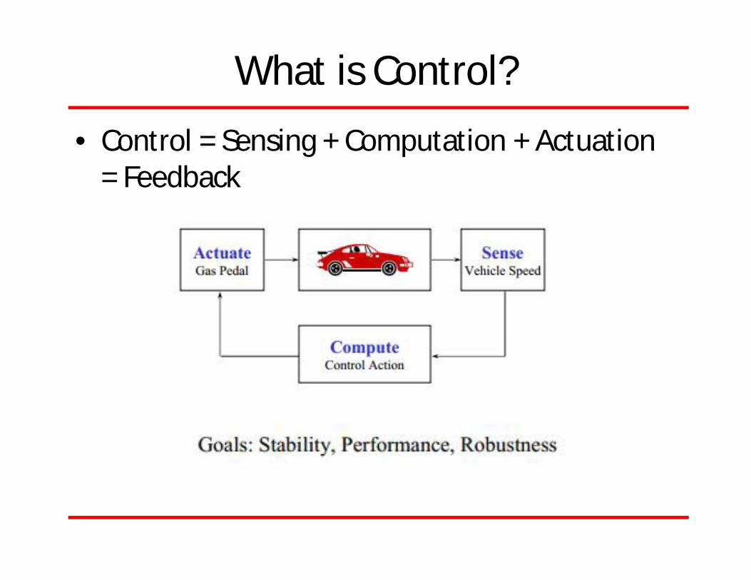
What is Control?
• Control = Sensing + Computation + Actuation = Feedback

Control System
• A control system is an interconnected system to manage, command, direct or regulate some quantity of devices or systems– Some quantity : temperature, speed, distance, pH
level, altitude, voltage
Ref: Prof. Jonguen Choi, ME-451, Michigan State University

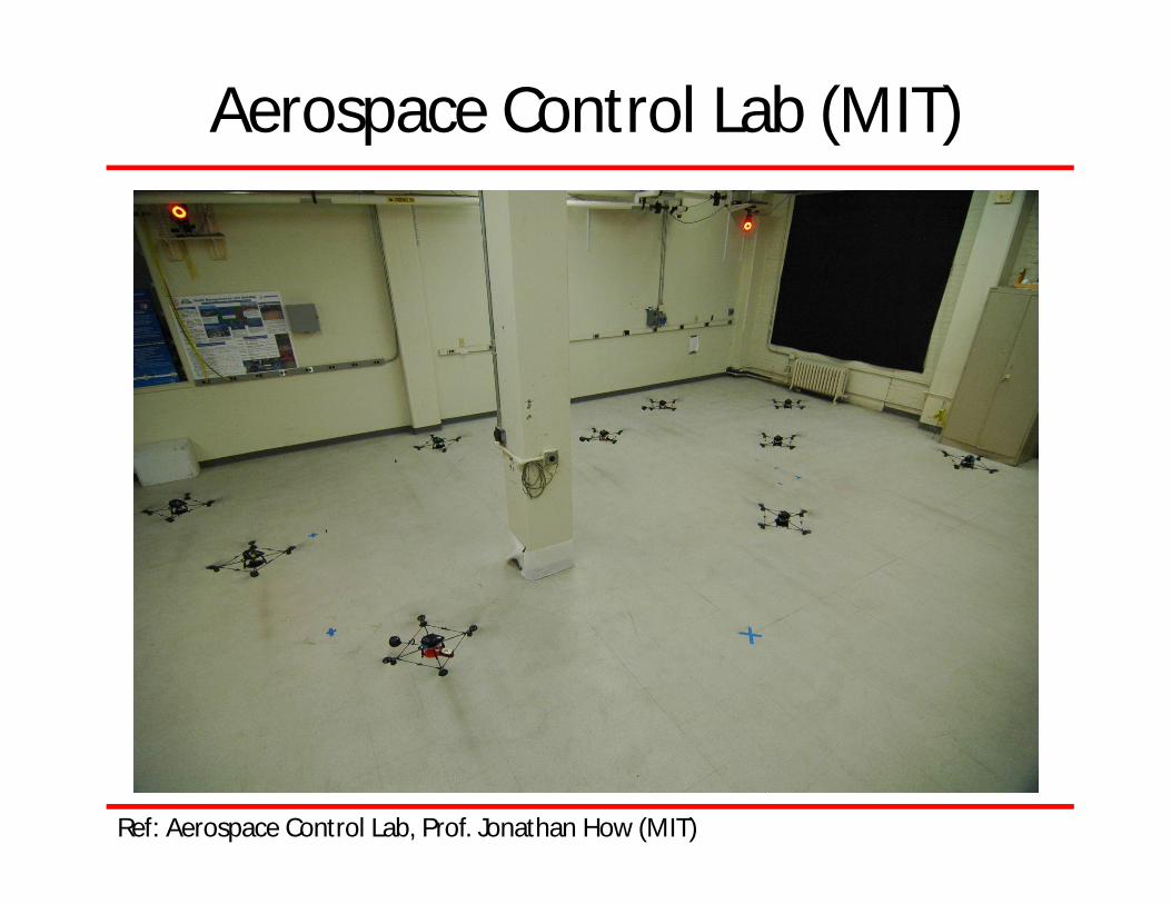
Aerospace Control Lab (MIT)
Ref: Aerospace Control Lab, Prof. Jonathan How (MIT)

NASA Intelligent Flight Control System
• The Intelligent Flight Control System (IFCS) flight research project at NASA Dryden Flight Research Center was established to incorporate self-learning neural network concepts into flight control software to enable a pilot to maintain control and safely land an aircraft that has suffered a failure to a control surface or damage to the airframe.
NASA Drysden’s modified F-15B
Ref: NASA
What is Control?
• Control = Sensing + Computation + Actuation = Feedback
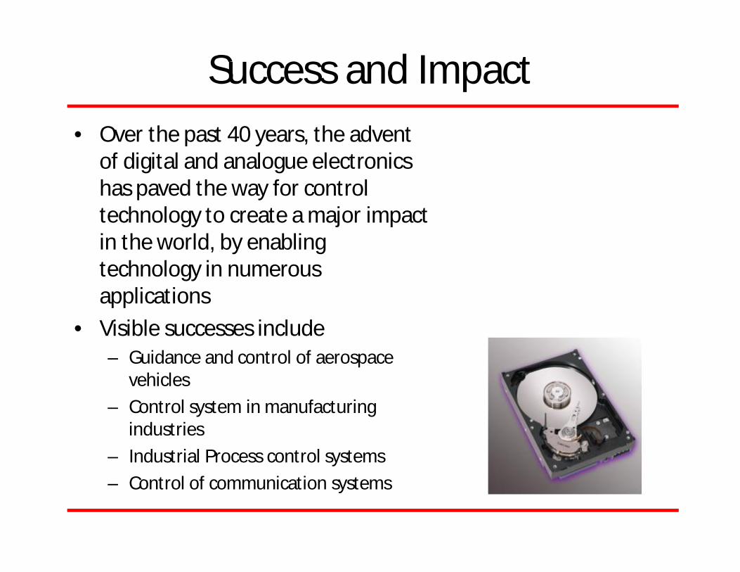
Success and Impact• Over the past 40 years, the advent
of digital and analogue electronics has paved the way for control technology to create a major impact in the world, by enabling technology in numerous applications
• Visible successes include– Guidance and control of aerospace
vehicles– Control system in manufacturing
industries– Industrial Process control systems– Control of communication systems

Feedback and Life• The ‘Feedback’ mechanism is central to hemeostasis
and life
• Ever wondered by we shiver when it is cold?
• As a technology, control dates back to two millennia
Hemeostasis: is the property of a system in which variables are regulated so that internal conditions remain stable and relatively constant. Examples of homeostasis include the regulation of temperature and the balance between acidity and alkalinity (pH). It is a process that maintains the stability of the human body's internal environment in response to changes in external conditions.
http://en.wikipedia.org/wiki/Homeostasis
[1] K. J., Astrom, and P. R. Kumar, “Control: A Perspective,” Automatica, vol. 50, pp. 3–43, 2014.
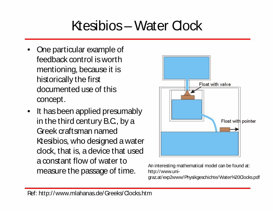
Ktesibios – Water Clock
• One particular example of feedback control is worth mentioning, because it is historically the first documented use of this concept.
• It has been applied presumably in the third century B.C., by a Greek craftsman named Ktesibios, who designed a water clock, that is, a device that used a constant flow of water to measure the passage of time.
Ref: http://www.mlahanas.de/Greeks/Clocks.htm
An interesting mathematical model can be found at: http://www.uni-graz.at/exp2www/Physikgeschichte/Water%20Clocks.pdf
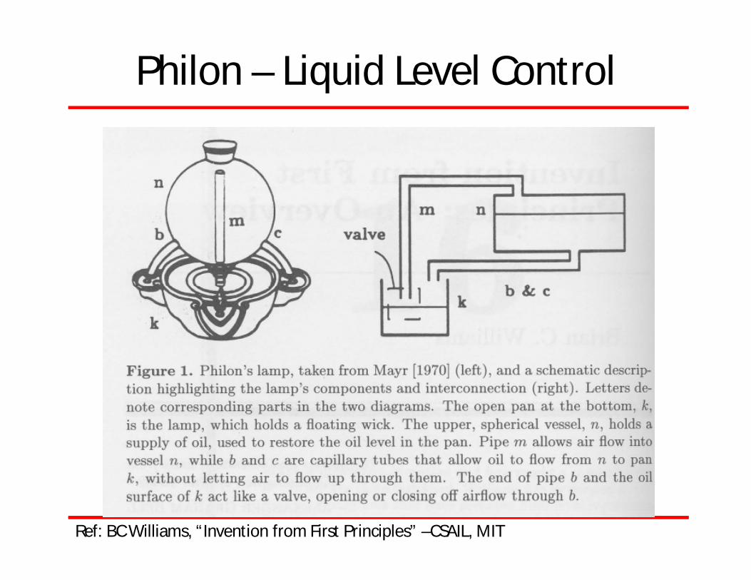
Philon – Liquid Level Control
Ref: BC Williams, “Invention from First Principles” –CSAIL, MIT

The Centrifugal Governer• James Watt invented the
centrifugal governer to fit the engine to keep it running at constant speed, and patented it in 1788
• The centrifugal governor combines sensing, actuationand control
• The basic governor yields proportional action because the change in the (valve) angle is proportional to the change in velocity.
Ref: Richad Murray, CDS, Caltech
The Birth of Mathematical Control Theory
• Theoretical investigation of governors started by Maxwell in 1868 in his famous paper “On Governors”
• He analyzed the system model and found the conditions for stability of systems upto third-order
• The general problem of stability was solved by Routh in his paper “Stability of Motion”
• Other early contributors to stability were Vyshenegradskii, Hurwitz, Stodola.
• By late 18th century, a firm mathematicalfoundation was being established in automatic control

Ship Steering• An important military
problem during the first world war was the control and navigation of ships
• Gyroscope was invented in 1910
• N. Minorsky introduced his three-term (PID) controller.
• First application of the PID control
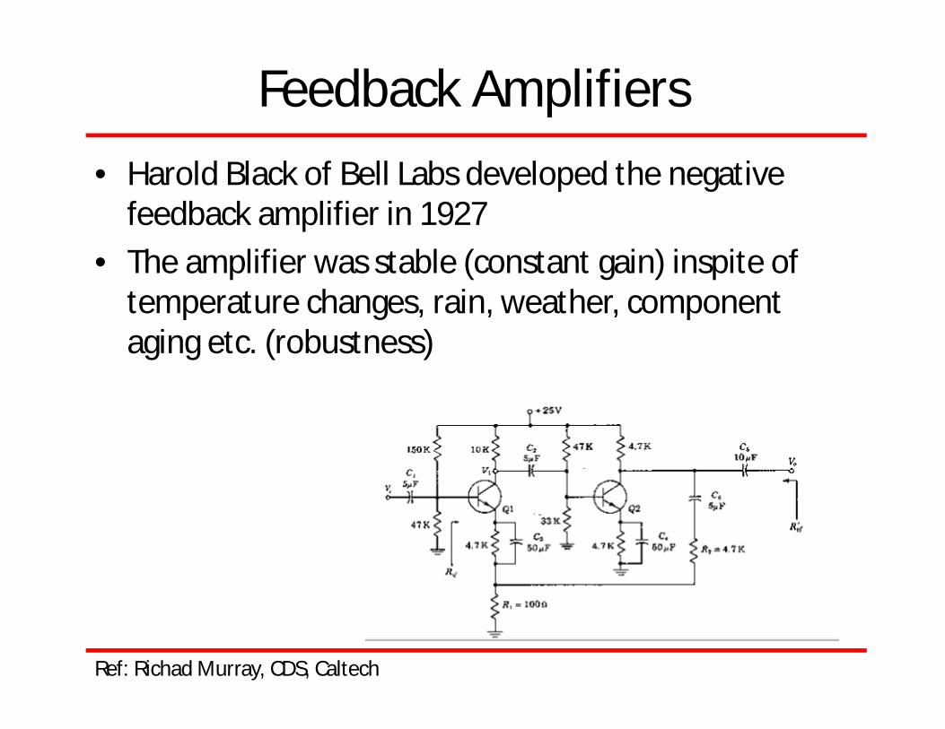
Feedback Amplifiers• Harold Black of Bell Labs developed the negative
feedback amplifier in 1927• The amplifier was stable (constant gain) inspite of
temperature changes, rain, weather, component aging etc. (robustness)
Ref: Richad Murray, CDS, Caltech

Modern Engineering Applications
• Flight Control Systems– Modern commercial and military aircraft are fly by
wire– UAVs
http://uav.ae.gatech.edu/pics/images.html
Ref: Richad Murray, CDS, Caltech
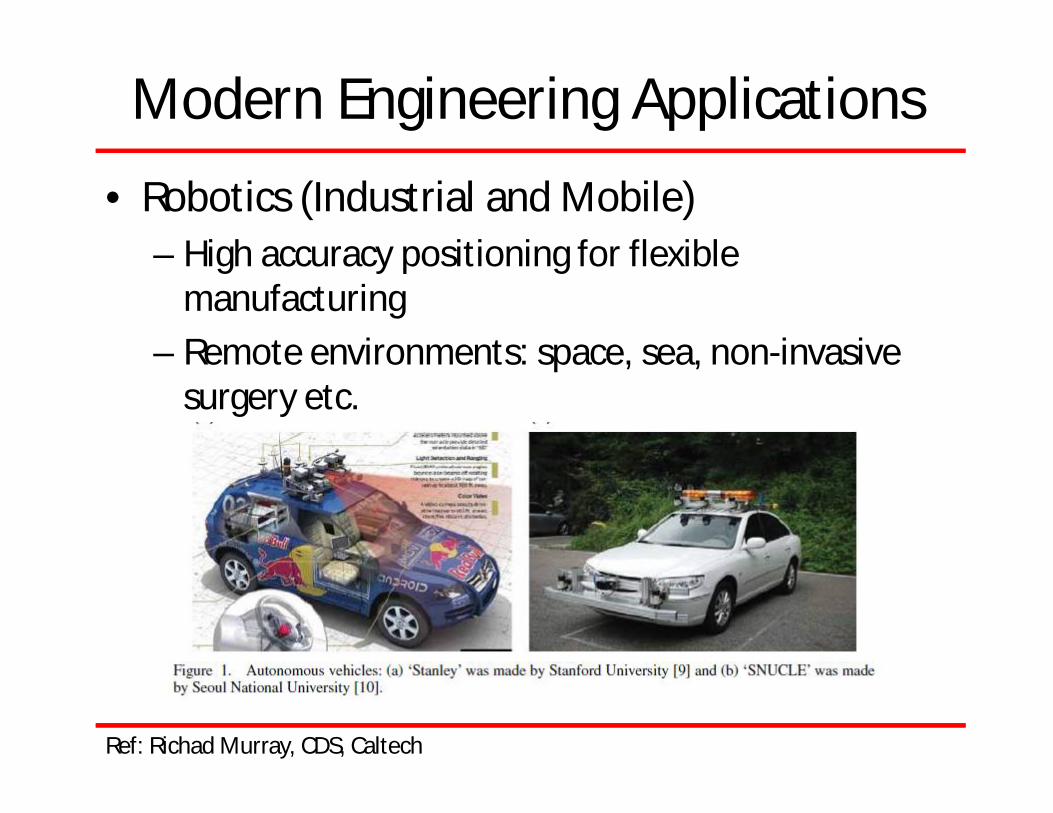
Modern Engineering Applications
• Robotics (Industrial and Mobile)– High accuracy positioning for flexible
manufacturing– Remote environments: space, sea, non-invasive
surgery etc.
Ref: Richad Murray, CDS, Caltech
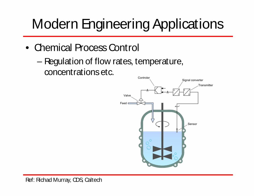
Modern Engineering Applications
• Chemical Process Control– Regulation of flow rates, temperature,
concentrations etc.
Ref: Richad Murray, CDS, Caltech
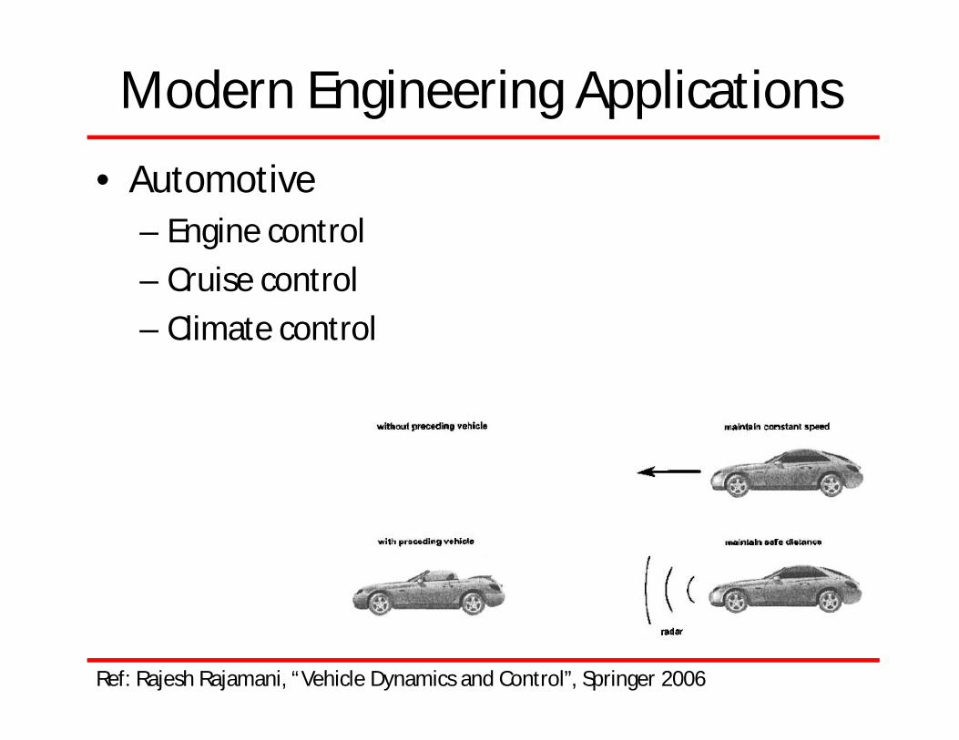
Modern Engineering Applications
• Automotive– Engine control– Cruise control– Climate control
Ref: Rajesh Rajamani, “Vehicle Dynamics and Control”, Springer 2006

Biology - locomotion• Control system and
feedback play a central role in locomotion
• A suite of neurosensory devices are used within the musculoskeletal system and are active throughout each cycle of locomotion
Ref: Richad Murray, CDS, Caltech

Biology – insect flight
• A: Cartoon of the adult fruit fly showing the three major sensor strictures used in flight: eyes, antennae, and halters (detect angular rotations)
• B: Example flight trajectories over a 1 meter circular arena, with and without internal targets.
• C: Schematic control model of the flight system
Ref: Richad Murray, CDS, Caltech
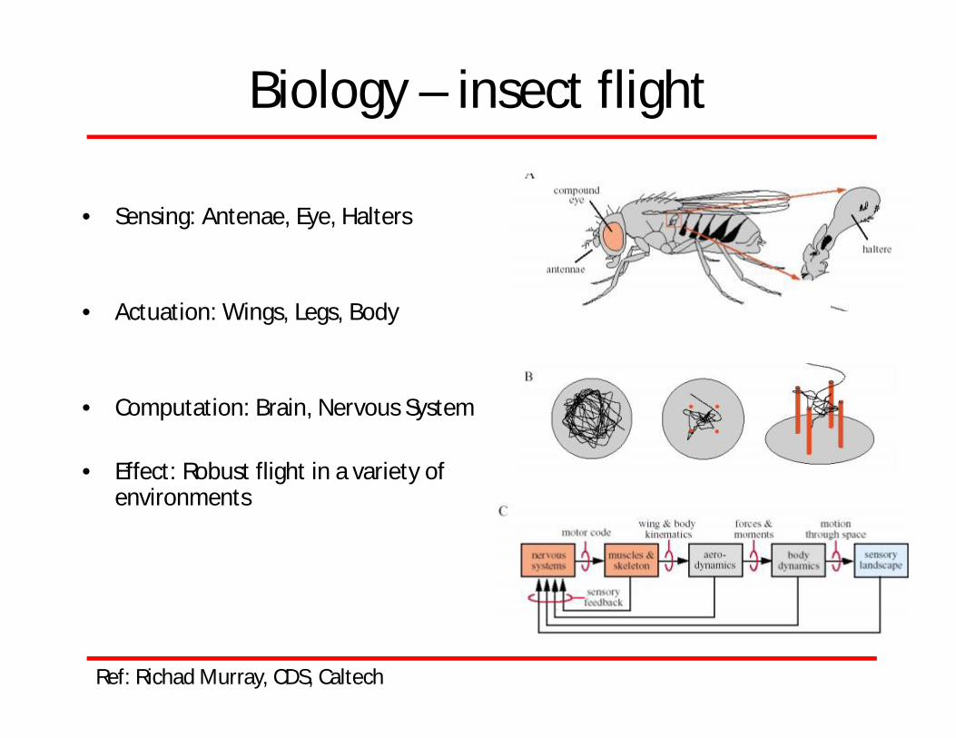
Biology – insect flight
• Sensing: Antenae, Eye, Halters
• Actuation: Wings, Legs, Body
• Computation: Brain, Nervous System
• Effect: Robust flight in a variety of environments
Ref: Richad Murray, CDS, Caltech
Control System: A Perspective
• Survey paper: very comprehensive review of the field:– K. J. Astrom, P. R. Kumar “Control: A Perspective”,
Automatica, 2014

COURSE MECHANICS

EE 379 – Course Overview (1/3)• EE 379
– Pre-requisites: None but prior study of ME-437 Mechanical Vibrations would be extremely helpful.
– Credit Hours: 3-1– Three hours of lectures, and three hours of labwork each
week (Six contact hours)• Course in nutshell
– Modeling of linear-time invariant systems (electrical, mechanical and electro-mechanical)
– Analyze the behaviour of the systems using mathematical and computational tools
– Design feedback controllers for the system to fulfil desired specifications
– Classical and Modern modeling and control techniques

EE 379 – Course Overview (2/3)
• By the end of the course you will (hopefully)– Formulate a mathematical model of a linear time-
invariant system, both in the s-domain (transfer functions/matrices) and time-domain (state-space)
– Analyze the system behaviour in the time and frequency domain
– Design feedback controllers and/or observers for the system to satisfy desired specifications
– Be ready to delve into more advanced control concepts such as adaptive filtering, optimal control, adaptive and robust control, nonlinear control etc.
EE 379 – Course Overview (3/3)• Text Book:
– Norman S. Nise, “Control Systems Engineering”,6th Edition, (Wiley)
– Stefani, Shahian, Savant Jr., Hostetter, “Design of Feedback Control Systems”, 4th edition, (Oxford Series in Electrical and Computer Engineering)
• Reference Books:– K. Ogata, “Modern Control Engineering”, 5th ed,
Prentice Hall• Bring a note pad and pen atleast (calculator
would be helpful but not necessary)

Tentative calender and order of lecturesWk. Topics
1 Introduction to CourseControl Systems: A Perspective (History, Current Trends, The Future, Applications etc.)Modeling in the Frequency Domain (Nise, Ch 2)
2 Modeling in the Frequency Domain
3 Modeling in the Time Domain (Nise, Ch 3)
4 Modeling in the Time Domain (Nise, Ch 3) cont.
5 Time Response (Nise, Ch 4)
6 Block Diagrams, Signal Flow graphs (Nise Ch 5)
7 Stability (Nise Ch 6)
8 Root Locus Techniques (Nise Ch 7)
9 Root Locus Design (Nise Ch 8)
10 Root Locus Design cont. (Nise Ch 8)
11 Frequency Response Techniques (Nise Ch 10)
12 Frequency Response Techniques (Nise Ch 10) cont.
13 Design via Frequency Response (Nise Ch 11) cont.
14 Design via Frequency Response (Nise Ch 11)
15 Design via State Space (Nise Ch 12)
16 Design via State Space (Nise Ch 12) cont.

Grading Policy EE 379 (Fall 2014)
2 x Sessional Exams 12.5 + 12.5 = 25 %
Lab (Lab Sessions, Lab Exams and Projects)
25 %
Quizzes/HW Problem Sets 10 %
Final Exam 40 %
• Lab – Conducted by Mr. Saad Bin Shams– Location: Elec-Lab II (DEE) ---- This might be changed in the future– Lab reports as per department policy
• 6 Quizzes, 4 Homework problem sets• 2 sessional exams, 1 final exam• 16 experiments in the Lab

Miscellaneous • Lectures:
– Syn A: Monday 0855-0945, Tuesday 0800-0945– Syn B: Wednesday 0855-1040, Thursday 0950-1040
• Course on the web + mailing list: http://groups.yahoo.com/groups/DE_34_MTS
• Office hours (ground floor): – Tuesday (0950-1040)– Thursday (1055-1240)

Open Loop vs Closed Loop
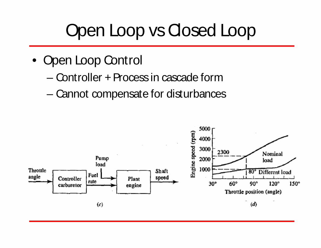
• Open Loop Control– Controller + Process in cascade form– Cannot compensate for disturbances
– Examples: Toaster, Microwave Oven, Shoot a Basketball
Open Loop vs Closed Loop
• Open Loop Control– Controller + Process in cascade form– Cannot compensate for disturbances
– Examples: Toaster, Microwave Oven, Shoot a Basketball
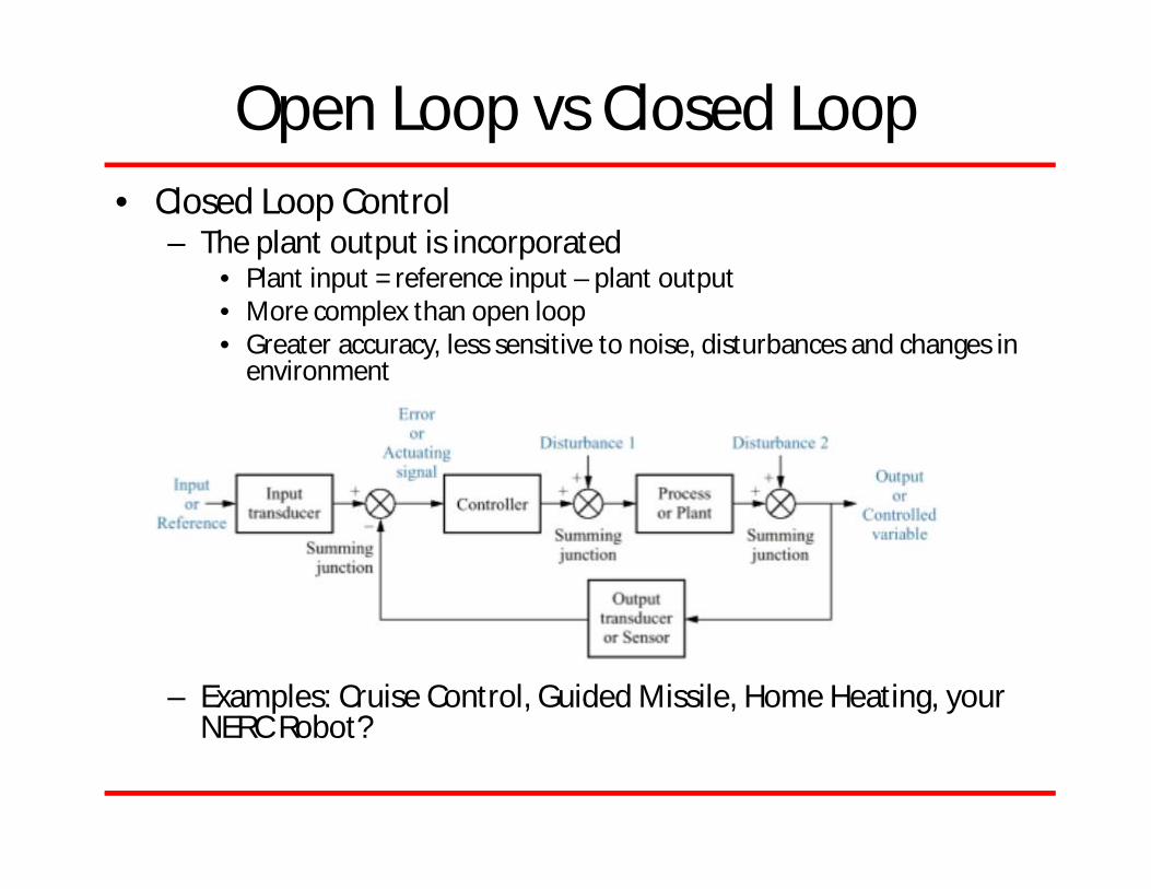
Open Loop vs Closed Loop• Closed Loop Control
– The plant output is incorporated• Plant input = reference input – plant output• More complex than open loop• Greater accuracy, less sensitive to noise, disturbances and changes in
environment
– Examples: Cruise Control, Guided Missile, Home Heating, your NERC Robot?

Open loop vs closed loop
Advantages of feedback
• Increased accuracy
• Reduced sensitivity to changes in components
• Reduced effects of disturbances
• Increased speed of response and bandwidth

Analysis and Design Objectives
• Major objective of system analysis and design– Producing the desired transient response– Reducing steady state error– Achieving stability
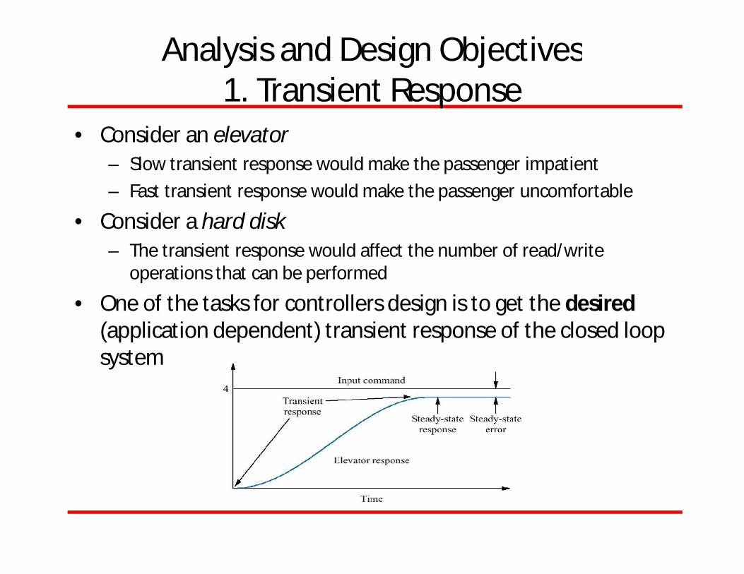
Analysis and Design Objectives1. Transient Response
• Consider an elevator– Slow transient response would make the passenger impatient– Fast transient response would make the passenger uncomfortable
• Consider a hard disk– The transient response would affect the number of read/write
operations that can be performed
• One of the tasks for controllers design is to get the desired(application dependent) transient response of the closed loop system

Analysis and Design Objectives2. Steady State Reponse
• Another goal of controller design is to eliminate stedy-state error (steady state difference between reference/desired output and actual output)
• Elevator, autonomous parking problem, altitude control of aircraft, antenna tracking problem
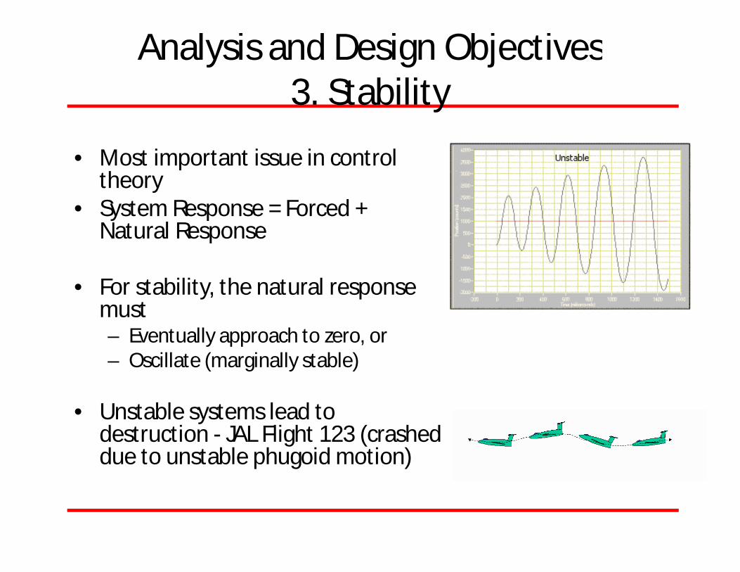
Analysis and Design Objectives3. Stability
• Most important issue in control theory
• System Response = Forced + Natural Response
• For stability, the natural response must– Eventually approach to zero, or– Oscillate (marginally stable)
• Unstable systems lead to destruction - JAL Flight 123 (crashed due to unstable phugoid motion)

Analysis and Design ObjectivesOther Consideratons
• Size, power of actuators• Sensory accuracy• Finances• Robustness• Nonlinearities
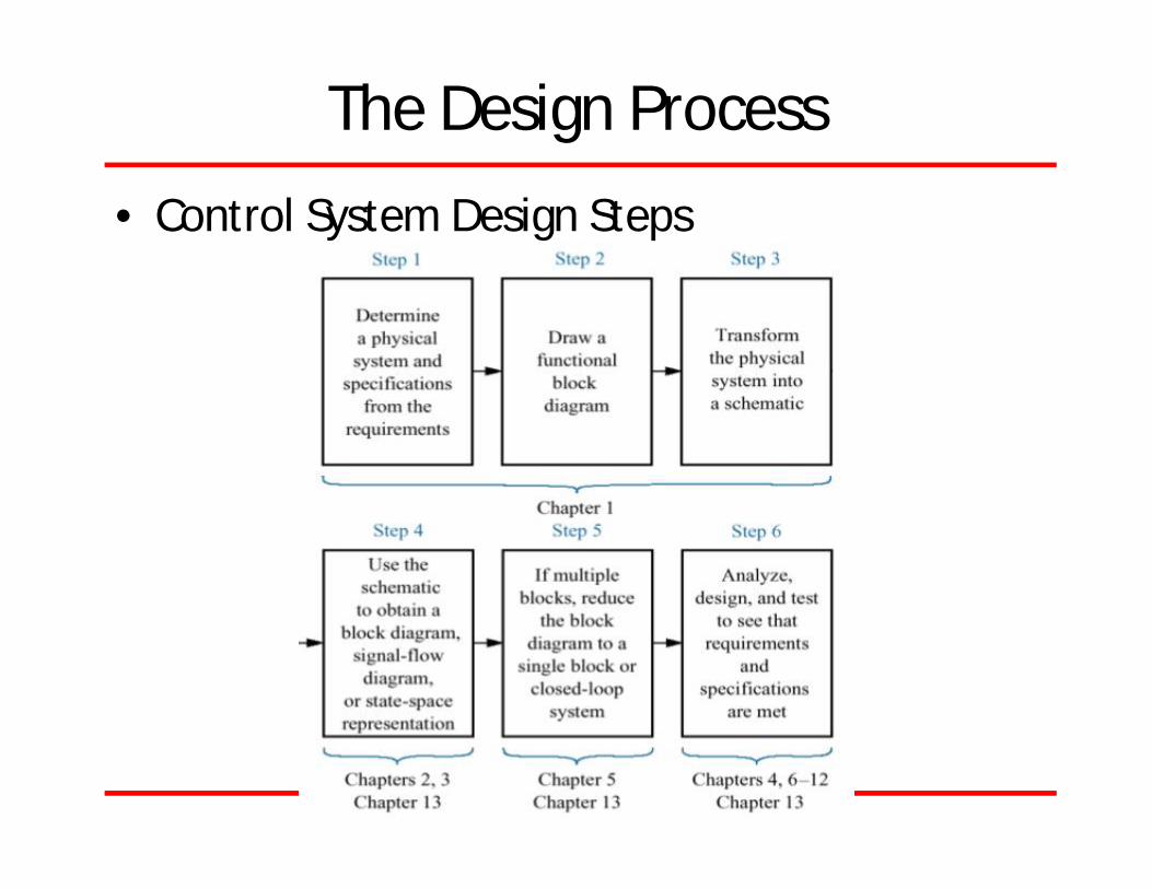
The Design Process
• Control System Design Steps
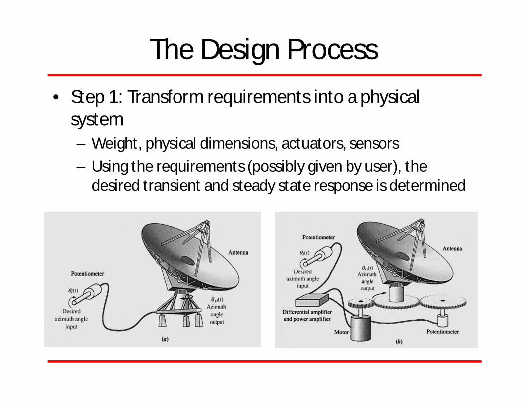
The Design Process• Step 1: Transform requirements into a physical
system– Weight, physical dimensions, actuators, sensors– Using the requirements (possibly given by user), the
desired transient and steady state response is determined
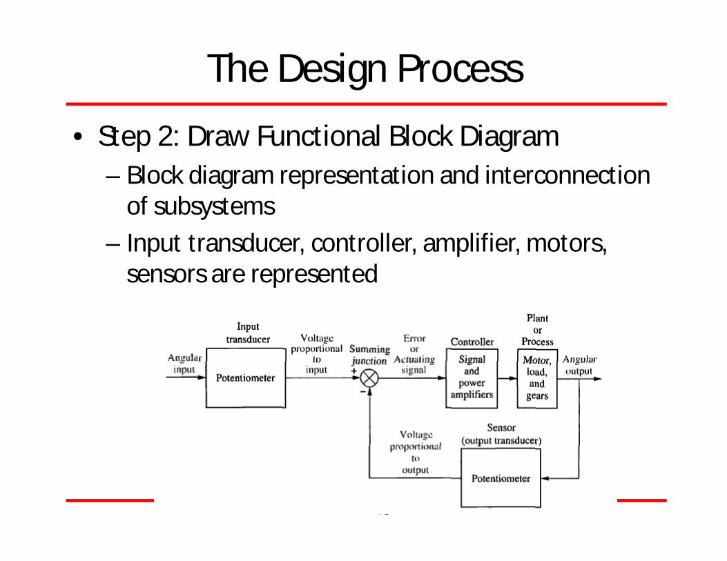
The Design Process
• Step 2: Draw Functional Block Diagram– Block diagram representation and interconnection
of subsystems– Input transducer, controller, amplifier, motors,
sensors are represented

The Design Process
• Step 3: Create a schematic– Position control systems consist of electrical,
mechanical and electro mechanical components– The schematic should be compact and simple, but
must be able to account for observed behavior of the system.
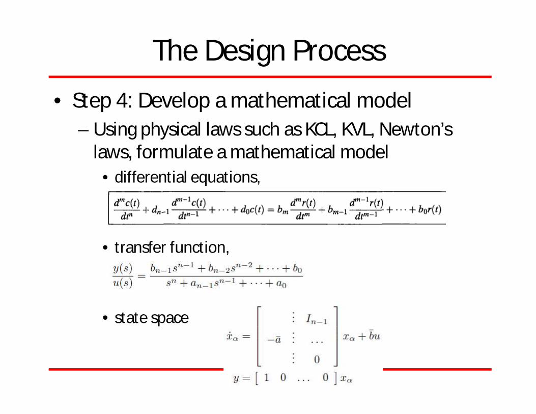
The Design Process
• Step 4: Develop a mathematical model– Using physical laws such as KCL, KVL, Newton’s
laws, formulate a mathematical model • differential equations,
• transfer function,
• state space
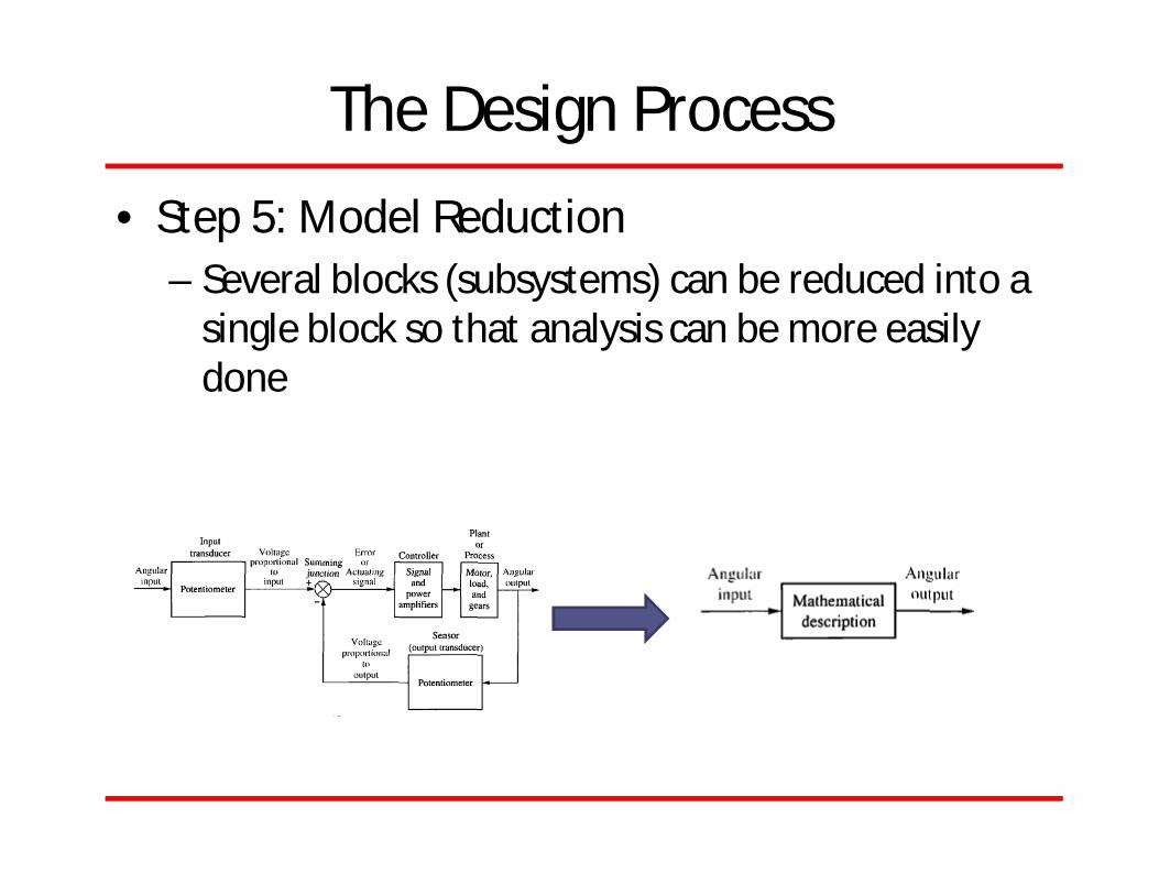
The Design Process
• Step 5: Model Reduction– Several blocks (subsystems) can be reduced into a
single block so that analysis can be more easily done

The Design Process
• Step 6: Analyze and Design– Analysis is done to see if the response
specifications and performance requirements are met by simple adjustments of system parameters
– Typical test signals:
Ref: Prof. Ju-Jang Lee, KAIST

The Design Process
• All steps must be followed to satisfy the design requirements in terms of– Stability– Transient Response– Steady State Response
• Other considerations– Robustness/Sensitivity– Linearity Assumptions/Nonlinearities

MODELING IN THE FREQUENCY DOMAIN
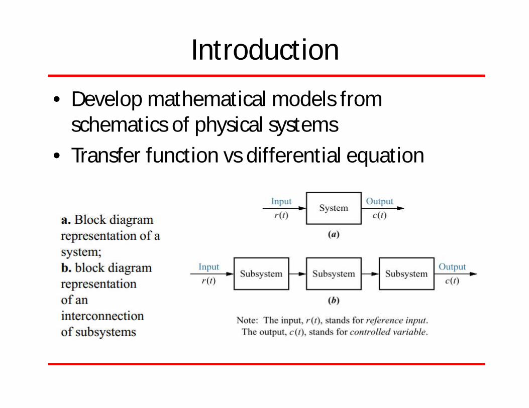
Introduction
• Develop mathematical models from schematics of physical systems
• Transfer function vs differential equation

Some material taken from Prof. Charlie Chen’s lecture notes (U of Wisconsin-Madison)
System
System System

The Laplace Transform
• The laplace transform of a function f(t) is defined as
• The inverse laplace transform is defined as

Laplace Transform (cont.)

Laplace Transform (cont.)

Laplace Transform
• Partial Fraction Expansion
– Let 퐹 푠 = ( )( ), and assume order of N(s) is less
than D(s)– Case I: Roots of D(s) are real and distinct

Laplace Transform
• Partial Fraction Expansion– Case I : Roots of D(s) are real and distinct
• Example:

Laplace Transform
• Partial Fraction Expansion– Case I : Roots of D(s) are real and distinct
• Example:
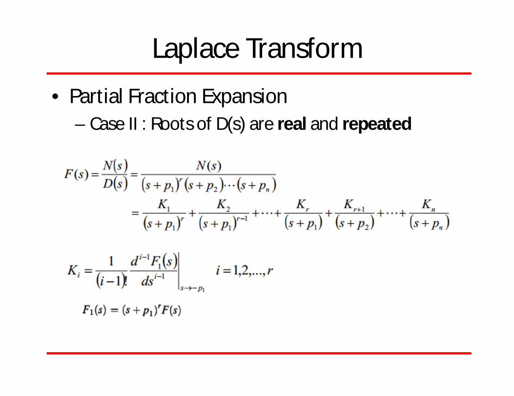
Laplace Transform
• Partial Fraction Expansion– Case II : Roots of D(s) are real and repeated

Laplace Transform
• Partial Fraction Expansion– Case II : Roots of D(s) are repeated– Example:

Laplace Transform
• Partial Fraction Expansion– Case III : Roots of D(s) are Complex or Imaginary
– Example:
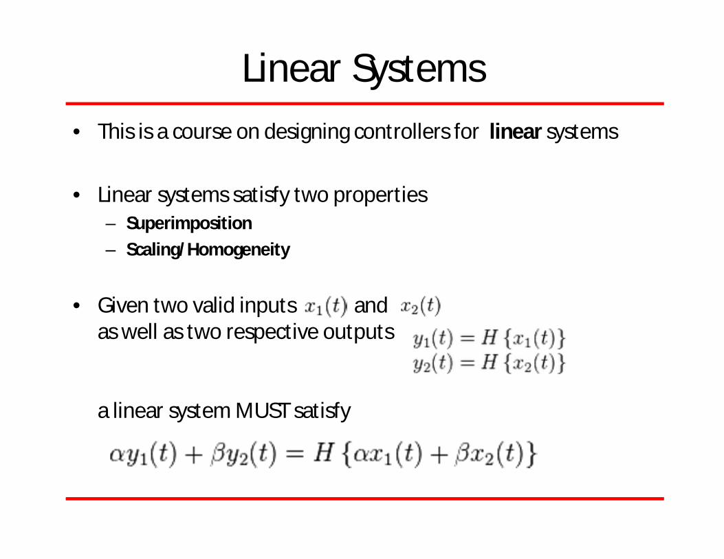
Linear Systems• This is a course on designing controllers for linear systems
• Linear systems satisfy two properties– Superimposition– Scaling/Homogeneity
• Given two valid inputs and as well as two respective outputs
a linear system MUST satisfy
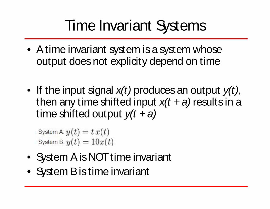
Time Invariant Systems• A time invariant system is a system whose
output does not explicity depend on time
• If the input signal x(t) produces an output y(t), then any time shifted input x(t + a) results in a time shifted output y(t + a)
• System A is NOT time invariant• System B is time invariant

Transfer Function
Any Linear System (e.g.Linear Amplifier)
Transfer Function:
The transfer function is the output of the system when the input is an impulse
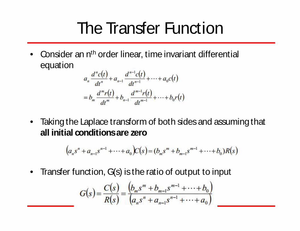
The Transfer Function• Consider an nth order linear, time invariant differential
equation
• Taking the Laplace transform of both sides and assuming that all initial conditions are zero
• Transfer function, G(s) is the ratio of output to input
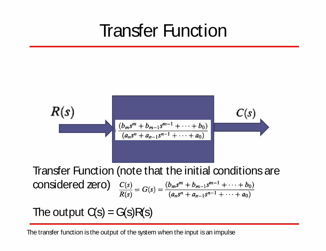
Transfer Function
Any Linear System (e.g.Linear Amplifier)
Transfer Function (note that the initial conditions are considered zero)
The output C(s) = G(s)R(s)
The transfer function is the output of the system when the input is an impulse

System Response from Transfer Function
• Best illustrated with an example• Find the transfer function represented by the
differential equation
• Find the system response, when input r(t) = u(t) (unit step) is applied to the system

Example
• We need to find the output c(t), whose transfer function is given above and when the input is r(t) = t (ramp)
• Use, C(s) = G(s) R(s)• Convert to time domain
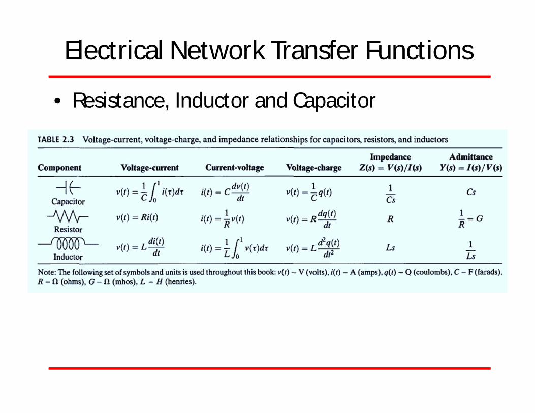
Electrical Network Transfer Functions
• Resistance, Inductor and Capacitor
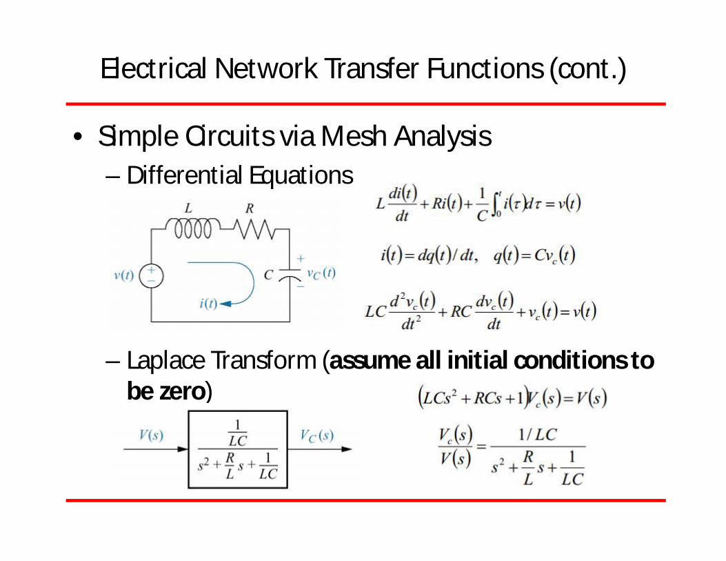
Electrical Network Transfer Functions (cont.)
• Simple Circuits via Mesh Analysis– Differential Equations
– Laplace Transform (assume all initial conditions to be zero)
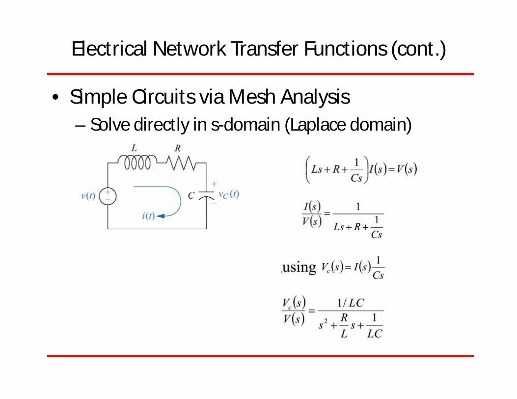
Electrical Network Transfer Functions (cont.)
• Simple Circuits via Mesh Analysis– Solve directly in s-domain (Laplace domain)

Electrical Network Transfer Functions (cont.)
• Simple Circuits via Nodal Analysis– Solve directly in s-domain (Laplace domain)
– Solve via voltage divider formula
Electrical Network Transfer Functions (cont.)
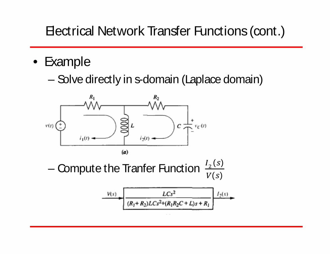
• Example– Solve directly in s-domain (Laplace domain)
– Compute the Tranfer Function ( )( )
Electrical Network Transfer Functions (cont.)
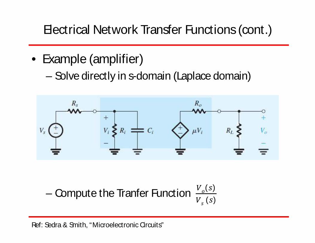
• Example (amplifier)– Solve directly in s-domain (Laplace domain)
– Compute the Tranfer Function ( )( )
Ref: Sedra & Smith, “Microelectronic Circuits”
Electrical Network Transfer Functions (cont.)
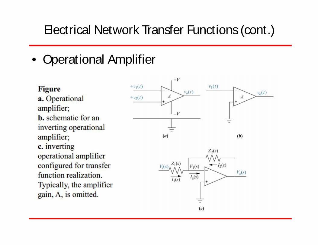
• Operational Amplifier
Electrical Network Transfer Functions (cont.)
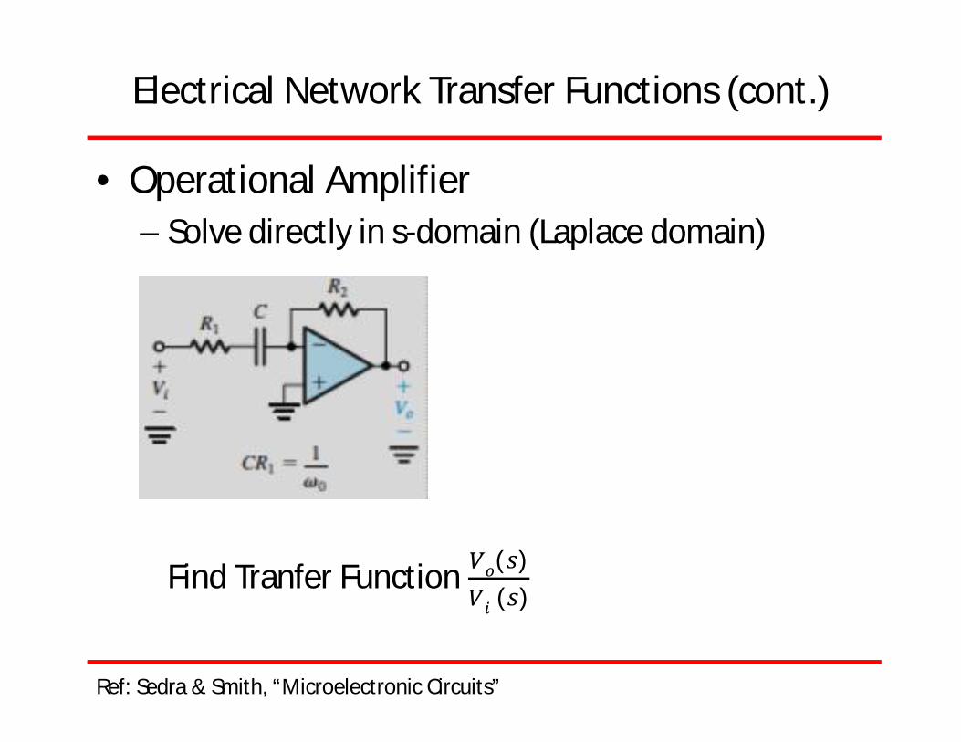
• Operational Amplifier– Solve directly in s-domain (Laplace domain)–
Find Tranfer Function ( )( )
Ref: Sedra & Smith, “Microelectronic Circuits”
Translational Mechanical System Transfer Functions

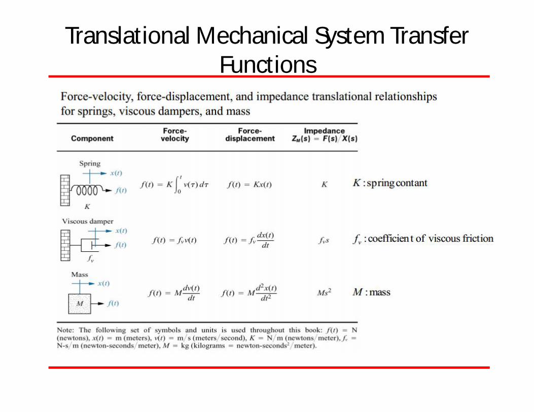
Translational Mechanical System Transfer Functions
• Analyzing translational mechanical systems1. Define positions with directional senses for each
mass in the system2. Draw free body diagrams for each of the masses,
expressing the forces on them in terms of mass position and velocity
3. Write an equation for each mass, equating the algebraic sum of forces (in point 2) and the inertial term due to acceleration to zero (i. e.ΣF – ma = 0), with appropriate signs keeping in view the directional sense of each force term
Fictitious force added due to acceleration

Translational Mechanical System Transfer Functions
Translational Mechanical System Transfer Functions

Translational Mechanical System Transfer Functions
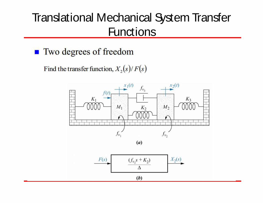
• a
Translational Mechanical System Transfer Functions
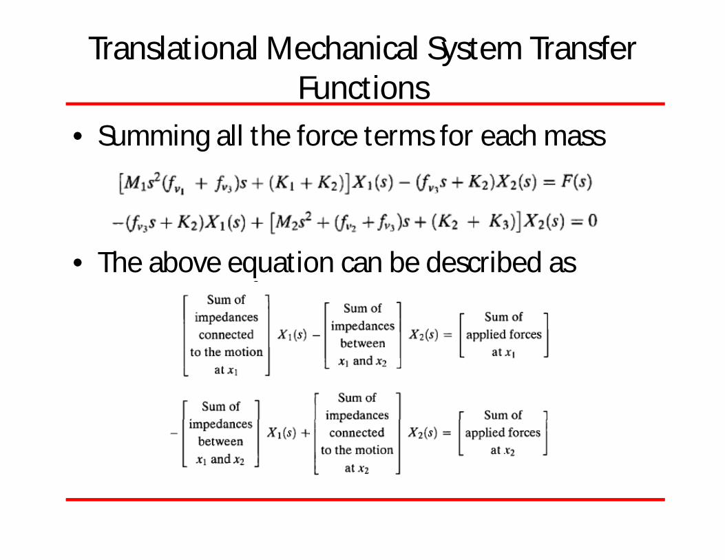
• Summing all the force terms for each mass
• The above equation can be described as

Translational Mechanical System Transfer Functions
• Summing all the force terms for each mass
• The above equation can be described as
Translational Mechanical System Transfer Functions
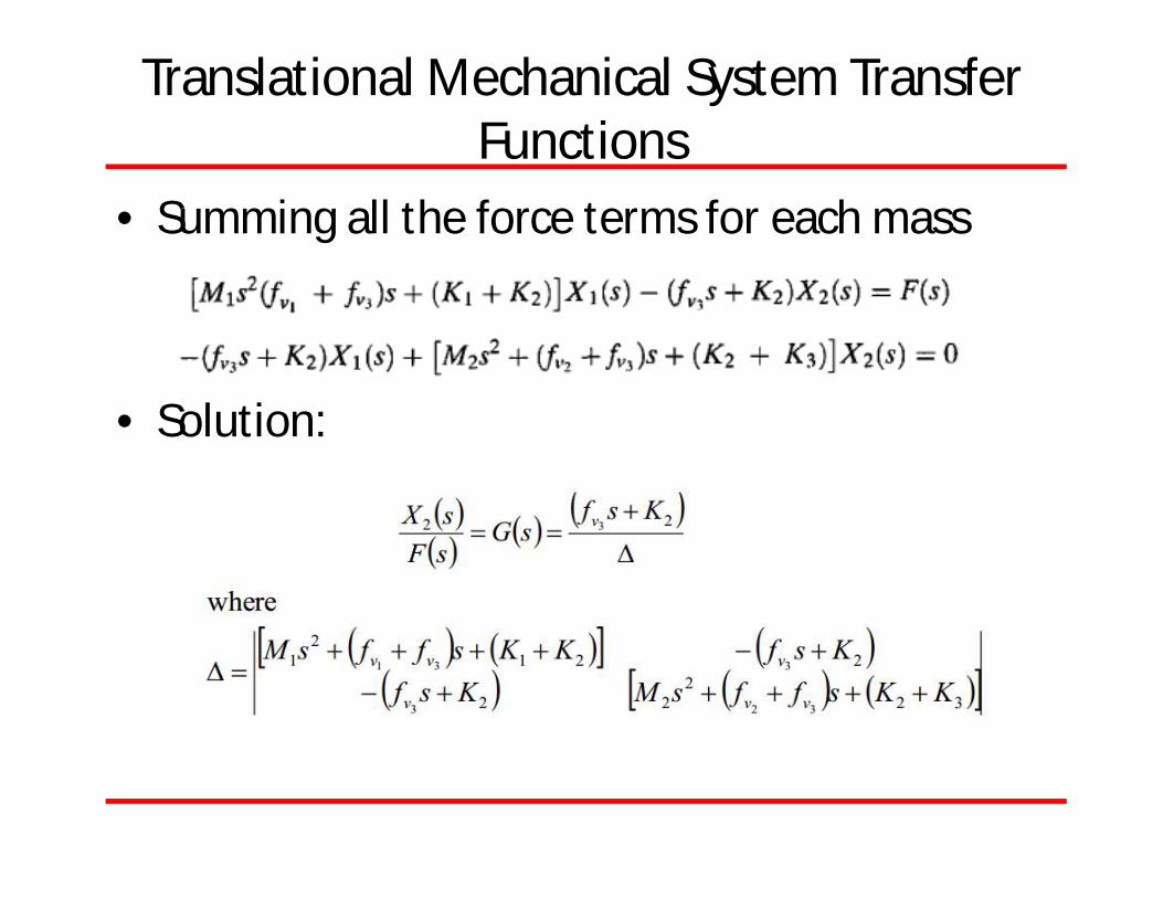
• Summing all the force terms for each mass
• Solution:
Translational Mechanical System Transfer Functions
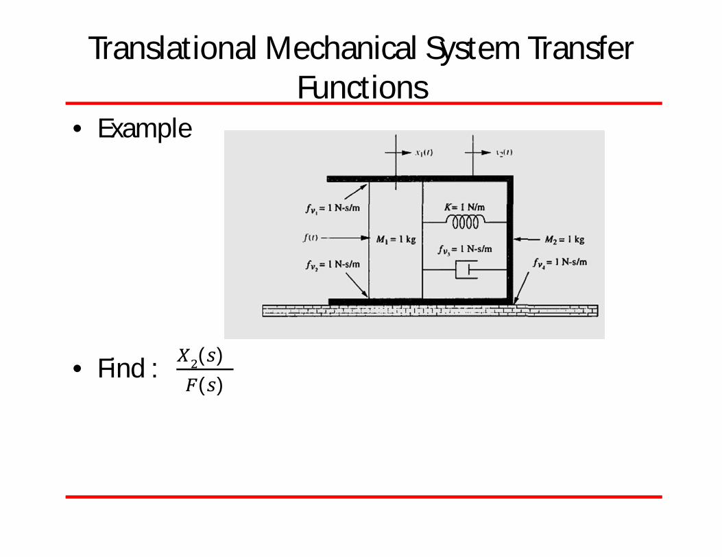
• Example
• Find : ( )( )
Rotational Mechanical System Transfer Functions
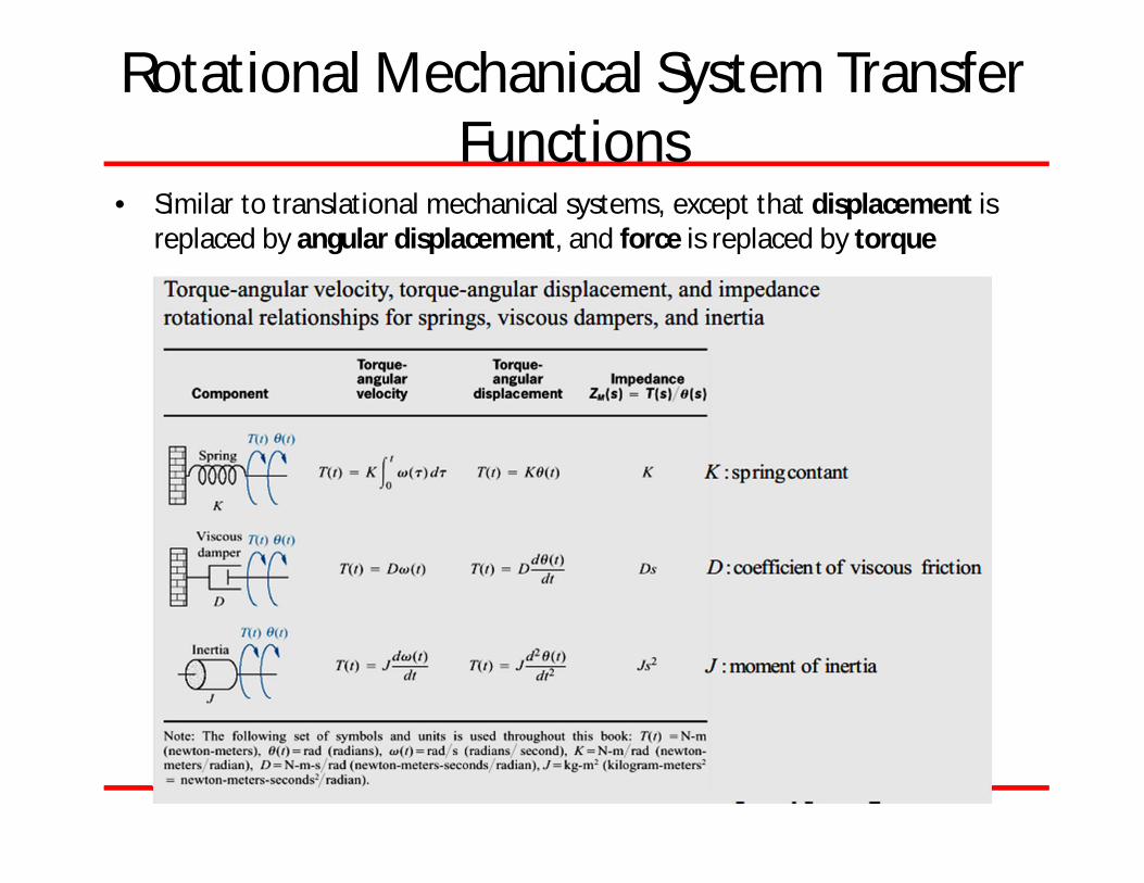
• Similar to translational mechanical systems, except that displacement is replaced by angular displacement, and force is replaced by torque
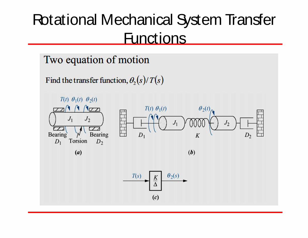
Rotational Mechanical System Transfer Functions
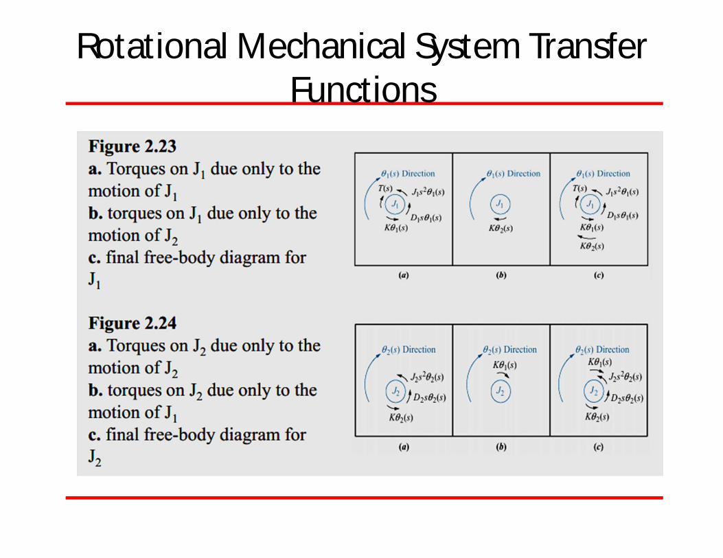
Rotational Mechanical System Transfer Functions
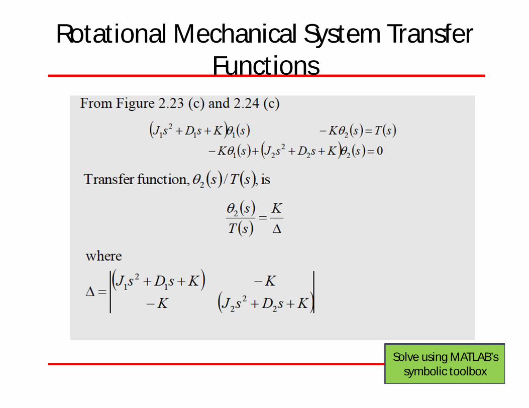
Rotational Mechanical System Transfer Functions
Solve using MATLAB’s symbolic toolbox
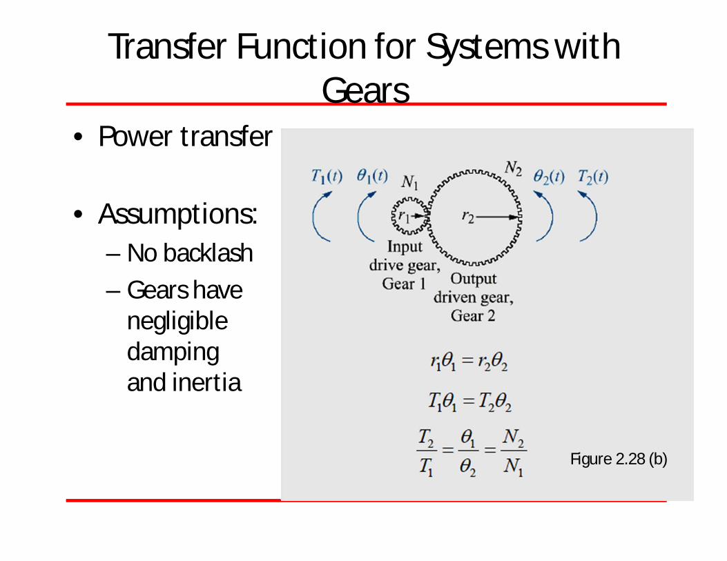
Transfer Function for Systems with Gears
• Power transfer
• Assumptions:– No backlash– Gears have
negligibledampingand inertia
Figure 2.28 (b)
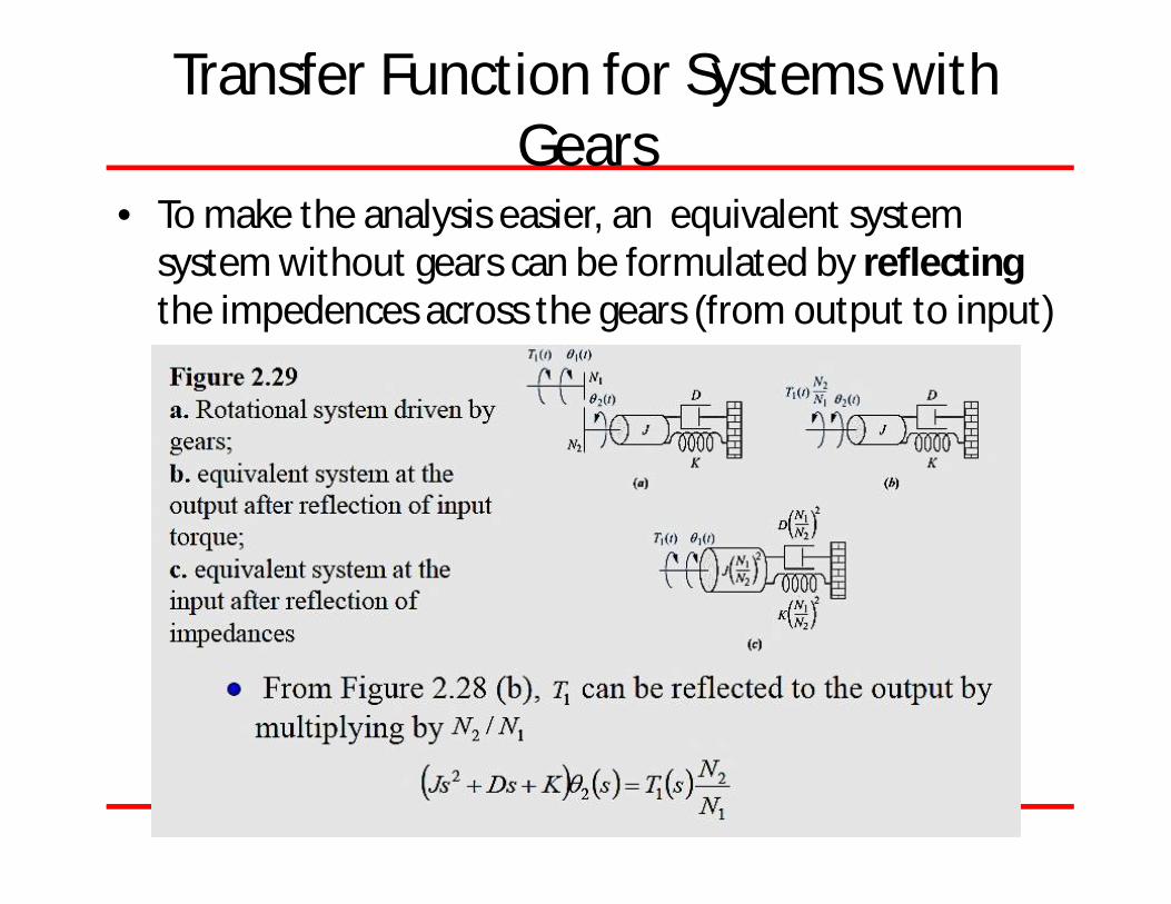
Transfer Function for Systems with Gears
• To make the analysis easier, an equivalent system system without gears can be formulated by reflecting the impedences across the gears (from output to input)
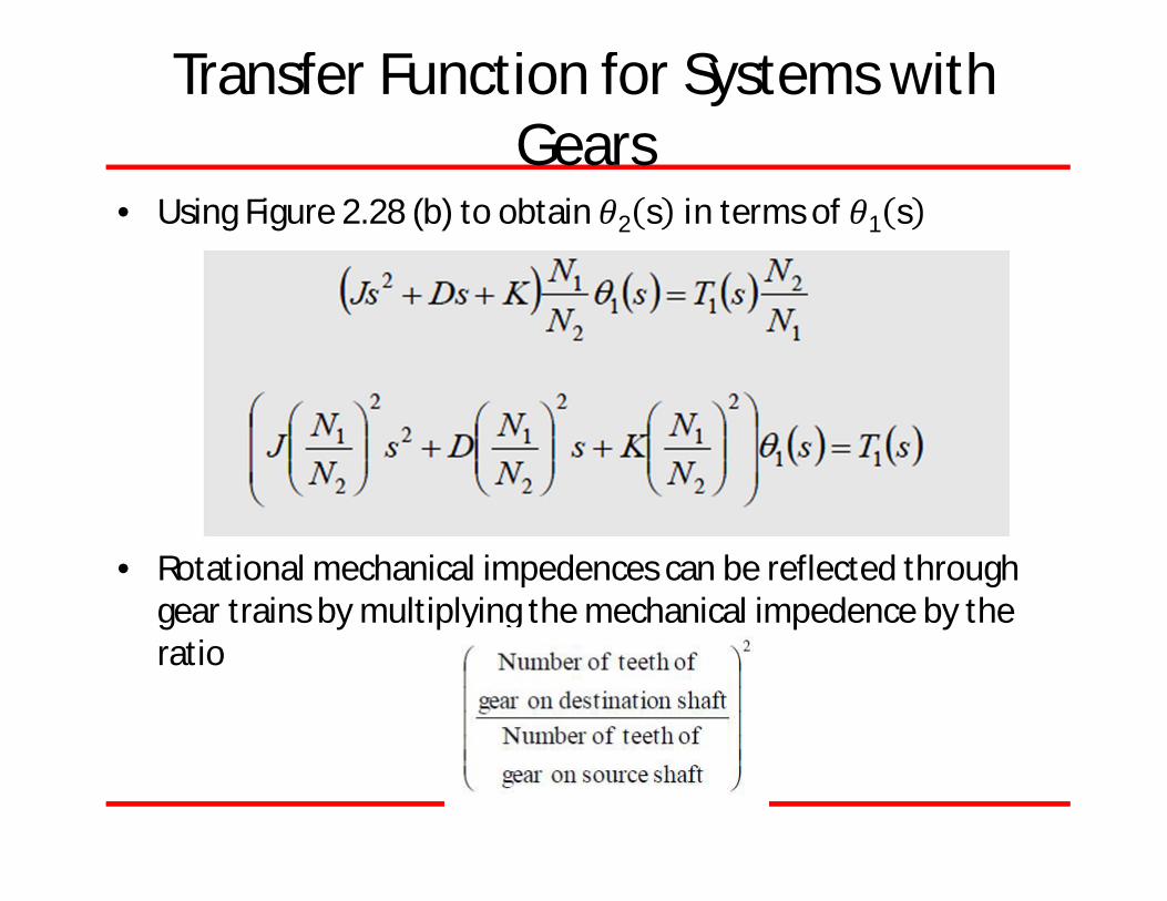
Transfer Function for Systems with Gears
• Using Figure 2.28 (b) to obtain 휃2 s in terms of 휃1 s
• Rotational mechanical impedences can be reflected through gear trains by multiplying the mechanical impedence by the ratio
Transfer Function for Systems with Gears
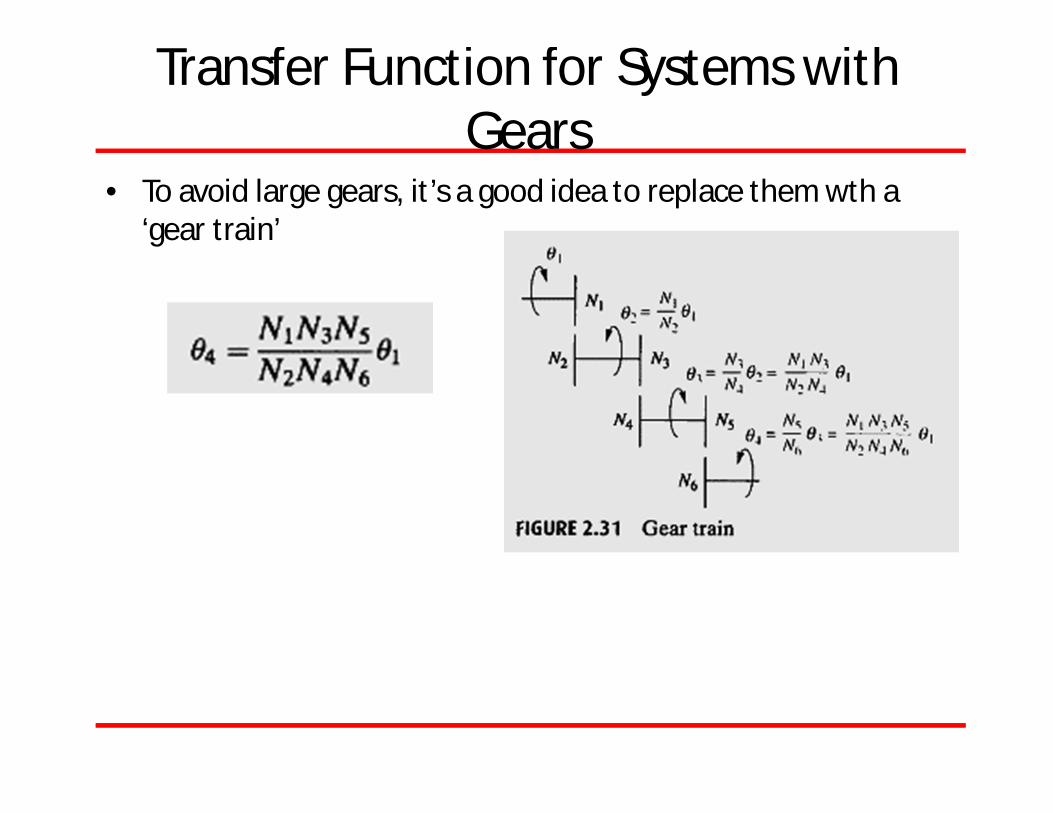
• To avoid large gears, it’s a good idea to replace them wth a ‘gear train’
The Transformer
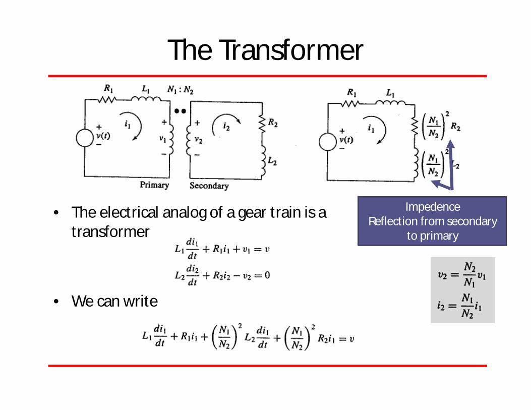
• The electrical analog of a gear train is a transformer
• We can write
ImpedenceReflection from secondary
to primary

Electro-mechanical Systems Transfer Functions
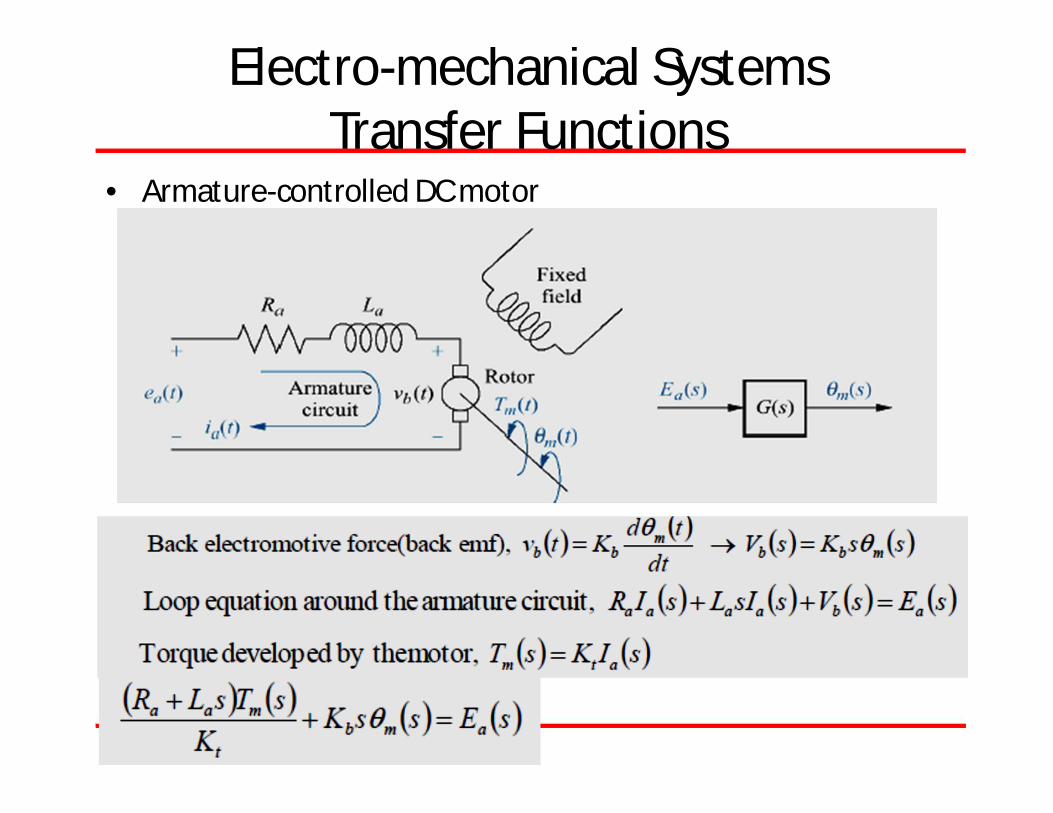
• Armature-controlled DC motor
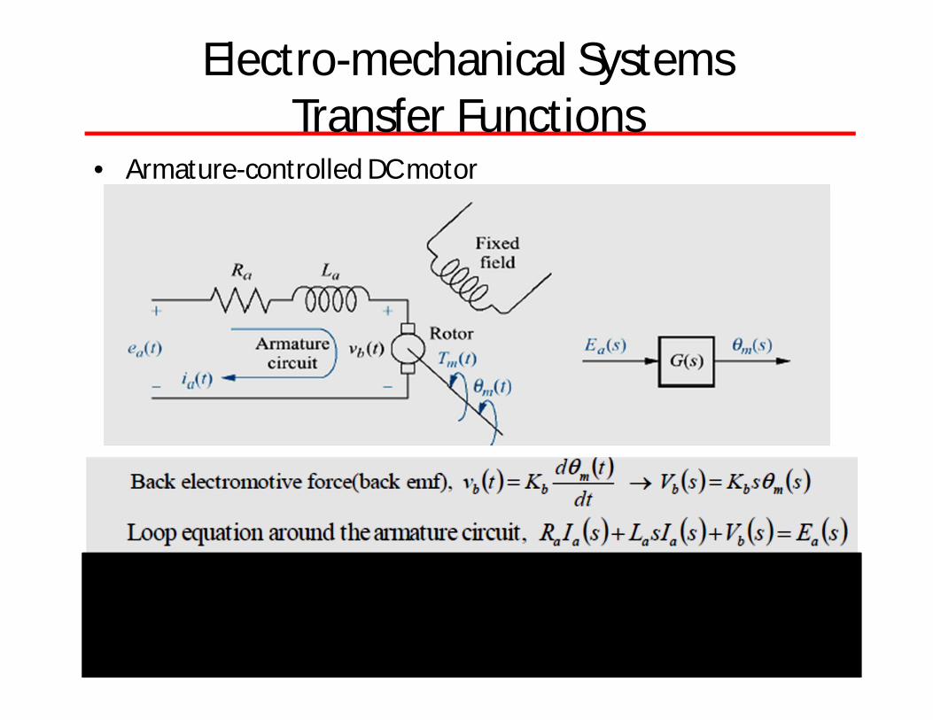
Electro-mechanical Systems Transfer Functions
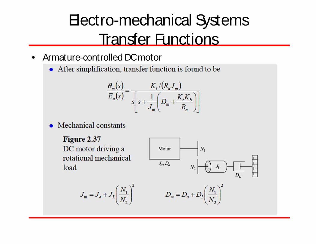
• Armature-controlled DC motor
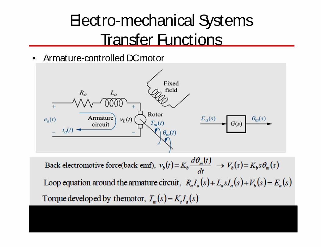
Electro-mechanical Systems Transfer Functions
• Armature-controlled DC motor
Electro-mechanical Systems Transfer Functions
• Armature-controlled DC motor

Electro-mechanical Systems Transfer Functions
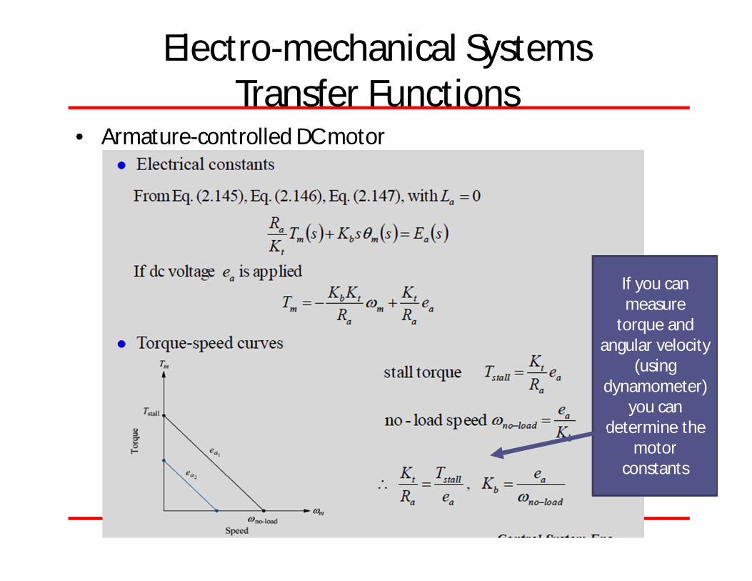
• Armature-controlled DC motor
Electro-mechanical Systems Transfer Functions
• Armature-controlled DC motor
Electro-mechanical Systems Transfer Functions
• Armature-controlled DC motor
If you can measure
torque and angular velocity
(using dynamometer)
you can determine the
motor constants
Electro-mechanical Systems Transfer Functions
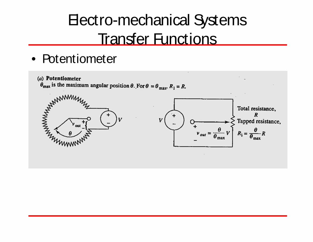
• Potentiometer
Electro-mechanical Systems Transfer Functions
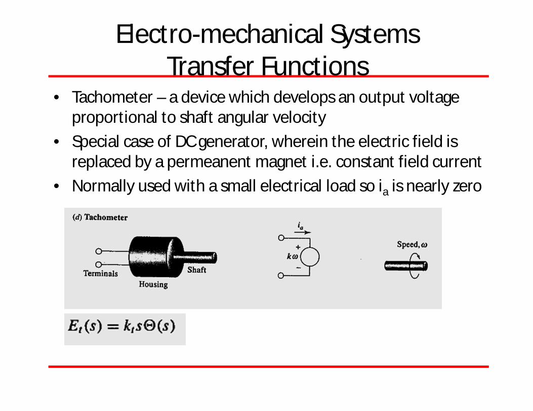
• Tachometer – a device which develops an output voltage proportional to shaft angular velocity
• Special case of DC generator, wherein the electric field is replaced by a permeanent magnet i.e. constant field current
• Normally used with a small electrical load so ia is nearly zero

Electro-mechanical Systems Transfer Functions
• Linear Actuator Solenoid
• The magnetic force caused by the current flowing through RL circuit causes the plunger mass to move

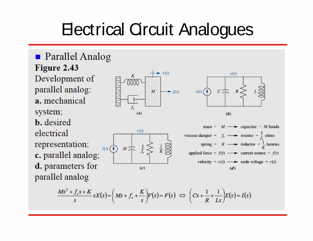
Electrical Circuit Analogues
• Mechanical systems can be represented by equilvalent electrical systems
• An electric circuit that is analogous to a system from another discipline is called electric circuit analogue
• They can be formulated by comparing the describing mathematical equations for the systems

Electrical Circuit Analogues
• Electric circuit analogies

Electrical Circuit Analogues• For more than one degree of freedom,
– The impedence associated with a motion appears as series electrical impedences in a mesh
– The impedences between adjacent motions are represented as series electrical impedences between two corresponding meshes
Electrical Circuit Analogues
• Aerodynamics
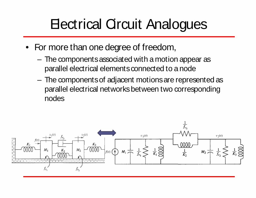
Electrical Circuit Analogues• For more than one degree of freedom,
– The components associated with a motion appear as parallel electrical elements connected to a node
– The components of adjacent motions are represented as parallel electrical networks between two corresponding nodes

Nonlinearity
• BJT transistor
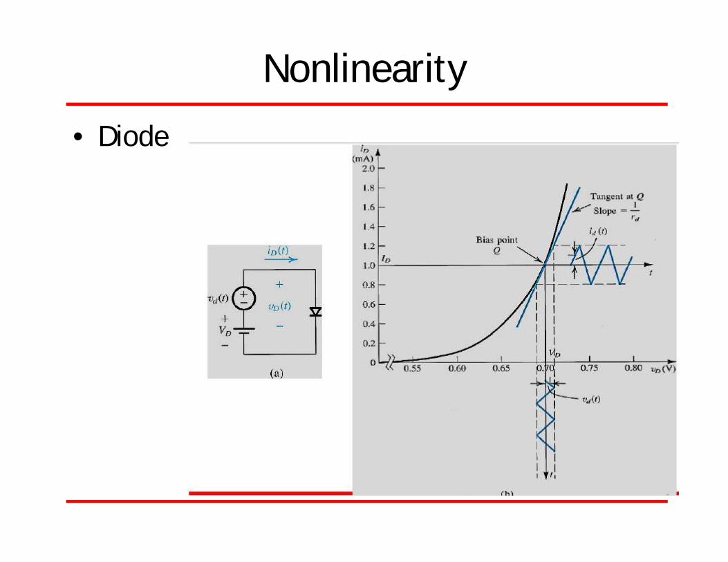
Nonlinearity
• Diode

Nonlinearity
• Actuator with saturation
System
[1] Tao and Kokotovic, "Adaptive Control of Systems with Actuators and Sensor Nonlinearities", John Wiley and Sons 1996
System

Nonlinearity
• Backlash in gears
http://www.wittenstein-us.com/tech-support/engineering-glossary/
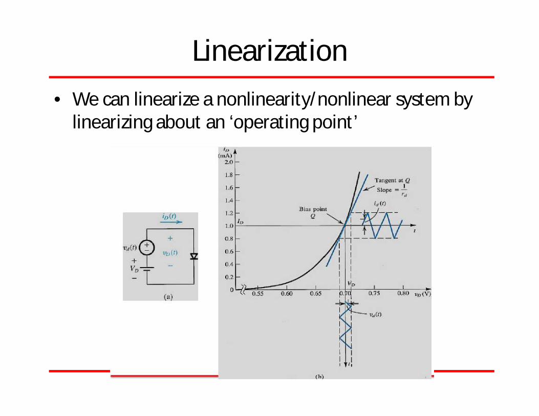
Linearization• We can linearize a nonlinearity/nonlinear system by
linearizing about an ‘operating point’
LinearizationTaylor Series
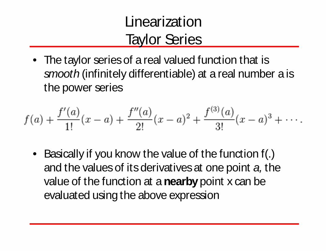
• The taylor series of a real valued function that is smooth (infinitely differentiable) at a real number a is the power series
• Basically if you know the value of the function f(.) and the values of its derivatives at one point a, the value of the function at a nearby point x can be evaluated using the above expression
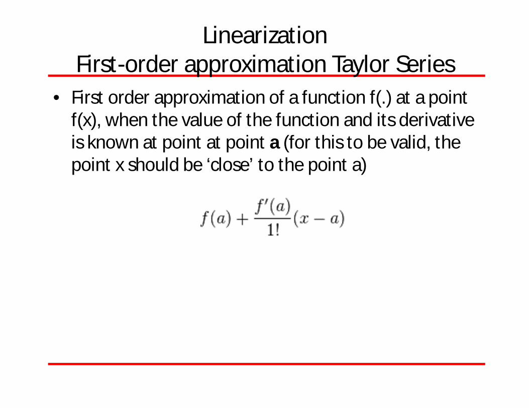
LinearizationFirst-order approximation Taylor Series
• First order approximation of a function f(.) at a point f(x), when the value of the function and its derivative is known at point at point a (for this to be valid, the point x should be ‘close’ to the point a)

Examplelinearization
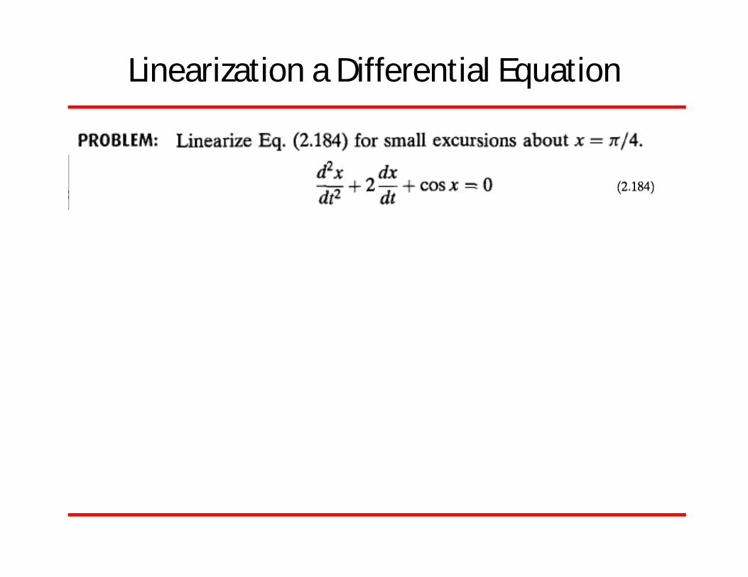
Linearization a Differential Equation
Related Documents