Layered occlusion map for soft shadow generation

Vis Comput (2010) 26: 1497–1512DOI 10.1007/s00371-010-0507-1

O R I G I NA L A RT I C L E

Layered occlusion map for soft shadow generation

Kien T. Nguyen · Hanyoung Jang · JungHyun Han

Published online: 28 April 2010© Springer-Verlag 2010

Abstract This paper presents a high-quality high-perfor-mance algorithm to compute plausible soft shadows forcomplex dynamic scenes. Given a rectangular light source,the scene is rendered from the viewpoint placed at the cen-ter of the light source, and discretized into a layered depthmap. For each scene point sampled in the depth map, theocclusion degree is computed, and stored in a layered oc-clusion map. When the scene is rendered from the camera’sviewpoint, the occlusion degree of a scene point is computedby filtering the layered occlusion map. The proposed algo-rithm produces soft shadows the quality of which is quiteclose to that of the ground truth reference. As it runs veryfast, a scene with a million polygons can be rendered in real-time. The proposed method does not require pre-processingand is easy to implement in contemporary graphic hard-ware.

Keywords Soft shadow algorithm · Image processing ·Hardware accelerated rendering · Real-time shadowing

1 Introduction

Shadows increase the realism of rendered images, and helpus understand the spatial relationships among objects in ascene. Two seminal works in shadow generation are shadowvolume [7] and shadow mapping [29]. The shadow volumeis an object-space technique. It describes the 3D volume oc-cluded from a light source, and determines if a pixel to berendered is within the volume. In contrast, shadow mapping

K.T. Nguyen · H. Jang · J. Han (�)Korea University, Seoul, Koreae-mail: [email protected]

is an image-space technique. It tests if a pixel to be renderedis visible from the light source, using a depth image fromthe viewpoint of the light source, stored in a texture namedshadow map.

The two original works assume a point light source, andgenerate hard shadows where a point in the scene is eitherfully lit by or fully occluded from the light source. How-ever, area or volumetric light sources in the real world gener-ate soft shadows, where a penumbra region lies between theumbra (fully occluded) region and the fully lit region. Fordecades, the shadow volume and the shadow mapping tech-niques have been extended to generate soft shadows, andmany real-time algorithms have been proposed.

Recently, many of the shadow mapping algorithms forsoft shadow generation have pursued a common technique.The shadow map is viewed as a discrete representation of thescene, and each sample in the map is considered as a micro-patch. To determine the percentage or degree of occlusion ata point, the micro-patches selected as the potential occludersare back-projected from the point to the light plane, and theoverlapped area is computed [4, 14].

This paper presents a high-quality high-performance al-gorithm along the lines of the micro-patch projection ap-proach. Given a light source, the scene is rendered from thelight source’s viewpoint, and discretized into a layered depthmap. (The layered depth map was initially proposed for ren-dering transparent objects [10].) For each scene point sam-pled in the layered depth map, the occlusion degree is com-puted through back-projection, and stored in the so-calledlayered occlusion map (LOM). When the scene is renderedfrom the camera’s viewpoint, the occlusion degree of a scenepoint is computed by filtering the LOM.

The LOM presented in this paper is constructed usingthe layered depth map and micro-patch back projection al-gorithm. The proposed method produces soft shadows, the

mailto:[email protected]

1498 K.T. Nguyen et al.

quality of which is quite close to that of the ground truthreference. It runs very fast such that a scene with a millionpolygons can be rendered in real-time.

The remainder of the paper is organized as follows. Sec-tion 2 reviews related work. Section 3 presents how to con-struct the layered depth map and the LOM, and Sect. 4presents how to render the shadowed scene using the twomaps. Section 5 discusses various optimization techniquesused to construct the maps. Section 6 presents the imple-mentation details, and Sect. 7 reports the experimental re-sults. Section 8 compares the proposed method with existingwork, and finally Sect. 9 concludes the paper.

2 Related work

An exhaustive survey of the numerous shadow algorithms isbeyond the scope of this section; readers are referred to Wooet al. [31] for a comprehensive survey on hard shadows, andHasenfratz et al. [16] for soft shadows. After briefly review-ing the shadow volume approach and a recently proposedalgorithm based on the pre-computed shadow fields, we willfocus on the shadow mapping algorithms closely related toour method.

The shadow volume approach [7] has been extended toproduce soft shadows. Akenine-Möller and Assarsson [2]construct a penumbra-wedge per silhouette edge which isseen from the light source center. The penumbra-wedgesare back-projected to the light source plane to accumulatethe occluded area of the light source. Laine et al. [19] com-bine penumbra-wedges with ray tracing for planar area lightsource. Forest et al. [12] use penumbra-wedge to identifythe visible surface points in the penumbra region. The vis-ibility of the light source from a surface point is computedusing the depth complexity between the point and a set oflight samples. Recently, Forest et al. [13] propose a soft tex-ture shadow volume to produce soft shadows for perforatedtriangles.

Sloan et al. [27] proposed to pre-compute radiance trans-fer for realtime rendering of low-frequency lighting by usinga spherical harmonic basis to store the pre-computed lighttransport at every point in the scene. Zhou et al. [33] pro-posed to construct shadow fields around each single objectwhich can be pre-computed independently of the scene con-figuration. This approach has been extended by [18, 20] tointeractively render a dynamic scene in realtime.

Shadow mapping was introduced by Williams [29]. Thescene is rendered from the light source’s viewpoint, and itsdepths are computed and stored in the shadow map. Hardshadows are produced by transforming each screen-spacepixel to the light space and then comparing its depth to theone in the shadow map. If the pixel depth is greater than thestored one, it is determined to be occluded from the light.

Following the seminal work of Williams, many algo-rithms have been presented to make soft shadows by extend-ing the shadow mapping technique. Reeves et al. [21] pro-posed the percentage closer filtering (PCF) method to softenthe hard shadow edges. Multiple sampling of the shadowmap is performed around the pixel to be rendered, and theresults are compared to the point’s depth, as in conventionalshadow mapping. The binary values are filtered to give theapproximate visibility of the point. Fernando [11] extendedthe PCF method. Given a pixel to be rendered, the depthmap is searched for its potential occluders, and the averageof their depths is computed to determine the kernel size. PCFis applied to the kernel to approximate the pixel’s visibility.

Heidrich et al. [17] produced soft shadows of a linearlight source by sampling it at two endpoints. For each lightsample, a soft shadow map is computed that consists of aconventional depth map and a visibility map. The visibilitymap at one light sample is computed by warping the triangu-lated depth points from the other light sample’s depth mapto its viewpoint. The soft shadows are produced by summingthe two visibility maps. Agrawala et al. [1] processed a setof samples of an area light source, and generated a depthmap for a sample. All points in the depth maps are warpedinto the viewpoint located at the light source center. Thosepoints are added into a multi-layer buffer, called the layerattenuation map, which contains depth and visibility infor-mation. The visibility at a point is computed by counting thenumber of visible light samples from the point. When ren-dering the scene from the camera’s viewpoint, a scene pointis transformed to the light space with respect to the light cen-ter, and the layer attenuation map is searched to obtain thevisibility of the point.

Arvo et al. [3] detected the hard shadow boundaries,in the screen space, that also store occluder informationfrom the depth map. A modified flood-fill method is usedto expand the penumbra regions from the boundaries. Thismethod heavily depends on the number of flood-fill steps.Rong and Tan [22] improved the work of Arvo et al. byproposing a quick flood-fill method ending in a few steps.Initially, a large kernel is used to spread out the occluderinformation from the boundaries. Then smaller kernels areused in an iterative fashion to correct the occluder informa-tion of a pixel in the penumbra.

Eisemann and Décoret [9] rendered the scene into amulti-sliced shadow map. Each slice of the shadow map ispre-filtered. In the final rendering step, the visibility of ascene point is computed from the filtered slices using a prob-abilistic approach. Their algorithm is sensitive to the slicepositions, i.e., where to place the slices.

Drettakis and Fiume [8] proposed a backprojection datastructure to represent the visible portion of a light sourcefrom any point in the scene. Since then, many algorithmshave extended the idea: the shadow map samples are con-verted into micro-patches, and then back-projected to the

Layered occlusion map for soft shadow generation 1499

light source plane [4–6, 14]. The idea of the micro-patch hasalso been extended into more complicated geometries, suchas micro-quads [23], micro-rects [25], and micro-tris [24].

Atty et al. [4] processed a micro-patch at a time to com-pute the region of the soft shadow map, affected by themicro-patch. For each pixel in the region, the micro-patchis back-projected to the light plane, and the occlusion de-gree is computed. The process is done for all micro-patches,and the occlusion degrees are accumulated into the softshadow map. Finally, the soft shadow map is projected ontothe scene to produce soft shadows. This algorithm distin-guishes between occluders and receivers, and thus cannotproduce self-shadows. Another disadvantage of the algo-rithm is that the shadow map (occluder map) generated byGPU is read back to the CPU that then invokes the GPUfor back-projection. The communication between CPU andGPU degrades the rendering performance.

Guennebaud et al. [14] took a similar approach, but back-projection was done from a screen-space pixel. Given apixel, the shadow map is searched for the samples workingas the potential occluders. They are back-projected into thelight plane. The algorithm proposed to extend the samplesizes to overcome the light leaking problem caused by thediscrete nature of the shadow map. However, the solutionoften leads to over-shadows.

Guennebaud et al. [15] improved the shadow quality bydetecting local contour edges at texel level of the shadowmap. Given a pixel of the screen space, the shadow mapsamples working as the potential occluders are identified,as was done in the previous work [14]. Instead of back-projecting each sample in the micro-patch form, however,a local contour edge is back-projected to the light sourceplane. The back-projected edge is clipped by the bordersof the light source, and the occluded area associated withthe edge is computed and accumulated. Then, the occlu-sion degree of the current pixel is computed. Yang et al.[32] adopted the technique of contour edge back-projection,and proposed a so-called packet-based method, where a setof screen-space pixels is processed simultaneously. The op-erations of shadow map access and contour extraction areperformed with respect to the set. Exploiting the penumbracoherence between the adjacent pixels leads to the perfor-mance increase.

The layered depth map was proposed by a few algo-rithms [5, 6, 23], to reduce the light leaking and over-shadowproblems; and the goal of reducing the artifact was largelyachieved. Like the work of Guennebaud et al. [14], however,these techniques process the screen-space pixels. As a result,the performance of the algorithm is sensitive to the percent-age of the penumbra pixels in the screen. When the penum-bra pixels take a larger part of the screen, performance dropssignificantly because more samples in the depth map shouldbe processed. Guennebaud et al. [15] alleviated this limita-tion using a pre-computed pattern to skip some screen pixels

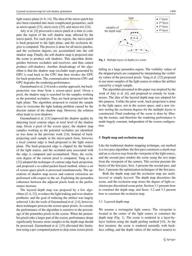
Fig. 1 Multiple layers of depths in a scene

falling in a large penumbra region. The visibility values ofthe skipped pixels are computed by interpolating the visibil-ity values of the processed pixels. Yang et al. [32] proposedto use more samples of the light source to reduce the artifactcaused by a single sample.

The algorithm presented in this paper was inspired by thework of Atty et al. [4], and proposed to remedy its weak-nesses. The idea of the layered depth map was adopted forthis purpose. Unlike the prior work, back-projection is donein the light space, not in the screen space, and a new tex-ture storing the occlusion degrees for the multiple layers isconstructed. Final rendering of the scene is done by filter-ing the texture, and therefore the rendering performance ismade largely constant, independent of the screen configura-tion.

3 Depth map and occlusion map

Like the traditional shadow mapping technique, our methodis a two-pass algorithm: the first pass constructs a depth mapand an occlusion map from the viewpoint of the light source,and the second pass renders the scene using the two mapsfrom the viewpoint of the camera. This section presents thebasics of the first pass, Sect. 4 presents the second pass, andSect. 5 presents the optimization techniques of the first pass.

Both the depth map and the occlusion map are multi-layered or simply layered. The depth map discretizes thescene, and the occlusion map stores the degree of light oc-clusion per discretized scene point. Section 3.1 presents howto construct the depth map, and Sects. 3.2 and 3.3 presenthow to construct the occlusion map.

3.1 Layered depth map

We assume a rectangular light source. The viewpoint islocated at the center of the light source to construct thedepth map (Fig. 1). The scene is rendered in a layer-by-layer fashion using the depth peeling method [10]. At thefirst iteration, the scene is rendered normally with back-face culling, and the depth values of the surfaces nearest to


the light source are stored in the first layer. The first layercontains the same information as the traditional shadowmap.

In the second iteration, the depths less than or equal tothose stored in the first layer are peeled away, and the secondlayer is filled. This process is repeated until the entire sceneis discretized. Figure 1 shows four depth layers of a scene.

Multiple layers are packed in a texture such that a sam-ple at (u, v) contains multiple depth values. A 4-channel(RGBA) texture is sufficient to represent the depth map forthe scene in Fig. 1. If a scene requires more than four depthlayers, we may use additional textures. Even in such a case,however, a single texture is sufficient in general, as will bediscussed in Sect. 5.1.

3.2 Collecting potential occludees

The layered occlusion map (LOM) is constructed using thedepth map. The two maps have the same structure, butthe depth map contains a depth value per discretized scenepoint, whereas LOM contains its occlusion degree, whichrepresents how much of light is occluded. The occlusion de-

Fig. 2 Algorithm for LOM construction

gree is in the range of [0,1], where 0 denotes ‘fully lit’ and1 denotes ‘fully occluded.’

Figure 2 shows the skeleton of the LOM constructionalgorithm. The algorithm processes a sample of the depthmap at a time. The depth values are retrieved from a sam-ple, and a rectangular micro-patch is placed at each depthvalue. For some of the scene points discretized in the depthmap, the light rays from the light source may be occludedby the micro-patches. Such scene points, called potentialoccludees, are identified using the method presented inthis sub-section. Then, the occlusion degree is computedfor each potential occludee by back-projecting the micro-patches, as presented in Sect. 3.3.

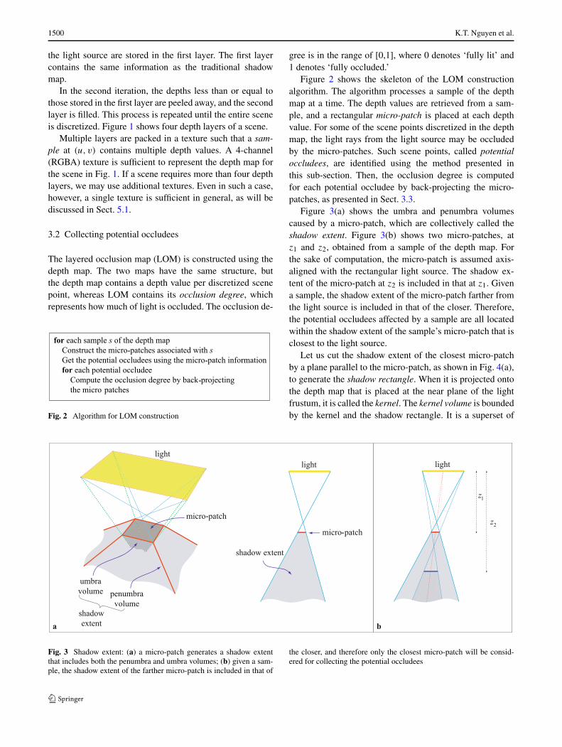
Figure 3(a) shows the umbra and penumbra volumescaused by a micro-patch, which are collectively called theshadow extent. Figure 3(b) shows two micro-patches, atz1 and z2, obtained from a sample of the depth map. Forthe sake of computation, the micro-patch is assumed axis-aligned with the rectangular light source. The shadow ex-tent of the micro-patch at z2 is included in that at z1. Givena sample, the shadow extent of the micro-patch farther fromthe light source is included in that of the closer. Therefore,the potential occludees affected by a sample are all locatedwithin the shadow extent of the sample’s micro-patch that isclosest to the light source.

Let us cut the shadow extent of the closest micro-patchby a plane parallel to the micro-patch, as shown in Fig. 4(a),to generate the shadow rectangle. When it is projected ontothe depth map that is placed at the near plane of the lightfrustum, it is called the kernel. The kernel volume is boundedby the kernel and the shadow rectangle. It is a superset of

Fig. 3 Shadow extent: (a) a micro-patch generates a shadow extentthat includes both the penumbra and umbra volumes; (b) given a sam-ple, the shadow extent of the farther micro-patch is included in that of

the closer, and therefore only the closest micro-patch will be consid-ered for collecting the potential occludees


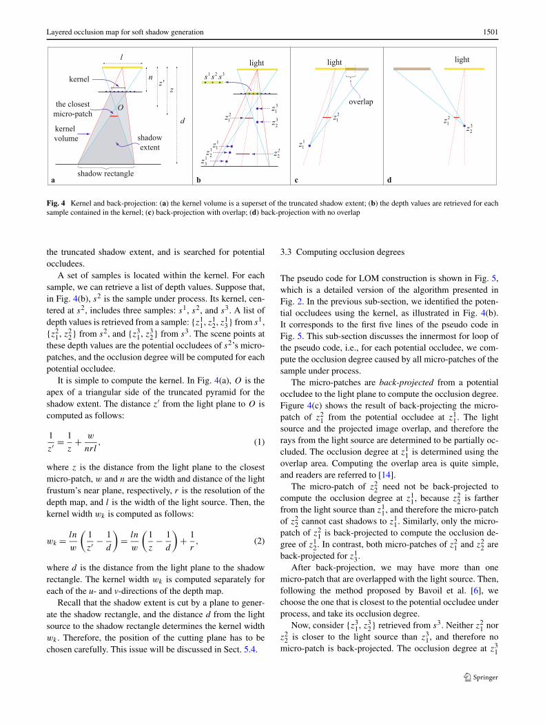
Fig. 4 Kernel and back-projection: (a) the kernel volume is a superset of the truncated shadow extent; (b) the depth values are retrieved for eachsample contained in the kernel; (c) back-projection with overlap; (d) back-projection with no overlap

the truncated shadow extent, and is searched for potentialoccludees.

A set of samples is located within the kernel. For eachsample, we can retrieve a list of depth values. Suppose that,in Fig. 4(b), s2 is the sample under process. Its kernel, cen-tered at s2, includes three samples: s1, s2, and s3. A list ofdepth values is retrieved from a sample: {z1

1, z12, z1

3} from s1,{z2

1, z22} from s2, and {z3

1, z32} from s3. The scene points at

these depth values are the potential occludees of s2’s micro-patches, and the occlusion degree will be computed for eachpotential occludee.

It is simple to compute the kernel. In Fig. 4(a), O is theapex of a triangular side of the truncated pyramid for theshadow extent. The distance z′ from the light plane to O iscomputed as follows:

1

z′ = 1

z+ w

nrl, (1)

where z is the distance from the light plane to the closestmicro-patch, w and n are the width and distance of the lightfrustum’s near plane, respectively, r is the resolution of thedepth map, and l is the width of the light source. Then, thekernel width wk is computed as follows:

wk = ln

w

(1

z′ − 1

d

)= ln

w

(1

z− 1

d

)+ 1

r, (2)

where d is the distance from the light plane to the shadowrectangle. The kernel width wk is computed separately foreach of the u- and v-directions of the depth map.

Recall that the shadow extent is cut by a plane to gener-ate the shadow rectangle, and the distance d from the lightsource to the shadow rectangle determines the kernel widthwk . Therefore, the position of the cutting plane has to bechosen carefully. This issue will be discussed in Sect. 5.4.

3.3 Computing occlusion degrees

The pseudo code for LOM construction is shown in Fig. 5,which is a detailed version of the algorithm presented inFig. 2. In the previous sub-section, we identified the poten-tial occludees using the kernel, as illustrated in Fig. 4(b).It corresponds to the first five lines of the pseudo code inFig. 5. This sub-section discusses the innermost for loop ofthe pseudo code, i.e., for each potential occludee, we com-pute the occlusion degree caused by all micro-patches of thesample under process.

The micro-patches are back-projected from a potentialoccludee to the light plane to compute the occlusion degree.Figure 4(c) shows the result of back-projecting the micro-patch of z2

1 from the potential occludee at z11. The light

source and the projected image overlap, and therefore therays from the light source are determined to be partially oc-cluded. The occlusion degree at z1

1 is determined using theoverlap area. Computing the overlap area is quite simple,and readers are referred to [14].

The micro-patch of z22 need not be back-projected to

compute the occlusion degree at z11, because z2

2 is fartherfrom the light source than z1

1, and therefore the micro-patchof z2

2 cannot cast shadows to z11. Similarly, only the micro-

patch of z21 is back-projected to compute the occlusion de-

gree of z12. In contrast, both micro-patches of z2

1 and z22 are

back-projected for z13.

After back-projection, we may have more than onemicro-patch that are overlapped with the light source. Then,following the method proposed by Bavoil et al. [6], wechoose the one that is closest to the potential occludee underprocess, and take its occlusion degree.

Now, consider {z31, z3

2} retrieved from s3. Neither z21 nor

z22 is closer to the light source than z3

1, and therefore nomicro-patch is back-projected. The occlusion degree at z3

1


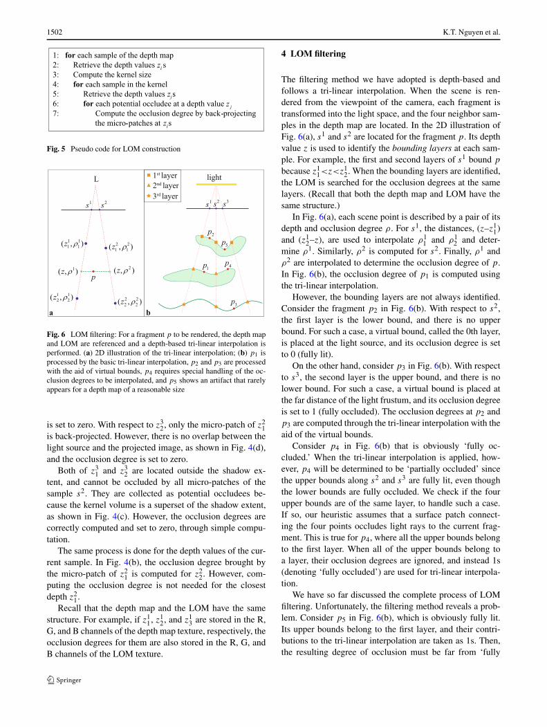
Fig. 5 Pseudo code for LOM construction

Fig. 6 LOM filtering: For a fragment p to be rendered, the depth mapand LOM are referenced and a depth-based tri-linear interpolation isperformed. (a) 2D illustration of the tri-linear interpolation; (b) p1 isprocessed by the basic tri-linear interpolation, p2 and p3 are processedwith the aid of virtual bounds, p4 requires special handling of the oc-clusion degrees to be interpolated, and p5 shows an artifact that rarelyappears for a depth map of a reasonable size

is set to zero. With respect to z32, only the micro-patch of z2

1is back-projected. However, there is no overlap between thelight source and the projected image, as shown in Fig. 4(d),and the occlusion degree is set to zero.

Both of z31 and z3

2 are located outside the shadow ex-tent, and cannot be occluded by all micro-patches of thesample s2. They are collected as potential occludees be-cause the kernel volume is a superset of the shadow extent,as shown in Fig. 4(c). However, the occlusion degrees arecorrectly computed and set to zero, through simple compu-tation.

The same process is done for the depth values of the cur-rent sample. In Fig. 4(b), the occlusion degree brought bythe micro-patch of z2

1 is computed for z22. However, com-

puting the occlusion degree is not needed for the closestdepth z2

1.Recall that the depth map and the LOM have the same

structure. For example, if z11, z1

2, and z13 are stored in the R,

G, and B channels of the depth map texture, respectively, theocclusion degrees for them are also stored in the R, G, andB channels of the LOM texture.

4 LOM filtering

The filtering method we have adopted is depth-based andfollows a tri-linear interpolation. When the scene is ren-dered from the viewpoint of the camera, each fragment istransformed into the light space, and the four neighbor sam-ples in the depth map are located. In the 2D illustration ofFig. 6(a), s1 and s2 are located for the fragment p. Its depthvalue z is used to identify the bounding layers at each sam-ple. For example, the first and second layers of s1 bound p

because z11<z<z1

2. When the bounding layers are identified,the LOM is searched for the occlusion degrees at the samelayers. (Recall that both the depth map and LOM have thesame structure.)

In Fig. 6(a), each scene point is described by a pair of itsdepth and occlusion degree ρ. For s1, the distances, (z–z1

1)and (z1

2–z), are used to interpolate ρ11 and ρ1

2 and deter-mine ρ1. Similarly, ρ2 is computed for s2. Finally, ρ1 andρ2 are interpolated to determine the occlusion degree of p.In Fig. 6(b), the occlusion degree of p1 is computed usingthe tri-linear interpolation.

However, the bounding layers are not always identified.Consider the fragment p2 in Fig. 6(b). With respect to s2,the first layer is the lower bound, and there is no upperbound. For such a case, a virtual bound, called the 0th layer,is placed at the light source, and its occlusion degree is setto 0 (fully lit).

On the other hand, consider p3 in Fig. 6(b). With respectto s3, the second layer is the upper bound, and there is nolower bound. For such a case, a virtual bound is placed atthe far distance of the light frustum, and its occlusion degreeis set to 1 (fully occluded). The occlusion degrees at p2 andp3 are computed through the tri-linear interpolation with theaid of the virtual bounds.

Consider p4 in Fig. 6(b) that is obviously ‘fully oc-cluded.’ When the tri-linear interpolation is applied, how-ever, p4 will be determined to be ‘partially occluded’ sincethe upper bounds along s2 and s3 are fully lit, even thoughthe lower bounds are fully occluded. We check if the fourupper bounds are of the same layer, to handle such a case.If so, our heuristic assumes that a surface patch connect-ing the four points occludes light rays to the current frag-ment. This is true for p4, where all the upper bounds belongto the first layer. When all of the upper bounds belong toa layer, their occlusion degrees are ignored, and instead 1s(denoting ‘fully occluded’) are used for tri-linear interpola-tion.

We have so far discussed the complete process of LOMfiltering. Unfortunately, the filtering method reveals a prob-lem. Consider p5 in Fig. 6(b), which is obviously fully lit.Its upper bounds belong to the first layer, and their contri-butions to the tri-linear interpolation are taken as 1s. Then,the resulting degree of occlusion must be far from ‘fully


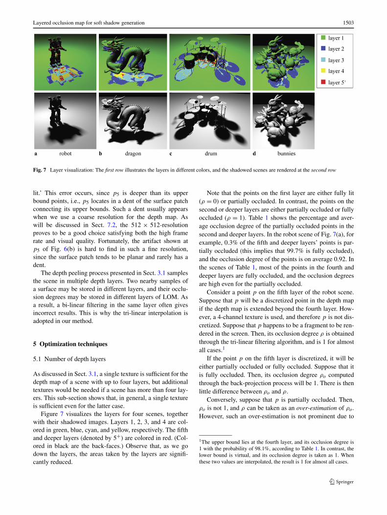
Fig. 7 Layer visualization: The first row illustrates the layers in different colors, and the shadowed scenes are rendered at the second row

lit.’ This error occurs, since p5 is deeper than its upperbound points, i.e., p5 locates in a dent of the surface patchconnecting its upper bounds. Such a dent usually appearswhen we use a coarse resolution for the depth map. Aswill be discussed in Sect. 7.2, the 512 × 512-resolutionproves to be a good choice satisfying both the high framerate and visual quality. Fortunately, the artifact shown atp5 of Fig. 6(b) is hard to find in such a fine resolution,since the surface patch tends to be planar and rarely has adent.

The depth peeling process presented in Sect. 3.1 samplesthe scene in multiple depth layers. Two nearby samples ofa surface may be stored in different layers, and their occlu-sion degrees may be stored in different layers of LOM. Asa result, a bi-linear filtering in the same layer often givesincorrect results. This is why the tri-linear interpolation isadopted in our method.

5 Optimization techniques

5.1 Number of depth layers

As discussed in Sect. 3.1, a single texture is sufficient for thedepth map of a scene with up to four layers, but additionaltextures would be needed if a scene has more than four lay-ers. This sub-section shows that, in general, a single textureis sufficient even for the latter case.

Figure 7 visualizes the layers for four scenes, togetherwith their shadowed images. Layers 1, 2, 3, and 4 are col-ored in green, blue, cyan, and yellow, respectively. The fifthand deeper layers (denoted by 5+) are colored in red. (Col-ored in black are the back-faces.) Observe that, as we godown the layers, the areas taken by the layers are signifi-cantly reduced.

Note that the points on the first layer are either fully lit(ρ = 0) or partially occluded. In contrast, the points on thesecond or deeper layers are either partially occluded or fullyoccluded (ρ = 1). Table 1 shows the percentage and aver-age occlusion degree of the partially occluded points in thesecond and deeper layers. In the robot scene of Fig. 7(a), forexample, 0.3% of the fifth and deeper layers’ points is par-tially occluded (this implies that 99.7% is fully occluded),and the occlusion degree of the points is on average 0.92. Inthe scenes of Table 1, most of the points in the fourth anddeeper layers are fully occluded, and the occlusion degreesare high even for the partially occluded.

Consider a point p on the fifth layer of the robot scene.Suppose that p will be a discretized point in the depth mapif the depth map is extended beyond the fourth layer. How-ever, a 4-channel texture is used, and therefore p is not dis-cretized. Suppose that p happens to be a fragment to be ren-dered in the screen. Then, its occlusion degree ρ is obtainedthrough the tri-linear filtering algorithm, and is 1 for almostall cases.1

If the point p on the fifth layer is discretized, it will beeither partially occluded or fully occluded. Suppose that itis fully occluded. Then, its occlusion degree ρo computedthrough the back-projection process will be 1. There is thenlittle difference between ρo and ρ.

Conversely, suppose that p is partially occluded. Then,ρo is not 1, and ρ can be taken as an over-estimation of ρo.However, such an over-estimation is not prominent due to

1The upper bound lies at the fourth layer, and its occlusion degree is1 with the probability of 98.1%, according to Table 1. In contrast, thelower bound is virtual, and its occlusion degree is taken as 1. Whenthese two values are interpolated, the result is 1 for almost all cases.


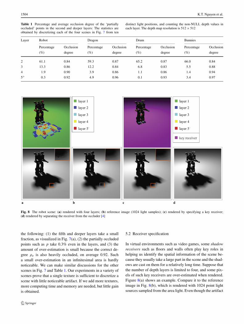
Table 1 Percentage and average occlusion degree of the ‘partiallyoccluded’ points in the second and deeper layers: The statistics areobtained by discretizing each of the four scenes in Fig. 7 from ten

distinct light positions, and counting the non-NULL depth values ineach layer. The depth map resolution is 512 × 512

Layer Robot Dragon Drum Bunnies

Percentage Occlusion Percentage Occlusion Percentage Occlusion Percentage Occlusion

(%) degree (%) degree (%) degree (%) degree

2 61.1 0.84 59.3 0.87 65.2 0.87 66.0 0.84

3 13.3 0.86 12.2 0.84 6.8 0.83 5.5 0.88

4 1.9 0.90 3.9 0.86 1.1 0.86 1.4 0.94

5+ 0.3 0.92 4.9 0.96 0.1 0.93 3.4 0.97

Fig. 8 The robot scene: (a) rendered with four layers; (b) reference image (1024 light samples); (c) rendered by specifying a key receiver;(d) rendered by separating the receiver from the occluder [4]

the following: (1) the fifth and deeper layers take a smallfraction, as visualized in Fig. 7(a), (2) the partially occludedpoints such as p take 0.3% even in the layers, and (3) theamount of over-estimation is small because the correct de-gree ρo is also heavily occluded, on average 0.92. Sucha small over-estimation in an infinitesimal area is hardlynoticeable. We can make similar discussions for the otherscenes in Fig. 7 and Table 1. Our experiments in a variety ofscenes prove that a single texture is sufficient to discretize ascene with little noticeable artifact. If we add more textures,more computing time and memory are needed, but little gainis obtained.

5.2 Receiver specification

In virtual environments such as video games, some shadowreceivers such as floors and walls often play key roles inhelping us identify the spatial information of the scene be-cause they usually take a large part in the scene and the shad-ows are cast on them for a relatively long time. Suppose thatthe number of depth layers is limited to four, and some pix-els of such key receivers are over-estimated when rendered.Figure 8(a) shows an example. Compare it to the referenceimage in Fig. 8(b), which is rendered with 1024 point lightsources sampled from the area light. Even though the artifact


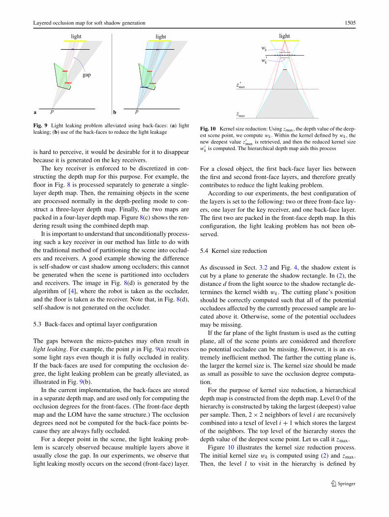
Fig. 9 Light leaking problem alleviated using back-faces: (a) lightleaking; (b) use of the back-faces to reduce the light leakage

is hard to perceive, it would be desirable for it to disappearbecause it is generated on the key receivers.

The key receiver is enforced to be discretized in con-structing the depth map for this purpose. For example, thefloor in Fig. 8 is processed separately to generate a single-layer depth map. Then, the remaining objects in the sceneare processed normally in the depth-peeling mode to con-struct a three-layer depth map. Finally, the two maps arepacked in a four-layer depth map. Figure 8(c) shows the ren-dering result using the combined depth map.

It is important to understand that unconditionally process-ing such a key receiver in our method has little to do withthe traditional method of partitioning the scene into occlud-ers and receivers. A good example showing the differenceis self-shadow or cast shadow among occluders; this cannotbe generated when the scene is partitioned into occludersand receivers. The image in Fig. 8(d) is generated by thealgorithm of [4], where the robot is taken as the occluder,and the floor is taken as the receiver. Note that, in Fig. 8(d),self-shadow is not generated on the occluder.

5.3 Back-faces and optimal layer configuration

The gaps between the micro-patches may often result inlight leaking. For example, the point p in Fig. 9(a) receivessome light rays even though it is fully occluded in reality.If the back-faces are used for computing the occlusion de-gree, the light leaking problem can be greatly alleviated, asillustrated in Fig. 9(b).

In the current implementation, the back-faces are storedin a separate depth map, and are used only for computing theocclusion degrees for the front-faces. (The front-face depthmap and the LOM have the same structure.) The occlusiondegrees need not be computed for the back-face points be-cause they are always fully occluded.

For a deeper point in the scene, the light leaking prob-lem is scarcely observed because multiple layers above itusually close the gap. In our experiments, we observe thatlight leaking mostly occurs on the second (front-face) layer.

Fig. 10 Kernel size reduction: Using zmax, the depth value of the deep-est scene point, we compute wk . Within the kernel defined by wk , thenew deepest value z′

max is retrieved, and then the reduced kernel sizew′

k is computed. The hierarchical depth map aids this process

For a closed object, the first back-face layer lies betweenthe first and second front-face layers, and therefore greatlycontributes to reduce the light leaking problem.

According to our experiments, the best configuration ofthe layers is set to the following: two or three front-face lay-ers, one layer for the key receiver, and one back-face layer.The first two are packed in the front-face depth map. In thisconfiguration, the light leaking problem has not been ob-served.

5.4 Kernel size reduction

As discussed in Sect. 3.2 and Fig. 4, the shadow extent iscut by a plane to generate the shadow rectangle. In (2), thedistance d from the light source to the shadow rectangle de-termines the kernel width wk . The cutting plane’s positionshould be correctly computed such that all of the potentialoccludees affected by the currently processed sample are lo-cated above it. Otherwise, some of the potential occludeesmay be missing.

If the far plane of the light frustum is used as the cuttingplane, all of the scene points are considered and thereforeno potential occludee can be missing. However, it is an ex-tremely inefficient method. The farther the cutting plane is,the larger the kernel size is. The kernel size should be madeas small as possible to save the occlusion degree computa-tion.

For the purpose of kernel size reduction, a hierarchicaldepth map is constructed from the depth map. Level 0 of thehierarchy is constructed by taking the largest (deepest) valueper sample. Then, 2 × 2 neighbors of level i are recursivelycombined into a texel of level i + 1 which stores the largestof the neighbors. The top level of the hierarchy stores thedepth value of the deepest scene point. Let us call it zmax.

Figure 10 illustrates the kernel size reduction process.The initial kernel size wk is computed using (2) and zmax.Then, the level l to visit in the hierarchy is defined by


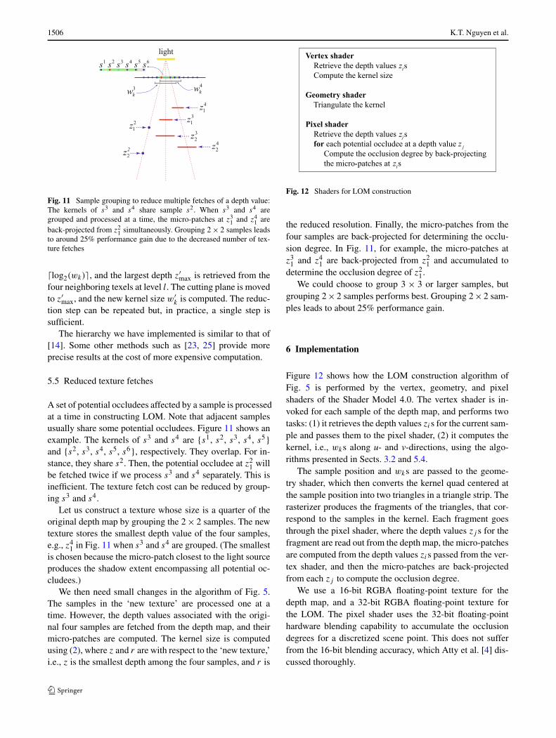
Fig. 11 Sample grouping to reduce multiple fetches of a depth value:The kernels of s3 and s4 share sample s2. When s3 and s4 aregrouped and processed at a time, the micro-patches at z3

1 and z41 are

back-projected from z21 simultaneously. Grouping 2 × 2 samples leads

to around 25% performance gain due to the decreased number of tex-ture fetches

�log2(wk)�, and the largest depth z′max is retrieved from the

four neighboring texels at level l. The cutting plane is movedto z′

max, and the new kernel size w′k is computed. The reduc-

tion step can be repeated but, in practice, a single step issufficient.

The hierarchy we have implemented is similar to that of[14]. Some other methods such as [23, 25] provide moreprecise results at the cost of more expensive computation.

5.5 Reduced texture fetches

A set of potential occludees affected by a sample is processedat a time in constructing LOM. Note that adjacent samplesusually share some potential occludees. Figure 11 shows anexample. The kernels of s3 and s4 are {s1, s2, s3, s4, s5}and {s2, s3, s4, s5, s6}, respectively. They overlap. For in-stance, they share s2. Then, the potential occludee at z2

1 willbe fetched twice if we process s3 and s4 separately. This isinefficient. The texture fetch cost can be reduced by group-ing s3 and s4.

Let us construct a texture whose size is a quarter of theoriginal depth map by grouping the 2 × 2 samples. The newtexture stores the smallest depth value of the four samples,e.g., z4

1 in Fig. 11 when s3 and s4 are grouped. (The smallestis chosen because the micro-patch closest to the light sourceproduces the shadow extent encompassing all potential oc-cludees.)

We then need small changes in the algorithm of Fig. 5.The samples in the ‘new texture’ are processed one at atime. However, the depth values associated with the origi-nal four samples are fetched from the depth map, and theirmicro-patches are computed. The kernel size is computedusing (2), where z and r are with respect to the ‘new texture,’i.e., z is the smallest depth among the four samples, and r is

Fig. 12 Shaders for LOM construction

the reduced resolution. Finally, the micro-patches from thefour samples are back-projected for determining the occlu-sion degree. In Fig. 11, for example, the micro-patches atz3

1 and z41 are back-projected from z2

1 and accumulated todetermine the occlusion degree of z2

1.We could choose to group 3 × 3 or larger samples, but

grouping 2 × 2 samples performs best. Grouping 2 × 2 sam-ples leads to about 25% performance gain.

6 Implementation

Figure 12 shows how the LOM construction algorithm ofFig. 5 is performed by the vertex, geometry, and pixelshaders of the Shader Model 4.0. The vertex shader is in-voked for each sample of the depth map, and performs twotasks: (1) it retrieves the depth values zis for the current sam-ple and passes them to the pixel shader, (2) it computes thekernel, i.e., wks along u- and v-directions, using the algo-rithms presented in Sects. 3.2 and 5.4.

The sample position and wks are passed to the geome-try shader, which then converts the kernel quad centered atthe sample position into two triangles in a triangle strip. Therasterizer produces the fragments of the triangles, that cor-respond to the samples in the kernel. Each fragment goesthrough the pixel shader, where the depth values zj s for thefragment are read out from the depth map, the micro-patchesare computed from the depth values zis passed from the ver-tex shader, and then the micro-patches are back-projectedfrom each zj to compute the occlusion degree.

We use a 16-bit RGBA floating-point texture for thedepth map, and a 32-bit RGBA floating-point texture forthe LOM. The pixel shader uses the 32-bit floating-pointhardware blending capability to accumulate the occlusiondegrees for a discretized scene point. This does not sufferfrom the 16-bit blending accuracy, which Atty et al. [4] dis-cussed thoroughly.


7 Experimental results

The experiments were performed on an Intel Core2 CPU1.86 GHz with an NVIDIA GeForce 8800 GTS graphicscard. The GPU code is in DirectX 10 and HLSL. All im-ages were rendered in 1024 × 768 resolution.

7.1 Scene complexity

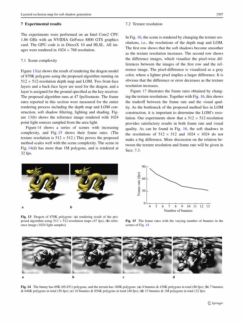
Figure 13(a) shows the result of rendering the dragon modelof 870K polygons using the proposed algorithm running on512 × 512-resolution depth map and LOM. Two front-facelayers and a back-face layer are used for the dragon, and alayer is assigned for the ground specified as the key receiver.The proposed algorithm runs at 47 fps/footnote. The framerates reported in this section were measured for the entirerendering process including the depth map and LOM con-struction, soft shadow filtering, lighting and shading. Fig-ure 13(b) shows the reference image rendered with 1024point light sources sampled from the area light.

Figure 14 shows a series of scenes with increasingcomplexity, and Fig. 15 shows their frame rates. (Thetexture resolution is 512 × 512.) This proves the proposedmethod scales well with the scene complexity. The scene inFig. 14(d) has more than 1M polygons, and is rendered at32 fps.

Fig. 13 Dragon of 870K polygons: (a) rendering result of the pro-posed algorithm using 512 × 512-resolution maps (47 fps); (b) refer-ence image (1024 light samples)

7.2 Texture resolution

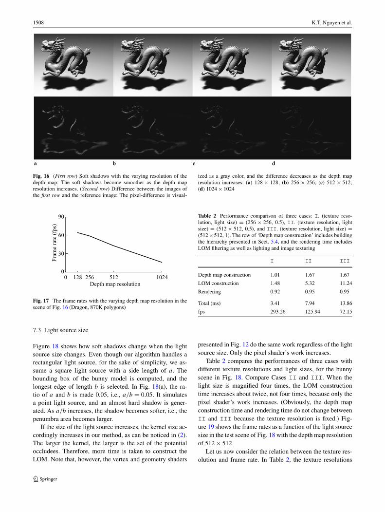
In Fig. 16, the scene is rendered by changing the texture res-olutions, i.e., the resolutions of the depth map and LOM.The first row shows that the soft shadows become smootheras the texture resolution increases. The second row showsthe difference images, which visualize the pixel-wise dif-ferences between the images of the first row and the ref-erence image. The pixel-difference is visualized as a graycolor, where a lighter pixel implies a larger difference. It isobvious that the difference or error decreases as the textureresolution increases.

Figure 17 illustrates the frame rates obtained by chang-ing the texture resolutions. Together with Fig. 16, this showsthe tradeoff between the frame rate and the visual qual-ity. As the bottleneck of the proposed method lies in LOMconstruction, it is important to determine the LOM’s reso-lution. Our experiments show that a 512 × 512-resolutionprovides satisfactory results in both frame rate and visualquality. As can be found in Fig. 16, the soft shadows inthe resolutions of 512 × 512 and 1024 × 1024 do notmake a big difference. More discussion on the relation be-tween the texture resolution and frame rate will be given inSect. 7.3.

Fig. 15 The frame rates with the varying number of bunnies in thescenes of Fig. 14

Fig. 14 The bunny has 69K (69,451) polygons, and the terrain has 160K polygons: (a) 4 bunnies & 438K polygons in total (86 fps); (b) 7 bunnies& 646K polygons in total (56 fps); (c) 10 bunnies & 854K polygons in total (40 fps); (d) 13 bunnies & 1M polygons in total (32 fps)


Fig. 16 (First row) Soft shadows with the varying resolution of thedepth map: The soft shadows become smoother as the depth mapresolution increases. (Second row) Difference between the images ofthe first row and the reference image: The pixel-difference is visual-

ized as a gray color, and the difference decreases as the depth mapresolution increases: (a) 128 × 128; (b) 256 × 256; (c) 512 × 512;(d) 1024 × 1024

Fig. 17 The frame rates with the varying depth map resolution in thescene of Fig. 16 (Dragon, 870K polygons)

7.3 Light source size

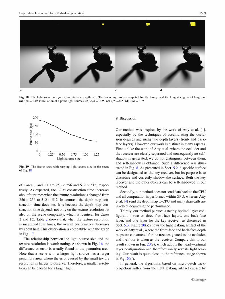
Figure 18 shows how soft shadows change when the lightsource size changes. Even though our algorithm handles arectangular light source, for the sake of simplicity, we as-sume a square light source with a side length of a. Thebounding box of the bunny model is computed, and thelongest edge of length b is selected. In Fig. 18(a), the ra-tio of a and b is made 0.05, i.e., a/b = 0.05. It simulatesa point light source, and an almost hard shadow is gener-ated. As a/b increases, the shadow becomes softer, i.e., thepenumbra area becomes larger.

If the size of the light source increases, the kernel size ac-cordingly increases in our method, as can be noticed in (2).The larger the kernel, the larger is the set of the potentialoccludees. Therefore, more time is taken to construct theLOM. Note that, however, the vertex and geometry shaders

Table 2 Performance comparison of three cases: I. (texture reso-lution, light size) = (256 × 256, 0.5), II. (texture resolution, lightsize) = (512 × 512, 0.5), and III. (texture resolution, light size) =(512 × 512, 1). The row of ‘Depth map construction’ includes buildingthe hierarchy presented in Sect. 5.4, and the rendering time includesLOM filtering as well as lighting and image texturing

I II III

Depth map construction 1.01 1.67 1.67

LOM construction 1.48 5.32 11.24

Rendering 0.92 0.95 0.95

Total (ms) 3.41 7.94 13.86

fps 293.26 125.94 72.15

presented in Fig. 12 do the same work regardless of the lightsource size. Only the pixel shader’s work increases.

Table 2 compares the performances of three cases withdifferent texture resolutions and light sizes, for the bunnyscene in Fig. 18. Compare Cases II and III. When thelight size is magnified four times, the LOM constructiontime increases about twice, not four times, because only thepixel shader’s work increases. (Obviously, the depth mapconstruction time and rendering time do not change betweenII and III because the texture resolution is fixed.) Fig-ure 19 shows the frame rates as a function of the light sourcesize in the test scene of Fig. 18 with the depth map resolutionof 512 × 512.

Let us now consider the relation between the texture res-olution and frame rate. In Table 2, the texture resolutions


Fig. 18 The light source is square, and its side length is a. The bounding box is computed for the bunny, and the longest edge is of length b:(a) a/b = 0.05 (simulation of a point light source); (b) a/b = 0.25; (c) a/b = 0.5; (d) a/b = 0.75

Fig. 19 The frame rates with varying light source size in the sceneof Fig. 18

of Cases I and II are 256 × 256 and 512 × 512, respec-tively. As expected, the LOM construction time increasesabout four times when the texture resolution is changed from256 × 256 to 512 × 512. In contrast, the depth map con-struction time does not. It is because the depth map con-struction time depends not only on the texture resolution butalso on the scene complexity, which is identical for CasesI and II. Table 2 shows that, when the texture resolutionis magnified four times, the overall performance decreasesby about half. This observation is compatible with the graphin Fig. 17.

The relationship between the light source size and thetexture resolution is worth noting. As shown in Fig. 16, thedifference or error is usually found in the penumbra area.Note that a scene with a larger light source has a largerpenumbra area, where the error caused by the small textureresolution is harder to observe. Therefore, a smaller resolu-tion can be chosen for a larger light.

8 Discussion

Our method was inspired by the work of Atty et al. [4],especially by the techniques of accumulating the occlu-sion degrees and using two depth layers (front- and back-face layers). However, our work is distinct in many aspects.First, unlike the work of Atty et al. where the occluder andthe receiver are clearly separated and consequently no self-shadow is generated, we do not distinguish between them,and self-shadow is obtained. Such a difference was illus-trated in Fig. 8. As presented in Sect. 5.2, a specific surfacecan be designated as the key receiver, but its purpose is todiscretize and correctly shadow the surface. Both the keyreceiver and the other objects can be self-shadowed in ourmethod.

Secondly, our method does not send data back to the CPUand all computation is performed within GPU, whereas Attyet al. [4] send the depth map to CPU and many drawcalls areinvoked, degrading the performance.

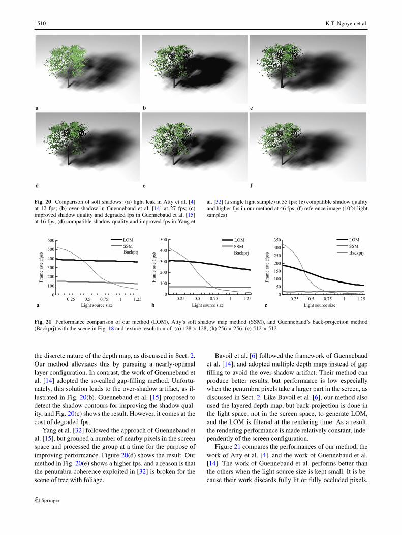
Thirdly, our method pursues a nearly-optimal layer con-figuration: two or three front-face layers, one back-facelayer, and one layer for the key receiver, as discussed inSect. 5.3. Figure 20(a) shows the light leaking artifact of thework of Atty et al., where the front-face and back-face depthmaps are constructed for the tree designated as the occluder,and the floor is taken as the receiver. Compare this to ourresult shown in Fig. 20(e), which adopts the nearly-optimallayer configuration and therefore rarely reveals light leak-ing. Our result is quite close to the reference image shownin Fig. 20(f).

In general, the algorithms based on micro-patch back-projection suffer from the light leaking artifact caused by


Fig. 20 Comparison of soft shadows: (a) light leak in Atty et al. [4]at 12 fps; (b) over-shadow in Guennebaud et al. [14] at 27 fps; (c)improved shadow quality and degraded fps in Guennebaud et al. [15]at 16 fps; (d) compatible shadow quality and improved fps in Yang et

al. [32] (a single light sample) at 35 fps; (e) compatible shadow qualityand higher fps in our method at 46 fps; (f) reference image (1024 lightsamples)

Fig. 21 Performance comparison of our method (LOM), Atty’s soft shadow map method (SSM), and Guennebaud’s back-projection method(Backprj) with the scene in Fig. 18 and texture resolution of: (a) 128 × 128; (b) 256 × 256; (c) 512 × 512

the discrete nature of the depth map, as discussed in Sect. 2.Our method alleviates this by pursuing a nearly-optimallayer configuration. In contrast, the work of Guennebaud etal. [14] adopted the so-called gap-filling method. Unfortu-nately, this solution leads to the over-shadow artifact, as il-lustrated in Fig. 20(b). Guennebaud et al. [15] proposed todetect the shadow contours for improving the shadow qual-ity, and Fig. 20(c) shows the result. However, it comes at thecost of degraded fps.

Yang et al. [32] followed the approach of Guennebaud etal. [15], but grouped a number of nearby pixels in the screenspace and processed the group at a time for the purpose ofimproving performance. Figure 20(d) shows the result. Ourmethod in Fig. 20(e) shows a higher fps, and a reason is thatthe penumbra coherence exploited in [32] is broken for thescene of tree with foliage.

Bavoil et al. [6] followed the framework of Guennebaudet al. [14], and adopted multiple depth maps instead of gapfilling to avoid the over-shadow artifact. Their method canproduce better results, but performance is low especiallywhen the penumbra pixels take a larger part in the screen, asdiscussed in Sect. 2. Like Bavoil et al. [6], our method alsoused the layered depth map, but back-projection is done inthe light space, not in the screen space, to generate LOM,and the LOM is filtered at the rendering time. As a result,the rendering performance is made relatively constant, inde-pendently of the screen configuration.

Figure 21 compares the performances of our method, thework of Atty et al. [4], and the work of Guennebaud et al.[14]. The work of Guennebaud et al. performs better thanthe others when the light source size is kept small. It is be-cause their work discards fully lit or fully occluded pixels,


and processes only the penumbra pixels. When the light sizeis small, the penumbra area is small, and therefore fewerpixels are processed. When the light size increases, how-ever, more pixels have to be processed, and therefore per-formance degrades. Figures 20 and 21 show that, in general,our method excels the others.

9 Conclusions and future work

In this paper, we presented a high-performance and high-quality algorithm to produce soft shadows. The algorithm isimage-based, requires no pre-computation, maximally uti-lizes the GPU, demands no CPU read-back, runs quite fast,and generates self-shadows.

Although not physically correct, the resulting shadowsare close to those of the ground truth reference image. Theproposed method can be combined with some of the ad-vanced shadow map techniques [28, 30] which enhance theobject discretization quality in the shadow map.

Using a fixed number of layers in the depth and occlusionmaps, we have obtained high-quality soft shadows, i.e., theresulting artifact is hardly prominent. Nonetheless, there ex-ists a possibility of further enhancing the proposed methodby using, for example, the shadow map list [26] in order tocomplement the information for missing discretized points.

Acknowledgements We would like to thank Gaël Guennebaud andKiwon Um for valuable discussions and suggestions. The StanfordBunny and Dragon models were digitized and kindly provided bythe Stanford University Computer Graphics Laboratory. The Waterlily,Robot, Drum set and Tree models appearing in this paper and in theaccompanying video are downloaded from 3dxtras.com. This researchwas supported by MKE, Korea under ITRC NIPA-2010-(C1090-1021-0008).

References

1. Agrawala, M., Ramamoorthi, R., Heirich, A., Moll, L.: Efficientimage-based methods for rendering soft shadows. In: Proc. ofSIGGRAPH’00, pp. 375–384 (2000)

2. Akenine-Möller, T., Assarsson, U.: Approximate soft shadows onarbitrary surfaces using penumbra wedges. In: Rendering Tech-niques, pp. 297–305 (2002)

3. Arvo, J., Hirvikorpi, M., Tyystjärvi, J.: Approximate soft shad-ows using image-space flood-fill algorithm. Comput. Graph. Fo-rum 23(3), 271–280 (2004). (Proc. of Eurographics’04)

4. Atty, L., Holzschuch, N., Lapierre, M., Hasenfratz, J.M., Hansen,C., Sillion, F.: Soft shadow maps: Efficient sampling of lightsource visibility. Comput. Graph. Forum 25(4) (2006)

5. Bavoil, L., Silva, C.T.: Real-time soft shadows with cone culling.In: Technical Sketches and Applications at SIGGRAPH’06(2006)

6. Bavoil, L., Callahan, S.P., Silva, C.T.: Robust soft shadow map-ping with backprojection and depth peeling. J. Graph. Tools 13(1),19–30 (2008)

7. Crow, F.C.: Shadow algorithms for computer graphics. Comput.Graph. 11(2), 242–248 (1977). (Proc. of SIGGRAPH’77)

8. Drettakis, G., Fiume, E.: A fast shadow algorithm for area lightsources using backprojection. Comput. Graph. Forum 28, 223–230 (1994)

9. Eisemann, E., Décoret, X.: Occlusion textures for plausible softshadows. Comput. Graph. Forum 27(1), 13–23 (2008)

10. Everitt, C.: Interactive order-independent transparency. Tech. rep.,NVIDIA Corporation (2001)

11. Fernando, R.: Percentage-closer soft shadows. In: ACM SIG-GRAPH 2005 Sketches and Applications, p. 35 (2005)

12. Forest, V., Barthe, L., Paulin, M.: Accurate shadows by depth com-plexity sampling. Comput. Graph. Forum 27(2), 663–674 (2008).(Eurographics 2008 Proceedings)

13. Forest, V., Barthe, L., Guennebaud, G., Paulin, M.: Soft tex-tured shadow volume. Comput. Graph. Forum 28(4), 1111–1121(2009). (Eurographics Symposium on Rendering 2009)

14. Guennebaud, G., Barthe, L., Paulin, M.: Real-time soft shadowmapping by backprojection. In: Proc. of Eurographics Symposiumon Rendering, pp. 227–234 (2006)

15. Guennebaud, G., Barthe, L., Paulin, M.: High quality adaptive softshadow mapping. Comput. Graph. Forum 26(3) (2007). (Proc. ofEurographics’07)

16. Hasenfratz, J.M., Lapierre, M., Holzschuch, N., Sillion, F.: A sur-vey of real-time soft shadows algorithms. Comput. Graph. Forum22(4), 753–774 (2003)

17. Heidrich, W., Brabec, S., Seidel, H.P.: Soft shadow maps for linearlights. In: Proc. of the 11th Eurographics Workshop on Rendering,pp. 269–280 (2000)

18. Iwasaki, K., Dobashi, Y., Yoshimoto, F., Nishita, T.: Precomputedradiance transfer for dynamic scenes taking into account light in-terreflection. In: Proc. of the Eurographics Symposium on Ren-dering, pp. 35–44 (2007)

19. Laine, S., Aila, T., Assarsson, U., Lehtinen, J., Akenine-Möller, T.:Soft shadow volumes for ray tracing. ACM Trans. Graph. 24(3),1156–1165 (2005)

20. Pan, M., Wang, R., Liu, X., Peng, Q., Bao, H.: Precomputed radi-ance transfer field for rendering interreflections in dynamic scenes.Comput. Graph. Forum 26(3), 485–493 (2007)

21. Reeves, W.T., Salesin, D.H., Cook, R.L.: Rendering antialiasedshadows with depth maps. Comput. Graph. 21(4), 283–291(1987). (Proc. of SIGGRAPH’87)

22. Rong, G., Tan, T.S.: Jump Flooding: An Efficient and EffectiveCommunication Pattern for Use on GPUs, pp. 185–192. CharlesRiver Media (2006). Chap. 3

23. Schwarz, M., Stamminger, M.: Bitmask soft shadows. Comput.Graph. Forum 26(3) (2007). (Proc. of Eurographics’07)

24. Schwarz, M., Stamminger, M.: Microquad soft shadow mappingrevisited. In: Eurographics’06 Short Paper (2008)

25. Schwarz, M., Stamminger, M.: Quality scalability of soft shadowmapping. In: Proc. of Graphics Interface’08 (2008)

26. Sintorn, E., Eisemann, E., Assarsson, U.: Sample-based visibilityfor soft shadows using alias-free shadow maps. Comput. Graph.Forum 27(4), 1285–1292 (2008). (Proc. of the Eurographics Sym-posium on Rendering 2008)

27. Sloan, P.P.J., Kautz, J., Snyder, J.: Precomputed radiance transferfor real-time rendering in dynamic, low-frequency lighting envi-ronments. In: Proc. of SIGGRAPH’02, pp. 527–536 (2002)

28. Stamminger, M., Drettakis, G.: Perspective shadow maps. ACMTrans. Graph. 21(3), 557–562 (2002). (Proc. of SIGGRAPH2002)

29. Williams, L.: Casting curved shadows on curved surfaces. Com-put. Graph. 12(3), 270–274 (1978). (Proc. of SIGGRAPH’78)

30. Wimmer, M., Scherzer, D., Purgathofer, W.: Light space perspec-tive shadow maps. In: Rendering Techniques 2004 (Proc. Euro-graphics Symposium on Rendering), pp. 143–151 (2004)

http://3dxtras.com


31. Woo, A., Poulin, P., Fournier, A.: A survey of shadow algorithms.IEEE Comput. Graph. Appl. 10(6), 13–32 (1990)

32. Yang, B., Feng, J., Guennebaud, G., Liu, X.: Packet-based hierar-chal soft shadow mapping. Comput. Graph. Forum 28(4), 1121–1130 (2009). (Proceedings of Eurographics Symposium on Ren-dering 2009)

33. Zhou, K., Hu, Y., Lin, S., Guo, B., Shum, H.Y.: Precomputedshadow fields for dynamic scenes. ACM Trans. Graph. 24(3),1196–1201 (2005)

Kien T. Nguyen is a Ph.D. studentin the Department of Computer Sci-ence and Engineering at Korea Uni-versity. He received his B.S. degreein Applied Mathematics from HanoiUniversity of Science in 1999 andM.S. degree in Computer Sciencefrom Le-Quy-Don Technical Uni-versity in 2003. His research in-terests include global illumination,shadows and image based render-ing.

Hanyoung Jang is a Ph.D. studentat Korea University. He receivedboth of M.S. and B.S. degrees in theCollege of Information and Com-munications at Korea University.Since 2005, he has been working inthe fields of collision detection andaccessibility analysis for robotics.Currently, his primary research in-terest lies in real-time rendering ofcomplex scenes.

JungHyun Han is a professor inthe Department of Computer Sci-ence and Engineering at KoreaUniversity, where he directs theInteractive 3D Media Laboratoryand Game Research Center sup-ported by Korea Ministry of Cul-ture, Sports, and Tourism. Prior tojoining Korea University, he workedat the School of Information andCommunications Engineering ofSungkyunkwan University, in Ko-rea, and at the Manufacturing Sys-tems Integration Division of the USDepartment of Commerce National

Institute of Standards and Technology (NIST). He received a B.S. de-gree in Computer Engineering at Seoul National University, an M.S.degree in Computer Science at the University of Cincinnati, and aPh.D. degree in Computer Science at USC. His research interests in-clude real-time simulation and animation for games.

Layered occlusion map for soft shadow generation

Documents