Lavopa, Elisabetta (2011) A novel control technique for active shunt power filters for aircraft applications. PhD thesis, University of Nottingham. Access from the University of Nottingham repository: http://eprints.nottingham.ac.uk/12049/1/Elisabetta_Lavopa_Thesis.pdf Copyright and reuse: The Nottingham ePrints service makes this work by researchers of the University of Nottingham available open access under the following conditions. This article is made available under the University of Nottingham End User licence and may be reused according to the conditions of the licence. For more details see: http://eprints.nottingham.ac.uk/end_user_agreement.pdf For more information, please contact [email protected]

Welcome message from author
This document is posted to help you gain knowledge. Please leave a comment to let me know what you think about it! Share it to your friends and learn new things together.
Transcript

Lavopa, Elisabetta (2011) A novel control technique for active shunt power filters for aircraft applications. PhD thesis, University of Nottingham.
Access from the University of Nottingham repository: http://eprints.nottingham.ac.uk/12049/1/Elisabetta_Lavopa_Thesis.pdf
Copyright and reuse:
The Nottingham ePrints service makes this work by researchers of the University of Nottingham available open access under the following conditions.
This article is made available under the University of Nottingham End User licence and may be reused according to the conditions of the licence. For more details see: http://eprints.nottingham.ac.uk/end_user_agreement.pdf
For more information, please contact [email protected]

A Novel Control Technique for Active Shunt
Power Filters for Aircraft Applications
Elisabetta Lavopa, M.Eng
Submitted to the University of Nottingham for the degree of Doctor of
Philosophy, June 2011.

Abstract
The More Electric Aircraft is a technological trend in modern aerospace industry
to increasingly use electrical power on board the aircraft in place of mechanical,
hydraulic and pneumatic power to drive aircraft subsystems. This brings major
changes to the aircraft electrical system, increasing the complexity of the network
topology together with stability and power quality issues. Shunt active power fil-
ters are a viable solution for power quality enhancement, in order to comply with
the standard recommendations. The aircraft electrical system is characterized by
variable supply frequency in the range 360-900Hz, hence the harmonic compo-
nents occur at high and variable frequencies, compared to the terrestrial 50/60Hz
systems. In this kind of system, fast and accurate algorithms for the detection of
the reference signal for the active filter control and robust high-bandwidth con-
trol techniques are needed, in order for the active filter to perform the harmonic
elimination successfully.
In this thesis, two novel algorithms are proposed. The first algorithm is a frequency
and harmonic detection technique, particularly suitable for tracking the variable
supply frequency and the harmonic components of voltages and currents in the
aircraft electrical system. Complete identification of the reference signal for the
active filter control is possible when applying this technique. The second algorithm
is a control technique based on the use of multiple rotating reference frames.
Only the measurement of the voltage at the Point of Common Coupling and
the active filter output current are needed, hence no current sensors are required
on the distorting loads. Both the techniques have been validated by means of
simulation and experimental analysis. The results show that the proposed methods
are effective for a successful harmonic compensation by means of active shunt
filters, in the More Electric Aircraft environment.
i
Contents
1 Introduction 2
1.1 Structure of the thesis . . . . . . . . . . . . . . . . . . . . . . . . . 5
2 The More Electric Aircraft 7
2.1 Introduction . . . . . . . . . . . . . . . . . . . . . . . . . . . . . . . 7
2.2 The More Electric Aircraft concept . . . . . . . . . . . . . . . . . . 7
2.3 Power quality in the aircraft power system . . . . . . . . . . . . . . 11
2.4 Summary . . . . . . . . . . . . . . . . . . . . . . . . . . . . . . . . 14
3 Real-time Frequency and Harmonic Estimation Technique 15
3.1 Introduction . . . . . . . . . . . . . . . . . . . . . . . . . . . . . . . 15
3.2 Overview of frequency and harmonic estimation techniques . . . . . 16
3.3 Frequency estimation technique . . . . . . . . . . . . . . . . . . . . 17
3.3.1 Choice of algorithm parameters . . . . . . . . . . . . . . . . 23
3.3.2 Analysis of a sinusoidal signal . . . . . . . . . . . . . . . . . 24
ii
CONTENTS iii
3.3.3 Analysis of a distorted signal . . . . . . . . . . . . . . . . . 25
3.3.4 Algorithm tuning . . . . . . . . . . . . . . . . . . . . . . . . 27
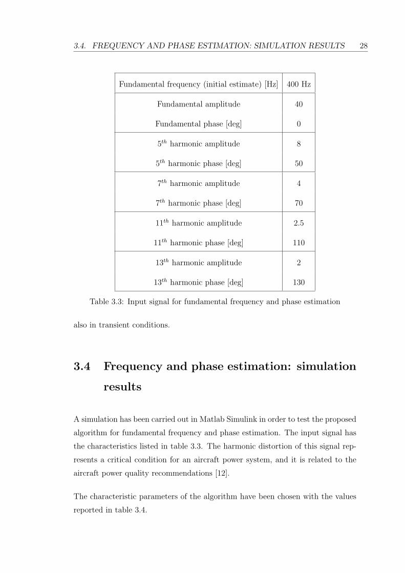
3.4 Frequency and phase estimation: simulation results . . . . . . . . . 28
3.5 Harmonic estimation technique . . . . . . . . . . . . . . . . . . . . 33
3.6 Harmonic estimation : simulation results . . . . . . . . . . . . . . . 37
3.6.1 Relative phase of the harmonics with respect to the funda-
mental . . . . . . . . . . . . . . . . . . . . . . . . . . . . . . 37
3.7 Frequency estimation: experimental results . . . . . . . . . . . . . . 44
3.8 Harmonic estimation : experimental results . . . . . . . . . . . . . . 52
3.9 Harmonic estimation : transient analysis . . . . . . . . . . . . . . . 59
3.10 Summary . . . . . . . . . . . . . . . . . . . . . . . . . . . . . . . . 68
4 Comparison between the real-time DFT technique and the Phase
Locked Loop 73
4.1 Introduction . . . . . . . . . . . . . . . . . . . . . . . . . . . . . . . 73
4.2 The Phase Locked Loop . . . . . . . . . . . . . . . . . . . . . . . . 74
4.3 Comparison with the DFT algorithm: simulation results . . . . . . 76
4.3.1 Sinusoidal signal . . . . . . . . . . . . . . . . . . . . . . . . 76
4.3.2 Distorted signal . . . . . . . . . . . . . . . . . . . . . . . . . 80
4.4 Comparison with the DFT algorithm: experimental results . . . . . 82
4.4.1 Sinusoidal signal . . . . . . . . . . . . . . . . . . . . . . . . 84
CONTENTS iv
4.4.2 Distorted signal . . . . . . . . . . . . . . . . . . . . . . . . . 88
4.5 Summary . . . . . . . . . . . . . . . . . . . . . . . . . . . . . . . . 91
5 Multiple Reference Frames Voltage Detection Control Technique 92
5.1 Introduction . . . . . . . . . . . . . . . . . . . . . . . . . . . . . . . 92
5.2 Decoupling the Rotating Reference Frames . . . . . . . . . . . . . . 93
5.3 Harmonic decoupling terms . . . . . . . . . . . . . . . . . . . . . . 96
5.4 Examples of accurate and inaccurate decoupling . . . . . . . . . . . 98
5.5 Control of a shunt active filter . . . . . . . . . . . . . . . . . . . . . 106
5.6 Voltage detection control technique . . . . . . . . . . . . . . . . . . 109
5.6.1 The fundamental control loop . . . . . . . . . . . . . . . . . 111
5.6.1.1 The fundamental current control loop . . . . . . . 112
5.6.1.2 The DC link voltage control loop . . . . . . . . . . 117
5.6.2 The harmonics control loops . . . . . . . . . . . . . . . . . . 120
5.6.2.1 The harmonic voltage control loop . . . . . . . . . 123
5.7 Summary . . . . . . . . . . . . . . . . . . . . . . . . . . . . . . . . 128
6 Voltage Detection Control Technique: Simulation Results 129
6.1 Introduction . . . . . . . . . . . . . . . . . . . . . . . . . . . . . . . 129
6.2 Description of the simulation model . . . . . . . . . . . . . . . . . . 129
6.3 Simulation results . . . . . . . . . . . . . . . . . . . . . . . . . . . . 131
CONTENTS v
6.4 Summary . . . . . . . . . . . . . . . . . . . . . . . . . . . . . . . . 146
7 Voltage Detection Control Technique: Experimental Results 151
7.1 Introduction . . . . . . . . . . . . . . . . . . . . . . . . . . . . . . . 151
7.2 Description of the experimental setup . . . . . . . . . . . . . . . . . 151
7.3 Experimental results . . . . . . . . . . . . . . . . . . . . . . . . . . 154
7.4 Summary . . . . . . . . . . . . . . . . . . . . . . . . . . . . . . . . 173
8 Conclusions 175
8.1 Further Work . . . . . . . . . . . . . . . . . . . . . . . . . . . . . . 178
A Papers Published 188
B Decoupling 190

List of Figures
2.1 Power sources distribution on the conventional aircraft . . . . . . . 9
2.2 Power sources distribution on the More Electric Aircraft . . . . . . 9
2.3 Scheme of an aircraft power network (half) . . . . . . . . . . . . . . 11
3.1 Example of ∆f calculation when the actual value of frequency is
460Hz and the initial estimate is 400Hz . . . . . . . . . . . . . . . . 21
3.2 Scheme of the DFT algorithm . . . . . . . . . . . . . . . . . . . . . 22
3.3 DFT block diagram for the calculation of the amplitude am1 and
the phase ϕ1 . . . . . . . . . . . . . . . . . . . . . . . . . . . . . . . 23
3.4 Response to a frequency step for different buffer sizes . . . . . . . . 30
3.5 Response of the phase estimate to a frequency step. Case (a) . . . . 31
3.6 Response of the phase estimate to a frequency step. Case (b) . . . . 32
3.7 Response of the phase estimate to a frequency step. Case (c) . . . . 32
3.8 Response of the phase estimate to a frequency step. Case (d) . . . . 33
3.9 Scheme of the DFT algorithm for harmonic estimation. No sub-
traction of the fundamental . . . . . . . . . . . . . . . . . . . . . . 34
vi
LIST OF FIGURES vii
3.10 Scheme of the DFT algorithm for harmonic estimation. Subtraction
of the fundamental . . . . . . . . . . . . . . . . . . . . . . . . . . . 34
3.11 5th harmonic . . . . . . . . . . . . . . . . . . . . . . . . . . . . . . . 35
3.12 5th harmonic . . . . . . . . . . . . . . . . . . . . . . . . . . . . . . . 35
3.13 7th harmonic . . . . . . . . . . . . . . . . . . . . . . . . . . . . . . . 35
3.14 7th harmonic . . . . . . . . . . . . . . . . . . . . . . . . . . . . . . . 35
3.15 11th harmonic estimate . . . . . . . . . . . . . . . . . . . . . . . . . 36
3.16 11th harmonic estimate . . . . . . . . . . . . . . . . . . . . . . . . . 36
3.17 13th harmonic . . . . . . . . . . . . . . . . . . . . . . . . . . . . . . 36
3.18 13th harmonic . . . . . . . . . . . . . . . . . . . . . . . . . . . . . . 36
3.19 5th harmonic amplitude estimate in the four cases . . . . . . . . . . 38
3.20 7th harmonic amplitude estimate in the four cases . . . . . . . . . . 38
3.21 11th harmonic amplitude estimate in the four cases . . . . . . . . . 39
3.22 13th harmonic amplitude estimate in the four cases . . . . . . . . . 39
3.23 5th harmonic phase estimate in the four cases . . . . . . . . . . . . 40
3.24 7th harmonic phase estimate in the four cases . . . . . . . . . . . . 40
3.25 11th harmonic phase estimate in the four cases . . . . . . . . . . . . 41
3.26 13th harmonic phase estimate in the four cases . . . . . . . . . . . . 41
3.27 Fundamental and 5th harmonic on the αβ plane . . . . . . . . . . . 44
3.28 Estimate of the initial phase of the fundamental . . . . . . . . . . . 45
LIST OF FIGURES viii
3.29 Estimate of the initial phase of the 5th harmonic . . . . . . . . . . . 45
3.30 Estimate of the initial phase of the 7th harmonic . . . . . . . . . . . 46
3.31 Estimate of the initial phase of the 11th harmonic . . . . . . . . . . 46
3.32 Estimate of the initial phase of the 13th harmonic . . . . . . . . . . 47
3.33 Input line-to-line voltage in the time domain . . . . . . . . . . . . . 49
3.34 FFT spectrum of the amplitude of input line-to-line voltage . . . . 49
3.35 FFT spectrum of the phase of input line-to-line voltage . . . . . . . 50
3.36 Experimental response to a frequency step for different buffer sizes . 50
3.37 Fundamental amplitude estimated experimentally. Cases a and b . 53
3.38 Fundamental amplitude estimated experimentally. Cases c and d . . 53
3.39 5th harmonic amplitude estimated experimentally. Cases a and b . . 54
3.40 5th harmonic amplitude estimated experimentally. Cases c and d . . 54
3.41 7th harmonic amplitude estimated experimentally. Cases a and b . . 55
3.42 7th harmonic amplitude estimated experimentally. Cases c and d . . 55
3.43 Fundamental phase estimated experimentally. Cases a and b . . . . 56
3.44 Fundamental phase estimated experimentally. Cases c and d . . . . 56
3.45 5th harmonic phase estimated experimentally. Cases a and b . . . . 57
3.46 5th harmonic phase estimated experimentally. Cases c and d . . . . 57
3.47 7th harmonic phase estimated experimentally. Cases a and b . . . . 58

LIST OF FIGURES ix
3.48 7th harmonic phase estimated experimentally. Cases c and d . . . . 58
3.49 FFT spectrum with fundamental frequency 400 Hz . . . . . . . . . 60
3.50 FFT spectrum with fundamental frequency 500 Hz . . . . . . . . . 60
3.51 FFT spectrum with fundamental frequency 700 Hz . . . . . . . . . 61
3.52 FFT spectrum with fundamental frequency 800 Hz . . . . . . . . . 62
3.53 5th harmonic . . . . . . . . . . . . . . . . . . . . . . . . . . . . . . . 63
3.54 5th harmonic . . . . . . . . . . . . . . . . . . . . . . . . . . . . . . . 64
3.55 7th harmonic . . . . . . . . . . . . . . . . . . . . . . . . . . . . . . . 64
3.56 7th harmonic . . . . . . . . . . . . . . . . . . . . . . . . . . . . . . . 65
3.57 11th harmonic . . . . . . . . . . . . . . . . . . . . . . . . . . . . . . 65
3.58 11th harmonic . . . . . . . . . . . . . . . . . . . . . . . . . . . . . . 66
3.59 13th harmonic . . . . . . . . . . . . . . . . . . . . . . . . . . . . . . 66
3.60 13th harmonic . . . . . . . . . . . . . . . . . . . . . . . . . . . . . . 67
3.61 5th harmonic . . . . . . . . . . . . . . . . . . . . . . . . . . . . . . . 68
3.62 5th harmonic . . . . . . . . . . . . . . . . . . . . . . . . . . . . . . . 69
3.63 7th harmonic . . . . . . . . . . . . . . . . . . . . . . . . . . . . . . . 69
3.64 7th harmonic . . . . . . . . . . . . . . . . . . . . . . . . . . . . . . . 70
3.65 11th harmonic . . . . . . . . . . . . . . . . . . . . . . . . . . . . . . 70
3.66 11th harmonic . . . . . . . . . . . . . . . . . . . . . . . . . . . . . . 71
LIST OF FIGURES x
3.67 13th harmonic . . . . . . . . . . . . . . . . . . . . . . . . . . . . . . 71
3.68 13th harmonic . . . . . . . . . . . . . . . . . . . . . . . . . . . . . . 72
4.1 Block diagram representing the basic structure of the PLL . . . . . 74
4.2 Block diagram of the implemented PLL . . . . . . . . . . . . . . . . 75
4.3 Comparison of the frequency estimate for a sinusoidal signal. Step
of frequency . . . . . . . . . . . . . . . . . . . . . . . . . . . . . . . 78
4.4 Comparison of the phase estimate for a sinusoidal signal . . . . . . 78
4.5 Comparison of the frequency estimate for a sinusoidal signal. Step
of frequency . . . . . . . . . . . . . . . . . . . . . . . . . . . . . . . 79
4.6 Comparison of the phase estimate for a sinusoidal signal . . . . . . 80
4.7 Distorted noisy signal for the simulation comparison . . . . . . . . . 82
4.8 Comparison of the frequency estimate for a noisy and distorted
signal. Ramp of frequency . . . . . . . . . . . . . . . . . . . . . . . 83
4.9 Frequency estimation error for both algorithms . . . . . . . . . . . . 83
4.10 Phase estimation error for both algorithms . . . . . . . . . . . . . . 84
4.11 Comparison of the frequency estimate for a sinusoidal signal. Volt-
age rms 50V . . . . . . . . . . . . . . . . . . . . . . . . . . . . . . . 85
4.12 Comparison of the phase estimate for a sinusoidal signal . . . . . . 86
4.13 Comparison of the frequency estimate for a sinusoidal signal. Volt-
age amplitude 10V . . . . . . . . . . . . . . . . . . . . . . . . . . . 87
4.14 Comparison of the phase estimate for a sinusoidal signal . . . . . . 87

LIST OF FIGURES xi
4.15 Distorted noisy voltage for the experimental comparison . . . . . . 89
4.16 Comparison of the frequency estimate for a noisy and distorted
voltage. Ramp of frequency . . . . . . . . . . . . . . . . . . . . . . 90
5.1 Distorted waveform on dq rotating frame without decoupling . . . . 95
5.2 Distorted waveform on dq rotating frame with decoupling . . . . . . 96
5.3 Distorted input signal . . . . . . . . . . . . . . . . . . . . . . . . . 99
5.4 Fundamental d and q components . . . . . . . . . . . . . . . . . . . 100
5.5 5th harmonic d and q components . . . . . . . . . . . . . . . . . . . 101
5.6 7th harmonic d and q components . . . . . . . . . . . . . . . . . . . 101
5.7 11th harmonic d and q components . . . . . . . . . . . . . . . . . . 102
5.8 13th harmonic d and q components . . . . . . . . . . . . . . . . . . 102
5.9 Phase angles calculated using inverse tangent . . . . . . . . . . . . 104
5.10 Phase angles calculated using the PLL . . . . . . . . . . . . . . . . 105
5.11 Inaccurate decoupling due to inaccurate phase angle estimation . . 106
5.12 Principle of operation of the shunt active filter . . . . . . . . . . . . 107
5.13 Topology of the shunt active filter . . . . . . . . . . . . . . . . . . . 107
5.14 Scheme of the system where the active filter is connected . . . . . . 110
5.15 Scheme of the overall fundamental control loop . . . . . . . . . . . . 113
5.16 Decoupling block . . . . . . . . . . . . . . . . . . . . . . . . . . . . 114
5.17 Scheme of the circuit for the fundamental current dynamics . . . . . 114

LIST OF FIGURES xii
5.18 Fundamental current control loop . . . . . . . . . . . . . . . . . . . 117
5.19 dq equivalent circuit of the active filter . . . . . . . . . . . . . . . . 119
5.20 DC link voltage control loop . . . . . . . . . . . . . . . . . . . . . . 120
5.21 Scheme of the 5th harmonic control system . . . . . . . . . . . . . . 122
5.22 Scheme of the overall control system . . . . . . . . . . . . . . . . . 124
5.23 Equivalent circuit of the system at the harmonic frequencies . . . . 125
5.24 Harmonic voltage control loop . . . . . . . . . . . . . . . . . . . . . 127
6.1 d and q components of the PCC voltage on the 5th harmonic frame 133
6.2 d and q components of the PCC voltage on the 7th harmonic frame 133
6.3 d and q components of the PCC voltage on the 11th harmonic frame134
6.4 d and q components of the PCC voltage on the 13th harmonic frame134
6.5 FFT of the d component of the PCC voltage on the 5th harmonic
frame . . . . . . . . . . . . . . . . . . . . . . . . . . . . . . . . . . . 135
6.6 FFT of the d component of the PCC voltage on the 7th harmonic
frame . . . . . . . . . . . . . . . . . . . . . . . . . . . . . . . . . . . 135
6.7 FFT of the d component of the PCC voltage on the 11th harmonic
frame . . . . . . . . . . . . . . . . . . . . . . . . . . . . . . . . . . . 136
6.8 FFT of the d component of the PCC voltage on the 13th harmonic
frame . . . . . . . . . . . . . . . . . . . . . . . . . . . . . . . . . . . 136
6.9 d and q components of the active filter current on the fundamental
frame . . . . . . . . . . . . . . . . . . . . . . . . . . . . . . . . . . . 138
LIST OF FIGURES xiii
6.10 d and q components of the active filter current on the 5th harmonic
frame . . . . . . . . . . . . . . . . . . . . . . . . . . . . . . . . . . . 138
6.11 d and q components of the active filter current on the 5th harmonic
frame: expanded view of the steady state . . . . . . . . . . . . . . . 139
6.12 d and q components of the active filter current on the 7th harmonic
frame . . . . . . . . . . . . . . . . . . . . . . . . . . . . . . . . . . . 139
6.13 d and q components of the active filter current on the 7th harmonic
frame: expanded view of the steady state . . . . . . . . . . . . . . . 140
6.14 d and q components of the active filter current on the 11th harmonic
frame . . . . . . . . . . . . . . . . . . . . . . . . . . . . . . . . . . . 140
6.15 d and q components of the active filter current on the 11th harmonic
frame: expanded view of the steady state . . . . . . . . . . . . . . . 141
6.16 d and q components of the active filter current on the 13th harmonic
frame . . . . . . . . . . . . . . . . . . . . . . . . . . . . . . . . . . . 141
6.17 d and q components of the active filter current on the 13th harmonic
frame: expanded view of the steady state . . . . . . . . . . . . . . . 142
6.18 PCC three-phase voltage before the active filter compensation . . . 142
6.19 PCC three-phase voltage after the active filter compensation . . . . 143
6.20 FFT spectrum of the PCC voltage before the active filter compen-
sation . . . . . . . . . . . . . . . . . . . . . . . . . . . . . . . . . . 144
6.21 FFT spectrum of the PCC voltage after the active filter compensation144
6.22 FFT spectrum of the PCC voltage before the active filter compen-
sation: expanded view of the harmonics . . . . . . . . . . . . . . . . 145
LIST OF FIGURES xiv
6.23 FFT spectrum of the PCC voltage after the active filter compensa-
tion: expanded view of the harmonics . . . . . . . . . . . . . . . . . 145
6.24 Three-phase supply current before the active filter compensation . . 147
6.25 Three-phase supply current after the active filter compensation . . . 147
6.26 FFT spectrum of the supply current before the active filter com-
pensation . . . . . . . . . . . . . . . . . . . . . . . . . . . . . . . . 148
6.27 FFT spectrum of the supply current after the active filter compen-
sation . . . . . . . . . . . . . . . . . . . . . . . . . . . . . . . . . . 148
6.28 FFT spectrum of the supply current before the active filter com-
pensation: expanded view of the harmonics . . . . . . . . . . . . . . 149
6.29 FFT spectrum of the supply current after the active filter compen-
sation: expanded view of the harmonics . . . . . . . . . . . . . . . . 149
7.1 Scheme of the laboratory experimental setup . . . . . . . . . . . . . 152
7.2 Picture of the active filter and the control boards . . . . . . . . . . 155
7.3 Picture of the whole laboratory bench . . . . . . . . . . . . . . . . . 155
7.4 Picture of the programmable power supply . . . . . . . . . . . . . . 156
7.5 d component of the PCC voltage on the 5th harmonic frame . . . . 157
7.6 q component of the PCC voltage on the 5th harmonic frame . . . . 157
7.7 d component of the PCC voltage on the 7th harmonic frame . . . . 158
7.8 q component of the PCC voltage on the 7th harmonic frame . . . . 158
7.9 FFT of the d component of the PCC voltage on the 5th harmonic
frame . . . . . . . . . . . . . . . . . . . . . . . . . . . . . . . . . . . 159

LIST OF FIGURES xv
7.10 FFT of the d component of the PCC voltage on the 7th harmonic
frame . . . . . . . . . . . . . . . . . . . . . . . . . . . . . . . . . . . 160
7.11 d component of the active filter current on the fundamental frame . 162
7.12 q component of the active filter current on the fundamental frame . 163
7.13 d component of the active filter current on the 5th harmonic frame 163
7.14 q component of the active filter current on the 5th harmonic frame 164
7.15 d component of the active filter current on the 7th harmonic frame 164
7.16 q component of the active filter current on the 7th harmonic frame 165
7.17 PCC three-phase voltage before the active filter compensation . . . 165
7.18 PCC three-phase voltage after the active filter compensation . . . . 166
7.19 FFT spectrum of the PCC voltage before the active filter compen-
sation . . . . . . . . . . . . . . . . . . . . . . . . . . . . . . . . . . 167
7.20 FFT spectrum of the PCC voltage after the active filter compensation167
7.21 FFT spectrum of the PCC voltage before the active filter compen-
sation: expanded view of the harmonics . . . . . . . . . . . . . . . . 168
7.22 FFT spectrum of the PCC voltage after the active filter compensa-
tion: expanded view of the harmonics . . . . . . . . . . . . . . . . . 168
7.23 Three-phase supply current before the active filter compensation . . 170
7.24 Three-phase supply current after the active filter compensation . . . 170
7.25 FFT spectrum of the supply current before the active filter com-
pensation . . . . . . . . . . . . . . . . . . . . . . . . . . . . . . . . 171
LIST OF FIGURES xvi
7.26 FFT spectrum of the supply current after the active filter compen-
sation . . . . . . . . . . . . . . . . . . . . . . . . . . . . . . . . . . 171
7.27 FFT spectrum of the supply current before the active filter com-
pensation: expanded view of the harmonics . . . . . . . . . . . . . . 172
7.28 FFT spectrum of the supply current after the active filter compen-
sation: expanded view of the harmonics . . . . . . . . . . . . . . . . 172
7.29 Oscilloscope capture before the harmonic compensation . . . . . . . 174
7.30 Oscilloscope capture after the harmonic compensation . . . . . . . . 174
List of Tables
1.1 Main objectives of the thesis . . . . . . . . . . . . . . . . . . . . . . 5
3.1 Effect of the harmonics using an 8 points buffer . . . . . . . . . . . 26
3.2 Effect of the harmonics using a 20 points buffer . . . . . . . . . . . 26
3.3 Input signal for fundamental frequency and phase estimation . . . . 28
3.4 Frequency detection algorithm parameters . . . . . . . . . . . . . . 29
3.5 Transient and steady-state performance of the frequency step esti-
mation . . . . . . . . . . . . . . . . . . . . . . . . . . . . . . . . . . 31
3.6 Harmonic detection algorithm parameters . . . . . . . . . . . . . . 37
3.7 Input signal with fundamental initial phase different from zero . . . 42
3.8 Input signal for experimental validation . . . . . . . . . . . . . . . . 48
3.9 Frequency detection algorithm parameters for the experimental im-
plementation . . . . . . . . . . . . . . . . . . . . . . . . . . . . . . 51
3.10 Transient and steady-state performance of the frequency step esti-
mation . . . . . . . . . . . . . . . . . . . . . . . . . . . . . . . . . . 51
xvii
LIST OF TABLES 1
4.1 Transient and steady-state performance of the frequency step esti-
mation . . . . . . . . . . . . . . . . . . . . . . . . . . . . . . . . . . 81
4.2 Input signal for fundamental frequency and phase estimation . . . . 81
4.3 Transient and steady-state performance of the frequency step esti-
mation . . . . . . . . . . . . . . . . . . . . . . . . . . . . . . . . . . 88
4.4 Experimental voltage for fundamental frequency and phase estimation 89
5.1 Relative harmonic orders on the rotating frames of reference . . . . 94
5.2 Input signal for decoupling example . . . . . . . . . . . . . . . . . . 100
5.3 Errors in harmonic detection due to inaccurate PLL estimation . . . 104
6.1 Characteristic parameters of the simulation model . . . . . . . . . . 130
6.2 Harmonics as seen in the FFT spectrum of the voltage on the dif-
ferent reference frames . . . . . . . . . . . . . . . . . . . . . . . . . 137
6.3 Voltage harmonic reduction . . . . . . . . . . . . . . . . . . . . . . 146
6.4 Current harmonic reduction . . . . . . . . . . . . . . . . . . . . . . 150
7.1 Harmonics as seen in the FFT spectrum of the voltage on the dif-
ferent reference frames . . . . . . . . . . . . . . . . . . . . . . . . . 161
7.2 Voltage harmonic reduction . . . . . . . . . . . . . . . . . . . . . . 169
7.3 Current harmonic reduction . . . . . . . . . . . . . . . . . . . . . . 173
Chapter 1
Introduction
The latest research about civil aircraft systems has moved towards the increasing
use of electric power in place of other conventional sources like mechanical, hy-
draulic, pneumatic power. This technological trend is known as the More Electric
Aircraft.
Recent advances in the areas of power electronics, electric devices, control elec-
tronics, and microprocessors have allowed fast improvements in the performance
of aircraft electrical systems. The use of more electric power brings significant
advantages for the operation of the whole system. These advantages are listed
here.
Advantages of the increasing use of electric power in the aircraft system:
• optimization of the performance
• optimization of the life cycle cost
• reduction of weight and size of the equipment
• increased reliability
Important changes are brought to the aircraft electrical system due to the increas-
ing use of electric power on board. These changes are listed below.
2
CHAPTER 1. INTRODUCTION 3
Consequences of the increasing use of electric power on the aircraft electrical
system:
• more electrical loads
• more complex topology of the electrical network
• more generation demand
• more power electronic equipment
• more stability issues
• more power quality issues
These aspects have to be taken into account when designing the devices in the
system. It is crucial to guarantee that not only the device itself functions prop-
erly according to the specifications, but also that the interaction with the whole
system respects the required conditions. In a system like the aircraft power net-
work, the amount of generated power cannot be considered as infinite compared
to the demanded power. Furthermore, maximum reliability is required from all
the subsystems, hence multiple levels of redundancy and high fault tolerance level
characterize the devices. Strict limitations are imposed on the stability and the
power quality of the aircraft power system, in order to guarantee its optimal per-
formance. Particularly, limitations on the voltage and current harmonics injected
by the distorting loads are strictly recommended by aircraft regulations. In order
to respect these conditions, the power electronic devices used on board have to be
designed in order to inject the minimum amount of harmonics and the harmonics
which exceed the maximum allowed level have to be eliminated or compensated.
Shunt active power filters provide an effective solution for the harmonic elimination
and the improvement of the power quality in this kind of system. The shunt active
filter works as a controlled current source which injects into the grid an amount
of harmonic current equal to the one drawn by the distorting loads. A closed-loop
control system is implemented so that the active filter injects a current which
follows the reference signal, corresponding to the harmonic content of the load.

CHAPTER 1. INTRODUCTION 4
The main challenge encountered when designing an active filter for an aircraft
power system is related to the supply fundamental frequency, which is chosen
to be variable in the range 360-900Hz (frequency-wild power system). Due to
such values of fundamental frequency, the harmonic components occur at high
frequencies, compared to the terrestrial 50/60Hz electric grid. The two main issues
which have to be addressed when designing the control for an active filter are: the
generation of the reference signal and the reference signal tracking. These two
issues are related to the two main objectives of the work presented in this thesis.
Both objectives have been analysed and a solution to both challenges has been
investigated and validated through simulation and experimental work.
In order to generate the reference signal for the active filter, an accurate estimation
algorithm is required. The high frequency harmonic content of the current drawn
by the distorting load has to be detected in real-time and fed into the control
system. This work proposes a real-time detection algorithm based on the Discrete
Fourier Transform (DFT), which can estimate the fundamental frequency and
phase and the amplitudes and phases of the harmonics. This technique is suitable
for the aircraft frequency-wild system.
In order to track the reference, a robust and accurate control method has to
be applied. This work proposes a control technique based on the detection of
the voltage at the Point of Common Coupling (PCC) between the power supply,
the active filter and the distorting loads. Multiple rotating reference frames are
implemented in order to develop as many control loops as the harmonics to be
compensated. The harmonic content of the current drawn by the distorting loads
is estimated on the basis of the measurement and analysis of the PCC voltage,
hence no current sensors on the load are needed. In this way, the active filter can
work as a plug-and-play system that can eliminate the harmonics at the point of
the network where it is installed.
The main goals of this work, and the proposed solutions to achieve them are
summarized in table 1.1.

1.1. STRUCTURE OF THE THESIS 5
Goal Proposed solution
1 Generating the reference Real-time DFT-based detection algorithm
2 Tracking the reference Control technique based on the PCC voltage detection
Table 1.1: Main objectives of the thesis
1.1 Structure of the thesis
The thesis is structured in the following way.
In Chapter 2 the concept of the More Electric Aircraft is presented. The chapter
describes how the challenges posed by the More Electric Aircraft are related to
the work proposed in this project and how the proposed solutions can improve the
operating conditions of the aircraft power network.
Chapter 3 presents a novel technique for frequency and harmonic estimation based
on the Discrete Fourier Transform (DFT). This technique allows the estimation
of fundamental frequency, fundamental phase angle and harmonic amplitudes and
phases of a time-varying distorted signal in real time. The results obtained from
the simulation and experimental validation are presented and discussed.
The DFT-based detection technique is compared with a standard Phase-Locked
Loop in Chapter 4. Simulation and experimental validation show the differences
between the performances of the two algorithms. The results are presented and
discussed in this chapter.
Chapter 5 presents a multiple reference frames control technique based on the
measurement of the voltage at the PCC. This technique allows the harmonic com-
pensation to be performed without using any sensor on the distorting load, but
only on the PCC and on the active filter itself. The multiple reference frame imple-
mentation is discussed, along with the decoupling technique between the different
frames. A description of the control structure and the design of the controllers is
given.

1.1. STRUCTURE OF THE THESIS 6
The results obtained from the simulation and experimental validation of the volt-
age detection control technique proposed in Chapter 5 are given in Chapter 6 and
Chapter 7 respectively. From the comparison between Chapter 6 and Chapter 7
a good accordance between the simulation and experimental results can be seen.
In Chapter 8, conclusions are drawn from the work presented and the goals
achieved. Also, areas of further research are highlighted.

Chapter 2
The More Electric Aircraft
2.1 Introduction
This chapter describes the concept of the More Electric Aircraft, its characteristics
and advantages with respect to the conventional aircraft system. The consequences
of the choice of the new technology on the aircraft electric system are listed. The
chapter finally describes how the challenges posed by the More Electric Aircraft
are related to the work proposed in this project and how the proposed solutions
can improve the operating conditions of the aircraft power network, particularly
with regard to the power quality and harmonic cancellation by means of power
active shunt filters.
2.2 The More Electric Aircraft concept
The More Electric Aircraft follows the technological trend in modern aircraft to
increasingly use electrical power on board of the aircraft in place of mechanical,
hydraulic and pneumatic power to drive aircraft subsystems [1] [2] [3]. Recent
advances in the areas of power electronics, electric devices, control electronics, and
microprocessors have allowed a fast improvement in the performance of aircraft
7
2.2. THE MORE ELECTRIC AIRCRAFT CONCEPT 8
electrical systems.
The increased use of electrical power presents significant advantages such as opti-
mization of the performance and the life cycle cost of the aircraft, reduction of the
fuel consumption, and reduction of the weight and size of the system equipment as
well as the potential for improved condition monitoring and maintenance cycles.
However the More Electric Aircraft brings major changes in the aircraft electrical
power system, such as an increase of electrical loads and power electronic equip-
ment, a more complex topology for the electrical network, significantly higher
levels of electrical distribution which in turn result in greater power quality and
stability problems [4].
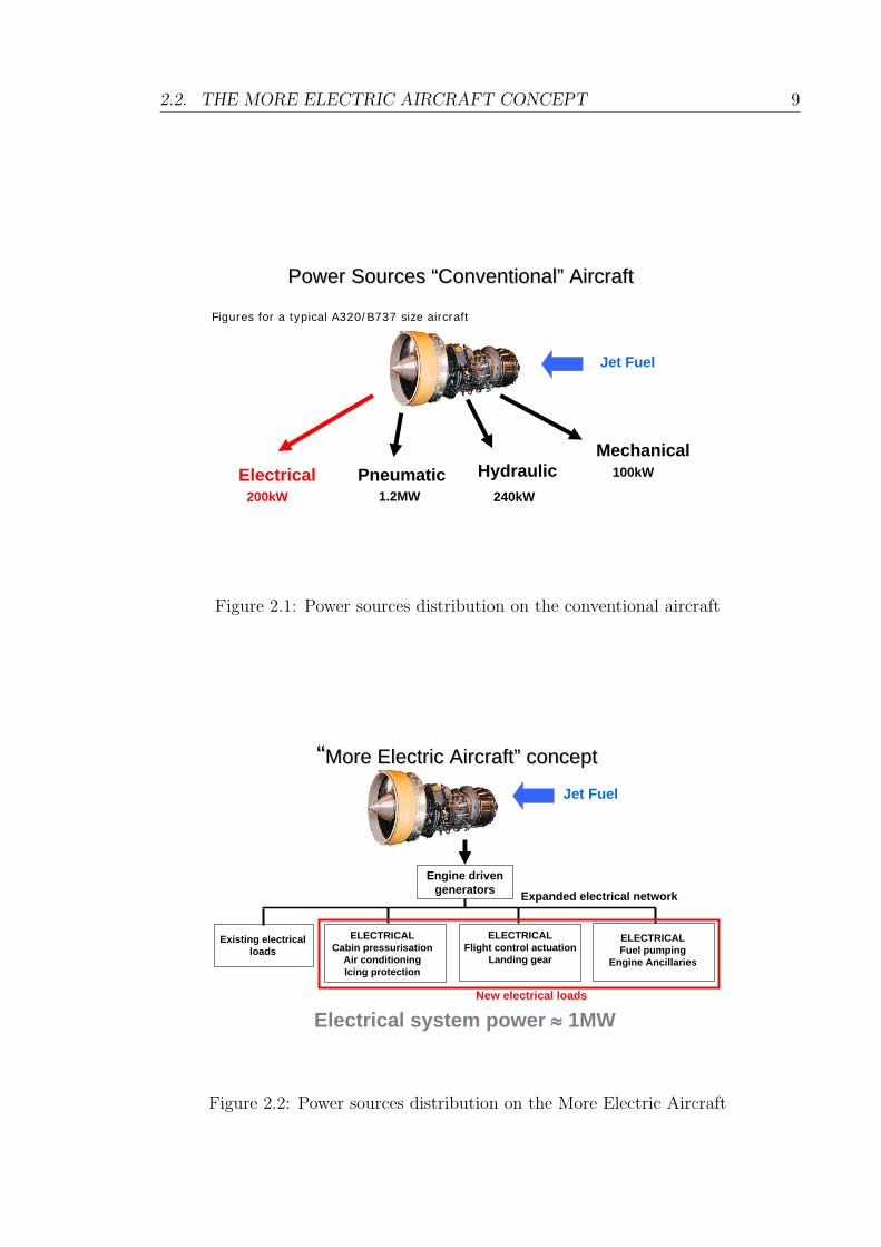
The schemes in figures 2.1 and 2.2 show the distribution of the power sources in the
conventional aircraft and the More Electric Aircraft respectively [5]. In the first
scheme it can be seen that the conventional aircraft subsystems operate by means
of different kinds of power sources. The second scheme shows that the electrical
power generated on board of a More Electric Aircraft is much higher than in the
conventional aircraft and most of the subsystems are electrically operated. The
electrical power on board of a More Electric Aircraft is about 1MW magnitude [5].
The subsystems conventionally supplied by electrical power are: energy storage
system, engine starting system, ignition system, de-icing system, landing gear con-
trol, anti-skid control system, passenger cabin services, avionics, lighting systems.
In the More Electric Aircraft, the electrically powered subsystems are: flight con-
trol systems, electric anti-icing, environmental systems, electric-actuated brakes,
utility actuators, fuel pumping. In the conventional aircraft the distribution net-
work is a point-to-point topology in which all the electrical wirings are distributed
from the main bus to the different loads through relays and switches. This kind
of distribution network leads to expensive and heavy wiring circuits, and it is
not suitable for a system where bigger electrical power is involved. In the More
Electric Aircraft, different kinds of loads are used which require different levels of
voltage, therefore the future aircraft electrical systems will employ multi-voltage
level hybrid DC and AC systems. As a result, different kinds of power electronic
converters such as AC/DC rectifiers, DC/AC inverters and DC/DC choppers are
2.2. THE MORE ELECTRIC AIRCRAFT CONCEPT 9
Jet Fuel
HydraulicPneumaticMechanical
200kW 1.2MW 240kW
100kWElectrical
Power Sources Power Sources ““ConventionalConventional”” AircraftAircraft
Figures for a typical A320/B737 size aircraft
Figure 2.1: Power sources distribution on the conventional aircraft
Expanded electrical network
Engine driven generators
Existing electrical loads
Electrical system power
1MWNew electrical loads
ELECTRICALFlight control actuation
Landing gear
ELECTRICALCabin pressurisation
Air conditioningIcing protection
ELECTRICALFuel pumping
Engine Ancillaries
Jet Fuel
““More Electric AircraftMore Electric Aircraft”” conceptconcept
Figure 2.2: Power sources distribution on the More Electric Aircraft
2.2. THE MORE ELECTRIC AIRCRAFT CONCEPT 10
required [6].
The typical aircraft electrical system of the past was the twin 28 VDC system. It
was commonly used on twin-engined aircraft, where each engine powered a 28 VDC
generator. Due to the increase in the power requirements, the electrical generation
on board of the aircraft changed into the 115 VAC system. The AC distribution
in the aircraft power network can be at constant frequency, equal to 400Hz, or
at variable frequency, from 360Hz to 900Hz. In the first case, the frequency-wild
power from the AC generator is converted to 400Hz constant frequency 115VAC
power by means of a solid-state Variable-Speed/Constant-Frequency (VSCF) con-
verter [7] [8]. In the second case, the power is distributed at variable frequency and
converted locally for the loads which need constant frequency supply, by means of
power electronics converters [9] [10].
In the latest research concerning the More Electric Aircraft, great attention is
being paid on the ever increasing levels of power requirements, due to the replace-
ment of many non-electrical loads with electrical ones. In order to meet the high
power requirements, a distribution system characterized by a voltage level equal
to 230 VAC, with frequency variable between 360Hz and 900Hz, and 540 VDC is
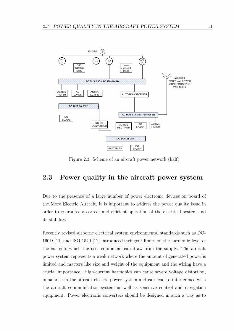
considered the most viable solution. Figure 2.3 shows the general scheme of one
half of an aircraft power network (assuming a symmetrical system). In the scheme
the main parts of the network are the two electrical generators connected to the
engine, the AC and DC buses, the loads connected to them, the electronic power
converters and the active filters installed for harmonic compensation.
Generally the aircraft power system is symmetrical, with two generators G1 and
G2 and two Auxiliary Power Units APU1 and APU2 connected to each engine.
The loads can be classified as essential and non-essential. Each generation channel
supplies a set of non-essential loads, while the essential loads are supplied by both
generators in parallel. The electrical power is distributed at different levels of
voltage: 230 VAC, 115 VAC, 540 VDC, 28 VAC.
2.3. POWER QUALITY IN THE AIRCRAFT POWER SYSTEM 11
AC BUS 230 VAC 360÷900 Hz
G1 G2
ACTIVE FILTER
ACTIVERECTIFIER
DC BUS 540 VDC
AC BUS 115 VAC 360÷900 Hz
AC LOADS
DC LOADS
AUTOTRANSFORMER
ACTIVE FILTER
DC-DC CONVERTER
DC BUS 28 VDC
ACTIVE RECTIFIER
AIRPORT EXTERNAL POWER CONNECTION 115
VAC 400 Hz
DC LOADSBATTERIES
E
AC LOADS
ENGINE
APU2
APU1
Non-essential
loads
Non-essential
loads
Figure 2.3: Scheme of an aircraft power network (half)
2.3 Power quality in the aircraft power system
Due to the presence of a large number of power electronic devices on board of
the More Electric Aircraft, it is important to address the power quality issue in
order to guarantee a correct and efficient operation of the electrical system and
its stability.
Recently revised airborne electrical system environmental standards such as DO-
160D [11] and ISO-1540 [12] introduced stringent limits on the harmonic level of
the currents which the user equipment can draw from the supply. The aircraft
power system represents a weak network where the amount of generated power is
limited and matters like size and weight of the equipment and the wiring have a
crucial importance. High-current harmonics can cause severe voltage distortion,
unbalance in the aircraft electric power system and can lead to interference with
the aircraft communication system as well as sensitive control and navigation
equipment. Power electronic converters should be designed in such a way as to
2.3. POWER QUALITY IN THE AIRCRAFT POWER SYSTEM 12
reduce the harmonic distortion or filtering solutions can be implemented in order
to compensate for the harmonics generated by the distorting loads.
In an aircraft power system, designing a converter that can meet the power quality
requirements is challenging because of the high fundamental frequency (400Hz at
constant frequency or 360-900Hz at variable frequency). Achieving low input
current distortion and unity power factor at such high frequencies requires much
wider control bandwidth compared to what is necessary for terrestrial 50/60Hz
systems.
Several studies have been carried out on the operation and control of the power
electronic converters on board of the aircraft, and different solutions have been
investigated in order to limit the voltage and current harmonic distortion. In
[13] the authors investigate the power quality problems related to the dynamic
interaction between AC/DC converters with active power factor correction (PFC)
and the power supply. A solution for the elimination of the undesirable interactions
by means of proper damping of the PFC converter input filter is proposed and
validated. In [14] the design of a zero-voltage-switching active-clamped isolated
low-harmonic SEPIC rectifier is presented, for aircraft applications. The design
is carried out in order to meet the power quality requirements and harmonic
distortion limits recommended by the regulations.
In order to compensate for the harmonics injected by the distorting loads in the
system, it is not only necessary to utilize converters with a suitable topology and
design which meet the power quality standards, but it is also important to imple-
ment filtering. Traditionally, several topologies of passive filters have been utilized
for the elimination of the harmonics. The most popular configuration is the L-C
tuned filter which works like a low-impedance path for the harmonic component to
be eliminated. However, passive filters present several drawbacks, such as ageing
and tuning problems, series and parallel resonances, bulk passive components and
low flexibility in the compensation characteristics. These drawbacks represent a
strong limitation in the choice of passive filters in a system like the aircraft elec-
tric network, because of the weight and size of the components, and the variable
supply frequency.
2.3. POWER QUALITY IN THE AIRCRAFT POWER SYSTEM 13
Active power filters represent a feasible solution to the problems caused by the non-
linear loads. The active filters can compensate for the harmonics, correct the power
factor and work as a reactive power compensator, thus providing enhancement of
the power quality in the system. In [15] the performance of an aircraft power
system is investigated and harmonic compensation by means of a shunt active
power filter is analysed. In [16] an active power filter is designed for harmonic
compensation, power factor correction and minimization of the load unbalance,
for an aircraft power system with Variable-Speed Constant-Frequency (VSCF)
generating system.
The main challenge related to the implementation of harmonic compensation by
means of an active filter in a system like the aircraft power network is, as mentioned
above, the fundamental frequency, which varies in a range of high values, compared
to the conventional 50/60Hz of terrestrial systems. In order for the control of the
active filter to work properly, it is necessary to perform an accurate calculation
of the reference and to implement a control technique with high bandwidth or
generally able to track high frequency harmonics.
With regard to the calculation of the reference for the active filter control, in this
project a novel frequency and harmonic detection technique is proposed. It is
suitable for the accurate calculation of the reference in a system where the supply
frequency is variable and ranges between high values.
With regard to the active filter control, this project proposes a novel control
technique based on the decoupling between different rotating reference frames
and the detection of the harmonic content on the basis of the voltage at the Point
of Common Coupling (PCC). This technique is suitable for a system like the
aircraft power network. The current harmonics injected by a group of non-linear
loads can be detected by measuring the harmonic content of the voltage at the
point where the active filter is connected. In this way there is no need to employ
current transducers on each of the distorting loads, and the same active filter can
be utilized as a plug-and-play device that compensates the harmonic distortion in
different points of the distribution bus. The active filter can be connected in order
to provide harmonic compensation locally for a specific distorting load or for a
2.4. SUMMARY 14
big group of loads (for an adequate power level). These characteristics represent
a big advantage in a system where the size and the weight of the equipment have
a crucial importance.
In the future development of More Electric Aircraft power systems, a coordinated
control of several active filters through the use of a communication network would
bring advantages like better control of the power quality in any point of the net-
work, control of local energy storage to assist with fault clearance and supply
distribution.
2.4 Summary
In this chapter the concept of the More Electric Aircraft has been presented and
explained. The use of electrical power in place of other conventional sources of
power to run the aircraft subsystems presents several advantages in terms of effi-
ciency, maintenance, cost, size and weight, but it introduces major changes in the
aircraft power system. The consequence of this is a more complex electric net-
work, with increased power quality and stability problems. An effective solution
for power quality improvement in this kind of system is the power active shunt
filter. For the work presented in this thesis a novel solution for the calculation of
the reference for the active filter control and a novel control technique are pro-
posed. The proposed techniques are suitable for applications in the More Electric
Aircraft power system.
Chapter 3
Real-time Frequency and
Harmonic Estimation Technique
3.1 Introduction
This chapter presents a novel technique for frequency and harmonic estimation
based on the Discrete Fourier Transform (DFT). This technique allows the estima-
tion of fundamental frequency, fundamental phase angle and harmonic amplitudes
and phases of a time-varying distorted signal in real time. The technique has been
validated both through simulation analysis and experimental tests. Section 3.2
presents the state of the art of the most common harmonic detection techniques.
Sections 3.3 and 3.4 describe the frequency detection algorithm, by explaining
its mathematical foundations, and present the simulation results. In sections 3.5
and 3.6 the technique for the estimation of harmonic amplitudes and phases and
the simulation results are presented. Sections 3.7 and 3.8 present the results ob-
tained by means of the experimental validation. In section 3.9 some considerations
about the transient analysis of the harmonic estimation are discussed.
15

3.2. OVERVIEW OF FREQUENCY AND HARMONIC ESTIMATIONTECHNIQUES 16
3.2 Overview of frequency and harmonic estima-
tion techniques
A fast and exact estimation of fundamental line frequency, phase and harmonic
content of the current drawn by a non-linear load is required in order to calcu-
late an accurate reference signal for the active filter control algorithm, to achieve
precise harmonic compensation. Several algorithms for frequency estimation and
harmonic analysis have been proposed in the literature. Some of the most impor-
tant and commonly used methods are listed here and described.
One of the first methods used for harmonic and frequency detection is the Re-
cursive Discrete Fourier Transform (RDFT) [17–21]. This method utilizes a state
variable representation of the time-discrete signal and a recursive deadbeat ob-
server. Such a technique was developed in order to overcome problems of real
time computational complexity related to DFT calculations.
A widely used method for frequency estimation is the least squares error technique
[22–25], where the aim is to minimize the square error between the measured signal
and the modelled signal. The performance of the algorithm is affected by the width
of the observation window, the choice of the sampling frequency, the choice of the
reference time, and the Taylor Series truncation.
Another broadly used technique is the Kalman Filter [26–31], a recursive stochastic
technique that gives an optimal estimation of state variables of a given dynamic
system from noisy measurements. At every iteration step a prediction of the state
is calculated on the basis of the state at the previous step and the measurement and
the prediction is corrected in order to minimize the error. The main drawback of
Kalman filter-based algorithms is represented by the choice of the initial covariance
matrices of the model and measurement errors.
The Phase Locked Loop (PLL) is also widely used for frequency and phase de-
tection [32–37]. Its basic configuration consists of a feedback loop which includes
a phase detector, a low-pass filter and a voltage controlled oscillator. The PLL
provides fast and robust frequency estimation, even for distorted and unbalanced
3.3. FREQUENCY ESTIMATION TECHNIQUE 17
conditions; however in some cases its performance can be affected by a wrong
choice of the centre frequency, undesired oscillations due to harmonics and sub-
harmonics, transient errors due to a narrow bandwidth chosen to achieve a good
noise rejection. The PLL technique will be described in more detail in this chap-
ter. Furthermore a comparison with the technique proposed in this work will be
presented in Chapter 4.
Other categories of techniques for frequency and harmonic detection are: genetic
algorithms, wavelet transform, PQ theory, neural networks [38–43].
In this project an algorithm based on the Discrete Fourier Transform is proposed
for frequency and harmonic detection. It gives real-time estimation of fundamen-
tal frequency, fundamental amplitude, fundamental phase, and harmonic ampli-
tudes and phases, for a noisy distorted signal with time-varying amplitude and
frequency. The frequency and phase estimation provided by this method is char-
acterized by high accuracy and low sensitivity to harmonic distortion and noise.
It shows good tracking performance for signals with variable frequency. Also, the
harmonic amplitudes and phases are identified with high accuracy. The charac-
teristic parameters of the algorithm can be easily set. Furthermore, for a given set
of parameters, the estimation can be performed for a broad range of frequencies
and amplitudes of the signal, without the need to re-tune the initial settings.
A description of this estimation technique is given in the next section.
3.3 Frequency estimation technique
The technique here proposed to detect the fundamental frequency is based on the
principle that, in the FFT spectrum of a signal, the fundamental component has
the highest amplitude. When the exact value of fundamental frequency is un-
known it can be detected, within the limits of the frequency resolution, by finding
the highest component in the voltage (or current) spectrum and calculating its
corresponding frequency. In the hypothesis that an initial estimate of frequency is
known, the spectrum of the signal can be scanned in a narrow range of frequency
3.3. FREQUENCY ESTIMATION TECHNIQUE 18
around the first estimate, in order to find the highest spectral component within
the leakage sideband. This process can be iterated by means of a closed-loop con-
trol system. The leakage is due to the time domain truncation occurring when
windowing the signal for spectral analysis. For this kind of frequency analysis
and for its application it is preferable that the spread of the spectral lines is in
a short interval of frequency (short-range leakage), because if the spread is long
(long-range leakage) harmonic interference can occur so that larger errors result,
as will be explained further on in this chapter. To avoid long-range leakage, suit-
able windows must be applied to the signal. Among different types of window, a
normalized Hamming window has been chosen. It was observed that the perfor-
mance obtained using this window was particularly good in terms of short-range
leakage characteristics, compared to other types of window.
In the hypothesis that a rough idea of the value of frequency is known, which is
often the case in an electrical power system, an initial value f1 is chosen for the
estimate. Given the initial estimate f1, it is possible to obtain an estimate ∆f of
the difference between f1 and the actual value of the fundamental frequency. The
estimated ∆f depends on the amplitudes of three spectral components [44]: the
one at f1 and the two adjacent ones at f1± df , where df is the spectral resolution
chosen to represent the signal in the frequency domain. ∆f is calculated according
to (3.1):
∆f =1.5 · df · am1 · (am11 − am12)
(am1 + am11) · (am1 + am12)(3.1)
where am1 is the amplitude of the spectral line at frequency f1, am11 and am12
are the amplitudes of the right and the left components at f1 + df and f1 − df
respectively. The mathematical demonstration of (3.1) is presented in Appendix
A of [45].
The three amplitudes can be calculated by means of a procedure based on the
Discrete Fourier Transform, as follows. The voltage or current in a sinusoidal
single-phase circuit can be represented by a rotating vector, as well as a complex
quantity with real and imaginary parts which vary sinusoidally in the time domain.
It is possible to express this complex quantity with the following exponential

3.3. FREQUENCY ESTIMATION TECHNIQUE 19
function:
Aejϕ = Acos(ϕ) + jAsin(ϕ) (3.2)
where
ϕ =
∫ t
0
ω(t)dt (3.3)
A is the amplitude and ω is the angular frequency. The real and imaginary parts
are the projections on a pair of cartesian axes of a vector rotating with speed
ω(t). In a three-phase system the voltage (or current) is represented by a rotating
vector, and this vector can be expressed as the sum of a positive, a negative and
a zero sequence component. The three voltages va, vb, vc are commonly expressed
using a reference frame αβ0 defined as follows:
vαβ = vα(t) + jvβ(t) = 2
3
[va(t) + vb(t)e
j 23π + vc(t)e
j 43π]
v0(t) = 13
[va(t) + vb(t) + vc(t)](3.4)
where va(t), vb(t), vc(t) are the phase voltages expressed in the time domain. It
is possible to prove that if the three voltages va, vb, vc form a positive sequence
of voltages, vαβ is a vector rotating at speed +ω, whereas if it forms a negative
sequence of voltages, it is represented by a vector rotating at −ω (where the
positive sense is anti-clockwise by convention). A distorted three-phase voltage
(or current) can then be represented as the sum of as many rotating vectors as
the harmonics it is composed of, rotating at speed ±mω (+ for positive sequence
harmonics and - for negative ones), where m is the harmonic order. This concept
is mathematically expressed by the Discrete Fourier Transform:
Xαβ(k) =N−1∑n=0
xαβ(n)e−j2πkn/N k = 0, 1, ..., N − 1 (3.5)
Where Xαβ(k) is the frequency domain signal, expressed in the discrete frequency
3.3. FREQUENCY ESTIMATION TECHNIQUE 20
variable k , N is the number of samples of the signal, xαβ(n) is the time domain
signal, expressed in the discrete time variable n. The complex exponential func-
tions in the Discrete Fourier Transform are harmonically related, because their
frequencies are multiples of the fundamental frequency. In order to extract the
mth harmonic component from the signal, this needs to be represented in a new
reference frame rotating at the same speed as the rotating vector corresponding
with that harmonic, which means at speed ±mω. In this new reference frame, the
vector corresponding to the mth harmonic is the only component appearing as a
DC quantity and for this reason the only one having non-zero mean value over a
time interval equal to a multiple of the fundamental period. This concept will be
explained in better detail in section 5.2. The transformation from the stationary
reference frame to the rotating one can be carried out by multiplying the entire
signal by another complex exponential function with amplitude equal to 1 and
frequency equal to ±mω.
In the proposed algorithm the input signal, which can represent either a three-
phase voltage or a three-phase current, is transformed from the abc system of
coordinates into the αβ0 reference frame and then expressed by means of its αβ
components (where α and β components are respectively the real and imaginary
part of vαβ). The signal is then transformed into three different reference frames
rotating respectively at ω1 , ω1 + dω, ω1 − dω, by multiplying it by the complex
quantities e−jω1t , e−j(ω1+dω)t , e−j(ω1−dω)t. This procedure allows the three spectral
lines at the three frequencies ω1 , ω1 + dω, ω1 − dω to be extracted, which, in the
frequency spectrum, corresponds to the extraction of the spectral line correspond-
ing to the frequency f1 and the two lines next to it. These signals are windowed by
means of a Hamming window and their mean values are calculated. These mean
values yield the amplitudes and phases of the signal components at frequencies f1,
f1 + df and f1 − df , and the three amplitudes can be used to calculate the fre-
quency correction factor ∆f as in (3.1). The value ∆f is then minimized using a
closed loop system and a Proportional Integral controller, in order to estimate the
value of the fundamental frequency. The estimated frequency is then multiplied
by 2π and integrated to obtain the estimated phase of the fundamental signal and
this is used to calculate the three amplitudes am1, am11 and am12 using the DFT
algorithm.
3.3. FREQUENCY ESTIMATION TECHNIQUE 21
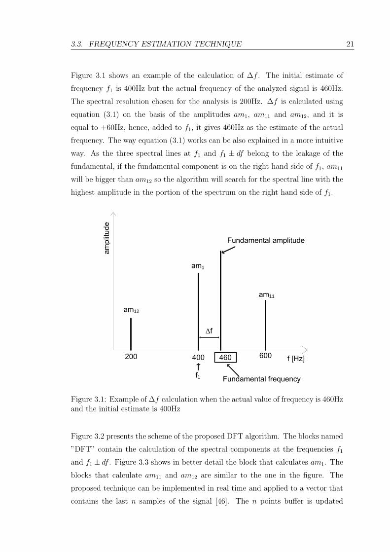
Figure 3.1 shows an example of the calculation of ∆f . The initial estimate of
frequency f1 is 400Hz but the actual frequency of the analyzed signal is 460Hz.
The spectral resolution chosen for the analysis is 200Hz. ∆f is calculated using
equation (3.1) on the basis of the amplitudes am1, am11 and am12, and it is
equal to +60Hz, hence, added to f1, it gives 460Hz as the estimate of the actual
frequency. The way equation (3.1) works can be also explained in a more intuitive
way. As the three spectral lines at f1 and f1 ± df belong to the leakage of the
fundamental, if the fundamental component is on the right hand side of f1, am11
will be bigger than am12 so the algorithm will search for the spectral line with the
highest amplitude in the portion of the spectrum on the right hand side of f1.
11
1
12
1
Figure 3.1: Example of ∆f calculation when the actual value of frequency is 460Hzand the initial estimate is 400Hz
Figure 3.2 presents the scheme of the proposed DFT algorithm. The blocks named
”DFT” contain the calculation of the spectral components at the frequencies f1
and f1 ± df . Figure 3.3 shows in better detail the block that calculates am1. The
blocks that calculate am11 and am12 are similar to the one in the figure. The
proposed technique can be implemented in real time and applied to a vector that
contains the last n samples of the signal [46]. The n points buffer is updated

3.3. FREQUENCY ESTIMATION TECHNIQUE 22
at every step with a First In First Out logic. The αβ vector representing the
input signal is multiplied by the complex quantity e−jθ1 in order to transform
it into the reference frame rotating at ω1. The signal is also multiplied by the
Hamming window (also in the form of a n point buffer which is fixed). The mean
value of the vector obtained from the multiplication is calculated, by summing
all its components and dividing the sum by its length. A scaling factor equal to
1.8519 is also applied in the mean value calculation, in order to compensate for the
multiplication by 0.54 introduced by the Hamming window. The mathematical
expression of the Hamming window is shown in (3.6).
w(i) = 0.54− 0.46cos
(2πi
n
)(3.6)
Where i is an integer number with values 0 ≤ i ≤ n.
The mean value calculation yields an average vector, whose amplitude and phase
are the amplitude am1 and the phase variation ∆ϑ1 which, summed with the phase
ϑ1, gives the fundamental phase ϕ1.
Δf f1
df
df
θ1
θ12
θ11
Three-phase signal
αβ
Δf
am12
am1
am11
φ1
-
+
+
+
Figure 3.2: Scheme of the DFT algorithm

3.3. FREQUENCY ESTIMATION TECHNIQUE 23
θ1 e-jθ1 n points buffer
αβ signal
Hamming window
cartesian to polar Δθ1
++
am1
Amplitude estimate
Phase estimate
φ1 = θ1 + Δθ
n points buffer n
8519.1
Figure 3.3: DFT block diagram for the calculation of the amplitude am1 and thephase ϕ1
3.3.1 Choice of algorithm parameters
In order to perform in real time all the calculations described above, a limited
portion of the input signal is analyzed, which means a limited observation window
is used to observe and process the signal. A fixed length buffer is used to store the
analyzed portion of the signal and at every sampling step the buffer is updated
with a new acquired sample, discarding the oldest one (First In First Out logic).
This buffer of samples is weighted by means of a normalized Hamming window
of the same length and the mean value of the weighed portion of the signal is
calculated. The observation window Tobs (which should be an integer multiple of
the fundamental period) and the spectral resolution df are related by the following
relation:
df =1
Tobs=
1
nTs=fsn
(3.7)
where n is the number of samples contained in one observation window and fs
is the sampling frequency, which is chosen taking into account the computational
capability of the microprocessor used for the digital implementation. The choice
of Tobs and df is a crucial point in the algorithm design. A large observation
window - high Tobs - makes the spectral resolution smaller, thus improving the

3.3. FREQUENCY ESTIMATION TECHNIQUE 24
resolution of the spectrum. However it increases the computational effort as a
higher number of samples of the signal are required in order to perform all the
calculations in one step. Hence, in this case, the technique is less able to track
high speed transients of frequency. A narrow observation window decreases the
computational time but on the other hand it worsens the spectral resolution: in
this case harmonic interference can occur, as the two spectral lines next to the
one in f1 might correspond with some harmonic components, resulting in an error
in the frequency estimation. Therefore, in order to choose an appropriate set of
parameters for the algorithm, a compromise should be found, between a high value
of Tobs, corresponding with a small value of df (high spectral accuracy) and a small
value of Tobs (low spectral accuracy).
3.3.2 Analysis of a sinusoidal signal
If the signal contains a single sinusoidal component and the observation window is
not an integer multiple of the fundamental period, the amplitudes of the spectral
components obtained by means of the DFT are independent of the portion of
signal being analyzed. They only depend on the length of the observation window
(the number of samples).
For example, assuming that a 400 Hz three phase sinusoidal signal having ampli-
tude equal to 1 is analysed using an 8 point buffer sampled at 8 kHz, the frequency
resolution of the DFT is 1000 Hz (according to (3.7)). If the initial estimate of
frequency is 400 Hz, it is possible to calculate the DFT amplitudes at -600 Hz,
400 Hz and 1400 Hz, which are equal to am12 = 0.4627, am1 = 0.9333 and am11
= 0.4627 respectively. If the signal amplitude was not 1 the DFT results would
be multiplied by the actual signal amplitude. The value obtained from (3.1) is
not affected by the signal amplitude and would be equal to 0 in the proposed
example. Since the portion of the signal being analysed is smaller than a period
of the signal itself, there is an error in the calculated signal amplitude as well
as a strong leakage effect. Equation (3.1) provides a correct calculation of the
signal frequency after several iterations, as the frequency error is minimized by a
PI controller so ∆f converges to zero at the steady-state, regardless of the initial
3.3. FREQUENCY ESTIMATION TECHNIQUE 25
estimate f1. Similarly any single sinusoidal signal would produce constant am
coefficients, independent of the portion of the signal being analysed. For example,
the calculation of the DFT amplitudes at the same frequency as the previous case,
with an 800 Hz signal would give am12 = 0.0846, am1 = 0.5988 and am11 = 0.9082
resulting in f = 379 Hz, close to the correct value of 400 Hz.
3.3.3 Analysis of a distorted signal
When the signal contains several sinusoidal components, the DFT values are the
sum of the DFT of each sinusoid due to the linearity property of DFT. Since the
DFT values are complex, the amplitude of the sum of the DFT values is not the
sum of the amplitudes. Moreover the DFT amplitudes become functions of the
portion of the signal being analysed. Since it is difficult to give a mathematical
representation of the DFT amplitudes when the signal is distorted, they have been
calculated by analysing all the possible portions of the signal supposing that the
signal is composed of a fundamental component at 400 Hz and a single harmonic.
The calculation has been repeated considering different harmonics having attenu-
ations, with respect to the fundamental component, in the range [-20 dB -60 dB].
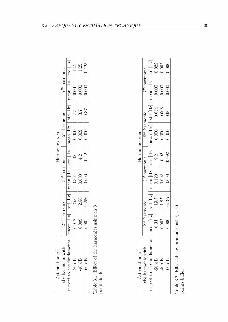
The DFT amplitudes and the ∆f values have been calculated using buffers of 8
points and 20 points. The latter value corresponds to one complete period of the
400 Hz signal, given the sampling frequency of 8 kHz. This also implies that the
DFT frequency resolution equals 400 Hz and the spectral component amplitudes
will be calculated at 0 Hz, 400 Hz and 800 Hz. The mean values of ∆f together
with their standard deviations are given in tables 3.1 and 3.2.
The influence of the harmonics rapidly decreases with their amplitude. This is
shown by the fact that ∆f is closer to zero when the harmonic amplitude decreases,
zero is the value that would be obtained if the 400Hz signal was sinusoidal, with
an initial estimate equal to 400Hz. Increasing the size of the buffer clearly makes
the method less sensitive to the signal harmonic content as shown by a comparison
of tables 3.1 and 3.2. The buffer size affects the sensitivity of the technique to the
harmonics also because of the possible harmonic interference occurring between the
leakage of the fundamental and the leakage of the harmonics at frequencies f1±df .
3.3. FREQUENCY ESTIMATION TECHNIQUE 26
Att
enuat
ion
ofH
arm
onic
order
the
har
mon
icw
ith
2nd
har
mon
ic3rd
har
mon
ic5th
har
mon
ic7th
har
mon
icre
spec
tto
the
fundam
enta
lm
ean
[Hz]
std
[Hz]
mea
n[H
z]st
d[H
z]m
ean
[Hz]
std
[Hz]
mea
n[H
z]st
d[H
z]-2
0dB
0.01
225
.60.
364
420.
600
370.
061
12.5
-40
dB
0.00
92.
560.
003
4.2
0.00
93.
70.
000
1.25
-60
dB
0.00
10.
256
0.00
00.
420.
000
0.37
0.00
00.
125
Tab
le3.
1:E
ffec
tof
the
har
mon
ics
usi
ng
an8
poi
nts
buff
er
Att
enuat
ion
ofH
arm
onic
order
the
har
mon
icw
ith
2nd
har
mon
ic3rd
har
mon
ic5th
har
mon
ic7th
har
mon
icre
spec
tto
the
fundam
enta
lm
ean
[Hz]
std
[Hz]
mea
n[H
z]st
d[H
z]m
ean
[Hz]
std
[Hz]
mea
n[H
z]st
d[H
z]-2
0dB
0.34
19.7
0.12
09.
20.
000
0.08
40.
000
0.02
2-4
0dB
0.00
21.
970.
002
0.92
0.00
00.
008
0.00
00.
002
-60
dB
0.00
00.
197
0.00
00.
092
0.00
00.
001
0.00
00.
000
Tab
le3.
2:E
ffec
tof
the
har
mon
ics
usi
ng
a20
poi
nts
buff
er
3.3. FREQUENCY ESTIMATION TECHNIQUE 27
The chance of interference is higher when the frequency resolution is increased,
which means a smaller buffer size is used. This is a rule of thumb that has to
be carefully applied. For example, when 20 points are analyzed the frequency
f1 + df is coincident with the second harmonic at 800 Hz and the estimation error
heavily depends on the second harmonic amplitude. The buffer size choice should
then consider that the frequencies f1 ± df have to be far enough from any large
harmonic components of the signal.
3.3.4 Algorithm tuning
Due to the presence of the harmonics, the calculated ∆f value has an offset with
respect to the actual frequency error and can oscillate. It was found that the
standard deviation of the calculated ∆f decreases with the same rate as the har-
monic amplitude. The standard deviation of ∆f limits the bandwidth reachable
by the DFT algorithm. It is possible to filter out the ∆f oscillations and obtain a
flat frequency estimate by a proper selection of the PI gains, eventually reducing
the DFT bandwidth. As a rule of thumb, when the standard deviation of ∆f is
below a few percent of the signal fundamental frequency it is possible to obtain a
good dynamic performance. The tolerable value of the ∆f offset depends on the
required accuracy of the frequency estimation technique because the frequency es-
timate will have a bias equal to the average value of ∆f . It is worth highlighting
that the bias in the frequency estimate does not correspond to an error in the
estimation of the phase of the signals. This will be demonstrated by the results
shown in the next sections and means that the fundamental signal component can
be accurately tracked even when there is an error in the frequency estimate. It
can be concluded from the considerations above that an 8 points buffer is a good
choice when the harmonic level is below -20 dB, otherwise a larger buffer has to
be chosen or some signal pre-filtering is necessary. It is important to remark that,
even if the computational burden is not a primary concern, an excessive buffer
size would compromise the transient performance of the frequency estimation al-
gorithm. When fast changes of the fundamental frequency are expected, the buffer
size should be kept as small as possible in order to allow good frequency tracking
3.4. FREQUENCY AND PHASE ESTIMATION: SIMULATION RESULTS 28
Fundamental frequency (initial estimate) [Hz] 400 Hz
Fundamental amplitude 40
Fundamental phase [deg] 0
5th harmonic amplitude 8
5th harmonic phase [deg] 50
7th harmonic amplitude 4
7th harmonic phase [deg] 70
11th harmonic amplitude 2.5
11th harmonic phase [deg] 110
13th harmonic amplitude 2
13th harmonic phase [deg] 130
Table 3.3: Input signal for fundamental frequency and phase estimation
also in transient conditions.
3.4 Frequency and phase estimation: simulation
results
A simulation has been carried out in Matlab Simulink in order to test the proposed
algorithm for fundamental frequency and phase estimation. The input signal has
the characteristics listed in table 3.3. The harmonic distortion of this signal rep-
resents a critical condition for an aircraft power system, and it is related to the
aircraft power quality recommendations [12].
The characteristic parameters of the algorithm have been chosen with the values
reported in table 3.4.
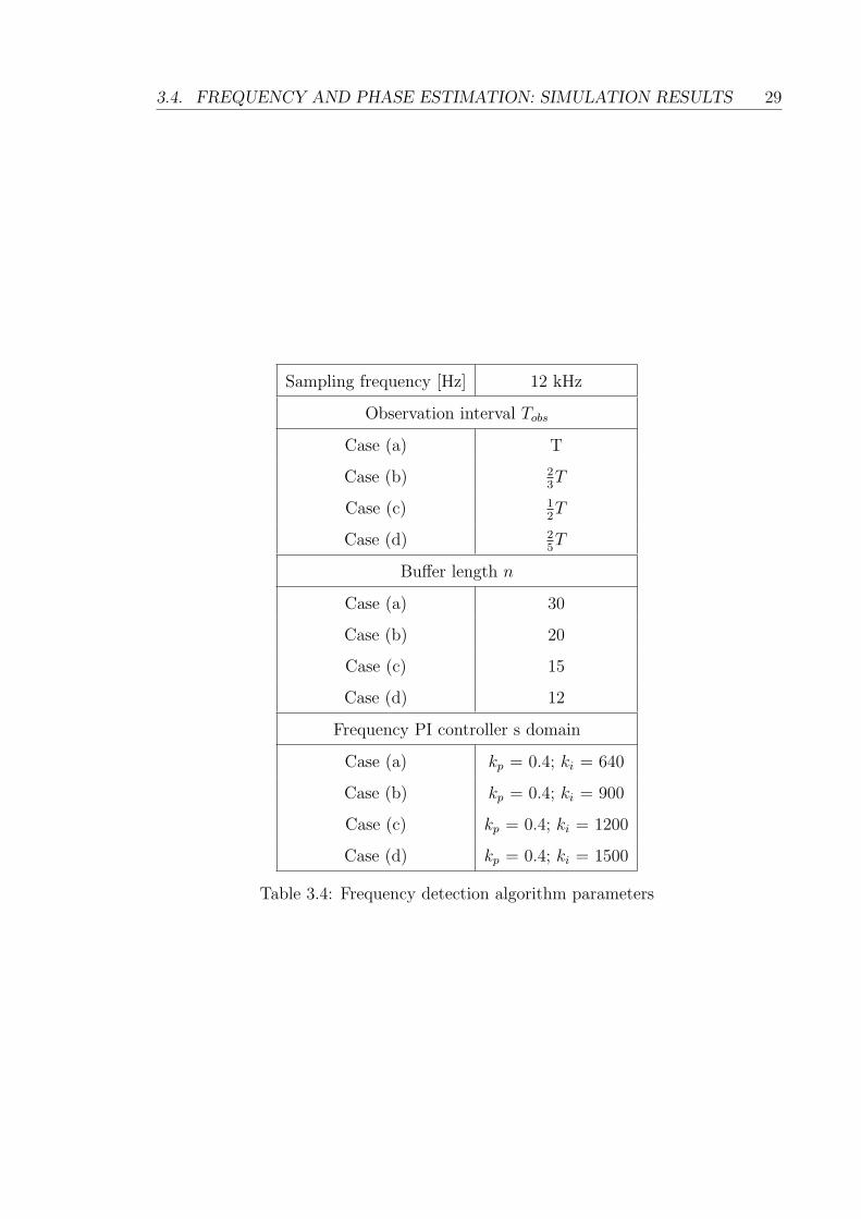
3.4. FREQUENCY AND PHASE ESTIMATION: SIMULATION RESULTS 29
Sampling frequency [Hz] 12 kHz
Observation interval Tobs
Case (a) T
Case (b) 23T
Case (c) 12T
Case (d) 25T
Buffer length n
Case (a) 30
Case (b) 20
Case (c) 15
Case (d) 12
Frequency PI controller s domain
Case (a) kp = 0.4; ki = 640
Case (b) kp = 0.4; ki = 900
Case (c) kp = 0.4; ki = 1200
Case (d) kp = 0.4; ki = 1500
Table 3.4: Frequency detection algorithm parameters
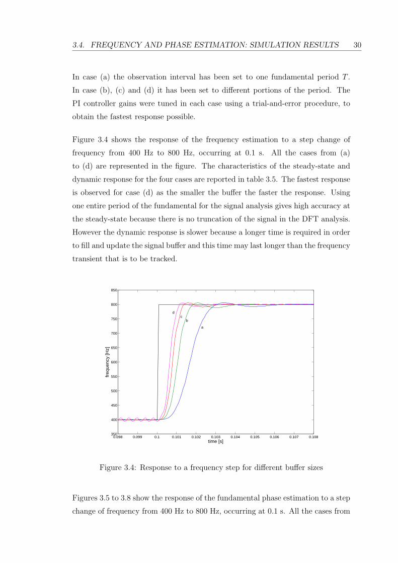
3.4. FREQUENCY AND PHASE ESTIMATION: SIMULATION RESULTS 30
In case (a) the observation interval has been set to one fundamental period T .
In case (b), (c) and (d) it has been set to different portions of the period. The
PI controller gains were tuned in each case using a trial-and-error procedure, to
obtain the fastest response possible.
Figure 3.4 shows the response of the frequency estimation to a step change of
frequency from 400 Hz to 800 Hz, occurring at 0.1 s. All the cases from (a)
to (d) are represented in the figure. The characteristics of the steady-state and
dynamic response for the four cases are reported in table 3.5. The fastest response
is observed for case (d) as the smaller the buffer the faster the response. Using
one entire period of the fundamental for the signal analysis gives high accuracy at
the steady-state because there is no truncation of the signal in the DFT analysis.
However the dynamic response is slower because a longer time is required in order
to fill and update the signal buffer and this time may last longer than the frequency
transient that is to be tracked.
0.098 0.099 0.1 0.101 0.102 0.103 0.104 0.105 0.106 0.107 0.108350
400
450
500
550
600
650
700
750
800
850
time [s]
freq
uenc
y [H
z]
a
bc
d
Figure 3.4: Response to a frequency step for different buffer sizes
Figures 3.5 to 3.8 show the response of the fundamental phase estimation to a step
change of frequency from 400 Hz to 800 Hz, occurring at 0.1 s. All the cases from

3.4. FREQUENCY AND PHASE ESTIMATION: SIMULATION RESULTS 31
case (a) case (b) case (c) case (c)Maximum overshoot [%] 1.37 1.37 1.37 1.37
Delay time [s] 0.1017 0.1011 0.1008 0.1006Rise time [s] 0.0015 0.0009 0.0007 0.0006
Settling time 5% [s] 0.1027 0.1016 0.1012 0.101Peak time [s] 0.1034 0.1021 0.1016 0.1012
Steady-state oscillation max amplitude(% of the steady-state value) 0.00075 0.0063 0.0325 0.25
Steady-state error [Hz] 0 0 0 0.0078
Table 3.5: Transient and steady-state performance of the frequency step estimation
(a) to (d) are represented in the figures. In these figures, the phase estimate is
compared with the fundamental phase of the input signal used in the simulation.
It can be noticed that the smaller the buffer of samples the faster the response.
This depends on the fact that, when processing the signal with a bigger buffer, the
computational time increases and the estimation transient is longer. In the case
(a) the phase estimate locks to the actual phase in 0.004 s, after the frequency
step occurs. In the cases (b), (c) and (d) the phase estimate settles in 0.0025 s,
0.002 s and 0.0015 s respectively.
0.098 0.099 0.1 0.101 0.102 0.103 0.104 0.105
0
1
2
3
4
5
6
time [s]
phas
e [r
ad]
estimateactual
Figure 3.5: Response of the phase estimate to a frequency step. Case (a)
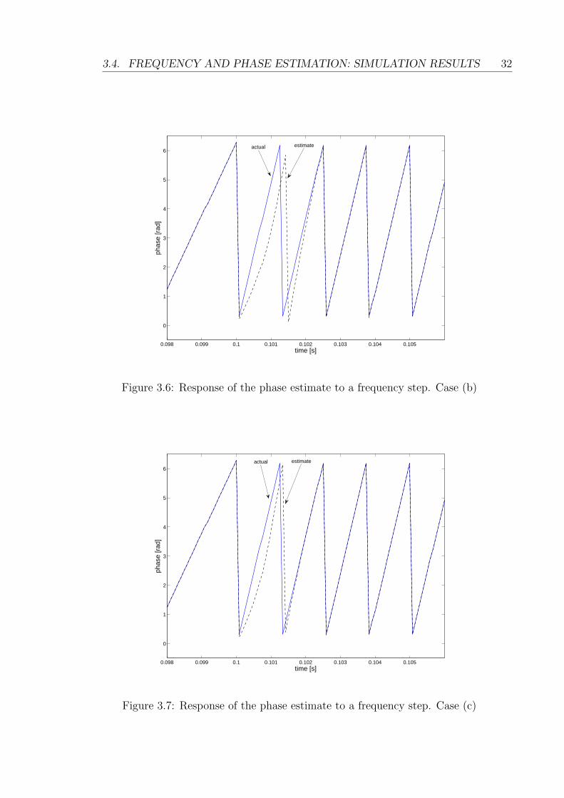
3.4. FREQUENCY AND PHASE ESTIMATION: SIMULATION RESULTS 32
0.098 0.099 0.1 0.101 0.102 0.103 0.104 0.105
0
1
2
3
4
5
6
time [s]
phas
e [r
ad]
estimateactual
Figure 3.6: Response of the phase estimate to a frequency step. Case (b)
0.098 0.099 0.1 0.101 0.102 0.103 0.104 0.105
0
1
2
3
4
5
6
time [s]
phas
e [r
ad]
estimateactual
Figure 3.7: Response of the phase estimate to a frequency step. Case (c)

3.5. HARMONIC ESTIMATION TECHNIQUE 33
0.098 0.099 0.1 0.101 0.102 0.103 0.104 0.105
0
1
2
3
4
5
6
time [s]
phas
e [r
ad]
estimateactual
Figure 3.8: Response of the phase estimate to a frequency step. Case (d)
3.5 Harmonic estimation technique
In the previous sections, the DFT technique for the real-time estimation of the
fundamental frequency and the fundamental phase has been described. The same
technique can be also used for the estimation of the harmonic amplitudes and
phases of a distorted signal. There are two ways in which the harmonic estimation
algorithm can be implemented: in the first one, the DFT is applied to the whole
distorted signal and the different harmonic components are extracted. In the
second method, the fundamental component, estimated by means of the DFT
technique described above, is subtracted from the signal. In this way only the
distorted part of the signal is analysed using the same DFT technique, in order to
extract the harmonics.
In order to estimate the mth harmonic component, the distorted signal (or the
distorted signal minus the fundamental) is multiplied by the exponential function
e(−j)(±m)(ϕ1), where + is used for positive sequence harmonics and - for negative
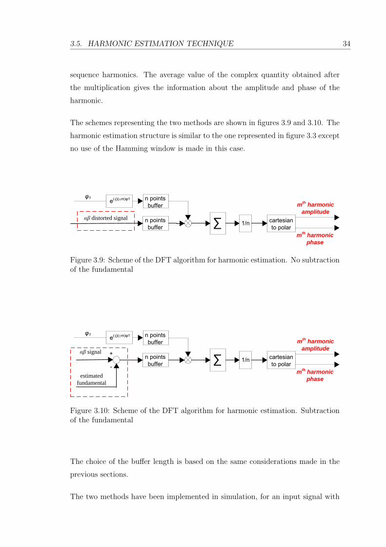
3.5. HARMONIC ESTIMATION TECHNIQUE 34
sequence harmonics. The average value of the complex quantity obtained after
the multiplication gives the information about the amplitude and phase of the
harmonic.
The schemes representing the two methods are shown in figures 3.9 and 3.10. The
harmonic estimation structure is similar to the one represented in figure 3.3 except
no use of the Hamming window is made in this case.
φ1 e(-j)(±m)φ1 n points buffer
1/n cartesian to polar
mth harmonic amplitude
n points buffer
mth harmonic phase
αβ distorted signal
Figure 3.9: Scheme of the DFT algorithm for harmonic estimation. No subtractionof the fundamental
φ1 e(-j)(±m)φ1 n points buffer
1/n cartesian to polar
mth harmonic amplitude
n points buffer
mth harmonic phase
αβ signal +
-estimated
fundamental
Figure 3.10: Scheme of the DFT algorithm for harmonic estimation. Subtractionof the fundamental
The choice of the buffer length is based on the same considerations made in the
previous sections.
The two methods have been implemented in simulation, for an input signal with
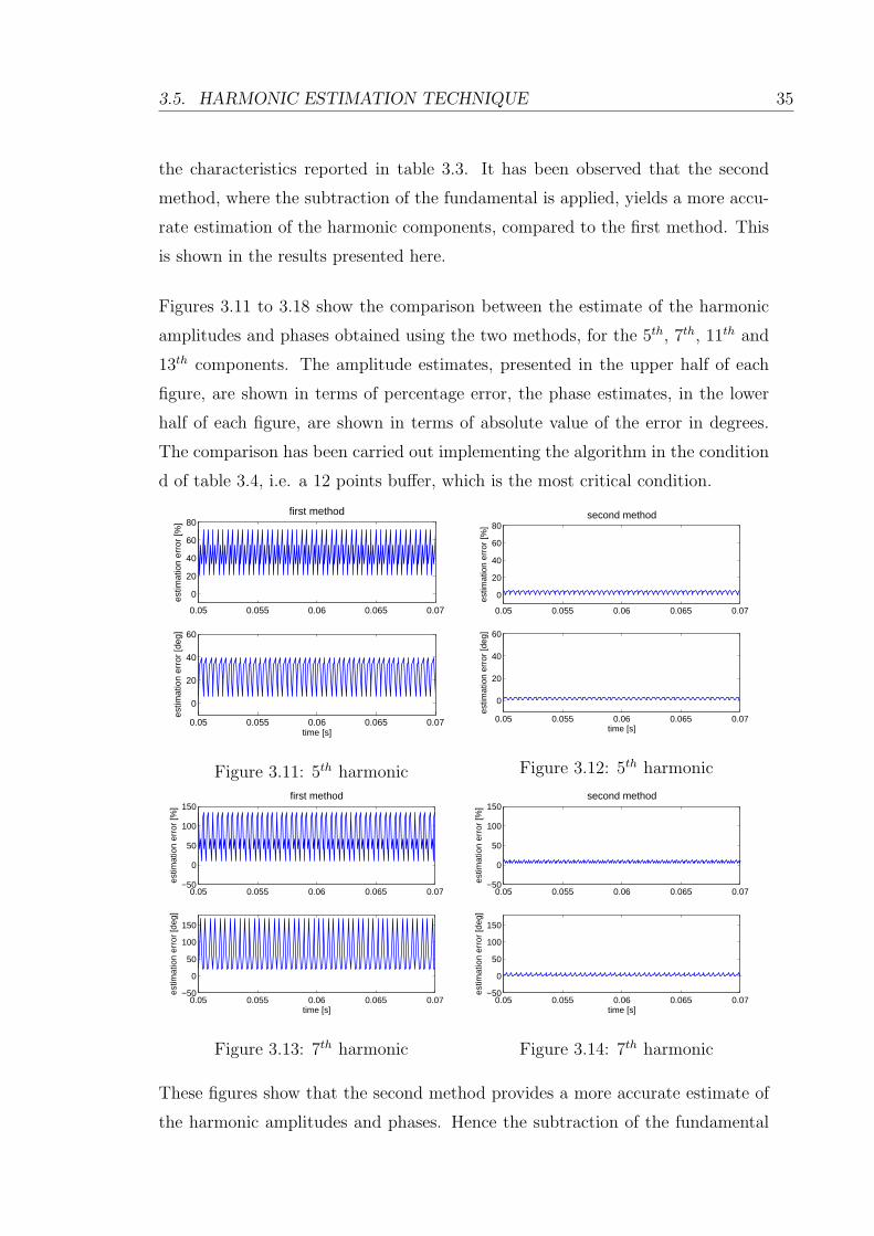
3.5. HARMONIC ESTIMATION TECHNIQUE 35
the characteristics reported in table 3.3. It has been observed that the second
method, where the subtraction of the fundamental is applied, yields a more accu-
rate estimation of the harmonic components, compared to the first method. This
is shown in the results presented here.
Figures 3.11 to 3.18 show the comparison between the estimate of the harmonic
amplitudes and phases obtained using the two methods, for the 5th, 7th, 11th and
13th components. The amplitude estimates, presented in the upper half of each
figure, are shown in terms of percentage error, the phase estimates, in the lower
half of each figure, are shown in terms of absolute value of the error in degrees.
The comparison has been carried out implementing the algorithm in the condition
d of table 3.4, i.e. a 12 points buffer, which is the most critical condition.
0.05 0.055 0.06 0.065 0.07
0
20
40
60
80
estim
atio
n er
ror
[%]
first method
0.05 0.055 0.06 0.065 0.07
0
20
40
60
time [s]
estim
atio
n er
ror
[deg
]
Figure 3.11: 5th harmonic
0.05 0.055 0.06 0.065 0.07
0
20
40
60
80
estim
atio
n er
ror
[%]
second method
0.05 0.055 0.06 0.065 0.07
0
20
40
60
time [s]
estim
atio
n er
ror
[deg
]
Figure 3.12: 5th harmonic
0.05 0.055 0.06 0.065 0.07−50
0
50
100
150
estim
atio
n er
ror
[%]
first method
0.05 0.055 0.06 0.065 0.07−50
0
50
100
150
time [s]
estim
atio
n er
ror
[deg
]
Figure 3.13: 7th harmonic
0.05 0.055 0.06 0.065 0.07−50
0
50
100
150
estim
atio
n er
ror
[%]
second method
0.05 0.055 0.06 0.065 0.07−50
0
50
100
150
time [s]
estim
atio
n er
ror
[deg
]
Figure 3.14: 7th harmonic
These figures show that the second method provides a more accurate estimate of
the harmonic amplitudes and phases. Hence the subtraction of the fundamental

3.5. HARMONIC ESTIMATION TECHNIQUE 36
0.05 0.055 0.06 0.065 0.07−50
0
50
100
150
estim
atio
n er
ror
[%]
first method
0.05 0.055 0.06 0.065 0.07−50
0
50
100
150
time [s]
estim
atio
n er
ror
[deg
]
Figure 3.15: 11th harmonic estimate
0.05 0.055 0.06 0.065 0.07−50
0
50
100
150
estim
atio
n er
ror
[%]
second method
0.05 0.055 0.06 0.065 0.07−50
0
50
100
150
time [s]es
timat
ion
erro
r [d
eg]
Figure 3.16: 11th harmonic estimate
0.05 0.055 0.06 0.065 0.07
0
50
100
estim
atio
n er
ror
[%]
first method
0.05 0.055 0.06 0.065 0.07−50
0
50
100
150
200
time [s]
estim
atio
n er
ror
[deg
]
Figure 3.17: 13th harmonic
0.05 0.055 0.06 0.065 0.07
0
50
100
estim
atio
n er
ror
[%]
second method
0.05 0.055 0.06 0.065 0.07−50
0
50
100
150
200
time [s]
estim
atio
n er
ror
[deg
]
Figure 3.18: 13th harmonic
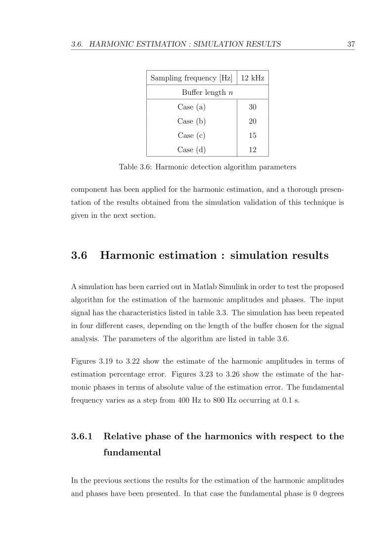
3.6. HARMONIC ESTIMATION : SIMULATION RESULTS 37
Sampling frequency [Hz] 12 kHz
Buffer length n
Case (a) 30
Case (b) 20
Case (c) 15
Case (d) 12
Table 3.6: Harmonic detection algorithm parameters
component has been applied for the harmonic estimation, and a thorough presen-
tation of the results obtained from the simulation validation of this technique is
given in the next section.
3.6 Harmonic estimation : simulation results
A simulation has been carried out in Matlab Simulink in order to test the proposed
algorithm for the estimation of the harmonic amplitudes and phases. The input
signal has the characteristics listed in table 3.3. The simulation has been repeated
in four different cases, depending on the length of the buffer chosen for the signal
analysis. The parameters of the algorithm are listed in table 3.6.
Figures 3.19 to 3.22 show the estimate of the harmonic amplitudes in terms of
estimation percentage error. Figures 3.23 to 3.26 show the estimate of the har-
monic phases in terms of absolute value of the estimation error. The fundamental
frequency varies as a step from 400 Hz to 800 Hz occurring at 0.1 s.
3.6.1 Relative phase of the harmonics with respect to the
fundamental
In the previous sections the results for the estimation of the harmonic amplitudes
and phases have been presented. In that case the fundamental phase is 0 degrees
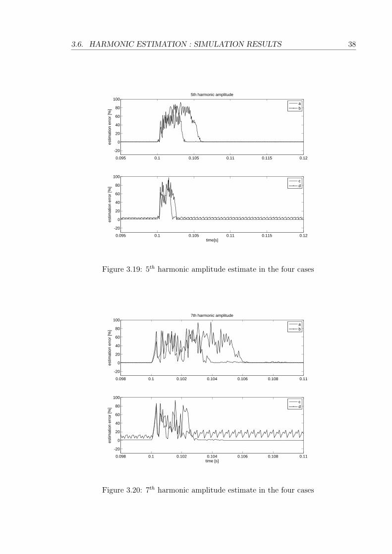
3.6. HARMONIC ESTIMATION : SIMULATION RESULTS 38
0.095 0.1 0.105 0.11 0.115 0.12
-20
0
20
40
60
80
100
estim
atio
n er
ror [
%]
5th harmonic amplitude
0.095 0.1 0.105 0.11 0.115 0.12
-20
0
20
40
60
80
100
time[s]
estim
atio
n er
ror [
%]
ab
cd
Figure 3.19: 5th harmonic amplitude estimate in the four cases
0.098 0.1 0.102 0.104 0.106 0.108 0.11
-20
0
20
40
60
80
100
estim
atio
n er
ror [
%]
7th harmonic amplitude
0.098 0.1 0.102 0.104 0.106 0.108 0.11
-20
0
20
40
60
80
100
time [s]
estim
atio
n er
ror [
%]
cd
ab
Figure 3.20: 7th harmonic amplitude estimate in the four cases
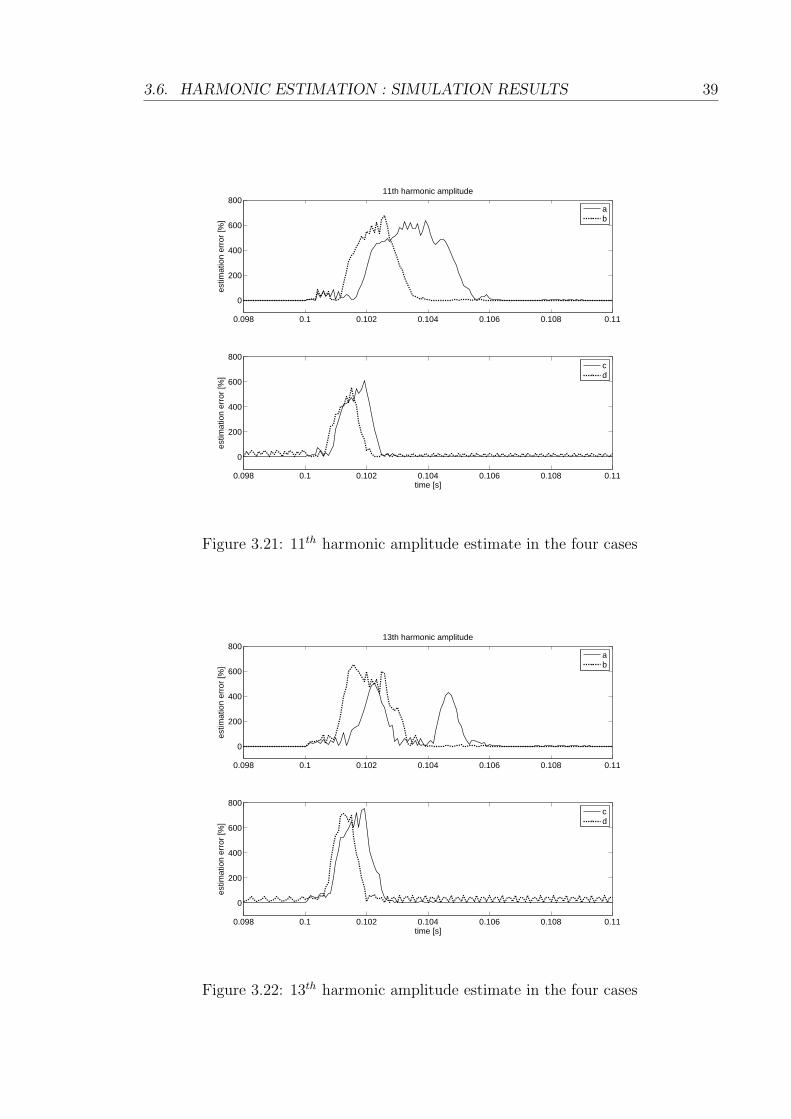
3.6. HARMONIC ESTIMATION : SIMULATION RESULTS 39
0.098 0.1 0.102 0.104 0.106 0.108 0.11
0
200
400
600
800
estim
atio
n er
ror [
%]
11th harmonic amplitude
0.098 0.1 0.102 0.104 0.106 0.108 0.11
0
200
400
600
800
time [s]
estim
atio
n er
ror [
%]
ab
cd
Figure 3.21: 11th harmonic amplitude estimate in the four cases
0.098 0.1 0.102 0.104 0.106 0.108 0.11
0
200
400
600
800
estim
atio
n er
ror [
%]
13th harmonic amplitude
0.098 0.1 0.102 0.104 0.106 0.108 0.11
0
200
400
600
800
time [s]
estim
atio
n er
ror [
%]
ab
cd
Figure 3.22: 13th harmonic amplitude estimate in the four cases
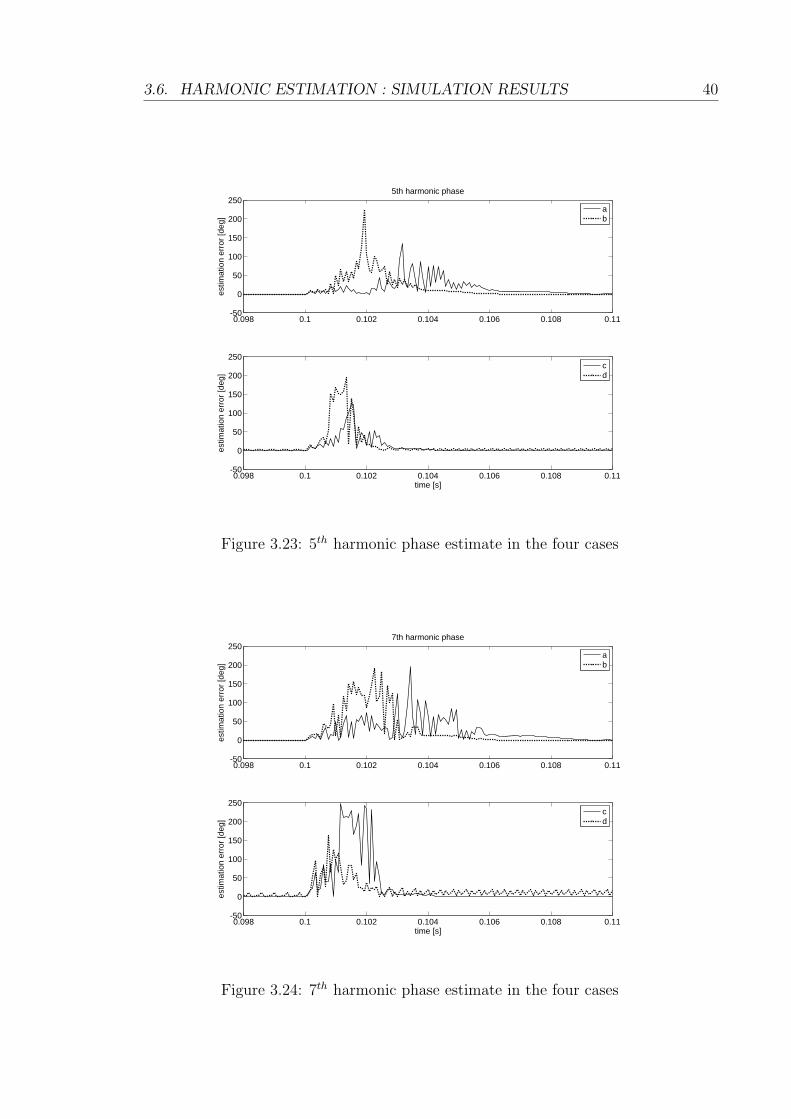
3.6. HARMONIC ESTIMATION : SIMULATION RESULTS 40
0.098 0.1 0.102 0.104 0.106 0.108 0.11-50
0
50
100
150
200
2505th harmonic phase
estim
atio
n er
ror [
deg]
0.098 0.1 0.102 0.104 0.106 0.108 0.11-50
0
50
100
150
200
250
time [s]
estim
atio
n er
ror [
deg]
ab
cd
Figure 3.23: 5th harmonic phase estimate in the four cases
0.098 0.1 0.102 0.104 0.106 0.108 0.11-50
0
50
100
150
200
2507th harmonic phase
estim
atio
n er
ror [
deg]
0.098 0.1 0.102 0.104 0.106 0.108 0.11-50
0
50
100
150
200
250
time [s]
estim
atio
n er
ror [
deg]
ab
cd
Figure 3.24: 7th harmonic phase estimate in the four cases
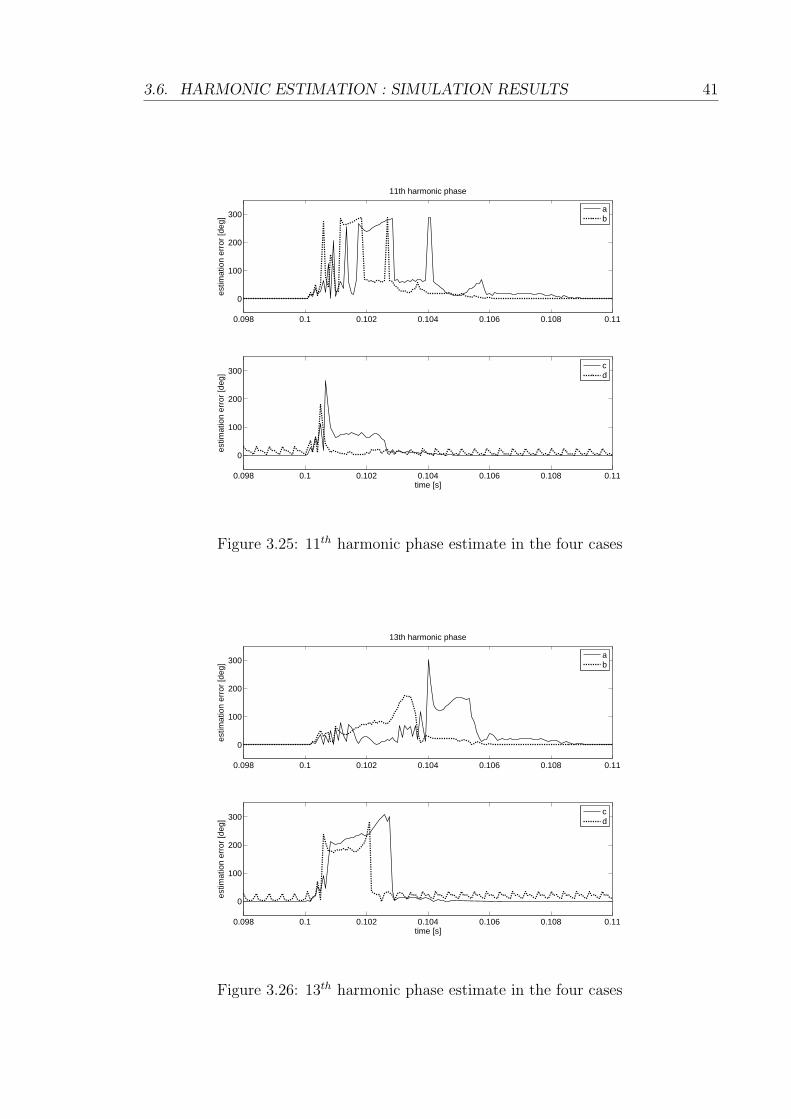
3.6. HARMONIC ESTIMATION : SIMULATION RESULTS 41
0.098 0.1 0.102 0.104 0.106 0.108 0.11
0
100
200
300
11th harmonic phase
estim
atio
n er
ror [
deg]
0.098 0.1 0.102 0.104 0.106 0.108 0.11
0
100
200
300
time [s]
estim
atio
n er
ror [
deg]
ab
cd
Figure 3.25: 11th harmonic phase estimate in the four cases
0.098 0.1 0.102 0.104 0.106 0.108 0.11
0
100
200
300
13th harmonic phase
estim
atio
n er
ror [
deg]
0.098 0.1 0.102 0.104 0.106 0.108 0.11
0
100
200
300
time [s]
estim
atio
n er
ror [
deg]
ab
cd
Figure 3.26: 13th harmonic phase estimate in the four cases
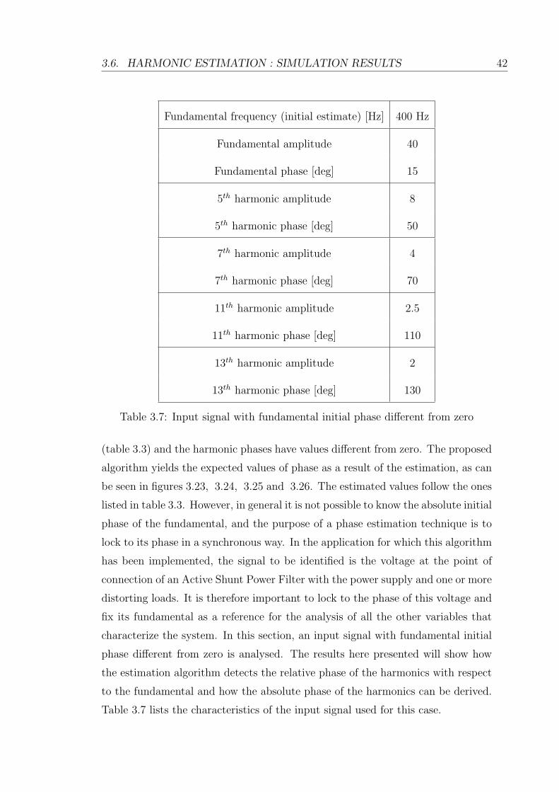
3.6. HARMONIC ESTIMATION : SIMULATION RESULTS 42
Fundamental frequency (initial estimate) [Hz] 400 Hz
Fundamental amplitude 40
Fundamental phase [deg] 15
5th harmonic amplitude 8
5th harmonic phase [deg] 50
7th harmonic amplitude 4
7th harmonic phase [deg] 70
11th harmonic amplitude 2.5
11th harmonic phase [deg] 110
13th harmonic amplitude 2
13th harmonic phase [deg] 130
Table 3.7: Input signal with fundamental initial phase different from zero
(table 3.3) and the harmonic phases have values different from zero. The proposed
algorithm yields the expected values of phase as a result of the estimation, as can
be seen in figures 3.23, 3.24, 3.25 and 3.26. The estimated values follow the ones
listed in table 3.3. However, in general it is not possible to know the absolute initial
phase of the fundamental, and the purpose of a phase estimation technique is to
lock to its phase in a synchronous way. In the application for which this algorithm
has been implemented, the signal to be identified is the voltage at the point of
connection of an Active Shunt Power Filter with the power supply and one or more
distorting loads. It is therefore important to lock to the phase of this voltage and
fix its fundamental as a reference for the analysis of all the other variables that
characterize the system. In this section, an input signal with fundamental initial
phase different from zero is analysed. The results here presented will show how
the estimation algorithm detects the relative phase of the harmonics with respect
to the fundamental and how the absolute phase of the harmonics can be derived.
Table 3.7 lists the characteristics of the input signal used for this case.

3.6. HARMONIC ESTIMATION : SIMULATION RESULTS 43
Considering that the fundamental initial phase in this case is 15 degrees, it is
expected that the harmonic phases estimated by the algorithm are not the same
as their absolute phases listed in the table. Figure 3.27 shows as an example the
fundamental and the 5th harmonic component of a signal, in the αβ plane. The
amplitude and initial absolute phase of the fundamental are indicated as A1 and
θ1 respectively. The amplitude and initial absolute phase of the 5th harmonic
are indicated as A5 and θ5 respectively. If the two vectors were rotating at the
same speed, the relative phase between the two of them would simply be the
difference between the absolute phases θ1 and θ5. However the two vectors are not
synchronous as the 5th harmonic rotates at 5 times the speed of the fundamental,
so their relative position in the αβ plane is defined by (3.8).
θm(rel) = ± · [θm(abs)−m · θ1(abs)] (3.8)
(3.8) takes into account the difference between the angular speed of the two
vectors. θm(abs) and θm(rel) are respectively the absolute initial phase of the mth
harmonic and its relative phase with respect to the fundamental. θ1(abs) is the
absolute initial phase of the fundamental. The + and - signs are used for positive
and negative sequence harmonics respectively.
A simulation has been carried out in the conditions of case (a). The fundamen-
tal frequency varies as a step from 400 Hz to 800 Hz, occurring at 0.1 s. The
fundamental initial phase is estimated as zero, regardless of its absolute value,
because the algorithm locks to it, transforming all the variables into a reference
frame synchronous with the fundamental. This is represented in figure 3.28. The
fundamental phase becomes the zero reference for all the harmonics; the values of
the estimated phase of the harmonics correspond with the values of the relative
phases obtained by means of formula (3.8). In this case the absolute phases are
the ones indicated in table 3.7. The relative phases, according to (3.8), are:
5th harmonic 25 degrees
7th harmonic -35 degrees

3.7. FREQUENCY ESTIMATION: EXPERIMENTAL RESULTS 44
1
15
1
15
Figure 3.27: Fundamental and 5th harmonic on the αβ plane
11th harmonic 55 degrees
13th harmonic -65 degrees
Figures 3.29 to 3.32 show the result of the estimation of the initial phase of the
harmonics. The absolute value of the estimation error is represented in these
figures.
3.7 Frequency estimation: experimental results
An experimental validation has been carried out for the frequency and harmonic
detection algorithm. The algorithm has been tested on a voltage signal generated
by a programmable power supply, the Chroma 61705 [47]. The algorithm was
implemented on the Texas Instruments TMS320C6713B 32 bit floating point Dig-
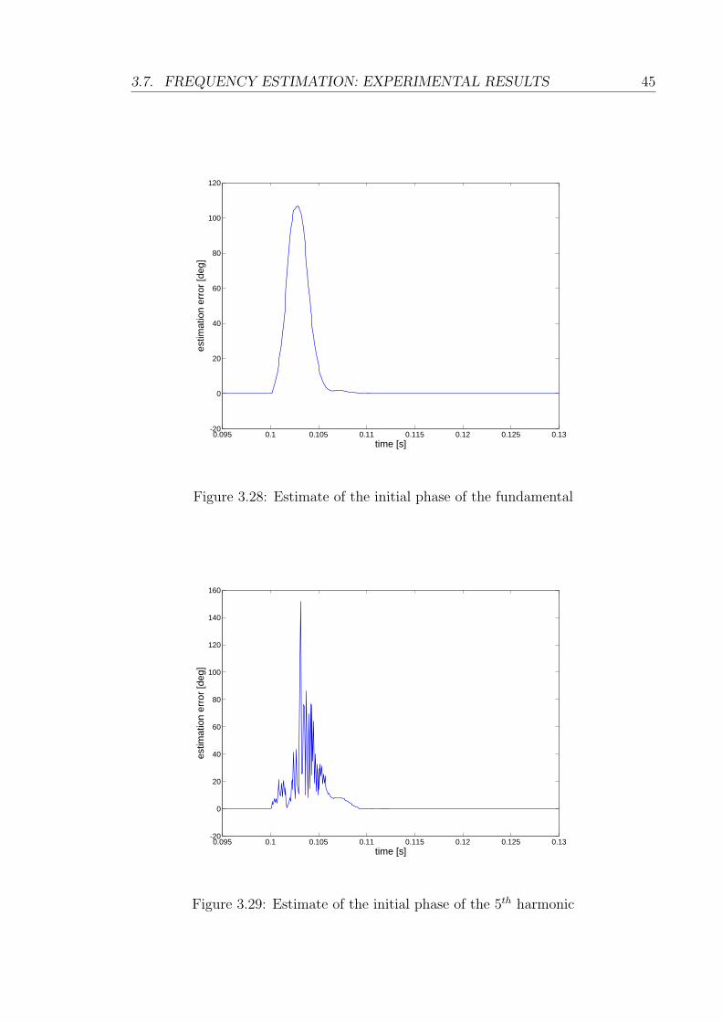
3.7. FREQUENCY ESTIMATION: EXPERIMENTAL RESULTS 45
0.095 0.1 0.105 0.11 0.115 0.12 0.125 0.13-20
0
20
40
60
80
100
120
time [s]
estim
atio
n er
ror [
deg]
Figure 3.28: Estimate of the initial phase of the fundamental
0.095 0.1 0.105 0.11 0.115 0.12 0.125 0.13-20
0
20
40
60
80
100
120
140
160
time [s]
estim
atio
n er
ror [
deg]
Figure 3.29: Estimate of the initial phase of the 5th harmonic

3.7. FREQUENCY ESTIMATION: EXPERIMENTAL RESULTS 46
0.095 0.1 0.105 0.11 0.115 0.12 0.125 0.13-20
0
20
40
60
80
100
120
140
160
180
200
time [s]
estim
atio
n er
ror [
deg]
Figure 3.30: Estimate of the initial phase of the 7th harmonic
0.095 0.1 0.105 0.11 0.115 0.12 0.125 0.13
0
50
100
150
200
250
time [s]
estim
atio
n er
ror [
deg]
Figure 3.31: Estimate of the initial phase of the 11th harmonic

3.7. FREQUENCY ESTIMATION: EXPERIMENTAL RESULTS 47
0.095 0.1 0.105 0.11 0.115 0.12 0.125 0.13
0
50
100
150
200
250
time [s]
estim
atio
n er
ror [
deg]
Figure 3.32: Estimate of the initial phase of the 13th harmonic
ital Signal Processor (DSP) [48]. The data acquisition was carried out by means
of a Field Programmable Gate Array (FPGA) board, Actel ProAsic A500K050
Package PQ208 [49], with 12 bit Analog to Digital Converters LTC 1400 [50].
The voltage measurement was carried out by means of LEM LV 25-P voltage
transducers [51].
In this section the experimental results for the frequency and fundamental phase
estimation are shown. In the next section the experimental results for the harmonic
estimation are reported.
The characteristics of the input signal voltage processed by the algorithm are listed
in table 3.8. The voltage generated by the power supply is line-to-line voltage.
The table lists the characteristics of the line-to-line voltage Vab on the left hand
side, and the characteristics of the phase-to-neutral voltage Van. The latter is
derived from the former by dividing the amplitude of each component by√
3 and
by adding ±30 degrees to the phase of each component, depending whether the
component is a negative or positive sequence. The table indicates the absolute

3.7. FREQUENCY ESTIMATION: EXPERIMENTAL RESULTS 48
Vab Van
Fund. freq. [Hz] 400 Hz Fund. freq. [Hz] 400 Hz
Fund. ampl. [V] 65.2 Fund. ampl. [V] 37.6432
Fund. phase [deg] 13.6 Fund. phase [deg] -16.4; 0 (rel)
5th harm. amplitude [V] 10 5th harm. ampl. [V] 5.7735
5th harm. phase [deg] -49.5 5th harm. phase [deg] -19.5; -62.5 (rel)
7th harm. ampl. [V] 6.9 7th harm. ampl. [V] 3.9837
7th harm. phase [deg] 9 7th harm. phase [deg] -21; -266.2 (rel)
11th harm. ampl. [V] 4.3 11th harm. ampl. [V] 2.4826
11th harm. phase [deg] -36.7 11th harm. phase [deg] -6.7; -173.7 (rel)
13th harm. ampl. [V] 2.6 13th harm. ampl. [V] 1.5011
13th harm. phase [deg] 10.5 13th harm. phase [deg] -19.5; -166.3 (rel)
Table 3.8: Input signal for experimental validation
phase of each component and, for Van, also the relative phase with respect to the
fundamental, according to (3.8).
Figure 3.33 shows the input signal in the time domain. Figures 3.34 and 3.35 show
the FFT spectrum of the signal.
The characteristic parameters of the algorithm have been chosen with the values
reported in table 3.9. The sampling frequency chosen for the experimental imple-
mentation is 8 kHz, because of the computational limitations of the DSP. It should
be noted that the 13th harmonic frequency occurs above the Nyquist frequency.
The PI controller gains have been chosen by trial and error, in order to obtain the
same dynamic response between each case in table 3.9 and its correspondent case
in table 3.4.
Figure 3.36 shows the response of the frequency estimation to a step change of
frequency from 400 Hz to 800 Hz. All the cases from (a) to (d) are represented
in the figure. The characteristics of the steady-state and dynamic response in the
four cases are reported in table 3.10. The slowest response is observed in case (a)
as a buffer containing an entire period of the fundamental is analysed.
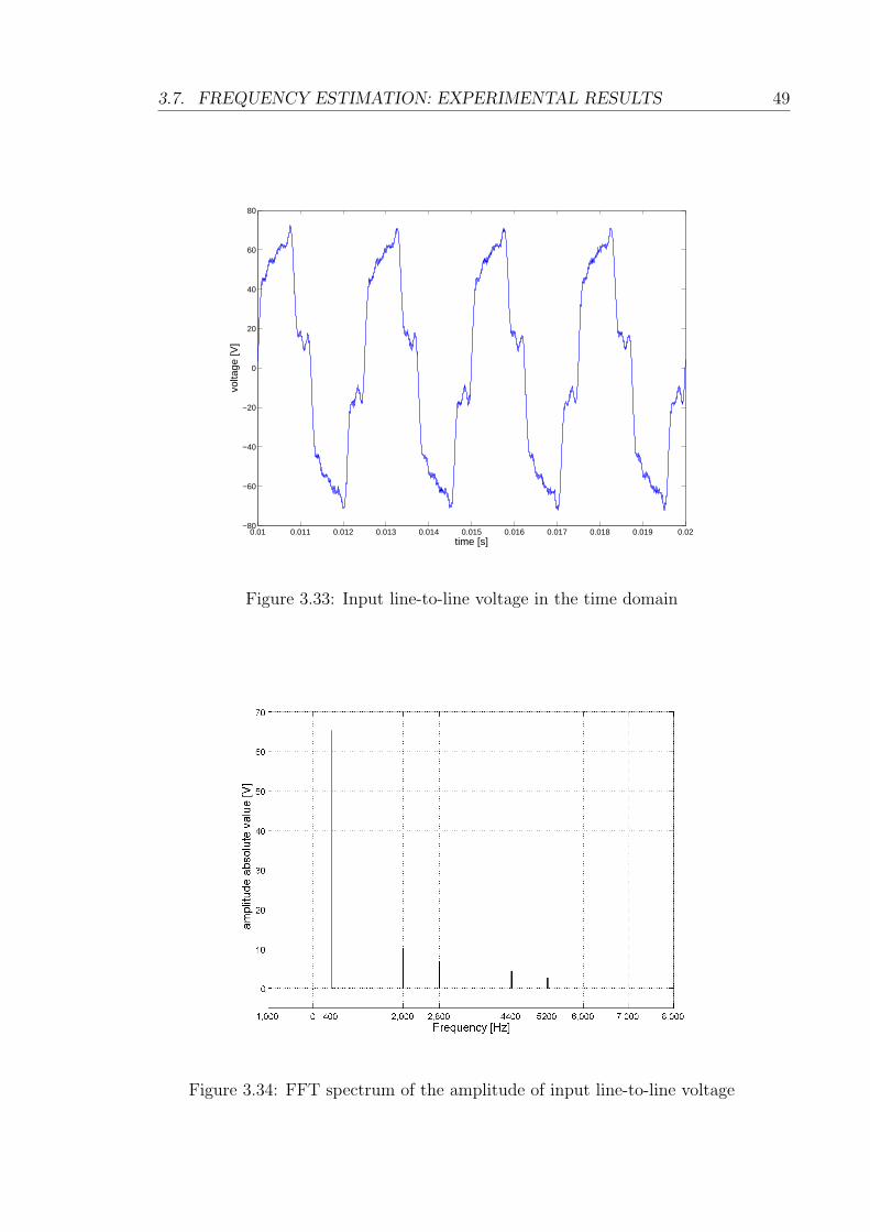
3.7. FREQUENCY ESTIMATION: EXPERIMENTAL RESULTS 49
0.01 0.011 0.012 0.013 0.014 0.015 0.016 0.017 0.018 0.019 0.02−80
−60
−40
−20
0
20
40
60
80
time [s]
volta
ge [V
]
Figure 3.33: Input line-to-line voltage in the time domain
Figure 3.34: FFT spectrum of the amplitude of input line-to-line voltage
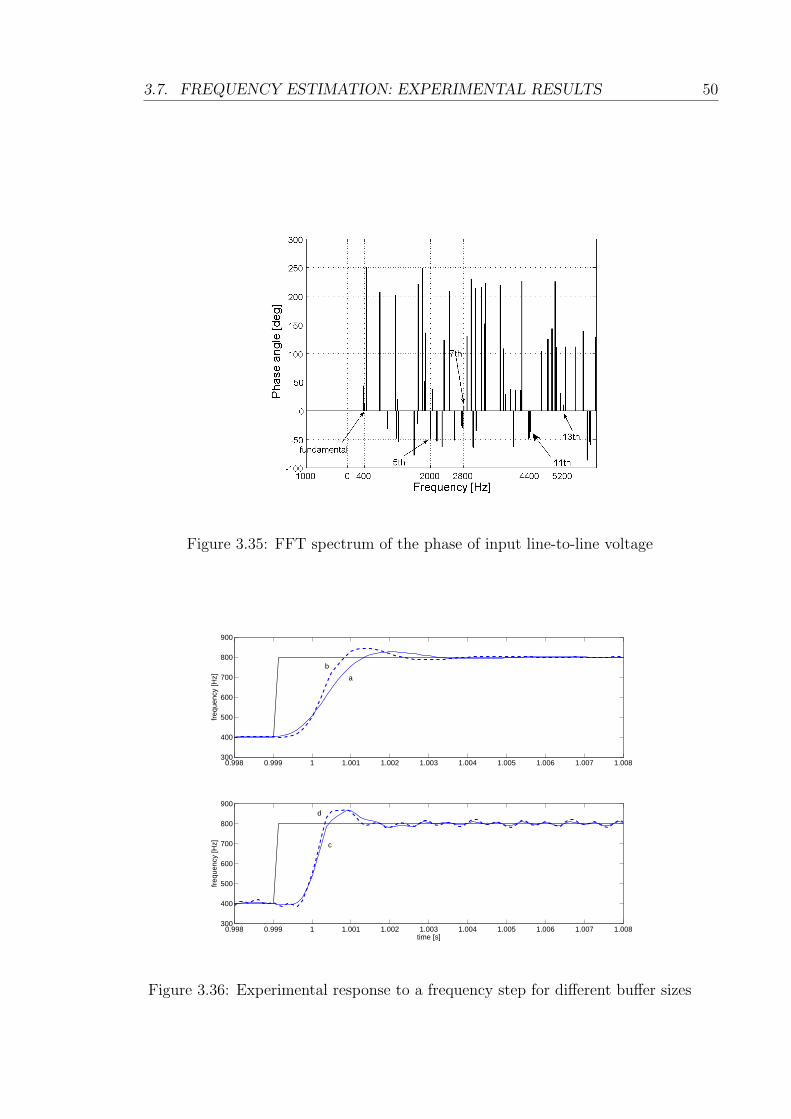
3.7. FREQUENCY ESTIMATION: EXPERIMENTAL RESULTS 50
Figure 3.35: FFT spectrum of the phase of input line-to-line voltage
0.998 0.999 1 1.001 1.002 1.003 1.004 1.005 1.006 1.007 1.008300
400
500
600
700
800
900
freq
uenc
y [H
z]
0.998 0.999 1 1.001 1.002 1.003 1.004 1.005 1.006 1.007 1.008300
400
500
600
700
800
900
time [s]
freq
uenc
y [H
z]
a
c
d
b
Figure 3.36: Experimental response to a frequency step for different buffer sizes

3.7. FREQUENCY ESTIMATION: EXPERIMENTAL RESULTS 51
Sampling frequency [Hz] 8 kHz
Observation interval Tobs
Case (a) T
Case (b) 33T
Case (c) 12T
Case (d) 25T
Buffer length n
Case (a) 20
Case (b) 15
Case (c) 10
Case (d) 8
Frequency PI controller s domain
Case (a) kp = 0.4; ki = 640
Case (b) kp = 0.4; ki = 820
Case (c) kp = 0.4; ki = 1230
Case (d) kp = 0.4; ki = 1550
Table 3.9: Frequency detection algorithm parameters for the experimental imple-mentation
case (a) case (b) case (c) case (c)Maximum overshoot [%] 6.5 11.25 16.7 17.1
Delay time [s] 0.0004 0.0002 0.0001 0.0001Rise time [s] 0.0014 0.0008 0.0005 0.0005
Settling time 5% [s] 0.0025 0.002 0.0014 0.0012Peak time [s] 0.002 0.0014 0.001 0.0009
Steady-state oscillation max amplitude(% of the steady-state value) 0.25 0.5 2.5 5
Steady-state error [Hz] 0.0347 0.0308 0.0244 0.0095
Table 3.10: Transient and steady-state performance of the frequency step estima-tion
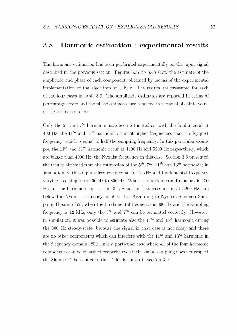
3.8. HARMONIC ESTIMATION : EXPERIMENTAL RESULTS 52
3.8 Harmonic estimation : experimental results
The harmonic estimation has been performed experimentally on the input signal
described in the previous section. Figures 3.37 to 3.48 show the estimate of the
amplitude and phase of each component, obtained by means of the experimental
implementation of the algorithm at 8 kHz. The results are presented for each
of the four cases in table 3.9. The amplitude estimates are reported in terms of
percentage errors and the phase estimates are reported in terms of absolute value
of the estimation error.
Only the 5th and 7th harmonic have been estimated as, with the fundamental at
400 Hz, the 11th and 13th harmonic occur at higher frequencies than the Nyquist
frequency, which is equal to half the sampling frequency. In this particular exam-
ple, the 11th and 13th harmonic occur at 4400 Hz and 5200 Hz respectively, which
are bigger than 4000 Hz, the Nyquist frequency in this case. Section 3.6 presented
the results obtained from the estimation of the 5th, 7th, 11th and 13th harmonics in
simulation, with sampling frequency equal to 12 kHz and fundamental frequency
varying as a step from 400 Hz to 800 Hz. When the fundamental frequency is 400
Hz, all the harmonics up to the 13th, which in that case occurs at 5200 Hz, are
below the Nyquist frequency at 6000 Hz. According to Nyquist-Shannon Sam-
pling Theorem [52], when the fundamental frequency is 800 Hz and the sampling
frequency is 12 kHz, only the 5th and 7th can be estimated correctly. However,
in simulation, it was possible to estimate also the 11th and 13th harmonic during
the 800 Hz steady-state, because the signal in that case is not noisy and there
are no other components which can interfere with the 11th and 13th harmonic in
the frequency domain. 800 Hz is a particular case where all of the four harmonic
components can be identified properly, even if the signal sampling does not respect
the Shannon Theorem condition. This is shown in section 3.9.
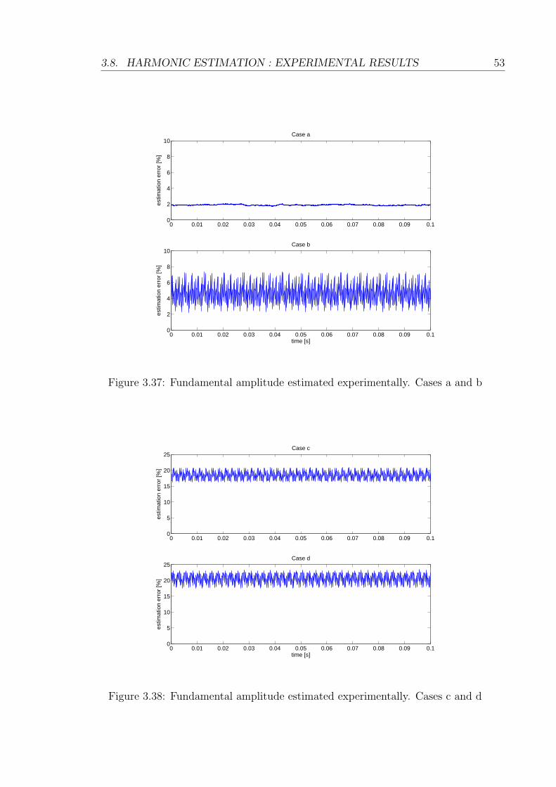
3.8. HARMONIC ESTIMATION : EXPERIMENTAL RESULTS 53
0 0.01 0.02 0.03 0.04 0.05 0.06 0.07 0.08 0.09 0.10
2
4
6
8
10
estim
atio
n er
ror [
%]
Case a
0 0.01 0.02 0.03 0.04 0.05 0.06 0.07 0.08 0.09 0.10
2
4
6
8
10
time [s]
estim
atio
n er
ror [
%]
Case b
Figure 3.37: Fundamental amplitude estimated experimentally. Cases a and b
0 0.01 0.02 0.03 0.04 0.05 0.06 0.07 0.08 0.09 0.10
5
10
15
20
25
estim
atio
n er
ror [
%]
Case c
0 0.01 0.02 0.03 0.04 0.05 0.06 0.07 0.08 0.09 0.10
5
10
15
20
25
time [s]
estim
atio
n er
ror [
%]
Case d
Figure 3.38: Fundamental amplitude estimated experimentally. Cases c and d

3.8. HARMONIC ESTIMATION : EXPERIMENTAL RESULTS 54
0 0.01 0.02 0.03 0.04 0.05 0.06 0.07 0.08 0.09 0.1-10
0
10
20
30
40
estim
atio
n er
ror [
%]
Case a
0 0.01 0.02 0.03 0.04 0.05 0.06 0.07 0.08 0.09 0.1-10
0
10
20
30
40
time [s]
estim
atio
n er
ror [
%]
Case b
Figure 3.39: 5th harmonic amplitude estimated experimentally. Cases a and b
0 0.005 0.01 0.015 0.02 0.025 0.03 0.035 0.04 0.045 0.050
50
100
150
estim
atio
n er
ror [
%]
Case c
0 0.005 0.01 0.015 0.02 0.025 0.03 0.035 0.04 0.045 0.050
50
100
150
time [s]
estim
atio
n er
ror [
%]
Case d
Figure 3.40: 5th harmonic amplitude estimated experimentally. Cases c and d

3.8. HARMONIC ESTIMATION : EXPERIMENTAL RESULTS 55
0 0.01 0.02 0.03 0.04 0.05 0.06 0.07 0.08 0.09 0.1
0
20
40
60
80
100
estim
atio
n er
ror [
%]
Case a
0 0.01 0.02 0.03 0.04 0.05 0.06 0.07 0.08 0.09 0.1
0
20
40
60
80
100
time [s]
estim
atio
n er
ror [
%]
Case b
Figure 3.41: 7th harmonic amplitude estimated experimentally. Cases a and b
0 0.005 0.01 0.015 0.02 0.025 0.03 0.035 0.04 0.045 0.05-50
0
50
100
150
200
250
300
estim
atio
n er
ror [
%]
Case c
0 0.005 0.01 0.015 0.02 0.025 0.03 0.035 0.04 0.045 0.05-50
0
50
100
150
200
250
300
time [s]
estim
atio
n er
ror [
%]
Case d
Figure 3.42: 7th harmonic amplitude estimated experimentally. Cases c and d

3.8. HARMONIC ESTIMATION : EXPERIMENTAL RESULTS 56
0 0.01 0.02 0.03 0.04 0.05 0.06 0.07 0.08 0.09 0.1-5
0
5
10Case a
estim
atio
n er
ror [
deg]
0 0.01 0.02 0.03 0.04 0.05 0.06 0.07 0.08 0.09 0.1-5
0
5
10
time [s]
estim
atio
n er
ror [
deg]
Case b
Figure 3.43: Fundamental phase estimated experimentally. Cases a and b
0 0.01 0.02 0.03 0.04 0.05 0.06 0.07 0.08 0.09 0.1-5
0
5
10
15Case c
estim
atio
n er
ror [
deg]
0 0.01 0.02 0.03 0.04 0.05 0.06 0.07 0.08 0.09 0.1-5
0
5
10
15
time [s]
estim
atio
n er
ror [
deg]
Case d
Figure 3.44: Fundamental phase estimated experimentally. Cases c and d

3.8. HARMONIC ESTIMATION : EXPERIMENTAL RESULTS 57
0 0.01 0.02 0.03 0.04 0.05 0.06 0.07 0.08 0.09 0.1-5
0
5
10
15
20
25Case a
estim
atio
n er
ror [
deg]
0 0.01 0.02 0.03 0.04 0.05 0.06 0.07 0.08 0.09 0.1-5
0
5
10
15
20
25
time [s]
estim
atio
n er
ror [
deg]
Case b
Figure 3.45: 5th harmonic phase estimated experimentally. Cases a and b
0 0.005 0.01 0.015 0.02 0.025 0.03 0.035 0.04 0.045 0.050
50
100
150
200
250
300Case c
estim
atio
n er
ror [
deg]
0 0.005 0.01 0.015 0.02 0.025 0.03 0.035 0.04 0.045 0.050
50
100
150
200
250
300
time [s]
estim
atio
n er
ror [
deg]
Case d
Figure 3.46: 5th harmonic phase estimated experimentally. Cases c and d
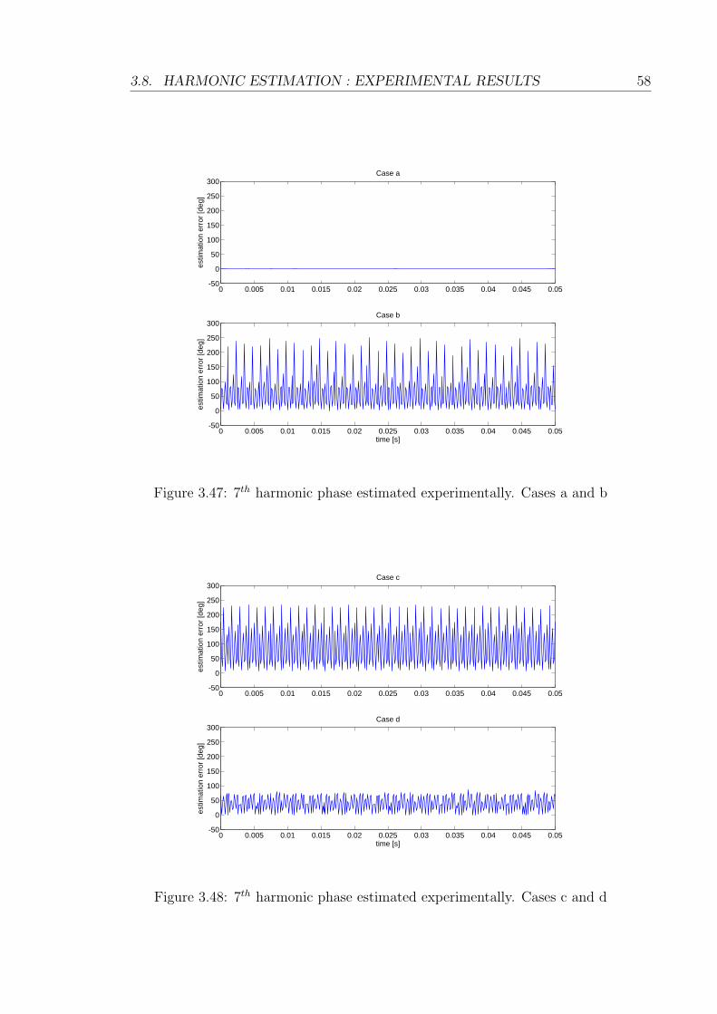
3.8. HARMONIC ESTIMATION : EXPERIMENTAL RESULTS 58
0 0.005 0.01 0.015 0.02 0.025 0.03 0.035 0.04 0.045 0.05-50
0
50
100
150
200
250
300Case a
estim
atio
n er
ror [
deg]
0 0.005 0.01 0.015 0.02 0.025 0.03 0.035 0.04 0.045 0.05-50
0
50
100
150
200
250
300
time [s]
estim
atio
n er
ror [
deg]
Case b
Figure 3.47: 7th harmonic phase estimated experimentally. Cases a and b
0 0.005 0.01 0.015 0.02 0.025 0.03 0.035 0.04 0.045 0.05-50
0
50
100
150
200
250
300Case c
estim
atio
n er
ror [
deg]
0 0.005 0.01 0.015 0.02 0.025 0.03 0.035 0.04 0.045 0.05-50
0
50
100
150
200
250
300
time [s]
estim
atio
n er
ror [
deg]
Case d
Figure 3.48: 7th harmonic phase estimated experimentally. Cases c and d
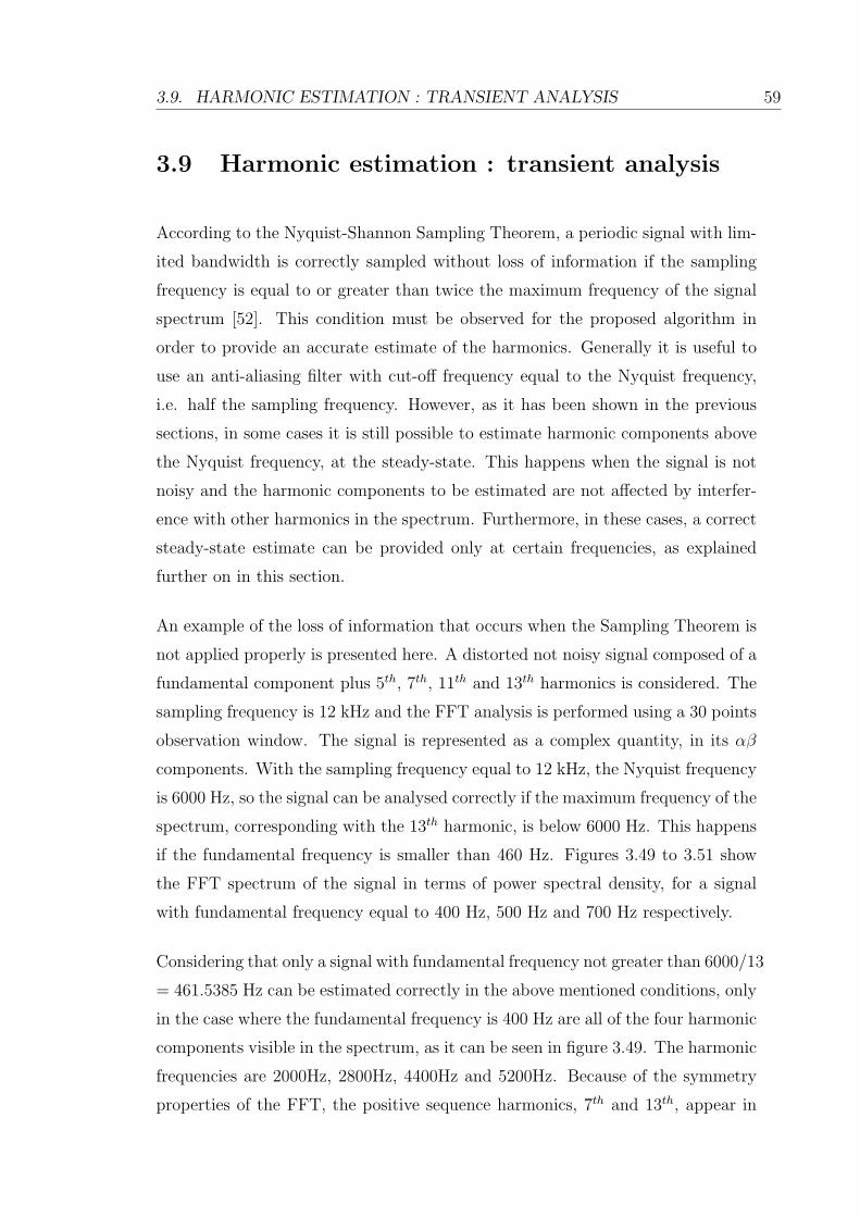
3.9. HARMONIC ESTIMATION : TRANSIENT ANALYSIS 59
3.9 Harmonic estimation : transient analysis
According to the Nyquist-Shannon Sampling Theorem, a periodic signal with lim-
ited bandwidth is correctly sampled without loss of information if the sampling
frequency is equal to or greater than twice the maximum frequency of the signal
spectrum [52]. This condition must be observed for the proposed algorithm in
order to provide an accurate estimate of the harmonics. Generally it is useful to
use an anti-aliasing filter with cut-off frequency equal to the Nyquist frequency,
i.e. half the sampling frequency. However, as it has been shown in the previous
sections, in some cases it is still possible to estimate harmonic components above
the Nyquist frequency, at the steady-state. This happens when the signal is not
noisy and the harmonic components to be estimated are not affected by interfer-
ence with other harmonics in the spectrum. Furthermore, in these cases, a correct
steady-state estimate can be provided only at certain frequencies, as explained
further on in this section.
An example of the loss of information that occurs when the Sampling Theorem is
not applied properly is presented here. A distorted not noisy signal composed of a
fundamental component plus 5th, 7th, 11th and 13th harmonics is considered. The
sampling frequency is 12 kHz and the FFT analysis is performed using a 30 points
observation window. The signal is represented as a complex quantity, in its αβ
components. With the sampling frequency equal to 12 kHz, the Nyquist frequency
is 6000 Hz, so the signal can be analysed correctly if the maximum frequency of the
spectrum, corresponding with the 13th harmonic, is below 6000 Hz. This happens
if the fundamental frequency is smaller than 460 Hz. Figures 3.49 to 3.51 show
the FFT spectrum of the signal in terms of power spectral density, for a signal
with fundamental frequency equal to 400 Hz, 500 Hz and 700 Hz respectively.
Considering that only a signal with fundamental frequency not greater than 6000/13
= 461.5385 Hz can be estimated correctly in the above mentioned conditions, only
in the case where the fundamental frequency is 400 Hz are all of the four harmonic
components visible in the spectrum, as it can be seen in figure 3.49. The harmonic
frequencies are 2000Hz, 2800Hz, 4400Hz and 5200Hz. Because of the symmetry
properties of the FFT, the positive sequence harmonics, 7th and 13th, appear in

3.9. HARMONIC ESTIMATION : TRANSIENT ANALYSIS 60
0 2 4 6 8 102.8 7.65.20.4−120
−110
−100
−90
−80
−70
−60
−50
−40
−30
−20
Frequency [kHz]
Pow
er/fr
eque
ncy
[dB
/Hz]
Periodogram Power Spectral Density Estimate
fundamental
7th harmonic
13th harmonic11th harmonic
5th harmonic
Figure 3.49: FFT spectrum with fundamental frequency 400 Hz
0 2 4 6 8 100.5 9.53.5 6.5−100
−90
−80
−70
−60
−50
−40
−30
−20
Frequency [Hz]
Pow
er/fr
eque
ncy
[dB
/Hz]
Periodogram Power Spectral Density Estimate
fundamental
7th harmonic
11th and 13th harmonic
5th harmonic
Figure 3.50: FFT spectrum with fundamental frequency 500 Hz

3.9. HARMONIC ESTIMATION : TRANSIENT ANALYSIS 61
0 2 4 6 8 100.7 8.54.9−110
−100
−90
−80
−70
−60
−50
−40
−30
−20
Frequency [Hz]
Pow
er/fr
eque
ncy
[dB
/Hz]
Periodogram Power Spectral Density Estimate
fundamental
5th harmonic
7th harmonic
Figure 3.51: FFT spectrum with fundamental frequency 700 Hz
the left hand side of the spectrum, the negative sequence harmonics, 5th and 11th
appear in the right hand side of the spectrum, at frequencies equal to 12000-2000
= 10000 Hz and 12000-4400 = 7600 Hz, as indicated in the figure.
For a signal with fundamental frequency equal to 500 Hz, not all of the four
harmonic components are visible in the spectrum. The harmonic frequencies are
2500Hz, 3500Hz, 5500Hz and 6500Hz. The 7th and 13th harmonic appear at 3500
and 6500 Hz, the 5th and 11th harmonic appear at 12000-2500 = 9500 Hz and
12000-5500 = 6500 Hz. The 13th harmonic overlaps to the 11th harmonic in the
spectrum so it is not identified properly.
For a signal with fundamental frequency equal to 700 Hz, the harmonic frequencies
are 3500Hz, 4900Hz, 7700Hz and 9100Hz. As shown in the figure, the 11th and
13th harmonic are not identified in the spectrum.
Figure 3.52 shows the FFT spectrum in terms of power spectral density, for a
signal with fundamental frequency equal to 800 Hz. 800 Hz is a particular case

3.9. HARMONIC ESTIMATION : TRANSIENT ANALYSIS 62
where all of the four harmonic components are visible because of their position in
the spectrum, although the Shannon Theorem condition is not respected.
0 2 4 80.8 5.6 10.4−100
−90
−80
−70
−60
−50
−40
−30
−20
Frequency [Hz]
Pow
er/fr
eque
ncy
[dB
/Hz]
Periodogram Power Spectral Density Estimate
fundamental
7th harmonic
5th harmonic
13th harmonic
11th harmonic
Figure 3.52: FFT spectrum with fundamental frequency 800 Hz
The performance of the proposed real-time DFT algorithm for harmonic estima-
tion has been evaluated in simulation in order to show its behaviour in cases where
the Shannon Theorem condition is valid and cases where it is not. Assuming that
the sampling frequency is 12 kHz the maximum value of fundamental frequency
such that the 5th, 7th, 11th and 13th harmonic can all be correctly estimated is
461.5385 Hz. Figures 3.53 to 3.59 show the estimates of the harmonic amplitudes
and phases for a signal with harmonic distortion like in table 3.3, with fundamen-
tal frequency varying as a step from 200 Hz to 400 Hz, which are values below the
maximum value for the validity of the Shannon Theorem condition. Figures 3.54
to 3.60 show the estimates of the harmonic amplitudes and phases for a signal with
fundamental frequency varying as a step from 500 Hz to 700 Hz, which are values
above the maximum value for the validity of the Shannon Theorem condition. For
each of the two cases a buffer with size equal to one period of the fundamental at
the minimum frequency in the step has been chosen. With the sampling frequency

3.9. HARMONIC ESTIMATION : TRANSIENT ANALYSIS 63
equal to 12 kHz, for the 200-400 Hz step, the buffer size is 60 points; for the 500-
700 Hz step it is equal to 24 points. From these figures it can be noticed that the
steady-state accuracy of the estimate provided by the algorithm when the 200-400
Hz frequency step is applied is higher than in the case of a frequency step from
500 to 700 Hz. The transient response depends on the gains of the PI controller
chosen for the frequency estimation, which in this case have not been tuned in
order to yield a similar transient response for both cases, as the analysis in this
section focuses only the steady-state performance of the harmonic estimation for
different values of fundamental frequency.
0.1 0.15 0.2 0.25 0.3 0.35 0.4 0.45 0.5
0
20
40
60
80
100
erro
r [%
]
step 200-400Hz
0.1 0.15 0.2 0.25 0.3 0.35 0.4 0.45 0.5-50
0
50
100
150
200
250
time [s]
erro
r [de
g]
Figure 3.53: 5th harmonic
In order for the algorithm to be able to estimate all the harmonic components
correctly, given a certain fundamental frequency, the sampling frequency should
be increased. The limitation on the sampling frequency depends on the com-
putational burden of the algorithm and the computational power of the digital
processor. Given a sampling frequency of 8 kHz, the Nyquist frequency is 4 kHz,
so the maximum fundamental frequency at which the algorithm is able to estimate
all the harmonics up to the 13th is 4000/13 = 307.6923 Hz.
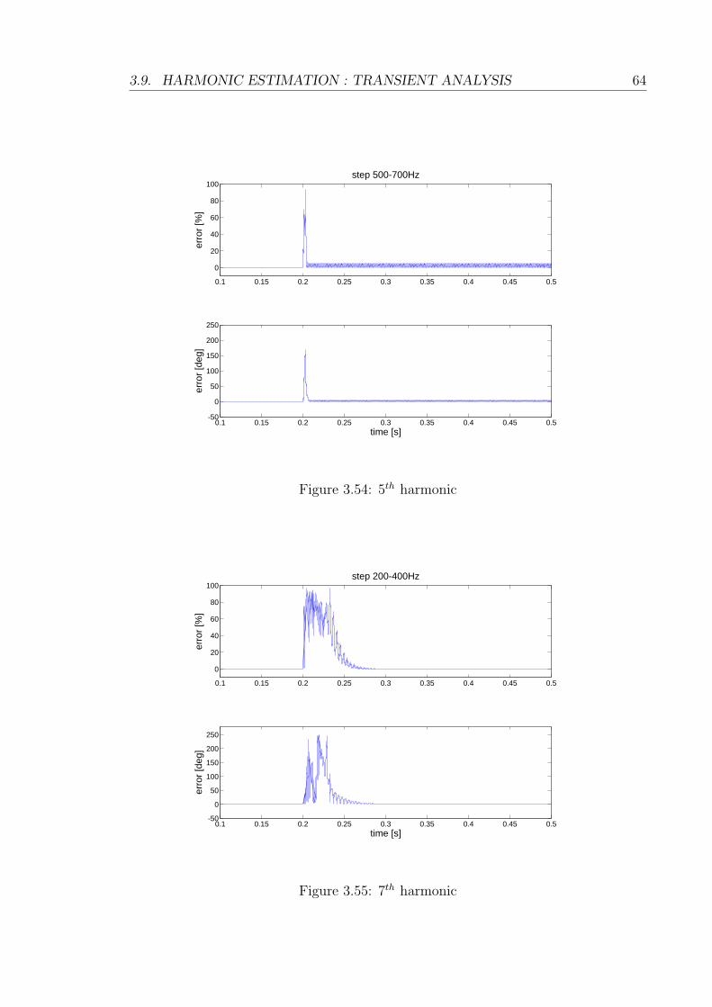
3.9. HARMONIC ESTIMATION : TRANSIENT ANALYSIS 64
0.1 0.15 0.2 0.25 0.3 0.35 0.4 0.45 0.5
0
20
40
60
80
100
erro
r [%
]
step 500-700Hz
0.1 0.15 0.2 0.25 0.3 0.35 0.4 0.45 0.5-50
0
50
100
150
200
250
time [s]
erro
r [de
g]
Figure 3.54: 5th harmonic
0.1 0.15 0.2 0.25 0.3 0.35 0.4 0.45 0.5
0
20
40
60
80
100
erro
r [%
]
step 200-400Hz
0.1 0.15 0.2 0.25 0.3 0.35 0.4 0.45 0.5-50
0
50
100
150
200
250
time [s]
erro
r [de
g]
Figure 3.55: 7th harmonic
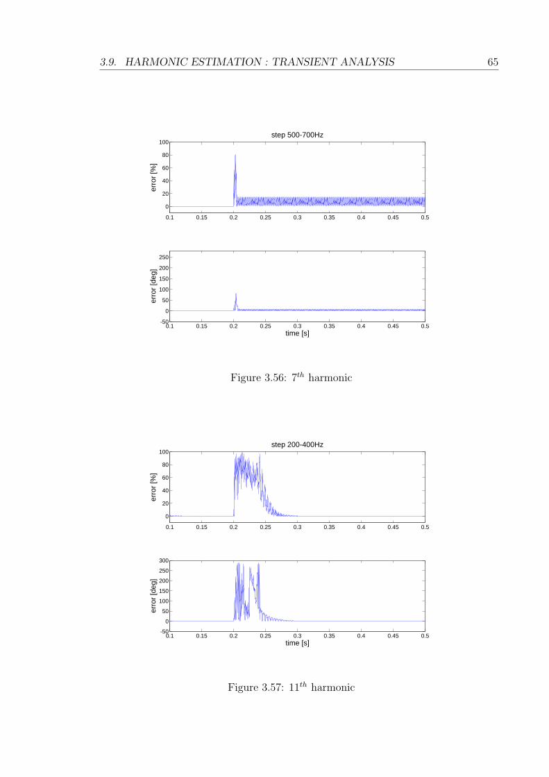
3.9. HARMONIC ESTIMATION : TRANSIENT ANALYSIS 65
0.1 0.15 0.2 0.25 0.3 0.35 0.4 0.45 0.5
0
20
40
60
80
100
erro
r [%
]
step 500-700Hz
0.1 0.15 0.2 0.25 0.3 0.35 0.4 0.45 0.5-50
0
50
100
150
200
250
time [s]
erro
r [de
g]
Figure 3.56: 7th harmonic
0.1 0.15 0.2 0.25 0.3 0.35 0.4 0.45 0.5
0
20
40
60
80
100
erro
r [%
]
step 200-400Hz
0.1 0.15 0.2 0.25 0.3 0.35 0.4 0.45 0.5-50
0
50
100
150
200
250
300
time [s]
erro
r [de
g]
Figure 3.57: 11th harmonic
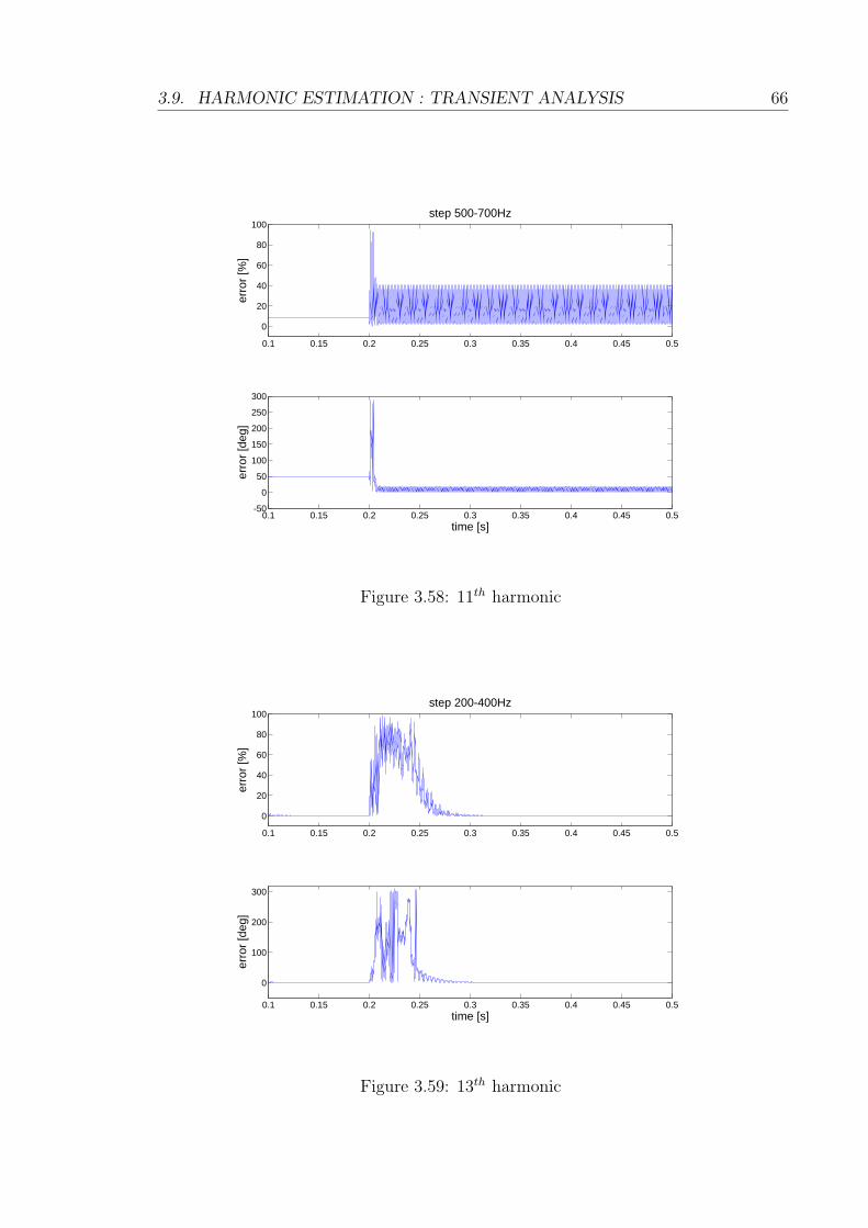
3.9. HARMONIC ESTIMATION : TRANSIENT ANALYSIS 66
0.1 0.15 0.2 0.25 0.3 0.35 0.4 0.45 0.5
0
20
40
60
80
100
erro
r [%
]
step 500-700Hz
0.1 0.15 0.2 0.25 0.3 0.35 0.4 0.45 0.5-50
0
50
100
150
200
250
300
time [s]
erro
r [de
g]
Figure 3.58: 11th harmonic
0.1 0.15 0.2 0.25 0.3 0.35 0.4 0.45 0.5
0
20
40
60
80
100
erro
r [%
]
step 200-400Hz
0.1 0.15 0.2 0.25 0.3 0.35 0.4 0.45 0.5
0
100
200
300
time [s]
erro
r [de
g]
Figure 3.59: 13th harmonic
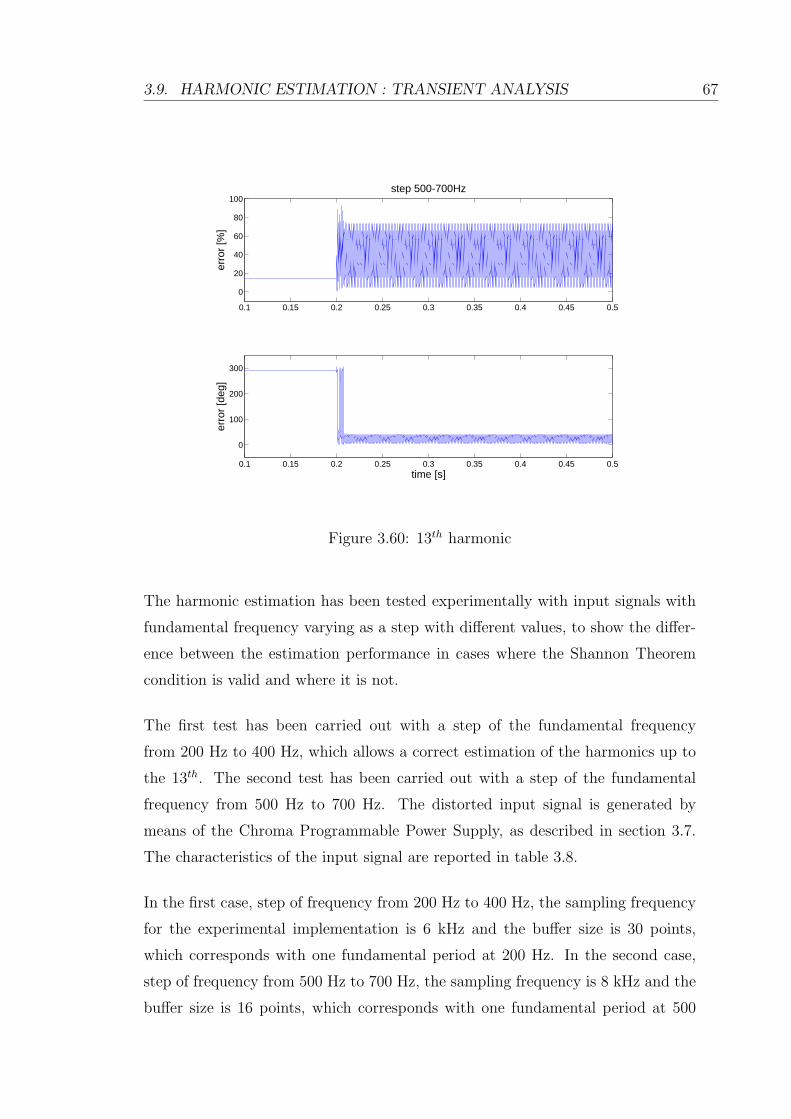
3.9. HARMONIC ESTIMATION : TRANSIENT ANALYSIS 67
0.1 0.15 0.2 0.25 0.3 0.35 0.4 0.45 0.5
0
20
40
60
80
100
erro
r [%
]
step 500-700Hz
0.1 0.15 0.2 0.25 0.3 0.35 0.4 0.45 0.5
0
100
200
300
time [s]
erro
r [de
g]
Figure 3.60: 13th harmonic
The harmonic estimation has been tested experimentally with input signals with
fundamental frequency varying as a step with different values, to show the differ-
ence between the estimation performance in cases where the Shannon Theorem
condition is valid and where it is not.
The first test has been carried out with a step of the fundamental frequency
from 200 Hz to 400 Hz, which allows a correct estimation of the harmonics up to
the 13th. The second test has been carried out with a step of the fundamental
frequency from 500 Hz to 700 Hz. The distorted input signal is generated by
means of the Chroma Programmable Power Supply, as described in section 3.7.
The characteristics of the input signal are reported in table 3.8.
In the first case, step of frequency from 200 Hz to 400 Hz, the sampling frequency
for the experimental implementation is 6 kHz and the buffer size is 30 points,
which corresponds with one fundamental period at 200 Hz. In the second case,
step of frequency from 500 Hz to 700 Hz, the sampling frequency is 8 kHz and the
buffer size is 16 points, which corresponds with one fundamental period at 500
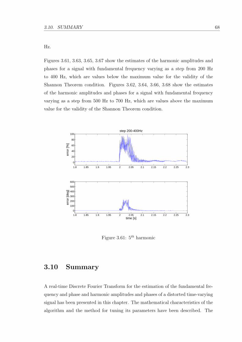
3.10. SUMMARY 68
Hz.
Figures 3.61, 3.63, 3.65, 3.67 show the estimates of the harmonic amplitudes and
phases for a signal with fundamental frequency varying as a step from 200 Hz
to 400 Hz, which are values below the maximum value for the validity of the
Shannon Theorem condition. Figures 3.62, 3.64, 3.66, 3.68 show the estimates
of the harmonic amplitudes and phases for a signal with fundamental frequency
varying as a step from 500 Hz to 700 Hz, which are values above the maximum
value for the validity of the Shannon Theorem condition.
1.8 1.85 1.9 1.95 2 2.05 2.1 2.15 2.2 2.25 2.3
0
20
40
60
80
100
erro
r [%
]
step 200-400Hz
1.8 1.85 1.9 1.95 2 2.05 2.1 2.15 2.2 2.25 2.3
0
100
200
300
400
500
600
time [s]
erro
r [de
g]
Figure 3.61: 5th harmonic
3.10 Summary
A real-time Discrete Fourier Transform for the estimation of the fundamental fre-
quency and phase and harmonic amplitudes and phases of a distorted time-varying
signal has been presented in this chapter. The mathematical characteristics of the
algorithm and the method for tuning its parameters have been described. The

3.10. SUMMARY 69
1.8 1.85 1.9 1.95 2 2.05 2.1 2.15 2.2 2.25 2.3
0
20
40
60
80
100
erro
r [%
]
step 500-700Hz
1.8 1.85 1.9 1.95 2 2.05 2.1 2.15 2.2 2.25 2.3
0
100
200
300
400
500
600
time [s]
erro
r [de
g]
Figure 3.62: 5th harmonic
1.8 1.85 1.9 1.95 2 2.05 2.1 2.15 2.2 2.25 2.3-50
0
50
100
150
erro
r [%
]
step 200-400Hz
1.8 1.85 1.9 1.95 2 2.05 2.1 2.15 2.2 2.25 2.3
0
100
200
300
400
500
600
time [s]
erro
r [de
g]
Figure 3.63: 7th harmonic
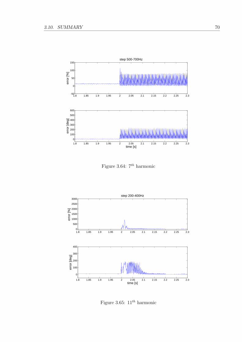
3.10. SUMMARY 70
1.8 1.85 1.9 1.95 2 2.05 2.1 2.15 2.2 2.25 2.3-50
0
50
100
150
erro
r [%
]
step 500-700Hz
1.8 1.85 1.9 1.95 2 2.05 2.1 2.15 2.2 2.25 2.3
0
100
200
300
400
500
600
time [s]
erro
r [de
g]
Figure 3.64: 7th harmonic
1.8 1.85 1.9 1.95 2 2.05 2.1 2.15 2.2 2.25 2.30
500
1000
1500
2000
2500
3000
erro
r [%
]
step 200-400Hz
1.8 1.85 1.9 1.95 2 2.05 2.1 2.15 2.2 2.25 2.3
0
100
200
300
400
time [s]
erro
r [de
g]
Figure 3.65: 11th harmonic
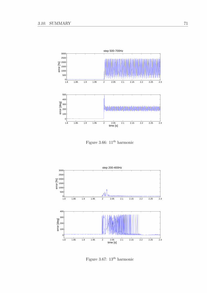
3.10. SUMMARY 71
1.8 1.85 1.9 1.95 2 2.05 2.1 2.15 2.2 2.25 2.30
500
1000
1500
2000
2500
3000
erro
r [%
]
step 500-700Hz
1.8 1.85 1.9 1.95 2 2.05 2.1 2.15 2.2 2.25 2.3
0
100
200
300
400
500
time [s]
erro
r [de
g]
Figure 3.66: 11th harmonic
1.8 1.85 1.9 1.95 2 2.05 2.1 2.15 2.2 2.25 2.30
500
1000
1500
2000
2500
3000
erro
r [%
]
step 200-400Hz
1.8 1.85 1.9 1.95 2 2.05 2.1 2.15 2.2 2.25 2.3
0
100
200
300
400
time [s]
erro
r [de
g]
Figure 3.67: 13th harmonic
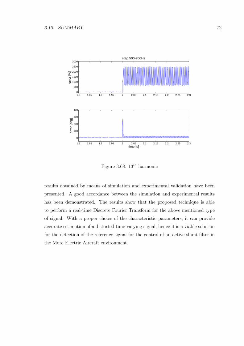
3.10. SUMMARY 72
1.8 1.85 1.9 1.95 2 2.05 2.1 2.15 2.2 2.25 2.30
500
1000
1500
2000
2500
3000
erro
r [%
]
step 500-700Hz
1.8 1.85 1.9 1.95 2 2.05 2.1 2.15 2.2 2.25 2.3
0
100
200
300
400
time [s]
erro
r [de
g]
Figure 3.68: 13th harmonic
results obtained by means of simulation and experimental validation have been
presented. A good accordance between the simulation and experimental results
has been demonstrated. The results show that the proposed technique is able
to perform a real-time Discrete Fourier Transform for the above mentioned type
of signal. With a proper choice of the characteristic parameters, it can provide
accurate estimation of a distorted time-varying signal, hence it is a viable solution
for the detection of the reference signal for the control of an active shunt filter in
the More Electric Aircraft environment.
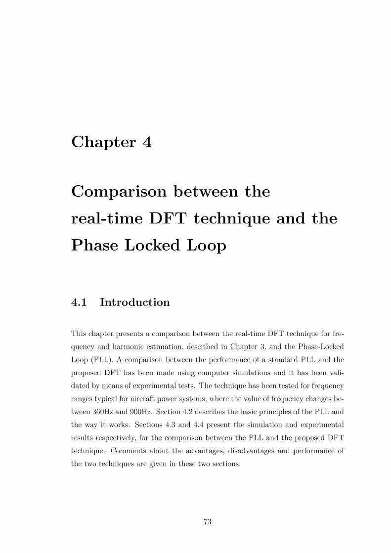
Chapter 4
Comparison between the
real-time DFT technique and the
Phase Locked Loop
4.1 Introduction
This chapter presents a comparison between the real-time DFT technique for fre-
quency and harmonic estimation, described in Chapter 3, and the Phase-Locked
Loop (PLL). A comparison between the performance of a standard PLL and the
proposed DFT has been made using computer simulations and it has been vali-
dated by means of experimental tests. The technique has been tested for frequency
ranges typical for aircraft power systems, where the value of frequency changes be-
tween 360Hz and 900Hz. Section 4.2 describes the basic principles of the PLL and
the way it works. Sections 4.3 and 4.4 present the simulation and experimental
results respectively, for the comparison between the PLL and the proposed DFT
technique. Comments about the advantages, disadvantages and performance of
the two techniques are given in these two sections.
73

4.2. THE PHASE LOCKED LOOP 74
4.2 The Phase Locked Loop
A PLL is a device which causes one signal to track another one. It keeps an
output signal synchronized with a reference input signal in frequency as well as in
phase. The PLL can be considered as a servo system, which controls the phase
of its output signal in such a way that the phase error between output phase and
reference phase reduces to a minimum [53]. The functional block diagram of a
PLL is shown in figure 4.1. It consists of a phase detector, a loop filter and a
controlled oscillator.
9
Phase Detector
Reference input
Loop Filter
9 9 Controlled oscillator
Phase error
Figure 4.1: Block diagram representing the basic structure of the PLL
All types of PLL have the same basic structure and differ mainly because of the
method of implementation of the phase detector. The most rudimentary type of
phase detector is the zero-crossing detection. Product-type, or mixer, phase detec-
tors are well-known and widely implemented and utilized [54, 55]. In three-phase
systems the most common phase detector is the one based on the synchronous dq
reference frame [54,55]. The loop filter is a low-pass filter. It is used to suppress the
noise and high-frequency signal components from the phase detector and provide a
DC-controlled signal for the voltage-controlled oscillator. The voltage-controlled
oscillators used in the PLL are similar to the ones used in other applications
like modulation and automatic frequency control. The main requirements for the
voltage-controlled oscillator are: phase stability, large frequency deviation, high
modulation sensitivity, linearity of frequency versus voltage control and capability
for accepting wide-band modulation [53].
The PLL analysed and implemented in this work has the structure shown in
figure 4.2.
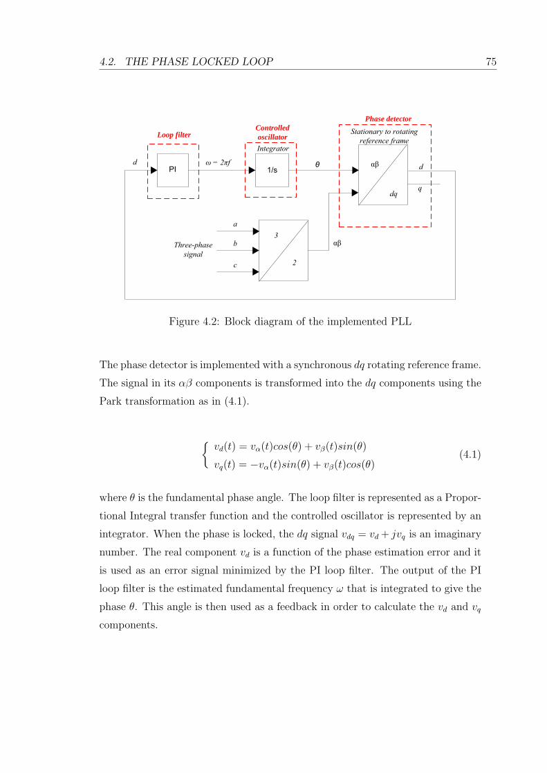
4.2. THE PHASE LOCKED LOOP 75
9 9
Integrator
dq
d d
q
2
3
99
9
a
b
c
Three-phase signal
ω = 2πf θ
Stationary to rotating reference frame
Loop filterControlled oscillator
Phase detector
9
Figure 4.2: Block diagram of the implemented PLL
The phase detector is implemented with a synchronous dq rotating reference frame.
The signal in its αβ components is transformed into the dq components using the
Park transformation as in (4.1).
vd(t) = vα(t)cos(θ) + vβ(t)sin(θ)
vq(t) = −vα(t)sin(θ) + vβ(t)cos(θ)(4.1)
where θ is the fundamental phase angle. The loop filter is represented as a Propor-
tional Integral transfer function and the controlled oscillator is represented by an
integrator. When the phase is locked, the dq signal vdq = vd + jvq is an imaginary
number. The real component vd is a function of the phase estimation error and it
is used as an error signal minimized by the PI loop filter. The output of the PI
loop filter is the estimated fundamental frequency ω that is integrated to give the
phase θ. This angle is then used as a feedback in order to calculate the vd and vq
components.
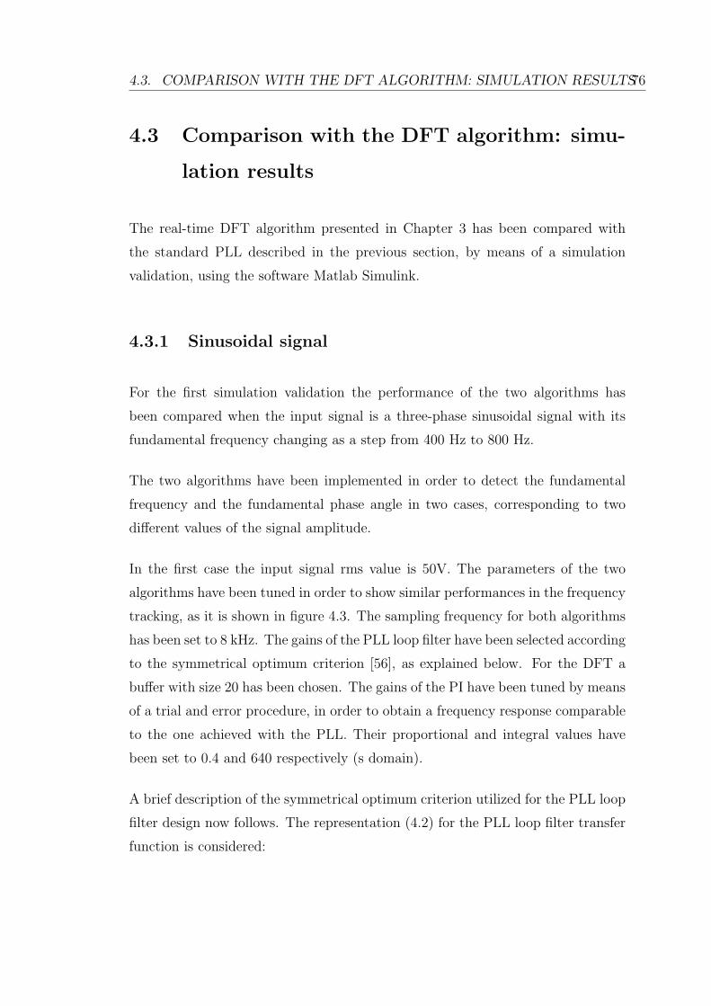
4.3. COMPARISON WITH THE DFT ALGORITHM: SIMULATION RESULTS76
4.3 Comparison with the DFT algorithm: simu-
lation results
The real-time DFT algorithm presented in Chapter 3 has been compared with
the standard PLL described in the previous section, by means of a simulation
validation, using the software Matlab Simulink.
4.3.1 Sinusoidal signal
For the first simulation validation the performance of the two algorithms has
been compared when the input signal is a three-phase sinusoidal signal with its
fundamental frequency changing as a step from 400 Hz to 800 Hz.
The two algorithms have been implemented in order to detect the fundamental
frequency and the fundamental phase angle in two cases, corresponding to two
different values of the signal amplitude.
In the first case the input signal rms value is 50V. The parameters of the two
algorithms have been tuned in order to show similar performances in the frequency
tracking, as it is shown in figure 4.3. The sampling frequency for both algorithms
has been set to 8 kHz. The gains of the PLL loop filter have been selected according
to the symmetrical optimum criterion [56], as explained below. For the DFT a
buffer with size 20 has been chosen. The gains of the PI have been tuned by means
of a trial and error procedure, in order to obtain a frequency response comparable
to the one achieved with the PLL. Their proportional and integral values have
been set to 0.4 and 640 respectively (s domain).
A brief description of the symmetrical optimum criterion utilized for the PLL loop
filter design now follows. The representation (4.2) for the PLL loop filter transfer
function is considered:

4.3. COMPARISON WITH THE DFT ALGORITHM: SIMULATION RESULTS77
LF = Kpll1 + sTpllsTpll
(4.2)
According to the method of symmetrical optimum [56], the loop filter gains Kpll
and Tpll are selected such that the frequency response of the amplitude and phase of
the open loop transfer functionHol are symmetrical around the crossover frequency
ωc, which corresponds to the geometrical mean of the two corner frequencies of
Hol. Given a normalizing factor α, the parameters ωc, Kpll and Tpll are related as
shown in (4.3).
ωc = 1αTs
Tpll = α2Ts
Kpll =(
1α
) (1
UTs
) (4.3)
where Ts is the sampling period and U is the amplitude of the input signal. It can
be demonstrated that the normalizing factor α is related to the damping factor ξ
by relation (4.4) [56].
ξ =α− 1
2(4.4)
Figure 4.4 compares the phase estimation errors obtained with the two techniques,
for the sinusoidal signal with frequency step from 400 Hz to 800 Hz and rms equal
to 50.
The input signal rms value has then been changed to 10 V, without re-tuning
the parameters according to the new amplitude. Figure 4.5 shows the frequency
estimate provided by the two algorithm in this case. It can be seen that the real-
time DFT algorithm is not affected by the change of the signal amplitude, while
the PLL performance is worse than in the previous case. In order for the PLL to
yield a more accurate estimate of the frequency in this case, the PI loop filter gains
should be re-tuned. On the other hand, the parameters of the DFT algorithm do
not need to be tuned according to the change of the input signal amplitude.
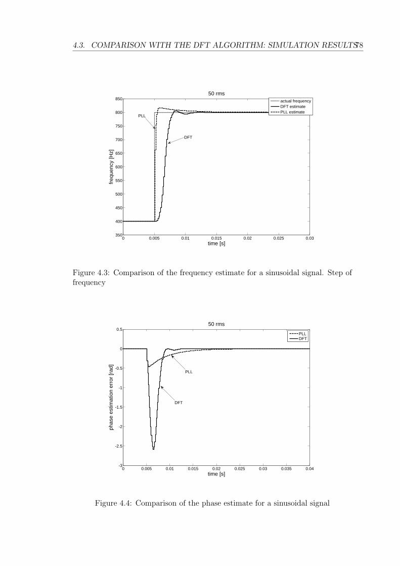
4.3. COMPARISON WITH THE DFT ALGORITHM: SIMULATION RESULTS78
0 0.005 0.01 0.015 0.02 0.025 0.03350
400
450
500
550
600
650
700
750
800
850
time [s]
frequ
ency
[Hz]
50 rms
actual frequencyDFT estimatePLL estimate
DFT
PLL
Figure 4.3: Comparison of the frequency estimate for a sinusoidal signal. Step offrequency
0 0.005 0.01 0.015 0.02 0.025 0.03 0.035 0.04-3
-2.5
-2
-1.5
-1
-0.5
0
0.550 rms
time [s]
phas
e es
timat
ion
erro
r [ra
d]
PLLDFT
PLL
DFT
Figure 4.4: Comparison of the phase estimate for a sinusoidal signal
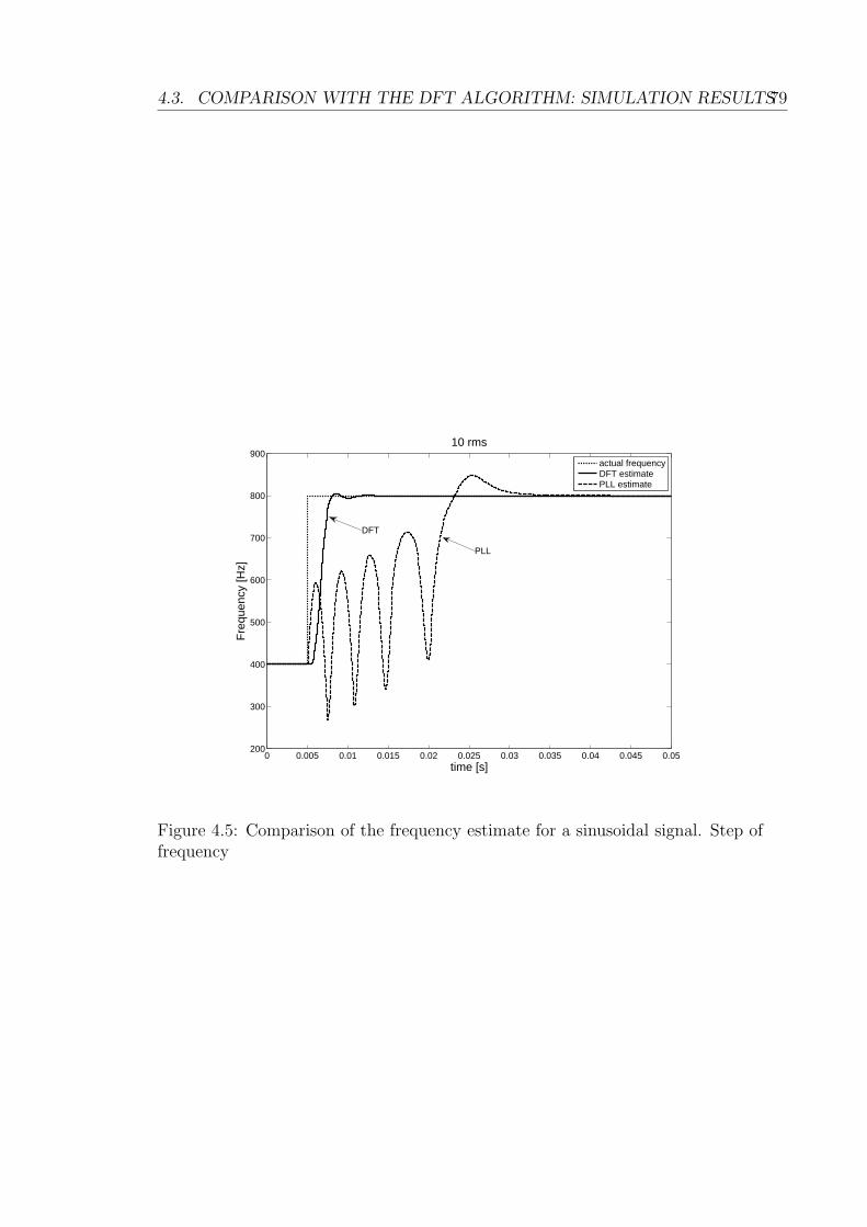
4.3. COMPARISON WITH THE DFT ALGORITHM: SIMULATION RESULTS79
0 0.005 0.01 0.015 0.02 0.025 0.03 0.035 0.04 0.045 0.05200
300
400
500
600
700
800
900
time [s]
Freq
uenc
y [H
z]
10 rms
actual frequencyDFT estimatePLL estimate
PLL
DFT
Figure 4.5: Comparison of the frequency estimate for a sinusoidal signal. Step offrequency

4.3. COMPARISON WITH THE DFT ALGORITHM: SIMULATION RESULTS80
Figure 4.6 compares the phase estimation errors obtained with the two techniques,
for the sinusoidal signal with frequency step from 400 Hz to 800 Hz and rms equal
to 10.
0 0.005 0.01 0.015 0.02 0.025 0.03 0.035 0.04 0.045 0.05-4
-3
-2
-1
0
1
2
3
410 rms
time [s]
phas
e es
timat
ion
erro
r [ra
d]
PLLDFT
PLL
DFT
Figure 4.6: Comparison of the phase estimate for a sinusoidal signal
The characteristics of the frequency response in the two cases are reported in
table 4.1.
4.3.2 Distorted signal
The second simulation validation has been carried out using a three-phase dis-
torted noisy (noise with power spectral density equal to 10−7) signal as input,
with frequency variable as a ramp from 400 to 800 Hz, with slope 8000 Hz/s.
The harmonic distortion is specified in table 4.2. Figure 4.7 shows the signal
represented in the time domain.
Figure 4.8 shows the frequency estimate obtained with the two algorithms for a
ramp of frequency, with the input signal described above. The PLL estimate has

4.3. COMPARISON WITH THE DFT ALGORITHM: SIMULATION RESULTS81
50 V 10 V
DFT PLL DFT PLL
Maximum overshoot [%] 1.25 4.125 1.25 12.0825
Delay time [s] 0.0016 0.000125 0.0016 0.0038
Rise time [s] 0.0015 0.00025 0.0015 0.0171
Settling time 5% [s] 0.0026 0.000375 0.0026 0.0231
Peak time [s] 0.0034 0.000875 0.0034 0.0204
Steady-state oscillation max amplitude
(% of the steady-state value) 0 0 0 0
Steady-state error [Hz] 0.0001 0.0665 0.0001 0.007
Table 4.1: Transient and steady-state performance of the frequency step estimation
5th harmonic amplitude [% of fundamental] 22
7th harmonic amplitude [% of fundamental] 10
11th harmonic amplitude [% of fundamental] 6.7
13th harmonic amplitude [% of fundamental] 5
17th harmonic amplitude [% of fundamental] 3
19th harmonic amplitude [% of fundamental] 2.2
Table 4.2: Input signal for fundamental frequency and phase estimation

4.4. COMPARISON WITH THE DFT ALGORITHM: EXPERIMENTALRESULTS 82
0 0.001 0.002 0.003 0.004 0.005 0.006 0.007 0.008 0.009 0.01-300
-200
-100
0
100
200
300
time [s]
volta
ge [V
]
alphabeta
Figure 4.7: Distorted noisy signal for the simulation comparison
bigger oscillations compared to the DFT estimate, thus showing a bigger sensitivity
to the harmonic distortion and the noise.
Figures 4.9 and 4.10 show the frequency estimation error and the phase estimation
error respectively, for both algorithms. From these figures it can be seen that the
DFT technique shows a reduced sensitivity to harmonics and noise. For both
algorithms the phase estimation error is negligible at steady-state.
4.4 Comparison with the DFT algorithm: ex-
perimental results
The comparison between the proposed DFT technique and the PLL has been
validated experimentally, using the same laboratory set-up described in section 3.7.
In order to perform the tests, the input voltage signals have been generated by
the Chroma programmable power supply, described in section 3.7.
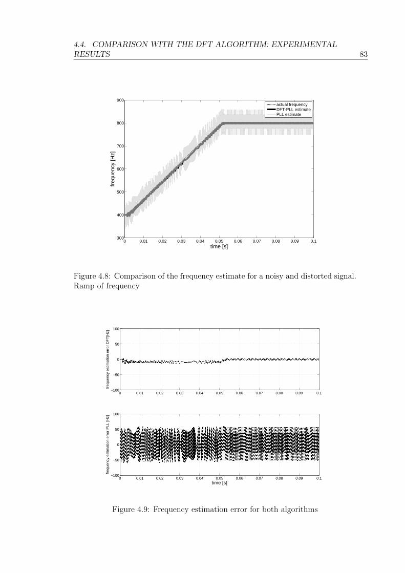
4.4. COMPARISON WITH THE DFT ALGORITHM: EXPERIMENTALRESULTS 83
0 0.01 0.02 0.03 0.04 0.05 0.06 0.07 0.08 0.09 0.1300
400
500
600
700
800
900
time [s]
frequ
ency
[Hz]
actual frequencyDFT-PLL estimatePLL estimate
Figure 4.8: Comparison of the frequency estimate for a noisy and distorted signal.Ramp of frequency
0 0.01 0.02 0.03 0.04 0.05 0.06 0.07 0.08 0.09 0.1−100
−50
0
50
100
freq
uenc
y es
timat
ion
erro
r D
FT
[Hz]
0 0.01 0.02 0.03 0.04 0.05 0.06 0.07 0.08 0.09 0.1−100
−50
0
50
100
time [s]
freq
uenc
y es
timat
ion
erro
r P
LL [H
z]
Figure 4.9: Frequency estimation error for both algorithms
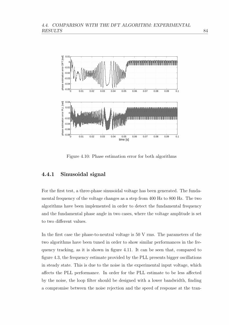
4.4. COMPARISON WITH THE DFT ALGORITHM: EXPERIMENTALRESULTS 84
0 0.01 0.02 0.03 0.04 0.05 0.06 0.07 0.08 0.09 0.1-0.05
-0.04
-0.03
-0.02
-0.01
0
0.01
phas
e es
timat
ion
erro
r DFT
[rad
]
0 0.01 0.02 0.03 0.04 0.05 0.06 0.07 0.08 0.09 0.1-0.08
-0.06
-0.04
-0.02
0
0.02
0.04
time [s]
phas
e es
timat
ion
erro
r PLL
[rad
]
Figure 4.10: Phase estimation error for both algorithms
4.4.1 Sinusoidal signal
For the first test, a three-phase sinusoidal voltage has been generated. The funda-
mental frequency of the voltage changes as a step from 400 Hz to 800 Hz. The two
algorithms have been implemented in order to detect the fundamental frequency
and the fundamental phase angle in two cases, where the voltage amplitude is set
to two different values.
In the first case the phase-to-neutral voltage is 50 V rms. The parameters of the
two algorithms have been tuned in order to show similar performances in the fre-
quency tracking, as it is shown in figure 4.11. It can be seen that, compared to
figure 4.3, the frequency estimate provided by the PLL presents bigger oscillations
in steady state. This is due to the noise in the experimental input voltage, which
affects the PLL performance. In order for the PLL estimate to be less affected
by the noise, the loop filter should be designed with a lower bandwidth, finding
a compromise between the noise rejection and the speed of response at the tran-
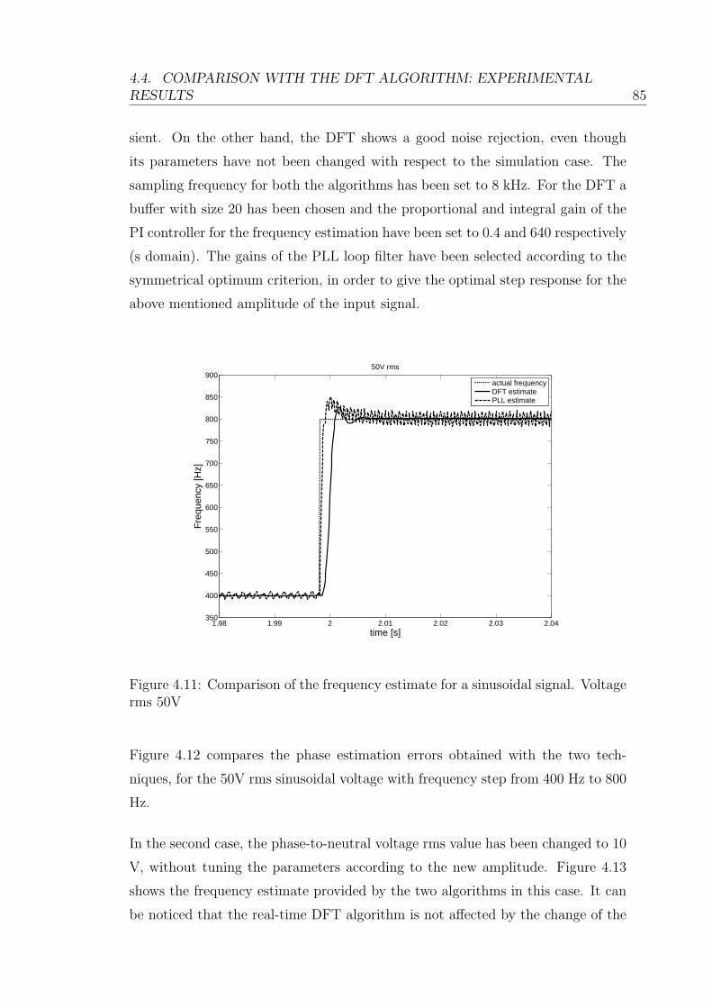
4.4. COMPARISON WITH THE DFT ALGORITHM: EXPERIMENTALRESULTS 85
sient. On the other hand, the DFT shows a good noise rejection, even though
its parameters have not been changed with respect to the simulation case. The
sampling frequency for both the algorithms has been set to 8 kHz. For the DFT a
buffer with size 20 has been chosen and the proportional and integral gain of the
PI controller for the frequency estimation have been set to 0.4 and 640 respectively
(s domain). The gains of the PLL loop filter have been selected according to the
symmetrical optimum criterion, in order to give the optimal step response for the
above mentioned amplitude of the input signal.
1.98 1.99 2 2.01 2.02 2.03 2.04350
400
450
500
550
600
650
700
750
800
850
900
time [s]
Freq
uenc
y [H
z]
50V rms
actual frequencyDFT estimatePLL estimate
Figure 4.11: Comparison of the frequency estimate for a sinusoidal signal. Voltagerms 50V
Figure 4.12 compares the phase estimation errors obtained with the two tech-
niques, for the 50V rms sinusoidal voltage with frequency step from 400 Hz to 800
Hz.
In the second case, the phase-to-neutral voltage rms value has been changed to 10
V, without tuning the parameters according to the new amplitude. Figure 4.13
shows the frequency estimate provided by the two algorithms in this case. It can
be noticed that the real-time DFT algorithm is not affected by the change of the
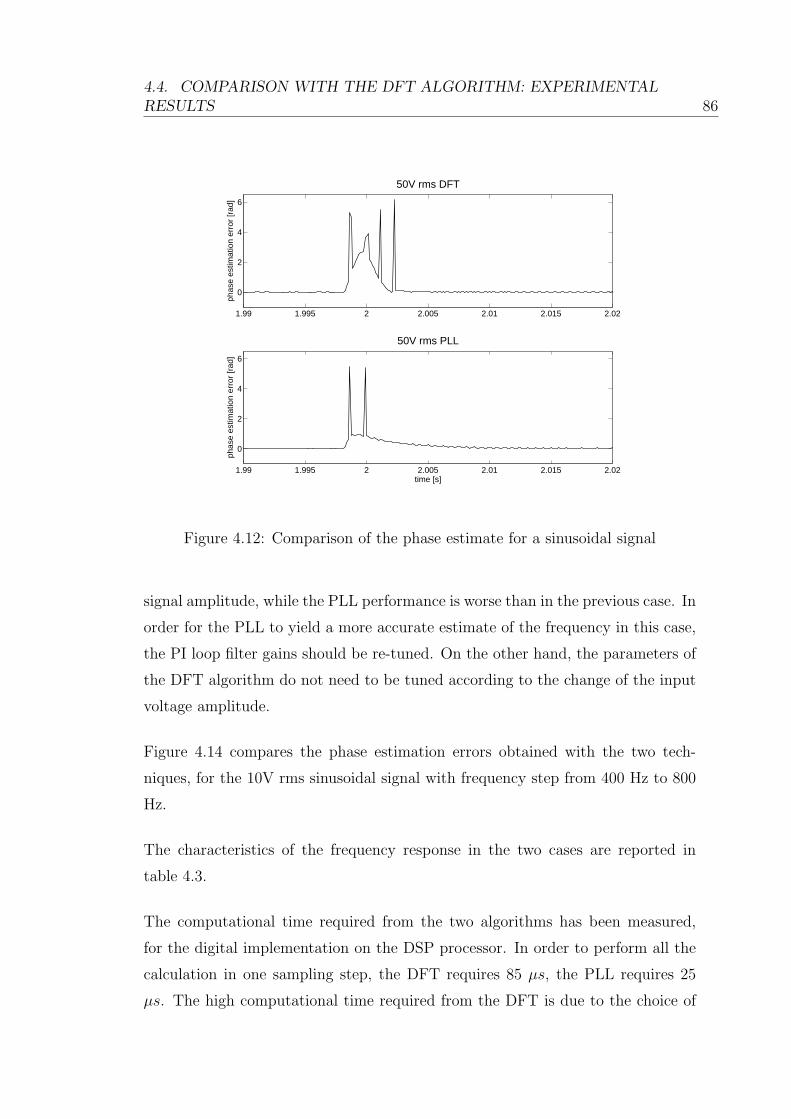
4.4. COMPARISON WITH THE DFT ALGORITHM: EXPERIMENTALRESULTS 86
1.99 1.995 2 2.005 2.01 2.015 2.02
0
2
4
6
phas
e es
timat
ion
erro
r [ra
d]
50V rms DFT
1.99 1.995 2 2.005 2.01 2.015 2.02
0
2
4
6
phas
e es
timat
ion
erro
r [ra
d]
time [s]
50V rms PLL
Figure 4.12: Comparison of the phase estimate for a sinusoidal signal
signal amplitude, while the PLL performance is worse than in the previous case. In
order for the PLL to yield a more accurate estimate of the frequency in this case,
the PI loop filter gains should be re-tuned. On the other hand, the parameters of
the DFT algorithm do not need to be tuned according to the change of the input
voltage amplitude.
Figure 4.14 compares the phase estimation errors obtained with the two tech-
niques, for the 10V rms sinusoidal signal with frequency step from 400 Hz to 800
Hz.
The characteristics of the frequency response in the two cases are reported in
table 4.3.
The computational time required from the two algorithms has been measured,
for the digital implementation on the DSP processor. In order to perform all the
calculation in one sampling step, the DFT requires 85 µs, the PLL requires 25
µs. The high computational time required from the DFT is due to the choice of

4.4. COMPARISON WITH THE DFT ALGORITHM: EXPERIMENTALRESULTS 87
1.98 2 2.02 2.04 2.06 2.08 2.1 2.12 2.14300
400
500
600
700
800
900
time [s]
Freq
uenc
y [H
z]
10V rms
actual frequencyDFT estimatePLL estimate
Figure 4.13: Comparison of the frequency estimate for a sinusoidal signal. Voltageamplitude 10V
2 2.01 2.02 2.03 2.04 2.05 2.06 2.07 2.08 2.09 2.1
0
2
4
6
phas
e es
timat
ion
erro
r [ra
d]
10V rms DFT
2 2.01 2.02 2.03 2.04 2.05 2.06 2.07 2.08 2.09 2.1
0
2
4
6
time [s]
phas
e es
timat
ion
erro
r [ra
d]
10V rms PLL
Figure 4.14: Comparison of the phase estimate for a sinusoidal signal

4.4. COMPARISON WITH THE DFT ALGORITHM: EXPERIMENTALRESULTS 88
50 V 10 V
DFT PLL DFT PLL
Maximum overshoot [%] 6.5 12.75 7 10
Delay time [s] 0.0019 0.0004 0.002 0.0464
Rise time [s] 0.0014 0.0006 0.0014 0.0889
Settling time 5% [s] 0.0041 0.0083 0.0042 0.0975
Peak time [s] 0.0036 0.0021 0.0036 0.0947
Steady-state oscillation max amplitude
(% of the steady-state value) 0.15 5 0.625 1.175
Steady-state error [Hz] 0.0379 2.25 0.0361 1.4007
Table 4.3: Transient and steady-state performance of the frequency step estimation
the buffer size, which in this case is 20 points, equal to one entire period of the
fundamental at 400 Hz (with 8 kHz sampling frequency). The buffer size could
be set to a smaller value, like one quarter of the fundamental period, in that case
the computational burden would significantly reduce.
4.4.2 Distorted signal
For the second test, a three-phase distorted voltage has been generated. The
fundamental frequency of the voltage changes as a ramp from 400 Hz to 800 Hz,
with slope 400 Hz/s. The phase-to-neutral voltage rms is equal to 50 V. The two
algorithms have been implemented in order to detect the fundamental frequency
and the fundamental phase angle of the input signal. The harmonic distortion of
the voltage is specified in table 4.4. Figure 4.15 shows the voltage represented in
the time domain.
Figure 4.16 shows the frequency estimate obtained with the two algorithms for
the ramp of frequency, with the input signal described above. The PLL estimate
has bigger oscillations compared to the DFT estimate, thus showing a bigger
sensitivity to the harmonic distortion and the noise.
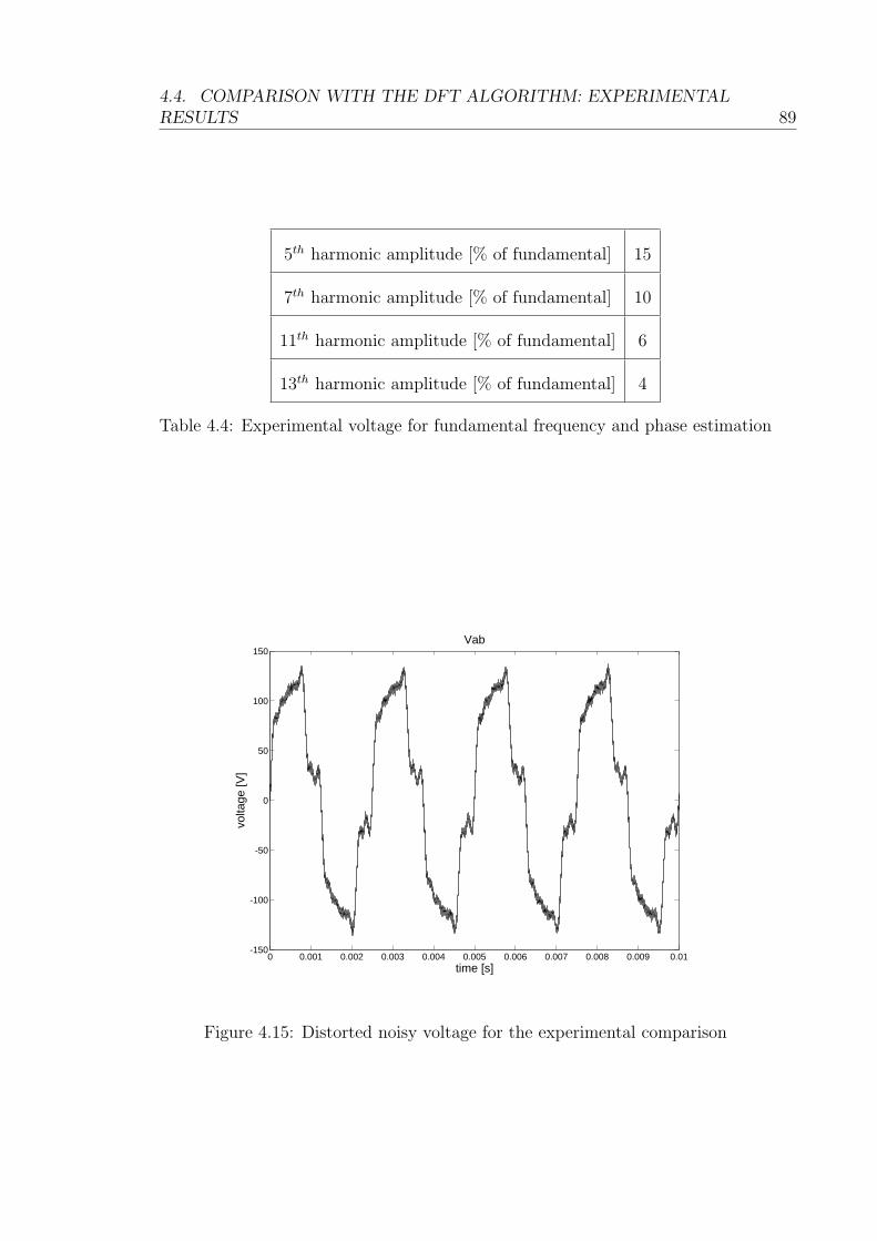
4.4. COMPARISON WITH THE DFT ALGORITHM: EXPERIMENTALRESULTS 89
5th harmonic amplitude [% of fundamental] 15
7th harmonic amplitude [% of fundamental] 10
11th harmonic amplitude [% of fundamental] 6
13th harmonic amplitude [% of fundamental] 4
Table 4.4: Experimental voltage for fundamental frequency and phase estimation
0 0.001 0.002 0.003 0.004 0.005 0.006 0.007 0.008 0.009 0.01-150
-100
-50
0
50
100
150
time [s]
volta
ge [V
]
Vab
Figure 4.15: Distorted noisy voltage for the experimental comparison

4.4. COMPARISON WITH THE DFT ALGORITHM: EXPERIMENTALRESULTS 90
0.5 1 1.5 2 2.50
200
400
600
800
1000
frequ
ency
[Hz]
DFT estimate
0.5 1 1.5 2 2.50
200
400
600
800
1000
frequ
ency
[Hz]
time [s]
PLL estimate
Figure 4.16: Comparison of the frequency estimate for a noisy and distorted volt-age. Ramp of frequency
4.5. SUMMARY 91
4.5 Summary
In this chapter a comparison between the real-time DFT algorithm presented
in Chapter 3 and the Phase-Locked Loop has been presented. Simulation and
experimental results show the difference between the performances of the two
techniques, for the frequency estimation of sinusoidal or distorted signals with
time-varying frequency, in the typical range of aircraft power systems. From the
comparison it can be concluded that the DFT exhibits better dynamic performance
and reduced sensitivity to harmonics, noise, and signal amplitude variations. In
order to obtain a good performance from the PLL, it is necessary to tune the
parameters, particularly the loop filter gains, depending on the characteristics of
the signal which is to be identified. A compromise should be found between the
desired speed of response and the steady-state accuracy. In terms of computational
burden, the DFT implementation is characterized by higher execution time, on a
digital processor board, compared to the PLL. However, the DFT implementation
can be tuned and optimized in order to reduce the calculation time and still provide
fast and accurate estimation of the frequency and the fundamental phase.
Chapter 5
Multiple Reference Frames
Voltage Detection Control
Technique
5.1 Introduction
This chapter presents a novel control technique for shunt active filters, based on
the measurement of the voltage at the Point of Common Coupling (PCC). This
technique allows the harmonic compensation to be performed without using any
sensor on the distorting load, but only on the PCC and on the active filter itself,
making it a plug-and-play sensorless system that can compensate for the harmonic
distortion in any point of the network. The control technique is structured with
multiple rotating reference frames, which are decoupled one from another. There
is one control loop for the fundamental plus as many control loops as the har-
monic components to be compensated. Section 5.2, Section 5.3 and Section 5.4
describe the decoupling technique, presenting the equations utilized and some ex-
amples. Section 5.6 describes the control technique, with the design criteria of the
controllers and the dynamic characteristics of the control loops.
92
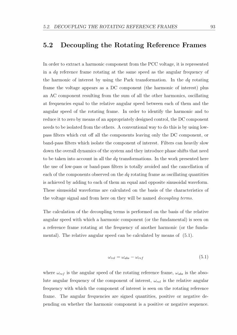
5.2. DECOUPLING THE ROTATING REFERENCE FRAMES 93
5.2 Decoupling the Rotating Reference Frames
In order to extract a harmonic component from the PCC voltage, it is represented
in a dq reference frame rotating at the same speed as the angular frequency of
the harmonic of interest by using the Park transformation. In the dq rotating
frame the voltage appears as a DC component (the harmonic of interest) plus
an AC component resulting from the sum of all the other harmonics, oscillating
at frequencies equal to the relative angular speed between each of them and the
angular speed of the rotating frame. In order to identify the harmonic and to
reduce it to zero by means of an appropriately designed control, the DC component
needs to be isolated from the others. A conventional way to do this is by using low-
pass filters which cut off all the components leaving only the DC component, or
band-pass filters which isolate the component of interest. Filters can heavily slow
down the overall dynamics of the system and they introduce phase shifts that need
to be taken into account in all the dq transformations. In the work presented here
the use of low-pass or band-pass filters is totally avoided and the cancellation of
each of the components observed on the dq rotating frame as oscillating quantities
is achieved by adding to each of them an equal and opposite sinusoidal waveform.
These sinusoidal waveforms are calculated on the basis of the characteristics of
the voltage signal and from here on they will be named decoupling terms.
The calculation of the decoupling terms is performed on the basis of the relative
angular speed with which a harmonic component (or the fundamental) is seen on
a reference frame rotating at the frequency of another harmonic (or the funda-
mental). The relative angular speed can be calculated by means of (5.1).
ωrel = ωabs − ωref (5.1)
where ωref is the angular speed of the rotating reference frame, ωabs is the abso-
lute angular frequency of the component of interest, ωrel is the relative angular
frequency with which the component of interest is seen on the rotating reference
frame. The angular frequencies are signed quantities, positive or negative de-
pending on whether the harmonic component is a positive or negative sequence.

5.2. DECOUPLING THE ROTATING REFERENCE FRAMES 94
Harmonic component
Fund. 5th 7th 11th 13th
Fund. DC -6 +6 -12 +12
Frame 5th +6 DC +12 -6 +18
of 7th -6 -12 DC -18 +6
reference 11th +12 +6 +18 DC +24
13th -12 -18 -6 -24 DC
Table 5.1: Relative harmonic orders on the rotating frames of reference
According to the formula (5.1), on the reference frame rotating at the fundamental
frequency, the 5th and 7th harmonic are seen as 6th harmonic. Table 5.1 shows for
each harmonic component (including the fundamental) the harmonic order with
which they are seen on all the other reference frames. The sign indicates the sense
of rotation of the harmonic as seen when represented on the reference frame.
Figures 5.1 and 5.2 show an example of how the decoupling works. In Figure 5.1
a distorted signal composed of a fundamental component at 50Hz with amplitude
100 and a 5th harmonic with amplitude 20 is represented. The left hand column of
the figure shows the abc component of the fundamental, of the 5th harmonic and
the distorted signal respectively (looking from the top to the bottom), the right
hand column shows the same components transformed into a dq frame rotating at
50Hz: the fundamental appears as a DC quantity in the new reference frame, the
5th harmonic appears as a 300Hz signal, i.e. like a 6th harmonic (according to the
formula (5.1)), the distorted signal appears as an oscillating component at 300Hz
with a DC offset equal to the amplitude of the fundamental.
Figure 5.2 shows how the d component of the distorted signal summed with the
d axis decoupling term, which is equal and opposite to the oscillating component,
gives as a result the DC quantity corresponding to the d component of the funda-
mental. Given a dq frame rotating at a certain harmonic frequency, the d and q
components of the distorted signal have a DC offset corresponding to the d and q
components of the harmonic synchronous with the rotating frame and an oscillat-
ing part corresponding to all the other harmonics as seen on that reference frame,
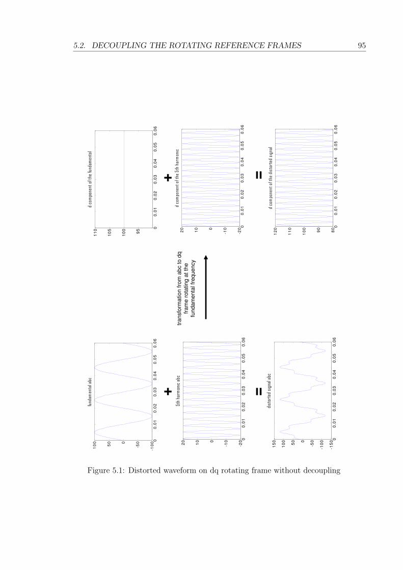
5.2. DECOUPLING THE ROTATING REFERENCE FRAMES 95
+
00
.01
0.0
20
.03
0.0
40
.05
0.0
6
95
10
0
10
5
11
0
d co
mpo
nent
oft
hefu
ndam
enta
l
00
.01
0.0
20
.03
0.0
40
.05
0.0
6-2
0
-100
10
20
d co
mpo
nent
of t
he 5
thha
rmon
ic
00
.01
0.0
20
.03
0.0
40
.05
0.0
68
0
90
10
0
11
0
12
0d
com
pone
ntof
the
dis
tort
ed s
igna
l
=
00
.01
0.0
20
.03
0.0
40
.05
0.0
6-1
00
-500
50
10
0fu
ndam
enta
l abc
00
.01
0.0
20
.03
0.0
40
.05
0.0
6-2
0
-100
10
20
5th
harm
onic
abc
+ =
00
.01
0.0
20
.03
0.0
40
.05
0.0
6-1
50
-10
0
-500
50
10
0
15
0di
stor
ted
sign
alab
c
transfo
rmation f
rom
abc
to d
q
fram
e r
ota
ting a
t th
e
fundam
enta
l fr
equency
Figure 5.1: Distorted waveform on dq rotating frame without decoupling
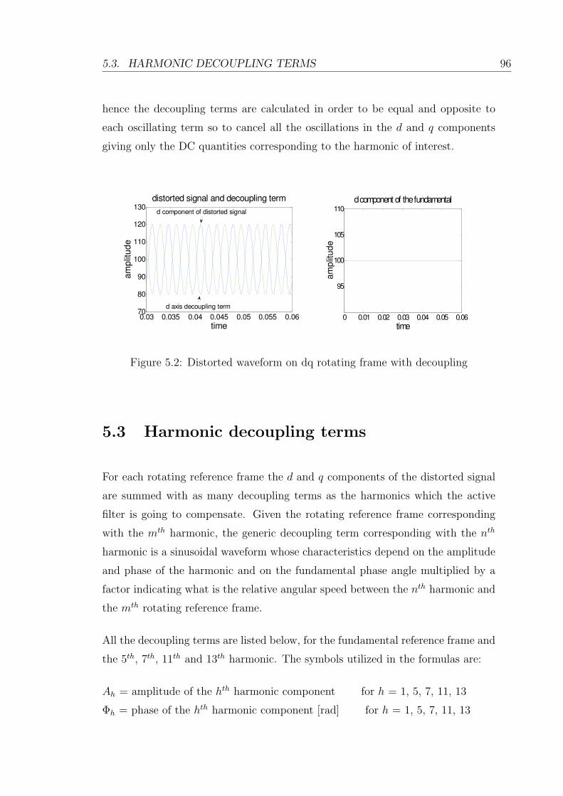
5.3. HARMONIC DECOUPLING TERMS 96
hence the decoupling terms are calculated in order to be equal and opposite to
each oscillating term so to cancel all the oscillations in the d and q components
giving only the DC quantities corresponding to the harmonic of interest.
0.03 0.035 0.04 0.045 0.05 0.055 0.0670
80
90
100
110
120
130distorted signal and decoupling term
time
am
plit
ud
e
d component of distorted signal
d axis decoupling term
0 0.01 0.02 0.03 0.04 0.05 0.06
95
100
105
110
timea
mp
litu
de
d component of the fundamental
Figure 5.2: Distorted waveform on dq rotating frame with decoupling
5.3 Harmonic decoupling terms
For each rotating reference frame the d and q components of the distorted signal
are summed with as many decoupling terms as the harmonics which the active
filter is going to compensate. Given the rotating reference frame corresponding
with the mth harmonic, the generic decoupling term corresponding with the nth
harmonic is a sinusoidal waveform whose characteristics depend on the amplitude
and phase of the harmonic and on the fundamental phase angle multiplied by a
factor indicating what is the relative angular speed between the nth harmonic and
the mth rotating reference frame.
All the decoupling terms are listed below, for the fundamental reference frame and
the 5th, 7th, 11th and 13th harmonic. The symbols utilized in the formulas are:
Ah = amplitude of the hth harmonic component for h = 1, 5, 7, 11, 13
Φh = phase of the hth harmonic component [rad] for h = 1, 5, 7, 11, 13

5.3. HARMONIC DECOUPLING TERMS 97
ϑfund = fundamental phase angle for ϑfund ∈ [0; 2π]
The decoupling terms for each harmonic on the fundamental reference frame (rep-
resented with both their d and q components) are here listed. The decoupling
terms for all the other reference frames are reported in Appendix B.
Reference frame rotating at the fundamental frequency
5th harmonic d component:
A5 · sin(
6ϑfund + Φ5 −π
2
)(5.2)
5th harmonic q component:
A5 · sin (6ϑfund + Φ5) (5.3)
7th harmonic d component:
A7 · sin(
6ϑfund + Φ7 +π
2
)(5.4)
7th harmonic q component:
A7 · sin (6ϑfund + Φ7) (5.5)

5.4. EXAMPLES OF ACCURATE AND INACCURATE DECOUPLING 98
11th harmonic d component:
−A11 · sin(
12ϑfund + Φ11 −π
2
)(5.6)
11th harmonic q component:
−A11 · sin (12ϑfund + Φ11) (5.7)
13th harmonic d component:
−A13 · sin(
12ϑfund + Φ13 +π
2
)(5.8)
13th harmonic q component:
−A13 · sin (12ϑfund + Φ13) (5.9)
5.4 Examples of accurate and inaccurate decou-
pling
This section presents an example of how the decoupling is carried out properly
when the decoupling terms are calculated correctly and an example that shows
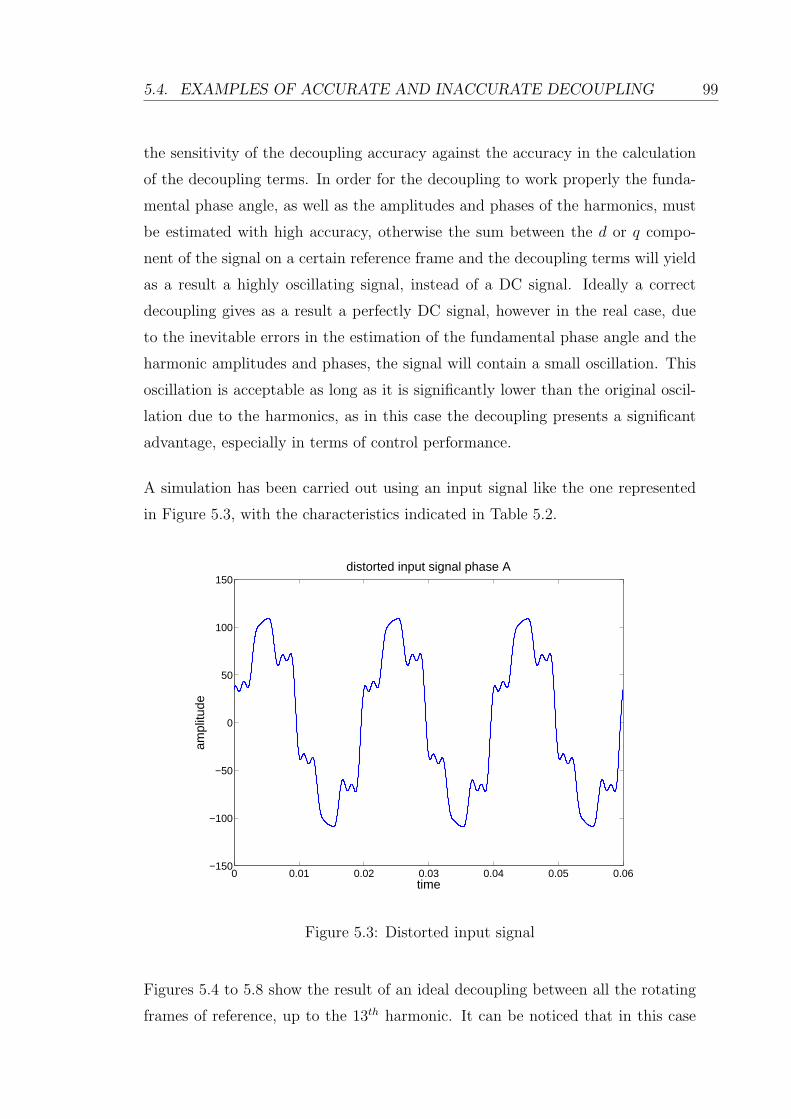
5.4. EXAMPLES OF ACCURATE AND INACCURATE DECOUPLING 99
the sensitivity of the decoupling accuracy against the accuracy in the calculation
of the decoupling terms. In order for the decoupling to work properly the funda-
mental phase angle, as well as the amplitudes and phases of the harmonics, must
be estimated with high accuracy, otherwise the sum between the d or q compo-
nent of the signal on a certain reference frame and the decoupling terms will yield
as a result a highly oscillating signal, instead of a DC signal. Ideally a correct
decoupling gives as a result a perfectly DC signal, however in the real case, due
to the inevitable errors in the estimation of the fundamental phase angle and the
harmonic amplitudes and phases, the signal will contain a small oscillation. This
oscillation is acceptable as long as it is significantly lower than the original oscil-
lation due to the harmonics, as in this case the decoupling presents a significant
advantage, especially in terms of control performance.
A simulation has been carried out using an input signal like the one represented
in Figure 5.3, with the characteristics indicated in Table 5.2.
0 0.01 0.02 0.03 0.04 0.05 0.06−150
−100
−50
0
50
100
150distorted input signal phase A
ampl
itude
time
Figure 5.3: Distorted input signal
Figures 5.4 to 5.8 show the result of an ideal decoupling between all the rotating
frames of reference, up to the 13th harmonic. It can be noticed that in this case

5.4. EXAMPLES OF ACCURATE AND INACCURATE DECOUPLING 100
Fundamental frequency [Hz] 50 HzFundamental amplitude 100Fundamental phase [deg] 05th harmonic amplitude 205th harmonic phase [deg] 507th harmonic amplitude 107th harmonic phase [deg] 7011th harmonic amplitude 711th harmonic phase [deg] 11013th harmonic amplitude 513th harmonic phase [deg] 130
Table 5.2: Input signal for decoupling example
all the d and q components are pure DC quantities.
0 0.01 0.02 0.03 0.04 0.05 0.0685
90
95
100
105
110d component on the fundamental rotating frame
time
ampl
itude
0 0.01 0.02 0.03 0.04 0.05 0.06−40
−20
0
20
40q component on the fundamental rotating frame
time
ampl
itude
Figure 5.4: Fundamental d and q components
The reason why the dq components initially oscillate for a time interval equal
to 0.02 s is that the identification of the fundamental and harmonic amplitudes
and phases is carried out by means of the Discrete Fourier Transform, with a
window of observation of the signal equal to one period of the fundamental, which
at 50Hz corresponds to 0.02 s. The DFT algorithm takes a time equal to one
observation window to start the identification. The case represented in these
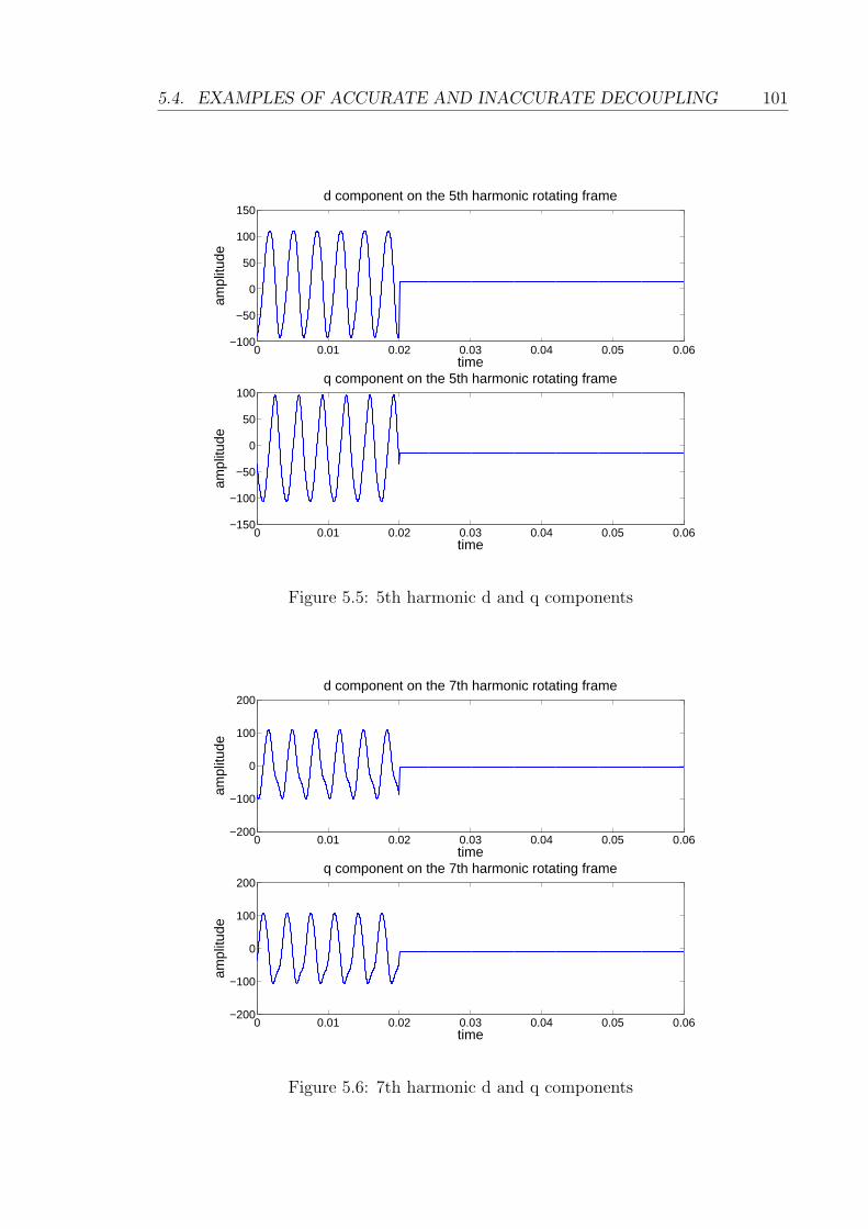
5.4. EXAMPLES OF ACCURATE AND INACCURATE DECOUPLING 101
0 0.01 0.02 0.03 0.04 0.05 0.06−100
−50
0
50
100
150
time
ampl
itude
d component on the 5th harmonic rotating frame
0 0.01 0.02 0.03 0.04 0.05 0.06−150
−100
−50
0
50
100
time
ampl
itude
q component on the 5th harmonic rotating frame
Figure 5.5: 5th harmonic d and q components
0 0.01 0.02 0.03 0.04 0.05 0.06−200
−100
0
100
200d component on the 7th harmonic rotating frame
time
ampl
itude
0 0.01 0.02 0.03 0.04 0.05 0.06−200
−100
0
100
200q component on the 7th harmonic rotating frame
time
ampl
itude
Figure 5.6: 7th harmonic d and q components

5.4. EXAMPLES OF ACCURATE AND INACCURATE DECOUPLING 102
0 0.01 0.02 0.03 0.04 0.05 0.06−200
−100
0
100
200
time
ampl
itude
d component on the 11th harmonic rotating frame
0 0.01 0.02 0.03 0.04 0.05 0.06−200
−100
0
100
200
time
ampl
itude
q component on the 11th harmonic rotating frame
Figure 5.7: 11th harmonic d and q components
0 0.01 0.02 0.03 0.04 0.05 0.06−200
−100
0
100
200d component on the 13th harmonic rotating frame
time
ampl
itude
0 0.01 0.02 0.03 0.04 0.05 0.06−200
−100
0
100
200q component on the 13th harmonic rotating frame
time
ampl
itude
Figure 5.8: 13th harmonic d and q components

5.4. EXAMPLES OF ACCURATE AND INACCURATE DECOUPLING 103
figures corresponds to an ideal decoupling, obtained in simulation by using an
arbitrary input signal where all the harmonic components are known in amplitude
and phase (see Table 5.2), the fundamental phase angle ϑfund utilized to calculate
the decoupling terms is obtained from the alpha and beta components of the
fundamental, as shown in the formula (5.10), where alpha and beta are obtained
using the Clarke transformation.
ϑfund = arctan(beta
alpha) (5.10)
The possible causes of error when decoupling one reference frame from the oth-
ers are: errors in the estimation of the fundamental phase angle, errors in the
estimation of the amplitudes and phases of the fundamental and the harmonics.
The estimation of the fundamental phase angle is a crucial point in the whole
decoupling strategy performance: when the signal to be processed is distorted, it
is not possible to obtain accurate results using conventional estimation methods
for the phase, like the inverse tangent of the alpha − beta components, or a con-
ventional Phase Locked Loop, but more complex methods should be implemented,
as explained in Chapter 3. The errors in the estimation of the harmonic ampli-
tudes and phases are due to the inaccuracy of the harmonic detection method
and they are ultimately related to the inaccuracy of the phase estimation. Here
follows an example of how the inaccuracies in the fundamental phase angle and
the harmonic detection can affect the decoupling. If the fundamental phase angle
is calculated by means of the inverse tangent of the alpha − beta components of
the whole input signal, instead of its fundamental components, the resulting esti-
mation error for the fundamental phase angle can be very high. Figure 5.9 shows
the comparison between the angle obtained from the fundamental component and
the one obtained using the whole distorted signal. Normally, in order to avoid
such high inaccuracy in the phase estimation, better techniques are used, such
as the Phase Locked Loop. Figure 5.10 shows the comparison between the angle
obtained applying the PLL to the fundamental component and the one obtained
applying the PLL to the whole distorted signal. In the examined case the signal is
not noisy (see Figure 5.3) and although the distortion affects the accuracy of the
PLL estimation the error is not very large. However this affects the accuracy of the
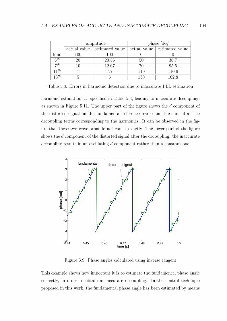
5.4. EXAMPLES OF ACCURATE AND INACCURATE DECOUPLING 104
amplitude phase [deg]actual value estimated value actual value estimated value
fund 100 100 0 05th 20 20.56 50 36.77th 10 12.67 70 95.511th 7 7.7 110 110.613th 5 6 130 162.8
Table 5.3: Errors in harmonic detection due to inaccurate PLL estimation
harmonic estimation, as specified in Table 5.3, leading to inaccurate decoupling,
as shown in Figure 5.11. The upper part of the figure shows the d component of
the distorted signal on the fundamental reference frame and the sum of all the
decoupling terms corresponding to the harmonics. It can be observed in the fig-
ure that these two waveforms do not cancel exactly. The lower part of the figure
shows the d component of the distorted signal after the decoupling: the inaccurate
decoupling results in an oscillating d component rather than a constant one.
0.44 0.45 0.46 0.47 0.48 0.49 0.5−4
−3
−2
−1
0
1
2
3
4
time [s]
phas
e [r
ad]
fundamental distorted signal
Figure 5.9: Phase angles calculated using inverse tangent
This example shows how important it is to estimate the fundamental phase angle
correctly, in order to obtain an accurate decoupling. In the control technique
proposed in this work, the fundamental phase angle has been estimated by means
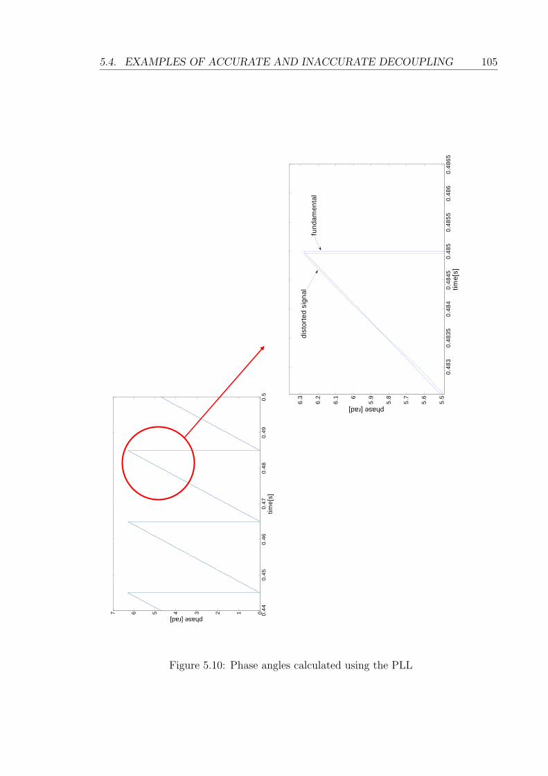
5.4. EXAMPLES OF ACCURATE AND INACCURATE DECOUPLING 105
0.44
0.45
0.46
0.47
0.48
0.49
0.5
01234567
time[
s]
phase [rad]
0.48
30.
4835
0.48
40.
4845
0.48
50.
4855
0.48
60.
4865
5.5
5.6
5.7
5.8
5.96
6.1
6.2
6.3
time[
s]
phase [rad]
fund
amen
tal
dist
orte
d si
gnal
Figure 5.10: Phase angles calculated using the PLL

5.5. CONTROL OF A SHUNT ACTIVE FILTER 106
0.48 0.485 0.49 0.495 0.580
85
90
95
100
105
110
115
120
time
ampl
itude
d component of the fundamental after the decoupling
0.48 0.485 0.49 0.495 0.570
80
90
100
110
120
130
timeam
plitu
de
distorted signal and decoupling term
distorted signal decoupling term
Figure 5.11: Inaccurate decoupling due to inaccurate phase angle estimation
of the DFT detection algorithm described in Chapter 3. This method proved to
be highly accurate and showed low sensitivity to distortion and noise, hence it
represents an effective means for the decoupling between the harmonic reference
frames.
5.5 Control of a shunt active filter
The shunt active filter is a power electronic device designed to compensate the
harmonics generated by one or more distorting loads. Connected in parallel with
the power supply and the loads, the shunt active filter injects a harmonic current
in order to cancel the one absorbed by the distorting load, and make the supply
current sinusoidal. This concept is explained in figure 5.12. iF and iH represent
the fundamental and the harmonic part of the current, respectively.
The circuit topology of a three-phase shunt active filter comprises a three-phase
voltage source inverter, a DC link capacitor and a three-phase line inductor. The
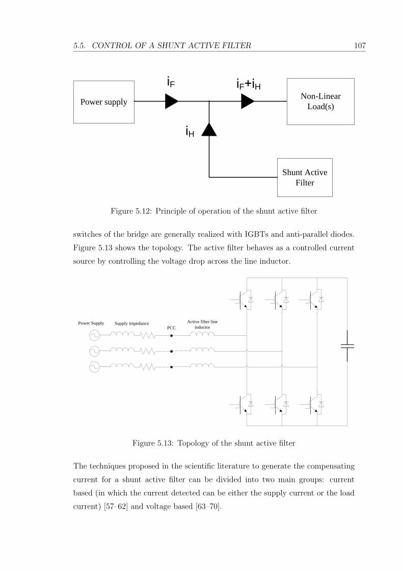
5.5. CONTROL OF A SHUNT ACTIVE FILTER 107
Power supply
Shunt Active Filter
Non-Linear Load(s)
F
H
F H
Figure 5.12: Principle of operation of the shunt active filter
switches of the bridge are generally realized with IGBTs and anti-parallel diodes.
Figure 5.13 shows the topology. The active filter behaves as a controlled current
source by controlling the voltage drop across the line inductor.
Supply impedance Active filter line inductor
Power SupplyPCC
Figure 5.13: Topology of the shunt active filter
The techniques proposed in the scientific literature to generate the compensating
current for a shunt active filter can be divided into two main groups: current
based (in which the current detected can be either the supply current or the load
current) [57–62] and voltage based [63–70].

5.5. CONTROL OF A SHUNT ACTIVE FILTER 108
In the current based methods the reference current can be either calculated on the
basis of the supply current or on the basis of the harmonic current drawn by the
load. In the former method only the measurement of the PCC voltage and the
supply current are needed, but the disadvantage is that the active filter current is
not available to the controllers, which can create problems related to overcurrent
protection. The latter method, which uses the measurement of the load current,
has the advantage that both the load current and the active filter current are
available for the controllers, but the measurement of the load current, the active
filter current and the PCC voltage are needed.
The voltage detection method has been investigated in the past decade by differ-
ent authors. In [63] the authors present a control method for a shunt active power
filter based on the detection of the voltage at the PCC and the real-time simula-
tion of an LC filter by means of a digital signal processor. The work presented
in [65] deals with the control strategy of a shunt active filter, based on voltage
detection. Furthermore in this paper the best location of the filter in the power
distribution system is selected, in order to obtain the best performance in damp-
ing the harmonics generated by resonance between the capacitors and inductors
in the network. In [67–69] the authors investigate a control method for voltage
feedback, selective harmonic, shunt active filters, analysing the advantages of the
technique and the stability issues. In [70] a voltage feedback control technique for
shunt active filters is presented, with multiple reference frames.
In the voltage detection methods the reference current is derived from the mea-
surement of the PCC voltage and the active filter current, therefore only these
two measurements are needed. Generally also the information about the supply
impedance is required, although a rough estimate is sufficient for a robust control
(in the method proposed in this work, it has been observed that a mismatch of up
to 100% in the supply impedance estimate does not compromise the stability of
the control). The advantage of this method is primarily that the active filter can
be used for the compensation of both identified loads whose location and charac-
teristics are well known, and unidentified loads. The active filter in this case can
be seen as a plug-and-play sensorless system installed directly on the bus bar with-
out requiring any external current transducer to measure the distorting non-linear
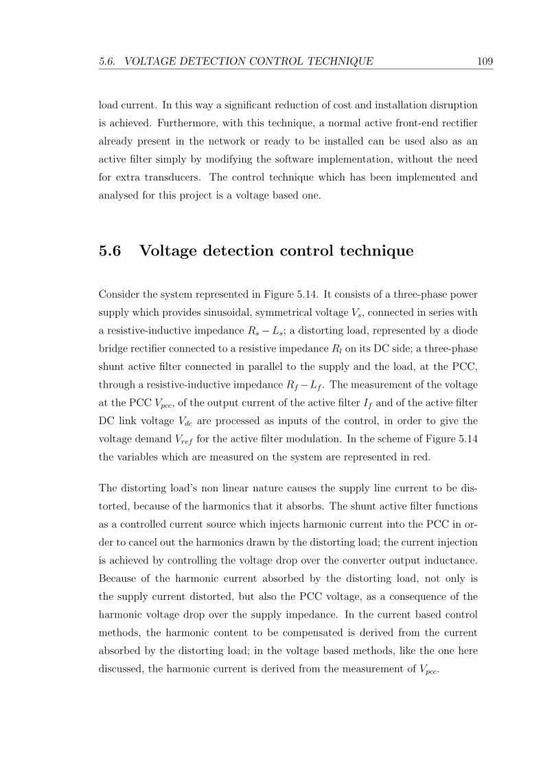
5.6. VOLTAGE DETECTION CONTROL TECHNIQUE 109
load current. In this way a significant reduction of cost and installation disruption
is achieved. Furthermore, with this technique, a normal active front-end rectifier
already present in the network or ready to be installed can be used also as an
active filter simply by modifying the software implementation, without the need
for extra transducers. The control technique which has been implemented and
analysed for this project is a voltage based one.
5.6 Voltage detection control technique
Consider the system represented in Figure 5.14. It consists of a three-phase power
supply which provides sinusoidal, symmetrical voltage Vs, connected in series with
a resistive-inductive impedance Rs−Ls; a distorting load, represented by a diode
bridge rectifier connected to a resistive impedance Rl on its DC side; a three-phase
shunt active filter connected in parallel to the supply and the load, at the PCC,
through a resistive-inductive impedance Rf−Lf . The measurement of the voltage
at the PCC Vpcc, of the output current of the active filter If and of the active filter
DC link voltage Vdc are processed as inputs of the control, in order to give the
voltage demand Vref for the active filter modulation. In the scheme of Figure 5.14
the variables which are measured on the system are represented in red.
The distorting load’s non linear nature causes the supply line current to be dis-
torted, because of the harmonics that it absorbs. The shunt active filter functions
as a controlled current source which injects harmonic current into the PCC in or-
der to cancel out the harmonics drawn by the distorting load; the current injection
is achieved by controlling the voltage drop over the converter output inductance.
Because of the harmonic current absorbed by the distorting load, not only is
the supply current distorted, but also the PCC voltage, as a consequence of the
harmonic voltage drop over the supply impedance. In the current based control
methods, the harmonic content to be compensated is derived from the current
absorbed by the distorting load; in the voltage based methods, like the one here
discussed, the harmonic current is derived from the measurement of Vpcc.
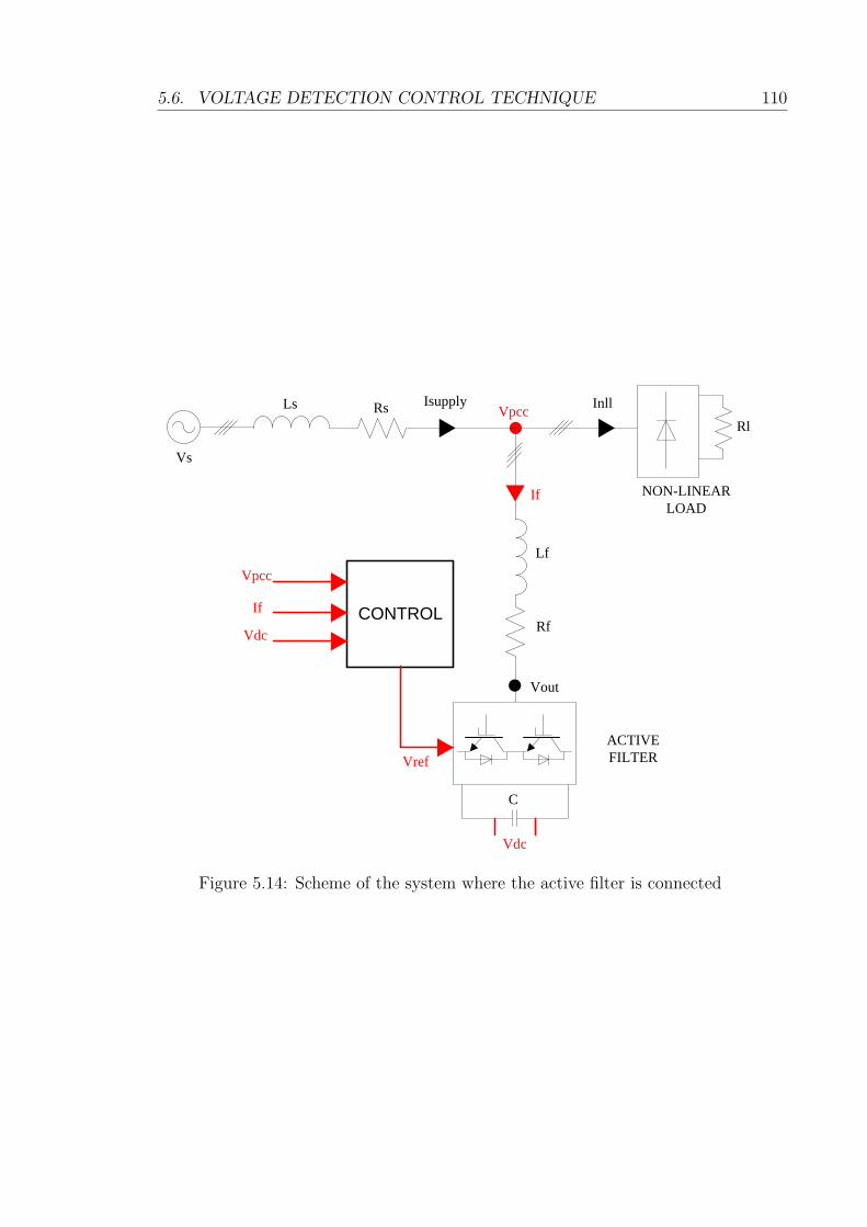
5.6. VOLTAGE DETECTION CONTROL TECHNIQUE 110
Vs
Vdc
If
Vpcc
CONTROL
Ls Rs
Lf
Rf
Rl
Vpcc
If
Vdc
NON-LINEAR LOAD
ACTIVE FILTER Vref
Vout
Isupply Inll
C
Figure 5.14: Scheme of the system where the active filter is connected

5.6. VOLTAGE DETECTION CONTROL TECHNIQUE 111
The PCC voltage abc components are transformed into dq components on different
rotating reference frames (as many as the harmonics which need to be compen-
sated, plus the fundamental). The dq components on each frame are decoupled
from all the other harmonics in order to obtain DC quantities representing the
harmonic synchronous with that particular reference frame. The control structure
is composed of one control system for the fundamental and one for each harmonic.
In the following sections the fundamental and the harmonic control loop structure
are described.
5.6.1 The fundamental control loop
The fundamental control system is composed of two sections, one for the d axis
and the other for the q axis. The d axis section is represented by two cascaded
loops, one for the DC link voltage and one for the d component of the fundamental
current, while the q axis section consists only of the current control loop for the
q component of the fundamental current. The DC link voltage control keeps the
voltage constantly equal to a reference value V dcref and regulates the exchange
of active power between the active filter and the supply. Under ideal conditions,
with no losses in the system, the active filter does not exchange active power with
the supply and the DC link voltage is kept constant without any control action. In
the real system a voltage controller is necessary to achieve that. The output of the
voltage loop represents the current reference on the d axis, id1ref . The current
control on the q axis regulates the exchange of reactive power between the active
filter and the supply. In the case examined for this work the fundamental current
reference on the q axis, iq1ref , is set to zero as the active filter is utilized only for
harmonic compensation and not for reactive power regulation. The two current
controllers, one on each axis, process the error between the dq components of the
measured output current and their references, id1ref and iq1ref and generate a
voltage demand in order to ideally reduce the error to zero. The DC link voltage
control has been designed with much a lower bandwidth than the current control,
so that the two dynamics can be considered independent one from the other, as it
is explained in the following section. Figure 5.15 shows a schematic of the whole
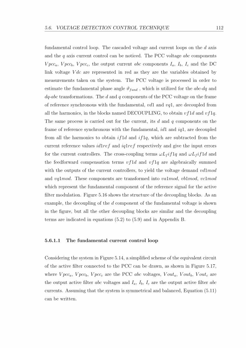
5.6. VOLTAGE DETECTION CONTROL TECHNIQUE 112
fundamental control loop. The cascaded voltage and current loops on the d axis
and the q axis current control can be noticed. The PCC voltage abc components
V pcca, V pccb, V pccc, the output current abc components Ia, Ib, Ic and the DC
link voltage V dc are represented in red as they are the variables obtained by
measurements taken on the system. The PCC voltage is processed in order to
estimate the fundamental phase angle ϑfund , which is utilized for the abc-dq and
dq-abc transformations. The d and q components of the PCC voltage on the frame
of reference synchronous with the fundamental, vd1 and vq1, are decoupled from
all the harmonics, in the blocks named DECOUPLING, to obtain vf1d and vf1q.
The same process is carried out for the current, its d and q components on the
frame of reference synchronous with the fundamental, id1 and iq1, are decoupled
from all the harmonics to obtain if1d and if1q, which are subtracted from the
current reference values id1ref and iq1ref respectively and give the input errors
for the current controllers. The cross-coupling terms ωLf if1q and ωLf if1d and
the feedforward compensation terms vf1d and vf1q are algebraically summed
with the outputs of the current controllers, to yield the voltage demand vd1mod
and vq1mod. These components are transformed into va1mod, vb1mod, vc1mod
which represent the fundamental component of the reference signal for the active
filter modulation. Figure 5.16 shows the structure of the decoupling blocks. As an
example, the decoupling of the d component of the fundamental voltage is shown
in the figure, but all the other decoupling blocks are similar and the decoupling
terms are indicated in equations (5.2) to (5.9) and in Appendix B.
5.6.1.1 The fundamental current control loop
Considering the system in Figure 5.14, a simplified scheme of the equivalent circuit
of the active filter connected to the PCC can be drawn, as shown in Figure 5.17,
where V pcca, V pccb, V pccc are the PCC abc voltages, V outa, V outb, V outc are
the output active filter abc voltages and Ia, Ib, Ic are the output active filter abc
currents. Assuming that the system is symmetrical and balanced, Equation (5.11)
can be written.

5.6. VOLTAGE DETECTION CONTROL TECHNIQUE 113
Vpcc
a
Vpcc
b
Vpcc c
θ fund
estimation
θ fund
Vdcref
+
-Vdc
DC
link
vo
ltage
co
ntro
ller
id1ref
+
-
if1d
d ax
is
curr
ent
cont
rolle
r
-
+
if1q
iq1ref
q ax
is
curr
ent
cont
rolle
r
-+ +
-
+ -
vf1d
vf1q
ωLf
if1q
ωLf
if1d
vd1mod
vq1mod
dq
abc
va1mod
vb1mod
vc1mod
Vpcc a
Vpcc b
Vpcc
c
abc
dq
vd1
vq1
DEC
OU
PLIN
G
DEC
OU
PLIN
G
vf1d
vf1q
I a I b I c
abc
dq
id1
iq1
DEC
OU
PLIN
G
DEC
OU
PLIN
G
if1d
if1q
θ fund
θ fund
θ fund
*
* see
nex
t fig
ure
Figure 5.15: Scheme of the overall fundamental control loop
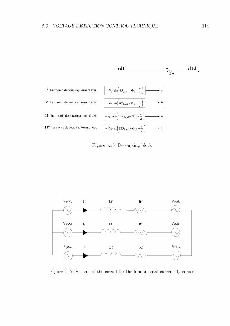
5.6. VOLTAGE DETECTION CONTROL TECHNIQUE 114
vd1 ++
vf1d
+
+
+
+
5th harmonic decoupling term d axis
26sin 55
fundV
26sin 77
fundV
212sin 1111
fundV
212sin 1313
fundV
7th harmonic decoupling term d axis
11th harmonic decoupling term d axis
13th harmonic decoupling term d axis
Figure 5.16: Decoupling block
Ia Lf Rf VoutaVpcca
Ib Lf Rf VoutbVpccb
Ic Lf Rf VoutcVpccc
Figure 5.17: Scheme of the circuit for the fundamental current dynamics
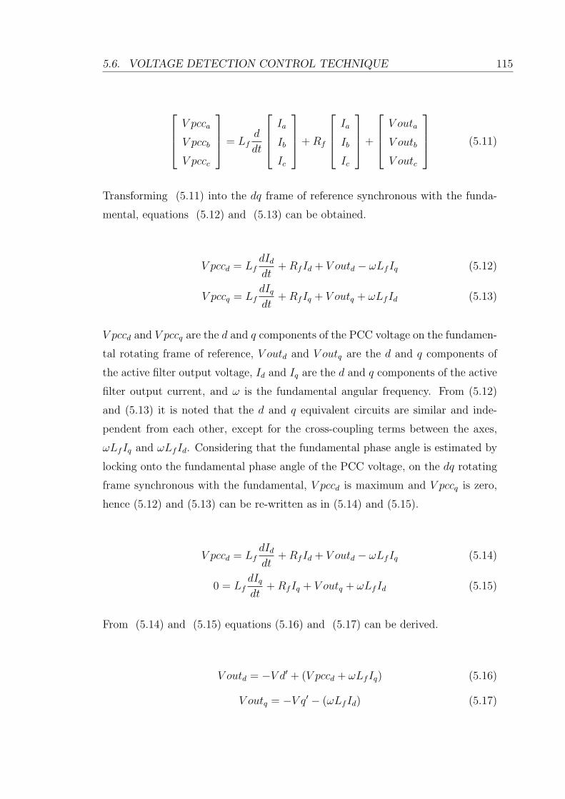
5.6. VOLTAGE DETECTION CONTROL TECHNIQUE 115
V pcca
V pccb
V pccc
= Lfd
dt
Ia
Ib
Ic
+Rf
Ia
Ib
Ic
+
V outa
V outb
V outc
(5.11)
Transforming (5.11) into the dq frame of reference synchronous with the funda-
mental, equations (5.12) and (5.13) can be obtained.
V pccd = LfdIddt
+RfId + V outd − ωLfIq (5.12)
V pccq = LfdIqdt
+RfIq + V outq + ωLfId (5.13)
V pccd and V pccq are the d and q components of the PCC voltage on the fundamen-
tal rotating frame of reference, V outd and V outq are the d and q components of
the active filter output voltage, Id and Iq are the d and q components of the active
filter output current, and ω is the fundamental angular frequency. From (5.12)
and (5.13) it is noted that the d and q equivalent circuits are similar and inde-
pendent from each other, except for the cross-coupling terms between the axes,
ωLfIq and ωLfId. Considering that the fundamental phase angle is estimated by
locking onto the fundamental phase angle of the PCC voltage, on the dq rotating
frame synchronous with the fundamental, V pccd is maximum and V pccq is zero,
hence (5.12) and (5.13) can be re-written as in (5.14) and (5.15).
V pccd = LfdIddt
+RfId + V outd − ωLfIq (5.14)
0 = LfdIqdt
+RfIq + V outq + ωLfId (5.15)
From (5.14) and (5.15) equations (5.16) and (5.17) can be derived.
V outd = −V d′ + (V pccd + ωLfIq) (5.16)
V outq = −V q′ − (ωLfId) (5.17)
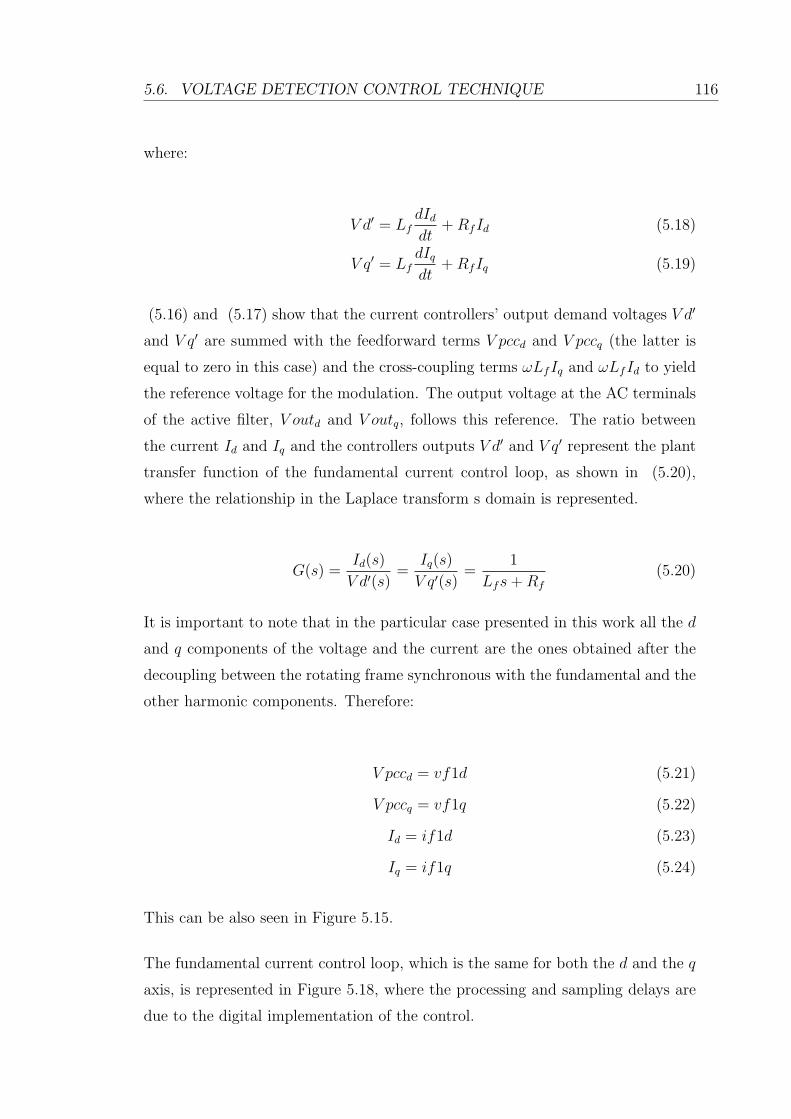
5.6. VOLTAGE DETECTION CONTROL TECHNIQUE 116
where:
V d′ = LfdIddt
+RfId (5.18)
V q′ = LfdIqdt
+RfIq (5.19)
(5.16) and (5.17) show that the current controllers’ output demand voltages V d′
and V q′ are summed with the feedforward terms V pccd and V pccq (the latter is
equal to zero in this case) and the cross-coupling terms ωLfIq and ωLfId to yield
the reference voltage for the modulation. The output voltage at the AC terminals
of the active filter, V outd and V outq, follows this reference. The ratio between
the current Id and Iq and the controllers outputs V d′ and V q′ represent the plant
transfer function of the fundamental current control loop, as shown in (5.20),
where the relationship in the Laplace transform s domain is represented.
G(s) =Id(s)
V d′(s)=
Iq(s)
V q′(s)=
1
Lfs+Rf
(5.20)
It is important to note that in the particular case presented in this work all the d
and q components of the voltage and the current are the ones obtained after the
decoupling between the rotating frame synchronous with the fundamental and the
other harmonic components. Therefore:
V pccd = vf1d (5.21)
V pccq = vf1q (5.22)
Id = if1d (5.23)
Iq = if1q (5.24)
This can be also seen in Figure 5.15.
The fundamental current control loop, which is the same for both the d and the q
axis, is represented in Figure 5.18, where the processing and sampling delays are
due to the digital implementation of the control.

5.6. VOLTAGE DETECTION CONTROL TECHNIQUE 117
Current controller
iref ProcessingDelay
+-
Sample &Hold
1
f fL s R
Figure 5.18: Fundamental current control loop
The fundamental current controller has been designed in the form of a Proportional
Integral (PI) regulator. Considering that the reference current to be tracked is a
slowly variable quantity (on the d axis) or a constant value (on the q axis), and
the feedback current presents only very small oscillations due to the small error
in the decoupling, the closed loop bandwidth required is not very high. The plant
transfer function parameters are based on the active filter inductor used for the
simulation and experimental validation:
Lf = 3mH;Rf = 0.1Ω (5.25)
The controller has been designed using the MatLab SISOTOOL toolbox. Its
transfer function in the s domain is:
4.5s+ 2115
s(5.26)
The closed loop poles coordinates in the s plane are -577+j441, the natural fre-
quency is 116 Hz, the damping factor is 0.794, the closed loop bandwidth is 243
Hz.
5.6.1.2 The DC link voltage control loop
The DC link voltage control aims at regulating the exchange of active power
between the active filter and the power supply. Under ideal conditions and with
no load connected to the DC side of the converter, there are no losses in the

5.6. VOLTAGE DETECTION CONTROL TECHNIQUE 118
DC link and in the converter switches, therefore the DC link voltage is kept at a
constant value without utilizing a regulation. However in practice there are losses
in the DC capacitor, in the switching devices and in the resistive component of the
active filter line inductor, therefore it is necessary to regulate the DC link voltage,
keeping it constant by absorbing a limited amount of active power from the power
network in order to match the losses. The equations that describe the DC link
voltage control and from which it is possible to derive the plant transfer function
will be now presented [71]. Let the current flowing in the DC link be indicated as
Idc and the voltage across the DC link be indicated as V dc. The power balance
between the input and the output can be expressed by the formula (5.27).
Idc = 3IdV outd + IqV outq
V dc(5.27)
If the losses in the DC link, in the switches and in the line inductor are neglected:
V outd = V pccd;V outq = V pccq = 0 (5.28)
Therefore (5.27) can be written as (5.29); furthermore equations (5.30) and (5.31)
can be stated.
Idc = 3IdV pccdV dc
(5.29)
m =2√
2V pccdV dc
(5.30)
CdV dc
dt= Idc (5.31)
Where m is the modulation index. (5.29) and (5.30) can be combined to yield
equation (5.32):

5.6. VOLTAGE DETECTION CONTROL TECHNIQUE 119
Idc =3mId
2√
2(5.32)
(5.31) and (5.32) can be combined to yield equation (5.33), which represents the
s domain transfer function of the DC link voltage control loop plant:
V dc(s)
Id(s)=
3m
2√
2Cs(5.33)
From (5.12), (5.13) and (5.29) to (5.31) it is possible to draw the active filter
fundamental equivalent circuit in the dq reference frame as depicted in Figure 5.19.
Vpccd
Lf RfωLfIq
Voutd
Vpccq
Lf RfωLfId
Voutq
CVdc
Idc
Figure 5.19: dq equivalent circuit of the active filter
The DC link voltage control loop is represented in Figure 5.20, where the process-
ing and sampling delays are due to the digital implementation of the control.
The DC link voltage controller has been designed in the form of a Proportional
Integral (PI) regulator, with a much lower bandwidth than the fundamental cur-
rent control, so that the two control loops can be considered independent one from
the other. The plant transfer function parameters are based on the active filter
capacitor used for the simulation and experimental validation:
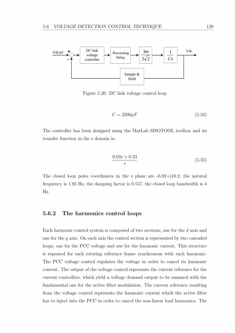
5.6. VOLTAGE DETECTION CONTROL TECHNIQUE 120
DC link voltage
controller
Vdcref
Sample &Hold
22
3m
Cs
1 VdcProcessingDelay
Figure 5.20: DC link voltage control loop
C = 2200µF (5.34)
The controller has been designed using the MatLab SISOTOOL toolbox and its
transfer function in the s domain is:
0.03s+ 0.33
s(5.35)
The closed loop poles coordinates in the s plane are -6.82+j10.2, the natural
frequency is 1.95 Hz, the damping factor is 0.557, the closed loop bandwidth is 4
Hz.
5.6.2 The harmonics control loops
Each harmonic control system is composed of two sections, one for the d axis and
one for the q axis. On each axis the control section is represented by two cascaded
loops, one for the PCC voltage and one for the harmonic current. This structure
is repeated for each rotating reference frame synchronous with each harmonic.
The PCC voltage control regulates the voltage in order to cancel its harmonic
content. The output of the voltage control represents the current reference for the
current controllers, which yield a voltage demand output to be summed with the
fundamental one for the active filter modulation. The current reference resulting
from the voltage control represents the harmonic current which the active filter
has to inject into the PCC in order to cancel the non-linear load harmonics. The
5.6. VOLTAGE DETECTION CONTROL TECHNIQUE 121
detection of this current is not carried out by direct measurement of the harmonics
absorbed by the non-linear load but from the measurement of the PCC voltage
and the analysis of its harmonic content. The voltage harmonics are due to the
voltage drop of the current harmonics on the supply impedance, and are generally
smaller than the current harmonics, hence good precision in the voltage harmonic
analysis is necessary in order for a successful compensation to be achieved.
Figure 5.21 shows a schematic of the 5th harmonic control system, including cas-
caded voltage and current loop on the d axis and the q axis. The PCC voltage abc
components V pcca, V pccb, V pccc and the output current abc components Ia, Ib,
Ic are represented in red as they are the only variables obtained by measurements
taken on the system. The d and q components of the PCC voltage on the reference
frame synchronous with the 5th harmonic, vd5 and vq5, are obtained by using the
angle −5ϑfund and decoupled from the fundamental and all the other harmonics, in
the blocks names DECOUPLING, to obtain vf5d and vf5q. The same approach
is used for the current. Its d and q components on the reference frame synchronous
with the 5th harmonic, id5 and iq5, are decoupled from the fundamental and all
the other harmonics to obtain if5d and if5q. vf5d and vf5q are subtracted from
the voltage reference values vf5dref and vf5qref respectively to give the input
error for the voltage controllers. vf5dref and vf5qref are set to zero in order to
cancel the voltage 5th harmonic. if5d and if5q are subtracted from the current
reference values if5dref and if5qref respectively to give the input error for the
current controllers. The output of the current controllers gives the voltage demand
for the modulation vd5mod and vq5mod. These components are then transformed
into va5mod, vb5mod, vc5mod which represent the 5th harmonic component of the
reference signal for the active filter modulation.
The control structure for the other harmonic components is similar to the one just
described apart from the decoupling terms, which are calculated as presented in
Section 5.3 and Appendix B, and the angle utilized for the dq transformations.
This is equal to ±hϑfund, where h is the harmonic order and the sign depends on
the harmonic being positive or negative sequence.
Figure 5.22 shows the schematic of the overall control. The fundamental control
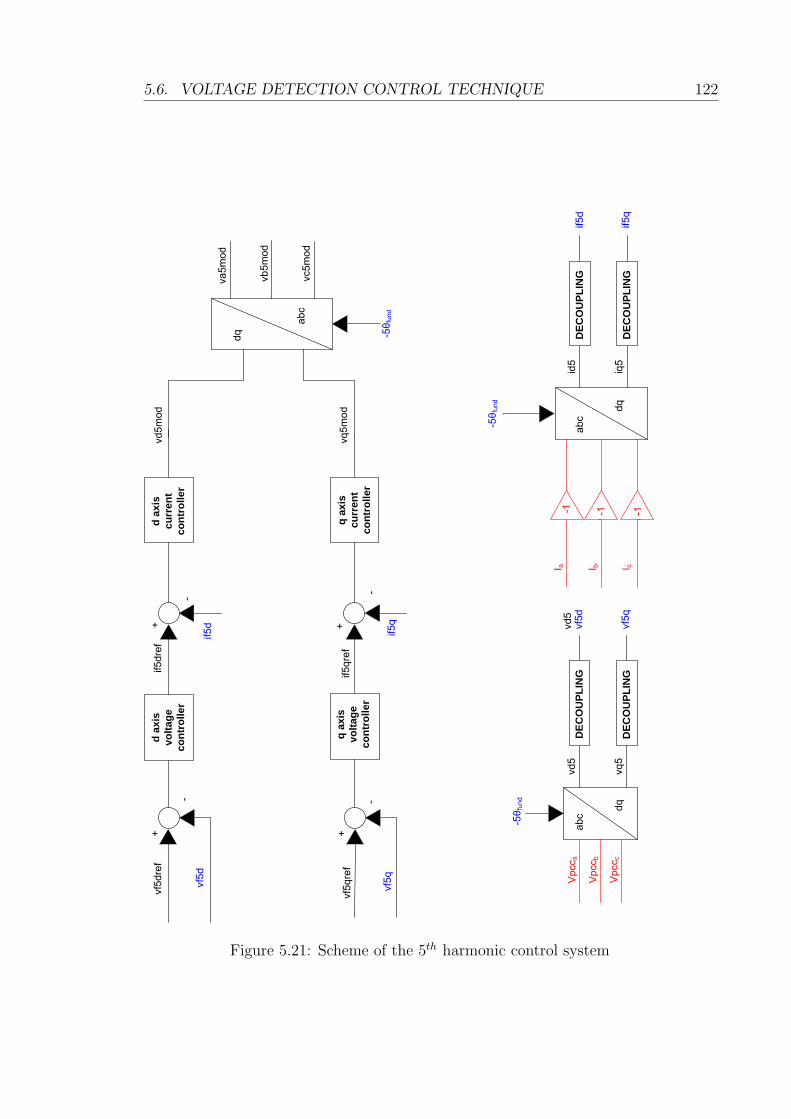
5.6. VOLTAGE DETECTION CONTROL TECHNIQUE 122
vf5dref
+
-vf5d
d ax
is
volta
ge
cont
rolle
r
if5dref
+
-
if5d
d ax
is
curr
ent
cont
rolle
r
-
+ if5q
if5qref
q ax
is
curr
ent
cont
rolle
r
vd5mod
vq5mod
dq
abc
va5mod
vb5mod
vc5mod
Vpcc a
Vpcc b
Vpcc c
abc
dq
vd5
vq5
DEC
OU
PLIN
G
DEC
OU
PLIN
G
vf5d
vf5q
I a I b I c
abc
dq
id5
iq5
DEC
OU
PLIN
G
DEC
OU
PLIN
G
if5d
if5q
-5θ fund
-5θ fund
-5θ fund
-1 -1 -1
vf5qref
+
-vf5q
q ax
is
volta
ge
cont
rolle
r
vd5
Figure 5.21: Scheme of the 5th harmonic control system
5.6. VOLTAGE DETECTION CONTROL TECHNIQUE 123
system and the harmonic control systems, from the 5th to the nth harmonic, yield
the modulating outputs which, summed together on each phase, represent the
reference voltage for the active filter modulation, indicated as varef , vbref and
vcref .
5.6.2.1 The harmonic voltage control loop
This section will show the calculation of the plant transfer function for the har-
monic voltage control and the design of the controller. A small signal model of the
system is considered for this analysis [72]. Figure 5.23 shows the equivalent circuit
for the harmonic frequencies: the power supply is represented as a short circuit in
this model as it generates only fundamental voltage. The active filter and the non-
linear load are represented as sources of current at the generic harmonic frequency
±hω. They are connected in parallel at the PCC and their generated currents are
indicated as Iasf and Iload. The supply impedance Rs, Ls is also represented in
Figure 5.23.
From Figure 5.23 Equation (5.36) can be written.
0− V pcca0− V pccb0− V pccc
= Lsd
dt
Ia
Ib
Ic
+Rs
Ia
Ib
Ic
(5.36)
Transforming (5.36) into the dq frame of reference synchronous with the hth
harmonic, equations (5.37) and (5.38) can be obtained.
−V pccd = LsdIddt
+RsId − ωLsIq (5.37)
−V pccq = LsdIqdt
+RsIq + ωLsId (5.38)
The current I represents the sum between the active filter current and the non-
linear load current:

5.6. VOLTAGE DETECTION CONTROL TECHNIQUE 124
Vs
Vdc
If
Vpc
cLs
Rs
Lf Rf
Rl
Vpc
c
If Vdc
NO
N-L
INEA
R
LOA
D
AC
TIV
E FI
LTER
Vre
f
Vou
t
Isup
ply
Inll
C
FUN
DA
MEN
TAL
CO
NTR
OL
LOO
P
5TH H
AR
MO
NIC
C
ON
TRO
L LO
OP
7TH H
AR
MO
NIC
C
ON
TRO
L LO
OP
nTH
HA
RM
ON
IC
CO
NTR
OL
LOO
P
va1m
od
vb1m
od
vc1m
od
va5m
od
vb5m
od
vc5m
od
va7m
od
vb7m
od
vc7m
od
vanm
od
vbnm
od
vcnm
od
va1m
od
va5m
od
va7m
od
vanm
od
vb1m
od
vb5m
od
vb7m
od
vbnm
od
vc1m
od
vc5m
od
vc7m
od
vcnm
od
vare
f
vbre
f
vcre
f
Figure 5.22: Scheme of the overall control system

5.6. VOLTAGE DETECTION CONTROL TECHNIQUE 125
I Ls RsPCC
IloadIasf
Figure 5.23: Equivalent circuit of the system at the harmonic frequencies
Id = Id asf + Id load (5.39)
Iq = Iq asf + Iq load (5.40)
So equations (5.37) and (5.38) can be written as:
−V pccd = Lsd
dt(Id asf + Id load) +Rs(Id asf + Id load)− ωLs(Iq asf + Iq load) (5.41)
−V pccq = Lsd
dt(Iq asf + Iq load) +Rs(Iq asf + Iq load) + ωLs(Id asf + Id load) (5.42)
Applying a perturbation to each variable and carrying out the Laplace transfor-
mation to (5.41) and (5.42):
−∆V pccd = (Lss+Rs)(∆Id asf + ∆Id load)− ωLs(∆Iq asf + ∆Iq load) (5.43)
−∆V pccq = (Lss+Rs)(∆Iq asf + ∆Iq load) + ωLs(∆Id asf + ∆Id load) (5.44)
Assuming that the load current does not change during the short time interval
chosen for the small signal analysis, it is possible to write:
5.6. VOLTAGE DETECTION CONTROL TECHNIQUE 126
∆Id load = 0 (5.45)
∆Iq load = 0 (5.46)
Hence (5.43) and (5.44) can be written as:
−∆V pccd = (Lss+Rs)(∆Id asf )− ωLs∆Iq asf (5.47)
−∆V pccq = (Lss+Rs)(∆Iq asf ) + ωLs∆Id asf (5.48)
Equations (5.47) and (5.48) show that the d and q axes present similar dynamics
and they are independent one from another, excluding the cross-coupling terms
ωLsIqasfand ωLsIdasf
. On each axis the ratio between the PCC voltage variation
and the variation of the current is given by equation (5.49), which presents the s
domain transfer function for the harmonic voltage control :
G(s) =∆V pccd∆Id asf
=∆V pccq∆Iq asf
= Lss+Rs (5.49)
It is important to note that in the particular case presented in this work the voltage
and current d and q components are the ones obtained after the decoupling between
the rotating frame synchronous with the hth harmonic and all the other harmonic
components including the fundamental. Therefore:
V pccd = vfhd (5.50)
V pccq = vfhq (5.51)
Id asf = ifhd (5.52)
Iq asf = ifhq (5.53)
This can be also seen in Figure 5.21.
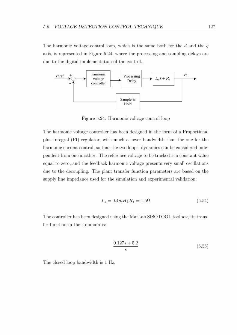
5.6. VOLTAGE DETECTION CONTROL TECHNIQUE 127
The harmonic voltage control loop, which is the same both for the d and the q
axis, is represented in Figure 5.24, where the processing and sampling delays are
due to the digital implementation of the control.
harmonic voltage
controller
vhref
Sample &Hold
ss RsL vhProcessing
Delay
Figure 5.24: Harmonic voltage control loop
The harmonic voltage controller has been designed in the form of a Proportional
plus Integral (PI) regulator, with much a lower bandwidth than the one for the
harmonic current control, so that the two loops’ dynamics can be considered inde-
pendent from one another. The reference voltage to be tracked is a constant value
equal to zero, and the feedback harmonic voltage presents very small oscillations
due to the decoupling. The plant transfer function parameters are based on the
supply line impedance used for the simulation and experimental validation:
Ls = 0.4mH;Rf = 1.5Ω (5.54)
The controller has been designed using the MatLab SISOTOOL toolbox, its trans-
fer function in the s domain is:
0.127s+ 5.2
s(5.55)
The closed loop bandwidth is 1 Hz.

5.7. SUMMARY 128
5.7 Summary
This chapter has presented a control technique for active shunt power filters based
on the detection of the voltage at the Point of Common Coupling. The extraction
of the harmonics is carried out by means of multiple rotating reference frames,
decoupled one from each other. The decoupling technique allows accurate identi-
fication of the harmonic components to be compensated, without using low-pass
or band-pass filters. The decoupling equations, with examples that show accurate
decoupling and the possible causes of inaccurate decoupling, have been presented
in this chapter. The control structure has also been described, with demonstra-
tions of how the control dynamics are represented mathematically, and description
of the controllers design. The description of the control technique shows how it is
possible to identify the reference current for the active filter, and to control the
current that it injects in the system just by measuring the PCC voltage without
the need for extra current sensors on the distorting load. In the next chapter the
results obtained in simulation by implementing this technique will be presented
and analysed in order to prove the effectiveness of the method.
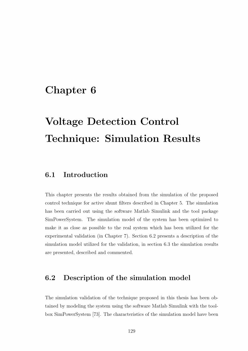
Chapter 6
Voltage Detection Control
Technique: Simulation Results
6.1 Introduction
This chapter presents the results obtained from the simulation of the proposed
control technique for active shunt filters described in Chapter 5. The simulation
has been carried out using the software Matlab Simulink and the tool package
SimPowerSystem. The simulation model of the system has been optimized to
make it as close as possible to the real system which has been utilized for the
experimental validation (in Chapter 7). Section 6.2 presents a description of the
simulation model utilized for the validation, in section 6.3 the simulation results
are presented, described and commented.
6.2 Description of the simulation model
The simulation validation of the technique proposed in this thesis has been ob-
tained by modeling the system using the software Matlab Simulink with the tool-
box SimPowerSystem [73]. The characteristics of the simulation model have been
129
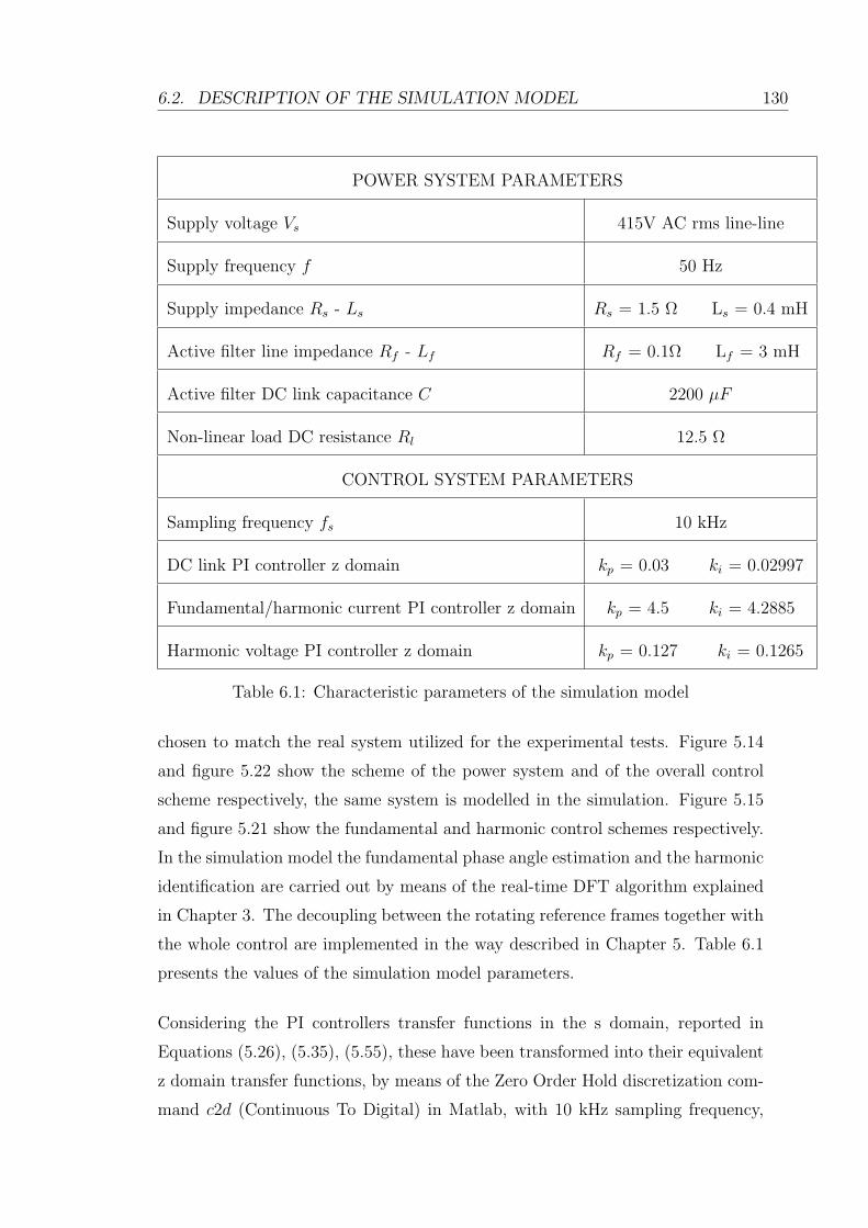
6.2. DESCRIPTION OF THE SIMULATION MODEL 130
POWER SYSTEM PARAMETERS
Supply voltage Vs 415V AC rms line-line
Supply frequency f 50 Hz
Supply impedance Rs - Ls Rs = 1.5 Ω Ls = 0.4 mH
Active filter line impedance Rf - Lf Rf = 0.1Ω Lf = 3 mH
Active filter DC link capacitance C 2200 µF
Non-linear load DC resistance Rl 12.5 Ω
CONTROL SYSTEM PARAMETERS
Sampling frequency fs 10 kHz
DC link PI controller z domain kp = 0.03 ki = 0.02997
Fundamental/harmonic current PI controller z domain kp = 4.5 ki = 4.2885
Harmonic voltage PI controller z domain kp = 0.127 ki = 0.1265
Table 6.1: Characteristic parameters of the simulation model
chosen to match the real system utilized for the experimental tests. Figure 5.14
and figure 5.22 show the scheme of the power system and of the overall control
scheme respectively, the same system is modelled in the simulation. Figure 5.15
and figure 5.21 show the fundamental and harmonic control schemes respectively.
In the simulation model the fundamental phase angle estimation and the harmonic
identification are carried out by means of the real-time DFT algorithm explained
in Chapter 3. The decoupling between the rotating reference frames together with
the whole control are implemented in the way described in Chapter 5. Table 6.1
presents the values of the simulation model parameters.
Considering the PI controllers transfer functions in the s domain, reported in
Equations (5.26), (5.35), (5.55), these have been transformed into their equivalent
z domain transfer functions, by means of the Zero Order Hold discretization com-
mand c2d (Continuous To Digital) in Matlab, with 10 kHz sampling frequency,

6.3. SIMULATION RESULTS 131
and the gains are indicated in Table 6.1. It is possible to use this method because
the ratio between the sampling frequency and the natural frequency of the closed
loop system is bigger than 15. The controller is designed in the s domain and its
transfer function is discretized directly, with no need to design the controller in
the z domain.
C(s) =4.5s+ 2115
s−→ C(z) =
4.5z − 4.2885
z − 1(6.1)
C(s) =0.03s+ 0.33
s−→ C(z) =
0.03z − 0.02997
z − 1(6.2)
C(s) =0.127s+ 5.2
s−→ C(z) =
0.127z − 0.1265
z − 1(6.3)
In the simulation validation, the magnitudes of the PCC voltage harmonics to
be compensated are: 11.66V, 6.05V, 4.65V, 3.36V for the 5th, 7th, 11th and 13th
respectively. The magnitudes of the current harmonics to be compensated are:
7.18A, 3.50A, 2.27A, 1.50A for the 5th, 7th, 11th and 13th respectively.
6.3 Simulation results
In this section the simulation results are presented and commented. Figures 6.1
to 6.4 show the d and q components of the PCC voltage on the different harmonic
rotating reference frames where the compensation of 5th, 7th, 11th and 13th is
tested. Particularly the control transient is shown: the control is enabled at 0.5
s. Before the control is enabled, the voltage mean value is different from zero and
it depends on the voltage harmonic value. After the control is enabled, the mean
value of the voltage settles to zero, which is the reference.
It can be seen that the q component of the voltage on each reference frame is zero
not only after the control is enabled but also before that. This is due to the charac-
teristics of the non-linear load included in the simulation model. It consists of an

6.3. SIMULATION RESULTS 132
ideal three-phase diode bridge rectifier and it is simulated by means of the block
”‘Universal bridge”’ in Simulink SimPowerSystems. When using this block, the
current absorbed by the distorting load is characterized by relative phase between
each harmonic and the fundamental equal to zero. Therefore, when transform-
ing the supply current into each harmonic reference frame, using the fundamental
phase angle multiplied by the harmonic index, the harmonic presents zero q com-
ponent in the rotating frame. Since the supply impedance in the simulation is
mainly resistive (the simulation model represents the system used for the experi-
mental validation, in which a high supply resistance has been used in order to get a
voltage drop high enough to be measured by the voltage transducers), the voltage
harmonics, caused by the voltage drop, are almost in phase with the harmonic
currents, so also the voltage harmonics have zero q component on the different
harmonic reference frames.
Both before and after the control enabling instant, the voltage is decoupled from
all the other harmonics, nevertheless in the figures an oscillation can be noticed.
This is due to the presence of all the other harmonics injected by the non-linear
load, above the 13th, and the harmonics injected by the active filter itself. These
harmonics are not included in the decoupling system, so they are found in the
feedback path of the harmonic voltage control.
Figures 6.5 to 6.8 show the FFT spectrum of the d components of the PCC voltage
on the harmonic rotating reference frames.
From figures 6.5 to 6.8 it can be seen that the 0 Hz component is reduced to nearly
0 V, because of the control action. The components with the highest amplitudes
in the spectrum can be seen at the frequencies: 300 Hz, 600 Hz, 900 Hz, 1200 Hz,
1500 Hz, 1800 Hz, 2100 Hz, 2400 Hz, 2700 Hz. These components correspond to
the harmonics injected by the non-linear load, with an order higher than 13. They
are not compensated by the control system and they are not taken into account
in the decoupling, so they are bound to be observed in the PCC voltage, feedback
of the control. As well as the high order harmonics due to the distorting load,
other harmonics due to the active filter itself can be seen, such as those at 150
Hz and 450 Hz. As explained in Section 5.2, each harmonic is seen on a rotating

6.3. SIMULATION RESULTS 133
0.4 0.45 0.5 0.55 0.6 0.65−10
0
10
20
30
40
vf5dvo
ltage
[V]
refvf5d
0.4 0.45 0.5 0.55 0.6 0.65−20
−15
−10
−5
0
5
10
15
20vf5q
time [s]
volta
ge [V
]
refvf5q
vf5d
ref
Figure 6.1: d and q components of the PCC voltage on the 5th harmonic frame
0.4 0.45 0.5 0.55 0.6 0.65−20
−10
0
10
20
30vf7d
volta
ge [V
]
refvf7d
0.4 0.45 0.5 0.55 0.6 0.65−20
−10
0
10
20
30vf7q
time [s]
volta
ge [V
]
refvf7q
ref
vf7d
Figure 6.2: d and q components of the PCC voltage on the 7th harmonic frame
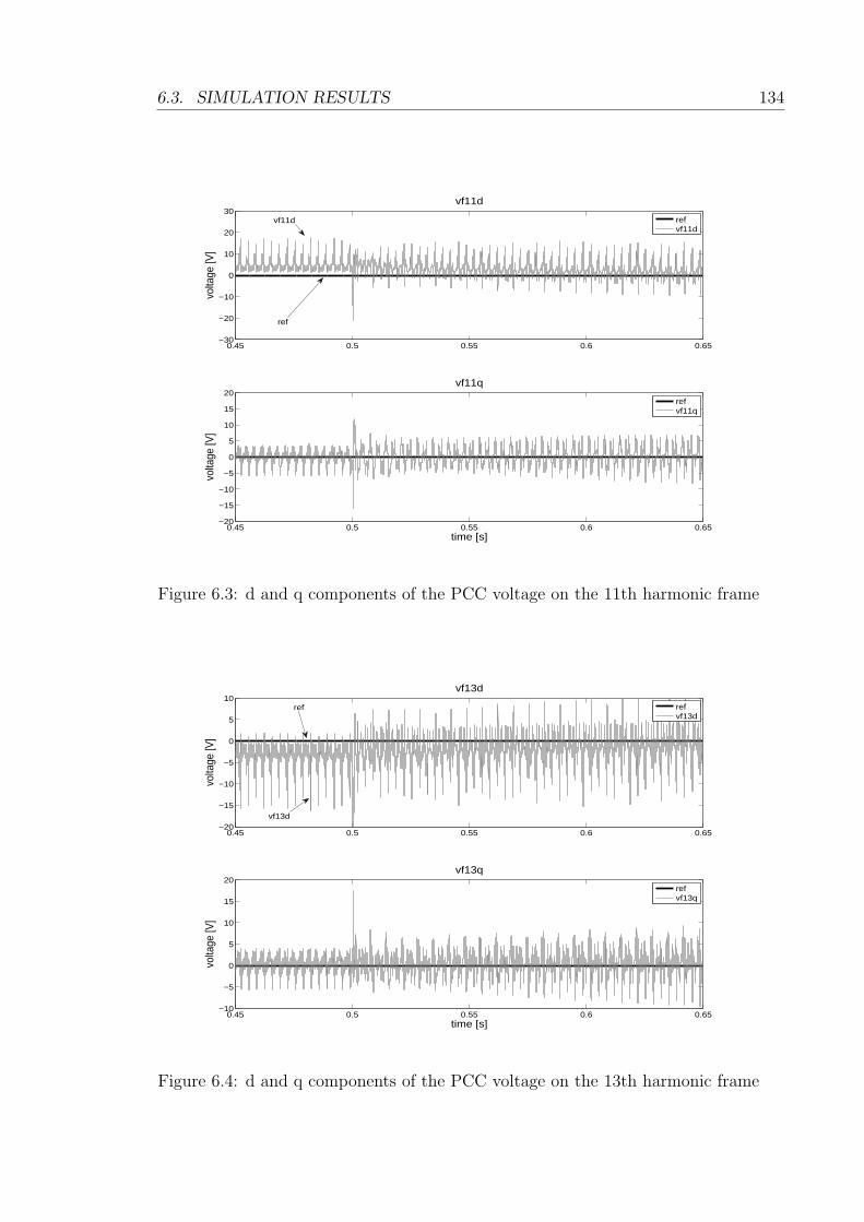
6.3. SIMULATION RESULTS 134
0.45 0.5 0.55 0.6 0.65−30
−20
−10
0
10
20
30vf11d
volta
ge [V
]
refvf11d
0.45 0.5 0.55 0.6 0.65−20
−15
−10
−5
0
5
10
15
20vf11q
time [s]
volta
ge [V
]
refvf11q
ref
vf11d
Figure 6.3: d and q components of the PCC voltage on the 11th harmonic frame
0.45 0.5 0.55 0.6 0.65−20
−15
−10
−5
0
5
10vf13d
volta
ge [V
]
refvf13d
0.45 0.5 0.55 0.6 0.65−10
−5
0
5
10
15
20vf13q
time [s]
volta
ge [V
]
refvf13q
ref
vf13d
Figure 6.4: d and q components of the PCC voltage on the 13th harmonic frame

6.3. SIMULATION RESULTS 135
0 150 300 450 600 900 1200 1500 1800 2100 2400 2700 30000
0.2
0.4
0.6
0.8
1
1.2
frequency [Hz]
perc
enta
ge o
f th
e fundam
enta
l
Figure 6.5: FFT of the d component of the PCC voltage on the 5th harmonicframe
0 150 450 600 900 1200 1500 1800 2100 2400 2700 30000
0.1
0.2
0.3
0.4
0.5
0.6
0.7
0.8
0.9
1
pe
rce
nta
ge
of
the
fu
nd
am
en
tal
Figure 6.6: FFT of the d component of the PCC voltage on the 7th harmonicframe

6.3. SIMULATION RESULTS 136
0 150 300 450 600 900 1,200 1,500 1800 2100 2700 300024000
0.2
0.4
0.6
0.8
1
1.2
frequency [Hz]
pe
rce
nta
ge
of
the
fu
nd
am
en
tal
Figure 6.7: FFT of the d component of the PCC voltage on the 11th harmonicframe
0 150 300 450 600 900 1200 1500 1800 2100 2400 2700 30000
0.1
0.2
0.3
0.4
0.5
0.6
0.7
0.8
0.9
1
frequency [Hz]
pe
rce
nta
ge
of
the
fu
nd
am
en
tal
Figure 6.8: FFT of the d component of the PCC voltage on the 13th harmonicframe
6.3. SIMULATION RESULTS 137
Reference Harmonics as seen in the spectrum [Hz]
frame 150 300 450 600 900 1200 1500 1800 2100 2400 2700
5 2;8 4;14 17 23 19;29 25;35 31;41 37;47 43;53 49;59
7 4;10 2;16 19 25 17;31 23;37 29;43 35;49 41;55 47;61
11 8;14 17 2;20 23 29 35 19;41 25;47 31;53 37;59 43;65
13 10;16 19 4;22 25 31 37 17;43 23;49 29;55 35;61 41;67
Table 6.2: Harmonics as seen in the FFT spectrum of the voltage on the differentreference frames
reference frame as a sinusoidal component oscillating at its relative angular speed.
The relative angular speed is given by (5.1). Table 6.2 specifies the absolute har-
monic order corresponding to each harmonic component of the spectrum seen in
the rotating reference frames. Only the components with the largest amplitudes
have been considered. The cells which have been left blank correspond to the
components which have zero amplitude in that particular spectrum: they corre-
spond to harmonics which have been decoupled. The double numbers in some
cells correspond to the two harmonics (one positive sequence and one negative
sequence) which are seen with the same relative frequency in that reference frame.
In some cells only one harmonic order is reported, as the other harmonic seen with
the same relative frequency has been decoupled so it does not contribute to the
component in the spectrum.
Figures 6.9 to 6.17 show the d and q components of the active filter current on the
harmonic rotating reference frames. The same considerations made for the voltage
oscillations can be made for the current. Particularly figures 6.11, 6.13, 6.15, 6.17
show an expanded view of the current control steady-state. It can be seen that
the reference current and the output current do not match perfectly: the current
PI controller has been designed with a low bandwidth, because it does not need
to track the high order oscillations of the current, but only the DC component of
the reference.
Figures 6.18 and 6.19 show the PCC voltage on the phase A before and after the
active filter harmonic compensation.
It is not easy to see the action of the voltage harmonic compensation in the time

6.3. SIMULATION RESULTS 138
0.45 0.5 0.55 0.6 0.65
−4
−2
0
2
4
6
8
10
12
if1d
curr
ent [
A]
refif1d
0.45 0.5 0.55 0.6 0.65−10
−5
0
5
10if1q
time [s]
curr
ent [
A]
refif1q
Figure 6.9: d and q components of the active filter current on the fundamentalframe
0.45 0.5 0.55 0.6 0.65−10
−5
0
5
10
15if5d
curr
ent [
A]
refif5d
0.45 0.5 0.55 0.6 0.65−10
−5
0
5
10if5q
time [s]
curr
ent [
A]
refif5q
Figure 6.10: d and q components of the active filter current on the 5th harmonicframe

6.3. SIMULATION RESULTS 139
1.35 1.355 1.36 1.365 1.37 1.375 1.38−10
−9
−8
−7
−6
−5
−4if5d
curr
ent [
A]
refif5d
1.35 1.355 1.36 1.365 1.37 1.375 1.38−3
−2
−1
0
1
2if5q
time [s]
curr
ent [
A]
refif5q
Figure 6.11: d and q components of the active filter current on the 5th harmonicframe: expanded view of the steady state
0.45 0.5 0.55 0.6 0.65
−4
−2
0
2
4
6
8
10
12
if7d
curr
ent [
A]
refif7d
0.45 0.5 0.55 0.6 0.65−6
−4
−2
0
2
4
if7q
time [s]
curr
ent [
A]
refif7q
Figure 6.12: d and q components of the active filter current on the 7th harmonicframe
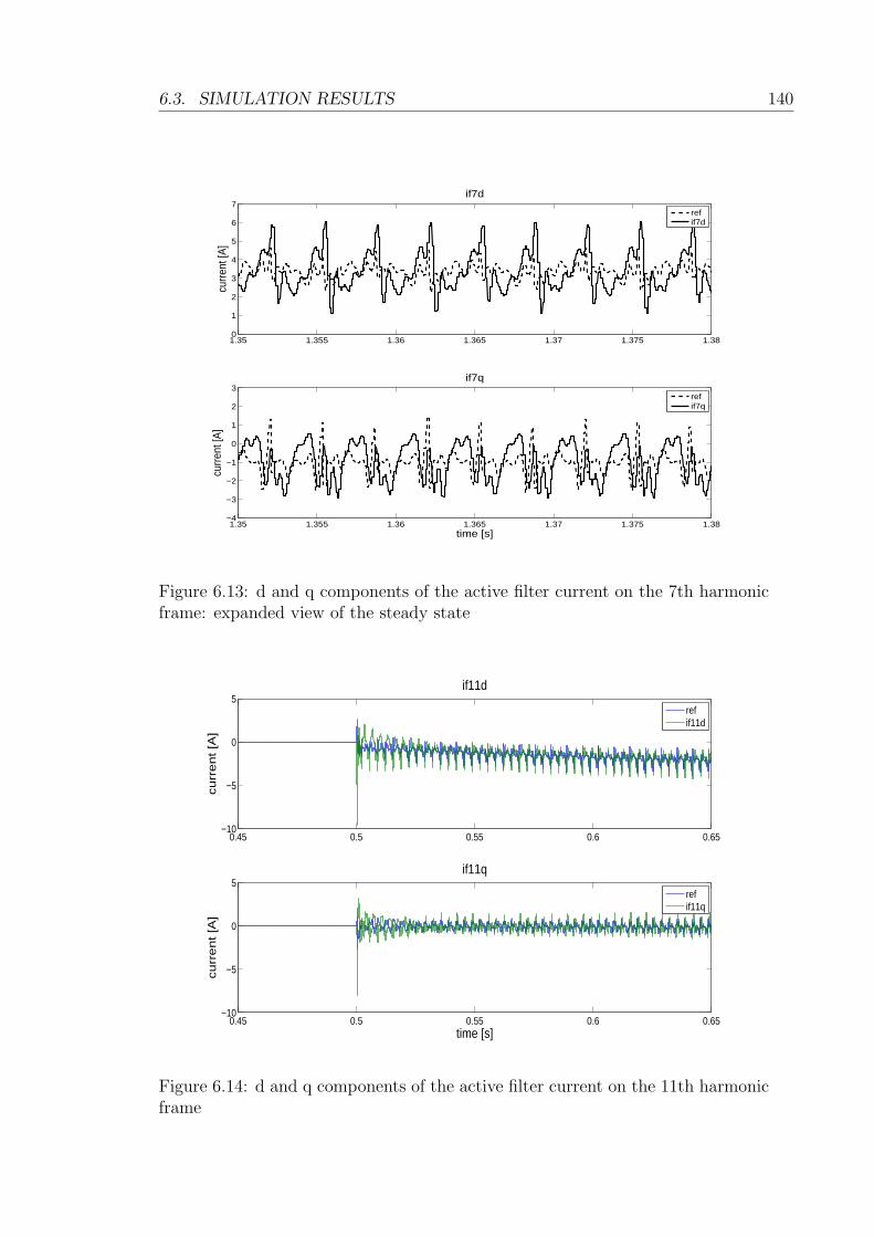
6.3. SIMULATION RESULTS 140
1.35 1.355 1.36 1.365 1.37 1.375 1.380
1
2
3
4
5
6
7if7d
curr
ent [
A]
refif7d
1.35 1.355 1.36 1.365 1.37 1.375 1.38−4
−3
−2
−1
0
1
2
3if7q
time [s]
curr
ent [
A]
refif7q
Figure 6.13: d and q components of the active filter current on the 7th harmonicframe: expanded view of the steady state
0.45 0.5 0.55 0.6 0.65−10
−5
0
5if11d
cu
rre
nt [A
]
refif11d
0.45 0.5 0.55 0.6 0.65−10
−5
0
5if11q
time [s]
cu
rre
nt [A
]
refif11q
Figure 6.14: d and q components of the active filter current on the 11th harmonicframe
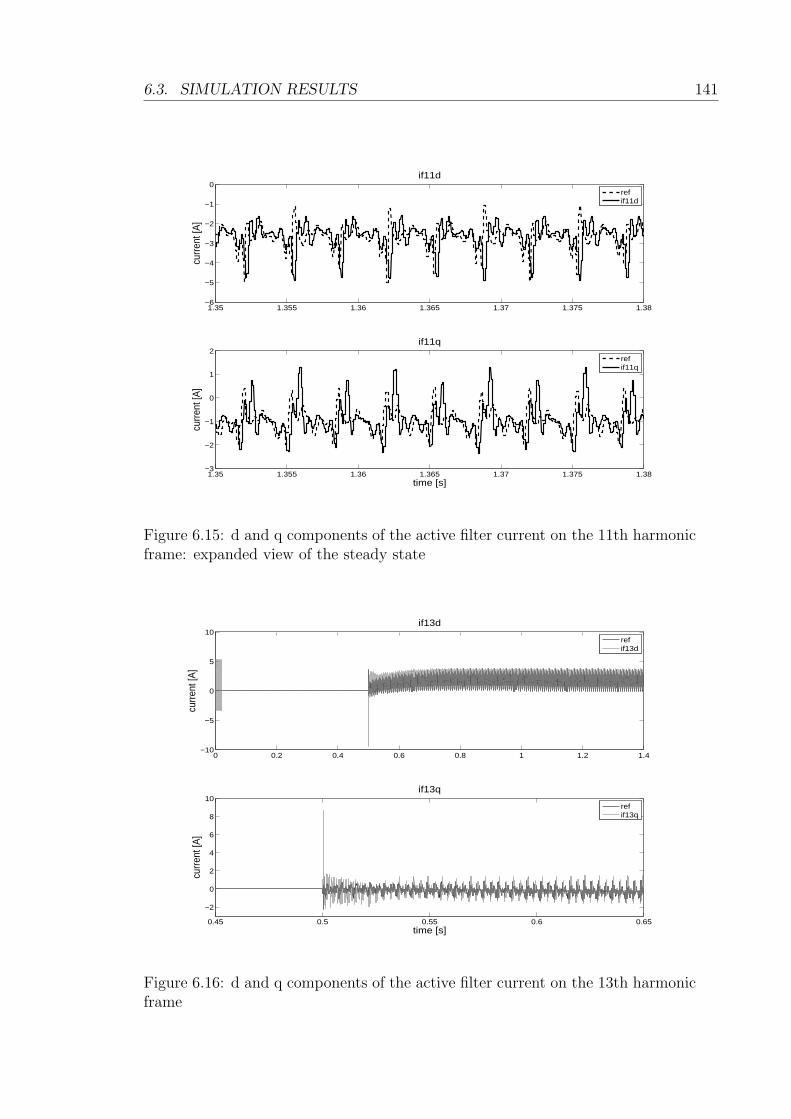
6.3. SIMULATION RESULTS 141
1.35 1.355 1.36 1.365 1.37 1.375 1.38−6
−5
−4
−3
−2
−1
0if11d
curr
ent [
A]
refif11d
1.35 1.355 1.36 1.365 1.37 1.375 1.38−3
−2
−1
0
1
2if11q
time [s]
curr
ent [
A]
refif11q
Figure 6.15: d and q components of the active filter current on the 11th harmonicframe: expanded view of the steady state
0 0.2 0.4 0.6 0.8 1 1.2 1.4−10
−5
0
5
10if13d
curr
ent [
A]
refif13d
0.45 0.5 0.55 0.6 0.65
−2
0
2
4
6
8
10if13q
time [s]
curr
ent [
A]
refif13q
Figure 6.16: d and q components of the active filter current on the 13th harmonicframe

6.3. SIMULATION RESULTS 142
1.35 1.355 1.36 1.365 1.37 1.375 1.38−1
0
1
2
3
4
5if13d
curr
ent [
A]
refif13d
1.35 1.355 1.36 1.365 1.37 1.375 1.38−3
−2
−1
0
1
2if13q
time [s]
curr
ent [
A]
refif13q
Figure 6.17: d and q components of the active filter current on the 13th harmonicframe: expanded view of the steady state
0.2 0.205 0.21 0.215 0.22 0.225 0.23−300
−200
−100
0
100
200
300PCC voltage
time [s]
volta
ge [V
]
Figure 6.18: PCC three-phase voltage before the active filter compensation
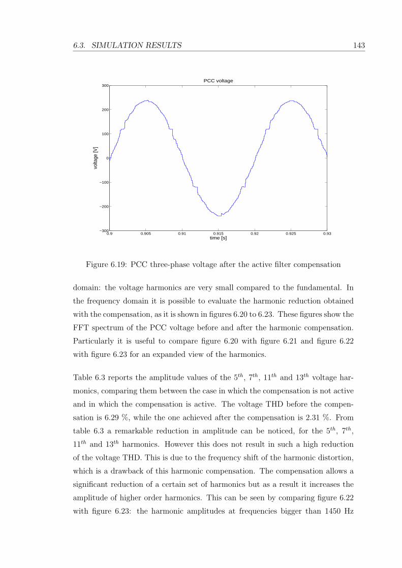
6.3. SIMULATION RESULTS 143
0.9 0.905 0.91 0.915 0.92 0.925 0.93−300
−200
−100
0
100
200
300PCC voltage
time [s]
volta
ge [V
]
Figure 6.19: PCC three-phase voltage after the active filter compensation
domain: the voltage harmonics are very small compared to the fundamental. In
the frequency domain it is possible to evaluate the harmonic reduction obtained
with the compensation, as it is shown in figures 6.20 to 6.23. These figures show the
FFT spectrum of the PCC voltage before and after the harmonic compensation.
Particularly it is useful to compare figure 6.20 with figure 6.21 and figure 6.22
with figure 6.23 for an expanded view of the harmonics.
Table 6.3 reports the amplitude values of the 5th, 7th, 11th and 13th voltage har-
monics, comparing them between the case in which the compensation is not active
and in which the compensation is active. The voltage THD before the compen-
sation is 6.29 %, while the one achieved after the compensation is 2.31 %. From
table 6.3 a remarkable reduction in amplitude can be noticed, for the 5th, 7th,
11th and 13th harmonics. However this does not result in such a high reduction
of the voltage THD. This is due to the frequency shift of the harmonic distortion,
which is a drawback of this harmonic compensation. The compensation allows a
significant reduction of a certain set of harmonics but as a result it increases the
amplitude of higher order harmonics. This can be seen by comparing figure 6.22
with figure 6.23: the harmonic amplitudes at frequencies bigger than 1450 Hz
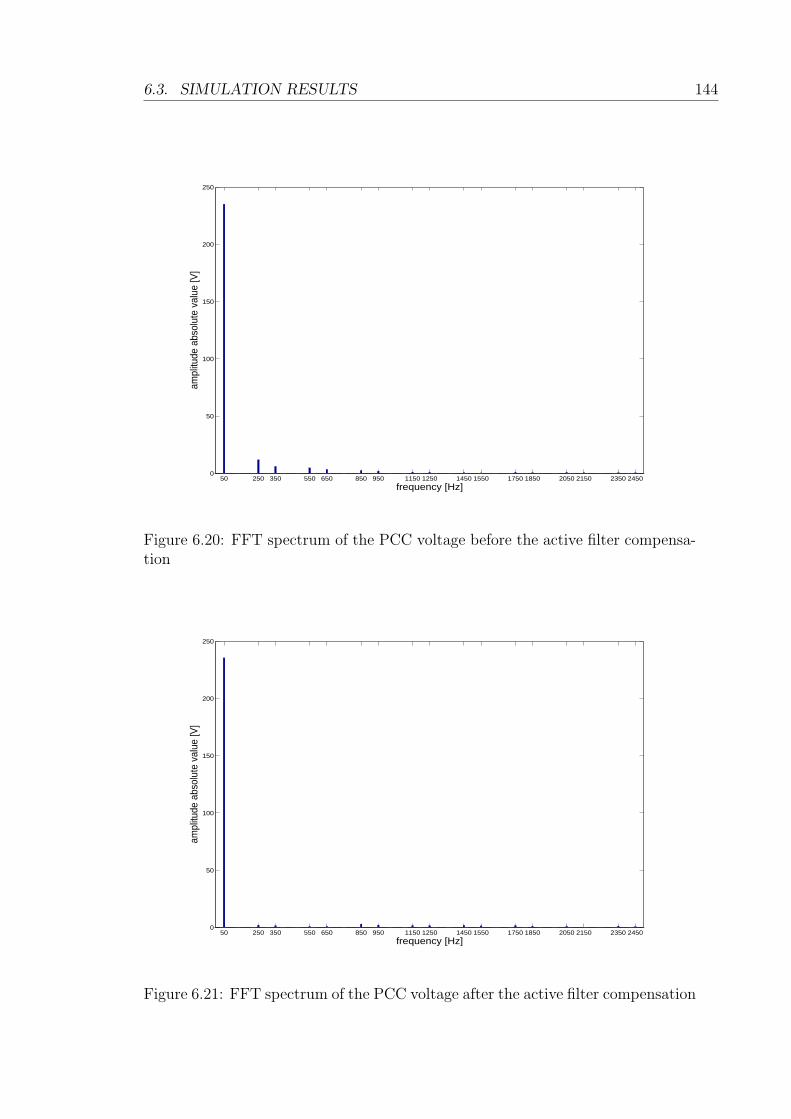
6.3. SIMULATION RESULTS 144
50 250 350 550 650 850 950 1150 1250 1450 1550 1750 1850 2050 2150 2350 24500
50
100
150
200
250
frequency [Hz]
ampl
itude
abs
olut
e va
lue
[V]
Figure 6.20: FFT spectrum of the PCC voltage before the active filter compensa-tion
50 250 350 550 650 850 950 1150 1250 1450 1550 1750 1850 2050 2150 2350 24500
50
100
150
200
250
frequency [Hz]
ampl
itude
abs
olut
e va
lue
[V]
Figure 6.21: FFT spectrum of the PCC voltage after the active filter compensation

6.3. SIMULATION RESULTS 145
250 350 550 650 850 950 1150 1250 1450 1550 1750 1850 2050 2150 2350 24500
2
4
6
8
10
12
frequency [Hz]
ampl
itude
abs
olut
e va
lue
[V]
Figure 6.22: FFT spectrum of the PCC voltage before the active filter compensa-tion: expanded view of the harmonics
250 350 550 650 850 950 1150 1250 1450 1550 1750 1850 2050 2150 2350 24500
2
4
6
8
10
12
frequency [Hz]
ampl
itude
abs
olut
e va
lue
[V]
Figure 6.23: FFT spectrum of the PCC voltage after the active filter compensa-tion: expanded view of the harmonics

6.4. SUMMARY 146
Voltage harmonic amplitude Harmonic
before compensation after compensation reduction
[V] [% of fund.] [V] [% of fund.]
5th 11.66 4.97 1.87 0.79 83.96 %
7th 6.05 2.57 1.32 0.56 78.18 %
11th 4.65 1.98 0.77 0.33 83.44 %
13th 3.36 1.43 0.88 0.37 73.81 %
Table 6.3: Voltage harmonic reduction
increase.
Figures 6.24 and 6.25 show the supply current on the phase A before and after
the active filter harmonic compensation.
Figures 6.26 to 6.29 show the FFT spectrum of the supply current in both the
aforementioned cases. Particularly it is useful to compare figure 6.26 with fig-
ure 6.27 and figure 6.28 with figure 6.29 for an expanded view of the harmonics.
Table 6.4 reports the amplitude values of the 5th, 7th, 11th and 13th current har-
monics, comparing them between the case in which the compensation is not active
and in which the compensation is active. The current THD before the compensa-
tion is 25.28 %, while the one achieved after the compensation is 4.64 %.
6.4 Summary
This chapter has presented the simulation results that validate the multiple ref-
erence frames voltage detection control technique for shunt active power filters,
presented in Chapter 5. The simulations have been carried out using the software
Matlab Simulink. The PCC voltage and active filter current, represented on a
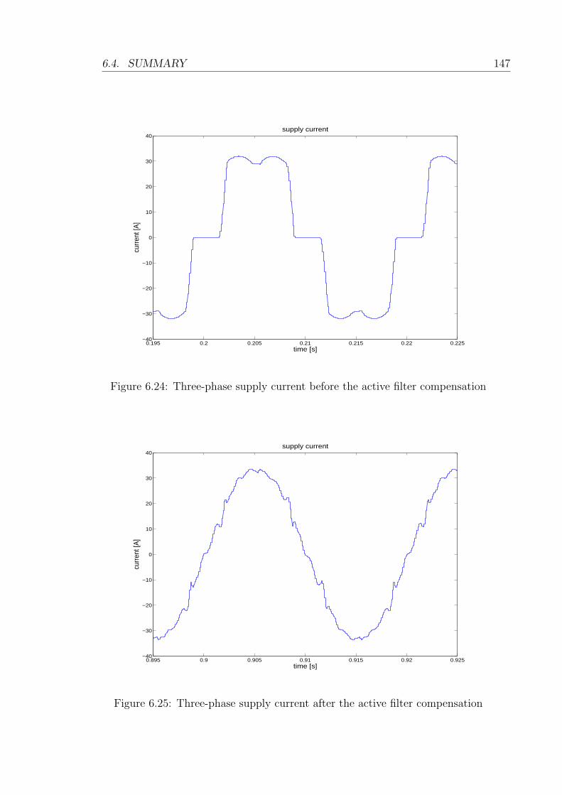
6.4. SUMMARY 147
0.195 0.2 0.205 0.21 0.215 0.22 0.225−40
−30
−20
−10
0
10
20
30
40supply current
time [s]
curr
ent [
A]
Figure 6.24: Three-phase supply current before the active filter compensation
0.895 0.9 0.905 0.91 0.915 0.92 0.925−40
−30
−20
−10
0
10
20
30
40supply current
time [s]
curr
ent [
A]
Figure 6.25: Three-phase supply current after the active filter compensation
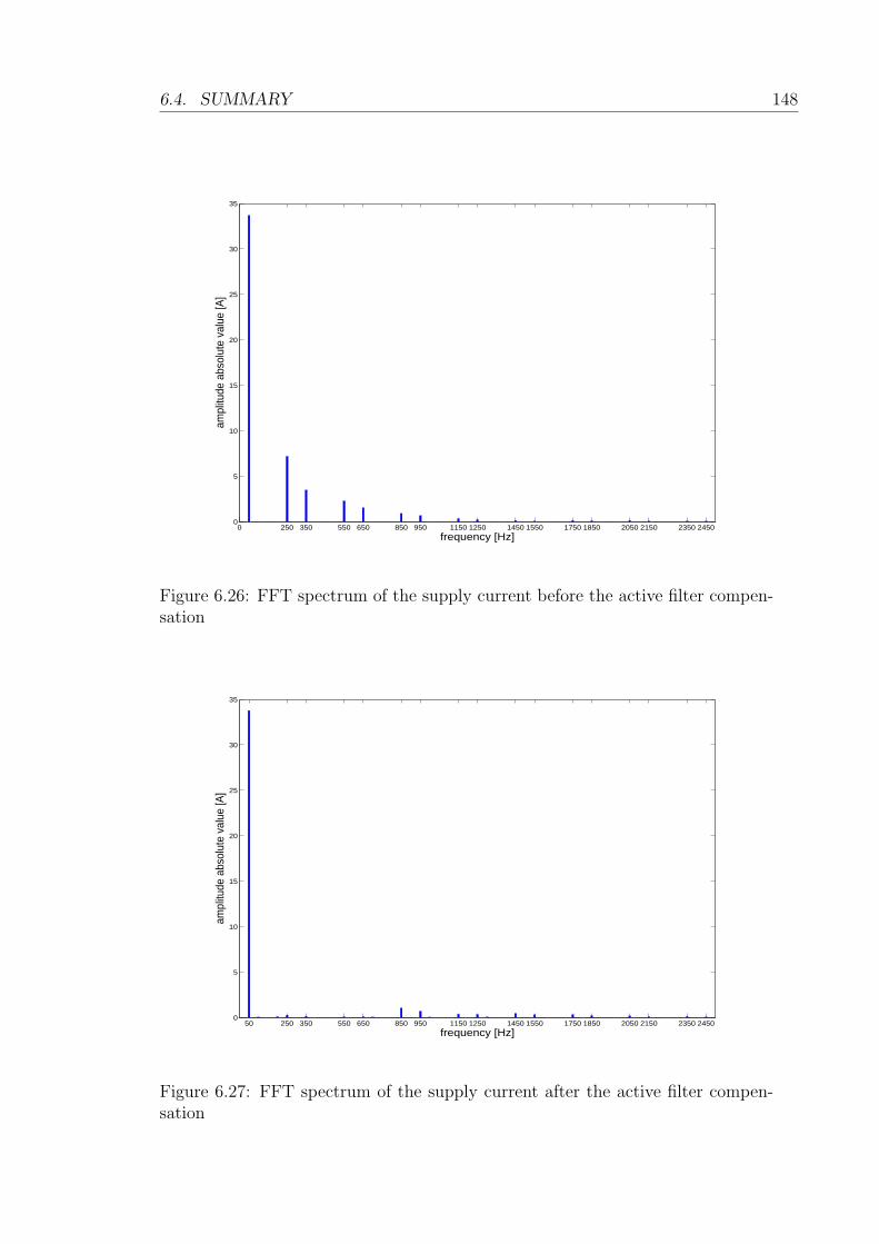
6.4. SUMMARY 148
0 250 350 550 650 850 950 1150 1250 1450 1550 1750 1850 2050 2150 2350 24500
5
10
15
20
25
30
35
frequency [Hz]
ampl
itude
abs
olut
e va
lue
[A]
Figure 6.26: FFT spectrum of the supply current before the active filter compen-sation
50 250 350 550 650 850 950 1150 1250 1450 1550 1750 1850 2050 2150 2350 24500
5
10
15
20
25
30
35
frequency [Hz]
ampl
itude
abs
olut
e va
lue
[A]
Figure 6.27: FFT spectrum of the supply current after the active filter compen-sation
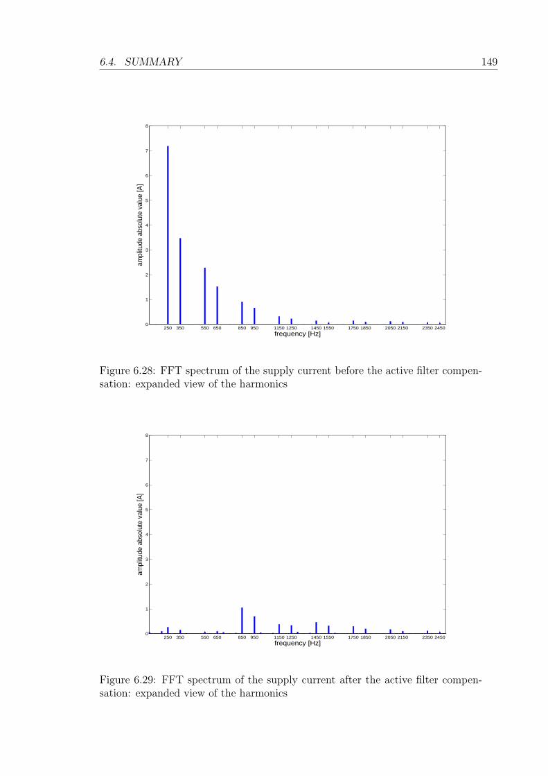
6.4. SUMMARY 149
250 350 550 650 850 950 1150 1250 1450 1550 1750 1850 2050 2150 2350 24500
1
2
3
4
5
6
7
8
frequency [Hz]
ampl
itude
abs
olut
e va
lue
[A]
Figure 6.28: FFT spectrum of the supply current before the active filter compen-sation: expanded view of the harmonics
250 350 550 650 850 950 1150 1250 1450 1550 1750 1850 2050 2150 2350 24500
1
2
3
4
5
6
7
8
frequency [Hz]
ampl
itude
abs
olut
e va
lue
[A]
Figure 6.29: FFT spectrum of the supply current after the active filter compen-sation: expanded view of the harmonics
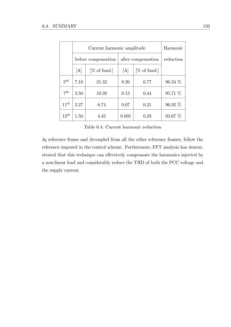
6.4. SUMMARY 150
Current harmonic amplitude Harmonic
before compensation after compensation reduction
[A] [% of fund.] [A] [% of fund.]
5th 7.18 21.32 0.26 0.77 96.34 %
7th 3.50 10.39 0.15 0.44 95.71 %
11th 2.27 6.74 0.07 0.21 96.92 %
13th 1.50 4.45 0.095 0.28 93.67 %
Table 6.4: Current harmonic reduction
dq reference frame and decoupled from all the other reference frames, follow the
reference imposed in the control scheme. Furthermore, FFT analysis has demon-
strated that this technique can effectively compensate the harmonics injected by
a non-linear load and considerably reduce the THD of both the PCC voltage and
the supply current.

Chapter 7
Voltage Detection Control
Technique: Experimental Results
7.1 Introduction
This chapter presents the results obtained from the experimental validation of
the proposed control technique for active shunt filters described in Chapter 5.
The experimental tests have been carried out using a laboratory setup comprising
a programmable power supply, a resistive-inductive supply impedance, a three-
phase shunt active power filter, a three-phase distorting load. Section 7.2 presents
a description of the laboratory experimental setup utilized for the validation, in
section 7.3 the experimental results are presented, described and commented.
7.2 Description of the experimental setup
The experimental validation of the multiple reference frames voltage detection
control technique for shunt active power filters has been carried out using a labo-
ratory equipment setup. The setup represents a small scale version of a real power
network where a shunt active power filter is applied.
151

7.2. DESCRIPTION OF THE EXPERIMENTAL SETUP 152
The control technique can be utilized both for a normal 50Hz grid and for aircraft
power systems, where the fundamental frequency varies in the range 360 to 900
Hz. However, for the work presented in this project, this technique has not been
tested at values of frequency typical of an aircraft system, because of the limita-
tions on the computational capability of the digital signal processor utilized for
the validation. The whole implementation has been carried out at fundamental
frequency equal to 50Hz, as shown in Chapter 6, but the results obtained can be
extended to the variable frequency range of the aircraft power networks.
Figure 7.1 shows a scheme of the experimental setup utilized for the laboratory
testing. The circuit represented in this figure is similar to the one represented in
figure 5.14.
Gate drivers
Ls Rs
Lf
Rf
Rl
DIODE-BRIDGE RECTIFIER
ACTIVE FILTER
C
Chroma programmable power supply
DSP+FPGAADCtransducers
Vpcc
If
Vdc
Vpcc
IfVdc
Figure 7.1: Scheme of the laboratory experimental setup
The experimental setup comprises a three-phase programmable power supply con-
nected in series with a resistive-inductive impedance, representing the supply
impedance, a laboratory-built three-phase shunt active power filter prototype, a
three-phase diode bridge rectifier representing the distorting load that the active
filter compensates for. The control algorithm is implemented on a 32 bit floating
point Digital Signal Processor (DSP). The data acquisition is carried out by means
of a Field Programmable Gate Array (FPGA) board. The variables measured by
means of the voltage and current transducers are converted from analog to digital

7.2. DESCRIPTION OF THE EXPERIMENTAL SETUP 153
signals by means of Analog to Digital Converters (ADC) connected to the FPGA.
A detailed description of the devices and components is given here. It can be
seen that the supply resistance is 1.5 Ω. This high value has been chosen in order
to increase the voltage drop of the harmonic current, as the voltage transducers
utilized here present low accuracy for values of voltage smaller than 5V.
POWER SUPPLY
Chroma Programmable AC Source 61705 [47]
SUPPLY IMPEDANCE
Resistors:
resistance = 1.5 Ω
rated current = 11.8A
power rating = 751W
Inductors:
inductance = 0.4mH
rated current = 16A
SHUNT ACTIVE POWER FILTER
IGBT modules: DYNEX DIM200WHS12-A000 [74]
DC link capacitance = 2200 µF
Line inductor:
inductance = 3mH
rated voltage = 750V
rated current = 16A rms

7.3. EXPERIMENTAL RESULTS 154
NON-LINEAR LOAD
three IRKD101-14 diode modules [75]
load resistance = 12.5 Ω
MEASUREMENT
Voltage transducers: LEM LV 25-P [51]
Current transducers: LEM LA 55-P [76]
CONTROL
DSP: Texas Instruments TMS320C6713B 32 bit floating point [48]
FPGA: Actel ProAsic A500K050 Package PQ208 [49]
Analog to Digital Converters: 12 bit LTC 1400 [50]
Figures 7.2 to 7.4 show the pictures of the laboratory bench utilized for the ex-
perimental tests.
7.3 Experimental results
For the experimental validation, the supply voltage has been set to 120V rms line-
line. The DC link voltage during the active filter operation was 200V. The voltage
level at which the experimental tests have been carried out is lower than the full
voltage of the mains because of the limitations in the rated current of the passive
components utilized in the experimental setup. Because of the computational
limitations of the DSP, the sampling frequency, equal to the switching frequency,
has been set to 4 kHz, and only the 5th and 7th are compensated by the active
filter in the tests presented here.
Figures 7.5 to 7.8 show the d and q components of the PCC voltage on the 5th
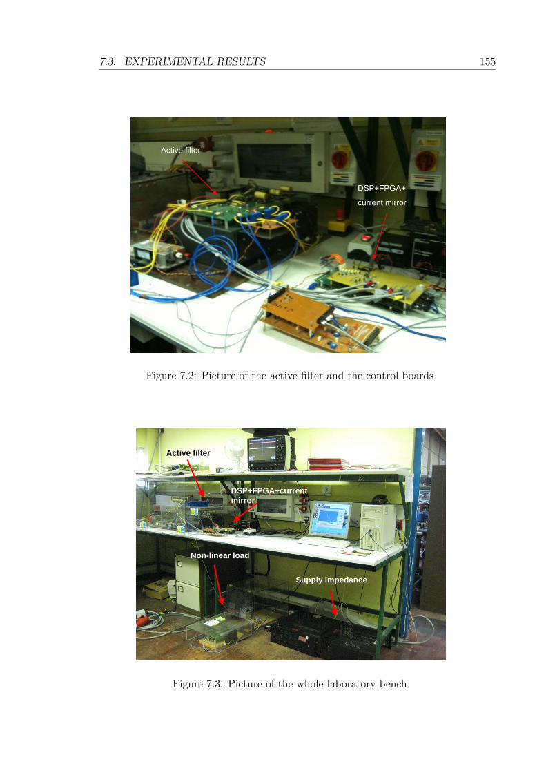
7.3. EXPERIMENTAL RESULTS 155
Active filter
DSP+FPGA+
current mirror
Figure 7.2: Picture of the active filter and the control boards
Active filter
DSP+FPGA+current mirror
Non-linear load
Supply impedance
Figure 7.3: Picture of the whole laboratory bench
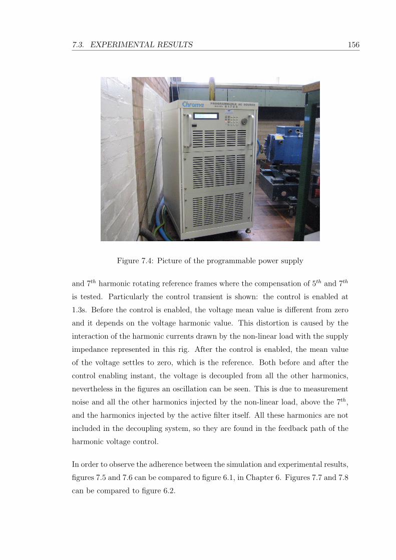
7.3. EXPERIMENTAL RESULTS 156
Figure 7.4: Picture of the programmable power supply
and 7th harmonic rotating reference frames where the compensation of 5th and 7th
is tested. Particularly the control transient is shown: the control is enabled at
1.3s. Before the control is enabled, the voltage mean value is different from zero
and it depends on the voltage harmonic value. This distortion is caused by the
interaction of the harmonic currents drawn by the non-linear load with the supply
impedance represented in this rig. After the control is enabled, the mean value
of the voltage settles to zero, which is the reference. Both before and after the
control enabling instant, the voltage is decoupled from all the other harmonics,
nevertheless in the figures an oscillation can be seen. This is due to measurement
noise and all the other harmonics injected by the non-linear load, above the 7th,
and the harmonics injected by the active filter itself. All these harmonics are not
included in the decoupling system, so they are found in the feedback path of the
harmonic voltage control.
In order to observe the adherence between the simulation and experimental results,
figures 7.5 and 7.6 can be compared to figure 6.1, in Chapter 6. Figures 7.7 and 7.8
can be compared to figure 6.2.

7.3. EXPERIMENTAL RESULTS 157
0 0.5 1 1.5 2 2.5 3 3.5 4 4.5 5−3
−2
−1
0
1
2
3
4
5
time [s]
volta
ge [V
]
refvf5d
Figure 7.5: d component of the PCC voltage on the 5th harmonic frame
0 0.5 1 1.5 2 2.5 3 3.5 4 4.5 5−2
−1.5
−1
−0.5
0
0.5
1
1.5
2
time [s]
volta
ge [V
]
refvf5q
Figure 7.6: q component of the PCC voltage on the 5th harmonic frame

7.3. EXPERIMENTAL RESULTS 158
0 0.5 1 1.5 2 2.5 3 3.5 4 4.5 5−2
−1.5
−1
−0.5
0
0.5
1
1.5
2
time [s]
volta
ge [V
]
refvf7d
Figure 7.7: d component of the PCC voltage on the 7th harmonic frame
0 0.5 1 1.5 2 2.5 3 3.5 4 4.5 5−2
−1.5
−1
−0.5
0
0.5
1
1.5
2
time [s]
volta
ge [V
]
refvf7q
Figure 7.8: q component of the PCC voltage on the 7th harmonic frame
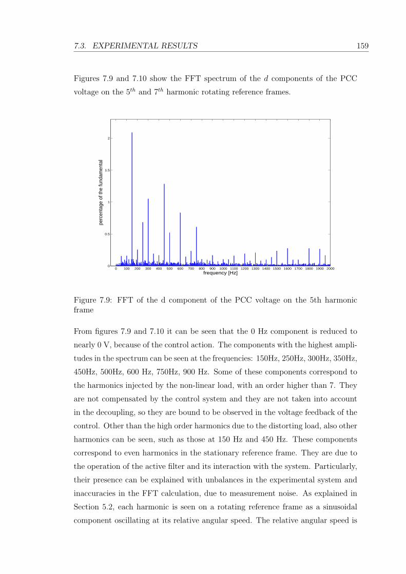
7.3. EXPERIMENTAL RESULTS 159
Figures 7.9 and 7.10 show the FFT spectrum of the d components of the PCC
voltage on the 5th and 7th harmonic rotating reference frames.
0 100 200 300 400 500 600 700 800 900 1000 1100 1200 1300 1400 1500 1600 1700 1800 1900 20000
0.5
1
1.5
2
frequency [Hz]
perc
enta
ge o
f the
fund
amen
tal
Figure 7.9: FFT of the d component of the PCC voltage on the 5th harmonicframe
From figures 7.9 and 7.10 it can be seen that the 0 Hz component is reduced to
nearly 0 V, because of the control action. The components with the highest ampli-
tudes in the spectrum can be seen at the frequencies: 150Hz, 250Hz, 300Hz, 350Hz,
450Hz, 500Hz, 600 Hz, 750Hz, 900 Hz. Some of these components correspond to
the harmonics injected by the non-linear load, with an order higher than 7. They
are not compensated by the control system and they are not taken into account
in the decoupling, so they are bound to be observed in the voltage feedback of the
control. Other than the high order harmonics due to the distorting load, also other
harmonics can be seen, such as those at 150 Hz and 450 Hz. These components
correspond to even harmonics in the stationary reference frame. They are due to
the operation of the active filter and its interaction with the system. Particularly,
their presence can be explained with unbalances in the experimental system and
inaccuracies in the FFT calculation, due to measurement noise. As explained in
Section 5.2, each harmonic is seen on a rotating reference frame as a sinusoidal
component oscillating at its relative angular speed. The relative angular speed is
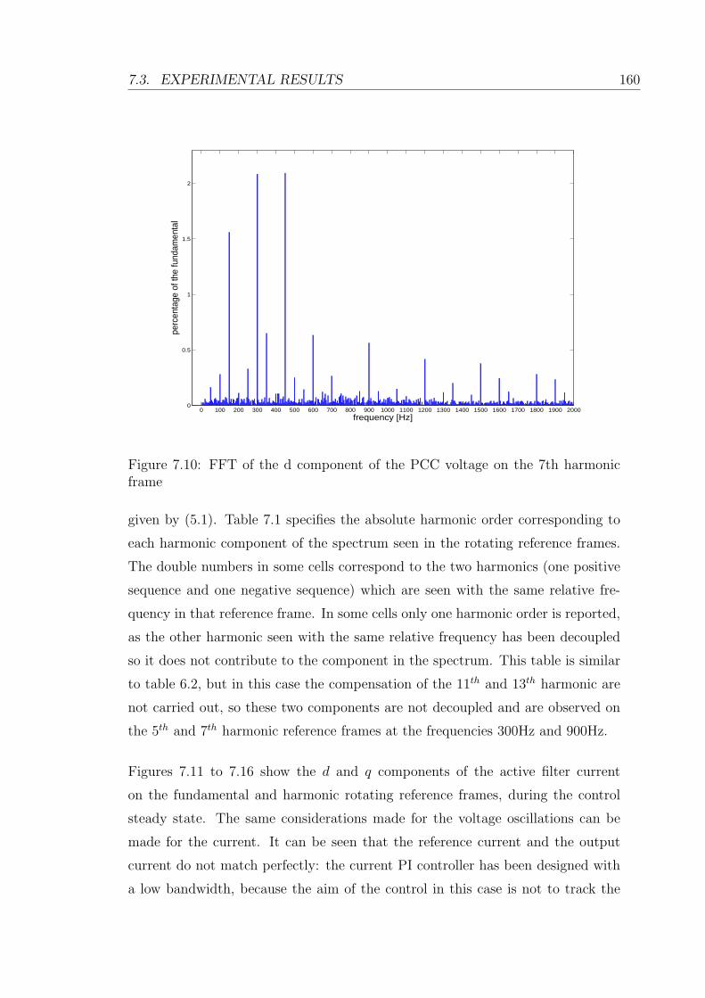
7.3. EXPERIMENTAL RESULTS 160
0 100 200 300 400 500 600 700 800 900 1000 1100 1200 1300 1400 1500 1600 1700 1800 1900 20000
0.5
1
1.5
2
frequency [Hz]
perc
enta
ge o
f the
fund
amen
tal
Figure 7.10: FFT of the d component of the PCC voltage on the 7th harmonicframe
given by (5.1). Table 7.1 specifies the absolute harmonic order corresponding to
each harmonic component of the spectrum seen in the rotating reference frames.
The double numbers in some cells correspond to the two harmonics (one positive
sequence and one negative sequence) which are seen with the same relative fre-
quency in that reference frame. In some cells only one harmonic order is reported,
as the other harmonic seen with the same relative frequency has been decoupled
so it does not contribute to the component in the spectrum. This table is similar
to table 6.2, but in this case the compensation of the 11th and 13th harmonic are
not carried out, so these two components are not decoupled and are observed on
the 5th and 7th harmonic reference frames at the frequencies 300Hz and 900Hz.
Figures 7.11 to 7.16 show the d and q components of the active filter current
on the fundamental and harmonic rotating reference frames, during the control
steady state. The same considerations made for the voltage oscillations can be
made for the current. It can be seen that the reference current and the output
current do not match perfectly: the current PI controller has been designed with
a low bandwidth, because the aim of the control in this case is not to track the

7.3. EXPERIMENTAL RESULTS 161
Ref
eren
ceH
arm
onic
sas
seen
inth
esp
ectr
um
[Hz]
fram
e15
030
045
060
090
012
0015
0018
0021
0024
0027
00
52;
811
4;14
1713
;23
19;2
925
;35
31;4
137
;47
43;5
349
;59
74;
1013
2;16
1911
;25
17;3
123
;37
29;4
335
;49
41;5
547
;61
118;
1417
2;20
2329
3519
;41
25;4
731
;53
37;5
943
;65
1310
;16
194;
2225
3137
17;4
323
;49
29;5
535
;61
41;6
7
Tab
le7.
1:H
arm
onic
sas
seen
inth
eF
FT
spec
trum
ofth
evo
ltag
eon
the
diff
eren
tre
fere
nce
fram
es
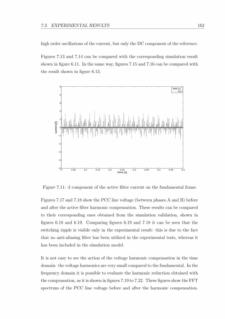
7.3. EXPERIMENTAL RESULTS 162
high order oscillations of the current, but only the DC component of the reference.
Figures 7.13 and 7.14 can be compared with the corresponding simulation result
shown in figure 6.11. In the same way, figures 7.15 and 7.16 can be compared with
the result shown in figure 6.13.
0 0.05 0.1 0.15 0.2 0.25 0.3 0.35 0.4 0.45 0.5−5
−4
−3
−2
−1
0
1
2
3
4
5
time [s]
curr
ent [
A]
refif1d
Figure 7.11: d component of the active filter current on the fundamental frame
Figures 7.17 and 7.18 show the PCC line voltage (between phases A and B) before
and after the active filter harmonic compensation. These results can be compared
to their corresponding ones obtained from the simulation validation, shown in
figures 6.18 and 6.19. Comparing figures 6.19 and 7.18 it can be seen that the
switching ripple is visible only in the experimental result: this is due to the fact
that no anti-aliasing filter has been utilized in the experimental tests, whereas it
has been included in the simulation model.
It is not easy to see the action of the voltage harmonic compensation in the time
domain: the voltage harmonics are very small compared to the fundamental. In the
frequency domain it is possible to evaluate the harmonic reduction obtained with
the compensation, as it is shown in figures 7.19 to 7.22. These figures show the FFT
spectrum of the PCC line voltage before and after the harmonic compensation.
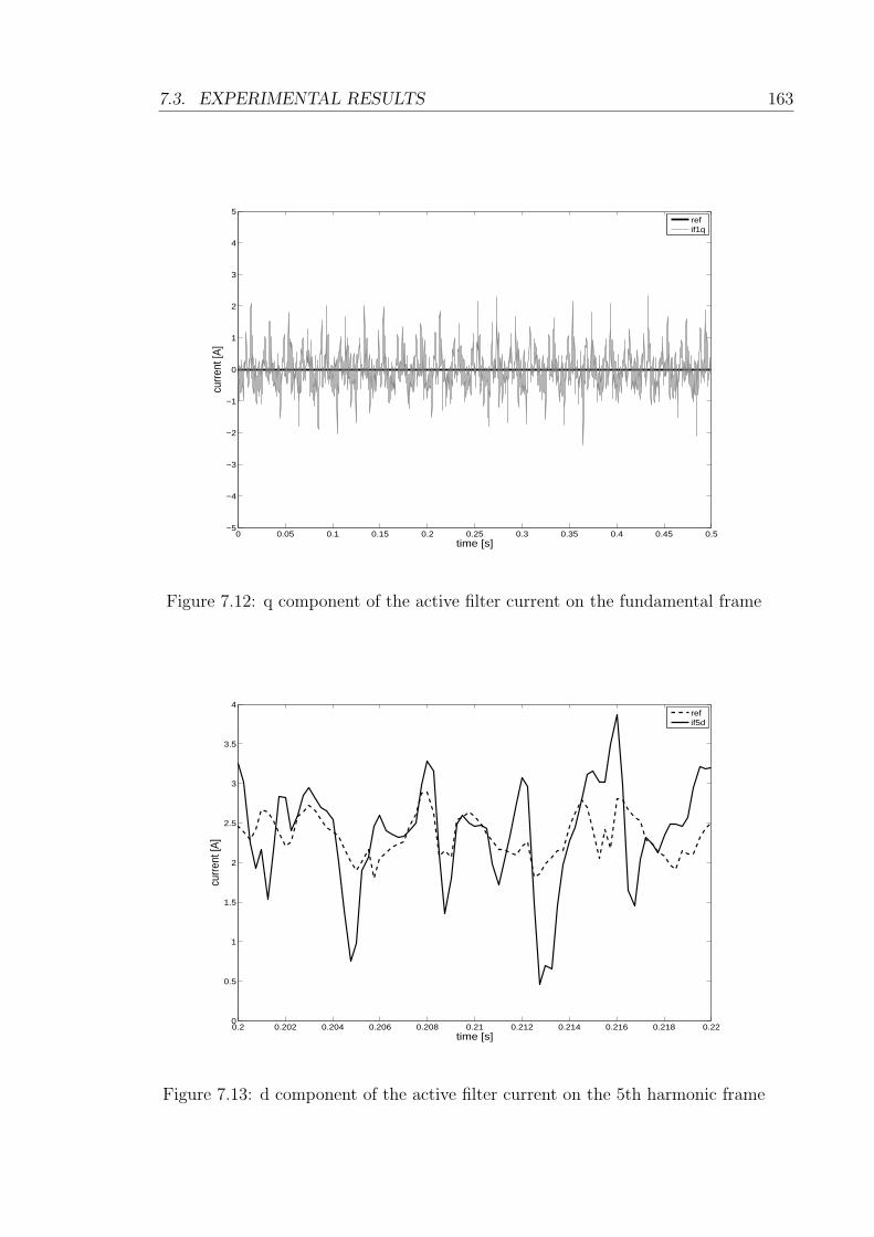
7.3. EXPERIMENTAL RESULTS 163
0 0.05 0.1 0.15 0.2 0.25 0.3 0.35 0.4 0.45 0.5−5
−4
−3
−2
−1
0
1
2
3
4
5
time [s]
curr
ent [
A]
refif1q
Figure 7.12: q component of the active filter current on the fundamental frame
0.2 0.202 0.204 0.206 0.208 0.21 0.212 0.214 0.216 0.218 0.220
0.5
1
1.5
2
2.5
3
3.5
4
time [s]
curr
ent [
A]
refif5d
Figure 7.13: d component of the active filter current on the 5th harmonic frame
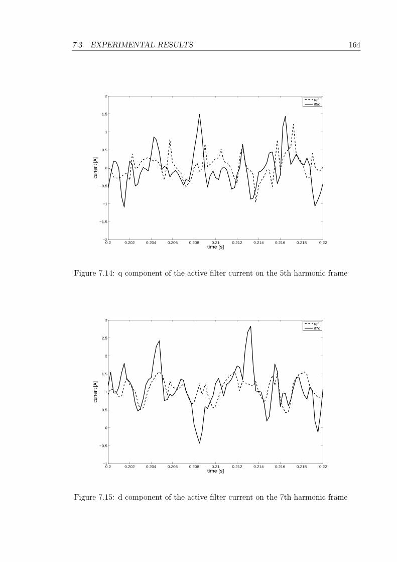
7.3. EXPERIMENTAL RESULTS 164
0.2 0.202 0.204 0.206 0.208 0.21 0.212 0.214 0.216 0.218 0.22−2
−1.5
−1
−0.5
0
0.5
1
1.5
2
time [s]
curr
ent [
A]
refif5q
Figure 7.14: q component of the active filter current on the 5th harmonic frame
0.2 0.202 0.204 0.206 0.208 0.21 0.212 0.214 0.216 0.218 0.22−1
−0.5
0
0.5
1
1.5
2
2.5
3
time [s]
curr
ent [
A]
refif7d
Figure 7.15: d component of the active filter current on the 7th harmonic frame

7.3. EXPERIMENTAL RESULTS 165
0.2 0.202 0.204 0.206 0.208 0.21 0.212 0.214 0.216 0.218 0.22−2
−1.5
−1
−0.5
0
0.5
1
1.5
2
time [s]
curr
ent [
A]
refif7q
Figure 7.16: q component of the active filter current on the 7th harmonic frame
0.02 0.025 0.03 0.035 0.04 0.045 0.05-200
-150
-100
-50
0
50
100
150
200
time [s]
volta
ge [V
]
Figure 7.17: PCC three-phase voltage before the active filter compensation
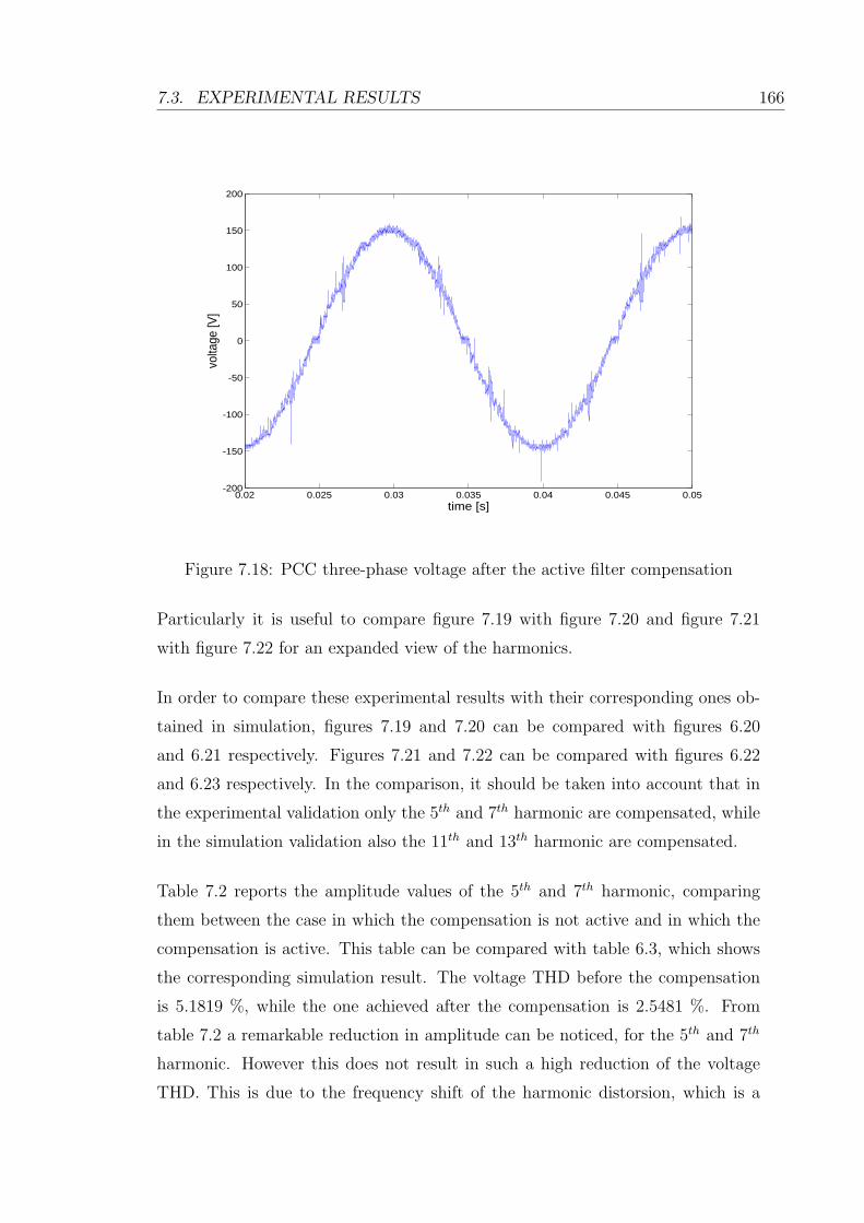
7.3. EXPERIMENTAL RESULTS 166
0.02 0.025 0.03 0.035 0.04 0.045 0.05-200
-150
-100
-50
0
50
100
150
200
time [s]
volta
ge [V
]
Figure 7.18: PCC three-phase voltage after the active filter compensation
Particularly it is useful to compare figure 7.19 with figure 7.20 and figure 7.21
with figure 7.22 for an expanded view of the harmonics.
In order to compare these experimental results with their corresponding ones ob-
tained in simulation, figures 7.19 and 7.20 can be compared with figures 6.20
and 6.21 respectively. Figures 7.21 and 7.22 can be compared with figures 6.22
and 6.23 respectively. In the comparison, it should be taken into account that in
the experimental validation only the 5th and 7th harmonic are compensated, while
in the simulation validation also the 11th and 13th harmonic are compensated.
Table 7.2 reports the amplitude values of the 5th and 7th harmonic, comparing
them between the case in which the compensation is not active and in which the
compensation is active. This table can be compared with table 6.3, which shows
the corresponding simulation result. The voltage THD before the compensation
is 5.1819 %, while the one achieved after the compensation is 2.5481 %. From
table 7.2 a remarkable reduction in amplitude can be noticed, for the 5th and 7th
harmonic. However this does not result in such a high reduction of the voltage
THD. This is due to the frequency shift of the harmonic distorsion, which is a
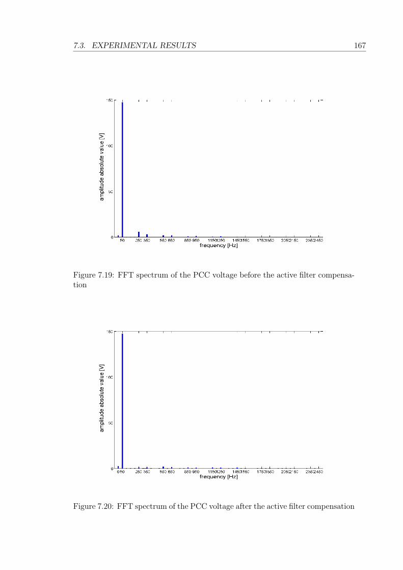
7.3. EXPERIMENTAL RESULTS 167
Figure 7.19: FFT spectrum of the PCC voltage before the active filter compensa-tion
Figure 7.20: FFT spectrum of the PCC voltage after the active filter compensation
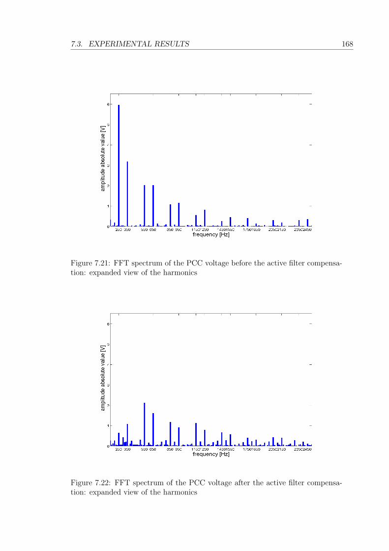
7.3. EXPERIMENTAL RESULTS 168
Figure 7.21: FFT spectrum of the PCC voltage before the active filter compensa-tion: expanded view of the harmonics
Figure 7.22: FFT spectrum of the PCC voltage after the active filter compensa-tion: expanded view of the harmonics

7.3. EXPERIMENTAL RESULTS 169
Voltage harmonic amplitude Harmonic
before compensation after compensation reduction
[V] [% of fund.] [V] [% of fund.]
5th 5.95 4.03 0.66 0.45 88.90 %
7th 3.18 2.16 1.08 0.73 66.04 %
Table 7.2: Voltage harmonic reduction
drawback of this harmonic compensation. The compensation allows a significant
reduction of a certain set of harmonics but as a result it increases the amplitude of
higher order harmonics. This can be seen by comparing figure 7.21 with figure 7.22:
the harmonic amplitudes at frequencies bigger than 1150Hz increase.
Figures 7.23 and 7.24 show the supply current on the phase A before and after
the active filter harmonic compensation. These results can be compared to their
corresponding ones obtained from the simulation validation, shown in figures 6.24
and 6.25. The same consideration about the switching ripple, made for the voltage,
can be also made for the current.
Figures 7.25 to 7.28 show the FFT spectrum of the supply current in both the
aforementioned cases. Particularly it is useful to compare figure 7.25 with fig-
ure 7.26 and figure 7.27 with figure 7.28 for an expanded view of the harmonics.
In order to compare these experimental results with their corresponding ones ob-
tained in simulation, figures 7.25 and 7.26 can be compared with figures 6.26
and 6.27 respectively. Figures 7.27 and 7.28 can be compared with figures 6.28
and 6.29 respectively. In the comparison, it should be taken into account that in
the experimental validation only the 5th and 7th harmonic are compensated, while
in the simulation validation also the 11th and 13th harmonic are compensated.
Table 7.3 reports the amplitude values of the 5th and 7th current harmonic, compar-
ing them between the case in which the compensation is not active and in which
the compensation is active. This table can be compared with table 6.4, which
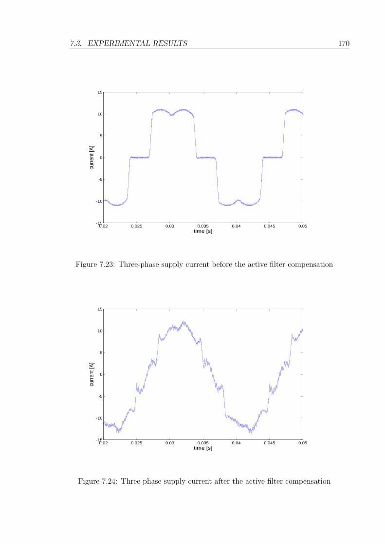
7.3. EXPERIMENTAL RESULTS 170
0.02 0.025 0.03 0.035 0.04 0.045 0.05-15
-10
-5
0
5
10
15
time [s]
curre
nt [A
]
Figure 7.23: Three-phase supply current before the active filter compensation
0.02 0.025 0.03 0.035 0.04 0.045 0.05-15
-10
-5
0
5
10
15
time [s]
curre
nt [A
]
Figure 7.24: Three-phase supply current after the active filter compensation

7.3. EXPERIMENTAL RESULTS 171
Figure 7.25: FFT spectrum of the supply current before the active filter compen-sation
Figure 7.26: FFT spectrum of the supply current after the active filter compen-sation

7.3. EXPERIMENTAL RESULTS 172
Figure 7.27: FFT spectrum of the supply current before the active filter compen-sation: expanded view of the harmonics
Figure 7.28: FFT spectrum of the supply current after the active filter compen-sation: expanded view of the harmonics

7.4. SUMMARY 173
Current harmonic amplitude Harmonic
before compensation after compensation reduction
[A] [% of fund.] [A] [% of fund.]
5th 2.56 22.16 0.45 3.90 82.42 %
7th 1.28 11.08 0.45 3.90 64.84 %
Table 7.3: Current harmonic reduction
shows the corresponding simulation result. The current THD before the com-
pensation is 27.4179 %, while the one achieved after the compensation is 11.3931
%.
Figures 7.29 and 7.30 show the oscilloscope screen capture during the experimental
tests, before and after enabling the active filter harmonic compensation respec-
tively. In these figures, the supply current, the PCC voltage and the active filter
output voltage are represented and indicated. The effectiveness of the harmonic
compensation can be seen comparing the supply current and the PCC voltage in
the two figures.
7.4 Summary
This chapter has presented the experimental results that validate the multiple
reference frames voltage detection control technique for shunt active power filters,
presented in Chapter 5. The experimental tests have been carried out using a lab-
oratory built prototype of an active filter, connected in parallel to a three-phase
power supply and a distorting load. The experimental results show that the active
filter, operating using the proposed control technique, effectively compensates for
the 5th and 7th harmonic injected by the non-linear load. Furthermore the ex-
perimental results show good adherence with the simulation results presented in
Chapter 6.
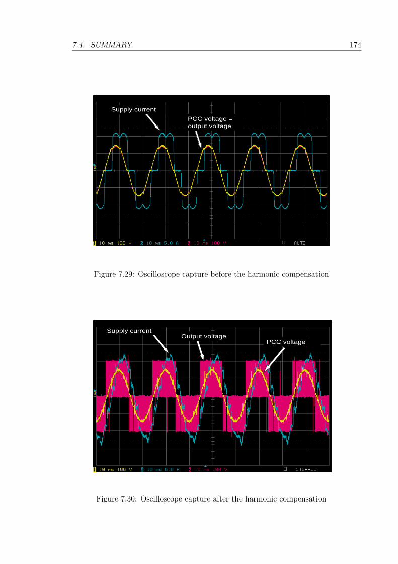
7.4. SUMMARY 174
Supply currentPCC voltage = output voltage
Figure 7.29: Oscilloscope capture before the harmonic compensation
Supply currentOutput voltage
PCC voltage
Figure 7.30: Oscilloscope capture after the harmonic compensation
Chapter 8
Conclusions
In the work presented in this thesis, a novel algorithm for the detection of the fun-
damental frequency and harmonic components of a distorted signal and a novel
control technique for shunt active power filters have been proposed. The applica-
tion for which this work has been developed is the More Electric Aircraft.
In the future civil aircraft systems, the increasing use of electric power in place
of conventional sources of power, like mechanical, hydraulic and pneumatic, will
bring major changes to the aircraft power system. A more complex topology of
the network, a bigger amount of generated and demanded power and an increasing
use of power electronic devices on board can give rise to significant stability and
power quality problems.
The shunt active power filter is an effective solution for the harmonic elimination
and the power quality enhancement in the electrical system. This allows the
system to operate within the limits recommended by the aircraft regulations.
The biggest challenge encountered when designing and controlling an active fil-
ter in the More Electric Aircraft power system is related to the high values of
fundamental frequency, variable between 360 and 900Hz. An accurate algorithm
for the real-time estimation of the reference signal and a high bandwidth control
system are needed in order for the active filer to inject the right amount of har-
175
CHAPTER 8. CONCLUSIONS 176
monic current into the Point of Common Coupling. At these values of frequency,
the harmonic components occur at high frequencies compared to the conventional
50/60Hz terrestrial systems.
As explained in the Introduction of this thesis, the main goals of the work were:
to implement an accurate real-time estimation technique for the generation of the
reference signal for the active filter control and to implement an effective control
technique, suitable for this kind of application.
The first goal has been achieved by means of a real-time Discrete Fourier Transform
based algorithm which estimates the fundamental frequency and phase angle and
the harmonic components of a distorted time-varying signal. The second goal
has been achieved by implementing a multiple reference frame voltage detection
control technique.
The DFT-based detection technique proved effective both in simulation and exper-
imentally for the real-time estimation of the fundamental and harmonic compo-
nents of a distorted signal. This technique detects the fundamental frequency using
a closed loop system, where the estimation error is minimized by a Proportional
Integral controller. The fundamental and harmonic components are identified by
means of real-time implementation of the Discrete Fourier Transform, where the
observation window of the signal is updated at each step. From the validation of
the method, a good accordance between the simulation and experimental results
has been demonstrated. The results showed that the proposed technique is effec-
tive for the harmonic identification of a distorted signal with variable frequency,
hence it is a viable solution for the detection of the reference signal for the control
of an active shunt filter in the aircraft power system.
The DFT-based technique has been compared with the standard Phase-Locked
Loop (PLL) in order to evaluate its performance. The main advantage of the DFT
method lies in the possibility to apply the algorithm to a signal varying in a broad
range of frequencies and amplitudes without having to re-tune the parameters.
On the other hand, the PLL needs an accurate tuning of the PI controller gains,
depending on the characteristics of the signal and the required accuracy and speed

CHAPTER 8. CONCLUSIONS 177
of the estimation response. The DFT method also proved more effective than the
PLL in cases where noise and distortion affect the input signal. Furthermore,
it showed a better performance in tracking the variable fundamental frequency
when it presents a fast variation. The comparison has been carried out both in
simulation and experimentally, and a good accordance between the simulation and
experimental results has been shown in the thesis.
The multiple reference frame voltage detection technique proposed in this work
is based on the implementation of several rotating reference frames, one for each
harmonic component to be compensated. The reference frames are decoupled from
one another by means of equations which are listed in the thesis. The control tech-
nique structure consists of as many control loops as the number of the harmonics
to be compensated. Each harmonic appears as a DC quantity in the reference
frame it is synchronous with, hence a simple low bandwidth PI control can track
the reference with zero steady state error. The reference for the control is derived
from the measurement of the voltage at the PCC, which is distorted due to the
voltage drop of the load harmonics across the supply impedance. Two control
loops, an external one for the voltage and an internal one for the active filter cur-
rent, are implemented. The reference for the voltage loop is set to zero on each
axis of every harmonic reference frame, in order to minimize the harmonic content
of the PCC voltage, hence of the supply current. The control technique has been
implemented in combination with the DFT real-time detection method mentioned
above, as an accurate knowledge of the fundamental and harmonic components
of the PCC voltage and the active filter current are needed for the transforma-
tion into the multiple reference frames and the decoupling between each of them.
Simulation and experimental results have been presented, with good adherence
between the two. The control method proved successful for the compensation of
the harmonics injected by the distorting load and a significant reduction of the
voltage and current THD was achieved.
8.1. FURTHER WORK 178
8.1 Further Work
Future developments of the work presented here concern the improvement of the
proposed techniques and the validation in different conditions.
The main limitation of the harmonic detection DFT method regards the compu-
tational capability of the digital signal processors utilized for its digital implemen-
tation. The computational capability of DSPs is constantly increasing and in the
future a more powerful processor will be able to perform the real-time estimation
in a shorter time, hence with higher sampling frequency. Therefore, an idea for
the future development of this work is to implement it on a faster and more pow-
erful DSP, in order to reduce the computational time and increase the estimation
accuracy.
With regard to the voltage detection technique, the same considerations mentioned
above can be made. In the work presented in this thesis, the simulation and
experimental validation has been shown for a fundamental frequency equal to
50Hz, because the computational limitations of the DSP did not allow to work at a
higher sampling frequency. By using a more powerful DSP the control method can
be easily implemented at a higher sampling frequency, thus allowing the algorithm
to process the high frequency harmonics typical of the aircraft frequency-wild
power system.
In simulation, the control method has been validated for the compensation of the
5th, 7th, 11th and 13th harmonic, while only the 5th and 7th harmonic have been
compensated in the experimental implementation. With a more powerful DSP the
compensation can be extended to a higher number of harmonics, thus improving
the THD of the voltage and the current, in order to comply with the power quality
standards recommended by the regulations for the More Electric Aircraft power
systems.
An interesting aspect that can be investigated in the future concerns the char-
acteristics of the PCC voltage. In the work presented in this thesis it has been
assumed that the harmonic content of the PCC voltage is only due to the distort-
8.1. FURTHER WORK 179
ing loads connected in parallel with the active shunt filter. An idea for a future
development of the control technique is to test it when the distortion also comes
from the power supply and other devices connected to the PCC, provided that the
power level of the active filter is high enough to allow for an effective compensation
of the harmonic distortion.
The interaction between the active filter and the system it is connected to can
also be the subject for future investigation. Particularly, it would be interesting
to analyse the harmonic distortion introduced by the active filter and caused by
the interaction with the system.
Finally, a coordinated control of several active filters in different points of the
distribution bus could be implemented. In this way, the power quality of the
network can be significantly enhanced, and coordinated energy storage and high
reliability can be provided.

References
[1] Maldonado M A, Shah N M, Cleek K J, and Korba J, “Power Management
and Distribution System for a More-Electric Aircraft (MADMEL),” IEEE
AES Systems Magazine, 1999.
[2] Jones R I, “The More Electric Aircraft: the past and the future?,” Electrical
Machines and Systems for the More Electric Aircraft (Ref. No. 1999/180),
IEE Colloquium on, pp. 1/1 – 1/4, 1999.
[3] Quigley R E J, “More Electric Aircraft,” Applied Power Electronics Confer-
ence and Exposition, 1993. APEC ’93. Conference Proceedings 1993, pp. 906
– 911, 1993.
[4] Rosero J A, Ortega J A, Aldabas E, and Romeral L, “Moving towards a more
electric aircraft,” Aerospace and Electronic Systems Magazine, IEEE, vol. 22,
pp. 3 – 9, Mar 2007.
[5] Wheeler P, “The More Electric Aircraft. Why Aerospace Needs Power Elec-
tronics,” Presentation. University of Nottingham.
[6] Emadi A and Ehsani M, “Aircraft power systems: technology, state of the
art and future trends,” Aerospace and Electronic Systems Magazine, IEEE,
vol. 15, pp. 28 – 32, Jan 2000.
[7] Rosswurm M A, “Design considerations of dc-link aircraft generation sys-
tems,” Proceedings of Aerospace Congress Expo, Anaheim, CA, 1981, pp. 1 –
15, 1981.
180
REFERENCES 181
[8] Yorksie D S and Hyvarinen W E, “The effects of critical design parameters
on the selection of a VSCF system,” Proceedings of Aerospace Congress Expo,
Anaheim, CA, 1981, pp. 43 – 50, 1981.
[9] Moir I and Seabridge A, “Aircraft systems: mechanical, electrical and avionics
subsystem integration,” London: Professional Engineering, 2001.
[10] Pallett E H J, “Aircraft electrical systems,” London: Addison Wesley Long-
man Limited, 1998.
[11] “Environmental conditions and test procedures for airborne equipment,” DO-
160D.
[12] “Characteristics of aircraft electrical systems,” ISO 1540:2006, 2006.
[13] Sun J, Chen M, and Karimi K J, “Aircraft Power System Harmonics Involving
Single-Phase PFC Converters,” IEEE Transactions on Aerospace and Elec-
tronic Systems, vol. 44, pp. 217 – 226, Jan 2008.
[14] Athalye P, Maksimovic D, and Erickson R, “High-performance Front-End
Converter for Avionics Applications,” IEEE Transactions on Aerospace and
Electronic Systems, vol. 39, pp. 462 – 470, Apr 2003.
[15] Eid A, Abdel-Salam M, El-Hishky H, and El-Mohandes T, “Active power
filters for harmonic cancellation in conventional and advanced aircraft electric
power systems,” Electric power system research, Elsevier, vol. 79, pp. 81 –
88, 2009.
[16] Eid A, Abdel-Salam M, El-Hishky H, and El-Mohandes T, “On Power Qual-
ity of Variable-Speed Constant-Frequency Aircraft Electric Power Systems,”
IEEE Transactions on Power Delivery, vol. 25, pp. 55 – 65, Jan 2010.
[17] Hostetter G H, “Recursive discrete Fourier transformation,” IEEE Transac-
tions on Acoustics, Speech and Signal Processing, vol. 28, pp. 184 – 190, Apr
1980.
[18] Peceli G, “A common structure for Recursive Discrete Transforms,” IEEE
Transactions on Circuits and Systems, vol. 33, pp. 184 – 190, Oct 1986.

REFERENCES 182
[19] Peceli G, “Resonator-based digital filters,” IEEE Transactions on Circuits
and Systems, vol. 33, pp. 184 – 190, Jan 1989.
[20] Padmanabhan M and Martin K, “Resonator-based filter-banks for frequency-
domain applications,” IEEE Transactions on Circuits and Systems, vol. 38,
pp. 1145 – 1159, Oct 1991.
[21] Dolen M and Lorenz R D, “An industrially useful means for decomposition
and differentiation of harmonic components of periodic waveforms,” Applied
Power Electronics Conference and Exposition, 1993. APEC ’93. Conference
Proceedings 1993, pp. 906 – 911, Mar 1993.
[22] Sachdev M S and Giray M M, “A least error squares technique for determin-
ing power system frequency,” IEEE Transactions on Power Apparatus and
Systems, vol. PAS-104, pp. 437 – 444, Feb 1985.
[23] Terzija V, Djuric M, and Kovacevic B, “A new self-tuning algorithm for the
frequency estimation of distorted signals,” IEEE Transactions on Power De-
livery, vol. 10, pp. 1779 – 1785, Oct 1995.
[24] Simon G, Pintelon R, Sujbert L, and Schoukens J, “An efficient nonlinear least
square multisine fitting algorithm,” IEEE Transactions on Instrumentation
and Measurements, vol. 51, pp. 750 – 755, Aug 2002.
[25] Chattopadhyay B, Ivanov C, and Sachdev M S, “A new frequency mea-
surement algorithm in the presence of harmonics using instantaneous phasor
quantities,” Canadian Conference on Electrical and Computer Engineering,
vol. 1, pp. 130 – 133, May 1996.
[26] Beides H M and Heydt G T, “Dynamic state estimation of power system
harmonics using Kalman filter methodology,” IEEE Transactions on Power
Delivery, vol. 6, pp. 1663 – 1670, Oct 1991.
[27] Dash P K, Pradhan A K, and Panda G, “Frequency estimation of distorted
power system signals using extended complex Kalman filter,” IEEE Transac-
tions on Power Delivery, vol. 14, pp. 761 – 766, Jul 1999.
REFERENCES 183
[28] Barros J and Perez E, “An adaptive method for determining the reference
compensating current in single-phase shunt active power filters,” IEEE Trans-
actions on Power Delivery, vol. 18, pp. 1578 – 1580, Oct 2003.
[29] Cupertino F, Marinelli M, and Salvatore L, “EKF and Wavelet-based algo-
rithms applied to harmonic detection for active shunt filters,” 11th Interna-
tional Conference on Harmonics and Quality of Power.
[30] Macias J A R and Exposito A G, “Self tuning of Kalman filters for harmonic
computation,” IEEE Transactions on Power Delivery, vol. 21, pp. 501 – 503,
Jan 2006.
[31] Pigazo A and Moreno V M, “3phi-3w signal model for power system harmon-
ics and unbalance identification using Kalman filtering,” IEEE Transactions
on Power Delivery, vol. 23, pp. 1260 – 1261, Apr 2008.
[32] Rolim L G B, da Costa D R, and Aredes M, “Analysis and software imple-
mentation of a robust synchronizing PLL circuit based on the pq theory,”
IEEE Transactions on Industrial Electronics, vol. 53, pp. 1919 – 1926, Dec
2006.
[33] Karimi H, Karimi-Garthemani M, and Iravani M R, “Estimation of frequency
and its rate of change for applications in power systems,” IEEE Transactions
on Power Delivery, vol. 19, pp. 472 – 480, Apr 2004.
[34] Comanescu M and Xu L, “An improved flux observer based on PLL fre-
quency estimator for sensorless vector control of induction motors,” IEEE
Transactions on Industrial Electronics, vol. 53, pp. 50 – 56, Feb 2006.
[35] Cataliotti A, Cosentino V, and Nuccio S, “A Phase-Locked Loop for the
Synchronization of Power Quality Instruments in the Presence of Stationary
and Transient Disturbances,” IEEE Transactions on Instrumentation and
Measurement, vol. 56, pp. 2232 – 2239, Dec 2007.
[36] Rodriguez P, Pou J, Bergas J, Candela J I, Burgos R P, and Boroyevich D,
“Decoupled Double Synchronous Reference Frame PLL for Power Converters
Control,” IEEE Transactions on Power Electronics, vol. 22, pp. 584 – 592,
Mar 2007.

REFERENCES 184
[37] Santos Filho R M, Seixas P F, Cortizo P C, Torres L A B, and Souza A
F, “Comparison of three single-phase PLL algorithms for UPS applications,”
IEEE Transactions on Industrial Electronics, vol. 55, pp. 2923 – 2932, Aug
2008.
[38] Macedo R A, da Silva D, Coury D V, and de Carvalho A C P L F, “A new tech-
nique based on genetic algorithms for tracking of power system harmonic,”
IEEE Proceedings of the VII Brazilian Symposium on Neural Networks, pp. 7
– 12.
[39] Bettayeb M and Uvais Q, “A hybrid least squares-GA-based algorithm for
harmonic estimation,” IEEE Transactions on Power Delivery, vol. 18, pp. 377
– 382, Apr 2003.
[40] Bertoluzzo M, Buja G S, Castellan S, and Fiorentin P, “Neural network tech-
nique for the joint time-frequency analysis of distorted signal,” IEEE Trans-
actions on Industrial Electronics, vol. 50, pp. 1109 – 1115, Dec 2003.
[41] Liu Y Z, “A Wavelet based model for on-line tracking of power systems har-
monics using Kalman filtering,” IEEE Power Engineering Society Summer
Meeting, vol. 2, pp. 1237 – 1242, Jul 2001.
[42] Ming-Tang Chen and Sakis Metiopoulos A P, “A hybrid digital algorithm
for harmonic and flicker measurements,” IEEE Power Engineering Society
Winter Meeting, vol. 2, pp. 1488 – 1493, Aug 2002.
[43] Hyosung Kim, Blaabjerg F, and Bak-Jensen B, “Spectral analysis of instan-
taneous powers in single-phase and three-phase systems with use of p-q-r
theory,” IEEE Transactions on Power Electronics, vol. 17, pp. 711 – 720, Sep
2002.
[44] Andria G, Dell’Aquila A, and Salvatore L, “Analysis of distorted unbal-
anced waveforms in inverter drives,” IEEE Transactions on Power Electron-
ics, vol. 4, pp. 298 – 310, Apr 1989.
[45] Lavopa E, Zanchetta P, Sumner M, and Cupertino F, “Real-Time Estimation
of Fundamental Frequency and Harmonics for Active Shunt Power Filters in
REFERENCES 185
Aircraft Electrical Systems,” IEEE Transactions on Industrial Electronics,
vol. 56, pp. 2875 – 2884, Aug 2009.
[46] Olkkonen H, “Computation of running discrete Hartley transform coeffi-
cients,” IEEE Transactions on Signal Processing, vol. 25, pp. 107 – 110, Oct
1991.
[47] Chroma, “Programmable AC Source 61705,” User’s Manual, 2007.
[48] Texas Instruments, “TMS320C6713B Floating-Point Digital Signal Proces-
sor,” Datasheet, 2006.
[49] Actel, “Actel ProAsic A500K050 Package PQ208,” Datasheet.
[50] Linear Technology, “LTC 1400 Complete SO-8, 12-Bit, 400ksps ADC with
Shutdown,” Datasheet, 2006.
[51] LEM, “Voltage Transducer LV 25-P,” Datasheet.
[52] D’Antona G and Ferrero A, “Digital Signal Processing for Measurement Sys-
tems. Theory and Applications,” Springer, 2006.
[53] Hsieh G C and Hung J C, “Phase-Locked Loop Techniques. A Survey,” IEEE
Transactions on Industrial Electronics, vol. 43, pp. 609 – 615, Dec 1996.
[54] Egan W F, “Phase-Lock Basics, 2nd edition,” Wiley-IEEE Press, 2007.
[55] Gardner F, “Phaselock Techniques, 2nd edition,” NY Wiley & Sons, 1979.
[56] Kaura V and Blasko V, “Operation of a phase locked loop system under
distorted utility conditions,” IEEE Transactions on Industry Applications,
vol. 33, pp. 58 – 63, Jan 1997.
[57] Pottker F and Barbi I, “Power Factor Correction of Non-linear Loads Em-
ploying a Single Phase Active Power Filter,” Conference Recording of IEEE
Power Electronics Specialists Conference, pp. 107 – 109, 1997.
[58] Bhattacharya S, Frank T M, Divan D M, and Banerjee B, “Active Filter Sys-
tem Implementation,” IEEE Industry Applications Magazine, vol. 4, pp. 47
– 63, Sep-Oct 1998.
REFERENCES 186
[59] Verdelho P and Marques G D, “An Active Power Filter and Unbalanced
Current Compensator,” IEEE Transactions on Industrial Electronics, vol. 44,
pp. 321 – 328, Jun 1997.
[60] Lee S-Y, Chae Y-M, Cho J-S, Choe G-H, Mok H S, and Jang D H, “A New
Control Strategy for Instantaneous Voltage Compensator using Three-Phase
PWM Inverter,” Conference Recording of IEEE Power Electronics Specialists
Conference, pp. 248 – 254, 1998.
[61] Cheng P T, Bhattacharya S, and Divan D M, “Control of Square-Wave In-
verters in High Power Hybrid Active Filter Systems,” IEEE Transactions on
Industrial Electronics, vol. 34, pp. 459 – 472, May-Jun 1998.
[62] Buso S, Malesani L, Mattavelli P, and Veronese R, “Design and Fully Digital
Control of Parallel Active Filters for Thyristor Rectifiers to Comply with IEC-
1000-3-2 Standards,” IEEE Transactions on Industry Applications, vol. 34,
pp. 508 – 517, May-Jun 1998.
[63] Sato Y, Nagayama S, Chigira H, and Kataoka T, “An Adaptive Control
Strategy for Active Power Filters with Voltage Detection,” 13th IAS Annual
Meeting, Industry Application Conference, vol. 2, pp. 1356 – 1363, 1998.
[64] Sato Y, Nagayama S, Chigira H, and Kataoka T, “A New Control Method
for Active Power Filters with Voltage Detection,” Proceedings of Power Con-
version Conference, vol. 1, pp. 169 – 174, 1997.
[65] Akagi H, “Control Strategy and Site Selection of a Shunt Active Filter for
Damping of Harmonic Propagation in Power Distribution Systems,” IEEE
Transactions on Power Delivery, vol. 12, pp. 354 – 362, Jan 1997.
[66] Malesani L, Mattavelli P, and Buso S, “On the Applications of Active Filters
to Generic Loads,” Proceedings of 8th International Conference on Harmonics
and Quality of Power, vol. 1, pp. 310 – 319, 1998.
[67] Brogan P and Yacamini R, “An Active Filter Based on Voltage Feedback,”
Proceedings of 7th International Conference on Power Electronics and Vari-
able Speed Drives, pp. 1 – 2, 1998.
REFERENCES 187
[68] Brogan P and Yacamini R, “Stability of an Active Filter Based on Voltage
Feedback,” Proceedings of 8th European Conference on Power Electronics
Applications, 1999.
[69] Brogan P and Yacamini R, “Stability of Selective Harmonic Active Filters,”
Proceedings of 8th International Conference on Power Electronics and Vari-
able Speed Drives, pp. 416 – 421, 2000.
[70] Ladisa C, Zanchetta P, and Sumner M, “Improved Voltage Harmonic Con-
trol for Shunt Active Power Filters using Multiple Reference Frames,” IEEE
International Symposium on Industrial Electronics, ISIE 2007, pp. 844 – 849,
2007.
[71] D. Butt, An Investigation of Harmonic Correction Techniques using Active
Filtering. PhD thesis, University of Nottingham, England, 1999.
[72] P. Srithorn, Control of a Statcom with Supercapacitor Energy Storage. PhD
thesis, University of Nottingham, England, 2009.
[73] MathWorks, “Simulink SimPowerSystems 7.0 R2007b,” User’s guide, 2007.
[74] Dynex, “DIM200WHS12-A000 Half Bridge IGBT Module,” Datasheet, 2004.
[75] International Rectifier, “IRKD101-14 Center-Tapped Silicon Diode Doubler,”
Datasheet.
[76] LEM, “Current Transducer LA 55-P,” Datasheet.
Appendix A
Papers Published
Cupertino F, Lavopa E, Zanchetta P, Sumner M, Salvatore L, “Running DFT-
based PLL Algorithm for Frequency, Phase and Amplitude Tracking in Aircraft
Electrical Systems”,IEEE Transactions on Industrial Electronics, Apr. 2010, Dig-
ital Object Identifier : 10.1109/TIE.2010.2048293.
Lavopa E, Zanchetta P, Sumner M, Bolognesi P, “Improved voltage harmonic con-
trol for sensorless shunt active power filters”,International Symposium on Power
Electronics Electrical Drives Automation and Motion (SPEEDAM), 2010, Pisa,
June 2010.
Cupertino F, Salvatore L, Lavopa E, Sumner M, Zanchetta P, “A DFT-based phase
locked loop for phase and amplitude tracking in aircraft electrical systems”,Electric
Machines and Drives Conference 2009. IEMDC 2009, IEEE International. Mi-
ami, FL, May 2009.
Lavopa E, Zanchetta P, Sumner M, Cupertino F, “Real-Time Estimation of Fun-
damental Frequency and Harmonics for Active Shunt Power Filters in Aircraft
Electrical Systems”,IEEE Transactions on Industrial Electronics, vol. 56, pp.
2875-2884, Aug. 2009.
Lavopa E, Sumner M, Zanchetta P, Ladisa C, Cupertino F, “Real-time estimation
of fundamental frequency and harmonics for active power filters applications in
188

APPENDIX A. PAPERS PUBLISHED 189
aircraft electrical systems”,European Conference on Power Electronics and Appli-
cations, EPE 2007, Aalborg, September 2007.
Appendix B
Decoupling
In Section 5.3 the decoupling terms for the 5th, 7th, 11th and 13th harmonic on the
fundamental reference frame are listed.
In this appendix, all the decoupling terms for the fundamental, the 5th, 7th, 11th
and 13th harmonic are listed, for each harmonic reference frame.
Reference frame rotating at the 5th harmonic frequency
fundamental d component:
A1 · sin(
6ϑfund + Φ1 −π
2
)(B.1)
fundamental q component:
A1 · sin (6ϑfund + Φ1 − π) (B.2)
190

APPENDIX B. DECOUPLING 191
7th harmonic d component:
−A7 · sin(
12ϑfund + Φ7 −π
2
)(B.3)
7th harmonic q component:
−A7 · sin (12ϑfund + Φ7 − π) (B.4)
11th harmonic d component:
A11 · sin(
6ϑfund + Φ11 +π
2
)(B.5)
11th harmonic q component:
A11 · sin (6ϑfund + Φ11 − π) (B.6)
13th harmonic d component:
A13 · sin(
18ϑfund + Φ13 −π
2
)(B.7)
13th harmonic q component:
A13 · sin (18ϑfund + Φ13 − π) (B.8)
APPENDIX B. DECOUPLING 192
Reference frame rotating at the 7th harmonic frequency
fundamental d component:
A1 · sin(
6ϑfund − Φ1 −π
2
)(B.9)
fundamental q component:
A1 · sin (6ϑfund − Φ1) (B.10)
5th harmonic d component:
−A5 · sin(
12ϑfund + Φ5 +π
2
)(B.11)
5th harmonic q component:
−A5 · sin (12ϑfund + Φ5 + π) (B.12)
11th harmonic d component:
A11 · sin(
18ϑfund + Φ11 +π
2
)(B.13)

APPENDIX B. DECOUPLING 193
11th harmonic q component:
A11 · sin (18ϑfund + Φ11 − π) (B.14)
13th harmonic d component:
A13 · sin(
6ϑfund + Φ13 −π
2
)(B.15)
13th harmonic q component:
A13 · sin (6ϑfund + Φ13 − π) (B.16)
Reference frame rotating at the 11th harmonic frequency
fundamental d component:
−A1 · sin(
12ϑfund + Φ1 +π
2
)(B.17)
fundamental q component:
−A1 · sin (12ϑfund + Φ1) (B.18)
APPENDIX B. DECOUPLING 194
5th harmonic d component:
A5 · sin(
6ϑfund − Φ5 −π
2
)(B.19)
5th harmonic q component:
A5 · sin (6ϑfund − Φ5 − π) (B.20)
7th harmonic d component:
A7 · sin(
18ϑfund + Φ7 +π
2
)(B.21)
7th harmonic q component:
A7 · sin (18ϑfund + Φ7) (B.22)
13th harmonic d component:
−A13 · sin(
24ϑfund + Φ13 +π
2
)(B.23)
13th harmonic q component:
APPENDIX B. DECOUPLING 195
−A13 · sin (24ϑfund + Φ13) (B.24)
Reference frame rotating at the 13th harmonic frequency
fundamental d component:
−A1 · sin(
12ϑfund − Φ1 +π
2
)(B.25)
fundamental q component:
−A1 · sin (12ϑfund − Φ1 − π) (B.26)
5th harmonic d component:
A5 · sin(
18ϑfund + Φ5 −π
2
)(B.27)
5th harmonic q component:
A5 · sin (18ϑfund + Φ5) (B.28)
7th harmonic d component:
APPENDIX B. DECOUPLING 196
A7 · sin(
6ϑfund − Φ7 +π
2
)(B.29)
7th harmonic q component:
A7 · sin (6ϑfund − Φ7 − π) (B.30)
11th harmonic d component:
−A11 · sin(
24ϑfund + Φ11 −π
2
)(B.31)
11th harmonic q component:
−A11 · sin (24ϑfund + Φ11) (B.32)
Related Documents