DIPLOMARBEIT Lattice Path Combinatorics Ausgeführt am Institut für Diskrete Mathematik und Geometrie der Technischen Universität Wien unter der Anleitung von Univ.Prof. Dipl.-Ing. Dr. Michael Drmota durch Michael Wallner Siccardsburggasse 40/120 1100 Wien Datum Unterschrift

Welcome message from author
This document is posted to help you gain knowledge. Please leave a comment to let me know what you think about it! Share it to your friends and learn new things together.
Transcript
D I P L O M A R B E I T
Lattice Path Combinatorics
Ausgeführt am Institut fürDiskrete Mathematik und Geometrie
der Technischen Universität Wien
unter der Anleitung von Univ.Prof. Dipl.-Ing. Dr. Michael Drmota
durch
Michael WallnerSiccardsburggasse 40/120
1100 Wien
Datum Unterschrift
D I P L O M A T H E S I S
Lattice Path Combinatorics
Author:
Michael Wallner
Supervisor:
Univ.-Prof. Dipl.-Ing. Dr. Michael Drmota

Abstract
This thesis focuses on three big topics of lattice path theory: Directed lattice paths with focuson applications of the kernel method on the Euclidean lattice, walks confined to the quarterplane with focus on the model of small steps also on the Euclidean lattice and self-avoidingwalks where the derivation of the exact value of the connective constant on the hexagonallattice is presented. The nature of the generating functions (GFs) lies in the center of interest,namely the question concerning its rational, algebraic or holonomic (D-finite) character. Theused definitions and the derived theory is put under a unified framework with the goal of givinga coherent and thorough but still deep and applied introduction to the theory of lattice paths.
Directed lattice paths possess a well understood structure, as their GF is always algebraic.This result is generalized to walks confined to the half-plane and it is shown how the kernelmethod can be used to derive similar results from the different view point of linear recurrencerelations. The next natural generalization is the restriction to the quarter plane, wherethe nature of GFs gets much more complicated. For the class of walks with small steps aconnection between the GF and the group of the walk is shown and a general result is derived.Fifty years ago the conjecture has been raised that the value of the connective constant on
the hexagonal lattice equals√
2 +√
2. The problem has been solved only recently and thegiven solution is an attractive example of the efficiency of interdisciplinary exchange (herecombinatorics and complex analysis).

Zusammenfassung
Diese Diplomarbeit befasst sich mit drei großen Gebieten der Gitterpunktpfadtheorie: Ge-richteten Gitterpunktpfaden mit Fokus auf Anwendungen der „Kernel Method“ auf dem Eu-klidischen Gitter, Pfaden begrenzt auf den ersten Quadranten mit Fokus auf Modelle mit„kleinen Schritten“ ebenfalls auf dem Euklidischen Gitter und selbstvermeidenden Pfadenwobei die Herleitung des exakten Wertes der Gitterkonstante („connective constant“) aufdem hexagonalen Gitter präsentiert wird. Im Zentrum des Interesses liegt die Natur derErzeugenden Funktionen (EF), im Konkreten wird die Frage behandelt, ob diese rational,algebraisch oder holonomisch sind. Die eingeführten Definitionen und die abgeleitete The-orie werden in einheitlicher Weise dargestellt, um eine verständliche und vollständige, aberdennoch tiefgehende und angewandte Einführung in obige Theorie zu geben.
Gerichtete Gitterpunktpfade stellen eine gut verstandene Klasse dar, deren EF stets alge-braisch sind. Dieses Resultat wird auf Pfade verallgemeinert, welche nur auf der oberenHalbebene agieren und es wird gezeigt, wie die „Kernel Method“ verwendet werden kann, umähnliche Resultate aus einem anderen, aber verwandten Blickwinkel der linearen Rekursionenabzuleiten. Die nächste natürliche Verallgemeinerung stellt die Einschränkung auf den erstenQuadranten dar, was in einer vielfältigeren Theorie der betreffenden EF resultiert. Für dieKlasse von Pfaden mit „kleinen Schritten“ wird eine Verbindung zwischen EF und der Gruppedes Pfades gezeigt, wodurch ein allgemeines Ergebnis abgeleitet werden kann. Vor 50 Jahrenwurde die Hypothese aufgestellt, dass die Gitterkonstante des hexagonalen Gitters gleich√
2 +√
2 ist. Die erst vor kurzem präsentierte Lösung stellt ein ansprechendes Beispiel fürden Erfolg von interdisziplinärem Austausch dar (hier Kombinatorik und Komplexe Analysis).

Preface
The enumeration of lattice paths is a classical topic in combinatorics which is still a veryactive field of research. Its (and my) fascination is founded in the fact, that despite the easilyunderstood construction of lattice paths, most of their properties remain unproven or evenunknown. Figure 1 gives an intuition of this statement: In the small scale, lattice pathsappear like mathematical doodles, but when looking at them a few steps further away, theyshow a completely different pattern. A fractal structure is visible, which gives a glimpseof the difficulties encountered in lattice path combinatorics. This justifies the richness oftheir applications, as they encode many combinatorial objects like trees, maps, permutations,lattice polygons, Young tableaux, queues, etc. [7].
The aim of this diploma thesis is to give a complete introduction to lattice path combinatoricsby combining theory and practice, as the origins of this field lie in applied sciences likechemistry, physics and computer science. A unified framework is derived in order to presentall methods and ideas as easily accessible as possible. All necessary derivations are madeexplicit and connections to other parts in literature are added.
(a) A Random Walk on a Euclidean Lattice (b) A Random Walk with 5000 steps
Figure 1: Examples of two Random Walks in the Euclidean Plane
In Chapter 1 we present the basics of lattice path enumeration and answer the foremostquestion, about what kind of object a lattice path is at all. Moreover, a short recap of allneeded concepts from discrete mathematics like formal power series is given and all necessary
iii

results from complex analysis in order to understand the subsequent chapters are stated.
Chapter 2 introduces the most important object for the following discussion: GeneratingFunctions (GFs). Correspondingly, the symbolic method from analytic combinatorics is pre-sented, which will deal as the standard tool to derive a functional equation on GFs. Finally, wegive a characterization of the nature of GFs into rational, algebraic and holonomic functions,which proved to be very useful in this field. The derived theory is combined with classicalexamples of lattice path counting, like Dyck Paths or the Ballot Problem.
In Chapter 3 we investigate directed paths, which are walks with one fixed direction of in-crease. This theory includes walks confined to the half-space and we show the connectionsto the theory of linear recurrences. The most important tool in this context is the kernelmethod. We mainly follow the presentation of [3] in the first part and [8] in the second.
The next natural class of problems discussed in Chapter 4 are walks which are constrained tolie in the intersection of two rational half-spaces, where we choose the quarter plane (i.e. firstquadrant). In particular the nature of the GFs for the class of walks with small steps is derived.This chapter is a nice example of how interdisciplinary work (algebra, analytic combinatoricsand complex analysis) is able to deal with unsolved problems. The discussion is along thelines of [7].
Chapter 5 presents the up-to-date topic of self-avoiding walks. They are the object of choice tomodel polymers in chemistry. At the beginning we introduce some basic properties which laythe foundation for the recent proof of the value for the connective constant on the honeycomblattice. We also draw some unmentioned connections between the used constants in the finalremark after the proof. This exposition is mainly based on [10].
Michael Wallner
iv

Acknowledgements
First of all I want to thank my supervisor, Dr. Michael Drmota, for introducing the fascinatingfields of discrete mathematics and number theory to me and his excellent support while writingthis thesis.
Furthermore I want to thank my parents Margarete and Hans Wallner for their moral andfinancial support during my studies. Without their help all that would not have been possible.
Last but not least I am greatly indebted to my girlfriend, Birgit Ondra, for her constantsupport during all times of my studies and all her motivating words which encouraged me toexplore the different fields of mathematics even further.
v

Contents
Abstract i
Zusammenfassung ii
Preface iii
Acknowledgements v
1 Preliminaries 1
1.1 What is a Lattice Path? . . . . . . . . . . . . . . . . . . . . . . . . . . . . . . 1
1.2 Formal Power Series . . . . . . . . . . . . . . . . . . . . . . . . . . . . . . . . 4
1.3 Asymptotic Notation . . . . . . . . . . . . . . . . . . . . . . . . . . . . . . . . 6
1.4 Complex Analysis . . . . . . . . . . . . . . . . . . . . . . . . . . . . . . . . . 6
2 Analytic Combinatorics 8
2.1 Combinatorial Classes and Ordinary Generating Functions . . . . . . . . . . . 9
2.2 Classification of Ordinary Generating Functions . . . . . . . . . . . . . . . . . 13
2.3 Multivariate Generating Functions . . . . . . . . . . . . . . . . . . . . . . . . 17
2.4 Why is it important to be holonomic? . . . . . . . . . . . . . . . . . . . . . . 20
3 Directed Lattice Paths 22
3.1 Walks and Bridges . . . . . . . . . . . . . . . . . . . . . . . . . . . . . . . . . 24
3.2 Meanders and Excursions . . . . . . . . . . . . . . . . . . . . . . . . . . . . . 28
3.3 Walks confined to the Half-Plane . . . . . . . . . . . . . . . . . . . . . . . . . 32
3.4 Kernel Method and Linear Recurrences . . . . . . . . . . . . . . . . . . . . . 35
4 Walks confined to the Quarter Plane 45
4.1 Definitions . . . . . . . . . . . . . . . . . . . . . . . . . . . . . . . . . . . . . . 46
4.2 Walks with Small Steps . . . . . . . . . . . . . . . . . . . . . . . . . . . . . . 47
4.2.1 Classification of Models with Small Steps . . . . . . . . . . . . . . . . 47
4.2.2 The Group of the Walk . . . . . . . . . . . . . . . . . . . . . . . . . . 50
4.2.3 Orbit Sums and a General Result . . . . . . . . . . . . . . . . . . . . . 57
5 Self-Avoiding Walks 62
5.1 Definitions . . . . . . . . . . . . . . . . . . . . . . . . . . . . . . . . . . . . . . 62
5.1.1 Critical Exponents . . . . . . . . . . . . . . . . . . . . . . . . . . . . . 65
5.2 Bridges and the Hammersley-Welsh Bound . . . . . . . . . . . . . . . . . . . 67
vi

5.3 Connective Constant of the Honeycomb Lattice equals√
2 +√
2 . . . . . . . 725.3.1 Notation . . . . . . . . . . . . . . . . . . . . . . . . . . . . . . . . . . . 725.3.2 The Holomorphic Observable . . . . . . . . . . . . . . . . . . . . . . . 735.3.3 Proof of Theorem 5.13 . . . . . . . . . . . . . . . . . . . . . . . . . . . 77
5.4 Open Problems . . . . . . . . . . . . . . . . . . . . . . . . . . . . . . . . . . . 82
List of Figures 85
Bibliography 87
Index 91
vii

Chapter 1
Preliminaries
1.1 What is a Lattice Path?
The central topic of investigation in this thesis are lattice paths. As the name suggests, theydepend on a lattice, which can be described informally as a regular arrangement of pointsin the Euclidean space Rn. Note, that they have many applications in physics, mathematicsand computer science, like the solution of integer programming problems, cryptanalysis butthey also appear in crystallography and sphere packing.
We start with a general and for our purpose suitable definition of the term lattice. Note, thatthere are various ways of how to define this term. A common and widely-used one is whatwe understand in the following under a periodic lattice (see below).
Definition 1.1: A lattice Λ = (V,E) is a mathematical model of a discrete space. It consistsof two sets, a set V ⊂ Rn of vertices and a set E ⊂ Rn × Rn of edges, with no more thantwo edges between any two vertices. If two vectors are connected via an edge, we call themnearest neighbors.
A lattice is called
• periodic, if there exist vectors v1, . . . , vk, such that the lattice is mapped to itself underany arbitrary translation
∑j αjvj where αj ∈ Z for j = 1, . . . , k. Vectors with this
property are called lattice vectors.• Bravais lattice, if any vector r which is the difference between the position vectors of
two lattice points is a valid lattice vector.
♦
The importance of periodic lattices lies in the fact that they have a form of translation invari-ance. Thus, in this sense the Bravais lattice has the simplest possible form of translationalinvariance.
Some examples are shown in Figure 1.1. All of these lattices are periodic, but only the squarelattice and the triangular lattice are of the Bravais type. This is due to the fact that thereexist different types of nodes on these lattices. For example, in the case of the hexagonallattice there are vertices with a horizontal edge on the left, and others with a horizontal edgeon the right. Therefore there exist vectors which are the difference of two vertices, which do
1

1.1. What is a Lattice Path? 2
not map the lattice to itself.
The expression “lattice” actually stems from physics. In mathematics and computer sciencelattices are also called graphs or networks.
(a) Square Lattice (b) Triangular Lattice
(c) Hexagonal Lattice (d) Kagomé Lattice
Figure 1.1: Examples of Lattices
On a lattice we want to look at walks, that connect the vertices of the lattice. The basiccomponent of a walk is a step, which essentially is nothing else than an edge.
Definition 1.2: Let Λ = (V,E). An n-step lattice path or lattice walk or walk from s ∈ Vto x ∈ V is a sequence ω = (ω0, ω1, . . . , ωn) of elements in V , such that
1. ω0 = s, ωn = x,2. (ωi, ωi+1) ∈ E.
The length |ω| of a lattice path is the number n of steps (edges) in the sequence ω. ♦
In most cases of this work we are going to work on the Euclidean Lattice, which we defineto consist of the vertices Zd and to be periodic. The edges are mostly defined through a socalled step set. On this lattice an alternative definition via the step set can be used.
Definition 1.3: A step set S ⊂ Zd is the fixed and finite set of possible steps. The primaryexamples which are considered are
(nearest-neighbor model) S = x ∈ Λ : ‖x‖1 = 1,
(spread-out model) S = x ∈ Λ : 0 < ‖x‖∞ ≤ L,
where L is a fixed integer. The elements of S are called steps. ♦
In Chapter 4 we are mainly going to work with a special kind of step set, so called smallsteps.
Definition 1.4: If the step set S is a subset of −1, 0, 12 \ (0, 0), then we say S is a set

1.1. What is a Lattice Path? 3
of small steps. ♦
In order to simplify notation, it is sometimes more convenient to use a more intuitive ter-minology by representing a step set by the corresponding points on a compass or by a smallpicture. In Figure 1.2 the full set of small steps is depicted. In this special case moving from(1, 0) counterclockwise corresponds to E, NE, N, NW, W, SW, S and SE.
Figure 1.2: The full set of Small Steps
Definition 1.5: An n-step lattice path or lattice walk or walk from s ∈ Zd to x ∈ Zd relativeto S is a sequence ω = (ω0, ω1, . . . , ωn) of elements in Zd, such that
1. ω0 = s, ωn = x,2. ωi+1 − ωi ∈ S.
The length |ω| of a lattice path is the number n of steps in the sequence ω. ♦
Comparing Definitions 1.2 and 1.5 we see, that in the second case V = Zd and the set ofpossible edges E is recursively defined over the set of allowed steps. The edge (x, y) ∈ E existsif and only if (y − x) ∈ S. The advantage of the second definition is its recursive characterand its compact form, which is why we are going to choose this one for the remainder of thisthesis. Note, that this definition can be adapted to apply for all lattices of Bravais type.
Remark 1.6: In most cases we are going to consider the Euclidean Lattice. Here we willconcretize Definition 1.5 to start from the origin s = (0, 0), i.e. ω0 = (0, 0). But this fact,will not represent a restriction on our discussion, as we are going to consider homogeneouslattices, in the sense that the number of n-step walks starting from s is independent for allvalues of n. This is a general property of periodic lattices, which we will not proof here.
For more details on the basic properties of lattices we refer to [21].
In the remainder of this work, we are going to work in the Euclidean plane only. Here we canalso describe a lattice path by a polygonal line. An example is shown in Figure 1.3, where anunrestricted walk on the lattice Z2 and the set of small steps, from which it was constructed,is shown. Unrestricted in this context means, that there are no boundaries on the domain(lattice), that we allow self-intersections and that the walk ends at an arbitrary point.
Obviously, there is another equivalent representation of a walk with a fixed start point, by thesequence of performed steps. In particular, the walk in Figure 1.3b is given by the sequence
(NW,SW,SE,SE,NE,NE,NE,NW,SW,SE,SE)
or(տ,ւ,ց,ց,ր,ր,ր,տ,ւ,ց,ց).
The concept of steps is also useful for introducing weights on paths, which are needed formany applications.
Definition 1.7: For a given step set S = s1, . . . , sk we define the respective system of

1.2. Formal Power Series 4
(a) S = NE,SE,NW,SW (b) Unrestricted Walk with Loops and 11 steps
Figure 1.3: Unrestricted Path with Loops in Z2
weights as Π = w1, . . . , wk with wj > 0 the associated weight to step sj for j = 1, . . . , k.The weight of a path is defined as the product of the weights of its individual steps. ♦
Some useful choices are:
• wj = 1: Combinatorial paths in the standard sense;• wj ∈ N: Paths with colored steps, i.e. wj = 2 means that the associated step has two
possible colors;• ∑j wj = 1: Probabilistic model of paths, i.e. step sj is chosen with probability wj .
1.2 Formal Power Series
Formal power series are the central object of investigation. For a ring R we denote by R[z]the ring of polynomials in z with coefficients in R.
Definition 1.8: Let R be a ring with unity. The ring of formal power series R[[z]] consistsof all formal sums of the form
∑
n≥0
anzn = a0 + a1z + a2z
2 + . . . ,
with coefficients an ∈ R.
The sum of two formal power series∑
n≥0 anzn,∑
n≥0 bnzn is defined by
∑
n≥0
anzn +
∑
n≥0
bnzn =
∑
n≥0
(an + bn)zn
and their product by
∑
n≥0
anzn ·∑
n≥0
bnzn =
∑
n≥0
(n∑
k=0
akbn−k
)zn.
♦
Definition 1.9: Let A(z) =∑
n≥0 anzn be a formal power series. We define the linear
operator [zn]A(z) as
[zn]A(z) = an,

1.2. Formal Power Series 5
called the coefficient extraction operator. ♦
The coefficient extraction operator satisfies the following identity for all suitable k, i.e. allexpressions have to be well-defined.
[zn−k]A(z) = [zn]zkA(z). (1.1)
Definition 1.10: Let R be a ring with unity and A(z) =∑
n≥0 anzn ∈ R[[z]]. Then the
formal derivative A′(z) is given by
A′(z) =∑
n≥0
(n+ 1)an+1zn.
The formal derivative fulfils all known rules from real analysis for derivatives, i.e. linearity,product-, quotient- and chain-rule, etc. ♦
We introduce a topology on the ring of formal power series. Via this we are able to considerlimits.
Definition 1.11: Let R be a ring with unity, A(z) =∑
n≥0 anzn ∈ R[[z]]. The valuation is
a function v : R[[z]]→ N ∪ ∞ defined as
v(A(z)) =
∞, if A(z) ≡ 0,
minn | an 6= 0, otherwise.
Let B(z) =∑
n≥0 bnzn. The distance between two formal power series is defined as
d(A(z), B(z)) = 2−v(A(z)−B(z)).
♦
Let ε > 0. If d(A(z), B(z)) < ε then v(A(z) − B(z)) > log2 ε. This implies, that [zk]A(z) =[zk]B(z) for all k ≤ log2 ε. In other words, a small value ε means, that the first “few”coefficients of the two formal power series are equal, and they may only differ in terms of highorder.
Theorem 1.12: The metric space 〈R[[z]], d〉 employing the formal topology is complete.
A sketch of the proof is given in [13, pp. 731]. More details on formal power series can befound in [16,44].
In the end, we want to recall some important power series expansions:
1
1− x =∑
n≥0
xn, ex =∑
n≥0
1
n!xn,
(1 + x)α =∑
n≥0
(α
n
)xn, log(1 + x) =
∑
n≥0
(−1)n+1
n!xn,
where(α
n
)= α(α− 1) · · · (α− n+ 1)/n!.

1.3. Asymptotic Notation 6
1.3 Asymptotic Notation
These definitions draw from [13, Chapter A.2], where more examples can be found.
Let S be a set and s0 ∈ S. We assume a notion of neighborhood to exist in S, e.g. S = C
and s0 = 0. Two functions f, g : S \ s0 → R(C) are given.
• O-notation: Denote
f(s) =s→s0
O(g(s))
if the ratio f(s)/g(s) stays bound as s → s0 in S. In other words, there exists aneighborhood V of s0 and a constant C > 0, such that
|f(s)| ≤ C|g(s)| s ∈ V, s 6= s0.
This is also known, as “Big-Oh-notation”.
• ∼-notation: Denote
f(s) ∼s→s0
O(g(s))
if the ratio f(s)/g(s) tends to 1 as s→ s0 in S. One also says f and g are asymptoticallyequivalent (as s tends to s0).
• o-notation: Denote
f(s) =s→s0
o(g(s))
if the ratio f(s)/g(s) tends to 0 as s → s0 in S. In other words, for any ε > 0, thereexists a neighborhood V of s0, such that
|f(s)| ≤ ε|g(s)| s ∈ V, s 6= s0.
This is also known, as “little-Oh-notation”.
1.4 Complex Analysis
We assume basic understanding of complex analysis, however we want to cite some impor-tant theorems which are going to be applied. The definitions of analytic, holomorphic andmeromorphic functions as well as the basics of the analysis of singularities are left to morefocused texts. The following theorems are taken from [27].
Let Ur(w) be the ball in C around w with radius r and with respect to ‖ ·‖2 = | · |. We denotethe path γ : [0, 2π]→ C with γ(t) = w + r exp(it) as ~∂Uρ(w).
Theorem 1.13 (Cauchy’s Integralformula): Let f : D → Y be holomorphic. For fixedw ∈ D it holds that
f(w) =1
2πi
∫
γ
f(ζ)
ζ − w dζ,

1.4. Complex Analysis 7
for every closed, continuous, piecewise continuous differentiable path γ : [0, 2π] → D \ w,which in D \ w is homotopic to ~∂Uρ(w), where ρ > 0 such that Kρ(w) ⊆ D.
The above statement can be generalized to derivatives, as every holomorphic functions isinfinitely differentiable: Under the same conditions as in the last theorem it holds that
f (n)(w) =n!
2πi
∫
γ
f(ζ)
(ζ − w)n+1dζ.
For a holomorphic f : D \ w → C, with the Laurent series f(z) =∑∞
n=−∞ an(z − w)n thecoefficient a−1 =: Res(f,w) is called residue of f at w.
Theorem 1.14 (Residue Theorem): Let D ⊆ C be open, w1, . . . , wn ∈ D and f : D \w1, . . . , wn → C holomorphic. Let γ : [0, 2π] → D \ w1, . . . , wn be a closed, continuous,piecewise continuous differentiable path which is null-homotopic in D, i.e. n(γ, z) = 0 for allz ∈ C \D, then
1
2πi
∫
γf(ζ), dζ =
n∑
j=1
Res(f,wj)n(γ,wj).
The following lemma gives a way to calculate the residue for a special type of functions.
Lemma 1.15: Let D ⊆ C be open, w ∈ D and f = hg for two on D holomorphic functions
g and h. Furthermore, let h(w) 6= 0 and assume w is a simple root of g (i.e. multiplicity 1).Then
Res
(h
g,w
)=h(w)
g′(w).

Chapter 2
Analytic Combinatorics
“Combinatorics, the branch of mathematics concerned with the theory of enumeration, orcombinations and permutations, in order to solve problems about the possibility of
constructing arrangements of objects which satisfy specified conditions.”1
The focus of this thesis with regards to the preceding definition lies on the enumeration ofobjects, which are mostly described by recursions and boundary conditions, namely latticepaths. A standard tool in this context are generating functions which were introduced asformal power series whose coefficients give the sizes of a sought family of objects with respectto a parameter encoded in the exponent. A very colorful description from Wilf2 [46] says
“A generating function is a clothesline on which we hang upa sequence of numbers for display.”3
It describes quite vividly the idea of generating functions. This tool has led to many newinsights in the field of combinatorics, by introducing new possible solution strategies. Theirimportance can be seen in the vast amount of available literature, like the books from Stanley4
[43, 44] which, among other things, introduce a classification of generating functions, whichhas proved to be useful and applicable for lattice path combinatorics.
Furthermore they served as a link for interdisciplinary applications of techniques from differentbranches of mathematics. One very important field, which found entrance to combinatorics,is complex analysis. It revolutionized the field and founded the new branch of AnalyticCombinatorics. The fathers of this development are Flajolet5 and Sedgewick6 in [13]. Theyinterpret the formerly only algebraically investigated formal power series as complex analyticfunctions on their radii of convergence. This allows the extraction of the asymptotic behaviorand much more.
1CollinsDictionary.com, http://www.collinsdictionary.com/dictionary/english/combinatorics, ac-cessed 12/08/2013.
2Herbert Wilf, 13.6.1931-7.1.20123Wilf, generatingfunctionology, p. 14Richard Peter Stanley, 23.6.1944-5Philippe Flajolet, 1.12.1948-22.3.20116Robert Sedgewick, 20.12.1946-
8

2.1. Combinatorial Classes and Ordinary Generating Functions 9
The structure of the subsequent chapter was inspired by [26, Chapter 4] and gives an intro-duction to symbolic methods, using [13,43,44,46].
2.1 Combinatorial Classes and Ordinary Generating Functions
Following [13, pp. 16] we give a short introduction to the symbolic method. In particular, weemphasize on the topics important for lattice path combinatorics.
Definition 2.1: A combinatorial class, or simply a class, is a finite or denumerable set onwhich a size function is defined, satisfying the following conditions:
1. the size of an element is a non-negative integer;2. the number of elements of any given size is finite.
♦
If A is a class, the size of an element α ∈ A is denoted by |α|, or |α|A in the few cases wherethe underlying class is not clear from the context. Using this size function, we decomposeA into disjoint subclasses An, which contain all elements of A of size n and we denote thecardinality of these subsets by an = card(An).
In accordance with this definition we define the class W =WS,Λ to be the set of all walks ona lattice Λ with respect to the step set S = SΛ. Here, |ω| is the length of a walk ω ∈ W.
Definition 2.2: The counting sequence of a combinatorial class A is defined as the sequenceof integers (an)n≥0. ♦
Definition 2.3: Two combinatorial classes A and B are said to be (combinatorial) isomor-phic, which is written A ∼= B, if and only if their counting sequences are identical. Thiscondition is equivalent to the existence of a bijection from A to B that preserves size. Onealso says A and B are bijectively equivalent. ♦
Note, that this bijection, despite it needs to exist, is not always easy to be found nor doesit have to behave in a nice and natural manner. The enumerative information of a class isstored in the formal power series A(z).
Definition 2.4: The ordinary generating function (OGF) of a sequence (an)n≥0 is the formalpower series
A(z) =∞∑
n=0
anzn.
The OGF of a combinatorial class A is the generating function for the counting sequencean = card(An), n ≥ 0. Equivalently, the combinatorial form
A(z) =∑
α∈Az|α|
is employed. We say the variable z marks the size in the generating function. ♦

2.1. Combinatorial Classes and Ordinary Generating Functions 10
Note, that there are two special classes:
Class Nr. of elements Weights OGF
Empty class E 1 0 E(z) = 1
Atomic class Z 1 1 Z(z) = z
Here is a brief summary of the introduced naming convention:
Class Subclasses of elements of size n Cardinality of subclasses OGF
A An an A(z)
Generating functions are elements of the ring of formal power series C[[z]], thus they can bemanipulated algebraically. Two basic operations are the sum and the Cauchy product, whichwe want to introduce now.
Firstly, let A and B be two disjoint classes. Their union C = A ∪ B represents a new classwith size defined consistently as
|γ|C =
|γ|A, if η ∈ A,|γ|B, if η ∈ B.
This translates naturally into cn = an + bn, which concluded the intuition for the generatingfunction of C:
C(z) = A(z) +B(z) =∑
n≥0
(an + bn)zn.
Secondly, their Cartesian product C = A×B = γ = (α, β) | α ∈ A, β ∈ B represents a newclass with size defined consistently as
|γ|C = |α|A + |β|B.
In this case we have to consider all possibilities in the manner of a Cauchy product, hencecn =
∑nk=0 akbn−k, and we conclude as anticipated
C(z) = A(z) ·B(z) =∑
n≥0
(n∑
k=0
akbn−k
)zn.
The true power resulting from the symbolic method, is best understood by examples. Let’sconsider two cases, which apply the above definitions and operations.
Example 2.5 (Unrestricted Paths): Consider the class W of unrestricted lattice pathsemploying the step set S = NE,SE and illustrated in Figure 2.1a. There are many waysto describe the construction of lattice paths. The most natural way is a step-by-step con-struction, from which one can deduce a recursive definition for the number of sought lattice
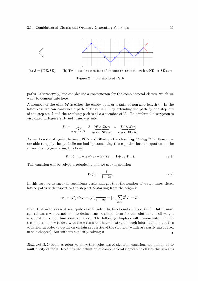
2.1. Combinatorial Classes and Ordinary Generating Functions 11
(a) S = NE,SE (b) Two possible extensions of an unrestricted path with a NE- or SE-step
Figure 2.1: Unrestricted Path
paths. Alternatively, one can deduce a construction for the combinatorial classes, which wewant to demonstrate here.
A member of the class W is either the empty path or a path of non-zero length n. In thelatter case we can construct a path of length n + 1 by extending the path by one step outof the step set S and the resulting path is also a member of W. This informal description isvisualized in Figure 2.1b and translates into
W = E︸︷︷︸empty walk
∪ W × ZNE︸ ︷︷ ︸append NE-step
∪ W × ZSE︸ ︷︷ ︸append SE-step
As we do not distinguish between NE- and SE-steps the class ZNE∼= ZSE
∼= Z. Hence, weare able to apply the symbolic method by translating this equation into an equation on thecorresponding generating functions:
W (z) = 1 + zW (z) + zW (z) = 1 + 2zW (z). (2.1)
This equation can be solved algebraically and we get the solution
W (z) =1
1− 2z. (2.2)
In this case we extract the coefficients easily and get that the number of n-step unrestrictedlattice paths with respect to the step set S starting from the origin is
wn = [zn]W (z) = [zn]1
1− 2z= [zn]
∑
k≥0
2kzk = 2n.
Note, that in this case it was quite easy to solve the functional equation (2.1). But in mostgeneral cases we are not able to deduce such a simple form for the solution and all we getis a relation on the functional equation. The following chapters will demonstrate differenttechniques on how to deal with these cases and how to extract enough information out of thisequation, in order to decide on certain properties of the solution (which are partly introducedin this chapter), but without explicitly solving it.
Remark 2.6: From Algebra we know that solutions of algebraic equations are unique up tomultiplicity of roots. Recalling the definition of combinatorial isomorphic classes this gives us

2.1. Combinatorial Classes and Ordinary Generating Functions 12
an easy way of checking such isomorphisms. If the generating functions of two classes satisfythe same functional equation, then the coefficient sequences satisfy the same recursion. Inorder to prove isomorphism, all which is left, is to check the “start values”, this can also beachieved by comparison of the first “few” (depending on the order of the recursion/equation)terms of the sequence. A straightforward example of two classes whose generating functionsfulfil the same functional equation are the empty class E and the atomic class Z. Both OGFsatisfy the equation A(z)2 = A(z), but they are not the same, as E(z) = 1 and Z(z) = z,respectively.
Figure 2.2: Dyck Path of length 18
Example 2.7 (Dyck Paths, [13, pp. 319]): The probably most famous example of aclass of lattice paths is the class of Dyck Paths D. These are paths on the same step setS = NE,SE as before, but implying the restrictions, that they start at the origin, neverleave the first quadrant and end on the x-axis. An example is shown in Figure 2.2.
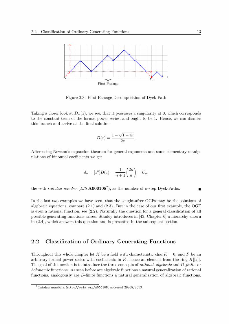
As before, we are able to construct a functional equation for the OGF D(z) of Dyck Pathsusing the introduced operations: The technique we will apply is known as First passagedecomposition. Basically it decomposes an arbitrary path ω ∈ D into two, possibly emptypaths also belonging to D.
A member of the class D is either the empty path or a path of non-zero length. If it is ofnon-zero length, after the initial point of contact at the origin, there will be another pointof contact with the x-axis. Denote the first such second point as x0. Now consider the pathfrom the origin to x0 without the initial NE- and the final SE-step. This, possible emptysub-path is also a legitimate Dyck path that belongs to D. (Recall that the empty path isalso a member of D.) After the “first passage”, which ends at x0, there will be another pathstarting at x0 and ending on the x-axis. This path could be empty as well, but it is, as before,again a Dyck Path. The described procedure is depicted in Figure 2.3.
This informal description translates into
D = E︸︷︷︸empty walk
∪ ZNE ×D ×ZSE︸ ︷︷ ︸first passage
×D.
The symbolic method gives with the same reasoning as before
D(z) = 1 + z ·D(z) · z ·D(z) = 1 + z2(D(z))2. (2.3)
Here we obtained a quadratic functional equation, which has the two possible solutions
D±(z) =1±√1− 4z
2z.
2.2. Classification of Ordinary Generating Functions 13
First Passage
x0
Figure 2.3: First Passage Decomposition of Dyck Path
Taking a closer look at D+(z), we see, that it possesses a singularity at 0, which correspondsto the constant term of the formal power series, and ought to be 1. Hence, we can dismissthis branch and arrive at the final solution
D(z) =1−√
1− 4z
2z.
After using Newton’s expansion theorem for general exponents and some elementary manip-ulations of binomial coefficients we get
dn = [zn]D(z) =1
n+ 1
(2n
n
)= Cn,
the n-th Catalan number (EIS A0001087), as the number of n-step Dyck-Paths.
In the last two examples we have seen, that the sought-after OGFs may be the solutions ofalgebraic equations, compare (2.1) and (2.3). But in the case of our first example, the OGFis even a rational function, see (2.2). Naturally the question for a general classification of allpossible generating functions arises. Stanley introduces in [43, Chapter 6] a hierarchy shownin (2.4), which answers this question and is presented in the subsequent section.
2.2 Classification of Ordinary Generating Functions
Throughout this whole chapter let K be a field with characteristic charK = 0, and F be anarbitrary formal power series with coefficients in K, hence an element from the ring K[[z]].The goal of this section is to introduce the three concepts of rational, algebraic and D-finite orholonomic functions. As seen before are algebraic functions a natural generalization of rationalfunctions, analogously are D-finite functions a natural generalization of algebraic functions.
7Catalan numbers; http://oeis.org/A000108, accessed 26/08/2013.

2.2. Classification of Ordinary Generating Functions 14
Thus we get the hierarchy
D-finite/holonomic
↑algebraic (2.4)
↑rational
Stanley remarks, that this hierarchy is by far not exhaustive, as various classes could beadded, but these three seem the most useful for enumerative combinatorics.
Definition 2.8: A formal power series F ∈ K[[z]] is rational if there exist polynomialsP (z), Q(z) ∈ K[z], with Q(z) 6= 0, such that
F =P (z)
Q(z).
♦
As mentioned before we have already seen a rational OGF in (2.2). Note, that rationalitycorresponds to a linear recurrence relation, which follows immediately from rearranging theabove definition to F (z)Q(z) = P (z) in the language of OGFs. The concept of algebraicfunctions is a natural generalization to higher degrees.
Definition 2.9: A formal power series F ∈ K[[z]] is algebraic if there exist polynomialsP0(z), P1(z), . . . , Pd(z) ∈ K[z], not all 0, such that
Pd(z)F d + Pd−1(z)F d−1 + . . .+ P1(z)F + P0(z) = 0.
The smallest positive integer d for which this equation holds is called the degree of F . ♦
Example 2.10: As seen in Example 2.7 the OGF D(z) = 1−√
1−4z2z of Dyck paths satisfies
z2D(z)2 −D(z) + 1 = 0.
Thus, D is algebraic and of degree 2.
But there exists a larger class of functions, which encloses all algebraic functions: the D-finite (short for differentiably finite) or holonomic functions.
Definition 2.11: A formal power series F ∈ K[[z]] is D-finite or holonomic, if there existpolynomials P0(z), P1(z), . . . , Pd(z) ∈ K[z], with Pd(z) 6= 0, such that
Pd(z)F (d) + Pd−1(z)F (d−1) + . . . + P1(z)F ′ + P0(z)F = 0, (2.5)
where F (j) = djF/dzj and d ∈ N is the order of the differential equation. ♦
Remark 2.12: The historical source of holonomic functions is found in the theory of linearrecursions. A sequence (fn)n∈N of complex numbers is holonomic or P-recursive (short for
2.2. Classification of Ordinary Generating Functions 15
polynomially recursive) if it satisfies a homogeneous linear recurrence relation of finite degreewith polynomial coefficients, i.e.
pd(n)fn+d + pd−1(n)fn+d−1 + · · ·+ p0(n)fn = 0, n ≥ 0,
for some polynomials pi(x) ∈ C[x]. Let F (z) =∑
n≥0 fnzn be the formal power series formed
by the sequence (fn)n∈N. As anticipated by the naming convention, a sequence is holonomicif and only if its generating function is holonomic, see [43, Proposition 6.4.3].
Proposition 2.13 [43, Proposition 6.4.1]: Let U ∈ K[[z]]. The following three condi-tions are equivalent:
(i) U is holonomic.(ii) There exist polynomials Q0(z), . . . , Qm(z), Q(z) ∈ K[z], with Qm(z) 6= 0, such that
Qm(z)U (m) +Qm−1(z)U (m−1) + . . . +Q1(z)U ′ +Q0(z)U = Q(z). (2.6)
(iii) The vector space over K(z) spanned by U and all its derivatives U ′, U ′′, . . . is finite-dimensional, i.e.
dimK(z)
[K(z)U +K(z)U ′ +K(z)U ′′ + . . .
]<∞.
Proof: (i) ⇒ (ii): Trivial.
(ii) ⇒ (iii): Suppose (2.6) holds and t is the degree of Q(z). After differentiating (2.6) t + 1times we get an equation in the form of (2.5), with d = m + t + 1 and Pd(z) = Qm(z) 6= 0.Solving for U (d) yields
U (d) = h0(z)U + h1(z)U ′ + . . . + hd−1(z)U (d−1), (2.7)
with polynomials h0(z), . . . , hd−1 ∈ K[z] ⊂ K(z). Differentiating this expression with respectto z we get
U (d+1) = h0(z)U + h1(z)U ′ + . . .+ hd−1(z)U (d−1) + hd(z)U (d)
∈ K(z)U +K(z)U ′ + . . .+K(z)U (d−1),
with polynomials h0(z), . . . , hd(z) ∈ K[z] and the last member relation holds due to (2.7).By induction it holds that,
U (d+k) ∈ K(z)U +K(z)U ′ + . . .+K(z)U (d−1),
for all k ≥ 0.
(iii) ⇒ (i): Suppose
dimK(z)
[K(z)U +K(z)U ′ +K(z)U ′′ + . . .
]= d.
Thus u, u′, . . . , u(d) are linearly dependent over K(z). This dependence relation, after clearingthe denominators so that the coefficients are polynomials in K[z], results in an equation ofthe form (2.5).

2.2. Classification of Ordinary Generating Functions 16
Example 2.14: The following functions are holonomic:
1. U = z−23z+4 , as (z − 2)(3z + 4)U ′ − 10U = 0.
2. U = ez , as U ′ = U and U = log(z), as zU ′ = 1 or zU ′′ + U ′ = 0.
3. U = zmeaz , as U ′ = (mz + a)U .
4. U = cos(z), as U ′′ = −U . The same holds obviously for sin(z).
5. U =∑
n≥0 n!zn, since (zU)′ =∑
n≥0(n + 1)!zn This implies that z(zU)′ + 1 = U orreordered in the form of (2.6): z2U ′ + (z − 1)U = −1.
We end this section with the proof of the missing link between holonomic and algebraicfunctions.
Theorem 2.15 [43, Proposition 6.4.6]: Let U ∈ K[[z]] be algebraic of degree d, then Uis holonomic.
Proof: If U(z) is algebraic, there is some polynomial 0 6= P (z, y) ∈ K(z, y) of minimal degreesuch that P (z, U) = 0. It holds, that
0 =d
dzP (z, U) =
∂P (z, y)
∂z
∣∣∣∣y=U
+ U ′ ∂P (z, y)
∂y
∣∣∣∣y=U
Since P (z, y) is of minimal degree, and therefore irreducible over K(x), it follows, that∂P (z, y)/∂y is non-zero (remember charK = 0) and a polynomial in y of smaller degree
than P , so ∂P (z,y)∂y
∣∣∣y=U6= 0. Hence, we get
U ′ = −∂P (z,y)
∂z
∣∣∣y=U
∂P (z,y)∂y
∣∣∣y=U
∈ K(z, U).
In other words, U ′ is a rational function in z and U . By induction we get that U (k) ∈ K(z, U)for all k ≥ 0. But due to the fact, that U is algebraic, we get dimK(z)K(z, U) = d and so it
follows that U,U ′, . . . , U (d) are linearly dependent over K(z). This yields an equation of theform (2.5), which proves that U is holonomic.
Example 2.16 [43, Ex. 6.1]: Not all holonomic functions are algebraic. ConsiderU(z) = ez: If it would be algebraic of degree d it would satisfy an equation of the form
Pd(z)edz + Pd−1(z)e(d−1)z + . . .+ P1(z)ez + P0(z) = 0,
where P0(z), . . . , Pd(z) ∈ C[z] and Pd(z) is of minimal degree. Differentiating this equationand subtracting the initial one multiplied by d, gives
P ′de
dz +(P ′
d−1 − Pd−1
)e(d−1)z + . . .+
(P ′
1 − (d− 1)P1)ez +
(P ′
0 − dP0)
= 0,
2.3. Multivariate Generating Functions 17
which either has degree less than d, and contradicts the fact that U(z) is algebraic of degreed, or the degree is the same, which contradicts the choice of Pd(z) to be of minimal degree.
The class of holonomic function enjoys rich closure properties. Note, that the followingtheorem mentions only the operations we are going to encounter in this thesis. For moredetails see [13, Theorem B.2].
Theorem 2.17: The class of univariate holonomic functions is closed under the following op-erations: sum (+), product (×), differentiation (∂z), indefinite integration (
∫ z) and algebraicsubstitution (z 7→ y(z) for some algebraic function y(z)).
Proof: The proof is omitted here. A sketch of a proof can be found in [13, Theorem B.2], fulldetails are discussed in [43, Chapter 6].
The discussion so far only considered univariate or ordinary generating functions, i.e. functionsin one variable. In order to encode more information, it is sometimes necessary to introducemore than one variable. This fact has already been used in the proof of Theorem 2.15. Thenecessary theory is presented in the next section.
2.3 Multivariate Generating Functions
So far we have considered only univariate formal power series, but this concept can be easilygeneralized to multivariate formal power series. In the same manner OGFs generalize to mul-tivariate generating functions (MGFs). As Flajolet and Sedgewick put it [13, Chapter III], themain advantage of several variables is the possibility to keep track of a collection of parametersdefined over combinatorial objects. But their big applicability results from a straightforwardgeneralization of the symbolic method, which proved so powerful in the ongoing discussion.The main message is, that we can use the symbolic method not just to count combinatorialobjects but also to quantify their properties.
In the case of lattice path combinatorics we will need the notion of a trivariate generatingfunction, with two parameters keeping track of the end-point in the first quadrant and oneparameter encoding the length of a lattice path. This translates into
Q(x, y; z) =∑
i,j,n≥0
q(i, j;n)xiyjzn.
Note, that it can also be interpreted as a formal power series in z with coefficients in Q[x, y],where for all n, almost all coefficients q(i, j;n) are zero. This interpretation somehow closesthe circle and links MGFs with OGFs.
Another generalization is the usage of formal Laurent series instead of formal power series.All definitions and observations stay the same and can be straightforwardly adapted to thisnew case. As a short-hand we define
x :=1
x.

2.3. Multivariate Generating Functions 18
This notion allows us to encode paths of length n ending anywhere in the Euclidean plane:
Q(x, y; z) =∑
i,j∈Zn≥0
q(i, j;n)xiyjzn.
In the following we want to discuss the changes as part of a hands-on example on the simplestMGF, a bivariate generating function (BGF). A rigorous introduction to MGF can be foundin [13, Chapter III].
A BGF is a formal power series (formal Laurent series) in two variables. Hence, there are twopossible parameters which we could keep track of. One suitable definition for lattice paths,is the use of one variable as the length of the path, and the second one as the final height ofthe path, i.e. the stopping y-coordinate.
F (y; z) =∑
i∈Zn≥0
f(i;n)yizn,
where the coefficients [zn]F (y; z) are in Q[y, y], and for all n almost all f(i;n) are zero.
Definition 2.18: The positive part of F (y; z) in y is the following series, which has coefficientsin Q[y] as power series in z:
[y>]F (y; z) :=∑
i>0n≥0
f(i;n)yizn.
Similarly we define the negative, non-negative and non-positive parts of F (y; z) in y, whichwe denote respectively by [y<]F (y; z), [y≥]F (y; z) and [y≤]F (y; z). The operator [y<]F (y; z)is also called the projection onto the pole part of F (y; z), i.e. the partial sum of F (y; z) whereall terms contain a negative index of y. ♦
Example 2.19: We will continue the analysis started in Example 2.5 of unrestricted pathsW starting from the origin and using the step set S = NE,SE. We derived the followingrelation on the combinatorial classes
W = E ∪ W × ZNE ∪ W × ZSE.
The difference now, is that we have to distinguish between NE- and SE-steps. We kind ofabuse the notation now, because a NE-step increases the height by one and hence correspondsto the generating function y, but a SE-step decreases the height by one and hence correspondsto y = 1
y . Additionally, both steps increase the length by 1. Note, that we will work in thering of formal Laurent series Z[[y, y]]. Let’s define the bivariate generating function associatedwith W as
W2(y; z) =∑
i∈Zn≥0
w(i;n)yizn.
This gives
W2(y; z) = 1 + yzW2(y; z) +z
yW2(y; z).

2.3. Multivariate Generating Functions 19
Solving this equation for W2 results in
W2(y; z) =1
1− z(y + 1
y
) .
Next we will perform a coefficient extraction in order to get w(j;m), the number of walks oflength m stopping at height j. Firstly, we start by fixing n by m:
[zm]W2(y; z) =
(y +
1
y
)m
.
This is a Laurent polynomial in y. Secondly, we apply the shift identity of the coefficientextraction (1.1) to get
w(j;m) = [yj ]
(y +
1
y
)m
= [ym+j ](y2 + 1
)m
=
0, for m+ j ≡ 1 mod (2) or |m| > j,(m
m+j2
), for m+ j ≡ 0 mod (2).
Note, that the BGF can be easily transformed into the OGF we found in Example 2.5, bysubstituting y = 1. This action sums over all possible heights at fixed length n:
W2(1; z) =1
1− 2z= W (z)
∑
i∈Z
w(i;m) =∑
i=−m,−m+2,...m
(m
m+i2
)=
m∑
j=0
(m
j
)= 2m
In general, we have to be careful here. We are only dealing with formal power series, which isthe reason why insertion of special values for variables is in general not well-defined. So, wehave to ensure that all operations are legitimate, e.g.: there are no singularities and all sumsare finite, etc.
The classification of multivariate formal power series can be directly generalized from theunivariate case.
Definition 2.20: Let K be field of characteristic charK = 0 and F ∈ K[[z1, . . . , zn]] be amultivariate formal power series. We call K
• rational, if there exist polynomials P,Q ∈ K[z1, . . . , zn] such that
QF = P,
• algebraic, if there exist polynomials P0, P1, . . . , Pd ∈ K[z1, . . . , zn], not all 0, such that
PdFd + Pd−1F
d−1 + . . . + P1F + P0 = 0.
The smallest positive integer d for which this equation holds is called the degree of F .

2.4. Why is it important to be holonomic? 20
• D-finite or holonomic, if there exist polynomials Pℓ,i ∈ K[z1, . . . , zn], i = 0, . . . , n,ℓ = 0, . . . , di with Pdi
(z) 6= 0, i = 0, . . . , n, such that
di∑
ℓ=0
Pℓ,i∂ℓF
∂zℓi
= 0 for all i = 1, . . . , n, (2.8)
where di ∈ N is the order of the partial differential equation in zi.
♦
The class of MGF is also closed under various operations. Note, that as in the univariate casethe following theorem mentions only the operations we are going to encounter in this thesis.For more details see [13, Theorem B.3].
Theorem 2.21: The class of multivariate holonomic functions is closed under the followingoperations: sum (+), product (×), differentiation (∂), indefinite integration (
∫), algebraic
substitution and specialization (setting some variable to a constant).
Proof: For the proof we refer to the paper from Lipshitz [34].
In the proof of Theorem 4.14 we will need the following result:
Proposition 2.22: If F (x, y; z) is a rational power series in z, with coefficients in C(x)[y, y],then [y>]F (x, y; z) is algebraic over C(x, y, z). If the latter series has coefficients in C[x, x, y],its positive part in x, the series [x>][y>]F (x, y; z), is a trivariate holonomic series.
Proof: The first statement is a simple adaption of [15, Theorem 6.1]. The series F (x, y; z) isinterpreted as element of (C(x)[y])[[y, z]], where y = x and z = y and instead of extractingthe elements of the diagonal, the sub-series
∑i≥0
([y0zi]F (x, y; z)
)zi is chosen. The proof
idea is complete analogous, the key tool is to expand F (x, y; z) in partial fractions of y (resp.z).
The second statement follows from the fact, that the diagonal of a holonomic series is holo-nomic [46, Theorem 6.3.3].
2.4 Why is it important to be holonomic?
After this short exposition on holonomic functions, one might ask why they are relevant tocombinatorics, as they are one central topic of investigation in this work. The subsequentshort summary of possible answers is derived from [31, pp. 12]. One unanswered question, isthe size of this special class. Are at the end nearly all functions anyway holonomic? Flajolet,Gerhold and Salvy [12] conjecture the following
“. . . a rough heuristic in this range of problem is the following: Almost anything isnon-holonomic unless it is holonomic by design.”

2.4. Why is it important to be holonomic? 21
But they invalidate their self-called naive statement in the next sentence, as there are manyknown combinatorial structures of holonomic character which arise naturally from differentfields. Some examples are the enumerations of k-regular graphs or the Apéry sequence
An =n∑
k=0
(n
k
)2(n+ k
k
)2
for which a proof was needed that it satisfies the recurrence
(n+ 2)3Bn+2 − (34n3 + 153n2 + 231n + 117)Bn+1 + (n+ 1)3Bn = 0, n ≥ 0,
with B0 = 1 and B1 = 5. This was the last missing link in the proof of the irrationality ofζ(3) [45]. A possible proof uses the closure properties of holonomic functions and associatedalgorithms, see [13, p. 752].
The intuition is, that holonomic functions possess a “nice” structure. This can be seen forexample in the asymptotic growth rate of a holonomic sequence, that is typically of the form
a(n) ∼ CeP (n1/r)nµnnθ log(n)β,
where P is a polynomial, β, r, µ ∈ N and C, θ ∈ C, see [28, Theorem 2] and the originalwork [47]. This form is important because many applications in lattice path enumeration areinterested in the asymptotic behavior.
Another important property of the class of holonomic functions, is the fact that the class isreasonable small but still large enough, so that it contains enough quantities that arise inapplications. A small class is a class where strong assumptions are imposed on its elements.An example for a small class is the set of all polynomial functions. The advantage of smallclasses is that they admit a finite representation, e.g. in form of their coefficients. The biggestdisadvantage of small classes is, that they mostly do not cover the important cases whicharise in applications. But large classes, which are more interesting, normally do not admita finite representation of its elements. Think of the set of all functions which allow a powerseries expansion. Now holonomic functions have proved to be a good compromise betweenthese two extremes. For more details see Kauers compact introduction to the field of symboliccomputation with regards to holonomic functions in [28].
But why do we look for such a class? One answer can be found in the field of symboliccomputing. If a class of functions possesses a finite description it is most likely that efficientalgorithms exist to manipulate its elements. And in the case of holonomic functions, suchalgorithms exist indeed. Examples for such algorithms are presented in [39]. These algorithmsare also used in computer-aided proofs which provide completely new possibilities to tackleso far unsolved problems. The proof that the GF of Gessel8 Walks is algebraic in [6] is anice example, where the technique of guessing is applied to find a recurrence relation forthe number of such walks of given length. First a finite number of terms of this sequenceis computed numerically, then the algorithm tries to guess the recurrence relation based onthese few values and lastly, one has to prove that this recurrence holds for all elements of thesequence. An introduction to this technique can also be found in [28, Chapter 4].
Last but not least we want to mention the closure properties of holonomic functions again, compare Theorems 2.17 and 2.21. They are the source for many algorithms on holonomicfunctions and justify their choice as a large but useful class of combinatorial objects.
8Ira Martin Gessel, 9.4.1951-

Chapter 3
Directed Lattice Paths
As an introduction to lattice path theory, we are going to consider directed paths. Theseare paths with a fixed direction of increase which we choose to be the positive horizontalaxis. This is described by the allowed steps: if (i, j) ∈ S then i > 0. One first importantobservation, is that the geometric realization of the path always lives in the right half-planeZ+ × Z. But it essentially means that directed paths are one-dimensional objects.
The following chapter mainly focuses on the expositions of Banderier1 and Flajolet givenin [3]. But it also draws from [8] in terms of applications of the kernel method which will beintroduced in this chapter.
Definition 3.1: Along these restrictions, we introduce the following classes (see Table 3.1):
• A bridge is a path whose end-point ωn lies on the x-axis;• A meander is a path that lies in the quarter plane Z2
+;• An excursion is a path that is at the same time a meander and a bridge, i.e. it connects
the origin with a point lying on the x-axis and involves no point with negative y-coordinate.
Additionally, we call a family of paths or steps to be simple if each allowed step in S is of theform (1, b) with b ∈ Z. In this case, we denote S = b1, . . . , bk. ♦
In the remainder of this section, if not specified differently, we will always consider simplepaths.
Definition 3.2: Let S = b1, . . . , bk be a simple set of steps, with Π = w1, . . . , wk thecorresponding system of weights. The characteristic polynomial of S is the Laurent polynomialS(u), defined as
S(u) :=k∑
i=1
wiubi .
Define c := −mini bi and d := maxi bi as the two extreme vertical amplitudes. We assumethroughout this chapter c, d > 0.
1Cyril Banderier, 19.5.1975-
22

23
ending anywhere ending at 0
unconstrained(on Z)
walk/path (W) bridge (B)
W (z) = 11−zS(1) B(z) = z
c∑i=1
u′
i(z)ui(z)
constrained(on Z+)
meander (M) excursion (E)
M(z) = 11−zS(1)
c∏i=1
(1− ui(z)) E(z) = (−1)c−1
p−cz
c∏i=1
ui(z)
Table 3.1: The four types of paths: walks, bridges, meanders and excursion and thecorresponding GFs [3, Fig. 1].
The characteristic curve of the lattice paths determined by S is the plane algebraic curvedefined by the equation
1− zS(u) = 0, or equivalently K(u, z) := uc − z (ucS(u)) = 0. (3.1)
The quantity K(u, z) is the kernel of the lattice paths and the equation is also referred to askernel equation. ♦
Remark, that the left equation in (3.1) is a rational function in u, while the second form iscalled its entire version, i.e. it contains no negative powers.
A useful property of (converging) power series/polynomials with positive coefficients is, that|S(u)| ≤ S(|u|), which follows from a straightforward application of the triangle inequality:|∑k
i=1 wiubi | ≤ ∑k
i=1wi|u|bi . Another important property of such power series is that theyare monotonically increasing in the argument for positive values.
It increases readability to rewrite
S(u) =d∑
i=−c
piui,
where not needed powers are canceled by zero coefficients.
Examining equation (3.1) near z = 0 with respect to asymptotic considerations shows that

3.1. Walks and Bridges 24
the kernel equation can only be satisfied if one of the two relations
pdzud ∼
z→01 or p−czu
−c ∼z→0
1 (3.2)
is satisfied. This is because u can be interpreted as function of z by the implicit definition ofthe kernel equation. Then it follows again by the kernel equation, that u must be unboundor go to zero as z tends to 0. If it would be bounded and not 0, the limit would lead to thecontradiction 0 = 1 in the kernel equation. Hence, u ∼ zα for z → 0. This leads to the aboveresult.
The entire version of the kernel equation is of degree c + d in u and it is known, that ithas c + d roots. These are the branches of a single algebraic curve, given by the kernelequation, which is then called the characteristic curve. As suggested by (3.2), one expects inthe complex domain and for z near 0, c “small branches” that we write as u1, . . . , uc and d“large branches” denoted as v1
∼= uc+1, . . . , vd∼= uc+d, satisfying
uj(z) ∼ e2πi(j−1)/c (p−c)1/c z1/c, vℓ(z) ∼ e2πi(1−ℓ)/d (p−d)−1/d z−1/d. (3.3)
Written in formulas, this means for z in a small enough neighborhood of 0, that
uc − z(ucS(u)) = −pdzc∏
i=1
(u− ui(z))d∏
j=1
(u− vj(z)). (3.4)
In order to ensure uniqueness, we employ the standard approach and restrict ourself to thecomplex plane slit along the negative real axis. That allows us to talk about the individualbranches in the sequel. More details about the theory of algebraic curves can be foundin [1, 36].
The graph of branches is obtained by interchanging the axes in the graph of 1/S(u), with u1
appearing as the real positive branch near the origin, see Figure 3.12.
3.1 Walks and Bridges
The first cases we are going to consider, are the unconstrained walks and bridges. Theseare the easiest models, but the following classification theorem shows already nicely, how theabove theory of algebraic curves is applied.
In the following proof we will need the following definition
Definition 3.3: A function f : D → R, D ⊆ R is called unimodal, if there exists a valuexm ∈ D, such that it is monotonically increasing for x ≤ xm and monotonically decreasingfor x ≥ xm. ♦
By the definition it is clear, that the maximum is f(xm).
Theorem 3.4 [3, Theorem 1]: The bivariate generating function of paths (z marking sizeand u marking final altitude) relative to a simple step set S with characteristic polynomial
2All plots created in Maple 12.0.

3.1. Walks and Bridges 25
Figure 3.1: Graphs associated with the step set S = −1, 0, 1, 2, with characteristicpolynomial S(u) = u−1 + 1 + u+ u2. Top: the graphs of S(u) and 1/S(u) for real u.
Bottom: the three branches of the characteristic polynomial of the characteristic curve:a small one of order z and two large ones of order ±z−1/2.
S(u) is a rational function. It is given by
W (u; z) =1
1− zS(u).
The generating function of bridges is an algebraic function given by
B(z) = zc∑
j=1
u′j(z)
uj(z)= z
d
dzlog(u1(z), . . . , uc(z)), (3.5)
where u1, . . . , uc are all small branches of the characteristic curve (3.1). Generally the GFWk(z) of paths terminating at altitude k is, for −∞ < k < c,
Wk(z) = zc∑
j=1
u′j(z)
uj(z)k+1= −z
k
d
dz
c∑
j=1
uj(z)−k
, (3.6)
and for −d < k <∞,
Wk(z) = −zd∑
j=1
v′j(z)
vj(z)k+1= −z
k
d
dz
d∑
j=1
vj(z)−k
, (3.7)
where v1, . . . , vd are the large branches. For W0(z), the second form is to be taken in the limitsense k → 0.

3.1. Walks and Bridges 26
Proof: We start with a decomposition argument for walks: Fix n ∈ N and let wn(u) =[zn]W (u; z) be the Laurent polynomial that describes the possible altitudes and the numberof ways to reach them in n steps. We have
• w0(u) = 1, as we can never return to the origin, after leaving it;• w1(u) = S(u), as length 1 corresponds to one step from the used step set S;• wn+1(u) = wn(u)S(u), as a walk of length n+ 1 is constructed from a walk of length n
by appending an additional step from S.
Hence, we obtain wn(u) = S(u)n and therefore
W (u; z) =∑
n≥0
wn(u)zn =∑
n≥0
S(u)nzn =1
1− zS(u).
We know from comparison with the geometric series, that this sum converges for |z| < 1/S(|u|)where we have used, that |S(u)| ≤ S(|u|). Thus, it represents an analytic function in twovariables, and beyond that it is entire in z and of the Laurent type in u, because it involvesarbitrary negative powers of u.
Next we are going to consider bridges. For positive u, the radius of convergence of W (u; z)viewed as a function of z is exactly 1/S(u). Due to the fact, that every bridge is also a specialunconstrained walk (i.e. [u0]W (u; z) = B(z)), we get that the number of bridges of givenlength n is dominated by the number of walks, i.e. Bn ≤ wn(1) = S(1)n. This implies, thatthe radius of convergence of B(z) as a function of z is at least 1/S(1).
We claim, that 1/S(u) is continuous and unimodal for u ∈ (0,+∞). The continuity is clearbecause 0 /∈ (0,+∞). It is unimodal, because P is a convex function (S′′(u) =
∑di=−c i(i −
1)piui−2 > 0) that satisfies 1/S(0) = 1/S(∞) = 0.
Let |z| < r, with r := 12
1S(1) . By the previous result, there exists an interval (α, β) such that for
α ≤ u ≤ β we have 1/S(u) > r. (The maximal possible interval would be (1/S(·))−1(r,+∞).)Reconsidering the properties of W (u; z) we get from this consideration, that W (u; z) is ana-lytic in the open product domain
V := z : |z| < r × u : α < |u| < β.
Thus, by Cauchy’s Integralformula, Theorem 1.13, applied to the function W (u; z) (viewedas a function of u) integrating over the closed circle |z| = α+β
2 which lies completely in thedomain V, we get
B(z) = [u0]W (u; z) =1
2πi
∫
|u|=(α+β)/2W (u; z)
du
u.
By (3.3) we can choose z small enough, so that all the large branches that escape to infinitylie outside of |u| ≤ (α + β)/2 and all the small branches are distinct. Then only the smallbranches remain inside and since they have only simple poles we are able to calculate theabove integral with the Residue Theorem 1.14. The residues are
Res
(W (u; z)
u, u = uj
)= Res
(1
u(1− zS(u)), u = uj
)= − 1
zujS′(uj),

3.1. Walks and Bridges 27
where we have used Lemma 1.15 with h(u) = 1/u and g(u) = 1 − zS(u). This value can besimplified, since differentiation of the characteristic curve yields
−S(u)− zS′(u)u′ = 0
⇔ S′(u) = −S(u)
zu′(S(u)= 1
z)
= − 1
z2u′
The integration contour can be shrunk to 0, which is legitimate since W (u; z) remains O(1).Hence it can be chosen small enough so that only small branches contribute and the ResidueTheorem gives
B(z) =c∑
j=1
− 1
zujS′(uj)= z
c∑
i=1
u′j(z)
uj(z)(3.8)
The same procedure is applicable to
Wk(z) = [uk]W (u; z) =1
2πi
∫
|u|=(α+β)/2W (u; z)
du
uk+1.
the integration contour can be shrunk to zero, provided the integrand remains bounded asu → 0. As the integrand is of order uc−k−1 this requires k ≤ (c − 1). Thus we get (3.6) byresidue calculation involving small branches. In the same manner as above, the formula isvalid in a small neighborhood of the origin. Therefore the identities are a posteriori valid asidentities between formal power series.
In the case that k > −d the residue calculation has to be adapted, by extending the contourto a large circle at ∞. By doing so, the large branches contribute and this shows (3.7).
It can be easily shown, that algebraic functions are closed under sums, products and multi-plicative inverses (compare Theorem 2.17). Therefore, we see by (3.8) that B(z) is algebraic,as all small branches uj(z) are algebraic. The same argument also shows, that Wk(z) is alge-braic.
Remark 3.5: The algebraic (holonomic) character of B(z) also follows from the fact thatB(z) ≡W0(z) is equivalently given as the diagonal of a bivariate rational function
B(z) =∑
n≥0
([znucn]
1
1− zucS(u)
)zn,
which follows immediately from Proposition 2.22.
After this short (and superficial) excursion into the field of algebraic curves we turn back toour lattice path problems. More details and a list of references on the theory of algebraiccurves are given in [3]. First we show how the introduced theory is applied.
Example 3.6 (Dyck Prefixes): The step set S = NE,SE = +1,−1 corresponds tothe walks of Dyck prefixes. The characteristic polynomial is S(u) = u−1 + u, and hence thecharacteristic curve reads
1− z(
1
u+ u
)= 0.
3.2. Meanders and Excursions 28
We see immediately from the step set, that c = 1 and d = 1. Therefore, the kernel equationis of degree 2:
u− z(1 + u2) = 0.
There exists one small branch and one large branch. In this case, they can be easily computed,by solving the equation of degree 2:
u1(z) =1−√
1− 4z2
2z∼
z→0z
v1(z) =1 +√
1− 4z2
2z∼
z→0
1
z
We see very good how the theory of algebraic curves predicts the solution in this example,compare (3.3). We used the fact, that
√1− 4z2 =
∑n≥0
(1/2n
)(−4)nz2n in a small neighbor-
hood of 0.
But what we really want, is top apply Theorem 3.4. This gives the GF for bridges in thiscase as
B(z) = zu′
1(z)
u1(z)=
1√1− 4z2
= 1 + 2z2 + 6z4 + 70z8 + 252z10 + . . .
The coefficients are known as EIS A0009843
[zn]B(z) =
(2n
n
)= [tn](1 + t2)n (3.9)
and called central binomial numbers. They are closely related to the Catalan numbers.
3.2 Meanders and Excursions
In this section we restrict the paths to the quarter plane Z2+. After this introduction, we
pursue this approach much further in Chapter 4, where we consider a special class of walkswhich are not necessary directed. Walks that stay in the first quadrant are called meandersand such whose final altitude is 0 are called excursions.
Let f(k;n) be the number of meanders of size (i.e. length) n that end at altitude k and usestep set S. The corresponding BGF is
F (u; z) :=∑
n,k≥0
f(k;n)ukzn,
which is now an entire series in both z and u. With similar arguments as in the analysis ofW (u; z) in the previous chapter, one can show that F (u; z) is bivariate analytic for |u| ≤ 1and |z| ≤ 1/S(1).
3Central binomial coefficients; http://oeis.org/A000984, accessed 26/08/2013.
3.2. Meanders and Excursions 29
We also need the polynomials Fk(z) that describe the possible ways to reach altitude k. Theyare defined by
F (u; z) =∑
k≥0
Fk(z)uk.
Analogously to the last section, we construct the walks recursively: A meander is either theempty one, or it has non-zero length n + 1. In the second case it is constructed from ameander of length n by appending a possible step from S. But as we are restricted to thefirst quadrant, we are not allowed to construct a walk, that crosses the x-axis. Hence, wemust not add a y-negative step to a walk of length n that ends on the x-axis. This proceduretranslates directly into the language of generating functions as
F (u; z) = 1︸︷︷︸empty path
+ zS(u)F (u; z)︸ ︷︷ ︸append step
− z[u<](S(u)F (u; z))︸ ︷︷ ︸paths leaving Z2
+
, (3.10)
where [u<] is the negative part in u from Definition 2.18. This relation is the fundamentalfunctional equation defining meanders. Rearranging this relation, reveals the kernel equa-tion (3.1). Note that S(u) involves only a finite number of negative powers (maximal c), sothat
F (u; z)(1 − zS(u)) = 1− zc−1∑
k=0
rk(u)Fk(z), (3.11)
for some Laurent polynomials rk(u) that are immediately computable via (3.10):
rk(u) := [u<](S(u)uk) =−k−1∑
j=−c
pjuj+k.
Theorem 3.7 [3, Theorem 2]: For a simple set of steps, the BGF of meanders (with zmarking size and u marking final altitude) relative to a simple set of paths S is algebraic. Itis given in terms of small and large branches of the characteristic curve of S by
F (u; z) =
∏cj=1(u− uj(z))
uc(1− zS(u))= − 1
pdz
d∏
ℓ=1
1
u− vℓ(z).
In particular the GF of excursions, E(z) = F (0; z), satisfies
E(z) =(−1)c−1
p−cz
c∏
j=1
uj(z) = −(−1)d−1
pdz
d∏
ℓ=1
1
vℓ(z). (3.12)
Proof: The main difficulty lies in the fact, that the fundamental equation (3.11) is massivelyundetermined. It involves the c unknown functions F0(z), . . . , Fc−1(z) and the also unknownbivariate function F (u; z). The guiding idea is a method known as the kernel method. In anutshell, we try to bind z and u in such a way, that the kernel 1 − zS(u) and therefore theleft-hand side vanishes.

3.2. Meanders and Excursions 30
As a first step we remove the negative coefficients of (3.11) by multiplying it with uc. Weobtain the entire kernel K(u, z) = uc− zucS(u) known from (3.1). From the discussion of thekernel equation K(u, z) = 0 we know, that there exist c small branches u1(z), . . . , uc(z) whichsatisfy this equation. By the theory of algebraic curves we are able to take |z| < 1/S(1) andrestrict z to a small neighborhood of the origin in such a way that:
1. all small branches are distinct;2. all the small branches satisfy |uj(z)| < 1.
This justifies the substitution analytically, and provides us with a system of c equations inthe unknowns F0, . . . , Fc−1:
uc1 − z
c−1∑
k=0
uc1rk(u1)Fk = 0
...
ucc − z
c−1∑
k=0
uccrk(uc)Fk = 0
This linear system in (Fk)c−1k=0 is a variant of a Vandermonde matrix. Therefore its determinant
is non-zero, as all small branches are distinct and by that it follows that this system is non-singular. Thus, each of the Fk is an algebraic function expressible rationally in terms of thealgebraic branches uj .
Next we need an observation of Bousquet-Mélou [8]. Let
N(u; z) := uc − zc−1∑
k=0
ucrk(u)Fk, (3.13)
and observe that (3.13) is a polynomial in u with its roots at the small branches uj . As itsleading monomial is uc it factorizes to
N(u; z) =c∏
j=1
(u− uj(z)). (3.14)
Now consider the constant term, it is at the same time
• (−1)cu1 · · · uc (consider above factorization) and• −zpcF0, which follows from (3.13) and the fact that only r0 start from u−c.
Hence, we get the GF for excursions E(z) = F (0; z) = F0(z).
The final result for meanders follows from the entire version of (3.11) and from the factoriza-tion (3.14)
F (u; z) =N(u; z)
uc(1− zS(u))=
∏cj=1(u− uj(z))
uc(1− zS(u)).
The second identities for F (u; z) and E(z) stated in the theorem follow immediately by taking(3.4) into account.

3.2. Meanders and Excursions 31
It is very easy to deduce the GFs for all paths and meanders from the last two theorems.
Corollary 3.8 [3, Corollary 1]: The GFs of all paths (W ) and all meanders (M) are
W (z) = W (1; z) =1
1− zS(1),
M(z) = F (1; z) =1
1− zS(1)
c∏
j=1
(1− uj(z)) = − 1
pdz
d∏
ℓ=1
1
1− vℓ(z). (3.15)
A more interesting and non-trivial connection between bridges and excursions, can be easilydeduced from their GFs by comparing (3.5) and (3.12). This is a nice example, of how a GFis able to point out new properties of a problem, as in this case it links two related but notdirectly connected problems.
Corollary 3.9 [3, Corollary 2]: For the GFs of bridges (B) and excursions (E) holds
B(z) = 1 + zd
dz(logE(z)) = 1 + z
E′(z)E(z)
E(z) = exp
(∫ z
0
B(t)− 1
tdt
).
Example 3.10 (Dyck Paths and the Ballot Problem): Continuing Example 3.6, weask for the number of paths with the step set S = +1,−1 that end on the x-axis but neverleave the first quadrant, i.e. never go below the x-axis. In the language of lattice paths, wewant to determine the number of excursions for this given step set. We may directly applyTheorem 3.7 as we have already computed the small and large branch above and get for theGF of excursions
E(z) =1−√
1− 4z2
2z2=∑
n≥0
1
n+ 1
(2n
n
)z2n =
∑
n≥0
Cnz2n,
where the coefficients Cn are the Catalan numbers.
The ballot problem asks for the probability in a two candidate election between A and B thateventually ends in a tie, while A is dominating B throughout the poll. This problem can bemodeled as a lattice path starting from the origin, with the steps NE representing a vote forcandidate A and SE being a vote for candidate B. The fact that it ends in a tie, translatesinto a walk that ends on the x-axis, and the condition of A dominating B is modeled by therestriction, that the walk must not leave the first quadrant. Hence, we are dealing with aDyck Path.
The total number of possible walks from (0, 0) to (2n, 0) is(2n
n
), which are the number of
bridges with respect to this step set, compare (3.9). The asked probability is
P(tie, A dominates B throughout) =
1
n+1 , 2n votes,
0, 2n+1 votes.

3.3. Walks confined to the Half-Plane 32
Example 3.11: The step set from Figure 3.1 is S = −1, 0, 1, 2. We know already from thefigure, that there will be one small branch of order 1 and two large branches of order −1/2.The entire version of the characteristic equation is
u− z(1 + u+ u2 + u3
)= 0.
The one small branch is given by
u1(z) = z + z2 + 2z3 + 5z4 + 13z5 + 36z6 + 104z7 + 309z8 + . . . ,
and the two large branches are conjugate
v1(z) = z1/2 − 12 − 3
8z1/2 − 1
2z − 41128z
3/2 − 12z
2 − 7631024z
3/2 − z3 + . . . ,
v2(z) = −z1/2 − 12 + 3
8z1/2 − 1
2z + 41128z
3/2 − 12z
2 + 7631024z
3/2 − z3 + . . . .
The first few terms of the GF for excursions are easily computed by (3.12)
E(z) =u1(z)
z= 1 + z + 2z2 + 5z3 + 13z4 + 36z5 + 104z6 + 309z7 + . . . ,
and similarly for meanders by (3.15)
M(z) =1− u1(z)
1− 4z= 1 + 3z + 11z2 + 42z3 + 163z4 + 639z5 + . . . .
Obviously the second representations for E(z) and M(z) in terms of the large branches leadto the same result, but are much more complicated to calculate in this case.
3.3 Walks confined to the Half-Plane
The derived theory for directed lattice paths can be applied to classify and enumerate morecomplicated problems. The first generalization is the consideration of real 2-dimensionalwalks, which means that walks are not directed anymore but can vary in both coordinates.In other words, the walks are allowed to go back and forth. Additionally we introduce therestriction, that the walks are confined to the upper half-plane Z × Z+, shortly called half-plane in the sequel. We are going to construct a bijection between all these walks and directedmeanders. The ideas of this approach are taken from [26, Chapter 6].
In detail, we are going to show, that the generating functions for walks confined to the half-plane are always algebraic. It holds, that they can be derived automatically using the kernelmethod, see Section 3.4 for details.
Definition 3.12: A walk ω = (ω0, ω1, . . . , ωn) of length n constructed from the step setS ⊂ Z2 is called confined to the half-plane if all its points ωk = (i, j) satisfy j ≥ 0 for alli = 1, . . . , n (see Figure 3.2). The associated class is called H and the number of walks oflength n is denoted by h(n). ♦
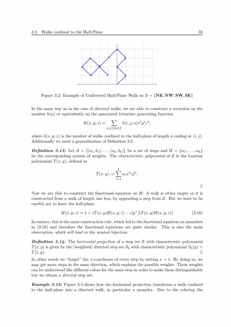
3.3. Walks confined to the Half-Plane 33
Figure 3.2: Example of Undirected Half-Plane Walk on S = NE,NW,SW,SE
In the same way as in the case of directed walks, we are able to construct a recursion on thenumber h(n) or equivalently on the associated trivariate generating function
H(x, y; z) =∑
n,j≥0;i∈Z
h(i, j;n)xiyjzn,
where h(x, y; z) is the number of walks confined to the half-plane of length n ending at (i, j).Additionally we need a generalization of Definition 3.2:
Definition 3.13: Let S = (a1, b1), . . . , (ak, bk) be a set of steps and Π = w1, . . . , wkbe the corresponding system of weights. The characteristic polynomial of S is the Laurentpolynomial T (x, y), defined as
T (x, y) :=k∑
i=1
wixaiybi .
♦
Now we are able to construct the functional equation on H: A walk is either empty or it isconstructed from a walk of length one less, by appending a step from S. But we have to becareful not to leave the half-plane.
H(x, y; z) = 1 + zT (x, y)H(x, y; z) − z[y<](T (x, y)H(x, y; z)) (3.16)
In essence, this is the same construction rule, which led to the functional equation on meandersin (3.10) and therefore the functional equations are quite similar. This is also the mainobservation, which will lead to the wanted bijection.
Definition 3.14: The horizontal projection of a step set S with characteristic polynomialT (x, y) is given by the (weighted) directed step set Sh with characteristic polynomial Sh(y) =T (1, y). ♦
In other words we “forget” the x-coordinate of every step by setting x = 1. By doing so, wemay get more steps in the same direction, which explains the possible weights. These weightscan be understood like different colors for the same step in order to make them distinguishablebut we obtain a directed step set.
Example 3.15: Figure 3.4 shows how the horizontal projection transforms a walk confinedto the half-plane into a directed walk, in particular a meander. Due to the coloring the

3.3. Walks confined to the Half-Plane 34
transformation is reversible, and in particular it is the wanted bijection (see Proposition 3.16).The step set S = NE,NW,SW,SE is transformed into the step set Sh = NE,SE withweights Π = (2, 2) or two colors for each step, represented by the dashed red and straightblue line (see Figure 3.3).
Note, that the transformation can also be interpreted as a flip of the x-negative steps alonga vertical line. This is also a possible way to construct the associated meander, by iterative“flipping” of x-negative steps into x-positive ones starting from the origin.
Figure 3.3: Horizontal Projection of S = NE,NW,SW,SE
Figure 3.4: Horizontal Projection of Half-Plane Walk into its associated Meander
Proposition 3.16: The class H of undirected half-plane walks on S is bijectively equivalentto the class M of directed meanders on Sh. In particular is the length generating function ofundirected half-plane walks always algebraic.
Proof: The functional equation for the GF of undirected half-plane walks H(x, y, z) wasderived in (3.16). The horizontal projections transforms it into
H(1, y; z) = 1 + zT (1, y)H(1, y; z) − z[y<](T (1, y)H(1, y; z)).
Define the projection of the characteristic polynomial to be S(y) := T (1, y), then we get
H(1, y; z) = 1 + zS(y)H(1, y; z) − z[y<](S(y)H(1, y; z)).
But at the same time this equation is satisfied by FSh(y; z) which is the GF of meanders on
the step set Sh. Thus, H(1, y; z) and FSh(y) satisfy the same functional equation and because
of that their coefficients satisfy the same recursion. In addition the first few terms agreewhich implies that the counting sequences are the same, compare Definition 2.3.
In other words
H(1, y; z) ≡ FSh(y; z).

3.4. Kernel Method and Linear Recurrences 35
The algebraic character of the length GF follows now directly from Theorem 3.7.
Remark 3.17: The above proof suppresses the x-coordinate by setting it to 1. This opera-tion of horizontal projection is well suited to solve this problem, as only the y-coordinate ofevery step is significant in order to impose the half-space restriction.
Example 3.18: Let’s investigate the step set S = NE,NW,SW,SE of Example 3.15further. In particular we want to derive the number of such walks of length n, i.e. h(n). Thecharacteristic polynomial of S is
T (x, y) = xy +x
y+y
x+
1
xy,
hence, the associated functional equation (3.16) for H(x, y; z) is given by
H(x, y; z) = 1 + z
(xy +
x
y+y
x+
1
xy
)H(x, y; z) − z
(x
y+
1
xy
)H(x, 0; z).
The horizontal projection introduces weights on the step set and yields
H(1, y; z) = 1 + z
(2y +
2
y
)H(1, y; z) − z
(2
y
)H(1, 0; z).
By rearranging this equation we obtain the kernel equation (3.1) and we get(
1− z(
2y +2
y
))
︸ ︷︷ ︸=K(y,z)/y
H(1, y; z) = 1− 2z
yH(1, 0; z).
Now we can apply the full theory of the previous sections. Note, that the kernel K(y, z) ischosen to be entire, which is why the value in the equation above is divided by y. SolvingK(y, z) = 0 gives the two branches
u1(z) =1−√
1− 16z2
4zv1(z) =
1 +√
1− 16z2
4z.
Corollary 3.8 tells us immediately the wanted GF for the number of walks confined to thehalf-plane with length n
H(1, 1; z) =2
1− 4z +√
1− 16z2= 1 + 2z + 8z2 + 24z3 + 96z4 + . . . .
For the power series expansion Newton’s expansion theorem was used.
3.4 Kernel Method and Linear Recurrences
We first give a short introduction on the origins of the kernel method. According to Banderierand Flajolet [3, pp. 55] the “kernel method” has been a part of the folklore of combinatorialistsfor some time. First references deal with a functional equation of the form
K(u, z)F (u; z) = A(u; z) +B(u; z)G(z) (3.17)
3.4. Kernel Method and Linear Recurrences 36
with F , G being the unknown functions and when there is only one small branch u1, suchthat K(u1(z), z) = 0. In this case a simple substitution solves the problem and G(z) =−A(u1(z); z)/B(u1(z); z). One clear source of this is the exercise section of Knuth’s book [29],published in 1968: The detailed solution to Exercise 2.2.1.1-4 presents a “new method forsolving the ballot problem”, for which the characteristic equation is quadratic. Anotherapplication can be found in Exercise 2.2.1.11 of the very same book.
But the topic is still alive in the mathematical community. The technique proved espe-cially valuable in lattice path enumeration problems, as we have already seen in the previoussections. One very important contribution from the end of the last century comes fromBousquet-Mélou and Petkovšek whose paper offers deep insights into the usefulness of thetechnique if applied to multi-dimensional walks and recurrences [8]. We are going to discussselected parts, which are especially useful for our goal of lattice path enumeration.
Finally it should be noted, that according to Banderier and Flajolet probabilists had knowna lot since the early 1950s regarding related questions. The technique seems to share strongparallels with the so-called Wiener-Hopf approach. But for more details and references torelated literature we refer to [3, p. 56].
In the remainder of this section we will discuss the results from [8]. We have seen in theprevious results, that the enumeration of every lattice path problem starts with a recursiveconstruction of the concerned walks. From this construction arises naturally a linear recur-rence relation with constant coefficients, from which the associated generating functions areconstructed. Hence we see, that the nature of the GF depends completely on the nature of theunderlying recurrence relation. This is the reason why we focus our studies on these objectsnow.
First some words on the used notation:
• We write u = (u1, u2, . . . , ud) for d-tuples of numbers or indeterminates like: 0 =(0, 0, . . . , 0), 1 = (1, 1, . . . , 1).
• Vector-valued inequalities are defined in the usual way as u ≥ v when ui ≥ vi for all1 ≤ i ≤ d and u < v when ui < vi for all 1 ≤ i ≤ d.
• The monomial xu11 · · · xud
d is denoted as xu.• For u,v ∈ Zd the scalar product u1v1 + . . .+ udvd is denoted as u · v.• The convex hull of a set H ⊆ Rd is denoted as convH.
The general form of a linear recurrence relation with constant coefficients is
an = ch1an+h1 + ch2an+h2 + . . . + chkan+hk
for n ≥ s.
Existence and Uniqueness
In the beginning we ask ourselves, what conditions are necessary in order to guarantee theexistence and uniqueness of a solution. These conditions can be derived in a more generalcontext.
Definition 3.19: Let A be a non-empty set. A d-dimensional recurrence equation is of theform
an = Φ(an+h1 , an+h2, . . . , an+hk) for n ≥ s, (3.18)
3.4. Kernel Method and Linear Recurrences 37
where a : Nd → A is the unknown d-dimensional sequence of elements of A, Φ : Ak → A isa given function, H = h1,h2, . . . ,hk ⊆ Zd is the set of shifts, and s ∈ Nd is the startingpoint satisfying s +H ⊆ Nd. A given function ϕ specifies the initial conditions:
an = ϕ(n) for n ≥ 0, n 6≥ s. (3.19)
♦
The idea of the proof is to characterize the set H and find conditions for which there is anordering of Nd of order type4 ω such that the points n + h1,n + h2, . . . ,n + hk precede n inthis ordering. The conclusion will be, that then there exists a unique solution of (3.18)-(3.19)and for any n ∈ Nd it is possible to compute the value of an directly from these equations ina finite number of steps.
Theorem 3.20 [8, Theorem 5]: Let H ⊆ Zd be a non-empty set which satisfies
x ∈ Rd : x ≥ 0 ∩ convH = ∅. (3.20)
Then there exists a unique d-dimensional sequence a : Nd → A which satisfies (3.18)-(3.19).
We omit the proof here, because it brings no new insights on our applications.
Remark 3.21: In [8] it is shown that condition (3.20) is equivalent to the fact that thereexists v ∈ Nd, v > 0, such that v · h < 0 for all h ∈ H. Furthermore it is also equivalent tothe existence of an ordering that depends on H that is well founded or can be extended toan ordering of Nd of order type ω (compare [8, Theorem 3]). We will not need these charac-terizations.
The nature of the solution
Due to the fact, that lattice path enumeration problems involve only linear recurrences withconstant coefficients we turn back to these problems. Hence we study the recurrence relation
an =
∑h∈H chan+h, for n ≥ s,
ϕ(n), for n ≥ 0 and n 6≥ s,(3.21)
where (ch)h∈H are given non-zero constants from A. Let A be a field of characteristic zero andH be a finite non-empty set from Zd satisfying (3.20). We assume s ∈ Nd and s +H ⊆ Nd.
Let a be the unique solution of the above recurrence. The corresponding GF is given by
Fs(x) =∑
n≥s
anxn−s.
As a first step we transform the recurrence relation into a functional equation satisfied by theGF Fs(x). We proceed the standard way: Multiply (3.21) with xn−s and sum over all n ≥ s:
Fs(x) =∑
h∈H
ch
∑
n≥s
an+hxn−s =∑
h∈H
chx−h∑
n≥s+h
anxn−s
=∑
h∈H
chx−h (Fs(x) + Ph(x)−Mh(x)) (3.22)
4The ordinal number ω is the least infinite one and identified with the cardinal number ℵ0.

3.4. Kernel Method and Linear Recurrences 38
where
Ph(x) =∑
n 6≥sn≥s+h
anxn−s =∑
n6≥sn≥s+h
ϕ(n)xn−s and (3.23)
Mh(x) =∑
n≥sn6≥s+h
anxn−s. (3.24)
With these definitions we can express the simple relation between Fs(x) and the full GF F (x)explicitly:
F (x) =∑
n≥0
anxn = xs
∑
n≥0
anxn−s +∑
n 6≥sn≥0
anxn−s
= xs (Fs(x) + P
−s(x)) . (3.25)
Next we rewrite equation (3.22) with the structure of (3.17) in mind into
1−
∑
h∈H
chx−h
Fs(x) =
∑
h∈H
chx−h (Ph(x)−Mh(x)) . (3.26)
To clear denominators on the left-hand side we introduce the notion of an apex which, as wewill see shortly, is strongly related to the nature of the GF.
Definition 3.22: Let H ⊂ Zd be a finite set. The apex of H is the point p = (p1, p2, . . . , pd) ∈Nd, such that
pi := maxhi : h ∈ H ∪ 0 i = 1, 2, . . . , d.
♦
Multiplying (3.26) by xp yields5
K(x)Fs(x) = A(x)−G(x) (3.27)
where
K(x) = xp −∑
h∈H
chxp−h,
A(x) =∑
h∈H
chxp−hPh(x),
G(x) =∑
h∈H
chxp−hMh(x).
The definition of the apex provides that K(x) is a polynomial in x which is called the kernel ofthe recursion (compare Lemma 4.12). Note that the coefficients of K(x) and A(x) are givendirectly by the coefficients of the recurrence relation and by the initial conditions, respectively.
5In the original paper [8] a different naming convention is used: K(x) is called Q(x), A(x) is called K(x)and G(x) is called U(x). We want to stick with the intuitive convention of calling the kernel K(x) here.

3.4. Kernel Method and Linear Recurrences 39
The coefficients of G(x) can be computed from (3.21) but are not given explicitly. Thereforewe call A(x) the known initial function and G(x) the unknown initial function.
If we now look at the functional equation (3.27) again (which is equivalent to our initialproblem (3.21)) it seems like we have rather made the problem more complicated becausethere are now two unknown functions Fs(x) and G(x). But we have also gained something:The initial conditions are now implicitly included and we have only one equation to deal with.Moreover, there is a strong connection between the two unknown functions, given over thekernel. The overall idea is, that if we are able to find G(x) explicitly then the GF of theunique solution to (3.21) is given by
Fs(x) =A(x)−G(x)
K(x). (3.28)
Definition 3.23: Let F (x1, . . . , xd) =∑
n≥0 an1,...,ndxn be a formal power series in d
variables. A section of F is any sub-series of F obtained by fixing some of the indices ofn = (n1, . . . , nd). ♦
Sections are important in this context, as all sections of rational (resp. algebraic, holonomic)series are also rational (resp. algebraic, holonomic). For details in the holonomic case werefer to [34, Proposition 2.5]. We start the analysis of (3.27) with some simple observations.
Proposition 3.24 [8, Proposition 11]: Let Fs(x) be the GF of the unique solution of(3.21). Then the series Fs(x) is rational (resp. algebraic, holonomic) if and only if both itsunknown initial function A(x) and G(x) are rational (resp. algebraic, holonomic).
Proof: Remember that rational, algebraic and holonomic power series are closed under thesum and the product, respectively (compare Theorem 2.21). Hence, if A and G are rational(resp. algebraic, holonomic) then by (3.28) Fs is also rational (resp. algebraic, holonomic).
Conversely, observe that for h ∈ H, the series Mh from (3.24) is a finite linear combination ofsections of Fs. Consequently the same holds for G. Hence, if Fs is rational (resp. algebraic,holonomic), then so is G(x). Finally (3.27) implies that the same holds for A(x).
Remark 3.25: Above argumentation for Mh cannot be used for Ph, as by (3.23) it is a lin-ear combination of sections of the full GF F (x) =
∑n≥0 anxn, but not of sections of Fs(x).
The last proposition tells us that the nature of Fs is completely determined by the natureof G because the nature of A is known beforehand as it depends solely on the initial valuesgiven by the function ϕ and is therefore explicitly known.
Theorem 3.26 [8, Theorem 12]: Assume the apex p of H is 0. Then the GF Fs(x) ofthe unique solution of (3.21) is rational if and only if the known initial function A(x) itself isrational.
Proof: The assumption guarantees that for each h ∈ H we have h ≤ 0 and therefore s+h ≤ s
and Mh(x) = 0, compare (3.24). This implies G(x) = 0 and so (3.28) simplifies to
Fs(x) =A(x)
K(x).

3.4. Kernel Method and Linear Recurrences 40
We know that K(x) is a polynomial in x and it follows that Fs(x) is rational if and only ifA(x) is.
Example 3.27 (Binomial Coefficients): Let’s shade some light on the theory whichwas covered so far by considering an easy example on the well-known binomial coefficients.Therefore, let n and k be integers such that 0 ≤ k ≤ q. We want to determine in how manyways we can choose a subset of k objects from the set 1, 2, . . . , n? For now, we pretend thatwe don’t know the answer.
Let an,k be the answer to this question. First we need to derive a recurrence relation: Considerthe collection of all possible subsets of k of these n objects. Next we fix the element n. Ifa subset of this collection contains the element n it contains k − 1 elements out of the set1, 2, . . . , n − 1. If it does not contain the element n it consists out of k elements from1, 2, . . . , n − 1. Therefore we obtain the recursion
an,k = an−1,k−1 + an−1,k, for n, k ≥ 1,
with the initial conditions ϕ(m, 0) = am,0 = 1 for all m ≥ 0 and ϕ(0, ℓ) = a0,ℓ = 0 for allℓ > 0.
The set of shifts is given by H = (−1,−1), (−1, 0) and the starting point by s = (1, 1).Hence, condition (3.20) is satisfied and there exists a unique solution to this problem.
The apex p is (0, 0) and due to Theorem 3.26 the solution Fs = F(1,1) is rational if and onlyif A is rational. We want to check this condition.
Computing Ph for h ∈ H via (3.23) gives
P(−1,−1)(x, y) =∑
(n,k)6≥(1,1)(n,k)≥(0,0)
ϕ(n, k)xn−1yk−1 =∑
n≥0k=0
xn−1yk−1 =1
xy
1
1− x,
P(−1,0)(x, y) =∑
(n,k)6≥(1,1)(n,k)≥(0,1)
ϕ(n, k)xn−1yk−1 ≡ 0.
Therefore we get for the known initial function A(x, y)
A(x, y) = 1 · xyP(−1,−1)(x, y) + 1 · xP(−1,0)(x, y) =1
1− x.
Thus, Theorem 3.26 implies that Fs is rational. The kernel is given by
K(x, y) = 1− x− xy
and due to that Fs is by (3.28) equal to
Fs(x, y) = F(1,1)(x, y) =1
1− x1
1− x− xy .
To check this answer, it is easy to compute the complete GF F (x, y) by
F (x, y) =∑
n,k≥0
(n
k
)xnyk =
∑
n≥0
(n∑
k=0
(n
k
)yk
)xn =
∑
n≥0
(1 + y)nxn =1
1− x− xy .

3.4. Kernel Method and Linear Recurrences 41
An easy computation shows, that our solution is correct. See also (3.25) for a connectionbetween Fs and F .
Obviously not all GFs are rational. The next theorem generalizes the last result and states asufficient condition for algebraic GFs.
Theorem 3.28 [8, Theorem 13]: Take A = C and assume that the apex p of H has atmost one positive coordinate. Then the GF Fs(x) of the unique solution of (3.21) is algebraicif and only if the known initial function A(x) itself is algebraic.
Proof: Due to Proposition 3.24 it holds that if Fs is algebraic then so is A.
If p = 0, then the proof is similar to that of Theorem 3.26. Assume now that exactly onecoordinate of p is positive. Without loss of generality we assume that p1 = . . . = pd−1 = 0and pd > 0. The idea of the following proof is to investigate this special coordinate xd. Firstwe note
G(x) =∑
h∈H
chxp−h∑
n≥sn 6≥s+h
anxn−s
=∑
h∈Hhd>0
chxp−hsd+hd−1∑
nd=sd
∑
(n1,...,nd−1)≥(s1,...,sd−1)
anxn−s.
Observe that all exponents of xd are positive, which is the reason that G(x) is a polynomialin xd of degree at most pd − 1. Rearranging (3.27) yields another representation of G:
G(x) = A(x)−K(x)Fs(x), (3.29)
with the kernel
K(x) = xpdd −
∑
h∈H
chxp−h,
which is a polynomial in xd of degree at most pd. Next we want to apply what is commonlyknown as the “kernel method”: We are going to prove that K(x) regarded as polynomial inxd admits (at least) pd roots ξi(x1, . . . , xd−1), counted with multiplicities, such that
ξi(0, . . . , 0) = 0.
This condition is necessary, as we want to substitute xd with ξi in (3.29). But this equation,interpreted as equation between converging power series, is only valid in some neighborhoodof the origin. (Remark, it can be shown that Fs is analytic in a neighborhood of the origin,if there exist constants m > 0 and u ∈ Rd such that |ϕ(n)| ≤ mu·n for all n 6≤ s, compare [8,Theorem 7].)
The existence of the ξi follows directly from the observation that
K(0, . . . , 0, xd) = xpdd −
∑
h∈Hh1=...=hd−1=0
chxpd−hdd .

3.4. Kernel Method and Linear Recurrences 42
Because of the overall assumption (3.20) we have x ∈ Rd : x ≥ 0 ∩ H = ∅ and thereforehd < 0 for all h ∈ H with h1 = . . . = hd−1 = 0 if such exist. This implies pd − hd > pd for allsuch h and therefore is xd = 0 a root of K(0, . . . , 0, xd) of multiplicity pd. If no such h ∈ Hexists, this is also true as in this case the sum vanishes.
Now we can replace xd by ξi(x1, . . . , xd−1) in (3.29) and obtain, if ξi is a root of multiplicitym, that
G(ξi) = A(ξi),∂
∂xdG(ξi) = ∂
∂xdA(ξi), . . . , ∂m−1
∂xm−1d
G(ξi) = ∂m−1
∂xm−1d
A(ξi),
where G(ξi) is short for G(x1, . . . , xd−1, ξi(x1, . . . , xd−1)) and A(ξi) analogously. Thus, the pd
roots of K provide a total of pd equations for the polynomial G of degree at most pd−1. So weare able to reconstruct G by means of the Hermite interpolation formula, which simplifies ifG has no multiple roots to the special case of the well-known Lagrange interpolation formula.
Because the ξi are algebraic functions of x1, . . . , xd−1 (they are the roots of the polynomialK in xd) this shows that G(x) is algebraic provided A(x) is. By Proposition 3.24 the sameholds for Fs(x).
Remark 3.29: The above proof not only shows existence but is also constructive in thesense, that it provides an algorithm to compute the GF of the solution. However, it involvesthe explicit knowledge of the roots of the kernel equation, and as this equation could havequite high degree, it need not to be an efficient or even applicable algorithm.
In the case that the known initial function A(x) itself is a polynomial (what happens quiteoften in enumerative combinatorics), the polynomial A(x)−G(x) has at least pd roots (namelyξ1, . . . , ξpd
, compare (3.27)). Under the conditions of Theorem 3.28 the polynomial G(x) hasdegree at most pd− 1 in xd and therefore A has degree at least pd. If A has exactly degree pd
then
A(x)−G(x) = lc(A)pd∏
i=1
(xd − ξi(x1, . . . , xd−1)),
where lc(A) denotes the leading coefficient of K with respect to xd. The degree of K in xd ispd + r, where r = max−hd : h ∈ H ∪ 0. The kernel K has the pd roots ξ1, . . . , ξpd
due to(3.27), and denote the remaining r roots as µ1, . . . , µr. Hence, we get
K(x) = lc(K)pd∏
i=1
(xd − ξi)r∏
j=1
(xd − µj).
Then the formula (3.28) simplifies to
Fs(x) =A(x)−G(x)
K(x)=
lc(A)
lc(K)
r∏
j=1
1
xd − µj.
We will illustrate the usefulness of the derived formula in the next example.
Example 3.30 (Generalized Dyck Paths, [8, Example 3]): The problem of General-ized Dyck Paths deals with a step set of the form S = (r1, s1), . . . , (rk, sk) where ri, si ∈ Z

3.4. Kernel Method and Linear Recurrences 43
and ri > 0 (directed problem). Let bn,m denote the number of paths going from (0, 0) to(m,n) using only steps from S and staying within the first quadrant. In this problem we aremainly interested in the numbers bm,0 =: bm. The recurrence relation is given by
bm,n =
∑i:(ri,si)≤(m,n) bm−ri,n−si, if m,n ≥ 0 and (m,n) 6= (0, 0),
1, if m = n = 0.
This form does not fit the one we have been working with so far, compare (3.21), but can beeasily brought into the desired form. Let r := max1≤i≤k ri and s := max1≤i≤k si. Interpretthe family (bm,n)m,n∈N as array b and attach r columns of zeros to the left of b and s rowsof zeros below. Call the resulting array a and number its rows and columns starting with 0.Then
bm,n = am+r,n+s, for m,n ≥ 0.
Finally only a technical step is missing: Let (ρ, σ) be any step in S which is maximal withrespect to the partial order ≤ (e.g. the lexicographically largest step). Set ar−ρ,s−σ := 1.Then we attain the desired form (3.21)
am,n =
am−r1,n−s1 + . . .+ am−rk,n−sk
, if m ≥ r and n ≥ s,δ(m,n),(r−ρ,s−σ), if m < r and n < s.
The set of shifts is given by H = (−r1,−s1), . . . , (−rk,−sk), the starting point s = (r, s)and ch = 1 for all h ∈ H. From the fact that ri > 0 for all i = 1, . . . , k it follows thatx ∈ Rd : x ≥ 0 ∩ convH = ∅ and by Theorem 3.20 there exists a unique solution.
The apex p = (0,max0, t) with t := −mins1, . . . , sk. We distinguish two cases:
(1) If si ≥ 0 for all i = 1, . . . , k, then the apex is (0, 0). Then we are in the case of Theorem3.26 and the GF of Fs will be rational. Let’s make this explicit:
The kernel is K(x, y) = 1 − xr1yx1 − . . . − xrkysk and the known initial function isA(x, y) = 1. Hence, we obtain for the GF B(x, y) enumerating bm,n
B(x, y) =∑
m,n≥0
bm,nxmyn =
∑
m≥r;n≥s
am,nxm−ryn−s = Fs(x, y)
=1
1− xr1ys1 − . . .− xrkysk.
The GF B0(x) for paths ending on the horizontal axis reads
B0(x) =∑
m≥0
bmxm = G(x, 0) =
1
1−∑1≤i≤k;si=0 xri.
(2) If there exists i = 1, . . . , k such that si < 0, then the apex of H is (0, t) with t > 0 andwe are in the case of Theorem 3.28 and the corresponding GF is algebraic.
Similarly as before we find
K(x, y) = yt − xr1ys1+t − . . . − xrkysk+t, A(x, y) = yt.

3.4. Kernel Method and Linear Recurrences 44
We are now in a special case discussed in Remark 3.29. The kernel K has degree t+ s iny with leading coefficient −∑i:si=s x
ri . Assume s > 0 to avoid trivial cases, because weare confined to the first quadrant. According to the proof of Theorem 3.28 there exist troots ξ1(x), . . . , ξt(x) with ξi(0) = 0 satisfying K(x, ξi(x)) = 0. Let µ1(x), . . . , µs(x) bethe s remaining roots. Hence, we get
B(x, y) =∑
m,n≥0
bm,nxmyn = Fs(x, y) =
1
K(x, y)
t∏
i=1
(y − ξi(x))
= − 1∑i:si=s x
ri
s∏
j=1
1
y − µj(x),
B0(x) =∑
m≥0
bmxm = G(x, 0) =
(−1)t
K(x, 0)
t∏
i=1
ξi(x) =(−1)s+1
∑i:si=s x
ri
s∏
j=1
1
µj(x). (3.30)
As special cases, this example includes some well-known lattice path enumeration problems.Let us state some famous ones and the GF B0(x) of paths ending on the horizontal axis givenby (3.30). Remark, that the set of steps S and the set of shifts H are naturally connected viaH = −S = (−r,−s) : (r, s) ∈ S. This is due to the fact, that lattice paths with the stepset S = (r1, s1), . . . , (rk, sk) can be recursively constructed with the recurrence relation
am,n = am−r1,n−s1 + . . .+ am−rk,n−skfor all (m,n) ≥ (r, s).
• Dyck Paths: S = (1,−1), (1, 1) with the kernel K(x, y) = y − xy2 − x,
B0(x) =1−√
1− 4x2
2x2.
• Motzkin Paths: S = (1,−1), (1, 1), (1, 0) with the kernel K(x, y) = y − xy2 − x− xy,
B0(x) =1− x−
√1− 2x− 3x2
2x2.
• Schröder Paths: S = (1,−1), (1, 1), (2, 0) with the kernel K(x, y) = y−xy2−x−x2y,
B0(x) =1− x2 −
√1− 6x2 + x4
2x2.
• Delannoy Paths: S = (1, 0), (0, 1), (1, 1) with the kernel K(x, y) = 1− x− xy − y,
B(x, y) =x+ xy + y
1− x− xy − y , B0(x) =1
1− x.
Note that the apex is (0, 0) and we get a rational GF.
At the end of this chapter we want to emphasize that not all recurrence relations need to haverational, algebraic or even holonomic solutions. There are also problems which have a non-holonomic and maybe even irrational solution. One example is the Knight’s Walk studiedin detail in [8]. Hereby we understand a walk that starts anywhere on the lines x = 0, 1or y = 0, 1, takes only two kinds of steps (−1, 2) and (2,−1) and remains in the regionx ≥ 2, y ≥ 2 once it leaves the starting point.

Chapter 4
Walks confined to the
Quarter Plane
The properties of lattice paths are, as the name suggests, very dependent on the nature of theunderlying lattice. These can differ in the chosen types (square lattice, hexagonal lattice, etc.)but also in their spacial expansion. By the latter we understand various types of restrictions,like the restriction to a half-plane or quarter plane of the lattice Z2. In the following chapterwe want to study such walks confined to the positive quarter plane (or positive quadrant) Z2
+
also noted as N2.
The motivation in the choice of these walks lies in the vast number and richness of applications.The following list from [42], gives a glimpse of different fields, which are effected by this theory:
• combinatorics: Many combinatorial objects (e.g. maps, permutations, trees or Youngtableaux) can be encoded in lattice walks, in particular by walks in the quarter plane,see [6, 7].
• population biology: The quarter plane is the natural space to parametrize any two-dimensional population, see [32].
• probability theory: One very recent topic are random walks in cones (quantum randomwalks, non-colliding random walks, etc.), see [21].
• queuing theory: Any two-dimensional queue can be modeled by random walks in thequarter plane.
• complex analysis: The inclusion Z2+ ⊂ C turns out to be convenient for applying methods
from complex analysis, see [11].
• finance: The dynamics of certain limit order books may be approximated by randomprocesses in the quarter plane.
• etc.
45
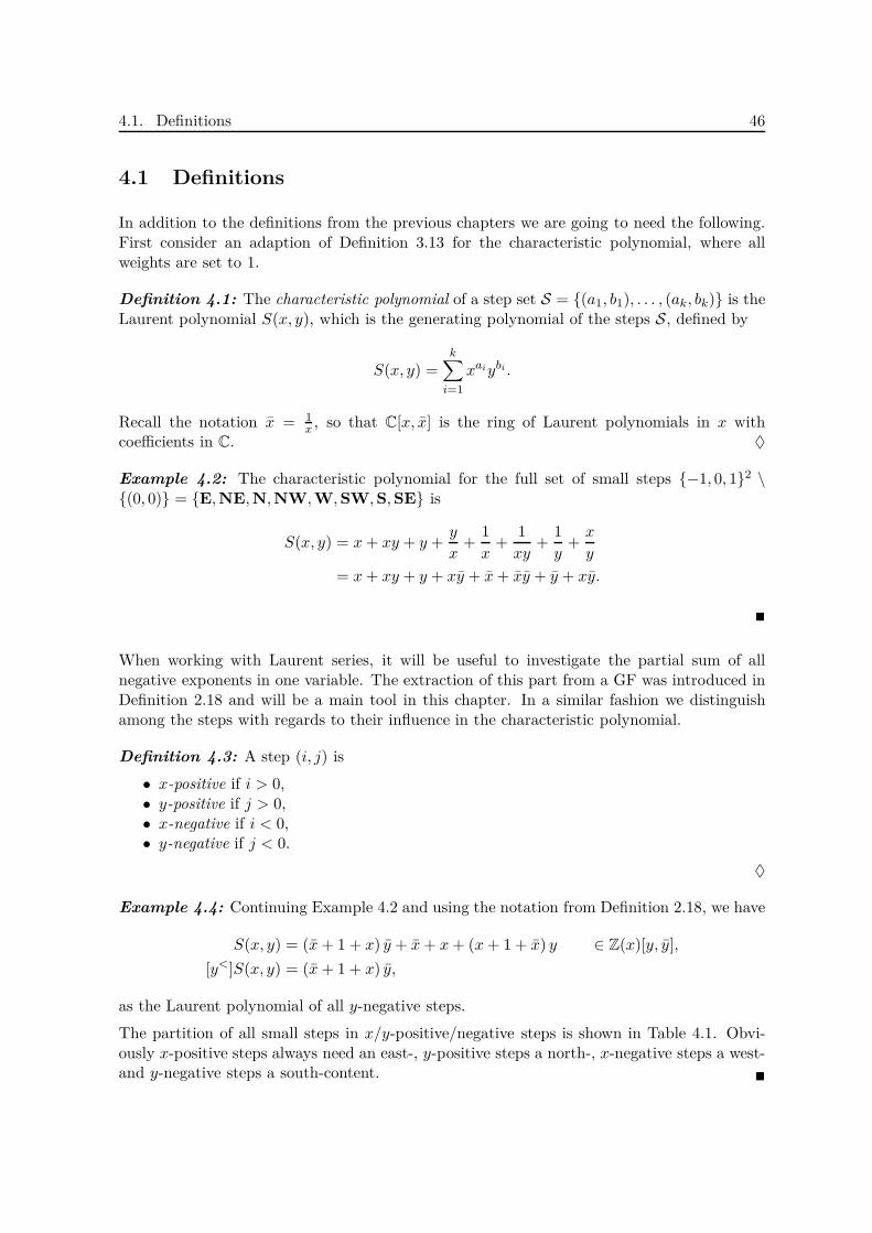
4.1. Definitions 46
4.1 Definitions
In addition to the definitions from the previous chapters we are going to need the following.First consider an adaption of Definition 3.13 for the characteristic polynomial, where allweights are set to 1.
Definition 4.1: The characteristic polynomial of a step set S = (a1, b1), . . . , (ak, bk) is theLaurent polynomial S(x, y), which is the generating polynomial of the steps S, defined by
S(x, y) =k∑
i=1
xaiybi .
Recall the notation x = 1x , so that C[x, x] is the ring of Laurent polynomials in x with
coefficients in C. ♦
Example 4.2: The characteristic polynomial for the full set of small steps −1, 0, 12 \(0, 0) = E,NE,N,NW,W,SW,S,SE is
S(x, y) = x+ xy + y +y
x+
1
x+
1
xy+
1
y+x
y
= x+ xy + y + xy + x+ xy + y + xy.
When working with Laurent series, it will be useful to investigate the partial sum of allnegative exponents in one variable. The extraction of this part from a GF was introduced inDefinition 2.18 and will be a main tool in this chapter. In a similar fashion we distinguishamong the steps with regards to their influence in the characteristic polynomial.
Definition 4.3: A step (i, j) is
• x-positive if i > 0,• y-positive if j > 0,• x-negative if i < 0,• y-negative if j < 0.
♦
Example 4.4: Continuing Example 4.2 and using the notation from Definition 2.18, we have
S(x, y) = (x+ 1 + x) y + x+ x+ (x+ 1 + x) y ∈ Z(x)[y, y],
[y<]S(x, y) = (x+ 1 + x) y,
as the Laurent polynomial of all y-negative steps.
The partition of all small steps in x/y-positive/negative steps is shown in Table 4.1. Obvi-ously x-positive steps always need an east-, y-positive steps a north-, x-negative steps a west-and y-negative steps a south-content.

4.2. Walks with Small Steps 47
Type Steps
x-positive SE E NE
y-positive NE N NW
x-negative NW W SW
y-negative SW S SE
Table 4.1: Partitioning of Small Steps in x/y-positive/negative Steps
4.2 Walks with Small Steps
This section is devoted to the analysis of walks confined to the quarter plane employing smallsteps, i.e. S = −1, 0, 12 \ (0, 0) (recall Definition 1.4). The investigation was started byBousquet-Mélou and Mishna in [7] who laid the foundation for many follow-up papers on thistopic [5, 6, 26, 30, 42]. It was the first to the author known approach to enumerate a “big”class of lattice paths restricted to the quarter plane.
A priori there are 28 different problems of this type. But among these, some are trivial, someare equivalent to models confined to the half-plane and some are equivalent to others up to ax/y-symmetry. This analysis results in 79 inherently different problems.
Their core step introduces algebra or in particular Galois theory to the problem of lattice pathenumeration. Each of the problems is associated with a group G of birational transformations.This group is finite for 23 cases and infinite for the remaining 56 other cases.
Finally, they present a way for solving 22 of 23 problems, which are associated with a finitegroup and show that the corresponding generating functions are holonomic. In the mean timeBostan and Kauers provided a computer aided proof for the 23rd case in [6] and showed thatits generating function is algebraic, hence holonomic.
For the 56 models with an infinite group the conjecture is raised from Bousquet-Mélou andMishna that they have non-holonomic generating functions. This is proven in [30] by Kurkovaand Raschel with analytic tools, like Riemann surfaces, universal covers, branches of mero-morphic functions, etc.
In the remainder of this chapter, we want to present the derivation and analysis of Bousquet-Mélou and Mishna from [7], which shows, how a systematic approach is able to succeed ona so far unsolved problem. It is impressive to discover, that only the interdisciplinary andcombined effort of different people and fields, like analytic combinatorics, complex analysisand algebra led to the successful solution of the problem.
4.2.1 Classification of Models with Small Steps
Figure 4.1: The full set of Small Steps

4.2. Walks with Small Steps 48
As we are investigating only small steps, there are only 28 = 256 cases to study, all possiblesubsets of the full step set S shown in Figure 4.1. As a first simplification, we can discardtrivial models, like S = ∅ or S = x. Hence, we first consider some easy algebraic cases:
1. No x-positive step: If S contains no x-positive step, we can ignore its x-negative steps,as they would only lead us out of the quarter plane. Therefore, these walks degenerateto walks consisting of vertical steps on the vertical half-line. We know already thatthese are always algebraic and even rational if the degenerated set is S = ∅, S = yor S = y. In fact we have already solved the algebraic case S = y, y explicitly, asthere is an obvious bijection to Dyck Prefixes confined to the first quadrant (i.e. me-anders), compare Theorem 3.7 and Example 3.10 where the special case of Dyck Paths(i.e. excursions) is discussed.
Another way to show that the GF is algebraic is to consider its recurrence relation. Wedefine ay,n to be the number of steps ending at altitude y after n steps. Then
ay,n = ay−1,n−1 + ay+1,n−1 for y, n ≥ 1
ay,0 = δy,0
a0,n = [zn]1−√
1− 4z2
z=
1
n+ 1Cn
The number a0,n represents all paths starting from (0, 0) and ending at (0, 0) which nevergo below the x-axis. Hence, as mentioned before, these are Dyck Paths and therefore weknow its GF from Example 2.7. This gives the set of shift H = (−1,−1), (1,−1), thestarting point s = (1, 1) and an algebraic known initial function A(y, z). Additionallywe see that the apex p = (1, 0) has only one positive coordinate, which implies byTheorem 3.28 that its GF is algebraic.
2. No y-positive step: Symmetric arguments lead to the same conclusion, that this problemhas an algebraic solution.
3. No x-negative step: The walks starting in the origin (0, 0) and employing this stepset always stay in the right half-plane x ≥ 0. If we now impose the restriction ofstaying in the quarter plane, this is equivalent to staying in the upper half-plane. Thecorresponding theory discussed in Section 3.3 implies that the GFs are always algebraic(compare Proposition 3.16).
4. No y-negative step: Again, by symmetry we obtain algebraic solutions.
This short analysis shows, that our step set has to contain x-positive, x-negative, y-positiveand y-negative steps. In order to enumerate the solution we introduce the OGF P (z) =∑8
n=0 pnzn where pn is the number of models employing a step set of size n, which have not
been covered yet. Observe, that there are in total 5 non-x-positive, non-x-negative, non-y-positive and non-y-negative steps each, shown in Figure 4.2. Thus, by an inclusion-exclusionargument we get the intermediate result
P1(z) = (1 + z)8 − 4(1 + z)5 + 2(1 + z)2 + 4(1 + z)3 − 4(1 + z) + 1
= 2z2 + 20z3 + 50z4 + 52z5 + 28z6 + 8z7 + z8.

4.2. Walks with Small Steps 49
(a) no x-positive step (b) no x-negative step (c) no y-positive step (d) no y-negative step
Figure 4.2: Small Steps which contain no x/y-positive/negative step, respectively
A short explanation of the above formula:
• (1 + z)8: all possible 28 subsets• (1 + z)4: counts sets with no x-positive step, . . .• (1 + z)2: counts sets with no x-positive nor x-negative step, . . .• (1 + z)3: counts sets with no x-positive nor y-positive step, . . .• (1 + z): counts sets with no x-positive nor x-negative nor y-positive step, . . .• 1: counts the empty set
Secondly, among the remaining 161 sets, there are some which do not contain any step withboth coordinates non-negative: In this case the only quarter plane walk is the emptywalk (see Figure 4.3a). These sets are subsets of x, y, xy, xy, xy. But due to the previousstep the used step set must contain x-positive and y-positive steps, hence, xy and xy belongto S. Therefore, we exclude 23 step sets, and get
P2(z) = P1(z)− z2(1 + z)3 = z2 + 17z3 + 47z4 + 51z5 + 28z6 + 8z7 + z8.
(a) x-negative ory-negative
(b) above first diagonal,x-cond. forces y-cond.
(c) below first diagonal,y-cond. forces x-cond.
Figure 4.3: Step Sets with respect to Diagonals
Thirdly, there exist models in which one of the quarter plane constraints implies the
other: In this case the model is equivalent to problems of walks confined to a half-space:their GF is always algebraic and can be derived using the kernel method [3].
Assume that all walks with steps in S that end at a non-negative abscissa automatically endat a non-negative ordinate (we say the x-condition forces/implies the y-condition). This canonly be if y and xy are not part of S. But as at this stage we need a y-negative step, xy mustbe in S. Under the prerequisite that the x-condition forces the y-condition, x cannot be in S,otherwise a walk could have non-negative final abscissa, but negative final ordinate. But nowwe exclude xy and x, which is why xy must be in S, because we need at least one x-positivestep. This implies that S \ xy, xy ⊆ x, y, xy. Observe, that these 3(5) steps are the oneslying (strictly) above the first diagonal, see Figure 4.3b.
Symmetric arguments lead to the fact, that if the y-condition implies the x condition we musthave: S \ xy, xy ⊆ x, y, xy, which corresponds to the steps below the first diagonal, seeFigure 4.3c. A final inclusion-exclusion arguments gives 138 remaining cases
P3(z) = P2(z)− 2z2(1 + z)3 + z2 = 11z3 + 41z4 + 49z5 + 28z6 + 8z7 + z8.

4.2. Walks with Small Steps 50
Lastly, we consider symmetries. When looking at the quarter plane embedded in the Eu-clidean plane, there is one obvious symmetry which jumps to one’s eye: The x/y-symmetryor reflection along the first diagonal. This is the only one, which leaves the quarter planefixed. (Note, that all 8 symmetries of the square act on the step sets, but none except thisone maps the quarter plane to itself.) Thus, two step sets, which can be transformed intoeach other applying this symmetry lead to equivalent counting problems. From now on, weunderstand symmetry always with respect to the first diagonal.
We want to find all non-equivalent problems, so we eliminate these among the remaining 138problems. We are going to achieve this by counting all symmetric models which are part of thepreviously counted ones. All others have a partner which is not the same and can be obtainedthrough reflection, but possesses the same counting sequence. Hence, we successively repeatthe last three steps:
1. There are 2 steps which are symmetric (ր and ւ) and 3 pairs of symmetric stepsubsets: ↑,→, տ,ց and ←, ↓. We discard all S which miss x- or y-positive, orx- or y-negative steps.
P sym1 (z) = (1 + z)2(1 + z2)3 − 2(1 + z)(1 + z2) + 1
2. No S is allowed, where all steps are negative in at least one coordinate. The ones whichhave to be excluded must obey xy, xy ⊆ S. Hence, there are only two possible choicesleft: xy and x, y.
P sym2 (z) = P sym
1 (z)− z2(1 + z)(1 + z2)
3. One quarter plane constraint implies the other. Here, only S = xy, xy is to beexcluded.
P sym3 (z) = P sym
2 (z)− z2 = 3z3 + 5z4 + 5z5 + 4z6 + 2z7 + z8
Therefore we get as the final result the generating polynomial
P (z) =1
2(P3(z) + P sym
3 (z)) = 7z3 + 23z4 + 27z5 + 16z6 + 5z7 + z8,
and a total of 79 non-equivalent models for step sets S with small steps.
In the next section we are going to introduce the core idea of the following proof, where weintroduce algebra into the field of lattice path counting.
4.2.2 The Group of the Walk
Recall the characteristic polynomial S(x, y) =∑
(i,j)∈S xiyj . By fixing x we can interpret it
as Laurent polynomial in y with coefficients in Q(x) and vice versa. This gives rise to thefollowing representation:
S(x, y) = A−1(x)y +A0(x) +A1(x)y
= B−1(y)x+B0(y) +B1(y)x(4.1)
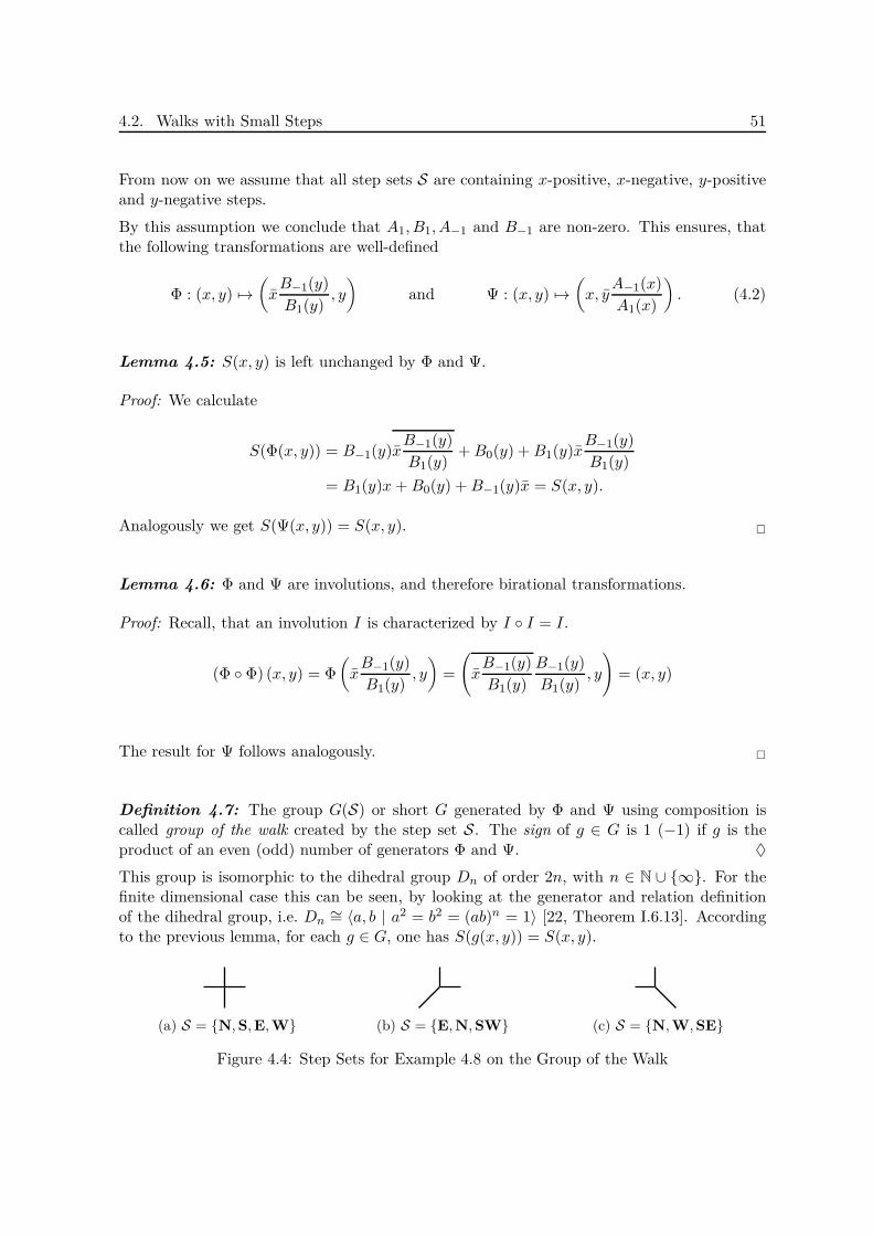
4.2. Walks with Small Steps 51
From now on we assume that all step sets S are containing x-positive, x-negative, y-positiveand y-negative steps.
By this assumption we conclude that A1, B1, A−1 and B−1 are non-zero. This ensures, thatthe following transformations are well-defined
Φ : (x, y) 7→(xB−1(y)
B1(y), y
)and Ψ : (x, y) 7→
(x, y
A−1(x)
A1(x)
). (4.2)
Lemma 4.5: S(x, y) is left unchanged by Φ and Ψ.
Proof: We calculate
S(Φ(x, y)) = B−1(y)xB−1(y)
B1(y)+B0(y) +B1(y)x
B−1(y)
B1(y)
= B1(y)x+B0(y) +B−1(y)x = S(x, y).
Analogously we get S(Ψ(x, y)) = S(x, y).
Lemma 4.6: Φ and Ψ are involutions, and therefore birational transformations.
Proof: Recall, that an involution I is characterized by I I = I.
(Φ Φ) (x, y) = Φ
(xB−1(y)
B1(y), y
)=
(xB−1(y)
B1(y)
B−1(y)
B1(y), y
)= (x, y)
The result for Ψ follows analogously.
Definition 4.7: The group G(S) or short G generated by Φ and Ψ using composition iscalled group of the walk created by the step set S. The sign of g ∈ G is 1 (−1) if g is theproduct of an even (odd) number of generators Φ and Ψ. ♦
This group is isomorphic to the dihedral group Dn of order 2n, with n ∈ N ∪ ∞. For thefinite dimensional case this can be seen, by looking at the generator and relation definitionof the dihedral group, i.e. Dn
∼= 〈a, b | a2 = b2 = (ab)n = 1〉 [22, Theorem I.6.13]. Accordingto the previous lemma, for each g ∈ G, one has S(g(x, y)) = S(x, y).
(a) S = N,S,E,W (b) S = E,N,SW (c) S = N,W,SE
Figure 4.4: Step Sets for Example 4.8 on the Group of the Walk
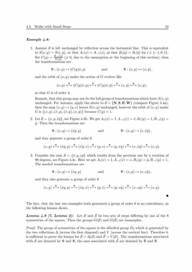
4.2. Walks with Small Steps 52
Example 4.8:
1. Assume S is left unchanged by reflection across the horizontal line. This is equivalentto S(x, y) = S(x, y), or that A1(x) = A−1(x), or that Bi(y) = Bi(y) for i ∈ −1, 0, 1.Set C(y) = B−1(y)
B1(y) (6= 0, due to the assumption at the beginning of this section), thenthe transformations are
Φ : (x, y) 7→ (C(y)x, y) and Ψ : (x, y) 7→ (x, y) ,
and the orbit of (x, y) under the action of G evolves like
(x, y)Φ←→ (C(y)x, y)
Ψ←→ (C(y)x, y)Φ←→ (x, y)
Ψ←→ (x, y),
so that G is of order 4.
Remark, that this group may not be the full group of transformations which leave S(x, y)unchanged. For instance, apply the above to S = N,S,E,W (compare Figure 4.4a),then the map (x, y) 7→ (y, x) leaves S(x, y) unchanged, however the orbit of (x, y) underG is (x, y), (x, y), (x, y), (x, y) because C(y) = 1.
2. Let S = x, y, xy, see Figure 4.4b. We get A1(x) = 1, A−1(x) = x, B1(y) = 1, B−1(y) =y. Then the transformations are
Φ : (x, y) 7→ (xy, y) and Ψ : (x, y) 7→ (x, xy) ,
and they generate a group of order 6
(x, y)Φ←→ (xy, y)
Ψ←→ (xy, x)Φ←→ (y, x)
Ψ←→ (y, xy)Φ←→ (x, xy)
Ψ←→ (x, y).
3. Consider the case S = x, y, xy which results from the previous one by a rotation of90 degrees, see Figure 4.4c. Here we get A1(x) = 1, A−1(x) = x,B1(y) = y, B−1(y) = 1.The needed transformations are
Φ : (x, y) 7→ (xy, y) and Ψ : (x, y) 7→ (x, xy) ,
and they also generate a group of order 6
(x, y)Φ←→ (xy, y)
Ψ←→ (xy, x)Φ←→ (y, x)
Ψ←→ (y, xy)Φ←→ (x, xy)
Ψ←→ (x, y).
The fact, that the last two examples both generated a group of order 6 is no coincidence, asthe following lemma shows.
Lemma 4.9 [7, Lemma 2]: Let S and S be two sets of steps differing by one of the 8symmetries of the square. Then the groups G(S) and G(S) are isomorphic.
Proof: The group of symmetries of the square is the dihedral group D4 which is generated bythe two reflections ∆ (across the first diagonal) and V (across the vertical line). Therefore itis sufficient to prove the lemma for S = ∆(S) and S = V (S). The transformations associatedwith S are denoted by Φ and Ψ, the ones associated with S are denoted by Φ and Ψ.

4.2. Walks with Small Steps 53
Assume S = ∆(S). Then the values of Ai(x) and Bi(y) swap, i.e. Ai(x) = Bi(x) andBi(y) = Ai(y). We reconstruct this swap with the involution δ(x, y) = (y, x).
Φ(x, y) =
(xB−1(y)
B1(y), y
)=
(xA−1(y)
A1(y), y
)= δ
(y, x
A−1(y)
A1(y)
)= (δ Ψ δ)(x, y),
Ψ = δ Ψ δ,
where the second result follows similarly. Hence the groups G(S) and G(S) are conjugate byδ and therefore isomorphic.
Assume S = V (S). Then Ai(x) = Ai(x) and Bi(y) = B−i(y). We reconstruct this symmetryby the involution v(x, y) = (x, y).
Φ(x, y) =
(xB−1(y)
B1(y), y
)=
(xB1(y)
B−1(y), y
)= v
(xB−1(y)
B1(y), y
)= (v Φ v)(x, y),
Ψ(x, y) =
(x, y
A−1(x)
A1(x)
)=
(x, y
A−1(x)
A1(x)
)= v
(x, y
A−1(x)
A1(x)
)= (v Ψ v)(x, y),
Hence the groups G(S) and G(S) are conjugate by v.
Theorem 4.10 [7, Theorem 3]: Out of the 79 models under construction, exactly 23 areassociated with a finite group:
• 16 have a vertical symmetry and thus a group of order 4,• 4 have a group of order 6,• 2 have a group of order 8.
Proof: From earlier considerations we know that G(S) is a dihedral group of order 2n withn ∈ N ∪ ∞. As Φ and Ψ are involutions, the group is of order 2n if and only if Θ := Ψ Φis of order n. Now it’s easy to check if a given group is of order 2n. Compute all iterates ofΘ and the first that is the identity gives you the half of the order.
By applying Lemma 4.9 to the first case of Example 4.8 we get, that the step sets with avertical symmetry have order 4. It is straightforward to check the other assertions. All resultsare summarized in Tables 1-3 in [7]. The step sets of the walks we are talking about are shownin Figures 4.5, 4.6 and 4.7.
The difficult task, is to prove that the remaining models possess an infinite group. Thereare 2 different strategies depending on S necessary to achieve this goal. For sets shown inFigure 4.8 a valuation argument is used. These sets are special, as all elements (i, j) satisfyi+ j ≥ 0. For the remaining cases a fixed point argument is used. It is interesting to note,that both strategies are necessary, i.e. the second one, does not solve the first cases.
1. The valuation argument
First, we introduce the general idea: We want to “project” the complicated case of a groupin (Z[x, x, y, y])2 to a simpler version in Z2, where we can perform simple calculations.
Let z be an indeterminate and let x and y be Laurent series in z with coefficients in Q, andrespective valuation a and b. Furthermore, we assume that the trailing coefficients of these

4.2. Walks with Small Steps 54
Figure 4.5: The 16 models whose group G(S) is isomorphic to D2. All of them possess avertical symmetry and have a holonomic GF [7, Table 1].
Figure 4.6: The 5 models whose group G(S) is isomorphic to D3. All have a holonomic GF,the last three even possess an algebraic GF [7, Table 2].
Figure 4.7: The 2 models whose group G(S) is isomorphic to D4. Both models have aholonomic GF, the second one even possesses an algebraic GF [7, Table 3].
The Second one is Gessel’s Walk which was solved in [6].
Figure 4.8: Five step sets with an infinite group, where i+ j ≥ 0 for all steps (i, j)

4.2. Walks with Small Steps 55
series, namely [za]x and [zb]y, are positive. Now define (x′, y) := Φ(x, y). Then by (4.2) thetrailing coefficient of x′ (and y) is positive, and the valuation of x′ (and y) only depends ona and b:
φ(a, b) := (val(x′), val(y)) =
(−a+ b(v(y)−1 − v
(y)1 ), b), if b ≥ 0,
(−a+ b(d(y)−1 − d
(y)1 ), b), if b ≤ 0,
where v(y)i (respectively d
(y)i ) denotes the valuation (resp. degree) in y of Bi(y), for i = ±1.
All this follows by the elementary construction of the inverse x(z) of the Laurent series x(z)of valuation a: Let x(z) =
∑n≥a xnz
n and x =∑
n≥α xnzn. A comparison of coefficients in
1 = x(z) · x(z) =∑
n≥a+α
(n∑
k=0
xk+axn−k+α
)zn,
gives that α = −a and that the trailing coefficient of x is (xa)−1 and therefore positive if xa
is positive. All other parts follow analogously.
The two different cases are necessary, because a polynomial with degree d has valuation −dafter evaluating at 1/z, e.g. p(z) = 1 + z2, p(1/z) = 1/z2 + 1. Similarly, (x, y′) := Ψ(x, y) isdefined, and the valuation of x and y′ only depends on a and b:
ψ(a, b) := (val(x), val(y′)) =
(a,−b+ a(v(x)−1 − v
(x)1 )), if a ≥ 0,
(a,−b+ a(d(x)−1 − d
(x)1 )), if a ≤ 0,
where v(x)i (respectively d
(x)i ) denotes the valuation (resp. degree) in y of Ai(x), for i = ±1.
This construction provides a simplification of the problem, as, in order to prove that G isinfinite, it suffices to prove that the group G′ generated by φ and ψ is infinite. To prove thelatter it is sufficient to exhibit (a, b) ∈ Z2, such that the orbit of (a, b) under the action of G′
is infinite.
After these preparations we are ready to consider the particular case of the five sets shownin Figure 4.8. In all 5 cases xy and xy are part of S and they are also the only x-negative or
y-negative steps respectively. Hence, A−1(x) = x and B−1(y) = y and v(x)−1 = d
(x)−1 = v
(y)−1 =
d(y)−1 = 1. Additionally we know that v
(x)1 = v
(y)1 = −1, again because of the steps xy and xy
which imply that x is a term in A1(x) and y is a term in B1(y). Applying this we get
φ(a, b) =
(−a+ 2b, b) , if b ≥ 0,(−a+ b(1 − d(y)
1 ), b), if b ≤ 0,
ψ(a, b) :=
(a, 2a− b) , if a ≥ 0,(a,−b+ a(1− d(x)
1 )), if a ≤ 0.
The only thing which is left, is to find a suitable pair for (a, b) ∈ Z2 that produces an infinitegroup. Consider (ψ φ)(a, b) = (−a + 2b,−2a + 3b) with the constraints b ≥ 0 and 2b ≥ a.Hence, e.g. (a, b) = (1, 2) is a possible choice. It is easy to show by induction that
(ψ φ)n(1, 2) = (2n + 1, 2n + 2) and φ(ψ φ)n(1, 2) = (2n+ 3, 2n + 2).
As all these pairs have positive entries, we never need to know d(y)1 or d
(x)1 . This proves that
the orbit of (1, 2) under G′ is infinite, and so are the groups G′ and G.

4.2. Walks with Small Steps 56
2. The fixed point argument
There are 51 models remaining. Due to Lemma 4.9 this number can be reduced to 14 modelsto study. Note, that this is roughly a quarter and not an eighth, because we already consideredx/y-symmetries. They are listed in [7, Table 5].
Let us introduce the general strategy again first: Assume Θ = Ψ Φ is well-defined in theneighborhood of (a, b) ∈ C2, and this point is fixed by Θ, i.e. Θ(a, b) = (a, b). Note, that thisimplies that a and b are algebraic over Q. Now, write Θ = (Θ1,Θ2) for the two coordinatesof Θ, i.e. Θi ∈ Q(x, y), i = 1, 2. We look at the local expansion of Θ around (a, b):
Θ(a+ u, b+ v) = (a, b) + (u, v)Ja,b +O(u2) +O(v2) +O(uv),
where Ja,b is the Jacobian Matrix of Θ at (a, b), i.e.
Ja,b =
∂Θ1∂x (a, b) ∂Θ2
∂x (a, b)
∂Θ1∂y (a, b) ∂Θ2
∂y (a, b)
.
Iterating the above expansion yields, for m ≥ 1:
Θm(a+ u, b+ v) = (a, b) + (u, v)Jma,b +O(u2) +O(v2) +O(uv).
Assume now, that G(S) is finite of order 2n, then Θ is of order n which means that Θn(a+u, b+v) = (a, b)+(u, v). This can only be, if Jn
a,b is the identity matrix. Let λ be an eigenvalueof Ja,b with eigenvector v, then we get
v = Jna,bv = λnv,
which implies, that all eigenvalues of Ja,b are roots of unity.
This gives a general strategy for proving that a group G(S) is infinite:
1. Find a fixed point (a, b) of Θ;2. Compute its characteristic polynomial χ(X) of the Jacobian matrix Ja,b (χ(X) ∈
Q(a, b)[X]);3. Eliminate a and b from the equation χ(X) = 0 to obtain a polynomial χ(X) ∈ Q[X]
that vanishes at all eigenvalues of Ja,b;4. If none of its factors is cyclotomic, we can conclude that G(S) is infinite.
Remark, that as a and b are algebraic step is 3 always possible. Furthermore, step 4 is moreeffective than it looks like on the first view, as all cyclotomic polynomials of given degree areknown. As short recap, remember its definition:
Definition 4.11: The nth cyclotomic polynomial is given by
Φn :=∏
ω∈C primitiventh root of unity
(X − ω) =∏
1≤k<ngcd(k,n)=1
(X − e 2πikn ) ∈ C[X].
♦
From its definition it follows immediately, that the deg Φn = ϕ(n), where ϕ(n) is Euler’stotient function.

4.2. Walks with Small Steps 57
Let us perform one case in detail. Let S = x, y, xy, xy. Here we have
Φ(x, y) =
(x
y
1 + y, y
)and Ψ(x, y) =
(x, y
x
1 + x
).
A straightforward calculation shows, that
Θ(x, y) = (Ψ Φ)(x, y) =
(1
xy(1 + y), y
(xy(1 + y))2
1 + xy(1 + y)
).
Checking the fixed point condition, we get, that every pair (a, a) such that a4 + a3 = 1 isfixed by Θ. We skip the technical calculations of the Jacobian matrix, note that it might beeasier by setting C(x, y) = xy(1 + y). At the end we get
Ja,b =
−1 2− a3
a3 − 2 a(3a+2)(1+a)2
.
All we have used, was the fact, that a4+a3 = 1, or in an equivalent form 1a(a+1) = a2, as a 6= 0.
This equation can also be used to reduce the powers of a. As a characteristic polynomial weget
χ(X) := det(XId− Ja,b) = X2 + (1− a(2 + 3a)7)X + a6 − 4a3 + 4− a(2 + 3a)7.
By eliminating a from this expression, we obtain
χ(X) = X8 − 19X7 −X6 − 124X5 + 3X4 − 124X3 −X2 − 19X + 1.
This polynomial is irreducible and distinct from all cyclotomic polynomials of degree 8. Thiscan be easily seen, by the fact, that cyclotomic polynomials have mostly small coefficients, inthe sense, that the smallest order of a cyclotomic polynomial1 containing a coefficient ≥ 2 or≤ −2 is 105 (Note, that the smallest order for a coefficient −124 to occur is 40755.) Hence,none of its roots is a root of unity and that is why no power of Ja,b is equal to the identitymatrix. Thus, G(S) is infinite.
4.2.3 Orbit Sums and a General Result
A functional equation
Let S be an arbitrary step set, and Q be the class of walks that start from the origin (0, 0),take their steps from S and always stay in the first quadrant. Let q(i, j;n) be the number ofsuch walks that have length n and end at position (i, j). The main question of concern is thetrivariate generating function
Q(x, y; z) =∑
i,j,n≥0
q(i, j;n)xiyjzn,
1Smallest order of cyclotomic polynomial containing n or −n as a coefficient; http://oeis.org/A013594,accessed 26/08/2013.

4.2. Walks with Small Steps 58
whose nature will be determined. As a short hand we denote Q(x, z) ≡ Q(x, y; z).
Lemma 4.12 [7, Lemma 4]: Following functional equaion characterizes Q(x, y):
K(x, y)xyQ(x, y) = xy − zxA−1(x)Q(x, 0) − zyB−1(y)Q(0, y) + zǫQ(0, 0), (4.3)
where
K(x, y) = 1− zS(x, y) = 1− z∑
(i,j)∈Sxiyj
is called the kernel of the equation. The polynomials A−1(x) and B−1(y) are the coefficientsof y and x in S(x, y), as described by (4.1), and ǫ is 1 if (−1,−1) is one of the allowed steps,and 0 otherwise.
Proof: The structure of the functional equation is a direct consequence of a step-by-stepconstruction of walks using only steps from S: A walks is either the empty walk or it hasnon-zero length. A non-empty walk of length n is obtained, by concatenating a step from Sto a walk of length n− 1. But we have to enforce the restriction, that the walks are confinedto the quarter plane, hence we have to take special care at the borders. On the x-axis, anyy-negative step leaves the quarter plane and such walks are removed again. Symmetricallyfor the y-axis. Denote the set of y-negative (x-negative) steps from S as S−
y (S+x ) and the
set of walks ending on the x-axis (y-axis) as Q0x (Q0
y). Finally, if (−1,−1) ∈ S we removed ittwice with the previous operation, hence we have to add it again.
This procedure summarized in formulas on classes is given by
Q = E ∪ (Z×S×Q) \(Z×S−
y×Q0x
)\(Z×S+
x×Q0y
)∪Z×S(−1,−1)×Q0,0 if (−1,−1) ∈ S,∅ otherwise,
which translates by the symbolic method directly into the functional equation
Q(x, y) = 1 + zS(x, y)Q(x, y) − zyA−1(x)Q(x, 0) − zxB−1(y)Q(0, y) + ǫzxyQ(0, 0).
Multiplying this equation by xy, gives the equation of the lemma.
The fact, that it characterizes Q(x, y) completely (as a power series in z) is justified by thefact, that the coefficient of zn in Q(x, y) can be computed inductively using this equation.This reflects the recursive description given above.
Orbit sums
We have seen in Lemma 4.5 that all transformation g of the group G leave the characteristicpolynomial S(x, y) unchanged. Thus, the kernel K(x, y) = 1− zS(x, y) is also left unchangedby them. Now we want to exploit this property: Write equation (4.3) as
K(x, y)xyQ(x, y) = xy − F (x)−G(y) + zǫQ(0, 0),
with F (x) := zxA−1(x)Q(x, 0) and G(y) := zyB−1(y)Q(0, y). As a next step, replace (x, y)by (x′, y) := Φ(x, y):
K(x, y)x′yQ(x′, y) = x′y − F (x′)−G(y) + zǫQ(0, 0).

4.2. Walks with Small Steps 59
By taking the difference between these two equations and we get
K(x, y)(xyQ(x, y)− x′yQ(x′, y)
)= xy − x′y − F (x) + F (x′).
Due to the fact, that Φ does not changed the y-value, the G(y) term has disappeared. Thisprocess can be repeated, by adding to the last identity equation (4.3) evaluated at (x′, y′) :=Ψ(x′, y) = (Ψ Φ)(x, y). This gives
K(x, y)(xyQ(x, y)−x′yQ(x′, y)+x′y′Q(x′, y′)
)= xy−x′y+x′y′−F (x)−G(y′)+zǫQ(0, 0).
This results in the disappearance of the term F (x′). If G is finite of order 2n, we can repeatthis process by traversing the orbit of (x, y) until we come back to (Ψ Φ)n(x, y) = (x, y).All known functions on the right-hand side eventually vanish (note, that zǫQ(0, 0) vanishes,as the order is even). For convenience we introduce the following definition
g(A(x, y)) := A(g(x, y)) for g ∈ G.
So we have proved the following proposition:
Proposition 4.13 [7, Proposition 5]: Assume the group G(S) is finite. Then
∑
g∈G
sign(g)g(xyQ(x, y; z)) =1
K(x, y; z)
∑
g∈G
sign(g)g(xy).
The remarkable observation is, that the right-hand side is a rational function.
A general result
After the classification, the second main result is the proof that 22 of the 23 step sets, thatgenerate a finite group are holonomic. As mentioned in the introduction, the holonomy ofthe 23rd walk, namely Gessel’s walk, was shown in [6].
We show the general result, that applies to 19 of the 23 step sets. As the others have to bediscussed in detail step-by-step, we refer to the original paper for the proofs. Before studyingfollowing Proposition recall Proposition 2.22.
Theorem 4.14 [7, Proposition 8]: For the 23 models associated with a finite group,except from the four cases S = x, y, xy, S = x, y, xy, S = x, y, x, y, xy, xy and S =x, x, xy, xy, the following holds. The rational function
R(x, y; z) =1
K(x, y; z)
∑
g∈G
sign(g)g(xy)
is a power series in z with coefficients in Q(x)[y, y]. Moreover, the positive part in y ofR(x, y; z), denoted R+(x, y; z), is a power series in z with coefficients in Q[x, x, y]. Extractingthe positive part in x of R+(x, y; z) gives xyQ(x, y; z). In brief
xyQ(x, y; z) = [x>][y>]R(x, y; z). (4.4)

4.2. Walks with Small Steps 60
In particular, Q(x, y; z) is holonomic. The number of n-step walks ending at (i, j) is
q(i, j;n) = [xi+1yj+1]
∑
g∈G
sign(g)g(xy)
S(x, y)n.
Proof: The theorem applies to all step sets of Table 4.5, the first two of Table 4.6 and thefirst one of Table 4.7.
We are going to distinguish two cases: First we cover the 16 models associated with a groupof order 4 (compare Theorem 4.10), then we address the 3 remaining cases, namely S =x, y, xy, S = x, x, xy, xy and S = x, x, y, y, xy, xy.As seen in Theorem 4.10, all models of order 4 possess a vertical symmetry, i.e. K(x, y) =K(x, y). In a similar manner as in Example 4.8, the orbit for step sets with a verticalsymmetry is obtained as
(x, y)Φ←→ (x, y)
Ψ←→ (x, C(x)y)Φ←→ (x,C(x)y)
Ψ←→ (x, y),
with C(x) = A−1(x)A1(x) . This information is used to evaluate the orbit sum of Proposition 4.13:
xyQ(x, y)− xyQ(x, y) + xyC(x)Q(x, C(x)y)− xyC(x)Q(x,C(x)y) = R(x, y).
Observe, that both sides of this identity are series in z with coefficients in Q(x)[y, y]. For thepositive part in y only the first two terms of the left-hand side contribute, hence extractingit yields
xyQ(x, y)− xyQ(x, y) = R+(x, y).
From the expression of the left-hand side, it is clear that R+(x, y) has coefficients in Q[x, x, y],because all terms are polynomials and no truly rational functions from Q(x)[y]\Q[x, x, y] areinvolved. Extracting the positive part in x shows (4.4), as the second term of the left-handxyQ(x, y) contains only powers of x.
Secondly, we consider the cases S = x, y, xy, S = x, x, y, y, xy, xy and S = x, x, xy, xy,shown in Figure 4.9.
(a) S = x, y, xy (b) S = x, x, y, y, xy, xy (c) S = x, x, xy, xy
Figure 4.9: Non-vertically symmetric step sets for which general result of Theorem 4.14applies
Analogously, as in the first case we want to apply the result of orbit sums. Hence, we firstneed to consider the orbits of these step sets:
(a) S = x, y, xy: same as (b).

4.2. Walks with Small Steps 61
(b) S = x, x, y, y, xy, xy: Φ(x, y) = (xy, y), Ψ(x, y) = (x, xy)
(x, y)Φ←→ (xy, y)
Ψ←→ (xy, x)Φ←→ (y, x)
Ψ←→ (y, xy)Φ←→ (x, xy)
Ψ←→ (x, y)
(c) S = x, x, xy, xy: Φ(x, y) = (xy, y), Ψ(x, y) =(x, x2y
)
(x, y)Φ↔ (xy, y)
Ψ↔ (xy, x2y)Φ↔ (x, x2y)
Ψ↔ (x, y)Φ↔ (xy, y)
Ψ↔ (xy, x2y)Φ↔ (x, x2y)
Ψ↔ (x, y)
All elements in these orbits are of the form (xayb, xcyd) with a, b, c, d ∈ Z. This special casesensures that R(x, y) is a series in z with coefficients in Q[x, x, y, y] (compare Theorem 4.13).When extracting the positive part in x and y it is easily checked, that in each of the threecases only the term xyQ(x, y) contributes on the left-hand side. Note, that all pairs exceptthe first one contain either x or y.
So in all cases Proposition 2.22 applies and it follows that Q(x, y; z) is holonomic. The ex-pression of q(i, j;n) follows from a simple coefficient extraction.
Remark 4.15: The remaining 4 step sets, depicted in Figure 4.10, which also generatea finite group G are associated with not only holonomic, but even algebraic generatingfunctions. Bousquet-Mélou and Mishna show this for S = x, y, xy, S = x, y, xy andS = x, y, x, y, xy, xy. The proofs are given Propositions 13 − 15 in [7]. However, the laststep set S = x, x, xy, xy is solved by Bostan and Kauers in [6].
(a) S = x, y, xy (b) S = x, y, xy (c) S = x, y, x, y, xy, xy
(d) S = x, x, xy, xy,Gessel’s Walk
Figure 4.10: The 4 exceptions to the general result which still allow a holonomic (evenalgebraic) generating function

Chapter 5
Self-Avoiding Walks
The interest in self-avoiding walks (SAWs) probably first arose in the field of chemistry inthe 1950s, in order to model the behavior of polymer chains, whose physical volume prohibitsmultiple occupation of the same spatial point (i.e. excluded volume constraint). They wereintroduced by the famous chemist and Nobel laureate P. Flory1 who derived the first non-rigorous results on SAWs [14]. But SAWs have also found interesting applications in differentsciences, such as the physics of magnetic materials and the study of phase transitions [20].Needless to say they are also of great interest as purely mathematical objects leading to richmathematical theories and challenging questions [35].
Despite the basic definition of the problem and more than 70 years of mathematical investi-gation, rigorous results about properties of SAWs remain scarce. On the contrary there existsa huge amount of numerical information which supports many conjectures, and most of themare universally believed to be true, but they remain unproven. It is interesting to observe,that all exact and conjectural information we have, applies only to the model on the two-dimensional lattice [17]. The focus of this chapter lies on one special property of SAWs on atwo-dimensional lattice. In particular we discuss the proof of the exact value of the connectiveconstant on the hexagonal lattice in 2D which was found recently by H. Duminil-Copin2 andS. Smirnov3 [10].
5.1 Definitions
As in the previous part of this work we are going to work with the nearest-neighbor modelwhich consists of the following step set
S = x ∈ Zd : ‖x‖1 = 1. (5.1)
Definition 5.1: An n-step self-avoiding walk (SAW) from 0 ∈ Zd to any x ∈ Zd relative toS is a sequence ω = (ω0, ω1, . . . , ωn) of elements in Zd, such that
1Paul John Flory, 19.6.1910-9.9.19852Hugo Duminil-Copin, 26.8.1985-3Stanislav Konstantinowitsch Smirnov, 3.9.1970-
62

5.1. Definitions 63
1. ω0 = 0, ωn = x,2. ωi+1 − ωi ∈ S,3. ωi 6= ωj for all i 6= j (self-avoidance).
Let cn denote the number of SAWs of length n. ♦
Remark 5.2: The same reasoning as in Remark 1.6 leads to the conclusion, that Definition5.1 could be generalized to SAWs starting at a specific point s ∈ Zd by replacing the origin asfirst element of the sequence with s, i.e. ω0 = s. But this fact does not represent a restrictionon our discussion as we are going to consider homogeneous lattices, in the sense that thenumber cn of n-step SAWs starting from s is independent for all values of n.
Condition 2 simply means, that |ωi+1−ωi| = 1, for the Euclidean distance, as we are consid-ering the nearest-neighbor model.
When studying SAWs there are three major questions which arise (nearly) naturally [17]:
1. How many SAWs are there of length n?
2. How “big” is the typical n-step SAW? How might we actually measure size?
3. What is the scaling limit of SAWs?
Concerning question 1 the asymptotic behavior of cn is of particular interest. From numericalexperiments and intuitive reasoning by comparison to similar families of walks, the approxi-mative number of n-step SAWs may be loosely stated as
cn ≈ µn (5.2)
where the growth rate µ is called the connective constant of the lattice [21, pp. 423].
The following lemma implies the existence of the connective constant.
Lemma 5.3 (Fekete [40, p. 24/198]): Let (an)n∈N be a sequence of non-negative realnumbers satisfying the subadditivity inequality
an+m ≤ an + am. (5.3)
Then the sequence(an
n
)n∈N
converges to its lower bound infn∈Nann <∞.
Proof: Observe from the non-negativity of an that the sequence an/n ∈ R is bounded frombelow by zero. Hence, by the completeness property of the real numbers it possess a greatestlower bound or infimum α = infn∈N
ann ∈ R. This implies that for every ε > 0 exists an index
m ∈ N such thatam
m< α+
ε
2.
Any number n ∈ N can be decomposed into n = qm + r where q, r ∈ N and 0 ≤ r ≤ m− 1.We define a0 = 0. Then we derive by the subadditivity
an = aqm+r ≤ am + am + . . . am︸ ︷︷ ︸q times
+ar = qam + ar,
an
n≤ qam + ar
qm+ r=am
m
qm
qm+ r+ar
n≤(α+
ε
2
)qm
qm+ r+ar
n.

5.1. Definitions 64
By choosing N large enough to provide maxa1,a2,...,am−1n < ε
2 for all n ≥ N we get
α ≤ an
n≤ α+
ε
2+
maxa1, a2, . . . , am−1n
≤ α+ ε, ∀n ≥ N.
As ε was arbitrary this proves the lemma.
We will proof the next theorem in a more general context than we are going to need it. Itformulates the necessary conditions for the connective constant to exist on a lattice whichnot necessarily corresponds with the Euclidean Lattice Zd (compare Section 1.1).
Theorem 5.4 (Hammersley-Morton, [21, p. 424]): Assume that a lattice has thefollowing properties
(i) the lattice is homogenous in the sense of Remark 5.2,(ii) for each positive integer n, at least one n-step SAW is possible (i.e. cn ≥ 1),(iii) the number of edges leading out of any vertex is finite (the number leading into any
vertex need not be finite).
Then
limn→∞
1
nlog cn = log µ (5.4)
exists, where 1 ≤ µ <∞. Moreover, for each value of n
1
nlog cn ≥ log µ. (5.5)
Proof: First note that condition (iii) is clearly necessary, as cn has to be finite for every nto be well-defined. An (n + m)-step SAW can be uniquely decomposed into an n-step SAWfollowed by a translation of an m-step SAW starting at the endpoint of the n-step walk.Hence, cn satisfies the following submultiplicative inequality
cn+m ≤ cncm, (5.6)
that is strict for sufficiently large values of n and m. The reverse inequality is of course false.As cn ≥ 1 for all n we may take logarithms to deduce a subadditive inequality in the mannerof (5.3) for the sequence
an = log cn
of non-negative real numbers. The theorem now follows directly from Lemma 5.3.
The result (5.4) finally makes precise what is meant by assertion (5.2):
cn ∼ f(n)µn, where log f(n) = o(n), (5.7)
while the bound (5.5) may be used to derive upper bounds on the connective constant bycareful enumeration of all possible SAWs of a finite number of steps.

5.1. Definitions 65
Obviously the connective constant depends on the geometry of the lattice. For the nearest-neighbor model the connective constant only depends on the dimension d of the lattice.Trivial bounds may be found by considering only walks that move in positive coordinatedirections, and by counting walks that are restricted only to prevent immediate reversals ofsteps [4, p. 398]. Hereby we obtain
dn ≤ cn ≤ 2d(2d − 1)n−1 which implies d ≤ µ ≤ 2d− 1 (5.8)
as limn→∞(cn)1/n = µ.
For d = 2 the following rigorous bounds are known:
µ ∈ [2.625622, 2.679193].
The lower bound is due to Jensen (2004) [24] via bridge enumeration, while the upper boundis due to Pönitz and Tittmann (2000) [41]. The estimate
µ = 2.63815853031(3)
is given in [23] by Jensen, who achieved it with a parallel algorithm on a cluster consistingof 500 1GHz processors with a total peak speed over 1Tflop. The 3 in parentheses representsthe spread (basically one standard deviation) among the approximants. Jensen remarksthat this error bound should not be viewed as a measure of the true error as it cannotinclude possible systematic sources of error. On the square lattice it has been observed that1/µ is well approximated by the unique positive root of the polynomial 581x4 + 7x2 − 13[9,25]. This “conjecture” has to be treated carefully, as it has been derived by the idea, that
the connective constant of the honeycomb lattice µh =√
2 +√
2 (see Section 5.3) satisfiesa quadratic equation in 1/µ2
h. Therefore Conway, Enting and Guttmann tried to find ananalogous equation with “small” integer coefficients for an approximation of the connectiveconstant on the square lattice. This result remains a purely numerical observation, and laterevidence has raised doubts about its validity [23, p. 11].
Table 5.1 states some results of upper and lower bounds for the connective constant µ ondifferent lattices. Examples of the quoted lattices are shown in Figure 1.1.
Lattice Lower Bound µ Upper Bound
Square 2.625622 2.63815853031(3) 2.679193Triangular 4.118935 4.150797226(26) 4.25152Hexagonal 1.841925 1.847759065 . . . 1.868832Kagomé 2.548497 2.560576765(10) 2.590301
Table 5.1: Jensen’s collection of results (2004) for the connective constant µ from [24, p. 10];The lower bounds are from Jensen; the upper bounds from Pönitz/Tittman, Alm,
Alm/Parviainen and Guttman/Parviainen/Rechnitzer, respectively.
5.1.1 Critical Exponents
Models of statistical mechanics possess the characteristic feature, that there exist criticalexponents at the the critical point which describe the asymptotic behavior on the large scale.

5.1. Definitions 66
Numerical experiments lead to the conjecture, that these critical exponents are universal inthe sense, that they depend only on the spatial dimension d but not on specific details of thelattice in Rd [4, p. 399].
As seen in (5.7) the asymptotic behavior of the number of SAWs cn depends on a functionf(n). It is generally accepted in physics literature that for n→∞,
cn ∼ Aµnnγ−1, (5.9)
where A ∈ R is a lattice dependent constant and the exponent γ depends only on the dimen-sion of the lattice. From (5.5) we have that cn ≥ µn, and so if the exponent γ exists, it holdsγ ≥ 1. The predicted values of the critical exponent are:
γ =
1 d = 1,4332 d = 2,
1.16 . . . d = 3,
1 d ≥ 4.
The case d = 4 is irregular, as it involves a logarithmic correction:
cn ∼ Aµn(log n)1/4.
The case γ = 1 of dimensions d ≥ 5 reflects the intuition, that for large dimensions thedefining restrictive behavior of a SAW does not influence its asymptotic number anymore.We can see that in the case of a simple random walk we have cn = |S|n, i.e. µ = |S| andγ = 1.
Note, that the critical exponent also has a probabilistic interpretation for SAWs. Drawingtwo n-step SAWs ω1, ω2 uniformly at random, it holds that
P(ω1 ∩ ω2 = 0) =c2n
c2n
∼ C 1
nγ−1.
for a constant C ∈ R. Hence, γ is a measure of how likely it is for two SAWs to avoid eachother.
Similar to previous conjectures, these too withstood all attempts of rigorous proofs so far andthe best known bounds are more than 50 years old. In [18] Hammersley4 and Welsh5 provedthat for all d ≥ 2 and all n ∈ N there exists a constant κ > 0 depending on d such that
µn ≤ cn ≤ µneκ√
n. (5.10)
Although (5.10) is an improvement over cn ≤ µneo(n), which follows directly from (5.7), it isstill much larger than the predicted growth rate cn ∼ Aµnnγ−1.
One year later in 1963 Kesten proved that there exists a constant A > 0 such that
∣∣∣∣cn+2
cn− µ2
∣∣∣∣ ≤ An−1/3. (5.11)
4John Michael Hammersley, 21.3.1920-2.5.20045Dominic James Anthony Welsh, 29.8.1938-

5.2. Bridges and the Hammersley-Welsh Bound 67
This inequality has an interesting application. Combining (5.11) with the trivial boundsµ ≥ d and cn+1 ≤ (2d− 1)cn, which were shown in (5.8), we obtain
cn ≤4
3µ−2cn+2 ≤
4
3
2d− 1
d2cn+1 ≤ cn+1
for all n large enough (see below). The last inequality holds because d ≥ 2. The first inequalityis a bit tricky. It follows from (5.11): As the right-hand side tends to zero for n→∞ we canchoose it arbitrarily small, let’s say we choose 0 < ε < µ2. Then we deduce
µ2 − cn+2
cn≤ ε ⇔
cn ≤1
µ2 − εcn+2 =1
1− εµ2
µ−2cn+2.
Hence, choosing n as large as that ε ≤ µ2
4 holds, we get the first inequality above. In thiscontext it is interesting to note, that the proof of cn ≤ cn+1 for all n is a non-trivial resultproved by O’Brien in 1990 [38]. Above argumentation is inspired by N. Madras, mentionedin the same paper.
5.2 Bridges and the Hammersley-Welsh Bound
In this section we introduce and study bridges, a specific class of SAWs and show that thenumber of bridges grows with the same exponential rate as the number of SAWs, namelyµn. In Section 5.3 an analogous result will play a key role in the derivation of the connectiveconstant for the hexagonal lattice H. The goal of this section is to prove the Hammersley-Welsh bound (5.10), which is founded on the idea of bridge decomposition. We are going tofollow mainly the ideas of [4, Section 2.1].
Definition 5.5: For an n-step SAW ω = (ω0, ω1, . . . , ωn), we denote by ω[1]
i the first spacialcoordinate of ωi for i = 0, 1, . . . , n.
An n-step bridge is an n-step SAW ω, such that
ω[1]
0 < ω[1]
i ≤ ω[1]
n for i = 1, 2, . . . , n.
Define bn as the number of n-step bridges with ω0 = 0 for n > 1 and b0 := 1. ♦
We see directly from the definition, that the number of bridges is supermultiplicative, i.e.
bn+m ≥ bnbm, (5.12)
in contrast to the number of SAWs cn which is submultiplicative by (5.6). Applying Lemma 5.3to − log bn, we derive the existence of the bridge growth constant
µBridge = limn→∞ b1/n
n = supn≥1
b1/nn . (5.13)
Due to the definition, we get the trivial inequality µBridge ≤ µ which implies directly that
bn ≤ µnBridge ≤ µn. (5.14)

5.2. Bridges and the Hammersley-Welsh Bound 68
Next we consider a generalization of bridges, by dropping the maximality property in the firstcomponent of the end-point ωn.
Definition 5.6: An n-step half-space walk is an n-step SAW ω with
ω[1]
0 < ω[1]
i for i = 1, 2, . . . , n.
Define hn as the number of n-step half-space walks with ω0 = 0 for n > 1 and h0 := 1. ♦
Definition 5.7: The span of an n-step SAW ω is defined as
max0≤i≤n
ω[1]
i − min0≤i≤n
ω[1]
i .
Define bn,A as the number of n-step bridges with span A. ♦
In two dimensions, the span can be interpreted as the “width” of a SAW.
In the study of bridges, the following asymptotic result on integer partitions from Hardy6 andRamanujan7 will be useful.
Theorem 5.8 [19, p. 260]: For an integer N ≥ 1, let PD(N) denote the number of waysof writing N = N1 +N2 + . . . Nk with N1 > N2 > . . . > Nk ≥ 1 for any k ≥ 1. Then
log PD(N) ∼ π√N
3(5.15)
for N →∞.
This structural property will appear in the following proof, while applying a bridge decom-position argument on any SAW ω.
Proposition 5.9: hn ≤ PD(n)bn for all n ≥ 1.
Proof: Let ω be any n-step SAW. Set n0 = 0 and inductively define the following auxiliaryvariables
Ai+1 = maxj>ni
(−1)i(ω
[1]
j − ω[1]
ni
)
and
ni+1 = maxj > ni : (−1)i
(ω
[1]
j − ω[1]
ni
)= Ai+1
.
By construction, n1 maximizes ω[1]
j , n2 minimizes ω[1]
j for j > n1, n3 maximizes ω[1]
j forj > n3, and so on in an alternating pattern. Additionally, these values are the last timesthese extrema are attained. The Ai correspond to the largest distances in the first componentwhile traversing through the walk starting from ni till the end. Compare Figure 5.1 for details.
As the walk ω is finite, this procedure stops at some step K ≥ 1 where nK = n. Observe, thatthe Ai form a strictly monotonically decreasing sequence, as the ni are chosen to be maximal.
6Godfrey Harold Hardy, 7.2.1877-1.12.19477Srinivasa Ramanujan Aiyangar, 22.12.1887-26.4.1920
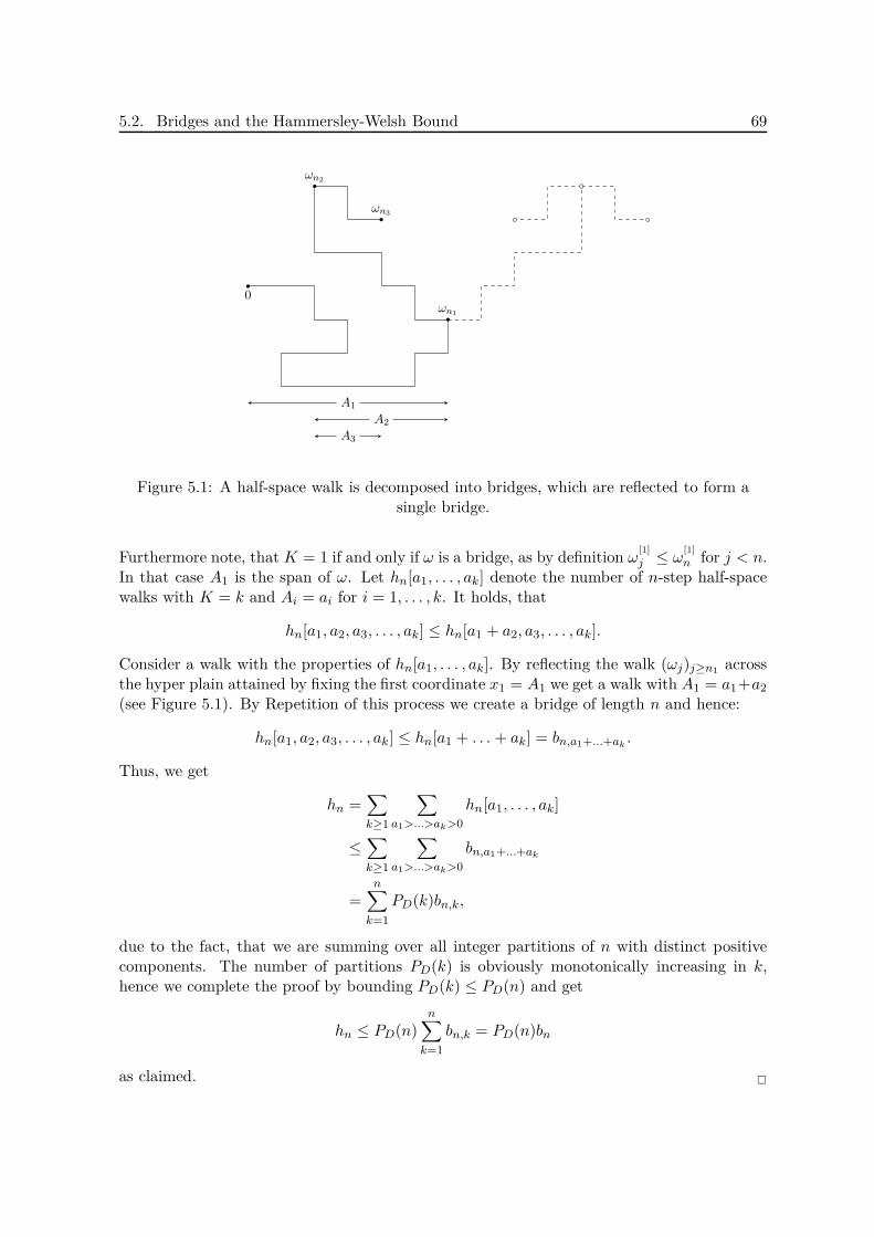
5.2. Bridges and the Hammersley-Welsh Bound 69
0ωn1
ωn2
ωn3
A1
A2
A3
Figure 5.1: A half-space walk is decomposed into bridges, which are reflected to form asingle bridge.
Furthermore note, that K = 1 if and only if ω is a bridge, as by definition ω[1]
j ≤ ω[1]
n for j < n.In that case A1 is the span of ω. Let hn[a1, . . . , ak] denote the number of n-step half-spacewalks with K = k and Ai = ai for i = 1, . . . , k. It holds, that
hn[a1, a2, a3, . . . , ak] ≤ hn[a1 + a2, a3, . . . , ak].
Consider a walk with the properties of hn[a1, . . . , ak]. By reflecting the walk (ωj)j≥n1 acrossthe hyper plain attained by fixing the first coordinate x1 = A1 we get a walk with A1 = a1+a2
(see Figure 5.1). By Repetition of this process we create a bridge of length n and hence:
hn[a1, a2, a3, . . . , ak] ≤ hn[a1 + . . . + ak] = bn,a1+...+ak.
Thus, we get
hn =∑
k≥1
∑
a1>...>ak>0
hn[a1, . . . , ak]
≤∑
k≥1
∑
a1>...>ak>0
bn,a1+...+ak
=n∑
k=1
PD(k)bn,k,
due to the fact, that we are summing over all integer partitions of n with distinct positivecomponents. The number of partitions PD(k) is obviously monotonically increasing in k,hence we complete the proof by bounding PD(k) ≤ PD(n) and get
hn ≤ PD(n)n∑
k=1
bn,k = PD(n)bn
as claimed.

5.2. Bridges and the Hammersley-Welsh Bound 70
Finally, we need an elementary lemma about binomial equations.
Lemma 5.10: Let x, y ≥ 0. Then√x+√y ≤ √2x+ 2y.
Proof: As both sides are positive squaring the inequality gives
x+ 2√xy + y ≤ 2x+ 2y ⇔2√xy ≤ x+ y ⇔
0 ≤ (√x−√y)2.
With the last three auxiliary results we are able to prove the Hammersley-Welsh bound [4,18].
0
ωm ωn
ωm − e1
Figure 5.2: Decomposition of a SAW into two half-space walks.
Theorem 5.11 (Hammersley-Welsh): Fix B > π(23 )1/2. Then there is an n0 = n0(B)
independent of the dimension d ≥ 2, such that
cn ≤ bn+1eB
√n ≤ µn+1eB
√n for n ≥ n0.
Proof: First we show that any n-step SAW can be transformed into two half-space walks andwe obtain
cn ≤n∑
m=0
hn−mhm+1. (5.16)
This is achieved by using the decomposition sketched in Figure 5.2 as follows. Let ω be ann-step SAW and define
x1 := min0≤i≤n
ω[1]
i , m := maxi : ω
[1]
i = x1
.
Let e1 be the unit vector in the first coordinate direction of Zd. Now we construct out of ωtwo half-space walks of length n−m and m+ 1.

5.2. Bridges and the Hammersley-Welsh Bound 71
1. By the choice of m the walk (ωj)j≥m is an (n−m)-step half-space walk starting at ωm.After translation it starts at the origin and is part of all half-space walks counted byhn−m.
2. Again by the choice of m the walk (ωm − e1, ωm, ωm−1, . . . , ω1, ω0) is an (m + 1)-stephalf-space walk starting at ωm − e1. With the same arguments as above it is countedby hm+1.
Next, we apply Proposition 5.9 in (5.16) and use the supermultiplicity of bn (5.12) to get
cn ≤n∑
m=0
PD(n−m)PD(m+ 1)bn−mbm+1
≤ bn+1
n∑
m=0
PD(n−m)PD(m + 1).
(5.17)
We want to apply the asymptotic result for integer partitions. By Theorem 5.8 we get forany ε > 0 a natural number N0 ≥ 0 such that
logPD(N) ≤ (1 + ε)π
√N
3= (1 + ε)π
√2
3︸ ︷︷ ︸=:B′(ε)
√N
2for all N > N0.
As ε > 0 is arbitrary, we can choose B′ := B′(ε) small enough so that B > B′ > π√
23 .
Additionally, there exists a K > 0 such that
PD(N) ≤ K exp
B′
√N
2
for all N ≥ 0.
For example set K = maxPD(1), . . . , PD(N0) in order to cover the first N0 cases. Note,that this holds because exp(B′√N/2) ≥ 1 for all N ≥ 0. Consequently we obtain
PD(n−m)PD(m+ 1) ≤ K2 exp
[B′(√
n−m2
+
√m+ 1
2
)].
Applying Lemma 5.10 to (5.17) gives
cn ≤ (n+ 1)K2eB′√
n+1bn+1 = exp
[(log
((n+ 1)K2
)
B√n
+B′
B
√1 +
1
n
)
︸ ︷︷ ︸≤1 for n≥n0(B)
B√n
]bn+1.
Hence, by (5.14) the result follows:
cn ≤ eB√
nbn+1 ≤ eB√
nµn+1 for n ≥ n0(B).
From the previous theorem we directly get:
Corollary 5.12: For n > n0(B),
bn ≥ cn−1e−B
√n−1 ≥ µn−1e−B
√n−1. (5.18)

5.3. Connective Constant of the Honeycomb Lattice equals√
2 +√
2 72
In particular b1/nn → µ and thus µBridge = µ.
Proof: From (5.5) we know that cn ≥ µn for all n ∈ N. Combining this with the result fromTheorem 5.11 yields for n > n0(B)
µn−1 ≤ cn−1 ≤ bneB
√n−1 ≤ µneB
√n−1.
Rearranging this inequality chain gives the asserted (5.18). Because of (5.13) taking the n-throot and letting n→∞ shows µBridge = µ .
5.3 Connective Constant of the Honeycomb Lattice equals√2 +√
2
In the following we are mainly going to follow the notation and structure of Duminil-Copinand Smirnov [10] combined with definitions and remarks from [4, Section 3].
Throughout this section we consider SAWs on the hexagonal lattice H applying the nearest-neighbor model. Our primary goal of this section is the proof of the following theorem.
Theorem 5.13: For the hexagonal lattice H,
µ =
√2 +√
2.
Remark 5.14: In 1982 based on Coulomb gas formalism the physicist B. Nienhuis [37] (seealso [21, Section 7.6.5]) predicted the connective constant µ for the hexagonal lattice to be
equal to√
2 +√
2. The arguments in the following differ from the ones Nienhuis used, butthey are similarly motivated by considerations of vertex operations in the O(n)-model. Theinterested reader is referred to [21, Section 7.6.1] for an introduction to the O(n)-model fromstatistical mechanics.
5.3.1 Notation
We are going to consider walks between mid-edges of H, i.e. centers of edges of H (see Figure5.3a). The set of all mid-edges will be called H. We define ω : a→ E for all walks ω startingat mid-edge a ∈ H and ending at some mid-edge of E ⊂ H. If E = b we also writeω : a→ b. The length ℓ(ω) of the walk ω is the number of vertices in H belonging to ω.
We define the generating function
C(x) =∑
n≥0
cnxn (5.19)
of SAWs. More often we will use the following representation
C(x) =∑
ω:a→H
xℓ(ω). (5.20)

5.3. Connective Constant of the Honeycomb Lattice equals√
2 +√
2 73
As our lattice is homogeneous it does not depend on the choice of a and is increasing in x, dueto ℓ(ω) ∈ N. To simplify the formulas below and in order to use notation which anticipatesour conclusion we define the two important values
xc :=1√
2 +√
2, (5.21)
j := e2πi/3. (5.22)
Lemma 5.15: The value µ =√
2 +√
2 is equivalent to
1. C(x) = +∞ for x > xc and2. C(x) < +∞ for x < xc.
Proof: From calculus of power series we know, that C(x) is associated with a radius ofconvergence R ≥ 0. The power series diverges for |x| > R and converges (absolutely) for|x| < R. This radius can be calculated from representation (5.19) of C(x) using the coefficientscn in the following way
R =1
lim supn→∞
c1/nn
.
We know from Hammersley and Morton (Theorem 5.4) that the limit of the sequence (c1/nn )n∈N
exists and is equal to µ. Hence,
R =1
µ
proves the statement.
Due to this reason the value xc is also called the critical value or critical point of the generatingfunction C(x).
5.3.2 The Holomorphic Observable
The core idea of the proof is the use of a generalization of (5.20) which we call holomorphicobservable8. This is achieved by introducing weights on individual walks which depend on itswinding (see below).
Definition 5.16: A domain Ω ⊂ H is the union of all mid-edges emanating from a givenconnected collection of vertices V (Ω) (see Figure 5.3a). A mid-edge z belongs to Ω if at leastone endpoint of its associated edge is in V (Ω).
The boundary ∂Ω consists of the mid-edges z whose associated edge has exactly one endpointin V (Ω). ♦
8In the original paper this function is called parafermionic observable.

5.3. Connective Constant of the Honeycomb Lattice equals√
2 +√
2 74
a
x
vertex
mid-edge
(a) Hexagonal Domain Ω
a
b
Wω(a, b) = 0
a
b
Wω(a, b) = 2π
(b) Winding of SAW ω
Figure 5.3: A hexagonal domain Ω in gray whose boundary mid-edges are pictured by smallblack squares. Vertices of V (Ω) correspond to circles and a sample walk from a to x.
In the following we assume Ω to be simply-connected, i.e. having a connected complement inthe Riemann sphere [27, Korollar 4.2.9].
Definition 5.17: The winding number Wω(a, b) of a SAW ω between mid-edges a and b (notnecessarily the start and the end) is the total rotation in radians when ω is traversed from ato b (compare Figure 5.3b). ♦
Now we are able to describe our main tool for the following analysis.
Definition 5.18: Fix a ∈ ∂Ω and σ ∈ R. The holomorphic observable for z ∈ Ω and x ≥ 0is defined by
Fx(z) =∑
ω⊂Ω:a→z
e−iσWω(a,z)xℓ(ω). (5.23)
♦
Note, that that the term e−iσWω(a,z) can be interpreted as a complex weight, which simplifiesto a product of values λ and λ per left or right turn of ω, with
λ = exp
(−iσπ
3
). (5.24)
Here we used that a turn on the hexagonal lattice is exactly π/3 radians.
Lemma 5.19: If x = xc and σ = 58 , then Fz satisfies for every vertex v ∈ V (Ω)
(p− v)Fxc(p) + (q − v)Fxc(q) + (r − v)Fxc(r) = 0, (5.25)
where p, q, r are the mid-edges of the three edges adjacent to v (see Figure 5.4a).

5.3. Connective Constant of the Honeycomb Lattice equals√
2 +√
2 75
vp
q
r
(a) Adjacent Mid-Edges
p
q
r
2π3
−2π3
v
(b) Edge Rotation
Figure 5.4: Hexagonal Lattice Details
Proof: Without loss of generality assume that p, q and r are oriented counter-clockwise aroundv. Next we interpret (5.25) as one sum over all walks ω starting at a and ending at either p, qor r, i.e. with E = p, q, r it is equivalent to
∑
ω:a→E
c(ω) = 0,
where c(ω) is one contribution in (5.25) over all possible SAWs ω ending at p, q or r. Forinstance, if ω ends at mid-edge p, it will be
c(ω) = (p − v)e−iσWω(a,p)xℓ(ω).
Next we want to partition the set of walks finishing in E into pairs and triplets of walks inthe following way (see Figure 5.5):
• Pairs: If a SAW ω1 visits all three mid-edges p, q, r, there exists a partition of the walkinto a SAW plus (up to a half-edge) a self-avoiding loop from v to v. One can associateto ω1 the walk ω2 passing through the same edges, but traversing the loop from v to vin the other direction. Like this, walks visiting all three mid-edges can be grouped inpairs.
• Triplets: If a walk ω1 visits only one mid-edge, it can be associated to two walks ω2 andω3 that visit exactly two mid-edges by extending the walk one step further to the twopossible choices. Now consider the reverse: A walk that visits exactly two mid-edgesis naturally associated to a walk visiting only one mid-edge, by erasing the last step.Thus, walks visiting one or two mid-edges can be grouped in triplets.
As last step we will show that the sum of contributions for each pair or triplet vanishes whichimplies naturally that the total sum is zero.
Firstly, let ω1 and ω2 be two associated walks from the first case. Without loss of generality,we assume that ω1 ends at q, ω2 ends at r and both pass through p. Let a denote theircommon starting point. Due to their association they are equal up to the mid-edge p, andfollow an almost complete loop in two opposite directions. We deduce
ℓ(ω1) = ℓ(ω2) and
Wω1(a, q) = Wω1(a, p) +Wω1(p, q) = Wω1(a, p)− 4π
3 ,
Wω2(a, r) = Wω2(a, p) +Wω2(p, r) = Wω1(a, p) + 4π3 .

5.3. Connective Constant of the Honeycomb Lattice equals√
2 +√
2 76
ω1 ω2 ω1 ω2 ω3
Figure 5.5: Left: Pair of walks visiting three mid-edges and grouped together.Right: Triplet of walks, one visiting one mid-edge, the two others visiting two mid-edges
each. All matched together [10, p. 4].
For the evaluation of Wω1(p, q) we used that a is on the boundary ∂Ω and Ω is simply-connected. These conditions guarantee that ω1 does not traverse in one or more loops aroundthe starting point a. This would increase the value by 2πk for k ∈ Z counting the loopsaround a in positive or negative direction.
Using notation (5.24) for λ and j = e2πi/3 we conclude
c(ω1) + c(ω2) = (q − v)e−iσWω1 (a,q)xℓ(ω1)c + (r − v)e−iσWω2 (a,r)xℓ(ω2)
c
= e−iσWω1 (a,p)xℓ(ω1)c
((q − v)eiσ 4π
3 + (r − v)e−iσ 4π3
)
= (p− v)e−iσWω1 (a,p)xℓ(ω1)c
(jλ4 + jλ4
).
The last equality holds, as (p − v)e2πi/3 = (q − v) and (p − v)e−2πi/3 = (r − v) (compareFigure 5.4b).
Now we set σ = 58 and obtain
jλ4 + jλ4 = ei 3π2 + e−i 3π
2 = 2 cos
(3π
2
)= 0, (5.26)
and hence c(ω1) + c(ω2) = 0.
Secondly, let ω1, ω2, ω3 be three walks matched like in the second case. Without loss ofgenerality, assume ω1 ends at p and that ω2 and ω3 extend to q and r, respectively. Withsimilar arguments as before we see
ℓ(ω2) = ℓ(ω3) = ℓ(ω1) + 1 and
Wω2(a, q) = Wω2(a, p) +Wω2(p, q) = Wω1(a, p) − π
3 ,
Wω3(a, r) = Wω3(a, p) +Wω3(p, r) = Wω1(a, p) + π3 .
These values give
c(ω1) + c(ω2) + c(ω3) = (p − v)e−iσWω1 (a,p)xℓ(ω1)c
(1 + xcjλ+ xcjλ
). (5.27)
Due to the choice of σ = 58 we get λ = exp
(−i5π
24
). Hence, we get analogously jλ + jλ =
2 cos(7π8 ) = −2 cos(π
8 ). Therefore the claim that (5.27) vanishes is equivalent to
2 cos
(π
8
)· xc = 1. (5.28)

5.3. Connective Constant of the Honeycomb Lattice equals√
2 +√
2 77
This equation holds, because 2 cos(π8 ) =
√2 +√
2 which can be easily proved by using the
identity cos(
x2
)= sign(cos(x
2 ))√
1+cos(x)2 . This is the only point in the entire proof of Theorem
5.13 where we explicitly need the choice x = xc = 1/√
2 +√
2.
Finally the claim of the lemma follows by summing over all pairs and triplets of walks.
Remark 5.20: As seen in the above proof, the coefficients of (5.25) are three cube rootsof unity multiplied by p − v (compare Figure 5.4b). So its left hand-side can be interpretedas a discrete dz-integral along an elementary contour on the dual lattice. The fact that theintegral of the holomorphic observable along discrete contours vanishes justifies its name, asit suggests that it is discrete holomorphic.
5.3.3 Proof of Theorem 5.13
To reduce the complexity of the problem, we consider a vertical strip domain ST composedof T strips of hexagons, and its finite version ST,L cut at heights ±L at angles ±π/3, seeFigure 5.6. In other words, position a hexagonal lattice H of meshsize9 1 in C so that thereexists a horizontal edge e with the mid-edge a being 0. Then10
V (ST ) = z ∈ V (H) : 0 ≤ Re(z) ≤ 3T + 1
2,
V (ST,L) = z ∈ V (ST ) : |2 Im(z)− Re(z)| ≤√
3(2L+ 1).
The left and right boundaries of ST and ST,L are denoted by α and β, respectively. The topand bottom boundaries of ST,L are denoted by ε and ε, respectively. In accordance with thesedeclarations we define the following positive partition functions
AT,L(x) =∑
ω⊂ST,L:a→α\axℓ(ω),
BT,L(x) =∑
ω⊂ST,L:a→β
xℓ(ω),
ET,L(x) =∑
ω⊂ST,L:a→ε∪ε
xℓ(ω).
This decomposition allows us to deduce a global identity from equation (5.25) without complexbut positive weights on the introduced strip domain.
Lemma 5.21: For x = xc, the following identity holds
1 = cαAT,L(xc) +BT,L(xc) + cεET,L(xc), (5.29)
with positive coefficients cα = cos(
3π8
)and cε = cos
(π4
).
9The diameter of one hexagon.10In the original paper the upper bound in V (ST ) is specified as (3T + 1)/2, and V (ST,L) is bounded by
|√
3 Im(z) − Re(z)| ≤ 3L, but the used definition of meshsize is not stated.

5.3. Connective Constant of the Honeycomb Lattice equals√
2 +√
2 78
a
α
β
ε
ε
ST,L
T cells
L cells
Figure 5.6: Domain ST,L and boundary intervals α, β, ε and ε [10, p. 5].
Proof: To improve readability we fix x = xc and drop it from notation, e.g. F := Fx. As a firststep we sum (5.25) over all vertices in V (ST,L). All contributions of interior mid-edges vanish,because both end-points are parts of this sum. Particularly, fix one interior mid-edge p ∈ Hwith two end-points v1, v2 ∈ V (ST,L). The total sum contains the two terms (p−v1)F (p) and(p− v2)F (p), whose sum vanishes as (p − v1) = −(p− v2). Hence, we deduce
0 = −∑
z∈α
F (z) +∑
z∈β
F (z) + j∑
z∈ε
F (z) + j∑
z∈ε
F (z). (5.30)
Next we are going to consider these sums individually. The winding from any SAW from a tothe top part of α is π, while the winding to the bottom part is −π. Furthermore, we can usethe symmetry of our domain with respect to the real axis, which implies F (z) = F (z) andthe fact that the only SAW from a to a has length 0. This gives for the first sum
∑
z∈α
F (z) = F (a) +∑
z∈α\aF (z) = F (a) +
1
2
∑
z∈α\a(F (z) + F (z)) = 1 +
e−iσπ + eiσπ
2AT,L
= 1 + cos (σπ)AT,L = 1− cos
(3π
8
)AT,L = 1− cαAT,L.
Similarly we get, that the winding number from a to any half-edge in β, ε or ε is 0, 2π3 or
−2π3 and therefore, again using symmetry, for the other sums
∑
z∈β
F (z) = BT,L,
j∑
z∈ε
F (z) + j∑
z∈ε
F (z) =j
2e−iσ 2π
3 ET,L +j
2eiσ 2π
3 ET,L =ei 2π
3(1−σ) + e−i 2π
3(1−σ)
2ET,L
= cos
(2π
3(1− σ)
)ET,L = cos
(π
4
)ET,L(x) = cεET,L.

5.3. Connective Constant of the Honeycomb Lattice equals√
2 +√
2 79
The lemma follows now directly by inserting the last three formulas into (5.30).
Next, we are going to extend the finite strip domain ST,L to its unbounded version ST .Therefore, observe that the sequences (AT,L(x))L>0 and (BT,L(x))L>0 are increasing in L andare bounded for x < xc, due to (5.29) and their monotonicity in x. Thus they have limits
AT (x) = limL→∞
AT,L(x) =∑
ω⊂ST :a→α\axℓ(ω),
BT (x) = limL→∞
BT,L(x) =∑
ω⊂ST :a→β
xℓ(ω).
As the coefficients cα and cε in (5.30) are positive for x = xc, this identity implies that(ET,L(x))L>0 decreases and converges to a limit ET (x) = limL→∞ET,L(x). Hence, we obtain
1 = cαAT (xc) +BT (xc) + cεET (xc). (5.31)
For the final step we need one last definition which is an adaption of Definition 5.5.
Definition 5.22: A bridge on H is a SAW, which never revisits the vertical line throughits starting point and never visits a vertical line to the right of the vertical line through itsendpoint. Furthermore it starts and ends at the mid-edge of a horizontal edge.
The width of a bridge is the horizontal distance between its start- and end-point. ♦
We denote the number of n-step bridges in H, which start from 0 by bn and its generatingfunction by B(z) =
∑n≥0 bnz
n.
Proof of Theorem 5.13: First note, that similar arguments as in the proof of Hammersley-Welsh in Section 5.2 on the hexagonal lattice lead to the conclusion µBridge = µ also on H.Hence, it is sufficient to show that
µBridge =
√2 +√
2.
Observe, that the bridge generating function is given by B(z) =∑∞
T =0 BT (z).
First, assume x < xc. By (5.31) we get BT (x) ≤ 1 as all constants (i.e. cα and cε) are positive.Now note, that a bridge of width T has at least length T , i.e. BT (x) =
∑n≥T bnx
n. We obtain
BT (x) ≤(x
xc
)T
BT (xc) ≤(x
xc
)T
,
and hence B(x) is finite for x < xc as we found a summable geometric series as a majorant.
It remains to show, that Z(xc) = ∞ or B(xc) = ∞ which implies that µ ≥√
2 +√
2 byLemma 5.15. This is done, by considering two separate cases. First suppose that for some T ,ET (xc) > 0. As observed above ET,L(xc) decreases in L and therefore
Z(xc) ≥∑
L>0
ET,L(xc) ≥∑
L>0
ET (xc) =∞.
On the contrary, assume ET (xc) = 0 for all T , which simplifies (5.31) to
1 = cαAT (xc) +BT (xc). (5.32)

5.3. Connective Constant of the Honeycomb Lattice equals√
2 +√
2 80
Let us consider the geometry of walks ω contributing to AT +1(xc) but not to AT (xc). Thesewalks must visit some vertex adjacent to the right edge of ST +1. Cutting the walk ω at thefirst such point (and adding half-edges to the two halves), we uniquely decompose it into twobridges of width T + 1 in ST +1, which together are one step longer than ω. We conclude
AT +1(xc)−AT (xc) ≤ xc (BT +1(xc))2 . (5.33)
Combining (5.32) for two consecutive values of T with (5.33) we get
0 = (cαAT +1(xc) +BT +1(xc))− (cαAT (xc) +BT (xc))
≤ cαxc (BT +1(xc))2 +BT +1(xc)−BT (xc),
which is equivalent to
cαxc (BT +1(xc))2 +BT +1(xc) ≥ BT (xc).
We are going to use this relation to show by induction, that
BT (xc) ≥ minB1(xc), 1/(cαxc)/Tfor every T ≥ 1.
For brevity define ζ := cαxc > 0, η := minB1(xc), 1/ζ ≥ 0 and write BT = BT (xc). Hence,we show BT ≥ η
T by induction. By the choice of η the case T = 1 is trivial. ConsiderT → T + 1: From the induction hypothesis (IH) we get
cB2T +1 +BT +1 ≥ BT
(IH)
≥ η
T.
Solving the quadratic equation cB2T +1 +BT +1 − η
T = 0 gives the only possible result BT +1 =−1+√
1+4ζη/T
2ζ because BT +1 ≥ 0. Now we use this value, to check the induction assumption:
BT +1 =−1 +
√1 + 4 ζη
T
2ζ
!≥ η
T + 1⇔
1 + 4ζη
T
!≥ 1 + 4
ζη
T + 1+ 4
(ζη
T + 1
)2
⇔
1
T− 1
T + 1
!≥ ζη
(T + 1)2 ⇔
1
T≥ ζη
T + 1
The last inequality holds, as ζη = minζB1, 1 ≤ 1.
This implies
B(xc) ≥∑
T >0
BT (xc) =∞
and completes the proof.
Remark 5.23: The value of the connective constant was motivated in Remark 5.14 byempirical experiments performed by Nienhuis, but the value of σ in the holomorphic observ-able (5.23) seems quite arbitrary or at least suitable for doing the purpose. Clearly these

5.3. Connective Constant of the Honeycomb Lattice equals√
2 +√
2 81
two values are interconnected, but how is not completely obvious. We want to give a moti-vation of these two values here, by showing how they arise naturally out of the usage of theholomorphic observable, which was the main tool in the entire process.
The power of the holomorphic observable is founded in its discrete holomorphy shown inLemma 5.19. The main reasons for this property can be found in equations (5.26) and (5.28),in particular we needed
jλ4 + jλ4 = 0, (a)
1 + xc
(jλ+ jλ
)= 0. (b)
Equation (a) is equivalent to
exp
(2πi
3(1 + 2σ)
)= − exp
(−2πi
3(1 + 2σ)
)= exp
(πi
3(1− 4σ)
).
Considering that the complex exponential function is 2πi-periodic we get
2πi
3(1 + 2σ) =
πi
3(1− 4σ) + 2πik
⇒ σ =6k − 1
8for k ∈ Z.
Setting k = 1 gives the known value σ = 5/8.
Equation (b) can now be used to extract the critical value xc. Observe jλ+ jλ = 2 Re(jλ) =2 cos((2 + σ)π
3 ). Inserting the above value for σ we obtain
xc
(2 cos
(6k + 15
24π
))= −1.
Note, that by its definition as the reciprocal of the connective constant, xc must be positiveas µ is positive. Thus, the above equation implies that 2 cos(6k+15
24 π) < 0. Up to periodicitythe only values we get are k ∈ 0, 1, 2, 3 and as the cosine function is symmetric with respectto π, we only need to consider k = 0 and k = 1.
By using the identity cos(
x2
)= sign(cos(x
2 ))√
1+cos(x)2 , which was also needed in the end of
the proof of Lemma 5.19 and by observing that the cosine is negative for these two values ofk, we get:
xc = −(
2 cos
(2k + 5
8π
))−1
=
2
√√√√1 + cos(
2k+54 π
)
2
−1
=
1/√
2−√
2, k = 0,
1/√
2 +√
2, k = 1.
Up to now there are two possibilities for σ and xc which would do the job:
k σ xc
0 −18 1/
√2−√
2
1 −58 1/
√2 +√
2

5.4. Open Problems 82
As a next step in the proof we restricted ourselves to the vertical strip domain ST andintroduced partition functions AT,L(x), BT,L(x) and ET,L(x) in Section 5.3.3. These functionswere needed to translate the discrete holomorphy equation (5.25) in Lemma 5.21 to the verticalstrip domain. As a result we got two coefficients cα and cε, which were derived as
cα = − cos(σπ) =
− cos
(π8
), k = 0,
cos(
3π8
), k = 1,
cε = cos
(2π
3(1− σ)
)=
cos(
3π4
), k = 0,
cos(π
4
), k = 1.
These coefficients were needed for the derivations of the limits AT (x), BT (x) and ET (x) ofthe partition functions as L tends to infinity. In particular, the limits existed, because thepartition functions and the coefficients cα and cε in (5.29) were positive. But if we considerthe above coefficients for k = 0, we see, that they are negative, which does not allow the usedargumentation. Hence, the only possible values for xc and σ (up to periodicity) are the usedones and we see that they arise naturally from the holomorphic observable:
k σ xc cα cε
0 −18 1/
√2−√
2 − cos(
π8
)= −√
2+√
22 < 0 cos
(3π4
)= −
√2
2 < 0
1 −58 1/
√2 +√
2 cos(
3π8
)=
√2−
√2
2 > 0 cos(π
4
)=
√2
2 > 0
5.4 Open Problems
The knowledge of the connective constant brings us one step closer to reveal the true natureof lattice paths. However, Nienhuis proposed more than just the value of this parameter.In [37] he also states the conjecture that the asymptotic behavior for the number of SAWs is
cn ∼ Anγ−1√
2 +√
2n
, (5.34)
with γ = 43/32 and A ∈ R as n→∞. Moreover, he argued that the mean square displacement〈|ωn|2〉 representing a measure for the distance a random walker covers on average (withrespect to a certain number of experiments) over a certain period of time is equal to
〈|ωn|2〉 =1
cn
∑
ω n−step SAW
|ωn|2 = n2ν+o(1),
with ν = 3/4. These two problems remain open questions, where the best known rigorousbounds on (5.34) have been introduced in Sections 5.1.1 and 5.2.
A possible way to solve these problems could be found in the theory of Schramm-LoewnerEvolutions. In [33] Lawler, Schramm and Werner show that γ and ν could be computed ifthe SAW would possess a conformally invariant scaling limit.
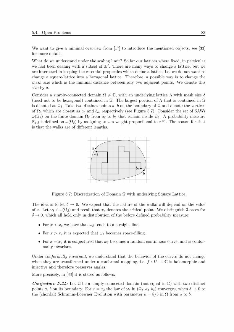
5.4. Open Problems 83
We want to give a minimal overview from [17] to introduce the mentioned objects, see [33]for more details.
What do we understand under the scaling limit? So far our lattices where fixed, in particularwe had been dealing with a subset of Zd. There are many ways to change a lattice, but weare interested in keeping the essential properties which define a lattice, i.e. we do not want tochange a square-lattice into a hexagonal lattice. Therefore, a possible way is to change themesh size which is the minimal distance between any two adjacent points. We denote thissize by δ.
Consider a simply-connected domain Ω 6= C, with an underlying lattice Λ with mesh size δ(need not to be hexagonal) contained in Ω. The largest portion of Λ that is contained in Ωis denoted as Ωδ. Take two distinct points a, b on the boundary of Ω and denote the verticesof Ωδ which are closest as aδ and bδ, respectively (see Figure 5.7). Consider the set of SAWsω(Ωδ) on the finite domain Ωδ from aδ to bδ that remain inside Ωδ. A probability measurePx,δ is defined on ω(Ωδ) by assigning to ω a weight proportional to x|ω|. The reason for thatis that the walks are of different lengths.
aδ
bδ
a
b
Figure 5.7: Discretization of Domain Ω with underlying Square Lattice
The idea is to let δ → 0. We expect that the nature of the walks will depend on the valueof x. Let ωδ ∈ ω(Ωδ) and recall that xc denotes the critical point. We distinguish 3 cases forδ → 0, which all hold only in distribution of the before defined probability measure:
• For x < xc we have that ωδ tends to a straight line.
• For x > xc it is expected that ωδ becomes space-filling.
• For x = xc it is conjectured that ωδ becomes a random continuous curve, and is confor-mally invariant.
Under conformally invariant, we understand that the behavior of the curves do not changewhen they are transformed under a conformal mapping, i.e. f : U → C is holomorphic andinjective and therefore preserves angles.
More precisely, in [33] it is stated as follows:
Conjecture 5.24: Let Ω be a simply-connected domain (not equal to C) with two distinctpoints a, b on its boundary. For x = xc the law of ωδ in (Ωδ, aδ, bδ) converges, when δ → 0 tothe (chordal) Schramm-Loewner Evolution with parameter κ = 8/3 in Ω from a to b.
5.4. Open Problems 84
A Schramm-Loewner Evolution with parameter κ (SLEκ) can be described as follows. LetC+ be the upper half-plane of C. Consider a path ω starting at the boundary and endingat an internal vertex. Then C+ \ ω is a slit upper half-plane (complement of the path) andtherefore simply-connected. From the Riemann Mapping Theorem we know, that it can beconformally mapped to the upper half-plane. The mapping satisfies a differential equation,the Löwner Equation and can be alternatively described by a real-valued function. In detail,the Löwner Equation generates a set of conformal maps, driven by a continuous real-valuedfunction. Schramm’s idea was to use a Brownian Motion Bt as the driving function.
In formula: Let Bt, t ≥ 0 be a Standard Brownian Motion on R and let κ be a real parameter.Then SLEκ is the family of conformal maps gt, t ≥ 0 defined by the Löwner Equation
∂
∂tgt(z) =
2
gt(z)−√κBt
, g0(z) = z.
This is actually called chordal SLEκ as it describes paths growing from the boundary andending on the boundary.
Therefore, understanding SAWs boils down to understanding the theory of SLEκ. The pa-rameter κ plays a very important role. For κ > 0 the curve is always fractal, and becomesmore fractal the higher values are chosen. The following summary is taken from [2].
• For κ ≤ 4 the curve is almost surely simple, i.e. it does not touch itself and it does notintersect the real line (ω ∩ R = 0).
• For 4 < κ < 8 the curve touches itself but does not cross itself. Furthermore it intersectsparts of the real line (ω ∩R ( R).
• For κ ≥ 8 the curve is space-filling and hits every point on the real axis (ω ∩R = R).

List of Figures
1 Examples of two Random Walks in the Euclidean Plane . . . . . . . . . . . . iii
1.1 Examples of Lattices . . . . . . . . . . . . . . . . . . . . . . . . . . . . . . . . 2
1.2 The full set of Small Steps . . . . . . . . . . . . . . . . . . . . . . . . . . . . . 3
1.3 Unrestricted Path with Loops in Z2 . . . . . . . . . . . . . . . . . . . . . . . 4
2.1 Unrestricted Path . . . . . . . . . . . . . . . . . . . . . . . . . . . . . . . . . . 11
2.2 Dyck Path of length 18 . . . . . . . . . . . . . . . . . . . . . . . . . . . . . . . 12
2.3 First Passage Decomposition of Dyck Path . . . . . . . . . . . . . . . . . . . 13
3.1 Branches of Characteristic Curve . . . . . . . . . . . . . . . . . . . . . . . . . 25
3.2 Example of Undirected Half-Plane Walk on S = NE,NW,SW,SE . . . . 33
3.3 Horizontal Projection of S = NE,NW,SW,SE . . . . . . . . . . . . . . . 34
3.4 Horizontal Projection of Half-Plane Walk into its associated Meander . . . . . 34
4.1 The full set of Small Steps . . . . . . . . . . . . . . . . . . . . . . . . . . . . . 47
4.2 Small Steps which contain no x/y-positive/negative Step . . . . . . . . . . . . 49
4.3 Step Sets with respect to Diagonals . . . . . . . . . . . . . . . . . . . . . . . . 49
4.4 Step Sets for subsequent example on the Group of the Walk . . . . . . . . . . 51
4.5 The 16 models whose group G(S) is isomorphic to D2 . . . . . . . . . . . . . 54
4.6 The 5 models whose group G(S) is isomorphic to D3 . . . . . . . . . . . . . . 54
4.7 The 2 models whose group G(S) is isomorphic to D4 . . . . . . . . . . . . . . 54
4.8 Five step sets with an infinite group, where i+ j ≥ 0 for all steps (i, j) . . . . 54
4.9 Non-vertically symmetric step sets of General Result . . . . . . . . . . . . . . 60
4.10 The 4 exceptions to the General Result with holonomic GF . . . . . . . . . . 61
5.1 Half-Space Walk Decomposition into Bridges . . . . . . . . . . . . . . . . . . 69
5.2 Decomposition of a SAW into two half-space walks. . . . . . . . . . . . . . . . 70
5.3 A Hexagonal Domain with a sample Walk . . . . . . . . . . . . . . . . . . . . 74
85
List of Figures 86
5.4 Hexagonal Lattice Details . . . . . . . . . . . . . . . . . . . . . . . . . . . . . 75
5.5 Matching Pairs/Triplets of Walks which vanish on Discrete Contour Integral . 76
5.6 Domain ST,L and boundary intervals α, β, ε and ε . . . . . . . . . . . . . . . . 78
5.7 Discretization of Domain Ω with underlying Square Lattice . . . . . . . . . . 83

Bibliography
[1] Shreeram S. Abhyankar. Algebraic geometry for scientists and engineers, volume 35 ofMathematical Surveys and Monographs. American Mathematical Society, Providence,RI, 1990.
[2] Tom Alberts. An introduction to the schramm-loewner evolution. Talk,http://www.math.caltech.edu/~alberts/talks/SLEintro.pdf, 2008. Online; ac-cessed 26/08/2013.
[3] Cyril Banderier and Philippe Flajolet. Basic analytic combinatorics of directed latticepaths. Theoret. Comput. Sci., 281(1-2):37–80, 2002. Selected papers in honour of MauriceNivat.
[4] Roland Bauerschmidt, Hugo Duminil-Copin, Jesse Goodman, and Gordon Slade. Lec-tures on self-avoiding walks. Probability and Statistical Physics in Two and More Dimen-sions (D. Ellwood, CM Newman, V. Sidoravicius, and W. Werner, eds.), Clay Mathe-matics Institute Proceedings, 15:395–476, 2012.
[5] Alin Bostan and Manuel Kauers. Automatic classification of restricted lattice walks.In 21st International Conference on Formal Power Series and Algebraic Combinatorics(FPSAC 2009), Discrete Math. Theor. Comput. Sci. Proc., AK, pages 201–215. Assoc.Discrete Math. Theor. Comput. Sci., Nancy, 2009.
[6] Alin Bostan and Manuel Kauers. The complete generating function for Gessel walks isalgebraic. Proc. Amer. Math. Soc., 138(9):3063–3078, 2010. With an appendix by Markvan Hoeij.
[7] Mireille Bousquet-Mélou and Marni Mishna. Walks with small steps in the quarter plane.In Algorithmic probability and combinatorics, volume 520 of Contemp. Math., pages 1–39.Amer. Math. Soc., Providence, RI, 2010.
[8] Mireille Bousquet-Mélou and Marko Petkovšek. Linear recurrences with constant coeffi-cients: the multivariate case. Discrete Mathematics, 225(1–3):51 – 75, 2000. FPSAC’98.
[9] Andrew R. Conway, Ian G. Enting, and Anthony J. Guttmann. Algebraic techniquesfor enumerating self-avoiding walks on the square lattice. J. Phys. A, 26(7):1519–1534,1993.
[10] Hugo Duminil-Copin and Stanislav Smirnov. The connective constant of the honeycomb
lattice equals√
2 +√
2. Ann. of Math. (2), 175(3):1653–1665, 2012.
87

Bibliography 88
[11] Guy Fayolle, Roudolf Iasnogorodski, and Vadim Malyshev. Random walks in the quarter-plane, volume 40 of Applications of Mathematics (New York). Springer-Verlag, Berlin,1999. Algebraic methods, boundary value problems and applications.
[12] Philippe Flajolet, Stefan Gerhold, and Bruno Salvy. On the non-holonomic character oflogarithms, powers, and the nth prime function. Electron. J. Combin., 11(2):Article 2,16, 2004/06.
[13] Philippe Flajolet and Robert Sedgewick. Analytic Combinatorics. Cambridge UniversityPress, New York, NY, USA, 1 edition, 2009.
[14] Paul J. Flory. Principles of Polymer Chemistry. Cornell University Press, London, 1953.
[15] Ira M. Gessel. A factorization for formal laurent series and lattice path enumeration.Journal of Combinatorial Theory, Series A, 28(3):321 – 337, 1980.
[16] Bernhard Gittenberger. Diskrete Methoden. Course Notes, Institut für DiskreteMathematik und Geometrie, Technische Universität Wien. Version Summer term2010. http://www.dmg.tuwien.ac.at/gittenberger/dmeth.pdf. Online; accessed08/07/2013.
[17] Anthony J. Guttmann. Self-avoiding walks and polygons – an overview, December 2012.
[18] John M. Hammersley and Dominic J. A. Welsh. Further results on the rate of convergenceto the connective constant of the hypercubical lattice. Quart. J. Math. Oxford Ser. (2),13:108–110, 1962.
[19] Godfrey H. Hardy and Srinivasa Ramanujan. Asymptotic formulæ for the distribution ofintegers of various types [Proc. London Math. Soc. (2) 16 (1917), 112–132]. In Collectedpapers of Srinivasa Ramanujan, pages 245–261. AMS Chelsea Publ., Providence, RI,2000.
[20] Brian Hayes. How to avoid yourself. American Scientist, 86(4), July-August1998. http://www.americanscientist.org/issues/pub/how-to-avoid-yourself/.Online; accessed 18/05/2013.
[21] Barry D. Hughes. Random walks and random environments. Vol. 1. Oxford SciencePublications. The Clarendon Press Oxford University Press, New York, 1995. Randomwalks.
[22] Thomas W. Hungerford. Algebra, volume 73 of Graduate Texts in Mathematics. Springer-Verlag, New York, 1980. Reprint of the 1974 original.
[23] Iwan Jensen. A parallel algorithm for the enumeration of self-avoiding polygons on thesquare lattice. J. Phys. A, 36(21):5731–5745, 2003.
[24] Iwan Jensen. Improved lower bounds on the connective constants for two-dimensionalself-avoiding walks. Journal of Physics A: Mathematical and General, 37(48):11521, 2004.
[25] Iwan Jensen and Anthony J. Guttmann. Self-avoiding polygons on the square lattice. J.Phys. A, 32(26):4867–4876, 1999.

Bibliography 89
[26] Samuel Johnson. Analytic combinatorics of planar lattice paths. Master’s thesis, SimonFraser University, 2012.
[27] Michael Kaltenbäck and Harald Woracek. Komplexe Analysis für Technische Mathe-matik. Course Notes, Institut ASC, Technische Universität Wien. Version 25.6.2013.http://asc.tuwien.ac.at/~funkana/kaltenbaeck/mykana/mykana.pdf. Online; ac-cessed 07/08/2013.
[28] Manuel Kauers. The holonomic toolkit. In Computer Algebra in Quantum Field The-ory: Integration, Summation and Special Functions, Texts and Monographs in SymbolicComputation. Springer, 2013.
[29] Donald E. Knuth. The art of computer programming. Vol. 1: Fundamental algorithms.Second printing. Addison-Wesley Publishing Co., Reading, Mass.-London-Don Mills,Ont, 1969.
[30] Irina Kurkova and Kilian Raschel. On the functions counting walks with small steps inthe quarter plane. Publications mathématiques de l’IHÉS, 116(1):69–114, 2012.
[31] David Fernand Laferrière. Classification of walks in wedges. Master’s thesis, SimonFraser University, 2007.
[32] Pauline Lafitte-Godillon, Kilian Raschel, and Viet Chi Tran. Extinction probabilities fora distylous plant population modeled by an inhomogeneous random walk on the positivequadrant. SIAM J. Appl. Math., 73(2):700–722, 2013.
[33] Gregory F. Lawler, Oded Schramm, and Wendelin Werner. On the scaling limit of planarself-avoiding walk. In Fractal geometry and applications: a jubilee of Benoît Mandelbrot,Part 2, volume 72 of Proc. Sympos. Pure Math., pages 339–364. Amer. Math. Soc.,Providence, RI, 2004.
[34] Leonard Lipshitz. D-finite power series. J. Algebra, 122(2):353–373, 1989.
[35] Neal Madras and Gordon Slade. The self-avoiding walk. Modern Birkhäuser Classics.Birkhäuser/Springer, New York, 2013. Reprint of the 1993 original.
[36] Rick Miranda. Algebraic curves and Riemann surfaces, volume 5. Amer MathematicalSociety, 1995.
[37] Bernard Nienhuis. Exact critical point and critical exponents of O(n) models in twodimensions. Phys. Rev. Lett., 49(15):1062–1065, 1982.
[38] George L. O’Brien. Monotonicity of the number of self-avoiding walks. J. Statist. Phys.,59(3-4):969–979, 1990.
[39] Marko Petkovšek, Herbert B. Wilf, and Doron Zeilberger. A = B. AK Peters, Ltd,Wellesley, MA, first edition edition, 1996.
[40] George Pólya and Gabor Szegő. Problems and theorems in analysis. I. Classics inMathematics. Springer-Verlag, Berlin, 1998. Series, integral calculus, theory of functions,Translated from the German by Dorothee Aeppli, Reprint of the 1978 English translation.

Bibliography 90
[41] André Pönitz and Peter Tittmann. Improved upper bounds for self-avoiding walks inZd. Electron. J. Combin., 7:Research Paper 21, 10 pp. (electronic), 2000.
[42] Kilian Raschel. Walks in the quarter plane: analytic approach and applica-tions. To be published in ESAIM:Proceedings, 2013, CNRS & Universite de Tours,http://www.lmpt.univ-tours.fr/~raschel/MAS2012Raschel.pdf. Online; accessed03/08/2013.
[43] Richard P. Stanley. Enumerative combinatorics. Vol. 2, volume 62 of Cambridge Stud-ies in Advanced Mathematics. Cambridge University Press, Cambridge, 1999. With aforeword by Gian-Carlo Rota and appendix 1 by Sergey Fomin.
[44] Richard P. Stanley. Enumerative combinatorics. Volume 1, volume 49 of Cambridge Stud-ies in Advanced Mathematics. Cambridge University Press, Cambridge, second edition,2011.
[45] Alfred Van der Poorten and R Apéry. A proof that euler missed... The MathematicalIntelligencer, 1(4):195–203, 1979.
[46] Herbert S. Wilf. generatingfunctionology. Academic Press Inc., Boston, MA, secondedition, 1994.
[47] Jet Wimp and Doron Zeilberger. Resurrecting the asymptotics of linear recurrences. J.Math. Anal. Appl., 111(1):162–176, 1985.

Index
algebraic, 14, 19apex, 38
bivariate generating function, 18bridge, 67, 79
growth constant, 67supermultiplicative, 67width, 79
characteristic curve, 23characteristic polynomial, 22, 33, 46combinatorial class, 9
bijectively equivalent, 9combinatorial isomorphic, 9counting sequence, 9
conformally invariant, 83connective constant, 63critical exponent, 65critical value/point, 73cyclotomic polynomial, 56
D-finite, 14, 20discrete holomorphic, 77Dyck Path, 12, 31, 42Dyck Prefixes, 27
formal Laurent seriespositive part, 18
formal power series, 4coefficient extraction, 5distance, 5formal derivative, 5section, 39valuation, 5
group of the walk, 51sign, 51
half-space walk, 68holomorphic observable, 73, 74holonomic, 14, 20
horizontal projection, 33
kernel, 23, 38, 58kernel equation, 23kernel method, 29, 35, 41
lattice, 1Bravais, 1Euclidean, 2homogeneous, 3, 63periodic, 1
lattice path, 2, 3bridge, 22directed, 22excursion, 22first passage decomposition, 12meander, 22self-avoiding, 62simple, 22weights, 4
multivariate generating function, 17
nearest-neighbor, 1, 2, 62
ordinary generating function, 9coefficient extraction, 5valuation, 5
P-recursive, 14
rational, 14, 19
Schramm-Loewner Evolution, 82, 84step set, 2, 62
small steps, 3symbolic method, 10
unimodal, 24
walk, 2, 3winding number, 74
x/y-positive/negative, 46
91
Related Documents