Lattice Barrier for the Hidden Number Problem

On Bounded Distance Decoding with Predicate:Breaking the “Lattice Barrier” for the Hidden

Number Problem

Martin R. Albrecht1 and Nadia Heninger2?

1 Information Security Group, Royal Holloway, University of London2 University of California, San Diego

Abstract. Lattice-based algorithms in cryptanalysis often search for atarget vector satisfying integer linear constraints as a shortest or closestvector in some lattice. In this work, we observe that these formulationsmay discard non-linear information from the underlying application thatcan be used to distinguish the target vector even when it is far from beinguniquely close or short.We formalize lattice problems augmented with a predicate distinguishinga target vector and give algorithms for solving instances of these prob-lems. We apply our techniques to lattice-based approaches for solvingthe Hidden Number Problem, a popular technique for recovering secretDSA or ECDSA keys in side-channel attacks, and demonstrate that ouralgorithms succeed in recovering the signing key for instances that werepreviously believed to be unsolvable using lattice approaches. We carriedout extensive experiments using our estimation and solving framework,which we also make available with this work.

1 Introduction

Lattice reduction algorithms [53, 72, 73, 34, 61] have found numerous applicationsin cryptanalysis. These include several general families of cryptanalytic appli-cations including factoring RSA keys with partial information about the secretkey via Coppersmith’s method [26, 64], the (side-channel) analysis of lattice-based schemes [57, 8, 44, 4, 27], and breaking (EC)DSA and Diffie-Hellman viaside-channel attacks using the Hidden Number Problem.

In the usual statement of the Hidden Number Problem (HNP) [21], theadversary learns some most significant bits of random multiples of a secret integermodulo some known integer. This information can be written as integer-linear

? The research of MA was supported by EPSRC grants EP/S020330/1, EP/S02087X/1,by the European Union Horizon 2020 Research and Innovation Program Grant 780701and Innovate UK grant AQuaSec; NH was supported by the US NSF under grantsno. 1513671, 1651344, and 1913210. Part of this work was done while the authorswere visiting the Simons Institute for the Theory of Computing. Our experimentswere carried out on Cisco UCS equipment donated by Cisco and housed at UCSD.The full version of this work is available at https://ia.cr/2020/1540.

https://ia.cr/2020/1540

constraints on the secret. The problem can then be formulated as a variant of theClosest Vector Problem (CVP) known as Bounded Distance Decoding (BDD),which asks one to find a uniquely closest vector in a lattice to some target pointt. A sufficiently strong lattice reduction will find this uniquely close vector, whichcan then be used to recover the secret.

The requirement of uniqueness constrains the instances that can be successfullysolved with this approach. In short, a fixed instance of the problem is not expectedto be solvable when few samples are known, since there are expected to be manyspurious lattice points closer to the target than the desired solution. As thenumber of samples is increased, the expected distance between the target andthe lattice shrinks relative to the normalized volume of the lattice, and at somepoint the problem is expected to become solvable. For some choices of inputparameters, however, the problem may be infeasible to solve using these methodsif the attacker cannot compute a sufficiently reduced lattice basis to find thissolution; if the number of spurious non-solution vectors in the lattice does notdecrease fast enough to yield a unique solution; or if simply too few samplescan be obtained. In the context of the Hidden Number Problem, the expectedinfeasibility of lattice-based algorithms for certain parameters has been referredto as the “lattice barrier” in numerous works [12, 30, 79, 75, 66].

Nevertheless, the initial cryptanalytic problem may remain well defined evenwhen the gap between the lattice and the target is not small enough to expect aunique closest vector. This is because formulating a problem as a HNP instanceomits information: the cryptanalytic applications typically imply non-linearconstraints that restrict the solution, often to a unique value. For example, inthe most common application of the HNP to side-channel attacks, breakingECDSA from known nonce bits [18, 45], the desired solution corresponds to thediscrete logarithm of a public value that the attacker knows. We may considersuch additional non-linear constraints as a predicate h(·) that evaluates to trueon the unique secret and false elsewhere. Thus, we may reformulate the searchproblem as a BDD with predicate problem: find a vector v in the lattice withinsome radius R to the target t such that f(v − t) := h(g(v − t)) returns true,where g(·) is a function extracting a candidate secret s from the vector v − t.

Contributions. In this work, we define the BDD with predicate problem andgive algorithms to solve it. To illustrate the performance of our algorithms, weapply them to the Hidden Number Problem lattices arising from side-channelattacks recovering ECDSA keys from known nonce bits.

In more detail, in Section 3, we give a simple refinement of the analysis of the“lattice barrier” and show how this extends the range of parameters that can besolved in practice.

In Section 4 we define the Bounded Distance Decoding with predicate(BDDα,f(·)) and the unique Shortest Vector with predicate (uSVPf(·)) prob-lems and mention how Kannan’s embedding enables us to solve the former viathe latter.

We then give two algorithms for solving the unique Shortest Vector withpredicate problem in Section 5. One is based on lattice-point enumeration and inprinciple supports any normR of the target vector. This algorithm exploits the factthat enumeration is exhaustive search inside a given radius. Our other algorithmis based on lattice sieving and is expected to succeed when R ≤

√4/3 · gh(Λ)

where gh(Λ) is the expected norm of a shortest vector in a lattice Λ under theGaussian heuristic (see below).3 This algorithm makes use of the fact that asieve produces a database of short vectors in the lattice, not just a single shortestvector. Thus, the key observation exploited by all our algorithms is that efficientSVP solvers are expected to consider every vector of the lattice within someradius R. Augmenting these algorithms with an additional predicate check then

follows naturally. In both algorithms the predicate is checked (R/ gh(Λ))d+o(d)

times, where d is the dimension of the lattice, which is asymptotically smallerthan the cost of the original algorithms.

In Section 6, we experimentally demonstrate the performance of our algorithmsin the context of ECDSA signatures with partial information about nonce bits.Here, although the lattice-based HNP algorithm has been a well-appreciated toolin the side-channel cryptanalysis community for two decades [65, 55, 17, 70, 71,63, 80, 46, 24], we show how our techniques allow us to achieve previous recordswith fewer samples, bring problem instances previously believed to be intractableinto feasible range, maximize the algorithm’s success probability when only afixed number of samples are available, increase the algorithm’s success probabilityin the presence of noisy data, and give new tradeoffs between computation timeand sample collection. We also present experimental evidence of our techniques’ability to solve instances given fewer samples than required by the informationtheoretic limit for lattice approaches. This is enabled by our predicate uniquelydetermining the secret.

Our experimental results are obtained using a Sage [74]/Python frameworkfor cost-estimating and solving uSVP instances (with predicate). This frameworkis available at [7] and attached to the electronic version of this work. We expectit to have applications beyond this work.

Related work. There are two main algorithmic approaches to solving theHidden Number Problem in the cryptanalytic literature. In this work, we focuson lattice-based approaches to solving this problem. An alternative approach, aFourier analysis-based algorithm due to Bleichenbacher [18], has generally beenconsidered to be more robust to errors, and able to solve HNP instances withfewer bits known, but at the cost of requiring orders of magnitude more samplesand a much higher computational cost [30, 12, 75, 13]. Our work can be viewed asextending the applicability of lattice-based HNP algorithms well into parametersbelieved to be only tractable to Bleichenbacher’s algorithm, thus showing how

3 We note that this technique conflicts with “dimensions for free” [32, 5] and thus theexpected performance improvement when arbitrarily many samples are available issmaller compared to state-of-the-art sieving (see Section 5.3 for details).

these instances can be solved using far fewer samples and less computational timein practice (see Table 4), while gracefully handling input errors (see Figure 7).

In particular, our work can be considered a systematization, formalization,and generalization of folklore (and often ad hoc) techniques in the literature onlattice-reduction aided side-channel attacks such as examining the entire reducedbasis to find the target vector [22, 46] or the technique briefly mentioned in [17]of examining candidates after each “tour” of BKZ (BKZ is described below).4

More generally, our work can be seen as a continuation of a line of recentworks that “open up” SVP oracles, i.e. that forgo treating (approximate) SVPsolvers as black boxes inside algorithms. In particular, a series of recent workshave taken advantage of the exponentially many vectors produced by a sieve:in [10] the authors use the exponentially many vectors to cost the so-called“dual attack” on LWE [69]; in [32, 52, 5] the authors exploit the same propertyto improve sieving algorithms and block-wise lattice reduction; and in [31] theauthors use this fact to compute approximate Voronoi cells.

Our work may also be viewed in line with [27], which augments a BDDsolver for LWE with “hints” by transforming the input lattice. While thesehints must be linear(izable) (with noise), the authors demonstrate the utilityof integrating such hints to reduce the cost of finding a solution. On the onehand, our approach allows us to incorporate arbitrary, non-linear hints, as longas these can be expressed as an efficiently computable predicate; this makesour approach more powerful. On the other hand, the scenarios in which ourtechniques can be applied are much more restricted than [27]. In particular, [27]works for any lattice reduction algorithm and, specifically, for block-wise latticereduction. Our work, in contrast, does not naturally extend to this setting; thismakes our approach less powerful in comparison. We discuss this in Section 5.4.

2 Preliminaries

We denote the logarithm with base two by log(·). We start indexing at zero.

2.1 Lattices

A lattice Λ is a discrete subgroup of Rd. When the rows b0, . . . , bd−1 of Bare linearly independent we refer to it as the basis of the lattice Λ(B) ={∑vi · bi | vi ∈ Z}, i.e. we consider row-representations for matrices in this work.The algorithms considered in this work make use of orthogonal projections πi :

Rd 7→ span (b0, . . . , bi−1)⊥

for i = 0, . . . , d− 1. In particular π0(·) is the identity.The Gram–Schmidt orthogonalization (GSO) of B is B∗ = (b∗0, . . . , b

∗d−1), where

the Gram–Schmidt vector b∗i is πi(bi). Then b∗0 = b0 and b∗i = bi −∑i−1j=0 µi,j ·

b∗j for i = 1, . . . , d− 1 and µi,j =〈bi,b

∗j 〉

〈b∗j ,b∗j 〉. Norms in this work are Euclidean and

4 For the purposes of this work, the CVP technique used in [17] is not entirely clearfrom the account given there. We confirmed with the authors that is the analogousstrategy to their SVP approach: CVP enumeration interleaved with tours of BKZ.

denoted ‖ · ‖. We write λi(Λ) for the radius of the smallest ball centred at theorigin containing at least i linearly independent lattice vectors, e.g. λ1(Λ) is thenorm of a shortest vector in Λ.

The Gaussian heuristic predicts that the number |Λ ∩ B| of lattice pointsinside a measurable body B ⊂ Rn is approximately equal to Vol(B)/Vol(Λ).Applied to Euclidean d-balls, it leads to the following prediction of the length ofa shortest non-zero vector in a lattice.

Definition 1 (Gaussian heuristic). We denote by gh(Λ) the expected firstminimum of a lattice Λ according to the Gaussian heuristic. For a full rank latticeΛ ⊂ Rd, it is given by:

gh(Λ) =

(Vol(Λ)

Vol(Bd(1))

)1/d

=Γ(1 + d

2

)1/d√π

·Vol(Λ)1/d ≈

√d

2πe·Vol(Λ)

1/d

where Bd(R) denotes the d-dimensional Euclidean ball with radius R.

2.2 Hard problems

A central hard problem on lattices is to find a shortest vector in a lattice.

Definition 2 (Shortest Vector Problem (SVP)). Given a lattice basis B,find a shortest non-zero vector in Λ(B).

In many applications, we are interested in finding closest vectors, and we havethe additional guarantee that our target vector is not too far from the lattice.This is known as Bounded Distance Decoding.

Definition 3 (α-Bounded Distance Decoding (BDDα)). Given a latticebasis B, a vector t, and a parameter 0 < α such that the Euclidean distancebetween t and the lattice dist(t,B) < α·λ1(Λ(B)), find the lattice vector v ∈ Λ(B)which is closest to t.

To guarantee a unique solution, it is required that α < 1/2. However, theproblem can be generalized to 1/2 ≤ α < 1, where we expect a unique solutionwith high probability. Asymptotically, for any polynomially-bounded γ ≥ 1 thereis a reduction from BDD1/(

√2 γ) to uSVPγ [14]. The unique shortest vector

problem (uSVP) is defined as follows:

Definition 4 (γ-unique Shortest Vector Problem (uSVPγ)). Given a lat-tice Λ such that λ2(Λ) > γ · λ1(Λ) find a nonzero vector v ∈ Λ of length λ1(Λ).

The reduction is a variant of the embedding technique, due to Kannan [48],that constructs

L =

(B 0t τ

)where τ is some embedding factor (the reader may think of τ = E

[‖t− v‖/

√d]).

If v is the closest vector to t then the lattice Λ(L) contains (t− v, τ) which issmall.

2.3 Lattice algorithms

Enumeration [68, 47, 33, 73, 60, 2] solves the following problem: Given some

matrix B and some bound R, find v =∑d−1i=0 ui ·bi with ui ∈ Z where at least one

ui 6= 0 such that ‖v‖2 ≤ R2. By picking the shortest vector encountered, we canuse lattice-point enumeration to solve the shortest vector problem. Enumerationalgorithms make use of the fact that the vector v can be rewritten with respectto the Gram–Schmidt basis:

v =

d−1∑i=0

ui · bi =

d−1∑i=0

ui ·

b∗i +

i−1∑j=0

µi,j · b∗j

=

d−1∑j=0

uj +

d−1∑i=j+1

ui · µij

· b∗j .Since all the b∗i are pairwise orthogonal, we can express the norms of projec-

tions of v simply as

‖πk (v) ‖2 =

∥∥∥∥∥∥d−1∑j=k

uj +

d−1∑i=j+1

ui µi,j

b∗j

∥∥∥∥∥∥2

=

d−1∑j=k

uj +

d−1∑i=j+1

ui µi,j

2

· ‖b∗j‖2.

In particular, vectors do not become longer by projecting. Enumeration algorithmsexploit this fact by projecting the problem down to a one dimensional problem offinding candidate πd(v) such that ‖πd (v) ‖2 ≤ R2. Each such candidate is thenlifted to a candidate πd−1(v) subject to the constraint ‖πd−1 (v) ‖2 ≤ R2.

That is, lattice-point enumeration is a depth-first tree search through a treedefined by the ui. It starts by picking a candidate for ud−1 and then exploresthe subtree “beneath” this choice. Whenever it encounters an empty interval ofchoices for some ui it abandons this branch and backtracks. When it reaches theleaves of the tree, i.e. u0 then it compares the candidate for a full solution to thepreviously best found and backtracks.

Lattice-point enumeration is expected [42] to consider

Hk =1

2· Vol(Bd−k(R))∏d−1

i=k ‖b∗i ‖

nodes at level k and∑d−1k=0Hk nodes in total. In particular, enumeration finds

the shortest non-zero vector in a lattice in dd/(2e)+o(d) time and polynomialmemory [42]. It was recently shown that when enumeration is used as the SVPoracle inside block-wise lattice reduction the time is reduced to dd/8+o(d) [2].However, the conditions for this improvement are mostly not met in our setting.Significant gains can be made in lower-order terms by considering a different Rion each level 0 ≤ i < d instead of a fixed R. Since this prunes branches of thesearch tree that are unlikely to lead to a solution, this is known as “pruning”in the literature. When the Ri are chosen such that the success probability isexponentially small in d we speak of “extreme pruning” [35].

A state-of-the-art implementation of lattice-point enumeration can be foundin FPLLL [76]. This is the implementation we adapt in this work. It visits about

2d log d

2e −0.995 d+16.25 nodes to solve SVP in dimension d [2].

Sieving [1, 59, 16, 51, 15, 43] takes as input a list of lattice points, L ⊂ Λ, andsearches for integer combinations of these points that are short. If the initial listis sufficiently large, SVP can be solved by performing this process recursively.Each point in the initial list can be sampled at a cost polynomial in d [50]. Hence

the initial list can be sampled at a cost of |L|1+o(1).Sieves that combine k points at a time are called k-sieves; 2-sieves take integer

combinations of the form u ± v with u,v ∈ L and u 6= ±v. Heuristic sievingalgorithms are analyzed under the heuristic that the points in L are independentlyand identically distributed uniformly in a thin spherical shell. This heuristic wasintroduced by Nguyen and Vidick in [67]. As a further simplification, it is assumedthat the shell is very thin and normalized such that L is a subset of the unitsphere in Rd. As such, a pair (u,v) is reducible if and only if the angle betweenu and v satisfies θ(u,v) < π/3, where θ(u,v) = arccos (〈u,v〉/(‖u‖ · ‖v‖)),arccos(x) ∈ [0, π]. Under these assumptions, we require |L| ≈

√4/3

din order to

see “collisions”, i.e. reductions. Lattice sieves are expected to output a list of

(4/3)d/2+o(d)

short lattice vectors [32, 5]. The asymptotically fastest sieve has aheuristic running time of 20.292 d+o(d) [15].

We use the performant implementations of lattice sieving that can be foundin G6K [78, 5] in this work, which includes a variant of [16] (“BGJ1”) and [43](3-Sieve). BGJ1 heuristically runs in time 20.349 d+o(d) and memory 20.205 d+o(d).The 3-Sieve heuristically runs in time 20.372 d+o(d) and memory 20.189 d+o(d).5

BKZ [72, 73] can be used to solve the unique shortest vector problem and thusBDD. BKZ makes use of an oracle that solves the shortest vector problem indimension β. This oracle can be instantiated using enumeration or sieving. Thealgorithm then asks the oracle to solve SVP on the first block of dimension βof the input lattice, i.e. of the lattice spanned by b0, . . . , bβ−1. This vector isthen inserted into the basis and the algorithm asks the SVP oracle to returna shortest vector for the block π1 (b1) , . . . , π1 (bβ). The algorithm proceeds inthis fashion until it reaches πd−2 (bd−2) , πd−2 (bd−1). It then starts again byconsidering b0, . . . , bβ−1. One such loop is called a “tour” and the algorithm willcontinue with these tours until no more (or only small changes) are made to thebasis. For many applications a small, constant number of tours is sufficient forthe basis to stabilize.

The key parameter for BKZ is the block size β, i.e. the maximal dimension ofthe underlying SVP oracle, and we write “BKZ-β”. The expected norm of theshortest vector found by BKZ-β and inserted into the basis as b0 for a random

lattice is ‖b0‖ ≈ δd−1β ·Vol(Λ)1/d

for some constant δβ ∈ O(β1/(2 β)

)depending

on β.6

5 In G6K the 3-Sieve is configured to use a database of size 20.205 d+o(d) by default,which lowers its time complexity.

6 The constant is typically defined as ‖b0‖ ≈ δdβ ·Vol(Λ)1/d in the literature. From theperspective of the (worst-case) analysis of underlying algorithms, though, normalizingby d− 1 rather than d is appropriate.

In [10] the authors formulate a success condition for BKZ-β solving uSVP ona lattice Λ in the language of solving LWE. Let e be the unusually short vector inthe lattice and let c∗i be the Gram–Schmidt vectors of a typical BKZ-β reducedbasis of a lattice with the same volume and dimension as Λ. Then in [10] it isobserved that when BKZ considers the last full block πd−β (bd−β) , . . . πd−β (bd−1)it will insert πd−β (e) at index d− β if that projection is the shortest vector inthe sublattice spanned by the last block. Thus, when

‖πd−β (e) ‖ < ‖c∗d−β‖ (1)

≈√β/d · E[‖e‖ ] < δ2β−d−1β ·Vol(Λ)

1/d(2)

we expect the behavior of BKZ-β on our lattice Λ to deviate from that of arandom lattice. This situation is illustrated in Figure 1. Indeed, in [6] it wasshown that once this event happens, the internal LLL calls of BKZ will “lift”and recover e. Thus, these works establish a method for estimating the requiredblock size for BKZ to solve uSVP instances. We use this estimate to chooseparameters in Section 6: given a dimension d, volume Vol(Λ) and E[‖e‖ ], we pickthe smallest β such that Inequality (2) is satisfied. Note, however, that in smalldimensions this reasoning is somewhat complicated by “double intersections” [6]and low “lifting” probability [27]; as a result estimates derived this way arepessimistic for small block sizes. In that case, the model in [27] provides accuratepredictions. Instead of only running BKZ, a performance gain can be achievedby following BKZ with one SVP/CVP call in a larger dimension than the BKZblock size [55, 5].

0 20 40 60 80 100 120 140 160 180

2

4

6

8

d− β

projection index i

log2(‖·‖

)

‖c?i ‖‖πi(e)‖

Fig. 1: BKZ−β uSVP Success Condition. Expected norms for lattices of dimensiond = 183 and volume qm−n after BKZ-β reduction for LWE parameters n =65,m = 182, q = 521, standard deviation σ = 8/

√2π and β = 56. BKZ is

expected to succeed in solving a uSVP instance when the two curves intersect atindex d− β as shown, i.e. when Inequality (1) holds. Reproduced from [6].

2.4 The Hidden Number Problem

In the Hidden Number Problem (HNP) [21], there is a secret integer α and apublic modulus n. Information about α is revealed in the form of what we callsamples: an oracle chooses a uniformly random integer 0 < ti < n, computessi = ti · α mod n where the modular reduction is taken as a unary operator sothat 0 ≤ si < n, and reveals some most significant bits of si along with ti. Wewill write this as ai + ki = ti · α mod n, where ki < 2` for some ` ∈ Z that is aparameter to the problem. For each sample, the adversary learns the pair (ti, ai).We may think of the Hidden Number Problem as 1-dimensional LWE [69].

2.5 Breaking ECDSA from nonce bits

Many works in the literature have exploited side-channel information about(EC)DSA nonces by solving the Hidden Number Problem (HNP), e.g. [65, 19,55, 12, 70, 75, 71, 63, 80, 46], since the seminal works of Bleichenbacher [18] andHowgrave-Graham and Smart [45]. The latter solves HNP using lattice reduction;the former deploys a combinatorial algorithm that can be cast as a variant ofthe BKW algorithm [20, 3, 49, 40]. The latest in this line of research is [13]which recovers a key from less than one bit of the nonce using Bleichenbacher’salgorithm. More recently, in [56] the authors found the first practical attackscenario that was able to make use of Boneh and Venkatesan’s [21] originalapplication of the HNP to prime-field Diffie-Hellman key exchange.

Side-channel attacks. Practical side-channel attacks against ECDSA typicallyrun in two stages. First, the attacker collects many signatures while performingside-channel measurements. Next, they run a key recovery algorithm on a suitablychosen subset of the traces. Depending on the robustness of the measurements,the data collection phase can be quite expensive. As examples, in [62] the authorsdescribe having to repeat their attack 10,000 to 20,000 times to obtain one byteof information; in [37] the authors measured 5,000 signing operations, each taking0.1 seconds, to obtain 114 usable traces; in [63] the authors describe generating40,000 signatures in 80 minutes in order to obtain 35 suitable traces to carry outan attack.

Thus in the side-channel literature, minimizing the amount of data requiredto mount a successful attack is often an important metric [70, 46]. Using ourmethods as described below will permit more efficient overall attacks.

ECDSA. The global parameters for an ECDSA signature are an elliptic curveE(Fp) and a generator point G on E of order n. A signing key is an integer0 ≤ d < n, and the public verifying key is a point dG. To generate an ECDSAsignature on a message hash h, the signer generates a random integer noncek < n, and computes the values r = (kG)x where x subscript is the x coordinateof the point, and s = k−1 · (h+ d · r) mod n. The signature is the pair (r, s).

ECDSA as a HNP. In a side-channel attack against ECDSA, the adversarymay learn some of the most significant bits of the signature nonce k. Withoutloss of generality, we will assume that these bits are all 0. Then rearranging theformula for the ECDSA signature s, we have −s−1 · h + k ≡ s−1 · r · d mod n,and thus a HNP instance with ai = −s−1 · h, ti = s−1 · r, and α = d.

Solving the HNP with lattices. Boneh and Venkatesan give this lattice forsolving the Hidden Number Problem with a BDD oracle:

n 0 0 · · · 0 00 n 0 · · · 0 0

... · · ·0 0 0 · · · n 0t0 t1 t2 · · · tm−1 1/n

The target is a vector (a0, . . . , am−1, 0) and the lattice vector

(t0 · α mod n, . . . , tm−1 · α mod n, α/n)

is within√m+ 1 · 2` of this target when |ki| < 2`.

Most works solve this BDD problem via Kannan’s embedding i.e. by con-structing the lattice generated by the rows of

n 0 0 · · · 0 0 00 n 0 · · · 0 0 0

......

0 0 0 · · · n 0 0t0 t1 t2 · · · tm−1 2`/n 0a0 a1 a2 · · · am−1 0 2`

This lattice contains a vector

(k0, k1, . . . , km−1, 2` · α/n, 2`)

that has norm at most√m+ 2 · 2`. This lattice also contains (0, 0, . . . , 0, 2`, 0),

so the target vector is not generally the shortest vector. There are variousimprovements we can make to this lattice.

Reducing the size of k by one bit. In an ECDSA input, k is generally positive, sowe have 0 ≤ ki < 2`. The lattice works for any sign of k, so we can reduce thebit length of k by one bit by writing k′i = ki − 2`−1. This modification provides asignificant improvement in practice and is described in [65], but is not consistentlytaken advantage of in practical applications.

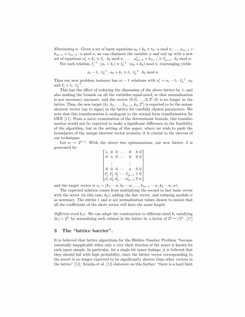
Eliminating α. Given a set of input equations a0 + k0 ≡ t0 ·α mod n, . . . , am−1 +km−1 = tm−1 · α mod n, we can eliminate the variable α and end up with a newset of equations a′1 + k1 ≡ t′1 · k0 mod n, . . . , a′m−1 + km−1 ≡ t′m−1 · k0 mod n.

For each relation, t−1i · (ai + ki) ≡ t−10 · (a0 + k0) mod n; rearranging yields

ai − ti · t−10 · a0 + ki ≡ ti · t−10 · k0 mod n.

Thus our new problem instance has m − 1 relations with a′i = ai − ti · t−10 · a0and t′i = ti · t−10 .

This has the effect of reducing the dimension of the above lattice by 1, andalso making the bounds on all the variables equal-sized, so that normalizationis not necessary anymore, and the vector (0, 0, . . . , 0, 2`, 0) is no longer in thelattice. Thus, the new target (k1, k2, . . . , km−1, k0, 2

`) is expected to be the uniqueshortest vector (up to signs) in the lattice for carefully chosen parameters. Wenote that this transformation is analogous to the normal form transformation forLWE [11]. From a naive examination of the determinant bounds, this transfor-mation would not be expected to make a significant difference in the feasibilityof the algorithm, but in the setting of this paper, where we wish to push theboundaries of the unique shortest vector scenario, it is crucial to the success ofour techniques.

Let w = 2`−1. With the above two optimizations, our new lattice Λ isgenerated by:

n 0 0 · · · 0 0 00 n 0 · · · 0 0 0

......

0 0 0 · · · n 0 0t′1 t

′2 t′3 · · · t′m−1 1 0

a′1 a′2 a′3 · · · a′m−1 0 w

and the target vector is vt = (k1 − w, k2 − w, . . . , km−1 − w, k0 − w,w).

The expected solution comes from multiplying the second to last basis vectorwith the secret (in this case, k0), adding the last vector, and reducing modulo nas necessary. The entries 1 and w are normalization values chosen to ensure thatall the coefficients of the short vector will have the same length.

Different-sized kis. We can adapt the construction to different-sized ki satisfying|ki| < 2`i by normalizing each column in the lattice by a factor of 2`max/2`i . [17]

3 The “lattice barrier”.

It is believed that lattice algorithms for the Hidden Number Problem “becomeessentially inapplicable when only a very short fraction of the nonce is known foreach input sample. In particular, for a single-bit nonce leakage, it is believed thatthey should fail with high probability, since the lattice vector corresponding tothe secret is no longer expected to be significantly shorter than other vectors inthe lattice” [13]. Aranha et al. [12] elaborate on this further: “there is a hard limit

50 100 150 200 250 300 350 400

252

254

256

258

m

log(·

)

gh(Λ) 1-bit bias, max ‖v‖2-bit bias, max ‖v‖ 3-bit bias, max ‖v‖

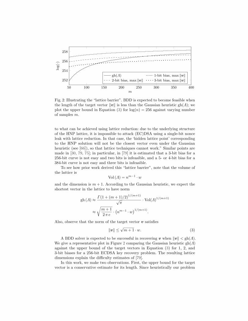
Fig. 2: Illustrating the “lattice barrier”. BDD is expected to become feasible whenthe length of the target vector ‖v‖ is less than the Gaussian heuristic gh(Λ); weplot the upper bound in Equation (3) for log(n) = 256 against varying numberof samples m.

to what can be achieved using lattice reduction: due to the underlying structureof the HNP lattice, it is impossible to attack (EC)DSA using a single-bit nonceleak with lattice reduction. In that case, the ‘hidden lattice point’ correspondingto the HNP solution will not be the closest vector even under the Gaussianheuristic (see [66]), so that lattice techniques cannot work.” Similar points aremade in [30, 79, 75]; in particular, in [79] it is estimated that a 3-bit bias for a256-bit curve is not easy and two bits is infeasible, and a 5- or 4-bit bias for a384-bit curve is not easy and three bits is infeasible.

To see how prior work derived this “lattice barrier”, note that the volume ofthe lattice is

Vol (Λ) = nm−1 · w

and the dimension is m+ 1. According to the Gaussian heuristic, we expect theshortest vector in the lattice to have norm

gh (Λ) ≈ Γ (1 + (m+ 1)/2)1/(m+1)

√π

·Vol(Λ)1/(m+1)

≈√m+ 1

2π e·(nm−1 · w

)1/(m+1).

Also, observe that the norm of the target vector v satisfies

‖v‖ ≤√m+ 1 · w. (3)

A BDD solver is expected to be successful in recovering v when ‖v‖ < gh(Λ).We give a representative plot in Figure 2 comparing the Gaussian heuristic gh(Λ)against the upper bound of the target vectors in Equation (3) for 1, 2, and3-bit biases for a 256-bit ECDSA key recovery problem. The resulting latticedimensions explain the difficulty estimates of [79].

In this work, we make two observations. First, the upper bound for the targetvector is a conservative estimate for its length. Since heuristically our problem

50 100 150 200 250 300 350 400

252

254

256

258

m

log(·

)

gh(Λ) 1-bit bias, E[‖v‖ ]2-bit bias, E [‖v‖ ] 3-bit bias, E[‖v‖ ]

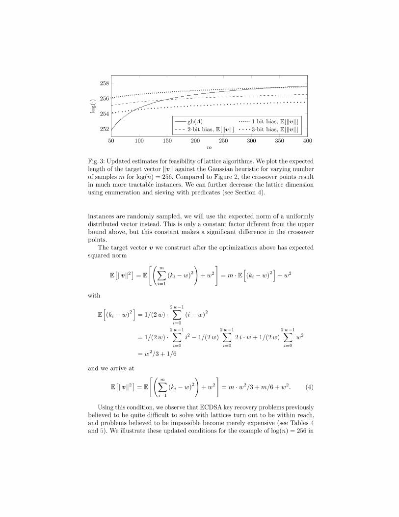
Fig. 3: Updated estimates for feasibility of lattice algorithms. We plot the expectedlength of the target vector ‖v‖ against the Gaussian heuristic for varying numberof samples m for log(n) = 256. Compared to Figure 2, the crossover points resultin much more tractable instances. We can further decrease the lattice dimensionusing enumeration and sieving with predicates (see Section 4).

instances are randomly sampled, we will use the expected norm of a uniformlydistributed vector instead. This is only a constant factor different from the upperbound above, but this constant makes a significant difference in the crossoverpoints.

The target vector v we construct after the optimizations above has expectedsquared norm

E[‖v‖2

]= E

[(m∑i=1

(ki − w)2

)+ w2

]= m · E

[(ki − w)

2]

+ w2

with

E[(ki − w)

2]

= 1/(2w) ·2w−1∑i=0

(i− w)2

= 1/(2w) ·2w−1∑i=0

i2 − 1/(2w)

2w−1∑i=0

2 i · w + 1/(2w)

2w−1∑i=0

w2

= w2/3 + 1/6

and we arrive at

E[‖v‖2

]= E

[(m∑i=1

(ki − w)2

)+ w2

]= m · w2/3 +m/6 + w2. (4)

Using this condition, we observe that ECDSA key recovery problems previouslybelieved to be quite difficult to solve with lattices turn out to be within reach,and problems believed to be impossible become merely expensive (see Tables 4and 5). We illustrate these updated conditions for the example of log(n) = 256 in

Figure 3. The crossover points accurately predict the experimental performanceof our algorithms in practice; compare to the experimental results plotted inFigure 4.

The second observation we make in this work is that we show that latticealgorithms can still be applied when ‖v‖ ≥ gh(Λ), i.e. when the “lattice vectorcorresponding to the secret is no longer expected to be significantly shorter thanother vectors in the lattice” [13]. That is, we observe that the “lattice barrier”is soft, and that violating it simply requires spending more computational time.This allows us to increase the probability of success at the crossover points inFigure 3 and successfully solve instances with fewer samples than suggested bythe crossover points.

An even stronger barrier to the applicability of any algorithm for solving theHidden Number Problem comes from the amount of information about the secretencoded in the problem itself: each sample reveals log(n)− ` bits of informationabout the secret d. Thus, we expect to require m ≥ log(n)/(log(n)−`) in order torecover d; heuristically, for random instances, below this point we do not expectthe solution to be uniquely determined by the lattice, no matter the algorithmused to solve it. We will see below that our techniques allow us to solve instancespast both the “lattice barrier” and the information-theoretic limit.

4 Bounded Distance Decoding with predicate

We now define the key computational problem in this work:

Definition 5 (α-Bounded Distance Decoding with predicate (BDDα,f(·))).Given a lattice basis B, a vector t, a predicate f(·), and a parameter 0 < α suchthat the Euclidean distance dist(t,B) < α·λ1(B), find the lattice vector v ∈ Λ(B)satisfying f(v − t) = 1 which is closest to t.

We will solve the BDDα,f(·) using Kannan’s embedding technique. However,the lattice we will construct does not necessarily have a unique shortest vector.Rather, uniqueness is expected due to the addition of a predicate f(·).

Definition 6 (unique Shortest Vector Problem with predicate (uSVPf(·))).Given a lattice Λ and a predicate f(·) find the shortest nonzero vector v ∈ Λsatisfying f(v) = 1.

Remark 1. Our nomenclature—“BDD” and “uSVP”—might be considered con-fusing given that the target is neither unusually close nor short. However, thedistance to the lattice is still bounded in the first case and the presence of thepredicate ensures uniqueness in the second case. Thus, we opted for those namesover “CVP” and “SVP”.

Explicitly, to solve BDDα,f(·) using an oracle solving uSVPf(·), we considerthe lattice

L =

(B 0t τ

)

where τ ≈ E[‖v − t‖/

√d]

is some embedding factor. If v is the closest vector

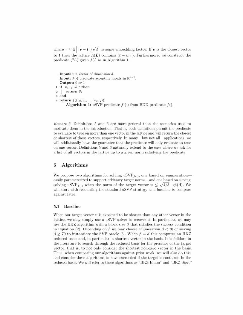
to t then the lattice Λ(L) contains (t − v, τ). Furthermore, we construct thepredicate f ′(·) given f(·) as in Algorithm 1.

Input: v a vector of dimension d.Input: f(·) predicate accepting inputs in Rd−1.Output: 0 or 1

1 if |vd−1| 6= τ then2 return 0 ;3 end4 return f((v0, v1, . . . , vd−2));

Algorithm 1: uSVP predicate f ′(·) from BDD predicate f().

Remark 2. Definitions 5 and 6 are more general than the scenarios used tomotivate them in the introduction. That is, both definitions permit the predicateto evaluate to true on more than one vector in the lattice and will return the closestor shortest of those vectors, respectively. In many—but not all—applications, wewill additionally have the guarantee that the predicate will only evaluate to trueon one vector. Definitions 5 and 6 naturally extend to the case where we ask fora list of all vectors in the lattice up to a given norm satisfying the predicate.

5 Algorithms

We propose two algorithms for solving uSVPf(·), one based on enumeration—easily parameterized to support arbitrary target norms—and one based on sieving,solving uSVPf(·) when the norm of the target vector is ≤

√4/3 · gh(Λ). We

will start with recounting the standard uSVP strategy as a baseline to compareagainst later.

5.1 Baseline

When our target vector v is expected to be shorter than any other vector in thelattice, we may simply use a uSVP solver to recover it. In particular, we mayuse the BKZ algorithm with a block size β that satisfies the success conditionin Equation (2). Depending on β we may choose enumeration β < 70 or sievingβ ≥ 70 to instantiate the SVP oracle [5]. When β = d this computes an HKZreduced basis and, in particular, a shortest vector in the basis. It is folklore inthe literature to search through the reduced basis for the presence of the targetvector, that is, to not only consider the shortest non-zero vector in the basis.Thus, when comparing our algorithms against prior work, we will also do this,and consider these algorithms to have succeeded if the target is contained in thereduced basis. We will refer to these algorithms as “BKZ-Enum” and “BKZ-Sieve”

depending on the oracle used. We may simply write BKZ-β or BKZ when theSVP oracle or the block size do not need to specified. When β = d we will alsorefer to this approach as the “SVP approach”, even though a full HKZ reducedbasis is computed and examined. When we need to spell out the SVP oracle used,we will write “Sieve” and “Enum” respectively.

5.2 Enumeration

Our first algorithm is to augment lattice-point enumeration, which is exhaustivesearch over all points in a ball of a given radius, with a predicate to immediatelygive an algorithm that exhaustively searches over all points in a ball of a givenradius that satisfy a given predicate. In other words, our modification to lattice-point enumeration is simply to add a predicate check whenever the algorithmreaches a leaf node in the tree, i.e. has recovered a candidate solution. If thepredicate is satisfied the solution is accepted and the algorithm continues itssearch trying to improve upon this candidate. If the predicate is not satisfied,the algorithm proceeds as if the search failed. This augmented enumerationalgorithm is then used to enumerate all points in a radius R corresponding to the(expected) norm of the target vector. We give pseudocode (adapted from [28])for this algorithm in Algorithm 2. Our implementation of this algorithm is in theclass USVPPredEnum in the file usvp.py available at [7].

Theorem 1. Let Λ ⊂ Rd be a lattice containing vectors v such that ‖v‖ ≤ R =ξ · gh(Λ) and f(v) = 1. Assuming the Gaussian heuristic, then Algorithm 2 findsthe shortest vector v satisfying f(v) = 1 in ξd · dd/(2e)+o(d) steps. Algorithm 2will make ξd+o(d) calls to f(·).

Proof (sketch). Let Ri = R. Enumeration runs in

d−1∑k=0

1

2· Vol(Bd−k(R))∏d−1

i=k ‖b∗i ‖

steps [42] which scales by ξd+o(d) when R scales by ξ. Solving SVP with enumer-ation takes dd/(2e)+o(d) steps [42]. By the Gaussian heuristic we expect ξd pointsin Bd(R) ∩ Λ on which the algorithm may call the predicate f(·).

Implementation. Modifying FPLLL [76, 77] to implement this functionality isrelatively straightforward since it already features an Evaluator class to validatefull solutions—i.e. leaves—with high precision, which we subclassed. We then callthis modified enumeration code with a search radius R that corresponds to theexpected length of our target. We make use of (extreme) pruned enumeration bycomputing pruning parameters using FPLLL’s Pruner module. Here, we makethe implicit assumption that rerandomizing the basis means the probability offinding the target satisfying our predicate is independent from previous attempts.We give some example performance figures in Table 1.

Input: Lattice basis b0, . . . , bd−1.Input: Pruning parameters R0, . . . , Rd−1, such that R = R0.Input: Predicate f(·).Output: umin such that ‖v‖ with v =

∑d−1i=0 (umin)i · bi is minimal subject to

‖πj (v) ‖ ≤ Rj and f(v) = 1 or ⊥.1 umin ← (1, 0, . . . , 0) ∈ Zd; // Final result

2 u← (1, 0, . . . , 0) ∈ Zd; // Current candidate

3 c← (0, 0, . . . , 0) ∈ Rd; // Centers

4 `← (0, 0, . . . , 0) ∈ Zd+1; // Squared Norms5 Compute µi,j and ‖b∗i ‖ for 0 ≤ i, j < d;6 t← 0;7 while t < d do8 backtrack← 1;9 `t ← `t+1 + (ut + ct) · ‖b∗t ‖;

10 if `t < Rt then11 if t > 0 then12 t← t− 1; // Go down a layer

13 ct ← −∑d−1i=t+1 ut · µi,t;

14 ut ← dctc;15 backtrack← 0;

16 else if f(∑d−1i=0 ui · bi) = 1 and ‖

∑d−1i=0 ui · bi‖ < ‖

∑d−1i=0 umin,i · bi‖

then17 umin ← u;18 backtrack← 1;

19 end20 if backtrack = 1 then21 t← t+ 1;22 Pick next value for ut using the zig-zag pattern

(ct + 0, ct + 1, ct − 1, ct + 2, ct − 2, . . . );

23 end

24 end

25 if f(∑d−1i=0 (umin)i · bi) = 1 then

26 return umin;27 else28 return ⊥;29 end

Algorithm 2: Enumeration with Predicate (Enum-Pred)

Table 1: Enumeration with predicate performance datatime #calls to f(·)

ξ s/r observed expected observed (1.01 ξ)d

1.0287 62% 3.1h 2.4h 1104 301.0613 61% 5.1h 5.1h 2813 4831.1034 62% 11.8h 15.1h 15274 154111.1384 64% 25.3h 40.1h 169950 248226

ECDSA instances (see Section 6) with d = 89 and USVPPredEnum. Expected runningtime is computed using FPLLL’s Pruner module, assuming 64 CPU cycles are requiredto visit one enumeration node. Our implementation of Algorithm 2 enumerates a radiusof 1.01 · ξ · gh(Λ). We give the median of 200 experiments. The column “s/r” gives thesuccess rate of recovering the target vector in those experiments.

Relaxation. Algorithm 2 is easily augmented to solve the more general problemof returning all satisfying vectors, i.e. with f(v) = 1 within a given radius R, bystoring all candidates in a list in line 17.

5.3 Sieving

Our second algorithm is simply a sieving algorithm “as is”, followed by a predicatecheck over the database. That is, taking a page from [32, 5], we do not treat alattice sieve as a black box SVP solver, but exploit that it outputs exponentiallymany short vectors. In particular, under the heuristic assumptions mentionedin the introduction—all vectors in the database L are on the surface of a d-dimensional ball—a 2-sieve, in its standard configuration, will output all vectorsof norm R ≤

√4/3 · gh(Λ) [32].7 Explicitly:

Assumption 1 When a 2-sieve algorithm terminates, it outputs a database Lcontaining all vectors with norm ≤

√4/3 · gh(Λ).

Thus, our algorithm simply runs the predicate on each vector of the database.We give pseudocode in Algorithm 3. Our implementation of this algorithm is inthe class USVPPredSieve in the file usvp.py available at [7].

Theorem 2. Let Λ ⊂ Rd be a lattice containing a vector v such that ‖v‖ ≤ R =√4/3 · gh(Λ). Under Assumption 1 Algorithm 3 is expected to find the minimal

v satisfying f(v) = 1 in 20.292 d+o(d) steps and (4/3)d/2+o(d)

calls to f(·).

Implementation. Implementing this algorithm is trivial using G6K [78]. How-ever, some parameters need to be tuned to make Assumption 1 hold (approx-imately) in practice. First, since deciding if a vector is a shortest vector is a

7 The radius√

4/3 · gh(Λ) can be parameterized in sieving algorithms by adapting therequired angle for a reduction and thus increasing the database size. This was usedin e.g. [31] to find approximate Voronoi cells.

hard problem, sieve algorithms and implementations cannot use this test todecide when to terminate. As a consequence, implementations of these algorithmssuch as G6K use a saturation test to decide when to stop: this measures thenumber of vectors with norm bounded by C · gh(Λ) in the database. In G6K,C =

√4/3 by default. The required fraction in [78] is controlled by the variable

saturation_ratio, which defaults to 0.5. Since we are interested in all vectorswith norms below this bound, we increase this value. However, increasing thisvalue also requires increasing the variable db_size_factor, which controls the sizeof L. If db_size_factor is too small, then the sieve cannot reach the saturationrequested by saturation_ratio. We compare our final settings with the G6Kdefaults in Table 2. We justify our choices with the experimental data presentedin Table 3. As Table 3 shows, increasing the saturation ratio increases the rate ofsuccess and in several cases also decreases the running time normalized by therate of success. However, this increase in the saturation ratio benefits from anincreased database size, which might be undesirable in some applications.

Second, we preprocess our bases with BKZ-(d − 20) before sieving. Thisdeviates from the strategy in [5] where such preprocessing is not necessary.Instead, progressive sieving gradually improves the basis there. However, inour experiments we found that this preprocessing step randomized the basis,preventing saturation errors and increasing the success rate. We speculate thatthis behavior is an artifact of the sampling and replacement strategy used insideG6K.

Relaxation. Algorithm 3 is easily augmented to solve the more general problemof returning all satisfying vectors, i.e. with f(v) = 1, within radius

√4/3 · gh(Λ),

by storing all candidates in a list in line 5.

Conflict with D4F. The performance of sieving in practice benefits greatlyfrom the “dimensions for free” technique introduced in [32]. This technique,which inspired our algorithm, starts from the observation that a sieve willoutput all vectors of norm

√4/3 · gh(Λ). This observation is then used to

Input: Lattice basis b0, . . . , bd−1.Input: Predicate f(·).Output: v such that ‖v‖ ≤

√4/3 · gh(Λ(B)) and f(v) = 1 or ⊥.

1 r ← ⊥;2 Run sieving algorithm on b0, . . . , bd−1 and denote output list as L;3 for v ∈ L do4 if f(v) = 1 and (r = ⊥ or ‖v‖ < ‖r‖) then5 r ← v;6 end

7 end8 return r;

Algorithm 3: Sieving with Predicate (Sieve-Pred)

Table 2: Sieving parametersParameter G6K This work

BKZ preprocessing none d− 20saturation ratio 0.50 0.70db size factor 3.20 3.50

Table 3: Sieving parameter exploration3-sieve BGJ1

sat dbf s/r time time/rate s/r time time/rate

0.5 3.5 61% 4062s 6715s 61% 4683s 7678s0.5 4.0 60% 4592s 7654s 65% 4832s 7493s0.5 4.5 60% 5061s 8508s 65% 5312s 8500s0.5 5.0 58% 5652s 9831s 66% 5443s 8311s



We empirically explored sieving parameters to justify the choices in our experiments. Inthis table, times are wall times. These results are for lattices Λ of dimension 88 wherethe target vector is expected to have norm 1.1323 ·gh(Λ). The column “sat” gives valuesfor saturation ratio; the column “dbf” gives values for db size factor; the columns“s/r” give the rate of success.

solve SVP in dimension d using a sieve in dimension d′ = d − Θ(d/ log d).In particular, if the projection πd−d′ (v) of the shortest vector v has norm‖πd−d′ (v) ‖ ≤

√4/3·gh(Λd−d′), where Λd−d′ is the lattice obtained by projecting

Λ orthogonally to the first d − d′ vectors of B then it is expected that Babailifting will find v. Clearly, in our setting where the target itself is expected tohave norm > gh(Λ) this optimization may not be available. Thus, when there is achoice to construct a uSVP lattice or a uSVPf(·) lattice in smaller dimension, weshould compare the sieving dimension d′ of the former against the full dimensionof the latter. In [32] an “optimistic” prediction for d′ is given as

d′ = d− d log(4/3)

log(d/(2πe))(5)

which matches the experimental data presented in [32] well. However, we notethat G6K achieves a few extra dimensions for free via “on the fly” lifting [5]. Weleave investigating an intermediate regime—fewer dimensions for free—for futurework.

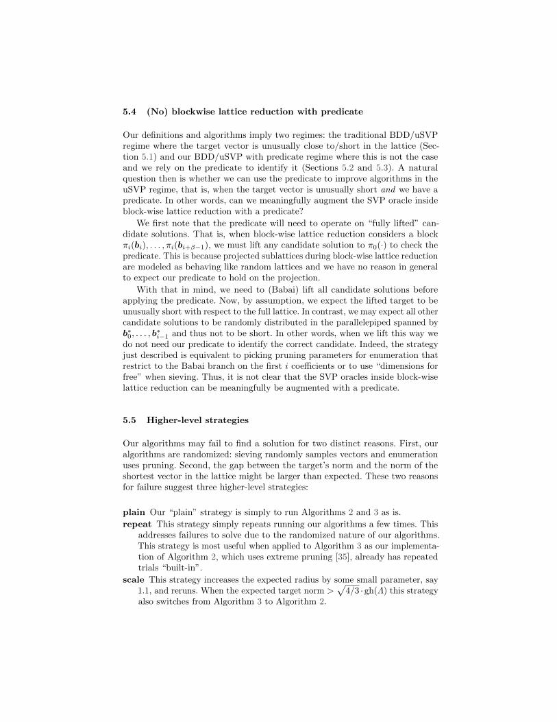
5.4 (No) blockwise lattice reduction with predicate

Our definitions and algorithms imply two regimes: the traditional BDD/uSVPregime where the target vector is unusually close to/short in the lattice (Sec-tion 5.1) and our BDD/uSVP with predicate regime where this is not the caseand we rely on the predicate to identify it (Sections 5.2 and 5.3). A naturalquestion then is whether we can use the predicate to improve algorithms in theuSVP regime, that is, when the target vector is unusually short and we have apredicate. In other words, can we meaningfully augment the SVP oracle insideblock-wise lattice reduction with a predicate?

We first note that the predicate will need to operate on “fully lifted” can-didate solutions. That is, when block-wise lattice reduction considers a blockπi(bi), . . . , πi(bi+β−1), we must lift any candidate solution to π0(·) to check thepredicate. This is because projected sublattices during block-wise lattice reductionare modeled as behaving like random lattices and we have no reason in generalto expect our predicate to hold on the projection.

With that in mind, we need to (Babai) lift all candidate solutions beforeapplying the predicate. Now, by assumption, we expect the lifted target to beunusually short with respect to the full lattice. In contrast, we may expect all othercandidate solutions to be randomly distributed in the parallelepiped spanned byb∗0, . . . , b

∗i−1 and thus not to be short. In other words, when we lift this way we

do not need our predicate to identify the correct candidate. Indeed, the strategyjust described is equivalent to picking pruning parameters for enumeration thatrestrict to the Babai branch on the first i coefficients or to use “dimensions forfree” when sieving. Thus, it is not clear that the SVP oracles inside block-wiselattice reduction can be meaningfully be augmented with a predicate.

5.5 Higher-level strategies

Our algorithms may fail to find a solution for two distinct reasons. First, ouralgorithms are randomized: sieving randomly samples vectors and enumerationuses pruning. Second, the gap between the target’s norm and the norm of theshortest vector in the lattice might be larger than expected. These two reasonsfor failure suggest three higher-level strategies:

plain Our “plain” strategy is simply to run Algorithms 2 and 3 as is.

repeat This strategy simply repeats running our algorithms a few times. Thisaddresses failures to solve due to the randomized nature of our algorithms.This strategy is most useful when applied to Algorithm 3 as our implementa-tion of Algorithm 2, which uses extreme pruning [35], already has repeatedtrials “built-in”.

scale This strategy increases the expected radius by some small parameter, say1.1, and reruns. When the expected target norm >

√4/3 ·gh(Λ) this strategy

also switches from Algorithm 3 to Algorithm 2.

6 Application to ECDSA key recovery

The source code for the experiments in this section is in the file ecdsa hnp.pyavailable at [7].

Varying the number of samples m. We carried out experiments for commonelliptic curve lengths and most significant bits known from the signature nonceto evaluate the success rate of different algorithms as we varied the number ofsamples, thus varying the expected ratio of the target vector to the shortestvector in the lattice.

As predicted theoretically, the shortest vector technique typically fails whenthe expected length of the target vector is longer than the Gaussian heuristic, andits success probability rises as the relative length of the target vector decreases.We recall that we considered the shortest vector approach a success if the targetvector was contained in the reduced basis. Both the enumeration and sievingalgorithms have success rates well above zero when the expected length of thetarget vector is longer than the expected length of the shortest vector, thusdemonstrating the effectiveness of our techniques past the “lattice barrier”.

Figure 4 shows the success rate of each algorithm for common parametersof interest as we vary the number of samples. Each data point represents 32experiments for smaller instances, or 8 experiments for larger instances. Thecorresponding running times for these algorithms and parameters are plotted inFigure 5. We parameterized Algorithm 2 to succeed at a rate of 50%. For some ofthe larger lattice dimensions, enumeration algorithms were simply infeasible, andwe do not report enumeration results for these parameters. These experimentsrepresent more than 60 CPU-years of computation time spread over around twocalendar months on a heterogeneous collection of computers with Intel Xeon 2.2and 2.3GHz E5-2699, 2.4GHz E5-2699A, and 2.5GHz E5-2680 processors.

Table 4 gives representative running times and success rates for Algorithm 3,sieving with predicate, for popular curve sizes and numbers of bits known, andlists similar computations from the literature where we could determine theparameters used. It illustrates how our techniques allow us to solve instanceswith fewer samples than previous work. We recall that most applications oflattice algorithms for solving ECDSA-HNP instances seem to arbitrarily choosea small block size for BKZ, and experimentally determine the number of samplesrequired. For 3 bits known on a 256-bit curve, there are multiple algorithmicresults reported in the literature. In [75] the authors report a running time of 238CPU-hours to run the first phase of Bleichenbacher’s algorithm on 223 samples.In [54] the authors report applying BKZ-20 followed by enumeration with linearpruning to achieve a 21% success probability in five hours. Sieving with predicatetook 1.5 CPU-hours to solve the same parameters with a 63% success probabilityusing 87 samples.

Table 4 also gives running times and success rates for Algorithm 2, enumerationwith predicate, in solving instances beyond the information-theoretic barrier,that is, when the number of samples available was not large enough to expect the

50 55 60 65 70 75 80 85 90 95 100 1050

50

100

2 bits known3 bits known

mSucc

ess

pro

babilit

y

log(n) = 160

BKZ-Sieve

BKZ-Enum

Sieve-Pred

Enum-Pred

1.47 1.21 1.02 0.89 0.79 0.71 - 1.19 1.11 1.04 0.98 0.93 γ

60 65 70 75 80 85 90 95 100 105 1100

50

100


mSucc

ess

pro

babilit

y

log(n) = 192

BKZ-Sieve

BKZ-Enum

Sieve-Pred

Enum-Pred

1.35 1.14 0.99 0.87 - - - 1.20 1.12 1.05 0.99 γ

60 65 70 75 80 85 90 95 1000

50

100


mSucc

ess

pro

babilit

y

log(n) = 256

BKZ-Sieve

BKZ-Enum

Sieve-Pred

Enum-Pred

1.41 1.13 0.93 0.79 - 1.19 1.06 0.96 0.87 γ

75 80 85 90 95 100 105 1100

50

100


mSucc

ess

pro

babilit

y

log(n) = 384

BKZ-Sieve

BKZ-Enum

Sieve-Pred

Enum-Pred

1.28 1.03 0.85 - 1.21 1.06 0.93 0.83 γ

70 75 80 85 90 95 1000

50

100


mSucc

ess

pro

babilit

y

log(n) = 521

BKZ-Enum

Sieve-Pred

Enum-Pred

1.59 1.13 0.84 - 1.02 0.83 0.69 γ

Fig. 4: Comparison of algorithm success rates for ECDSA. We generated HNPinstances for common ECDSA parameters and compared the success rates of eachalgorithm on identical instances. The x-axis labels show the number of samples mand γ = E[‖v‖] /E[‖b0‖], the corresponding ratio between the expected lengthof the target vector v and the expected length of the shortest vector b0 in arandom lattice.

50 55 60 65 70 75 80 85 90 95 100 105100

103

106


Samples

CP

USec

onds

log(n) = 160

BKZ-Enum

BKZ-Sieve

Enum-Pred

Sieve-Pred

60 70 80 90 100 110 120 130

102

104

106


Samples

CP

USec

onds

log(n) = 192

BKZ-enum

BKZ-Sieve

Enum-Pred

Sieve-Pred

60 65 70 75 80 85 90 95 100

102

104

106


Samples

CP

USec

onds

log(n) = 256

BKZ-Enum

BKZ-Sieve

Enum-Pred

Sieve-Pred

80 90 100 110 120 130 140101

103

105


Samples

CP

USec

onds

log(n) = 384

70 75 80 85 90 95 100101

103

105


Samples

CP

USec

onds

log(n) = 521

Fig. 5: Comparison of algorithm running times for ECDSA. We plot the algorithmrunning times in CPU-seconds for the experiments in Figure 4 on a log scale.

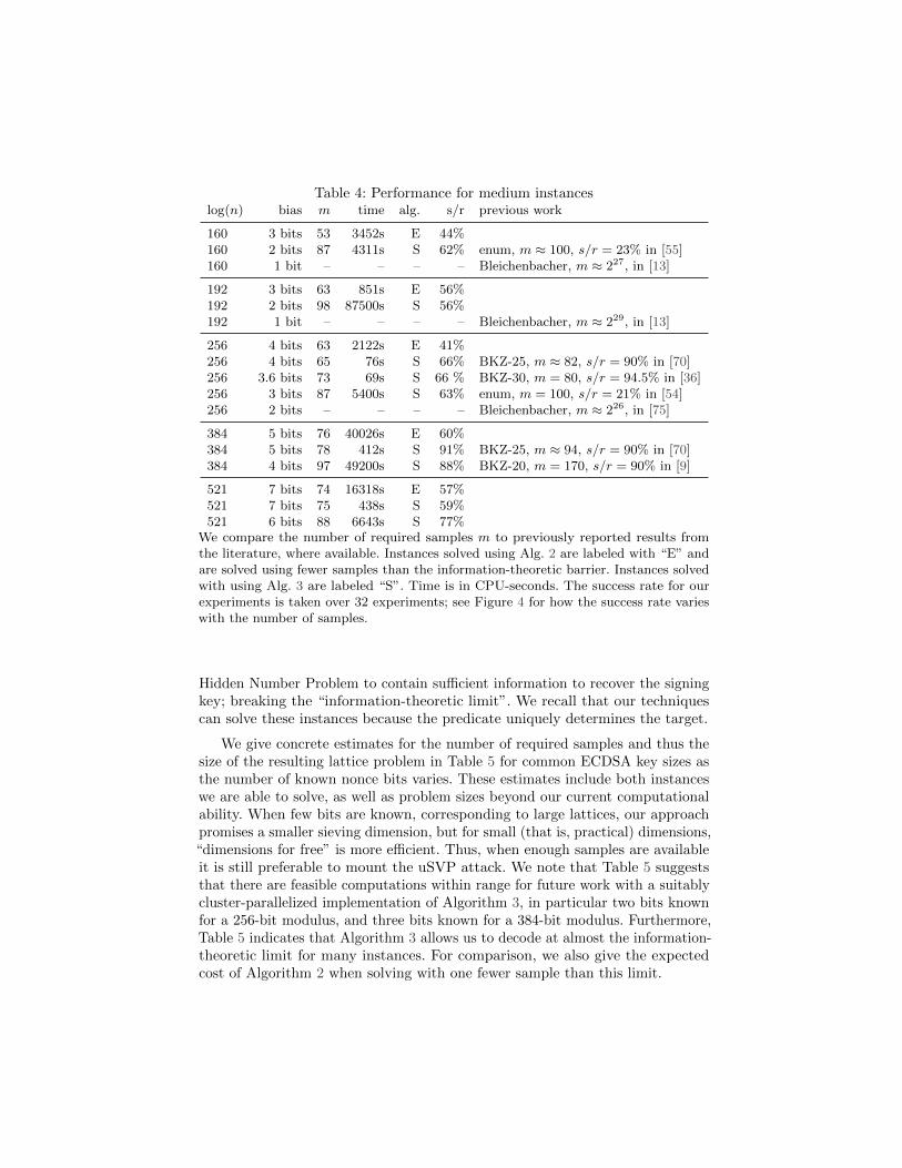
Table 4: Performance for medium instanceslog(n) bias m time alg. s/r previous work

160 3 bits 53 3452s E 44%160 2 bits 87 4311s S 62% enum, m ≈ 100, s/r = 23% in [55]160 1 bit – – – – Bleichenbacher, m ≈ 227, in [13]

192 3 bits 63 851s E 56%192 2 bits 98 87500s S 56%192 1 bit – – – – Bleichenbacher, m ≈ 229, in [13]

256 4 bits 63 2122s E 41%256 4 bits 65 76s S 66% BKZ-25, m ≈ 82, s/r = 90% in [70]256 3.6 bits 73 69s S 66 % BKZ-30, m = 80, s/r = 94.5% in [36]256 3 bits 87 5400s S 63% enum, m = 100, s/r = 21% in [54]256 2 bits – – – – Bleichenbacher, m ≈ 226, in [75]

384 5 bits 76 40026s E 60%384 5 bits 78 412s S 91% BKZ-25, m ≈ 94, s/r = 90% in [70]384 4 bits 97 49200s S 88% BKZ-20, m = 170, s/r = 90% in [9]

521 7 bits 74 16318s E 57%521 7 bits 75 438s S 59%521 6 bits 88 6643s S 77%

We compare the number of required samples m to previously reported results fromthe literature, where available. Instances solved using Alg. 2 are labeled with “E” andare solved using fewer samples than the information-theoretic barrier. Instances solvedwith using Alg. 3 are labeled “S”. Time is in CPU-seconds. The success rate for ourexperiments is taken over 32 experiments; see Figure 4 for how the success rate varieswith the number of samples.

Hidden Number Problem to contain sufficient information to recover the signingkey; breaking the “information-theoretic limit”. We recall that our techniquescan solve these instances because the predicate uniquely determines the target.

We give concrete estimates for the number of required samples and thus thesize of the resulting lattice problem in Table 5 for common ECDSA key sizes asthe number of known nonce bits varies. These estimates include both instanceswe are able to solve, as well as problem sizes beyond our current computationalability. When few bits are known, corresponding to large lattices, our approachpromises a smaller sieving dimension, but for small (that is, practical) dimensions,“dimensions for free” is more efficient. Thus, when enough samples are availableit is still preferable to mount the uSVP attack. We note that Table 5 suggeststhat there are feasible computations within range for future work with a suitablycluster-parallelized implementation of Algorithm 3, in particular two bits knownfor a 256-bit modulus, and three bits known for a 384-bit modulus. Furthermore,Table 5 indicates that Algorithm 3 allows us to decode at almost the information-theoretic limit for many instances. For comparison, we also give the expectedcost of Algorithm 2 when solving with one fewer sample than this limit.

Table 5: Resources required to solve ECDSA with known nonce bits.

log(n) = 160

bits known 8 7 6 5 4 3 2 1Sieve m/d 21/− 2 25/9 29/15 35/23 45/33 61/49 99/84 258/232Sieve-Pred m/d 21/22 24/25 28/29 33/34 42/43 57/58 87/88 193/194Sieve-Pred cost 40.2 38.3 36.4 34.9 33.6 34.4 41.5 80.9limit m 20 23 27 32 40 54 80 160limit −1 cost 23.5 23.6 24.7 27.9 31.1 36.5 50.6 104.0

log(n) = 192

bits known 8 7 6 5 4 3 2 1Sieve m/d 25/9 29/15 34/21 41/29 51/39 70/57 110/94 255/229Sieve-Pred m/d 25/26 28/29 33/34 39/40 49/50 65/66 98/99 200/201Sieve-Pred cost 37.8 36.4 34.9 33.9 33.7 35.7 45.2 83.5limit m 24 28 32 39 48 64 96 192limit −1 cost 23.7 23.7 26.0 27.2 31.5 38.3 54.2 118.6

log(n) = 256


log(n) = 384


log(n) = 521


Sieve Number of samples m required for solving uSVP as in Section 5.1 and sieving dimensionaccording to Equation (5) (called d′ there).

Sieve-Pred Number of samples m required for Algorithm 3 and sieving dimension d = m+ 1.Sieve-Pred cost Log of expected cost in CPU cycles; cost is estimated as 0.658 · d− 21.11 log(d)+

119.91 which does not match the asymptotics but approximates experiments up to dimension100.

limit Information theoretic limit for m of pure lattice approach: dlog(n)/bits knowne.limit −1 cost Log of expected cost for Algorithm 2 in CPU cycles withm = dlog(n)/bits knowne−1

samples.

Fixed number of samples m. An implication of Table 5 is that our approachallows us to solve the Hidden Number Problem with fewer samples than theunique SVP bounds would imply. In some attack settings, the attacker may havea hard limit on the number of samples available. Using Algorithms 2 and 3,enumeration and sieving with predicate, allows us to increase the probability ofa successful attack in this case, and increase the range of parameters for which afeasible attack is possible.

This scenario arose in [22], where the authors searched for flawed ECDSAimplementations by applying lattice attacks to ECDSA signatures gathered frompublic data sources including cryptocurrency blockchains and internet-wide scansof protocols like TLS and SSH. In these cases, the attacker has access to a fixednumber of signature samples generated from a given public key, and wishes tomaximize the probability of a successful attack against this fixed number ofsignatures, for as few bits known as possible.

126 127 128 129 130 131 132 133 134 135 136

0

50

100

Unknown nonce bits

Succ

ess

pro

babilit

y

log(n) = 256,m = 2

BKZ

Enum-Pred

Sieve-Pred

Fig. 6: Algorithm success rates in a small fixed-sample regime. We plot theexperimental success rate of each algorithm in recovering a varying number ofnonce bits using two samples. Each data point represents the success rate of thealgorithm over 100 experiments. Using sieving and enumeration with a predicateallows the attacker to increase the probability of a successful attack even whenmore samples cannot be collected. We parameterized enumeration with predicateto succeed with probability 1/2.

The paper of [22] reported using BKZ in very small dimensions to find 287distinct keys that used nonce lengths of 160, 128, 110, 64, and less than 32 bitsfor ECDSA signatures with the 256-bit secp256k1 curve used for Bitcoin. Theyreported finding two distinct keys using 128-bit nonces in two signatures each.

Experimentally, the BKZ algorithm only has a 70% success rate at recoveringthe private key for 128-bit nonces with two signature samples, and the success ratedrops precipitously as the number of unknown nonce bits increases. In contrast,sieving with predicate has a 100% success rate up to around 132-bit nonces. See

Figure 6 for a comparison of these algorithms as the number of signatures is fixedto two and the number of unknown nonce bits varies.

We hypothesized that this failure rate may have caused the results of [22] toomit some vulnerable keys. Thus, we ran our sieving with predicate approachagainst the same Bitcoin blockchain snapshot data from September 2018 as usedin [22], targeting only 128-bit nonces using pairs of signatures. This snapshotcontained 569,396,463 signatures that had been generated by a private key thatgenerated two or more signatures. For the set of m signatures generated by eachdistinct key, we applied the sieving with predicate algorithm to 2m pairs ofsignatures to check for nonces of length less than 128 bits. Using this approach,we were able to compute the private keys for 9 more distinct secret keys.

0 0.1 0.2 0.3 0.4 0.5

101

103

105

Fraction of errors

CP

U-s

econds

log(n) = 256, log(k) = 252

m = 70m = 75m = 80m = 85m = 90

Fig. 7: Search time in the presence of errors. We plot the experimental computationtime of the “scale” strategy to find the target vector as we varied the number oferrors in the sample. For these experiments, each “error” is a nonce that is onebit longer than the length supplied to the algorithm. Increasing the number ofsamples decreases the search time.

Handling errors. In practical side-channel attacks, it is common to have somefraction of measurement errors in the data. In a common setting for ECDSA keyrecovery from known nonce bits, the side channel leaks the number of leadingzeroes of the nonce, but the signal is noisy and thus data may be mislabeled. Ifthe estimate is below the true number, this is not a problem, since the targetvector will be even shorter than estimated and thus easier to find. However, ifthe true number of zero bits is smaller than the estimate, then the desired vectorwill be larger than estimated which can cause the key recovery algorithm to fail.

It is believed that lattice approaches to the Hidden Number Problem do notdeal well with noisy data [70] and “assume that inputs are perfectly correct” [13].There are a few techniques in the literature to work around these limitations andto deal with noise [46]. The most common approach is simply to repeatedly try

running the lattice algorithm on subsamples of the data until one succeeds [23].Alternatively, one can use more samples in the lattice, in order to increase theexpected gap between the target vector and the lattice. For example, it wasalready observed in [29] that using a lattice construction with more samplesincreases the success rate in the presence of errors, even using the same blocksize.

However, the most natural approach does not appear to have been consideredin the literature before: Use an estimate of the error rate to compute a new targetnorm as in Eq. (4) and pick the block size or enumeration radius parametersaccordingly. That is, when the error rate can be estimated, this is simply a specialcase of estimating the norm of the target vector. As before, even if the numberm of samples is limited, Algorithm 2 in principle can search out to arbitrarilylarge target norms.

The most difficult case to handle is when more samples are not availableand the error rate is unknown or difficult to estimate properly. In this case, astrategy is to repeatedly increase the expected target norm of the vector, pick analgorithm that solves for this target norm R and attempt to solve the instance:BKZ for R < gh(Λ), Algorithm 3 for R ≤

√4/3 · gh(Λ) and Algorithm 2 for

R >√

4/3 · gh(Λ). We refer to this strategy as “scale” in Section 5.5.Figure 7 illustrates how the running time of the “scale” strategy varies with

the fraction of errors and the number of samples used in the lattice.

Acknowledgments

We thank Joe Rowell and Jianwei Li for helpful discussions on an earlier draft ofthis work, Daniel Genkin for suggesting additional references and a discussion onerror resilience, Noam Nissan for feedback on our implementation, and SamuelNeves for helpful sugestions on our characterization of previous work.

References

1. Ajtai, M., Kumar, R., Sivakumar, D.: A sieve algorithm for the shortest latticevector problem. In: 33rd ACM STOC. pp. 601–610. ACM Press (Jul 2001)

2. Albrecht, M.R., Bai, S., Fouque, P.A., Kirchner, P., Stehle, D., Wen, W.: Fasterenumeration-based lattice reduction: Root hermite factor k1/(2k) time kk/8+o(k). In:Micciancio and Ristenpart [58], pp. 186–212

3. Albrecht, M.R., Cid, C., Faugere, J., Fitzpatrick, R., Perret, L.: On the complexityof the BKW algorithm on LWE. Des. Codes Cryptogr. 74(2), 325–354 (2015)

4. Albrecht, M.R., Deo, A., Paterson, K.G.: Cold boot attacks on ring and moduleLWE keys under the NTT. IACR TCHES 2018(3), 173–213 (2018), https://tches.iacr.org/index.php/TCHES/article/view/7273

5. Albrecht, M.R., Ducas, L., Herold, G., Kirshanova, E., Postlethwaite, E.W., Stevens,M.: The general sieve kernel and new records in lattice reduction. In: Ishai, Y.,Rijmen, V. (eds.) EUROCRYPT 2019, Part II. LNCS, vol. 11477, pp. 717–746.Springer, Heidelberg (May 2019)

https://tches.iacr.org/index.php/TCHES/article/view/7273


6. Albrecht, M.R., Gopfert, F., Virdia, F., Wunderer, T.: Revisiting the expectedcost of solving uSVP and applications to LWE. In: Takagi, T., Peyrin, T. (eds.)ASIACRYPT 2017, Part I. LNCS, vol. 10624, pp. 297–322. Springer, Heidelberg(Dec 2017)

7. Albrecht, M.R., Heninger, N.: Bounded distance decoding with predicate sourcecode. https://github.com/malb/bdd-predicate/ (Dec 2020)

8. Albrecht, M.R., Player, R., Scott, S.: On the concrete hardness of Learning withErrors. Journal of Mathematical Cryptology 9(3), 169–203 (2015)

9. Aldaya, A.C., Brumley, B.B., ul Hassan, S., Garcıa, C.P., Tuveri, N.: Port contentionfor fun and profit. In: 2019 IEEE Symposium on Security and Privacy. pp. 870–887.IEEE Computer Society Press (May 2019)

10. Alkim, E., Ducas, L., Poppelmann, T., Schwabe, P.: Post-quantum key exchange -A new hope. In: Holz, T., Savage, S. (eds.) USENIX Security 2016. pp. 327–343.USENIX Association (Aug 2016)

11. Applebaum, B., Cash, D., Peikert, C., Sahai, A.: Fast cryptographic primitives andcircular-secure encryption based on hard learning problems. In: Halevi [41], pp.595–618

12. Aranha, D.F., Fouque, P.A., Gerard, B., Kammerer, J.G., Tibouchi, M., Zapalowicz,J.C.: GLV/GLS decomposition, power analysis, and attacks on ECDSA signatureswith single-bit nonce bias. In: Sarkar, P., Iwata, T. (eds.) ASIACRYPT 2014, Part I.LNCS, vol. 8873, pp. 262–281. Springer, Heidelberg (Dec 2014)

13. Aranha, D.F., Novaes, F.R., Takahashi, A., Tibouchi, M., Yarom, Y.: LadderLeak:Breaking ECDSA with less than one bit of nonce leakage. Cryptology ePrint Archive,Report 2020/615 (2020), https://eprint.iacr.org/2020/615

14. Bai, S., Stehle, D., Wen, W.: Improved reduction from the bounded distance decod-ing problem to the unique shortest vector problem in lattices. In: Chatzigiannakis,I., Mitzenmacher, M., Rabani, Y., Sangiorgi, D. (eds.) ICALP 2016. LIPIcs, vol. 55,pp. 76:1–76:12. Schloss Dagstuhl (Jul 2016)

15. Becker, A., Ducas, L., Gama, N., Laarhoven, T.: New directions in nearest neighborsearching with applications to lattice sieving. In: Krauthgamer, R. (ed.) 27th SODA.pp. 10–24. ACM-SIAM (Jan 2016)

16. Becker, A., Gama, N., Joux, A.: Speeding-up lattice sieving without increasing thememory, using sub-quadratic nearest neighbor search. Cryptology ePrint Archive,Report 2015/522 (2015), http://eprint.iacr.org/2015/522

17. Benger, N., van de Pol, J., Smart, N.P., Yarom, Y.: “ooh aah... just a little bit”: Asmall amount of side channel can go a long way. In: Batina, L., Robshaw, M. (eds.)CHES 2014. LNCS, vol. 8731, pp. 75–92. Springer, Heidelberg (Sep 2014)

18. Bleichenbacher, D.: On the generation of one-time keys in DL signature schemes.In: Presentation at IEEE P1363 working group meeting. p. 81 (2000)

19. Bleichenbacher, D.: Experiments with DSA. CRYPTO 2005–Rump Session (2005)

20. Blum, A., Kalai, A., Wasserman, H.: Noise-tolerant learning, the parity problem,and the statistical query model. In: 32nd ACM STOC. pp. 435–440. ACM Press(May 2000)

21. Boneh, D., Venkatesan, R.: Hardness of computing the most significant bits ofsecret keys in Diffie-Hellman and related schemes. In: Koblitz, N. (ed.) CRYPTO’96.LNCS, vol. 1109, pp. 129–142. Springer, Heidelberg (Aug 1996)

22. Breitner, J., Heninger, N.: Biased nonce sense: Lattice attacks against weak ECDSAsignatures in cryptocurrencies. In: Goldberg, I., Moore, T. (eds.) FC 2019. LNCS,vol. 11598, pp. 3–20. Springer, Heidelberg (Feb 2019)

https://github.com/malb/bdd-predicate/

https://eprint.iacr.org/2020/615

http://eprint.iacr.org/2015/522

23. Brumley, B.B., Tuveri, N.: Remote timing attacks are still practical. In: Atluri, V.,Dıaz, C. (eds.) ESORICS 2011. LNCS, vol. 6879, pp. 355–371. Springer, Heidelberg(2011)

24. Cabrera Aldaya, A., Pereida Garcıa, C., Brumley, B.B.: From A to Z: Projectivecoordinates leakage in the wild. IACR TCHES 2020(3), 428–453 (2020), https://tches.iacr.org/index.php/TCHES/article/view/8596

25. Capkun, S., Roesner, F. (eds.): USENIX Security 2020. USENIX Association (Aug2020)

26. Coppersmith, D.: Finding a small root of a bivariate integer equation; factoringwith high bits known. In: Maurer, U.M. (ed.) EUROCRYPT’96. LNCS, vol. 1070,pp. 178–189. Springer, Heidelberg (May 1996)

27. Dachman-Soled, D., Ducas, L., Gong, H., Rossi, M.: LWE with side information:Attacks and concrete security estimation. In: Micciancio and Ristenpart [58], pp.329–358

28. Dagdelen, O., Schneider, M.: Parallel enumeration of shortest lattice vectors. LectureNotes in Computer Science p. 211–222 (2010)

29. Dall, F., De Micheli, G., Eisenbarth, T., Genkin, D., Heninger, N., Moghimi, A.,Yarom, Y.: CacheQuote: Efficiently recovering long-term secrets of SGX EPID viacache attacks. IACR TCHES 2018(2), 171–191 (2018), https://tches.iacr.org/index.php/TCHES/article/view/879

30. De Mulder, E., Hutter, M., Marson, M.E., Pearson, P.: Using Bleichenbacher’ssolution to the hidden number problem to attack nonce leaks in 384-bit ECDSA. In:Bertoni, G., Coron, J.S. (eds.) CHES 2013. LNCS, vol. 8086, pp. 435–452. Springer,Heidelberg (Aug 2013)

31. Doulgerakis, E., Laarhoven, T., Weger, B.: Finding closest lattice vectors usingapproximate voronoi cells. In: Ding, J., Steinwandt, R. (eds.) Post-Quantum Cryp-tography - 10th International Conference, PQCrypto 2019. pp. 3–22. Springer,Heidelberg (2019)

32. Ducas, L.: Shortest vector from lattice sieving: A few dimensions for free. In: Nielsen,J.B., Rijmen, V. (eds.) EUROCRYPT 2018, Part I. LNCS, vol. 10820, pp. 125–145.Springer, Heidelberg (Apr / May 2018)

33. Fincke, U., Pohst, M.: Improved methods for calculating vectors of short length ina lattice, including a complexity analysis. Mathematics of Computation 44(170),463–471 (1985)

34. Gama, N., Nguyen, P.Q.: Finding short lattice vectors within Mordell’s inequality.In: Ladner, R.E., Dwork, C. (eds.) 40th ACM STOC. pp. 207–216. ACM Press(May 2008)

35. Gama, N., Nguyen, P.Q., Regev, O.: Lattice enumeration using extreme pruning.In: Gilbert [39], pp. 257–278

36. Garcıa, C.P., Brumley, B.B.: Constant-time callees with variable-time callers. In:Kirda, E., Ristenpart, T. (eds.) USENIX Security 2017. pp. 83–98. USENIX Asso-ciation (Aug 2017)

37. Genkin, D., Pachmanov, L., Pipman, I., Tromer, E., Yarom, Y.: ECDSA keyextraction from mobile devices via nonintrusive physical side channels. In: Weippl,E.R., Katzenbeisser, S., Kruegel, C., Myers, A.C., Halevi, S. (eds.) ACM CCS 2016.pp. 1626–1638. ACM Press (Oct 2016)

38. Gennaro, R., Robshaw, M.J.B. (eds.): CRYPTO 2015, Part I, LNCS, vol. 9215.Springer, Heidelberg (Aug 2015)

39. Gilbert, H. (ed.): EUROCRYPT 2010, LNCS, vol. 6110. Springer, Heidelberg(May / Jun 2010)





40. Guo, Q., Johansson, T., Stankovski, P.: Coded-BKW: Solving LWE using latticecodes. In: Gennaro and Robshaw [38], pp. 23–42

41. Halevi, S. (ed.): CRYPTO 2009, LNCS, vol. 5677. Springer, Heidelberg (Aug 2009)42. Hanrot, G., Stehle, D.: Improved analysis of kannan’s shortest lattice vector al-

gorithm. In: Menezes, A. (ed.) CRYPTO 2007. LNCS, vol. 4622, pp. 170–186.Springer, Heidelberg (Aug 2007)

43. Herold, G., Kirshanova, E.: Improved algorithms for the approximate k-list problemin euclidean norm. In: Fehr, S. (ed.) PKC 2017, Part I. LNCS, vol. 10174, pp. 16–40.Springer, Heidelberg (Mar 2017)

44. Herold, G., Kirshanova, E., May, A.: On the asymptotic complexity of solving LWE.Des. Codes Cryptogr. 86(1), 55–83 (2018)

45. Howgrave-Graham, N., Smart, N.P.: Lattice attacks on digital signature schemes.Des. Codes Cryptogr. 23(3), 283–290 (2001)

46. Jancar, J., Sedlacek, V., Svenda, P., Sys, M.: Minerva: The curse of ECDSAnonces. IACR TCHES 2020(4), 281–308 (2020), https://tches.iacr.org/index.php/TCHES/article/view/8684

47. Kannan, R.: Improved algorithms for integer programming and related latticeproblems. In: 15th ACM STOC. pp. 193–206. ACM Press (Apr 1983)

48. Kannan, R.: Minkowski’s convex body theorem and integer programming. Math.Oper. Res. 12(3), 415–440 (Aug 1987)

49. Kirchner, P., Fouque, P.A.: An improved BKW algorithm for LWE with applicationsto cryptography and lattices. In: Gennaro and Robshaw [38], pp. 43–62

50. Klein, P.N.: Finding the closest lattice vector when it’s unusually close. In: Shmoys,D.B. (ed.) 11th SODA. pp. 937–941. ACM-SIAM (Jan 2000)

51. Laarhoven, T.: Search problems in cryptography: From fingerprinting to latticesieving. Ph.D. thesis, Eindhoven University of Technology (2015)

52. Laarhoven, T., Mariano, A.: Progressive lattice sieving. In: Lange, T., Steinwandt,R. (eds.) Post-Quantum Cryptography - 9th International Conference, PQCrypto2018. pp. 292–311. Springer, Heidelberg (2018)

53. Lenstra, A.K., Lenstra Jr., H.W., Lovasz, L.: Factoring polynomials with rationalcoefficients. Mathematische Annalen 261, 366–389 (1982)

54. Liu, M., Chen, J., Li, H.: Partially known nonces and fault injection attacks onsm2 signature algorithm. In: Lin, D., Xu, S., Yung, M. (eds.) Information Securityand Cryptology. pp. 343–358. Springer International Publishing, Cham (2014)

55. Liu, M., Nguyen, P.Q.: Solving BDD by enumeration: An update. In: Dawson, E.(ed.) CT-RSA 2013. LNCS, vol. 7779, pp. 293–309. Springer, Heidelberg (Feb / Mar2013)

56. Merget, R., Brinkmann, M., Aviram, N., Somorovsky, J., Mittmann, J., Schwenk,J.: Raccoon Attack: Finding and exploiting most-significant-bit-oracles in TLS-DH(E). https://raccoon-attack.com/RacoonAttack.pdf (Sep 2020), accessed 11September 2020

57. Micciancio, D., Regev, O.: Lattice-based cryptography. In: Bernstein, D.J., Buch-mann, J., Dahmen, E. (eds.) Post-Quantum Cryptography, pp. 147–191. Springer,Heidelberg, Berlin, Heidelberg, New York (2009)

58. Micciancio, D., Ristenpart, T. (eds.): CRYPTO 2020, Part II, LNCS, vol. 12171.Springer, Heidelberg (Aug 2020)

59. Micciancio, D., Voulgaris, P.: Faster exponential time algorithms for the shortestvector problem. In: Charika, M. (ed.) 21st SODA. pp. 1468–1480. ACM-SIAM (Jan2010)

60. Micciancio, D., Walter, M.: Fast lattice point enumeration with minimal overhead.In: Indyk, P. (ed.) 26th SODA. pp. 276–294. ACM-SIAM (Jan 2015)



https://raccoon-attack.com/RacoonAttack.pdf

61. Micciancio, D., Walter, M.: Practical, predictable lattice basis reduction. In: Fischlin,M., Coron, J.S. (eds.) EUROCRYPT 2016, Part I. LNCS, vol. 9665, pp. 820–849.Springer, Heidelberg (May 2016)

62. Moghimi, D., Lipp, M., Sunar, B., Schwarz, M.: Medusa: Microarchitectural dataleakage via automated attack synthesis. In: Capkun and Roesner [25], pp. 1427–1444

63. Moghimi, D., Sunar, B., Eisenbarth, T., Heninger, N.: TPM-FAIL: TPM meetstiming and lattice attacks. In: Capkun and Roesner [25], pp. 2057–2073

64. Nemec, M., Sys, M., Svenda, P., Klinec, D., Matyas, V.: The return of coppersmith’sattack: Practical factorization of widely used RSA moduli. In: Thuraisingham, B.M.,Evans, D., Malkin, T., Xu, D. (eds.) ACM CCS 2017. pp. 1631–1648. ACM Press(Oct / Nov 2017)

65. Nguyen, P.Q., Shparlinski, I.: The insecurity of the digital signature algorithm withpartially known nonces. Journal of Cryptology 15(3), 151–176 (Jun 2002)

66. Nguyen, P.Q., Tibouchi, M.: Lattice-based fault attacks on signatures. pp. 201–220.ISC, Springer, Heidelberg (2012)

67. Nguyen, P.Q., Vidick, T.: Sieve algorithms for the shortest vector problem arepractical. J. of Mathematical Cryptology 2(2) (2008)

68. Phost, M.: On the computation of lattice vectors of minimal length, successiveminima and reduced bases with applications. SIGSAM Bulletin 15, 37–44 (1981)

69. Regev, O.: On lattices, learning with errors, random linear codes, and cryptography.In: Gabow, H.N., Fagin, R. (eds.) 37th ACM STOC. pp. 84–93. ACM Press (May2005)

70. Ryan, K.: Return of the hidden number problem. IACR TCHES 2019(1), 146–168(2018), https://tches.iacr.org/index.php/TCHES/article/view/7337

71. Ryan, K.: Hardware-backed heist: Extracting ECDSA keys from qualcomm’s Trust-Zone. In: Cavallaro, L., Kinder, J., Wang, X., Katz, J. (eds.) ACM CCS 2019. pp.181–194. ACM Press (Nov 2019)

72. Schnorr, C.P.: A hierarchy of polynomial time lattice basis reduction algorithms.Theor. Comput. Sci. 53, 201–224 (1987)

73. Schnorr, C., Euchner, M.: Lattice basis reduction: Improved practical algorithmsand solving subset sum problems. Math. Program. 66, 181–199 (1994)

74. Stein, W., et al.: Sage Mathematics Software Version 9.0. The Sage DevelopmentTeam (2019), http://www.sagemath.org

75. Takahashi, A., Tibouchi, M., Abe, M.: New Bleichenbacher records: Fault attackson qDSA signatures. IACR TCHES 2018(3), 331–371 (2018), https://tches.iacr.org/index.php/TCHES/article/view/7278

76. The FPLLL development team: FPLLL, a lattice reduction library (2020), https://github.com/fplll/fplll, available at https://github.com/fplll/fplll

77. The FPLLL development team: FPyLLL, a Python interface to FPLLL (2020),https://github.com/fplll/fpylll, available at https://github.com/fplll/fpylll

78. The G6K development team: G6K (2020), https://github.com/fplll/g6k, availableat https://github.com/fplll/g6k

79. Tibouchi, M.: Attacks on (ec)dsa with biased nonces (2017), https://ecc2017.cs.ru.nl/slides/ecc2017-tibouchi.pdf, elliptic Curve Cryptography Workshop

80. Weiser, S., Schrammel, D., Bodner, L., Spreitzer, R.: Big numbers - big troubles:Systematically analyzing nonce leakage in (EC)DSA implementations. In: Capkunand Roesner [25], pp. 1767–1784


http://www.sagemath.org



https://github.com/fplll/fplll



https://github.com/fplll/fpylll

https://github.com/fplll/fpylll

https://github.com/fplll/g6k

https://github.com/fplll/g6k

https://ecc2017.cs.ru.nl/slides/ecc2017-tibouchi.pdf

https://ecc2017.cs.ru.nl/slides/ecc2017-tibouchi.pdf

Lattice Barrier for the Hidden Number Problem

Documents