Latitudinal and seasonal capacity of the surface oceans as a reservoir of polychlorinated biphenyls

Latitudinal and seasonal capacity of the surface oceans as areservoir of polychlorinated biphenyls

Elena Juradoa, Rainer Lohmannb, Sandra Meijera,b, Kevin C. Jonesb, Jordi Dachsa,*aDepartment of Environmental Chemistry, IIQAB-CSIC, Jordi Girona 18-26, Barcelona 08034, Catalunya, Spain

bEnvironmental Science Department, Lancaster University, Lancaster LA1 4YQ, UK

Received 14 July 2003; accepted 11 August 2003

Abstract

‘‘Capsule’’: Model calculations estimate the latitudinal and seasonal storage capacity of the surface oceans for PCBs.

The oceans play an important role as a global reservoir and ultimate sink of persistent organic pollutants (POPs) such as poly-

chlorinated biphenyls congeners (PCBs). However, the physical and biogeochemical variables that affect the oceanic capacity to retainPCBs show an important spatial and temporal variability which have not been studied in detail, so far. The objective of this paper is toassess the seasonal and spatial variability of the ocean’s maximum capacity to act as a reservoir of atmospherically transported and

deposited PCBs. A level I fugacity model is used which incorporates the environmental variables of temperature, phytoplankton biomass,and mixed layer depth, as determined from remote sensing and from climatological datasets. It is shown that temperature, phytoplanktonbiomass and mixed layer depth influence the potential PCB reservoir of the oceans, being phytoplankton biomass specially important inthe oceanic productive regions. The ocean’s maximum capacities to hold PCBs are estimated. They are compared to a budget of PCBs in

the surface oceans derived using a level III model that assumes steady state and which incorporates water column settling fluxes as aloss process. Results suggest that settling fluxes will keep the surface oceanic reservoir of PCBs well below its maximum capacity,especially for the more hydrophobic compounds. The strong seasonal and latitudinal variability of the surface ocean’s storage

capacity needs further research, because it plays an important role in the global biogeochemical cycles controlling the ultimate sinkof PCBs. Because this modeling exercise incorporates variations in downward fluxes driven by phytoplankton and the extent of thewater column mixing, it predicts more complex latitudinal variations in PCBs concentrations than those previously suggested.

# 2003 Elsevier Ltd. All rights reserved.

Keywords: POP; PCB; Global dynamics; Marine pollution; Fugacity model

1. Introduction

The oceans play an important role in controlling theenvironmental transport, fate and sinks of persistentorganic pollutants (POPs) at regional and global scales(Wania and Mackay, 1996; Dachs et al., 2002). Eventhough POP concentrations in the open ocean arelower than those observed in coastal areas (Iwata etal., 1993; Dachs et al., 1997a; Schulz-Bull et al., 1998),the large oceanic volumes imply that they may repre-sent an important inventory of POPs. This has beenconfirmed in budgets performed for some marineregions, such as the Western Mediterranean, and may

be true for the global oceans (Dachs et al., 1997a;Tolosa et al., 1997).Wania and Mackay (1996) suggested that temperature

plays a significant role in determining the transport andsinking of POPs in the oceans at the global scale,through the processes of cold condensation, global dis-tillation and latitudinal fractionation. This would resultin an inverted concentration gradient of POPs, with lowconcentrations in the tropics and high concentrations inthe polar regions. On the other hand, less volatile com-pounds are deposited close to their sources, while morevolatile compounds travel further toward the poles,where they deposit preferentially due to lower temper-atures. Therefore it has been suggested that temperaturecould largely explain the oceanic concentrations ofPOPs due to its influence on air–water exchange andother partitioning processes (Wania and Mackay, 1996).

0269-7491/$ - see front matter # 2003 Elsevier Ltd. All rights reserved.

doi:10.1016/j.envpol.2003.08.039

Environmental Pollution 128 (2004) 149–162

www.elsevier.com/locate/envpol

* Corresponding author. Tel.: +34-93-4006118.

E-mail address: [email protected] (J. Dachs).

However, due to the hydrophobic character of POPs,the spatial and temporal variability in the distribution ofwater column organic matter has an important influenceon the oceanic inventory of POPs. Recently, it has beenshown that phytoplankton uptake and settling of parti-culate matter is a driver of the oceanic sink of POPs suchas polychlorinated biphenyls (PCBs) and dibenzo-p-diox-ins and-furans (PCDD/Fs) (Dachs et al., 1999, 2000, 2002;Skei et al., 2000; Wania and Daly, 2002) and that the deepocean is an important global sink for the more hydro-phobic POPs (Wania and Daly, 2002). Besides the rolethat organic matter plays on the settling of POPs, noassessment exists of the potential influence of the spatialvariability of organic matter and other biogeophysicalvariables on the capacity of the surface oceans as a reser-voir of POPs. The physical and biogeochemical variableswith potential influence on the oceanic inventory of POPs,such as phytoplankton biomass and mixed layer depth,show an important spatial and seasonal variability whichpresumably affects the cycling and long term fate of POPs.Soil and vegetation organic matter, such as forested

surfaces, has traditionally been considered in modelsthat study the global distribution of POPs in terrestrialenvironments (Eisenberg et al., 1998; Scheringer et al.,2000; Wania and McLachlan, 2001). These studies haveshown that terrestrial organic matter has an importantinfluence on the dynamics and inventory of POPs.Therefore, it seems logical that high productivity ocea-nic areas may exert an important influence on the globaldistribution of POPs. Specifically, this work will befocused in POPs, such as PCBs, that are found pre-ferentially in the gas-phase (Van Drooge et al., 2002).The objectives of this work are to study the influence of

environmental variables such as temperature, biomassand mixed layer depth on the reservoir capacity of PCBsby the suface oceans. The role of settling fluxes driven byenhanced phytoplankton productivity is assessed as akey factor affecting the global oceanic inventory ofPCBs. The results are compared with those predicted bythe global distillation theory under equilibrium condi-tions. Finally, the predicted inventory of PCBs in thesurface ocean is compared with that reported in soils.

2. Data sources and field sampling

2.1. Physical and biogeochemical data

The global distribution of sea surface temperature(SST), chlorophyll a concentrations, and the mixedlayer depth (MLD) were assessed as potential variablesaffecting the reservoir capacity of oceans on a globalscale. Data on their global distribution and variabilitywere obtained by remote sensing from satellites and cli-matological datasets. SSTs were obtained from theAlong Track Scanning Radiometer (ATSR) installed in

the European Space Agency ERS-2 satellite (ATSRproject web page http://www.atsr.rl.ac.uk/). SST imagesconsist of monthly averaged data with a resolution of ahalf degree and an accuracy of +/�0.3 K.Chlorophyll a concentrations were estimated from

fluorescence signals obtained from the Sea-viewingWide Field-of-view Sensor (SeaWIFS) mission fundedby NASA’s Mission To Planet Earth (MTPE) Program(http://seawifs.gsfc.nasa.gov/SEAWIFS.html). Data areaveraged monthly at 1��1� resolution and an estimatederror of 15%. Chlorophyll a concentrations allow anestimation of the spatial and seasonal phytoplanktonbiomass distribution in the surface mixed layer.The Samuels and Cox monthly global climatologies of

the MLD (prepared from the NOAA database) wereobtained from the National Center for AtmosphericResearchwebsite (http://dss.ucar.edu/catalogs).MLDdatasets were available at a 1��1� resolution. The atmosphericmixing layer (AML) corresponding to themarine boundarylayer was assumed to be constant and equal to 1000m (VanDrooge et al., 2002). Even though this assumptionmay notbe realistic in some regions, this assumption does not mod-ify the conclusions of this study as discussed below. Thepresent study is based on monthly values obtained fromaveraging the values corresponding to three consecutiveyears (1998, 1999, 2000) in order to obtain a climatological-like data set of biogeophysical variables.

2.2. Latitudinal profiles of physical and biogeochemicalvariables

Latitudinally averaged profiles of SST, chlorophyll aand MLD values for two representative months (Jan-uary and July), are shown in Fig. 1.In contrast to the smooth temperature profile

(Fig. 1a), the latitudinal profile of chlorophyll a con-centrations (Fig. 1b) shows substantial variability, withpronounced and changing gradients over the wholeprofile, particularly at mid-high latitudes. Chlorophyll a(Fig. 1b) exhibits the patchiness usually encountered inbiological variables, corresponding to a non-uniformspatial distribution of phytoplankton biomass (Valiela,1995). Seasonality is higher than for temperature: inJanuary there is more phytoplankton biomass in thesouthern oceans, whereas in July productivity increasesin high latitudes of the northern hemisphere.The extend of the MLD (Fig. 1c) largely determines

the nutrient supply within the photic zone and howdeeply the phytoplankton is carried by vertical mixingof water (Valiela, 1995). The MLD is greater in zoneswith formation of deep water and poorer water columnstratification, such as the North Atlantic ocean in winter(Apel, 1990). The latitudinal profile of the MLD has astronger seasonality than temperature and chlorophylla. However, along and around the equator, MLD valuesremain fairly constant all year round.

150 E. Jurado et al. / Environmental Pollution 128 (2004) 149–162

The extent of the MLD may influence the verticaltransport of PCBs, an issue that has not been studied indetail, so far. For example, a large MLD would causePCBs to be in contact with the deep layers of the ocean.In contrast, a shallow MLD would cause concentrationsin surface water to increase as a result of air–waterexchange (Dachs et al., 1999).

Due to the observed seasonality and spatial variabilityof the physical and biological data, temporal and spatialchanges in the capacity of the surface oceans as a reser-voir of PCBs can be expected.

2.3. Field measurements of atmospheric PCBconcentrations

Gas phase measurements of PCB concentrations havebeen reported for a north–south Atlantic transect fromGermany to Chile (46N–46S) during the fall (October–December) of 1990. Details on the cruise route, sampling,and analytical procedures are given elsewhere (Schreit-muller et al., 1994). These atmospheric concentrationshave been assumed to be representative of those found inthe world oceans. Concentrations at latitudes higherthan those reported in this study have been extrapolatedassuming they decrease steadily towards the poles. Thissimplification is supported by the well known tempera-ture dependence of gas phase concentrations, and com-pilations of measurements that show a decrease withlatitude (Axelman and Gustafsson, 2002). The Arcticocean is not covered in this study.

3. Model description

3.1. Inventory of PCBs in the surface oceans

The inventory (ng m�2) of a given POP in the surfacemixed layer of the oceanic water column is given by thesum of the concentration of the chemical in the dis-solved (CW, ng m�3) and particulate phases (CP, ngm�3), multiplied by the mixed layer depth (MLD, m).Only the MLD of the water column is consideredbecause it is the seawater mass under the direct influenceof air–water exchange.In most cases, phytoplankton uptake may control the

aquatic partitioning of POPs (Swackhamer and Sko-glund, 1991) and phytoplankton accounts for most ofthe organic matter in the photic water column (Gasolet al., 1997). Furthermore, it has been shown that thevertical and spatial variability of particulate-phasePOPs such as PCBs and PAHs follow the phyto-plankton biomass variability (Dachs et al., 1997 a,b).In addition, it is considered that Cp is only relevant inthe photic zone of the MLD (approximately 0–100 m).Therefore, the POP inventory in the MLD [ng m�2] isgiven by:

INVENTORY ¼ CW þ CPð Þ �MLD

MLD4 100 mð1Þ

INVENTORY ¼ CW �MLDþ Cp � 100� �

MLD > 100 m

Fig. 1. Latitudinally averaged profiles of the biogeophysical data in

the Atlantic ocean, in January and July (climatological months):

(a) Temperature, (b) Chlorophyll a concentrations, (c) MLD.

E. Jurado et al. / Environmental Pollution 128 (2004) 149–162 151

where Cw (ng m�3) and Cp (ng m�3) are the POP con-centrations of the dissolved and particulate (mainlyphytoplankton) phases, respectively.

3.2. Ratio of maximum reservoir capacities (MRC)

The atmosphere is the main transport vector and dif-fusive air–water exchange the main input route to thewater column for PCBs and other POPs which atmo-spheric occurrence is mainly in the gas phase (Dachs etal., 1999; Van Drooge et al., 2002). Indeed, the dryparticle deposition of aerosol associated PCBs is negli-gible as an atmosphere ocean transfer process of PCBs(Dachs et al., 2002; Jurado and Dachs, unpublisheddata). Therefore, the maximum reservoir capacity(MRC) of the surface ocean to hold PCBs will be givenby the ratio of the inventory in the surface ocean to theamount of PCBs in the atmospheric mixed layer.

MRC ¼Cw þ Cp

� ��MLD

Cg � AMLMLD4 100 m ð2Þ

MRC ¼Cw �MLDþ Cp � 100

Cg � AMLMLD > 100 m

where Cg (ng m�3) is the POP gas phase concentration.Aerosol phase concentrations are assumed to be negli-gible in comparison to those in the gas phase and thusnot contributing to the atmospheric inventory of PCBs.Estimated MRC values from Eq. (2) assume equilibriumbetween phases, consistent with a Level I fugacitymodel. This ratio allows an estimation of the totalloading of a given PCB in the surface ocean water col-umn, derived from an atmospheric concentration. It isimportant to stress that the inventory derived in this waywill be an estimate of the maximum capacity of thesurface oceans to hold PCBs.

3.2.1. Level I fugacity modelThe chemical is assumed to be at equilibrium between

the gaseous, dissolved and particulate (mainly phyto-plankton) phases. Specifically, PCBs in phytoplanktonwill move towards equilibrium with the dissolved phase;the latter will approach equilibrium with the gas phase.Air-water and water-phytoplankton exchange are viewedas reversible processes. Therefore, only the fugacity-driven processes of diffusive air–water exchange andphytoplankton uptake are considered. It is important tonote that phytoplankton uptake is the first transfer stepto food webs; the results presented here can thereforealso be linked to consider the exposure of aquatic foodwebs to POPs.The biological pump (sinking of phytoplankton asso-

ciated pollutants) and oceanic circulation are processesthat work against equilibrium in the ocean (Murray,1992), causing the real inventory of PCBs in surface

oceans to be presumably lower than that given by theMRC ratio. Vertical sinking of particle-associated pol-lutants is not considered in the level I predictions modelbecause it is a non-fugacity driven process, but it will beconsidered in Section 5 below.Equilibrium occurs when the fugacity of each phase

matches the rest of the fugacities (Mackay and Pater-son, 1981; Mackay, 2001). Fugacity can be regarded asthe ‘‘escaping tendency’’ of a chemical substance from agiven phase and has units of pressure. At equilibrium:

fg ¼ fw ¼ fp ð3Þ

where fg (Pa) is the fugacity in the gas phase, fw (Pa), inwater and fp (Pa), in the phytoplankton biomass.Fugacity is linearly related to concentration, by meansof a fugacity ‘‘phase-specific’’ capacity constant: Z. Thisterm quantifies the capacity of a given phase to hold thechemical, so that toxic substances tend to accumulate inphases where Z is high. It is thus possible to write afugacity–concentration relationship in each phase:

Cg ¼ fg � Zg �MW� 109

Cw ¼ fw � Zw �MW� 109

Cp ¼ fp � Zp �MW� 109

ð4Þ

where MW is the chemical molecular weight (g mol�1)and Zg, Zw and Zp are the ‘‘fugacity capacities’’ (molPa�1 m�3) in the gas, dissolved and phytoplanktonphases, respectively, given by:

Zg ¼1

R� Tð5Þ

Zw ¼1

Hð6Þ

Zp ¼r� COC � BCF

Hð7Þ

whereR is the ideal gas constant (8.314 Pam3mol�1 K�1),T is the temperature (K), H is the Henry’s law constant(Pa m3 mol�1), r is the ratio between the amount oforganic matter and the amount of organic carbon [kgOM/kgOC], COC is the concentration of organic carbon (kgOC

m�3), and BCF is the PCB bioconcentration factor inphytoplankton (m3/kg phytoplankton).The temperature dependence of the dimensionless

Henry’s Law constant (H’) is described by the Gibbs–Helmholtz equation:

ln H 0 ¼ -DHH

R� TþDSH

Rð8Þ

where dHH and dSH, (J mol�1), are the enthalpy andentropy of the phase change from the dissolved phase tothe gas phase and are independent of temperature. Theseare obtained from Bamford et al. (2000, 2002). Dissolvedsalts increase the value of H. In the case of PCBs, studied

152 E. Jurado et al. / Environmental Pollution 128 (2004) 149–162

here, this effect can be parameterized using a salting outconstant of 0.3 (Schwarzenbach et al., 1993) by:

H 0sal ¼ H 0 � exp 0:3�

37

58:5

� �ð9Þ

Chlorophyll a concentrations may be used to estimatethe concentration of organic carbon (COC) and hencethe phytoplankton biomass (Valiela, 1995; Gasol et al.,1997).The ratio of chlorophyll to organic carbon is assumed

to be 3�10�3 (kgalgae chlorophyll/kgOC) (Jorgensen et al.,2000) and the value of r used is 2 kgOM/kgOC (Hedges etal., 2002). Phytoplankton is supposed to account for themajority of organic matter as discussed above.The BCF is the ratio between the dissolved and phy-

toplankton PCB concentrations at equilibrium. In orderto obtain the BCF, it should be noted that phyto-plankton uptake is modeled using a two compartmentsystem: first there is a fast adsorption to the phyto-plankton surface (BCFs), then a diffusion into thematrix via partitioning (BCFm). Hence, the overall BCFis expressed as the sum of the BCFm and BCFs (Sko-glund et al., 1996; Dachs et al., 1999, 2000; Del Ventoand Dachs, 2002).

BCF ¼ BCFs þ BCFm ð10Þ

BCFs and BCFm are related to compound physical-che-mical properties, such as the octanol-water partitioncoefficient (KOW) at 298 K (Hawker and Connell, 1988).

log BCFm ð298Þ ¼ 1:085� logKOW � 3:770

logKOW < 6:4ð11Þ

log BCFm ð298Þ ¼ 0:343� logKOW þ 0:913

logKOW 4 6:4

BCFs ð298Þ ¼ 233:61logKOW � 1084:05

logKOW < 6:3ð12Þ

BCFs ð298Þ ¼ 398 6:34 logKOW < 7:0

BCF ð298Þ ¼ �285:61logK þ 2401:52

logKOW 5 7:0

Temperature affects bioaccumulation and uptakekinetics by microorganisms. The influence of tempera-ture on the bioconcentration factor is given in the fol-lowing expression:

BCFðTÞ

BCFð298Þ¼ exp

DHs

R�

1

T�

1

298

� �� �ð13Þ

where #Hs (KJ/mol) is the enthalpy of sorption, con-sidered 35 KJ/mol for all the PCB compounds.

3.2.2. Air–water-phytoplankton equilibrium[(Cp+Cw)/Cg]A first approximation to the study of the variables

affecting the MRC can be obtained from considering theratio (Cp+Cw)/Cg which shows the tendency of thechemical to partition in aquatic phases in comparison tothe gas phase. This enables the influence of temperatureand phytoplankton biomass to be assessed, withouttaking into account the variability associated with MLDand AML. Using Eqs. (3) and (4), and assuming equili-brium conditions, the following expression is inferred:

Cw þ Cp

Cg¼

Zw þ Zp

Zgð14Þ

Replacing each fugacity capacity given in expressions(5), (6) and (7) gives:

Cw þ Cp

Cg¼

1 þ r� COC � BCF

H 0ð15Þ

3.2.3. Estimation of the ratio of maximum reservoircapacities (MRC)For the estimation of MRC, in addition to tempera-

ture and phytoplankton biomass, two new variablesneed to be considered: the mixed layer depth in thewater column (MLD) and the atmospheric mixed layerdepth (AML). As discussed above, MLD is obtainedfrom a climatological data set, whilst AML is assumedto be constant and equal to 1000 m (Van Drooge et al.,2002). This assumption does not affect the conclusionsof this study since it is mainly focused on the marineside rather than the atmospheric. Thus, assuming equi-librium in all phases and combining Eqs. (2) and (15),MRC can be expressed as a function of the concen-tration of organic matter, temperature, MLD and thephysico-chemical properties of the PCBs:

MRC ¼Zw þ Zp

� ��MLD

Zg � AML

¼1þ r� COC � BCFð Þ �MLD

H 0 �ML

MLD4 100m

ð16Þ

MRC ¼Zw �MLDþ Zp � 100

Zg � AML

¼MLDþ r� COC � BCF� 100

H 0 � AML

MLD > 100m

4. Results and discussion

4.1. Spatial and seasonal variability of (Cw+Cp)/Cg

For the calculations in this section, PCB 28 (3 chlor-ine atoms) and PCB 153 (6 chlorine atoms) have been

E. Jurado et al. / Environmental Pollution 128 (2004) 149–162 153

selected as indicative of PCBs with different physical–chemical properties. Fig. 2 shows the latitudinally aver-aged profiles of the maxima, minima and mean valuesof (Cw+Cp)/Cg for PCB 28 and 153 in the Atlanticocean, in July. Examination of this ratio first, ratherthan studying MRC directly, facilitates an under-standing of the latitudinal and seasonal behavior ofMRC without considering the MLD, which sometimesmasks the results due to its high variability in someregions. At first glance, Fig. 2 shows strong bimodallatitudinal trends, with greater values for this ratio atmid-high latitudes. A drop in the ratio is particularlypronounced in the subtropical regions. According to thecold condensation scenario, POPs volatilize from warmand temperate zones, undergo long range atmospheric

transport and subsequently recondense at colder, higherlatitudes (Wania and Mackay 1996). Thus, this theorypredicts lower (Cw+Cp)/Cg values at low latitudes andhigher (Cw+Cp)/Cg values at high latitudes. Therefore,the observed variability in Fig. 2 is only partially con-sistent with the temperature-driven latitudinal profilessuggested by the global distillation hypothesis. Indeed,the latitudinal profiles in Fig. 2 show a large differencebetween maxima and minima, notably at high latitudes,and important gradients and variability throughout theprofile. The largest peak is not located in the highestlatitude, as would happen if the ratio was solely gov-erned by temperature; rather it is located around 60�N.Furthermore, at a given latitude, there is a 10 foldvariability in the (Cw+Cp)/Cg values, mainly as a con-

Fig. 2. Maps and latitudinally averaged profiles of mean, maximum and minimum of (Cw+Cp)/Cg in July for: (A) PCB 28, (B) PCB 153.

154 E. Jurado et al. / Environmental Pollution 128 (2004) 149–162

sequence of phytoplankton patchiness. This importantspatial variability can not be predicted taking intoaccount solely the influence of temperature.A closer examination of the averaged profile for PCB

28 (Fig. 2) shows variations between the maximum andminimum of a factor of 4–10, whereas for PCB 153 thisis a factor of 100–1000. The increase of (Cw+Cp)/Cg inmid-high latitudes is greater for the more hydrophobicPCB because of the major role of phytoplanktonuptake.The spatial, and specially the latitudinal variability of

this ratio results from the dual variability in temperatureand phytoplankton biomass. It is difficult to distinguishthe effect of those two variables, because both increase atmid-high latitudes. An study of the latitudinal variabilityof temperature and phytoplankton biomass and theirinfluence on the (Cw+Cp)/Cg ratio has been performed.

4.1.1. Latitudinal variability of (Cw+Cp)/Cg that canbe attributed to the variability of input parametersThe influence of temperature and chlorophyll a on the

latitudinal profile of (Cw+Cp)/Cg was investigated byvarying one parameter at a time, whilst maintaining theother constant. Hence, to assess the variability attrib-uted to temperature, the latitudinal profile of (Cw+Cp)/Cg was estimated by using the average value of chloro-phyll a (0.75 mg/m3) in the oceans (Dachs et al., 2002).Conversely, the variability attributed to phytoplanktonbiomass (i.e. chlorophyll concentration) was consideredusing a constant value of temperature of 286 K (Dachset al., 2002). Results for PCB 28 and 153 are shown inFig. 3a and b respectively. Chlorophyll a concentrationproduces a ‘spikiness’ in the latitudinal response, whiletemperature has a smoother effect latitudinally. Anexamination of individual plots suggests that for themore hydrophobic PCBs, the effect of biomass is stron-ger. On the other hand, temperature has a greaterinfluence between 30 and 60�—in the zone where thegradient of T is greatest. Chlorophyll a concentrationexerts its influence across the rest of the latitude range.Phytoplankton biomass is also responsible for theobserved spatial patchiness. Thus, it is clear that tem-perature and compound physico-chemical properties areinsufficient by themselves to predict the reservoir capacityof the surface oceans, especially for the more hydro-phobic congeners.

4.1.2. Seasonal variability of (Cw+Cp)/Cg

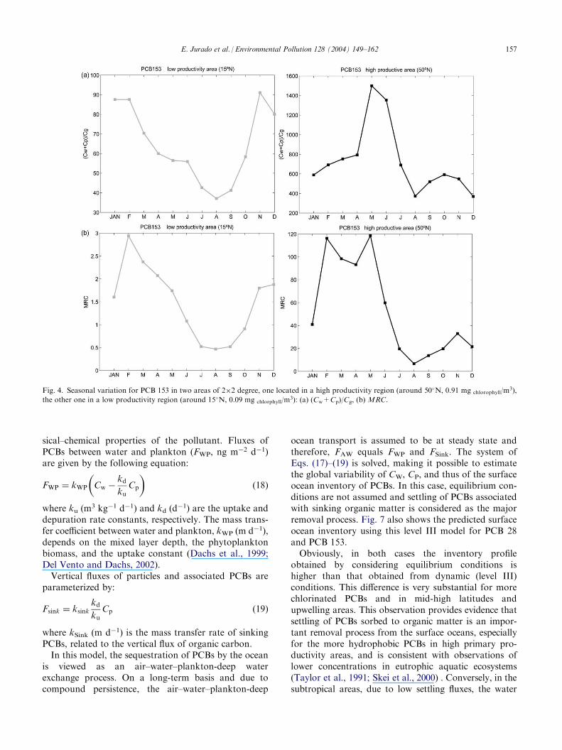
The predicted seasonal trends of (Cw+Cp)/Cg areshown in Fig. 4a for PCB 153 in two contrasting areasof the north eastern Atlantic Ocean, one of high pro-ductivity (at 50�N), the other of low productivity (at15�N). Average chlorophyll a concentrations and MLDin the two differentiate climatic regions are: 0.84 mgm�3 and 86.7 m (50�N); 0.47 mg m�3 and 22.1 m(15�N), respectively.

The seasonal trends at the mid-high latitude area followa similar pattern to that of the chlorophyll a concen-tration, with a marked peak in spring (May–June) duringthe phytoplankton bloom. Lower values are predicted forthe late summer, due to a decrease of phytoplankton bio-mass and higher temperatures. The area located in a sub-tropical region (15�N) is driven mostly by the effect oftemperature, which has a dominant influence on H.Indeed, the profile is little altered during the bloom andshows a negative correlation with temperature. Theminimum occurs in July–August and the maximum inDecember–January. In this area, phytoplankton bio-mass is very low and thus its seasonal variability is alsoof limited importance (see Figs. 2 and 3). Conversely, inthe high productivity region, the (Cw+Cp)/Cg ratio is ata maximum during the spring phytoplankton bloomoverwhelming the opposite influence of temperature.

4.2. Spatial and seasonal variability of the MRC

4.2.1. Seasonal trends of the MRCFig. 4b exhibits the annual profile of the MRC in a

high productivity area around 50�N and in a low pro-ductivity area around 15�N. In the low productivityarea, in early spring the MLD decreases, leading tolowerMRC values during late spring and summer. How-ever, for the high productivity area this decrease occursafter the spring phytoplankton bloom. Therefore, for thehigh productivity zone,MRC has a similar pattern to theseasonal variation in the amount of biomass and MLD,while for the low productivity area,MRC is largely drivenby the effect of temperature andMLD.

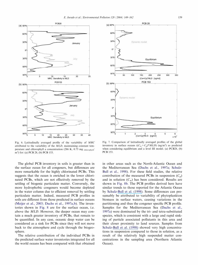
4.2.2. Spatial variability of the MRCFig. 5 shows the spatially variability and the latitud-

inally averaged profiles of the MRC for PCB 28 andPCB 153. To illustrate the importance of seasonalvariations of the MLD, the MRC calculated for Jan-uary and July are compared. As observed for(Cw+Cp)/Cg (Fig. 2), a bimodal MRC trend isobserved, with higher values at mid-high latitudes. TheMRC peaks around 60�, due to higher values of phyto-plankton biomass and MLD at this latitude. Fig. 5shows that the factors driving the MLD variabilityhave a strong influence on the MRC which has notconsidered in previous studies. The longitudinal varia-bility of MRC appears to be of relatively minorimportance than when just the (Cw+Cp)/Cg ratio isconsidered; however, it is still important. MRCpatchiness due to phytoplankton biomass seems to bepartially ‘‘damped’’ by the MLD when looking at theaverage latitudinal MRC values. MRC ratios aregreater for PCB 153 than for PCB 28 (by about afactor of 10), in particular in mid-high latitudes. Thisis in agreement with the higher BCF values of PCB153 than PCB 28.

E. Jurado et al. / Environmental Pollution 128 (2004) 149–162 155

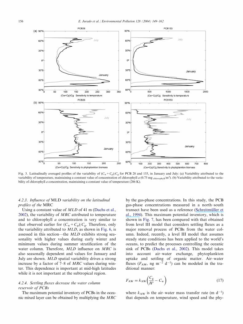
4.2.3. Influence of MLD variability on the latitudinalprofiles of the MRCUsing a constant value of MLD of 41 m (Dachs et al.,

2002), the variability of MRC attributed to temperatureand to chlorophyll a concentration is very similar tothat observed earlier for (Cw+Cp)/Cg. Therefore, onlythe variability attributed to MLD, as shown in Fig. 6, isassessed in this section—the MLD exhibits strong sea-sonality with higher values during early winter andminimum values during summer stratification of thewater column. Therefore, MLD influence on MRC isalso seasonally dependent and values for January andJuly are shown. MLD spatial variability drives a strongincrease by a factor of 7–8 of MRC values during win-ter. This dependence is important at mid-high latitudeswhile it is not important at the subtropical region.

4.2.4. Settling fluxes decrease the water columnreservoir of PCBsThe maximum potential inventory of PCBs in the ocea-

nic mixed layer can be obtained by multiplying the MRC

by the gas-phase concentrations. In this study, the PCBgas-phase concentrations measured in a north–southtransect have been used as a reference (Schreitmuller etal., 1994). This maximum potential inventory, which isshown in Fig. 7, has been compared with that obtainedfrom level III model that considers settling fluxes as amajor removal process of PCBs from the water col-umn. Indeed, recently, a level III model that assumessteady state conditions has been applied to the world’soceans, to predict the processes controlling the oceanicsink of PCBs (Dachs et al., 2002). This model takesinto account air–water exchange, phytoplanktonuptake and settling of organic matter. Air–waterfluxes (FAW, ng m�2 d�1) can be modeled in the tra-ditional manner:

FAW ¼ kAWCg

H 0� Cw

� �ð17Þ

where kAW is the air–water mass transfer rate (m d�1)that depends on temperature, wind speed and the phy-

Fig. 3. Latitudinally averaged profiles of the variability of (Cw+Cp)/Cg for PCB 28 and 153, in January and July: (a) Variability attributed to the

variability of temperature, maintaining a constant value of concentration of chlorophyll a (0.75 mg chlorophyll/m3). (b) Variability attributed to the varia-

bility of chlorophyll a concentration, maintaining a constant value of temperature (286 K).

156 E. Jurado et al. / Environmental Pollution 128 (2004) 149–162

sical–chemical properties of the pollutant. Fluxes ofPCBs between water and plankton (FWP, ng m�2 d�1)are given by the following equation:

FWP ¼ kWP Cw �kdku

Cp

� �ð18Þ

where ku (m3 kg�1 d�1) and kd (d

�1) are the uptake anddepuration rate constants, respectively. The mass trans-fer coefficient between water and plankton, kWP (m d�1),depends on the mixed layer depth, the phytoplanktonbiomass, and the uptake constant (Dachs et al., 1999;Del Vento and Dachs, 2002).Vertical fluxes of particles and associated PCBs are

parameterized by:

Fsink ¼ ksinkkdku

Cp ð19Þ

where kSink (m d�1) is the mass transfer rate of sinkingPCBs, related to the vertical flux of organic carbon.In this model, the sequestration of PCBs by the ocean

is viewed as an air–water–plankton-deep waterexchange process. On a long-term basis and due tocompound persistence, the air–water–plankton-deep

ocean transport is assumed to be at steady state andtherefore, FAW equals FWP and FSink. The system ofEqs. (17)–(19) is solved, making it possible to estimatethe global variability of CW, CP, and thus of the surfaceocean inventory of PCBs. In this case, equilibrium con-ditions are not assumed and settling of PCBs associatedwith sinking organic matter is considered as the majorremoval process. Fig. 7 also shows the predicted surfaceocean inventory using this level III model for PCB 28and PCB 153.Obviously, in both cases the inventory profile

obtained by considering equilibrium conditions ishigher than that obtained from dynamic (level III)conditions. This difference is very substantial for morechlorinated PCBs and in mid-high latitudes andupwelling areas. This observation provides evidence thatsettling of PCBs sorbed to organic matter is an impor-tant removal process from the surface oceans, especiallyfor the more hydrophobic PCBs in high primary pro-ductivity areas, and is consistent with observations oflower concentrations in eutrophic aquatic ecosystems(Taylor et al., 1991; Skei et al., 2000) . Conversely, in thesubtropical areas, due to low settling fluxes, the water

Fig. 4. Seasonal variation for PCB 153 in two areas of 2�2 degree, one located in a high productivity region (around 50�N, 0.91 mg chlorophyll/m3),

the other one in a low productivity region (around 15�N, 0.09 mg chlorphyll/m3): (a) (Cw+Cp)/Cg, (b) MRC.

E. Jurado et al. / Environmental Pollution 128 (2004) 149–162 157

column inventory is predicted to be close to equilibriumfor all PCB congeners.

5. Relative importance of the surface ocean as a

reservoir of PCBs

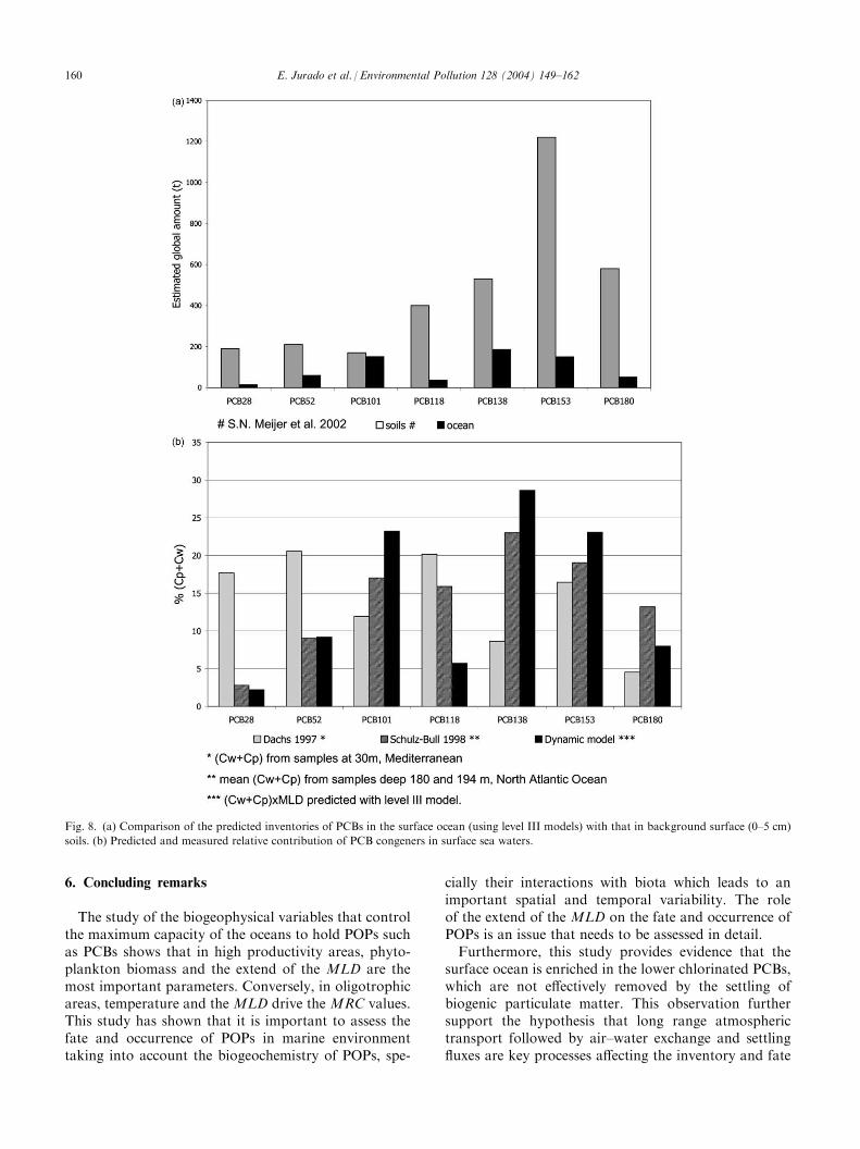
Surface water inventories have been integrated for allthe world oceans and for seven representative PCBcongeners (PCBs 28, 52, 101, 118, 138, 153, 180) aspredicted from the level III model. These inventorieshave been compared with those reported for soils at theglobal scale (Meijer et al., 2002) as shown in Fig. 8a.

The magnitude of these inventories is obviously depen-dent on the magnitude and distribution of CG usedwhen applying the level III model [Eqs. (17)–(19)] andthe uncertainty of these gas-phase concentrations affectthe predictions shown in Fig. 8a. The concentrationsand latitudinal distributions reported elsewhere(Schreitmuller et al., 1994) are consistent with othermeasurements of gas-phase concentrations made overthe ocean and in oceanic islands (Iwata et al., 1993;Lohmann et al., 2001; Van Drooge et al., 2002) andpresumably the uncertainty associated to these con-centrations and the predicted inventory in the surfaceocean is lower than a factor of two.

Fig. 5. Maps and latitudinally averaged profiles of MRC in January and July for: (A) PCB 28, (B) PCB 153.

158 E. Jurado et al. / Environmental Pollution 128 (2004) 149–162

The global PCB inventory in soils is greater than inthe surface ocean for all congeners, but differences aremore remarkable for the highly chlorinated PCBs. Thissuggests that the ocean is enriched in the lower chlori-nated PCBs, which are not effectively removed by thesettling of biogenic particulate matter. Conversely, themore hydrophobic congeners would become depletedin the water column due to efficient removal by settlingparticulate matter. Indeed, measured PCB profiles insoils are different from those predicted in surface oceans(Meijer et al., 2003; Dachs et al., 1997a,b). The inven-tories shown in Fig. 8 are for the surface ocean, i.e.above the MLD. However, the deeper ocean may con-tain a much greater inventory of PCBs, that remain tobe quantified. In any case, oceanic deep water can beconsidered as a sink for PCBs since they will not moveback to the atmosphere and cycle through the biogeo-sphere.The relative contribution of the individual PCBs in

the predicted surface water inventories integrated for allthe world oceans has been compared with that obtained

in other areas such as the North-Atlantic Ocean andthe Mediterranean Sea (Dachs et al., 1997a; Schulz-Bull et al., 1998). For these field studies, the relativecontribution of the measured PCBs in suspension (Cp)and in solution (Cw) has been considered. Results areshown in Fig. 8b. The PCB profiles derived here havesimilar trends to those reported for the Atlantic Oceanby Schulz-Bull et al. (1998). Some differences can pre-sumably be attributed to variability of phytoplanktonbiomass in surface waters, causing variations in thepartitioning and thus the congener specific PCB profile.Samples for the Mediterranean Sea (Dachs et al.,1997a) were dominated by the tri- and tetra-substitutedspecies, which is consistent with a large and rapid sink-ing of particle associated pollutants in this area andtheir closer proximity to land sources. Samples fromSchulz-Bull et al. (1998) showed very high concentra-tions in suspension compared to those in solution, as aresult of the relatively high suspended matter con-centrations in the sampling area (Northern AtlanticOcean).

Fig. 6. Latitudinally averaged profile of the variability of MRC

attributed to the variability of the MLD, maintaining constant tem-

perature and chlorophyll a concentration (286 K, 0.75 mg chlorophyll/

m3) for: (a) PCB 28, (b) PCB 153.

Fig. 7. Comparison of latitudinally averaged profiles of the global

inventory in surface oceans ((Cw+Cp)*MLD) (ng/m2) as predicted

when considering equilibrium and a level III model. (a) PCB28, (b)

PCB 153.

E. Jurado et al. / Environmental Pollution 128 (2004) 149–162 159

6. Concluding remarks

The study of the biogeophysical variables that controlthe maximum capacity of the oceans to hold POPs suchas PCBs shows that in high productivity areas, phyto-plankton biomass and the extend of the MLD are themost important parameters. Conversely, in oligotrophicareas, temperature and the MLD drive the MRC values.This study has shown that it is important to assess thefate and occurrence of POPs in marine environmenttaking into account the biogeochemistry of POPs, spe-

cially their interactions with biota which leads to animportant spatial and temporal variability. The roleof the extend of the MLD on the fate and occurrence ofPOPs is an issue that needs to be assessed in detail.Furthermore, this study provides evidence that the

surface ocean is enriched in the lower chlorinated PCBs,which are not effectively removed by the settling ofbiogenic particulate matter. This observation furthersupport the hypothesis that long range atmospherictransport followed by air–water exchange and settlingfluxes are key processes affecting the inventory and fate

Fig. 8. (a) Comparison of the predicted inventories of PCBs in the surface ocean (using level III models) with that in background surface (0–5 cm)

soils. (b) Predicted and measured relative contribution of PCB congeners in surface sea waters.

160 E. Jurado et al. / Environmental Pollution 128 (2004) 149–162

of PCBs in the surface oceans. Furthermore, at the glo-bal scale, it can be hypothesized that continent-oceaninteractions may play an important role of the globaldynamics of PCBs and be responsible for the differencesobserved between soil and seawater profiles (Fig. 8).However, further research is needed to better assesstransport routes and to understand the interactionsbetween continents and oceans in terms of POP occur-rence and transport.

Acknowledgements

Dr. Rafel Simo is kindly acknowledged for fruitfuldiscussions and as coordinator of the AMIGOS project.The authors would like to thank the SeaWiFS Projectteam and particularly W. Gregg from the GoddardSpace Flight Center (NASA) for providing the satellitechlorophyll climatology and reviewers, who providedvery valuable comments. This work was supported bythe Spanish Ministry of Scince and Technology throughproject AMIGOS (REN2001-3462/CLI).

References

Apel, J.R., 1990. Principles of Ocean Physics. Academic Press.

Axelman, J., Gustafsson, O., 2002. Global sinks of PCBs: a critical

assessment of the vapour-phase hydroxy radical sink emphasizing

field diagnostic and model assumptions. Global Biogeochemical

Cycles 16 (4), 58/1–58/13.

Bamford, H.A., Poster, D.L., Baker, J.E., 2000. Henry’s Law con-

stants of polychlorinated biphenyl congeners and their variation

with temperature. J. Chem. Eng. Data 45, 1069–1074.

Bamford, H.A., Poster, D.L., Huie, R.E., Baker, J.E., 2002. Using

extrathermodynamic relationships to model the temperature depen-

dence of Henry’s Law constants of 209 PCB congeners. Environ-

mental Science Technology 36 (2), 4395–4402.

Dachs, J., Bayona, J.M., Albaiges, J., 1997. Spatial distribution,

vertical profiles and budget of organochlorine compounds in

Western Mediterranean seawater. Marine Chemistry 57 (3–4),

313–324.

Dachs, J., Bayona, J.M., Raoux, C., Albaiges, J., 1997. Spatial, ver-

tical distribution and budget of Polycyclic Aromatic Hydrocarbons

in Western Mediterranean seawater. Environmental Science Tech-

nology 31 (3), 682–688.

Dachs, J., Eisenreich, S.J., Baker, J.E., Ko, F.-C., Jeremiason, J.D.,

1999. Coupling of phytoplankton uptake and air–water exchange of

persistent organic pollutants. Environmental Science Technology 33

(20), 3653–3660.

Dachs, J., Eisenreich, S.J., Hoff, R.M., 2000. Influence of eutrophica-

tion on air–water exchange, vertical fluxes, and phytoplankton

concentrations of persistent organic pollutants. Environmental

Science Technology 34 (6), 1095–1102.

Dachs, J., Lohmann, R., Ockenden, W.A., Mejanelle, L., Eisenreich,

S.J., Jones, K.C., 2002. Oceanic biogeochemical controls on global

dynamics of persistent organic pollutants. Environmental Science

Technology 36 (20), 4229–4237.

Del Vento, S., Dachs, J., 2002. Prediction of uptake dynamics of per-

sistent organic pollutants by bacteria and phytoplankton. Environ-

mental Toxicology and Chemistry 21 (10), 2099–3017.

Eisenberg, J.N.S., Bennett, D.H., Mckone, T.E., 1998. Chemical

dynamics of Persistent Organic Polluytants: a sensitivity analysis

relating soil concentration levels to atmospheric emissions. Envir-

onmental Science Technology 32 (1), 115–123.

Gasol, J., Del Giorgio, P., Duarte, C., 1997. Biomass distribution in

marine planktonic communities. Limnol Oceanogr 42 (6), 1353–

1363.

Hawker, D.W., Connell, D.W., 1988. Octanol-Water partition coeffi-

cients of polychlorinated biphenyl congeners. Environmental

Science Technology 22 (4), 382–387.

Hedges, J.I., Baldock, J.A., Gelinas, Y., Lee, C., Peterson, M.L.,

Wakeham, S.G., 2002. The biochemical and elemental compositions

of marine plankton: a NMR perspective. Marine Chemistry 78 (1),

47–63.

Iwata, I., Tanabe, S., Sakai, N., Tatsukawa, R., 1993. Distribution of

persistent organochlorines in the oceanic air and surface seawater

and the role of ocean on their global transport and fate. Environ-

mental Science Technology 27, 1080–1098.

Jorgensen, L.A., Jorgensen, S.E., Nielsen, S.N., 2000. ECOTOX:

Ecological Modelling and Ecotoxicology. Elsevier, Amsterdam.

Lohmann, R., Ockenden, W.A., Shears, J., Jones, K.C., 2001. Atmo-

pheric distribution of polychlorinated dibenzo-p-dioxins, dibenzo-

furans (PCDD/Fs), and non-ortho biphenyls (PCBs) along a north–

south transect. Environmental Science Technology 35 (20), 4046–

4053.

Mackay, D., 2001. Multimedia Environmental Models. The Fugacity

Approach. Lewis Publishers.

Mackay, D., Paterson, S., 1981. Calculating fugacity. Environmental

Science Technology 15 (9), 1006–1014.

Meijer, S. N., Ockenden, W. A., Sweetman, A. J., Breivik, K., Gri-

malt, J. O., Jones, K. C.,2002. Global distribution and budget of

PCBs and HCB in background surface soils: implications for sour-

ces and environmental processes. Environmental Science Technol-

ogy (submitted).

Murray, J.W., 1992. The Oceans. Global Biogeochemical Cycles. A. P.

Limited.

Scheringer, M., Wegmann, F., Fenner, K., Hungerbuhler, K., 2000.

Investigation of the cold condensation of persistent organic pollu-

tants with a global multimedia fate model. Environmental Science

Technology 34, 1842–1850.

Schreitmuller, J., Vigneron, M., Bacher, R., Ballschmiter, K., 1994.

Pattern analysis of polychlorinated biphenyls (PCB) in marine air of

Atlantic ocean. Int. J. Environ. Anal. Chem. 57, 33–52.

Schulz-Bull, D.E., Petrick, G., Bruhn, R., Duinker, J.C., 1998. Chloro-

biphenyls (PCB) and PAHs in water masses of the northern North

Atlantic. Marine Chemistry 61 (1–2), 101–114.

Schwarzenbach, R.P., Gschwend, P.M., Imboden, D.M., 1993. Envir-

onmental Organic Chemistry. Wiley-Interscience.

Skei, J., Larsson, P., Rosenberg, R., Jonsson, P., Olsson, M., Broman,

D., 2000. Eutrophication and contaminants in aquatic ecosystems.

Ambio 29 (4–5), 184–194.

Skoglund, R.S., Stange, K., Swackhamer, D., 1996. A kinetics model

for predicting the accumulation of PCBs in phytoplankton. Envir-

onmental Science Technology 30 (7), 2113–2120.

Swackhamer, D.L., Skoglund, R.S., 1991. The role of phytoplankton

in the partitioning of hydrophobic organic contaminants in water.

Lewis publishers II.

Taylor, W.D., Carey, J.H., Lean, D.R.S., McQueen, D.J., 1991.

Organochlorine concentrations in the plankton of lakes in southern

Ontario and their relationship to plankton biomass. Can. J. Fish.

Aquat. Sci. 48, 1960–1966.

Tolosa, I., Readman, J.W., Fowler, S.W., Villeneuve, J.P., Dachs, J.,

Bayona, J.M., Albaiges, J., 1997. PCBs in the western Mediterra-

nean. Temporal trends and mass balance assessment. Deep-Sea

Research II 44 (3–4), 907–928.

Valiela, I., 1995. Marine Ecological Processes. Springer, New York.

Van Drooge, B.L., Grimalt, J.O., Torres Garcia, C.J., Cuevas, E.,

2002. Semivolatile organochlorine compounds in the free tropo-

E. Jurado et al. / Environmental Pollution 128 (2004) 149–162 161

sphere of the Northeastern Atlantic. Environmental Science Tech-

nology 36 (6), 1155–1161.

Wania, F., Daly, G.L., 2002. Estimating the contribution of degrada-

tion in air and deposition to the deep sea to the global loss of PCBs.

Atmospheric Environment 36 (36–37), 5581–5593.

Wania, F., Mackay, D., 1996. Tracking the distribution of persistent

organic pollutants. Environmental Science Technology 30 (9), 390.

A-396A.

Wania, F., McLachlan, M.S., 2001. Estimating the influence of forests

on the overall fate of semivolatile organic compounds using a

multimedia fate model. Environmental Science Technology 35 (3),

582–590.

162 E. Jurado et al. / Environmental Pollution 128 (2004) 149–162