Latent class analysis variable selection - Statistics - University of

Ann Inst Stat Math (2010) 62:11–35DOI 10.1007/s10463-009-0258-9

Latent class analysis variable selection

Nema Dean · Adrian E. Raftery

Received: 19 July 2008 / Revised: 22 April 2009 / Published online: 24 July 2009© The Institute of Statistical Mathematics, Tokyo 2009

Abstract We propose a method for selecting variables in latent class analysis, whichis the most common model-based clustering method for discrete data. The methodassesses a variable’s usefulness for clustering by comparing two models, given theclustering variables already selected. In one model the variable contributes informa-tion about cluster allocation beyond that contained in the already selected variables,and in the other model it does not. A headlong search algorithm is used to explore themodel space and select clustering variables. In simulated datasets we found that themethod selected the correct clustering variables, and also led to improvements in clas-sification performance and in accuracy of the choice of the number of classes. In tworeal datasets, our method discovered the same group structure with fewer variables. Ina dataset from the International HapMap Project consisting of 639 single nucleotidepolymorphisms (SNPs) from 210 members of different groups, our method discoveredthe same group structure with a much smaller number of SNPs.

Keywords Bayes factor · BIC · Categorical data · Feature selection · Model-basedclustering · Single nucleotide polymorphism (SNP)

1 Introduction

Latent class analysis is used to discover groupings in multivariate categorical data.It models the data as a finite mixture of distributions, each one corresponding to aclass (or cluster or group). Because of the underlying statistical model it is possible

N. DeanDepartment of Statistics, University of Glasgow, Glasgow G12 8QQ, Scotland, UK

A. E. Raftery (B)Department of Statistics, University of Washington, Box 354320, Seattle, WA 98195-4320, USAe-mail: [email protected]

123

12 N. Dean, A. E. Raftery

to determine the number of classes using model selection methods. But the model-ing framework does not currently address the selection of the variables to be used;typically all variables are used in the model.

Selecting variables for latent class analysis can be desirable for several reasons. Itcan help interpretability of the model, and it can also make it possible to fit a modelwith a larger number of classes than would be possible with all the variables, for iden-tifiability reasons. In general, removing unnecessary variables and parameters can alsoimprove classification performance and the precision of parameter estimates.

In this paper, we propose a method for selecting the variables to be used for clus-tering in latent class analysis. This is based on the method of Raftery and Dean (2006)for variable selection in model-based clustering of continuous variables. The methodassesses a variable’s usefulness for clustering by comparing two models, given theclustering variables already selected. In one model the variable contributes informa-tion about cluster allocation beyond that contained in the already selected variables,and in the other model it does not. We then present a new search algorithm, based onBadsberg (1992), for exploring the space of possible models. The resulting methodselects both the variables and the number of classes in the model.

In Sect. 2 we review some aspects of latent class analysis and in Sect. 3 we describeour variable selection methodology. In Sect. 4 we give results from simulated data andin Sect. 5 we give results for two real datasets, including one with a large number ofvariables and a much smaller number of data points. Issues arising with the methodare discussed in Sect. 6.

2 Latent class analysis

2.1 Latent class analysis model

Latent class analysis was proposed by Lazarsfeld (1950a,b) and Lazarsfeld and Henry(1968) and can be viewed as a special case of model-based clustering, for multivari-ate discrete data. Model-based clustering assumes that each observation comes fromone of a number of classes, groups or subpopulations, and models each with its ownprobability distribution (Wolfe 1963; McLachlan and Peel 2000; Fraley and Raftery2002). The overall population thus follows a finite mixture model, namely

x ∼G∑

g=1

πg fg(x),

where fg is the density for group g, G is the number of groups, πg are the mixtureproportions, 0 < πg < 1, ∀g and

∑Gg=1 πg = 1. Often, in practice, the fg are from

the same parametric family (as is the case in latent class analysis) and we can writethe overall density as:

x ∼G∑

g=1

πg f (x | θg),

where θg is the set of parameters for the gth group.

123

Latent class analysis variable selection 13

In latent class analysis, the variables are usually assumed to be independent givenknowledge of the group an observation came from, an assumption called local inde-pendence. Each variable within each group is then modeled with a multinomial density.The general density of a single variable x (with categories 1, . . . , d) given that it is ingroup g is then

x | g ∼d∏

j=1

p1{x= j}jg ,

where 1{x = j} is the indicator function equal to 1 if the observation of the variabletakes value j and 0 otherwise, p jg is the probability of the variable taking value j ingroup g, and d is the number of possible values or categories the variable can take.

Since we are assuming conditional independence, if we have k variables, their jointgroup density can be written as a product of their individual group densities. If wehave x = (x1, . . . , xk), we can write the joint group density as:

x | g ∼k∏

i=1

di∏

j=1

p1{xi = j}i jg ,

where 1{xi = j} is the indicator function equal to 1 if the observation of the i thvariable takes value j and 0 otherwise, pi jg is the probability of variable i takingvalue j in group g and di is the number of possible values or categories the i th vari-able can take. The overall density is then a weighted sum of these individual productdensities, namely

x ∼G∑

g=1

⎛

⎝πg

k∏

i=1

di∏

j=1

p1{xi = j}i jg

⎞

⎠ ,

where 0 < πg < 1, ∀g and∑G

g=1 πg = 1.The model parameters {pi jg, πg : i = 1, . . . , k, j = 1, . . . , di , g = 1, . . . , G}

can be estimated from the data (for a fixed value of G) by maximum likelihood usingthe EM algorithm or the Newton–Raphson algorithm or a hybrid of the two. Thesealgorithms require starting values which are usually randomly generated. Because thealgorithms are not guaranteed to find a global maximum and are usually fairly depen-dent on good starting values, it is routine to generate a number of random startingvalues and use the best solution given by one of these. In Appendix B, we present anadjusted method useful for the cases where an inordinately large number of startingvalues is needed to get good estimates of the latent class models and G > 2.

Goodman (1974) discussed the issue of checking whether a latent class modelwith a certain number of classes was identifiable for a given number of variables. Anecessary condition for identifiability when there are G classes and k variables withnumbers of categories d = (d1, . . . , dk) is

123


k∏

i=1

di >

(k∑

i=1

di − k + 1

)× G.

This basically amounts to checking that there are enough pieces of information (or cellcounts or pattern combinations) to estimate the number of parameters in the model.However, in practice, not all possible pattern combinations are observed (some ormany cell counts may be zero) and so the actual information available may be less.When selecting the number of latent classes in the data, we consider only numbers ofclasses for which this necessary condition is satisfied.

For reviews of latent class analysis, see Clogg (1981), McCutcheon (1987), Clogg(1995) and Hagenaars and McCutcheon (2002).

2.2 Selecting the number of latent classes

Each different value of G, the number of latent classes, defines a different model forthe data. A method is needed to select the number of latent classes present in the data.Since a statistical model for the data is used, model selection techniques can be appliedto this question.

In order to choose the best number of classes for the data we need to choose thebest model (and the related number of classes). Bayes factors (Kass and Raftery 1995)are used to compare these models.

The Bayes factor for comparing model Mi versus model M j is equal to the ratio ofthe posterior odds for Mi versus M j to the prior odds for Mi versus M j . This reducesto the posterior odds when the prior model probabilities are equal. The general formfor the Bayes factor is:

Bi j = p(Y | Mi )

p(Y | M j ),

where p(Y |Mi ) is known as the integrated likelihood of model Mi (given data Y ).It is called the integrated likelihood because it is obtained by integrating over all themodel parameters, namely the mixture proportions and the group variable probabili-ties. Unfortunately the integrated likelihood is difficult to compute (it has no closedform) and some form of approximation is needed for calculating Bayes factors inpractice.

In our approximation we use the Bayesian information criterion (BIC), which isvery simple to compute. The BIC is defined by

BIC = 2 × log(maximized likelihood) − (no. of parameters) × log(n), (1)

where n is the number of observations.Twice the logarithm of the Bayes factor is approximately equal to the difference

between the BIC values for the two models being compared. We choose the numberof latent classes by recognizing that each different number of classes defines a model,which can then be compared to others using BIC. Keribin (1998) showed BIC to be

123


consistent for the choice of the number of components in a mixture model under cer-tain conditions, when all variables are relevant to the grouping. A rule of thumb fordifferences in BIC values is that a difference of less than 2 is viewed as barely worthmentioning, while a difference greater than 10 is seen as constituting strong evidence(Kass and Raftery 1995).

3 Variable selection in latent class analysis

3.1 Variable selection method

At any stage in the procedure we can partition the collection of variables into threesets: Y (clust), Y (?) and Y (other), where:

• Y (clust) is the set of variables already selected as useful for clustering,• Y (?) is the variable(s) being considered for inclusion into/exclusion from Y (clust),• Y (other) is the set of all other variables.

Given this partition and the (unknown) clustering memberships z we can recast thequestion of the usefulness of Y (?) for clustering as a model selection question. Thequestion becomes one of choosing between two different models, M1 which assumesthat Y (?) is not useful for clustering, and M2 which assumes that it is.

The two models are specified as follows:

M1 : p(Y |z) = p(Y (clust), Y (?), Y (other)|z)= p(Y (other)|Y (?), Y (clust))p(Y (?))p(Y (clust)|z),

M2 : p(Y |z) = p(Y (clust), Y (?), Y (other)|z) (2)

= p(Y (other)|Y (?), Y (clust))p(Y (?), Y (clust)|z)= p(Y (other)|Y (?), Y (clust))p(Y (?)|z)p(Y (clust)|z),

where z is the (unobserved) set of cluster memberships. Model M1 specifies that, givenY (clust), Y (?) is independent of the cluster memberships (defined by the unobservedvariables z), that is, Y (?) gives no further information about the clustering. ModelM2 implies that Y (?) does provide information about clustering membership, beyondthat given just by Y (clust). The difference between the assumptions underlying the twomodels is illustrated in Fig. 1, where arrows indicate dependency.

We assume that the remaining variables Y (other) are conditionally independent ofthe clustering given Y (clust) and Y (?) and belong to the same parametric family in bothmodels.

This basically follows the approach used in Raftery and Dean (2006) for model-based clustering with continuous data and Gaussian clusters. One difference is thatconditional independence of the variables was not assumed there, so that instead ofp(Y (?)) in model M1 we had p(Y (?)|Y (clust)). This assumed conditional independenceinstead of full independence, i.e. the assumption in model M1 previously was thatgiven the information in Y (clust), Y (?) had no additional clustering information. Note,that unlike Fig. 1 in Raftery and Dean (2006) there are no lines between the subsets ofvariables Y (clust) and Y (?) in Fig. 1, due to the conditional independence assumption.

123


Y otherY other

Y?Y clustY?Y clust

M1 M2

Z Z

Fig. 1 Graphical Representation of Models M1 and M2 for Latent Class Variable Selection. In model M1,the candidate set of additional clustering variables, Y (?), is independent of the cluster memberships, z, giventhe variables Y (clust) already in the model. In model M2, this is not the case. In both models, the set ofother variables considered, Y (other), is conditionally independent of cluster membership given Y (clust) andY (?), but may be associated with Y (clust) and Y (?)

Models M1 and M2 are compared via an approximation to the Bayes factor whichallows the high-dimensional p(Y (other)|Y (clust), Y (?)) to cancel from the ratio. TheBayes factor, B12, for M1 against M2 based on the data Y is given by

B12 = p(Y |M1)/p(Y |M2),

where p(Y |Mk) is the integrated likelihood of model Mk (k = 1, 2), namely

p(Y |Mk) =∫

p(Y |θk, Mk)p(θk |Mk) dθk . (3)

In (3), θk is the vector-valued parameter of model Mk , and p(θk |Mk) is its priordistribution (Kass and Raftery 1995).

Let us now consider the integrated likelihood of model M1,p(Y |M1) = p(Y (clust), Y (?), Y (other)|M1). From (2), the model M1 is specified bythree probability distributions: the latent class model that specifies p(Y (clust)|θ1, M1),and the distributions p(Y (?)|θ1, M1) and p(Y (other)|Y (?), Y (clust), θ1, M1). We denotethe parameter vectors that specify these three probability distributions by θ11, θ12, andθ13, and we assume that their prior distributions are independent. Then the integratedlikelihood itself factors as follows:

123


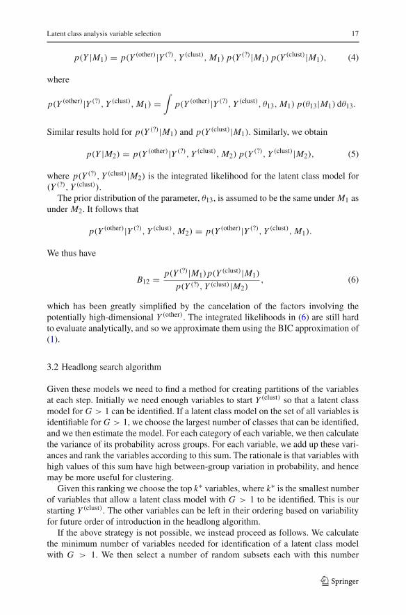
p(Y |M1) = p(Y (other)|Y (?), Y (clust), M1) p(Y (?)|M1) p(Y (clust)|M1), (4)

where

p(Y (other)|Y (?), Y (clust), M1) =∫

p(Y (other)|Y (?), Y (clust), θ13, M1) p(θ13|M1) dθ13.

Similar results hold for p(Y (?)|M1) and p(Y (clust)|M1). Similarly, we obtain

p(Y |M2) = p(Y (other)|Y (?), Y (clust), M2) p(Y (?), Y (clust)|M2), (5)

where p(Y (?), Y (clust)|M2) is the integrated likelihood for the latent class model for(Y (?), Y (clust)).

The prior distribution of the parameter, θ13, is assumed to be the same under M1 asunder M2. It follows that

p(Y (other)|Y (?), Y (clust), M2) = p(Y (other)|Y (?), Y (clust), M1).

We thus have

B12 = p(Y (?)|M1)p(Y (clust)|M1)

p(Y (?), Y (clust)|M2), (6)

which has been greatly simplified by the cancelation of the factors involving thepotentially high-dimensional Y (other). The integrated likelihoods in (6) are still hardto evaluate analytically, and so we approximate them using the BIC approximation of(1).

3.2 Headlong search algorithm

Given these models we need to find a method for creating partitions of the variablesat each step. Initially we need enough variables to start Y (clust) so that a latent classmodel for G > 1 can be identified. If a latent class model on the set of all variables isidentifiable for G > 1, we choose the largest number of classes that can be identified,and we then estimate the model. For each category of each variable, we then calculatethe variance of its probability across groups. For each variable, we add up these vari-ances and rank the variables according to this sum. The rationale is that variables withhigh values of this sum have high between-group variation in probability, and hencemay be more useful for clustering.

Given this ranking we choose the top k∗ variables, where k∗ is the smallest numberof variables that allow a latent class model with G > 1 to be identified. This is ourstarting Y (clust). The other variables can be left in their ordering based on variabilityfor future order of introduction in the headlong algorithm.

If the above strategy is not possible, we instead proceed as follows. We calculatethe minimum number of variables needed for identification of a latent class modelwith G > 1. We then select a number of random subsets each with this number

123


of variables. Then for the initial Y (clust) we choose the variable set that gives thegreatest overall average variance of categories’ probabilities across the groups (giventhe best latent class model identified). If the minimum number of variables is smallenough, we enumerate all possible subsets to choose the best initial Y (clust), instead ofsampling.

Once we have an initial set of clustering variables, Y (clust), we can proceed withthe inclusion and exclusion steps of the headlong algorithm.

First we must define the constants upper and lower . The constant upper is thequantity above which the difference in BIC for models M2 and M1 will result in avariable being included in Y (clust) and below which the difference in BIC for modelsM2 and M1 will result in a variable being excluded from Y (clust). The constant loweris the quantity below which the difference in BIC for models M2 and M1 will result ina variable being removed from consideration for the rest of the procedure. A naturalvalue for upper is 0, by which we mean that any positive difference in BIC for modelsM2 and M1 is taken as evidence of a variable’s usefulness for clustering and any neg-ative difference is taken as evidence of a variable’s lack of usefulness. A difference oflower is taken to indicate that a variable is unlikely to ever be useful as a clusteringvariable and is no longer even checked. In general a large negative number such as−100 (which by our rule of thumb would constitute strong evidence against) makes asensible value for lower .

• Inclusion Step: Propose each variable in Y (other) singly in turn for Y (?). Calculatethe difference in BIC for models M2 and M1 given the current Y (clust).If the variable’s BIC difference is:– between upper and lower , do not include in Y (clust) and return variable to the

end of the list of variables in Y (other);– below lower , do not include in Y (clust) and remove variable from Y (other);– above upper , include variable in Y (clust) and stop inclusion step.If we reach the end of the list of variables in Y (other), the inclusion step is stopped.

• Exclusion Step: Propose each variable in Y (clust) singly in turn for Y (?) (with theremaining variables in Y (clust) not including current Y (?) now defined as Y (clust)

in M1 and M2). Calculate the difference in BIC for models M2 and M1. If thevariable’s BIC difference is:– between upper and lower , exclude the variable from (the original) Y (clust) and

return variable to the end of the list of variables in Y (other) and stop exclusionstep;

– below lower , exclude the variable from (the original) Y (clust) and from Y (other)

and stop exclusion step;– above upper , do not exclude the variable from (the original) Y (clust).If we reach the end of the list of variables in Y (clust) the exclusion step isstopped.

If Y (clust) remains the same after consecutive inclusion and exclusion steps theheadlong algorithm stops because it has converged.

123


Table 1 Model parameters usedto generate binary data example

Variable Probability of success

Class 1 (mixture Class 2 (mixtureproportion = 0.6) proportion = 0.4)

1 0.6 0.2

2 0.8 0.5

3 0.7 0.4

4 0.6 0.9

5 0.5 0.5

6 0.4 0.4

7 0.3 0.3

8 0.2 0.2

9 0.9 0.9

10 0.6 0.6

11 0.7 0.7

12 0.8 0.8

13 0.1 0.1

4 Simulated data results

4.1 Binary simulated data example

Five hundred points were simulated from a two-class model satisfying the local inde-pendence assumption. There were four variables separating the classes (variables 1–4)and nine noise variables, i.e. variables that have the same probabilities in each class(variables 5–13). The actual model parameters are shown in Table 1.

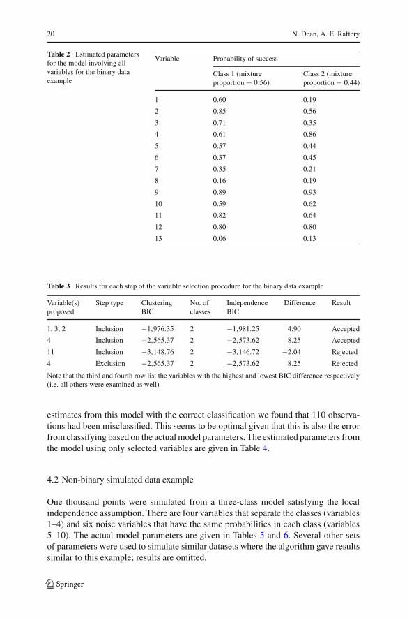
When we estimated the latent class model based on all thirteen variables, BICselected a two-class model. Since we simulated the data and hence know the actualmembership of each point, we can compare the correct classification with that pro-duced by the model estimated using all the variables. The number of observationsincorrectly classified by this model was 123. The number of observations that wouldbe incorrectly classified by using the model with the actual parameter values is 110.The estimated parameters from the model with all variables are given in Table 2.

The variables ordered according the variability of their estimated probabilities (indecreasing order) are: 1, 3, 2, 4, 11, 7, 5, 6, 13, 9, 8, 10, 12. As expected, the firstfour variables are the clustering variables. We note that the difference between thetrue probabilities across groups is 0.4 for variable 1 and 0.3 for variables 2–4. Sincevariable 1 therefore gives better separation of the classes, we would expect it to befirst in the list. The number of variables needed in order to estimate a latent classmodel with at least 2 classes is 3. So the starting clustering variables are {1, 3, 2}.The individual step results for the variable selection procedure starting with this setare given in Table 3.

When clustering on the four selected variables only, BIC again chose 2 classes asthe best fitting model. Comparing the classification of the observations based on the

123


Table 2 Estimated parametersfor the model involving allvariables for the binary dataexample

Variable Probability of success


1 0.60 0.19

2 0.85 0.56

3 0.71 0.35

4 0.61 0.86

5 0.57 0.44

6 0.37 0.45

7 0.35 0.21

8 0.16 0.19

9 0.89 0.93

10 0.59 0.62

11 0.82 0.64

12 0.80 0.80

13 0.06 0.13

Table 3 Results for each step of the variable selection procedure for the binary data example

Variable(s) Step type Clustering No. of Independence Difference Resultproposed BIC classes BIC

1, 3, 2 Inclusion −1,976.35 2 −1,981.25 4.90 Accepted

4 Inclusion −2,565.37 2 −2,573.62 8.25 Accepted

11 Inclusion −3,148.76 2 −3,146.72 −2.04 Rejected

4 Exclusion −2,565.37 2 −2,573.62 8.25 Rejected

Note that the third and fourth row list the variables with the highest and lowest BIC difference respectively(i.e. all others were examined as well)

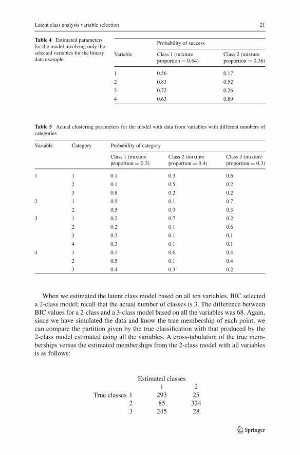
estimates from this model with the correct classification we found that 110 observa-tions had been misclassified. This seems to be optimal given that this is also the errorfrom classifying based on the actual model parameters. The estimated parameters fromthe model using only selected variables are given in Table 4.

4.2 Non-binary simulated data example

One thousand points were simulated from a three-class model satisfying the localindependence assumption. There are four variables that separate the classes (variables1–4) and six noise variables that have the same probabilities in each class (variables5–10). The actual model parameters are given in Tables 5 and 6. Several other setsof parameters were used to simulate similar datasets where the algorithm gave resultssimilar to this example; results are omitted.

123


Table 4 Estimated parametersfor the model involving only theselected variables for the binarydata example

Probability of success

Variable Class 1 (mixture Class 2 (mixtureproportion = 0.64) proportion = 0.36)

1 0.56 0.17

2 0.83 0.52

3 0.72 0.26

4 0.63 0.89

Table 5 Actual clustering parameters for the model with data from variables with different numbers ofcategories

Variable Category Probability of category

Class 1 (mixture Class 2 (mixture Class 3 (mixtureproportion = 0.3) proportion = 0.4) proportion = 0.3)

1 1 0.1 0.3 0.6

2 0.1 0.5 0.2

3 0.8 0.2 0.2

2 1 0.5 0.1 0.7

2 0.5 0.9 0.3

3 1 0.2 0.7 0.2

2 0.2 0.1 0.6

3 0.3 0.1 0.1

4 0.3 0.1 0.1

4 1 0.1 0.6 0.4

2 0.5 0.1 0.4

3 0.4 0.3 0.2

When we estimated the latent class model based on all ten variables, BIC selecteda 2-class model; recall that the actual number of classes is 3. The difference betweenBIC values for a 2-class and a 3-class model based on all the variables was 68. Again,since we have simulated the data and know the true membership of each point, wecan compare the partition given by the true classification with that produced by the2-class model estimated using all the variables. A cross-tabulation of the true mem-berships versus the estimated memberships from the 2-class model with all variablesis as follows:

True classes

Estimated classes1 2

1 293 252 85 3243 245 28

123


Table 6 Actual non-clustering parameters for the model with data from variables with different numbersof categories



5 1 0.4 0.4 0.4

2 0.5 0.5 0.5

3 0.1 0.1 0.1

6 1 0.2 0.2 0.2

2 0.4 0.4 0.4

3 0.1 0.1 0.1

4 0.3 0.3 0.3

7 1 0.2 0.2 0.2

2 0.3 0.3 0.3

3 0.3 0.3 0.3

4 0.1 0.1 0.1

5 0.1 0.1 0.1

8 1 0.2 0.2 0.2

2 0.8 0.8 0.8

9 1 0.7 0.7 0.7

2 0.1 0.1 0.1

3 0.2 0.2 0.2

10 1 0.1 0.1 0.1

2 0.2 0.2 0.2

3 0.1 0.1 0.1

4 0.6 0.6 0.6

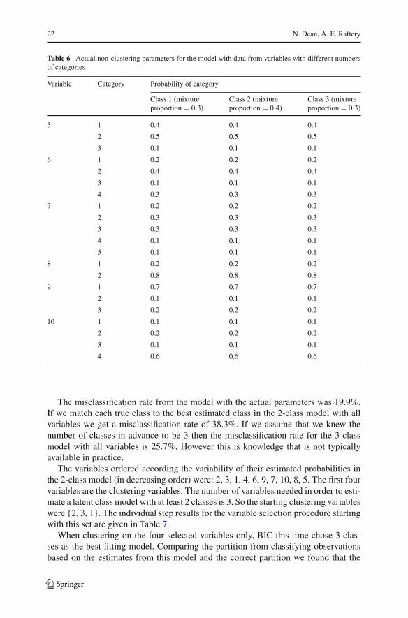
The misclassification rate from the model with the actual parameters was 19.9%.If we match each true class to the best estimated class in the 2-class model with allvariables we get a misclassification rate of 38.3%. If we assume that we knew thenumber of classes in advance to be 3 then the misclassification rate for the 3-classmodel with all variables is 25.7%. However this is knowledge that is not typicallyavailable in practice.

The variables ordered according the variability of their estimated probabilities inthe 2-class model (in decreasing order) were: 2, 3, 1, 4, 6, 9, 7, 10, 8, 5. The first fourvariables are the clustering variables. The number of variables needed in order to esti-mate a latent class model with at least 2 classes is 3. So the starting clustering variableswere {2, 3, 1}. The individual step results for the variable selection procedure startingwith this set are given in Table 7.

When clustering on the four selected variables only, BIC this time chose 3 clas-ses as the best fitting model. Comparing the partition from classifying observationsbased on the estimates from this model and the correct partition we found that the

123


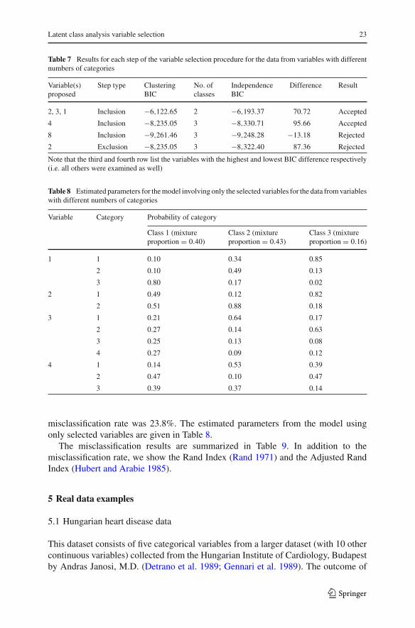
Table 7 Results for each step of the variable selection procedure for the data from variables with differentnumbers of categories

Variable(s) Step type Clustering No. of Independence Difference Resultproposed BIC classes BIC

2, 3, 1 Inclusion −6,122.65 2 −6,193.37 70.72 Accepted

4 Inclusion −8,235.05 3 −8,330.71 95.66 Accepted

8 Inclusion −9,261.46 3 −9,248.28 −13.18 Rejected

2 Exclusion −8,235.05 3 −8,322.40 87.36 Rejected

Note that the third and fourth row list the variables with the highest and lowest BIC difference respectively(i.e. all others were examined as well)

Table 8 Estimated parameters for the model involving only the selected variables for the data from variableswith different numbers of categories



1 1 0.10 0.34 0.85

2 0.10 0.49 0.13

3 0.80 0.17 0.02

2 1 0.49 0.12 0.82

2 0.51 0.88 0.18

3 1 0.21 0.64 0.17

2 0.27 0.14 0.63

3 0.25 0.13 0.08

4 0.27 0.09 0.12

4 1 0.14 0.53 0.39

2 0.47 0.10 0.47

3 0.39 0.37 0.14

misclassification rate was 23.8%. The estimated parameters from the model usingonly selected variables are given in Table 8.

The misclassification results are summarized in Table 9. In addition to themisclassification rate, we show the Rand Index (Rand 1971) and the Adjusted RandIndex (Hubert and Arabie 1985).

5 Real data examples

5.1 Hungarian heart disease data

This dataset consists of five categorical variables from a larger dataset (with 10 othercontinuous variables) collected from the Hungarian Institute of Cardiology, Budapestby Andras Janosi, M.D. (Detrano et al. 1989; Gennari et al. 1989). The outcome of

123


Table 9 Misclassification summary for the data from variables with different numbers of categories

Variables No. of Misclassification Rand Adjusted Randincluded classes selected rate (%) index index

All 2 38.3 0.65 0.30All 3a 25.7 0.72 0.401, 2, 3, 4 3 23.8 0.74 0.43a The number of classes was constrained to this value in advance. Recall that the minimum misclassificationrate from the model based on the actual parameters is 19.9%

interest is diagnosis of heart disease (angiographic disease status) into two categories:<50% diameter narrowing and >50% diameter narrowing in any major vessel. Theoriginal paper (Detrano et al. 1989) looked at the data in a supervised learning contextand achieved a 77% accuracy rate. Originally there was information about 294 sub-jects but 10 subjects had to be removed due to missing data. The five variables givenare gender (male/female) [sex], chest pain type (typical angina/atypical angina/non-anginal pain/asymptomatic) [cp], fasting blood sugar >120 mg/dl (true/false) [fbs],resting electrocardiographic results (normal/having ST-T wave abnormality/showingprobable or definite left ventricular hypertrophy by Estes’ criteria) [restecg] and exer-cise induced angina (yes/no) [exang].

When BIC is used to select the number of classes in a latent class model with allof the variables, it decisively selects 2 (with a difference of at least 38 points between2 classes and any other identifiable number of classes). When the variables are put indecreasing order of variance of estimated probabilities between classes the orderingis the following: cp, exang, sex, restecg and fbs.

Observations were classified into whichever group their estimated membershipprobability was greatest for. The partition estimated by this method is compared withthe clinical partition below:

<50% narrowing >50% narrowingClass 1 134 13Class 2 47 90

If class 1 is matched with the <50% class and class 2 with the >50% class there is acorrect classification rate of 78.9%. This gives a sensitivity of 87.4% and a specificityof 74%.

The variable selection method chooses 3 variables: cp, exang and sex. BIC selects 2classes for the latent class model on these variables. The partition given by this modelis the same as the one given by the model with all variables. The largest difference inestimated group membership probabilities between the two latent class models is 0.1.The estimated model parameters in the variables common to both latent class modelsand the mixing proportions differ between models by at most 0.003. Both modelshave the same correct classification, specificity and sensitivity rate. Thus our methodidentifies the fact that it is possible to reduce the number of variables from 5 to 3 withno cost in terms of clustering.

123


Table 10 Estimated parameters for the model involving all variables for Hungarian heart disease data



Chest pain type Typical angina 0.07 0.00

Atypical Angina 0.64 0.08

Non-anginal pain 0.29 0.08

Asymptomatic 0.00 0.83

Exercise induced No 0.98 0.42

Angina Yes 0.02 0.58

Gender Female 0.38 0.16

Male 0.62 0.84

Resting Normal 0.82 0.80

Electrocardiographic Having ST-T wave abnormality 0.15 0.20

Results Showing probable or definite 0.03 0.01

left ventricular hypertrophy

by Estes’ criteria

Fasting blood sugar False 0.94 0.92

>120 mg/dl True 0.06 0.08

Table 11 Estimated parameters for the model involving the selected variables for Hungarian heart diseasedata



Chest pain type Typical angina 0.07 0.00

Atypical angina 0.64 0.08

Non-anginal pain 0.28 0.08

Asymptomatic 0.00 0.84

Exercise induced angina No 0.97 0.42

Yes 0.03 0.58

Gender Female 0.38 0.16

Male 0.62 0.84

The estimated parameters for the latent class model with all variables included isgiven in Table 10 and the estimated parameters for the latent class model with onlythe selected variables included is given in Table 11.

5.2 HapMap data

The HapMap project (The International HapMap Consortium 2003) was set up toexamine patterns of DNA sequence variation across human populations. A consortium

123


Table 12 Information on thesubject populations for theHapMap data

Code Descriptions Number ofindividuals

CEU Utah residents with ancestryfrom Northern and WesternEurope

60

CHB Han Chinese in Beijing,China

45

JPT Japanese in Tokyo, Japan 45

YRI Yoruban in Ibadan, Nigeria(West Africa)

60

Table 13 BIC values fordifferent sets of variables anddifferent numbers of classes forthe HapMap data

Data Two classes Three classes Four classes

All variables −142,711 −141,418 −146,662

Selected variables −93,471 −91,147 −94,491

with members including the United States, United Kingdom, Canada, Nigeria, Japanand China is attempting to identify chromosomal regions where genetic variants areshared across individuals. One of the most common types of these variants is the singlenucleotide polymorphism (SNP). A SNP occurs when a single nucleotide (A, T, C orG) in the genome differs across individuals. If a particular locus has either A or G thenthese are called the two alleles. Most SNPs have only two alleles.

This dataset is from a random selection of 3,389 SNPs on 210 individuals (out of4 million available in the HapMap public database). Of these 801 had complete setsof measurements from all subjects and a further subset of 639 SNPs had non-zerovariability. Details of the populations and numbers of subjects are given in Table 12.

There are two possible correct groupings of the data. The first one is into threegroups: European (CEU), African (YRI) and Asian (CHB + JPT), and the second isinto four groups: European (CEU), African (YRI), Japanese (JPT) and Chinese (CHB).

When all 639 SNPs are used to build latent class models, BIC selects the best num-ber of classes as 3. The resulting estimated partition matches up exactly with the first3-group partition. The variable selection procedure selects 413 SNPs as importantto the clustering, reducing the number of variables by over a third. Using only theselected variables, BIC again selects a 3-class model whose estimated partition againgives perfect 3-group classification. The BIC values for models using both sets of datafrom 2 to 4 classes are given in Table 13. Note that comparing within rows in Table 13is appropriate, but comparing between rows is not because different rows correspondto different datasets.

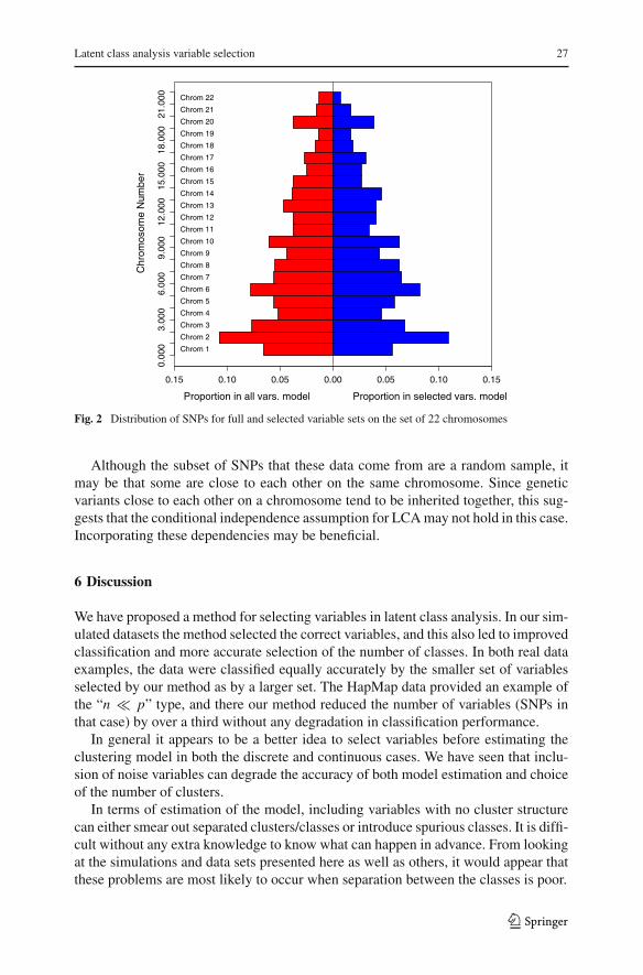
The HapMap project is also interested in the position of SNPs that differ betweenpopulations, so we can look at the distribution of all 639 SNPs across the 22 chro-mosomes and compare it to the distribution of the selected SNPs. This is presented inFig. 2.

123


0.15 0.10 0.05 0.00 0.05 0.10 0.15

0.00

03.

000

6.00

09.

000

12.0

0015

.000

18.0

0021

.000

Proportion in all vars. model Proportion in selected vars. model

Chr

omos

ome

Num

ber

Chrom 1

Chrom 2

Chrom 3

Chrom 4

Chrom 5

Chrom 6

Chrom 7

Chrom 8

Chrom 9

Chrom 10

Chrom 11

Chrom 12

Chrom 13

Chrom 14

Chrom 15

Chrom 16

Chrom 17

Chrom 18

Chrom 19

Chrom 20

Chrom 21

Chrom 22

Fig. 2 Distribution of SNPs for full and selected variable sets on the set of 22 chromosomes

Although the subset of SNPs that these data come from are a random sample, itmay be that some are close to each other on the same chromosome. Since geneticvariants close to each other on a chromosome tend to be inherited together, this sug-gests that the conditional independence assumption for LCA may not hold in this case.Incorporating these dependencies may be beneficial.

6 Discussion

We have proposed a method for selecting variables in latent class analysis. In our sim-ulated datasets the method selected the correct variables, and this also led to improvedclassification and more accurate selection of the number of classes. In both real dataexamples, the data were classified equally accurately by the smaller set of variablesselected by our method as by a larger set. The HapMap data provided an example ofthe “n � p” type, and there our method reduced the number of variables (SNPs inthat case) by over a third without any degradation in classification performance.

In general it appears to be a better idea to select variables before estimating theclustering model in both the discrete and continuous cases. We have seen that inclu-sion of noise variables can degrade the accuracy of both model estimation and choiceof the number of clusters.

In terms of estimation of the model, including variables with no cluster structurecan either smear out separated clusters/classes or introduce spurious classes. It is diffi-cult without any extra knowledge to know what can happen in advance. From lookingat the simulations and data sets presented here as well as others, it would appear thatthese problems are most likely to occur when separation between the classes is poor.

123


The headlong search algorithm is different from the greedy search algorithmdescribed in Raftery and Dean (2006) in two ways:

1. The best variable (in terms of the BIC difference) is not necessarily selected ineach inclusion and exclusion step in the headlong search.

2. It is possible that some variables are not looked at in any step after a certain pointin the headlong algorithm (after being removed from consideration).

The headlong search is substantially faster than the greedy search and in spite ofpoint 2 above, usually gives comparable or sometimes better results (perhaps due tothe local nature of the search).

Galimberti and Soffritti (2006) considered the problem of finding multiple clusterstructures in latent class analysis. In this problem the data are divided into subsets,each of which obeys a different latent class model. The models in the different subsetsmay include different variables. This is a somewhat different problem from the one weaddress here, but it also involves a kind of variable selection in latent class analysis.

Keribin (1998) showed that BIC was consistent for choice of the number of com-ponents in a mixture model under certain conditions, notably assuming that all vari-ables were relevant to the clustering. Empirical evidence seems to suggest that whennoise/irrelevant variables are present, BIC is less likely to select the correct number ofclasses. The general correctness of the BIC approximation in a specific case of binaryvariables with two classes in a naive Bayes network (which is equivalent to a 2-classlatent class model with the local independence assumption satisfied) was looked atby Rusakov and Geiger (2005). The authors found that although the traditional BICpenalty term of # of parameters × log(# of observations) (or half this depending onthe definition) was correct for regular points in the data space, it was not correct forsingularity points (with two different types of singularity points requiring two adjustedversions of the penalty term). The first type of singularity points were those sets ofparameters that could arise from a naive Bayes model with all but at most 2 linksremoved (type 1) and those that could arise from a model with all links removed(type 2), representing a set of mutually independent variables. Similarly in the case ofredundant or irrelevant variables being included (which is closely related to the twosingularity point types) they found that the two adjusted penalty terms were correct.These issues with clustering with noise variables reinforce the arguments for variableselection in latent class analysis.

Appendix A: Headlong search algorithm for variable selectionin latent class analysis

Here we give a more complete description of the headlong search variable selectionand clustering algorithm for the case of discrete data modeled by conditionally inde-pendent multinomially distributed groups. Note that for each latent class model fittedin this algorithm one must run a number of random starts to find the best estimate ofthe model (in terms of BIC). We recommend at least 5 for small to medium problemsbut for bigger problems hundreds may be needed to get a decent model estimate. Theissue of getting good starting values without multiple generation of random starts isdealt with in Appendix B.

123


• Choose Gmax, the maximum number of clusters/classes to be considered for thedata. Make sure that this number is identifiable for your data! Define constantsupper (default 0) and lower (default −100), where upper is the quantity abovewhich the difference in BIC for models M2 and M1 will result in a variable beingincluded in Y (clust) and below which the difference in BIC for models M2 and M1will result in a variable being excluded from Y (clust), and lower is the quantitybelow which the difference in BIC for models M2 and M1 will result in a variablebeing removed from consideration for the rest of the procedure.

• First step One way of choosing the initial clustering variable set is by estimating alatent class model with at least 2 classes for all variables (if more classes are iden-tifiable, estimate all identifiable class numbers and choose the model with the bestnumber of classes via BIC). Order the variables in terms of variability of their esti-mated probabilities across classes. Choose the minimum top variables that allow atleast a 2-class model to be identified. This is the initial Y (clust). We do not requirethat the BIC difference between clustering and a model with a single class for ourY (clust) to be positive at this point because we need a set of starting variables for thealgorithm. These can be removed later if there are not truly clustering variables.Specifically we estimate the {pi jg, i = 1, . . . , k, j = 1, . . . , di , g = 1, . . . , G}where k is the number of variables, di is the number of categories for the i thvariables and G is the number of classes. For each variable i we calculate V (i) =∑di

j=1 V ar(pi jg). We order the variables in decreasing order of V (i): y(1),

y(2), . . . , y(k) and find m the minimum number of top variables that will iden-tify a latent class model with G ≥ 2.

Y (clust) = {y(1), y(2), . . . , y(m)},Y (other) = {y(m+1), . . . , y(k)}.

If the previous method is not possible (data cannot identify latent class model forG > 1) then split the variables randomly into subsets with enough variables toidentify a latent class model for at least 2 classes, estimate the latent models foreach subset and calculate the BICs, estimate the single class (G = 1) models foreach subset and calculate these 1 class BICs and choose the subset with the highestdifference between latent class model (G ≥ 2) and 1 class model BICs as theinitial Y (clust).Specifically look at the list of numbers of categories d = (d1, . . . , dk) and workout the minimum number of variables m that allows a latent class model for G ≥ 2to be identified. Split the variables into S subsets of at least m variables in each.For each set Ys, s = 1, . . . , S estimate:

BICdiff(Ys) = BICclust(Ys) − BICnot clust(Ys),

where BICclust(Ys) = max2≤G≤Gmaxs{BICG(Ys)}, with BICG(Ys) being the BICgiven in (1) for the latent class model for Ys with G classes and Gmaxs being the

123


maximum number of identifiable classes for Ys , and BICnot clust(Ys) = BIC1(Ys).We choose the best variable subset, Ys1 , such that

s1 = arg maxs:Ys∈Y

(BICdiff(Ys))

and create

Y (clust) = Ys1

and

Y (other) = Y\Ys1 ,

where Y\Ys1 denotes the set of variables Y excluding the subset Ys1 .• Second step Next we look at each variable in Y (other) singly in order as the new

variable under consideration for inclusion into Y (clust). For each variable we lookat the difference between the BIC for clustering on the set of variables includingthe variables selected in the first set and the new variable (maximized over numberof clusters from 2 up to Gmax) and the sum of the BIC for the clustering of thevariables chosen in the first step and the BIC for the single class latent class modelfor the new variable. If this difference is less than lower the variable is removedfrom consideration for the rest of the procedure and we continue checking the nextvariable. Once the difference is greater than upper we stop and this variable isincluded in the set of clustering variables. Note that if no variable has differencegreater than upper we include the variable with the largest difference in the setof clustering variables. We force a variable to be selected at this stage to give onefinal extra starting variable.Specifically, we split Y (other) into its variables y1, . . . , yD2 . For each j in 1, . . . , D2until BICdiff(y j ) > upper , we compute the approximation to the Bayes factor in(6) by

BICdiff(y j ) = BICclust(y j ) − BICnot clust(y j ),

where BICclust(y j ) = max2≤G≤Gmaxj{BICG(Y (clust), y j )} with BICG(Y (clust), y j )

being the BIC given in (1) for the latent class clustering model for the datasetincluding both the previously selected variables (contained in Y (clust)) and the newvariable y j with G classes, and BICnot clust(y j ) = BICreg +BICclust(Y (clust)) whereBICreg is BIC1(y j ) and BICclust(Y (clust)) is the BIC for the latent class clusteringmodel with only the currently selected variables in Y (clust).We choose the first variable, y j2 , such that

BICdiff(y j2) > upper

or if no such j2 exists,

j2 = arg maxj :y j ∈Y (other)

(BICdiff(y j ))

123


and create

Y (clust) = Y (clust) ∪ y j2

and

Y (other) = Y (other)\y j2 ,

where Y (clust) ∪ y j2 denotes the set of variables including those in Y (clust) andvariable y j2 .

• General Step [Inclusion part] Each variable in Y (other) is proposed singly (in order),until the difference between the BIC for clustering with this variable included inthe set of currently selected clustering variables (maximized over numbers of clus-ters from 2 up to Gmax) and the sum of the BIC for the clustering with only thecurrently selected clustering variables and the BIC for the single class latent classmodel of the new variable, is greater than upper .

• The variable with BIC difference greater than upper is then included in the set ofclustering variables and we stop the step. Any variable whose BIC difference isless than lower is removed from consideration for the rest of the procedure. If novariable has BIC difference greater than upper no new variable is included in theset of clustering variablesSpecifically, at step t we split Y (other) into its variables y1, . . . , yDt . For j in1, . . . , Dt we compute the approximation to the Bayes factor in (6) by

BICdiff(y j ) = BICclust(y j ) − BICnot clust(y j ), (7)

where BICclust(y j ) = max2≤G≤Gmaxj{BICG(Y (clust), y j )}, with BICG(Y (clust), y j )

being the BIC given in (1) for the latent class clustering model for the datasetincluding both the previously selected variables (contained in Y (clust)) and the newvariable y j with G clusters, and BICnot clust(y j ) = BICreg+BICclust(Y (clust)) whereBICreg is the single class latent class model for variable y j and BICclust(Y (clust)) isthe BIC for the clustering with only the currently selected variables in Y (clust).We check if BICdiff(y j ) > upper ,if so we stop and set

Y (clust) = Y (clust) ∪ y j if BICdiff(y j ) > upper

and

Y (other) = Y (other)\y j if BICdiff(y j ) > upper

if not we increment j and re-calculate BICdiff(y j ). If BICdiff(y j ) < lower weremove it from both Y (clust) and Y (other).If no j has BICdiff(y j ) > upper leave Y (clust) = Y (clust) and Y (other) = Y (other).

• General Step [Removal part] Each variable in Y (clust) is proposed singly (in order),until the difference between the BIC for clustering with this variable included in

123


the set of currently selected clustering variables (maximized over numbers of clus-ters from 2 up to Gmax) and the sum of the BIC for the clustering with only theother currently selected clustering variables (and not the variable under consid-eration) and the BIC for the single class latent class model of the variable underconsideration, is less than upper .

• The variable with BIC difference less than upper is then removed from the set ofclustering variables and we stop the step. If the difference is greater than lowerwe include the variable at the end of the list of variables in Y (other). If not weremove it entirely from consideration for the rest of the procedure. If no variablehas BIC difference less than upper no variable is excluded from the current set ofclustering variablesIn terms of equations for step t +1, we split Y (clust) into its variables y1, . . . , yDt+1 .For each j in 1, . . . , Dt+1 we compute the approximation to the Bayes factor in(6) by

BICdiff(y j ) = BICclust − BICnot clust(y j ),

where BICclust = max2≤G≤Gmax{BICG(Y (clust))} with BICG,m(Y (clust)) being theBIC given in (1) for the model-based clustering model for the dataset includ-ing the previously selected variables (contained in Y (clust)) with G clusters, andBICnot clust(y j ) = BICreg + BICclust(Y (clust)\y j ) where BICreg is the single classlatent class model for variable y j and BICclust(Y (clust)\y j ) is the BIC for the clus-tering with all the currently selected variables in Y (clust) except for y j .We check if BICdiff(y j ) < upper ,if so we stop and set

Y (clust) = Y (clust)\y j if BICdiff(y j ) < upper

and

Y (other) = Y (other) ∪ y j if lower < BICdiff(y j ) < upper

if not we increment j and re-calculate BICdiff(y j ). If BICdiff(y j ) < lower weremove it from both Y (clust) and Y (other).If no j has BICdiff(y j ) < upper leave Y (clust) = Y (clust) and Y (other) = Y (other).

• After the first and second steps the general step is iterated until consecutive inclu-sion and removal proposals are rejected. At this point the algorithm stops as anyfurther proposals will be the same ones already rejected.

Appendix B: Starting values for latent class analysisin the headlong search algorithm

In the previous appendix we discussed the details of the headlong algorithm for latentclass variable selection. In each step multiple latent class models for different set of

123


data/variables and classes are estimated. Previously we have only mentioned that start-ing values are generated randomly for each model several times and the best (in termsof BIC/likelihood) of the resulting estimated models is chosen as the single estimatefor a particular latent class model. This means that for each different dataset and eachdifferent number of classes we are required to generate random starting values andestimate the model via EM numerous times. For datasets with reasonable numbers ofvariables this is not too computationally expensive but for more complex datasets itis burdensome. Also with increasing numbers of observations and/or variables and/orclasses more random starts are needed to have any confidence in finding the globalmaximum likelihood for the model as the likelihood surface becomes more complex,with increasing numbers of local maxima.

Because of the stepwise nature of the algorithm we can use models estimatedbefore to give good starting values for new models. By starting values here we meanthe matrix z of conditional probabilities of membership in the different classes foreach observation.

At the end of each step (either inclusion or exclusion) we have a set of currentlyselected clustering variables. At some point in the step we have estimated the latentclass model for this set over a range of classes (or sometimes just one, 2 classes) andchosen the model with the number of classes that gives us the highest BIC. We cancall this model LCAcurrent and the number of classes in this best model for the currentset of clustering variables Gcurrent. We can also save the z matrix for this model andcall it zcurrent.

In our next step we will be either looking at models for Y (clust) with a new additionalvariable (inclusion step) or models for Y (clust) leaving out one of the current clusteringvariables. It seems obvious that a reasonable starting z matrix for models involving thenew dataset (which is either a sub- or super-set of the old one) and number of classesGcurrent would be zcurrent, because the dataset will only have changed by one variable.So instead of randomly generating multiple z matrixes (or other starting parameters)to try to get the global maximum likelihood for our latent class model, we merely usewhat we believe to be a good set starting z matrix (which hopefully will be reasonablyclose to the global maximum in the new likelihood space).

However, we may still wish to have good starting values for the new dataset withdifferent numbers of classes, Gcurrent ±c. But our zcurrent will be an n ×Gcurrent matrix(where n is the number of observations) and we need n × (Gcurrent ±c) matrices. Howcan we sensibly create a new matrix with c more/less columns given our zcurrent?

We will look at the case for +1 and −1 separately (the analog for general +c and−c should be obvious). It will be rare in practice to need more than ±1 at each step asthe number of identifiable classes will only generally increase fairly slowly with thenumber of variables selected.

For −1 we want to reduce the number of columns of our zcurrent by 1. A sensibleway to do this is to collapse the two closest classes (in terms of Euclidean distancein the parameter space). We calculate the distances between the classes’ estimatedparameters/probabilities from LCAcurrent and select the closest two. We then simplyremove the two columns corresponding to those classes from zcurrent and replace themwith one column equal to the sum (across rows) of the removed columns. This is ournew starting z matrix for the model with Gcurrent − 1 classes. In terms of a single

123


observation with probability p1 of being in the first chosen class and probability p2 ofbeing the second chosen class we are saying the observation has probability p1 + p2 ofbeing in the new class created from the amalgamation of the two, i.e. the observationwill be in the new class if he is in either of the old classes. Note that if we wish to, wecan weight the distances with the mixing proportions, making it more likely that wewould join smaller close classes.

For −c we can use the resulting matrix from the process described in the previousparagraph to estimate the model for Gcurrent − 1 classes and then reduce the resultingestimated z from this model by one column in the same fashion, continuing on in thesame way until we have removed c columns.

For +1 we want to increase the number of columns of our zcurrent by 1. An obviousway to do this is by splitting a class in two. We choose the largest class (in terms ofmixing proportions). We then remove the column corresponding to that class fromzcurrent and call this w and estimate a two class latent class model using the data pointsweighted by w. Obviously we have returned to problem of needing starting values forestimating our 2-class model. However usually a small number of randomly generatedstarts, say 5, for this number of classes will result in an estimated model achievingthe global maximum likelihood and this is usually not too computationally expensive.Once we have our 2-class model estimate of the z matrix, called z2, we can multiplythis by w and add the resulting two columns to the original zcurrent (less the removedcolumn), giving us a starting z matrix for estimating the Gcurrent + 1 class model. Wecan think of w as being the conditional probability of an observation being in the oldselected class and then the new z2 matrix as being the probability for an observationbeing in either of the two new sub-classes given it was in the old class.

Again for +c we can use the resulting matrix from the process described in theprevious paragraph to estimate the model for Gcurrent +1 classes and then increase theresulting estimated z from this model by one column in the same fashion, continuingon in the same way until we have added c columns.

Acknowledgments Both authors were supported by NIH grant 8 R01 EB002137-02. Raftery was alsosupported by NICHD grant 1 R01HD O54511, NSF grant IIS0534094 and NSF grant ATM0724721. Theauthors would like to thank Matthew Stephens and Paul Scheet for their preparation of the HapMap datafor this paper.

References

Badsberg, J. H. (1992). Model search in contingency tables by CoCo. In Y. Dodge, J. Whittaker (Eds.),Computational statistics (Vol. 1, pp. 251–256). Heidelberg: Physica Verlag.

Clogg, C. C. (1981). New developments in latent structure analysis. In D. J. Jackson, E. F. Borgatta (Eds.),Factor analysis and measurement in sociological research (pp. 215–246). Beverly Hills: Sage.

Clogg, C. C. (1995). Latent class models. In G. Arminger, C. C. Clogg, M. E. Sobel (Eds.), Handbook ofstatistical modeling for the social and behavioral sciences (pp. 311–360). New York: Plenum.

Detrano, R., Janosi, A., Steinbrunn, W., Pfisterer, M., Schmid, J.-J., Sandhu, S., Guppy, K. H., Lee, S.,Froelicher, V. (1989). International application of a new probability algorithm for the diagnosis ofcoronary artery disease. American Journal of Cardiology, 64, 304–310.

Fraley, C., Raftery, A. E. (2002). Model-based clustering, discriminant analysis, and density estimation.Journal of the American Statistical Association, 97, 611–631.

123


Galimberti, G., Soffritti, G. (2006). Identifying multiple cluster structures through latent class models. InM. Spiliopoulou, R. Kruse, C. Borgelt, A. Nürnberger, W. Gaul (Eds.), From data and informationanalysis to knowledge engineering (pp. 174–181). Berlin: Springer.

Gennari, J. H., Langley, P., Fisher, D. (1989). Models of incremental concept formation. ArtificialIntelligence, 40, 11–61.

Goodman, L. A. (1974). Exploratory latent structure analysis using both identifiable and unidentifiablemodels. Biometrika, 61, 215–231.

Hagenaars, J. A., McCutcheon, A. L. (2002). Applied latent class analysis. Cambridge: CambridgeUniversity Press.

Hubert, L., Arabie, P. (1985). Comparing partitions. Journal of Classification, 2, 193–218.Kass, R. E., Raftery, A. E. (1995). Bayes factors. Journal of the American Statistical Association, 90,

773–795.Keribin, C. (1998). Consistent estimate of the order of mixture models. Comptes Rendues de l’Academie

des Sciences, Série I-Mathématiques, 326, 243–248.Lazarsfeld, P. F. (1950a). The logical and mathematical foundations of latent structure analysis. In S. A.

Stouffer (Ed.), Measurement and prediction, the American soldier: studies in social psychology inWorld War II (Vol. IV, Chap. 10, pp. 362–412). Princeton, NJ: Princeton University Press.

Lazarsfeld, P. F. (1950b). The interpretation and computation of some latent structures. In S. A. Stouffer(Ed.), Measurement and prediction, the American soldier: studies in social psychology in World WarII (Vol. IV, Chap. 11, pp. 413–472). Princeton, NJ: Princeton University Press.

Lazarsfeld, P. F., Henry, N. W. (1968). Latent structure analysis. Boston: Houghton Mifflin.McCutcheon, A. L. (1987). Latent class analysis. Newbury Park, CA: Sage.McLachlan, G. J., Peel, D. (2000). Finite mixture models. New York: Wiley.Raftery, A. E., Dean, N. (2006). Variable selection for model-based clustering. Journal of the American

Statistical Association, 101, 168–178.Rand, W. M. (1971). Objective criteria for the evaluation of clustering methods. Journal of the American

Statistical Association, 66, 846–850.Rusakov, D., Geiger, D. (2005). Asymptotic model selection for naive Bayesian networks. Journal of

Machine Learning Research, 6, 1–35.The International HapMap Consortium (2003). The international hapmap project. Nature, 426, 789–796.Wolfe, J. H. (1963). Object cluster analysis of social areas. Master’s thesis, University of California,

Berkeley.

123

Latent class analysis variable selection - Statistics - University of

Documents