Latent Class Analysis For you to leave here knowing… • When is latent class analysis (LCA) model useful? • What is the LCA model its underlying assumptions? • How are LCA parameters

Latent Class Analysis

Karen Bandeen-Roche

October 27, 2016

Objectives For you to leave here knowing…

•  When is latent class analysis (LCA) model useful?

•  What is the LCA model its underlying assumptions? •  How are LCA parameters interpreted?

•  How are LCA parameters commonly estimated?

•  How is LCA fit adjudicated?

•  What are considerations for identifiability / estimability?

Motivating Example Frailty of Older Adults

“…the sixth age shifts into the lean and

slipper’d pantaloon, with spectacles on nose and pouch on side, his youthful hose well sav’d, a world too wide, for his shrunk shank…”

-- Shakespeare, “As You Like It”

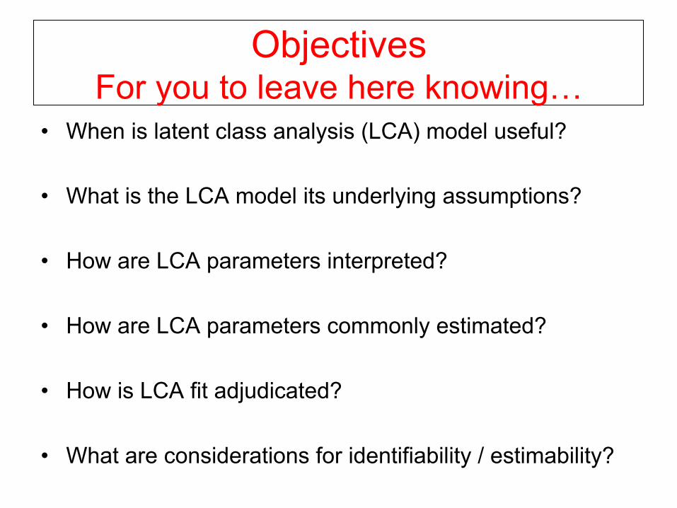
The Frailty Construct

Fried et al., J Gerontol 2001; Bandeen-Roche et al., J Gerontol, 2006

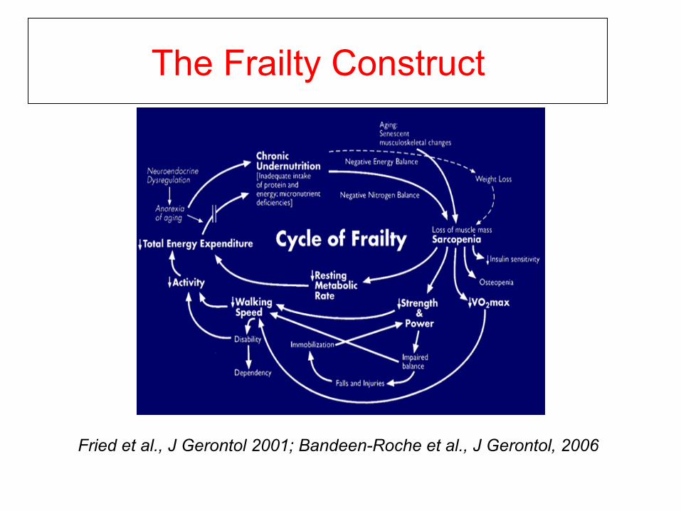
Frailty as a latent variable

•  “Underlying”: status or degree of syndrome

•  “Surrogates”: Fried et al. (2001) criteria

–  weight loss above threshold –  low energy expenditure –  low walking speed –  weakness beyond threshold –  exhaustion

Part I: Model

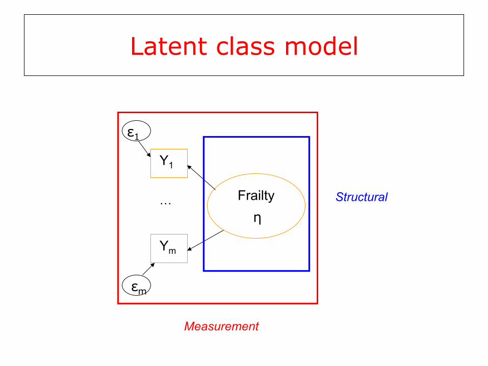
Latent class model

Frailty

Y1

Ym

…

εm

ε1

η

Measurement

Structural

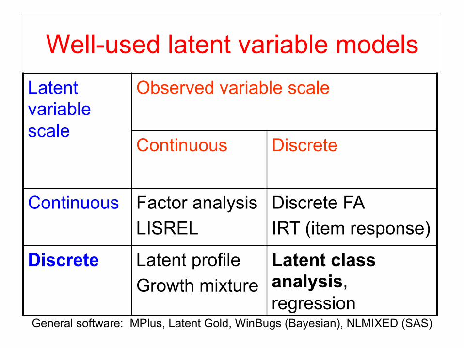
Well-used latent variable models Latent variable scale

Observed variable scale

Continuous Discrete

Continuous Factor analysis LISREL

Discrete FA IRT (item response)

Discrete Latent profile Growth mixture

Latent class analysis, regression

General software: MPlus, Latent Gold, WinBugs (Bayesian), NLMIXED (SAS)

Analysis of underlying subpopulations Latent class analysis

POPULATION

… P1 PJ

Ui

Y1 YM Y1 YM … …

∏11 ∏1M ∏J1 ∏JM

Lazarsfeld & Henry, Latent Structure Analysis, 1968; Goodman, Biometrika, 1974

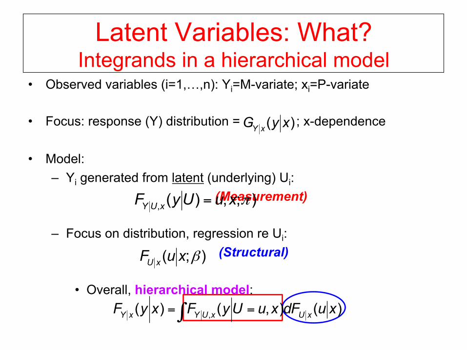
Latent Variables: What? Integrands in a hierarchical model

•  Observed variables (i=1,…,n): Yi=M-variate; xi=P-variate •  Focus: response (Y) distribution = GYx(y/x) ; x-dependence •  Model:

–  Yi generated from latent (underlying) Ui: (Measurement)

–  Focus on distribution, regression re Ui:

(Structural)

•  Overall, hierarchical model:

);( βxuF xU

);,)(, πxuUyF xUY =

∫ == )(),()( , xudFxuUyFxyF xUxUYxY

)( xyG xY

Latent Variable Models Latent Class Regression (LCR) Model

•  Model:

•  Structural model:

•  Measurement model:

= “conditional probabilities” > is MxJ

•  Compare to general form:

∏∑=

−

=

−=M

m

ymj

ymj

J

jjxY

mmPxyf1

1

1

)1()( ππ

[ ] { } { } JjPjjUxU jiii ,...,1,PrPr ====== η

[ ]ii UY

{ } { }jYjUY iimiimmj ====== ηπ 1Pr1Pr

π

∫ == )(),()( , xudFxuUyFxyF xUxUYxY

Latent Variable Models Latent Class Regression (LCR) Model

•  Model:

•  Measurement assumptions: – Conditional independence

Ø {Yi1,…,YiM} mutually independent conditional on Ui

Ø Reporting heterogeneity unrelated to measured, unmeasured characteristics

( )m

m

yJ

j

M

mmj

ymjjxY Pxyf

−

= =∑ ∏ −=

1

1 11)( ππ

[ ]ii UY

Latent Variable Models Latent Class Regression (LCR) Model

•  Model:

•  Measurement assumptions: – Conditional independence

Ø {Yi1,…,YiM} mutually independent conditional on Ci

Ø Reporting heterogeneity unrelated to measured, unmeasured characteristics

( )m

m

yJ

j

M

mmj

ymjjxY Pxyf

−

= =∑ ∏ −=

1

1 11)( ππ

[ ]ii CY

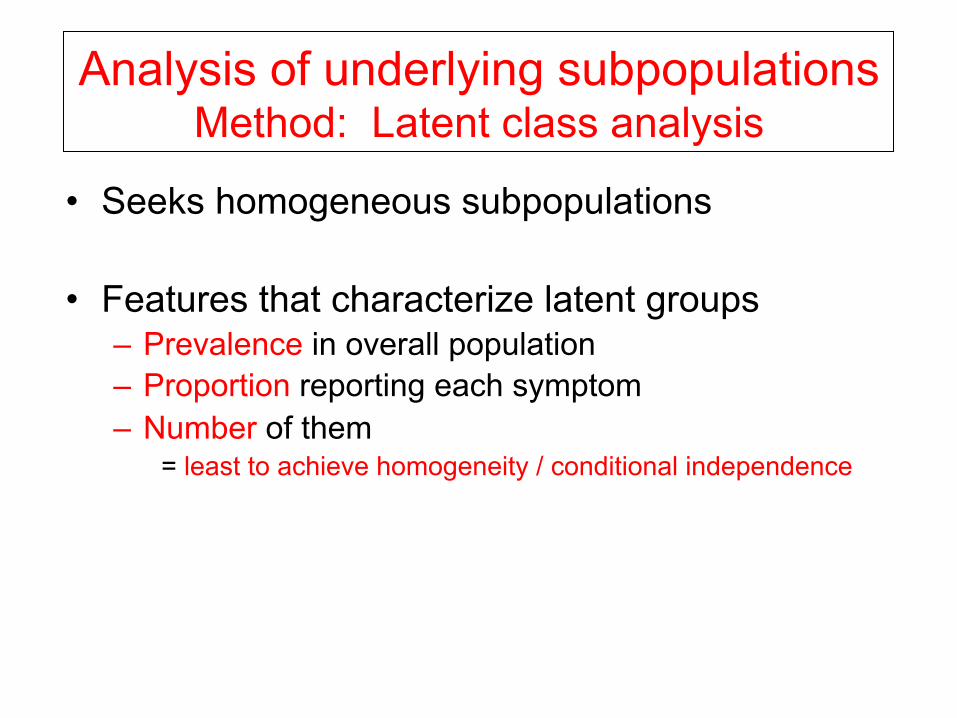
Analysis of underlying subpopulations Method: Latent class analysis

•  Seeks homogeneous subpopulations •  Features that characterize latent groups

–  Prevalence in overall population –  Proportion reporting each symptom –  Number of them

= least to achieve homogeneity / conditional independence

Latent class analysis Prediction

•  Of interest: Pr(C=j|Y=y) = posterior probability of class membership

•  Once model is fit, a straightforward calculation

Pr(C=j|Y=y) =

=

= ij when evaluated at yi

( )( )yY

yY=

==Pr

,Pr jC

( )

( )∑ ∏

∏

= =

−

−

=

−

−

J

k

m

m

ymk

ymkk

ymj

M

m

ymjj

mm

mm

P

P

1 1

1

1

1

1

1

ππ

ππ

θ

Part II: Fitting

Estimation Broad Strokes

•  Maximum likelihood –  EM Algorithm –  Simplex method (Dayton & Macready, 1988) –  Possibly with weighting, robust variance correction

•  ML software –  Specialty: Mplus, Latent Gold –  Stata: gllamm –  SAS: macro –  R: poLCA

•  Bayesian: winBugs

Estimation Methods other than EM algorithm

• Bayesian

• MCMC methods (e.g. per Winbugs) • A challenge: label-switching • Reversible-jump methods

• Advantages: feasibility, philosophy

• Disadvantages • Prior choice (high-dimensional; avoiding illogic) • Burn-in, duration • May obscure identification problems

A process of averaging over missing data – in this case, missing data is class membership.

Estimation Likelihood maximization: E-M algorithm

Estimation Likelihood maximization: E-M algorithm

• Rationale: LVs as “missing” data

• Brief review • “Complete” data

• Complete data log likelihood taken as a function of ϕ • Iterate between

• (K+1) E-Step: evaluate

• (K+1) M-Step: maximize wrt ϕ

• Convergence to a local likelihood maximum under regularity Dempster, Laird, and Rubin, JRSSB, 1977

{ }uxYW ,,=

),|,(log |, φxuyF xuy=

)|( ww φ=

[ ])(,|)( ;,|)|()|( k

wxyuk xyWEQ φφφφ =

)|( )(kQ φφ

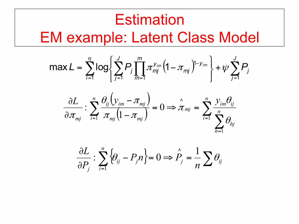
Estimation EM example: Latent Class Model

( ) ∑∑ ∏∑== =

−

=

+⎭⎬⎫

⎩⎨⎧

−=J

jj

i

m

m

ymj

ymj

J

jj PPL imim

11 1

1

11logmax

η

ψππ

( )( ) ∑

∑∑

=

=

∧

=

=⇒=−

−

∂∂ n

in

hhj

ijimmj

n

i mjmj

mjimij

mj

yyL1

1

1

01

:θ

θπ

ππ

πθ

π

{ }∑ ∑=

∧

=⇒=−∂∂ n

iijjjij

j nPnP

PL

1

10: θθ

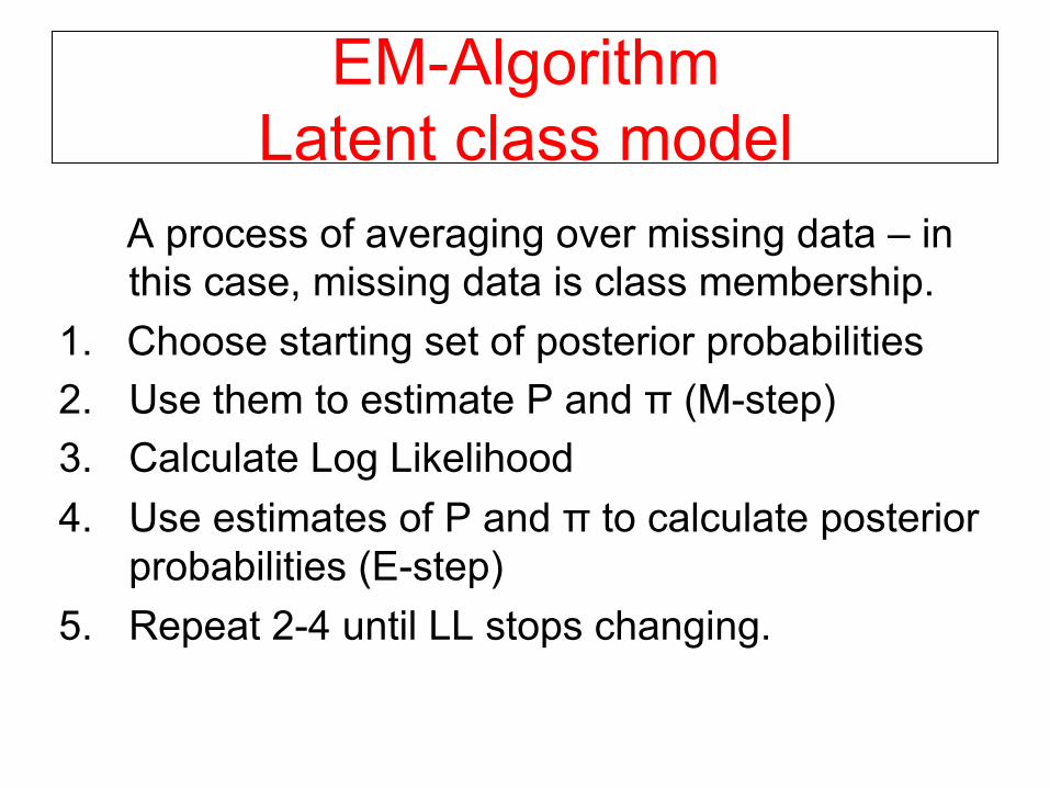
EM-Algorithm Latent class model

A process of averaging over missing data – in this case, missing data is class membership.

1. Choose starting set of posterior probabilities 2.  Use them to estimate P and π (M-step) 3.  Calculate Log Likelihood 4.  Use estimates of P and π to calculate posterior

probabilities (E-step) 5.  Repeat 2-4 until LL stops changing.

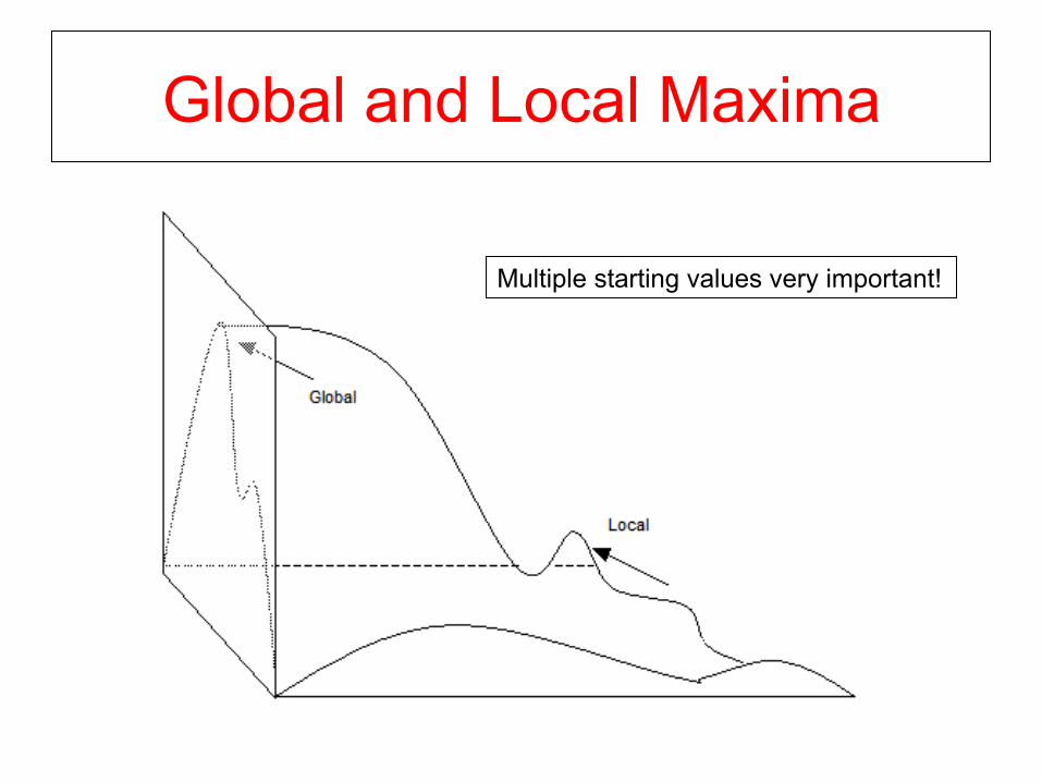
Global and Local Maxima

Multiple starting values very important!

Example: Frailty Women’s Health & Aging Studies

•  Longitudinal cohort studies to investigate –  Causes / course of physical and cognitive disability –  Physiological determinants of frailty –  Up to 7 rounds spanning 15 years

•  Companion studies in community, Baltimore, MD –  ≥ moderately disabled women 65+ years: n=1002 –  ≤ mildly disabled women 70-79 years: n=436

•  This project: n=786 age 70-79 years at baseline –  Probability-weighted analyses

Guralnik et al., NIA, 1995; Fried et al., J Gerontol, 2001

Example: Latent Frailty Classes Women’s Health and Aging Study

Criterion

2-Class Model

3-Class Model

CL. 1 “NON-FRAIL”

CL. 2 “FRAIL”

CL. 1 “ROBUST”

CL. 2 “INTERMED.”

CL. 3 “FRAIL”

Weight Loss

.073

.26

.072

.11

.54

Weakness

.088

.51

.029

.26

.77

Slowness

.15

.70

.004

.45

.85

Low Physical Activity

.078

.51

.000

.28

.70

Exhaustion

.061

.34

.027

.16

.56

Class Prevalence (P) (%)

73.3

26.7

39.2

53.6

7.2

Bandeen-Roche et al., J Gerontol, 2006

Conditional Probabilities (π)

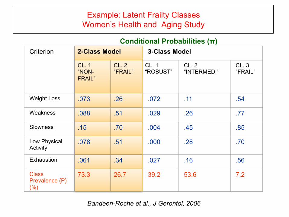
Example: Latent Frailty Classes Women’s Health and Aging Study

Criterion

2-Class Model

3-Class Model

CL. 1 “NON-FRAIL”

CL. 2 “FRAIL”

CL. 1 “ROBUST”

CL. 2 “INTERMED.”

CL. 3 “FRAIL”

Weight Loss

.073

.26

.072

.11

.54

Weakness

.088

.51

.029

.26

.77

Slowness

.15

.70

.004

.45

.85

Low Physical Activity

.078

.51

.000

.28

.70

Exhaustion

.061

.34

.027

.16

.56

Class Prevalence (P) (%)

73.3

26.7

39.2

53.6

7.2

Bandeen-Roche et al., J Gerontol, 2006

Conditional Probabilities (π)

We estimate that 26% in the “frail” Subpopulation exhibit weight loss”

Part III: Evaluating Fit

Choosing the Number of Classes

•  a priori theory •  Chi-Square goodness of fit •  Entropy •  Information Statistics

– AIC, BIC, others •  Lo-Mendell-Rubin (LMR)

– Not recommended (designed for normal Y) •  Bootstrapped Likelihood Ratio Test

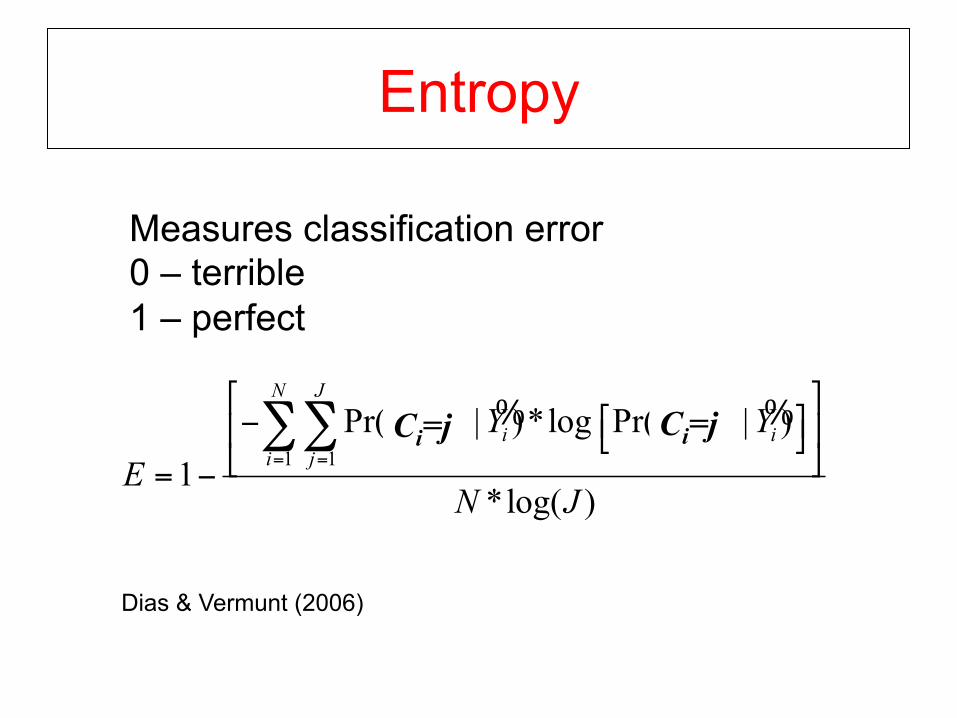
Entropy

1 1Pr( | )*log Pr( | )

1*log( )

N J

i i i ii j

S j Y S j YE

N J= =

⎡ ⎤⎡ ⎤− = =⎢ ⎥⎣ ⎦

⎣ ⎦= −∑∑ % %

Measures classification error 0 – terrible 1 – perfect

Dias & Vermunt (2006)

Ci=j Ci=j

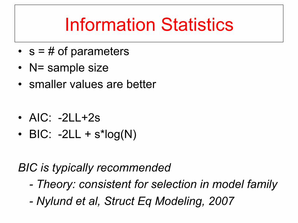
Information Statistics •  s = # of parameters •  N= sample size •  smaller values are better •  AIC: -2LL+2s •  BIC: -2LL + s*log(N) BIC is typically recommended

- Theory: consistent for selection in model family - Nylund et al, Struct Eq Modeling, 2007

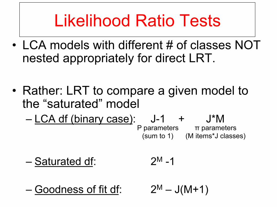
Likelihood Ratio Tests •  LCA models with different # of classes NOT

nested appropriately for direct LRT. •  Rather: LRT to compare a given model to

the “saturated” model – LCA df (binary case): J-1 + J*M

– Saturated df: 2M -1

– Goodness of fit df: 2M – J(M+1)

P parameters (sum to 1)

π parameters (M items*J classes)

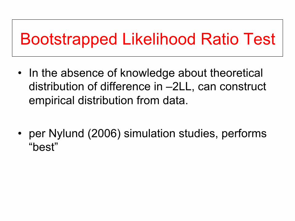
Bootstrapped Likelihood Ratio Test

•  In the absence of knowledge about theoretical distribution of difference in –2LL, can construct empirical distribution from data.

•  per Nylund (2006) simulation studies, performs “best”

•  Internal convergent validity

•  Criteria manifestation is syndromic

“a group of signs and symptoms that occur together and characterize a particular abnormality”

- Merriam-Webster Medical Dictionary

Example: Frailty Construct Validation Women’s Health & Aging Studies

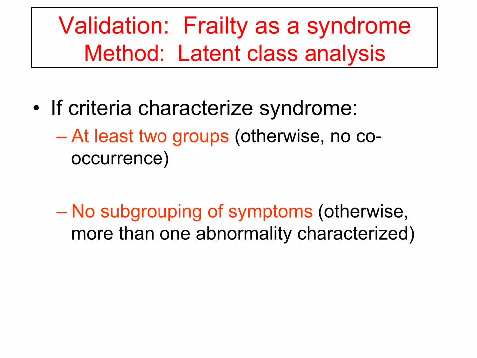
Validation: Frailty as a syndrome Method: Latent class analysis

•  If criteria characterize syndrome: – At least two groups (otherwise, no co-

occurrence) – No subgrouping of symptoms (otherwise,

more than one abnormality characterized)

Conditional Probabilities of Meeting Criteria in Latent Frailty Classes WHAS

Criterion

2-Class Model

3-Class Model

CL. 1 “NON-FRAIL”

CL. 2 “FRAIL”

CL. 1 “ROBUST”

CL. 2 “INTERMED.”

CL. 3 “FRAIL”

Weight Loss

.073

.26

.072

.11

.54

Weakness

.088

.51

.029

.26

.77

Slowness

.15

.70

.004

.45

.85

Low Physical Activity

.078

.51

.000

.28

.70

Exhaustion

.061

.34

.027

.16

.56

Class Prevalence (%)

73.3

26.7

39.2

53.6

7.2

Bandeen-Roche et al., J Gerontol, 2006

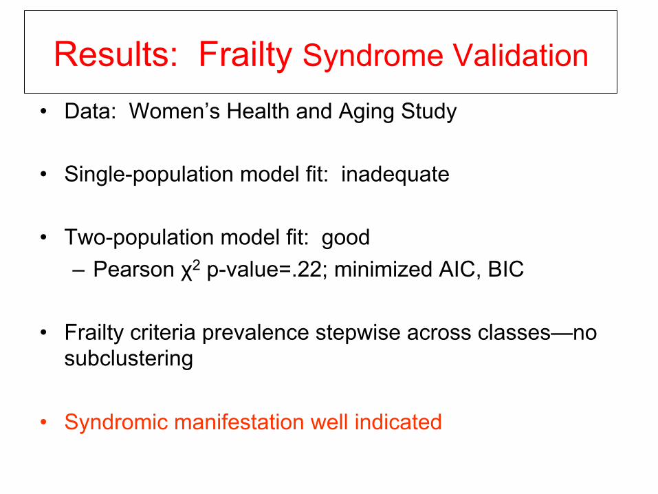
Results: Frailty Syndrome Validation

•  Data: Women’s Health and Aging Study

•  Single-population model fit: inadequate

•  Two-population model fit: good –  Pearson χ2 p-value=.22; minimized AIC, BIC

•  Frailty criteria prevalence stepwise across classes—no subclustering

•  Syndromic manifestation well indicated

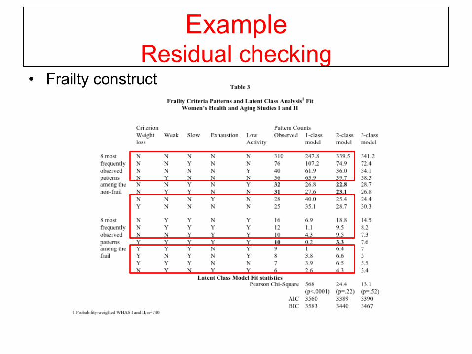
Example Residual checking

•  Frailty construct

Part IV: Identifiability / Estimability

Identifiability

{ } .);,(F Φ∈=Φ φφyF

•  Rough idea for “non”-identifiability: More unknowns than there are (independent) equations to solve for them

•  Definition: Consider a family of distributions

The parameter is (globally) identifiable iff

Φ∈φ

. )F(y,=)F(y,: ** a.eno φφφ Φ∈∃

Identifiability Related concepts

• Local identifiability • Basic idea: ϕ identified within a neighborhood

• Definition: F is locally identifiable at if there exists a neighborhood τ about

for all τ Φ.

0φ⇒= ),();(: 00 φφφ yFyF

0φφ = ∈φ

• Estimability, empirical identifiability: The information matrix for ϕ given y1,…,yn is non-singular.

⊂

Identifiability Latent class (binary Y)

• Latent class analysis (measurement only)

•  Parameter dimension: 2M -1 •  Unconstrained J-class model: J-1 + J*M

•  Need 2M ≥ J(M+1) (necessary, not sufficient)

• Local identifiability: evaluate the Jacobian of the likelihood function (Goodman, 1974)

• Estimability: Avoid fewer than 10 allocation per “cell” •  n > 10*(2M) (rule of thumb)

Identifiability / estimability Frailty example

• Latent class analysis

•  Need 2M ≥ J(M+1) (necessary, not sufficient) •  M=5; J=3; •  32 ≥ 3·(5+1) – YES •  By this criterion, could fit up to 9 classes

• Local identifiability: evaluate the Jacobian of the likelihood function (Goodman, 1974)

• Estimability: n > 10*(2M) •  n > 10*(25) = 320 - YES

Objectives For you to leave here knowing…

•  When is latent class analysis (LCA) model useful?

•  What is the LCA model its underlying assumptions? •  How are LCA parameters interpreted?

•  How are LCA parameters commonly estimated?

•  How is LCA fit adjudicated?

•  What are considerations for identifiability / estimability?