Laser radar for terrain and vegetation mapping. - FOI

Sensor Technology

SE-581 11 Linköping

FOI-R--0232--SE

October 2001

ISSN 1650-1942

Scientific report

Ove Steinvall, Dietmar Letalick, Ulf Söderman,

Lars Ulander, Anders Gustavsson

Laser radar for terrain and vegetation mapping

SWEDISH DEFENCE RESEARCH AGENCY FOI-R--0232--SE

October 2001

ISSN 1650-1942

Sensor Technology P.O. Box 1165 SE-581 11 Linköping

Scientific report

Ove Steinvall, Dietmar Letalick, Ulf Söderman,

Lars Ulander, Anders Gustavsson

Laser radar for terrain and vegetation mapping

2

Issuing organization Report number, ISRN Report type FOI – Swedish Defence Research Agency FOI-R--0232--SE Scientific report

Research area code

9. Civil applications Month year Project no.

October 2001 E3901 Customers code

5. Contracted Research Sub area code

Sensor Technology P.O. Box 1165 SE-581 11 Linköping

91 Civil Applications

Author/s (editor/s) Project manager Ove Steinvall Hans Hellsten/Lars Ulander Dietmar Letalick Approved by Ulf Söderman Lars Ulander Lars Ulander Sponsoring agency Anders Gustavsson Scientifically and technically responsible Ove Steinvall Report title

Laser radar for terrain and vegetation mapping

Abstract (not more than 200 words)

In this report we investigate the potential future for airborne laser systems for forestry applications. The report has been prepared as part of an internal FOI project on Remote Sensing for Forestry, with the aim of looking into future systems for civilian use, but keeping a glance at the military potential. We have also made a brief survey of recent relevant publications. Airborne laser scanning (ALS) systems can provide tree and ground height data and enable derivation of other important parameters like biomass estimation, tree type, etc. In analogy with the development of ALS systems for sea charting, both military and civilian applications can be identified for land applications. Military applications include mapping and reconnaissance, e.g. terrain maps to evaluate the accessibility in a terrain section. ALS systems can perform precise measurements with high accuracy and resolution, e.g. mapping of the detailed crown shape. The price to pay for this high resolution is a lower coverage rate in comparison to e.g. synthetic aperture radar (SAR) methods. For future work we suggest the development of technology and methods for fast mapping of forest and terrain with airborne laser scanning systems. Such a development would be of interest for both civilian and military applications. In particular, we suggest the development of small systems, which would lead to fast and cost effective mapping.

Keywords

airborne laser scanning, laser radar, terrain mapping, vegetation mapping

Further bibliographic information Language English

ISSN 1650-1942 Pages 108 p.

Price acc. to pricelist

Security classification

3

Utgivare Rapportnummer, ISRN Klassificering Totalförsvarets Forskningsinstitut - FOI FOI-R--0232--SE Vetenskaplig rapport

Forskningsområde

9. Övriga civila tillämpningar Månad, år Projektnummer

Oktober 2001 E3901 Verksamhetsgren

5. Uppdragsfinansierad verksamhet Delområde

Sensorteknik Box 1165 581 11 Linköping

91 Övriga civila tillämpningar

Författare/redaktör Projektledare Ove Steinvall Hans Hellsten/Lars Ulander Dietmar Letalick Godkänd av Ulf Söderman Lars Ulander Lars Ulander Uppdragsgivare/kundbeteckning Anders Gustavsson Tekniskt och/eller vetenskapligt ansvarig Ove Steinvall Rapportens titel (i översättning)

Laserradar för flygburen vegetationsmätning

Sammanfattning (högst 200 ord)

I denna rapport undersöker vi potentialen för framtida flygburna lasersystem för skogstillämpningar. Rapporten har vuxit fram som del i ett internt FOI-projekt inom fjärranalys för skogstillämpningar, med syfte att studera framtida system för civilt bruk, men där det även finns en militär potential. Vi har också gjort en översiktlig genomgång av relevant modern litteratur.Flygburna laserskanningssystem kan ge höjddata för mark och träd, vilket möjliggör beräkning av trädhöjd och andra viktiga parametrar såsom biomassa, trädtyp etc. I likhet med utvecklingen av flygburna lasersystem för sjökartering finns både militära och civila tillämpningar även för landtillämpningar. Militära tillämpningar är bl.a. kartering och spaning, t.ex. terrängkartor för att utröna tillgängligheten i ett terrängavsnitt. Med flygburna laserskanningssystem kan mätningar med hög noggrannhet och precision göras, t.ex. kartläggning av detaljerad kronform. Priset för denna höga upplösning är dock en lägre yttäckningshastighet jämfört med t.ex. SAR-system.För fortsatt arbete föreslår vi utveckling av teknik och metoder för snabb kartering av skog och terräng med flygburna lasersystem. Sådan utveckling skulle vara av intresse både för civila och militära tillämpningar. Speciellt föreslår vi utveckling av små och enkla system, vilket möjliggör snabb och kostnadseffektiv kartering.

Nyckelord

flygburen laserskanning, laserradar, terrängkartering, skogskartering

Övriga bibliografiska uppgifter Språk Svenska

ISSN 1650-1942 Antal sidor: 108 s.

Distribution enligt missiv Pris: Enligt prislista

Sekretess

FO

I100

4 U

tgåv

a 08

200

1.09

ww

w.s

igno

n.se

/FO

I S

ign

On

AB

FOI-R--00232--SE

5

%

1 Introduction 7

1.1 Background 7

1.2 Laser remote sensing in forestry 7

1.3 Relevant issues in forestry remote sensing 9

2 Laser methods for forest remote sensing 11

2.1 Range finding principles 11 2.1.1 Performance calculations for rangefinder systems 12 2.1.2 Simple waveform simulations – large and small footprints 16 2.1.3 Simulation results 19

2.2 Range imaging by gated viewing 23 2.2.1 Performance calculations for gated viewing systems 25

2.3 Streak camera 28

3 Technology 30

3.1 Lasers 30 3.1.1 Diode lasers 30 3.1.2 Solid state flash lamp pumped lasers 30 3.1.3 Diode solid state pumped lasers 30 3.1.4 Diode pumped crystal lasers 31 3.1.5 Fibre lasers 31 3.1.6 Micro-chip lasers 32

3.2 Detectors 33 3.2.1 Three dimensional technology 33 3.2.2 Photodiodes 33 3.2.3 Focal plane arrays 33 3.2.4 Intensified photodiodes 34 3.2.5 Avalanche photodiodes 35

3.3 Scanning techniques 36 3.3.1 Mechanical scanning 37 3.3.2 Types of scanners 38 3.3.3 Scanner examples in airborne laser systems 42 3.3.4 Conclusions about scanning 44

3.4 Errors in airborne scanning laser radar data 44

4 Data processing 48

4.1 Small footprint systems 48 4.1.1 Analysis of small footprint data 51 4.1.2 Tree discrimination 59 4.1.3 Tree and stand attribute estimation 60

4.2 Large footprint systems 60 4.2.1 Analysis of large footprint data 61

5 International activities in airborne laser terrain mapping 64

5.1 Examples of existing systems 66 5.1.1 The Laser Vegetation Imaging Sensor (LVIS) 66 5.1.2 TopoSys 68 5.1.3 Airborne Laser Terrain Mapper (ALTM) 69

FOI-R--00232--SE

6

5.1.4 TopEye 71 5.1.5 Riegl 71 5.1.6 Digital Airborne Topographical Imaging System 72 5.1.7 Aeroscan 73 5.1.8 Digital Orthophotography 74 5.1.9 ATLAS-SL 75 5.1.10 Toposense 75 5.1.11 Vegetation Canopy Lidar (VCL) 77

5.2 Examples of military and other developments 78 5.2.1 Low Cost Autonomous Attack System (LOCAAS) 78 5.2.2 Rapid Terrain Visualization program 79 5.2.3 Carnegie Mellon University (CMU) autonomous helicopter 79

6 Laser scanning compared with other remote sensing techniques 81

6.1 Radar 81 6.1.1 Synthetic Aperture Radar 82 6.1.2 GeoSAR 84 6.1.3 AeS-1 86 6.1.4 CARABAS-II 88

6.2 Photogrammetry (passive EO sensors) 90

7 Examples of laser system concepts for remote sensing 92

7.1 Small compact laser radar for autonomous helicopter 92

7.2 Helicopter or aircraft mounted laser/EO systems 94

7.3 Aircraft mounted radar/laser/EO systems 96

7.4 Ground based sensors 98

8 Discussion 102

9 References 104

FOI-R--00232--SE

7

&$

During the past couple of years there has been an increasing interest in airborne remote sens-ing using Digital Elevation Models (DEM) for use in city planning, mobile phone networks, forestry, flood risk assessment, power cable monitoring etc. A number of technologies can be applied to generate DEM’s from the well-established aerial photography, interferometric radar and synthetic aperture radar (SAR). Airborne laser radar is another technology with great promise.

Recently a number of airborne nadir scanning laser radars have been developed for both military and civilian applications1. These have range resolutions on the order of 10 cm but relatively moderate area coverage rates, in the range 1000-10 000 m2/s (3.6-36 km2/h) when operating in a high resolution mode with 0.25 m spot distance. Technology development in laser sources, scanning techniques and signal processing will probably improve the area cov-erage substantially and lead to compact systems suitable for new applications, including the use in unmanned aerial vehicles (UAV). In this report, we will investigate the potential for future for airborne laser systems in forestry applications. The report has been prepared as part of an internal FOI-project on Remote Sensing for Forestry, with the aim of looking into future systems for civilian use, but keeping a glance at the military potential.

In order to identify relevant issues for laser remote sensing in forestry we have discussed with researchers at the Swedish University of Agricultural Sciences, Department of Forest Resource Management and Geomatics (SLU). We have also made a brief survey of recent relevant publications. Today there is an increasing interest in this field and it has a potential to expand much farther. This potential was recognized early and research and investigations has been conducted in the past two decades covering many different applications.

Early airborne laser systems have been used to describe forest landscape topography includ-ing canopy height profile2,3, and forest vegetation characterization as canopy cover, biomass, and timber volume4,5,6. These early laser systems measured the distance to the trees and to the ground along a profile under the aircraft. Since then, laser technology has improved, scanning laser systems have been developed, and the combined use of kinematical global positioning system (GPS) and Inertial Navigation Systems (INS) has revolutionised aircraft positioning. Recent commercial high-resolution small-footprint laser scanning systems have been used to estimate tree and stand heights, stand volume, canopy cover, basal area and biomass7-12. High-resolution georeferenced DEMs has also been obtained for both ground and canopy sur-face13,14. Recent research instruments from NASA (SLICER, LVIS) use large footprints and allow utilization of the complete time varying distribution of the return pulse energy, or wave-form. This provides means for measuring topography, vegetation characterization and canopy vertical structure15-17.

Studies about forestry measurements using scanning laser have been published by Nilsson7 and Naesset9. Nilsson investigated whether tree heights and bole volumes in a young pine forest could be estimated. The results, which indicated that this was possible, were also well in accordance with earlier results18.

In 1991, a test was made together with FOI in Linköping. The aim was to evaluate tree height and bole volume estimation using a scanning laser. The test was made for a limited area (27 sample plots) in the archipelago of Stockholm, and was repeated during three different sea-

FOI-R--00232--SE

8

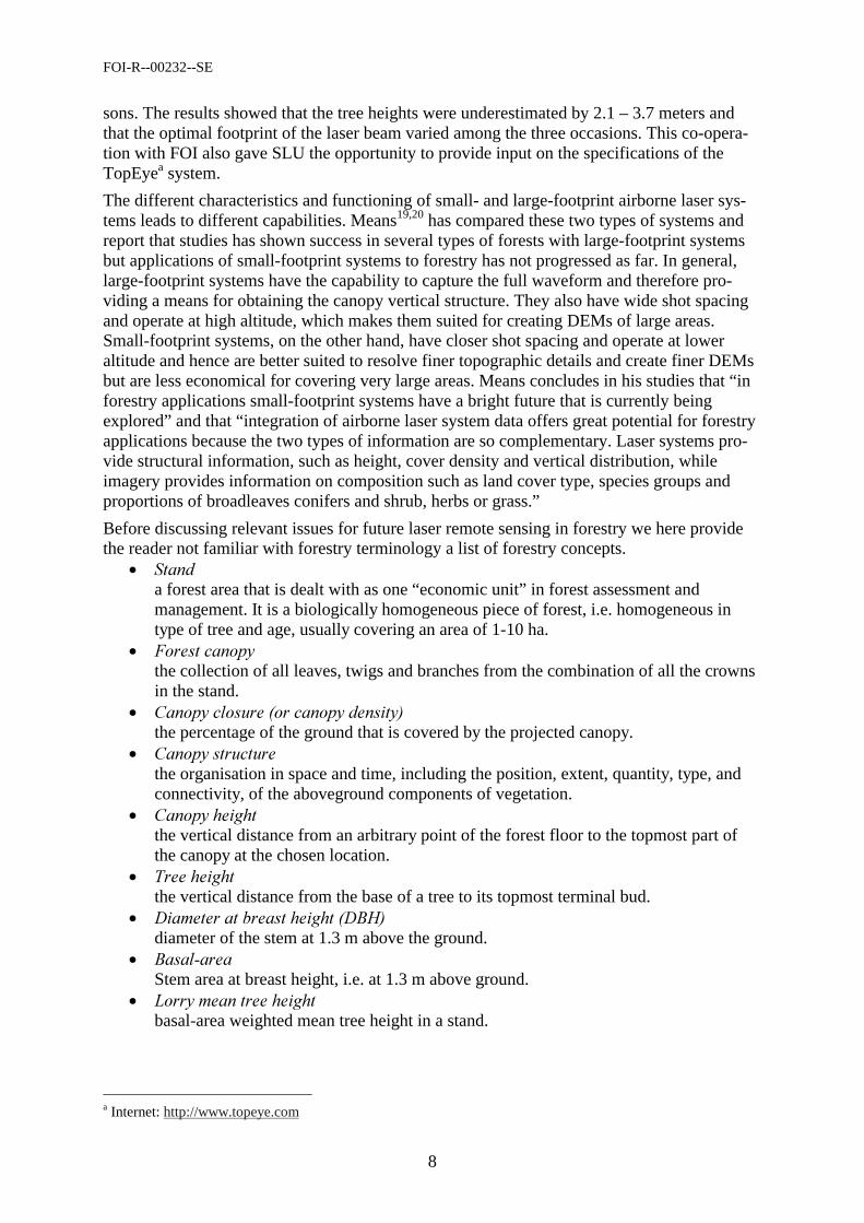
sons. The results showed that the tree heights were underestimated by 2.1 – 3.7 meters and that the optimal footprint of the laser beam varied among the three occasions. This co-opera-tion with FOI also gave SLU the opportunity to provide input on the specifications of the TopEyea system.

The different characteristics and functioning of small- and large-footprint airborne laser sys-tems leads to different capabilities. Means19,20 has compared these two types of systems and report that studies has shown success in several types of forests with large-footprint systems but applications of small-footprint systems to forestry has not progressed as far. In general, large-footprint systems have the capability to capture the full waveform and therefore pro-viding a means for obtaining the canopy vertical structure. They also have wide shot spacing and operate at high altitude, which makes them suited for creating DEMs of large areas. Small-footprint systems, on the other hand, have closer shot spacing and operate at lower altitude and hence are better suited to resolve finer topographic details and create finer DEMs but are less economical for covering very large areas. Means concludes in his studies that “in forestry applications small-footprint systems have a bright future that is currently being explored” and that “integration of airborne laser system data offers great potential for forestry applications because the two types of information are so complementary. Laser systems pro-vide structural information, such as height, cover density and vertical distribution, while imagery provides information on composition such as land cover type, species groups and proportions of broadleaves conifers and shrub, herbs or grass.”

Before discussing relevant issues for future laser remote sensing in forestry we here provide the reader not familiar with forestry terminology a list of forestry concepts.

• a forest area that is dealt with as one “economic unit” in forest assessment and management. It is a biologically homogeneous piece of forest, i.e. homogeneous in type of tree and age, usually covering an area of 1-10 ha.

• the collection of all leaves, twigs and branches from the combination of all the crowns in the stand.

• the percentage of the ground that is covered by the projected canopy.

• the organisation in space and time, including the position, extent, quantity, type, and connectivity, of the aboveground components of vegetation.

• the vertical distance from an arbitrary point of the forest floor to the topmost part of the canopy at the chosen location.

• the vertical distance from the base of a tree to its topmost terminal bud.

• diameter of the stem at 1.3 m above the ground.

• Stem area at breast height, i.e. at 1.3 m above ground.

• basal-area weighted mean tree height in a stand.

a Internet: http://www.topeye.com

FOI-R--00232--SE

9

It is clear that there are many potential areas of application of airborne laser scanning in for-estry. For small-footprint systems, the most imitated ones seem to be in stand or small region forest inventory and mapping. The technology seems to have the best potential of producing better, faster and cheaper results than traditional methods, which usually are time consuming, laborious and expensive.

Tree height measurements, for example, have traditionally been done either by hand in the field or by photogrammetric measurements using aerial photos. Manual measurements are often both difficult and time consuming and are especially problematic when the forest canopy is dense. Photogrammetric approaches consist of finding the difference between tree altitude and nearby ground altitude using stereo comparisons. However, since seeing the ground is of critical importance, good results can only be achieved in open forest covers, a situation seldom encountered in mature commercial stands of boreal forest. Methods based on airborne laser scanner systems, on the other hand, are expected to be able to provide good estimates of tree height and have also been give considerable attention in various studies10,12,21,22.

For large-footprint systems, which still only exist as research systems, the main applications are in research concerning forest ecosystem. Future potential applications can be found in environment management, e.g. landscape rehabilitation, ecological sustainability, studies con-cerning the “greenhouse effect”, etc. There is also a potential for large-footprint systems in forestry mapping, in order to give a measure of tree mean height and crown density.

In forest inventory and mapping there are many stand structure and/or tree attributes of inter-est. We have found the following attributes as the most important from point of view of a laser system measurement:

• canopy height, canopy closure, canopy size, canopy form, • tree height, tree position, • tree species and proportions, • canopy vertical structure.

Using these attributes as indices many other attributes of interest can be estimated using sta-tistical methods, for example, stand heights, stand volume, stem diameter, basal area, size and number of stems per unit area, age classes, biomass, foliage amount and foliage spatial den-sity etc.

The focus of this report is on potential future laser methods in forest remote sensing. Having stated that, we will primarily discuss issues involving the attributes mentioned above. In that context, we have found the following issues most relevant for laser remote sensing in forestry:

• To be able to discriminate and count the individual trees in forest stands and for each one of them obtain: - position, - height, - canopy closure, - canopy form, - species.

• To be able to repeat the measurements later on (one or more years later), and to iden-tify and correlate the obtained tree attributes with earlier measurements.

• To be able to obtain canopy vertical structure.

It should be noted that airborne laser scanner data collected over forests provide canopy height and that laser canopy heights always underestimate the true tree and stand height. This

FOI-R--00232--SE

10

since most of the laser hits is at locations below the treetops. In the case of canopy gaps, the ground level or the side of a tree is measured.

To obtain good estimates of tree heights data processing is necessary. The most straightfor-ward approach is to take the difference between an estimate of the height of the top of the tree and an estimate of the ground level beneath the tree. Is not straightforward to estimate the accurate height of a tree, as laser hits are “randomly” distributed on the tree canopy. High density of laser measurements and support from ancillary data like imagery can make it easier to accurately locate the top and estimates its height. This is also true for canopy form and tree species. To estimate the ground level special data processing is necessary. Ground measure-ments must be separated from canopy measurements. A number of approaches for obtaining DEMs of the ground exist today. One promising approach has been developed at FOI in Linköping. We will review these in a later section when discussing data processing.

Beside the requirement of high-density measurements for the first issue, the second issue implies a requirement of high accuracy georeferencing and the last issue a requirement that the laser system have the capability to capture and store all the data necessary to describe the full waveform. Fortunately, technology development is heading in a direction having the potential of making all this possible, which we will discuss and demonstrate in this report.

FOI-R--00232--SE

11

'

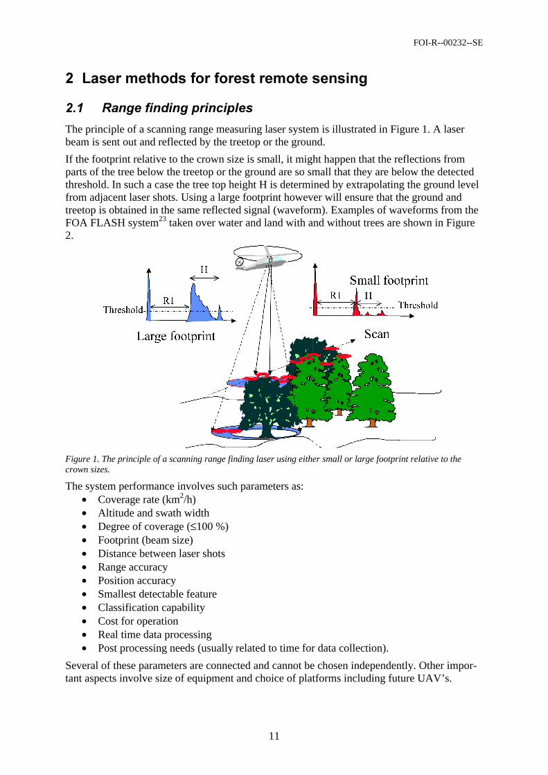
The principle of a scanning range measuring laser system is illustrated in Figure 1. A laser beam is sent out and reflected by the treetop or the ground.

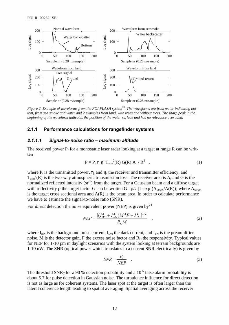
If the footprint relative to the crown size is small, it might happen that the reflections from parts of the tree below the treetop or the ground are so small that they are below the detected threshold. In such a case the tree top height H is determined by extrapolating the ground level from adjacent laser shots. Using a large footprint however will ensure that the ground and treetop is obtained in the same reflected signal (waveform). Examples of waveforms from the FOA FLASH system23 taken over water and land with and without trees are shown in Figure 2.

Figure 1. The principle of a scanning range finding laser using either small or large footprint relative to the crown sizes.

The system performance involves such parameters as: • Coverage rate (km2/h) • Altitude and swath width • Degree of coverage (≤100 %) • Footprint (beam size) • Distance between laser shots • Range accuracy • Position accuracy • Smallest detectable feature • Classification capability • Cost for operation • Real time data processing • Post processing needs (usually related to time for data collection).

Several of these parameters are connected and cannot be chosen independently. Other impor-tant aspects involve size of equipment and choice of platforms including future UAV’s.

FOI-R--00232--SE

12

0

100

200

0 50 100 150 200

Normal waveform

Sample nr (0.28 m/sample)

Log

sig

nal

0

100

200

0 50 100 150 200

Waveform from seasmoke

Sample nr (0.28 m/sample)

Log

sig

nal

0

100

200

300

0 50 100 150 200

Waveform from land

Sample nr (0.28 m/sample)

Log

sig

nal

0

100

200

300

0 50 100 150 200

Waveform from land

Sample nr (0.28 m/sample)L

og s

igna

l

Water backscatter

Bottom

Water backscatter

Ground

Tree signal

Ground return

Figure 2. Example of waveforms from the FOI FLASH system23. The waveforms are from water indicating bot-tom, from sea smoke and water and 2 examples from land, with trees and without trees. The sharp peak in the beginning of the waveform indicates the position of the water surface and has no relevance over land.

(( ) $ *

The received power Pr for a monostatic laser radar looking at a target at range R can be writ-ten

Pr= Pt ηrηt Tatm2(R) G(R) Ar / R

2 , (1)

where Pt is the transmitted power, ηr and ηt the receiver and transmitter efficiency, and Tatm

2(R) is the two-way atmospheric transmission loss. The receiver area is Ar and G is the normalized reflected intensity (sr-1) from the target. For a Gaussian beam and a diffuse target with reflectivity ρ the target factor G can be written G= ρ/ -exp-(Atarget/A(R))] where Atarget is the target cross sectional area and A(R) is the beam area. In order to calculate performance we have to estimate the signal-to-noise ratio (SNR).

For direct detection the noise equivalent power (NEP) is given by24

!!!"#$

'

31'1%1

2/12222 ])[( ++= , (2)

where IBN is the background noise current, IDN the dark current, and IPN is the preamplifier noise. M is the detector gain, F the excess noise factor and RD the responsivity. Typical values for NEP for 1-10 µm in daylight scenarios with the system looking at terrain backgrounds are 1-10 nW. The SNR (optical power which translates to a current SNR electrically) is given by

"#$$

" U= . (3)

The threshold SNRT for a 90 % detection probability and a 10-5 false alarm probability is about 5.7 for pulse detection in Gaussian noise. The turbulence influence for direct detection is not as large as for coherent systems. The laser spot at the target is often larger than the lateral coherence length leading to spatial averaging. Spatial averaging across the receiver

FOI-R--00232--SE

13

will also reduce scintillation effects. For direct detection systems atmospheric turbulence can be treated as an SNR-enhancement factor, FSNR, given by25

( ),G,615$% ln

21ln 5,0)12(2exp σσ +−= −

, (4)

where σ2lnI is the aperture averaged log-intensity variance, erf the error function and Pd the

detection probability. The aperture averaging will be of importance when the Fresnel radius (λR)0,5 is smaller than the receiver aperture diameter. For 1 µm this occurs for ranges less than 10 km and for 10 µm for ranges less than about 1 km. The aperture averaging can be esti-mated from Fried26. In general, we find from excellent agreement between theory and experi-ment concerning aperture averaging and the lognormal distribution of the turbulence below saturation using direct detection27. Normally we find that the turbulence effects are small for nadir looking systems due to the decrease of turbulence with altitude.

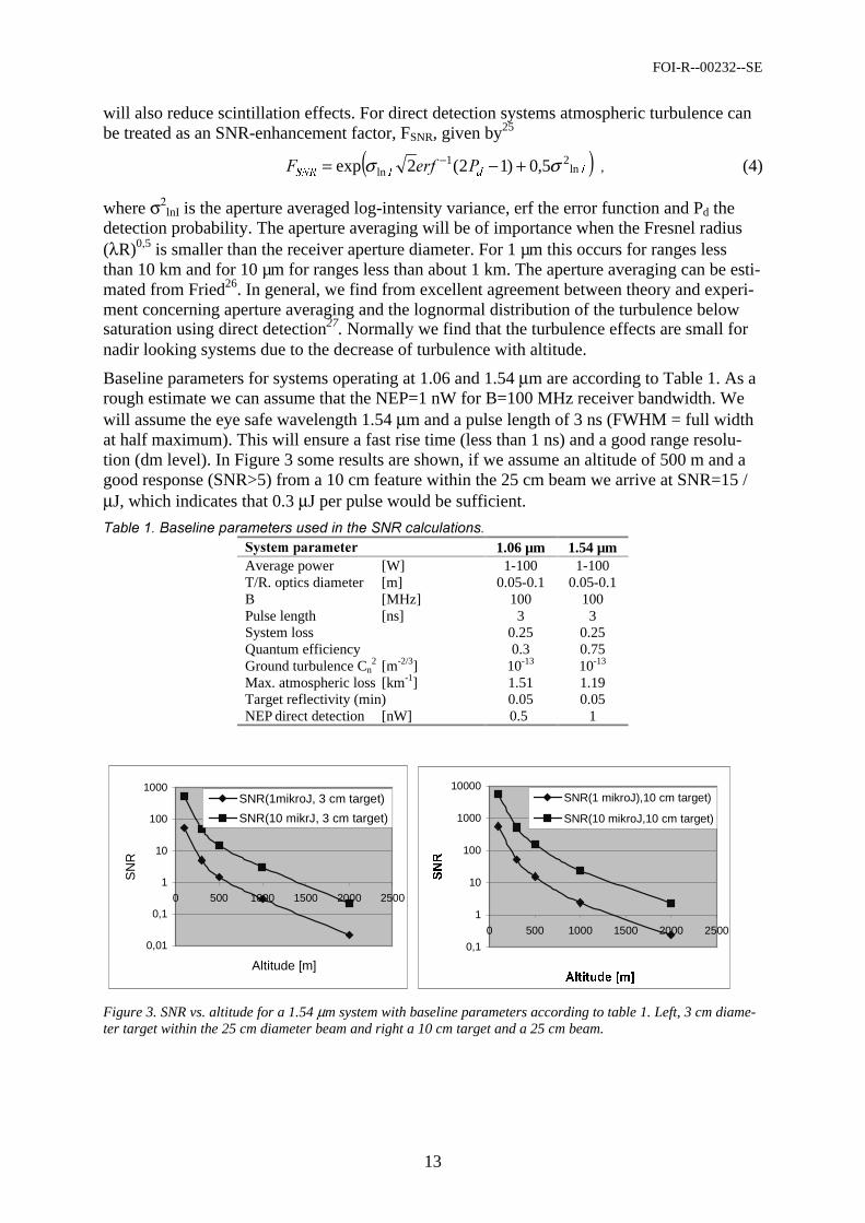
Baseline parameters for systems operating at 1.06 and 1.54 µm are according to Table 1. As a rough estimate we can assume that the NEP=1 nW for B=100 MHz receiver bandwidth. We will assume the eye safe wavelength 1.54 µm and a pulse length of 3 ns (FWHM = full width at half maximum). This will ensure a fast rise time (less than 1 ns) and a good range resolu-tion (dm level). In Figure 3 some results are shown, if we assume an altitude of 500 m and a good response (SNR>5) from a 10 cm feature within the 25 cm beam we arrive at SNR=15 / µJ, which indicates that 0.3 µJ per pulse would be sufficient.

1.06 µm 1.54 µm Average power [W] 1-100 1-100 T/R. optics diameter [m] 0.05-0.1 0.05-0.1 B [MHz] 100 100 Pulse length [ns] 3 3 System loss 0.25 0.25 Quantum efficiency 0.3 0.75 Ground turbulence Cn

2 [m-2/3] 10-13 10-13 Max. atmospheric loss [km-1] 1.51 1.19 Target reflectivity (min) 0.05 0.05 NEP direct detection [nW] 0.5 1

0,01

0,1

1

10

100

1000

0 500 1000 1500 2000 2500

Altitude [m]

SN

R

SNR(1mikroJ, 3 cm target)

SNR(10 mikrJ, 3 cm target)

0,1

1

10

100

1000

10000

0 500 1000 1500 2000 2500

$OWLWXGH>P@

615

SNR(1 mikroJ),10 cm target)

SNR(10 mikroJ,10 cm target)

Figure 3. SNR vs. altitude for a 1.54 µm system with baseline parameters according to table 1. Left, 3 cm diame-ter target within the 25 cm diameter beam and right a 10 cm target and a 25 cm beam.

FOI-R--00232--SE

14

!"

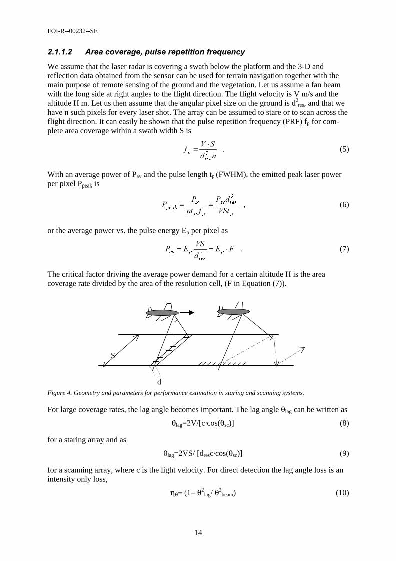
We assume that the laser radar is covering a swath below the platform and the 3-D and reflection data obtained from the sensor can be used for terrain navigation together with the main purpose of remote sensing of the ground and the vegetation. Let us assume a fan beam with the long side at right angles to the flight direction. The flight velocity is V m/s and the altitude H m. Let us then assume that the angular pixel size on the ground is d2

res, and that we have n such pixels for every laser shot. The array can be assumed to stare or to scan across the flight direction. It can easily be shown that the pulse repetition frequency (PRF) fp for com-plete area coverage within a swath width S is

&%

UHV

S

⋅= . (5)

With an average power of Pav and the pulse length tp (FWHM), the emitted peak laser power per pixel Ppeak is

S

UHVDY

SS

DYSHDN &

$%

$$ == , (6)

or the average power vs. the pulse energy Ep per pixel as

#

&#$ S

UHV

SDY ⋅== . (7)

The critical factor driving the average power demand for a certain altitude H is the area coverage rate divided by the area of the resolution cell, (F in Equation (7)).

Figure 4. Geometry and parameters for performance estimation in staring and scanning systems.

For large coverage rates, the lag angle becomes important. The lag angle θlag can be written as

θlag=2V/[c·cos(θsc)] (8)

for a staring array and as

θlag=2VS/ [dresc·cos(θsc)] (9)

for a scanning array, where c is the light velocity. For direct detection the lag angle loss is an intensity only loss,

ηθ= (1− θ2lag/ θ2

beam) (10)

S

d

FOI-R--00232--SE

15

As long as 4· θ2lag/ θ2

beam<<1 this loss is small.

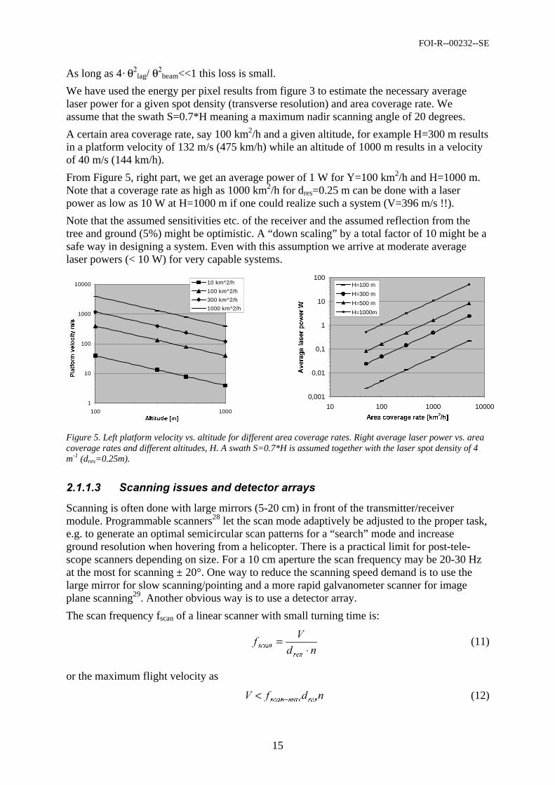
We have used the energy per pixel results from figure 3 to estimate the necessary average laser power for a given spot density (transverse resolution) and area coverage rate. We assume that the swath S=0.7*H meaning a maximum nadir scanning angle of 20 degrees.

A certain area coverage rate, say 100 km2/h and a given altitude, for example H=300 m results in a platform velocity of 132 m/s (475 km/h) while an altitude of 1000 m results in a velocity of 40 m/s (144 km/h).

From Figure 5, right part, we get an average power of 1 W for Y=100 km2/h and H=1000 m. Note that a coverage rate as high as 1000 km2/h for dres=0.25 m can be done with a laser power as low as 10 W at H=1000 m if one could realize such a system (V=396 m/s !!).

Note that the assumed sensitivities etc. of the receiver and the assumed reflection from the tree and ground (5%) might be optimistic. A “down scaling” by a total factor of 10 might be a safe way in designing a system. Even with this assumption we arrive at moderate average laser powers (< 10 W) for very capable systems.

1

10

100

1000

10000

100 1000$OWLWXGH>P@

3ODWIRUPYHORFLW\PV

10 km^2/h

100 km^2/h

300 km^2/h

1000 km^2/h

0,001

0,01

0,1

1

10

100

10 100 1000 10000

$UHDFRYHUDJHUDWH>NPK@

$YHUDJHODVHUSRZHU:

H=100 m

H=300 m

H=500 m

H=1000m

Figure 5. Left platform velocity vs. altitude for different area coverage rates. Right average laser power vs. area coverage rates and different altitudes, H. A swath S=0.7*H is assumed together with the laser spot density of 4 m-1 (dres=0.25m).

Scanning is often done with large mirrors (5-20 cm) in front of the transmitter/receiver module. Programmable scanners28 let the scan mode adaptively be adjusted to the proper task, e.g. to generate an optimal semicircular scan patterns for a “search” mode and increase ground resolution when hovering from a helicopter. There is a practical limit for post-tele-scope scanners depending on size. For a 10 cm aperture the scan frequency may be 20-30 Hz at the most for scanning ± 20°. One way to reduce the scanning speed demand is to use the large mirror for slow scanning/pointing and a more rapid galvanometer scanner for image plane scanning29. Another obvious way is to use a detector array.

The scan frequency fscan of a linear scanner with small turning time is:

&%

UHV

VFDQ ⋅= (11)

or the maximum flight velocity as

%& UHVPD[VFDQ−< (12)

FOI-R--00232--SE

16

For fscan-max= 20 Hz and dres=0.25m results in a velocity V of <5*n m/s. A detector array with n>10 is needed to get reasonable velocities and area coverage rates.

#

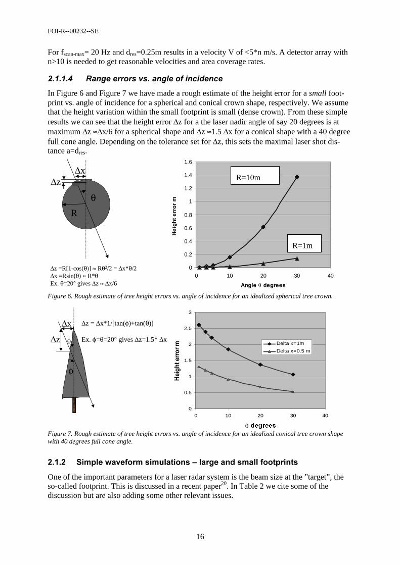
In Figure 6 and Figure 7 we have made a rough estimate of the height error for a small foot-print vs. angle of incidence for a spherical and conical crown shape, respectively. We assume that the height variation within the small footprint is small (dense crown). From these simple results we can see that the height error ∆z for a the laser nadir angle of say 20 degrees is at maximum ∆z ≈∆x/6 for a spherical shape and ∆z ≈1.5 ∆x for a conical shape with a 40 degree full cone angle. Depending on the tolerance set for ∆z, this sets the maximal laser shot dis-tance a=dres.

θR

∆z∆x

∆z =R[1-cos(θ)] ≈ Rθ2/2 = ∆x*θ/2 ∆x =Rsin(θ) ≈ R*θEx. θ=20° gives ∆z ≈ ∆x/6

Figure 6. Rough estimate of tree height errors vs. angle of incidence for an idealized spherical tree crown.

φ

θ

∆x

∆z

∆z = ∆x*1/[tan(φ)+tan(θ)]

Ex. φ=θ=20° gives ∆z=1.5* ∆x

Figure 7. Rough estimate of tree height errors vs. angle of incidence for an idealized conical tree crown shape with 40 degrees full cone angle.

(( + $,

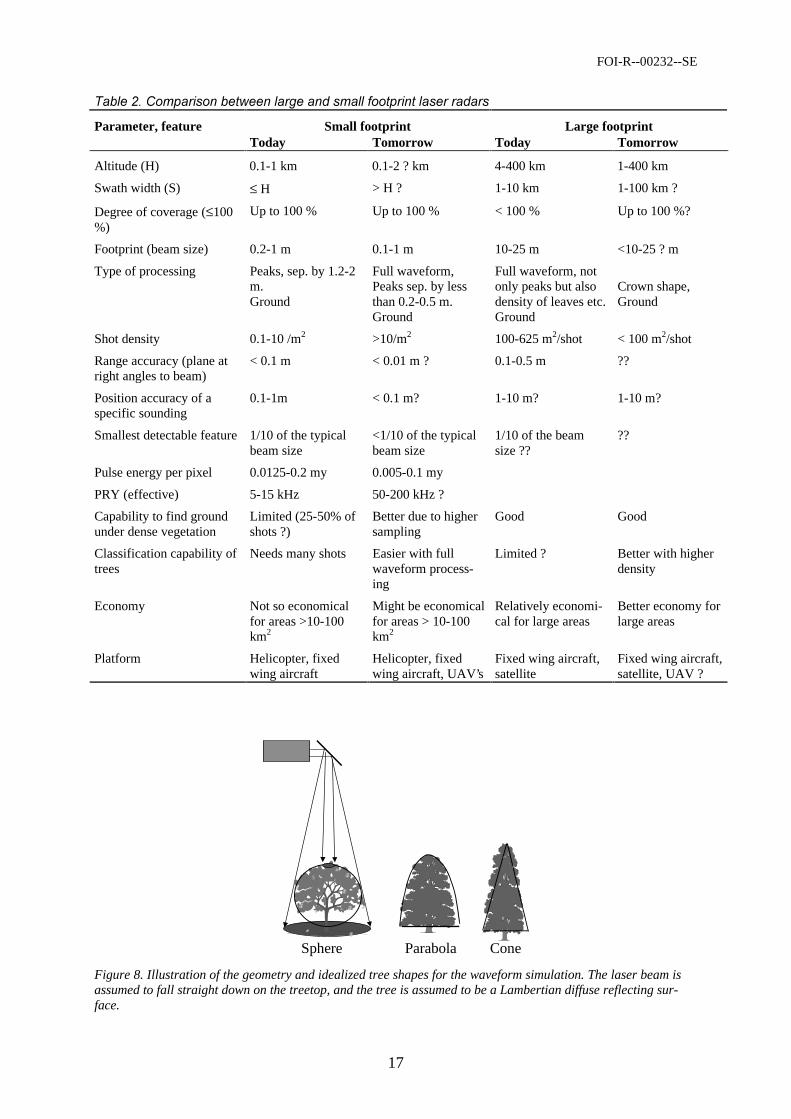
One of the important parameters for a laser radar system is the beam size at the ”target”, the so-called footprint. This is discussed in a recent paper20. In Table 2 we cite some of the discussion but are also adding some other relevant issues.

0

0.2

0.4

0.6

0.8

1

1.2

1.4

1.6

0 10 20 30 40

Angle θ degrees

Hei

ght e

rror

mR=10m

R=1m

0

0.5

1

1.5

2

2.5

3

0 10 20 30 40

θGHJUHHV

- ' Delta x=1m

Delta x=0.5 m

FOI-R--00232--SE

17

Parameter, feature Small footprint Large footprint Today Tomorrow Today Tomorrow

Altitude (H) 0.1-1 km 0.1-2 ? km 4-400 km 1-400 km

Swath width (S) ≤ H > H ? 1-10 km 1-100 km ?

Degree of coverage (≤100 %)

Up to 100 % Up to 100 % < 100 % Up to 100 %?

Footprint (beam size) 0.2-1 m 0.1-1 m 10-25 m <10-25 ? m

Type of processing Peaks, sep. by 1.2-2 m. Ground

Full waveform, Peaks sep. by less than 0.2-0.5 m. Ground

Full waveform, not only peaks but also density of leaves etc. Ground

Crown shape, Ground

Shot density 0.1-10 /m2 >10/m2 100-625 m2/shot < 100 m2/shot

Range accuracy (plane at right angles to beam)

< 0.1 m < 0.01 m ? 0.1-0.5 m ??

Position accuracy of a specific sounding

0.1-1m < 0.1 m? 1-10 m? 1-10 m?

Smallest detectable feature 1/10 of the typical beam size

<1/10 of the typical beam size

1/10 of the beam size ??

??

Pulse energy per pixel 0.0125-0.2 my 0.005-0.1 my

PRY (effective) 5-15 kHz 50-200 kHz ?

Capability to find ground under dense vegetation

Limited (25-50% of shots ?)

Better due to higher sampling

Good Good

Classification capability of trees

Needs many shots Easier with full waveform process-ing

Limited ? Better with higher density

Economy Not so economical for areas >10-100 km2

Might be economical for areas > 10-100 km2

Relatively economi-cal for large areas

Better economy for large areas

Platform Helicopter, fixed wing aircraft

Helicopter, fixed wing aircraft, UAV’s

Fixed wing aircraft, satellite

Fixed wing aircraft, satellite, UAV ?

$

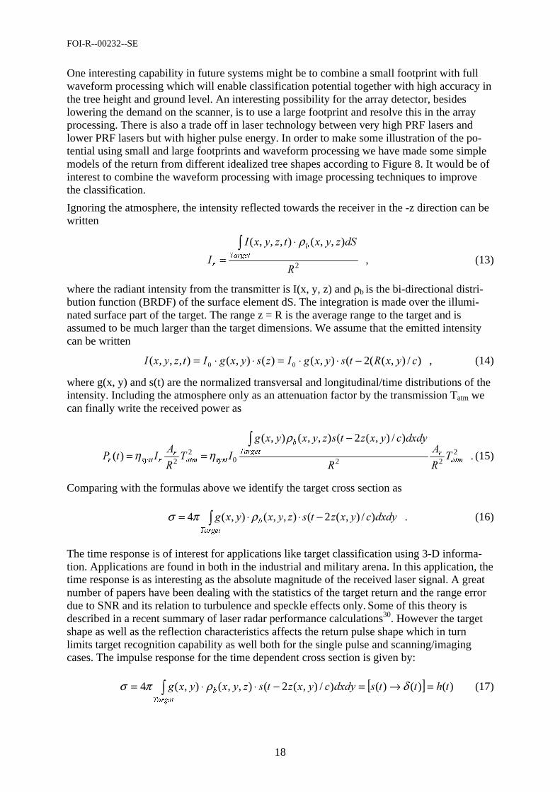
Sphere Parabola Cone Figure 8. Illustration of the geometry and idealized tree shapes for the waveform simulation. The laser beam is assumed to fall straight down on the treetop, and the tree is assumed to be a Lambertian diffuse reflecting sur-face.

FOI-R--00232--SE

18

One interesting capability in future systems might be to combine a small footprint with full waveform processing which will enable classification potential together with high accuracy in the tree height and ground level. An interesting possibility for the array detector, besides lowering the demand on the scanner, is to use a large footprint and resolve this in the array processing. There is also a trade off in laser technology between very high PRF lasers and lower PRF lasers but with higher pulse energy. In order to make some illustration of the po-tential using small and large footprints and waveform processing we have made some simple models of the return from different idealized tree shapes according to Figure 8. It would be of interest to combine the waveform processing with image processing techniques to improve the classification.

Ignoring the atmosphere, the intensity reflected towards the receiver in the -z direction can be written

2

),,(),,,(

'('(!

! 7DUJHW

E

U

∫ ⋅=

ρ , (13)

where the radiant intensity from the transmitter is I(x, y, z) and ρb is the bi-directional distri-bution function (BRDF) of the surface element dS. The integration is made over the illumi-nated surface part of the target. The range z = R is the average range to the target and is assumed to be much larger than the target dimensions. We assume that the emitted intensity can be written

)/),((2(),()(),(),,,( 00 ( (!'(!'(! −⋅⋅=⋅⋅= , (14)

where g(x, y) and s(t) are the normalized transversal and longitudinal/time distributions of the intensity. Including the atmosphere only as an attenuation factor by the transmission Tatm we can finally write the received power as

2220

22

)/),(2(),,(),(

)( DWPU7DUJHW

E

V\VWDWPU

UV\VWU

)

((''((

!

)!$

∫ −==

ρηη . (15)

Comparing with the formulas above we identify the target cross section as

∫ −⋅⋅=7DUJHW

E ((''(( )/),(2(),,(),(4 ρπσ . (16)

The time response is of interest for applications like target classification using 3-D informa-tion. Applications are found in both in the industrial and military arena. In this application, the time response is as interesting as the absolute magnitude of the received laser signal. A great number of papers have been dealing with the statistics of the target return and the range error due to SNR and its relation to turbulence and speckle effects only. Some of this theory is described in a recent summary of laser radar performance calculations30. However the target shape as well as the reflection characteristics affects the return pulse shape which in turn limits target recognition capability as well both for the single pulse and scanning/imaging cases. The impulse response for the time dependent cross section is given by:

[ ] )()()()/),(2(),,(),(4 ((''((7DUJHW

E =→=−⋅⋅= ∫ δρπσ (17)

FOI-R--00232--SE

19

The derivation of the impulse response h(t) is thus straightforward as it only depends on the product of the target shape function and the reflectivity distribution. Using the impulse response for an arbitrary laser pulse shape is obtained from the well-known relation in linear system theory:

∫∞

∞−

−= τττ )()()( (18)

Below we will show the impulse response for the objects under investigation.

(( $ $

In the simulations below, we have assumed a Gaussian beam profile with an irradiance profile:

)2exp(2

2

*

!! −⋅= (19)

with a 1/e2 radius =w. The outgoing laser pulse has been given the time function

)exp(

+

$ −⋅= (20)

A pulse with τ=1 ns (i.e. FWHM=3.6 ns has been chosen) as a reasonable laser pulse time. The energy has been kept constant for each pulse. The trees have been assumed to be dif-fusely reflecting with no transmission and with the same reflection coefficient as the flat ground.

$

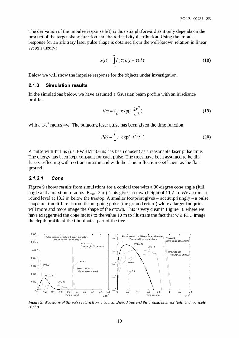
Figure 9 shows results from simulations for a conical tree with a 30-degree cone angle (full angle and a maximum radius, Rmax=3 m). This gives a crown height of 11.2 m. We assume a round level at 13.2 m below the treetop. A smaller footprint gives – not surprisingly – a pulse shape not too different from the outgoing pulse (the ground return) while a larger footprint will more and more image the shape of the crown. This is very clear in Figure 10 where we have exaggerated the cone radius to the value 10 m to illustrate the fact that w ≥ Rmax image the depth profile of the illuminated part of the tree.

0 0.2 0.4 0.6 0.8 1 1.2 1.4 1.6 1.8

x 10-7

0

0.002

0.004

0.006

0.008

0.01

0.012

0.014Pulse returns for different beam diameter.

Simulated tree: cone shape

Time seconds

(ground echo =laser puse shape)

w=6 m

w=3 m

w=0.3

Rmax=3 m Cone angle 30 degrees

w=1.2 m

0 0.2 0.4 0.6 0.8 1 1.2 1.4

x 10-7

10-6

10-5

10-4

10-3

10-2 Pulse returns for different beam diameter.

Simulated tree: cone shape

Time seconds

(ground echo =laser puse shape)

w=6 m

w=3 m

w=0.3

Rmax=3 m Cone angle 30 degrees

w=1.2 m

Figure 9. Waveform of the pulse return from a conical shaped tree and the ground in linear (left) and log scale (right).

FOI-R--00232--SE

20

0 0.5 1 1.5 2 2.5

x 10-8

0

5

10

15

20

25

30

35

40

45

Rmax=10 m Cone Cone angle=30 degrees

Time seconds

Laser pulse

Wbeam= 1m

Wbeam= 0.5 m

Wbeam= 10m

Wbeam=100 m Wbeam=200 m

Tree profile

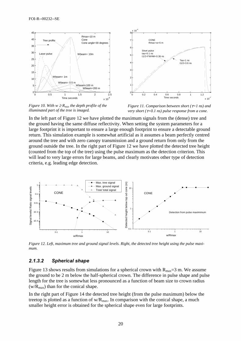
Figure 10. With w ≥ Rmax the depth profile of the illuminated part of the tree is imaged.

0 0.2 0.4 0.6 0.8 1 1.2

x 10-7

0

1

2

3

4

5

6

7

8x 10

-4

Time seconds

CONERmax=w=5 m

Short pulse tau=0.1 nst1/2=FWHM=0.36 ns

Tau=1 nst1/2=3.6 ns

Figure 11. Comparison between short (τ=1 ns) and very short (τ=0.1 ns) pulse response from a cone.

In the left part of Figure 12 we have plotted the maximum signals from the (dense) tree and the ground having the same diffuse reflectivity. When setting the system parameters for a large footprint it is important to ensure a large enough footprint to ensure a detectable ground return. This simulation example is somewhat artificial as it assumes a beam perfectly centred around the tree and with zero canopy transmission and a ground return from only from the ground outside the tree. In the right part of Figure 12 we have plotted the detected tree height (counted from the top of the tree) using the pulse maximum as the detection criterion. This will lead to very large errors for large beams, and clearly motivates other type of detection criteria, e.g. leading edge detection.

0.1 1 10

1E-4

1E-3

0.01

0.1

1

CONE

Max. tree signal Max. ground signal Tree/ total signal

Sig

nal l

evel

s/ R

atio

sig

nal l

evel

s

w/Rmax

0.1 1 100.1

1

10

CONE

Detection from pulse maximimum

Det

ecte

d he

ight

bel

ow to

p od

con

e (m

)

w/Rmax Figure 12. Left, maximum tree and ground signal levels. Right, the detected tree height using the pulse maxi-mum.

%%

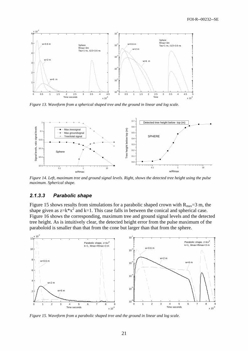
Figure 13 shows results from simulations for a spherical crown with Rmax=3 m. We assume the ground to be 2 m below the half-spherical crown. The difference in pulse shape and pulse length for the tree is somewhat less pronounced as a function of beam size to crown radius (w/Rmax) than for the conical shape.

In the right part of Figure 14 the detected tree height (from the pulse maximum) below the treetop is plotted as a function of w/Rmax. In comparison with the conical shape, a much smaller height error is obtained for the spherical shape even for large footprints.

FOI-R--00232--SE

21

0 0.5 1 1.5 2 2.5 3 3.5 4 4.5

x 10-8

1

2

3

4

5

6x 10

-3

Time seconds

w=0.6 m Sphere Rmax=3m Tau=1 ns, t1/2=3.6 ns

w=2 m

w=6 m

0 0.5 1 1.5 2 2.5 3 3.5 4 4.5 5

x 10-8

10-6

10-5

10-4

10-3

10-2

10-1

Time

w=0.6 m

Sphere Rmax=3m Tau=1 ns, t1/2=3.6 ns

w=2 m

w=6 m

Figure 13. Waveform from a spherical shaped tree and the ground in linear and log scale.

0.1 1 101E-5

1E-4

1E-3

0.01

0.1

1

Sphere

Max.treesignal Max.groundsignal Tree/total signal

Sig

nal l

evel

s, r

atio

sig

nal l

evel

s

w/Rmax

0.1 1 10

0.0

0.1

0.2

0.3

0.4

0.5

0.6

0.7

SPHERE

Detected tree height below top (m)

Tre

e he

ight

bel

ow to

p (m

)

w/Rmax Figure 14. Left, maximum tree and ground signal levels. Right, shows the detected tree height using the pulse maximum. Spherical shape.

&'%

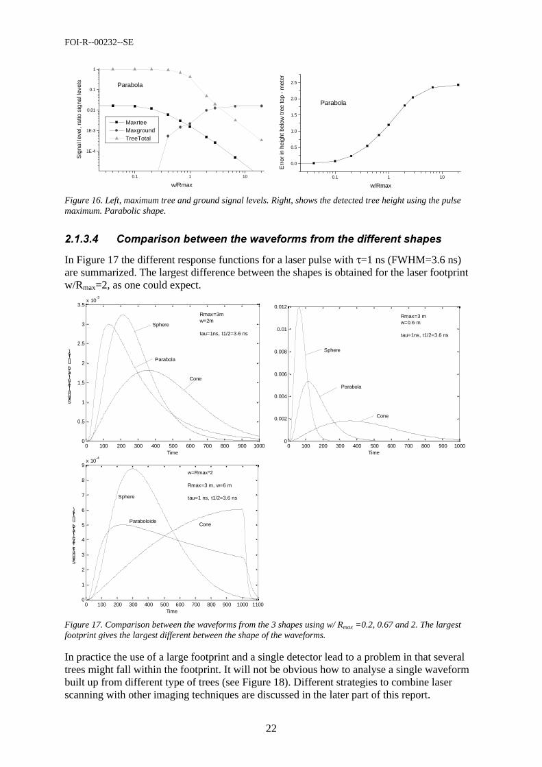
Figure 15 shows results from simulations for a parabolic shaped crown with Rmax=3 m, the shape given as z=k*x2 and k=1. This case falls in between the conical and spherical case. Figure 16 shows the corresponding, maximum tree and ground signal levels and the detected tree height. As is intuitively clear, the detected height error from the pulse maximum of the paraboloid is smaller than that from the cone but larger than that from the sphere.

0 1 2 3 4 5 6 7 8 9

x 10-8

2

4

6

8

10

12x 10

-3

Time seconds

w=0.6 m

w=2 m

w=6 m

Parabolic shape, z=kx2 k=1, Xmax=Rmax=3 m

Figure 15. Waveform from a parabolic shaped tree and the ground in linear and log scale.

0 1 2 3 4 5 6 7 8 9

x 10-8

10-6

10-5

10-4

10-3

10-2

10-1

Time seconds

w=0.6 m

w=2 m

w=6 m

Parabolic shape, z=kx2 k=1, Xmax=Rmax=3 m

FOI-R--00232--SE

22

0.1 1 10

1E-4

1E-3

0.01

0.1

1

Parabola

Maxrtee Maxground TreeTotal

Sig

nal l

evel

, rat

io s

igna

l lev

els

w/Rmax0.1 1 10

0.0

0.5

1.0

1.5

2.0

2.5

Parabola

Err

or in

hei

ght b

elow

tree

top

- m

eter

w/Rmax Figure 16.Left, maximum tree and ground signal levels. Right, shows the detected tree height using the pulse maximum. Parabolic shape.

# $'(%(% %

In Figure 17 the different response functions for a laser pulse with τ=1 ns (FWHM=3.6 ns) are summarized. The largest difference between the shapes is obtained for the laser footprint w/Rmax=2, as one could expect.

0 100 200 300 400 500 600 700 800 900 10000

0.5

1

1.5

2

2.5

3

3.5x 10

-3

Time

Signal level (arb. units)

Sphere

Parabola

Cone

Rmax=3m w=2m tau=1ns, t1/2=3.6 ns

0 100 200 300 400 500 600 700 800 900 10000

0.002

0.004

0.006

0.008

0.01

0.012

Time

Sphere

Parabola

Cone

Rmax=3 m w=0.6 m tau=1ns, t1/2=3.6 ns

0 100 200 300 400 500 600 700 800 900 1000 11000

1

2

3

4

5

6

7

8

9x 10

-4

Time

Signale level (arb. units)

w=Rmax*2 Rmax=3 m, w=6 m tau=1 ns, t1/2=3.6 ns

Cone

Sphere

Paraboloide

Figure 17. Comparison between the waveforms from the 3 shapes using w/ Rmax =0.2, 0.67 and 2. The largest footprint gives the largest different between the shape of the waveforms.

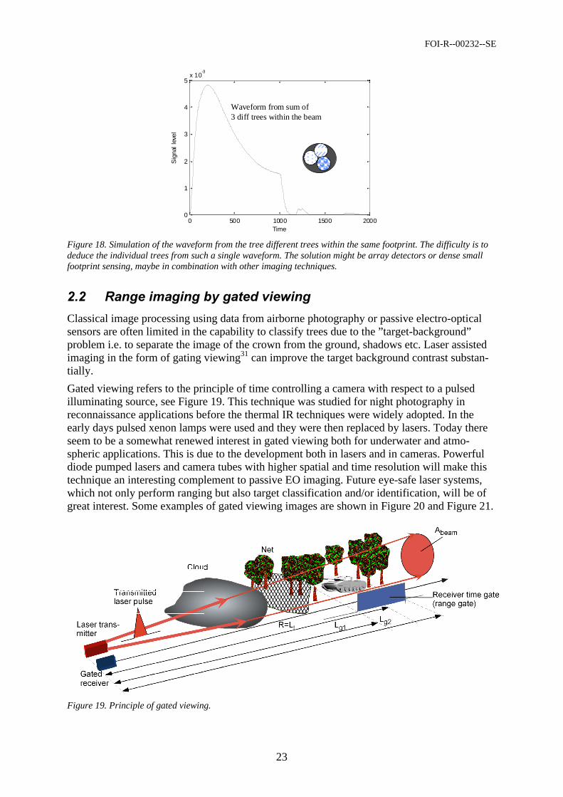
In practice the use of a large footprint and a single detector lead to a problem in that several trees might fall within the footprint. It will not be obvious how to analyse a single waveform built up from different type of trees (see Figure 18). Different strategies to combine laser scanning with other imaging techniques are discussed in the later part of this report.

FOI-R--00232--SE

23

0 500 1000 1500 20000

1

2

3

4

5x 10

-3

Sig

nal

leve

l

Time

Waveform from sum of 3 diff trees within the beam

Figure 18. Simulation of the waveform from the tree different trees within the same footprint. The difficulty is to deduce the individual trees from such a single waveform. The solution might be array detectors or dense small footprint sensing, maybe in combination with other imaging techniques.

' (

Classical image processing using data from airborne photography or passive electro-optical sensors are often limited in the capability to classify trees due to the ”target-background” problem i.e. to separate the image of the crown from the ground, shadows etc. Laser assisted imaging in the form of gating viewing31 can improve the target background contrast substan-tially.

Gated viewing refers to the principle of time controlling a camera with respect to a pulsed illuminating source, see Figure 19. This technique was studied for night photography in reconnaissance applications before the thermal IR techniques were widely adopted. In the early days pulsed xenon lamps were used and they were then replaced by lasers. Today there seem to be a somewhat renewed interest in gated viewing both for underwater and atmo-spheric applications. This is due to the development both in lasers and in cameras. Powerful diode pumped lasers and camera tubes with higher spatial and time resolution will make this technique an interesting complement to passive EO imaging. Future eye-safe laser systems, which not only perform ranging but also target classification and/or identification, will be of great interest. Some examples of gated viewing images are shown in Figure 20 and Figure 21.

Figure 19. Principle of gated viewing.

FOI-R--00232--SE

24

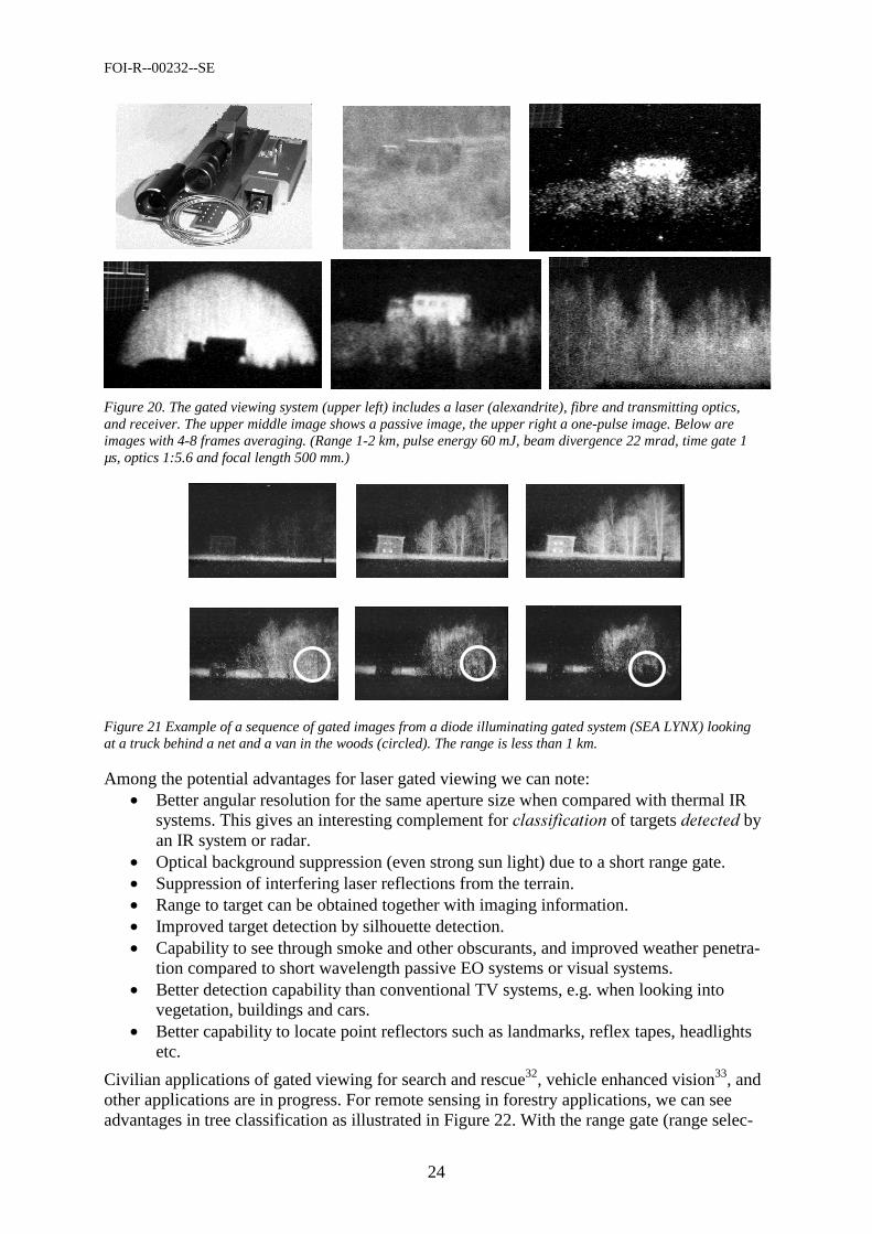
Figure 20. The gated viewing system (upper left) includes a laser (alexandrite), fibre and transmitting optics, and receiver. The upper middle image shows a passive image, the upper right a one-pulse image. Below are images with 4-8 frames averaging. (Range 1-2 km, pulse energy 60 mJ, beam divergence 22 mrad, time gate 1 µs, optics 1:5.6 and focal length 500 mm.)

Figure 21 Example of a sequence of gated images from a diode illuminating gated system (SEA LYNX) looking at a truck behind a net and a van in the woods (circled). The range is less than 1 km.

Among the potential advantages for laser gated viewing we can note: • Better angular resolution for the same aperture size when compared with thermal IR

systems. This gives an interesting complement for % of targets by an IR system or radar.

• Optical background suppression (even strong sun light) due to a short range gate. • Suppression of interfering laser reflections from the terrain. • Range to target can be obtained together with imaging information. • Improved target detection by silhouette detection. • Capability to see through smoke and other obscurants, and improved weather penetra-

tion compared to short wavelength passive EO systems or visual systems. • Better detection capability than conventional TV systems, e.g. when looking into

vegetation, buildings and cars. • Better capability to locate point reflectors such as landmarks, reflex tapes, headlights

etc.

Civilian applications of gated viewing for search and rescue32, vehicle enhanced vision33, and other applications are in progress. For remote sensing in forestry applications, we can see advantages in tree classification as illustrated in Figure 22. With the range gate (range selec-

FOI-R--00232--SE

25

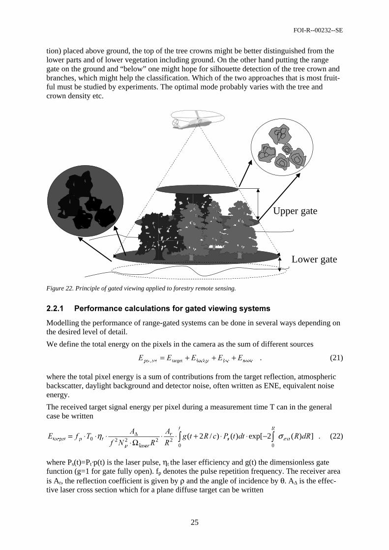
tion) placed above ground, the top of the tree crowns might be better distinguished from the lower parts and of lower vegetation including ground. On the other hand putting the range gate on the ground and “below” one might hope for silhouette detection of the tree crown and branches, which might help the classification. Which of the two approaches that is most fruit-ful must be studied by experiments. The optimal mode probably varies with the tree and crown density etc.

Upper gate

Lower gate

Figure 22. Principle of gated viewing applied to forestry remote sensing.

(( ) $ +*

Modelling the performance of range-gated systems can be done in several ways depending on the desired level of detail.

We define the total energy on the pixels in the camera as the sum of different sources

QRLVHEVFEDFNJUWRWSL[ ##### +++= target, . (21)

where the total pixel energy is a sum of contributions from the target reflection, atmospheric backscatter, daylight background and detector noise, often written as ENE, equivalent noise energy.

The received target signal energy per pixel during a measurement time T can in the general case be written

])(2exp[)()/2(00

22220 $

)

"%

)%# H[W

5

V

7U

ODVHUS

WSWDUJHW ση ∫∫ −⋅⋅+⋅⋅Ω⋅

⋅⋅⋅= ∆ . (22)

where Ps(t)=Pt·p(t) is the laser pulse, ηt the laser efficiency and g(t) the dimensionless gate function (g=1 for gate fully open). fp denotes the pulse repetition frequency. The receiver area is Ar, the reflection coefficient is given by ρ and the angle of incidence by θ. A∆ is the effec-tive laser cross section which for a plane diffuse target can be written

FOI-R--00232--SE

26

target

)cos()) ⋅=∆ π

θρ ; (laser beam area > the target area Atarget) 23

or

2 )ODVHU

Ω⋅=∆ πρ

; (beam area< the target area Atarget) . (24)

In the case of a single pulse within the gate (g=1) and constant extinction, Eq. (22) can be simplified to

222

0 )2exp(

W

WH[W

SODVHU

UWS

WDUJHW

"%

)##

σπρη −⋅⋅

Ω= , (25)

where Lt is the target range (=altitude H).

The sun or diffuse daylight will generate a background power at the receiver as

UU

EDFNJU

EDFNJU )$ ⋅Ω⋅⋅⋅∆⋅=π

ρλλ 0 , (26)

where Lλ is the background spectral irradiance, ∆λ the optical band pass filter, Ωr is the receiver solid angle and ρbackgr is an average reflection coefficient of the illuminated back-ground scene. This will for low visibility also include atmospheric backscatter from the sun. Conservative values for Lλ -2µm-1. The detected energy corresponding to the background during a gate interval ∆τ is

τ∆⋅= EDFNJUEDFNJU $# . (27)

It is often convenient to refer to an equivalent pixel background value for comparison with the detector noise figure in the data sheet of the camera tube. Assuming a resolution of Np line pairs/mm and a focal length of f mm we obtain

τπ

ρηλλ ∆⋅⋅⋅⋅⋅⋅∆⋅= U

S

EDFNJU

USL[EDFNJU )"%

#22.

11 . (28)

The noise figure (ENE) for a generation II red tube is about 6·10-18 J/pixel and the corre-sponding figure for a generation III tube can be as low as 6·10-20 J/pixel, according to data from Xybiona.

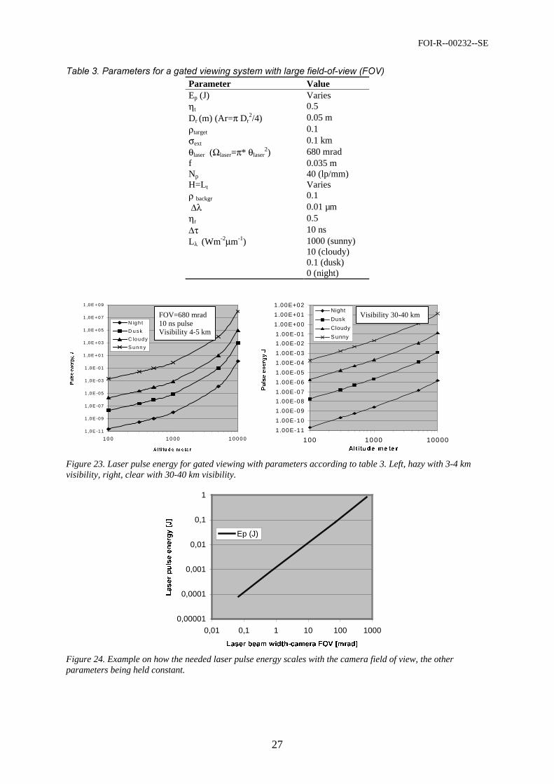
In Figure 23 we have plotted the laser pulse energy for gated viewing with parameters accord-ing to Table 3, and in Figure 24 we show an example on how the needed laser pulse energy scales with the camera field of view, while the other parameters are kept constant.

a Internet: http://www.xybion.com/

FOI-R--00232--SE

27

!"" #$%&'Parameter ValueEp (J) Varies ηt 0.5 Dr (m) (Ar=π Dr

2/4) 0.05 m ρtarget 0.1 σext 0.1 km θlaser (Ωlaser=π* θlaser

2) 680 mrad f 0.035 m Np 40 (lp/mm) H=Lt Varies ρ backgr 0.1 ∆λ 0.01 µm ηr 0.5 ∆τ 10 ns Lλ (Wm-2µm-1) 1000 (sunny)

10 (cloudy) 0.1 (dusk) 0 (night)

1 ,0 E -11

1 ,0 E -09

1 ,0 E -07

1 ,0 E -05

1 ,0 E -03

1 ,0 E -01

1 ,0 E + 01

1 ,0 E + 03

1 ,0 E + 05

1 ,0 E + 07

1 ,0 E + 09

1 0 0 1 0 00 1 0 0 0 0

$ OW LWX G H P H WH U

3XOVHHQHUJ\-

N ig h t

D u s k

C lo u d y

S u n n y

1 .00E-11

1 .00E-10

1 .00E-09

1 .00E-08

1 .00E-07

1 .00E-06

1 .00E-05

1 .00E-04

1 .00E-03

1 .00E-02

1 .00E-01

1 .00E+00

1 .00E+01

1 .00E+02

100 1000 10000$OWLWXGH PH WH U

3XOVHHQHUJ\-

Night

Dusk

Cloudy

S unny

Figure 23. Laser pulse energy for gated viewing with parameters according to table 3. Left, hazy with 3-4 km visibility, right, clear with 30-40 km visibility.

0,00001

0,0001

0,001

0,01

0,1

1

0,01 0,1 1 10 100 1000

/DVHUEHDPZLGWKFDPHUD)29>PUDG@

/DVHUSXOVHHQHUJ\>-@

Ep (J)

Figure 24. Example on how the needed laser pulse energy scales with the camera field of view, the other parameters being held constant.

FOV=680 mrad 10 ns pulse Visibility 4-5 km

Visibility 30-40 km

FOI-R--00232--SE

28

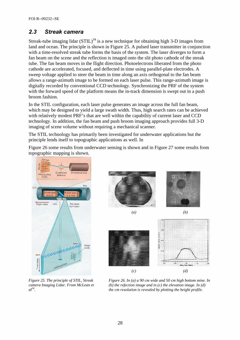
Streak-tube imaging lidar (STIL)34 is a new technique for obtaining high 3-D images from land and ocean. The principle is shown in Figure 25. A pulsed laser transmitter in conjunction with a time-resolved streak tube forms the basis of the system. The laser diverges to form a fan beam on the scene and the reflection is imaged onto the slit photo cathode of the streak tube. The fan beam moves in the flight direction. Photoelectrons liberated from the photo cathode are accelerated, focused, and deflected in time using parallel-plate electrodes. A sweep voltage applied to steer the beam in time along an axis orthogonal to the fan beam allows a range-azimuth image to be formed on each laser pulse. This range-azimuth image is digitally recorded by conventional CCD technology. Synchronizing the PRF of the system with the forward speed of the platform means the in-track dimension is swept out in a push broom fashion.

In the STIL configuration, each laser pulse generates an image across the full fan beam, which may be designed to yield a large swath width. Thus, high search rates can be achieved with relatively modest PRF’s that are well within the capability of current laser and CCD technology. In addition, the fan beam and push broom imaging approach provides full 3-D imaging of scene volume without requiring a mechanical scanner.

The STIL technology has primarily been investigated for underwater applications but the principle lends itself to topographic applications as well. In

Figure 26 some results from underwater sensing is shown and in Figure 27 some results from topographic mapping is shown.

Figure 25. The principle of STIL, Streak camera Imaging Lidar. From McLean et al34.

(a) (b)

(c) (d)

Figure 26. In (a) a 90 cm wide and 50 cm high bottom mine. In (b) the refection image and in (c) the elevation image. In (d) the cm resolution is revealed by plotting the height profile.

FOI-R--00232--SE

29

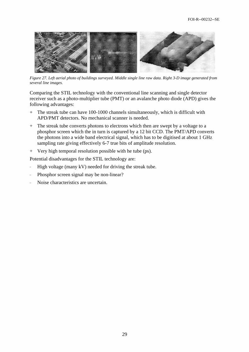
Figure 27. Left aerial photo of buildings surveyed. Middle single line raw data. Right 3-D image generated from several line images.

Comparing the STIL technology with the conventional line scanning and single detector receiver such as a photo-multiplier tube (PMT) or an avalanche photo diode (APD) gives the following advantages:

+ The streak tube can have 100-1000 channels simultaneously, which is difficult with APD/PMT detectors. No mechanical scanner is needed.

+ The streak tube converts photons to electrons which then are swept by a voltage to a phosphor screen which the in turn is captured by a 12 bit CCD. The PMT/APD converts the photons into a wide band electrical signal, which has to be digitised at about 1 GHz sampling rate giving effectively 6-7 true bits of amplitude resolution.

+ Very high temporal resolution possible with he tube (ps).

Potential disadvantages for the STIL technology are:

High voltage (many kV) needed for driving the streak tube.

Phosphor screen signal may be non-linear?

Noise characteristics are uncertain.

FOI-R--00232--SE

30

. '*

The demand on lasers for terrain mapping might be summarized as: 1. Have a short pulse or modulation giving a high range resolution and a high range accuracy 2. Having enough pulse energy enabling a flight altitude in the 300-500 m range (at least). 3. Enabling a high area coverage rate 4. Eye safe emission for people on the ground looking into the beam. 5. Be compact, efficient, and reliable.

The types of lasers that come into consideration are: • Diode lasers • Solid state flash lamp pumped lasers • Solid state diode pumped lasers • Microchip lasers • Fibre lasers

These laser types and some of their features will be discussed in more detail below.

((

Diode lasers are compact and can have high average powers. Short pulses with high energy are not easy to obtain due to the physical nature of the diode laser (damage risk of facets etc.). Diode lasers are perhaps suitable for an amplitude modulated (AM) concept. Average powers in the range of 10 W can be used. The range resolution from an AM system is

)24( ⋅⋅⋅=∆ " % P

π , (29)

where c is the light velocity. A modulation frequency fm of 10 MHz enables a range resolution of 16 cm at an SNR of 10. With 10 W output power the maximum range can exceed 1 km even during daytime. One problem with AM is ambiguity. The use of two or several frequen-cies will reduce this problem. Diode-based imaging laser radars have been developed by Hughes Danbury35 USA, now Raytheon.

(( '$

These lasers are mature but not especially suitable for high average powers and high PRF systems. The heat management problem and the replacement of flash lamps will reduce the use of these lasers in terrain mapping lasers.

(( $

The development of solid state lasers is of high interest for airborne laser radar applications due to the long lifetime of high efficient laser diodes used as a pump source for laser crystals or doped fibres. Diode pump lasers are compact and can deliver high average powers due to the high efficiency for laser diodes (up to 30-40 %, electrical-optical). The relatively high cost for laser diodes has hampered the introduction of diode solid state pumped lasers (DSSPL) in many applications. Recent increasing use of DSSPL in material processing and medicine, together with more competition between diode manufacturers, will however result in lower prices.

FOI-R--00232--SE

31

((/ $ *

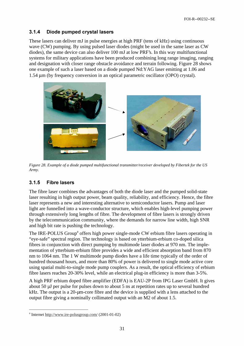
These lasers can deliver mJ in pulse energies at high PRF (tens of kHz) using continuous wave (CW) pumping. By using pulsed laser diodes (might be used in the same laser as CW diodes), the same device can also deliver 100 mJ at low PRF’s. In this way multifunctional systems for military applications have been produced combining long range imaging, ranging and designation with closer range obstacle avoidance and terrain following. Figure 28 shows one example of such a laser based on a diode pumped Nd:YAG laser emitting at 1.06 and 1.54 µm (by frequency conversion in an optical parametric oscillator (OPO) crystal).

Figure 28. Example of a diode pumped multifunctional transmitter/receiver developed by Fibertek for the US Army.

((0 12

The fibre laser combines the advantages of both the diode laser and the pumped solid-state laser resulting in high output power, beam quality, reliability, and efficiency. Hence, the fibre laser represents a new and interesting alternative to semiconductor lasers. Pump and laser light are funnelled into a wave-conductor structure, which enables high-level pumping power through extensively long lengths of fibre. The development of fibre lasers is strongly driven by the telecommunication community, where the demands for narrow line width, high SNR and high bit rate is pushing the technology.

The IRE-POLUS Groupa offers high power single-mode CW erbium fibre lasers operating in “eye-safe” spectral region. The technology is based on ytterbium-erbium co-doped silica fibres in conjunction with direct pumping by multimode laser diodes at 970 nm. The imple-mentation of ytterbium-erbium fibre provides a wide and efficient absorption band from 870 nm to 1064 nm. The 1 W multimode pump diodes have a life time typically of the order of hundred thousand hours, and more than 80% of power is delivered to single mode active core using spatial multi-to-single mode pump couplers. As a result, the optical efficiency of erbium fibre lasers reaches 20-30% level, while an electrical plug-in efficiency is more than 3-5%.

A high PRF erbium doped fibre amplifier (EDFA) is EAU-2P from IPG Laser GmbH. It gives about 50 µJ per pulse for pulses down to about 5 ns at repetition rates up to several hundred kHz. The output is a 20-µm-core fibre and the device is supplied with a lens attached to the output fibre giving a nominally collimated output with an M2 of about 1.5.

a Internet http://www.ire-polusgroup.com/ (2001-01-02)

FOI-R--00232--SE

32

Other suppliers of fibre lasers in the wavelength region around 1.5-1.6 µm is e.g. IONASa, who provides single frequency distributed feed-back (DFB) rare-earth doped fibre laser with narrow line width, very high SNR, low random internal noise (RIN), and excellent wave-length selectability in the 1520 nm- 1610 nm region. The CW laser is well suited for high bit-rate, externally modulated, dense wavelength division multiplexing (DWDM) networks, where it increases the capacity and flexibility by increasing the available bandwidth. The fibre laser provides stable single-mode and single-polarisation lasing. Combining the fibre laser with a fibre amplifier results in a master oscillator and power amplifier (MOPA) fibre laser offering an outstanding performance on line width (5 kHz) and output power (10 dBm).

(( 3'

The microchip laser is a compact monolithic diode pumped, passively Q-switched laser. These devices have very short (< 1 ns) pulses at kW peak powers and can be run at high PRF’s (tens of kHz). The wavelength can be either 1.06 or 1.54 µm (or other harmonics of 1.06 µm) and the beam profile is superb with a linearly polarized output. The robustness, compactness, low cost and the potential for array fabrication make theses lasers ideal for terrain mapping.

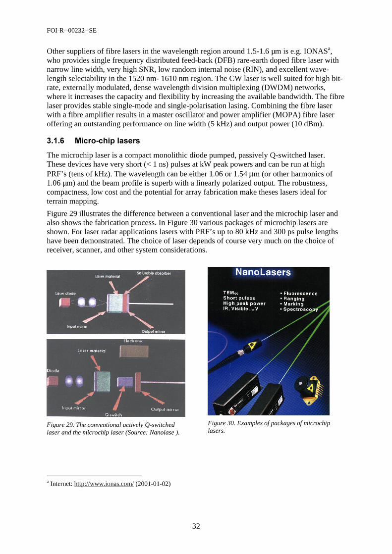
Figure 29 illustrates the difference between a conventional laser and the microchip laser and also shows the fabrication process. In Figure 30 various packages of microchip lasers are shown. For laser radar applications lasers with PRF’s up to 80 kHz and 300 ps pulse lengths have been demonstrated. The choice of laser depends of course very much on the choice of receiver, scanner, and other system considerations.

a Internet: http://www.ionas.com/ (2001-01-02)

Figure 29. The conventional actively Q-switched laser and the microchip laser (Source: Nanolase ).

Figure 30. Examples of packages of microchip lasers.

FOI-R--00232--SE

33

)

(( .' '*

A three dimensional imaging array can be implemented with a two dimensional detector array sensitive to short wave-length radiation, typically in at the 1.54 µm eye-safe region. At each detector, high-speed electronics sample the return signal from the target, and determine the time of arrival at each pixel. Since the signal return is relatively small, only a few photons arrive at each pixel, and gain at the pixel is necessary to raise the signal level above amplifier noise. The gain mechanism can be achieved in several ways, but must not add excess noise to the detected signal. In one method, an avalanche gain in each detector, combined with a low noise amplifier in each unit cell, raises return signal above the noise. Other features, which may be included in the array, include output analog to digital conversion and gain/bias control at each pixel to optimise the detector operating point.

(( )'

When using a semiconductor photo detector for low-light-level measurement, it is necessary to consider overall performance, including not only the semiconductor photo detector charac-teristics, but the readout circuit (operational amplifier) noise as well. When a silicon photo-diode is used as a photo detector, the lower detection limit is usually determined by the read-out circuit noise because photodiode noise level is very low. This tendency becomes more obvious when high frequency signals are to be detected. This is because the high-speed read-out circuit usually exhibits larger noise, resulting in a predominant source of noise in the entire circuit system. In such cases, if the detector itself has an internal gain mechanism and if the output signal from the detector is thus adequately amplified, the readout circuit can be operated so that its noise contribution is minimized to level equal to one divided by gain (1/10 to 1/100). In this way, when the lower detection limit is determined by the readout circuit, use of an avalanche photodiode (APD) offers the advantage which the lower detection limit can be improved by the APD gain factor to a level 1/10 to 1/100 of the lower detection limit obtained with normal photodiodes. The spectral response range is 400 nm to 1000 nm, with peak sensitivity at 800 nm.

The InGaAs linear image sensorsa are self-scanning photodiode arrays designed specifically for detectors in near infrared multi-channel spectroscopy that incorporate an InGaAs photo-diode array chip, a thermoelectric-cooler and C-MOS multiplexers with charge integration amplifiers. The spectral response range is 0.9 to 1.7 µm, with peak sensitivity wavelength 1.55 µm. The number of pixels is 128 or 256.

(( 1 *

The MXA-256-X series detectorb is a hybrid focal plane InGaAs PIN photodiode array with wavelength response ranging from 800 nm to 1700 nm. The array has 256 elements con-figured in a linear orientation with standard array length of 0.5 mm. A buffered multiplexer provides individual CMOS amplifiers for each photodiode. The integrated amplifier maintains zero volt bias across each InGaAs photodiode minimizing dark current and low frequency noise allowing for longer exposure times with increased sensitivity. A static shift register scanning circuit sequentially selects sample-and-hold integrator output voltages which are

a Internet: http://www.hamamatsu.co.uk/ (2000-07-05) b From PerkinElmer Optoelectronics, Inc., Internet: http://opto.perkinelmer.com/ (2000-07-04)

FOI-R--00232--SE

34

proportional to input optical power. On-chip correlated double sampling removes integrator offsets and further suppresses low frequency noise. The array is available in a 28 pin dual-in-line package. Included in the assembly are a single-stage thermoelectric cooler, silicon multi-plexer, bias resistor and bypass capacitors.

Sensors Unlimiteda manufactures a hybrid FPA consisting of an InGaAs photodiode array operable in the 0.9 µm to 1.7 µm spectrum at room temperature. The SU320-1.7T1 contains a single stage thermoelectric cooler with an integrated thermistor allowing the user to reduce the temperature for “high sensitivity” applications, such as low light level detection, or to stabilize the FPA in a varying ambient temperature. This high resolution FPA is used in many industrial and commercial applications such as eye-safe covert surveillance, spectroscopy, laser beam profiling, laser and light detection and ranging, machine vision and many other applications where near infrared detection is required. Some features are

• High quantum efficiency in the operating range of 1.0 – 1.6 µm • Room temperature stabilized • Active pixel architecture • High fill factor • No external cooling • High resolution, 320 x 240 pixels on 40 µm pitch • 1 inch camera format • One stage thermoelectric cooler • 13 bit dynamic range

((/ & '

The intensified photodiode (IPD) is a solid-state hybrid photo multiplier vacuum tube using high quantum efficiency transmission mode III-V photo cathodesb. The IPD is an alternative to conventional photo multiplier tubes. It combines the advantages of APD and diode tech-nology with high performance, III-V, transmission mode photo cathodes developed for the GEN III night vision industry.

The IPD is comprised of three main components: a III-V based photo cathode structure sealed to a glass faceplate, a body composed of a brazed stack of ceramic rings and electrostatic electron focusing aperture electrodes, and an anode composed of a GaAs diode bonded to a ceramic header. The anode output is via an SMA connector. Nominally, the photo cathode and two electrode focusing rings are biased –4 kV to –8 kV with respect to the anode during operation. Electrons emitted by the 8mm diameter negative electron affinity (NEA) photo cathode are accelerated and focused by this bias and penetrate the surface of the GaAs Schottky diode anode to a depth of less than 1µm. Electrons deposit energy in the GaAs lattice via an ionisation avalanching process with an efficiency of approximately 4 eV/el-h pair. Optionally, the Schottky avalanche photodiode (SAPD) anode provides a second stage avalanche multiplication in a high field region 2 µm below the Schottky contact metallisation. Noise due to this second stage process is greatly mitigated by the higher gain low noise elec-tron bombarded multiplication. This second stage avalanche multiplication process provides adequate gain to achieve excellent multiple photon pulse height distribution. The IPD is pot-ted for high voltage protection. It operates from a single cathode voltage, with a built in voltage divider to provide all necessary focusing electrode voltages. The diode output is normally operated at ground but can be biased to decrease response time.

a From Sensors Unlimited, Inc., Internet: http://www.sensorsinc.com/ (2000-07-04) b From Intevac, Inc., Internet: http://www.intevac.com/photonics/index.html (2001-09-03)

FOI-R--00232--SE

35

The large area transmission mode photo cathode is fabricated using GaAs, GaAsP, or InGaAs/InP based heterostructures. Depending on the spectral content of the incoming signal the following material is recommended: GaAsP -0.3 to 0.7 µm, GaAs -0.4 to 0.9 µm, and InGaAs/InP -0.95 to 1.65 µm.

Electron bombarded current gain of the standard Schottky diode anode IPD is approximately 103 at 8kV tube bias. Alternatively, the SAPD version of the IPD has a gain of greater than 1.5 x 104. Both devices have an associated noise factor of less than 1.1. The IPD can be connected through its 50-Ohm coaxial connector directly to a bias tee and preamplifier to achieve low noise gain up to 1 GHz bandwidth.

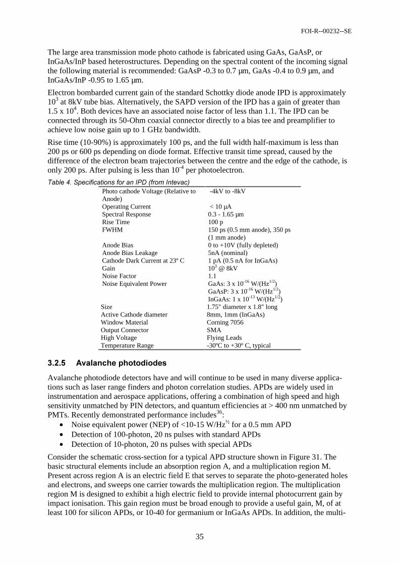
Rise time (10-90%) is approximately 100 ps, and the full width half-maximum is less than 200 ps or 600 ps depending on diode format. Effective transit time spread, caused by the difference of the electron beam trajectories between the centre and the edge of the cathode, is only 200 ps. After pulsing is less than 10-4 per photoelectron.

( )*#) 'Photo cathode Voltage (Relative to Anode)

-4kV to -8kV

Operating Current < 10 µA Spectral Response 0.3 - 1.65 µm Rise Time 100 p FWHM 150 ps (0.5 mm anode), 350 ps

(1 mm anode) Anode Bias 0 to +10V (fully depleted) Anode Bias Leakage 5nA (nominal) Cathode Dark Current at 23º C 1 pA (0.5 nA for InGaAs) Gain 103 @ 8kV Noise Factor 1.1 Noise Equivalent Power GaAs: 3 x 10-16 W/(Hz1/2)

GaAsP: 3 x 10-16 W/(Hz1/2) InGaAs: 1 x 10-13 W/(Hz1/2)

Size 1.75" diameter x 1.8" long Active Cathode diameter 8mm, 1mm (InGaAs) Window Material Corning 7056 Output Connector SMA High Voltage Flying Leads Temperature Range -30ºC to +30º C, typical

((0 "' '

Avalanche photodiode detectors have and will continue to be used in many diverse applica-tions such as laser range finders and photon correlation studies. APDs are widely used in instrumentation and aerospace applications, offering a combination of high speed and high sensitivity unmatched by PIN detectors, and quantum efficiencies at > 400 nm unmatched by PMTs. Recently demonstrated performance includes36:

• Noise equivalent power (NEP) of <10-15 W/Hz½ for a 0.5 mm APD • Detection of 100-photon, 20 ns pulses with standard APDs • Detection of 10-photon, 20 ns pulses with special APDs

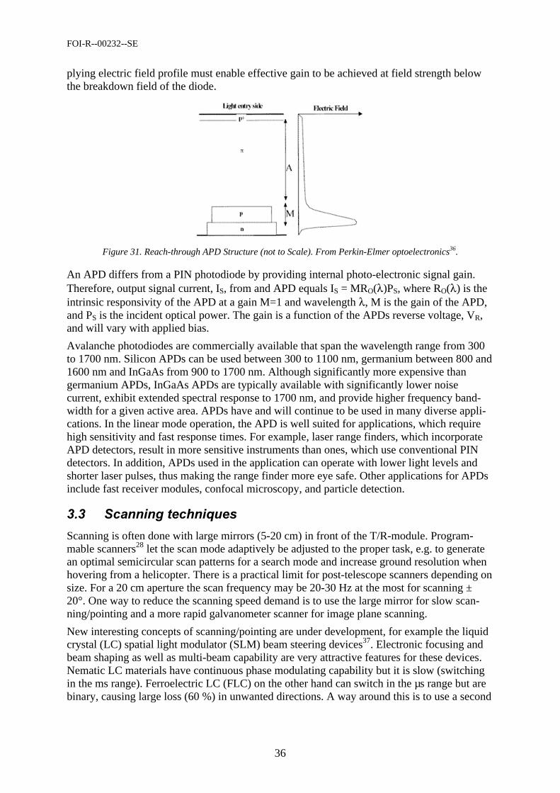
Consider the schematic cross-section for a typical APD structure shown in Figure 31. The basic structural elements include an absorption region A, and a multiplication region M. Present across region A is an electric field E that serves to separate the photo-generated holes and electrons, and sweeps one carrier towards the multiplication region. The multiplication region M is designed to exhibit a high electric field to provide internal photocurrent gain by impact ionisation. This gain region must be broad enough to provide a useful gain, M, of at least 100 for silicon APDs, or 10-40 for germanium or InGaAs APDs. In addition, the multi-

FOI-R--00232--SE

36

plying electric field profile must enable effective gain to be achieved at field strength below the breakdown field of the diode.

Figure 31. Reach-through APD Structure (not to Scale). From Perkin-Elmer optoelectronics36.

An APD differs from a PIN photodiode by providing internal photo-electronic signal gain. Therefore, output signal current, IS, from and APD equals IS = MRO(λ)PS, where RO(λ) is the intrinsic responsivity of the APD at a gain M=1 and wavelength λ, M is the gain of the APD, and PS is the incident optical power. The gain is a function of the APDs reverse voltage, VR, and will vary with applied bias.

Avalanche photodiodes are commercially available that span the wavelength range from 300 to 1700 nm. Silicon APDs can be used between 300 to 1100 nm, germanium between 800 and 1600 nm and InGaAs from 900 to 1700 nm. Although significantly more expensive than germanium APDs, InGaAs APDs are typically available with significantly lower noise current, exhibit extended spectral response to 1700 nm, and provide higher frequency band-width for a given active area. APDs have and will continue to be used in many diverse appli-cations. In the linear mode operation, the APD is well suited for applications, which require high sensitivity and fast response times. For example, laser range finders, which incorporate APD detectors, result in more sensitive instruments than ones, which use conventional PIN detectors. In addition, APDs used in the application can operate with lower light levels and shorter laser pulses, thus making the range finder more eye safe. Other applications for APDs include fast receiver modules, confocal microscopy, and particle detection.

%"

Scanning is often done with large mirrors (5-20 cm) in front of the T/R-module. Program-mable scanners28 let the scan mode adaptively be adjusted to the proper task, e.g. to generate an optimal semicircular scan patterns for a search mode and increase ground resolution when hovering from a helicopter. There is a practical limit for post-telescope scanners depending on size. For a 20 cm aperture the scan frequency may be 20-30 Hz at the most for scanning ± 20°. One way to reduce the scanning speed demand is to use the large mirror for slow scan-ning/pointing and a more rapid galvanometer scanner for image plane scanning.

New interesting concepts of scanning/pointing are under development, for example the liquid crystal (LC) spatial light modulator (SLM) beam steering devices37. Electronic focusing and beam shaping as well as multi-beam capability are very attractive features for these devices. Nematic LC materials have continuous phase modulating capability but it is slow (switching in the ms range). Ferroelectric LC (FLC) on the other hand can switch in the µs range but are binary, causing large loss (60 %) in unwanted directions. A way around this is to use a second

FOI-R--00232--SE

37

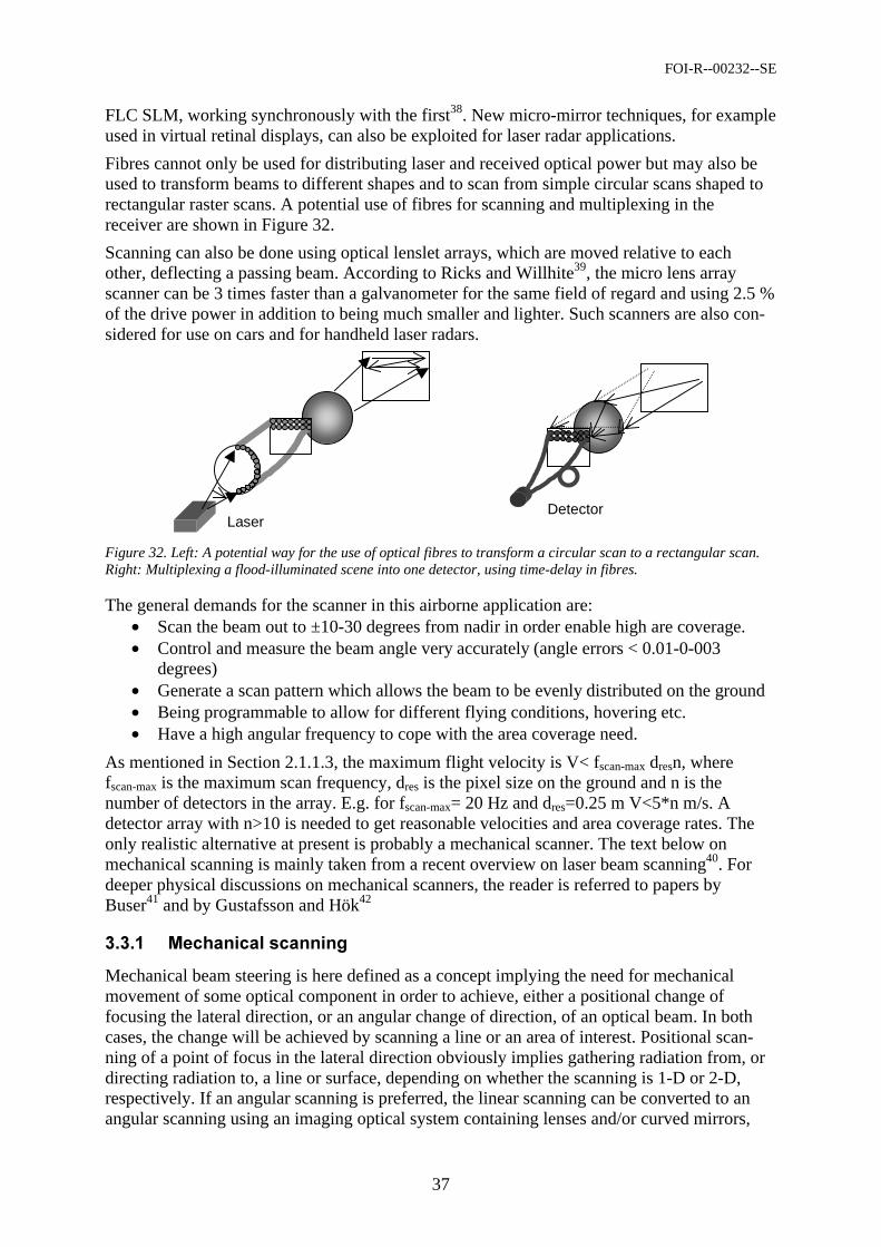
FLC SLM, working synchronously with the first38. New micro-mirror techniques, for example used in virtual retinal displays, can also be exploited for laser radar applications.

Fibres cannot only be used for distributing laser and received optical power but may also be used to transform beams to different shapes and to scan from simple circular scans shaped to rectangular raster scans. A potential use of fibres for scanning and multiplexing in the receiver are shown in Figure 32.

Scanning can also be done using optical lenslet arrays, which are moved relative to each other, deflecting a passing beam. According to Ricks and Willhite39, the micro lens array scanner can be 3 times faster than a galvanometer for the same field of regard and using 2.5 % of the drive power in addition to being much smaller and lighter. Such scanners are also con-sidered for use on cars and for handheld laser radars.

Laser Detector

Figure 32. Left: A potential way for the use of optical fibres to transform a circular scan to a rectangular scan. Right: Multiplexing a flood-illuminated scene into one detector, using time-delay in fibres.

The general demands for the scanner in this airborne application are: • Scan the beam out to ±10-30 degrees from nadir in order enable high are coverage. • Control and measure the beam angle very accurately (angle errors < 0.01-0-003

degrees) • Generate a scan pattern which allows the beam to be evenly distributed on the ground • Being programmable to allow for different flying conditions, hovering etc. • Have a high angular frequency to cope with the area coverage need.

As mentioned in Section 2.1.1.3, the maximum flight velocity is V< fscan-max dresn, where fscan-max is the maximum scan frequency, dres is the pixel size on the ground and n is the number of detectors in the array. E.g. for fscan-max= 20 Hz and dres=0.25 m V<5*n m/s. A detector array with n>10 is needed to get reasonable velocities and area coverage rates. The only realistic alternative at present is probably a mechanical scanner. The text below on mechanical scanning is mainly taken from a recent overview on laser beam scanning40. For deeper physical discussions on mechanical scanners, the reader is referred to papers by Buser41 and by Gustafsson and Hök42

(( 3 '

Mechanical beam steering is here defined as a concept implying the need for mechanical movement of some optical component in order to achieve, either a positional change of focusing the lateral direction, or an angular change of direction, of an optical beam. In both cases, the change will be achieved by scanning a line or an area of interest. Positional scan-ning of a point of focus in the lateral direction obviously implies gathering radiation from, or directing radiation to, a line or surface, depending on whether the scanning is 1-D or 2-D, respectively. If an angular scanning is preferred, the linear scanning can be converted to an angular scanning using an imaging optical system containing lenses and/or curved mirrors,

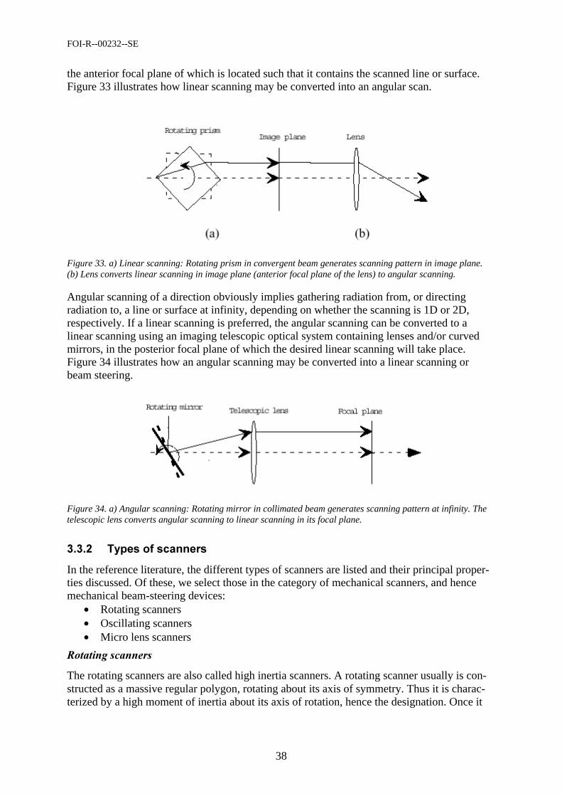
FOI-R--00232--SE

38

the anterior focal plane of which is located such that it contains the scanned line or surface. Figure 33 illustrates how linear scanning may be converted into an angular scan.

Figure 33. a) Linear scanning: Rotating prism in convergent beam generates scanning pattern in image plane. (b) Lens converts linear scanning in image plane (anterior focal plane of the lens) to angular scanning.

Angular scanning of a direction obviously implies gathering radiation from, or directing radiation to, a line or surface at infinity, depending on whether the scanning is 1D or 2D, respectively. If a linear scanning is preferred, the angular scanning can be converted to a linear scanning using an imaging telescopic optical system containing lenses and/or curved mirrors, in the posterior focal plane of which the desired linear scanning will take place. Figure 34 illustrates how an angular scanning may be converted into a linear scanning or beam steering.

Figure 34. a) Angular scanning: Rotating mirror in collimated beam generates scanning pattern at infinity. The telescopic lens converts angular scanning to linear scanning in its focal plane.

(( .*

In the reference literature, the different types of scanners are listed and their principal proper-ties discussed. Of these, we select those in the category of mechanical scanners, and hence mechanical beam-steering devices:

• Rotating scanners • Oscillating scanners • Micro lens scanners

The rotating scanners are also called high inertia scanners. A rotating scanner usually is con-structed as a massive regular polygon, rotating about its axis of symmetry. Thus it is charac-terized by a high moment of inertia about its axis of rotation, hence the designation. Once it

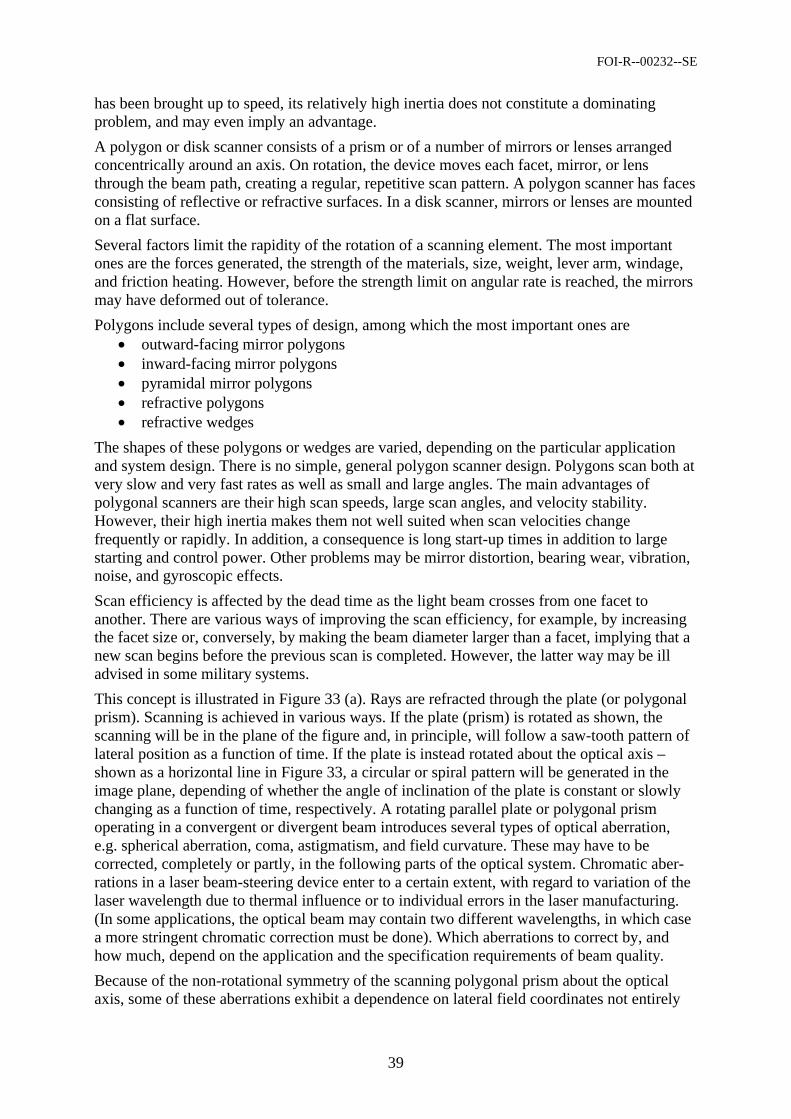
FOI-R--00232--SE

39

has been brought up to speed, its relatively high inertia does not constitute a dominating problem, and may even imply an advantage.

A polygon or disk scanner consists of a prism or of a number of mirrors or lenses arranged concentrically around an axis. On rotation, the device moves each facet, mirror, or lens through the beam path, creating a regular, repetitive scan pattern. A polygon scanner has faces consisting of reflective or refractive surfaces. In a disk scanner, mirrors or lenses are mounted on a flat surface.

Several factors limit the rapidity of the rotation of a scanning element. The most important ones are the forces generated, the strength of the materials, size, weight, lever arm, windage, and friction heating. However, before the strength limit on angular rate is reached, the mirrors may have deformed out of tolerance.

Polygons include several types of design, among which the most important ones are • outward-facing mirror polygons • inward-facing mirror polygons • pyramidal mirror polygons • refractive polygons • refractive wedges

The shapes of these polygons or wedges are varied, depending on the particular application and system design. There is no simple, general polygon scanner design. Polygons scan both at very slow and very fast rates as well as small and large angles. The main advantages of polygonal scanners are their high scan speeds, large scan angles, and velocity stability. However, their high inertia makes them not well suited when scan velocities change frequently or rapidly. In addition, a consequence is long start-up times in addition to large starting and control power. Other problems may be mirror distortion, bearing wear, vibration, noise, and gyroscopic effects.

Scan efficiency is affected by the dead time as the light beam crosses from one facet to another. There are various ways of improving the scan efficiency, for example, by increasing the facet size or, conversely, by making the beam diameter larger than a facet, implying that a new scan begins before the previous scan is completed. However, the latter way may be ill advised in some military systems.

This concept is illustrated in Figure 33 (a). Rays are refracted through the plate (or polygonal prism). Scanning is achieved in various ways. If the plate (prism) is rotated as shown, the scanning will be in the plane of the figure and, in principle, will follow a saw-tooth pattern of lateral position as a function of time. If the plate is instead rotated about the optical axis – shown as a horizontal line in Figure 33, a circular or spiral pattern will be generated in the image plane, depending of whether the angle of inclination of the plate is constant or slowly changing as a function of time, respectively. A rotating parallel plate or polygonal prism operating in a convergent or divergent beam introduces several types of optical aberration, e.g. spherical aberration, coma, astigmatism, and field curvature. These may have to be corrected, completely or partly, in the following parts of the optical system. Chromatic aber-rations in a laser beam-steering device enter to a certain extent, with regard to variation of the laser wavelength due to thermal influence or to individual errors in the laser manufacturing. (In some applications, the optical beam may contain two different wavelengths, in which case a more stringent chromatic correction must be done). Which aberrations to correct by, and how much, depend on the application and the specification requirements of beam quality.

Because of the non-rotational symmetry of the scanning polygonal prism about the optical axis, some of these aberrations exhibit a dependence on lateral field coordinates not entirely

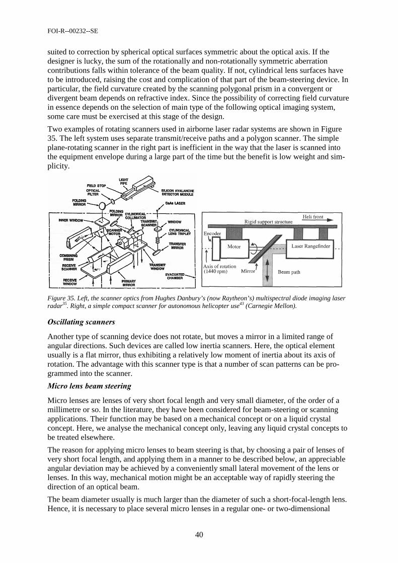
FOI-R--00232--SE

40

suited to correction by spherical optical surfaces symmetric about the optical axis. If the designer is lucky, the sum of the rotationally and non-rotationally symmetric aberration contributions falls within tolerance of the beam quality. If not, cylindrical lens surfaces have to be introduced, raising the cost and complication of that part of the beam-steering device. In particular, the field curvature created by the scanning polygonal prism in a convergent or divergent beam depends on refractive index. Since the possibility of correcting field curvature in essence depends on the selection of main type of the following optical imaging system, some care must be exercised at this stage of the design.

Two examples of rotating scanners used in airborne laser radar systems are shown in Figure 35. The left system uses separate transmit/receive paths and a polygon scanner. The simple plane-rotating scanner in the right part is inefficient in the way that the laser is scanned into the equipment envelope during a large part of the time but the benefit is low weight and sim-plicity.

Figure 35. Left, the scanner optics from Hughes Danbury’s (now Raytheon’s) multispectral diode imaging laser radar35. Right, a simple compact scanner for autonomous helicopter use43 (Carnegie Mellon).

Another type of scanning device does not rotate, but moves a mirror in a limited range of angular directions. Such devices are called low inertia scanners. Here, the optical element usually is a flat mirror, thus exhibiting a relatively low moment of inertia about its axis of rotation. The advantage with this scanner type is that a number of scan patterns can be pro-grammed into the scanner.

Micro lenses are lenses of very short focal length and very small diameter, of the order of a millimetre or so. In the literature, they have been considered for beam-steering or scanning applications. Their function may be based on a mechanical concept or on a liquid crystal concept. Here, we analyse the mechanical concept only, leaving any liquid crystal concepts to be treated elsewhere.

The reason for applying micro lenses to beam steering is that, by choosing a pair of lenses of very short focal length, and applying them in a manner to be described below, an appreciable angular deviation may be achieved by a conveniently small lateral movement of the lens or lenses. In this way, mechanical motion might be an acceptable way of rapidly steering the direction of an optical beam.

The beam diameter usually is much larger than the diameter of such a short-focal-length lens. Hence, it is necessary to place several micro lenses in a regular one- or two-dimensional

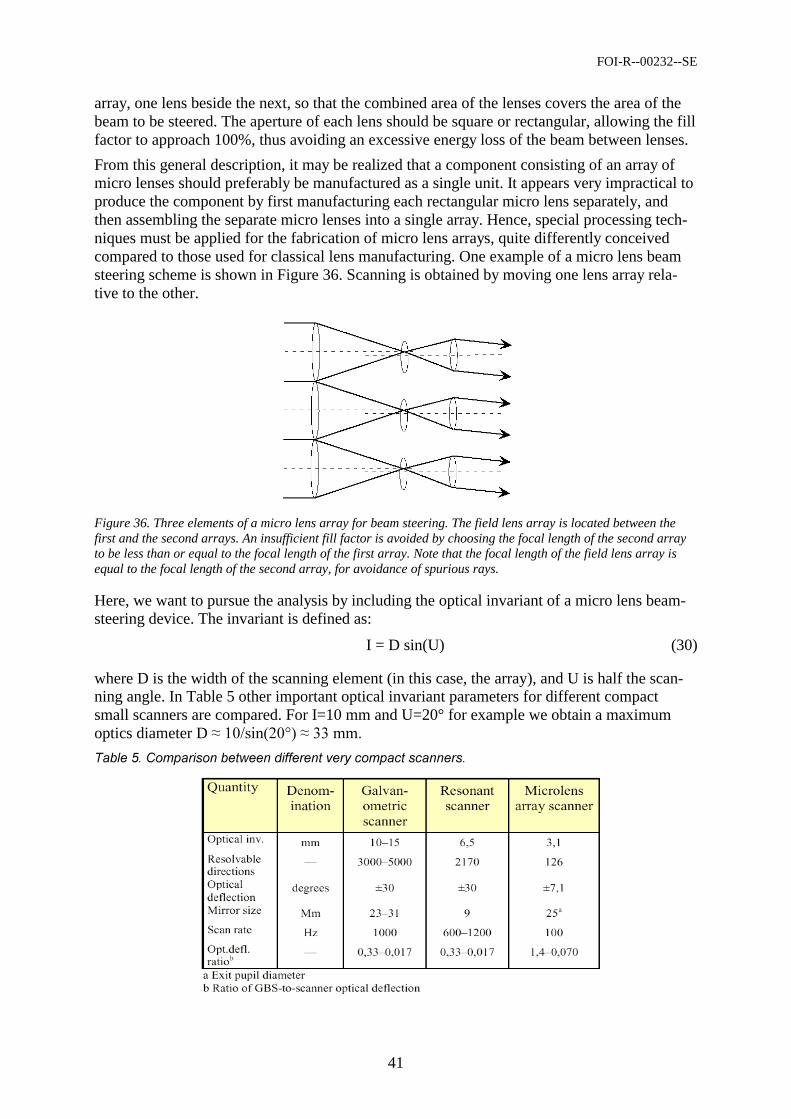
FOI-R--00232--SE

41

array, one lens beside the next, so that the combined area of the lenses covers the area of the beam to be steered. The aperture of each lens should be square or rectangular, allowing the fill factor to approach 100%, thus avoiding an excessive energy loss of the beam between lenses.

From this general description, it may be realized that a component consisting of an array of micro lenses should preferably be manufactured as a single unit. It appears very impractical to produce the component by first manufacturing each rectangular micro lens separately, and then assembling the separate micro lenses into a single array. Hence, special processing tech-niques must be applied for the fabrication of micro lens arrays, quite differently conceived compared to those used for classical lens manufacturing. One example of a micro lens beam steering scheme is shown in Figure 36. Scanning is obtained by moving one lens array rela-tive to the other.

Figure 36. Three elements of a micro lens array for beam steering. The field lens array is located between the first and the second arrays. An insufficient fill factor is avoided by choosing the focal length of the second array to be less than or equal to the focal length of the first array. Note that the focal length of the field lens array is equal to the focal length of the second array, for avoidance of spurious rays.

Here, we want to pursue the analysis by including the optical invariant of a micro lens beam-steering device. The invariant is defined as:

I = D sin(U) (30)

where D is the width of the scanning element (in this case, the array), and U is half the scan-ning angle. In Table 5 other important optical invariant parameters for different compact small scanners are compared. For I=10 mm and U=20° for example we obtain a maximum optics diameter D

+ !

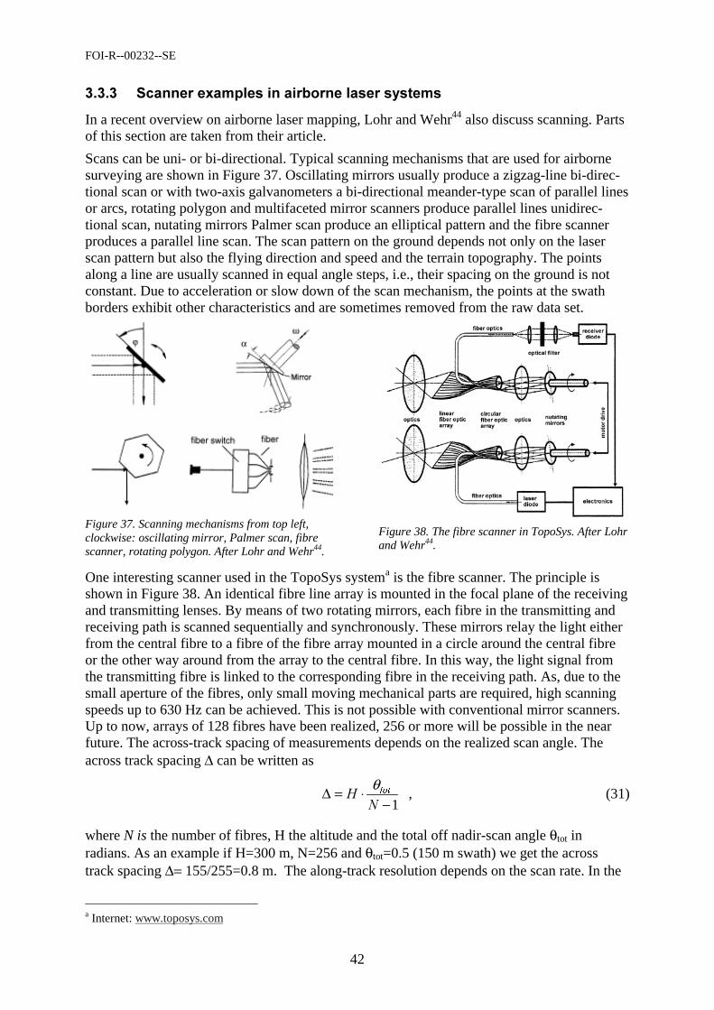
FOI-R--00232--SE

42

(( 4 2 *

In a recent overview on airborne laser mapping, Lohr and Wehr44 also discuss scanning. Parts of this section are taken from their article.

Scans can be uni- or bi-directional. Typical scanning mechanisms that are used for airborne surveying are shown in Figure 37. Oscillating mirrors usually produce a zigzag-line bi-direc-tional scan or with two-axis galvanometers a bi-directional meander-type scan of parallel lines or arcs, rotating polygon and multifaceted mirror scanners produce parallel lines unidirec-tional scan, nutating mirrors Palmer scan produce an elliptical pattern and the fibre scanner produces a parallel line scan. The scan pattern on the ground depends not only on the laser scan pattern but also the flying direction and speed and the terrain topography. The points along a line are usually scanned in equal angle steps, i.e., their spacing on the ground is not constant. Due to acceleration or slow down of the scan mechanism, the points at the swath borders exhibit other characteristics and are sometimes removed from the raw data set.

Figure 37. Scanning mechanisms from top left, clockwise: oscillating mirror, Palmer scan, fibre scanner, rotating polygon. After Lohr and Wehr44.

Figure 38. The fibre scanner in TopoSys. After Lohr and Wehr44.

One interesting scanner used in the TopoSys systema is the fibre scanner. The principle is shown in Figure 38. An identical fibre line array is mounted in the focal plane of the receiving and transmitting lenses. By means of two rotating mirrors, each fibre in the transmitting and receiving path is scanned sequentially and synchronously. These mirrors relay the light either from the central fibre to a fibre of the fibre array mounted in a circle around the central fibre or the other way around from the array to the central fibre. In this way, the light signal from the transmitting fibre is linked to the corresponding fibre in the receiving path. As, due to the small aperture of the fibres, only small moving mechanical parts are required, high scanning speeds up to 630 Hz can be achieved. This is not possible with conventional mirror scanners. Up to now, arrays of 128 fibres have been realized, 256 or more will be possible in the near future. The across-track spacing of measurements depends on the realized scan angle. The across track spacing ∆ can be written as

1−

⋅=∆"

WRWθ

, (31)

where N is the number of fibres, H the altitude and the total off nadir-scan angle θtot in radians. As an example if H=300 m, N=256 and θtot=0.5 (150 m swath) we get the across track spacing ∆= 155/255=0.8 m. The along-track resolution depends on the scan rate. In the

a Internet: www.toposys.com

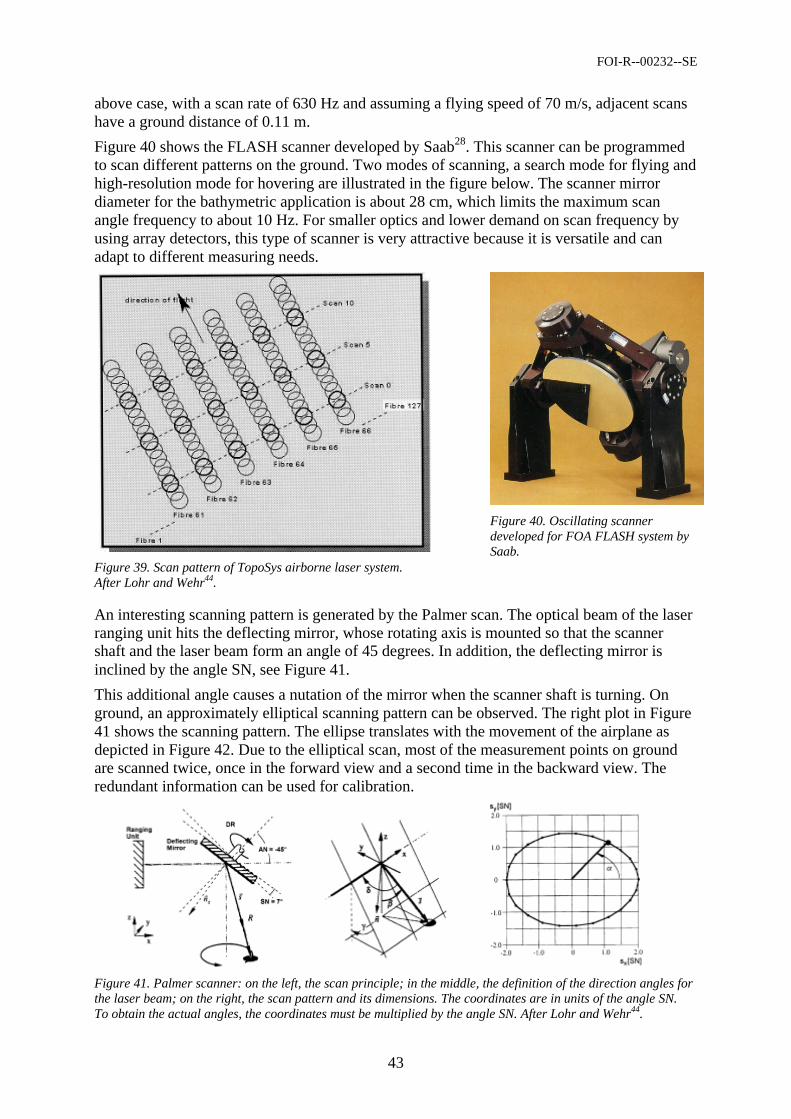
FOI-R--00232--SE

43

above case, with a scan rate of 630 Hz and assuming a flying speed of 70 m/s, adjacent scans have a ground distance of 0.11 m.

Figure 40 shows the FLASH scanner developed by Saab28. This scanner can be programmed to scan different patterns on the ground. Two modes of scanning, a search mode for flying and high-resolution mode for hovering are illustrated in the figure below. The scanner mirror diameter for the bathymetric application is about 28 cm, which limits the maximum scan angle frequency to about 10 Hz. For smaller optics and lower demand on scan frequency by using array detectors, this type of scanner is very attractive because it is versatile and can adapt to different measuring needs.

Figure 39. Scan pattern of TopoSys airborne laser system. After Lohr and Wehr44.

Figure 40. Oscillating scanner developed for FOA FLASH system by Saab.

An interesting scanning pattern is generated by the Palmer scan. The optical beam of the laser ranging unit hits the deflecting mirror, whose rotating axis is mounted so that the scanner shaft and the laser beam form an angle of 45 degrees. In addition, the deflecting mirror is inclined by the angle SN, see Figure 41.

This additional angle causes a nutation of the mirror when the scanner shaft is turning. On ground, an approximately elliptical scanning pattern can be observed. The right plot in Figure 41 shows the scanning pattern. The ellipse translates with the movement of the airplane as depicted in Figure 42. Due to the elliptical scan, most of the measurement points on ground are scanned twice, once in the forward view and a second time in the backward view. The redundant information can be used for calibration.

Figure 41. Palmer scanner: on the left, the scan principle; in the middle, the definition of the direction angles for the laser beam; on the right, the scan pattern and its dimensions. The coordinates are in units of the angle SN. To obtain the actual angles, the coordinates must be multiplied by the angle SN. After Lohr and Wehr44.

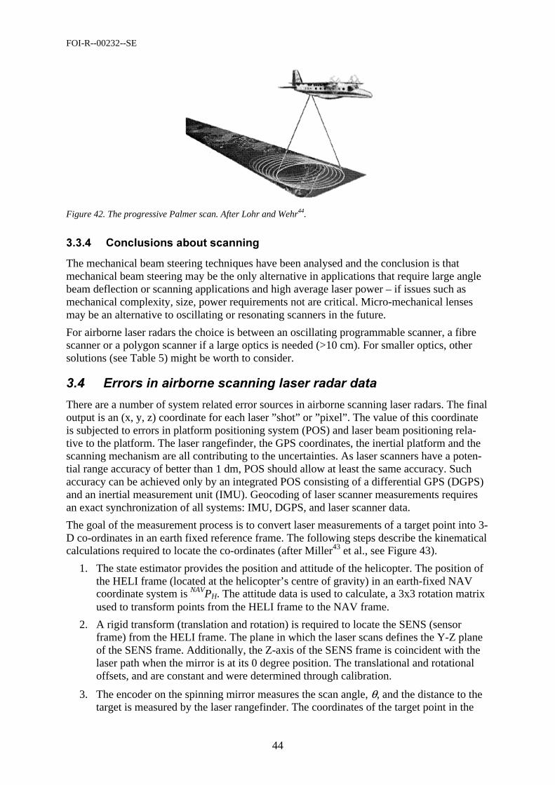
FOI-R--00232--SE

44

Figure 42. The progressive Palmer scan. After Lohr and Wehr44.

((/ %$2$

The mechanical beam steering techniques have been analysed and the conclusion is that mechanical beam steering may be the only alternative in applications that require large angle beam deflection or scanning applications and high average laser power – if issues such as mechanical complexity, size, power requirements not are critical. Micro-mechanical lenses may be an alternative to oscillating or resonating scanners in the future.

For airborne laser radars the choice is between an oscillating programmable scanner, a fibre scanner or a polygon scanner if a large optics is needed (>10 cm). For smaller optics, other solutions (see Table 5) might be worth to consider.

# *'

There are a number of system related error sources in airborne scanning laser radars. The final output is an (x, y, z) coordinate for each laser ”shot” or ”pixel”. The value of this coordinate is subjected to errors in platform positioning system (POS) and laser beam positioning rela-tive to the platform. The laser rangefinder, the GPS coordinates, the inertial platform and the scanning mechanism are all contributing to the uncertainties. As laser scanners have a poten-tial range accuracy of better than 1 dm, POS should allow at least the same accuracy. Such accuracy can be achieved only by an integrated POS consisting of a differential GPS (DGPS) and an inertial measurement unit (IMU). Geocoding of laser scanner measurements requires an exact synchronization of all systems: IMU, DGPS, and laser scanner data.

The goal of the measurement process is to convert laser measurements of a target point into 3-D co-ordinates in an earth fixed reference frame. The following steps describe the kinematical calculations required to locate the co-ordinates (after Miller43 et al., see Figure 43).

1. The state estimator provides the position and attitude of the helicopter. The position of the HELI frame (located at the helicopter’s centre of gravity) in an earth-fixed NAV coordinate system is NAVPH. The attitude data is used to calculate, a 3x3 rotation matrix used to transform points from the HELI frame to the NAV frame.

2. A rigid transform (translation and rotation) is required to locate the SENS (sensor frame) from the HELI frame. The plane in which the laser scans defines the Y-Z plane of the SENS frame. Additionally, the Z-axis of the SENS frame is coincident with the laser path when the mirror is at its 0 degree position. The translational and rotational offsets, and are constant and were determined through calibration.

3. The encoder on the spinning mirror measures the scan angle, θ, and the distance to the target is measured by the laser rangefinder. The coordinates of the target point in the

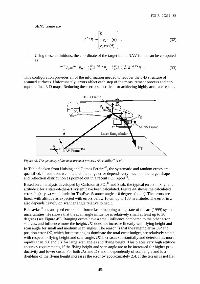
FOI-R--00232--SE

45

SENS frame are

−=

)cos(

)sin(

0

θθ

6

67

6(16

$ . (32)

4. Using these definitions, the coordinate of the target in the NAV frame can be computed as

7

6(16+(/,

6(16

1$9

+(/,6

+(/,1$9

+(/,+

1$9

7

1$9 $ $ $$ ⋅⋅+⋅+= . (33)

This configuration provides all of the information needed to recover the 3-D structure of scanned surfaces. Unfortunately, errors affect each step of the measurement process and cor-rupt the final 3-D maps. Reducing these errors is critical for achieving highly accurate results.

Figure 43. The geometry of the measurement process. After Miller43 et al.

In Table 6 taken from Huising and Gomes Pereira45, the systematic and random errors are quantified. In addition, we note that the range error depends very much on the target shape and reflection distribution as pointed out in a recent FOI report46.

Based on an analysis developed by Carlsson at FOI47 and Saab, the typical errors in x, y, and altitude z for a state-of-the-art system have been calculated. Figure 44 shows the calculated errors in (x, y, z) vs. altitude for TopEye. Scanner angle = 0 degrees (nadir). The errors are linear with altitude as expected with errors below 10 cm up to 100 m altitude. The error in z also depends heavily on scanner angle relative to nadir.

Baltsavias48 has analysed errors in airborne laser mapping using state of the art (1999) system uncertainties. He shows that the scan angle influence is relatively small at least up to 30 degrees (see Figure 45). Ranging errors have a small influence compared to the other error sources, and influence more the height.Z does not increase linearly with flying height and scan angle for small and medium scan angles. The reason is that the ranging error DR and position error Z, which for these angles dominate the total error budget, are relatively stable with respect to flying height and scan angle. DZ increases substantially and deteriorates more rapidly than X and DY for large scan angles and flying height. This places very high attitude accuracy requirements, if the flying height and scan angle are to be increased for higher pro-ductivity and lower costs. For both X and DY and independently of scan angle and k, a doubling of the flying height increases the error by approximately 2.4. If the terrain is not flat,

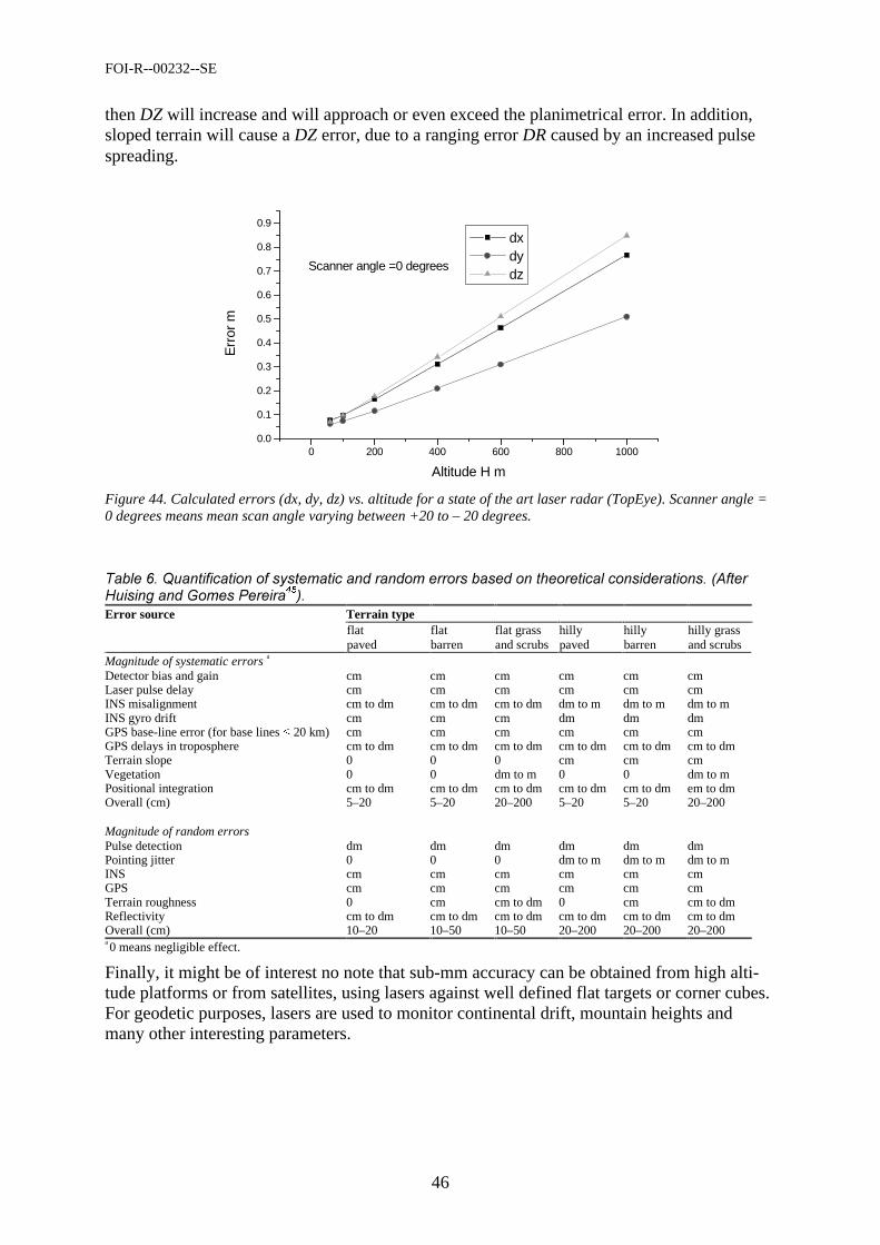
FOI-R--00232--SE

46

then DZ will increase and will approach or even exceed the planimetrical error. In addition, sloped terrain will cause a DZ error, due to a ranging error DR caused by an increased pulse spreading.

0 200 400 600 800 10000.0

0.1

0.2

0.3

0.4

0.5

0.6

0.7

0.8

0.9

Scanner angle =0 degrees

dx dy dz

Err

or m

Altitude H m Figure 44. Calculated errors (dx, dy, dz) vs. altitude for a state of the art laser radar (TopEye). Scanner angle = 0 degrees means mean scan angle varying between +20 to – 20 degrees.

,-!#./0'Error source Terrain type

flat flat flat grass hilly hilly hilly grass paved barren and scrubs paved barren and scrubs Magnitude of systematic errors a Detector bias and gain cm cm cm cm cm cm Laser pulse delay cm cm cm cm cm cm INS misalignment cm to dm cm to dm cm to dm dm to m dm to m dm to m INS gyro drift cm cm cm dm dm dm GPS base-line error (for base lines 20 km) cm cm cm cm cm cm GPS delays in troposphere cm to dm cm to dm cm to dm cm to dm cm to dm cm to dm Terrain slope 0 0 0 cm cm cm Vegetation 0 0 dm to m 0 0 dm to m Positional integration cm to dm cm to dm cm to dm cm to dm cm to dm em to dm Overall (cm) 5–20 5–20 20–200 5–20 5–20 20–200 Magnitude of random errors Pulse detection dm dm dm dm dm dm Pointing jitter 0 0 0 dm to m dm to m dm to m INS cm cm cm cm cm cm GPS cm cm cm cm cm cm Terrain roughness 0 cm cm to dm 0 cm cm to dm Reflectivity cm to dm cm to dm cm to dm cm to dm cm to dm cm to dm Overall (cm) 10–20 10–50 10–50 20–200 20–200 20–200 a 0 means negligible effect.

Finally, it might be of interest no note that sub-mm accuracy can be obtained from high alti-tude platforms or from satellites, using lasers against well defined flat targets or corner cubes. For geodetic purposes, lasers are used to monitor continental drift, mountain heights and many other interesting parameters.

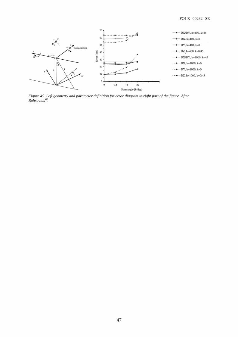
FOI-R--00232--SE

47

Figure 45. Left geometry and parameter definition for error diagram in right part of the figure. After Baltsavias48.

FOI-R--00232--SE

48

/ Effective and reliable data analysis is crucial for the success of laser remote sensing in forestry. Development and evaluation of new methods is an active and growing area of research today and new results are continuously reported. Selection of appropriate analysis methods depends on the forestry application at hand, the characteristics of the laser measure-ment system and the type of data it produces. In laser remote sensing for forestry two main categories of laser measurement systems are employed, (i) small footprint systems and (ii) large footprint and full waveform systems. These systems produce quite different data sets and hence necessarily call for different kinds of methods for data analysis.

• Small footprint systems are characterised by high pulse repetition rate, fast scanning and recording of range measurement obtained from on-line digital signal processing.

• Large footprint systems are characterised by slower pulse repetition rate, slower scanning and recording of fully digitised waveforms.

In Table 7 and Table 8 below, taken from a comparison of small and large footprint systems by Means20, the different design, functioning and purposes of small and large footprint sys-tems are summarised. Below we will discuss some important data analysis methods of interest in laser remote sensing in forestry.

1! ! ! Small footprint Large footprint

Common Goals - ground surface elevation, DTMs - canopy top elevation

- ground surface elevation, DTMs - canopy top elevation

Different Goals - 0.5-3 m horizontal resolution - 10-25 m horizontal resolution - vertical distribution of canopy surfaces

2*! !3!

Horizontal point spacing, m 0.2 – 3 10 – 25

Footprint diameter, m 0.2 – 0.9 10 – 25

Reflection collection 1-5 discrete reflections, separated by minimum 1.5-2m

Full waveform digitisation

Energy, mJ/pulse 0.0125 – 0.2 5 – 10

Pulse Rate, kHz 5 – 15 0.1 - 0.5

Flying height, km 0.2 - 1.0 4 – 400

Swath width, m 70 – 1200 800 – 8000 (discontinuous)

Platform Helicopter, fixed wing Fixed wing, earth orbit

#

Small footprint systems are primarily developed for the acquisition of x, y and z co-ordinates of arbitrary points on the terrain surface or on other natural or artificial objects. Besides this basic operation, many systems also have various additional features. One common feature is the capability to discriminate multiple returns (or reflections) of an individual laser pulse and hence record multiple (x,y,z) co-ordinate triples. Typically, this arises when different parts of a laser footprint are reflected at different ranges. One example is given by the case where the footprint is split by the edge of a roof and one part is being reflected from the roof and the

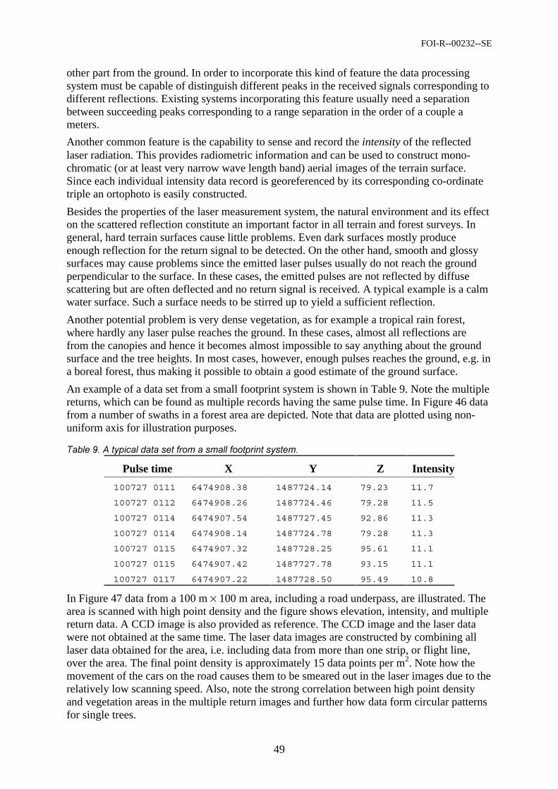
FOI-R--00232--SE

49

other part from the ground. In order to incorporate this kind of feature the data processing system must be capable of distinguish different peaks in the received signals corresponding to different reflections. Existing systems incorporating this feature usually need a separation between succeeding peaks corresponding to a range separation in the order of a couple a meters.

Another common feature is the capability to sense and record the intensity of the reflected laser radiation. This provides radiometric information and can be used to construct mono-chromatic (or at least very narrow wave length band) aerial images of the terrain surface. Since each individual intensity data record is georeferenced by its corresponding co-ordinate triple an ortophoto is easily constructed.

Besides the properties of the laser measurement system, the natural environment and its effect on the scattered reflection constitute an important factor in all terrain and forest surveys. In general, hard terrain surfaces cause little problems. Even dark surfaces mostly produce enough reflection for the return signal to be detected. On the other hand, smooth and glossy surfaces may cause problems since the emitted laser pulses usually do not reach the ground perpendicular to the surface. In these cases, the emitted pulses are not reflected by diffuse scattering but are often deflected and no return signal is received. A typical example is a calm water surface. Such a surface needs to be stirred up to yield a sufficient reflection.

Another potential problem is very dense vegetation, as for example a tropical rain forest, where hardly any laser pulse reaches the ground. In these cases, almost all reflections are from the canopies and hence it becomes almost impossible to say anything about the ground surface and the tree heights. In most cases, however, enough pulses reaches the ground, e.g. in a boreal forest, thus making it possible to obtain a good estimate of the ground surface.

An example of a data set from a small footprint system is shown in Table 9. Note the multiple returns, which can be found as multiple records having the same pulse time. In Figure 46 data from a number of swaths in a forest area are depicted. Note that data are plotted using non-uniform axis for illustration purposes.

4.! !

Pulse time X Y Z Intensity

100727 0111

100727 0112

100727 0114

100727 0114

100727 0115

100727 0115

100727 0117

6474908.38

6474908.26

6474907.54

6474908.14

6474907.32

6474907.42

6474907.22

1487724.14

1487724.46

1487727.45

1487724.78

1487728.25

1487727.78

1487728.50

79.23

79.28

92.86

79.28

95.61

93.15

95.49

11.7

11.5

11.3

11.3

11.1

11.1

10.8

In Figure 47 data from a 100 m × 100 m area, including a road underpass, are illustrated. The area is scanned with high point density and the figure shows elevation, intensity, and multiple return data. A CCD image is also provided as reference. The CCD image and the laser data were not obtained at the same time. The laser data images are constructed by combining all laser data obtained for the area, i.e. including data from more than one strip, or flight line, over the area. The final point density is approximately 15 data points per m2. Note how the movement of the cars on the road causes them to be smeared out in the laser images due to the relatively low scanning speed. Also, note the strong correlation between high point density and vegetation areas in the multiple return images and further how data form circular patterns for single trees.

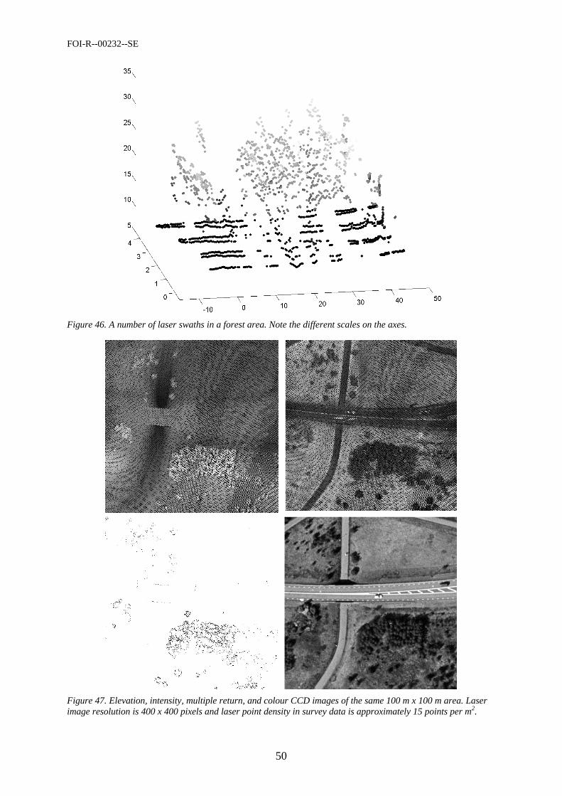
FOI-R--00232--SE

50

Figure 46. A number of laser swaths in a forest area. Note the different scales on the axes.

Figure 47. Elevation, intensity, multiple return, and colour CCD images of the same 100 m x 100 m area. Laser image resolution is 400 x 400 pixels and laser point density in survey data is approximately 15 points per m2.

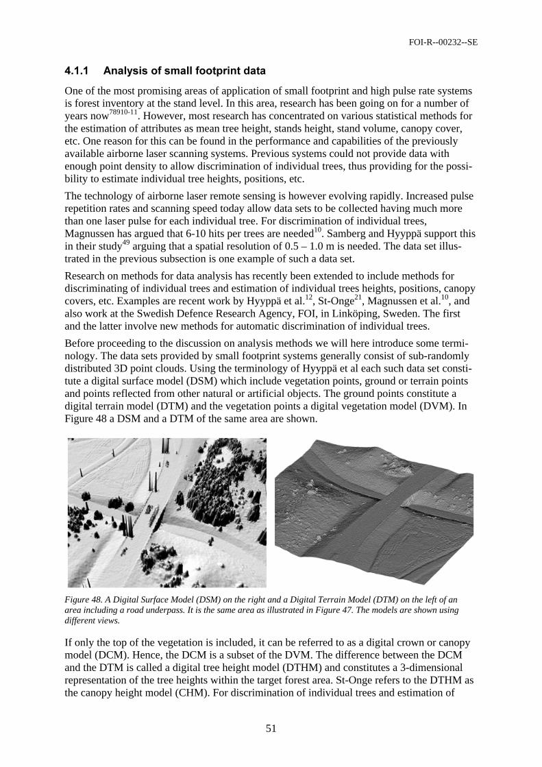
FOI-R--00232--SE

51

/(( "*

One of the most promising areas of application of small footprint and high pulse rate systems is forest inventory at the stand level. In this area, research has been going on for a number of years now78910-11. However, most research has concentrated on various statistical methods for the estimation of attributes as mean tree height, stands height, stand volume, canopy cover, etc. One reason for this can be found in the performance and capabilities of the previously available airborne laser scanning systems. Previous systems could not provide data with enough point density to allow discrimination of individual trees, thus providing for the possi-bility to estimate individual tree heights, positions, etc.

The technology of airborne laser remote sensing is however evolving rapidly. Increased pulse repetition rates and scanning speed today allow data sets to be collected having much more than one laser pulse for each individual tree. For discrimination of individual trees, Magnussen has argued that 6-10 hits per trees are needed10. Samberg and Hyyppä support this in their study49 arguing that a spatial resolution of 0.5 – 1.0 m is needed. The data set illus-trated in the previous subsection is one example of such a data set.

Research on methods for data analysis has recently been extended to include methods for discriminating of individual trees and estimation of individual trees heights, positions, canopy covers, etc. Examples are recent work by Hyyppä et al.12, St-Onge21, Magnussen et al.10, and also work at the Swedish Defence Research Agency, FOI, in Linköping, Sweden. The first and the latter involve new methods for automatic discrimination of individual trees.

Before proceeding to the discussion on analysis methods we will here introduce some termi-nology. The data sets provided by small footprint systems generally consist of sub-randomly distributed 3D point clouds. Using the terminology of Hyyppä et al each such data set consti-tute a digital surface model (DSM) which include vegetation points, ground or terrain points and points reflected from other natural or artificial objects. The ground points constitute a digital terrain model (DTM) and the vegetation points a digital vegetation model (DVM). In Figure 48 a DSM and a DTM of the same area are shown.

Figure 48. A Digital Surface Model (DSM) on the right and a Digital Terrain Model (DTM) on the left of an area including a road underpass. It is the same area as illustrated in Figure 47. The models are shown using different views.

If only the top of the vegetation is included, it can be referred to as a digital crown or canopy model (DCM). Hence, the DCM is a subset of the DVM. The difference between the DCM and the DTM is called a digital tree height model (DTHM) and constitutes a 3-dimensional representation of the tree heights within the target forest area. St-Onge refers to the DTHM as the canopy height model (CHM). For discrimination of individual trees and estimation of

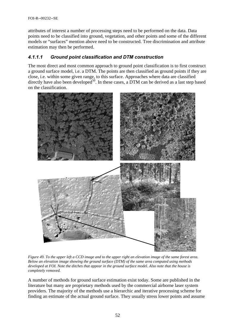
FOI-R--00232--SE

52

attributes of interest a number of processing steps need to be performed on the data. Data points need to be classified into ground, vegetation, and other points and some of the different models or “surfaces” mention above need to be constructed. Tree discrimination and attribute estimation may then be performed.

# + ),-

The most direct and most common approach to ground point classification is to first construct a ground surface model, i.e. a DTM. The points are then classified as ground points if they are close, i.e. within some given range, to this surface. Approaches where data are classified directly have also been developed50. In these cases, a DTM can be derived as a last step based on the classification.

Figure 49. To the upper left a CCD image and to the upper right an elevation image of the same forest area. Below an elevation image showing the ground surface (DTM) of the same area computed using methods developed at FOI. Note the ditches that appear in the ground surface model. Also note that the house is completely removed.

A number of methods for ground surface estimation exist today. Some are published in the literature but many are proprietary methods used by the commercial airborne laser system providers. The majority of the methods use a hierarchic and iterative processing scheme for finding an estimate of the actual ground surface. They usually stress lower points and assume

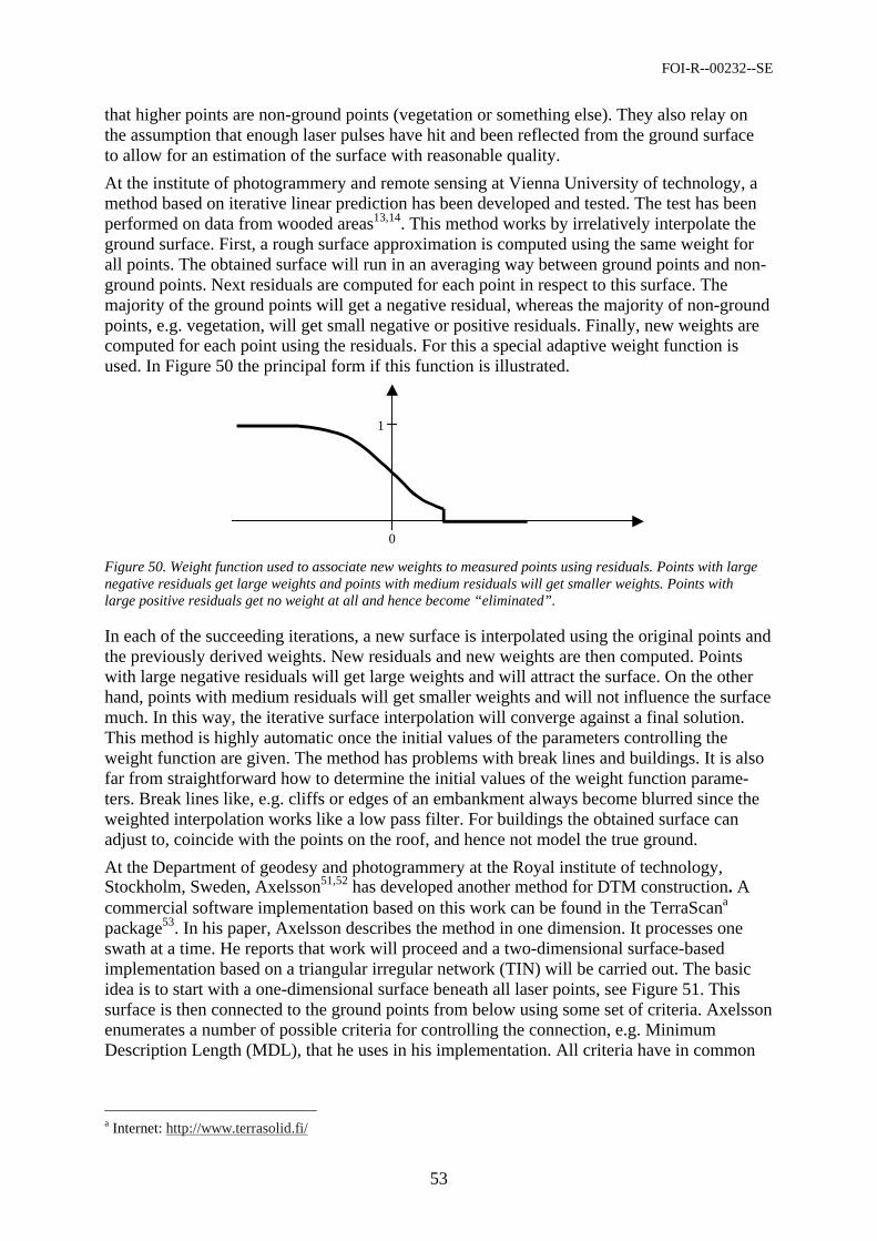
FOI-R--00232--SE

53

that higher points are non-ground points (vegetation or something else). They also relay on the assumption that enough laser pulses have hit and been reflected from the ground surface to allow for an estimation of the surface with reasonable quality.

At the institute of photogrammery and remote sensing at Vienna University of technology, a method based on iterative linear prediction has been developed and tested. The test has been performed on data from wooded areas13,14. This method works by irrelatively interpolate the ground surface. First, a rough surface approximation is computed using the same weight for all points. The obtained surface will run in an averaging way between ground points and non-ground points. Next residuals are computed for each point in respect to this surface. The majority of the ground points will get a negative residual, whereas the majority of non-ground points, e.g. vegetation, will get small negative or positive residuals. Finally, new weights are computed for each point using the residuals. For this a special adaptive weight function is used. In Figure 50 the principal form if this function is illustrated.

1

0 Figure 50. Weight function used to associate new weights to measured points using residuals. Points with large negative residuals get large weights and points with medium residuals will get smaller weights. Points with large positive residuals get no weight at all and hence become “eliminated”.

In each of the succeeding iterations, a new surface is interpolated using the original points and the previously derived weights. New residuals and new weights are then computed. Points with large negative residuals will get large weights and will attract the surface. On the other hand, points with medium residuals will get smaller weights and will not influence the surface much. In this way, the iterative surface interpolation will converge against a final solution. This method is highly automatic once the initial values of the parameters controlling the weight function are given. The method has problems with break lines and buildings. It is also far from straightforward how to determine the initial values of the weight function parame-ters. Break lines like, e.g. cliffs or edges of an embankment always become blurred since the weighted interpolation works like a low pass filter. For buildings the obtained surface can adjust to, coincide with the points on the roof, and hence not model the true ground.

At the Department of geodesy and photogrammery at the Royal institute of technology, Stockholm, Sweden, Axelsson51,52 has developed another method for DTM construction. A commercial software implementation based on this work can be found in the TerraScana package53. In his paper, Axelsson describes the method in one dimension. It processes one swath at a time. He reports that work will proceed and a two-dimensional surface-based implementation based on a triangular irregular network (TIN) will be carried out. The basic idea is to start with a one-dimensional surface beneath all laser points, see Figure 51. This surface is then connected to the ground points from below using some set of criteria. Axelsson enumerates a number of possible criteria for controlling the connection, e.g. Minimum Description Length (MDL), that he uses in his implementation. All criteria have in common

a Internet: http://www.terrasolid.fi/

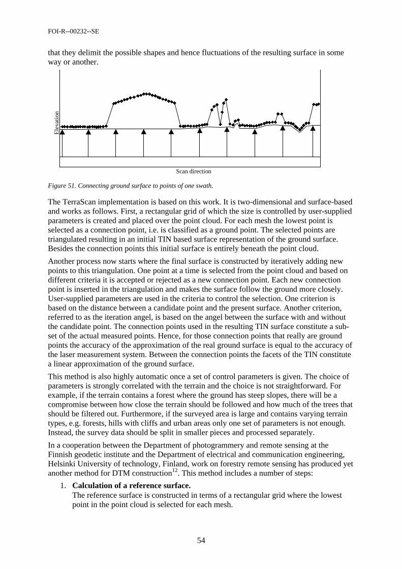
FOI-R--00232--SE

54

that they delimit the possible shapes and hence fluctuations of the resulting surface in some way or another.

u u u u u u u u u u u u u u u u u u u u

u u u u u u u

u u u u u u u u

u u u

u

u u u u

u u u u u

u

u

u u

u u

u

u u

u

u

u

u u

u u u u u u u u u u u

u u u

u u

u u

u

u

u

u u

u u u

u u u u u

u

u

Ele

vati

on

Scan direction Figure 51. Connecting ground surface to points of one swath.

The TerraScan implementation is based on this work. It is two-dimensional and surface-based and works as follows. First, a rectangular grid of which the size is controlled by user-supplied parameters is created and placed over the point cloud. For each mesh the lowest point is selected as a connection point, i.e. is classified as a ground point. The selected points are triangulated resulting in an initial TIN based surface representation of the ground surface. Besides the connection points this initial surface is entirely beneath the point cloud.

Another process now starts where the final surface is constructed by iteratively adding new points to this triangulation. One point at a time is selected from the point cloud and based on different criteria it is accepted or rejected as a new connection point. Each new connection point is inserted in the triangulation and makes the surface follow the ground more closely. User-supplied parameters are used in the criteria to control the selection. One criterion is based on the distance between a candidate point and the present surface. Another criterion, referred to as the iteration angel, is based on the angel between the surface with and without the candidate point. The connection points used in the resulting TIN surface constitute a sub-set of the actual measured points. Hence, for those connection points that really are ground points the accuracy of the approximation of the real ground surface is equal to the accuracy of the laser measurement system. Between the connection points the facets of the TIN constitute a linear approximation of the ground surface.

This method is also highly automatic once a set of control parameters is given. The choice of parameters is strongly correlated with the terrain and the choice is not straightforward. For example, if the terrain contains a forest where the ground has steep slopes, there will be a compromise between how close the terrain should be followed and how much of the trees that should be filtered out. Furthermore, if the surveyed area is large and contains varying terrain types, e.g. forests, hills with cliffs and urban areas only one set of parameters is not enough. Instead, the survey data should be split in smaller pieces and processed separately.

In a cooperation between the Department of photogrammery and remote sensing at the Finnish geodetic institute and the Department of electrical and communication engineering, Helsinki University of technology, Finland, work on forestry remote sensing has produced yet another method for DTM construction12. This method includes a number of steps:

1. Calculation of a reference surface. The reference surface is constructed in terms of a rectangular grid where the lowest point in the point cloud is selected for each mesh.

FOI-R--00232--SE

55

2. Classification of vegetation and removal of vegetation from the reference surface. It is assumed that the ground surface does not have any significant local changes. For each grid point, a gradient is computed and if the value is above a certain threshold, the point is considered vegetation and its elevation value is removed. For each such grid point, a new elevation value is determined by interpolation using the near-by points.

3. Classification of ground points in the original point cloud. The distance between points in the original point cloud and the reference surface rep-resented by the grid are now determined. If the value lies within a certain range, the point is classified as a ground point. The range value must be specified by the user. It depends on the terrain type and slope. A value of 60 cm has been used and according to the authors, it produces an ideal point cloud for the final DTM construction.

4. Construction of a DTM using ground points. The DTM is constructed as a rectangular grid. Elevation values are computed using mean and median values of the classified ground points. Grid points with missing ele-vation values are interpolated using near-by elevation values.

This method is developed for forestry applications and hence primarily for use in forest areas. It should not be expected to produce high quality ground surface approximations if there are buildings and other man-made objects in the survey area. This method is also highly auto-matic once the user has supplied the necessary parameters. As for the previous methods, the choice of parameters depends on the terrain type.

At the Department of Laser systems at FOI in Linköping, another method has been developed54. It is related to the method presented by Axelsson and is based on the idea of moving a surface upwards from below. The main differences are found in the criteria used. This method is based on the theory on active contours55,56 and it works in two separate phases. In the fist phase the surface is moved upwards controlled by one set of criteria and in the second phase, the surface is adjusted using a slightly different set of criteria. In this way, a high quality approximation of the ground surface is achieved. The method has been imple-mented and tested in an experimental set-up. For simplicity and speed of computation, the implementation works only on rectangular grid data. However, it is straightforward to modify the implementation to use the original point cloud and create a surface in terms of a TIN.

The theory of active contours has its roots in image processing where it is mainly used for detection of contours in images. It is usually referred to as snakes, especially when referring to two-dimensional contours. In such a case, the snake is a continuous spline, open with loose ends or closed in a loop. The method described here uses a three dimensional active contour that is a continuous open surface. In general, the shape of an active contour depends on the physical characteristics associated with it and the potential field from the data set. The physi-cal characteristics are material properties like elasticity and rigidity. The solution is the con-tour that minimizes an energy function. An active contour may stick to a local minimum and it should be noted that the desired solution is not always the global minimum.

The contour used in this method acts like a sticky rubber cloth or a rubber band net that is being pulled upwards from underneath. The net is attracted by the grid points and sticks to points that (are assumed to) represent the true ground. The elasticity forces in the rubber band stops the net from reaching points not representing the true ground. The net forms a continu-ous model of the ground surface. It is a robust method for ground surface estimation and it is possible to adjust the parameters to achieve different behaviour of the net. For example, if it is preferred that rocks in the terrain are part of the ground surface then the net should be more elastic and sense a greater attraction from the measured points.

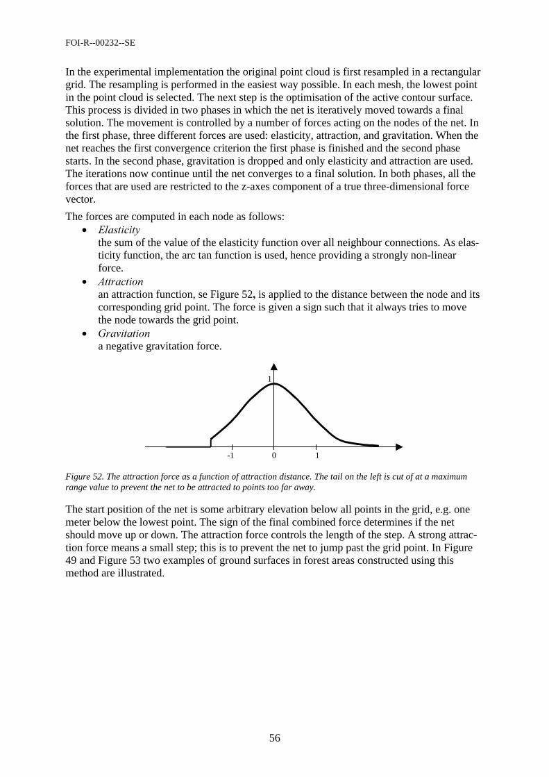
FOI-R--00232--SE

56

In the experimental implementation the original point cloud is first resampled in a rectangular grid. The resampling is performed in the easiest way possible. In each mesh, the lowest point in the point cloud is selected. The next step is the optimisation of the active contour surface. This process is divided in two phases in which the net is iteratively moved towards a final solution. The movement is controlled by a number of forces acting on the nodes of the net. In the first phase, three different forces are used: elasticity, attraction, and gravitation. When the net reaches the first convergence criterion the first phase is finished and the second phase starts. In the second phase, gravitation is dropped and only elasticity and attraction are used. The iterations now continue until the net converges to a final solution. In both phases, all the forces that are used are restricted to the z-axes component of a true three-dimensional force vector.

The forces are computed in each node as follows: • #

the sum of the value of the elasticity function over all neighbour connections. As elas-ticity function, the arc tan function is used, hence providing a strongly non-linear force.

• ) an attraction function, se Figure 52is applied to the distance between the node and its corresponding grid point. The force is given a sign such that it always tries to move the node towards the grid point.

• ,- a negative gravitation force.

1

0 1 -1

Figure 52. The attraction force as a function of attraction distance. The tail on the left is cut of at a maximum range value to prevent the net to be attracted to points too far away.

The start position of the net is some arbitrary elevation below all points in the grid, e.g. one meter below the lowest point. The sign of the final combined force determines if the net should move up or down. The attraction force controls the length of the step. A strong attrac-tion force means a small step; this is to prevent the net to jump past the grid point. In Figure 49 and Figure 53 two examples of ground surfaces in forest areas constructed using this method are illustrated.

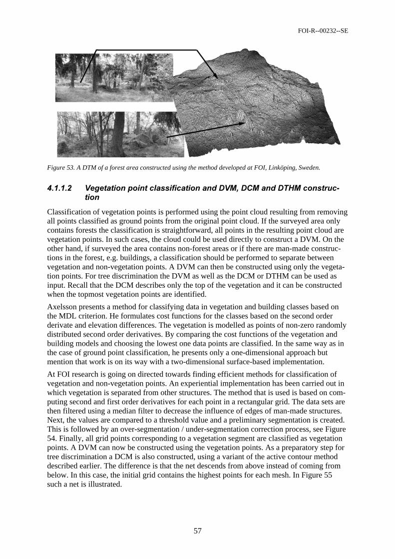
FOI-R--00232--SE

57

Figure 53. A DTM of a forest area constructed using the method developed at FOI, Linköping, Sweden.

# . ).-!)$- ),/-

Classification of vegetation points is performed using the point cloud resulting from removing all points classified as ground points from the original point cloud. If the surveyed area only contains forests the classification is straightforward, all points in the resulting point cloud are vegetation points. In such cases, the cloud could be used directly to construct a DVM. On the other hand, if surveyed the area contains non-forest areas or if there are man-made construc-tions in the forest, e.g. buildings, a classification should be performed to separate between vegetation and non-vegetation points. A DVM can then be constructed using only the vegeta-tion points. For tree discrimination the DVM as well as the DCM or DTHM can be used as input. Recall that the DCM describes only the top of the vegetation and it can be constructed when the topmost vegetation points are identified.

Axelsson presents a method for classifying data in vegetation and building classes based on the MDL criterion. He formulates cost functions for the classes based on the second order derivate and elevation differences. The vegetation is modelled as points of non-zero randomly distributed second order derivatives. By comparing the cost functions of the vegetation and building models and choosing the lowest one data points are classified. In the same way as in the case of ground point classification, he presents only a one-dimensional approach but mention that work is on its way with a two-dimensional surface-based implementation.

At FOI research is going on directed towards finding efficient methods for classification of vegetation and non-vegetation points. An experiential implementation has been carried out in which vegetation is separated from other structures. The method that is used is based on com-puting second and first order derivatives for each point in a rectangular grid. The data sets are then filtered using a median filter to decrease the influence of edges of man-made structures. Next, the values are compared to a threshold value and a preliminary segmentation is created. This is followed by an over-segmentation / under-segmentation correction process, see Figure 54. Finally, all grid points corresponding to a vegetation segment are classified as vegetation points. A DVM can now be constructed using the vegetation points. As a preparatory step for tree discrimination a DCM is also constructed, using a variant of the active contour method described earlier. The difference is that the net descends from above instead of coming from below. In this case, the initial grid contains the highest points for each mesh. In Figure 55 such a net is illustrated.

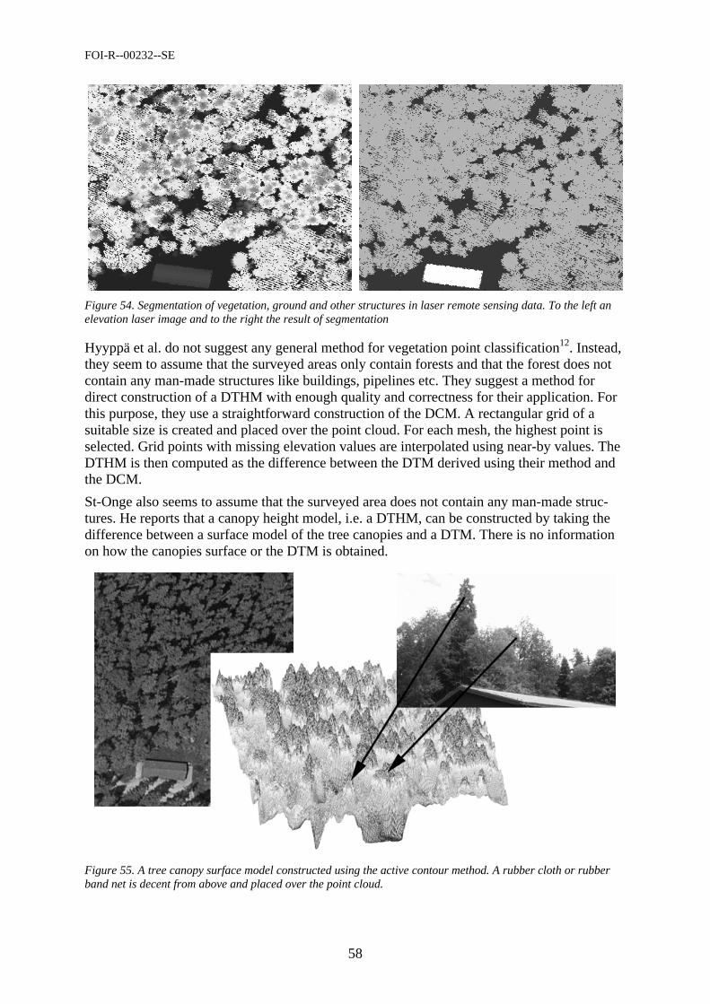
FOI-R--00232--SE

58

Figure 54. Segmentation of vegetation, ground and other structures in laser remote sensing data. To the left an elevation laser image and to the right the result of segmentation

Hyyppä et al. do not suggest any general method for vegetation point classification12. Instead, they seem to assume that the surveyed areas only contain forests and that the forest does not contain any man-made structures like buildings, pipelines etc. They suggest a method for direct construction of a DTHM with enough quality and correctness for their application. For this purpose, they use a straightforward construction of the DCM. A rectangular grid of a suitable size is created and placed over the point cloud. For each mesh, the highest point is selected. Grid points with missing elevation values are interpolated using near-by values. The DTHM is then computed as the difference between the DTM derived using their method and the DCM.

St-Onge also seems to assume that the surveyed area does not contain any man-made struc-tures. He reports that a canopy height model, i.e. a DTHM, can be constructed by taking the difference between a surface model of the tree canopies and a DTM. There is no information on how the canopies surface or the DTM is obtained.

Figure 55. A tree canopy surface model constructed using the active contour method. A rubber cloth or rubber band net is decent from above and placed over the point cloud.

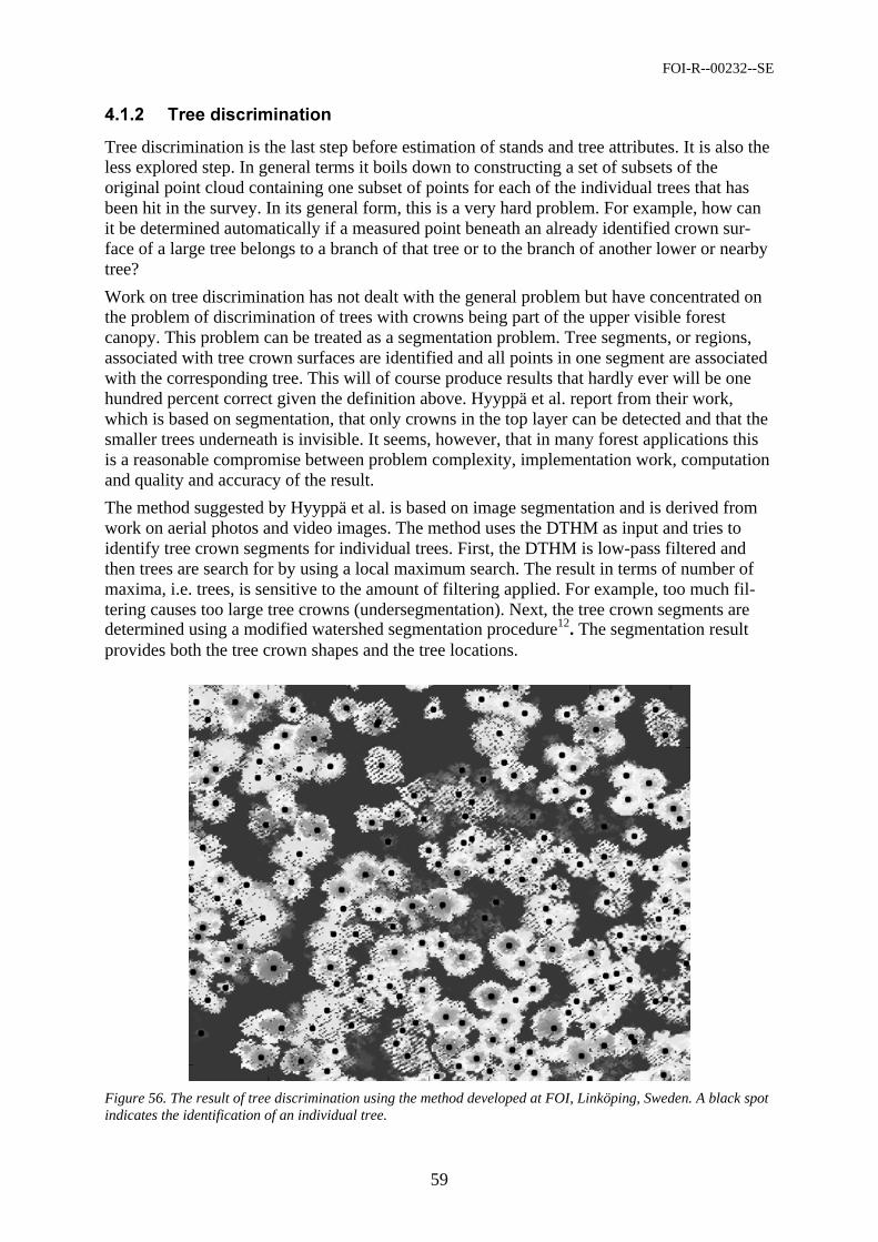
FOI-R--00232--SE

59

/(( .

Tree discrimination is the last step before estimation of stands and tree attributes. It is also the less explored step. In general terms it boils down to constructing a set of subsets of the original point cloud containing one subset of points for each of the individual trees that has been hit in the survey. In its general form, this is a very hard problem. For example, how can it be determined automatically if a measured point beneath an already identified crown sur-face of a large tree belongs to a branch of that tree or to the branch of another lower or nearby tree?

Work on tree discrimination has not dealt with the general problem but have concentrated on the problem of discrimination of trees with crowns being part of the upper visible forest canopy. This problem can be treated as a segmentation problem. Tree segments, or regions, associated with tree crown surfaces are identified and all points in one segment are associated with the corresponding tree. This will of course produce results that hardly ever will be one hundred percent correct given the definition above. Hyyppä et al. report from their work, which is based on segmentation, that only crowns in the top layer can be detected and that the smaller trees underneath is invisible. It seems, however, that in many forest applications this is a reasonable compromise between problem complexity, implementation work, computation and quality and accuracy of the result.

The method suggested by Hyyppä et al. is based on image segmentation and is derived from work on aerial photos and video images. The method uses the DTHM as input and tries to identify tree crown segments for individual trees. First, the DTHM is low-pass filtered and then trees are search for by using a local maximum search. The result in terms of number of maxima, i.e. trees, is sensitive to the amount of filtering applied. For example, too much fil-tering causes too large tree crowns (undersegmentation). Next, the tree crown segments are determined using a modified watershed segmentation procedure12. The segmentation result provides both the tree crown shapes and the tree locations.

Figure 56. The result of tree discrimination using the method developed at FOI, Linköping, Sweden. A black spot indicates the identification of an individual tree.

FOI-R--00232--SE

60

At FOI in Linköping ongoing work have independently followed a similar approach for tree discrimination. This method is applied to a DCM, which is constructed using a variant of the active contour method described above. The DCM is low-pass filtered using two different filters. This produces two filtered models in which the trees are search for using a combined segmentation and local maximum search. The results are then compared and combined. An experimental implementation has been carried out and evaluation is going on at the time of writing. A preliminary result is illustrated in Figure 56.

St-Onge also reports on tree discrimination as a step before attribute estimation. He performs the work by hand and does not suggest any automatic method. It is interesting to note though that he tries to incorporate orthophotos from the surveyed area in the process. This is an inter-esting approach for a future work.

/(( . 2$

We will here briefly touch upon attribute estimation. For forest inventory at the stand level tree height, crown cover and tree diameter is the main attributes to estimate. Tree position is also interesting. Many other attributes of interest can be derived from them using existing methods.

Tree height is the most important attribute and the one most treated in the literature. The common conclusion is that laser remote sensing can be used for tree height estimation. It is however, also a common conclusion that a direct estimation of tree height from laser data always underestimates the height. This was found early and has been verified in recent investigations7, 9, 12, 21. The reason is that laser hits are randomly distributed on the tree crown and that there is no guarantee that the highest point is being measured. To solve this problem reliable statistical and/or geometrical methods must be developed. Correlation between laser measurements and field inventories are important in this work.

Crown cover is most straightforwardly estimated using the area of the associated tree seg-ment. The accuracy of this kind of estimation is, however, not known in detail today. The quality of the segmentation method and also the point density and footprint size is assumed to influence the result. Further research on this subject is necessary. Correlation between esti-mated values and field data should be investigated and evaluated.

Tree position is important for automated correlation of laser measurements and GPS based field inventories. It is also necessary in applications where the same forest area is surveyed at several occasions and tree attributes data need to be correlated and compared over time. Esti-mation of tree position can be done using the position of the maximum elevation point of the tree segment or using the point of gravity of the segment area or maybe a combination of both. This is subject for future work

#

Beside the large footprint, the main characteristic of existing large footprint systems used for forestry applications is their capability to fully capture digitised waveforms. This makes them powerful tools for characterizing the complete vertical canopy structure. The large footprint also makes it possible to avoid some of the problems encountered using small footprint sys-tems. Since the large footprint usually fully covers tree crowns of individual trees, measure-ments will include the highest points of the trees and hence the problem with randomly distributed measurements on three crowns are avoided. Further, since canopy areas covered by the large footprints typically contains some openings, even in the case of dense tropical forests, reflections from the ground are almost always obtained, making it possible to accu-rately estimate the vegetation height.

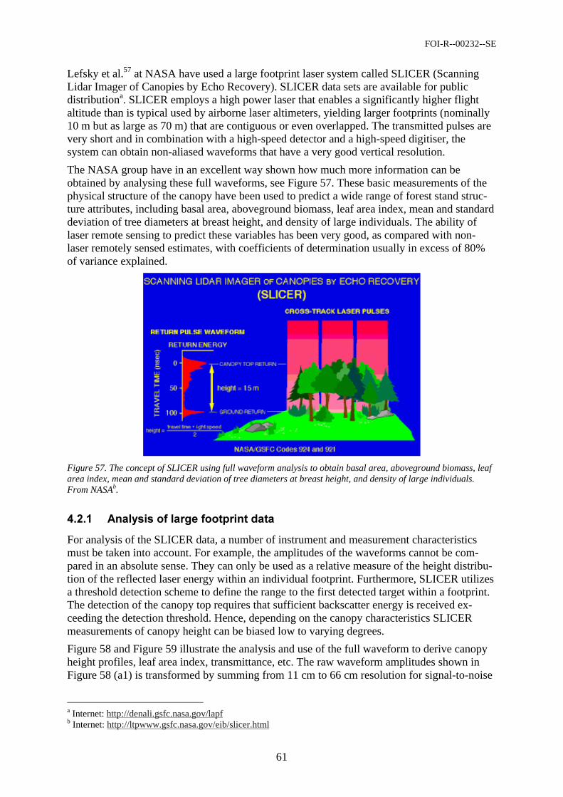
FOI-R--00232--SE

61

Lefsky et al.57 at NASA have used a large footprint laser system called SLICER (Scanning Lidar Imager of Canopies by Echo Recovery). SLICER data sets are available for public distributiona. SLICER employs a high power laser that enables a significantly higher flight altitude than is typical used by airborne laser altimeters, yielding larger footprints (nominally 10 m but as large as 70 m) that are contiguous or even overlapped. The transmitted pulses are very short and in combination with a high-speed detector and a high-speed digitiser, the system can obtain non-aliased waveforms that have a very good vertical resolution.

The NASA group have in an excellent way shown how much more information can be obtained by analysing these full waveforms, see Figure 57. These basic measurements of the physical structure of the canopy have been used to predict a wide range of forest stand struc-ture attributes, including basal area, aboveground biomass, leaf area index, mean and standard deviation of tree diameters at breast height, and density of large individuals. The ability of laser remote sensing to predict these variables has been very good, as compared with non-laser remotely sensed estimates, with coefficients of determination usually in excess of 80% of variance explained.

Figure 57. The concept of SLICER using full waveform analysis to obtain basal area, aboveground biomass, leaf area index, mean and standard deviation of tree diameters at breast height, and density of large individuals. From NASAb.

/(( "*

For analysis of the SLICER data, a number of instrument and measurement characteristics must be taken into account. For example, the amplitudes of the waveforms cannot be com-pared in an absolute sense. They can only be used as a relative measure of the height distribu-tion of the reflected laser energy within an individual footprint. Furthermore, SLICER utilizes a threshold detection scheme to define the range to the first detected target within a footprint. The detection of the canopy top requires that sufficient backscatter energy is received ex-ceeding the detection threshold. Hence, depending on the canopy characteristics SLICER measurements of canopy height can be biased low to varying degrees.

Figure 58 and Figure 59 illustrate the analysis and use of the full waveform to derive canopy height profiles, leaf area index, transmittance, etc. The raw waveform amplitudes shown in Figure 58 (a1) is transformed by summing from 11 cm to 66 cm resolution for signal-to-noise

a Internet: http://denali.gsfc.nasa.gov/lapf b Internet: http://ltpwww.gsfc.nasa.gov/eib/slicer.html

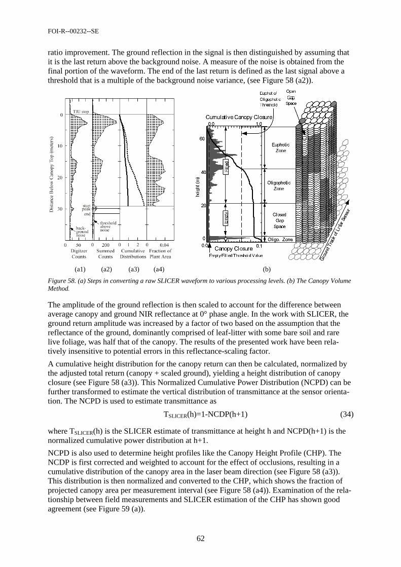
FOI-R--00232--SE

62

ratio improvement. The ground reflection in the signal is then distinguished by assuming that it is the last return above the background noise. A measure of the noise is obtained from the final portion of the waveform. The end of the last return is defined as the last signal above a threshold that is a multiple of the background noise variance, (see Figure 58 (a2)).

(a1) (a2) (a3) (a4) (b)

Figure 58. (a) Steps in converting a raw SLICER waveform to various processing levels. (b) The Canopy Volume Method.

The amplitude of the ground reflection is then scaled to account for the difference between average canopy and ground NIR reflectance at 0° phase angle. In the work with SLICER, the ground return amplitude was increased by a factor of two based on the assumption that the reflectance of the ground, dominantly comprised of leaf-litter with some bare soil and rare live foliage, was half that of the canopy. The results of the presented work have been rela-tively insensitive to potential errors in this reflectance-scaling factor.

A cumulative height distribution for the canopy return can then be calculated, normalized by the adjusted total return (canopy + scaled ground), yielding a height distribution of canopy closure (see Figure 58 (a3)). This Normalized Cumulative Power Distribution (NCPD) can be further transformed to estimate the vertical distribution of transmittance at the sensor orienta-tion. The NCPD is used to estimate transmittance as

TSLICER(h)=1-NCDP(h+1) (34)

where TSLICER(h) is the SLICER estimate of transmittance at height h and NCPD(h+1) is the normalized cumulative power distribution at h+1.

NCPD is also used to determine height profiles like the Canopy Height Profile (CHP). The NCDP is first corrected and weighted to account for the effect of occlusions, resulting in a cumulative distribution of the canopy area in the laser beam direction (see Figure 58 (a3)). This distribution is then normalized and converted to the CHP, which shows the fraction of projected canopy area per measurement interval (see Figure 58 (a4)). Examination of the rela-tionship between field measurements and SLICER estimation of the CHP has shown good agreement (see Figure 59 (a)).

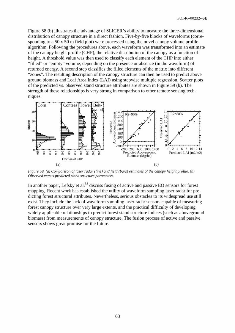
FOI-R--00232--SE

63

Figure 58 (b) illustrates the advantage of SLICER’s ability to measure the three-dimensional distribution of canopy structure in a direct fashion. Five-by-five blocks of waveforms (corre-sponding to a 50 x 50 m field plot) were processed using the novel canopy volume profile algorithm. Following the procedures above, each waveform was transformed into an estimate of the canopy height profile (CHP), the relative distribution of the canopy as a function of height. A threshold value was then used to classify each element of the CHP into either “filled” or “empty” volume, depending on the presence or absence (in the waveform) of returned energy. A second step classifies the filled elements of the matrix into different “zones”. The resulting description of the canopy structure can then be used to predict above ground biomass and Leaf Area Index (LAI) using stepwise multiple regression. Scatter plots of the predicted vs. observed stand structure attributes are shown in Figure 59 (b). The strength of these relationships is very strong in comparison to other remote sensing tech-niques.

0.00

0.05

0.10

0.15

0.00

0.05

0.10

0.00

0.05

0.00

0.05

Heig

ht (m

)

Corn Tower

Fraction of CHP

Contees Belt- woods

0.00

0.05

0.10

0.15

0.00

0.05

0.10

0.00

0.05

0.00

0.05

Heig

ht (m

)

40

30

20

10

0

-2000

200400600800

100012001400

-200 200 600 1000 1400Predicted Aboveground

Biomass (Mg/ha)

R2=90%

02468

101214

0 2 4 6 8 10 12 14Predicted LAI (m2/m2)

R2=88%O

bser

ved

Abo

vegr

ound

Bio

mas

s

Obs

erve

d L

AI

(a) (b)

Figure 59. (a) Comparison of laser radar (line) and field (bars) estimates of the canopy height profile. (b) Observed versus predicted stand structure parameters.

In another paper, Lefsky et al.58 discuss fusing of active and passive EO sensors for forest mapping. Recent work has established the utility of waveform sampling laser radar for pre-dicting forest structural attributes. Nevertheless, serious obstacles to its widespread use still exist. They include the lack of waveform sampling laser radar sensors capable of measuring forest canopy structure over very large extents, and the practical difficulty of developing widely applicable relationships to predict forest stand structure indices (such as aboveground biomass) from measurements of canopy structure. The fusion process of active and passive sensors shows great promise for the future.

FOI-R--00232--SE

64

0 & 2 Martin Flood has written a recent overview of the commercial development of laser altim-etry59. He states:

”Airborne laser altimetry is an emerging technology in the commercial remote sensing industry that is capable of rapidly generating high-density, high-accuracy, digital elevation data. It is an attractive technology for a variety of data end-users in various survey applications since the cost to produce the elevation data, point for point, can be significantly less than other forms of traditional data collection. To a commercial survey company, laser altimetry offers unique technical capabilities, lower field-operation costs and reduced post-processing time and effort compared to traditional survey methods. While laser altimetry has been under investigation since the 1960s, the commercial development of the technology has been driven by the relatively recent availability of rugged, low-cost solutions for each of the core subsystems of the instruments. For many applications, airborne laser altimetry is currently deployed in conjunction with other more tradi-tional sensors including standard aerial film cameras, digital cameras, hyper spectral scanners, or thermal imagery. In general, laser altimetry is best viewed as an addition to the remote sensing toolbox that can add sig-nificant value to the data products produced, either independently or in conjunction with other sensor systems”.

The general characteristics and specifications of the current generation of commercial systems are summarized in Table 10.

5! !#!!6'$$

Specification Typical Value Wavelength a 1.064 µm Pulse Repetition Rate 5 - 15 kHz (25 kHz max) Pulse Energy 100s µJ Pulse Width 10 ns Beam Divergence 0.25 - 2 mrad Scan Angle (full angle) 40° (75° max) Scan Rate 25 - 40 Hz Scan Pattern Zigzag, parallel, elliptical, sinusoidal GPS Frequency 1 - 2 INS Frequency 50 (200 max) Operating Altitude 500 - 1000 m (6000 m max) Footprint 0.25 - 2 m (from 1000 m) Multiple Elevation Capture 2 - 5 Grid Spacing 0.5 - 2 m Accuracy (elevation) 15+ cm Accuracy (planimetrical) 10-100 cm Post-Processing Software b Proprietary Price (standard) $0,850k - $1,000k Price (custom) $1,000k - $2,000k Delivery (standard) 20 - 26 weeks a Generally diode-pumped Nd:YAG, Nd:YLF and Nd:YVO4 although there are some sys-tems operating at 1.5 µm.

b Refers to geo-referencing of laser slant ranges to an established reference frame, nor-mally WGS84.

FOI-R--00232--SE

65

Current commercial instruments are mainly based on research at NASA, University of Stuttgart, FOI, and Optech Inc. in Canada. The whole issue of the ISPRS Journal of Photo-grammetry & Remote Sensing (vol. 54 1999) is devoted to airborne laser scanning covering everything from systems, technology, and measurement analysis to applications. The reader is highly recommended to read more in that issue.

The development in the laser aerial mapping is very rapid and an estimate is that about 50 systems or so are operating throughout the world. The world market demand indicates 200 systems or so by the year 2000. Some applications are summarized in Table 11. To our know-ledge the key operational systems are:

• TopoSys – Germany • ALTM – Optech, Canada • Top Eye – Top Eye AB, Sweden • DATIS, Eaglescan • AeroScan – developed by Azimuth Corporation • ATLAS-SL • Toposense • Vegetation Canopy lidar – NASA

. !

Application Comments

Digital Elevation Mapping The technology allows large area topographic surveys to be completed significantly faster and at a reduced cost compared to traditional survey methods.

Forestry Tree heights and densities, tree classification (research), volume estimates, terrain and topography beneath the tree canopy.

Coastal Engineering Traditional photogrammetry is difficult to use in areas of limited contrast, such as beaches and coastal zones. Laser altimetry offers the ability to complete surveys that would be too costly using other methods.

Corridor or Right-of-Way Mapping Gas pipelines, highways, power lines clearance, tower location, catenary models

Flood Plain Mapping Modelling of flood plains is critical for both disaster planning and insurance purposes. Snow height and water volume calculations.

Wetlands and Other Restricted Access Areas

Many environmentally sensitive areas such as wetlands offer limited ground access and due to vegetation cover are difficult to assess with traditional photogrammetry.

Urban Modelling Telecommunications, microclimate modelling, wireless communications, law enforcement, and disaster planning.

Disaster Response and Damage Assessment

Major natural disasters such as hurricanes or earthquakes stress an emer-gency response organization’s abilities to plan and respond. Airborne laser mapping allows timely, accurate survey data to be rapidly incorporated directly into on-going disaster management efforts and allows rapid post-disaster damage assessments

Military Rapid terrain visualization, cruise missiles, UAV’s, training, synthetic environments etc.

There are also developments within the military and civilian research community, which from a technical point of view is of interest for remote sensing. Examples of such systems are:

• LOCAAS – US Air Force, Eglin AFB. • Rapid terrain visualization – US Army

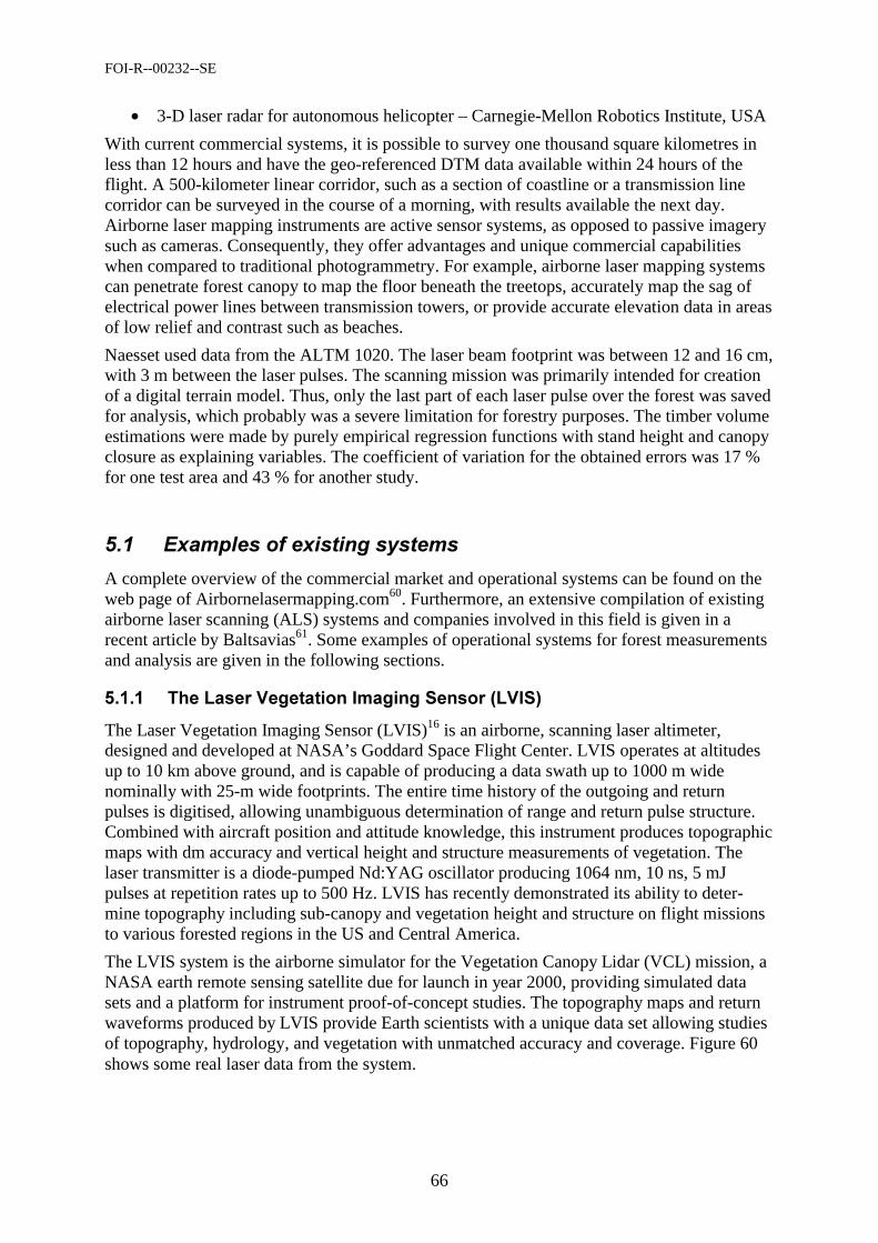
FOI-R--00232--SE

66

• 3-D laser radar for autonomous helicopter – Carnegie-Mellon Robotics Institute, USA

With current commercial systems, it is possible to survey one thousand square kilometres in less than 12 hours and have the geo-referenced DTM data available within 24 hours of the flight. A 500-kilometer linear corridor, such as a section of coastline or a transmission line corridor can be surveyed in the course of a morning, with results available the next day. Airborne laser mapping instruments are active sensor systems, as opposed to passive imagery such as cameras. Consequently, they offer advantages and unique commercial capabilities when compared to traditional photogrammetry. For example, airborne laser mapping systems can penetrate forest canopy to map the floor beneath the treetops, accurately map the sag of electrical power lines between transmission towers, or provide accurate elevation data in areas of low relief and contrast such as beaches.

Naesset used data from the ALTM 1020. The laser beam footprint was between 12 and 16 cm, with 3 m between the laser pulses. The scanning mission was primarily intended for creation of a digital terrain model. Thus, only the last part of each laser pulse over the forest was saved for analysis, which probably was a severe limitation for forestry purposes. The timber volume estimations were made by purely empirical regression functions with stand height and canopy closure as explaining variables. The coefficient of variation for the obtained errors was 17 % for one test area and 43 % for another study.

0 *

A complete overview of the commercial market and operational systems can be found on the web page of Airbornelasermapping.com60. Furthermore, an extensive compilation of existing airborne laser scanning (ALS) systems and companies involved in this field is given in a recent article by Baltsavias61. Some examples of operational systems for forest measurements and analysis are given in the following sections.

0(( .' 5 & 65&7

The Laser Vegetation Imaging Sensor (LVIS)16 is an airborne, scanning laser altimeter, designed and developed at NASA’s Goddard Space Flight Center. LVIS operates at altitudes up to 10 km above ground, and is capable of producing a data swath up to 1000 m wide nominally with 25-m wide footprints. The entire time history of the outgoing and return pulses is digitised, allowing unambiguous determination of range and return pulse structure. Combined with aircraft position and attitude knowledge, this instrument produces topographic maps with dm accuracy and vertical height and structure measurements of vegetation. The laser transmitter is a diode-pumped Nd:YAG oscillator producing 1064 nm, 10 ns, 5 mJ pulses at repetition rates up to 500 Hz. LVIS has recently demonstrated its ability to deter-mine topography including sub-canopy and vegetation height and structure on flight missions to various forested regions in the US and Central America.

The LVIS system is the airborne simulator for the Vegetation Canopy Lidar (VCL) mission, a NASA earth remote sensing satellite due for launch in year 2000, providing simulated data sets and a platform for instrument proof-of-concept studies. The topography maps and return waveforms produced by LVIS provide Earth scientists with a unique data set allowing studies of topography, hydrology, and vegetation with unmatched accuracy and coverage. Figure 60 shows some real laser data from the system.

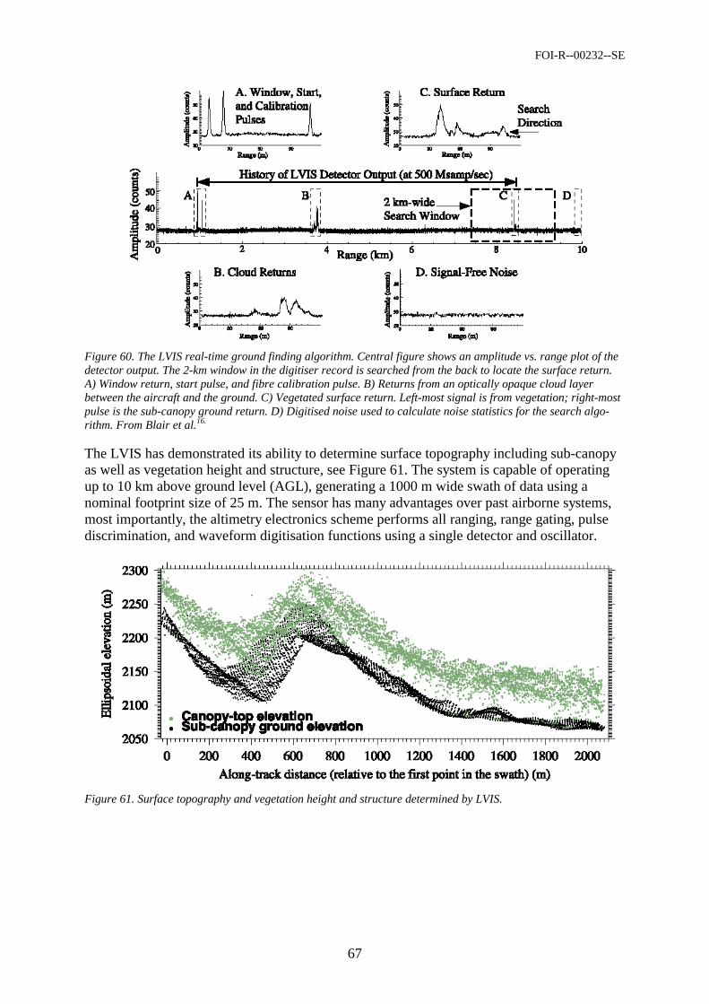
FOI-R--00232--SE

67

Figure 60. The LVIS real-time ground finding algorithm. Central figure shows an amplitude vs. range plot of the detector output. The 2-km window in the digitiser record is searched from the back to locate the surface return. A) Window return, start pulse, and fibre calibration pulse. B) Returns from an optically opaque cloud layer between the aircraft and the ground. C) Vegetated surface return. Left-most signal is from vegetation; right-most pulse is the sub-canopy ground return. D) Digitised noise used to calculate noise statistics for the search algo-rithm. From Blair et al.16.

The LVIS has demonstrated its ability to determine surface topography including sub-canopy as well as vegetation height and structure, see Figure 61. The system is capable of operating up to 10 km above ground level (AGL), generating a 1000 m wide swath of data using a nominal footprint size of 25 m. The sensor has many advantages over past airborne systems, most importantly, the altimetry electronics scheme performs all ranging, range gating, pulse discrimination, and waveform digitisation functions using a single detector and oscillator.

Figure 61. Surface topography and vegetation height and structure determined by LVIS.

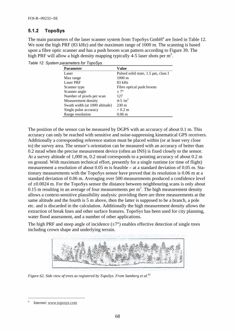
FOI-R--00232--SE

68

0(( .*

The main parameters of the laser scanner system from TopoSys GmbHa are listed in Table 12. We note the high PRF (83 kHz) and the maximum range of 1000 m. The scanning is based upon a fibre optic scanner and has a push broom scan pattern according to Figure 39. The high PRF will allow a high density mapping typically 4-5 laser shots per m2.

! !Parameter Value Laser Pulsed solid state, 1.5 µm, class I Max range 1000 m Laser PRF 83 kHz Scanner type Fibre optical push broom Scanner angle ± 7° Number of pixels per scan 127 Measurement density 4-5 /m2 Swath width (at 1000 altitude) 230 m Single pulse accuracy < 0.2 m Range resolution 0.06 m

The position of the sensor can be measured by DGPS with an accuracy of about 0.1 m. This accuracy can only be reached with sensitive and noise-suppressing kinematical GPS receivers. Additionally a corresponding reference station must be placed within (or at least very close to) the survey area. The sensor’s orientation can be measured with an accuracy of better than 0.2 mrad when the precise measurement device (often an INS) is fixed closely to the sensor. At a survey altitude of 1,000 m, 0.2 mrad corresponds to a pointing accuracy of about 0.2 m on ground. With maximum technical effort, presently for a single runtime (or time of flight) measurement a resolution of about 0.05 m is feasible – at a standard deviation of 0.05 m. Sta-tionary measurements with the TopoSys sensor have proved that its resolution is 0.06 m at a standard deviation of 0.06 m. Averaging over 500 measurements produced a confidence level of ±0.0024 m. For the TopoSys sensor the distance between neighbouring scans is only about 0.15 m resulting in an average of four measurements per m2. The high measurement density allows a context-sensitive plausibility analysis: providing there are three measurements at the same altitude and the fourth is 5 m above, then the latter is supposed to be a branch, a pole etc. and is discarded in the calculation. Additionally the high measurement density allows the extraction of break lines and other surface features. TopoSys has been used for city planning, water flood assessment, and a number of other applications.

The high PRF and steep angle of incidence (±7°) enables effective detection of single trees including crown shape and underlying terrain.

Figure 62. Side view of trees as registered by TopoSys. From Samberg et al.62

a Internet: www.toposys.com

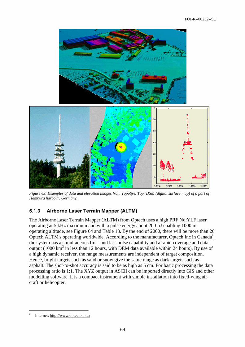
FOI-R--00232--SE

69

Figure 63. Examples of data and elevation images from TopoSys. Top: DSM (digital surface map) of a part of Hamburg harbour, Germany.

0(( "2 . 3 6".37

The Airborne Laser Terrain Mapper (ALTM) from Optech uses a high PRF Nd:YLF laser operating at 5 kHz maximum and with a pulse energy about 200 µJ enabling 1000 m operating altitude, see Figure 64 and Table 13. By the end of 2000, there will be more than 26 Optech ALTM's operating worldwide. According to the manufacturer, Optech Inc in Canadaa, the system has a simultaneous first- and last-pulse capability and a rapid coverage and data output (1000 km2 in less than 12 hours, with DEM data available within 24 hours). By use of a high dynamic receiver, the range measurements are independent of target composition. Hence, bright targets such as sand or snow give the same range as dark targets such as asphalt. The shot-to-shot accuracy is said to be as high as 5 cm. For basic processing the data processing ratio is 1:1. The XYZ output in ASCII can be imported directly into GIS and other modelling software. It is a compact instrument with simple installation into fixed-wing air-craft or helicopter.

a Internet: http://www.optech.on.ca

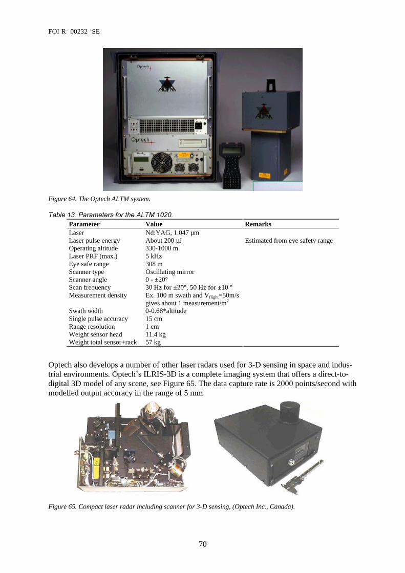
FOI-R--00232--SE

70

Figure 64. The Optech ALTM system.

.7855Parameter Value Remarks Laser Nd:YAG, 1.047 µm Laser pulse energy About 200 µJ Estimated from eye safety range Operating altitude 330-1000 m Laser PRF (max.) 5 kHz Eye safe range 308 m Scanner type Oscillating mirror Scanner angle 0 - ±20° Scan frequency 30 Hz for ±20°, 50 Hz for ±10 ° Measurement density Ex. 100 m swath and Vflight=50m/s

gives about 1 measurement/m2

Swath width 0-0.68*altitude Single pulse accuracy 15 cm Range resolution 1 cm Weight sensor head 11.4 kg Weight total sensor+rack 57 kg

Optech also develops a number of other laser radars used for 3-D sensing in space and indus-trial environments. Optech’s ILRIS-3D is a complete imaging system that offers a direct-to-digital 3D model of any scene, see Figure 65. The data capture rate is 2000 points/second with modelled output accuracy in the range of 5 mm.

Figure 65. Compact laser radar including scanner for 3-D sensing, (Optech Inc., Canada).

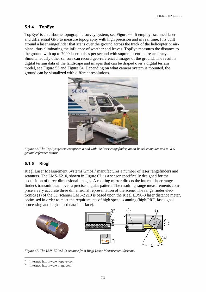
FOI-R--00232--SE

71

0((/ .8*

TopEyea is an airborne topographic survey system, see Figure 66. It employs scanned laser and differential GPS to measure topography with high precision and in real time. It is built around a laser rangefinder that scans over the ground across the track of the helicopter or air-plane, thus eliminating the influence of weather and leaves. TopEye measures the distance to the ground with up to 7000 laser pulses per second with supreme centimetre accuracy. Simultaneously other sensors can record geo-referenced images of the ground. The result is digital terrain data of the landscape and images that can be draped over a digital terrain model, see Figure 53 and Figure 54. Depending on what camera system is mounted, the ground can be visualized with different resolutions.

Figure 66. The TopEye system comprises a pod with the laser rangefinder, an on-board computer and a GPS ground reference station.

0((0 9

Riegl Laser Measurement Systems GmbHb manufactures a number of laser rangefinders and scanners. The LMS-Z210, shown in Figure 67, is a sensor specifically designed for the acquisition of three-dimensional images. A rotating mirror directs the internal laser range-finder’s transmit beam over a precise angular pattern. The resulting range measurements com-prise a very accurate three dimensional representation of the scene. The range finder elec-tronics (1) of the 3D scanner LMS-Z210 is based upon the Riegl LD90-3 laser distance meter, optimised in order to meet the requirements of high speed scanning (high PRF, fast signal processing and high speed data interface).

Figure 67. The LMS-Z210 3-D scanner from Riegl Laser Measurement Systems.

a Internet: http://www.topeye.com b Internet: http://www.riegl.com

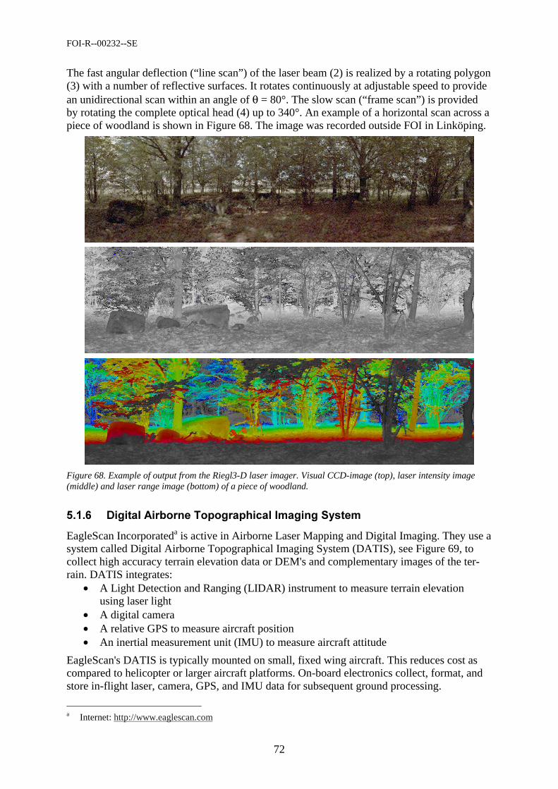
FOI-R--00232--SE

72

The fast angular deflection (“line scan”) of the laser beam (2) is realized by a rotating polygon (3) with a number of reflective surfaces. It rotates continuously at adjustable speed to provide an unidirectional scan within an angle of θ = 80°. The slow scan (“frame scan”) is provided by rotating the complete optical head (4) up to 340°. An example of a horizontal scan across a piece of woodland is shown in Figure 68. The image was recorded outside FOI in Linköping.

Figure 68. Example of output from the Riegl3-D laser imager. Visual CCD-image (top), laser intensity image (middle) and laser range image (bottom) of a piece of woodland.

0(( "2 .'&*

EagleScan Incorporateda is active in Airborne Laser Mapping and Digital Imaging. They use a system called Digital Airborne Topographical Imaging System (DATIS), see Figure 69, to collect high accuracy terrain elevation data or DEM's and complementary images of the ter-rain. DATIS integrates:

• A Light Detection and Ranging (LIDAR) instrument to measure terrain elevation using laser light

• A digital camera • A relative GPS to measure aircraft position • An inertial measurement unit (IMU) to measure aircraft attitude

EagleScan's DATIS is typically mounted on small, fixed wing aircraft. This reduces cost as compared to helicopter or larger aircraft platforms. On-board electronics collect, format, and store in-flight laser, camera, GPS, and IMU data for subsequent ground processing.

a Internet: http://www.eaglescan.com

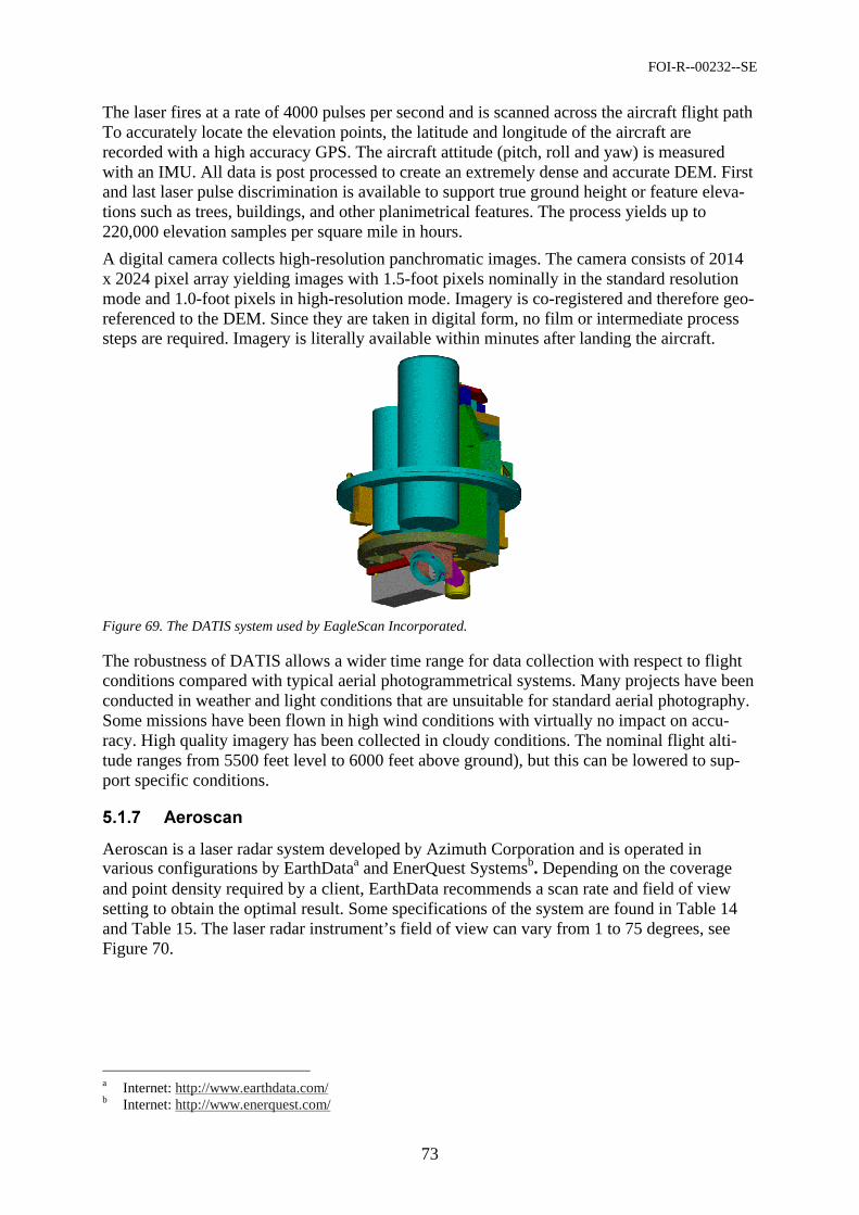
FOI-R--00232--SE

73

The laser fires at a rate of 4000 pulses per second and is scanned across the aircraft flight path To accurately locate the elevation points, the latitude and longitude of the aircraft are recorded with a high accuracy GPS. The aircraft attitude (pitch, roll and yaw) is measured with an IMU. All data is post processed to create an extremely dense and accurate DEM. First and last laser pulse discrimination is available to support true ground height or feature eleva-tions such as trees, buildings, and other planimetrical features. The process yields up to 220,000 elevation samples per square mile in hours.

A digital camera collects high-resolution panchromatic images. The camera consists of 2014 x 2024 pixel array yielding images with 1.5-foot pixels nominally in the standard resolution mode and 1.0-foot pixels in high-resolution mode. Imagery is co-registered and therefore geo-referenced to the DEM. Since they are taken in digital form, no film or intermediate process steps are required. Imagery is literally available within minutes after landing the aircraft.

Figure 69. The DATIS system used by EagleScan Incorporated.

The robustness of DATIS allows a wider time range for data collection with respect to flight conditions compared with typical aerial photogrammetrical systems. Many projects have been conducted in weather and light conditions that are unsuitable for standard aerial photography. Some missions have been flown in high wind conditions with virtually no impact on accu-racy. High quality imagery has been collected in cloudy conditions. The nominal flight alti-tude ranges from 5500 feet level to 6000 feet above ground), but this can be lowered to sup-port specific conditions.

0(( "

Aeroscan is a laser radar system developed by Azimuth Corporation and is operated in various configurations by EarthDataa and EnerQuest Systemsb. Depending on the coverage and point density required by a client, EarthData recommends a scan rate and field of view setting to obtain the optimal result. Some specifications of the system are found in Table 14 and Table 15. The laser radar instrument’s field of view can vary from 1 to 75 degrees, see Figure 70.

a Internet: http://www.earthdata.com/ b Internet: http://www.enerquest.com/

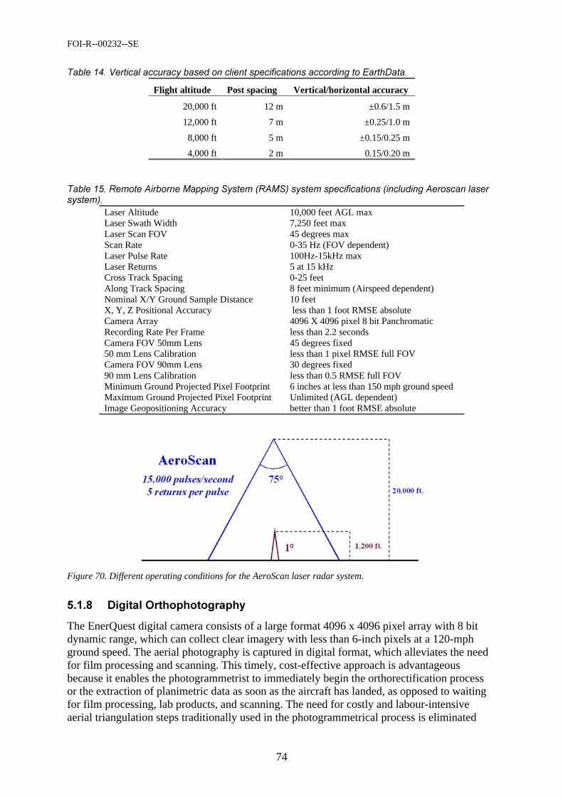
FOI-R--00232--SE

74

(&! 9*

Flight altitude Post spacing Vertical/horizontal accuracy

20,000 ft 12 m ±0.6/1.5 m

12,000 ft 7 m ±0.25/1.0 m

8,000 ft 5 m ±0.15/0.25 m

4,000 ft 2 m 0.15/0.20 m

+.8 !#.8'! #.!'

Laser Altitude 10,000 feet AGL max Laser Swath Width 7,250 feet max Laser Scan FOV 45 degrees max Scan Rate 0-35 Hz (FOV dependent) Laser Pulse Rate 100Hz-15kHz max Laser Returns 5 at 15 kHz Cross Track Spacing 0-25 feet Along Track Spacing 8 feet minimum (Airspeed dependent) Nominal X/Y Ground Sample Distance 10 feet X, Y, Z Positional Accuracy less than 1 foot RMSE absolute Camera Array 4096 X 4096 pixel 8 bit Panchromatic Recording Rate Per Frame less than 2.2 seconds Camera FOV 50mm Lens 45 degrees fixed 50 mm Lens Calibration less than 1 pixel RMSE full FOV Camera FOV 90mm Lens 30 degrees fixed 90 mm Lens Calibration less than 0.5 RMSE full FOV Minimum Ground Projected Pixel Footprint 6 inches at less than 150 mph ground speed Maximum Ground Projected Pixel Footprint Unlimited (AGL dependent) Image Geopositioning Accuracy better than 1 foot RMSE absolute

Figure 70. Different operating conditions for the AeroScan laser radar system.

0((: '''*

The EnerQuest digital camera consists of a large format 4096 x 4096 pixel array with 8 bit dynamic range, which can collect clear imagery with less than 6-inch pixels at a 120-mph ground speed. The aerial photography is captured in digital format, which alleviates the need for film processing and scanning. This timely, cost-effective approach is advantageous because it enables the photogrammetrist to immediately begin the orthorectification process or the extraction of planimetric data as soon as the aircraft has landed, as opposed to waiting for film processing, lab products, and scanning. The need for costly and labour-intensive aerial triangulation steps traditionally used in the photogrammetrical process is eliminated

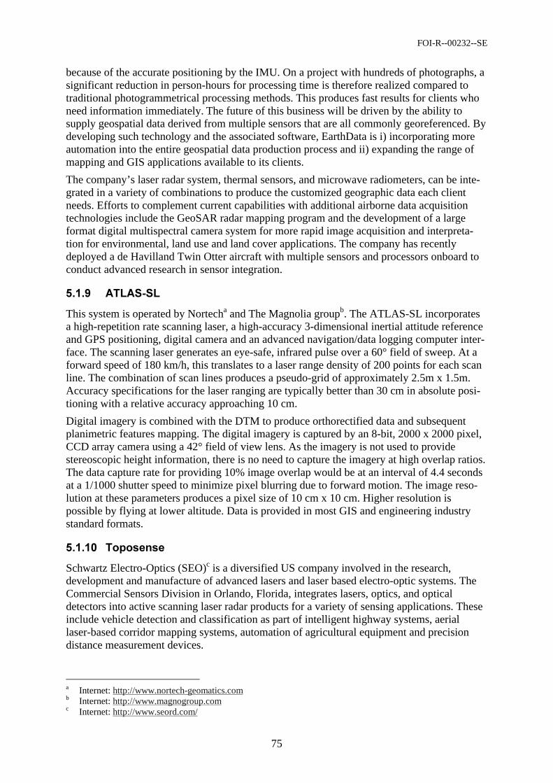
FOI-R--00232--SE

75

because of the accurate positioning by the IMU. On a project with hundreds of photographs, a significant reduction in person-hours for processing time is therefore realized compared to traditional photogrammetrical processing methods. This produces fast results for clients who need information immediately. The future of this business will be driven by the ability to supply geospatial data derived from multiple sensors that are all commonly georeferenced. By developing such technology and the associated software, EarthData is i) incorporating more automation into the entire geospatial data production process and ii) expanding the range of mapping and GIS applications available to its clients.

The company’s laser radar system, thermal sensors, and microwave radiometers, can be inte-grated in a variety of combinations to produce the customized geographic data each client needs. Efforts to complement current capabilities with additional airborne data acquisition technologies include the GeoSAR radar mapping program and the development of a large format digital multispectral camera system for more rapid image acquisition and interpreta-tion for environmental, land use and land cover applications. The company has recently deployed a de Havilland Twin Otter aircraft with multiple sensors and processors onboard to conduct advanced research in sensor integration.

0((; "."

This system is operated by Nortecha and The Magnolia groupb. The ATLAS-SL incorporates a high-repetition rate scanning laser, a high-accuracy 3-dimensional inertial attitude reference and GPS positioning, digital camera and an advanced navigation/data logging computer inter-face. The scanning laser generates an eye-safe, infrared pulse over a 60° field of sweep. At a forward speed of 180 km/h, this translates to a laser range density of 200 points for each scan line. The combination of scan lines produces a pseudo-grid of approximately 2.5m x 1.5m. Accuracy specifications for the laser ranging are typically better than 30 cm in absolute posi-tioning with a relative accuracy approaching 10 cm.

Digital imagery is combined with the DTM to produce orthorectified data and subsequent planimetric features mapping. The digital imagery is captured by an 8-bit, 2000 x 2000 pixel, CCD array camera using a 42° field of view lens. As the imagery is not used to provide stereoscopic height information, there is no need to capture the imagery at high overlap ratios. The data capture rate for providing 10% image overlap would be at an interval of 4.4 seconds at a 1/1000 shutter speed to minimize pixel blurring due to forward motion. The image reso-lution at these parameters produces a pixel size of 10 cm x 10 cm. Higher resolution is possible by flying at lower altitude. Data is provided in most GIS and engineering industry standard formats.

0(( .

Schwartz Electro-Optics (SEO)c is a diversified US company involved in the research, development and manufacture of advanced lasers and laser based electro-optic systems. The Commercial Sensors Division in Orlando, Florida, integrates lasers, optics, and optical detectors into active scanning laser radar products for a variety of sensing applications. These include vehicle detection and classification as part of intelligent highway systems, aerial laser-based corridor mapping systems, automation of agricultural equipment and precision distance measurement devices.

a Internet: http://www.nortech-geomatics.com b Internet: http://www.magnogroup.com c Internet: http://www.seord.com/

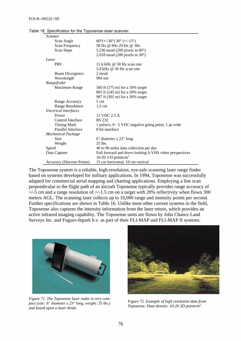
FOI-R--00232--SE

76

, Scanner

Scan Angle 60°(+/-30°) 30° (+/-15°) Scan Frequency 58 Hz @ 60o 29 Hz @ 30o Scan Steps 5.236 mrad (200 pixels in 60°)

2.618 mrad (200 pixels in 30°) Laser

PRF 11.6 kHz @ 58 Hz scan rate 5.8 kHz @ 30 Hz scan rate

Beam Divergence 2 mrad Wavelength 904 nm

Rangefinder Maximum Range 560 ft (175 m) for a 10% target

805 ft (245 m) for a 20% target 987 ft (301 m) for a 30% target

Range Accuracy 5 cm Range Resolution 1,5 cm

Electrical Interfaces Power 12 VDC 2.5 A Control Interface RS 232 Timing Mark 1 pulse/s, 0 - 5 VDC negative going pulse, 1 µs wide Parallel Interface 8 bit interface

Mechanical Package Size 6" diameter x 23" long Weight 25 lbs.

Speed 40 to 90 miles data collection per day Data Capture Full forward and down looking S-VHS video perspectives

10-20 3-D points/m2 Accuracy (Discrete Points) 15 cm horizontal, 10 cm vertical

The Toposense system is a reliable, high-resolution, eye-safe scanning laser range finder based on systems developed for military applications. In 1994, Toposense was successfully adapted for commercial aerial mapping and charting applications. Employing a line scan perpendicular to the flight path of an aircraft Toposense typically provides range accuracy of +/-5 cm and a range resolution of +/-1.5 cm on a target with 20% reflectivity when flown 300 meters AGL. The scanning laser collects up to 10,000 range and intensity points per second. Further specifications are shown in Table 16. Unlike most other current systems in the field, Toposense also captures the intensity information from the laser return, which provides an active infrared imaging capability. The Toposense units are flown by John Chance Land Surveys Inc. and Fuguro-Inpark b.v. as part of their FLI-MAP and FLI-MAP II systems.

Figure 71. The Toposense laser radar is very com-pact (size: 6" diameter x 23" long, weight: 25 lbs.) and based upon a laser diode.

Figure 72. Example of high resolution data from Toposense. Data density: 10-20 3D points/m2.

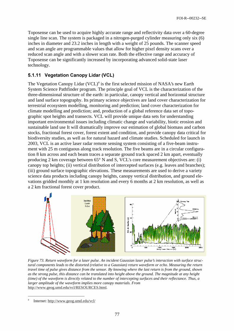
FOI-R--00232--SE

77

Toposense can be used to acquire highly accurate range and reflectivity data over a 60-degree single line scan. The system is packaged in a nitrogen-purged cylinder measuring only six (6) inches in diameter and 23.2 inches in length with a weight of 25 pounds. The scanner speed and scan angle are programmable values that allow for higher pixel density scans over a reduced scan angle and with a slower scan rate. Both the effective range and accuracy of Toposense can be significantly increased by incorporating advanced solid-state laser technology.

0(( 5 %*65%7

The Vegetation Canopy Lidar (VCL)a is the first selected mission of NASA’s new Earth System Science Pathfinder program. The principle goal of VCL is the characterization of the three-dimensional structure of the earth: in particular, canopy vertical and horizontal structure and land surface topography. Its primary science objectives are land cover characterization for terrestrial ecosystem modelling, monitoring and prediction; land cover characterization for climate modelling and prediction; and, production of a global reference data set of topo-graphic spot heights and transects. VCL will provide unique data sets for understanding important environmental issues including climatic change and variability, biotic erosion and sustainable land use It will dramatically improve our estimation of global biomass and carbon stocks, fractional forest cover, forest extent and condition, and provide canopy data critical for biodiversity studies, as well as for natural hazard and climate studies. Scheduled for launch in 2003, VCL is an active laser radar remote sensing system consisting of a five-beam instru-ment with 25 m contiguous along track resolution. The five beams are in a circular configura-tion 8 km across and each beam traces a separate ground track spaced 2 km apart, eventually producing 2 km coverage between 65° N and S, VCL's core measurement objectives are: (i) canopy top heights; (ii) vertical distribution of intercepted surfaces (e.g. leaves and branches); (iii) ground surface topographic elevations. These measurements are used to derive a variety science data products including canopy heights, canopy vertical distribution, and ground ele-vations gridded monthly at 1 km resolution and every 6 months at 2 km resolution, as well as a 2 km fractional forest cover product.

Figure 73. Return waveform for a laser pulse. An incident Gaussian laser pulse’s interaction with surface struc-tural components leads to the distorted (relative to a Gaussian) return waveform or echo. Measuring the return travel time of pulse gives distance from the sensor. By knowing where the last return is from the ground, shown as the strong pulse, this distance can be translated into height above the ground. The magnitude at any height (time) of the waveform is directly related to the number of intercepting surfaces and their reflectance. Thus, a larger amplitude of the waveform implies more canopy materials. From http://www.geog.umd.edu/vcl/RESOURCES.html.

a Internet: http://www.geog.umd.edu/vcl/

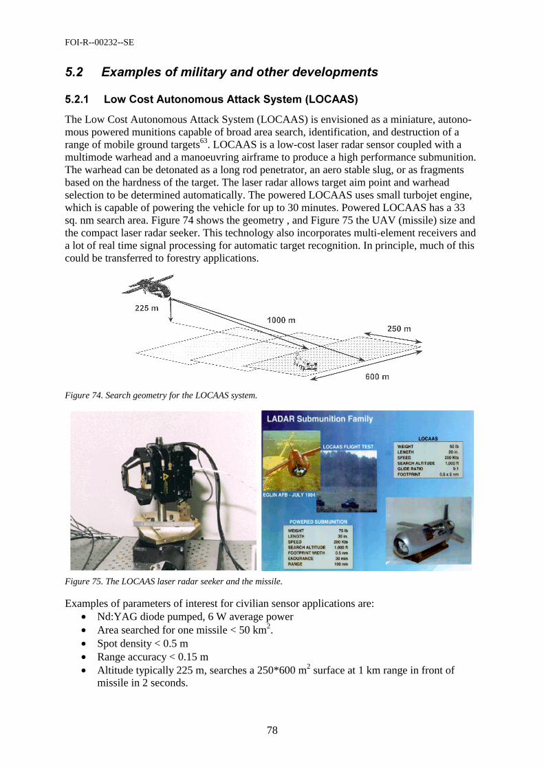
FOI-R--00232--SE

78

0 * %

0(( +%"$$"* 6%""7

The Low Cost Autonomous Attack System (LOCAAS) is envisioned as a miniature, autono-mous powered munitions capable of broad area search, identification, and destruction of a range of mobile ground targets63. LOCAAS is a low-cost laser radar sensor coupled with a multimode warhead and a manoeuvring airframe to produce a high performance submunition. The warhead can be detonated as a long rod penetrator, an aero stable slug, or as fragments based on the hardness of the target. The laser radar allows target aim point and warhead selection to be determined automatically. The powered LOCAAS uses small turbojet engine, which is capable of powering the vehicle for up to 30 minutes. Powered LOCAAS has a 33 sq. nm search area. Figure 74 shows the geometry , and Figure 75 the UAV (missile) size and the compact laser radar seeker. This technology also incorporates multi-element receivers and a lot of real time signal processing for automatic target recognition. In principle, much of this could be transferred to forestry applications.

Figure 74. Search geometry for the LOCAAS system.

Figure 75. The LOCAAS laser radar seeker and the missile.

Examples of parameters of interest for civilian sensor applications are: • Nd:YAG diode pumped, 6 W average power • Area searched for one missile < 50 km2. • Spot density < 0.5 m • Range accuracy < 0.15 m • Altitude typically 225 m, searches a 250*600 m2 surface at 1 km range in front of

missile in 2 seconds.

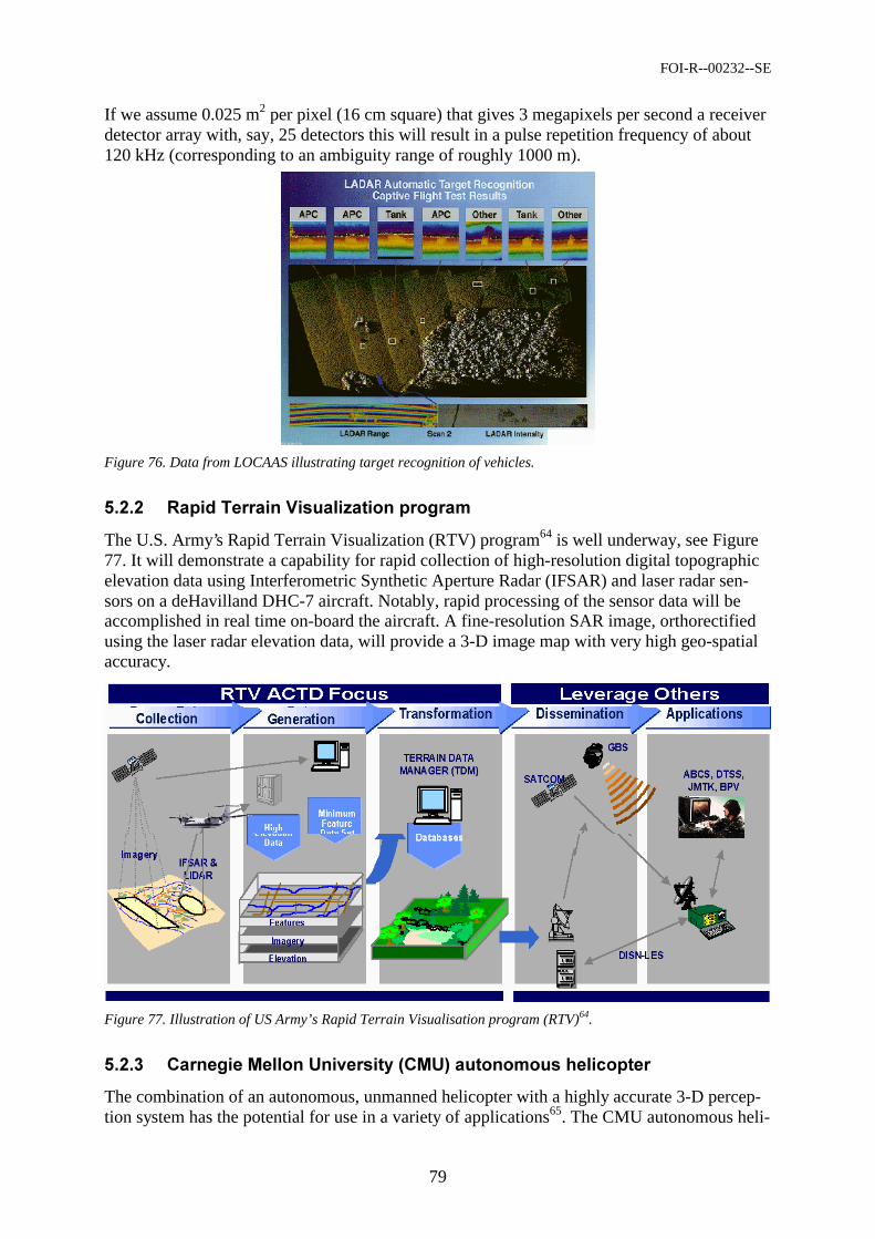
FOI-R--00232--SE

79

If we assume 0.025 m2 per pixel (16 cm square) that gives 3 megapixels per second a receiver detector array with, say, 25 detectors this will result in a pulse repetition frequency of about 120 kHz (corresponding to an ambiguity range of roughly 1000 m).

Figure 76. Data from LOCAAS illustrating target recognition of vehicles.

0(( 9. 5$<

The U.S. Army’s Rapid Terrain Visualization (RTV) program64 is well underway, see Figure 77. It will demonstrate a capability for rapid collection of high-resolution digital topographic elevation data using Interferometric Synthetic Aperture Radar (IFSAR) and laser radar sen-sors on a deHavilland DHC-7 aircraft. Notably, rapid processing of the sensor data will be accomplished in real time on-board the aircraft. A fine-resolution SAR image, orthorectified using the laser radar elevation data, will provide a 3-D image map with very high geo-spatial accuracy.

Figure 77. Illustration of US Army’s Rapid Terrain Visualisation program (RTV)64.

0(( % 3 *6%3 7$$'

The combination of an autonomous, unmanned helicopter with a highly accurate 3-D percep-tion system has the potential for use in a variety of applications65. The CMU autonomous heli-

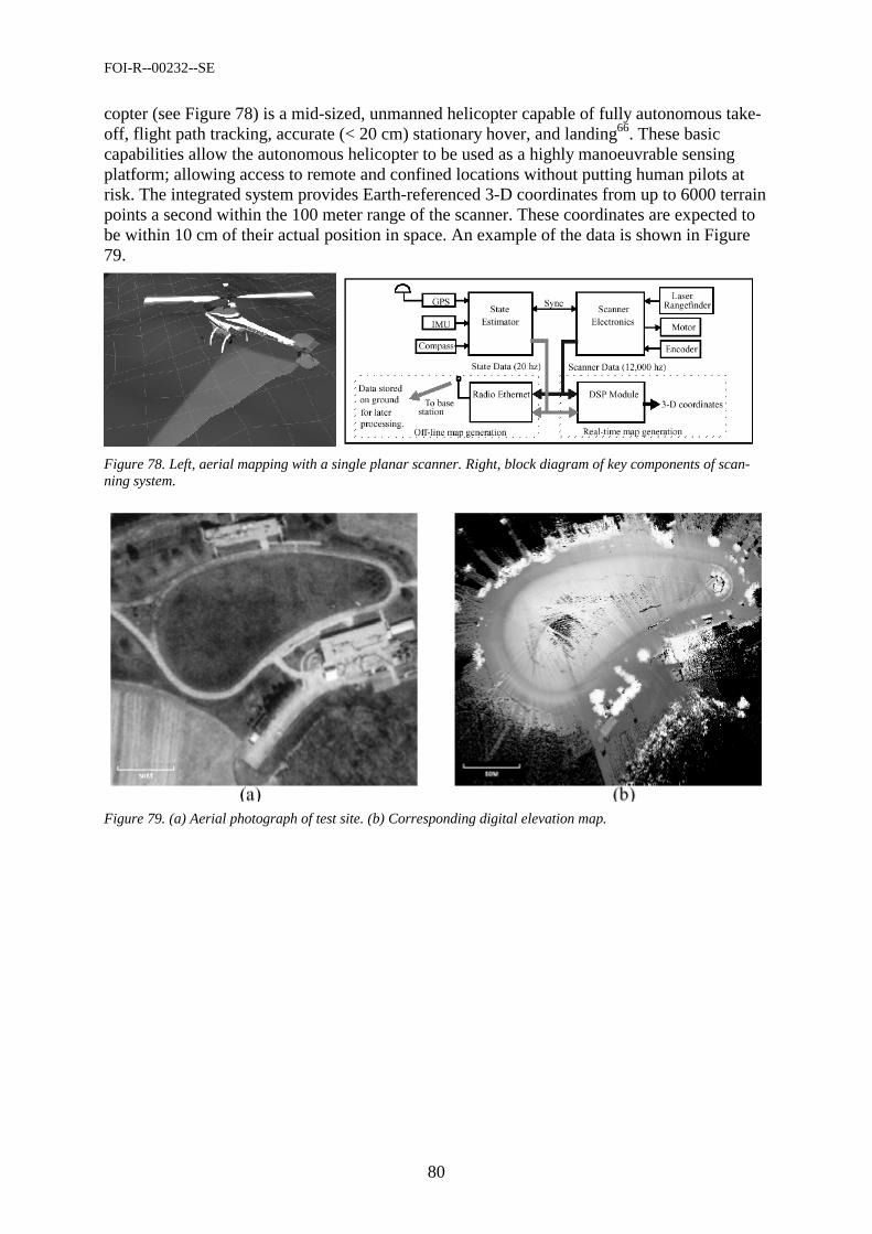
FOI-R--00232--SE

80

copter (see Figure 78) is a mid-sized, unmanned helicopter capable of fully autonomous take-off, flight path tracking, accurate (< 20 cm) stationary hover, and landing66. These basic capabilities allow the autonomous helicopter to be used as a highly manoeuvrable sensing platform; allowing access to remote and confined locations without putting human pilots at risk. The integrated system provides Earth-referenced 3-D coordinates from up to 6000 terrain points a second within the 100 meter range of the scanner. These coordinates are expected to be within 10 cm of their actual position in space. An example of the data is shown in Figure 79.

Figure 78. Left, aerial mapping with a single planar scanner. Right, block diagram of key components of scan-ning system.

Figure 79. (a) Aerial photograph of test site. (b) Corresponding digital elevation map.

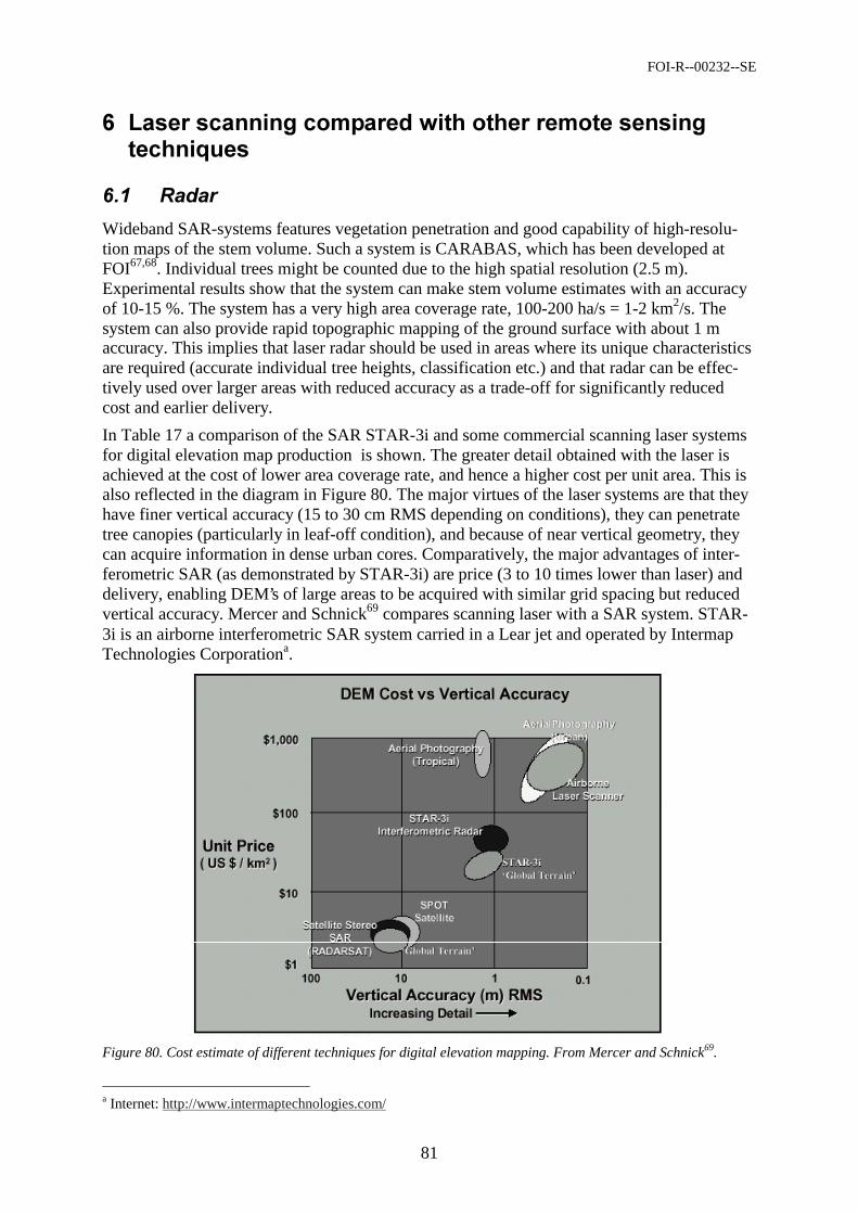
FOI-R--00232--SE

81

Wideband SAR-systems features vegetation penetration and good capability of high-resolu-tion maps of the stem volume. Such a system is CARABAS, which has been developed at FOI67,68. Individual trees might be counted due to the high spatial resolution (2.5 m). Experimental results show that the system can make stem volume estimates with an accuracy of 10-15 %. The system has a very high area coverage rate, 100-200 ha/s = 1-2 km2/s. The system can also provide rapid topographic mapping of the ground surface with about 1 m accuracy. This implies that laser radar should be used in areas where its unique characteristics are required (accurate individual tree heights, classification etc.) and that radar can be effec-tively used over larger areas with reduced accuracy as a trade-off for significantly reduced cost and earlier delivery.

In Table 17 a comparison of the SAR STAR-3i and some commercial scanning laser systems for digital elevation map production is shown. The greater detail obtained with the laser is achieved at the cost of lower area coverage rate, and hence a higher cost per unit area. This is also reflected in the diagram in Figure 80. The major virtues of the laser systems are that they have finer vertical accuracy (15 to 30 cm RMS depending on conditions), they can penetrate tree canopies (particularly in leaf-off condition), and because of near vertical geometry, they can acquire information in dense urban cores. Comparatively, the major advantages of inter-ferometric SAR (as demonstrated by STAR-3i) are price (3 to 10 times lower than laser) and delivery, enabling DEM’s of large areas to be acquired with similar grid spacing but reduced vertical accuracy. Mercer and Schnick69 compares scanning laser with a SAR system. STAR-3i is an airborne interferometric SAR system carried in a Lear jet and operated by Intermap Technologies Corporationa.

Figure 80. Cost estimate of different techniques for digital elevation mapping. From Mercer and Schnick69.

a Internet: http://www.intermaptechnologies.com/

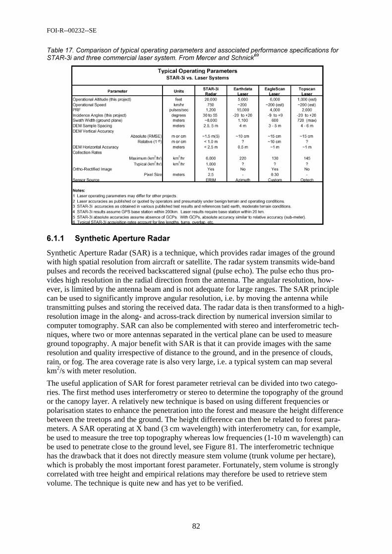
FOI-R--00232--SE

82

Synthetic Aperture Radar (SAR) is a technique, which provides radar images of the ground with high spatial resolution from aircraft or satellite. The radar system transmits wide-band pulses and records the received backscattered signal (pulse echo). The pulse echo thus pro-vides high resolution in the radial direction from the antenna. The angular resolution, how-ever, is limited by the antenna beam and is not adequate for large ranges. The SAR principle can be used to significantly improve angular resolution, i.e. by moving the antenna while transmitting pulses and storing the received data. The radar data is then transformed to a high-resolution image in the along- and across-track direction by numerical inversion similar to computer tomography. SAR can also be complemented with stereo and interferometric tech-niques, where two or more antennas separated in the vertical plane can be used to measure ground topography. A major benefit with SAR is that it can provide images with the same resolution and quality irrespective of distance to the ground, and in the presence of clouds, rain, or fog. The area coverage rate is also very large, i.e. a typical system can map several km2/s with meter resolution.

The useful application of SAR for forest parameter retrieval can be divided into two catego-ries. The first method uses interferometry or stereo to determine the topography of the ground or the canopy layer. A relatively new technique is based on using different frequencies or polarisation states to enhance the penetration into the forest and measure the height difference between the treetops and the ground. The height difference can then be related to forest para-meters. A SAR operating at X band (3 cm wavelength) with interferometry can, for example, be used to measure the tree top topography whereas low frequencies (1-10 m wavelength) can be used to penetrate close to the ground level, see Figure 81. The interferometric technique has the drawback that it does not directly measure stem volume (trunk volume per hectare), which is probably the most important forest parameter. Fortunately, stem volume is strongly correlated with tree height and empirical relations may therefore be used to retrieve stem volume. The technique is quite new and has yet to be verified.

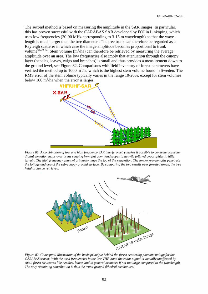
FOI-R--00232--SE

83

The second method is based on measuring the amplitude in the SAR images. In particular, this has proven successful with the CARABAS SAR developed by FOI in Linköping, which uses low frequencies (20-90 MHz corresponding to 3-15 m wavelength) so that the wave-length is much larger than the tree diameter . The tree trunk can therefore be regarded as a Rayleigh scatterer in which case the image amplitude becomes proportional to trunk volume68,70-73. Stem volume (m3/ha) can therefore be retrieved by measuring the average amplitude over an area. The low frequencies also imply that attenuation through the canopy layer (needles, leaves, twigs and branches) is small and thus provides a measurement down to the ground level, see Figure 82. Comparisons with field inventory of forest parameters have verified the method up to 1000 m3/ha which is the highest stem volume found in Sweden. The RMS error of the stem volume typically varies in the range 10-20%, except for stem volumes below 100 m3/ha when the error is larger.

Figure 81. A combination of low and high frequency SAR interferometry makes it possible to generate accurate digital elevation maps over areas ranging from flat open landscapes to heavily foliated geographies in hilly terrain. The high frequency channel primarily maps the top of the vegetation. The longer wavelengths penetrate the foliage and depict the sub-canopy ground surface. By comparing the two results over forested areas, the tree heights can be retrieved.

CARABAS radar imageForest

Figure 82. Conceptual illustration of the basic principle behind the forest scattering phenomenology for the CARABAS sensor. With the used frequencies in the low VHF-band the radar signal is virtually unaffected by small forest structures like needles, leaves and in general branches if not too large compared to the wavelength. The only remaining contribution is thus the trunk-ground dihedral mechanism.

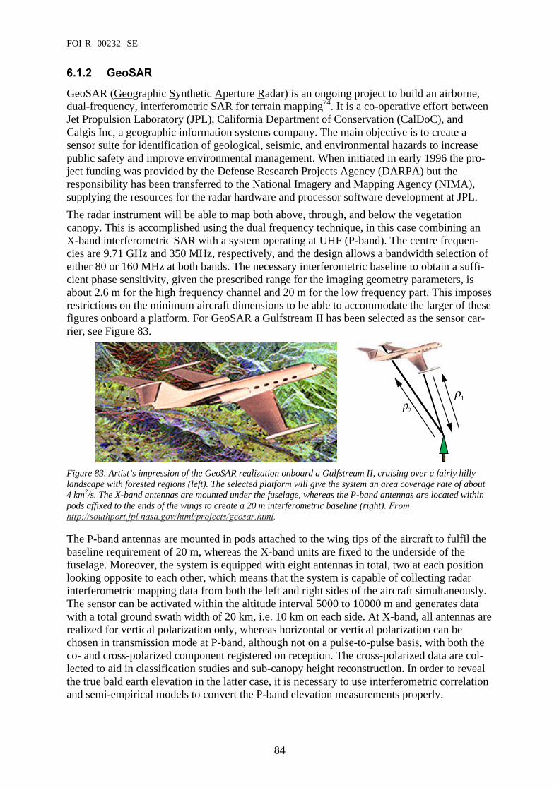
FOI-R--00232--SE

84

GeoSAR (Geographic Synthetic Aperture Radar) is an ongoing project to build an airborne, dual-frequency, interferometric SAR for terrain mapping74. It is a co-operative effort between Jet Propulsion Laboratory (JPL), California Department of Conservation (CalDoC), and Calgis Inc, a geographic information systems company. The main objective is to create a sensor suite for identification of geological, seismic, and environmental hazards to increase public safety and improve environmental management. When initiated in early 1996 the pro-ject funding was provided by the Defense Research Projects Agency (DARPA) but the responsibility has been transferred to the National Imagery and Mapping Agency (NIMA), supplying the resources for the radar hardware and processor software development at JPL.

The radar instrument will be able to map both above, through, and below the vegetation canopy. This is accomplished using the dual frequency technique, in this case combining an X-band interferometric SAR with a system operating at UHF (P-band). The centre frequen-cies are 9.71 GHz and 350 MHz, respectively, and the design allows a bandwidth selection of either 80 or 160 MHz at both bands. The necessary interferometric baseline to obtain a suffi-cient phase sensitivity, given the prescribed range for the imaging geometry parameters, is about 2.6 m for the high frequency channel and 20 m for the low frequency part. This imposes restrictions on the minimum aircraft dimensions to be able to accommodate the larger of these figures onboard a platform. For GeoSAR a Gulfstream II has been selected as the sensor car-rier, see Figure 83.

ρ1ρ2

Figure 83. Artist’s impression of the GeoSAR realization onboard a Gulfstream II, cruising over a fairly hilly landscape with forested regions (left). The selected platform will give the system an area coverage rate of about 4 km2/s. The X-band antennas are mounted under the fuselage, whereas the P-band antennas are located within pods affixed to the ends of the wings to create a 20 m interferometric baseline (right).

The P-band antennas are mounted in pods attached to the wing tips of the aircraft to fulfil the baseline requirement of 20 m, whereas the X-band units are fixed to the underside of the fuselage. Moreover, the system is equipped with eight antennas in total, two at each position looking opposite to each other, which means that the system is capable of collecting radar interferometric mapping data from both the left and right sides of the aircraft simultaneously. The sensor can be activated within the altitude interval 5000 to 10000 m and generates data with a total ground swath width of 20 km, i.e. 10 km on each side. At X-band, all antennas are realized for vertical polarization only, whereas horizontal or vertical polarization can be chosen in transmission mode at P-band, although not on a pulse-to-pulse basis, with both the co- and cross-polarized component registered on reception. The cross-polarized data are col-lected to aid in classification studies and sub-canopy height reconstruction. In order to reveal the true bald earth elevation in the latter case, it is necessary to use interferometric correlation and semi-empirical models to convert the P-band elevation measurements properly.

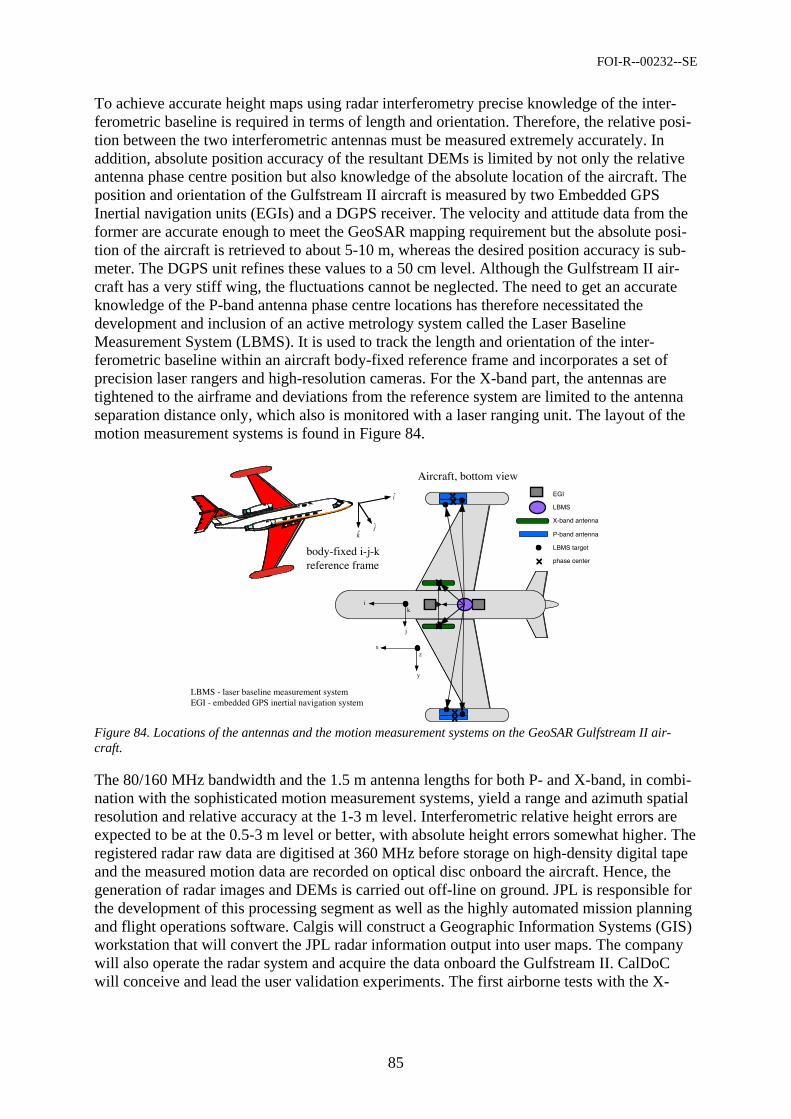
FOI-R--00232--SE

85

!

" #$

%&'((' () ((

*+ ,'#((

To achieve accurate height maps using radar interferometry precise knowledge of the inter-ferometric baseline is required in terms of length and orientation. Therefore, the relative posi-tion between the two interferometric antennas must be measured extremely accurately. In addition, absolute position accuracy of the resultant DEMs is limited by not only the relative antenna phase centre position but also knowledge of the absolute location of the aircraft. The position and orientation of the Gulfstream II aircraft is measured by two Embedded GPS Inertial navigation units (EGIs) and a DGPS receiver. The velocity and attitude data from the former are accurate enough to meet the GeoSAR mapping requirement but the absolute posi-tion of the aircraft is retrieved to about 5-10 m, whereas the desired position accuracy is sub-meter. The DGPS unit refines these values to a 50 cm level. Although the Gulfstream II air-craft has a very stiff wing, the fluctuations cannot be neglected. The need to get an accurate knowledge of the P-band antenna phase centre locations has therefore necessitated the development and inclusion of an active metrology system called the Laser Baseline Measurement System (LBMS). It is used to track the length and orientation of the inter-ferometric baseline within an aircraft body-fixed reference frame and incorporates a set of precision laser rangers and high-resolution cameras. For the X-band part, the antennas are tightened to the airframe and deviations from the reference system are limited to the antenna separation distance only, which also is monitored with a laser ranging unit. The layout of the motion measurement systems is found in Figure 84.

Figure 84. Locations of the antennas and the motion measurement systems on the GeoSAR Gulfstream II air-craft.

The 80/160 MHz bandwidth and the 1.5 m antenna lengths for both P- and X-band, in combi-nation with the sophisticated motion measurement systems, yield a range and azimuth spatial resolution and relative accuracy at the 1-3 m level. Interferometric relative height errors are expected to be at the 0.5-3 m level or better, with absolute height errors somewhat higher. The registered radar raw data are digitised at 360 MHz before storage on high-density digital tape and the measured motion data are recorded on optical disc onboard the aircraft. Hence, the generation of radar images and DEMs is carried out off-line on ground. JPL is responsible for the development of this processing segment as well as the highly automated mission planning and flight operations software. Calgis will construct a Geographic Information Systems (GIS) workstation that will convert the JPL radar information output into user maps. The company will also operate the radar system and acquire the data onboard the Gulfstream II. CalDoC will conceive and lead the user validation experiments. The first airborne tests with the X-

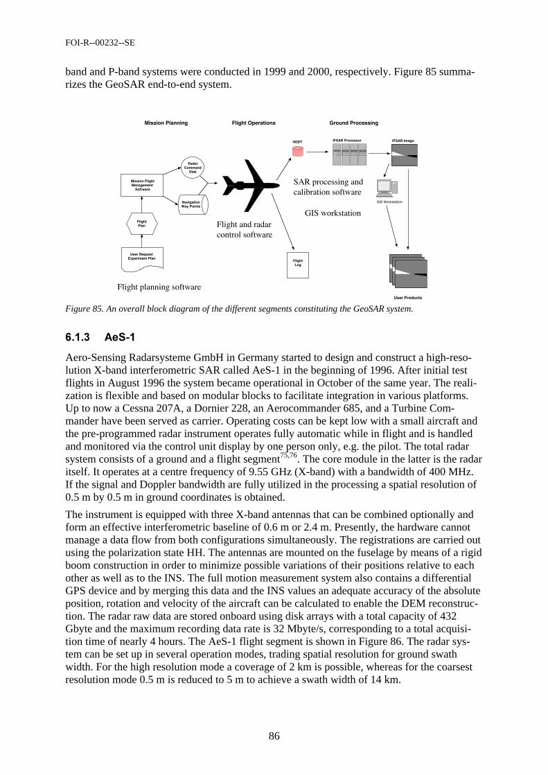
FOI-R--00232--SE

86

band and P-band systems were conducted in 1999 and 2000, respectively. Figure 85 summa-rizes the GeoSAR end-to-end system.

Figure 85. An overall block diagram of the different segments constituting the GeoSAR system.

Aero-Sensing Radarsysteme GmbH in Germany started to design and construct a high-reso-lution X-band interferometric SAR called AeS-1 in the beginning of 1996. After initial test flights in August 1996 the system became operational in October of the same year. The reali-zation is flexible and based on modular blocks to facilitate integration in various platforms. Up to now a Cessna 207A, a Dornier 228, an Aerocommander 685, and a Turbine Com-mander have been served as carrier. Operating costs can be kept low with a small aircraft and the pre-programmed radar instrument operates fully automatic while in flight and is handled and monitored via the control unit display by one person only, e.g. the pilot. The total radar system consists of a ground and a flight segment75,76. The core module in the latter is the radar itself. It operates at a centre frequency of 9.55 GHz (X-band) with a bandwidth of 400 MHz. If the signal and Doppler bandwidth are fully utilized in the processing a spatial resolution of 0.5 m by 0.5 m in ground coordinates is obtained.

The instrument is equipped with three X-band antennas that can be combined optionally and form an effective interferometric baseline of 0.6 m or 2.4 m. Presently, the hardware cannot manage a data flow from both configurations simultaneously. The registrations are carried out using the polarization state HH. The antennas are mounted on the fuselage by means of a rigid boom construction in order to minimize possible variations of their positions relative to each other as well as to the INS. The full motion measurement system also contains a differential GPS device and by merging this data and the INS values an adequate accuracy of the absolute position, rotation and velocity of the aircraft can be calculated to enable the DEM reconstruc-tion. The radar raw data are stored onboard using disk arrays with a total capacity of 432 Gbyte and the maximum recording data rate is 32 Mbyte/s, corresponding to a total acquisi-tion time of nearly 4 hours. The AeS-1 flight segment is shown in Figure 86. The radar sys-tem can be set up in several operation modes, trading spatial resolution for ground swath width. For the high resolution mode a coverage of 2 km is possible, whereas for the coarsest resolution mode 0.5 m is reduced to 5 m to achieve a swath width of 14 km.

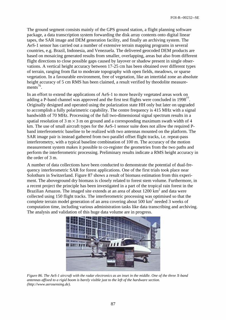
FOI-R--00232--SE

87

The ground segment consists mainly of the GPS ground station, a flight planning software package, a data transcription system forwarding the disk array contents onto digital linear tapes, the SAR image and DEM generation facility, and finally an archiving system. The AeS-1 sensor has carried out a number of extensive terrain mapping programs in several countries, e.g. Brazil, Indonesia, and Venezuela. The delivered geocoded DEM products are based on mosaicing generated results from smaller, overlapping, areas but also from different flight directions to close possible gaps caused by layover or shadow present in single obser-vations. A vertical height accuracy between 17-25 cm has been obtained over different types of terrain, ranging from flat to moderate topography with open fields, meadows, or sparse vegetation. In a favourable environment, free of vegetation, like an intertidal zone an absolute height accuracy of 5 cm RMS has been claimed, a result verified by theodolite measure-ments76.

In an effort to extend the applications of AeS-1 to more heavily vegetated areas work on adding a P-band channel was approved and the first test flights were concluded in 199877. Originally designed and operated using the polarization state HH only but later on upgraded to accomplish a fully polarimetric capability. The centre frequency is 415 MHz with a signal bandwidth of 70 MHz. Processing of the full two-dimensional signal spectrum results in a spatial resolution of 3 m × 3 m on ground and a corresponding maximum swath width of 4 km. The use of small aircraft types for the AeS-1 sensor suite does not allow the required P-band interferometric baseline to be realized with two antennas mounted on the platform. The SAR image pair is instead gathered from two parallel offset flight tracks, i.e. repeat-pass interferometry, with a typical baseline combination of 100 m. The accuracy of the motion measurement system makes it possible to co-register the geometries from the two paths and perform the interferometric processing. Preliminary results indicate a RMS height accuracy in the order of 3 m.

A number of data collections have been conducted to demonstrate the potential of dual-fre-quency interferometric SAR for forest applications. One of the first trials took place near Solothurn in Switzerland. Figure 87 shows a result of biomass estimation from this experi-ment. The aboveground dry biomass is closely related to forest stem volume. Furthermore, in a recent project the principle has been investigated in a part of the tropical rain forest in the Brazilian Amazon. The imaged site extends at an area of about 1200 km2 and data were collected using 150 flight tracks. The interferometric processing was optimised so that the complete terrain model generation of an area covering about 500 km2 needed 3 weeks of computation time, including various administration tasks like data transcribing and archiving. The analysis and validation of this huge data volume are in progress.

Figure 86. The AeS-1 aircraft with the radar electronics as an inset in the middle. One of the three X-band antennas affixed to a rigid boom is barely visible just to the left of the hardware section. (http://www.aerosensing.de).

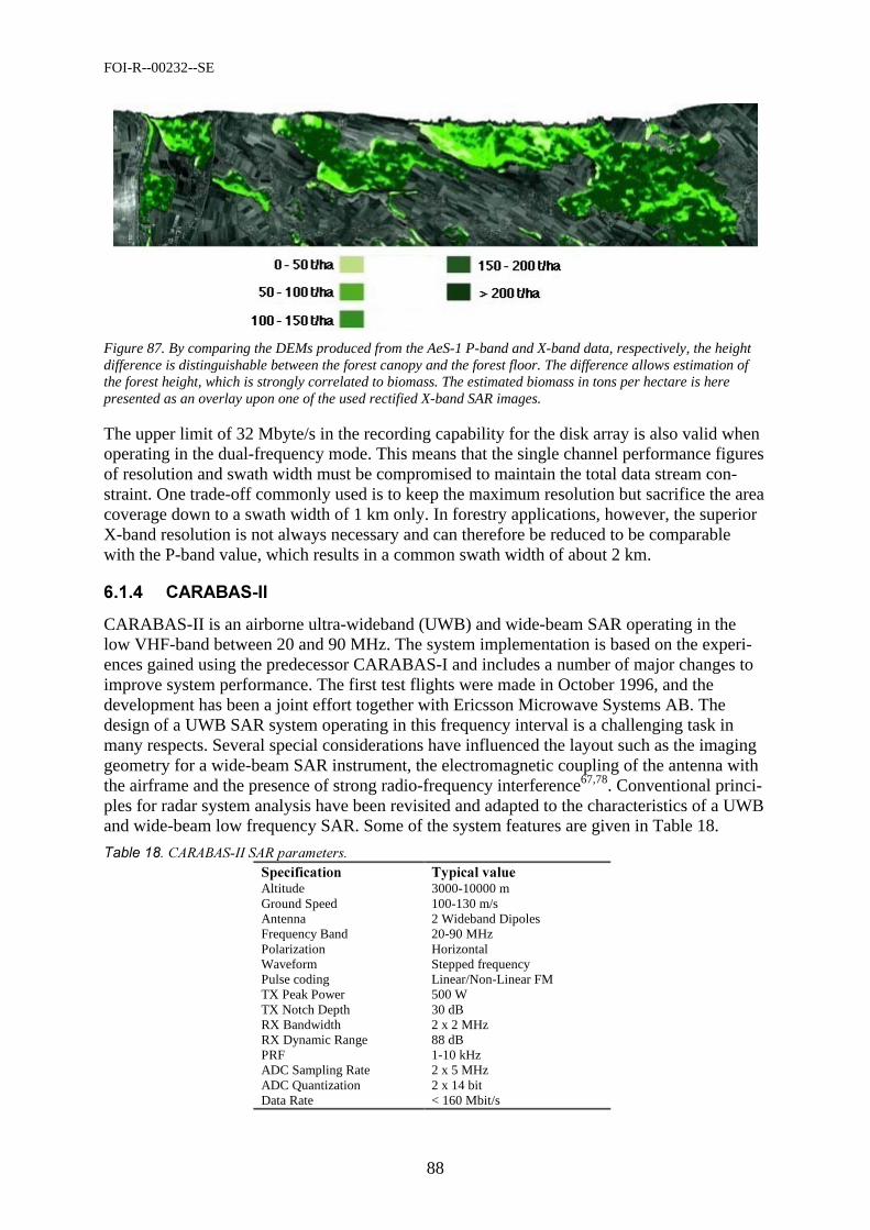
FOI-R--00232--SE

88

Figure 87. By comparing the DEMs produced from the AeS-1 P-band and X-band data, respectively, the height difference is distinguishable between the forest canopy and the forest floor. The difference allows estimation of the forest height, which is strongly correlated to biomass. The estimated biomass in tons per hectare is here presented as an overlay upon one of the used rectified X-band SAR images.

The upper limit of 32 Mbyte/s in the recording capability for the disk array is also valid when operating in the dual-frequency mode. This means that the single channel performance figures of resolution and swath width must be compromised to maintain the total data stream con-straint. One trade-off commonly used is to keep the maximum resolution but sacrifice the area coverage down to a swath width of 1 km only. In forestry applications, however, the superior X-band resolution is not always necessary and can therefore be reduced to be comparable with the P-band value, which results in a common swath width of about 2 km.

!""

CARABAS-II is an airborne ultra-wideband (UWB) and wide-beam SAR operating in the low VHF-band between 20 and 90 MHz. The system implementation is based on the experi-ences gained using the predecessor CARABAS-I and includes a number of major changes to improve system performance. The first test flights were made in October 1996, and the development has been a joint effort together with Ericsson Microwave Systems AB. The design of a UWB SAR system operating in this frequency interval is a challenging task in many respects. Several special considerations have influenced the layout such as the imaging geometry for a wide-beam SAR instrument, the electromagnetic coupling of the antenna with the airframe and the presence of strong radio-frequency interference67,78. Conventional princi-ples for radar system analysis have been revisited and adapted to the characteristics of a UWB and wide-beam low frequency SAR. Some of the system features are given in Table 18.

!

Altitude 3000-10000 m Ground Speed 100-130 m/s Antenna 2 Wideband Dipoles Frequency Band 20-90 MHz Polarization Horizontal Waveform Stepped frequency Pulse coding Linear/Non-Linear FM TX Peak Power 500 W TX Notch Depth 30 dB RX Bandwidth 2 x 2 MHz RX Dynamic Range 88 dB PRF 1-10 kHz ADC Sampling Rate 2 x 5 MHz ADC Quantization 2 x 14 bit Data Rate < 160 Mbit/s

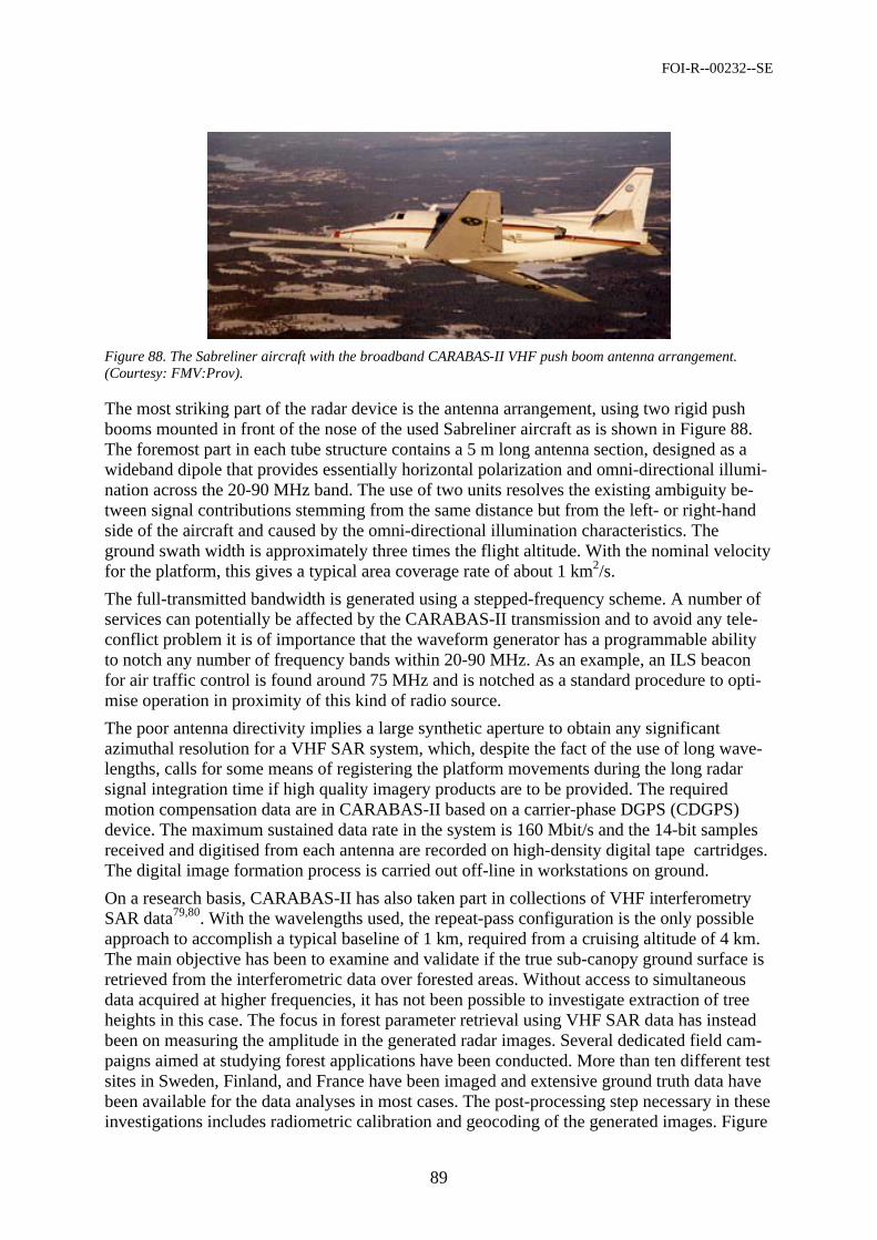
FOI-R--00232--SE

89

Figure 88. The Sabreliner aircraft with the broadband CARABAS-II VHF push boom antenna arrangement. (Courtesy: FMV:Prov).

The most striking part of the radar device is the antenna arrangement, using two rigid push booms mounted in front of the nose of the used Sabreliner aircraft as is shown in Figure 88. The foremost part in each tube structure contains a 5 m long antenna section, designed as a wideband dipole that provides essentially horizontal polarization and omni-directional illumi-nation across the 20-90 MHz band. The use of two units resolves the existing ambiguity be-tween signal contributions stemming from the same distance but from the left- or right-hand side of the aircraft and caused by the omni-directional illumination characteristics. The ground swath width is approximately three times the flight altitude. With the nominal velocity for the platform, this gives a typical area coverage rate of about 1 km2/s.

The full-transmitted bandwidth is generated using a stepped-frequency scheme. A number of services can potentially be affected by the CARABAS-II transmission and to avoid any tele-conflict problem it is of importance that the waveform generator has a programmable ability to notch any number of frequency bands within 20-90 MHz. As an example, an ILS beacon for air traffic control is found around 75 MHz and is notched as a standard procedure to opti-mise operation in proximity of this kind of radio source.

The poor antenna directivity implies a large synthetic aperture to obtain any significant azimuthal resolution for a VHF SAR system, which, despite the fact of the use of long wave-lengths, calls for some means of registering the platform movements during the long radar signal integration time if high quality imagery products are to be provided. The required motion compensation data are in CARABAS-II based on a carrier-phase DGPS (CDGPS) device. The maximum sustained data rate in the system is 160 Mbit/s and the 14-bit samples received and digitised from each antenna are recorded on high-density digital tape cartridges. The digital image formation process is carried out off-line in workstations on ground.

On a research basis, CARABAS-II has also taken part in collections of VHF interferometry SAR data79,80. With the wavelengths used, the repeat-pass configuration is the only possible approach to accomplish a typical baseline of 1 km, required from a cruising altitude of 4 km. The main objective has been to examine and validate if the true sub-canopy ground surface is retrieved from the interferometric data over forested areas. Without access to simultaneous data acquired at higher frequencies, it has not been possible to investigate extraction of tree heights in this case. The focus in forest parameter retrieval using VHF SAR data has instead been on measuring the amplitude in the generated radar images. Several dedicated field cam-paigns aimed at studying forest applications have been conducted. More than ten different test sites in Sweden, Finland, and France have been imaged and extensive ground truth data have been available for the data analyses in most cases. The post-processing step necessary in these investigations includes radiometric calibration and geocoding of the generated images. Figure

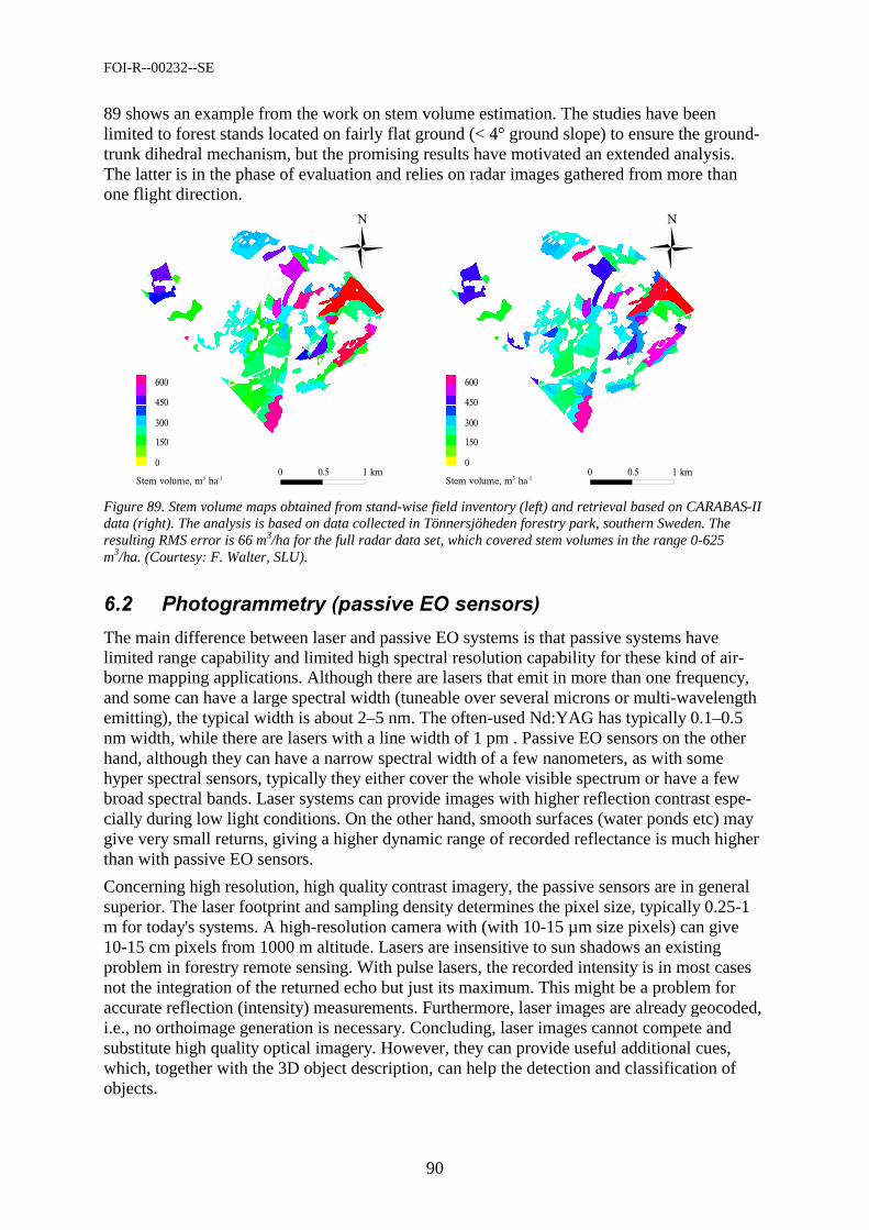
FOI-R--00232--SE

90

89 shows an example from the work on stem volume estimation. The studies have been limited to forest stands located on fairly flat ground (< 4° ground slope) to ensure the ground-trunk dihedral mechanism, but the promising results have motivated an extended analysis. The latter is in the phase of evaluation and relies on radar images gathered from more than one flight direction.

N

0

300

150

450

600

0 0.5 1 kmStem volume, m3 ha-1

N

0

300

150

450

600

0 0.5 1 kmStem volume, m3 ha-1

Figure 89. Stem volume maps obtained from stand-wise field inventory (left) and retrieval based on CARABAS-II data (right). The analysis is based on data collected in Tönnersjöheden forestry park, southern Sweden. The resulting RMS error is 66 m3/ha for the full radar data set, which covered stem volumes in the range 0-625 m3/ha. (Courtesy: F. Walter, SLU).

The main difference between laser and passive EO systems is that passive systems have limited range capability and limited high spectral resolution capability for these kind of air-borne mapping applications. Although there are lasers that emit in more than one frequency, and some can have a large spectral width (tuneable over several microns or multi-wavelength emitting), the typical width is about 2–5 nm. The often-used Nd:YAG has typically 0.1–0.5 nm width, while there are lasers with a line width of 1 pm . Passive EO sensors on the other hand, although they can have a narrow spectral width of a few nanometers, as with some hyper spectral sensors, typically they either cover the whole visible spectrum or have a few broad spectral bands. Laser systems can provide images with higher reflection contrast espe-cially during low light conditions. On the other hand, smooth surfaces (water ponds etc) may give very small returns, giving a higher dynamic range of recorded reflectance is much higher than with passive EO sensors.

Concerning high resolution, high quality contrast imagery, the passive sensors are in general superior. The laser footprint and sampling density determines the pixel size, typically 0.25-1 m for today's systems. A high-resolution camera with (with 10-15 µm size pixels) can give 10-15 cm pixels from 1000 m altitude. Lasers are insensitive to sun shadows an existing problem in forestry remote sensing. With pulse lasers, the recorded intensity is in most cases not the integration of the returned echo but just its maximum. This might be a problem for accurate reflection (intensity) measurements. Furthermore, laser images are already geocoded, i.e., no orthoimage generation is necessary. Concluding, laser images cannot compete and substitute high quality optical imagery. However, they can provide useful additional cues, which, together with the 3D object description, can help the detection and classification of objects.

FOI-R--00232--SE

91

A comparison between data acquisition and processing from passive optical sensors and air-borne laser scanning is presented by Baltsavias81. He has the following conclusions after dis-cussing photogrammetry and laser scanning systems:

”With respect to future developments, ALS (Airborne Laser Scanning) has a much higher potential. It is a newer technology and thus, has a greater margin for improvement, especially in the processing algorithms, and soft-ware and system development, while with its ‘discovery’ by users new applications will come up. Furthermore, laser is a technology with much broader base and interests, and the research in this field as well as the commercialisation of new findings are intense and advancing rapidly. Although many new developments are and will be in lasers that cannot be used in photogrammetry, some benefits will certainly result also for ALS, as laser-based earth observation from airplanes and satellites, as well as military applications, are important applications where improvements of the ranging and imaging capabilities of laser are expected. Furthermore, recording and exploitation of information with respect to signal properties like amplitude, polarisation, phase, frequency shifts and vertical profile can greatly improve the object classification and identification capabilities of ALS.

ALS is here to stay with us and hopefully flourish. It definitely has an over-lap to existing photogrammetric processes, competes with them, and will also partly replace them. Its major advantages are density and accuracy of measurements, high automation and fast delivery times, the costs being a topic still to be resolved. However, to the greater extent, there is a comple-mentarity between the two technologies. ALS can perform some tasks, which photogrammetry anyway could not or very poorly perform and vice-versa. Furthermore, the use of ALS has concentrated up to now in large scale mapping and engineering surveys. Both technologies share similar methods for integration with GPS/ INS and have the same nuts to crack, when it comes to automation of object recognition. An integration of ALS with digital POS and GPS/INS can open up new revolutionary approaches in the whole photogrammetric.

Thus, ALS should not be mainly seen as a competition, but as an additional versatile tool to choose from. Photogrammetrists should decisively contribute, in close cooperation with open-minded firms, in the definition, standardisation and development of high-quality methods for the whole processing chain, and especially in the postprocessing phase of object filtering, extraction and classification, the integration with other sensors, and tighter coupling of technology and applications.”

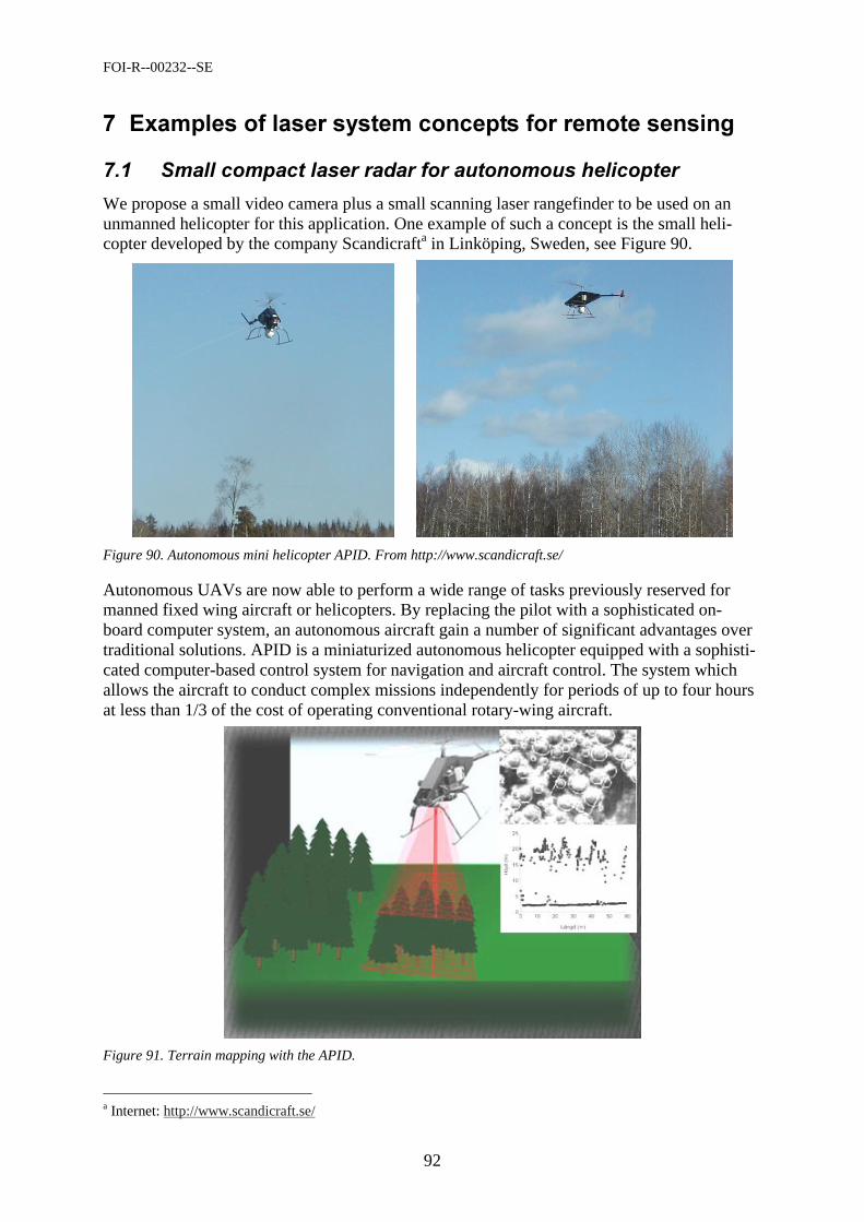
FOI-R--00232--SE

92

# $% &'& '

We propose a small video camera plus a small scanning laser rangefinder to be used on an unmanned helicopter for this application. One example of such a concept is the small heli-copter developed by the company Scandicrafta in Linköping, Sweden, see Figure 90.

Figure 90. Autonomous mini helicopter APID. From http://www.scandicraft.se/

Autonomous UAVs are now able to perform a wide range of tasks previously reserved for manned fixed wing aircraft or helicopters. By replacing the pilot with a sophisticated on-board computer system, an autonomous aircraft gain a number of significant advantages over traditional solutions. APID is a miniaturized autonomous helicopter equipped with a sophisti-cated computer-based control system for navigation and aircraft control. The system which allows the aircraft to conduct complex missions independently for periods of up to four hours at less than 1/3 of the cost of operating conventional rotary-wing aircraft.

Figure 91. Terrain mapping with the APID.

a Internet: http://www.scandicraft.se/

FOI-R--00232--SE

93

With a payload capacity of 20 kga (45 lbs.), the vehicle is able to carry a wide array of instru-ments, ranging from stabilized cameras, infrared sensors, and laser. Real-time communica-tions capabilities allow control of the craft and sensors as well as the transmission of data to the ground.

" ## Specification Typical value

Operating altitude, H 30-300 m Footprint 0.05-0.5 m Flying speed V 10-50 m/s Swath S < H m Grid spacing a 0.05-0.5 m Area coverage rate Min (fp*a2 m2/s , S*V)

Wavelength a 0.9-1.5 µm Pulse repetition rate (fp) 1-500 kHz depending on approach Pulse energy 10-50 µJ Pulse width 3-5 ns Beam divergence < 2 mrad

Type Avalanche photo diode (APD) NEP 1 nW Bandwidth 100 MHz

Type Rotating polygon Scan angle (full angle) 60° Scan frequency fs 30-60 Hz (has to fit the relation fs=fp*a/S) Scan pattern Zigzag, parallel

GPS frequency -- belong to aircraft INS frequency ---- Range accuracy/resolution 3 cm / 1 cm

Multiple elevation capture 4 -5 echoes per pulse

!"

Tree altitude and position Yes to 50 cm level or better Tree species and proportion Yes by 3-D and video. Canopy structure Canopy cover Crown size, form Accuracy ground (elevation) 5-10 cm Accuracy (planimetrical) 10-50 cm

Total weight 10-15 kg (low PRF 5-10 kHz) Size < 15 cm diameter * 50 cm length Power consumption 12 V DC 2-5 A

Compared to other available solutions, the APID is not only affordable, but also easy to handle and operate, even with a small crew. With a main rotor diameter of only 3 m (10 ft.), the vehicle and associated ground-support equipment are easily transported in a trailer or full-size van and can be deployed in less than one hour.

The APID Mark-III is suited for extern payload, while the APID Mark-IIIb has an integrated gyrostabilized payload platform. A number of sensors provide information on vehicle attitude, position, speed, and direction of travel to the on-board navigation and control computer

a There are a number of other autonomous helicopters which can carry higher payloads (up to 100-200 kg).

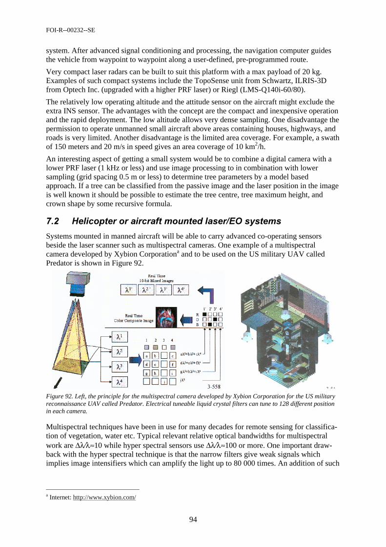
FOI-R--00232--SE

94

system. After advanced signal conditioning and processing, the navigation computer guides the vehicle from waypoint to waypoint along a user-defined, pre-programmed route.

Very compact laser radars can be built to suit this platform with a max payload of 20 kg. Examples of such compact systems include the TopoSense unit from Schwartz, ILRIS-3D from Optech Inc. (upgraded with a higher PRF laser) or Riegl (LMS-Q140i-60/80).

The relatively low operating altitude and the attitude sensor on the aircraft might exclude the extra INS sensor. The advantages with the concept are the compact and inexpensive operation and the rapid deployment. The low altitude allows very dense sampling. One disadvantage the permission to operate unmanned small aircraft above areas containing houses, highways, and roads is very limited. Another disadvantage is the limited area coverage. For example, a swath of 150 meters and 20 m/s in speed gives an area coverage of 10 km2/h.

An interesting aspect of getting a small system would be to combine a digital camera with a lower PRF laser (1 kHz or less) and use image processing to in combination with lower sampling (grid spacing 0.5 m or less) to determine tree parameters by a model based approach. If a tree can be classified from the passive image and the laser position in the image is well known it should be possible to estimate the tree centre, tree maximum height, and crown shape by some recursive formula.

! "

Systems mounted in manned aircraft will be able to carry advanced co-operating sensors beside the laser scanner such as multispectral cameras. One example of a multispectral camera developed by Xybion Corporationa and to be used on the US military UAV called Predator is shown in Figure 92.

Figure 92. Left, the principle for the multispectral camera developed by Xybion Corporation for the US military reconnaissance UAV called Predator. Electrical tuneable liquid crystal filters can tune to 128 different position in each camera.

Multispectral techniques have been in use for many decades for remote sensing for classifica-tion of vegetation, water etc. Typical relevant relative optical bandwidths for multispectral work are ∆λ⁄λ≈10 while hyper spectral sensors use ∆λ⁄λ≈100 or more. One important draw-back with the hyper spectral technique is that the narrow filters give weak signals which implies image intensifiers which can amplify the light up to 80 000 times. An addition of such

a Internet: http://www.xybion.com/

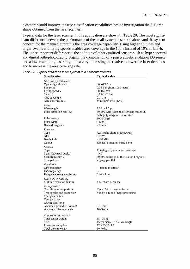
FOI-R--00232--SE

95

a camera would improve the tree classification capabilities beside investigation the 3-D tree shape obtained from the laser scanner.

Typical data for the laser scanner in this application are shown in Table 20. The most signifi-cant difference between the performance of the small system described above and the system concept for the manned aircraft is the area coverage capability. Using higher altitudes and larger swaths and flying speeds enables area coverage in the 100’s instead of 10’s of km2/h. The other important difference is the addition of other qualified sensors such as hyper spectral and digital orthophotography. Again, the combination of a passive high-resolution EO sensor and a lower sampling laser might be a very interesting alternative to lower the laser demands and to increase the area coverage rate.

$% &Specification Typical value

Operating altitude, H 300-6000 m Footprint 0.25-1 m (from 1000 meter) Flying speed V 50-150 m/s Swath S (0.7-1) *H m Grid spacing a 0.1-1 m Area coverage rate Min (fp*a2 m2/s , S*V)

Wavelength a 1.06 or 1.5 µm Pulse repetition rate (fp) 30-500 KHz (Note that 100 kHz means an

ambiguity range of 1.5 km etc.) Pulse energy 100-500 µJ Pulse width 3-5 ns Beam divergence < 2 mrad

Type Avalanche photo diode (APD) NEP <1 nW Bandwidth >100 MHz Output Range(12 bits), intensity 8 bits

Type Rotating polygon or galvanometer Scan angle (full angle) < 60° Scan frequency fs 30-60 Hz (has to fit the relation fs=fp*a/S) Scan pattern Zigzag, parallel

GPS frequency -- belong to aircraft INS frequency ---- 3 cm / 1 cm

Multiple elevation capture 4-5 echoes per pulse

!"

Tree altitude and position Yes to 50 cm level or better Tree species and proportion Yes by 3-D and image processing Canopy structure Canopy cover Crown size, form Accuracy ground (elevation) 5-10 cm Accuracy (planimetrical) 10-50 cm

Total sensor weight 15 –25 kg Size 15 cm diameter * 50 cm length Power consumption 12 V DC 2-5 A Total system weight 60-70 kg

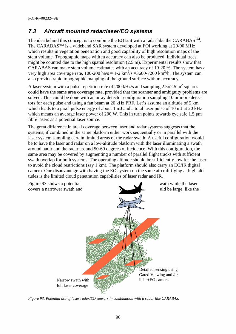
FOI-R--00232--SE

96

# $ ""

The idea behind this concept is to combine the EO suit with a radar like the CARABASTM. The CARABAS™ is a wideband SAR system developed at FOI working at 20-90 MHz which results in vegetation penetration and good capability of high resolution maps of the stem volume. Topographic maps with m accuracy can also be produced. Individual trees might be counted due to the high spatial resolution (2.5 m). Experimental results show that CARABAS can make stem volume estimates with an accuracy of 10-20 %. The system has a very high area coverage rate, 100-200 ha/s = 1-2 km2/s =3600-7200 km2/h. The system can also provide rapid topographic mapping of the ground surface with m accuracy.

A laser system with a pulse repetition rate of 200 kHz/s and sampling 2.5×2.5 m2 squares could have the same area coverage rate, provided that the scanner and ambiguity problems are solved. This could be done with an array detector configuration sampling 10 or more detec-tors for each pulse and using a fan beam at 20 kHz PRF. Let’s assume an altitude of 5 km which leads to a pixel pulse energy of about 1 mJ and a total laser pulse of 10 mJ at 20 kHz which means an average laser power of 200 W. This in turn points towards eye safe 1.5 µm fibre lasers as a potential laser source.

The great difference in areal coverage between laser and radar systems suggests that the systems, if combined in the same platform either work sequentially or in parallel with the laser system sampling certain limited areas of the radar swath. A useful configuration would be to have the laser and radar on a low-altitude platform with the laser illuminating a swath around nadir and the radar around 50-60 degrees of incidence. With this configuration, the same area may be covered by augmenting a number of parallel flight tracks with sufficient swath overlap for both systems. The operating altitude should be sufficiently low for the laser to avoid the cloud restrictions (say 1 km). The platform should also carry an EO/IR digital camera. One disadvantage with having the EO system on the same aircraft flying at high alti-tudes is the limited cloud penetration capabilities of laser radar and IR.

Figure 93 shows a potential sensor system. The radar covers a wide swath while the laser covers a narrower swath and/or selected small areas. The footprint could be large, like the

Narrow swath with full laser coverage

Detailed sensing usingGated Viewing and /or lidar+EO camera

Figure 93. Potential use of laser radar/EO sensors in combination with a radar like CARABAS.

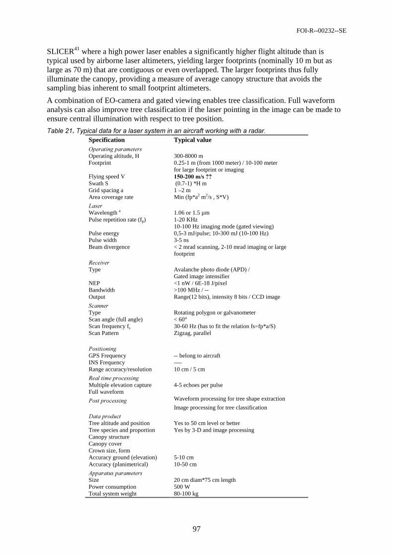
FOI-R--00232--SE

97

SLICER41 where a high power laser enables a significantly higher flight altitude than is typical used by airborne laser altimeters, yielding larger footprints (nominally 10 m but as large as 70 m) that are contiguous or even overlapped. The larger footprints thus fully illuminate the canopy, providing a measure of average canopy structure that avoids the sampling bias inherent to small footprint altimeters.

A combination of EO-camera and gated viewing enables tree classification. Full waveform analysis can also improve tree classification if the laser pointing in the image can be made to ensure central illumination with respect to tree position.

$ ' 'Specification Typical value

Operating altitude, H 300-8000 m Footprint 0.25-1 m (from 1000 meter) / 10-100 meter

for large footprint or imaging Flying speed V Swath S (0.7-1) *H m Grid spacing a 1 –2 m Area coverage rate Min (fp*a2 m2/s , S*V)

Wavelength a 1.06 or 1.5 µm Pulse repetition rate (fp) 1-20 KHz

10-100 Hz imaging mode (gated viewing) Pulse energy 0,5-3 mJ/pulse; 10-300 mJ (10-100 Hz) Pulse width 3-5 ns Beam divergence < 2 mrad scanning, 2-10 mrad imaging or large

footprint

Type Avalanche photo diode (APD) / Gated image intensifier

NEP <1 nW / 6E-18 J/pixel Bandwidth >100 MHz / -- Output Range(12 bits), intensity 8 bits / CCD image

Type Rotating polygon or galvanometer Scan angle (full angle) < 60° Scan frequency fs 30-60 Hz (has to fit the relation fs=fp*a/S) Scan Pattern Zigzag, parallel

GPS Frequency -- belong to aircraft INS Frequency ---- Range accuracy/resolution 10 cm / 5 cm

Multiple elevation capture 4-5 echoes per pulse Full waveform

Waveform processing for tree shape extraction

Image processing for tree classification

!"

Tree altitude and position Yes to 50 cm level or better Tree species and proportion Yes by 3-D and image processing Canopy structure Canopy cover Crown size, form Accuracy ground (elevation) 5-10 cm Accuracy (planimetrical) 10-50 cm

Size 20 cm diam*75 cm length Power consumption 500 W Total system weight 80-100 kg

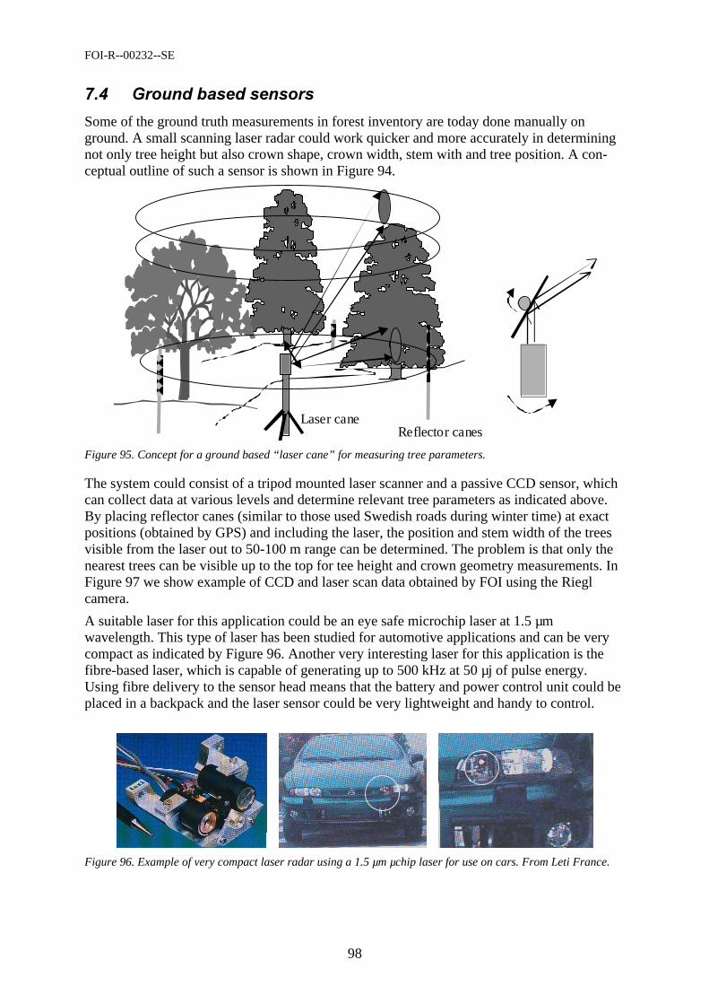
FOI-R--00232--SE

98

% & '

Some of the ground truth measurements in forest inventory are today done manually on ground. A small scanning laser radar could work quicker and more accurately in determining not only tree height but also crown shape, crown width, stem with and tree position. A con-ceptual outline of such a sensor is shown in Figure 94.

Reflector canesLaser cane

Figure 95. Concept for a ground based “laser cane” for measuring tree parameters.

The system could consist of a tripod mounted laser scanner and a passive CCD sensor, which can collect data at various levels and determine relevant tree parameters as indicated above. By placing reflector canes (similar to those used Swedish roads during winter time) at exact positions (obtained by GPS) and including the laser, the position and stem width of the trees visible from the laser out to 50-100 m range can be determined. The problem is that only the nearest trees can be visible up to the top for tee height and crown geometry measurements. In Figure 97 we show example of CCD and laser scan data obtained by FOI using the Riegl camera.

A suitable laser for this application could be an eye safe microchip laser at 1.5 µm wavelength. This type of laser has been studied for automotive applications and can be very compact as indicated by Figure 96. Another very interesting laser for this application is the fibre-based laser, which is capable of generating up to 500 kHz at 50 µj of pulse energy. Using fibre delivery to the sensor head means that the battery and power control unit could be placed in a backpack and the laser sensor could be very lightweight and handy to control.

Figure 96. Example of very compact laser radar using a 1.5 µm µchip laser for use on cars. From Leti France.

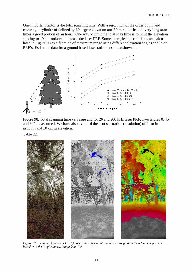
FOI-R--00232--SE

99

One important factor is the total scanning time. With a resolution of the order of cm and covering a cylinder of defined by 60 degree elevation and 50 m radius lead to very long scan times a good portion of an hour). One way to limit the total scan time is to limit the elevation spacing to 10 cm and/or to increase the laser PRF. Some examples of scan times are calcu-lated in Figure 98 as a function of maximum range using different elevation angles and laser PRF’s. Estimated data for a ground based laser radar sensor are shown in

θ

Ra

20 40 60 80 100

0.1

1

10T

otal

sca

ntim

e m

inut

es

0D[LPXPUDQJHP

max 60 dg angle, 20 kHz max 45 dg, 20 kHz max 60 dg, 200 khz max 45 dg, 200 kHz

Figure 98. Total scanning time vs. range and for 20 and 200 kHz laser PRF. Two angles θ, 45º and 60º are assumed. We have also assumed the spot separation (resolution) of 2 cm in azimuth and 10 cm in elevation.

Table 22.

Figure 97. Example of passive EO(left), laser intensity (middle) and laser range data for a forest region col-lected with the Riegl camera. Image fromFOI.

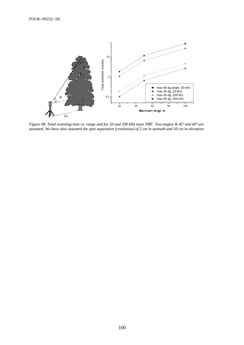
FOI-R--00232--SE

100

θ

Ra

20 40 60 80 100

0.1

1

10

Tot

al s

cant

ime

min

utes

0D[LPXPUDQJHP

max 60 dg angle, 20 kHz max 45 dg, 20 kHz max 60 dg, 200 khz max 45 dg, 200 kHz

Figure 98. Total scanning time vs. range and for 20 and 200 kHz laser PRF. Two angles θ, 45# and 60# are assumed. We have also assumed the spot separation (resolution) of 2 cm in azimuth and 10 cm in elevation.

FOI-R--00232--SE

101

$$(#

Specification Typical value

Footprint at 50 m range 1-2 cm Grid Spacing a 1–2 cm Area coverage time (cylinder 60°*360°) at 50 m sugin 2 cm grid in azimuth and 10 cm in elevation

11.31 minutes (20 kHz laser), 1.13 min. (200 kHz laser)

Max. range 50 meter

Wavelength a 1.5 µm Pulse Repetition Rate (fp) 20 kHz (200 kHz) Pulse Energy 5-10 µJ Pulse Width 1-3 ns Beam Divergence < 2 mrad scanning

Type Avalanche photo diode (APD NEP <1 nW Bandwidth >100 MHz / -- Output Range(12 bits), intensity 8 bits / CCD image

Type Rotating mirror Scan Angle (full angle) < 60° Scan frequency fs Scan Pattern Circular

GPS !!"!# $%"&$

1 cm / 3 cm

Multiple Elevation Capture 4-5 echoes per pulse

Range processing for tree shape extraction Image/range processing for tree classification

!"

Tree altitude and position Yes to 30 cm level or better Tree classification Yes by 3-D , image processing Canopy structure Canopy cover Crown size, form Stem diameter About 1 cm accuracy

Total sensor weight 1 – 3 kg Size 10 cm diameter * 20 cm length Power consumption 50-500 W Total system weight 3-4 kg incl. tripod

FOI-R--00232--SE

102

( )Airborne laser scanning systems can perform precise measurements with high accuracy and resolution, e.g. mapping of the detailed crown shape. The price to pay for this high resolution is a lower coverage rate in comparison to e.g. SAR methods. ALS has some strengths, which can be favourably exploited in certain applications:

• In mapping of surfaces with very little or no texture or poor definition image matching delivers very poor results, and manual measurements are poor or slow and cumber-some.

• In mapping of forests and vegetated areas, ALS systems can provide measurements on the ground. The penetration rate mainly depends on type of trees (deciduous or coniferous) and season. Useful results, depending also on the terrain roughness, can be achieved even with penetration rates of 20–30%. ALS systems that record $ first and last, or $ even more than two echoes of each pulse, can more easily provide tree and ground height and those with more than two echoes can, in addition, measure a verti-cal object profile, thus enabling derivation of other important parameters like biomass estimation, tree type, etc.

With respect to future developments, ALS has a high potential. It is a new technology and thus, has a margin for improvement, especially in the processing algorithms, and software and system development. Furthermore, recording and exploitation of information with respect to signal properties like amplitude, polarisation, phase, frequency shifts and vertical profile can greatly improve the object classification and identification capabilities of ALS.

The combination of ALS with other sensor like passive optical scanners, digital cameras, and radar has a great potential, which is so far hardly exploited. The combination can be obtained from simultaneously working sensor in the same platform to combination of data from different platforms flying at altitudes most suitable for each sensor.

After consultation with experts in forestry remote sensing, we have found the following appli-cation areas to be of special importance:

• The use of digital cameras and small ALS in UAV:s for detailed measurements in smaller areas (typical 10 ha).

• Development of operational methods for rapid terrain visualisation for use in forestry applications.

• The use of laser data to calibrate the more rapid CARABAS system for biomass measurements.

• The use of a combined laser scanner and optical multispectral scanner for a high coverage rate system operating at km altitudes.

From the technical point of view, we see the need for: • Development of low cost compact light weight ALS-systems suitable for UAV

applications • Development of advanced multielement transmitters and receivers to increase

coverage rates and lower the demands on the scanning system or even eliminate the need for scanner.

• Digitisation and storage of the full waveform and the development of signal processing using the full waveform, as in bathymetric applications.

• Optimisation of the design and usage of combined passive EO and laser systems. • Development of rapid and robust signal processing for multisensor systems.

FOI-R--00232--SE

103

In analogy with the development of ALS systems for sea charting, both military and civilian applications can be identified for land applications. Vegetation and terrain mapping is of great interest also in military applications such as mapping and reconnaissance. For future work, we suggest the development of technology and methods for fast mapping of forest and terrain with airborne laser scanning systems. Such a development would be of interest for both civil-ian and military applications. Military applications include e.g. terrain maps to evaluate the accessibility in a terrain section. In particular, we suggest the development of small systems – which would lead to fast and cost effective mapping. Interesting topics for a system study could be a UAV or mini helicopter equipped with a laser radar and digital camera. Such a system could be used in forestry planning.

FOI-R--00232--SE

104

* '

1 O. Steinvall, U. Söderman, S. Ahlberg, M. Sandberg, D. Letalick, and E. Jungert, “Airborne laser radar: Systems and methods for reconnaissance and terrain modeling”, Proc. SPIE Vol. 3707, pp. 12-26 (1999).

2 H. Schreier, J. Lougheed, C. Tucker, D. Leckie, “Automated measurements of terrain reflection and height variations using airborne infrared laser system”, Int. J. Remote Sensing, Vol. 6, No. 1, 1985.

3 J. C. Ritche, ”Airborne laser altimeter measurements of landscape topography”, Remote Sensing of Environment, Vol. 53, 1995.

4 R. Nelson, R. Swift, W. Krabill, “Using airborne lasers to estimate forest canopy and stand characteristics”, J. of Forestry, Vol. 86, 1988.

5 G. A. Maclean, W. B Krabill, “Gross-merchantable timber volume estimation using and airborne lidar system”, Can. J. Remote Sens., Vol. 12, No. 1, 1986.

6 A. H. Aldred and G. M. Bonner, “Application of airborne laser to forest surveys”, Information report PI-X-51. Canadian Forest Service, Petawawa National Forest Institute. Chalk River, 1985.

7 M. Nilsson, “Estimation of tree heights and stand volume using an airborne lidar system”, Remote Sens. of Environ. Vol. 56:1-7, 1996.

8 R. F. Nelson, R. Oderwald, T. G. Gregoire, “ Separating the ground and airborne laser sampling phases to estimate tropical forest basal area, volume and biomass”, Remote Sens. of Environ. Vol 60, 1997.

9 E. Næsset, “Estimating timber volume of forest stands using airborne laser scanner data”, Remote Sens. of Environ. Vol 61, pp. 246-253, 1997.

10 S. Magnussen, P. Eggermont, V. N. LaRiccia, ”Recovering tree heights from airborne scanner data”, Forest Science, Vol. 45 No. 3, 1999.

11 W. Rieger, O. Eckmüllner, H. Müllner, T. Reiter, “Laser-scanning for the derivation of forest stand parameters”, Proceeding of the ISPRS III workshop on Mapping surface structure and topography by airborne and spaceborne lasers, La Jolla, CA, Nov 1999.

12 J. Hyyppä, H. Hyyppä, G. Ruppert, “Automatic derivation of features related to forest stand attributes using laser scanner”, Int. Arch. of Photogrammetry and Remote Sens., Vol. XXXIII, Part B3, Amsterdam 2000.

13 K. Kraus, N. Pfeifer, ”Determination of terrain models in wooded areas with airborne scanner data”, ISPRS J. of Photogrammetry and Remote Sens, Vol 53, 1998.

14 N. Pfeifer, T. Reiter, C. Briese, W. Rieger, “Interpolation of high quality ground models from laser scanner data in forested areas”, Proceeding of the ISPRS III workshop on Mapping surface structure and topography by airborne and spaceborne lasers, La Jolla, CA, Nov 1999.

15 J. E. Means, S. A. Acker, D. J. Harding, J. B. Blair, M. A. Lefsky, W. B. Cohen, M. E. Harmon, W. A. McKee, “ Use of a large-footprint scanning airborne lidar to estimate forest stand characteristics in the western cascades of Oregon”, Remote Sens. of Environ. Vol 67, 1999.

FOI-R--00232--SE

105

16 J. B. Blair, D. L. Rabine, M. A. Hofton, “The Laser Vegetation Imaging Sensor: a medium-altitude, digitisation-only, airborne laser altimeter for mapping vegetation and topography”, ISPRS J. Photogram. Rem. Sensing, Vol. 54, 1999, pp. 115–122.

17 M. A. Lefsky, D. Harding, W. B. Cohen, G. Parker, H. H. Shugart, “Surface lidar remote sensing of basal area and biomass in deciduous forests of eastern Maryland, USA”, Remote Sens. of Environ. Vol 70, 1999.

18 M. Nilsson, “Wood volume estimation using satellite spectral data and tree height data”, in M. Nilsson, Estimation of forest variables using satellite image data and airborne Lidar. Doctoral thesis. Acta Universitatis Agriculturae Sueciae, Silvestria 17, 1997.

19 J. E. Means, “Design, capabilities and uses of large-footprint and small-footprint lidar systems”, Proceeding of the ISPRS III workshop on Mapping surface structure and topography by airborne and spaceborne lasers, La Jolla, CA, Nov 1999.

20 J. E. Means, “Comparison of large-footprint and small-footprint lidar systems: design, capabilities and uses”, Proceeding of the Second International Conference on Geospatial Information in Agriculture and Forestry, Lake Buena Vista, Florida, Jan 2000, pp. 185-192.

21 S. Magnussen, P. Boudewyn, “Derivation of stand heights from airborne laser scanner data with canopy-based quantile estimator”, Can. J. For. Res., Vol . 28, 1998.

22 B. A. St-Onge, “Estimating individual tree heights of the boreal forest using airborne laser alimetry and digital videography”, Proceeding of the ISPRS III workshop on Mapping surface structure and topography by airborne and spaceborne lasers, La Jolla, CA, Nov 1999.

23 O. Steinvall, K. Koppari, “Depth sounding lidar – An overview of Swedish activities and with future prospects”, CIS Selected papers on Laser Remote Sensing in Natural Waters: From Theory to Practice, Proc. SPIE, Vol. 2964, pp. 2-25, V. I. Feigels; Y. I. Kopilevich; Eds., 1996.

24 The Infrared and Electro-Optical Systems Handbook, vol. 6, Ch. 2, SPIE, 1993. 25 D. L. Knepp, G. C. Valley, “Properties of joint Gaussian statistics”, Radio Sc., Vol. 13, p.

59, 1978. 26 D. L. Fried, “Aperture averaging of Scintillation”, J. Opt. Soc. Am., Vol. 57, p.169, 1967. 27 G. Bolander and O. Steinvall, FOI, unpublished results. 28 R. Axelsson, O. Steinvall, and P. Sundberg, “Programmable scanner for laser bathymetry”,

International Hydrographic Rev., Vol. 67, No.1, pp. 161-170, January 1990. 29 J. M. Vaughan, K. O. Steinvall, C. Werner and P. H. Flamant, “Coherent laser radar in

Europe”, Proc. IEEE, Vol. 84, No. 2, pp. 205-226, February 1996. 30 O. Steinvall, “Theory for laser systems performance modelling”,

FOA-R--97-00599-612--SE, Oct., 1997. 31 O. Steinvall, H. Olsson, G. Bolander, C. Carlsson, and D. Letalick, “Gated viewing for

target detection and target recognition”, Proc SPIE. Vol. 3703, pp. 432-448, Laser Radar Technology and Applications IV, Orlando, 6-9 April, 1999.

FOI-R--00232--SE

106

32 D. Bonnier, “Range-gated active-imaging system for search-and-rescue and surveillance operations”, Proc. SPIE Vol. 2744, pp. 134-145, Infrared Technology and Applications XXII, 1996.

33 P. Pencikowski, “A low cost vehicle-mounted enhanced vision system comprised of a laser illuminator and a range-gated camera”, Proc. SPIE, Vol. 2736, pp. 222-227, Enhanced and Synthetic Vision 1996, Orlando April 1996.

34 J. W. McLean, J. M Murray, “Streak tube lidar allows ocean surveillance”, Laser Focus World, pp. 171-176, Jan. 1998.

35 W. Krohn and W. Matthews, “Multispectral diode-based imaging laser radar”, Laser Radar VII, Proc. SPIE Vol. 1633, pp. 294-303, 1992.

36 “Avalanche photodiodes: A user’s guide”, PerkinElmer Optoelectronics Inc., Internet: http://opto.perkinelmer.com/library/papers/tp5.htm

37 P. F. McManamon, T. A. Dorschner, D. L. Corcum, L. J. Friedman, D. S. Hobbs, M. Holz, S. Liberman, H. Q. Nqyen, D. P. Reisler, R. C. Sharp, and E. A. Watson, “Optical phased array technology”, Proc. IEEE, Vol. 84, No. 2, pp. 268-298, 1996.

38 B. Löfving, S. Hård, “Beam steering with two ferroelectric liquid crystal spatial light modulators”, Opt. Lett., Vol. 23, No. 19, pp. 1-3, 1998.

39 D. W. Ricks, H. W. Willhite, “Hand-held imaging laser radar”, Proc. SPIE, Vol. 3065, pp. 30-41, Laser Radar Technology and Applications II, 1997.

40 S. Hård, S. Jacobsson, B. Löfving, U. Olin, P. Rudquist, L. Sjöqvist, O. Steinvall, and S. Walles, ”Laser beam steering - an introductory study”, FOA-R--99-01158-408--SE, 1999.

41 R. A. Buser, ”Principles and possibilities of small actuators”, Eurosensors X, Leuven, Belgium, 8–11 September 1996, pp. 1013–1021.

42 K. Gustafsson and B. Hök, “Light scanning techniques – a critical review”, Int. J. Optoelectronics, Vol 4 (1989), pp 33-52.

43 R. Miller and O. Amidi, “3-D site mapping with CMU autonomous helicopter”, 5th International Conference on intelligent Autonomous Systems, IAS-5, June 1998.

44 A. Wehr, U. Lohr, “Airborne laser scanning – an introduction and overview”, ISPRS Journal of Photogrammetry & Remote Sensing 54 1999, pp. 68–82.

45 E. J. Huising, L. M. Gomes Pereira, “Errors and accuracy estimates of laser data acquired by various laser scanning systems for topographic applications,” ISPRS Journal of Photogrammetry & Remote Sensing 53, pp. 245–261 (1998).

46 O. Steinvall, “Waveform simulation for 3-D sensing laser radar”, FOA-R--00-01530-612,408--SE, May 2000.

47 C. Carlsson, “Calculation of measurement uncertainties in TopEye data”, FOA-D--00-00492-408--SE, June 2000.

48 E. P. Baltsavias, “Airborne laser scanning: basic relations and formulas”, ISPRS J. Photogram. Rem. Sensing, Vol. 54, 1999, pp. 199–214.

49 A. Samberg, J. Hyyppä, “Assessing tree attributes from the laser scanner data: the high-scan case”, in Proceeding of the Fourth International Airborne Remote Sensing Conference and Exhibition / 21st Canadian Symposium on Remote Sensing, Ottawa, Ontario, Canada, June 1999.

FOI-R--00232--SE

107

50 J. Kilian, J. Haala, M. Englich, “Capture and evaluation of airborne laser scanner data”, Int Arch of Photogrammetry and Remote Sens, Vol XXXI, Part B3, Vienna, Austria, 1996.

51 P. Axelsson, “Processing of laser scanner data – algorithms and applications”, ISPRS Journal of Photogrammetry & Remote Sensing 54 (2), 1999.

52 P. Axelsson personal communication 1999-2000. 53 TerraScan, “TerraScan for microStation user’s guide”, TerraSolid Ltd, 1999. 54 M. Elmqvist, “Automatic Ground Modelling using Laser radar Data”, Master's Thesis,

Linköping University, LiTH-ISY-EX-3061, March 2000. 55 M. Kass, A. Witkin, and D. Terzopoulos, “Snakes: active contour models”, Int. J. of

Computer Vision, 1:321-331, 1988. 56 L. D. Cohen, “On active contour models and balloons”, Computer Vision, Graphics, and

Image Processing, 53 211-218, 1991. 57 M. A. Lefsky, D. J. Harding, G. G. Parker ,W. B. Cohen, and S. A. Acker, “Progress in

lidar altimeter remote sensing of stand structure in deciduous coniferous forests using SLICER data”, Conf. on Mapping Surface Structure and Topography by Airborne and Spaceborne Lasers, La Jolla, USA, 1999.

58 M. A. Lefsky, W. B. Cohen, A. Hudak, S. A. Acker, and J. L. Ohmann, “Integration of LIDAR, LANDSAT ETM+ and forest inventory data for regional forests mapping”, Conf. on Mapping Surface Structure and Topography by Airborne and Spaceborne Lasers, La Jolla, USA, 1999.

59 M. Flood, “Commercial development of airborne laser altimetry” A review of the commercial instrument market and its projected growth, “Mapping Surface Structure and Topography by Airborne and Spaceborne Lasers” in La Jolla, USA.

60 Internet: http://www.airbornelasermapping.com 61 E. P. Baltsavias, “Airborne laser scanning: existing systems and firms and other

resources”, ISPRS J. Photogram. Rem. Sensing, Vol. 54, 1999, pp. 164–198. 62 A. Samberg, J. Hyypää, G. Ruppert, H. Hyypää, M. Ziegler, M. Schardt and A. Soininen,

“An evaluation of the laser scanner data in the forest area”, SPIE Proc. Vol. 3707, Euro-Opto Conference on Laser Radar Technology and Applications, Munich, 1999.

63 See for example Internet: http://sun00781.dn.net/man/dod-101/sys/smart/locaas.htm. 64 Internet: http://peoiews.monmouth.army.mil/jpsd/rtv/rtv_desc.htm 65 R. Miller and O. Amidi, “3-D Site Mapping with the CMUAutonomous Helicopter”, 5th

International Conference on Intelligent Autonomous Systems. (IAS-5) June 1998. 66 O. Amidi, T. Kanade and R. Miller, “Vision-based autonomous helicopter research at

Carnegie Mellon Robotics Institute.” Proceedings of Heli Japan ‘98. Gifu, Japan, April 1998.

67 H. Hellsten, L. M. H. Ulander, A. Gustavsson, and B. Larsson, “Development of VHF CARABAS II SAR,” "%&, SPIE vol. 2747, Orlando, FL, 8-9 April 1996, pp. 48-60.

FOI-R--00232--SE

108

68 J. E. S. Fransson, F. Walter, and L. M. H. Ulander, “Estimation of forest parameters using CARABAS-II VHF SAR data”, IEEE Trans. Geosci. Remote Sensing, Vol. 38, pp. 720-727, March 2000.

69 J. B. Mercer and S. Schnick, “Comparison of DEMs from STAR-3i Interferometric SAR and scanning laser”, Workshop on laser remote sensing La Jolla, USA, 1999 ?

70 H. Israelsson, L. M. H. Ulander, T. Martin, and J. I. H. Askne, “A coherent scattering model to determine forest backscattering in the VHF-band,” '''% ( , vol. 38, no. 1, pp. 238-248, Jan. 2000.

71 G. Smith and L. M. H. Ulander, “A model relating VHF-band backscatter to stem volume of coniferous boreal forest,” '''% ( , vol. 38, no. 2, pp. 728-740, Mar. 2000.

72 G. Smith, Radar Remote Sensing of Forests using CARABAS and ERS, PhD thesis, Technical Report 393, Chalmers University of Technology, 2001.

73 L. M. H. Ulander et al., “Retrieval of Stem Volume in Coniferous Forest from Low VHF-band SAR,” International Geoscience and Remote Sensing Symposium, 24-28 July 2000, Honolulu, Hawaii, pp. 441-443, 2000.

74 K. Wheeler and S. Hensley, “The Geosar airborne mapping system,” ''')***"+, Alexandria, VA, 7-12 May 2000, pp. 831-835.

75 M. Schwäbisch and J. Moreira, “The high resolution airborne interferometric SAR AeS-1,” ,+"'-,)."&, Ottawa, Canada, 21-24 June 1999, pp. I-540 - I-547.

76 C. Wimmer, R. Siegmund, and M. Schwäbisch, “Generation of high precision DEMs of the Wadden Sea with airborne interferometric SAR,” '''% ( , vol. 38, no. 5, pp. 2234-2245, Sep. 2000.

77 C. Hofmann, M. Schwäbisch, S. Och, C. Wimmer, and J. Moreira, “Multipath P-band interferometry - First results,” ,+"'-,)."&, Ottawa, Canada, 21-24 June 1999, pp. II-732 - II-737.

78 B. Larsson, P.-O. Frölind, A. Gustavsson, H. Hellsten, T. Jonsson, G. Stenström, and L. M. H. Ulander, “Some results from the new CARABAS II VHF SAR system,” /",+"'-,, Copenhagen, Denmark, 7-10 July 1997, pp. I-25-I-32.

79 L. M. H. Ulander and P.-O. Frölind, “Ultra-wideband SAR interferometry,” '''% ( , vol. 36, no. 5, pp. 1540-1550, Sep. 1998.

80 P.-O. Frölind, L. M. H. Ulander, and A. Gustavsson, “Repeat-pass VHF interferometry over forest covered terrain,” '0)***1/"'+&", Munich, Germany, 23-25 May 2000, pp. 119-122.

81 E. P. Baltsavias, “A comparison between photogrammetry and laser scanning”, ISPRS J. Photogram. Rem. Sensing, Vol. 54, 1999, pp. 83–94.