Large-scale seabed dynamics in offshore morphology: Modeling human intervention

LARGE-SCALE SEABED DYNAMICS IN OFFSHOREMORPHOLOGY:MODELING HUMAN INTERVENTION

Pieter C. Roos and Suzanne J. M. H. HulscherWater Engineering and Management, University of Twente,Enschede, Netherlands

Received 23 October 2002; revised 28 January 2003; accepted 19 February 2003; published 28 June 2003.

[1] We extend the class of simple offshore models thatdescribe large-scale bed evolution in shallow shelf seas.In such seas, shallow water flow interacts with the seabedthrough bed load and suspended load transport. Forarbitrary topographies of small amplitude we derivegeneral bed evolution equations. The initial topographicimpulse response (initial sedimentation and erosion pat-terns around an isolated feature on a flat seabed) pro-vides analytical expressions that provide insight into theinherent instability of the flat seabed, the Coriolis-in-duced preference for cyclonically oriented features, andbed load transport being a limiting case of suspendedload transport. The general evolution equation can be

used to describe sandbank formation, known as theresult of self-organization. Examples of human interven-tion at the seabed include applications to a dredgedchannel and an offshore sandpit. An outlook towardfuture research is also presented. INDEX TERMS: 3210 Mathe-matical Geophysics: Modeling; 1824 Hydrology: Geomorphology(1625); 1815 Hydrology: Erosion and sedimentation; 1255 Geodesyand gravity: Tides-ocean (4560) 4508 Oceanography: Physical: Corioliseffects; KEYWORDS: morphodynamics, offshore, morphology, sand-banksCitation: Roos P. C., and S. J. M. H. Hulscher, Large-scale seabeddynamics in offshore morphology: Modeling human intervention, Rev.Geophys., 41(2), 1010, doi:10.1029/2002RG000120, 2003.

1. INTRODUCTION

[2] The North Sea is a tidally dominated shelf sea inwhich complex morphodynamic processes take place.This can be seen from the variety of rhythmic patternson different length scales that cover the North Sea bed[Knaapen et al., 2001a; Hulscher and Van den Brink,2001]. In addition to this natural behavior, man also usesthe seabed in various ways, for example, navigationdredging, pipeline construction, and sand mining. Thelong-term fate of such morphological intervention isunclear, as it may interfere with natural seabed dynamicsthat, despite considerable advances (see, e.g., the reviewby Blondeaux [2001]), are not yet fully understood.

[3] We focus on an offshore tidally dominated envi-ronment and restrict our study to large-scale seabeddynamics, i.e., on horizontal length scales of the order ofkilometers. Our goal is to derive evolution equations forarbitrary seabed topographies, such as sandbank pat-terns, isolated sandbanks, dredged channels, or sandpits.This can be done by studying the topographic impulseresponse: the initial bed response, i.e., initial sedimen-tation and erosion (ISE) patterns, induced by an isolatedtopographic feature on an otherwise flat seabed (Figure1). The response to an arbitrary topography, which can

be seen as a superposition of such features, follows fromthe convolution integral of impulse response and topog-raphy. The impulse response, effectively containing allinformation of a linear system, turns out to provide alink between studies into natural seabed dynamics (sand-bank formation) and studies into the morphodynamicimpact of human intervention (dredged channel, off-shore sandpit, etc.). We focus on the class of linear,process-based, offshore models with a two-dimensionalhorizontal flow model in combination with a sedimenttransport mechanism.

[4] Past research within this class of models focusedmainly on the formation of tidal sandbanks, with awavelength of several kilometers, a height of up to 80%of the water depth, and a slightly cyclonic crest orienta-tion with respect to the tidal current [Dyer and Huntley,1999]. Huthnance [1982a] was the first to explain theirformation as a morphodynamic instability of a flat sea-bed subject to tidal flow. Friction-topography and Co-riolis-topography interactions [Zimmerman, 1981;Loder, 1980; Robinson, 1983; Pattiaratchi and Collins,1987] over a wavy bed trigger a secondary flow, thuscausing (bed load) sediment transport, which results inbank growth. Subsequent analyses have further elabo-rated on this idea, considering more realistic flow con-ditions and alternative transport mechanisms [De Vriend,

Copyright 2003 by the American Geophysical Union. Reviews of Geophysics, 41, 2 / 1010 2003

8755-1209/03/2002RG000120$15.00 doi:10.1029/2002RG000120● 5-1 ●

1990; Hulscher et al., 1993]. Huthnance [1982a] describedthe evolution of wavy bed patterns of infinite spatialextent. In a companion paper, Huthnance [1982b] de-scribed the evolution of a sandbank of finite horizontalextent. He investigated the impulse response to an iso-lated hump but neglected Coriolis effects and consid-ered only bed load transport. More recently, the sametype of model was applied in relation to human inter-vention at the seabed. Roos et al. [2001] used the resultsof a stability analysis to describe the evolution of large-scale offshore sandpits. Fluit and Hulscher [2002] andRoos and Hulscher [2002] used similar models to de-scribe the seabed evolution induced by a gas-minedseabed depression. Recently, Van de Kreeke et al. [2002]studied the evolution of a trench cross section subject toan asymmetric tide (perpendicular to the trench axis),leading to predictions of trench migration and diffusion.

[5] We will show that the various elements in thelinear modeling of offshore morphodynamics followfrom the concept of impulse response, as depicted inFigure 1, to either the isolated ridge (a one-dimensionalimpulse, as the topography depends on only one hori-zontal coordinate) or the isolated hump (a two-dimen-sional impulse) (Figure 1). The former represents anovel approach, which is tailored to the analysis ofarbitrary, one-dimensional topographies, such as sand-banks and dredged trenches. The latter, designed tostudy arbitrary (two-dimensional) topographies, is anextension of earlier results by Huthnance [1982b] byincluding Coriolis effects, considering both bed load andsuspended load transport, and allowing for asymmetricflow. The bed response consists of growth or decay of the

ridge or hump itself, possible migration effects due totidal asymmetry along with sedimentation, and erosionpatterns around the ridge or hump. The one-dimen-sional impulse will be used to study sandbank formation,reproducing the results of earlier analysis, as well as theevolution of a dredged trench, whereas the two-dimen-sional impulse will be used in a study of offshore sand-pits or sandbanks of finite horizontal extent (Figure 1).

[6] Closer to the coast, sandy shelf seas like the NorthSea usually exhibit large-scale features that differ fromthe offshore tidal sandbanks discussed above. For theformation and evolution of these so-called shoreface-connected ridges, alternative models have been devel-oped in which the presence of a coastline and a slopinginner shelf are crucial elements [Trowbridge, 1995; Cal-vete et al., 2002, and references therein].

[7] In section 2 we describe the morphodynamicmodel, with particular attention paid to the process oflinearization; Figure 2 explains general concepts of mor-phodynamic modeling. In section 3 we derive the re-sponse to an isolated ridge, use it to obtain the results ofa linear stability analysis, and discuss similarities. Section4 focuses on the evolution of a dredged channel. Wepresent the response to the isolated hump in section 5.The physical mechanisms are explained in Figure 9.Section 6 contains its application in the study of offshoresandpits (or sandbanks of finite horizontal extent). Fi-nally, section 7 presents the discussion, conclusions, andan outlook on future research, with particular attentionto comparing data and modeling as described in thispaper (Figures 13 and 14).

Figure 1. Schematic representation of linear modeling of offshore morphodynamics and its relation to thetopographic impulse response. The arrows show how the various items can be derived from the impulseresponses and how the two impulse responses relate to each other.

5-2 ● Roos and Hulscher: OFFSHORE SEABED DYNAMICS 41, 2 / REVIEWS OF GEOPHYSICS

2. THE MODEL

2.1. Flow, Sediment Transport, and Bed Evolution[8] We refer to Figure 2 for general concepts of

morphodynamic modeling in a tidally dominated envi-ronment. Consider a tidal wave with maximum velocityU* and tidal frequency �* in an offshore part of ashallow sea of undisturbed depth H*. Unsteady flow canbe described by the depth-averaged shallow water equa-tions, i.e., by two momentum equations and a massbalance. In dimensional form (an asterisk denotes adimensional quantity) the model reads

g*�*z*s ��u*�t* � u* � �*u* � f *ez � u*

�r*u*

H* � z*s � z*b� 0 (1)

� z*s�t* �

� z*b�t* � �* � ��H* � z*s � z*b�u*� � 0. (2)

Here u*� (u*,v*), which are the velocity components inthe directions of the horizontal coordinates x* � (x*,y*),respectively, and we define �* � (�/�x*,�/�y*). The z*axis, with unit vector ez� (0,0,1), points upward with thefree surface elevation at z* � z*s and the bed level at z*�H* � z*b (Figure 3). Furthermore, g* is the gravita-tional acceleration, effects of the Earth�s rotation areaccounted for by Coriolis parameter ƒ*, t* is time, andwe adopt a linear friction law with parameter r*. Theboundaries of the offshore system are taken infinitely faraway.

[9] The seabed is assumed to consist of cohesionlesssediment of uniform size, which is transported as bedload or as suspended load. The volumetric bed loadsediment flux (in m2 s1) is described by a generalizationof an empirical relationship, which includes a slopecorrection [see, e.g., Van Rijn, 1993]:

S* � *b�u*��b� u*�u*� � �*�*z*b� . (3)

Three parameters appear: the proportionality parameter*b; the power �b, usually valued between 3 and 5, re-flecting the faster than linear dependency of sedimenttransport on the flow velocity; and the bed slope param-eter �*, quantifying the downhill preference of movingsediment. Values for these parameters, taken fromHulscher et al. [1993], are given in dimensionless form insection 2.2.

[10] Suspended load transport requires a differentdescription. The depth-averaged volumetric concentra-tion c* can be described by an advection equation [DeVriend, 1990]:

�c*�t* � u* � �*c* �

*s�u*��s

H* � z*s � z*b� *c*. (4)

The right-hand side models the exchange between bedand fluid column due to entrainment and deposition.Entrainment is assumed to be proportional to somepower �s of the depth-averaged flow velocity magnitude(usually 2 [Dyer, 1986]), with a factor *s. The depositionis proportional to c* with factor *. We neglect thediffusion of suspended sediment.

Figure 2. The essential elements in morphodynamic model-ing. They are found in the morphological loop, which weexplain here for the case of a tidally dominated offshoreenvironment. The separation in two timescales is important,with a fast time t for the hydrodynamics and sediment trans-port within the tidal cycle (half a day) and a slow time � for theseabed evolution (decades to centuries). After specifying aninitial topography, the next step is to solve the hydrodynamics,i.e., to determine currents, tides, and waves. These processesare defined on the fast time, i.e., within the tidal cycle. Forlarge-scale computations in a shallow water domain a depth-averaged approach is usually suitable, and the Coriolis forceand bottom friction should be included. The tidally averagedflow pattern, called the residual flow, can be nonzero even ifthe hydrodynamic forcing itself is symmetric (Figure 9). De-pending on flow conditions and sediment characteristics, non-cohesive sediment can be transported in two modes: eitherrolling and sliding close to the seabed, i.e., as bed load, orpicked up and carried in suspension by the flow, i.e., as sus-pended load. Semiempirical formulas exist to model the bedload flux and the entrainment of suspended matter, usuallyexpressed in terms of the bed shear stress but expressed here asa function of the depth-averaged flow quantities. Divergencesof the bed load flux along with the difference between entrain-ment and deposition of suspended matter cause erosion orsedimentation throughout the domain. However, these bedchanges are so slow that only the tidal average of the sedimenttransport matters. We thus end up with an updated topographyat a new level in morphodynamic time.

Figure 3. Definition sketch of the model geometry.

41, 2 / REVIEWS OF GEOPHYSICS Roos and Hulscher: OFFSHORE SEABED DYNAMICS ● 5-3

[11] The local rate of bed change is due then to boththe divergences in bed load transport and the differencebetween deposition and entrainment, i.e.,

�1 � �p�� z*b�t* � �* � S* � *s�u*��s

� *�H* � z*s � z*b�c* � 0. (5)

Here �p is the bed porosity (usually �0.4). We limit ourstudy to offshore situations where wave effects on sedi-ment transport, other than those incorporated in *b and*s such as stirring, can be neglected.

2.2. Scaling Procedure and Timescales[12] Next, the model is cast in nondimensional form,

in which we furthermore distinguish two timescales. Byintroducing the scaled variables

u �u*U*, t � �*t*, x �

�*x*U* , zb �

z*bH*,

zs �g*z*sU*2 , S �

S**bU*�b, c �

*H*c**sU*�s ,

(6)

we arrive at the following nondimensional model:

�zs ��u�t � u � �u � fez � u �

ru1 � zb

� 0, (7)

� � ��1 � zb�u� � 0, (8)

S � �u��b� u�u� � ��zb� , (9)

A��c�t � u � �c� ��u��s

1 � zb� c, (10)

� zb

�� b� � �S� �

s

A ��u��s � �1 � zb�c� � 0. (11)

Here � � (�/�x, �/�y). We have omitted terms propor-tional to Fr2 � U*2/(g*H*), corresponding to a rigid lidapproach. The angle brackets denote tidal averaging.

[13] The model contains two timescales. Besides thefast hydrodynamic timescale t, we have introduced aslow morphodynamic timescale �, associated with thestrongest of the two types of sediment transport:

� � �t, � � max�b,s�. (12)

We assume that the flow and sediment transport quan-tities evolve on both timescales t and �, whereas theseabed zb evolves only on the slow timescale �. Hence thefast bed changes within the tidal cycle (�zb/�t) are ne-glected, which effectively decouples the hydrodynamicsand sediment transport (equations (7)–(10)) from thebed evolution (equation (11)); this is a quasi-stationaryapproach. Moreover, in equation (11) only the tidallyaveraged sediment transport contributes to the bed evo-lution.

[14] In the scaled model and the slow timescale � thefollowing nondimensional parameters appear:

r �r*�*H*, f �

f *�*, � �

H*�*�*U* , A �

�* *,

b �b

�, b �

*bU*�b1

�1 � �p�H*, (13)

s �s

�, s �

*sU*�s

�1 � �p�H* *.

Here A is the ratio of the timescale of the depositionprocess for suspended sediment and the tidal period.Appropriate parameter values are r � 0.2372.37, ƒ� 0.83, � � 0.0084 , A � 0.01, b � 5 � 107 5 �106, and s � 1.5 � 104. Note that, by definition of� in equation (12), either b or s equals one. Theother is smaller and can be set to zero to isolate thetransport mechanisms from each other.

[15] We will further simplify by omitting inertialterms, i.e., �u/�t from the momentum equation (7) and�c/�t from the concentration equation (10). This meansthat the flow adapts instantaneously to changes in thetidal forcing, and the sediment concentration adaptsinstantaneously to changes in the flow. Huthnance[1982a] and De Vriend [1988] have shown that neglectinginertial terms hardly affects the stability properties ofthe flat seabed.

2.3. Basic State and Linearization[16] The morphodynamic model consists of a set of

nonlinear equations which cannot be solved in closedform. Hence we resort to an approximation technique.Let

� � �u, zb, �zs, S, c� (14)

denote the state of the system. The spatially uniform buttime-dependent state �0, given by

�0 � �u0, 0, ��zs�0, S0, c0�, (15)

is a solution to the set of equations. It describes a flatbed subject to a spatially uniform tidal flow and will becalled the basic state. For the basic flow u0 one can takevarious representations, such as a unidirectional current[Huthnance, 1982a, 1982b], a sinusoidal M2 componentin one direction [Huthnance, 1982a], or one with a cer-tain ellipticity [Hulscher et al., 1993], possibly including aresidual M0 component and an M4 overtide [Roos et al.,2001]. We keep the basic flow as simple as possible,while still allowing it to mimic tidal (a)symmetry. To thatend, we propose a block flow inclined at an angle � withrespect to the x axis:

u0�t� � I�t��cos �, sin � �,(16)

I�t� � � I1 0 � t/�2�� I2 � � t/�2�� 1 ,


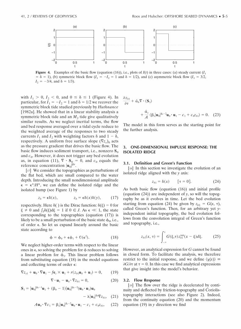
with I1 � 0, I2 � 0, and 0 � � � 1 (Figure 4). Inparticular, for I1 � I2 � 1 and � � 1/2 we recover thesymmetric block tide studied previously by Huthnance[1982a]. He showed that in a linear stability analysis asymmetric block tide and an M2 tide give qualitativelysimilar results. As we neglect inertial terms, the flowand bed response averaged over a tidal cycle reduce tothe weighted average of the responses to two steadycurrents I1 and I2 with weighting factors � and 1 �,respectively. A uniform free surface slope (�zs)0 actsas the pressure gradient that drives the basic flow. Thebasic flow induces sediment transport, i.e., nonzero S0and c0. However, it does not trigger any bed evolutionas, in equation (11), � � S0 � 0, and c0 equals thereference concentration �u0��s.

[17] We consider the topographies as perturbations ofthe flat bed, which are small compared to the waterdepth. Introducing the small nondimensional amplitude� � �*/H*, we can define the isolated ridge and theisolated hump (see Figure 1) by

zb � �� x�, zb � �� x�� y�, (17)

respectively. Here �( ) is the Dirac function: �(�)� 0 for� � 0 and �J�(�)d� � 1 if 0 � J. As � �� 1, the statecorresponding to the topographies (equation (17)) islikely to be a small perturbation of the basic state �0, i.e.,of order �. So let us expand linearly around the basicstate according to

� � �0 � ��1 � ��2�. (18)

We neglect higher-order terms with respect to the linearones in �, so solving the problem for � reduces to solvinga linear problem for �1. This linear problem followsfrom substituting equation (18) in the model equationsand collecting terms of order �:

�zs1 � u0 � �u1 � fez � u1 � r� zb1u0 � u1� � 0, (19)

� � u1 � u0 � �zb1 � 0, (20)

S1 � �u0��b1u1 � ��b � 1��u0��b3�u0 � u1�u0

� ��u0��b�zb1, (21)

Au0 � �c1 � �s�u0��s2u0 � u1 � c1 � c0zb1, (22)

� zb1

�� b� � �S1�

�s

A ��s�u0��s2u0 � u1 � c1 � c0zb1� � 0. (23)

The model in this form serves as the starting point forthe further analysis.

3. ONE-DIMENSIONAL IMPULSE RESPONSE: THEISOLATED RIDGE

3.1. Definition and Green’s Function[18] In this section we investigate the evolution of an

isolated ridge aligned with the y axis:

zb1 � �� x� �� 0�. (24)

As both basic flow (equation (16)) and initial profile(equation (24)) are independent of y, so will the topog-raphy be as it evolves in time. Let the bed evolutionstarting from equation (24) be given by zb1 � G(x, �),called Green�s function. Then, for an arbitrary yet y-independent initial topography, the bed evolution fol-lows from the convolution integral of Green�s functionand topography, i.e.,

zb1� x, ��

�

G��,�� zb1init� x � ��d�. (25)

However, an analytical expression for G cannot be foundin closed form. To facilitate the analysis, we thereforerestrict to the initial response, and we define ��(x)� �G/�� at � � 0. In this case we find analytical expressionsthat give insight into the model�s behavior.

3.2. Flow Response[19] The flow over the ridge is decelerated by conti-

nuity and deflected by friction-topography and Coriolis-topography interactions (see also Figure 2). Indeed,from the continuity equation (20) and the momentumequation (19) in y direction we find

Figure 4. Examples of the basic flow (equation (16)), i.e., plots of I(t) in three cases: (a) steady current (I1

� � � 1), (b) symmetric block flow (I1 � I2 � 1 and � � 1/2), and (c) asymmetric block flow (I1 � 3/2,I2 � 3/4, and � � 1/3).


u1 � I�� x�cos � (26)

v1 � I�rtan � � f �erx/�Icos � �H�Ix�. (27)

Here H( ) is the Heaviside function: Its value is unity fora positive argument and zero otherwise. The exponentialdecay of v1 downstream of the ridge is due to advectionand bottom friction, where the parameter �I�r1cos �determines the (e-folding) length of hydrodynamic influ-ence. In the limiting case � � !�/2, i.e., when the basicflow is aligned with the ridge, this length vanishes, andthe flow response reduces to u1 � (0, I�(x)). The mo-mentum equation in x direction can be used to find zs1,which we do not pursue here as it does not contribute tothe bed evolution.

3.3. Bed Evolution for Bed Load Transport[20] The perturbed bed load sediment flux S1 follows

from substituting the basic flow equation (16) along withthe perturbed velocities equations (26) and (27) into thelinearized transport formula (21). Next, the bed evolu-tion equation (23) with s� 0 (no suspended load) leadsto an evolution equation for arbitrary topographieszb1(x):

� zb1

�� "b1

� zb1

� x � "b2

�2zb1

� x2

� P�� "b0zb1 � ��

�

"b3�� zb1� x � ��d��. (28)

The nonnegative "b0, "b1, "b2, and "b3(x) are specifiedin Appendix A; P(�) will be specified and analyzedbelow. Because of the structure of "b3(x) we cannotsolve equation (28) in a convenient closed form, ex-cept when P(�) � 0.

[21] Neglecting the term in P(�) for the moment, theevolution equation (28) reduces to an advection-diffu-sion equation, leading to

Gb0� x,�� 1

�4�"b2�exp �� x � "b1��

2

4"b2�� . (29)

The migration term "b1 is nonzero only in the case ofasymmetric block flow not parallel to the ridge (� �!�/2). The diffusion of the ridge is directly associatedwith bed slope effects.

[22] The last term of equation (28) disrupts its advec-tive-diffusive character by introducing an additional re-distribution of sediment. The sign and magnitude ofP(�), given by

P�� sin ��r sin � � f cos ��, (30)

determines its character and importance, respectively.The quantity P(�) combines frictional and Coriolis ef-fects with the basic flow angle. We identify two parts.Evolution of the form itself is incorporated in the termin "b0, and the sign of P(�) determines whether this is

growth or decay. The form decays for 0 � tan � � ƒ/r(assuming ƒ � 0, which applies to the Northern Hemi-sphere); it is unaffected for � � 0 or � � arctan ƒ/r andgrows otherwise. Apparently, Coriolis effects disturb thesymmetry about � � 0. Form decay is strongest for�d �

12 arctan ƒ/r, while form growth is maximal for

�g �12 �arctan ƒ/r � ��. These properties of P(�) (depict-

ed in Figure 6a) again show up in a harmonic stabilityanalysis (see section 3.5). The amount of sand involvedin form growth (or decay) equals the surrounding ero-sion (or sedimentation), given by "b3(x). Possible asym-metry of the basic flow will cause "b3(x) to be asymmetricin x.

3.4. Bed Evolution for Suspended Load Transport[23] The perturbed concentration follows from substi-

tuting the basic flow equation (16) and the flow responseequations (26) and (27) into the equations for suspendedload transport equation (22) (Appendix A). Substitutingthe result and the perturbed velocities into equation (23)with b � 0 (no bed load transport) and taking the tidalaverage now results in an evolution equation for arbi-trary topographies zb1(x):

� zb1

�� "s0zb1 � �

�

�

�P�� "s31�� "s32��zb1� x � ��d�.

(31)

The nonnegative "s0 along with "s31(x) and "s32(x) arespecified in Appendix A. The form now always turnsout to be decaying as "s0 � 0. In contrast with the bedload case we find neither migration nor diffusionterms. Migratory effects are contained in the scour ordeposition function "s3(x), which is more complicatedthan in the bed load case. It involves terms exponen-tially decaying determined by friction and advection ofsediment, respectively. The amount of sand releasedby the form decay equals surrounding deposition,given by the convolution term in "s32.

[24] Finally, we can link the two transport mecha-nisms by noting that, for �s � �b 1, � � 0, and in thelimit A 2 0, the bed evolution equations (28) and (31)become identical. This means that, neglecting bed slopeeffects, bed load transport is a special case of suspendedload transport in the limit of zero advection.

3.5. Relation With Harmonic Stability Analysis:Sandbank Formation

[25] Here we will apply the general bed evolutionequations (28) and (31) to a wavy topography zb1 � a(�)cos kx. These are the eigenfunctions of the linearizedsystem, so we actually perform a harmonic stability anal-ysis [Huthnance, 1982; De Vriend, 1990; Hulscher et al.,1993]. Such an analysis, aimed at explaining the forma-tion of tidal sandbank patterns in, for example, the


North Sea (Figure 5) predicts exponential growth ordecay along with migration:

zb1� x, �� e#r�cos �kx � #it�, # � #r � i#i. (32)

The growth rate # is a complex number that dependsboth on the orientation � of the perturbation with re-spect to the tide and on its wavelength 2�/k, as well as onthe Coriolis parameter ƒ, friction coefficient r, sedimenttransport parameters �b, �, A, and �s, and on the char-acteristics of the basic flow u0. The real part determinesthe growth or decay, whereas the imaginary part isassociated with migration.

[26] For a symmetric block flow (Figure 4b) thegrowth rate is real and, in the case of bed load transport,given by

#b ��b � 1�P�� k2 cos2 �

r2 � k2 cos2 �� k2. (33)

This agrees with the results found by Huthnance [1982a]and Fluit and Hulscher [2002]. As equation (33) is basedon a symmetric block flow, we cannot compare thisresult with growth rates that correspond to alternative,more realistic types of basic flow [Huthnance, 1982a; De

Vriend, 1990; Hulscher et al., 1993] (section 2.3). Themode for which the real part of the growth rate isgreatest is called the fastest growing mode (FGM), de-picted in Figure 6b. Its characteristics kfgm $ 4 and �fgm$60% correspond to dimensional wavelengths between5 and 10 km and crests oriented counterclockwise at 30%with respect to the tidal current. This agrees with thecharacteristics of tidal sandbanks in the North Sea.

[27] For suspended load transport the expression forthe growth rate is more complicated:

#s ��sP�� k2 cos2 �

r2 � k2 cos2 � � 1 � Ar1 � A2k2 cos2 ��

�Ak2 cos2 � �1 � �s cos2 � �

1 � A2k2 cos2 �. (34)

We identify the following three properties of suspendedload transport (Figure 6). First, it promotes the growthof features with crests slightly more aligned with the flowthan in the case of bed load transport [De Vriend, 1990].Second, the absence of a diffusive bed slope mechanismcauses the lobes with positive growth rates to be un-bounded, which is physically unrealistic. However, like

Figure 5. Sandbank patterns in the southern part of the North Sea [Van de Meene, 1994].


bed load transport, suspended load is susceptible to bedslope effects [Parker, 1978; Talmon et al., 1995]. Indeed,analogously to the bed load case, adding a bed slopeterm to the bed evolution equation (5) would solve thisdeficiency. Third, for �s� �b 1 and � � 0, we find that

limA20

#s � #b, (35)

again showing that bed load transport acts as a limitingcase of suspended load transport.

[28] Now let us revisit the role of the parameter P(�)as given by equation (30). Besides controlling the dy-namics of the ridge, it also tells us how the growth rates(equations (33) and (34)) of wavy features depend ontheir orientation �. Indeed, in the � interval 0 � tan � �ƒ/r, where P(�) � 0, both the ridge and wavy perturba-tions decay. Moreover, positive growth rates only occurfor � values for which the ridge grows as well, i.e., whenP(�) � 0. The parameter P(�) obviously does not incor-porate the damping of short wavelengths by the slopeeffect on bed load transport, which causes negativegrowth rates for large k. Finally, the angle �g

�12 �arctan ƒ/r � �� of maximal ridge growth turns out

to predict the angle of the FGM well (Figures 6b and6c).

[29] Green�s function, introduced in section 3.1, canbe expressed in terms of the obtained growth ratesequations (33) and (34) according to

G� x, ��

�

e#�k��eikxdk � c.c. (36)

Here c.c. means complex conjugation. However, thisintegral is too complicated for further evaluation. Sec-tion 5 will show that the same holds for Green�s functionin two dimensions.

4. APPLICATION: EVOLUTION OF A DREDGEDCHANNEL

[30] We now apply the bed evolution equation (28)for bed load transport to investigate the morphodynamicevolution of a dredged trench. Let us consider a Gauss-ian cross section, i.e.,

zb1� x� �1

�tr�� exp �� x � xc�2

�tr2 � . (37)

The center of the trench is located at x � xc, while �tr isa characteristic half width: At x � xc ! �tr, the trenchdepth is reduced by a factor e1 $ 0.37 (Figure 7a).

[31] For a basic flow that mimics an asymmetric tide(Figure 4c), we identify two qualitatively different kindsof behavior. First, for P(�) � 0, the trench migrates, andon both sides of the trench, additional humps appear,thus forming some sort of pattern of adjacent banks.This type of behavior closely follows the inherent insta-bility of the flat seabed discussed in section 3.5 anddepicted in Figure 6. Second, for P(�) � 0, the trenchmigrates, and diffusion causes the shape to flatten outtoward a flat bed. As a special case we consider a basicflow perpendicular to the trench, i.e., � � 0 and P(�) �0. The approximation (29) of Green�s function is now

Figure 6. Stability properties of the flat seabed in polar (k,�) plots. (a) Properties of P(�), i.e., the regionP(�) � 0 (shaded) and P(�) � 0 (open), along with the angles of maximum decay �d and maximum growth �g

(solid lines). Contour plots of typical growth rates for (b) bed load and (c) suspended load. Shading and solidcontours indicate positive growth rates; open areas and dotted contours indicate negative growth rates.Parameter values are the following: r � 1, ƒ � 0.83, �b � 3, � � 0.0084, �s � 2, and A � 0.1. The fastestgrowing mode is denoted with a cross.


exact. It predicts trench migration and diffusion, withtrench center and width developing according to

xc�� "b1�, �tr�� 4"b2� � �tr,02 , (38)

with �tr,0 the half width at � � 0. The Gaussian shapeequation (37) is thus preserved (Figure 7).

[32] With a model similar to the one presented here,Van de Kreeke et al. [2002] studied the morphodynamicsof the access channel to the Port of Amsterdam. Theyreport observations over a period of 2.3 years showingmigration in the direction of net sediment transport at arate of 2–4 m yr1. At the same time the channel widensand becomes shallower. In the model, Van de Kreeke etal. [2002] assumed tidal flow with M0, M2, and M4 com-ponents, directed perpendicular to the trench, i.e., � � 0,and used parameter values much like the ones presentedin section 2. This leads to migration estimates between2.3 m yr1 for bed load transport and 4.5 m yr1 forsuspended load transport, along with initial rates of halfwidth increase of 0.4 m yr1 and 2.5 m yr1, respectively.Van de Kreeke et al. [2002] furthermore showed thathigher-order effects create asymmetry.

5. TWO-DIMENSIONAL IMPULSE RESPONSE: THEISOLATED HUMP

5.1. Definition and Green’s Function[33] In this section we investigate the evolution of an

isolated hump in the horizontal plane, given by

zb1 � �� x�� y� �� 0�. (39)

The basic flow is given by equation (16), but contrary tothe ridge case the orientation � has become meaningless.Hence we choose � � 0, i.e., u0 � (I, 0). The evolutionstarting from equation (39) now depends on both hori-zontal coordinates: zb1 � G(x, y, �). The evolution of anarbitrary initial topography follows from the convolutionintegral of topography and Green�s function, i.e.,

zb1� x, y, ��

� ��

�

G��, &, �� zb1init� x � �, y � &�d�d&.

(40)

As in the one-dimensional case, G(x, y, �) cannot befound in a convenient closed form (in Appendix B weexpress G in terms of the growth rates obtained insection 3.5). We therefore restrict to the initial bedevolution: ��(x,y)� �G/�� at � � 0. For simplicity, wefurthermore restrict to steady basic flow and symmetricbasic flow (Figures 4a and 4b).

5.2. Flow Response[34] It turns out that the problem can be conveniently

solved in terms of the vorticity and the stream function.We therefore rewrite the flow equations (19) and (20) as

I�'1

� x � r'1 � I� r� zb1

� y � f� zb1

� x � (41)

�2(1 � '1 � I� zb1

� x . (42)

Here the vorticity is given by '1 �v1/�x �u1/�y, andthe perturbed stream function (1 satisfies �(1/�y � u1 zb1u0 and �(1/�x � v1 ) zb1v0 (both are order � quan-tities).

[35] We can divide equation (41) into two differentproblems, each of which can be solved with the aid ofGreen�s representation theorem (Appendix B). To thatend, we write

'1 � 'r � 'f, (1 � (r � (f, (43)

effectively distinguishing a frictionally induced contribu-tion and one due to Coriolis effects. In the tidally aver-aged sense the expressions read (Appendix B)

Figure 7. (a) Gaussian trench shape (equation (37)) with � � 1 and xc� 0. Evolution of this trench with bedload transport, subject to the forcing of Figure 4c, directed (b) perpendicular to the ridge (� � 0) and (c) atan angle � � �g$63%. Plotted is zb1(�) at � � 0 (solid), � � 1/2 (dashed), and � � 1 (dash-dotted). Parametervalues are the following: � � 3 and � � 0.0084.


�(r� �ry4� �

0

�

er�� 1� x � ��2 � y2 �

1� x � ��2 � y2d�

(44)

�(f� �f

4� � log� x2 � y2� �r2�

0

�

er�*log�� x � ��2 � y2�

� log�� x � ��2 � y2�+d�� . (45)

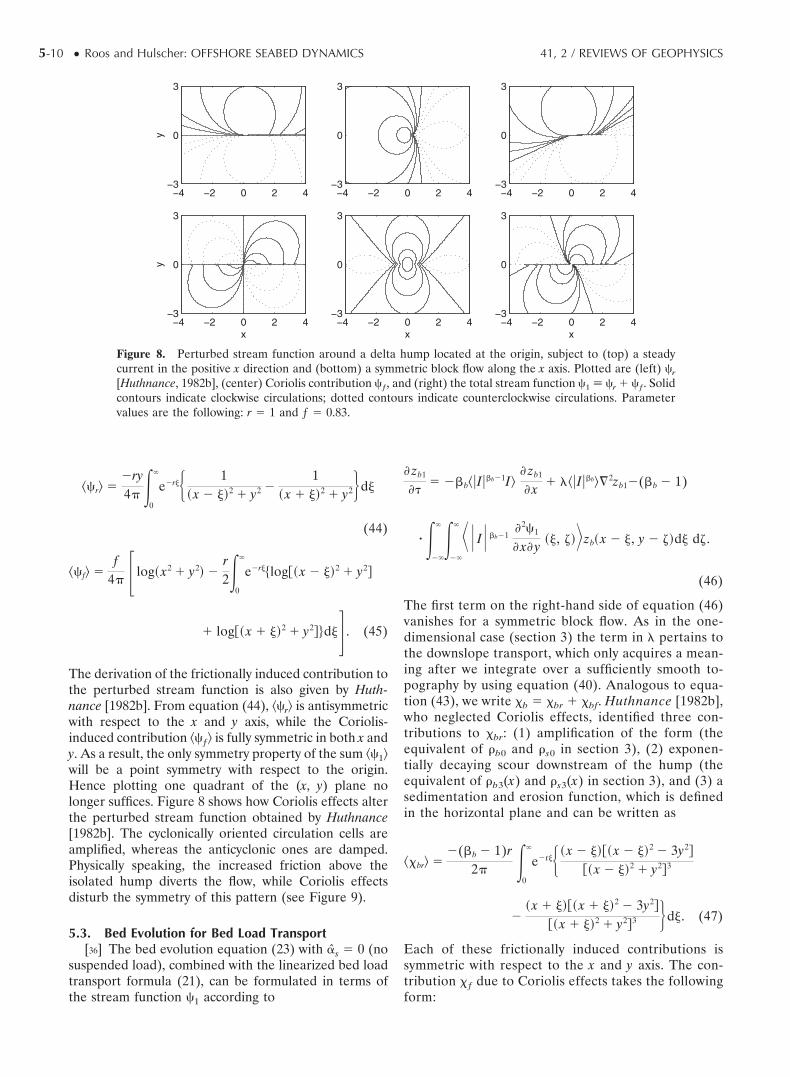
The derivation of the frictionally induced contribution tothe perturbed stream function is also given by Huth-nance [1982b]. From equation (44), �(r� is antisymmetricwith respect to the x and y axis, while the Coriolis-induced contribution �(ƒ� is fully symmetric in both x andy. As a result, the only symmetry property of the sum �(1�will be a point symmetry with respect to the origin.Hence plotting one quadrant of the (x, y) plane nolonger suffices. Figure 8 shows how Coriolis effects alterthe perturbed stream function obtained by Huthnance[1982b]. The cyclonically oriented circulation cells areamplified, whereas the anticyclonic ones are damped.Physically speaking, the increased friction above theisolated hump diverts the flow, while Coriolis effectsdisturb the symmetry of this pattern (see Figure 9).

5.3. Bed Evolution for Bed Load Transport[36] The bed evolution equation (23) with s � 0 (no

suspended load), combined with the linearized bed loadtransport formula (21), can be formulated in terms ofthe stream function (1 according to

� zb1

�� b��I��b1I�

� zb1

� x � ��I��b��2zb1(�b � 1)

� ��

� ��

� � I� �b1�2(1

� x� y ��, &��zb� x � �, y � &�d� d&.

(46)

The first term on the right-hand side of equation (46)vanishes for a symmetric block flow. As in the one-dimensional case (section 3) the term in � pertains tothe downslope transport, which only acquires a mean-ing after we integrate over a sufficiently smooth to-pography by using equation (40). Analogous to equa-tion (43), we write �b � �br ) �bf. Huthnance [1982b],who neglected Coriolis effects, identified three con-tributions to �br: (1) amplification of the form (theequivalent of "b0 and "s0 in section 3), (2) exponen-tially decaying scour downstream of the hump (theequivalent of "b3(x) and "s3(x) in section 3), and (3) asedimentation and erosion function, which is definedin the horizontal plane and can be written as

��br� �(�b � 1)r

2� �0

�

er�� x � �� x � ��2 � 3y2�

�� x � ��2 � y2�3

�� x � �� x � ��2 � 3y2�

�� x � ��2 � y2�3 d�. (47)

Each of these frictionally induced contributions issymmetric with respect to the x and y axis. The con-tribution �ƒ due to Coriolis effects takes the followingform:

Figure 8. Perturbed stream function around a delta hump located at the origin, subject to (top) a steadycurrent in the positive x direction and (bottom) a symmetric block flow along the x axis. Plotted are (left) (r

[Huthnance, 1982b], (center) Coriolis contribution (ƒ, and (right) the total stream function (1 (r) (ƒ. Solidcontours indicate clockwise circulations; dotted contours indicate counterclockwise circulations. Parametervalues are the following: r � 1 and ƒ � 0.83.


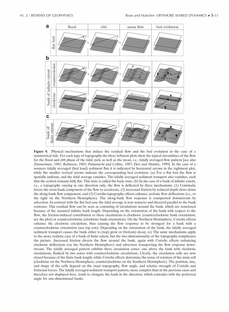
Figure 9. Physical mechanisms that induce the residual flow and the bed evolution in the case of asymmetrical tide. For each type of topography the three leftmost plots show the typical streamlines of the flowfor the flood and ebb phase of the tidal cycle as well as the mean, i.e., tidally averaged flow pattern [see alsoZimmerman, 1981; Robinson, 1983; Pattiaratchi and Collins, 1987; Dyer and Huntley, 1999]. In the case of anonzero tidally averaged (bed load) sediment flux it is indicated by horizontal arrows in the rightmost plot,while the smaller vertical arrows indicate the corresponding bed evolution. (a) For a flat bed the flow isspatially uniform, and the tidal average vanishes. The tidally averaged sediment transport also vanishes, suchthat the seabed remains fully flat. This state is called the basic state. (b) In the case of a bank of infinite extent,i.e., a topography varying in one direction only, the flow is deflected by three mechanisms: (1) Continuityforces the cross-bank component of the flow to accelerate, (2) increased friction by reduced depth slows downthe along-bank flow component, and (3) Coriolis-topography effects enhance cyclonic flow deflections (i.e., tothe right on the Northern Hemisphere). The along-bank flow response is transported downstream byadvection. In contrast with the flat bed case the tidal average is now nonzero and directed parallel to the bankcontours. This residual flow can be seen as consisting of circulations around the bank, which are nonclosedbecause of the assumed infinite bank length. Depending on the orientation of the bank with respect to theflow, the friction-induced contribution to these circulations is clockwise (counterclockwise bank orientation,see the plot) or counterclockwise (clockwise bank orientation). On the Northern Hemisphere, Coriolis effectsenhance the clockwise circulation, thus causing the flow response to be strongest for a bank with acounterclockwise orientation (see top row). Depending on the orientation of the bank, the tidally averagedsediment transport causes the bank either to (top) grow or (bottom) decay. (c) The same mechanisms applyto the more realistic case of a bank of finite extent, but the two-dimensionality of the topography complicatesthe picture. Increased friction diverts the flow around the bank, again with Coriolis effects enhancingclockwise deflections (on the Northern Hemisphere) and advection transporting the flow response down-stream. The tidally averaged pattern exhibits three circulation zones: one above the bank with clockwisecirculations, flanked by two zones with counterclockwise circulations. Clearly, the circulation cells are nowclosed because of the finite bank length, while Coriolis effects determine the sense of rotation of the main cell(clockwise on the Northern Hemisphere, counterclockwise on the Southern Hemisphere). The position, size,and shape of the cells depend on the exact topography, flow angle, and relative strength of Coriolis andfrictional forces. The tidally averaged sediment transport pattern, more complex than in the previous cases andtherefore not displayed here, tends to elongate the bank in the direction, which coincides with the preferredangle for one-dimensional banks.


��bf� ��b � 1� fxy

� � 1� x2 � y2�2

�r2�

0

�

er�y4 � � x2 � �2�� x2 � 2y2 � 3�2�

�� x � ��2 � y2�2�� x � ��2 � y2�2d� . (48)

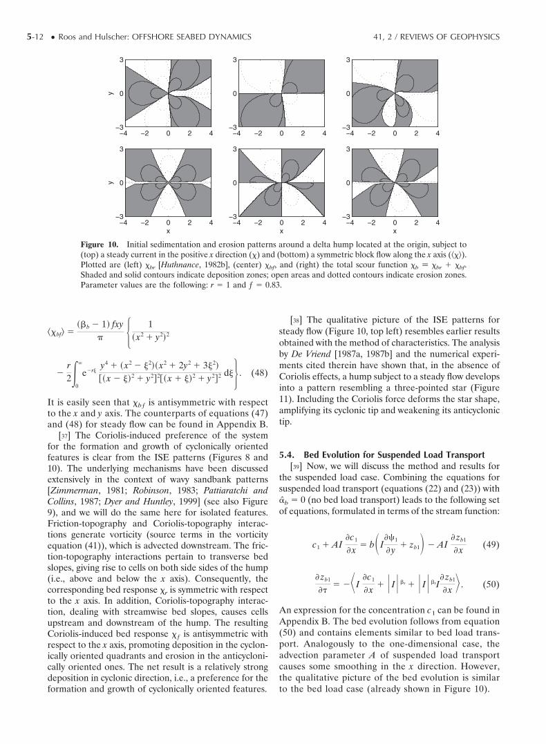
It is easily seen that �bƒ is antisymmetric with respectto the x and y axis. The counterparts of equations (47)and (48) for steady flow can be found in Appendix B.

[37] The Coriolis-induced preference of the systemfor the formation and growth of cyclonically orientedfeatures is clear from the ISE patterns (Figures 8 and10). The underlying mechanisms have been discussedextensively in the context of wavy sandbank patterns[Zimmerman, 1981; Robinson, 1983; Pattiaratchi andCollins, 1987; Dyer and Huntley, 1999] (see also Figure9), and we will do the same here for isolated features.Friction-topography and Coriolis-topography interac-tions generate vorticity (source terms in the vorticityequation (41)), which is advected downstream. The fric-tion-topography interactions pertain to transverse bedslopes, giving rise to cells on both side sides of the hump(i.e., above and below the x axis). Consequently, thecorresponding bed response �r is symmetric with respectto the x axis. In addition, Coriolis-topography interac-tion, dealing with streamwise bed slopes, causes cellsupstream and downstream of the hump. The resultingCoriolis-induced bed response �ƒ is antisymmetric withrespect to the x axis, promoting deposition in the cyclon-ically oriented quadrants and erosion in the anticycloni-cally oriented ones. The net result is a relatively strongdeposition in cyclonic direction, i.e., a preference for theformation and growth of cyclonically oriented features.

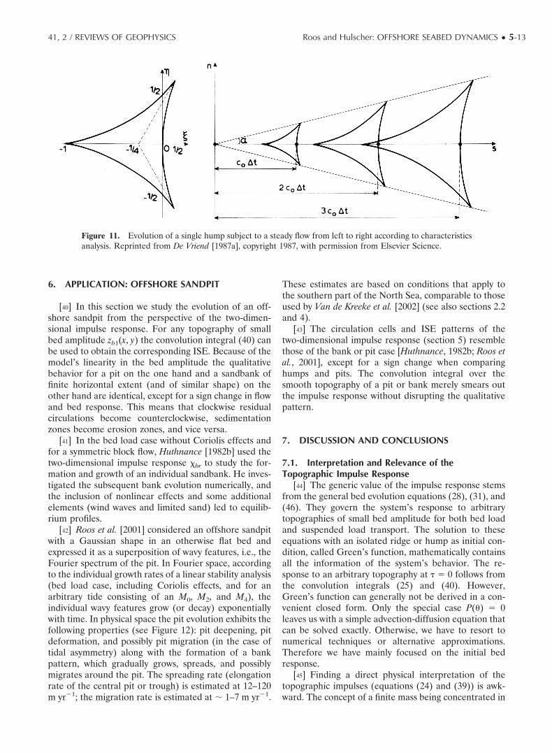
[38] The qualitative picture of the ISE patterns forsteady flow (Figure 10, top left) resembles earlier resultsobtained with the method of characteristics. The analysisby De Vriend [1987a, 1987b] and the numerical experi-ments cited therein have shown that, in the absence ofCoriolis effects, a hump subject to a steady flow developsinto a pattern resembling a three-pointed star (Figure11). Including the Coriolis force deforms the star shape,amplifying its cyclonic tip and weakening its anticyclonictip.

5.4. Bed Evolution for Suspended Load Transport[39] Now, we will discuss the method and results for

the suspended load case. Combining the equations forsuspended load transport (equations (22) and (23)) withb � 0 (no bed load transport) leads to the following setof equations, formulated in terms of the stream function:

c1 � AI�c1

� x � b� I�(1

� y � zb1� � AI� zb1

� x (49)

� zb1

�� I

�c1

� x � � I� �s � � I� �sI� zb1

� x� . (50)

An expression for the concentration c1 can be found inAppendix B. The bed evolution follows from equation(50) and contains elements similar to bed load trans-port. Analogously to the one-dimensional case, theadvection parameter A of suspended load transportcauses some smoothing in the x direction. However,the qualitative picture of the bed evolution is similarto the bed load case (already shown in Figure 10).

Figure 10. Initial sedimentation and erosion patterns around a delta hump located at the origin, subject to(top) a steady current in the positive x direction (�) and (bottom) a symmetric block flow along the x axis (��).Plotted are (left) �br [Huthnance, 1982b], (center) �bf, and (right) the total scour function �b �br ) �bf.Shaded and solid contours indicate deposition zones; open areas and dotted contours indicate erosion zones.Parameter values are the following: r � 1 and ƒ � 0.83.


6. APPLICATION: OFFSHORE SANDPIT

[40] In this section we study the evolution of an off-shore sandpit from the perspective of the two-dimen-sional impulse response. For any topography of smallbed amplitude zb1(x, y) the convolution integral (40) canbe used to obtain the corresponding ISE. Because of themodel�s linearity in the bed amplitude the qualitativebehavior for a pit on the one hand and a sandbank offinite horizontal extent (and of similar shape) on theother hand are identical, except for a sign change in flowand bed response. This means that clockwise residualcirculations become counterclockwise, sedimentationzones become erosion zones, and vice versa.

[41] In the bed load case without Coriolis effects andfor a symmetric block flow, Huthnance [1982b] used thetwo-dimensional impulse response �br to study the for-mation and growth of an individual sandbank. He inves-tigated the subsequent bank evolution numerically, andthe inclusion of nonlinear effects and some additionalelements (wind waves and limited sand) led to equilib-rium profiles.

[42] Roos et al. [2001] considered an offshore sandpitwith a Gaussian shape in an otherwise flat bed andexpressed it as a superposition of wavy features, i.e., theFourier spectrum of the pit. In Fourier space, accordingto the individual growth rates of a linear stability analysis(bed load case, including Coriolis effects, and for anarbitrary tide consisting of an M0, M2, and M4), theindividual wavy features grow (or decay) exponentiallywith time. In physical space the pit evolution exhibits thefollowing properties (see Figure 12): pit deepening, pitdeformation, and possibly pit migration (in the case oftidal asymmetry) along with the formation of a bankpattern, which gradually grows, spreads, and possiblymigrates around the pit. The spreading rate (elongationrate of the central pit or trough) is estimated at 12–120m yr1; the migration rate is estimated at � 1–7 m yr1.

These estimates are based on conditions that apply tothe southern part of the North Sea, comparable to thoseused by Van de Kreeke et al. [2002] (see also sections 2.2and 4).

[43] The circulation cells and ISE patterns of thetwo-dimensional impulse response (section 5) resemblethose of the bank or pit case [Huthnance, 1982b; Roos etal., 2001], except for a sign change when comparinghumps and pits. The convolution integral over thesmooth topography of a pit or bank merely smears outthe impulse response without disrupting the qualitativepattern.

7. DISCUSSION AND CONCLUSIONS

7.1. Interpretation and Relevance of theTopographic Impulse Response

[44] The generic value of the impulse response stemsfrom the general bed evolution equations (28), (31), and(46). They govern the system�s response to arbitrarytopographies of small bed amplitude for both bed loadand suspended load transport. The solution to theseequations with an isolated ridge or hump as initial con-dition, called Green�s function, mathematically containsall the information of the system�s behavior. The re-sponse to an arbitrary topography at � � 0 follows fromthe convolution integrals (25) and (40). However,Green�s function can generally not be derived in a con-venient closed form. Only the special case P(�) � 0leaves us with a simple advection-diffusion equation thatcan be solved exactly. Otherwise, we have to resort tonumerical techniques or alternative approximations.Therefore we have mainly focused on the initial bedresponse.

[45] Finding a direct physical interpretation of thetopographic impulses (equations (24) and (39)) is awk-ward. The concept of a finite mass being concentrated in

Figure 11. Evolution of a single hump subject to a steady flow from left to right according to characteristicsanalysis. Reprinted from De Vriend [1987a], copyright 1987, with permission from Elsevier Science.


a single point may even tempt one into confusing geo-metrical perceptions. Therefore one should bear in mindthat the primary role of the impulse response is that ofa tool to be used in the integrated sense according toequations (25) and (40). However, we have seen cases inwhich most of the qualitative features of the impulseresponse are retained throughout this integration pro-cedure (e.g., when going from the isolated ridge to thestability analysis in section 3.5 or from the isolated humpto an offshore sandpit in section 6). Apparently, theanalytical expression of the impulse response alreadyprovides fundamental information on the system�s be-havior.

[46] Finally, note that the isolated ridge can be seen asan infinite sequence of isolated humps. Hence the one-dimensional impulse can be derived from the two-di-mensional one by choosing zb1 � �(x) in equation (40)(see also the leftmost arrow in Figure 1). Nevertheless,we chose to investigate the isolated ridge separately, as itgives more direct insight into the evolution of y-indepen-dent topographies zb1(x).

[47] Despite their limitations, analytical solutions forthe flow and bed evolution can be useful for the verifi-cation of numerical models. The isolated hump can beimplemented easily and, more importantly, does notinterfere with the boundaries of a finite numerical do-

main, as these can be chosen sufficiently far away. Thewavy topographies studied in a stability analysis alsopermit analytical solutions, but the infinite spatial extentof such patterns is likely to cause complications at theboundaries of the numerical domain.

[48] In order to explain the fundamental mechanismsthe examples presented here deal mainly with idealizedgeometries. However, the results also apply to arbitrarytopographies (of small amplitude), and the hydrody-namic and morphodynamic response to such a topogra-phy can be numerically obtained with the presentmethod. However, alternative numerical methods maybe more appropriate for this purpose.

7.2. Model Assumptions and Limitations[49] By treating the flow in a depth-averaged way, we

neglect the vertical flow structure. As such, we are un-able to describe the mechanisms related to sand waveformation and dynamics [Hulscher, 1996] as these orig-inate from variations in the vertical flow structure. Thislimits the applicability of the system to the horizontallength scales of sandbanks (on the order of thousands ofmeters) rather than those of sand waves (hundreds ofmeters).

[50] The model is linear in the bed amplitude. Con-sequently, the topographies under consideration should

Figure 12. Evolution of a Gaussian sandpit subject to an asymmetric tide in the x direction (highestvelocities from left to right) in the case of bed load transport: (top) bed evolution and (bottom) residualcurrents and from left to right the evaluation times � � 0, � � 2, � � 4, and � � 6. Troughs are black, crestsare white, and the undisturbed seabed is shaded. Solid streamlines correspond to counterclockwise rotation,whereas dashed ones correspond to clockwise rotation. The plotted region covers a dimensional area of about70 � 70 km2. Parameter values are the following: r � 0.6, ƒ � 0.83, �b � 3, and � � 0.0084 [after Roos et al.,2001].


have small bed amplitudes, compared to the waterdepth. Nonlinear effects should be taken into accountwhen bed amplitudes are no longer small with respect tothe water depth.

[51] The analysis follows a stability concept in whichthe rigid lid approximation, i.e., neglecting the contribu-tion of z*s to the water depth in the model equations, iscrucial. Without this assumption an analytical expressionfor a spatially uniform basic state cannot be found. AsFroude numbers are small (Fr $ 0.06), the rigid lidapproximation is indeed appropriate. In order to facili-tate the analysis we furthermore restrict the basic stateto a block flow, and we omit inertial terms in momentumequations.

[52] Furthermore, we neglect wind wave effects,which limits the model�s applicability to tide-dominated,thus offshore, conditions. For a detailed description ofwave effects in a harmonic stability analysis we refer toDe Vriend [1990].

7.3. Conclusion[53] The present analysis shows that the concept of

topographic impulse response provides a link between

various research subjects within the class of offshoremorphodynamic models. A crucial property herein is theinherent instability of the flat seabed, i.e., the tendencyof topographic undulations on a flat bed to develop intoa pattern of banks, with a preference for cyclonicallyoriented features. Investigations into the seabed behav-ior on the corresponding length scales (kilometers) andtimescales (decades to centuries) should include theunderlying physical mechanisms, such as Coriolis andfrictional effects. Furthermore, in predicting the mor-phodynamic fate of large-scale human intervention, suchas navigation dredging and sand extraction, the stabilityproperties should be kept in mind. For instance, model-ing a sandpit in either a flat seabed, as carried out in thepresent study, or in some finite-amplitude equilibriumtopography may lead to qualitatively different behavior.To what extent the results will differ strongly depends onthe stability properties of such an equilibrium profile aswell as on the ratio of pit depth to sandbank height.Furthermore, the model shows that bed load transportcan be seen as a limiting case of suspended load trans-port.

Figure 13. Part of the North Sea bed (area of 10 km2) [after Knaapen et al., 2001a, Figure 4]. Here thesandbank mode is hardly visible as the smaller-scale sand waves are quite dominant. Figure 13 shows a partof the offshore seabed, large enough to show the topographic variations due to sandbanks and sand waves. Thelatter mode is not included in two-dimensionally horizontal (2DH) models. The topography on the scalesrelevant for 2DH models itself is hardly visible, which is not so surprising as nearly one wavelength fits in thisfigure. Next, the 2DH modeling approach as discussed in this paper predicts a regular pattern of similarlyshaped banks (see, e.g., Figure 12). These points illustrate the question in comparing large-scale topographicdata with 2DH morphodynamic models: When may we be confident that the data are in agreement with the2DH morphodynamic model or vice versa? Natural large-scale features as sandbanks always show largeirregularities, which may have a stochastic nature or may be due to large-scale nonlinear dynamics. Anotherproblem in performing such comparisons is that the current data sets are not large enough (space), longenough (time), and accurately spaced enough to allow direct comparisons and perform statistics. See colorversion of this figure at back of this issue.


7.4. Outlook[54] Further steps toward a better understanding of

large-scale offshore morphodynamics are briefly dis-cussed now. From a modeling point of view a next stepis to investigate the morphodynamic model equations(1)–(5) in the nonlinear regime as well. Possible equilib-rium topographies then serve as an alternative startingpoint to model the morphodynamic impact of humanintervention.

[55] Accurate data sets, extensive in both space andtime, are currently becoming available. In combiningwith (non)linear models they can be used for validationof the model or processes within the model. Knaapen etal. [2001b] showed this for alternate bars, i.e., a large-scale pattern in the fluvial environment. Until now,validation was mostly based on comparing observationswith modeled characteristics such as wavelength, etc. Werecommend also including comparisons in Fourierspace; see, for example, Knaapen et al. [2001a] or wave-let methods (Figures 13 and 14). Combining data withnonlinear models may result in locally tuned morphody-namic models as shown by Knaapen and Hulscher [2002]for the case of the smaller-scale sandwaves. Data assim-

ilation is not likely to enable a similar study of sandbankdynamics as was carried out for alternate bars [Knaapenand Hulscher, 2003], since the data sets are quite limitedcompared with the morphodynamic timescale. To ex-plore these aspects, a data set comprising more than 100years of North Sea sandbank observations is currentlyunder investigation.

[56] Sandbanks show irregularities that, so far, deter-ministic depth-averaged modeling has not reflected. Theunderlying reasons for observed spatial or temporal vari-ations of amplitudes and wavelengths are not under-stood, neither from a theoretical nor from an observa-tional point of view. This aspect could be investigated bya cellular automata model, as was done for beach cuspsby Coco et al. [2001], or by reflecting the stochasticnature of specific parameters (e.g., individual storms,meteorological tide, and sediment properties). A secondoption is that these deviations from regularity are due tolonger-term and/or larger-scale periodicity in hydrody-namic forcing (e.g., variation of the astronomical tideand seasonal or climatological variations). The latteridea is based on the analogy of this morphodynamicsystem with the coupled atmosphere-ocean system. The

Figure 14. The Fourier transform of the region shown in Figure 13. Herein sandbanks are visible as arelative concentration of energy in the small wave numbers, nearly parallel the principal direction of tidalmotion. Besides comparing data with models in the physical domain, one may shift to Fourier space. Figure14 shows the Fourier transform of Figure 13. Now we observe quite clearly a concentration of energy in thesmaller wave numbers, corresponding to the length scale relevant for 2DH models. In this approach the mainidea is to find the (mean and deviation) wave number and orientation, which can be converted directly forcomparison to the wave vector predicted by the 2DH model; see for example, Figure 6. Besides this theprocedure can also be used to filter the smaller-scale features. A more sophisticated way to perform this isusing wavelets. See color version of this figure at back of this issue.


separated scales of dynamics have been shown to resultin intermittency, periods of regular behavior separatedby periods of chaos [Van Veen et al., 2001; L. Van Veen,Baroclinic flow and the Lorenz-84 model, preprint 1210,Department of Mathematics, University of Utrecht,Utrecht, Netherlands, 2002]. The behavior within these“regular” periods was not necessarily the same. Deter-mining the origin of the irregularities will spawn a betterunderstanding and subsequently a better predictabilityof the effects of human intervention.

[57] In estuaries and rivers, biology and morphody-namics interact to a large degree. Organisms influencesediment characteristics, and hence seabed morphology,directly and indirectly (e.g., trawler nets ploughing theseabed in chase of bed-resident fish), whereas depth andsediment composition are important habitat parametersfor these organisms. It is unknown whether and to whatextent biogeomorphology is an issue in the offshoreenvironment. If so, these interactions have to be in-cluded for correct modeling of large-scale morphody-namics. Furthermore, the influences of graded sedimenton the morphodynamics of offshore features (see, e.g.,Walgreen [2003] for the case of shoreface-connectedridges or Blom [2003] for the case of dunes in rivers) areworth being investigated.

[58] Komarova and Newell [2000] have shown thatnonlinear interaction between smaller-scale rhythmicfeatures, initiated by vertical flow circulations, mightlead to topographic features on the spatial scales of tidalsandbanks. As their two-dimensionally vertical modelwas limited to one horizontal orientation, the character-istic sandbank orientation could not be verified. There-fore, at the moment, it is unknown to what extent thismechanism interferes with the depth-averaged morpho-dynamic modeling as reviewed in this paper. We recom-mend investigating its impact and, if relevant, the possi-bilities of modeling this mechanism in a simpler way sothat it can be incorporated or simulated in two-dimen-sionally horizontal models.

[59] Gas mining has been shown to be able to causethe formation of tidal sandbanks [Fluit and Hulscher,2002; Roos and Hulscher, 2002]. This type of humanintervention was modeled as a dish-like depression, sub-siding at a constant rate. Other forms of offshore humanintervention, large enough to have an impact on sand-bank scales, are windmill farms and artificial islands.However, it is yet unclear how the morphodynamic im-pact of such large-scale intervention can be modeled.

APPENDIX A: DERIVATION OF THE ONE-DIMENSIONAL IMPULSE RESPONSE

[60] The quantities "b0, "b1, "b2, and "b3(x) in the bedevolution equation (28) for bed load transport are givenby

"b0 � ��b � 1��I��b�, (A1)

"b1 � cos ��1 � ��b � 1�cos2 ��I��b1I�, (A2)

"b2 � ��I��b�, (A3)

"b3 ��b � 1�r

cos � ��I��b1erx/�Icos � �H�Ix��. (A4)

The perturbed concentration is given by

c1 � �I��s11 � �s cos2 �

A cos � ex/�IA cos � �H�Ix�

� �I��s�sP��

�1 � Ar� cos � �ex/�IA cos � � � erx/�I cos � ��H�Ix�,

(A5)

with P(�) from equation (30). The quantities "s0, "s31(x),and "s32(x) in the bed evolution equation (31) for sus-pended load transport are given by

"s0 �1 � �s cos2 �

A ��I��s�, (A6)

"s31� x�

��s��I��sex/�IA cos � �H�Ix�� Ar��I��serx/�I cos � �H�Ix��

A�1 � Ar� cos � ,

(A7)

"s32� x� �1 � �s cos2 �

A2 cos � ��I��s1ex/�IA cos � �H�Ix��. (A8)

APPENDIX B: DERIVATION OF THE TWO-DIMENSIONAL IMPULSE RESPONSE

[61] Green�s function in two dimensions, expressed interms of the growth rates obtained in section 3.5, readsas follows:

G� x, y, �� / 2

�/ 2 ��

�

e#�k,� ��eik� x cos �)y sin � �k dk d� � c.c.

(B1)

Green�s representation theorem in two dimensions isgiven by [Gradshteyn and Ryzhik, 2000]

G�x� �1

2��2G��log �x � ��d�, (B2)

with � � (�,&). In order to find the frictionally inducedstream function (r in equation (43) we follow Huthnance[1982b], who employed the transformation 'r � �,/�yand (r � �G/�y. Next, G ensues from Green�s represen-tation theorem (60), which, in turn, leads to an expres-sion for (r:

, � IreIrxH�Ix�� y�, (B3)


G �� I4� *log � x2 � y2� � r

��

�

H�I��eIr�log �� x � ��2 � y2�d�+, (B4)

(r ��G� y �

� Iy2� � 1

x2 � y2 � r��

� H�I��eIr�

� x � ��2 � y2 d�� .

(B5)

The Coriolis-induced contribution can be found by usingthe transformation 'ƒ � �,/�x. Then, the derivation isgiven by

, � � IfeIrxH�Ix�� y�, (B6)

'f ��,

� x � feIrx�rH�Ix� � �� x�� y�, (B7)

(f �f

4� �log� x2 � y2� � r��

�

H�I��eIr�log�� x � ��2

� y2�d��. (B8)

The frictionally induced and Coriolis-induced ISE pat-terns for steady flow and bed load transport are given by

�br �(�b � 1)Ix

� � x2 � 3y2

� x2 � y2�3

� r��

�

H�I��eIr�� x � ��2 � 3y2

�� x � ��2 � y2�3d� , (B9)

�bf ��b � 1� fxy

� � 1� x2 � y2�2

� r��

� H�I��eIr�

�� x � ��2 � y2�2d� , (B10)

respectively. We write the perturbed concentration asthe sum of two terms c1 � c� ) cA, for which we find

c� ��s

A ��

�

e�/�IA��(1

� y � x � �, y�d�

� H�Ix�ex/�IA�� y�� , (B11)

�c�� s

2 A ��

�

e�/A��(1

� y � x � �, y��I�1

��(1

� y � x � �, y��I�1

�d� � e�x�/A�� y� . (B12)

The derivation of cA requires an additional transforma-tion cA � �Q/�x, leading to

Q � AIeIx/AH�Ix�� y�, (B13)

cA ��Q� x � �H�Ix�eIx/A � A�� x�� y�, (B14)

�cA� �12 e�x�/A�� y� � A�� x�� y�. (B15)

[62] ACKNOWLEDGMENTS. We thank Aart van Harten,Huib de Vriend, and an anonymous reviewer for their com-ments and Michiel Knaapen for providing Figures 13 and 14.This research was carried out within the EU-project HUMOR,contract number EVK3-CT-2000-00037.

[63] Thomas Torgersen is the Editor responsible for thispaper. He thanks four anonymous technical reviewers and onecross-disciplinary reviewer.

REFERENCESBlom, A., A vertical sorting model for rivers with non-uniform

sediment and dunes, Ph.D. thesis, Univ. of Twente, 287 pp.,Enschede, Netherlands, 2003.

Blondeaux, P., Mechanics of coastal forms, Annu. Rev. FluidMech., 33, 339–370, 2001.

Calvete, D., H. E. De Swart, and A. Falques, Effect of depth-dependent wave stirring on the final amplitude of shore-face-connected sand ridges, Cont. Shelf Res., 22(18–19),2763–2776, 2002.

Coco, G., D. A. Huntley, and T. J. O�Hare, Regularity andrandomness in the formation of beach cusps, Mar. Geol.,178, 1–9, 2001.

De Vriend, H. J., 2DH mathematical modelling of morpholog-ical evolutions in shallow water, Coastal Eng., 11, 1–27,1987a.

De Vriend, H. J., Analysis of horizontally two-dimensionalmorphological evolutions in shallow water, J. Geophys. Res.,92, 3877–3893, 1987b.

De Vriend, H. J., Inherent stability of depth-integrated math-ematical models of coastal morphology, paper presented atIAHR Symposium, Int. Assoc. for Hydraul. Res., Copen-hagen, 1988.

De Vriend, H. J., Morphological processes in shallow tidalseas, in Residual Currents and Long Term Transport, editedby R. T. Cheng, Coastal Estuarine Stud., vol. 38, pp. 276–301, Springer-Verlag, New York, 1990.

Dyer, K. R., Coastal and Estuarine Sediment Dynamics, JohnWiley, New York, 1986.

Dyer, K. R., and D. A. Huntley, The origin, classification andmodelling of sand banks and ridges, Cont. Shelf Res., 19,1285–1330, 1999.

Fluit, C. C. J. M., and S. J. M. H. Hulscher, Morphologicalresponse to a North Sea bed depression induced by gasmining, J. Geophys. Res., 107(C3), 3022, doi:10.1029/2001JC000851, 2002.

Gradshteyn, I. S., and I. M. Ryzhik, Table of Integrals, Seriesand Products, 6th ed., edited by A., Jeffrey and D. Zwill-


inger, translated from Russian, Academic, San Diego, Cal-if., 2000.

Hulscher, S. J. M. H., Tidal-induced large-scale regular bedform patterns in a three-dimensional shallow water model,J. Geophys. Res., 101(C9), 20,727–20,744, 1996.

Hulscher, S. J. M. H., and G. M. Van den Brink, Comparisonbetween predicted and observed sand waves and sand banksin the North Sea, J. Geophys. Res., 106(C5), 9327–9338,2001.

Hulscher, S. J. M. H., H. E. De Swart, and H. J. De Vriend,The generation of offshore tidal sand banks and sandwaves, Cont. Shelf Res., 13, 1183–1204, 1993.

Huthnance, J. M., On one mechanism forming linear sandbanks, Estuarine Coastal Shelf Sci., 14, 74–99, 1982a.

Huthnance, J. M., On the formation of sand banks of finiteextent, Estuarine Coastal Shelf Sci., 15, 277–299, 1982b.

Knaapen, M. A. F., and S. J. M. H. Hulscher, Regeneration ofsand waves after dredging, Coastal Eng., 46, 277–289, 2002.

Knaapen, M. A. F., and S. J. M. H. Hulscher, Use of a geneticalgorithm to improve predictions of alternate bar dynamics,Water Resour. Res., 39, doi:10.1029/2002WR001793, inpress, 2003.

Knaapen, M. A. F., S. J. M. H. Hulscher, and H. J. De Vriend,A new type of sea bed waves, Geophys. Res. Lett., 28(7),1323–1326, 2001a.

Knaapen, M. A. F., S. J. M. H. Hulscher, H. J. De Vriend, andA. Van Harten, Height and wavelength of alternate bars inrivers: Modelling vs. laboratory experiments, J. Hydraul.Res., 39(2), 147–153, 2001b.

Komarova, N. L., and A. C. Newell, Nonlinear dynamics ofsand banks and sand waves, J. Fluid Mech., 415, 285–312,2000.

Loder, J. W., Topographic rectification of tidal currents on thesides of Georges Bank, J. Phys. Oceanogr., 10, 1399–1416,1980.

Parker, G., Self-formed straight rivers with equilibrium banksand mobile bed. Part 1. The sand-silt river, J. Fluid Mech.,89, 109–125, 1978.

Pattiaratchi, C., and M. Collins, Mechanisms for linear sand-bank formation and maintenance in relation to dynamicaloceanographic observations, Prog. Oceanogr., 19, 117–176,1987.

Robinson, I. S., Tidally induced residual flows, in Physical

Oceanography of Coastal and Shelf Seas, edited by B. Johns,pp. 321–356, Elsevier Sci., New York, 1983.

Roos, P. C., and S. J. M. H. Hulscher, Formation of offshoretidal sand banks triggered by a gasmined bed subsidence,Cont. Shelf Res., 22, 2807–2818, 2002.

Roos, P. C., S. J. M. H. Hulscher, B. G. T. M. Peters, and A. A.Nemeth, A simple morphodynamic model for sand banksand large-scale sand pits subject to asymmetrical tides,paper presented at Second IAHR Symposium on River,Coastal and Estuarine Morphodynamics, Int. Assoc. forHydraul. Res., Hokkaido, Japan, 2001.

Talmon, A. M., M. C. L. M. Van Mierlo, and N. Struiksma,Laboratory measurements of the direction of sedimenttransport on transverse alluvial slopes, J. Hydraul. Res., 33,495–517, 1995.

Trowbridge, J. H., A mechanism for the formation and main-tenance of shore-oblique sand ridges on storm-dominatedshelves, J. Geophys. Res., 100(C8), 16,071–16,086, 1995.

Van de Kreeke, J., S. E. Hoogewoning, and M. Verlaan,Morphodynamics of a trench in the presence of tidal cur-rents, Cont. Shelf Res., 22, 1811–1820, 2001.

Van de Meene, J. W. H., The Shoreface Connected RidgesAlong the Central Dutch Coast, Neth. Geogr. Stud., vol. 174,Kon. Ned. Aardnjksk. Genoot./Fac. Ruimtelijke Wetensch.Univ. Utrecht, Utrecht, Netherlands, 1994.

Van Rijn, L. C., Handbook of Sediment Transport by Currentsand Waves, Delft Hydraul., Delft, Netherlands, 1993.

Van Veen, L., T. Opsteegh, and F. Verhulst, Active andpassive ocean regimes in a low-order climate model, Tellus,Ser. A, 53, 616–628, 2001.

Walgreen, M., H. E. De Swart, and D. Calvete, Effect of grainsize sorting on the formation of shoreface-connected sandridges, J. Geophys. Res., 108(C3), 3063, doi:10.1029/2002JC001435, 2003.

Zimmerman, J. T. F., Dynamics, diffusion and geomorphologi-cal significance of tidal residual eddies, Nature, 290, 549–555, 1981.

S. J. M. H. Hulscher and P. C. Roos, Water Engineering andManagement, University of Twente, P.O. Box 217,7500 AEEnschede, Netherlands. ([email protected]; [email protected])


Figure 13. Part of the North Sea bed (area of 10 km2) [after Knaapen et al., 2001a, Figure 4]. Here thesandbank mode is hardly visible as the smaller-scale sand waves are quite dominant. Figure 13 shows a partof the offshore seabed, large enough to show the topographic variations due to sandbanks and sand waves. Thelatter mode is not included in two-dimensionally horizontal (2DH) models. The topography on the scalesrelevant for 2DH models itself is hardly visible, which is not so surprising as nearly one wavelength fits in thisfigure. Next, the 2DH modeling approach as discussed in this paper predicts a regular pattern of similarlyshaped banks (see, e.g., Figure 12). These points illustrate the question in comparing large-scale topographicdata with 2DH morphodynamic models: When may we be confident that the data are in agreement with the2DH morphodynamic model or vice versa? Natural large-scale features as sandbanks always show largeirregularities, which may have a stochastic nature or may be due to large-scale nonlinear dynamics. Anotherproblem in performing such comparisons is that the current data sets are not large enough (space), longenough (time), and accurately spaced enough to allow direct comparisons and perform statistics.

Roos and Hulscher: OFFSHORE SEABED DYNAMICS 41, 2 / REVIEWS OF GEOPHYSICS

● 5 - 15 ●

Figure 14. The Fourier transform of the region shown in Figure 13. Herein sandbanks are visible as arelative concentration of energy in the small wave numbers, nearly parallel the principal direction of tidalmotion. Besides comparing data with models in the physical domain, one may shift to Fourier space. Figure14 shows the Fourier transform of Figure 13. Now we observe quite clearly a concentration of energy in thesmaller wave numbers, corresponding to the length scale relevant for 2DH models. In this approach the mainidea is to find the (mean and deviation) wave number and orientation, which can be converted directly forcomparison to the wave vector predicted by the 2DH model; see for example, Figure 6. Besides this theprocedure can also be used to filter the smaller-scale features. A more sophisticated way to perform this isusing wavelets.

41, 2 / REVIEWS OF GEOPHYSICS Roos and Hulscher: OFFSHORE SEABED DYNAMICS

● 5 - 16 ●

Large-scale seabed dynamics in offshore morphology: Modeling human intervention

Documents