Large Scale Manifold Transduction Michael Karlen Jason Weston Ayse Erkan Ronan Collobert ICML 2008.

Large Scale Manifold Transduction

Michael Karlen Jason WestonAyse Erkan Ronan Collobert

ICML 2008

Index

• Introduction

• Problem Statement

• Existing Approaches– Transduction :- TSVM – Manifold – Regularization :- LapSVM

• Proposed Work

• Experiments

Introduction

• Objective :- Discriminative classification using unlabeled data.

• Popular methods– Maximizing margin on unlabeled data as in

TSVM so that decision rule lies in low density. – Learning cluster or manifold structure from

unlabeled data as in cluster kernels, label propagation and Laplacian SVMs.

Problem Statement

• Inability of the existing techniques to scale to very large datasets, also online data.

Existing Techniques

• TSVM– Problem Formulation :-

- Non-Convex Problem

2

, 1 1

min ( ), * ( ( *))L U

i i iw b i i

w l f x y l f x

* ( *) max(0,1 | ( *) |)

( ) max(0,1 ( *))

where l f x f x

l f x yf x

• Problems with TSVM :-– When dimension >> L ( no of Labeled examples), all

unlabeled points may be classified to one class while still classifying the labeled data correctly, giving lower objective value.

• Solution :- – Introduce a balancing constraint in the objective

function.

Implementations to Solve TSVM

• S3VM :-– Mixed Integer Programming. Intractable for large data

sets.

• SVMLight-TSVM :-– Initially fixes labels of unlabeled examples and then

iteratively switches those labels to improve TSVM objective function, solving convex objective function at each step.

– Introduces balancing constraint. – Handles few thousand examples.

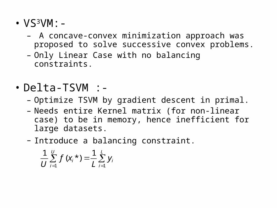
• VS3VM:-– A concave-convex minimization approach was

proposed to solve successive convex problems.– Only Linear Case with no balancing constraints.

• Delta-TSVM :-– Optimize TSVM by gradient descent in primal.– Needs entire Kernel matrix (for non-linear case) to be

in memory, hence inefficient for large datasets.

– Introduce a balancing constraint.

1 1

1 1( *)

U L

i ii i

f x yU L

• CCCP-TSVM:-– Concave-Convex procedure. – Non-linear extension of VS3VMs. – Same balancing constraint as delta-TSVM. – 100-time faster than SVM-light and 50-times faster

than delta-TSVM. – 40 hours to solve 60,000 unlabeled example in non-

linear case. Still not scalable enough.

• Large Scale Linear TSVMs :-– Same label switching technique as in SVM-Light, but

considered multiple labels at once. – Solved in the primal formulation. – Not good for non-linear case.

Manifold-Regularization

• Two Stage Problem :-– Learn an embedding

• E.g. Laplacian Eigen-maps, Isomap or spectral clustering.

– Train a Classifier in this new space.

• Laplacian SVM :-2

2

, 1 , 1

min ( ( ), ) ( *) ( *)L U

ij i jw b i i j

l f xi yi w W f x f x

Laplacian Eigen Map

Using Both Approaches

• LDS (Low Density Separation)– First, Isomap-like embedding method of

“graph”-SVM is used, whereby data is clustered.

– In the new embedding space, Delta-TSVM is applied.

• Problems – The two-stage approach seems ad-hoc– Method is slow.

Proposed Approach

• Objective Function

• Non-Convex

21 , 1

1( ( ), ) ( ( *), * ({ , }))

* ( ) ( *)

L U

i i ij ii i j

kk N

l f x y W l f x y i jL U

where

y N sign f x

Details

• The primal problem is solved by gradient descent. So, online semi-supervised learning is possible.

• For non-linear case, a multi-layer architecture is implemented. This makes training and testing faster than computing the kernel. (Hard Tanh – function is used)

• Also, recommendation for online balancing constraint is given.

Balancing Constraint

• A cache of last 25c predictions f(xi*), where c is the number of class, is preserved.

• Next balanced prediction is made by assuming a fixed estimate pest(y) of the probability of each class, which can be estimated from the distribution of labeled data.

:( )

itrn

i y ip y i

L

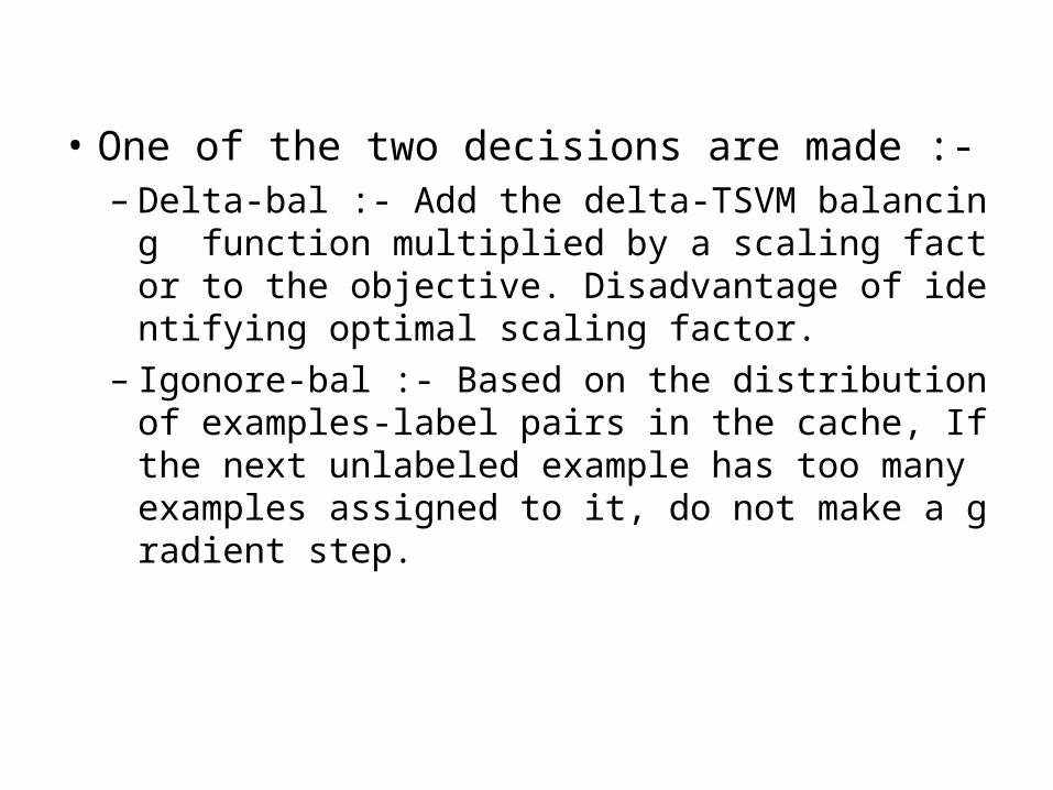
• One of the two decisions are made :-– Delta-bal :- Add the delta-TSVM balancing fu

nction multiplied by a scaling factor to the objective. Disadvantage of identifying optimal scaling factor.

– Igonore-bal :- Based on the distribution of examples-label pairs in the cache, If the next unlabeled example has too many examples assigned to it, do not make a gradient step.

• Further a smooth version of ptrn can be achieved by labeling the unlabeled data by k nearest neighbors of each labeled data.

• We derive pknn, that can be used for implementing the balancing constraint.

Online Manifold Transduction

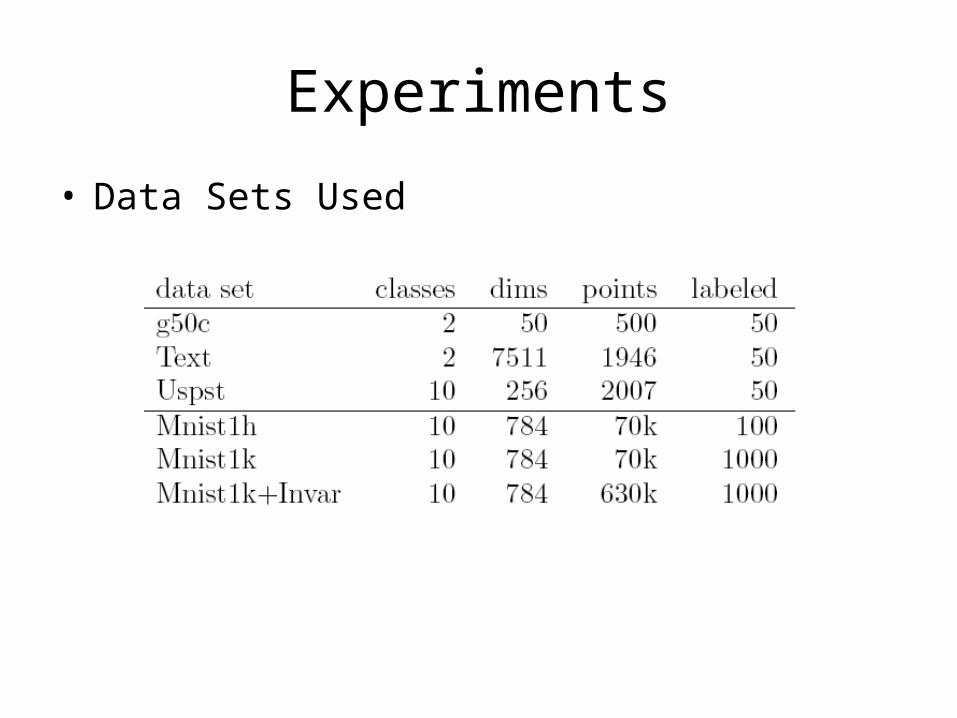
Experiments

• Data Sets Used

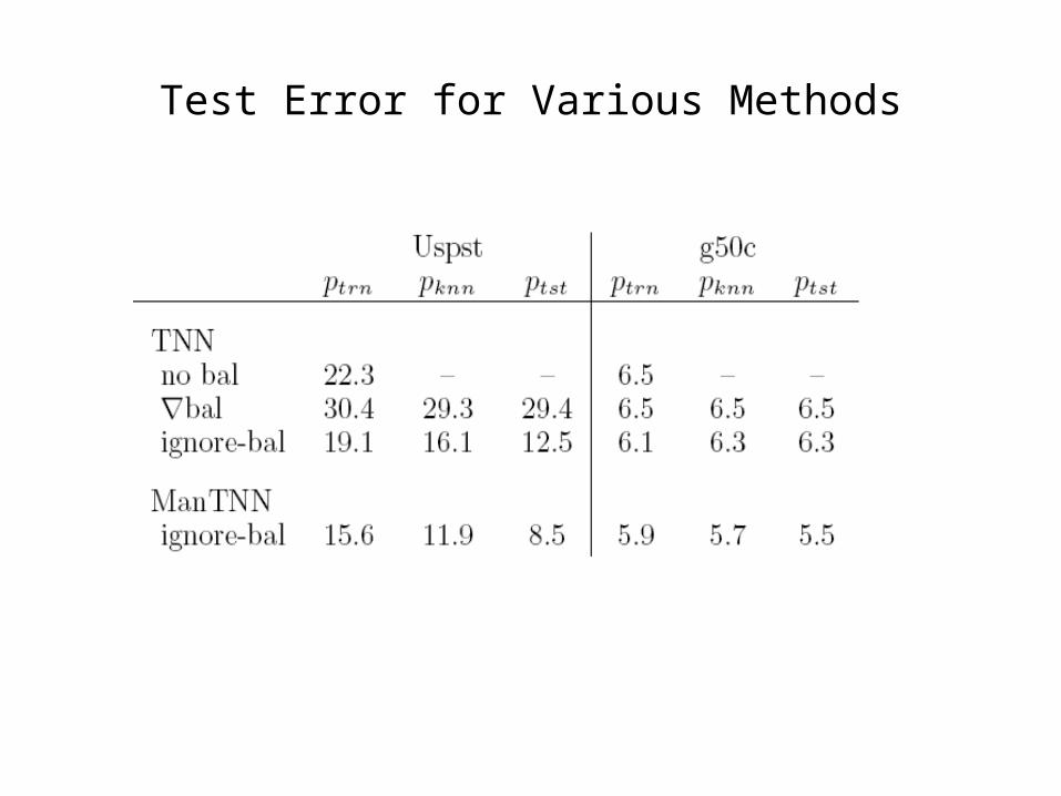
Test Error for Various Methods

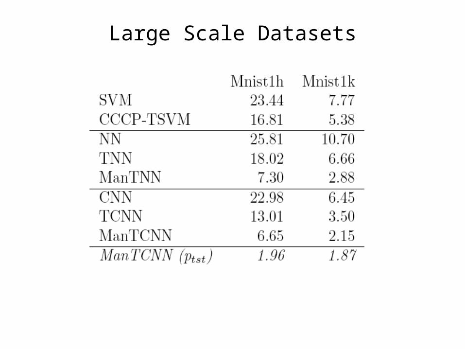
Large Scale Datasets