Large Scale Document Image Retrieval by Automatic …cvit.iiit.ac.in/images/ConferencePapers/2014/Pramod2013Large.pdf · Large Scale Document Image Retrieval by Automatic ... script.

Noname manuscript No.(will be inserted by the editor)

Large Scale Document Image Retrieval by AutomaticWord Annotation

Pramod Sankar K. · R. Manmatha · C. V. Jawahar

Received: date / Accepted: date

Abstract In this paper, we present a practical and

scalable retrieval framework for large-scale document

image collections, for an Indian language script that

does not have a robust OCR. OCR-based methods face

difficulties in character segmentation and recognition,

especially for the complex Indian language scripts. We

realize that character recognition is only an interme-

diate step towards actually labeling words. Hence we

re-pose the problem as one of directly performing word

annotation. This new approach has better recognition

performance, as well as easier segmentation require-

ments. However, the number of classes in word an-

notation is much larger than those for character recog-

nition, making such a classification scheme expensive

to train and test. To address this issue, we present a

novel framework that replaces naive classification with

a carefully designed mixture of indexing and classifica-

tion schemes. This enables us to build a search system

over a large collection of 1000 books of Telugu, consist-

ing of 120K document images or 36M individual words.

This is the largest searchable document image collec-

tion for a script without an OCR, that we are aware of.

Our retrieval system performs significantly well with a

mean average precision of 0.8.

Pramod Sankar K.Xerox Research Center India

Bengaluru, India.E-mail: [email protected]

R. ManmathaMulti-media Indexing and Retrieval group, Dept. of Computer

Science, University of Massachusetts, Amherst, USA.E-mail: [email protected]

C. V. Jawahar

Center for Visual Information Technology

IIIT-Hyderabad, India.E-mail: [email protected]

Keywords Image Retrieval · Automatic Annotation ·Document Images · OCR-free annotation

1 Introduction

Traditionally, digital libraries of scanned English books

are made searchable by converting images to text us-

ing an optical character recognizer (OCR). Example

projects include Google Books [1], Internet Archive [2]

and Universal Digital Library (UDL) [3]. However, for

Indian language scripts, there are no robust OCR en-

gines available, as yet [4]. While there is active research

on building OCR engines for Indian languages [4],

their performance is not yet good enough for use. The

fundamental challenges in building an accurate Indic-

OCR are: an extended character set, complex script lay-

out [5], conjoined vowel/consonant modifiers for each

consonant (see Figure 1), etc. Additionally, degrada-

tions such as cuts and merges have a more pronounced

effect (than on English) with regards to character and

component segmentation. Finally, with a digital-library-

scale dataset, the framework enabling retrieval needs to

be efficient and scalable.

In this paper, our goal is to build a searchable li-

brary of printed books in Indian languages such as Tel-

ugu. We overcome many of the issues with Indian lan-

guage character recognition, by re-posing the problem

to one of word-annotation. By focusing on recognizing

words, instead of characters, better character disam-

biguation is possible as well as difficult character seg-

mentation is avoided. The scalability of this approach is

achieved by proposing an efficient indexing based classi-

fication scheme. The specific contributions of our paper

include:

2

1. A novel direction in building document retrieval sys-

tems based on word-annotation [6]; which is distinct

from existing approaches.

2. A unique framework to scale recognition systems

to large scale test collections, by avoiding repeti-

tive classification of similar features [7]. This results

in an improvement in annotation complexity from

O(N1 ·N2) to O(logN1 · logN2 ·K2), where N1, N2

are the sizes of training and test datasets and K is

the branching factor of the cluster hierarchy. Conse-

quently, a tremendous speed-up of more than 2000×is obtained over traditional approaches.

3. A thorough evaluation of features and indexing sche-

mes for the task of word-recognition, over a chal-

lenging real-world dataset [8] created by us.

4. The largest collection of Indic document images,

120K from 1000 books, made searchable at the word-

level. A significant retrieval performance with a mean

Average Precision of 0.8, was achieved.

The rest of the paper is organized as follows. In the

following section, we outline the datasets that we work

with. In Section 2, we discuss the previous work towards

document image retrieval and we shall elaborate on why

previous methods are not adequate to address our prob-

lem. We present our new solution direction in Section 3,

and detail the processes involved in our framework in

Section 4 and Section 5. Especially in Section 5, we

outline a scheme for scaling our approach to large col-

lections. We analyze the subtleties of our approach in

Section 6, and present experimental details and results

in Section 7. We compare this work with other similar

previous work in Section 8 and conclude in Section 9.

1.1 Datasets

Our datasets come from document images of printed

Telugu books from the Digital Library of India [9]. The

collection has a variety of print quality, font and style;

at varying levels of ink and page degradation. We shall

refer to three sets of data in this paper:

Test Data: Our Test data consists of 1000 books, in-

cluding many classical poetic, prose and fiction works

in the language of Telugu - a language with 75 million

speakers. The Test dataset amounts to 120K document

images with 36 million word-images. This is the largest

Indic dataset ever attempted for a document retrieval

system. This is the dataset that we would like to build

a retrieval system for, as a consequence of this work.

There is a significant variation in the fonts, typeset

styles and print quality in the dataset. Varying levels

of degradations, such as cuts, merges, salt-and-pepper

Fig. 1 Examples demonstrating the subtleties of the Telugu

script. In (a) the consonant modifier is shown to be displacedfrom the consonant in different ways (b) the two characters ma

and ya are distinguished only by the relative size of the circle (c)

the small stroke at the top changes the vowel that modifies theconsonant

noise etc. are also present in the data. Figure 2 shows

this variation for one word across the collection.

Validation Data: This is a hand-labeled groundtruth

dataset of 33,000 word-images, belonging to 1000 dis-

tinct words. Each of these word-images is labeled with

the corresponding text label. The number of occur-

rences of each label in the groundtruth dataset varies

from 5 to 500. The size of the word-images range from

30× 30 to 500× 300 pixels. We shall use the Validation

data to optimize the settings of our framework. The

Validation dataset, which we call IIIT-H Telugu Word

Dataset, is available for download from [8].

Labeled/Training Data: The Training data is a set

of 33 books consisting of 3000 document images. Un-

like the Validation data that consists of 33,000 accu-

rately labeled word-images, the training data is a much

larger set of word-images with a slightly erroneous la-

beling (about 80% accuracy). The labeling is obtained

by aligning page-level transcriptions to their correspond-

ing word-images. This was achieved by performing a

text-driven segmentation of the document image. From

the text we are aware of the number of lines in the page,

number of words in each line and the (approximate)

number of characters in each word. This information

can be used to drive the page segmentation.

The process begins by performing line-segmentation

of the document image. If the number of lines from the

segmentation is less than the number of lines in the text,

it means two text lines have been erroneously merged

by the segmentation algorithm. This often happens be-

cause of overlapping ink pixels between the two lines,

3

Fig. 2 Multiple instances of a single word kaalamu from the book dataset. Notice the large variations in the font, and the large

amount of degradations in the words.

(a) (b) (c)

Fig. 3 (a) Example segment from a typical document image of our collection. Notice the considerable degradations, cuts, mergesetc. in the passage. The groundtruth segmentation of characters is given as bounding boxes. (b) The connected-components of the

segment in (a). One can observe the over segmentation of characters due to degradations. An OCR would not be able to recognize the

characters in this situation. (c) Segmentation of the image at the word level. The effect of the degradations is much less severe in thiscase. We propose the matching of word-images in lieu of recognizing the characters.

due to the presence of consonant-conjuncts (see Fig-

ure 1).To correct this, the tallest lines are split until

the number of lines match between the image and the

text. On the other hand, if the number of lines from

segmentation is more than those in text, it indicates

that some lines were split by the segmentation. This is

corrected by merging the smallest lines together. In the

second step, each line is similarly segmented into words

depending on the known number of words in the given

line. Labeled exemplars for the keywords are obtained

from this dataset.

2 Previous Work

Early document retrieval addressed the problem of doc-

ument retrieval as a whole. Such work uses document

level features or local features that collectively repre-

sent the document image [10,11]. An application of such

work was applied for document tracking on a camera-

based desk [12]. However, the shortcoming of whole-

document retrieval is that users typically prefer to query

and retrieve documents at content-level, more specifi-

cally with words as queries, a natural extension of web-

search.

There have been two major approaches in litera-

ture towards building content-level retrieval systems.

The first is a recognition-based approach involving the

building of an Optical Character Recognizer (OCR)

along with its post-processing modules. The other is

the recognition-free Word-Spotting approach.

2.1 OCR

OCRs have had a long history, and surveys can be found

in [13,14]. OCRs begin by segmenting the document

image to connected components, each of which is con-

sidered as an isolated character. These components are

represented using features such as patch-based, PCA,

LDA, or other statistical features. The classifiers used

to recognize characters have evolved over time from

Neural Networks [15,16] to Support Vector Machines

(SVM) [17]. Since SVMs are mostly suitable for two-

class classification problems, a chaining architecture such

as a directed acyclic graph is used to combine multi-

ple classifiers [18]. Errors in classification are typically

corrected using post-processing based on character er-

ror models [19], dictionaries [20] or statistical language

models [15,21]. OCRs such as the Byblos system [22,

21] use HMMs to encode the n-gram statistics towards

refining character labels. However, such methods inher-

ently use gradient based features, which we shall show

(in Section 7.1) are not reliable in the presence of severe

degradations present in our data.

In the case of Indic OCRs, despite significant ef-

forts [4], their performance is not comparable to that

of English. The major road-blocks towards building In-

dic OCRs are:

– An extended character set, almost 5 times that of

English, requiring the classifier architectures to scale

to a much larger number of classes.

4

– A complex style of writing, where each character is

a conjoint of a consonant and a vowel, making it

difficult to segment the individual components for

subsequent recognition. Some examples are shown

in Figure 1 (a).

– A number of similar-looking character pairs, distin-

guished by very subtle differences, see Figure 1 (b)

& (c). This calls for very strong classifiers which are

both hard to train and expensive to test.

– A large lexicon that is almost 10x that of English,

making language models challenging to build [23].

Moreover, a poor OCR performance translates to

unacceptable word-level accuracies. Typical character

recognition accuracies over document images similar to

our collections are less than 90%. Assuming an average

word length of 6, the word recognition accuracy would

be (0.90)6, or only 53%. Retrieval from such erroneous

recognition results would result in poor precision and

recall.

2.2 Word-Spotting

As an alternative to OCR, a number of authors have

proposed techniques that avoid the use of character

recognition. One such approach is based on character

shape codes for word detection [24]. A set of 5 character

shape codes encode each connected component, which

is prone to errors from component segmentation and

degradations. A few shape coding works avoid charac-

ter segmentation, by proposing novel features such as

stroke coding [25], topological shapes and character ex-

tremum points [26]. However, these techniques are lim-

ited by the shape-code vocabulary and are typically not

invariant to font and style variations (for e.g. italics).

The more popular recognition-free approach is called

word-spotting, where word-images are holistically repre-

sented in a visual feature space and matched with the

queries in the feature space itself. Queries are either

given as word-image examples or are synthetically gen-

erated [7,27]. Features proposed for representing words

include profiles [28], Gradient-based binary features [29],

HoG [30] or shape-context [31]. In most cases, the fea-

tures used to represent the word-images are of non-

uniform length, depending on the word-image’s width.

With variable length features, word-images are matched

using Dynamic Time Warping (DTW) [28,32]. Apart

from DTW, matching techniques using HMMs [33] (that

needed to be pre-trained) and Hough transform of dis-

tance matrix images [34] were proposed. More recently,

BLSTM neural networks [35,36] have been used to ob-

tain a pseudo-character representation, which is then

matched with the query using edit distance. In the case

of historical documents, a segmentation-free word spot-

ting was presented [37] where features are extracted on

blocks of the document images, which are then matched

with the query. Word-spotting approaches have been

extended to retrieve/recognize from hand-written doc-

uments as well [38–40].

The more successful DTW based approach is com-

putationally intensive, with an estimated query time

of 416 days for searching a single query within our

test collection of 36M words. A suggested approach

to overcome the impractical retrieval times is to per-

form an offline-indexing using either clustering [28], or

with Locality Sensitive Hashing [41]. However, index-

ing the features from large datasets (about 210 GB for

1000 books), is infeasible even on advanced comput-

ers. Also, some of the features such as the split-style

HoG feature [30] are of a very high dimension, making

it unsuitable to manage for large collections. Further,

word-spotting systems can only be queried-by-example,

while users prefer text querying. Text querying requires

that text labels be provided to the word images. In [42],

such labels were obtained over handwritten documents,

by applying a relevance model learnt from transcribed

documents.

2.3 Dataset Size Comparisons

With regards to scalability aspects, much of the previ-

ous work has been restricted to laboratory settings or

small document collections. Due to the unavailability

of a large labeled corpus, most of the experiments were

done only on a limited number of pages [43]. The UNLV

dataset [44] evaluated OCRs on a set of 2000 pages. In

word-spotting techniques, the test set sizes range from

a few tens of images [45–48,28] to a few books [49].

The largest handwritten collection of about 1000 pages

comes from George Washington’s diary consisting [42].

One of our previous papers [7] was the first to build a re-

trieval system over a collection of 500 (printed) Telugu

books, consisting of 75,000 document images. In this pa-

per, we shall extend our previous work to a much larger

collection, while significantly boosting performance and

slashing computational requirements.

3 Our Approach

At the outset, we realize that in order to replicate web-

search characteristics and performance on document

images, a text-based retrieval system is the best option.

A textual representation also allows for many break-

throughs in text retrieval, summarization and transla-

tion to be applied to document images in the future.

5

Aspect OCR Word Spotting (DTW based) Our Approach

Text querying Yes No YesRetrieval time Instantaneous Time-consuming Instantaneous

Accuracy Poor for Indian languages Acceptable State-of-the-artDegradation Serious Effects in Segmentation Lesser Effects in Segmentation Lesser Effects in SegmentationFont Sensitivity Limited to Training Fonts Robust to Font Variations Robust to Font Variations

Data Scalability Scalable Not Scalable ScalableVocabulary Coverage Limited by Post-processing Limited by Manual Annotation Limited by Training data

Table 1 A comparison of our approach with the most popular techniques available for document retrieval. Our approach has multipleadvantages over either approach taken alone.

Since OCRs are not the effective approach to obtain

the corresponding text, we re-pose the problem to one

of word-annotation.

3.1 Towards Annotating Words

The move from character to word labeling is motivated

by these observations:

1. Word-images contain a lot more information, than

individual characters. This contextual information

present within a word helps in better disambigua-

tion between word-images, which would otherwise

result in errors when recognised at character level.

For example, in the word “image”, the “m” could

easily be misclassified as “in” or “ni” if there is a

cut. However, the word as a whole will most likely

match with the right label.

2. Segmentation of the document to words is much

more reliable than segmenting to characters and com-

ponents. Component segmentation is highly inaccu-

rate, especially in the presence of complex scripts,and degradations. For the example document image

given in Figure 3 (a), the component segmentation

over-segments the characters, as can be seen in Fig-

ure 3 (b). On the other hand, the word segmentation

shown in Figure 3 (c) is very accurate.

3. For the purpose of retrieval, character/component

level labeling is not required. Character recogni-

tion is only an intermediary step towards performing

word annotation. Another advantage with recogniz-

ing words is that dictionary based verification could

be performed as part of the recognition step itself,

hence avoiding an additional post-processing step.

Further, not all words in document images are infor-

mative towards indexing them. Since it only suffices to

label those words that are useful from a search perspec-

tive, our process is one of annotation instead of full-

fledged recognition. The comparison of our approach

with OCR and word-spotting is given in Table 1. Our

approach is distinct yet combines the advantages of

both these directions into a new framework.

3.2 Problem Setting

We begin with two inputs: i) a set of test document

images D1, D2, ..., DN , each document Di consisting of

word-images W 1i ,W

2i , ...,W

nii , and ii) a set of words (in

text) forming the vocabulary-of-interest, V1, V2, ..., VM .

The word-image set W ji and the text-vocabulary Vk

are drawn from different datasets, hence there is no

knowledge if a given word-image W ji corresponds to a

text label Vk. The word-annotation problem now boils

down to finding the appropriate word Vk, if it exists,

for each word W ji . Without any loss of generality, the

same problem can also be posed as one of finding all

the words W ji that correspond to the given word Vk

in the vocabulary. Such a labeling will directly result

in a search index over the documents. Since, the task

of finding datum corresponding to a given keyword, is

the conceptual opposite of the traditional annotation

scheme, we call such a process Reverse Annotation [7].

Algorithm 1 Word Annotation FrameworkOffline Phase

Training Phase

- Identify appropriate features and parameters fromV alidation dataset

- Learn classifiers for word-annotation using labeled

data from Training datasetTest Phase

- Index/Cluster Test dataset

- Classify one (or k) data-points per cluster againstlearnt classifiers

- Annotate all points of cluster, with appropriate labelIndex Building

Index word-images based on their text-labels

Rank the points within an indexOnline Phase

Obtain textual query from user

Retrieve ranked lists for each query wordRe-rank documents using TF-IDF

A conceptual overview of our framework is presented

in Algorithm 1. We shall now proceed to elaborate on

the design choices for each of the steps in this algo-

6

rithm. For each Section, we indicate the corresponding

step of the algorithm in parentheses.

4 Classifier Design for Word Annotation

(Offline Phase - Training)

4.1 Identifying the Vocabulary (Classes)

In retrieval systems, the choice of vocabulary {Vk}, that

can be searched for is an important design criterion.

Practical text search engines do not index (and an-

swer) all possible queries, since such an index could

span all possible unique words in the language. For ex-

ample, search engines such as Lemur [50], Galago [51],

etc do not index strings made up of special characters.

The goal of building a search index, is to optimize the

percentage of queries that can be answered and docu-

ments that can be retrieved. Similarly in our work, we

could limit the vocabulary size to optimize the query-

document coverage.

The distribution of the keywords in our training

dataset is shown in Figure 4. It follows the well known

Zipf’s law [52], that states that the frequency of any

word is inversely proportional to its rank in the fre-

quency table. At the head of the distribution, we find

what are called stop-words, such as {the, a, an, and, ...}.Stop-words do not contribute to the retrieval task, hence

it would only be a waste of index space. The distribu-

tion also has a long-tail, consisting of a large number of

words that occur only a few times.

Consequently, we design the vocabulary-of-interest

Vk, such that a large percentage of documents are in-

dexed and large percentage of queries are answered. We

first remove stop-words, by thresholding on the inverse

document frequency (IDF) measure. The IDF is defined

as log( |D||d:t∈d| ), where |D| is the number of documents

in the collection and the denominator is the number

of documents containing the given term. We consider

all the words that occur in one-tenth of the document

collection, as stop words. This corresponds to an IDF

threshold of 2.3. Rare-words are removed by threshold-

ing the term frequency (TF) at 10. Our vocabulary-of-

interest consists of 100K words.

4.2 Building the Classifier

When we re-pose the problem from character recog-

nition to word annotation, the number of classes that

need to be learnt, expands from the character set (of

about 300) to the size of the vocabulary (100K in our

case). Such a class size is quite large compared to typ-

ical machine learning problems addressed in the litera-

Fig. 4 The distribution between the word rank and word fre-

quency from our training dataset. As expected, the distributionfollows Zipf’s law, an exponential relationship between the fre-

quency of a word and its rank based on the frequency. An ideal

Zipf’s distribution follows a straight line on the log-log plot be-tween rank and frequency.

ture [53,54]. This results in two issues: i) the classifiers

need to be designed to scale to the large number of

classes and ii) significant amount of reliable training

data is required to learn the classifiers.

In picking a classifier, apart from high performance,

the major requirement is that the classifier scheme be

scalable to huge test collections. In traditional machine

learning work, the focus has been on improving classi-

fication accuracy and/or the training times. We believe

however, that for our problem, scalability in the test

phase is more important. Accordingly, we examine two

distinct classifier schemes: i) Nearest Neighbor and ii)

Support Vector Machines (SVM), to measure suitabil-

ity of each for word-image annotation.

SVMs are inherently two-class classifiers. Multi-class

classification with SVMs is performed by either building

|C| one-vs-rest classifiers, or |C| · |C − 1|/2 one-vs-one

classifiers. Each data point is classified as belonging to

the classifier with biggest margin (for one-vs-rest), or

the class that is selected by most classifiers (for one-

vs-one). The major issue with one-vs-rest classifiers is

the lack of a reliable mechanism to combine classifier

scores, especially when the internal parameters of the

individual SVMs depend on the data or class distribu-

tions. The second approach is obviously prohibitive to

train and test for our problem where |C| is 100K. Each

data point would then have to be classified by 5 · 109

SVMs, which would be infeasible. Moreover, SVMs re-

quire large amounts of training data to learn the clas-

sifier accurately.

We experimentally verify this intuition over our val-

idation dataset of 32K word-images belonging to 1000

classes. SVMs were built for each of the 1000 classes us-

ing half the validation data as training set and the other

half for testing. The classifier with the maximum score

is chosen as the class for the test point. Results from

this experiment are shown in Table 2. As can be seen,

7

Classifier Distance/Kernel Accuracy Training Time Test Time

SVM Linear Kernel 58% 8 min 21 Hours

SVM Polynomial Kernel 46.8% 9 min 23 Hours

Nearest-Neighbor DTW 81% 0 75 Hours

Nearest-Neighbor Euclidean 78.6% 0 4 HoursNearest-Neighbor Manhattan 82.8% 0 3.5 Hours

Table 2 Word Recognition accuracy using SVMs and Nearest Neighbor classifiers, using Profile features over our validation dataset

consisting of 32K words from 1000 word classes; 16K used for training and 16K for testing. SVMs are easily out-performed by a NearestNeighbor classifier, both in accuracy and classification time.

SVMs perform much poorer than a Nearest Neighbor

classifier using the same features. Apart from perfor-

mance, SVMs are also slow to train and test, due to

the 1000 classifiers (one for each word) that needed to

be learned and classified against.

5 Annotation on a Large Scale

(Offline Phase - Testing)

The challenge in the testing phase is scalability of the

classifier scheme to large test collections. For example,

the NN classifier requires about 0.77 second per test

sample. The time required to classify our test dataset

against all 100K classifiers would require about 90 years

of compute time, which is clearly not the optimal clas-

sification scheme. We shall address the scalability chal-

lenge by proposing a novel mechanism based on this

unique premise:

One need not classify every given data-point.

Classification can be re-used across similar data.

In a typical machine learning scheme, each test case

is considered isolated and classified independent of each

other. With such a naive classification, the complexity

of classification is O(NTest ·O(C)), where NTest is the

number of data points to classify and O(C) is the inher-

ent complexity of the classifier for the classes of inter-

est. However, we observe that this is quite un-necessary,

since the test samples follow an inherent distribution.

A number of samples are either repetitions or near-

duplicates of other samples. Consider a scenario where

one could identify if a data point has the same (or simi-

lar) features as another data point. In such a case, only

one of these features needs to be classified, and the clas-

sification result can be re-used for the other point. Such

a scheme would be effective under the following fairly

generic conditions:

1. The size of the test data is much greater than the

number of classes (NTest >> |C|).2. The test samples follow a distribution that is not ar-

bitrary, but closely reflects the distribution of train-

ing data. This ensures that the priors learnt by the

classifiers are valid for the test data as well.

3. Smoothness Assumption: If two points x1, x2 are

close, then so should their corresponding classifier

outputs y1, y2. Consequently, if y1 ≈ y2, then the

two points can be assigned the same label V1 = V2.

For the case of document images, we find that all

these assumptions are valid. It is quite obvious that

the list of classes in the word-annotation is limited by

the known vocabulary size of the language. The data,

however, that can be indexed with such a vocabulary

could be limitless. It is also known that the test data

follows a Zipf’s distribution, similar to the training set.

With Zipf’s distribution, a large amount of the mass is

present in a small percentage of the distribution. This is

an ideal candidate to re-use classification scores, when

multiple instances of the same data are seen often. The

third condition only requires that the matching scheme

be robust to noise. In cases where condition 3 is false, it

would imply that two features that are close in the given

feature space, actually belong to different categories.

This would mean that the features and/or the distance

measure are highly sensitive to noise, and hence not the

right setting to learn the classifier. As we shall show in

Section 7, our features and classifiers are indeed robust,

hence satisfying condition 3.

Given the validity of the above assumptions, as a

consequence, we now make the “Cluster Assumption”:

if points {x1, x2, ..., xn} all belong to the same cluster,

they are likely to be of the same class. More precisely,

for a given point xi, and its cluster centroid C(xi), for

some reasonable τ :

y(xi) = y(C(xi)) if d(xi, C(xi)) < τ

where y(.) is the label for the given data point.

Thus, if we were able to cluster the word-images,

such that the maximum radius of the cluster is less than

a certain threshold τ , then it would suffice to classify

only one point, namely the centroid of the cluster. We

could then propagate the class label of the centroid to

the rest of the cluster, without having to classify every

single point.

8

In the case of word-images, the centroid is typically

a very clean representative candidate of the various in-

stances of word-image occurrences across the data col-

lection. Thus, the classification of the centroid is much

more accurate than classification of those points at the

fringe of the cluster.

5.1 Clustering Training Data

With the clustering scheme, the computational cost of

using a classifier reduces from O(NTest ·O(C)) to O(K ·O(C)). Here K is the number of clusters in the test

data, K is typically a small multiple of the number

of classes, C. In the specific case of Nearest Neighbor

classifiers, a further cost saving could be achieved. We

observe that the keyword-exemplars themselves are not

totally isolated in the feature space. While multiple ex-

emplars of the same word would be clustered together

at the lower levels of the cluster hierarchy, at a higher

level similar words that vary in only a few characters

would be found together. Thus, keyword-exemplars can

also be clustered based on the similarity in their repre-

sentative features. If the exemplar set is larger than the

size of M , we built forests of keyword exemplars too.

Matching Clusters Through Trees: Imagine we are

given a pair of trees TD and TK , one belonging to the

unlabeled word-image dataset and another from the

keyword exemplar set. The problem of word-annotation

is now the task of matching the clusters at the leaf node

of TD, to the specific exemplar belonging to TK . Un-

like an exhaustive matching between all the leaf nodes

between the pair of trees, we could exploit the paths be-

tween the leaf nodes to prune out unsuccessful matches

beforehand. We assume that two clusters will not match

at a lower level, unless their parent nodes match. This is

a fair assumption, even in cases where the clusters in the

two trees partition the feature space differently. This

technique is depicted in Figure 5. Using this method,

the complexity of matching exemplars with features

is now reduced to O(logN1 · logN2 · B2), instead of

O(N1 ·N2) for a regular Nearest Neighbor (NN) classi-

fier.

5.2 Efficient Clustering Schemes

In the previous section, we introduced the concept of

clustering for avoiding repeated classification of similar

points. However, the process of clustering itself is ex-

pensive, typically requiring O(NTest.K) time, where K

is the number of clusters. Another limitation of the K-

Means clustering algorithm is the necessity to fix K be-

forehand. If K is less than the number of unique words

in the collection, it would mean that some of the clus-

ters would have different words in them. A larger K

reduces the chance that images corresponding to differ-

ent words will be part of the same cluster. The trade-off

is that a larger K will lead to multiple clusters for the

same word. However, this would increase the compute

time. We shall look at two approaches to perform this

process in reasonable time.

Hierarchical K-Means (HKM) is a way to approxi-

mate K-Means fast. The idea [55] is that a small num-

ber of clusters - say B - are created at the top level,

B is known as the branching factor. In the next step,

each of these B clusters is expanded to B more clus-

ters giving B2 clusters at the second level. This pro-

cess is repeated up to a certain depth D so that BD

clusters or leaf nodes are formed at depth D, typi-

cally D = logB(NTest). To build the entire HKM tree

requires O(NTest · K · D) time while K-Means would

require O(NTest · KD). For a million data points, the

speed-up is from 31 yrs for K-Means to 13 hrs for HKM.

Once the HKM tree is built, given a new point it takes

B ·D comparisons to find out which cluster it belongs

to, unlike traditional K-Means which would take BD

comparisons. For example, if B = 10, D = 6 then there

are one million leaf nodes. While K-Means requires 106

comparisons while HKM only needs 60.

Another approach to speeding up clustering is by us-

ing approximate nearest neighbor search. In K-Means,

the most expensive step is the mapping of data to the

closest provisional centroid, at each iteration. This is

essentially the problem of nearest neighbor matching,

which can be approximated using indexing schemes such

as Locality Sensitive Hashing or Random Forest of KD-

Trees.

Locality Sensitive Hashing: In Locality Sensitive

Hashing [56] (LSH), data points are projected onto ran-

dom subspaces, such as a line or hyperplane. The pro-

jected subspace is divided into spatial bins; each point is

assigned to the bin it falls into. The assumption is that

points close to each other in a high dimension space will

most likely fall into the same bin in the low-dimensional

projection. Multiple such hash functions are generally

used to collect additional evidence to determine NNs.

A feature vector x, is mapped onto a set of integers by

each hash function ha,b(x). For a pre-defined bin-width

w, the hash function ha,b is given by,

ha,b(x) = ba · x+ b

wc.

9

Fig. 5 Word Annotation by efficient comparison of hierarchical clusters of labeled and unlabeled word-images. For brevity, only one

tree is shown for the index of each dataset. In reality, a forest of trees is used to index the exemplar and test datasets.

Feature vectors that are close in the feature space

are expected to fall into the same hash bin. As a corol-

lary, data points that have the same hash value over

multiple hash functions are expected (but not neces-

sary) to be close in the feature space. Following this, for

each test feature, the hashed values in the same bins as

the test feature are returned as the approx-NNs.

Random Forest of KD-Trees: Another approach to

addressing the approximate NN problem uses a ran-

dom forest of KD-Trees [57]. A KD-Tree partitions the

feature space with axis-parallel hyperplanes. The algo-

rithm splits the data in half at each level of the tree

on the dimension for which the data exhibits the great-

est variance. The tree is looked up for NNs, by com-

paring the query with the bin-boundary at each level

of the tree(s). Building a KD-tree from n points takes

O(n log n) time, by using a linear median finding algo-

rithm. Inserting a new point takes O(log n) and query-

ing for nearest neighbors takes O(n1−1/k +m), where k

is the dimension of the KD-Tree and m is the number

of nearest neighbors. The algorithm [57] first traverses

the KD-tree and adds the unexplored branches in each

node along the path to a priority queue. It then finds the

closest center in the priority queue to the given query,

and uses this node to restart the traversal. The process

is stopped when a predetermined number of nodes are

visited. Further, a Random Forest of multiple KD-Trees

is used to improve the ANN evidence for better cluster-

ing quality. When building a random forest, the split

dimension is chosen randomly from the first D dimen-

sions on which data has the greatest variance. Multiple

trees define an overlapping split of the feature-space.

These trees are looked up for NNs, by comparing the

query with the bin-boundary at each level of the tree(s).

By using a voting scheme over the different trees, we

obtain very reliable clusters.

Incremental Indexing Irrespective of the indexing

scheme used to speedup clustering, memory limitations

are easy to breach in large datasets. To begin with,

the features for our test dataset (36M word-images) oc-

cupy a diskspace of 210 GB, which cannot be loaded in

one instance on a single machine. Further, all indexing

schemes have large memory overheads, where memory

is traded for speedup. For example, the storage com-

plexity of LSH is of the order O(NTest.|H|), n being

the number of features hashed and H is the set of hash

functions. Since the optimal |H| depends on the size

of the dataset NTest, the memory required for a large

dataset could be more than what modern computers

can handle [58]. We address this issue, by dividing the

dataset into subsets, say M of them, and build separate

indexes over each subset. The size of the subset is deter-

mined by the maximum number of features that can be

indexed in one instance. Once the indexes are built, the

approximate nearest neighbors are obtained by looking

up each subset against the index of every other subset

(including itself). Thus, the process of clustering would

involve M indexing steps, and M2 lookup steps.

5.3 Indexing of Document Images

(Indexing Phase)

At the end of the word-annotation procedure, we have

an index of the word-images against the keywords. How-

ever, the index does not lend itself to ranking the word-

images for retrieval purposes, since the associations in

the index are binary. The ranking is based on a proba-

bility that consists of two parts. The first part measures

the quality of labeling of a cluster (i.e. its centroid) with

10

the given keyword-exemplar. The second term measures

the association of the word-images to the cluster.

Let us assume that the word-image ti is the centroid

of a certain cluster, and the set of word-images in this

cluster are represented by {t1i , t2i , ..., tni }. If the closest

keyword to this cluster is given as Vk, then the proba-

bility that word-image tji matches this keyword is given

as:

p(Vk|tji ) =s(Vk||ti)∑

i

∑k s(Vk||ti)

× s(ti||tji )∑j s(ti||t

ji )

(1)

where s(x||y) is a similarity measure (inverse of a dis-

tance measure). Since we assign a single label to each

cluster, for Vk′ 6= Vk, p(Vk′ |tji ) = 0.

The denominator of the first term involves the sum-

mation over all keywords and all clusters (a modified

version of that used in [7]). While computing the de-

nominator is expensive, we observe that it remains a

constant for all word-image and keyword cluster pairs.

For ranking purposes we can ignore the denominator

while computing the score. The computation of the

score can thus be performed only between the pairs of

exemplar and test-set clusters which match in the word-

image annotation phase, hence preserving the compu-

tational advantages of the framework.

5.4 Ranking of Retrieved Documents

(Online Phase)

Given the ranking of word-images against the query, the

relevant documents are ranked using a function similar

to the Term Frequency/Inverse Document Frequency

(TF-IDF) measure. In the ranking function, the sum

over the number of words is replaced with their prob-

abilities given by Equation 1. TF measures the impor-

tance of the keyword for the image, and is normalized

by the document length to avoid bias to longer docu-

ments. The document length is replaced by the sum of

the probability scores of all the words within the doc-

ument, against their respective keywords. This scheme

ignores the words that are not labeled in the annotation

step. For the query-word Vk, the TF for a document Di

containing word-images {W ji }, is defined as,

TF (Di|Vk) =

∑j p(Vk|W

ji )∑

j,k p(Vk|Wji ). (2)

where the denominator is a sum of all the scores be-

tween the word-images and their matched keywords.

When the search query consists of multiple words,

the relative importance of the words in the query is

an important distinguishing factor during ranking. This

is estimated by the inverse document frequency (IDF)

measure, which indicates the overall importance of the

given keyword in the entire collection. It is basically the

logarithm of the total number of documents over those

containing the given term. The modified IDF measure

is defined as

IDF (Vk) = log|D|

1 +∑

i δ(∑

j p(Vk|Wji ))

. (3)

The δ function ensures that multiple word-occurrences

within a document are counted only once:

δ(x) =

{1 : x > 0

0 : x = 0(4)

The TF×IDF provides the final ranking of documents

for the given query-words.

6 Analysis of the Solution

Effect of Clustering Errors: Clustering of data is

crucial to our solution. It is possible that some of the

clusters are not “pure”. This could be because of multi-

ple reasons: i) the words are inherently similar looking,

ii) degradations cause the words to appear similar or

iii) the cluster centers are initialized in the intra-class

region in the feature space. One of the solutions that we

suggest to improve cluster purity is by allowing multi-

ple clusters for each word in the vocabulary. Ideally, if

the vocabulary size |V | is known, the number of clusters

“K” should be equal to the number of unique words. Us-

ing K < |V | will inevitably result in clustering errors.

When the vocabulary size is unknown, it is suggested

to use a large K, thereby allowing multiple clusters for

some of the words, but not constraining the different

words to fall into a limited number of clusters.

The effect of cluster size on the purity of the cluster-

ing was analysed over the validation dataset (described

in 1.1). The dataset consists of 32K word images belong-

ing to a vocabulary size of 1000. The precision, recall

and F-measure of various cluster sizes is shown in Fig-

ure 6. As can be seen, when K < |V |, the precision of

the clusters is very poor. The precision improves as K

increases, with the most precision of 1.0 reached when

each data point is a separate cluster. However, the re-

call value of the clustering would tend to 0.0 in such a

case. Consequently, we choose an operating point where

there is sufficient trade-off between precision and recall

as defined by the F-measure. From our experiments,

we observe that an acceptable F-measure was when the

number of clusters was around 5 times the vocabulary

size. We use this observation while building the clusters

over our test data.

Further, instead of creating a single cluster tree over

the data, multiple such trees, are generated for the same

11

Fig. 6 Clustering accuracy across number of clusters, over the

Validation dataset (32K word-images, 1000 unique-words). The

precision increases while the recall drops with increasing K. TheF-measure is used to identify the optimal trade-off between pre-

cision and recall.

set of data, and a voting scheme is used to identify

clusters that are reliable. In cases where errors remain

in the cluster, we do end up with errors in their labeling.

However, as we shall see in Section 7.2, the drop in

recognition performance due to the clustering scheme

is less than 3%, while providing tremendous speed-up.

Refuse to Label & Soft Labeling: In our problem

definition, we restrict ourselves to a subset of the vocab-

ulary, which allows us to focus more on labeling those

words that would be useful for retrieval. Consequently,

there would be many word-image clusters, that do not

belong to the vocabulary of interest. In order to avoid

labeling such clusters, we assign labels only if the clas-

sifier score for the closest keyword, is greater than a

pre-defined threshold. The reject threshold is chosen

by analyzing the effect of the threshold on the preci-sion of classification and the accept-rate (or recall) of

the classification.

The effect of the threshold over classification of the

validation dataset is shown in Figure 7. As observed

from the plot for 1-NN classification, the precision is

high across various recall points. We choose the thresh-

old where recall is atleast 0.8, i.e. atleast 80% of the

points are assigned a suitable label. At this threshold,

the accuracy of classification is more than 95%. Fur-

ther, we observe that with the k−NN classifier, better

performance is observed with smaller k. The 1-NN clas-

sifier gives the best recognition accuracy across different

k.

On the other hand, instead of assigning a single label

to a cluster (or word-image), one could also label the

word-images with multiple matching keywords, along

with storing their match score. This would partially ad-

dress the presence of similar-looking but distinct word-

images within a cluster. By assigning the top-m word

labels to a given cluster, one could improve recall for

Fig. 7 Performance of classification across reject-threshold and

the k−NN settings of the classifier, over the V alidation dataset.The 1-NN classifier works best, and we choose a reject threshold

that gives a recall of atleast 80%. The precision at this operating

point is more than 95%.

rare words that are not large enough to form a distinct

cluster in the feature space. This would require a small

change in the computation of probabilities of Equa-

tion 1, by computing probabilities over all valid Vk for a

given cluster centroid ti. The results in this paper were

obtained without assigning soft labels, owing to mem-

ory constraints on storing and accessing the large in-

dexes. Soft labeling could also be employed by allowing

each word-image to belong to multiple clusters, drawing

from success of such methods in object retrieval [59].

Some of the advantages of soft-clustering are implic-

itly obtained by building multiple cluster trees. Explicit

soft-labeling, however, would hurt the speedup that we

gain from assigning word-images to a single cluster.

Effect of Segmentation Errors: Though the seg-

mentation requirements at the word-level are much eas-

ier to handle than character segmentation, errors occur

occasionally in word segmentation. This could be due

to overlapping ink pixels across multiple lines of text,

or due to insufficient inter-word spaces. In our frame-

work we match words as a whole, refraining from partial

matching (using DTW), to save on computational ex-

pense. This results in words with segmentation errors

to be rejected or mis-labeled in the annotation phase.

Scaling to Larger Collection: Once the index is

built over a 1000 books, one can examine the prospect of

adding more books to the searchable collection. Given

another 1000 books, the same process can be repeated:

i) divide the collection into M subsets each, ii) build

hierarchical clusters over each of the M subsets and iii)

match these trees with those built over the Training

set. It can be inferred that the process is linear in col-

lection sizes, thus the framework is scalable to bigger

digital libraries.

12

7 Experimental Results

In this section, we shall evaluate various choices avail-

able for building our framework. The evaluation of fea-

tures (Section 7.1), indexing schemes (Section 7.2 and

labeled data quantity (Section 7.3) is based on the ground-

truthed validation dataset (described in 1.1). The per-

formance of our approach on the Test dataset is pre-

sented in Section 7.4.

7.1 Feature Evaluation

The features that represent the word-images are re-

quired to be robust to variations in font, style and

degradations. We examine three holistic features that

have been popularly used in the document recognition

community:

– Profile features

– Scale Invariant Feature Transform (SIFT) + Bag-

of-Words

– Pyramid Histogram of Oriented Gradients (PHOG)

Profile Features: Profile features were popularized

by Rath and Manmatha [60], where these features were

used to represent words from handwritten documents.

The profile features we extract include (see [60] for more

details):

– The Projection Profile is the number of ink pixels

in each column.

– Upper and Lower Profile measures the number of

background pixels between the word and the word-

boundary– Transition Profile is calculated as number of ink-

background transitions per column.

Each profile is a vector whose size is the same as the

width of the word. The dimensionality of the feature,

therefore, varies with the word used. Such variable-

length features are typically matched using Dynamic

Time Warping (DTW) [60,61]. However, owing to the

computational cost of DTW, an alternative fixed length

representation was obtained by scaling the word images

to a canonical size before extracting the Profiles.

SIFT + BoW: An alternative to Profile features

is to use a point-based representation for the word-

images. SIFT [62] (Scale Invariant Feature Transform)

has proved to be very successful in many computer vi-

sion tasks. The SIFT operator contains two parts - an

interest point detector and a descriptor. The interest

point detector is based on the difference between multi-

scale Gaussians of the given image. The descriptor is a

histogram of oriented gradients. The scale-invariance

Feature Distance Accuracy Time

Profile Features DTW 81% 75 HoursProfiles (Scaled) Euclidean 78.6% 4 Hours

Profiles (Scaled) Manhattan 82.8% 3.5 Hours

SIFT (1000) Euclidean 26.4% 4 HoursSIFT (100K) Euclidean 8% 11 Hours

PHOG (100) Euclidean 35.2% 30 MinutesPHOG (1000) Euclidean 41.8% 4 HoursPHOG (100K) Euclidean 14.1% 11 Hours

Table 3 Word Recognition accuracy across various features andmatching schemes. The number of visterms used for SIFT and

PHOG are mentioned in parentheses. Profile features work the

best, while SIFT and PHOG are seriously affected by the degra-dations (cuts and merges) present in the images

property of SIFT and its high repeatability across var-

ious affine transformations makes it a good candidate

to be used in document images [45].

Pairwise matching of SIFT features between word

images is time consuming. To alleviate this, the fea-

tures are mapped to a unique ID, called the visterm.

Images can now be matched by counting the overlap

between corresponding visterms. The visterms are ob-

tained by vector quantizing the SIFT features using

K-Means clustering. Each feature in a word-image is

represented as the index of the cluster visterm. The

word-image is then represented as a histogram of the

occurrences of each visterm. Given this representation,

two words are compared by finding the distance be-

tween the corresponding histogram feature vectors.

PHOG + BoW: Unlike SIFT, which is a sparse

detector, we also examine a dense representation with

similar descriptors such as Histograms of oriented gradi-ents (HoG) [63]. We use a pyramidal HoG [64] to repre-

sent each word-image. To compute this feature, a fixed

size window is moved across the word-image, and at

each instance a HoG descriptor is computed. Once the

entire word-image is scanned by the window, the win-

dow size is doubled and the process repeated, till the

window size exceeds the word-image’s size. The set of

extracted features are vector quantized, and the word-

image is represented as a histogram of the occurrences

of each visterm.

Performance of the features is reported in Table 3,

which shows that the best performing feature was the

scaled-profiles with L1 distance matching (83%). Thus,

our setting outperforms the state-of-the-art DTW match-

ing of Profile features (81 %), which also has the addi-

tional disadvantage of high time complexity. The recog-

nition over the validation dataset set alone takes around

75 hours with DTW, as opposed to 3.5 hours using

scaled-profiles. Further, the gradient features - SIFT

and PHOG - perform rather poorly in spite of their

13

Word

Correctly Recognized Words Errors

niivu

man

’ch

iad

hyaayam

u

Fig. 8 Example recognition results from the book collection. Notice the severe degradations in some of the correctly recognized words.

We recognize these words where OCR easily fails. Most of the errors are due to similar looking words (or part of), or due to erroneouslabeled data.

great success with generic vision tasks. This is not sur-

prising, given the large amount of degradations present

in our document images which drastically affect the ori-

ented gradients. The profile features are thus more ro-

bust to degradations.

Example results from our annotation module are

given in Figure 8. As we observe, a large number of

words are correctly recognized in spite of heavy degra-

dations and font variations. We benefit from the pres-

ence of similar looking labeled exemplars in the training

set. It is important to note that the best performing Tel-

ugu OCR does poorly on the kind of degraded words

that we successfully label.

In cases where our procedure fails, the features are

unable to distinguish between different words. For ex-

ample, consider the results for the word man’chi (row

2) of Figure 8. The first erroneous word is man’ta, which

differs in the last (third) character. Notice the strong

similarity between the first correct and the first erro-

neous word. In the second erroneous example, the sec-

ond half of the word (lin’chi) matches with the label,

and is hence misclassified. We also observe some errors

due to erroneously labeled training images.

7.2 Performance of Indexing Schemes

Our next experiment evaluates the performance of var-

ious indexing schemes. The evaluation results from this

experiment are given in Table 4. The features used here

are scaled-profiles, and the distance measure is either

Euclidean or Manhattan. As can be seen, the indexing

schemes give a large speedup of over 500 times as com-

pared to a brute-force NN classifier. The small loss in

accuracy of 2.5%, from the use of indexing is an accept-

Matching Scheme Distance Accuracy Time

NN Classifier Euclidean 78.6% 4 hours

NN Classifier Manhattan 82.8% 3.5 hours

HKM (B = 8) Euclidean 76.5% 22s

HKM (B = 32) Euclidean 75.1% 32sHKM (B = 8) Manhattan 77.5% 22sHKM (B = 32) Manhattan 77.2% 32s

KD-Tree (T = 8) Euclidean 69.4% 28s

KD-Tree (T = 32) Euclidean 72.9% 41sKD-Tree (T = 8) Manhattan 71.5% 24sKD-Tree (T = 32) Manhattan 75.2% 45s

LSH Euclidean 78.3% 18 m 14s

LSH Manhattan 80.1% 16 m 38s

HKM + KD-Tree Euclidean 76.8% 37s

HKM + KD-Tree Manhattan 80.3% 37s

Table 4 Word Recognition accuracy using various indexing

schemes. For HKM B is the branching factor, and T is the number

of KD-Trees used for indexing. Features used in this evaluationare scaled-profiles. The drop in performance due to the indexing

scheme, is about 2.5%, which is easily compensated for by more

than 340x speedup in classification.

able trade-off for such a speedup. The best performing

scheme is the composite of KD-Tree and HKM, used

with the L1-Norm. For KDTrees and HKM, we use the

FLANN software provided by [57].

7.3 Effect of Labeled Data Quantity

Another aspect that we evaluate, is what amount of

labeled word-images, is required to reliably recognize

unlabeled word-images. Unlike a 50:50 split that was

used in the experiments of Sections 7.1, 7.2, we shall

vary the split proportions here. We stick to the scaled-

profiles and the Euclidean distance based NN classifier

14

Fig. 9 Graph of % Training data Vs Recognition performance

with HKM index. The recognition accuracy for different

percentage of training data is shown in Figure 9. For the

NN classifier, it can be seen that for a labeled dataset

of as small as 20%, the recognition performance is a

respectable 71%. The performance improves with addi-

tional data until it tapers around 76.5% (for the 50:50

split), after which there is no significant improvement.

For the HKM approach with B = 8, we can achieve

70% accuracy with just 30% of the data.

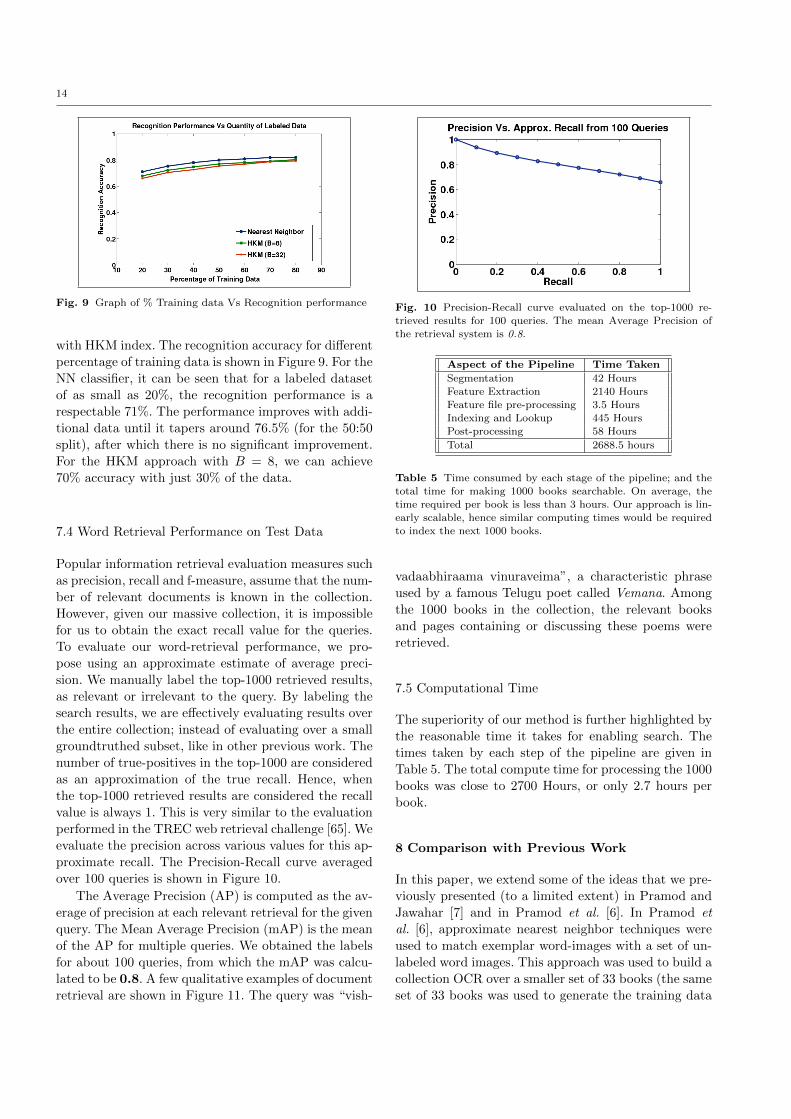
7.4 Word Retrieval Performance on Test Data

Popular information retrieval evaluation measures such

as precision, recall and f-measure, assume that the num-

ber of relevant documents is known in the collection.

However, given our massive collection, it is impossible

for us to obtain the exact recall value for the queries.

To evaluate our word-retrieval performance, we pro-

pose using an approximate estimate of average preci-

sion. We manually label the top-1000 retrieved results,

as relevant or irrelevant to the query. By labeling the

search results, we are effectively evaluating results over

the entire collection; instead of evaluating over a small

groundtruthed subset, like in other previous work. The

number of true-positives in the top-1000 are considered

as an approximation of the true recall. Hence, when

the top-1000 retrieved results are considered the recall

value is always 1. This is very similar to the evaluation

performed in the TREC web retrieval challenge [65]. We

evaluate the precision across various values for this ap-

proximate recall. The Precision-Recall curve averaged

over 100 queries is shown in Figure 10.

The Average Precision (AP) is computed as the av-

erage of precision at each relevant retrieval for the given

query. The Mean Average Precision (mAP) is the mean

of the AP for multiple queries. We obtained the labels

for about 100 queries, from which the mAP was calcu-

lated to be 0.8. A few qualitative examples of document

retrieval are shown in Figure 11. The query was “vish-

Fig. 10 Precision-Recall curve evaluated on the top-1000 re-trieved results for 100 queries. The mean Average Precision of

the retrieval system is 0.8.

Aspect of the Pipeline Time Taken

Segmentation 42 Hours

Feature Extraction 2140 Hours

Feature file pre-processing 3.5 HoursIndexing and Lookup 445 Hours

Post-processing 58 Hours

Total 2688.5 hours

Table 5 Time consumed by each stage of the pipeline; and the

total time for making 1000 books searchable. On average, the

time required per book is less than 3 hours. Our approach is lin-early scalable, hence similar computing times would be required

to index the next 1000 books.

vadaabhiraama vinuraveima”, a characteristic phrase

used by a famous Telugu poet called Vemana. Among

the 1000 books in the collection, the relevant books

and pages containing or discussing these poems were

retrieved.

7.5 Computational Time

The superiority of our method is further highlighted by

the reasonable time it takes for enabling search. The

times taken by each step of the pipeline are given in

Table 5. The total compute time for processing the 1000

books was close to 2700 Hours, or only 2.7 hours per

book.

8 Comparison with Previous Work

In this paper, we extend some of the ideas that we pre-

viously presented (to a limited extent) in Pramod and

Jawahar [7] and in Pramod et al. [6]. In Pramod et

al. [6], approximate nearest neighbor techniques were

used to match exemplar word-images with a set of un-

labeled word images. This approach was used to build a

collection OCR over a smaller set of 33 books (the same

set of 33 books was used to generate the training data

15

Fig. 11 Document images containing or discussing the poems written by Vemana were retrieved by querying for a characteristic

phrase used by the poet.

for this paper). On the other hand, in [7], word-images

from the document-images were matched against syn-

thetic labeled exemplars that were obtained by font-

rendering with a single canonical font. The word-images

and exemplars were represented using the profile fea-

tures [66], which were matched with a Dynamic Time

Warping (DTW) based distance measure. Due to this

distance measure, clustering of word-images was needed

to be performed using Hierarchical agglomerative clus-

tering. The approach was demonstrated over a collec-

tion of 500 books consisting of 75,000 document images

in the Telugu script. However, the clustering was com-

putationally intensive, requiring close to 21,000 hours of

computing (30 machines running for 30 days). This was

thus, not scalable to much larger collections; doubling

the dataset would have required twice the computing

time. Though the complexity of scaling is linear in col-

lection size, the constant is very large, making it quickly

unacceptable.

In this paper, we have modified the techniques, by

which we reduced the clustering and annotation process

to less than 500 hours, a speedup of more than 85 times.

This was achieved by representing word-images using

fixed-length representations, which allowed the use of

simpler distance metrics. The clustering is speeded up

using approximate-NN techniques such as Locality Sen-

sitive Hashing, KDTrees and Hierarchical K-Means. Fur-

ther, the synthetic labeled exemplars are replaced by

16

training samples obtained from document images. Due

to the similarity in appearance with word-images, the

new training exemplars significantly improved the la-

beling accuracy.

9 Conclusions

In this work, we have presented a successful and scal-

able framework to enable retrieval from a large collec-

tion of document images. Our approach is applicable to

many languages for which robust OCRs are not avail-

able. In future work, we could explore methods to allow

indexing of a much larger vocabulary, in the absence of

training data. This would enable retrieving for rare-

word queries, especially nouns. Further, we could con-

sider the possibility of applying similar techniques for

other visual recognition tasks.

Acknowledgments

This work was supported in part by the Ministry of

Communications and Information Technology, Govt. of

India. R. Manmatha was supported in part by the Cen-

ter for Intelligent Information Retrieval and by the Na-

tional Science Foundation grant #IIS-0910884. Any opin-

ions, findings and conclusions or recommendations ex-

pressed in this material are the authors and do not nec-

essarily reflect those of the sponsors.

References

1. Google Books at: http://books.google.com.

2. Internet Archive at: http://www.archive.org.

3. Universal Library at: http://www.ulib.org/.

4. Govindaraju, V., Setlur, S., eds.: Guide to OCR for Indic

Scripts. Springer (2009)

5. Kumar, K.S.S., Kumar, S., Jawahar, C.V.: On segmentation

of documents in complex scripts. In: Proc. ICDAR. (2007)1243–1247

6. Pramod Sankar K., Jawahar, C.V., Manmatha, R.: NearestNeighbor based Collection OCR. In: Proc. DAS. (2010)

7. Pramod Sankar, K., Jawahar, C.V.: Probabilistic reverseannotation for large scale image retrieval. In: Proc. CVPR.(2007)

8. IIIT-H Telugu Word Recognition Dataset, available at:

http://cvit.iiit.ac.in/index.php?page=resources.

9. Digital Library of India at: http://dli.iiit.ac.in.

10. Doermann, D.: The indexing and retrieval of document im-ages: a survey. Computer Vision and Image Understanding

70 (1998) 287–298

11. Marinai, S.: A survey of document image retrieval in digitallibraries. In: Colloque International Francophone sur l’Ecritet le Document (CIFED). (2006) 193–198

12. Kim, J., Seitz, S.M., Agrawala, M.: Video-based documenttracking: Unifying your physical and electronic desktops. In:Proc. UIST. (2004) 99–107

13. Nagy, G.: At the frontiers of OCR. IEEE 80 (1992) 1093–1100

14. Pal, U., Chaudhuri, B.: Indian script character recognition:

A survey. Pattern Recognition 37(9) (2004) 1887–189915. Tong, X., Evans, D.A.: A statistical approach to automatic

ocr error correction in context. In: Proc. WVLC. (1996) 88–

1016. Francesconi, E., Gori, M., Marinai, S., Soda, G.: A serial

combination of connectionist-based classifiers for OCR. IJ-DAR 3 (2001) 160–168

17. Byun, H., Lee, S.W.: Applications of support vector ma-

chines for pattern recognition: A survey. In: Proceedings

of the First International Workshop on Pattern Recognitionwith Support Vector Machines. (2002) 213–236

18. Jawahar, C.V., Kumar, M.P., Ravikiran, S.S.: A bilingual

OCR system for hindi-telugu documents and its applications.In: Proc ICDAR. (2003) 408–413

19. Kahan, S., Pavlidis, T., Baird, H.S.: On the recognition of

printed character of any font and size. IEEE PAMI 9(2)

(1987) 274–28820. Lehal, G.S., Singh, C., Lehal, R.: A shape based post proces-

sor for gurumukhi OCR. In: Proc. ICDAR. (2001) 1105–110921. Natarajan, P., MacRostie, E., Decerbo, M.: The BBN Byblos

Hindi OCR System. Guide to OCR for Indic Scripts (2009)173–180

22. Lu, Z., Schwartz, R., Natarajan, P., Bazzi, I., Makhoul, J.:

Advances in the bbn byblos ocr system. In: Proc. ICDAR.

(1999) 337–34023. Bharati, A., Rao, P., Sangal, R., Bendre, S.M.: Basic sta-

tistical analaysis of corpus and cross comparision. In: Proc.

ICON. (2002)24. Spitz, A.L.: Using character shape codes for word spotting in

document images. Shape, Structure and Pattern Recognition(1995) 382–389

25. Li, L., Lu, S.J., Tan, C.L.: A fast keyword-spotting technique.

In: Proc. ICDAR. (2007) 68–7226. Lu, S., Li, L., Tan, C.L.: Document image retrieval through

word shape coding. IEEE PAMI 30(11) (2008) 1913–191827. Kesidis, A.L., Galiotou, E., Gatos, B., Pratikakis, I.: A

word spotting framework for historical machine-printed doc-

uments. IJDAR 14 (2011) 131–14428. Rath, T.M., Manmatha, R.: Word spotting for historical

documents. IJDAR 9(2-4) (2007) 139–15229. Zhang, B., Srihari, S.N., Huang, C.: Word image retrieval

using binary features. In: DRR’04. (2004) 45–5330. Terasawa, K., Tanaka, Y.: Slit style hog feature for document

image word spotting. In: Proc. ICDAR. (2009) 116–12031. Llados, J., Sanchez, G.: Indexing historical documents by

word shape signatures. In: Proc. ICDAR. (2007) 362–36632. Meshesha, M., Jawahar, C.V.: Matching word images for

content-based retrieval from printed document images. IJ-DAR (2008) 29–38

33. Kuo, S.S., Agazzi, O.E.: Keyword spotting in poorly printeddocuments using pseudo 2-d hidden markov models. IEEE

PAMI 16 (1994) 842–84834. Nishi, H., Kimura, Y., Iguchi, R.: A new word spotting frame-

work using hough transform of distance matrix images. In:Proc. IMECS. (2010) 280–285

35. Frinken, V., Fischer, A., Bunke, H., Manmatha, R.: Adapt-ing BLSTM neural network based keyword spotting trained

on modern data to historical documents. In: Proc. ICFHR.

(2010) 352–35736. Jain, R., Frinken, V., Jawahar, C.V., Manmatha, R.: BLSTM

Neural Network based Word Retrieval for Hindi Documents.

In: Proc. ICDAR. (2011) 83–8737. Gatos, B., Pratikakis, I.: Segmentation-free word spotting

in historical printed documents. In: Proc. ICDAR. (2009)271–275

17

38. Madhvanath, S., Govindaraju, V.: The role of holisticparadigms in handwritten word recognition. IEEE PAMI

23 (2001) 149–16439. Srihari, S., Srinivasan, H., Babu, P., Bhole, C.: Handwritten

arabic word spotting using the cedarabic document analysissystem. In: Proc. Symposium on Document Image Under-

standing Technology (SDIUT). (2005) 123–13240. Adamek, T., O’Connor, N.E., Smeaton, A.F.: Word match-

ing using single closed contours for indexing handwritten his-torical documents. IJDAR 9(2-4) (2007) 153–165

41. Kumar, A., Jawahar, C.V., Manmatha, R.: Efficient search

in document image collections. In: Proc. ACCV. (2007) 586–

59542. Rath, T., Manmatha, R., Lavrenko, V.: A search engine for

historical manuscript images. In: Proc. SIGIR. (2004) 369–

37643. Atul Negi, Chakravarthy Bhagvati, B.K.: An ocr system for

telugu. In: Proc. ICDAR. (2001) 1110–111444. Rice, S.V., Jenkins, F.R., Nartker, T.A.: The fifth annual

test of ocr accuracy. Technical report, UNLV (1996)45. Ataer, E., Duygulu, P.: Matching Ottoman words: An image

retrieval approach to historical document indexing. In: Proc.

CIVR. (2007) 341–34746. Xiu, P., Baird, H.S.: Scaling up whole-book recognition. In:

Proc. ICDAR. (2009) 698–70247. Konidaris, T., Gatos, B., Ntzios, K., Pratikakis, I., Theodor-

idis, S., Perantonis, S.J.: Keyword-guided word spotting in

historical printed documents with synthetic data and userfeedback. IJDAR (2007) 167–177

48. Lavrenko, V., Rath, T.M., Manmatha, R.: Holistic wordrecognition for handwritten historical documents. In: Proc.

DIAL. (2004) 278–28749. Chan, J., Ziftci, C., Forsyth, D.A.: Searching off-line arabic

documents. In: Proc. CVPR. (2006) 1455–146250. Lemur search engine: http://www.lemurproject.org/.51. Galago search engine: http://www.galagosearch.org/.52. Zipf, G.: Human Behaviour and the Principle of Least Effort.

Addison-Wesley, Cambridge, MA (1949)53. Liu, T.Y., Yang, Y., Wan, H., Zeng, H.J., Chen, Z., Ma,

W.Y.: Support vector machines classification with a very

large-scale taxonomy. SIGKDD Explor. Newsl. 7 (2005) 36–43

54. Deng, J., Berg, A.C., Li, K., Fei-Fei, L.: What does classifyingmore than 10, 000 image categories tell us? In: ECCV (5).

(2010) 71–8455. Nister, D., Stewenius, H.: Scalable recognition with a vocab-

ulary tree. In: Proc. CVPR. (2006) 2161–216856. Indyk, P., Motwani, R.: Approximate nearest neighbors: to-

wards removing the curse of dimensionality. In: Proc. STOC.

(1998) 604–61357. Muja, M., Lowe, D.G.: Fast approximate nearest neighbors

with automatic algorithm configuration. In: Proc. VISAPP.(2009) 331–340

58. Andoni, A., Datar, M., Immorlica, N., Indyk, P., Mirrokni,V.: Locality-sensitive hashing scheme based on p-stable dis-

tributions. Nearest Neighbor Methods in Learning and Vi-sion: Theory and Practice (2006)

59. Philbin, J., Chum, O., Isard, M., Sivic, J., Zisserman, A.:

Lost in quantization: Improving particular object retrieval

in large scale image databases. In: Proc. CVPR. (2008)60. Rath, T.M., Manmatha, R.: Word image matching using

dynamic time warping. In: Proc. CVPR. (2003) 521–52761. Balasubramanian, A., Meshesha, M., Jawahar, C.V.: Re-

trieval from document image collections. In: Proc. DAS.

(2006) 1–1262. Lowe, D.G.: Distinctive image features from scale-invariant

keypoints. IJCV 60(2) (2004) 91–110

63. Dalal, N., Triggs, B.: Histograms of oriented gradients for

human detection. In: Proc. CVPR. (2005) 886–89364. Bosch, A., Zisserman, A., Munoz, X.: Scene classification

using a hybrid generative/discriminative approach. IEEE

PAMI 30(4) (2008) 712–72765. C.L.A. Clarke, N. Craswell, I. Soboroff, Overview of the

TREC 2009 Web Track (online resource).

66. Rath, T., Manmatha, R.: Features for word matching inhistorical manuscripts. In: Proc. ICDAR. (2003) 218–222