J. Fluid Mech. (2003), vol. 484, pp. 223–253. c 2003 Cambridge University Press DOI: 10.1017/S0022112003004257 Printed in the United Kingdom 223 Large-eddy simulations of ducts with a free surface By RICCARDO BROGLIA 1 , ANDREA PASCARELLI 1 AND UGO PIOMELLI 2 1 INSEAN, Via di Vallerano 139, 00128 Roma, Italy 2 Department of Mechanical Engineering, University of Maryland, College Park, MD 20742, USA (Received 27 March 2002 and in revised form 7 January 2003) This work studies the momentum and energy transport mechanisms in the corner between a free surface and a solid wall. We perform large-eddy simulations of the incompressible fully developed turbulent flow in a square duct bounded above by a free-slip wall, for Reynolds numbers based on the mean friction velocity and the duct width equal to 360, 600 and 1000. The flow in the corner is strongly affected by the advection due to two counter-rotating secondary-flow regions present immediately below the free surface. Because of the convection of the inner eddy, as the free surface is approached, the friction velocity on the sidewall first decreases, then increases again. A similar behaviour is observed for the surface-parallel Reynolds-stress components, which first decrease and then increase again very close to the surface. The budgets of the Reynolds stresses show a strong reduction of all terms of the dissipation tensor in both the inner and outer near-corner regions. They exhibit a reduction in both production and dissipation towards the free surface. Very close to the solid boundary, within 15–20 viscous lengths of the sidewall, the turbulent kinetic energy production and the surface-parallel fluctuations rebound in the thin layer adjacent to the free surface. The Reynolds-stress anisotropy appears to be the main factor in the generation of the mean secondary flow. The multi-layer structure of the boundary layer near the free surface is also discussed. 1. Introduction Mixed-boundary corner flows occur at the juncture of a no-slip wall and a free surface. They can be found in a variety of practical applications: the flow around hulls of ships is perhaps the most common example of this configuration, which also occurs on the sidewall boundary of an open channel or of a partially filled container, and in rivers. An important feature of these flows is the interaction of wall turbulence with a free surface. When turbulence interacts with either a free surface or a solid wall, it becomes highly anisotropic. The character of the anisotropy, however, is substantially different in the two cases. A free surface cannot support mean shear, and restricts motion in the direction normal to the surface only, while a solid wall forces all the velocity components to vanish at the boundary. The no-slip condition at a solid wall makes turbulence production and dissipation significant there, whereas at a free surface turbulence production is negligible and the dissipation rate is smaller than in the bulk of the flow because of the vanishing of the velocity gradients. Near a mixed-boundary corner, the interaction of the eddies generated by these different

Welcome message from author
This document is posted to help you gain knowledge. Please leave a comment to let me know what you think about it! Share it to your friends and learn new things together.
Transcript

J. Fluid Mech. (2003), vol. 484, pp. 223–253. c© 2003 Cambridge University Press
DOI: 10.1017/S0022112003004257 Printed in the United Kingdom223
Large-eddy simulations of ducts witha free surface
By RICCARDO BROGLIA1, ANDREA PASCARELLI1
AND UGO PIOMELLI21INSEAN, Via di Vallerano 139, 00128 Roma, Italy
2Department of Mechanical Engineering, University of Maryland, College Park,MD 20742, USA
(Received 27 March 2002 and in revised form 7 January 2003)
This work studies the momentum and energy transport mechanisms in the cornerbetween a free surface and a solid wall. We perform large-eddy simulations of theincompressible fully developed turbulent flow in a square duct bounded above by afree-slip wall, for Reynolds numbers based on the mean friction velocity and the ductwidth equal to 360, 600 and 1000. The flow in the corner is strongly affected by theadvection due to two counter-rotating secondary-flow regions present immediatelybelow the free surface. Because of the convection of the inner eddy, as the free surfaceis approached, the friction velocity on the sidewall first decreases, then increases again.A similar behaviour is observed for the surface-parallel Reynolds-stress components,which first decrease and then increase again very close to the surface. The budgetsof the Reynolds stresses show a strong reduction of all terms of the dissipationtensor in both the inner and outer near-corner regions. They exhibit a reduction inboth production and dissipation towards the free surface. Very close to the solidboundary, within 15–20 viscous lengths of the sidewall, the turbulent kinetic energyproduction and the surface-parallel fluctuations rebound in the thin layer adjacent tothe free surface. The Reynolds-stress anisotropy appears to be the main factor in thegeneration of the mean secondary flow. The multi-layer structure of the boundarylayer near the free surface is also discussed.
1. IntroductionMixed-boundary corner flows occur at the juncture of a no-slip wall and a free
surface. They can be found in a variety of practical applications: the flow aroundhulls of ships is perhaps the most common example of this configuration, whichalso occurs on the sidewall boundary of an open channel or of a partially filledcontainer, and in rivers. An important feature of these flows is the interaction of wallturbulence with a free surface. When turbulence interacts with either a free surface ora solid wall, it becomes highly anisotropic. The character of the anisotropy, however,is substantially different in the two cases. A free surface cannot support mean shear,and restricts motion in the direction normal to the surface only, while a solid wallforces all the velocity components to vanish at the boundary. The no-slip conditionat a solid wall makes turbulence production and dissipation significant there, whereasat a free surface turbulence production is negligible and the dissipation rate is smallerthan in the bulk of the flow because of the vanishing of the velocity gradients. Neara mixed-boundary corner, the interaction of the eddies generated by these different
224 R. Broglia, A. Pascarelli and U. Piomelli
mechanisms creates additional physical complexities (compared either with the freesurface or the solid wall alone) that affect the transport of mass, momentum andenergy. In order to predict the flow fields in the applications mentioned above, betterunderstanding of their physics is required.
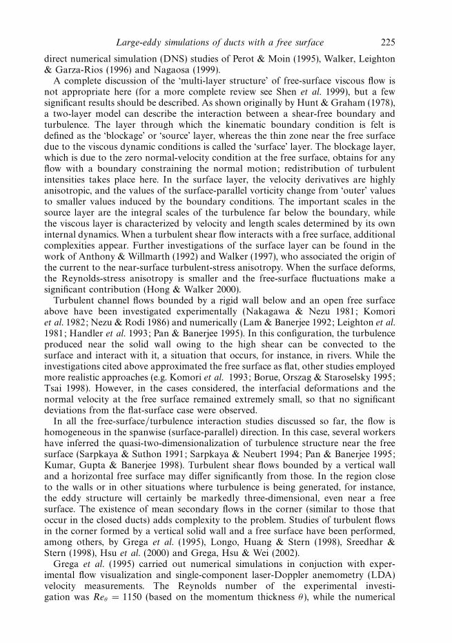
The characteristics of the flow near a solid flat surface are well known and willnot be discussed here. Descriptions of the statistical aspects of the flow and ofthe turbulent eddies can be found in many textbooks and reviews (see, e.g. Pope2000; Robinson 1991). The structure of the wall turbulence, however, is significantlyaltered in the corner between two solid walls, where the anisotropy of the Reynoldsstresses generates turbulence-driven secondary flows in the plane perpendicular to thestreamwise direction, commonly referred to as ‘secondary flows of Prandtl’s secondkind’. In straight square ducts, the secondary flow is directed from the centre of theduct toward the corners along the corner bisectors. Although the magnitude of thesesecondary velocities is extremely small (of the order of 2–3% of the bulk streamwisevelocity), the distortion of the axial flow can alter the distribution of the frictioncoefficient (and thus the mean flow).
Because of the complex physics coupled with a simple geometry, these flows havebeen studied extensively, both experimentally and numerically. While the experiments(Launder & Ying 1972; Melling & Whitelaw 1976; Gessner, Po & Emery 1979) werethe first to quantify the mean flow, numerical calculations (Madabhushi & Vanka1991; Gavrilakis 1992; Huser & Biringen 1993; Huser, Biringen & Hatay 1994; Su &Friedrich 1994) have been instrumental in addressing questions related to turbulentkinetic energy (TKE) production and transfer, as well as to the modifications tothe turbulence structure in these configurations. Huser et al. (1994) investigatedthe details of the Reynolds stress budgets and performed quadrant analysis toexamine the dominant structures which give rise to the generation of secondary flows.They observed that the dominant ejections contain two streamwise counter-rotatingvortices.
Modifications to the turbulence structure occur also when turbulence interacts witha free surface, where the relative velocity between the fluid and the surface interfacevanishes, the tangential stresses are zero, and the normal stress must balance theambient pressure. In addition, in the free-surface case, the boundary can deform. Ifthe free surface can be considered flat, the tangential vorticity vanishes at the freesurface but not the component normal to the surface, while in the case of a shear-free deformed free surface, the vorticity at the free surface is non-zero and the surfaceacquires a solid-body rotation. The non-dimensional groups that appear in theseflows are the Reynolds number, the Froude number and the Weber number, definedas Fr = ur/
√glr and We = ρlru
2r /σs , respectively, where g is the acceleration due to
gravity, σs the surface tension, and ur and lr are a reference velocity and length. TheFroude number, which is related to the deformation of the free surface, is the mostimportant one for the present study; low Froude numbers correspond to negligiblefree-surface deformations.
Perhaps the main feature of the interaction of turbulence with the free surface isthe modification of the inter-component energy transfer, which has been observedby virtually all the workers who have examined this problem. In the boundary layeradjacent to the free surface, the fluctuations parallel to the surface are essentiallyunaltered, while the Reynolds-stress component normal to the surface is redistributedinto surface-parallel components, which increase with decreasing distance from thefree surface. In the case of a free-slip flat surface, a picture of the vortex/surfaceinteractions on the dynamics of turbulence under the free surface emerges from the
Large-eddy simulations of ducts with a free surface 225
direct numerical simulation (DNS) studies of Perot & Moin (1995), Walker, Leighton& Garza-Rios (1996) and Nagaosa (1999).
A complete discussion of the ‘multi-layer structure’ of free-surface viscous flow isnot appropriate here (for a more complete review see Shen et al. 1999), but a fewsignificant results should be described. As shown originally by Hunt & Graham (1978),a two-layer model can describe the interaction between a shear-free boundary andturbulence. The layer through which the kinematic boundary condition is felt isdefined as the ‘blockage’ or ‘source’ layer, whereas the thin zone near the free surfacedue to the viscous dynamic conditions is called the ‘surface’ layer. The blockage layer,which is due to the zero normal-velocity condition at the free surface, obtains for anyflow with a boundary constraining the normal motion; redistribution of turbulentintensities takes place here. In the surface layer, the velocity derivatives are highlyanisotropic, and the values of the surface-parallel vorticity change from ‘outer’ valuesto smaller values induced by the boundary conditions. The important scales in thesource layer are the integral scales of the turbulence far below the boundary, whilethe viscous layer is characterized by velocity and length scales determined by its owninternal dynamics. When a turbulent shear flow interacts with a free surface, additionalcomplexities appear. Further investigations of the surface layer can be found in thework of Anthony & Willmarth (1992) and Walker (1997), who associated the origin ofthe current to the near-surface turbulent-stress anisotropy. When the surface deforms,the Reynolds-stress anisotropy is smaller and the free-surface fluctuations make asignificant contribution (Hong & Walker 2000).
Turbulent channel flows bounded by a rigid wall below and an open free surfaceabove have been investigated experimentally (Nakagawa & Nezu 1981; Komoriet al. 1982; Nezu & Rodi 1986) and numerically (Lam & Banerjee 1992; Leighton et al.1981; Handler et al. 1993; Pan & Banerjee 1995). In this configuration, the turbulenceproduced near the solid wall owing to the high shear can be convected to thesurface and interact with it, a situation that occurs, for instance, in rivers. While theinvestigations cited above approximated the free surface as flat, other studies employedmore realistic approaches (e.g. Komori et al. 1993; Borue, Orszag & Staroselsky 1995;Tsai 1998). However, in the cases considered, the interfacial deformations and thenormal velocity at the free surface remained extremely small, so that no significantdeviations from the flat-surface case were observed.
In all the free-surface/turbulence interaction studies discussed so far, the flow ishomogeneous in the spanwise (surface-parallel) direction. In this case, several workershave inferred the quasi-two-dimensionalization of turbulence structure near the freesurface (Sarpkaya & Suthon 1991; Sarpkaya & Neubert 1994; Pan & Banerjee 1995;Kumar, Gupta & Banerjee 1998). Turbulent shear flows bounded by a vertical walland a horizontal free surface may differ significantly from those. In the region closeto the walls or in other situations where turbulence is being generated, for instance,the eddy structure will certainly be markedly three-dimensional, even near a freesurface. The existence of mean secondary flows in the corner (similar to those thatoccur in the closed ducts) adds complexity to the problem. Studies of turbulent flowsin the corner formed by a vertical solid wall and a free surface have been performed,among others, by Grega et al. (1995), Longo, Huang & Stern (1998), Sreedhar &Stern (1998), Hsu et al. (2000) and Grega, Hsu & Wei (2002).
Grega et al. (1995) carried out numerical simulations in conjuction with exper-imental flow visualization and single-component laser-Doppler anemometry (LDA)velocity measurements. The Reynolds number of the experimental investi-gation was Reθ = 1150 (based on the momentum thickness θ), while the numerical
226 R. Broglia, A. Pascarelli and U. Piomelli
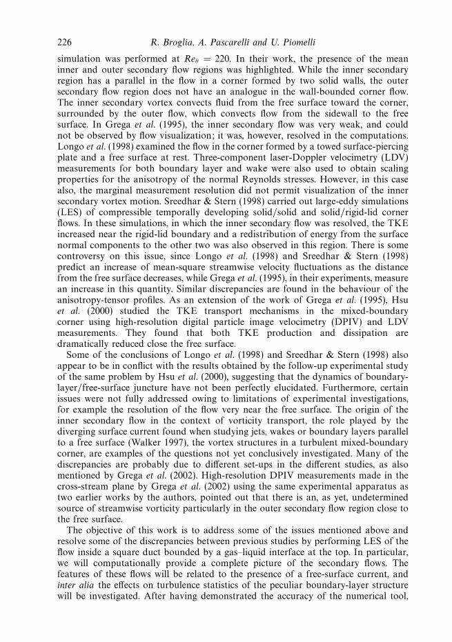
simulation was performed at Reθ = 220. In their work, the presence of the meaninner and outer secondary flow regions was highlighted. While the inner secondaryregion has a parallel in the flow in a corner formed by two solid walls, the outersecondary flow region does not have an analogue in the wall-bounded corner flow.The inner secondary vortex convects fluid from the free surface toward the corner,surrounded by the outer flow, which convects flow from the sidewall to the freesurface. In Grega et al. (1995), the inner secondary flow was very weak, and couldnot be observed by flow visualization; it was, however, resolved in the computations.Longo et al. (1998) examined the flow in the corner formed by a towed surface-piercingplate and a free surface at rest. Three-component laser-Doppler velocimetry (LDV)measurements for both boundary layer and wake were also used to obtain scalingproperties for the anisotropy of the normal Reynolds stresses. However, in this casealso, the marginal measurement resolution did not permit visualization of the innersecondary vortex motion. Sreedhar & Stern (1998) carried out large-eddy simulations(LES) of compressible temporally developing solid/solid and solid/rigid-lid cornerflows. In these simulations, in which the inner secondary flow was resolved, the TKEincreased near the rigid-lid boundary and a redistribution of energy from the surfacenormal components to the other two was also observed in this region. There is somecontroversy on this issue, since Longo et al. (1998) and Sreedhar & Stern (1998)predict an increase of mean-square streamwise velocity fluctuations as the distancefrom the free surface decreases, while Grega et al. (1995), in their experiments, measurean increase in this quantity. Similar discrepancies are found in the behaviour of theanisotropy-tensor profiles. As an extension of the work of Grega et al. (1995), Hsuet al. (2000) studied the TKE transport mechanisms in the mixed-boundarycorner using high-resolution digital particle image velocimetry (DPIV) and LDVmeasurements. They found that both TKE production and dissipation aredramatically reduced close the free surface.
Some of the conclusions of Longo et al. (1998) and Sreedhar & Stern (1998) alsoappear to be in conflict with the results obtained by the follow-up experimental studyof the same problem by Hsu et al. (2000), suggesting that the dynamics of boundary-layer/free-surface juncture have not been perfectly elucidated. Furthermore, certainissues were not fully addressed owing to limitations of experimental investigations,for example the resolution of the flow very near the free surface. The origin of theinner secondary flow in the context of vorticity transport, the role played by thediverging surface current found when studying jets, wakes or boundary layers parallelto a free surface (Walker 1997), the vortex structures in a turbulent mixed-boundarycorner, are examples of the questions not yet conclusively investigated. Many of thediscrepancies are probably due to different set-ups in the different studies, as alsomentioned by Grega et al. (2002). High-resolution DPIV measurements made in thecross-stream plane by Grega et al. (2002) using the same experimental apparatus astwo earlier works by the authors, pointed out that there is an, as yet, undeterminedsource of streamwise vorticity particularly in the outer secondary flow region close tothe free surface.
The objective of this work is to address some of the issues mentioned above andresolve some of the discrepancies between previous studies by performing LES of theflow inside a square duct bounded by a gas–liquid interface at the top. In particular,we will computationally provide a complete picture of the secondary flows. Thefeatures of these flows will be related to the presence of a free-surface current, andinter alia the effects on turbulence statistics of the peculiar boundary-layer structurewill be investigated. After having demonstrated the accuracy of the numerical tool,
Large-eddy simulations of ducts with a free surface 227
we will study the inner secondary flow in the context of the streamwise budgetof momentum equation and vorticity transport; then, we will attempt to providea detailed description of the turbulent energy transport mechanisms in the mixed-boundary corner. The use of LES (rather than DNS) allows us to perform calculationsat three Reynolds numbers, Reτ = 360, 600 and 1000 (based on the mean frictionvelocity and the duct width).
The paper is organized as follow: in the next section, the problem formulation,numerical method and subgrid-scale model used are briefly described. Then, theresults of a closed-duct calculation will be presented to validate the code. Discussionof the mean flow, Reynolds stress and vorticity statistics will follow. Finally, someconclusions will be drawn in the last section.
2. Problem formulation2.1. Governing equations and numerical method
The governing equations for LES are obtained by the application of a spatial filterto the Navier–Stokes equations to separate the effects of the (large) resolved scalefrom the (small) subgrid-scale (SGS) eddies; in the case of an incompressible viscousflow in presence of body forces, they can be written in the following form:
∂ui
∂t+
∂
∂xj
(ujui) = − ∂p
∂xi
+1
Reτ
∇2ui − ∂τji
∂xj
+ fi,∂uj
∂xj
= 0, (2.1)
where the overbar denotes filtered variables and the effect of the subgrid scales appearsthrough the SGS stresses τij = uiuj − uiuj ; uj is the fluid velocity component in thej -direction and p is the pressure divided by the constant density. Equations (2.1) arenon-dimensionalized using the mean friction velocity, uτ , and the duct width, D, ascharacteristic velocity and length scales, respectively. Thus, the Reynolds number isdefined as Reτ = uτD/ν, where ν is the kinematic viscosity. The flow is driven bya constant body force per unit mass, f1. Periodic boundary conditions are used inthe streamwise directions and no-slip boundary conditions are imposed on walls. Theboundary conditions enforced on the top surface of the computational domain areeither the no-slip conditions
u = 0, v = 0, w = 0, (2.2)
or the no-stress boundary conditions
∂u
∂z= 0,
∂v
∂z= 0, w = 0. (2.3)
Despite the limitations of these assumptions, previous numerical studies have shownthat a rigid free-slip wall approximation allows us to predict many of the phenomenaseen in experiments with waveless interfaces (Lam & Banerjee 1992; Leighton et al.1981; Handler et al. 1993; Pan & Banerjee 1995).
In the present work, the SGS stresses τij are parameterized by an eddy-viscositymodel of the form:
τij − 13δij τkk = −2νTSij = −2C�2|S|Sij , (2.4)
where δij is Kronecker’s delta, |S| = (2SijSij )1/2 is the magnitude of the large-
scale strain-rate tensor Sij = (∂ui/∂xj + ∂uj/∂xi)/2, and � = 2 (�x�y�z)1/3 is thefilter width. Closure of the SGS stresses τij is obtained through specification of the
228 R. Broglia, A. Pascarelli and U. Piomelli
model coefficient C appearing in (2.4). In the present work, the dynamic procedureproposed by Germano et al. (1991) and Lilly (1992) is used to determine the eddy-viscosity coefficient C. The constant C is averaged along the homogeneous streamwisedirection; this type of averaging is effective in removing spurious fluctuations of C
which tend to destabilize the calculations, and has been used in several calculationsof turbulent flows that are homogeneous in one direction only (Akselvoll & Moin1996; Mittal & Moin 1997), with accurate results. The sum of the laminar and eddyviscosity is set to zero wherever it becomes negative.
The numerical approach employed for the solution of (2.1) is the fractional stepmethod (Chorin 1967; Kim & Moin 1985). The time-advancement for the intermediateadvection-diffusion step is performed in a semi-implicit fashion with a two-substepsecond-order accurate Runge–Kutta algorithm. This is followed by the pressure-correction step, which enforces the divergence-free condition; the Poisson equationfor the pressure-like function is solved once per time step. All the spatial derivatives areapproximated using a second-order-accurate central discretization on a non-uniformcollocated grid. Solution of the Poisson equation is obtained by means of a successivelyover-relaxed Gauss–Seidel method; a multigrid algorithm of a correction-scheme typeis used to accelerate the convergence toward the solution. Implicit treatment of thediffusive terms allows a larger time step, which is only limited by the explicit treatmentof the advective and SGS terms. The overall accuracy of the method is second orderin time and space.
Parallelization of the code is achieved by an effective domain decompositiontechnique; the domain is divided into a number of subdomains along the streamwisedirection. Communications between processors are made by using the message-passingprogramming and the send, receive and reduce statements of the message-passinglibrary Message-Passing Interface (MPI). This algorithm is described in detail inBroglia, Di Mascio & Muscari (1999).
2.2. Geometry and grid parameters
The Navier–Stokes equations are solved numerically in a rectangular domain of size2πD × D × D in the x-, y- and z-directions, respectively. The streamwise length of thedomain was chosen based on the two-point velocity correlations computed by Huser &Biringen (1993) to ensure that the domain is large enough to contain the longeststructure present in the flow.
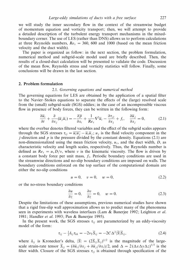
The physical domain is discretized using between 4.7 × 10⁵ grid points for the low-Reynolds-number simulation, and 5.6×10⁶ grid points for the high-Reynolds-numberone. All the discretizations are uniform in the streamwise (x) direction, whereas in thespanwise and normal directions (y and z, respectively) points are clustered towardsthe walls; in particular, for all the simulations, the first point close to the wall isplaced at y+ or z+ = 0.5 and at least 13 points are in the near-wall region (y+ orz+ < 10). Points are also clustered toward the slip wall, with a minimum grid spacingof about 1.5 wall units for the high Reynolds numbers and 0.5 for the lowest one.The problem geometry is sketched in figure 1, and the mesh characteristics are givenin table 1.
The equations were integrated in time until a statistical steady state was reached(the steady state was determined by monitoring the time history of the total wallshear stress). After that, data for the statistics were collected for several large-eddyturnover times (LETOTs) D/uτ . Streamwise homogeneity and symmetry about theplane y = 0.5D were used to increase the sample size. The sampling interval for eachcase (also in LETOTs) is reported in table 2. The relevant non-dimensional parameters
Large-eddy simulations of ducts with a free surface 229
�y+ �z+ Points inSimulation nx × ny × nz �x+ min–max min–max y+ or z+ < 10
Closed duct, Reτ = 360 50 × 97 × 97 48.1 0.5–8.1 0.5–8.1 13Closed duct, Reτ = 600 82 × 129 × 129 47.7 0.5–10.7 0.5–10.7 14Open duct, Reτ = 360 50 × 97 × 97 48.1 0.5–8.1 0.5–8.1 13Open duct, Reτ = 600 82 × 129 × 129 47.7 0.5–10.7 0.5–10.7 14Open duct, Reτ = 1000 144 × 197 × 197 43.9 0.5–11.6 0.5–11.9 15
Table 1. Grid characteristics.
Simulation Sampling time �t Ub Uc Computed uτ Reb
Duct Reτ = 360 16.19 15.35 19.30 1.0012 5526Duct Reτ = 600 9.42 16.54 20.27 1.0055 9924Open duct Reτ = 360 12.77 15.48 18.39 1.0006 5571Open duct Reτ = 600 13.08 16.41 19.12 1.0024 9844Open duct Reτ = 1000 5.03 17.13 20.12 0.9953 17 130
Table 2. Averaging and global flow characteristics. Uc is the maximum velocity in the duct.
Solid wall
Free-slip wall
z
x
Ly = 1
Lz = 1
Lx = 2π
y
z
Ly = 1
Lz
= 1
Lx = 2π
y
x
Figure 1. Sketch of the problems.
are the Reynolds number based on the friction velocity uτ and the duct width D,Reτ = uτD/ν, and the bulk Reynolds number defined using the bulk (area-averaged)streamwise velocity Ub, Reb = UbD/ν. In table 2, the Reynolds numbers and someglobal results of the present simulations are shown. The value of uτ obtained fromthe calculations is within 0.5% of the nominal value uτ = 1. This difference suppliesan estimate of the sampling error for the first- and second-order statistics, which was,respectively, 0.5% and 1%.
In the following discussions, the angular brackets, 〈·〉, denote an average over timeand the homogeneous direction, whereas a double prime denotes fluctuation withrespect to mean resolved quantity, q ′′ = q − 〈q〉; thus, the resolved quantities aredecomposed into mean values and resolved fluctuations:
ui = 〈ui〉 + u′′i , p = 〈p〉 + p′′, τij = 〈τij 〉 + τ ′′
ij . (2.5)
230 R. Broglia, A. Pascarelli and U. Piomelli
20
15
10
5
0100 101 102
(a)
u+ = y+
u+ = 2.5 ln (y+) + 5.5
⟨u+⟩
y+
⟨�w⟩
1.5
1.0
0.5
0 0.1 0.2 0.3 0.4 0.5
y
(b)
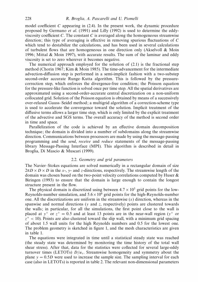
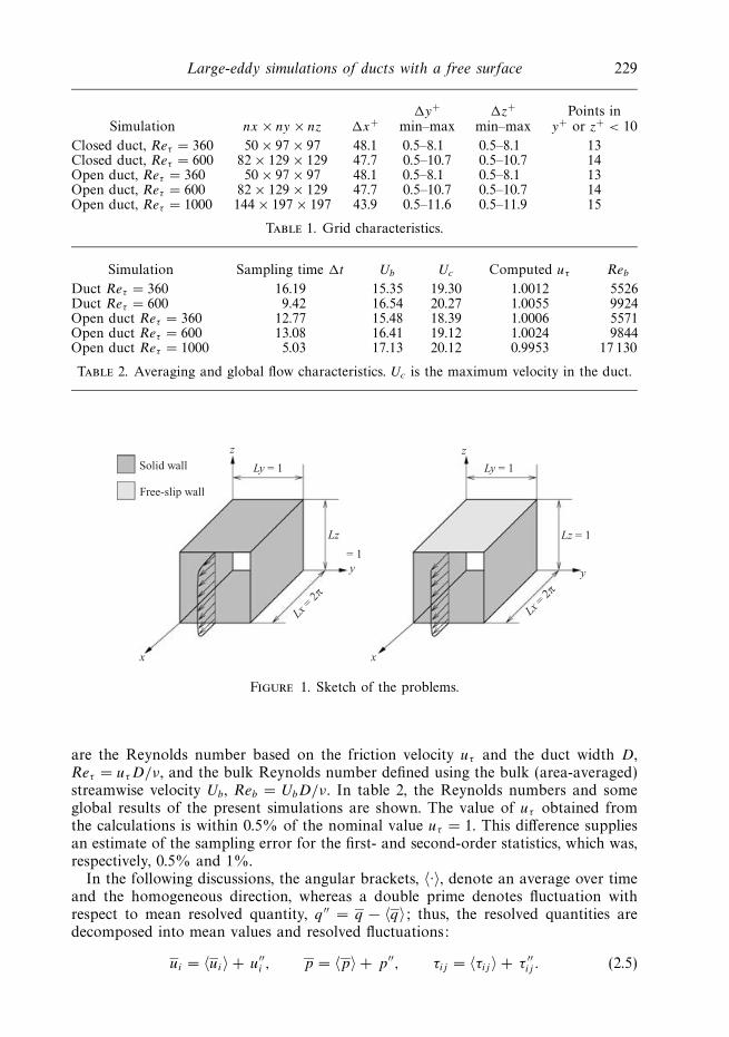
Figure 2. Duct flow. (a) Mean streamwise velocity profiles along the wall bisector; (b) wallstress distribution along the sidewall. ——, Reτ = 360; · · · · · ·,Reτ = 600; �, DNS at Reτ = 300(Gavrilakis 1992); �, DNS at Reτ = 600 (Huser & Biringen 1993).
3.5
0 0.1
(a)
u rm
s
y
1.5
y
(b) (c)3.0
2.5
2.0
1.5
1.0
0.5
0.2 0.3 0.4 0.5 0 0.1
v rm
s
1.0
0.5
0.2 0.3 0.4 0.5
1.5
0 0.1
wrm
s
1.0
0.5
0.2 0.3 0.4 0.5y
Figure 3. Duct flow. Root mean square velocity fluctuations along the wall bisector. (a) u;(b) v; (c) w. ——, Reτ = 360; – – –, Reτ = 600; �, DNS at Reτ = 300 (Gavrilakis 1992); �,DNS at Reτ = 600 (Huser & Biringen 1993).
Thus, the averaged resolved velocity and turbulent stresses are denoted by 〈ui〉 and〈u′′
i u′′j 〉, respectively.
3. Results and discussion3.1. Validation: closed duct flow
To determine the accuracy of the present numerical method in configurations similarto the open duct, LES of fully developed turbulent flow in a closed square ductwere performed and compared with the available DNS data. The current LESsolutions at Reτ = 360 and 600 are compared with low-Reynolds-number DNSsolution by Gavrilakis (1992) at Reτ = 300 (Reb = 4410) and with those by Huser &Biringen (1993) at Reτ = 600 (Reb = 10 320).
Mean turbulent statistics are shown in figures 2 and 3. Here and in the following,unless otherwise stated, all quantities are normalized using the mean uτ and D. Theagreement with the DNS data is good. In particular, the overshoot in the logarithmiclayer (figure 2a) observed in the DNS is captured quite well. The main topologicalfeatures of the flow, such as the secondary vortices often observed in the corner region,are also captured well. Gavrilakis (1992) performed a DNS using a second-order finitedifference on a staggered grid with up to 16.1×10⁶ grid points (768×127×127) and a
Large-eddy simulations of ducts with a free surface 231
(b)1.0
0.5
0 0.5
19
1
1.0
0.5
0 0.5
20
–20
y
(e)
0 0.5y
0.5
0
1.0
20
–20
(c)1.0
0.5
19
1
( f )
0.5
0 0.5y
(a)1.0
z 0.5
0 0.5
19
1
(d )1.0
z 0.5
20
–20
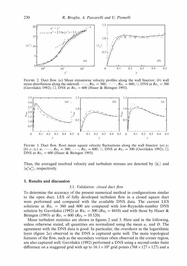
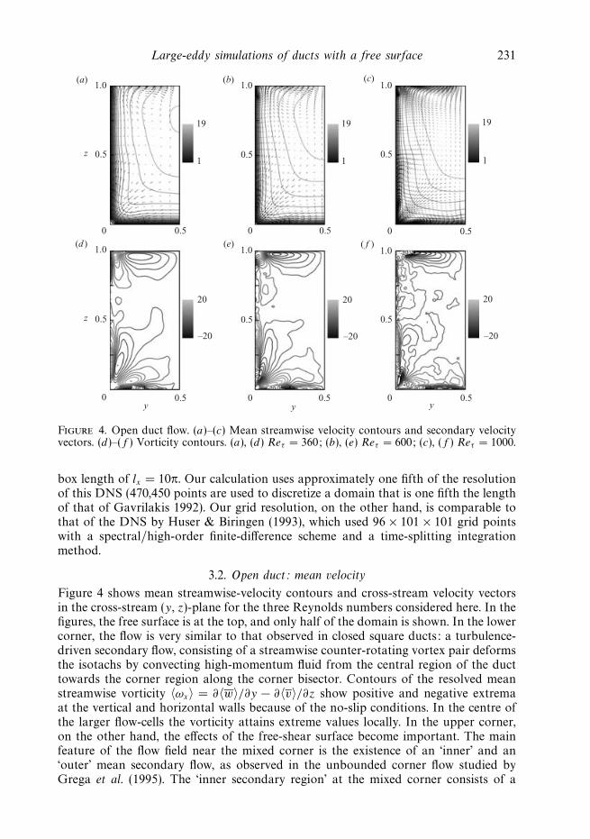
Figure 4. Open duct flow. (a)–(c) Mean streamwise velocity contours and secondary velocityvectors. (d)–(f ) Vorticity contours. (a), (d) Reτ = 360; (b), (e) Reτ = 600; (c), (f ) Reτ = 1000.
box length of lx = 10π. Our calculation uses approximately one fifth of the resolutionof this DNS (470,450 points are used to discretize a domain that is one fifth the lengthof that of Gavrilakis 1992). Our grid resolution, on the other hand, is comparable tothat of the DNS by Huser & Biringen (1993), which used 96 × 101 × 101 grid pointswith a spectral/high-order finite-difference scheme and a time-splitting integrationmethod.
3.2. Open duct: mean velocity
Figure 4 shows mean streamwise-velocity contours and cross-stream velocity vectorsin the cross-stream (y, z)-plane for the three Reynolds numbers considered here. In thefigures, the free surface is at the top, and only half of the domain is shown. In the lowercorner, the flow is very similar to that observed in closed square ducts: a turbulence-driven secondary flow, consisting of a streamwise counter-rotating vortex pair deformsthe isotachs by convecting high-momentum fluid from the central region of the ducttowards the corner region along the corner bisector. Contours of the resolved meanstreamwise vorticity 〈ωx〉 = ∂〈w〉/∂y − ∂〈v〉/∂z show positive and negative extremaat the vertical and horizontal walls because of the no-slip conditions. In the centre ofthe larger flow-cells the vorticity attains extreme values locally. In the upper corner,on the other hand, the effects of the free-shear surface become important. The mainfeature of the flow field near the mixed corner is the existence of an ‘inner’ and an‘outer’ mean secondary flow, as observed in the unbounded corner flow studied byGrega et al. (1995). The ‘inner secondary region’ at the mixed corner consists of a
232 R. Broglia, A. Pascarelli and U. Piomelli
20
15
10
5
0100 101 102
(a)
u+ = z+
u+ = 2.5 ln (z+) + 5.5
⟨u+⟩
z+
⟨u� ⟩
1.2
0.4
0.2
0 0.2 0.4 0.6 0.8 1.0z
(b)
101
0.6
0.8
1.0
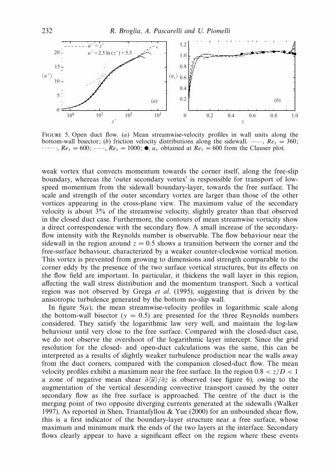
Figure 5. Open duct flow. (a) Mean streamwise-velocity profiles in wall units along thebottom-wall bisector; (b) friction velocity distributions along the sidewall. ——, Reτ = 360;· · · · · ·, Reτ = 600; – – –, Reτ = 1000; �, uτ obtained at Reτ = 600 from the Clauser plot.
weak vortex that convects momentum towards the corner itself, along the free-slipboundary, whereas the ‘outer secondary vortex’ is responsible for transport of low-speed momentum from the sidewall boundary-layer, towards the free surface. Thescale and strength of the outer secondary vortex are larger than those of the othervortices appearing in the cross-plane view. The maximum value of the secondaryvelocity is about 3% of the streamwise velocity, slightly greater than that observedin the closed duct case. Furthermore, the contours of mean streamwise vorticity showa direct correspondence with the secondary flow. A small increase of the secondary-flow intensity with the Reynolds number is observable. The flow behaviour near thesidewall in the region around z = 0.5 shows a transition between the corner and thefree-surface behaviour, characterized by a weaker counter-clockwise vortical motion.This vortex is prevented from growing to dimensions and strength comparable to thecorner eddy by the presence of the two surface vortical structures, but its effects onthe flow field are important. In particular, it thickens the wall layer in this region,affecting the wall stress distribution and the momentum transport. Such a vorticalregion was not observed by Grega et al. (1995), suggesting that is driven by theanisotropic turbulence generated by the bottom no-slip wall.
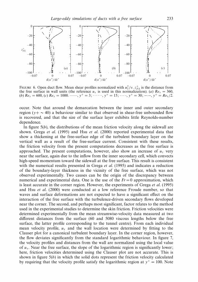
In figure 5(a), the mean streamwise-velocity profiles in logarithmic scale alongthe bottom-wall bisector (y = 0.5) are presented for the three Reynolds numbersconsidered. They satisfy the logarithmic law very well, and maintain the log-lawbehaviour until very close to the free surface. Compared with the closed-duct case,we do not observe the overshoot of the logarithmic layer intercept. Since the gridresolution for the closed- and open-duct calculations was the same, this can beinterpreted as a results of slightly weaker turbulence production near the walls awayfrom the duct corners, compared with the companion closed-duct flow. The meanvelocity profiles exhibit a maximum near the free surface. In the region 0.8 < z/D < 1a zone of negative mean shear ∂〈u〉/∂z is observed (see figure 6), owing to theaugmentation of the vertical descending convective transport caused by the outersecondary flow as the free surface is approached. The centre of the duct is themerging point of two opposite diverging currents generated at the sidewalls (Walker1997). As reported in Shen, Triantafyllou & Yue (2000) for an unbounded shear flow,this is a first indicator of the boundary-layer structure near a free surface, whosemaximum and minimum mark the ends of the two layers at the interface. Secondaryflows clearly appear to have a significant effect on the region where these events
Large-eddy simulations of ducts with a free surface 233
0
–0.07
(a) (b) (c)
–20
0
–40
–60
–80
–100
z+FS
d⟨u+ ⟩ /dz+
0
0.07
–20
0
–40
–60
–80
–100
d⟨u+ ⟩ /dz+
0
0.07
–20
0
–40
–60
–80
–100
d⟨u+ ⟩ /dz+–0.07 0.07–0.07
Figure 6. Open duct flow. Mean shear profiles normalized with u2τ /ν. z+
FS is the distance fromthe free surface in wall units (the reference uτ is used in this normalization). (a) Reτ = 360,(b) Reτ = 600, (c) Reτ = 1000. ——, y+ = 3; · · · · · ·, y+ = 15; – – –, y+ = 30; −·−, y+ = Reτ /2.
occur. Note that around the demarcation between the inner and outer secondaryregion (y+ ∼ 40) a behaviour similar to that observed in shear-free unbounded flowis recovered, and that the size of the surface layer exhibits little Reynolds-numberdependence.
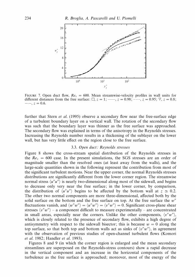
In figure 5(b), the distributions of the mean friction velocity along the sidewall areshown. Grega et al. (1995) and Hsu et al. (2000) reported experimental data thatshow a thickening at the free-surface edge of the turbulent boundary layer on thevertical wall as a result of the free-surface current. Consistent with these results,the friction velocity from the present computations decreases as the free surface isapproached. The present computations, however, also show an increase of uτ verynear the surface, again due to the inflow from the inner secondary cell, which convectshigh-speed momentum toward the sidewall at the free surface. This result is consistentwith the numerical results presented in Grega et al. (1995) and indicates a reductionof the boundary-layer thickness in the vicinity of the free surface, which was notobserved experimentally. Two causes can be the origin of the discrepancy betweennumerical and experimental data. One is the use of the Fr = 0 approximation, whichis least accurate in the corner region. However, the experiments of Grega et al. (1995)and Hsu et al. (2000) were conducted at a low reference Froude number, so thatwaves and surface deformations are not expected to have a significant effect on theinteraction of the free surface with the turbulence-driven secondary flows developednear the corner. The second, and perhaps most significant, factor relates to the methodused in the experimental studies to determine the skin friction. Friction velocities weredetermined experimentally from the mean streamwise-velocity data measured at twodifferent distances from the surface (60 and 5080 viscous lengths below the freesurface, the latter profile corresponding to the tunnel centre). From each individualmean velocity profile, uτ and the wall location were determined by fitting to theClauser plot for a canonical turbulent boundary layer. In the corner region, however,the flow deviates significantly from the standard logarithmic behaviour. In figure 7,the velocity profiles and distances from the wall are normalized using the local valueof uτ . Near the free surface, the slope of the logarithmic region is significantly lower;here, friction velocities determined using the Clauser plot are not accurate. This isshown in figure 5(b) in which the solid dots represent the friction velocity calculatedby requiring that the velocity profile satisfy the logarithmic region at y+ = 100. Note
234 R. Broglia, A. Pascarelli and U. Piomelli
20
16
12
8
4
0100 101 102
yl+
ul+
Figure 7. Open duct flow, Reτ = 600. Mean streamwise-velocity profiles in wall units fordifferent distances from the free surface: �, z = 1; ——, z = 0.98; – – –, z = 0.95; �, z = 0.8;−·−, z = 0.6.
further that Stern et al. (1995) observe a secondary flow near the free-surface edgeof a turbulent boundary layer on a vertical wall. The rotation of the secondary flowwas such that the boundary layer was thinner as the free surface was approached.The secondary flow was explained in terms of the anisotropy in the Reynolds stresses.Increasing the Reynolds number results in a thickening of the sublayer on the lowerwall, but has very little effect on the region close to the free surface.
3.3. Open duct: Reynolds stresses
Figure 8 shows the cross-stream spatial distribution of the Reynolds stresses inthe Reτ = 600 case. In the present simulations, the SGS stresses are an order ofmagnitude smaller than the resolved ones (at least away from the walls), and thelarge-scale quantities shown in the following represent the contribution from most ofthe significant turbulent motions. Near the upper corner, the normal Reynolds stressesdistributions are significantly different from the lower corner region. The streamwisenormal stress 〈u′′u′′〉 is nearly two-dimensional along most of the sidewall, and beginsto decrease only very near the free surface; in the lower corner, by comparison,the distribution of 〈u′′u′′〉 begins to be affected by the bottom wall at z � 0.2.The other two normal components are more three-dimensional, affected both by thesolid surface on the bottom and the free surface on top. At the free surface the w′′
fluctuations vanish, and 〈w′′w′′〉 = 〈u′′w′′〉 = 〈v′′w′′〉 = 0. Significant cross-plane shearstresses 〈v′′w′′〉 – a component difficult to measure experimentally – are concentratedin small areas, especially near the corners. Unlike the other components, 〈v′′w′′〉,which is closely related to the presence of secondary flow, exhibits a high degree ofantisymmetry with respect to the sidewall bisector; this is because w = 0 along thetop surface, so that both top and bottom walls act as sinks of 〈v′′w′′〉, in agreementwith the observation of previous studies of open-channel turbulent flows (Komoriet al. 1982; Handler et al. 1993).
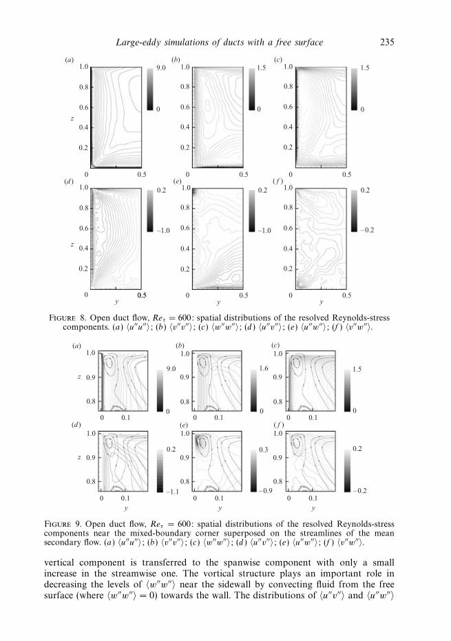
Figures 8 and 9 (in which the corner region is enlarged and the mean secondarystreamlines are superposed on the Reynolds-stress contours) show a rapid decreasein the vertical component and an increase in the horizontal components of theturbulence as the free surface is approached; moreover, most of the energy of the
Large-eddy simulations of ducts with a free surface 235
(b)
1.0
0 0.5y
(e)
y
(c)
0
( f )
y
(a)1.0
z
0.8
0 0.5
9.0
0
(d )
z
–1.0
0.6
0.4
0.2
1.0
0.8
0 0.5
1.5
00.6
0.4
0.2
1.0
0.8
0 0.5
1.5
0.6
0.4
0.2
0.21.0
0.8
0.5
0.6
0.4
0.2
0.8
0 0.5
0.6
0.4
0.2
1.0
0.8
0 0.5
0.6
0.4
0.2
–1.0
0.2
–0.2
0.2
Figure 8. Open duct flow, Reτ = 600: spatial distributions of the resolved Reynolds-stresscomponents. (a) 〈u′′u′′〉; (b) 〈v′′v′′〉; (c) 〈w′′w′′〉; (d ) 〈u′′v′′〉; (e) 〈u′′w′′〉; (f ) 〈v′′w′′〉.
(b)
0
(e)
(c)
( f )
(a)
(d )
z
–1.10.1
1.0
0.8
0.90.2
0
z
0.1
1.0
0.8
0.9
0
1.6
y
–0.9
0.3
0 0.1
1.0
0.8
0.9
0
1.5
0
9.0
0 0.1y
0.2
–0.20 0.1
y
1.0
0.8
0.9
1.0
0.8
0.9
1.0
0.8
0.9
0 0.1
Figure 9. Open duct flow, Reτ = 600: spatial distributions of the resolved Reynolds-stresscomponents near the mixed-boundary corner superposed on the streamlines of the meansecondary flow. (a) 〈u′′u′′〉; (b) 〈v′′v′′〉; (c) 〈w′′w′′〉; (d ) 〈u′′v′′〉; (e) 〈u′′w′′〉; (f ) 〈v′′w′′〉.
vertical component is transferred to the spanwise component with only a smallincrease in the streamwise one. The vortical structure plays an important role indecreasing the levels of 〈w′′w′′〉 near the sidewall by convecting fluid from the freesurface (where 〈w′′w′′〉 = 0) towards the wall. The distributions of 〈u′′v′′〉 and 〈u′′w′′〉
236 R. Broglia, A. Pascarelli and U. Piomelli
0
–1.2
(a) (b) (c)–20
0
–40
–60
–80
–100
z+FS
⟨u�� v��⟩
0
–20
–40
–60
–80
–100
0
–20
–40
–60
–80
–100–0.8 –0.4 –1.2 0
⟨u�� v��⟩–0.8 –0.4 –1.2 0
⟨u�� v��⟩–0.8 –0.4
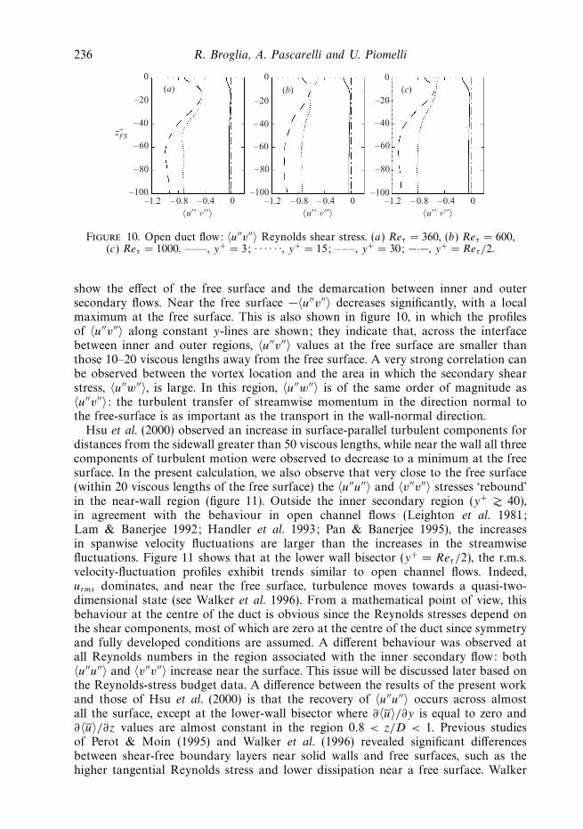
Figure 10. Open duct flow: 〈u′′v′′〉 Reynolds shear stress. (a) Reτ = 360, (b) Reτ = 600,(c) Reτ = 1000. ——, y+ = 3; · · · · · ·, y+ = 15; – – –, y+ = 30; −·−, y+ = Reτ /2.
show the effect of the free surface and the demarcation between inner and outersecondary flows. Near the free surface −〈u′′v′′〉 decreases significantly, with a localmaximum at the free surface. This is also shown in figure 10, in which the profilesof 〈u′′v′′〉 along constant y-lines are shown; they indicate that, across the interfacebetween inner and outer regions, 〈u′′v′′〉 values at the free surface are smaller thanthose 10–20 viscous lengths away from the free surface. A very strong correlation canbe observed between the vortex location and the area in which the secondary shearstress, 〈u′′w′′〉, is large. In this region, 〈u′′w′′〉 is of the same order of magnitude as〈u′′v′′〉: the turbulent transfer of streamwise momentum in the direction normal tothe free-surface is as important as the transport in the wall-normal direction.
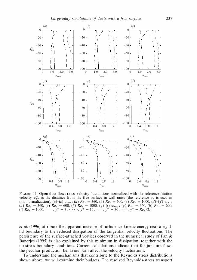
Hsu et al. (2000) observed an increase in surface-parallel turbulent components fordistances from the sidewall greater than 50 viscous lengths, while near the wall all threecomponents of turbulent motion were observed to decrease to a minimum at the freesurface. In the present calculation, we also observe that very close to the free surface(within 20 viscous lengths of the free surface) the 〈u′′u′′〉 and 〈v′′v′′〉 stresses ‘rebound’in the near-wall region (figure 11). Outside the inner secondary region (y+ � 40),in agreement with the behaviour in open channel flows (Leighton et al. 1981;Lam & Banerjee 1992; Handler et al. 1993; Pan & Banerjee 1995), the increasesin spanwise velocity fluctuations are larger than the increases in the streamwisefluctuations. Figure 11 shows that at the lower wall bisector (y+ = Reτ/2), the r.m.s.velocity-fluctuation profiles exhibit trends similar to open channel flows. Indeed,urms dominates, and near the free surface, turbulence moves towards a quasi-two-dimensional state (see Walker et al. 1996). From a mathematical point of view, thisbehaviour at the centre of the duct is obvious since the Reynolds stresses depend onthe shear components, most of which are zero at the centre of the duct since symmetryand fully developed conditions are assumed. A different behaviour was observed atall Reynolds numbers in the region associated with the inner secondary flow: both〈u′′u′′〉 and 〈v′′v′′〉 increase near the surface. This issue will be discussed later based onthe Reynolds-stress budget data. A difference between the results of the present workand those of Hsu et al. (2000) is that the recovery of 〈u′′u′′〉 occurs across almostall the surface, except at the lower-wall bisector where ∂〈u〉/∂y is equal to zero and∂〈u〉/∂z values are almost constant in the region 0.8 < z/D < 1. Previous studiesof Perot & Moin (1995) and Walker et al. (1996) revealed significant differencesbetween shear-free boundary layers near solid walls and free surfaces, such as thehigher tangential Reynolds stress and lower dissipation near a free surface. Walker
Large-eddy simulations of ducts with a free surface 237
0
3.0
(a) (b)
–20
0
–40
–60
–80
–100
z+FS
1.0 2.0urms
0
1.2
(d )
–20
0
–40
–60
–80
–100
z+FS
0.4 0.8vrms
0
1.2
(g)
–20
0
–40
–60
–80
–100
z+FS
0.4 0.8wrms
0
3.0
–20
0
–40
–60
–80
–1001.0 2.0
urms
0(e)
–20
–40
–60
–80
–100
vrms
0(h)
–20
–40
–60
–80
–100
0
3.0
(c)
–20
0
–40
–60
–80
–1001.0 2.0
urms
0( f )
–20
–40
–60
–80
–100
vrms
0(i)
–20
–40
–60
–80
–1001.20 0.4 0.8
wrms
1.20 0.4 0.8wrms
1.20 0.4 0.8 1.20 0.4 0.8
Figure 11. Open duct flow: r.m.s. velocity fluctuations normalized with the reference frictionvelocity. z+
FS is the distance from the free surface in wall units (the reference uτ is used inthis normalization). (a)–(c) urms; (a) Reτ = 360, (b) Reτ = 600, (c) Reτ = 1000. (d)–(f ) vrms;(d ) Reτ = 360, (e) Reτ = 600, (f ) Reτ = 1000. (g)–(i) wrms; (g) Reτ = 360, (h) Reτ = 600,(i ) Reτ = 1000. ——, y+ = 3; · · · · · ·, y+ = 15; – – –, y+ = 30; −·−, y+ = Reτ /2.
et al. (1996) attribute the apparent increase of turbulence kinetic energy near a rigid-lid boundary to the reduced dissipation of the tangential velocity fluctuations. Thepersistence of the surface-attached vortices observed in the numerical study of Pan &Banerjee (1995) is also explained by this minimum in dissipation, together with theno-stress boundary conditions. Current calculations indicate that for juncture flowsthe peculiar production behaviour can affect the velocity fluctuations.
To understand the mechanisms that contribute to the Reynolds stress distributionsshown above, we will examine their budgets. The resolved Reynolds-stress transport
238 R. Broglia, A. Pascarelli and U. Piomelli
equations are of the form:
0 = −〈uk〉∂〈u′′
i u′′j 〉
∂xk
+ Pij − εij + Dij + φij + ψij + Tij , (3.1)
where the terms on the right-hand side represent (rate of) advection, production, dis-sipation, viscous diffusion, pressure–strain, pressure diffusion, and turbulent diffusiontensors, respectively. The last six terms in (3.1) are defined as:
Pij = −[(
〈u′′ju
′′k〉∂〈ui〉
∂xk
+ 〈u′′i u
′′k〉∂〈uj 〉
∂xk
)+
(〈τik〉〈Sjk〉 + 〈τjk〉〈Sik〉
)], (3.2)
εij =
[2
Reτ
⟨∂u′′
i
∂xk
∂u′′j
∂xk
⟩−
(〈τikSjk〉 + 〈τjkSik〉
)], (3.3)
Dij =1
Reτ
∂2〈u′′i u
′′j 〉
∂xk∂xk
, (3.4)
φij =
⟨p′′
(∂u′′
i
∂xj
+∂u′′
j
∂xi
)⟩, (3.5)
ψij = − ∂
∂xk
(〈p′′u′′
j 〉δik + 〈p′′u′′i 〉δjk
), (3.6)
Tij = −[∂〈u′′
i u′′ju
′′k〉
∂xk
+∂
∂xk
(〈u′′
j τ′′ik〉 + 〈u′′
i τ′′jk〉
)]. (3.7)
The dissipation and turbulent diffusion consist of two parts: a resolved and a subgrid-scale contribution. To quantify the contribution of the SGS eddies to the terms inthe Reynolds-stress budgets, we compare the SGS dissipation εsgs = −〈τijSij 〉, the netlarge-scale energy drained by the subgrid scales, to the total (molecular + SGS) one,ε. This is the most significant of the SGS terms that appear in (3.1). The volume-averaged εsgs is 18%, 19% and 21% of the total volume-averaged dissipation, for thethree Reynolds numbers considered. Using LES and DNS of mixing layers, Geurts &Frohlich (2002) found that, when this measure of ‘subgrid-activity’ is less than 30%,the modelling errors are less than 1%.
Figure 12 shows the terms in the budget of the turbulent kinetic energy K =〈u′′
i u′′i 〉/2. Here and in the following, all terms are normalized by uτ and ν. Advection
is negligible everywhere except in the mixed-boundary corner, as will be discussedlater, and is not shown in this figure. Along the side and bottom walls the budgetresembles that observed in a flat-plate boundary layer: production and dissipation arenearly in balance, except very near the wall itself, where turbulent and viscous diffusionbecome important. An enlargement of the corner region, in which the secondary-flowstreamlines are superposed on the budget terms and advection is shown in figure 13.
The turbulent kinetic energy is dominated by the streamwise stress 〈u′′u′′〉, whoseproduction (shown in figure 14c) includes the main shear components, ∂〈u〉/∂y,∂〈u〉/∂z. The terms in the budgets for the two other normal components (shown infigures 15 and 16, respectively) are smaller than those in the streamwise one by anorder of magnitude, reflecting the absence of a significant shear in the productionterm. All terms contribute to the budgets of 〈v′′v′′〉 and 〈w′′w′′〉.
Hsu et al. (2000), observed that both TKE production and dissipation are drama-tically reduced in the near-corner region, close to the free surface. Far from the wall,this results in an increase of the surface-parallel fluctuations very close to the freesurface. Close to the sidewall and within 20 viscous lengths of the free surface, all
Large-eddy simulations of ducts with a free surface 239
(b)
(e)
(c)
( f )
(a)
(d )
z
y
0.4
0.6
y0 0.4
y
0.8
1.0
0.2
0.2
(b)
0.4
0.6
0 0.4
0.8
1.0
0.2
0.2
0.4
0.6
0 0.4
0.8
1.0
0.2
0.2
0.3
–0.3
z
0.4
0.6
0 0.4
0.8
1.0
0.2
0.2
0.4
0.6
0 0.4
0.8
1.0
0.2
0.2
0.4
0.6
0 0.4
0.8
1.0
0.2
0.2
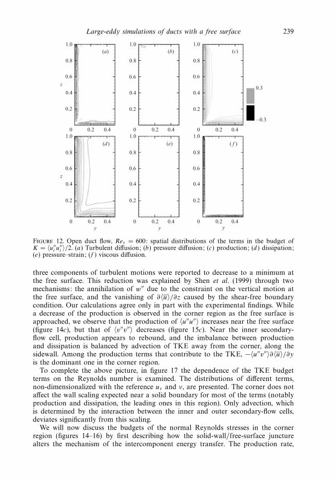
Figure 12. Open duct flow, Reτ = 600: spatial distributions of the terms in the budget ofK = 〈u′′
i u′′i 〉/2. (a) Turbulent diffusion; (b) pressure diffusion; (c) production; (d ) dissipation;
(e) pressure–strain; (f ) viscous diffusion.
three components of turbulent motions were reported to decrease to a minimum atthe free surface. This reduction was explained by Shen et al. (1999) through twomechanisms: the annihilation of w′′ due to the constraint on the vertical motion atthe free surface, and the vanishing of ∂〈u〉/∂z caused by the shear-free boundarycondition. Our calculations agree only in part with the experimental findings. Whilea decrease of the production is observed in the corner region as the free surface isapproached, we observe that the production of 〈u′′u′′〉 increases near the free surface(figure 14c), but that of 〈v′′v′′〉 decreases (figure 15c). Near the inner secondary-flow cell, production appears to rebound, and the imbalance between productionand dissipation is balanced by advection of TKE away from the corner, along thesidewall. Among the production terms that contribute to the TKE, −〈u′′v′′〉∂〈u〉/∂yis the dominant one in the corner region.
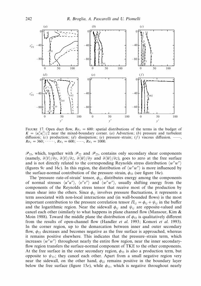
To complete the above picture, in figure 17 the dependence of the TKE budgetterms on the Reynolds number is examined. The distributions of different terms,non-dimensionalized with the reference uτ and ν, are presented. The corner does notaffect the wall scaling expected near a solid boundary for most of the terms (notablyproduction and dissipation, the leading ones in this region). Only advection, whichis determined by the interaction between the inner and outer secondary-flow cells,deviates significantly from this scaling.
We will now discuss the budgets of the normal Reynolds stresses in the cornerregion (figures 14–16) by first describing how the solid-wall/free-surface juncturealters the mechanism of the intercomponent energy transfer. The production rate,
240 R. Broglia, A. Pascarelli and U. Piomelli
(b)
(e)
(c)
( f )
(a)
(d )
z
y y
(b)
0.20.1
0.3
–0.3
z
0
0.9
0.8
1.0
0
0.9
0.8
1.0
y0.20.1
0.9
0.8
1.0
0
0.9
0.8
1.0
0.20.1
0.9
0.8
1.0
0
0.9
0.8
1.0
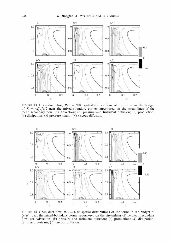
Figure 13. Open duct flow, Reτ = 600: spatial distributions of the terms in the budgetof K = 〈u′′
i u′′i 〉/2 near the mixed-boundary corner superposed on the streamlines of the
mean secondary flow. (a) Advection; (b) pressure and turbulent diffusion; (c) production;(d ) dissipation; (e) pressure–strain; (f ) viscous diffusion.
(b)
(e)
(c)
( f )
(a)
(d )
z
y y
(b)
0.20.1
0.40
–0.40
z
0
0.9
0.8
1.0
0
0.9
0.8
1.0
y0.20.1
0.9
0.8
1.0
0
0.9
0.8
1.0
0.20.1
0.9
0.8
1.0
0
0.9
0.8
1.0
0.20.10 0.20.10 0.20.10
Figure 14. Open duct flow, Reτ = 600: spatial distributions of the terms in the budget of〈u′′u′′〉 near the mixed-boundary corner superposed on the streamlines of the mean secondaryflow. (a) Advection; (b) pressure and turbulent diffusion; (c) production; (d ) dissipation;(e) pressure–strain; ( f ) viscous diffusion.
Large-eddy simulations of ducts with a free surface 241
(b)
(e)
(c)
( f )
(a)
(d )
z
y y
(b)
0.20.1
0.04
–0.04
z
0
0.9
0.8
1.0
0
0.9
0.8
1.0
y0.20.1
0.9
0.8
1.0
0
0.9
0.8
1.0
0.20.1
0.9
0.8
1.0
0
0.9
0.8
1.0
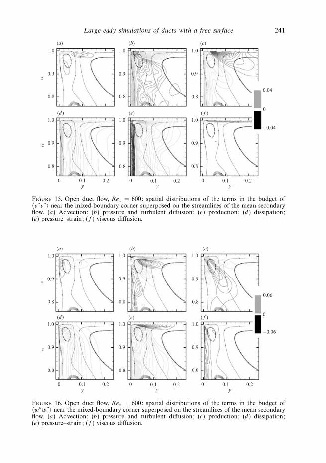
Figure 15. Open duct flow, Reτ = 600: spatial distributions of the terms in the budget of〈v′′v′′〉 near the mixed-boundary corner superposed on the streamlines of the mean secondaryflow. (a) Advection; (b) pressure and turbulent diffusion; (c) production; (d ) dissipation;(e) pressure–strain; ( f ) viscous diffusion.
(b)
(e)
(c)
( f )
(a)
(d )
z
y y
(b)
0.20.1
0.06
–0.06
z
0
0.9
0.8
1.0
0
0.9
0.8
1.0
y0.20.1
0.9
0.8
1.0
0
0.9
0.8
1.0
0.20.1
0.9
0.8
1.0
0
0.9
0.8
1.0
Figure 16. Open duct flow, Reτ = 600: spatial distributions of the terms in the budget of〈w′′w′′〉 near the mixed-boundary corner superposed on the streamlines of the mean secondaryflow. (a) Advection; (b) pressure and turbulent diffusion; (c) production; (d ) dissipation;(e) pressure–strain; ( f ) viscous diffusion.
242 R. Broglia, A. Pascarelli and U. Piomelli
0
100
(a) (b)
–40
–80
z+FS
0 50
0
(d )
0
–40
–80
z+FS
50
0
–40
–80
0
(e)
–40
–80
100
(c)
0
–40
–80
0
( f )
–40
–60
1000 50 1000 50
1000 50 1000 50
y+ y+ y+
–0.01
–0.10
–0.15
–0.05
–0.02
–0.040
–0.002
0.3
0.1
–0.05
–0.01
Figure 17. Open duct flow, Reτ = 600: spatial distributions of the terms in the budget ofK = 〈u′′
i u′′i 〉/2 near the mixed-boundary corner. (a) Advection; (b) pressure and turbulent
diffusion; (c) production; (d ) dissipation; (e) pressure–strain; ( f ) viscous diffusion. ——,Reτ = 360; · · · · · ·, Reτ = 600; – – –, Reτ = 1000.
P33, which, together with P22 and P23, contains only secondary shear components(namely, ∂〈v〉/∂y, ∂〈v〉/∂z, ∂〈w〉/∂y and ∂〈w〉/∂z), goes to zero at the free surfaceand is not directly related to the corresponding Reynolds stress distribution 〈w′′w′′〉(figures 9c and 16c). In this region, the distribution of 〈w′′w′′〉 is more influenced bythe surface-normal contribution of the pressure–strain, φ33 (see figure 16e).
The ‘pressure–rate-of-strain’ tensor, φij , distributes energy among the componentsof normal stresses 〈u′′u′′〉, 〈v′′v′′〉 and 〈w′′w′′〉, usually shifting energy from thecomponents of the Reynolds stress tensor that receive most of the production bymean shear into the others. Since φij involves pressure fluctuations, it represents aterm associated with non-local interactions and (in wall-bounded flows) is the mostimportant contribution to the pressure correlation tensor Πij = φij +ψij in the bufferand the logarithmic region. Near the sidewall φij and ψij are opposite-valued andcancel each other (similarly to what happens in plane channel flow (Mansour, Kim &Moin 1988). Toward the middle plane the distribution of φ33 is qualitatively differentfrom the results of open-channel flow (Handler et al. 1993; Komori et al. 1993).In the corner region, up to the demarcation between inner and outer secondaryflow, φ33 decreases and becomes negative as the free surface is approached, whereasit remains positive elsewhere. This indicates that the pressure–strain term, whichincreases 〈w′′w′′〉 throughout nearly the entire flow region, near the inner secondary-flow region transfers the surface-normal component of TKE to the other components.At the free surface in the outer secondary region, φ33 is also a production term, butopposite to ψ33; they cancel each other. Apart from a small negative region verynear the sidewall, on the other hand, φ22 remains positive in the boundary layerbelow the free surface (figure 15e), while φ11, which is negative throughout nearly
Large-eddy simulations of ducts with a free surface 243
–0.05
(a) (b) (c)1.00
0
0.96
0.92
0.88
z
0.05 –0.05
1.00
0
0.96
0.92
0.88
0.05–0.05
1.00
0
0.96
0.92
0.88
φi j
0.05φ
i jφ
i j
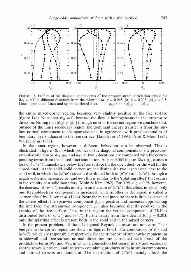
Figure 18. Profiles of the diagonal components of the pressure-strain correlation tensor forReτ = 600 at different distances from the sidewall: (a) y = 0.065; (b) y = 0.203; (c) y = 0.5.Lines: open duct. Lines and symbols: closed duct. ——, φ11; · · · · · ·, φ22; – – –, φ33.
the entire mixed-corner region, becomes very slightly positive at the free surface(figure 14e). Note that ψ11 = 0, because the flow is homogeneous in the streamwisedirection. Noting that |φ22| > |φ11| through most of the corner region we conclude that,outside of the inner secondary region, the dominant energy transfer is from the sur-face-normal component to the spanwise one, in agreement with previous studies ofboundary layers adjacent to the free surface (Handler et al. 1993; Perot & Moin 1995;Walker et al. 1996).
In the inner region, however, a different behaviour can be observed. This isillustrated in figure 18, in which profiles of the diagonal components of the pressure–rate-of-strain tensor, φ11, φ22 and φ33, at two y-locations are compared with the corres-ponding terms from the closed-duct simulation. At y = 0.065 (figure 18a), φ33 causes aloss of 〈w′′w′′〉 immediately below the free surface (in the open duct) or the wall (in theclosed duct). At the solid–solid corner, we can distinguish two layers: one, next to thesolid wall, in which the 〈w′′w′′〉 stress is distributed both to 〈u′′u′′〉 and 〈v′′v′′〉 through anegative φ33 and increased φ11 and φ22; this is similar to the ‘splatting effect’ that occursin the vicinity of a solid boundary (Moin & Kim 1982). For 0.95 < z < 0.98, however,the decrease of 〈w′′w′′〉 results mostly in an increase of 〈v′′v′′〉; this effect, in which onlyone Reynolds-stress component is increased, while another is decreased, is called a‘corner effect’ by Huser et al. (1994). Near the mixed juncture there is little evidence ofthe corner effect: the spanwise component φ22 is positive and increases approachingthe interface; the streamwise component φ11 also becomes slightly positive in thevicinity of the free surface. Thus, in this region the vertical component of TKE isdistributed both to 〈u′′u′′〉 and 〈v′′v′′〉. Further away from the sidewall, for y = 0.203,only the splatting effect is present both in the solid and in the mixed corners.
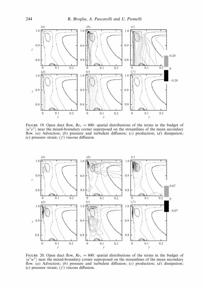
In the present problem, all the off-diagonal Reynolds stresses are non-zero. Theirbudgets in the corner region are shown in figures 19–21. The contours of 〈u′′v′′〉 and〈u′′w′′〉, which are responsible, respectively, for the transport of streamwise momentumin sidewall and free-surface normal directions, are correlated with those of theproduction terms P12 and P13, in which a connection between primary and secondaryshear stresses is present, and the terms containing products of main strain componentsand normal stresses are dominant. The distribution of 〈v′′v′′〉 mainly affects the
244 R. Broglia, A. Pascarelli and U. Piomelli
(b)
(e)
(c)
( f )
(a)
(d )
z
y y
(b)
0.20.1
0.20
–0.20
z
0
0.9
0.8
1.0
0
0.9
0.8
1.0
y0.20.1
0.9
0.8
1.0
0
0.9
0.8
1.0
0.20.1
0.9
0.8
1.0
0
0.9
0.8
1.0
0.20.10 0.20.10 0.20.10
Figure 19. Open duct flow, Reτ = 600: spatial distributions of the terms in the budget of〈u′′v′′〉 near the mixed-boundary corner superposed on the streamlines of the mean secondaryflow. (a) Advection; (b) pressure and turbulent diffusion; (c) production; (d ) dissipation;(e) pressure–strain; ( f ) viscous diffusion.
(b)
(e)
(c)
( f )
(a)
(d )
z
y y
(b)
0.20.1
0.07
–0.07
z
0
0.9
0.8
1.0
0
0.9
0.8
1.0
y0.20.1
0.9
0.8
1.0
0
0.9
0.8
1.0
0.20.1
0.9
0.8
1.0
0
0.9
0.8
1.0
0.20.10 0.20.10 0.20.10
Figure 20. Open duct flow, Reτ = 600: spatial distributions of the terms in the budget of〈u′′w′′〉 near the mixed-boundary corner superposed on the streamlines of the mean secondaryflow. (a) Advection; (b) pressure and turbulent diffusion; (c) production; (d ) dissipation;(e) pressure–strain; ( f ) viscous diffusion.
Large-eddy simulations of ducts with a free surface 245
(b)
(e)
(c)
( f )
(a)
(d )
z
y y
(b)
0.20.1
0.06
–0.06
z
0
0.9
0.8
1.0
0
0.9
0.8
1.0
y0.20.1
0.9
0.8
1.0
0
0.9
0.8
1.0
0.20.1
0.9
0.8
1.0
0
0.9
0.8
1.0
0.20.10 0.20.10 0.20.10
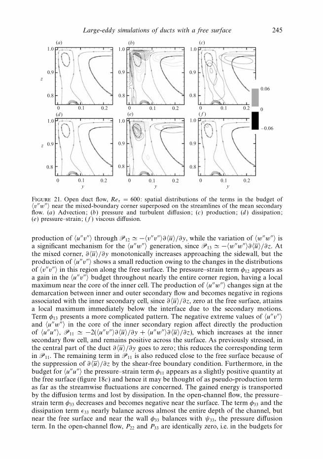
Figure 21. Open duct flow, Reτ = 600: spatial distributions of the terms in the budget of〈v′′w′′〉 near the mixed-boundary corner superposed on the streamlines of the mean secondaryflow. (a) Advection; (b) pressure and turbulent diffusion; (c) production; (d ) dissipation;(e) pressure–strain; ( f ) viscous diffusion.
production of 〈u′′v′′〉 through P12 � −〈v′′v′′〉∂〈u〉/∂y, while the variation of 〈w′′w′′〉 isa significant mechanism for the 〈u′′w′′〉 generation, since P13 � −〈w′′w′′〉∂〈u〉/∂z. Atthe mixed corner, ∂〈u〉/∂y monotonically increases approaching the sidewall, but theproduction of 〈u′′v′′〉 shows a small reduction owing to the changes in the distributionsof 〈v′′v′′〉 in this region along the free surface. The pressure–strain term φ12 appears asa gain in the 〈u′′v′′〉 budget throughout nearly the entire corner region, having a localmaximum near the core of the inner cell. The production of 〈u′′w′′〉 changes sign at thedemarcation between inner and outer secondary flow and becomes negative in regionsassociated with the inner secondary cell, since ∂〈u〉/∂z, zero at the free surface, attainsa local maximum immediately below the interface due to the secondary motions.Term φ13 presents a more complicated pattern. The negative extreme values of 〈u′′v′′〉and 〈u′′w′′〉 in the core of the inner secondary region affect directly the productionof 〈u′′u′′〉, P11 � −2(〈u′′v′′〉∂〈u〉/∂y + 〈u′′w′′〉∂〈u〉/∂z), which increases at the innersecondary flow cell, and remains positive across the surface. As previously stressed, inthe central part of the duct ∂〈u〉/∂y goes to zero; this reduces the corresponding termin P11. The remaining term in P11 is also reduced close to the free surface because ofthe suppression of ∂〈u〉/∂z by the shear-free boundary condition. Furthermore, in thebudget for 〈u′′u′′〉 the pressure–strain term φ11 appears as a slightly positive quantity atthe free surface (figure 18c) and hence it may be thought of as pseudo-production termas far as the streamwise fluctuations are concerned. The gained energy is transportedby the diffusion terms and lost by dissipation. In the open-channel flow, the pressure–strain term φ33 decreases and becomes negative near the surface. The term φ33 and thedissipation term ε33 nearly balance across almost the entire depth of the channel, butnear the free surface and near the wall φ33 balances with ψ33, the pressure diffusionterm. In the open-channel flow, P22 and P33 are identically zero, i.e. in the budgets for
246 R. Broglia, A. Pascarelli and U. Piomelli
〈v′′v′′〉 and 〈w′′w′′〉, no direct production term exists. Here, at the lower wall bisector,P22 � −2〈v′′v′′〉∂〈v〉/∂y and P33 � −2〈w′′w′′〉∂〈w〉/∂z. While the latter goes to zero atthe interface, the former is a positive quantity. This difference balances with a negativeφ22 (see figure 18c). Since Πkk = 0 from continuity, an increase in φ22 can be expectedto result in a decrease in the magnitude of φ33. The budget for 〈w′′w′′〉 confirms thisline of reasoning. It should be noted here that, as is the case in solid–solid corners(Huser et al. 1994), the turbulence dissipation-rate tensor contributes significantly tothe Reynolds stress balance, both near the walls and far from them. Figure 20 showshigh-dissipation events in the high-turbulence production area.
The cross-plane Reynolds stress, 〈v′′w′′〉 (which is identically zero in two-dimensional turbulent shear flows) together with the anisotropy of the normal stressesin the (y, z)-plane, controls the production of the mean streamwise vorticity, whosecomplete balance is deferred to the next paragraph. In the present configuration, theReynolds stress production rates that contain the secondary shear stress, 〈v′′w′′〉, areweak. Previous studies on three-dimensional duct flows have shown that generation of〈v′′w′′〉 results from two mechanisms, one associated with the gradients of secondaryvelocities, the other with the distortion of primary velocity gradients (Perkins 1970).The former mechanism seems more effective that the latter (Demuren & Rodi 1984).Along the sidewall there is a positive production of 〈v′′w′′〉 caused by the secondaryReynolds stresses; this P23 balances the negative contribution from ε23. Along thefree surface, on the other hand, the magnitudes of all terms on the right-hand side ofthe 〈v′′w′′〉 balance equation, although small, appear to be of equal magnitude.
3.4. Open duct: vorticity
As outlined above, in an open square duct, mean three-dimensionality results in non-zero mean streamwise vorticity 〈ωx〉 = ∂〈w〉/∂y − ∂〈v〉/∂z. The origin of the meansecondary flow can be linked to the same mechanisms as those in a closed squareduct, since in both cases the anisotropy of the turbulence stress is the driving forcethat generates the secondary flows. The relationship between the Reynolds-stressanisotropy and the secondary flow is illustrated by the transport equation for 〈ωx〉. Ina statistically steady fully developed turbulent flow, in which streamwise gradients areidentically zero, the quasi-inviscid stretching and deflection (skew-induced) generationterm cancels and this equation reads
〈v〉∂〈ωx〉∂y
+ 〈w〉∂〈ωx〉∂z︸ ︷︷ ︸
I
− 1
Reτ
(∂2〈ωx〉∂y2
+∂2〈ωx〉
∂z2
)︸ ︷︷ ︸
II
− ∂2
∂y∂z
(〈v′′2 + τyy〉 − 〈w′′2 + τzz〉
)︸ ︷︷ ︸
III
−(
∂2
∂y2− ∂2
∂z2
)〈v′′w′′ + τyz〉︸ ︷︷ ︸
IV
= 0. (3.8)
Term I represents advection of the mean streamwise vorticity by mean secondaryvelocities; term II is the diffusion of vorticity due to viscosity; III and IV areproduction terms (resolved + SGS) due to the gradient of the difference in thenormal Reynolds stresses (〈v′′2 + τyy〉 − 〈w′′2 + τzz〉), and to the difference in thegradient of the secondary shear Reynolds stress (〈v′′w′′ + τyz〉), respectively.
It has been argued by other investigators (see, for example, Perkins 1970) that, forfully developed flows, the imbalance between gradients of normal stresses is primarilyresponsible for the production of secondary flow vorticity, whereas the shear-stresscontribution, if not negligible, acts like a transport term in (3.8). For a more thorough
Large-eddy simulations of ducts with a free surface 247
z
y0.500.25
1.0
–1.0
0
1.0
0.8
0
0.4
0.2
0.6
0
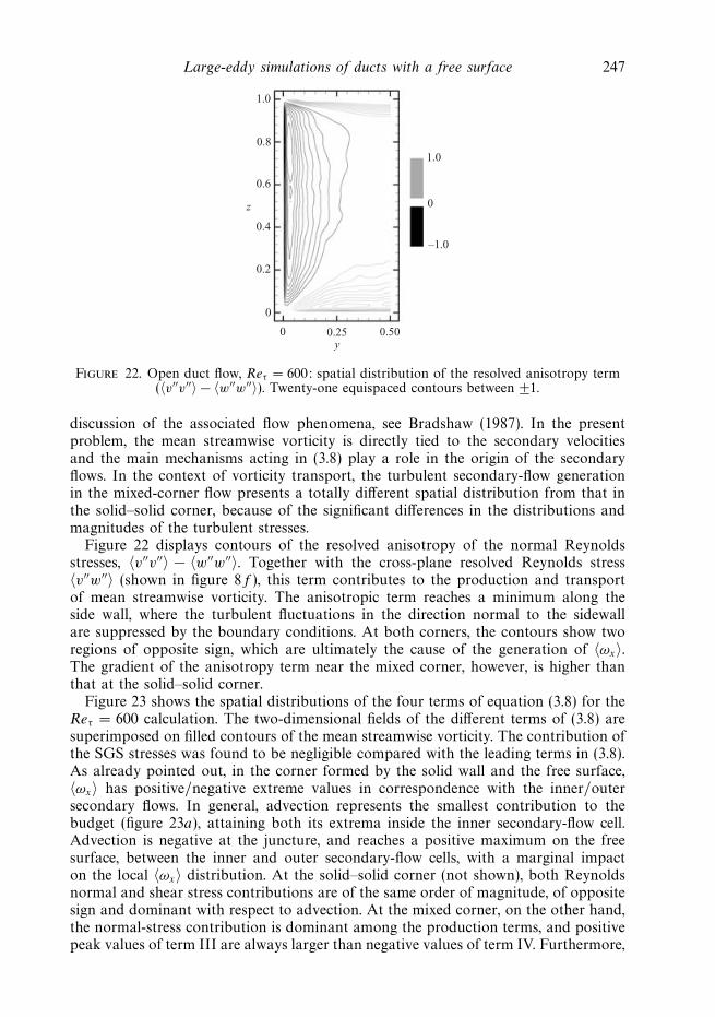
Figure 22. Open duct flow, Reτ = 600: spatial distribution of the resolved anisotropy term(〈v′′v′′〉 − 〈w′′w′′〉). Twenty-one equispaced contours between ±1.
discussion of the associated flow phenomena, see Bradshaw (1987). In the presentproblem, the mean streamwise vorticity is directly tied to the secondary velocitiesand the main mechanisms acting in (3.8) play a role in the origin of the secondaryflows. In the context of vorticity transport, the turbulent secondary-flow generationin the mixed-corner flow presents a totally different spatial distribution from that inthe solid–solid corner, because of the significant differences in the distributions andmagnitudes of the turbulent stresses.
Figure 22 displays contours of the resolved anisotropy of the normal Reynoldsstresses, 〈v′′v′′〉 − 〈w′′w′′〉. Together with the cross-plane resolved Reynolds stress〈v′′w′′〉 (shown in figure 8f ), this term contributes to the production and transportof mean streamwise vorticity. The anisotropic term reaches a minimum along theside wall, where the turbulent fluctuations in the direction normal to the sidewallare suppressed by the boundary conditions. At both corners, the contours show tworegions of opposite sign, which are ultimately the cause of the generation of 〈ωx〉.The gradient of the anisotropy term near the mixed corner, however, is higher thanthat at the solid–solid corner.
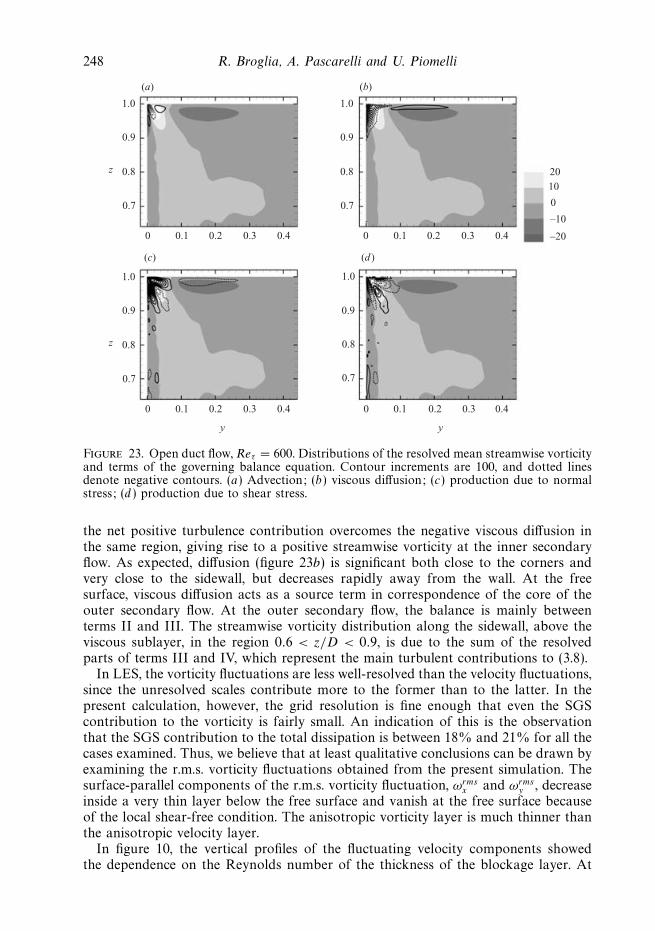
Figure 23 shows the spatial distributions of the four terms of equation (3.8) for theReτ = 600 calculation. The two-dimensional fields of the different terms of (3.8) aresuperimposed on filled contours of the mean streamwise vorticity. The contribution ofthe SGS stresses was found to be negligible compared with the leading terms in (3.8).As already pointed out, in the corner formed by the solid wall and the free surface,〈ωx〉 has positive/negative extreme values in correspondence with the inner/outersecondary flows. In general, advection represents the smallest contribution to thebudget (figure 23a), attaining both its extrema inside the inner secondary-flow cell.Advection is negative at the juncture, and reaches a positive maximum on the freesurface, between the inner and outer secondary-flow cells, with a marginal impacton the local 〈ωx〉 distribution. At the solid–solid corner (not shown), both Reynoldsnormal and shear stress contributions are of the same order of magnitude, of oppositesign and dominant with respect to advection. At the mixed corner, on the other hand,the normal-stress contribution is dominant among the production terms, and positivepeak values of term III are always larger than negative values of term IV. Furthermore,
248 R. Broglia, A. Pascarelli and U. Piomelli
z
y
20
–20
0
1.0
0.8
0.7
0.9
(a)
0 0.1 0.2 0.3 0.4
z
1.0
0.8
0.7
0.9
(c)
0 0.1 0.2 0.3 0.4
y
1.0
0.8
0.7
0.9
(b)
0 0.1 0.2 0.3 0.4
1.0
0.8
0.7
0.9
(d )
0 0.1 0.2 0.3 0.4
–10
10
Figure 23. Open duct flow, Reτ = 600. Distributions of the resolved mean streamwise vorticityand terms of the governing balance equation. Contour increments are 100, and dotted linesdenote negative contours. (a) Advection; (b) viscous diffusion; (c) production due to normalstress; (d ) production due to shear stress.
the net positive turbulence contribution overcomes the negative viscous diffusion inthe same region, giving rise to a positive streamwise vorticity at the inner secondaryflow. As expected, diffusion (figure 23b) is significant both close to the corners andvery close to the sidewall, but decreases rapidly away from the wall. At the freesurface, viscous diffusion acts as a source term in correspondence of the core of theouter secondary flow. At the outer secondary flow, the balance is mainly betweenterms II and III. The streamwise vorticity distribution along the sidewall, above theviscous sublayer, in the region 0.6 < z/D < 0.9, is due to the sum of the resolvedparts of terms III and IV, which represent the main turbulent contributions to (3.8).
In LES, the vorticity fluctuations are less well-resolved than the velocity fluctuations,since the unresolved scales contribute more to the former than to the latter. In thepresent calculation, however, the grid resolution is fine enough that even the SGScontribution to the vorticity is fairly small. An indication of this is the observationthat the SGS contribution to the total dissipation is between 18% and 21% for all thecases examined. Thus, we believe that at least qualitative conclusions can be drawn byexamining the r.m.s. vorticity fluctuations obtained from the present simulation. Thesurface-parallel components of the r.m.s. vorticity fluctuation, ωrms
x and ωrmsy , decrease
inside a very thin layer below the free surface and vanish at the free surface becauseof the local shear-free condition. The anisotropic vorticity layer is much thinner thanthe anisotropic velocity layer.
In figure 10, the vertical profiles of the fluctuating velocity components showedthe dependence on the Reynolds number of the thickness of the blockage layer. At
Large-eddy simulations of ducts with a free surface 249
0(a) (b)
–20
0
–40
–60
–80
–100
z+FS
0.1 0.2� rms
x
0
0.3
(d )
–20
0
–40
–60
–80
–100
z+FS
0.1 0.2
0
0.3
(g)
–20
0
–40
–60
–80
–100
z+FS
0.1 0.2
0
–20
0
–40
–60
–80
–1000.1 0.2
0(e)
–20
–40
–60
–80
–100
(h)
0
0.2
(c)
–20
0
–40
–60
–80
–1000.1
0( f )
–20
–40
–60
–80
(i)
0
� rmsy
� rmsz
� rmsx � rms
x
0.4 0.5
0.4 0.50.3 0 0.1 0.2� rms
y
0.4 0.5 0 0.1 0.2� rms
y
0.4 0.50.3 0.3
0
0.3
–20
0
–40
–60
–80
–1000.1 0.2
� rmsz
0.4 0.5
0
0.3
–20
0
–40
–60
–80
–1000.1 0.2
� rmsz
0.4 0.5
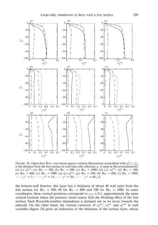
Figure 24. Open duct flow: root-mean-square vorticity fluctuations normalized with u2τ /ν. z+
FSis the distance from the free surface in wall units (the reference uτ is used in this normalization).(a)–(c) ωrms
x ; (a) Reτ = 360, (b) Reτ = 600, (c) Reτ = 1000. (d)–(f ) ωrmsy ; (d ) Reτ = 360,
(e) Reτ = 600, ( f ) Reτ = 1000. (g)–(i) ωrmsz ; (g) Reτ = 360, (h) Reτ = 600, (i ) Reτ = 1000.
——, y+ = 3; · · · · · ·, y+ = 15; – – – y+ = 30; —·— , y+ = Reτ /2.
the bottom-wall bisector, this layer has a thickness of about 40 wall units from thefree surface for Reτ = 360, 60 for Reτ = 600 and 100 for Reτ = 1000. In outercoordinates, these vertical positions correspond to zFS � 0.1, approximately the samevertical location where the pressure–strain tensor feels the blocking effect of the freesurface. Such Reynolds-number dependence is damped out as we move towards thesidewall. On the other hand, the vertical variation of ωrms
x , ωrmsy and ωrms
z in wallvariables (figure 24) gives an indication of the thickness of the surface layer, whose
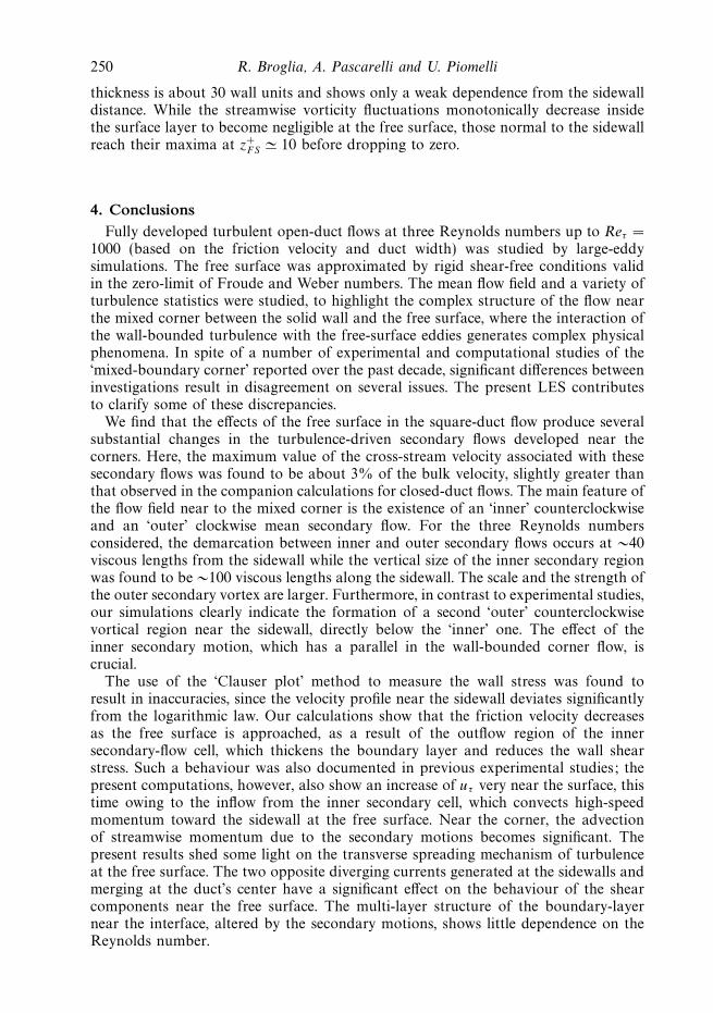
250 R. Broglia, A. Pascarelli and U. Piomelli
thickness is about 30 wall units and shows only a weak dependence from the sidewalldistance. While the streamwise vorticity fluctuations monotonically decrease insidethe surface layer to become negligible at the free surface, those normal to the sidewallreach their maxima at z+
FS � 10 before dropping to zero.
4. ConclusionsFully developed turbulent open-duct flows at three Reynolds numbers up to Reτ =
1000 (based on the friction velocity and duct width) was studied by large-eddysimulations. The free surface was approximated by rigid shear-free conditions validin the zero-limit of Froude and Weber numbers. The mean flow field and a variety ofturbulence statistics were studied, to highlight the complex structure of the flow nearthe mixed corner between the solid wall and the free surface, where the interaction ofthe wall-bounded turbulence with the free-surface eddies generates complex physicalphenomena. In spite of a number of experimental and computational studies of the‘mixed-boundary corner’ reported over the past decade, significant differences betweeninvestigations result in disagreement on several issues. The present LES contributesto clarify some of these discrepancies.
We find that the effects of the free surface in the square-duct flow produce severalsubstantial changes in the turbulence-driven secondary flows developed near thecorners. Here, the maximum value of the cross-stream velocity associated with thesesecondary flows was found to be about 3% of the bulk velocity, slightly greater thanthat observed in the companion calculations for closed-duct flows. The main feature ofthe flow field near to the mixed corner is the existence of an ‘inner’ counterclockwiseand an ‘outer’ clockwise mean secondary flow. For the three Reynolds numbersconsidered, the demarcation between inner and outer secondary flows occurs at ∼40viscous lengths from the sidewall while the vertical size of the inner secondary regionwas found to be ∼100 viscous lengths along the sidewall. The scale and the strength ofthe outer secondary vortex are larger. Furthermore, in contrast to experimental studies,our simulations clearly indicate the formation of a second ‘outer’ counterclockwisevortical region near the sidewall, directly below the ‘inner’ one. The effect of theinner secondary motion, which has a parallel in the wall-bounded corner flow, iscrucial.
The use of the ‘Clauser plot’ method to measure the wall stress was found toresult in inaccuracies, since the velocity profile near the sidewall deviates significantlyfrom the logarithmic law. Our calculations show that the friction velocity decreasesas the free surface is approached, as a result of the outflow region of the innersecondary-flow cell, which thickens the boundary layer and reduces the wall shearstress. Such a behaviour was also documented in previous experimental studies; thepresent computations, however, also show an increase of uτ very near the surface, thistime owing to the inflow from the inner secondary cell, which convects high-speedmomentum toward the sidewall at the free surface. Near the corner, the advectionof streamwise momentum due to the secondary motions becomes significant. Thepresent results shed some light on the transverse spreading mechanism of turbulenceat the free surface. The two opposite diverging currents generated at the sidewalls andmerging at the duct’s center have a significant effect on the behaviour of the shearcomponents near the free surface. The multi-layer structure of the boundary-layernear the interface, altered by the secondary motions, shows little dependence on theReynolds number.
Large-eddy simulations of ducts with a free surface 251
This was the first investigation of ‘mixed-boundary corner’ flows in which anexplanation of the existence and origin of secondary motions could be offered in thecontext of several balance equations. All of the terms in the streamwise momentumequation, vorticity transport, Reynolds stress budgets and turbulent energy transportwere computed from the present LES. Two regions can be distinguished, one in whichthe advection increases the x-momentum, immediately below the surface, and onefurther away from the corner, in which the momentum is decreased. The Reynolds-stress gradient adjusts to maintain the balance. The turbulent kinetic energy andReynolds stress distributions are also significantly affected by the secondary motionsin the corner.
Of particular interest are the Reynolds-stress budgets. Two factors play importantroles in the Reynolds stress distributions: the pressure–strain redistribution termand the production. Production dominates the budgets whenever the mean shearenters the production term (i.e. for the 〈u′′u′′〉, 〈u′′v′′〉 and 〈u′′w′′〉 components ofthe Reynolds-stress tensor). The budgets of the other terms are dominated by thepressure–strain term. Outside the inner secondary region, the stress normal to thefree surface, 〈w′′w′′〉, is transferred mainly to the streamwise one 〈u′′u′′〉, in agreementwith previous studies of boundary layers adjacent to the free surface. In the innersecondary region, 〈w′′w′′〉 is distributed both to 〈u′′u′′〉 and 〈v′′v′′〉 through the free-surface normal distribution of the pressure–strain term φ33. The physical reasons forthe TKE increase in the inner region can be summarized as follows: the primaryoff-diagonal Reynolds stresses, 〈u′′v′′〉 and 〈u′′w′′〉, fed by 〈u′′u′′〉 and 〈v′′v′′〉 throughthe production terms, affect directly the production of 〈u′′u′′〉, which increases atthe inner secondary flow cell, and remains positive across the surface. At the freesurface, as the distance from the sidewall increases, the pressure–strain term φ33
changes from a destruction to a production term at the demarcation between innerand outer flow regions. The mean secondary motion is driven by the anisotropyof Reynolds stresses; in the mean streamwise vorticity equation, at the mixedcorner, the normal-stress contribution is dominant among the production terms.The positive contribution of the turbulence overcomes the negative viscous diffusionin this region, giving rise to positive streamwise vorticity at the inner secondaryflow.
The Reynolds-number dependence of the terms in the TKE budget was investigated,and it was found that (within the range of Reynolds numbers examined in this work)the corner does not affect the wall scaling expected near a solid boundary for most ofthe terms. Only advection deviates significantly from this scaling. While the source-layer thickness is sensitive to the distance from the sidewall, the surface-layer thickness,approximately 30 viscous lengths, is only weakly affected by the wall distance.
Taken together, the results presented in the present paper can contribute to thedevelopment of turbulence models for RANS equations, as well as elucidate someimportant physical mechanisms in this very important configuration. In this regard,this investigation is the precursor of a follow-up flow study in which wave-inducedeffects are not negligible.
The work of R.B. and A.P. was performed under the auspices of the Italian Ministryof Transportation within the framework of INSEAN Research Plan 2000–02. Thecomputational resources were provided by CINECA (Bologna, Italy) and CASPUR(Roma, Italy). U.P. acknowledges the support of the Office of Naval Research throughGrant N000140110993, monitored by Drs L. P. Purtell and R. D. Joslin.
252 R. Broglia, A. Pascarelli and U. Piomelli
REFERENCES
Akselvoll, K. & Moin, P. 1996 Large-eddy simulation of turbulent confined coannular jets. J. FluidMech. 315, 387–411.
Anthony, D. G. & Willmarth, W. W. 1992 Turbulence measurements in a round jet near a freesurface. J. Fluid Mech. 243, 699–720.
Borue, V., Orszag, S. & Staroselsky, S. A. 1995 Interaction of surface waves with turbulence:direct numerical simulations of turbulent open-channel flow. J. Fluid Mech. 286, 1–23.
Bradshaw, P. 1987 Turbulent secondary flows. Annu. Rev. Fluid Mech. 19, 53–74.
Broglia, R., Di Mascio, A. & Muscari, R. 1999 Numerical simulations of turbulent flows with afree-surface. In Proc. 7th Intl Conf. on Numerical Ship Hydrodynamics, pp. 2.2.1–2.2.7, Nantes,France, 19–22 July.
Chorin, A. J. 1967 A numerical method for solving incompressible viscous flow problems.J. Comput. Phys. 2, 12–26.
Demuren, A. O. & Rodi, W. 1984 Calculation of turbulence-driven secondary motion in non-circularducts. J. Fluid Mech. 140, 189–222.
Gavrilakis, S. 1992 Numerical simulation of low-Reynolds-number turbulent flow through astraight square duct. J. Fluid Mech. 244, 101–129.
Germano, M., Piomelli, U., Moin, P. & Cabot, W. H. 1991 A dynamic subgrid-scale eddy-viscositymodel. Phys. Fluids A 3, 1760–1765.
Gessner, F. B., Po, J. K. & Emery, A. F. 1979 Measurements of developing turbulent flow in asquare duct. In Turbulent Shear Flows I (ed. F. Durst, B. E. Lavender, F. W. Schmidt, &J. H. Whitelaw). Springer.
Geurts, B. & Frohlich, J. 2002 A framework for predicting accuracy limitations in large-eddysimulation. Phys. Fluids 14, L41–L44.
Grega, L. M., Hsu, T. Y. & Wei, T. 2002 Vorticity transport in a corner formed by a solid wall anda free surface. J. Fluid Mech. 465, 331–352.
Grega, L. M., Wey, T., Leighton, R. I. & Neves, J. C. 1995 Turbulent mixed-boundary flow in acorner formed by a solid wall and a free-surface. J. Fluid Mech. 294, 17–46.
Handler, R. A., Swean, T. F., Leighton, R. I. & Swearingen, J. D. 1993 Length scales and theenergy balance for turbulence near a free surface. AIAA J. 31, 1998–2007.
Hong, W. L. & Walker, D. T. 2000 Reynolds-averaged equations for free-surface flows withapplication to high-Froude-number jet spreading. J. Fluid Mech. 417, 183–209.
Hsu, T. Y., Grega, L. M., Leighton, R. I. & Wei, T. 2000 Turbulent kinetic energy transport in acorner formed by a solid wall and a free-surface. J. Fluid Mech. 410, 343–366.
Hunt, J. C. R. & Graham, J. M. R. 1978 Free stream turbulence near plane boundaries. J. FluidMech. 84, 209–235.
Huser, A. & Biringen, S. 1993 Direct numerical simulation of turbulent flow in a square duct.J. Fluid Mech. 257, 65–95.
Huser, A., Biringen, S. & Hatay, F. F. 1994 Direct simulation of turbulent flow in a square duct:Reynolds-stress budgets. Phys. Fluids 6, 3144–3152.
Kim, J. & Moin, P. 1985 Application of a fractional-step method to incompressible Navier–Stokesequations. J. Comput. Phys. 59, 308–323
Komori, S., Nagaosa, N., Murakami, Y., Chiba, S., Ishii, K. & Kuwahara, K. 1993 Directnumerical simulation of three-dimensional open-channel flow with zero-shear gas–liquidinterface. Phys. Fluids A 5, 115–125.
Komori, S., Ueda, H., Ogino, F. & Mizushina, T. 1982 Turbulent structure and transport mechanismat the free-surface in an open-channel flow. Intl J. Heat Mass Transfer 25, 513–521.
Kumar, S., Gupta, R. & Banerjee, S. 1998 An experimental investigation on the characteristics offree-surface turbulence in channel flow. Phys. Fluids 10, 437–456.
Lam, K. & Banerjee, S. 1992 On the condition of streak formation in a bounded turbulent flow.Phys. Fluids A 4, 306–320.
Launder, B. E. & Ying, W. G. 1972 Secondary flows in ducts of square cross-section. J. FluidMech. 54, 289–295.
Leighton, R. I., Swean, T. F., Handler, R. A. & Swearingen, J. D. 1981 Interaction of vorticitywith a free-surface in turbulent open-channel flow. AIAA Paper 91–0236.
Large-eddy simulations of ducts with a free surface 253
Lilly, D. K. 1992 A proposed modification of the Germano subgrid-scale closure method. Phys.Fluids A 4, 633–635.
Longo, J., Huang, H. P. & Stern, F. 1998 Solid/free-surface juncture boundary layer and wake.Exps. Fluids 25, 283–297.
Madabhushi, R. K. & Vanka, S. P. 1991 Large eddy simulation of turbulence-driven secondaryflow in a square duct. Phys. Fluids A 3, 2734–2745.
Mansour, N. N., Kim, J. & Moin, P. 1988 Reynolds-stress and dissipation rate budgets in aturbulent channel flow. J. Fluid Mech. 194, 15–44.
Melling, A. & Whitelaw, J. H. 1976 Turbulent flow in a rectangular duct. J. Fluid Mech. 78,289–315.
Mittal, R. & Moin, P. 1997 Suitability of upwind biased schemes for large-eddy simulation ofturbulent flows. AIAA J. 35, 1415–1417.
Moin, P. & Kim, J. 1982 Numerical investigation of turbulent channel flow. J. Fluid Mech. 118,341–378.
Nakagawa, H. & Nezu, I. 1981 Structure of space–time correlations of bursting phenomena in anopen-channel flow. J. Fluid Mech. 104, 1–43.
Nagaosa, R. 1999 Direct numerical simulation of the vortex structures and turbulent scalar transferacross a free surface in a fully developed turbulence. Phys. Fluids 11, 1581–1595.
Nezu, I. & Rodi, W. 1986 Open-channel flow measurements with a laser Doppler anemometer.J. Hydraul. Engng ASCE 112, 335–355.
Pan, Y. & Banerjee, S. 1995 A numerical study of free-surface turbulence in channel flow.Phys. Fluids 7, 1649–1664.
Perkins, H. J. 1970 The formation of streamwise vorticity in turbulent flow. J. Fluid Mech. 44,721–740.
Perot, B. & Moin, P. 1995 Shear-free turbulent boundary layers. Part 1. Physical insight intonear-wall turbulence. J. Fluid Mech. 295, 199–227.
Pope, S. 2000 Turbulent Flows. Cambridge University Press.
Robinson, S. K. 1991 Coherent motions in the turbulent boundary layer. Annu. Rev. Fluid Mech. 23,601–640.
Sarpkaya, T. & Neubert, D. 1994 Interaction of a streamwise vortex with a free surface. AIAAJ. 32, 594–600.
Sarpkaya, T. & Suthon, P. 1991 Interaction of a vortex couple with a free surface. Exps. Fluids 11,205–217.
Shen, L., Triantafyllou, G. S. & Yue, D. K. 2000 Turbulent diffusion near a free surface. J. FluidMech. 407, 145–166.
Shen, L., Zhang, X., Yue, D. K. & Triantafyllou, G. S. 1999 The surface layer for free-surfaceturbulent flows. J. Fluid Mech. 386, 167–212.
Sreedhar, M. & Stern, F. 1998 Large eddy simulation of temporally developing juncture floes.Intl J. Numer. Meth. Fluids 28, 47–72.
Stern, F., Parthasarathy, R., Huang, H. P. & Longo, J. 1995 Effects of waves and free surfaceturbulence in the boundary layer of a surface-piercing flat plate. In Proc. ASME Fluids EngngConf. Symp. on Free-Surface Turbulence (ed. E. Rood & J. Katz). ASME, New York.
Su, M. D. & Friedrich, R. 1994 Investigation of fully developed turbulent flow in a straight ductwith large eddy simulation. J. Fluid. Engng 116, 677–684.
Tsai, W. T. 1998 A numerical study of the evolution and structure of a turbulent shear layer undera free surface. J. Fluid Mech. 354, 239–276.
Walker, D. T. 1997 On the origin of the ‘surface current’ in turbulent free-surface flows. J. FluidMech. 339, 275–285.
Walker, D. T., Leighton, R. I. & Garza-Rios, L. O. 1996 Shear-free turbulence near a solid flatfree-surface. J. Fluid Mech. 320, 19–51.
Related Documents