Large eddy simulation of turbulent heat transport in the Strait of Gibraltar

Available online at www.sciencedirect.com

Mathematics and Computers in Simulation 79 (2009) 3444–3454

Large eddy simulation of turbulent heat transportin the Strait of Gibraltar

Mofdi El-Amrani a,∗, Mohammed Seaïd b

a Universidad Rey Juan Carlos, Dpto. Matemática Aplicada, 28933 Madrid, Spainb School of Engineering, University of Durham, South Road DH1 3LE, UK

Received 30 January 2008; received in revised form 20 January 2009; accepted 9 April 2009Available online 23 April 2009

Abstract

We develop a numerical model for large eddy simulation of turbulent heat transport in the Strait of Gibraltar. The flow equations arethe incompressible Navier–Stokes equations including Coriolis forces and density variation through the Boussinesq approximation.The turbulence effects are incorporated in the system by considering the Smagorinsky model. As a numerical solver we propose afinite element semi-Lagrangian method. The solution procedure consists of combining a non-oscillatory semi-Lagrangian scheme fortime discretization with the finite element method for space discretization. Numerical results illustrate a buoyancy-driven circulationsalong the Strait of Gibraltar and the sea-surface temperature is flushed out and move to northeast coast. The Ocean discharge andthe temperature difference are shown to control the plume structure.© 2009 IMACS. Published by Elsevier B.V. All rights reserved.

Keywords: Large eddy simulation; Heat transport; Semi-Lagrangian scheme; Finite elements method; Strait of Gibraltar

1. Introduction

The mean flow in the Strait of Gibraltar has been the subject of numerous numerical investigations, we refer to [1]for a survey and more details. Most of the studies carried out on the Strait of Gibraltar used the shallow water equationsto model the mean flow and no thermal effects have been taking into account. However, observations reported in [9]indicate that water level in the sea surface is driven by temperature changes while the deeper layers salinity also becomesimportant. Furthermore, authors in [11] claimed that sea-surface temperature is considered to play an important rolein the Mediterranean circulation through the Strait of Gibraltar. Therefore, the aim of the present work is to investigatethe evolution of sea-surface temperature in the Strait of Gibraltar using a finite element semi-Lagrangian method.

The Strait of Gibraltar is bounded to the north and south by the Iberian and African continental forelands, and tothe west and east by the Atlantic Ocean and the Mediterranean sea, respectively. The basic circulation in the Straitof Gibraltar consists in an upper layer of cold, fresh surface Atlantic water and an opposite deep current of warmer,salty Mediterranean outflowing water, compare [1,7,6]. The sea-surface temperatures in the Strait of Gibraltar aremaxima in summer (August–September) with average values of 23–24 ◦ C and minima in winter (January–February)

∗ Corresponding author. Tel: +34 914887098; fax: +34 914887338.E-mail address: [email protected] (M. El-Amrani).

0378-4754/$36.00 © 2009 IMACS. Published by Elsevier B.V. All rights reserved.doi:10.1016/j.matcom.2009.04.013

M. El-Amrani, M. Seaïd / Mathematics and Computers in Simulation 79 (2009) 3444–3454 3445

with averages of 11–12 ◦C. The north Atlantic water is about 5–6 ◦ C colder than the Mediterranean water, elaboratedetails are available in [11,9]. Furthermore, due to the Ocean discharge and the tidal waves occurring in the Strait,the hydrologycal flow may turn from laminar to turbulent flow. Thus a model to capture the small scales in turbulentflow is required. In general, there are three approaches to model turbulent flows: direct numerical simulation (DNS),Reynolds averaged numerical simulation (RANS) and large eddy simulation (LES). In this paper we consider the LESusing a Smagorinsky subgrid model, compare [12,13] among others. The LES model is selected for turbulent heattransport in the Strait of Gibraltar because of it simplicity and robustness compared to the DNS and RANS models. Asa numerical solver for the LES we apply the stabilized finite element semi-Lagrangian (FEMSLAG) method developedby the authors in [3,5] for solving incompressible viscous flows with heat transfer. To avoid the principal drawbackof the conventional FEMSLAG method, that is the failure to preserve monotonicity, we incorporate limiters into ourFEMSLAG algorithm to convert the method to non-oscillatory and quasi-monotone at minor additional computationalcost. A numerical comparison between this method and the conventional FEMSLAG is presented for the Zalesak discproblem [15].

The objective of this study is twofold, on one hand to test the capability of the FEMSLAG method to handle LESin complex geometry and on the other hand to develop mathematical tools to study LES of turbulent heat transport inthe Strait of Gibraltar. To the best knowledge of the authors, these issues have never been investigated in the literature.After defining the equations for LES in Section 2, we briefly describe the FEMSLAG method in Section 3. Numericalresults are presented in Section 4. Section 5 contains some conclusions.

2. Equations for turbulent heat transport

To model heat transport in the Strait of Gibraltar we consider the incompressible Navier–Stokes/Boussinesq equa-tions in two space dimensions. It should be stressed that the validity of the considered model is supported by thegeometry of the Strait and the temperature differences between the Mediterranean and the Atlantic water bodies. Thebasic idea of LES is to compute a space averaged flow accurately. To achieve this, each flow variable ψ is decom-posed into a large-scale component ψ and a subgrid scale component ψ′. The large-scale component is obtained by anapplication of a filter operator. This operator is a convolution integral of the form:

ψ(x, t) =∫R2G�(|x − y|)ψ(y, t) dy,

where x = (x, y)T is the space coordinate, t denotes the time and G� is the filter such as volume-average box-filter[12]. Hence, the filtered governing Navier–Stokes/Boussinesq equations are

∇ · u = 0,

ρ∞(∂u∂t

+ u · ∇u)

+ ∇p = ∇ · (2νS(u)) − ∇ · T(u) + f u⊥ + F,

ρ∞cp(∂�

∂t+ u · ∇�

)= ∇ · (κ∇�) − ∇ · H(�),

(1)

where u = (u, v)T is the velocity field, p the pressure, � the temperature, ρ∞ the reference density, ν the kinematicviscosity, cp the specific heat at constant pressure, f the Coriolis coefficient, and κ the thermal diffusivity coefficient.In Eq. (1), u⊥ = (−v, u)T , S(u) = (∇u + ∇uT )/2 is the strain-rate tensor, and the force term due to the Boussinesqapproximation is defined as

F = ρ∞(1 − β(�−�∞))g,

with g is the gravity force and β the coefficient of thermal expansion. Here, the Reynolds subgrid-scale tensor T(u)and the heat subgrid-scale term H(�) are

T(u) = u ⊗ uT − u ⊗ uT , H(�) = u�− u�.

3446 M. El-Amrani, M. Seaïd / Mathematics and Computers in Simulation 79 (2009) 3444–3454

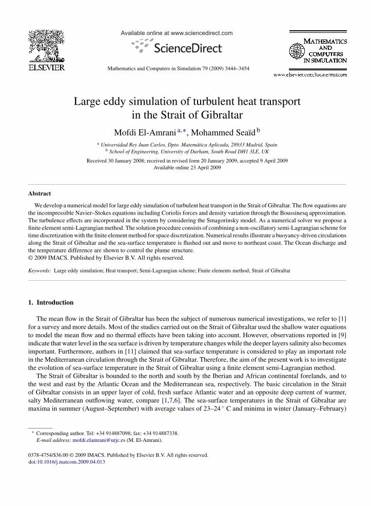
Fig. 1. Domain configuration used in LES and its associated finite element mesh.

To model these subgrid-scales in terms of filtered velocity field u and filtered temperature � we use the Smagorinskymodel [13]:

T(u) ≈ −νtS(u), H(�) ≈ −κt∇(�). (2)

The turbulent viscosity νt and the turbulent thermal diffusivity κt are

νt = (cs �)2‖S(u)‖, κt = νt

PrT, ‖S(u)‖ = (S(u) : S(u))1/2,

where cs is a model constant which has to be chosen apriori,� is the grid filter width, and PrT is the turbulent Prandtlnumber set to 0.9 in our LES results. Substituting (2) into (1) gives

∇ · u = 0,

ρ∞(∂u∂t

+ u · ∇u)

+ ∇p = ∇ · ((2ν + νt)S(u)) + f u⊥ + F,

ρ∞cp(∂�

∂t+ u · ∇�

)= ∇ · ((κ + κt)∇�).

(3)

The LES Eq. (3) are solved in the computational domain shown in Fig. 1. The domain is about 60 km long betweenits west Barbate-Tangier section and its east Gibraltar–Sebta section. Its width varies from a minimum of about 14 kmat Tarifa-Punta Cires section and a maximum of 44 km at Barbate–Tangier section. Here, the simulation domain isrestricted by the Tangier–Barbate axis from the Atlantic ocean and the Sebta–Algeciras axis from the Mediterranean.This domain is taken in the simulation mainly because measured data is usually provided by stations located on theabove mentioned cities. Therefore, we have adapted the same domain for our LES simulations. The model is startedfrom warm rest and it is only driven by the density difference between the two sub-basins, in particular the temperaturefields of the Atlantic and Mediterranean waters have been obtained from an average of the spring data [11]. At theleft and right boundary regions we use cold and hot temperature data, respectively. The top and bottom coastlines areconsidered as adiabatic boundaries. For the water flow, a well developed velocity profile with a maximum velocity u∞is imposed at the western entrance of the Strait of Gibraltar. This profile corresponds to the annual mean of the Atlanticinput flux [1] and it is also comparable to the main semidiurnal tidal component M2 [6,7]. At the eastern exit of thestrait we impose the pseudo-stress condition:

−pn + ν∂u∂n

= 0,

whereas no-slip conditions are used on the remaining boundaries. The parameters appearing in Eq. (3) are definedusing the reference values listed in Table 1.

M. El-Amrani, M. Seaïd / Mathematics and Computers in Simulation 79 (2009) 3444–3454 3447

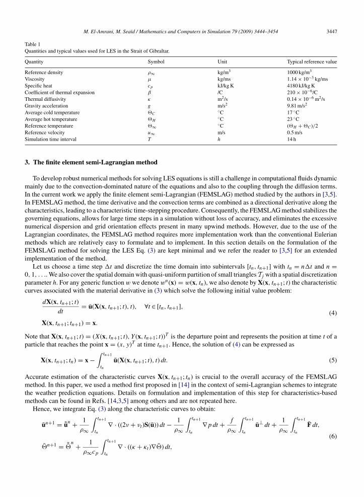
Table 1Quantities and typical values used for LES in the Strait of Gibraltar.

Quantity Symbol Unit Typical reference value

Reference density ρ∞ kg/m3 1000 kg/m3

Viscosity μ kg/ms 1.14 × 10−3 kg/msSpecific heat cp kJ/kg K 4180 kJ/kg KCoefficient of thermal expansion β /C 210 × 10−6/CThermal diffusivity κ m2/s 0.14 × 10−6 m2/sGravity acceleration g m/s2 9.81 m/s2

Average cold temperature �C◦C 17 ◦C

Average hot temperature �H◦C 23 ◦C

Reference temperature �∞ ◦C (�H +�C)/2Reference velocity u∞ m/s 0.5 m/sSimulation time interval T h 14 h

3. The finite element semi-Lagrangian method

To develop robust numerical methods for solving LES equations is still a challenge in computational fluids dynamicmainly due to the convection-dominated nature of the equations and also to the coupling through the diffusion terms.In the current work we apply the finite element semi-Lagrangian (FEMSLAG) method studied by the authors in [3,5].In FEMSLAG method, the time derivative and the convection terms are combined as a directional derivative along thecharacteristics, leading to a characteristic time-stepping procedure. Consequently, the FEMSLAG method stabilizes thegoverning equations, allows for large time steps in a simulation without loss of accuracy, and eliminates the excessivenumerical dispersion and grid orientation effects present in many upwind methods. However, due to the use of theLagrangian coordinates, the FEMSLAG method requires more implementation work than the conventional Eulerianmethods which are relatively easy to formulate and to implement. In this section details on the formulation of theFEMSLAG method for solving the LES Eq. (3) are kept minimal and we refer the reader to [3,5] for an extendedimplementation of the method.

Let us choose a time step �t and discretize the time domain into subintervals [tn, tn+1] with tn = n�t and n =0, 1, . . .. We also cover the spatial domain with quasi-uniform partition of small triangles Tj with a spatial discretizationparameter h. For any generic functionwwe denotewn(x) = w(x, tn), we also denote by X(x, tn+1; t) the characteristiccurves associated with the material derivative in (3) which solve the following initial value problem:

dX(x, tn+1; t)

dt= u(X(x, tn+1; t), t), ∀t ∈ [tn, tn+1],

X(x, tn+1; tn+1) = x.

(4)

Note that X(x, tn+1; t) = (X(x, tn+1; t), Y (x, tn+1; t))T is the departure point and represents the position at time t of aparticle that reaches the point x = (x, y)T at time tn+1. Hence, the solution of (4) can be expressed as

X(x, tn+1; tn) = x −∫ tn+1

tn

u(X(x, tn+1; t), t) dt. (5)

Accurate estimation of the characteristic curves X(x, tn+1; tn) is crucial to the overall accuracy of the FEMSLAGmethod. In this paper, we used a method first proposed in [14] in the context of semi-Lagrangian schemes to integratethe weather prediction equations. Details on formulation and implementation of this step for characteristics-basedmethods can be found in Refs. [14,3,5] among others and are not repeated here.

Hence, we integrate Eq. (3) along the characteristic curves to obtain:

un+1 = ˜un + 1

ρ∞

∫ tn+1

tn

∇ · ((2ν + νt)S(u)) dt − 1

ρ∞

∫ tn+1

tn

∇pdt + f

ρ∞

∫ tn+1

tn

u⊥ dt + 1

ρ∞

∫ tn+1

tn

F dt,

�n+1 = ˜�n + 1

ρ∞cp

∫ tn+1

tn

∇ · ((κ + κt)∇�) dt,

(6)

3448 M. El-Amrani, M. Seaïd / Mathematics and Computers in Simulation 79 (2009) 3444–3454

with ˜un(x) = u(X(x, tn+1; tn), tn+1) and ˜�n(x) = �(X(x, tn+1; tn), tn+1). The conforming finite element spaces for

velocity/temperature and pressure that we use are Taylor–Hood finite elements P2/P1, i.e., polynomial of seconddegree for the velocity/temperature and polynomial of first degree for the pressure on simplices, respectively. Hence,we formulate the finite element solutions to un(x), vn(x), �n(x) and pn(x) as

unh =M∑j=1

Unj φj, vnh =M∑j=1

V nj φj, �nh =M∑j=1

�njφj, pnh =N∑j=1

Pnj ψj, (7)

where M and N are, respectively, the number of velocity/temperature and pressure mesh points in the triangleTj . The functions Unj , V nj , �nj and Pnj are, respectively, the corresponding nodal values of unh(x), vnh(x), �nh(x)

and pnh(x) defined as Unj = unh(xj), V nj = vnh(xj), �nj = �nh(xj) and Pnj = pnh(yj) where {xj}Mj=1 and {yj}Nj=1are

the set of velocity/temperature and pressure mesh points in the partition �h, respectively, so that N < M and{y1, . . . , yN} ⊂ {x1, . . . , xM}. In (7), {φj}Mj=1 and {ψj}Nj=1are, respectively, the set of global nodal basis functionsof Vh and Qh characterized by the property φi(xj) = δij and ψi(yj) = δij with δij denoting the Kronecker symbol. Forthe results presented in Section 4, the degrees of freedom within a finite element are six for the velocity and temperaturesolutions, and three for the pressure solution.

Analogously, the finite element solutions to ˜unh, ˜vnh and ˜�n

h are approximated by

˜unh =M∑j=1

˜Un

jφj, ˜vnh =M∑j=1

˜Vn

jφj,˜�n

h =M∑j=1

˜�n

jφj, (8)

where ˜Un

j , ˜Vn

j and ˜�n

j are evaluated by finite element interpolation of unh(x), vnh(x) and �nh(x) at the feet of characteristiccurves X(x, tn+1; t). This procedure needs less computational work than using a piecewise exact method for projectingthe information from the background Eulerian grid onto the Lagrangian grid as in [10].

Here, we discretize Eq. (6) in time using the second-order Crank–Nicolson method for all terms involving velocityand temperature variables, whereas a first-order implicit Euler scheme is used for the pressure variable. Using aprojection-type method, the procedure to advance the solution of (3) from a time tn to the next time tn+1 can be carriedout in the following steps:

(1) Solve for �n+1:

�n+1 − ˜�n

�t− 1

ρ∞cp∇ · ((κ + κt)∇�n+1/2) = 0. (9)

(2) Solve for un+1:

un+1 − ˜un

�t+ 1

ρ∞∇pn − 1

ρ∞∇ · ((2ν + νt)S(un+1/2)) − 1

ρ∞u⊥n+1/2 = f

ρ∞Fn+1

. (10)

(3) Solve for p and un+1:

un+1 − un+1

�t+ 1

ρ∞∇p = 0,

∇ · un+1 = 0,

(11)

(4) Update pn+1:

pn+1 = pn + 2p.

M. El-Amrani, M. Seaïd / Mathematics and Computers in Simulation 79 (2009) 3444–3454 3449

In (9) and (10), �n+1/2 = (1/2) ˜�n + (1/2)�n+1 and un+1/2 = (1/2) ˜un + (1/2)un+1. Note that, the solution of

(11) leads to a pressure-Poisson problem for p of the form:

�p = ρ∞�t

∇ · un+1. (12)

A detailed analysis of convergence and stability of this method for the laminar incompressible Navier–Stokes has beencarried out in [4] whereas, its analysis in an Eulerian framework can be found in [2]. Notice that the finite elementdiscretization of Eqs. (9)–(12) is trivial and is omitted here. It is described in many text books, compare [8] amongothers. In addition, the discretization procedure gives rise to uncoupled elliptic problems such that their finite elementdiscretization leads to well-conditioned linear systems of algebraic equations for which, very efficient solvers canbe implemented. Therefore, by taking advantage of these properties we can solve linear systems in the FEMSLAGalgorithm by preconditioned conjugate gradient solvers. This yields a very powerful and efficient method for solvingthis class of linear systems of algebraic equations.

Various types of interpolation procedures can be used in the FEMSLAG method, but for computational rea-sons, the most common one in practical applications is the Lagrangian interpolation of degree higher than one.However, most of interpolation procedures do not preserve monotonicity of the approximate solutions. In orderto overcome this drawback, we incorporate to our FEMSLAG method a limiting approach. This implies that avalue, obtained by interpolating in a grid element, lies between the maximum and minimum values in the ver-tices of this grid element. In this way we obtain a non-oscillatory algorithm at minor additional computationalcost that possesses good shape preserving of the advected fields in the vicinity of strong gradients and maintainsthe order of convergence in regions where the solution is sufficiently smooth. We should point out that, the keyidea used by our FEMSLAG method to calculate the approximate solution at the mesh points is inspired by Zale-sak flux corrected transport technique reported in [15], which consists of computing the mesh point values of thenumerical solution by adding to the values of a low-order solution, which is monotone, a correction term that con-tains the contribution of a high-order solution and does not violate the monotonicity properties of the low-ordersolution.

Next, we formulate the resulting non-oscillatory algorithm for the convective solutions in (9)–(12). Here, weformulate the algorithm only for the temperature variable and similar work is done for the velocity field. Thus, thenumerical procedure to approximate the temperature solution ˜�

nin (9) is performed in the following steps:

(1) Evaluate the high-order gridpoint approximation:

˜�n

Hj =NH∑k=1

˜�kφk(Xj(xj, tn+1; tn)),

where {φ1, . . . , φNH } are the local basis functions of the element Tj where the characteristic foot Xj(xj, tn+1; tn)is located.

(2) Evaluate the low-order gridpoint approximation

˜�n

Lj =NL∑k=1

˜�kϕk(Xj(xj, tn+1; tn)),

where {ϕ1, . . . , ϕNL} are the linear local basis functions of the element Tj . Recall that the linear interpolationpreserves the monotonicity of the solution. Therefore, the numerical solution obtained by linear interpolation isfree of oscillations and artificial extrema.

(3) Update the solution ˜�n

j according to

˜�n

j = αnj˜�n

Hj + (1 − αnj ) ˜�n

Lj, (13)

3450 M. El-Amrani, M. Seaïd / Mathematics and Computers in Simulation 79 (2009) 3444–3454

where 0 ≤ αnj ≤ 1, is a limiting coefficient chosen to control the amount of correction in the low-order approxi-mation in order to obtain a non-oscillatory solution. It is defined as

αnj =

⎧⎪⎪⎪⎪⎪⎪⎪⎪⎪⎪⎨⎪⎪⎪⎪⎪⎪⎪⎪⎪⎪⎩

min

(1,�

+j − ˜�

n

Lj

˜�n

Lj − ˜�n

Hj

), if ˜�

n

Lj − ˜�n

Hj > 0,

min

(1,�

−j − ˜�

n

Lj

˜�n

Lj − ˜�n

Hj

), if ˜�

n

Lj − ˜�n

Hj < 0,

1, if ˜�n

Lj − ˜�n

Hj = 0,

(14)

where �+j and �−

j are, respectively, the maximum and minimum solution values at the element Tj which consistof the node j and its nearest neighbours at time tn, i.e.:

�+j = max(�nj1, . . . , �

njNH ), �−

j = min(n

�j1, . . . , �njNH ).

Note that by the limiting procedure we force the interpolated value to remain within the largest and the smallestvalues of the solution in a set of points surrounding the characteristics feet. So that, the interpolation procedure doesnot generate any extrema which is not possessed by the solution in a neighborhood of the feet of characteristics. Theanalysis of convergence and stability of the FEMSLAG method using the limiting (14) has been performed in [4] forthe laminar incompressible Navier–Stokes.

4. Numerical results

We first present a comparison between results obtained by the conventional FEMSLAG method (i.e. αnj = 0 in Eq.(13)) and our adjusted FEMSLAG method (i.e. αnj calculated according to Eq. (14)) for the canonical test exampleof Zalesak disc [15]. Then, we show numerical results for turbulent heat transport in the Strait of Gibraltar. In all ourcomputations, all the linear systems of algebraic equations are solved using a preconditioned conjugate gradient solverwith a stopping criteria set to 10−5. All the computations are performed on a Pentium PC with one processor of 512MB of RAM and 166 MHz using serial Fortran codes under Linux 2.2.

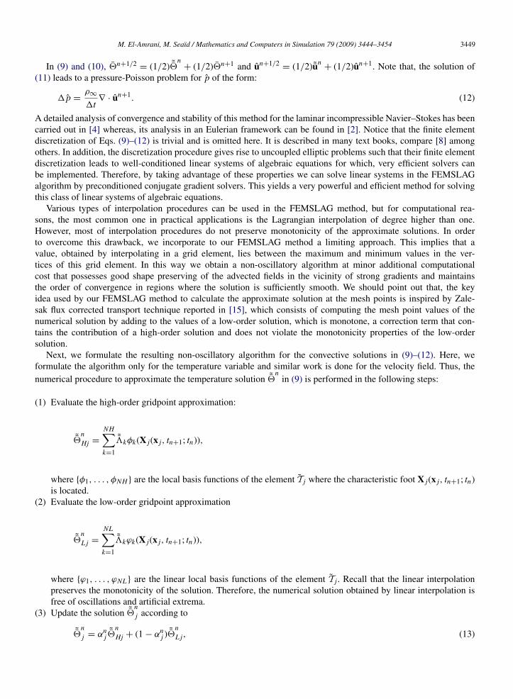
Fig. 2. Results for the advection of the slotted cylinder after one revolution.

M. El-Amrani, M. Seaïd / Mathematics and Computers in Simulation 79 (2009) 3444–3454 3451

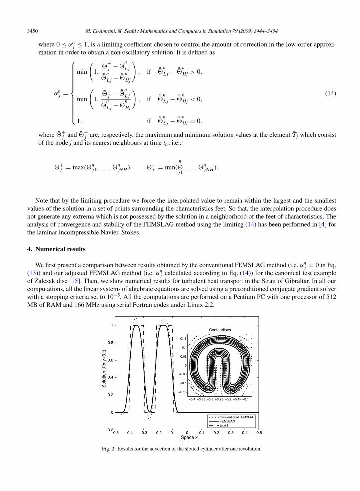
Table 2Mesh statistics, maximum and minimum values of the temperature at time t = T/4, and computational times (in min) for the considered meshes.

Elements u/ � nodes p nodes max� min� CPU

Mesh A 360 777 209 41.33 19.77 17.5Mesh B 1,440 2,993 777 23.67 19.95 91.25Mesh C 5,760 11,745 2,993 23.009 17.07 505Mesh D 23,040 46,529 11,745 23.008 17.002 2087.5Reference 92,160 1,85,217 46,529 23 17 10,555

4.1. Advection of a slotted cylinder

To ascertain the performance of our FEMSLAG algorithm we consider the test example of a passive advection ofthe slotted cylinder proposed in [15]. The problem statement is given by

∂�

∂t+ u

∂�

∂x+ v

∂�

∂y= 0, (x, y) ∈� = [−0.5, 0.5] × [−0.5, 0.5], (15)

where u(x, y) = +ωy and v(x, y) = −ωx, with ω = 0.3636 × 10−4. The cylinder is centered at (−0.25, 0) of radius0.15 and height of 4 along with a slot of width 0.06 and a length of 0.22. The time needed to complete a revolution is2π/ω. We discretize the domain � into a uniform mesh of 100 × 100 gridpoints. The CFL number associated to Eq.(15) is ω(

√2/2)(�t/�x) and it is set to 4.4

Fig. 3. Horizontal cross-sections of the temperature, u-velocity, streamfunction and pressure at time t = T/2 on five different meshes.

3452 M. El-Amrani, M. Seaïd / Mathematics and Computers in Simulation 79 (2009) 3444–3454

In Fig. 2 we display the solutions obtained by our FEMSLAG method and the conventional FEMSLAG method afterone revolution. The one-dimensional plots correspond to a cross section at y = 0, while 7 equi-distributed contourlinesare plotted in the two-dimensional figures. A visual comparison of the results in this figure shows severe undershoot,deformation and phase errors in the conventional FEMSLAG solutions. After one revolution, the conventional FEM-SLAG method exhibits non-physical oscillations and substantially greater distortion, especially at the feet and theupper face of the slotted cylinder where the gradient is sharper. From the same figure we observe a complete absence ofthese oscillations in our FEMSLAG results. It should be mentioned that in all our computations the CPU time neededfor our FEMSLAG method is less than 1.5 times more than that needed for the conventional FEMSLAG method. Theadditional computational effort used by the limiting procedure has been kept to the minimum that our FEMSLAGmethod is still effective.

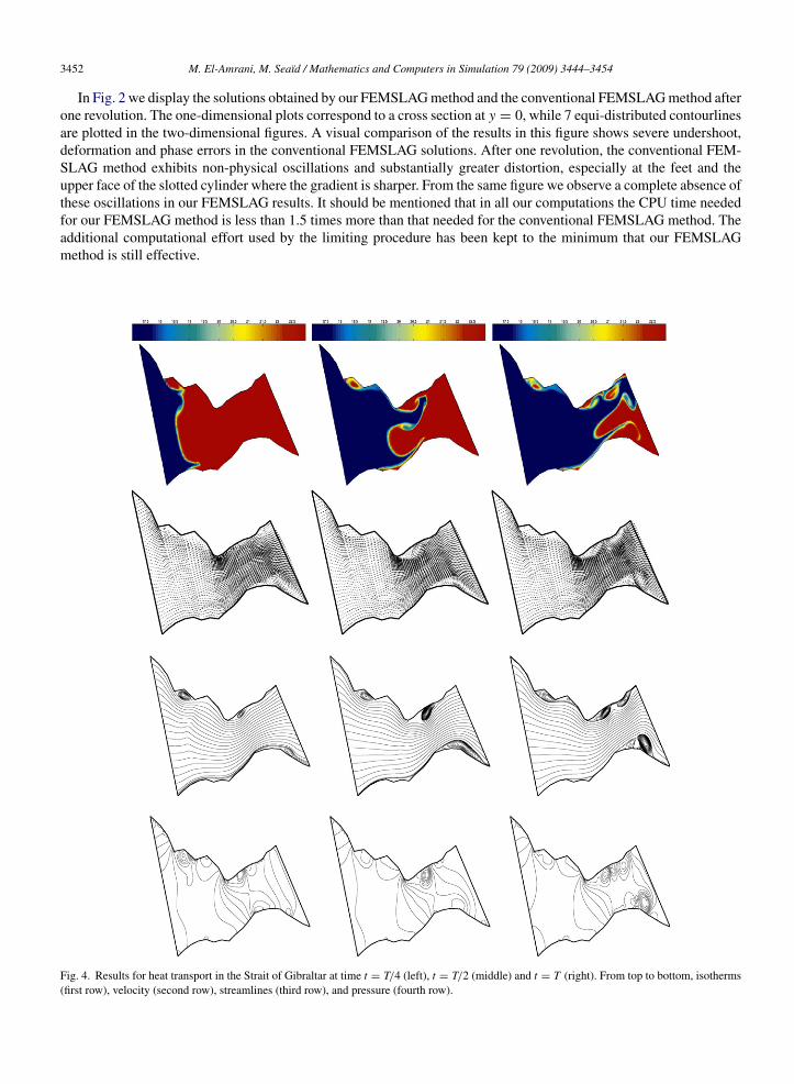
Fig. 4. Results for heat transport in the Strait of Gibraltar at time t = T/4 (left), t = T/2 (middle) and t = T (right). From top to bottom, isotherms(first row), velocity (second row), streamlines (third row), and pressure (fourth row).

M. El-Amrani, M. Seaïd / Mathematics and Computers in Simulation 79 (2009) 3444–3454 3453

4.2. Application to the Strait of Gibraltar

In our computations, we consider a series of non-uniform meshes with triangular P2/P1 finite elements, thedimensionless time step�t is fixed to 0.1 and Smagorinsky constant cs = 0.18. The corresponding statistics of veloc-ity/temperature and pressure nodes are listed in Table 2. Fig. 3 illustrates horizontal cross-sections of the temperature,u-velocity, streamfunction and pressure at the latitude 21◦10′ of the Strait. It is easy to see that solutions obtainedusing the Mesh A are far from those obtained by the Reference Mesh. Increasing the density of elements, the resultsfor the Mesh C, Mesh D and Reference Mesh are roughly similar. To further quantify the results for these mesheswe summarize in Table 2 the computational times, maximum and minimum values of the temperature. As can beobserved, there is little differences between the last three mesh levels. For instance, the discrepancies in the maximumand minimum values of temperature on Mesh C and Reference Mesh are less than 0.1%. These differences becomeless than 0.05% on Mesh D and Reference Mesh. Therefore, bearing in mind the slight change in the results from MeshC and Mesh D at the expanse of rather significant increase in CPU times, the Mesh C is believed to be adequate toobtain the results free of grid effects. Hence, the results presented herein for LES are based on the Mesh C displayedin the right plot of Fig. 1.

Fig. 4 shows the temperature distribution, velocity vectors, streamlines field and pressure contours at three differenttimes, namely t = T/4, t = T/2 and t = T . At earlier time of the simulation, the cold Atlantic front entering the Straitstarts to develop and will be advected later on by the flow at far exit of the Strait. The interaction between the heat transferand the water flow is detected across the strait during the simulation time. It can be clearly seen that the complicatedtemperature and flow structures are captured by our FEMSLAG method. We can see that two major vortices are locatednear the Tarrifa narrow and Sebta basin. Inside these vortices, there is a more complex vortex pattern. The decreaseand increase of the strengths of vortices with respect to time can be seen in Fig. 4.

From the computed results we can observe that, for the considered flow and heat conditions, the temperature istransported towards the Spanish coast. The cold front follows the stream induced by the mean flow entering theStrait of Gibraltar from the Atlantic ocean. During its advection, the heat transfer alerts the flow structure developingrecirculation zones with different order of magnitude in the vicinity of Tarrifa narrow. The downstream recirculationzone near Sebta basin is mainly due to the temperature differences at the region near the exit boundary. In summary,the heat transport is captured accurately, the flow field is resolved reasonably well, and the temperature front is shapepreserving. All these features have been achieved using time steps larger than those required for Eulerian-based methodsin convection-dominated flows.

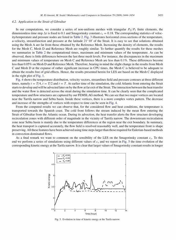
As a final remark we want to comment on the sensibility of the LES on the Smagorinsky constant cs. To thisend we perform a series of simulations using different values of cs and we report in Fig. 5 the time evolution of thecorresponding kinetic energy at the Tarifa narrow. It is clear that larger values of Smagorinsky constant results in longer

Fig. 5. Evolution in time of kinetic energy at the Tarifa narrow.

3454 M. El-Amrani, M. Seaïd / Mathematics and Computers in Simulation 79 (2009) 3444–3454

fluctuations in the kinetic energy before the later stabilizes to a stationary state. It is evident that further investigationson the influence of the Smagorinsky constant is needed.

5. Conclusions

A two-dimensional numerical model was implemented and applied to simulate turbulent heat transport in the Straitof Gibraltar. The heat transport was included in the incompressible Navier–Stokes equations using the Boussinesqapproximation. The turbulence effects were incorporated in the system by considering the Smagorinsky model. TheCoriolis term was also considered in the model. A combined finite element semi-Lagrangian method was developed forthe numerical solution of the coupled problem. The method was verified for a rotating slotted cylinder and then used tosimulate temperature transport in the Strait of Gibraltar. The presented results demonstrated good eddy resolution withhigh accuracy in smooth regions and without any non-physical oscillations near the moving fronts. The results alsoreveal that the combination of hydraulic-driven and buoyancy-driven recirculation enhances the plume region alongthe Strait of Gibraltar.

Acknowledgment

The project, under which this study was conducted, was supported by the Agencia Espanola de CooperaciónInternacional (AECI), under grant number 5/04/AC. The financial support is highly appreciated.

References

[1] J.I. Almazán, H. Bryden, T. Kinder, G. Parrilla (Eds.), Seminario Sobre la Oceanografía Física del Estrecho de Gibraltar, SECEG, Madrid,1988.

[2] E.J. Dean, R. Glowinski, On some finite elements methods for the numerical simulation of incompressible viscous flow, in: M.D. Gunzburger,R.A. Nicolaides (Eds.), Incompressible Computational Fluid Dynamics, Cambridge University Press, Cambridge, 1993.

[3] M. El-Amrani, M. Seaïd, A finite element modified method of characteristics for convective heat transport, Numer. Methods Part. Diff. Eq. 24(2008) 776–798.

[4] M. El-Amrani, M. Seaïd, Convergence and stability of finite element modified method of characteristics for the incompressible Navier–Stokesequations, J. Numer. Math. 15 (2007) 101–135.

[5] M. El-Amrani, M. Seaïd, Numerical simulation of natural and mixed convection flows by Galerkin-characteristic method, Int. J. Numer.Methods Fluids 53 (2007) 1819–1845.

[6] M. González, A. Sánchez-Arcilla, Un modelo numérico en elementos finitos para la corriente inducida por la marea. Aplicaciones al Estrechode Gibraltar, Rev. Int. Métodos Numér. Cálculo y Diseno Ing.’ıa 11 (1995) 383–400.

[7] M. González, M. Seaïd, Finite element modified method of characteristics for shallow water flows: application to the Strait of Gibraltar, Prog.Ind. Math. 8 (2005) 518–522.

[8] C. Johnson, Numerical Solution of Partial Differential Equations by the Finite Element Method, Cambridge University Press, Cambridge–Lund,1987.

[9] M. Millán, M.J. Estrela, V. Caselles, Torrential precipitations on the Spanish East coast: the role of the Mediterranean sea surface temperature,Atmos. Res. 36 (1995) 1–16.

[10] O. Pironneau, On the transport-diffusion algorithm and its applications to the Navier–Stokes equations, Numer. Math. 38 (1982) 309–332.[11] B.G. Polyak, M. Fernández, M.D. Khutorskoy, J.I. Soto, I.A. Basov, M.C. Comas, V.Ye. Khain, B. Alonso, G.V. Agapova, I.S. Mazurova, A.

Negredo, V.O. Tochitsky, J. de la Linde, N.A. Bogdanov, E. Banda, Heat flow in the Alboran sea, Western Mediterranean, Tectonophysics 263(1996) 191–218.

[12] P. Sagaut, Large Eddy Simulation for Incompressible Flows, Springer, Berlin, Heidelberg, New York, 2001.[13] J.S. Smagorinsky, General circulation experiments with the primitive equations, Mon. Weather Rev. 91 (1963) 99–164.[14] C. Temperton, A. Staniforth, An efficient two-time-level semi-Lagrangian semi-implicit integration scheme, Q. J. R. Meteorol. Soc. 113 (1987)

1025–1039.[15] S. Zalesak, Fully multidimensional flux-corrected transport algorithms for fluids, J. Comp. Phys. 31 (1979) 335–362.