Large deviations and ruin probabilities for solutions to stochastic recurrence equations with heavy-tailed innovations

The Annals of Probability2005, Vol. 33, No. 5, 1992–2035DOI 10.1214/009117905000000350© Institute of Mathematical Statistics, 2005

LARGE DEVIATIONS AND RUIN PROBABILITIESFOR SOLUTIONS TO STOCHASTICRECURRENCE EQUATIONS WITH

HEAVY-TAILED INNOVATIONS

BY DIMITRIOS G. KONSTANTINIDES AND THOMAS MIKOSCH1

University of the Aegean and University of Copenhagen

In this paper we consider the stochastic recurrence equation Yt =AtYt−1 + Bt for an i.i.d. sequence of pairs (At ,Bt ) of nonnegative randomvariables, where we assume that Bt is regularly varying with index κ > 0and EAκ

t < 1. We show that the stationary solution (Yt ) to this equation hasregularly varying finite-dimensional distributions with index κ . This impliesthat the partial sums Sn = Y1 + · · ·+Yn of this process are regularly varying.In particular, the relation P(Sn > x) ∼ c1nP (Y1 > x) as x → ∞ holdsfor some constant c1 > 0. For κ > 1, we also study the large deviationprobabilities P(Sn − ESn > x), x ≥ xn, for some sequence xn → ∞ whosegrowth depends on the heaviness of the tail of the distribution of Y1. Weshow that the relation P(Sn−ESn > x) ∼ c2nP (Y1 > x) holds uniformly forx ≥ xn and some constant c2 > 0. Then we apply the large deviation resultsto derive bounds for the ruin probability ψ(u) = P(supn≥1((Sn − ESn) −µn) > u) for any µ > 0. We show that ψ(u) ∼ c3uP (Y1 > u)µ−1(κ − 1)−1

for some constant c3 > 0. In contrast to the case of i.i.d. regularly varyingYt ’s, when the above results hold with c1 = c2 = c3 = 1, the constants c1, c2and c3 are different from 1.

1. Introduction. The stochastic recurrence equation

Yt = AtYt−1 + Bt, t ∈ Z,(1.1)

and its stationary solution have attracted much attention over the last years. Here((At ,Bt )) is an i.i.d. sequence of pairs of nonnegative random variables At and Bt .[In what follows, we write A,B,Y, . . . , for generic elements of the stationarysequences (At ), (Bt ), (Yt ), etc. We also write c for any positive constant whosevalue is not of interest.]

Major applications of stochastic recurrence equations are in financial time seriesanalysis. For example, the squares of the GARCH process can be embedded in

Received January 2004; revised November 2004.1Supported by MaPhySto, the Danish Research Network for Mathematical Physics and

Stochastics, DYNSTOCH, a research training network under the Improving Human PotentialProgramme financed by the Fifth Framework Programme of the European Commission, and by theDanish Natural Science Research Council (SNF) Grant 21-01-0546.

AMS 2000 subject classifications. Primary 60F10; secondary 91B30, 60G70, 60G35.Key words and phrases. Stochastic recurrence equation, large deviations, regular variation, ruin

probability.

1992

RECURRENCE EQUATIONS WITH HEAVY-TAILED INNOVATIONS 1993

a stochastic recurrence equation of type (1.1); we refer to Section 8.4 in [15]for an introduction to stochastic recurrence equations and [1] and [23] forrecent surveys on the mathematics of GARCH models, their properties andrelation with stochastic recurrence equations. The stochastic recurrence equationapproach has also proved useful for the estimation of GARCH and related models;see [27, 37, 38]. In a financial or insurance context, the stochastic recurrenceequation (1.1) has natural interpretations. For example, Bt can be considered asannual payment and At as a discount factor. The value Yt is then the aggregatedvalue of past discounted payments. In a life insurance context, (Yt ) is referred toas a perpetuity; see, for example, [14]. Stochastic recurrence equations have alsobeen used to describe evolutions in biology; see [2] and the references therein.

It will be convenient to use the notation

�s,t ={

As, . . . ,At , s ≤ t ,

1, s > t ,�t = �1,t .

It is well known [5] that, under the assumptions E log+ A < ∞ and E log+ B < ∞,(1.1) has a unique strictly stationary ergodic causal solution (Yt ) [i.e., Yt is afunction only of (As,Bs), s ≤ t] if and only if

−∞ ≤ E logA < 0.(1.2)

In what follows, we always assume these conditions to be satisfied. The stationarysolution has representation

Yt =t∑

i=−∞�i+1,tBi = Bt +

t−1∑i=−∞

�i+1,tBi, t ∈ Z.(1.3)

We say that any nonnegative random variable Z and its distribution are regularlyvarying with index κ if its right tail is of the form

P(Z > x) = L(x)

xκ, x > 0,

for some κ ≥ 0 and a slowly varying function L. A result of Kesten [21] shows thatthe stationary solution to the stochastic recurrence equation (1.1) has regularlyvarying distribution, under quite general conditions on A and B . We cite thisbenchmark result for comparison with the results we obtain in this paper.

THEOREM 1.1 (Kesten [21]). Assume that the following conditions hold:

• For some ε > 0, EAε < 1.• The set

{log(an · · ·a1) : n ≥ 1, an · · ·a1 > 0 and an, . . . , a1 ∈ the support of PA}generates a dense group in R with respect to summation and the Euclideantopology. Here PA denotes the distribution of A.

1994 D. G. KONSTANTINIDES AND T. MIKOSCH

• There exists κ0 > 0 such that

EAκ0 ≥ 1,(1.4)

and E(Aκ0 log+ A) < ∞.

Then the following statements hold:

1. There exists a unique solution κ ∈ (0, κ0] to the equation

EAκ = 1.

2. If EBκ < ∞, there exists a unique strictly stationary ergodic causal solution(Yt ) to the stochastic recurrence equation (1.1) with representation (1.3).

3. If EBκ < ∞, then Y is regularly varying with index κ > 0. In particular, thereexists c > 0 such that

P(Y > x) ∼ cx−κ , x → ∞.

Condition (1.4) is crucial. Goldie and Grübel [17] show that P(Y > x) candecay exponentially fast to zero if (1.4) is not satisfied. Notice that (1.4) ensuresthat the support of A is spread out sufficiently far.

The set-up of this paper is different from the one in Kesten’s Theorem 1.1. Thelatter result is surprising insofar that a light-tailed distribution of A (such as theexponential or the truncated normal distribution) can cause the stationary solution(Yt ) to (1.1) to have a marginal distribution with Pareto-like tails. In this paper weconsider the case when B is regularly varying with index κ and A has a lighterright tail than B . In this case the conditions of Kesten’s theorem are not met.In particular, we always assume that EAκ < 1. The marginal distribution of thestationary solution (Yt ) turns out to be regularly varying with the same index κ asthe innovations Bt .

It is the objective of this paper to study the interplay of the regular variationof Y and the particular dependence structure of the Yt ’s with respect to the partialsums

Sn = Y1 + · · · + Yn, n ≥ 1.

Due to (multivariate) regular variation of the finite-dimensional distributionsof (Yt ), Sn is regularly varying with index κ , and we establish the precise tailasymptotics for P(Sn > x) for fixed n and as x → ∞. We will see that, in contrastto i.i.d. regularly varying random variables Yt (cf. Lemma 1.3.1 in [15]), therelation

limx→∞

P(Sn > x)

nP (Y > x)= 1, n ≥ 2,


does not hold for the stationary solution (Yt ) to (1.1), neither under theconditions of Kesten’s theorem nor under the conditions imposed in this paper;see Section 3.3. We will show in Proposition 3.3 that

limx→∞

P(Sn > x)

P (Y > x)(1.5)

= E

(n∑

i=1

�i

)κ

+ (1 − EAκ)

n−1∑t=0

E

(t∑

i=0

�i

)κ

, n ≥ 2.

A question which is closely related to (1.5) concerns the large deviations of thepartial sum process (Sn). In this case, one is interested in the asymptotic behaviorof the tail P(Sn > xn) for real sequences (xn) increasing to infinity sufficientlyfast. Classical results (see, e.g., [8, 29, 30]; cf. the surveys in Section 8.6 in [15]and [24]) say that, for i.i.d. (Yt ) and thresholds xn → ∞, the relation

P(Sn > xn) ∼ nP (Y > xn)(1.6)

∼ P(max(Y1, . . . , Yn) > xn

)holds. For reasons of comparison, we quote a general large deviation result fori.i.d. random variables.

THEOREM 1.2. Assume that B > 0 is regularly varying with index κ > 0.

1. ([29, 30]) Assume that κ > 2. Then

P

(n∑

t=1

(Bt − EB) > x

)= ��(x/

√n)(

1 + o(1))+ nP (B > x)

(1 + o(1)

),

as n → ∞ and uniformly for x ≥ √n, where �� = 1 − � is the right tail of the

standard normal distribution function �. In particular,

P

(n∑

t=1

(Bt − EB) > x

)= ��(x/

√n)(

1 + o(1))

uniformly for√

n ≤ x ≤ √an logn and a < κ − 2, and

P

(n∑

t=1

(Bt − EB) > x

)= nP (B > x)

(1 + o(1)

)uniformly for x ≥ √

an logn and a > κ − 2.2. ([8]) Assume that κ ∈ (1,2). Then

P

(n∑

t=1

(Bt − EB) > x

)= nP (B > x)

(1 + o(1)

),(1.7)

as n → ∞ and uniformly for x ≥ ancn, where (an) satisfies nP (B > an) ∼ 1and (cn) is any sequence satisfying cn → ∞.


The uniformity of these large deviation results refers to the fact that the errorbounds hold uniformly for the indicated x-regions. For example, in the caseκ ∈ (1,2), (1.7) means that

limn→∞ sup

x≥xn

∣∣∣∣P(∑n

t=1(Bt − EB) > x)

nP (B > x)− 1

∣∣∣∣= 0,(1.8)

where xn = ancn.We will show in Theorem 4.2 that the following analog to Theorem 1.2 holds,

under the more restrictive condition that (At ) and (Bt ) are independent:

limn→∞ sup

x≥xn

∣∣∣∣∣P(Sn − ESn > x)

nP (Y > x)− (1 − EAκ)E

( ∞∑i=0

�i

)κ ∣∣∣∣∣= 0.(1.9)

The question about large deviations is closely related to the ruin probability ofthe random walk (Sn). Given that EY < ∞, this is the probability

ψ(u) = P

(supn≥1

[(Sn − ESn) − µn] > u

), u,µ > 0.

It is one of the very well studied objects of applied probability theory, startingwith classical work by Cramér in the 1930s. For i.i.d. regularly varying and, moregenerally, subexponential Yt ’s, the asymptotic behavior of ψ(u) as u → ∞ wasstudied by various authors; see Chapter 1 in [15]. The following benchmark resultis classical in the context of ruin for heavy-tailed distributions. We cite it here forcomparison with the results of this paper.

THEOREM 1.3. Assume that B is regularly varying with index κ > 1. Thenfor any µ > 0,

P

(supn≥1

(n∑

t=1

(Bt − EB) − µn

)> u

)∼ 1

µ

1

κ − 1uP (B > u), u → ∞.

In Theorem 4.9 we prove an analogous result for (Yt ):

ψ(u) ∼ 1

µ

1

κ − 1(1 − EAκ)E

( ∞∑i=0

�i

)κ

uP (Y > u).(1.10)

The results of this paper are derived by applications of the heavy-tailed largedeviations heuristics. In the case of i.i.d. Yt ’s, this means that a large deviationof the random walk Sn from its mean ESn must be due to exactly one unusuallylarge value Yt , whereas the Ys ’s for s = t are small compared to Yt . We referto [35] for a review on these heuristics which can be exploited in the contextof various applied probability models. For dependent Yt ’s, as considered in thispaper, the large deviations heuristics has to be combined with the understandingof the dependence structure of the random walk Sn exceeding high thresholds. In


the proof of the ruin probability result, it turns out that the ruin probability of therandom walk (Sn) behaves very much like the ruin probability of the random walk∑n

t=1 BtCt , where Ct =∑∞i=t �t+1,i , t ∈ Z. This is another stationary sequence,

but, under the conditions of this paper, its marginal distributions have tails lessheavy than (Bt ). Since we assume independence of (At ) and (Bt ), hence, of (Ct )

and (Bt ), in Section 4.2, it is likely that a large value of Sn is now caused by a largevalue BtCt , which in turn is caused by a large value of Bt . We make this intuitionprecise by showing (1.10).

The results (1.5) on the tail of Sn for fixed n, (1.9) on the large deviations of (Sn)

and (1.10) on the ruin probability of (Sn) and their analogs for i.i.d. Yt ’s illustratesome crucial differences between the behavior of a random walk with dependentand independent heavy-tailed step sizes far away from the origin. The constantson the right-hand sides of (1.5), (1.9) and (1.10), which differ from those in thecase of i.i.d. regularly varying Yt ’s, can be considered as alternative measures ofthe extremal clustering behavior of the Yt ’s. Similar results were obtained onlyfor a few classes of stationary processes (Yt ). Those include results by Mikoschand Samorodnitsky [25, 26] on large deviations and ruin for random walks withstep sizes which constitute a linear process with regularly varying innovations or astationary ergodic stable process, and by Davis and Hsing [9] on large deviationsfor random walks with infinite variance regularly varying step sizes. So far theknown results do not allow one to draw a general picture which would allowone to classify stationary sequences of regularly varying random variables Yt

with respect to their extremal behavior of the random walk with negative drift((Sn − ESn) − µn). The cited results and also those of the present paper aresteps in the search for appropriate measures of extremal dependence in a stationarysequence by studying the behavior of suitable functionals acting on the sequence.

The paper is organized as follows. In Section 2 we give conditions under whichthe stationary solution (Yt ) to the stochastic recurrence equation (1.1) has regularlyvarying finite-dimensional distributions. In Section 3 we consider applications ofthis property to the weak convergence of related point processes, the central limittheorem of (Sn) and the partial maxima of (Yt ). In Section 4.1 we study the largedeviations of (Sn) and in Section 4.2 we give our main result on the asymptoticbehavior of the ruin probability ψ(u). Since the proofs of the main results arequite technical, we postpone them to particular sections at the end of the paper.The proof of Theorem 4.2 will be given in Section 5 and the one of Theorem 4.9in Section 6.

2. Regular variation of the solution to the stochastic recurrence equation.

2.1. Preliminaries. We start with some auxiliary results in order to establishregular variation of Y . In what follows, we write �F(x) = 1−F(x) for the right tailof any distribution function F .


LEMMA 2.1 (Davis and Resnick [12]). Let F be a distribution functionconcentrated on (0,∞). Assume Z1, . . . ,Zn are independent nonnegative randomvariables satisfying

limx→∞

P(Zi > x)

�F(x)= ci(2.1)

for some nonnegative finite values ci , where F(x) = P(Z1 ≤ x), and

limx→∞

P(Zi > x,Zj > x)

�F(x)= 0, i = j.(2.2)

Then

limx→∞

P(Z1 + · · · + Zn > x)

�F(x)= c1 + · · · + cn.

We will frequently make use of the following elementary property which wasproved by Breiman [7] in a special case. We refer to it as Breiman’s result andprove a uniform version of it for further use.

LEMMA 2.2 (Breiman [7]). Let ξ, η be independent nonnegative nondegen-erate random variables such that ξ is regularly varying with index κ > 0 andEηκ+ε < ∞ for some ε > 0. Then for any sequence xn → ∞,

limn→∞ sup

x≥xn

∣∣∣∣P(ξη > x)

P (ξ > x)− Eηκ

∣∣∣∣= 0.

This means that the product ξη inherits regular variation from ξ .

PROOF. Fix M > 0. Then

(x) = P(ξη > x)

P (ξ > x)− Eηκ

=∫[0,M]

[P(ξy > x)

P (ξ > x)− yκ

]dP (η ≤ y)

− EηκI(M,∞)(η) +∫(M,∞)

P (ξy > x)

P (ξ > x)dP (η ≤ y)

= 1(x) − 2 + 3(x).

Obviously,

limM→∞2 = 0.


Moreover, the uniform convergence theorem for regularly varying functions(see [4]) implies that, for every fixed M > 0,

supx≥xn

|1(x)| ≤ supx≥xn

∫[0,M]

∣∣∣∣P(ξy > x)

P (ξ > x)− yκ

∣∣∣∣dP (η ≤ y)

≤ supx≥xn

supy≤M

∣∣∣∣P(ξy > x)

P (ξ > x)− yκ

∣∣∣∣→ 0.

An application of the Potter bounds for regularly varying functions (see [4],page 25) yields, for x, x/y ≥ x0, for sufficiently large x0 > 0 and all y > M > 1,that

P(ξ > x/y)

P (ξ > x)≤ yκ+ε.

Hence,

supx≥xn

|3(x)| ≤ supx≥xn

∫M<y≤x/x0

yκ+ε dP (η ≤ y) + supx≥xn

P (η > x/x0)

P (ξ > x)

→ 0

by first letting n → ∞ and then M → ∞, since Eηκ+ε < ∞. This proves thelemma. �

We now turn to the stochastic recurrence equation (1.1). After n iterations, weobtain

Yn = �nY0 +n∑

t=1

�t+1,nBt .(2.3)

As in Section 1, we assume that ((At ,Bt )) is an i.i.d. sequence of pairs ofnonnegative random variables At and Bt . In addition, suppose that B is regularlyvarying with index κ > 0 and EAκ+δ < ∞ for some δ > 0. Then Breiman’s result(Lemma 2.2) applies:

P(�i−1Bi > x)

P (B > x)∼ (EAκ)i−1 as x → ∞.(2.4)

The following result will be crucial for the property of regular variation ofthe finite-dimensional distributions of the stationary solution (Yn) to (1.1). Forits formulation, we assume that Y0 = c in (2.3) for some constant c. We use thesame notation (Yn) in this case, slightly abusing notation since (Yn) is then not thestationary solution to (1.1).

PROPOSITION 2.3. Assume B is regularly varying with index κ > 0 andEAκ+δ < ∞ for some δ > 0. Then the following relation holds for fixed n ≥ 1


and Yn defined in (2.3) with Y0 = c:

P(Yn > x) ∼ P(B > x)

n−1∑i=0

(EAκ)i as x → ∞.

PROOF. We write

Z0 = �nc, Zt = �t−1Bt, t = 1, . . . , n.

Observe that

Yn = �nc +n∑

t=1

�t+1,nBtd= �nc +

n∑t=1

�t−1Bt =n∑

t=0

Zt .

We have, for 1 ≤ i < j ≤ n,

P(Zi > x,Zj > x) ≤ P(�i−1 min(Bi,�i,j−1Bj) > x

).

Since EAκ+δ < ∞ and B is regularly varying with index κ , we can find a functiong(x) → ∞ such that g(x)/x → 0, and P(max(Ai,�i) > g(x)) = o(P (B > x)).Hence, for i < j ,

P(Zi > x,Zj > x)

P (B > x)

≤ P(�i−1 min(Bi,�i,j−1Bj) > x,max(Ai,�i) > g(x))

P (B > x)

+ P(�i−1 min(Bi,�i,j−1Bj) > x,max(Ai,�i) ≤ g(x))

P (B > x)

≤ P(max(Ai,�i) > g(x))

P (B > x)+ P(�i−1Bi > x,�i+1,j−1Bj > x/g(x))

P (B > x)

= o(1) + (EAκ)j−2P(B > x/g(x)

)(1 + o(1)

)→ 0.

In the last step we made multiple use of Breiman’s result and the independence of�i−1Bi and �i+1,j−1Bj . By Markov’s inequality, we also have, for 1 ≤ i ≤ n,

P(Z0 > x,Zi > x)

P (B > x)≤ P(Z0 > x)

P (B > x)≤ cn (EAκ+δ)nx−κ−δ

P (B > x)→ 0.

Hence, we are in the framework of Lemma 2.1 with c0 = 0 and ci = (EAκ)i−1,i = 1, . . . , n; see (2.4). This proves the proposition. �

2.2. Univariate regular variation of Y . In this section we indicate regularvariation of the marginal distribution of the stationary solution to the stochastic


recurrence equation (1.1). From Proposition 2.3 and the representation (1.3) of thestationary solution (Yt ), we conclude that

lim infx→∞

P(Y > x)

P (B > x)≥ lim

x→∞P(∑n

i=1 �i−1Bi > x)

P (B > x)=

n−1∑i=0

(EAκ)i.(2.5)

Letting n → ∞ yields a lower bound for P(Y > x). This relation suggests that

P(Y > x) ∼ P(B > x)

∞∑i=0

(EAκ)i, x → ∞,(2.6)

holds under the conditions that B is regularly varying with index κ > 0 andEAκ < 1. Obviously, only if the latter condition holds, relation (2.6) is meaningful.This also means that the conditions of Kesten’s Theorem 1.1 cannot be satisfied. Inthat case, the index of regular variation κ of Y satisfies EAκ = 1 and EBκ < ∞.Since in our case B is assumed to be regularly varying with index κ , the momentcondition on B is not necessarily met either.

PROPOSITION 2.4 (Grey [18]). Assume that B is regularly varying with indexκ > 0, EAκ+δ < ∞ for some δ > 0 and EAκ < 1. Then a unique strictly stationarysolution (Yt ) to the stochastic recurrence equation (1.1) exists and satisfies

P(Y > x) ∼ P(B > x)(1 − EAκ)−1.(2.7)

PROOF. The function g(h) = EAh satisfies g(0) = 1, g(κ) < 1 and it iscontinuous and convex in [0, κ]. Therefore, g′(0+) = E logA < 0 and (1.2) andE log+ A < ∞ hold. Moreover, since EBγ < ∞ for γ < κ , E log+ B < ∞ issatisfied and, hence, a unique stationary solution (Yt ) to (1.1) exists.

Relation (2.7) follows from Theorem 1 in [18]. �

2.3. Regular variation of the finite-dimensional distributions of (Yt ). In whatfollows, we assume that the conditions of Proposition 2.4 are satisfied. The latterresult states that the marginal distribution of the stationary sequence (Yn) isregularly varying with the same index κ as the innovations Bt . It is the aimof this section to extend this result to the finite-dimensional distributions of theprocess (Yt ).

For this reason, we introduce the notion of regular variation for an m-dimensio-nal random vector: the vector Y ∈ R

m is regularly varying with index κ > 0 if thereexists a nonnull Radon measure µ on the Borel σ -field B of [0,∞]m \ {0} suchthat

nP (a−1n Y ∈ ·) v→ µ.

Here the sequence (an) satisfies P(|Y| > an) ∼ n−1,v→ denotes vague conver-

gence in B, and µ is a measure with the property µ(t ·) = t−κµ(·) for all t > 0;


see [32] for an introduction to regular variation, related point process convergenceand vague convergence. An equivalent way to characterize the limiting measure µ

is via a presentation in spherical coordinates. This means that, for every fixed t > 0and (an) as above,

nP (|Y| > tan,Y/|Y| ∈ ·) v→ t−κP (� ∈ ·),where | · | is any fixed norm,

v→ refers to vague convergence on the Borel σ -fieldof the unit sphere S

d−1 corresponding to this norm and � is a vector with valuesin S

d−1. Its distribution is referred to as the spectral distribution of Y.For fixed m ≥ 1, we have

Ym = (Y1, . . . , Ym)′

= (�1,�2, . . . ,�m)′Y0 +(B1,B2 + A2B1, . . . ,Bm +

m−1∑i=1

�i+1,mBi

)′

=

�1�2�3...

�m−1�m

Y0 +

1�2,2�2,3

...

�2,m−1�2,m

B1 +

01

�3,3...

�3,m−1�3,m

B2 + · · · +

000...

01

Bm

=: A0Y0 + A1B1 + · · · + AmBm.

Notice that A0 and Y0 are independent, and so are Ai and Bi for every i. SinceE|Ai |κ+δ < ∞ for some δ > 0 and Y0,B1, . . . ,Bm are independent and regularlyvarying with index κ , a multivariate version of Breiman’s result (cf. [1, 33]) appliesto conclude that each of the vectors A0Y0, A1B1, . . . ,AmBm is regularly varyingwith index κ with corresponding limiting measures µ0, . . . ,µm. We mention thatthe normalizing sequences for these vectors are of the same size since, by the one-dimensional Breiman result and Proposition 2.4, as x → ∞,

P(|A0Y0| > x) ∼ E|A0|κP (Y0 > x) ∼ E|A0|κ(1 − EAκ)−1P(B > x),

P (|AiBi | > x) ∼ E|Ai |κP (B > x), i = 1, . . . ,m.

We choose one normalizing sequence (an) for all vectors such that nP (|A0|Y0 >

an) ∼ 1. We can characterize µi via its spectral distribution. Indeed, by Breiman’sresult, we have, for any Borel set S ⊂ S

d−1 whose boundary has mean zero withrespect to the spectral distribution,

nP (|Ai |Bi > tan,Ai/|Ai | ∈ S) ∼ t−κnP (B > an)E[|Ai |κIS(Ai/|Ai |)],and, therefore, the spectral distribution of AiYi for these sets S is given by

E[|Ai |κIS(Ai/|Ai |)]E|Ai |κ .


Adapting the proof of Lemma 2.1 in [12] to the multivariate case, it follows thatYm is regularly varying with index κ and limiting measure

µ(dx) = µ0(dx) + c1µ1(dx) + · · · + cmµm(dx),(2.8)

where

ci = E|Ai |κE|A0|κ (1 − EAκ),

provided that the following relations holds for any Borel sets C1,C2 ⊂ [0,∞]m \{0} which are bounded away from zero:

nP (a−1n AiBi ∈ C1, a

−1n AjBj ∈ C2) → 0, 0 ≤ i < j ≤ m,

where we write B0 = Y0 for the sake of simplicity. Since C1 and C2 are boundedaway from zero, there exists M > 0 such that |x| > M for all x ∈ C1,C2. Therefore,for i < j and any γ > 0,

{a−1n AiBi ∈ C1, a

−1n AjBj ∈ C2}

⊂ {|Ai |Bi > anM, |Aj |Bj > anM}⊂ {γBi > Man, γBj > Man}

∪ {γBi > Man, |Aj |I(γ,∞)(|Aj |)Bj > Man

}∪ {

γBj > Man, |Ai |I(γ,∞)(|Ai |)Bi > Man

}∪ {|Ai |I(γ,∞)(|Ai |)Bi > Man, |Aj |I(γ,∞)(|Aj |)Bj > Man

}= D1 ∪ · · · ∪ D4.

By definition of (an) and the independence of Bi and Bj , it follows immediatelythat nP (D1) → 0. A similar approach applies to D2 since Bi is independent ofBj Aj and, by Breiman’s result,

nP (D2) ∼ nP (γBi > Man)E|Aj |κI(γ,∞)(|Aj |)P (Bj > Man) → 0.

Similarly,

nP (D3) ≤ nP(|Ai |I(γ,∞)(|Ai |)Bi > Man

)∼ nE|Ai |κI(γ,∞)(|Ai |)P (Bi > Man),

and by, the Lebesgue dominated convergence,

limγ→∞ lim sup

n→∞nP (D3) = 0.

The relation nP (D4) → 0 can be proved in the same way.We summarize our findings.

PROPOSITION 2.5. If the conditions of Proposition 2.4 hold, then thefinite-dimensional distributions of the stationary solution (Yt ) to the stochasticrecurrence equation (1.1) are regularly varying with index κ and limiting measuregiven in (2.8).


3. Some applications of the regular variation property. In this section weconsider some applications of the property of regular variation of the solution(Yt ) to the stochastic recurrence equation (1.1). In particular, we are interestedin functionals of the Yt ’s and their limit behavior. The results include the centrallimit theorem for the partial sums of the sequence (Yt ) and limit theory for itspartial maxima.

3.1. A remark about the strong mixing property of (Yt ). Recall that astationary ergodic sequence (Yt ) is said to be strongly mixing if

αk = supA∈σ(Ys,s≤0),B∈σ(Ys,s≥k)

|P(A ∩ B) − P(A)P (B)| → 0,

and it is said to be strongly mixing with geometric rate if there are constantsr ∈ (0,1) and c > 0 such that αk ≤ crk for all k ≥ 1; see [34], compare [13]. Undergeneral conditions, the latter property is satisfied for the stationary solution (Yt ) ofthe stochastic recurrence equation (1.3).

PROPOSITION 3.1. Assume EAε < 1, EBε < ∞ for some ε > 0. Then thestochastic recurrence equation (1.1) has a stationary ergodic solution (Yt ) whichis also strongly mixing with geometric rate if one of the following conditions holds:

1. The Markov chain (Yt ) is µ-irreducible, that is, there exists a measure µ suchthat, for any Borel set R in the support supp(Y ) of Y with µ(R) > 0, the relation∑∞

n=1 P(Yn ∈ R|Y0 = x) > 0 holds.2. An = A(En) and Bn = B(En), where A(x) and B(x) are polynomial functions

of x and (En) are i.i.d. random variables. Moreover, A(0) < 1 and E1 has ana.e. positive Lebesgue density on [0, x0] for some 0 < x0 ≤ ∞.

PROOF. Strong mixing of (Yt ) with geometric rate under µ-irreducibilityfollows from Theorem 2.8 in [1], using standard results on mixing Markovchains; see [22]. For polynomial An and Bn, the mixing property follows fromTheorem 4.5 in [27] or from Theorem 4.3 in [28].

REMARK 3.2. Squared GARCH processes satisfy a (in general multivariate)version of (1.1). They were found to be strongly mixing with geometric rate;see [6] who proved µ-irreducibility with µ Lebesgue measure. A sufficientcondition for µ-irreducibility is that µ(R) > 0 for any R ⊂ supp(Y ) impliesP(A1x + B1 ∈ R) = P(A1Y0 + B1 ∈ R|Y0 = x) > 0. This is satisfied if A1x + B1has an a.e. positive density on supp(Y ) with respect to Lebesgue measure µ forevery x ∈ supp(Y ). Alternatively, it suffices to show that P(Yn ∈ R|Y0 = x) > 0for sufficiently large n (possibly depending on x and R). The latter condition isoften more difficult to verify.

The relation P(A1x + B1 ∈ R|Y0 = x) > 0 also holds if µ(R) > 0 for µ

Lebesgue measure and At and Bt have a joint independent multiplicative factor


which has an a.e. positive density on (0,∞), that is, At = FtAt and Bt = FtBt ,where (Ft ) is an i.i.d. sequence and for every t , Ft and (At , Bt ) are independent.The squared ARCH(1) process satisfies this condition if its innovations have apositive Lebesgue density on the real line; see [10] where the innovations of theARCH(1) process were assumed to be i.i.d. Gaussian, but the same methodologycan be used in the general case.

3.2. The central limit theorem. If the assumptions of Propositions 2.4 and 3.1hold, we may conclude from Propositions 2.4, 2.5 and 3.1 that there exists aunique stationary solution (Yt ) to the stochastic recurrence equation (1.1) whichis strongly mixing with geometric rate and which has regularly varying finite-dimensional distributions with index κ > 0.

If κ > 2, a standard central limit theorem for stationary ergodic martingaledifference sequences applies to (Yt ) and no further mixing condition is needed.Indeed, we have

n−1/2(Sn − ESn)

= n−1/2n∑

t=1

[(At − EA)Yt−1 + (Bt − EB)] + n−1/2EA

n∑t=1

(Yt−1 − EY).

Hence,

n−1/2(Sn −ESn) = n−1/2(1 −EA)−1n∑

t=1

[(At −EA)Yt−1 + (Bt −EB)]+ oP (1).

The sequence [(At − EA)Yt−1 + (Bt − EB)] is a stationary ergodic martingaledifference sequence with respect to the filtration Ft = σ((Ax,Bx), x ≤ t).Therefore, the central limit theorem from [3], Chapter 23, applies:

n−1/2(Sn − ESn)d→ N(0, σ 2

Y ),

where σ 2Y = var(Y ). Notice that EA < 1 since EAκ < 1, κ > 2 and g(h) = EAh

is a convex function.If κ < 2, infinite variance limits may occur for (Sn); see [9, 10]. The proof relies

on a point process argument for the lagged vectors Yt (m) = (Yt , . . . , Yt+m)′ whichis identical to the proof of Theorem 2.10 in [1] and requires regular variation ofthe finite-dimensional distributions and the strong mixing condition for (Yt ) withgeometric rate. It implies weak convergence of the point processes

Nn =n∑

t=1

εYt (m)/an

d→ N.(3.1)

The limiting Poisson point process N is described in [1] and (an) is a sequencesatisfying nP (Y > an) ∼ 1.


The convergence result (3.1) and the arguments in [1, 9, 10] imply the weakconvergence of the partial sums, sample autocovariances, sample autocorrelationsand the partial maxima of the sequence (Yt ). For details, we refer to the mentionedliterature. For example, if κ ∈ (0,2) \ {1},

a−1n (Sn − bn)

d→ Zκ,

where Zκ is totally skewed to the right infinite variance κ-stable randomvariable, bn = ESn for κ > 1 and bn = 0 for κ < 1. (We refer to [36] for anencyclopedic treatment of stable distributions and processes.) The proof of theweak convergence of the sample autocovariances and sample autocorrelationsis identical to the one treated in [1] for solutions to the stochastic recurrenceequation (1.1).

Moreover,

a−1n max(Y1, . . . , Yn)

d→ Rκ(θ),

where P(Rκ ≤ x) = e−x−κ, x > 0, is the Fréchet distribution function with shape

parameter κ , P(Rκ(θ) ≤ x) = [P(Rκ ≤ x)]θ and θ ∈ (0,1) is the extremal indexof the sequence (Yt ). See [15] for an introduction to extreme value theory and,in particular, Section 8.1, where the notion of extremal index is treated. Extremevalue theory for the solution (Yt ) to (1.1), under the conditions of Kesten’sTheorem 1.1, was studied in [19]. In their Theorem 2.1, they calculate

θ =∫ ∞

1P

(maxj≥1

j∏i=1

Ai ≤ y−1

)κyκ−1 dy.

We mention that the same proof as in [19] [with n1/κ replaced by (an) as above]applies under the conditions of Proposition 2.4, when Kesten’s result does notapply. Indeed, an inspection of their proof shows that it only requires the structureof the stochastic recurrence equation (1.1), the definition of (an), the regularvariation of (Yt ) and the existence of some h > 0 such that EAh < 1.

The definition of the extremal index θ implies that, for xn ≥ an,

P(max(Y1, . . . , Yn) > xn

)∼ θnP (Y > xn).

This is in contrast to i.i.d. Yt ’s, where this relation holds with θ = 1. In thei.i.d. case we also know that P(Sn − ESn > xn) ∼ P(max(Y1, . . . , Yn) > xn)

for suitable sequences (xn) with xn → ∞. The various results proved in thispaper, including Proposition 3.3 and Theorem 4.2, show that the exceedances ofthe random walk (Sn) and of the partial maxima (max(Y1, . . . , Yn)) above highthresholds have different asymptotic behavior which is also different from the caseof i.i.d. Yt ’s.


3.3. Regular variation of sums. In what follows we study the tail behavior ofthe sums

Sn = Y1 + · · · + Yn

for fixed n ≥ 1 under the assumptions of Proposition 2.5. It follows fromProposition 2.5 that all linear combinations of the lagged vector Ym are regularlyvarying with index κ . In particular, Sn is regularly varying with index κ . In thissection we give a precise description of the tail asymptotics of P(Sn > x) for fixedn as x → ∞.

We have

Sn =n∑

i=1

(�iY0 +

i∑t=1

�t+1,iBt

)= Y0

n∑i=1

�i +n∑

t=1

Bt

n∑i=t

�t+1,i .(3.2)

Write

Z0 = Y0

n∑i=1

�i and Zt = Bt

n∑i=t

�t+1,i , t = 1, . . . , n.

Notice that Y0 is independent of∑n

i=1 �i and Bt is independent of∑n

i=t �t+1,i .Now an argument similar to the one in the proof of Proposition 2.3 shows that, for0 ≤ s < t ≤ n,

P(Zt > x,Zs > x)

P (Z0 > x)→ 0, x → ∞.

Also notice that the same result holds if Y0 = c is a constant initial value. Anapplication of Lemma 2.1 yields the following result.

PROPOSITION 3.3. Assume that the conditions of Proposition 2.4 hold. If (Yn)

is the stationary solution to the stochastic recurrence equation (1.1), then

limx→∞

P(Sn > x)

P (B > x)= (1 − EAκ)−1E

(n∑

i=1

�i

)κ

+n−1∑t=0

E

(t∑

i=0

�i

)κ

.(3.3)

If (Yn) satisfies the stochastic recurrence equation (1.1) with Y0 = c for someconstant c, then

limx→∞

P(Sn > x)

P (B > x)=

n−1∑t=0

E

(t∑

i=0

�i

)κ

.

For comparison, assume for the moment that (Yt ) is an i.i.d. sequence Y1d= Y

and Y has the stationary distribution given by (1.3). Then for every fixed n ≥ 1,

limx→∞

P(Y1 + · · · + Yn > x)

nP (Y > x)= 1.(3.4)


This is the subexponential property of a regularly varying distribution; see [15],Section 1.3.2 and Appendix A3 for an extensive discussion of subexponentialdistributions. Property (3.4) does not remain valid for dependent stationarysequences with regularly varying finite-dimensional distributions. This was shownin [25] for the case of linear processes. In that case the limiting constant in (3.4) is,in general, different from 1 and depends on the coefficients of the linear process.Proposition 3.3 shows that a similar behavior can be expected for other nonlinearstationary processes. In particular, by Proposition 3.3, relation (3.3) can be re-written in the form

limx→∞

P(Sn > x)

P (Y > x)= E

(n∑

i=1

�i

)κ

+ (1 − EAκ)

n−1∑t=0

E

(t∑

i=0

�i

)κ

.(3.5)

It is interesting to observe that a similar relationship holds if the (At ,Bt )’ssatisfy the conditions of Kesten’s Theorem 1.1. In that case, the conditionEAκ = 1 is needed for regular variation of the stationary solution (Yt ) to thestochastic recurrence equation (1.1) with index κ > 0. Assume, in addition, thatEBκ+δ and EAκ+δ are finite for some δ > 0. Then we may conclude from therepresentation (3.2), regular variation of Y0 and Breiman’s result that

limx→∞

P(Sn > x)

P (Y > x)= E

(n∑

i=1

�i

)κ

.

In a sense, this is the limiting result in (3.5) for EAκ = 1.

4. Large deviations and ruin probabilities.

4.1. Results on large deviations. In this subsection we couple the increase ofx with n to obtain probabilities of large deviations of the type

P(Sn − ESn > x) ∼ nECκP (B > x) uniformly for x ≥ xn,

and appropriate sequences xn → ∞. Here C is a generic element of the stationarysequence

Ct =∞∑i=t

�t+1,i , t ∈ Z.(4.1)

We start with an auxiliary result, where we collect some useful properties of thissequence.

LEMMA 4.1. Assume that (At ) is an i.i.d. sequence and EAκ < 1 for someκ > 0.

1. The sequence (Ct ) defined in (4.1) is well defined and strictly stationary.


2. The random variable C has finite pth moment if and only if EAp < ∞ forp > 0.

3. The sequences (Ct ) and (Dt) given by (4.2) have the same finite-dimensionaldistributions. If A has an a.e. positive Lebesgue density on [0, x0] for somex0 ≤ ∞, then (Dt) is strongly mixing with geometric rate.

PROOF. 1. The sequence (Ct ) has the same distribution as the sequence

Dt =t∑

i=−∞�i+1,t , t ∈ Z.(4.2)

The latter satisfies the stochastic recurrence equation

Dt = 1 + At

t−1∑i=−∞

�i+1,t−1 = 1 + AtDt−1, t ∈ Z.(4.3)

It constitutes a unique strictly stationary sequence if E logA < 0 and E log+ A <

∞, see (1.2), which is satisfied if EAκ < 1 for some κ > 0.2. From (4.3), the independence of Dt−1 and At and the stationarity of (Dt),

we conclude that Dt has finite pth moment if and only if At has. Since Dd= C, the

statement follows.3. Follows from the second part of Proposition 3.1 with A(x) = x, B(x) = 1,

Ei = Ai . �

In the following result we assume, in addition, that the sequences (At ) and (Bt ),hence, (Ct ) and (Bt ), are independent. Although we conjecture that this assump-tion can be avoided, we need the independence at various technical steps in theproof.

THEOREM 4.2. Assume that (At ) and (Bt ) are independent i.i.d. sequences ofnonnegative random variables, B is regularly varying with index κ > 1, EAκ < 1and EA2κ < ∞. Consider a sequence of positive numbers such that nP (B >

xn) → 0 and, for every c > 0,

limn→∞ sup

x≥xn

∣∣∣∣∣(P

(var

(BI[0,x](B)

) n∑t=1

C2t > cx2/ logx

)

+ P

(∣∣∣∣∣n∑

t=1

(Ct − EC)

∣∣∣∣∣> cx

))× (

nP (B > x))−1

∣∣∣∣∣(4.4)

= 0.

Then the large deviation relations

limn→∞ sup

x≥xn

∣∣∣∣P(Sn − ESn > x)

nP (B > x)− ECκ

∣∣∣∣= 0(4.5)


and

limn→∞ sup

x≥xn

P (Sn − ESn ≤ −x)

nP (B > x)= 0(4.6)

are satisfied.

The proof of the theorem is rather technical and therefore postponed untilSection 5.

REMARK 4.3. The validation of (4.4) is, in general, difficult. Sufficientconditions for (4.4) can be verified by assuming certain mixing conditions on (Ct );see Lemma 4.6 below and Lemma 4.1 part 3.

REMARK 4.4. Theorem 4.2 is applicable for finite or infinite variancesequences (Bt ). The infinite variance comes into the picture in condition (4.4).For κ > 2, var(BI[0,x](B)) → c for some finite c > 0. Hence, condition (4.4)can be formulated without var(BI[0,x](B)). If κ < 2 or κ = 2 and var(B) = ∞,var(BI[0,x](B)) → ∞. In particular, for κ = 2, var(BI[0,x](B)) is a slowly varyingfunction which increases to infinity. If κ ∈ (1,2), an application of Karamata’stheorem yields, for some c > 0, var(BI[0,x](B)) ∼ cx2P(B > x) → ∞.

REMARK 4.5. The literature on large deviations for sums of stationary heavy-tailed random variables is rather sparse. The case of linear processes Yt =∑∞

j=−∞ ϕjZt−j for i.i.d. regularly varying sequences (Zt ) was treated in [25].In this case, the limit of (P (Sn − ESn > x)/(nP (Y > x)) is approximateduniformly for x ≥ cn, any positive c. The limit depends in a complicated way onthe coefficients ϕj and on the coefficient of regular variation. Davis and Hsing[9] seems to be the only reference, where large deviation results were provedfor general regularly varying stationary sequences, assuming certain mixingconditions and κ < 2. They exploit point process convergence results and expressthe limit of the sequence (P (Sn > xn)/(nP (Y > xn)) in terms of the limiting pointprocess, which is difficult to interpret. Unfortunately, their approach seems to workonly in the case of infinite variance random variables.

We continue by giving some sufficient conditions for the validity of therelation (4.4).

LEMMA 4.6. Assume A has an a.e. positive Lebesgue density on its support[0, x0] for some x0 ≤ ∞, B is regularly varying with index κ and EAκ < 1 forsome κ > 1.

1. Assume

supx≥xn

n(κ+γ )/2−1(x/√var(BI[0,x](B)

)logx

)−(γ+κ)/P (B > x) → 0(4.7)

and EAκ+γ < ∞ for some γ such that κ + γ > 2. Then relation (4.4) holds.


2. Assume that C ≤ c a.s. for some constant c > 0 and for some d, ε > 0,

supx≥xn

e−d(x/√

n )2/(logx var(BI[0,x](B)))

nP (B > x)+ sup

x≥xn

e−(x/√

n )n−ε

nP (B > x)→ 0.(4.8)

Then relation (4.4) holds.

REMARK 4.7. In particular, (4.4) holds for (xn) with (4.8) if A ≤ c0 for someconstant c0 < 1 and B is regularly varying with index κ > 1. Indeed, then EAd < 1for all d > 0 and C ≤∑∞

i=0 ci0 = (1 − c0)

−1.

REMARK 4.8. We discuss the conditions on the x-regions where (4.4) holds.If κ > 2, var(B) < ∞. Writing P(B > x) = x−κL(x) for some slowly varyingfunction L, (4.7) is satisfied if[

n(κ+γ )/2−1x−γn

]supx≥xn

[(logx)(κ+γ )/2/L(x)

]→ 0.(4.9)

Since (logx)(κ+γ )/2/L(x) ≤ xε , for every ε > 0 and sufficiently large x,(4.9) holds if xn = n0.5+δ with δ > γ −1(κ/2 − 1). This δ can be chosen the closerto zero the more moments of A exist, that is, the larger γ can be chosen. Thesegrowth rates are comparable to the case of i.i.d. Yt ’s for κ > 2, see Theorem 1.2,where one could choose xn = c

√n logn for some constant c > 0. Such precise

results are hard to derive in the case of dependent Yt ’s.If κ ∈ (1,2), a similar remark applies. Then xn can be chosen of the order

n(1/κ)+δ for some δ > 0 which is in agreement with the order of magnitude of(xn) for i.i.d. sequences, see again Theorem 1.2.

Notice that, under the above conditions, xn = cn can be chosen in most cases ofinterest for κ > 1.

PROOF. By Lemma 4.1 part 3, the sequence (Dt)d= (Ct ) is strongly mixing

with geometric rate and so is (NtDt), where the i.i.d. standard normal sequence(Nt) is assumed to be independent of (Dt). This follows by standard results onstrong mixing; see, for example, [13].

By Markov’s inequality, for every y > 0 and γ > 0 such that EAκ+γ < ∞,

P

(n∑

t=1

C2t > y

)≤ y−(γ+κ)/2E

(n∑

t=1

C2t

)(κ+γ )/2

= y−(γ+κ)/2E

∣∣∣∣∣n∑

t=1

DtNt

∣∣∣∣∣κ+γ/

E|N |(κ+γ )/2(4.10)

≤ c(n/y)(γ+κ)/2.


In the last step we applied a moment estimate for sums of strongly mixing randomvariables with geometric rate and used the fact that γ + κ > 2; see [13], page 31.Applying (4.10) for x > 1, d > 0, we obtain

P(var(BI[0,x](B))∑n

t=1 C2t > dx2/ logx)

nP (B > x)

≤ c(x/

√logx var(BI[0,x](B)) )−(γ+κ)n(κ+γ )/2

nP (B > x),

and the right-hand side converges to zero uniformly for x ≥ xn, by virtue ofassumption (4.7).

Similarly, if C ≤ c a.s., applying an exponential Markov inequality for h > 0,

P

(n∑

t=1

C2t > y

)≤ e−(h2/2)(y/n)Ee(h2/2)n−1∑n

t=1 C2t

= e−(h2/2)(y/n)Eehn−1/2∑nt=1 DtNt .

The central limit theorem for strongly mixing random variables with geometricrate (see [20]) yields

n−1/2n∑

t=1

DtNtd→ N(0, σ 2),

where σ 2 = var(D). Moreover,

Ee(h2/2)n−1∑nt=1 C2

t ≤ Ee(h2/2)C21 < ∞.

Applying a domination argument, the central limit theorem and assumption (4.8)prove that

P(var(BI[0,x](B))∑n

t=1 C2t > dx2/ logx)

nP (B > x)

≤ ce−(h2/2)d(x/

√n )2/(logx var(BI[0,x](B)))

nP (B > x)→ 0.

The estimates for P(∑n

t=1(Ct − EC) > x) can be derived in a similar fashion. IfEAκ+γ < ∞, we have

P

(∣∣∣∣∣n∑

t=1

(Ct − EC)

∣∣∣∣∣> x

)≤ x−(κ+γ )E

∣∣∣∣∣n∑

t=1

(Ct − EC)

∣∣∣∣∣κ+γ

≤ cx−(κ+γ )n(κ+γ )/2.


Now assume C ≤ c a.s. Since (Ct ) is strongly mixing with geometric rate, thefollowing exponential bound holds (see [13], page 34). For any ε < 0.5, thereexists a constant h > 0 such that

P

(n∑

t=1

(Ct − EC) > x

)≤ e−h(x/

√n )n−ε

.

This concludes the proof. �

4.2. Results on ruin probabilities. In this subsection we study the ruinprobability

ψ(u) = P

(supn≥0

((Sn − ESn) − µn

)> u

),

when the initial capital u → ∞ and µ > 0. Here (Yt ) is the unique stationaryergodic solution to (1.3), (At ) and (Bt ) are independent and satisfy the conditionsof Theorem 4.2. In particular, we assume that κ > 1. Then EB < ∞ and EA < 1since EAκ < 1. In particular, EY = EB(1 − EA)−1 = EBEC is well defined.This choice and the strong law of large numbers ensure that the random walk((Sn − ESn) − µn)n≥0 has a negative drift.

THEOREM 4.9. Assume that the conditions of Theorem 4.2 hold, that κ > 1and xn = cn is a possible threshold sequence for every c > 0. Moreover, assumethere exists γ > κ such that ECκ+γ < ∞. Assume that (Ct ) is strongly mixingwith geometric rate. Then we have, for any µ > 0,

limu→∞

ψ(u)

uP (B > u)= ECκ 1

µ

1

κ − 1.(4.11)

We postpone the proof of Theorem 4.9 to Section 6.

REMARK 4.10. The assumption that Theorem 4.2 holds for xn = cn is notreally a strong restriction. Indeed, we discussed in Remark 4.8 that this conditionis satisfied under very mild conditions.

REMARK 4.11. This result is similar to the case of i.i.d. Yt ’s; see Theorem 1.3above. To compare with the latter one, we mention that (4.11) can be reformulatedby using Proposition 2.4:

limu→∞

ψ(u)

uP (Y > u)= (1 − EAκ)ECκ 1

µ

1

κ − 1.


5. Proof of Theorem 4.2. We will make use of the decomposition

Sn = Y0

n∑i=1

�i +n∑

t=1

Bt

∞∑i=t

�t+1,i −n∑

t=1

Bt

∞∑i=n+1

�t+1,i

(5.1)= Sn,1 + Sn,2 − Sn,3.

PROOF OF (4.5). We start with an upper bound. Observe that, for small ε > 0,

P(Sn − ESn > x)

≤ P(Sn,1 − ESn,1 > xε/2)

+ P(Sn,2 − ESn,2 > x(1 − ε)

)+ P(−Sn,3 + ESn,3 > xε/2)

= I1(x) + I2(x) + I3(x).

We bound the Ij ’s in a series of lemmas.

LEMMA 5.1. We have

lim supn→∞

supx≥xn

Ij (x)

nP (B > x)= 0, j = 1,3.

PROOF. We start with I1. The random variable Y0 is regularly varying withindex κ , by virtue of Proposition 2.4, and independent of (�i). Moreover,

n∑i=1

�i ↑∞∑i=1

�id= C − 1.

We also see that

ESn,1 = EY

n∑i=1

(EA)i ↑ EYEA

1 − EA= c′.

The expectation EA is smaller than one since EAκ < 1 for some κ > 1 and g(h) =EAh is a convex function; see the discussion in the proof of Proposition 2.4. Anapplication of Breiman’s result (Lemma 2.2) and Proposition 2.4 yield that, forindependent C,Y ,

supx≥xn

I1(x)

nP (B > x)≤ sup

x≥xn

P (|Sn,1 − ESn,1| > εx/2)

nP (B > x)

≤ supx≥xn

P (Y (C − 1) > εx/2 − c′)nP (B > x)

(5.2)

≤ c supx≥xn

P (Y > εx/2)E(C − 1)κ

nP (B > x)→ 0.


For Breiman’s result, one needs that ECκ+δ < ∞ for some δ > 0. This conditionis satisfied since EA2κ < ∞, by virtue of Lemma 4.1 part 2.

Now we turn to I3. We have

Sn,3 =n∑

t=1

Bt�t+1,n+1

∞∑i=n+1

�n+2,id= A0Cn+1

n∑t=1

Bt�t−1(5.3)

d→ AC

∞∑t=1

Bt�t−1 = ACY ′,(5.4)

where Y ′,A,C are independent and Yd= Y ′. Similar arguments as for I1 show that

supx≥xn

I3(x)

nP (B > x)≤ sup

x≥xn

P (|Sn,3 − ESn,3| > xε/2)

nP (B > x)→ 0.(5.5)

This proves the lemma. �

LEMMA 5.2. We have

limε↓0

lim supn→∞

supx≥xn

(I2(x)

nP (B > x)− ECκ

)≤ 0.

PROOF. Write, for any δ > 0,

Qn,1(δ) = ⋃1≤t<s≤n

{Bt > δx,Bs > δx},

Qn,2(δ) ={

maxt≤n

Bt ≤ δx

},

Qn,3(δ) =n⋃

t=1

{Bt > δx,Bs ≤ δx,1 ≤ s = t ≤ n}.

Then

I2(x)

nP (B > x)= P({Sn,2 − ESn,2 > x(1 − ε)} ∩ Qn,1(δ))

nP (B > x)

+ P({Sn,2 − ESn,2 > x(1 − ε)} ∩ Qn,2(δ))

nP (B > x)

+ P({Sn,2 − ESn,2 > x(1 − ε)} ∩ Qn,3(δ))

nP (B > x)

= I2,1(x) + I2,2(x) + I2,3(x).

Obviously, for any δ > 0,

limn→∞ sup

x≥xn

I2,1(x) = 0.


Writing for any t ∈ Z, x > 0,

Bt,x = BtI[0,x](Bt ),

we obtain

supx≥xn

I2,2(x) ≤ supx≥xn

P (∑n

t=1(Bt,δxCt − EB1,δxEC) > (1 − ε)x)

nP (B > x).

Notice that

supx≥xn

I2,2(x) ≤ supx≥xn

P (E1)

nP (B > x)+ sup

x≥xn

P (E2)

nP (B > x),

where

E1 ={

n∑t=1

(Bt,δx − EB1,δx)Ct > 0.5(1 − ε)x

},

E2 ={EB1,δx

n∑t=1

(Ct − EC) > 0.5(1 − ε)x

}.

Conditioning on (Ct ) and using the Fuk–Nagaev inequality (inequality (2.79) onpage 78 in [31] with p = 2κ), we have, with EC2κ < ∞,

E[P(E1|(Ct ))]

≤ cE

((0.5(1 − ε)x

)−2κn∑

t=1

C2κt

+ exp

{−c

(0.5(1 − ε)x

)2[var(B1,δx)

n∑t=1

C2t

]−1})

≤ cx−2κnEC2κ

(5.6)

+ cE

(exp

{−c

(0.5(1 − ε)x

)2[var(B1,δx)

n∑t=1

C2t

]−1}

× I{var(B1,δx)∑n

t=1 C2t ≤dx2/ logx}

)

+ P

(var(B1,δx)

n∑t=1

C2t > dx2/ logx

)= J1(x) + J2(x) + J3(x),

where d > 0 is chosen small enough such that d ′ = d ′(d) = c[0.5(1 − ε)]2/d islarge enough, implying

supx≥xn

J2(x)

nP (B > x)≤ sup

x≥xn

e−c(0.5(1−ε))2 logx/d

nP (B > x)= sup

x≥xn

x−d ′

nP (B > x)→ 0.


We also have

supx≥xn

J1(x)

nP (B > x)→ 0.

The relations

supx≥xn

J3(x)

nP (B > x)→ 0 and sup

x≥xn

P (E2)

nP (B > x)→ 0

follow by assumption (4.4). Collecting the above estimates, we proved, for every δ,

limn→∞ sup

x≥xn

I2,2(x) = 0.

Thus, it remains to show that

limε↓0

limδ↓0

lim supn→∞

supx≥xn

(I2,3(x) − ECκ)≤ 0.(5.7)

We have

I2,3(x) ≤n∑

t=1

(P

(BtCt +

n∑s=1,s =t

(BsCs − EBEC) > x(1 − ε),

Bt > δx, max1≤s≤n,s =t

Bs ≤ δx

))

× (nP (B > x)

)−1

≤n∑

t=1

P(Bt min(Ct , δ−1(1 − 2ε)) > (1 − 2ε)x)

nP (B > x)

+n∑

t=1

(P

(n∑

s=1,s =t

(BsCs − EBEC) > xε,

Bt > δx, max1≤s≤n,s =t

Bs ≤ δx

))× (

nP (B > x))−1

≤ P(B1 min(C1, δ−1(1 − 2ε)) > (1 − 2ε)x)

P (B > x)

+n∑

t=1

(P

(n∑

s=1,s =t

(BsCs − EBEC) > xε,

max1≤s≤n,s =t

Bs ≤ δx

)P(B > δx)

)

×(nP (B > x))−1

= L1(x) + L2(x).


By Breiman’s result,

limε↓0

limδ↓0

lim supn→∞

supx≥xn

[(L1(x) − E[(min(C, δ−1(1 − 2ε)))κ ]

(1 − 2ε)κ

)

+(

E[(min(C, δ−1(1 − 2ε)))κ ](1 − 2ε)κ

− ECκ

)]= 0.

Similar calculations as for I2,2(x) yield that, for every δ, ε,

limn→∞ sup

x≥xn

L2(x) = 0.

We conclude that (5.7) holds. This completes the proof of the lemma. �

Lemmas 5.1 and 5.2 prove that

lim supn→∞

supx≥xn

(P(Sn − ESn > x)

nP (B > x)− ECκ

)≤ 0.(5.8)

We conclude the proof of (4.5) with the bound

lim supn→∞

supx≥xn

(ECκ − P(Sn − ESn > x)

nP (B > x)

)≤ 0.(5.9)

Arguing as for (5.8), we see that, for any δ > 0, uniformly for x ≥ xn,

P(Sn − ESn > x)

nP (B > x)

∼ P({Sn,2 − ESn,2 > x} ∩ Qn,2(δ))

nP (B > x)

+ P({Sn,2 − ESn,2 > x} ∩ Qn,3(δ))

nP (B > x)

= K1(x) + K2(x).

It follows by analogous arguments as for I2,2(x) that

supx≥xn

K1(x)

nP (B > x)→ 0.

Write, for ε > 0,

Lt = {Bt min

(Ct, δ

−1(1 + ε))> (1 + ε)x

}, t ∈ Z.


As regards K2(x), we have

K2(x) =n∑

t=1

(P

(BtCt +

n∑s=1,s =t

BsCs > x + nEBEC,Bt > δx,

maxs≤n,s =t

Bs ≤ δx

))

×(nP (B > x))−1

≥ [P(B1 ≤ δx)]n−1n∑

t=1

P(Lt)

nP (B > x)

−n∑

t=1

(P

({n∑

s=1,s =t

(BsCs − EBEC) < −εx + EBEC

}

∩ Lt ∩{

maxs≤n,s =t

Bs ≤ δx

}))

×(nP (B > x))−1

= K2,1(x) − K2,2(x).

Since nP (B > δxn) → 0, we have

supx≥xn

|[P(B ≤ δx)]n−1 − 1| → 0.

Therefore and by regular variation of B ,

supx≥xn

((1 + ε)−κE

[min

(C,δ−1(1 + ε)

)]κ − K2,1(x))→ 0.(5.10)

Write

Tn,t ={

n∑s=1,s =t

(Bs,δxCs − EBEC) ≤ −εx + EBEC

}.

As regards K2,2(x), we have, for 0 < m < M < ∞,

nP (B > x)K2,2(x)

≤n∑

t=1

P(Tn,t ∩ Lt ∩ {Ct ≤ m}) +n∑

t=1

P(Tn,t ∩ Lt ∩ {Ct > M})

+n∑

t=1

P(Tn,t ∩ Lt ∩ {Ct ∈ (m,M]})

= K2,2,1(x) + K2,2,2(x) + K2,2,3(x).


Then for small δ > 0, by the uniform convergence theorem for regularly varyingfunctions,

limm→0

limn→∞ sup

x≥xn

K2,2,1(x)

nP (B > x)≤ lim

m→0lim

n→∞ supx≥xn

P (mB > (1 + ε)x)

P (B > x)

= limm→0

mκ(1 + ε)−κ = 0.

Moreover, by Breiman’s result and Lebesgue dominated convergence,

limM→∞ lim

n→∞ supx≥xn

K2,2,2(x)

nP (B > x)

= limM→∞ lim

n→∞ supx≥xn

P (CI{C>M}B > (1 + ε)x)

P (B > x)

= limM→∞E

(CκI(M,∞)(C)

)(1 + ε)−κ

= 0.

Finally, using the same method of proof as for I2,2(x),

supx≥xn

K2,2,3(x)

nP (B > x)

≤ supx≥xn

n−1c

n∑t=1

P(Tn,t )

≤ supx≥xn

P

(n∑

s=1

(Bs,δxCs − EBEC) ≤ −εx/2

)+ sup

x≥xn

P (B1,δxC > xε/2)

→ 0.

Taking the above bounds and, in particular, (5.10) into account, we conclude that

limn→∞ sup

x≥xn

((1 + ε)−κE

[min

(C,δ−1(1 + ε)

)]κ − K2(x))= 0,

and letting δ ↓ 0, ε ↓ 0, (5.9) follows.The proof of relation (4.5) is now complete. �

PROOF OF (4.6). The proof is similar to the one for (4.5). It follows fromrelations (5.2) and (5.5) that it suffices to show

supx≥xn

P (Sn,2 − ESn,2 ≤ −xr)

nP (B > x)→ 0

for any r > 0. We proceed similarly as for I2(x) and use the same notation. Thenfor any δ > 0,

supx≥xn

P ({Sn,2 − ESn,2 ≤ −xr} ∩ Qn,1(δ))

nP (B > x)≤ sup

x≥xn

P (Qn,1(δ))

nP (B > x)→ 0.


Moreover, by the uniform convergence theorem for regularly varying functions,

limδ→∞ lim

n→∞ supx≥xn

P ({Sn,2 − ESn,2 ≤ −xr} ∩ Qn,3(δ))

nP (B > x)

≤ limδ→∞ lim

n→∞ supx≥xn

P (B > δx)

P (B > x)

= limδ→∞ δ−κ = 0.

Finally, uniformly for x ≥ xn, sufficiently large n,

� = P({Sn,2 − ESn,2 ≤ −xr} ∩ Qn,2(δ))

nP (B > x)

≤ P(∑n

t=1(Bt,δxCt − EB1,δxEC) ≤ −xr + nECE(BI(δx,∞)(B)))

nP (B > x)

≤ P(∑n

t=1(Bt,δxCt − EB1,δxEC) ≤ −xr/2)

nP (B > x).

Here we used the fact that, by Karamata’s theorem, since x ≥ xn and nP (B >

xn) → 0,

nECE(BI(δx,∞)(B)

)≤ cnxP (B > x) ≤ cnxP (B > xn) = o(x).

Hence,

� ≤ P(∑n

t=1(Bt,δx − EB1,δx)Ct ≤ −xr/4)

nP (B > x)

+ P(EB1,δx

∑nt=1(Ct − EC) ≤ −xr/4)

nP (B > x)

= �1(x) + �2(x).

The relation supx≥xn�2(x) → 0 follows from assumption (4.4). The relation

supx≥xn�1(x) → 0 follows by another application of the Fuk–Nagaev inequality

in the same way as for P(E1) in combination with assumption (4.4). �

6. Proof of Theorem 4.9. We will use the notation

T0 = 0, Tn = (Y1 − EY) + · · · + (Yn − EY), n ≥ 1.

Proof of the upper bound. First, we show the relation

lim supu→∞

ψ(u)

uP (B > u)≤ ECκ 1

µ

1

κ − 1,(6.1)

by a series of auxiliary results. Before we proceed with them, we give someintuition on the steps of the proof:


• In Lemmas 6.1 and 6.2 we show that the event {supn≤u/M(Tn − µn) > u} doesnot contribute to the order of ψ(u) for sufficiently large u and M .

• In Lemma 6.3 we show that the order of ψ(u) is essentially determined by theevent D(u) = {supn≥u/M(

∑nt=[u/M](Bt − EB)Ct − µn) > u}.

• In Lemma 6.4 we show that it is unlikely that D(u) is caused by more than onelarge value Bt > θt for any θ > 0.

• In Lemma 6.5 we show that it is unlikely that D(u) occurs if all Bt ’s in the sum∑nt=[u/M](Bt − EB)Ct are bounded by θ(t + u).

• In Lemma 6.6 we finally show that D(u) is essentially caused by exactly oneunusually large value Bt > δ(µt + u), whereas all other values Bs , s = t , are ofsmaller order. This lemma also gives the desired upper bound (6.1) of ψ(u).

LEMMA 6.1. For any µ > 0,

limM→∞ lim sup

u→∞P(supn≤u/M(Tn − µn) > u)

uP (B > u)= 0.

PROOF. We have

P

(sup

n≤u/M

(Tn − µn) > u

)≤ P

(T[u/M] > u − EY [u/M]).(6.2)

For sufficiently large M , (1 − EY/M) > 0. Then an application of the largedeviation result of Theorem 4.2 yields that the right-hand side in (6.2) is of theorder

∼ c[u/M](1 − EY/M)−κP (B > u), u → ∞.

The latter estimate implies the statement of the lemma by letting M → ∞. �

LEMMA 6.2. We have, for any µ > 0,

limM→∞ lim sup

u→∞P(supn≥u/M(T[u/M] − µn) > u)

uP (B > u)= 0.

PROOF. We have, by virtue of the large deviation results,

P(supn≥u/M(T[u/M] − µn) > u)

uP (B > u)

≤ P(T[u/M] > u + µ[u/M])uP (B > u)

∼ c[u/M]P(B > u(1 + µ/M))

uP (B > u), u → ∞,

∼ cM−1(1 + µ/M)−κ → 0, M → ∞. �


In the light of the two lemmas, it suffices to bound the probability

J (u) = P

(sup

n≥u/M

[(Tn − T[u/M]

)− (1 − ε)µn]> (1 − ε)u

)for fixed M > 0 and any small ε > 0. By (5.1) and by virtue of Breiman’s result,for large u,

J (u) ≤ P

(Y0

∞∑i=1

�i

+ supn≥u/M

(n∑

t=[u/M]+1

(BtCt − EBEC) − (1 − ε)µn

)> (1 − 2ε)u

)

≤ P

(Y0

∞∑i=1

�i > εu

)

+ P

(sup

n≥u/M

(n∑

t=[u/M]+1


)> (1 − 3ε)u

)

∼ ε−κP (Y > u)E(C − 1)κ

+ P

(sup

n≥u/M

(n∑

t=[u/M]+1


)> (1 − 3ε)u

)

≤ cP (Y > u)

+ P

(sup

n≥u/M

(n∑

t=[u/M]+1

(Bt − EB)Ct − (1 − ε/2)µn

)> (1 − 4ε)u

)

+ P

(sup

n≥u/M

(EB

n∑t=[u/M]+1

(Ct − EC) − εµn/2

)> εu

)

= J1(u) + J2(u) + J3(u).

We show that

J3(u) = o(uP (Y > u)

).

LEMMA 6.3. Assume (Ct ) is strongly mixing with geometric rate andECκ+γ < ∞ for some γ > κ . Then for any M,µ > 0,

limu→∞

P(supn≥u/M(∑n

t=[u/M]+1(Ct − EC) − µn) > u)

uP (B > u)= 0.


PROOF. We have, by Markov’s inequality,

P

(sup

n≥u/M

(n∑

t=[u/M]+1

(Ct − EC) − µn

)> u

)

≤∞∑

n=[u/M]P

(n∑

t=[u/M]+1

(Ct − EC) > µn + u

)(6.3)

≤∞∑

n=[u/M](µn + u)−(κ+γ )E

∣∣∣∣∣n∑

t=[u/M]+1

(Ct − EC)

∣∣∣∣∣κ+γ

≤ c

∞∑n=[u/M]

(n + u)−(κ+γ )n(κ+γ )/2.

In the last step we applied the moment estimate

E

∣∣∣∣∣n−1/2n∑

t=1

(Ct − EC)

∣∣∣∣∣κ+γ

≤ c,

which is valid for strongly mixing sequences with geometric rate if γ > κ andECγ+κ < ∞, see, e.g., [13], page 31. An application of Karamata’s theoremshows that (6.3) is of the order

∼ cu1−(κ+γ )/2 = o(uP (B > u)

),

for γ > κ . �

Thus, it remains to estimate J2(u). We proceed by a series of lemmas.

LEMMA 6.4. For every θ > 0,

P(Bt > θt for at least two t ≥ u) = o(uP (B > u)

).

PROOF. We have, by Karamata’s theorem,

P(Bt > θt for at least two t ≥ u)

≤∞∑

t=[u]P(Bt > θt,Bj > θj for some j = t)

≤∞∑

t=[u]P(B > θt)

∞∑j=[u],j =t

P (B > θj)

∼ c[uP (B > u)]2,

from which the statement of the lemma follows. �


LEMMA 6.5. Assume (Ct ) is strongly mixing with geometric rate,ECκ+γ < ∞ for some γ > κ . Then for every M,µ, θ > 0,

J (u) = P(Au) = o(uP (B > u)

),

where

Au = ⋃n≥[u/M]

{n∑

t=[u/M]+1

(Bt − EB)Ct > (1 − 4ε)(µn + u),

Bj ≤ θ(j + u) for all j = [u/M] + 1, . . . , n

}.

PROOF. We have

J (u) ≤∞∑

n=[u/M]P

(n∑

t=[u/M]+1

(Bt − EB)Ct > (1 − 4ε)(µn + u),

maxj=[u/M]+1,...,n

Bj ≤ θ(n + u)

)

≤∞∑

n=[u/M]P

(n∑

t=[u/M]+1

(Bt,θ(n+u) − EB1,θ(n+u)

)Ct > (1 − 4ε)(µn + u)

),

where

Bt,x = BtI[0,x](Bt ), x > 0.

Analogously to (5.6), an application of the Fuk–Nagaev inequality, conditionallyon (Ct ), yields, for d > 0 and d ′ = d ′(d) > 0,

J (u) ≤ c

∞∑n=[u/M]

n(n + u)−2κ + c

∞∑n=[u/M]

(n + u)−d ′

+ c

∞∑n=[u/M]

P

(var

(B1,θ(n+u)

)

×n∑

t=1

C2t > d[(1 − 4ε)(µn + u)]2/ log

((1 − 4ε)(µn + u)

))

= J1(u) + J2(u) + J3(u).

Choosing d > 0 sufficiently small such that d ′ becomes sufficiently large, anapplication of Karamata’s theorem yields

J1(u) ≤ cu2−2κ = o(uP (B > u)

)


and

J2(u) ≤ cu1−d ′ = o(uP (B > u)

).

An application of (4.10) yields, for γ > κ ,

J3(u) ≤ c

∞∑n=[u/M]

n(κ+γ )/2(

(µn + u)2

log(µn + u)var(B1,θ(n+u))

)−(κ+γ )/2

.(6.4)

If κ ≥ 2, var(B1,x) is slowly varying and if κ ∈ (1,2), var(B1,x) ∼ cx2P(B > x).This follows by Karamata’s theorem. These facts and (6.4) ensure that J3(u) =o(uP (B > u)). This proves the lemma. �

Finally, we bound J2(u) and obtain the desired upper bound (6.1) in thetheorem.

LEMMA 6.6. The following result holds:

limε↓0

lim supu→∞

J2(u)

uP (B > u)≤ ECκ 1

µ

1

κ − 1.

PROOF. By virtue of Lemmas 6.4 and 6.5,

lim supu→∞

J2(u)

uP (B > u)

≤ lim supu→∞

P(⋃

n≥u/M{∑nt=[u/M]+1(Bt − EB)Ct > (1 − 4ε)(µn + u)} ∩ Aδ)

uP (B > u),

where, for any δ > 0,

Aδ =∞⋃

t=[u/M]{Bt > δ(µt + u),Bs ≤ δ(µs + u) for all s ≥ [u/M], s = t}.

Hence,

lim supu→∞

J2(u)

uP (B > u)

≤ lim supu→∞

∑∞t=1 P(B1 min(C1, δ

−1(1 − 5ε)) > (1 − 5ε)(µt + u))

uP (B > u)

+ lim supu→∞

∞∑t=[u/M]

P(B > δ(µt + u))

uP (B > u)

× P

( ⋃t>n≥[u/M]

{n∑

s=[u/M]+1

(Bs − EB)Cs > (1 − 4ε)(µn + u)

}


∪ ⋃n≥t

{n∑

s=[u/M]+1,s =t

(Bs − EB)Cs > ε(µn + u)

}

∩ {Bs ≤ δ(µs + u), all s = t})

= lim supu→∞

K1(u) + lim supu→∞

K2(u).

Similar arguments as for J (u) above show that

K2(u) = o(1)

∞∑t=[u/M]

P(B > δ(µt + u))

uP (B > u)= o(1).

An application of Breiman’s result and Karamata’s theorem yields

K1(u) ∼ (1 − 5ε)−κE[min

(C1, δ

−1(1 − 5ε))]κ 1

µ

1

κ − 1.

Noticing that

limε↓0

limδ↓0

(1 − 5ε)−κE[min

(C1, δ

−1(1 − 5ε))]κ = ECκ,

the lemma is proved. �

Proof of the lower bound. Now we want to prove that

lim infu→∞

ψ(u)

uP (B > u)≥ ECκ 1

µ

1

κ − 1.(6.5)

Again, we proceed by a series of auxiliary results. We start with a short outline ofthe steps in the proof:

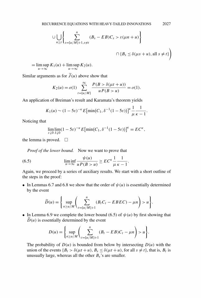
• In Lemmas 6.7 and 6.8 we show that the order of ψ(u) is essentially determinedby the event

D(u) ={

supn≥u/M

(n∑

t=[u/M]+1

(BtCt − EBEC) − µn

)> u

}.

• In Lemma 6.9 we complete the lower bound (6.5) of ψ(u) by first showing thatD(u) is essentially determined by the event

D(u) ={

supn≥u/M

(n∑

t=[u/M]+1

(Bt − EB)Ct − µn

)> u

}.

The probability of D(u) is bounded from below by intersecting D(u) with theunion of the events {Bt > δ(µt +u),Bs ≤ δ(µt +u), for all s = t}, that is, Bt isunusually large, whereas all the other Bs ’s are smaller.


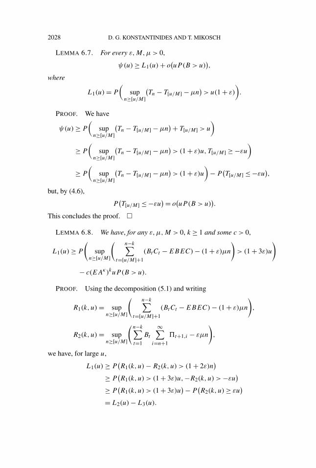
LEMMA 6.7. For every ε,M,µ > 0,

ψ(u) ≥ L1(u) + o(uP (B > u)

),

where

L1(u) = P

(sup

n≥[u/M](Tn − T[u/M] − µn

)> u(1 + ε)

).

PROOF. We have

ψ(u) ≥ P

(sup


)+ T[u/M] > u

)

≥ P

(sup


)> (1 + ε)u,T[u/M] ≥ −εu

)

≥ P

(sup


)> (1 + ε)u

)− P

(T[u/M] ≤ −εu

),

but, by (4.6),

P(T[u/M] ≤ −εu

)= o(uP (B > u)

).

This concludes the proof. �

LEMMA 6.8. We have, for any ε,µ,M > 0, k ≥ 1 and some c > 0,

L1(u) ≥ P

(sup

n≥[u/M]

(n−k∑

t=[u/M]+1

(BtCt − EBEC) − (1 + ε)µn

)> (1 + 3ε)u

)

− c(EAκ)kuP (B > u).

PROOF. Using the decomposition (5.1) and writing

R1(k, u) = supn≥[u/M]

(n−k∑

t=[u/M]+1

(BtCt − EBEC) − (1 + ε)µn

),


(n−k∑t=1

Bt

∞∑i=n+1

�t+1,i − εµn

),

we have, for large u,

L1(u) ≥ P(R1(k, u) − R2(k, u) > (1 + 2ε)n

)≥ P

(R1(k, u) > (1 + 3ε)u,−R2(k, u) > −εu

)≥ P

(R1(k, u) > (1 + 3ε)u

)− P(R2(k, u) ≥ εu

)= L2(u) − L3(u).


We show that

L3(u) ≤ c(EAκ)kuP (B > u).

We have, for k ≥ 1,

L3(u) ≤ P

(sup

n≥[u/M]

( [u/M]∑t=1

Bt�t+1,n+1Cn+1 − εµn/2

)≥ εu/2

)

+ P

(sup

n≥[u/M]

(n−k∑

t=[u/M]+1

Bt�t+1,n+1Cn+1 − εµn/2

)≥ εu/2

)

= L3,1(u) + L3,2(u).

Then, by (5.3) and Markov’s inequality, for 0 < δ < 1,

L3,1(u) ≤∞∑

n=[u/M]P

( [u/M]∑t=1

Bt�t+1,[u/M]�[u/M]+1,n+1Cn+1 > (ε/2)(µn + u)

)

≤∞∑

n=[u/M]P(Y0�[u/M]+1,n+1Cn+1 > (ε/2)(µn + u)

)

≤ c

∞∑n=[u/M]

(EAκ−δ)n−[u/M](n + u)−κ+δ

≤ cu−κ+δ = o(uP (B > u)

).

Moreover, by (5.3) and Breiman’s result,

L3,2(u) ≤∞∑

n=[u/M]P

(n−k∑

t=[u/M]+1

Bt�t+1,n−k�n−k+1,n+1Cn+1 > (ε/2)(µn + u)

)

≤∞∑

n=[u/M]P(Y0�n−k+1,n+1Cn+1 > (ε/2)(µn + u)

)≤ c(EAκ)kuP (B > u). �

Next we bound L2.

LEMMA 6.9. We have, for every k ≥ 1,

limε↓0

lim infu→∞

L2(u)


µ

1

κ − 1.


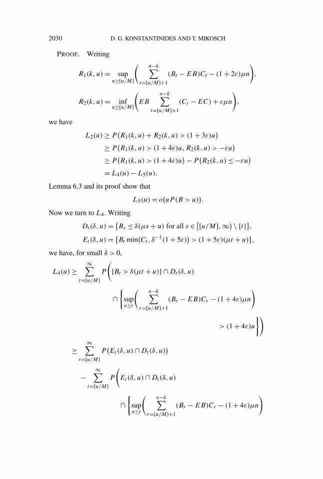
PROOF. Writing


(n−k∑

t=[u/M]+1

(Bt − EB)Ct − (1 + 2ε)µn

),

R2(k, u) = infu≥[u/M]

(EB

n−k∑t=[u/M]+1

(Ct − EC) + εµn

),

we have

L2(u) ≥ P(R1(k, u) + R2(k, u) > (1 + 3ε)u

)≥ P

(R1(k, u) > (1 + 4ε)u,R2(k, u) > −εu

)≥ P

(R1(k, u) > (1 + 4ε)u

)− P(R2(k, u) ≤ −εu

)= L4(u) − L5(u).

Lemma 6.3 and its proof show that

L5(u) = o(uP (B > u)

).

Now we turn to L4. Writing

Dt(δ, u) = {Bs ≤ δ(µs + u) for all s ∈ [[u/M],∞) \ {t}},

Et (δ, u) = {Bt min

(Ct, δ

−1(1 + 5ε))> (1 + 5ε)(µt + u)

},

we have, for small δ > 0,

L4(u) ≥∞∑

t=[u/M]P

({Bt > δ(µt + u)} ∩ Dt(δ, u)

∩{

supn≥t

(n−k∑

r=[u/M]+1

(Br − EB)Cr − (1 + 4ε)µn

)

> (1 + 4ε)u

})

≥∞∑

t=[u/M]P(Et(δ, u) ∩ Dt(δ, u)

)

−∞∑

t=[u/M]P

(Et(δ, u) ∩ Dt(δ, u)

∩{

supn≥t

(n−k∑

r=[u/M]+1

(Br − EB)Cr − (1 + 4ε)µn

)


≤ (1 + 4ε)u

})

≥∞∑

t=[u/M]P(E1(δ, u)

)P(Bs ≤ δ(µs + u) for all s ≥ [u/M])

−∞∑

t=[u/M]P

(Et(δ, u) ∩ Dt(u, δ)

∩{

supn≥t

(n−k∑

r=[u/M]+1,r =t

(Br − EB)Cr − (1 + 4ε)µn

)

≤ (1 + 4ε)u − (1 + 5ε)(µt + u) + EBCt

})= L4,1(u) − L4,2(u).

By Breiman’s result and Karamata’s theorem, as u → ∞,

L4,1(u) ∼∞∑

t=[u/M]

[(1 + 5ε)−κE

[min

(C1, δ

−1(1 + 5ε))]κ

P (B > µt + u)]

× P(Bs ≤ δ(µs + u) for all s ≥ [u/M])

≥ (1 + 6ε)−κE[min

(C1, δ

−1(1 + 5ε))]κ ∞∑

t=[u/M]P(B > µt + u)

∼ (1 + 6ε)−κE[min

(C1, δ

−1(1 + 5ε))]κ 1

µ

1

κ − 1P(B > u).

We conclude that

limε↓0

limδ↓0

lim infu→∞

I4,1(u)


µ

1

κ − 1.

As regards L4,2(u), we have

L4,2(u) ≤ c

∞∑t=[u/M]

P(B > t + u)

× P

(supn≥t

(n−k∑

r=[u/M]+1,r =t

(Br − EB)Cr − (1 + 4ε)µn

)

≤ −εu − (1 + 5ε)µt + EBCt

)


≤ c

∞∑t=[u/M]

P(B > t + u)

× P

(supn≥t

(n−k∑

r=[u/M]+1,r =t

(Br − EB)Cr − (1 + 4ε)µn

)

≤ −εu − (1 + 5ε)µt + EBM

)

+ c

∞∑t=[u/M]

P(B > t + u)P (C > M)

= I4,2,1(u) + I4,2,2(u).

We have

limM→∞ lim sup

u→∞I4,2,2(u)

uP (B > u)≤ c lim

M→∞P(C > M) = 0.

Observe that, for large u,

P

(supn≥t

(n−k∑

r=[u/M]+1,r =t

(Br − EB)Cr − (1 + 4ε)µn

)

≤ −εu − (1 + 5ε)µt + EBM

)

≤ P

(( [u/M]+u−k∑r=[u/M]+1,r =t

(Br − EB)Cr − (1 + 4ε)µ([u/M] + u)

)≤ −εu

).

Now an argument similar to the one for Theorem 4.2 shows that

I4,2,1(u) = o(uP (B > u)

).

This proves the lemma. �

Now a combination of the above lemmas shows that the lower bound (6.5)holds. Indeed, we have, for any k ≥ 1,

lim infu→∞

ψ(u)

uP (B > u)≥ lim inf

u→∞L1(u)

uP (B > u)≥ lim inf

u→∞L2(u)

uP (B > u)− c(EAκ)k.

Now, observing that EAκ < 1, let k → ∞, ε ↓ 0. This proves the theorem. �


Extensions. A careful study of the proofs in the previous sections showsthat the particular structure of the sequence (Yt ) was inessential for the proofs.Indeed, we made extensive use of the fact that the random walk (Sn) can beapproximated by the random walk Sn = ∑n

t=1 BtCt . It is not difficult to see thatthe results of Theorems 4.2 and 4.9 remain valid if Sn is replaced by Sn and thefollowing conditions on any stationary sequence (Ct ) hold: (Bt ) is independentof (Ct ), (Ct ) is strongly mixing with geometric rate, ECκ+γ < ∞ for someγ > κ and (4.4) holds. Moreover, the assertion of Lemma 4.6 remains valid.A stationary sequence Xt = BtCt for (Bt ) and (Ct ) independent is called astochastic volatility model in the econometrics literature; see [11] for some theoryand further references.

Acknowledgments. We thank the referee for constructive remarks which ledto an improved presentation of the paper. We are grateful to Qihe Tang who kindlypointed out to us that the proof of Proposition 2.4 can be found in Grey’s paper.

REFERENCES

[1] BASRAK, B., DAVIS, R. A. and MIKOSCH. T. (2002). Regular variation of GARCH processes.Stochastic Process. Appl. 99 95–116.

[2] BAXENDALE, P. H. and KHASMINSKII, R. Z. (1998). Stability index for products of randomtransformations. Adv. in Appl. Probab. 30 968–988.

[3] BILLINGSLEY, P. (1968). Convergence of Probability Measures. Wiley, New York.[4] BINGHAM, N. H., GOLDIE, C. M. and TEUGELS, J. L. (1987). Regular Variation. Cambridge

Univ. Press.[5] BOUGEROL, P. and PICARD, N. (1992). Strict stationarity of generalized autoregressive

processes. Ann. Probab. 20 1714–1730.[6] BOUSSAMA, F. (1998). Ergodicité, mélange et estimation dans le modelès GARCH. Ph.D.

thesis, Univ. Paris 7.[7] BREIMAN, L. (1965). On some limit theorems similar to the arc-sin law. Theory Probab. Appl.

10 323–331.[8] CLINE, D. B. H. and HSING, T. (1991). Large deviation probabilities for sums and maxima of

random variables with heavy or subexponential tails. Texas A&M Univ. Preprint.[9] DAVIS, R. A. and HSING, T. (1995). Point process and partial sum convergence for weakly

dependent random variables with infinite variance. Ann. Probab. 23 879–917.[10] DAVIS, R. A. and MIKOSCH, T. (1998). The sample autocorrelations of heavy-tailed processes

with applications to ARCH. Ann. Statist. 26 2049–2080.[11] DAVIS, R. A. and MIKOSCH, T. (2001). Point process convergence of stochastic volatility

processes with application to sample autocorrelations. J. Appl. Probab. Special Volume:A Festschrift for David Vere-Jones 38A 93–104.

[12] DAVIS, R. A. and RESNICK, S. I. (1996). Limit theory for bilinear processes with heavy-tailednoise. Ann. Appl. Probab. 6 1191–1210.

[13] DOUKHAN, P. (1994). Mixing. Properties and Examples. Lecture Notes in Statist. 85. Springer,New York.

[14] DUFRESNE, D. (1990). The distribution of a perpetuity, with application to risk theory. Scand.Actuar. J. 39–79.


[15] EMBRECHTS, P., KLÜPPELBERG, C. and MIKOSCH, T. (1997). Modelling Extremal Eventsfor Insurance and Finance. Springer, Berlin.

[16] FELLER, W. (1971). An Introduction to Probability Theory and Its Applications II, 2nd ed.Wiley, New York.

[17] GOLDIE, C. M. and GRÜBEL, R. (1996). Perpetuities with thin tails. Adv. in Appl. Probab. 28463–480.

[18] GREY, D. R. (1994). Regular variation in the tail behaviour of solutions to random differenceequations. Ann. Appl. Probab. 4 169–183.

[19] DE HAAN, L., RESNICK, S. I., ROOTZÉN, H. and DE VRIES, C. (1989). Extremal behaviourof solutions to a stochastic difference equation with applications to ARCH processes.Stochastic Process. Appl. 32 213–224.

[20] IBRAGIMOV, I. A. and LINNIK, YU. V. (1971). Independent and Stationary Sequences ofRandom Variables. Wolters–Noordhoff, Groningen.

[21] KESTEN, H. (1973). Random difference equations and renewal theory for products of randommatrices. Acta Math. 131 207–248.

[22] MEYN, S. P. and TWEEDIE, R. L. (1993). Markov Chains and Stochastic Stability. Springer,London.

[23] MIKOSCH, T. (2003). Modeling dependence and tails of financial time series. In ExtremeValues in Finance, Telecommunications, and the Environment (B. Finkenstädt andH. Rootén, eds.) 185–286. Chapman and Hall, Boca Raton.

[24] MIKOSCH, T. and NAGAEV, A. V. (1998). Large deviations of heavy-tailed sums withapplications to insurance. Extremes 1 81–110.

[25] MIKOSCH, T. and SAMORODNITSKY, G. (2000). The supremum of a negative drift randomwalk with dependent heavy-tailed steps. Ann. Appl. Probab. 10 1025–1064.

[26] MIKOSCH, T. and SAMORODNITSKY, G. (2000). Ruin probability with claims modeled by astationary ergodic stable process. Ann. Probab. 28 1814–1851.

[27] MIKOSCH, T. and STRAUMANN, D. (2005). Stable limits of martingale transforms withapplication to the estimation of GARCH parameters. Ann. Statist. To appear.

[28] MOKKADEM, A. (1990). Propriétés de mélange des processus autorégressifs polynomiaux.Ann. Inst. H. Poincaré Probab. Statist. 26 219–260.

[29] NAGAEV, A. V. (1969). Limit theorems for large deviations when Cramér’s conditions areviolated. Izv. Akad. Nauk UzSSR Ser. Fiz.–Mat. Nauk 6 17–22. (In Russian.)

[30] NAGAEV, S. V. (1979). Large deviations of sums independent random variables. Ann. Probab.7 745–789.

[31] PETROV, V. V. (1995). Limit Theorems of Probability Theory. Oxford Univ. Press.[32] RESNICK, S. I. (1987). Extreme Values, Regular Variation, and Point Processes. Springer, New

York.[33] RESNICK, S. I. and WILLEKENS, E. (1991). Moving averages with random coefficients

and random coefficient autoregressive models. Commun. Statistics: Stochastic Models 7511–525.

[34] ROSENBLATT, M. (1956). A central limit theorem and a strong mixing condition. Proc. Natl.Acad. Sci. USA 42 43–47.

[35] SAMORODNITSKY, G. (2002). Long Range Dependence, Heavy Tails and Rare Events.MaPhySto Lecture Notes. Available at http://www.maphysto.dk/.

[36] SAMORODNITSKY, G. and TAQQU, M. S. (1994). Stable Non-Gaussian Random Processes.Stochastic Models with Infinite Variance. Chapman and Hall, London.

[37] STRAUMANN, D. (2003). Estimation in conditonally heteroscedastic time series models. Ph.D.thesis, Institute of Mathematical Science, Univ. Copenhagen.


[38] STRAUMANN, D. and MIKOSCH, T. (2005). Quasi-maximum likelihood estimation inheteroscedastic time series: A stochastic recurrence equations approach. Ann. Statist.To appear.

DEPARTMENT OF STATISTICS

AND ACTUARIAL SCIENCE

UNIVERSITY OF THE AEGEAN

KARLOVASSI

GR-83 200 SAMOS

GREECE

E-MAIL: [email protected]: www.samos.aegean.gr/math/konstant

LABORATORY OF ACTUARIAL MATHEMATICS

UNIVERSITY OF COPENHAGEN

UNIVERSITETSPARKEN 5DK-2100 COPENHAGEN

DENMARK

AND

MAPHYSTO

THE DANISH RESEARCH NETWORK

IN MATHEMATICAL PHYSICS AND STOCHASTICS

E-MAIL: [email protected]: www.math.ku.dk/∼mikosch

Large deviations and ruin probabilities for solutions to stochastic recurrence equations with heavy-tailed innovations

Documents