Large Deformations on Elongated Bodies

Flow Induced Vibration, Zolotarev & Horacek eds. Institute of Thermomechanics, Prague, 2008

LARGE DEFORMATIONS ON ELONGATED BODIES

De Nayer Guillaume, Visonneau Michel, Leroyer AlbanEcole Centrale Nantes, Nantes, France

Boyer FredericEcole des Mines de Nantes, Nantes, France

ABSTRACT

In this paper the coupling of a structural solverfor elongated structures in large deformationsand in large displacements with the flow solverISIS-CFD is presented. ISIS-CFD is a 3D fi-nite volume solver based on the incompressibleunsteady Reynolds-averaged Navier-Stokes equa-tions. The finite element structural solver is also3D and uses Euler-Bernoulli or Rayleigh kine-matics with the Cosserat hypothesis. A remesh-ing procedure based on the pseudo-solid approxi-mation is detailed. This coupled algothim is firstvalidated and then applied to a geometrically sim-ple 2D test case.

1. INTRODUCTION

Elongated structures, like pillars supporting oilplatforms or cables and risers, are frequently metin the industrial domain. The stakes of thefluid/structure interaction (FSI) around thesebodies are therefore important. This is the rea-son why the CFD team of the Fluid MechanicsLaboratory from Centrale Nantes has started thedevelopment of FSI for elongated structures withthe help of its in-house RANSE solver ISIS-CFD.

To carry out FSI modelling, four points areessential to address :

• The transfer of the efforts exerted by thefluid on the structure,

• The transfer of structure displacements tothe fluid field,

• The fluid domain remeshing,

• The resolution of the dynamic structureproblem.

2. ISIS-CFD, THE FLOW SOLVER

The ISIS-CFD flow solver, developed by theEMN (Equipe Modelisation Numerique) of the

Fluid Mechanics Laboratory of the Ecole Cen-trale of Nantes, uses the incompressible un-steady Reynolds-averaged Navier-Stokes equa-tions (RANSE). The solver is based on the finitevolume method to build a spatial discretization ofthe transport equations. The face-based methodis generalized to two-dimensional or three di-mensional unstructured meshes for which non-overlapping control volumes are bounded by anarbitrary number of constitutive faces. The ve-locity field is obtained from the momentum con-servation equations and the pressure field is ex-tracted from the mass conservation constraint, orcontinuity equation, transformed into a pressure-equation. A second-order accurate three-levelfully implicit time discretization is used. Surfaceand volume integrals are evaluated using second-order accurate approximation. In the case ofturbulent flows, additional transport equationsfor modelled variables are solved in a form simi-lar to the momentum equations and they can bediscretized and solved using the same principles.Several turbulence models, ranging from the one-equation Spalart-Allmaras model (cf P. Spalartand S. Allmaras (1992)), two-equation k−ω clo-sures (cf F.R. Menter (1993)), to a full stresstransport Rij − ω model (cf G.B. Deng and al(2005)), are implemented in the flow solver totake into account the turbulence phenomena.

3. FLOW FIELDS TRANFERBETWEEN SOLID AND FLUID

MESHES

One of the difficulties in fluid/structure interac-tion is that the fluid and solid meshes do notmatch at the body boundary (cf A. de Boeret al. (2007)). In the special case of elongatedstructures, these ones are modelled by the beamtheory. The solid grid is consequently the beamneutral line, whereas the structure is viewed fromthe fluid domain by a set of faces around this neu-tral line. In order to calculate the fluid efforts on

beam mesh

fluid mesh

Beam part center

Projection

Effort transfert

Virtual face

Fluid mesh node

Beam mesh node

Figure 1: Fluid efforts interpolation on the beam

the beam, an interpolation is needed. The globalconservation of the efforts being the most impor-tant property to fulfill, an ad-hoc interpolationhas been developed.

The connectivities between fluid boundary-nodes and the beam sections are generated onceat the launch of ISIS-CFD. They allow to deter-mine to which part of the beam the orthogonalprojection of the fluid boundary-nodes belongs.One has also the possibility to know the orthog-onal projection of the beam nodes on the fluidboundary faces. With these data, the efforts arelinearly interpolated. A fluid face, which entirelybelongs to a beam section, provides the total fluideffort. In case of an orthogonal plane to a beamnode cutting a fluid face, this one is virtually di-vided and the efforts are linearly distributed be-tween the corresponding beam parts (cf fig. 1).

After the calculation of the beam deformation,this one is transmitted to the fluid grid with thesame connectivities which were used before. Thefluid mesh nodes which belong to the structureare displaced according to the beam kinematics.

4. FLUID DOMAIN REMESHING

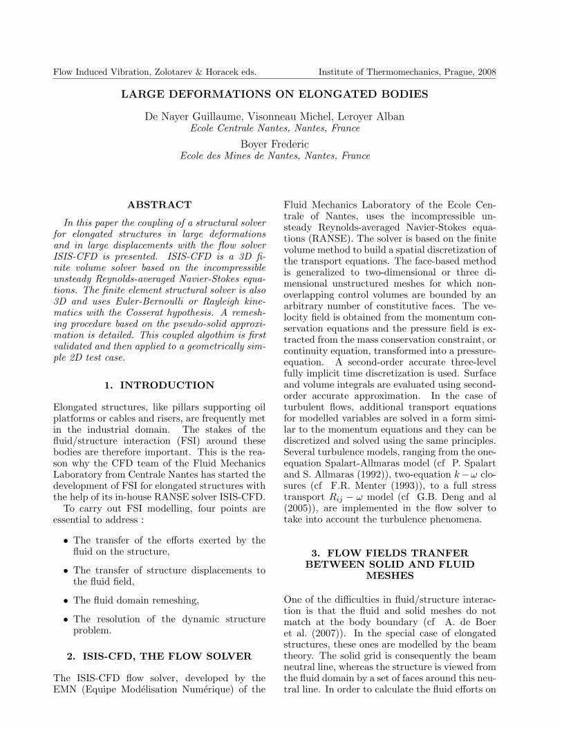
At the end, the fluid mesh must be deformed inorder to take into account the new beam po-sition. ISIS-CFD integrates several remeshingtools. The first is an analytic regridding basedon a weighting coefficient (cf fig. 2) which canbe used with confidence for small and moderatedeformations (cf A. Leroyer and M. Visonneau(2005)). Another regridding module has been de-veloped in order to account for large deforma-tions. This one is based on a pseudo-solid ap-proach to build a consistent and robust unstruc-tured grid deformation strategy. The fluid do-main is considered as a linear elastic solid struc-ture obeying structural equations which are lin-earised and used even in the case of large defor-mations since one does not need to follow thephysics for this virtual elastic grid. The controlparameters are the non-uniform Young modulusE, Poisson Coefficient µ and shearing coefficientG.

0

0.2

0.4

0.6

0.8

1

Figure 2: weighting coefficient calculated with aresolution of a lagrangian

4.1. Discretisations

In order to solve the structural problem, severalbehaviour laws have been studied. At first, asimple one, based on the isotropic case, has beenimplemented:

⇒σ= 2µ

⇒ε +λtr(

⇒ε )⇒I

So we have :∫ ∫ ∫Vdiv(

⇒σ )dV = 0⇐⇒∫ ∫

Sµ

⇒

grad−→U .−→n dS + (µ+ λ)

⇒

div(−→U ) .−→n dS = 0

where−→U is the field of cell centers displacements,

with 8>><>>:µ =

E

2(1 + ν)

λ =νE

(1 + ν)(1− 2ν)

This first deformation approach is easy to im-plement, but does not allow to control the shearstress coefficient G (in this isotropic case G =Giso). With this coefficient and the introducedstructural anisotropy, one can theoretically main-tain a rigid movement near the body and keepthe orthogonality of cells near the body wall, ahighly desirable property for finite-volume dis-cretizations. Therefore, a 2D/3D volume finitediscretisation using G has been developed :

For an orthotropical (orthogonal +anisotropic) material, the following behaviourlaw is given (hat notation) :

bσ =

266664σxσyσzσxyσyzσxz

377775 = K

2666666664

1 ν1−ν

ν1−ν 0 0 0

ν1−ν 1 ν

1−ν 0 0 0ν

1−νν

1−ν 1 0 0 0

0 0 0GxyK

0 0

0 0 0 0GyzK

0

0 0 0 0 0 GxzK

3777777775

266664εxεyεzεxyεyzεxz

377775

with K = E(1−ν)(1+ν)(1−2ν)

and εxy = 12( ∂U∂y

+ ∂V∂x

) where

Gij is the shear stress coefficient in the−→i and

−→j

directions.This symmetrical matrix gives an anisotropic

discretisation with main directions. But the goalis to maintain the orthogonality of the mesh

around the structure during the deformation. So,one defines this matrix in a local basis (−→n ,

−→t2 ,−→t3 ),

with the vector −→n directed along the gradientvector of the weighting coefficient (their isovaluesfollow the body surfaces curves as shows in fig.2). So the main deformation directions are local.And consequently one has a local behaviour de-pending to the local orientation of body surface.The general problem is expressed with the carte-sian basis, so the behaviour law matrix must berewritten in the cartesian basis.

Let P be the basis transformation matrix(−→x ,−→y ,−→z ) to (−→n ,

−→t2 ,−→t3 ), one has :

σ(−→x ,−→y ,−→z ) = Pσ(−→n ,−→t2 ,

−→t3 )P−1

with−→n = nx

−→x + ny−→y + nz

−→z

P =

"nx P12 P13

ny P22 P23

nz P32 P33

#and consequently :

bσ =

266664σxσyσzσxyσyzσxz

377775 = K

266664C11 C12 C13 C14 C15 C16C12 C22 C23 C24 C25 C26C13 C23 C33 C34 C35 C36C14 C24 C34 C44 C45 C46C15 C25 C35 C45 C55 C56C16 C26 C36 C46 C56 C66

377775266664εxεyεzεxyεyzεxz

377775

The Cij coefficients have been calculated withMAPLE.

One notices that the Gij coefficients are in-dependent. Gnt2 and Gnt3 are chosen equal andstronger than the isotropic value, instead of Gt2t3which is taken equal to Giso = E

(1+ν) . Therefore,the behaviour of a transverse isotropic materialis obtained.

In order to have the mode implicit resolutionof the problem, one rewrites the previous matrixso that the isotropic term appears :

bσ = K

266666664

1 ν1−ν

ν1−ν 0 0 0

ν1−ν 1 ν

1−ν 0 0 0ν

1−νν

1−ν 1 0 0 0

0 0 0 GisoK

0 0

0 0 0 0 GisoK

0

0 0 0 0 0 GisoK

377777775bε +

K [C − Ciso]

266664εxεyεzεxyεyzεxz

377775

The first matrix is calculated as the isotropiccase (implicit calculation). The second matrix isexplicitly taken into account.

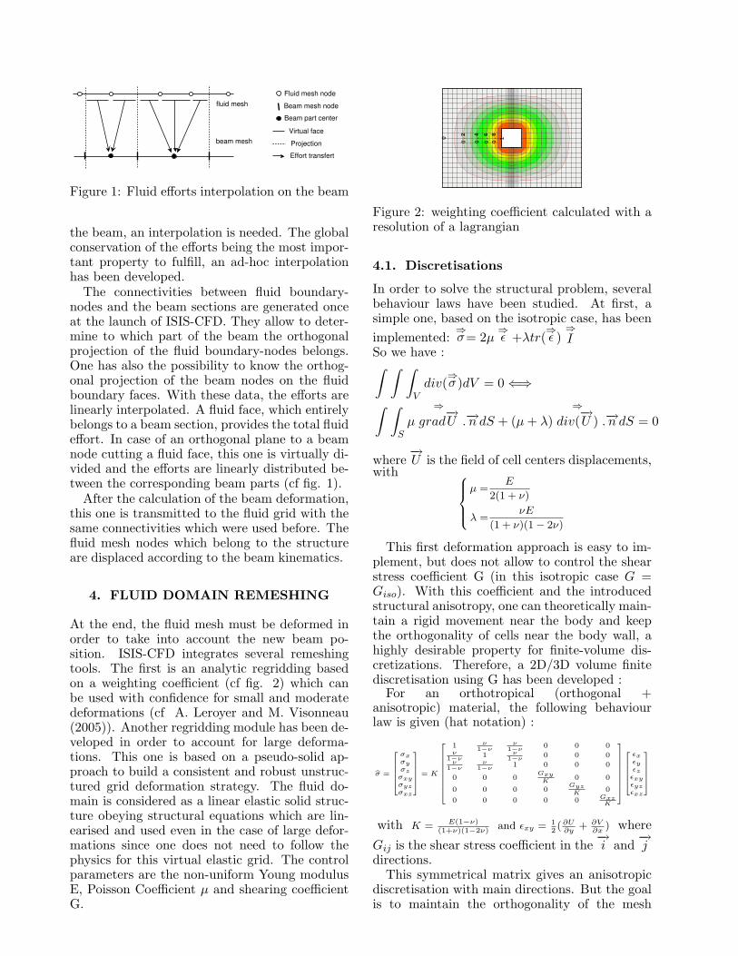
This remeshing technique allows to update agrid around deformable (cf fig. 3) or unde-formable bodies. With the use of the shear stress

X

Y

Z

Figure 3: 3D meshes deformations around aneel-like body (ROBEA project) (cf A. Leroyer(2004))

coefficient G one can maintain a rigid movementnear the body and so keep the orthogonality ofcells near the body wall. One has also the possi-bility to couple this regridding process with oneof the others in order to obtain a better control ofthe deformation. This module uses the same dis-cretisation tools as the fluid solver and the con-nectivities are identical. Moreover, the mesh de-formation is entirely parallelized using MPI com-munication tools.

5. THE STRUCTURAL SOLVER

5.1. Modelisation and hypothesis

With the distribution on the beam of the effortsexerted by the fluid, one can calculate its defor-mation, i.e. the displacements of its nodes. Thestructural solver is a “black box” based on thework of F. Boyer and D. Primault (cf F. Boyer(2004) and F. Boyer (2005)). The structuralsolver implemented into ISIS-CFD is based onthe Cosserat approximation. The beam is consid-ered as a monodimensional medium, built with acontinuous stack of rigid micro-solid structures(cf E. and F. Cosserat (1909)). In this approx-imation, the beam sections must be rigid andplane. Without any other hypothesis, this kine-matic is called “Timoshenko Reissner” (cf W.Weaver, Timoshenko and al (1990) and E. Reiss-ner (1973)).

In our case, the beams are fine and elongated(cables, risers...). Then the Kirchoff hypothesiscan be used with confidence : the beam sec-tions are orthogonal to the neutral line of thebeam. With this kinematic called “Kirchoff”,two beam models are built : the “Rayleigh”model (cf L. Meirovitch (1967)) and the “Euler-

Bernoulli” model (cf L. Meirovitch (1967)). Inthis last model, the angular kinetic energy of thebeam sections is neglected. With this simplifi-cation, the analytic equations are lighter. But aproblem arises when the beam is free to rotateon itself.

The structural solver integrates both beammodels resulting from the Kirchoff hypothesis :the “Rayleigh” and “Euler-Bernoulli” models.

5.2. The Euler-Bernoulli & Rayleigh kine-matics

The Rayleigh kinematics (cf F. Boyer (2004)and F. Boyer (2005)) allow to solve correctlythe cables problems thanks to the flexion-torsioncoupling. Indeed the numerical solution is basedon a variational formulation of the Kirchoff kine-matics and on an exact modelisation of the mostcomplex geometrical non-linearity : the flexion-torsion coupling (cf J.C. Alexander and Antman(1982)). An important notion appears here :the geometrically exact approach. This expres-sion comes from Simo (cf J.C. Simo (1985)) andmeans that the approximations are done at theend of all the developments.

This kinematic needs a parametrisation. Therotation parametrisation is the most complex. Inthe Reissner kinematic case, the SO3 Lie groupis used. But the Kirchoff constraint reduces thisspace to a bidimensional SO3 subspace. This oneis parametrized by the position field of the beamneutral line and becomes the SO2 plane rotationsgroup. At first the rotation field is changed tothe composition of two rotations : the movementof the beam neutral line only and the movementaround this neutral line. Several parametrisa-tions can be done for the rotation angles. Inthe implemented structural solver, the Eulerianparametrisation is used, due to its relative sim-plicity.

5.3. Validation test cases

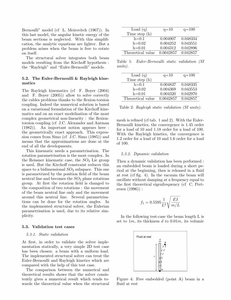
5.3.1. Static validation

At first, in order to validate the solver imple-mentation statically, a very simple 2D test casehas been chosen: a beam with a uniform load.The implemented structural solver can treat theEuler-Bernoulli and Rayleigh kinetics which arecompared with the help of this test case.

The comparison between the numerical andtheoretical results shows that the solver consis-tently gives a numerical result which tends to-wards the theoretical value when the structural

Load (q) q=10 q=100Time step (h)

h=0.1 0.004907 0.048334h=0.02 0.004252 0.043551h=0.01 0.004312 0.042896

Theoretical value 0.0042857 0.042857

Table 1: Euler-Bernoulli static validation (SIunits).

Load (q) q=10 q=100Time step (h)

h=0.1 0.004837 0.048335h=0.02 0.004369 0.043553h=0.01 0.004320 0.042970

Theoretical value 0.0042857 0.042857

Table 2: Rayleigh static validation (SI units).

mesh is refined (cf tab. 1 and 2). With the Euler-Bernoulli kinetics, the convergence is 1.45 orderfor a load of 10 and 1.18 order for a load of 100.With the Rayleigh kinetics, the convergence is1.2 order for a load of 10 and 1.6 order for a loadof 100.

5.3.2. Dynamic validation

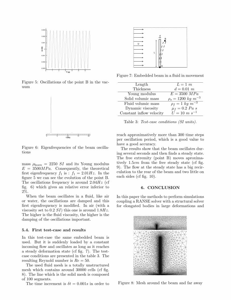
Then a dynamic validation has been performed :an embedded beam is loaded during a short pe-riod at the beginning, then is released in a fluidat rest (cf fig. 4). In the vacuum the beam willoscillate without damping at a frequency equal tothe first theoretical eigenfrequency (cf C. Pert-ersen (1996)) :

f1 = 0.55951L2

√EI

m/L

In the following test-case the beam length L isset to 1m, its thickness d to 0.01m, its volumic

B

d

L

Fluid at rest

A

Figure 4: Free embedded (point A) beam in afluid at rest

T (s)

∆x(m)

0 1 2 3 4 5 6

­0.003

­0.002

­0.001

0

0.001

0.002

0.003

Figure 5: Oscillations of the point B in the vac-uum

f (Hz)0 5 10 15 20

Figure 6: Eigenfrequencies of the beam oscilla-tions

mass ρbeam = 2250 SI and its Young modulusE = 3500MPa. Consequently, the theoreticalfirst eigenfrequency f1 is : f1 = 2.01Hz. In thefigure 5 we can see the evolution of the point B.The oscillations frequency is around 2.04Hz (cffig. 6) which gives an relative error inferior to2%.

When the beam oscillates in a fluid, like airor water, the oscillations are damped and thisfirst eigenfrequency is modified. In air (with aviscosity set to 0.2 SI) this one is around 1.8Hz.The higher is the fluid viscosity, the higher is thedamping of the oscillations important.

5.4. First test-case and results

In this test-case the same embedded beam isused. But it is suddenly loaded by a constantincoming flow and oscillates as long as it reachesa steady deformation state (cf fig. 7). The test-case conditions are presented in the table 3. Theresulting Reynold number is Re = 50.

The used fluid mesh is a totally unstructuredmesh which contains around 30000 cells (cf fig.8). The line which is the solid mesh is composedof 100 segments.

The time increment is δt = 0.001s in order to

B

d

L

U

A

Figure 7: Embedded beam in a fluid in movement

Length L = 1 mThickness d = 0.01 m

Young modulus E = 3500 MPaSolid volumic mass ρs = 1200 kg m−3

Fluid volumic mass ρf = 1 kg m−3

Dynamic viscosity µf = 0.2 Pa sConstant inflow velocity U = 10 m s−1

Table 3: Test-case conditions (SI units).

reach approximatively more than 300 time stepsper oscillation period, which is a good value tohave a good accuracy.

The results show that the beam oscillates dur-ing several seconds and then finds a steady state.The free extremity (point B) moves aproxima-tively 1.5cm from the free steady state (cf fig.9). The flow at the steady state has a big recir-culation to the rear of the beam and two little oneach sides (cf fig. 10).

6. CONCLUSION

In this paper the methods to perform simulationscoupling a RANSE solver with a structural solverfor elongated bodies in large deformations and

Figure 8: Mesh around the beam and far away

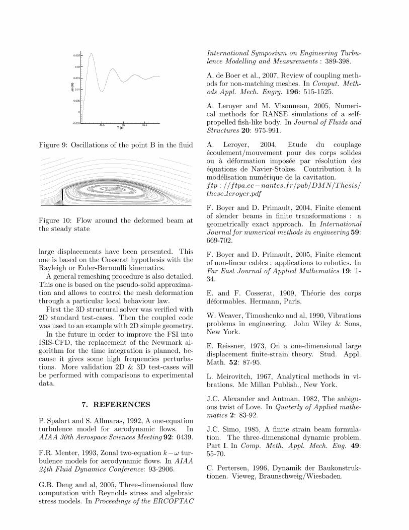
T (s)

∆x(m)

45.5 46 46.5­0.005

0

0.005

0.01

0.015

0.02

0.025

Figure 9: Oscillations of the point B in the fluid

Figure 10: Flow around the deformed beam atthe steady state

large displacements have been presented. Thisone is based on the Cosserat hypothesis with theRayleigh or Euler-Bernoulli kinematics.

A general remeshing procedure is also detailed.This one is based on the pseudo-solid approxima-tion and allows to control the mesh deformationthrough a particular local behaviour law.

First the 3D structural solver was verified with2D standard test-cases. Then the coupled codewas used to an example with 2D simple geometry.

In the future in order to improve the FSI intoISIS-CFD, the replacement of the Newmark al-gorithm for the time integration is planned, be-cause it gives some high frequencies perturba-tions. More validation 2D & 3D test-cases willbe performed with comparisons to experimentaldata.

7. REFERENCES

P. Spalart and S. Allmaras, 1992, A one-equationturbulence model for aerodynamic flows. InAIAA 30th Aerospace Sciences Meeting 92: 0439.

F.R. Menter, 1993, Zonal two-equation k−ω tur-bulence models for aerodynamic flows. In AIAA24th Fluid Dynamics Conference: 93-2906.

G.B. Deng and al, 2005, Three-dimensional flowcomputation with Reynolds stress and algebraicstress models. In Proceedings of the ERCOFTAC

International Symposium on Engineering Turbu-lence Modelling and Measurements : 389-398.

A. de Boer et al., 2007, Review of coupling meth-ods for non-matching meshes. In Comput. Meth-ods Appl. Mech. Engrg. 196: 515-1525.

A. Leroyer and M. Visonneau, 2005, Numeri-cal methods for RANSE simulations of a self-propelled fish-like body. In Journal of Fluids andStructures 20: 975-991.

A. Leroyer, 2004, Etude du couplageecoulement/mouvement pour des corps solidesou a deformation imposee par resolution desequations de Navier-Stokes. Contribution a lamodelisation numerique de la cavitation.ftp : //ftpa.ec−nantes.fr/pub/DMN/Thesis/these leroyer.pdf

F. Boyer and D. Primault, 2004, Finite elementof slender beams in finite transformations : ageometrically exact approach. In InternationalJournal for numerical methods in engineering 59:669-702.

F. Boyer and D. Primault, 2005, Finite elementof non-linear cables : applications to robotics. InFar East Journal of Applied Mathematics 19: 1-34.

E. and F. Cosserat, 1909, Theorie des corpsdeformables. Hermann, Paris.

W. Weaver, Timoshenko and al, 1990, Vibrationsproblems in engineering. John Wiley & Sons,New York.

E. Reissner, 1973, On a one-dimensional largedisplacement finite-strain theory. Stud. Appl.Math. 52: 87-95.

L. Meirovitch, 1967, Analytical methods in vi-brations. Mc Millan Publish., New York.

J.C. Alexander and Antman, 1982, The anbigu-ous twist of Love. In Quaterly of Applied mathe-matics 2: 83-92.

J.C. Simo, 1985, A finite strain beam formula-tion. The three-dimensional dynamic problem.Part I. In Comp. Meth. Appl. Mech. Eng. 49:55-70.

C. Pertersen, 1996, Dynamik der Baukonstruk-tionen. Vieweg, Braunschweig/Wiesbaden.