Large auctions with risk-averse bidders

Int J Game Theory (2010) 39:359–390DOI 10.1007/s00182-009-0181-6

Large auctions with risk-averse bidders

Gadi Fibich · Arieh Gavious

Accepted: 10 September 2009 / Published online: 27 September 2009© Springer-Verlag 2009

Abstract We study private-value auctions with n risk-averse bidders, where n islarge. We first use asymptotic analysis techniques to calculate explicit approximationsof the equilibrium bids and of the seller’s revenue in any k-price auction (k = 1, 2, . . .).These explicit approximations show that in all large k-price auctions the effect ofrisk-aversion is O(1/n2) small. Hence, all large k-price auctions with risk-averse bid-ders are O(1/n2) revenue equivalent. The generalization, that all large auctions areO(1/n2) revenue equivalent, is false. Indeed, we show that there exist auction mech-anisms for which the limiting revenue as n −→ ∞ with risk-averse bidders is strictlybelow the risk-neutral limit. Therefore, these auction mechanisms are not revenueequivalent to large k-price auctions even to leading-order as n −→ ∞.

Keywords Large auctions · Risk aversion · Asymptotic analysis · Revenueequivalence · Equilibrium strategy

1 Introduction

Many auctions, such as those that appear on the Internet, have a large number of bid-ders. The standard approach to study large auctions has been to consider their limit asn, the number of bidders, approaches infinity. Using this approach, it has been shownfor private-value auctions under quite general conditions that as n goes to infinity, the

G. FibichSchool of Mathematical Sciences, Tel Aviv University, 69978 Tel Aviv, Israele-mail: [email protected]

A. Gavious (B)Department of Industrial Engineering and Management, Faculty of Engineering Sciences, Ben-GurionUniversity, P.O. Box 653, 84105 Beer-Sheva, Israele-mail: [email protected]

123

360 G. Fibich, A. Gavious

equilibrium bid approaches the true value, the seller’s expected revenue approaches themaximal possible value, and the auction becomes efficient (Wilson 1977; Pesendorferand Swinkels 1997; Kremer 2002; Swinkels 1999, 2001; Bali and Jackson 2002).Most of the studies that adopted this approach, however, do not provide the rate ofconvergence to the limit. Therefore, it is unclear how large n should be (5, 10, 100?) inorder for the auction “to be large” i.e., in order for the limiting results for n = ∞ to beapplicable. Convergence rates were obtained by Satterthwaite and Williams (1989),who showed that the rate of convergence of the bid to the true value in a double auctionis O(1/m), where m is the number of traders on each side of the market, by Rustichiniet al. (1994), who showed that the rate of convergence of the bid to the true value ina k-double auction is O(1/m) and the corresponding inefficiency is O(1/m2), andby Hong and Shum (2004), who calculated the convergence rate in common-valuemulti-unit first-price auctions.

In this paper, we extend the study of large auctions in two ways:

1. We allow bidders to be risk-averse, rather than risk neutral. Our results show thatrisk-aversion has a small effect in all large k-price auctions. Surprisingly, how-ever, this is not the case for all large auctions. Indeed, we show that there existother auction mechanisms for which the effect of risk-aversion does not becomenegligible as n −→ ∞.

2. We use asymptotic analysis techniques in order to go beyond rate-of-convergenceresults, i.e., we explicitly calculate the O(1/n) correction term in the expressionsfor the equilibrium bids and the seller’s revenue. Since our explicit asymptoticapproximations include both the limiting value and the O(1/n) correction term,they are O(1/n2) accurate. Hence, the number of bidders at which they becomevalid is considerably smaller than the number of bidders at which the limitingvalues (which are only O(1/n) accurate) become valid. Roughly speaking, if werequire 1% accuracy, than our O(1/n2) asymptotic approximations are alreadyvalid for n = 10 bidders, whereas the limiting-value approximations becomevalid only for n = 100 bidders.

The paper is organized as follows. In Sect. 2, we introduce the model of symmetricprivate-value auctions with risk-averse bidders. In Sect. 3, we calculate asymptoticapproximations of the equilibrium bids and of the seller’s revenue in large first-priceauctions with risk-averse bidders. This calculation shows that the differences in theequilibrium bids and in the seller’s revenue between risk-neutral and risk-averse bid-ders are only O(1/n2).

One measure of a ‘good’ asymptotic technique is that it can be used, at least intheory, to calculate as many terms in the expansion as desired. To show that this is thecase here, we calculate explicitly the next-order, O(1/n2) terms in the expressions forthe equilibrium bids and the revenue. This calculation shows that the O(1/n2) affectof risk aversion is proportional to the Arrow–Pratt measure of risk aversion at zero. Inaddition, this calculation provides an analytic estimate for the value of the constant ofthe O(1/n2) error term.

In Sect. 3.1, we present numerical examples that suggest that the asymptotic approx-imations derived in this study are quite accurate even for auctions with as few asn = 6 bidders. Although we present only a few numerical examples, we note that the

123

Large auctions with risk-averse bidders 361

parameters of these examples were chosen “at random”, and that we observed thesame behavior in numerous other examples that we tested.1

In Sect. 4, we calculate asymptotic approximations of the equilibrium bids andof the seller’s revenue in large symmetric k-price auctions (k = 3, 4, . . .) with risk-averse bidders. As in the case of first-price auctions, this calculation shows that thedifferences in the equilibrium bids and in the seller’s revenue between risk-neutral andrisk-averse bidders are only O(1/n2). Since in the risk-neutral case all k-price auc-tions are revenue equivalent, we conclude that all large k-price auctions (k = 1, 2, . . .)with risk-averse or risk-neutral bidders are O(1/n2) revenue equivalent.2

Since the revenue differences among all large k-price auctions with n risk-aversebidders are O(1/n2), it seems natural to conjecture that this result should extend toall incentive-compatible and individually-rational mechanisms that deliver efficientallocations. This, however, is not the case. Indeed, in Sect. 5 we prove that the limit-ing revenue as n −→ ∞ in generalized all-pay auctions3 with risk-averse bidders isstrictly below the risk-neutral limit, and in Sect. 6 we show that this also true for last-price auctions.4 Therefore, unlike large k-price auctions where risk-aversion has onlyan O(1/n2) effect on the revenue, in the case of large all-pay and last price auctionsrisk-aversion has an O(1) effect on the revenue. To the best of our knowledge, theseare the first examples of private-value auctions whose limiting revenue is not equal tothe risk-neutral limit.

The above results raise the question of whether there is a condition that would implythat the limiting revenue with risk-averse bidders is equal to the risk-neutral limit. InSect. 7 we prove that if the equilibrium payment of the winning bidder approacheshis type as n −→ ∞ uniformly for all types, then the limiting revenue with risk-averse bidders is equal to the risk-neutral limit (Proposition 6). We then show that itis sufficient for this condition to hold only at an O(1/n) neighborhood of the highesttype.

In Sect. 8 we discuss the advantages and disadvantages of the applied math approachused in Sects. 3 and 4. The Appendix contains proofs omitted from the main body ofthe paper.

Finally, we note that this paper differs from our previous work, in which we usedperturbation analysis techniques to analyze auctions with weakly asymmetric bidders(Fibich and Gavious 2003; Fibich et al. 2004) and with weakly risk-averse bidders(Fibich et al. 2006), in two important ways:

1. In those papers we had to assume that the level of risk-aversion (or asymmetry)is small. The results of this paper are stronger, since no such assumption is made.

2. In those papers we used perturbation techniques that “essentially” amount toTaylor expansions in a small parameter that lead to convergent sums. In contrast,

1 The fact that an expansion for large n is already valid for n = 6 may be surprising to researchers notfamiliar with asymptotic expansions. However, quite often, this is the case with asymptotic expansions (seee.g., Bender and Orszag 1978).2 Recall that revenue equivalence fails under risk aversion (Maskin and Riley 1984; Matthews 1987).3 I.e., when the highest bidder wins the object and pays his bid, and the losing bidders pay a fixed fractionof their bids.4 I.e., when the highest bidder wins the object and pays the lowest bid.

123


here we use asymptotic methods (e.g., Laplace method for evaluation of inte-grals) which typically lead to divergent sums if carried out to all orders (see, e.g.,Murray 1984). To the best of our knowledge, these asymptotic methods have notbeen used in auction theory so far. It is quite likely that these and other asymptoticmethods (WKB, method of steepest descent, etc.) will be useful in the asymptoticanalysis of other models, e.g., multi-unit auctions with many units (Jackson andKremer 2004, 2006).

2 The model

Consider a large number (n � 1) of bidders vying for a single object. Bidder i’svaluation vi is a private information, and bidders are symmetric such that for anyi = 1, . . . , n, vi is independently distributed according to a common distributionfunction F(v) on the interval [0, 1]. Denote by f = F ′ the corresponding densityfunction. We assume that F is twice continuously differentiable and that f > 0 in[0, 1]. We assume that each bidder’s utility is given by a function U (v − b), which istwice continuously differentiable, monotonically increasing, concave, and normalizedto have a zero utility at zero, i.e.,

U (x) ∈ C2, U (0) = 0, U ′(x) > 0, U ′′(x) < 0. (1)

3 First-price auctions

Consider a first-price auction with risk-averse bidders, in which the bidder with thehighest bid wins the object and pays his bid. In this case, the inverse equilibrium bidssatisfy the ordinary-differential equation5

v′(b) = 1

n − 1

F(v(b))

f (v(b))

U ′(v(b) − b)

U (v(b) − b), v(0) = 0. (2)

Unlike the risk-neutral case, there are no explicit formulae for the equilibrium bidsand for the revenue, except in special cases. Recently, Fibich et al. (2006) obtainedexplicit approximations of the equilibrium bids for the case of weak risk aversion.Here we relax the assumption that risk aversion is weak.

Proposition 1 Consider a symmetric first-price auction with n bidders with utilityfunction U (x) that satisfies (1). Then, the equilibrium bid for sufficiently large n isgiven by

b(v) = v − 1

n − 1

F(v)

f (v)+ O

(1

n2

), (3)

5 Under the conditions of Sect. 2, existence of a symmetric equilibrium follows from Maskin and Riley(1984).

123


and the seller’s expected revenue is given by

Rran = 1 − 2

n

1

f (1)+ O

(1

n2

). (4)

Proof Since limn→∞ v(b) = b, we can look for a solution of (2) of the form

v(b) = b + 1

n − 1v1(b) + O

(1

n2

).

Substitution in (2) gives

1 + O

(1

n

)= 1

n − 1

F(b) + (v1/(n − 1)) f (b) + O(n−2)

f (b) + (v1/(n − 1)) f ′(b) + O(n−2)

×U ′(0) + (v1/(n − 1))U ′′(0) + O(n−2)

U (0) + (v1/(n − 1))U ′(0) + O(n−2).

Since U (0) = 0 and U ′(0) > 0, the balance of the leading order terms gives

1 = F(b)

f (b)· U ′(0)

v1U ′(0).

Therefore, v1(b) = F(b)/ f (b) and the inverse equilibrium bids are given by

v(b) = b + 1

n − 1

F(b)

f (b)+ O

(1

n2

).

Inverting this relation (see Lemma 1) shows that the equilibrium bids are given by (3).To calculate the expected revenue, we use (3) to obtain

Rran =

1∫0

b(v) d Fn(v) = b(1) −1∫

0

b′(v)Fn(v) dv

= 1 − 1

n

1

f (1)+ O

(1

n2

)−

∫ 1

0[1 + O(1/n)]Fn(v) dv.

Therefore, by Lemma 2 (see Appendix A), the result follows. ��It is worth noting here the power of this asymptotic analysis approach. While it is

not possible to determine the exact expression for the equilibrium bids, it only requireda few lines of calculation to obtain an expression with an O(1/n2) accuracy. We notethat Caserta and de Vries (2002) used extreme value theory to derive an asymptoticexpression for the revenue which is equivalent to (4). However, the result of Casertaand de Vries (2002) holds only in the risk-neutral case, where an explicit expressionfor the revenue is available. In addition, the calculation using extreme value theoryrequires considerably more work.

123


Since the utility function U (x) does not appear in the O(1/n) term, Proposition 1shows that the differences in equilibrium bids and in the seller’s revenue between first-price auctions with risk-neutral and with risk-averse bidders are at most O(1/n2). Inother words, risk aversion has (at most) an O(1/n2) effect on the equilibrium bids andon the revenues in symmetric first-price auctions.

Proposition 1 raises two questions:

1. Is the effect of risk-aversion truly O(1/n2), or is it even smaller?2. Can we estimate the constants in the O(1/n2) error terms?

We answer these questions by calculating explicitly the O(1/n2) terms:

Proposition 2 Consider a symmetric first-price auction with n bidders whose utilityfunction U (x) satisfy (1). Then, the equilibrium bid for sufficiently large n is given by

b(v) = v − 1

n − 1

F(v)

f (v)+ 1

(n − 1)2

[F(v)

f (v)− F2(v) f ′(v)

f 3(v)− F2(v)

2 f 2(v)

U ′′(0)

U ′(0)

]

+O

(1

n3

), (5)

and the seller’s expected revenue is given by

Rran = 1 − 1

n

2

f (1)+ 1

n2

[2

f (1)− 3 f ′(1)

f 3(1)− 1

2 f 2(1)

U ′′(0)

U ′(0)

]+ O

(1

n3

). (6)

Proof The proof is the same as for Proposition 1, except that one has to keep also theO(1/(n − 1)2) terms, see Appendix B. ��

Thus, risk-aversion has an O(1/n2) effect on the bid when U ′′(0) = 0, but asmaller effect if U ′′(0) = 0. As expected, the bids and revenue increase (decrease)for risk-averse (risk-loving) bidders. Note that the magnitude of risk-aversion effect isdetermined, to leading-order, by −U ′′(0)/U ′(0), i.e., by the value of the Arrow–Prattabsolute risk-aversion at zero.6

The observation that risk-aversion has a small effect on the revenue in large first-price auctions has the following intuitive explanation. Since in large first-price auctionsthe bids are close to the values, one can approximate U (v −b) ≈ (v −b)U ′(0), whichis the risk-neutral case. Similarly, adding the next term in the Taylor expansion gives

U (v − b) ≈ U ′(0)

[(v − b) + (v − b)2

2

U ′′(0)

U ′(0)

]. (7)

Hence, for large n, the leading-order effect of risk-aversion is proportional to−U ′′(0)/U ′(0).

6 Although we assume in (1) that bidders are risk averse, the results of this section hold for risk lovingbidders as well.

123


0 0.2 0.4 0.6 0.8 10

0.2

0.4

0.6

0.8

1

v

bids

n = 2

0 0.2 0.4 0.6 0.8 10

0.2

0.4

0.6

0.8

1

v

bids

n = 4

0 0.2 0.4 0.6 0.8 10

0.2

0.4

0.6

0.8

1

v

bids

n = 6

0 0.2 0.4 0.6 0.8 10

0.2

0.4

0.6

0.8

1

v

bids

n = 8

risk−averserisk−neutral

Fig. 1 Equilibrium bids in a first-price auction with risk-averse (solid) and risk-neutral (dashes) bidders

3.1 Examples

Consider a first-price auction where bidders’ valuations are uniformly distributed on[0, 1], i.e., F(v) = v. Assume first that each bidder has a CARA utility functionU (x) = 1 − e−λx where λ > 0. In Fig. 1 we compare the (exact) equilibrium bid7

for λ = 2, with the equilibrium bid in the risk-neutral case, for n = 2, 4, 6, and8 bidders.8 Already for n = 6 bidders, the equilibrium bids in the risk-neutral andrisk averse cases are almost identical. This observation is consistent with Dyer et al.(1989), who found in experiments that in a first-price auction the actual highest bidwas much higher than the theoretical risk-neutral equilibrium bid with three players,but very close to the risk-neutral one with six players.

Next, we consider the revenue in a first-price auction with n = 6 risk-averse play-ers, denoted by Rra

n (where n = 6). Recall that when F(v) = v, the revenue in therisk-neutral case with n players is equal to Rrn

n = (n − 1)/(n + 1). Therefore, in thecase of six players, Rrn

6 = 5/7 ≈ 0.7143. In Table 1 we give the value of Rra6 and

the relative change in the revenue due to risk-aversion for four different utility

7 Namely, the numerical solution of Eq. 2.8 Observe that as λ → 0, U (x) ∼ λx , i.e., the utility of risk-neutral bidders. Therefore, λ = 2 correspondsto a significant deviation from risk-neutrality.

123


Table 1 Expected revenue in asymmetric first-price auctionwith six players with a utilityfunction U (x)

U (x) Rra6

Rra6 −Rrn

6Rra

6

x − x2/2 0.7220 1.08%

ln(1 + x) 0.7209 0.92%

CARA (λ = 1) 0.7214 0.99%

CARA (λ = 2) 0.7278 1.89%

Table 2 Expected revenue in asymmetric first-price auctionwith two players with a utilityfunction U (x)

U (x) Rra2

Rra2 −Rrn

2Rrn

2

x − x2/2 0.3592 7.7%

ln(1 + x) 0.3508 5.25%

CARA (λ = 1) 0.3541 6.2%

CARA (λ = 2) 0.3741 12.2%

functions. The first thing to observe is that in all four cases the effect of risk-aver-sion is small (less that 2%), even though the number of players is not really large, andthe utility functions are not close to risk-neutrality. The second thing to observe is thatin the first three cases the effect of risk-aversion on the revenue is nearly the same(≈1%), even though the three utility functions are quite different. The reason for thisis that the difference between the revenue in the risk-averse and risk-neutral case isgiven by, see Proposition 2,

Rran − Rrn

n ≈ − 1

n2

1

2 f 2(1)

U ′′(0)

U ′(0).

Hence, the effect of risk-aversion is proportional to the value of the absolute riskaversion −U ′′(0)/U ′(0). In the first three cases −U ′′(0)/U ′(0) is identical (=1),explaining why they have “the same” effect on the revenue. In the fourth case −U ′′(0)/U ′(0) = 2, and indeed, the change in the revenue nearly doubles.

In Table 2, we repeat the simulations of Table 1, but with n = 2 players. In this case,the revenue in the risk-neutral case is equal to Rrn

2 = 1/3 ≈ 0.3333. As expected,the relative effect of risk-aversion is much larger than for n = 6 players, showing thatrisk-aversion cannot be neglected in small first-price auctions. In addition, as before,the effect of risk-aversion depends predominantly on −U ′′(0)/U ′(0), which is whythe additional revenues due to risk aversion are roughly the same in the first threecases, but roughly double in the fourth case.

4 k-price auctions

Consider k-price auctions in which the bidder with the highest bid wins the auctionand pays the k-th highest bid. The results of Proposition 1 can be generalized to anyk-price auction as follows:

123


Proposition 3 Consider a symmetric k-price auction (k = 1, 2, 3, . . .) with n bid-ders, each with a utility function U (x) that satisfies (1). Then, the equilibrium bid forsufficiently large n is

b(v) = v + k − 2

n − k

F(v)

f (v)+ O

(1

n2

), (8)

and the seller’s expected revenue is given by (4).

Proof The case k = 1 was proved in Proposition 1. When k = 2 the result followsimmediately, since b(v) = v. Therefore, we only need to consider k ≥ 3. In that case,the equilibrium strategies in k-price auctions are the solutions of (see Monderer andTennenholtz 2000)

v∫0

U (v − b(t))Fn−k(t)(F(v) − F(t))k−3 f (t) dt = 0. (9)

Defining m = n − k and t = v − s, we can rewrite Eq. 9 as

0 =v∫

0

U (v − b(t))Fm(t)(F(v) − F(t))k−3 f (t) dt

=v∫

0

em ln(F(t))U (v − b(t))(F(v) − F(t))k−3 f (t) dt

= em ln F(v)

v∫0

em·h(s,v) g(s, v) ds, (10)

where

h = ln F(v − s) − ln F(v), g = U (v − b(v − s))(F(v) − F(v − s))k−3 f (v − s).

Since h and g are independent of m, we can calculate an asymptotic approximation ofthe last integral using the Laplace method for integrals (see, e.g., Murray 1984). Thismethod is based on two key observations:

1. As m −→ ∞, essentially all the contribution to the integral comes from theneighborhood of the point smax where h(s) attains its global maximum in [0, v].

2. Therefore, one can compute the integral, with exponential accuracy, by replacingh and g with their Taylor expansions around smax.

Since the maximum of h for 0 ≤ s ≤ v is attained at smax = 0, we make thechange of variables x(s) = [ln F(v) − ln F(v − s)] and expand all the terms in the

123


last integral in a Taylor series in s near s = 0. Expansion of x(s) near s = 0 givesx = s f (v)/F(v) + O(s2). Therefore,

dx

ds= f (v)/F(v) + O(s), s = x

F(v)

f (v)+ O(s2), ds = dx

f (v)/F(v)[1 + O(x)] .

Let us expand the solution b(v) in a power series in m, i.e.,

b(v) = b0(v) + 1

mb1(v) + O

(1

m2

).

Therefore, near s = 0,

b(v − s) = b0(v) − sb′0(v) + 1

mb1(v) − 1

msb′

1(v) + O(s2) + O

(1

m2

).

In addition,

(F(v) − F(v − s))k−3 = (s f (v) + O(s2))k−3 = sk−3 f k−3(v)[1 + O(s)],

and

f (v − s) = f (v) + O(s).

Substitution all the above in (10) gives

0 =v∫

0

{e−mx U

[v −

(b0(v) − sb′

0(v) + b1(v)

m− sb′

1(v)

m+ O(s2) + O

(1

m2

))]

× sk−3 f k−3(v) [1 + O(s)] [ f (v) + O(s)]

}ds

∼∞∫

0

{e−mx U

[v −

(b0(v) − x

F(v)

f (v)b′

0(v) + 1

mb1(v) − x

m

F(v)

f (v)b′

1(v) + O(x2)

+O

(1

m2

))]× xk−3 Fk−3(v) [1 + O(x)] [ f (v) + O(x)]

× dx

f (v)/F(v)[1 + O(x)]

}

= Fk−2(v)

∞∫0

{e−mx

[U (v − b0(v)) + U ′(v − b0(v))

(x

F(v)

f (v)b′

0(v) − b1(v)

m

+ x

m

F(v)

f (v)b′

1(v)

)+ O(x2) + O

(1

m2

)]xk−3 [1 + O(x)]

}dx . (11)

123


We recall that for p integer,∫ ∞

0 e−mx x p dx = p!/m p+1 = 0. Therefore, balancingthe leading O(m−(k−2)) terms gives

U (v − b0(v))Fk−2(v)

∞∫0

e−mx xk−3 dx = 0.

Since U (z) = 0 only at z = 0, this implies that b0(v) ≡ v. Using this and U ′(0) = 0,Eq. 11 reduces to

0 =∞∫

0

{e−mx

(x

F(v)

f (v)− 1

mb1(v) + x

m

F(v)

f (v)b′

1(v)

) [xk−3 + O(xk−2)

]}dx .

Therefore, balance of the next-order O(m−(k−1)) terms gives

F(v)

f (v)

∞∫0

e−mx xk−2 dx − 1

mb1(v)

∞∫0

e−mx xk−3 dx = 0,

or

F(v)

f (v)

(k − 2)!mk−1 − (k − 3)!

mk−1 b1(v) = 0.

Therefore,

b1(v) = (k − 2)F(v)

f (v).

Hence, we proved (8).The seller’s expected revenue in a k-price auction is given by Rk

n = ∫ 10 b(v)d Fk(v),

where b(v) is the equilibrium bid in the k price auction and Fk(v) is the distribution ofthe k-th valuation in order (i.e., kth-order statistic of the bidders private valuations).Substituting the asymptotic expansion for the equilibrium bids gives

Rkn =

1∫0

[v + k − 2

n − k

F(v)

f (v)

]d Fk(v) + O

(1

n2

).

Since the asymptotic expansion for the equilibrium bid is independent of the utilityfunction U until order O( 1

n2 ), the revenue in the risk-averse case is the same as in

the risk-neutral case, up to O( 1n2 ) accuracy. By the revenue equivalence theorem, the

latter is given by (4). ��

123


In the risk-neutral case U (x) = x , the equilibrium bids in k-price auctions (k =2, 3, . . .) are given by (Wolfstetter 1995)

b(v) = v + k − 2

n − k + 1

F(v)

f (v). (12)

Comparison with Eq. 8 shows that in large symmetric k-price auctions, risk aversiononly has an O(1/n2) effect on the equilibrium bids. Proposition 3 also shows thatrisk aversion only has an O(1/n2) effect on the revenue in large symmetric k-priceauctions.9 Since all k-price auctions are revenue equivalent in the risk-neutral case,this implies, in particular, that all large symmetric k-price auctions with risk-aversebidders are O(1/n2) revenue equivalent.

5 All-pay auctions

In Proposition 3 we saw that all large k-price auctions with risk-averse bidders areO(1/n2) revenue equivalent. A natural conjecture is that this O(1/n2) asymptoticrevenue equivalence holds for “all” auction mechanisms. To see that this is not thecase, consider an all-pay auction with risk-averse bidders in which the highest bidderwins the object and all bidders pay their bid. In this case, the limiting value of therevenue is strictly below the risk-neutral limit:

Proposition 4 Consider a symmetric all-pay auction with n bidders that have a utilityfunction U that satisfies (1), and let Rra

n be the seller’s expected revenue in equilibrium.Then,

limn→∞ Rra

n < limn→∞ Rrn

n .

Proof This is a special case of Proposition 5. ��Therefore, even the limiting revenue of all-pay auctions is not revenue equiva-

lent to that of k-price auctions with risk-averse bidders. Surprisingly, the effect ofrisk-aversion does not disappear as n −→ ∞.

In (Fibich et al. 2006) it was shown that in the case of all-pay auctions, risk-aversionlowers the equilibrium bids of the low types but increases the bids of the high types.As a result, the seller’s revenue may either increase or decrease due to risk-aversion.In the case of large all-pay auctions, however, Proposition 5 shows that risk aversionalways lowers the expected revenue.

Example 1 In Fig. 2 we graph the expected revenue as a function of n for an all-payaction with F(v) = v and U (x) = x − 0.5x2. In this case, risk-aversion increasesthe expected revenue when the number of bidders is small. As n increases, however,

9 As in the case of first-price auctions (see Sect. 3), we can calculate explicitly the O(1/n2) terms in orderto see that the leading-order effect of risk-aversion is truly O(1/n2) and is proportional to −U ′′(0)/U ′(0).Indeed, since limn→∞ b(v) = v, see Eq. 8, this conclusion follows from Eq. 7.

123


101

102

103 10

4

0.5

1

number of players (n)

Rev

enue

Fig. 2 Expected revenue in all-pay auction with risk-averse (solid) and risk-neutral (dashes) players, as afunction of the number of players. Data plotted on a semi-logarithmic scale

this trend reverses and risk-aversion decreases the expected revenue. In particular, asn −→ ∞, the expected revenue in the risk-averse case approaches ≈0.74, which iswell below the risk-neutral limit of 1 = limn→∞ Rrn

n .10

Proposition 5 holds also for generalized all-pay auctions, where losing bidders payα times their bid, where 0 ≤ α ≤ 111:

Proposition 5 Consider a generalized all-pay auction where bidders have a utilityfunction U that satisfies (1). Then,

limn→∞ Rra

n < limn→∞ Rrn

n , f or 0 < α ≤ 1.

Proof See Appendix C. ��

6 Last-price auctions

So far, the only case where risk-aversion reduced the limiting revenue was of gener-alized all-pay auctions, in which the losing bidders pay a fixed portion of their bid.We therefore ask whether risk-aversion can reduce the limiting revenue even whenonly the winner pays. To see that this is possible, we consider an auction in which thehighest-bidder wins the object and pays the lowest bid, i.e., a last-price auction.

Example 2 Consider a last-price auction with n bidders that are risk averse with theCARA utility function U (x) = 1 − e−λx , where λ > 0. Assume that bidders valuesare distributed uniformly in [0, 1]. Then,

limn→∞ Rlast-price

n < limn→∞ Rrn

n .

Proof See Appendix D. ��Although a last-price auction is a k-price auction with k = n, the results of Sect. 4

do not apply here. In a last-price auction k −→ ∞ as n −→ ∞, hence the kth valueapproaches 0 as n −→ ∞. In contrast, in the k-price auctions of Sect. 4, k is heldfixed as n −→ ∞. Hence, the kth value approaches 1 as n −→ ∞.

10 In the case of risk-loving bidders the limiting revenue is above the risk-neutral limit. For example, wefind numerically for U (x) = x + 0.5x2 that limn→∞ Rra

n ≈ 1.26.11 Thus, α = 1 corresponds to the standard all-pay auction, and α = 0 to the first-price auction.

123


7 An asymptotic revenue equivalence theorem

We saw that in the case of risk-averse bidders, all large k-price auctions are O(1/n2)

revenue equivalent to each other, but not to large all-pay auctions or last-price auc-tions. In particular, the limiting revenue approaches the risk-neutral limit for all k-priceauctions, but not for all-pay auctions or last-price auctions. Here we give a sufficientcondition for the limiting revenue to approach the risk-neutral limit.

Proposition 6 Consider any symmetric auction where bidders have a utility func-tion U that satisfies (1). Let βwin(vi , v−i ) denote the equilibrium payment of bid-der i when he wins with type vi , and the other bidders have types v−i = (v1,

. . . , vi−1, vi+1, . . . , vn). Assume that βwin(vi , v−i ) −→ vi uniformly as n −→ ∞,i.e., that there exists a sequence εn −→ 0 such that

|vi − βwin(vi , v−i )| ≤ εn, 0 ≤ vi ≤ 1, 0 ≤ v−i ≤ vi . (13)

Then, the limiting revenue approaches the risk-neutral limit, i.e.,

limn→∞ Rra

n = limn→∞ Rrn

n . (14)

Proof See Appendix E. ��Remark The opposite direction is not necessarily true, see Example 3 below.

Condition (13) says that the equilibrium payment of a player who wins with value vi

approaches vi uniformly as the number of bidders goes to infinity. The motivation forthis condition is as follows. When the bidder wins and Condition (13) is satisfied, thenhis utility is U (v − βwin) ∼ (v − βwin)U ′(0). Therefore, U (x) can be approximatedby U ′(0)x , the utility of a risk-neutral bidder.

In principle, there should be a second condition in Proposition 6 that would implythat when the bidder loses, his utility is U (−βlose) ∼ −U ′(0)βlose, i.e., the utilityof a risk-neutral bidder, where βlose is the equilibrium payment of a losing bidder.This second condition is not needed, however, for the following reason. The seller’srevenue can be written as

Rran = Rwin

n + Rlosen , (15)

where

Rwinn =

n∑i=1

1∫0

Ev−i [βwin(vi , v−i )]Fn−1(v) f (v) dv,

Rlosen =

n∑i=1

1∫0

Ev−i [βlose(vi , v−i )](1 − Fn−1(v)) f (v) dv,

(16)

123


are the revenues due to payments of the winning and losing bidders, respectively.When Condition (13) is satisfied, then limn→∞ Rlose = 0, see Eq. 35, or equivalently,

limn→∞ Rra

n = limn→∞ Rwin

n . (17)

Therefore, even if the payments of the losing bidders are affected by risk-aversion,this has no effect on the limiting revenue.

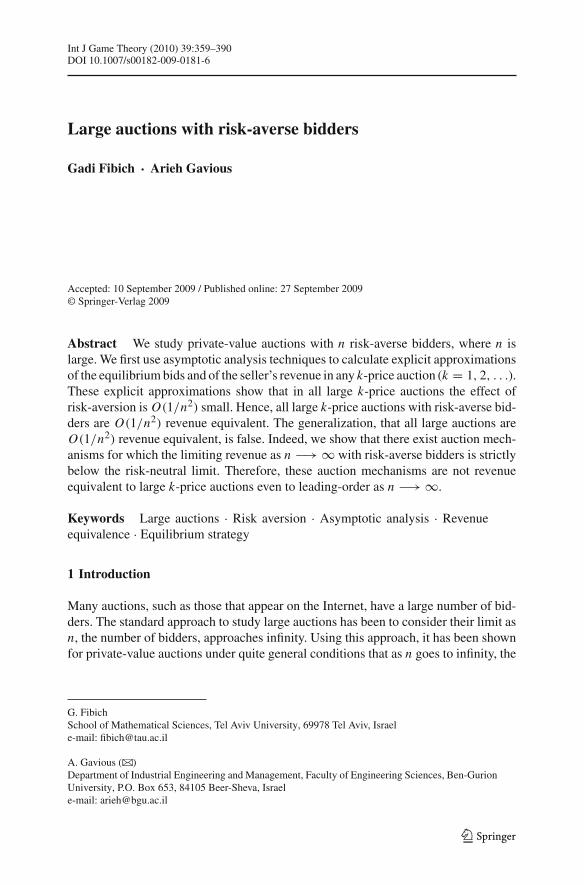
From the proof of Proposition 6 it follows immediately that the pointwise Condition(13) can be replaced with the weaker condition that Ev−i [vi − βwin(vi , v−i )] ≤ εn

for 0 ≤ vi ≤ 1. An even weaker condition can be derived as follows. As noted, thelimiting revenue is only due to the contribution of the payments of the winning bid-ders. Because Rwin has the multiplicative term Fn−1(v) which is exponentially smallexcept in an O(1/n) region near the maximal value, Condition (13) can be relaxed tohold only in this shrinking region:

Corollary 1 Proposition 6 remains valid if we replace Condition (13) with the weakercondition that there exists a sequence εn −→ 0, such that for any C > 0,

|vi − βwin(vi , v−i )| ≤ εn, 1 − C/n ≤ vi ≤ 1, 0 ≤ v−i ≤ vi . (18)

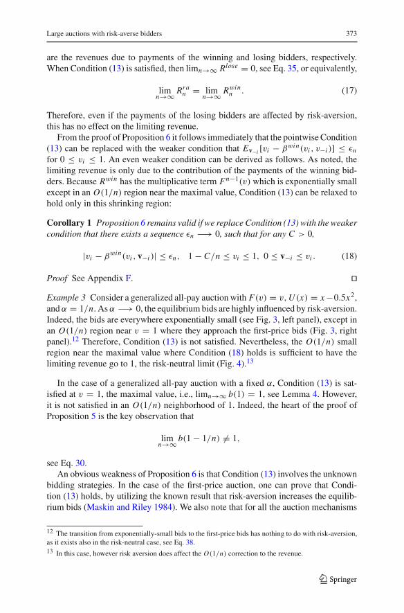
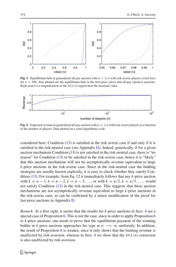
Proof See Appendix F. ��Example 3 Consider a generalized all-pay auction with F(v) = v, U (x) = x −0.5x2,and α = 1/n. As α −→ 0, the equilibrium bids are highly influenced by risk-aversion.Indeed, the bids are everywhere exponentially small (see Fig. 3, left panel), except inan O(1/n) region near v = 1 where they approach the first-price bids (Fig. 3, rightpanel).12 Therefore, Condition (13) is not satisfied. Nevertheless, the O(1/n) smallregion near the maximal value where Condition (18) holds is sufficient to have thelimiting revenue go to 1, the risk-neutral limit (Fig. 4).13

In the case of a generalized all-pay auction with a fixed α, Condition (13) is sat-isfied at v = 1, the maximal value, i.e., limn→∞ b(1) = 1, see Lemma 4. However,it is not satisfied in an O(1/n) neighborhood of 1. Indeed, the heart of the proof ofProposition 5 is the key observation that

limn→∞ b(1 − 1/n) = 1,

see Eq. 30.An obvious weakness of Proposition 6 is that Condition (13) involves the unknown

bidding strategies. In the case of the first-price auction, one can prove that Condi-tion (13) holds, by utilizing the known result that risk-aversion increases the equilib-rium bids (Maskin and Riley 1984). We also note that for all the auction mechanisms

12 The transition from exponentially-small bids to the first-price bids has nothing to do with risk-aversion,as it exists also in the risk-neutral case, see Eq. 38.13 In this case, however risk aversion does affect the O(1/n) correction to the revenue.

123


0 0.2 0.4 0.6 0.8 10

0.2

0.4

0.6

0.8

1

value (v)

bid

0.95 0.96 0.97 0.98 0.99 10

0.2

0.4

0.6

0.8

1

value (v)

bid

Fig. 3 Equilibrium bids in generalized all-pay auction with α = 1/n with risk-averse players (solid line)for n = 100. Also plotted are the equilibrium bids in the first-price (dots) and all-pay (dashes) auctions.Right panel is a magnification of the O(1/n) region near the maximal value

101

102

103

0

0.5

1

number of players (n)

Rev

enue

Fig. 4 Expected revenue in generalized all-pay auction with α = 1/n with risk-averse players as a functionof the number of players. Data plotted on a semi-logarithmic scale

considered here, Condition (13) is satisfied in the risk-averse case if and only if it issatisfied in the risk-neutral case (see Appendix G). Indeed, generically, if for a givenauction mechanism Condition (13) is not satisfied in the risk-neutral case, there is “noreason” for Condition (13) to be satisfied in the risk-averse case, hence it is “likely”that this auction mechanism will not be asymptotically revenue equivalent to largek-price auctions in the risk-averse case. Since in the risk-neutral case the biddingstrategies are usually known explicitly, it is easy to check whether they satisfy Con-dition (13). For example, from Eq. 12 it immediately follows that any k-price auctionwith k = n − 1, k = n − 2, k = n − 3, . . ., or with k = n/2, k = n/3, . . . , wouldnot satisfy Condition (13) in the risk-neutral case. This suggests that these auctionmechanisms are not asymptotically revenue equivalent to large k-price auctions inthe risk-averse case, as can be confirmed by a minor modification of the proof forlast-price auctions in Appendix D.

Remark At a first sight, it seems that the results for k-price auctions in Sect. 4 are aspecial case of Proposition 6. This is not the case, since in order to apply Proposition 6to k-price auctions, one needs to prove that the equilibrium payment of the winningbidder in k-price auctions approaches his type as n −→ ∞ uniformly. In addition,the result of Proposition 6 is weaker, since it only shows that the limiting revenue isunaffected by risk-aversion, whereas in Sect. 4 we show that the O(1/n) correctionis also unaffected by risk-aversion.

123


8 Final remarks

In this study we used two different mathematical approaches for studying the effect ofrisk-aversion in large private-value auctions. The results on all-pay auctions, last-priceauctions, and the asymptotic revenue equivalence theorem (Sects. 5–7) were provedusing rigorous techniques which are standard in auction theory. Hence, these results areof interest mostly for their economic implications. In contrast, the results on first-priceand k-price auctions (Sects. 3, 4) were proved using asymptotic analysis techniquessuch as the Laplace method for integrals which, to the best of our knowledge, have notbeen used before in auction theory. Since these techniques can be applied to numerousother problems in auction theory, these results are also of interest for their “appliedmath approach”.

There are some obvious disadvantages for using applied math techniques such asasymptotic analysis, as compared with the standard rigorous approach used in auctiontheory. Thus, the results are not “exact”, but “only” approximate.14 Moreover, one cansometimes construct pathological “counter-examples” for which the results “do nothold”.15 In other words, while the results hold “generically”, it is not always easy oreven possible to formulate the exact conditions under which they hold.

Addressing this “criticism” would probably seem out of place in a physical or anengineering journal, where such applied math techniques have been in use for over200 years. Indeed, these (and similar) techniques and approximations have been rou-tinely used in the design of airplanes, nuclear plants, bridges, medical instruments,etc. However, as these techniques have not been in use in the auction (and, more gen-erally, the economic) literature, in what follows we will “defend” the legitimacy ofthis “applied math approach”.

One obvious advantage of these applied math techniques is that they can be used tosolve (“to leading-order”) hard problems, which cannot be solved exactly. For exam-ple, the explicit expressions for the bids and revenue in large first-price auctions withrisk-averse bidders cannot be calculated exactly, but can be easily calculated asymp-totically (Proposition 1). Essentially, this is because by solving “to leading-order” wereplace the original “hard” nonlinear problem, with a linear problem for the leading-order correction.

Even when results can be calculated using the standard techniques, in many casesthe applied math techniques require substantially less work. For example, in the specialcase of risk-neutrality, the result of Proposition 1 is equivalent to the one obtained byCaserta and de Vries (2002) using extreme value theory. Their calculation, however,required considerably more work.

The assumptions made on F and U do not cover all possible cases. For example,our asymptotic results do not cover the case when f (1) = 0. We stress, however, thatthis case can be analyzed using the same techniques, with only minor modifications.When f (1) is positive but very small, our asymptotic results are valid as n −→ ∞.In that case, however, the value of n should be significantly larger for them to be

14 E.g., they are O(1/n2) accurate in this study.15 E.g., one can find distribution functions F for which f (1) is positive but extremely small, for which ourasymptotic expansions provide a poor approximation at values of n which are already “large”.

123


accurate. It is possible to estimate the value of n for which they become accurate (e.g.,by calculating the next-order term).

As was discussed in the Introduction, the asymptotic expansions allowed us toobtain results which are stronger than the limiting results and also from the rate-of-convergence results. In particular, the asymptotic expansions become applicable atmuch smaller values of n. This is important when one wants to analyze a specificauction, since then the number of bidders is given, and does not go to infinity.

Finally, we acknowledge that k-price auctions rarely appear in real-life auctions.Nevertheless, they are of interest from a theoretical point of view. Moreover, the resultthat the effect of risk aversion decays as 1/n2 for all k-price auctions, makes our dis-covery that there exist auction mechanisms for which the effect of risk aversion doesnot disappear as n −→ ∞, all the more surprising.

Acknowledgments We thank Aner Sela, Eilon Solan and Steven Schochet for useful discussions. Theresearch of G. Fibich was partially supported by a F.I.R.S.T grant number 1460/04 from the Israel ScienceFoundation (ISF)

A Auxiliary Lemmas

Lemma 1 Let n � 1, let b(v) = v + (1/n)B1(v) + (1/n2)B2(v) + O(1/n3), andlet v(b) = b + 1

n v1(b) + 1n2 v2(b) + O(1/n3) be the inverse function of b(v). Then,

B1(v) = −v1(v), B2(v) = −B1(v)v′1(v) − v2(v). (19)

Proof We substitute the two expansions into the identity v ≡ v(b(v)) and expandin 1/n:

v = v(b(v)) = b(v) + 1

nv1(b(v)) + 1

n2 v2(b(v)) + O(1/n3)

= v + 1

nB1(v) + 1

n2 B2(v) + 1

nv1

(v + 1

nB1(v)

)+ 1

n2 v2(v) + O(1/n3)

= v + 1

n[B1(v) + v1(v)] + 1

n2

[B2(v) + B1(v)v′

1(v) + v2(v)] + O

(1

n3

).

Balancing the O(1/n) and O(1/n2) terms proves (19). ��In the following we calculate an asymptotic expansion of the integral

∫ v

0 Fn(x) dxusing integration by parts (for an introduction to asymptotic evaluation of integralsusing integration by parts, see, e.g., Murray 1984):

Lemma 2 Let F(v)be a twice-continuously differentiable, function and let f = F ′>0.Then, for a sufficiently large n,

v∫0

Fn(x) dx = 1

n

Fn+1(v)

f (v)

[1 + O

(1

n

)]. (20)

123


Proof Using integration by parts,

v∫0

Fn(x) dx =v∫

0

[Fn(x) f (x)] 1

f (x)dx = 1

n + 1

Fn+1(v)

f (v)

+ 1

n + 1

v∫0

[Fn+1(x) f (x)] f ′(x)

f 3(x)dx = 1

n + 1

Fn+1(v)

f (v)

+ 1

n + 1

1

n + 2Fn+2(v)

f ′(v)

f 3(v)− 1

n + 1

1

n + 2

v∫0

Fn+2(x)

(f ′(x)

f 3(x)

)′dx .

Therefore, the result follows. ��

B Proof of Proposition 2

Since limn→∞ v(b) = b, we can look for a solution of the form

v(b) = b + 1

n − 1v1(b) + 1

(n − 1)2 v2(b) + O

(1

n3

). (21)

Substituting (21) in (2) and using U (0) = 0 and 0 < U ′(0) < ∞ gives

1 + 1

n − 1v′

1(b) + O

(1

n2

)= 1

n − 1

F(b) + v1n−1 f (b) + O(n−2)

f (b) + v1n−1 f ′(b) + O(n−2)

× U ′(0) + v1n−1U ′′(0) + O(n−2)

U (0) +(

v1n−1 + v2

(n−1)2

)U ′(0) + v2

12(n−1)2 U ′′(0) + O(n−3)

= F(b) + v1n−1 f (b) + O(n−2)

f (b) + v1n−1 f ′(b) + O(n−2)

· U ′(0) + v1n−1U ′′(0) + O(n−2)(

v1 + v2(n−1)

)U ′(0) + v2

12(n−1)

U ′′(0) + O(n−2)

=(

F(b)

f (b)+ v1

n − 1+ O(n−2)

)(1 − v1

n − 1

f ′(b)

f (b)+ O(n−2)

)

×(

1

v1+ 1

n − 1

U ′′(0)

U ′(0)+ O(n−2)

)

×(

1 − 1

(n − 1)

v2

v1− v1

2(n − 1)

U ′′(0)

U ′(0)+ O(n−2)

)

= F(b)

f (b)

1

v1+ 1

n − 1

[1 − f ′(b)F(b)

f 2(b)+ F(b)

2 f (b)

U ′′(0)

U ′(0)− F(b)

f (b)

v2

v21

]+ O(n−2).

123


Balancing the O(1) terms gives, as before,

v1(b) = F(b)

f (b). (22)

Balancing the O(

1n−1

)terms gives

v′1(b) = 1 − f ′(b)F(b)

f 2(b)+ F(b)

2 f (b)

U ′′(0)

U ′(0)− F(b)

f (b)

v2

v21

.

Substituting v1(b) = F(b)/ f (b) and v′1(b) = 1 − F(b) f ′(b)

f 2(b)gives

v2(b) = F2(b)

2 f 2(b)

U ′′(0)

U ′(0). (23)

Using Lemma 1 and (22,23) to invert the expansion (21) gives

b(v) = v + 1

n − 1B1(v) + 1

(n − 1)2 B2(v) + O

(1

n3

),

where

B1(v) = − F(v)

f (v), B2(v) = F(v)

f (v)− F2(v) f ′(v)

f 3(v)− F2(v)

2 f 2(v)

U ′′(0)

U ′(0).

This completes the proof of (5).To calculate the expected revenue, we first use (5) to obtain

Rran =

1∫0

b(v) d Fn(v) = b(1) −1∫

0

b′(v)Fn(v) dv

= 1 − 1

n − 1

1

f (1)+ 1

(n − 1)2

[1

f (1)− f ′(1)

f 3(1)− 1

2 f 2(1)

U ′′(0)

U ′(0)

]

−1∫

0

[1 − 1

n − 1

(F(v)

f (v)

)′]Fn(v) dv + O

(1

n3

).

Integration by integration by parts (as in Lemma 2) gives,

1∫0

Fn(v) dv = 1

n + 1

1

f (1)+ 1

n + 1

1

n + 2

f ′(1)

f 3(1)+ O

(1

n3

),

123


and

1∫0

(F(v)

f (v)

)′Fn(v) dv = 1

n + 1

1

f (1)

(F(v)

f (v)

)′

v=1+ O

(1

n2

).

Therefore,

1∫0

[1 − 1

n − 1

(F(v)

f (v)

)′]Fn(v) dv

= 1

n

1

1 + 1n

1

f (1)+ 1

n2

f ′(1)

f 3(1)− 1

n2

1

f (1)

(1 − f ′(1)

f 2(1)

)+ O

(1

n3

)

= 1

n

1

f (1)− 1

n2

2

f (1)+ 2

n2

f ′(1)

f 3(1)+ O

(1

n3

).

Substitution in the expression for Rran proves (6). ��

C Proof of Proposition 5

We first show that the maximal bid b(1) is monotonically increasing in α:

Lemma 3 Consider a generalized all-pay auction where bidders valuations are dis-tributed according to F(v) in [0, 1], and bidders have a utility function U that satisfies(1). Then,

∂b(1)

∂α> 0, 0 ≤ α ≤ 1.

Proof Let

V (v) = Fn−1(v)U (v − b(v)) + (1 − Fn−1(v)U (−αb(v)) (24)

be the expected utility of a bidder with value v. By the envelope theorem,

V ′(v) = Fn−1(v)U ′(v − b(v)). (25)

In addition, differentiating (24) with respect to α gives

∂V (v)

∂α= − ∂b

∂α

(Fn−1(v)U ′(v − b(v)) + (1 − Fn−1(v))U ′(−αb(v))

)

−b(v)(1 − Fn−1(v))U ′(−αb(v)). (26)

We now prove that ∂V (v)∂α

< 0 for all 0 < α, v ≤ 1. By negation, assume that∂V (v)

∂α≥ 0 for some 0 < v1, α1 ≤ 1. Then, from Eq. 26 it follows that ∂b

∂α|v1,α1 < 0.

123


Hence, by risk aversion and (25),

∂

∂αV ′(v)

∣∣∣∣v1,α1 = − ∂b

∂αFn−1(v)U ′′(v − b(v))

∣∣∣∣v1,α1

< 0. (27)

Denote y(v) = Vα1+�α(v) − Vα1(v), where 0 < �α. By the negation assumption,if �α is sufficiently small, then y(v1) ≥ 0. Hence, by (27), y′(v1) = V ′

α+�(v1) −V ′

α(v1) < 0. Thus, y(t) = Vα+�(t) − Vα(t) > 0 for t slightly below v1, and there-fore by a continuation argument for every 0 ≤ t < v1. This contradicts the fact thaty(0) = Vα+�(0) − Vα(0) = 0, since V (0) = 0 for every α.

We have thus proved that

0 >∂V (1)

∂α= −∂b(1)

∂αU ′(1 − b(1)).

Therefore, the result follows. ��

Therefore, the maximal bid approaches the maximal value:

Lemma 4 Under the conditions of Lemma 3,

limn→∞ b(1) = 1, 0 ≤ α ≤ 1.

Proof From Lemma 3 we have that b(1) is monotonically increasing in α. Therefore,

b(1;α = 0) < b(1;α) ≤ 1.

Since for α = 0 we have a first price auction, from Eq. 3 it follows thatlimn→∞ b(1;α = 0) = 1. Therefore, the result follows. ��

We now prove Proposition 5. Let V (v), defined by (24), be the expected utility ofa bidder with value v in equilibrium. Then,

0 ≤ n

1∫0

V (v) f (v) dv = nU ′(0)

1∫0

[vFn−1(v) − αb − (1 − α)Fn−1(v)b] f (v) dv

−Cn = U ′(0)An − U ′(0)Rran − Cn,

123


where

Cn = nU ′(0)

1∫0

[vFn−1(v) − αb − (1 − α)Fn−1(v)b] f (v) dv − n

1∫0

V (v) f (v) dv,

An = n

1∫0

vFn−1(v) f (v) dv,

Rran = n

1∫0

[bFn−1 + αb(1 − Fn−1] f dv.

Therefore,

Rran ≤ An − Cn

U ′(0).

Since

An =1∫

0

v(Fn)′ = 1 −1∫

0

Fn = 1 + O(1/n),

see Eq. 20, then limn→∞ An = 1. Therefore, to complete the proof, we only need toshow that limn→∞ Cn > 0.

Now,

Cn = −n

1∫0

[Fn−1(v)

(U (v − b) − (v − b)U ′(0)

) + (1 − Fn−1(v)) (U (−αb)

+αbU ′(0))]

f (v) dv

= −n

1∫0

[Fn−1(v)

(v − b)2

2U ′′(θ1(v))+(1−Fn−1(v))

α2b2

2U ′′(θ2(v))

]f (v) dv,

where 0 < θ1(v) < v − b(v) and −b(v) < θ2(v) < 0. Since −U ′′ ≥ M > 0, wehave that

Cn ≥ Mn

1∫0

[Fn−1(v)

(v − b)2

2+ (1 − Fn−1(v))

α2b2

2

]f (v) dv

≥ Mn

1∫0

Fn−1(v)(v − b)2

2f (v) dv. (28)

123


We now show that the limit of (28) is strictly positive. Indeed,

1∫0

nFn−1(v) f (v)(v − b)2 dv =1∫

0

(Fn(v)

)′(v − b)2 dv

= Fn(v)(v − b)2∣∣∣1

0− 2

1∫0

Fn(v)(v − b)(1 − b′) dv

= (1 − b(1))2 − 2

1∫0

Fn(v)(v − b) dv + 2

1∫0

Fn(v)(v − b)b′ dv. (29)

We claim that the first two terms go to zero, but the third term goes to a positive con-stant. Since limn→∞ b(1) = 1, by Lemma 4, the first term in (29) approaches zero.Since (v − b) is bounded, by Lemma 2 the second term also goes to zero. As for thethird term,

1∫0

Fn(v)(v − b)b′dv ≥1∫

1−1/n

Fn(v)(v − b)b′ dv.

Now, Fn(1 − 1/n) ≥ C1 > 0. Indeed,

F

(1 − 1

n

)= 1 − 1

nf (θ), 1 − 1

n< θ < 1.

Therefore,

Fn(

1 − 1

n

)≥

(1 − max f

n

)n

−→ e− max f .

Therefore,

1∫1−1/n

Fn(v)(v − b)b′dv ≥ C1

1∫1−1/n

(v − b)b′dv.

123


In addition,

1∫1−1/n

(v − b)b′ dv = vb

∣∣∣∣∣∣∣11−1/n −

1∫1−1/n

b dv − b2

2

∣∣∣∣∣∣∣

1

1−1/n

= b(1) − (1 − 1/n)b(1 − 1/n) −1∫

1−1/n

b dv − b2(1)

2+ b2(1 − 1/n)

2.

As n goes to infinity, b(1) → 1 and∫ 1

1−1/n b dv → 0. Hence,

limn→∞

1∫1−1/n

(v − b)b′ dv = 1

2(1 − X∞)2,

where

X∞ = limn→∞ Xn, Xn = b(1 − 1/n).

We now show that

X∞ < 1, (30)

and this will complete the proof. By Taylor expansion,

1 − Xn = 1 − b(1) + 1

nb′(θ), 1 − 1/n < θ < 1. (31)

Recall that

b′(v) = (n − 1)Fn−2(v) f (v)U (v − b(v)) − U (−αb(v))

Fn−1(v)U ′(v − b(v)) + α(1 − Fn−1(v))U ′(−αb(v)).

Now, for v ∈ (1 − 1/n, 1), as n −→ ∞,

Fn−2(v) ≥ Fn(v) ≥ C1, f (v) ≥ min f (v),

U (v − b(v)) − U (−αb(v)) = (v − (1 − α)b(v))U ′(θ2)

≥ (v − (1 − α)v)U ′(θ2) ≥ α(1 − 1/n)U ′(1),

and

Fn−1(v)U ′(v − b(v)) + α(1 − Fn−1(v))U ′(−αb(v)) ≤ U ′(−1).

123


Therefore, there exists C2 > 0 such that

b′(v) ≥ (n − 1)C2, 1 − 1/n < v < 1.

Thus, since 1 − b(1) → 0, Eq. 31 implies that limn→∞(1 − Xn) ≥ C2 > 0. ��

D Last-price auctions

The equilibrium bid function in a last-price auctions with F(x) = x and a CARAutility U (x) = 1 − e−λx is the solution of, see Eq. 9,

v∫0

[1 − e−λ(v−b(t))](v − t)n−3 dt = 0.

Therefore,

v∫0

eλb(t)(v − t)n−3 dt = eλv vn−2

n − 2.

Differentiating n − 3 times with respect to v gives

(n − 3)!v∫

0

eλb(t) dt = dn−3

dvn−3

(eλv vn−2

n − 2

).

One more differentiation gives

(n − 2)!eλb(v) = dn−2

dvn−2

(eλvvn−2

).

Therefore,

b(v) = 1

λln

[1

(n − 2)!dn−2

dvn−2

(eλvvn−2

)]= 1

λln

[eλv

n−2∑k=0

(n − 2

k

)1

k!λkvk

]

= v + 1

λln

[n−2∑k=0

(n − 2

k

)1

k!λkvk

]≤ v + 1

λln

[n−2∑k=0

(n − 2

k

)λkvk

]

= v + 1

λln

[(1 + λv)n−2

]≤ v + 1

λln

[(eλv)n−2

]= (n − 1)v = brn(v),

123


where brn(v) is the equilibrium strategy in the risk-neutral case, see Eq. 12. Hence,

λ(brn − b) ≥ ln

[n−2∑k=0

(n − 2

k

)λkvk

]− ln

[n−2∑k=0

(n − 2

k

)1

k!λkvk

]

≥ ln

[n−2∑k=0

(n − 2

k

)λkvk

]

− ln

[−1

2

(n − 2

k

)λ2v2 +

n−2∑k=0

(n − 2

k

)λkvk

]

= ln[(1 + λv)n−2

]− ln

[−1

2

(n − 2

2

)λ2v2 + (1 + λv)n−2

].

Since ln b − ln a ≥ (b − a)/b for 0 < a < b, we get that

λ(brn − b) ≥ 1

2

(n − 2

2

)λ2v2 1

(1 + λv)n−2 .

The distribution function of the lowest value is F(n) = 1 − (1 − v)n , hence the

expected revenue is given by Rlast-pricen = ∫ 1

0 b(v) d F(n) = n∫ 1

0 b(v)(1 − v)n−1 dv.Therefore,

Rrnn − Rlast-price

n = n

1∫0

[brn(v) − b(v)](1 − v)n−1 dv

≥ λ

4n(n − 2)(n − 3)

1/n∫0

v2 1

(1 + λv)n−2 (1 − v)n−1 dv

≥ λ

4n(n − 2)(n − 3)

1/n∫0

v2 1

(1 + λ/n)n−2 (1 − 1/n)n−1 dv

= λ

4n(n − 2)(n − 3)

1

3n3

1

(1 + λ/n)n−2 (1 − 1/n)n−1.

Taking the limit, we have that

limn→∞(Rrn

n − Rlast-pricen ) ≥ λ

12e−λ−1 > 0.

��

123


E Proof of Proposition 6

Let P(v) = Fn−1(v) be the probability of winning of a bidder with value v. Sincen

∫ 10 P(v) f (v) dv = 1, from Condition (13) it follows that

n

1∫0

Ev−i [βwin(vi , v−i ) − vi ]P(vi ) f (vi ) dvi = O(εn). (32)

Let

Si (vi ) = Ev−i

[U (vi − β(vi , v−i ))|i wins

]P(vi )

+Ev−i

[U (−β(vi , v−i ))|i loses

](1 − P(vi )),

be the expected surplus of a risk-averse bidder i when his type is vi . From now on,we suppress the subindex i and the dependence on v−i , and introduce the notationsβwin and βlose for the equilibrium payment when bidder i wins or loses, respectively.Therefore, the last relation can be rewritten as

S(v) = E[U (v − βwin(v))

]P(v) + E

[U (−βlose(v))

](1 − P(v)). (33)

Similarly, the expected revenue can be written as R = Rwin + Rlose, where

Rwinn = n

1∫0

E[βwin(v)]P(v) f (v) dv,

Rlosen = n

1∫0

E[βlose(v))](1 − P(v)) f (v) dv.

From Eq. 32 it follows that

Rwinn = n

1∫0

vP(v) f (v) dv + O(εn) = 1 + O(1/n) + O(εn)

= Rrnn + O(1/n) + O(εn). (34)

We now show that relation (32) implies that

Rlosen = O(εn). (35)

Indeed, from Eq. 33 and the fact that Si ≥ 0, we have that

− E[U (−βlose(v))

](1 − P(v)) ≤ E

[U (v − βwin(v))

]P(v). (36)

123


Since U (−x) = −xU ′(0) + x2/2U ′′(θ(−x)) < −xU ′(0), it follows that xU ′(0) ≤−U (−x). Therefore, by (36) and the fact that the payments are positive,

0 ≤ U ′(0)E[βlose(v)

](1 − P(v)) ≤ E

[U (v − βwin(v))

]P(v).

Hence,

0 ≤ U ′(0)n

1∫0

E[βlose(v))

](1 − P(v)) f (v) dv

≤ n

1∫0

E[U (v − βwin(v))

]P(v) f (v) dv = O(εn),

where is the last stage we used (32). Therefore, we proved (35).Combining (34,35) we get that Rra

n = Rrnn + O(1/n) + O(εn). Therefore, we

proved Eq. 14. ��

F Proof of Corollary 1

In the proof of Proposition 6 we used Condition (13) to conclude that

limn→∞ n

1∫0

E[βwin(v) − v]P(v) f (v) dv = 0.

Therefore, we need to show that this limit does not change even if (13) holds “only”for 1 − C/n ≤ v ≤ 1. To see that, we note that

n

1∫0

E[βwin(v) − v]P(v) f (v) dv = I1 + I2,

where

I1 = n

1−C/n∫0

E[βwin(v) − v]P(v) f (v) dv,

I2 = n

1∫1−C/n

E[βwin(v) − v]P(v) f (v) dv.

123


Since 0 ≤ E[βwin(v)] ≤ v ≤ 1,

I1 ≤ n

1−C/n∫0

P(v) f (v) dv = Fn(1 − C/n).

Now,

F (1 − C/n) = 1 − C/n f (θn), 1 − C/n < θn < 1.

Therefore, as n −→ ∞,

Fn (1 − C/n) =(

1 − C f (θn)

n

)n

−→ e−C f (1). (37)

Therefore, we can choose C sufficiently large so that |I1| ≤ ε/2. In addition,

|I2| ≤ εnn

1∫1−C/n

P(v) f (v) dv ≤ εnn

1∫0

P(v) f (v) dv = εn .

Therefore, we can choose n sufficiently large so that |I2| ≤ ε/2. Therefore, the resultfollows. ��

G Condition (13) in the risk-neutral case

• The risk-neutral equilibrium bids, hence payments, in the first-price and all-payauctions are given by

β1strn (v) = b1st

rn (v) = v − 1

Fn−1(v)

v∫0

Fn−1(s) ds,

βallrn (v) = ball

rn (v) = Fn−1(v)β1strn (v).

Hence, by Lemma 2, as n −→ ∞,

β1strn (v) ∼ v − 1

n

F(v)

f (v), βall

rn (v) ∼ Fn−1(v)

[v − 1

n

F(v)

f (v)

].

Therefore, Condition (13) is satisfied for (risk-neutral) first-price auction, but notfor the all-pay auction.

123


• In the case of generalized all-pay auctions, the equilibrium bid function is thesolution of

b′(v) = (n − 1)Fn−2(v) f (v)

× U (v − b(v)) − U (−αb(v))

Fn−1(v)U ′(v − b(v)) + α(1 − Fn−1(v))U ′(−αb(v)),

b(0) = 0.

This equation can be explicitly solved in the risk-neutral case, yielding

(β

gen-allrn

)win(v) = bgen-all

rn (v) =vFn−1(v) −

v∫0

Fn−1(s) ds

α + (1 − α)Fn−1(v)

= Fn−1(v)

α + (1 − α)Fn−1(v)b1st

rn (v). (38)

Hence, (βgen-allrn )win(v) −→ v provided that Fn−1(v)

α+(1−α)Fn−1(v)−→ 1. If α is held

constant, then Fn−1(v)

α+(1−α)Fn−1(v)−→ 1 when Fn−1(v) −→ 1, i.e., for 1 − v � 1/n

but not for 1 − v = O(1/n). Therefore, Condition (13) is not satisfied. If, how-

ever, α = α(n) and limn→∞ α = 0, then by (37) Fn−1(v)

α+(1−α)Fn−1(v)−→ 1 for

1 − v = O(1/n), but not for all 0 ≤ v ≤ 1. Therefore, Condition (13) is notsatisfied, but its weaker form (see Corollary 1) is satisfied.

• In the case of k-price auctions, limn→∞ bk−pricern (v) = v, see Eq. 12. In addition,

as n −→ ∞, the kth value approach the value of the winning bidder. Therefore,limn→∞ β

k−pricern (v) = v, so that Condition (13) is satisfied.

• Finally, in the case of last-price auctions,

(βlastrn )win(vi , v−i ) = blast

rn (vmin) = vmin + (n − 2)F(vmin)

f (vmin), vmin = min

j =iv j ,

see Eq. 12. In addition, since blastrn (vmin) is independent of v, then it is not con-

verging to v for all v as n −→ ∞. Therefore, Condition (13) is not satisfied.��

References

Bali V, Jackson M (2002) Asymptotic revenue equivalence in auctions. J Econ Theory 106:161–176Bender CM, Orszag S (1978) Advanced mathematical methods for scientists and engineers. McGraw-Hill,

New YorkCaserta S, de Vries C (2002) Auctions with numerous bidders, mimeoDyer D, Kagel JH, Levin D (1989) Resolving uncertainty about the number of bidders in independent

private-value auctions: an experimental analysis. Rand J Econ 20(2):268–279Fibich G, Gavious A (2003) Asymmetric first-price auctions—a perturbation approach. Math Oper Res

28:836–852

123


Fibich G, Gavious A, Sela A (2004) Revenue equivalence in asymmetric auctions. J Econ Theory 115:309–321

Fibich G, Gavious A, Sela A (2006) All-pay auctions with risk-averse buyers. Int J Game Theory 34:583–599

Hong H, Shum M (2004) Rates of information aggregation in common value auctions. J Econ Theory116:1–40

Jackson MO, Kremer I (2004) The relationship between the allocation of goods and a seller’s revenue.J Math Econ 40:371–392

Jackson MO, Kremer I (2006) The relevance of a choice of auction format in a competitive environment.Rev Econ Stud 73:961–981

Klemperer P (1999) Auction theory: a guide to the literature. J Econ Surv 13:227–286Kremer I (2002) Information aggregation in common value auctions. Econometrica 70(4):1675–1682Krishna V (2002) Auction theory. Academic Press, New YorkMaskin E, Riley JG (1984) Optimal auctions with risk averse buyers. Econometrica 6:1473–1518Matthews S (1987) Comparing auctions for risk averse buyers: a buyer’s point of view. Econometrica 55:

636–646Monderer D, Tennenholtz M (2000) K-price auctions. Games Econ Behav 31:220–244Murray JD (1984) Asymptotic analysis. Springer-Verlag, New YorkPesendorfer W, Swinkels JM (1997) The loser’s curse and information aggregation in common value auc-

tions. Econometrica 65:1247–1282Rustichini A, Satterthwaite MA, Williams SR (1994) Convergence to efficiency in a simple market with

incomplete information. Econometrica 62:1041–1063Satterthwaite MA, Williams SR (1989) The rate of convergence to efficiency in the buyer’s bid double

auction as the market becomes large. Rev Econ Stud 56:477–498Swinkels JM (1999) Asymptotic efficiency for discriminatory private value auctions. Rev Econ Stud 66:

509–528Swinkels JM (2001) Efficiency of large private value auctions. Econometrica 69:37–68Wilson R (1977) A bidding model of perfect competition. Rev Econ Stud 44:511–518Wolfstetter E (1995) Third- and higher-price auctions, mimeo

123

Large auctions with risk-averse bidders

Documents