Lapped Solid Textrues Filling a Model with Anisotropic Textures Kenshi Takayama, Makoto Okabe, Takashi Ijiri, Takeo Igarashi The University of Tokyo 발표.

Lapped Solid TextruesFilling a Model with Anisotropic Textures

Kenshi Takayama, Makoto Okabe, Takashi Ijiri, Takeo Igarashi

The University of Tokyo

발표 : 이성호

2

Abstract

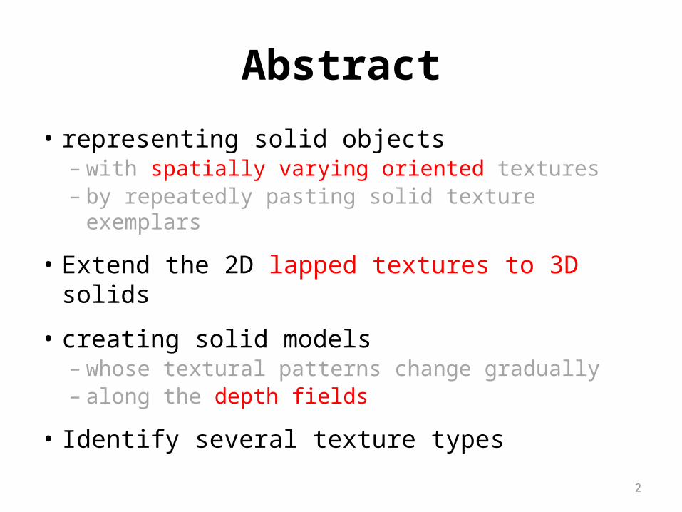
• representing solid objects – with spatially varying oriented textures– by repeatedly pasting solid texture exemplars

• Extend the 2D lapped textures to 3D solids

• creating solid models – whose textural patterns change gradually – along the depth fields

• Identify several texture types

3

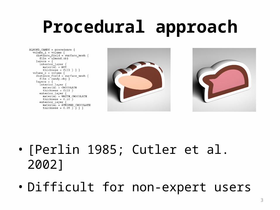
Procedural approach

• [Perlin 1985; Cutler et al. 2002]

• Difficult for non-expert users

4

2D texture synthesis on cross sections

• [Owada et al. 2004; Pietroni et al. 2007]

• Limitations– Inconsistency among dif-

ferent cross-sections– Difficulty in handling tex-

tures with discontinuous elements• Such as seeds

5

Example-based 3D solid texture synthesis

• [Jagnow et al. 2004; Kopf et al. 2007]

• For large-scale solid models– The amount of data and computational cost become

problematic

6

Lapped textures

7

Lapped solid textures

• Arrange solid textures along a tensor field

• handle spatially-varying textures

• classify solid textures into several types– according to the amount of anisotropy and spatial variation

• Designed easily and created efficiently

• Little memory and computational cost

8

Classification of solid textures

9

• [Kopf et al. 2007]– 1-a

• [Owada et al. 2004]– 1-b

• This paper– 2-a and 2-b

• Not considered– 2-c and 2-d

10

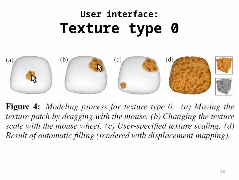
User interface:

Texture type 0

11

Type 1-a

12

Type 1-b

13

Type 2-a

14

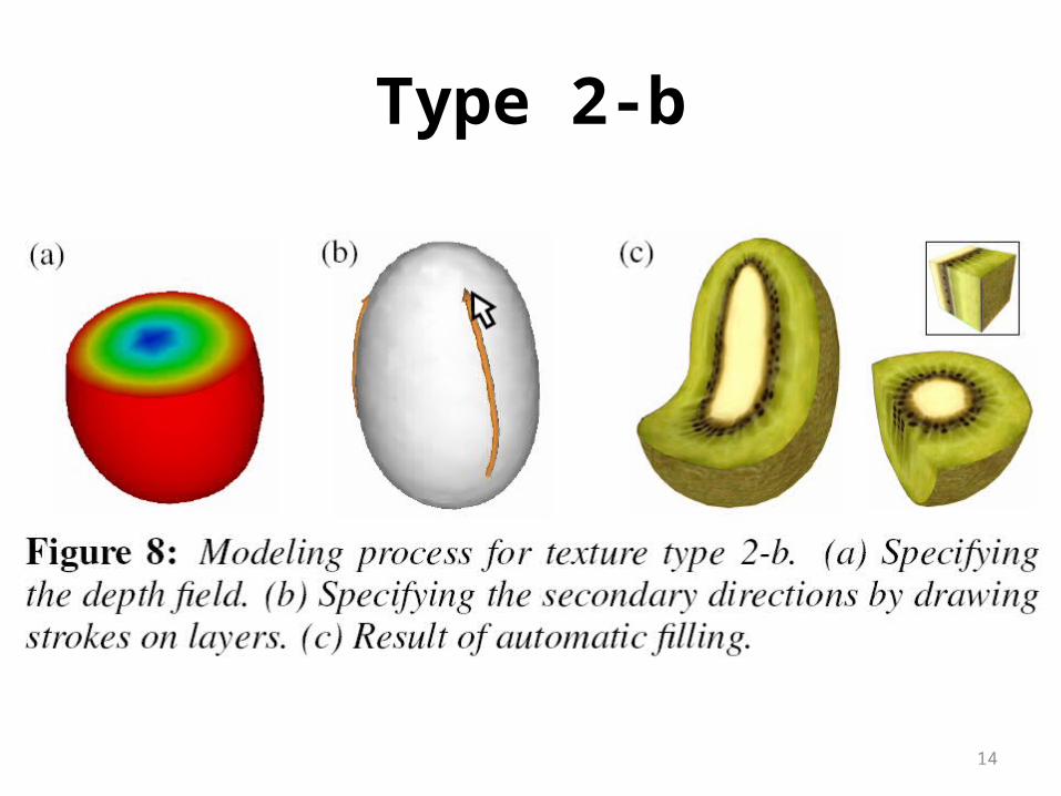
Type 2-b

15

Manual pasting of tex-tures

16

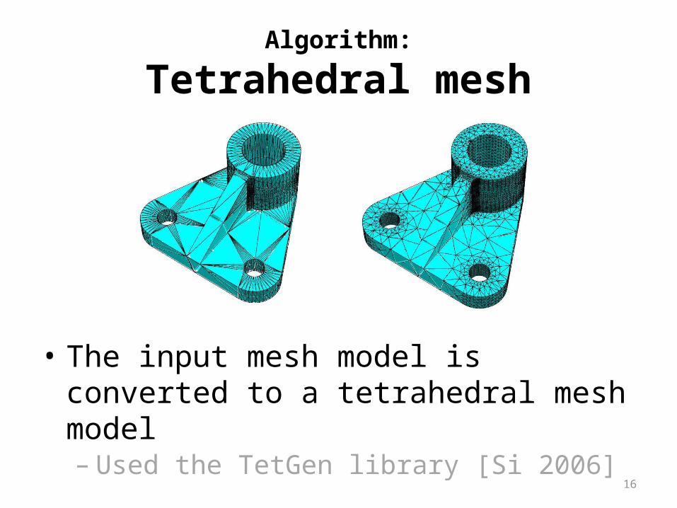
Algorithm:

Tetrahedral mesh

• The input mesh model is converted to a tetrahedral mesh model– Used the TetGen library [Si 2006]

17

Preparation of solid texture exemplars

• Solid texture synthesis [Kopf et al. 2007]

• Noise functions [Cook and DeRose 2005]

• Volume capturing using slicers [Banvard 2002]

• In-house voxel editor (this paper)– Created manually from photographs

18

Rendering an LST model

• convert tetrahedron model– Into a polygonal model– That consists of surface triangles – with a list of 3D texture coordinates as-

signed to each of its three vertices

• Each surface triangle is rendered multi-ple times– Approximately 10–20 times

• in most of our results– With alpha blending enabled

19

Cutting

• Constructs a scalar field– Using radial basis function (RBF) interpolation [Turk and O’Brien

1999]

• Texture coordinates for each triangle on the cross-section– obtained by linear interpolation

20

Volume rendering

• Construct a scalar field– over the mesh vertices– To give the distance between the cam-

era and each vertex

• Calculate a large number of slices of the model– perpendicular to the camera direction – by iso-surface extraction

21

Creating an alpha mask of the solid texture

• Create 3D mask– Using [Nealen et al. 2007]– The alpha value drops off around the boundary of the mask

• We assume all the textures in our examples are less struc-tured– Use a constant “splotch” mask shown in Fig. 11

• for all the textures

22

Constructing a tensor field

• Type 1-a and 1-b– First direction

• user-drawn strokes (1-a)• Gradient direction of the depth field (1-b)

– Other direction is chosen randomly• when pasting each patch

• Type 2-a and 2-b– First direction

• Gradient direction of the depth field– Second direction

• User-drawn strokes– Third direction

• Cross product of the two

• Magnitudes of tensors– User-specified texture scaling values– Except for types 1-b and 2-b

• Set automatically from the depth field

23

Interpolating tensor field (1/3)

• Laplacian smoothing [Fu et al. 2007]

24

Interpolating tensor field (2/3)

• Minimizing Laplacians (Eq. 1) while satisfying the collec-tion of constraints (Eq. 2) in a least squares sense forms a sparse linear system, which can be solved quickly.

25

Interpolating tensor field (3/3)

• Perform Laplacian smoothing– for each x-, y-, and z-component of the

vectors• which are later combined and normalized.

• Types 2-a and 2-b,– no guarantee that resulting vectors will– always be orthogonal to the first direction– orthogonalize these vectors

• To the first direction after smoothing

26

27

• Obtain a depth field– By using thin-plate RBF interpolation in the 3D

Euclidean space [Turk and O’Brien 1999]• the depth field must be defined as a smooth function

in 3D space

• Assign depth values– of 0 and 1 to the outermost (red) and the in-

nermost (blue) regions, respectively

• Types 1-b and 2-b,– These depth values are used directly

• As one of the three texture coordinates

28

Selecting a seed tetra-hedron

• Initialize a list of “uncovered” tetrahedra

• One is selected at random– For each pasting operation

• Tetrahedra are removed from the list – If they are completely covered

• Repeat this process– Until the “uncovered” list becomes empty

• Manual pasting of the textures– Seed tetrahedron is set to the one

• Clicked by the user

29

Growing a clump of tetrahedra

30

Texture optimization

31

32

Coverage test of tetra-hedron

• linearly sample the alpha values of the mask – at these discrete points of each

tetrahedron – in the clump– which are then accumulated.

• Assume that the tetrahedron is completely covered by the over-lapping textures– If the accumulated alpha values of all

the sampling points of a tetrahedron reach 255

33

Creation of depth-varying solid models

• Map the clump of tetrahedra– Into the corresponding depth position • In the texture space • Instead of the central position

• alter the positional constraints – from (0.5, 0.5, 0.5)t to (0.5, dseed, 0.5, )t,

– dseed is the depth value assigned to Tseed • Assuming the s-axis corresponds to the

depth orientation

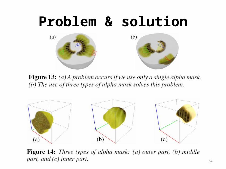
34

Problem & solution

35

Results

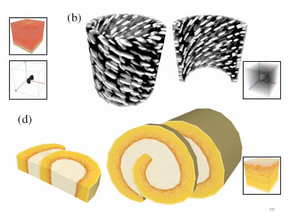
36

37

38

Limitations and future work

• Patch seams– a texture with strong low-frequency components

• Singularities of the tensor field

• blurring artifacts

• Preparation of exemplar solid textures