Laplace–Beltrami spectra as ‘Shape-DNA’ of surfaces and solids Martin Reuter, Franz-Erich Wolter * , Niklas Peinecke Division of CG, University of Hannover, Welfenlab, D-30167 Hannover, Germany Received 25 May 2005; accepted 31 October 2005 Abstract This paper introduces a method to extract ‘Shape-DNA’, a numerical fingerprint or signature, of any 2d or 3d manifold (surface or solid) by taking the eigenvalues (i.e. the spectrum) of its Laplace–Beltrami operator. Employing the Laplace–Beltrami spectra (not the spectra of the mesh Laplacian) as fingerprints of surfaces and solids is a novel approach. Since the spectrum is an isometry invariant, it is independent of the object’s representation including parametrization and spatial position. Additionally, the eigenvalues can be normalized so that uniform scaling factors for the geometric objects can be obtained easily. Therefore, checking if two objects are isometric needs no prior alignment (registration/localization) of the objects but only a comparison of their spectra. In this paper, we describe the computation of the spectra and their comparison for objects represented by NURBS or other parametrized surfaces (possibly glued to each other), polygonal meshes as well as solid polyhedra. Exploiting the isometry invariance of the Laplace–Beltrami operator we succeed in computing eigenvalues for smoothly bounded objects without discretization errors caused by approximation of the boundary. Furthermore, we present two non-isometric but isospectral solids that cannot be distinguished by the spectra of their bodies and present evidence that the spectra of their boundary shells can tell them apart. Moreover, we show the rapid convergence of the heat trace series and demonstrate that it is computationally feasible to extract geometrical data such as the volume, the boundary length and even the Euler characteristic from the numerically calculated eigenvalues. This fact not only confirms the accuracy of our computed eigenvalues, but also underlines the geometrical importance of the spectrum. With the help of this Shape-DNA, it is possible to support copyright protection, database retrieval and quality assessment of digital data representing surfaces and solids. A patent application based on ideas presented in this paper is pending. q 2005 Elsevier Ltd. All rights reserved. Keywords: Laplace–Beltrami operator; Shape invariants; Fingerprints; Shape matching; Database retrieval; Copyright protection; NURBS; Parameterized surfaces and solids; Polygonal meshes 1. Introduction The characterization and design of the shape of 3d-objects are central problems in computer graphics and geometric modeling. The development of software and hardware tools to design and visualize the shape of 3d-objects has advanced rapidly during the past twenty years. Nonetheless, fundamental problems pertaining to the characterization of shape are still widely unresolved. It is, for example, a basic question to quickly identify and retrieve a given object stored in a huge database or to find all similarly shaped objects. During the past forty years, a vast number of shape matching and searching techniques have been developed (e.g. using moments, spherical harmonics or Reeb graphs—a recent survey can be found in Iyer et al. [39], see also [30]). It should be pointed out that most approaches dealing with shape matching describe procedures to realign the geometric objects, usually called localization or registration (cf. [53,60]), and work only on a specific representation (mainly polygonal meshes) of the object. Other techniques describe subdivision or decomposition of an object into smaller features (e.g. [9] or [37]) that are then compared in a second step. The point-set of a solid 3d-object with smooth boundary may be described in very different ways (cf. [65]), for example in boundary representation (B-Rep) using NURBS surface patches. This may cause difficulties to decide if two objects have the same or different shapes. Even when restricted to NURBS surfaces, it is not easy to decide if the given objects are similar in their shape. A simple comparison of the control points used to represent the boundary surfaces does not help at all, because identical patches can be represented with different control points. Both patches first need to be represented with Computer-Aided Design 38 (2006) 342–366 www.elsevier.com/locate/cad 0010-4485//$ - see front matter q 2005 Elsevier Ltd. All rights reserved. doi:10.1016/j.cad.2005.10.011 * Corresponding author. E-mail addresses: [email protected] (M. Reuter), [email protected] hannover.de (F.-E. Wolter), [email protected] (N. Peinecke).

Welcome message from author
This document is posted to help you gain knowledge. Please leave a comment to let me know what you think about it! Share it to your friends and learn new things together.
Transcript

Laplace–Beltrami spectra as ‘Shape-DNA’ of surfaces and solids
Martin Reuter, Franz-Erich Wolter *, Niklas Peinecke
Division of CG, University of Hannover, Welfenlab, D-30167 Hannover, Germany
Received 25 May 2005; accepted 31 October 2005
Abstract
This paper introduces a method to extract ‘Shape-DNA’, a numerical fingerprint or signature, of any 2d or 3d manifold (surface or solid) by
taking the eigenvalues (i.e. the spectrum) of its Laplace–Beltrami operator. Employing the Laplace–Beltrami spectra (not the spectra of the mesh
Laplacian) as fingerprints of surfaces and solids is a novel approach. Since the spectrum is an isometry invariant, it is independent of the object’s
representation including parametrization and spatial position. Additionally, the eigenvalues can be normalized so that uniform scaling factors for
the geometric objects can be obtained easily. Therefore, checking if two objects are isometric needs no prior alignment (registration/localization)
of the objects but only a comparison of their spectra. In this paper, we describe the computation of the spectra and their comparison for objects
represented by NURBS or other parametrized surfaces (possibly glued to each other), polygonal meshes as well as solid polyhedra. Exploiting the
isometry invariance of the Laplace–Beltrami operator we succeed in computing eigenvalues for smoothly bounded objects without discretization
errors caused by approximation of the boundary. Furthermore, we present two non-isometric but isospectral solids that cannot be distinguished by
the spectra of their bodies and present evidence that the spectra of their boundary shells can tell them apart. Moreover, we show the rapid
convergence of the heat trace series and demonstrate that it is computationally feasible to extract geometrical data such as the volume, the
boundary length and even the Euler characteristic from the numerically calculated eigenvalues. This fact not only confirms the accuracy of our
computed eigenvalues, but also underlines the geometrical importance of the spectrum. With the help of this Shape-DNA, it is possible to support
copyright protection, database retrieval and quality assessment of digital data representing surfaces and solids.
A patent application based on ideas presented in this paper is pending.
q 2005 Elsevier Ltd. All rights reserved.
Keywords: Laplace–Beltrami operator; Shape invariants; Fingerprints; Shape matching; Database retrieval; Copyright protection; NURBS; Parameterized surfaces
and solids; Polygonal meshes
1. Introduction
The characterization and design of the shape of 3d-objects
are central problems in computer graphics and geometric
modeling. The development of software and hardware tools to
design and visualize the shape of 3d-objects has advanced
rapidly during the past twenty years. Nonetheless, fundamental
problems pertaining to the characterization of shape are still
widely unresolved. It is, for example, a basic question to
quickly identify and retrieve a given object stored in a huge
database or to find all similarly shaped objects. During the past
forty years, a vast number of shape matching and searching
techniques have been developed (e.g. using moments, spherical
0010-4485//$ - see front matter q 2005 Elsevier Ltd. All rights reserved.
doi:10.1016/j.cad.2005.10.011
* Corresponding author.
E-mail addresses: [email protected] (M. Reuter), [email protected]
hannover.de (F.-E. Wolter), [email protected] (N. Peinecke).
harmonics or Reeb graphs—a recent survey can be found in
Iyer et al. [39], see also [30]). It should be pointed out that most
approaches dealing with shape matching describe procedures
to realign the geometric objects, usually called localization or
registration (cf. [53,60]), and work only on a specific
representation (mainly polygonal meshes) of the object.
Other techniques describe subdivision or decomposition of an
object into smaller features (e.g. [9] or [37]) that are then
compared in a second step.
The point-set of a solid 3d-object with smooth boundary
may be described in very different ways (cf. [65]), for example
in boundary representation (B-Rep) using NURBS surface
patches. This may cause difficulties to decide if two objects
have the same or different shapes. Even when restricted to
NURBS surfaces, it is not easy to decide if the given objects are
similar in their shape. A simple comparison of the control
points used to represent the boundary surfaces does not help at
all, because identical patches can be represented with different
control points. Both patches first need to be represented with
Computer-Aided Design 38 (2006) 342–366
www.elsevier.com/locate/cad
M. Reuter et al. / Computer-Aided Design 38 (2006) 342–366 343
the same basis functions implying equal knot vectors and equal
degrees of the employed NURBS basis functions. The problem
becomes even more complicated if we consider the possibility
that the solid’s boundary surfaces might be represented in
various other ways, e.g. by trigonometric functions, by
implicitly defined functions or by polygonal meshes (planar
polygonal faces), that have to be compared with each other.
In some of these cases, the problem of identifying shapes
(for example, to protect the copyright of the designer) has been
approached with the help of watermarks. For this purpose,
visible or invisible watermark information is embedded into
the representation or geometry of an object. Later on, this
information can be retrieved and the object can be identified.
This is of special interest when dealing with delicate high
precision material, e.g. turbine blades, whose design needs
major research effort and expensive investments. Even though
NURBS patches are very popular today, most watermark
techniques deal with polygonal meshes only. Often the
watermark data is embedded into these meshes by slightly
modifying the vertex location, the connectivity of the mesh or
the frequency domain employing mesh-spectral analysis (cf.
[6,49]). For NURBS surfaces watermarking is more difficult
and only very few algorithms exist. An algorithm proposed by
Ohbuchi et al. [48] does not change the surface, but is not very
robust. Generally, watermarks can be destroyed by a
representation change or by a reparametrization of the object,
if they are not embedded into the geometry. On the other hand,
embedding data into the geometry rather than into the
representation changes the shape of the object which is
unacceptable in many cases. It should be noted that the
watermarking technique is limited to the comparison of
watermark information, which in general is not related to the
shape. Therefore, it cannot be used for shape matching but only
for the identification of previously marked objects.
A superior identification method avoiding both problems of
watermarking (i.e. geometry changes or representation
dependency) is to identify the shape of an object by geometric
invariants that we will call fingerprints or signatures. An
example for a fingerprint of shape intrinsic information to
identify shape via registration/alignment of umbilics can be
found in [42] or [43]. However, our approach is different
because we use sets of geometric invariants that are sufficiently
complete to identify isometric objects so we can avoid
realignment procedures as a safeguard for tests of identical
shape. Of course, fingerprint techniques cannot distinguish
between several copies of the same object, since they only
depend on the shape. In such a case, watermarks have to be
applied in order to discriminate identical copies. Nevertheless,
an advantage of the use of shape related fingerprints is that
shape can be compared indirectly through the fingerprints
(especially if similar shapes lead to similar fingerprints). In
addition to shape identification, the fingerprint technique can
therefore be used for shape matching.
Shape intrinsic information does not depend on the given
representation of the shape and can be understood as a
fingerprint of the shape (if enough information is contained).
Many geometric shape invariants (e.g. circumference, surface
area, volume, bounding sphere or eigenvalues of the inertia
tensor) have strong limitations with respect to the amount of
completeness up to which these invariants determine the shape
of an object. Therefore, we propose the following properties
that optimally should be fulfilled by a shape fingerprint (e.g. a
vector of numbers/shape invariants associated with the given
object):
1. [ISOMETRY]: Congruent solids (or isometric sur-
faces) should have the same finger-
print independently of the object’s
given representation and location.
Therefore, the fingerprint should be
an isometry invariant.
2. [SCALING]: For some applications, it is necessary
that the fingerprint is independent of
the object’s size, therefore the fin-
gerprint should optionally be scaling
invariant.
3. [SIMILARITY]: Similarly, shaped solids should have
similar fingerprints. The fingerprint
should depend continuously on shape
deformations.
4. [EFFICIENCY]: The effort needed to compute those
fingerprints should be reasonable.
5. [COMPLETENESS]: Ideally, those fingerprints should
give a complete characterization of
the shape, thus representing the shape
uniquely. One step further it would
be desirable that those fingerprints
could be used to reconstruct the solid.
6. [COMPRESSION]: In addition it would also be desirable
that the fingerprint data should not be
redundant, i.e. a part of it could not
be computed from the rest of the data.
7. [PHYSICALITY]: Furthermore, it would be nice if an
intuitive geometric or physical
interpretation of the meaning of the
fingerprints would be available.
Concerning property [ISOMETRY] let us give the
following definitions:
Definition 1 (Isometry)
Two geometric objects are isometric if a homeomorphism from
one to the other exists preserving (geodesic) distances, i.e.
mapping curves to curves with equal arc length. This
homeomorphism is then called an isometry.
Definition 2 (Congruency)
Two geometric objects are congruent if they can be
transformed into each other by rigid motions (translations
and rotations) as well as reflections.
It should be noted that isometric planar domains in 2d and
isometric solids in 3d Euclidean space are already uniquely
determined in their respective space up to rigid motions and
reflections. For planar shapes and 3d-solids congruency and

M. Reuter et al. / Computer-Aided Design 38 (2006) 342–366344
isometry are the same. Surfaces on the other hand that are bend
or folded without stretching (without changing the metric) stay
isometric even though they are not congruent. The property
[ISOMETRY] (and of course [SIMILARITY]) is important
in situations where near isometric surfaces like hands with
different finger positions or faces with different expressions are
to be compared and identified. See, e.g. [27] for a method using
discrete geodesic distances and multidimensional scaling to
generate similar signature surfaces (that still need to be aligned
for final comparison), and see [14] for an application to face
recognition. An isometry invariant fingerprint is often desired
in shape matching, since it depends
† only on the (intrinsic) shape, independent of any represen-
tation;
† not on the actual embedding and is therefore independent
of the spatial position and isometric deformation of the
object.
Very often invariants are used to classify objects. For
example in knot theory, a branch of topology, knot invariants
(e.g. the Alexander polynomial or the more recent Jones and
the Homfly polynomials) are used to distinguish knotted space
curves (cf. [1]). For surfaces there exist, for example,
topological invariants (cf. [57]) such as homotopy invariants
including, e.g. homotopy groups and homology groups or the
well-known Euler characteristic. Another important topologi-
cal invariant of a manifold is its orientability (being a non-
homotopic invariant, because the non-orientable Moebius strip
and the orientable cylinder have the circle as deformation
retract and are therefore homotopic to it). Although all these
topological shape invariants are interesting and useful, they
cannot distinguish any two homeomorphic objects such as two
3d-solids, e.g. obtained by deforming a topological full 3d-
disk.
There exist theoretical invariants determining the isometry
type of a surface or solid completely up to isometry. Indeed, the
first fundamental tensor (defined independently of a parame-
trization) is a complete isometry invariant [25]. However, this
invariant can generally not be used to check if two given
parametrizations represent isometric manifolds. In order to
compare this invariant for two objects, they first have to be
parametrized on a common parameter space. These parame-
trizations have to be constructed in a way that they map the
same point in parameter space to the two corresponding points
on each manifold. This task is as difficult as finding the
isometry itself, which generally is a very difficult problem. The
first fundamental tensor can be used to check if a
diffeomorphism is an isometry. But even this task is difficult,
as it requires checking every point.
A manifold can theoretically be determined completely up
to translation and rotation by the first and the second
fundamental tensor [25]. Like before, those two tensors do
not provide an easy tool to check if two distinct parametriza-
tions refer to congruent manifolds. The medial axis transform
(MAT) (defined uniquely for a solid body) provides a shape
invariant that is a complete shape descriptor (cf. reconstruction
theorem [64–66]). Using the MAT for testing the congruence
of two given 3d-solids would also require checking if the
respective medial axis sets (usually collections of surface
patches) are congruent, a task that again is not easy at all in
general. Therefore, all shape invariants listed above cannot be
used efficiently to detect if two distinct geometrical object
representations refer to congruent or isometric objects. We
think that this paper offers a remedy for the aforementioned
difficulties occurring in shape comparison problems. This holds
because the shape invariants presented in this paper can be used
efficiently for shape comparison (once they have been
computed).
This paper proposes to use the sequence of eigenvalues
(spectrum) of the Laplace operator of a planar domain or 3d-
solid or the Laplace–Beltrami operator of a surface or
parametrized solid in Euclidean space as a fingerprint. The
Laplace operator can be seen as the special case of
the Laplace–Beltrami operator with a Euclidean metric.
These Laplace operators are linear differential operators
defined on a corresponding vector space of differentiable
functions, the latter being defined on a domain in Euclidean
space or on a Riemannian manifold, respectively. Those
differentiable functions are supposed to be zero on the
boundary of the surface or of the domain in case the boundary
is not empty (Dirichlet boundary condition). The Neumann
boundary condition forces their derivatives in the normal
direction of the boundary curve to be a fixed function or to be
constantly zero. The Laplace operators assign the trace of their
Hessian to the latter functions (defined on the domain or on the
surface). In the surface case, the Hessian must be defined
invariantly of the surface parametrization using only the
Riemannian metric of the surface.
This fingerprint (i.e. the eigenvalues) can be calculated for
different object representations in different dimensions and can
even be calculated for grayscale or color images. We consider a
gray scale image as a surface defined by the graph of a height
function being the gray scale intensity function of the image.
The color image can, e.g. be understood as a surface (two-
manifold) in a five-dimensional Euclidean space whose
coordinates include the intensity parameters of the red, green,
blue values assigned to any (x, y) pixel of the image. It is
possible as well to understand other even higher dimensional
signals as height functions and therefore as manifolds, whose
Laplace–Beltrami spectra can be computed. Another advan-
tage of this method is that it can even be applied to solids
containing cavities (solids bounded by several not connected
surfaces), for example, an ice-cube containing fully enclosed
bubbles. Most techniques only working on boundary represen-
tations, not on the solid itself, have difficulties with several
boundary components. With our method, one can compare the
2d boundary as well as the 3d volume for two given solids.
The fingerprint presented here fulfills the desired properties
above (with the only exception of [COMPLETENESS]). Since
the eigenvalues are isometry invariants, this fingerprint is
independent of the objects representation (especially its
parametrization), its spatial position and, as we will see later,
even of the object’s size [SCALING] (if desired). This
M. Reuter et al. / Computer-Aided Design 38 (2006) 342–366 345
isometry invariance makes registration or localization of the
objects completely unnecessary. The isometry invariance is
very restrictive compared to the topological invariance. As
mentioned before, isometry even determines the congruence of
objects in important cases such as planar shapes or 3d-solids. In
other words, if limited to these very common solid objects,
their shapes are uniquely determined by their isometry class.
The fingerprint proposed here consists of a family of non-
negative numbers (the eigenvalues) that can be compared
easily and fast, permitting this approach to be used in time-
critical applications such as database retrieval. Because the
spectrum of the Laplace–Beltrami operator contains intrinsic
shape information we call it ‘Shape-DNA’. We will show that
this Shape-DNA can be used (like DNA-tests) to identify
objects in practical applications. As in real life, the DNA does
not completely characterize a subject. As we will discuss later
identical twins exist with different shape but exactly the same
Shape-DNA. Even though these twins are shaped differently
they still have quite a few common geometric properties
(exactly those properties that are determined by the spectrum).
It should be noted that in real life human fingerprints
(determined by phenotype) can distinguish identical twins,
while DNA-tests (genotype) cannot. Therefore, we think that
Shape-DNA is the more appropriate term. Beyond the
identification of shapes, the Shape-DNA can even be used to
detect similarities.
A special name for the Laplace–Beltrami spectra is even
helpful to distinguish it from other spectra. To avoid any
misunderstanding, note that the continuous Laplace–Bel-
trami operator does not operate on any mesh vertices, but
rather on the underlying manifold itself. It is therefore
different from discrete Laplacians on graphs or meshes.
Even though these discrete Laplacians have been used for,
e.g. dimensionality reduction [5] or mesh compression [41],
the introduction of our computation of the Laplace–Beltrami
spectra of the underlying manifolds in the areas of
geometric modeling—CAD in particular and in computer
graphics in general—is completely new. The only excep-
tions are our recent proceedings publication [56] outlining
briefly some of the ideas and results presented in this paper
and [65] containing a sketchy description of some basic
ideas and goals. More details and background can be found
in [55]. Moreover, the application of the Laplace–Beltrami
spectra as Shape-DNA in order to discriminate and search
for objects in geometric databases is new (cf. our german
patent application [67]). Although a considerable amount of
theoretical research has been done in geometry on the
Laplace–Beltrami operator, very little work dealing with
computational research exists (see e.g. Huntebrinker [38] for
a numerical computation of the Laplace–Beltrami spectrum
on 3d hyperbolic spaces).
One of the reasons why the spectra of the continuous
Laplace and especially the Laplace–Beltrami operator have not
yet been considered in the area of geometric modeling and
computer graphics is that their computation is not easy at all,
with respect to the theoretical effort (employing Riemannian
geometry), and somewhat cumbersome with respect to the
numerical effort involved. However, with the recent and
continuing advancement of hardware development, the
computations needed to determine surface spectra (e.g. the
first 1000 or more eigenvalues) of the Laplace–Beltrami
operator have become conveniently feasible even on a fairly
modest personal computer. This shows that the requested
[EFFICIENCY] can be achieved as well. Improvements
concerning the efficient computation of the spectrum are also
foreseeable.
We shall present this paper in a self-contained way such that
it should be accessible to a researcher in geometric modeling
who is not an expert on the tools from partial differential
equations and differential geometry used here. Therefore, we
will review some concepts from analysis and elements from
differential geometry used for the Laplace–Beltrami operator
and its properties (Section 2). We also need some concepts
from numerical analysis on finite element methods used to
compute solutions for partial differential equations (Section 3)
and describe some techniques (like meshing) needed for the
actual implementation (Section 4). Then we present a method
to numerically extract geometric data from the eigenvalues
(Section 5) and show how the Shape-DNA can be used to
identify shapes and detect similarities for use in innovative
applications (Section 6).
2. Theoretical background
In this section we will explain the theoretical background
that is needed to understand the spectrum of the Laplace
operator and its computation.
Let f be a real-valued function, with f2C2, defined on a
Riemannian manifold M (differentiable manifold with Rie-
mannian metric, cf. Berger [7]). With another function g
defined like f we define the Nabla operator V (that will be
needed later for the variational formulation) and the Laplace–
Beltrami operator D to be
Vðf ; gÞdhgrad f ; grad gi Df ddivðgrad f Þ (1)
with h , i being the scalar product, grad f the gradient of f and div
the divergence on the manifold [17].
The Nabla operator and the Laplace–Beltrami operator are
linear differential operators. They can be calculated in local
coordinates. Given a local parametrization
j : Rn/RnCk (2)
of a submanifold M of RnCk with
gij :Z hvij; vjji; G :Z ðgijÞ; W :Zffiffiffiffiffiffiffiffiffiffiffidet G
p;
ðgijÞ :ZGK1:
(3)

M. Reuter et al. / Computer-Aided Design 38 (2006) 342–366346
(where i, jZ1,.,n and det denotes the determinant), we get:
Vðf ; gÞZXi;j
gijvifvjg and
Df Z1
W
Xi;j
viðgijWvjf Þ
(4)
If M is a domain in the Euclidean plane M3R2, the
Laplace–Beltrami operator reduces to the well-known Lapla-
cian:
Df Zv2f
ðvxÞ2C
v2f
ðvyÞ2(5)
The Helmholtz equation (also known as the Laplacian
eigenvalue problem) is stated as
Df ZKlf : (6)
The solutions of this equation represent the spatial part of
the solutions of the wave equation. In the surface case f(u, v) in
Eq. (6) can be understood as the natural vibration form (also
eigenfunction) of a homogeneous membrane with the
eigenvalue l. The solutions of the general vibration problem
are the solutions f(u, v) of this differential equation on the
surface. Any constants of the material are ignored. The
standard boundary condition of a fixed membrane is fh0 on
the boundary of the surface domain (Dirichlet boundary
condition) (see Fig. 1 for two eigenfunctions of the disk).
Because of this physical interpretation, the question whether
the eigenvalues of the Laplace operator determine the shape of
a planar domain, has been rephrased by the late mathematician
L. Bers in a terse, impressively concise and pictorial way: ‘Can
one hear the shape of a drum?’ (cf. Protter [54] for a historic
account). Another important boundary condition (namely the
Neumann condition) does not force the function to a given
value on the boundary but rather forces its derivative in the
normal direction of the boundary curve to a fixed function
(often to zero). Since the boundary of a membrane can
therefore vibrate freely this condition is sometimes called
natural boundary condition (instead of forced or essential as for
the Dirichlet condition). The advantage of the Neumann
condition is that a small hole in the surface (e.g. a missing
triangle) does not change the spectrum as much as in the case of
the Dirichlet condition. For manifolds without boundary, the
spectrum is of course equal to the spectrum with Dirichlet
boundary condition.
Fig. 1. Eigenfunction 30 and 50 of the disk.
2.1. Properties of the spectrum
The following paragraphs will describe well-known results
on the Laplace–Beltrami operator.
† The spectrum is defined to be the family of eigenvalues of
the Helmholtz equation (Eq. (6)), consisting of a diverging
sequence 0%l1%l2%/[CN, with each eigenvalue
repeated according to its multiplicity and with each
associated finite dimensional eigenspace [8, p. 142]. In
the case of a closed manifold without a boundary, the first
eigenvalue l1 is always equal to zero, because in this case
the constant functions are non-trivial solutions of the
Helmholtz equation. If a Dirichlet boundary exists, the first
eigenvalue is always greater than zero, since the only
constant solution is trivial (because of the boundary
condition). Generally, the first eigenvalue is always simple
and the corresponding eigenfunction has no nodal lines
(zero sets of the function). The nodal lines of the nth
eigenfunction subdivide the domain into maximal n
subdomains [20]. In case only the Neumann boundary
condition is used, the first eigenvalue will always be zero
with all constant eigenfunctions.
† The spectrum is an isometric invariant as it only depends on
the gradient and divergence which in turn are defined to be
dependent only on the Riemannian structure of the manifold
(Eq. (4)). This implies property [ISOMETRY].
† Furthermore, we know that scaling a n-dimensional
manifold by the factor a results in scaled eigenvalues by
the factor 1/a2. Therefore, by normalizing the eigenvalues,
shape can be compared regardless of the object’s scale
(property [SCALING]). This fact can be proved quite easily
for any dimension n.
Let M be a compact n-dimensional Riemannian manifold of
class CN with the local parametrization h : Rn/RnCk. The
scaled manifold with the parametrization �hdah possesses the
partial derivatives
vk �hZ avkh ðkZ 1;.; nÞ implying �gij Z1
a2gij and
�W Z a2W ;
using the notation defined in Eq. (3).
With u being a solution to
DhuZ1
W
Xi;j
viðgijW vjuÞZKlu
we have found u as a solution to
D �huZ �WK1Xi;j
við �gij �W vjuÞZ
1
a2W
Xi;j
viðgijW vjuÞZK
1
a2lu:
† The spectrum depends continuously on the shape of the
membrane [20], thus complying with property [SIMI-
LARITY]. Moreover, it can be shown with similar

Fig. 2. Isospectral planar domains.
M. Reuter et al. / Computer-Aided Design 38 (2006) 342–366 347
arguments that the spectrum depends continuously on the
Riemannian metric of the manifold in general.
† The numerical computation of the spectrum as described
later in Section 3 can already be done with a standard
personal computer, therefore the requested [EFFICIENCY]
can be satisfied as well.
† The property [COMPLETENESS] is not fulfilled by
the spectrum, because some non-isometric manifolds
with the same spectrum exist (see Section 2.2 for more
details).
† The question if a sequence of n real numbers (SZ{a1Z0!a2%a3%/%an}) can be the beginning of the spectrum of
a compact Riemannian manifold X has been discussed by
Colin de Verdiere [19]. It is shown that for any such finite
sequence S, there always exists a compact Riemannian
manifold X with dim(X)R3 always exists realizing S as the
beginning of its Laplace spectrum. This result also means
that given any positive integer n, a Riemannian manifold
exists, such that the multiplicity of the first non-zero
eigenvalue is n. In the case of a closed Riemannian surface
(dim(X)Z2), there are bounds to the multiplicities
depending linearly on the genus. However, in the case of
a surface, the result by Colin de Verdiere holds also for
finite sequences of the form SZ{a1Z0!a2!a3!/!an}. These results are interesting in the context of property
[COMPRESSION]. We can now prove Assertion 1.
Assertion 1 (Mutual independency of eigenvalues)
An arbitrary eigenvalue lk of a compact Riemannian
manifold (M, g) cannot be computed from a finite number
of other eigenvalues of (M, g) in general (i.e. if the manifold
is unknown). Precisely, it is not possible to find a function
h(S) (called redundancy function) depending on a finite
subsequence S of the eigenvalues l1/ln, that computes a
special eigenvalue lk;S so that for all compact Rieman-
nian manifolds containing S in their spectra, lk is also
contained in their spectra (at the same position k). We will
prove this indirectly.
Proof. Let h(S) be a redundancy function as stated above
computing a lk;S. If we construct the smallest sequence S0
of values containing lk as well as S then S0 is still finite. We
can violate the redundancy h(S) by replacing lk with a
different value and call this new sequence S1. Because S1
violates the redundancy h (that was valid for all manifolds
containing S in their spectra), it cannot be the beginning of a
valid spectrum, so no compact Riemannian manifold (M, g)
with S1 as the beginning sequence of its spectrum can exist.
This yields a contradiction to the result of Colin de Verdiere,
since a manifold exists for any finite beginning sequence of
its spectrum. ,
Another interesting (but weaker) result following directly
from Assertion 1 can be stated.
Corollary 1 (Impossibility of finite characterization)
No subsequence S of a spectrum Spec(M) of any unknown
compact Riemannian manifold M already determines the
whole spectrum.
Proof. Since no redundancy function h(S) computing just a
single eigenvalue lk can be found (see Assertion 1), it is of
course impossible to find a function h(S) computing several
eigenvalues (or even the whole spectrum). ,
Of course, classes of manifolds exist (like the disks or the
rectangle) where one or two eigenvalues already determine
the size and the shape and therefore the whole spectrum. In
other words, if we know we have a rectangle, we need just
two eigenvalues to find its side lengths. Corollary 1 states
that without prior knowledge of the manifold, a character-
ization is impossible by a finite subsequence of the
spectrum. Therefore, the spectrum cannot be compressed
into a finite subsequence (see property [COMPRESSION])
without losing information. As we will discuss later, the
whole spectrum on the other hand determines the shape of
some manifolds (e.g. balls in any dimension among solids,
cf. Remark 1).
† A substantial amount of geometrical and topological
information is known to be contained in the spectrum (see
Section 2.3), therefore the property [PHYSICALITY] is
fulfilled. Even though we cannot crop a spectrum without
losing information, we will show that it is possible to
extract important information just from the first few
eigenvalues (approx. 500).
2.2. Isospectrality
Unfortunately, the spectrum does not completely determine
the shape of the underlying manifold, even though geometrical
data is contained in the eigenvalues. Manifolds with identical
spectra will be called isospectral manifolds. The question
formulated by L. Bers and first published by Kac in 1966 (see
[40]), asking if the shape of a planar region is determined by
the spectrum of the Laplacian, has been answered negatively.
Originally, the question was stated by Gel’fand in a more
general and theoretical context concerning arbitrary manifolds
(see [32]). After many years of research in 1992, it could be
shown (cf. [34]) that pairs of isospectral but not congruent
planar domains exist. Meanwhile, various pairs of planar (and
also non-planar) non-isometric but isospectral manifolds are
known. Fig. 2 shows two isospectral planar domains found by
Buser et al. [16]. One can show these domains to be isospectral
by using the technique of transplanting the eigenfunctions of
one domain to the other.

M. Reuter et al. / Computer-Aided Design 38 (2006) 342–366348
Therefore, it will not be possible to satisfy property
[COMPLETENESS]. Nevertheless, no three pairwise isospec-
tral but non-isometric manifolds have been constructed so far
and all known pairs of isospectral planar domains have been
shown to be non-convex with non-smooth boundaries. The only
examples of pairs of convex domains in Euclidean space, being
isospectral but not congruent, were found in four or higher
dimensional spaces [33]. It is not sure if triples or isospectral
continuous deformations exist in lower dimensions at all. The
constructed examples (i.e. pairs of isospectral domains) were
always somewhat artificial and appear to be exceptional.
Furthermore, some shapes can be characterized completely by
their spectrum (e.g. simple analytic surfaces of revolution
among their type, cf. Zelditch [69] or the n-dimensional disks
among solids, cf. Kac [40] for planar disks and see Remark 1 in
Section 6.1. for higher dimensions). Therefore, there is some
hope that isospectrality of non-isometric manifolds (at least in
lower dimensions up to 3) is a relatively rare phenomenon. For
instance, Osgood et al. [52] showed that isospectral families of
metrics on a given surface are compact in a naturalCN topology.
Furthermore, for the special case of Riemann surfaces (namely
surfaces with constant negative curvature), Buser [15] was able
to derive an upper bound for the number of isospectral but non-
isometric surfaces depending only on the genus. For all of these
reasons and also based on experimental studies, we feel that the
spectra of the Laplace–Beltrami operator have significant
discrimination power, strong enough to be used in contemporary
applications.
In this context, it should be noted that there is evidence that in
the case of a fixed graph, the unknown weight function can be
reconstructed by knowledge of the discrete spectrum of the graph.
This graph spectrum can be obtained by the discrete analogue of
the Laplacian, the Laplace–Kirchhoff operator (cf. [36]). The
weight reconstruction is still an area of active research. For the
‘reverse’ case of a given weight function (satisfying special
conditions), the unknown graph structure can be reconstructed by
knowledge of the spectrum of the Laplace–Kirchhoff operator
(see Halbeisen and Hungerbuhler [36]).
2.3. Geometric information
A substantial amount of geometric and topological
information is known to be contained in the spectrum. These
results endorse property [PHYSICALITY]. Beyond that, they
even contribute towards the desired property [COMPLETE-
NESS] considering that all geometrical and topological
properties determined by the spectrum have to be identical
for isospectral objects. In this section we will present an
overview on known results. Finally, we state our Theorem 4
that ensures the rapid convergence of the ‘heat trace’ and thus
the possibility to actually compute geometric and topological
information with only the first few eigenvalues of an object.
In response to the question ‘can one hear the shape of a
drum?’, it is possible to ‘hear’ the following information:
(1) It has been shown that if two compact Riemannian
manifolds M and �M are isospectral, then dimMZdim �M
and (Riemannian) volumeðMÞZvolumeð �MÞ [8, p. 215].
Hence, the spectrum determines the dimension and the
volume of a Riemannian manifold. McKean and Singer
[44] showed the equality of the respective curvature
integrals for the scalar curvature K (i.e. the Gauss
curvature in case of a surface) for isospectral manifoldsÐM kZ
�M�K
� �:
(2) In the case of a compact d-dimensional manifold M with
compact (dK1)-dimensional boundary B in addition to the
results in (1), the (Riemannian) volume of the boundary B
can be ‘heard’ [44]. However, in order to obtain the
curvature integral of M and the integrated mean curvatureÐB J the spectrum of the double of M is generally needed.
(3) In the cases of a closed surface (dimZ2) and of a planar
domain with a smooth boundary, McKean and Singer [44]
deduced the possibility to ‘hear’ the Euler characteristic
from the spectrum. Thus, Kac’s conjecture [40] of hearing
the number of holes in the case of a planar region M with
smooth boundary B can be obtained. For surfaces with
smooth boundary, the Euler characteristic and the geodesic
curvature integral of the boundary curve can be obtained
from spectral data as well, if one additionally employs the
spectrum of the surface double.
Remark. On a surface (dim(M)Z2), the Riemannian volume
of M is the surface area and the Riemannian volume of the
boundary is its length.
We will now give a short overview on the background
needed to understand the connection between the eigenvalues
and the geometric data mentioned above [in (1)–(3)]. More
details can be found in Berger [7], and in [22]. Everything
started with the following result by Weyl [62] for the two-
dimensional [63] for the three-dimensional case for a planar
domain with boundary (cf. also [7] or [17]).
Theorem 1 (Weyl—Asymptotic growth of eigenvalues)
If D is a bounded region of Rd with piecewise smooth boundary
B and if 0!l1%l2/ is the spectrum and N(l) the number of
eigenvalues %l, counted with multiplicity, then
NðlÞwudvolðDÞld=2
ð2pÞd(7)
as l/CN, where vol(D) is the volume of D and
uddpd=2
G d2C1
� � (8)
is the volume of the unit disk in Rd. In particular,
lnw4p2 n
udvolðDÞ
� �2=d
as n[N (9)
especially,
lnw4p
volðDÞn for dZ2; and
lnw6p2
volðDÞ
� �2=3
n2=3 for dZ3:
(10)
M. Reuter et al. / Computer-Aided Design 38 (2006) 342–366 349
Minakshisundaram and Pleijel [46] extended this result and
showed more generally that for a closed Riemannian manifold,
N(l) has also an asymptotic approximation whose first term is
determined by the volume of the manifold and its dimension.
Not much later the heat kernel, the fundamental solution of the
heat equation, was constructed by Minakshisundaram [45] and
the asymptotic expansion of the heat trace was inspected. We
will give a short explanation of these concepts, as they are the
basis of our computations.
Let M be a Riemannian manifold. The heat equation is
given by
vu
vtCD2ðuÞZ0; u : ½0;NÞ!M/R; (11)
with D2 being the Laplace–Beltrami operator with respect to
the second variable (i.e. the space variable x). Here, u(t, x) is
the temperature at the point x2M at time t. Given an initial
temperature distribution u(0, x)Zf(x) and a Dirichlet boundary
condition (u(t, x)h0 for x on the boundary of M) then a
fundamental solution of the heat equation on M (also called
heat kernel) is a function K:(0,N)!M!M/M, satisfying:
(1) K(t, x, y) is C1 in t and C2 in x and y.
(2) K solves the heat equation: ðvK=vtÞCD2ðKÞZ0.
(3) K fulfills the boundary condition: K(t, x, y)Z0 if x is on the
boundary of M, and
(4) limt/0CÐMKðt;x;yÞf ðyÞdVðyÞZf ðxÞ uniformly for every
function f that is continuous on M and vanishes on the
boundary of M.
A solution of the heat equation (11) can be obtained with the
heat kernel by adding the contribution of each point to the
initial data:
uðt;xÞZ
ðM
Kðt;x;yÞf ðyÞdVðyÞ: (12)
For Theorem 2, refer to Chavel [17, p. 139 and 169].
Theorem 2 (Sturm–Liouville decomposition)
Let (M, g) be an n-dimensional compact Riemannian manifold,
with eigenvalues (counted with multiplicities) ln (nR1) and
associated orthonormal real eigenfunctions xn. A unique heat
kernel K(t, x, y) exists on (M, g). The heat kernel can be
expressed as
Kðt;x;yÞZXNnZ1
eKlntxnðxÞxnðyÞ (13)
with absolute and uniform convergence for each tO0. The heat
trace of the Dirichlet Laplacian D on a Riemannian manifold
M is defined by
ZðtÞd
ðM
Kðt;x;xÞdVðxÞ (14)
and can thus be expressed by
ZðtÞZXNnZ1
eKlnt
ðM
ðxiðxÞÞ2dVðxÞZ
XNnZ1
eKlnt (15)
Z(t) is sometimes called the partition function of (M, g).
Theorem 3 (Asymptotic heat trace expansion)
The heat trace has the following asymptotic expansion when
(t/0C), (cf. [45,54] for an overview):
ZðtÞZð4ptÞKdimðMÞ
2
XniZ0
citi2 Coðt
nC12 Þ
!(16)
With one of the Landau symbols, O:
f ðtÞZ0ðgðtÞÞ :5dk2R :f ðtÞ
gðtÞ
��������!kwhen ðt/0Þ: (17)
c0 of the asymptotic expansion Z(t) is the volume of the
manifold, but even more geometric information can be
extracted as shown by McKean and Singer [44] who obtained
the first three coefficients in the case of smooth compact
d-dimensional Riemannian manifolds M with or without
compact (dK1)-dimensional boundary B
c0 ZvolðMÞ; c1 ZK
ffiffiffiffip
p
2areaðBÞ; and
c2 Z1
3
ðM
KK1
6
ðB
J
(18)
with the scalar curvature K and the mean curvature J at
the boundary. Therefore, for a planar region with a
smooth boundary B the number of holes h!N can be
obtained
c2 Z2p
3ð1KhÞ (19)
and for closed two-dimensional manifolds the Euler
characteristic E:
c2 Z2p
3E (20)
These results confirm the earlier results by Weyl and
Kac for planar regions, namely that the area and the length
of the boundary curve can be extracted (see above).
Further coefficients of the asymptotic expansion above have
been calculated (see Protter [54]).
Weyl’s law (Eq. (9)) can be described as a result of Theorem
3 (using Karamata’s Tauberian theorem and writing
Xn
eKlntZ
ðN0
eKlnt dNðlÞ cf:
[28, p. 446, theo. 4]). It is therefore valid for Riemannian
manifolds in general. Using Weyl’s law we will now discuss
how fast the series defining Z(t0) in Eq. (15) converges for a
fixed t0. We derive the subsequent result (that we could not find
in the literature).

M. Reuter et al. / Computer-Aided Design 38 (2006) 342–366350
Theorem 4 (Rapid convergence of heat trace series)
The remainder term Rn0ðtÞZZðtÞKZn0
ðtÞ of the n0th partial sum
Zn0ðtÞd
Xn0
nZ1
eKlnt (21)
describing the heat trace Z(t) vanishes very fast:
Rn0ðtÞ!
n1Kk1t0
k1tK1Z:R1ðtÞ when tO
1
k1
(22)
Here k1 is a constant depending on the geometry of the domain
and on n0. In the special case of a two-dimensional manifold, the
remainder is bounded from above by
Rn0ðtÞ!
eKðn0C1Þk0t
1KeKk0tZ:R0ðtÞ (23)
with a constant k0 depending on the geometry of the domain and
on n0.
Proof. We can write Weyl’s law (Eq. (9)) as
lnw4p2 n
udvolðDÞ
� �2=d
Zan2=d as n[N (24)
with the substitution ad4p2(udvol(D))K2/d (only depending on
the dimension d of M). This asymptotic relationship means that
lnwan2=d5 limn/N
ln
anð2=dÞZ1
5c3O0dn0 :ln
anð2=dÞK1
��������%3 ðcnRn0Þ
5��lnKanð2=dÞ
��%3 anð2=dÞ ðcnRn0Þ
(25)
If ln%an2/d it follows that
lnRð1K3Þan2=d (26)
In the other case (lnRan(2/d)), Eq. (26) holds trivially when
choosing 0!3!1. Therefore, we can write
lnOk0n2=d (27)
and because exponential decay is much faster than polynomial we
get
lnOk1 lnn (28)
in general (for all ln with nOn0 and n0 depending on the constant).
We can now find an upper bound for the remainder term
Rn0ðtÞ for a fixed t using Eq. (28):
Rn0ðtÞZ
XNnZn0C1
eKtln!XN
nZn0C1
eKk1t ln n
ZXN
nZn0C1
nKk1t!
ðNn0
xKk1tdxZ1
k1tK1n
1Kk1t0
if k1tO1:
(29)
This term vanishes very rapidly. The condition k1tO1 can be
fulfilled for small t by choosing n0 large enough to get a
sufficiently large k1.
Of course the real convergence of Z(t) is even faster, since
the term above is just a rough upper bound. A tighter upper
bound to the remainder term can be given in the case of a
surface (dZ2) with Eq. (27), because the series describing
Z(t0) converges as rapidly as the geometric series:
Rn0ðtÞZ
XNnZn0C1
eKtln!XN
nZn0C1
eKk0tnZXN
nZn0C1
ðeKk0tÞn
ZeKðn0C1Þk0t
1KeKk0t(30)
,
Our observations above regarding the rapid convergence of
the series describing Z(t0) imply that there is hope to obtain a
decent approximation of the first coefficients ci in Eq. (16)
using a moderate number of eigenvalues that can be
determined by feasible numerical computations.
3. Numerical computation
In this section we will explain the numerical computation of
the eigenvalues of surfaces and solids with the help of finite
elements. Readers familiar with the finite element method may
simply skip this section.
3.1. Variational problem
For the numerical computation (next section), the first step is to
translate the Laplacian eigenvalue problem into a variational
problem. To accomplish this, we use Greens formulað ð4Df dsZK
ð ðVðf ;4Þds (31)
with 4h0 on the boundary [11, p. 227] and the Nabla operator
Vðf ;4ÞZX
gijvif vj4 (32)
We multiply the Helmholtz equation with test functions
42C2 (4h0 on the boundary). Integrating over the area and
using Greens formula we obtainð ð4Df dsZKl
ð ð4f ds
5
ð ðXgijvif vj4dsZl
ð ð4f ds
(33)
with dsZW du dv being the surface element in the surface case.
Every function f2C2 on the open domain and continuous on the
boundary solving the variational equation for all test functions 4
is a solution to the Laplace eigenvalue problem [13, p. 35].
3.2. Discretization
For the numerical computation of the eigenvalues and
eigenfunctions, a discretization of the problem is necessary.
The solution of the variational problem in the surface case is

Fig. 3. Surface sensitive meshing.
M. Reuter et al. / Computer-Aided Design 38 (2006) 342–366 351
approximated using the Galerkin technique as follows (see, e.g.
Strang [58]):
† Firstly we choose n linearly independent form functions:
F1ððxÞ;.;FnððxÞ defined on the parameter space.
† Secondly we use these functions as a basis of a vector space
and allow the following linear combination as approxi-
mation of the solution:
f ððxÞzFððxÞ :ZU1F1ððxÞC/CUnFnððxÞ:
† Finally we calculate the n unknown coefficients Ui2R by
substituting f in the variational equation and by choosing n
different test functions 4i to get n equations. In order to keep
the problem symmetric we choose the test functions to be
the n-form functions.
As form functions for the Finite Element Method, we used
linear, quadratic and cubic polynomials defined on triangular
elements in the parameter space of the surface or on tetrahedral
elements in case of a solid. The higher degree functions lead to
a better approximation and consequently to better results.
Employing Eq. (33) then with the two symmetric matrices
AZðalmÞ :Z
ð ð Xj;k
ðvjFlÞðvkFmÞgjkÞds
! !
BZðblmÞ :Z
ð ðFlFmds
� � (34)
the variational equation can be written as the general
eigenvalue problem:
AUZlBU (35)
Here U is the vector (U1,.,Un) and A, B are sparse positive
(semi-) definite symmetric matrices since all eigenvalues are
greater or equal to zero. The solution vectors U (eigenfunc-
tions) with corresponding eigenvalues l can then be calculated.
It should be noted that the integrals mentioned above are
computed on the surface (not on vertices of a given mesh) and
therefore independent of the given mesh (as long as the mesh
fulfills some refinement and condition standards). Beyond that,
this method is completely independent of the given
parametrization.
Fig. 4. Triangle refined with edge trisection.
4. Implementation
In the present state we can use the following object
representations as input: A triangulation of a 2d-parameter
space together with any given parametrized surface as input
(our sample computations include NURBS, faceted surfaces,
etc.). Furthermore, polyhedra or tetrahedrized 3d-parameter
spaces can be used as input. As we will see later, it is possible
to glue parameter spaces to each other or to themselves in order
to construct closed or more complex objects.
Different techniques are used for mesh generation. The
triangulation of the parameter space employs a Delaunay
triangulation technique, resulting in triangles whose smallest
angles are maximized [51]. Furthermore, a surface sensitive
triangulation technique based on Chen and Bishop [18] has
been implemented for the creation of high quality meshes on
surfaces. This method uses surface curvature and circumel-
lipses (instead of circumcircles) in the parameter space to
control the surface mesh quality and density (see Fig. 3).
In order to be independent of the given resolution, it is
possible to further refine a triangulation or tetrahedrization.
Since we are interested in many eigenvalues and eigenfunc-
tions at once and since we do not know beforehand where a
dense mesh is needed for a specific eigenfunction, it is wise to
refine the mesh globally. It is also possible to refine locally.
This makes sense, for example, in areas with concavities or
with high surface curvature, since most eigenfunctions will
need fine meshes in these areas. Furthermore, for local
refinement an a posteriori error estimate can be used to
improve the calculation of a specific eigenfunction. For
example, the error estimate of Zienkiewicz-Zhu (see Ains-
worth and Oden [2]) detects regions where the approximation
of an eigenfunction yields errors. These regions can then be
refined locally to improve the results in a second computation.
Often the global refinement of a given triangulation is done
by dividing every edge into halves, thus creating four smaller
triangles within each triangle, each of them similar to their
parent. Further refinement can be achieved by repeating this
step. The problem with this method is that the total number of
triangles t raises exponentially with the steps n of refinement
(tZ4ntold) (with told triangles in the initial mesh). After only a
few steps the mesh is too large for efficient FEM computations.
It is therefore helpful to have a refinement method that provides
more densely spaced refinement steps. In this way the maximal
possible number of triangles can be approached without
exceeding it to early.
In order to be able to generate more closely spaced levels of
global refinement, the simple approach from above can be
modified slightly. Every edge can be divided into n equidistant
segments (see Fig. 4). This way, it is possible to generate n2
similar smaller triangles in just a single step. Since only this

M. Reuter et al. / Computer-Aided Design 38 (2006) 342–366352
single refinement step will be used, the total number of finer
triangles t yields a polynomial growth (tZn2told).
Even though this method seems to be very simple, it is quite
tricky to implement. The creation of a huge amount of triangles
in a single step makes bookkeeping very complicated. Many
new neighborhood relations have to be generated and the
uniqueness of every new vertex has to be assured. This turns
out to be challenging especially with vertices and neighbor-
hood relations at the edges of each parent triangle. The new
neighbor-triangles might not yet exist (the neighbor parent
might not have been visited yet). In order to avoid revisiting
triangles later, the triangle indices of the future neighbors have
to be pre-calculated. Nevertheless, all of this can be done
within a single run through the triangle list, resulting in a very
time efficient and flexible routine for global refinement.
To be able to glue different patches to each other or even
glue a patch to itself we developed a special data structure
called ‘structural atlas’. The structural atlas consists of one or
several polygonal triangulated parameter spaces, associated
parametrizations (functions mapping a point of the parameter
space into R3) and a list of edge pairs glued to each other. The
glued edges must lie on the boundaries of the parameter spaces.
With the help of this data structure, it is possible to use a broad
variety of parametrizations to construct surfaces, since the
boundary of the parameter space does not necessarily need to
be the boundary of the surface patch anymore. The atlas can
easily be employed to construct a torus, a sphere and many
other closed or non-closed surfaces. It is not necessary that
pairs of glued edges are mapped to identical positions,
therefore even objects like flat tori that cannot be embedded
in R3 can be constructed. This is a great advantage since
models with correct topology (e.g. boundary representations
where the patches are glued correctly to each other) but with
gaps or holes in the geometry can be given as input without any
pre-processing.
Fig. 5 shows the construction of a cylinder with spherical
caps. The cylinder with spherical caps consists of three
parameter spaces glued to each other with corresponding
parametrizations mapping the triangles to hemispheres and the
rectangle to the cylinder shell. The reason why it is possible to
Fig. 5. Glued parameter spaces of a cylinder with spherical caps.
glue different patches to each other is simply that different local
parametrizations do not change the values of the integrals used
to compute the two matrices A and B, defined invariantly only
employing the Riemannian metric. Therefore, our method also
works with faceted surfaces (such as the boundary of 3d-
polyhedra).
Finally, before computing the surface integrals mentioned
earlier, the Cuthill algorithm [23] is applied to the interior
vertices of the triangulation or tetrahedrization to keep the
usage of memory small. By renumbering the vertices in a way
that adjacent vertices get numbers close to each other, the
bandwidth of the two resulting sparse symmetric matrices can
be reduced. These band matrices can be stored very efficiently.
Because of the boundary condition (fh0 on the boundary), the
vertices on the boundary do not need to be indexed. After
calculating the integrals (being the entries of the two matrices),
a NAG (Numerical Algorithms Group) FORTRAN library [47]
is used to solve the general eigenvalue problem. In addition to
the eigenvalues, it is possible to compute the eigenfunction in
the same manner. If only a small number of eigenvalues is
needed, a Lanczos algorithm [35] can be employed to solve
large symmetric eigenvalue problems even faster than this is
possible with the direct method used in the NAG library.
4.1. Convergence and accuracy
It is well known that the convergence rate of the FEM
method with degree p behaves asymptotically (with an error of
order O(hpC1)) as the element size h tends to zero and if the
exact solution contains no singularities (see, e.g. Zienkiewicz
and Taylor [70]). Given two approximate solutions, u1 obtained
with mesh size h and u2 with mesh size h/2, then a close
approximation of the exact solution u can be calculated from
OðhpC1Þ
OðhpC1=2pC1Þ
� �z
u1Ku
u2Kuz2pC1 (36)
in most practical cases [70]. This is possible because the
described convergence rate is generally reached very fast. It
should be noted that many discrete Laplace–Beltrami operators
defined on meshes and used for computer graphics applications
are not convergent in general, some of them are not even an
approximation of the continuous case (cf. Xu [68]). Further-
more, most of these discrete operators are only discretizations
of the Laplacian in the case of manifolds without boundary.
In addition to the known convergence rate, further
possibilities exist to assess our results. Our FEM computation
yields very accurate results as can be verified when comparing
the approximated results with the exact ones known from
theory in some cases (rectangle, circle, sphere, cube, ball,
cylinder, etc.). Additionally, the fact that we are able to extract
the correct geometrical data (volume, boundary length, Euler
characteristic) from the heat trace expansion indicates that the
calculated eigenvalues are very precise.

Fig. 6. Subdomains of polygon.
M. Reuter et al. / Computer-Aided Design 38 (2006) 342–366 353
4.2. Planar polygonal domains
For planar polygonal domains, there exists a method for
calculating the eigenvalues of the Laplacian that uses the
knowledge of the correct solution at the singularities (the
vertex points of the polygon) employing radial basis functions
in polar coordinates and the integration of Fourier–Bessel
functions on subdomains. This method was proposed by
Descloux and Tolley [24] and improved by Driscoll [26] and
yields very exact results (proven in [10]). To be able to use
their method for any planar polygonal domain, we had to
extend it to handle inner domains. We also developed and
implemented a fully automatic algorithm to subdivide any
polygon into subdomains (see Fig. 6 for an example). The star
shaped subdomains around each center need to obey special
conditions dictated by Descloux and Tolleys method. For
example, the size of each subdomain is bounded by the
distance of its center to the closest neighbor center. With our
software, it is possible to find a close approximation to an
eigenvalue inside a specified interval. It is therefore efficiently
possible to calculate a few eigenvalues very exactly. For larger
quantities of eigenvalues (e.g. 100 or even 1000), this method
is not suitable, though it might be possible to combine it with
our FEM computation to improve our pre-calculated results.
Note that Descloux and Tolley [24] were already inspired by
the method of particular solutions that had been proposed by
Fox et al. [29]. This method has been revived by Betcke and
Trefethen [10] quite recently. They were able to overcome its
numerical limitations by forcing the solutions to be largely
non-zero in the interior of the planar domain. With their refined
method they computed highly accurate eigenvalues and
verified their correctness.
Fig. 7. Spectrum of the sphere with lower bounds.
5. Extraction of geometric data
5.1. Error computation and extrapolation
The numerical extraction of geometric data from the heat
trace (cf. Eqs. (15) and (16)) appears to be completely new. The
asymptotic expansion (16) as (t/0C) can be understood as
XðtÞ :Zð4ptÞdimðMÞ=2ZðtÞZXniZ0
citi=2COðtðnC1Þ=2Þ (37)
With the substitution xdffiffit
pand dddim(M) we get
XðxÞZð4pÞd=2XNiZ1
xd eKlix2
ZXniZ0
cixiCOðxnC1Þ (38)
and for (x/0C) the first coefficient c0 can be calculated:
limx/0
XðxÞZ limx/0
XniZ0
cixiCOðxnC1Þ
!Zc0 (39)
The coefficients c1 and c2 can be calculated similarly using
the limit values of the derivatives
c1 Z limx/0
X 0ðxÞZ limx/0
ð4pÞd=2XNiZ1
xdK1ðdK2lix2ÞeKlix
2
c2 Z1
2limx/0
X 00ðxÞ
(40)
The only handicap is that instead of the whole spectrum
only the first n eigenvalues li are known. Therefore, the infinite
sum in X(x) can only be evaluated partially for the first n
summands. However, as we showed in Theorem 4, we receive
good results for sufficiently large x because the convergence
rate is fast enough for x large enough. Of course, the function
XnðxÞdð4pÞd=2XniZ1
xd eKlix2
(41)
and its derivatives yield a large error if x gets too small, since
the infinite sum is replaced by a finite summation. Therefore,
the values ci have to be computed by extrapolation. Actually,
the error stays quite small for larger x and then increases
rapidly if x drops below a certain value. In Figs. 8 and 9 (that
we will discuss in more detail later), the function X1000(x) is
plotted with the first 1000 known eigenvalues of the sphere. It
can be seen that X(x) breaks away when x gets smaller than 0.1.
The interesting question, which values of X(x) are reliable and
which are not, can now be answered with the help of Theorem 4
via computation of the constants k0(1000) and k1(1000).
We can see in Fig. 7, where the first 5000 eigenvalues of the
sphere are plotted (step function S(n)), that we can get a safe
approximation of k1Z143 since the linear growth of the
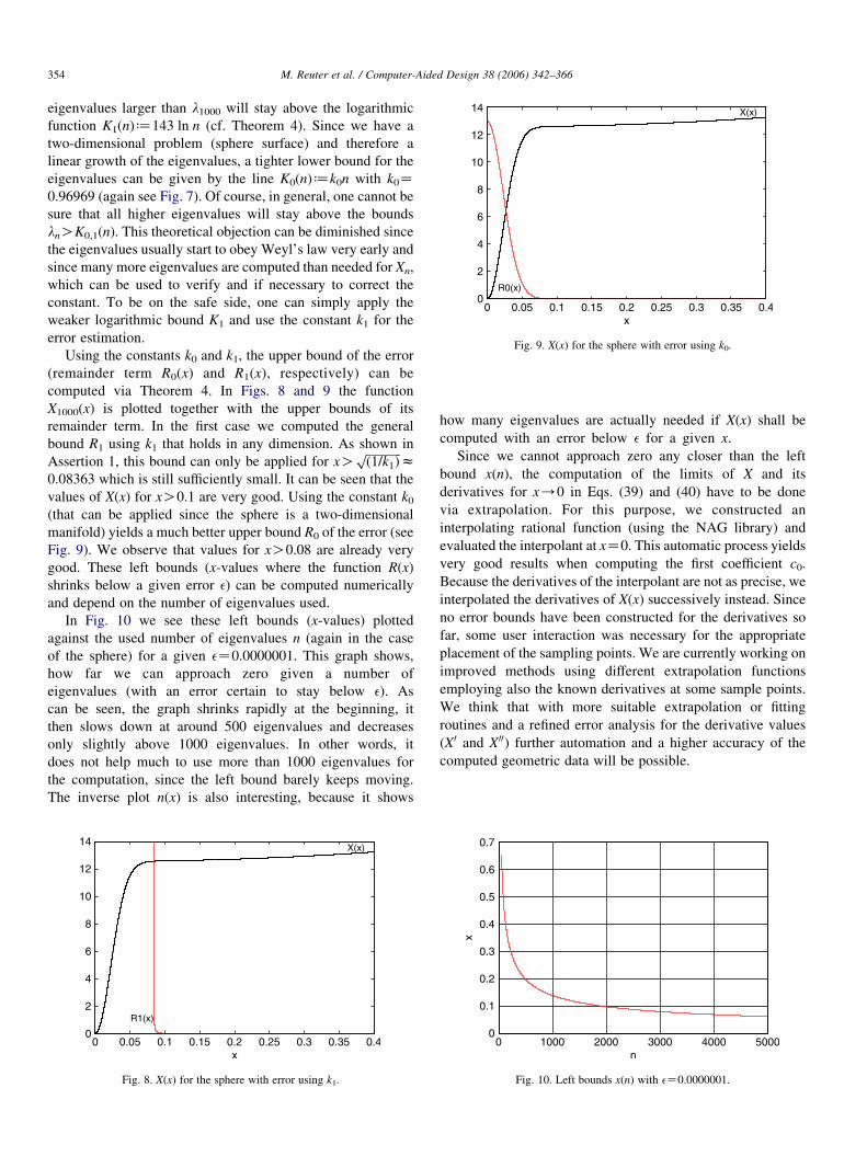
Fig. 9. X(x) for the sphere with error using k0.
M. Reuter et al. / Computer-Aided Design 38 (2006) 342–366354
eigenvalues larger than l1000 will stay above the logarithmic
function K1(n)d143 ln n (cf. Theorem 4). Since we have a
two-dimensional problem (sphere surface) and therefore a
linear growth of the eigenvalues, a tighter lower bound for the
eigenvalues can be given by the line K0(n)dk0n with k0Z0.96969 (again see Fig. 7). Of course, in general, one cannot be
sure that all higher eigenvalues will stay above the bounds
lnOK0,1(n). This theoretical objection can be diminished since
the eigenvalues usually start to obey Weyl’s law very early and
since many more eigenvalues are computed than needed for Xn,
which can be used to verify and if necessary to correct the
constant. To be on the safe side, one can simply apply the
weaker logarithmic bound K1 and use the constant k1 for the
error estimation.
Using the constants k0 and k1, the upper bound of the error
(remainder term R0(x) and R1(x), respectively) can be
computed via Theorem 4. In Figs. 8 and 9 the function
X1000(x) is plotted together with the upper bounds of its
remainder term. In the first case we computed the general
bound R1 using k1 that holds in any dimension. As shown in
Assertion 1, this bound can only be applied for xOffiffiffiffiffiffiffiffiffiffiffiffið1=k1Þ
pz
0:08363 which is still sufficiently small. It can be seen that the
values of X(x) for xO0.1 are very good. Using the constant k0
(that can be applied since the sphere is a two-dimensional
manifold) yields a much better upper bound R0 of the error (see
Fig. 9). We observe that values for xO0.08 are already very
good. These left bounds (x-values where the function R(x)
shrinks below a given error e) can be computed numerically
and depend on the number of eigenvalues used.
In Fig. 10 we see these left bounds (x-values) plotted
against the used number of eigenvalues n (again in the case
of the sphere) for a given eZ0.0000001. This graph shows,
how far we can approach zero given a number of
eigenvalues (with an error certain to stay below e). As
can be seen, the graph shrinks rapidly at the beginning, it
then slows down at around 500 eigenvalues and decreases
only slightly above 1000 eigenvalues. In other words, it
does not help much to use more than 1000 eigenvalues for
the computation, since the left bound barely keeps moving.
The inverse plot n(x) is also interesting, because it shows
Fig. 8. X(x) for the sphere with error using k1.
how many eigenvalues are actually needed if X(x) shall be
computed with an error below e for a given x.
Since we cannot approach zero any closer than the left
bound x(n), the computation of the limits of X and its
derivatives for x/0 in Eqs. (39) and (40) have to be done
via extrapolation. For this purpose, we constructed an
interpolating rational function (using the NAG library) and
evaluated the interpolant at xZ0. This automatic process yields
very good results when computing the first coefficient c0.
Because the derivatives of the interpolant are not as precise, we
interpolated the derivatives of X(x) successively instead. Since
no error bounds have been constructed for the derivatives so
far, some user interaction was necessary for the appropriate
placement of the sampling points. We are currently working on
improved methods using different extrapolation functions
employing also the known derivatives at some sample points.
We think that with more suitable extrapolation or fitting
routines and a refined error analysis for the derivative values
(X0 and X00) further automation and a higher accuracy of the
computed geometric data will be possible.
Fig. 10. Left bounds x(n) with eZ0.0000001.

Fig. 11. Extrapolation of X500(x) for the ellipse.
Fig. 12. Extrapolation of X 00500ðxÞ for the annulus.
M. Reuter et al. / Computer-Aided Design 38 (2006) 342–366 355
5.2. Examples
5.2.1. Ellipse
In the case of the ellipse with radii (r1Z1.0, r2Z1.5), we
used an affine transformation of the disk for the numerical
eigenvalue computation (cf. Section 6.1 and Fig. 13 for a
parametrization), keeping the mesh well conditioned. In Fig. 11
the function X500(x) is plotted together with its extrapolating
rational function E(x). The computed value AZE(0)Zc0Z4.71075 describes the area of the ellipse, a number quite close
to the real area 1.5pz4.712389. A different polynomial
extrapolation function
ApdEpðxÞZ4:71121K7:04364xC0:19791x2 (42)
looks exactly the same, but yields an even better approximation
of the area
Epð0ÞZc0z4:71121: (43)
The approximated boundary length
LzK2ffiffiffiffip
p c1zK2ffiffiffiffip
p ðK7:02176Þz7:9232 (44)
which is close to the real length 7.93272 (computed by
integration of the boundary curve) could be obtained by
extrapolating the first derivative X0(x). Furthermore, the
number of holes h, a topological invariant and determining
the Euler characteristic
hZK3c2
2pC1z
K3!2:0862
2pC1z0:00391z0 (45)
could be obtained correctly (of course, the result has to be an
integer value). All the results with relative error can be found in
Table 1.
Table 1
Geometric data of ellipse
Real Extracted Error (%)
A 4.712389 4.71075 0.035
Ap 4.712389 4.71121 0.025
L 7.93272 7.9232 0.12
h 0 0.00391 –
5.2.2. Annulus
Using the Laplace–Beltrami operator on a parametrization
of the annulus with outer radius 1 and inner radius 1/3 for the
computation of the spectrum, we extracted its area and
boundary length exactly at least up to the third decimal place
and obtained the number of holes hZ1 (since c2 is almost zero,
as can be seen in Fig. 12).
5.2.3. Sphere
The sphere with radius 1 has a surface area of 4pz12.5664.
We extracted the area
AZ12:557 (46)
from the computed eigenvalues employing the Laplace–
Beltrami operator on the surface. The boundary length LZ0
is already known from the fact that the first eigenvalue is also
zero (since the sphere is a closed surface, cf. Section 2.1). The
extracted Euler characteristic
EZ1:902z2 (47)
is a close approximation to the real characteristic. The results
can be found in Table 2.
Table 2
Geometric data of sphere
Real Extracted Error (%)
A 12.5664 12.557 0.075
E 2 1.902 –

Table 3
Geometric data of ellipsoidal hemisphere
Real Extracted Error (%)
A 8.459 8.459 0
L 2pz6.283 6.25761 0.404
M. Reuter et al. / Computer-Aided Design 38 (2006) 342–366356
5.2.4. Ellipsoidal hemisphere
The ellipsoidal hemisphere with radii (r1Zr2Z1, r3Z1.5)
serves as an example for a bounded, curved surface. The
extracted surface area and boundary length together with the
relative error can be found in Table 3.
5.2.5. Ball
For the solid ball we deformed a cube using the
parametrization as described in Section 6.1. Even the
extraction of the volume V and the boundary surface area A
for this smoothly bounded 3d solid was possible. Table 4
presents the exact and the extracted values together with the
relative error. We notice a larger error than in the 2d surface
examples presented above. This is due to the fact that the
additional complexity of the new dimension results in denser
and larger matrices and therefore allows only coarser meshes.
As we will show later, these coarse meshes are good enough for
the first lowest eigenvalues to be quite accurate. The larger lnwith n around 500 however show errors up to 11%. We also
obtained similar results for the unity cube (see [55]).
5.2.6. Remarks
Furthermore, we obtained very good results for the torus
extracting its area and Euler characteristic (see [55]), employ-
ing the ‘Atlas’ data structure for the construction and
computation. In all examples above we used only the first
500 eigenvalues. Of course all of the shown values can be
improved if higher sufficiently correct eigenvalues are used
(using a higher refinement of the mesh or more accurate and
faster computation methods available for special cases, e.g.
planar shapes).
Table 4
Geometric data of the ball
Real Extracted Error (%)
V 4/3pr3Z4.18879 c0Z4.058 3.12
A 4pr2Z12.56637 ðK2=ffiffiffiffip
pÞc1Z12:049 4.12
6. Applications
Before we look at some application examples, we want to
give a brief overview on the necessary steps described so far:
(1) Pre-process. Some objects might need to be pre-processed
for the computation of the eigenvalues. Pre-processing
includes, e.g. conversion into a dataformat supported by
the FEM engine (like triangular meshes, surface para-
metrizations such as spline patches or composed patches as
a ‘structural atlas’, tetrahedrizations of solids, parame-
trized solids). If the given object is not a manifold, or
consists of several separated components, it first has to be
repaired or the desired component has to be selected. If the
eigenvalue computation of a scene containing several
components is carried out at once the resulting Shape-
DNA is the union of the eigenvalues of the single
components ordered by size. In such a case, shape
matching is still possible (if, e.g. the whole scene needs
to be compared to a scene with similar components or if
single components shall be found) whereas the extraction
of geometric data cannot be accomplished in this way.
(2) Eigenvalue computation. The computation of the eigen-
values is the most time consuming step. It can be done with
the FEM method. In the case of a solid tetrahedrization or
planar triangulation, a commercial software package can
be employed for this task. For the parametrized objects
(using the Laplace–Beltrami operator, Eq. (4)) and for 3d-
meshes such a software package needs to be expanded, or
proprietary FEM software solving the Helmholtz equation
(6) for these cases needs to be developed. To get accurate
results, remeshing or mesh refinement of the object might
be necessary (see also Section 4). In some cases (where the
initial mesh is too fine), mesh simplification can be applied
to speed up the computation. The FE-method can be
divided into two parts. The first part creates a discrete
generalized eigenvalue problem AxZlBx with two large
and sparse symmetric positive (semi-)definite matrices A
and B (Eq. (34)). The second part solves this problem
(employing standard libraries as, e.g. ARPACK or NAG).
The computation time of the FE-method depends on the
degrees of freedom (dimension of the matrices). The
dimension depends on the number of elements (triangles or
tetrahedra), on the connectivity of the mesh and on the
degree used for the FEM computation. Usually, we use
cubic elements. If the given surface or solid has a
boundary, generally the Dirichlet boundary condition
(fixed membrane) is applied. If objects with small holes
or missing triangles are to be compared the Neumann
boundary condition can be used instead, because the
unwanted holes appear not to change the Neumann
spectrum not as much as in the Dirichlet case.
(3) Post-process. When the eigenvalues of the surface or solid
have been computed, they can be post-processed depend-
ing on the desired application. As will be described in the
next sections, scaling can be undone using different
approaches. Furthermore, geometric data can be extracted,

Fig. 13. Parameter space of the disk.
M. Reuter et al. / Computer-Aided Design 38 (2006) 342–366 357
or the Shape-DNAs (vectors of eigenvalues) can be
compared for shape identification or matching.
With the help of this Shape-DNA, several applications can
be realized. As mentioned before, one can use the Shape-DNA
to identify objects for the purpose of copyright protection, even
when they are given in different representations. Similar
objects having similar Shape-DNA can be detected fast by
comparing only the Shape-DNA, enabling the use of our
technique for database retrieval and shape matching. Further-
more, the Shape-DNA can be used for quality assessment, e.g.
when converting or producing objects to prove that the shape of
the converted object has not been modified. In order to apply
our technique in these areas, three requirements need to be
fulfilled:
† Firstly, the Shape-DNA needs to be very accurate, ensuring
that the same Shape-DNA is calculated for an object when
using different meshes or even when it is calculated
analytically. This requirement can be fulfilled by using
sufficiently dense meshes, since the convergence of the
FEM is known.
† Secondly, similar but different objects should have different
Shape-DNA, making it possible to discriminate between
these objects. This property is only violated by the
artificially constructed isospectral but not isometric objects
(identical twins) described earlier. Anyhow, we will present
evidence in Section 6.3.4 that for some isospectral 3d-
solids, the Shape-DNA of the boundary surface can be used
as a discrimination criterion.
† Thirdly, similar objects need to have similar Shape-DNA in
order to detect the similarity. This requirement is
completely fulfilled by the spectra. We will show in Section
6.3.6 that this property allows the detection of small
deformation and leads to a clustering of similar objects
when applied for shape matching.
In order to discriminate and compare similar objects via
their Shape-DNA, a distance measure for Shape-DNA will be
constructed. Before we look at the accuracy of the compu-
tation, we want to give Definition 3.
Definition 3 (Shape-DNA)
Let M be a Riemannian manifold with a metric g and let
specðM;gÞZfl0%l1%l2%/g (48)
be the function computing the spectrum of (M, g) for a given
boundary condition (we use the zero Dirichlet condition if not
noted otherwise). spec :M/RNR0 maps a Riemannian mani-
fold ðM;gÞ2M to the positive infinite dimensional space. The
cropped spectrum containing only the first n eigenvalues
cspecnðM;gÞZ fl0%l1%l2%/%lng2RnR0 (49)
is called Shape-DNA of (M, g) and can be seen as a point in the
n-dimensional positive Euclidean space RnR0.
We compute these cropped spectra (Shape-DNA) contain-
ing a finite number n of eigenvalues (50–100, or up to 500 for
the extraction of data), since the numerical computation of the
whole spectrum is generally not possible.
6.1. Accuracy
At first we want to corroborate the requirement ‘accuracy’
by looking at a few example calculations where the exact
eigenvalues are known. If not noted otherwise, the computation
was done on a standard PC (AthlonXP running at 1667 MHz).
The eigenvalues of the unit disk, for example, are the squares
of the roots of the Bessel functions Jn [20, p. 261]. By
approximating the area of the disk with linearly bounded
triangles, one always gets a discretization error at the boundary.
Therefore, the resulting eigenvalues are not very accurate
compared to the superior technique used below. In this
computation (with cubic elements and 4021 degrees of
freedom), the first eigenvalue already shows an error of
approx. 0.067%. Higher eigenvalues are even more erroneous.
These results can be improved by exploiting the fact that the
Laplace–Beltrami operator (due to its invariance properties)
yields the same eigenvalues even if a different parametrization
of the same surface is applied. Of course, the Laplace–Beltrami
operator can be applied to parametrizations of planar objects as
well as for surfaces in 3d. In this example, we choose a special
parametrization f (not the identity as above) defined on a
polygonal parameter space glued to itself at the appropriate
boundary edges (as can be seen in Fig. 13). This parametriza-
tion f maps the triangular parameter space onto the disk
f ðu;vÞZrv
cospu
v
sinpu
v
0
0BBBBB@
1CCCCCA with 0!v%1; juj%v (50)
additionally defining f(0, 0)d(0, 0, 0).
This method leads to a computation of the smoothly
bounded disk without any discretization error at the boundary.
Another advantage of the parametrization f (compared to polar
coordinates, where a whole edge of the parameter space
boundary collapses if rZ0) is that we have well-behaved
triangles at the center that do not degenerate when using a
higher resolution (refinement). Therefore, with only 3781
degrees of freedom the first eigenvalue is exact up to the eighth
decimal place and even l99 is approximated with a relative
error of only 0.027%.

Table 5
Eigenvalues of the cylinder with spherical caps
EV Real FEM (18,254) FEM (974)
Time – 58 sC5 s 3 sC0 s
l1 0 0 0
l2 0.5974034 0.5974034 0.5974034
l3, l4 1.3450307 1.3450624 1.3456242
l5 2.1930427 2.1930427 2.1930430
l6, l7 2.5588079 2.5589283 2.5610538
l8 4.4586760 4.4586760 4.4586826
l9 4.5416743 4.5416754 4.5421094
M. Reuter et al. / Computer-Aided Design 38 (2006) 342–366358
The aforementioned free choice of a parametrization that is
especially suited for the numerical computation is only possible
because of the property of the Laplace–Beltrami operator to be
independent of any isometric reparametrization. This does not
hold for the classical continuous Laplace operator since it
operates on functions defined directly on the Euclidean space
(with Euclidean metric). Generally, we observe an advantage of
the Laplace–Beltrami operator over the simple Laplacian even
for planar domains: using the free choice of a parametrization
we have utilized something like ‘free form finite elements’. That
way, any surface can be triangulated without discretization error
at the boundary. The computations of eigenvalues based on
these parametrizations are very accurate.
Remark 1 (Spectral determination of some shapes)
Since we know what happens to the eigenvalues when scaling
the area (see Section 2), the eigenvalues of a disk with radius r
can be calculated as
ln;mZk2n;m
r2with the Bessel function Jnðkn;mÞZ0 (51)
Kac [40] proved that no planar shape is isospectral to the
disk, except the disk itself. Therefore, given a planar shape, it is
possible to calculate the radius with the first eigenvalue
rzk0;1ffiffiffiffiffil1
p (52)
It is then possible to test the assumption that a given shape is a
disk with further eigenvalues. In fact, all Euclidean balls are
determined among solids by their spectra in any dimension. This
follows from the fact that the volume and the boundary area of
the domain are determined by its spectrum (cf. heat coefficients
in Eq. (18)) and using that an isoperimetric region (a region with
maximal volume related to the boundary size) in Rn is always a
ball (see [3]). A similar argument leads to the result that all
regular polygons D2R2 with n sides are spectrally determined
among planar polygons with not more than n sides (since the
area and boundary ratio is again fixed by an isoperimetric
equality [3]). Furthermore, Tanno [59] proved that all round
spheres in dimensions up to 6 are completely characterized by
their spectra. For higher dimensions, the validity of this result
appears to be still open.
A similar eigenvalue calculation as in the disk case can be
done for the sphere. Even though the sphere is a surface with
curvature, the eigenvalues computed with this parametrization
are very accurate. With 5447 nodal points we approximated
l101 Z110z110:55599 (53)
with a relative error of 0.5055% in 4 s and with 11,522 nodal
points we obtained
l101 Z110z110:0003989 (54)
with a relative error of only 0.0004% in 73 s. Generally, these
high resolutions are not necessary for most applications.
In order to show that we can use a 3d triangle mesh (a
surface consisting of planar triangular faces) instead of a
parametrized surface as input, we calculated the eigenvalues of
a triangle mesh approximating the unit sphere with 11,522
degrees of freedom and 2560 triangles using cubic elements in
5 s. The eigenvalues
l1z0; l24z2:005; l45z6:014. (55)
are very close to the eigenvalues of the sphere (0, 2 and 6), as
expected, since the triangle mesh approximates the real surface
very exactly (with a maximal distance of only 0.0026) and
because of the continuity property of the spectrum (cf. Section
2.1). Yet it should be noted that this faceted sphere is of course
only an approximation and not the sphere itself, therefore the
spectra have to differ slightly from each other. An advantage of
using polygonal meshes instead of parametrized surfaces is that
no numeric integration (cubature) is needed by the FE-method
for the construction of the matrices. Since all triangles are
planar, the integral equations (34) can be evaluated for the
unity triangle once and then transported to an arbitrary triangle,
resulting in an enormous speed-up in computation.
For the computation of the eigenvalues of the round sphere,
the parameter space of the sphere was glued to itself. Similarly,
we computed the eigenvalues of tori. Since the correct
eigenvalues of non-flat tori are not known from theory, they
cannot be used to verify our computations and will therefore
not be discussed here. More complex objects can be
constructed by gluing different patches to each other. The
cylinder with spherical caps presented in Section 4 and Fig. 5,
for example, consists of three surface patches. Since the real
eigenvalues of this compound surface can be derived from
results in [4], we will present a comparison with our values (see
Table 5). For the first computation, we used the Laplace–
Beltrami operator on the surface with 4056 cubic elements
(18,254 degrees of freedom) to approximate the eigenvalues
very exactly. The construction of the matrices A and B together
with the pre-processing (refinement) took 58 s and the
computation of the first 10 smallest eigenvalues using the
ARPACK library approx. 5 s. In a faster computation, we only
used 216 cubic elements (974 degrees of freedom) and
computed the shown values in 3 s.
As examples of 3d-solids we will look at the 3d-cube and
the 3d-ball. The eigenvalues of the cuboid with side lengths a,
b, c are known from theory
lUM;N;OZp2 M2
a2C
N2
b2C
O2
c2
� �with M;N;OZ1;2;. (56)
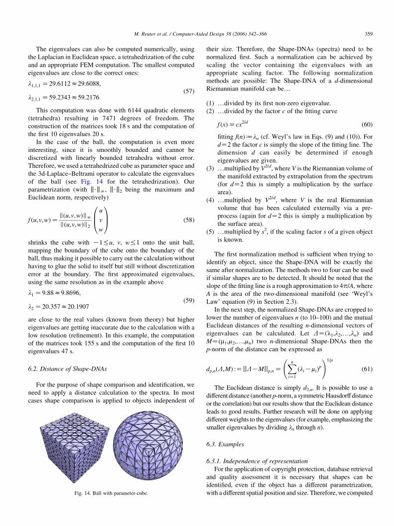
M. Reuter et al. / Computer-Aided Design 38 (2006) 342–366 359
The eigenvalues can also be computed numerically, using
the Laplacian in Euclidean space, a tetrahedrization of the cube
and an appropriate FEM computation. The smallest computed
eigenvalues are close to the correct ones:
l1;1;1 Z29:6112z29:6088;
l2;1;1 Z59:2343z59:2176(57)
This computation was done with 6144 quadratic elements
(tetrahedra) resulting in 7471 degrees of freedom. The
construction of the matrices took 18 s and the computation of
the first 10 eigenvalues 20 s.
In the case of the ball, the computation is even more
interesting, since it is smoothly bounded and cannot be
discretized with linearly bounded tetrahedra without error.
Therefore, we used a tetrahedrized cube as parameter space and
the 3d-Laplace–Beltrami operator to calculate the eigenvalues
of the ball (see Fig. 14 for the tetrahedrization). Our
parametrization (with k$kN, k$k2 being the maximum and
Euclidean norm, respectively)
f ðu;v;wÞZsðu;v;wÞsNsðu;v;wÞs2
u
v
w
0B@
1CA (58)
shrinks the cube with K1%u, v, w%1 onto the unit ball,
mapping the boundary of the cube onto the boundary of the
ball, thus making it possible to carry out the calculation without
having to glue the solid to itself but still without discretization
error at the boundary. The first approximated eigenvalues,
using the same resolution as in the example above
l1 Z9:88z9:8696;
l2 Z20:357z20:1907(59)
are close to the real values (known from theory) but higher
eigenvalues are getting inaccurate due to the calculation with a
low resolution (refinement). In this example, the computation
of the matrices took 155 s and the computation of the first 10
eigenvalues 47 s.
6.2. Distance of Shape-DNAs
For the purpose of shape comparison and identification, we
need to apply a distance calculation to the spectra. In most
cases shape comparison is applied to objects independent of
Fig. 14. Ball with parameter-cube.
their size. Therefore, the Shape-DNAs (spectra) need to be
normalized first. Such a normalization can be achieved by
scaling the vector containing the eigenvalues with an
appropriate scaling factor. The following normalization
methods are possible: The Shape-DNA of a d-dimensional
Riemannian manifold can be.
(1) .divided by its first non-zero eigenvalue.
(2) .divided by the factor c of the fitting curve
f ðxÞZcx2=d (60)
fitting f(n)dln (cf. Weyl’s law in Eqs. (9) and (10)). For
dZ2 the factor c is simply the slope of the fitting line. The
dimension d can easily be determined if enough
eigenvalues are given.
(3) .multiplied by V2/d, where V is the Riemannian volume of
the manifold extracted by extrapolation from the spectrum
(for dZ2 this is simply a multiplication by the surface
area).
(4) .multiplied by V2/d, where V is the real Riemannian
volume that has been calculated externally via a pre-
process (again for dZ2 this is simply a multiplication by
the surface area).
(5) .multiplied by s2, if the scaling factor s of a given object
is known.
The first normalization method is sufficient when trying to
identify an object, since the Shape-DNA will be exactly the
same after normalization. The methods two to four can be used
if similar shapes are to be detected. It should be noted that the
slope of the fitting line is a rough approximation to 4p/A, where
A is the area of the two-dimensional manifold (see ‘Weyl’s
Law’ equation (9) in Section 2.3).
In the next step, the normalized Shape-DNAs are cropped to
lower the number of eigenvalues n (to 10–100) and the mutual
Euclidean distances of the resulting n-dimensional vectors of
eigenvalues can be calculated. Let LZ(l1,l2,.,ln) and
MZ(m1,m2,.,mn) two n-dimensional Shape-DNAs then the
p-norm of the distance can be expressed as
dp;nðL;MÞ :Z jjLKMjjp;nZXniZ1
ðliKmiÞp
!1=p
(61)
The Euclidean distance is simply d2,n. It is possible to use a
different distance (anotherp-norm, a symmetric Hausdorff distance
or the correlation) but our results show that the Euclidean distance
leads to good results. Further research will be done on applying
different weights to the eigenvalues (for example, emphasizing the
smaller eigenvalues by dividing ln through n).
6.3. Examples
6.3.1. Independence of representation
For the application of copyright protection, database retrieval
and quality assessment it is necessary that shapes can be
identified, even if the object has a different parametrization,
with a different spatial position and size. Therefore, we computed
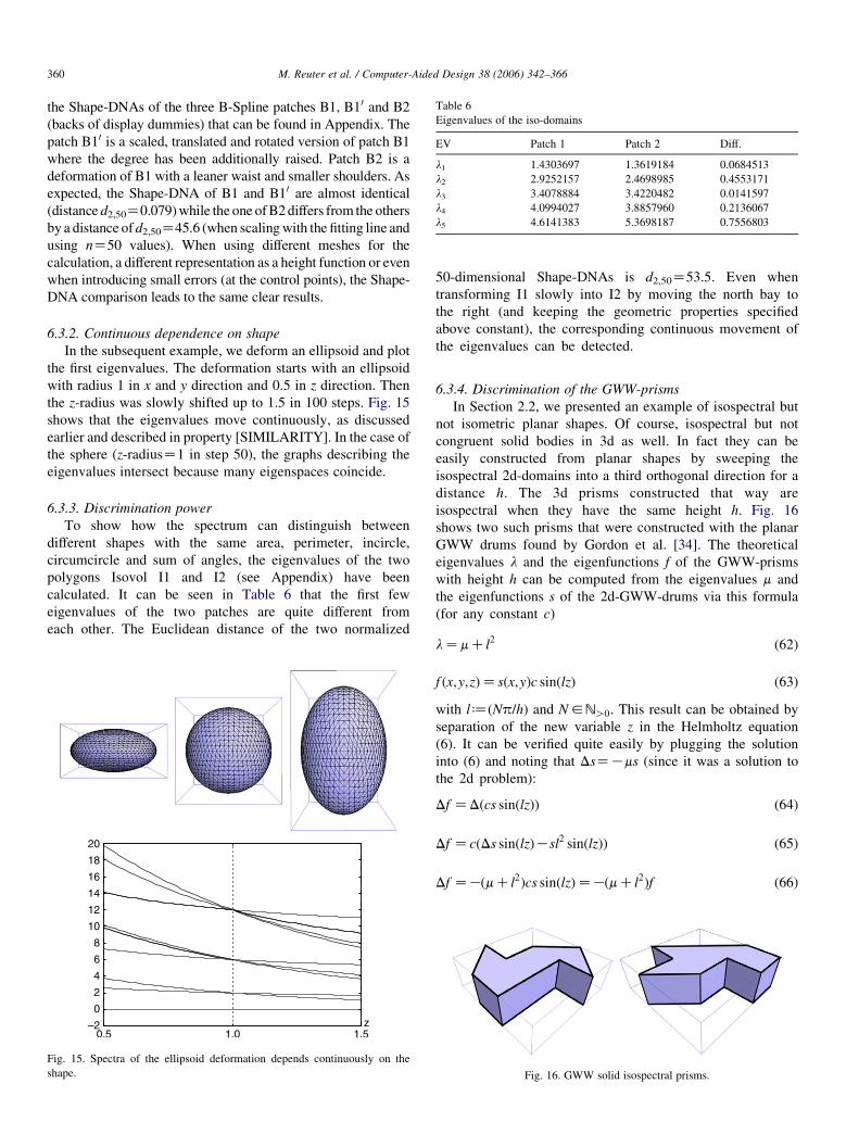
Table 6
Eigenvalues of the iso-domains
EV Patch 1 Patch 2 Diff.
l1 1.4303697 1.3619184 0.0684513
l2 2.9252157 2.4698985 0.4553171
l3 3.4078884 3.4220482 0.0141597
l4 4.0994027 3.8857960 0.2136067
l5 4.6141383 5.3698187 0.7556803
M. Reuter et al. / Computer-Aided Design 38 (2006) 342–366360
the Shape-DNAs of the three B-Spline patches B1, B10 and B2
(backs of display dummies) that can be found in Appendix. The
patch B10 is a scaled, translated and rotated version of patch B1
where the degree has been additionally raised. Patch B2 is a
deformation of B1 with a leaner waist and smaller shoulders. As
expected, the Shape-DNA of B1 and B10 are almost identical
(distance d2,50Z0.079) while the one of B2 differs from the others
by a distance of d2,50Z45.6 (when scaling with the fitting line and
using nZ50 values). When using different meshes for the
calculation, a different representation as a height function or even
when introducing small errors (at the control points), the Shape-
DNA comparison leads to the same clear results.
6.3.2. Continuous dependence on shape
In the subsequent example, we deform an ellipsoid and plot
the first eigenvalues. The deformation starts with an ellipsoid
with radius 1 in x and y direction and 0.5 in z direction. Then
the z-radius was slowly shifted up to 1.5 in 100 steps. Fig. 15
shows that the eigenvalues move continuously, as discussed
earlier and described in property [SIMILARITY]. In the case of
the sphere (z-radiusZ1 in step 50), the graphs describing the
eigenvalues intersect because many eigenspaces coincide.
6.3.3. Discrimination power
To show how the spectrum can distinguish between
different shapes with the same area, perimeter, incircle,
circumcircle and sum of angles, the eigenvalues of the two
polygons Isovol I1 and I2 (see Appendix) have been
calculated. It can be seen in Table 6 that the first few
eigenvalues of the two patches are quite different from
each other. The Euclidean distance of the two normalized
Fig. 15. Spectra of the ellipsoid deformation depends continuously on the
shape.
50-dimensional Shape-DNAs is d2,50Z53.5. Even when
transforming I1 slowly into I2 by moving the north bay to
the right (and keeping the geometric properties specified
above constant), the corresponding continuous movement of
the eigenvalues can be detected.
6.3.4. Discrimination of the GWW-prisms
In Section 2.2, we presented an example of isospectral but
not isometric planar shapes. Of course, isospectral but not
congruent solid bodies in 3d as well. In fact they can be
easily constructed from planar shapes by sweeping the
isospectral 2d-domains into a third orthogonal direction for a
distance h. The 3d prisms constructed that way are
isospectral when they have the same height h. Fig. 16
shows two such prisms that were constructed with the planar
GWW drums found by Gordon et al. [34]. The theoretical
eigenvalues l and the eigenfunctions f of the GWW-prisms
with height h can be computed from the eigenvalues m and
the eigenfunctions s of the 2d-GWW-drums via this formula
(for any constant c)
lZmCl2 (62)
f ðx;y;zÞZsðx;yÞc sinðlzÞ (63)
with ld(Np/h) and N2NO0. This result can be obtained by
separation of the new variable z in the Helmholtz equation
(6). It can be verified quite easily by plugging the solution
into (6) and noting that DsZKms (since it was a solution to
the 2d problem):
Df ZDðcs sinðlzÞÞ (64)
Df ZcðDs sinðlzÞKsl2 sinðlzÞÞ (65)
Df ZKðmCl2Þcs sinðlzÞZKðmCl2Þf (66)
Fig. 16. GWW solid isospectral prisms.
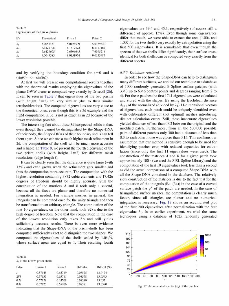
Table 7
Eigenvalues of the GWW-prisms
EV Theoretical Prism 1 Prism 2
l1 5.0053451 5.0128509 5.0129320
l2 6.1229108 6.1317422 6.1317167
l3 7.6429605 7.6596645 7.6595216
l4 9.0049585 9.0151974 9.0153987
M. Reuter et al. / Computer-Aided Design 38 (2006) 342–366 361
and by verifying the boundary condition for zZ0 and h
(sin(0)Z0Zsin(lh)).
At first we will present our computational results together
with the theoretical results employing the eigenvalues of the
planar GWW drums as computed very exactly by Driscoll [26].
It can be seen in Table 7 that eigenvalues of the two prisms
(with height hZ2) are very similar (due to their similar
tetrahedrization). The computed eigenvalues are very close to
the theoretical ones, even though this is a 3d example and the
FEM computation in 3d is not as exact as in 2d because of the
lower resolution possible.
The interesting fact about these 3d isospectral solids is that,
even though they cannot be distinguished by the Shape-DNA
of their body, the Shape-DNAs of their boundary shells can tell
them apart. Since we can use a much higher mesh refinement in
2d, the computation of the shell will be much more accurate
and reliable. In Table 8, we present the fourth eigenvalue of the
two prism shells (with height hZ2) for different mesh
resolutions (edge length l).
It can be clearly seen that the difference is quite large (with
13%) and even grows when the refinement gets smaller and
thus the computation more accurate. The computation with the
highest resolution containing 3872 cubic elements and 17,426
degrees of freedom should be highly accurate. Still the
construction of the matrices A and B took only a second,
because all the faces are planar and therefore no numerical
integration is needed. For triangle meshes in general, the
integrals can be computed once for the unity triangle and then
be transformed to an arbitrary triangle. The computation of the
first 10 eigenvalues, on the other hand, took 928 s due to the
high degree of freedom. Note that the computation in the case
of the lowest resolution only takes 2 s and still yields
sufficiently accurate results. There is even more evidence
indicating that the Shape-DNA of the prism-shells has been
computed sufficiently exact to distinguish the two shapes. We
computed the eigenvalues of the shells scaled by 1:0=ffiffiffiA
p,
whose surface areas are equal to 1. Their resulting fourth
Table 8
l4 of the GWW prism-shells
Edge Prism 1 Prism 2 Diff-abs Diff-rel (%)
l 0.57145 0.65719 0.08575 13.0474
2l/3 0.57133 0.65711 0.08578 13.0543
0.5l 0.57128 0.65708 0.08580 13.0571
0.4l 0.57125 0.65706 0.08581 13.0590
eigenvalues are 39.4 and 45.3, respectively (of course still a
difference of approx. 13%). Even though some eigenvalues
differ that much, we were able to extract the area (1.004 and
1.007 for the two shells) very exactly by extrapolation using the
first 500 eigenvalues. It is remarkable that even though the
spectra of the two shells differ significantly, their surface areas,
identical for both shells, can be computed very exactly from the
different spectra.
6.3.5. Database retrieval
In order to see how the Shape-DNA can help to distinguish
many different surfaces, we applied our technique to a database
of 1000 randomly generated B-Spline surface patches (with
3!3 up to 6!6 control points and degrees ranging from 2 to
4). For these patches the first 1741 eigenvalues were calculated
and stored with the shapes. By using the Euclidean distance
d2,11 of the normalized (divided by l1) 11-dimensional vectors
of eigenvalues, each patch could be uniquely identified even
with deliberately different (not optimal) meshes introducing
distinct calculation errors. Still, these inaccurate eigenvalues
yielded distances of less than 0.02 between the original and the
modified patch. Furthermore, from all the 500,000 possible
pairs of different patches only 300 had a distance of less than
0.3 to each other, none was closer than 0.15. This confirms our
assumption that our method is sensitive enough to be used for
identifying patches even with reduced capacities for calcu-
lation (since only the first 11 eigenvalues were used). The
construction of the matrices A and B for a given patch took
approximately 100 s (we used the SISL Spline Library) and the
computation of the first 10 eigenvalues took less than a second
as did the actual comparison of a computed Shape-DNA with
all the Shape-DNA contained in the database. The relatively
slow construction of the matrices is due to the fact that for the
computation of the integrals (Eq. (34)) in the case of a curved
surface patch the gjk of the patch are needed. In the case of
triangulated surface meshes, the computation is clearly much
faster, since all triangles are planar and no numerical
integration is necessary. Fig. 17 shows an accumulated plot
of the first 200 eigenvalues after normalization with the first
eigenvalue l1. In an earlier experiment, we tried the same
techniques using a database of 1625 randomly generated
Fig. 17. Accumulated spectra (ln) of the patches.

Fig. 18. 2d MDS plot of Shape-DNAs.
M. Reuter et al. / Computer-Aided Design 38 (2006) 342–366362
polynomial patches of degree 10. The results were similar:
Each patch could be easily identified by its first few
eigenvalues.
It is perfectly possible that one could also identify any single
NURBS patch within a large collection of NURBS patches
using other isometric invariants like: boundary length, surface
area, Gauss curvature integral, geodesic curvature of the
boundary curve, Euler characteristic, etc. However, since these
invariants contain very little information with respect to the
amount of completeness up to which they determine the shape
of an object, it is not very difficult to construct examples using
(e.g. non-isometric) subdomains of the plane (see Section
6.3.3) and of the sphere sharing surface area, length and total
curvature of their boundary curves. Those subdomains share
also the Gauss curvature that is either zero or determined by the
area of the respective domain in these examples. It confirms the
discrimination power of the spectrum that those domains
sharing the aforementioned geometric invariants have signifi-
cant differences even in their respective first few eigenvalues
(cf. Section 6.3.3). Obviously, the spectrum must have more
discrimination power than the combination of the invariants
consisting of length of boundary curves and surface area, as
those invariants and even more information can be computed
from the spectrum. Additionally, employing the spectrum of
the double of the given surface, all the geometric information
described in Section 2.3 can be obtained.
6.3.6. Shape matching
To demonstrate how the Shape-DNA can be used for shape
matching we will calculate the Shape-DNAs of all the objects
depicted in Appendix. We have already referred to B1, B10, B2,
I1 and I2 in Sections 6.3.1 and 6.3.3. The objects N1 and N2
(parts of a bottle neck) are deformations of each other (N2 is
slimmer). The Shape-DNA of the unit square has been
calculated with our FEM method (S1) and analytically. In the
case of the square (even for an arbitrary rectangle, see Courant
[20, p. 258]) the exact eigenvalues are known. Therefore, they
can be used to verify the computational accuracy of our
numerical results. The eigenvalues of a rectangular area with
edge lengths a and b can be computed analytically as follows:
lUM;N Zp2 M2
a2C
N2
b2
� �with M;NZ1;2;. (67)
For the comparison we also computed these exact values
(represented by SR). The disk’s Shape-DNA has been
computed with a fine (D1) and a coarser (D2) mesh (both
having smooth boundary) and by using a polygonal disk
approximation (linearly bordered D3). All of these objects are
now compared with each other in a way that not only identifies
identical shapes, but also detects similarities. For this purpose,
the Shape-DNAs were first normalized by the slope of the
fitting line (Eq. (60)) and then cropped to contain only the first
50 eigenvalues. To visualize their positions, these vectors were
embedded linearly into the two-dimensional space with the
help of classical multidimensional scaling (MDS), a method
performing a principal coordinate analysis (PCA). When
plotting only the first two dimensions, the display error of the
real mutual distances is kept as small as possible [21]. The 2d-
MDS plot (Fig. 18) can be understood as an orthogonal
projection of the 50-dimensional vectors onto their best 2d-
fitting-plane. It shows very well how identical objects are
mapped to the same spot and how similar objects form groups.
These are very good results, considering that only the first two
most important dimensions are plotted and that further
information is contained in higher (less important) dimensions.
As a final example, we will compare the objects (given as
triangular meshes) depicted in Appendix. The Shape-DNA of
the rabbit has been computed for three meshes of different
resolution (containing 10,000, 1000 and 400 triangles). The
simplified meshes could be quickly obtained with the program
QSlim (using a method described in Garland [31]). Since the
rabbit looks like a deformed ellipsoid, we computed the Shape-
DNA of the ellipsoid as well. The helmet is in fact nearly
isometric to the ellipsoid, even though it does not look like it,
because it consists of an inner and an outer shell, which are
connected. Flipping the inner shell to the outside, one gets a
deformed ellipsoid. Another group of test objects consists of
animals (a camel, a cat, a cow and a horse), all of which have
legs or arms, some have tails and some long necks. Another
subject is the Santa, who is also equipped with arms and legs
and wears a long jelly bag cap. The final test group is supplied
by the screwdriver with its deformations. First the tip has been
stretched and twisted, then bend over and last but not least the
handle has been deformed. The stretching and the deformation
of the handle are the most serious changes since the surface
area (being a global feature) is modified.
The 2d MDS plot, that has been constructed like in the
example before, can be seen in Fig. 19. Again we observe a
nice clustering of the objects. The strongest modifications of
the screwdriver are well reflected by the larger distance of the
corresponding Shape-DNA projections. Furthermore, the
deformed ellipsoids are well separated from the animals with
the Santa. Note that the MDS plot is merely used for the
visualization of the position of the 50-dimensional Shape-
DNA. The measuring of the distance is done in higher
dimensions. Even though the MDS plot shows the first two

Fig. 19. 2d MDS plot of mesh Shape-DNAs.
M. Reuter et al. / Computer-Aided Design 38 (2006) 342–366 363
most important principal components, important information
might be contained in higher dimensions as well. A
dimensionality reduction therefore might lead to the collapse
of clusters onto each other. For real time database applications,
the eigenvalues of an object have to be computed very fast.
This can be achieved with coarser meshes (that can be
constructed quickly) yielding very similar Shape-DNA as can
be seen in the case of the rabbit.
Furthermore, when dealing with a large database, the search
for nearest neighbors might be too slow in high dimensional
spaces. Then it might be helpful that global shape information is
already contained in the first eigenvalues while smaller details
seem to be encoded in higher values. Because of the property
[SIMILARITY], the Shape-DNA depends continuously on the
shape deformation. As we have seen in Section 6.3.2, the
deformation of an object changes the li(t) continuously with a
deformation parameter t. Therefore, the Shape-DNA of all
shapes that can possibly be obtained through a deformation of an
object are contained in a path-connected subset.
It is generally possible that all n dimensions of the space
containing the Shape-DNA are equally important when filled
with the Shape-DNA of all deformations of a single shape. In
real world applications we often want to compare one object
with the finite amount of objects contained in a database. The
Shape-DNA of these objects often do not vary equally strongly
in all dimensions n. With the help of PCA we can choose the
dimension n0!n of the best fitting n0-dimensional subspace
(the shape space) in a way that keeps the approximation error
of the set of Shape-DNA sufficiently small. This leads to a
distinct dimensionality reduction with only little error. The
Shape-DNA can then be represented in the lower dimensional
shape space (in more than two dimensions as in the plots above,
but still in less than the number of eigenvalues needed for
efficient comparison). Similar to the approach of Turk and
Pentland [61], who use eigenvectors of PCA (called
eigenfaces) for face recognition, it can then be decided quickly
if a new geometric object has a match in the database
represented by the point set of Shape-DNA by measuring the
distance of its Shape-DNA to shape space and by checking if its
projection into shape space lies in or close to a cluster. If a
Shape-DNA lies far away from the shape space and the
corresponding object has to be added to the database, a new
shape space has to be constructed, containing the new object.
For this purpose, the PCA needs to be repeated for the Shape-
DNA of all objects, so that future queries can again be
processed quickly.
7. Conclusion
We have introduced a novel method that uses the
eigenvalues of the Laplace–Beltrami operator as Shape-DNA
(a fingerprint) for a given 2d or 3d manifold (surface or solid).
Even though the proposed Shape-DNA does not meet the
property [COMPLETENESS] entirely, since (artificially
constructed) identical twins exist, we were able to demonstrate
that it satisfies other important properties (like [ISOMETRY],
[SCALING], [SIMILARITY], [EFFICIENCY], [COM-
PRESSION] and [PHYSICALITY]). We introduced the
possibility of numerically calculating the Shape-DNA for
different types of geometric objects (compound parametrized
surfaces including NURBS, polygonal meshes and solid
polyhedra). The computed results were shown to be indepen-
dent of the given spatial location and scaled size and above all
independent of the objects representation (especially of the
chosen parametrization). Our method is also robust under
variations in the quality of the model. We demonstrated that
shape identification and comparison can be done using only a
few eigenvalues, making it possible to locate objects rapidly
within huge databases. Via comparison of the Shape-DNA, it is
possible to compare a suspicious object with a copyrighted one
to detect if the object might be an illegal copy. As shown, it is
even possible to use the Euclidean distance of normalized
Shape-DNA to detect similar objects. Shape-DNA can also be
used as a quality measure when converting surfaces or solids
into different representations utilizing the fact that the spectrum
of a correctly converted object must agree with the spectrum of
the original one.
We proved some propositions about the mutual indepen-
dence of the eigenvalues and about the rapid convergence of
the heat trace series. Moreover, we succeeded in numerically
extracting the volume, boundary length and Euler character-
istic from the computed Shape-DNA of the respective surface.
Those numerical computations appear to be new.
Further research will extend this work to implicitly defined
surfaces and solids employing, e.g. new concepts [12,50]
useful to mesh implicit surfaces. As another extension, parallel
processing and multigrid methods could be used to speed up
and improve our eigenvalue computation making it possible to
use higher resolutions and to compute spectra, especially of 3d-
solids, more accurately. It is of interest as well as to study the
combination of subdivision (or feature decomposition tech-
niques) with the Shape-DNA to be able to match object parts.
Additionally, more experiments will be done on larger shape
databases (for meshes and for CAD-models), extending the
concepts used for similarity detection (i.e. PCA) as described in
the last section.

M. Reuter et al. / Computer-Aided Design 38 (2006) 342–366364
Appendix
References
[1] Adams C. The knot book. New York: Freeman; 1994.
[2] Ainsworth M, Oden J. A posteriori error estimation in finite element
analysis. London: Wiley; 2000.
[3] Bandle C. Isoperimetric inequalities and applications. London: Pitman;
1980.
[4] Beekmann B. Eigenfunktionen und Eigenwerte des Laplaceoperators auf
Drehflachen und die Gliederung des Spektrums nach den Darstellungen
der Isometriengruppe. PhD Thesis. Mathematisches Institut der Uni-
versitat Munster; 1988.
[5] Belkin M, Niyogi P. Laplacian eigenmaps for dimensionality reduction
and data representation. Neural Comput 2003;15:1373–96.
[6] Benedens O. Geometry-based watermarking of 3D models. IEEE Comput
Graphics Appl 1999;19(1):46–55.
[7] Berger M. Riemannian geometry during the second half of the
20th century. Providence, RI: American Mathematical Society;
2000.
[8] Berger M, Gauduchon P, Mazet E. Le spectre d’une variete riemannienne.
Lecture notes in Mathematics, vol. 194. Berlin: Springer; 1971.
[9] Bespalov D, Shokoufandeh A, Regli WC, Sun W. Scale-space
representation of 3d models and topological matching. In: ISM’03:
Proceedings of the eighth ACM symposium on solid modeling and
applications. New York: ACM Press; 2003. p. 208–15.
[10] Betcke T, Trefethen LN. Reviving the method of particular solutions.
SIAM Rev 2005;47(3):469–91.

M. Reuter et al. / Computer-Aided Design 38 (2006) 342–366 365
[11] Blascke W, Leichtweib K. Elementare differentialgeometrie. Berlin:
Springer; 1973.
[12] Boissonnat J-D, Cohen-Steiner D, Vegter G. Isotopic implicit
surface meshing. In: Proceedings of the 36th annual ACM
symposium on theory of computing. New York: ACM Press; 2004.
p. 301–9.
[13] Braess D. Finite elemente. Berlin: Springer; 1997.
[14] Bronstein AM, Bronstein MM, Kimmel R. Expression-invariant 3d face
recognition. In: Proceedings of the AVBPA. Lecture notes in computer
science no. 2688. Berlin: Springer; 2003. p. 62–9.
[15] Buser P. Geometry and spectra of compact Riemann surfaces. Basel:
Birkhauser; 1992.
[16] Buser P, Conway J, Doyle P, Semmler K-D. Some planar isospectral
domains. Int Math Res Not 1994;9:391–400.
[17] Chavel I. Eigenvalues in Riemannian geometry. London: Academic
Press; 1984.
[18] Chen H, Bishop J. Delaunay triangulation for curved surfaces.
In: Sixth international meshing roundtable proceedings; 1997.
p. 115–27.
[19] Colin de Verdiere Y. Construction de Laplaciens dont une partie finie du
spectre est donnee. Ann Sci Ecole Norm S 1987;20(4):599–615.
[20] Courant R, Hilbert D. Mehods of mathematical physics, vol. I. New York:
Interscience; 1953.
[21] Cox TF, Cox MAA. Multidimensional scaling. 2nd ed. London: Chapman
& Hall; 2001.
[22] Craioveanu M, Puta M, Rassias T. Old and new aspects in spectral
geometry. Dordrecht: Kluwer; 2001.
[23] Cuthill E, McKee J. Reducing the bandwidth of sparse symmetric
matrices. In: Proceedings of the 24th ACM national conference; 1969.
p. 157–72.
[24] Descloux J, Tolley M. An accurate algorithm for computing the
eigenvalues of a polygonal membrane. Comput Methods Appl Mech
Eng 1983;39:37–53.
[25] do Carmo MP. Differential geometry of curves and surfaces. Englewood
Cliffs, NJ: Prentice-Hall; 1976.
[26] Driscoll T. Eigenmodes of isospectral drums. SIAM 1997;39(1):1–17.
[27] Elad A, Kimmel R. On bending invariant signatures for surfaces. IEEE
Trans PAMI 2003;25(10):1285–95.
[28] Feller W. An introduction to probability theory and its applications, vol.
II. London: Wiley; 1971.
[29] Fox L, Henrici P, Moler C. Approximations and bounds for eigenvalues of
elliptic operators. SIAM J Numer Anal 1967;4:89–102.
[30] Funkhouser T, Min P, Kazhdan M, Chen J, Halderman A, Dobkin D,
et al. A search engine for 3d models. ACM Trans Graph 2003;22(1):
83–105.
[31] Garland M, Heckbert PS. Surface simplification using quadric error
metrics. Comput Graphics Annu Conf Ser 1997;31:209–16.
[32] Gel’fand I. Automorphic functions and the theory of representations. In:
Proceedings of the international congress of mathematics. Stockholm:
Almqvist & Wiksell; 1963. p. 74–85.
[33] Gordon C, Webb D. Isospectral convex domains in euclidean space. Math
Res Lett 1994;1:539–45.
[34] Gordon C, Webb D, Wolpert S. Isospectral plane domains and surfaces
via Riemannian orbifolds. Invent Math 1992;110:1–22.
[35] Grimes RG, Lewis JG, Simon HD. A shifted block lanczos algorithm for
solving sparse symmetric generalized eigenproblems. SIAM J Matrix
Anal Appl 1994;15(1):228–72.
[36] Halbeisen L, Hungerbuhler N. Reconstruction of weighted graphs by their
spectrum. Eur J Comb 2000;21(5):641–50.
[37] Hilaga M, Yoshihisnagawa, Kohmura T, Kunii TL. Topology matching
for fully automatic similarity estimation of 3d shapes. In: SIGGRAPH
2001. New York: ACM Press; 2001. p. 203–12.
[38] Huntebrinker W. Numerische Bestimmung von Eigenwerten des
Laplace—Beltrami-Operators auf dreidimensionalen hyperbolischen
Raumen mit Finite-Element-Methoden. PhD Thesis. Heinrich-Heine-
Universitat Dusseldorf; 1995.
[39] Iyer N, Jayanti S, Lou K, Kalyanaraman Y, Ramani K. Three-dimensional
shape searching: state-of-the-art review and future trends. Comput Aided
Des 2005;37(5):509–30.
[40] Kac M. Can one hear the shape of a drum? Am Math Mon 1966;73(4):
1–23.
[41] Karni Z, Gotsman C. Spectral compression of mesh geometry. In:
Akeley K, editor. Siggraph 2000, computer graphics proceedings. New
York: ACM Press; 2000. p. 279–86.
[42] Ko KH, Maekawa T, Patrikalakis NM, Masuda H, Wolter F-E. Shape
intrinsic fingerprints for free-form object matching. In: Proceedings of the
eigth ACM symposium on solid modeling and applications; June 2003. p.
196–207.
[43] Ko KH, Maekawa T, Patrikalakis NM, Masuda H, Wolter F-E. Shape
intrinsic properties for free-form object matching. ASME J Comput Inf
Sci Eng 2003;3(4):325–33.
[44] McKean H, Singer I. Curvature and the eigenvalues of the Laplacian.
J Differ Geom 1967;1:43–69.
[45] Minakshisundaram S. Eigenfunctions on Riemanian manifolds. J Indian
Math Soc 1953;17:159–65.
[46] Minakshisundaram S, Pleijel A. Some properties of the eigenfunctions of
the Laplace-operator on Riemannian manifolds. Can J Math 1949;1:
242–56.
[47] Numerical-Algorithms-Group. NAG-FORTRAN library. http://www.
nag.co.uk
[48] Ohbuchi R, Masuda H, Aono M. A shape-preserving data embedding
algorithm for nurbs curves and surfaces. In: Proceedings of CGI’99.
Silver Spring, MD: IEEE Computer Society; 1999. p. 180–7.
[49] Ohbuchi R, Mukaiyama A, Takahashi S. A frequency-domain approach
to watermarking 3d shapes. Comput Graphics Forum 2002;21(3):
373–82.
[50] Ohtake Y, Belyaev AG. Dual/primal mesh optimization for polygonized
implicit surfaces. In: Proceedings of the seventh ACM symposium on
solid modeling and applications. New York: ACM Press; 2002. p.
171–8.
[51] Okabe A, Boots B, Sugihara K, Chiu SN, Sugihara K, Chiu SN. Spatial
tessellations. London: Wiley; 1992.
[52] Osgood B, Phillips R, Sarnak P. Compact isospectral sets of surfaces.
J Funct Anal 1988;80:212–34.
[53] Prokop RJ, Reeves AP. A survey of moment-based techniques for
unoccluded object representation and recognition. CVGIP Graph Models
Image Process 1992;54(5):438–60.
[54] Protter MH. Can one hear the shape of a drum? Revisited. SIAM Rev
1987;29(2):185–97.
[55] Reuter M. Laplace spectra for shape recognition. PhD Thesis. Divison of
Computer Graphics, Institute for Man Machine Interaction, University of
Hannover; 2005.
[56] Reuter M, Wolter F-E, Peinecke N. Laplace-spectra as fingerprints for
shape matching. In: SPM’05: Proceedings of the 2005 ACM symposium
on solid and physical modeling. New York: ACM Press; 2005. p.
101–6.
[57] Seifert H, Threlfall W. A textbook of topology. Pure and applied
mathematics, vol. 89. London: Academic Press; 1980.
[58] Strang G. Introduction to applied mathematics. Reading, MA: Wesley—
Cambridge Press; 1986.
[59] Tanno S. Eigenvalues of the Laplacian of Riemannian manifolds. Tohoku
Math J 1973;25:391–403.
[60] Tucker TM, Kurfess TR. Newton methods for parametric
surface registration. Part I. Theory. Comput Aided Des 2003;
35(1):107–14.
[61] Turk M, Pentland A. Eigenfaces for recognition. J Cogn Neurosci 1991;
3(1):71–86.
[62] Weyl H. Uber die asymptotische Verteilung der Eigenwerte. Nachrichten
von der (koniglichen) Gesellschaft der Wissenschaften zu Gottingen;
1911. p. 110–7.
[63] Weyl H. Das asymptotische verteilungsgesetz der eigenwerte linearer
partieller differentialgleichungen. Math Ann 1912;441–69.

M. Reuter et al. / Computer-Aide366
[64] Wolter F-E. Cut locus and medial axis in global shape interrogation and
representation. MIT sea grant report MIT-T-93-002. US National Sea
Grant Library; 1993. 44 pp.
[65] Wolter F-E, Friese K. Local and global geometric methods for analysis,
interrogation, reconstruction, modification and design of shape. In:
Proceedings of the CGI’00. Silver Spring, MD: IEEE Computer Society;
2000. p. 137–51.
[66] Wolter F-E, Peinecke M, Reuter N. Geometric modeling of complex
shapes and engineering artifacts. In: Stein E, de Borst R, Hughes T,
editors. Encyclopedia of computational mechanics, vol. 1. London:
Wiley; 2004. p. 475–95 [chapter 16].
[67] Wolter F-E, Reuter M, Peinecke N. Verfahren zur Charakterisierung
von Objekten, German patent application 10 2005 025 578.7,
pending; 2005.
[68] Xu G. Discrete Laplace—Beltrami operators and their convergence.
Comput Aided Geom Des 2004;21:767–84.
[69] Zelditch S. The inverse spectral problem for surfaces of revolution.
J Differ Geom 1998;49(2):207–64.
[70] Zienkiewicz O, Taylor R. The finite element method—volume 1: the
basis. London: Butterworth & Heinemann; 2000.
Martin Reuter obtained his Diploma (MSc) in
mathematics with a second major in computer
science and a minor in business information
technology from the University of Hannover in
2001. He is a PhD student at the Welfenlab,
Division of Computer Graphics at Hannover
University and just completed his PhD thesis in
the area of shape recognition. His research interests
include computational geometry and topology,
computer aided design, geometric modeling and
computer graphics.
d Design 38 (2006) 342–366
Dr. Wolter has been a full professor of computer
science at the University of Hannover since the
winter term of 1994/1995 where he directs the
Division of Computer Graphics and Geometric
Modeling called Welfenlab. Before coming to
Hannover, Dr. Wolter held faculty positions at the
University of Hamburg (in 1994), MIT (1989–1993)
and Purdue University in the USA (1987–1989).
Prior to this he developed industrial expertise as a
software and development engineer with AEG in
Germany (1986–1987). Dr. Wolter obtained his PhD
in 1985 from the department of mathematics at the Technical University of
Berlin, Germany, in the area of Riemannian manifolds. In 1980 he graduated in
mathematics and theoretical physics from the Free University of Berlin. At MIT
Dr. Wolter codeveloped the geometric modeling system Praxiteles for the US
Navy from 1989 to 1993 and published various papers that broke new ground
applying concepts from differential geometry and topology on problems and
design of new methods used in geometric modeling and CAD systems. Dr Wolter
is a research affiliate of the MIT department of mechanical engineering.
Niklas Peinecke received his Diploma (MSc) in
mathematics with a second major in computer
science and a minor in sociology in 2001 at the
University of Hannover. Presently, he is a PhD
student at the Welfenlab, Division of Computer
Graphics. His research interests include image
recognition, computational geometry and top-
ology, computer graphics and object oriented
programming theory.
Related Documents

![Discrete Riemann surfaces - IMPA · 2017-02-14 · Discrete Laplace Beltrami Operator [B., Springborn ’06] I discrete Laplace Beltrami operator on a simplicial surface by cotan-formula](https://static.cupdf.com/doc/110x72/5ece0804be5372253b6695a9/discrete-riemann-surfaces-impa-2017-02-14-discrete-laplace-beltrami-operator.jpg)