Laplace Transforms: Theory, Problems, and Solutions Marcel B. Finan Arkansas Tech University c All Rights Reserved 1

Welcome message from author
This document is posted to help you gain knowledge. Please leave a comment to let me know what you think about it! Share it to your friends and learn new things together.
Transcript
Laplace Transforms: Theory, Problems, andSolutions
Marcel B. FinanArkansas Tech University
c©All Rights Reserved
1
Contents
43 The Laplace Transform: Basic Definitions and Results 3
44 Further Studies of Laplace Transform 15
45 The Laplace Transform and the Method of Partial Fractions 28
46 Laplace Transforms of Periodic Functions 35
47 Convolution Integrals 45
48 The Dirac Delta Function and Impulse Response 53
49 Solving Systems of Differential Equations Using Laplace Trans-form 61
50 Solutions to Problems 68
2
43 The Laplace Transform: Basic Definitions
and Results
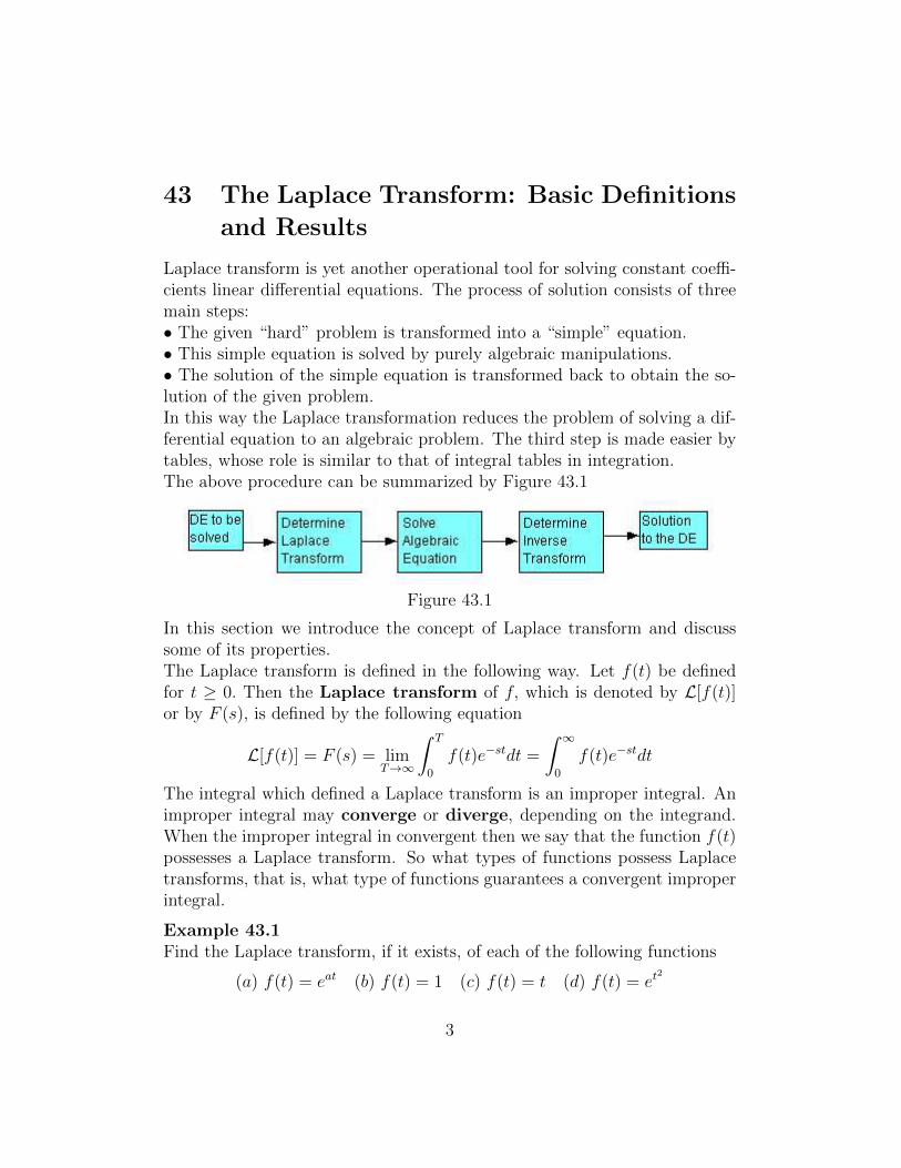
Laplace transform is yet another operational tool for solving constant coeffi-cients linear differential equations. The process of solution consists of threemain steps:• The given “hard” problem is transformed into a “simple” equation.• This simple equation is solved by purely algebraic manipulations.• The solution of the simple equation is transformed back to obtain the so-lution of the given problem.In this way the Laplace transformation reduces the problem of solving a dif-ferential equation to an algebraic problem. The third step is made easier bytables, whose role is similar to that of integral tables in integration.The above procedure can be summarized by Figure 43.1
Figure 43.1
In this section we introduce the concept of Laplace transform and discusssome of its properties.The Laplace transform is defined in the following way. Let f(t) be definedfor t ≥ 0. Then the Laplace transform of f, which is denoted by L[f(t)]or by F (s), is defined by the following equation
L[f(t)] = F (s) = limT→∞
∫ T
0
f(t)e−stdt =
∫ ∞0
f(t)e−stdt
The integral which defined a Laplace transform is an improper integral. Animproper integral may converge or diverge, depending on the integrand.When the improper integral in convergent then we say that the function f(t)possesses a Laplace transform. So what types of functions possess Laplacetransforms, that is, what type of functions guarantees a convergent improperintegral.
Example 43.1Find the Laplace transform, if it exists, of each of the following functions
(a) f(t) = eat (b) f(t) = 1 (c) f(t) = t (d) f(t) = et2
3
Solution.(a) Using the definition of Laplace transform we see that
L[eat] =
∫ ∞0
e−(s−a)tdt = limT→∞
∫ T
0
e−(s−a)tdt.
But ∫ T
0
e−(s−a)tdt =
{T if s = a
1−e−(s−a)T
s−a if s 6= a.
For the improper integral to converge we need s > a. In this case,
L[eat] = F (s) =1
s− a, s > a.
(b) In a similar way to what was done in part (a), we find
L[1] =
∫ ∞0
e−stdt = limT→∞
∫ T
0
e−stdt =1
s, s > 0.
(c) We have
L[t] =
∫ ∞0
te−stdt =
[−te
−st
s− e−st
s2
]∞0
=1
s2, s > 0.
(d) Again using the definition of Laplace transform we find
L[et2
] =
∫ ∞0
et2−stdt.
If s ≤ 0 then t2−st ≥ 0 so that et2−st ≥ 1 and this implies that
∫∞0et
2−stdt ≥∫∞0. Since the integral on the right is divergent, by the comparison theorem
of improper integrals (see Theorem 43.1 below) the integral on the left is alsodivergent. Now, if s > 0 then
∫∞0et(t−s)dt ≥
∫∞sdt. By the same reasoning
the integral on the left is divergent. This shows that the function f(t) = et2
does not possess a Laplace transform
The above example raises the question of what class or classes of functionspossess a Laplace transform. Looking closely at Example 43.1(a), we noticethat for s > a the integral
∫∞0e−(s−a)tdt is convergent and a critical compo-
nent for this convergence is the type of the function f(t). To be more specific,if f(t) is a continuous function such that
|f(t)| ≤Meat, t ≥ C (1)
4
where M ≥ 0 and a and C are constants, then this condition yields∫ ∞0
f(t)e−stdt ≤∫ C
0
f(t)e−stdt+M
∫ ∞C
e−(s−a)tdt.
Since f(t) is continuous in 0 ≤ t ≤ C, by letting A = max{|f(t)| : 0 ≤ t ≤ C}we have ∫ C
0
f(t)e−stdt ≤ A
∫ C
0
e−stdt = A
(1
s− e−sC
s
)<∞.
On the other hand, Now, by Example 43.1(a), the integral∫∞Ce−(s−a)tdt is
convergent for s > a. By the comparison theorem of improper integrals (seeTheorem 43.1 below) the integral on the left is also convergent. That is, f(t)possesses a Laplace transform.We call a function that satisfies condition (1) a function with an exponentialorder at infinity. Graphically, this means that the graph of f(t) is containedin the region bounded by the graphs of y = Meat and y = −Meat for t ≥ C.Note also that this type of functions controls the negative exponential in thetransform integral so that to keep the integral from blowing up. If C = 0then we say that the function is exponentially bounded.
Example 43.2Show that any bounded function f(t) for t ≥ 0 is exponentially bounded.
Solution.Since f(t) is bounded for t ≥ 0, there is a positive constant M such that|f(t)| ≤ M for all t ≥ 0. But this is the same as (1) with a = 0 and C = 0.Thus, f(t) has is exponentially bounded
Another question that comes to mind is whether it is possible to relax thecondition of continuity on the function f(t). Let’s look at the following situ-ation.
Example 43.3Show that the square wave function whose graph is given in Figure 43.2possesses a Laplace transform.
5
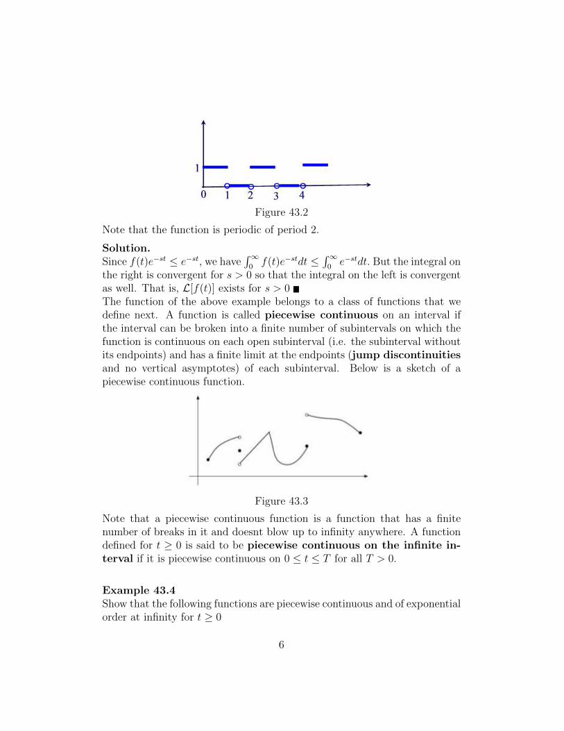
Figure 43.2
Note that the function is periodic of period 2.
Solution.Since f(t)e−st ≤ e−st, we have
∫∞0f(t)e−stdt ≤
∫∞0e−stdt. But the integral on
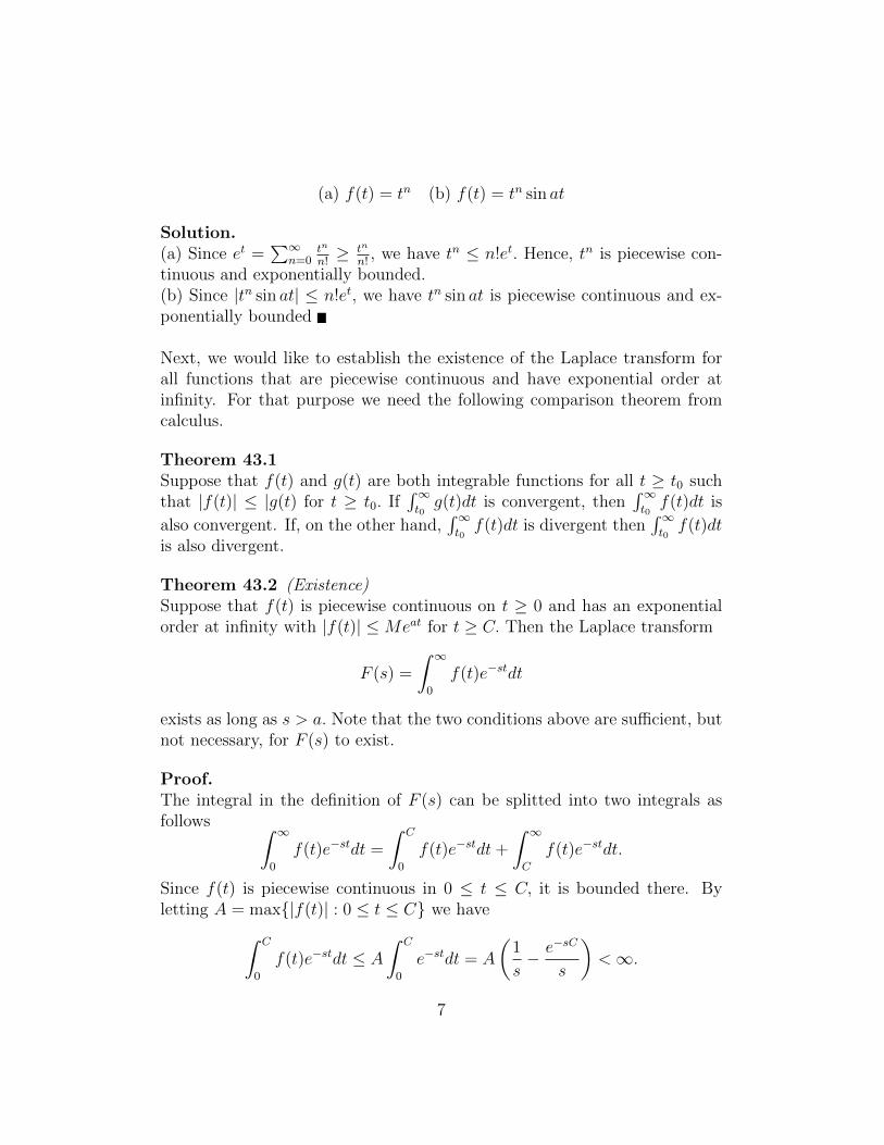
the right is convergent for s > 0 so that the integral on the left is convergentas well. That is, L[f(t)] exists for s > 0The function of the above example belongs to a class of functions that wedefine next. A function is called piecewise continuous on an interval ifthe interval can be broken into a finite number of subintervals on which thefunction is continuous on each open subinterval (i.e. the subinterval withoutits endpoints) and has a finite limit at the endpoints (jump discontinuitiesand no vertical asymptotes) of each subinterval. Below is a sketch of apiecewise continuous function.
Figure 43.3
Note that a piecewise continuous function is a function that has a finitenumber of breaks in it and doesnt blow up to infinity anywhere. A functiondefined for t ≥ 0 is said to be piecewise continuous on the infinite in-terval if it is piecewise continuous on 0 ≤ t ≤ T for all T > 0.
Example 43.4Show that the following functions are piecewise continuous and of exponentialorder at infinity for t ≥ 0
6
(a) f(t) = tn (b) f(t) = tn sin at
Solution.(a) Since et =
∑∞n=0
tn
n!≥ tn
n!, we have tn ≤ n!et. Hence, tn is piecewise con-
tinuous and exponentially bounded.(b) Since |tn sin at| ≤ n!et, we have tn sin at is piecewise continuous and ex-ponentially bounded
Next, we would like to establish the existence of the Laplace transform forall functions that are piecewise continuous and have exponential order atinfinity. For that purpose we need the following comparison theorem fromcalculus.
Theorem 43.1Suppose that f(t) and g(t) are both integrable functions for all t ≥ t0 suchthat |f(t)| ≤ |g(t) for t ≥ t0. If
∫∞t0g(t)dt is convergent, then
∫∞t0f(t)dt is
also convergent. If, on the other hand,∫∞t0f(t)dt is divergent then
∫∞t0f(t)dt
is also divergent.
Theorem 43.2 (Existence)Suppose that f(t) is piecewise continuous on t ≥ 0 and has an exponentialorder at infinity with |f(t)| ≤Meat for t ≥ C. Then the Laplace transform
F (s) =
∫ ∞0
f(t)e−stdt
exists as long as s > a. Note that the two conditions above are sufficient, butnot necessary, for F (s) to exist.
Proof.The integral in the definition of F (s) can be splitted into two integrals asfollows ∫ ∞
0
f(t)e−stdt =
∫ C
0
f(t)e−stdt+
∫ ∞C
f(t)e−stdt.
Since f(t) is piecewise continuous in 0 ≤ t ≤ C, it is bounded there. Byletting A = max{|f(t)| : 0 ≤ t ≤ C} we have∫ C
0
f(t)e−stdt ≤ A
∫ C
0
e−stdt = A
(1
s− e−sC
s
)<∞.
7
Now, by Example 43.1(a), the integral∫∞Cf(t)e−stdt is convergent for s > a.
By Theorem 43.1 the integral on the left is also convergent. That is, f(t)possesses a Laplace transform
In what follows, we will denote the class of all piecewise continuous func-tions with exponential order at infinity by PE . The next theorem shows thatany linear combination of functions in PE is also in PE . The same is true forthe product of two functions in PE .
Theorem 43.3Suppose that f(t) and g(t) are two elements of PE with
|f(t)| ≤M1ea1t, t ≥ C1 and |g(t)| ≤M2e
a1t, t ≥ C2.
(i) For any constants α and β the function αf(t) +βg(t) is also a member ofPE . Moreover
L[αf(t) + βg(t)] = αL[f(t)] + βL[g(t)].
(ii) The function h(t) = f(t)g(t) is an element of PE .
Proof.(i) It is easy to see that αf(t) + βg(t) is a piecewise continuous function.Now, let C = C1 + C2, a = max{a1, a2}, and M = |α|M1 + |β|M2. Then fort ≥ C we have
|αf(t) + βg(t)| ≤ |α||f(t)|+ |β||g(t)| ≤ |α|M1ea1t + |β|M2e
a2t ≤Meat.
This shows that αf(t) + βg(t) is of exponential order at infinity. On theother hand,
L[αf(t) + βg(t)] = limT→∞∫ T0
[αf(t) + βg(t)]dt
= α limT→∞∫ T0f(t)dt+ β limT→∞
∫ T0g(t)dt
= αL[f(t)] + βL[g(t)]
(ii) It is clear that h(t) = f(t)g(t) is a piecewise continuous function. Now,letting C = C1 +C2, M = M1M2, and a = a1 +a2 then we see that for t ≥ Cwe have
|h(t)| = |f(t)||g(t)| ≤M1M2e(a1+a2)t = Meat.
8
Hence, h(t) is of exponential order at infinity. By Theorem 43.2 , L[h(t)]exists for s > a
We next discuss the problem of how to determine the function f(t) if F (s)is given. That is, how do we invert the transform. The following result onuniqueness provides a possible answer. This result establishes a one-to-onecorrespondence between the set PE and its Laplace transforms. Alterna-tively, the following theorem asserts that the Laplace transform of a memberin PE is unique.
Theorem 43.4Let f(t) and g(t) be two elements in PE with Laplace transforms F (s) andG(s) such that F (s) = G(s) for some s > a. Then f(t) = g(t) for all t ≥ 0where both functions are continuous.
The standard techniques used to prove this theorem( i.e., complex analysis,residue computations, and/or Fourier’s integral inversion theorem) are gen-erally beyond the scope of an introductory differential equations course. Theinterested reader can find a proof in the book ”Operational Mathematics”by Ruel Vance Churchill or in D.V. Widder ”The Laplace Transform”.With the above theorem, we can now officially define the inverse Laplacetransform as follows: For a piecewise continuous function f of exponentialorder at infinity whose Laplace transform is F, we call f the inverse Laplacetransform of F and write f = L−1[F (s)]. Symbolically
f(t) = L−1[F (s)]⇐⇒ F (s) = L[f(t)].
Example 43.5Find L−1
(1s−1
), s > 1.
Solution.From Example 43.1(a), we have that L[eat] = 1
s−a , s > a. In particular, for
a = 1 we find that L[et] = 1s−1 , s > 1. Hence, L−1
(1s−1
)= et, t ≥ 0 .
The above theorem states that if f(t) is continuous and has a Laplace trans-form F (s), then there is no other function that has the same Laplace trans-form. To find L−1[F (s)], we can inspect tables of Laplace transforms ofknown functions to find a particular f(t) that yields the given F (s).When the function f(t) is not continuous, the uniqueness of the inverse
9
Laplace transform is not assured. The following example addresses theuniqueness issue.
Example 43.6Consider the two functions f(t) = h(t)h(3− t) and g(t) = h(t)− h(t− 3).
(a) Are the two functions identical?(b) Show that L[f(t)] = L[g(t).
Solution.(a) We have
f(t) =
{1, 0 ≤ t ≤ 30, t > 3
and
g(t) =
{1, 0 ≤ t < 30, t ≥ 3
So the two functions are equal for all t 6= 3 and so they are not identical.(b) We have
L[f(t)] = L[g(t)] =
∫ 3
0
e−stdt =1− e−3s
s, s > 0.
Thus, both functions f(t) and g(t) have the same Laplace transform eventhough they are not identical. However, they are equal on the interval(s)where they are both continuous
The inverse Laplace transform possesses a linear property as indicated inthe following result.
Theorem 43.5Given two Laplace transforms F (s) and G(s) then
L−1[aF (s) + bG(s)] = aL−1[F (s)] + bL−1[G(s)]
for any constants a and b.
Proof.Suppose that L[f(t)] = F (s) and L[g(t)] = G(s). Since L[af(t) + bg(t)] =aL[f(t)] + bL[g(t)] = aF (s) + bG(s) we have L−1[aF (s) + bG(s)] = af(t) +bg(t) = aL−1[F (s)] + bL−1[G(s)]
10
Practice Problems
Problem 43.1Determine whether the integral
∫∞0
11+t2
dt converges. If the integral con-verges, give its value.
Problem 43.2Determine whether the integral
∫∞0
t1+t2
dt converges. If the integral con-verges, give its value.
Problem 43.3Determine whether the integral
∫∞0e−t cos (e−t)dt converges. If the integral
converges, give its value.
Problem 43.4Using the definition, find L[e3t], if it exists. If the Laplace transform existsthen find the domain of F (s).
Problem 43.5Using the definition, find L[t− 5], if it exists. If the Laplace transform existsthen find the domain of F (s).
Problem 43.6Using the definition, find L[e(t−1)
2], if it exists. If the Laplace transform
exists then find the domain of F (s).
Problem 43.7Using the definition, find L[(t − 2)2], if it exists. If the Laplace transformexists then find the domain of F (s).
Problem 43.8Using the definition, find L[f(t)], if it exists. If the Laplace transform existsthen find the domain of F (s).
f(t) =
{0, 0 ≤ t < 1
t− 1, t ≥ 1
11
Problem 43.9Using the definition, find L[f(t)], if it exists. If the Laplace transform existsthen find the domain of F (s).
f(t) =
0, 0 ≤ t < 1
t− 1, 1 ≤ t < 20, t ≥ 2.
Problem 43.10Let n be a positive integer. Using integration by parts establish the reductionformula ∫
tne−stdt = −tne−st
s+n
s
∫tn−1e−stdt, s > 0.
Problem 43.11For s > 0 and n a positive integer evaluate the limits
limt→0 tne−st (b) limt→∞ t
ne−st
Problem 43.12(a) Use the previous two problems to derive the reduction formula for theLaplace transform of f(t) = tn,
L[tn] =n
sL[tn−1], s > 0.
(b) Calculate L[tk], for k = 1, 2, 3, 4, 5.(c) Formulate a conjecture as to the Laplace transform of f(t), tn with n apositive integer.
From a table of integrals,∫eαu sin βudu = eαu α sinβu−β sinβu
α2+β2∫eαu cos βudu = eαu α cosβu+β sinβu
α2+β2
Problem 43.13Use the above integrals to find the Laplace transform of f(t) = cosωt, if itexists. If the Laplace transform exists, give the domain of F (s).
Problem 43.14Use the above integrals to find the Laplace transform of f(t) = sinωt, if itexists. If the Laplace transform exists, give the domain of F (s).
12
Problem 43.15Use the above integrals to find the Laplace transform of f(t) = cosω(t− 2),if it exists. If the Laplace transform exists, give the domain of F (s).
Problem 43.16Use the above integrals to find the Laplace transform of f(t) = e3t sin t, if itexists. If the Laplace transform exists, give the domain of F (s).
Problem 43.17Use the linearity property of Laplace transform to find L[5e−7t + t + 2e2t].Find the domain of F (s).
Problem 43.18Consider the function f(t) = tan t.
(a) Is f(t) continuous on 0 ≤ t < ∞, discontinuous but piecewise contin-uous on 0 ≤ t <∞, or neither?(b) Are there fixed numbers a and M such that |f(t)| ≤Meat for 0 ≤ t <∞?
Problem 43.19Consider the function f(t) = t2e−t.
(a) Is f(t) continuous on 0 ≤ t < ∞, discontinuous but piecewise contin-uous on 0 ≤ t <∞, or neither?(b) Are there fixed numbers a and M such that |f(t)| ≤Meat for 0 ≤ t <∞?
Problem 43.20Consider the function f(t) = et
2
e2t+1.
(a) Is f(t) continuous on 0 ≤ t < ∞, discontinuous but piecewise contin-uous on 0 ≤ t <∞, or neither?(b) Are there fixed numbers a and M such that |f(t)| ≤Meat for 0 ≤ t <∞?
Problem 43.21Consider the floor function f(t) = btc, where for any integer n we havebtc = n for all n ≤ t < n+ 1.
(a) Is f(t) continuous on 0 ≤ t < ∞, discontinuous but piecewise contin-uous on 0 ≤ t <∞, or neither?(b) Are there fixed numbers a and M such that |f(t)| ≤Meat for 0 ≤ t <∞?
13
Problem 43.22Find L−1
(3s−2
).
Problem 43.23Find L−1
(− 2s2
+ 1s+1
).
Problem 43.24Find L−1
(2s+2
+ 2s−2
).
14
44 Further Studies of Laplace Transform
Properties of the Laplace transform enable us to find Laplace transformswithout having to compute them directly from the definition. In this sec-tion, we establish properties of Laplace transform that will be useful forsolving ODEs.
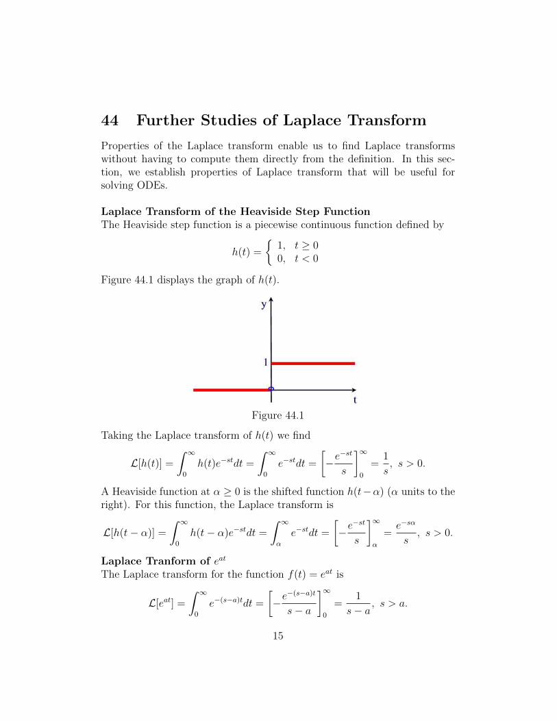
Laplace Transform of the Heaviside Step FunctionThe Heaviside step function is a piecewise continuous function defined by
h(t) =
{1, t ≥ 00, t < 0
Figure 44.1 displays the graph of h(t).
Figure 44.1
Taking the Laplace transform of h(t) we find
L[h(t)] =
∫ ∞0
h(t)e−stdt =
∫ ∞0
e−stdt =
[−e−st
s
]∞0
=1
s, s > 0.
A Heaviside function at α ≥ 0 is the shifted function h(t−α) (α units to theright). For this function, the Laplace transform is
L[h(t− α)] =
∫ ∞0
h(t− α)e−stdt =
∫ ∞α
e−stdt =
[−e−st
s
]∞α
=e−sα
s, s > 0.
Laplace Tranform of eat
The Laplace transform for the function f(t) = eat is
L[eat] =
∫ ∞0
e−(s−a)tdt =
[−e−(s−a)t
s− a
]∞0
=1
s− a, s > a.
15
Laplace Tranforms of sin at and cos atUsing integration by parts twice we find
L[sin at] =∫∞0e−st sin atdt
=[− e−st sin at
s− ae−st cos at
s2
]∞0− a2
s2
∫∞0e−st sin atdt
= − as2− a2
s2L[sin at](
s2+a2
s2
)L[sin at] = a
s2
L[sin at] = as2+a2
, s > 0
A similar argument shows that
L[cos at] =s
s2 + a2, s > 0.
Laplace Transforms of cosh at and sinh atUsing the linear property of L we can write
L[cosh at] = 12
(L[eat] + L[e−at])
= 12
(1s−a + 1
s+a
), s > |a|
= ss2−a2 , s > |a|
A similar argument shows that
L[sin at] =a
s2 − a2, s > |a|.
Laplace Transform of a PolynomialLet n be a positive integer. Using integration by parts we can write∫ ∞
0
tne−stdt = −[tne−st
s
]∞0
+n
s
∫ ∞0
tn−1e−stdt.
By repeated use of L’Hopital’s rule we find limt→∞ tne−st = limt→∞
n!snest
= 0for s > 0. Thus,
L[tn] =n
sL[tn−1], s > 0.
16
Using induction on n = 0, 1, 2, · · · one can easily eastablish that
L[tn] =n!
sn+1, s > 0.
Using the above result together with the linearity property of L one can findthe Laplace transform of any polynomial.The next two results are referred to as the first and second shift theorems.As with the linearity property, the shift theorems increase the number offunctions for which we can easily find Laplace transforms.
Theorem 44.1 (First Shifting Theorem)If f(t) is a piecewise continuous function for t ≥ 0 and has exponential orderat infinity with |f(t)| ≤Meat, t ≥ C, then for any real number α we have
L[eαtf(t)] = F (s− α), s > a+ α
where L[f(t)] = F (s).
Proof.From the definition of the Laplace transform we have
L[eatf(t)] =
∫ ∞0
e−steatf(t)dt =
∫ ∞0
e−(s−a)tf(t)dt.
Using the change of variable β = s− a the previous equation reduces to
L[eatf(t)] =
∫ ∞0
e−steatf(t)dt =
∫ ∞0
e−βtf(t)dt = F (β) = F (s−a), s > a+α
Theorem 44.2 (Second Shifting Theorem)If f(t) is a piecewise continuous function for t ≥ 0 and has exponential orderat infinity with |f(t)| ≤ Meat, t ≥ C, then for any real number α ≥ 0 wehave
L[f(t− α)h(t− α)] = e−αsF (s), s > a
where L[f(t)] = F (s) and h(t) is the Heaviside step function.
Proof.From the definition of the Laplace transform we have
L[f(t− α)h(t− α)] =
∫ ∞0
f(t− α)h(s− α)e−stdt =
∫ ∞α
f(t− α)e−stdt.
17
Using the change of variable β = t− α the previous equation reduces to
L[f(t− α)h(t− α)] =∫∞0f(β)e−s(β+α)dβ
= e−sα∫∞0f(β)e−sβdβ = e−sαF (s), s > a
Example 44.1Find
(a) L[e2tt2] (b) L[e3t cos 2t] (c) L−1[e−2ts2]
Solution.(a) By Theorem 44.1, we have L[e2tt2] = F (s − 2) where L[t2] = 2!
s3=
F (s), s > 0. Thus, L[e2tt2] = 2(s−2)3 , s > 2.
(b) As in part (a), we have L[e3t cos 2t] = F (s−3) where L[cos 2t] = F (s−3).But L[cos 2t] = s
s2+4, s > 0. Thus,
L[e3t cos 2t] =s− 3
(s− 3)2 + 4, s > 3
(c) Since L[t] = 1s2, by Theorem 44.2, we have
e−2t
s2= L[(t− 2)h(t− 2)].
Therefore,
L−1[e−2t
s2
]= (t− 2)h(t− 2) =
{0, 0 ≤ t < 2
t− 2, t ≥ 2
The following result relates the Laplace transform of derivatives and integralsto the Laplace transform of the function itself.
Theorem 44.3Suppose that f(t) is continuous for t ≥ 0 and f ′(t) is piecewise continuousof exponential order at infinity with |f ′(t)| ≤Meat, t ≥ C Then
(a) f(t) is of exponential order at infinity.(b) L[f ′(t)] = sL[f(t)]− f(0) = sF (s)− f(0), s > max{a, 0}+ 1.(c) L[f ′′(t)] = s2L[f(t)] − sf(0) − f ′(0) = s2F (s) − sf(0) − f(0), s >max{a, 0}+ 1.
(d) L[∫ t
0f(u)du
]= L[f(t)]
s= F (s)
s, s > max{a, 0}+ 1.
18
Proof.(a) By the Fundamental Theorem of Calculus we have f(t) = f(0)−
∫ t0f ′(u)du.
Also, since f ′ is piecewise continuous, |f ′(t)| ≤ T for some T > 0 and all0 ≤ t ≤ C. Thus,
|f(t)| =∣∣∣f(0)−
∫ t0f ′(u)du
∣∣∣ = |f(0)−∫ C0f ′(u)du−
∫ tCf ′(u)du|
≤ |f(0)|+ TC +M∫ tCeaudu
Note that if a > 0 then∫ t
C
eaudu =1
a(eat − eaC) ≤ eat
a
and so
|f(t)| ≤ [|f(0)|+ TC +M
a]eat.
If a = 0 then ∫ t
C
eaudu = t− C
and therefore
|f(t)| ≤ |f(0)|+ TC +M(t− C) ≤ (|f(0)|+ TC +M)et.
Now, if a < 0 then ∫ t
C
eaudu =1
a(eat − eaC) ≤ 1
|a|
so that
|f(t)| ≤ (|f(0)|+ TC +M
|a|)et
It follows that|f(t)| ≤ Nebt, t ≥ 0
where b = max{a, 0}+ 1.
(b) From the definition of Laplace transform we can write
L[f ′(t)] = limA→∞
∫ A
0
f ′(t)e−stdt.
19
Since f ′(t) may have jump discontinuities at t1, t2, · · · , tN in the interval0 ≤ t ≤ A, we can write∫ A
0
f ′(t)e−stdt =
∫ t1
0
f ′(t)e−stdt+
∫ t2
t1
f ′(t)e−stdt+ · · ·+∫ A
tN
f ′(t)e−stdt.
Integrating each term on the RHS by parts and using the continuity of f(t)to obtain∫ t1
0f ′(t)e−stdt = f(t1)e
−st1 − f(0) + s∫ t10f(t)e−stdt∫ t2
t1f ′(t)e−stdt = f(t2)e
−st2 − f(t1)e−st1 + s
∫ t2t1f(t)e−stdt
...∫ tNtN−1
f ′(t)e−stdt = f(tN)e−stN − f(tN−1)e−stN−1 + s
∫ tNtN−1
f(t)e−stdt
∫ AtNf ′(t)e−stdt = f(A)e−sA − f(tN)e−stN + s
∫ AtNf(t)e−stdt
Also, by the continuity of f(t) we can write∫ A
0
f(t)e−stdt =
∫ t1
0
f(t)e−stdt+
∫ t2
t1
f(t)e−stdt+ · · ·+∫ A
tN
f(t)e−stdt.
Hence, ∫ A
0
f ′(t)e−stdt = f(A)e−sA − f(0) + s
∫ A
0
f(t)e−stdt.
Since f(t) has exponential order at infinity,limA→∞ f(A)e−sA = 0. Hence,
L[f ′(t)] = sL[f(t)]− f(0).
(c) Using part (b) we find
L[f ′′(t)] = sL[f ′(t)]− f ′(0)= s(sF (s)− f(0))− f ′(0)= s2F (s)− sf(0)− f ′(0), s > max{a, 0}+ 1
(d) Since ddt
(∫ t0f(u)du
)= f(t), by part (b) we have
F (s) = L[f(t)] = sL{∫ t
0
f(u)du
}20
and therefore
L[∫ t
0
f(u)du
]=L[f(t)]
s=F (s)
s, s > max{a, 0}+ 1
The argument establishing part (b) of the previous theorem can be extendedto higher order derivatives.
Theorem 44.4Let f(t), f ′(t), · · · , f (n−1)(t) be continuous and f (n)(t) be piecewise continu-ous of exponential order at infinity with |f (n)(t)| ≤Meat, t ≥ C. Then
L[f (n)(t)] = snL[f(t)]−sn−1f(0)−sn−2f ′(0)−· · ·−f (n−1)(0), s > max{a, 0}+1.
We next illustrate the use of the previous theorem in solving initial valueproblems.
Example 44.2Solve the initial value problem
y′′ − 4y′ + 9y = t, y(0) = 0, y′(0) = 1.
Solution.We apply Theorem 44.4 that gives the Laplace transform of a derivative. Bythe linearity property of the Laplace transform we can write
L[y′′]− 4L[y′] + 9L[y] = L[t].
Now since
L[y′′] = s2L[y]− sy(0)− y′(0) = s2Y (s)− 1L[y′] = sY (s)− y(0) = sY (s)L[t] = 1
s2
where L[y] = Y (s), we obtain
s2Y (s)− 1− 4sY (s) + 9Y (s) =1
s2.
Rearranging gives
(s2 − 4s+ 9)Y (s) =s2 + 1
s2.
21
Thus,
Y (s) =s2 + 1
s2(s2 − 4s+ 9)
and
y(t) = L−1[
s2 + 1
s2(s2 − 4s+ 9)
]In the next section we will discuss a method for finding the inverse Laplacetransform of the above expression.
Example 44.3Consider the mass-spring oscillator without friction: y′′ + y = 0. Supposewe add a force which corresponds to a push (to the left) of the mass as itoscillates. We will suppose the push is described by the function
f(t) = −h(t− 2π) + u(t− (2π + a))
for some a > 2π which we are allowed to vary. (A small a will correspondto a short duration push and a large a to a long duration push.) We areinterested in solving the initial value problem
y′′ + y = f(t), y(0) = 1, y′(0) = 0.
Solution.To begin, determine the Laplace transform of both sides of the DE:
L[y′′ + y] = L[f(t)]
or
s2Y − sy(0)− y′(0) + Y (s) = −1
se−2πs +
1
se−(2π+a)s.
Thus,
Y (s) =e−(2π+a)s
s(s2 + 1)− e−2πs
s(s2 + 1)+
s
s2 + 1.
Now since 1s(s2+1)
= 1s− s
s2+1we see that
Y (s) = e−(2π+a)s[
1
s− s
s2 + 1
]− e−2πs
[1
s− s
s2 + 1
]+
s
s2 + 1
22
and therefore
y(t) = h(t− (2π + a))[L−1
(1s− s
s2+1
)](t− (2π + a))
− h(t− 2π)[L−1
(1s− s
s2+1
)](t− 2π) + cos t
= h(t− (2π + a))[1− cos (t− (2π + a))]− u(t− 2π)[1− cos (t− 2π)]+ cos t
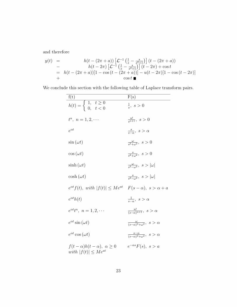
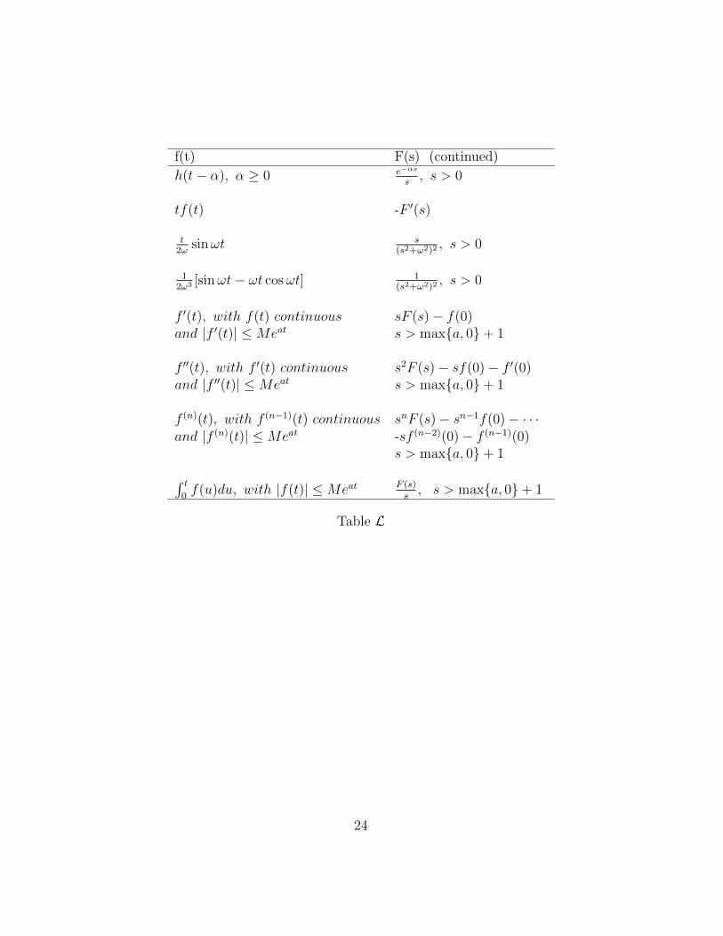
We conclude this section with the following table of Laplace transform pairs.
f(t) F(s)
h(t) =
{1, t ≥ 00, t < 0
1s, s > 0
tn, n = 1, 2, · · · n!sn+1 , s > 0
eαt ss−α , s > α
sin (ωt) ωs2+ω2 , s > 0
cos (ωt) ss2+ω2 , s > 0
sinh (ωt) ωs2−ω2 , s > |ω|
cosh (ωt) ss2−ω2 , s > |ω|
eαtf(t), with |f(t)| ≤Meat F (s− α), s > α + a
eαth(t) 1s−α , s > α
eαttn, n = 1, 2, · · · n!(s−α)n+1 , s > α
eαt sin (ωt) ω(s−α)2+ω2 , s > α
eαt cos (ωt) s−α(s−α)2+ω2 , s > α
f(t− α)h(t− α), α ≥ 0 e−αsF (s), s > awith |f(t)| ≤Meat
23
f(t) F(s) (continued)
h(t− α), α ≥ 0 e−αs
s, s > 0
tf(t) -F ′(s)
t2ω
sinωt s(s2+ω2)2
, s > 0
12ω3 [sinωt− ωt cosωt] 1
(s2+ω2)2, s > 0
f ′(t), with f(t) continuous sF (s)− f(0)and |f ′(t)| ≤Meat s > max{a, 0}+ 1
f ′′(t), with f ′(t) continuous s2F (s)− sf(0)− f ′(0)and |f ′′(t)| ≤Meat s > max{a, 0}+ 1
f (n)(t), with f (n−1)(t) continuous snF (s)− sn−1f(0)− · · ·and |f (n)(t)| ≤Meat -sf (n−2)(0)− f (n−1)(0)
s > max{a, 0}+ 1∫ t0f(u)du, with |f(t)| ≤Meat F (s)
s, s > max{a, 0}+ 1
Table L
24
Practice Problems
Problem 44.1Use Table L to find L[2et + 5].
Problem 44.2Use Table L to find L[e3t−3h(t− 1)].
Problem 44.3Use Table L to find L[sin2 ωt].
Problem 44.4Use Table L to find L[sin 3t cos 3t].
Problem 44.5Use Table L to find L[e2t cos 3t].
Problem 44.6Use Table L to find L[e4t(t2 + 3t+ 5)].
Problem 44.7Use Table L to find L−1[ 10
s2+25+ 4
s−3 ].
Problem 44.8Use Table L to find L−1[ 5
(s−3)4 ].
Problem 44.9Use Table L to find L−1[ e−2s
s−9 ].
Problem 44.10Use Table L to find L−1[ e
−3s(2s+7)s2+16
].
Problem 44.11Graph the function f(t) = h(t − 1) + h(t − 3) for t ≥ 0, where h(t) is theHeaviside step function, and use Table L to find L[f(t)].
Problem 44.12Graph the function f(t) = t[h(t− 1)− h(t− 3)] for t ≥ 0, where h(t) is theHeaviside step function, and use Table L to find L[f(t)].
25
Problem 44.13Graph the function f(t) = 3[h(t− 1)− h(t− 4)] for t ≥ 0, where h(t) is theHeaviside step function, and use Table L to find L[f(t)].
Problem 44.14Graph the function f(t) = |2− t|[h(t− 1)− h(t− 3)] for t ≥ 0, where h(t) isthe Heaviside step function, and use Table L to find L[f(t)].
Problem 44.15Graph the function f(t) = h(2− t) for t ≥ 0, where h(t) is the Heaviside stepfunction, and use Table L to find L[f(t)].
Problem 44.16Graph the function f(t) = h(t − 1) + h(4 − t) for t ≥ 0, where h(t) is theHeaviside step function, and use Table L to find L[f(t)].
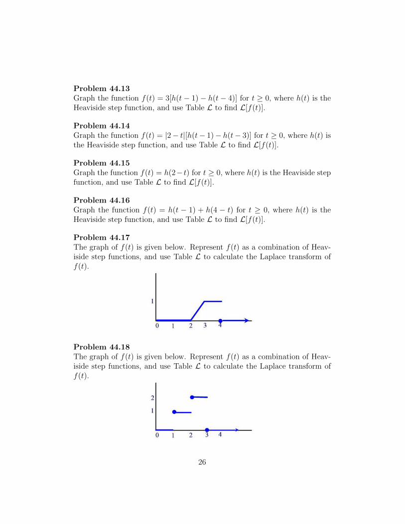
Problem 44.17The graph of f(t) is given below. Represent f(t) as a combination of Heav-iside step functions, and use Table L to calculate the Laplace transform off(t).
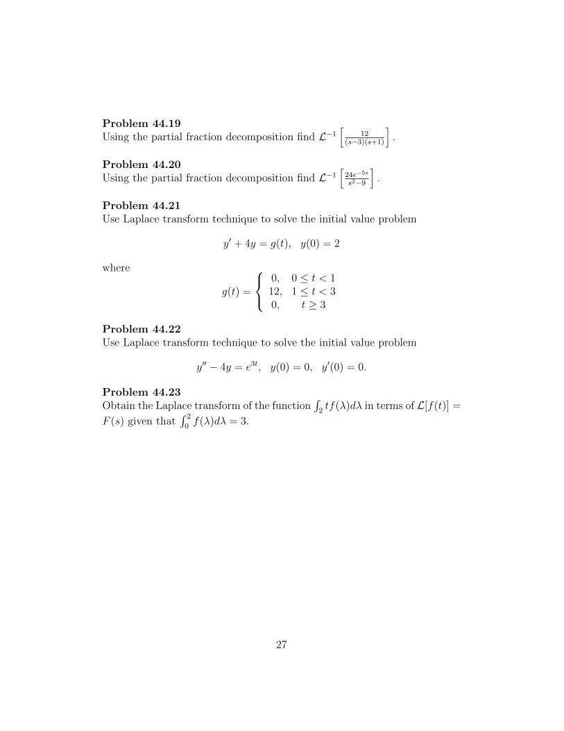
Problem 44.18The graph of f(t) is given below. Represent f(t) as a combination of Heav-iside step functions, and use Table L to calculate the Laplace transform off(t).
26
Problem 44.19Using the partial fraction decomposition find L−1
[12
(s−3)(s+1)
].
Problem 44.20Using the partial fraction decomposition find L−1
[24e−5s
s2−9
].
Problem 44.21Use Laplace transform technique to solve the initial value problem
y′ + 4y = g(t), y(0) = 2
where
g(t) =
0, 0 ≤ t < 112, 1 ≤ t < 30, t ≥ 3
Problem 44.22Use Laplace transform technique to solve the initial value problem
y′′ − 4y = e3t, y(0) = 0, y′(0) = 0.
Problem 44.23Obtain the Laplace transform of the function
∫2tf(λ)dλ in terms of L[f(t)] =
F (s) given that∫ 2
0f(λ)dλ = 3.
27
45 The Laplace Transform and the Method
of Partial Fractions
In the last example of the previous section we encountered the equation
y(t) = L−1[
s2 + 1
s2(s2 − 4s+ 9)
].
We would like to find an explicit expression for y(t). This can be done usingthe method of partial fractions which is the topic of this section. According
to this method, finding L−1(N(s)D(s)
), where N(s) and D(s) are polynomials,
require decomposing the rational function into a sum of simpler expressionswhose inverse Laplace transform can be recognized from a table of Laplacetransform pairs.The method of integration by partial fractions is a technique for integratingrational functions, i.e. functions of the form
R(s) =N(s)
D(s)
where N(s) and D(s) are polynomials.The idea consists of writing the rational function as a sum of simpler frac-tions called partial fractions. This can be done in the following way:
Step 1. Use long division to find two polynomials r(s) and q(s) such that
N(s)
D(s)= q(s) +
r(s)
D(s).
Note that if the degree of N(s) is smaller than that of D(s) then q(s) = 0and r(s) = N(s).
Step 2. Write D(s) as a product of factors of the form (as + b)n or (as2 +bs+c)n where as2+bs+c is irreducible, i.e. as2+bs+c = 0 has no real zeros.
Step 3. Decompose r(s)D(s)
into a sum of partial fractions in the followingway:(1) For each factor of the form (s− α)k write
A1
s− α+
A2
(s− α)2+ · · ·+ Ak
(s− α)k,
28
where the numbers A1, A2, · · · , Ak are to be determined.(2) For each factor of the form (as2 + bs+ c)k write
B1s+ C1
as2 + bs+ c+
B2s+ C2
(as2 + bs+ c)2+ · · ·+ Bks+ Ck
(as2 + bs+ c)k,
where the numbers B1, B2, · · · , Bk and C1, C2, · · · , Ck are to be determined.
Step 4. Multiply both sides by D(s) and simplify. This leads to an ex-pression of the form
r(s) = a polynomial whose coefficients are combinations of Ai,Bi, and Ci.
Finally, we find the constants, Ai, Bi, and Ci by equating the coefficients oflike powers of s on both sides of the last equation.
Example 45.1Decompose into partial fractions R(s) = s3+s2+2
s2−1 .
Solution.Step 1. s3+s2+2
s2−1 = s+ 1 + s+3s2−1 .
Step 2. s2 − 1 = (s− 1)(s+ 1).Step 3. s+3
(s+1)(s−1) = As+1
+ Bs−1 .
Step 4. Multiply both sides of the last equation by (s− 1)(s+ 1) to obtain
s+ 3 = A(s− 1) +B(s+ 1).
Expand the right hand side, collect terms with the same power of s, andidentify coefficients of the polynomials obtained on both sides:
s+ 3 = (A+B)s+ (B − A).
Hence, A+B = 1 and B −A = 3. Adding these two equations gives B = 2.Thus, A = −1 and so
s3 + s2 + 2
s2 − 1= s+ 1− 1
s+ 1+
2
s− 1.
Now, after decomposing the rational function into a sum of partial fractionsall we need to do is to find the Laplace transform of expressions of the form
A(s−α)n or Bs+C
(as2+bs+c)n.
29
Example 45.2
Find L−1[
1s(s−3)
].
Solution.We write
1
s(s− 3)=A
s+
B
s− 3.
Multiply both sides by s(s− 3) and simplify to obtain
1 = A(s− 3) +Bs
or1 = (A+B)s− 3A.
Now equating the coefficients of like powers of s to obtain −3A = 1 andA+B = 0. Solving for A and B we find A = −1
3and B = 1
3. Thus,
L−1[
1s(s−3)
]= −1
3L−1
[1s
]+ 1
3L−1
[1s−3
]= −1
3h(t) + 1
3e3t, t ≥ 0
where h(t) is the Heaviside unit step function
Example 45.3Find L−1
[3s+6s2+3s
].
Solution.We factor the denominator and split the integrand into partial fractions:
3s+ 6
s(s+ 3)=A
s+
B
s+ 3.
Multiplying both sides by s(s+ 3) to obtain
3s+ 6 = A(s+ 3) +Bs= (A+B)s+ 3A
Equating the coefficients of like powers of x to obtain 3A = 6 and A+B = 3.Thus, A = 2 and B = 1. Finally,
L−1[
3s+ 6
s2 + 3s
]= 2L−1
[1
s
]+ L−1
[1
s+ 3
]= 2h(t) + e−3t, t ≥ 0.
30
Example 45.4
Find L−1[
s2+1s(s+1)2
].
Solution.We factor the denominator and split the rational function into partial frac-tions:
s2 + 1
s(s+ 1)2=A
s+
B
s+ 1+
C
(s+ 1)2.
Multiplying both sides by s(s+ 1)2 and simplifying to obtain
s2 + 1 = A(s+ 1)2 +Bs(s+ 1) + Cs= (A+B)s2 + (2A+B + C)s+ A.
Equating coefficients of like powers of s we find A = 1, 2A + B + C = 0and A + B = 1. Thus, B = 0 and C = −2. Now finding the inverse Laplacetransform to obtain
L−1[s2 + 1
s(s+ 1)2
]= L−1
[1
s
]− 2L−1
[1
(s+ 1)2
]= h(t)− 2te−t, t ≥ 0.
Example 45.5Use Laplace transform to solve the initial value problem
y′′ + 3y′ + 2y = e−t, y(0) = y′(0) = 0.
Solution.By the linearity property of the Laplace transform we can write
L[y′′] + 3L[y′] + 2L[y] = L[e−t].
Now sinceL[y′′] = s2L[y]− sy(0)− y′(0) = s2Y (s)L[y′] = sY (s)− y(0) = sY (s)L[e−t] = 1
s+1
where L[y] = Y (s), we obtain
s2Y (s) + 3sY (s) + 2Y (s) =1
s+ 1.
31
Rearranging gives
(s2 + 3s+ 2)Y (s) =1
s+ 1.
Thus,
Y (s) =1
(s+ 1)(s2 + 3s+ 2).
and
y(t) = L−1[
1
(s+ 1)(s2 + 3s+ 2)
].
Using the method of partial fractions we can write
1
(s+ 1)(s2 + 3s+ 2)=
1
s+ 2− 1
s+ 1+
1
(s+ 1)2.
Thus,
y(t) = L−1[
1
s+ 2
]−L−1
[1
s+ 1
]+L−1
[1
(s+ 1)2
]= e−2t−e−t+te−t, t ≥ 0
32
Practice Problems
In Problems 45.1 - 45.4, give the form of the partial fraction expansion forF (s). You need not evaluate the constants in the expansion. However, if thedenominator has an irreducible quadratic expression then use the completingthe square process to write it as the sum/difference of two squares.
Problem 45.1
F (s) =s3 + 3s+ 1
(s− 1)3(s− 2)2.
Problem 45.2
F (s) =s2 + 5s− 3
(s2 + 16)(s− 2).
Problem 45.3
F (s) =s3 − 1
(s2 + 1)2(s+ 4)2.
Problem 45.4
F (s) =s4 + 5s2 + 2s− 9
(s2 + 8s+ 17)(s− 2)2.
Problem 45.5Find L−1
[1
(s+1)3
].
Problem 45.6Find L−1
[2s−3
s2−3s+2
].
Problem 45.7Find L−1
[4s2+s+1s3+s
].
Problem 45.8Find L−1
[s2+6s+8s4+8s2+16
].
33
Problem 45.9Use Laplace transform to solve the initial value problem
y′ + 2y = 26 sin 3t, y(0) = 3.
Problem 45.10Use Laplace transform to solve the initial value problem
y′ + 2y = 4t, y(0) = 3.
Problem 45.11Use Laplace transform to solve the initial value problem
y′′ + 3y′ + 2y = 6e−t, y(0) = 1, y′(0) = 2.
Problem 45.12Use Laplace transform to solve the initial value problem
y′′ + 4y = cos 2t, y(0) = 1, y′(0) = 1.
Problem 45.13Use Laplace transform to solve the initial value problem
y′′ − 2y′ + y = e2t, y(0) = 0, y′(0) = 0.
Problem 45.14Use Laplace transform to solve the initial value problem
y′′ + 9y = g(t), y(0) = 1, y′(0) = 0
where
g(t) =
{6, 0 ≤ t < π0, π ≤ t <∞
Problem 45.15Determine the constants α, β, y0, and y′0 so that Y (s) = 2s−1
s2+s+2is the Laplace
transform of the solution to the initial value problem
y′′ + αy′ + βy = 0, y(0) = y0, y′(0) = y′0.
Problem 45.16Determine the constants α, β, y0, and y′0 so that Y (s) = s
(s+1)2is the Laplace
transform of the solution to the initial value problem
y′′ + αy′ + βy = 0, y(0) = y0, y′(0) = y′0.
34
46 Laplace Transforms of Periodic Functions
In many applications, the nonhomogeneous term in a linear differential equa-tion is a periodic function. In this section, we derive a formula for the Laplacetransform of such periodic functions.Recall that a function f(t) is said to be T−periodic if we have f(t+T ) = f(t)whenever t and t + T are in the domain of f(t). For example, the sine andcosine functions are 2π−periodic whereas the tangent and cotangent func-tions are π−periodic.If f(t) is T−periodic for t ≥ 0 then we define the function
fT (t) =
{f(t), 0 ≤ t ≤ T
0, t > T
The Laplace transform of this function is then
L[fT (t)] =
∫ ∞0
fT (t)e−stdt =
∫ T
0
f(t)e−stdt.
The Laplace transform of a T−periodic function is given next.
Theorem 46.1If f(t) is a T−periodic, piecewise continuous fucntion for t ≥ 0 then
L[f(t)] =L[fT (t)]
1− e−sT, s > 0.
Proof.Since f(t) is piecewise continuous, it is bounded on the interval 0 ≤ t ≤ T.By periodicity, f(t) is bounded for t ≥ 0. Hence, it has an exponential orderat infinity. By Theorem 43.2, L[f(t)] exists for s > 0. Thus,
L[f(t)] =
∫ ∞0
f(t)e−stdt =∞∑n=0
∫ T
0
fT (t− nT )h(t− nT )e−stdt,
where the last sum is the result of decomposing the improper integral into asum of integrals over the constituent periods.By the Second Shifting Theorem (i.e. Theorem 44.2) we have
L[fT (t− nT )h(t− nT )] = e−nTsL[fT (t)], s > 0
35
Hence,
L[f(t)] =∞∑n=0
e−nTsL[fT (t)] = L[fT (t)]
(∞∑n=0
e−nTs
).
Since s > 0, it follows that 0 < e−nTs < 1 so that the series∑∞
n=0 e−nTs is a
convergent geoemetric series with limit 11−e−sT . Therefore,
L[f(t)] =L[fT (t)]
1− e−sT, s > 0
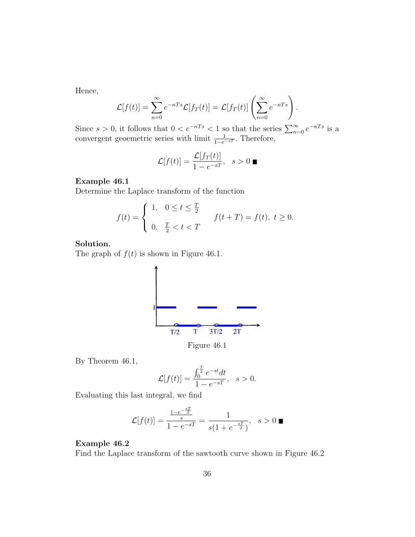
Example 46.1Determine the Laplace transform of the function
f(t) =
1, 0 ≤ t ≤ T
2
f(t+ T ) = f(t), t ≥ 0.0, T
2< t < T
Solution.The graph of f(t) is shown in Figure 46.1.
Figure 46.1
By Theorem 46.1,
L[f(t)] =
∫ T2
0e−stdt
1− e−sT, s > 0.
Evaluating this last integral, we find
L[f(t)] =1−e−
sT2
s
1− e−sT=
1
s(1 + e−sT2 ), s > 0
Example 46.2Find the Laplace transform of the sawtooth curve shown in Figure 46.2
36
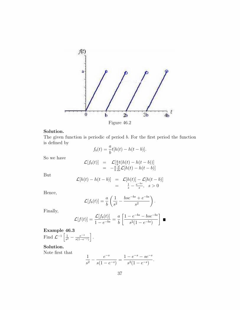
Figure 46.2
Solution.The given function is periodic of period b. For the first period the functionis defined by
fb(t) =a
bt[h(t)− h(t− b)].
So we haveL[fb(t)] = L[a
bt(h(t)− h(t− b))]
= −abddsL[h(t)− h(t− b)]
ButL[h(t)− h(t− b)] = L[h(t)]− L[h(t− b)]
= 1s− e−bs
s, s > 0
Hence,
L[fb(t)] =a
b
(1
s2− bse−bs + e−bs
s2
).
Finally,
L[f(t)] =L[fb(t)]
1− e−bs=a
b
[1− e−bs − bse−bs
s2(1− e−bs)
]Example 46.3
Find L−1[
1s2− e−s
s(1−e−s)
].
Solution.Note first that
1
s2− e−s
s(1− e−s)=
1− e−s − se−s
s2(1− e−s).
37
According to the previous example with a = 1 and b = 1 we find that
L−1[
1s2− e−s
s(1−e−s)
]is the sawtooth function shown in Figure 46.2
Linear Time Invariant Systems and the Transfer FunctionThe Laplace transform is a powerful technique for analyzing linear time-invariant systems such as electrical circuits, harmonic oscillators, optical de-vices, and mechanical systems, to name just a few. A mathematical modeldescribed by a linear differential equation with constant coefficients of theform
any(n) +an−1y
(n−1) + · · ·+a1y′+a0y = bmu
(m) + bm−1u(m−1) + · · ·+ b1u
′+ b0u
is called a linear time invariant system. The function y(t) denotes thesystem output and the function u(t) denotes the system input. The system iscalled time-invariant because the parameters of the system are not changingover time and an input now will give the same result as the same input later.Applying the Laplace transform on the linear differential equation with nullinitial conditions we obtain
ansnY (s)+an−1s
n−1Y (s)+· · ·+a0Y (s) = bmsmU(s)+bm−1s
m−1U(s)+· · ·+b0U(s).
The function
Φ(s) =Y (s)
U(s)=bms
m + bm−1sm−1 + · · ·+ b1s+ b0
ansn + an−1sn−1 + · · ·+ a1s+ a0
is called the system transfer function. That is, the transfer function ofa linear time-invariant system is the ratio of the Laplace transform of itsoutput to the Laplace transform of its input.
Example 46.4Consider the mathematical model described by the initial value problem
my′′ + γy′ + ky = f(t), y(0) = 0, y′(0) = 0.
The coefficients m, γ, and k describe the properties of some physical system,and f(t) is the input to the system. The solution y is the output at time t.Find the system transfer function.
38
Solution.By taking the Laplace transform and using the initial conditions we obtain
(ms2 + γs+ k)Y (s) = F (s).
Thus,
Φ(s) =Y (s)
F (s)=
1
ms2 + γs+ k(2)
Parameter IdentificationOne of the most useful applications of system transfer functions is for systemor parameter identification.
Example 46.5Consider a spring-mass system governed by
my′′ + γy′ + ky = f(t), y(0) = 0, y′(0) = 0. (3)
Suppose we apply a unit step force f(t) = h(t) to the mass, initially atequilibrium, and you observe the system respond as
y(t) = −1
2e−t cos t− 1
2e−t sin t+
1
2.
What are the physical parameters m, γ, and k?
Solution.Start with the model (3)) with f(t) = h(t) and take the Laplace transform ofboth sides, then solve to find Y (s) = 1
s(ms2+γs+k). Since f(t) = h(t), F (s) = 1
s.
Hence
Φ(s) =Y (s)
F (s)=
1
ms2 + γs+ k.
On the other hand, for the input f(t) = h(t) the corresponding observedoutput is
y(t) = −1
2e−t cos t− 1
2e−t sin t+
1
2.
Hence,Y (s) = L[−1
2e−t cos t− 1
2e−t sin t+ 1
2]
= −12
s+1(s+1)2+1
− 12
1(s+1)2+1
+ 12s
= 1s(s2+2s+2)
39

Thus,
Φ(s) =Y (s)
F (s)=
1
s2 + 2s+ 2.
By comparison we conclude that m = 1, γ = 2, and k = 2
40
Practice Problems
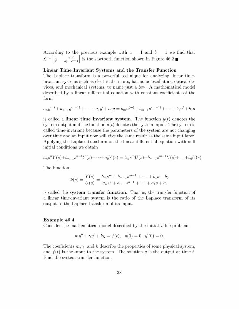
Problem 46.1Find the Laplace transform of the periodic function whose graph is shown.
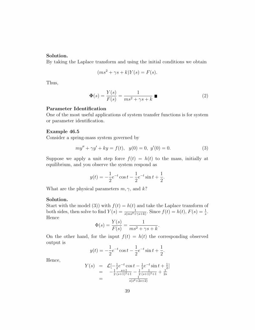
Problem 46.2Find the Laplace transform of the periodic function whose graph is shown.
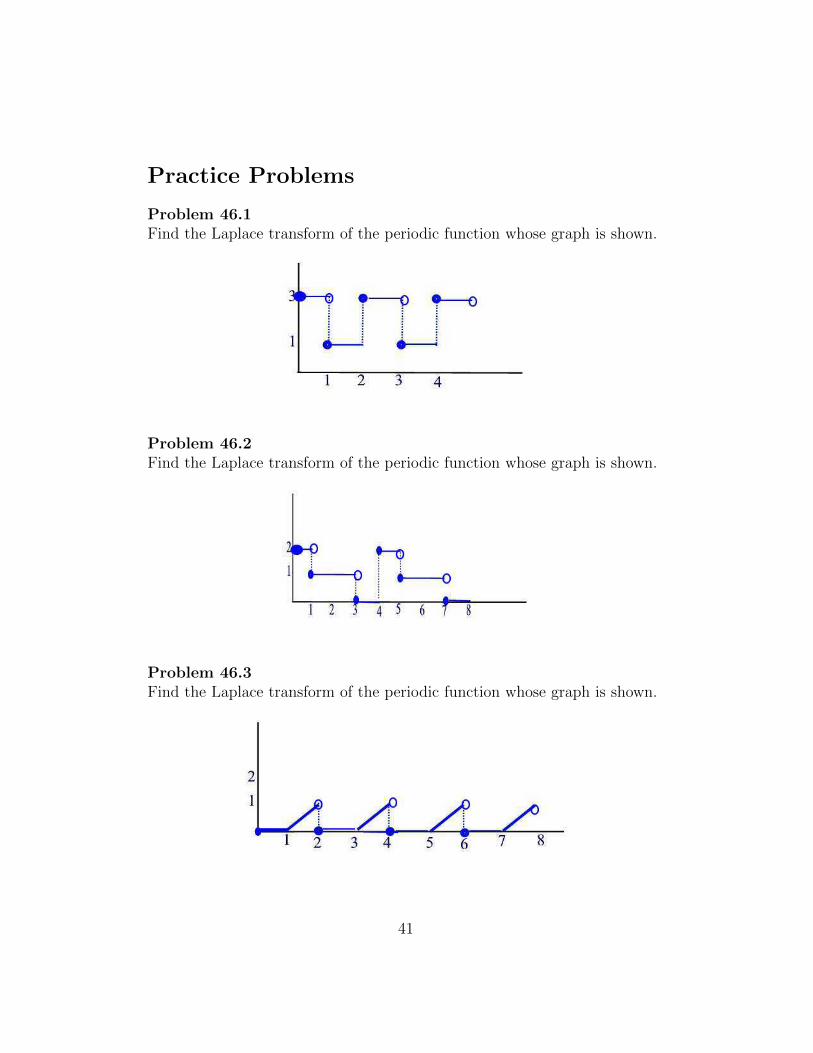
Problem 46.3Find the Laplace transform of the periodic function whose graph is shown.
41
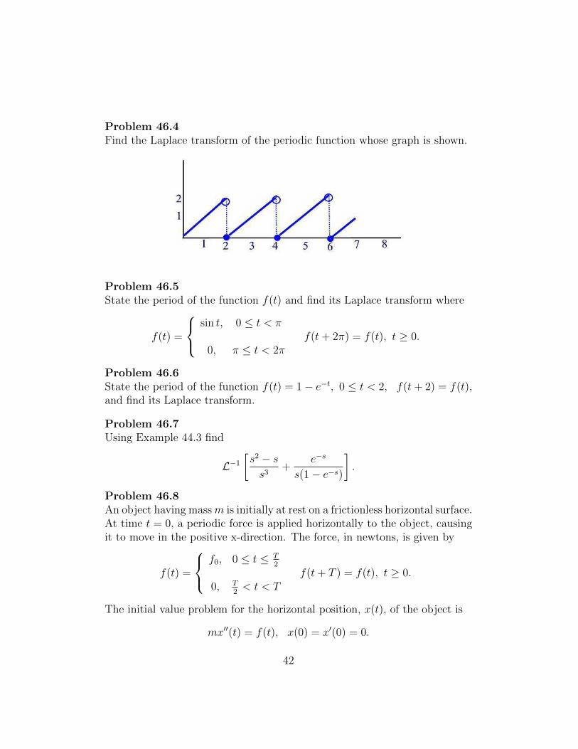
Problem 46.4Find the Laplace transform of the periodic function whose graph is shown.
Problem 46.5State the period of the function f(t) and find its Laplace transform where
f(t) =
sin t, 0 ≤ t < π
f(t+ 2π) = f(t), t ≥ 0.0, π ≤ t < 2π
Problem 46.6State the period of the function f(t) = 1− e−t, 0 ≤ t < 2, f(t+ 2) = f(t),and find its Laplace transform.
Problem 46.7Using Example 44.3 find
L−1[s2 − ss3
+e−s
s(1− e−s)
].
Problem 46.8An object having massm is initially at rest on a frictionless horizontal surface.At time t = 0, a periodic force is applied horizontally to the object, causingit to move in the positive x-direction. The force, in newtons, is given by
f(t) =
f0, 0 ≤ t ≤ T
2
f(t+ T ) = f(t), t ≥ 0.0, T
2< t < T
The initial value problem for the horizontal position, x(t), of the object is
mx′′(t) = f(t), x(0) = x′(0) = 0.
42
(a) Use Laplace transforms to determine the velocity, v(t) = x′(t), and theposition, x(t), of the object.(b) Let m = 1 kg, f0 = 1 N, and T = 1 sec. What is the velocity, v, andposition, x, of the object at t = 1.25 sec?
Problem 46.9Consider the initial value problem
ay′′ + by′ + cy = f(t), y(0) = y′(0) = 0, t > 0
Suppose that the transfer function of this system is given by Φ(s) = 12s2+5s+2
.(a) What are the constants a, b, and c?(b) If f(t) = e−t, determine F (s), Y (s), and y(t).
Problem 46.10Consider the initial value problem
ay′′ + by′ + cy = f(t), y(0) = y′(0) = 0, t > 0
Suppose that an input f(t) = t, when applied to the above system producesthe output y(t) = 2(e−t − 1) + t(e−t + 1), t ≥ 0.(a) What is the system transfer function?(b) What will be the output if the Heaviside unit step function f(t) = h(t)is applied to the system?
Problem 46.11Consider the initial value problem
y′′ + y′ + y = f(t), y(0) = y′(0) = 0,
where
f(t) =
1, 0 ≤ t ≤ 1
f(t+ 2) = f(t)−1, 1 < t < 2
(a) Determine the system transfer function Φ(s).(b) Determine Y (s).
Problem 46.12Consider the initial value problem
y′′′ − 4y = et + t, y(0) = y′(0) = y′′(0) = 0.
(a) Determine the system transfer function Φ(s).(b) Determine Y (s).
43
Problem 46.13Consider the initial value problem
y′′ + by′ + cy = h(t), y(0) = y0, y′(0) = y′0, t > 0.
Suppose that L[y(t)] = Y (s) = s2+2s+1s3+3s2+2s
. Determine the constants b, c, y0,and y′0.
44
47 Convolution Integrals
We start this section with the following problem.
Example 47.1A spring-mass system with a forcing function f(t) is modeled by the followinginitial-value problem
mx′′ + kx = f(t), x(0) = x0, x′(0) = x′0.
Find solution to this initial value problem using the Laplace transform method.
Solution.Apply Laplace transform to both sides of the equation to obtain
ms2X(s)−msx0 −mx′0 + kX(s) = F (s).
Solving the above algebraic equation for X(s) we find
X(s) = F (s)ms2+k
+ msx0ms2+k
+mx′0ms2+k
= 1m
F (s)
s2+ km
+ sx0s2+ k
m
+x′0
s2+ km
Apply the inverse Laplace transform to obtain
x(t) = L−1[X(s)]
= 1mL−1
{F (s)
s2+ km
}+ x0L−1
{s
s2+ km
}+ x′0L−1
{1
s2+ km
}= 1
mL−1
{F (s) · 1
s2+ km
}+ x0 cos
(√km
)t+ x′0
√mk
sin(√
km
)t
Finding L−1{F (s) · 1
s2+ km
},i.e., the inverse Laplace transform of a product,
requires the use of the concept of convolution, a topic we discuss in thissectionConvolution integrals are useful when finding the inverse Laplace transformof products H(s) = F (s)G(s). They are defined as follows: The convolutionof two scalar piecewise continuous functions f(t) and g(t) defined for t ≥ 0is the integral
(f ∗ g)(t) =
∫ t
0
f(t− s)g(s)ds.
45
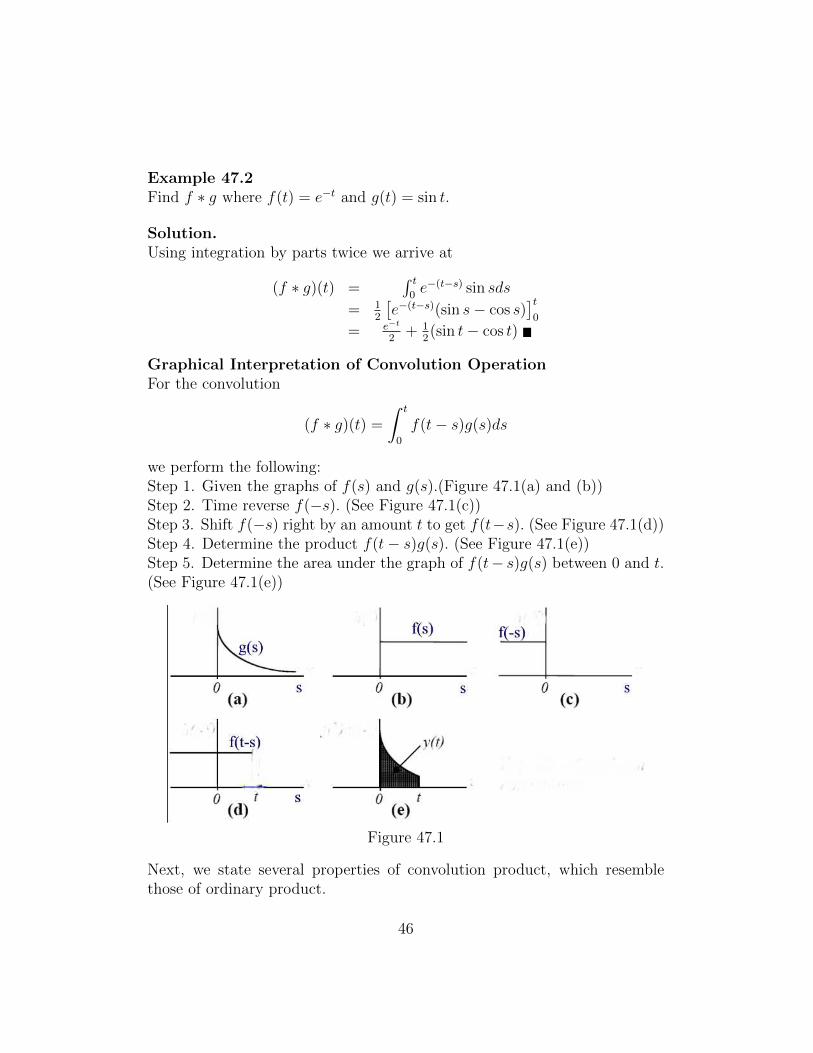
Example 47.2Find f ∗ g where f(t) = e−t and g(t) = sin t.
Solution.Using integration by parts twice we arrive at
(f ∗ g)(t) =∫ t0e−(t−s) sin sds
= 12
[e−(t−s)(sin s− cos s)
]t0
= e−t
2+ 1
2(sin t− cos t)
Graphical Interpretation of Convolution OperationFor the convolution
(f ∗ g)(t) =
∫ t
0
f(t− s)g(s)ds
we perform the following:Step 1. Given the graphs of f(s) and g(s).(Figure 47.1(a) and (b))Step 2. Time reverse f(−s). (See Figure 47.1(c))Step 3. Shift f(−s) right by an amount t to get f(t−s). (See Figure 47.1(d))Step 4. Determine the product f(t− s)g(s). (See Figure 47.1(e))Step 5. Determine the area under the graph of f(t− s)g(s) between 0 and t.(See Figure 47.1(e))
Figure 47.1
Next, we state several properties of convolution product, which resemblethose of ordinary product.
46
Theorem 47.1Let f(t), g(t), and k(t) be three piecewise continuous scalar functions definedfor t ≥ 0 and c1 and c2 are arbitrary constants. Then(i) f ∗ g = g ∗ f (Commutative Law)(ii) (f ∗ g) ∗ k = f ∗ (g ∗ k) (Associative Law)(iii) f ∗ (c1g + c2k) = c1f ∗ g + c2f ∗ k (Distributive Law)
Proof.(i) Using the change of variables τ = t− s we find
(f ∗ g)(t) =∫ t0f(t− s)g(s)ds
= −∫ 0
tf(τ)g(t− τ)dτ
=∫ t0g(t− τ)f(τ)dτ = (g ∗ f)(t)
(ii) By definition, we have
[(f ∗ g) ∗ k)](t) =∫ t0(f ∗ g)(t− u)k(u)du
=∫ t0
[∫ t−u0
f(t− u− w)g(w)k(u)dw]du
For the integral in the bracket, make change of variable w = s− u. We have
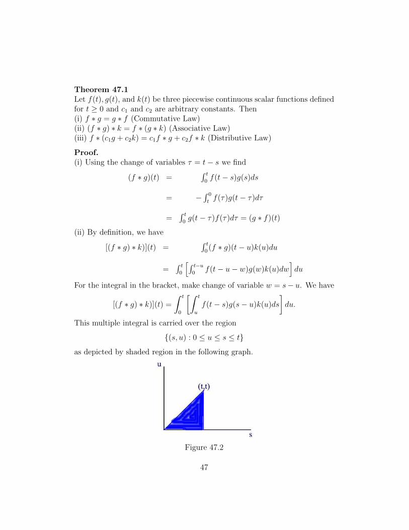
[(f ∗ g) ∗ k)](t) =
∫ t
0
[∫ t
u
f(t− s)g(s− u)k(u)ds
]du.
This multiple integral is carried over the region
{(s, u) : 0 ≤ u ≤ s ≤ t}
as depicted by shaded region in the following graph.
Figure 47.2
47
Changing the order of integration, we have
[(f ∗ g) ∗ k)](t) =∫ t0
[∫ s0f(t− s)g(s− u)k(u)du
]ds
=∫ t0f(t− s)(g ∗ k)(s)ds
= [f ∗ (g ∗ k)](t)
(iii) We have
(f ∗ (c1g + c2k))(t) =∫ t0f(t− s)(c1g(s) + c2k(s))ds
= c1∫ t0f(t− s)g(s)ds+ c2
∫ t0f(t− s)k(s)ds
= c1(f ∗ g)(t) + c2(f ∗ k)(t)
Example 47.3Express the solution to the initial value problem y′ + αy = g(t), y(0) = y0in terms of a convolution integral.
Solution.Solving this initial value problem by the method of integrating factor we find
y(t) = e−αty0 +
∫ t
0
e−α(t−s)g(s)ds = e−αty0 + e−αt ∗ g(t)
Example 47.4If f(t) is an m×n matrix function and g(t) is an n× p matrix function thenwe define
(f ∗ g)(t) =
∫ t
0
f(t− s)g(s)ds, t ≥ 0.
Express the solution to the initial value problem y′ = Ay + g(t), y(0) = y0
in terms of a convolution integral.
Solution.The unique solution is given by
y(t) = etAy0 +
∫ t
0
eA(t−s)g(s)ds = etAy0 + etA ∗ g(t)
The following theorem, known as the Convolution Theorem, provides a wayfor finding the Laplace transform of a convolution integral and also findingthe inverse Laplace transform of a product.
48
Theorem 47.2If f(t) and g(t) are piecewise continuous for t ≥ 0, and of exponential orderat infinity then
L[(f ∗ g)(t)] = L[f(t)]L[g(t)] = F (s)G(s).
Thus, (f ∗ g)(t) = L−1[F (s)G(s)].
Proof.First we show that f ∗ g has a Laplace transform. From the hypotheses wehave that |f(t)| ≤ M1e
a1t for t ≥ C1 and |g(t)| ≤ M2ea2t for t ≥ C2. Let
M = M1M2 and C = C1 + C2. Then for t ≥ C we have
|(f ∗ g)(t)| =∣∣∣∫ t0 f(t− s)g(s)ds
∣∣∣ ≤ ∫ t0 |f(t− s)||g(s)|ds
≤ M1M2
∫ t0ea1(t−s)ea2sds
=
{Mtea1t, a1 = a2
M ea2t−ea1ta2−a1 , a1 6= a2
This shows that f ∗ g is of exponential order at infinity. Since f and g arepiecewise continuous, the first fundamental theorem of calculus implies thatf ∗ g is also piecewise continuous. Hence, f ∗ g has a Laplace transform.Next, we have
L[(f ∗ g)(t)] =∫∞0e−st
(∫ t0f(t− τ)g(τ)dτ
)dt
=∫∞t=0
∫ tτ=0
e−stf(t− τ)g(τ)dτdt
Note that the region of integration is an infinite triangular region and theintegration is done vertically in that region. Integration horizontally we find
L[(f ∗ g)(t)] =
∫ ∞τ=0
∫ ∞t=τ
e−stf(t− τ)g(τ)dtdτ.
We next introduce the change of variables β = t−τ . The region of integrationbecomes τ ≥ 0, t ≥ 0. In this case, we have
L[(f ∗ g)(t)] =∫∞τ=0
∫∞β=0
e−s(β+τ)f(β)g(τ)dτdβ
=(∫∞
τ=0e−sτg(τ)dτ
) (∫∞β=0
e−sβf(β)dβ)
= G(s)F (s) = F (s)G(s)
49
Example 47.5Use the convolution theorem to find the inverse Laplace transform of
H(s) =1
(s2 + a2)2.
Solution.Note that
H(s) =
(1
s2 + a2
)(1
s2 + a2
).
So, in this case we have, F (s) = G(s) = 1s2+a2
so that f(t) = g(t) = 1a
sin (at).Thus,
(f ∗ g)(t) =1
a2
∫ t
0
sin (at− as) sin (as)ds =1
2a3(sin (at)− at cos (at))
Convolution integrals are useful in solving initial value problems with forcingfunctions.
Example 47.6Solve the initial value problem
4y′′ + y = g(t), y(0) = 3, y′(0) = −7
Solution.Take the Laplace transform of all the terms and plug in the initial conditionsto obtain
4(s2Y (s)− 3s+ 7) + Y (s) = G(s)
or(4s2 + 1)Y (s)− 12s+ 28 = G(s).
Solving for Y (s) we find
Y (s) = 12s−284(s2+ 1
4)+ G(s)
4(s2+ 14)
= 3s
s2+(( 12)2 − 7
( 12)
2
s2+( 12)
2 + 14G(s)
( 12)
2
s2+( 12)
2
Hence,
y(t) = 3 cos
(t
2
)− 7 sin
(t
2
)+
1
2
∫ t
0
sin(s
2
)g(t− s)ds.
So, once we decide on a g(t) all we need to do is to evaluate the integral andwe’ll have the solution
50
Practice Problems
Problem 47.1Consider the functions f(t) = g(t) = h(t), t ≥ 0 where h(t) is the Heavisideunit step function. Compute f ∗ g in two different ways.(a) By directly evaluating the integral.(b) By computing L−1[F (s)G(s)] where F (s) = L[f(t)] and G(s) = L[g(t)].
Problem 47.2Consider the functions f(t) = et and g(t) = e−2t, t ≥ 0. Compute f ∗ g intwo different ways.(a) By directly evaluating the integral.(b) By computing L−1[F (s)G(s)] where F (s) = L[f(t)] and G(s) = L[g(t)].
Problem 47.3Consider the functions f(t) = sin t and g(t) = cos t, t ≥ 0. Compute f ∗ g intwo different ways.(a) By directly evaluating the integral.(b) By computing L−1[F (s)G(s)] where F (s) = L[f(t)] and G(s) = L[g(t)].
Problem 47.4Use Laplace transform to comput the convolution P ∗ y, where |bfP (t) =[h(t) et
0 t
]and y(t) =
[h(t)e−t
].
Problem 47.5Compute and graph f ∗ g where f(t) = h(t) and g(t) = t[h(t)− h(t− 2)].
Problem 47.6Compute and graph f ∗ g where f(t) = h(t)− h(t− 1) and g(t) = h(t− 1)−2h(t− 2)].
Problem 47.7Compute t ∗ t ∗ t.
Problem 47.8Compute h(t) ∗ e−t ∗ e−2t.
Problem 47.9Compute t ∗ e−t ∗ et.
51
Problem 47.10
Suppose it is known that
n functions︷ ︸︸ ︷h(t) ∗ h(t) ∗ · · · ∗ h(t) = Ct8. Determine the con-
stants C and the poisitive integer n.
Problem 47.11Use Laplace transform to solve for y(t) :∫ t
0
sin (t− λ)y(λ)dλ = t2.
Problem 47.12Use Laplace transform to solve for y(t) :
y(t)−∫ t
0
e(t−λ)y(λ)dλ = t.
Problem 47.13Use Laplace transform to solve for y(t) :
t ∗ y(t) = t2(1− e−t).
Problem 47.14Use Laplace transform to solve for y(t) :
y′ = h(t) ∗ y, y(0) =
[12
].
Problem 47.15Solve the following initial value problem.
y′ − y =
∫ t
0
(t− λ)eλdλ, y(0) = −1.
52
48 The Dirac Delta Function and Impulse Re-
sponse
In applications, we are often encountered with linear systems, originally atrest, excited by a sudden large force (such as a large applied voltage to anelectrical network) over a very short time frame. In this case, the outputcorresponding to this sudden force is referred to as the ”impulse response”.Mathematically, an impulse can be modeled by an initial value problem witha special type of function known as the Dirac delta function as the externalforce, i.e., the nonhomogeneous term. To solve such IVP requires finding theLaplace transform of the delta function which is the main topic of this section.
An Example of Impulse ResponseConsider a spring-mass system with a time-dependent force f(t) applied tothe mass. The situation is modeled by the second-order differential equation
my′′ + γy′ + ky = f(t) (4)
where t is time and y(t) is the displacement of the mass from equilibrium.Now suppose that for t ≤ 0 the mass is at rest in its equilibrium position, soy(0) = y′(0) = 0. Hence, the situation is modeled by the initial value problem
my′′ + γy′ + ky = f(t), y(0) = 0, y′(0) = 0. (5)
Solving this equation by the method of variation of parameters one finds theunique solution
y(t) =
∫ t
0
φ(t− s)f(s)ds (6)
where
φ(t) =
e(−γ/2m)t sin
(t√
km− γ2
4m2
)m√
km− γ2
4m2
.
Next, we consider the problem of strucking the mass by an ”instantaneous”hammer blow at t = 0. This situation actually occurs frequently in practice-asystem sustains a forceful, almost-instantaneous input. Our goal is to modelthe situation mathematically and determine how the system will respond.
53
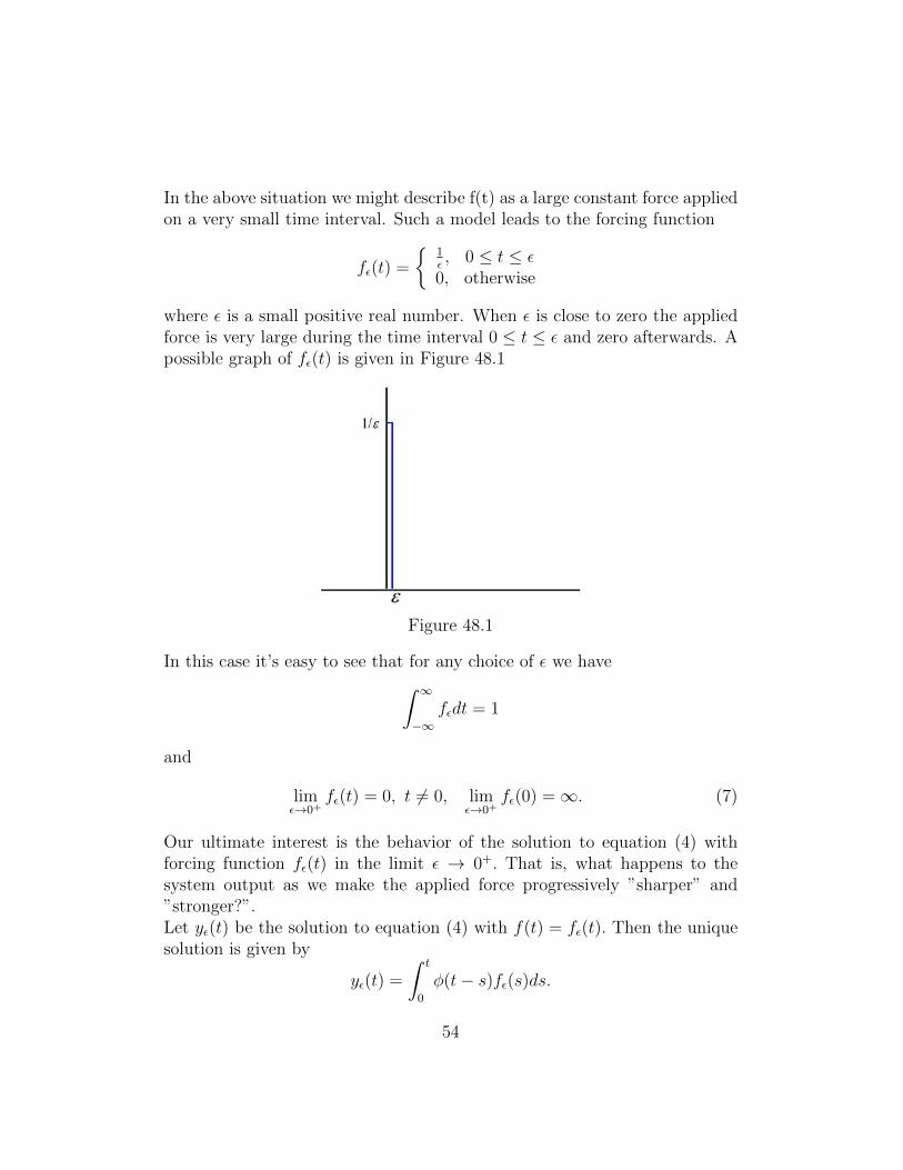
In the above situation we might describe f(t) as a large constant force appliedon a very small time interval. Such a model leads to the forcing function
fε(t) =
{1ε, 0 ≤ t ≤ ε
0, otherwise
where ε is a small positive real number. When ε is close to zero the appliedforce is very large during the time interval 0 ≤ t ≤ ε and zero afterwards. Apossible graph of fε(t) is given in Figure 48.1
Figure 48.1
In this case it’s easy to see that for any choice of ε we have∫ ∞−∞
fεdt = 1
and
limε→0+
fε(t) = 0, t 6= 0, limε→0+
fε(0) =∞. (7)
Our ultimate interest is the behavior of the solution to equation (4) withforcing function fε(t) in the limit ε → 0+. That is, what happens to thesystem output as we make the applied force progressively ”sharper” and”stronger?”.Let yε(t) be the solution to equation (4) with f(t) = fε(t). Then the uniquesolution is given by
yε(t) =
∫ t
0
φ(t− s)fε(s)ds.
54
For t ≥ ε the last equation becomes
yε(t) =1
ε
∫ ε
0
φ(t− s)ds.
Since φ(t) is continuous for all t ≥ 0 we can apply the mean value theoremfor integrals and write
yε(t) = φ(t− ψ)
for some 0 ≤ ψ ≤ ε. Letting ε→ 0+ and using the continuity of φ we find
y(t) = limε→0+
yε(t) = φ(t).
We call y(t) the impulse response of the linear system.
The Dirac Delta FunctionThe problem with the integral∫ t
0
φ(t− s)fε(s)ds
is that limε→0+ fε(0) is undefined. So it makes sense to ask the question ofwhether we can find a function δ(t) such that
limε→0+ yε(t) = limε→0+∫ t0φ(t− s)fε(s)ds
=∫ t0φ(t− s)δ(s)ds
= φ(t)
where the role of δ(t) would be to evaluate the integrand at s = 0. Note thatbecause of Fig 48.1 and (7), we cannot interchange the opeartions of limitand integration in the above limit process. Such a function δ exist in thetheory of distributions and can be defined as follows:If f(t) is continuous in a ≤ t ≤ b then we define the function δ(t) by theintegral equation∫ b
a
f(t)δ(t− t0)dt = limε→0+
∫ b
a
f(t)fε(t− t0)dt.
The object δ(t) on the left is called the Dirac Delta function, or just thedelta function for short.
55
Finding the Impulse Function Using Laplace TransformFor ε > 0 we can solve the initial value problem (5) using Laplace transforms.To do this we need to compute the Laplace transform of fε(t), given by theintegral
L[fε(t)] =
∫ ∞0
fε(t)e−stdt =
1
ε
∫ ε
0
e−stdt =1− e−εs
εs.
Note that by using L’Hopital’s rule we can write
limε→0+
L[fε(t)] = limε→0+
1− e−εs
εs= 1, s > 0.
Now, to find yε(t), we apply the Laplace transform to both sides of equation(4) and using the initial conditions we obtain
ms2Y ε(s) + γsYε(s) + kYε(s) =1− e−εs
εs.
Solving for Yε(s) we find
Yε(s) =1
ms2 + γs+ k
1− e−εs
εs.
Letting ε→ 0+ we find
Y (s) =1
ms2 + γs+ k
which is the transfer function of the system. Now inverse transform Y (s) tofind the solution to the initial value problem. That is,
y(t) = L−1(
1
ms2 + γs+ k
)= φ(t).
Now, impulse inputs are usually modeled in terms of delta functions. Thus,knowing the Laplace transform of such functions is important when solvingdifferential equations. The next theorem finds the Laplace transform of thedelta function.
56
Theorem 48.1With δ(t) defined as above, if a ≤ t0 < b∫ b
a
f(t)δ(t− t0)dt = f(t0).
Proof.We have ∫ b
af(t)δ(t− t0) = limε→0+
∫ baf(t)fε(t− t0)dt
= limε→0+1ε
∫ t0+εt0
f(t)dt
= limε→0+1εf(t0 + βε)ε = f(t0)
where 0 < β < 1 and the mean-value theorem for integrals has been used
Remark 48.1Since pε(t−t0) = 1
εfor t0 ≤ t ≤ t0+ε and 0 otherwise we see that
∫ baf(t)δ(t−
a)dt = f(a) and∫ baf(t)δ(t− t0)dt = 0 for t0 ≥ b.
It follows immediately from the above theorem that
L[δ(t− t0)] =
∫ ∞0
e−stδ(t− t0)dt = e−st0 , t0 ≥ 0.
In particular, if t0 = 0 we find
L[δ(t)] = 1.
The following example illustrates the formal use of the delta function.
Example 48.1A spring-mass system with mass 2, damping 4, and spring constant 10 issubject to a hammer blow at time t = 0. The blow imparts a total impulse of1 to the system, which was initially at rest. Find the response of the system.
Solution.The situation is modeled by the initial value problem
2y′′ + 4y′ + 10y = δ(t), y(0) = 0, y′(0) = 0.
57
Taking Laplace transform of both sides we find
2s2Y (s) + 4sY (s) + 10Y (s) = 1.
Solving for Y (s) we find
Y (s) =1
2s2 + 4s+ 10.
The impulsive response is
y(t) = L−1(
1
2
1
(s+ 1)2 + 22
)=
1
4e−2t sin 2t
Example 48.2A 16 lb weight is attached to a spring with a spring constant equal to 2lb/ft. Neglect damping. The weight is released from rest at 3 ft below theequilibrium position. At t = 2π sec, it is struck with a hammer, providing animpulse of 4 lb-sec. Determine the displacement function y(t) of the weight.
Solution.This situation is modeled by the initial value problem
16
32y′′ + 2y = 4δ(t− 2π), y(0) = 3, y′(0) = 0.
Apply Laplace transform to both sides to obtain
s2Y (s)− 3s+ 4Y (s) = 8e−2πs.
Solving for Y (s) we find
Y (s) =3s
s2 + 4+
e−2πs
s2 + 4.
Now take the inverse Laplace transform to get
y(t) = L−1[Y (s)] = 3 cos 2t+ 8h(t− 2π)f(t− 2π)
where
f(t) = L−1{
1
s2 + 4
}=
1
2sin 2t.
Hence,
y(t) = 3 cos 2t+ 4h(t− 2π) sin 2(t− 2π) = 3 cos 2t+ 4h(t− 2π) sin 2t
or more explicitly
y(t) =
{3 cos 2t, t < 2π
3 cos 2t+ 4 sin 2t, t ≥ 2π
58
Practice Problems
Problem 48.1Evaluate
(a)∫ 3
0(1 + e−t)δ(t− 2)dt.
(b)∫ 1
−2(1 + e−t)δ(t− 2)dt.
(c)∫ 2
−1
[cos 2tte−t
]δ(t)dt.
(d)∫ 2
−1(e2t + t)
δ(t+ 2)δ(t− 1)δ(t− 3)
dt.Problem 48.2Let f(t) be a function defined and continuous on 0 ≤ t <∞. Determine
(f ∗ δ)(t) =
∫ t
0
f(t− s)δ(s)ds.
Problem 48.3Determine a value of the constant t0 such that
∫ 1
0sin2 [π(t− t0)]δ(t− 1
2)dt = 3
4.
Problem 48.4If∫ 5
1tnδ(t− 2)dt = 8, what is the exponent n?
Problem 48.5Sketch the graph of the function g(t) which is defined by g(t) =
∫ t0
∫ s0δ(u−
1)duds, 0 ≤ t <∞.
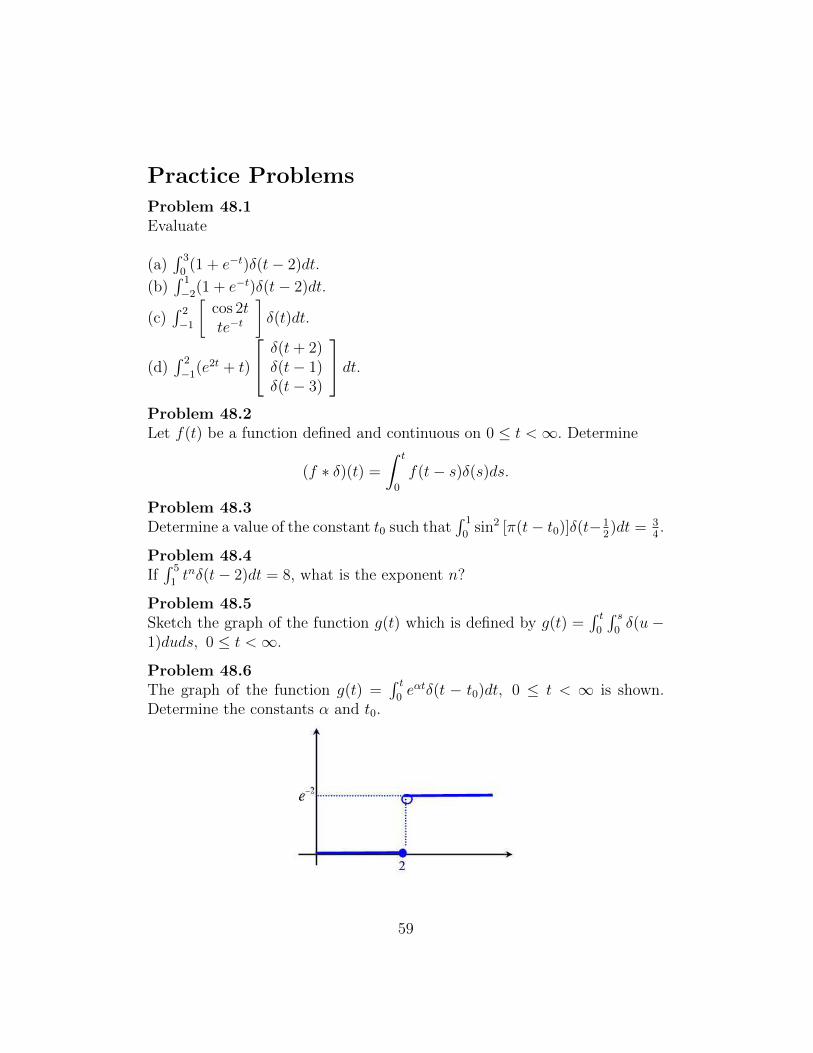
Problem 48.6The graph of the function g(t) =
∫ t0eαtδ(t − t0)dt, 0 ≤ t < ∞ is shown.
Determine the constants α and t0.
59
Problem 48.7(a) Use the method of integarting factor to solve the initial value problemy′ − y = h(t), y(0) = 0.(b) Use the Laplace transform to solve the initial value problem φ′ − φ =δ(t), φ(0) = 0.(c) Evaluate the convolution φ∗h(t) and compare the resulting function withthe solution obtained in part(a).
Problem 48.8Solve the initial value problem
y′ + y = 2 + δ(t− 1), y(0) = 0, 0 ≤ t ≤ 6.
Graph the solution on the indicated interval.
Problem 48.9Solve the initial value problem
y′′ = δ(t− 1)− δ(t− 3), y(0) = 0, y′(0) = 0, 0 ≤ t ≤ 6.
Graph the solution on the indicated interval.
Problem 48.10Solve the initial value problem
y′′ − 2y′ = δ(t− 1), y(0) = 1, y′(0) = 0, 0 ≤ t ≤ 2.
Graph the solution on the indicated interval.
Problem 48.11Solve the initial value problem
y′′ + 2y′ + y = δ(t− 2), y(0) = 0, y′(0) = 1, 0 ≤ t ≤ 6.
Graph the solution on the indicated interval.
60
49 Solving Systems of Differential Equations
Using Laplace Transform
In this section we extend the definition of Laplace transform to matrix-valuedfunctions and apply this extension to solving systems of differential equations.Let y1(t), y2(t), · · · , yn(t) be members of PE . Consider the vector-valuedfunction
y(t) =
y1(t)y2(t)
...yn(t)
The Laplace transform of y(t) is
L[y(t)] =∫∞0
y(t)e−stdt
=
∫∞0y1(t)e
−stdt∫∞0y2(t)e
−stdt...∫∞
0yn(t)e−stdt
=
L[y1(t)]L[y2(t)]
...L[yn(t)]
In a similar way, we define the Laplace transform of an m × n matrix tobe the m× n matrix consisting of the Laplace transforms of the componentfunctions. If the Laplace transform of each component exists then we sayy(t) is Laplace transformable.
Example 49.1Find the Laplace transform of the vector-valued function
y(t) =
t2
1et
61
Solution.The Laplace transform is
L[y(t)] =
6s3
1s
1s−1
, s > 1
The linearity property of the Laplace transform can be used to establish thefollowing result.
Theorem 49.1If A is a constant n × n matrix and B is an n × p matrix-valued functionthen
L[AB(t)] = AL[B(t)].
Proof.Let A = (aij) and B(t) = (bij(t)). Then AB(t) = (
∑nk=1 aikbkp). Hence,
L[AB(t)] = [L(n∑k=1
aikbkp)] = [n∑k=1
aikL(bkp)] = AL[B(t)]
Theorem 42.3 can be extended to vector-valued functions.
Theorem 49.2(a) Suppose that y(t) is continuous for t ≥ 0 and let the components of thederivative vector y′ be members of PE . Then
L[y′(t)] = sL[y(t)]− y(0).
(b) Let y′(t) be continuous for t ≥ 0, and let the entries of y′′(t) be membersof PE . Then
L[y′′(t)] = s2L[y(t)]− sy(0)− y′(0).
(c) Let the entries of y(t) be members of PE . Then
L{∫ t
0
y(s)ds
}=L[y(t)]
s.
62
Proof.(a) We have
L[y′(t)] =
L[y′1(t)]L[y′2(t)]
...L[y′n(t)]
=
sL[y1(t)]− y1(0)sL[y2(t)]− y2(0)
...sL[yn(t)]− yn(0)
= sL[y(t)]− y(0)
(b) We haveL[y′′(t)] = sL[y′(t)]− y′(0)
= s(sL[y(t)]− y(0))− y′(0)= s2L[y(t)]− sy(0)− y′(0)
(c) We have
L[y(t)] = sL{∫ t
0
y(s)ds
}so that
L{∫ t
0
y(s)ds
}=L[y(t)]
s
The above two theorems can be used for solving the following initial valueproblem
y′(t) = Ay + g(t), y(0) = y0, t > 0 (8)
where A is a constant matrix and the components of g(t) are members ofPE .Using the above theorems we can write
sY(s)− y0 = AY(s) + G(s)
or(sI−A)Y(s) = y0 + G(s)
63
where L[g(t)] = G(s). If s is not an eigenvalue of A then the matrix sI−Ais invertible and in this case we have
Y(s) = (sI−A)−1[y0 + G(s)]. (9)
To compute y(t) = L−1[Y(s)] we compute the inverse Laplace transformof each component of Y(s). We illustrate the above discussion in the nextexample.
Example 49.2Solve the initial value problem
y′ =
[1 22 1
]y +
[e2t
−2t
], y(0) =
[1−2
]Solution.We have
(sI−A)−1 =1
(s+ 1)(s− 3)
[s− 1 2
2 s− 1
]and
G(s) =
[1s−2− 2s2
].
Thus,Y(s) = (sI−A)−1[y0 + G(s)]
= 1(s+1)(s−3)
[s− 1 2
2 s− 1
] [1 + 1
s−2−2− 2
s2
]
=
[s4−6s3+9s2−4s+8s2(s+1)(s−2)(s−3)−2s4+8s3−8s2+6s−4s2(s+1)(s−2)(s−3)
]Using the method of partial fractions we can write
Y1(s) = 43
1s2− 8
91s
+ 73
1s+1− 1
31s−2 −
19
1s−3
Y2(s) = −23
1s2
+ 109
1s− 7
31s+1− 2
31s−2 −
19
1s−3
Therefore
y1(t) = L−1[Y1(s)] = 43t− 8
9+ 7
3e−t − 1
3e2t − 1
9e3t
y2(t) = L−1[Y2(s)] = −23t+ 10
9− 7
3e−t − 2
3e2t − 1
9e3t, t ≥ 0
64
Hence, for t ≥ 0
y(t) = t
[43
−23
]+
[−8
9109
]+ e−t
[7373
]+ e2t
[−1
3
−23
]+ e3t
[−1
9
−19
]System Transfer Matrix and the Laplace Transform of etA
The vector equation (8) is a linear time invariant system whose Laplaceinput is given by y0 + G(s) and the Laplace output Y(s). According to(9) the system tranform matrix is given by (sI − A)−1. We will show thatthis matrix is the Laplace transform of the exponential matrix function etA.Indeed, etA is the solution to the initial value problem
Φ′(t) = AΦ(t), Φ(0) = I,
where I is the n×n identity matrix and A is a constant n×n matrix. TakingLaplace of both sides yields
sL[Φ(t)]− I = AL[Φ(t)].
Solving for L[Φ(t)] we find
L[Φ(t)] = (sI−A)−1 = L[etA].
65
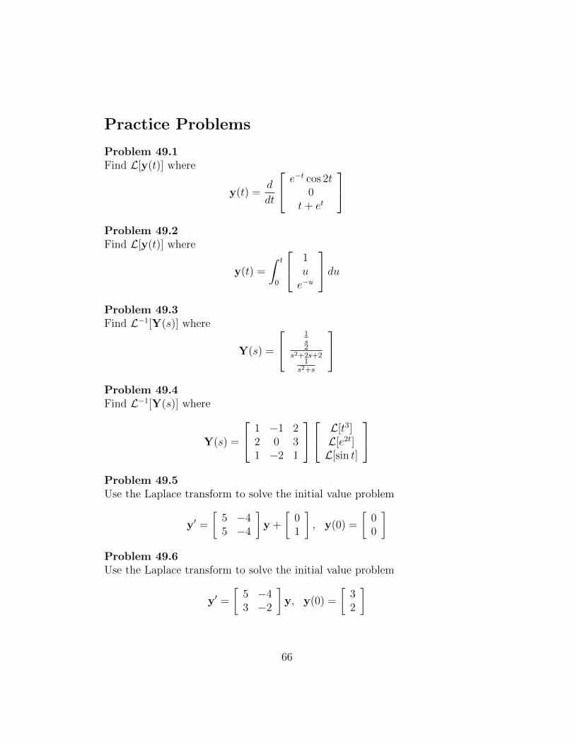
Practice Problems
Problem 49.1Find L[y(t)] where
y(t) =d
dt
e−t cos 2t0
t+ et
Problem 49.2Find L[y(t)] where
y(t) =
∫ t
0
1ue−u
duProblem 49.3Find L−1[Y(s)] where
Y(s) =
1s2
s2+2s+21
s2+s
Problem 49.4Find L−1[Y(s)] where
Y(s) =
1 −1 22 0 31 −2 1
L[t3]L[e2t]L[sin t]
Problem 49.5Use the Laplace transform to solve the initial value problem
y′ =
[5 −45 −4
]y +
[01
], y(0) =
[00
]Problem 49.6Use the Laplace transform to solve the initial value problem
y′ =
[5 −43 −2
]y, y(0) =
[32
]
66
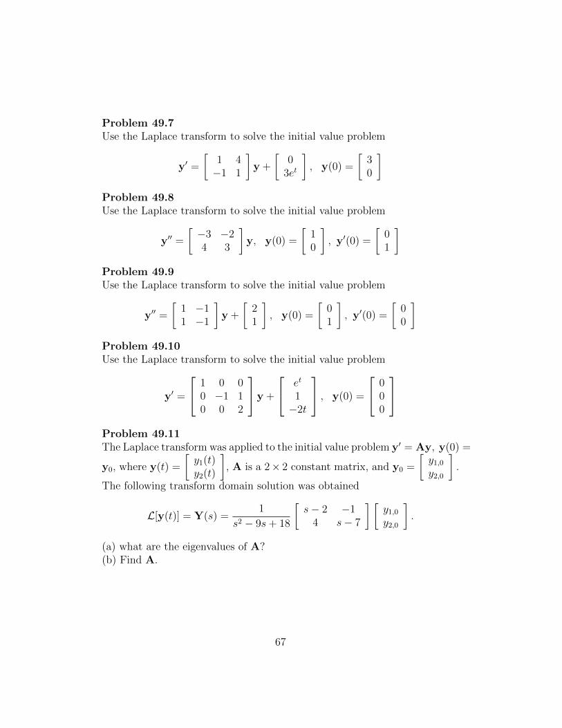
Problem 49.7Use the Laplace transform to solve the initial value problem
y′ =
[1 4−1 1
]y +
[0
3et
], y(0) =
[30
]Problem 49.8Use the Laplace transform to solve the initial value problem
y′′ =
[−3 −24 3
]y, y(0) =
[10
], y′(0) =
[01
]Problem 49.9Use the Laplace transform to solve the initial value problem
y′′ =
[1 −11 −1
]y +
[21
], y(0) =
[01
], y′(0) =
[00
]Problem 49.10Use the Laplace transform to solve the initial value problem
y′ =
1 0 00 −1 10 0 2
y +
et
1−2t
, y(0) =
000
Problem 49.11The Laplace transform was applied to the initial value problem y′ = Ay, y(0) =
y0, where y(t) =
[y1(t)y2(t)
], A is a 2× 2 constant matrix, and y0 =
[y1,0y2,0
].
The following transform domain solution was obtained
L[y(t)] = Y(s) =1
s2 − 9s+ 18
[s− 2 −1
4 s− 7
] [y1,0y2,0
].
(a) what are the eigenvalues of A?(b) Find A.
67
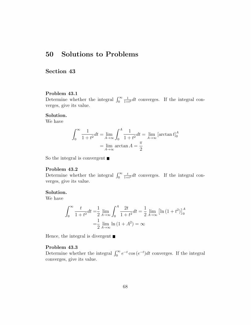
50 Solutions to Problems
Section 43
Problem 43.1Determine whether the integral
∫∞0
11+t2
dt converges. If the integral con-verges, give its value.
Solution.We have ∫ ∞
0
1
1 + t2dt = lim
A→∞
∫ A
0
1
1 + t2dt = lim
A→∞[arctan t]A0
= limA→∞
arctanA =π
2
So the integral is convergent
Problem 43.2Determine whether the integral
∫∞0
t1+t2
dt converges. If the integral con-verges, give its value.
Solution.We have ∫ ∞
0
t
1 + t2dt =
1
2limA→∞
∫ A
0
2t
1 + t2dt =
1
2limA→∞
[ln (1 + t2)
]A0
=1
2limA→∞
ln (1 + A2) =∞
Hence, the integral is divergent
Problem 43.3Determine whether the integral
∫∞0e−t cos (e−t)dt converges. If the integral
converges, give its value.
68
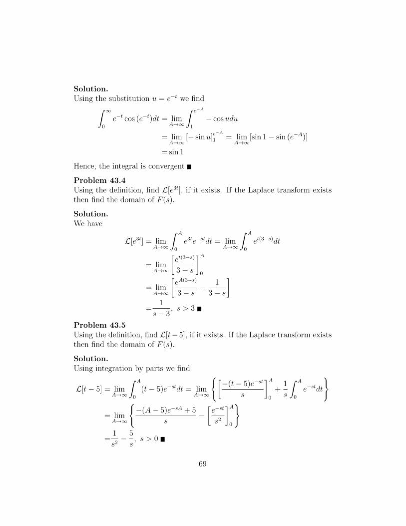
Solution.Using the substitution u = e−t we find∫ ∞
0
e−t cos (e−t)dt = limA→∞
∫ e−A
1
− cosudu
= limA→∞
[− sinu]e−A
1 = limA→∞
[sin 1− sin (e−A)]
= sin 1
Hence, the integral is convergent
Problem 43.4Using the definition, find L[e3t], if it exists. If the Laplace transform existsthen find the domain of F (s).
Solution.We have
L[e3t] = limA→∞
∫ A
0
e3te−stdt = limA→∞
∫ A
0
et(3−s)dt
= limA→∞
[et(3−s)
3− s
]A0
= limA→∞
[eA(3−s)
3− s− 1
3− s
]=
1
s− 3, s > 3
Problem 43.5Using the definition, find L[t− 5], if it exists. If the Laplace transform existsthen find the domain of F (s).
Solution.Using integration by parts we find
L[t− 5] = limA→∞
∫ A
0
(t− 5)e−stdt = limA→∞
{[−(t− 5)e−st
s
]A0
+1
s
∫ A
0
e−stdt
}
= limA→∞
{−(A− 5)e−sA + 5
s−[e−st
s2
]A0
}=
1
s2− 5
s, s > 0
69
Problem 43.6Using the definition, find L[e(t−1)
2], if it exists. If the Laplace transform
exists then find the domain of F (s).
Solution.We have ∫ ∞
0
e(t−1)2
e−stdt =
∫ ∞0
e(t−1)2−stdt.
Since limt→∞(t− 1)2 − st = limt→∞ t2(
1− (2+s)t
+ 1t2
)=∞, for any fixed s
we can choose a positive C such that (t− 1)2− st ≥ 0 for t ≥ C. In this case,e(t−1)
2−st ≥ 1 and this implies that∫∞0e(t−1)
2−stdt ≥∫∞Cdt. The integral on
the right is divergent so that the integral on the left is also divergent by thecomparison theorem of improper integrals. Hence, f(t) = e(t−1)
2does not
have a Laplace transform
Problem 43.7Using the definition, find L[(t − 2)2], if it exists. If the Laplace transformexists then find the domain of F (s).
Solution.We have
L[(t− 2)2] = limT→∞
∫ T
0
(t− 2)2e−stdt.
Using integration by parts with u′ = e−st and v = (t− 2)2 we find∫ T
0
(t− 2)2e−stdt =−[
(t− 2)2e−st
s
]T0
+2
s
∫ T
0
(t− 2)e−stdt
=4
s− (T − 2)2e−sT
s+
2
s
∫ T
0
(t− 2)e−stdt.
Thus,
limT→∞
∫ T
0
(t− 2)2e−stdt =4
s+
2
slimT→∞
∫ T
0
(t− 2)e−stdt.
Using by parts with u′ = e−st and v = t− 2 we find∫ T
0
(t− 2)e−stdt =
[−(t− 2)e−st
s− 1
s2e−st
]T0
.
70
Letting T →∞ in the above expression we find
limT→∞
∫ T
0
(t− 2)e−stdt = −2
s+
1
s2, s > 0.
Hence,
F (s) =4
s+
2
s
(−2
s+
1
s2
)=
4
s− 4
s2+
2
s3, s > 0
Problem 43.8Using the definition, find L[f(t)], if it exists. If the Laplace transform existsthen find the domain of F (s).
f(t) =
{0, 0 ≤ t < 1
t− 1, t ≥ 1
Solution.We have
L[f(t)] = limT→∞
∫ T
1
(t− 1)e−stdt.
Using integration by parts with u′ = e−st and v = t− 1 we find
limT→∞
∫ T
1
(t− 1)e−stdt = limT→∞
[−(t− 1)e−st
s− 1
s2e−st
]T1
=e−s
s2, s > 0
Problem 43.9Using the definition, find L[f(t)], if it exists. If the Laplace transform existsthen find the domain of F (s).
f(t) =
0, 0 ≤ t < 1
t− 1, 1 ≤ t < 20, t ≥ 2.
Solution.We have
L[f(t)] =
∫ 2
1
(t− 1)e−stdt =
[−(t− 1)e−st
s− 1
s2e−st
]21
=− e−2s
s+
1
s2(e−s − e−2s), s 6= 0
71
Problem 43.10Let n be a positive integer. Using integration by parts establish the reductionformula ∫
tne−stdt = −tne−st
s+n
s
∫tn−1e−stdt, s > 0.
Solution.Let u′ = e−st and v = tn. Then u = − e−st
sand v′ = ntn−1. Hence,∫
tne−stdt = −tne−st
s+n
s
∫tn−1e−stdt, s > 0
Problem 43.11For s > 0 and n a positive integer evaluate the limits
(a) limt→0 tne−st (b) limt→∞ t
ne−st
Solution.(a) limt→0 t
ne−st = limt→0tn
est= 0
1= 0.
(b) Using L’Hopital’s rule repeatedly we find
limt→∞
tne−st = · · · = limt→∞
n!
snest= 0
Problem 43.12(a) Use the previous two problems to derive the reduction formula for theLaplace transform of f(t) = tn,
L[tn] =n
sL[tn−1], s > 0.
(b) Calculate L[tk], for k = 1, 2, 3, 4, 5.(c) Formulate a conjecture as to the Laplace transform of f(t), tn with n apositive integer.
Solution.(a) Using the two previous problems we find
L[tn] = limT→∞
∫ T
0
tne−stdt = limT→∞
{−[tne−st
s
]T0
+n
s
∫ T
0
tn−1e−stdt
}
=n
slimT→∞
∫ T
0
tn−1e−stdt =n
sL[tn−1], s > 0
72
(b) We have
L[t] =1
s2
L[t2] =2
sL[t] =
2
s3
L[t3] =3
sL[t2] =
6
s4
L[t4] =4
sL[t3] =
24
s5
L[t5] =5
sL[t4] =
120
s5
(c) By induction, one can easily show that for n = 0, 1, 2, · · ·
L[tn] =n!
sn+1, s > 0
From a table of integrals,∫eαu sin βudu =eαu
α sin βu− β cos βu
α2 + β2∫eαu cos βudu =eαu
α cos βu+ β sin βu
α2 + β2
Problem 43.13Use the above integrals to find the Laplace transform of f(t) = cosωt, if itexists. If the Laplace transform exists, give the domain of F (s).
Solution.We have
L[cosωt] = limT→∞
−
{e−st
[−s cosωt+ ω sinωt
s2 + ω2
]T0
}=
s
s2 + ω2, s > 0
Problem 43.14Use the above integrals to find the Laplace transform of f(t) = sinωt, if itexists. If the Laplace transform exists, give the domain of F (s).
Solution.We have
L[sinωt] = limT→∞
−
{e−st
[−s sinωt+ ω cosωt
s2 + ω2
]T0
}=
ω
s2 + ω2, s > 0
73
Problem 43.15Use the above integrals to find the Laplace transform of f(t) = cosω(t− 2),if it exists. If the Laplace transform exists, give the domain of F (s).
Solution.Using a trigonometric identity we can write f(t) = cosω(t− 2) = cosωt cos 2ω+sinωt sin 2ω. Thus, using the previous two problems we find
L[cosω(t− 2)] =s cos 2ω + ω sin 2ω
s2 + ω2, s > 0
Problem 43.16Use the above integrals to find the Laplace transform of f(t) = e3t sin t, if itexists. If the Laplace transform exists, give the domain of F (s).
Solution.We have
L[e3t sin t] = limT→∞
∫ T
0
e−(s−3)t sin tdt
= limT→∞
−
{e−(s−3)t
[(s− 3) sin t+ cos t
(s− 3)2 + 1
]T0
}=
1
(s− 3)2 + 1, s > 3
Problem 43.17Use the linearity property of Laplace transform to find L[5e−7t + t + 2e2t].Find the domain of F (s).
Solution.We have L[e−7t] = 1
s+7, s > −7, L[t] = 1
s2, s > 0, and L[e2t] = 1
s−2 , s > 2.Hence,
L[5e−7t + t+ 2e2t] = 5L[e−7t] + L[t] + 2L[e2t] =5
s+ 7+
1
s2+
2
s− 2, s > 2
Problem 43.18Consider the function f(t) = tan t.(a) Is f(t) continuous on 0 ≤ t <∞, discontinuous but piecewise continuouson 0 ≤ t <∞, or neither?(b) Are there fixed numbers a and M such that |f(t)| ≤Meat for 0 ≤ t <∞?
74
Solution.(a) Since f(t) = tan t = sin t
cos tand this function is discontinuous at t = (2n +
1)π2. Since this function has vertical asymptotes there it is not piecewise
continuous.(b) The graph of the function does not show that it can be bounded byexponential functions. Hence, no such numbers a and M
Problem 43.19Consider the function f(t) = t2e−t.(a) Is f(t) continuous on 0 ≤ t <∞, discontinuous but piecewise continuouson 0 ≤ t <∞, or neither?(b) Are there fixed numbers a and M such that |f(t)| ≤Meat for 0 ≤ t <∞?
Solution.(a) Since t2 and e−t are continuous everywhere, f(t) = t2e−t is continuous on0 ≤ t <∞.(b) By L’Hopital’s rule one has
limt→∞
t2
et= 0
Since f(0) = 0, f(t) is bounded. Since f ′(t) = (2t − t2)e−t, f(t) has amaximum when t = 2. The value of this maximum is f(2) = 4e−2. Hence,M = 4e−2 and a = 0
Problem 43.20Consider the function f(t) = et
2
e2t+1.
(a) Is f(t) continuous on 0 ≤ t <∞, discontinuous but piecewise continuouson 0 ≤ t <∞, or neither?(b) Are there fixed numbers a and M such that |f(t)| ≤Meat for 0 ≤ t <∞?
Solution.(a) Since et2 and e2t+1 are continuous everywhere, f(t) = et
2
e2t+1is continuous
on 0 ≤ t <∞.(b) Since e2t + 1 ≤ e2t + e2t = 2e2t, f(t) ≥ 1
2et
2e−2t = 1
2et
2−2t. But for t ≥ 4
we have t2 − 2t > t2
2. Hence, f(t) > 1
2et2
2 . So f(t) is not of exponential orderat infinity
75
Problem 43.21Consider the floor function f(t) = btc, where for any integer n we havebtc = n for all n ≤ t < n+ 1.(a) Is f(t) continuous on 0 ≤ t <∞, discontinuous but piecewise continuouson 0 ≤ t <∞, or neither?(b) Are there fixed numbers a and M such that |f(t)| ≤Meat for 0 ≤ t <∞?
Solution.(a) The floor function is a piecewise continuous function on 0 ≤ t <∞.(b) Since btc ≤ t < et for 0 ≥ t <∞ we find M = 1 and a = 1
Problem 43.22Find L−1
(3s−2
).
Solution.Since L
(1s−a
)= 1
s−a , s > a we find
L−1(
3
s− 2
)= 3L−1
(1
s− 2
)= 3e2t, t ≥ 0
Problem 43.23Find L−1
(− 2s2
+ 1s+1
).
Solution.Since L[t] = 1
s2, s > 0 and L
(1s−a
)= 1
s−a , s > a we find
L−1(− 2
s2+
1
s+ 1
)=− 2L−1
(1
s2
)+ L−1
(1
s+ 1
)=− 2t+ e−t, t ≥ 0
Problem 43.24Find L−1
(2s+2
+ 2s−2
).
Solution.We have
L−1(
2
s+ 2+
2
s− 2
)= 2L−1
(1
s+ 2
)+2L−1
(1
s− 2
)= 2(e−2t+e2t), t ≥ 0
76
Section 44
Problem 44.1Use Table L to find L[2et + 5].
Solution.
L[2et + 5] = 2L[et] + 5L[1] =2
s− 1+
5
s, s > 1
Problem 44.2Use Table L to find L[e3t−3h(t− 1)].
Solution.
L[e3t−3h(t− 1)] = L[e3(t−1)h(t− 1)] = e−sL[e3t] =e−s
s− 3, s > 3
Problem 44.3Use Table L to find L[sin2 ωt].
Solution.
L[sin2 ωt] = L[1− cos 2ωt
2] =
1
2(L[1]−L[cos 2ωt]) =
1
2
(1
s− s
s2 + 4ω2
), s > 0
Problem 44.4Use Table L to find L[sin 3t cos 3t].
Solution.
L[sin 3t cos 3t] = L[
sin 6t
2
]=
1
2L[sin 6t] =
3
s2 + 36, s > 0
Problem 44.5Use Table L to find L[e2t cos 3t].
Solution.
L[e2t cos 3t] =s− 2
(s− 2)2 + 9, s > 2
77
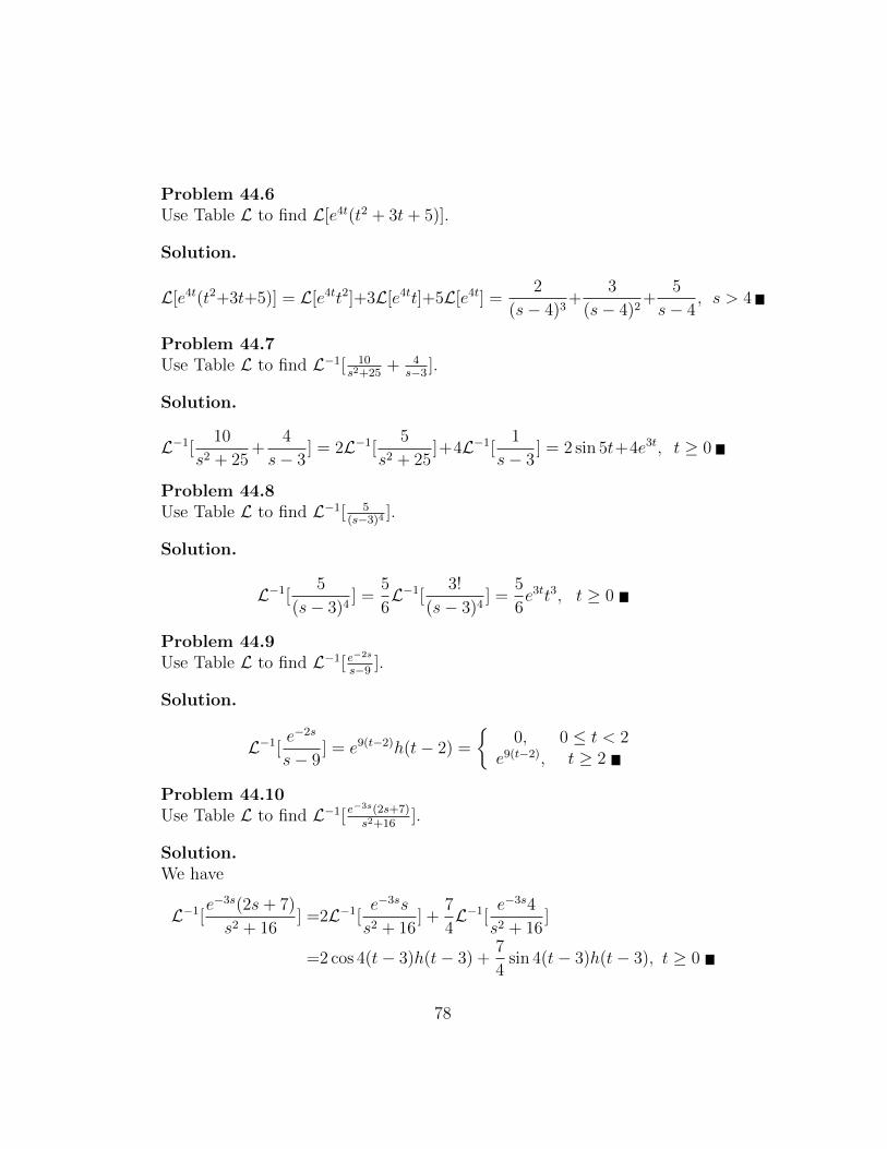
Problem 44.6Use Table L to find L[e4t(t2 + 3t+ 5)].
Solution.
L[e4t(t2+3t+5)] = L[e4tt2]+3L[e4tt]+5L[e4t] =2
(s− 4)3+
3
(s− 4)2+
5
s− 4, s > 4
Problem 44.7Use Table L to find L−1[ 10
s2+25+ 4
s−3 ].
Solution.
L−1[ 10
s2 + 25+
4
s− 3] = 2L−1[ 5
s2 + 25]+4L−1[ 1
s− 3] = 2 sin 5t+4e3t, t ≥ 0
Problem 44.8Use Table L to find L−1[ 5
(s−3)4 ].
Solution.
L−1[ 5
(s− 3)4] =
5
6L−1[ 3!
(s− 3)4] =
5
6e3tt3, t ≥ 0
Problem 44.9Use Table L to find L−1[ e−2s
s−9 ].
Solution.
L−1[ e−2s
s− 9] = e9(t−2)h(t− 2) =
{0, 0 ≤ t < 2
e9(t−2), t ≥ 2
Problem 44.10Use Table L to find L−1[ e
−3s(2s+7)s2+16
].
Solution.We have
L−1[e−3s(2s+ 7)
s2 + 16] =2L−1[ e
−3ss
s2 + 16] +
7
4L−1[ e
−3s4
s2 + 16]
=2 cos 4(t− 3)h(t− 3) +7
4sin 4(t− 3)h(t− 3), t ≥ 0
78
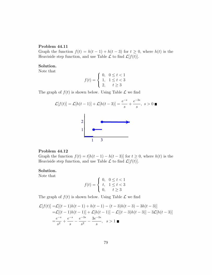
Problem 44.11Graph the function f(t) = h(t − 1) + h(t − 3) for t ≥ 0, where h(t) is theHeaviside step function, and use Table L to find L[f(t)].
Solution.Note that
f(t) =
0, 0 ≤ t < 11, 1 ≤ t < 32, t ≥ 3
The graph of f(t) is shown below. Using Table L we find
L[f(t)] = L[h(t− 1)] + L[h(t− 3)] =e−s
s+e−3s
s, s > 0
Problem 44.12Graph the function f(t) = t[h(t− 1)− h(t− 3)] for t ≥ 0, where h(t) is theHeaviside step function, and use Table L to find L[f(t)].
Solution.Note that
f(t) =
0, 0 ≤ t < 1t, 1 ≤ t < 30, t ≥ 3
The graph of f(t) is shown below. Using Table L we find
L[f(t)] =L[(t− 1)h(t− 1) + h(t− 1)− (t− 3)h(t− 3)− 3h(t− 3)]
=L[(t− 1)h(t− 1)] + L[h(t− 1)]− L[(t− 3)h(t− 3)]− 3L[h(t− 3)]
=e−s
s2+e−s
s− e−3s
s2− 3e−3s
s, s > 1
79
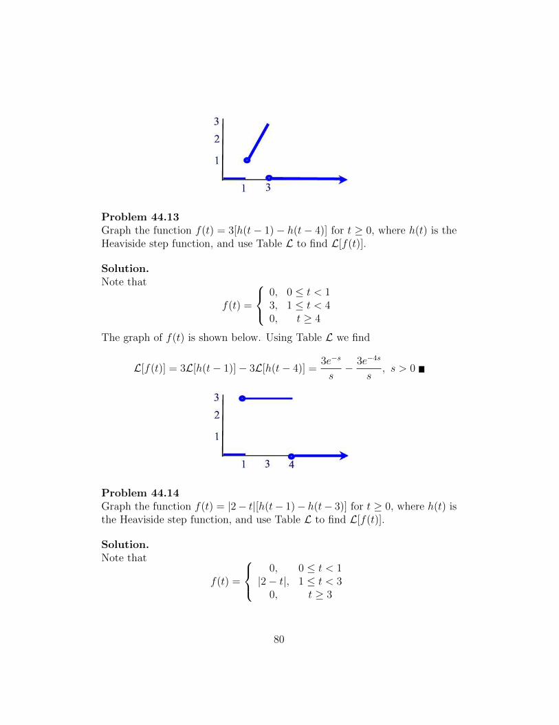
Problem 44.13Graph the function f(t) = 3[h(t− 1)− h(t− 4)] for t ≥ 0, where h(t) is theHeaviside step function, and use Table L to find L[f(t)].
Solution.Note that
f(t) =
0, 0 ≤ t < 13, 1 ≤ t < 40, t ≥ 4
The graph of f(t) is shown below. Using Table L we find
L[f(t)] = 3L[h(t− 1)]− 3L[h(t− 4)] =3e−s
s− 3e−4s
s, s > 0
Problem 44.14Graph the function f(t) = |2− t|[h(t− 1)− h(t− 3)] for t ≥ 0, where h(t) isthe Heaviside step function, and use Table L to find L[f(t)].
Solution.Note that
f(t) =
0, 0 ≤ t < 1
|2− t|, 1 ≤ t < 30, t ≥ 3
80
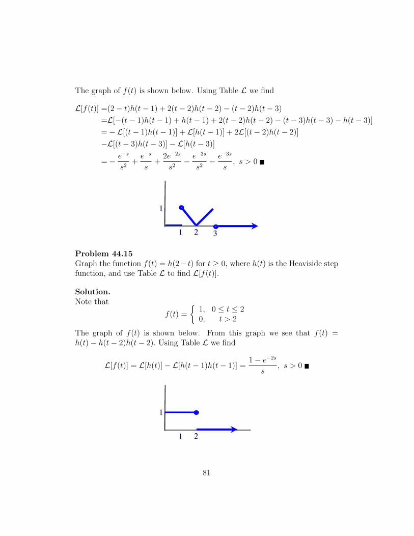
The graph of f(t) is shown below. Using Table L we find
L[f(t)] =(2− t)h(t− 1) + 2(t− 2)h(t− 2)− (t− 2)h(t− 3)
=L[−(t− 1)h(t− 1) + h(t− 1) + 2(t− 2)h(t− 2)− (t− 3)h(t− 3)− h(t− 3)]
=− L[(t− 1)h(t− 1)] + L[h(t− 1)] + 2L[(t− 2)h(t− 2)]
−L[(t− 3)h(t− 3)]− L[h(t− 3)]
=− e−s
s2+e−s
s+
2e−2s
s2− e−3s
s2− e−3s
s, s > 0
Problem 44.15Graph the function f(t) = h(2− t) for t ≥ 0, where h(t) is the Heaviside stepfunction, and use Table L to find L[f(t)].
Solution.Note that
f(t) =
{1, 0 ≤ t ≤ 20, t > 2
The graph of f(t) is shown below. From this graph we see that f(t) =h(t)− h(t− 2)h(t− 2). Using Table L we find
L[f(t)] = L[h(t)]− L[h(t− 1)h(t− 1)] =1− e−2s
s, s > 0
81
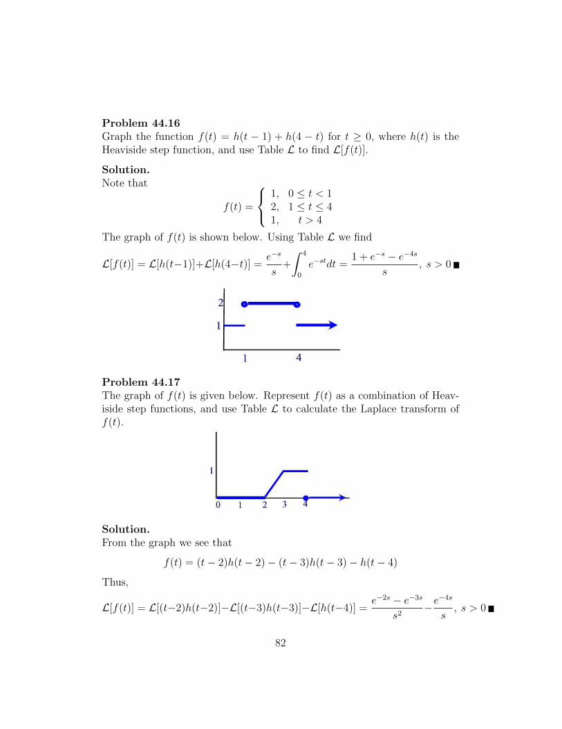
Problem 44.16Graph the function f(t) = h(t − 1) + h(4 − t) for t ≥ 0, where h(t) is theHeaviside step function, and use Table L to find L[f(t)].
Solution.Note that
f(t) =
1, 0 ≤ t < 12, 1 ≤ t ≤ 41, t > 4
The graph of f(t) is shown below. Using Table L we find
L[f(t)] = L[h(t−1)]+L[h(4−t)] =e−s
s+
∫ 4
0
e−stdt =1 + e−s − e−4s
s, s > 0
Problem 44.17The graph of f(t) is given below. Represent f(t) as a combination of Heav-iside step functions, and use Table L to calculate the Laplace transform off(t).
Solution.From the graph we see that
f(t) = (t− 2)h(t− 2)− (t− 3)h(t− 3)− h(t− 4)
Thus,
L[f(t)] = L[(t−2)h(t−2)]−L[(t−3)h(t−3)]−L[h(t−4)] =e−2s − e−3s
s2−e−4s
s, s > 0
82
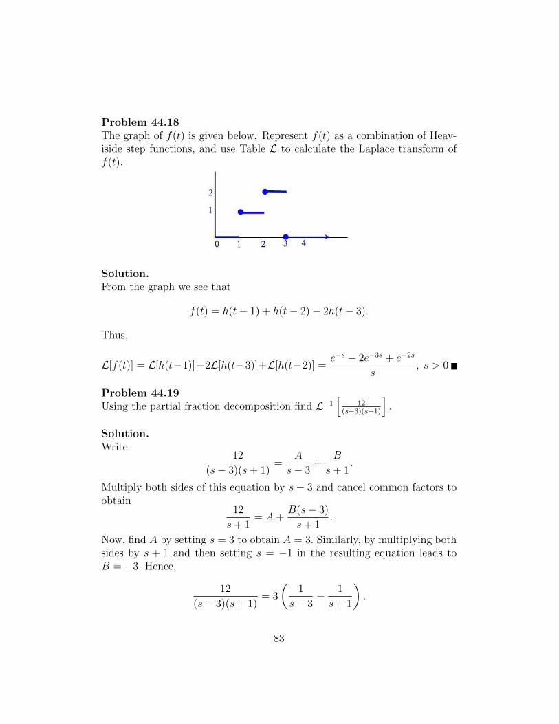
Problem 44.18The graph of f(t) is given below. Represent f(t) as a combination of Heav-iside step functions, and use Table L to calculate the Laplace transform off(t).
Solution.From the graph we see that
f(t) = h(t− 1) + h(t− 2)− 2h(t− 3).
Thus,
L[f(t)] = L[h(t−1)]−2L[h(t−3)]+L[h(t−2)] =e−s − 2e−3s + e−2s
s, s > 0
Problem 44.19Using the partial fraction decomposition find L−1
[12
(s−3)(s+1)
].
Solution.Write
12
(s− 3)(s+ 1)=
A
s− 3+
B
s+ 1.
Multiply both sides of this equation by s− 3 and cancel common factors toobtain
12
s+ 1= A+
B(s− 3)
s+ 1.
Now, find A by setting s = 3 to obtain A = 3. Similarly, by multiplying bothsides by s + 1 and then setting s = −1 in the resulting equation leads toB = −3. Hence,
12
(s− 3)(s+ 1)= 3
(1
s− 3− 1
s+ 1
).
83
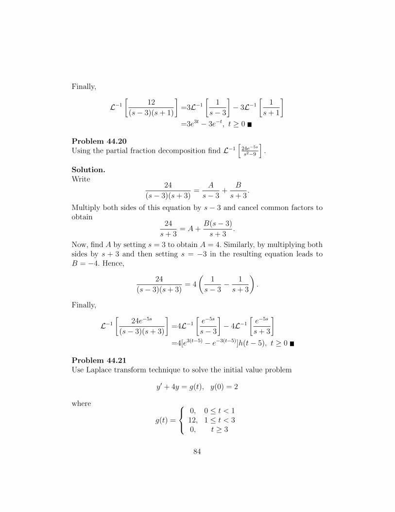
Finally,
L−1[
12
(s− 3)(s+ 1)
]=3L−1
[1
s− 3
]− 3L−1
[1
s+ 1
]=3e3t − 3e−t, t ≥ 0
Problem 44.20Using the partial fraction decomposition find L−1
[24e−5s
s2−9
].
Solution.Write
24
(s− 3)(s+ 3)=
A
s− 3+
B
s+ 3.
Multiply both sides of this equation by s− 3 and cancel common factors toobtain
24
s+ 3= A+
B(s− 3)
s+ 3.
Now, find A by setting s = 3 to obtain A = 4. Similarly, by multiplying bothsides by s + 3 and then setting s = −3 in the resulting equation leads toB = −4. Hence,
24
(s− 3)(s+ 3)= 4
(1
s− 3− 1
s+ 3
).
Finally,
L−1[
24e−5s
(s− 3)(s+ 3)
]=4L−1
[e−5s
s− 3
]− 4L−1
[e−5s
s+ 3
]=4[e3(t−5) − e−3(t−5)]h(t− 5), t ≥ 0
Problem 44.21Use Laplace transform technique to solve the initial value problem
y′ + 4y = g(t), y(0) = 2
where
g(t) =
0, 0 ≤ t < 112, 1 ≤ t < 30, t ≥ 3
84
Solution.Note first that g(t) = 12[h(t− 1)− h(t− 3)] so that
L[g(t)] = 12L[h(t− 1)]− 12L[h(t− 3)] =12(e−s − e−3s)
s, s > 0.
Now taking the Laplace transform of the DE and using linearity we find
L[y′] + 4L[y] = L[g(t)].
But L[y′] = sL[y]− y(0) = sL[y]− 2. Letting L[y] = Y (s) we obtain
sY (s)− 2 + 4Y (s) = 12e−s − e−3s
s.
Solving for Y (s) we find
Y (s) =2
s+ 4+ 12
e−s − e−3s
s(s+ 4).
But
L−1[
2
s+ 4
]= 2e−4t
and
L−1[12e−s − e−3s
s(s+ 4)
]=3L−1
[(e−s − e−3s)
(1
s− 1
s+ 4
)]=3L−1
[e−s
s
]− 3L−1
[e−3s
s
]− 3L−1
[e−s
s+ 4
]+ 3L−1
[e−3s
s+ 4
]=3h(t− 1)− 3h(t− 3)− 3e−4(t−1)h(t− 1) + 3e−4(t−3)h(t− 3)
Hence,
y(t) = 2e−4t+3[h(t−1)−h(t−3)]−3[e−4(t−1)h(t−1)−e−4(t−3)h(t−3)], t ≥ 0
Problem 44.22Use Laplace transform technique to solve the initial value problem
y′′ − 4y = e3t, y(0) = 0, y′(0) = 0.
85
Solution.Taking the Laplace transform of the DE and using linearity we find
L[y′′]− 4L[y] = L[e3t].
But L[y′′] = s2L[y]− sy(0)− y′(0) = s2L[y]. Letting L[y] = Y (s) we obtain
s2Y (s)− 4Y (s) =1
s− 3.
Solving for Y (s) we find
Y (s) =1
(s− 3)(s− 2)(s+ 2).
Using partial fraction decomposition
1
(s− 3)(s− 2)(s+ 2)=
A
s− 3+
B
s+ 2+
C
s− 2
we find A = 15, B = 1
20, and C = −1
4. Thus,
y(t) =L−1[
1
(s− 3)(s− 2)(s+ 2)
]=
1
5L−1
[1
s− 3
]+
1
20L−1
[1
s+ 2
]− 1
4L−1
[1
s− 2
]=
1
5e3t +
1
20e−2t − 1
4e2t, t ≥ 0
Problem 44.23Obtain the Laplace transform of the function
∫ t2f(λ)dλ in terms of L[f(t)] =
F (s) given that∫ 2
0f(λ)dλ = 3.
Solution.We have
L[∫ t
2
f(λ)dλ
]=L
[∫ t
0
f(λ)dλ−∫ 2
0
f(λ)dλ
]=F (s)
s− L[3]
=F (s)
s− 3
s, s > 0
86
Section 45
In Problems 45.1 - 45.4, give the form of the partial fraction expansion forF (s). You need not evaluate the constants in the expansion. However, if thedenominator has an irreducible quadratic expression then use the completingthe square process to write it as the sum/difference of two squares.
Problem 45.1
F (s) =s3 + 3s+ 1
(s− 1)3(s− 2)2.
Solution.
F (s) =A1
(s− 1)3+
A2
(s− 1)2+
A3
s− 1+
B1
(s− 2)2+
B2
s− 2
Problem 45.2
F (s) =s2 + 5s− 3
(s2 + 16)(s− 2).
Solution.
F (s) =A1s+ A2
s2 + 16+
B1
s− 2
Problem 45.3
F (s) =s3 − 1
(s2 + 1)2(s+ 4)2.
Solution.
F (s) =A1s+ A2
(s2 + 1)2+A3s+ A4
s2 + 1+
B1
(s+ 4)2+
B2
s+ 4
Problem 45.4
F (s) =s4 + 5s2 + 2s− 9
(s2 + 8s+ 17)(s− 2)2.
87
Solution.
F (s) =A1
(s− 2)2+
A2
s− 2+
B1s+B2
(s+ 4)2 + 1
Problem 45.5Find L−1
[1
(s+1)3
].
Solution.Using Table L we find L−1
[1
(s+1)3
]= 1
2e−tt2, t ≥ 0
Problem 45.6Find L−1
[2s−3
s2−3s+2
].
Solution.We factor the denominator and split the rational function into partial frac-tions:
2s− 3
(s− 1)(s− 2)=
A
s− 1+
B
s− 2.
Multiplying both sides by (s− 1)(s− 2) and simplifying to obtain
2s− 3 =A(s− 2) +B(s− 1)
=(A+B)s− 2A−B.
Equating coefficients of like powers of s we obtain the system{A+B = 2−2A−B = −3.
Solving this system by elimination we find A = 1 and B = 1. Now findingthe inverse Laplace transform to obtain
L−1[
2s− 3
(s− 1)(s− 2)
]= L−1
[1
s− 1
]+ L−1
[1
s− 2
]= et + e2t, t ≥ 0.
Problem 45.7Find L−1
[4s2+s+1s3+s
].
88
Solution.We factor the denominator and split the rational function into partial frac-tions:
4s2 + s+ 1
s(s2 + 1)=A
s+Bs+ C
s2 + 1.
Multiplying both sides by s(s2 + 1) and simplifying to obtain
4s2 + s+ 1 =A(s2 + 1) + (Bs+ C)s
=(A+B)s2 + Cs+ A.
Equating coefficients of like powers of s we obtain A+B = 4, C = 1, A = 1.Thus, B = 3. Now finding the inverse Laplace transform to obtain
L−1[
4s2 + s+ 1
s(s2 + 1)
]=L−1
[1
s
]+ 3L−1
[s
s2 + 1
]+ L−1
[1
s2 + 1
]=1 + 3 cos t+ sin t, t ≥ 0
Problem 45.8Find L−1
[s2+6s+8s4+8s2+16
].
Solution.We factor the denominator and split the rational function into partial frac-tions:
s2 + 6s+ 8
(s2 + 4)2=B1s+ C1
s2 + 4+B2s+ C2
(s2 + 4)2.
Multiplying both sides by (s2 + 4)2 and simplifying to obtain
s2 + 6s+ 8 =(B1s+ C1)(s2 + 4) +B2s+ C2
=B1s3 + C1s
2 + (4B1 +B2)s+ 4C1 + C2.
Equating coefficients of like powers of s we obtain B1 = 0, C1 = 1, B2 = 6,and C2 = 4. Now finding the inverse Laplace transform to obtain
L−1[s2 + 6s+ 8
(s2 + 4)2
]=L−1
[1
s2 + 4
]+ 6L−1
[s
(s2 + 4)2
]+ 4L−1
[1
(s2 + 4)2
]=
1
2sin 2t+ 6
(t
4sin 2t
)+ 4
(1
16[sin 2t− 2t cos 2t]
)=
3
2t sin 2t+
3
4sin 2t− 1
2t cos 2t, t ≥ 0
89
Problem 45.9Use Laplace transform to solve the initial value problem
y′ + 2y = 26 sin 3t, y(0) = 3.
Solution.Taking the Laplace of both sides to obtain
L[y′] + 2L[y] = 26L[sin 3t].
Using Table L the last equation reduces to
sY (s)− y(0) + 2Y (s) = 26
(3
s2 + 9
).
Solving this equation for Y (s) we find
Y (s) =3
s+ 2+
78
(s+ 2)(s2 + 9).
Using the partial fraction decomposition we can write
1
(s+ 2)(s2 + 9)=
A
s+ 2+Bs+ C
s2 + 9.
Multipliying both sides by (s+ 2)(s2 + 9) to obtain
1 =A(s2 + 9) + (Bs+ C)(s+ 2)
=(A+B)s2 + (2B + C)s+ 9A+ 2C.
Equating coefficients of like powers of s we find A+B = 0, 2B+C = 0, and9A + 2C = 1. Solving this system we find A = 1
13, B = − 1
13, and C = 2
13.
Thus,
Y (s) =9
s+ 2− 6
(s
s2 + 9
)+ 4
(3
s2 + 9
).
Finally,
y(t) = L−1[Y (s)] = 9L−1[
1
s+ 2
]− 6L−1
[s
s2 + 9
]+ 4L−1
[3
s2 + 9
]= 9e−2t − 6 cos 3t+ 4 sin 3t, t ≥ 0
90
Problem 45.10Use Laplace transform to solve the initial value problem
y′ + 2y = 4t, y(0) = 3.
Solution.Taking the Laplace of both sides to obtain
L[y′] + 2L[y] = 4L[t].
Using Table L the last equation reduces to
sY (s)− y(0) + 2Y (s) =4
s2.
Solving this equation for Y (s) we find
Y (s) =3
s+ 2+
4
(s+ 2)s2.
Using the partial fraction decomposition we can write
1
(s+ 2)s2=
A
s+ 2+Bs+ C
s2.
Multipliying both sides by (s+ 2)s2 to obtain
1 = As2 + (Bs+ C)(s+ 2)
= (A+B)s2 + (2B + C)s+ 2C
Equating coefficients of like powers of s we find A+B = 0, 2B+C = 0, and2C = 1. Solving this system we find A = 1
4, B = −1
4, and C = 1
2. Thus,
Y (s) =4
s+ 2− 1
s+ 2
1
s2.
Finally,
y(t) = L−1[Y (s)] = 4L−1[
1
s+ 2
]− L−1
[1
s
]+ 2L−1
[1
s2
]= 4e−2t − 1 + 2t, t ≥ 0
91
Problem 45.11Use Laplace transform to solve the initial value problem
y′′ + 3y′ + 2y = 6e−t, y(0) = 1, y′(0) = 2.
Solution.Taking the Laplace of both sides to obtain
L[y′′] + 3L[y′] + 2L[y] = 6L[e−t].
Using Table L the last equation reduces to
s2Y (s)− sy(0)− y′(0) + 3(sY (s)− y(0)) + 2Y (s) =6
s+ 1.
Solving this equation for Y (s) we find
Y (s) =s+ 5
(s+ 1)(s+ 2)+
6
(s+ 2)(s+ 1)2=
s2 + 6s+ 11
(s+ 1)2(s+ 2).
Using the partial fraction decomposition we can write
s2 + 6s+ 11
(s+ 2)(s+ 1)2=
A
s+ 2+
B
s+ 1+
C
(s+ 1)2.
Multipliying both sides by (s+ 2)(s+ 1)2 to obtain
s2 + 6s+ 11 = A(s+ 1)2 +B(s+ 1)(s+ 2) + C(s+ 2)
= (A+B)s2 + (2A+ 3B + C)s+ A+ 2B + 2C
Equating coefficients of like powers of s we find A+B = 1, 2A+3B+C = 6,and A + 2B + 2C = 11. Solving this system we find A = 3, B = −2, andC = 6. Thus,
Y (s) =3
s+ 2− 2
s+ 1+
6
(s+ 1)2.
Finally,
y(t) = L−1[Y (s)] = 3L−1[
1
s+ 2
]− 2L−1
[1
s+ 1
]+ 6L−1
[1
(s+ 1)2
]= 3e−2t − 2e−t + 6te−t, t ≥ 0
92
Problem 45.12Use Laplace transform to solve the initial value problem
y′′ + 4y = cos 2t, y(0) = 1, y′(0) = 1.
Solution.Taking the Laplace of both sides to obtain
L[y′′] + 4L[y] = L[cos 2t].
Using Table L the last equation reduces to
s2Y (s)− sy(0)− y′(0) + 4Y (s) =s
s2 + 4.
Solving this equation for Y (s) we find
Y (s) =s+ 1
s2 + 4+
s
(s2 + 4)2.
Using Table L again we find
y(t) = L−1[
s
s2 + 4
]+
1
2L−1
[2
s2 + 4
]+ L−1
[s
(s2 + 4)2
]= cos 2t+
1
2sin 2t+
t
4sin 2t, t ≥ 0
Problem 45.13Use Laplace transform to solve the initial value problem
y′′ − 2y′ + y = e2t, y(0) = 0, y′(0) = 0.
Solution.Taking the Laplace of both sides to obtain
L[y′′]− 2L[y′] + L[y] = L[e2t].
Using Table L the last equation reduces to
s2Y (s)− sy(0)− y′(0)− 2sY (s) + 2y(0) + Y (s) =1
s− 2.
93
Solving this equation for Y (s) we find
Y (s) =1
(s− 1)2(s− 2).
Using the partial fraction decomposition, we can write
Y (s) =A
s− 1+
B
(s− 1)2+
C
s− 2.
Multipliying both sides by (s− 2)(s− 1)2 to obtain
1 = A(s− 1)(s− 2) +B(s− 2) + C(s− 1)2
= (A+ C)s2 + (−3A+B − 2C)s+ 2A− 2B + C
Equating coefficients of like powers of s we find A+C = 0, −3A+B−2C = 0,and 2A − 2B + C = 1. Solving this system we find A = −1, B = −1, andC = 1. Thus,
Y (s) = − 1
s− 1− 1
(s− 1)2+
1
s− 2.
Finally,
y(t) = L−1[Y (s)] = −L−1[
1
s− 1
]− L−1
[1
(s− 1)2
]+ L−1
[1
s− 2
]= −et − tet + e2t, t ≥ 0
Problem 45.14Use Laplace transform to solve the initial value problem
y′′ + 9y = g(t), y(0) = 1, y′(0) = 3
where
g(t) =
{6, 0 ≤ t < π0, π ≤ t <∞
Solution.Taking the Laplace of both sides to obtain
L[y′′] + 9L[y] = L[g(t)] = 6L[h(t)− h(t− π)].
94
Using Table L the last equation reduces to
s2Y (s)− sy(0)− y′(0) + 9Y (s) =6
s− 6e−πs
s.
Solving this equation for Y (s) we find
Y (s) =s+ 3
s2 + 9+
6
s(s2 + 9)(1− e−πs).
Using the partial fraction decomposition, we can write
6
s(s2 + 9)=A
s+Bs+ C
s2 + 9.
Multipliying both sides by s(s2 + 9) to obtain
6 = A(s2 + 9) + (Bs+ C)s
= (A+B)s2 + Cs+ 9A
Equating coefficients of like powers of s we find A + B = 0, C = 0, and9A = 6. Solving this system we find A = 2
3, B = −2
3, and C = 0. Thus,
Y (s) =s
s2 + 9+
3
s2 + 9+ (1− e−πs)
(2
3
1
s− 2
3
s
s2 + 9
).
Finally,
y(t) = L−1[Y (s)] = cos 3t+ sin 3t+2
3(1− cos 3t)− 2
3(1− cos 3(t− π))h(t− π)
= cos 3t+ sin 3t+2
3(1− cos 3t)− 2
3(1 + cos 3t)h(t− π), t ≥ 0
Problem 45.15Determine the constants α, β, y0, and y′0 so that Y (s) = 2s−1
s2+s+2is the Laplace
transform of the solution to the initial value problem
y′′ + αy′ + βy = 0, y(0) = y0, y′(0) = y′0.
Solution.Taking the Laplace transform of both sides we find
s2Y (s)− sy0 − y′0 + αsY (s)− αy0 + βY (s) = 0.
95
Solving for Y (s) we find
Y (s) =sy0 + (y′0 + αy0)
s2 + αs+ β=
2s− 1
s2 + s+ 2.
By identification we find α = 1, β = 2, y0 = 2, and y′0 = −3
Problem 45.16Determine the constants α, β, y0, and y′0 so that Y (s) = s
(s+1)2is the Laplace
transform of the solution to the initial value problem
y′′ + αy′ + βy = 0, y(0) = y0, y′(0) = y′0.
Solution.Taking the Laplace transform of both sides we find
s2Y (s)− sy0 − y′0 + αsY (s)− αy0 + βY (s) = 0.
Solving for Y (s) we find
Y (s) =sy0 + (y′0 + αy0)
s2 + αs+ β=
s
s2 + 2s+ 1.
By identification we find α = 2, β = 1, y0 = 1, and y′0 = −2
96
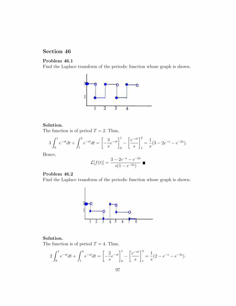
Section 46
Problem 46.1Find the Laplace transform of the periodic function whose graph is shown.
Solution.The function is of period T = 2. Thus,
3
∫ 1
0
e−stdt+
∫ 2
1
e−stdt =
[−3
se−st
]10
−[e−st
s
]21
=1
s(3− 2e−s − e−2s).
Hence,
L[f(t)] =3− 2e−s − e−2s
s(1− e−2s)
Problem 46.2Find the Laplace transform of the periodic function whose graph is shown.
Solution.The function is of period T = 4. Thus,
2
∫ 1
0
e−stdt+
∫ 3
1
e−stdt =
[−2
se−st
]10
−[e−st
s
]31
=1
s(2− e−s − e−3s).
97
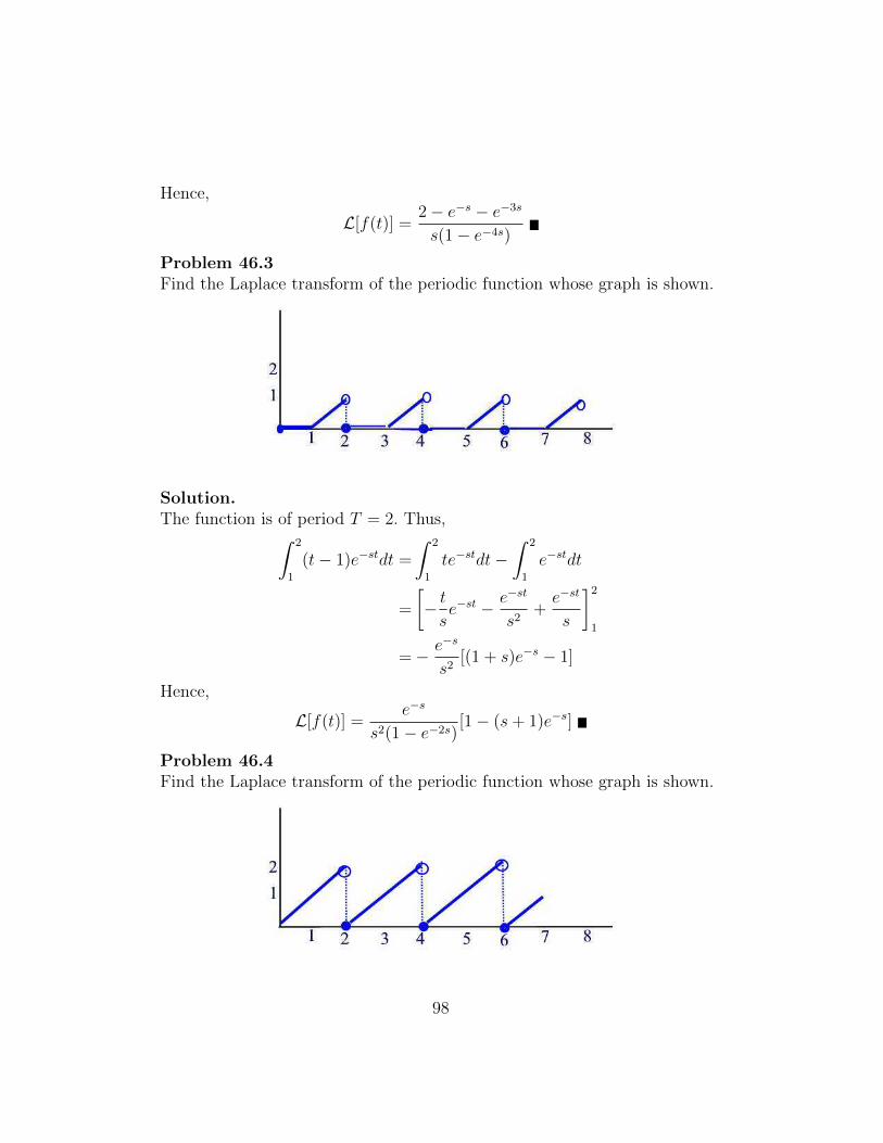
Hence,
L[f(t)] =2− e−s − e−3s
s(1− e−4s)Problem 46.3Find the Laplace transform of the periodic function whose graph is shown.
Solution.The function is of period T = 2. Thus,∫ 2
1
(t− 1)e−stdt =
∫ 2
1
te−stdt−∫ 2
1
e−stdt
=
[− tse−st − e−st
s2+e−st
s
]21
=− e−s
s2[(1 + s)e−s − 1]
Hence,
L[f(t)] =e−s
s2(1− e−2s)[1− (s+ 1)e−s]
Problem 46.4Find the Laplace transform of the periodic function whose graph is shown.
98
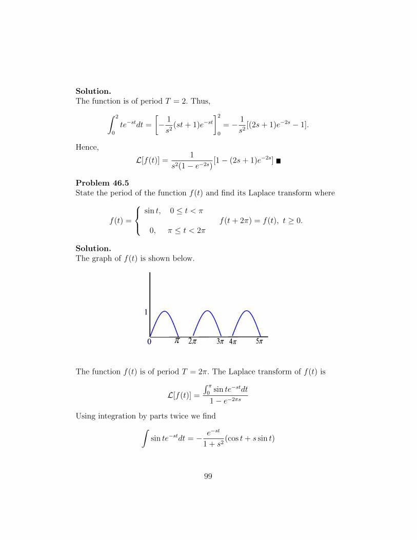
Solution.The function is of period T = 2. Thus,∫ 2
0
te−stdt =
[− 1
s2(st+ 1)e−st
]20
= − 1
s2[(2s+ 1)e−2s − 1].
Hence,
L[f(t)] =1
s2(1− e−2s)[1− (2s+ 1)e−2s]
Problem 46.5State the period of the function f(t) and find its Laplace transform where
f(t) =
sin t, 0 ≤ t < π
f(t+ 2π) = f(t), t ≥ 0.0, π ≤ t < 2π
Solution.The graph of f(t) is shown below.
The function f(t) is of period T = 2π. The Laplace transform of f(t) is
L[f(t)] =
∫ π0
sin te−stdt
1− e−2πs
Using integration by parts twice we find∫sin te−stdt = − e−st
1 + s2(cos t+ s sin t)
99
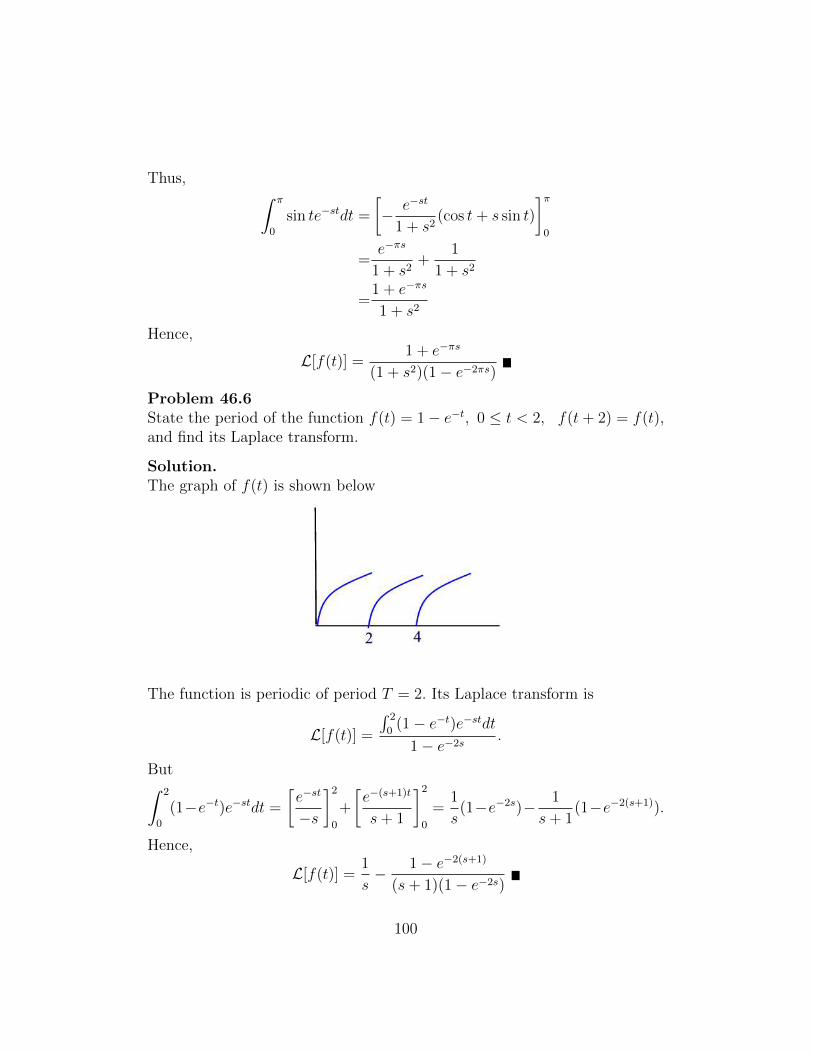
Thus, ∫ π
0
sin te−stdt =
[− e−st
1 + s2(cos t+ s sin t)
]π0
=e−πs
1 + s2+
1
1 + s2
=1 + e−πs
1 + s2
Hence,
L[f(t)] =1 + e−πs
(1 + s2)(1− e−2πs)Problem 46.6State the period of the function f(t) = 1− e−t, 0 ≤ t < 2, f(t+ 2) = f(t),and find its Laplace transform.
Solution.The graph of f(t) is shown below
The function is periodic of period T = 2. Its Laplace transform is
L[f(t)] =
∫ 2
0(1− e−t)e−stdt
1− e−2s.
But∫ 2
0
(1−e−t)e−stdt =
[e−st
−s
]20
+
[e−(s+1)t
s+ 1
]20
=1
s(1−e−2s)− 1
s+ 1(1−e−2(s+1)).
Hence,
L[f(t)] =1
s− 1− e−2(s+1)
(s+ 1)(1− e−2s)
100
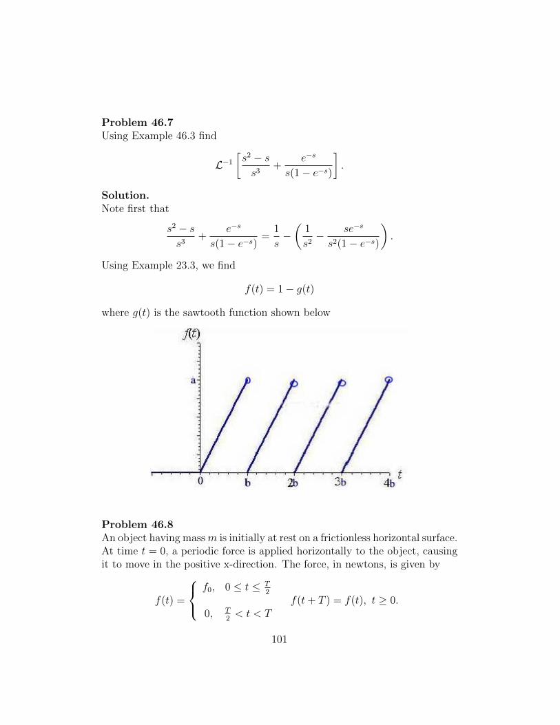
Problem 46.7Using Example 46.3 find
L−1[s2 − ss3
+e−s
s(1− e−s)
].
Solution.Note first that
s2 − ss3
+e−s
s(1− e−s)=
1
s−(
1
s2− se−s
s2(1− e−s)
).
Using Example 23.3, we find
f(t) = 1− g(t)
where g(t) is the sawtooth function shown below
Problem 46.8An object having massm is initially at rest on a frictionless horizontal surface.At time t = 0, a periodic force is applied horizontally to the object, causingit to move in the positive x-direction. The force, in newtons, is given by
f(t) =
f0, 0 ≤ t ≤ T
2
f(t+ T ) = f(t), t ≥ 0.0, T
2< t < T
101
The initial value problem for the horizontal position, x(t), of the object is
mx′′(t) = f(t), x(0) = x′(0) = 0.
(a) Use Laplace transforms to determine the velocity, v(t) = x′(t), and theposition, x(t), of the object.(b) Let m = 1 kg, f0 = 1 N, and T = 1 sec. What is the velocity, v, andposition, x, of the object at t = 1.25 sec?
Solution.
(a) Taking Laplace transform of both sides we find ms2X(s) =f0
∫ T2
0 e−stdt
1−e−sT =
f0s
(1−e−s
T2
1−e−sT
). Solving for X(s) we find
X(s) =f0m· 1
s3· 1
1 + e−sT2
.
Also,
V (s) = L[v(t)] = sX(s) =f0m· 1
s2· 1
1 + e−sT2
=1
m· 1
s· 1
s(1 + e−sT2 ).
Hence, by Example 46.1 and Table L we can write
v(t) =1
m
∫ t
0
f(u)du.
Since X(s) = 1m
1s2
f0
s(1+e−sT2 )
= 1mL[t]L[f(t)] = 1
mL[t ∗ f(t)] we have
x(t) =1
m(t ∗ f(t)) =
1
m
∫ t
0
(t− u)f(u)du.
(b) We have x(1.25) =∫ 1
2
0(54−u)du+
∫ 54
1(54−w)dw = 17
32meters and v(1.25) =∫ 5
4
0f(u)du =
∫ 12
0dt+
∫ 54
1dt = 3
4m/sec
Problem 46.9Consider the initial value problem
ay′′ + by′ + cy = f(t), y(0) = y′(0) = 0, t > 0.
Suppose that the transfer function of this system is given by Φ(s) = 12s2+5s+2
.(a) What are the constants a, b, and c?(b) If f(t) = e−t, determine F (s), Y (s), and y(t).
102
Solution.(a) Taking the Laplace transform of both sides we find as2Y (s) + bsY (s) +cY (s) = F (s) or
Φ(s) =Y (s)
F (s)=
1
as2 + bs+ c=
1
2s2 + 5s+ 2.
By identification we find a = 2, b = 5, and c = 2.(b) If f(t) = e−t then F (s) = L[e−t] = 1
s+1. Thus,
Y (s) = Φ(s)F (s) =1
(s+ 1)(2s2 + 5s+ 2).
Using partial fraction decomposition
1
(s+ 1)(2s+ 1)(s+ 2)=
A
s+ 1+
B
2s+ 1+
C
s+ 2
Multiplying both sides by s + 1 and setting s = −1 we find A = −1. Next,multiplying both sides by 2s+1 and setting s = −1
2we find B = 4
3. Similarly,
multiplying both sides by s+ 2 and setting s = −2 we find C = 13. Thus,
y(t) =− L−1[
1
s+ 1
]+
2
3L−1
[1
s+ 12
]+
1
3L−1
[1
s+ 2
]=− e−t +
2
3e−
t2 +
1
3e−2t, t ≥ 0
Problem 46.10Consider the initial value problem
ay′′ + by′ + cy = f(t), y(0) = y′(0) = 0, t > 0
Suppose that an input f(t) = t, when applied to the above system producesthe output y(t) = 2(e−t − 1) + t(e−t + 1), t ≥ 0.(a) What is the system transfer function?(b) What will be the output if the Heaviside unit step function f(t) = h(t)is applied to the system?
Solution.(a) Since f(t) = t we find F (s) = 1
s2. Aslo, Y (s) = L[y(t)] = L[2e−t − 2 +
103
te−t + t] = 2s+1− 2
s+ 1
(s+1)2+ 1
s2= 1
s2(s+1)2. But Φ(s) = Y (s)
F (s)= 1
(s+1)2.
(b) If f(t) = h(t) then F (s) = 1s
and Y (s) = Φ(s)F (s) = 1s(s+1)2
. Usingpartial fraction decomposition we find
1
s(s+ 1)2=A
s+
B
s+ 1+
C
(s+ 1)2
1 =A(s+ 1)2 +Bs(s+ 1) + Cs
1 =(A+B)s2 + (2A+B + C)s+ A
Equating coefficients of like powers of s we find A = 1, B = −1, andC = −1. Therefore,
Y (s) =1
s− 1
s+ 1− 1
(s+ 1)2
andy(t) = L−1[Y (s)] = 1− e−t − te−t, t ≥ 0
Problem 46.11Consider the initial value problem
y′′ + y′ + y = f(t), y(0) = y′(0) = 0,
where
f(t) =
1, 0 ≤ t ≤ 1
f(t+ 2) = f(t)−1, 1 < t < 2
(a) Determine the system transfer function Φ(s).(b) Determine Y (s).
Solution.(a) Taking the Laplace transform of both sides we find
s2Y (s) + sY (s) + Y (s) = F (s)
so that
Φ(s) =Y (s)
F (s)=
1
s2 + s+ 1.
104
(b) But ∫ 2
0
f(t)e−stdt =
∫ 1
0
e−stdt−∫ 2
1
e−stdt
=
[e−st
−s
]10
−[e−st
−s
]21
=1
s(1− e−s) +
1
s(e−2s − e−s)
=(1− e−s)2
s
Hence,
F (s) =(1− e−s)2
s(1− e−2s)=
(1− e−s)s(1 + e−s)
and
Y (s) = Φ(s)F (s) =(1− e−s)
s(1 + e−s)(s2 + s+ 1)
Problem 46.12Consider the initial value problem
y′′′ − 4y = et + t, y(0) = y′(0) = y′′(0) = 0.
(a) Determine the system transfer function Φ(s).(b) Determine Y (s).
Solution.(a) Taking Laplace transform of both sides we find
s3Y (s)− 4Y (s) = F (s).
Thus,
Φ(s) =Y (s)
F (s)=
1
s3 − 4.
(b) We have
F (s) = L[et + t] =1
s− 1+
1
s2=s2 + s− 1
(s− 1)s2.
Hence,
Y (s) =s2 + s− 1
s2(s− 1)(s3 − 4)
105
Problem 46.13Consider the initial value problem
y′′ + by′ + cy = h(t), y(0) = y0, y′(0) = y′0, t > 0.
Suppose that L[y(t)] = Y (s) = s2+2s+1s3+3s2+2s
. Determine the constants b, c, y0,and y′0.
Solution.Take the Laplace transform of both sides to obtain
s2Y (s)− sy0 − y′0 + bsY (s)− by0 + cY (s) =1
s.
Solve to find
Y (s) =s2y0 + s(y′0 + by0) + 1
s3 + bs2 + cs
=s2 + 2s+ 1
s3 + 3s2 + 2s.
By comparison we find b = 3, c = 2, y0 = 1, and y′0 + by0 = 2 or y′0 = −1
106
Section 47
Problem 47.1Consider the functions f(t) = g(t) = h(t), t ≥ 0 where h(t) is the Heavisideunit step function. Compute f ∗ g in two different ways.(a) By directly evaluating the integral.(b) By computing L−1[F (s)G(s)] where F (s) = L[f(t)] and G(s) = L[g(t)].
Solution.(a) We have
(f ∗ g)(t) =
∫ t
0
f(t− s)g(s)ds =
∫ t
0
h(t− s)h(s)ds =
∫ t
0
ds = t, t ≥ 0.
(b) Since F (s) = G(s) = L[h(t)] = 1s
we have (f ∗ g)(t) = L−1[F (s)G(s)] =L−1[ 1
s2] = t, t ≥ 0
Problem 47.2Consider the functions f(t) = et and g(t) = e−2t, t ≥ 0. Compute f ∗ g intwo different ways.(a) By directly evaluating the integral.(b) By computing L−1[F (s)G(s)] where F (s) = L[f(t)] and G(s) = L[g(t)].
Solution.(a) We have
(f ∗ g)(t) =
∫ t
0
f(t− s)g(s)ds =
∫ t
0
e(t−s)e−2sds
=et∫ t
0
e−3sds =
[e(t−3s)
−3
]t0
=et − e−2t
3, t ≥ 0.
(b) Since F (s) = L[et] = 1s−1 and G(s) = L[e−2t] = 1
s+2we find (f ∗ g)(t) =
L−1[F (s)G(s)] = L−1[ 1(s−1)(s−2) ]. Using partial fractions decomposition we
find1
(s− 1)(s+ 2)=
1
3(
1
s− 1− 1
s+ 2).
107
Thus,
(f∗g)(t) = L−1[F (s)G(s)] =1
3
(L−1[ 1
s− 1]− L−1[ 1
s+ 2]
)=et − e−2t
3, t ≥ 0
Problem 47.3Consider the functions f(t) = sin t and g(t) = cos t, t ≥ 0. Compute f ∗ g intwo different ways.(a) By directly evaluating the integral.(b) By computing L−1[F (s)G(s)] where F (s) = L[f(t)] and G(s) = L[g(t)].
Solution.(a) Using the trigonometric identity 2 sin p cos q = sin (p+ q)+sin (p− q) wefind that 2 sin (t− s) cos s = sin t+ sin (t− 2s). Hence,
(f ∗ g)(t) =
∫ t
0
f(t− s)g(s)ds =
∫ t
0
sin (t− s) cos sds
=1
2[
∫ t
0
sin tds+
∫ t
0
sin (t− 2s)ds]
=t sin t
2+
1
4
∫ t
−tsinudu
=t sin t
2.t ≥ 0.
(b) Since F (s) = L[sin t] = 1s2+1
and G(s) = L[cos t] = ss2+1
we find
(f ∗ g)(t) = L−1[F (s)G(s)] = L−1[ s
(s2 + 1)2] =
t
2sin t, t ≥ 0
Problem 47.4Compute and graph f ∗ g where f(t) = h(t) and g(t) = t[h(t)− h(t− 2)].
Solution.Since f(t) = h(t), F (s) = 1
s. Similarly, since g(t) = th(t) − th(t − 2) =
th(t)− (t−2)h(t−2)−2h(t−2), G(s) = 1s2− e−2s
s2− 2e−2s
s. Thus, F (s)G(s) =
1s3− e−2s
s3− 2e−2s
s2. It follows that
(f ∗ g)(t) =t2
2− (t− 2)2
2h(t− 2)− 2(t− 2)h(t− 2), t ≥ 0.
The graph of (f ∗ g)(t) is given below
108
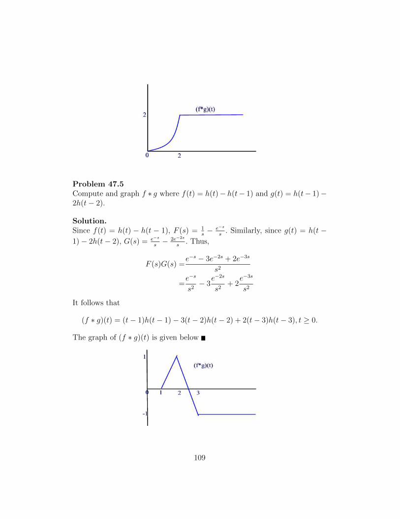
Problem 47.5Compute and graph f ∗ g where f(t) = h(t)− h(t− 1) and g(t) = h(t− 1)−2h(t− 2).
Solution.Since f(t) = h(t) − h(t − 1), F (s) = 1
s− e−s
s. Similarly, since g(t) = h(t −
1)− 2h(t− 2), G(s) = e−s
s− 2e−2s
s. Thus,
F (s)G(s) =e−s − 3e−2s + 2e−3s
s2
=e−s
s2− 3
e−2s
s2+ 2
e−3s
s2
It follows that
(f ∗ g)(t) = (t− 1)h(t− 1)− 3(t− 2)h(t− 2) + 2(t− 3)h(t− 3), t ≥ 0.
The graph of (f ∗ g)(t) is given below
109
Problem 47.6Compute t ∗ t ∗ t.
Solution.By the convolution theorem we have L[t∗t∗t] = (L[t])3 =
(1s2
)3= 1
s6. Hence,
t ∗ t ∗ t = L−1[
1s6
]= t5
5!= t5
120, t ≥ 0
Problem 47.7Compute h(t) ∗ e−t ∗ e−2t.
Solution.By the convolution theorem we have L[h(t)∗e−t∗e−2t] = L[h(t)]L[e−t]L[e−2t] =1s· 1s+1· 1s+2
. Using the partial fractions decomposition we can write
1
s(s+ 1)(s+ 2)=
1
2s− 1
s+ 1+
1
2· 1
s+ 2.
Hence,
h(t) ∗ e−t ∗ e−2t =1
2− e−t +
1
2e−2t, t ≥ 0
Problem 47.8Compute t ∗ e−t ∗ et.
Solution.By the convolution theorem we have L[t ∗ e−t ∗ et] = L[t]L[e−t]L[et] = 1
s2·
1s+1· 1s−1 . Using the partial fractions decomposition we can write
1
s2(s+ 1)(s− 1)= − 1
s2+
1
2· 1
s− 1− 1
2· 1
s+ 1.
Hence,
t ∗ e−t ∗ et = −t+et
2− e−t
2, t ≥ 0
Problem 47.9
Suppose it is known that
n functions︷ ︸︸ ︷h(t) ∗ h(t) ∗ · · · ∗ h(t) = Ct8. Determine the con-
stants C and the positive integer n.
110
Solution.
We know that L[
n functions︷ ︸︸ ︷h(t) ∗ h(t) ∗ · · · ∗ h(t)] = (L[h(t)])n = 1
snso that L−1[ 1
sn] =
tn−1
(n−1)! = Ct8. It follows that n = 9 and C = 18!
Problem 47.10Use Laplace transform to solve for y(t) :∫ t
0
sin (t− λ)y(λ)dλ = t2.
Solution.Note that the given equation reduces to sin t ∗ y(t) = t2. Taking Laplace
transform of both sides we find Y (s)s2+1
= 2s3. This implies Y (s) = 2(s2+1)
s3=
2s
+ 2s3. Hence, y(t) = L−1[2
s+ 2
s3] = 2 + t2, t ≥ 0
Problem 47.11Use Laplace transform to solve for y(t) :
y(t)−∫ t
0
e(t−λ)y(λ)dλ = t.
Solution.Note that the given equation reduces to et ∗ y(t) = y(t)− t. Taking Laplace
transform of both sides we find Y (s)s−1 = Y (s) − 1
s2. Solving for Y (s) we find
Y (s) = s−1s2(s−2) . Using partial fractions decomposition we can write
s− 1
s2(s− 2)=−1
4
s+
12
s2+
14
(s− 2).
Hence,
y(t) = −1
4+t
2+
1
4e2t, t ≥ 0
Problem 47.12Use Laplace transform to solve for y(t) :
t ∗ y(t) = t2(1− e−t).
111
Solution.Taking Laplace transform of both sides we find Y (s)
s2= 2
s3− 2
(s+1)3. This implies
Y (s) = 2s− 2s2
(s+1)3. Using partial fractions decomposition we can write
s2
(s+ 1)3=
1
s+ 1− 2
(s+ 1)2+
1
(s+ 1)3.
Hence,
y(t) = 2− 2(e−t − 2te−t +t2
2e−t) = 2
(1− (1− 2t+
t2
2)e−t
), t ≥ 0
Problem 47.13Solve the following initial value problem.
y′ − y =
∫ t
0
(t− λ)eλdλ, y(0) = −1.
Solution.Note that y′ − y = t ∗ et. Taking Lalplace transform of both sides we findsY − (−1) − Y = 1
s2· 1s−1 . This implies that Y (s) = − 1
s−1 + 1s2(s−1)2 . Using
partial fractions decomposition we can write
1
s2(s− 1)2=
2
s+
1
s2− 2
s− 1+
1
(s− 1)2.
Thus,
Y (s) = − 1
s− 1+
2
s+
1
s2− 2
s− 1+
1
(s− 1)2=
2
s+
1
s2− 3
s− 1+
1
(s− 1)2.
Finally,y(t) = 2 + t− 3et + tet, t ≥ 0
112
Section 48
Problem 48.1Evaluate
(a)∫ 3
0(1 + e−t)δ(t− 2)dt.
(b)∫ 1
−2(1 + e−t)δ(t− 2)dt.
Solution.(a)∫ 3
0(1 + e−t)δ(t− 2)dt = 1 + e−2.
(b)∫ 1
−2(1 + e−t)δ(t− 2)dt = 0 since 2 lies outside the integration interval
Problem 48.2Let f(t) be a function defined and continuous on 0 ≤ t <∞. Determine
(f ∗ δ)(t) =
∫ t
0
f(t− s)δ(s)ds.
Solution.Let g(s) = f(t− s). Then
(f ∗ δ)(t) =
∫ t
0
f(t− s)δ(s)ds =
∫ t
0
g(s)δ(s)ds
=g(0) = f(t)
Problem 48.3Determine a value of the constant t0 such that
∫ 1
0sin2 [π(t− t0)]δ(t− 1
2)dt = 3
4.
Solution.We have ∫ 1
0
sin2 [π(t− t0)]δ(t−1
2)dt =
3
4
sin2
[π
((1
2− t0
)]=
3
4
sin
[π
((1
2− t0
)]=±
√3
2.
Thus, a possible value is when π((12− t0
)= π
3. Solving for t0 we find t0 = 1
6
113
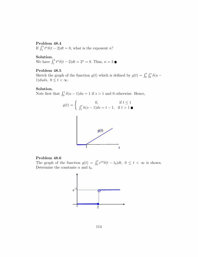
Problem 48.4If∫ 5
1tnδ(t− 2)dt = 8, what is the exponent n?
Solution.We have
∫ 5
1tnδ(t− 2)dt = 2n = 8. Thus, n = 3
Problem 48.5Sketch the graph of the function g(t) which is defined by g(t) =
∫ t0
∫ s0δ(u−
1)duds, 0 ≤ t <∞.
Solution.Note first that
∫ s0δ(u− 1)du = 1 if s > 1 and 0 otherwise. Hence,
g(t) =
{0, if t ≤ 1∫ t
1h(s− 1)ds = t− 1, if t > 1
Problem 48.6The graph of the function g(t) =
∫ t0eαtδ(t − t0)dt, 0 ≤ t < ∞ is shown.
Determine the constants α and t0.
114
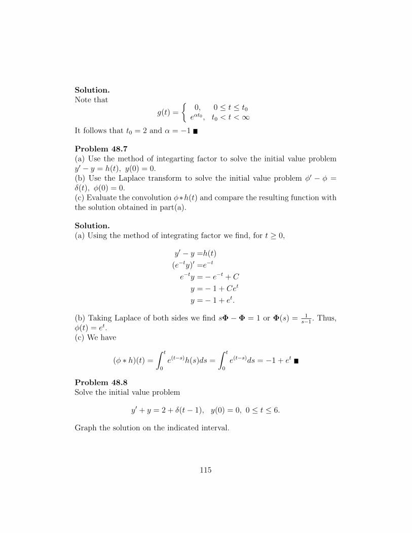
Solution.Note that
g(t) =
{0, 0 ≤ t ≤ t0eαt0 , t0 < t <∞
It follows that t0 = 2 and α = −1
Problem 48.7(a) Use the method of integarting factor to solve the initial value problemy′ − y = h(t), y(0) = 0.(b) Use the Laplace transform to solve the initial value problem φ′ − φ =δ(t), φ(0) = 0.(c) Evaluate the convolution φ∗h(t) and compare the resulting function withthe solution obtained in part(a).
Solution.(a) Using the method of integrating factor we find, for t ≥ 0,
y′ − y =h(t)
(e−ty)′ =e−t
e−ty =− e−t + C
y =− 1 + Cet
y =− 1 + et.
(b) Taking Laplace of both sides we find sΦ −Φ = 1 or Φ(s) = 1s−1 . Thus,
φ(t) = et.(c) We have
(φ ∗ h)(t) =
∫ t
0
e(t−s)h(s)ds =
∫ t
0
e(t−s)ds = −1 + et
Problem 48.8Solve the initial value problem
y′ + y = 2 + δ(t− 1), y(0) = 0, 0 ≤ t ≤ 6.
Graph the solution on the indicated interval.
115
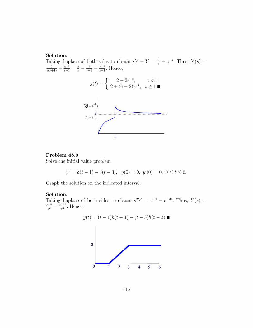
Solution.Taking Laplace of both sides to obtain sY + Y = 2
s+ e−s. Thus, Y (s) =
2s(s+1)
+ e−s
s+1= 2
s− 2
s+1+ e−s
s+1. Hence,
y(t) =
{2− 2e−t, t < 1
2 + (e− 2)e−t, t ≥ 1
Problem 48.9Solve the initial value problem
y′′ = δ(t− 1)− δ(t− 3), y(0) = 0, y′(0) = 0, 0 ≤ t ≤ 6.
Graph the solution on the indicated interval.
Solution.Taking Laplace of both sides to obtain s2Y = e−s − e−3s. Thus, Y (s) =e−s
s2− e−3s
s2. Hence,
y(t) = (t− 1)h(t− 1)− (t− 3)h(t− 3)
116
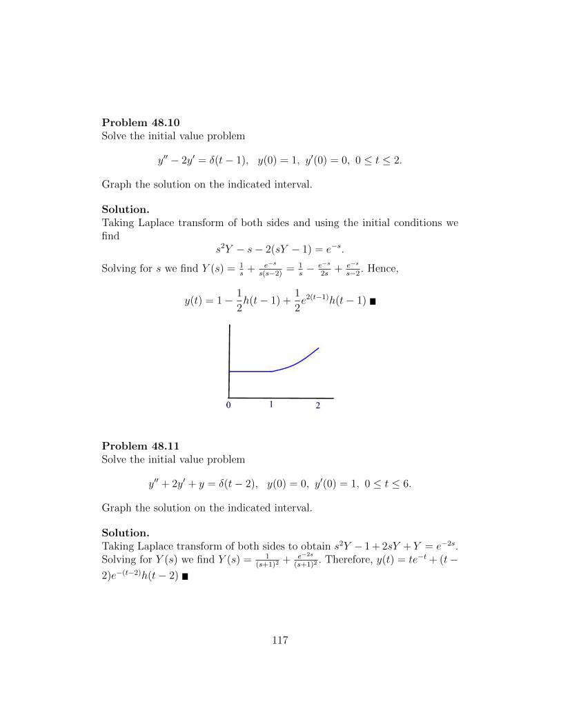
Problem 48.10Solve the initial value problem
y′′ − 2y′ = δ(t− 1), y(0) = 1, y′(0) = 0, 0 ≤ t ≤ 2.
Graph the solution on the indicated interval.
Solution.Taking Laplace transform of both sides and using the initial conditions wefind
s2Y − s− 2(sY − 1) = e−s.
Solving for s we find Y (s) = 1s
+ e−s
s(s−2) = 1s− e−s
2s+ e−s
s−2 . Hence,
y(t) = 1− 1
2h(t− 1) +
1
2e2(t−1)h(t− 1)
Problem 48.11Solve the initial value problem
y′′ + 2y′ + y = δ(t− 2), y(0) = 0, y′(0) = 1, 0 ≤ t ≤ 6.
Graph the solution on the indicated interval.
Solution.Taking Laplace transform of both sides to obtain s2Y − 1 + 2sY + Y = e−2s.Solving for Y (s) we find Y (s) = 1
(s+1)2+ e−2s
(s+1)2. Therefore, y(t) = te−t + (t−
2)e−(t−2)h(t− 2)
117
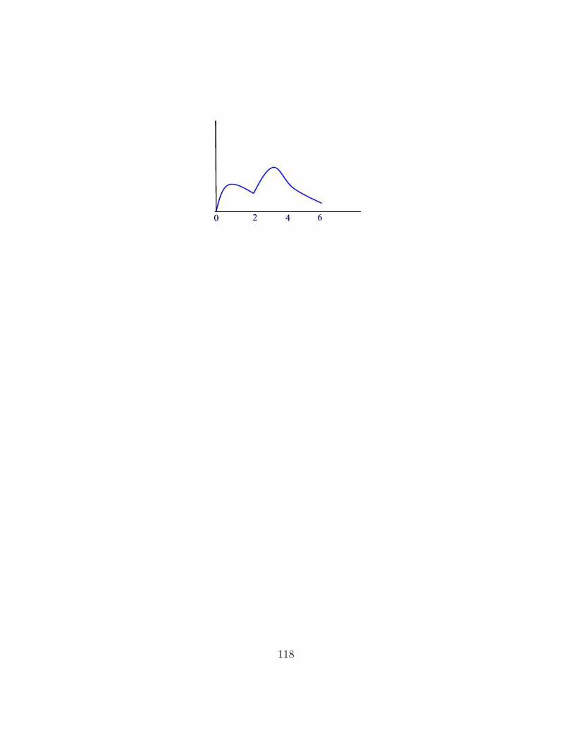
118
Section 49
Problem 49.1Find L[y(t)] where
y(t) =d
dt
e−t cos 2t0
t+ et
Solution.
L[y(t)] = L
−e−t cos 2t+ 2e−t sin 2t
01 + et
=
− s+1(s+1)2+4
+ 4(s+1)2+4
01s
+ 1s−1
=
3−s(s+1)2+4
01s
+ 1s−1
Problem 49.2Find L[y(t)] where
y(t) =
∫ t
0
1ue−u
duSolution.
L[y(t)] = L
t
t2
2
−e−t + 1
=
1s21s3
1s− 1
s+1
Problem 49.3Find L−1[Y(s)] where
Y(s) =
1s2
s2+2s+21
s2+s
119
Solution.We have
L−1[1s] = 1
L−1[ 2s2+2s+2
] = L−1[ 2(s+1)2+12
] = 2e−t sin t
L−1[ 1s2+s
] = L−1[1s− 1
s+1] = 1− e−t
Thus,
L−1[Y(s)] =
12e−t sin t1− e−t
Problem 49.4Find L−1[Y(s)] where
Y(s) =
1 −1 22 0 31 −2 1
L[t3]L[e2t]L[sin t]
Solution.We have
Y(s) =
1 −1 22 0 31 −2 1
L[t3]L[e2t]L[sin t]
= L
1 −1 2
2 0 31 −2 1
t3
e2t
sin t
= L
t3 − e2t + 2 sin t
2t3 + 3 sin tt3 − 2e2t + sin t
Thus,
L−1[Y(s)] =
t3 − e2t + 2 sin t2t3 + 3 sin t
t3 − 2e2t + sin t
Problem 49.5Use the Laplace transform to solve the initial value problem
y′ =
[5 −45 −4
]y +
[01
], y(0) =
[00
]
120
Solution.Taking Laplace of both sides and using the initial condition we find
sY =
[5 −45 −4
]Y +
[0 1
s
]Solving this matrix equation for Y we find
Y(s) =
[− 4s2(s−1)s−5
s2(s−1)
].
Using partial fractions decomposition we find
− 4
s2(s− 1)=
4
s2+
4
s− 4
s− 1
ands− 5
s2(s− 1)=
5
s2+
4
s− 4
s− 1.
Hence,
Y(s) =
[4s2
+ 4s− 4
s−15s2
+ 4s− 4
s−1
].
Finally,
y(t) =
[4t+ 4− 4et
5t+ 4− 4et
]Problem 49.6Use the Laplace transform to solve the initial value problem
y′ =
[5 −43 −2
]y, y(0) =
[32
]Solution.Taking Laplace of both sides and using the initial condition we find
sY −[
32
]=
[5 −43 −2
]Y
121
Solving this matrix equation for Y we find
Y(s) = 1(s−1)(s−2)
[s+ 2 −4
3 s− 5
] [32
]
= 1(s−1)(s−2)
[3s− 22s− 1
]Using partial fractions decomposition we find
3s− 2
(s− 1)(s− 2)=−1
s− 1+
4
s− 2
and2s− 1
(s− 1)(s− 2)=−1
s− 1+
3
s− 2.
Hence,
Y(s) =
[ −1s−1 + 4
s−2−1s−1 + 3
s−2
].
Finally,
y(t) =
[−et + 4e2t
−et + 3e2t
]Problem 49.7Use the Laplace transform to solve the initial value problem
y′ =
[1 4−1 1
]y +
[0
3et
], y(0) =
[30
]Solution.Taking Laplace of both sides and using the initial condition we find
sY −[
30
]=
[1 4−1 1
]Y +
[03s−1
][s− 1 −4
1 s− 1
]Y =
[33s−1
]
122
Solving this matrix equation for Y we find
Y(s) = 1(s−1)2+4
[s− 1 4−1 s− 1
] [33s−1
]
= 1(s−1)2+4
[3(s− 1) + 12
s−10
]Using partial fractions decomposition we find
3(s− 1) + 12s−1
(s− 1)2 + 4= 3
s− 1
(s− 1)2 + 4+
12
(s− 1)[(s− 1)2 + 4].
But12
(s− 1)[(s− 1)2 + 4]=
3
s− 1− 3
s− 1
(s− 1)2 + 4.
Hence,
Y(s) =
[3s−10
].
Finally,
y(t) =
[3et
0
]Problem 49.8Use the Laplace transform to solve the initial value problem
y′′ =
[−3 −24 3
]y, y(0) =
[10
], y′(0) =
[01
]Solution.Taking Laplace of both sides and using the initial condition we find
s2Y − s[
10
]−[
01
]=
[−3 −24 3
]Y
[s2 + 3 2−4 s2 − 3
]Y =
[s1
]
123
Solving this matrix equation for Y we find
Y(s) = 1s4−1
[s2 − 3 −2
4 s2 + 3
] [s1
]
= 1s4−1
[s3 − 3s− 2s2 + 4s+ 3
]Using partial fractions decomposition we find
s3 − 3s− 2
s4 − 1= − 1
s− 1+ 2
s
s2 + 1+
1
s2 + 1
and
s2 + 4s+ 3
(s− 1)(s+ 1)(s2 + 1)=
s+ 3
(s− 1)(s2 + 1)=
2
s− 1− s
s2 + 1− 1
s2 + 1.
Hence,
Y(s) =
[− 1s−1 + 2 s
s2+1+ 1
s2+12s−1 −
ss2+1− 1
s2+1
].
Finally,
y(t) =
[−et + 2 cos t+ sin t2et − cos t− sin t
]Problem 49.9Use the Laplace transform to solve the initial value problem
y′′ =
[1 −11 −1
]y +
[21
], y(0) =
[01
], y′(0) =
[00
]Solution.Taking Laplace of both sides and using the initial condition we find
s2Y − s[
01
]=
[1 −11 −1
]Y +
[2s1s
][s2 − 1 1−1 s2 + 1
]Y =
[2s
1s
+ s
]
124

Solving this matrix equation for Y we find
Y(s) = 1s4
[s2 + 1 −1
1 s2 − 1
] [2s
1s
+ s
]
=
[1s3
+ 1s5
1s
+ 1s5
]
y(t) =
[t2
2+ t3
4!
1 + t4
4!
]Problem 49.10Use the Laplace transform to solve the initial value problem
y′ =
1 0 00 −1 10 0 2
y +
et
1−2t
, y(0) =
000
Solution.Taking Laplace of both sides and using the initial condition we find
sY =
1 0 00 −1 10 0 2
Y +
1s−11s
− 2s2
s− 1 0 0
0 s+ 1 −10 0 s− 2
Y =
1s−11s
− 2s2
Solving this matrix equation for Y we find
Y(s) =
1s−1 0 0
0 1s+1
1(s+1)(s−2)
0 0 1s−2
1s−11s
− 2s2
=
1
(s−1)2s(s−2)−2
s2(s+1)(s−2)−2
s2(s−2)
125
Using partial fractions decomposition we find
s(s− 2)− 2
s2(s+ 1)(s− 2)=
1
s2+
1
2s− 1
3· 1
s+ 1− 1
6· 1
s− 2
and−2
s2(s− 2)=
1
s2+
1
2s− 1
2· 1
s− 2.
Hence,
Y(s) =
1(s−1)2
1s2
+ 12s− 1
3· 1s+1− 1
6· 1s−2
1s2
+ 12s− 1
2· 1s−2
.Finally,
y(t) =
tet
t+ 12− 1
3e−t − 1
6e2t
t+ 12− 1
2e2t
Problem 49.11The Laplace transform was applied to the initial value problem y′ = Ay, y(0) =
y0, where y(t) =
[y1(t)y2(t)
], A is a 2× 2 constant matrix, and y0 =
[y1,0y2,0
].
The following transform domain solution was obtained
L[y(t)] = Y(s) =1
s2 − 9s+ 18
[s− 2 −1
4 s− 7
] [y1,0y2,0
].
(a) what are the eigenvalues of A?(b) Find A.
Solution.(a) det(sI−A) = s2 − 9s + 18 = (s− 3)(s− 6) = 0. Hence, the eigenvaluesof A are r1 = 3 and r2 = 6.(b) Taking Laplace transform of both sides of the differential equation wefind
sY − y0 = AYY = (sI−A)−1y0
Letting s = 0 we find
Y(0) = −A−1 =1
18
[−2 −14 −7
]126
Hence,
A−1 =1
18
[2 1−4 7
]and
det(A−1) =1
18.
It follows that
A = (A−1)−1 =
[7 −14 2
]
127
Related Documents


