Lane Detection for DEXTER, an Autonomous Robot, in the ...

Lane Detection for DEXTER, an Autonomous Robot, in the Urban 

Challenge  

 by 

SCOTT MCMICHAEL 

Submitted in partial fulfillment of the requirements  

For the degree of Master of Science 

Thesis Adviser: Dr. Wyatt Newman 

Department of Electrical Engineering and Computer Science 

CASE WESTERN RESERVE UNIVERSITY 

May 2008   

CASE WESTERN RESERVE UNIVERSITY

SCHOOL OF GRADUATE STUDIES

We hereby approve the thesis/dissertation of

_____________________________________________________

candidate for the ______________________degree *.

(signed)_______________________________________________ (chair of the committee) ________________________________________________ ________________________________________________ ________________________________________________ ________________________________________________ ________________________________________________ (date) _______________________ *We also certify that written approval has been obtained for any proprietary material contained therein.

2  

Table of Contents 

Table of Contents ................................................................................................................ 2 

Table of Figures ................................................................................................................... 6 

1 ‐ Abstract .......................................................................................................................... 8 

2 ‐ Introduction ................................................................................................................... 9 

3 ‐ Background .................................................................................................................. 11 

4 ‐ Hardware Platform ...................................................................................................... 14 

4.1 ‐ DEXTER .................................................................................................................. 14 

4.2 ‐ Cameras ................................................................................................................. 16 

4.3 ‐ Laser Scanners ....................................................................................................... 19 

4.4 ‐ Infrared Cameras ................................................................................................... 20 

4.5 ‐ Computers ............................................................................................................. 21 

5 ‐ Software Architecture .................................................................................................. 22 

5.1 ‐ Overview ............................................................................................................... 23 

5.2 ‐ Lane Detection System .......................................................................................... 25 

5.2.1 ‐ Sensor Fusion Theory ..................................................................................... 26 

5.2.2 – Steering Command Chain .............................................................................. 28 

6 ‐ Road Detection Modules ............................................................................................. 29 

6.1 ‐ Rake Edge Detector ............................................................................................... 31 

3  

6.2 ‐ Color Roadbed Detector ....................................................................................... 31 

6.3 ‐ Texture Road Detector .......................................................................................... 33 

6.4 ‐ Side Camera Road Detectors ................................................................................ 33 

6.5 ‐ LIDAR Road Detector ............................................................................................. 34 

7 ‐ Edge Crawler ................................................................................................................ 34 

7.1 ‐ Curve Extraction .................................................................................................... 35 

7.2 ‐ Curve Filtering ....................................................................................................... 37 

7.2.1 ‐ Simple Filtering ............................................................................................... 38 

7.2.2 ‐ Curve Breakup ................................................................................................ 38 

7.2.3 ‐ Curve Fit Filtering ........................................................................................... 40 

7.2.4 ‐ Expectation Filtering ....................................................................................... 41 

7.3 ‐ Confidence Estimation and Formatting ................................................................ 43 

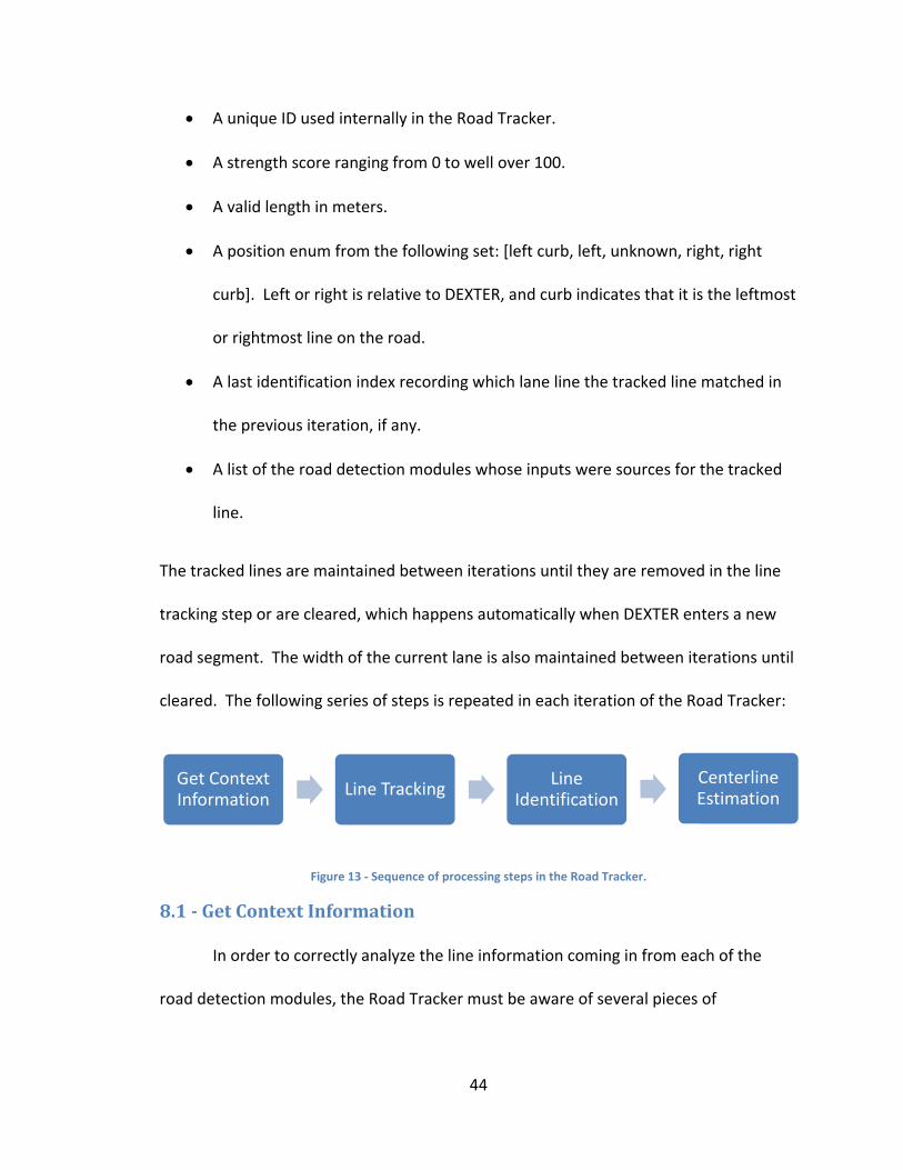
8 ‐ Road Tracker ................................................................................................................ 43 

8.1 ‐ Get Context Information ....................................................................................... 44 

8.2 ‐ Line Tracking ......................................................................................................... 46 

8.2.1 ‐ Line Input ........................................................................................................ 46 

8.2.2 ‐ Line Maintenance ........................................................................................... 46 

8.2.3 ‐ Line Merging ................................................................................................... 47 

8.3 ‐ Line Identification ................................................................................................. 49 

4  

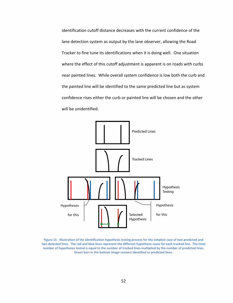
8.4 ‐ Centerline Estimation ............................................................................................ 53 

9 ‐ Lane Observer .............................................................................................................. 55 

9.1 ‐ Map Query Sequence ............................................................................................ 55 

9.2 ‐ Sensor Filtering ...................................................................................................... 57 

9.3 ‐ Source Selection .................................................................................................... 59 

10 ‐ Test Site Performance ................................................................................................ 64 

10.1 ‐ Case Quad ........................................................................................................... 64 

10.2 ‐ Squire Valleview Farm ......................................................................................... 68 

10.3 ‐ Beachwood .......................................................................................................... 69 

10.4 ‐ Plumbrook ........................................................................................................... 70 

10.5 ‐ National Qualifying Event ................................................................................... 77 

11 ‐ Analysis and Future Work .......................................................................................... 80 

11.1 ‐ Edge Crawler ....................................................................................................... 80 

11.2 ‐ Road Tracker ....................................................................................................... 82 

11.3 ‐ Lane Observer ..................................................................................................... 84 

11.4 ‐ Future Development ........................................................................................... 85 

12 ‐ Conclusions ................................................................................................................ 86 

13 ‐ Appendices ................................................................................................................. 87 

Appendix A – Common Algorithms ............................................................................... 87 

5  

A1 ‐ Line Fit Difference Calculation ........................................................................... 87 

A2 ‐ Polynomial Fitting............................................................................................... 87 

A3 ‐ Line Fit Merging .................................................................................................. 87 

A4 ‐ RANSAC Line Fit .................................................................................................. 91 

A5 –Path Divergence Detection ................................................................................. 93 

Appendix B – Sensor Calibration ................................................................................... 93 

Appendix C – Coordinate Frames .................................................................................. 95 

Appendix D – Position Shift Steering............................................................................. 97 

14 ‐ References ............................................................................................................... 100 

6  

Table of Figures 

Figure 1 ‐ DEXTER as received by Team CASE.. ................................................................. 14 

Figure 2 ‐ DEXTER as it competed in the National Qualifying Event.. .............................. 16 

Figure 3 – Lane detection sensor diagram. ....................................................................... 18 

Figure 4 ‐ Computer usage by the lane detection system. ............................................... 22 

Figure 5 ‐ Diagram of DEXTER's software architecture..................................................... 23 

Figure 6 – Three tiered hierarchy of DEXTER’s lane detection system ............................ 26 

Figure 7 ‐ Flow of steering commands on DEXTER ........................................................... 28 

Figure 8 – Edge Crawler color plane use ........................................................................... 36 

Figure 9 – Edge Crawler preprocessing steps ................................................................... 37 

Figure 10 – Edge Crawler curve filtering sequence .......................................................... 38 

Figure 11 – Edge Crawler curve breakup example ........................................................... 40 

Figure 12 – Edge Crawler expectation filetering example ................................................ 42 

Figure 13 ‐ Sequence of processing steps in the Road Tracker. ....................................... 44 

Figure 14 – Road Tracker line type compatibility table .................................................... 50 

Figure 15 – Road Tracker identification hypothesis illustration ....................................... 52 

Figure 16 – Road tracker centerline extraction illustration .............................................. 54 

Figure 17 – Lane Observer map query example ............................................................... 57 

Figure 18 – Lane Observer sensor filtering example ........................................................ 59 

Figure 19 – Lane Observer source merging example ....................................................... 62 

Figure 20 – Lane Observer source merging example image. ............................................ 63 

Figure 21 – Satellite image of the Case quad ................................................................... 65 

7  

Figure 22 ‐ Images from the Case Quad ........................................................................... 66 

Figure 23 – Composite lane detection example ............................................................... 67 

Figure 24 ‐ Images from the Case Farm ............................................................................ 69 

Figure 25 ‐ Images from the Beachwood test site ............................................................ 70 

Figure 26 ‐ Images from Plum Brook ................................................................................ 72 

Figure 27 – Lane detection path driving analysis ............................................................. 73 

Figure 28 – Lane detection path error analysis ................................................................ 75 

Figure 29 – Lane detection path self assessment ............................................................. 76 

Figure 30 – Lane detection path initial view ..................................................................... 77 

Figure 31 ‐ Images from the NQE test sites ...................................................................... 78 

Figure 32 – NQE area C results sample ............................................................................. 79 

Figure 33 – Fit merging example ....................................................................................... 90 

Figure 34 – RANSAC fit example ....................................................................................... 92 

Figure 35 – Calibration visualization image ...................................................................... 95 

Figure 36 – Physical state shifting illustration .................................................................. 97 

8  

Lane Detection for DEXTER, an Autonomous Robot, in the Urban Challenge  

Abstract 

By 

SCOTT MCMICHAEL 

  This thesis describes the lane detection system developed for the autonomous 

robot DEXTER in the 2007 DARPA Urban Challenge.  Though DEXTER was capable of 

navigating purely off of GPS signals, it often needed to drive in areas where GPS 

navigation could not be trusted completely.  In these areas it was necessary to use a 

method of automatically detecting the lane of travel so that DEXTER could drive 

properly within it.  The developed system functions by merging the outputs of a number 

of independent road detection modules coming from several sensors into a single 

drivable output path.  This sensor derived path is compared with the map derived path 

in order to produce an optimal output based on the relative confidences of the two 

information sources.  The full lane detection system is able to adaptively drive according 

to the best information source and perform well in a variety of diverse driving 

environments. 

9  

2 ­ Introduction 

The DARPA Urban Challenge, announced in May of 2006, called on entrants to 

attempt to solve several key challenges in automation research.  One of these key 

challenges is the autonomous navigation of a vehicle based on real‐time road detection 

methods.  Research in this area has been ongoing for many years (1), however Team 

Case was faced with the challenge of designing a lane detection system with limited 

experience in the field, limited manpower, a limited budget, and in a short amount of 

time.  The approach which was chosen to address these challenges was to develop a 

relatively large number of independent road detection methods which were then 

combined in order to generate a best estimate of the lane position.  This fused result is 

then combined with the a priori map of the driving area, if available, in a separate step.  

This approach offers a number of advantages and disadvantages over other possible 

implementations: 

Advantages  ‐  

• It is not necessary to create a general purpose algorithm that would be 

effective and accurate in every situation.  Different modules can use very 

different techniques, each most suitable in different areas, so long as at least 

one of them is effective at each instant.   

• Allows highly parallel development work on road detection.  This fits well 

into the uncertain nature of university development schedules since 

incomplete modules will not hold up work on other modules. 

10  

• Leads to a robust system.  If individual modules are not completed in time or 

fail due to hardware problems on the robot the lane detection system can 

still operate, albeit with reduced effectiveness, based on the remaining 

modules. 

Disadvantages –  

• Not completely parallelized.  Development of lower level modules of 

processing can still hold up development of the modules that perform the 

fusion steps. 

• Fusion steps are difficult.  Since self evaluation of results by the road 

detection modules is often inaccurate, it can be difficult to select which 

one(s) to trust at a given time. 

• Possibly computationally inefficient.  A parallel approach requires multiple 

sensors and computers regardless of whether they are truly necessary. 

The strategy described above was implemented as a set of individual road 

detection modules along with two fusion modules, the Road Tracker and the Lane 

Observer, which operated in series with the road detection modules.  The system was 

implemented on DEXTER, Team Case’s entry into the 2007 Urban Challenge.  A set of 

cameras and a single laser scanner unit were mounted on the robot for the exclusive 

purpose of road detection.  Though DEXTER’s lane detection system was not used in 

actual competition its results from iterative testing at multiple locations and post‐

processing of the National Qualifying Event (NQE) logs are analyzed in this document.   

11  

3 ­ Background 

  Development of autonomous vehicle technology has been ongoing for 

approximately the last 30 years (1) and has been making real progress during this time.  

Development of lane detection techniques has typically been the main focus of such 

efforts.  These research projects have begun to yield some marketable driver assistance 

products (2) but achieving a reliable system independent of supervision remains elusive.   

Several government programs have been important in driving research in the 

field.  These include the DRIVE and PROMETHEUS programs in Europe (3) and the 

DARPA Grand Challenge series of programs in the US.  Perhaps the most significant 

research program in Europe was that run under Ernst Dickmanns in Germany, producing 

the VaMoRs, VaMP, and VITA2 series of vehicles (4).  The European projects had the 

goal of developing technology to reduce traffic accidents and thus focused mostly on 

highway and city driving.  This research began in the 1980’s and produced several 

impressive milestones, including long distance traveled over the Autobahn at high 

speeds (1).  These achievements relied on an approach inspired by control engineering 

techniques and referred to as 4D processing (5), (6).  Limitations posed by computers of 

this time period required special purpose computers known as transputers in order to 

keep up with the data processing demands  (7). 

More recently, the Defense Advanced Research Projects Agency (DARPA) in the 

US has sponsored a series of three challenges for autonomous robotics: the two desert 

Grand Challenges of 2004 and 2005 and the Urban Challenge of 2007 (8).   These 

12  

challenges, unlike the European programs, had the goal of spurring technological 

development for military purposes and have focused on off‐road desert terrain and 

urban settings such as might be encountered at a military base.  In terms of technology, 

the DARPA challenges have placed increased reliance on GPS based navigation and seen 

the predominant use of laser scanners for obstacle detection in place of the heavy 

reliance on vision during the earlier European development (9).   

Prior to the Grand Challenges in the US, a major source of robotics research was 

the NavLab program at Carnegie Mellon University.  This program produced a series of 

11 NavLab robots and made a significant achievement with the 1995 ‘No Hands Across 

America’ test in which the robot NavLab 5 exhibited lateral steering control over 2797 

miles of a 2849 mile cross‐country trip (10).  Given this level of success in 1995 the 

relatively slow progress of on‐road robotic navigation since then could be questioned.  

Some explanation can be found by more closely examining the achievements of Navlab 

5.  The driving system used by NavLab 5 had a number of limitations: it was only aware 

of a single lane at once and had no capability to switch lanes, it only designed for the 

comparatively easy case of driving on highways, and it required human control of the 

throttle and brake.  Its control architecture was also limited by the fact that steering 

commands were issued directly from the lane detection module, eliminating the 

possibility of intervention by other AI routines (11).  Finally, the percentage of distance 

driven autonomously was only 98.2% which falls short of the 100% accuracy which will 

eventually be required of a robotic driving system.  Achieving those last few percentage 

points represents an enormous technical challenge. 

13  

An increasing amount of research around the globe is being performed 

independently of the large projects described above.  This work spans a range of 

different approaches to lane detection including methods based on color (12), (13), (14), 

texture (15), (16), active contours (17), (18), stereo cameras (19), (20), laser scanners 

(21), (22), or some combination thereof (23).  Advances in computing hardware have 

assisted progress, with standard computers now possessing the processing speeds 

needed for real time road detection.  Development of sensors has continued, 

particularly with sophisticated new laser rangefinder technology such as the Velodyne 

sensor widely used in the 2007 Urban Challenge (24) but also including new methods of 

utilizing cameras (25), (26).  

  In addition to research focused on lane detection, more research has been 

performed in other aspects of a complete lane detection system.  These areas of 

research include the effectiveness of different road models (27), (28), real‐time 

identification of road configurations (29), (30), and automated parameter learning 

methods (31), (32).  In addition, increased attention is being paid to the fusion of data 

from the multiple sensors which are now often added to autonomous robots.  

Unfortunately much of the research into sensor fusion techniques is either very abstract 

(33), or is testing in a situation with an extremely limited output configuration space 

(34), (35).  On the other hand, the concrete development that has been performed 

tends to be very special case and inapplicable to DEXTER’s lane detection needs (36), 

(37). 

14  

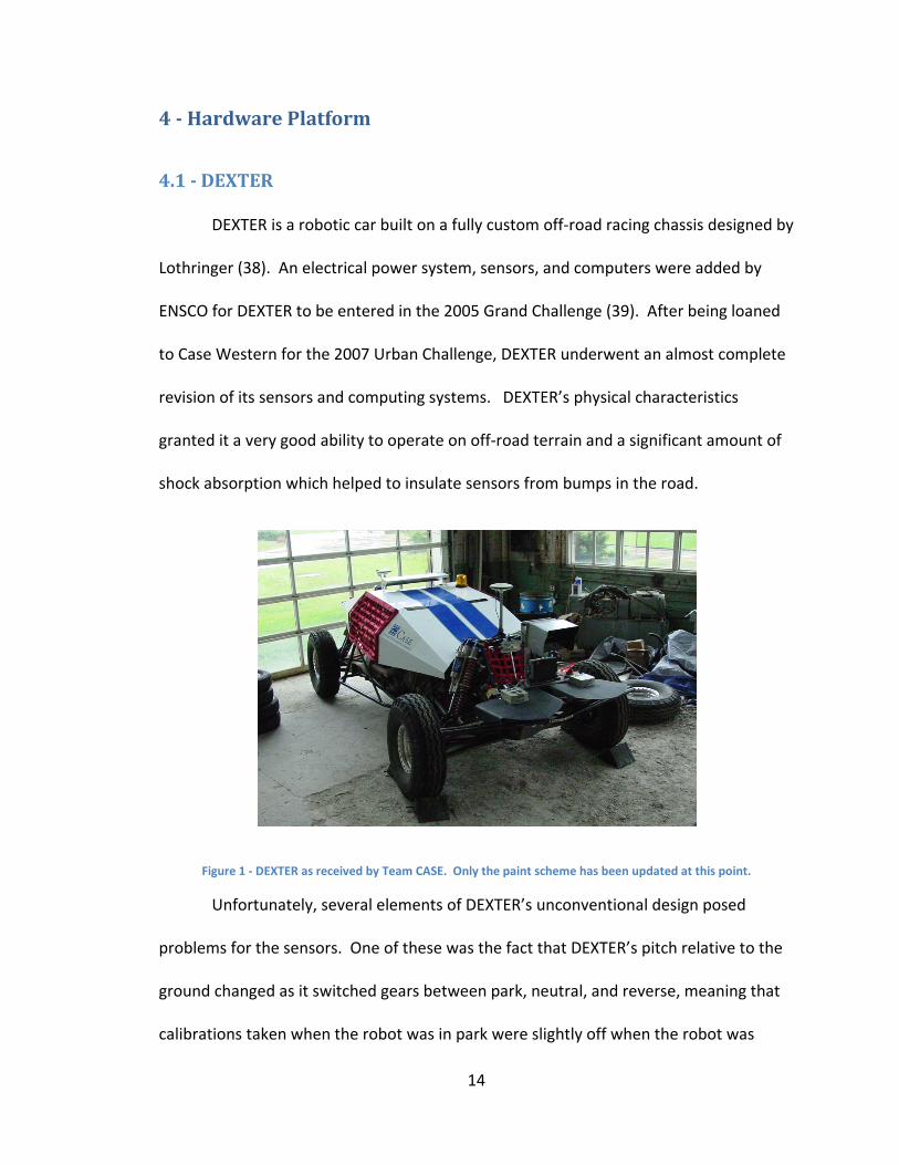
4 ­ Hardware Platform 

4.1 ­ DEXTER 

  DEXTER is a robotic car built on a fully custom off‐road racing chassis designed by 

Lothringer (38).  An electrical power system, sensors, and computers were added by 

ENSCO for DEXTER to be entered in the 2005 Grand Challenge (39).  After being loaned 

to Case Western for the 2007 Urban Challenge, DEXTER underwent an almost complete 

revision of its sensors and computing systems.   DEXTER’s physical characteristics 

granted it a very good ability to operate on off‐road terrain and a significant amount of 

shock absorption which helped to insulate sensors from bumps in the road.   

Figure 1 ‐ DEXTER as received by Team CASE.  Only the paint scheme has been updated at this point. 

Unfortunately, several elements of DEXTER’s unconventional design posed 

problems for the sensors.  One of these was the fact that DEXTER’s pitch relative to the 

ground changed as it switched gears between park, neutral, and reverse, meaning that 

calibrations taken when the robot was in park were slightly off when the robot was 

15  

actually moving.  Luckily these discrepancies did not seem to be significant enough to 

noticeably affect the performance of the road detection system.  A second difficulty of 

DEXTER’s design was the tendency of the engine to produce strong vibrations in the 

robot.  Though it may have been possible to address this fault with adjustments to the 

engine, this was primarily dealt with by using vibration dampening on the sensor 

mounts.  The problem was also most severe while the robot was in park, meaning that 

things improved greatly when DEXTER was actively operating. 

The enclosures designed for DEXTER’s numerous cameras were very effective in 

isolating the cameras from vibrations due to the engine and the road.  This was 

particularly apparent when the logs from DEXTER’s onboard were compared to the 

extremely jittery videos from an HD camera that had been directly affixed to DEXTER 

during several NQE runs.  The enclosures were capable of being adjusted on four 

different axes and could be mounted on many different locations on DEXTER, allowing 

for optimal positioning of each of the cameras.  The enclosures also offered significant 

shielding from the sun and rain.  

16  

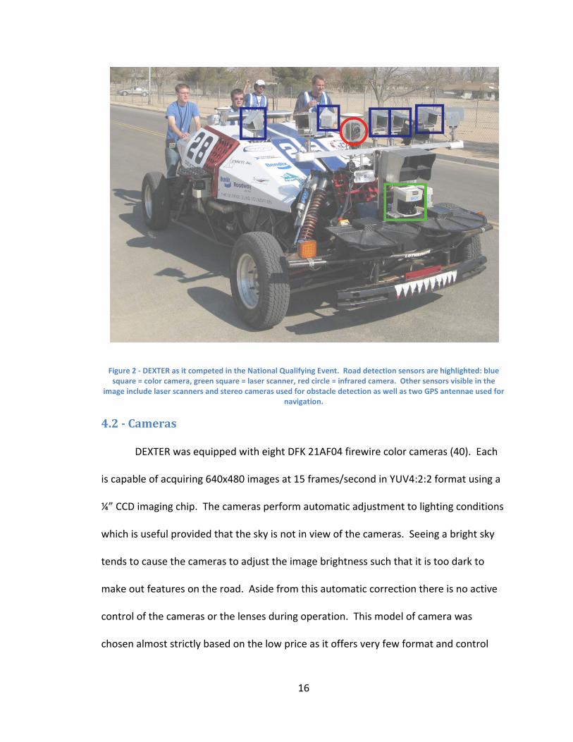
Figure 2 ‐ DEXTER as it competed in the National Qualifying Event.  Road detection sensors are highlighted: blue square = color camera, green square = laser scanner, red circle = infrared camera.  Other sensors visible in the 

image include laser scanners and stereo cameras used for obstacle detection as well as two GPS antennae used for navigation. 

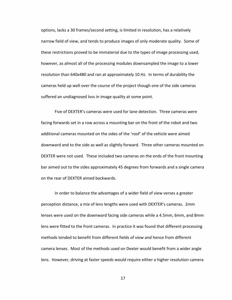
4.2 ­ Cameras 

  DEXTER was equipped with eight DFK 21AF04 firewire color cameras (40).  Each 

is capable of acquiring 640x480 images at 15 frames/second in YUV4:2:2 format using a 

¼” CCD imaging chip.  The cameras perform automatic adjustment to lighting conditions 

which is useful provided that the sky is not in view of the cameras.  Seeing a bright sky 

tends to cause the cameras to adjust the image brightness such that it is too dark to 

make out features on the road.  Aside from this automatic correction there is no active 

control of the cameras or the lenses during operation.  This model of camera was 

chosen almost strictly based on the low price as it offers very few format and control 

17  

options, lacks a 30 frames/second setting, is limited in resolution, has a relatively 

narrow field of view, and tends to produce images of only moderate quality.  Some of 

these restrictions proved to be immaterial due to the types of image processing used, 

however, as almost all of the processing modules downsampled the image to a lower 

resolution than 640x480 and ran at approximately 10 Hz.  In terms of durability the 

cameras held up well over the course of the project though one of the side cameras 

suffered an undiagnosed loss in image quality at some point. 

  Five of DEXTER’s cameras were used for lane detection.  Three cameras were 

facing forwards set in a row across a mounting bar on the front of the robot and two 

additional cameras mounted on the sides of the ‘roof’ of the vehicle were aimed 

downward and to the side as well as slightly forward.  Three other cameras mounted on 

DEXTER were not used.  These included two cameras on the ends of the front mounting 

bar aimed out to the sides approximately 45 degrees from forwards and a single camera 

on the rear of DEXTER aimed backwards.   

  In order to balance the advantages of a wider field of view verses a greater 

perception distance, a mix of lens lengths were used with DEXTER’s cameras.  2mm 

lenses were used on the downward facing side cameras while a 4.5mm, 6mm, and 8mm 

lens were fitted to the front cameras.  In practice it was found that different processing 

methods tended to benefit from different fields of view and hence from different 

camera lenses.  Most of the methods used on Dexter would benefit from a wider angle 

lens.  However, driving at faster speeds would require either a higher resolution camera 

18  

or a lens with a narrower field of view.  Some difficulties were had over the course of 

the project with inexpensive lenses shifting out of focus or becoming damaged to the 

point where they could not be refocused.  Surprisingly these difficulties were never 

encountered with the 2mm side camera lenses which lacked any sort of locking 

mechanism. 

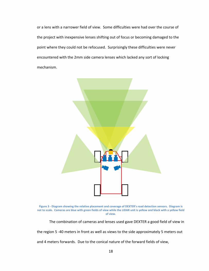
Figure 3 ‐ Diagram showing the relative placement and coverage of DEXTER's road detection sensors.  Diagram is not to scale.  Cameras are blue with green fields of view while the LIDAR unit is yellow and black with a yellow field 

of view. 

  The combination of cameras and lenses used gave DEXTER a good field of view in 

the region 5 ‐40 meters in front as well as views to the side approximately 5 meters out 

and 4 meters forwards.  Due to the conical nature of the forward fields of view, 

19  

DEXTER’s road detection capabilities in tight turns and intersections were poor as only 

the side cameras could provide updates once DEXTER entered a tight turn.  This fact, 

combined with the inherent difficulty of the task, led to the decision to exclude 

intersection traversal as a capability of DEXTER’s lane detection system.   This forced the 

robot to rely on an accurate a priori map and GPS signal in intersection situations.  

4.3 ­ Laser Scanners 

  DEXTER possessed a single laser scanner which was aimed downwards at an 

angle for the purpose of road detection.  The scanner was a SICK model LMS291‐S14 

FAST, (41) mounted at the front of the robot and aimed to intersect the ground at a 

distance of approximately 7 meters.  DEXTER’s laser scanners are referred to as LIDAR 

(LIght Detection And Ranging) units.  The scanner sweeps out a 90 degree arc in front, 

returning 181 distance measurements at ½ degree intervals and 181 reflectivity 

measurements at the same ½ degree intervals.  A scan of this region allowed the LIDAR 

unit to detect multiple curbs and lane lines when on multi‐lane roads but tended not to 

be of use when DEXTER was making tight turns.  

In general the scanner does a good job of detecting reflectivity differences of 

surfaces and painted lines ahead as well as the distance profiles representing curves.  

Several factors increase the difficulty of accurately detecting the road, however.  In 

many of the test areas in which DEXTER operated both curbs and lane lines were non‐

existent or intermittent, forcing reliance on the detection of less pronounced pavement‐

grass borders.  In clearer situations, obstructions and variations in pavement reflectivity 

20  

can cause difficulties in road detection.  DEXTER’s low profile added another difficulty to 

the operation of the laser scanner by forcing a relatively shallow intersection angle with 

the road in order to look any significant distance ahead.  A shallow angle makes the 

intensity measure of the scanner prone to erroneous high readings which must be 

filtered out. 

4.4 ­ Infrared Cameras 

  Infrared (IR) cameras were tested for possible use in road detection and obstacle 

detection.  While they did not seem usable for obstacle detection, they appeared to be 

potentially useful in road detection when a road was bordered by grass or foliage.  Some 

very promising results were obtained and an IR camera was mounted on DEXTER for this 

use.  Unfortunately, later testing revealed that except in very specific road and 

temperature conditions the IR image of the road was very difficult for either humans or 

algorithms to decipher.  Several properties of the IR cameras contributed to this 

problem.  First, the heat intensity detected in any location of the IR image was relative 

to the surrounding area, meaning that the center of a section of pavement might not 

look any brighter than the center of a patch of grass to the side of the road.  Second, 

shadows, cracks, and other road imperfections stood out strongly on the road, adding 

unwanted noise to the image.  Lane markings were also visible in the image but not 

reliably enough that they could usually be detected, rendering them another source of 

noise when attempting to detect the asphalt surface.  Finally, the appearance of vehicles 

on the road was very inconsistent which made them very difficult to detect or filter out.  

Road detection software was developed for the IR camera but due to the 

21  

aforementioned inconsistencies in IR images it was found to be too unreliable for 

practical use.  The 6.2 ‐ Color Roadbed Detector described in section 6.2 was actually an 

offshoot of the IR road detection program and is nearly identical to what was developed 

for the IR camera. 

4.5 ­ Computers 

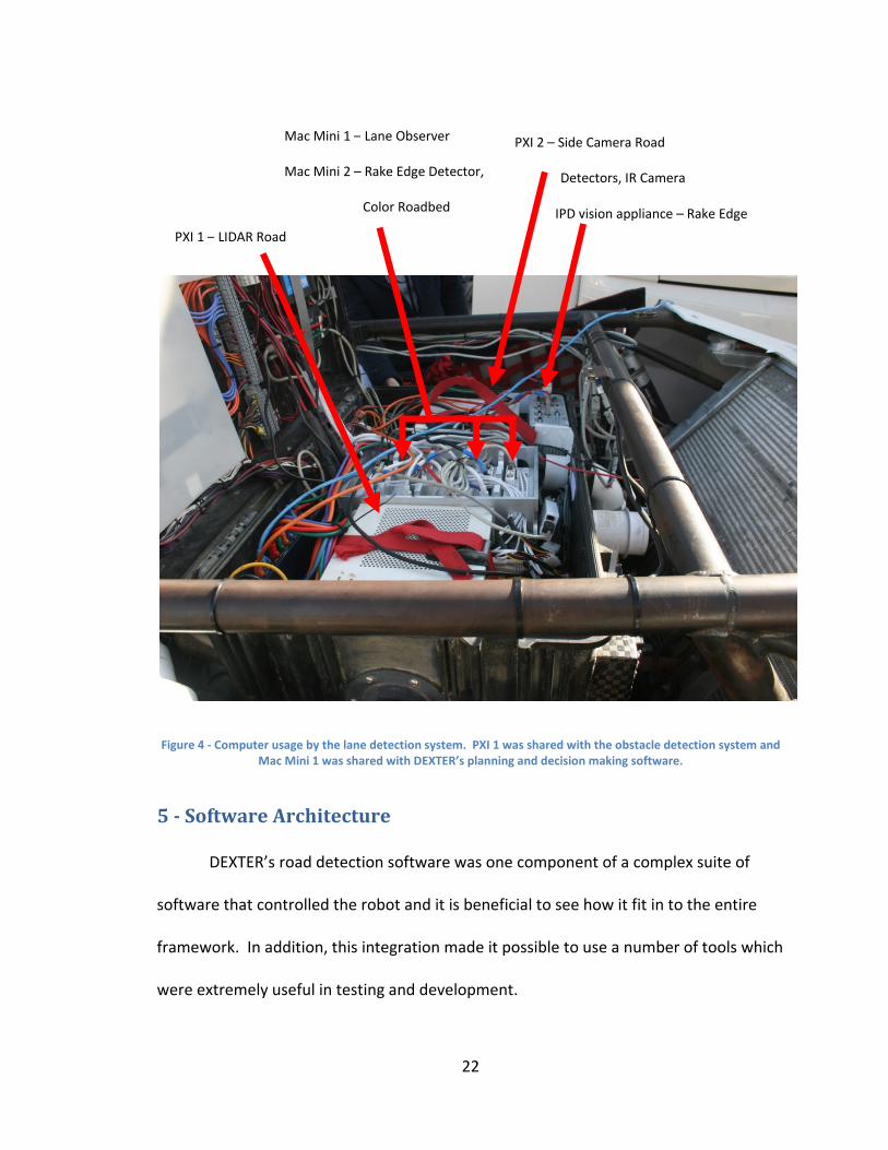
   A total of eight computers were available for use by DEXTER’s upper level AI, 

consisting of two National Instruments PXI machines (42), five Intel Mac minis, and one 

IPD vision appliance (43) comprising a total of 15 processing cores.  Of these eight 

machines, four were devoted to different lane detection systems.  The downward facing 

LIDAR was processed on a fifth computer that was also responsible for processing the 

obstacle detection LIDAR scanners.  Since firewire cameras were used to collect images 

it was not possible to easily share the output of a single camera between computers; 

because of this each camera was connected to a single computer and all processing 

modules for a given camera needed to be run on the same computer.  The primary 

reason why DEXTER has three forward facing cameras with similar fields of view is to 

allow the computational load of multiple image processing methods to be spread over 

several computers.  The allocation of computational resources allowed the entire lane 

detection system to run at a consistent speed of 10 Hz. 

22  

Figure 4 ‐ Computer usage by the lane detection system.  PXI 1 was shared with the obstacle detection system and Mac Mini 1 was shared with DEXTER’s planning and decision making software. 

5 ­ Software Architecture 

  DEXTER’s road detection software was one component of a complex suite of 

software that controlled the robot and it is beneficial to see how it fit in to the entire 

framework.  In addition, this integration made it possible to use a number of tools which 

were extremely useful in testing and development. 

IPD vision appliance – Rake Edge 

PXI 2 – Side Camera Road 

Detectors, IR Camera 

Mac Mini 1 – Lane Observer               

Mac Mini 2 – Rake Edge Detector,       

Color Roadbed 

PXI 1 – LIDAR Road 

23  

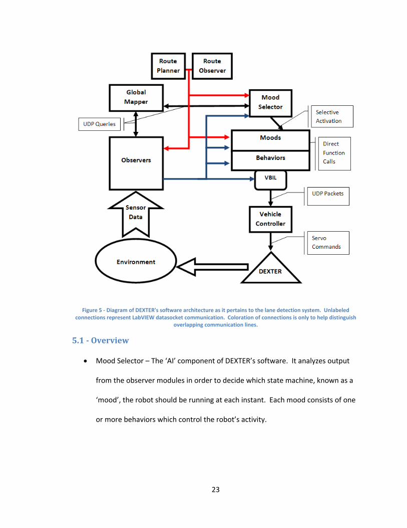
Figure 5 ‐ Diagram of DEXTER's software architecture as it pertains to the lane detection system.  Unlabeled connections represent LabVIEW datasocket communication.  Coloration of connections is only to help distinguish 

overlapping communication lines. 

5.1 ­ Overview 

• Mood Selector – The ‘AI’ component of DEXTER’s software.  It analyzes output 

from the observer modules in order to decide which state machine, known as a 

‘mood’, the robot should be running at each instant.  Each mood consists of one 

or more behaviors which control the robot’s activity. 

24  

• Route Planner – This module estimates the fastest set of road choices to reach a 

target checkpoint and is capable of replanning to account for blocked road 

segments upon request from the Mood Selector. 

• Route Observer – This module keeps track of DEXTER’s location on the DARPA 

RNDF data structure which defines the road layouts and connectivity. 

• Vehicle Controller – Converts paths generated by behaviors in DEXTER’s state 

machines into a set of steering and throttle commands to drive the robot.  The 

Physical State Observer which keeps track of the robot’s position and ego‐

motion inhabits the Vehicle Controller module. 

• Global Mapper – Stores a high resolution GPS map of each of the road segments 

specified in the DARPA RNDF.  This map may either be automatically generated 

or created manually and can be accessed by a set of queries which can be sent to 

the Mapper. 

• Observers – Performs all of the sensor processing on DEXTER, with tasks 

including obstacle detection, intersection monitoring, and lane detection. 

The vast majority of DEXTER’s software is written in the LabVIEW programming 

language (44) though most of the exceptions to this are in fact road detection modules.  

All of the LabVIEW components are integrated through a program known as 

DEXLAUNCH, the primary function of which is to automatically launch the correct 

software on each computer but which also makes possible several other functions.  The 

most important of these to the lane detection system are the logging and playback 

systems.  DEXLAUNCH makes possible a centralized logging system in which all modules 

25  

start and stop logs simultaneously in easy to create batches.  The logs are saved with 

timing information which allows playback, essentially a flexible user controlled “scroll 

bar” method of looking simultaneously through the logged data of as many modules as 

desired.  Being able to easily synchronize and flexibly play back logs was essential to the 

rapid development of DEXTER’s lane detection system.   

Inter‐process communication is performed via datasockets, a custom TCP 

implementation of LabVIEW.  This allows each module to publish information which any 

other module can then read, a process that is handled automatically even when the 

modules are running on different computers.  Use of datasocket communication allows 

processes to easily request pieces of information calculated in other modules.  Two 

important exceptions to datasocket use are the Vehicle Controller and the Global 

Mapper.  The Vehicle Controller receives UDP packets containing driving paths of 

‘breadcrumbs’ while the Global Mapper uses a custom UDP query system to receive 

data requests and then sends out a UDP response with the requested data. 

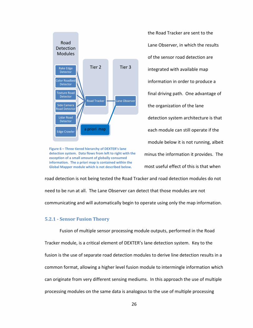
5.2 ­ Lane Detection System 

  DEXTER’s lane detection system is implemented in a three tiered approach.  At 

the bottom level are multiple road detection modules which analyze raw sensor data in 

order to produce possible lane line locations.  Each of these modules sends their results 

in a common format to the Road Tracker, a module whose purposes are to fuse the 

results of the different road detection modules and then to extract the correct lane 

centerline from that data and context information from other modules.  The results of 

26  

the Road Tracker are sent to the 

Lane Observer, in which the results 

of the sensor road detection are 

integrated with available map 

information in order to produce a 

final driving path.  One advantage of 

the organization of the lane 

detection system architecture is that 

each module can still operate if the 

module below it is not running, albeit 

minus the information it provides.  The 

most useful effect of this is that when 

road detection is not being tested the Road Tracker and road detection modules do not 

need to be run at all.  The Lane Observer can detect that those modules are not 

communicating and will automatically begin to operate using only the map information. 

5.2.1 ­ Sensor Fusion Theory 

Fusion of multiple sensor processing module outputs, performed in the Road 

Tracker module, is a critical element of DEXTER’s lane detection system.  Key to the 

fusion is the use of separate road detection modules to derive line detection results in a 

common format, allowing a higher level fusion module to intermingle information which 

can originate from very different sensing mediums.  In this approach the use of multiple 

processing modules on the same data is analogous to the use of multiple processing 

Road Detection Modules

Tier 2 Tier 3

Lane ObserverRoad Tracker

Rake Edge Detector

Color Roadbed Detector

Texture Road Detector

Side Camera Road Detector

Lidar Road Detector

Edge Crawler

Figure 6 – Three tiered hierarchy of DEXTER’s lane detection system.  Data flows from left to right with the exception of a small amount of globally consumed information.  The a priori map is contained within the Global Mapper module which is not described below. 

a priori  map

27  

modules operating on multiple sensors collecting entirely different types of data; the 

two cases are handled identically in the Road Tracker.  This proves to be a key 

advantage when relying on cameras for road detection due to the relative unreliability 

of image processing and the wide variety of techniques which can be used to analyze 

the same images.  By analyzing an image with a diverse set of methods the likelihood 

that all will fail at the same time decreases greatly.  Due to inaccuracy in confidence self‐

reporting it can still be difficult to select the currently correct modules while ignoring 

currently erroneous modules and this is a key challenge for the software to address. 

Another important attribute of the sensor fusion technique used is its capability 

to flexibly use the information provided by each of the road detection modules.  

Detection of the same feature by multiple modules, detection of multiple features, 

detection of different sections of the same feature, and blends of the above cases with 

erroneous or missing data are all handled without requiring explicit information about 

the individual road detection modules involved.  Handling of multiple features in this 

manner is more complex than what is possible through ‘black box’ fusion methods such 

as in (45) using common machine learning approaches to the problem.  This flexibility, 

combined with the ability to use feedback‐incorporating prediction information 

published by the system, allows much more comprehensive use of sensor data than 

would be possible with a tightly‐coupled, inflexible system such as in (46). 

28  

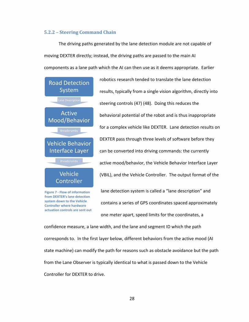
5.2.2 – Steering Command Chain 

  The driving paths generated by the lane detection module are not capable of 

moving DEXTER directly; instead, the driving paths are passed to the main AI 

components as a lane path which the AI can then use as it deems appropriate.  Earlier 

robotics research tended to translate the lane detection 

results, typically from a single vision algorithm, directly into 

steering controls (47) (48).  Doing this reduces the 

behavioral potential of the robot and is thus inappropriate 

for a complex vehicle like DEXTER.  Lane detection results on 

DEXTER pass through three levels of software before they 

can be converted into driving commands: the currently 

active mood/behavior, the Vehicle Behavior Interface Layer 

(VBIL), and the Vehicle Controller.  The output format of the 

lane detection system is called a “lane description” and 

contains a series of GPS coordinates spaced approximately 

one meter apart, speed limits for the coordinates, a 

confidence measure, a lane width, and the lane and segment ID which the path 

corresponds to.  In the first layer below, different behaviors from the active mood (AI 

state machine) can modify the path for reasons such as obstacle avoidance but the path 

from the Lane Observer is typically identical to what is passed down to the Vehicle 

Controller for DEXTER to drive.   

Road Detection SystemLane Description

Active Mood/Behavior

Breadcrumbs

Vehicle Behavior Interface Layer

Breadcrumbs

Vehicle Controller

Figure 7 ‐ Flow of information from DEXTER’s lane detection system down to the Vehicle Controller where hardware actuation controls are sent out 

29  

Some specific situations in which the output from the Lane Observer is ignored 

entirely are inside parking lots and during U‐turns; driving paths for those instances are 

generated entirely by specialized behaviors.  In all cases the path which is eventually 

output from the active behavior is no longer in the lane description format but instead is 

formatted as a series of “breadcrumbs”.  These breadcrumbs contain very similar 

information to what is in the lane description but in a format digestible by the Vehicle 

Controller.  Before being sent to the Vehicle Controller the breadcrumbs are passed 

through the VBIL which performs two functions.  First, it checks several aspects of the 

path to see if it is drivable, and then it adjusts speed limits along the path to ensure safe 

turns and speeds which will not collide with a vehicle or object in front of DEXTER.  If the 

drivability checks are passed then the speed‐adjusted breadcrumb trail is sent via UDP 

to the Vehicle Controller to be converted into the actual steering, throttle, and brake 

commands which will drive the robot. 

6 ­ Road Detection Modules 

  In order to create a lane detection system which was capable of performing in a 

wide variety of environments, a variety of different lane detection modules were 

created by several individuals.  The purpose of the road detection modules is to report 

the locations of lane boundary and divider lines to the Road Tracker which can use the 

line location to determine where DEXTER ought to drive.  Each of the modules had its 

own advantages and drawbacks, some of which were uniquely addressed in the Road 

Tracker.  Since these modules represent the work of other students they are only 

30  

described briefly below.   Each of the modules (and the Edge Crawler described in more 

detail later) shares the following attributes: 

• Detected lines are published to datasocket as a three‐parameter polynomial fit 

in the local coordinate frame in the form x = ay2 + by + c.  The x= equation form is 

chosen because road lines tend to be more vertical than horizontal in the local 

coordinate frame. 

• A confidence score between 0 and 1 is associated with each line fit 

• A valid length estimate in meters is associated with each line fit.  This is usually 

calculated by taking the distance to the farthest point that was used in the line 

fit. 

• A position enum from the following set: [left curb, left, unknown, right, right 

curb] is associated with each line fit, indicating the line’s position with respect to 

DEXTER.   

Several pieces of context information are available to each of the road detection 

modules to assist in their work.  The Road Tracker continuously publishes to a 

datasocket containing information such as the expected lane line positions based on 

previous results, whether the current section of road is expected to be straight, and the 

current lane width.  Each road detection module is free to use this information as it 

wishes.  The predicted lane locations are generated by taking the last output of the lane 

detection system and extrapolating lane boundaries using the current lane width and 

number of lanes. 

31  

6.1 ­ Rake Edge Detector 

  The Rake Edge Detector module was written using the Sherlock machine vision 

package from IPD  (49).  It relies on two large image rakes, each a set of parallel lines 

across which an edge detection routine is performed.  The two rakes cover the left and 

right halves of the screen and each returns a separate set of edge points which are used 

in a RANSAC (RANdom SAmple Consensus) (50)  2nd order fit similar to the process 

described in Appendix A4.  A shape‐based method for detecting painted lane lines is also 

used to contribute additional edges to the set of points used to fit the lines.  In order to 

take advantage of previous lane detection results, the most recent lane detection 

results are input as one of the candidate fits in the RANSAC procedure.  In this module 

the top two distinct fits for both the left and the right sides of the image are returned 

rather than just a single fit for each side.  Confidence scores are calculated based on the 

number of points in the fit, the quality of the RANSAC fit, and several other factors.  A 

LabVIEW interface module converts the reported lines into world coordinates and 

reduces the confidence on lines which are not consistent over time before publishing 

the final results to datasocket.  The Rake Edge Detector tends to perform best on 

consistent road surfaces with painted lane lines.  Performance suffers when the road 

surface was noisy due to shadows or cracks.   

6.2 ­ Color Roadbed Detector 

  The Color Roadbed Detector was written entirely in LabVIEW.  It functions by 

using a road width estimate for the current road segment to create a set of parallel 

horizontal lines on a heavily downsampled image, each of which has a width equal to 

32  

how wide the road is expected to appear on that row of the image.  These lines are 

shifted from left to right on a chosen color plane in the image in order to search for the 

shift position which achieves one of the following:  1) The maximum summed pixel value 

across the line, 2) the minimum summed pixel value across the line, 3) the minimum 

summed absolute pixel value difference across the line from a target pixel intensity.  The 

three options enable tuning for roads brighter than their surroundings, darker than their 

surroundings, or matching an intensity in a given color plane learned from a training 

section of the image.   While using the third option, a target pixel intensity is generated 

from a training line drawn down the image at the location of the last road centerline 

reported in the final output of the entire lane detection system.  This represents the 

best guess of DEXTER as to where the road lies and thus incorporates all of the 

independent road detection techniques, which can be seen as an extension of single‐

sensor type feedback as in (51). 

The endpoints of the resulting shifted lines are then filtered to remove 

inconsistent sections, put through a RANSAC line fit to extract 2nd order line fits in local 

coordinates, and published to datasocket.  Confidence scores for the lines are 

determined by the quality of the RANSAC line fits and the stability of the fits over time.  

A unique attribute of this road detection method is that the lines it identifies are always 

at the edges of the road, never at any of the edges between lanes.  This information is 

useful during the line identification step of the Road Tracker module.  The downside of 

this approach is that it is only valid if a reasonable estimate of the road width is available 

and the road is not wider than the camera’s field of view or bordered by pavement or 

33  

sidewalk.  The Color Roadbed Detector performs well on roads with noisy surfaces but is 

limited as mentioned above. 

6.3 ­ Texture Road Detector 

  The Texture Roadbed Detector was written using a C++ dll which was called by a 

LabVIEW interface.  It relies on a classification of the image based on a texture measure 

followed by expanding a set of horizontal lines up from the bottom of the image until 

boundaries in the texture classified image are reached.  The left and right endpoints of 

these horizontal lines are passed to the LabVIEW interface which converts the points 

into local coordinates, fits a 2nd order line to them using RANSAC, and publishes them to 

datasocket.  Confidence scores for the lines are based on the quality of the RANSAC line 

fits and the stability of the fits over time.  The Texture Roadbed Detector performs 

poorly when the road surface has large cracks or surface changes but does a good job 

finding road edges when curbs and painted lines are not present. 

6.4 ­ Side Camera Road Detectors 

  The Side Camera Road Detector module operating on both of DEXTER’s side 

cameras used a similar procedure to what was used for the Texture Road Detector.  The 

program is essentially the same except that the texture boundary detection lines 

propagate vertically from the bottom of the image and only a single line fit is found for 

each of the side cameras.  The results are individually published to datasocket.  

Confidence scores for the lines are based on the quality of the RANSAC line fits and the 

stability of the fits over time.  The side cameras have a limited detection range ahead of 

34  

DEXTER but are particularly useful in turns, when forward view is obstructed by another 

vehicle, or when the forward cameras are affected by glare. 

6.5 ­ LIDAR Road Detector 

  The LIDAR Road Detector was written entirely in LabVIEW.  It is the only non‐

camera road detection system on the robot and relies on the single downward facing 

LIDAR unit to collect distance and reflectivity scans of the road.  Normalized edges and 

flat regions in both the distance and reflectivity scans are analyzed to identify likely road 

edges and lane lines.  These edges are collected over time and used to fit 2nd order lines 

in local coordinates.  These lines are then published to datasocket.  This module has the 

capability to distinguish between physical curbs and painted lines, an attribute that 

helps in the line identification step of the Road Tracker module.  The LIDAR Road 

Detector is very effective when consistent curbs are present but is much less reliable 

without them. 

7 ­ Edge Crawler 

  The Edge Crawler is a road detection module that was originally developed with 

the goal of allowing DEXTER to drive in the rapidly varying “road” conditions posed by 

the Case quad.  The module is based on the detection of edges similar in shape to the 

ones that typically border roads, but it is not capable of distinguishing between actual 

road edges and many of the other edges present in the environment.  These traits allow 

it to work in environments such as roads paved with cobblestones but also pose some 

unique difficulties. 

35  

7.1 ­ Curve Extraction 

  The core of the Edge Crawler module is the ‘Extract Curves’ function which is 

built into the LabVIEW image processing toolkit.  This function searches a grayscale 

image or selected color plane for continuous edges according to a set of input 

parameters.  Each curve is returned with a set of edge strength statistics, an indicator if 

it is a closed curve, and a list of each of the pixel coordinates that make up the curve.  

The VI does a good job picking out real road boundaries in most images, but its 

performance can be improved with some preprocessing steps.  Three distinct 

preprocessing steps were implemented in order to achieve more robust performance. 

First, down sampling the image from 640x480 to 320x240 or 160x120 produced 

a moderate increase in speed and also some improvement in performance by reducing 

the effect of high frequency image content.  Second, performing histogram equalization 

tends to greatly enhance the intensity differences between the road and its 

surroundings.  The equalization also brings out small variations in the road surface, 

however, so it is followed by a low‐pass filter to minimize this affect while retaining the 

large edge along the road boundary. Lastly, applying the preprocessing and color 

extraction routines to multiple color planes increases the chances that useful curves will 

be extracted.  The blue color plane was found to be the most useful for road detection 

in general while the red color plane was used as a secondary plane for its effectiveness 

in finding painted yellow lines.  The second preprocessing step in particular is important 

in areas of very low image contrast but proved to be harmful in images which already 

possessed high contrast levels.  It was removed in the final iteration of the edge crawler 

36  

due to high contrast conditions at the NQE but the other two preprocessing steps 

remained. 

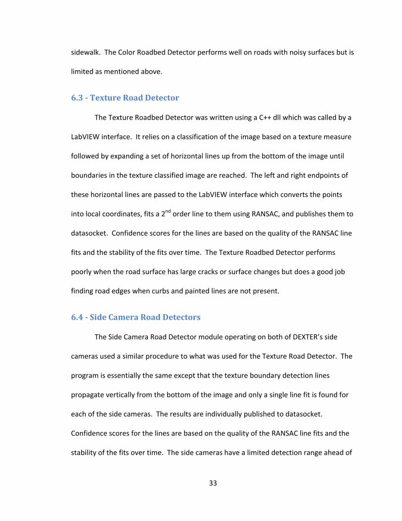
Figure 8 – Labeled images demonstrating the use of multiple color planes for curve extraction.  In both single plane images the red outlines show the output from the curve extraction function.  In this frame the curve extraction 

function is only capable of detecting the yellow centerline in the red plane.  The blue plane typically works best for detecting road boundaries with grass or shadowed curbs.   

RGB Image 

Blue Plane Red Plane

37  

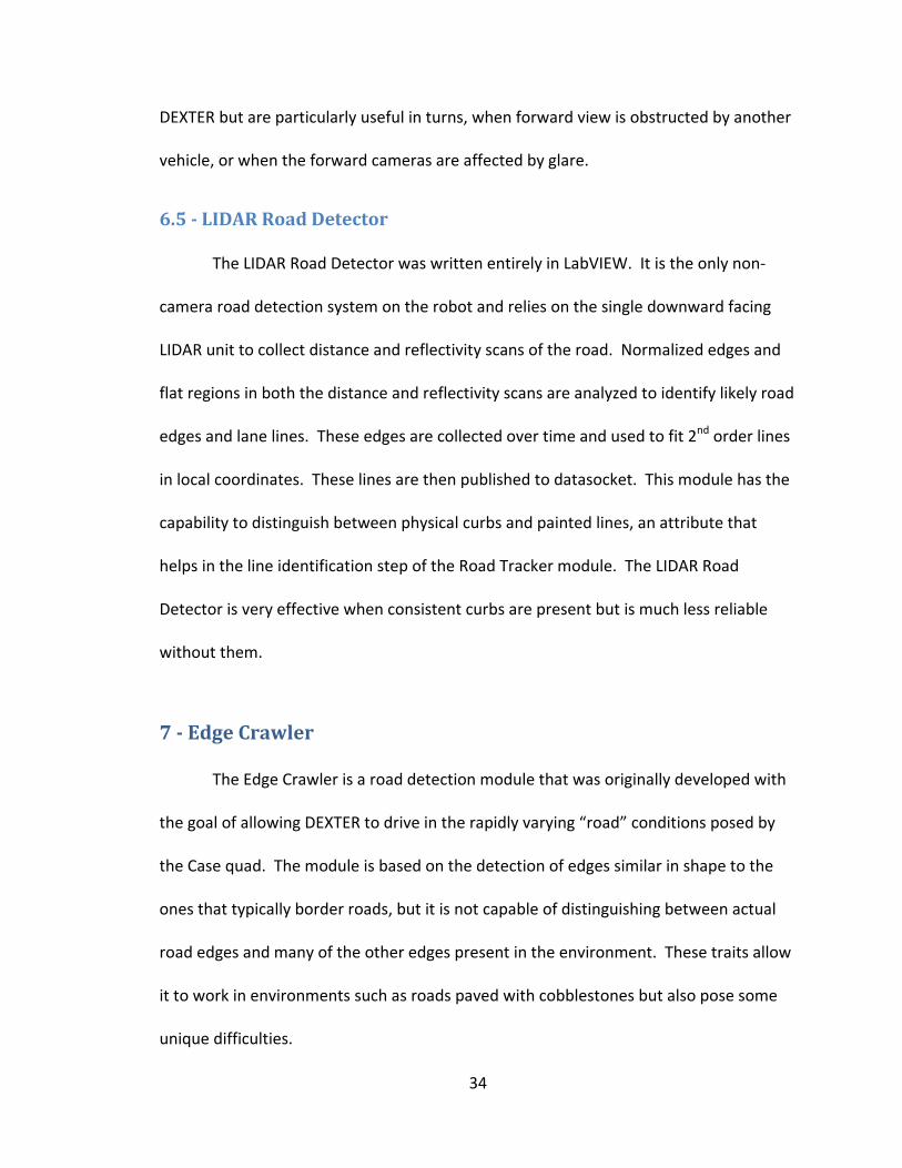
Figure 9 – The effects of downsampling, equalization, and smoothing are shown in the bottom right image.  The bottom left image has had the curve extraction routine applied directly to the blue plane of the image.  These preprocessing steps typically increase detection results along rough boundaries such as grass and reduce the 

amount of lines generated by image noise.  Due to the reduced image resolution, execution time is significantly faster with the additional processing steps. 

7.2 ­ Curve Filtering 

  The complete set of curves extracted in the previous step are put through a 

series of filters in order to narrow them down to a set that may represent the road 

boundaries.  Lines are removed and broken into segments as they pass through the 

Blue Plane 

RGB Image

ProcessedBlue Plane 

38  

filtering steps.

Figure 10 ‐ Filtering sequence applied to curves extracted from an image in the Edge Crawler. 

7.2.1 ­ Simple Filtering 

  This step iterates through the extracted curve set and removes curves which are 

below a minimum length or are below a minimum average strength score, both pieces 

of information returned by the Extract Curves LabVIEW function.  Length is calculated in 

image coordinates (pixels) in this step to achieve more consistent results: short lines 

caused by the road surroundings often occur near the top of the image where relatively 

few pixels translate into a large distance in meters.  Closed curves (those which form a 

closed loop) are not removed since curbs are often detected as closed curves.  Typically 

few lines are removed by this filtering step as the lines have not been broken up into 

smaller segments yet and the average strength score is too poor of a predictor of line 

accuracy to filter aggressively based on it. 

7.2.2 ­ Curve Breakup 

  The curved breakup filter in the Edge Crawler exists to handle several scenarios 

that arise from the output of the Extract Curves function. One scenario occurs when a 

valid curb or line is connected to an object in the background such as a mailbox near the 

end of the curb.  Successful curve breakup in this case will make the road line usable 

while allowing the mailbox line to be discarded.  Another situation occurs near corners 

Curve Extraction

Simple Filtering

Curve Breakup

Curve Fit Filtering

Expectation Filtering

39  

when a single curb must be broken up into two sections, each corresponding to one of 

the intersecting road segments at the corner.  The last situation in which curve breakup 

often has an effect occurs when a curve is found around the entire length of a curb, 

looping back at one end of the image to end at the section of curb where it began.  

Curve breakup has minimal effect on the resulting line fit but no harm is caused by 

creating two curves instead of one at the correct location.  Curve breakup is performed 

in the following steps, all performed in image coordinates: 

1) A 2nd order polynomial is fit to all of the image points contained within the curve.  

If the mean squared error (mse) of the fit is below a cutoff than the curve is 

accepted. 

2) If a curve’s fit mse is too high, each of the points along the curve is checked for 

perpendicular distance to a straight line connecting the endpoints of the curve.  

If the maximum distance from this perpendicular line at any location is below a 

cutoff than the curve is accepted. 

3) If a line has failed the two checks above then it is split at the point with the 

maximum perpendicular distance.  Both lines resulting from the split are checked 

to see if they are greater than a minimum length and if so they are sent back to 

step 1 above, otherwise they are discarded. 

4) All lines which have passed through steps 1‐3 are accepted if they are above a 

minimum length. 

40  

7.2.3 ­ Curve Fit Filtering 

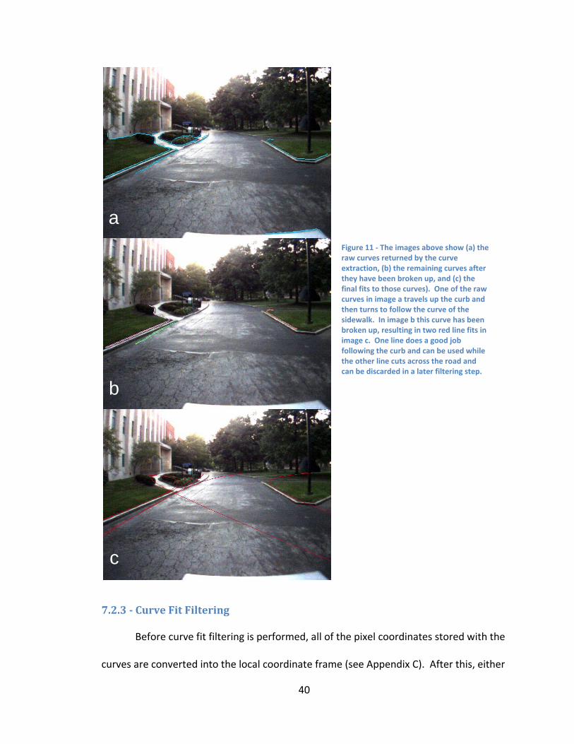
  Before curve fit filtering is performed, all of the pixel coordinates stored with the 

curves are converted into the local coordinate frame (see Appendix C).  After this, either 

a

b

c

Figure 11 ‐ The images above show (a) the raw curves returned by the curve extraction, (b) the remaining curves after they have been broken up, and (c) the final fits to those curves).  One of the raw curves in image a travels up the curb and then turns to follow the curve of the sidewalk.  In image b this curve has been broken up, resulting in two red line fits in image c.  One line does a good job following the curb and can be used while the other line cuts across the road and can be discarded in a later filtering step. 

41  

a 1st or 2nd order polynomial fit is performed for each of the curves depending on 

whether the context information published by the Road Tracker indicates that the road 

is straight or not.  Lines below a length threshold are always fit using 1st order lines 

because short curves tend to produce very erratic 2nd order fits.  Lines which have a fit 

mse greater than a threshold are removed.  In addition to removing lines which do not 

have a road‐like shape, this step is used to generate the local fit parameters for all of the 

remaining lines. 

7.2.4 ­ Expectation Filtering 

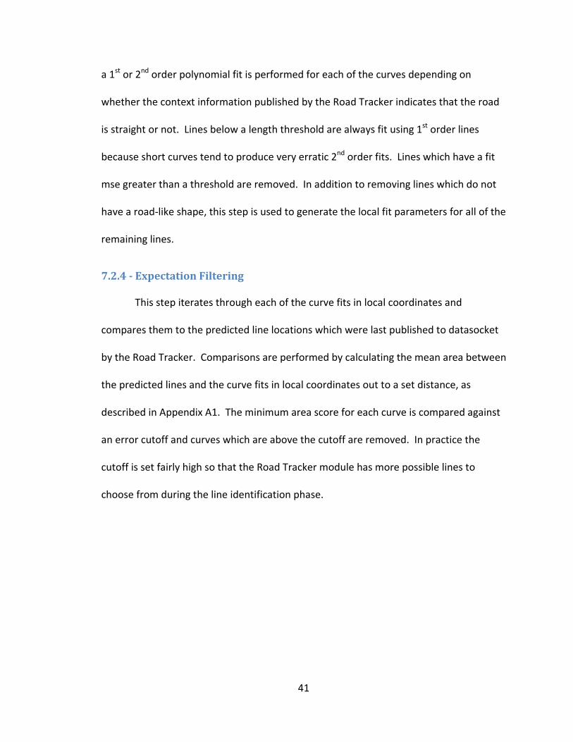
  This step iterates through each of the curve fits in local coordinates and 

compares them to the predicted line locations which were last published to datasocket 

by the Road Tracker.  Comparisons are performed by calculating the mean area between 

the predicted lines and the curve fits in local coordinates out to a set distance, as 

described in Appendix A1.  The minimum area score for each curve is compared against 

an error cutoff and curves which are above the cutoff are removed.  In practice the 

cutoff is set fairly high so that the Road Tracker module has more possible lines to 

choose from during the line identification phase. 

42  

a

c

b

Figure 12 – Images demonstrating the effects of filtering by angle.  (a) a set of line fits prior to angle filtering, (b) a graph showing the same line fits in local coordinates.  The red box lines are the predicted line locations and the dashed lines are the fits which are allowed to pass through the filter.  (c) the remaining fits on the image after filtering, corresponding to the dashed lines in image b. 

43  

7.3 ­ Confidence Estimation and Formatting 

  The remaining curves are assigned a confidence score which is a weighted sum 

of three measures.   The mean edge strength reported by the Extract Curves VI is not a 

very reliable measure of validity but it is good enough to contribute to the line 

confidence with a low weight.  The length of the curve is the best indicator of validity as 

curves extracted from noise on or off the road tend not to be long.  Lastly, a penalty is 

assigned based on how far the nearest point on the curve is from DEXTER.  This last 

factor is used to reduce the confidence in lines fit from curves far out ahead of the robot 

which are less likely to be accurate at short distances.  The weighted sum of these 

measures is constrained to lie between 0 and 1.  A valid length for the line is estimated 

by taking the distance from DEXTER to the most distant of the two curve endpoints.  

Due to the nature of the Edge Crawler, no position information to aid in line 

identification can be provided with the curves.  The local fit parameters of the remaining 

curves are published to datasocket along with their confidence and valid length scores. 

8 ­ Road Tracker 

  The Road Tracker module has three main functions:  1) merge the outputs of the 

various road detection modules, 2) use context information about the road to return a 

path corresponding to the correct lane, and 3) smooth out the results of the sensor road 

detection.  In order to do this the road tracker maintains a set of tracked lines, each of 

which is composed of the following information: 

• Fit parameters for a 2nd order polynomial in local coordinate space. 

44  

• A unique ID used internally in the Road Tracker. 

• A strength score ranging from 0 to well over 100. 

• A valid length in meters. 

• A position enum from the following set: [left curb, left, unknown, right, right 

curb].  Left or right is relative to DEXTER, and curb indicates that it is the leftmost 

or rightmost line on the road. 

• A last identification index recording which lane line the tracked line matched in 

the previous iteration, if any. 

• A list of the road detection modules whose inputs were sources for the tracked 

line. 

The tracked lines are maintained between iterations until they are removed in the line 

tracking step or are cleared, which happens automatically when DEXTER enters a new 

road segment.  The width of the current lane is also maintained between iterations until 

cleared.  The following series of steps is repeated in each iteration of the Road Tracker:  

Figure 13 ‐ Sequence of processing steps in the Road Tracker. 

8.1 ­ Get Context Information 

  In order to correctly analyze the line information coming in from each of the 

road detection modules, the Road Tracker must be aware of several pieces of 

Get Context Information Line Tracking Line 

IdentificationCenterline Estimation

45  

information contained in other software modules.  The following pieces of information 

are read as inputs by the Road Tracker: 

• The desired observation lane from a datasocket published by the Mood Selector.  

This indicates which of the current available lanes DEXTER’s AI wishes to receive 

from the road detection system. 

• The expected width of the current lane, queried from the Global Mapper once 

per segment. 

• The Route Localization from a datasocket published by the Route Observer.  This 

indicates the current lane and segment that DEXTER believes he is driving in, 

ignoring necessary travel in opposing traffic lanes. 

• The physical state from a datasocket published by the Physical State Observer. 

• The route information from a datasocket published by the Route Observer.  This 

lets the Road Tracker determine how many lanes are in the current segment and 

their arrangement by ID. 

• The Lane Description from a datasocket published by the Lane Observer.  This is 

used to generate predicted lane line locations in combination with the other 

context information including the number of lanes and the lane width.  The 

number of predicted lines is equal to the number of lanes in the segment + 1. 

The predicted lane locations are combined with several other pieces of information 

and published to datasocket as a collection of road knowledge which the various 

road detection modules can take advantage of. 

46  

8.2 ­ Line Tracking 

8.2.1 ­ Line Input 

  The first step in Line Tracking is to read the outputs of all of the Road Detection 

modules via their respective datasockets.  Timeouts on all of the datasocket reads 

ensure that a dropped sensor does not impact the system beyond the loss of its 

information.  Input lines are formatted as a tracked line with an initial strength equal to 

their confidence score multiplied by ten.  After doing this, input lines with zero 

confidence or zero valid length distances are removed.  Also, the lines are temporarily 

converted into image coordinates so that lines which are vertical in image space can be 

removed.  This step is very effective at removing erroneous detections resulting from 

glare on the lens, trees, and other vertical objects.  The actual road lines are very rarely 

near vertical in the image so there is little loss of valid information due to this step.  

After this the lines in local coordinates are passed on to the next step. 

8.2.2 ­ Line Maintenance 

  Before the existing tracked lines can be merged with the new input lines, their 

parameters in local coordinate space are shifted to correspond with the change in 

DEXTER’s physical state since the last iteration of the Road Tracker.  This is done by 

generating a set of points along the fit from each line (still in local coordinates), shifting 

and rotating them according to the physical state change since the last iteration, and 

refitting new lines from the points.  This step performs two functions.  First, it shifts the 

positions of tracked lines so that they remain in the correct position while moving 

47  

around turns.  Second, it reduces the valid length of the line by the distance traveled so 

that a line will not be followed beyond its real world valid distance.  After the lines have 

been shifted, their confidence scores are decayed by a percentage in order to gradually 

eliminate lines which are infrequently updated.  Tracked lines that have a valid distance 

less than or equal to zero or have a strength score less than a minimum threshold are 

removed.  The confidences of lines are also capped at a maximum score in this step, 

preventing lines from exceeding a chosen confidence limit prior to the merging step.  

After a fixed number of iterations, the source list of each of the tracked lines is cleared 

to insure that source listings only persist for a limited period of time.  In the last step 

prior to merging, lines currently classified as left, unknown, and right are reclassified.  

This is done by evaluating the positions of lines at constant distances ahead of and 

behind DEXTER’s position and determining if they are to the left or right of DEXTER. 

8.2.3 ­ Line Merging 

  For each input line, a distance score is calculated between it and each of the 

tracked lines using the method described in Appendix A1.  The result of this step is a 

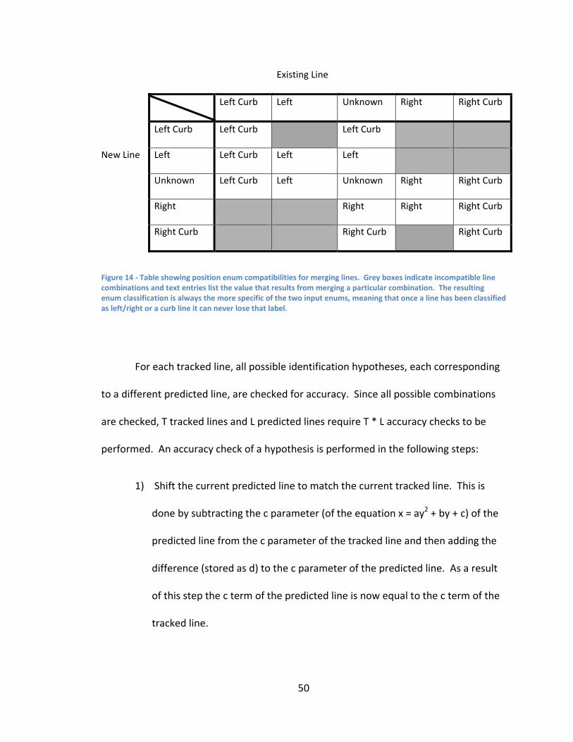
triangular matrix of line distance scores.  If the position enums of two lines are 

incompatible according to the table in Figure 14 then their distance in the matrix is set 

to infinite and no calculations are performed.  For each input line, If the distance to the 

nearest tracked line is below a cutoff, the input line and tracked line are merged.  

Merging involves the following steps: 

48  

1) The valid length is set to a weighted average of the two lines with the longer line 

having a greater weight. 

2) If the line source (the road detection module that reported the input line, such 

as the Edge Crawler) is not currently associated with the tracked line it is added 

to the source list. 

3)  The strengths of the two lines are added together with a limiting factor that the 

output strength cannot be increased by this addition to an amount greater than 

the new input line strength * 10.  The purpose of this limitation is to bound the 

degree to which a low confidence input line can accumulate a high strength 

score via repeated low confidence detections.  Note that the input line strength 

will be in the range from 0 to 10, meaning that line merging cannot raise a 

confidence score above 100. 

4) The line fit parameters are merged via the routine described in Appendix entry 

A3. 

Input lines which are not a close enough match to any of the tracked lines are given 

their own unique ID and added to the tracked line list with a strength score equal to the 

input line strength * 10.  After all of the input lines have been handled a routine checks 

each of the tracked lines against each other to determine if they should be merged into 

a single tracked line.  This is performed in a manner similar to how the input lines are 

merged with the tracked lines and serves to consolidate the number of tracked lines.  

Line pairs in this step are merged if their position enums are compatible and they are 

within a cutoff distance of each other.  Finally, all of the remaining tracked lines are re‐

49  

evaluated to determine their position enum in a manner identical to the process 

described at the end of 8.2.2. 

8.3 ­ Line Identification 

  In the line identification step, the collection of tracked lines is compared against 

the predicted lines in order to determine which correspond to each other.  The tracked 

fits are sorted by their strength score and only the N strongest fits are identified in the 

following process.  When selecting the N strongest fits, tracked lines with multiple 

sources and lines which were identified in the previous iteration are given a strength 

boost.  After selecting the strongest lines, a triangular distance matrix is built between 

each of the predicted lines and each of the tracked lines, with incompatible position 

enums resulting in an infinite distance.  The distance to a predicted line is reduced by a 

fraction if a tracked line was identified as that predicted line on the previous iteration, 

resulting in tracked lines being more likely to retain their previous identifications than to 

adopt new identifications.  This helps to improve the stability of line classification results 

between iterations.   

50  

Figure 14 ‐ Table showing position enum compatibilities for merging lines.  Grey boxes indicate incompatible line combinations and text entries list the value that results from merging a particular combination.  The resulting enum classification is always the more specific of the two input enums, meaning that once a line has been classified as left/right or a curb line it can never lose that label. 

For each tracked line, all possible identification hypotheses, each corresponding 

to a different predicted line, are checked for accuracy.  Since all possible combinations 

are checked, T tracked lines and L predicted lines require T * L accuracy checks to be 

performed.  An accuracy check of a hypothesis is performed in the following steps: 

1)  Shift the current predicted line to match the current tracked line.  This is 

done by subtracting the c parameter (of the equation x = ay2 + by + c) of the 

predicted line from the c parameter of the tracked line and then adding the 

difference (stored as d) to the c parameter of the predicted line.  As a result 

of this step the c term of the predicted line is now equal to the c term of the 

tracked line. 

      Existing Line       

    Left Curb  Left  Unknown  Right  Right Curb 

  Left Curb  Left Curb    Left Curb     

New Line  Left  Left Curb  Left  Left     

  Unknown  Left Curb  Left  Unknown  Right  Right Curb 

  Right      Right  Right  Right Curb 

  Right Curb      Right Curb    Right Curb 

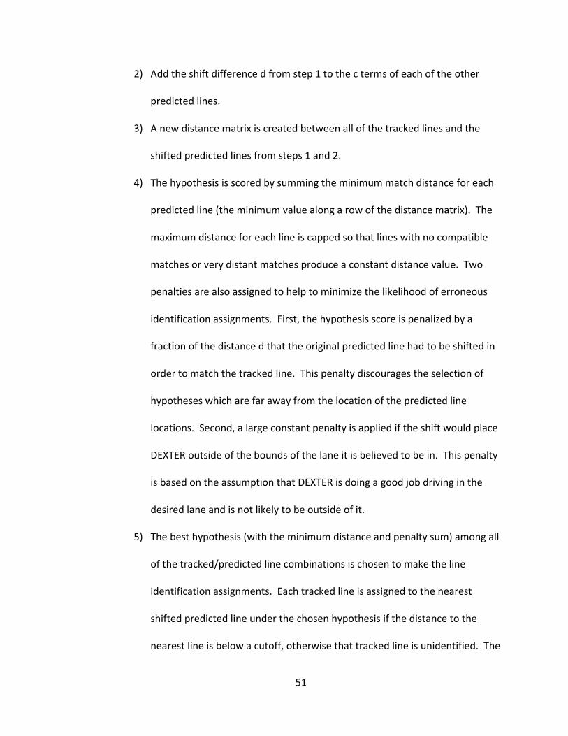
51  

2) Add the shift difference d from step 1 to the c terms of each of the other 

predicted lines.   

3) A new distance matrix is created between all of the tracked lines and the 

shifted predicted lines from steps 1 and 2. 

4) The hypothesis is scored by summing the minimum match distance for each 

predicted line (the minimum value along a row of the distance matrix).  The 

maximum distance for each line is capped so that lines with no compatible 

matches or very distant matches produce a constant distance value.  Two 

penalties are also assigned to help to minimize the likelihood of erroneous 

identification assignments.  First, the hypothesis score is penalized by a 

fraction of the distance d that the original predicted line had to be shifted in 

order to match the tracked line.  This penalty discourages the selection of 

hypotheses which are far away from the location of the predicted line 

locations.  Second, a large constant penalty is applied if the shift would place 

DEXTER outside of the bounds of the lane it is believed to be in.  This penalty 

is based on the assumption that DEXTER is doing a good job driving in the 

desired lane and is not likely to be outside of it. 

5) The best hypothesis (with the minimum distance and penalty sum) among all 

of the tracked/predicted line combinations is chosen to make the line 

identification assignments.  Each tracked line is assigned to the nearest 

shifted predicted line under the chosen hypothesis if the distance to the 

nearest line is below a cutoff, otherwise that tracked line is unidentified.  The 

52  

identification cutoff distance decreases with the current confidence of the 

lane detection system as output by the lane observer, allowing the Road 

Tracker to fine tune its identifications when it is doing well.  One situation 

where the effect of this cutoff adjustment is apparent is on roads with curbs 

near painted lines.  While overall system confidence is low both the curb and 

the painted line will be identified to the same predicted line but as system 

confidence rises either the curb or painted line will be chosen and the other 

will be unidentified. 

Figure 15 ‐ Illustration of the identification hypothesis testing process for the simplest case of two predicted and two detected lines.  The red and blue lines represent the different hypothesis cases for each tracked line.  The total number of hypotheses tested is equal to the number of tracked lines multiplied by the number of predicted lines.  

Green bars in the bottom image connect identified to predicted lines. 

Hypotheses 

for this 

Hypothesis 

for this 

53  

8.4 ­ Centerline Estimation 

  Once one or more tracked lines have been identified, the centerline of the 

desired lane can be estimated.  This is done by using the current lane width to shift all of 

the identified lines over an appropriate number of lane widths to correspond to either 

the left or right line of DEXTER’s current lane.  Lines already identified as matching the 

left and right lines of DEXTER’s current lane are not shifted.  Each of the two sets of 

lines, left and right, is merged into a conglomerated single line so that only one line 

remains on each side.  Merging the lines in this manner may require multiple merges as 

in appendix A3.  These two lines are shifted over by half a lane width so that each forms 

an estimate of the centerline of DEXTER’s lane.  The two centerline estimates are then 

compared to see if it is possible to merge them according to the procedure in appendix 

section A3.  If the average distance between the two centerline estimates is a significant 

fraction of the current lane width or the variation in distance between the two 

estimates is above a threshold then the stronger of the two centerline estimates is 

returned as the output from the centerline estimation step.  Otherwise, the two lines 

are merged in the manner described in appendix A3.  If the two lines are similar enough 

to be merged then the current lane width is adjusted by a fraction to be closer to the 

average distance between the conglomerate left and right lane lines. 

54  

Figure 16 – A hypothetical centerline estimation example is depicted in six frames from top to bottom on the left followed by top to bottom on the right.  DEXTER’s position in a three lane road is indicated by the orange box in each of the frames.  In the middle left and lower left frames line colors correspond to the predicted lines in the top left image that they have been identified with.  The colors in the right three frames are unique since line identifications are irrelevant in those steps. 

  The centerline is published to a datasocket which is read by the Lane Observer 

along with several other pieces of information.  Two confidence scores are provided; 

one is a value that is reported only as none, low, moderate, or high and is composed of 

the following factors: 

• Confidence is higher in straighter lines 

• More input sources increases confidence 

• The strength score of the centerline adjusts confidence 

• If both the left and right lane lines were used for centerline estimation 

confidence is greater 

• The final confidence score is put through a low‐pass filter 

55  

A more detailed confidence report is also provided in case other software modules wish 

to know more detailed information.  This confidence report includes the final numerical 

strength total of the merged left and right lines, which of those lines are being used to 

define the output path, and the final numeric strength assigned to the output path.  In 

most cases it is best to trust the simplified confidence evaluation provided by the Road 

Tracker. 

9 ­ Lane Observer 

  The role of the Lane Observer in DEXTER’s lane detection system is to obtain the 

GPS map of the area ahead of DEXTER and to merge this with the results of sensor road 

detection.  The main components of this are building a query sequence to request the 

correct map points and making automated decisions about how much to trust the 

sensor information when a map is available. 

9.1 ­ Map Query Sequence 

  In order for DEXTER to operate on a given course, an RNDF (Route Network 

Definition File) must exist for that course.  The RNDF specifies the connectivity of roads 

and lanes on the course and also provides a rough set of waypoints to follow while 

navigating the course.  The points can be interpolated between, either automatically or 

by hand, to generate sequences of GPS coordinates which DEXTER can drive along.  

These GPS point sequences are stored in the Global Mapper Software module.  

Communication with the Global Mapper is accomplished via UDP queries with a number 

of parameters for requesting points at different locations.  In order to know which 

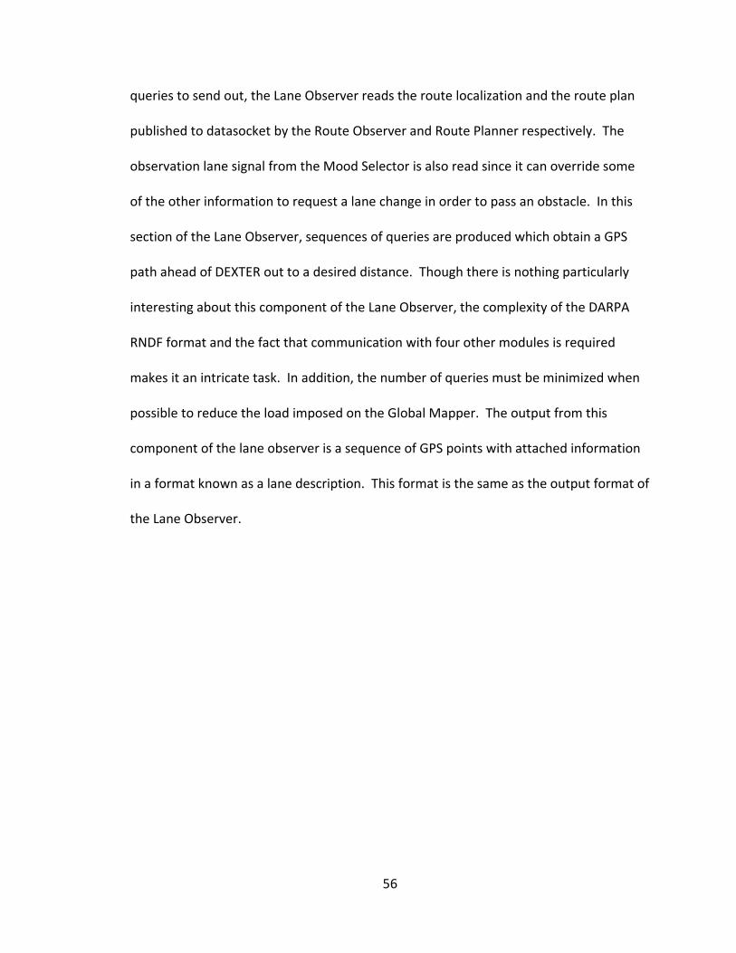
56  

queries to send out, the Lane Observer reads the route localization and the route plan 

published to datasocket by the Route Observer and Route Planner respectively.  The 

observation lane signal from the Mood Selector is also read since it can override some 

of the other information to request a lane change in order to pass an obstacle.  In this 

section of the Lane Observer, sequences of queries are produced which obtain a GPS 

path ahead of DEXTER out to a desired distance.  Though there is nothing particularly 

interesting about this component of the Lane Observer, the complexity of the DARPA 

RNDF format and the fact that communication with four other modules is required 

makes it an intricate task.  In addition, the number of queries must be minimized when 

possible to reduce the load imposed on the Global Mapper.  The output from this 

component of the lane observer is a sequence of GPS points with attached information 

in a format known as a lane description.  This format is the same as the output format of 

the Lane Observer. 

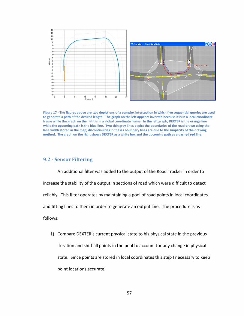
57  

Figure 17 ‐ The figures above are two depictions of a complex intersection in which five sequential queries are used to generate a path of the desired length.  The graph on the left appears inverted because it is in a local coordinate frame while the graph on the right is in a global coordinate frame.  In the left graph, DEXTER is the orange line while the upcoming path is the blue line.  Two thin grey lines depict the boundaries of the road drawn using the lane width stored in the map; discontinuities in theses boundary lines are due to the simplicity of the drawing method.  The graph on the right shows DEXTER as a white box and the upcoming path as a dashed red line. 

9.2 ­ Sensor Filtering 

  An additional filter was added to the output of the Road Tracker in order to 

increase the stability of the output in sections of road which were difficult to detect 

reliably.  This filter operates by maintaining a pool of road points in local coordinates 

and fitting lines to them in order to generate an output line.  The procedure is as 

follows:  

1) Compare DEXTER’s current physical state to his physical state in the previous 

iteration and shift all points in the pool to account for any change in physical 

state.  Since points are stored in local coordinates this step I necessary to keep 

point locations accurate. 

58  

2) Generate a set of points in local coordinates at one meter intervals along the 

current line output from the Road Tracker.  Assign each of these points a weight 

according to the confidence of the Road Tracker line and add them to the point 

pool.  These weights do not change until the point is deleted. 

3) Fit a 2nd order polynomial line through all of the points in the pool, using the 

weights each of the points was stored with originally.  This fit is the output of the 

sensor filtering procedure. 

4) Delete any points from the pool which are more than a certain distance behind 

DEXTER.  If the number of remaining points is above a cutoff, randomly delete a 

fixed percentage of points which brings the total number below the cutoff. 

59  

Figure 18 ‐ Sample results from sensor filtering in the Lane Observer.  The red points represent the point pool which has been generated from previous line outputs from the Road Tracker.  The most recent output from the Road Tracker, the blue line, has generated a set of erroneous points which can be seen beneath the blue line.  Occasional errors such as this are suppressed by the black line fit through the point pool, corresponding with step 3 in the filtering process. 

9.3 ­ Source Selection 

  The Lane Observer is capable of generating a drivable path for the robot with 

any available combination of the sensor information from the Road Tracker (having 

passed through the sensor filtering step above) and a valid map from the Global 

Mapper.  Its preferred method of operation is to use a weighted average of the paths 

from the map and from the sensor data, but depending on the confidence and 

availability of the sources it will vary its output.  A variety of configuration options can 

60  

be used to control the behavior of the source selection.  There are several primary 

modes of operation which are listed below: 

• Zero confidence map – This mode is used when an a priori map is unavailable or 

has been flagged as no confidence.  In each iteration the current sensor road 

detection readings are combined with the previous sensor results to generate a 

path.  If the sensors stop returning a path, the last determined path is followed 

until the end of it is reached.  If the sensors do not return a new path by that 

point then the zero confidence map (if available) will be used until the sensors 

reacquire a path. 

• Single source steering – If one path source is significantly more confident than 

the other than the influence of the less confident source may be ignored 

entirely.  This situation results in either strict following of either the a priori map 

or of the path returned from the Road Tracker.  Manual configuration to single 

source steering is also extremely useful for limiting the scope of robot behavior 

during specific tests.  Map‐only steering can be used to limit sensor road 

detection’s effect to shifting DEXTER’s physical state perpendicular to the path of 

the lane description.  This alternative steering technique is discussed in Appendix 

D. 

• All sources available – If the confidence of the map and the sensors are roughly 

equal then they will be merged.  This process is similar to the way that two line 

fits are merged in the road tracker (see Appendix A3) but with two additional 

steps.  First, the map path must be converted from a GPS path into a fit in local 

61  

coordinates.  Second, if the sensor path diverges in direction from the map path 

then the sensor path will only be used until the divergence occurs.  This 

effectively filters out situations such as the sensors guiding the robot down the 

wrong road at an intersection.  Appendix A5 describes the divergence detection 

algorithm. 

• All sources available, but DEXTER is far from the map points – DEXTER will 

operate in a similar manner to the mode above but will automatically shift the 

map points so that their starting point is centered at DEXTER’s current location.  

The shifted map points are then compared to the sensor output.  The principle 

behind this procedure is that the shifted map points may be able to give the 

sensor based lane detection a good estimate of the shape of the road even 

though his current physical state lies far from the map.   

62  

Figure 19 – The two input paths to the Lane Observer are shown with the output path.  All three paths include thinner lines to the sides which indicate the width of the road.  The red output path was generated by merging the white sensor and blue a priori map paths as described in the ‘All sources available’ entry in the list above.  In this case the sensor path reported a lower confidence than the map path, resulting in the merged path being weighted sleightly closer to the map path than to the sensor path.  If only a single source was chosen then the red output path would lie on top of either the blue or white input paths.   

A priori mapRoad Tracker

OutputDEXTER

63  

Figure 20 – The red (Lane Observer output) and white (Road Tracker output) paths in this image correspond to the paths shown in Figure 19.  The a priori map path is not overlaid on the image but if shown it would be to the left of the red output path.  The purple lines and labels are lines being tracked inside the Road Tracker.  In this example the combination of the two paths is more accurate than either of the paths independently.  The sensor based lane detection is usually able to improve on the position of the a priori map.  In situations where the sensor results are incorrect the map path serves as a restraining factor that prevents DEXTER from straying too far off course until the sensor accuracy improves.  The difference in curvature between the white line in Figure 19 and this figure is due to decreasing camera calibration accuracy farther out in the image, a problem which was corrected after this data was collected. 

Once the appropriate path has been built the Lane Observer publishes the path via 

datasocket to the rest of DEXTER’s AI in lane description format.  A confidence score is 

reported as either none, low, moderate, or high.  This confidence score is the calculated 

as follows:  max(RoadTrackerConfidence, min(CurrentMapConfidence, 

PhysicalStateConfidence) ).   DEXTER’s AI can react to a low road confidence score by 

limiting speed or avoiding risky maneuvers such as passing a moving obstacle. 

64  

10 ­ Test Site Performance 

10.1 ­ Case Quad 

  The large loop on Case Quad was the first area on which DEXTER’s vision system 

was developed and tested, initially using only the Edge Crawler module for line 

detection.  It is characterized by widely varying features and road widths, several types 

of noisy surface textures, a lack of painted lines, and a preponderance of fearless 

pedestrians.  The GPS signal in the quad is also very poor, however, so sensor guidance 

is critical to allow driving on the quad loop.  The results of the road detection system on 

the quad were generally good but unfortunately were not able to guide the robot 

through one particularly tight turn of the loop, marked ‘c’ in the map below.  DEXTER 

was capable of driving accurately through the rest of the course, including the 

transitions between the grass‐bordered regions and the cobblestone areas. 

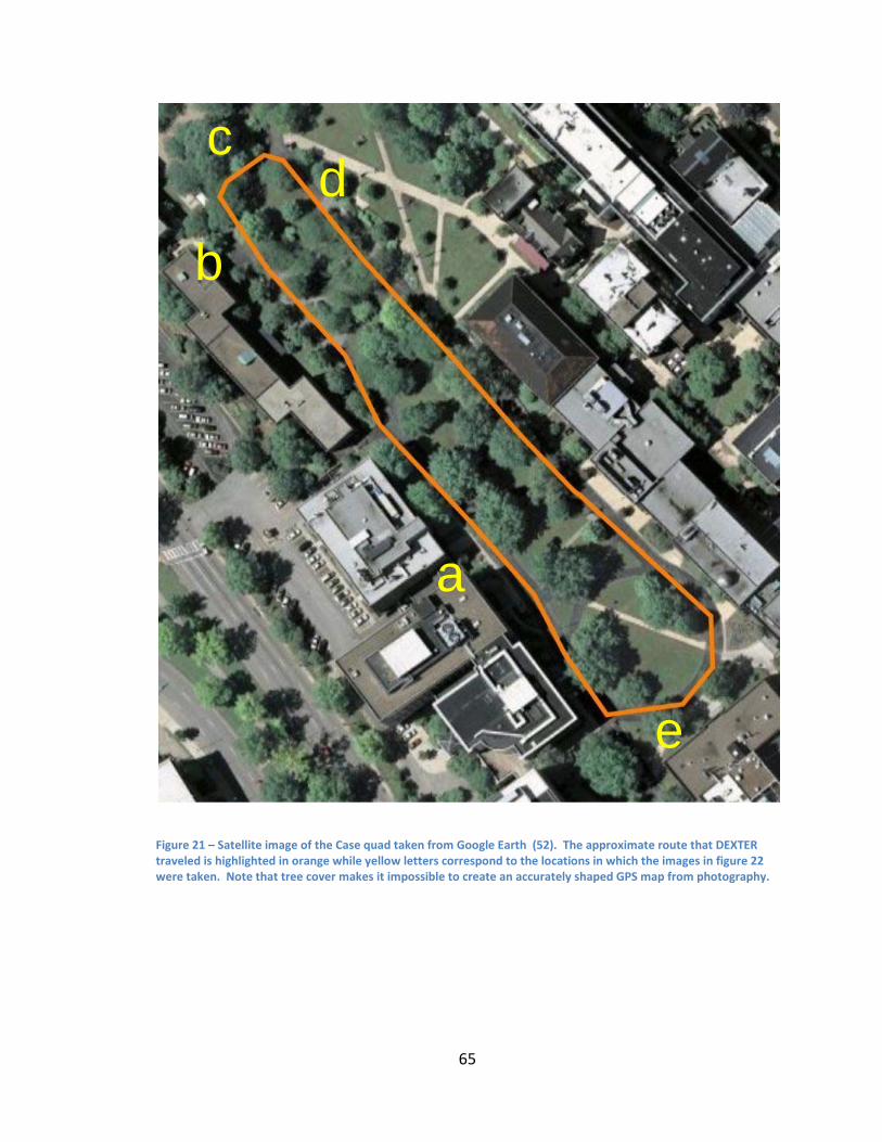
65  

Figure 21 – Satellite image of the Case quad taken from Google Earth  (52).  The approximate route that DEXTER traveled is highlighted in orange while yellow letters correspond to the locations in which the images in figure 22 were taken.  Note that tree cover makes it impossible to create an accurately shaped GPS map from photography. 

a

b

c d

e

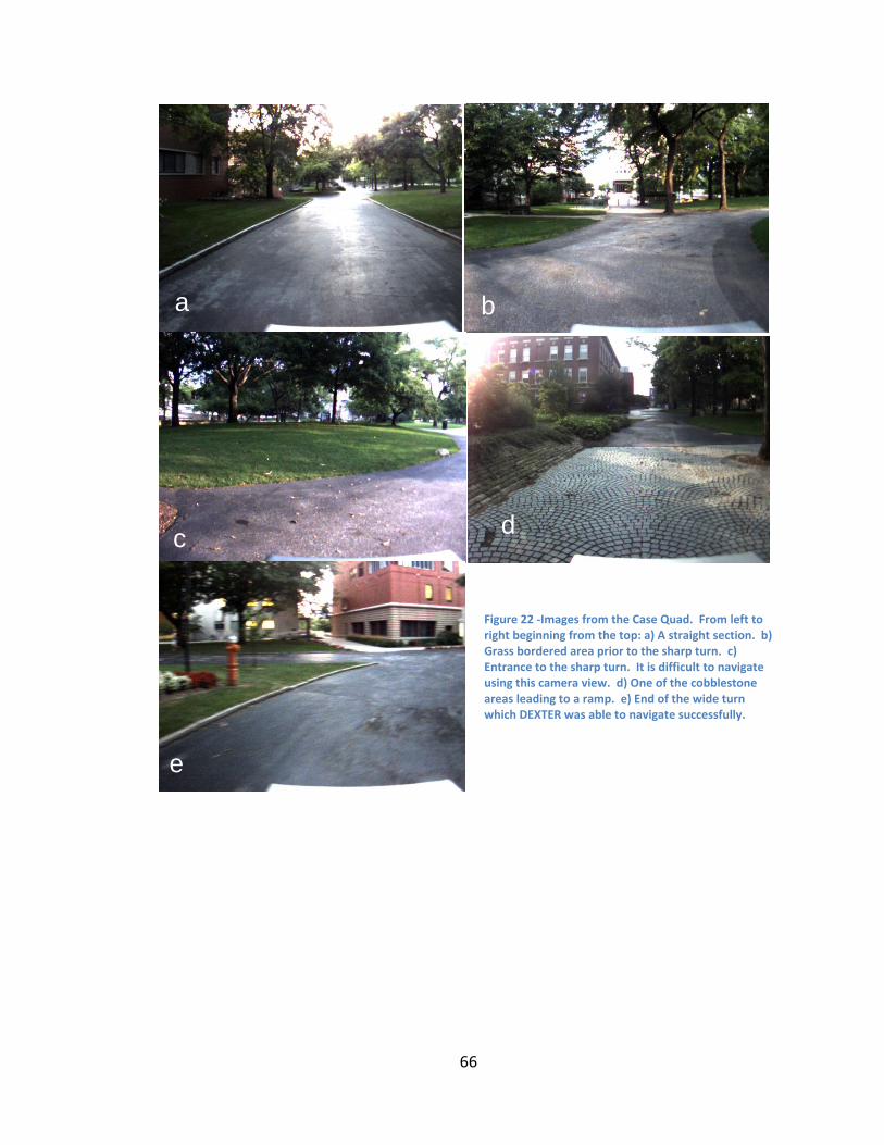
66  

Figure 22 ‐Images from the Case Quad.  From left to right beginning from the top: a) A straight section.  b) Grass bordered area prior to the sharp turn.  c) Entrance to the sharp turn.  It is difficult to navigate using this camera view.  d) One of the cobblestone areas leading to a ramp.  e) End of the wide turn which DEXTER was able to navigate successfully.  

a b

c d

e

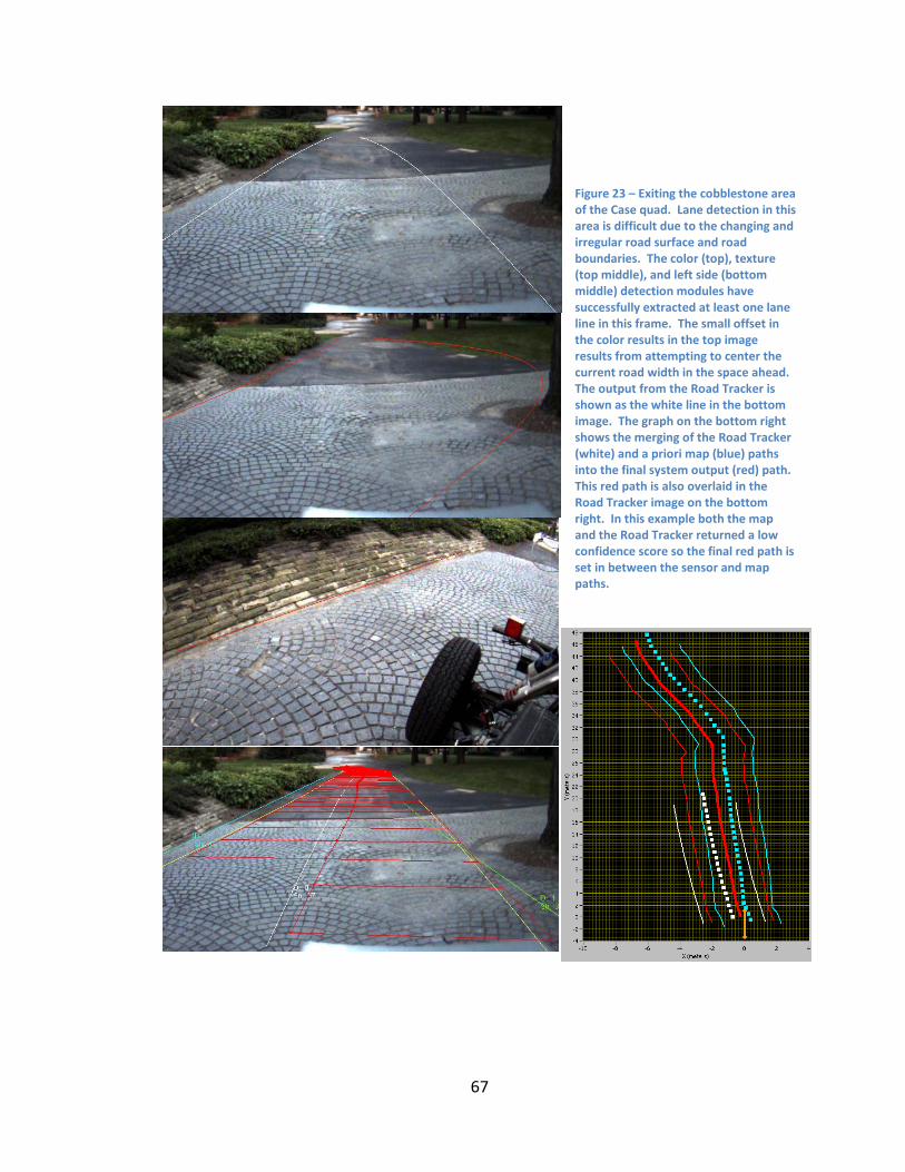
67  

Figure 23 – Exiting the cobblestone area of the Case quad.  Lane detection in this area is difficult due to the changing and irregular road surface and road boundaries.  The color (top), texture (top middle), and left side (bottom middle) detection modules have successfully extracted at least one lane line in this frame.  The small offset in the color results in the top image results from attempting to center the current road width in the space ahead.  The output from the Road Tracker is shown as the white line in the bottom image.  The graph on the bottom right shows the merging of the Road Tracker (white) and a priori map (blue) paths into the final system output (red) path.  This red path is also overlaid in the Road Tracker image on the bottom right.  In this example both the map and the Road Tracker returned a low confidence score so the final red path is set in between the sensor and map paths. 

68  

10.2 ­ Squire Valleview Farm 

  Case’s Squire Valleview Farm was the second location in which DEXTER’s road 

detection was tested.  It features a gravel track, a nicely paved winding path, and several 

sharp turns.  In addition, the GPS signal is only accurate on certain sections of the route.  

DEXTER was able to accurately navigate the winding road but unfortunately the road 

detection system was not designed to handle the very sharp turns which were required.  

In this situation, the road detection system was successful in switching over to map‐

based navigation during the turns.  In earlier iterations of the road detection system 

DEXTER had a tendency to take the wrong turn at those intersections, favoring a right 

turn in image b and going straight in image d from the set of images below.  The gravel 

track section was a unique challenge since its topography does not match the 

expectation of the lane detection system that lane lines border the outsides of the lane.  

DEXTER was able to traverse the gravel path with only a slight offset despite this 

problem. 

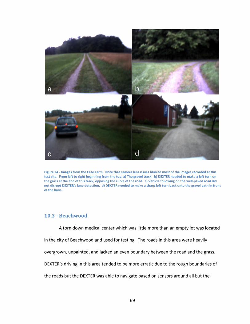
69  

Figure 24 ‐ Images from the Case Farm.  Note that camera lens issues blurred most of the images recorded at this test site.  From left to right beginning from the top: a) The gravel track.  b) DEXTER needed to make a left turn on the grass at the end of this track, opposing the curve of the road.  c) Vehicle following on the well‐paved road did not disrupt DEXTER’s lane detection.  d) DEXTER needed to make a sharp left turn back onto the gravel path in front of the barn. 

10.3 ­ Beachwood 

  A torn down medical center which was little more than an empty lot was located 

in the city of Beachwood and used for testing.  The roads in this area were heavily 

overgrown, unpainted, and lacked an even boundary between the road and the grass.  

DEXTER’s driving in this area tended to be more erratic due to the rough boundaries of 

the roads but the DEXTER was able to navigate based on sensors around all but the 

a b

c d

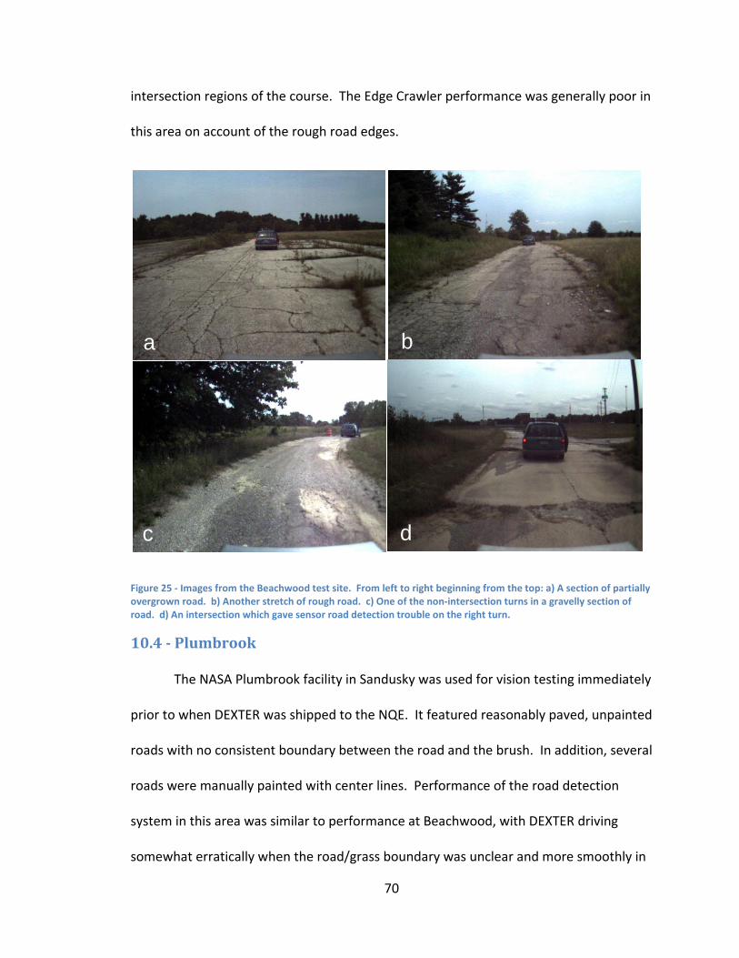
70  

intersection regions of the course.  The Edge Crawler performance was generally poor in 

this area on account of the rough road edges. 

Figure 25 ‐ Images from the Beachwood test site.  From left to right beginning from the top: a) A section of partially overgrown road.  b) Another stretch of rough road.  c) One of the non‐intersection turns in a gravelly section of road.  d) An intersection which gave sensor road detection trouble on the right turn. 

10.4 ­ Plumbrook 

  The NASA Plumbrook facility in Sandusky was used for vision testing immediately 

prior to when DEXTER was shipped to the NQE.  It featured reasonably paved, unpainted 

roads with no consistent boundary between the road and the brush.  In addition, several 

roads were manually painted with center lines.  Performance of the road detection 

system in this area was similar to performance at Beachwood, with DEXTER driving 

somewhat erratically when the road/grass boundary was unclear and more smoothly in 

a b

c d

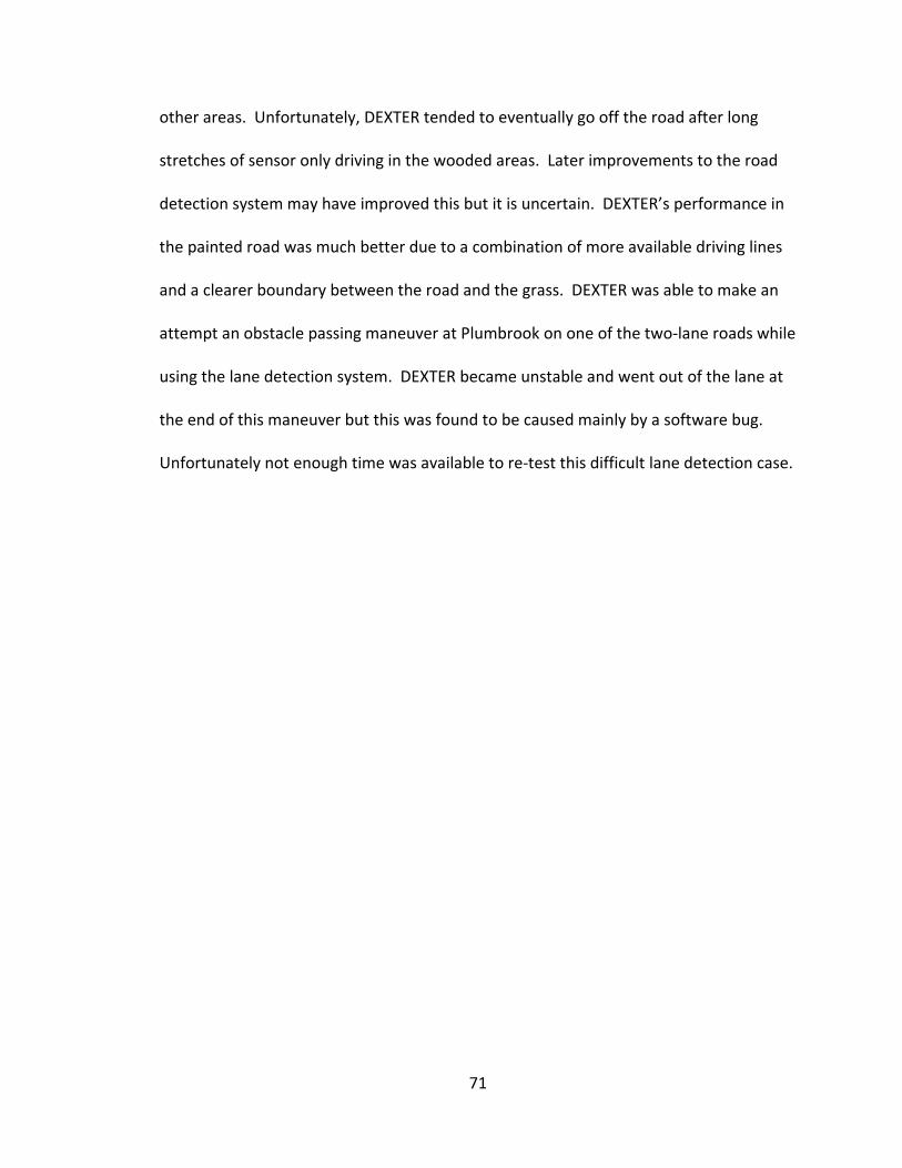
71  

other areas.  Unfortunately, DEXTER tended to eventually go off the road after long 

stretches of sensor only driving in the wooded areas.  Later improvements to the road 

detection system may have improved this but it is uncertain.  DEXTER’s performance in 

the painted road was much better due to a combination of more available driving lines 

and a clearer boundary between the road and the grass.  DEXTER was able to make an 

attempt an obstacle passing maneuver at Plumbrook on one of the two‐lane roads while 

using the lane detection system.  DEXTER became unstable and went out of the lane at 

the end of this maneuver but this was found to be caused mainly by a software bug.  

Unfortunately not enough time was available to re‐test this difficult lane detection case. 

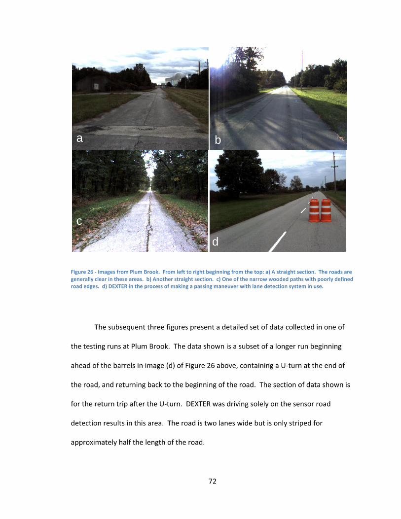
72  

Figure 26 ‐ Images from Plum Brook.  From left to right beginning from the top: a) A straight section.  The roads are generally clear in these areas.  b) Another straight section.  c) One of the narrow wooded paths with poorly defined road edges.  d) DEXTER in the process of making a passing maneuver with lane detection system in use.   

The subsequent three figures present a detailed set of data collected in one of 

the testing runs at Plum Brook.  The data shown is a subset of a longer run beginning 

ahead of the barrels in image (d) of Figure 26 above, containing a U‐turn at the end of 

the road, and returning back to the beginning of the road.  The section of data shown is 

for the return trip after the U‐turn.  DEXTER was driving solely on the sensor road 

detection results in this area.  The road is two lanes wide but is only striped for 

approximately half the length of the road. 

a b

c

d

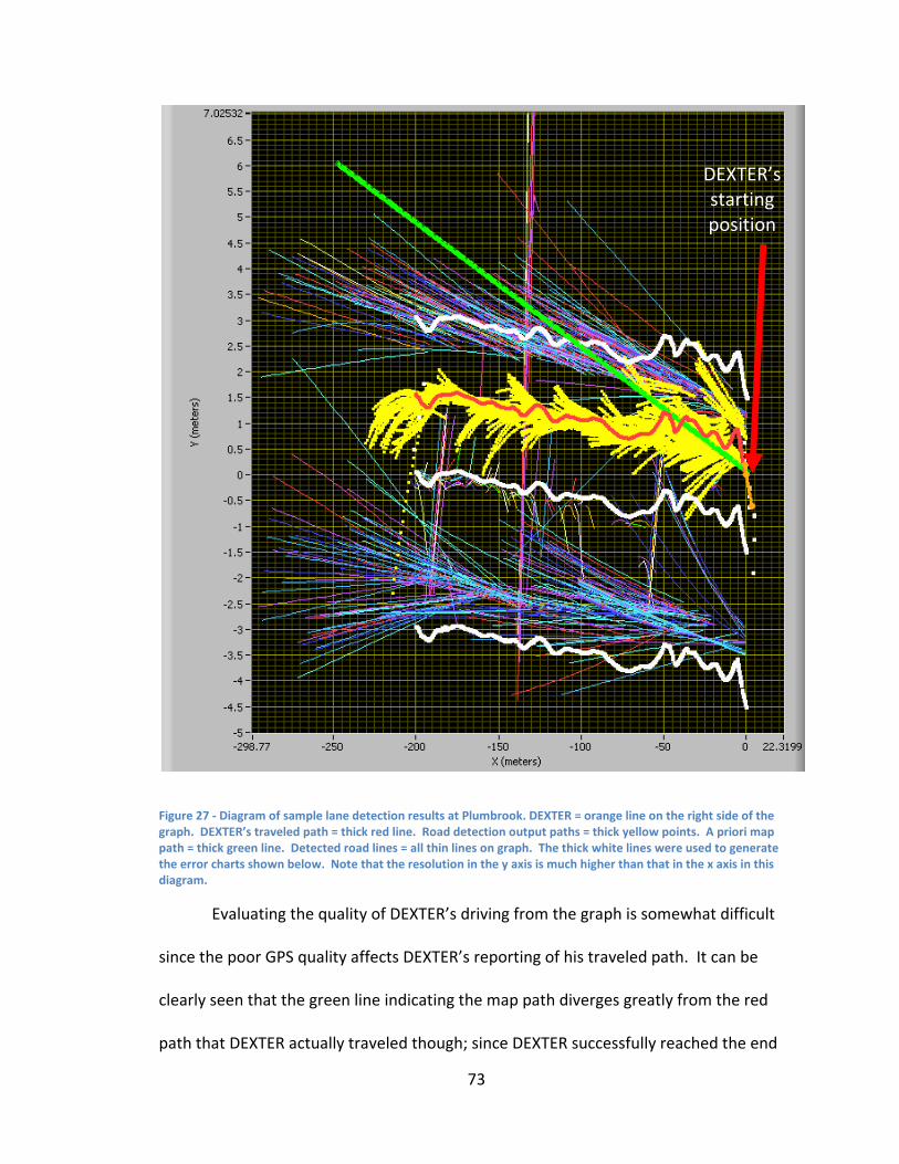
73  

Figure 27 ‐ Diagram of sample lane detection results at Plumbrook. DEXTER = orange line on the right side of the graph.  DEXTER’s traveled path = thick red line.  Road detection output paths = thick yellow points.  A priori map path = thick green line.  Detected road lines = all thin lines on graph.  The thick white lines were used to generate the error charts shown below.  Note that the resolution in the y axis is much higher than that in the x axis in this diagram. 

  Evaluating the quality of DEXTER’s driving from the graph is somewhat difficult 

since the poor GPS quality affects DEXTER’s reporting of his traveled path.  It can be 

clearly seen that the green line indicating the map path diverges greatly from the red 

path that DEXTER actually traveled though; since DEXTER successfully reached the end 

DEXTER’s starting position 

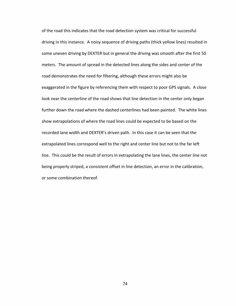
74  

of the road this indicates that the road detection system was critical for successful 

driving in this instance.  A noisy sequence of driving paths (thick yellow lines) resulted in 

some uneven driving by DEXTER but in general the driving was smooth after the first 50 

meters.  The amount of spread in the detected lines along the sides and center of the 

road demonstrates the need for filtering, although these errors might also be 

exaggerated in the figure by referencing them with respect to poor GPS signals.  A close 

look near the centerline of the road shows that line detection in the center only began 

further down the road where the dashed centerlines had been painted.  The white lines 

show extrapolations of where the road lines could be expected to be based on the 

recorded lane width and DEXTER’s driven path.  In this case it can be seen that the 

extrapolated lines correspond well to the right and center line but not to the far left 

line.  This could be the result of errors in extrapolating the lane lines, the center line not 

being properly striped, a consistent offset in line detection, an error in the calibration, 

or some combination thereof. 

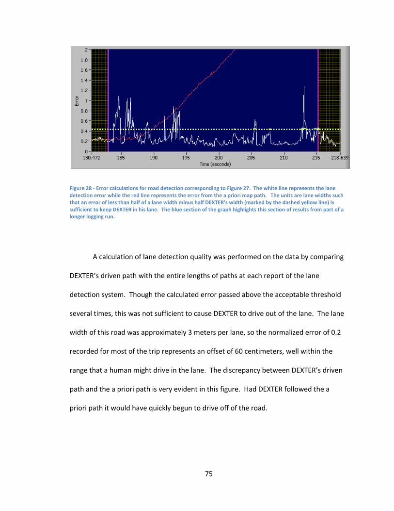
75  

Figure 28 ‐ Error calculations for road detection corresponding to Figure 27.  The white line represents the lane detection error while the red line represents the error from the a priori map path.   The units are lane widths such that an error of less than half of a lane width minus half DEXTER’s width (marked by the dashed yellow line) is sufficient to keep DEXTER in his lane.  The blue section of the graph highlights this section of results from part of a longer logging run. 

  A calculation of lane detection quality was performed on the data by comparing 

DEXTER’s driven path with the entire lengths of paths at each report of the lane 

detection system.  Though the calculated error passed above the acceptable threshold 

several times, this was not sufficient to cause DEXTER to drive out of the lane.  The lane 

width of this road was approximately 3 meters per lane, so the normalized error of 0.2 

recorded for most of the trip represents an offset of 60 centimeters, well within the 

range that a human might drive in the lane.  The discrepancy between DEXTER’s driven 

path and the a priori path is very evident in this figure.  Had DEXTER followed the a 

priori path it would have quickly begun to drive off of the road. 

76  

Figure 29 ‐ Numerical evaluation of the confidence of the lane detection system results shown in the previous two figures.  The white line indicates the total output strength, the red line shows the right line strength, and the green line shows the left output strength.  The dashed blue line indicates as a step function whether zero, one, or both sides are being used to determine the output path.  In this data at least one side is in use at all times. 

  Figure 29, above, shows the internal strength score calculated by the Road 

Tracker for the lane detections over the data segment.  The data shows that DEXTER’s 

confidence scores increased from initial lower values and remained reasonably steady 

for the rest of the run.  This corresponds to Figure 27 in which it can be seen that 

DEXTER’s path becomes steadier after an initial oscillating segment.  Comparison with 

the camera logs reveals that the early segment occupied a span of time between when 

DEXTER began moving while oriented at an angle to the road and the time when DEXTER 

settled into driving straight down the lane.  Lines to both the left and right of DEXTER 

were used to guide driving for almost the entirety of this segment. 

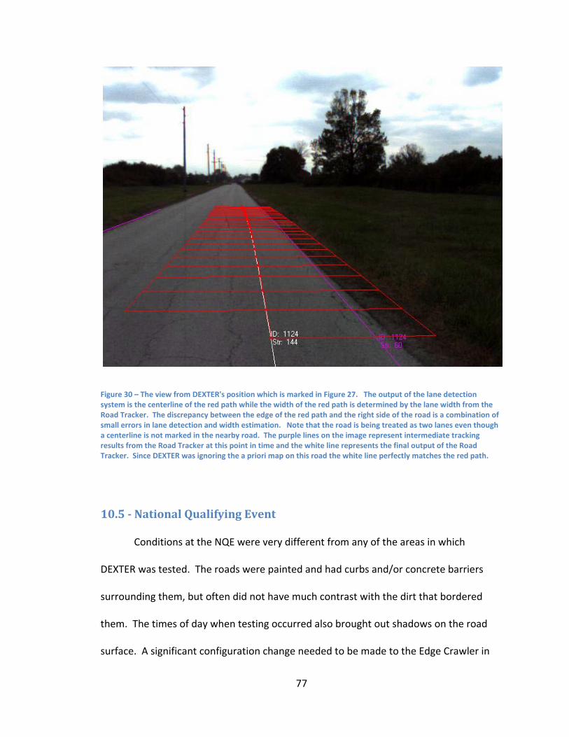
77  

Figure 30 – The view from DEXTER's position which is marked in Figure 27.   The output of the lane detection system is the centerline of the red path while the width of the red path is determined by the lane width from the Road Tracker.  The discrepancy between the edge of the red path and the right side of the road is a combination of small errors in lane detection and width estimation.   Note that the road is being treated as two lanes even though a centerline is not marked in the nearby road.  The purple lines on the image represent intermediate tracking results from the Road Tracker at this point in time and the white line represents the final output of the Road Tracker.  Since DEXTER was ignoring the a priori map on this road the white line perfectly matches the red path. 

10.5 ­ National Qualifying Event 

  Conditions at the NQE were very different from any of the areas in which 

DEXTER was tested.  The roads were painted and had curbs and/or concrete barriers 

surrounding them, but often did not have much contrast with the dirt that bordered 

them.  The times of day when testing occurred also brought out shadows on the road 

surface.  A significant configuration change needed to be made to the Edge Crawler in 

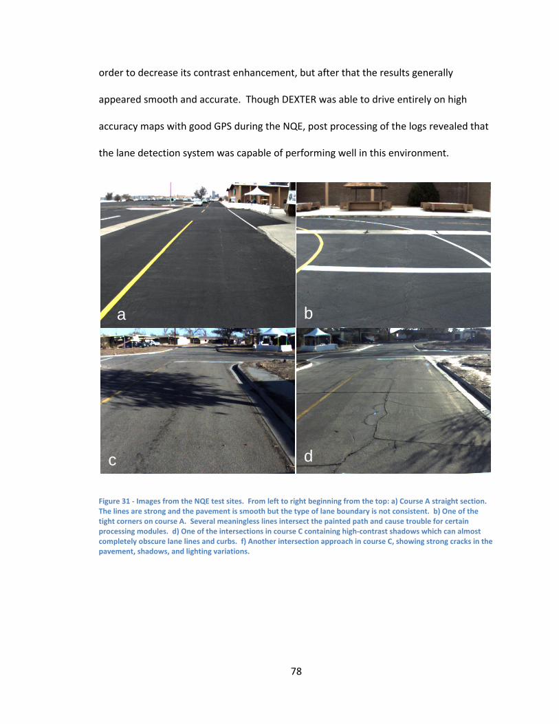
78  

order to decrease its contrast enhancement, but after that the results generally 

appeared smooth and accurate.  Though DEXTER was able to drive entirely on high 

accuracy maps with good GPS during the NQE, post processing of the logs revealed that 

the lane detection system was capable of performing well in this environment. 

Figure 31 ‐ Images from the NQE test sites.  From left to right beginning from the top: a) Course A straight section.  The lines are strong and the pavement is smooth but the type of lane boundary is not consistent.  b) One of the tight corners on course A.  Several meaningless lines intersect the painted path and cause trouble for certain processing modules.  d) One of the intersections in course C containing high‐contrast shadows which can almost completely obscure lane lines and curbs.  f) Another intersection approach in course C, showing strong cracks in the pavement, shadows, and lighting variations. 

a b

c d

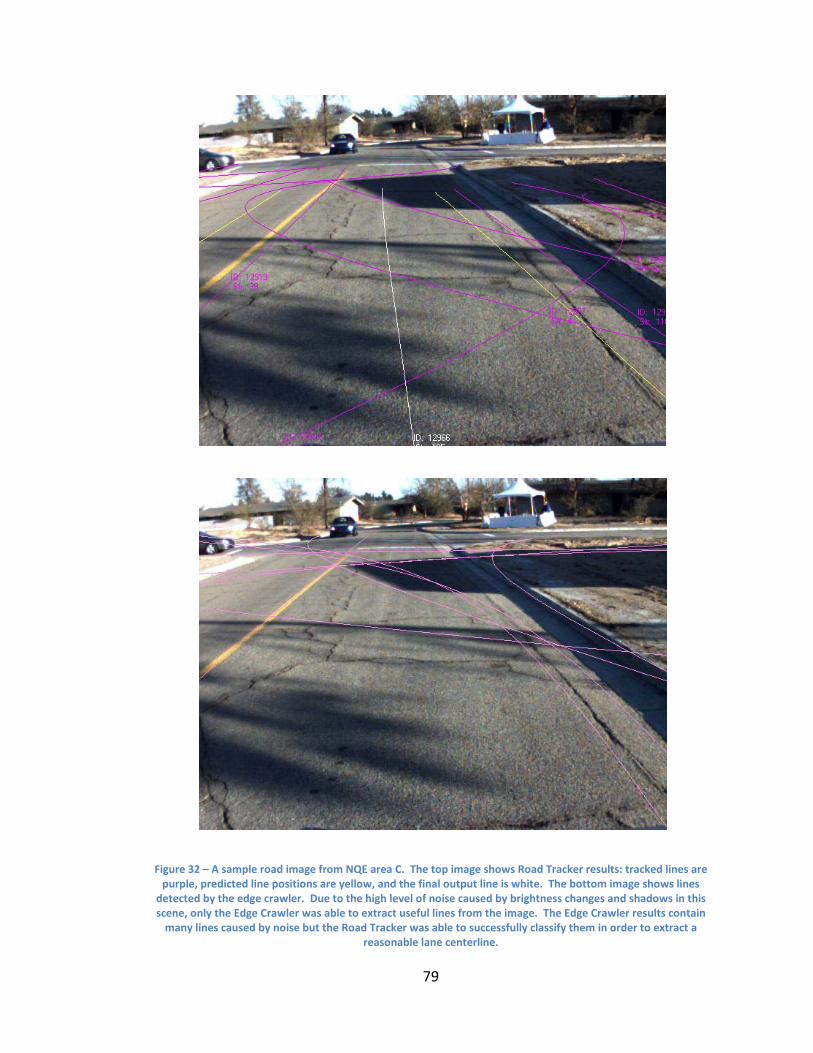
79  

Figure 32 – A sample road image from NQE area C.  The top image shows Road Tracker results: tracked lines are purple, predicted line positions are yellow, and the final output line is white.  The bottom image shows lines 

detected by the edge crawler.  Due to the high level of noise caused by brightness changes and shadows in this scene, only the Edge Crawler was able to extract useful lines from the image.  The Edge Crawler results contain many lines caused by noise but the Road Tracker was able to successfully classify them in order to extract a 

reasonable lane centerline.   

80  

11 ­ Analysis and Future Work 

Due to the nature of preparation for the Urban Challenge competition, DEXTER’s 

lane detection system as it exists now represents only the furthest snapshot in what 

could be an ongoing development process.  Most elements of the system could benefit 

from at least some additional development. 

11.1 ­ Edge Crawler 

  In its role as a very flexible road detector the Edge Crawler works very well.  It 

also tends to produce very accurate lines in areas with clearly visible curves and lines.  

The initial method by which curves are extracted from an image is powerful in a large 

part because shadows and obstructions of some parts of the road do not affect line 

detection in other regions of the image, unlike many other road detection methods.  

The technique also allows simultaneous detection of multiple lane lanes, an advantage 

on large multi‐lane roads.  There are, however, a number of specific drawbacks to this 

approach to road detection, some of which would be easier to address than others. 

  An inherent flaw with the Edge Crawler is that it sends out the most data 

(number of lines) with the least dense information: the lines cannot be classified as to 

the left/right of DEXTER and are fairly likely not to be lane lines.  This shifts a lot of the 

work that might normally be done by the road detection module onto the Road Tracker.  

Without a priori expectations of where the road should be located or lines from other 

road detection modules it can be difficult to select which lines from the Edge Crawler 

are the correct ones when conditions are noisy.  A related but special case flaw arises 

81  

with sidewalks and walls adjacent to the road.  These typically have strong edges in a 

shape similar and parallel to the lines of the actual road.  Consequently, without the 

support of accurate a priori road information or detections from other modules it is easy 

for these parallel lines to be merged with or selected over the actual road lines.  

Depending on whether both sides of the lane are being tracked and the width of the 

road this error may not be serious, however it can easily cause the robot to drive off of 

the road towards a wall or sidewalk.  Specific code to reduce the strength of exterior 

parallel edge crawler lines was added in the Road Tracker in order to reduce the 

occurrence of this error. 

Perhaps the most serious problem with the Edge Crawler, and one inherent with 

its line detection method, is that it is unable to recognize what is producing the lines it 

detects.  It tends to find lines even when none really exist, such as when the robot is 

driving over a uniform surface such as grass or a parking lot.  This can be a problem, 

particularly if the robot sees one of these lines consistently enough to detect a path off 

the road onto the surrounding terrain.  Again, a priori road information and support 

from other road detection modules help alleviate this flaw.  A final problem with the 

Edge Crawler as written is the lack of an edge detection sensitivity auto‐adjust for 

images with different amounts of noise and contrast.  This is not a problem particular to 

the Edge Crawler since many image processing algorithms suffer from the lack of such a 

feature, but the implementation of one would greatly improve the Edge Crawler. 

82  

11.2 ­ Road Tracker 

  Overall the Road Tracker performs its job well; however there are several 

specific areas that could use improvement.  Perhaps its strongest attribute is its ability 

to obtain and fuse the inputs from the multitude of road detection modules.  The 

combination process used works well in the majority of cases and operates with any 

combination of input modules.  This attribute proved to be critical since road detection 

modules changed very frequently due to fluctuating code states and late stage 

hardware changes on the robot.  Evaluation of the road detection confidence also works 

well with the exception of confidence assignment on the low end in rough conditions.  

Assignments of high and moderate confidences are very accurate but the low 

confidence assignment occupies a large set of circumstances.  Many of these low 

confidence results are the correct path but enough of them are erroneous that it is 

dangerous to trust low confidence results in general.  Properly sectioning out the 

correct instances into the moderate confidence range would constitute a significant 

improvement to the Road Tracker.  When DEXTER’s speed is directly governed by the 

road detection confidence the effects are immediately noticeable in the field.  In clear, 

straight sections of road DEXTER will begin driving more smoothly and quickly accelerate 

to a higher speed, slowing back down once rougher road conditions are reached.  A 

deficiency of the line tracking system in general which arose only later in the 

development cycle is the fact that line fits published by the road detection modules 

come with a maximum valid length but no minimum valid length.  This only proved to be 

an issue when malfunctioning wide angle lenses were replaced with lenses possessing a 

83  

narrower field of view, resulting in line detections based solely on data some distance 

ahead of DEXTER.  Reverting to wide angle lenses would fix the problem but changes 

would be needed in order to allow the use of zoom lenses. 

  The second two sections of the Road Tracker, line identification and centerline 

estimation, generally work quite well but suffer from the fact that insufficient protection 

exists against abrupt jumps in output.  While individual tracked lines are prevented from 

moving in this manner, changes in the line identification assignments or which identified 

lines are used for driving are able to cause non‐continuous jumps in the output of the 

Road Tracker.  An additional layer of complexity would need to be added to the line 

identification step in order to correct this problem but improving the centerline 

estimation would likely be easier.  With the exception of the discrete jumps both of 

these sections perform well.  DEXTER is capable of driving based on any of the lane lines 

on a multi‐lane road and can handle individual lines appearing or disappearing along a 

given road segment.  This offers flexibility to the road detection modules since a module 

whose output jumps between two different lane lines will still be fully utilized.  Correct 

lane line identifications can also be maintained during obstacle passing maneuvers in 

which most of the road is not visible, though testing of this capability was limited.  The 

Road Tracker is also capable of maintaining an accurate estimate of the lane width even 

in rapidly changing areas such as the Case Quad. 

84  

11.3 ­ Lane Observer 

  Though the Lane Observer performed well in its roles, its performance cannot be 

quantified as readily as the modules described above.  The map query sequencing 

appears to work smoothly and in an efficient manner, however given the complexity of 

the RNDF format and the comparative lack of exhaustive testing it is likely that there are 

still some bugs present in the query request logic.  No problems occurred during the 

National Qualifying Event or prior testing in the field though, so any remaining bugs are 

likely confined to odd corner cases.  The sensor filtering algorithm also appears to work 

well, however it was added very late in the development cycle and has not actually been 

in use while DEXTER was using primarily sensor based steering.  The primary motivation 

for creating it was to shore up some of the discrete jump shortcomings of the Road 

Tracker, so if further development were to eliminate those jumps than the need to use 

an additional layer of filtering might vanish. 

  The source selection section of the Lane Observer was tested for a longer period 

in the project and appears to work well, particularly in areas such as Case Quad where 

road detection cannot operate in all areas of the course.  In that and other areas the 

Lane Observer is very accurate in selecting the correct driving path source to use.  This 

ability allows the sensor results to improve or replace the map path while still using the 

a priori map to bound some of the errors from the sensor results.  The ability to 

selectively use a subsection of the sensor path according to how well it corresponds to 

the map geometry is also important, allowing road detection results to be of use even if 

they veer off the road after some distance down the path.  It also allows for smoother 

85  

transitions between road segments in which road detection is used and intersections 

where DEXTER can only rely on map coordinates for guidance. 

11.4 ­ Future Development 

Development of DEXTER’s lane detection system makes clear a number o f the 

most difficult challenges facing the development of a truly robust lane detection system.  

One area which was not even touched on by DEXTER’s system was detection of 

intersections and guidance of the vehicle through them.  Performing this task will 

require both sophisticated new software and a hardware configuration which allows for 

road detection in all geometries which may be present at an intersection.  Research on 

this topic exists but has not yet arrived at a robust solution (52), (53).  Other areas are 

handling of partial sensor obstruction, poor weather conditions, and the adjustments 

needed for high speed driving.  For driving in moving traffic it would also be very 

beneficial if the lane detection system could use vehicle detection results to assist in 

determining distant road locations.  The assistance of an existing map greatly improves 

the performance of the road detection system by bounding its results and smoothing its 

output.  Such maps are difficult to create and maintain, however, so in the future similar 

results might be achieved by building up a rough map dynamically.  The map created 

need not be an accurate drivability map; instead it could consist of a set of high level 

instructions such as “straight road”, “left turn”, and “intersection”.  If such a map were 

tied to recognizable landmarks then it would probably be a very close model to 

navigation strategies used by human drivers. 

86  

12 ­ Conclusions 

  During testing at a number of diverse locations it became clear that lane 

detection technology would be critical for accurate driving at these locations.  DEXTER’s 

lane detection system, developed primarily in the span of five months, was able to make 

dramatic improvements in each of these settings and was critical to the success of 

several live demonstrations of the robot.  Similarly, more sophisticated lane detection 

systems will be critical if autonomous vehicles are ever to be used in the real world.  The 

lane detection system implemented on DEXTER, while far from perfect, suggests that 

effective systems may be attainable within the near future if sufficient effort is invested 

in them.  DEXTER’s lane system is capable of operating with high levels of success on a 

great variety of road surfaces at a reasonable cost in equipment.  Practical applications 

of this type of technology, such as lane departure warning devices, are already 

beginning to appear in the market.  With continued interest and funding in this area, full 

autonomous control should be achievable in the not too distant future. 

87  

13 ­ Appendices 

Appendix A – Common Algorithms 

  Several routines are used repeatedly at different points in the programs 

described in this paper.  For simplicity, they are described in detail in this section and 

referenced in the rest of the paper. 

A1 ­ Line Fit Difference Calculation 

  The difference between two 2nd order line fits is calculated as the integral of the 

squared difference between the two lines divided by the length along which the integral 

was taken: 

  a x    b x    c     a x    b x    c  

This expression produces reasonable estimations of line similarity in the distance 

regions of concern to DEXTER.   

A2 ­ Polynomial Fitting 

  1st and 2nd order polynomial fits are performed in many sections of DEXTER’s 

lane detection system.  These fits are calculated using the General Polynomial Fit 

function included with the LabVIEW analysis package.  The fits all use a least square 

method for determining a mean error. 

A3 ­ Line Fit Merging 

  The aim of the line merge algorithm described below is to ensure that the 

merged line carries as much information as possible from the two input lines.  Up to the 

88  

valid length of the shorter line, both lines contribute to the shape and position of the 

output line.  After this point, the remainder of the longer line is used but with its 

position shifted to correspond to the first line section.  This takes advantage of the fact 

that lines with short valid lengths are often located in the correct location but possess a 

curvature that will be inaccurate if extrapolated from.  The exact steps for merging two 

2nd order line fits are listed below.  An input alpha where 0 < α < 1 sets the weight of line 

1 in the merge. 

1) Generate a point array for both fits from 0 out to the minimum of the valid 

lengths of the two lines.  Store this minimum value as b. 

2) For each point in one of the arrays, find the closest point in the other array.  

Calculate the variance of the distances and the mean of the distances between 

the closest point pairs.  If the variance is above a threshold or the mean is 

greater than a constant fraction of the lane width, the merge is aborted at this 

point unless a ‘force merge’ input is set to true. 

3) If the merge is not aborted, for each pair of closest points from lines 1 and 2, 

create a point between them a fraction α of the distance from the point on line 1 

to the point on line 2. 

4) Generate points for the longer of the two lines from length b out to the valid 

length of the longer line.   

5) Subtract the x value of the last point created in step 3 from the first point 

created in step 4, then subtract the difference from the x value of each point in 

89  

step 4.  This serves to shift the points generated in step 4 so that they begin at 

the location where the points from step 3 end. 

6) Concatenate the array resulting from step 5 after the array resulting from step 4 

and fit a 2nd order polynomial line to the point array.  This fit is the output of the 

merging procedure. 

In addition to merging the locations of two line fits, the line fit merging procedure 

combines several other characteristics of tracked line fits when used inside the Road 

Tracker module:   

‐ The output strength score of the merged line is equal to the maximum of the 

two input strength scores plus the lesser score multiplied by a fraction.  A 

smaller fraction reduces the rate at which strength increases by repeated line 

merges. 

‐ The valid length returned is equal to α*length1 + (1‐ α)*length2.  If the maximum 

length were to always be retained in merges than occasional lines with 

erroneously high valid length scores would have a disproportional influence on 

future calculations since merged lines would only increase in size. 

‐ The source lists of the two input lines are merged such that each entry present 

in either of the two input lists appears once in the output list. 

Note that in some situations (such as in section 8.2.3) these methods of handling 

the additional characteristics are overridden by special case calculations. 

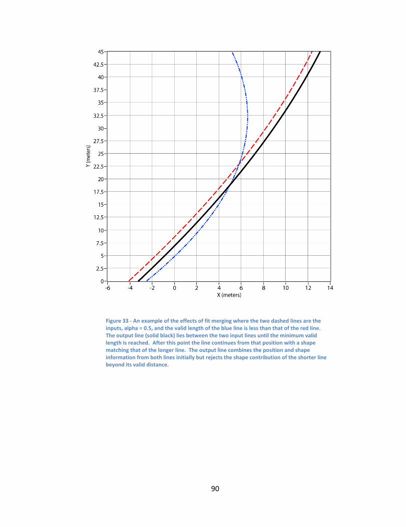
90  

Figure 33 ‐ An example of the effects of fit merging where the two dashed lines are the inputs, alpha = 0.5, and the valid length of the blue line is less than that of the red line.  The output line (solid black) lies between the two input lines until the minimum valid length is reached.  After this point the line continues from that position with a shape matching that of the longer line.  The output line combines the position and shape information from both lines initially but rejects the shape contribution of the shorter line beyond its valid distance. 

91  

A4 ­ RANSAC Line Fit 

  The implementation of the RANSAC (RANdom SAmple Consensus) differs slightly 

from its original presentation (50).  The algorithm used for line fits in several of the road 

detection modules were implemented as follows: 

1) A fixed number of points to be fit (or all the points if few are available) are 

chosen randomly and a 2nd or 1st order line is fit to the chosen points. 

2) All of the points are compared against the line fit by subtraction of X values, 

producing a distance measure for each point.  A match cutoff is generated by 

interpolating between a max and min cutoff at a max and min distance.  Typically 

these constants are set up by the road detection modules to allow more lenient 

matching of the fit at greater distances while being stricter at shorter distances. 

3) The number of points with difference measure below the match cutoff is used as 

a score for the line fit and his score is compared against the current best score.  

Since the number of points matched is often equal, a measure of the sum of the 

squared distance measures is used as a tiebreaker measure. 

4) Repeat from step 1 for a specified number of line fits.  More fits increases the 

consistency of the fit result, hopefully on the correct fit. 

The random nature of the RANSAC fit adds an element of instability to the road 

detection system.  However, the ability of the RANSAC fit to vary between multiple 

candidate fits is very useful as it results in multiple available fits for the Road Tracker to 

use to determine the correct lane line.  

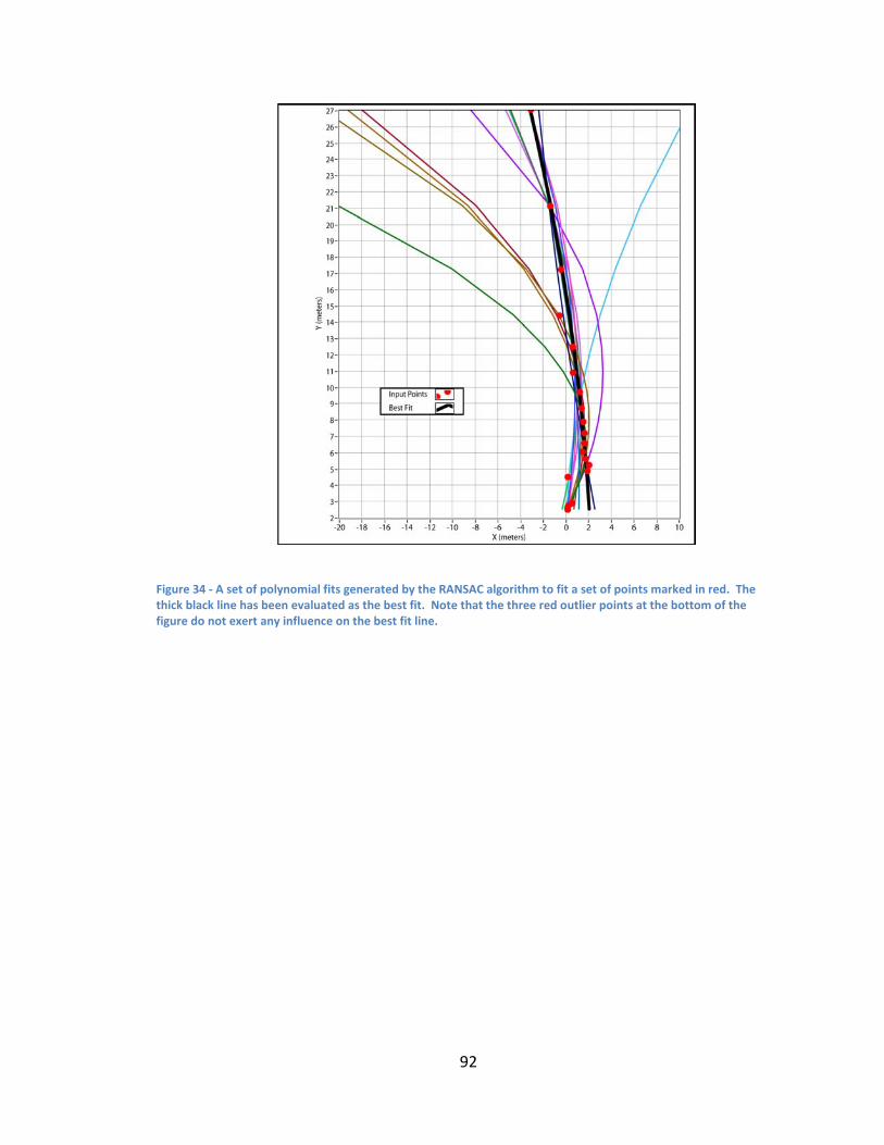
92  

Figure 34 ‐ A set of polynomial fits generated by the RANSAC algorithm to fit a set of points marked in red.  The thick black line has been evaluated as the best fit.  Note that the three red outlier points at the bottom of the figure do not exert any influence on the best fit line. 

93  

A5 –Path Divergence Detection 

  When merging two paths it can be useful to define a point at which the paths 

diverge so much that they can no longer be merged.  This is used when combining a 

sensor generated path and a map generated path to detect points where the sensor 

path has clearly gone a different route than DEXTER is expected to travel.  A separation 

point is determined by the following steps: 

1) Convert the map path into local coordinates if it is not already in this form. 

2) Compute the heading between each of the successive points in the map path 

and store the results in an array.  Do the same for the sensor path. 

3) Subtract the two heading arrays to produce a difference array. 

4) Take the absolute value of the difference array. 

5) Convolve a flat smoothing filter with the array result from step 4. 

6) Search the smoothed array for the first value that exceeds a selected threshold.  

If a value is found it marks the point at which the two paths are believed to 

diverge. 

Appendix B – Sensor Calibration 

  For the purpose of road detection there are two types of sensors that need to be 

calibrated: DEXTER’s multiple cameras and the single downward facing LIDAR unit.  

Since the LIDAR unit returns R ‐ θ (radius – angle) pairs, it can be calibrated by 

converting its results to x,y pairs and multiplying by a coordinate transform matrix 

encoding the position of the LIDAR unit on DEXTER.  This matrix is generated by 

94  

measuring the translation, pitch, roll, and yaw of the unit relative to the GPS center 

point on DEXTER.  These measurements can be adjusted so that a measured test object 

in the field of view of the unit appears at the measured location and so that the 

measurements of multiple LIDAR units match up with each other. 

  The goal of the camera calibration techniques that were used was to obtain 

I,j/x,y image/local coordinate point pairs which can be fed into a Labview VI which then 

generates a data structure used to perform coordinate system transforms for the 

camera.  Since local coordinates are used in this calibration, it is not necessary to 

measure the locations of the cameras on DEXTER.  One method of generating the point 

pairs is to measure out a set of easily identifiable objects in front of a camera, take a 

snapshot, and mark the I,j coordinates by hand.  This method is robust and effective but 

is quite tedious.  An alternative point collection method was developed involving the 

LIDAR scanners used for obstacle detection to automate some of the process.  This 

method relied on using an object (an orange construction barrel) that could be 

automatically identified in an image by a vision algorithm.  Images collected were 

synchronized with ‘snapshots’ of the LIDAR scanners and a separate algorithm was used 

to identify the barrel in the LIDAR scan.  The two identifications were combined to 

generate point pairs over multiple snapshots.  The downside of this point collection 

method was that it required a mostly unobstructed space in order for the LIDAR object 

identification algorithm to perform.  In addition, care had to be taken that the objects 

were reasonably well spaced out in the image in order for the resulting calibration to be 

accurate across the entire image. 

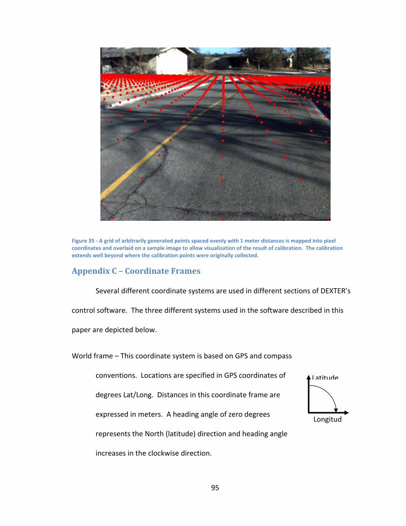
95  

Figure 35 ‐ A grid of arbitrarily generated points spaced evenly with 1 meter distances is mapped into pixel coordinates and overlaid on a sample image to allow visualization of the result of calibration.  The calibration extends well beyond where the calibration points were originally collected. 

Appendix C – Coordinate Frames 

  Several different coordinate systems are used in different sections of DEXTER’s 

control software.  The three different systems used in the software described in this 

paper are depicted below. 

World frame – This coordinate system is based on GPS and compass 

conventions.  Locations are specified in GPS coordinates of 

degrees Lat/Long.  Distances in this coordinate frame are 

expressed in meters.  A heading angle of zero degrees 

represents the North (latitude) direction and heading angle 

increases in the clockwise direction. 

Longitud

Latitude

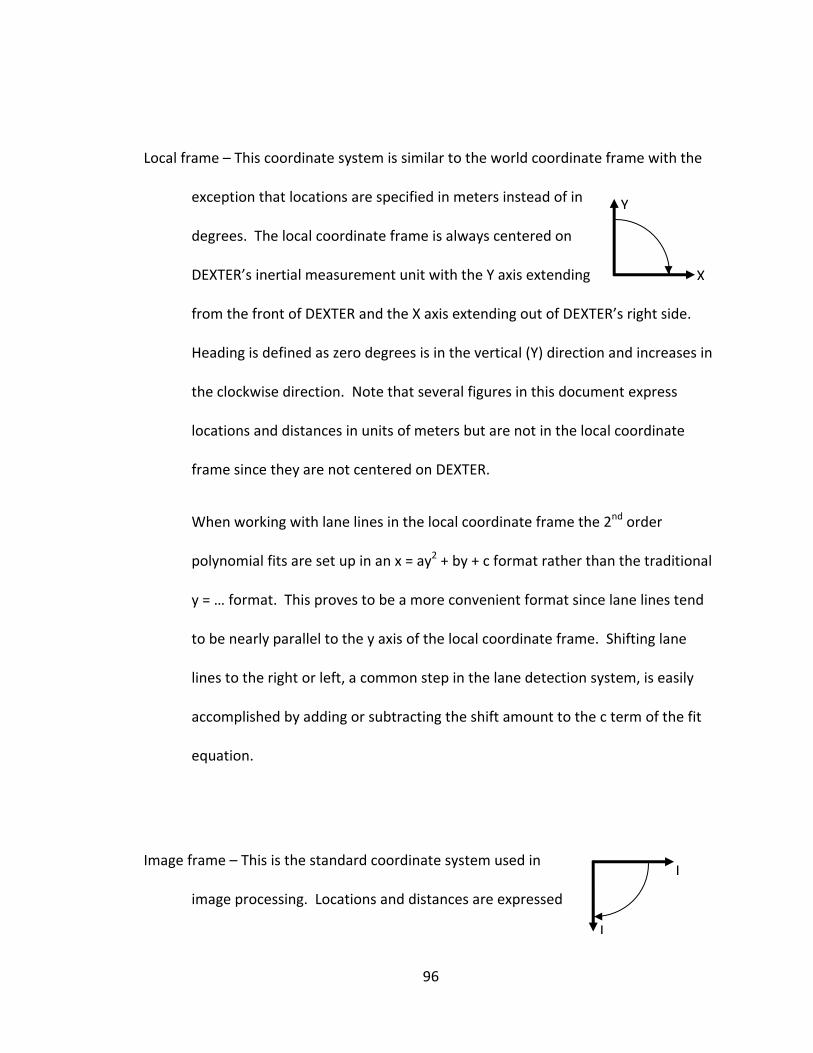
96  

Local frame – This coordinate system is similar to the world coordinate frame with the 

exception that locations are specified in meters instead of in 

degrees.  The local coordinate frame is always centered on 

DEXTER’s inertial measurement unit with the Y axis extending 

from the front of DEXTER and the X axis extending out of DEXTER’s right side.  

Heading is defined as zero degrees is in the vertical (Y) direction and increases in 

the clockwise direction.  Note that several figures in this document express 

locations and distances in units of meters but are not in the local coordinate 

frame since they are not centered on DEXTER. 

  When working with lane lines in the local coordinate frame the 2nd order 

polynomial fits are set up in an x = ay2 + by + c format rather than the traditional 

y = … format.  This proves to be a more convenient format since lane lines tend 

to be nearly parallel to the y axis of the local coordinate frame.  Shifting lane 

lines to the right or left, a common step in the lane detection system, is easily 

accomplished by adding or subtracting the shift amount to the c term of the fit 

equation. 

Image frame – This is the standard coordinate system used in 

image processing.  Locations and distances are expressed 

X

Y

I

J

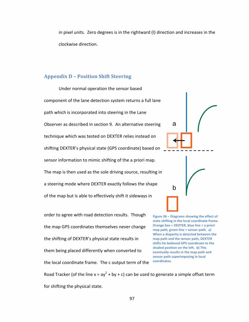
97  

in pixel units.  Zero degrees is in the rightward (I) direction and increases in the 

clockwise direction. 

Appendix D – Position Shift Steering 

  Under normal operation the sensor based 

component of the lane detection system returns a full lane 

path which is incorporated into steering in the Lane 

Observer as described in section 9.  An alternative steering 

technique which was tested on DEXTER relies instead on 

shifting DEXTER’s physical state (GPS coordinate) based on 

sensor information to mimic shifting of the a priori map.  

The map is then used as the sole driving source, resulting in 

a steering mode where DEXTER exactly follows the shape 

of the map but is able to effectively shift it sideways in 

order to agree with road detection results.  Though 

the map GPS coordinates themselves never change 

the shifting of DEXTER’s physical state results in 

them being placed differently when converted to 

the local coordinate frame.  The c output term of the 

Road Tracker (of the line x = ay2 + by + c) can be used to generate a simple offset term 

for shifting the physical state. 

a

b

Figure 36 – Diagrams showing the effect of state shifting in the local coordinate frame.  Orange box = DEXTER, blue line = a priori map path, green line = sensor path.  a) When a disparity is detected between the map path and the sensor path, DEXTER shifts his believed GPS coordinate to the shaded position on the left.  b) This eventually results in the map path and sensor path superimposing in local coordinates. 

98  

  Removing the shape component of the upcoming path from sensor control 

reduces the potential variability of the upcoming path and allows for much heavier 

filtering of the sensor influence on steering.  The result of this is smoother steering and 

decreased possibility of lane detection errors sending the robot off the road.  In 

addition, this control style ensures that no discontinuities exist when the robot reaches 

an intersection which is to be traversed purely according to the a priori map.  Sensor 

placement on the robot could be optimized for this form of control by focusing their 

fields of view on more easily observable sections of road near the robot rather than 

attempting to provide guidance which extends into the distance. 

There are several drawbacks to this method of control which offset its positive 

attributes.  First, a near perfect a priori map is required in order to insure that the robot 

is able to stay in the lanes.  Though the shift capabilities provide some amount of 

adaptability, the heavy filtering placed on the sensor results does not allow enough 

adaptability to overcome more than minor errors.  If the physical state of the robot is 

allowed to shift too rapidly than different software modules which take movement into 

account suffer.  The second requirement for this form of control is a very good estimate 

of how far the robot has traveled down the lane.  If this odometry calculation is 

incorrect then the robot will be sent the wrong section of path to follow, potentially 

sending it out of lane.  Given the drawbacks of this control method, it is only a suitable 

option in situations where a perfect map can somehow be obtained and some form of 

accurate odometry reference (possibly GPS) is available periodically.  In situations where 

these conditions exist this form of control permits a useful simplification of the lane 

99  

detection problem.  Modifications to this technique to retain some sensor control of 

path shape might allow some of these benefits to be used in more diverse situations. 

100  

14 ­ References 

1. The development of machine vision for road vehicles in the last decade. Dickmanns, 

Ernst. 2002, The development of machine vision for road vehicles in the last decade, pp. 

268‐281, vol 1. 

2. Mobileye. Lane Departure Warning. Mobileye. [Online] 2007. [Cited: 12 2, 2007.] 

http://www.mobileye‐vision.com/default.asp?PageID=214. 

3. Road Transport Informatics in Europe ‐ Major Programs and Demonstration. Catling, 

Ian and McQueen, Bob. 1991, IEEE Transactons on Vehicular Technology, Vol 40 No 1, 

pp. 132‐140. 

4. A Compact Vision System for Road Vehicle Guidance. M. Maurer, R. Behringer, S. 

Furst, F. Thomanek, E.D. Dickmanns,. 1996, pp. 313‐317. 

5. The 4D‐Approach to Dynamic Machine Vision. Dickmanns, E. D. Lake Buena Vista, Fl, 

US : s.n., 1994. The 33rd Conference on Decision and Control. pp. 3770‐3775. 

6. Subject‐Object Discrimination in 4D‐Dynamic Scene Interpretation for Machine Vision. 

Dickmanns, Ernst. Irving, California : s.n., 1989. Proceedings of Workshop on Visual 

Motion. pp. 298‐304. 

7. E.D. Dickmanns, R. Behringer, C. Brudigam, D. Dickmanns. F. Thomanek, V. Holt. An 

All‐Transputer Visual Autobahn‐Autopilot/Copilot. [book auth.] Jens Hektor, Susan C. 

Hilton, Mike R. Jane, Peter H. Welch Reinhard Grebe. Transputer Applications and 

Systems '93. Aachen, Germany : IOS Press, 1993, pp. 42‐51. 

101  

8. Unmanned Vehicles Come of Age: The DARPA Grand Challenge. Guna Seetharaman, 

Arun Lakhotia, Erik Blasch. 2006, pp. 26‐29. 

9. VisLab and the Evolution of Vision‐Based UGVs. Massimo Bertozzi, Alberto Broggi, 

Alessandra Fascioli. 2006, pp. 31‐38. 

10. Dean Pamerleau, Todd Jochem. No Hands Across America. No Hands Across 

America. [Online] [Cited: 11 27, 2007.] 

http://www.cs.cmu.edu/afs/cs/user/tjochem/www/nhaa/nhaa_home_page.html. 

11. RAPLH; Rapidly Adapting Lateral Position Handler. Pomerleau, Dean. Detroit, MI : 

s.n., 1995. Proceedings of the Itelligent Vehicles '95 Symposium. pp. 506‐511. 

12. A New Method of Unstructured Road Detection Based on HSV Color Space and Road 

Features. Jingang Huang, Bin Kong, Bichun Li, Fei Zheng. Jeju City, Korea : ?, 2007. 2007 

International Conference on Information Acquisition. pp. 596‐601. 

13. A Color Vision System for Real‐Time Analysis of Road Scenes. Konstantin Kiy, Ernst 

Dickmanns. Parma, Italy : s.n., 2004. 2004 IEEE Inteligent Vehicles Symposium. pp. 54‐

59. 

14. Color‐Based Road Detection in Urban Traffic Scenes. Yinghua He, Hong Wang, Bo 

Zhang. 2004, IEEE Transactions on Intelligent Transportation Systems, Vol 5 No 4, pp. 

309‐318. 

102  

15. Combining Laser Range, Color, and Texture for Autonomous Road Following. 

Rasmussen, Christopher. Washington DC : ?, 2002. 2002 IEEE International Conference 

on Robotics and Automation. pp. 4320‐4325. 

16. Off‐road Path Following using Region Classification and Geometric Projection 

Constraints. Yaniv Alon, Andras Ferencz, Amnon Shashua. 2006. 2006 IEEE Computer 

Society Conference on Computer Vision and Pattern Recognition. Vol. 1, pp. 689‐696. 

17. Lane Detection Using B‐Snake. Yue Wang, Eam Khwang Teoh, Diggang Shen. 1999. 

1999 International Conference on Information Intelligence and Systems. pp. 438‐443. 

18. A Deformable‐Template Approach to Lane Detection. Karl Kluge, Sridhar 

Lakshmanan. Detroit, Michigan : s.n., 95. Proceedings of the Intelligent Vehicles '95 

Symposium. pp. 54‐59. 

19. 3D Lane Detection System Based on Stereovision. Segiu Nedevschi, Rolf Schmidt, 

Thorsten Graf, Radu Danescu, Dan Frentiu, Tiberiu Marita, Florin Oniga, Ciprian Pocol. 

Washington DC, USA : s.n., 2004. IEEE Transportation Systems Conference. pp. 161‐166. 

20. Unified Stereovision for Ground, Road, and Obstacle Detection. Paolo Lombardi, 

Michele Zanin, Stefano Messelodi. 2005, ?, pp. 783‐788. 

21. Lane Detection and Street Type Classification using Laser Range Images. Jan 

Sparbert, Klaus Dietmayer, Daniel Streller. Oakland (CA), USA : s.n., 2001. 2001 IEEE 

Intelligent Transportation Systems Conference Proceedings. pp. 454‐459. 

103  

22. A Lidar‐Based Approach for Near Range Lane Detection. Alexander von Reyher, 

Armin Joos, Hermann Winner. 2005. IEEE Proceedings of the Intelligent Vehicles 

Symposium, 2005. pp. 147‐152. 

23. Road Detection and Classification in Urban Environments Using Conditional Random 

Field Models. Jyun‐Fan Tsai, Shih‐Shinh Huang, Yi‐Meng Chan, Chan‐Yu Huang, Li‐Chen 

Fu, Pei‐Yung Hsiao. Toronto, Canada : s.n., 2006. 2006 IEEE Intelligent Transportation 

Systems Conference. pp. 963‐967. 

24. Velodyne Acoustics. Velodyne's HDL‐64E: A High Definition Lidar Sensor for 3‐D 

Applications. 2007. White Paper. 

25. A Camera Platform for Intelligent Vehicles. Dickmanns, J. Schielen and E.D. 1994. 

Proceedings of the Intelligent Vehicles '94 Symposium. pp. 393‐398. 

26. Lane detection for intelligent vehicle employing omni‐directional camera. Miwako 

Amemiya, Ken Ishkawa, Kazuyuki Kobayashi, Kajiro Watanabe. Sapproro, Japan : ?, 

2004. SICE Annual Conference in Sapporo. pp. 2166‐2170. 

27. Lane Detection in Some Complex Conditions. Zhu Wennan, Chen Qiang, Wang Hong. 

Beijing, China : ?, 2006. Proceedings of the 2006 IEEE/RSJ International Conference on 

Intelligent Robots and Systems. pp. 117‐122. 

28. Switching Models for Vision‐based On‐Board Road Detection. Paolo Lombardi, 

Michele Zanin, Stefano Messelodi. Vienna, Austria : ?, 2005. IEEE Conference on 

Intelligent Transportation Systems. pp. 67‐72. 

104  

29. Symbolic Road Perception‐based Autonomous Driving in Urban Environments. M 

Foedisch, R Madhavan, C Schlenoff. 2006. 35th Applied Imagery and Pattern 

Recognition Workshop. p. ? 

30. A Multi‐Modal Lane Detector that Handles Road Singularities. Raphael Labayrade, 

Jerome Douret, Didier Aubert. Toronto, Canada : ?, 2006. 2006 IEEE Intelligent 

Transportation Systems Conference. pp. 1143‐1148. 

31. Learning of Kalman Filter Parameters for Lane Detection. Thorsten Suttorp, THomas 

Nucher. Tokyo, Japan : s.n., 2006. Intelligent Vehicles Symposium 2006. pp. 552‐557. 

32. Road Following in an Unstructured Desert Environment Based on the 

EM(Expectation‐Maximization) Algorithm. Jaesang Lee, Carl Crane III. Bexco, Busan, 

Korea : s.n., 2006. SICE‐ICASE International Joint Conference 2006. pp. 2969‐2974. 

33. Sensor Fusion for a Network of Processes/Systems with Highly Autonomous Sensors. 

Fernando Figueroa, Xiaojing Yuan. Budapest, Hungary : s.n., 2001. IEEE International 

Workshop on Virtual and Intelligent Measurement Systems. pp. 4‐10. 

34. Sensor Fusion Using Dempster‐Shafer Theory. Huadong Wu, Mel Siegel, Rainer 

Stiefelhagen, Jie Yang. Achorage AK, USA : s.n., 2002. IEEE Instrumentation and 

Measurement Technology Conference. pp. 7‐12. 

35. Sensor Fusion Using Dempster‐Shafer Theory II: Static Weighting and Kalman Filter‐

like Dynamic Weighting. Huadong WU, Mel Siegel, Sevim Ablay. Vail CO, USA : s.n., 

2003. Instrumentation and Measurement Technology Conference. pp. 907‐912. 

105  

36. Development of a Practical Sensor Fusion Module for Environment Modeling. S. H. 

Park, J. R. Kim, S. R. Oh, B. H. Lee. 2003. 2003 IEEE/ASME International Conference on 

Advance Intelligent Mechatronics. pp. 454‐459. 

37. Practical Environment Modeling Based on a Heuristic Sensor Fusion Method. S. H. 

Park, B. H. Lee. New Orelans LA, US : s.n., 2004. International Conference on Robotics 

and Automation. pp. 200‐205. 

38. Lothringer Racing. Lothringer Race Cars. La Verne, California : 

http://www.lothringer.com/. 

39. ENSCO Inc. DEXTER, ENSCO's Fully Autonomous Ground Vehicle. Technology 

Solutions ‐ Robotics. [Online] [Cited: 12 2, 2007.] 

http://www.ensco.com/pdf/view/dexter. 

40. The Imaging Source Europe. DFK 21AF04 ‐ Specification. The Imaging Source: Image 

Processing Components. [Online] 2007. [Cited: 11 28, 2007.] 

http://www.theimagingsource.com/en/products/cameras/firewire_color/dfk21af04/sp

ecification/. 

41. SICK. LMS200/211/221/291 Laser Measurement Systems. SICK ‐ Sensor Intelligence. 

[Online] 12 2006. [Cited: 12 2, 2007.] 

http://www.mysick.com/saqqara/pdf.aspx?id=im0012759. 

42. National Instruments. PXI. National Instruments. [Online] 2007. [Cited: 12 2, 2007.] 

http://www.ni.com/pxi/. 

106  

43. IPD. VA40 Multi Camera Vision Appliance. IPD ‐ Machine Vision Made Simple. 

[Online] 2 2006. [Cited: 12 2, 2007.] 

http://www.goipd.com/Products/appliances/VA40_spec.pdf. 

44. National Instruments. NI Labview. [Online] 2007. [Cited: 11 28, 2007.] 

http://www.ni.com/labview/. 

45. Combining Intelligent Techniques For Sensor Fusion. Faceli, Katti. 2002. 9th 

International Conference on Neural Information Processing, Vol 4. pp. 1998‐2002. 

46. Laser and Vision Sensing for Road Detection and Reconstruction. W S Wijesoma, K R 

S Kodagoda, A P Balasuriya. Singapore : s.n., 2002. The IEEE 5th International 

Conference on Intelligent Transportation Systems. pp. 248‐253. 

47. Extracting Road Curvature and Orientation From Image Edge Points Without 

Perceptual Grouping Into Features. Kluge, Karl. 1994. Proceedings of the Intelligent 

Vehicles '94 Symposium. pp. 109‐114. 

48. Pomerleau, Dean. Neural Network Based Autonomous Navigation. Vision and 

Naviation: The CMU Navlab. s.l. : Kluwer Academic Publishers, 1990, pp. 83‐92. 

49. DALSA. Sherlock Applicaton Interface. IPD Machine Vision Solutions. [Online] 2007. 

[Cited: 11 28, 2007.] http://www.goipd.com/Products/Sherlock/default.htm. 

50. Random sample consensus: a paradigm for model fitting with applications to image 

analysis and automated cartography. Martin A. Fischler, Robert C. Bolles. 1981, 

Communications of the ACM, Volume 24, Issue 6, pp. 381‐395. 

107  

51. Self‐supervised Monocular Road Detection in Desert Terrain. Hendrik Dahlkamp, 

Adrian Kaehler, David Stavens, Sebastian Thrun, Gary Bradski. Cuernavaca, Morelos, 

Mexico : s.n., 2007. Electronics, Robotics, and Automotive Mechanics Conference 2007. 

pp. 253‐259. 

52. SCARF: A Color Vision System that Tracks Roads and Intersections. Jill D. Crisman, 

Charles E. Thorpe. 1, 1993, IEEE Transactions on Robotics and Automation, Vol. 9, pp. 

49‐58. 

53. EMS‐Vision: Recognition of Intersections on Unmarked Road Networks. M Lutzler, E. 

D. Dickmanns. Dearborn Michigan : s.n., 2000. IEEE Intelligent Vehicles Symposium 

2000. pp. 302‐307. 

54. Systems for Safety and Autonomous Behavior in Cars: The DARPA Grand Challenge 

Experience. Umit Ozguner, Christoph Stiller, Keith Redmill. 2007, Proceedings of the 

IEEE, Vol 95, No 2, pp. 397‐412.