Lane Departure Warning and Object Detection Through …publications.lib.chalmers.se/records/fulltext/223154/223154.pdf · Lane Departure Warning and Object Detection Through Sensor

Lane Departure Warning and ObjectDetection Through Sensor Fusion ofCellphone DataMaster’s thesis in Applied Physics and Complex Adaptive Systems

JESPER ERIKSSONJONAS LANDBERG

Department of Applied MechanicsCHALMERS UNIVERSITY OF TECHNOLOGYGoteborg, Sweden 2015

MASTER’S THESIS IN APPLIED PHYSICS AND COMPLEX ADAPTIVE SYSTEMS

Lane Departure Warning and Object Detection Through Sensor Fusion ofCellphone Data

JESPER ERIKSSONJONAS LANDBERG

Department of Applied MechanicsDivision of Vehicle Engineering and Autonomous Systems

CHALMERS UNIVERSITY OF TECHNOLOGY

Goteborg, Sweden 2015

Lane Departure Warning and Object Detection Through Sensor Fusion of Cellphone DataJESPER ERIKSSONJONAS LANDBERG

c© JESPER ERIKSSON, JONAS LANDBERG, 2015

Master’s thesis 2015:03ISSN 1652-8557Department of Applied MechanicsDivision of Vehicle Engineering and Autonomous SystemsChalmers University of TechnologySE-412 96 GoteborgSwedenTelephone: +46 (0)31-772 1000

Cover:Example output from the model

Chalmers ReproserviceGoteborg, Sweden 2015

Lane Departure Warning and Object Detection Through Sensor Fusion of Cellphone DataMaster’s thesis in Applied Physics and Complex Adaptive SystemsJESPER ERIKSSONJONAS LANDBERGDepartment of Applied MechanicsDivision of Vehicle Engineering and Autonomous SystemsChalmers University of Technology

Abstract

This master thesis focus on active safety for the automotive industry. The aim is to test an inexpensiveimplementation of some common functions realized using a cellphone to gather data. A Matlab Simulinkmodel is developed for the purpose, and then the agility of the model is tested by generating c code and runningit on a single board computer.

A robust lane detection algorithm is developed by using Hough lines. To better cope with curves in theroad, the Hough lines are combined with a parabolic second degree fitting. The Hough lines are also used for aLane Departure Warning system. Using edge filtering and connected component labeling an obstacle warningis implemented.

Overall the model works well and is fast enough to meet the real time requirements when run on a computer.On the Raspberry Pi 2 chosen as the single board computer the processing is unfortunately not quite fastenough for high speed driving. However when the object detection is removed the Raspberry Pi 2 meets thereal time requirements as well.

Keywords: active safety, cellphone, digital image processing, Hough lines, Hough transform, image processing,lane detection, lane departure, LDW, Matlab, object detection, object tracking, obstacle detection, RaspberryPi 2, Simulink, single board computer

i

ii

Preface

As the final part of our M.Sc. degree at Chalmers University of Technology, this report represents the result ofour master’s thesis work carried out at AF AB.

AF is a large consultant firm, with a lot of representatives working in the automotive industry. As such,their combined experience and knowledge within the area of active safety is vast. Many of the big automotivecompanies are competing to be among the first to release fully autonomous vehicles, and AF as a consultantcompany wants to be an active part in the success of such vehicles. However, many active safety systemsare based on equipment expensive both financially and computationally. AF is therefore interested to see ifcheaper equipment such as a cellphone can be used to obtain safe results, preferably in such a way that it canbe implemented on an electrical test vehicle.

Acknowledgements

We would like to extend our sincerest gratitude to Erik Karlsson at AF AB for coming up with the idea forthis thesis work, and for his guidance and motivational work as our immediate supervisor. Further, we wouldlike to thank Dr. Krister Wolff, our examiner at Chalmers University of Technology.

We would also like to thank AF consulting company for supporting this project, contributing both to thesuccess of this thesis and to our personal development.

Patrik Jarlebrantd, Mans Larsson and Louise Kempe are all heroes for stepping through roughly 2x400frames of video manually labeling 4 points in each frame. No quantitative data would have been obtained if itweren’t for you!

Finally, we would like to thank our collegues at AF for all the coffee breaks, lunch discussions and positivefeedback throughout the work.

iii

iv

Nomenclature

A small glossary of words and abreviations used in this thesis. The page reference is a guide to where theglossary might be used or explained in more detail.

AUTOSAR (AUTomotive Open System ARchitecture), A global development partnership of vehicle manufac-turers, suppliers and other companies from the electronics, semiconductor and software industry designed toeliminate the barrier between hardware and software [1], page 2EDF (Edge Distribution Function), A one dimensional function describing the number of edges in each directionin the image, page 5FPS (Frames Per Second), Number of frames displayed each second, page 3GPIO (General-Purpose Input/Output), A generic pin on an integrated circuit whose behavior, includingwhether it is an input or output pin, can be controlled by the user at run time, page 15GPS (Global Positioning System), Space based location system that provides details regarding current positionif there is an unobstructed line to at least 4 GPS satelites, page 2IPM (Inverse Perspective Mapping), The mapping of an image to a top-view representation, page 5LBROI (Lane Boundary Region Of Interest), Number of frames displayed each second, page 5LDW (Lane Departure Warning), A warning triggered when vehicle is about to leave the traveling lane, page 2OBD-II (On-Board Diagnostics version 2), An output plug in modern cars providing information from theinternal network of the car, page 8Pixel (-), Unicolor segment of an image, page 3ROI (Region Of Interest), The part of an image expected to contain all the wanted information, page 3

v

vi

Contents

Abstract i

Preface iii

Acknowledgements iii

Nomenclature v

Contents vii

1 Introduction 11.1 Purpose . . . . . . . . . . . . . . . . . . . . . . . . . . . . . . . . . . . . . . . . . . . . . . . . . . . 11.2 Contributions . . . . . . . . . . . . . . . . . . . . . . . . . . . . . . . . . . . . . . . . . . . . . . . . 11.3 Limitations . . . . . . . . . . . . . . . . . . . . . . . . . . . . . . . . . . . . . . . . . . . . . . . . . 21.4 Function Definitions . . . . . . . . . . . . . . . . . . . . . . . . . . . . . . . . . . . . . . . . . . . . 21.5 Related Work . . . . . . . . . . . . . . . . . . . . . . . . . . . . . . . . . . . . . . . . . . . . . . . . 21.6 Reading Guidance . . . . . . . . . . . . . . . . . . . . . . . . . . . . . . . . . . . . . . . . . . . . . 2

2 Theory 32.1 Image processing Basics . . . . . . . . . . . . . . . . . . . . . . . . . . . . . . . . . . . . . . . . . . 32.1.1 Pixels and Colors . . . . . . . . . . . . . . . . . . . . . . . . . . . . . . . . . . . . . . . . . . . . . 32.1.2 Filtering . . . . . . . . . . . . . . . . . . . . . . . . . . . . . . . . . . . . . . . . . . . . . . . . . . 32.1.3 Sobel Filtering . . . . . . . . . . . . . . . . . . . . . . . . . . . . . . . . . . . . . . . . . . . . . . 32.1.4 Valid Numbers and Padding . . . . . . . . . . . . . . . . . . . . . . . . . . . . . . . . . . . . . . 42.1.5 Otsu’s Method for Autotresholding . . . . . . . . . . . . . . . . . . . . . . . . . . . . . . . . . . . 42.1.6 Connected Component Labeling . . . . . . . . . . . . . . . . . . . . . . . . . . . . . . . . . . . . 42.2 Lane Detection . . . . . . . . . . . . . . . . . . . . . . . . . . . . . . . . . . . . . . . . . . . . . . . 52.2.1 Related Work . . . . . . . . . . . . . . . . . . . . . . . . . . . . . . . . . . . . . . . . . . . . . . . 52.2.2 Hough Transform . . . . . . . . . . . . . . . . . . . . . . . . . . . . . . . . . . . . . . . . . . . . 52.3 Object Detection . . . . . . . . . . . . . . . . . . . . . . . . . . . . . . . . . . . . . . . . . . . . . . 62.3.1 Related Work . . . . . . . . . . . . . . . . . . . . . . . . . . . . . . . . . . . . . . . . . . . . . . . 62.4 Safety Standards . . . . . . . . . . . . . . . . . . . . . . . . . . . . . . . . . . . . . . . . . . . . . . 72.4.1 Working Frames per Second . . . . . . . . . . . . . . . . . . . . . . . . . . . . . . . . . . . . . . . 72.4.2 Definition of Safety Zone . . . . . . . . . . . . . . . . . . . . . . . . . . . . . . . . . . . . . . . . 7

3 Method 83.1 Gathering Data . . . . . . . . . . . . . . . . . . . . . . . . . . . . . . . . . . . . . . . . . . . . . . . 83.2 Model Outline . . . . . . . . . . . . . . . . . . . . . . . . . . . . . . . . . . . . . . . . . . . . . . . 83.3 Preprocess Video . . . . . . . . . . . . . . . . . . . . . . . . . . . . . . . . . . . . . . . . . . . . . . 93.4 Lane Detection . . . . . . . . . . . . . . . . . . . . . . . . . . . . . . . . . . . . . . . . . . . . . . . 93.4.1 Near Field . . . . . . . . . . . . . . . . . . . . . . . . . . . . . . . . . . . . . . . . . . . . . . . . 103.4.2 Far Field . . . . . . . . . . . . . . . . . . . . . . . . . . . . . . . . . . . . . . . . . . . . . . . . . 103.5 Lane Departure . . . . . . . . . . . . . . . . . . . . . . . . . . . . . . . . . . . . . . . . . . . . . . . 113.6 Obstacle Detection . . . . . . . . . . . . . . . . . . . . . . . . . . . . . . . . . . . . . . . . . . . . . 123.6.1 Filtering and Blob Detection . . . . . . . . . . . . . . . . . . . . . . . . . . . . . . . . . . . . . . 123.6.2 Merging Blobs . . . . . . . . . . . . . . . . . . . . . . . . . . . . . . . . . . . . . . . . . . . . . . 133.6.3 Line Classifiers . . . . . . . . . . . . . . . . . . . . . . . . . . . . . . . . . . . . . . . . . . . . . . 143.6.4 Obstacle Warning Algorithm Triggers . . . . . . . . . . . . . . . . . . . . . . . . . . . . . . . . . 143.7 Raspberry Pi 2 . . . . . . . . . . . . . . . . . . . . . . . . . . . . . . . . . . . . . . . . . . . . . . . 153.7.1 Generating Code . . . . . . . . . . . . . . . . . . . . . . . . . . . . . . . . . . . . . . . . . . . . . 153.7.2 Inputs . . . . . . . . . . . . . . . . . . . . . . . . . . . . . . . . . . . . . . . . . . . . . . . . . . . 153.7.3 Outputs . . . . . . . . . . . . . . . . . . . . . . . . . . . . . . . . . . . . . . . . . . . . . . . . . . 163.8 Validation of Results . . . . . . . . . . . . . . . . . . . . . . . . . . . . . . . . . . . . . . . . . . . . 163.8.1 Test Videos and Gold Standard . . . . . . . . . . . . . . . . . . . . . . . . . . . . . . . . . . . . . 16

vii

3.8.2 Comparison Between Algorithm and Humans . . . . . . . . . . . . . . . . . . . . . . . . . . . . . 16

4 Results and Discussion 174.1 Lane Detection - Near Field . . . . . . . . . . . . . . . . . . . . . . . . . . . . . . . . . . . . . . . . 174.1.1 Gold Standard . . . . . . . . . . . . . . . . . . . . . . . . . . . . . . . . . . . . . . . . . . . . . . 184.2 Lane Detection - Far Field . . . . . . . . . . . . . . . . . . . . . . . . . . . . . . . . . . . . . . . . . 194.3 Obstacle Detection . . . . . . . . . . . . . . . . . . . . . . . . . . . . . . . . . . . . . . . . . . . . . 204.4 Lane Departure Warning . . . . . . . . . . . . . . . . . . . . . . . . . . . . . . . . . . . . . . . . . 234.5 Evaluation of Algorithm Speed . . . . . . . . . . . . . . . . . . . . . . . . . . . . . . . . . . . . . . 23

5 Conclusions and Future Work 255.1 Algorithms . . . . . . . . . . . . . . . . . . . . . . . . . . . . . . . . . . . . . . . . . . . . . . . . . 255.2 Model Extensions . . . . . . . . . . . . . . . . . . . . . . . . . . . . . . . . . . . . . . . . . . . . . . 255.3 Hardware Setup . . . . . . . . . . . . . . . . . . . . . . . . . . . . . . . . . . . . . . . . . . . . . . 265.4 Raspberry Pi 2 . . . . . . . . . . . . . . . . . . . . . . . . . . . . . . . . . . . . . . . . . . . . . . . 26

References 27

A Hardware Specifications 29A.1 Raspberry Pi 2 specifications . . . . . . . . . . . . . . . . . . . . . . . . . . . . . . . . . . . . . . . 29A.2 Computer . . . . . . . . . . . . . . . . . . . . . . . . . . . . . . . . . . . . . . . . . . . . . . . . . . 29

B Thresholds 30

viii

1 Introduction

In the latest years, the automotive industry has quickly developed towards safer vehicles. Active safety such asadaptive cruise control, automatic brake systems and assisted road tracking are existing techniques used bymost manufacturers. In the future the vehicles are moving towards even more technology in the cars since morefunctionality and faster and better data processing is constantly being developed. Data for these functions arecaptured using different types of sensors in the car.

Most existing techniques are currently quite inaccessible and expensive which means that vital safety featuresis limited to high end platforms. There is therefore a demand for cheaper techniques with similar performance.As one of the leading consultant companies in Sweden, AF wants to see if it is possible. They also want thedeveloped techniques to be deployed to an electrical test vehicle, Figure 1.1, to gain experience and knowledgeof how the algorithms can be implemented.

Figure 1.1: AF’s electrical test vehicle.

1.1 Purpose

The purpose of the thesis is to investigate the possibility to use simpler sensors like the camera and accelerometerin a cellphone as input to safety functions. The main points in this thesis can be summarizied as:

1. Can the simpler sensors in a cellphone be good enough to get reliable data for safety functions if the datais fused together?

2. Can the performance be improved by introduction of data from other sources, the OBD-II plug in the carfor instance?

3. Is it possible to design efficient algorithms such that they can be computed on a single board computersuch as a Raspberry Pi 2? The Raspberry Pi is a small low cost computer with 1 gb RAM and a 900MHz quad core processor [2].

4. Will the developed functions perform on par with the state of the art implementations existing todaywhen considering safety, stability and speed of the algorithm?

5. Can it be implemented on AF’s electrical test vehicle?

1.2 Contributions

The contribution of this thesis is mainly to the field of active safety. More specifically, it demonstrates the stepsneeded to create a simple and efficient model for lane departure warning and obstacle warning. The model isimplemented on a cheap single board computer, demonstrating that active safety does not need to be complexor use expensive hardware to be useful.

1

1.3 Limitations

This thesis work includes modeling lane and object detection as well as handling all the data and calculatingthe prediction. The model is implemented to work with a data stream that can be either replayed or a livefeed. Data from the OBD-II of the car can also be handled by the model, as well as data from sensors inthe cellphone, e.g. GPS or gyroscope. The work is focused primarily on handling data from near optimalconditions, not for instance smaller roads with no lane markings or snowy weather conditions. The model isdeveloped using methods inspired by the AUTOSAR standard, and implemented such that additional functionseasily can be developed and added in the model.

No cellphone app was developed, to collect the replay data. Instead existing apps were used to gatherOBD-II data that was used as inputs to the model. This limited the project from any live usage of the modelwith OBD-II data. The model is developed to handle slight differences in the position of the mounted cellphone,and its camera. However, it should be close to center of the front window, as high as possible, and facingstraight ahead. If the position deviates too much from this, the model will not perform as expected.

1.4 Function Definitions

The focus of this thesis is on active safety, and as such there is a wide range of functions that could be developed,the following were chosen.

A Lane Detection algorithm is developed, described in section 2.2. This function uses image analysis andGPS data to find the lane in which the vehicle is traveling by implementing a Hough transform in near fieldand a second degree polynomial fitting for the far field.

Lane Departure Warning, LDW, is a common feature in modern cars. With knowledge regarding wherein the image the vehicle is traveling, it is also possible to detect when the vehicle is about to leave its lane.This functionality is developed in this thesis as well, described in section 3.5.

As a mean to help the driver Object Detection was developed, as described in section 2.3. It localizesobjects ahead of the vehicle in the traveling lane. With information about the detected objects, differentwarnings or safety functions such as applying the brake or an audio alert can be developed as well.

To test the mobility and agility of the complete model it is ported to a Raspberry Pi 2 and run in fullscale using a Raspberry camera as input.

1.5 Related Work

In the field of active safety, a lot of work has been done already. Many different safety functions are in usetoday, as illustrated by Volkswagen’s description of their proximity sensing [3] or Volvo’s new IntelliSafe [4].Academic articles often focus on one safety function however, and for that reason each function developed inthis thesis has a dedicated section in the theory chapter describing work within respective field. Models thatcan detect the road are described in section 2.2.1 and object detection functions are described in 2.3.1.

1.6 Reading Guidance

This report is divided into three major chapters; Theory, Chapter 2, Method, Chapter 3, and Results andDiscussion, Chapter 4.

In the theory chapter, important underlying theory is explained in order to give the reader enough knowledgeto completely comprehend this thesis work.

Following the theory chapter, the method chapter thoroughly explains the process used in this work. Thischapter describes in detail the implementation of our model and validation of its functionality.

The Results and Discussion chapter feature the obtained results along with our comments and reflectionsregarding these results.

The final chapter of this report presents the conclusions drawn from this work, and a few suggestions forfuture work.

2

2 Theory

In this chapter a thorough explanation of theory needed to understand this thesis will be presented. To startof, some basic digital image processing concepts vital to this work is described. Anyone with experience inimage processing can most likely skip this section. After that more purpose specific theory such as lane andobject detection are treated. The final section of this chapter discusses applicable safety standards and howthey were implemented in the work.

2.1 Image processing Basics

In this section some basic image processing concepts are presented, described in much more detail in [5].

2.1.1 Pixels and Colors

A video is a constant stream of frames, in this thesis 30 frames per second, fps, unless otherwise specified. Eachof these frames is an image, consisting of different small parts called pixels. Each pixel represents a small partof the image with a solid color. To extract this information it is common standard to divide the informationinto three color levels: red, green and blue. For each color, the amount of that color in the pixel is described asa number. This means in practice that each frame can be represented by a [m, n, 3] matrix, where m is thewidth and n is the height of the image in pixels, and each of the layers in the third dimension represents thecolors.

2.1.2 Filtering

In order to manipulate the image matrix described above, different filters can be applied. For instance, one cansoften the image by averaging pixel values in the same neighbourhood.

Mathematically, a filter can be represented as a matrix. This matrix is then applied to the image matrixeither using correlation or convolution. When correlating the filter, each pixel value is obtained by adding orsubtracting neighbouring pixel values according to the matrix values. As an example, the matrix 0 0 0

−1 1 10 0 0

would mean that each pixel value would equal the original pixel value plus the value of the pixel to the rightsubtracted by the pixel to the left.

Convolution on the other hand can most easily be described as a matrix multiplication in Fourier space,and so requires the image and filter matrices to be transformed to Fourier space first, and then the resultingimage to be transformed back.

2.1.3 Sobel Filtering

The Sobel filter is commonly used within image processing for edge detection, as the gradient of the pixelintensity tends to be high on sharp edges. It is also fairly robust to noise, as it uses a weighted average over 3rows/columns.

The standard Sobel filter can be described as a derivation of the image along a certain axis. The filter hasthe mathematical form

Gx = ±

−1 0 1−2 0 2−1 0 1

Gy = ±

−1 −2 −10 0 01 2 1

. (2.1)

Note the ±, which is only important if one cares about in what direction the pixel intensity is changing,rather than the magnitude of the gradient. The magnitude |I ′| and direction ∠I ′xy of the total gradient can be

3

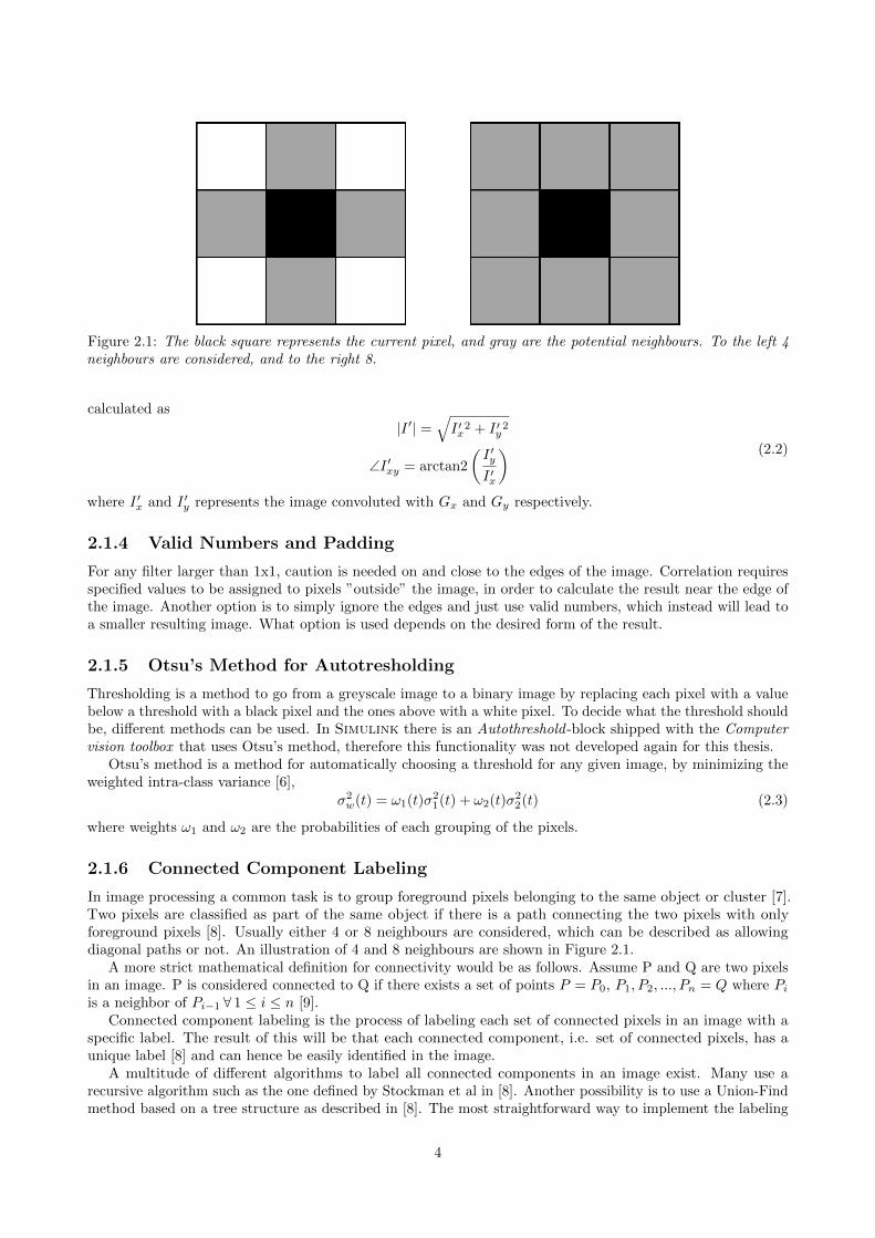
Figure 2.1: The black square represents the current pixel, and gray are the potential neighbours. To the left 4neighbours are considered, and to the right 8.

calculated as

|I ′| =√I ′x

2 + I ′y2

∠I ′xy = arctan2

(I ′yI ′x

) (2.2)

where I ′x and I ′y represents the image convoluted with Gx and Gy respectively.

2.1.4 Valid Numbers and Padding

For any filter larger than 1x1, caution is needed on and close to the edges of the image. Correlation requiresspecified values to be assigned to pixels ”outside” the image, in order to calculate the result near the edge ofthe image. Another option is to simply ignore the edges and just use valid numbers, which instead will lead toa smaller resulting image. What option is used depends on the desired form of the result.

2.1.5 Otsu’s Method for Autotresholding

Thresholding is a method to go from a greyscale image to a binary image by replacing each pixel with a valuebelow a threshold with a black pixel and the ones above with a white pixel. To decide what the threshold shouldbe, different methods can be used. In Simulink there is an Autothreshold -block shipped with the Computervision toolbox that uses Otsu’s method, therefore this functionality was not developed again for this thesis.

Otsu’s method is a method for automatically choosing a threshold for any given image, by minimizing theweighted intra-class variance [6],

σ2w(t) = ω1(t)σ2

1(t) + ω2(t)σ22(t) (2.3)

where weights ω1 and ω2 are the probabilities of each grouping of the pixels.

2.1.6 Connected Component Labeling

In image processing a common task is to group foreground pixels belonging to the same object or cluster [7].Two pixels are classified as part of the same object if there is a path connecting the two pixels with onlyforeground pixels [8]. Usually either 4 or 8 neighbours are considered, which can be described as allowingdiagonal paths or not. An illustration of 4 and 8 neighbours are shown in Figure 2.1.

A more strict mathematical definition for connectivity would be as follows. Assume P and Q are two pixelsin an image. P is considered connected to Q if there exists a set of points P = P0, P1, P2, ..., Pn = Q where Pi

is a neighbor of Pi−1 ∀ 1 ≤ i ≤ n [9].Connected component labeling is the process of labeling each set of connected pixels in an image with a

specific label. The result of this will be that each connected component, i.e. set of connected pixels, has aunique label [8] and can hence be easily identified in the image.

A multitude of different algorithms to label all connected components in an image exist. Many use arecursive algorithm such as the one defined by Stockman et al in [8]. Another possibility is to use a Union-Findmethod based on a tree structure as described in [8]. The most straightforward way to implement the labeling

4

however is in a sequential manner, as proposed by Rosenfeld and Pfaltz as early as 1966 [9]. Specifics aboutthe sequential algorithm used in this thesis can be found in section 3.6.1.

2.2 Lane Detection

The feature that was designed first in the developed algorithm was the lane detection. The main reason thatthe lane detection is needed is to find a safety zone in front of the vehicle, but it can also be used to estimatethe travel path of the moving vehicle or to implement an LDW. Lane detection can be implemented in manydifferent ways, some of which are described in Section 2.2.1. The Hough transform that has been chosen forthis project, are described further down in Section 2.2.2.

2.2.1 Related Work

A lot of different techniques have been used to detect road lanes in the last 20 years and it is hard to categorizethe different techniques because they are influenced by each other and many times combinations of severaltechniques have been used. Here follows a brief introduction to some of the most used techniques.

One method is to use a top-view image [10] called an Inverse Perspective Mapping, IPM, that is computedfrom the image acquired with the camera in the car. An IPM utilizes the position and angle of the camera aswell as the focal length of the lens in order to transform the image from image world to real world. The distancemeasures and image quality are highly dependent on accurate data regarding the position. The benefits of thismethod is that it is possible to get all distances and shapes in real-world units, such as the width of the lane inmeters and similar.

Using deformable models is another well-used technique for lane detection [11–15], where the detected lanepoints are fitted to a mathematical model. The models can use straight lines, parabolic curves or differenttypes of splines to represent the lane, all with different pros and cons. These models tend to be slower and morecomplex, which is a drawback for this application. However it has the potential to very accurately describecurvatures and other non-straight roads.

A color-based method is used in [16] to find the lanes, which is fast and efficient but have some problemswhen lights are reflected in the lane, or shadows cover part of the image. In [17] an Edge Distribution Function,EDF, is used to estimate the lane direction and determine if the car is leaving the lane. The EDF is a onedimensional function that estimates the angle of the lane boundaries by voting in the image. This method isbased on a linear model computed by Hough transforms, which comes with inherent problems in curves, as ittracks straight lines only.

Some methods [18, 19] are using a hypothesis of the lane that is then controlled. The two referenced articlesuse different techniques for the hypothesis model, a Neural Network [18] and Haar-like features filter[19]. Toachieve good results with these methods a large database of features is needed along with a longer trainingperiod in the case of a neural network.

Most implementations utilize a Region Of Interest, ROI, to speed up the calculations. In essence, this meansthat one limits the part of image to be analyzed to avoid processing the entire image. A more extreme way ofdoing this is to define a Lane Boundary Region Of Interest, LBROI. Here, the processed part of the image isnarrowed down to a small region close to where the lane boundary is expected to be found, as suggested by [15].

2.2.2 Hough Transform

The Hough transform can be used as a method to detect lines in a picture, and is described in much moredetail in [5]. Here we give a short summary of the method.

A line can be mathematically described as

ρ = x sin θ + y cos θ (2.4)

where (x, y) represent a pixel position in the image, θ is the angle of the line and ρ the distance to the origin.Further, there is an infinite number of lines that passes through each point (x, y) as ρ varies from 1 to thediagonal of the image and θ can take on an infinite number of values in the range [−90◦, 90◦], see Figure 2.2a.In order to achieve decent computational time, ρ and θ are discretized when using the Hough transform.

The output of the Hough transform is a 2D-matrix A. A(i, j) is calculated by summing the number ofvalues along the line represented by θ(i), ρ(j). Instead of the image one usually uses a binary input, so that

5

every foreground pixel has the value 1 and every background pixel 0. This reduces computational time, and canbe used to study certain features of an image. As an example, if the binary image is obtained by thresholdingthe Sobel gradient magnitude image, only edges will be used in the Hough transform.

The Hough transform can as described here be used to find lines in an image, by identifying peaks in theHough transform matrix. The peak value equals the number of active pixels along the represented line, and soa straight line will get a higher than average value.

The result of a Hough transform can be seen in Figure 2.2c, where a simple line has been run through thetransform. From the figure, we can see that lines with ρ ≈ 500 and θ ≈ 45 is represented with the highestintensity, which corresponds well with the actual line.

(a) Illustration of how ρ and θ arerepresented in the image plane.

(b) A sample input for the houghtransform.

(c) The resulting matrix of a Houghtransform when using 2.2b as input.

Figure 2.2: Descriptive images of the Hough transform process

2.3 Object Detection

When the current lane has been detected, the next safety feature to be implemented is an object detection. Ifsuccessful, warnings or instructions to the driver, whether virtual or human, can be sent to avoid colliding withobjects determined to be potentially dangerous.

2.3.1 Related Work

A lot of work regarding object detection has been done in the last decades. Commonly, a stereo camera isused in order to obtain a depth in the image [20]. Some implementations prefer a single camera coupled with aradar or sonar system in order to obtain this depth [21].

In the case of our system, a single camera is used for obstacle detection. In [22, 23] a mono-camera setup isused to track objects. Both articles focus on reversing a vehicle, and as such they are operating at low speeds,. 20 km/h. In our model, speeds up to 120 km/h are considered, hence these models at the very least need tobe modified.

A common way single camera setups determine distance to objects is through an inverse perspective mapping,as described in section 2.2.1. Due to the nature of this transform however, it is most accurate for short distances,far away the image is to low in resolution to be transformed using an IPM.

One way to find objects in an image is to use image differentials. This method is based on the fact thateverything moving at a different speed than the vehicle will be in different positions in two consecutive images.If one subtract consecutive images everything that is left will be objects moving relative to the vehicle velocity.The downside of this method is that there will be a lot of noise. Objects such as lane markers, safety barriersand everything else rooted will be moving compared to the vehicle. As an extension one can use the knownvehicle motion to calculate what should happen to the image, using so called optical flow [24–26]. Comparingthis to the actual new image will show everything that is moving compared to the vehicle, but is not standingstill. Unfortunately elements such as focal length, angle and position of the camera will again be vital data toachieve stable results. Accurate data regarding velocity and acceleration of the car is equally important.

6

2.4 Safety Standards

When discussing safety an important aspect to adress is the meaning of safe. Some things are obvious, such asstopping before hitting an object. Others are not so obvious, such as recommended distance to keep whendriving on the highway. In this section standard values for these cases are presented, and where applicableequations to describe the fundamental reasoning behind these standards are described.

In many cases, values have been determined by the writers using ”common sense”, as no strict recommen-dations or laws was found to support the claims.

2.4.1 Working Frames per Second

To make an informed decision regarding how many frames per second the model must treat to obtain satisfyingresults, one should consider how far the vehicle travels each frame. This can be determined depending on thevehicle speed v as in equation (2.5).

∆d =v

fps(2.5)

where ∆d is the traveled distance. When the car is traveling in 120 km/h = 33.33 m/s we get

∆d =33.33

30≈ 1.11 m

if the camera captures 30 frames each second. This is the maximum speed considered in this thesis, as noSwedish highways allow traveling faster. Since equation (2.5) is just a linear correlation, it is easy to see thatonly using every second frame would mean 2.22 m instead and etc.

Based on observations every fifth frame, or every 5.56 m, is considered enough for the lane detection. Onthe other hand, for obstacle detection every millisecond earlier that the object can be detected is important.Therefore, this should be done as often as possible without loosing the realtime requirements, i.e. the modelmust have sufficient time to finish one frame before it must start on next frame.

2.4.2 Definition of Safety Zone

In Sweden a common rule of thumb for distance keeping [27] is that one should keep the same distance inmeters as the driving speed in km/h. So when driving 90 km/h one should keep a minimum distance of 90 m toother cars in the same lane. Unfortunately with the angle the video is captured, it is very hard to separate50 m from 100 m, see Figure 2.3. In this image an attempt to count the number of dashes in the dashed lanemarker, could be made to determine how far away the car in front is. However, one would soon realize thatonly a few pixels difference on where objects far away is could translate to an extreme distance. For this reasonit was determined in this thesis to always look for objects all the way to the horizon.

Figure 2.3: Example images depicting how hard it might be to determine distances in a frame from the videocaptured. In the right image, the black car (in the same lane) and the white car (in the left lane) are almost nextto each other but in reality the white car already passed the black. But how far ahead of the black is the white?

7

3 Method

In this chapter the methodology of this thesis work will be described in detail. Throughout the thesis work,Matlab 2015a has been used, along with corresponding versions of Simulink and toolboxes, mainly theComputer Vision System toolbox and the Raspberry Pi support package.

In general, parameters and thresholds have been determined by visual inspection of the results while varyingthe values unless otherwise specified. All used values for thresholds can be found in Appendix B.

3.1 Gathering Data

Data needed to develop and evaluate the model was gathered using the android app Torque, with the pluginTrack recorder to enable saving video together with data. The cellphone was also coupled with an OBD-IIdevice via bluetooth, making it possible to save data from the car’s built in systems. While driving, the appwas set to save video and data from the phone sensors and OBD-II plug each 0.1 seconds. Note that GPS datain the cellphone is not updated as often. The video was recorded at 1080p and a frame rate of 30 frames persecond.

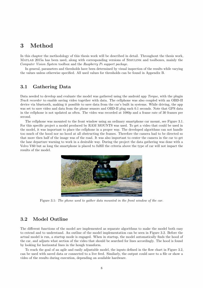
The cellphone was mounted to the front window using an ordinary smartphone car mount, see Figure 3.1.For this specific project a model produced by RAM MOUNTS was used. To get a video that could be used inthe model, it was important to place the cellphone in a proper way. The developed algorithms can not handletoo much of the hood nor no hood at all obstructing the frames. Therefore the camera had to be directed sothat more then half of the image was of the road. It was also important to center the camera in the car to getthe lane departure warning to work in a desirable way. During the project the data gathering was done with aVolvo V60 but as long the smartphone is placed to fulfill the criteria above the type of car will not impact theresults of the model.

Figure 3.1: The phone used to gather data mounted in the front window of the car.

3.2 Model Outline

The different functions of the model are implemented as separate algorithms to make the model both easyto extend and to understand. An outline of the model implementation can be seen in Figure 3.2. Before theactual model is run, a startup mode is engaged. When in startup, the model automatically finds the hood ofthe car, and adjusts what section of the video that should be searched for lines accordingly. The hood is foundby looking for horizontal lines in the hough transform.

To reach the goal of an agile and easily adjustable model, the inputs defined in the flow chart in Figure 3.2,can be used with saved data or connected to a live feed. Similarly, the output could save to a file or show avideo of the results during execution, depending on available hardware.

8

Videoinput

Data input

Preprocessthe video

LaneDetection

ObjectDetection

Calculateangular

velocity fromGPS bearing

LaneDepartureWarning

ObstacleWarning

Output

Figure 3.2: Flowchart of the model outline. Blue boxes represent different algorithms implemented and redellipses inputs and outputs.

3.3 Preprocess Video

The first module in the main model is a preprocess where the video is processed to speed up the computationsin the algorithms. The video was converted to 640x360 pixels in size to reduce the computational domain. Ifthe video used as input is in color it is also converted to a gray-scale.

Within this resized video a section is chosen where all relevant data is expected to be found, selected by thestartup algorithms. This section is then filtered with a Sobel filter to get the amplitude of the gradients, whichis then thresholded. The threshold is set using Otsu’s method, minimizing equation (2.3), to choose thresholdfor each image. The resulting binary edge image can be seen in Figure 3.3.

Figure 3.3: An example of the preprocessed video. Black represents a foreground pixel while white pixels areassumed to be background.

3.4 Lane Detection

In this section the methods used to locate a lane is described. The ultimate goal of this is to generate awell-defined zone in which obstacles, other cars and similar are considered dangerous or potentially dangerous.The results can also be used for lane departure detection or vehicle travel prediction. The lane detection isdivided into two regions, near field and far field as seen in Figure 3.4, for which different methods have beenused to find the lanes, similar to [15]. In the figure it can also be seen that instead of a normal coordinatesystem the x-axis is located in the center of the image where near field and far field are separated, and they-axis is pointing downwards.

9

Figure 3.4: The regions for lane detection.

3.4.1 Near Field

In the near field region the lanes are assumed to be straight lines and the lower part of the binary edge imagefrom the preprocess is used as input to a Hough transform as seen in Figure 3.5a. Since the value in the Houghtransform matrix represents the length of the line, a comparison with a threshold is done and only lines over acertain length is kept. From the thresholded Hough transform matrix the strongest lines are extracted andassumed to be the lane markers closest to the car, which are marked in Figure 3.5b. If no line is found, the lastline that was found is used instead.

(a) Binary edge image from preprocess. (b) Frame with the chosen Hough Lines.

(c) Edge image where undesired edges for left lines are re-moved.

(d) Final edge image used to find curved lines.

Figure 3.5: Binary frames used in lane detection.

3.4.2 Far Field

When the lines in the near field region have been calculated, the lines for the far field can be determined. Toget better results the binary edge image is calculated separately for the left and right line. In Figure 3.5c it canbe seen how undesired edges of the left line are removed based on their gradient angle, and in Figure 3.5d amedian-filter has also been applied to remove some noise. Those new edge images are then used for the farfield. Since the lanes can be curved in this part of the image, a second degree curve is used to describe the laneinstead of the straight lines. In the given coordinate system the lanes are given by the following equations

x = a+ by, y > 0

x = a+ by + cy2, y ≤ 0(3.1)

From the near field calculations the coefficients a and b are determined, which leaves the constant c, thecurvature constant. To determine c a linear optimization is used, where the x-values for all y-values in the farfield are calculated for a number of c-values. The calculated points are then compared to the filtered imagedescribed above. Then the c-value with highest number of matching points is chosen. To make the algorithmmore robust, points outside the LBROI was not counted. The LBROI was determine as 7 px in each x-directionfrom the last calculated line.

10

Angular Speed and Curvature Constant

To decrease computational time the considered c values are limited, and based on data from the GPS bearing.An approximation of how much the car is currently turning is calculated by using a discrete derivative of thebearing data. The result gives numbers approximate in the range -0.2 to 0.2, where 0 represents a straight road,-0.2 a tight left turn and 0.2 a tight right turn. This angular velocity, ω, is then combined with a standard cvector, cvec = [0 : 0.015 : 0.3], according to equation (3.2). The less the road is turning, the smaller c valuesleading to less curvy lines.

c(ω) =

ω2 · cvecmax(0.05, |ω|)

· sign(ω) if ω ≤ Tcurve

0 if ω < Tcurve

(3.2)

where sign is the sign function, returning -1 or 1 depending on the sign of ω. Tcurve is a threshold, by testsof the method found to work well with Tcurve = 0.01. The result of this function can be seen in Figure 3.6a.An example of the lines that this c represents are shown in Figure 3.6b. The most curved line represents thelargest c.

Angular Speed

0 0.02 0.04 0.06 0.08 0.1 0.12 0.14 0.16 0.18 0.2

c V

alu

es

0

0.01

0.02

0.03

0.04

0.05

0.06c values as a function of angular speed

(a) The c values used for far field curved line detection,based on the calculated angular speed. To stop the val-ues from escalating for high ω the equation is linear forω > 0.05.

(b) Illustrations of the curvature constant’s impact on thecurved lines, here depicting all possible choices in a frame.

Figure 3.6: Curvature constant illustrations.

3.5 Lane Departure

The implementation of lane departure warning in this thesis is based on the methods developed in [15, 17]. Thismethod is based on the hypothesis that there should be a symmetry between the left and right lane boundariesin the near field of the image, when a car with a centered camera is positioned in the middle of a lane, seeFigure 3.7. As the car moves towards one of the lane markers, this symmetry will change and the two angles ofthe left and right lines will no longer be equal in size. When the difference between the two angles are largerthan a predefined threshold the LDW is activated. This can be summarized as in equation (3.3).

LDW =

LDW left if θL − θR < −TLDW

LDW right if θL − θR > TLDW

0 otherwise(3.3)

where θL is the angle of the left line, θR the angle of the right line and TLDW the set threshold.

Since this method is based on the near field of the image, the lines from the Hough transform can be used.The nature of the Hough transform means that θL and θR are already calculated in another part of the model.This means that the only thing left to do is calculate the difference and trigger the LDW as in equation (3.3).An example of a triggered LDW can be seen in Figure 3.8.

11

Figure 3.7: Illustration of the symmetry between left and right lane boundary when the vehicle is placed in themiddle of the lane to the left. On the right side, the symmetry is broken as the car is moving towards the leftedge.

Figure 3.8: An example depicting the activated LDW, here crossing the lane to the right. The blue circle in thetop right corner is the LDW indicating a right turn.

3.6 Obstacle Detection

This section will describe the algorithm that is used to detect obstacles in front of the vehicle. The methodis divided into different parts and starts with filtering of the input image, where ground and lane edges areremoved. After filtering, a blob detection algorithm is applied on the image. These processes are described insection 3.6.1. Then the detected blobs are merged together to larger areas as described in section 3.6.2. Finally,too small objects are ruled out as obstacle candidates before issuing a warning.

3.6.1 Filtering and Blob Detection

The obstacle detection starts with the same preprocessed edge image as the lane detection and can be seenin Figure 3.9a. The first step is then to remove edges that are in the same direction as the lane that alreadyhas been detected. This is done to avoid detecting the lane markings as obstacles and can be done becauseobstacles that rises above the road will have vertical edges that are not removed. The effect of this is shown inFigure 3.9b. To make the obstacles more distinct an averaging filter is applied on the new image, as shown inFigure 3.9c.

12

(a) Binary edge image from preprocess. (b) Frame where edges in the lane direction are removed.

(c) Final edge image used for object detection. (d) Binary image where detected objects are marked with redsquares.

Figure 3.9: Binary frames used in object detection

When the filtering is done, the binary video is run through the developed connected-component labelingalgorithm, which is used to detect a rectangle around each blob with an area larger than a threshold. For thisthesis, 25 pixles were used. The algorithm uses a single pass to scan the image and label each connected regionwith the same label. To decide which region label to use, the labels of already visited neighbours of the currentpixel are scanned. The one with the lowest value is assigned to the current pixel. If any neighbour has anyother label value, all pixels with that label are replaced with the same label as the current pixel, since they arenow connected to the same region. The algorithm is presented in Algorithm 1. To speed up the detection theregion where the blobs are detected is determined by the safety zone. The final result is shown in Figure 3.9d.

Data: binaryVideo, leftLine, rightLineResult: labelscurrentLabel = 1;videoData = binaryVideo(min(leftLine):max(rightLine));for each row in videoData do

for each col in videoData doif foreground pixel then

testValues = videoData(row-1,col-1:col+1) ∪ videoData(row, col-1);labels(row,col) = min(testValues);if labels(row,col) equals 0 then

labels(row,col) = currentLabel;currentLabel = currentLabel +1;

endif testValues ∩ (0, labels(row,col)) not equals ∅ then

labels(labels==testValues ∩ (0, labels(row,col))) = labels(row,col) ;end

end

end

end

Algorithm 1: The algorithm used to detect blobs in the video, so called connected-component labeling.

3.6.2 Merging Blobs

The detected blobs close to each other in the image are considered to most likely be the same object detectedtwice, and should be merged to one blob. An embedded Matlab function was implemented to solve this. Itworks in iterations, and a maximum number of iterations can be set to keep computational time reasonable.Each iteration, the function calculates the distances between all blobs by using the center of the blob. It thenfinds all distances smaller than a set threshold, and starts merging one by one of the ones close to each other.Each iteration a specific blob can only be target of the merge once. If many blobs are located close to each

13

other, multiple iterations of the function is needed to merge them all. In the actual merge of two blobs, thenew center of the blob is calculated as the average of the two merging blobs’ centers. The new outer frame ofthe blob is the min and max corners from the two merged blobs.

After the blobs have been merged, a control of the size of the new blobs is included to remove some morenoise. The obstacle close to the car will be much larger in the image then obstacles further away. The controlequation (3.4) is used to determine which the minimum size Amin of an object should be to trigger a warning.The equation has been found efficient by trial and error.

Amin = (y − yh)3 · 10−4 + (y − yh)2 · 10−2 + 120; (3.4)

where y is the pixel distance from the top of the image and yh is the top of the zone, expected to be close tothe horizon. A sample of this function can be seen in Figure 3.10. When the zone is changed, only the x axiswill change. The shape of the function will be the same.

y pixel

200 220 240 260 280 300 320

Am

in

100

150

200

250

300

350

400

Figure 3.10: Example of the function used to determine the size of an object.

3.6.3 Line Classifiers

In order to avoid detecting lines as objects, an attempt at classifying lines was done. The classifier was basedon the area of the video where the Hough lines are found. A vector with six values was stored, the max andmin values of each color.

For each object the same values are calculated and compared to the classifier. If no value differentiatesmore than a threshold, the object is considered a line and disqualified from the obstacle warning process.

3.6.4 Obstacle Warning Algorithm Triggers

The obstacle warning can be triggered by a few different scenarios. First of all, and perhaps the most critical,the warning is triggered if an object is found too close to the hood. To control this, the algorithm determineswhich object is closest to the hood, and if it is closer than a certain threshold TobsClose, it triggers the warning.

Further, if an object is getting closer to the hood, the warning is triggered as well. The implementation ofthis simply consists of tracking the object closest to the hood. If it moves more than a threshold TobsFast inone frame step, or more than another threshold TobsSlow in 3 of the last 5 frame steps, the warning is triggered.The threshold values working best in this application were selected as

TobsClose 60 pxTobsFast 10 pxTobsSlow 2 px

When a warning is triggered it can produce a warning in two different ways depending on how the driverbehaves. If the driver is already braking, a weaker warning will occur. If the driver is accelerating when thewarning is triggered it will give a stronger warning. To check which warning that should be triggered the

14

acceleration data from the GPS is used. As can be seen in Figure 3.11, the accelerometer does peak when thedriver is brakeing.

Frame in video

60 70 80 90 100 110 120 130 140

Acce

lera

tio

n

-0.4

-0.2

0

0.2

0.4

0.6

0.8

1Speed and acceleration each frame

Sp

ee

d (

km

/h)

25

30

35

40

45

50

55

60

Figure 3.11: Example of how the accelerometer reacts when a brake occurs.

3.7 Raspberry Pi 2

In this section the specifics regarding porting to a single board computer are explained. For this thesis aRaspberry Pi 2 was chosen. For the technical data of the Raspberry Pi 2 refer to appendix A.1. An image of aRaspberry can be seen in Figure 3.12.

Figure 3.12: The Raspberry Pi 2

3.7.1 Generating Code

Porting the code to a Raspberry Pi 2 was done in Simulink by building to a real time target. Simulink supportpackage for Raspberry Pi can automatically generate code in the C language from a Simulink model thatcan be built and run on the single board computer. The support package also contains predefined methodsfor handling the standard onboard camera and setting the General Purpose Input/Output, GPIO pins of theRaspberry.

3.7.2 Inputs

The camera connected to the Raspberry takes images at a maximum of 10 fps, using a format of 4x3, asopposed to the cellphone camera which uses a 16x9 format at 30 fps. To handle this, the preprossesing waschanged in the Pi version such that the video was cropped to a correct format. Parameters such as the numberof frames to average over must also change to correspond to the different fps, as well as how often the modelis run. Unfortunately no GPS or OBD-II data was used with the Raspberry, as it does not natively supportBluetooth nor have any built in gyroscope or GPS.

15

3.7.3 Outputs

Since the Raspberry does not have any screen or monitor connected, it is not as straightforward to validate theresults. One option when replaying already collected data is to save the position of the calculated objects andlane lines in a text file, which can be analyzed after the run. When using a live feed however, it is not possibleto save the video to file as well, since this would very quickly fill the memory card used with the Pi.

The solution to the live feed output dilemma was to connect a few LED lights to the GPIO of the board,and turn on different lights in different situations. For instance, a red light is lit when there is an objectdetected in the safety zone. Two blue lights are used to signal when detecting a lane departure to the left orright respectively.

3.8 Validation of Results

3.8.1 Test Videos and Gold Standard

To generate quantitative results regarding the accuracy of the near field lane detection, i.e. the Hough lines, aset of lines picked by humans were collected, henceforth referred to as the gold standard1. Each evaluator wastold to mark the straight lines corresponding to the current lane boundary for each frame in the video, using asmall GUI created for the purpose, Figure 3.13. The average of all individual choices was then computed foreach frame, and considered the gold standard. As a means to evaluate the gold standards validity, the standarddeviation for each frame was computed as well.

Figure 3.13: The GUI used by the testers to determine the lane by dragging the blue stars in the image.

To evaluate the performance of our model two videos were used. The first one is a 30 second clip in heavyrain, with wipers on. We start on a larger road and then take an exit, under a bridge and into a fairly sharpturn. At one point the driving line divides into two lanes, one exiting the freeway and the other continuing.This video is referred to as rainyDay. The second video is in decent weather with overcast, driving on a largethree lane road. In this video the vehicle changes lane three times. This video is referred to as laneDep.

3.8.2 Comparison Between Algorithm and Humans

To be able to evaluate the output data from the algorithms a validation script was created. In that script theoutput of the algorithm was compared to the gold standard mentioned above. The script reads two saved.mat files, both the gold standard for a specific video and the model generated data points. It then computesdistance between lines as well as the difference in angles between the two versions.

1Gold standard is defined by the oxford dictionary as ”A thing of superior quality which serves as a point of reference againstwhich other things of its type may be compared” [28]

16

4 Results and Discussion

In this chapter all obtained results are presented and discussions regarding the results are included as well.The chapter is divided into sections starting with lane detection for near field and far field respectively. Thenext sections present the results from the obstacle detection and lane departure warning. The last section inthe chapter is an evaluation of the algorithm speed.

4.1 Lane Detection - Near Field

To compare the model results with the golden standard, each endpoint of the two near field lines were comparedto the corresponding points in the golden standard. The absolute distance between the model line and pickedline were calculated for each frame. A low distance value can be interpreted as a successful line detection. Theresult can be seen in Figure 4.1.

Frame

100 200 300 400 500 600 700 800 900

Dis

tan

ce

(p

ixe

ls)

0

1.2462

5

10

15

20

25Distance between points for each frame in laneDep

Left

Right

Total

Median

Frame

100 200 300 400 500 600 700 800 900

Dis

tan

ce

(p

ixe

ls)

0

0.8546

2

4

6

Distance between points for each frame in rainyDay

Left

Right

Total

Median

Figure 4.1: The Distance between the gold standard and the line picked by the model. To the left, the resultfrom video laneDep can be seen, and to the right rainyDay.

The model line angles were compared to the gold standard as well, which can be seen in Figure 4.2.

Frame

100 200 300 400 500 600 700 800 900

An

gle

(D

eg

ree

s)

-50

-40

-30

-20

-10

0

10

20

30

40

50Difference in angle for each frame in laneDep

Left angle diff

Right angle diff

Frame

100 200 300 400 500 600 700 800 900

An

gle

(D

eg

ree

s)

-10

-8

-6

-4

-2

0

2

4

6

8

10Difference in angle for each frame in rainyDay

Left angle diff

Right angle diff

Figure 4.2: The Distance between the gold standard and the line picked by the model. To the left, the resultfrom video laneDep can be seen, and to the right rainyDay.

17

Both Figure 4.1 and 4.2 show that the model performs very accurately for most frames. It is also veryobvious from these graphs where in the video the lane changes are happening. In the laneDep video, the threepeaks in the distance measure each represent a lane change. These three peaks corresponds well with the peaksin Figure 4.4, telling us that not only the developed model, but also humans, have trouble determining wherethe ”current lane” is situated during these lane changes. The median in both rainyDay and laneDep are closeto 1 pixel, which has to be considered very accurate.

In the right graph in Figure 4.1 we can see that the left line deviates between frame 200 and 300, whilethe right remains low. This is because in this part of the video, the current lane is split in two. The rightline remains solid but the left line becomes two lines. Similar to a lane change this is hard to handle for bothhumans and the algorithm, as the same behavior is present in Figure 4.4 as well. The lane split is clearly visiblein Figure 4.3.

Figure 4.3: Frame 210 and frame 288 of the rainyDay video used for evaluation. The splitting of the left sidelane marker is clearly visible.

4.1.1 Gold Standard

To justify the use of a gold standard the standard deviation of the picks the testers made in the two videoshave been calculated and can be seen in Figure 4.4, illustrating in pixels how much the testers disagree. Thefigures are based on five testers’ picks. For most part of the video the testers agree, and the standard deviationis only a few pixels. However, during lane changes the deviation increases, since it is hard to know what linesto choose as the current lane boundaries when the car is in between two lanes. Even for a human, it is hardto determine when the lane change actually occurs, which makes it almost impossible for an algorithm. Thealgorithm can be run with a specified rule determining when to classify it as a lane change, but odds are thatnot all drivers will agree with that rule.

Frame

0 100 200 300 400 500 600 700 800 900

Sta

nd

ard

de

via

tio

n

0

2

3.43004

6

8

10

12

14

16

18

20Standard deviation for each frame in laneDep

Total

Mean

Frame

0 100 200 300 400 500 600 700 800 900

Sta

nd

ard

de

via

tio

n

0

2

3.70154

6

8

10

12

14

16

18

20Standard deviation for each frame in rainyDay

Total

Mean

Figure 4.4: The standard deviation over each frame based on each test persons’ choice.

18

4.2 Lane Detection - Far Field

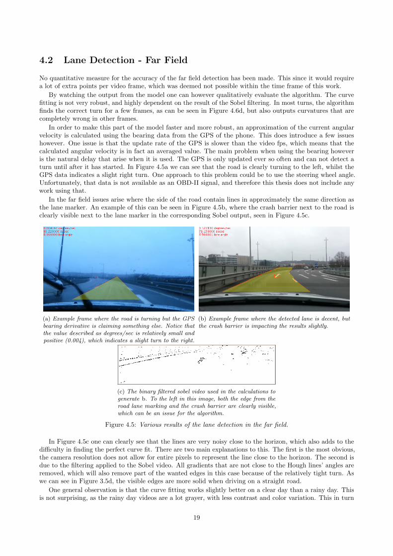
No quantitative measure for the accuracy of the far field detection has been made. This since it would requirea lot of extra points per video frame, which was deemed not possible within the time frame of this work.

By watching the output from the model one can however qualitatively evaluate the algorithm. The curvefitting is not very robust, and highly dependent on the result of the Sobel filtering. In most turns, the algorithmfinds the correct turn for a few frames, as can be seen in Figure 4.6d, but also outputs curvatures that arecompletely wrong in other frames.

In order to make this part of the model faster and more robust, an approximation of the current angularvelocity is calculated using the bearing data from the GPS of the phone. This does introduce a few issueshowever. One issue is that the update rate of the GPS is slower than the video fps, which means that thecalculated angular velocity is in fact an averaged value. The main problem when using the bearing howeveris the natural delay that arise when it is used. The GPS is only updated ever so often and can not detect aturn until after it has started. In Figure 4.5a we can see that the road is clearly turning to the left, whilst theGPS data indicates a slight right turn. One approach to this problem could be to use the steering wheel angle.Unfortunately, that data is not available as an OBD-II signal, and therefore this thesis does not include anywork using that.

In the far field issues arise where the side of the road contain lines in approximately the same direction asthe lane marker. An example of this can be seen in Figure 4.5b, where the crash barrier next to the road isclearly visible next to the lane marker in the corresponding Sobel output, seen in Figure 4.5c.

(a) Example frame where the road is turning but the GPSbearing derivative is claiming something else. Notice thatthe value described as degrees/sec is relatively small andpositive (0.004), which indicates a slight turn to the right.

(b) Example frame where the detected lane is decent, butthe crash barrier is impacting the results slightly.

(c) The binary filtered sobel video used in the calculations togenerate b. To the left in this image, both the edge from theroad lane marking and the crash barrier are clearly visible,which can be an issue for the algorithm.

Figure 4.5: Various results of the lane detection in the far field.

In Figure 4.5c one can clearly see that the lines are very noisy close to the horizon, which also adds to thedifficulty in finding the perfect curve fit. There are two main explanations to this. The first is the most obvious,the camera resolution does not allow for entire pixels to represent the line close to the horizon. The second isdue to the filtering applied to the Sobel video. All gradients that are not close to the Hough lines’ angles areremoved, which will also remove part of the wanted edges in this case because of the relatively tight turn. Aswe can see in Figure 3.5d, the visible edges are more solid when driving on a straight road.

One general observation is that the curve fitting works slightly better on a clear day than a rainy day. Thisis not surprising, as the rainy day videos are a lot grayer, with less contrast and color variation. This in turn

19

leads to less sharp edges resulting in a blurry Sobel video compared to a clear day.More results of the curved line fitting can be seen in Figure 4.6.

(a) When driving on a straight roadthe far field is just the extension of thestraight lines from near field detection,which is fairly robust.

(b) The right line does not trace thecurve of the line, but the safety zone isdecent anyway.

(c) A curve farther ahead in the drivinglane is not detected by the algorithmsince the GPS has not reacted yet.

(d) Good result despite the rain. (e) Similar to b but in rain. (f) The algorithm is not detecting theleft line in the turn perfectly.

Figure 4.6: More results from the lane detection in far field region. Notice the marker in the right cornerindicating a false LDW triggered in d and f.

4.3 Obstacle Detection

In general the obstacle detection algorithm developed works well when observed while testing. In Figure 4.7 afew examples where the object detection is detecting real objects are shown.

Figure 4.7: Examples of where the object detection is working as expected. The big yellow circles in two of theimages are the weaker version of the triggered obstacle warning.

When running the model some issues are observed. The algorithm as it is developed is tuned to detect toomuch rather than too little, to avoid missing something. This means unfortunately that it also detects objectsthat should not be detected, which may lead to an unwanted triggering of the obstacle warning. Below a fewdifferent scenarios where the algorithm does not work as good are discussed.

20

No sideline

Both videos tested with the gold standard are on highways with lane markers visible. When the lane markersdisappear, the model has nothing to track. An example when this happens is shown in Figure 4.8. As we cansee in the right image in the figure, there are no edges appearing in the Sobel video meaning the algorithm cannot find the lane. Because of this, there is a false obstacle warning triggered in the frame, since the algorithmis tracking something on the sidewalk.

Figure 4.8: An example where there is no side line markers, and so the lane is not detected accurately. The bigred circle in the top of the image is the obstacle warning that has been triggered.

Shadows and Lane markers

In Figure 4.9 one can clearly see how shadows are detected by the object detection algorithm. The shadow of acar is included in the detected object, which leads to a larger object than expected. However, this is not amajor issue since the car should be detected anyway.

Figure 4.9: Examples where shadows spoil the result of the object detection algorithm. To the left, the shadowof a car is included as part of the object. To the right, the shadow from a road sign hanging over the road isdetected as an object.

The other image in Figure 4.9 illustrates how shadows can be detected by themselves. This is a big problemfor the developed algorithm as it will always lead to a false positive, and many times triggers the obstaclewarning. It is however a hard task to get rid of these false positives without any kind of depth. Any radar,sonar or stereo camera setup could clearly detect that the shadow is flat on the ground and so is not a realobstacle. Our setup however has no means to do so.

A similar problem arise when driving over road markers on the road, as in Figure 4.10. The line classifierscan sometimes remove these objects because they have similar attributes in the color spectra as the lanemarkers on the side of the road. When they do not match it is usually because the asphalt is significantlylighter where the wheels of cars usually travel, compared to close to the side line markers where the asphalt isdarker. If the classifier fails the lines will simply be detected, due once again to the lack of dept in the singleimage. Generally the line classifiers are observed to work worse on rainy days than clear days. Just like thecurved line fitting, the line classifiers have less contrast to work with.

21

Figure 4.10: Examples of arrows on the lane that are not detected and detected respectively.

Permanent Objects

In most of the videos, and almost no matter how the phone is mounted, some part of the car hood is visible.This is preferred by the model, as the startup function looks for the hood when determining where in theimage the lane zone is most likely placed. However, in some videos there are other objects present, which is notdesired. For instance, in Figure 4.9, the mount holding the phone is clearly visible on the right side of theimage. Because of the placement of the mount, it never triggers an obstacle warning, since it will never beinside the lane. In the same image there is also a black dot close to the left lane line because the window wasnot clean. This dot is in fact found by the algorithm each frame, but then ruled out because it is too small.The only way it could impact the result is if there is a real object close to that dot. Then the merge objectpart of the algorithm will merge them. In this case no false obstacle warning will be triggered, meaning that inworst case the object will be deemed larger than expected.

The wipers in figure 4.11 are not triggering any object either. This is perhaps a bit more surprising. Firstof all, the wipers are close to the camera, which means that they are not in focus. This combined with theirmovement results in blurry representations in the still images treated by the algorithm, as can be seen in Figure4.11a. Although true in most cases, in Figure 4.11b the wiper is in its end position, where it is standing stillfor a moment resulting in less blurry edges. Looking at Figure 4.11c we can see that the wiper is not present,meaning the filters are actively removing it. Specifically, the filter specifying what direction the gradient shouldhave for the algorithm to keep the edge as foreground is removing the wiper.

(a) Example of the wiper in the middle of a rotation.The wiper is blurred because of its motion and thereforeno edges are detected.

(b) Example of the wiper in its stop position where itis less blurry.

(c) Filtered Sobel video corresponding to b. As can be seen,the wiper is removed by the filtering process.

Figure 4.11: Evaluation of why the wiper blades are not detected by the algorithm.

22

4.4 Lane Departure Warning

The Lane Departure Warning system constructed works fairly good. After watching videos with 30 real lanechanges, the algorithm detects 19 (63 %) of those, while triggering 21 false positives. While this does not soundgreat it is actually not that bad compared to other sources. In [17] for instance Lee claim to be approximately96 % accurate in detecting lane departures. To get this number however the Lee uses the number of framesas a measure, which will give completely different data to ours. In fact, Lee has more frames with a falselytriggered LDW than he has with a correctly triggered one, 42 false and 29 correct. This is comparable to ourdata, meaning that this model does in fact perform at least on par with Lee’s.

Upon closer investigation of why the LDW is not perfect, a few things that would improve the performanceis obvious. The algorithm is based on the angle of the lines, which is closely related to the position of thecellphone. If the phone is not pointing straight ahead, the normal straight case will have an angle differencebetween left and right line. If one knew the angle of the phone, the angle difference could easily be biasedto neutralize this offset. Unfortunately the angle of the phone is not available to the model. In reality thisgenerates a few false positives when driving closer to one side of the lane and having the camera positioned offand can lead to a few missed warnings where the LDW should have triggered.

The biggest issue with the LDW as it is designed here however is that the lane detection in close field isdesigned to find lane markers when the car is driving in the lane. As soon as the car starts to drift over a line,that algorithm is usually not as stable. This means that every now and then, a lane change is made but theangle never increase enough to trigger the LDW, because the lane markers start to drift over the new laneinstead, illustrated in Figure 4.12.

Figure 4.12: A frame where the lane markers have drifted to the right as the car is moving from the left to theright lane. The drift occurs because no new lines are detected and therefore the old ones are kept.

4.5 Evaluation of Algorithm Speed

Since the algorithm is required to run in real time, the running speed is essential. The evaluation speed hasbeen tested by timing the model when it runs a given number of frames, from which the fps was calculated.This test has been done for a full model with all safety functions included and one model where only the nearfield detection and LDW is included. The test has been done on both a computer and a Raspberry Pi 2 tocompare the difference in performance. On the computer the test has also been done when the video inputis in lower resolution from the beginning and no resize of the video input is done in the model. This is donebecause the image processing part of the algorithm is the most time consuming part. In Table 4.1 the runtimefps and the time to process a frame for the different tested models are presented.

Hardware Video Resolutionfps seconds per frame

Full Model Only LDW Full Model Only LDWComputer 720x1280 3.79 5.87 0.26 0.17Computer 360x640 5.80 14.96 0.17 0.07

Raspberry Pi 2 480x640 4.16 8.66 0.24 0.12

Table 4.1: Table of the FPS and process time for a frame for the different models.

23

The results in Table 4.1 shows that the fps is influenced quite a lot by the resize function that convert thevideo from 720x1280 px to 360x640 px and reduce the fps. The fps alone may not explain very well the effectof the different versions of the model tested. But by instead studying the time it takes to process each frame,one get a better picture. To obtain the time each frame takes to process the fps is inverted. By comparing therows in Table 4.1, we can see that reading the larger video file and then resizing it to the desired dimensionstakes roughly 0.1 s. Comparing the LDW model to the full model, the same amount of time, 0.1 s, is saved foreach frame when run on the computer. On the Raspberry Pi 2 however the difference is slightly larger, 0.12 s.This is most likely due to the different type of processor and memory used on the single board computer, butcould also be affected by the inaccuracy in the benchmarking used.

The time measures of the Pi should not be compared directly with the times for the computer models.When run on the Pi a live camera is used as an input whilst the computer model reads the video from file. Thelatter requires time to get the data from the file, while the foremost needs timing with the camera and couldalso lead to buffering or other factors that might affect the processing speeds. In general it does appear to beslightly slower processing speeds on the Raspberry Pi 2.

In section 2.4.1 the needed frame rate is introduced to be around 6 fps to get a working lane departurewarning in speeds up to 120 km/h. The working speed for full model working at the larger video input and theRaspberry Pi 2 is therefore to slow to be safe. On the other hand if the model with only LDW is used theRaspberry Pi 2 will be able to process the data in a safe way. When using a smaller video input the full modelcan be processed in 5.80 fps that is enough and the model with only LDW is even faster.

The Raspberry Pi 2 is too slow to run the full model at max vehicle speeds, but for lower speeds the framerate will satisfy the requirements. Therefore the Raspberry Pi 2 could be used in applications for bikes or anyslower moving vehicles, unless the model optimized further.

24

5 Conclusions and Future Work

This chapter contains conclusions drawn from this thesis work along with suggestions for future work.

5.1 Algorithms

For lane detection in near field the Hough lines are performing very accurately. Compared to the gold standard,the model is for most frames within the standard deviation of the gold standard values and comparable to ahuman. It is also fast enough to be deployed to a real time target though with a lower frame rate required.

The extension with curved lines, where a parabolic curve is fitted to maximize the number of coveredforeground pixels, is not very accurate. It can sometimes find the correct line, but most of the time it does not.As for speed it is one of the slower parts of the model, and therefore for future work another method to detectcurved lines should be implemented.

The connected-component labeling algorithm is theoretically perfect in accuracy, as it labels all objects.However, since it iterates over the entire image and sometimes manipulates large areas of the correspondingmatrix multiple times each execution it is relatively slow. In the developed model roughly 30 % of thecomputational time is spent on this task alone. Since it labels everything, it is not a matter of missingobjects but rather how one can filter out objects that are not interesting. For future improvements of thisfunctionality investigating other methods of ignoring the lines and other objects on the ground plane areproposed. Alternatively using a stereo-camera or a radar system to create a real 3D image of the environmentcould be a solution.

The algorithm is robust to noise that is permanently present in the image as long as it is small. Further,wiper blades are not detected as obstacles by the algorithm in the general case. A large object on either side ofthe frame will not trigger the system either, as it is not inside the lane.

The object tracking used to trigger the obstacle warning does a decent job for its purpose. For a futuremodel, a more complicated method where all objects are tracked should probably be implemented. Onlykeeping track of the object closest to the hood can lead to missing objects, e.g. objects that are closing in fast.

5.2 Model Extensions

Since the data can be gathered by a cellphone alone, and the power of a Raspberry Pi 2 is enough to run themodel with only LDW, it should be possible to do that in an app for a phone. Such an app would have a greatvalue for demonstrating some functions that can be developed in the field of active safety, especially for peoplewho are not familiar with the field. It could also be used in literary any car, assuming one owns a holder for thephone. The only drawback might be the warning signals, which could be hard to interpret on a small screen.Perhaps sounds could be used as warnings instead.

The addition of a cheap radar or sonar sensor to the system could potentially contribute greatly. Pointing itto the sides one could easily find the edge of the road, greatly assisting the lane detection systems. Havingaccess to steering wheel angle and turn signal would also be beneficial. The steering wheel angle could provideinfo for the curved road detection. Turn indicator signals could prevent unwanted LDWs, as no warning needto be issued in a planned lane change.

Another proposed extension of the model would be to also trace the lane next to the driving lane. Thatwould require additional work, but could enable detecting cars turning into the current lane, bikes in the bikelane etc.

During the lane change the obstacle warning is turned off completely in this model, because the detectedlane is not robust leading to a lot of false obstacle warnings. In future work a special method developed tohandle the lane detection during lane change to ensure robust safety zone definitions should be developed.

25

5.3 Hardware Setup

The used setup in the thesis is working well, but to improve the model a few minor changes could be done tothe hardware. Filming in too high quality is not necessary because it will not improve the result but are moretime consuming. The processing power required to resize the video to a smaller format is extensive resulting ina time-consuming process. This could easily be avoided by setting the camera to the correct size when filming.To make the model run faster on a Raspberry Pi 2 it should also be developed for the Raspberry Camera’s 4x3resolution from the beginning, eliminating yet another image conversion.

If the model could be based on a known fixed camera position some of the inaccuracies could be removed.The angle difference in the LDW would never need a bias for instance, and the safety zone’s y height in thevideo frames could be fixed as well.

In this work’s setup the camera uses an autofocus, which means that sometimes the focus is not good. Acamera with a fixed lens and focus point could probably generate sharper video in better quality using thesame frame rate and resolution as the cellphone.

5.4 Raspberry Pi 2

The slightly modified model developed in the thesis can be run on the Raspberry Pi 2 without any complications.The computational power of the Pi does however limit the usability as the working fps is very low. From anactive safety standpoint it is therefore concluded that the Raspberry Pi 2 along with this model does not meetthe requirements. The Pi can be used to show simple functions that will work for easy demonstrations though.For instance, an LDW based on only Hough lines runs smoothly with more than 8 fps.

A model that works on the Raspberry Pi 2 could be developed by using the speed of the vehicle as an input,and then use the full model for low speeds and the only LDW model for high speeds. To get the speed fromthe car, a way to read the OBD-II signals to the Raspberry Pi 2 has to be developed. If such OBD-II readeris developed, it will also be possible to read more signals from the car that could help make the model morerobust.

26

References

[1] AUTOSAR. Welcome to the AUTOSAR development partnership. 2015. url: http://www.autosar.org/(visited on 05/05/2015).

[2] R. P. FOUNDATION. What is a Raspberry Pi. 2015. url: https://www.raspberrypi.org/help/what-is-a-raspberry-pi/ (visited on 05/05/2015).

[3] Volkswagen. Proximity Sensing. 2015. url: http://www.volkswagen.co.uk/technology/proximity-sensing (visited on 05/08/2015).

[4] V. C. Corporation. IntelliSafe. 2015. url: http://www.volvocars.com/intl/about/our-innovation-brands/intellisafe (visited on 05/08/2015).

[5] R. Gonzalez and R. Woods. Digital Image Processing. third. International edition. Pearson Education,2010. isbn: 9780133002324.

[6] N. Otsu. A Threshold Selection Method from Gray-Level Histograms. English. IEEE transactions onsystems, man, and cybernetics 9.1 (1979), 62–66.

[7] M. Dillencourt, H. Samet, and M. Tamminen. A general approach to connected-component labeling forarbitrary image representations. English. Journal of the ACM (JACM) 39.2 (1992), 253–280.

[8] G. Stockman and L. Shapiro. Computer vision. first. Prentice Hall, 2001. Chap. 3, pp. 69–75. isbn:0130307963.

[9] A. Rosenfeld and J. Pfaltz. Sequential Operations in Digital Picture Processing. English. Journal of theACM (JACM) 13.4 (1966), 471–494.

[10] A. Broggi. A massively parallel approach to real-time vision-based road markings detection. English(1995), 84–89.

[11] D. J. Kang, J. W. Choi, and I. S. Kweon. “Finding and tracking road lanes using ”line-snakes””. English.1996, pp. 189–194. isbn: 9780780336520; 0780336526.

[12] Y. Wang, D. Shen, and E. K. Teoh. Lane detection using spline model. English. Pattern RecognitionLetters 21.8 (2000), 677–689.

[13] Y. Wang, E. K. Teoh, and D. Shen. Lane detection and tracking using B-Snake. English. Image andVision Computing 22.4 (2004), 269–280.

[14] J. W. Park, J. W. Lee, and K. Y. Jhang. A lane-curve detection based on an LCF. English. PatternRecognition Letters 24.14 (2003), 2301–2313.

[15] C. R. Jung and C. R. Kelber. Lane following and lane departure using a linear-parabolic model. English.Image and Vision Computing 23.13 (2005), 1192–1202.

[16] K.-Y. Chiu and S.-F. Lin. “Lane detection using color-based segmentation”. English. Vol. 2005. 2005,pp. 706–711. isbn: 0780389611; 9780780389618.

[17] J. W. Lee. A Machine Vision System for Lane-Departure Detection. English. Computer Vision and ImageUnderstanding 86.1 (2002), 52–78.

[18] Z. Kim. Robust Lane Detection and Tracking in Challenging Scenarios. Intelligent Transportation Systems,IEEE Transactions on 9.1 (Mar. 2008), 16–26. issn: 1524-9050. doi: 10.1109/TITS.2007.908582.

[19] H. Jung, J. Min, and J. Kim. “An efficient lane detection algorithm for lane departure detection”. English.IEEE, 2013, pp. 976–981. isbn: 1931-0587.

[20] M. Nishigaki et al. “Moving obstacle detection using cameras for driver assistance system”. English.IEEE, 2010, pp. 805–812. isbn: 1931-0587.

[21] M. Bertozzi et al. “Obstacle detection and classification fusing radar and vision”. English. IEEE, 2008,pp. 608–613. isbn: 1931-0587.

[22] Z. Yankun, C. Hong, and N. Weyrich. “A single camera based rear obstacle detection system”. English.IEEE, 2011, pp. 485–490. isbn: 1931-0587.

[23] J. Lalonde, R. Laganiere, and L. Martel. “Single-view obstacle detection for smart back-up camerasystems”. English. IEEE, 2012, pp. 1–8. isbn: 2160-7508.

[24] S. Carlsson. “Object detection using model based prediction and motion parallax”. English. ComputerVision — ECCV 90. Ed. by O. Faugeras. Vol. 427. Lecture Notes in Computer Science. SpringerBerlin Heidelberg, 1990, pp. 297–306. isbn: 978-3-540-52522-6. doi: 10.1007/BFb0014876. url: http://dx.doi.org/10.1007/BFb0014876.

27

[25] C. Braillon et al. “Real-time moving obstacle detection using optical flow models”. English. IEEE, 2006,pp. 466–471. isbn: 9784901122863; 490112286X.

[26] G. Ma et al. “A real-time rear view camera based obstacle detection”. English. 2009, pp. 1–6. isbn:1424455197; 9781424455195.

[27] H. Media. Korning pa landsvag, Halla ratt avstand. 2015. url: https://korkortonline.se/teori/landsvag/ (visited on 04/13/2015).

[28] O. U. Press. Definition of gold standard in English from the Oxford dictionary. 2015. url: http:

//www.oxforddictionaries.com/definition/english/gold-standard (visited on 04/28/2015).

28

A Hardware Specifications

A.1 Raspberry Pi 2 specifications

The Raspberry Pi 2 model B+ used in this thesis has the following components:

• A 900 MHz quad-core ARM Cortex-A7 CPU

• 1 Gb of RAM

• 4 USB ports

• 40 GPIO pins

• Full HDMI port

• Combined 3.4 mm audio jack and composite video

• Camera interface (CSI)

• Display interface (DSI)

• Micro SD card slot

• VideoCore IV 3D graphics core

A.2 Computer

The computer used for performance measurements had the following specifications.

• A 2.53 GHz 64 bit Intel core i5 processor (M540)

• 4 gb of RAM

• An Intel X-25M SSD hard disk drive

29

B Thresholds

In this short chapter, all thresholds used together with their value and a short explanation of the are presented.

Threshold Value Explanation

Min hough line 30 Minimum length of a detected Hough line

Tcurve 0.01 The angular speed needed to start looking for curved lane markers

TLDW 8 Angle difference of lane markers to trigger the LDW

Min size of objects 25 px Smallest pixel value of area of a detected object for it to be saved

Max distance formerging

20 px The maximum distance between two objects for them to be merged as 1object

TobsClose 60 px Trigger obstacle warning if any object is closer than this threshold

TobsFast 10 px Trigger obstacle warning if any object moves more than this threshold closeto the car during 1 frame

TSlow 2 px Trigger obstacle warning if any object moves more than this threshold for 3out of 5 of the last frames

30