Landslide Susceptibility Assessment with Machine Learning Algorithms

Landslide susceptibility assessment with machine learning algorithms

Miloš Marjanovi Department of Geoinformatics, Faculti of Science

Palacky University Olomouc, Czech Republic

e-mail: [email protected]

Branislav Bajat, Miloš Kova evi Faculty of Civil Engineering

University of Belgrade Belgrade,Serbia

e-mail: [email protected], [email protected]

Abstract— Case study addresses NW slopes of Fruška Gora Mountain, Serbia. Landslide activity is quite notorious in this region, especially along the Danube’s right river bank, and recently intensified seismicity coupled with atmospheric precipitation might be critical for triggering new landslide occurrences. Hence, it is not a moment too soon for serious landslide susceptibility assessment in this region. State-of-the-art approaches had been taken into consideration, cutting down to the Support Vector Machine (SVM) and k-Nearest Neighbor (k-NN) algorithms, trained upon expert based model of landslide susceptibility (a multi-criteria analysis). The latter involved Analytical Hierarchy Process (AHP) for weighting influences of different input parameters. These included elevation, slope angle, aspect, distance from flows, vegetation cover, lithology, and rainfall, to represent the natural factors of the slope stability. Processed in a GIS environment (as discrete or float raster layers) trough AHP, those parameters yielded susceptibility pattern, classified by the entropy model into four classes. Subsequently the susceptibility pattern has been featured as training set in SVM and k-NN algorithms. Detailed fitting involved several cases, among which SVM with Gaussian kernel over geo-dataset (coordinates and input parameters) reached the highest accuracy (88%) outperforming other considered cases by far.

Keywords- AHP, k-NN, Landslide susceptibility, SVM

I. INTRODUCTION The environmental hazards dealt within the Engineering

Geology scope, affect both, the social and the economic aspects of human lives. Hazardous phenomena trouble at different scales, with different intervals and endurance, leaving the different outcomes. The strategies of their management need to treat the existing hotspots, but nonetheless to deal with potentially new ones by predicting their behavior, volume and severeness, prior to their potential triggering. Herein, one of the most widespread hazardous phenomena is to be considered [1], [2]. This addresses landslides and alike mass movements i.e. their susceptibility.

Landslide susceptibility stands for likelihood of landslide occurrence over an area. Its assessment had been illustrated in versatile techniques in various case studies, yielding more

or less reliable results depending on the complexity of the approach [3], [4]. The central idea of all the studies implies the processing of input geo-parameters into a single final model through various weighting and interpolating methods i.e. statistical analysis, probabilistic approach, machine learning, expert-based opinion and so forth. However, the latter is characterized as quite accurate when combined with other techniques, and the closest to the original geotechnical assessment [5]. It has also been shown that the combination of expert-based and machine learning techniques tend to be particularly convenient for the regional problematic [6]. In regional studies, certain generalization is necessary, so direct modeling could be extremely time-consuming and inefficient unlike machine learning trained over an expert-based model. Namely, the algorithm that is generated while the machine is being trained is readily applicable to a much wider area than the training set encompasses. Hence, a proper reconstruction of the final model is possible with sparse geo-inputs [7].

Accordingly, the foci of this research were fabrication and fitting of the machine learning algorithms for the landslide susceptibility assessment over a wider (coarser scale) mountain area. The approach is two-folded, initially being introduced through multi-criteria analysis in GIS environment and secondly, through machine learning. (Their duality will reflect the organization of this paper). The former involves results readily presented by the author [8], whereas the latter regards the main objective of this study.

Finally, it would be appropriate to mention that this approach turns unprecedented for the area of interest, as well as for the geotechnical practice in Serbia. In fact, there is generally limited number of studies which addresses methodology adhered to herein, such as the case studies of landslide susceptibility in Hong Kong area [6], slope stability assessment by [9], or general geotechnical 3D modeling capabilities with machine learning [7]. The presented study gains gravity for its practical contribution in both, local and global scales.

II. CASE STUDY The area of interest encompasses NW slopes of the

Fruška Gora Mountain, in vicinity of Novi Sad, NW Serbia.

2009 International Conference on Intelligent Networking and Collaborative Systems

978-0-7695-3858-7/09 $26.00 © 2009 IEEE

DOI 10.1109/INCOS.2009.25

273

The sight (N 45°09’20”, E 19°32’34” – N 45°12’25”, E 19°37’46”) spreads over approximately 40 km2 of hilly landscape, but yet with an interesting dynamics, since these remote slopes have been chosen by abundance in landslide occurrences and their indications. In geotechnical practice, it is rather believed that the superficial dynamics directly depend on geological background, meaning that the rocks behavior under agencies of different processes yields diverse geodynamical outcomes [10]. Hence it is necessary to become conversant with basic geological fabric of the ambient.

Geological setting of the entire mountain reveals zonal structure caused by the complex E-W trended horst-anticline laying down the mountain’s core. The typical succession starts with low-grade Paleozoic crystal schists in the anticline base. Realms of metamorphic associations, denoted as Green formations, encompass the highest ground. They contain a mixture of altered magmatic and sedimentary blocks, dissected by regional faults of W-E trends. Triassic basal sediments (conglomerates and sandstones gradually shifting toward limestones) imply localized subsidence in the paleo-relief at the time of the basin formation. It only lasted till early Jurassic, when another intense uplift occurred, followed by some minor volcanic activity. In Jurassic period, closing of the oceanic basin on the south leaved peridotite thrusts and diapirs (now observable on the higher ground). This antecedence culminates in early Cretaceous, followed by minor gulf formations made of coral limestone sequences, known as Ba ko-banatska zone. Post-Mesozoic tectonics had reestablished W-E trends of structures at regional scale, but it also induced NW-SE oriented faults, traversing the former structures. Tertiary is chiefly represented by marine clastites, gaining more carbonate component as basin turned more limnic during the late Neogene. This is obviously the interval with utterly diverse lithology, ranging from sands and clays to limestones, via marls and other transitional forms. Colluvial processes (landslides in particular) are typically developed within these units [10]. The most significant and the most widespread Quaternary unit is loess. It covers lower landscape toward the Danube's alluvion, ending with the steep cliffs facing the river. The most recent Quaternary unites include fluvial deposits of permanent and intermittent flows, represented by gravels and sands or their loose aggregations [11].

With this kind of geological complexity, it is no wonder that very mountain itself represents a remarkable and exceptional ambient. As the matter of fact some of the phenomena are over-amplified, and even though the mountain is not of significant height (the summit being slightly over 500 m) it expresses features reserved for much higher ground. This addresses climatic diversity, especially regarding the structure and distribution of the rainfall, as well as hydrological features, geomorphological entities (particularly the drainage pattern) and accordingly, the bio-diversity [12].

III. METHOD There are two parts of this research that could be

methodologically distinguished: the expert-based opinion

featured in multi-criteria analysis, and machine learning featured by SVM and k-NN algorithms. Both will be represented in brief, since they are available elsewhere in detail (refer to [13], [14] for multi-criteria analysis and [15], [16] for machine learning algorithms).

A. Multi-criteria analysis Multi-criteria analysis is a widespread tool for various

types of assessments, yet especially for spatial implications. It implements a procedure where several inputs fuse a single outcome of the modeled phenomenon. However, these input geo-parameters have got different importance for the phenomenon, requiring to be leveled up in some fashion, which brings us to the Analytical Hierarchy Process (AHP).

AHP is a decision making tool, pioneered in 1980’s by T. Saaty, being broadly applied ever since. In context of the research i.e. the research predating this one [8], a standard first-level AHP was performed over input raster sets. Inputs represent geological, morphometrical and environmental parameters fairly significant for the problem and yet appropriate for raster modeling in coarser scale [13], [14], [17], [18]. However, those initial input sets were refashioned and adapted to meet the purpose in chosen machine learning approaches. In addition, the final outcome of multi-criteria stage (model of landslide susceptibility) together with the spatial coordinates of ground elements (corresponding pixels, equally sized and geo-referenced in all raster sets) had been appended to complete the input set for the training mode of the algorithm, as will be presented later. A brief preview of initial parameters Pi and appended inputs goes as follows:

• elevation (P7) – float raster of Digital Elevation Model (DEM), computed from the digitized topographic contour maps of the area, at 1:50000 scale (Fig. 1-a).

• slope angle (P2) – float raster revealing a morphometric feature computed directly from the DEM. (Fig. 1-b)

• aspect (P6) – float raster which refers to the spatial exposure of the ground element (its azimuth) also computed from the DEM (Fig. 1-c).

• distance from flows (P4) – buffer (float) raster computed from vectorized drainage pattern in order to depict the influence of linear erosion on the slope stability. (Fig. 1-d).

• vegetation cover (P5) – discrete raster input which separates heavily and sparsely vegetated areas processed by ratioing 3rd and 4th band of Landsat 7 TM via Normalized Difference Vegetation Index (Fig. 1-e) [19].

• lithology (P1) – discrete raster of present rock types derived after geological map 1:50000. (Fig. 1-f).

• rainfall (P3) – float raster, which tracks spatial distribution of the atmospheric precipitation, computed from table records of National Hydrometeorological Survey of Serbia (Fig. 1-g).

274

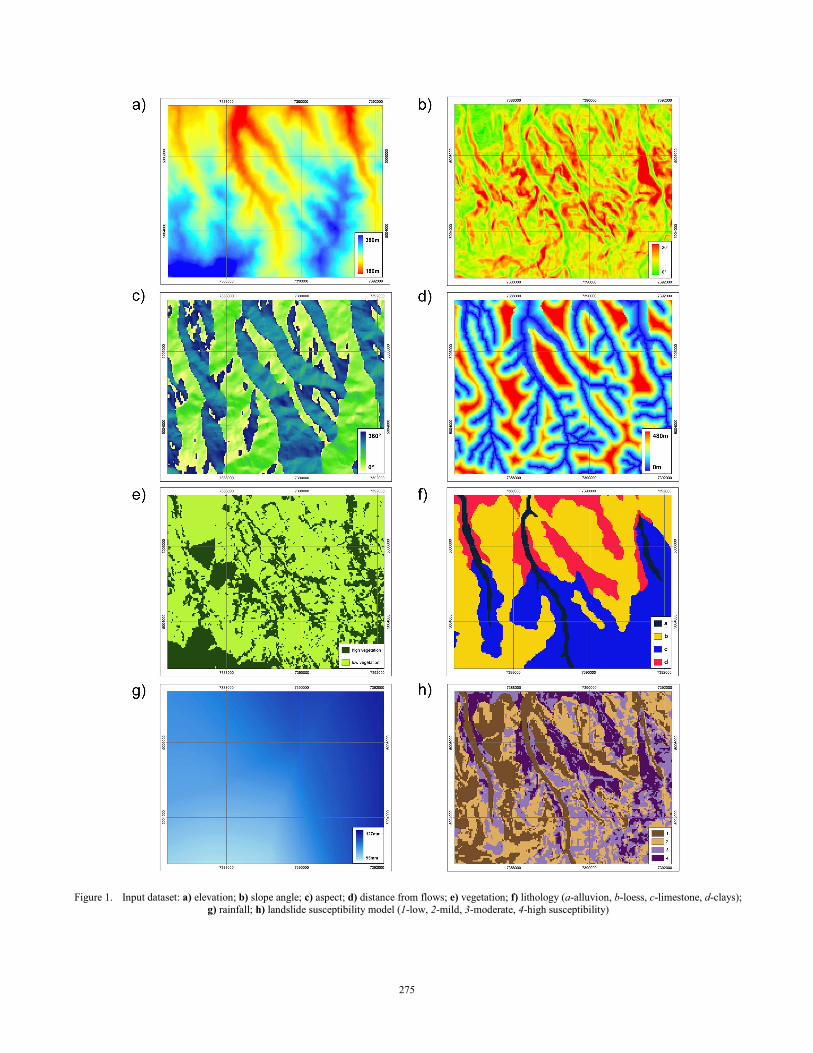
Figure 1. Input dataset: a) elevation; b) slope angle; c) aspect; d) distance from flows; e) vegetation; f) lithology (a-alluvion, b-loess, c-limestone, d-clays); g) rainfall; h) landslide susceptibility model (1-low, 2-mild, 3-moderate, 4-high susceptibility)

275

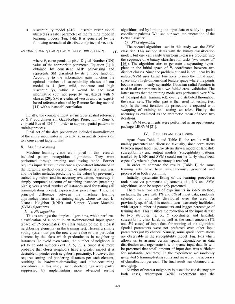
• susceptibility model (SM) – discrete raster model utilized as a label parameter of the training mode in learning process (Fig. 1-h). It is generated by the following normalized distribution (principal vector):

7654321 02,005,008,014,015,027,029,0 PPPPPPPSM ⋅+⋅+⋅+⋅+⋅+⋅+⋅= , (1)

where Pi corresponds to pixel Digital Number (DN) value of the appropriate parameter. Equation (1) is obtained by consistent AHP pair-wising and represents SM classified by its entropy function. According to the information gain function the optimal number of susceptibility classes of our model is 4 (low, mild, moderate and high susceptibility), while it would be the most informative (but not properly visualized) with 9 classes [20]. SM is evaluated versus another, expert-based reference obtained by Remote Sensing method [11] with substantial correlation.

Finally, the complete input set includes spatial reference

or X,Y coordinates (in Gaus-Krüger Projection – Zone 7, ellipsoid Bessel 1841) in order to support spatial patterns in training process.

Final act of the data preparation included normalization of the entire input raster set to a 0-1 span and its conversion to a convenient table format.

B. Machine learning Machine learning classifiers implied in this research

included pattern recognition algorithms. They were performed through training and testing mode. Former requires input dataset, in our case a geo-dataset introduced in the forgoing method description of multi-criteria analysis, and the latter includes predicting of the values by previously trained algorithm, and its accuracy evaluation. Accuracy is simply computed as count of matching instances (matching pixels) versus total number of instances used for testing (all training-testing pixels), expressed as percentage. Thus, the principal difference between the machine learning approaches occurs in the training stage, where we used k-Nearest Neighbor (k-NN) and Support Vector Machine (SVM) algorithms.

1) k-NN algorithm This is amongst the simplest algorithms, which performs

classification of a point in an n-dimensional input space (space of Pi coordinates) by class values of the k closest neighboring elements (in the training set). Herein, a simple voting system assigns the new class value to that particular element by the class which predominates in neighboring instances. To avoid even votes, the number of neighbors is set to an odd number (k=1, 3, 5, 7…). Since it is more probable that closer neighbors have a greater impact it is desirable to ponder each neighbor’s proximity. However, this requires sorting and pondering distances per each element, resulting in hardware-demanding and time-consuming procedures. In this study, such shortcomings were partly suppressed by implementing more advanced sorting

algorithms and by limiting the input dataset solely to spatial coordinate palettes. We used our own implementation of the k-NN classifier.

2) SVM algorithm The second algorithm used in this study was the SVM

classifier. This method deals with the binary classification model, but one can easily transform n-classes problem into the sequence of n binary classification tasks (one-versus-all [16]). The algorithm tries to generate a separating hyper-plane in the initial space of Pi coordinates between two distinct classes. Since the problem at hand is not linear by its nature, SVM uses kernel functions to map the initial input space into a high-dimensional feature space where the points become more linearly separable. Gaussian radial function is used in all experiments in a two-folded cross-validation. The latter means that the training mode was performed over 50% of the input data (training set), evenly distributed throughout the raster sets. The other part is then used for testing (test set). In the next iteration the procedure is repeated with swapping of training and testing set roles. Finally, the accuracy is evaluated as the arithmetic mean of those two iterations.

All SVM experiments were performed in an open-source package LIBSVM [21].

IV. RESULTS AND DISCUSSION Apart from Table I and Table II, the results will be

mainly presented and discussed textually, since correlations between input label (multi-criteria driven model of landslide susceptibility) and output models (susceptibility patterns tracked by k-NN and SVM) could not be fairly visualized, especially where higher accuracy is reached.

In order to compare the results (Table I) the same training sets have been simultaneously generated and processed in both algorithms.

Initially, systematic fitting of the learning procedures took place via parametric adjustments of k-NN and SVM algorithms, as to be respectively presented.

There were two sets of experiments in k-NN method, including the case with 1% and 5% of input data, randomly selected but uniformly distributed over the area. As previously specified, this method turns extremely inefficient with larger number of parameters and bigger percentage of training data. This justifies the reduction of the input dataset to two attributes i.e. X, Y coordinates and landslide susceptibility class label, as well as the small amount (1% and 5% cases) of input data for training of the algorithm. Spatial parameters were not preferred over other input parameters just by chance. Namely, some spatial correlations are observable in the susceptibility model (Fig. 1-h) which allows us to assume certain spatial dependence in data distribution and regenerate it with sparse input data (it will be presented that small amount of input data was sufficient for substantial accuracy). In the experiment we randomly generated 5 training-testing splits and measured the accuracy of classification per each. The final result was obtained after averaging.

Number of nearest neighbors is tested for consistency per both cases, whereupon 3-NN experiment met the

276

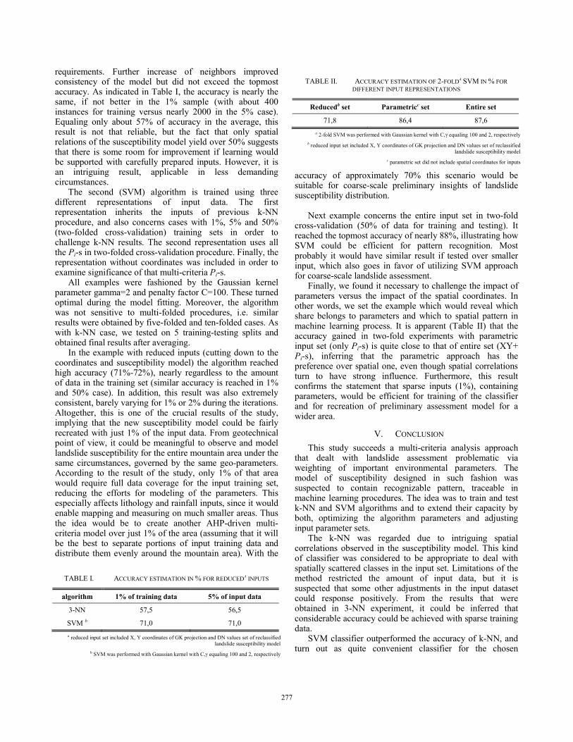
requirements. Further increase of neighbors improved consistency of the model but did not exceed the topmost accuracy. As indicated in Table I, the accuracy is nearly the same, if not better in the 1% sample (with about 400 instances for training versus nearly 2000 in the 5% case). Equaling only about 57% of accuracy in the average, this result is not that reliable, but the fact that only spatial relations of the susceptibility model yield over 50% suggests that there is some room for improvement if learning would be supported with carefully prepared inputs. However, it is an intriguing result, applicable in less demanding circumstances.

The second (SVM) algorithm is trained using three different representations of input data. The first representation inherits the inputs of previous k-NN procedure, and also concerns cases with 1%, 5% and 50% (two-folded cross-validation) training sets in order to challenge k-NN results. The second representation uses all the Pi-s in two-folded cross-validation procedure. Finally, the representation without coordinates was included in order to examine significance of that multi-criteria Pi-s.

All examples were fashioned by the Gaussian kernel parameter gamma=2 and penalty factor C=100. These turned optimal during the model fitting. Moreover, the algorithm was not sensitive to multi-folded procedures, i.e. similar results were obtained by five-folded and ten-folded cases. As with k-NN case, we tested on 5 training-testing splits and obtained final results after averaging.

In the example with reduced inputs (cutting down to the coordinates and susceptibility model) the algorithm reached high accuracy (71%-72%), nearly regardless to the amount of data in the training set (similar accuracy is reached in 1% and 50% case). In addition, this result was also extremely consistent, barely varying for 1% or 2% during the iterations. Altogether, this is one of the crucial results of the study, implying that the new susceptibility model could be fairly recreated with just 1% of the input data. From geotechnical point of view, it could be meaningful to observe and model landslide susceptibility for the entire mountain area under the same circumstances, governed by the same geo-parameters. According to the result of the study, only 1% of that area would require full data coverage for the input training set, reducing the efforts for modeling of the parameters. This especially affects lithology and rainfall inputs, since it would enable mapping and measuring on much smaller areas. Thus the idea would be to create another AHP-driven multi-criteria model over just 1% of the area (assuming that it will be the best to separate portions of input training data and distribute them evenly around the mountain area). With the

accuracy of approximately 70% this scenario would be suitable for coarse-scale preliminary insights of landslide susceptibility distribution.

Next example concerns the entire input set in two-fold

cross-validation (50% of data for training and testing). It reached the topmost accuracy of nearly 88%, illustrating how SVM could be efficient for pattern recognition. Most probably it would have similar result if tested over smaller input, which also goes in favor of utilizing SVM approach for coarse-scale landslide assessment.

Finally, we found it necessary to challenge the impact of parameters versus the impact of the spatial coordinates. In other words, we set the example which would reveal which share belongs to parameters and which to spatial pattern in machine learning process. It is apparent (Table II) that the accuracy gained in two-fold experiments with parametric input set (only Pi-s) is quite close to that of entire set (XY+ Pi-s), inferring that the parametric approach has the preference over spatial one, even though spatial correlations turn to have strong influence. Furthermore, this result confirms the statement that sparse inputs (1%), containing parameters, would be efficient for training of the classifier and for recreation of preliminary assessment model for a wider area.

V. CONCLUSION This study succeeds a multi-criteria analysis approach

that dealt with landslide assessment problematic via weighting of important environmental parameters. The model of susceptibility designed in such fashion was suspected to contain recognizable pattern, traceable in machine learning procedures. The idea was to train and test k-NN and SVM algorithms and to extend their capacity by both, optimizing the algorithm parameters and adjusting input parameter sets.

The k-NN was regarded due to intriguing spatial correlations observed in the susceptibility model. This kind of classifier was considered to be appropriate to deal with spatially scattered classes in the input set. Limitations of the method restricted the amount of input data, but it is suspected that some other adjustments in the input dataset could response positively. From the results that were obtained in 3-NN experiment, it could be inferred that considerable accuracy could be achieved with sparse training data.

SVM classifier outperformed the accuracy of k-NN, and turn out as quite convenient classifier for the chosen

TABLE I. ACCURACY ESTIMATION IN % FOR REDUCEDA INPUTS

algorithm 1% of training data 5% of input data

3-NN 57,5 56,5

SVM b 71,0 71,0 a reduced input set included X, Y coordinates of GK projection and DN values set of reclassified

landslide susceptibility model b SVM was performed with Gaussian kernel with C, equaling 100 and 2, respectively

TABLE II. ACCURACY ESTIMATION OF 2-FOLDA SVM IN % FOR DIFFERENT INPUT REPRESENTATIONS

Reducedb set Parametricc set Entire set

71,8 86,4 87,6 a 2-fold SVM was performed with Gaussian kernel with C, equaling 100 and 2, respectively

b reduced input set included X, Y coordinates of GK projection and DN values set of reclassified landslide susceptibility model

c parametric set did not include spatial coordinates for inputs

277

problem. In comparison to k-NN it turned more consistent and constantly more precise. The most important result is the one revealing that small training sets are sufficient to reach very high accuracy. In order to exploit these features, it has been suggested that the susceptibility model could be recreated for wider area, with less effort than in standard modeling procedures [3]. However, a multi-fold case with sparse data inputs yet needs to be confirmed.

Another curiosity is that this approach is entirely novel in landslides assessments and we hope that the future

experiments will show its applicability in this field.

REFERENCES [1] P. Aleotti and R. Chowdhury, “Landslide hazard assessment:

summary review and new perspectives,” Bull Eng Geol Environ, vol. 58, pp. 21-44, 1999.

[2] K. Smith, Environmental Hazards – Assessing the risk and reducing disaster, Routledge, London and New York (UK, USA), 2001, pp. 180-202.

[3] J. Chacón et al, “Engineering geology maps: landslides and geographical information systems,” Bull Eng Geol Environ, vol. 65, pp. 341-411, 2006.

[4] G. Bonham-Carter, Geographic information system for geosciences – Modeling with GIS, Pergamon, New York (USA), 1994, pp. 51-81, 177-334.

[5] M. Ercanoglu et al, “Adaptation and comparison of expert opinion to analytical hierarchy process for landslide susceptibility mapping,” Bull Eng Geol Environ, vol 67, pp. 565-578, 2008.

[6] X. Yao, L. G. Tham, F. C. Dai, “Landslide susceptibility mapping based on support vector machine: A case study on natural slopes of Hong Kong, China,” Geomorphology, vol. 101, pp. 572-582, 2008.

[7] A. Smirnoff, E. Boisvert, and S. J. Paradis, “Support vector machines for 3D modeling from sparse geological information of various origins,” Computers & Geosciences, vol. 34, pp. 127-143, 2008.

[8] M. Marjanovi , “Landslide susceptibility modeling: A case study on Fruška Gora Mountain, Serbia”, Geomorphologia Slovaca et Bohemica, vol 10, 2009, in press

[9] H. Zhao, “Slope reliability analysis using a support vector machine,” Computers and Geotechnics, vol. 35, pp. 459-467, 2008.

[10] M. Janji , Engineering Geology characteristics of terrains of National Republic of Serbia (Inženjerskogeološke karakteristike terena Narodne Republike Srbije), Geological and Geophysical Survey, Belgrade (Serbia), 1962, pp. 19-189.

[11] R. Pavlovi et al, “Geological conditions of racional usage and preservation of the Fruška Gora Mountain area (Geološki uslovi racionalnog koriš enja i zaštite prostora Fruške gore),” Specialist study, Department for Remote Sensing and Structural Geology, Faculty of Mining and Geology, University of Belgrade, 2005, unpublished

[12] T. upkovi , “Evolution of geomorphologic processes on Fruška Gora Mountain (Evolucija geomorfoloških procesa Fruške gore),” Master Thesis, Department for Remote Sensing and Structural Geology, Faculty of Mining and Geology, University of Belgrade, 1995, unpublished.

[13] M. Komac, “A landslide susceptibility model using the analytical hierarchy process method and multivariate statistics in perialpine Slovenia,” Geomorphology, vol. 74, pp. 17-28, 2005.

[14] A. Esmali and H. Ahmadi, “Using GIS & RS in mass movements hazard zonation – A case study in Germichay watershed, Aderbil, Iran,” Proc. Map Asia 2003, Kuala Lumpur (Malaysia), 13-15 October, 2003.

[15] V. Vapnik, The Nature of Statistical Learning Theory, 2nd ed. Springer-Verlag, New York (USA), 1995, pp 138-167.

[16] A. I. Belousov, S. A. Verzakov, J. Von Frese, “Applicational aspects of support vector machines,” J. Chemom, vol. 16, pp 482-489, 2002.

[17] C. Van Westen et al, “Landslide hazard and risk zonation – Why is it still so difficult?”, Bull Eng Geol Environ, vol. 65, pp. 197-205, 2006.

[18] V. Voženílek, “Landslide modeling for natural risk/hazard assessment with GIS,” Geographica, Acta Universitas Carolinae, vol. XXXV, pp. 145-155, 2000.

[19] G. Ravi, Remote sensing Geology, Springer-Verlag, Berlin (Germany), 2002, pp. 429-583.

[20] M. Marjanovi and B. Abolmasov, “AHP-driven multi-criteria analysis of landslide susceptibility on Fruška Gora Mountain,” unpublished

[21] C. C. Chang, and C. J. Lin, “LIBSVM: a library for support vector machines,” 2001, Software available at: http://www.csie.ntu.edu.tw/~cjlin/libsvm

This paper is written in the framework of Methods of artificial intelligence in GIS, a project of Czech Republic Grant Agency (CR GA 205/09/079)

278