LAND SURFACE MODELING OF ENERGY-BALANCE COMPONENTS: MODEL VALIDATION AND SCALING EFFECTS By VENKATARAMANA RAO SRIDHAR Bachelor of Engineering College of Agricultural Engineering Tamil Nadu Agricultural University Coimbatore, Tamil Nadu, India 1991 Master of Engineering Irrigation Engineering and Management School of Civil Engineering Asian Institute of Technology Bangkok, Thailand 1994 Submitted to the Faculty of the Graduate College of the Oklahoma State University in partial fulfillment of the requirements for the Degree of DOCTOR OF PHILOSOPHY August, 2001

Welcome message from author
This document is posted to help you gain knowledge. Please leave a comment to let me know what you think about it! Share it to your friends and learn new things together.
Transcript

LAND SURFACE MODELING OF ENERGY-BALANCE
COMPONENTS: MODEL VALIDATION AND
SCALING EFFECTS
By
VENKATARAMANA RAO SRIDHAR
Bachelor of Engineering College of Agricultural Engineering Tamil Nadu Agricultural University
Coimbatore, Tamil Nadu, India 1991
Master of Engineering Irrigation Engineering and Management
School of Civil Engineering Asian Institute of Technology
Bangkok, Thailand 1994
Submitted to the Faculty of the Graduate College of the
Oklahoma State University in partial fulfillment of
the requirements for the Degree of
DOCTOR OF PHILOSOPHY August, 2001

© Copyright by VENKATARAMANA RAO SRIDHAR 2001 All Rights Reserved.
iii
Name: Venkataramana Rao Sridhar Date of Degree: August, 2001
Institution: Oklahoma State University Location: Stillwater, Oklahoma
Title of Study: LAND SURFACE MODELING OF ENERGY-BALANCE COMPONENTS: MODEL VALIDATION AND SCALING EFFECTS
Pages in Study: 192 Candidate for the Degree of Doctor of Philosophy
Major Field: Biosystems Engineering
Scope and Method of Study: Appropriate quantification of surface energy balance
components that influence land-atmosphere exchange phenomena is important for improved weather prediction. The issue of scale interaction has emerged as one of the crucial challenges for the parameterization of general circulation models (GCMs) due to the strong interconnection between land and atmospheric processes. The objective of this study was to examine the effects of different spatial scales of input data on modeled net radiation, latent, sensible and ground heat fluxes and hence to understand the resolution needed for the realistic modeling of large-area land and atmospheric interactions. This study employed the NOAH-OSU (Oregon State University) Land Surface Model (LSM), which is a popular model used in a coupled fashion with the NCEP operational Eta and PSU/MM5 mesoscale models. Since the model requires downwelling longwave radiation as one of its inputs, a simple estimation procedure was developed and tested using nine Oklahoma Atmospheric Surface-Layer Instrumentation System (OASIS) sites. Then the full LSM was tested using seven OASIS sites with diverse soils, vegetation and climate. Finally, at three different spatial scales, model simulations were performed for the most homogeneous and the most heterogeneous areas of the Southern Great Plains 1997 study region.
Findings and Conclusions: The newly developed scheme for the estimation of downwelling
longwave radiation performed very well during both daytime and nighttime as well as under clear and cloudy sky conditions. Two methods of green vegetation fraction showed some differences in the estimates of latent and sensible heat fluxes. LSM validation using OASIS measurements at individual sites showed that the seven-site mean of modeled net radiation had a slight positive bias. It appeared that the model assigned most of this excess energy to latent heat flux. In the scaling study for the heterogeneous region, simulation results for the 200 m and 2 km scales matched well for net radiation, latent, sensible and ground heat fluxes while they differed at the 20 km resolution. For the homogeneous region, the model’s flux predictions at all three scales were in close agreement. The results suggested that the aggregation of spatially variable soil and vegetation inputs can have a significant impact on the quantification of surface energy-balance components and partitioning of latent and sensible heat fluxes. It was confirmed that the effects of scaling-up of input data on model estimates are more pronounced for heterogeneous areas than for homogeneous areas.
ADVISER’S APPROVAL: ____________________________________________________
(Ronald L. Elliott)
iv
LAND SURFACE MODELING OF ENERGY-BALANCE
COMPONENTS: MODEL VALIDATION AND
SCALING EFFECTS
Thesis Approved:
Thesis Adviser
Dean of the Graduate College

v
ACKNOWLEDGEMENTS
I would like to express immense thanks to my major adviser Dr. Ronald L. Elliott
for his guidance, support and encouragement throughout my study at OSU. His
dedication to work, in-depth understanding of issues and sincerity has taught me a lot and
inspired me greatly. Dr. Elliott ‘s contribution towards my completion of this research is
acknowledged with a great sense of gratitude and his professional and personal
framework will have a great positive impact in carrying me forward successfully. I also
extend my appreciation to my other committee members, Dr. Stephen J. Stadler, Dr. Fei
Chen and Dr. Michael A. Kizer for their advice and encouragement. Special thanks to
Dr. Fei Chen for his invaluable contribution with regard to model training for two
successive summers. I would like to extend my appreciation to Dr. C.T. Haan who was
on my committee until his retirement and I treasure his advice.
This research was made possible by EPSCoR grants from the National
Aeronautics and Space Administration (Cooperative Agreement Number NCC5-171) and
the National Science Foundation (Project Number EPS9550478). I would also like to
acknowledge the assistance of the Oklahoma Mesonet and the Oklahoma Agricultural
Experiment Station.
Appreciation is extended to Dr. Jerry Brotzge and Derek Arndt who provided the
OASIS and the Oklahoma Mesonet data for this study. I thank Dr. Daniel Itenfisu, Mark
Gregory and Pete Earls for extending a helping hand whenever I sought for it. I wish to

vi
express my thanks to Dr. Norm Elliott, USDA-ARS for providing me with the
FRAGSTAT software. The support and help that I received over the last few years at
OSU from many friends is tremendous. Kudos to Barbara T., Jana, Gloria, Marge and
Hope (for the administrative support), Drs. Hamilton and Senay (well-wisher and soccer-
fan) and Ron Tejral (for taking pictures at Mesonet sites).
Finally and above all, I thank my parents, brothers (and family) and my wife for
their support during all these years. They are with me guiding physically, emotionally
and more importantly spiritually that gave me endurance, courage and faith in all my
efforts.

vii
TABLE OF CONTENTS Chapter Page
I. INTRODUCTION................................................................................................... 1
Background ....................................................................................................... 1
Objectives.......................................................................................................... 3
Scope of the study ............................................................................................. 3
II. DESCRIPTION OF THE LAND SURFACE MODEL.......................................... 5
Overview ........................................................................................................... 5
Soil Hydrology .................................................................................................. 7
Soil Thermodynamics ..................................................................................... 13
III. VALIDATION OF A SIMPLE DOWNWELLING LONGWAVE RADIATION SCHEME FOR BOTH DAYTIME AND NIGHTTIME CONDITIONS ............ 16
Abstract ........................................................................................................... 16
Introduction ..................................................................................................... 17
Models for longwave radiation ....................................................................... 18
Data ................................................................................................................. 20
Model selection and calibration ...................................................................... 21
Results and Discussion.................................................................................... 28 Validation of calibrated model.................................................................. 28 Comparison of calibrated model with cloud-fraction
longwave model .................................................................................. 28 Summary ......................................................................................................... 36
IV. VALIDATION OF THE NOAH-OSU LAND SURFACE MODEL USING SURFACE FLUX MEASUREMENTS IN OKLAHOMA .................................. 37
Abstract ........................................................................................................... 37
Introduction ..................................................................................................... 38
Model Description........................................................................................... 40 Soil Hydrology .......................................................................................... 41

viii
Chapter Page
Soil Thermodynamics ............................................................................... 43 Previous studies using the LSM................................................................ 44
Field Instrumentation and Data ....................................................................... 45 Mesonet ..................................................................................................... 45 OASIS ....................................................................................................... 46 Green Vegetation Fraction ........................................................................ 50
Results and Discussion.................................................................................... 52 Sensitivity to Green Vegetation Fraction .................................................. 52 Daily Comparisons.................................................................................... 58 Hourly Comparisons ................................................................................. 63
Summary and Conclusions.............................................................................. 70
V. SCALING EFFECTS ON MODELED SURFACE ENERGY-BALANCE COMPONENTS USING THE NOAH-OSU LAND SURFACE MODEL ......... 80
Abstract ........................................................................................................... 80
Introduction ..................................................................................................... 81
Scaling concepts.............................................................................................. 83
Land surface model ......................................................................................... 86
Study area and data ......................................................................................... 87 Study area description ............................................................................... 87 Soil and vegetation data ............................................................................ 90 Identification of the homogeneous and the heterogeneous
cell ....................................................................................................... 90 Aggregation of the input data.................................................................... 94 Area-averaged and dominant-landuse-based NDVI for green
vegetation fraction............................................................................... 99 Weather data............................................................................................ 100
Results and Discussion.................................................................................. 101 Model sensitivity to the area-averaged and dominant-
landuse-based vegetation fraction ..................................................... 101 Model output ........................................................................................... 101 Time series comparison of the model output for the three
scales ................................................................................................. 102 Comparison of the bias in the model output for the three
scales ................................................................................................. 115 Deflections in the model output at 20-km scale...................................... 116
Summary and Conclusions............................................................................ 127
VI. SUMMARY, CONCLUSIONS AND RECOMMENDATIONS....................... 130
Summary ....................................................................................................... 130

ix
Chapter Page
Conclusions ................................................................................................... 134
Recommendations ......................................................................................... 136
REFERENCES................................................................................................................ 138
APPENDIX A--THE SOIL AND VEGETATION-RELATED PARAMETERS IN THE LAND SURFACE MODEL ....................................... 146
APPENDIX B--HOURLY OBSERVED AND PREDICTED DOWNWELLING LONGWAVE RADIATION FOR FIVE SITES...................... 149
APPENDIX C--COMPARISON OF OBSERVED AND MODELED ENERGY-BALANCE COMPONENTS FOR SEVEN SITES ................. 155
APPENDIX D--SCALE COMPARISONS OF MODELED SURFACE ENERGY-BALANCE COMPONENTS FOR THE HETEROGENEOUS AND THE HOMOGENEOUS AREA.. 170
x
LIST OF TABLES Table Page
3-1. Oklahoma Atmospheric Surface-layer Instrumentation System (OASIS) sites used in this study................................................................................................. 23
3-2. Comparison of 3 clear-sky downwelling longwave radiation schemes to observed hourly data. .......................................................................................... 24
3-3. Regression calibration of Brutsaert’s leading coefficient in equation (3-2). ...... 26
3-4. Validation of equation (3-7) using hourly data for June 1, 1999 though May 31, 2000. ................................................................................................................... 35
3-5. Comparison of equations (3-6) and (3-7) to hourly observed data for June 1 though August 25, 1999...................................................................................... 35
4-1. OASIS sites’ soil and vegetation types............................................................... 49
4-2 (a). Statistics of daily averaged Net Radiation (Rn) and Latent Heat (LH) flux for June ’99 – May ’00. ............................................................................................ 64
4-2 (b). Statistics of daily averaged Sensible Heat (SH) and Ground Heat (GH) flux for June ’99 – May ’00. ............................................................................................ 65
4-3 (a). Statistics of hourly averaged Net Radiation (Rn) and Latent Heat (LH) flux for June ’99 – May ’00. ............................................................................................ 71
4-3 (b). Statistics of hourly averaged Sensible Heat (SH) and Ground Heat (GH) flux for June ’99 – May ’00. ............................................................................................ 72
5-1. List of vegetation and soil parameters used in the land surface model. ............. 91
5-2. Landscape indices for the heterogeneous cell (#21) and the homogeneous cell (#9)...................................................................................................................... 93
5-3. Daily average modeled energy-balance components for the heterogeneous area (Cell 21) at three scales of input aggregation. .................................................. 103
5-4. Daily average modeled energy-balance components for the homogeneous area (Cell 9) at three scales of input aggregation. .................................................... 105
xi
LIST OF FIGURES Figure Page
2-1. Schematic diagram of the NOAH-OSU Land Surface Model (from Chen and Dudia, 2001). ........................................................................................................ 6
3-1. Location of Oklahoma Atmospheric Surface-layer Instrumentation System (OASIS) sites. ..................................................................................................... 22
3-2a. Comparison of hourly observed and predicted downwelling longwave radiation for the BESS site................................................................................................. 29
3-2b. Comparison of hourly observed and predicted downwelling longwave radiation for the BURN site. .............................................................................................. 30
3-2c. Comparison of hourly observed and predicted downwelling longwave radiation for the MARE site............................................................................................... 31
3-2d. Comparison of hourly observed and predicted downwelling longwave radiation for the NORM site. ............................................................................................. 32
3-2e. Comparison of hourly observed and predicted downwelling longwave radiation for the STIG site. ................................................................................................ 33
3-3. Comparison of hourly observed and predicted downwelling longwave radiation for the BURN site. .............................................................................................. 34
4-1. Location of Oklahoma Atmospheric Surface-layer Instrumentation System (OASIS) sites used in this study. ........................................................................ 48
4-2. Green vegetation fraction as derived by the Gutman-Ignatov (G-I) and Carlson-Ripley (C-R) schemes for BOIS and BURN ...................................................... 53
4-3. Sensitivity of the modeled net radiation using G-I and C-R green vegetation fraction methods. ................................................................................................ 54
4-4. Sensitivity of the modeled latent heat flux using G-I and C-R green vegetation fraction methods. ................................................................................................ 55
4-5. Sensitivity of the modeled sensible heat flux using G-I and C-R green vegetation fraction methods. ................................................................................................ 56
xii
Figure Page
4-6. Sensitivity of the modeled ground heat flux using G-I and C-R green vegetation fraction methods. ................................................................................................ 57
4-7. Sensitivity of the model to green vegetation fraction at BOIS for relatively wet and dry soil conditions (VWC1- Top soil layer volumetric water co ntent; VWC2-Root zone volumetric water content). .................................................... 59
4-8. Sensitivity of the model to green vegetation fraction at BURN for relatively wet and dry soil conditions (VWC1- Top soil layer volumetric water content; VWC2-Root zone volumetric water content). .................................................... 60
4-9. Comparison of daily average observed and modeled net radiation. ................... 66
4-10. Comparison of daily average observed and modeled latent heat flux. ............... 67
4-11. Comparison of daily average observed and modeled sensible heat flux. ........... 68
4-12. Comparison of daily average observed and modeled ground heat flux.............. 69
4-13. Comparison of hourly average observed and modeled net radiation.................. 73
4-14. Comparison of hourly average observed and modeled latent heat flux.............. 74
4-15. Comparison of hourly average observed and modeled sensible heat flux.......... 75
4-16. Comparison of hourly average observed and modeled ground heat flux. .......... 76
5-1. Location map of Southern Great Plains 97 (SGP97) and the study area. ........... 89
5-2a. Land use types of the heterogeneous area (Cell 21) at 200-m resolution........... 95
5-2b. Land use types of the heterogeneous area (Cell 21) at 2-km resolution............. 95
5-3a. Soil types of the heterogeneous area (Cell 21) at 200-m resolution. .................. 96
5-3b. Soil types of the heterogeneous area (Cell 21) at 2-km resolution..................... 96
5-4a. Land use types of the homogeneous area (Cell 9) at 200-m resolution.............. 97
5-4b. Land use types of the homogeneous area (Cell 9) at 2-km resolution................ 97
5-5a. Soil types of the homogeneous area (Cell 9) at 200-m resolution...................... 98
5-5b. Soil types of the homogeneous area (Cell 9) at 2-km resolution........................ 98
5-6. Modeled net radiation comparison among the three scales for the heterogeneous area on 18 June 97. ........................................................................................... 107
5-7. Modeled net radiation comparison among the three scales in the homogeneous area on 18 June 97. ........................................................................................... 108
5-8. Modeled latent heat flux comparison among the three scales for the heterogeneous area on 18 June 97. ................................................................... 109

xiii
Figure Page
5-9. Modeled latent heat flux comparison among the three scales for the homogeneous area on 18 June 97. .................................................................... 110
5-10. Modeled sensible heat flux comparison among the three scales for the heterogeneous area on 18 June 97. ................................................................... 111
5-11. Modeled sensible heat flux comparison among the three scales for the homogeneous area on 18 June 97. .................................................................... 112
5-12. Modeled ground heat flux comparison among the three scales for the heterogeneous area on 18 June 97 .................................................................... 113
5-13. Modeled ground heat flux comparison among the three scales for the homogeneous area on 18 June 97 ..................................................................... 114
5-14. Scale comparisons of the heterogeneous area (Cell 21) model output at 200-m, 2-km and 20-km resolutions. ............................................................................ 117
5-15. Scale comparisons of the homogeneous area (Cell 9)model output at 200-m, 2-km and 20-km resolutions................................................................................. 118
5-16. Equal-value plots of modeled net radiation for the three scales in the heterogeneous area (Cell 21). ........................................................................... 119
5-17. Equal-value plots of modeled latent heat flux for the three scales in the heterogeneous area (Cell 21). ........................................................................... 120
5-18. Equal-value plots of modeled sensible heat flux for the three scales in the heterogeneous area (Cell 21). ........................................................................... 121
5-19. Equal-value plots of modeled ground heat flux for the three scales in the heterogeneous area (Cell 21). ........................................................................... 122
5-20. Equal-value plots of modeled net radiation for the three scales in the homogeneous area (Cell 9). .............................................................................. 123
5-21. Equal-value plots of modeled latent heat flux for the three scales in the homogeneous area (Cell 9). .............................................................................. 124
5-22. Equal-value plots of modeled sensible heat flux for the three scales in the homogeneous area (Cell 9). .............................................................................. 125
5-23. Equal-value plots of modeled ground heat flux for the three scales in the homogeneous area (Cell 9). .............................................................................. 126
1
CHAPTER 1
INTRODUCTION
Background
Modeling the processes related to land-atmosphere interaction over a large area is
recognized as a complex and unresolved issue. Energy and water exchanges occur
continuously at the interface between the land surface and the lower atmosphere. These
exchanges are in the form of fluxes of radiant energy, latent heat and sensible heat.
While there have been significant efforts in data collection and model development,
validation and application, a number of issues are yet to be resolved. This is partly due to
the multi-disciplinary nature of land-atmosphere modeling, which involves at least,
hydrological, biophysical, and atmospheric science disciplines.
Scaling is an important issue that underlies modeling efforts. Models developed
to estimate the surface energy and mass balance components at a point scale may tend to
perform not as well when applied to larger areas. The land-atmosphere interaction
process is often viewed from a relatively large-area perspective (i.e., predicting
phenomena at regional to continental to global scales). Modeling the land surface
processes plays an important role in large-scale atmospheric models (e.g., Mintz, 1981;
Rowntree, 1983; Avissar and Pielke, 1989; Chen and Dudhia, 2001). Accurate
partitioning of energy balance components improves regional weather and also global
climate simulations. This necessitates the combined efforts of both hydrologists and

2
atmospheric scientists to deal with the land surface and the atmosphere as an interactively
coupled system.
The problems of land surface heterogeneity within modeling grid cells have long
been recognized. Traditionally the lumped model concept, where the spatially variable
inputs and parameters are assumed to be homogeneous, has been in wide use. But many
studies (e.g., Avissar and Pielke, 1989; Entekhabi and Eagleson, 1989; Avissar, 1992;
Famiglietti and Wood, 1994; Wood, 1994; Hu and Islam, 1997) have revealed that the
accuracy of the model response is very much dominated by sub-grid scale
parameterizations of inputs and parameters. The distributed modeling approach, which
accounts for spatial variability of input variables and parameters, can be adopted for large
areas should this be supported by better (physically-based) models and high-resolution
data sets. This approach could lead to improved predictions and reduced uncertainties in
large-scale simulations. There are unanswered questions about the scale required for
modeling a particular process, and the associated tradeoffs in data requirements and the
accuracy in the model output.
There are a number of soil-vegetation-atmosphere models available for use and
their characteristics in terms of model physics, number of parameters, time step, number
of users and level of acceptance vary considerably. The well-tested NOAH-OSU LSM
(National Centers for Environmental Prediction / Air Force/Office of Hydrology / Oregon
State University / Land Surface Model) is chosen for this study. This LSM has been
coupled to two mesoscale models, the NCEP operational Eta and the PSU/MM5 (Penn
State University/fifth –generation Mesoscale Model) models (Marshall, 1998; Chen and
Dudhia, 2001), and is well recognized by the land surface modeling community.

3
Objectives
The overall objective of this research is to examine the effects of different spatial
scales of input data on modeled net radiation, latent, sensible and ground heat fluxes, and
thereby understand the resolution needed for the realistic modeling of large-scale land
atmosphere interaction. This is the specific focus of Chapter 5 of the dissertation. In
support of this objective, there are two additional components of the study:
1. To evaluate the available techniques for estimating downwelling longwave radiation,
to investigate possible improvements and/or simplifications to those techniques, and
to incorporate nighttime as well as daytime conditions. This work is the subject of
Chapter 3 and was undertaken because the land surface model requires downwelling
longwave radiation as one of its inputs, which is not readily available from
observations.
2. To validate the land surface model using the net radiation, latent, sensible and ground
heat flux measurements from the Oklahoma Atmospheric Surface-layer
Instrumentation System. Model validation was deemed to be an important precursor
to the scaling analysis and is the focus of Chapter 4.
Scope of the study
Oklahoma was chosen as the geographic setting for this study because of: (1) its
natural variability in climate ranging from the sub-humid east to the semi-arid west; (2)
the availability of a unique combination of soil, land use, vegetation, weather, and surface
flux data sets; and (3) the recent history of large-scale experiments in this region. For the
longwave radiation and model validation analyses, a diversity of Oklahoma sites was
used and the study period encompassed all seasons of the year. Due to the complexity in

4
data acquisition and handling for large areas, the area for the scaling study was identified
using statistical analysis of land use and soil data. The scaling analysis then focused on
two specific “cells” reflecting extremes in spatial heterogeneity/homogeneity, with a
summertime study period of approximately five weeks that fall within the SGP97
(Southern Great Plains 97) experiment period.

5
CHAPTER 2
DESCRIPTION OF THE LAND SURFACE MODEL
The land surface model utilized in this study was originally developed at Oregon
State University (Pan and Mahrt, 1987) and then gradually enhanced over the next
decade. These enhancements have come primarily from work at the National Centers for
Environmental Prediction, the Air Force and the NOAA Office of Hydrology. The
evolving model has recently been dubbed the “NOAH-OSU LSM”, and this identifier or
simply “LSM” will be used to refer to the model herein. Dr. Fei Chen at the National
Center for Atmospheric Research provided a working version of the model and
associated user training.
This chapter contains a brief overview of the LSM, followed by a more detailed
description of the components addressing soil hydrology and soil thermodynamics. An
abbreviated description of the LSM is also contained in Chapter 4.
Overview
A schematic representation of the LSM is shown in Figure 2-1. Originally, the
LSM consisted of the diurnally-dependent Penman potential evaporation approach of
Mahrt and Ek (1984), the multi-layer soil model of Mahrt and Pan (1984) and the
primitive canopy model of Pan and Mahrt (1987). Later NCEP/Office of Hydrology
extended the improvements by including (1) a fairly complex canopy resistance

6
Figure 2-1. Schematic diagram of the NOAH-OSU Land Surface Model (from Chen and Dudia, 2001).
7
approach; (2) the bare soil evaporation approach of Noilhan and Planton (1989); (3) the
surface runoff scheme of Schaake et al. (1996); (4) a higher-order time integration
scheme by Kalnay and Kanamitsu (1988); and (5) refinements to the snowmelt algorithm
and the treatment of soil thermal and hydraulic properties. Chen et al. (1996) modified
the LSM to incorporate an explicit canopy resistance formulation used by Jacquemin and
Noilhan (1990).
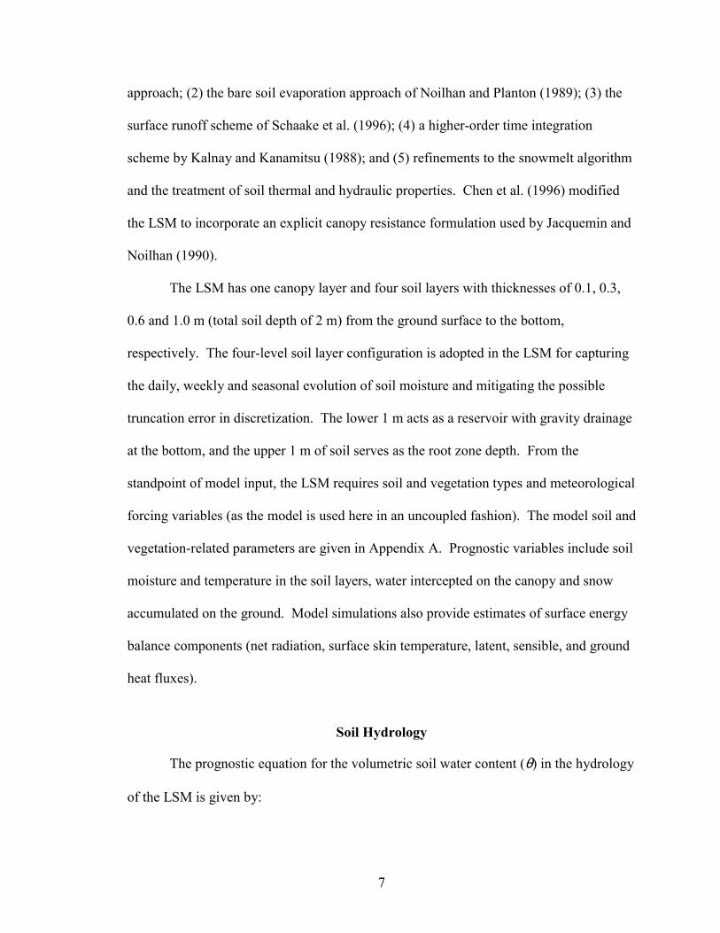
The LSM has one canopy layer and four soil layers with thicknesses of 0.1, 0.3,
0.6 and 1.0 m (total soil depth of 2 m) from the ground surface to the bottom,
respectively. The four-level soil layer configuration is adopted in the LSM for capturing
the daily, weekly and seasonal evolution of soil moisture and mitigating the possible
truncation error in discretization. The lower 1 m acts as a reservoir with gravity drainage
at the bottom, and the upper 1 m of soil serves as the root zone depth. From the
standpoint of model input, the LSM requires soil and vegetation types and meteorological
forcing variables (as the model is used here in an uncoupled fashion). The model soil and
vegetation-related parameters are given in Appendix A. Prognostic variables include soil
moisture and temperature in the soil layers, water intercepted on the canopy and snow
accumulated on the ground. Model simulations also provide estimates of surface energy
balance components (net radiation, surface skin temperature, latent, sensible, and ground
heat fluxes).
Soil Hydrology
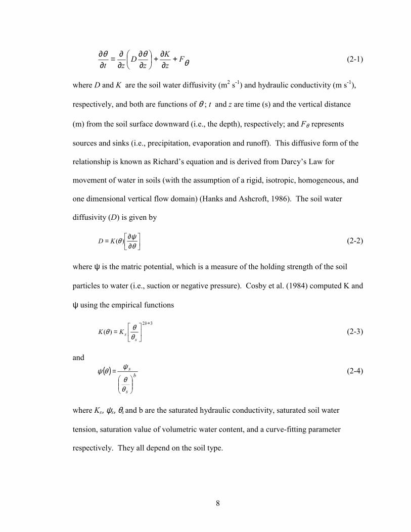
The prognostic equation for the volumetric soil water content (θ) in the hydrology
of the LSM is given by:
8
θθθ F
zK
zD
zt+
∂∂+�
�
���
�
∂∂
∂∂=
∂∂ (2-1)
where D and K are the soil water diffusivity (m2 s-1) and hydraulic conductivity (m s-1),
respectively, and both are functions of θ ; t and z are time (s) and the vertical distance
(m) from the soil surface downward (i.e., the depth), respectively; and Fθ represents
sources and sinks (i.e., precipitation, evaporation and runoff). This diffusive form of the
relationship is known as Richard’s equation and is derived from Darcy’s Law for
movement of water in soils (with the assumption of a rigid, isotropic, homogeneous, and
one dimensional vertical flow domain) (Hanks and Ashcroft, 1986). The soil water
diffusivity (D) is given by
��
���
�
∂∂
=θψθ )(KD (2-2)
where ψ is the matric potential, which is a measure of the holding strength of the soil
particles to water (i.e., suction or negative pressure). Cosby et al. (1984) computed K and
ψ using the empirical functions
32
)(+
��
���
�=
b
ssKK
θθθ (2-3)
and
( )b
s
s
���
����
�=
θθ
ψθψ (2-4)
where Ks, ψs, θs and b are the saturated hydraulic conductivity, saturated soil water
tension, saturation value of volumetric water content, and a curve-fitting parameter
respectively. They all depend on the soil type.
9
K and D are highly non-linear functions of soil moisture and in particular when
the soil is dry, they can change very rapidly by several orders of magnitude, for a small
variation in soil moisture. As the soil-water parameterization is very sensitive to the
diurnal partitioning of surface energy into latent and sensible heat (Cuenca et al., 1996),
Chen and Dudhia (2001) suggested the investigation of alternative soil hydraulic
parameterization schemes that would effectively accommodate the dynamic relationship
between hydraulic conductivity and soil moisture.
Expanding the source and sink term (Fθ) and integrating equation (2-1) over four soil
layers, as used in the MM5 model, yields:
111
11
tdirdzz
tz EERPKz
Dd −−−+−��
���
�
∂∂−=∂
∂ θθ (2-5)
22121
22 tzz
zzz EKK
zD
zD
td −−+�
�
���
�
∂∂−�
�
���
�
∂∂=
∂∂ θθθ (2-6)
33232
33 tzz
zzz EKK
zD
zD
td −−+�
�
���
�
∂∂−�
�
���
�
∂∂=
∂∂ θθθ (2-7)
433
44 zz
zz KK
zD
td −+�
�
���
�
∂∂=
∂∂ θθ (2-8)
where dzi is the i–th soil layer thickness, Pd is the precipitation not intercepted by the
canopy, R is the surface runoff, and Eti is the canopy transpiration taken by the canopy
root in the i-th layer within the root-zone layers. The soil water flux at the bottom of the
model domain (i.e., drainage) is determined from the gravitational percolation term Kz4,
and by assuming the hydraulic diffusivity to be zero at the bottom of the soil model.
Surface runoff is addressed in the LSM using the Simple Water Balance (SWB)
model approach given by Schaake et al. (1996). The SWB model is a two-reservoir
hydrological model that has been well calibrated for large river basins. It takes into

10
account the spatial heterogeneity of rainfall, soil moisture, and runoff. The excess of
precipitation that is not infiltrated into the soil is termed surface runoff (R = Pd - Imax ),
where the maximum infiltration, Imax, is given as:
( )
( )����
�� −−+
����
�� −−
=ikdtexDdP
ikdtexDdPI
δ
δ
1
1max (2-9)
( )�=
−∆=4
1iisix ZD θθ (2-10)
ref
srefdtdt K
Kkk
..= (2-11)
δi is the conversion of the current model time step δt (in seconds) into daily values (δi =
δt/86400), Ks is the saturated hydraulic conductivity which depends on soil texture, Dx is
soil moisture deficit, θs is the volumetric water content at saturation point, θi is the actual
volumetric water content, kdt is a runoff parameter, and kdtref = 3.0 and Kref = 2 x 10⁻⁶ m s-
1. Chen and Dudhia (2001) suggested the calibration of these parameters over various
basins with different precipitation characteristics.
The total evaporation, E, as formulated in the LSM, is the sum of 1) the direct
evaporation from the top shallow soil layer, Edir, 2) evaporation of precipitation
intercepted by the canopy, Ec, and 3) transpiration through canopy and roots, Et.
ctdir EEEE ++= (2-12)
The simple linear expression for bare soil evaporation is:
pwref
wdir EfE
��
�
�
��
�
�
−−
����
�� −=
θθθθ
σ ...1 (2-13)
11
where θw and θref are the soil wilting point and field capacity (dimensionless), σf is the
green vegetation fraction (dimensionless) which is critical for the partitioning of total
evaporation between bare-soil direct evaporation and canopy transpiration, and Ep is the
potential evaporation (ms-1), calculated by a Penman-based energy balance and given by:
( )
∆+−+−∆
=1
*)( qquCGRnEp ahρλ
(2-14)
where ∆ is the local derivative of saturation specific humidity (q*) with respect to
temperature (dimensionless), Rn and G are the surface net radiation and ground heat flux
( W m-2), ua is the surface layer wind speed ( m s-1), q is specific humidity and ρ, λ and
Ch are the air density (Kg m-3), latent heat of vaporization (J kg-1), and surface exchange
coefficient (m s-1), respectively.
Evaporation of rainfall intercepted by the canopy is governed by:
n
cpfc S
WEE ��
�
����
�= σ (2-15)
where Wc is the canopy intercepted water content (mm), S is the maximum allowed value
for Wc (specified here as 0.5 mm), and n = 0.5. Wc is determined by a budget equation:
cfc EDP
tW
−−=∂
∂σ (2-16)
where P is the total precipitation (kg m-2 s-1), and D is the drip or precipitation that
reaches the ground (mm). This implies that Pd in equation (2-5) is computed by:
( ) DPP fd +−= σ1 (2-17)
It is worthwhile to note that after significant rainfall, then Wc reaches S, and the
time tendency in equation (2-16) reduces to zero and Pd ≈ P. In other words, additional
rainfall drips off the canopy and reaches the ground (except the small amount lost to Ec)

12
Et is determined by:
��
�
�
��
�
�
���
�
�−=n
ccpft S
WBEE 1σ (2-18)
where Bc (dimensionless) is a function of canopy resistance and is expressed as:
rhc
rc
RCR
RB
∆++
∆+=
1
1 (2-19)
where Rr (dimensionless) is a function of surface air temperature, surface pressure and Ch
(m s-1), and Rc is the canopy resistance (s m-1). Details on Ch, Rr and ∆ are given by Ek
and Mahrt (1991). Rc is calculated using the formulation of Jacquemin and Noilhan
(1990):
4321
min.. FFFFLAI
cRcR = (2-20)
where
f
fRR
F cc
++
=1
1 maxmin
(2-21)
LAIR
Rf
gl
g 255.0= (2-22)
( )[ ]aass qTqhF
−+=
11
2 (2-23)
( )23 0016.01 aref TTF −−= (2-24)
( )( )( )�
= +−−
=3
1 214
i zzwref
ziwi
ddd
Fθθ
θθ (2-25)
F1, F2, F3 and F4 are all subject to 0 and 1 as lower and upper bounds and they represent
the effects of solar radiation, vapor pressure deficit, air temperature and soil moisture,
13
respectively. LAI is the leaf area index, Rcmin is the minimum stomatal resistance, and
Rcmax is the cuticular resistance of the leaves and is specified as 5000 s m-1 as in
Dickinson et al. (1993). Rgl (limiting value of photosynthetically active solar radiation) is
100 W m-2 and Rg is determined from radiation physics (Jacquemin and Noilhan, 1990);
qs(Ta) is the saturated water vapor mixing ratio at the air temperature Ta and qa is the
actual specific humidity. The parameter Tref is 298 K (Noilhan and Planton, 1989). The
soil moisture stress function, F4, embodies a linear relationship in soil moisture stress
between the field capacity θref and the wilting point θw, and is only integrated in the root-
zone which encompasses the first three soil layers in the current formulation.
Soil Thermodynamics
One of the primary functions of the coupled land surface model is to provide the
near-surface layer of an atmospheric model with sensible and latent heat fluxes, as well
as surface skin temperature to compute upward longwave radiation. The surface skin
temperature is determined following Mahrt and Ek [1984] by applying a single linearized
surface energy balance equation:
aTUCC
GERT
ahp
nskin +
−−=
ρλ (2-26)
where Rn is the net radiation (W m-2), G is the ground heat flux (W m-2), λE is the latent
heat flux (W m-2), Cp is the air heat capacity (J m-3 K-1), Ua is the surface layer wind
speed (m s-1), and Ta is the near-surface air temperature (K). Equation (2-26) expands the
sensible heat flux (H) term such that the relationship can be expressed in terms of Tskin.
As the skin is treated as an infinitesimally thin layer, and has no thermal inertia (heat
capacity) of its own, the skin temperature may be very sensitive to forcing (especially

14
radiation) errors. This expression has to be solved iteratively due to the implicit
relationship, as some of the terms on the right hand side of the equation also contain skin
temperature. The ground heat flux is governed by the diffusion equation for soil
temperature (T):
( ) ( ) ��
���
�
∂∂
∂∂=
∂∂
zTK
ztTC t θθ (2-27)
where C is the volumetric heat capacity (J m-3 K-1) and Kt is the thermal conductivity (W
m-1 K-1), and both are functions of θ ; θ is fraction of unit soil volume occupied by water;
and t and z are time (s) and the vertical distance (m) from the soil surface downward (i.e.,
the depth), respectively.
C and Kt are formulated as functions of volumetric water content, θ , and are
given by:
( ) ( ) airssoilswater CCCC θθθθθ −+−+= 1)( (2-28)
( )( )
��
��
�
<>
≤≤=
+−
0&1.5,1744.0
1.50,420
..
...
7.2
ff
fP
tPP
PfeK θ (2-29)
��
���
���
��=
bs
sfP θθψlog (2-30)
The volumetric heat capacities are Cwater = 4.2 x 10⁶ J m-3 K-1, Csoil = 1.26 x 10⁶ J
m-3 K-1, and Cair = 1004 J m-3 K-1. θs and ψs are maximum soil moisture (porosity) and
saturated soil potential (suction), respectively, and both depend on the soil texture (Cosby
et al., 1984). The Kt relationship used in the LSM, as suggested by McCumber and
Pielke (1981), has been used in many land surface models (e.g., Noilhan and Planton,
1989; Viterbo and Beljaars, 1995). However, Peters-Lidard et al. (1998) showed that this
approach tends to overestimate (underestimate) Kt during wet (dry) periods, and the

15
surface heat fluxes are sensitive to the treatment of thermal conductivity. In the LSM, Kt
is capped at 1.9 W m-1 K-1. Chen and Dudhia (2001) suggested that several thermal
conductivity formulations are needed to arrive at the best approach.
Expanding equation (2-27) for the ith soil layer yields:
ii z
tz
ti
ii zTK
zTK
tT
Cz ��
���
�
∂∂−�
�
���
�
∂∂=
∂∂
∆+1
(2-31)
where ∆zi is the thickness (m) of the i-th soil layer. The prediction of Ti is performed
using the fully implicit Crank-Nicholson scheme. In the top layer the last term in
equation (6) represents the surface ground heat flux and is computed using the surface
skin temperature. The gradient at the lower boundary, assumed to be 3 m below the
ground surface, is computed from a specified constant boundary temperature and is taken
as the mean annual near-surface air temperature.

16
CHAPTER 3
VALIDATION OF A SIMPLE DOWNWELLING LONGWAVE RADIATION SCHEME FOR BOTH DAYTIME AND NIGHTTIME CONDITIONS
Abstract
This chapter addresses the refinement and testing of a simple downwelling
longwave radiation model. Oklahoma Atmospheric Surface-layer Instrumentation
System (OASIS) radiation data in combination with Oklahoma Mesonet weather data
were used to evaluate various techniques for estimating downwelling longwave radiation,
for daytime and nighttime as well as clear and cloudy skies. The Brutsaert (1975)
equation, which requires near-surface temperature and vapor pressure data, was chosen
for further investigation. A simple regression calibration was performed for Brutsaert’s
leading coefficient using hourly data from four OASIS sites. The calibrated equation was
applied to five independent OASIS sites and the hourly predictions of downwelling
longwave radiation showed good agreement with the measurements. The mean bias error
ranged between –3.95 and 4.24 Wm-2, and the root mean square error was approximately
20 Wm-2 in all five cases. Comparisons to a more complex longwave radiation
formulation that explicitly considers cloudiness were also quite favorable. The
significance of this downwelling longwave radiation scheme is that it is simple and
seasonally invariant and predicts well during both daytime and nighttime conditions.

17
Introduction
A thorough understanding of the factors controlling the surface energy balance is
of paramount importance in effectively estimating evapotranspiration, soil moisture,
global climate change, and other phenomena. Accurate partitioning of energy balance
components also improves regional weather predictions and global climate simulations.
Downwelling longwave radiation plays a significant role in investigations of the energy
balance, and longwave radiation is a key component of the radiation budget found in land
surface models (Chen et al., 1996; Hatzianastassiou et al., 1999). Longwave radiation is
also an important component in sea ice modeling studies (Guest, 1998). When shortwave
components are relatively small in magnitude due to clouds, the season of the year, or
other factors, the accuracy in the measurement or computation of downwelling longwave
radiation becomes relatively more important.
As downwelling longwave radiation is more difficult and expensive to measure
than shortwave radiation (Esbensen and Kushnir, 1981; Francis, 1997; Hatzianastassiou
et al., 1999), it is frequently estimated from weather variables that are easier to measure
such as air temperature and vapor pressure (Morill et al., 1999). Various techniques have
been developed to estimate downwelling longwave radiation for daytime clear and
cloudy skies, and no single technique has emerged as the most appropriate one to use.
The focus in this study was to evaluate several of the available techniques, to investigate
possible improvements and/or simplifications to those techniques, and to incorporate
nighttime as well as daytime conditions. The goal was to identify a simple and reliable
technique that could be used to estimate downwelling longwave radiation for input to a
land surface model.

18
Models for longwave radiation
The general equation for calculating downwelling longwave radiation (LWin) for
clear sky conditions is given as
4TLW cin σε= (3-1)
where εc is the effective clear-sky atmospheric emissivity (dimensionless), σ is the
Stefan- Boltzmann constant (5.675 x 10⁻⁸J m-2 K-4 s-1), and T is the air temperature (K).
Though the amount of downwelling longwave radiation is dependent upon the
atmospheric emissivity and temperature, due to the difficulties associated in specifying
them, parameterizing the longwave downwelling radiation based upon near-surface
measurements of temperature and/or vapor pressure becomes critical. Many studies
(Brunt, 1932; Swinbank, 1963; Idso and Jackson, 1969; Aase and Idso, 1978; Hatfield et
al., 1983) suggested that atmospheric emittance can be related to either vapor pressure
only or vapor pressure and air temperature at screen height. These studies primarily
resulted in deriving location-specific atmospheric emittance formulations utilizing local
empirical coefficients. This leads to a natural concern about the transferability of these
estimations.
Brutsaert (1975) analytically derived an equation to compute downward longwave
radiation at ground level under clear skies and nearly standard atmospheric conditions:
47/1
1024.1 T
Te
LW din σ
��
�
�
��
�
�= (3-2)
where T is the air temperature (K), ed is the vapor pressure (kPa) at screen height and
LWin has the units of Wm-2. Using expressions by Idso (1981) and Anderson (1954) for
19
clear-sky atmospheric emittance, downwelling longwave radiation can be given
respectively as
45
1500exp10
5.597.0 TT
eLW din σ��
�
�
��
�
�
��
�
�
��
�
�+= (3-3)
( ) 410036.068.0 TdeinLW σ+= (3-4)
Though these three equations are prominent for clear sky conditions, they do not
explicitly consider clouds and their effect on the total effective emissivity of the sky.
Crawford and Duchon (1999) generalized the effect of clouds by introducing a cloud
fraction term, clf, defined as
sclf −=1 (3-5)
in which s is the ratio of the measured solar irradiance to the clear-sky irradiance. They
also considered equation (3-2) and suggested seasonal adjustments to the leading
coefficient ranging from 1.28 in January to 1.16 in July. Thus the Crawford and Duchon
(1999) downwelling longwave radiation equation is
4σT
7
1
T
de
6
π2)(m0.06sin1.22clf)(1clfinLW
��
��
�
��
��
�
���
���
�
�
��
��
���
�++−+=
(3-6)
where m is the numerical month (e.g., January = 1), T is the air temperature (K) and ed is
the vapor pressure (millibars). The estimation of cloud fraction in equation (3-6) requires
solar irradiance measurements during the daytime, and some means of estimating cloud
fraction for nighttime conditions. The sinusoidal variation as shown in equation (3-6)

20
results in the largest value for the leading coefficient in winter and the smallest in
summer.
Culf and Gash (1993) recommended 1.31 instead of 1.24 for Brutsaert’s leading
coefficient in equation (3-2) during dry seasons in Niger, and a reduced coefficient during
wet seasons. Traditional longwave models such as Swinbank (1963) and Idso and
Jackson (1969), which use only temperature for their emittance calculation, tend to be
location specific and inadequate in their estimation (Hatfield et al., 1983). These authors
also suggested that inclusion of a water vapor term leads to improvements in the
longwave estimation such that the error is less than 5% for clear skies. The recently
developed satellite-based longwave radiation scheme by Diak et al. (2000) included
cloudy conditions, but the empiricism in the scheme and the 10-km pixel size of the
Geostationary Operational Environmental Satellite (GOES) cloud product could result in
some uncertainties.
Data
The Oklahoma Mesonet (Brock et al., 1995; Elliott et al., 1994), a system of 114
automated measurement stations across Oklahoma, provides the platform for the
Oklahoma Atmospheric Surface-layer Instrumentation System (OASIS) project (Brotzge
et al., 1999). The OASIS project was designed to enhance the Mesonet’s capability to
measure boundary layer fluxes of sensible, latent, and ground heat, as well as the
radiation balance, and is believed to represent the most extensive flux measurement
network in the world.
At ten OASIS "super-sites," a Kipp & Zonen CNR1 four-component net
radiometer is used to measure incoming and outgoing shortwave and longwave radiation.
21
The integrated design of the CNR1 incorporates an upward-facing, ISO-class
(International Organization for Standardization), thermopile pyranometer and
pyrgeometer, and a complementary downward-facing pyranometer and pyrgeometer.
The body of the CNR1 houses a PT-100 RTD (Platinum Resistance Temperature
Detector) temperature sensor for accurate instrument body temperature measurements.
The sensitivity of all four sensors is trimmed and calibrated to a single identical
sensitivity coefficient, during manufacturing.
Downwelling longwave radiation data were measured at a height of 2 m, and
hourly averages were calculated from 5-minute average observations for this study.
Mesonet dewpoint temperature (which was used to derive vapor pressure) and air
temperature were measured at a 1.5-m height and also averaged over one hour. The
Mesonet's Li-Cor Model 200 silicon-cell pyranometers were used to measure solar
irradiance (at a height of 1.8 m) for the calculation of cloud fraction (equation 3-5). As
opposed to the CNR1, this instrument is available at all Mesonet sites and therefore more
suitable for any operational method requiring solar irradiance data. OASIS and Mesonet
data from nine sites as shown in Figure 3-1 and listed in Table 3-1 were used in this
study.
Model selection and calibration
Equations (3-2), (3-3) and (3-4) were used in their original form to observe their
performance for both clear and cloudy sky conditions during all hours of the day. That is,
model estimates were compared to observed data (daytime and nighttime) on an hourly
basis for a seven-month period (June, 1999 through December, 1999). The results are
shown in Table 3-2. Considering all three methods and all nine sites, the root mean

22
Figure 3-1. Location of Oklahoma Atmospheric Surface-layer Instrumentation System (OASIS) sites.

23
Table 3-1. Oklahoma Atmospheric Surface-layer Instrumentation System (OASIS) sites used in this study.

24
Table 3-2. Comparison of 3 clear-sky downwelling longwave radiation schemes to observed hourly data.
25
square error (RMSE) ranged between about 20 and 40 W m-2, with no one of the methods
appearing to be clearly superior in its ability to predict observed downwelling longwave
radiation. Equation (3-3) resulted in the smallest errors, but it can be seen from the mean
bias error (MBE) that equations (3-2) and (3-4) had a strong negative bias for all of the
sites, suggesting that an adjusted calibration could significantly improve model
predictions. The range of about 20 to 30 W m-2 in mean absolute error (MAE) and 5 to 8
percent in mean percent error (MPE) in equations (3-2), (3) and (4) also implied that all
of these models were performing similarly. Equation (3-2) was selected as the focus for
this effort because it was analytically derived and widely used, because the magnitude
and sign of its errors seemed quite consistent from site to site, and because the presence
of the leading coefficient (1.24) simplified the calibration process.
Equation (3-2) was calibrated for four sites (ALVA, FORA, GRAN and IDAB)
individually, using simple linear regression (intercept equal to zero). The resulting
leading coefficients for the four sites ranged from 1.30 to 1.32 as shown in Table 3-3.
The MBE was significantly reduced for all sites, and also for most sites the RMSE
decreased, with a slight increase only at IDAB. The simple averaging of the four
coefficients resulted in a value of 1.31, which represents different geographic locations
and climatic conditions within Oklahoma. While ALVA and FORA are situated in the
northern part of the state (west and east with an elevation of 450 m and 330 m
respectively), GRAN and IDAB are located in the southern part of the state (again, west
and east with an elevation of 342 m and 110 m respectively). The mean annual
temperature of ALVA and FORA is slightly lower (about 14 °C) than that of GRAN and
IDAB (about 17 °C).

26
Table 3-3. Regression calibration of Brutsaert’s leading coefficient in equation (3-2).
27
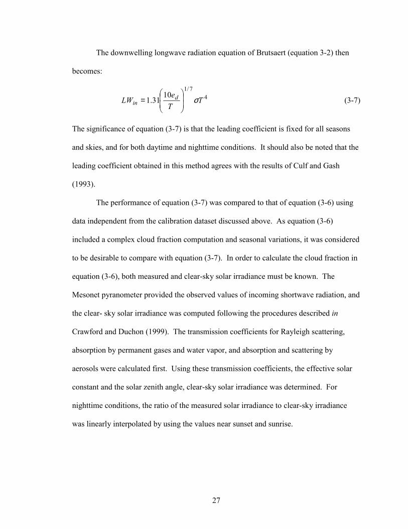
The downwelling longwave radiation equation of Brutsaert (equation 3-2) then
becomes:
47/1
1031.1 T
Te
LW din σ
��
�
�
��
�
�= (3-7)
The significance of equation (3-7) is that the leading coefficient is fixed for all seasons
and skies, and for both daytime and nighttime conditions. It should also be noted that the
leading coefficient obtained in this method agrees with the results of Culf and Gash
(1993).
The performance of equation (3-7) was compared to that of equation (3-6) using
data independent from the calibration dataset discussed above. As equation (3-6)
included a complex cloud fraction computation and seasonal variations, it was considered
to be desirable to compare with equation (3-7). In order to calculate the cloud fraction in
equation (3-6), both measured and clear-sky solar irradiance must be known. The
Mesonet pyranometer provided the observed values of incoming shortwave radiation, and
the clear- sky solar irradiance was computed following the procedures described in
Crawford and Duchon (1999). The transmission coefficients for Rayleigh scattering,
absorption by permanent gases and water vapor, and absorption and scattering by
aerosols were calculated first. Using these transmission coefficients, the effective solar
constant and the solar zenith angle, clear-sky solar irradiance was determined. For
nighttime conditions, the ratio of the measured solar irradiance to clear-sky irradiance
was linearly interpolated by using the values near sunset and sunrise.
28
Results and Discussion
Validation of calibrated model
The performance of equation (3-7) was validated using an independent dataset
obtained from five OASIS sites (BESS, BURN, MARE, NORM and STIG) for a one-
year period (June, 1999 through May, 2000). Figures (3-2a-e) are equal-value plots
illustrating the comparison for these sites over the one-year period. Figure 3-3 compares
the time series of observed and modeled (equation 3-7) downwelling longwave radiation
for the BURN site over the one-year period; time series plots for the other sites are very
similar as shown in Appendix B. It can be seen that the model performed well over an
extended period of time. As shown in Table 3-4, the MBE ranged between –3.95 and
4.24 Wm-2, and the RMSE was approximately 20 Wm-2 in all five cases. The sites that
were used for this validation represent different regions of the state and fall under
different climatic regimes. The predictions using equation (3-7) consistently agreed well
with the measurements, suggesting that the scheme could be used for any site in this
region and for any season of the year.
Comparison of calibrated model with cloud-fraction longwave model
Equation (3-7) compared very favorably with equation (3-6), as shown in Table 3-
5. The values of both MBE and RMSE were comparable for the two models. It is
important to note that this model comparison was carried out for a limited period of time
(85 days) from June 1 through August 25, 1999 in equation (3-6) and equation (3-7). The
four sites used were those with data available beginning on June 1. By using a summer
time period for the comparison, the number of nighttime hours is reduced and the

29
Figure 3-2a. Comparison of hourly observed and predicted downwelling longwave radiation for the BESS site.

30
Figure 3-2b. Comparison of hourly observed and predicted downwelling longwave radiation for the BURN site.

31
Figure 3-2c. Comparison of hourly observed and predicted downwelling longwave radiation for the MARE site.

32
Figure 3-2d. Comparison of hourly observed and predicted downwelling longwave radiation for the NORM site.

33
Figure 3-2e. Comparison of hourly observed and predicted downwelling longwave radiation for the STIG site.

34
Figure 3-3. Comparison of hourly observed and predicted downwelling longwave radiation for the BURN site.

35
Table 3-4. Validation of equation (3-7) using hourly data for June 1, 1999 though May 31, 2000.
Table 3-5. Comparison of equations (3-6) and (3-7) to hourly observed data for June 1 though August 25, 1999.

36
uncertainties in interpolating the cloud factor in equation (3-6) should be minimized. The
linear interpolation scheme was used between 18:00 and 7:00 CDT.
Even though equation (3-7) uses only temperature and vapor pressure as inputs,
and does not require solar irradiance or "cloudiness" data, it predicts downwelling
longwave radiation nearly as accurately as the more complex estimation method. The
RMSE using equation (3-7) was approximately 25 W m-2 for the four sites in Table 3-5.
The MBE was about 10 W m-2 and the mean percent error was about 5 percent and very
close to the predictions by equation (3-6).
Based on these results from Oklahoma, it appears that the downwelling longwave
radiation estimated by equation (3-7) is accurate enough to be used as the input for land
surface models. This relatively simple equation performed well at a variety of sites and
under both daytime and nighttime conditions. The mean absolute errors of approximately
20 W m-2 are less than 10% of measured downwelling longwave radiation, and rather
insignificant compared to total surface radiation forcing.
Summary
A modified form of Brutsaert's (1975) equation has been developed to estimate
downwelling longwave radiation for input to land surface models. The equation requires
near-surface measurements of temperature and vapor pressure, and can be used under all
sky conditions (day and night; clear and cloudy). The results show good agreement with
measured data from several Oklahoma sites. It also compared very well with a more
complex estimation method. The expression can be used reliably for climatologically
similar locations where measurements of downwelling longwave radiation are not
available.

37
CHAPTER 4
VALIDATION OF THE NOAH-OSU LAND SURFACE MODEL USING SURFACE FLUX MEASUREMENTS IN OKLAHOMA
Abstract
Oklahoma Atmospheric Surface-layer Instrumentation System (OASIS)
measurements of net radiation (Rn), latent heat flux (LH), sensible heat flux (SH) and
ground heat flux (GH) were used to validate the NOAH-OSU LSM (NOAH-Oregon State
University Land Surface Model). A one-year study period was used. Rn, LH, SH and
GH data from seven sites were screened based on an energy balance closure criterion
(daily/hourly sum of the flux components within the range of –10 W m-2 to +10 W m-2).
The vegetation fraction used in the model was computed using both the Gutman-Ignatov
(G-I) and the Carlson-Ripley (C-R) schemes. The simulated surface energy balance
components were found to be sensitive to the choice of vegetation scheme, however the
G-I approach was used for the validation study as it is widely used and linear in its form.
The daily aggregated model outputs showed that the predicted Rn had a positive bias of
0.8 MJ m-2 d-1 and an RMSE of 1.6 MJ m-2 d-1 when averaged over all seven sites. The
seven-site average bias in LH was about 0.9 MJ m-2 d-1 with an RMSE of 2.5 MJ m-2 d-1.
The bias in SH and GH was low and positive with an RMSE of about 2.2 MJ m-2 d-1 in
SH estimation. The hourly average output showed similar results, with the exception that
GH had a negative bias. The overall performance of the NOAH-OSU LSM was good for
a diverse set of Oklahoma conditions.
38
Introduction
A strong coupling exists between land surface hydrologic processes and climate.
Energy and water exchanges occur continuously at the interface between land surfaces
and the lower atmosphere. The energy and water balances are linked by the conversion
of thermal and radiative energy to latent heat. Realistic modeling of the processes of
land-atmosphere interaction over a large area is being advanced by the realization that it
should be addressed from both hydrologic and atmospheric science perspectives.
Modeling of land surface processes plays an important role, not only in large-scale
atmospheric models including general circulation models (GCMs), but also in regional
and mesoscale atmospheric models (Mintz, 1981; Rowntree, 1983; Avissar and Pielke,
1989; Chen and Dudhia, 2001).
It is understood that the atmospheric and soil – vegetation systems are
dynamically coupled through the physical processes which produce transport of thermal
energy and water mass across the land surface (Eagleson, 1978; Entekhabi, 1996). Many
studies have demonstrated the interaction between the atmosphere and the land surface
and the significant role played by soil moisture in regional weather predictions (e.g., Yan
and Anthes, 1988; Pielke, 1989; Avissar, 1992; Hipps et al., 1994; Chen and Brutsaert,
1995; Betts et al., 1996; Chen et al., 1996; Entekhabi et al., 1996; Henderson-Sellers,
1996; Betts et al., 1997; Sellers et al., 1997; Braud, 1998; Robock et al., 1998; Dirmeyer,
1999; Fennessy and Shukla, 1999; Silberstein et al., 1999; Dirmeyer et al., 2000).
Recently, Rodriguez-Iturbe (2000) asserted that “the interplay between climate, soil and
vegetation cannot be one of general and universal characteristics”. The near-surface
processes that include evapotranspiration and evaporation from bare soil and wet
vegetation contribute to the surface energy partition and subsequent evolution of the
39
convective boundary layer (CBL). Studies that analyzed the feedback mechanism
between precipitation and evaporation include Mintz (1984), Benjamin and Carlson
(1986), Lanicci et al. (1987), Oglesby (1991) and Betts et al. (1996). Generally they
suggested that more surface evaporation leads to more precipitation, causing greater
persistence of wet and dry spells. As Eagleson (1986) suggested, the issue of global scale
hydrology has reoriented the attention of hydrologists in considering the atmosphere and
the land surface as an interactively coupled system. Physically based modeling is an
important tool for studying the coupled system.
The purpose of this part of the present study was to validate the extended Oregon
State University Land Surface Model (hereafter referred to as “NOAH-OSU LSM” or
“NOAH LSM”), using surface flux measurements available from various sites in
Oklahoma. This model has been coupled to the NCEP operational Eta and PSU/MM5
mesoscale models (Marshall, 1998; Chen and Dudhia, 2001) and is in wide use by the
land surface research community. It is important to quantify model accuracy using
measured data. This investigation was supported by the availability of unparalleled
spatially distributed data from the Oklahoma Mesonet (Brock et al., 1995; Elliott et al.,
1994), the Oklahoma Atmospheric Surface-layer Instrumentation System (OASIS)
project (Brotzge et al., 1999) and extensive soil and landuse databases. These unique
data provide an incentive for using a study area such as Oklahoma to carry out this
validation task.

40
Model Description
Overview
Pan and Mahrt (1987) developed the original LSM that is the focus of this study.
Chen et al. (1996) modified the model to incorporate an explicit canopy resistance
formulation used by Jacquemin and Noilhan (1990). Originally, the LSM incorporated
the diurnally-dependent Penman potential evaporation approach of Mahrt and Ek (1984),
the multi-layer soil model of Mahrt and Pan (1984) and the primitive canopy model of
Pan and Mahrt (1987). Later the NCEP/Office of Hydrology extended the improvements
by including: (1) a fairly complex canopy resistance approach; (2) the bare soil
evaporation approach of Noilhan and Planton (1989); (3) the surface runoff scheme of
Schaake et al. (1996); (4) a higher-order time integration scheme by Kalnay and
Kanamitsu (1988); and (5) refinements to the snowmelt algorithm and the treatment of
soil thermal and hydraulic properties.
The LSM has one canopy layer and four soil layers with thicknesses of 0.1, 0.3,
0.6 and 1.0 m (total soil depth of 2 m) from the ground surface to the bottom,
respectively. The four-level soil layer configuration is adopted in the LSM for capturing
the daily, weekly and seasonal evolution of soil moisture and mitigating the possible
truncation error in discretization. The lower 1 m acts as a reservoir with gravity drainage
at the bottom, and the upper 1 m of soil serves as the root zone depth. From the
standpoint of model input, the LSM requires soil and vegetation types and meteorological
forcing variables (as the model is used here in an uncoupled fashion). Prognostic
variables include soil moisture and temperature in the soil layers, water intercepted on the
41
canopy and snow accumulated on the ground. Model simulations also provide estimates
of surface energy balance components (net radiation and latent, sensible, and ground heat
fluxes).
Soil Hydrology
The prognostic equation for the volumetric soil water content (θ) in the hydrology
model is given by:
θθθ F
zK
zD
zt+
∂∂+�
�
���
�
∂∂
∂∂=
∂∂ (4-1)
where D and K are the soil water diffusivity (m2 s-1) and hydraulic conductivity (m s-1),
respectively, and both are functions of θ ; t and z are time (s) and the vertical distance
(m) from the soil surface downward (i.e., the depth), respectively; and Fθ represents
sources and sinks (i.e., precipitation, evaporation and runoff). This diffusive form of the
relationship is known as Richard’s equation and is derived from Darcy’s Law for
movement of water in soils (with the assumption of a rigid, isotropic, homogeneous, and
one dimensional vertical flow domain) (Hanks and Ashcroft, 1986). K and D are highly
non-linear functions of soil moisture and in particular when the soil is dry, they can
change several orders of magnitude for a small variation in soil moisture. As the soil-
related parameterization is very sensitive to the diurnal partitioning of surface energy into
latent and sensible heat (Cuenca et al., 1996), Chen and Dudhia (2001) suggested the
investigation of alternative soil hydraulic parameterization schemes that would reflect the
relationship between hydraulic conductivity and soil water content.
Surface runoff is addressed in the LSM using the Simple Water Balance (SWB)
model approach given by Schaake et al. (1996). The SWB model is a two-reservoir
42
hydrological model that has been well calibrated for large river basins. It takes into
account the spatial heterogeneity of rainfall, soil moisture, and runoff. The total
evaporation is the sum of the direct evaporation from the top shallow soil layer,
evaporation of precipitation intercepted by the canopy, and transpiration through the
canopy via water uptake by roots. The bare soil evaporation scheme is governed by soil
wilting point and field capacity, green vegetation fraction cover, and a Penman-based
energy balance approach for potential evaporation. Evaporation of rainfall intercepted by
the canopy is a function of the canopy intercepted water content, which depends upon the
total precipitation and the precipitation that reaches the ground. The canopy transpiration
is determined by:
��
�
�
��
�
���
�
�−=n
ScW
cBpEftE 1σ (4-2)
where Et is canopy transpiration (m s-1), σf is the green vegetation fraction
(dimensionless), Ep is potential evaporation (m s-1), Wc is the canopy intercepted water
content (mm), S is the maximum allowed value for Wc (specified here as 0.5 mm), and n
= 0.5 (dimensionless). Bc is a function of canopy resistance and is expressed as:
rhc
rc
RCR
RB∆++
∆+=
1
1 (4-3)
where Ch is the surface exchange coefficient for heat and moisture (m s-1), ∆ is the slope
of the saturation-specific humidity curve (dimensionless), Rr is a function of surface air
temperature, surface pressure and Ch (dimensionless), and Rc is the canopy resistance (s
43
m-1). Details on Ch, Rr and ∆ are given by Ek and Mahrt (1991) and Rc is discussed by
Jacquemin and Noilhan (1990).
Soil Thermodynamics
One of the primary functions of the coupled land surface model is to provide the
near-surface layer of an atmospheric model with sensible and latent heat fluxes, and
surface skin temperature to compute upward longwave radiation. The surface skin
temperature is determined following Mahrt and Ek (1984) by applying a single linearized
surface energy balance equation, given by:
aahp
nskin T
UCCGER
T +−−
=ρ
λ (4-4)
where Rn is the net radiation (W m-2), λE is the latent heat flux (W m-2), G is the ground
heat flux (W m-2), ρ is the air density (Kg m-3), Cp is the air heat capacity (J m-3 K-1), Ch
is the surface exchange coefficient for heat and moisture (dimensionless), Ua is the
surface layer wind speed (m s-1), and Ta is the near-surface air temperature (K). Equation
(4-4) is the surface energy balance expression, with the sensible heat flux (H) term
expanded such that the relationship can be expressed in terms of Tskin. As the skin is
treated as an infinitesimally thin layer, and has no thermal inertia (heat capacity) of its
own, the skin temperature may be very sensitive to forcing (especially radiation) errors.
This expression has to be solved iteratively due to the implicit relationship, as some of
the terms on the right hand side of the equation also contain skin temperature. The
ground heat flux is governed by the diffusion equation for soil temperature (T):
( ) ( ) ��
���
�
∂∂
∂∂=
∂∂
zTK
ztTC t θθ (4-5)
44
where C is the volumetric heat capacity (J m-3 K-1) and Kt is the thermal conductivity (W
m-1 K-1), and both are functions of θ ; θ is fraction of unit soil volume occupied by water;
and t and z are time (s) and the vertical distance (m) from the soil surface downward (i.e.,
the depth), respectively. The Kt relationship used in the LSM, as suggested by
McCumber and Pielke (1981), has been used in many land surface models (e.g., Noilhan
and Planton, 1989; Viterbo and Beljaars, 1995). However, Peters-Lidard et al. (1998)
showed that this approach tends to overestimate (underestimate) Kt during wet (dry)
periods, and the surface heat fluxes are sensitive to the treatment of thermal conductivity.
In the LSM, Kt is capped at 1.9 W m-1 K-1. Chen and Dudhia (2001) suggested that
several thermal conductivity formulations are needed to arrive at the best approach.
Expanding equation (4-5) for the ith soil layer yields:
ii z
tz
ti
ii zTK
zTK
tT
Cz ��
���
�
∂∂−�
�
���
�
∂∂=
∂∂
∆+1
(4-6)
where ∆zi is the thickness (m) of the i-th soil layer. The prediction of Ti is performed
using the fully implicit Crank-Nicholson scheme. In the top layer the last term in
equation (4-6) represents the surface ground heat flux and is computed using the surface
skin temperature. The gradient at the lower boundary, assumed to be 3 m below the
ground surface, is computed from a specified constant boundary temperature and is taken
as the mean annual near-surface air temperature.
Previous studies using the LSM
Comparing against five months of the First International Satellite Land Surface
Climatology Project (ISLSCP) Field Experiment (FIFE) observations, the performance of
the modified LSM was superior to that of the simple bucket and fairly complex
45
Simplified Simple Biosphere (SSiB) models (Chen et al., 1996; Chen and Mitchell,
1999). The NOAH-LSM simulated the long-term observed diurnal variation of sensible
heat fluxes and surface skin temperature very well, and captured the diurnal and seasonal
evolution in evaporation and soil moisture. The NCEP implemented this NOAH-LSM in
its operational Eta model in February 1996 under the support of the NOAA GCIP
program (Marshall, 1998; Chen and Dudhia, 2001). Various studies (Betts et al., 1997;
Chen et al., 1997; Yucel et al., 1998) showed that “the coupled Eta/NOAH-OSU LSM
system indeed improved the short-range prediction of surface heat fluxes, near-surface
sensible variables, boundary layer and precipitation” (Chen and Dudhia, 2001). Marshall
(1998) studied the performance of this LSM in an uncoupled mode for Oklahoma
conditions and found that the model overestimated net radiation and underestimated
ground heat flux. He further suggested that the excess available energy resulted in an
inappropriate estimation of latent and sensible heat flux. Marshall’s (1998) study was
limited to one site, and latent and sensible heat fluxes were estimated using Bowen ratio
and aerodynamic approaches. As this NOAH-LSM is relatively simple (based on number
of parameters), efficient (simulates with adequate accuracy) and similar to the LSM used
in the NCEP’s operational global and regional models, it has been implemented in the
MM5 model (Chen and Dudhia, 2001).
Field Instrumentation and Data
Mesonet
The Oklahoma Mesonet (Elliott et al., 1994; Brock et al., 1995), a dense network
of 114 automated measurement stations across Oklahoma, provided the forcing data that
were used in this investigation. Each Mesonet station measures a number of
46
meteorological and hydrological variables. The Mesonet data used in this study were 5-
minute averages that were again averaged over one-hour intervals. The variables used
were air temperature (K), specific humidity (Kg Kg-1), wind speed (m s-1), pressure (Pa),
precipitation (kg m-2 s-1) and solar radiation (W m-2). It should be noted that air
temperature in degree K and specific humidity were derived quantities using the original
Mesonet variables. Other data used for initial conditions were soil temperature (K) at 5
cm, 25 cm, and 60 cm and the two-year average of 1.5 m air temperature (K) for
estimating soil temperature at 3 m. The scheme as shown in Chapter 3 was used for
estimating downwelling longwave radiation. The scheme uses near-surface vapor
pressure and air temperature data. The soil data for all the sites were also available from
the Mesonet.
OASIS
The Oklahoma Mesonet also provides the platform for the Oklahoma
Atmospheric Surface-layer Instrumentation System (OASIS) project (Brotzge et al.,
1999; Brotzge, 2000). Instruments have been added at approximately 90 Mesonet
stations, enabling routine surface energy budget measurements. These measurements
include net radiation (Rn), sensible heat flux (SH) and ground heat flux (GH). Latent heat
flux (LH) is estimated as the residual of the energy balance. Also, 10 of the 90
“Standard” sites are designated as “Super” sites and they have additional instrumentation
to verify the simpler standard instrumentation. The OASIS data used in this study were
from seven Super sites and included 5-minute averages of Rn, LH, SH and GH. Hourly
averages were then computed. These data spanned a one-year period from 1 June 1999
47
through 31 May 2000. The locations of the seven sites are shown in Figure 4-1 and the
soil and vegetation types are given in Table 4-1.
At each Super site a Kipp & Zonen CNR1 four-component net radiometer is used
to measure incoming and outgoing shortwave and longwave radiation. The design of the
CNR1 includes an upward-facing, ISO-class, thermopile pyranometer and pyrgeometer,
and a complementary downward-facing pyranometer and pyrgeometer in an integrated
fashion. The body of the CNR1 houses a PT-100 RTD temperature sensor for measuring
the instrument body temperature precisely. During manufacturing, the sensitivity of all
four sensors is trimmed and calibrated to a single identical sensitivity coefficient.
The latent and sensible heat flux measurements are done using a sonic
anemometer and Krypton KH20 hygrometer. The Campbell Scientific CSAT3 sonic
anemometer is mounted at the OASIS sites to measure wind speed and air temperature
using sound wave (sonic) theory. By measuring the speed of sound between two points,
the fluctuations of wind and temperature can be calculated. The sonic anemometer itself
measures an average u (east-west), w (north-south), and v (vertical) wind speed and mean
temperature (T) at a frequency of 8 Hz (8 times per second). Covariances of v and T are
calculated within the datalogger program and then used to obtain 5-minute means of
sensible heat flux. The Krypton hygrometer is mounted within 10 cm of the sonic
anemometer and the amount of absorption of Krypton between two points is proportional
to the specific humidity (q) of the air. The covariance of v and q is used to compute
latent heat flux.
Two REBS HFT3.1 heat flux plates are buried 5 cm below the soil surface at each
OASIS site. The plates have a horizontal separation of 1 m. Each plate has been

48
Figure 4-1. Location of Oklahoma Atmospheric Surface-layer Instrumentation System (OASIS) sites used in this study.

49
Table 4-1. OASIS sites’ soil and vegetation types.
50
individually calibrated. Two REBS Platinum Resistance Temperature Detectors
(PRTDs) are buried between 0 and 5 cm of the soil surface. A combination approach that
includes both ground heat flux (measured at 5 cm) and heat storage is used to estimate the
ground heat flux at the surface. Brotzge (2000) provided a detailed discussion of the
instrumentation at the OASIS sites including the quality of the data and source of errors
in the measurements.
Green Vegetation Fraction
Canopy conductance depends on leaf water potential (in addition to vapor
pressure deficit and temperature) and is a function of soil moisture potential and stress.
In addition to variables such as vegetation type, density, height, leaf area index, etc., the
unstressed or maximum canopy conductance is expected to vary as a function of canopy
greenness and incident photosynthetically active radiation (PAR). The green vegetation
fraction (fg) is defined as the fractional area of the vegetation occupying each grid-cell
wherein mid-day downward solar radiation is intercepted by photosynthetically active
green canopy. Vegetation indices derived from spectral reflectances seem to have a
linear relationship with the ratio of unstressed canopy conductance to incident flux of
PAR. That is, as the greenness of vegetation increases, the ratio of unstressed canopy
conductance to incident flux of PAR increases (Sellers et al., 1997).
Gutman and Ignatov (1998) suggested that evapotranspiration (also
photosynthesis) is controlled by green vegetation fraction and by green leaf area index.
The green vegetation fraction acts as a fundamental weighting coefficient in partitioning
the total evaporation into soil evaporation, evaporation of canopy intercepted
precipitation and transpiration in the LSM (Chen and Dudhia, 2001). Gutman and
51
Ignatov (1998) derived an expression for green vegetation fraction using the Normalized
Difference Vegetation Index (NDVI) as
( )
( )minmax
minNDVINDVI
NDVINDVIf g −−
= (4-7)
In equation (4-7) bare soil NDVI (NDVImin) and dense vegetation NDVI (NDVImax) are
prescribed as 0.04 and 0.52 respectively and they correspond to seasonally and
geographically invariant constants for desert and evergreen clusters.
Carlson and Ripley (1997) defined a scaled NDVI (N*) and derived a similar
expression for N* as
( )( )os
oNDVINDVINDVINDVI
N−−
=* (4-8)
where NDVIo and NDVIs correspond to the values of NDVI for bare soil (LAI=0) and a
surface with a fractional green vegetation cover of 100%, respectively. They also
suggested adopting a value of full-cover NDVI about 0.05 below the largest values of
NDVI in the image. Choudhury et al. (1994) and Gillies and Carlson (1995)
independently obtained an identical square root relation between N* and green vegetation
fraction, fg as,
2*gf N≈ (4-9)
In equation (4-8) the selection of a bare soil value of NDVI results in some uncertainty.
The values of fg obtained using equations (4-7) and (4-9) differ because of the form of the
equations and also the assumed upper and lower bounds on NDVI. Because fg serves as a
weighting coefficient for the partitioning of canopy evaporation and bare soil
evaporation, the effect of these alternative formulations was evaluated. Each value of
NDVI was obtained from Advanced Very High Resolution Radiometer (AVHRR)

52
satellite images and represented the 1 km pixel area that included the OASIS site. The
temporal variation in fg for two of the study sites is shown in Figure 4-2, and the
difference between the two schemes is apparent. When necessary, fg was truncated at a
value of 1.0. The model sensitivity to the fg derived based on these two different
formulations is discussed in the subsequent section.
Results and Discussion
Sensitivity to Green Vegetation Fraction
Prior to the validation analysis, the sensitivity of the model to each of the
Gutman-Ignatov (G-I) and Carlson-Ripley (C-R) green vegetation fraction schemes was
tested. The simulated surface energy balance components (i.e., net radiation (Rn), latent
heat flux (LH), sensible heat flux (SH) and ground heat flux (GH)) using G-I and C-R
green vegetation fractions were compared for four of the OASIS sites (BOIS, BURN,
MARE and NORM). The results are shown only for BOIS and BURN (Figures 4-3 – 4-
6) because the other two sites showed similar results. The short grass at BOIS has less
dense cover and the corresponding peak green vegetation fraction reaches only 0.64 in
the G-I scheme whereas it reaches the maximum of 1.0 for a summer month in the C-R
scheme. For both BOIS and BURN (warm season grass), the green vegetation fraction
by the C-R scheme was higher than that by the G-I scheme.
The simulated Rn using G-I and C-R green vegetation fraction for BOIS and
BURN showed a slight positive bias towards the C-R method as observed from the equal-
value plots shown in Figure 4-3. This indicated that the Rn was insensitive to the two
green vegetation fraction schemes. Figure 4-4 shows that the estimated LH for BOIS and
BURN had a similar positive bias for the C-R method. Model results for SH (Figure 4-5)

53
Figure 4-2. Green vegetation fraction as derived by the Gutman-Ignatov (G-I) and Carlson-Ripley (C-R) schemes for BOIS and BURN

54
Figure 4-3. Sensitivity of the modeled net radiation using G-I and C-R green vegetation fraction methods.
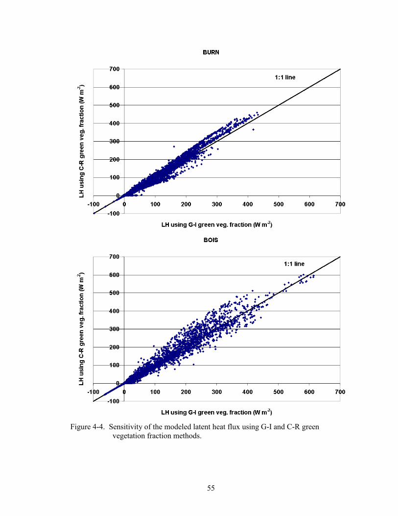
55
Figure 4-4. Sensitivity of the modeled latent heat flux using G-I and C-R green vegetation fraction methods.
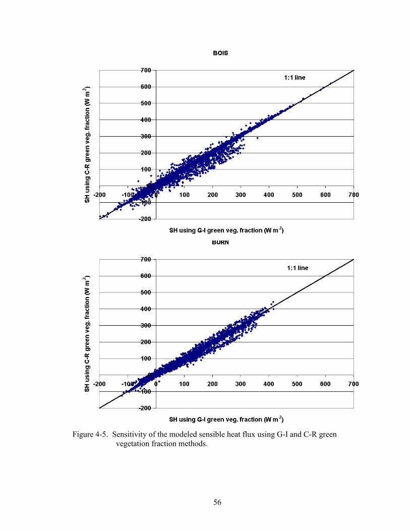
56
Figure 4-5. Sensitivity of the modeled sensible heat flux using G-I and C-R green vegetation fraction methods.

57
Figure 4-6. Sensitivity of the modeled ground heat flux using G-I and C-R green
vegetation fraction methods.
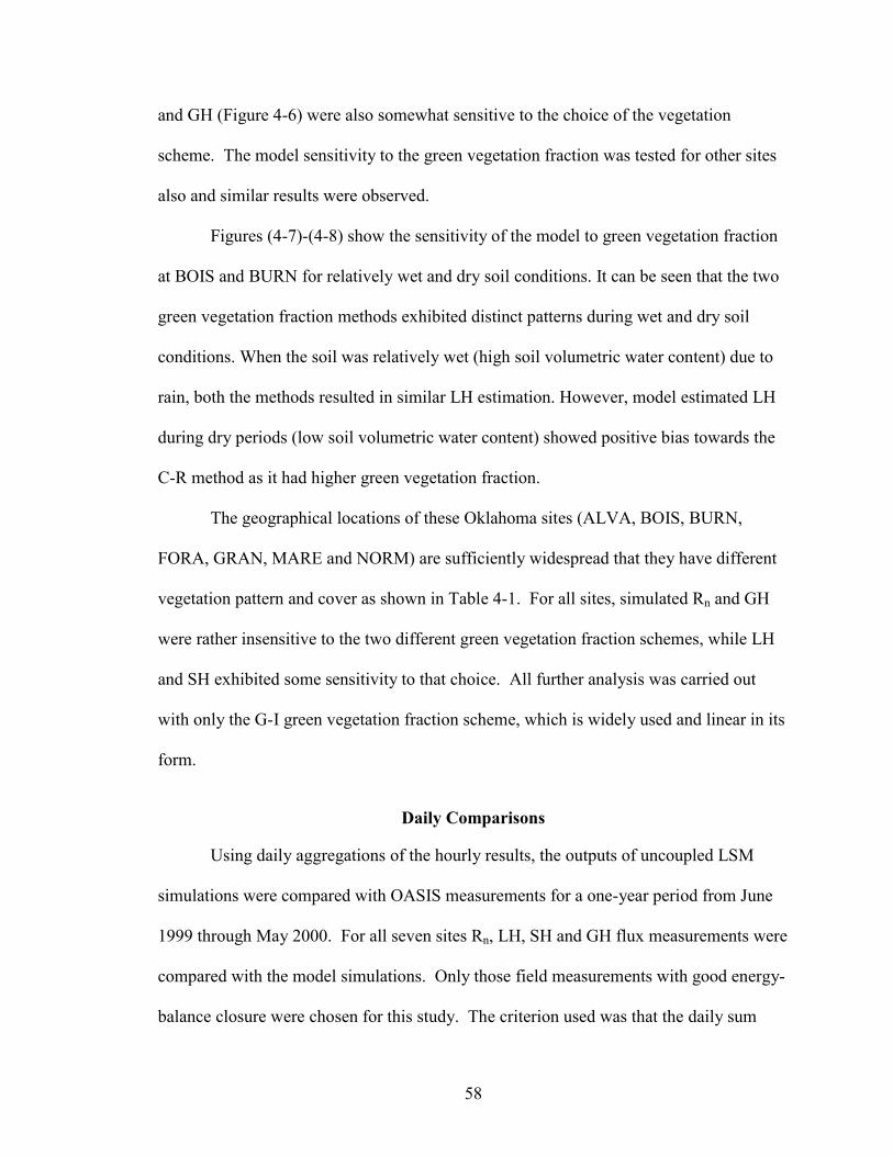
58
and GH (Figure 4-6) were also somewhat sensitive to the choice of the vegetation
scheme. The model sensitivity to the green vegetation fraction was tested for other sites
also and similar results were observed.
Figures (4-7)-(4-8) show the sensitivity of the model to green vegetation fraction
at BOIS and BURN for relatively wet and dry soil conditions. It can be seen that the two
green vegetation fraction methods exhibited distinct patterns during wet and dry soil
conditions. When the soil was relatively wet (high soil volumetric water content) due to
rain, both the methods resulted in similar LH estimation. However, model estimated LH
during dry periods (low soil volumetric water content) showed positive bias towards the
C-R method as it had higher green vegetation fraction.
The geographical locations of these Oklahoma sites (ALVA, BOIS, BURN,
FORA, GRAN, MARE and NORM) are sufficiently widespread that they have different
vegetation pattern and cover as shown in Table 4-1. For all sites, simulated Rn and GH
were rather insensitive to the two different green vegetation fraction schemes, while LH
and SH exhibited some sensitivity to that choice. All further analysis was carried out
with only the G-I green vegetation fraction scheme, which is widely used and linear in its
form.
Daily Comparisons
Using daily aggregations of the hourly results, the outputs of uncoupled LSM
simulations were compared with OASIS measurements for a one-year period from June
1999 through May 2000. For all seven sites Rn, LH, SH and GH flux measurements were
compared with the model simulations. Only those field measurements with good energy-
balance closure were chosen for this study. The criterion used was that the daily sum

59
Figure 4-7. Sensitivity of the model to green vegetation fraction at BOIS for relatively wet and dry soil conditions (VWC1- Top soil layer volumetric water content; VWC2-Root zone volumetric water content).

60
Figure 4-8. Sensitivity of the model to green vegetation fraction at BURN for relatively wet and dry soil conditions (VWC1- Top soil layer volumetric water content; VWC2-Root zone volumetric water content).

61
(Rn-LH-SH-GH) was to be within the range of -10 W m-2 to +10 W m-2. This reduced the
number of records to a certain extent but the filtered data provided a more valid
comparison to model results. In other words, judgments of model accuracy should not be
based on measured data that are internally inconsistent.
Figures 4-9 – 4-12 compare daily average observed and modeled net radiation,
latent heat flux, sensible heat flux and ground heat flux for four of the sites (ALVA,
BOIS, BURN and NORM). Appendix C contains these equal-value plots for all seven of
the sites. One note of caution is that the time scale on the horizontal axis is not
continuous (due to the above-described filtering based on energy-balance closure).
Table 4-2a shows daily averaged Mean Bias Error (MBE) and Root Mean Square
Error (RMSE) for all seven study sites. There was a slight bias of about 0.8 MJ m-2 d-1 in
net radiation when averaged over all sites and an RMSE of about 1.6 MJ m-2 d-1 (Figure
4-9). NORM had the highest positive bias of about 3.4 MJ m-2 d-1 and GRAN had the
lowest negative bias of about –0.6 MJ m-2 d-1. These discrepancies in net radiation may
be partially due to the uncertainty in the downwelling longwave radiation estimation
procedure. ALVA, BOIS, BURN and MARE showed a slight overestimation of Rn,
especially during summer and spring months, and NORM showed a still higher
estimation (NORM had limited data). FORA and GRAN showed a slight
underestimation of Rn except during winter. It could be beneficial to investigate the LSM
physics for the partitioning of incoming radiant energy, and to examine the
parameterizations involving green vegetation fraction, rooting depth, albedo and
minimum stomatal resistance. The model structure with its current version could
accommodate only a single soil texture even though it has four soil layers in its

62
configuration. This could be an important factor when partitioning the energy as well as
mass balance components. The energy balance in the LSM is formulated in such a way
that excess net radiation is redistributed into latent, sensible and ground heat fluxes as
shown in the equation below.
GSHLHRn ++= (4-10)
Thus, predicting net radiation becomes crucial in order to accurately quantify the sensible
and latent heat fluxes.
The positive bias in daily LH (MBE of about 0.9 MJ m-2 d-1 when averaged over
seven sites) is shown in Table 4-2a. The average RMSE was approximately 2.5 MJ m-2
d-1. The time series plots of observed and modeled LH are shown in Figure 4-10. As
with Rn, it was observed that the LH for the NORM site was higher than for the other
sites. This could be again partially due to the limited number of days used in the
comparisons for NORM, and the fact that more of those days were during the summer
months (when other sites showed a high positive bias). As pointed out earlier, most of
the excess energy from the modeled Rn can be directed into LH and was seen at those
sites where Rn was overestimated such as ALVA, BOIS, BURN and MARE. This is
because the LSM first computed potential evaporation and then actual evaporation, which
was used to determine the skin temperature at equilibrium state, and subsequently SH
was computed. As the LSM computed LH first, it tended to distribute excess energy to
that term.
For SH, the seven-site average of MBE showed that the model had a negative bias
of about –0.3 MJ m-2 d-1 and the average RMSE was about 2.2 MJ m-2 d-1 (Table 4-2b).
The magnitude of the site-by-site bias in SH estimation was smaller than that for Rn and

63
LH, as shown in Table 4-2a,b. The time series plots as shown in Figure 4-11 gave ample
indication that SH estimations tended to be the complement of LH simulations (meaning
the available energy is partitioned into LH and SH depending on the surface vegetation
and other parameterizations). The positive bias in daily averaged GH for all but FORA
and NORM was also relatively low, i.e., about 0.2 MJ m-2 d-1. The overall RMSE was
about 0.7 MJ m-2 d-1 (Figure 4-12). Betts et al. (1997) and Marshall (1998) suggested that
the GH estimations were sensitive to model errors in Rn computation. The mean absolute
errors (MAE) for LH and SH each tended to be greater than that for Rn.
Hourly Comparisons
The performance of the LSM was also analyzed using hourly data (Table 4-3a,b).
The graphic representation of the hourly results for FORA, GRAN and MARE is shown
in Figures 4-13 – 4-16. Appendix C (Figures (C-8) – (C14)) shows for each of the seven
sites, the equal-value plots for all four energy-balance components. As in the daily data
analysis, field data with good hourly energy-balance closure were chosen with the
criterion that the hourly sum (Rn-LH-SH-GH) was within the range of -10 W m-2 to +10
W m-2. As this criterion was applied to both daily and hourly data sets separately, it
should be remembered that this resulted in different data sets (i.e., not all hourly data that
met the criterion were from days that met the daily criterion). The net radiation plots in
Figure 4-13 suggested that model hourly estimates were not biased significantly. The
hourly average of Rn for BOIS had a high negative bias of about –9 W m-2 while NORM
showed a high positive bias of about 22 W m-2. The average of all seven sites’ hourly
averaged net radiation showed a very low positive bias of about 1.4 W m-2 and an RMSE
of approximately 60 W m-2. Given the fact that the simulation was carried out for a one-

64
Table 4-2 (a). Statistics of daily averaged Net Radiation (Rn) and Latent Heat (LH) flux for June ’99 – May ’00.

65
Table 4-2 (b). Statistics of daily averaged Sensible Heat (SH) and Ground Heat (GH) flux for June ’99 – May ’00.

66
Figure 4-9. Comparison of daily average observed and modeled net radiation.

67
Figure 4-10. Comparison of daily average observed and modeled latent heat flux.

68
Figure 4-11. Comparison of daily average observed and modeled sensible heat flux.

69
Figure 4-12. Comparison of daily average observed and modeled ground heat flux.

70
year period, including all seasons, an RMS error of about 60 W m-2 in Rn simulation is
relatively insignificant. The site bias for hourly LH ranged from – 3 to 22 W m-2 and
RMSE ranged between 16 and 52 W m-2 (Figure 4-14). NORM showed a high positive
bias of 22 W m-2 and BOIS had the least positive bias of 1.1 W m-2. FORA and GRAN
had a negative bias of –3 W m-2 as shown in Table 4-3a.
Conversely, from Table 4-3b it can be seen that the model overestimated SH at
FORA and GRAN. The hourly averaged SH for all seven sites was –0.18 W m-2 with an
average RMSE of approximately 42 W m-2 (Figure 4-15). The range was about –11 to 12
W m-2 and 37 to 50 W m-2 for MBE and RMSE, respectively. ALVA results indicated a
high negative bias of –11 W m-2 and FORA had a high positive bias of about 13 W m-2.
The GH simulations showed that FORA had a high negative bias of about –12 W m-2 as
seen in Figure 4-16 and the average of all seven sites yielded a negative bias of 5 W m-2.
The average RMSE was 28 W m-2. This was low when compared with the bias and
RMSE of the other energy balance components. With the exception of GH, the trends in
the hourly and daily component estimates were observed to be very similar for all sites.
Analysis of the hourly energy-balance components provided results that were similar to
the daily analysis. That is, the “sink” terms of the energy budget (LH and SH) tended to
be predicted less accurately than the “source” terms (Rn and GH).
Summary and Conclusions
Modeling land surface processes plays an important role in understanding the
interaction between the land surface and the atmosphere. Energy and water balances at
the land surface should impact mesoscale, regional and general circulation models. There
have been persistent efforts to develop and refine physically based land surface models.

71
Table 4-3 (a). Statistics of hourly averaged Net Radiation (Rn) and Latent Heat (LH) flux for June ’99 – May ’00.

72
Table 4-3 (b). Statistics of hourly averaged Sensible Heat (SH) and Ground Heat (GH) flux for June ’99 – May ’00.

73
Figure 4-13. Comparison of hourly average observed and modeled net radiation.

74
Figure 4-14. Comparison of hourly average observed and modeled latent heat flux.

75
Figure 4-15. Comparison of hourly average observed and modeled sensible heat flux.

76
Figure 4-16. Comparison of hourly average observed and modeled ground heat flux.
77
Quantifying the accuracy of such models using long periods of measurements becomes
crucial.
The purpose of this study was to validate the NOAH-OSU Land Surface Model
using measurements from the Oklahoma Mesonet and the Oklahoma Atmospheric
Surface-layer Instrumentation System (OASIS) project. Through the work of others, the
original Oregon State University Land Surface Model (OSU LSM) was extended by
incorporating a complex canopy resistance approach along with other improvements.
This extended model is used in a coupled fashion with the NCEP Eta and PSU/MM5
operational mesoscale models.
The Oklahoma Mesonet, comprising a network of 114 automated weather
stations, provided the meteorological forcing data for this study. The OASIS project used
the Mesonet as its foundation and supported the development of 10 “Super” sites. These
Mesonet sites are equipped with additional instrumentation for measuring surface energy
components (Rn, LH, SH and GH). Seven Super sites were the focus of this validation
study. Hourly averages of Mesonet and OASIS data were compiled for the period 1 June
1999 though 31 May 2000. The field data set was filtered for good energy balance
closure using the criterion that the daily (hourly) sum (Rn-LH-SH-GH) was within the
range of –10 W m-2 to +10 W m-2.
In order to provide green vegetation fraction data for the LSM, the Gutman-
Ignatov (1998) and Carlson-Ripley (1997) schemes for computing green vegetation
fraction from observed NDVI data were studied. The two schemes estimated
significantly different green vegetation fractions, which translated into some sensitivity in

78
the estimates of LH and SH. The Gutman-Ignatov (1998) scheme was selected for the
remainder of the study as it is in wide use and linear in its form.
Validation of the NOAH – OSU LSM using OASIS surface energy measurements
from seven sites (ALVA, BOIS, BURN, FORA, GRAN, MARE and NORM) was carried
out for daily and hourly time intervals. Based on the daily average values, it was
observed that the model tended to slightly overestimate Rn with both the MBE and RMSE
at about 0.8 MJ m-2 d-1 and 1.6 MJ m-2 d-1, respectively. The seven-site daily average
bias in LH was 0.9 MJ m-2 d-1, with an RMSE of 2.5 MJ m-2 d-1. NORM had a relatively
high bias in both Rn and LH, perhaps due to a limited data set dominated by summer
days. Model estimates of SH had a slight negative bias with an RMSE of 2.2 MJ m-2 d-1.
The mean bias error in GH was low when compared with the estimation of the other
energy balance components. The mean absolute errors for LH and SH were observed to
be greater than those for Rn. The model distributes any excess Rn into latent, sensible and
ground heat fluxes. It was observed that excess energy was predominantly assigned to
LH as opposed to SH and this was due to the model computation of LH first and
subsequent estimation of SH in the formulation.
In the hourly analysis, it appeared that the model tended to slightly overestimate
Rn as the average MBE was about 1.4 W m-2 and the RMSE was 58 W m-2. The hourly
average LH showed a positive bias of about 5.6 W m-2 and an RMSE of 32 W m-2. Both
SH and GH showed a slight negative bias for most of the sites with an RMSE of 42 W m-
2 and 29 Wm-2, respectively. Thus the trends observed in hourly and daily estimates for
all the energy balance components were similar except for GH, which had a slight
positive bias for the daily analysis.

79
The overall performance of the NOAH-OSU LSM was observed to be reasonably
good when tested for Oklahoma conditions. As with any model, the user must judge the
accuracy based on the particular application. It could be beneficial to investigate
refinements to the model physics and vegetation parameterization (green vegetation
fraction, rooting depth, albedo and minimum stomatal resistance). Incorporating vertical
heterogeneity in soil texture as opposed to the use of single top layer soil texture in the
model might improve the partitioning of LH and SH. The estimated downwelling
longwave radiation is another potential source of model uncertainty.

80
CHAPTER 5
SCALING EFFECTS ON MODELED SURFACE ENERGY-BALANCE COMPONENTS USING THE NOAH-OSU LAND SURFACE MODEL
Abstract
Accurate modeling of the hydrologic processes that influence land-atmosphere
exchange phenomena is crucial for better weather prediction. This is widely recognized
as an issue to be addressed from both hydrological and atmospheric science perspectives.
As surface exchange processes are highly non-linear and heterogeneous in space and
time, it is important to know the appropriate scale for the reasonable prediction of them.
The study region was chosen from the Southern Great Plains 1997 (SGP97) Hydrology
Experiment. A statistical procedure was followed to select two cells, each 20 km x 20
km, representing the most homogeneous and the most heterogeneous surface conditions
(based on soil and vegetation), recognizing that these areas might not represent the
typical variability when considered at regional or continental scales. Three scales of study
(200 m, 2 km and 20 km) were considered in order to investigate the impacts of the
aggregation of input data on the model output. Simulations were performed using the
NOAH-OSU (Oregon State University) Land Surface Model (LSM). Green vegetation
fraction was computed from Normalized Difference Vegetation Index data using two
different approaches, but the model results were insensitive to this choice. Model results
of net radiation, latent, sensible and ground heat fluxes were compared for the three

81
scales. For the heterogeneous area, the model output at the 20-km resolution showed
some differences when compared with the 200-m and 2-km resolutions. This was more
pronounced in latent and sensible heat estimation than in net radiation and ground heat
flux estimation. The scaling effects were much less for the relatively homogeneous land
area. The results suggested that considering sub-grid scale heterogeneity can be important
for realistic modeling of surface exchange processes.
Introduction
Realistic modeling of land-atmosphere interaction over a large area is being
advanced by the realization that it should be addressed from both hydrological and
atmospheric science perspectives. It is understood that the atmospheric and soil-
vegetation systems are dynamically coupled through the physical processes which
produce transport of thermal energy and water mass across the land surface (Eagleson,
1978). The issue of global scale hydrology has reoriented the attention of hydrologists in
considering the atmosphere and the land surface as an interactively coupled system
(Eagleson, 1986).
The large-scale processes influencing the terrestrial water balance (e.g.,
infiltration and the partitioning of net radiation into sensible and latent heat fluxes and
soil heat flux), are highly non-linear and also heterogeneous both in space and time due to
the natural variability in soil, land use, vegetation and weather. Studies have shown that
the complex land-atmosphere models often contain overly simplified parameterization of
land surface hydrology, thereby resulting in inaccurate representation of the real situation
(Wood et al., 1992; Sivapalan and Woods, 1995). The issue of scale interaction has

82
emerged as one of the crucial problems for the parameterization of general circulation
models (GCMs) due to the strong interconnection between land and atmospheric
processes. In order to address this issue, the understanding of the scaling properties of
water and energy fluxes with their corresponding storage term (soil moisture) becomes
significant (Wood, 1994).
Many times, soil moisture and evapotranspiration are either assumed to have
lesser significance or are misrepresented, resulting in simplification of these processes in
large-scale hydrological studies. For instance, some land surface modelers fail to consider
soil moisture and its related processes within their models as physically based, and
instead parameterize it as an index to be used for evapotranspiration and runoff
calculations rather than representative of the actual mass of moisture in the soil (Robock
et al., 1998). Evapotranspiration and runoff may not be sufficiently dependent upon the
soil moisture even in the simple monthly water balance simulation of land surface models
(Koster and Milly, 1997). Hence when these results are linked to GCMs, the
corresponding model responses can be grossly inaccurate.
To date, understanding the effects of land surface heterogeneity at the sub-GCM
grid scale level is an unfinished task due to the associated challenges. Traditionally the
lumped model concept, where the spatially variable inputs and parameters are assumed to
be homogeneous, has been widely used even in many large-scale water balance studies.
But the accuracy of the model response is very much dominated by sub-grid scale
parameterizations of inputs and parameters (Avissar and Pielke, 1989; Famiglietti and
Wood, 1994; Wood, 1994; Hu and Islam, 1997). If the model is process based, and if the

83
resolution of the model grid is increased, some of these modeling problems can be
addressed successfully. This would probably be the most accurate approach but not
always practical due to limitations in computing as well as data availability (Avissar and
Pielke, 1989). However, with the advent of high-speed computers, the problem of
voluminous data handling and processing can be overcome whereas the number and
measurements is still a problem. Oklahoma offers the best chance to address the problem
as the Mesonet provides high-resolution weather data both spatially and temporally. As
part of the realistic modeling of spatially variable water and energy balance processes,
one needs to understand sub-grid scale heterogeneity and its impact on model results.
This study will provide some insight into the effects of parameterization of land
surface heterogeneity on the quantification of surface energy-balance components
(namely net radiation and latent, sensible and ground heat fluxes). This will be done at
various scales using a distributed modeling approach. The overall objective is to examine
the effects of different spatial scales of input data on modeled fluxes, and thereby better
understand the resolution needed for the realistic modeling of large-scale land-
atmosphere interaction.
Scaling concepts
The term scale refers to the characteristic length (or time) of a process,
observation or model. Models and theories developed in darcian scale (point scale) may
be applied to larger scale predictions. Similarly large-area models and data are used for
small-area predictions. This transfer of information across scales is called scaling and the
problems associated with it are scale issues (Bloschl and Sivapalan, 1995). DeCoursey

84
(1996) defines scaling as the transcending concepts that link processes at different levels
of space and time.
Typical hydrological modeling scales (Dooge, 1982, 1986) in space are: local
scale (1 m), hillslope (reach) scale (100 m), catchment scale (10 km) and regional scale
(1000 km). Typical hydrological time scales are: event scale (1 day), seasonal scale (1 yr)
and the long-term scale (100 yrs). There is additional terminology related to scaling such
as upscaling and downscaling. For example, if we consider the problem of estimating
catchment rainfall from one or more rain gauge(s), upscaling rainfall from a dm2 scale to
a km2 scale involves distributing the point precipitation over the catchment and then
aggregating the spatial distribution of rainfall into one single value. Conversely,
downscaling involves disaggregating and singling out (Bloschl and Sivapalan, 1995).
A major complication in parameter specification is the fact that these parameters
vary from point to point because of the spatial variability always present in nature. One of
the merits of distributed models usually claimed is that the parameters have some
physical relevance and hence they should be measurable in the field. Jensen and
Mantoglou (1992) believed that a theoretically justified model would provide more
confident predictions and therefore the incentive to use physically-based models would
increase in the future. On the other hand Meentemeyer (1989) states that: “much of the
cherished detail of the reductionist sciences may not be needed, and indeed cannot be
used, in broad scale modeling”. Another perspective is that a model that is suitable at a
plot scale cannot be used to simulate a region if the simulator does not represent all
relevant phenomena existing at the larger scale. For instance, scaling up of a soil-plant
85
model in space and time involves the incorporation of additional phenomena that are not
incorporated at the small scale (Luxmoore et al., 1991). This has been termed
phenomena-added modeling. Examples of such additional phenomena include
topographic effects in watersheds and successional processes of forest communities.
Representing soil-vegetation-atmosphere transfer (SVAT) at larger scales is
extremely difficult due to the problems of spatial heterogeneity. Thus the question of
extrapolation of non-linear hydrological processes to large scales remains largely
unanswered. As scaling embodies such concepts as process descriptions, cartographic
considerations or pattern analysis, and spatial and temporal variability, simple integration
or aggregation of values at one level to achieve estimates at a more encompassing level
of consideration may not be acceptable (DeCoursey, 1996). Dooge (1986) observes:
To predict catchment behavior reliably we must either solve extremely complex physically based models which take full account of the spatial variability of various parameters or else derive realistic models on the catchment scale in which the global effect of these spatially variable properties is parameterized in some way. The former approach requires extremely sophisticated models and exceedingly expensive computers to have any hope of success. The latter approach requires the discovery of hydrologic laws at the catchment scale that represent more than mere data fitting.
A phenomenon termed ‘coarse-graining in hydrological observations’ occurs with
the transformation of a nonstationary hydrological process at a finer scale to a stationary
hydrologic process at a larger scale (Kavvas, 1999). With the loss of some information,
however, Kavvas (1999) stated that a simple expression that includes sub-grid scale
heterogeneity for large scales could be used successfully. Various studies have shown
that upscaled hydrologic equations preserve heterogeneity at field scales (Chen et al.,
86
1994a, 1994b; Kavvas and Karakas, 1996) and thus can be applied successfully for
regional scale land surface simulations (Kavvas et al., 1998).
While studies in the last few years have been consistently aimed at narrowing the
gap in the understanding of land-atmosphere interactions, Wood’s (1991) statement is
still valid:
The inadequate representation (of land-atmospheric interactions) reflects the recognition that the well-known physical relationships, which are well described at small scales, result in different relationships when represented at the scales used in climate models. Understanding this transition in the mathematical relationships with increased space-time scales appears to be very difficult, and has led to different approaches; at one extreme, the famous ‘bucket’ model where the land-surface is a simple one layer storage without vegetation; the other extreme may be Seller’s Simple Biosphere Model (SiB) where one big leaf covers the climate model grid.
Land surface model
There are several land surface models that are being used to simulate the
hydrologic processes governing biosphere-atmosphere interrelationships. Each of them
has distinct features with respect to model physics, parameters (including distributed or
lumped), time step, extent of testing and validation, and number of users. This study used
the NOAH- OSU (Oregon State University) Land Surface Model (LSM), which has been
widely recognized by the land-surface research community and which is coupled to the
NCEP operational Eta and PSU/MM5 mesoscale models. The LSM simulation of
seasonal and diurnal variation in evaporation, soil moisture, sensible heat flux and surface
skin temperature agrees well with field observations and its performance appears to be
better than many land surface models (Chen et al., 1996). Various studies (Betts et al.,
1997; Chen et al., 1997; Yucel et al., 1998, Chen and Dudhia, 2001) showed that the
coupled Eta/OSULSM system indeed improved the short-range prediction of surface heat

87
fluxes, near-surface sensible variables, planetary boundary layer and precipitation.
Marshall (1998) studied the performance of this LSM in an uncoupled mode for
Oklahoma conditions and found that the model overestimated net radiation and
underestimated ground heat flux and the study was limited to one site, and latent and
sensible heat fluxes were estimated using Bowen ratio and aerodynamic approaches.
Validation study of this LSM using Oklahoma Atmospheric Surface-layer
Instrumentation System (OASIS) measurements is in Chapter 4.
The energy balance in the model is formulated as shown in equation (5-1). Net
radiation (as the “source” term in the energy balance) is directed into latent, sensible and
ground heat fluxes:
GHSHLHRn ++= (5-1)
Each of these surface energy-balance components is computed using physically-based
formulations. A more detailed description of the model can be found in Chen and Dudhia
(2001).
Study area and data
Study area description
This research utilized the study area for the Southern Great Plains 1997 (SGP97)
Hydrology Experiment. SGP97 focused on the central section of Oklahoma from
Comanche and Stephens counties in the south to Grant and Kay counties in the north,
covering a soil moisture mapping area of about 50 km x 280 km (SGP97 Hydrology
Experimental Plan, 1997; Famiglietti et al., 1999; Jackson et al., 1999). SGP97 took
88
advantage of the availability of the Oklahoma Mesonet (Brock et al., 1995), and was built
upon the success of the Little Washita 1992 experiment (Jackson and Schiebe, 1993;
Jackson et al., 1995; Rodriguez-Iturbe et al., 1996) in demonstrating the viability of L-
band radiometry for remotely sensing surface moisture. The insight gained from the
Little Washita 1992 experiment and the emerging research needs associated with the
GEWEX Continental-scale International Project (SGP97 Hydrology Experimental Plan,
1997; Schneider and Fisher, 1997; International GEWEX Project Office, 1998) formed
the basis of the scientific objectives of SGP97. The main objective was understanding
soil moisture dynamics in space and time using remotely sensed and field measurements.
The schematic representation of the study area is shown in Figure 5-1.
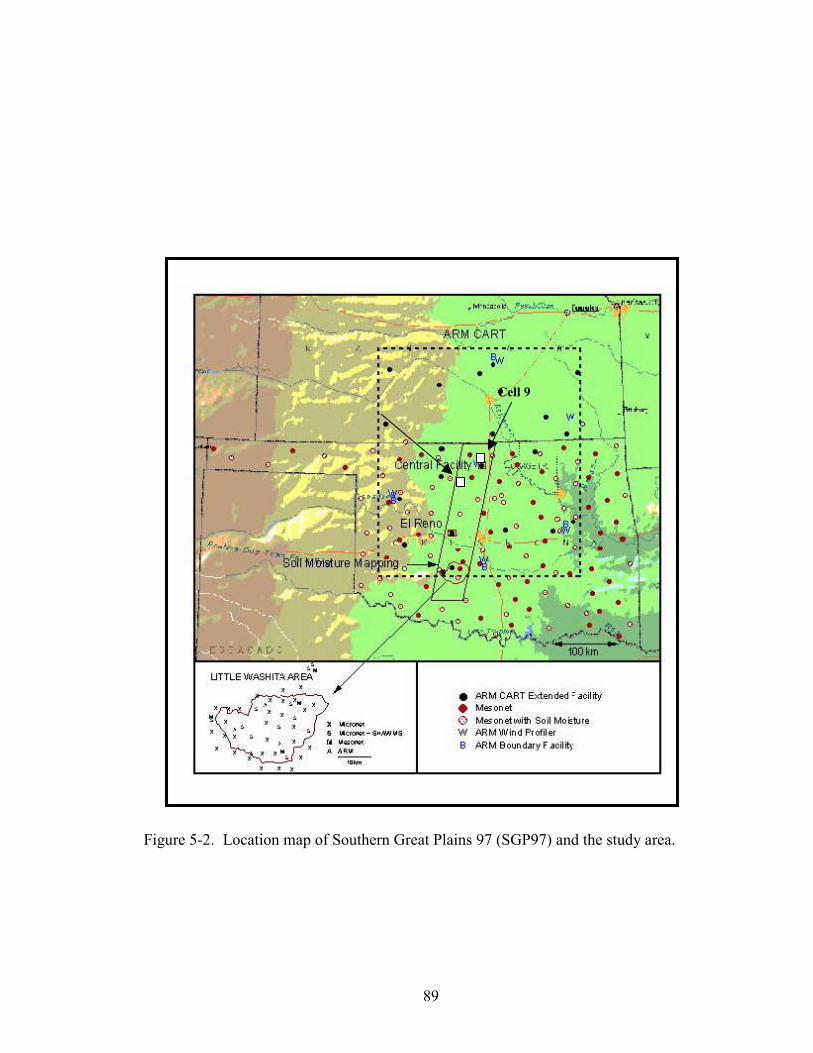
89
Figure 5-2. Location map of Southern Great Plains 97 (SGP97) and the study area.
Cell 9

90
Soil and vegetation data
The GIS (Geographic Information Systems) soil data for this study was available
from the MIADS (Map Information Analysis and Display System) of the USDA Natural
Resources Conservation Service. Soil surveys conducted for the individual counties had
been merged to create a seamless statewide data set in gridded format. The resolution of
the MIADS soil data was 200 m (4 ha).
Land-use-class information, derived from Landsat Thematic Mapper (TM) data,
was available for the SGP97 study area. These 30-m resolution land-use data were
aggregated (using a majority filter) in order to match the spatial resolution of the 200-m
soil data.
The Conterminous U.S. Advanced Very High Resolution Radiometer (AVHRR)
satellite data provided measurements of Normalized Difference Vegetation Index (NDVI)
with a 1-km resolution. A time series of biweekly composite NDVI data sets was
obtained from the USGS EROS Data Center. The model soil and vegetation parameters
are shown in Table 5-1.
Identification of the homogeneous and the heterogeneous cell
Due to the difficulties associated with handling and processing the huge volume
of 200-m resolution data, a representative subset of the SGP97 study area was selected
for the scaling analysis. A simple statistical analysis of the combined soil and land use
data was performed to identify the most homogeneous and the most heterogeneous 20-km
cells within the SGP97 area. Seventy cells, each 20 km x 20 km, were analyzed using
FRAGSTATS (McGarigal and Marks, 1995).

91
Table 5-1. List of vegetation and soil parameters used in the land surface model.
Vegetation parameters Soil parameters
Albedo
Roughness length
Shade factor
Root depth
Minimum stomatal resistance
A parameter in the radiation stress function
A parameter in the vapor pressure deficit function
Porosity
Air dry soil moisture content
Saturation soil suction
Saturation soil conductivity/diffusivity
Soil conductivity/diffusivity coefficient
Field capacity
Wilting point
Soil quartz content

92
Landscape indices were computed to find the fragmentation as shown in Table 5-
2. A total of 9 soil classes and 13 land-use classes were present in the 28,000 km2 area.
“Patches” in the landscape represent homogeneous, discrete areas with the smallest area
being 4 ha, in this study. The indices considered in the analysis included the number of
patches, the largest patch index (the area of the largest patch in the landscape divided by
total landscape area), patch density (number of patches in the landscape divided by total
landscape area), diversity index (sum of the proportional abundance of each patch type
multiplied by that proportion; it increases as the number of different patch types
increases), evenness index (sum of the proportional abundance of each patch type
multiplied by that proportion divided by the logarithm of the number of patch types),
interspersion/juxtaposition index (the observed interspersion over the maximum possible
interspersion for the given number of patch types), and the contagion index (observed
contagion over the maximum possible contagion for the given number of patch types).
An analysis of the various indices led to the identification of Cell 21 as the most
heterogeneous and Cell 9 as the most homogeneous of the 70 cells. These two cells were
selected for further study. It is important to mention that these areas were defined within
the SGP97 region and do not necessarily represent the degree of heterogeneity and
homogeneity that might be seen at continental or even regional scales.
Cell 21 was situated in the west-central part of SGP97 (Figure 5-1) and its
Universal Transverse Mercator (UTM) coordinates were (553000,3998000) and
(573000,4018000) for the southwest and northeast corners, respectively.

93
Table 5-2. Landscape indices for the heterogeneous cell (#21) and the homogeneous cell (#9).
LANDSCAPE INDICES Cell 21 Cell 9
Number of patches: 2455 1414
Largest Patch Index(%): 3.76 27.33
Patch Density (#/100 ha): 6.51 3.6
Shannon's Diversity Index: 3.28 1.94
Simpson's Diversity Index: 0.94 0.69
Modified Simpson's Diversity Index: 2.78 1.18
Shannon's Evenness Index: 0.73 0.46
Simpson's Evenness Index: 0.95 0.7
Modified Simpson's Evenness Index: 0.62 0.28
Interspersion/Juxtaposition Index (%) 65.58 50.49
Contagion Index (%): 39.57 61.06
94
The variability in soil and land use in this 20 x 20 km grid was very high. As shown in
Figure 5-2a, at the 200-m resolution, Cell 21 contained 13 vegetation classes with
pastureland (42%) and wheat (33%) as predominant types. The soil as shown in Figure 5-
3a consisted of 9 different textures, the major ones being sand (23%), silt loam (18%),
loamy sand (16%) and sandy loam (12%). Cell 9 was located in the northeast part of
SGP97 (Figure 5-1) and its UTM coordinates were (613000,4058000) and
(633000,4078000) for the southwest and northeast corners, respectively. This cell
primarily consisted of wheat (59%) and pastureland (24%) as shown in Figure 5-4a. Silt
loam occupied 83 % of the cell area with several other textures having minor presence
(Figure 5-5a).
Aggregation of the input data
The high resolution data (200 m) were used to develop the input data sets for two
coarser resolutions, i.e., 2 km and 20 km. These scales increase by a factor of 10 in each
case and were chosen in order to represent the scales that might be of interest for current
and (especially) future operational weather modeling. Also, the 20-km scale should
eventually be relevant to global climate modeling, as GCM grid cells continue to
decrease in size.
The soil and land use types were each aggregated using a majority filter on 100 of
the 200-m cells (in the case of the 2-km resolution) and on 10,000 of the 200-m cells (in
the case of the 20-km resolution). As shown in Figure 5-2b, land use types for Cell 21
were reduced to five classes at the 2-km resolution as compared to 13 classes at the 200-
m resolution. Similarly, Figure 5-3b shows that the number of soil types was reduced
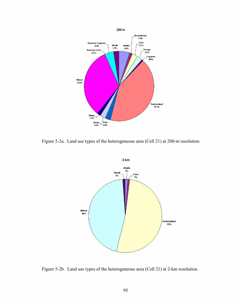
95
Figure 5-2a. Land use types of the heterogeneous area (Cell 21) at 200-m resolution.
Figure 5-2b. Land use types of the heterogeneous area (Cell 21) at 2-km resolution.

96
Figure 5-3a. Soil types of the heterogeneous area (Cell 21) at 200-m resolution.
Figure 5-3b. Soil types of the heterogeneous area (Cell 21) at 2-km resolution.
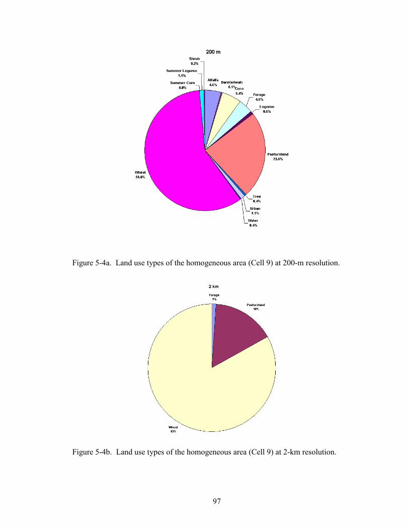
97
Figure 5-4a. Land use types of the homogeneous area (Cell 9) at 200-m resolution.
Figure 5-4b. Land use types of the homogeneous area (Cell 9) at 2-km resolution.
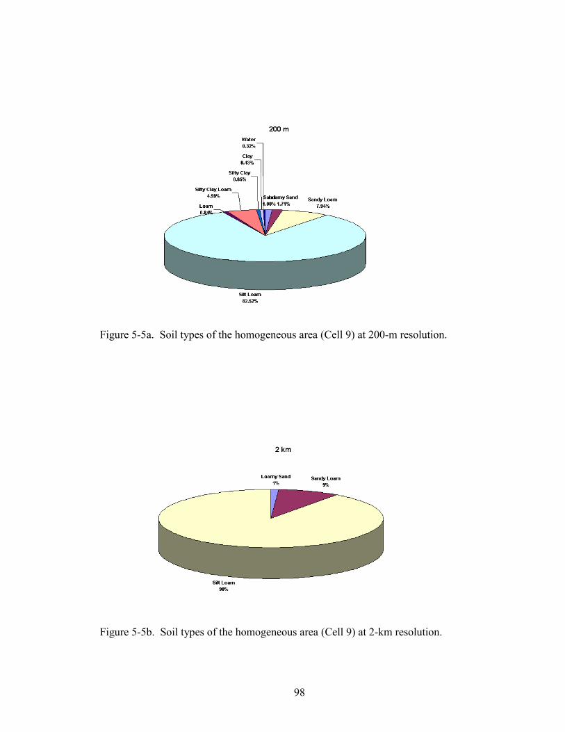
98
Figure 5-5a. Soil types of the homogeneous area (Cell 9) at 200-m resolution.
Figure 5-5b. Soil types of the homogeneous area (Cell 9) at 2-km resolution.

99
from nine to seven. The difference is even more dramatic for the homogeneous cell
(Cell9). As evident from Figure 5-4b, land use at the 2-km resolution was reduced from
13 classes to only three (with 83% wheat). Similarly, only three soil types remained in
Cell 9 at the 2-km resolution, with 90% silt loam (Figure 5-5b). So, the clear distinction
between the heterogeneous (#21) and homogeneous (#9) cells was still evident after the
aggregation to 2 km.
Area-averaged and dominant-landuse-based NDVI for green vegetation fraction
The land surface model requires green vegetation fraction as a key input. Using
GIS, “area-averaged” NDVI was computed and it is simply the numerical average of the
NDVI values over the given area. For instance, averages of 4 and 400 numerical values
of NDVI (1-km resolution) were computed to obtain a cell-average NDVI value for 2 km
and 20 km, respectively. An alternative approach ties the NDVI value for a given area to
the dominant land use in that area. “Dominant-land use-based” NDVI was computed by
first applying a majority filter on 100 and 10000 land use “pixels” (200-m resolution) in
GIS for 2 km and 20 km, respectively. Then an average was taken of the NDVI values for
all pixels with that majority land use. As opposed to the area-average, this approach was
more likely to result in an NDVI value that is consistent with the single vegetation type
assigned to a modeling area.
From both the area-averaged and dominant-landuse-based NDVI data, vegetation
fraction (fg) was computed using the Gutman-Ignatov (1998) method:
( )( )minmax
min
NDVINDVINDVINDVI
f g −−
= (5-2)
Bare soil NDVI (NDVImin) and dense vegetation NDVI (NDVImax) are defined as 0.04 and
0.52 respectively and they correspond to seasonally and geographically invariant

100
constants for desert and evergreen clusters. As NDVI was available from the biweekly
composite images, the computed vegetation fraction based on NDVI was then linearly
interpolated on a daily basis. The vegetation fractions derived based on area-averaged
based NDVI and dominant-landuse-based NDVI are referred to herein as the area-
averaged vegetation fraction and the dominant-landuse-based vegetation fraction,
respectively.
Weather data
The Oklahoma Mesonet, an automated network of 114 stations (Elliott et al.,
1994; Brock et al., 1995) provided meteorological data. The Mesonet sites used for this
study included LAHO (Lat: 36° 23′ 3′′ N, Long: 98° 6′ 41′′ W, elev: 395 m) and MEDF
(lat:36° 47′ 31′′ N, long: 97° 44′ 44′′ W, elev: 330 m). These sites were assigned to Cell
21 and Cell 9, respectively based on the nearest neighbor approach. The data from the
Oklahoma Mesonet consisted of 5-minute averages which were then averaged over one-
hour intervals. The variables used were air temperature (K), specific humidity (Kg Kg-1),
wind speed (m s-1), pressure (Pa), precipitation (kg m-2s-1) and solar radiation (W m-2). It
should be noted that air temperature in degree K and specific humidity were derived
quantities using the original Mesonet variables. Longwave downwelling radiation was
estimated using the scheme discussed in Chapter 3. This longwave radiation scheme uses
near-surface vapor pressure and air temperature data.
The model simulations were carried out over a five-month period (from 1 March
1997 through 31 July 1997). It should be noted that simulation from March through May
was considered as the model ‘spin-up’ period before the SGP97 duration of June-July.
The model was run on an hourly time step, and the results were aggregated daily. Though

101
the model was run continuously for a five-month period, due to the huge volume of
output generated at the 200-m resolution, the model was coded to write the output at the
200-m resolution only for selected days. The days were chosen to fall within the SGP97
period. Nine days with relatively high solar radiation were chosen as “clear days”
(18,25,27, and 30 June; 3,6,14,22, and 23 July), while four days with relatively low solar
radiation were considered as “cloudy days” (23 June; 11,15, and 20 July). For the 2-km
and the 20-km resolutions, simulation results were obtained throughout the study period.
Results and Discussion
Model sensitivity to the area-averaged and dominant-landuse-based vegetation fraction
The impact of the area-averaged versus dominant-landuse-based vegetation
fraction on the model results is discussed briefly here. The sensitivity of the model to the
two approaches was analyzed for both the cells, by comparing the model estimated
surface energy-balance components, i.e., net radiation, latent, sensible and ground heat
(GH) fluxes. There was virtually no difference in the model output resulting from these
two vegetation fractions. This was consistent for both clear and cloudy days. The results
of this analysis are tabulated in Appendix D (Table (D-1)–(D-2)). The differences in
NDVI values were not large enough to cause appreciable differences in the computed
vegetation fraction.
Model output
The hourly model simulations of surface energy-balance components were
aggregated on a daily basis. Then, the numerical average over the domain was computed
for comparing the results across the three scales, i.e., 200 m, 2 km and 20 km. The spatial

102
representations of the model output for Cell 21 and Cell 9 for 18 June 97 are shown in
Figures (5-6) – (5-13). Appendix D (Figures (D-1) – (D-16) contains the output for one
additional clear day and one cloudy day.
Tables (5-3) and (5-4) summarize the numerical model output. Maximum,
minimum and average values are shown for each study day. It was observed that the
range of the cell-by-cell model output was greater at the 200-m resolution than at the 2-
km resolution, for all of the components. In other words, the range of the lower-
resolution model output always fell within the range of the high-resolution output,
indicating that the variability in the output was reduced at coarser scales.
Time series comparison of the model output for the three scales
Figure 5-14 shows the time series plot of all four surface energy-balance
components at 200 m, 2 km and 20 km for Cell 21. The time period is June 15 through
July 25. As shown in Figure 5-14a, the discrete series of domain average net radiation for
200 m (13 days) agreed very well with the continuous time series for both the 2-km and
20-km resolutions. This indicated that, in spite of the aggregation of input variables from
200 m to 2 km and 20 km, the model estimates of net radiation were very closely
matched across these scales. This is perhaps to be expected because net radiation is
dominated by the magnitude of incoming solar radiation and is only minimally influenced
by vegetation and soil parameters (i.e., the albedo). It should be remembered that weather
data from a single site were applied at all three scales for the entire domain of Cell 21.
The 200-m and 2- km output for latent heat flux matched very closely while the 20-km
output did show some deviations (Figure 5-14b). Figure 5-14c suggested that the sensible
heat flux estimations at 20 km were higher than for the other two resolutions, and the

103
Table 5-3. Daily average modeled energy-balance components for the heterogeneous area (Cell 21) at three scales of input aggregation.

104
Table 5-3. Daily average modeled energy-balance components for the heterogeneous area (Cell 21) at three scales of input aggregation (contd.)

105
Table 5-4. Daily average modeled energy-balance components for the homogeneous area (Cell 9) at three scales of input aggregation.

106
Table 5-4. Daily average modeled energy-balance components for the homogeneous area (Cell 9) at three scales of input aggregation (contd.)

107
Figure 5-6. Modeled net radiation comparison among the three scales for the heterogeneous area on 18 June 97.

108
Figure 5-7. Modeled net radiation comparison among the three scales in the homogeneous area on 18 June 97.

109
Figure 5-8. Modeled latent heat flux comparison among the three scales for the heterogeneous area on 18 June 97.

110
Figure 5-9. Modeled latent heat flux comparison among the three scales for the homogeneous area on 18 June 97.

111
Figure 5-10. Modeled sensible heat flux comparison among the three scales for the heterogeneous area on 18 June 97.

112
Figure 5-11. Modeled sensible heat flux comparison among the three scales for the homogeneous area on 18 June 97.

113
Figure 5-12. Modeled ground heat flux comparison among the three scales for the heterogeneous area on 18 June 97

114
Figure 5-13. Modeled ground heat flux comparison among the three scales for the homogeneous area on 18 June 97

115
magnitude of difference was similar to that for the latent heat flux estimation. Finally, the
residual energy in the energy budget (the ground heat flux), as shown in Figure 5-14d,
tended to be predicted slightly higher at the 20-km resolution than at the 200-m and 2-km
resolution. Thus, scaling effects were manifested in the partitioning of the energy,
especially latent and sensible heat. These differences became evident at the 20-km scale.
The modeling results for the homogeneous area (Cell 9) were studied in a similar
way. Figure 5-15 represents the time series plots of simulated surface energy-balance
components for all three scales. The results of the simulated net radiation for 200 m, 2 km
and 20 km again agreed very well as shown in Figure 5-15a. Both latent heat flux (Figure
5-15b) and sensible heat flux (Figure 5-15c) showed slight deviations at the coarsest
scale, i.e., 20 km, but overall the results for the three scales agreed closely. Ground heat
flux matched very well at all three scales as shown in Figure 5-15d. As expected, the
aggregation of input data had less impact on the model output when the variability in
surface conditions was less.
Comparison of the bias in the model output for the three scales
This section discusses equal-value plots of all surface energy-balance components
for the three possible scale intercomparisons ( 2 km vs. 200 m, 20 km vs. 200 m and 20
km vs. 2 km) (Figures (5-16)–(5-19)). This is, in fact, another approach to visualizing
details of the scaling effects. Figure 5-16 (net radiation for the heterogeneous area)
clearly shows that there was no bias in the estimated net radiation across the three scales.
Figure 5-17 indicates that the estimation of latent heat flux at 200 m and 2 km agreed
very well while there was a negative bias in the estimation as the scale moved to 20 km.
Sensible heat flux predictions (Figure 5-18) again indicated a bias at the 20 km scale, but
116
in this case it was positive. The patterns for ground heat flux (Figure 5-19) were quite
similar to those for sensible heat flux. Thus, energy partitioning at the 20-km scale
became biased toward sensible heat and ground heat fluxes, and away from latent heat
flux. This trend is consistent with the soil and land use at the 20-km scale for Cell 21. The
sub-grid variability which was preserved at the 200-m and 2-km scales becomes non-
existent when a single soil type (sand) and single vegetation type (grassland) are assigned
for the entire domain of the 20-km resolution analysis. Obviously, the combination of
sand and grassland resulted in reduced latent heat flux at 20 km when compared with the
other two scales. More of the available energy was then partitioned into sensible and
ground heat fluxes.
Figures (5-20)- (5-23) are similar equal-value plots for Cell 9. All of these plots
confirm that, for the homogeneous cell, the scaling-up of input data had very little impact
on modeled surface energy-balance components. In other words, the results for Cell 9, a
homogeneous area in terms of soil and vegetation when compared with Cell 21, validated
the hypothesis that aggregating the surface conditions such as soil and vegetation when
there was less variability, would have less impact in the simulation of net radiation,
latent, sensible and ground heat fluxes.
Deflections in the model output at 20-km scale
Appendix D (Figures (D-17)-(D-20)) contains the deflection plots of modeled
surface energy-balance components for both Cell 21 and Cell 9. This is another way of
looking at the scale dependency of the model output. Although this analysis was done
using only three scales, the plots are somewhat analogous to a semivariogram analysis.
For both Cell 21 and Cell 9, no significant deviation was observed among the three

117
Figure 5-14. Scale comparisons of the heterogeneous area (Cell 21) model output at 200-m, 2-km and 20-km resolutions.

118
Figure 5-15. Scale comparisons of the homogeneous area (Cell 9)model output at 200-m, 2-km and 20-km resolutions.

119
Figure 5-16. Equal-value plots of modeled net radiation for the three scales in the heterogeneous area (Cell 21).

120
Figure 5-17. Equal-value plots of modeled latent heat flux for the three scales in the heterogeneous area (Cell 21).
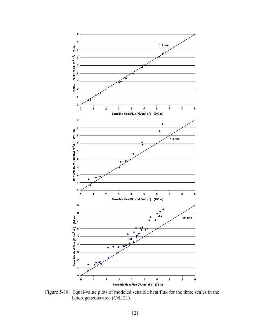
121
Figure 5-18. Equal-value plots of modeled sensible heat flux for the three scales in the heterogeneous area (Cell 21).
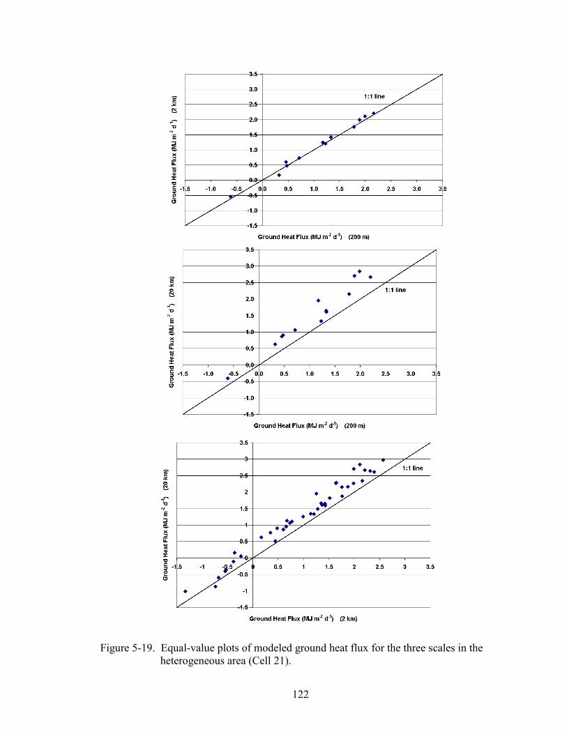
122
Figure 5-19. Equal-value plots of modeled ground heat flux for the three scales in the
heterogeneous area (Cell 21).
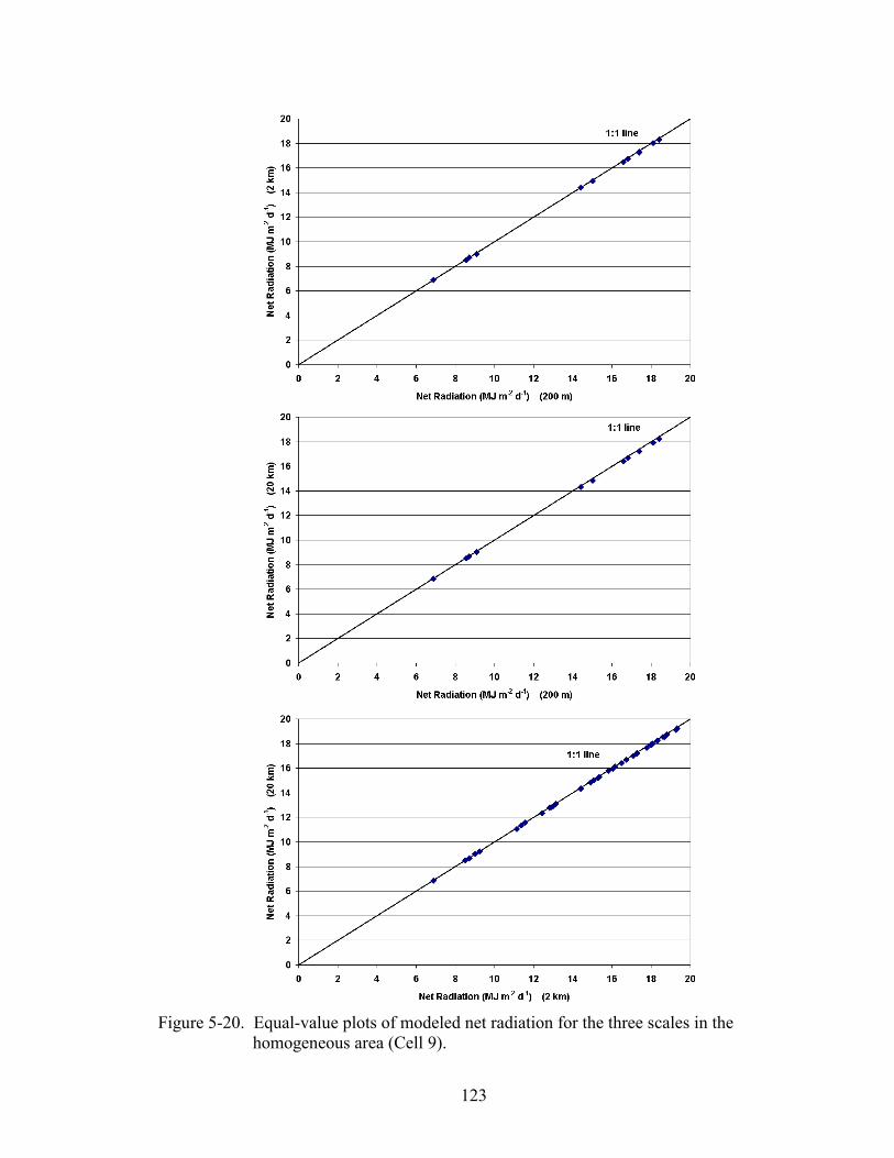
123
Figure 5-20. Equal-value plots of modeled net radiation for the three scales in the homogeneous area (Cell 9).
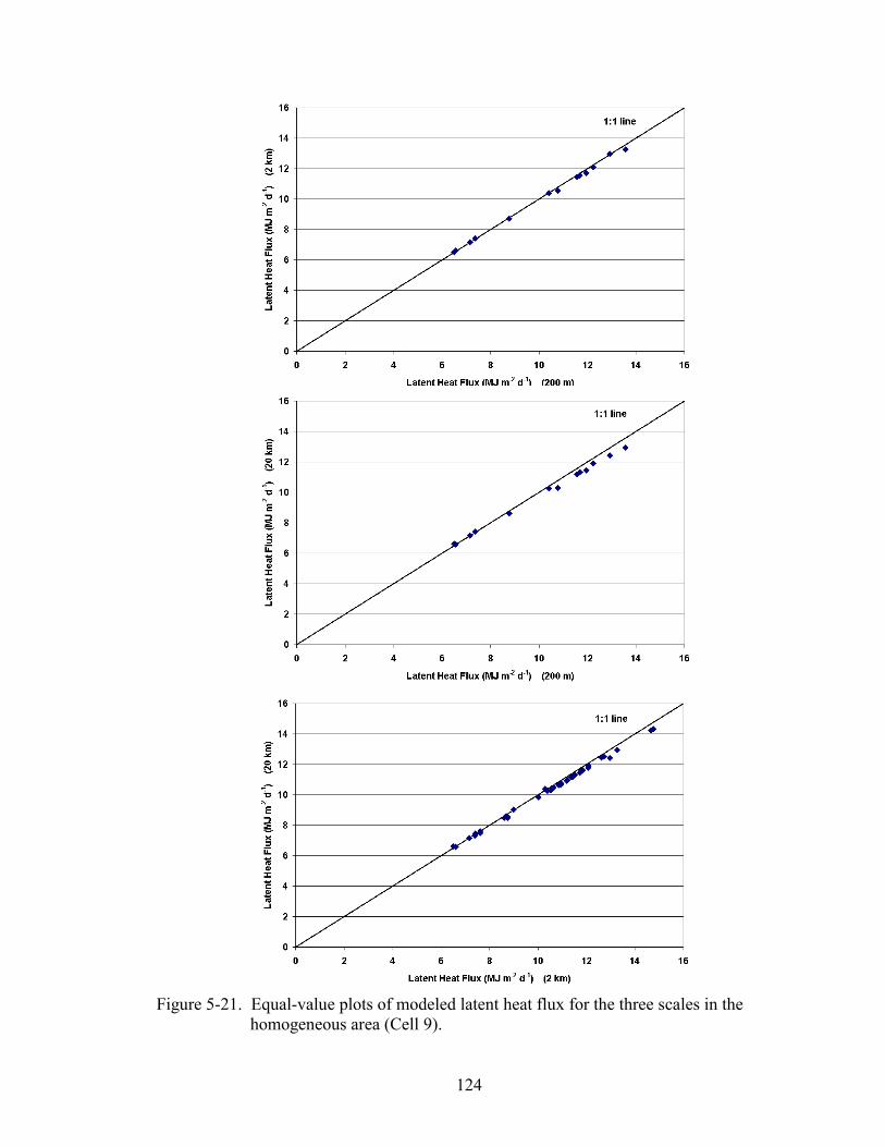
124
Figure 5-21. Equal-value plots of modeled latent heat flux for the three scales in the homogeneous area (Cell 9).

125
Figure 5-22. Equal-value plots of modeled sensible heat flux for the three scales in the homogeneous area (Cell 9).
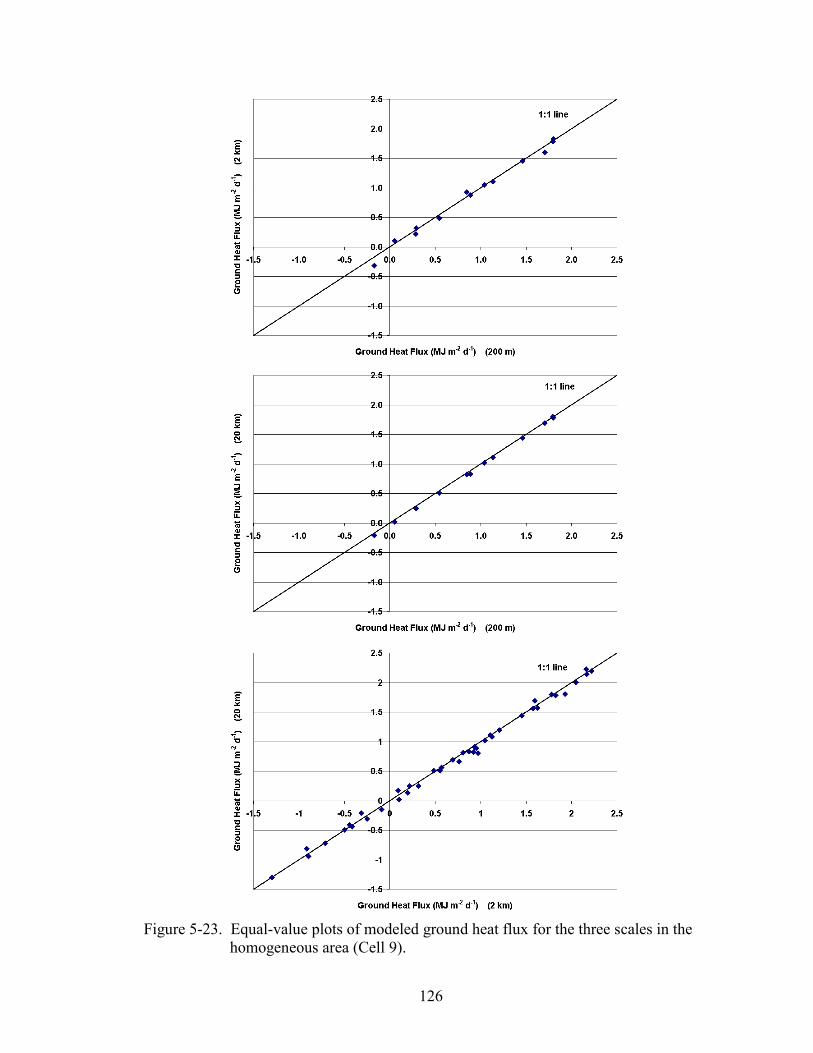
126
Figure 5-23. Equal-value plots of modeled ground heat flux for the three scales in the homogeneous area (Cell 9).
127
different scales for the estimation of net radiation, suggesting that its modeling scale is
independent. The latent heat flux comparisons implied that this energy-balance
component became scale dependent between 2 km and 20 km. This was predominantly
observed in Cell 21. The sensible heat flux also exhibited scale dependency beyond 2 km,
but only for Cell 21. Ground heat flux estimation showed a slight scale dependency for
Cell 21.
Summary and Conclusions
Large scale modeling of land surface processes is made more complex by sub-
grid scale heterogeneity. This research was focused on first identifying the variability in
vegetation and soil for the SGP97 region, secondly on quantifying modeled surface
energy-balance components at various spatial scales by aggregating certain input data,
and finally on analyzing the scale effects at a sub-grid level for better understanding of
land-atmosphere interactions. The well tested NOAH-OSU Land Surface Model (LSM)
was used for this study.
Starting with a 280 km x 100 km area in central Oklahoma, a statistical procedure
was followed to characterize the variability of soil and vegetation within 70 cells, each 20
km x 20 km. Cell 21 and Cell 9 were identified as the most heterogeneous and the most
homogeneous cell, respectively. These areas were found to be heterogeneous and
homogeneous in the context of the SGP97 region and not necessarily at regional or
continental scales.
The scaling study was performed at 200 m, 2 km and 20 km using each of these
two cells as a modeling domain. Soil and vegetation input data at the 200-m resolution

128
were aggregated to the coarser scales and model results were analyzed for the following
surface energy-balance components: net radiation, latent, sensible and ground heat fluxes.
The sensitivity analysis of the model to the vegetation fraction derived based on
area-averaged and dominant-landuse-based NDVI showed that there was essentially no
difference in the model outputs.
The domain average net radiation, latent, sensible, and ground heat fluxes
estimated for Cell 21 and Cell 9 at 200 m , 2 km and 20 km were compared individually.
The results indicated that the heterogeneous cell exhibited considerable differences in
latent and sensible heat fluxes when soil and vegetation data were aggregated from 200 m
to 20 km. The variations in the estimations were insignificant between 200 m and 2 km,
however. Though the magnitude of net radiation and thereby other fluxes tended to be
less for cloudy days, differences in the estimation of latent and sensible heat fluxes were
found to exist between the two coarser scales. Cell 9, the homogeneous cell, responded
differently to the aggregation process. For both clear and cloudy days, it was evident that
the quantification of domain average net radiation, latent, sensible and ground heat fluxes
showed no significant difference at the 200-m, 2-km and 20- km resolutions.
The results suggested that the aggregation of spatially variable soil and vegetation
inputs has a greater impact on the quantification of latent and sensible heat fluxes than
net radiation and ground heat flux. The change in model response occurred between the
2-km and 20-km scales; model output for the 200-m scale was very similar to that for the
2-km scale. Not surprisingly, scaling-up of input had much less impact for relatively
homogeneous land areas. Earlier studies implied that improper modeling of land surface
processes would impact the land-atmosphere exchange processes. This investigation

129
supported the argument that sub-grid variability should be considered for proper
quantification and partitioning of surface energy-balance components.

130
CHAPTER 6
SUMMARY, CONCLUSIONS AND RECOMMENDATIONS
Summary
Recent years have witnessed a dramatic increase in modeling of land-atmospheric
interactions. Factors influencing this trend include improved model physics, enhanced
computer capability, and the availability of high-resolution data sets including remotely
sensed data for larger areas and longer times. Convergence of land surface hydrology
with the atmospheric science discipline has energized scientific research efforts aimed at
improved weather forecasting and better energy, agriculture and natural resource
management.
Hydrological processes at the surface of the earth assume significance in the
context of soil-vegetation-atmosphere exchange modeling. Land-atmosphere exchange
processes include net radiation (Rn), latent heat (LH), sensible heat (SH) and ground heat
(GH) fluxes. Their interdepedence and non-linear behavior provide challenges,
especially when large scale modeling is attempted. Despite the recognition of the
feedback between the land and the atmosphere, and its impact on physically based
modeling, many issues are unresolved. Scaling is one of those key issues.
The main objective of this research was to examine the effects of different spatial
scales of input data on modeled net radiation, latent, sensible and ground heat fluxes, and
thereby understand the resolution needed for the realistic modeling of large-scale land
131
atmosphere interaction. For this investigation, the NOAH-OSU (Oregon State
University) Land Surface Model (LSM) was chosen because it is used operationally in
weather prediction and is widely recognized by the hydrology and atmospheric science
research community. Field measurements were available from the Oklahoma Mesonet
and the accompanying Oklahoma Atmospheric Surface-layer Instrumentation (OASIS)
project. There are 10 OASIS “Super sites” equipped with instrumentation for measuring
surface energy-balance components (Rn, LH, SH and GH).
The LSM needed downwelling longwave radiation as one of its forcing inputs,
and it is rarely measured. There are several downwelling longwave radiation models
available and no single technique has emerged as the most appropriate one to use. This
led to developing a methodology for estimating downwelling longwave radiation during
nighttime and daytime conditions and clear and cloudy sky conditions, as a function of
vapor pressure and air temperature.
Using a simple linear regression procedure, Brutsaert’s model for incoming
longwave radiation (LWin) was calibrated for four sites (ALVA, FORA, GRAN and
IDAB) individually. The resulting coefficients ranged in value from 1.30 to 1.32, with an
average of 1.31. The resulting expression was
47/1
1031.1 T
Te
LW din σ
��
�
�
��
�
�= (6-1)
where T is the air temperature (K), ed is the vapor pressure (kPa) at screen height, σ is the
Stefan- Boltzmann constant (5.675 x 10⁻⁸J m-2 K-4 s-1) and LWin has units of Wm-2. The
model was tested for five independent sites (BESS, BURN, MARE, NORM and STIG).
These validation sites represent different regions of the state of Oklahoma and fall under
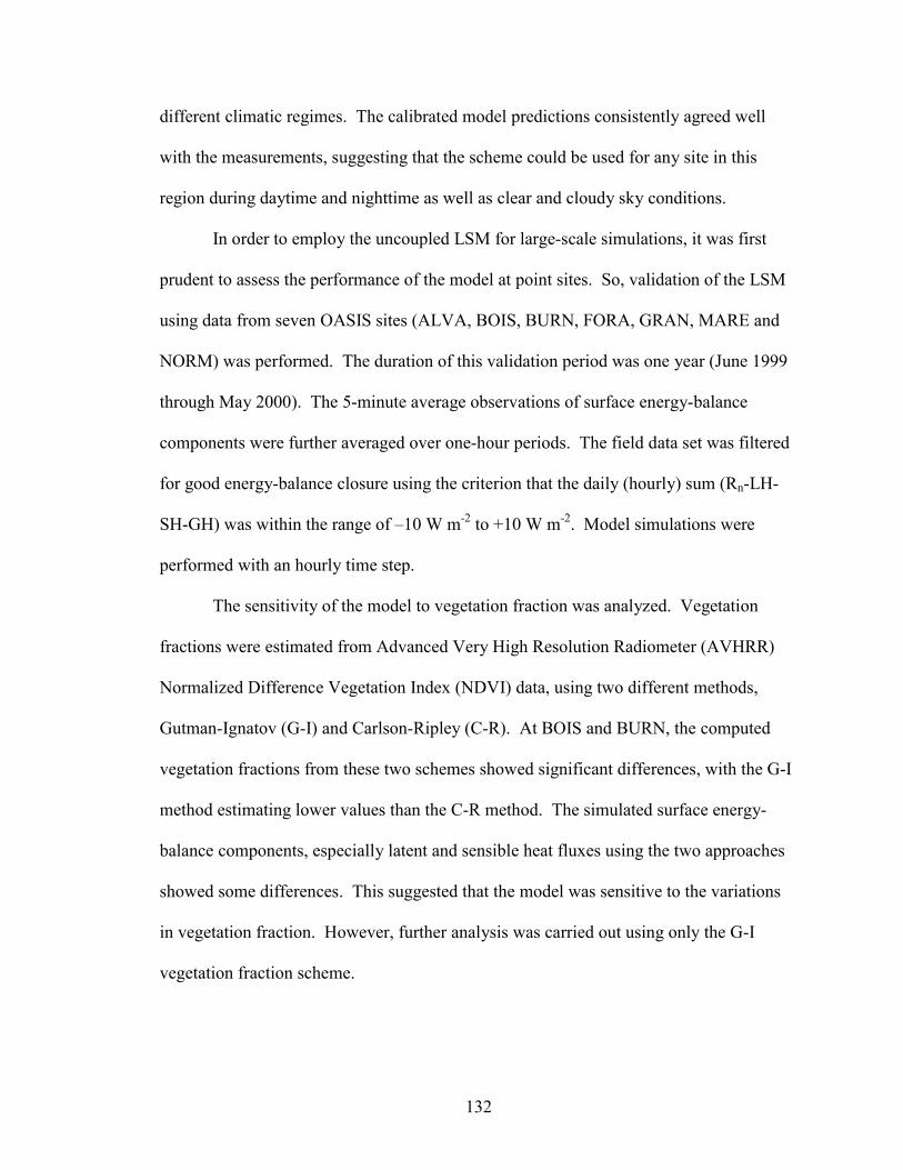
132
different climatic regimes. The calibrated model predictions consistently agreed well
with the measurements, suggesting that the scheme could be used for any site in this
region during daytime and nighttime as well as clear and cloudy sky conditions.
In order to employ the uncoupled LSM for large-scale simulations, it was first
prudent to assess the performance of the model at point sites. So, validation of the LSM
using data from seven OASIS sites (ALVA, BOIS, BURN, FORA, GRAN, MARE and
NORM) was performed. The duration of this validation period was one year (June 1999
through May 2000). The 5-minute average observations of surface energy-balance
components were further averaged over one-hour periods. The field data set was filtered
for good energy-balance closure using the criterion that the daily (hourly) sum (Rn-LH-
SH-GH) was within the range of –10 W m-2 to +10 W m-2. Model simulations were
performed with an hourly time step.
The sensitivity of the model to vegetation fraction was analyzed. Vegetation
fractions were estimated from Advanced Very High Resolution Radiometer (AVHRR)
Normalized Difference Vegetation Index (NDVI) data, using two different methods,
Gutman-Ignatov (G-I) and Carlson-Ripley (C-R). At BOIS and BURN, the computed
vegetation fractions from these two schemes showed significant differences, with the G-I
method estimating lower values than the C-R method. The simulated surface energy-
balance components, especially latent and sensible heat fluxes using the two approaches
showed some differences. This suggested that the model was sensitive to the variations
in vegetation fraction. However, further analysis was carried out using only the G-I
vegetation fraction scheme.

133
Each of the four modeled surface energy-balance components was analyzed for
both daily and hourly time scales. The overall results showed that the model predicted
well for the long period of time. The energy balance in the LSM is formulated in a such a
way that the excess net radiation is redistributed into latent, sensible and ground heat
fluxes:
GHSHLHRn ++= (6-2)
The seven-site average results indicated that the model tended to slightly
overestimate Rn. Most of this excess radiant energy was assigned to LH as opposed to
SH. This is because the LSM first computed potential evaporation and then actual
evaporation, which was used to determine the skin temperature at equilibrium state, and
subsequently SH was computed. As the LSM computed LH first, it tended to distribute
excess energy to that term. The model showed a positive bias in LH estimation and a
slight negative bias in SH estimation. The trends observed in hourly and daily estimates
for all energy-balance components were similar except for GH, which had a slight
positive bias for the daily analysis.
Following the validation analysis, the effects of scaling on modeled surface
energy-balance components were examined. The Southern Great Plains 1997 (SGP97)
Hydrology Experiment area was chosen for this study.
First, a 280 km x 100 km area in central Oklahoma was divided into 70 cells, each
20 km x 20 km. A statistical procedure was followed to characterize the variability of
soil and vegetation in these cells. Cell 21 and Cell 9 were identified as the most
heterogeneous and the most homogeneous cell, respectively. However, the
134
heterogeneity/homogeneity in this study region may not reflect that found over larger
areas.
The scaling analysis was carried out at 200-m, 2-km and 20-km resolutions using
each of the two cells as a modeling domain. Soil and vegetation input data at the high
spatial resolution (200 m) were aggregated to obtain the data sets for the 2-km and 20-km
resolutions. In order to study the effect of area-averaged vs. dominant-landuse-based
vegetation on the model output at 2 km and 20 km, simulations were performed using
vegetation fraction derived from NDVI by these two methods. There was essentially no
difference between the two vegetation fraction methods in the model estimation of Rn,
LH, SH and GH.
The simulations for the scaling analysis were carried out with proper initialization
of the model and a reasonable ‘spin-up’ period to remove any instability caused in the
beginning of the simulation. The SGP97 study period was between 18 June and 25 July
1997. For Cell 21, the heterogeneous cell, there was no appreciable difference between
the model simulations at the 200-m and 2-km resolutions but there were differences
between the 2-km and 20-km resolutions, especially for LH and SH. Similar trends were
evident for both clear and cloudy days. On the contrary and as expected, Cell 9, the most
homogeneous cell, showed very little difference in the model output across all three
resolutions.
Conclusions
Investigations of available downwelling longwave radiation schemes suggested
that a simple technique was needed to estimate downwelling longwave radiation for input
to the LSM. This technique would need to rely on readily available data, and should

135
perform well under both daytime and nighttime and clear and cloudy conditions. A
simple approach based on the Brutsaert equation and using near-surface vapor pressure
and air temperature was developed and presented. The predictions by this method
showed good agreement with field measurements and paved the way for its application in
the validation and scaling studies to follow.
As verification of the performance of the NOAH-OSU LSM for Oklahoma
conditions, model testing was done with the measurements from OASIS sites. Hourly
simulation results for a one-year period were compared with the observations. It was
found that the model slightly over predicted net radiation and this excess energy was
directed to latent heat flux as opposed to sensible heat flux. Ground heat flux estimations
were reasonably close to the field observations.
The effects of three different scales of input data on modeled net radiation, latent,
sensible and ground heat fluxes were analyzed for the heterogeneous area (Cell 21) and
the homogeneous area (Cell 9). The aggregation process undertaken for these two cells
resulted in fewer classes as the scale increased from 200 m to 2 km and a single class at
the 20-km resolution. The comparison of domain average net radiation, latent, sensible
and ground heat fluxes estimated for Cell 21 across the three scales showed that there
was good agreement between the 200-m and 2-km resolution model output. However,
the simulation results at the 20-km resolution showed appreciable differences for all four
components, especially latent and sensible heat fluxes for both clear and cloudy days.
The results for Cell 9 exhibited the expected trend. For all three scales, the estimated net
radiation, latent, sensible and ground heat fluxes were closely matched across all three
scales.

136
The results suggested that the aggregation of spatially variable soil and vegetation
inputs has a greater impact on the quantification of surface energy-balance components
and partitioning of latent, sensible heat fluxes. It was confirmed that the effects of
scaling-up of input data on model estimates are more pronounced for heterogeneous areas
than for homogeneous areas.
Recommendations
The objectives of this dissertation were accomplished as described in previous
chapters and summarized and concluded in the earlier sections of this chapter. However,
in continuing to address some of these issues, improvements could be made in the
following areas:
1. Although the soil hydrology model conceptually encompasses four soil layers, all of
the layers are considered to have the same soil texture in the current version of the
model formulation. This is considered to be an important limitation as the soil layers
could have different soil textures and hence different properties. Thus, consideration
of the individual textures for each layer is needed, should it be supported by the
available data.
2. In order to make the model more specific, it is necessary to include a greater number
of vegetation classes with reasonable parameters for each of them, and some effort
should be spent in testing those parameters as well.
3. The spatial variability in atmospheric forcing should also be considered, especially
for precipitation. Differences in the partitioning of latent and sensible heat fluxes
would be amplified by variability in precipitation and its impact on soil moisture.

137
Radar estimates of precipitation could provide a vehicle for incorporating this
variability into the modeling.
4. Model outputs were viewed using a Geographic Information System (Arc/Info).
However, a real-time user-friendly graphical interface could simplify the display of
the model output and increase the efficiency of modeling studies.

138
REFERENCES Aase, J.K., and Idso, S.B. (1978). A comparison of two formula types for calculating
long-wave radiation from atmosphere. Water Resources Research, 14, 623-625.
Anderson, E.R. (1954). Energy-budget studies, Water-loss investigations: Lake Hefner studies. U.S. Geological Survey Professional Paper 269, 71-119.
Avissar, R. (1992). Conceptual aspects of a statistical dynamical approach to represent landscape subgrid-scale heterogeneities in atmospheric models. Journal of Geophysical Research, 97(D3), 2729-2742.
Avissar, R. (1992). Conceptual aspects of a statistical dynamical approach to represent landscape subgrid-scale heterogeneities in atmospheric models. Journal of Geophysical Research, 97(D3), 2729-2742.
Benjamin, S.G., and Carlson, T.N. (1986). Some effects of surface heating and topography on the regional severe storm environment, I, Three-dimensional simulations, Monthly Weather Review, 114, 307-329.
Betts, A.K., Ball, J.H., Beljaars, A.C.M., Miller, M.J., and Viterbo, P. (1996). The land-surface-atmosphere interaction: a review based on observational and global modelling perspectives. Journal of Geophysical Research, 101, 7209-7225.
Betts, A.K., Chen, F., Mitchell, K., and Janjic, Z.I. (1997). Assessment of the land surface and boundary layer models in two operational versions of the NCEP Eta model using FIFE data. Monthly Weather Review, 125, 2896-2916.
Bloschl. G and Sivapalan, M. (1995). Scale issues in hydrological modelling: A review. In: Scale Issues in Hydrological Modelling. (eds.) J.D. Kalma and M. Sivapalan. John Wiley & Sons Ltd., England, 9-48.
Braud, I. (1998). Spatial variability of surface properties and estimation of surface fluxes of a savannah. Agricultural and Forest Meteorology, 89, 15-44.
Brock, F.V., Crawford, K.C., Elliott, R.L., Cuperus, G.W., Stadler, S.J., Johnson, H.L., and Eilts, M.D. (1995). The Oklahoma Mesonet: A technical overview. Journal of Atmospheric Ocean.Technology, 12(1), 5-19.
Brotzge, J.A. (2000). Closure of the surface energy budget. Ph.D. Dissertation. Univ. of Oklahoma, Norman, OK, 208pp.
Brotzge, J.A., Richardson, S.J., Crawford, K.C., Horst, T.W., Brock, F.V., Humes, K.S., Sorbjan, Z., and Elliott, R.L. (1999). The Oklahoma Atmospheric Surface-layer Instrumentation System (OASIS) Project. Thirteenth Conf. on Boundary-Layer Turb., Am. Meteorol. Soc., Dallas, TX, Jan.10-15.
139
Brunt, D. (1932). Notes on radiation in the atmosphere. Quart. J. Roy. Meteor. Soc., 58, 389-418.
Brutsaert, W. (1975). On a derivable formula for long-wave radiation from clear skies. Water Resources Research, 11(5), 742-744.
Carlson, T.N., and Ripley, D.A. (1997). On the relation between NDVI, fractional vegetation cover and leaf area index. Remote Sensing of Environment, 62, 241-252.
Chen, D., and Brutsaert, W. (1995). Diagnostics of land surface spatial variability and water vapor flux. Water Resources Research, 100(D12), 25,595-25,606.
Chen, F., and Dudhia, J. (2001). Coupling an advanced land-surface/hydrology model with the Penn State-NCAR MM5 modeling system. Part I: Model implementation and sensitivity. Monthly Weather Review, 129, 569-585.
Chen, F., and Mitchell, K. (1999). Using the GEWEX/ISLSCP forcing data to simulate global soil moisture fields and hydrological cycle for 1987-1988. Journal of the Meteorological Society of Japan , 77, 1B, 167-182.
Chen, F., Janjic, Z.I., and Mitchell, K. (1997). Impact of atmospheric surface-layer parameterization in the new land surface scheme of the NCEP mesoscale Eta numerical model. Boundary –Layer Meteorology, 85, 391-421.
Chen, F., Mitchell, K., Schaake, J., Xue, Y., Pan, H., Koren, V., Duan, Q.Y., Ek, M., and Betts, A. (1996). Modeling of land surface evaporation by four schemes and comparison with FIFE observations, Journal of Geophysical Research, 101, 7251-7268.
Chen, Z.-Q., Govindaraju, R.S., and Kavvas, M.L. (1994a). Spatial averaging of unsaturated flow equations under infiltration conditions over areally heterogeneous fields: 1. development of models. Water Resources Research, 30 (2), 523-533.
Chen, Z.-Q., Govindaraju, R.S., and Kavvas, M.L. (1994b). Spatial averaging of unsaturated flow equations under infiltration conditions over areally heterogeneous fields: 2. numerical simulations. Water Resources Research, 30 (2), 535-548.
Choudhury, B.J., Ahmed, N.U., Idso, S.B., Reginato, R.J., and Daughtry, C.S.T. (1994). Relations between evaporation coefficients and vegetation indices studied by model simulations. Remote Sensing of Environment, 50,1-17.
Cosby, B.J., Hornberger, G.M, Clapp, R.B., and Ginn, T. R. (1984). A statistical exploration of the relationships of soil moisture characteristics to the physical properties of soils. Water Resources Research, 20, 682-690.
Crawford, T.M., and Duchon, C.E. (1999). An improved parameterization for estimating effective atmospheric emissivity for use in calculating daytime downwelling longwave radiation. Journal of Applied Meteorology, 38, 474-480.
Cuenca, R.H., Ek, M., and Mahrt, L. (1996). Impact of soil water property parameterization on atmospheric boundary-layer simulation. Journal of Geophysical Research, 101, 7269-7277.

140
Culf, A.D., and Gash, J.H.C. (1993). Longwave radiation from clear skies in Niger: A comparison of observations with simple formulas. Journal of Applied Meteorology, 32, 539-547.
DeCoursey, D.G. (1996). Hydrological, climatological and ecological systems scaling: A review of selected literature and comments. Interim Progress Report. USDA-ARS-NPA. Fort Collins, CO.
Diak, G.R., Bland, W.L., Mecikalski, J.R., and Anderson, M.C. (2000). Satellite-based estimates of longwave radiation for agricultural applications. Agricultural and Forest Meteorology, 103, 349-355.
Dickinson, R.E., Henderson-Sellers, A., and Kennedy, P.J. (1993). Biosphere-Atmosphere Transfer Scheme (BATS) version 1e as coupled to the NCAR Community Climate Model. NCAR Technical Note. NCAR/TN-387+STR.
Dirmeyer, P.A. (1999). Assessing GCM sensitivity to soil wetness using GSWP data. Journal of the Meteorological Society of Japan, 77 (1B), 367-385.
Dirmeyer, P.A., Zeng, F.J., Ducharne, A., Morril, J.C., Koster, R.D. (2000). The sensitivity of surface fluxes to soil water content in three land surface schemes. Journal of Hydrometeorology, 1, 121-134.
Dooge, J.C.I. (1982). Parameterization of hydrologic processes. In: Land Surface Processes in Atmospheric General Circulation Models. (eds.) P.S. Eagleson. Cambridge University Press, London, 243-288.
Dooge, J.C.I. (1986). Looking for hydrologic laws. Water Resources Research, 22(9), 46S-58S.
Eagleson, P.S. (1978). Climate, soil and vegetation. 1. Introduction to water balance dynamics. Water Resources Research,14(5), 705-712.
Eagleson, P.S. (1986). The emergence of global-scale hydrology. Water Resources Research , 22(9), 6S-14S.
Ek, M., and Mahrt, L. (1991). OSU 1-D PBL model user’s guide. Department of Atmospheric Sciences, Oregon State University, Corvallis, Oregon 97331-2209.
Elliott, R.L., Brock, F.V., Stone, M.L. and Harp, S.L. (1994). Configuration decisions for an automated weather station network. Applied Engineering in Agriculture, 10(1), 45-51.
Entekhabi, D., and Eagleson, P.S.(1989). Land surface hydrology parameterization for atmospheric general circulation models including subgrid scale spatial variability. Journal of Climate, 2,816-831.
Entekhabi, D., Rodriguez-Iturbe, I., Castelli, F. (1996). Mutual interaction of soil moisture state and atmospheric processes. Journal of Hydrology, 184, 3-17.
Esbensen, S.K., and Kushnir, Y. (1981). The heat budget of the global oceans: An atlas based on surface marine observations. Rep. 29, Clim. Res. Inst., Org. State Univ., Corvallis.
141
Famiglietti, J.S. and Wood, E.F.(1994). Multiscale modeling of spatially variable water and energy balance processes. Water Resources Research, 30(11), 3061-3078.
Famiglietti, J.S., Devereaux, J.A., Laymon, C.A., Tsegaye, T., Houser, P.R., Jackson, T.J., Graham, S.T., Rodell, M. and Van Oevelen, P.J. (1999). Ground-based investigation of soil moisture variability within remote sensing footprints during the Southern Great Plains 1997 (SGP97) Hydrology Experiment. Water Resources Research , 35(6), 1839-1851.
Fennessy, M.J., and Shukla, J. (1999). Impact of initial soil wetness on seasonal atmospheric prediction. Journal of Climate, 12, 3167-3180.
Francis, J.A. (1997). A method to derive downwelling longwave fluxes at the Arctic surface from TIROS operational vertical sounder data, Journal of Geophysical Research, 102, 1795-1806.
Gillies, R.R., and Carlson, T.N. (1995). Thermal remote sensing of surface soil water content with partial vegetation cover for incorporation into climate models. Journal of Applied Meteorology, 34, 745-756.
Guest, P.S. (1998). Surface longwave radiation conditions in the eastern Weddell Sea during winter. Journal of Geophysical Research, 103, NO. C13, 30761-30771.
Gutman, G., and Ignatov, A. (1998). Derivation of green vegetation fraction from NOAA/AVHRR for use in numerical weather prediction models. International Journal of Remote Sensing, 19(8), 1533-1543.
Hanks, R.J., and Aschcroft, G.L. (1986). Applied Soil Physics. Springer-Verlag, NY, 159pp.
Hatfield, J.L., Reginato, R.J., and Idso, S.B. (1983).Comparison of long-wave radiation calculation methods over the United States. Water Resources Research, 19, 285-288.
Hatzianastassiou, N., Croke, B., Kortsalioudakis, N., Vardavas, I., and Koutoulaki, K. (1999). A model for the longwave radiation budget of the Northern Hemisphere: Comparison with Earth Radiation Budget Experiment data. Journal of Geophysical Research, 104, NO. D8, 9489-9500.
Henderson-Sellers, A. (1996). Soil moisture: A critical focus for global change studies. Global and Planetary Change, 13: 3-9.
Hipps, L.E., Swiatek, E., and Kustas, W.P. (1994). Interactions between regional fluxes and the atmospheric boundary layer over a heterogeneous watershed. Water Resources Research, 30(5), 1387-1392.
Hu, Z., and Islam, S., (1997). Effects of spatial variabilities on the scaling of land surface parameterizations. Boundary-Layer Meteorology, 83, 441-461.
Idso, S.B. (1981). A set of equations for full spectrum and 8-14 mm and 10.5-12.5 mm thermal radiation from cloudless skies. Water Resources Research, 17, 295-304.
Idso, S.B., and Jackson, R.D. (1969). Thermal radiation from atmosphere. Journal of Geophysical Research, 74, 3397-5403.

142
International GEWEX Project Office. (1998). Global Soil Wetness Project: Preliminary report on the pilot phase. IGPO Publication Series No. 29, 48pp.
Jackson, T.J. and Schiebe, F.R. (1993). Washita’92 data report. NAWQL Report 101, USDA National Agricultural Water Quality Lab, Durant, OK.
Jackson, T.J., Le Vine, D. M., Hsu, A.Y., Oldak, A., Starks, P.J., Swift, C.T., Isham, J.D., and Haken, M. (1999). Soil moisture mapping at regional scales using microwave radiometry: the Southern great plains hydrology experiment. IEEE Transactions on Geoscience Remote Sensing, 37 (5), 2136-2151.
Jackson, T.J., Le Vine, D.M., Swift, C.T., Schmugge, T.J. and Schiebe, F.R. (1995). Large area mapping of soil moisture using the ESTAR passive microwave radiometer in Washita’92. Remote Sensing Environment, 53, 27-37.
Jacquemin, B., and Noilhan, J. (1990). Sensitivity study and validation of a land surface parameterization using the HAPEX-MOBILHY dataset. Boundary-Layer Meteorology, 52, 93-134.
Jensen, K.H. and Mantoglou, A.(1992). Future of distributed modelling. Hydrological Processes, 6, 255-264.
Kalnay, E., and Kanamitsu, M. (1988). Time schemes for strongly nonlinear damping equations. Monthly Weather Review, 116, 1945-1958.
Kavvas, L.M. (1999). On the coarse-graining of hydrologic processes with increasing scales. Journal of Hydrology, 217, 191-202.
Kavvas, M.L. and Karakas, A. (1996). On the stochastic theory of solute transport by unsteady and steady groundwater flow in heterogeneous aquifers. Journal of Hydrology, 179, 321-351.
Kavvas, M.L., Chen, Z.Q., Tan, L., Soong, S. –T., Terakawa, A., Yoshitani, J., and Fukami, K. (1998). A regional-scale land surface parameterization based on areally-averaged hydrological conservation equations. Hydrological Sciences Journal, 43 (4), 611-631.
Koster, R.D. and Milly, P.C.D. (1997). The interplay between transpiration and runoff formulations in land surface schemes used with atmospheric models. Journal of Climate, 10,1578-1591.
Lanicci, J.M., Carlson, T.N., and Warner, T.T. (1987). Sensitivity of the great plains severe-storm environment to soil-moisture distribution, Monthly Weather Review, 115, 2660-2673.
Luxmoore, R.J., King, A.W. and Tharp, M.L. (1991). Approaches to scaling up physiologically based soil-plant models in space and time. Tree Physiology, 9, 281-292.
Mahrt, L., and Ek, K. (1984). The influence of atmospheric stability on potential evaporation. J. Clim. Appl. Meteor., 23, 222-234.
Mahrt, L., and Pan, H.L. (1984). A two-layer model of soil hydrology. Boundary-Layer Meteorology, 29,1-20.

143
Marshall, C. H. Jr., 1998. Evaluation of the new land-surface and planetary boundary layer parameterization schemes in the NCEP Mesoscale Eta model using Oklahoma Mesonet observations. M.S. Thesis., Univ. of Oklahoma. Norman, OK.,176pp.
McCumber, M.C., and Pielke, R. A. (1981). Simulation of the effects of surface fluxes of heat and moisture in a mesoscale numerical model soil layer. Journal of Geophysical Research, 86, 9929-9938.
McGarigal, K and Marks, B.J.(1995). FRAGSTATS: spatial pattern analysis program for quantifying landscape structure (version 2.1). Gen.Tech.Rep. PNW-GTR-351. Portland, OR: U.S. Department of Agriculture, Forest Service, Pacific Northwest Research Station. 122p.
Meentemeyer, V. (1989). Geographical perspectives of space, time and scale. Landscape Ecology, 3,163-173.
Mintz, Y. (1981). The sensitivity of numerically simulated climates to land surface boundary conditions. Proc. JSC Study Conf. On Land Surface Processes in Atmospheric GCM, Greenbelt, MD.
Mintz, Y. (1984). The sensitivity of numerically simulated climates to land-surface boundary conditions, in Global Climate, edited by. J.H. Houghton, 79-105, Cambridge University Press, Cambridge, England.
Morill, J.C., Dickinson, R.E. and Hahmann, A.N. (1999). Sensivity of a land surface model to the diurnal distribution of downward longwave radiation. Journal of Meteorological Society of Japan, 77, 265-279.
Noilhan, J., and Planton, S. (1989). A simple parameterization of land surface processes for meteorological models. Monthly Weather Review, 117, 536-549.
Oglesby, R.J. (1991). Springtime soil moisture variability, and North American drought as simulated by the NCAR Community Climate Model I, Journal of Climate, 4, 890-897.
Pan, H-L., and Mahrt, L. (1987). Interaction between soil hydrology and boundary-layer development. Boundary-Layer Meteorology, 38, 185-202.
Peters-Lidard, C.D., Blackburn, E., Liang, X., and Wood, E.F. (1998). The effect of soil thermal conductivity parameterization on surface energy fluxes and temperatures. Journal of Atmospheric Science, 55, 1209-1224.
Pielke, R.A. (1989). Influence on severe storm development of irrigated land. National Weather Digest, 24(2), 16-17.
Robock. A., Schlosser, C.A., Vinnikov, K.Ya., Speranskaya N.A., and Entin, J.K. (1998). Evaluation of AMIP soil moisture simulations. Global and Planetary Change, 19, 181-208.
Rodriguez-Iturbe, I. (2000). Ecohydrology: A hydrologic perspective of climate-soil-vegetation dynamics. Water Resources Research, 36(1), 3-9.
144
Rodriguez-Iturbe, I., Vogel, G.K., Rigon, R., Entekhabi, D., Castelli, F. and Rinaldo, A. (1996). On the spatial organization of soil moisture fields, Geophysical Research Letters, 22(20), 2757-2760.
Rowntree, P.R., 1983. Sensitivity of GCM to land surface processes. Proc. Work. in Intercomparison of Large Scale Models for extended Range Forecasts, ECMWF, Reading, England, 225-261.
Schaake, J.C., Koren, V.I., Duan, Q.Y., Mitchell, K., and Chen, F. (1996). A simple water balance model (SWB) for estimating runoff at different spatial and temporal scales. Journal of Geophysical Research, 101, 7461-7475.
Schneider, J.M., Fisher, D.K. (1997). Meeting GEWEX/GCIP measurement needs by adding automated measurements of soil water and temperature profiles to the DOE ARM/CART Southern Great Plains Site, Preprints AMS 13th Conf. on Hydrology, 265-268.
Sellers, P.J., Heiser, M.D., Hall, F.G., Verma, S.B., Desjardins, L.R., Schuepp, M.P., and MacPherson, J.I. (1997). The impact of using area-averaged land surface properties-topography, vegetation condition, soil wetness-in calculations of intermediate scale (approximately 10 km2) surface-atmosphere heat and moisture fluxes. Journal of Hydrology, 190, 269-301.
Silberstein, R.P., Sivapalan, M., and Wyllie, A. (1999). On the validation of a coupled water and energy balance model at small catchment scales. Journal of Hydrology, 220, 149-168.
Sivapalan, M. and Woods, R.A. (1995). Evaluation of the effects of general circulation models’ subgrid variability and patchiness of rainfall and soil moisture on land surface water balance fluxes. Scale issues in Hydrological Modeling (eds.) J.D. Kalma and M. Sivapalan. John Wiley & Sons Ltd., England, 453-473.
Southern Great Plains 1997 (SGP 97) hydrology experimental plan. (1997). USDA Agricultural Research Service, Beltsville, Maryland. 178 pp.
Swinbank, W.C. (1963). Long-wave radiation from clear skies. Quart. J. Roy. Meteor. Soc., 89, 339-348.
Viterbo, P., and Beljaars, A.C. (1995). An improved land surface parameterization scheme in the ECMWF model and its validation. Journal of Climate, 8, 2716-2748.
Wood, E.F. (1991). Land surface-atmospheric interactions for climate modeling: observations, models and analysis, Reprints from surveys in Geophysics, Vol. 12, Nos. 1-3, 1991. Kluwer Academic Publishers, Dordrecht, Boston and London.
Wood, E.F. (1994). Scaling, soil moisture and evapotranspiration in runoff models. Advances in Water Resources, 17, 25-34.
Wood, E.F., Lettenmaier, D.P., and Zartarian, V.G. (1992). A land-surface hydrology parameterization with subgrid variability for general circulation models. Journal of Geophyscial Research, 97, 2717-2728.
Yan, H., and Anthes, R. A. (1988). The effect of variations in surface moisture on mesoscale circulations. Monthly Weather Review, 116, 192-208.

145
Yucel, I., Shuttleworth, W.J., Washburne, J., and Chen, F. (1998). Evaluating NCEP Eta model derived data against observations. Monthly Weather Review, 126, 1977-1991.

146
APPENDIX A
THE SOIL AND VEGETATION-RELATED PARAMETERS IN THE LAND SURFACE MODEL
149
APPENDIX B
HOURLY OBSERVED AND PREDICTED DOWNWELLING LONGWAVE RADIATION FOR FIVE SITES
(Supplement to Chapter 3)

155
APPENDIX C
COMPARISON OF OBSERVED AND MODELED ENERGY-BALANCE COMPONENTS FOR SEVEN SITES
(Supplement to Chapter 4)

170
APPENDIX D
SCALE COMPARISONS OF MODELED SURFACE ENERGY-BALANCE COMPONENTS FOR THE HETEROGENEOUS AND THE HOMOGENEOUS
AREA
(Supplement to Chapter 5)
VITA
Venkataramana Rao Sridhar
Candidate for the Degree of
Doctor of Philosophy Thesis: LAND SURFACE MODELING OF ENERGY-BALANCE COMPONENTS:
MODEL VALIDATION AND SCALING EFFECTS Major Field: Biosystems Engineering Biographical: Personal Data: Born in Tirukoilur, Tamil Nadu, India, On July 24, 1969.
Education: Graduated (12th) from St. Joseph’s Higher Secondary School, Cuddalore, India in June 1986; received Bachelor of Engineering in Agricultural Engineering from the Tamil Nadu Agricultural University, Coimbatore, India in March 1991; received Master of Engineering in Irrigation Engineering and Management from the Asian Institute of Technology, Bangkok, Thailand in August 1994; completed the requirements for the Doctor of Philosophy with a major in Biosystems Engineering at Oklahoma State University in August 2001.
Experience: Employed as a Service Engineer by Tractor and Farm Equipment
Ltd., Madras, 1992; employed as a Consultant Engineer by Environmental Technologic Thai Co. Ltd., Bangkok, Thailand, 1994-95; employed as a Water Resources Engineer by STS Engineering Consultants Co. Ltd., Bangkok, Thailand, 1995-96; employed by the Department of Biosystems and Agricultural Engineering as a Graduate Research Assistant, Oklahoma State University, 1997 to present.
Professional Memberships: ASAE (The Society for Engineering in Agricultural, Food
and Biological Systems); American Geophysical Union, Asian Association for Agricultual Engineering; American Water Resources Association; American Society of Civil Engineers; Alpha Epsilon (The Honor Society of Agricultural Engineering); Gamma Sigma Delta (The Honor Society of Agriculture); Sigma Xi (The Scientific Research Society).
Related Documents