DISCUSSION PAPER May 2007 RFF DP 07-30 Land Cover in a Managed Forest Ecosystem Mexican Shade Coffee Allen Blackman, Heidi J. Albers, Beatriz Ávalos-Sartorio, and Lisa Crooks 1616 P St. NW Washington, DC 20036 202-328-5000 www.rff.org

Welcome message from author
This document is posted to help you gain knowledge. Please leave a comment to let me know what you think about it! Share it to your friends and learn new things together.
Transcript
DIS
CU
SSIO
N P
APE
R May 2007 RFF DP 07-30
Land Cover in a Managed Forest Ecosystem
Mexican Shade Coffee
Al len B lackman , He id i J . A lbers , Bea t r i z Áva los -Sar to r io , and L isa Crooks
1616 P St. NW Washington, DC 20036 202-328-5000 www.rff.org
© 2007 Resources for the Future. All rights reserved. No portion of this paper may be reproduced without permission of the authors.
Discussion papers are research materials circulated by their authors for purposes of information and discussion. They have not necessarily undergone formal peer review.
Land Cover in a Managed Forest Ecosystem: Mexican Shade Coffee
Allen Blackman, Heidi J. Albers, Beatriz Ávalos-Sartorio, and Lisa Crooks
Abstract Managed forest ecosystems—agroforestry systems in which crops such as coffee and
bananas are planted side-by-side with woody perennials—are being touted as a means of safeguarding forests along with the ecological services they provide. Yet we know little about the determinants of land cover in such systems, information needed to design effective forest conservation policies. This paper presents a spatial regression analysis of land cover in a managed forest ecosystem—a shade coffee region of coastal Mexico. Using high-resolution land cover data derived from aerial photographs along with data on the geophysical and institutional characteristics of the study area, we find that plots in close proximity to urban centers are less likely to be cleared, all other things equal. This result contrasts sharply with the literature on natural forests. In addition, we find that membership in coffee-marketing cooperatives, farm size, and certain soil types are associated with forest cover, while proximity to small town centers is associated with forest clearing.
Key Words: deforestation, managed forest ecosystem, agroforestry, shade-grown coffee, Mexico, spatial econometrics, land cover
JEL Classification Numbers: O13, Q15, Q23
Contents
1. Introduction......................................................................................................................... 1
2. Study Area: Definition, Land Uses, and Coffee Production ........................................... 3
3. Model.................................................................................................................................... 5
4. Data and Variables ............................................................................................................. 7
5. Methods and Results......................................................................................................... 14
5.1. Determinants of Forest Clearing Inside the Coffee Range ........................................ 15
5.2. Determinants of Forest Clearing Inside Versus Outside the Coffee Range............... 20
6. Conclusion ......................................................................................................................... 22
References.............................................................................................................................. 24
Appendix 1. Soil Variables ................................................................................................... 28
Appendix 2. Impedance-weighted Distances ...................................................................... 29
Appendix 3. Test for Exogeneity.......................................................................................... 30
Appendix 4. Spatial Sampling.............................................................................................. 31
Figures.................................................................................................................................... 32
Resources for the Future Blackman et al.
Land Cover in a Managed Forest Ecosystem: Mexican Shade Coffee
Allen Blackman,∗ Heidi J. Albers, Beatriz Ávalos-Sartorio, and Lisa Crooks
1. Introduction
To preserve forests and the ecological services they provide, policymakers in developing countries have traditionally relied on establishing protected areas, a strategy that has significant limitations. For economic and political reasons, only a small percentage of natural forests can be legally protected (Miller 1996). Also, prohibitions on forest clearing are difficult to enforce in countries with weak regulatory institutions (Repetto 1988). Given these drawbacks, alternative forest conservation strategies have begun to receive considerable attention. One such strategy is encouraging private agents to establish or retain “managed forest ecosystems”—agroforestry systems in which crops such as coffee, cocoa, and bananas are planted side-by-side with woody perennials (Szaro and Johnston 1996; Pagiola et al. 2002; Scherr and McNeely 2002). Although these systems sometimes entail pruning, partial removal, or substitution of the native trees and other plants, they still provide many of the ecological services associated with natural forests—for example, sequestering carbon, facilitating aquifer recharge, and preventing soil erosion—albeit at a lower level in most cases. In addition, they can serve as corridors between existing patches of natural forest, and can mitigate adverse “edge effects” that degrade natural forests bordering on cleared areas (Gajaseni et al. 1996).
Although the strategy of using managed forest ecosystems to preserve tree cover is increasingly popular, we know little about the factors that drive spatial patterns of clearing in such systems, information needed to design effective conservation policies.1
∗Corresponding author, Resources for the Future, 1616 P Street, NW, Washington, DC 20036, (202) 328-5073, [email protected]. The authors are grateful to the Tinker Foundation, the Commission for Environmental Cooperation, and Resources for the Future for financial assistance. Thanks—but no blame—are due to Walter Chomentowski and his staff at the BSRI laboratory at Michigan State University for constructing our land cover maps; Cameron Speir, Conrad Coleman, and Pablo Acosta for excellent research assistance; and Jim Sanchirico, Kris Wernstedt, and three anonymous reviewers for the American Journal of Agricultural Economics, for helpful comments and suggestions. This paper is a revised version of RFF Discussion Paper 03-60. 1 The literature on the economics of agroforestry is substantial, however. See, for example, Swinkels and Scherr (1991) and Montambault and Alavalapati (2005).
1
Resources for the Future Blackman et al.
Does clearing occur mainly in certain geophysical settings—for example, on plots close to urban centers? Or does it occur mainly in certain institutional settings—for example, where marketing cooperatives for nontimber forest products are absent?
Spatial regression models—that is, models that explicitly account for location within administrative units, such as counties and towns—are often used to explain patterns of land clearing in natural forests (for a review, see Kaimowitz and Angelsen 1998). These analyses typically find that land clearing is associated with proximity to urban centers, proximity to roads, and land deemed more suitable for conventional (nonagroforestry) agriculture because it is flat and has adequate drainage and relatively high soil fertility (Deininger and Minten 2002; Cropper et al. 2001; Nelson and Hellerstein 1997; Mertens and Lambin 1997; Chomitz and Gray 1996).
Intuition suggests, however, that the findings from spatial regression analyses of natural forests may not apply to managed forest ecosystems. For example, clearing tends to occur near urban areas mainly because the costs of transporting inputs and outputs associated with conventional agriculture are lower in such areas. But in managed forest ecosystems, proximity to urban centers also reduces the costs of transporting inputs and outputs associated with nontimber agroforestry, a factor that would encourage the preservation of tree cover. In essence, in managed forest ecosystems, conventional agriculture competes with agroforestry for land close to urban areas, and it is not clear which land use will dominate.
This paper presents an econometric analysis of spatial patterns of land cover in a managed forest ecosystem. To our knowledge, it is the first such analysis to appear. We analyze patterns of accumulated land clearing in 1993 in a coastal region of southern Mexico dominated by shade coffee—an agroforestry system in which coffee is grown alongside trees. Mexican shade coffee is a good example of a managed forest ecosystem that is receiving considerable attention for its conservation benefits. Deforestation rates in Mexico are among the highest in Latin America, and shade coffee is increasingly touted as a means of protecting tree cover in areas under pressure from loggers, ranchers, and conventional farmers.2 The ecological benefits of shade coffee depend on the density of
2 Deforestation rates in Mexico exceed 1 percent per year (World Bank 2005). The Commission for Environmental Cooperation, a trinational environmental agency created in conjunction with the North American Free Trade Agreement, has developed a program to promote shade coffee in Mexico. Also, Conservation International, Starbucks, and the World Bank are jointly promoting shade coffee near El Triunfo Biosphere Reserve in Chiapas, Mexico (Commission for Environmental Cooperation 2005).
2

Resources for the Future Blackman et al.
the associated tree cover, among other factors (Rappole et al. 2002). However, roughly half of Mexico’s coffee—including all the coffee in our study area—is grown in so-called traditional shaded systems characterized by dense tree cover consisting principally of native species (Rice and Ward 1996; Moguel and Toledo 1999). Such systems provide levels of ecological services that, in some respects, are on a par with levels found in natural forests (Perfecto et al. 1996).3
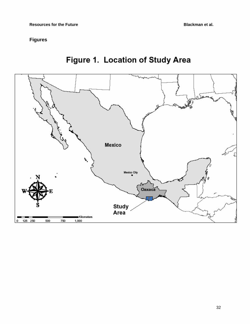
To identify the determinants of land cover in a Mexican shade coffee system, we develop a dichotomous choice model of land clearing in coastal Oaxaca, one of Mexico’s top shade coffee states (Figure 1). The data that underpin this analysis are notable for two reasons. First, whereas most land cover maps are derived from satellite images, ours are derived from high-resolution aerial photographs and are therefore unusually detailed. As a result, we are able to account for the relatively small patches of cleared land characteristic of our study area. Also, we use institutional data (on membership in marketing cooperatives and farm size) along with the geophysical data commonly used in spatial regression models.
We find that, at altitudes where shade coffee grows, plots closer to large coffee market towns and other sizable urban centers are less likely to be cleared, all other things equal—a pattern of land clearing generally not observed in natural forests. In addition, we find that membership in coffee-marketing cooperatives, farm size, and certain soil types are associated with tree cover, while proximity to small town centers is associated with clearing. The remainder of the paper is organized as follows. Section 2 provides additional background on shade coffee and our study area. Section 3 presents a model of land cover decision making. Section 4 discusses our data, and Section 5 presents our regression results. Finally, Section 6 discusses policy prescriptions.
2. Study Area: Definition, Land Uses, and Coffee Production
The Sierra Sur y Costa region in the state of Oaxaca produces about one-fifth of Mexico’s coffee. Our study area consists of a 634,000-hectare subset of this region (Figures 1 and 2). Within our study area, coffee grows in a 254,000-hectare “coffee
3 Shade coffee’s biodiversity benefits are particularly notable. The crop generally grows at altitudes where tropical and temperate climates overlap—areas that are extremely rich in biodiversity. All 14 of Mexico’s main coffee-growing regions have been designated biodiversity “hotspots” by the country’s national commission on biodiversity (Moguel and Toledo 1999).
3
Resources for the Future Blackman et al.
range” lying 400 to 1,600 meters above sea level (m.s.l.). The entire study area comprises 1,155 towns in 43 municipios (counties), and the coffee range comprises 427 towns in 33 municipios. The entire study area includes nine cities with populations exceeding 2,000, the largest of which are Puerto Escondido, Zicatela, Pochutla, Santa María Huatulco, and La Crucecita—all located on the coast. The 7,214-hectare Parque Nacional Huatulco, located just west of La Crucecita, is the only protected area in the larger study area. It lies well below the coffee range.
The vast majority of land inside the coffee range is managed by poor small-scale growers using a mixed agroecosystem comprising shade coffee, shifting subsistence agriculture, and natural forest used for hunting and foraging. In 1991, there were 6,700 to 8,200 coffee farms in our study area, producing approximately 39,000 tons of coffee cherries annually. The lion’s share of these farms was small-scale: 78 percent had less than 5 hectares of coffee. Collectively, shade coffee covered 37,000–53,000 hectares, about 15–21 percent of all of the land in the coffee range and about 18–26 percent of the land in this range with tree cover. Approximately 7 percent of the coffee range, and 15 percent of the entire study area, was planted in noncoffee agriculture. More than two-thirds of this non-coffee agricultural land was planted in corn and about a sixth in beans (CECAFE 1991; INEGI 1994).
According to local stakeholders, virtually all forest clearing within the coffee range results from shifting subsistence agriculture. Shifting systems are used because topsoil on the area’s steep slopes is rapidly eroded by heavy seasonal rainfall once trees are removed.4 Note that shifting subsistence agriculture generates a short-term payoff compared with shade coffee, which remains productive for decades if properly maintained. Under Mexican law, all persons wishing to clear forested land must obtain a federal permit, and in some cases a local permit, regardless of the scale of the clearing (NACEC 2003). However, persons clearing small plots for subsistence agriculture frequently ignore these requirements. Enforcement of forestry laws depends mainly on citizen denunciations of violators and, as a result, is haphazard, especially in remote areas.
4 Our data support anecdotal evidence that shifting subsistence agriculture is responsible for the bulk of deforestation. A comparison of agricultural survey data and our land cover data (discussed below) suggests that, within the coffee range, less than half of the nonurban cleared land was being used for agriculture in the early 1990s. Also, within the coffee range, the majority of the cleared patches are smaller than 1.5 hectares.
4
Resources for the Future Blackman et al.
Coffee grows on small tropical evergreen trees that produce fruit resembling cherries. In our study area, as in all shaded systems, this fruit is picked by hand, typically with the assistance of hired labor. After harvest, the pulp of the cherry is removed using simple, small-scale “wet process” machines and the beans are sorted and dried. Growers transport their beans by donkey or truck to the nearest cabecera (municipio capital), where they sell it to middlemen and marketing cooperatives. From there, the middlemen and cooperatives ship the coffee by truck to one of two large coffee market towns—Oaxaca City or Pochutla—where they sell it to large-scale buyers and exporters. Roads in our mountainous study area are quite poor, and therefore transportation is costly. Because they have to cover the costs of transporting coffee to Oaxaca City or Pochutla, middlemen and cooperatives pay significantly lower prices in cabeceras that are relatively far from these two cities (Ávalos and Becerra 1999). Hence, growers in such areas earn a lower return on their coffee. None of the shade coffee in our study area is certified as such, and as a result, neither growers nor middlemen receive a premium related to this attribute.
3. Model
We model a land manager’s decision to clear tree cover using the conventional “land rent” model modified slightly to highlight land cover instead of land use (Chomitz and Gray 1996; Nelson and Hellerstein 1997; Munroe et al. 2002). The model is premised on the simple idea that any given plot of land may be devoted to a number of competing uses, each of which generates a net rent (return) that depends on the characteristics of the plot, such as its elevation and proximity to agricultural markets, and on the fixed cost of converting it from one land use to another. The land manager chooses the land use—and associated land cover—that generates the highest net rent.
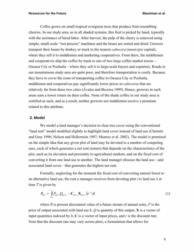
Formally, neglecting for the moment the fixed cost of converting natural forest to an alternative land use, the rent a manager receives from devoting plot i to land use k at time T is given by
( dteQPR tr
ttikTtikTtikTtikTikT
i−∞
=++++∫ −=
0
XC ) (1)
where R is present discounted value of a future stream of annual rents, P is the price of output associated with land use k, Q is quantity of this output, X is a vector of input quantities indexed by h, C is a vector of input prices, and r is the discount rate. Note that the discount rate may vary across plots, a formulation that allows for
5
Resources for the Future Blackman et al.
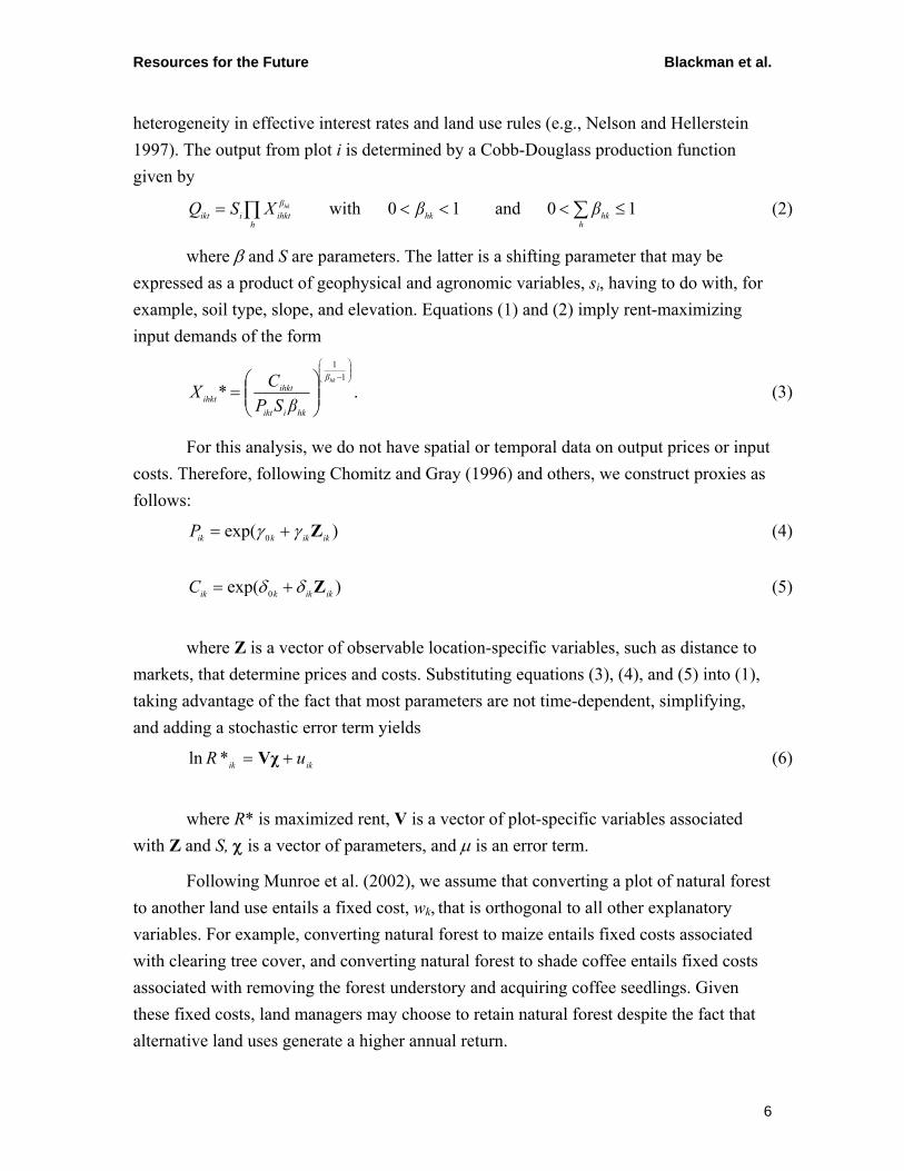
heterogeneity in effective interest rates and land use rules (e.g., Nelson and Hellerstein 1997). The output from plot i is determined by a Cobb-Douglass production function given by
10and10with ≤<<<= ∑∏h
hkhkh
βihktiikt ββXSQ hk (2)
where β and S are parameters. The latter is a shifting parameter that may be expressed as a product of geophysical and agronomic variables, si, having to do with, for example, soil type, slope, and elevation. Equations (1) and (2) imply rent-maximizing input demands of the form
⎟⎟⎠
⎞⎜⎜⎝
⎛−
⎟⎟⎠
⎞⎜⎜⎝
⎛=
11
*hkβ
hkiikt
ihktihkt βSP
CX . (3)
For this analysis, we do not have spatial or temporal data on output prices or input costs. Therefore, following Chomitz and Gray (1996) and others, we construct proxies as follows:
)exp( 0 ikikkikP Zγγ += (4)
)exp( 0 ikikkikC Zδδ += (5)
where Z is a vector of observable location-specific variables, such as distance to markets, that determine prices and costs. Substituting equations (3), (4), and (5) into (1), taking advantage of the fact that most parameters are not time-dependent, simplifying, and adding a stochastic error term yields
ikik uR += Vχ*ln (6)
where R* is maximized rent, V is a vector of plot-specific variables associated with Z and S, χ is a vector of parameters, and µ is an error term.
Following Munroe et al. (2002), we assume that converting a plot of natural forest to another land use entails a fixed cost, wk, that is orthogonal to all other explanatory variables. For example, converting natural forest to maize entails fixed costs associated with clearing tree cover, and converting natural forest to shade coffee entails fixed costs associated with removing the forest understory and acquiring coffee seedlings. Given these fixed costs, land managers may choose to retain natural forest despite the fact that alternative land uses generate a higher annual return.
6
Resources for the Future Blackman et al.
A land manager decides whether to clear tree cover on a plot of land by calculating and then comparing the net returns to different land uses—that is, the present discounted value of a stream of annual returns minus the fixed conversion cost. A land manager will clear the plot when maximum net return to the set of all land uses that involve clearing exceeds the maximum net return to the set of all land uses that do not involve clearing—that is, when
0 ) -(max- ) -(maxFD
≥=∈∈ kikkkikki wR*wR*R (7)
where D is the set of land uses that involve clearing and F is the set of land uses that do not. As discussed above, with rare exceptions, land use within the coffee range of our study area is limited to shifting subsistence agriculture, shade coffee, and natural forest. The first of these land uses requires clearing but the second and third do not. Hence, for most plots inside the coffee range, land managers decide whether to clear by comparing the net return to shifting subsistence agriculture with that to either shade coffee or natural forest.
Combining equations (6) and (7), we have
iR̂ = Wψ + ui (8)
where W is a vector of plot-specific variables associated with Z and S, and ψ is a vector of parameters. Although is latent and unobserved, we observe an indicator
variable, Li, such that iR̂
Li = 1 if > 0 iR̂
Li = 0 if ≤ 0. iR̂
Using this dichotomous dependent variable, equation (8) may be estimated as a probit or logit.
4. Data and Variables
Our land cover data are derived from digitized, distortion-corrected 1993 aerial photographs. We used geographic imaging software (ERDAS Imagine) calibrated by groundtruthing to convert these photographs into digital land cover maps with a two-meter resolution. The maps distinguish among four categories of land cover: presence of
7
Resources for the Future Blackman et al.
trees (includes shade coffee), vegetated but no trees (includes subsistence agriculture), urban, and water.5
Our land cover data’s main advantage is their unusually high resolution. Two limitations deserve mention. First, the data are not intertemporal: we rely on a single digital map to explain spatial patterns of land cover observed at one point in time rather than using two maps from two different years to explain intervening changes in land cover. Although fairly common in the literature (e.g., Nelson and Hellerstein 1997; Cropper et al. 2001), this cross-sectional approach entails the implicit assumption that the entire study area was, at one time, forested and that the observed spatial patterns of land cover were generated by human intervention. This is a reasonable assumption for areas, like ours, characterized throughout by dense forest (versus grassland, scrubland, etc.). A related concern is that we do not know when the clearing that generated the 1993 spatial patterns of land cover took place. As a result, we are not able to control for potential endogeneity by selecting independent variables that predate this clearing. We return to this issue in Section 5.
A second limitation of our land cover data is that it aggregates different land uses into two land cover categories: “cleared” and “noncleared” land. In our case, as noted above, available evidence suggests that while only one land use—subsistence agriculture—constitutes the first category, two land uses—shade coffee and natural forest—constitute the second. Such aggregation is an inherent feature of spatial econometric analyses of land cover, particularly those that use two land cover categories (e.g., Cropper et al 2001; Deininger and Minten 2002; Munroe et al. 2002). It implies that the econometric model measures the “net” effect of plot characteristics on the probability of clearing through the returns to the individual land uses that constitute the land cover categories. Therefore, hypotheses for, and explanations of, the effect of plot characteristics on land cover must be developed accordingly.6
5 The land cover maps also include locations of paved roads and major unpaved roads, the boundaries of municipios, and the locations of town centers. Data on roads and municipio boundaries were supplied by the Instituto Nacional de Estadística Geografía e Informática (INEGI). 6 For example, as discussed below, available evidence suggests that the altitude of a plot of land affects the return to two of the three land uses in our study area: higher altitude boosts the return to shade coffee and lowers the return to row agriculture. Our empirical model estimates the combined effect that altitude has on the probability of clearing through both channels.
8
Resources for the Future Blackman et al.
9
Our land cover map is composed of more than two billion pixels, or “plots,” each of which is 2 meters square. From this population, we constructed a regression sample as follows. First, we superimposed a 500-meter rectangular grid onto the study area and selected the plots where gridlines intersected. Our choice of a 500-meter grid was a compromise between the need for a scale of analysis fine enough to capture the spatial variation in our data set, and one coarse enough accommodate computational constraints. Next, we eliminated all plots classified as either “urban” or “water,” as well as plots for which data needed for the econometric analysis are missing. The resulting sample contains 20,283 2-meter-square plots, of which 7,156 are in the 400–1,600 m.s.l. coffee range.
The independent variable in our econometric analysis, CLEAR, is a dummy that indicates the complete absence of tree cover. That is, CLEAR takes the value of 1 if the plot lacks any tree cover, and 0 otherwise. CLEAR is equal to 0 on plots devoted to shade coffee but is equal to 1 on plots devoted to subsistence agriculture. Note that this definition of clearing does not take into consideration the density of tree cover. For example, CLEAR is equal to 0 both on plots with natural forest and on plots with shade coffee, even though tree cover on shade coffee plots may have been thinned to accommodate coffee bushes.
The independent variables in our econometric analysis are measures of the geophysical characteristics of the sample plots—directional orientation, altitude, slope, terrain, and soil characteristics—and of the characteristics of the farms on these plots—size and membership in marketing cooperatives. Table 1 presents detailed information on all the variables used in the regression analysis, including units, sources, scale, date, and mean values. The table presents means for the two samples used in our econometric analysis—one drawn from the entire study area (n = 20,283) and one drawn from our managed forest ecosystem, the 400–1,600 m.s.l. coffee range (n = 7,156). The remainder of this section describes each of the variables in Table 1 and discusses our a priori expectation as to the correlation of each variable with the probability of clearing inside the coffee range. As discussed in Section 2, this expectation depends, in turn, on the anticipated effect of each variable on the returns to the three land uses that dominate this area.

urces for the Future Blackman et al.
10
Table 1. Variables in the Econometric Analysis: Description and Summary Statistics
Variable Description Units Source Scale Date Mean entire study area Mean coffee range All Forest Cleared All Forest Cleared n=20,283 n=15,344 n= 5,131 n=7,156 n=5,635 n=1,521CLEAR land cleared? (0/1) INEGIa/ERDAS 2 m2 pixels 1993 0.24 0 1 0.21 0 1COF altitude 400-1600 m? (0/1) NIMAb 30 arc secondsc -- 0.35 0.37 0.37 1 1 1ALTIT Altitude m NIMA 30 arc seconds -- 1,058.11 1,092.09 949.21 936.29 931.23 955.05SLOPE Slope degrees NIMA 30 arc seconds -- 7.11 7.27 6.66 8.52 8.49 8.65N_FACE plot north facing? (0/1) NIMA 30 arc seconds -- 0.21 0.22 0.17 0.18 0.20 0.14 MTNS terrain mountainous? (0/1) CONABIOd 1:4,000,000 1992 0.81 0.82 0.80 1 1 1HILLS terrain hilly? (0/1) CONABIO 1:4,000,000 1992 0.10 0.11 0.04 0 0 0PLAINS terrain plains? (0/1) CONABIO 1:4,000,000 1992 0.09 0.07 0.16 0 0 0DIST_CMKT travel time to n./s. paved road hours ARCINFO 10 m2 pixels -- 2.26 2.38 1.88 2.57 2.56 2.57DIST_TWN travel time to nearest town ctr. hours ARCINFO 10 m2 pixels -- 0.50 0.55 0.34 0.45 0.46 0.41DIST_CITY travel time to nearest big city hours ARCINFO 10 m2 pixels -- 2.59 2.65 2.43 2.38 2.30 2.67SOILC_1 soil type: humic acrisol (0/1) CONABIO 1:1,000,000 1995 0.35 0.36 0.34 0.33 0.31 0.40SOILC_2 soil type: eutric cambisol (0/1) CONABIO 1:1,000,000 1995 0.21 0.18 0.31 0.18 0.17 0.23SOILC_3 soil type: rendzina (0/1) CONABIO 1:1,000,000 1995 0.01 0.00 0.01 0.00 0.00 0.00SOILC_4 soil type: haplic phaeozem (0/1) CONABIO 1:1,000,000 1995 0.03 0.03 0.01 0.07 0.08 0.02SOILC_5 soil type: lithosol (0/1) CONABIO 1:1,000,000 1995 0.01 0.01 0.01 0.01 0.02 0.00SOILC_6 soil type: eutric regosol (0/1) CONABIO 1:1,000,000 1995 0.39 0.41 0.32 0.41 0.42 0.34SOILT_1 soil texture: coarse (0/1) CONABIO 1:1,000,000 1995 0.26 0.24 0.28 0.02 0.02 0.01SOILT_2 soil texture: medium (0/1) CONABIO 1:1,000,000 1995 0.57 0.60 0.47 0.84 0.85 0.78SOILT_3 soil texture: fine (0/1) CONABIO 1:1,000,000 1995 0.17 0.15 0.24 0.14 0.12 0.22SOILF_0 soil physical characteristic: none (0/1) CONABIO 1:1,000,000 1995 0.57 0.55 0.62 0.50 0.50 0.53SOILF_5 soil physical characteristic: rock (0/1) CONABIO 1:1,000,000 1995 0.40 0.42 0.37 0.43 0.42 0.45SOILF_6 soil physical characteristic: stony (0/1) CONABIO 1:1,000,000 1995 0.03 0.03 0.01 0.07 0.08 0.02PARK plot in protected area? (0/1) SEMARNATe 1:1,000,000 1998 0.01 0.01 0 0 0 0COOP % coffee growers in coops. % CECAFEf municipio 1991 n/a n/a n/a 55.74 56.18 54.10FSIZE % coffee land on farms > 10 has. % CECAFE municipio 1991 n/a n/a n/a 46.66 48.55 39.65
aInstituto Nacional de Estadística Geografía e Informática (Mexico); bNational Imagery and Mapping Agency (USA); cApproximately 1 kilometer; dComisión Nacional para el Conocimiento y Uso de la Biodiversidad (Mexico); eSecretária de Medio Ambiente y Recursos Naturales (Mexico); fConsejo Estatal del Café de Oaxaca (Mexico)
Reso
Resources for the Future Blackman et al.
Of the independent variables in our regressions, the geophysical variables can be considered arguments of the production function shift parameter in the land rent model. N_FACE is a dummy that takes the value of 1 if the plot faces north, and 0 otherwise. Because Mexico is north of the equator, north-facing plots receive less direct sunlight and are relatively ill-suited to conventional row agriculture. Such plots also tend to be more humid, a characteristic that makes them particularly well-suited to shade coffee. Hence, we expect N_FACE to be negatively correlated with the probability of clearing, all other things equal.
In our study area—as in most coastal mountain ranges—altitude is highly correlated with both temperature and precipitation. Therefore, ALTIT, our altitude variable, is essentially a proxy for weather conditions. The best grades of coffee grow at higher altitudes, where lower temperatures cause the beans to mature more slowly. As a result, coffee farmers at higher altitudes in the coffee range earn higher rents on their crop. By contrast, conventional agriculture is generally less productive at higher altitudes. Thus, we expect ALTIT to be negatively correlated with the probability of clearing, all other things equal.
We include four topographical variables: SLOPE, a continuous variable measured in degrees, and three terrain dummy variables—MOUNTAINS, PLAINS, and HILLS. Of these topographical variables, only slope varies within the coffee range: all the land above 400 meters in our study area—including the entire coffee range and the land north of it—is classified as mountains, while the coastal area is split between plains in the west and hills in the east. We have no strong expectation about the sign of SLOPE inside the coffee range.
We use data on three soil attributes: type (SOILC_1 through SOILC_6), texture (SOILT_1 through SOILT_3), and physical characteristics (SOILF_0, SOILF_5 and SOILF_6). The meanings of these variables are listed in Table 1. Appendix 1 provides a more extensive discussion. Because many soils that are well suited to agriculture are also well suited to coffee, we do not have a strong expectation as to how the soil variables affect the probability of clearing inside the coffee range.
Finally, we use three impedance-weighted distance variables that are determinants of input and output prices: distance to the nearest town center (DIST_TWN), distance to the nearest city with a population greater than 2,000 (DIST_CITY), and distance from the nearest cabecera to the nearest coffee market town (DIST_CMKT). We have parameterized our weighting algorithm so that these distances approximate travel times in hours. Appendix 2 provides a more extensive discussion of this algorithm.
11
Resources for the Future Blackman et al.
The DIST_CMKT variable requires a brief explanation. As noted in Section 2, because middlemen and cooperatives must cover the costs of transporting coffee from cabeceras to one of the two coffee market towns in the state—Oaxaca City and Pochutla—the prices they pay to individual growers depend on the distance from the relevant cabecera to the relevant coffee market town. Cabeceras are not associated with specific coffee market towns. In any given year in any given cabecera, middlemen and cooperatives may ship coffee to both towns, depending on market conditions and the availability of transportation. Regardless of which market town they use, however, middlemen and cooperatives always first ship coffee from the cabecera to the one paved road connecting Oaxaca City in the north with Pochutla in the south (Figure 2). This first leg of the trip over rugged dirt roads typically accounts for the lion’s share of the cost of transporting coffee to market. Hence, our plot-specific proxy for distance to coffee markets is the weighted distance from the nearest cabecera to the north-south paved road.
Of the three distance variables, we have an unambiguous expectation about the sign of only one. Within the coffee range, we expect DIST_CMKT to be positively correlated with the probability of land clearing because the growers located far from coffee market towns receive relatively low prices for their crop and, therefore, earn relatively low rents on coffee farming. DIST_CMKT should not affect the return to either subsistence agriculture or natural forest.
By comparison, the expected effect of DIST_CITY on the probability of land clearing is complex. DIST_CITY affects the probability of land clearing through at least two channels: one has to do with transportation costs and the second with the effective cost of cleared land. DIST_CITY has countervailing impacts on the probability of clearing through the first channel. On the one hand, proximity to a relatively big city boosts the return to shade coffee because some coffee inputs are purchased there—most notably the labor used to harvest coffee. During the off-season, itinerant coffee laborers tend to live in cities, where nonfarm job opportunities are relatively plentiful. On the other hand, proximity to the nearest big city could also boost the return to conventional (nonagroforestry) agriculture because cities are markets for both agricultural inputs and outputs. The first effect implies that all other things equal, shade coffee—and therefore tree cover—is more likely to be found near big cities. The second effect implies that all other things equal, agriculture—and therefore cleared land—is more likely to be found near big cities. We expect the first effect to dominate the second because most conventional crops in our study area are grown for subsistence, not for sale in urban areas, and are produced mainly with household labor. Therefore, we do not expect a strong correlation between DIST_CITY and the return to conventional agriculture.
12
Resources for the Future Blackman et al.
DIST_CITY may also affect relative returns to alternative land uses by changing the effective cost of cleared land. Plots cleared without required permits that are closer to big cities are more likely to attract citizen denunciations and, therefore, the attention of regulatory authorities, in part simply because such authorities are located in big cities. Hence, the effective cost of cleared land may be higher near big cities. This implies that, all other things equal, cleared plots are less likely to be found near cities. Thus, DIST_CITY may have varied countervailing effects on the probability of clearing. Its net effect is an empirical question.
The same complex relationship between DIST_CITY and the probability of clearing applies to DIST_TWN, but with one caveat. As noted above, big cities—not smaller towns—are the primary repository for seasonal coffee labor. Hence, proximity to town centers may have less impact on the return to coffee—and on the probability of tree cover—than does proximity to cities.
In addition to variables that measure geophysical characteristics, we include two variables related to farm characteristics that are drawn from a 1991 municipio-level survey of coffee growers. COOP is the percentage of the coffee growers in each municipio who belong to marketing cooperatives. Cooperative members generally obtain a higher return on coffee than nonmembers for two reasons. First, they receive higher prices for their coffee than non-members because cooperatives tend to control quality better than independent growers and have more bargaining power vis-à-vis middlemen than do independent growers—in fact, some sell directly to exporters. Second, cooperative members typically pay lower prices for inputs than nonmembers because cooperatives generally subsidize postharvest processing, quality control, and agricultural extension. Hence, we expect COOP to be negatively correlated with the probability of clearing within the coffee range, all other things equal.
FSIZE is the percentage of coffee acreage in each municipio found on farms larger than 10 hectares. Anecdotal evidence suggests that the production and (especially) the marketing of shade coffee entail economies of scale. Hence, in terms of our model, FSIZE can be thought to affect the productivity of shade coffee. We expect it to be negatively correlated with the probability of clearing, all other things equal.
Finally, PARK is a dummy variable that indicates whether the plot is located in the one protected area in our study region. As noted above, this park is on the coastal plain, well outside the coffee range (Figure 2).
13
Resources for the Future Blackman et al.
5. Methods and Results
A common problem in spatial econometric models of land cover is spatial autocorrelation—the correlation of land cover on any given plot with that on neighboring plots (Anselin 2002). It may arise from spillovers among the dependent variables or from spillovers among the error terms. In the first case, land cover decisions on any given plot influence decisions on neighboring plots—for example, because land managers learn about cultivation or logging opportunities and techniques from their neighbors. In the second case, unobserved drivers of land cover—for example, the existence of socioeconomic networks among land managers—are correlated across space. Both phenomena may be an issue in our data. Many neighboring plots in our study area are on the same ejido or communidade—communal land tenure institutions consisting of individual farms (Brown 2004).7
Spatial autocorrelation generates heteroskedastic errors. As a result, standard discrete choice estimators will be inconsistent. In addition, such estimators will be inefficient because they assume independent errors and, therefore, ignore the information in the off-diagonal terms of the variance-covariance matrix (Fleming 2004). Using the sample drawn from inside the coffee range, we tested for spatial autocorrelation using Moran’s I test modified for probit (Kelejian and Prucha 2001). This test rejected the null hypothesis of no spatial autocorrelation at the 1 percent level.
To correct for spatial autocorrelation, we used the Bayesian heteroskedastic spatial autoregressive procedure for logit detailed in LeSage (2000). A key challenge in generating consistent and efficient estimators in the presence of spatial autocorrelation is the need to evaluate an n-dimensional integral in the course of solving the likelihood function. To overcome this problem, the LeSage procedure uses a Gibbs sampling (Markov chain Monte Carlo) simulation method based on the general concept that a large sample of parameter values in the posterior distribution can be used to estimate a probability density function for the parameters. This procedure generates unbiased estimates of standard errors for all model parameters (see
7 More than three-quarters of the land in our study area is under ejido or communidade tenure. The average size of an ejido/comunidade in our study is roughly 10,000 hectares (INEGI 1991). A 10,000-hectare ejido/commuidade could contain as many as 400 sample plots. On very large farms in our study area, some neighboring plots are likely to be on both the same ejido/commuidade and on the same farm. Only about a third of the farms in our study area are larger than 5 hectares, but these farms constitute 51 percent of all the land in our study area that is planted in coffee (CECAFE 1991). A 25-hectare farm could contain one to four sample plots.
14
Resources for the Future Blackman et al.
Fleming 2004 for a detailed discussion of the LeSage model and a comparison with competing procedures).
To estimate any spatial error model, including ours, it is necessary to make assumptions about the unobserved error process—that is, the structure of the spatial weights matrix (see Anselin 2006 for a discussion). We have no strong expectations about the characteristics of the spatial error process that would lead us to favor any particular structure. In Table 2, we report results from models that used Delaunay triangulation to generate the spatial weights matrix—the default method for the LeSage procedure.8 However, we also experimented with two alternative methods. We return to this issue at the end of Section 5.1.
We employ four econometric models. Models 1, 2, and 3 seek to identify the determinants of forest clearing inside the coffee range. Therefore, they use the 7,156 plots in our sample located between 400 and 1,600 meters in altitude and exclude the variables in Table 1 that are not relevant for this range (MTNS, HILLS, PLAINS, and PARK). Model 1 is a simple probit. Model 2 corrects for spatial autocorrelation using the procedure described above. Model 3 also corrects for spatial autocorrelation but excludes two potentially endogenous regressors. Finally, Model 4 tests whether the determinants of land clearing are the same inside the coffee range as outside it. It uses the entire sample of 20,283 plots in the study area and corrects for spatial autocorrelation.
5.1. Determinants of Forest Clearing Inside the Coffee Range
Table 2 presents our regression results. Qualitatively, the results for the simple probit (Model 1) and the model that corrects for spatial autocorrelation (Model 2) are virtually identical. We focus on the latter.
8 The Delaunay triangulation method defines the “neighbors” of plot i (i.e., the plots that influence i) as those plots that can be connected to i with a set of triangles such that i is at one corner, neighbors are at the other two corners, and circles drawn around all three corners of each triangle do not contain any other sample plots. All neighbors are assumed to have the same effect on i. Because the plots in our sample are arranged in a regular rectangular grid, this method returns 6 or 8 of the plots nearest to i, depending on stochastic features of the computational routine.
15
Resources for the Future Blackman et al.
Table 2. Regression Results (dependent variable = CLEAR)
Model 1 probit
coffee range only
Model 2 logit with spatial error
correctiona coffee range only
Model 3 logit with spatial error
correctiona coffee range only
Model 4 logit with spatial error
correctiona entire study area
n=7,156 n=7,156 n=7,156 n=20,283 Variable Coeff. (s.e.) M.E. Coeff. (s.e.) M.E. Coeff. (s.e.) Coeff. (s.e.) Constant -0.3223 (0.2324) -0.1225 (0.2330) -0.9561** (0.1781) -0.3955** (0.0979)
COF -0.7211** (0.2332) ALTIT -0.1788** (0.0719) -0.0491 -0.1195* (0.0702) -0.0277 -0.0434 0.0725 -0.1257** (0.0365)
ALTIT*COF 0.0823 (0.0795) SLOPE 0.1509** (0.0500) 0.0415 0.1108* (0.0551) 0.0257 0.0951* (0.0556) 0.0199 (0.0395)
SLOPE*COF 0.0826 (0.0686) N_FACE -0.2627** (0.0485) -0.0669 -0.1983** (0.0510) -0.0459 -0.1981** (0.0514) -0.1280** (0.0357)
N_FACE*COF -0.0827† (0.0582) HILLS -0.3834** (0.0592)
PLAINS 0.1542** (0.0521) DIST_CMKT 0.0422** (0.0140) 0.0116 0.0325** (0.0141) 0.0075 0.0383** (0.0143) -0.0227* (0.0118)
DIST_CMKT*CF 0.0667** (0.0199) DIST_TWN -0.6179** (0.0671) -0.1698 -0.4129** (0.0703) -0.0956 -0.4082** (0.0669) -0.4487** (0.0438)
DIST_TWN*COF 0.0227 (0.0772) DIST_CITY 0.0819** (0.0207) 0.0225 0.0465** (0.0206) 0.0108 0.0634** (0.0195) 0.0879** (0.0196)
DIST_CITY*CF -0.0188 (0.0269) SOILC_2 0.3649** (0.0949) 0.1099 0.2619** (0.0988) 0.0607 0.1685* (0.0934) 0.2173** (0.0882)
SOILC_2*COF -0.0420 (0.1315) SOILC_3 1.3781** (0.3673) 0.5025 1.1157** (0.4506) 0.2584 0.6789† (0.4353) 0.7662** (0.1406)
SOILC_3*COF -0.2326 (0.4818) SOILC_4 -0.5505** (0.1049) -0.1201 -0.2944** (0.0940) -0.0682 -0.2692** (0.0948) 0.0922 (0.1820)
SOILC_4*COF -0.3770* (0.2183) SOILC_5 -1.2571** (0.3802) -0.1809 -0.5872** (0.2559) -0.1360 -0.5474** (0.2165) -0.1217 (0.1242)
SOILC_5*COF -0.4710* 0.2604 SOILC_6 0.0406 (0.0713) 0.0112 0.0344 (0.0720) 0.0080 0.0166 (0.0712) 0.1697* (0.0864)
SOILC_6*COF -0.1653† (0.1164) SOILT_2 0.1766 (0.1844) 0.0460 0.0495 (0.1724) 0.0115 0.3145* (0.1653) 0.0043 (0.0481)
SOILT_2*COF 0.4051* (0.2131) SOILT_3 0.3949* (0.1967) 0.1209 0.199815 (0.1937) 0.0463 0.5326** (0.1759) 0.2460** (0.0743)
SOILT_3*COF 0.4173* (0.2221) SOILF_5 -0.4480** (0.0813) -0.1195 -0.3278** (0.0893) -0.0759 -0.0118 (0.0635) -0.0680* (0.0415)
SOILF_5*COF 0.0708 (0.0819) PARK -0.2106* (0.0380) COOP -0.2139** (0.0633) -0.0588 -0.1571** (0.0666) -0.0364 FSIZE -0.8605** (0.0861) -0.2365 -0.5811** (0.0946) -0.1346
Pseudo-R^2 0.0648 0.2349 0.1879 0.3375
aLeSage (2000) procedure with Delaunay triangulation spatial weights matrix ** significant at 1% level two tailed test * significant at 5% level two tailed test † significant at 10% level two tailed test
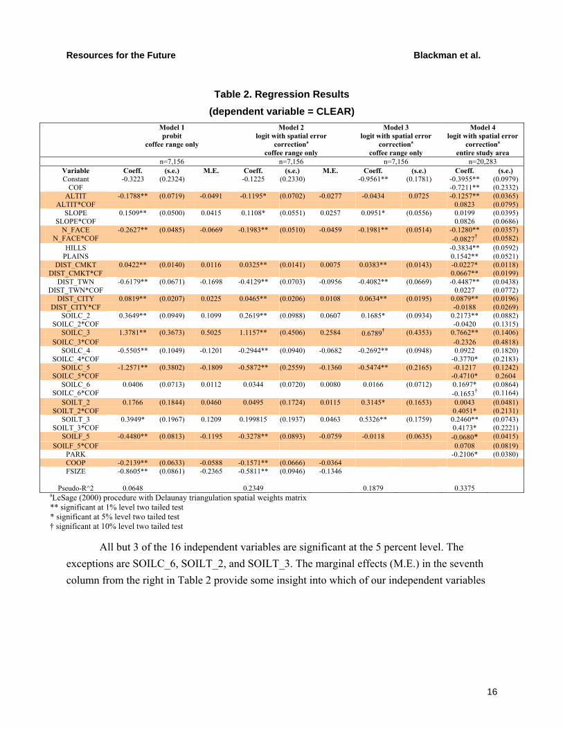
All but 3 of the 16 independent variables are significant at the 5 percent level. The exceptions are SOILC_6, SOILT_2, and SOILT_3. The marginal effects (M.E.) in the seventh column from the right in Table 2 provide some insight into which of our independent variables
16
Resources for the Future Blackman et al.
are most important economically.9 The signs of most of the coefficients are as expected. Of the regression results for the geophysical variables, the most interesting concern distance. As expected, DIST_CMKT is positively correlated with the probability of clearing. In other words, plots closer to coffee market towns are less likely to be cleared, all other things equal. This finding is the opposite of the standard result for natural forests. DIST_CITY is also positively correlated with the probability of land clearing, although this result must be interpreted cautiously because, as discussed below, it is sensitive to the specification of the spatial weights matrix. As noted in Section 4, this relationship likely stems from the fact that proximity to cities lowers transportation costs for coffee inputs (especially labor) and raises the effective cost of cleared land. DIST_TWN, however, is negatively correlated with the probability of clearing. Here, the conventional relationship between distance to urban areas and clearing holds.
With regard to the remaining geophysical variables, as expected, both N_FACE and ALTIT are negatively correlated with the probability of clearing. SLOPE is positively correlated with the probability of clearing. This last result contrasts with the typical finding for natural forests—in such forests, conventional agriculture is usually found on flat land.10
Five of the soil dummies are significant. SOILF_5, the soil physical characteristics dummy for rock, is negatively correlated with the probability of clearing, as is SOILC_5, the soil type dummy for lithosol, a particularly shallow soil. Presumably, neither coffee nor conventional crops are found on these soils. Both SOILC_2, the soil type dummy for eutric cambisol, and SOILC_3, the soil type dummy for rendzina, are positively correlated with the probability of clearing. This may reflect the fact that although both conventional crops and coffee can be grown on these soils, they are better suited to the former than the latter—eutric cambisol has a high clay content that inhibits coffee root growth, and rendzina is high in calcium carbonate, which can interfere with coffee nutrient uptake. Finally, SOILC_4, the soil type dummy for haplic phaeozem—generally considered the best soil type for both coffee and conventional agriculture—is negatively correlated with the probability of clearing. Presumably, in the coffee range, such soils are typically planted in coffee. Thus, conventional thinking about the types of
9 For the continuous variables, the marginal effect is the percentage change in the probability of clearing due to a one unit increase in the independent variable. For dummy variables, the marginal effect is the percentage change in the probability of clearing when the dummy is 1 instead of 0. Given this difference, caution must be exercised when comparing marginal effects for the two types of variables. 10 But note that our result is consistent with Chomitz and Gray (1996), who find that in Belize, semisubsistence agriculture is more likely to be found on land that is not flat, all other things equal.
17
Resources for the Future Blackman et al.
18
soils that promote clearing in natural forests does not necessarily hold in our study area. As in natural forests, particularly poor soils (e.g., rocky and shallow soils) are not associated with clearing. However, the “best” soils (e.g., haplic phaeozem) appear to attract coffee rather than conventional agriculture. Therefore, in contrast to natural forests, such soils are associated with tree cover, not clearing.
As for the nongeophysical variables, both have the expected sign. COOP and FSIZE are both negatively correlated with the probability of clearing, all other things equal. However, unlike our other regressors, which reflect unchanging geophysical characteristics of the sample plots, COOP and FSIZE reflect the season-by-season decision making of land managers. Therefore, these variables may be endogenous; that is, each may be simultaneously determined with CLEAR. We test for endogeneity using the standard procedure for limited dependent variables (Smith and Blundell 1986). The procedure, which is described in detail in Appendix 3, indicate that the null hypothesis of exogeneity cannot be rejected.11 However, the interaction between spatial autocorrelation and endogeneity is complex (Irwin and Bockstael 2001). Therefore, Model 3 omits the two potentially endogenous regressors. The qualitative results are the same as in Model 2 with minor exceptions (ALTIT is significant in Model 2 but not in Model 3, and SOILT_2 and SOILT_3 are significant in Model 3 but not in Model 2).
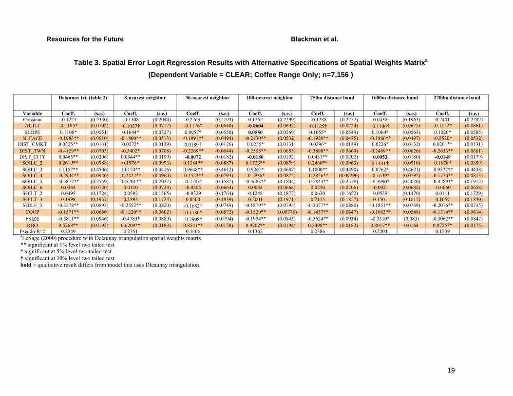
As noted above, although Model 2 used Delaunay triangulation to generate the spatial weights matrix, we also experimented with two alternative methods to test the robustness of our results: nearest neighbor matrices and distance band matrices.12 Table 3 reports the results. Eight-nearest neighbor and 750-meter distance band matrices generated results that were qualitatively identical to those reported in Table 2. At the other end of the spectrum, 100-nearest neighbor and 2,700-meter distance band matrices—the upper bound of computational feasibility given our hardware—also generated results that, qualitatively, were very similar to those in
11 The Smith and Blundell (1986) procedure involves two stages. In the first stage, each potentially endogenous variable is regressed onto a set of instrumental variables along with the remaining independent variables. In the second stage, CLEAR is regressed onto the residuals from the first-stage regressions along with predicted values of the potentially endogenous regressors from the first stage and the remaining independent variables. Under the null hypothesis of exogeneity, the residuals from the first stage should have no explanatory power. To instrument for COOP and FSIZE, we used HA_MUN_P, hectares in ejidos/comunidades, as a percentage of total land area by municipio, and P15NR, the adult literacy rate by town. 12 Distance band matrices define neighbors as plots within a specified distance from plot i, and k-nearest neighbors matrices define neighbors as the k plots closest to i. In our experiments with these methods, we assumed all neighbors have the same effect on i.
urces for the Future Blackman et al.
19
Table 3. Spatial Error Logit Regression Results with Alternative Specifications of Spatial Weights Matrixa (Dependent Variable = CLEAR; Coffee Range Only; n=7,156 )
Delaunay tri. (table 2) 8-nearest neighbor 36-nearest neighbor 100-nearest neighbor 750m distance band 1600m distance band 2700m distance band
Variable Coeff. (s.e.) Coeff. (s.e.) Coeff. (s.e.) Coeff. (s.e.) Coeff. (s.e.) Coeff. (s.e.) Coeff. (s.e.) Constant -0.1225 (0.2330) -0.1108 (0.2044) 0.2269 (0.2193) 0.1262 (0.2299) -0.1288 (0.2252) 0.0438 (0.1963) 0.2401 (0.2202)ALTIT -0.1195* (0.0702) -0.1057† (0.0717) -0.1176* (0.0640) -0.0604 (0.0692) -0.1125† (0.0724) -0.1106† (0.0675) -0.1152* (0.0661) SLOPE 0.1108* (0.0551) 0.1044* (0.0527) 0.0957* (0.0550) 0.0550 (0.0569) 0.1055* (0.0549) 0.1060* (0.0563) 0.1020* (0.0585)
N_FACE -0.1983** (0.0510) -0.1800** (0.0513) -0.1991** (0.0494) -0.2430** (0.0532) -0.1920** (0.0475) -0.1886** (0.0497) -0.2520* (0.0532) DIST_CMKT 0.0325** (0.0141) 0.0272* (0.0139) 0.0189† (0.0126) 0.0255* (0.0131) 0.0296* (0.0139) 0.0226* (0.0132) 0.0261** (0.0131)DIST_TWN -0.4129** (0.0703) -0.3402* (0.0708) -0.2269** (0.0644) -0.2555** (0.0655) -0.3898** (0.0669) -0.2469** (0.0626) -0.2633** (0.0661) DIST_CITY 0.0465** (0.0206) 0.0344** (0.0199) -0.0072 (0.0182) -0.0180 (0.0192) 0.0431** (0.0202) 0.0053 (0.0180) -0.0149 (0.0179)
SOILC_2 0.2619** (0.0988) 0.1976* (0.0993) 0.1384** (0.0887) 0.1733** (0.0879) 0.2468** (0.0963) 0.1441† (0.0910) 0.1678* (0.0859) SOILC_3 1.1157** (0.4506) 1.0174** (0.4416) 0.9648** (0.4612) 0.9261* (0.4687) 1.1000** (0.4490) 0.8762* (0.4621) 0.9577** (0.4438) SOILC_4 -0.2944** (0.0940) -0.2422** (0.0960) -0.1523** (0.0793) -0.1936* (0.0872) -0.2856** (0.09290) -0.1639* (0.0792) -0.1770** (0.0813) SOILC_5 -0.5872** (0.2559) -0.5701** (0.2037) -0.2783* (0.1582) -0.4663** (0.1804) -0.5843** (0.2558) -0.3990* (0.2020) -0.4289** (0.1912)SOILC_6 0.0344 (0.0720) 0.0110 (0.0724) -0.0205 (0.0664) 0.0044 (0.0668) 0.0250 (0.0706) -0.0021 (0.0682) -0.0060 (0.0658) SOILT_2 0.0495 (0.1724) 0.0592 (0.1565) -0.0329 (0.1764) 0.1248 (0.1877) 0.0630 (0.1652) 0.0539 (0.1470) 0.0111 (0.1729)SOILT_3 0.1998 (0.1937) 0.1893 (0.1724) 0.0500 (0.1839) 0.2001 (0.1971) 0.2115 (0.1857) 0.1501 (0.1617) 0.1057 (0.1840) SOILF_5 -0.3278** (0.0893) -0.2552** (0.0820) -0.1682† (0.0749) -0.1879** (0.0795) -0.3077** (0.0880) -0.1851** (0.0749) -0.2076** (0.0735)
COOP -0.1571** (0.0666) -0.1220** (0.0602) -0.1180† (0.0572) -0.1529** (0.05776) -0.1457** (0.0647) -0.1083** (0.0548) -0.1314** (0.0614) FSIZE -0.5811** (0.0946) -0.4785* (0.0889) -0.2908† (0.0794) -0.1954** (0.0843) -0.5624** (0.0934) -0.3310* (0.083) -0.3062** (0.0847)RHO 0.5268** (0.0193) 0.6209** (0.0183) 0.8541** (0.0158) 0.9202** (0.0194) 0.5498** (0.0183) 0.8017** 0.0164 0.8725** (0.0175)
Pseudo-R^2 0.2349 0.2351 0.1406 0.1362 0.2386 0.2204 0.1239aLeSage (2000) procedure with Delaunay triangulation spatial weights matrix ** significant at 1% level two tailed test * significant at 5% level two tailed test † significant at 10% level two tailed test bold = qualitative result differs from model that uses Dleaunay triangulation.
Reso
Resources for the Future Blackman et al.
Table 2, with the exception DIST_CITY, which was not significant in either regression and ALTIT and SLOPE which were not significant in the 100-nearest neighbor regression.
An alternative approach to correcting for spatial autocorrelation is spatial sampling, that is, selecting a sample comprised of plots at sufficient distance from one another that spatial autocorrelation is not a concern (Nelson and Hellerstein 1997; Carrión Flores and Irwin 2004). As discussed in Appendix 4, we are not able to use this approach because spatial samples continue to exhibit spatial autocorrelation.
5.2. Determinants of Forest Clearing Inside Versus Outside the Coffee Range
Model 4 uses a sample of 20,283 plots drawn from the entire study area (including plots located above and below the coffee range) to test whether the determinants of land clearing inside the coffee range are the same as those outside it. The model includes a dummy variable, COF, that identifies plots located inside the coffee range, as well as COF interaction terms for each regressor. Significance tests for the individual interaction terms indicate the extent to which each regressor has a different effect on the probability of clearing inside the coffee range versus outside.
Interaction terms aside, the specification of Model 4 differs slightly from that of Model 2. Model 4 omits COOP and FSIZE, which are not meaningful outside the coffee range, where there are no coffee farms, and includes three new dummy variables—PARK, HILLS, and PLAINS—that describe institutional and geophysical characteristics not found inside the coffee range.13 Table 2 presents the regression results for Model 4. First, note that COF is negatively correlated with the probability of clearing, all other things equal. Thus, as expected, shade coffee is associated with tree cover.
Of the geophysical variables, DIST_CMKT is negatively correlated with the probability of clearing. However, DIST_CMKT*COF is positively correlated with the probability of clearing, and its coefficient is almost three times that for DIST_CMKT. Thus, DIST_CMKT has a different effect inside the coffee range than it does outside it. Inside, plots closer to coffee
13 These differences in specification prevent us from using interaction terms to imbed Models 3 and 4. The omission of COOP and FSIZE in Model 4 may give rise to specification bias. However, as the results from Model 3 indicate, omitting COOP and FSIZE changes the magnitude and significance of the remaining coefficients very little, with the exception of several of the soil variables and ALTIT. This finding suggests that the omitted-variables bias is not severe.
20
Resources for the Future Blackman et al.
markets tend to be forested, while outside, such plots tend to be cleared—the conventional result for natural forests.
Unlike DIST_CMKT, both DIST_TWN and DIST_CITY have the same effect on the probability of clearing inside and outside the coffee range. DIST_TWN is negatively correlated with the probability of clearing, while the coefficient on DIST_TWN*COF is insignificant. DIST_CITY is positively correlated with the probability of clearing, while the coefficient on DIST_CITY*COF is insignificant. Thus, regardless of whether they are located inside the coffee range or outside, plots closer to town centers are more likely to be cleared, all other things equal, while plots closer to big cities are less likely to be cleared, all other things equal.
DIST_CITY merits a brief discussion. As noted above, DIST_CITY affects the probability of land clearing through transportation costs and through the effective cost of cleared land. Inside the coffee range, proximity to cities boosts the return to shade coffee by lowering the cost of seasonal agricultural labor, and it raises the effective cost of cleared land because restrictions on clear cutting are more likely to be enforced close to big cities. Both factors imply that, all other things equal, inside the coffee range one would expect to find tree cover in close proximity to cities. Outside the coffee range, the transportation costs effect does not come into play, but the enforcement effect does. Presumably, this second effect explains the effect of DIST_CITY outside the coffee range.
Of the remaining geophysical variables, some have different effects on the probability of clearing inside the coffee range, and others do not. The coefficient on N_FACE is negative and significant, as is the coefficient on N_FACE*COF, albeit weakly. Thus, the negative correlation between N_FACE and the probability of clearing is stronger inside the coffee range than outside it, a result that may stem from the relatively high opportunity costs of clearing inside the coffee range.
The coefficient on SLOPE is positive and insignificant as is the coefficient on SLOPE*COF. Thus, this model suggests that SLOPE has no discernible impact on the probability of clearing. This result could arise if slope is not correlated with the probability of clearing outside the coffee range.
ALTIT is negatively correlated with the probability of clearing, all other things equal, while the coefficient on ALTIT*COF is insignificant. Thus, the effect of ALTIT is the same inside and outside the coffee range: plots at higher elevations are less likely to be cleared, all other things equal. Outside the coffee range, this effect likely stems from the fact that low-lying plots are better suited to conventional agriculture and ranching.
21
Resources for the Future Blackman et al.
Of the eight soil variables, our results suggest that four—SOILC_4, SOILC_5, SOILC_6, SOILT_2, and SOILT_3—have different effects on the probability of clearing inside the coffee range than they do outside it. For example, SOILC_3, a dummy indicating the presence of rendzina, is insignificant. However, the coefficient on SOILC_3*COF is negative and significant. These results suggest that the presence of rendzina has no effect on the probability of clearing outside the coffee range but is associated with tree cover inside it. Given that many of the soil types and characteristics that promote agriculture also promote shade coffee, explanations for these differential effects are necessarily somewhat speculative. The general result is useful, however: soil characteristics may have different impacts on land cover in a managed forest ecosystem than in a natural forest.
The remaining covariates in Model 4—PARK, HILLS, and PLAINS—relate to characteristics of the study region outside the coffee range. PARK is negative and significant, a result that suggests that the one protected area in our study region has succeeded in preserving tree cover. HILLS is negatively correlated with the probability of clearing, and PLAINS is positively correlated with the probability of clearing.
6. Conclusion
We have used a set of spatial regression models to identify the determinants of tree cover in a region dominated by a managed forest ecosystem. Our results suggest that in such systems, the determinants differ from those in natural forests in several ways. In natural forests, proximity to urban centers as well as price and cost advantages for agricultural goods have been repeatedly linked to tree clearing. However, we find that in a managed forest ecosystem, these factors reduce the probability of clearing when the urban centers in question are also major markets for a nontimber agroforestry crop, and when the price and cost advantages in question are associated with that crop. Also, we find that soil types and certain topographical features linked with clearing in natural forests are instead associated with tree cover in a managed forest ecosystem. Several of our other findings are consistent with the literature on land cover in natural forests. We find that forest clearing is associated with proximity to small town centers and the directional orientation of land.
These findings suggest that at least two “conventional” policy prescriptions for preserving tree cover—that is, policy prescriptions based on studies of natural forests—may not hold in managed forest ecosystems. First, in natural forests, transportation investments that improve access to markets are generally thought to exacerbate deforestation. Our results suggest that in managed forest ecosystems, however, such investments could help to stem deforestation
22
Resources for the Future Blackman et al.
by raising the net return to agroforestry systems that preserve tree cover. The impact on tree cover of road building is likely to be complex, however. More and better roads will inevitably improve access to output and input markets for conventional agricultural goods and timber, as well as to markets for nontimber agroforestry crops. The net effect on tree cover is uncertain. Other means of improving market access, such as subsidizing or improving transportation services targeted specifically at producers of nontimber agroforestry crops, may have less ambiguous impacts.
Second, in natural forests, agricultural policies intended to benefit farmers, such as promoting marketing cooperatives and subsidizing inputs, are generally thought to promote forest clearing. Our results suggest that in a managed forest ecosystem, however, such policies may help preserve tree cover when the agricultural good in question is a nontimber agroforestry crop.
23
Resources for the Future Blackman et al.
References
Anselin, L. 2002. Under the Hood: Issues in the Specification and Interpretation of Spatial Regression Models. Agricultural Economics 17(3): 247–267.
Anselin, L. 2006. Spatial Econometrics. In T.C. Mills and K. Patterson, eds., Palgrave Handbook of Econometrics: Volume 1, Econometric Theory. Basingstoke, England: Palgrave Macmillan, 901–969.
Ávalos-Sartorio, B., and M. del R. Becerra Ortiz. 1999. La Economía de la Producción y Comercialización del Café en la Sierra Sur, Costa e Istmo del Estado de Oaxaca: Resultados Preliminares. Ciencia y Mar 3(8): 29–39.
Brown, J. 2004. Ejidos and Comunidades in Oaxaca, Mexico: Impact of the 1992 Reforms. Report on Foreign Aid and Development #120. Seattle, WA: Rural Development Institute.
Carrion-Flores, C., and E. Irwin. 2004. Determinants of Residential Land Use Conversion and Sprawl at the Rural-Urban Fringe. American Journal of Agricultural Economics 86: 889–904.
Consejo Estatal del Café de Oaxaca (CECAFE). 1991. Censo de Cultivadores del Café. Oaxaca, Mexico: CECEFE.
Commission for Environmental Cooperation. 2005. Annotated Bibliography: CEC Publications and Work on Shade-grown Coffee and Biodiversity in North America. Montreal: Commission for Environmental Cooperation.
Chomitz, K., and D. Gray. 1996. Roads, Land Use, and Deforestation: A Spatial Model Applied to Belize. World Bank Economic Review 10(3): 487–512.
Cropper, M., J. Puri, and C. Griffiths. 2001. Predicting the Location of Deforestation: The Role of Roads and Protected Areas in North Thailand. Land Economics 77(2): 172–186.
Deininger, K., and B. Minten. 2002. Determinants of Deforestation and the Economics of Protection: An Application to Mexico. American Journal of Agricultural Economics 84(4): 943–960.
24
Resources for the Future Blackman et al.
Eswaran, H. 2002. USDA Natural Resources Conservation Service. Personal Communication with Lisa Crooks. Nov. 26.
Fleming, M. 2004. Techniques for Estimating Spatially Dependent Discrete Choice Models. In L. Anselin, R. Floraz, and S. Rey, eds., Advances in Spatial Econometrics. Cambridge, MA: Springer Press, 145–167.
Food and Agriculture Organization of the United Nations (FAO). 1998. World Reference Base for Soil Resources: Introduction. World Soil Resources Report 84. Rome: FAO.
Gajaseni, J., R. Matta-Machado, and C. Jordan. 1996. Diversified Agroforestry Systems: Buffers for Biodiversity Reserves, and Landbridges for Fragmented Habitats in the Tropics. In R. Szaro and D. Johnston, eds. Biodiversity in Managed Landscapes, New York: Oxford University Press, 506–513.
Instituto Nacional de Estadística Geografía e Informática (INEGI). 1991. Oaxaca, Resultados del Censo Ejidal, 1991. Aguascalientes, Mexico: INEGI.
INEGI. 1994. Oaxaca, Resultados Definitivos VII Censo Agrícola-Ganadero, 1991. Vol. IV, Table 9. Aguascalientes, Mexico: INEGI.
Irwin, E., and N. Bockstael. 2001. The Problem of Identifying Land Use Spillovers: Measuring the Effects of Open Space on Residential Property Values. American Journal of Agricultural Economics 83(3): 689–704.
Kaimowitz, D., and A. Angelsen. 1998. Economic Models of Tropical Deforestation: A Review. Bogor, Indonesia: Center for International Forest Research.
Kelejian, H. and Prucha, I. 2001. On the Asymptotic Distribution of the Moran I Test Statistic with Applications. Journal of Econometrics 104: 219–257.
LeSage, J. P. 2000. Bayesian Estimation of Limited Dependent Variable Spatial Autoregressive Models. Geographical Analysis 32: 19–35.
Mertens, B., and E. Lambin. 1997. Spatial Modeling of Deforestation in Southern Cameroon: Spatial Desegregation of Diverse Deforestation Processes. Applied Geography 17: 143–168.
Miller, K. 1996. Conserving Biodiversity in Managed Landscapes. In R. Szaro and D. Johnston, eds., Biodiversity in Managed Landscapes. New York: Oxford University Press, 425–441.
25
Resources for the Future Blackman et al.
Moguel, P., and V. Toledo. 1999. Biodiversity Conservation in Traditional Coffee Systems of Mexico. Conservation Biology 13(1): 1–21.
Montambault, J., and J. Alavalapati. 2005. Socioeconomic Research in Agroforestry: a Decade in Review. Agroforestry Systems 65(2): 151–161.
Munroe, D., J. Southworth, and C. Tucker. 2002. The Dynamics of Land-Cover Change in Western Honduras: Exploring Spatial and Temporal Complexity. Agricultural Economics 27: 355–369.
Nelson, G., and D. Hellerstein. 1997. Do Roads Cause Deforestation? Using Satellite Images in Econometric Analysis of Land Use. American Journal of Agricultural Economics 79(1): 80–88.
North American Commission for Environmental Cooperation (NACEC). 2003. Mexican Law Governing Forests and Forest Management. www.cec.org/pubs_info_resources/law_treat_agree/summary_enviro_law.
Pagiola, S., J. Bishop, and N. Landell-Mills. 2002. Selling Forest Environmental Services. London: Earthscan.
Perfecto, I., R. Rice, R. Greenberg, and M. Van der Voort. 1996. Shade Coffee: A Disappearing Refuge for Biodiversity. Bioscience 46(8): 598–608.
Rapploe, J., D. King, and J. Vega Rivera. 2002. Coffee and Conservation. Conservation Biology 17(1): 334–336.
Repetto, R. 1988. The Forest for the Trees: Government Policies and the Misuse of Forest Resources. Washington, DC: World Resources Institute.
Rice, R., and J. Ward. 1996. Coffee, Conservation, and Commerce in the Western Hemisphere. Washington, DC: The Smithsonian Migratory Bird Center and the Natural Resources Defense Council.
Scherr, S., and J. McNeely. 2002. Ecoagriculture: Strategies to Feed the World and Save Biodiversity. Washington, DC: Island Press.
Smith, R., and R. Blundell. 1986. An Exogeneity Test for a Simultaneous Equation Tobit Model with an Application to Labor Supply. Econometrica 54(4): 676–686.
26
Resources for the Future Blackman et al.
Swinkels, R., and S. Scherr. 1991. Economic Analysis of Agroforestry Technologies: An Annotated Bibliography. Nairobi: International Center for Research in Agroforestry.
Szaro, R., and D. Johnston. 1996. Biodiversity in Managed Landscapes: Theory and Practice. New York: Oxford University Press.
Wellman, F. 1961. Coffee: Botany, Cultivation, and Utilization. New York: Interscience Publishers.
Willson, K.C. 1985. Climate and Soil. In M. Clifford and K. Willson. (eds.) Coffee: Botany, Biochemistry and Production of Beans and Beverage. Westport: AVI Publishing. 97–107.
Willson, K.C. 1999. Coffee, Cocoa and Tea. New York: CABI Publishing.
World Bank. 2005. World Development Indicators. Washington, DC: World Bank.
27
Resources for the Future Blackman et al.
Appendix 1. Soil Variables
Of the six soil types, haplic phaeozem (SOILC_4) is generally considered the best for all types of agriculture (including coffee) because it is characterized by high organic content, high base saturation, and low levels of calcium carbonate. Lithosol (SOILC_5), on the other hand, is generally considered the worst for all types of agriculture because it is characterized by extremely shallow soils. This feature makes it especially unsuitable for coffee which has relatively deep roots requiring up to three meters of soil. The remaining four soil types are considered usable—although less than ideal—for both conventional agriculture and coffee. Both humic acrisol (SOILC_1) and eutric cambisol (SOILC_2) are high in clay which can stunt root growth, a feature which makes them particularly problematic for deep-rooted plants like coffee. Rendzina (SOILC_3) is also viewed as poor soil for coffee because of high levels of calcium carbonate which inhibits nutrient uptake. Eutric regosol (SOILC_6) is considered poor for coffee due to low levels of organic matter. Of the three soil textures in our study area, fine (SOILT_3) is generally considered best for all types of agriculture. Of the three soil physical characteristics, no characteristics (SOILF_0) is generally considered the best for all types of agriculture and rock (SOILF_5) the worst (Eswaran 2002, FAO 1998, Willson 1985 and 1999 and Wellman 1961).
28

Resources for the Future Blackman et al.
Appendix 2. Impedance-weighted Distances
Impedance-weighted distances were calculated in ARCINFO by the following method. First, impedances were assigned to each pixel in our study area to account for slope and whether or not a road was present. More specifically, we used the following formulas: for pixels on paved roads, impedance is equal to one plus the square root of slope (in degrees); for pixels on secondary roads, impedance is equal to three plus the square root of slope; and for all other pixels impedance is equal to 10 plus three times the square root of slope. Calculated in this manner, impedance in our study area ranges from 1 to 105, and can be interpreted as the inverse ratio of the rate of travel in hundredths of a kilometer per hour. Thus, the rate of travel on a perfectly flat paved road is 100 kilometers per hour and the rate of travel on a steep pixel with no road is 0.95 kilometers per hour. Having assigned impedances to each pixel, we used standard iterative techniques to plot the minimum impedance routes from each pixel to the town center, from each pixel to the nearest city with a population greater than 2,000, and from each cabecera to the one north-south paved road in our study area. Finally, we divided each of these weighted distances by the constant needed to convert them into travel times in hours. (Our assumptions imply a linear relationship between impedance-weighted distance and the time needed to travel that distance). Thus, the variables DIST_TWN, DIST_CITY, and DIST_MKT may be interpreted as total travel times in hours.
29
Resources for the Future Blackman et al.
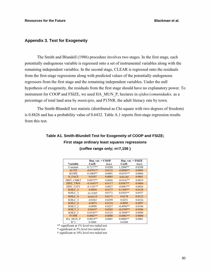
Appendix 3. Test for Exogeneity
The Smith and Blundell (1986) procedure involves two stages. In the first stage, each potentially endogenous variable is regressed onto a set of instrumental variables along with the remaining independent variables. In the second stage, CLEAR is regressed onto the residuals from the first-stage regressions along with predicted values of the potentially endogenous regressors from the first stage and the remaining independent variables. Under the null hypothesis of exogeneity, the residuals from the first stage should have no explanatory power. To instrument for COOP and FSIZE, we used HA_MUN_P, hectares in ejidos/comunidades, as a percentage of total land area by municipio, and P15NR, the adult literacy rate by town.
The Smith-Blundell test statistic (distributed as Chi-square with two degrees of freedom) is 0.8826 and has a probability value of 0.6432. Table A.1 reports first-stage regression results from this test.
Table A1. Smith-Blundell Test for Exogeneity of COOP and FSIZE;
First stage ordinary least squares regressions (coffee range only; n=7,156 )
Dep. var. = COOP Dep. var. = FSIZE
Variable Coeff. (s.e.) Coeff. (s.e.) Constant 0.7177** 0.0288 1.2880** 0.0208 ALTIT -0.0791** 0.0132 -0.0808** 0.0095 SLOPE 0.1084** 0.0091 -0.0191** 0.0066
N_FACE -0.0107 0.0085 0.0114† 0.0061 DIST_CMKT 0.0072** 0.0026 -0.0141** 0.0019 DIST_TWN -0.1643** 0.0117 0.0587** 0.0084 DIST_CITY -0.1101** 0.0037 -0.0067** 0.0026
SOILC_2 -0.0029 0.0177 0.1369** 0.0128 SOILC_3 -0.1338† 0.0772 0.8303** 0.0557 SOILC_4 -0.0331† 0.0171 0.0178 0.0123 SOILC_5 -0.0363 0.0299 0.0251 0.0216 SOILC_6 -0.0073 0.0134 0.0095 0.0097 SOILT_2 -0.0098 0.0257 -0.4996** 0.0186 SOILT_3 0.0563* 0.0285 -0.6789** 0.0206 SOILF_5 0.0336** 0.0125 -0.5898** 0.0090 P15PR 0.0002** 0.0000 -0.0001** 0.0000
HA_MUN_P 0.0014** 0.0001 0.0006** 0.0001 R^2 0.2880 0.6260
** significant at 1% level two tailed test * significant at 5% level two tailed test † significant at 10% level two tailed test
30
Resources for the Future Blackman et al.
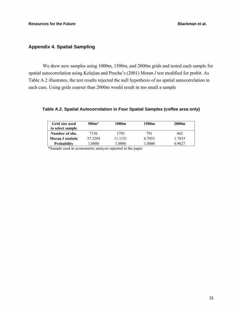
Appendix 4. Spatial Sampling
We drew new samples using 1000m, 1500m, and 2000m grids and tested each sample for spatial autocorrelation using Kelejian and Prucha’s (2001) Moran I test modified for probit. As Table A.2 illustrates, the test results rejected the null hypothesis of no spatial autocorrelation in each case. Using grids coarser than 2000m would result in too small a sample
Table A.2. Spatial Autocorrelation in Four Spatial Samples (coffee area only)
Grid size used
to select sample 500m* 1000m 1500m 2000m
Number of obs. 7156 1793 791 442 Moran I statistic 37.3294 11.1151 6.7053 1.7833
Probability 1.0000 1.0000 1.0000 0.9627 *Sample used in econometric analysis reported in the paper
31
Resources for the Future Blackman et al.
Figures
32
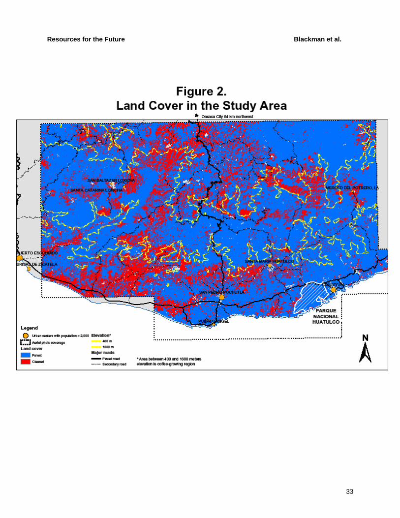
Resources for the Future Blackman et al.
33
Related Documents