Lack of Hyperbolicity in Asymptotic Erdös–Renyi Sparse Random Graphs

LACK OF SPECTRAL GAP AND HYPERBOLICITY IN ASYMPTOTIC

ERDOS-RENYI RANDOM GRAPHS

ONUTTOM NARAYAN, IRAJ SANIEE AND GABRIEL H. TUCCI

Abstract. In this work, we prove the absence of a spectral gap for the normalized Lapla-cian of the Erdos-Renyi random graph G(n, p) when p = d

nfor d > 1 as n→∞. We also

prove that for any positive δ the Erdos-Renyi random graph has a positive probability ofcontaining δ-fat triangles as n→∞.

1. Introduction and Motivation

Random graphs constitute an important and active research area with numerous applica-tions to geometry, percolation theory, information theory, queuing systems and communica-tion networks, to mention a few. They also provide analytical means to settle prototypicalquestions and conjectures that may be harder to resolve in specific circumstances. In thiswork we study two questions regarding the asymptotic geometry of Erdos-Renyi randomgraphs [1, 2, 3], partly motivated by suggestions that random graphs may have a spectralgap [4] or may be hyperbolic [5]. To fix notation, we denote such a graph with G(n, p)where n is the the number of nodes and p is the probability of an edge. The construction ofa G(n, p) graph therefore consists of connecting any pair of the n given nodes independentlyand with probability p1.

Our first result is that in the regime p = dn where d > 1, the spectral gap of the

normalized Laplacian of the graph G(n, p) goes to zero as the size of the graph increases.In other words, these graphs do not satisfy a linear isoperimetric inequality asymptoticallyas n → ∞. The linear isoperimetric inequality is an important geometric property ofcertain (geodesic) metric spaces, and it (roughly) states that any closed curve bounds aregion whose area is a linear function of the length of the curve.

Our second result is that, with positive probability, these graphs are not δ-hyperbolic inthe sense of Gromov [6] for any positive δ. Naively, one might think that this is equivalentto the first result, since Gromov’s notion of hyperbolicity and the linear isoperimetricinequality are intimately related (in a coarse sense, see [7]). In fact, despite the connectionbetween the two, neither implies the other in metric graphs, as discussed in more detail inSection 3. This implies that the questions of the spectral gap and hyperbolicity of randomgraphs need to be addressed independently, as we do here.

This paper is organized as follows. In Section 2 we study the connection between branch-ing processes and Erdos-Renyi random graphs and we prove that these graphs do not havea spectral gap. We also prove, using totally different techniques, a result of Dorogovtsev etal [8] regarding the size of the spectral gap for branching processes. In this Section we alsopresent numerical results that show a surprising degree of closeness between the spectral

I. Saniee and G. H. Tucci are with Bell Laboratories, Alcatel-Lucent, 600 Mountain Avenue, MurrayHill, New Jersey 07974, USA. O. Narayan is at Department of Physics, University of California, Santa Cruz,California 95064, USA. E-mail: [email protected], [email protected], [email protected].

1This is actually the G(n, p) model of a random graph due to Gilbert [2], rather than the Erdos-Renyi [1]model known as G(n,M); but we will follow the now almost universal proclivity of calling these graphsErdos-Renyi random graphs.

1

arX

iv:1

009.

5700

v1 [

mat

h.PR

] 2

8 Se

p 20

10

2 ONUTTOM NARAYAN, IRAJ SANIEE AND GABRIEL H. TUCCI

distribution of the normalized Laplacian of G(n, dn) and that of d-regular trees, based onwell-known explicit formulas due to McKay [9]. In Section 3, we show that G(n, p) are notδ-hyperbolic for any δ with positive probability. We also present plots that suggest that“fat” triangles not only exist with positive probability but are abundant in these randomgraphs.

2. Lack of Spectral Gap for the Erdos–Renyi Random Graphs

2.1. Branching Processes and Their Connection with Erdos–Renyi RandomGraphs. There are several ways to generate trees randomly. In this work we will fo-cus on a technique due to Beinayme in 1845 [10]. Given probabilities pk (k = 0, 1, 2, 3, . . .)with

∑∞0 pk = 1, we begin with one individual and let it reproduce according to these

probabilities, i.e., it has k children with probability pk. Each of these children (if thereare any) then reproduce independently with the same law, and so on forever or until somegeneration goes extinct. The family of trees produced by such a process are called (Bien-ayme)-Galton-Watson trees, for more details see [11].

Another well-known family of random graphs are the Erdos-Renyi random graphs, whichwill be the main focus of attention in this work. As we mention in the introduction, thesegraphs depend on two parameters n (the total number of nodes in the graph) and p (theprobability of connection) and will be denoted by G(n, p). The way they are constructedis very simple, for each pair of nodes we make a connection between them with probabilityp and independently of the other possible connections. These graphs have been studiedextensively since the late 1950’s and many results are well known (see [1, 2, 3] for more onthese graphs). Recently, a connection has been observed between the Erdos-Renyi randomgraphs and Galton-Watson trees. We will discuss this result and some of its consequencesbut first we will review some background and fix some notation.

2.2. Background and Notation. Let G = (V,E) be a graph with vertex set V and edgeset E. Let dv denote the degree of the vertex v. The normalized Laplacian of the graph Gis defined to be the operator

L(u, v) =

1 if u = v and dv 6= 0,

−1√dudv

if u and v are adjacent,

0 otherwise.

(2.1)

The operator L can be seen as an operator on the space of functions over the vertex setV . If the graph G is infinite and locally finite (every vertex has finite degree), then L isa well defined operator from l2(V ) to itself. In other words, L : l2(V ) → l2(V ) where foreach x ∈ l2(V ) we define Lx as

Lx(u) =1√du

∑v∼u

(x(u)√du− x(v)√

dv

). (2.2)

It is well known (see [3]) that the operator L is positive definite and its spectrum is containedin the interval [0, 2]. Moreover, if the graph is finite then 0 always belongs to the spectrum.This is not the case for infinite graphs, we say that an infinite graph has a spectral gap ifthe 0 does not belong to the spectrum of L. Since the spectrum of L is compact, this isequivalent to saying that the bottom of the spectrum λ0 defined as

λ0(G) = inf{λ ∈ spec(L)} = inf{‖Lx‖2 : ‖x‖2 = 1} (2.3)

is strictly positive. If the graph G is finite then λ0(G) is defined as the value of the secondeigenvalue.

LACK OF SPECTRAL GAP AND HYPERBOLICITY IN ERDOS-RENYI RANDOM GRAPHS 3

Another important property is the Cheeger constant. Given a graph G and S a subsetof of the vertices of G, we define vol(S), the volume of S, to be the sum of the degrees ofthe vertices in S: vol(S) =

∑x∈S dx,for S ⊂ V (G). Next, we define the edge boundary ∂S

of S to consist of all the edges with one endpoint in S and the other in the complementSc = V − S. The Cheeger constant of an infinite graph is defined as

hG = inf

{|∂S|

vol(S): S ⊂ V (G) with |S| <∞

}. (2.4)

It is a clear consequence of this definition that strictly positive Cheeger constant implieslinear isoperimetric inequality, since for every finite subset S of G we have that |∂S| ≥hG · vol(S). The following well-known result [3, 14, 13] relates the value of the Cheegerconstant with the bottom of the spectrum,

2hG ≥ λ0(G) ≥ 1−√

1− h2G

for any graph G, where the second inequality assumes that G is connected.

2.3. Asymptotic Gap of G(n, p). Let k ≥ 3 and let Tk be the infinite k−regular tree, alsoknown as the k−Bethe Lattice. It is known (see for example [9, 14]) that the spectral gap

for such a tree is equal to 1− 2√k−1k . A natural question to ask is the following. Consider

a branching process with probability distribution {pi}∞i=0, what is the spectral gap of thisrandom tree? Let us consider k the first non-zero pi in the sequence. In other words,p0 = p1 = . . . = pk−1 = 0 and pk > 0. Let us denote by T the tree generated by thisprocess. It is clear that a.s. every node in T has degree at least k + 1. Therefore, it is notsurprising to see that

λ0(T ) ≥ 1− 2√k

k + 1.

The following result shows that the converse inequality also holds. This was argued in [8]for which we provide a precise proof.

Theorem 2.1. Let T be the random tree generated by the branching process with probabil-ities {pi}∞i=0. Let k ≥ 0 the first non-zero entry in the sequence {pi}. If k = 0 then p0 > 0and λ0(T ) = 0. If k ≥ 1 then

λ0(T ) = 1− 2√k

k + 1. (2.5)

Proof. We will show the opposite inequality

λ0(T ) ≤ 1− 2√k

k + 1.

Now let Tk+1 be the infinite regular tree of degree k + 1 then

λ0(Tk+1) = inf{ ‖Lx‖2 : ‖x‖2 = 1} = inf{ ‖Lx‖2 : ‖x‖2 = 1 and supp(x) <∞}.Given ε > 0 there exist a vector x ∈ l2(V ) of finite support and unit norm ‖x‖2 = 1 suchthat

‖L(x)‖2 − ε < λ0(Tk+1) = 1− 2√k

k + 1.

Since the vector x has finite support there exists M > 0 sufficiently large such that

supp(x) ⊆ BTk+1(root,M)

where BTk+1(root,M) is the ball of radius M and center the root of Tk+1. Using the

second Borel-Cantelli Lemma and the fact that pk > 0 we see that for every M > 0there exist almost surely a copy of BTk+1

(root,M) inside the branching process T . As a

4 ONUTTOM NARAYAN, IRAJ SANIEE AND GABRIEL H. TUCCI

matter of fact, there are infinitely many copies. Fix one of these copies and consider thecorresponding isometric embedding φ : BTk+1

(root,M)→ T . Let y = φ(x). The vector y isa finitely supported vector in the vertex set of T . Since φ is an isometric embedding then‖y‖2 = ‖x‖2 = 1. Since both the Laplacian of Tk+1 and the Laplacian of T restricted toBTk+1

(root,M) and φ(BTk+1(root,M)) respectively are the same operator we see that

‖LT (y)‖2 = ‖LTk+1(x)‖ < 1− 2

√k

k + 1+ ε.

Since ε is arbitrary, this concludes the proof. �

Corollary 2.2. Let T be a branching process as before. If p0 > 0 or p1 > 0 then λ0(T ) = 0and the Cheeger constant hT = 0 with probability one.

We observe that the previous Corollary can be proved directly without using Theorem 2.1.For example, to prove that p1 > 0 would imply zero Cheeger constant it is enough toobserve that there will be arbitrarily long chains with positive probability and then use theBorel-Cantelli Lemma to see that we will have infinitely many of them with probability onein the infinite tree T .

Now we will discuss the connection between the Erdos-Renyi random graphs and branch-ing processes. Let d > 1 be fixed and consider the sequence of random graphs Gn = G(n, dn).For each n and each realization, the graph Gn has a Laplacian operator and this one hasan spectral measure. Let denote by µn the average over all the possible realizations. Inother words, µn is an average of probability measure supported in [0, 2]. It was provedby Bordenave and Lelarge [12] that this sequence of measure converges to a probabilitymeasure µ∞

µn → µ∞.

Moreover, they show that µ∞ is exactly the spectral measure of the Laplacian associatedwith the branching process with Poisson probability of parameter d. More precisely, foreach i ≥ 0

pi =d ie−d

i!.

This together with the previous corollary complete the proof of the following result:

Corollary 2.3. The measure µ∞ has no spectral gap.

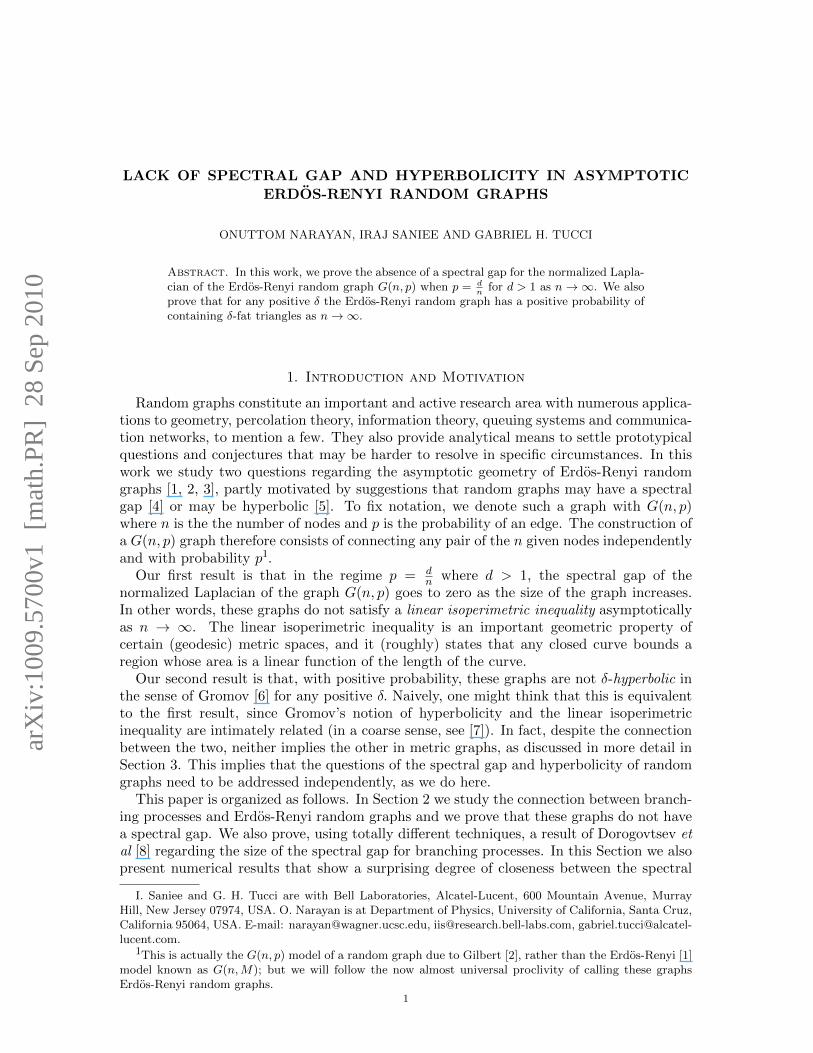
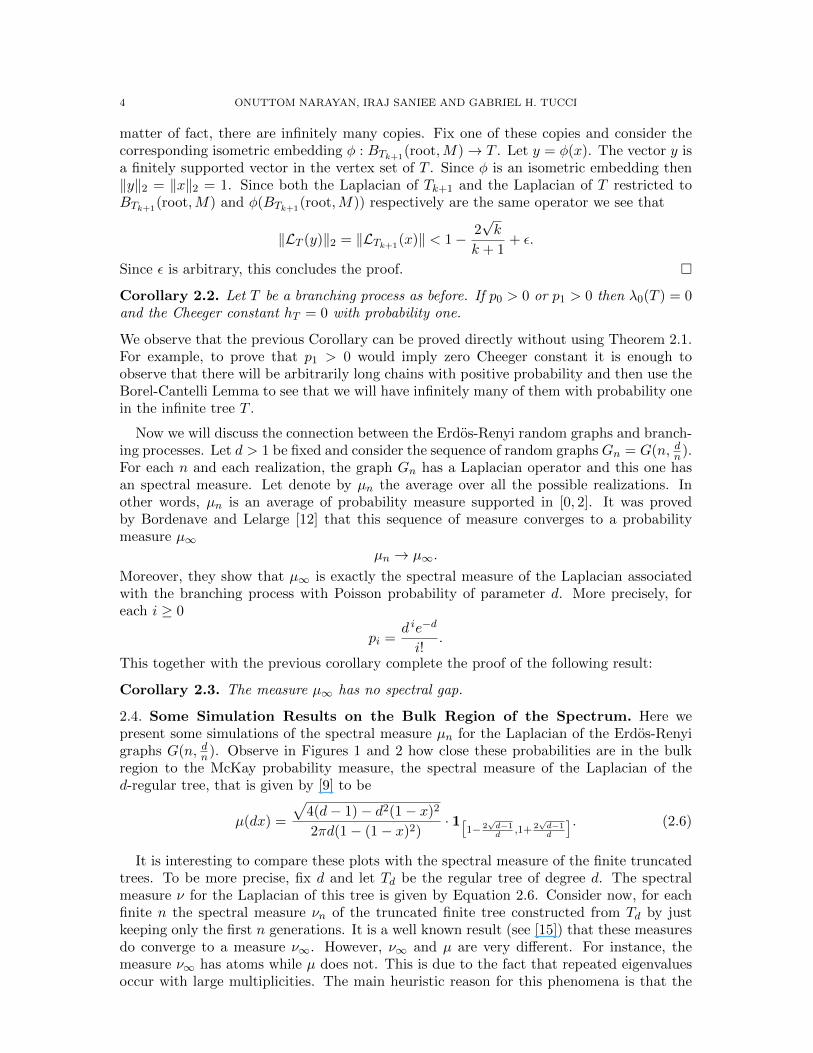
2.4. Some Simulation Results on the Bulk Region of the Spectrum. Here wepresent some simulations of the spectral measure µn for the Laplacian of the Erdos-Renyigraphs G(n, dn). Observe in Figures 1 and 2 how close these probabilities are in the bulkregion to the McKay probability measure, the spectral measure of the Laplacian of thed-regular tree, that is given by [9] to be

µ(dx) =

√4(d− 1)− d2(1− x)2

2πd(1− (1− x)2)· 1[

1− 2√d−1d

,1+ 2√d−1d

]. (2.6)

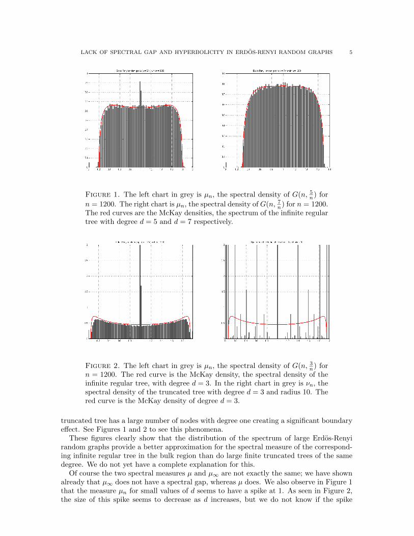
It is interesting to compare these plots with the spectral measure of the finite truncatedtrees. To be more precise, fix d and let Td be the regular tree of degree d. The spectralmeasure ν for the Laplacian of this tree is given by Equation 2.6. Consider now, for eachfinite n the spectral measure νn of the truncated finite tree constructed from Td by justkeeping only the first n generations. It is a well known result (see [15]) that these measuresdo converge to a measure ν∞. However, ν∞ and µ are very different. For instance, themeasure ν∞ has atoms while µ does not. This is due to the fact that repeated eigenvaluesoccur with large multiplicities. The main heuristic reason for this phenomena is that the

LACK OF SPECTRAL GAP AND HYPERBOLICITY IN ERDOS-RENYI RANDOM GRAPHS 5

Figure 1. The left chart in grey is µn, the spectral density of G(n, 5n) for

n = 1200. The right chart is µn, the spectral density of G(n, 7n) for n = 1200.

The red curves are the McKay densities, the spectrum of the infinite regulartree with degree d = 5 and d = 7 respectively.

Figure 2. The left chart in grey is µn, the spectral density of G(n, 3n) for

n = 1200. The red curve is the McKay density, the spectral density of theinfinite regular tree, with degree d = 3. In the right chart in grey is νn, thespectral density of the truncated tree with degree d = 3 and radius 10. Thered curve is the McKay density of degree d = 3.

truncated tree has a large number of nodes with degree one creating a significant boundaryeffect. See Figures 1 and 2 to see this phenomena.

These figures clearly show that the distribution of the spectrum of large Erdos-Renyirandom graphs provide a better approximation for the spectral measure of the correspond-ing infinite regular tree in the bulk region than do large finite truncated trees of the samedegree. We do not yet have a complete explanation for this.

Of course the two spectral measures µ and µ∞ are not exactly the same; we have shownalready that µ∞ does not have a spectral gap, whereas µ does. We also observe in Figure 1that the measure µn for small values of d seems to have a spike at 1. As seen in Figure 2,the size of this spike seems to decrease as d increases, but we do not know if the spike

6 ONUTTOM NARAYAN, IRAJ SANIEE AND GABRIEL H. TUCCI

disappears as n→∞ for fixed small d. Nevertheless, the close similarity observed betweenµ and µ∞ naturally raises the question: what is the probability distribution of the measureµ∞? More generally, if we consider the branching process generated by any probabilitydistribution in the natural numbers N, what is the spectral measure of the normalizedLaplacian for this graph?

3. Non-hyperbolicity for the Erdos–Renyi Random Graphs

3.1. Relationship Between Hyperbolicity and Spectral Gap. In this Section, wewill prove that Erdos–Renyi random graphs are not δ-hyperbolic in the sense of Gromov [6]for any δ. The concept of δ-hyperbolicity is often associated with the existence of a spectralgap. This is because for standard hyperbolic spaces with constant negative curvature, ormore pertinently for this discussion, their skeletal representations as hyperbolic graphs (e.g.,q–regular trees with q ≥ 3 or the Hp,q hyperbolic grids which are infinite planar graphswith uniform degree q and p–gons as faces with (p− 2)(q − 2) > 4), the two coincide.

Indeed, it might be thought that the existence of a spectral gap and δ-hyperbolicity areequivalent: the first is clearly equivalent to the existence of a linear isoperimetric inequalityfrom Eq.(2.2), and the second is shown to be equivalent to a linear isoperimetric inequalityin Proposition III.2.7 of [7]. However, the term “linear isoperimetric inequality” is used indifferent senses in the two cases. In the first, the entire perimeter of any arbitrary subsetS has to be considered. In the second, disk-like subsets are considered, and only the looppart of the perimeter (ignoring any boundary edges on the ‘flat’ part of the disk) is used.Thus neither does the existence of a spectral gap imply δ-hyperbolicity nor vice versa.2

As examples to illustrate this fact, we note that a graph that consists of an infinitechain (the integers Z) has a zero Cheeger constant and a zero spectral gap, even though itis δ-hyperbolic because — as discussed in the next subsection — all tree graphs triviallyare. On the other hand, the Cayley graph associated with the product of two free groups,G = F2 × F2, has a positive Cheeger constant and non-zero spectral gap. But since itincludes the graph H = Z×Z (the Euclidean grid) as a subgraph it is not hyperbolic. Thusquestions regarding the spectral gap and hyperbolicity need to be addressed independently.

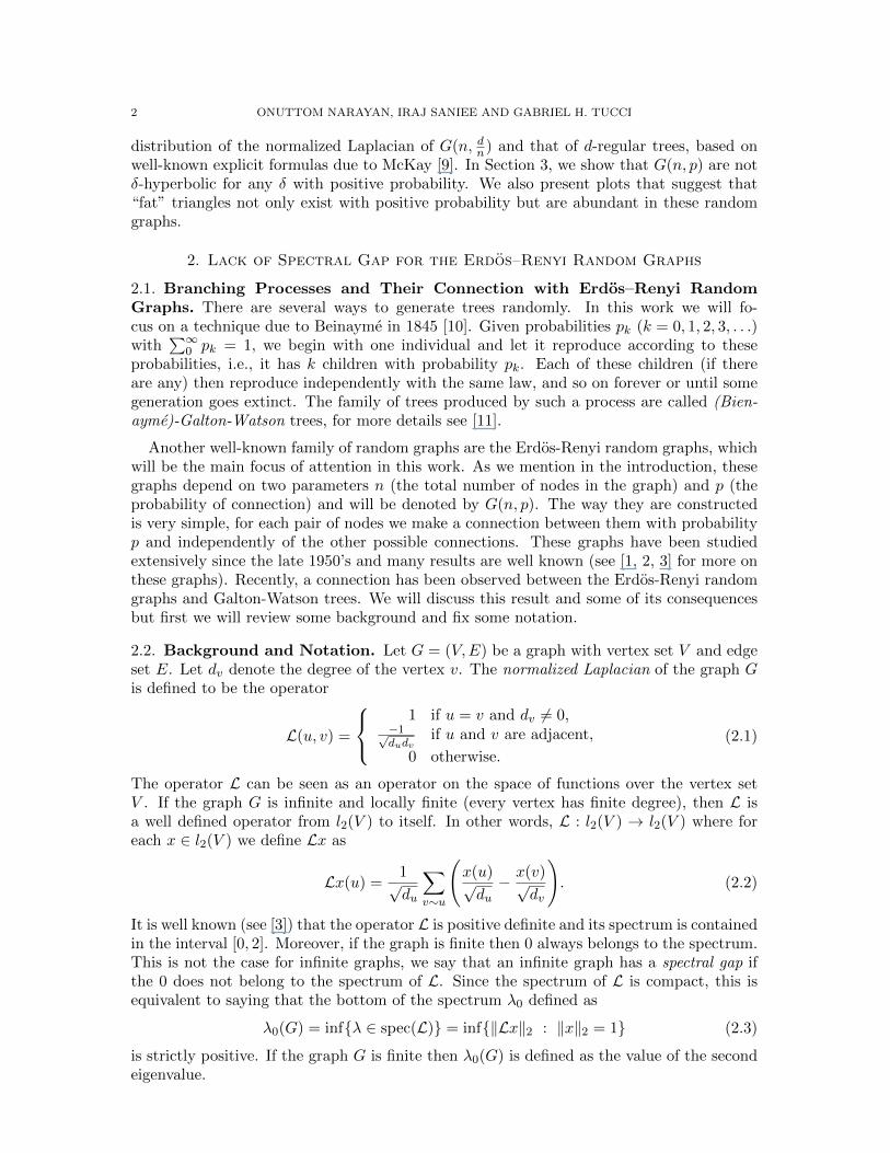
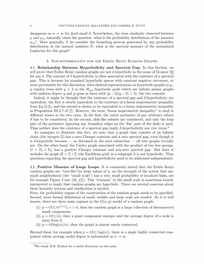
3.2. Positive Measure of Large Loops. It is commonly stated that the Erdos–Renyirandom graphs are “tree-like”for large values of n, on the strength of the notion that anysmall neighborhood (the “small scale”) has a very small probability of localized links, seefor example Figure 3 (see [16, 17]). This “treeness” in the small scale is sometimes looselyinterpreted to imply that random graphs are hyperbolic. There are several concerns aboutthese heuristic notions and clarification is needed.First, the probability regime of the construction of the random graph needs to be specified.Second, more formal definitions of small, middle and large scale are needed. As it is wellknown, there are three main regimes in the G(n, p) model of a random graph:

(1) p = O(1/n(1+ε)), ε > 0, then the random graph is a large collection of disconnectedsmall components.

(2) p = O(1/n), then a giant component emerges and the average degree of a node isaway from 0.

(3) p = O(log(n)/n), then the graph is almost surely connected.

Beyond these, for example when p = O(1/ log(n)), there is a single highly connected com-ponent whose average nodal degree is unbounded as n→∞.

2We thank M.R. Bridson for a useful discussion on this point.

LACK OF SPECTRAL GAP AND HYPERBOLICITY IN ERDOS-RENYI RANDOM GRAPHS 7

Figure 3. A small segment of a random graph G(n, 2/n) viewed close upfor n = 1000.

To define and clarify the relevant scale and the notion of hyperbolicity for random graphs,we use the definition of (coarse) hyperbolicity in the large scale as given by Gromov [6].The natural setting for the definition is within path-metric spaces, which for our purposessimplify to metric graphs in which a non-negative metric is defined on the links (or nodesor both) of a graph and thus all node pairs have at least one shortest path, or geodesic,between them. We denote a geodesic between a pair of nodes A and B by [AB], which, ifnecessary, may be regarded as just one of possibly many shortest paths between the saidnode pair. In a metric graph G a triangle ABC is called δ-thin if each of the shortest paths[AB], [BC] and [CA] is contained within the δ neighborhoods of the other two edges. Morespecifically,

[AB] ⊆ N ([BC], δ) ∪N ([CA], δ). (3.1)

and similarly for [BC] and [CA]. A triangle ABC is δ-fat if δ is the smallest δ for whichABC is δ-thin. The notion of (coarse) Gromov’s hyperbolicity is then defined as follows.

Definition 3.1. A metric graph is δ-hyperbolic if all geodesic triangles are δ-thin, for somefixed δ ≥ 0

It is immediately clear that all tree graphs are trivially δ-hyperbolic, with δ = 0. We alsoobserve that all finite graphs are δ-hyperbolic for large enough δ, e.g., by letting δ to beequal to the diameter of the graph. Thus the notion of coarse hyperbolicity is meaningfuland non-trivial for infinite graphs3.

With these clarifications, we make the following observations: First, random graphs inthe p = d

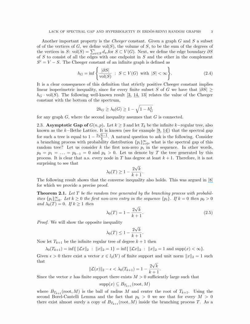
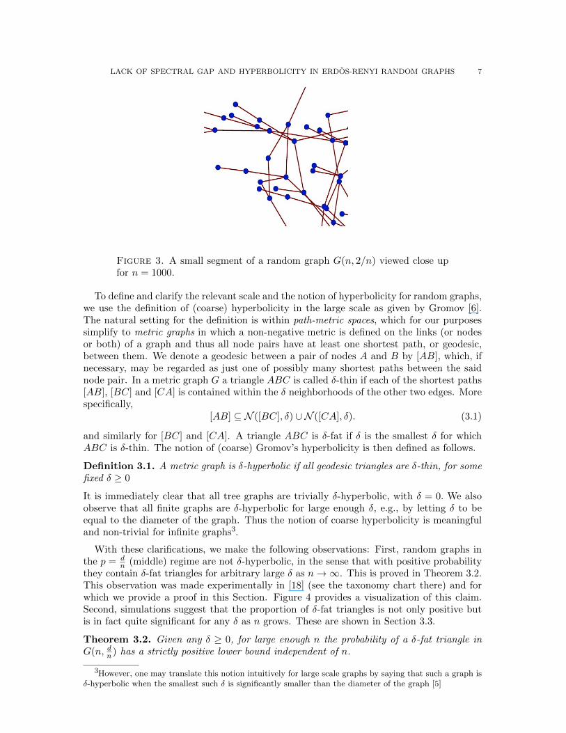
n (middle) regime are not δ-hyperbolic, in the sense that with positive probabilitythey contain δ-fat triangles for arbitrary large δ as n→∞. This is proved in Theorem 3.2.This observation was made experimentally in [18] (see the taxonomy chart there) and forwhich we provide a proof in this Section. Figure 4 provides a visualization of this claim.Second, simulations suggest that the proportion of δ-fat triangles is not only positive butis in fact quite significant for any δ as n grows. These are shown in Section 3.3.

Theorem 3.2. Given any δ ≥ 0, for large enough n the probability of a δ-fat triangle inG(n, dn) has a strictly positive lower bound independent of n.

3However, one may translate this notion intuitively for large scale graphs by saying that such a graph isδ-hyperbolic when the smallest such δ is significantly smaller than the diameter of the graph [5]

8 ONUTTOM NARAYAN, IRAJ SANIEE AND GABRIEL H. TUCCI

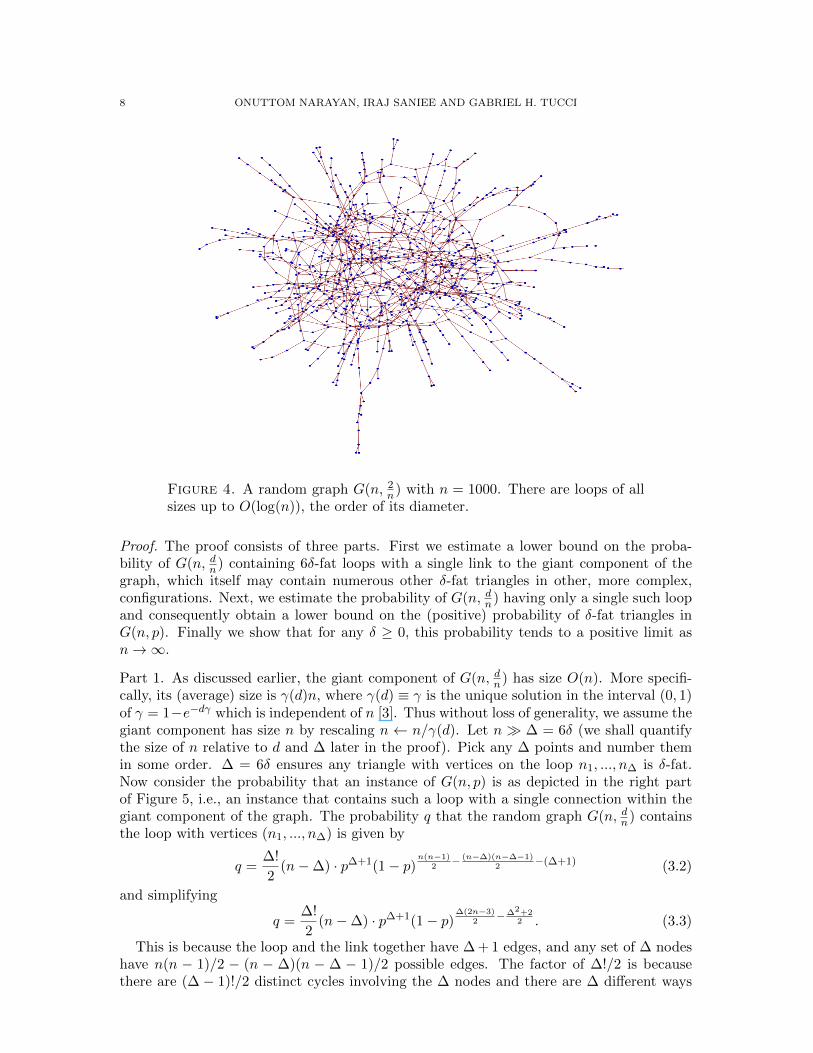
Figure 4. A random graph G(n, 2n) with n = 1000. There are loops of all

sizes up to O(log(n)), the order of its diameter.

Proof. The proof consists of three parts. First we estimate a lower bound on the proba-bility of G(n, dn) containing 6δ-fat loops with a single link to the giant component of thegraph, which itself may contain numerous other δ-fat triangles in other, more complex,configurations. Next, we estimate the probability of G(n, dn) having only a single such loopand consequently obtain a lower bound on the (positive) probability of δ-fat triangles inG(n, p). Finally we show that for any δ ≥ 0, this probability tends to a positive limit asn→∞.

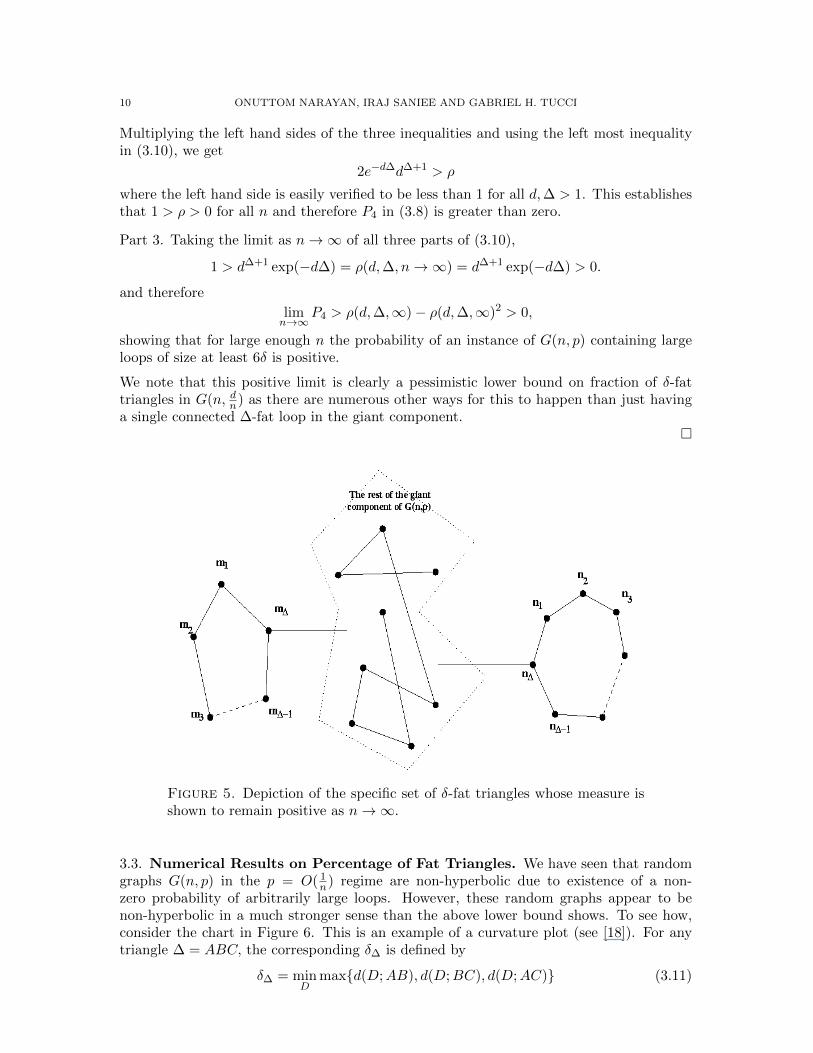
Part 1. As discussed earlier, the giant component of G(n, dn) has size O(n). More specifi-cally, its (average) size is γ(d)n, where γ(d) ≡ γ is the unique solution in the interval (0, 1)of γ = 1−e−dγ which is independent of n [3]. Thus without loss of generality, we assume thegiant component has size n by rescaling n ← n/γ(d). Let n � ∆ = 6δ (we shall quantifythe size of n relative to d and ∆ later in the proof). Pick any ∆ points and number themin some order. ∆ = 6δ ensures any triangle with vertices on the loop n1, ..., n∆ is δ-fat.Now consider the probability that an instance of G(n, p) is as depicted in the right partof Figure 5, i.e., an instance that contains such a loop with a single connection within thegiant component of the graph. The probability q that the random graph G(n, dn) containsthe loop with vertices (n1, ..., n∆) is given by

q =∆!

2(n−∆) · p∆+1(1− p)

n(n−1)2− (n−∆)(n−∆−1)

2−(∆+1) (3.2)

and simplifying

q =∆!

2(n−∆) · p∆+1(1− p)

∆(2n−3)2

−∆2+22 . (3.3)

This is because the loop and the link together have ∆ + 1 edges, and any set of ∆ nodeshave n(n − 1)/2 − (n − ∆)(n − ∆ − 1)/2 possible edges. The factor of ∆!/2 is becausethere are (∆ − 1)!/2 distinct cycles involving the ∆ nodes and there are ∆ different ways

LACK OF SPECTRAL GAP AND HYPERBOLICITY IN ERDOS-RENYI RANDOM GRAPHS 9

of connecting each cycle to the rest of the giant component via a single link, and the factorn − ∆ is because this link can end at any of the remaining n − ∆ nodes in the giantcomponent. This expression gives the probability of G(n, p) containing the specific set ofnodes n1, ..., n∆ in some cycle with a single connection to the giant component plus possiblyone or more other loops of length ∆ with one connection to the giant component whichhave not been excluded from the expression.

Part 2. We now wish to derive the probability that G(n, dn) contains only this given instance(n1, ..., n∆, n1) of a loop of length ∆ with one connection to the rest of the graph. q, thecomputed probability includes instances in which possibly other loops of length ∆ are alsoattached to the giant component via a single link. We may thus re-state q more preciselyas

q = P{∆-fat loop {n1, ..., n∆} with possible other ∆-fat loops}. (3.4)

The quantity we wish to compute is

P2 = P{∆-fat loop {n1, ..., n∆} with no other ∆-fat loops}. (3.5)

Observe that

P{∆-fat loops {n1, n2, .., n∆} with {m1,m2, ...,m∆} and possibly other ∆-fat loops} = q2,(3.6)

where {m1,m2, ...,m∆} is a distinct set of ∆ nodes and the two events – two distinct loopseach singly connected to the giant component – are independent of each other by construc-tion, as shown in Figure 5. Now, since there are M =

(n−∆

∆

)ways to pick {m1,m2, ...,m∆}

nodes distinctly from the set {n1, n2, ..., n∆},P3 = P{∆-fat cycle involving{n1, ..., n∆} with one or more ∆-fat loops} ≤Mq2. (3.7)

The inequality is due to the fact that Mq is an overestimate of the probability of additional∆-fat loops, since for any non-negative random variable x we have E(x) ≥ P (x > 0). Itfollows that

P2 = q − P3 ≥ q −Mq2

Now P2 is the probability of a single ∆-fat loop involving {n1, .., n∆} and no others set of∆ nodes. There are

(n∆

)distinct ways to select set of size ∆ such as {n1, n2, ..., n∆}, so that

P4 = P{at least one ∆-fat loop} >(n

∆

)P2 ≥

(n

∆

)(q −Mq2) > (ρ− ρ2) (3.8)

where ρ(d,∆, n) =(n∆

)q. Using the expression for q from (3.3) and the binomial inequalities

n∆/∆! >(n∆

)> (n−∆)∆/∆!, we get

n∆

∆!(n−∆)

∆!

2(d

n)∆+1(1− d

n)

∆(2n−3)−(∆2+2)2 > ρ(d,∆, n) >

(n−∆)∆

∆!(n−∆)

∆!

2(d

n)∆+1(1− d

n)

∆(2n−3)−(∆2+2)2 (3.9)

and collecting terms involving n

(n−∆

2n)(1− d

n)∆n(1− d

n)−

(∆+1)(∆+2)2 d∆+1 > ρ(d,∆, n) >

(n−∆)∆+1

2n∆+1(1− d

n)∆n(1− d

n)−

(∆+1)(∆+2)2 d∆+1. (3.10)

Now observe that 1 > (n−∆)∆+1

n∆+1 and e−d∆ > (1− dn)∆n, and

2 > (1− d

n)−

(∆+1)(∆+2)2 for n > d(1− 2

−2(∆+1)(∆+2) )−1.

10 ONUTTOM NARAYAN, IRAJ SANIEE AND GABRIEL H. TUCCI

Multiplying the left hand sides of the three inequalities and using the left most inequalityin (3.10), we get

2e−d∆d∆+1 > ρ

where the left hand side is easily verified to be less than 1 for all d,∆ > 1. This establishesthat 1 > ρ > 0 for all n and therefore P4 in (3.8) is greater than zero.

Part 3. Taking the limit as n→∞ of all three parts of (3.10),

1 > d∆+1 exp(−d∆) = ρ(d,∆, n→∞) = d∆+1 exp(−d∆) > 0.

and therefore

limn→∞

P4 > ρ(d,∆,∞)− ρ(d,∆,∞)2 > 0,

showing that for large enough n the probability of an instance of G(n, p) containing largeloops of size at least 6δ is positive.

We note that this positive limit is clearly a pessimistic lower bound on fraction of δ-fattriangles in G(n, dn) as there are numerous other ways for this to happen than just havinga single connected ∆-fat loop in the giant component.

�

Figure 5. Depiction of the specific set of δ-fat triangles whose measure isshown to remain positive as n→∞.

3.3. Numerical Results on Percentage of Fat Triangles. We have seen that randomgraphs G(n, p) in the p = O( 1

n) regime are non-hyperbolic due to existence of a non-zero probability of arbitrarily large loops. However, these random graphs appear to benon-hyperbolic in a much stronger sense than the above lower bound shows. To see how,consider the chart in Figure 6. This is an example of a curvature plot (see [18]). For anytriangle ∆ = ABC, the corresponding δ∆ is defined by

δ∆ = minD

max{d(D;AB), d(D;BC), d(D;AC)} (3.11)

LACK OF SPECTRAL GAP AND HYPERBOLICITY IN ERDOS-RENYI RANDOM GRAPHS 11

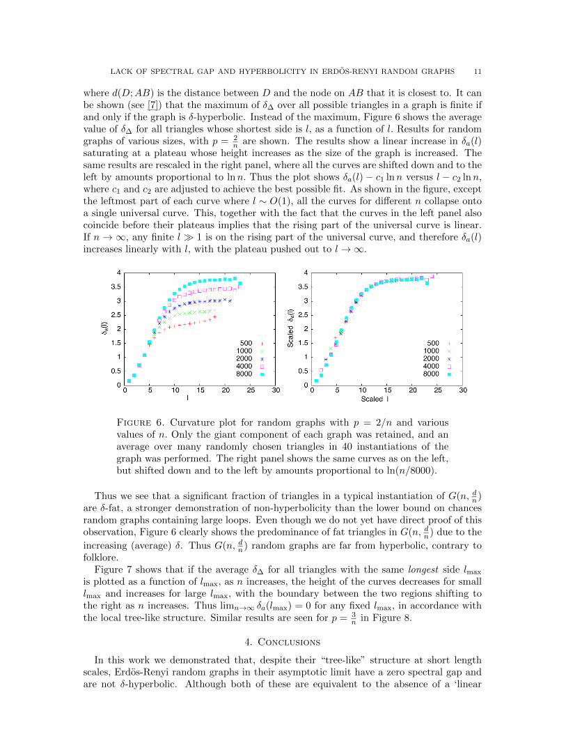
where d(D;AB) is the distance between D and the node on AB that it is closest to. It canbe shown (see [7]) that the maximum of δ∆ over all possible triangles in a graph is finite ifand only if the graph is δ-hyperbolic. Instead of the maximum, Figure 6 shows the averagevalue of δ∆ for all triangles whose shortest side is l, as a function of l. Results for randomgraphs of various sizes, with p = 2

n are shown. The results show a linear increase in δa(l)saturating at a plateau whose height increases as the size of the graph is increased. Thesame results are rescaled in the right panel, where all the curves are shifted down and to theleft by amounts proportional to lnn. Thus the plot shows δa(l) − c1 lnn versus l − c2 lnn,where c1 and c2 are adjusted to achieve the best possible fit. As shown in the figure, exceptthe leftmost part of each curve where l ∼ O(1), all the curves for different n collapse ontoa single universal curve. This, together with the fact that the curves in the left panel alsocoincide before their plateaus implies that the rising part of the universal curve is linear.If n → ∞, any finite l � 1 is on the rising part of the universal curve, and therefore δa(l)increases linearly with l, with the plateau pushed out to l→∞.

Figure 6. Curvature plot for random graphs with p = 2/n and variousvalues of n. Only the giant component of each graph was retained, and anaverage over many randomly chosen triangles in 40 instantiations of thegraph was performed. The right panel shows the same curves as on the left,but shifted down and to the left by amounts proportional to ln(n/8000).

Thus we see that a significant fraction of triangles in a typical instantiation of G(n, dn)are δ-fat, a stronger demonstration of non-hyperbolicity than the lower bound on chancesrandom graphs containing large loops. Even though we do not yet have direct proof of thisobservation, Figure 6 clearly shows the predominance of fat triangles in G(n, dn) due to the

increasing (average) δ. Thus G(n, dn) random graphs are far from hyperbolic, contrary tofolklore.

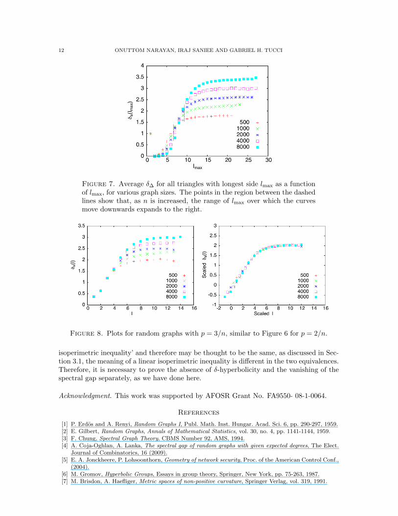
Figure 7 shows that if the average δ∆ for all triangles with the same longest side lmax

is plotted as a function of lmax, as n increases, the height of the curves decreases for smalllmax and increases for large lmax, with the boundary between the two regions shifting tothe right as n increases. Thus limn→∞ δa(lmax) = 0 for any fixed lmax, in accordance withthe local tree-like structure. Similar results are seen for p = 3

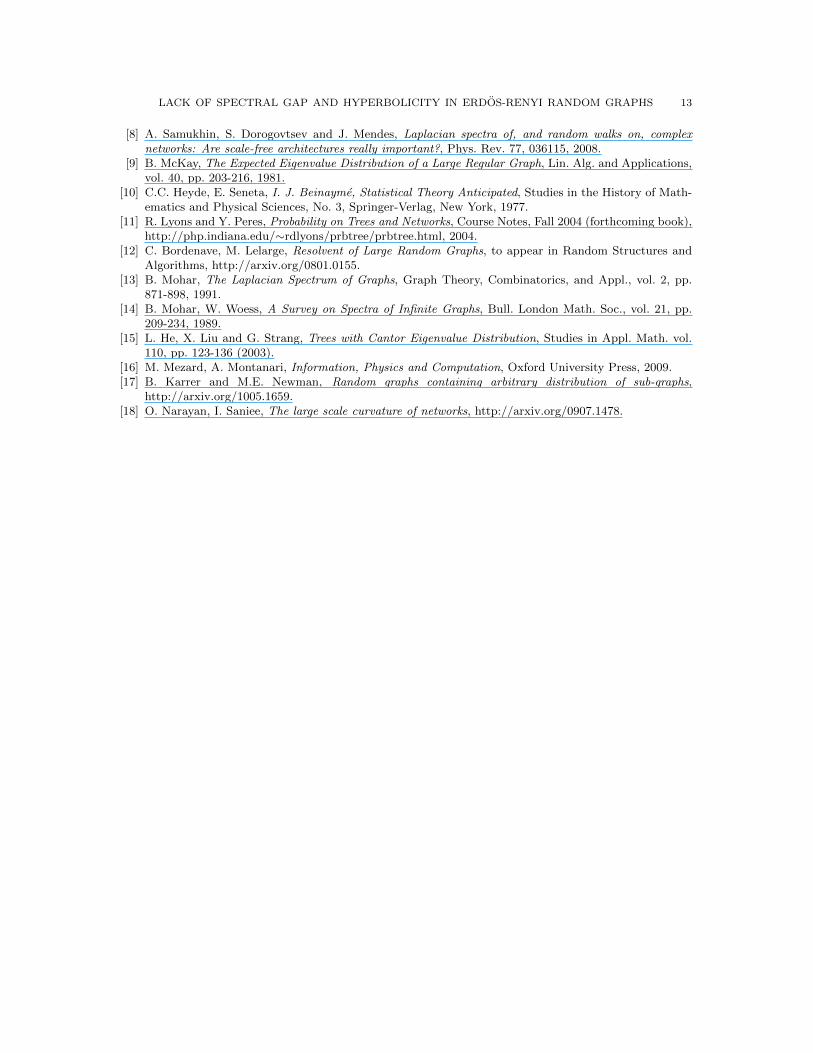
n in Figure 8.

4. Conclusions

In this work we demonstrated that, despite their “tree-like” structure at short lengthscales, Erdos-Renyi random graphs in their asymptotic limit have a zero spectral gap andare not δ-hyperbolic. Although both of these are equivalent to the absence of a ‘linear

12 ONUTTOM NARAYAN, IRAJ SANIEE AND GABRIEL H. TUCCI

Figure 7. Average δ∆ for all triangles with longest side lmax as a functionof lmax, for various graph sizes. The points in the region between the dashedlines show that, as n is increased, the range of lmax over which the curvesmove downwards expands to the right.

Figure 8. Plots for random graphs with p = 3/n, similar to Figure 6 for p = 2/n.

isoperimetric inequality’ and therefore may be thought to be the same, as discussed in Sec-tion 3.1, the meaning of a linear isoperimetric inequality is different in the two equivalences.Therefore, it is necessary to prove the absence of δ-hyperbolicity and the vanishing of thespectral gap separately, as we have done here.

Acknowledgment. This work was supported by AFOSR Grant No. FA9550- 08-1-0064.

References

[1] P. Erdos and A. Renyi, Random Graphs I, Publ. Math. Inst. Hungar. Acad. Sci. 6, pp. 290-297, 1959.[2] E. Gilbert, Random Graphs, Annals of Mathematical Statistics, vol. 30, no. 4, pp. 1141-1144, 1959.[3] F. Chung, Spectral Graph Theory, CBMS Number 92, AMS, 1994.[4] A. Coja-Oghlan, A. Lanka, The spectral gap of random graphs with given expected degrees, The Elect.

Journal of Combinatorics, 16 (2009).[5] E. A. Jonckheere, P. Lohsoonthorn, Geometry of network security, Proc. of the American Control Conf.,

(2004).[6] M. Gromov, Hyperbolic Groups, Essays in group theory, Springer, New York, pp. 75-263, 1987.[7] M. Brisdon, A. Haefliger, Metric spaces of non-positive curvature, Springer Verlag, vol. 319, 1991.

LACK OF SPECTRAL GAP AND HYPERBOLICITY IN ERDOS-RENYI RANDOM GRAPHS 13

[8] A. Samukhin, S. Dorogovtsev and J. Mendes, Laplacian spectra of, and random walks on, complexnetworks: Are scale-free architectures really important?, Phys. Rev. 77, 036115, 2008.

[9] B. McKay, The Expected Eigenvalue Distribution of a Large Regular Graph, Lin. Alg. and Applications,vol. 40, pp. 203-216, 1981.

[10] C.C. Heyde, E. Seneta, I. J. Beinayme, Statistical Theory Anticipated, Studies in the History of Math-ematics and Physical Sciences, No. 3, Springer-Verlag, New York, 1977.

[11] R. Lyons and Y. Peres, Probability on Trees and Networks, Course Notes, Fall 2004 (forthcoming book),http://php.indiana.edu/∼rdlyons/prbtree/prbtree.html, 2004.

[12] C. Bordenave, M. Lelarge, Resolvent of Large Random Graphs, to appear in Random Structures andAlgorithms, http://arxiv.org/0801.0155.

[13] B. Mohar, The Laplacian Spectrum of Graphs, Graph Theory, Combinatorics, and Appl., vol. 2, pp.871-898, 1991.

[14] B. Mohar, W. Woess, A Survey on Spectra of Infinite Graphs, Bull. London Math. Soc., vol. 21, pp.209-234, 1989.

[15] L. He, X. Liu and G. Strang, Trees with Cantor Eigenvalue Distribution, Studies in Appl. Math. vol.110, pp. 123-136 (2003).

[16] M. Mezard, A. Montanari, Information, Physics and Computation, Oxford University Press, 2009.[17] B. Karrer and M.E. Newman, Random graphs containing arbitrary distribution of sub-graphs,

http://arxiv.org/1005.1659.[18] O. Narayan, I. Saniee, The large scale curvature of networks, http://arxiv.org/0907.1478.