LabScribe2 User’s Manual

Welcome message from author
This document is posted to help you gain knowledge. Please leave a comment to let me know what you think about it! Share it to your friends and learn new things together.
Transcript

LabScribe2 User’s Manual

. .
Contents
Introduction
Welcome viiHow to Use This User’s Manual viiSystem Requirements viiInstallation vii
Installation From CD viiWindows viii
Macintosh OSX viii
Installation Download From User Area viiiiWorx.com User Area viiiComments and Suggestions viiiTechnical Support ixContacting Us ix
For Sales ixFor Technical Support ix
Chapter 1: The Display
Overview 1User Interface 1
The Main Window 1The Toolbar 2Channel Bar 3
Channel Sizing 4
Cursors 6Cursor Modes 6
Moving Cursors 6
Locking Cursor Separation 7
CURSOR EXERCISE 7
Marks 7Making Marks Online 7
Preset Marks 7
Making Marks Off-Line 9
Editing Marks 9
Navigating By Marks 9
Positioning Mark Comments 10
Sorting and Exporting Marks 11
MARKS EXERCISE 11
Views 11Creating and Editing Views 12
Units Conversion 13Inverting the Trace 16Voltmeter 16Online XY 17Other Display Windows 17
. .
Chapter 2: The Menus
Overview 18The Menus 18
File 18Edit 19View 20Tools 21Settings 23Advanced 24Help 25
Chapter 3: Acquisition
Overview 26Start Recording 26Settings 26Calling a Settings File 26
Main Window Display Considerations 27Managing Display Time 27
Display Time Setup Dialog 30
Managing Amplitude Display 30Zoom Tools 30
Set Scale 31
Preferred Scale 31
Scroll Up/Down 31
Signal Conditioning 31Gain 31
Bioamplifiers 32
DIN 8 Inputs 32
Offset 32Filters 32Averaging 33Outboard Conditioning 33
Chart Mode 33Selecting a Sampling Speed 34
SAMPLING SPEED EXERCISE 35
Vertical Resolution 35Starting Recording 36
User 36
Timed 36
External Trigger 36
Triggered from Channel 36
Pretriggering 37
Stopping 37User 37
Timed 37
Pausing Display 37
Preview Mode 37
Scope Mode 38When to Use the Scope Mode 38

. .
Acquiring Data in the Scope Mode 38Set Up the Software 38
Repetitive Mode 39
Multiple Sweep Mode 39
Averaged Mode 39
Sweep Length 39
Sampling Rate 40
Saving Your Data 40
Chapter 4: Creating Your Own Preferences and Settings
Overview 41The Preferences Dialog 41
Channel Page 41
Stimulator Page 42
Views Page 42
Sequences Page 43
Options Page 43
Events Page 44
Channel Events 44
Timed Events 45
Event Priority 45
The Settings Menu 45Creating a New Settings File 46Creating a New Settings Group 46
Helper Files 47
Chapter 5: The Stimulator
Overview 48Basic Stimulator Settings 48Pulse Protocols 49
Building Output Protocols in Pulse Mode 49
PULSE MODE STIMULATOR EXERCISE 50
Train Mode 52Building Output Protocols in Train Mode 52
TRAIN PROTOCOL STIMULATOR EXERCISE 52
Constant Voltage Mode 53Step Mode 53
Building Output Protocols in Step Mode 53
VOLTAGE STEP MODE STIMULATOR EXERCISE 54
Ramp Mode 56Triangle Mode 56The Stimulator Control Panel 57
Pulse Mode Control Panel 57
Train Mode Control Panel 57
Step Control Panel 58
Constant Voltage Mode Control Panel 58
Ramp Mode Control Panel 58
Triangle Mode Control Panel 59
. .
Stimulus Protocols Built with the Sequence Builder 59The Sequences Preferences Page 59
Building Output Protocols Using Sequences 59
SCOPE MODE SEQUENCE BUILDING EXERCISE 59
Chapter 6: Computed Channels
Overview 62Adding a Computed Function Channel 62The Functions 63
Periodic 63The Periodic Setup Dialog 63
PERIODIC FUNCTIONS SETUP EXERCISE 64
Using the Periodic Functions 64
Integral 65Zero 66
Using the Integral Functions 67
Derivative 67Using the Derivative Function 67
Spirometry 68Using the Spirometry Functions 68
MultiPoint Calibration 71Using the MultiPoint Calibration Function 71
Channel Math 71Using the Channel Math Function 72
Filter 72Using the Filter Functions 73
Smoothing 73Using the Smoothing Function 74
Auto Correlation 74Using the Autocorrelation Function 75
Power 75Using the Power Function 75
Cardiac 76Using the Cardiac Functions 76
EEG 77Using the EEG Functions 77
Gain Telegraph 78Using the Gain Telegraph Function 78
Digital Input 78CrossTime Channel Calculation 78
Using CrossTime Channel Calculations 79
Template Match 79Using Template Matching 79
PVLoop 80TimeShift Channel 80
Using Channel TimeShifting 80
Event Marker 80Using Event Markers 81
Sonomicrometry 81Using the Sonomicrometry Functions 81
. .
Chapter 7: Analysis
Overview 82The Analysis Window 82
Analysis Window Components 82Channel Menus in the Analysis Window 83The Functions 86
General 86
Derivative 86
Integral 87
Adding Functions to the Analysis Window 87
Tiled or Stacked Display 87Scope Mode Analysis Window Options 87Copy, Export, and Print Analysis Window Data 89
Redisplayed Data 89The XY View 89
XY View Components 89
Selecting the Displayed Channels 90
Channel Menus in the XY View 90
The XY Graph Window Menu 91
XY Graph Table Functions 91
Marker Data 92
Copy, Export, and Print XY View Window 92
FFT 92FFT Window Components 93
Configuring the FFT View 93
Channel Menu in the FFT View 94
The FFT Plot Menu 94
FFT Table Functions 94
Theoretical Considerations 95
Copy, Export, and Print FFT Windows 95
Find Functions 96Find Dialog Window 96
FIND EXERCISE 97
Auto Find Dialog Window 98
AUTO FIND EXERCISE 98
Other Analysis Tools 99Managing Scripts 99
Chapter 8: Advanced Analysis
Overview 100AutoMarks 100Calculations 100
PV Loops 100Online Calculations 100PVLoop Automarks 102Offline Calculations 103Calibration of Conductance Volume Data 107
Blood Pressure 110Online Blood Pressure Calculations 110
. .
Blood Pressure Automarks 112Offline Blood Pressure Calculations 113
ECG Analysis 116Automark 116
Configuring the AutoMark ECG Dialog 116
Offline Calculations 118Metabolic 122
Using Breath by Breath: Online Calculations 122Using Breath by Breath: Offline Calculations 124Using Mixing Chamber: Offline Calculations 126
AutoMark Peaks 127Peak Analysis AutoMarks 127
Normalization 129
Chapter 9: Digital Input and Output
Overview 131Digital Input 131Digital Output 132
Output States 132Naming States 133
Sequences 133Creating a Sequence 133
Triggering a Sequence 134
Chapter 10: The Journal and Data Export
The Journal 135The Journal Toolbar 136Adding Text, Images, and Data to the Journal 136Printing and Saving the Journal 137
Cutting, Copying and Pasting 137Saving and Saving As 138Printing 138Exporting Data 138
Exporting Images 139Exporting Numerical Data 139
. .
Introduction vii
Introduction
WelcomeThank you for choosing iWorx LabScribe2 Data Recording and Analysis Software. We are
confident that this software will make your data recording and analysis easier, and welcome
suggestions for improving our products. Please contact us with comments, concerns or sugges-
tions at (877) 273-7110 (Research products) or (800) 549-5748 (Teaching products). Interna-
tional customers should call (603) 742-2492.
Contact us via email at either: [email protected] or [email protected].
How to Use This User’s ManualThis User’s Manual assumes you are familiar with basic Windows and Macintosh OSX termi-
nology. The Table of Contents lists each chapter and its contents. You can use it or the Index
to locate pages on a particular subject.
Although it contains some practice exercises, this manual is not designed to be a tutorial, or an
introduction to LabScribe2. It is a reference manual covering all of the features and capabilities
of the software. Refer to the Quick Start guide for a practical overview of LabScribe2’s most
commonly used features. A tutorial containing a number of exercises is included in the
electronic laboratory manual that came with your software, and there are a number of video
tutorials available in the User Area at iworx.com.
System RequirementsLabScribe2 recording software requires a Windows (Windows 98 through Windows 7) or a
Macintosh (OSX 10.3 through OSX 10.6) computer.
If you are using a Windows computer, a Pentium 4 processor computer with at least 2 gigabytes
of RAM and 500 megabytes of free space on your hard drive is required. A Windows computer
with a Dual Core Processor with an AGP graphics card and 2 gigabytes of RAM is preferred.
If you are using a Macintosh, a G4 processor with at least 2 gigabytes of RAM and 500
megabytes of free space on your hard drive is required. An Intel Dual Core Processor and
dedicated graphics card are preferred.
Installation
Installation From CD
LabScribe2 software is provided on a hybrid CD-ROM, with software for both Windows and
Macintosh Operating Systems. If you don’t have a CD drive, the software installer can be
downloaded from our User Area. Point your browser to http://www.iworx.com and enter the User
Area (register first if necessary). All installers are available in the Software section of the User
Area.
Note: You will need to have administrative privileges to install LabScribe2 on some computers. Contact your IT department for assistance or to confirm your administrator status. Additionally, Windows users will need permissions to write to C:\Users\USERNAME\AppData\Local\LabScribe2. Do not connect your iWorx hardware to the computer until AFTER the software installation is complete.

. .
Introduction viii
Windows To install the software using the CD-ROM on a Windows computer:
• Insert the LabScribe2 installation CD.
• Double-click on the Setup icon.
• Follow the prompts in the Setup Wizard to complete installation.
• Once you have completed the installation process, remove the installation CD from the drive, then connect and turn on your iWorx data acquisition unit.
Note: When your hardware is connected for the first time, Windows will advise you “New Hardware found” and proceed to load the driver automatically. If for some reason Windows cannot locate the driver, locate the appropriate drivers for your operating system in the iWorx/LabScribe2/drivers folder in the Program Files folder on your C drive.
Macintosh OSX To install the software using the CD-ROM on Macintosh OSX 10.3 or later:
• Insert the LabScribe2 installation CD.
• Copy the files from the CD to the Applications folder of your computer.
• Remove the installation CD from the drive, then connect and turn on your iWorx hardware.
Installation Download From User Area
To install using a downloaded installer from our User Area:
• Go the User Area on the iworx.com website. Click on the Software link and select the proper installer for the Windows or Macintosh operating system on your computer. After downloading the LabScribe2 software installer, double click on the downloaded file. It is a self extracting archive, which will automati-cally launch the installer after it extracts.
• In Windows, follow the prompts to complete installation. Restart your computer once installation is complete.
• In Macintosh OSX, copy the files to your Applications folder.
• Once you have completed the installation process, connect and turn on your iWorx hardware.
iWorx.com User AreaThe User Area at iWorx.com contains a wealth of resources, including software files, experi-
ments, archived newsletters, hardware documentation, and a complete online catalog of our
research and teaching products. You will need to register and choose a password to access the
User Area. Simply click Register on the User Area home page for complete registration infor-
mation. By registering with us at iworx.com, you will be notified of updates and new releases,
and you will be able to access the free software upgrades you are entitled to for as long as you
use LabScribe2. iWorx Systems recommends using Firefox as your Web browser when
accessing the iworx.com website.
Comments and SuggestionsiWorx Systems understands that user feedback is critical to the improvement of any software. If
you have ideas, suggestions or criticisms, please contact us at either: [email protected]
(Research products) or [email protected] (Teaching products).

. .
Introduction ix
Technical SupportIf you cannot find an answer in this User’s Guide, please check the list of FAQ’s (Frequently
Asked Questions) on our website. If you still cannot find a solution to your problem, technical
support is available to all registered users at no charge via phone or email. When requesting
technical support, please follow the steps listed below:
• Write down your question or problem and the actions you took that created the problem.
• Be prepared to duplicate the problem.
• Note any error messages.
• Save a data file that can be emailed to an iWorx Technical Support representative.
• Note your computer model and operating system version.
• Note the amount of RAM (Random Access Memory) in your computer.
• Note your LabScribe2 Software version number.
Following these steps will enable the iWorx support staff to address your issues quickly and
efficiently.
Contacting UsiWorx Systems, Inc.
One Washington Street, Suite 404
Dover, NH 03820 USA
For Sales (800) 234-1757 (North America)
(603) 742-2492 (outside North America)
FAX: 603-742-2455
Email: [email protected]
Web: http://www.iworx.com
For Technical Support
Research products:
(877) 273-7110
Teaching products:
(800) 549-5748
International customers should call (603) 742-2492.
. .
1 The Display 1
Chapter 1: The Display
OverviewLabScribe2 both acquires data and uses an intuitive display that makes it possible for the user
to view, interpret, and manipulate the recorded data. This chapter discusses how data are
displayed in the various windows of the LabScribe2 user interface.
User Interface
The LabScribe2 user interface contains five primary display windows: the Main and Analysis
Windows, the XY and FFT Views, and the Journal. There are also dialog windows and control
panels, accessible through Toolbar icons and the software Preferences Dialog (accessed in
the Edit menu in Windows, and the LabScribe2 menu on the Macintosh), which displays the
Channel, Stimulator, Views, Sequences, Options and Events configurations. The Marks icon
in the Toolbar opens the Marks Dialog and the Stimulator icon opens the Stimulator Control
Panel directly beneath the Toolbar. The Main Window and Toolbar contain most of the controls
necessary for data acquisition.
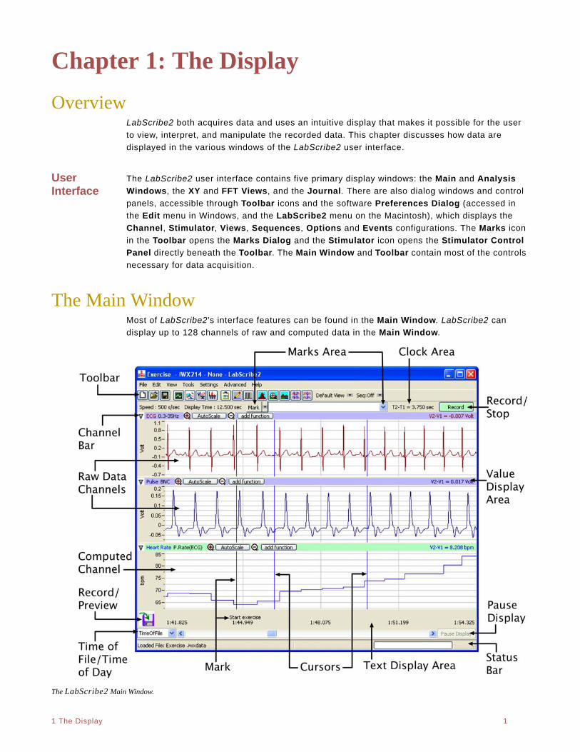
The Main WindowMost of LabScribe2’s interface features can be found in the Main Window. LabScribe2 can
display up to 128 channels of raw and computed data in the Main Window.
The LabScribe2 Main Window.
. .
1 The Display 2
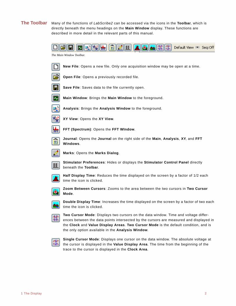
The Toolbar Many of the functions of LabScribe2 can be accessed via the icons in the Toolbar, which is
directly beneath the menu headings on the Main Window display. These functions are
described in more detail in the relevant parts of this manual.
The Main Window Toolbar.
New File: Opens a new file. Only one acquisition window may be open at a time.
Open File: Opens a previously recorded file.
Save File: Saves data to the file currently open.
Main Window: Brings the Main Window to the foreground.
Analysis: Brings the Analysis Window to the foreground.
XY View: Opens the XY View.
FFT (Spectrum): Opens the FFT WIndow.
Journal: Opens the Journal on the right side of the Main, Analysis, XY, and FFT
Windows.
Marks: Opens the Marks Dialog.
Stimulator Preferences: Hides or displays the Stimulator Control Panel directly
beneath the Toolbar.
Half Display Time: Reduces the time displayed on the screen by a factor of 1/2 each
time the icon is clicked.
Zoom Between Cursors: Zooms to the area between the two cursors in Two Cursor
Mode.
Double Display Time: Increases the time displayed on the screen by a factor of two each
time the icon is clicked.
Two Cursor Mode: Displays two cursors on the data window. Time and voltage differ-
ences between the data points intersected by the cursors are measured and displayed in
the Clock and Value Display Areas. Two Cursor Mode is the default condition, and is
the only option available in the Analysis Window.
Single Cursor Mode: Displays one cursor on the data window. The absolute voltage at
the cursor is displayed in the Value Display Area. The time from the beginning of the
trace to the cursor is displayed in the Clock Area.
. .
1 The Display 3
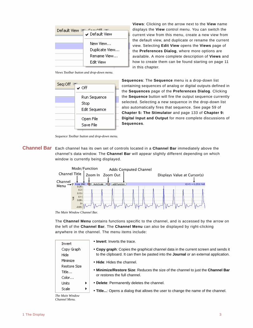
Views: Clicking on the arrow next to the View name
displays the View control menu. You can switch the
current view from this menu, create a new view from
the default view, and duplicate or rename the current
view. Selecting Edit View opens the Views page of
the Preferences Dialog, where more options are
available. A more complete description of Views and
how to create them can be found starting on page 11
in this chapter.Views Toolbar button and drop-down menu.
Sequences: The Sequence menu is a drop-down list
containing sequences of analog or digital outputs defined in
the Sequences page of the Preferences Dialog. Clicking
the Sequence button will fire the output sequence currently
selected. Selecting a new sequence in the drop-down list
also automatically fires that sequence. See page 59 of
Chapter 5: The Stimulator and page 133 of Chapter 9:
Digital Input and Output for more complete discussions of
Sequences.
Sequence Toolbar button and drop-down menu.
Channel Bar Each channel has its own set of controls located in a Channel Bar immediately above the
channel’s data window. The Channel Bar will appear slightly different depending on which
window is currently being displayed.
The Main Window Channel Bar.
The Channel Menu contains functions specific to the channel, and is accessed by the arrow on
the left of the Channel Bar. The Channel Menu can also be displayed by right-clicking
anywhere in the channel. The menu items include:
• Invert: Inverts the trace.
• Copy graph: Copies the graphical channel data in the current screen and sends it to the clipboard. It can then be pasted into the Journal or an external application.
• Hide: Hides the channel.
• Minimize/Restore Size: Reduces the size of the channel to just the Channel Bar or restores the full channel.
• Delete: Permanently deletes the channel.
• Title...: Opens a dialog that allows the user to change the name of the channel.The Main Window Channel Menu.

. .
1 The Display 4
• Color: Opens a color pallette that allows the user to change the color of the channel’s trace.
• Units: Choosing this menu item displays the Units Conversion options. Clicking in the Value Display Area will also display these options. Refer to the Units Conversion section beginning on page 13 of this chapter for a complete description of these options.
• Scale: Clicking this item displays the options for controlling the vertical scale of the channel. Refer to the discussion beginning on page 30 in Chapter 3: Acquisition for a complete description of these options.
When the Channel Menu is opened by right-clicking in the channel display area, an additional
menu item is added below the line at the bottom of the menu:
• Normalization: Choosing Normalization opens a submenu allowing the user to access the Normal-ization functions used to calibrate vessel size for the use of wire myographs. Normalization is a separately licensed software routine. Normalization is discussed in more detail beginning on page 129 in Chapter 8: Advanced Analysis Routines.
Refer to the appropriate sections of the manual for descriptions of the Channel Menu in the
Analysis Window (page 83), the XY View (page 89), and the FFT Window (page 92).
The Channel Title is displayed to the right of the Channel Menu arrow. The title can be
changed with the Title... option in the Channel Menu.
The Mode/Function position displays which input and hardware filters are being used on a raw
data channel. Clicking on Mode/Function will allow you to change these options. On a
computed function channel, Mode/Function displays the computed function. Clicking on Mode/
Function in a computed channel will display the list of available computed functions, allowing
the user to change the computed function of that channel. Refer to Chapter 6: Computed
Channels for a more complete discussion.
Zoom In, Autoscale, and Zoom Out set the vertical scale and are described more fully
beginning on page 30 of the Managing Amplitude Display section in Chapter 3: Acquisition.
Clicking add function adds a computed channel to the display. The functions are discussed in
Chapter 6: Computed Channels.
The Value Display Area located to the extreme right on the Channel Bar will display different
values depending on the state of the program:
• While recording, the Value Display Area shows the value of the last data point collected.
• Offline, in Single Cursor Mode, the Value Display Area displays the Y-axis value of the data point inter-sected by the cursor.
• In Two Cursor Mode, the Value Display Area displays the difference between the Y-axis values inter-sected by the two cursors.
Channel Sizing The amount of display area allotted to each channel in the Main Window can be controlled by
clicking and dragging on the top of the Channel Bar.
• To change the allocated space for a channel, position the cursor at the top of the Channel Bar until it becomes a double-headed arrow.
• Click and drag this arrow up or down to resize the channel, as illustrated in the figure on the next page.
. .
1 The Display 5
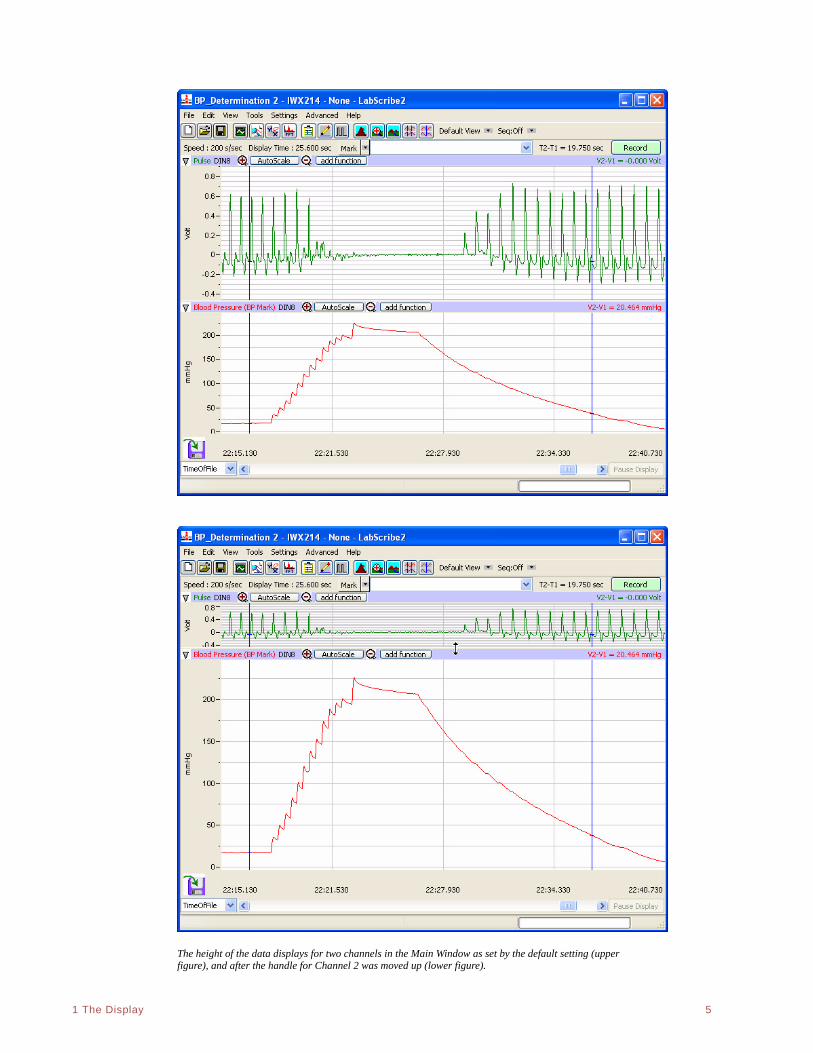
The height of the data displays for two channels in the Main Window as set by the default setting (upper figure), and after the handle for Channel 2 was moved up (lower figure).

. .
1 The Display 6
Cursors Many of the features of LabScribe2 allow the user to label, measure, compare, and analyze
specific data points or regions. LabScribe2 uses Cursors to identify and isolate the data points
of interest.
Cursor Modes Cursors are the vertical blue lines that pass through all channels. Icons in the Toolbar allow
you to choose between using Single Cursor or Two Cursor Modes.
Cursor controls on the Main Window Toolbar.
Single Cursor Mode
• To access Single Cursor Mode, click on the Single Cursor Mode icon in the Toolbar.
• The Value Display Area on the right side of each channel bar displays the voltage of the data point that is intersected by the cursor in that channel. The Clock Area in the upper right hand corner of the Main Window displays the corresponding time.
• Single Cursor Mode is used to determine values and to place marks in the record after recording has stopped.
Two Cursor Mode
• To access Two Cursor Mode, click on the Two Cursor Mode icon in the Toolbar.
• When using Two Cursor Mode, the cursor on the left is always Cursor 1 and the one to the right is always Cursor 2. If Cursor 2 is moved to the left of Cursor 1, it becomes Cursor 1.
• The Value Display Area displays the difference in voltage between the data points at Cursor 1 and Cursor 2. The value shown is always the amplitude at Cursor 2 minus the amplitude at Cursor 1, and can therefore be a negative number.
• The Clock Area reports the difference in time between the two cursors.
• In Two Cursor Mode, the cursors can also be used to define the left and right boundaries of a selection of data.
Moving Cursors A cursor may be moved by placing the mouse over the cursor, clicking, and dragging it to the
right or left.
Cursors may also be moved using the arrow keys on the keyboard.
• Pressing the RIGHT or LEFT arrow key on the keyboard moves the cursor one data point.
• In Two Cursor Mode, pressing the keyboard’s UP arrow changes the cursor that is moved.
• In the Analysis Window, holding the SHIFT key down while pressing the RIGHT or LEFT arrow causes the cursor to move five data points at a time.
• In the Analysis Window, holding the CONTROL key down while pressing the RIGHT or LEFT arrow moves the cursor ten points at a time.
. .
1 The Display 7
Locking Cursor Separation
The cursors may be locked a set duration apart allowing you to look at a consistent amount of
data between them. To lock the separation distance, positon the two cursors at the desired
separation and choose Lock Cursor Separation in the Tools menu. To unlock the cursors, click
Lock Cursor Separation a second time.
C U R S O R E X E R C I S E
1. Record some data using the pulse transducer, as demonstrated in the Tutorial exercise that came with your software.
2. Select Single Cursor Mode by pressing the Single Cursor Mode icon in the Toolbar.
3. Record the value that corresponds to the position of the cursor.
4. Click, hold, and drag the cursor over the highest point in a given cycle of the data. Adjust the position of the cursor bar left or right by using the LEFT or RIGHT arrow keys on the keyboard. Adjust the position of the cursor so that the value in the Value Display Area reads the maximum value.
5. Enter Two Cursor Mode by clicking the Two Cursor Mode icon in the Toolbar.
6. Position Cursor 1 so that it is over the minimum value in a given cycle, then position Cursor 2 over the maximum value of the beat to the right. The value reported will be positive and represents the amplitude of that pulse beat.
7. Now, drag Cursor 2 to the maximum value of the beat to the left of Cursor 1. When you release Cursor 2, it becomes Cursor 1 and the new value reported will be of a similar magnitude, but will be a negative number.
Marks LabScribe2 can record large amounts of data, so specific data of interest must be easily located
and retrieved to be useful. To locate and identify specific sections of data, it is possible to put
marks on the data while LabScribe2 is recording. Marks can also be inserted and edited after
the recording has stopped.
Making Marks Online
Marks can be placed on the recording without interrupting data recording.
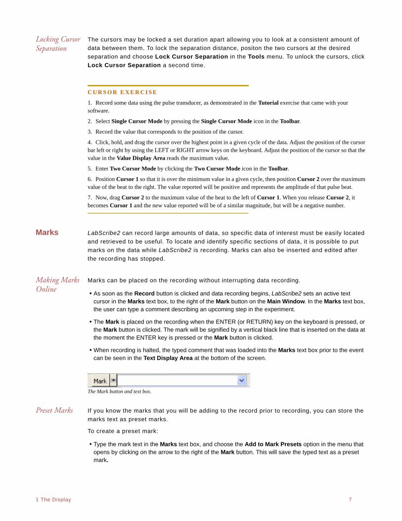
• As soon as the Record button is clicked and data recording begins, LabScribe2 sets an active text cursor in the Marks text box, to the right of the Mark button on the Main Window. In the Marks text box, the user can type a comment describing an upcoming step in the experiment.
• The Mark is placed on the recording when the ENTER (or RETURN) key on the keyboard is pressed, or the Mark button is clicked. The mark will be signified by a vertical black line that is inserted on the data at the moment the ENTER key is pressed or the Mark button is clicked.
• When recording is halted, the typed comment that was loaded into the Marks text box prior to the event can be seen in the Text Display Area at the bottom of the screen.
The Mark button and text box.
Preset Marks If you know the marks that you will be adding to the record prior to recording, you can store the
marks text as preset marks.
To create a preset mark:
• Type the mark text in the Marks text box, and choose the Add to Mark Presets option in the menu that opens by clicking on the arrow to the right of the Mark button. This will save the typed text as a preset mark.
. .
1 The Display 8
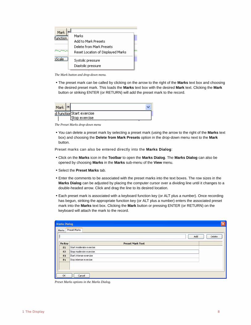
The Mark button and drop-down menu.
• The preset mark can be called by clicking on the arrow to the right of the Marks text box and choosing the desired preset mark. This loads the Marks text box with the desired Mark text. Clicking the Mark button or striking ENTER (or RETURN) will add the preset mark to the record.
The Preset Marks drop-down menu
• You can delete a preset mark by selecting a preset mark (using the arrow to the right of the Marks text box) and choosing the Delete from Mark Presets option in the drop-down menu next to the Mark button.
Preset marks can also be entered directly into the Marks Dialog:
• Click on the Marks icon in the Toolbar to open the Marks Dialog. The Marks Dialog can also be opened by choosing Marks in the Marks sub-menu of the View menu.
• Select the Preset Marks tab.
• Enter the comments to be associated with the preset marks into the text boxes. The row sizes in the Marks Dialog can be adjusted by placing the computer cursor over a dividing line until it changes to a double-headed arrow. Click and drag the line to its desired location.
• Each preset mark is associated with a keyboard function key (or ALT plus a number). Once recording has begun, striking the appropriate function key (or ALT plus a number) enters the associated preset mark into the Marks text box. Clicking the Mark button or pressing ENTER (or RETURN) on the keyboard will attach the mark to the record.
Preset Marks options in the Marks Dialog.
. .
1 The Display 9
Making Marks Off-Line
Marking events as they happen is a necessity for events that are time critical, like drug deliv-
eries or experimental interventions. Information about the experiment that is important, but not
time critical, can be marked on the recording after the recording is completed. An example of the
type of comment that could be added later would be a change in room temperature.
To add this information to the record after recording is completed:
• Click on the Single Cursor Mode icon in the Toolbar.
• Position the cursor on the record where the mark is to be positioned.
• Type the text (a maximum of 50 characters) associated with the new mark in the Marks text box. Click the Mark button or press the keyboard’s ENTER (or RETURN) key, and the mark and its text comment are inserted at the current position of the cursor.
• You can also add a mark to the record by selecting Add Mark from the Marks sub-menu of the View menu. Type your text into the window that opens and click OK. The mark will be added to the record at the current position of the cursor.
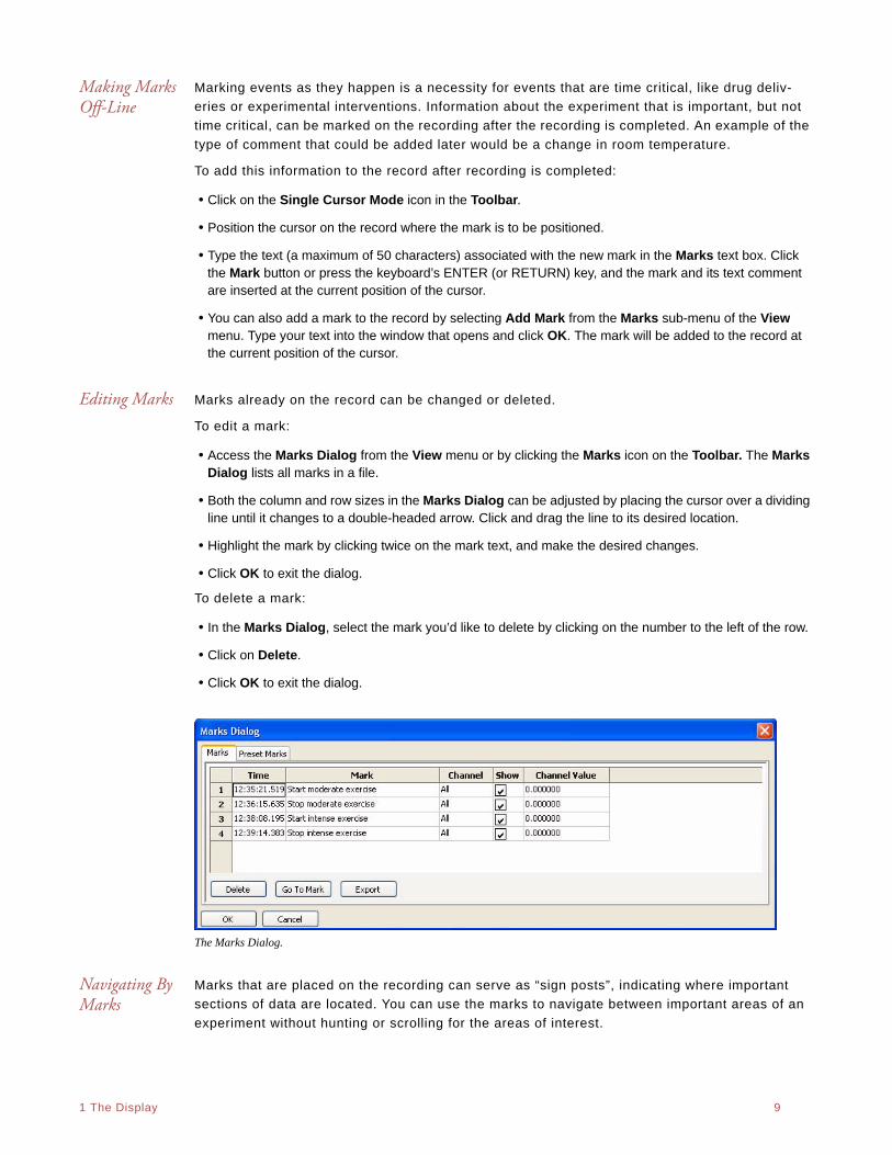
Editing Marks Marks already on the record can be changed or deleted.
To edit a mark:
• Access the Marks Dialog from the View menu or by clicking the Marks icon on the Toolbar. The Marks Dialog lists all marks in a file.
• Both the column and row sizes in the Marks Dialog can be adjusted by placing the cursor over a dividing line until it changes to a double-headed arrow. Click and drag the line to its desired location.
• Highlight the mark by clicking twice on the mark text, and make the desired changes.
• Click OK to exit the dialog.
To delete a mark:
• In the Marks Dialog, select the mark you’d like to delete by clicking on the number to the left of the row.
• Click on Delete.
• Click OK to exit the dialog.
The Marks Dialog.
Navigating By Marks
Marks that are placed on the recording can serve as “sign posts”, indicating where important
sections of data are located. You can use the marks to navigate between important areas of an
experiment without hunting or scrolling for the areas of interest.
. .
1 The Display 10
To navigate by marks:
• Click on the arrow next to the Mark button and choose the mark you want to “go to”. LabScribe2 will find the data point associated with that mark and display that section of data in the Main Window.
• Alternatively, select the mark in the Marks Dialog and click on Go To Mark.
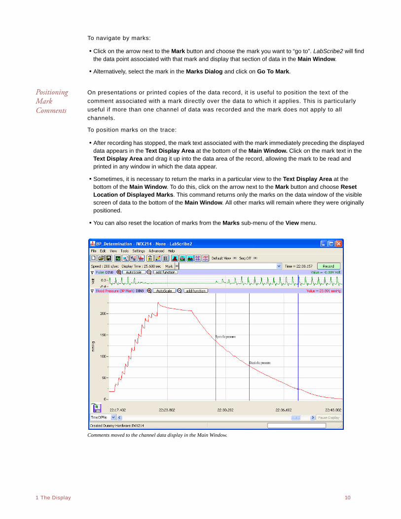
Positioning Mark Comments
On presentations or printed copies of the data record, it is useful to position the text of the
comment associated with a mark directly over the data to which it applies. This is particularly
useful if more than one channel of data was recorded and the mark does not apply to all
channels.
To position marks on the trace:
• After recording has stopped, the mark text associated with the mark immediately preceding the displayed data appears in the Text Display Area at the bottom of the Main Window. Click on the mark text in the Text Display Area and drag it up into the data area of the record, allowing the mark to be read and printed in any window in which the data appear.
• Sometimes, it is necessary to return the marks in a particular view to the Text Display Area at the bottom of the Main Window. To do this, click on the arrow next to the Mark button and choose Reset Location of Displayed Marks. This command returns only the marks on the data window of the visible screen of data to the bottom of the Main Window. All other marks will remain where they were originally positioned.
• You can also reset the location of marks from the Marks sub-menu of the View menu.
Comments moved to the channel data display in the Main Window.

. .
1 The Display 11
Sorting and Exporting Marks
The Marks Dialog displays the time that a mark was made, the text comment attached to the
mark, the channel on which the mark was made, and the value of the amplitude at the mark.
Marks can be sorted by time, channel, or the text comment of the mark by clicking on the
column titles. Click once to organize marks in ascending order and a second time to change to
descending order.
To export marks to a text file or spreadsheet program, select the mark in the Marks Dialog and
click the Export button.
M A R K S E X E R C I S E
1. Click Record and record a few minutes of pulse transducer data as demonstrated in the Tutorial exercise that came with your software.
2. As data are being recorded, type “Test 1” on the keyboard and strike the ENTER (or RETURN) key on the keyboard.
3. Wait one minute, type “Test 2" and strike the ENTER (or RETURN) key.
4. Click Stop. Scroll through the data using the scroll bar at the bottom of the Main Window until you locate “Test 1” in the Text Display Area.
5. Click on the arrow next to the Mark button and choose “Test 2". Notice that the data in the Main Window has moved to the “Test 2" mark.
6. Using the mouse, click and hold on the comment “Test 2" at the bottom of the screen. Continue holding the mouse button down, and drag the comment to a new position on one of the available channels.
7. Release the mouse button and the mark text is locked on the selected channel. Comments positioned in this way will remain where they are placed and will print exactly as you see them.
8. Try this exercise again with a mark created off-line. To create an off-line mark, open Single Cursor Mode by clicking the Single Cursor icon in the Toolbar. Position the cursor where the off-line mark is to be positioned. Type some text on the comment line at the top of the screen, and press the ENTER (or RETURN) key. The mark appears at the cursor location and the comment appears at the bottom of the screen.
Views The number of channels of raw data that LabScribe2 can acquire and display is limited to the
number of inputs on the hardware in use, but it can calculate data on up to 128 channels. The
extra channels can be used to display computed functions that are mathematically derived from
the raw data.
For example, the arterial pressure from four different animals could be recorded on Channels 1-
4. Simultaneously, the Rate function could be used on Channels 5-8 to calculate the heart rate
of each animal from its recorded blood pressure on Channels 1-4. Displaying more channels
means there is less space on the display for each one. In the case of a 16-channel Main
Window display, it is hard to resolve detail in the recorded data on each channel.
LabScribe2 solves this problem by allowing the user to create many different arrangements of
channels that are displayed on the screen at one time. Each arrangement of channels that is
displayed is known as a View. Using the example from the previous paragraph, a view could be
created that displayed only the arterial pressure from Channel 1 and the calculated heart rate
for the same animal displayed on Channel 5. The data from Channels 1 and 5 would appear in
the first and second data display areas, respectively. The other six raw data and computed heart
rate channels would not be displayed. For the data recorded from another animal on Channel 2,
another view with Channels 2 and 6 (its matching rate channel) can be created.
. .
1 The Display 12
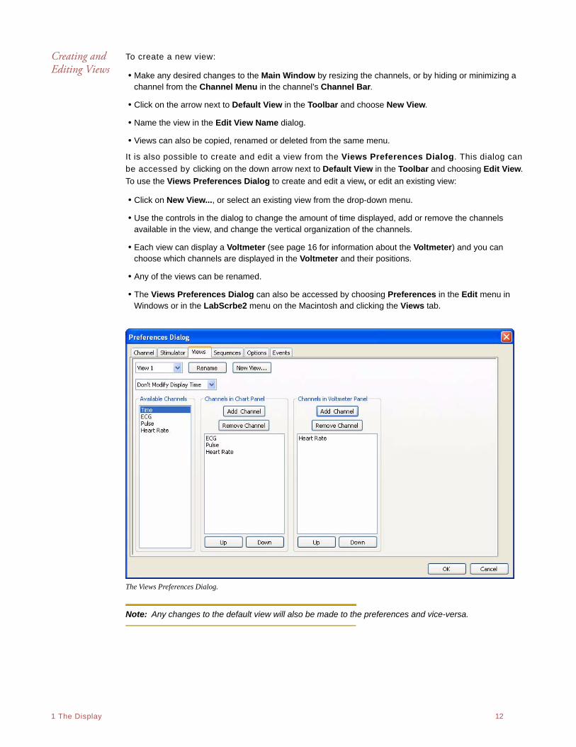
Creating and Editing Views
To create a new view:
• Make any desired changes to the Main Window by resizing the channels, or by hiding or minimizing a channel from the Channel Menu in the channel’s Channel Bar.
• Click on the arrow next to Default View in the Toolbar and choose New View.
• Name the view in the Edit View Name dialog.
• Views can also be copied, renamed or deleted from the same menu.
It is also possible to create and edit a view from the Views Preferences Dialog. This dialog can
be accessed by clicking on the down arrow next to Default View in the Toolbar and choosing Edit View.
To use the Views Preferences Dialog to create and edit a view, or edit an existing view:
• Click on New View..., or select an existing view from the drop-down menu.
• Use the controls in the dialog to change the amount of time displayed, add or remove the channels available in the view, and change the vertical organization of the channels.
• Each view can display a Voltmeter (see page 16 for information about the Voltmeter) and you can choose which channels are displayed in the Voltmeter and their positions.
• Any of the views can be renamed.
• The Views Preferences Dialog can also be accessed by choosing Preferences in the Edit menu in Windows or in the LabScrbe2 menu on the Macintosh and clicking the Views tab.
The Views Preferences Dialog.
Note: Any changes to the default view will also be made to the preferences and vice-versa.
. .
1 The Display 13
Units Conversion
When used with iWorx hardware, LabScribe2 functions as a calibrated voltmeter, which means
the software will accurately display the exact voltage that the user presents to the analog-to-
digital converter. The displayed (and default) units will always be volts. While this is useful in
many cases, it is not always the appropriate unit for the data being recorded.
If LabScribe2 is used to record the output of a transducer designed to measure a physical
parameter, such as force or pressure, other units are more appropriate. In these cases, volts
can be converted into milligrams, grams, or any other units. LabScribe2 can handle these
conversions easily, provided that the function that converts voltage into units appropriate to the
transducer is linear.
LabScribe2 offers several options for Units Conversion. They are listed in the Units submenu of
the Channel Menu.
• Invert: Inverts the trace.
• Simple... : Opens the Simple Units Conversion dialog.
• Advanced...: Opens the Advanced Units Conversion Dialog.
• Set Offset...: Allows the user to set an offset required by certain transducers.The Units submenu.
• Off (all blocks): Turns all units conversions off.
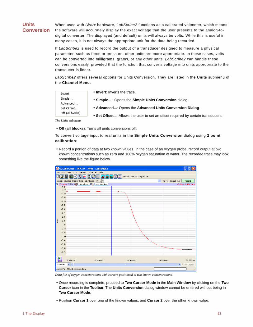
To convert voltage input to real units in the Simple Units Conversion dialog using 2 point
calibration:
• Record a portion of data at two known values. In the case of an oxygen probe, record output at two known concentrations such as zero and 100% oxygen saturation of water. The recorded trace may look something like the figure below.
Data file of oxygen concentrations with cursors positioned at two known concentrations.
• Once recording is complete, proceed to Two Cursor Mode in the Main Window by clicking on the Two Cursor icon in the Toolbar. The Units Conversion dialog window cannot be entered without being in Two Cursor Mode.
• Position Cursor 1 over one of the known values, and Cursor 2 over the other known value.
. .
1 The Display 14
• Open the Channel Menu by clicking on the arrow on the left end of the Channel Bar or right-click anywhere in the data channel and select Units from the Channel Menu. The Units menu can also be accessed by left-clicking on the Value Display Area of the Channel Bar.
• Select Simple.... to open the Simple Units Conversion dialog window.
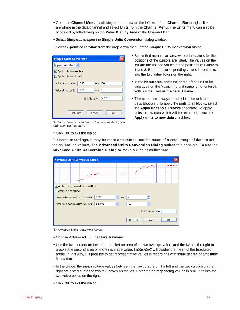
• Select 2-point calibration from the drop-down menu of the Simple Units Conversion dialog.
• Below that menu is an area where the values for the positions of the cursors are listed. The values on the left are the voltage values at the positions of Cursors 1 and 2. Enter the corresponding values in real units into the two value boxes on the right.
• In the Name area, enter the name of the unit to be displayed on the Y-axis. If a unit name is not entered, volts will be used as the default name.
• The units are always applied to the selected data block(s). To apply the units to all blocks, select the Apply units to all blocks checkbox. To apply units to new data which will be recorded select the Apply units to new data checkbox.
The Units Conversion dialog window showing the 2-point calibration configuration.
• Click OK to exit the dialog.
For some recordings, it may be more accurate to use the mean of a small range of data to set
the calibration values, The Advanced Units Conversion Dialog makes this possible. To use the
Advanced Units Conversion Dialog to make a 2 point calibration:
The Advanced Units Conversion Dialog.
• Choose Advanced... in the Units submenu.
• Use the two cursors on the left to bracket an area of known average value, and the two on the right to bracket the second area of known average value. LabScribe2 will display the mean of the bracketed areas. In this way, it is possible to get representative values in recordings with some degree of amplitude fluctuation.
• In the dialog, the mean voltage values between the two cursors on the left and the two cursors on the right are entered into the two text boxes on the left. Enter the corresponding values in real units into the two value boxes on the right.
• Click OK to exit the dialog.
. .
1 The Display 15
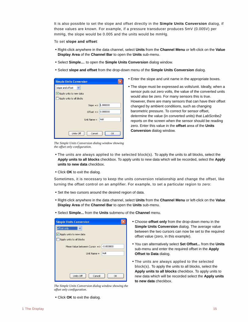
It is also possible to set the slope and offset directly in the Simple Units Conversion dialog, if
those values are known. For example, if a pressure transducer produces 5mV (0.005V) per
mmHg, the slope would be 0.005 and the units would be mmHg.
To set slope and offset:
• Right-click anywhere in the data channel, select Units from the Channel Menu or left-click on the Value Display Area of the Channel Bar to open the Units sub-menu.
• Select Simple.... to open the Simple Units Conversion dialog window.
• Select slope and offset from the drop-down menu of the Simple Units Conversion dialog.
• Enter the slope and unit name in the appropriate boxes.
• The slope must be expressed as volts/unit. Ideally, when a sensor puts out zero volts, the value of the converted units would also be zero. For many sensors this is true. However, there are many sensors that can have their offset changed by ambient conditions, such as changing barometric pressure. To correct for sensor offset, determine the value (in converted units) that LabScribe2 reports on the screen when the sensor should be reading zero. Enter this value in the offset area of the Units Conversion dialog window.
The Simple Units Conversion dialog window showing the offset only configuration.
• The units are always applied to the selected block(s). To apply the units to all blocks, select the Apply units to all blocks checkbox. To apply units to new data which will be recorded, select the Apply units to new data checkbox.
• Click OK to exit the dialog.
Sometimes, it is necessary to keep the units conversion relationship and change the offset, like
turning the offset control on an amplifier. For example, to set a particular region to zero:
• Set the two cursors around the desired region of data.
• Right-click anywhere in the data channel, select Units from the Channel Menu or left-click on the Value Display Area of the Channel Bar to open the Units sub-menu.
• Select Simple... from the Units submenu of the Channel menu.
• Choose offset only from the drop-down menu in the Simple Units Conversion dialog. The average value between the two cursors can now be set to the required offset value (zero, in this example).
• You can alternatively select Set Offset... from the Units sub-menu and enter the required offset in the Apply Offset to Data dialog.
• The units are always applied to the selected block(s). To apply the units to all blocks, select the Apply units to all blocks checkbox. To apply units to new data which will be recorded select the Apply units to new data checkbox.
The Simple Units Conversion dialog window showing the offset only configuration.
• Click OK to exit the dialog.
. .
1 The Display 16
Unit conversions can also be set from the Channel page of the Preferences Dialog. Each
channel can be set with the conversion factors provided by the transducer manufacturer (refer to
page 42 in Chapter 4: Creating Your Own Settings and Preferences).
At times, it may be desirable to turn off the Units Conversion and simply view the raw data in
the default unit, which is volts. You can turn off the units for all blocks directly from the Units
sub-menu or from the Simple Units Conversion dialog box.
Inverting the Trace
When recording physical parameters, such as temperature, pressure, or force, it is best if the
polarity of the data display matches the real-world behavior of the parameter. For example, if the
observed temperature goes up, the trace on the computer screen should go up. Increasing
pressure or force should also produce a positive or upward deflection of the trace.
Depending how sensors and amplifiers are wired, this may or may not be the case. In the event
that the data display has the wrong polarity, the trace can be inverted by selecting Invert from
the Channel Menu, Units sub-menu, or the right-click menu in any data channel. The Invert
function can be switched off at any time by selecting Invert a second time.
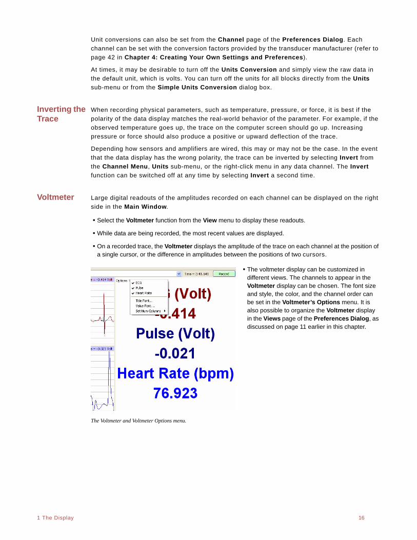
Voltmeter Large digital readouts of the amplitudes recorded on each channel can be displayed on the right
side in the Main Window.
• Select the Voltmeter function from the View menu to display these readouts.
• While data are being recorded, the most recent values are displayed.
• On a recorded trace, the Voltmeter displays the amplitude of the trace on each channel at the position of a single cursor, or the difference in amplitudes between the positions of two cursors.
• The voltmeter display can be customized in different views. The channels to appear in the Voltmeter display can be chosen. The font size and style, the color, and the channel order can be set in the Voltmeter’s Options menu. It is also possible to organize the Voltmeter display in the Views page of the Preferences Dialog, as discussed on page 11 earlier in this chapter.
The Voltmeter and Voltmeter Options menu.
. .
1 The Display 17
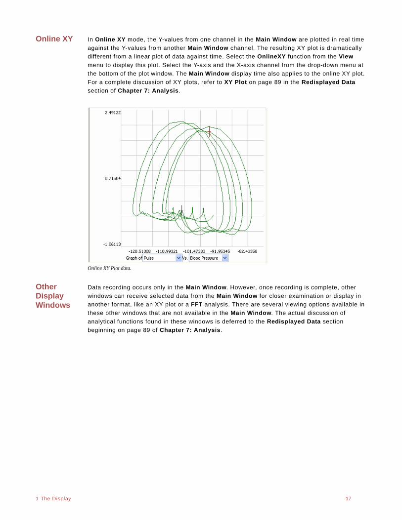
Online XY In Online XY mode, the Y-values from one channel in the Main Window are plotted in real time
against the Y-values from another Main Window channel. The resulting XY plot is dramatically
different from a linear plot of data against time. Select the OnlineXY function from the View
menu to display this plot. Select the Y-axis and the X-axis channel from the drop-down menu at
the bottom of the plot window. The Main Window display time also applies to the online XY plot.
For a complete discussion of XY plots, refer to XY Plot on page 89 in the Redisplayed Data
section of Chapter 7: Analysis.
Online XY Plot data.
Other Display Windows
Data recording occurs only in the Main Window. However, once recording is complete, other
windows can receive selected data from the Main Window for closer examination or display in
another format, like an XY plot or a FFT analysis. There are several viewing options available in
these other windows that are not available in the Main Window. The actual discussion of
analytical functions found in these windows is deferred to the Redisplayed Data section
beginning on page 89 of Chapter 7: Analysis.
. .
2 The Menus 18
Chapter 2: The Menus
OverviewWhile many of LabScribe2’s features can be accessed in more than one way, the main menus
and the dialogs they open provide a systematic way to access virtually every LabScribe2
feature.
The Menus
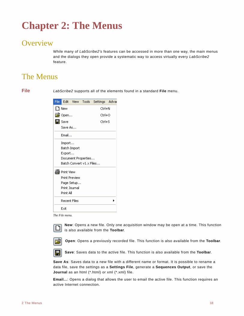
File LabScribe2 supports all of the elements found in a standard File menu.
The File menu.
New: Opens a new file. Only one acquisition window may be open at a time. This function
is also available from the Toolbar.
Open: Opens a previously recorded file. This function is also available from the Toolbar.
Save: Saves data to the active file. This function is also available from the Toolbar.
Save As: Saves data to a new file with a different name or format. It is possible to rename a
data file, save the settings as a Settings File, generate a Sequences Output, or save the
Journal as an html (*.html) or xml (*.xml) file.
Email...: Opens a dialog that allows the user to email the active file. This function requires an
active Internet connection.
. .
2 The Menus 19
Import...: Opens a dialog that allows the user to set the parameters for importing text data files.
This is a separately licensed feature of LabScribe2.
Batch Import: Once a single text file is imported, a number of additional files can be imported
with the same input parameters.
Export...: Allows the user to export the entire data file as text, or in a variety of formats appro-
priate to external analysis programs. These formats include Matlab (*.mat), DADISP (*.dat), and
Excel (*.xls). The current screen can be exported as a JPG (*.jpg) or Portable Network Graphics
(*.png) file. The current screen can also be exported as a LabScribe2 data file.
Document Properties...: Opens the Document Properties dialog that allows the user to
annotate the file wth notes, or to view the acquisition characteristics of the file, including the
date and time of recording, the sampling speed, and the number of input channels.
Batch Convert v1.x Files...: Converts all v1.x files in a folder to v2.x files.
Print View: Prints the active window.
Print Preview: Previews the image to be printed.
Page Setup...: Opens a dialog box that allows the user to set up page formatting features
specific to the printer being used.
Print Journal: Prints the Journal.
Recent Files: Opens a submenu displaying the last ten files opened. Choosing one closes the
current file and opens the selected data file.
Exit: Quits the program. On the Macintosh, use Quit Labscribe 2 in the Labscribe 2 menu.
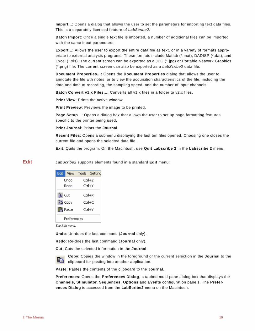
Edit LabScribe2 supports elements found in a standard Edit menu:
The Edit menu.
Undo: Un-does the last command (Journal only).
Redo: Re-does the last command (Journal only).
Cut: Cuts the selected information in the Journal.
Copy: Copies the window in the foreground or the current selection in the Journal to the
clipboard for pasting into another application.
Paste: Pastes the contents of the clipboard to the Journal.
Preferences: Opens the Preferences Dialog, a tabbed multi-pane dialog box that displays the
Channels, Stimulator, Sequences, Options and Events configuration panels. The Prefer-
ences Dialog is accessed from the LabScribe2 menu on the Macintosh.
. .
2 The Menus 20
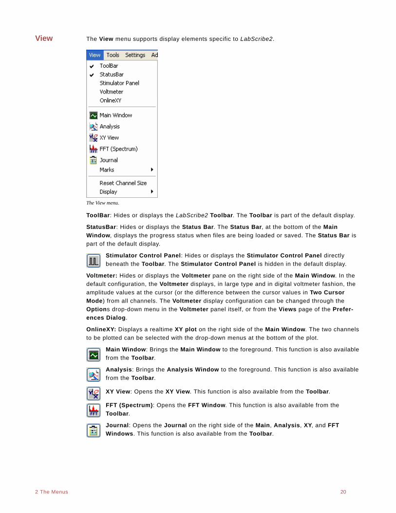
View The View menu supports display elements specific to LabScribe2.
The View menu.
ToolBar: Hides or displays the LabScribe2 Toolbar. The Toolbar is part of the default display.
StatusBar: Hides or displays the Status Bar. The Status Bar, at the bottom of the Main
Window, displays the progress status when files are being loaded or saved. The Status Bar is
part of the default display.
Stimulator Control Panel: Hides or displays the Stimulator Control Panel directly
beneath the Toolbar. The Stimulator Control Panel is hidden in the default display.
Voltmeter: Hides or displays the Voltmeter pane on the right side of the Main Window. In the
default configuration, the Voltmeter displays, in large type and in digital voltmeter fashion, the
amplitude values at the cursor (or the difference between the cursor values in Two Cursor
Mode) from all channels. The Voltmeter display configuration can be changed through the
Options drop-down menu in the Voltmeter panel itself, or from the Views page of the Prefer-
ences Dialog.
OnlineXY: Displays a realtime XY plot on the right side of the Main Window. The two channels
to be plotted can be selected with the drop-down menus at the bottom of the plot.
Main Window: Brings the Main Window to the foreground. This function is also available
from the Toolbar.
Analysis: Brings the Analysis Window to the foreground. This function is also available
from the Toolbar.
XY View: Opens the XY View. This function is also available from the Toolbar.
FFT (Spectrum): Opens the FFT Window. This function is also available from the
Toolbar.
Journal: Opens the Journal on the right side of the Main, Analysis, XY, and FFT
Windows. This function is also available from the Toolbar.
. .
2 The Menus 21
Marks: Opens a submenu with controls that open the Marks Dialog, add the mark in the Marks
text box to the recording, and reset the marks on the current screen to their original positions in
the Text Display Area at the base of the Main Window.
The Marks submenu.
Reset Channel Size: Returns all open channels to their default screen sizes.
Display: Opens a submenu with controls for changing display time parameters. These param-
eters are discussed starting on page 27 of Chapter 3: Acquisition.
The Display submenu.
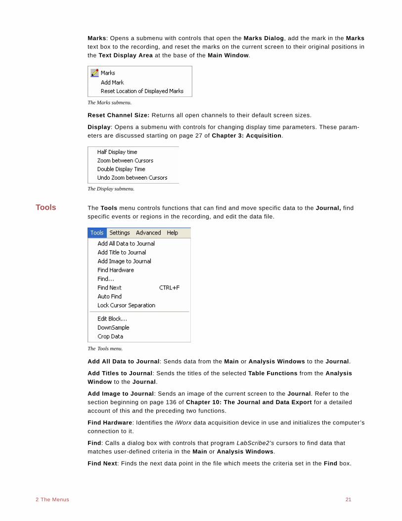
Tools The Tools menu controls functions that can find and move specific data to the Journal, find
specific events or regions in the recording, and edit the data file.
The Tools menu.
Add All Data to Journal: Sends data from the Main or Analysis Windows to the Journal.
Add Titles to Journal: Sends the titles of the selected Table Functions from the Analysis
Window to the Journal.
Add Image to Journal: Sends an image of the current screen to the Journal. Refer to the
section beginning on page 136 of Chapter 10: The Journal and Data Export for a detailed
account of this and the preceding two functions.
Find Hardware: Identifies the iWorx data acquisition device in use and initializes the computer’s
connection to it.
Find: Calls a dialog box with controls that program LabScribe2’s cursors to find data that
matches user-defined criteria in the Main or Analysis Windows.
Find Next: Finds the next data point in the file which meets the criteria set in the Find box.
. .
2 The Menus 22
Auto Find: Automatically finds each successive data point in the file that meets the criteria set
in the Find dialog box. Calculated values from the Table Functions selected in the Analysis
window can be automatically added to the Journal for each matching data point. Refer to the
Find Functions section beginning on page 96 of Chapter 7: Analysis for a complete discussion
of all the Find Functions.
Lock Cursor Separation: Locks the cursors at a fixed separation distance. Refer to Locking
Cursor Separation on page 7 in the Cursors section of Chapter 1: The Display for a complete
discussion.
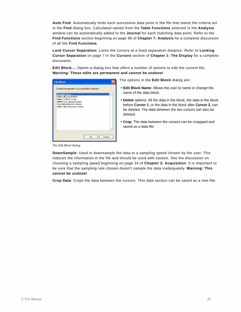
Edit Block...: Opens a dialog box that offers a number of options to edit the current file.
Warning: These edits are permanent and cannot be undone!
The options in the Edit Block dialog are:
• Edit Block Name: Allows the user to name or change the name of the data block.
• Delete options: All the data in the block, the data in the block before Cursor 1, or the data in the block after Cursor 2, can be deleted. The data between the two cursors can also be deleted.
• Crop: The data between the cursors can be croppped and saved as a data file.
The Edit Block dialog.
DownSample: Used to downsample the data to a sampling speed chosen by the user. This
reduces the information in the file and should be used with caution. See the discussion on
choosing a sampling speed beginning on page 34 of Chapter 3: Acquisition. It is important to
be sure that the sampling rate chosen doesn’t sample the data inadequately. Warning: This
cannot be undone!
Crop Data: Crops the data between the cursors. This data section can be saved as a new file.
. .
2 The Menus 23
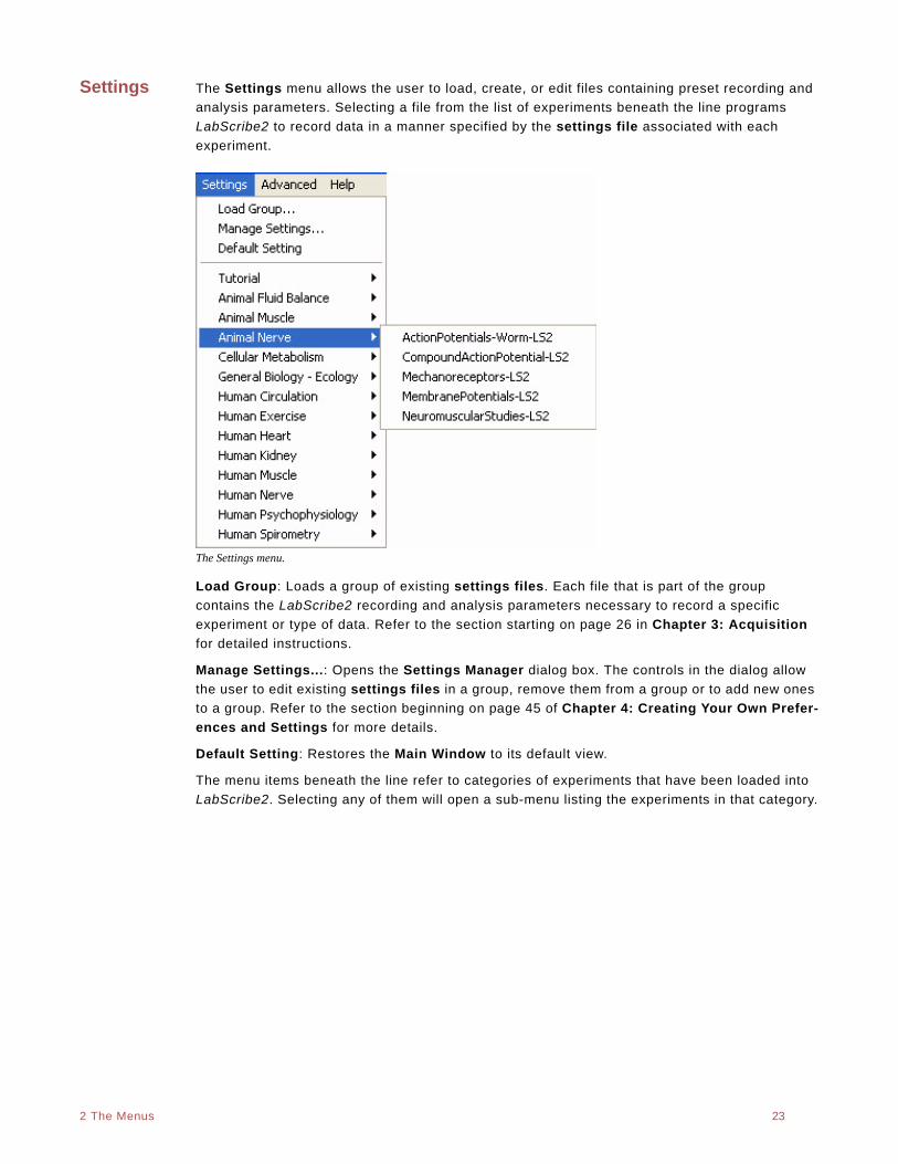
Settings The Settings menu allows the user to load, create, or edit files containing preset recording and
analysis parameters. Selecting a file from the list of experiments beneath the line programs
LabScribe2 to record data in a manner specified by the settings file associated with each
experiment.
The Settings menu.
Load Group: Loads a group of existing settings files. Each file that is part of the group
contains the LabScribe2 recording and analysis parameters necessary to record a specific
experiment or type of data. Refer to the section starting on page 26 in Chapter 3: Acquisition
for detailed instructions.
Manage Settings...: Opens the Settings Manager dialog box. The controls in the dialog allow
the user to edit existing settings files in a group, remove them from a group or to add new ones
to a group. Refer to the section beginning on page 45 of Chapter 4: Creating Your Own Prefer-
ences and Settings for more details.
Default Setting: Restores the Main Window to its default view.
The menu items beneath the line refer to categories of experiments that have been loaded into
LabScribe2. Selecting any of them will open a sub-menu listing the experiments in that category.
. .
2 The Menus 24
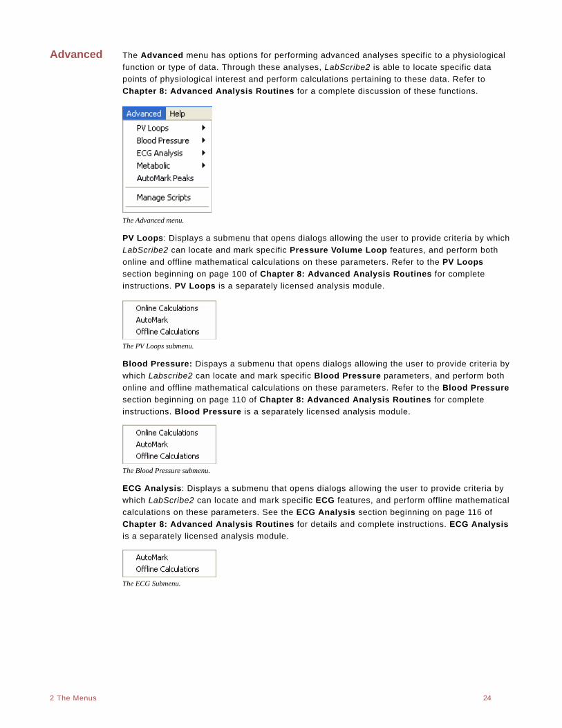
Advanced The Advanced menu has options for performing advanced analyses specific to a physiological
function or type of data. Through these analyses, LabScribe2 is able to locate specific data
points of physiological interest and perform calculations pertaining to these data. Refer to
Chapter 8: Advanced Analysis Routines for a complete discussion of these functions.
The Advanced menu.
PV Loops: Displays a submenu that opens dialogs allowing the user to provide criteria by which
LabScribe2 can locate and mark specific Pressure Volume Loop features, and perform both
online and offline mathematical calculations on these parameters. Refer to the PV Loops
section beginning on page 100 of Chapter 8: Advanced Analysis Routines for complete
instructions. PV Loops is a separately licensed analysis module.
The PV Loops submenu.
Blood Pressure: Dispays a submenu that opens dialogs allowing the user to provide criteria by
which Labscribe2 can locate and mark specific Blood Pressure parameters, and perform both
online and offline mathematical calculations on these parameters. Refer to the Blood Pressure
section beginning on page 110 of Chapter 8: Advanced Analysis Routines for complete
instructions. Blood Pressure is a separately licensed analysis module.
The Blood Pressure submenu.
ECG Analysis: Displays a submenu that opens dialogs allowing the user to provide criteria by
which LabScribe2 can locate and mark specific ECG features, and perform offline mathematical
calculations on these parameters. See the ECG Analysis section beginning on page 116 of
Chapter 8: Advanced Analysis Routines for details and complete instructions. ECG Analysis
is a separately licensed analysis module.
The ECG Submenu.
. .
2 The Menus 25
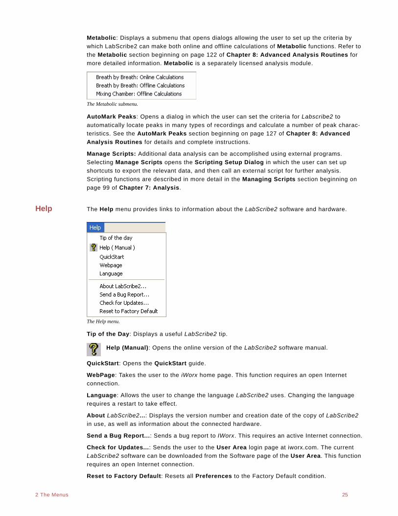
Metabolic: Displays a submenu that opens dialogs allowing the user to set up the criteria by
which LabScribe2 can make both online and offline calculations of Metabolic functions. Refer to
the Metabolic section beginning on page 122 of Chapter 8: Advanced Analysis Routines for
more detailed information. Metabolic is a separately licensed analysis module.
The Metabolic submenu.
AutoMark Peaks: Opens a dialog in which the user can set the criteria for Labscribe2 to
automatically locate peaks in many types of recordings and calculate a number of peak charac-
teristics. See the AutoMark Peaks section beginning on page 127 of Chapter 8: Advanced
Analysis Routines for details and complete instructions.
Manage Scripts: Additional data analysis can be accomplished using external programs.
Selecting Manage Scripts opens the Scripting Setup Dialog in which the user can set up
shortcuts to export the relevant data, and then call an external script for further analysis.
Scripting functions are described in more detail in the Managing Scripts section beginning on
page 99 of Chapter 7: Analysis.
Help The Help menu provides links to information about the LabScribe2 software and hardware.
The Help menu.
Tip of the Day: Displays a useful LabScribe2 tip.
Help (Manual): Opens the online version of the LabScribe2 software manual.
QuickStart: Opens the QuickStart guide.
WebPage: Takes the user to the iWorx home page. This function requires an open Internet
connection.
Language: Allows the user to change the language LabScribe2 uses. Changing the language
requires a restart to take effect.
About LabScribe2...: Displays the version number and creation date of the copy of LabScribe2
in use, as well as information about the connected hardware.
Send a Bug Report...: Sends a bug report to IWorx. This requires an active Internet connection.
Check for Updates...: Sends the user to the User Area login page at iworx.com. The current
LabScribe2 software can be downloaded from the Software page of the User Area. This function
requires an open Internet connection.
Reset to Factory Default: Resets all Preferences to the Factory Default condition.
. .
3 Acquisition 26
Chapter 3: Acquisition
Overview
Start Recording
The most basic control in LabScribe2 is the one that starts and stops the recording. This control
is found in the upper right hand corner of the Main Window. After ensuring that the source of
your signal is properly connected to your data acquisition unit, click the Record button to begin
recording.
While data are being recorded the Record button changes to Stop. Click Stop at any time to
end data recording.
Settings In addition to the hardware and software provided in its teaching kits, iWorx provides a variety of
experiments in electronic lab manuals. To support these experiments, iWorx has created
settings groups that contain links to settings files for each experiment in that group. Once a
settings group is loaded, the settings files within the group can be called from a list in the
Settings menu.
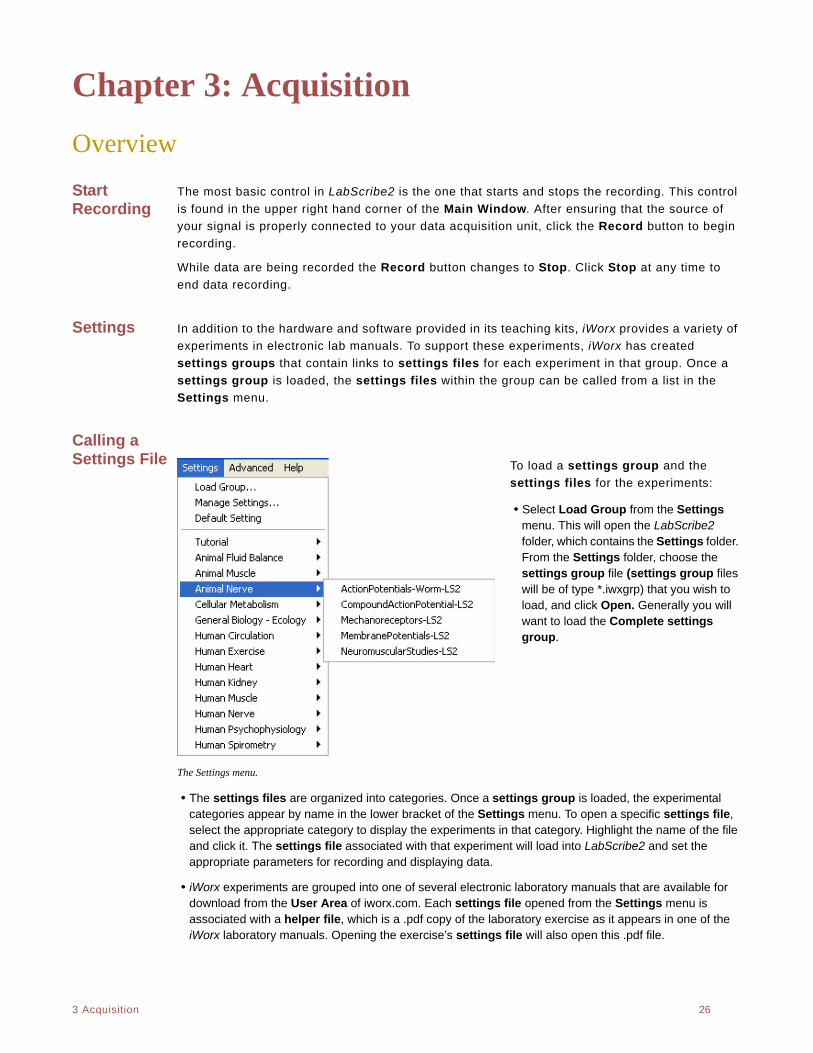
Calling a Settings File To load a settings group and the
settings files for the experiments:
• Select Load Group from the Settings menu. This will open the LabScribe2 folder, which contains the Settings folder. From the Settings folder, choose the settings group file (settings group files will be of type *.iwxgrp) that you wish to load, and click Open. Generally you will want to load the Complete settings group.
The Settings menu.
• The settings files are organized into categories. Once a settings group is loaded, the experimental categories appear by name in the lower bracket of the Settings menu. To open a specific settings file, select the appropriate category to display the experiments in that category. Highlight the name of the file and click it. The settings file associated with that experiment will load into LabScribe2 and set the appropriate parameters for recording and displaying data.
• iWorx experiments are grouped into one of several electronic laboratory manuals that are available for download from the User Area of iworx.com. Each settings file opened from the Settings menu is associated with a helper file, which is a .pdf copy of the laboratory exercise as it appears in one of the iWorx laboratory manuals. Opening the exercise’s settings file will also open this .pdf file.

. .
3 Acquisition 27
Main Window Display ConsiderationsRecorded data have two important dimensions: time and amplitude. Each of these has its own
set of controls.
Managing Display Time
The events recorded using LabScribe2 occur over very different time frames. For example,
recording the discharge curve of a 9-Volt battery takes hours, while recording the QRS complex
in a human electrocardiogram takes only a fraction of a second. LabScribe2 allows the recording
of both very slow and very fast events while displaying the data in a format that is easily inter-
preted. To manage the time component of recorded data, a parameter called Display Time is
used. Display Time is the amount of time represented by one full screen of data. When the
program opens, the default Display Time is set to 10 seconds. Settings files for specific lab
exercises may set a different Display Time. Display Time can be changed by the user by using
the display controls in the Toolbar, or by manually entering a Display Time on the Channel
page of the Preferences Dialog, which is launched by selecting Preferences in the Edit menu
in Windows, or in the LabScribe2 menu on the Macintosh.
Using the Toolbar icons to control Display Time:
• Clicking the Half Display Time icon (icon with the big mountain) in the Toolbar halves the screen time. If you clicked this icon once, a 10-second full-screen display would become a 5-second, full-screen display. This doubles the screen resolution, but cuts the amount of data seen on the screen in half. Using the Half Display Time tool expands the record as many times as requested, until there are only 10 data points on a screen of data. By the time this happens, the data will usually appear to “flatline” and events on this scale will not be recognizable.The Half Display Time command can also be accessed through the View menu’s Display submenu.
Display Time icons in the Main Window Toolbar.
• Clicking the Double Display Time icon (icon with the two smaller mountain peaks) in the Toolbar doubles the screen time. In this case, a 10-second, full-screen display would become 20-seconds wide. This reduces the screen resolution by half, but doubles the amount of data that you see on the screen. The display time can be doubled as many times as requested until the limit of the maximum size of the data file or 1,000,000 data points are displayed on one screen. By default, the maximum number of data points that may be displayed on the screen is 100,000. This can be changed on the Options page of the Preferences Dialog. The Double Display Time command can also be accessed through the View menu’s Display submenu.
• In Two Cursor Mode, clicking the Zoom Between Cursors icon fills the display with the data located between the cursors. You can undo the Zoom Between Cursors by choosing Undo Zoom Between Cursors in the Display submenu in the View menu.
There is a scrollbar at the bottom of the window that can be used to scroll through the data.
Scrolling can also be achieved by holding down the CRTL key (COMMAND on the Macintosh),
and clicking and dragging in the graph window.
. .
3 Acquisition 28
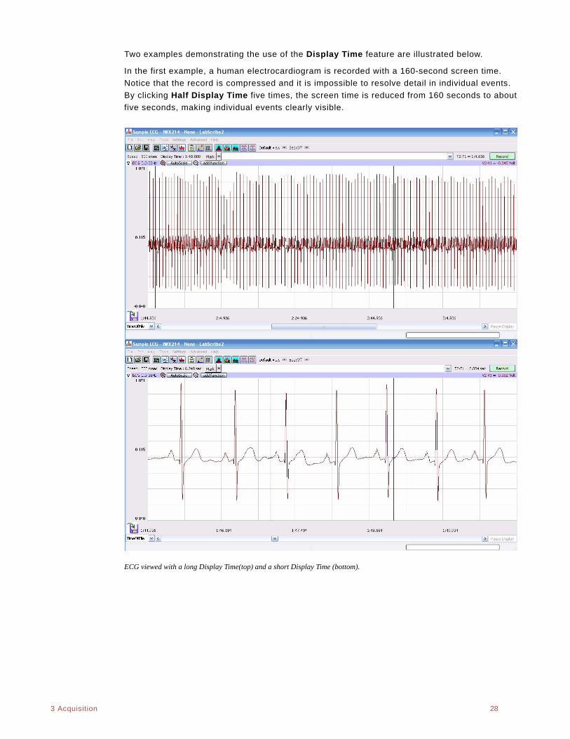
Two examples demonstrating the use of the Display Time feature are illustrated below.
In the first example, a human electrocardiogram is recorded with a 160-second screen time.
Notice that the record is compressed and it is impossible to resolve detail in individual events.
By clicking Half Display Time five times, the screen time is reduced from 160 seconds to about
five seconds, making individual events clearly visible.
ECG viewed with a long Display Time(top) and a short Display Time (bottom).
. .
3 Acquisition 29
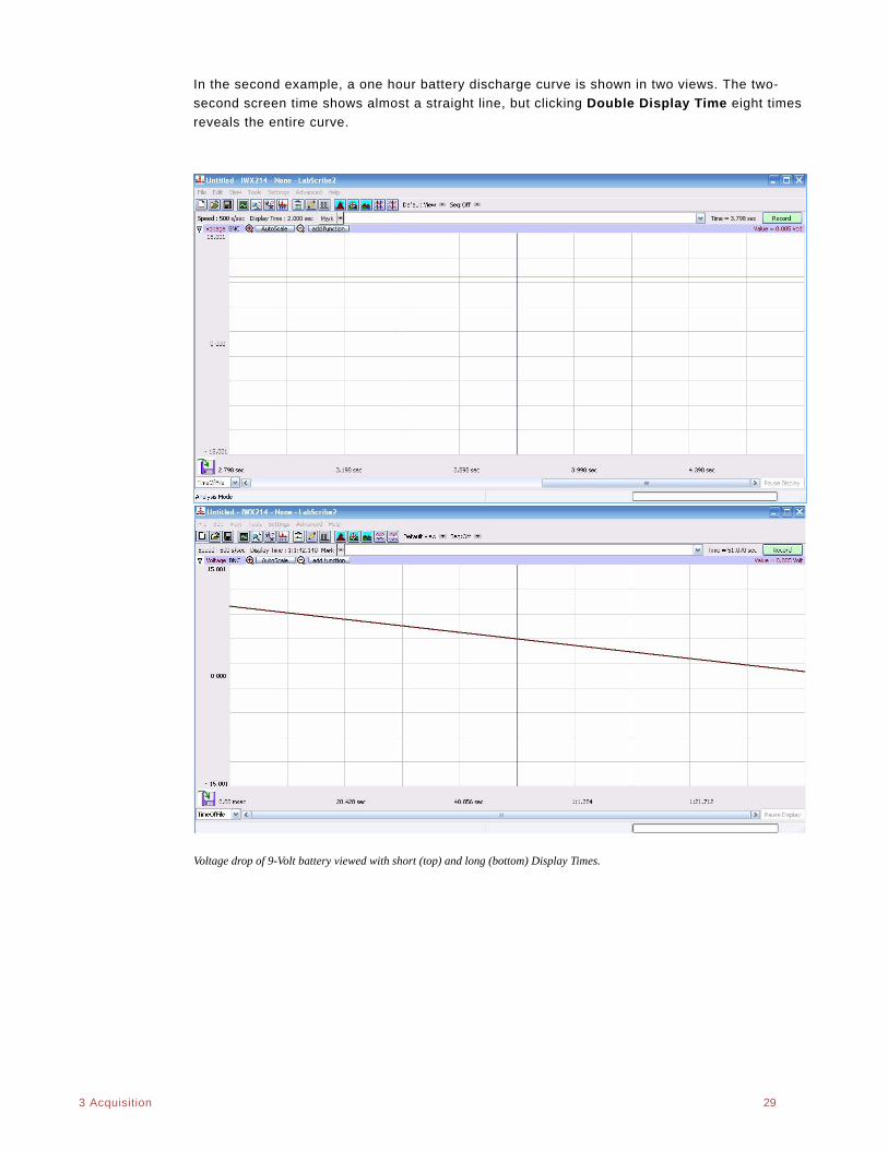
In the second example, a one hour battery discharge curve is shown in two views. The two-
second screen time shows almost a straight line, but clicking Double Display Time eight times
reveals the entire curve.
Voltage drop of 9-Volt battery viewed with short (top) and long (bottom) Display Times.
. .
3 Acquisition 30
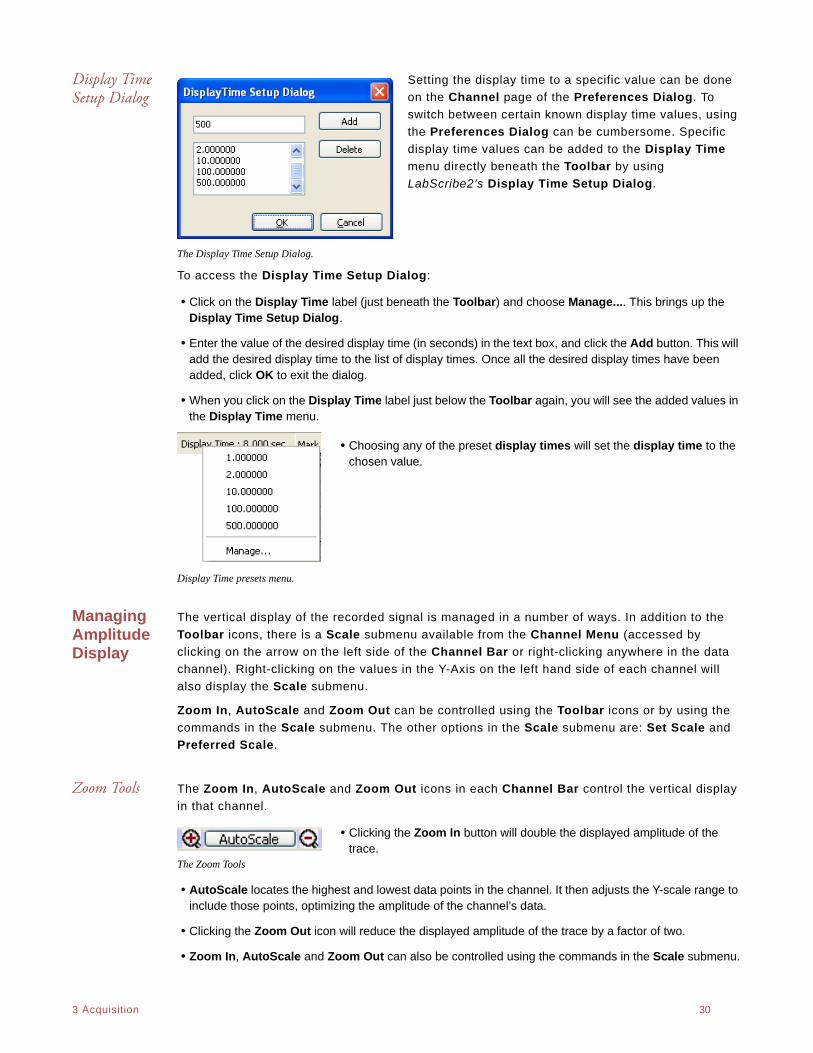
Display Time Setup Dialog
Setting the display time to a specific value can be done
on the Channel page of the Preferences Dialog. To
switch between certain known display time values, using
the Preferences Dialog can be cumbersome. Specific
display time values can be added to the Display Time
menu directly beneath the Toolbar by using
LabScribe2’s Display Time Setup Dialog.
The Display Time Setup Dialog.
To access the Display Time Setup Dialog:
• Click on the Display Time label (just beneath the Toolbar) and choose Manage.... This brings up the Display Time Setup Dialog.
• Enter the value of the desired display time (in seconds) in the text box, and click the Add button. This will add the desired display time to the list of display times. Once all the desired display times have been added, click OK to exit the dialog.
• When you click on the Display Time label just below the Toolbar again, you will see the added values in the Display Time menu.
• Choosing any of the preset display times will set the display time to the chosen value.
Display Time presets menu.
Managing Amplitude Display
The vertical display of the recorded signal is managed in a number of ways. In addition to the
Toolbar icons, there is a Scale submenu available from the Channel Menu (accessed by
clicking on the arrow on the left side of the Channel Bar or right-clicking anywhere in the data
channel). Right-clicking on the values in the Y-Axis on the left hand side of each channel will
also display the Scale submenu.
Zoom In, AutoScale and Zoom Out can be controlled using the Toolbar icons or by using the
commands in the Scale submenu. The other options in the Scale submenu are: Set Scale and
Preferred Scale.
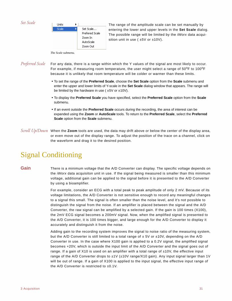
Zoom Tools The Zoom In, AutoScale and Zoom Out icons in each Channel Bar control the vertical display
in that channel.
• Clicking the Zoom In button will double the displayed amplitude of the trace.
The Zoom Tools
• AutoScale locates the highest and lowest data points in the channel. It then adjusts the Y-scale range to include those points, optimizing the amplitude of the channel’s data.
• Clicking the Zoom Out icon will reduce the displayed amplitude of the trace by a factor of two.
• Zoom In, AutoScale and Zoom Out can also be controlled using the commands in the Scale submenu.
. .
3 Acquisition 31
Set Scale The range of the amplitude scale can be set manually by
entering the lower and upper levels in the Set Scale dialog.
The possible range will be limited by the iWorx data acqui-
sition unit in use ( ±5V or ±10V).
The Scale submenu.
Preferred Scale For any data, there is a range within which the Y values of the signal are most likely to occur.
For example, if measuring room temperature, the user might select a range of 50oF to 100oF
because it is unlikely that room temperature will be colder or warmer than these limits.
• To set the range of the Preferred Scale, choose the Set Scale option from the Scale submenu and enter the upper and lower limits of Y-scale in the Set Scale dialog window that appears. The range will be limited by the hardware in use ( ±5V or ±10V).
• To display the Preferred Scale you have specified, select the Preferred Scale option from the Scale submenu.
• If an event outside the Preferred Scale occurs during the recording, the area of interest can be expanded using the Zoom or AutoScale tools. To return to the Preferred Scale, select the Preferred Scale option from the Scale submenu.
Scroll Up/Down When the Zoom tools are used, the data may drift above or below the center of the display area,
or even move out of the display range. To adjust the position of the trace on a channel, click on
the waveform and drag it to the desired position.
Signal Conditioning
Gain There is a minimum voltage that the A/D Converter can display. The specific voltage depends on
the iWorx data acquisiton unit in use. If the signal being measured is smaller than this minimum
voltage, additional gain can be applied to the signal before it is presented to the A/D Converter
by using a bioamplifier.
For example, consider an ECG with a total peak to peak amplitude of only 2 mV. Because of its
voltage limitations, the A/D Converter is not sensitive enough to record any meaningful changes
to a signal this small. The signal is often smaller than the noise level, and it’s not possible to
distinguish the signal from the noise. If an amplifier is placed between the signal and the A/D
Converter, the raw signal can be amplified by a selected gain. If the gain is 100 times (X100),
the 2mV ECG signal becomes a 200mV signal. Now, when the amplified signal is presented to
the A/D Converter, it is 100 times bigger, and large enough for the A/D Converter to display it
accurately and distinguish it from the noise.
Adding gain to the recording system improves the signal to noise ratio of the measuring system,
but the A/D Converter is still limited to a total range of ± 5V or ±10V, depending on the A/D
Converter in use. In the case where X100 gain is applied to a 0.2V signal, the amplified signal
becomes +20V, which is outside the input limit of the A/D Converter and the signal goes out of
range. If a gain of X10 is used on an amplifier with a total range of ±10V, the effective input
range of the A/D Converter drops to ±1V (±10V range/X10 gain). Any input signal larger than 1V
will be out of range. If a gain of X100 is applied to the input signal, the effective input range of
the A/D Converter is restricted to ±0.1V.
. .
3 Acquisition 32
Bioamplifiers The bioamplifier channels of the iWorx A/D converters apply gain to the input signals coming
through them. The gain and filter modes of channels equipped with a bioamplifier are selected
from the Mode/Function menu on the Channels page of the Preferences dialog window
(accessed from the Edit menu in Windows or from the LabScribe2 menu on the Macintosh), or
the Mode/Function button drop-down menu in the Channel Bar of the raw data channels with a
bioamplifier input. The LabScribe2 settings files set the appropriate mode for each experiment
that uses channels equipped with bioamplifiers.
DIN 8 Inputs The DIN 8 inputs on iWorx A/D Converters can apply up to X1000 gain. This is accomplished
through the placement of a gain programming resistor within the DIN 8 connector of the trans-
ducer or cable that can be plugged into the DIN 8 inputs of the iWorx units. Gain programming
resistors are already present in iWorx transducers. Gain programming resistors can be installed
on non-iWorx transducers by rewiring the connector. Consult the hardware documentation for
the pin configurations and diagrams of the DIN 8 connectors used with iWorx A/D Converters.
Offset Offset is sometimes referred to as “positioning”. Some recorders, amplifiers, and transducers
have a knob that positions the baseline of the recording on the screen. The positioning control
permits the the signal to be centered in the data window, making measurements more conve-
nient and lowering the baseline to accommodate the display of a signal that has more gain
applied to it. The availability of the AutoScale feature in the LabScribe2 software reduces the
need for a positioning knob. In fact, the very low noise of the iWorx A/D Converters makes
positioning controls unnecessary for many transducers as signals are automatically centered
and expanded to fill the recording screen when the AutoScale button is clicked. Positioning of
the waveform may be also be accomplished by clicking on the waveform and dragging it to the
desired position within the channel. Some transducers still require a positioning control in order
to position the trace within the data channel, and these iWorx transducers come equipped with
an offset control.
Filters Filters can be set to remove certain frequencies from signals. The goal of filtering is to remove
noise from the recording while passing those frequencies that make up the signal of interest.
There are two basic types of electronic filters: Low Pass and High Pass. When used in combi-
nation with each other, these filters can create either Band Pass or Band Reject (Notch) filters.
By definition, Low Pass filters pass only those frequencies below the set frequency. As an
example, a large percentage of ECG signal information is contained in frequencies below 40Hz.
A significant noise source in such recordings is the 60Hz line voltage (from 110V AC power, or
mains) used to power equipment and lights. A 50Hz Low Pass filter allows all frequencies below
50Hz (including most ECG information) to pass to the recorder, but excludes all frequencies
above 50Hz, including the 60Hz noise from the mains. Applying the 50Hz Low Pass filter creates
a quieter, more readable ECG. In general, the application of a low pass filter “quiets” high
frequency noise and improves the signal to noise ratio of the recording.
On the other hand, High Pass filters pass frequencies higher than the set frequency. These
filters can remove low frequency interference, such as slow baseline drift or a standing offset
voltage, so that the user sees a more stable baseline. The signals of interest (extracellularly
recorded action potentials) in neuronal extracellular recordings are of a very high frequency,
while there is little of biological interest in the lower frequencies, so High Pass filters are used
to filter out both 60Hz noise and slower oscillations that would otherwise cause the trace to drift
in and out of the data channel.
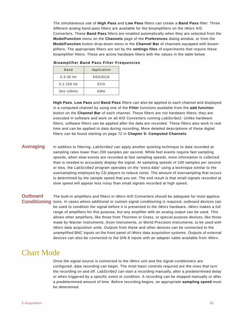
. .
3 Acquisition 33
The simultaneous use of High Pass and Low Pass filters can create a Band Pass filter. Three
different analog band pass filters are available for the bioamplifiers on the iWorx A/D
Converters. These Band Pass filters are enabled automatically when they are selected from the
Mode/Function menu on the Channels page of the Preferences dialog window, or from the
Mode/Function button drop-down menu in the Channel Bar of channels equipped with bioam-
plifiers. The appropriate filters are set by the settings files of experiments that require these
bioamplifier filters. These are active hardware filters with the values in the table below.
High Pass, Low Pass and Band Pass filters can also be applied to each channel and displayed
in a computed channel by using one of the Filter functions available from the add function
button on the Channel Bar of each channel. These filters are not hardware filters; they are
executed in software and work on all A/D Converters running LabScribe2. Unlike hardware
filters, software filters can be applied after the data are recorded. These filters also work in real
time and can be applied to data during recording. More detailed descriptions of these digital
filters can be found starting on page 72 in Chapter 5: Computed Channels.
Averaging In addition to filtering, LabScribe2 can apply another quieting technique to data recorded at
sampling rates lower than 200 samples per second. While fast events require fast sampling
speeds, when slow events are recorded at fast sampling speeds, more information is collected
than is needed to accurately display the signal. At sampling speeds of 100 samples per second
or less, the LabScribe2 program operates on the “extra data” using a technique similar to the
oversampling employed by CD players to reduce noise. The amount of oversampling that occurs
is determined by the sample speed that you set. The end result is that small signals recorded at
slow speed will appear less noisy than small signals recorded at high speed.
Outboard Conditioning
The built-in amplifiers and filters in iWorx A/D Converters should be adequate for most applica-
tions. In cases where additional or custom signal conditioning is required, outboard devices can
be used to condition the signal before it is presented to the iWorx hardware. iWorx makes a full
range of amplifiers for this purpose, but any amplifier with an analog output can be used. This
allows other amplifiers, like those from Thornton or Grass, or special purpose devices, like those
made by Warner Instruments, Axon Instruments, or World Precision Instruments, to be used with
iWorx data acquisition units. Outputs from these and other devices can be connected to the
unamplified BNC inputs on the front panel of iWorx data acquisition systems. Outputs of external
devices can also be connected to the DIN 8 inputs with an adapter cable available from iWorx.
Chart ModeOnce the signal source is connected to the iWorx unit and the signal conditioners are
configured, data recording can begin. The most basic controls required are the ones that turn
the recording on and off. LabScribe2 can start a recording manually, after a predetermined delay
or when triggered by a specific event or condition. A recording can be stopped manually or after
a predetermined amount of time. Before recording begins, an appropriate sampling speed must
be determined.
Bioamplif ier Band Pass Fi lter Frequencies
Band Appl icat ion
0.3-35 Hz EEG/ECG
0.1-150 Hz ECG
3Hz-10KHz EMG
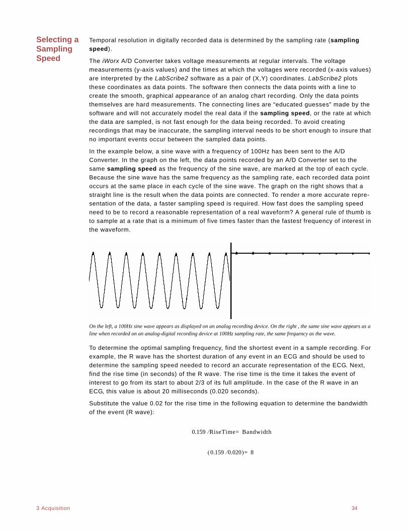
. .
3 Acquisition 34
Selecting a Sampling Speed
Temporal resolution in digitally recorded data is determined by the sampling rate (sampling
speed).
The iWorx A/D Converter takes voltage measurements at regular intervals. The voltage
measurements (y-axis values) and the times at which the voltages were recorded (x-axis values)
are interpreted by the LabScribe2 software as a pair of (X,Y) coordinates. LabScribe2 plots
these coordinates as data points. The software then connects the data points with a line to
create the smooth, graphical appearance of an analog chart recording. Only the data points
themselves are hard measurements. The connecting lines are “educated guesses” made by the
software and will not accurately model the real data if the sampling speed, or the rate at which
the data are sampled, is not fast enough for the data being recorded. To avoid creating
recordings that may be inaccurate, the sampling interval needs to be short enough to insure that
no important events occur between the sampled data points.
In the example below, a sine wave with a frequency of 100Hz has been sent to the A/D
Converter. In the graph on the left, the data points recorded by an A/D Converter set to the
same sampling speed as the frequency of the sine wave, are marked at the top of each cycle.
Because the sine wave has the same frequency as the sampling rate, each recorded data point
occurs at the same place in each cycle of the sine wave. The graph on the right shows that a
straight line is the result when the data points are connected. To render a more accurate repre-
sentation of the data, a faster sampling speed is required. How fast does the sampling speed
need to be to record a reasonable representation of a real waveform? A general rule of thumb is
to sample at a rate that is a minimum of five times faster than the fastest frequency of interest in
the waveform.
On the left, a 100Hz sine wave appears as displayed on an analog recording device. On the right , the same sine wave appears as a line when recorded on an analog-digital recording device at 100Hz sampling rate, the same frequency as the wave.
To determine the optimal sampling frequency, find the shortest event in a sample recording. For
example, the R wave has the shortest duration of any event in an ECG and should be used to
determine the sampling speed needed to record an accurate representation of the ECG. Next,
find the rise time (in seconds) of the R wave. The rise time is the time it takes the event of
interest to go from its start to about 2/3 of its full amplitude. In the case of the R wave in an
ECG, this value is about 20 milliseconds (0.020 seconds).
Substitute the value 0.02 for the rise time in the following equation to determine the bandwidth
of the event (R wave):
0.159 RiseTime Bandwidth=
0.159 0.020 8=
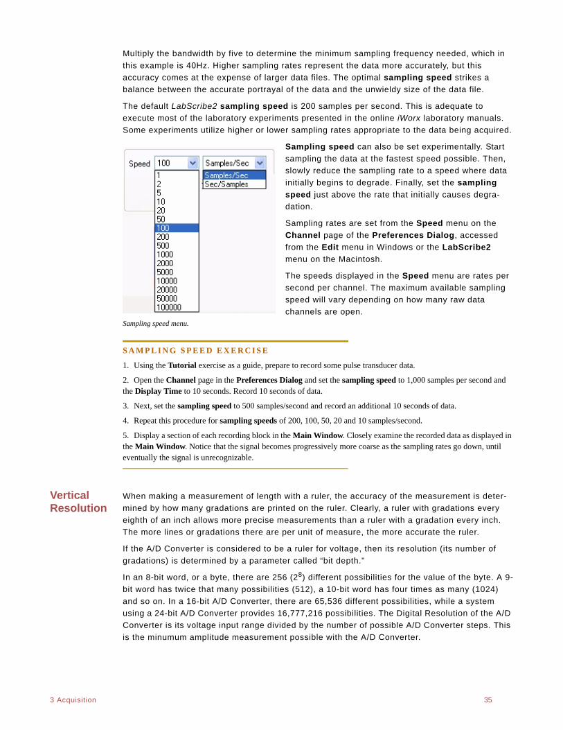
. .
3 Acquisition 35
Multiply the bandwidth by five to determine the minimum sampling frequency needed, which in
this example is 40Hz. Higher sampling rates represent the data more accurately, but this
accuracy comes at the expense of larger data files. The optimal sampling speed strikes a
balance between the accurate portrayal of the data and the unwieldy size of the data file.
The default LabScribe2 sampling speed is 200 samples per second. This is adequate to
execute most of the laboratory experiments presented in the online iWorx laboratory manuals.
Some experiments utilize higher or lower sampling rates appropriate to the data being acquired.
Sampling speed can also be set experimentally. Start
sampling the data at the fastest speed possible. Then,
slowly reduce the sampling rate to a speed where data
initially begins to degrade. Finally, set the sampling
speed just above the rate that initially causes degra-
dation.
Sampling rates are set from the Speed menu on the
Channel page of the Preferences Dialog, accessed
from the Edit menu in Windows or the LabScribe2
menu on the Macintosh.
The speeds displayed in the Speed menu are rates per
second per channel. The maximum available sampling
speed will vary depending on how many raw data
channels are open.Sampling speed menu.
S A M P L I N G S P E E D E X E R C I S E
1. Using the Tutorial exercise as a guide, prepare to record some pulse transducer data.
2. Open the Channel page in the Preferences Dialog and set the sampling speed to 1,000 samples per second and the Display Time to 10 seconds. Record 10 seconds of data.
3. Next, set the sampling speed to 500 samples/second and record an additional 10 seconds of data.
4. Repeat this procedure for sampling speeds of 200, 100, 50, 20 and 10 samples/second.
5. Display a section of each recording block in the Main Window. Closely examine the recorded data as displayed in the Main Window. Notice that the signal becomes progressively more coarse as the sampling rates go down, until eventually the signal is unrecognizable.
Vertical Resolution
When making a measurement of length with a ruler, the accuracy of the measurement is deter-
mined by how many gradations are printed on the ruler. Clearly, a ruler with gradations every
eighth of an inch allows more precise measurements than a ruler with a gradation every inch.
The more lines or gradations there are per unit of measure, the more accurate the ruler.
If the A/D Converter is considered to be a ruler for voltage, then its resolution (its number of
gradations) is determined by a parameter called “bit depth.”
In an 8-bit word, or a byte, there are 256 (28) different possibilities for the value of the byte. A 9-
bit word has twice that many possibilities (512), a 10-bit word has four times as many (1024)
and so on. In a 16-bit A/D Converter, there are 65,536 different possibilities, while a system
using a 24-bit A/D Converter provides 16,777,216 possibilities. The Digital Resolution of the A/D
Converter is its voltage input range divided by the number of possible A/D Converter steps. This
is the minumum amplitude measurement possible with the A/D Converter.
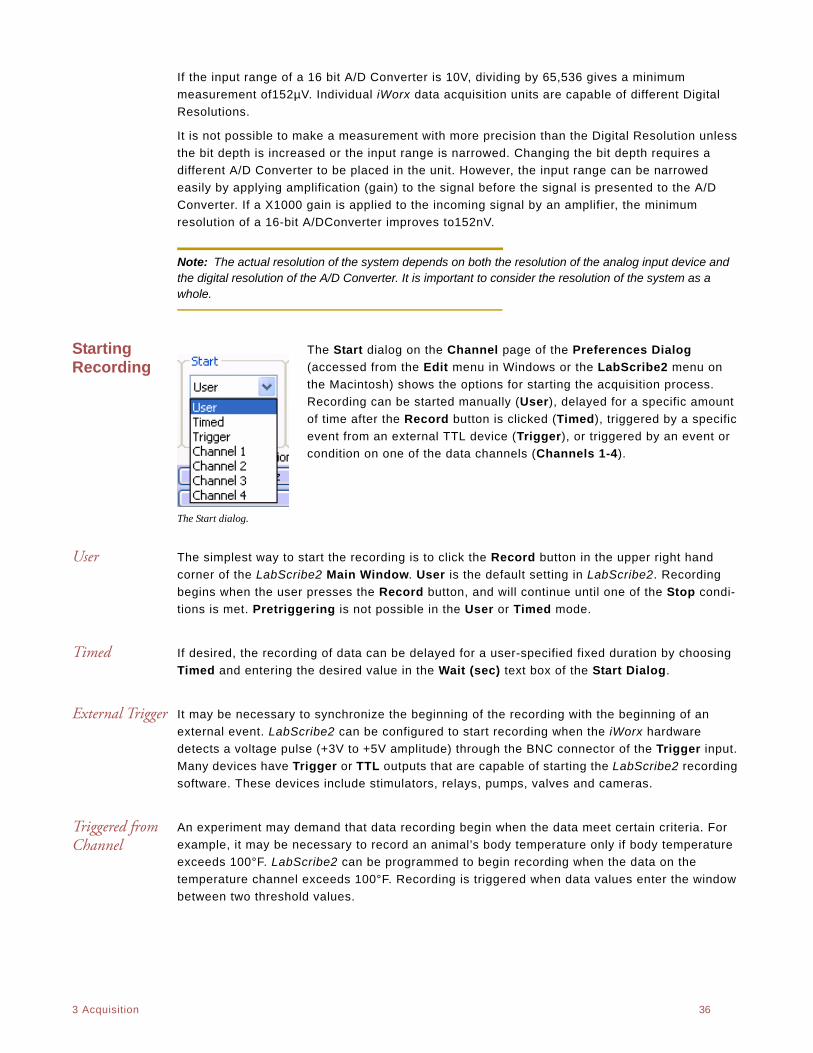
. .
3 Acquisition 36
If the input range of a 16 bit A/D Converter is 10V, dividing by 65,536 gives a minimum
measurement of152µV. Individual iWorx data acquisition units are capable of different Digital
Resolutions.
It is not possible to make a measurement with more precision than the Digital Resolution unless
the bit depth is increased or the input range is narrowed. Changing the bit depth requires a
different A/D Converter to be placed in the unit. However, the input range can be narrowed
easily by applying amplification (gain) to the signal before the signal is presented to the A/D
Converter. If a X1000 gain is applied to the incoming signal by an amplifier, the minimum
resolution of a 16-bit A/DConverter improves to152nV.
Note: The actual resolution of the system depends on both the resolution of the analog input device and the digital resolution of the A/D Converter. It is important to consider the resolution of the system as a whole.
Starting Recording
The Start dialog on the Channel page of the Preferences Dialog
(accessed from the Edit menu in Windows or the LabScribe2 menu on
the Macintosh) shows the options for starting the acquisition process.
Recording can be started manually (User), delayed for a specific amount
of time after the Record button is clicked (Timed), triggered by a specific
event from an external TTL device (Trigger), or triggered by an event or
condition on one of the data channels (Channels 1-4).
The Start dialog.
User The simplest way to start the recording is to click the Record button in the upper right hand
corner of the LabScribe2 Main Window. User is the default setting in LabScribe2. Recording
begins when the user presses the Record button, and will continue until one of the Stop condi-
tions is met. Pretriggering is not possible in the User or Timed mode.
Timed If desired, the recording of data can be delayed for a user-specified fixed duration by choosing
Timed and entering the desired value in the Wait (sec) text box of the Start Dialog.
External Trigger It may be necessary to synchronize the beginning of the recording with the beginning of an
external event. LabScribe2 can be configured to start recording when the iWorx hardware
detects a voltage pulse (+3V to +5V amplitude) through the BNC connector of the Trigger input.
Many devices have Trigger or TTL outputs that are capable of starting the LabScribe2 recording
software. These devices include stimulators, relays, pumps, valves and cameras.
Triggered from Channel
An experiment may demand that data recording begin when the data meet certain criteria. For
example, it may be necessary to record an animal’s body temperature only if body temperature
exceeds 100°F. LabScribe2 can be programmed to begin recording when the data on the
temperature channel exceeds 100°F. Recording is triggered when data values enter the window
between two threshold values.
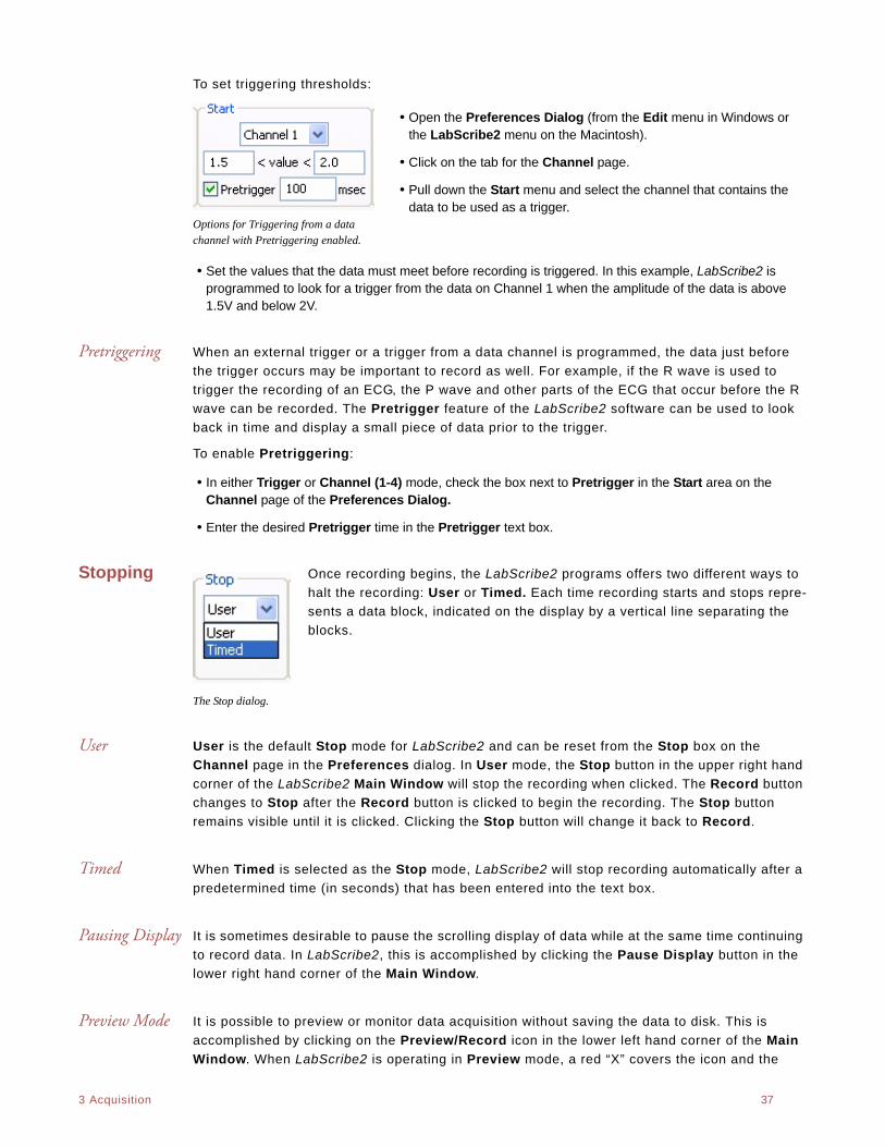
. .
3 Acquisition 37
To set triggering thresholds:
• Open the Preferences Dialog (from the Edit menu in Windows or the LabScribe2 menu on the Macintosh).
• Click on the tab for the Channel page.
• Pull down the Start menu and select the channel that contains the data to be used as a trigger.
Options for Triggering from a data channel with Pretriggering enabled.
• Set the values that the data must meet before recording is triggered. In this example, LabScribe2 is programmed to look for a trigger from the data on Channel 1 when the amplitude of the data is above 1.5V and below 2V.
Pretriggering When an external trigger or a trigger from a data channel is programmed, the data just before
the trigger occurs may be important to record as well. For example, if the R wave is used to
trigger the recording of an ECG, the P wave and other parts of the ECG that occur before the R
wave can be recorded. The Pretrigger feature of the LabScribe2 software can be used to look
back in time and display a small piece of data prior to the trigger.
To enable Pretriggering:
• In either Trigger or Channel (1-4) mode, check the box next to Pretrigger in the Start area on the Channel page of the Preferences Dialog.
• Enter the desired Pretrigger time in the Pretrigger text box.
Stopping Once recording begins, the LabScribe2 programs offers two different ways to
halt the recording: User or Timed. Each time recording starts and stops repre-
sents a data block, indicated on the display by a vertical line separating the
blocks.
The Stop dialog.
User User is the default Stop mode for LabScribe2 and can be reset from the Stop box on the
Channel page in the Preferences dialog. In User mode, the Stop button in the upper right hand
corner of the LabScribe2 Main Window will stop the recording when clicked. The Record button
changes to Stop after the Record button is clicked to begin the recording. The Stop button
remains visible until it is clicked. Clicking the Stop button will change it back to Record.
Timed When Timed is selected as the Stop mode, LabScribe2 will stop recording automatically after a
predetermined time (in seconds) that has been entered into the text box.
Pausing Display It is sometimes desirable to pause the scrolling display of data while at the same time continuing
to record data. In LabScribe2, this is accomplished by clicking the Pause Display button in the
lower right hand corner of the Main Window.
Preview Mode It is possible to preview or monitor data acquisition without saving the data to disk. This is
accomplished by clicking on the Preview/Record icon in the lower left hand corner of the Main
Window. When LabScribe2 is operating in Preview mode, a red “X” covers the icon and the
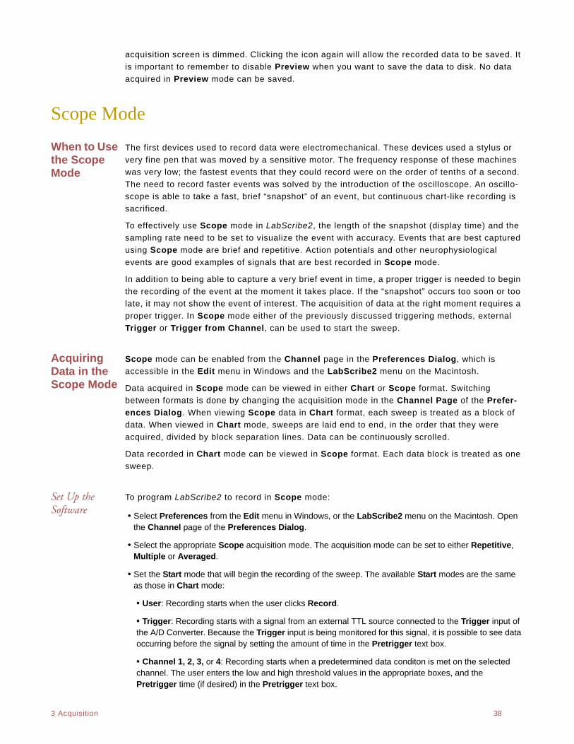
. .
3 Acquisition 38
acquisition screen is dimmed. Clicking the icon again will allow the recorded data to be saved. It
is important to remember to disable Preview when you want to save the data to disk. No data
acquired in Preview mode can be saved.
Scope Mode
When to Use the Scope Mode
The first devices used to record data were electromechanical. These devices used a stylus or
very fine pen that was moved by a sensitive motor. The frequency response of these machines
was very low; the fastest events that they could record were on the order of tenths of a second.
The need to record faster events was solved by the introduction of the oscilloscope. An oscillo-
scope is able to take a fast, brief “snapshot” of an event, but continuous chart-like recording is
sacrificed.
To effectively use Scope mode in LabScribe2, the length of the snapshot (display time) and the
sampling rate need to be set to visualize the event with accuracy. Events that are best captured
using Scope mode are brief and repetitive. Action potentials and other neurophysiological
events are good examples of signals that are best recorded in Scope mode.
In addition to being able to capture a very brief event in time, a proper trigger is needed to begin
the recording of the event at the moment it takes place. If the “snapshot” occurs too soon or too
late, it may not show the event of interest. The acquisition of data at the right moment requires a
proper trigger. In Scope mode either of the previously discussed triggering methods, external
Trigger or Trigger from Channel, can be used to start the sweep.
Acquiring Data in the Scope Mode
Scope mode can be enabled from the Channel page in the Preferences Dialog, which is
accessible in the Edit menu in Windows and the LabScribe2 menu on the Macintosh.
Data acquired in Scope mode can be viewed in either Chart or Scope format. Switching
between formats is done by changing the acquisition mode in the Channel Page of the Prefer-
ences Dialog. When viewing Scope data in Chart format, each sweep is treated as a block of
data. When viewed in Chart mode, sweeps are laid end to end, in the order that they were
acquired, divided by block separation lines. Data can be continuously scrolled.
Data recorded in Chart mode can be viewed in Scope format. Each data block is treated as one
sweep.
Set Up the Software
To program LabScribe2 to record in Scope mode:
• Select Preferences from the Edit menu in Windows, or the LabScribe2 menu on the Macintosh. Open the Channel page of the Preferences Dialog.
• Select the appropriate Scope acquisition mode. The acquisition mode can be set to either Repetitive, Multiple or Averaged.
• Set the Start mode that will begin the recording of the sweep. The available Start modes are the same as those in Chart mode:
• User: Recording starts when the user clicks Record.
• Trigger: Recording starts with a signal from an external TTL source connected to the Trigger input of the A/D Converter. Because the Trigger input is being monitored for this signal, it is possible to see data occurring before the signal by setting the amount of time in the Pretrigger text box.
• Channel 1, 2, 3, or 4: Recording starts when a predetermined data conditon is met on the selected channel. The user enters the low and high threshold values in the appropriate boxes, and the Pretrigger time (if desired) in the Pretrigger text box.
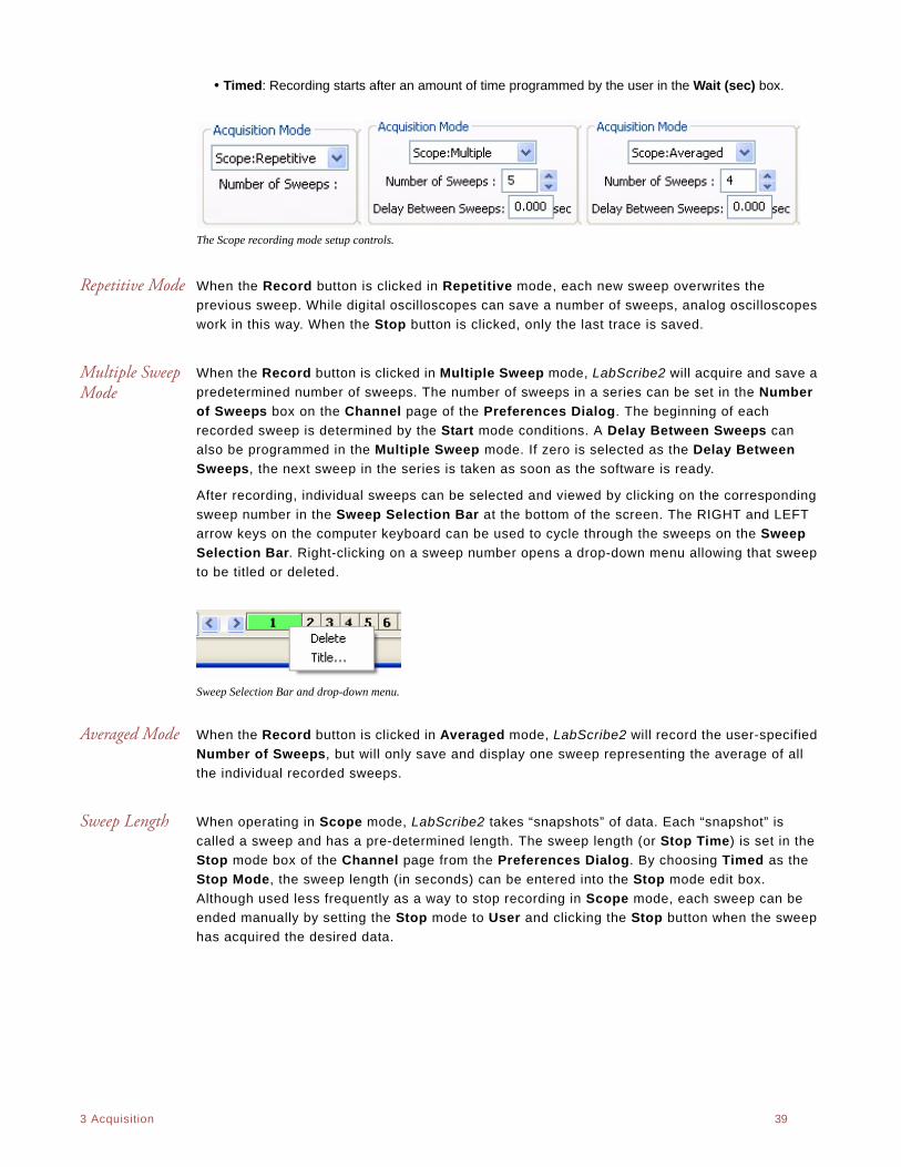
. .
3 Acquisition 39
• Timed: Recording starts after an amount of time programmed by the user in the Wait (sec) box.
The Scope recording mode setup controls.
Repetitive Mode When the Record button is clicked in Repetitive mode, each new sweep overwrites the
previous sweep. While digital oscilloscopes can save a number of sweeps, analog oscilloscopes
work in this way. When the Stop button is clicked, only the last trace is saved.
Multiple Sweep Mode
When the Record button is clicked in Multiple Sweep mode, LabScribe2 will acquire and save a
predetermined number of sweeps. The number of sweeps in a series can be set in the Number
of Sweeps box on the Channel page of the Preferences Dialog. The beginning of each
recorded sweep is determined by the Start mode conditions. A Delay Between Sweeps can
also be programmed in the Multiple Sweep mode. If zero is selected as the Delay Between
Sweeps, the next sweep in the series is taken as soon as the software is ready.
After recording, individual sweeps can be selected and viewed by clicking on the corresponding
sweep number in the Sweep Selection Bar at the bottom of the screen. The RIGHT and LEFT
arrow keys on the computer keyboard can be used to cycle through the sweeps on the Sweep
Selection Bar. Right-clicking on a sweep number opens a drop-down menu allowing that sweep
to be titled or deleted.
Sweep Selection Bar and drop-down menu.
Averaged Mode When the Record button is clicked in Averaged mode, LabScribe2 will record the user-specified
Number of Sweeps, but will only save and display one sweep representing the average of all
the individual recorded sweeps.
Sweep Length When operating in Scope mode, LabScribe2 takes “snapshots” of data. Each “snapshot” is
called a sweep and has a pre-determined length. The sweep length (or Stop Time) is set in the
Stop mode box of the Channel page from the Preferences Dialog. By choosing Timed as the
Stop Mode, the sweep length (in seconds) can be entered into the Stop mode edit box.
Although used less frequently as a way to stop recording in Scope mode, each sweep can be
ended manually by setting the Stop mode to User and clicking the Stop button when the sweep
has acquired the desired data.
. .
3 Acquisition 40
Sampling Rate The optimal sampling frequency in Scope mode can be determined by the same procedure used
in Chart mode. First, find the quickest event in the record. If the compound action potential is
used as an example, the spike goes from baseline to about 80% of its full amplitude in about
0.00035s. If you substitute 0.00035s for the rise time in the following equation:
Multiply the bandwidth by five and the minimum sampling frequency is 2270Hz. Doubling the
sampling rate to 5kHz ensures that the trace recorded is representative of the signal.
If the entire event of interest is only 0.1 seconds long, a sweep at 5,000 samples per second
uses only 500 data points. Since LabScribe2 can accommodate up to 1,000,000 points per
screen while recording, there is substantial room available for longer individual sweeps or a
faster sampling rate.
Saving Your DataEvery software manual has a section on the importance of backup and saving. LabScribe2 is no
different. SAVE YOUR DATA!
Consider that the data acquisition process imposes unique demands on the task of saving data.
A word processor or spreadsheet document can be saved anytime that the user thinks about it.
Most applications can also save data automatically, at regular intervals, and in the background.
In a data acquisition application, data are constantly being added, sometimes at remarkably high
rates (200,000 data points/second at top speed). To save data, the recording would have to be
stopped. In most recording applications, this is impractical.
Whenever it’s practical to do so, when recording is stopped, the user should instruct LabScribe2
to save the current data to disk. As a safeguard, LabScribe2 buffers the unsaved raw data to a
file on the hard disk. In the event of an unexpected loss of power or computer crash, the data
are preserved. When the LabScribe2 software is reopened after such an event, LabScribe2 will
ask the user if they want to recover the data. If the answer is yes, the backup file is recovered
and data are preserved. To permanently save the data, a new file should be created by using the
Save As function before recording any new data.
0.159 RiseTime Bandwidth=
0.159 0.00035 454=
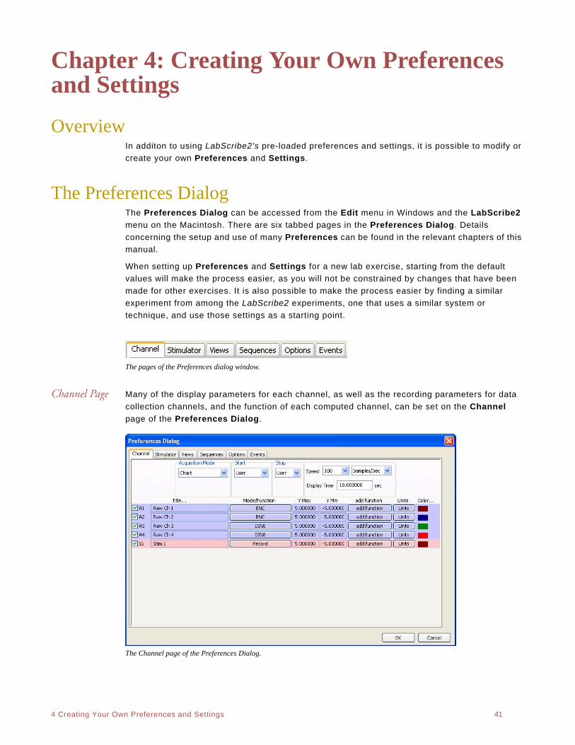
. .
4 Creating Your Own Preferences and Settings 41
Chapter 4: Creating Your Own Preferences and Settings
Overview In additon to using LabScribe2’s pre-loaded preferences and settings, it is possible to modify or
create your own Preferences and Settings.
The Preferences DialogThe Preferences Dialog can be accessed from the Edit menu in Windows and the LabScribe2
menu on the Macintosh. There are six tabbed pages in the Preferences Dialog. Details
concerning the setup and use of many Preferences can be found in the relevant chapters of this
manual.
When setting up Preferences and Settings for a new lab exercise, starting from the default
values will make the process easier, as you will not be constrained by changes that have been
made for other exercises. It is also possible to make the process easier by finding a similar
experiment from among the LabScribe2 experiments, one that uses a similar system or
technique, and use those settings as a starting point.
The pages of the Preferences dialog window.
Channel Page Many of the display parameters for each channel, as well as the recording parameters for data
collection channels, and the function of each computed channel, can be set on the Channel
page of the Preferences Dialog.
The Channel page of the Preferences Dialog.

. .
4 Creating Your Own Preferences and Settings 42
Some of the Preferences set on the Channel page apply to all channels (refer to the discussion
beginning on page 36 of Chapter 3: Acquisition):
• Acquisition Mode: Sets the type of acquisition: Chart, or one of the three Scope modes.
• Start: Sets the parameters that start the recording. The user can start the recording manually, recording can start a pre-determined amount of time after Record is clicked, or the start of recording can be triggered by an external event or by an event or condition on another channel.
• Stop: Sets the parameters to stop recording. Recording can be stopped manually by the user or after a pre-determined amount of time after recording starts.
• Speed: Sets the number of samples taken every second on each channel.
• Display Time: Sets the time and the amount of data displayed on one screen.
The Preferences that can be set for each individual channel include:
• Title...: Edits the title of each channel to better identify the parameter being recorded (titles can also be edited in the individual Channel Menus of the Main Window).
• Mode/Function: For raw data channels, clicking the Mode/Function button displays the input choices. These vary depending on the specific iWorx data acquisition unit. The filters applied to hardware channels with bioamplifiers can be selected, or the BNC or DIN8 input can be selected. On computed channels, clicking the Mode/Function button will display a list of the functions that can be applied to that channel instead of the one currently applied. Despite changing the function, it will still be computed from the same channel as the previous choice unless configured otherwise. Refer to Chapter 5: Computed Channels for a discussion of the functions available and how to configure them.
• Y Max, Y Min: Sets the maximum and minimum Y-axis values. These values can also be set in the Scale sub-menu of the Channel menu, or by right-clicking on the Y-axis. It is important to remember that each iWorx data acquisition unit is capable of recording a certain range of amplitude values, and not to set Y Max and Y Min outside these values.
• add function: Adds a computed function to a channel. Add function opens an additional channel that will display the function computed from the data in the chosen channel. The add function control can also be found on the individual Channel Bars. Refer to Chapter 6: Computed Channels for a discussion of the functions available.
• Units: Used to convert two raw data values in volts to the corresponding calculated values in units appropriate to the data being recorded. For more information refer to the Units Conversion discussion beginning on page 13 of Chapter 1: The Display.
• Color...: Sets the color of the channel’s trace. This can also be set from each individual Channel Menu.
Stimulator Page Some iWorx data acquisition units contain a Digital to Analog converter that can function as a
stimulator for use in experiments on excitable tissues. The stimulator(s) can be configured on
the Stimulator page of the Preferences Dialog. There are six stimulator protocols: Pulse,
Train, Constant, Step, Ramp and Triangle. The appropriate parameter values for each of these
modes can be preset and made part of a settings file. Refer to Chapter 5: The Stimulator for
information on programming the stimulator.
Views Page LabScribe2 can display various arrangments of the channels in the Main and Analysis
Windows. Refer to page 11 of Chapter 1: The Display for information on configuring Views.
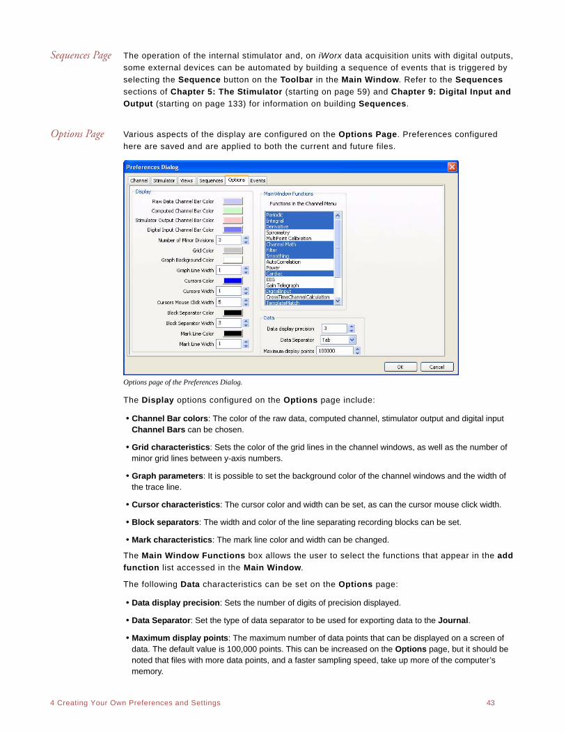
. .
4 Creating Your Own Preferences and Settings 43
Sequences Page The operation of the internal stimulator and, on iWorx data acquisition units with digital outputs,
some external devices can be automated by building a sequence of events that is triggered by
selecting the Sequence button on the Toolbar in the Main Window. Refer to the Sequences
sections of Chapter 5: The Stimulator (starting on page 59) and Chapter 9: Digital Input and
Output (starting on page 133) for information on building Sequences.
Options Page Various aspects of the display are configured on the Options Page. Preferences configured
here are saved and are applied to both the current and future files.
Options page of the Preferences Dialog.
The Display options configured on the Options page include:
• Channel Bar colors: The color of the raw data, computed channel, stimulator output and digital input Channel Bars can be chosen.
• Grid characteristics: Sets the color of the grid lines in the channel windows, as well as the number of minor grid lines between y-axis numbers.
• Graph parameters: It is possible to set the background color of the channel windows and the width of the trace line.
• Cursor characteristics: The cursor color and width can be set, as can the cursor mouse click width.
• Block separators: The width and color of the line separating recording blocks can be set.
• Mark characteristics: The mark line color and width can be changed.
The Main Window Functions box allows the user to select the functions that appear in the add
function list accessed in the Main Window.
The following Data characteristics can be set on the Options page:
• Data display precision: Sets the number of digits of precision displayed.
• Data Separator: Set the type of data separator to be used for exporting data to the Journal.
• Maximum display points: The maximum number of data points that can be displayed on a screen of data. The default value is 100,000 points. This can be increased on the Options page, but it should be noted that files with more data points, and a faster sampling speed, take up more of the computer’s memory.
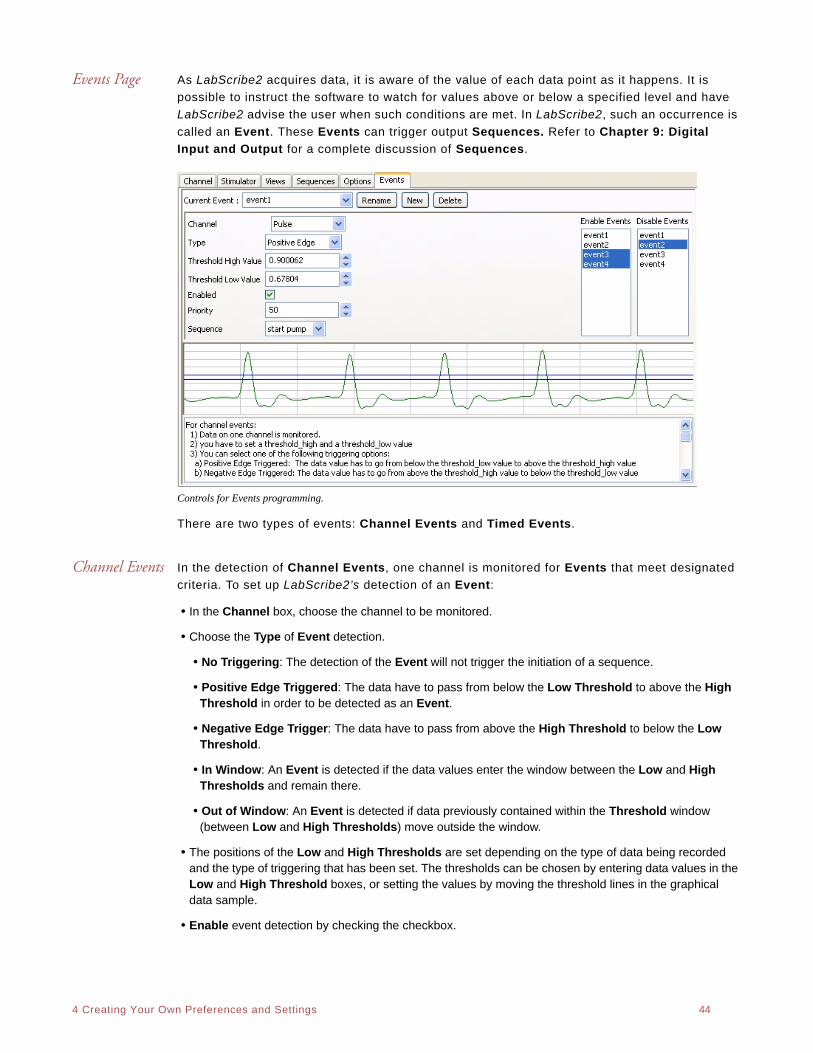
. .
4 Creating Your Own Preferences and Settings 44
Events Page As LabScribe2 acquires data, it is aware of the value of each data point as it happens. It is
possible to instruct the software to watch for values above or below a specified level and have
LabScribe2 advise the user when such conditions are met. In LabScribe2, such an occurrence is
called an Event. These Events can trigger output Sequences. Refer to Chapter 9: Digital
Input and Output for a complete discussion of Sequences.
Controls for Events programming.
There are two types of events: Channel Events and Timed Events.
Channel Events In the detection of Channel Events, one channel is monitored for Events that meet designated
criteria. To set up LabScribe2’s detection of an Event:
• In the Channel box, choose the channel to be monitored.
• Choose the Type of Event detection.
• No Triggering: The detection of the Event will not trigger the initiation of a sequence.
• Positive Edge Triggered: The data have to pass from below the Low Threshold to above the High Threshold in order to be detected as an Event.
• Negative Edge Trigger: The data have to pass from above the High Threshold to below the Low Threshold.
• In Window: An Event is detected if the data values enter the window between the Low and High Thresholds and remain there.
• Out of Window: An Event is detected if data previously contained within the Threshold window (between Low and High Thresholds) move outside the window.
• The positions of the Low and High Thresholds are set depending on the type of data being recorded and the type of triggering that has been set. The thresholds can be chosen by entering data values in the Low and High Threshold boxes, or setting the values by moving the threshold lines in the graphical data sample.
• Enable event detection by checking the checkbox.
. .
4 Creating Your Own Preferences and Settings 45
Timed Events Timed Events trigger a sequence after a designated amount of time has passed. To set the
criteria for the detection of a Timed Event:
• Choose Timed as the Type of Event.
• Set the Time (in seconds) that should pass before Events are detected, and after a previous Event if more than one is programmed.
• Set the Count, or the number of events to be detected. Set the Count to zero for continuous Events occurring at the programmed Time interval.
• Enable the event detection by checking the checkbox.
Event Priority The Event Priority is set in relation to other Events. Sequences triggered by Events inherit
their priority from the triggering Event. A higher priority Event can stop a lower priority
Sequence, but a lower priority Event cannot stop a higher priority Sequence.
If a Sequence is manually triggered by the user, the trigger is considered a User Event with a
priority of 50. Any Events with a higher priority than 50 will interrupt a user initiated Sequence,
while Events with a lower priority than the User Event cannot interrupt a user initiated
Sequence.
An Event can start in an enabled or disabled state. A disabled Event is ignored, but it can be
enabled by other Events. The Enable Events and Disable Events boxes determine which
Events enable or disable other Events. The Event being configured will enable Events
highlighted in the Enable Events box, and will disable Events in the Disable Events box,
regardless of relative priorities.
In the example shown on page 133 of Chapter 9: Digital Input and Output, the Pulse channel
is being monitored for a positive threshold crossing from below 0.67804 to above 0.900062. The
Event has a priority of 50 and is enabled to trigger the Sequence "Start Pump" when the
triggering criteria are satisfied. This event will also enable “event3” and “event4”, while
disabling “event2”.
The Settings MenuLabScribe2 offers users several choices for recording and displaying data. When certain choices
are used repeatedly, a template known as a settings file can be created to reduce the time
required to program the recording software and the A/D Converter.
To understand how to create and use Settings, two terms need to be defined: settings group
and settings file. A settings group is actually a simple text document that can contain links to
individual settings files. Each settings file is a collection of settings for performing an exper-
iment and is configured by using display controls and the options on the various pages of the
Preferences Dialog. The settings contained in a file determine the number and titles of
channels in the LabScribe2 windows, the sampling speed, the units conversions, the stimulator
settings, and more.
LabScribe2 experiments use preconfigured settings files. Users can modify these settings or
design their own settings groups and files. They can also associate their own settings files
with documentation (experimental procedures, protocols, instructions, lab exercises) of their
own design.
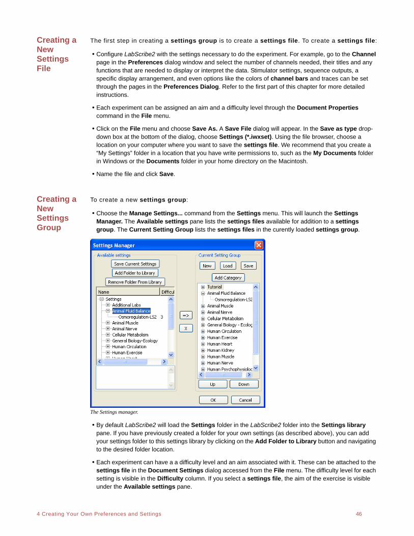
. .
4 Creating Your Own Preferences and Settings 46
Creating a New Settings File
The first step in creating a settings group is to create a settings file. To create a settings file:
• Configure LabScribe2 with the settings necessary to do the experiment. For example, go to the Channel page in the Preferences dialog window and select the number of channels needed, their titles and any functions that are needed to display or interpret the data. Stimulator settings, sequence outputs, a specific display arrangement, and even options like the colors of channel bars and traces can be set through the pages in the Preferences Dialog. Refer to the first part of this chapter for more detailed instructions.
• Each experiment can be assigned an aim and a difficulty level through the Document Properties command in the File menu.
• Click on the File menu and choose Save As. A Save File dialog will appear. In the Save as type drop-down box at the bottom of the dialog, choose Settings (*.iwxset). Using the file browser, choose a location on your computer where you want to save the settings file. We recommend that you create a “My Settings” folder in a location that you have write permissions to, such as the My Documents folder in Windows or the Documents folder in your home directory on the Macintosh.
• Name the file and click Save.
Creating a New Settings Group
To create a new settings group:
• Choose the Manage Settings... command from the Settings menu. This will launch the Settings Manager. The Available settings pane lists the settings files available for addition to a settings group. The Current Setting Group lists the settings files in the curently loaded settings group.
The Settings manager.
• By default LabScribe2 will load the Settings folder in the LabScribe2 folder into the Settings library pane. If you have previously created a folder for your own settings (as described above), you can add your settings folder to this settings library by clicking on the Add Folder to Library button and navigating to the desired folder location.
• Each experiment can have a a difficulty level and an aim associated with it. These can be attached to the settings file in the Document Settings dialog accessed from the File menu. The difficulty level for each setting is visible in the Difficulty column. If you select a settings file, the aim of the exercise is visible under the Available settings pane.
. .
4 Creating Your Own Preferences and Settings 47
• To create a new settings group, click the New button in the Current Settings Group area. This will remove the current group and clear the Current Settings Group box. Click Save to name the group (it will be given a .iwxgrp suffix) and place the settings group file in the folder with your settings.
• To load an existing group, click on the Load button in the Current Settings Group area. This will open a dialog where you can choose the settings group to load. Settings group files will have a .iwxgrp suffix. The settings files in the new settings group will now be displayed in the Current Settings Group window.
Settings files (*.iwxset) can be organized into categories within a group. To create a new
category in the settings group:
• Click on the Add Category button and name the category. You can add settings files from the list of available settings to any category or at the root level. Settings added to the root level are listed in the Current Settings Group below the designated categories.
• The category order can be changed by selecting a category in the Current Settings Group and moving it up or down the list with the Up or Down buttons.
Helper Files Helper files are documents with experimental instructions, diagrams and illustrations that can
be linked to settings files and displayed on the computer screen when a settings file is
selected. When a preconfigured iWorx settings group is loaded, a .pdf copy of each individual
lab experiment is linked to the corresponding settings file in the settings group. When you
select a settings file to do a particular experiment, a .pdf copy of the linked helper file (the
experimental write-up) opens in Acrobat Reader. You now have a set of instructions, on the
computer screen, to follow as you do the experiment. Alternatively, the .pdf file can be printed,
edited in a .pdf editor, or uploaded to a content management system such as Blackboard.
Users can attach their helper files to their own or pre-existing settings files. Although iWorx
Systems has chosen to attach .pdf documents to its setting files, any file (html, Microsoft Word,
Open Office, etc.) can be linked to a settings file.
To associate helper files with any settings file:
• Place your helper files in the same location as the settings file and give the helper file the same name as the settings file, but with the appropriate extension. For example, to associate a .pdf, an html and a .jpg file with the Tutorial.iwxset settings file, copy the .pdf, the html and the .jpg file to the same folder as the Tutorial.iwxset settings file. Name the .pdf file “Tutorial.pdf”, the html file ”Tutorial.html”, and the .jpg file ”Tutorial.jpg”. Now when the Tutorial settings file is chosen in LabScribe2, the Tutorial.pdf, the Tutorial.html and the Tutorial.jpg files will be opened as well.
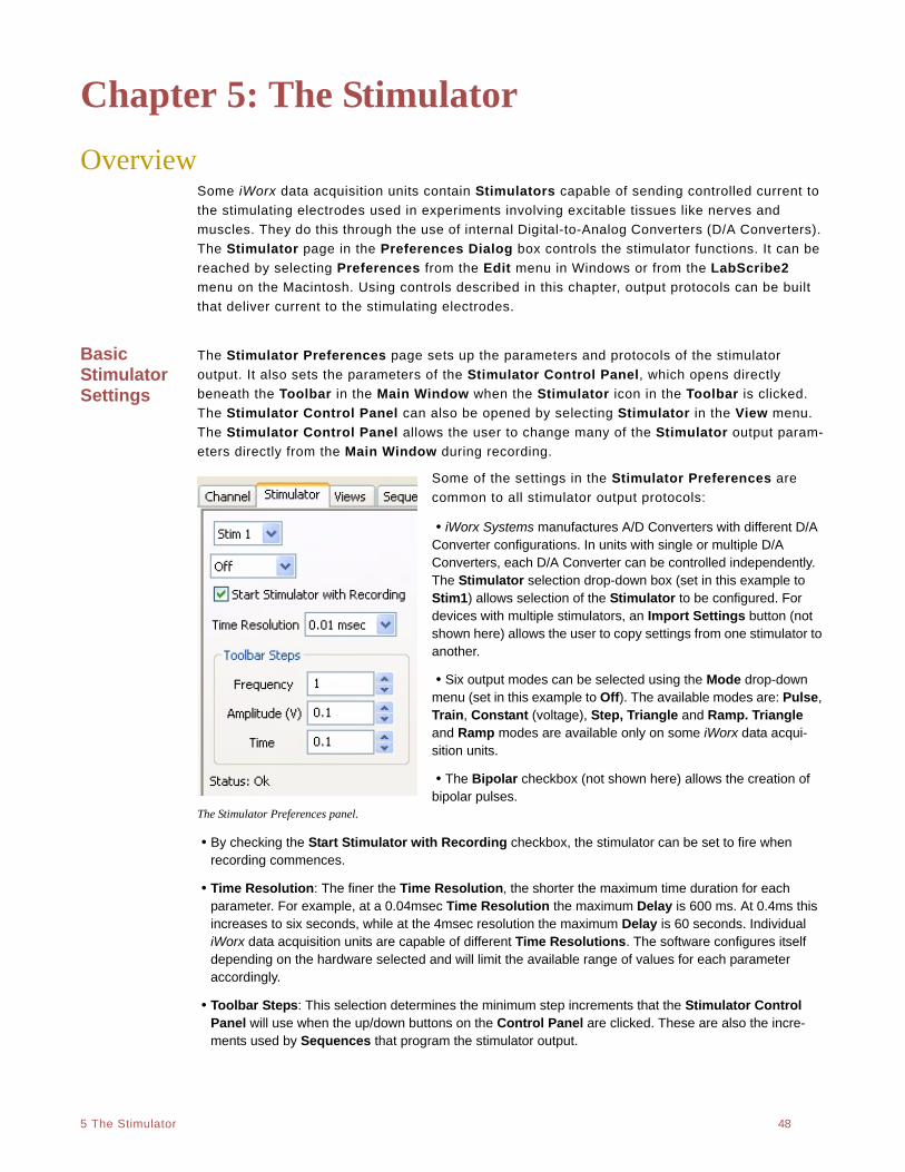
. .
5 The Stimulator 48
Chapter 5: The Stimulator
OverviewSome iWorx data acquisition units contain Stimulators capable of sending controlled current to
the stimulating electrodes used in experiments involving excitable tissues like nerves and
muscles. They do this through the use of internal Digital-to-Analog Converters (D/A Converters).
The Stimulator page in the Preferences Dialog box controls the stimulator functions. It can be
reached by selecting Preferences from the Edit menu in Windows or from the LabScribe2
menu on the Macintosh. Using controls described in this chapter, output protocols can be built
that deliver current to the stimulating electrodes.
Basic Stimulator Settings
The Stimulator Preferences page sets up the parameters and protocols of the stimulator
output. It also sets the parameters of the Stimulator Control Panel, which opens directly
beneath the Toolbar in the Main Window when the Stimulator icon in the Toolbar is clicked.
The Stimulator Control Panel can also be opened by selecting Stimulator in the View menu.
The Stimulator Control Panel allows the user to change many of the Stimulator output param-
eters directly from the Main Window during recording.
Some of the settings in the Stimulator Preferences are
common to all stimulator output protocols:
• iWorx Systems manufactures A/D Converters with different D/A Converter configurations. In units with single or multiple D/A Converters, each D/A Converter can be controlled independently. The Stimulator selection drop-down box (set in this example to Stim1) allows selection of the Stimulator to be configured. For devices with multiple stimulators, an Import Settings button (not shown here) allows the user to copy settings from one stimulator to another.
• Six output modes can be selected using the Mode drop-down menu (set in this example to Off). The available modes are: Pulse, Train, Constant (voltage), Step, Triangle and Ramp. Triangle and Ramp modes are available only on some iWorx data acqui-sition units.
• The Bipolar checkbox (not shown here) allows the creation of bipolar pulses.
The Stimulator Preferences panel.
• By checking the Start Stimulator with Recording checkbox, the stimulator can be set to fire when recording commences.
• Time Resolution: The finer the Time Resolution, the shorter the maximum time duration for each parameter. For example, at a 0.04msec Time Resolution the maximum Delay is 600 ms. At 0.4ms this increases to six seconds, while at the 4msec resolution the maximum Delay is 60 seconds. Individual iWorx data acquisition units are capable of different Time Resolutions. The software configures itself depending on the hardware selected and will limit the available range of values for each parameter accordingly.
• Toolbar Steps: This selection determines the minimum step increments that the Stimulator Control Panel will use when the up/down buttons on the Control Panel are clicked. These are also the incre-ments used by Sequences that program the stimulator output.
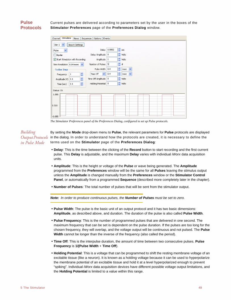
. .
5 The Stimulator 49
Pulse Protocols
Current pulses are delivered according to parameters set by the user in the boxes of the
Stimulator Preferences page of the Preferences Dialog window.
The Stimulator Preferences panel of the Preferences Dialog, configured to set up Pulse protocols.
Building Output Protocols in Pulse Mode
By setting the Mode drop-down menu to Pulse, the relevant parameters for Pulse protocols are displayed
in the dialog. In order to understand how the protocols are created, it is necessary to define the
terms used on the Stimulator page of the Preferences Dialog:
• Delay: This is the time between the clicking of the Record button to start recording and the first current pulse. This Delay is adjustable, and the maximum Delay varies with individual iWorx data acquisition units.
• Amplitude: This is the height or voltage of the Pulse or wave being generated. The Amplitude programmed from the Preferences window will be the same for all Pulses leaving the stimulus output unless the Amplitude is changed manually from the Preferences window or the Stimulator Control Panel, or automatically from a programmed Sequence (described more completely later in the chapter).
• Number of Pulses: The total number of pulses that will be sent from the stimulator output.
Note: In order to produce continuous pulses, the Number of Pulses must be set to zero.
• Pulse Width: The pulse is the basic unit of an output protocol and it has two basic dimensions: Amplitude, as described above, and duration. The duration of the pulse is also called Pulse Width.
• Pulse Frequency: This is the number of programmed pulses that are delivered in one second. The maximum frequency that can be set is dependent on the pulse duration. If the pulses are too long for the chosen frequency, they will overlap, and the voltage output will be continuous and not pulsed. The Pulse Width cannot be longer than the inverse of the frequency (also called the period).
• Time Off: This is the interpulse duration, the amount of time between two consecutive pulses. Pulse Frequency is 1/(Pulse Width + Time Off).
• Holding Potential: This is a voltage that can be programmed to shift the resting membrane voltage of an excitable tissue (like a neuron). It is known as a holding voltage because it can be used to hyperpolarize the membrane potential of an excitable tissue and hold it at a level hyperpolarized enough to prevent “spiking”. Individual iWorx data acquisition devices have different possible voltage output limitations, and the Holding Potential is limited to a value within this range.
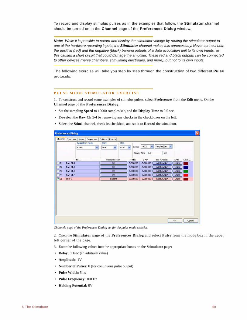
. .
5 The Stimulator 50
To record and display stimulus pulses as in the examples that follow, the Stimulator channel
should be turned on in the Channel page of the Preferences Dialog window.
Note: While it is possible to record and display the stimulator voltage by routing the stimulator output to one of the hardware recording inputs, the Stimulator channel makes this unnecessary. Never connect both the positive (red) and the negative (black) banana outputs of a data acquisition unit to its own inputs, as this causes a short circuit that could damage the amplifier. These red and black outputs can be connected to other devices (nerve chambers, stimulating electrodes, and more), but not to its own inputs.
The following exercise will take you step by step through the construction of two different Pulse
protocols.
P U L S E M O D E S T I M U L A T O R E X E R C I S E
1. To construct and record some examples of stimulus pulses, select Preferences from the Edit menu. On the Channel page of the Preferences Dialog:
• Set the sampling Speed to 10000 samples/sec, and the Display Time to 0.5 sec.
• De-select the Raw Ch 1-4 by removing any checks in the checkboxes on the left.
• Select the Stim1 channel, check its checkbox, and set it to Record the stimulator.
Channels page of the Preferences Dialog set for the pulse mode exercise.
2. Open the Stimulator page of the Preferences Dialog and select Pulse from the mode box in the upper left corner of the page.
3. Enter the following values into the appropriate boxes on the Stimulator page:
• Delay: 0.1sec (an arbitrary value)
• Amplitude: 1V
• Number of Pulses: 0 (for continuous pulse output)
• Pulse Width: 5ms
• Pulse Frequency: 100 Hz
• Holding Potential: 0V
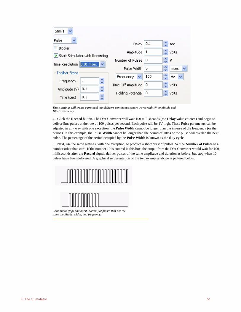
. .
5 The Stimulator 51
These settings will create a protocol that delivers continuous square waves with 1V amplitude and 100Hz frequency.
4. Click the Record button. The D/A Converter will wait 100 milliseconds (the Delay value entered) and begin to deliver 5ms pulses at the rate of 100 pulses per second. Each pulse will be 1V high. These Pulse parameters can be adjusted in any way with one exception: the Pulse Width cannot be longer than the inverse of the frequency (or the period). In this example, the Pulse Width cannot be longer than the period of 10ms or the pulse will overlap the next pulse. The percentage of the period occupied by the Pulse Width is known as the duty cycle.
5. Next, use the same settings, with one exception, to produce a short burst of pulses. Set the Number of Pulses to a number other than zero. If the number 10 is entered in this box, the output from the D/A Converter would wait for 100 milliseconds after the Record signal, deliver pulses of the same amplitude and duration as before, but stop when 10 pulses have been delivered. A graphical representation of the two examples above is pictured below.
Continuous (top) and burst (bottom) of pulses that are the same amplitude, width, and frequency.
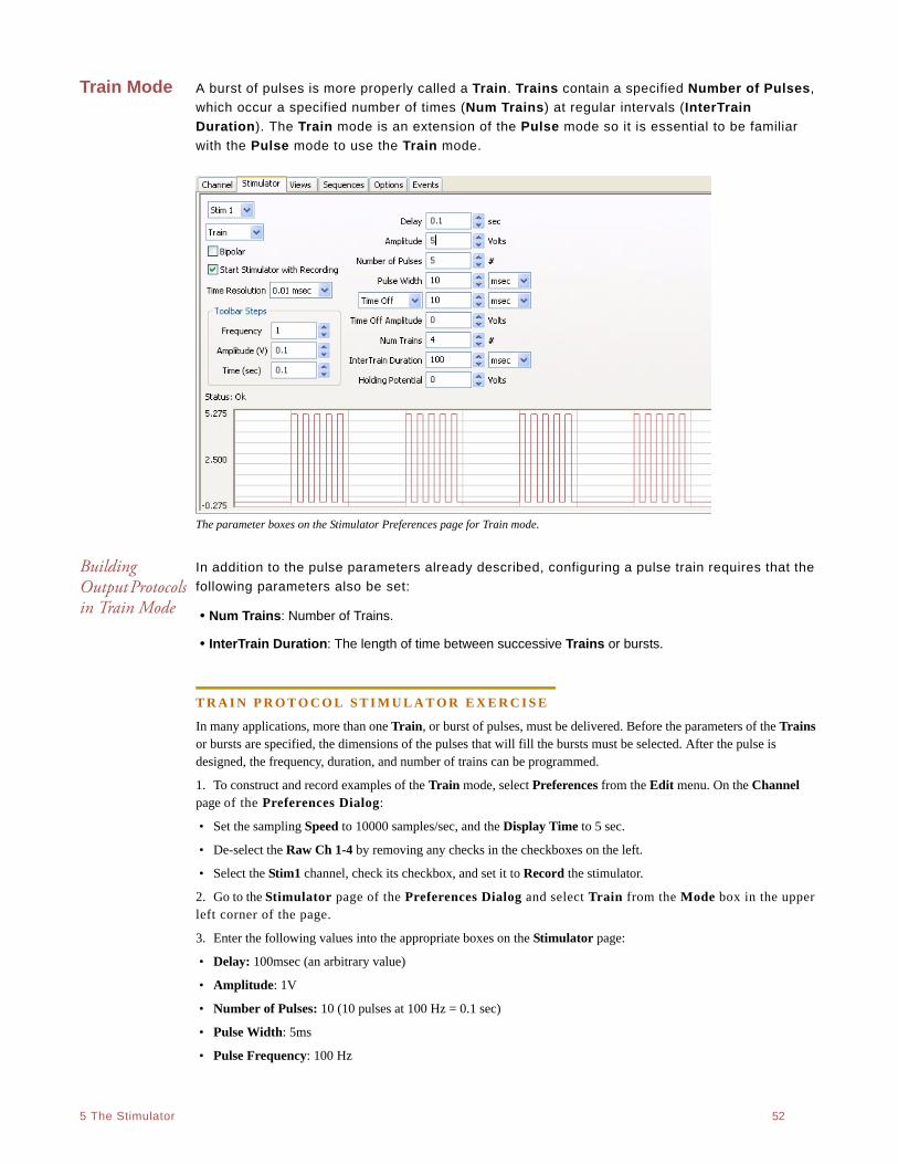
. .
5 The Stimulator 52
Train Mode A burst of pulses is more properly called a Train. Trains contain a specified Number of Pulses,
which occur a specified number of times (Num Trains) at regular intervals (InterTrain
Duration). The Train mode is an extension of the Pulse mode so it is essential to be familiar
with the Pulse mode to use the Train mode.
The parameter boxes on the Stimulator Preferences page for Train mode.
Building Output Protocols in Train Mode
In addition to the pulse parameters already described, configuring a pulse train requires that the
following parameters also be set:
• Num Trains: Number of Trains.
• InterTrain Duration: The length of time between successive Trains or bursts.
T R A I N P R O T O C O L S T I M U L A T O R E X E R C I S E
In many applications, more than one Train, or burst of pulses, must be delivered. Before the parameters of the Trains or bursts are specified, the dimensions of the pulses that will fill the bursts must be selected. After the pulse is designed, the frequency, duration, and number of trains can be programmed.
1. To construct and record examples of the Train mode, select Preferences from the Edit menu. On the Channel page of the Preferences Dialog:
• Set the sampling Speed to 10000 samples/sec, and the Display Time to 5 sec.
• De-select the Raw Ch 1-4 by removing any checks in the checkboxes on the left.
• Select the Stim1 channel, check its checkbox, and set it to Record the stimulator.
2. Go to the Stimulator page of the Preferences Dialog and select Train from the Mode box in the upper left corner of the page.
3. Enter the following values into the appropriate boxes on the Stimulator page:
• Delay: 100msec (an arbitrary value)
• Amplitude: 1V
• Number of Pulses: 10 (10 pulses at 100 Hz = 0.1 sec)
• Pulse Width: 5ms
• Pulse Frequency: 100 Hz
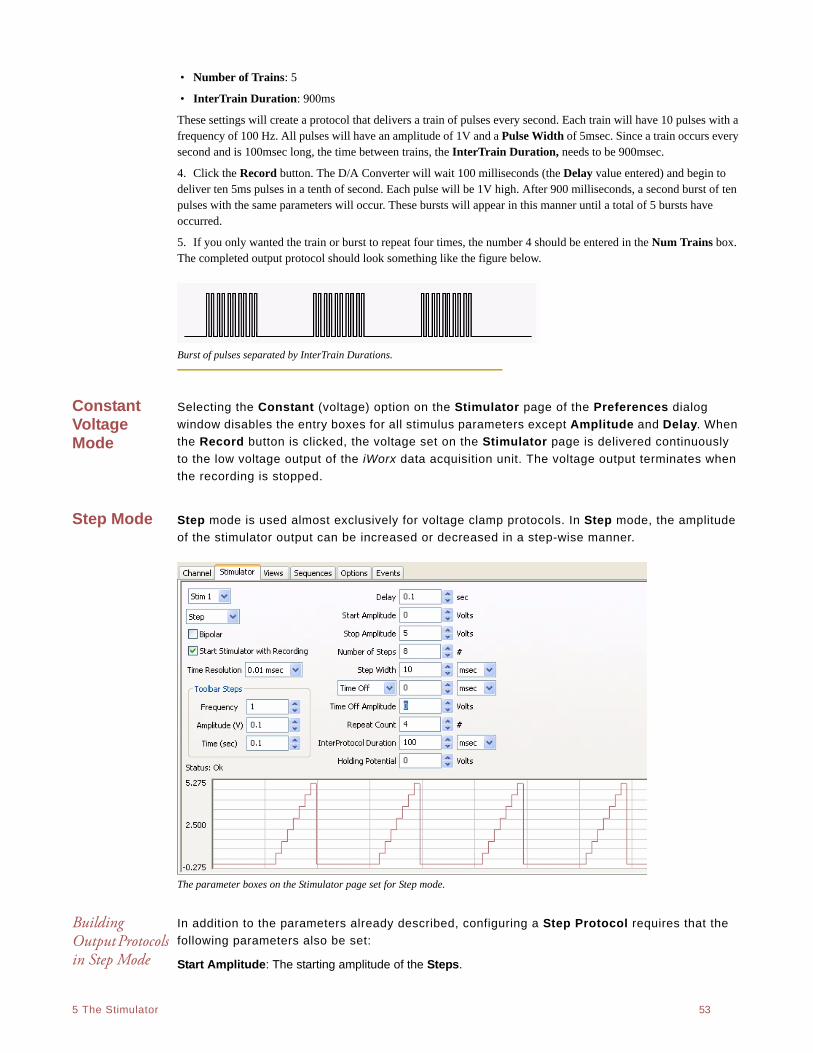
. .
5 The Stimulator 53
• Number of Trains: 5
• InterTrain Duration: 900ms
These settings will create a protocol that delivers a train of pulses every second. Each train will have 10 pulses with a frequency of 100 Hz. All pulses will have an amplitude of 1V and a Pulse Width of 5msec. Since a train occurs every second and is 100msec long, the time between trains, the InterTrain Duration, needs to be 900msec.
4. Click the Record button. The D/A Converter will wait 100 milliseconds (the Delay value entered) and begin to deliver ten 5ms pulses in a tenth of second. Each pulse will be 1V high. After 900 milliseconds, a second burst of ten pulses with the same parameters will occur. These bursts will appear in this manner until a total of 5 bursts have occurred.
5. If you only wanted the train or burst to repeat four times, the number 4 should be entered in the Num Trains box. The completed output protocol should look something like the figure below.
Burst of pulses separated by InterTrain Durations.
Constant Voltage Mode
Selecting the Constant (voltage) option on the Stimulator page of the Preferences dialog
window disables the entry boxes for all stimulus parameters except Amplitude and Delay. When
the Record button is clicked, the voltage set on the Stimulator page is delivered continuously
to the low voltage output of the iWorx data acquisition unit. The voltage output terminates when
the recording is stopped.
Step Mode Step mode is used almost exclusively for voltage clamp protocols. In Step mode, the amplitude
of the stimulator output can be increased or decreased in a step-wise manner.
The parameter boxes on the Stimulator page set for Step mode.
Building Output Protocols in Step Mode
In addition to the parameters already described, configuring a Step Protocol requires that the
following parameters also be set:
Start Amplitude: The starting amplitude of the Steps.
. .
5 The Stimulator 54
Stop Amplitude: The ending amplitude of the Steps.
Number of Steps: The number of Steps in each “staircase”, or protocol.
Step Width: The duration of each individual Step.
Time Off (or InterStep Width): Time between individual Steps.
Repeat Count: The number of times the Step protocol will repeat.
Interprotocol Duration: The duration of time between the termination of one protocol (one
“staircase”) and the initiation of the next.
The Amplitude of each individual Step in the protocol is determined by LabScribe2 with the
starting and ending Amplitudes and the Number of Steps entered on the Stimulator page. The
equation used to perform this calculation is:
(Start Amplitude - Stop Amplitude)/Number of Steps = Voltage Increment
If the user knows the voltage increment needed at each step, the equation can be transposed to
solve for the Number of Steps required in the protocol and this value can be entered on the
Stimulator page:
(Start Amplitude - Stop Amplitude)/Voltage Increment = Number of Steps
Likewise, if the user knows the previous amplitude and the voltage increment, the succeeding
amplitude can be calculated:
Previous Amplitude + Voltage Increment = Succeeding Amplitude
With the starting, ending and incremental voltages set through Preferences, the voltage will
change in a step-wise manner until the ending voltage is reached. The overall length of the
protocol is determined by the Step Width and the time between steps, the Time Off.
V O L T A G E S T E P M O D E S T I M U L A T O R E X E R C I S E
1. To construct and record an example of pulses in Step mode, select Preferences from the Edit menu. On the Channel page of the Preferences Dialog:
• Set the sampling Speed to 10000 samples/sec, and the Display Time to 2 sec.
• De-select the Raw Ch 1-4 by removing any checks in the checkboxes on the left.
• Select the Stim1 channel, check its checkbox, and set it to Record the stimulator.
2. Go to the Stimulator page of the Preferences dialog window and select Step from the Mode box in the upper left corner of the page.
3. Enter the following values into the appropriate boxes on the Stimulator page:
• Delay: 0
• Starting Amplitude: -1V
• Ending Amplitude: 1V
• Number of Steps: 8
• Step Width: 100ms
• Time Off: 0
• Repeat Count: 1
• Interprotocol duration: 0
• Holding Potential: 0
4. These settings will create a waveform that starts at -1V and climbs to +1V in eight Steps. Each Step has a voltage increment of 0.25V and is 100ms wide.
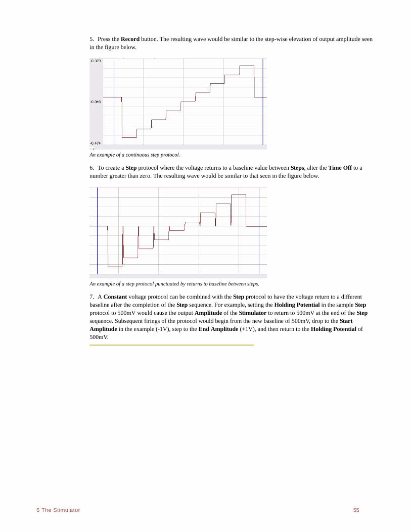
. .
5 The Stimulator 55
5. Press the Record button. The resulting wave would be similar to the step-wise elevation of output amplitude seen in the figure below.
An example of a continuous step protocol.
6. To create a Step protocol where the voltage returns to a baseline value between Steps, alter the Time Off to a number greater than zero. The resulting wave would be similar to that seen in the figure below.
An example of a step protocol punctuated by returns to baseline between steps.
7. A Constant voltage protocol can be combined with the Step protocol to have the voltage return to a different baseline after the completion of the Step sequence. For example, setting the Holding Potential in the sample Step protocol to 500mV would cause the output Amplitude of the Stimulator to return to 500mV at the end of the Step sequence. Subsequent firings of the protocol would begin from the new baseline of 500mV, drop to the Start Amplitude in the example (-1V), step to the End Amplitude (+1V), and then return to the Holding Potential of 500mV.
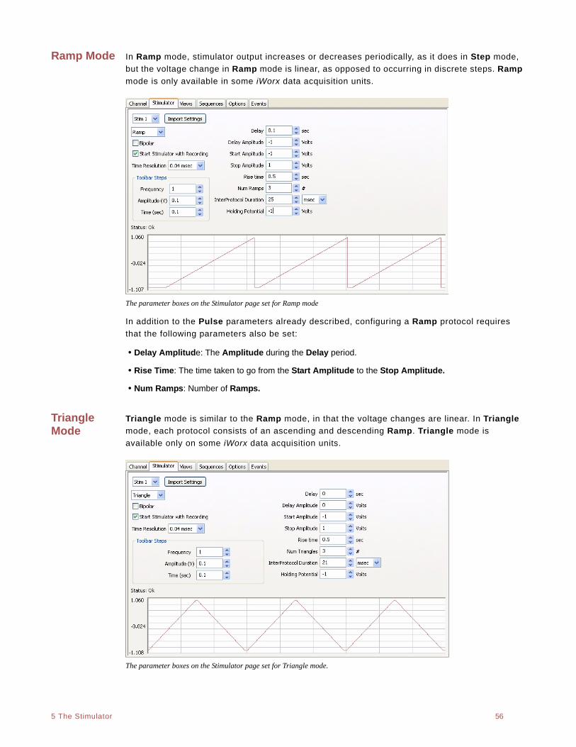
. .
5 The Stimulator 56
Ramp Mode In Ramp mode, stimulator output increases or decreases periodically, as it does in Step mode,
but the voltage change in Ramp mode is linear, as opposed to occurring in discrete steps. Ramp
mode is only available in some iWorx data acquisition units.
The parameter boxes on the Stimulator page set for Ramp mode
In addition to the Pulse parameters already described, configuring a Ramp protocol requires
that the following parameters also be set:
• Delay Amplitude: The Amplitude during the Delay period.
• Rise Time: The time taken to go from the Start Amplitude to the Stop Amplitude.
• Num Ramps: Number of Ramps.
Triangle Mode
Triangle mode is similar to the Ramp mode, in that the voltage changes are linear. In Triangle
mode, each protocol consists of an ascending and descending Ramp. Triangle mode is
available only on some iWorx data acquisition units.
The parameter boxes on the Stimulator page set for Triangle mode.
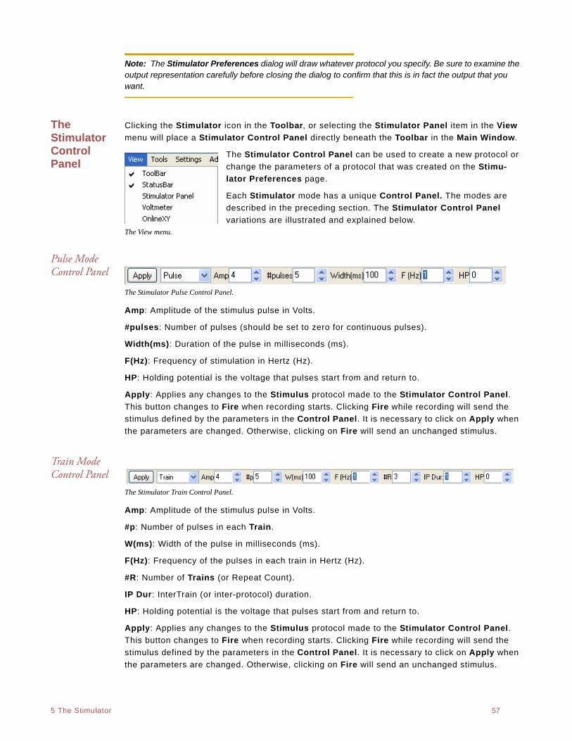
. .
5 The Stimulator 57
Note: The Stimulator Preferences dialog will draw whatever protocol you specify. Be sure to examine the output representation carefully before closing the dialog to confirm that this is in fact the output that you want.
The Stimulator Control Panel
Clicking the Stimulator icon in the Toolbar, or selecting the Stimulator Panel item in the View
menu will place a Stimulator Control Panel directly beneath the Toolbar in the Main Window.
The Stimulator Control Panel can be used to create a new protocol or
change the parameters of a protocol that was created on the Stimu-
lator Preferences page.
Each Stimulator mode has a unique Control Panel. The modes are
described in the preceding section. The Stimulator Control Panel
variations are illustrated and explained below.The View menu.
Pulse Mode Control Panel
The Stimulator Pulse Control Panel.
Amp: Amplitude of the stimulus pulse in Volts.
#pulses: Number of pulses (should be set to zero for continuous pulses).
Width(ms): Duration of the pulse in milliseconds (ms).
F(Hz): Frequency of stimulation in Hertz (Hz).
HP: Holding potential is the voltage that pulses start from and return to.
Apply: Applies any changes to the Stimulus protocol made to the Stimulator Control Panel.
This button changes to Fire when recording starts. Clicking Fire while recording will send the
stimulus defined by the parameters in the Control Panel. It is necessary to click on Apply when
the parameters are changed. Otherwise, clicking on Fire will send an unchanged stimulus.
Train Mode Control Panel
The Stimulator Train Control Panel.
Amp: Amplitude of the stimulus pulse in Volts.
#p: Number of pulses in each Train.
W(ms): Width of the pulse in milliseconds (ms).
F(Hz): Frequency of the pulses in each train in Hertz (Hz).
#R: Number of Trains (or Repeat Count).
IP Dur: InterTrain (or inter-protocol) duration.
HP: Holding potential is the voltage that pulses start from and return to.
Apply: Applies any changes to the Stimulus protocol made to the Stimulator Control Panel.
This button changes to Fire when recording starts. Clicking Fire while recording will send the
stimulus defined by the parameters in the Control Panel. It is necessary to click on Apply when
the parameters are changed. Otherwise, clicking on Fire will send an unchanged stimulus.
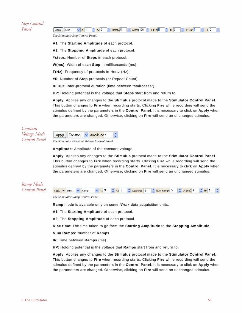
. .
5 The Stimulator 58
Step Control Panel
The Stimulator Step Control Panel.
A1: The Starting Amplitude of each protocol.
A2: The Stopping Amplitude of each protocol.
#steps: Number of Steps in each protocol.
W(ms): Width of each Step in milliseconds (ms).
F(Hz): Frequency of protocols in Hertz (Hz).
#R: Number of Step protocols (or Repeat Count).
IP Dur: Inter-protocol duration (time between “staircases”).
HP: Holding potential is the voltage that Steps start from and return to.
Apply: Applies any changes to the Stimulus protocol made to the Stimulator Control Panel.
This button changes to Fire when recording starts. Clicking Fire while recording will send the
stimulus defined by the parameters in the Control Panel. It is necessary to click on Apply when
the parameters are changed. Otherwise, clicking on Fire will send an unchanged stimulus.
Constant Voltage Mode Control Panel The Stimulator Constant Voltage Control Panel.
Amplitude: Amplitude of the constant voltage.
Apply: Applies any changes to the Stimulus protocol made to the Stimulator Control Panel.
This button changes to Fire when recording starts. Clicking Fire while recording will send the
stimulus defined by the parameters in the Control Panel. It is necessary to click on Apply when
the parameters are changed. Otherwise, clicking on Fire will send an unchanged stimulus.
Ramp Mode Control Panel
The Stimulator Ramp Control Panel.
Ramp mode is avalable only on some iWorx data acquisition units.
A1: The Starting Amplitude of each protocol.
A2: The Stopping Amplitude of each protocol.
Rise time: The time taken to go from the Starting Amplitude to the Stopping Amplitude.
Num Ramps: Number of Ramps.
IR: Time between Ramps (ms).
HP: Holding potential is the voltage that Ramps start from and return to.
Apply: Applies any changes to the Stimulus protocol made to the Stimulator Control Panel.
This button changes to Fire when recording starts. Clicking Fire while recording will send the
stimulus defined by the parameters in the Control Panel. It is necessary to click on Apply when
the parameters are changed. Otherwise, clicking on Fire will send an unchanged stimulus.

. .
5 The Stimulator 59
Triangle Mode Control Panel
The Stimulator Triangle Control Panel.
Triangle mode is available only in some iWorx data acquisition units.
A1: The Starting Amplitude of each protocol.
A2: The Stopping Amplitude of each protocol.
Rise time: The time taken to go from the Start Amplitude to the Stop Amplitude.
# Triangles: Number of Triangles.
IR: Time between Triangles.
HP: Holding potential is the voltage that the Triangles start from and return to.
Apply: Applies any changes to the Stimulus protocol made to the Stimulator Control Panel.
This button changes to Fire when recording starts. Clicking Fire while recording will send the
stimulus defined by the parameters in the Control Panel. It is necessary to click on Apply when
the parameters are changed. Otherwise, clicking on Fire will send an unchanged stimulus.
Stimulus Protocols Built with the Sequence Builder
Experiments are often designed to record the response of a cell (or a tissue) to progressively
larger or more frequent stimuli. In these cases, parameters of the stimulus are changed before
each recording of the cell’s response to the next stimulus. The Sequences Preferences, a
tabbed page in the Preferences dialog window, can be used to automatically change param-
eters of the D/A Converter stimuli.
For example, excitable tissues like nerves and muscles are composed of multiple fibers, each
with a different diameter, conduction velocity and threshold. Fibers with higher thresholds
require a larger stimulus to evoke their action potentials. Increasing the amplitude of the
stimulus sent to the excitable tissue will cause more fibers in the tissue to fire. This is known as
recruitment and is measured as an increase in the amplitude of the tissue’s compound action
potential.
The Sequences Preferences Page
The Sequences Preferences page is used to build Sequences that instruct LabScribe2 to
automate Sequences of commands. The user can name a Sequence and build a Sequence of
pre-defined States that is triggered by selecting the Sequence from the Toolbar in the Main
Window. Refer to the Digital Input and Output chapter for a more detailed discussion of
building Sequences in LabScribe2. Included in the pre-defined States are a number of stimu-
lator functions, which are used here to build a Sequence that will instruct the stimulator to
produce increasingly larger pulses.
Building Output Protocols Using Sequences
In Scope mode, each sweep can record the response of the excitable tissue to a stimulus and
the Sequence automatically increases the amplitude of the stimulus between each sweep. A
step by step exercise follows.
S C O P E M O D E S E Q U E N C E B U I L D I N G E X E R C I S E
1. To construct an example of a Sequence designed to control the D/A Converter in Scope mode, select Preferences from the Edit menu in Windows or the LabScribe2 menu on the Macintosh. On the Channels page of the Preferences Dialog:
• Set the Acquisition Mode to Scope: Multiple, and the Number of Sweeps to 10.
• Set the Delay Between Sweeps to 2 seconds.
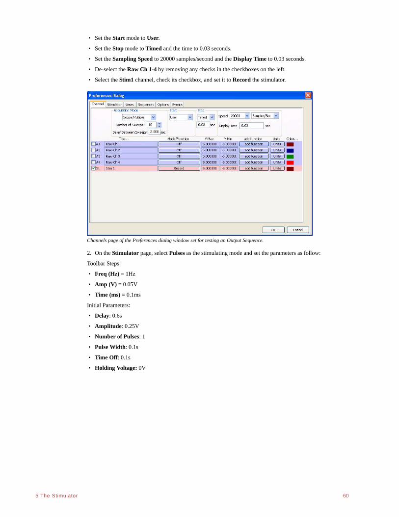
. .
5 The Stimulator 60
• Set the Start mode to User.
• Set the Stop mode to Timed and the time to 0.03 seconds.
• Set the Sampling Speed to 20000 samples/second and the Display Time to 0.03 seconds.
• De-select the Raw Ch 1-4 by removing any checks in the checkboxes on the left.
• Select the Stim1 channel, check its checkbox, and set it to Record the stimulator.
Channels page of the Preferences dialog window set for testing an Output Sequence.
2. On the Stimulator page, select Pulses as the stimulating mode and set the parameters as follow:
Toolbar Steps:
• Freq (Hz) = 1Hz
• Amp (V) = 0.05V
• Time (ms) = 0.1ms
Initial Parameters:
• Delay: 0.6s
• Amplitude: 0.25V
• Number of Pulses: 1
• Pulse Width: 0.1s
• Time Off: 0.1s
• Holding Voltage: 0V
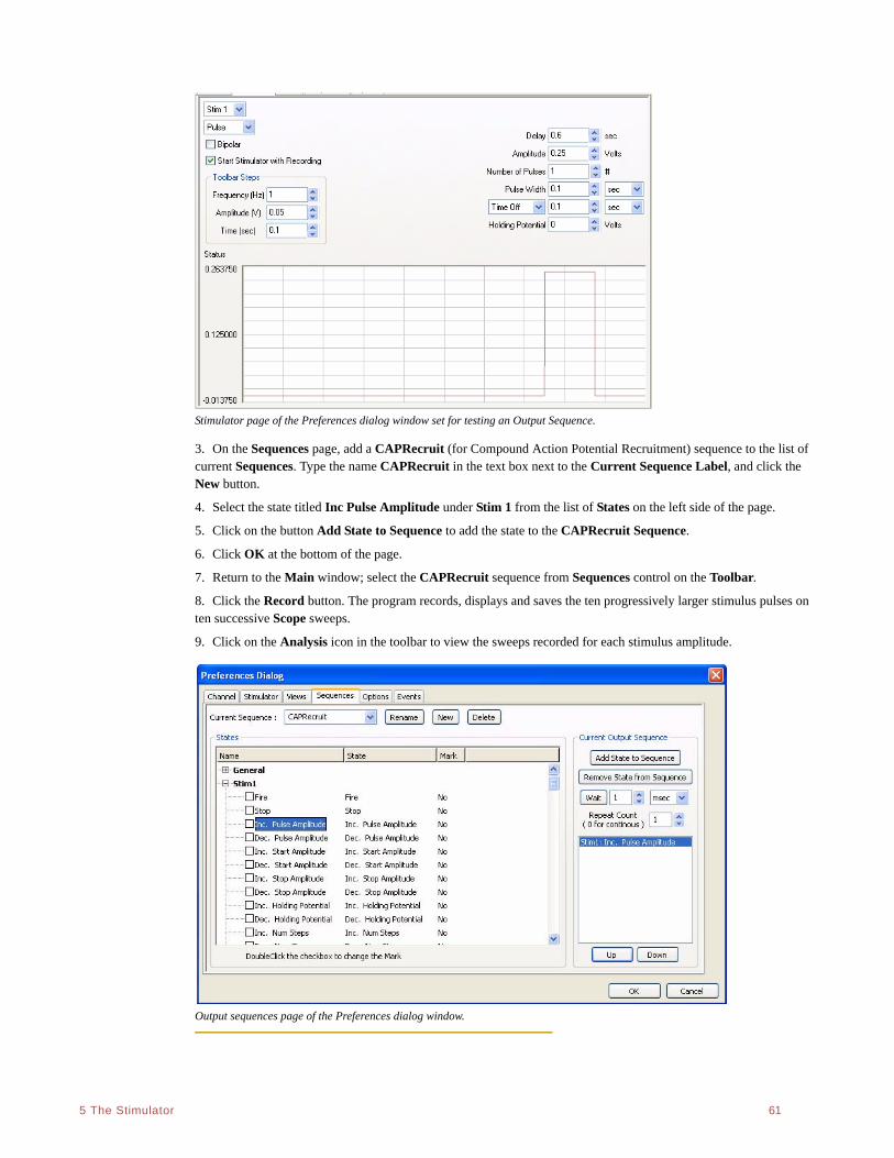
. .
5 The Stimulator 61
Stimulator page of the Preferences dialog window set for testing an Output Sequence.
3. On the Sequences page, add a CAPRecruit (for Compound Action Potential Recruitment) sequence to the list of current Sequences. Type the name CAPRecruit in the text box next to the Current Sequence Label, and click the New button.
4. Select the state titled Inc Pulse Amplitude under Stim 1 from the list of States on the left side of the page.
5. Click on the button Add State to Sequence to add the state to the CAPRecruit Sequence.
6. Click OK at the bottom of the page.
7. Return to the Main window; select the CAPRecruit sequence from Sequences control on the Toolbar.
8. Click the Record button. The program records, displays and saves the ten progressively larger stimulus pulses on ten successive Scope sweeps.
9. Click on the Analysis icon in the toolbar to view the sweeps recorded for each stimulus amplitude.
Output sequences page of the Preferences dialog window.
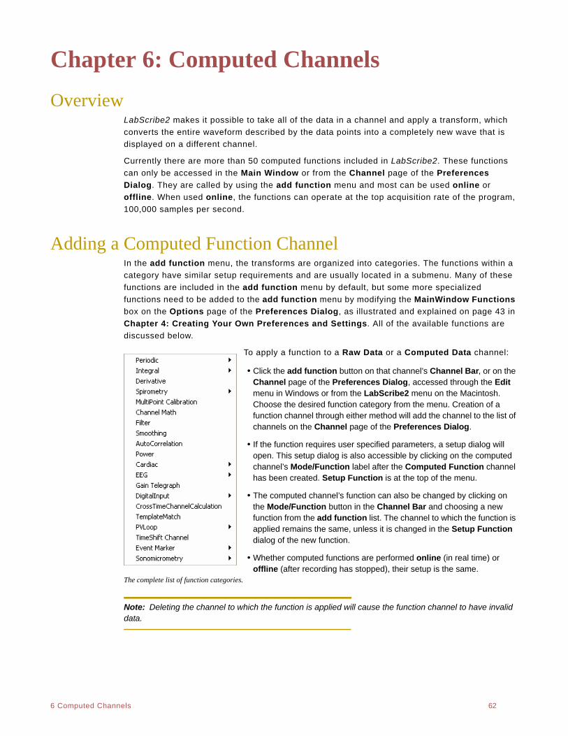
. .
6 Computed Channels 62
Chapter 6: Computed Channels
OverviewLabScribe2 makes it possible to take all of the data in a channel and apply a transform, which
converts the entire waveform described by the data points into a completely new wave that is
displayed on a different channel.
Currently there are more than 50 computed functions included in LabScribe2. These functions
can only be accessed in the Main Window or from the Channel page of the Preferences
Dialog. They are called by using the add function menu and most can be used online or
offline. When used online, the functions can operate at the top acquisition rate of the program,
100,000 samples per second.
Adding a Computed Function Channel In the add function menu, the transforms are organized into categories. The functions within a
category have similar setup requirements and are usually located in a submenu. Many of these
functions are included in the add function menu by default, but some more specialized
functions need to be added to the add function menu by modifying the MainWindow Functions
box on the Options page of the Preferences Dialog, as illustrated and explained on page 43 in
Chapter 4: Creating Your Own Preferences and Settings. All of the available functions are
discussed below.
To apply a function to a Raw Data or a Computed Data channel:
• Click the add function button on that channel’s Channel Bar, or on the Channel page of the Preferences Dialog, accessed through the Edit menu in Windows or from the LabScribe2 menu on the Macintosh. Choose the desired function category from the menu. Creation of a function channel through either method will add the channel to the list of channels on the Channel page of the Preferences Dialog.
• If the function requires user specified parameters, a setup dialog will open. This setup dialog is also accessible by clicking on the computed channel’s Mode/Function label after the Computed Function channel has been created. Setup Function is at the top of the menu.
• The computed channel’s function can also be changed by clicking on the Mode/Function button in the Channel Bar and choosing a new function from the add function list. The channel to which the function is applied remains the same, unless it is changed in the Setup Function dialog of the new function.
• Whether computed functions are performed online (in real time) or offline (after recording has stopped), their setup is the same.
The complete list of function categories.
Note: Deleting the channel to which the function is applied will cause the function channel to have invalid data.
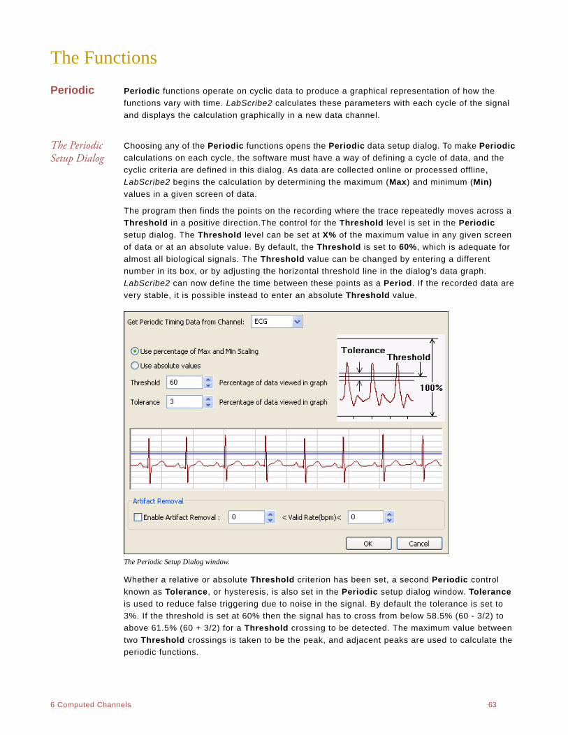
. .
6 Computed Channels 63
The Functions
Periodic Periodic functions operate on cyclic data to produce a graphical representation of how the
functions vary with time. LabScribe2 calculates these parameters with each cycle of the signal
and displays the calculation graphically in a new data channel.
The Periodic Setup Dialog
Choosing any of the Periodic functions opens the Periodic data setup dialog. To make Periodic
calculations on each cycle, the software must have a way of defining a cycle of data, and the
cyclic criteria are defined in this dialog. As data are collected online or processed offline,
LabScribe2 begins the calculation by determining the maximum (Max) and minimum (Min)
values in a given screen of data.
The program then finds the points on the recording where the trace repeatedly moves across a
Threshold in a positive direction.The control for the Threshold level is set in the Periodic
setup dialog. The Threshold level can be set at X% of the maximum value in any given screen
of data or at an absolute value. By default, the Threshold is set to 60%, which is adequate for
almost all biological signals. The Threshold value can be changed by entering a different
number in its box, or by adjusting the horizontal threshold line in the dialog’s data graph.
LabScribe2 can now define the time between these points as a Period. If the recorded data are
very stable, it is possible instead to enter an absolute Threshold value.
The Periodic Setup Dialog window.
Whether a relative or absolute Threshold criterion has been set, a second Periodic control
known as Tolerance, or hysteresis, is also set in the Periodic setup dialog window. Tolerance
is used to reduce false triggering due to noise in the signal. By default the tolerance is set to
3%. If the threshold is set at 60% then the signal has to cross from below 58.5% (60 - 3/2) to
above 61.5% (60 + 3/2) for a Threshold crossing to be detected. The maximum value between
two Threshold crossings is taken to be the peak, and adjacent peaks are used to calculate the
periodic functions.
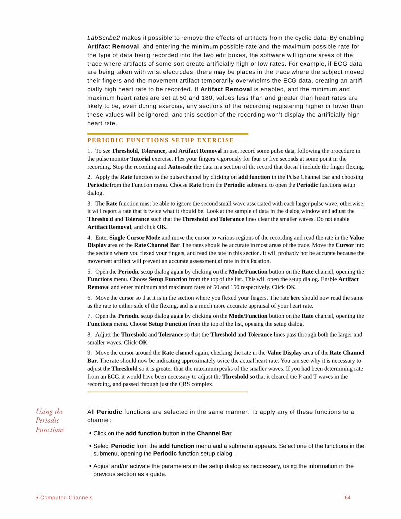
. .
6 Computed Channels 64
LabScribe2 makes it possible to remove the effects of artifacts from the cyclic data. By enabling
Artifact Removal, and entering the minimum possible rate and the maximum possible rate for
the type of data being recorded into the two edit boxes, the software will ignore areas of the
trace where artifacts of some sort create artificially high or low rates. For example, if ECG data
are being taken with wrist electrodes, there may be places in the trace where the subject moved
their fingers and the movement artifact temporarily overwhelms the ECG data, creating an artifi-
cially high heart rate to be recorded. If Artifact Removal is enabled, and the minimum and
maximum heart rates are set at 50 and 180, values less than and greater than heart rates are
likely to be, even during exercise, any sections of the recording registering higher or lower than
these values will be ignored, and this section of the recording won’t display the artificially high
heart rate.
P E R I O D I C F U N C T I O N S S E T U P E X E R C I S E
1. To see Threshold, Tolerance, and Artifact Removal in use, record some pulse data, following the procedure in the pulse monitor Tutorial exercise. Flex your fingers vigorously for four or five seconds at some point in the recording. Stop the recording and Autoscale the data in a section of the record that doesn’t include the finger flexing.
2. Apply the Rate function to the pulse channel by clicking on add function in the Pulse Channel Bar and choosing Periodic from the Function menu. Choose Rate from the Periodic submenu to open the Periodic functions setup dialog.
3. The Rate function must be able to ignore the second small wave associated with each larger pulse wave; otherwise, it will report a rate that is twice what it should be. Look at the sample of data in the dialog window and adjust the Threshold and Tolerance such that the Threshold and Tolerance lines clear the smaller waves. Do not enable Artifact Removal, and click OK.
4. Enter Single Cursor Mode and move the cursor to various regions of the recording and read the rate in the Value Display area of the Rate Channel Bar. The rates should be accurate in most areas of the trace. Move the Cursor into the section where you flexed your fingers, and read the rate in this section. It will probably not be accurate because the movement artifact will prevent an accurate assessment of rate in this location.
5. Open the Periodic setup dialog again by clicking on the Mode/Function button on the Rate channel, opening the Functions menu. Choose Setup Function from the top of the list. This will open the setup dialog. Enable Artifact Removal and enter minimum and maximum rates of 50 and 150 respectively. Click OK.
6. Move the cursor so that it is in the section where you flexed your fingers. The rate here should now read the same as the rate to either side of the flexing, and is a much more accurate appraisal of your heart rate.
7. Open the Periodic setup dialog again by clicking on the Mode/Function button on the Rate channel, opening the Functions menu. Choose Setup Function from the top of the list, opening the setup dialog.
8. Adjust the Threshold and Tolerance so that the Threshold and Tolerance lines pass through both the larger and smaller waves. Click OK.
9. Move the cursor around the Rate channel again, checking the rate in the Value Display area of the Rate Channel Bar. The rate should now be indicating approximately twice the actual heart rate. You can see why it is necessary to adjust the Threshold so it is greater than the maximum peaks of the smaller waves. If you had been determining rate from an ECG, it would have been necessary to adjust the Threshold so that it cleared the P and T waves in the recording, and passed through just the QRS complex.
Using the Periodic Functions
All Periodic functions are selected in the same manner. To apply any of these functions to a
channel:
• Click on the add function button in the Channel Bar.
• Select Periodic from the add function menu and a submenu appears. Select one of the functions in the submenu, opening the Periodic function setup dialog.
• Adjust and/or activate the parameters in the setup dialog as neccessary, using the information in the previous section as a guide.
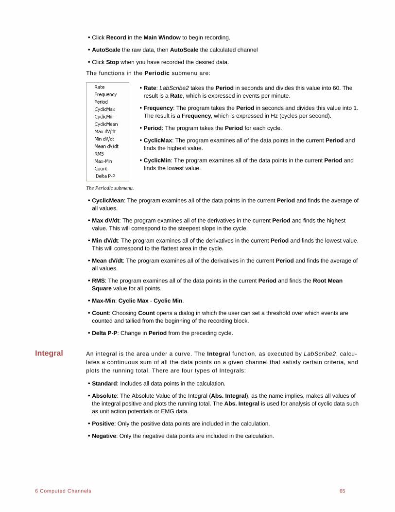
. .
6 Computed Channels 65
• Click Record in the Main Window to begin recording.
• AutoScale the raw data, then AutoScale the calculated channel
• Click Stop when you have recorded the desired data.
The functions in the Periodic submenu are:
• Rate: LabScribe2 takes the Period in seconds and divides this value into 60. The result is a Rate, which is expressed in events per minute.
• Frequency: The program takes the Period in seconds and divides this value into 1. The result is a Frequency, which is expressed in Hz (cycles per second).
• Period: The program takes the Period for each cycle.
• CyclicMax: The program examines all of the data points in the current Period and finds the highest value.
• CyclicMin: The program examines all of the data points in the current Period and finds the lowest value.
The Periodic submenu.
• CyclicMean: The program examines all of the data points in the current Period and finds the average of all values.
• Max dV/dt: The program examines all of the derivatives in the current Period and finds the highest value. This will correspond to the steepest slope in the cycle.
• Min dV/dt: The program examines all of the derivatives in the current Period and finds the lowest value. This will correspond to the flattest area in the cycle.
• Mean dV/dt: The program examines all of the derivatives in the current Period and finds the average of all values.
• RMS: The program examines all of the data points in the current Period and finds the Root Mean Square value for all points.
• Max-Min: Cyclic Max - Cyclic Min.
• Count: Choosing Count opens a dialog in which the user can set a threshold over which events are counted and tallied from the beginning of the recording block.
• Delta P-P: Change in Period from the preceding cycle.
Integral An integral is the area under a curve. The Integral function, as executed by LabScribe2, calcu-
lates a continuous sum of all the data points on a given channel that satisfy certain criteria, and
plots the running total. There are four types of Integrals:
• Standard: Includes all data points in the calculation.
• Absolute: The Absolute Value of the Integral (Abs. Integral), as the name implies, makes all values of the integral positive and plots the running total. The Abs. Integral is used for analysis of cyclic data such as unit action potentials or EMG data.
• Positive: Only the positive data points are included in the calculation.
• Negative: Only the negative data points are included in the calculation.
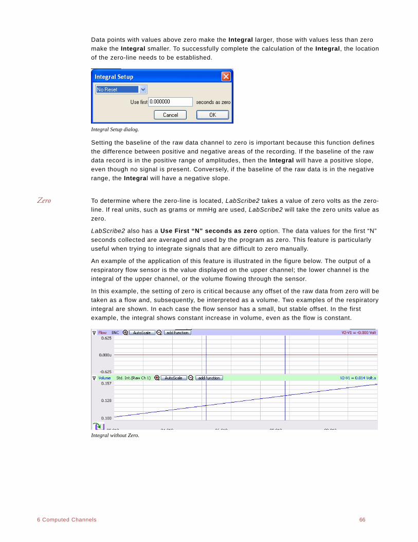
. .
6 Computed Channels 66
Data points with values above zero make the Integral larger, those with values less than zero
make the Integral smaller. To successfully complete the calculation of the Integral, the location
of the zero-line needs to be established.
Integral Setup dialog.
Setting the baseline of the raw data channel to zero is important because this function defines
the difference between positive and negative areas of the recording. If the baseline of the raw
data record is in the positive range of amplitudes, then the Integral will have a positive slope,
even though no signal is present. Conversely, if the baseline of the raw data is in the negative
range, the Integral will have a negative slope.
Zero To determine where the zero-line is located, LabScribe2 takes a value of zero volts as the zero-
line. If real units, such as grams or mmHg are used, LabScribe2 will take the zero units value as
zero.
LabScribe2 also has a Use First “N” seconds as zero option. The data values for the first “N”
seconds collected are averaged and used by the program as zero. This feature is particularly
useful when trying to integrate signals that are difficult to zero manually.
An example of the application of this feature is illustrated in the figure below. The output of a
respiratory flow sensor is the value displayed on the upper channel; the lower channel is the
integral of the upper channel, or the volume flowing through the sensor.
In this example, the setting of zero is critical because any offset of the raw data from zero will be
taken as a flow and, subsequently, be interpreted as a volume. Two examples of the respiratory
integral are shown. In each case the flow sensor has a small, but stable offset. In the first
example, the integral shows constant increase in volume, even as the flow is constant.
Integral without Zero.
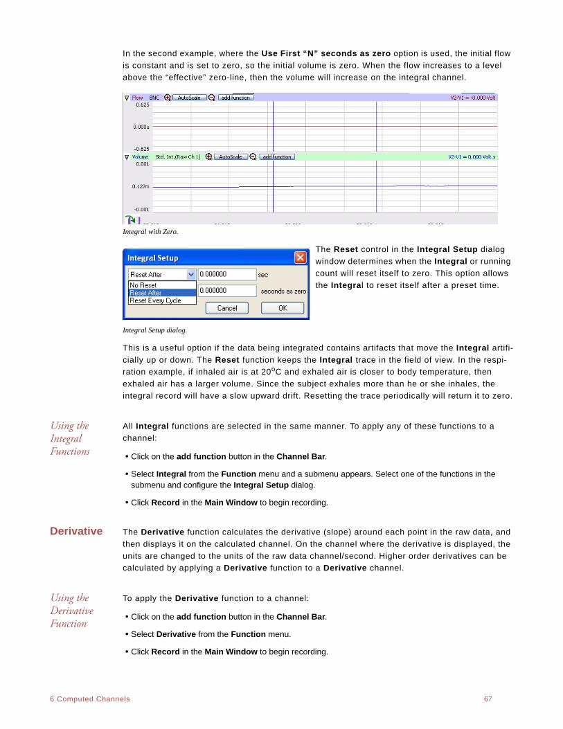
. .
6 Computed Channels 67
In the second example, where the Use First “N” seconds as zero option is used, the initial flow
is constant and is set to zero, so the initial volume is zero. When the flow increases to a level
above the “effective” zero-line, then the volume will increase on the integral channel.
Integral with Zero.
The Reset control in the Integral Setup dialog
window determines when the Integral or running
count will reset itself to zero. This option allows
the Integral to reset itself after a preset time.
Integral Setup dialog.
This is a useful option if the data being integrated contains artifacts that move the Integral artifi-
cially up or down. The Reset function keeps the Integral trace in the field of view. In the respi-
ration example, if inhaled air is at 20oC and exhaled air is closer to body temperature, then
exhaled air has a larger volume. Since the subject exhales more than he or she inhales, the
integral record will have a slow upward drift. Resetting the trace periodically will return it to zero.
Using the Integral Functions
All Integral functions are selected in the same manner. To apply any of these functions to a
channel:
• Click on the add function button in the Channel Bar.
• Select Integral from the Function menu and a submenu appears. Select one of the functions in the submenu and configure the Integral Setup dialog.
• Click Record in the Main Window to begin recording.
Derivative The Derivative function calculates the derivative (slope) around each point in the raw data, and
then displays it on the calculated channel. On the channel where the derivative is displayed, the
units are changed to the units of the raw data channel/second. Higher order derivatives can be
calculated by applying a Derivative function to a Derivative channel.
Using the Derivative Function
To apply the Derivative function to a channel:
• Click on the add function button in the Channel Bar.
• Select Derivative from the Function menu.
• Click Record in the Main Window to begin recording.
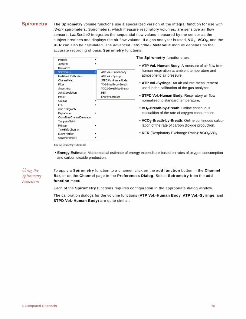
. .
6 Computed Channels 68
Spirometry The Spirometry volume functions use a specialized version of the integral function for use with
iWorx spirometers. Spirometers, which measure respiratory volumes, are sensitive air flow
sensors. LabScribe2 integrates the sequential flow values measured by the sensor as the
subject breathes and displays the air flow volume. If a gas analyzer is used, VO2, VCO2, and the
RER can also be calculated. The advanced LabScribe2 Metabolic module depends on the
accurate recording of basic Spirometry functions.
The Spirometry functions are:
• ATP Vol.-Human Body: A measure of air flow from human respiration at ambient temperature and atmospheric air pressure.
• ATP Vol.-Syringe: An air volume measurement used in the calibration of the gas analyzer.
• STPD Vol.-Human Body: Respiratory air flow normalized to standard temperature.
• VO2-Breath-by-Breath: Online continuous calcualtion of the rate of oxygen consumption.
• VCO2-Breath-by-Breath: Online continuous calcu-lation of the rate of carbon dioxide production.
• RER (Respiratory Exchange Ratio): VCO2/VO2.
The Spirometry submenu.
• Energy Estimate: Mathematical estimate of energy expenditure based on rates of oxygen consumption and carbon dioxide production.
Using the Spirometry Functions
To apply a Spirometry function to a channel, click on the add function button in the Channel
Bar, or on the Channel page in the Preferences Dialog. Select Spirometry from the add
function menu.
Each of the Spirometry functions requires configuration in the appropriate dialog window.
The calibration dialogs for the volume functions (ATP Vol.-Human Body, ATP Vol.-Syringe, and
STPD Vol.-Human Body) are quite similar.
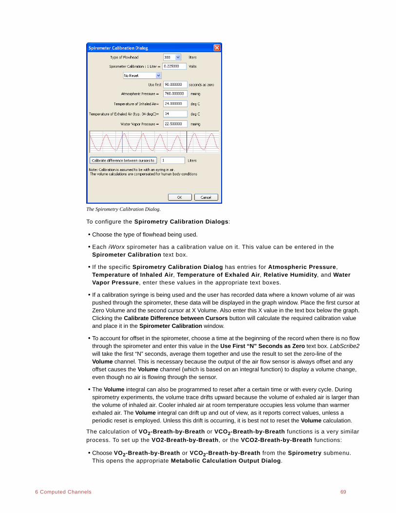
. .
6 Computed Channels 69
The Spirometry Calibration Dialog.
To configure the Spirometry Calibration Dialogs:
• Choose the type of flowhead being used.
• Each iWorx spirometer has a calibration value on it. This value can be entered in the Spirometer Calibration text box.
• If the specific Spirometry Calibration Dialog has entries for Atmospheric Pressure, Temperature of Inhaled Air, Temperature of Exhaled Air, Relative Humidity, and Water Vapor Pressure, enter these values in the appropriate text boxes.
• If a calibration syringe is being used and the user has recorded data where a known volume of air was pushed through the spirometer, these data will be displayed in the graph window. Place the first cursor at Zero Volume and the second cursor at X Volume. Also enter this X value in the text box below the graph. Clicking the Calibrate Difference between Cursors button will calculate the required calibration value and place it in the Spirometer Calibration window.
• To account for offset in the spirometer, choose a time at the beginning of the record when there is no flow through the spirometer and enter this value in the Use First “N” Seconds as Zero text box. LabScribe2 will take the first “N” seconds, average them together and use the result to set the zero-line of the Volume channel. This is necessary because the output of the air flow sensor is always offset and any offset causes the Volume channel (which is based on an integral function) to display a volume change, even though no air is flowing through the sensor.
• The Volume integral can also be programmed to reset after a certain time or with every cycle. During spirometry experiments, the volume trace drifts upward because the volume of exhaled air is larger than the volume of inhaled air. Cooler inhaled air at room temperature occupies less volume than warmer exhaled air. The Volume integral can drift up and out of view, as it reports correct values, unless a periodic reset is employed. Unless this drift is occurring, it is best not to reset the Volume calculation.
The calculation of VO2-Breath-by-Breath or VCO2-Breath-by-Breath functions is a very similar
process. To set up the VO2-Breath-by-Breath, or the VCO2-Breath-by-Breath functions:
• Choose VO2-Breath-by-Breath or VCO2-Breath-by-Breath from the Spirometry submenu. This opens the appropriate Metabolic Calculation Output Dialog.
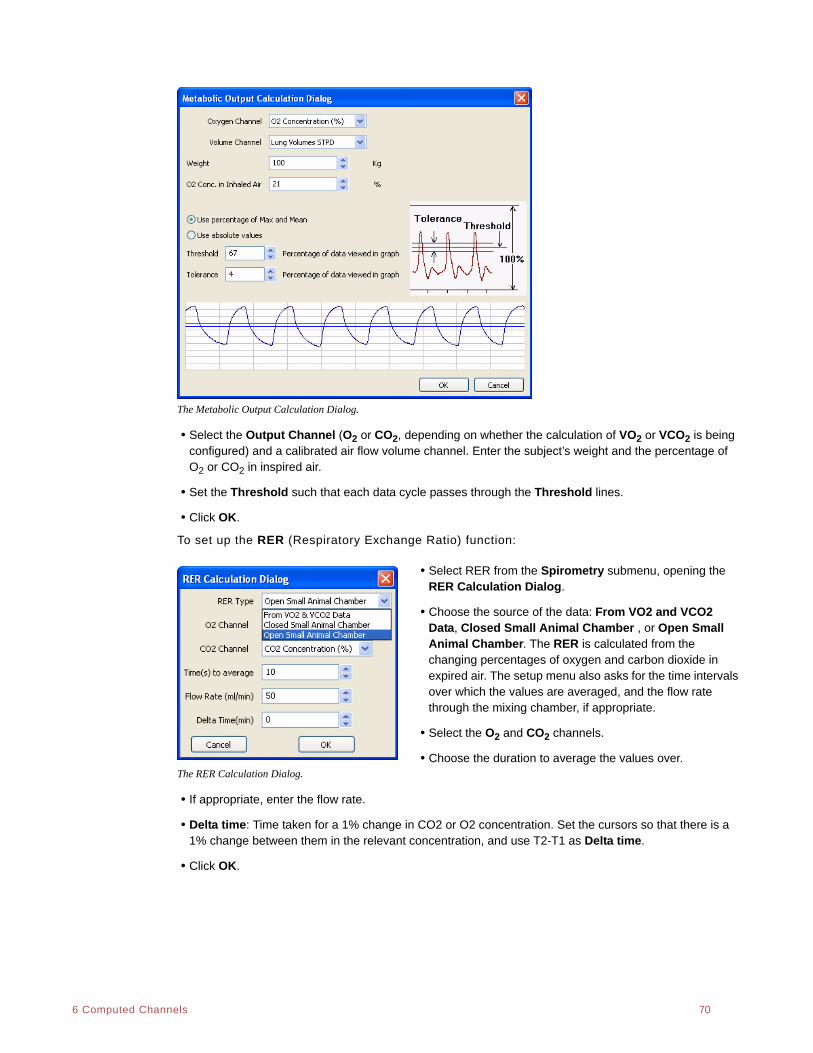
. .
6 Computed Channels 70
The Metabolic Output Calculation Dialog.
• Select the Output Channel (O2 or CO2, depending on whether the calculation of VO2 or VCO2 is being configured) and a calibrated air flow volume channel. Enter the subject’s weight and the percentage of O2 or CO2 in inspired air.
• Set the Threshold such that each data cycle passes through the Threshold lines.
• Click OK.
To set up the RER (Respiratory Exchange Ratio) function:
• Select RER from the Spirometry submenu, opening the RER Calculation Dialog.
• Choose the source of the data: From VO2 and VCO2 Data, Closed Small Animal Chamber , or Open Small Animal Chamber. The RER is calculated from the changing percentages of oxygen and carbon dioxide in expired air. The setup menu also asks for the time intervals over which the values are averaged, and the flow rate through the mixing chamber, if appropriate.
• Select the O2 and CO2 channels.
• Choose the duration to average the values over. The RER Calculation Dialog.
• If appropriate, enter the flow rate.
• Delta time: Time taken for a 1% change in CO2 or O2 concentration. Set the cursors so that there is a 1% change between them in the relevant concentration, and use T2-T1 as Delta time.
• Click OK.
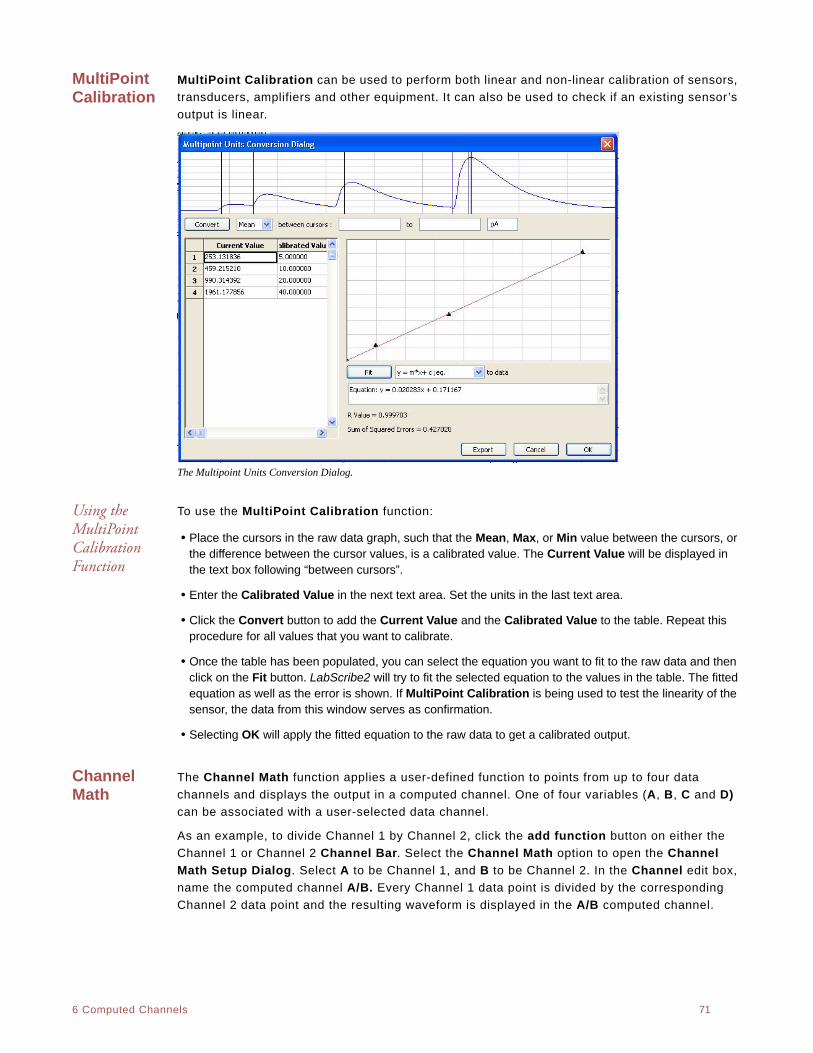
. .
6 Computed Channels 71
MultiPoint Calibration
MultiPoint Calibration can be used to perform both linear and non-linear calibration of sensors,
transducers, amplifiers and other equipment. It can also be used to check if an existing sensor’s
output is linear.
The Multipoint Units Conversion Dialog.
Using the MultiPoint Calibration Function
To use the MultiPoint Calibration function:
• Place the cursors in the raw data graph, such that the Mean, Max, or Min value between the cursors, or the difference between the cursor values, is a calibrated value. The Current Value will be displayed in the text box following “between cursors”.
• Enter the Calibrated Value in the next text area. Set the units in the last text area.
• Click the Convert button to add the Current Value and the Calibrated Value to the table. Repeat this procedure for all values that you want to calibrate.
• Once the table has been populated, you can select the equation you want to fit to the raw data and then click on the Fit button. LabScribe2 will try to fit the selected equation to the values in the table. The fitted equation as well as the error is shown. If MultiPoint Calibration is being used to test the linearity of the sensor, the data from this window serves as confirmation.
• Selecting OK will apply the fitted equation to the raw data to get a calibrated output.
Channel Math
The Channel Math function applies a user-defined function to points from up to four data
channels and displays the output in a computed channel. One of four variables (A, B, C and D)
can be associated with a user-selected data channel.
As an example, to divide Channel 1 by Channel 2, click the add function button on either the
Channel 1 or Channel 2 Channel Bar. Select the Channel Math option to open the Channel
Math Setup Dialog. Select A to be Channel 1, and B to be Channel 2. In the Channel edit box,
name the computed channel A/B. Every Channel 1 data point is divided by the corresponding
Channel 2 data point and the resulting waveform is displayed in the A/B computed channel.
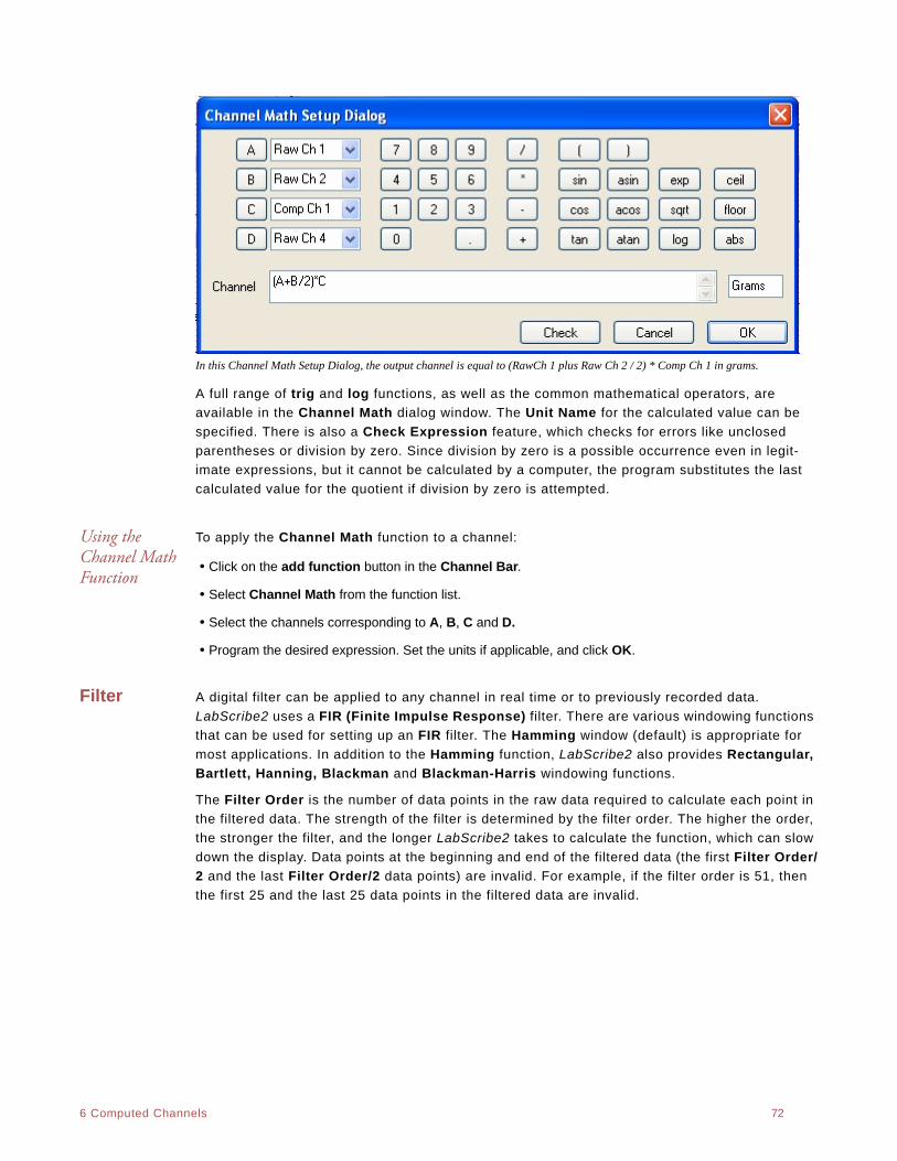
. .
6 Computed Channels 72
In this Channel Math Setup Dialog, the output channel is equal to (RawCh 1 plus Raw Ch 2 / 2) * Comp Ch 1 in grams.
A full range of trig and log functions, as well as the common mathematical operators, are
available in the Channel Math dialog window. The Unit Name for the calculated value can be
specified. There is also a Check Expression feature, which checks for errors like unclosed
parentheses or division by zero. Since division by zero is a possible occurrence even in legit-
imate expressions, but it cannot be calculated by a computer, the program substitutes the last
calculated value for the quotient if division by zero is attempted.
Using the Channel Math Function
To apply the Channel Math function to a channel:
• Click on the add function button in the Channel Bar.
• Select Channel Math from the function list.
• Select the channels corresponding to A, B, C and D.
• Program the desired expression. Set the units if applicable, and click OK.
Filter A digital filter can be applied to any channel in real time or to previously recorded data.
LabScribe2 uses a FIR (Finite Impulse Response) filter. There are various windowing functions
that can be used for setting up an FIR filter. The Hamming window (default) is appropriate for
most applications. In addition to the Hamming function, LabScribe2 also provides Rectangular,
Bartlett, Hanning, Blackman and Blackman-Harris windowing functions.
The Filter Order is the number of data points in the raw data required to calculate each point in
the filtered data. The strength of the filter is determined by the filter order. The higher the order,
the stronger the filter, and the longer LabScribe2 takes to calculate the function, which can slow
down the display. Data points at the beginning and end of the filtered data (the first Filter Order/
2 and the last Filter Order/2 data points) are invalid. For example, if the filter order is 51, then
the first 25 and the last 25 data points in the filtered data are invalid.
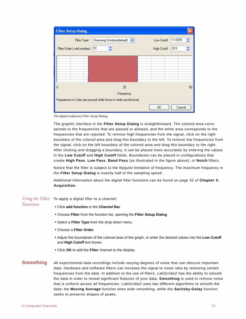
. .
6 Computed Channels 73
The digital (software) Filter Setup Dialog.
The graphic interface in the Filter Setup Dialog is straightforward. The colored area corre-
sponds to the frequencies that are passed or allowed, and the white area corresponds to the
frequencies that are rejected. To remove high frequencies from the signal, click on the right
boundary of the colored area and drag this boundary to the left. To remove low frequencies from
the signal, click on the left boundary of the colored area and drag this boundary to the right.
After clicking and dragging a boundary, it can be placed more accurately by entering the values
in the Low Cutoff and High Cutoff fields. Boundaries can be placed in configurations that
create High Pass, Low Pass, Band Pass (as illustrated in the figure above), or Notch filters.
Notice that the filter is subject to the Nyquist limitation of frequency. The maximum frequency in
the Filter Setup Dialog is exactly half of the sampling speed.
Additional information about the digital filter functions can be found on page 32 of Chapter 3:
Acquisition.
Using the Filter Functions
To apply a digital filter to a channel:
• Click add function in the Channel Bar.
• Choose Filter from the function list, opening the Filter Setup Dialog.
• Select a Filter Type from the drop-down menu.
• Choose a Filter Order.
• Adjust the boundaries of the colored area of the graph, or enter the desired values into the Low Cutoff and High Cutoff text boxes.
• Click OK to add the Filter channel to the display.
Smoothing All experimental data recordings include varying degrees of noise that can obscure important
data. Hardware and software filters can increase the signal to noise ratio by removing certain
frequencies from the data. In addition to the use of filters, LabScribe2 has the ability to smooth
the data in order to reveal significant features of your data. Smoothing is used to remove noise
that is uniform across all frequencies. LabScribe2 uses two different algorithms to smooth the
data; the Moving Average function does wide smoothing, while the Savitzky-Golay function
seeks to preserve shapes of peaks.
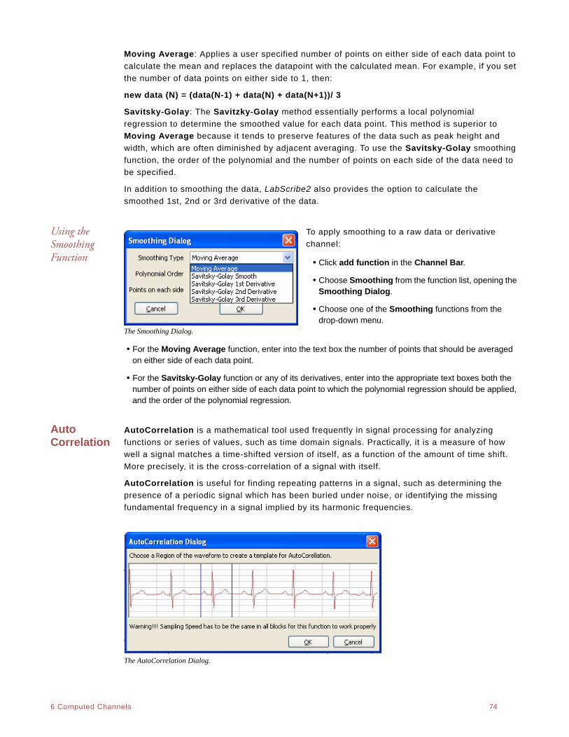
. .
6 Computed Channels 74
Moving Average: Applies a user specified number of points on either side of each data point to
calculate the mean and replaces the datapoint with the calculated mean. For example, if you set
the number of data points on either side to 1, then:
new data (N) = (data(N-1) + data(N) + data(N+1))/ 3
Savitsky-Golay: The Savitzky-Golay method essentially performs a local polynomial
regression to determine the smoothed value for each data point. This method is superior to
Moving Average because it tends to preserve features of the data such as peak height and
width, which are often diminished by adjacent averaging. To use the Savitsky-Golay smoothing
function, the order of the polynomial and the number of points on each side of the data need to
be specified.
In addition to smoothing the data, LabScribe2 also provides the option to calculate the
smoothed 1st, 2nd or 3rd derivative of the data.
Using the Smoothing Function
To apply smoothing to a raw data or derivative
channel:
• Click add function in the Channel Bar.
• Choose Smoothing from the function list, opening the Smoothing Dialog.
• Choose one of the Smoothing functions from the drop-down menu.
The Smoothing Dialog.
• For the Moving Average function, enter into the text box the number of points that should be averaged on either side of each data point.
• For the Savitsky-Golay function or any of its derivatives, enter into the appropriate text boxes both the number of points on either side of each data point to which the polynomial regression should be applied, and the order of the polynomial regression.
Auto Correlation
AutoCorrelation is a mathematical tool used frequently in signal processing for analyzing
functions or series of values, such as time domain signals. Practically, it is a measure of how
well a signal matches a time-shifted version of itself, as a function of the amount of time shift.
More precisely, it is the cross-correlation of a signal with itself.
AutoCorrelation is useful for finding repeating patterns in a signal, such as determining the
presence of a periodic signal which has been buried under noise, or identifying the missing
fundamental frequency in a signal implied by its harmonic frequencies.
The AutoCorrelation Dialog.
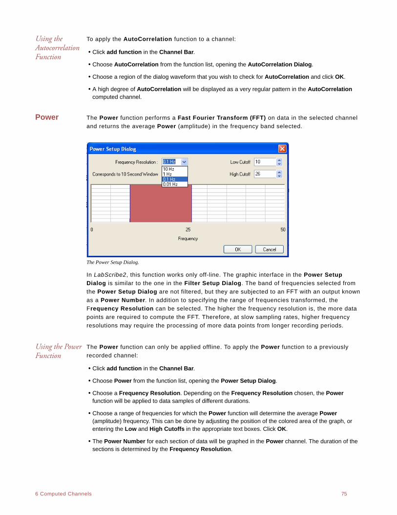
. .
6 Computed Channels 75
Using the Autocorrelation Function
To apply the AutoCorrelation function to a channel:
• Click add function in the Channel Bar.
• Choose AutoCorrelation from the function list, opening the AutoCorrelation Dialog.
• Choose a region of the dialog waveform that you wish to check for AutoCorrelation and click OK.
• A high degree of AutoCorrelation will be displayed as a very regular pattern in the AutoCorrelation computed channel.
Power The Power function performs a Fast Fourier Transform (FFT) on data in the selected channel
and returns the average Power (amplitude) in the frequency band selected.
The Power Setup Dialog.
In LabScribe2, this function works only off-line. The graphic interface in the Power Setup
Dialog is similar to the one in the Filter Setup Dialog. The band of frequencies selected from
the Power Setup Dialog are not filtered, but they are subjected to an FFT with an output known
as a Power Number. In addition to specifying the range of frequencies transformed, the
Frequency Resolution can be selected. The higher the frequency resolution is, the more data
points are required to compute the FFT. Therefore, at slow sampling rates, higher frequency
resolutions may require the processing of more data points from longer recording periods.
Using the Power Function
The Power function can only be applied offline. To apply the Power function to a previously
recorded channel:
• Click add function in the Channel Bar.
• Choose Power from the function list, opening the Power Setup Dialog.
• Choose a Frequency Resolution. Depending on the Frequency Resolution chosen, the Power function will be applied to data samples of different durations.
• Choose a range of frequencies for which the Power function will determine the average Power (amplitude) frequency. This can be done by adjusting the position of the colored area of the graph, or entering the Low and High Cutoffs in the appropriate text boxes. Click OK.
• The Power Number for each section of data will be graphed in the Power channel. The duration of the sections is determined by the Frequency Resolution.
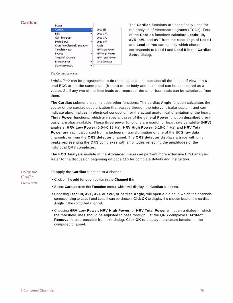
. .
6 Computed Channels 76
Cardiac The Cardiac functions are specifically used for
the analysis of electrocardiograms (ECGs). Four
of the Cardiac functions calculate Leads: III,
aVR, aVL and aVF from the recordings of Lead I
and Lead II. You can specify which channel
corresponds to Lead I and Lead II in the Cardiac
Setup dialog.
The Cardiac submenu.
LabScribe2 can be programmed to do these calculations because all the points of view in a 6-
lead ECG are in the same plane (frontal) of the body and each lead can be considered as a
vector. So if any two of the limb leads are recorded, the other four leads can be calculated from
them.
The Cardiac submenu also includes other functions. The cardiac Angle function calculates the
vector of the cardiac depolarization that passes through the interventricular septum, and can
indicate abnormalities in electrical conduction, or the actual anatomical orientation of the heart.
Three Power functions, which are special cases of the general Power function described previ-
ously, are also available. These three power functions are useful for heart rate variability (HRV)
analysis. HRV Low Power (0.04-0.15 Hz), HRV High Power (0.18-0.4 Hz) and HRV Total
Power are each calculated from a tachogram transformation of one of the ECG raw data
channels, or from the QRS detector channel. The QRS detector displays a trace with only
peaks representing the QRS complexes with amplitudes reflecting the amplitudes of the
individual QRS complexes.
The ECG Analysis module in the Advanced menu can perform more extensive ECG analysis.
Refer to the discussion beginning on page 116 for complete details and instruction.
Using the Cardiac Functions
To apply the Cardiac function to a channel:
• Click on the add function button in the Channel Bar.
• Select Cardiac from the Function menu, which will display the Cardiac submenu.
• Choosing Lead: III, aVL, aVF or aVR, or cardiac Angle, will open a dialog in which the channels corresponding to Lead I and Lead II can be chosen. Click OK to display the chosen lead or the cardiac Angle in the computed channel.
• Choosing HRV Low Power, HRV High Power, or HRV Total Power will open a dialog in which the threshold lines should be adjusted to pass through just the QRS complexes. Artifact Removal is also possible from this dialog. Click OK to display the chosen function in the computed channel.
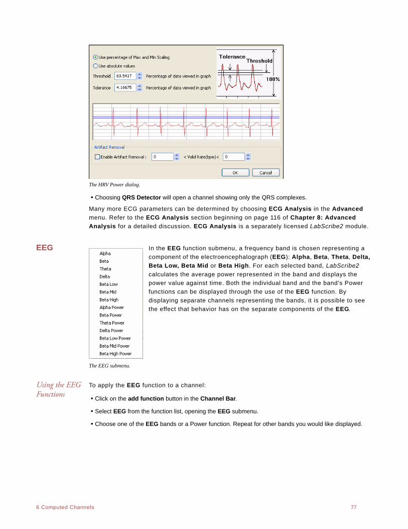
. .
6 Computed Channels 77
The HRV Power dialog.
• Choosing QRS Detector will open a channel showing only the QRS complexes.
Many more ECG parameters can be determined by choosing ECG Analysis in the Advanced
menu. Refer to the ECG Analysis section beginning on page 116 of Chapter 8: Advanced
Analysis for a detailed discussion. ECG Analysis is a separately licensed LabScribe2 module.
EEG In the EEG function submenu, a frequency band is chosen representing a
component of the electroencephalograph (EEG): Alpha, Beta, Theta, Delta,
Beta Low, Beta Mid or Beta High. For each selected band, LabScribe2
calculates the average power represented in the band and displays the
power value against time. Both the individual band and the band’s Power
functions can be displayed through the use of the EEG function. By
displaying separate channels representing the bands, it is possible to see
the effect that behavior has on the separate components of the EEG.
The EEG submenu.
Using the EEG Functions
To apply the EEG function to a channel:
• Click on the add function button in the Channel Bar.
• Select EEG from the function list, opening the EEG submenu.
• Choose one of the EEG bands or a Power function. Repeat for other bands you would like displayed.
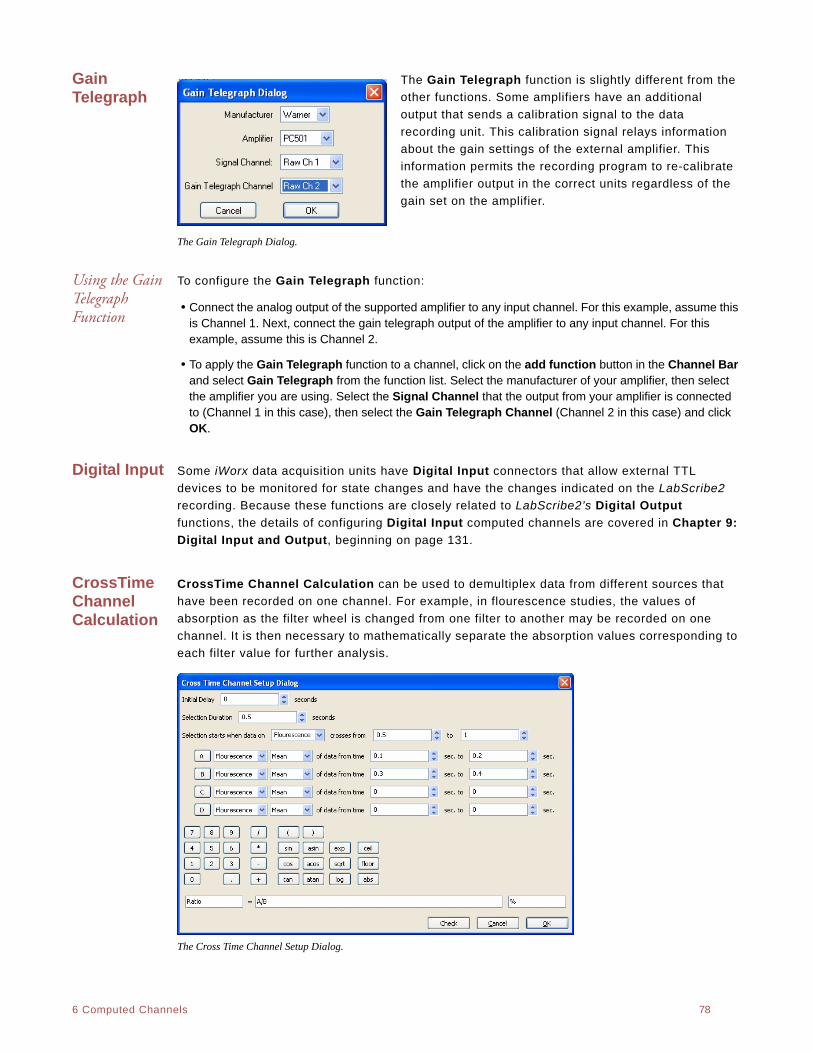
. .
6 Computed Channels 78
Gain Telegraph
The Gain Telegraph function is slightly different from the
other functions. Some amplifiers have an additional
output that sends a calibration signal to the data
recording unit. This calibration signal relays information
about the gain settings of the external amplifier. This
information permits the recording program to re-calibrate
the amplifier output in the correct units regardless of the
gain set on the amplifier.
The Gain Telegraph Dialog.
Using the Gain Telegraph Function
To configure the Gain Telegraph function:
• Connect the analog output of the supported amplifier to any input channel. For this example, assume this is Channel 1. Next, connect the gain telegraph output of the amplifier to any input channel. For this example, assume this is Channel 2.
• To apply the Gain Telegraph function to a channel, click on the add function button in the Channel Bar and select Gain Telegraph from the function list. Select the manufacturer of your amplifier, then select the amplifier you are using. Select the Signal Channel that the output from your amplifier is connected to (Channel 1 in this case), then select the Gain Telegraph Channel (Channel 2 in this case) and click OK.
Digital Input Some iWorx data acquisition units have Digital Input connectors that allow external TTL
devices to be monitored for state changes and have the changes indicated on the LabScribe2
recording. Because these functions are closely related to LabScribe2’s Digital Output
functions, the details of configuring DigitaI Input computed channels are covered in Chapter 9:
Digital Input and Output, beginning on page 131.
CrossTime Channel Calculation
CrossTime Channel Calculation can be used to demultiplex data from different sources that
have been recorded on one channel. For example, in flourescence studies, the values of
absorption as the filter wheel is changed from one filter to another may be recorded on one
channel. It is then necessary to mathematically separate the absorption values corresponding to
each filter value for further analysis.
The Cross Time Channel Setup Dialog.
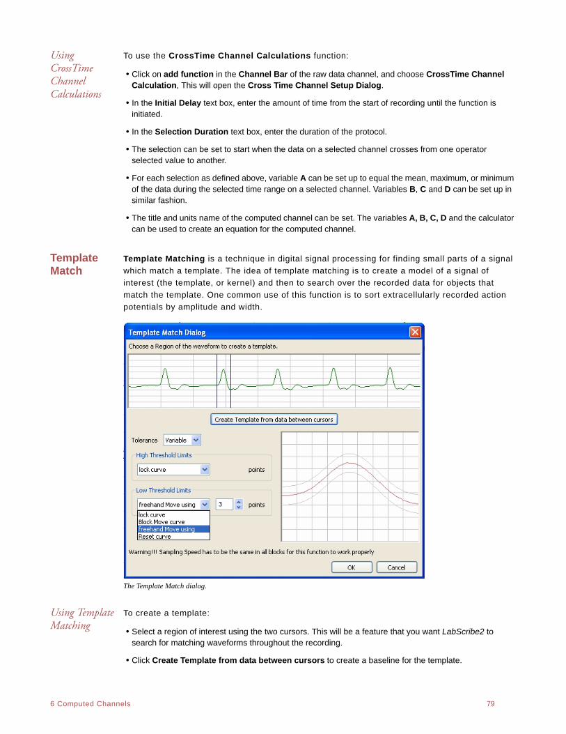
. .
6 Computed Channels 79
Using CrossTime Channel Calculations
To use the CrossTime Channel Calculations function:
• Click on add function in the Channel Bar of the raw data channel, and choose CrossTime Channel Calculation, This will open the Cross Time Channel Setup Dialog.
• In the Initial Delay text box, enter the amount of time from the start of recording until the function is initiated.
• In the Selection Duration text box, enter the duration of the protocol.
• The selection can be set to start when the data on a selected channel crosses from one operator selected value to another.
• For each selection as defined above, variable A can be set up to equal the mean, maximum, or minimum of the data during the selected time range on a selected channel. Variables B, C and D can be set up in similar fashion.
• The title and units name of the computed channel can be set. The variables A, B, C, D and the calculator can be used to create an equation for the computed channel.
Template Match
Template Matching is a technique in digital signal processing for finding small parts of a signal
which match a template. The idea of template matching is to create a model of a signal of
interest (the template, or kernel) and then to search over the recorded data for objects that
match the template. One common use of this function is to sort extracellularly recorded action
potentials by amplitude and width.
The Template Match dialog.
Using Template Matching
To create a template:
• Select a region of interest using the two cursors. This will be a feature that you want LabScribe2 to search for matching waveforms throughout the recording.
• Click Create Template from data between cursors to create a baseline for the template.
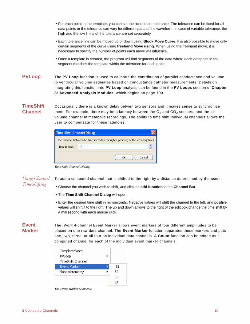
. .
6 Computed Channels 80
• For each point in the template, you can set the acceptable tolerance. The tolerance can be fixed for all data points or the tolerance can vary for different parts of the waveform. In case of variable tolerance, the high and the low limits of the tolerance are set separately.
• Each tolerance line can be moved up or down using Block Move Curve. It is also possible to move only certain segments of the curve using freehand Move using. When using the freehand move, it is necessary to specify the number of points each move will influence.
• Once a template is created, the program will find segments of the data where each datapoint in the segment matches the template within the tolerance for each point.
PVLoop The PV Loop function is used to calibrate the contribution of parallel conductance and volume
to ventricular volume estimates based on conductance catheter measurements. Details on
integrating this function into PV Loop analysis can be found in the PV Loops section of Chapter
8: Advanced Analysis Modules, which begins on page 100.
TimeShift Channel
Occasionally there is a known delay betwen two sensors and it makes sense to synchronize
them. For example, there may be a latency between the O2 and CO2 sensors, and the air
volume channel in metabolic recordings. The ability to time shift individual channels allows the
user to compensate for these latencies.
Time Shift Channel Dialog.
Using Channel TimeShifting
To add a computed channel that is shifted to the right by a distance determined by the user:
• Choose the channel you wish to shift, and click on add function in the Channel Bar.
• The Time Shift Channel Dialog will open.
• Enter the desired time shift in milliseconds. Negative values will shift the channel to the left, and positive values will shift it to the right. The up and down arrows to the right of the edit box change the time shift by a millisecond with each mouse click.
Event Marker
The iWorx 4-channel Event Marker allows event markers of four different amplitudes to be
placed on one raw data channel. The Event Marker function separates these markers and puts
one, two, three, or all four on individual data channels. A Count function can be added as a
computed channel for each of the individual event marker channels.
The Event Marker Submenu.
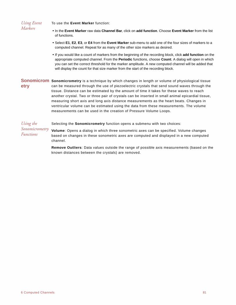
. .
6 Computed Channels 81
Using Event Markers
To use the Event Marker function:
• In the Event Marker raw data Channel Bar, click on add function. Choose Event Marker from the list of functions.
• Select E1, E2, E3, or E4 from the Event Marker sub-menu to add one of the four sizes of markers to a computed channel. Repeat for as many of the other size markers as desired.
• If you would like a count of markers from the beginning of the recording block, click add function on the appropriate computed channel. From the Periodic functions, choose Count. A dialog will open in which you can set the correct threshold for the marker amplitude. A new computed channel will be added that will display the count for that size marker from the start of the recording block.
Sonomicrometry
Sonomicrometry is a technique by which changes in length or volume of physiological tissue
can be measured through the use of piezoelectric crystals that send sound waves through the
tissue. Distance can be estimated by the amount of time it takes for these waves to reach
another crystal. Two or three pair of crystals can be inserted in small animal epicardial tissue,
measuring short axis and long axis distance measurements as the heart beats. Changes in
ventricular volume can be estimated using the data from these measurements. The volume
measurements can be used in the creation of Pressure Volume Loops.
Using the Sonomicrometry Functions
Selecting the Sonomicrometry function opens a submenu with two choices:
Volume: Opens a dialog in which three sonometric axes can be specified. Volume changes
based on changes in these sonometric axes are computed and displayed in a new computed
channel.
Remove Outliers: Data values outside the range of possible axis measurements (based on the
known distances between the crystals) are removed.
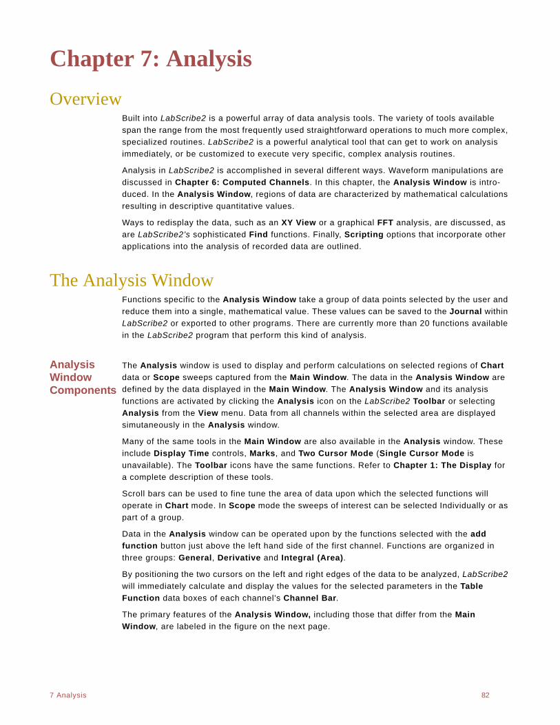
. .
7 Analysis 82
Chapter 7: Analysis
OverviewBuilt into LabScribe2 is a powerful array of data analysis tools. The variety of tools available
span the range from the most frequently used straightforward operations to much more complex,
specialized routines. LabScribe2 is a powerful analytical tool that can get to work on analysis
immediately, or be customized to execute very specific, complex analysis routines.
Analysis in LabScribe2 is accomplished in several different ways. Waveform manipulations are
discussed in Chapter 6: Computed Channels. In this chapter, the Analysis Window is intro-
duced. In the Analysis Window, regions of data are characterized by mathematical calculations
resulting in descriptive quantitative values.
Ways to redisplay the data, such as an XY View or a graphical FFT analysis, are discussed, as
are LabScribe2’s sophisticated Find functions. Finally, Scripting options that incorporate other
applications into the analysis of recorded data are outlined.
The Analysis WindowFunctions specific to the Analysis Window take a group of data points selected by the user and
reduce them into a single, mathematical value. These values can be saved to the Journal within
LabScribe2 or exported to other programs. There are currently more than 20 functions available
in the LabScribe2 program that perform this kind of analysis.
Analysis Window Components
The Analysis window is used to display and perform calculations on selected regions of Chart
data or Scope sweeps captured from the Main Window. The data in the Analysis Window are
defined by the data displayed in the Main Window. The Analysis Window and its analysis
functions are activated by clicking the Analysis icon on the LabScribe2 Toolbar or selecting
Analysis from the View menu. Data from all channels within the selected area are displayed
simutaneously in the Analysis window.
Many of the same tools in the Main Window are also available in the Analysis window. These
include Display Time controls, Marks, and Two Cursor Mode (Single Cursor Mode is
unavailable). The Toolbar icons have the same functions. Refer to Chapter 1: The Display for
a complete description of these tools.
Scroll bars can be used to fine tune the area of data upon which the selected functions will
operate in Chart mode. In Scope mode the sweeps of interest can be selected Individually or as
part of a group.
Data in the Analysis window can be operated upon by the functions selected with the add
function button just above the left hand side of the first channel. Functions are organized in
three groups: General, Derivative and Integral (Area).
By positioning the two cursors on the left and right edges of the data to be analyzed, LabScribe2
will immediately calculate and display the values for the selected parameters in the Table
Function data boxes of each channel’s Channel Bar.
The primary features of the Analysis Window, including those that differ from the Main
Window, are labeled in the figure on the next page.
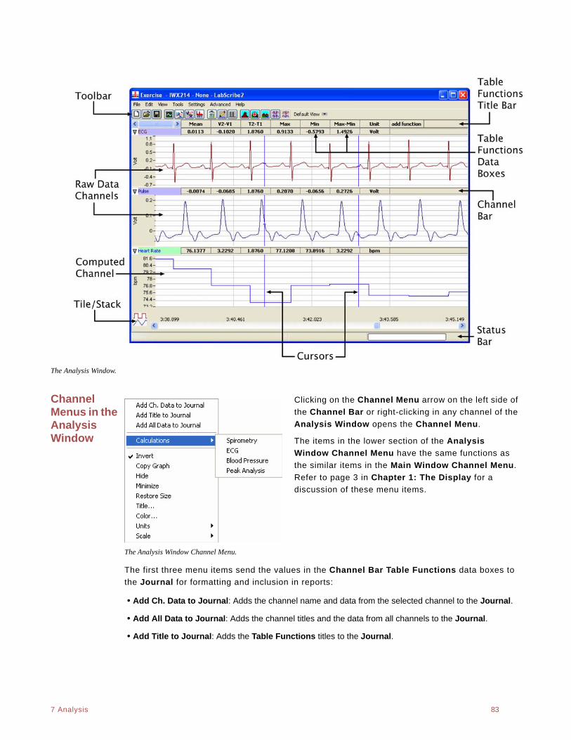
. .
7 Analysis 83
The Analysis Window.
Channel Menus in the Analysis Window
Clicking on the Channel Menu arrow on the left side of
the Channel Bar or right-clicking in any channel of the
Analysis Window opens the Channel Menu.
The items in the lower section of the Analysis
Window Channel Menu have the same functions as
the similar items in the Main Window Channel Menu.
Refer to page 3 in Chapter 1: The Display for a
discussion of these menu items.
The Analysis Window Channel Menu.
The first three menu items send the values in the Channel Bar Table Functions data boxes to
the Journal for formatting and inclusion in reports:
• Add Ch. Data to Journal: Adds the channel name and data from the selected channel to the Journal.
• Add All Data to Journal: Adds the channel titles and the data from all channels to the Journal.
• Add Title to Journal: Adds the Table Functions titles to the Journal.
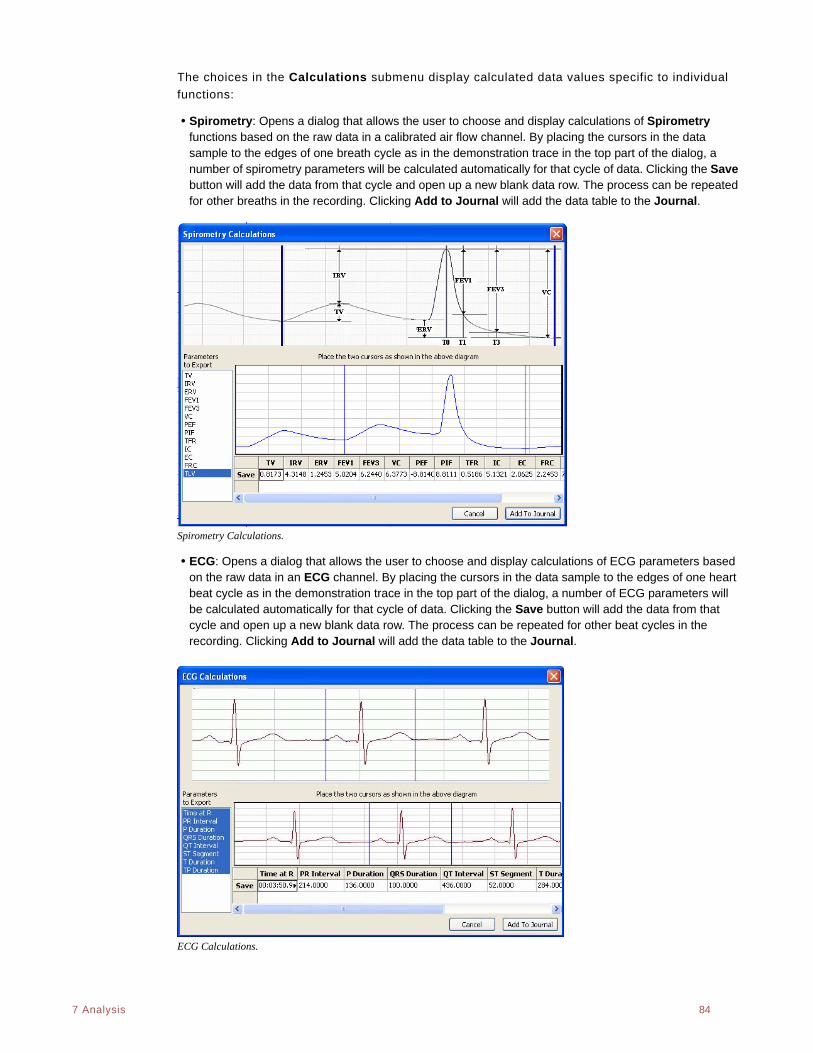
. .
7 Analysis 84
The choices in the Calculations submenu display calculated data values specific to individual
functions:
• Spirometry: Opens a dialog that allows the user to choose and display calculations of Spirometry functions based on the raw data in a calibrated air flow channel. By placing the cursors in the data sample to the edges of one breath cycle as in the demonstration trace in the top part of the dialog, a number of spirometry parameters will be calculated automatically for that cycle of data. Clicking the Save button will add the data from that cycle and open up a new blank data row. The process can be repeated for other breaths in the recording. Clicking Add to Journal will add the data table to the Journal.
Spirometry Calculations.
• ECG: Opens a dialog that allows the user to choose and display calculations of ECG parameters based on the raw data in an ECG channel. By placing the cursors in the data sample to the edges of one heart beat cycle as in the demonstration trace in the top part of the dialog, a number of ECG parameters will be calculated automatically for that cycle of data. Clicking the Save button will add the data from that cycle and open up a new blank data row. The process can be repeated for other beat cycles in the recording. Clicking Add to Journal will add the data table to the Journal.
ECG Calculations.
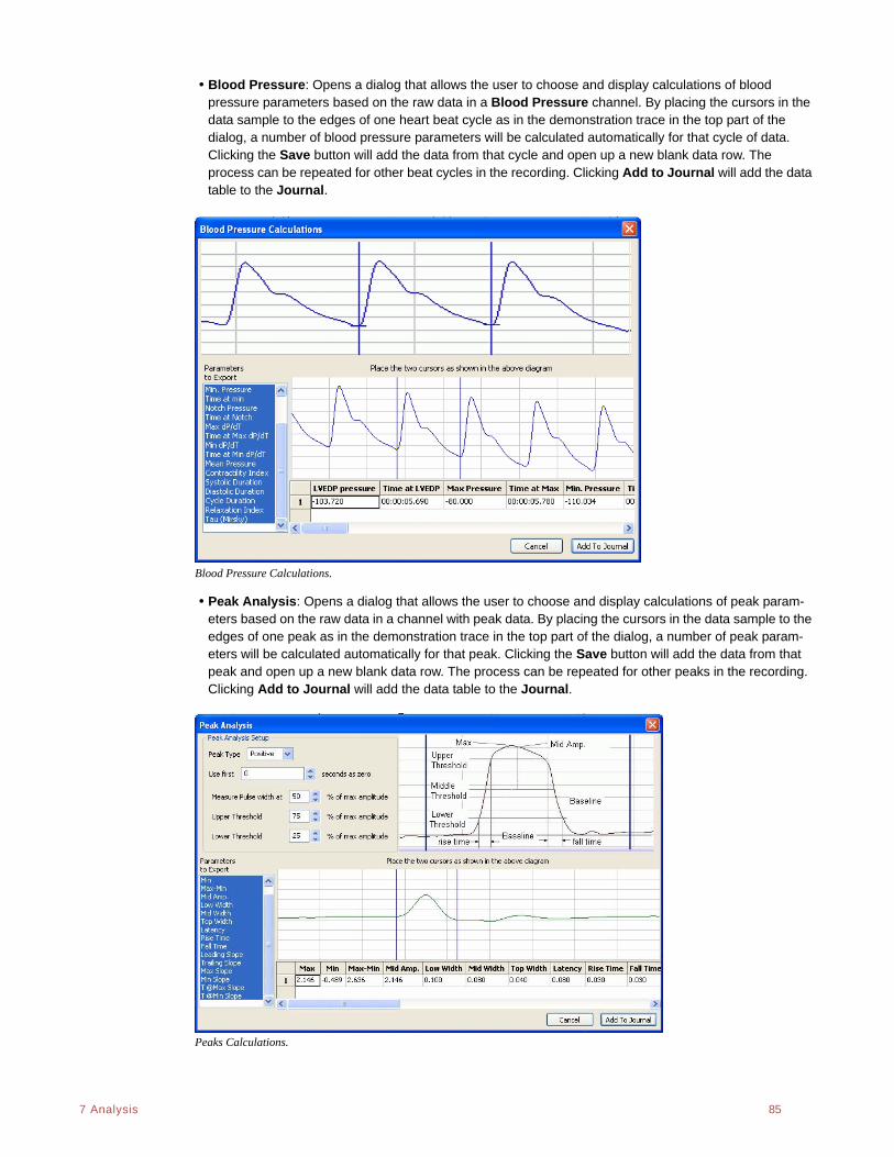
. .
7 Analysis 85
• Blood Pressure: Opens a dialog that allows the user to choose and display calculations of blood pressure parameters based on the raw data in a Blood Pressure channel. By placing the cursors in the data sample to the edges of one heart beat cycle as in the demonstration trace in the top part of the dialog, a number of blood pressure parameters will be calculated automatically for that cycle of data. Clicking the Save button will add the data from that cycle and open up a new blank data row. The process can be repeated for other beat cycles in the recording. Clicking Add to Journal will add the data table to the Journal.
Blood Pressure Calculations.
• Peak Analysis: Opens a dialog that allows the user to choose and display calculations of peak param-eters based on the raw data in a channel with peak data. By placing the cursors in the data sample to the edges of one peak as in the demonstration trace in the top part of the dialog, a number of peak param-eters will be calculated automatically for that peak. Clicking the Save button will add the data from that peak and open up a new blank data row. The process can be repeated for other peaks in the recording. Clicking Add to Journal will add the data table to the Journal.
Peaks Calculations.
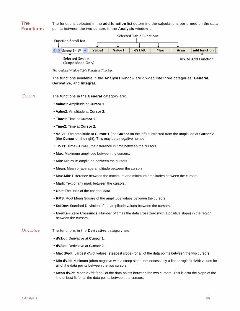
. .
7 Analysis 86
The Functions
The functions selected in the add function list determine the calculations performed on the data
points between the two cursors in the Analysis window .
The Analysis Window Table Functions Title Bar.
The functions available in the Analysis window are divided into three categories: General,
Derivative, and Integral.
General The functions in the General category are:
• Value1: Amplitude at Cursor 1.
• Value2: Amplitude at Cursor 2.
• Time1: Time at Cursor 1.
• Time2: Time at Cursor 2.
• V2-V1: The amplitude at Cursor 1 (the Cursor on the left) subtracted from the amplitude at Cursor 2 (the Cursor on the right). This may be a negative number.
• T2-T1: Time2-Time1, the difference in time between the cursors.
• Max: Maximum amplitude between the cursors.
• Min: Minimum amplitude between the cursors.
• Mean: Mean or average amplitude between the cursors.
• Max-Min: Difference between the maximum and minimum amplitudes between the cursors.
• Mark: Text of any mark between the cursors.
• Unit: The units of the channel data.
• RMS: Root Mean Square of the amplitude values between the cursors.
• StdDev: Standard Deviation of the amplitude values between the cursors.
• Events-# Zero Crossings: Number of times the data cross zero (with a positive slope) in the region between the cursors.
Derivative The functions in the Derivative category are:
• dV1/dt: Derivative at Cursor 1.
• dV2/dt: Derivative at Cursor 2.
• Max dV/dt: Largest dV/dt values (steepest slope) for all of the data points between the two cursors.
• Min dV/dt: Minimum (often negative with a steep slope; not necessarily a flatter region) dV/dt values for all of the data points between the two cursors.
• Mean dV/dt: Mean dV/dt for all of the data points between the two cursors. This is also the slope of the line of best fit for all the data points between the cursors.
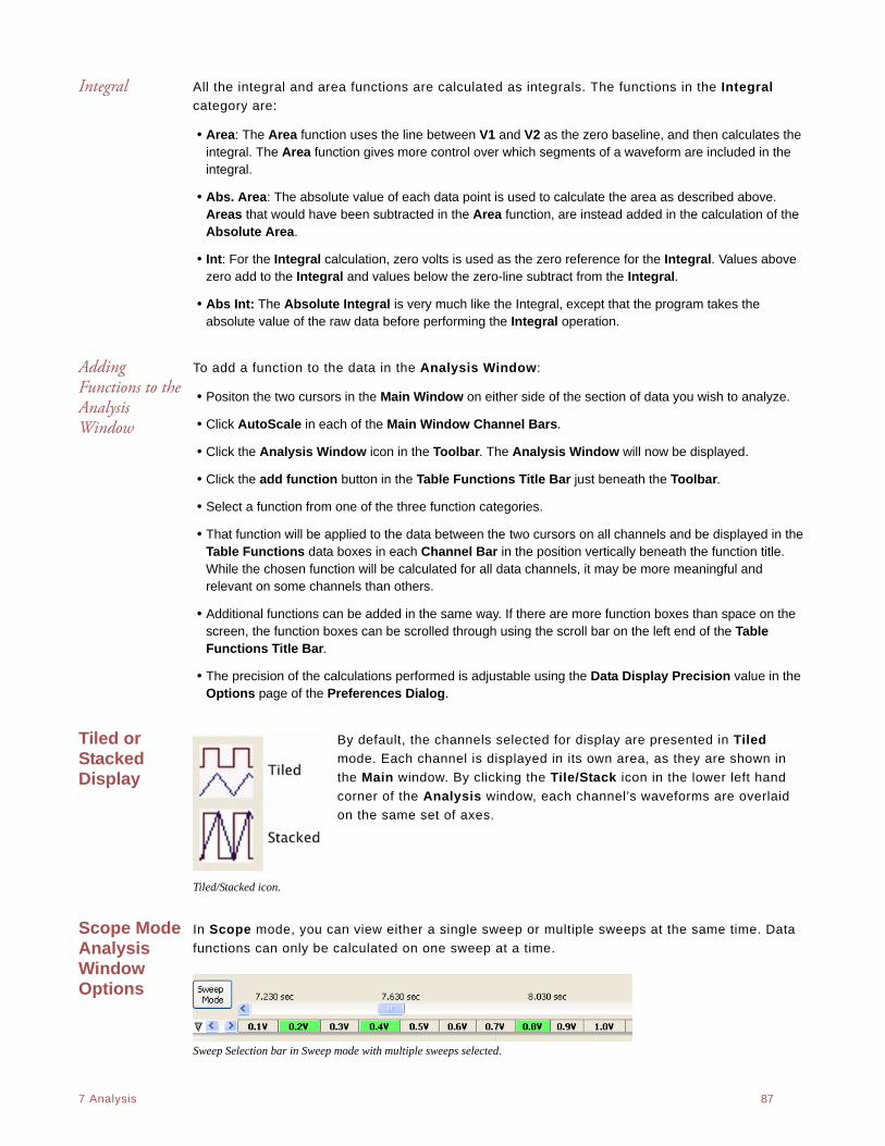
. .
7 Analysis 87
Integral All the integral and area functions are calculated as integrals. The functions in the Integral
category are:
• Area: The Area function uses the line between V1 and V2 as the zero baseline, and then calculates the integral. The Area function gives more control over which segments of a waveform are included in the integral.
• Abs. Area: The absolute value of each data point is used to calculate the area as described above. Areas that would have been subtracted in the Area function, are instead added in the calculation of the Absolute Area.
• Int: For the Integral calculation, zero volts is used as the zero reference for the Integral. Values above zero add to the Integral and values below the zero-line subtract from the Integral.
• Abs Int: The Absolute Integral is very much like the Integral, except that the program takes the absolute value of the raw data before performing the Integral operation.
Adding Functions to the Analysis Window
To add a function to the data in the Analysis Window:
• Positon the two cursors in the Main Window on either side of the section of data you wish to analyze.
• Click AutoScale in each of the Main Window Channel Bars.
• Click the Analysis Window icon in the Toolbar. The Analysis Window will now be displayed.
• Click the add function button in the Table Functions Title Bar just beneath the Toolbar.
• Select a function from one of the three function categories.
• That function will be applied to the data between the two cursors on all channels and be displayed in the Table Functions data boxes in each Channel Bar in the position vertically beneath the function title. While the chosen function will be calculated for all data channels, it may be more meaningful and relevant on some channels than others.
• Additional functions can be added in the same way. If there are more function boxes than space on the screen, the function boxes can be scrolled through using the scroll bar on the left end of the Table Functions Title Bar.
• The precision of the calculations performed is adjustable using the Data Display Precision value in the Options page of the Preferences Dialog.
Tiled or Stacked Display
By default, the channels selected for display are presented in Tiled
mode. Each channel is displayed in its own area, as they are shown in
the Main window. By clicking the Tile/Stack icon in the lower left hand
corner of the Analysis window, each channel’s waveforms are overlaid
on the same set of axes.
Tiled/Stacked icon.
Scope Mode Analysis Window Options
In Scope mode, you can view either a single sweep or multiple sweeps at the same time. Data
functions can only be calculated on one sweep at a time.
Sweep Selection bar in Sweep mode with multiple sweeps selected.
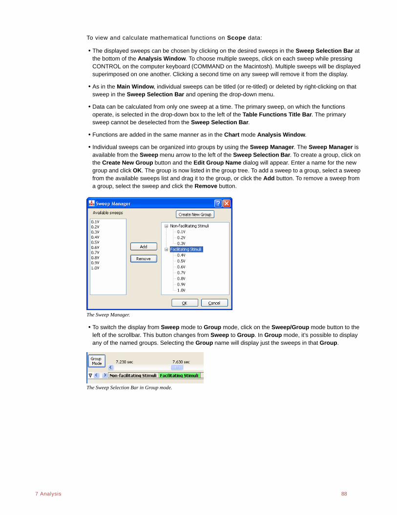
. .
7 Analysis 88
To view and calculate mathematical functions on Scope data:
• The displayed sweeps can be chosen by clicking on the desired sweeps in the Sweep Selection Bar at the bottom of the Analysis Window. To choose multiple sweeps, click on each sweep while pressing CONTROL on the computer keyboard (COMMAND on the Macintosh). Multiple sweeps will be displayed superimposed on one another. Clicking a second time on any sweep will remove it from the display.
• As in the Main Window, individual sweeps can be titled (or re-titled) or deleted by right-clicking on that sweep in the Sweep Selection Bar and opening the drop-down menu.
• Data can be calculated from only one sweep at a time. The primary sweep, on which the functions operate, is selected in the drop-down box to the left of the Table Functions Title Bar. The primary sweep cannot be deselected from the Sweep Selection Bar.
• Functions are added in the same manner as in the Chart mode Analysis Window.
• Individual sweeps can be organized into groups by using the Sweep Manager. The Sweep Manager is available from the Sweep menu arrow to the left of the Sweep Selection Bar. To create a group, click on the Create New Group button and the Edit Group Name dialog will appear. Enter a name for the new group and click OK. The group is now listed in the group tree. To add a sweep to a group, select a sweep from the available sweeps list and drag it to the group, or click the Add button. To remove a sweep from a group, select the sweep and click the Remove button.
The Sweep Manager.
• To switch the display from Sweep mode to Group mode, click on the Sweep/Group mode button to the left of the scrollbar. This button changes from Sweep to Group. In Group mode, it’s possible to display any of the named groups. Selecting the Group name will display just the sweeps in that Group.
The Sweep Selection Bar in Group mode.
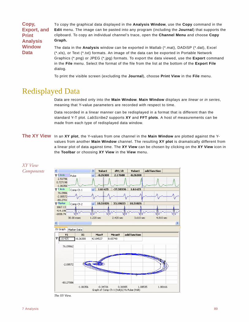
. .
7 Analysis 89
Copy, Export, and Print Analysis Window Data
To copy the graphical data displayed in the Analysis Window, use the Copy command in the
Edit menu. The image can be pasted into any program (including the Journal) that supports the
clipboard. To copy an individual channel’s trace, open the Channel Menu and choose Copy
Graph.
The data in the Analysis window can be exported in Matlab (*.mat), DADiSP (*.dat), Excel
(*.xls), or Text (*.txt) formats. An image of the data can be exported in Portable Network
Graphics (*.png) or JPEG (*.jpg) formats. To export the data viewed, use the Export command
in the File menu. Select the format of the file from the list at the bottom of the Export File
dialog.
To print the visible screen (excluding the Journal), choose Print View in the File menu.
Redisplayed DataData are recorded only into the Main Window. Main Window displays are linear or in series,
meaning that Y-value parameters are recorded with respect to time.
Data recorded in a linear manner can be redisplayed in a format that is different than the
standard Y-T plot. LabScribe2 supports XY and FFT plots. A host of measurements can be
made from each type of redisplayed data window.
The XY View In an XY plot, the Y-values from one channel in the Main Window are plotted against the Y-
values from another Main Window channel. The resulting XY plot is dramatically different from
a linear plot of data against time. The XY View can be chosen by clicking on the XY View icon in
the Toolbar or choosing XY View in the View menu.
XY View Components
The XY View.
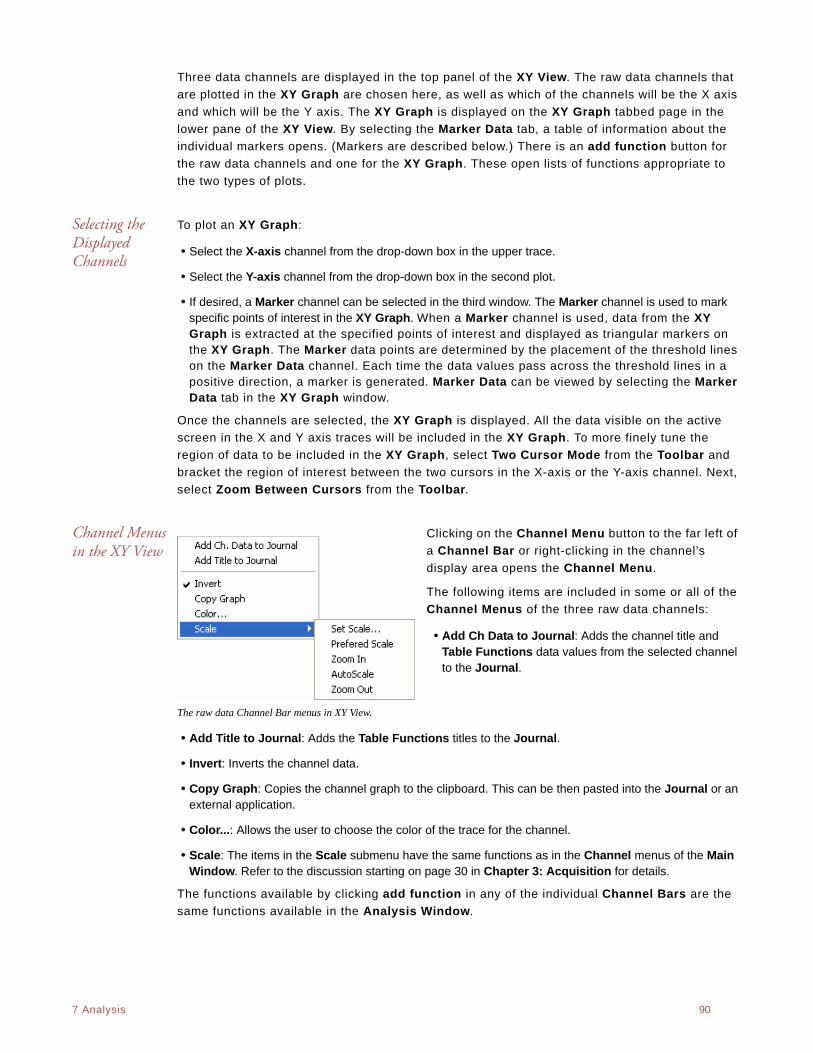
. .
7 Analysis 90
Three data channels are displayed in the top panel of the XY View. The raw data channels that
are plotted in the XY Graph are chosen here, as well as which of the channels will be the X axis
and which will be the Y axis. The XY Graph is displayed on the XY Graph tabbed page in the
lower pane of the XY View. By selecting the Marker Data tab, a table of information about the
individual markers opens. (Markers are described below.) There is an add function button for
the raw data channels and one for the XY Graph. These open lists of functions appropriate to
the two types of plots.
Selecting the Displayed Channels
To plot an XY Graph:
• Select the X-axis channel from the drop-down box in the upper trace.
• Select the Y-axis channel from the drop-down box in the second plot.
• If desired, a Marker channel can be selected in the third window. The Marker channel is used to mark specific points of interest in the XY Graph. When a Marker channel is used, data from the XY Graph is extracted at the specified points of interest and displayed as triangular markers on the XY Graph. The Marker data points are determined by the placement of the threshold lines on the Marker Data channel. Each time the data values pass across the threshold lines in a positive direction, a marker is generated. Marker Data can be viewed by selecting the Marker Data tab in the XY Graph window.
Once the channels are selected, the XY Graph is displayed. All the data visible on the active
screen in the X and Y axis traces will be included in the XY Graph. To more finely tune the
region of data to be included in the XY Graph, select Two Cursor Mode from the Toolbar and
bracket the region of interest between the two cursors in the X-axis or the Y-axis channel. Next,
select Zoom Between Cursors from the Toolbar.
Channel Menus in the XY View
Clicking on the Channel Menu button to the far left of
a Channel Bar or right-clicking in the channel’s
display area opens the Channel Menu.
The following items are included in some or all of the
Channel Menus of the three raw data channels:
• Add Ch Data to Journal: Adds the channel title and Table Functions data values from the selected channel to the Journal.
The raw data Channel Bar menus in XY View.
• Add Title to Journal: Adds the Table Functions titles to the Journal.
• Invert: Inverts the channel data.
• Copy Graph: Copies the channel graph to the clipboard. This can be then pasted into the Journal or an external application.
• Color...: Allows the user to choose the color of the trace for the channel.
• Scale: The items in the Scale submenu have the same functions as in the Channel menus of the Main Window. Refer to the discussion starting on page 30 in Chapter 3: Acquisition for details.
The functions available by clicking add function in any of the individual Channel Bars are the
same functions available in the Analysis Window.
. .
7 Analysis 91
The XY Graph Window Menu
Clicking the arrow to the left of add function in the XY Graph window opens the XY Graph
window menu with the following menu items:
• Add All Data to Journal: Adds the data from the XY Graph Table Functions boxes to the Journal.
• Add Title to Journal: Adds the Table Functions titles to the Journal.
• Copy graph: Copies the XY Graph to the Journal.
XY Graph Table Functions
The functions selected in the add function list of the XY Graph window determine the calcula-
tions performed on the data points in the XY Graph. The results of the selected calculations are
displayed in the Table Functions data boxes above the XY Graph.
The following functions are available in the XY Graph window:
General
• Y1: Value of the Y-Axis channel at Cursor 1.
• Y2: Value of the Y-Axis channel at Cursor 2.
• X1: Value of the X-Axis channel at Cursor 1.
• X2: Value of the X-Axis channel at Cursor 2.
• Y2-Y1: The difference in value of the Y-Axis channel between the cursors.
• X2-X1: The difference in value of the X-Axis channel between the cursors.
• MaxY: Maximum value of the Y-Axis channel between the cursors.
• MinY: Minimum value of the Y-Axis channel between the cursors.
• MeanY: Mean or average value of the Y-Axis channel between the cursors.
• MaxY-MinY: Difference between the maximum and minimum values of the Y-Axis channel between the cursors.
• MaxX: Maximum value of the X-Axis channel between the cursors.
• MinX: Minimum value of the X-Axis channel between the cursors.
• MeanX: Mean or Average value of the X-Axis channel between the cursors.
• MaxX-MinX: Difference between the maximum and minimum values of the X-Axis channel between the cursors.
• Length: Length of the line segment in the XY Graph between the two cursors.
Derivative
• dY1/dx: Slope of the XY Graph at Cursor 1.
• dY2/dx: Slope of the XY Graph at Cursor 2.
• Max dV/dt: Maximum slope of the XY Graph between the two cursors.
• Min dV/dt: Minimum slope of the XY Graph between the two cursors. This can be a steep negative slope.
• Mean dV/dt: Mean slope of the XY Graph between the two cursors. This is also the slope of the line of best fit for all the data points between the cursors.
. .
7 Analysis 92
Integral (Area)
All the integral and area functions are calculated as integrals.
• Area wrt Ymin: The minimum value of the Y channel is taken as baseline and the area beneath all points between the two cursors is calculated with respect to this baseline.
• Area wrt Zero: Zero is taken as baseline and the area between all points and zero is calculated for the points between the cursors.
• Area wrt Y1: The value of the Y-axis channel at Cursor 1 is taken as baseline and the area between all points and this value is calculated for the points between the cursors.
• Area Loop: The area of the loop as defined by the position of two cursors is calculated.
Marker Data By selecting the Marker Data tab next to the XY Graph tab in the XY Graph window, a table
displaying information about the markers opens. The time coordinate, the X value, the Y value,
and the Marker channel value of each marker are listed.
Copy, Export, and Print XY View Window
To copy the graphical data displayed in the XY View, use the Copy command in the Edit menu.
The image can be pasted into any application (including the Journal) that supports the
clipboard.
To export the data from the channels used to construct the XY Graph, as well as the Marker
Channel data, use the Export command in the File menu. Select the format of the file from the
list at the bottom of the Export File window.
To print the graphs in the current screen, choose Print View in the File menu.
FFT FFT is short for Fast Fourier Transform, a mathematical operation that displays recorded data
as the relative amplitudes of the frequency components that make up the recorded signal. FFT
plots have Frequency on the X-axis and the Power (amplitude) contained in each frequency on
the Y-axis. FFT analysis is used to determine the relative contributions of frequency components
in a raw signal. For example, in EEG studies, Alpha waves are EEG signals with frequencies
between 8 and 13 Hz. If an FFT is performed on an EEG recording that has a high number of
Alpha waves, the FFT will show a spike or a higher amplitude (Power) at the frequencies in the
Alpha band.
LabScribe2 can perform Fast Fourier Transforms on selected pieces of recorded data in the FFT
window. The FFT window is opened from the View menu or by clicking the FFT icon on the
Toolbar at the top of the Main Window. The selected data are moved to the Linear Display
area in the FFT window where adjustments can be made which optimize the size of the FFT plot.
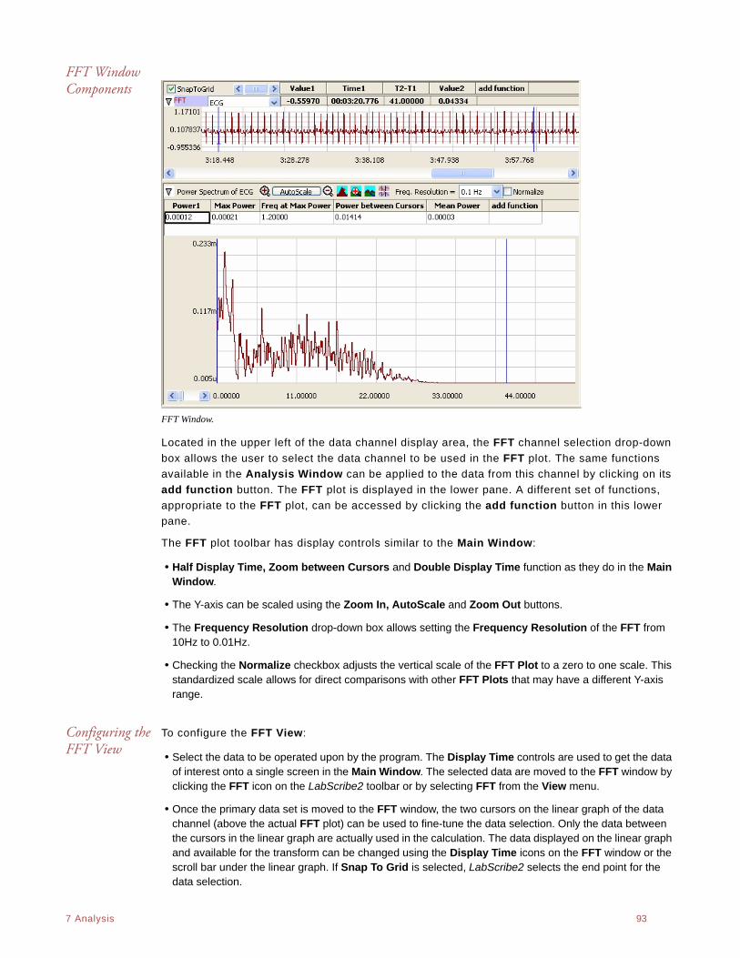
. .
7 Analysis 93
FFT Window Components
FFT Window.
Located in the upper left of the data channel display area, the FFT channel selection drop-down
box allows the user to select the data channel to be used in the FFT plot. The same functions
available in the Analysis Window can be applied to the data from this channel by clicking on its
add function button. The FFT plot is displayed in the lower pane. A different set of functions,
appropriate to the FFT plot, can be accessed by clicking the add function button in this lower
pane.
The FFT plot toolbar has display controls similar to the Main Window:
• Half Display Time, Zoom between Cursors and Double Display Time function as they do in the Main Window.
• The Y-axis can be scaled using the Zoom In, AutoScale and Zoom Out buttons.
• The Frequency Resolution drop-down box allows setting the Frequency Resolution of the FFT from 10Hz to 0.01Hz.
• Checking the Normalize checkbox adjusts the vertical scale of the FFT Plot to a zero to one scale. This standardized scale allows for direct comparisons with other FFT Plots that may have a different Y-axis range.
Configuring the FFT View
To configure the FFT View:
• Select the data to be operated upon by the program. The Display Time controls are used to get the data of interest onto a single screen in the Main Window. The selected data are moved to the FFT window by clicking the FFT icon on the LabScribe2 toolbar or by selecting FFT from the View menu.
• Once the primary data set is moved to the FFT window, the two cursors on the linear graph of the data channel (above the actual FFT plot) can be used to fine-tune the data selection. Only the data between the cursors in the linear graph are actually used in the calculation. The data displayed on the linear graph and available for the transform can be changed using the Display Time icons on the FFT window or the scroll bar under the linear graph. If Snap To Grid is selected, LabScribe2 selects the end point for the data selection.
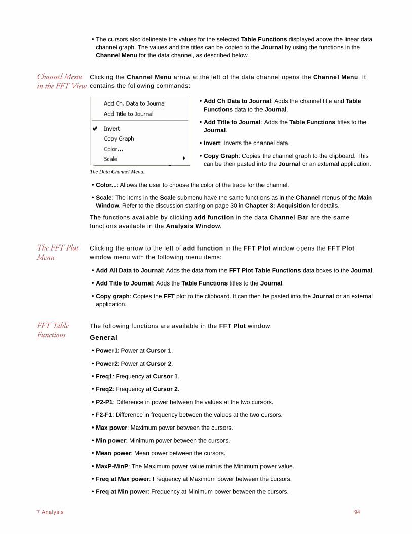
. .
7 Analysis 94
• The cursors also delineate the values for the selected Table Functions displayed above the linear data channel graph. The values and the titles can be copied to the Journal by using the functions in the Channel Menu for the data channel, as described below.
Channel Menu in the FFT View
Clicking the Channel Menu arrow at the left of the data channel opens the Channel Menu. It
contains the following commands:
• Add Ch Data to Journal: Adds the channel title and Table Functions data to the Journal.
• Add Title to Journal: Adds the Table Functions titles to the Journal.
• Invert: Inverts the channel data.
• Copy Graph: Copies the channel graph to the clipboard. This can be then pasted into the Journal or an external application.
The Data Channel Menu.
• Color...: Allows the user to choose the color of the trace for the channel.
• Scale: The items in the Scale submenu have the same functions as in the Channel menus of the Main Window. Refer to the discussion starting on page 30 in Chapter 3: Acquisition for details.
The functions available by clicking add function in the data Channel Bar are the same
functions available in the Analysis Window.
The FFT Plot Menu
Clicking the arrow to the left of add function in the FFT Plot window opens the FFT Plot
window menu with the following menu items:
• Add All Data to Journal: Adds the data from the FFT Plot Table Functions data boxes to the Journal.
• Add Title to Journal: Adds the Table Functions titles to the Journal.
• Copy graph: Copies the FFT plot to the clipboard. It can then be pasted into the Journal or an external application.
FFT Table Functions
The following functions are available in the FFT Plot window:
General
• Power1: Power at Cursor 1.
• Power2: Power at Cursor 2.
• Freq1: Frequency at Cursor 1.
• Freq2: Frequency at Cursor 2.
• P2-P1: Difference in power between the values at the two cursors.
• F2-F1: Difference in frequency between the values at the two cursors.
• Max power: Maximum power between the cursors.
• Min power: Minimum power between the cursors.
• Mean power: Mean power between the cursors.
• MaxP-MinP: The Maximum power value minus the Minimum power value.
• Freq at Max power: Frequency at Maximum power between the cursors.
• Freq at Min power: Frequency at Minimum power between the cursors.
. .
7 Analysis 95
• Mean Frequency: Mean frequency of the values between the cursors.
• Median Fequency: Median frequency of the values bewtween the cursors.
Integral
• Power between Cursors: Summed power data values between the cursors.
Theoretical Considerations
To ensure problem-free operation of the FFT function, certain premises need to be considered.
• The mathematical underpinnings of digital sampling, which makes the LabScribe2 software work, begin with a foundation known as the Nyquist Sampling Theorem. Harry Nyquist showed that the sampling rate must be at least twice the highest frequency in the sample to reconstruct the original signal and capture its fundamental frequency. The converse of this rule is that the fastest frequency that can be reliably recorded is half of the sampling rate. If a recording was made at 1000 samples per second, the maximum frequency that could be recorded reliably would be 500Hz. If a recording was made at 100 samples per second, the maximum frequency that could be recorded reliably would be 50Hz. When an FFT is performed on data recorded with LabScribe2, the program sets the X-axis to a scale from 0Hz (DC) to a frequency that is half of the sampling rate. A region of the scale can be expanded by using the cursors and the functions of the Channel menu, but frequencies greater than half the sampling rate cannot be viewed.
• To make an FFT work, the transform must operate on a specific number of data points. The number of data points used in the FFT is algorithm dependent. By default the Snap to Grid option is selected, which sets the second cursor to the location of the best selection of FFT data on the linear display section of the FFT View. If you make a different selection, LabScribe2 will fill in the remaining data points with zeros so the frequency content of the data that you did select will not be affected.
• As stated in the first rule that governs FFT functions, LabScribe2 sets the X-axis limits in the FFT window according to the sampling rate. Likewise, the number of data points used in the FFT calculation sets the resolution of the X-axis range. If more data points are used, the available Frequency Resolution will be greater. Frequency Resolution is set from the drop-down menu in the left hand margin of the FFT window. Resolution choices are limited to 100 Hz, 10 Hz, 1 Hz and 0.1 Hz. If the FFT cannot be displayed with the required frequency resolution, more data points need to be used to make the calcu-lation.
Copy, Export, and Print FFT Windows
Use the Copy command in the Edit menu to copy the view of data displayed in the FFT View.
This image can be pasted into any program (including the Journal) that supports the clipboard.
To export the data viewed, use the Export command in the File menu. Select the format of the
exported file from the list at the bottom of the Export File window.
Choosing Print View will print the current window.
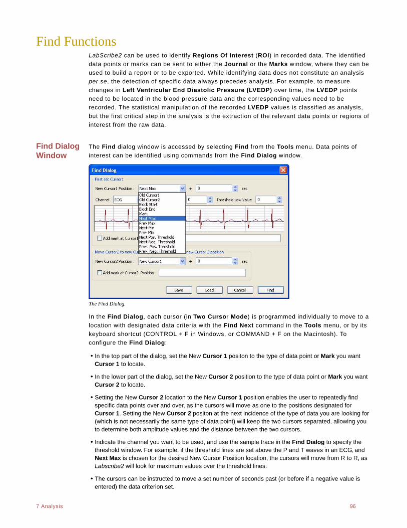
. .
7 Analysis 96
Find FunctionsLabScribe2 can be used to identify Regions Of Interest (ROI) in recorded data. The identified
data points or marks can be sent to either the Journal or the Marks window, where they can be
used to build a report or to be exported. While identifying data does not constitute an analysis
per se, the detection of specific data always precedes analysis. For example, to measure
changes in Left Ventricular End Diastolic Pressure (LVEDP) over time, the LVEDP points
need to be located in the blood pressure data and the corresponding values need to be
recorded. The statistical manipulation of the recorded LVEDP values is classified as analysis,
but the first critical step in the analysis is the extraction of the relevant data points or regions of
interest from the raw data.
Find Dialog Window
The Find dialog window is accessed by selecting Find from the Tools menu. Data points of
interest can be identified using commands from the Find Dialog window.
The Find Dialog.
In the Find Dialog, each cursor (in Two Cursor Mode) is programmed individually to move to a
location with designated data criteria with the Find Next command in the Tools menu, or by its
keyboard shortcut (CONTROL + F in Windows, or COMMAND + F on the Macintosh). To
configure the Find Dialog:
• In the top part of the dialog, set the New Cursor 1 positon to the type of data point or Mark you want Cursor 1 to locate.
• In the lower part of the dialog, set the New Cursor 2 position to the type of data point or Mark you want Cursor 2 to locate.
• Setting the New Cursor 2 location to the New Cursor 1 position enables the user to repeatedly find specific data points over and over, as the cursors will move as one to the positions designated for Cursor 1. Setting the New Cursor 2 positon at the next incidence of the type of data you are looking for (which is not necessarily the same type of data point) will keep the two cursors separated, allowing you to determine both amplitude values and the distance between the two cursors.
• Indicate the channel you want to be used, and use the sample trace in the Find Dialog to specify the threshold window. For example, if the threshold lines are set above the P and T waves in an ECG, and Next Max is chosen for the desired New Cursor Position location, the cursors will move from R to R, as Labscribe2 will look for maximum values over the threshold lines.
• The cursors can be instructed to move a set number of seconds past (or before if a negative value is entered) the data criterion set.
. .
7 Analysis 97
• Once the criteria are set, choosing Find Next, or using its keyboard shortcut (CONTROL + F in WIndows, COMMAND + F on the Macintosh), will move the cursors to their next positions.
• Although the Find commands work in the Main Window, using them in the Analysis Window will report specified values to the Table Functions data boxes, allowing the values to be sent to the Journal.
• Once the Find routine is defined, it can be saved by clicking the Save button on the Find Dialog window. The named routine is saved in the Auto Find folder as an .iwxfind file.
• In the example in the figure, using this Find routine on the ECG trace will cause both cursors to move as one from R to R to R, allowing you to locate the position and determine the amplitude of each R. If the New Cursor 2 were to be set instead at the next example of the type of data you were looking for, each time the Find command was called, the cursors would move individually and two R points would be located at each Find command, allowing the distance between Rs to be determined as well.
The locations that the cursors can be programmed to move to include:
• Old Cursor 1 and Old Cursor 2: The positions from which the Cursors will be moving with each Find Next command.
• New Cursor 1: The position to which Cursor 1 moves with each Find Next command.
• Block Start and Block End: The cursors can be instructed to move to the start or the end of the current block of data.
• Mark: The cursors can be instructed to move to a specifed mark.
• Next Max or Previous Max: The cursors can be instructed to move to the Next Maximum value or the Previous Maximum value. These Max points will be over the threshold set in the sample data.
• Next Min or Previous Min: The cursors can be instructed to move to the Next or Previous Minimum values, as determined by the Threshold position.
• Next or Previous Positive or Negative Threshold: Instructs the cursors to move to the Next or Previous Threshold line the data cross in either a positive or negative direction.
The calculations to be performed on the selected data points or on the data between the points
are chosen from the Table Functions list before the Find dialog window is opened.
F I N D E X E R C I S E
As an example, the Find function could be used to determine the time (T2-T1) between two events. Occasionally, R waves in an ECG have significantly higher amplitudes than the other R waves in the same recording. The Find function could be used to measure the time between adjacent supranormal R waves. To find these durations:
1. Use the LabScribe2 ECG Tutorial to create an ECG recording.
2. AutoScale the ECG recording and transfer the data of interest from the ECG recording from the Main Window to the Analysis Window.
3. Select the calculations ( T1, T2, T2-T1) to be performed on the data from the Table Functions list.
4. Pull down the Tools menu and select the Find function.
5. Program the cursor positions. To find the next supranormal R wave in the data, the Cursor 1 position is set equal to Next Max. The New Cursor 2 position is also set to Next Max and the data channel is selected.
6. Adjust the threshold amplitudes for both cursors, above which the Find function will Find the Next Max, so that only the supranormal R waves are above the threshold. Name and save the Find routine.
7. Click the Find button to place the cursors and to display the values for the selected Table Functions at the top of the Analysis window.
8. Copy values and their headings to the Journal via the Add Title to Journal and Add Data to Journal functions in the right-click menu of the Analysis window.
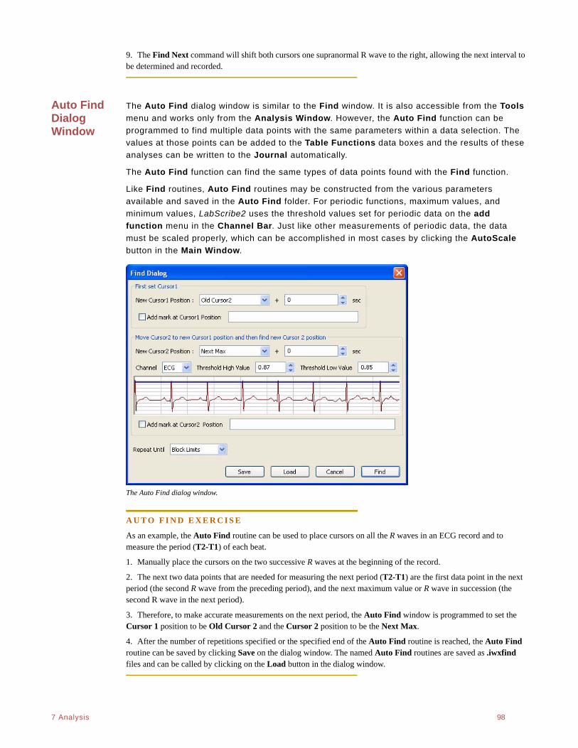
. .
7 Analysis 98
9. The Find Next command will shift both cursors one supranormal R wave to the right, allowing the next interval to be determined and recorded.
Auto Find Dialog Window
The Auto Find dialog window is similar to the Find window. It is also accessible from the Tools
menu and works only from the Analysis Window. However, the Auto Find function can be
programmed to find multiple data points with the same parameters within a data selection. The
values at those points can be added to the Table Functions data boxes and the results of these
analyses can be written to the Journal automatically.
The Auto Find function can find the same types of data points found with the Find function.
Like Find routines, Auto Find routines may be constructed from the various parameters
available and saved in the Auto Find folder. For periodic functions, maximum values, and
minimum values, LabScribe2 uses the threshold values set for periodic data on the add
function menu in the Channel Bar. Just like other measurements of periodic data, the data
must be scaled properly, which can be accomplished in most cases by clicking the AutoScale
button in the Main Window.
The Auto Find dialog window.
A U T O F I N D E X E R C I S E
As an example, the Auto Find routine can be used to place cursors on all the R waves in an ECG record and to measure the period (T2-T1) of each beat.
1. Manually place the cursors on the two successive R waves at the beginning of the record.
2. The next two data points that are needed for measuring the next period (T2-T1) are the first data point in the next period (the second R wave from the preceding period), and the next maximum value or R wave in succession (the second R wave in the next period).
3. Therefore, to make accurate measurements on the next period, the Auto Find window is programmed to set the Cursor 1 position to be Old Cursor 2 and the Cursor 2 position to be the Next Max.
4. After the number of repetitions specified or the specified end of the Auto Find routine is reached, the Auto Find routine can be saved by clicking Save on the dialog window. The named Auto Find routines are saved as .iwxfind files and can be called by clicking on the Load button in the dialog window.
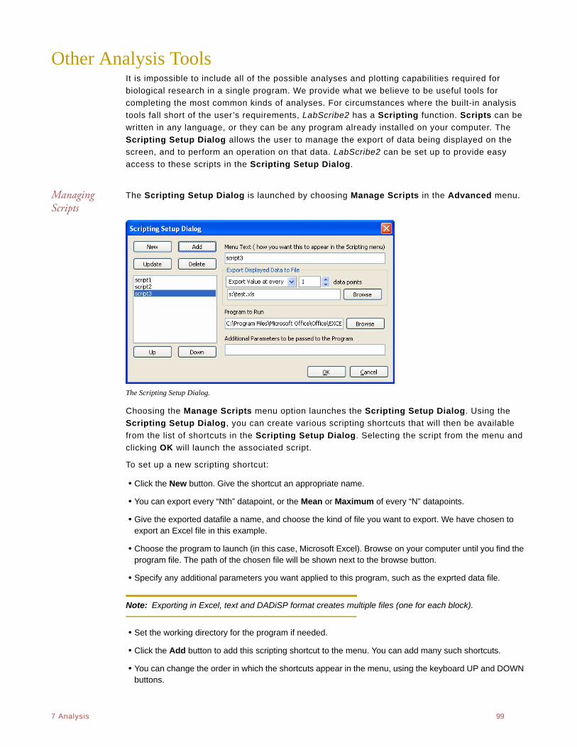
. .
7 Analysis 99
Other Analysis ToolsIt is impossible to include all of the possible analyses and plotting capabilities required for
biological research in a single program. We provide what we believe to be useful tools for
completing the most common kinds of analyses. For circumstances where the built-in analysis
tools fall short of the user’s requirements, LabScribe2 has a Scripting function. Scripts can be
written in any language, or they can be any program already installed on your computer. The
Scripting Setup Dialog allows the user to manage the export of data being displayed on the
screen, and to perform an operation on that data. LabScribe2 can be set up to provide easy
access to these scripts in the Scripting Setup Dialog.
Managing Scripts
The Scripting Setup Dialog is launched by choosing Manage Scripts in the Advanced menu.
The Scripting Setup Dialog.
Choosing the Manage Scripts menu option launches the Scripting Setup Dialog. Using the
Scripting Setup Dialog, you can create various scripting shortcuts that will then be available
from the list of shortcuts in the Scripting Setup Dialog. Selecting the script from the menu and
clicking OK will launch the associated script.
To set up a new scripting shortcut:
• Click the New button. Give the shortcut an appropriate name.
• You can export every “Nth” datapoint, or the Mean or Maximum of every “N” datapoints.
• Give the exported datafile a name, and choose the kind of file you want to export. We have chosen to export an Excel file in this example.
• Choose the program to launch (in this case, Microsoft Excel). Browse on your computer until you find the program file. The path of the chosen file will be shown next to the browse button.
• Specify any additional parameters you want applied to this program, such as the exprted data file.
Note: Exporting in Excel, text and DADiSP format creates multiple files (one for each block).
• Set the working directory for the program if needed.
• Click the Add button to add this scripting shortcut to the menu. You can add many such shortcuts.
• You can change the order in which the shortcuts appear in the menu, using the keyboard UP and DOWN buttons.
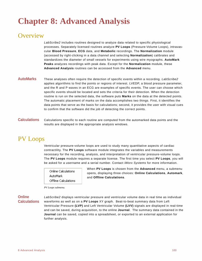
. .
8 Advanced Analysis 100
Chapter 8: Advanced Analysis
OverviewLabScribe2 includes routines designed to analyze data related to specific physiological
processes. Separately licensed routines analyze PV Loops (Pressure-Volume Loops), intravas-
cular Blood Pressure, ECG data, and Metabolic recordings. The Normalization module
(accessed by right-clicking in a data channel and selecting Normalization) calibrates and
standardizes the diameter of small vessels for experiments using wire myographs. AutoMark
Peaks analyzes recordings with peak data. Except for the Normalization module, these
Advanced Analysis routines can be accessed from the Advanced menu.
AutoMarks These analyses often require the detection of specific events within a recording. LabScribe2
applies algorithms to find the points or regions of interest. LVEDP, a blood pressure parameter,
and the R and P waves in an ECG are examples of specific events. The user can choose which
specific events should be located and sets the criteria for their detection. When the detection
routine is run on the selected data, the software puts Marks on the data at the detected points.
The automatic placement of marks on the data accomplishes two things. First, it identifies the
data points that serve as the basis for calculations; second, it provides the user with visual cues
to confirm that the software did the job of detecting the correct points.
Calculations Calculations specific to each routine are computed from the automarked data points and the
results are displayed in the appropriate analysis windows.
PV LoopsVentricular pressure-volume loops are used to study many quantitative aspects of cardiac
contractility. The PV Loops software module integrates the variables and measurements
necessary for the recording, analysis, and interpretation of ventricular pressure-volume loops.
The PV Loops module requires a separate license. The first time you select PV Loops, you will
be asked for a username and a serial number. Contact iWorx Systems for more information.
When PV Loops is chosen from the Advanced menu, a submenu
opens, displaying three choices: Online Calculations, Automark,
and Offline Calculations.
PV Loops submenu.
Online Calculations
LabScribe2 displays ventricular pressure and ventricular volume data in real time as individual
waveforms as well as on a PV Loops XY graph. Beat-to-beat summary data from Left
Ventricular Pressure (LVP) and Left Ventricular Volume (LVV) signals are displayed in real-time
and can be saved, during acquisition, to the online Journal. The summary data contained in the
Journal can be saved, copied into a spreadsheet, or exported to an external application for
further analysis.
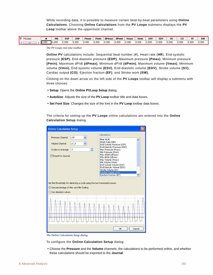
. .
8 Advanced Analysis 101
While recording data, it is possible to measure certain beat-by-beat parameters using Online
Calculations. Choosing Online Calculations from the PV Loops submenu displays the PV
Loop toolbar above the uppermost channel.
The PV Loops real time toolbar.
Online PV calculations include: Sequential beat number (#), Heart rate (HR), End-systolic
pressure (ESP), End-diastolic pressure (EDP), Maximum pressure (Pmax), Minimum pressure
(Pmin), Maximum dP/dt (dPmax), Minimum dP/dt (dPmin), Maximum volume (Vmax), Minimum
volume (Vmin), End-systolic volume (ESV), End-diastolic volume (EDV), Stroke volume (SV),
Cardiac output (CO), Ejection fraction (EF), and Stroke work (SW).
Clicking on the down arrow on the left side of the PV Loops toolbar will display a submenu with
three choices:
• Setup: Opens the Online PVLoop Setup dialog.
• AutoSize: Adjusts the size of the PV Loop toolbar title and data boxes.
• Set Font Size: Changes the size of the font in the PV Loop toolbar data boxes.
The criteria for setting up the PV Loops online calculations are entered into the Online
Calculation Setup dialog.
The Online Calculation Setup dialog.
To configure the Online Calculation Setup dialog:
• Choose the Pressure and the Volume channels, the calculations to be performed online, and whether these calculations should be exported to the Journal.
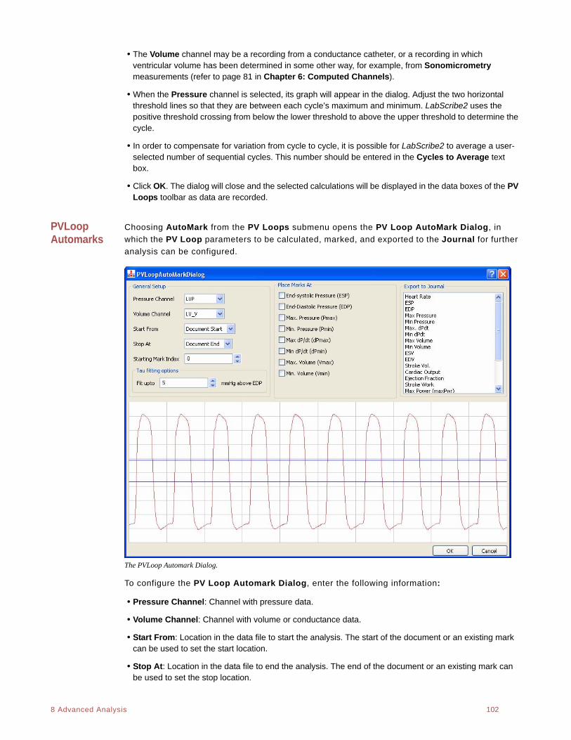
. .
8 Advanced Analysis 102
• The Volume channel may be a recording from a conductance catheter, or a recording in which ventricular volume has been determined in some other way, for example, from Sonomicrometry measurements (refer to page 81 in Chapter 6: Computed Channels).
• When the Pressure channel is selected, its graph will appear in the dialog. Adjust the two horizontal threshold lines so that they are between each cycle’s maximum and minimum. LabScribe2 uses the positive threshold crossing from below the lower threshold to above the upper threshold to determine the cycle.
• In order to compensate for variation from cycle to cycle, it is possible for LabScribe2 to average a user-selected number of sequential cycles. This number should be entered in the Cycles to Average text box.
• Click OK. The dialog will close and the selected calculations will be displayed in the data boxes of the PV Loops toolbar as data are recorded.
PVLoop Automarks
Choosing AutoMark from the PV Loops submenu opens the PV Loop AutoMark Dialog, in
which the PV Loop parameters to be calculated, marked, and exported to the Journal for further
analysis can be configured.
The PVLoop Automark Dialog.
To configure the PV Loop Automark Dialog, enter the following information:
• Pressure Channel: Channel with pressure data.
• Volume Channel: Channel with volume or conductance data.
• Start From: Location in the data file to start the analysis. The start of the document or an existing mark can be used to set the start location.
• Stop At: Location in the data file to end the analysis. The end of the document or an existing mark can be used to set the stop location.
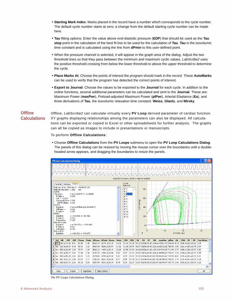
. .
8 Advanced Analysis 103
• Starting Mark Index: Marks placed in the record have a number which corresponds to the cycle number. The default cycle number starts at zero; a change from the default starting cycle number can be made here.
• Tau fitting options: Enter the value above end-diastolic pressure (EDP) that should be used as the Tau stop point in the calculation of the best fit line to be used for the calculation of Tau. Tau is the isovolumic time constant and is calculated using the line from dPmin to this user-defined point.
• When the pressure channel is selected, it will appear in the graph area of the dialog. Adjust the two threshold lines so that they pass between the minimum and maximum cyclic values. LabScribe2 uses the positive threshold crossing from below the lower threshold to above the upper threshold to determine the cycle.
• Place Marks At: Choose the points of interest the program should mark in the record. These AutoMarks can be used to verify that the program has detected the correct points of interest.
• Export to Journal: Choose the values to be exported to the Journal for each cycle. In addition to the online functions, several additional parameters can be calculated and sent to the Journal. These are: Maximum Power (maxPwr), Preload-adjusted Maximum Power (plPwr), Arterial Elastance (Ea), and three derivations of Tau, the isovolumic relaxation time constant: Weiss, Glantz, and Mirsky.
Offline Calculations
Offline, LabScribe2 can calculate virtually every PV Loop derived parameter of cardiac function.
XY graphs displaying relationships among the parameters can also be displayed. All calcula-
tions can be exported or copied to Excel or other spreadsheets for further analysis. The graphs
can all be copied as images to include in presentations or manuscripts.
To perform Offline Calculations:
• Choose Offline Calculations from the PV Loops submenu to open the PV Loop Calculations Dialog. The panels of this dialog can be resized by moving the mouse cursor over the boundaries until a double-headed arrow appears, and dragging the boundaries to resize the panels.
The PV Loops Calculations Dialog.
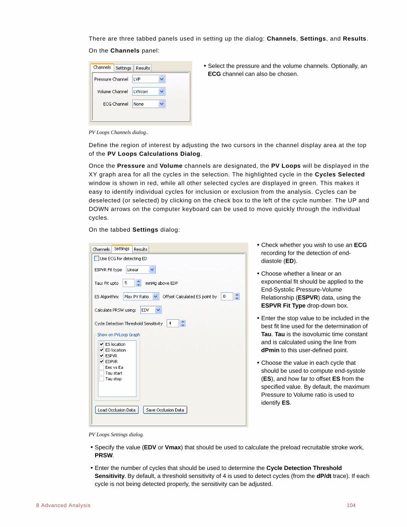
. .
8 Advanced Analysis 104
There are three tabbed panels used in setting up the dialog: Channels, Settings, and Results.
On the Channels panel:
• Select the pressure and the volume channels. Optionally, an ECG channel can also be chosen.
PV Loops Channels dialog..
Define the region of interest by adjusting the two cursors in the channel display area at the top
of the PV Loops Calculations Dialog.
Once the Pressure and Volume channels are designated, the PV Loops will be displayed in the
XY graph area for all the cycles in the selection. The highlighted cycle in the Cycles Selected
window is shown in red, while all other selected cycles are displayed in green. This makes it
easy to identify individual cycles for inclusion or exclusion from the analysis. Cycles can be
deselected (or selected) by clicking on the check box to the left of the cycle number. The UP and
DOWN arrows on the computer keyboard can be used to move quickly through the individual
cycles.
On the tabbed Settings dialog:
• Check whether you wish to use an ECG recording for the detection of end-diastole (ED).
• Choose whether a linear or an exponential fit should be applied to the End-Systolic Pressure-Volume Relationship (ESPVR) data, using the ESPVR Fit Type drop-down box.
• Enter the stop value to be included in the best fit line used for the determination of Tau. Tau is the isovolumic time constant and is calculated using the line from dPmin to this user-defined point.
• Choose the value in each cycle that should be used to compute end-systole (ES), and how far to offset ES from the specified value. By default, the maximum Pressure to Volume ratio is used to identify ES.
PV Loops Settings dialog.
• Specify the value (EDV or Vmax) that should be used to calculate the preload recruitable stroke work, PRSW.
• Enter the number of cycles that should be used to determine the Cycle Detection Threshold Sensitivity. By default, a threshold sensitivity of 4 is used to detect cycles (from the dP/dt trace). If each cycle is not being detected properly, the sensitivity can be adjusted.
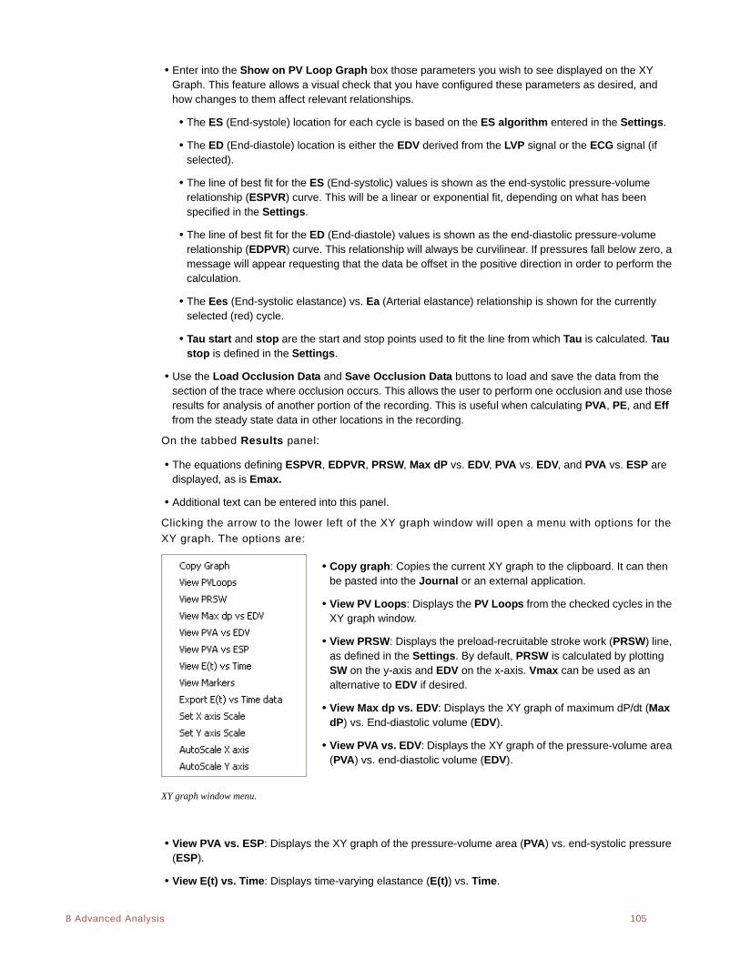
. .
8 Advanced Analysis 105
• Enter into the Show on PV Loop Graph box those parameters you wish to see displayed on the XY Graph. This feature allows a visual check that you have configured these parameters as desired, and how changes to them affect relevant relationships.
• The ES (End-systole) location for each cycle is based on the ES algorithm entered in the Settings.
• The ED (End-diastole) location is either the EDV derived from the LVP signal or the ECG signal (if selected).
• The line of best fit for the ES (End-systolic) values is shown as the end-systolic pressure-volume relationship (ESPVR) curve. This will be a linear or exponential fit, depending on what has been specified in the Settings.
• The line of best fit for the ED (End-diastole) values is shown as the end-diastolic pressure-volume relationship (EDPVR) curve. This relationship will always be curvilinear. If pressures fall below zero, a message will appear requesting that the data be offset in the positive direction in order to perform the calculation.
• The Ees (End-systolic elastance) vs. Ea (Arterial elastance) relationship is shown for the currently selected (red) cycle.
• Tau start and stop are the start and stop points used to fit the line from which Tau is calculated. Tau stop is defined in the Settings.
• Use the Load Occlusion Data and Save Occlusion Data buttons to load and save the data from the section of the trace where occlusion occurs. This allows the user to perform one occlusion and use those results for analysis of another portion of the recording. This is useful when calculating PVA, PE, and Eff from the steady state data in other locations in the recording.
On the tabbed Results panel:
• The equations defining ESPVR, EDPVR, PRSW, Max dP vs. EDV, PVA vs. EDV, and PVA vs. ESP are displayed, as is Emax.
• Additional text can be entered into this panel.
Clicking the arrow to the lower left of the XY graph window will open a menu with options for the
XY graph. The options are:
• Copy graph: Copies the current XY graph to the clipboard. It can then be pasted into the Journal or an external application.
• View PV Loops: Displays the PV Loops from the checked cycles in the XY graph window.
• View PRSW: Displays the preload-recruitable stroke work (PRSW) line, as defined in the Settings. By default, PRSW is calculated by plotting SW on the y-axis and EDV on the x-axis. Vmax can be used as an alternative to EDV if desired.
• View Max dp vs. EDV: Displays the XY graph of maximum dP/dt (Max dP) vs. End-diastolic volume (EDV).
• View PVA vs. EDV: Displays the XY graph of the pressure-volume area (PVA) vs. end-diastolic volume (EDV).
XY graph window menu.
• View PVA vs. ESP: Displays the XY graph of the pressure-volume area (PVA) vs. end-systolic pressure (ESP).
• View E(t) vs. Time: Displays time-varying elastance (E(t)) vs. Time.
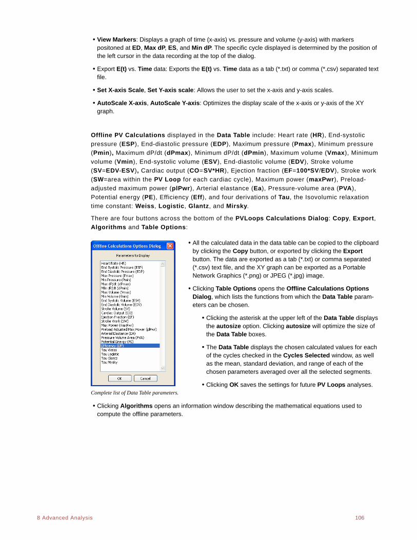
. .
8 Advanced Analysis 106
• View Markers: Displays a graph of time (x-axis) vs. pressure and volume (y-axis) with markers positoned at ED, Max dP, ES, and Min dP. The specific cycle displayed is determined by the position of the left cursor in the data recording at the top of the dialog.
• Export E(t) vs. Time data: Exports the E(t) vs. Time data as a tab (*.txt) or comma (*.csv) separated text file.
• Set X-axis Scale, Set Y-axis scale: Allows the user to set the x-axis and y-axis scales.
• AutoScale X-axis, AutoScale Y-axis: Optimizes the display scale of the x-axis or y-axis of the XY graph.
Offline PV Calculations displayed in the Data Table include: Heart rate (HR), End-systolic
pressure (ESP), End-diastolic pressure (EDP), Maximum pressure (Pmax), Minimum pressure
(Pmin), Maximum dP/dt (dPmax), Minimum dP/dt (dPmin), Maximum volume (Vmax), Minimum
volume (Vmin), End-systolic volume (ESV), End-diastolic volume (EDV), Stroke volume
(SV=EDV-ESV), Cardiac output (CO=SV*HR), Ejection fraction (EF=100*SV/EDV), Stroke work
(SW=area within the PV Loop for each cardiac cycle), Maximum power (maxPwr), Preload-
adjusted maximum power (plPwr), Arterial elastance (Ea), Pressure-volume area (PVA),
Potential energy (PE), Efficiency (Eff), and four derivations of Tau, the Isovolumic relaxation
time constant: Weiss, Logistic, Glantz, and Mirsky.
There are four buttons across the bottom of the PVLoops Calculations Dialog: Copy, Export,
Algorithms and Table Options:
• All the calculated data in the data table can be copied to the clipboard by clicking the Copy button, or exported by clicking the Export button. The data are exported as a tab (*.txt) or comma separated (*.csv) text file, and the XY graph can be exported as a Portable Network Graphics (*.png) or JPEG (*.jpg) image.
• Clicking Table Options opens the Offline Calculations Options Dialog, which lists the functions from which the Data Table param-eters can be chosen.
• Clicking the asterisk at the upper left of the Data Table displays the autosize option. Clicking autosize will optimize the size of the Data Table boxes.
• The Data Table displays the chosen calculated values for each of the cycles checked in the Cycles Selected window, as well as the mean, standard deviation, and range of each of the chosen parameters averaged over all the selected segments.
• Clicking OK saves the settings for future PV Loops analyses. Complete list of Data Table parameters.
• Clicking Algorithms opens an information window describing the mathematical equations used to compute the offline parameters.
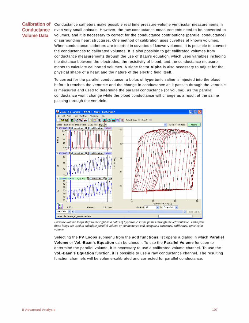
. .
8 Advanced Analysis 107
Calibration of Conductance Volume Data
Conductance catheters make possible real time pressure-volume ventricular measurements in
even very small animals. However, the raw conductance measurements need to be converted to
volumes, and it is necessary to correct for the conductance contributions (parallel conductance)
of surrounding heart structures. One method of calibration uses cuvettes of known volumes.
When conductance catheters are inserted in cuvettes of known volumes, it is possible to convert
the conductances to calibrated volumes. It is also possible to get calibrated volumes from
conductance measurements through the use of Baan’s equation, which uses variables including
the distance between the electrodes, the resistivity of blood, and the conductance measure-
ments to calculate calibrated volumes. A slope factor Alpha is also necessary to adjust for the
physical shape of a heart and the nature of the electric field itself.
To correct for the parallel conductance, a bolus of hypertonic saline is injected into the blood
before it reaches the ventricle and the change in conductance as it passes through the ventricle
is measured and used to determine the parallel conductance (or volume), as the parallel
conductance won’t change while the blood conductance will change as a result of the saline
passing through the ventricle.
Pressure-volume loops shift to the right as a bolus of hypertonic saline passes through the left ventricle. Data from these loops are used to calculate parallel volume or conductance and compute a corrected, calibrated, ventricular volume.
Selecting the PV Loops submenu from the add functions list opens a dialog in which Parallel
Volume or Vol.-Baan’s Equation can be chosen. To use the Parallel Volume function to
determine the parallel volume, it is necessary to use a calibrated volume channel. To use the
Vol.-Baan’s Equation function, it is possible to use a raw conductance channel. The resulting
function channels will be volume-calibrated and corrected for parallel conductance.
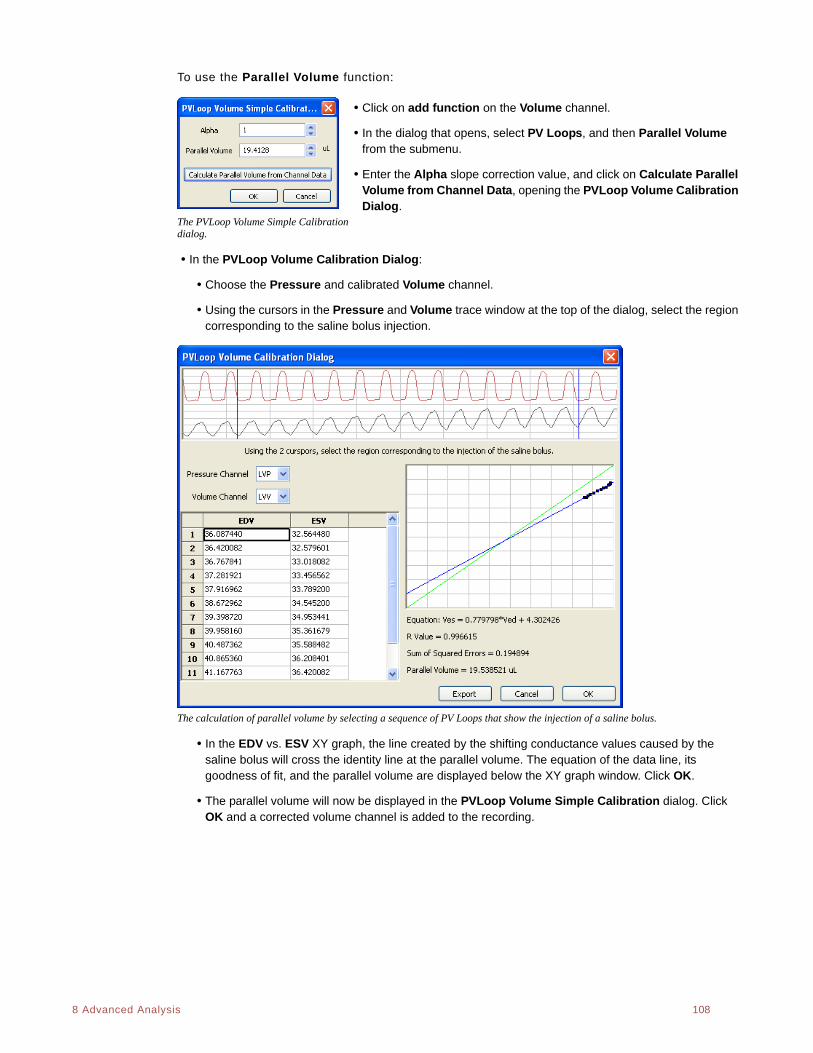
. .
8 Advanced Analysis 108
To use the Parallel Volume function:
• Click on add function on the Volume channel.
• In the dialog that opens, select PV Loops, and then Parallel Volume from the submenu.
• Enter the Alpha slope correction value, and click on Calculate Parallel Volume from Channel Data, opening the PVLoop Volume Calibration Dialog.
The PVLoop Volume Simple Calibration dialog.
• In the PVLoop Volume Calibration Dialog:
• Choose the Pressure and calibrated Volume channel.
• Using the cursors in the Pressure and Volume trace window at the top of the dialog, select the region corresponding to the saline bolus injection.
The calculation of parallel volume by selecting a sequence of PV Loops that show the injection of a saline bolus.
• In the EDV vs. ESV XY graph, the line created by the shifting conductance values caused by the saline bolus will cross the identity line at the parallel volume. The equation of the data line, its goodness of fit, and the parallel volume are displayed below the XY graph window. Click OK.
• The parallel volume will now be displayed in the PVLoop Volume Simple Calibration dialog. Click OK and a corrected volume channel is added to the recording.
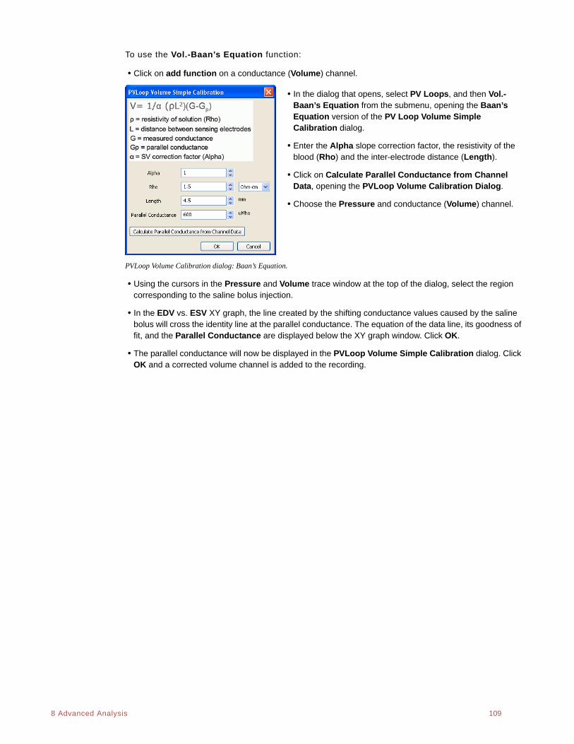
. .
8 Advanced Analysis 109
To use the Vol.-Baan’s Equation function:
• Click on add function on a conductance (Volume) channel.
• In the dialog that opens, select PV Loops, and then Vol.-Baan’s Equation from the submenu, opening the Baan’s Equation version of the PV Loop Volume Simple Calibration dialog.
• Enter the Alpha slope correction factor, the resistivity of the blood (Rho) and the inter-electrode distance (Length).
• Click on Calculate Parallel Conductance from Channel Data, opening the PVLoop Volume Calibration Dialog.
• Choose the Pressure and conductance (Volume) channel.
PVLoop Volume Calibration dialog: Baan’s Equation.
• Using the cursors in the Pressure and Volume trace window at the top of the dialog, select the region corresponding to the saline bolus injection.
• In the EDV vs. ESV XY graph, the line created by the shifting conductance values caused by the saline bolus will cross the identity line at the parallel conductance. The equation of the data line, its goodness of fit, and the Parallel Conductance are displayed below the XY graph window. Click OK.
• The parallel conductance will now be displayed in the PVLoop Volume Simple Calibration dialog. Click OK and a corrected volume channel is added to the recording.
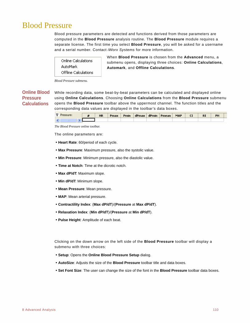
. .
8 Advanced Analysis 110
Blood PressureBlood pressure parameters are detected and functions derived from those parameters are
computed in the Blood Pressure analysis routine. The Blood Pressure module requires a
separate license. The first time you select Blood Pressure, you will be asked for a username
and a serial number. Contact iWorx Systems for more information.
When Blood Pressure is chosen from the Advanced menu, a
submenu opens, displaying three choices: Online Calculations,
Automark, and Offline Calculations.
Blood Pressure submenu.
Online Blood Pressure Calculations
While recording data, some beat-by-beat parameters can be calculated and displayed online
using Online Calculations. Choosing Online Calculations from the Blood Pressure submenu
opens the Blood Pressure toolbar above the uppermost channel. The function titles and the
corresponding data values are displayed in the toolbar’s data boxes.
The Blood Pressure online toolbar.
The online parameters are:
• Heart Rate: 60/period of each cycle.
• Max Pressure: Maximum pressure, also the systolic value.
• Min Pressure: Minimum pressure, also the diastolic value.
• Time at Notch: Time at the dicrotic notch.
• Max dP/dT: Maximum slope.
• Min dP/dT: Minimum slope.
• Mean Pressure: Mean pressure.
• MAP: Mean arterial pressure.
• Contractility Index: (Max dP/dT)/(Pressure at Max dP/dT).
• Relaxation Index: (Min dP/dT)/(Pressure at Min dP/dT).
• Pulse Height: Amplitude of each beat.
Clicking on the down arrow on the left side of the Blood Pressure toolbar will display a
submenu with three choices:
• Setup: Opens the Online Blood Pressure Setup dialog.
• AutoSize: Adjusts the size of the Blood Pressure toolbar title and data boxes.
• Set Font Size: The user can change the size of the font in the Blood Pressure toolbar data boxes.
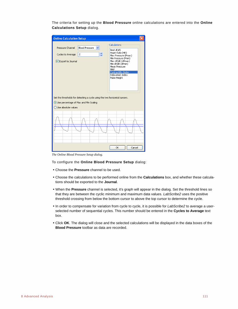
. .
8 Advanced Analysis 111
The criteria for setting up the Blood Pressure online calculations are entered into the Online
Calculations Setup dialog.
The Online Blood Pressure Setup dialog.
To configure the Online Blood Pressure Setup dialog:
• Choose the Pressure channel to be used.
• Choose the calculations to be performed online from the Calculations box, and whether these calcula-tions should be exported to the Journal.
• When the Pressure channel is selected, it’s graph will appear in the dialog. Set the threshold lines so that they are between the cyclic minimum and maximum data values. LabScribe2 uses the positive threshold crossing from below the bottom cursor to above the top cursor to determine the cycle.
• In order to compensate for variation from cycle to cycle, it is possible for LabScribe2 to average a user-selected number of sequential cycles. This number should be entered in the Cycles to Average text box.
• Click OK. The dialog will close and the selected calculations will be displayed in the data boxes of the Blood Pressure toolbar as data are recorded.
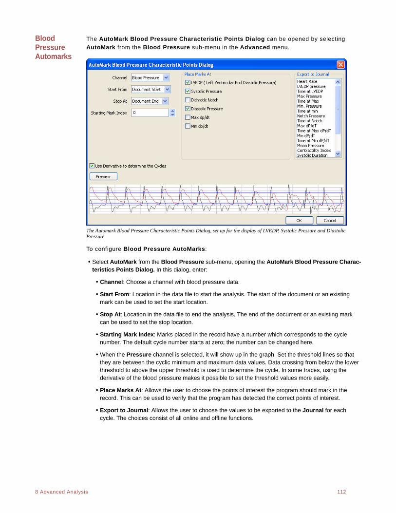
. .
8 Advanced Analysis 112
Blood Pressure Automarks
The AutoMark Blood Pressure Characteristic Points Dialog can be opened by selecting
AutoMark from the Blood Pressure sub-menu in the Advanced menu.
The Automark Blood Pressure Characteristic Points Dialog, set up for the display of LVEDP, Systolic Pressure and Diastolic Pressure.
To configure Blood Pressure AutoMarks:
• Select AutoMark from the Blood Pressure sub-menu, opening the AutoMark Blood Pressure Charac-teristics Points Dialog. In this dialog, enter:
• Channel: Choose a channel with blood pressure data.
• Start From: Location in the data file to start the analysis. The start of the document or an existing mark can be used to set the start location.
• Stop At: Location in the data file to end the analysis. The end of the document or an existing mark can be used to set the stop location.
• Starting Mark Index: Marks placed in the record have a number which corresponds to the cycle number. The default cycle number starts at zero; the number can be changed here.
• When the Pressure channel is selected, it will show up in the graph. Set the threshold lines so that they are between the cyclic minimum and maximum data values. Data crossing from below the lower threshold to above the upper threshold is used to determine the cycle. In some traces, using the derivative of the blood pressure makes it possible to set the threshold values more easily.
• Place Marks At: Allows the user to choose the points of interest the program should mark in the record. This can be used to verify that the program has detected the correct points of interest.
• Export to Journal: Allows the user to choose the values to be exported to the Journal for each cycle. The choices consist of all online and offline functions.
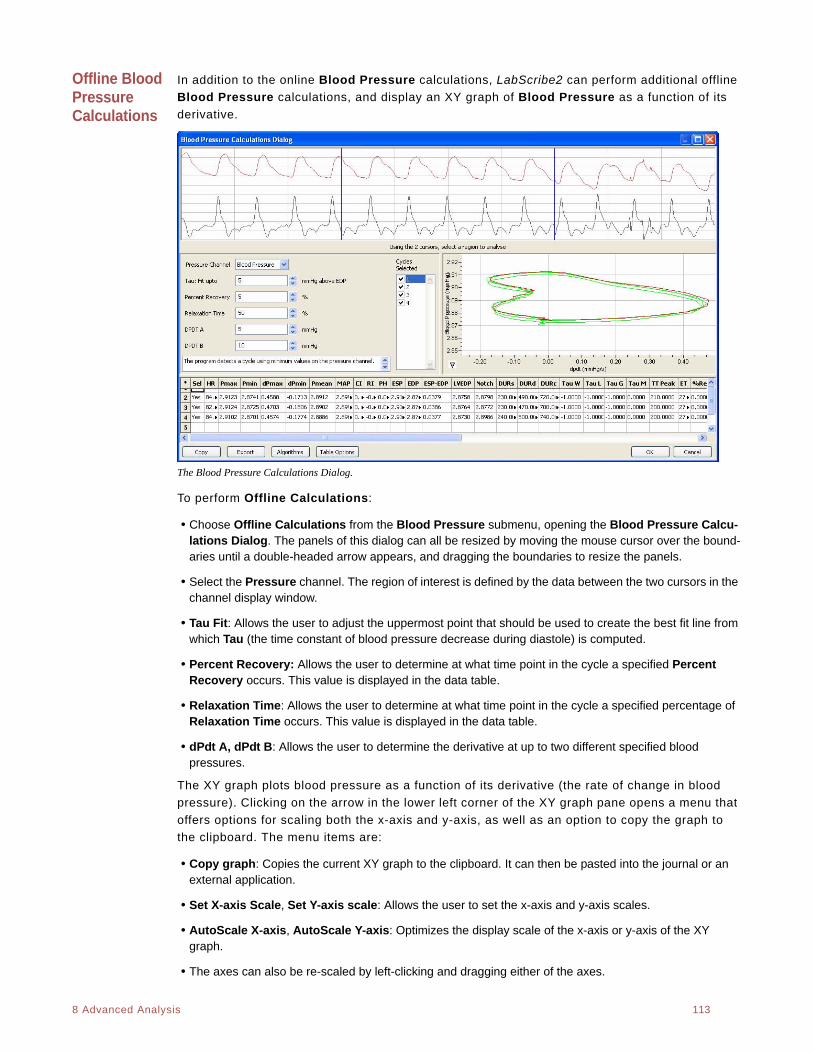
. .
8 Advanced Analysis 113
Offline Blood Pressure Calculations
In addition to the online Blood Pressure calculations, LabScribe2 can perform additional offline
Blood Pressure calculations, and display an XY graph of Blood Pressure as a function of its
derivative.
The Blood Pressure Calculations Dialog.
To perform Offline Calculations:
• Choose Offline Calculations from the Blood Pressure submenu, opening the Blood Pressure Calcu-lations Dialog. The panels of this dialog can all be resized by moving the mouse cursor over the bound-aries until a double-headed arrow appears, and dragging the boundaries to resize the panels.
• Select the Pressure channel. The region of interest is defined by the data between the two cursors in the channel display window.
• Tau Fit: Allows the user to adjust the uppermost point that should be used to create the best fit line from which Tau (the time constant of blood pressure decrease during diastole) is computed.
• Percent Recovery: Allows the user to determine at what time point in the cycle a specified Percent Recovery occurs. This value is displayed in the data table.
• Relaxation Time: Allows the user to determine at what time point in the cycle a specified percentage of Relaxation Time occurs. This value is displayed in the data table.
• dPdt A, dPdt B: Allows the user to determine the derivative at up to two different specified blood pressures.
The XY graph plots blood pressure as a function of its derivative (the rate of change in blood
pressure). Clicking on the arrow in the lower left corner of the XY graph pane opens a menu that
offers options for scaling both the x-axis and y-axis, as well as an option to copy the graph to
the clipboard. The menu items are:
• Copy graph: Copies the current XY graph to the clipboard. It can then be pasted into the journal or an external application.
• Set X-axis Scale, Set Y-axis scale: Allows the user to set the x-axis and y-axis scales.
• AutoScale X-axis, AutoScale Y-axis: Optimizes the display scale of the x-axis or y-axis of the XY graph.
• The axes can also be re-scaled by left-clicking and dragging either of the axes.
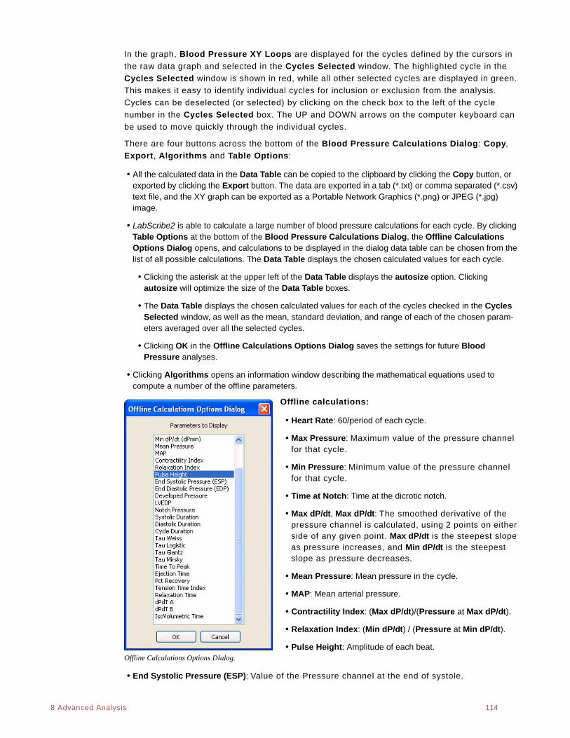
. .
8 Advanced Analysis 114
In the graph, Blood Pressure XY Loops are displayed for the cycles defined by the cursors in
the raw data graph and selected in the Cycles Selected window. The highlighted cycle in the
Cycles Selected window is shown in red, while all other selected cycles are displayed in green.
This makes it easy to identify individual cycles for inclusion or exclusion from the analysis.
Cycles can be deselected (or selected) by clicking on the check box to the left of the cycle
number in the Cycles Selected box. The UP and DOWN arrows on the computer keyboard can
be used to move quickly through the individual cycles.
There are four buttons across the bottom of the Blood Pressure Calculations Dialog: Copy,
Export, Algorithms and Table Options:
• All the calculated data in the Data Table can be copied to the clipboard by clicking the Copy button, or exported by clicking the Export button. The data are exported in a tab (*.txt) or comma separated (*.csv) text file, and the XY graph can be exported as a Portable Network Graphics (*.png) or JPEG (*.jpg) image.
• LabScribe2 is able to calculate a large number of blood pressure calculations for each cycle. By clicking Table Options at the bottom of the Blood Pressure Calculations Dialog, the Offline Calculations Options Dialog opens, and calculations to be displayed in the dialog data table can be chosen from the list of all possible calculations. The Data Table displays the chosen calculated values for each cycle.
• Clicking the asterisk at the upper left of the Data Table displays the autosize option. Clicking autosize will optimize the size of the Data Table boxes.
• The Data Table displays the chosen calculated values for each of the cycles checked in the Cycles Selected window, as well as the mean, standard deviation, and range of each of the chosen param-eters averaged over all the selected cycles.
• Clicking OK in the Offline Calculations Options Dialog saves the settings for future Blood Pressure analyses.
• Clicking Algorithms opens an information window describing the mathematical equations used to compute a number of the offline parameters.
Offline calculations:
• Heart Rate: 60/period of each cycle.
• Max Pressure: Maximum value of the pressure channel for that cycle.
• Min Pressure: Minimum value of the pressure channel for that cycle.
• Time at Notch: Time at the dicrotic notch.
• Max dP/dt, Max dP/dt: The smoothed derivative of the pressure channel is calculated, using 2 points on either side of any given point. Max dP/dt is the steepest slope as pressure increases, and Min dP/dt is the steepest slope as pressure decreases.
• Mean Pressure: Mean pressure in the cycle.
• MAP: Mean arterial pressure.
• Contractility Index: (Max dP/dt)/(Pressure at Max dP/dt).
• Relaxation Index: (Min dP/dt) / (Pressure at Min dP/dt).
• Pulse Height: Amplitude of each beat. Offline Calculations Options DIalog.
• End Systolic Pressure (ESP): Value of the Pressure channel at the end of systole.
. .
8 Advanced Analysis 115
• End Diastolic Pressure (EDP): Value of the Pressure channel at end of diastole.
• Developed Pressure: Difference between the systolic pressure and the left ventricular end diastolic pressure (SYS-LVEDP).
• LVEDP: Left Ventricular End Diastolic Pressure.
• Notch Pressure: Pressure at the dicrotic notch.
• Diastolic Duration: Time between Min dP/dt and the end of the cycle.
• Cycle Duration: Time between any two analogous points in two cycles (often the end of diastole).
• Tau Weiss: P(t) = Aexp(-t/Tau).
• Tau Logistic: P(t)= Aexp(-t/Tau) + B.
• Tau Glantz: Regression of dP/dt vs. Pressure.
• Tau Mirsky: Time required for LV pressure to fall to one-half of its value at end-systolic pressure (ESP).
• Time to Peak: Time from the start of the cycle to the beat’s maximum value.
• Ejection TIme: Time between the start of the cycle and the dichrotic notch.
• Percent Recovery: Designated percentage of the time it takes for the pressure to recover.
• Tension Time Index: The average pressure during systole multiplied by systolic duration.
• Relaxation Time: The time between Min dP/dt and the end of the cycle.
• dPdT A: Rate of pressure change as a function of time at user designated point A.
• dPdT B: Rate of pressure change as a function of time at user designated point B.
• IsoVolumetric Time: Duration of the isovolumetric contraction period.
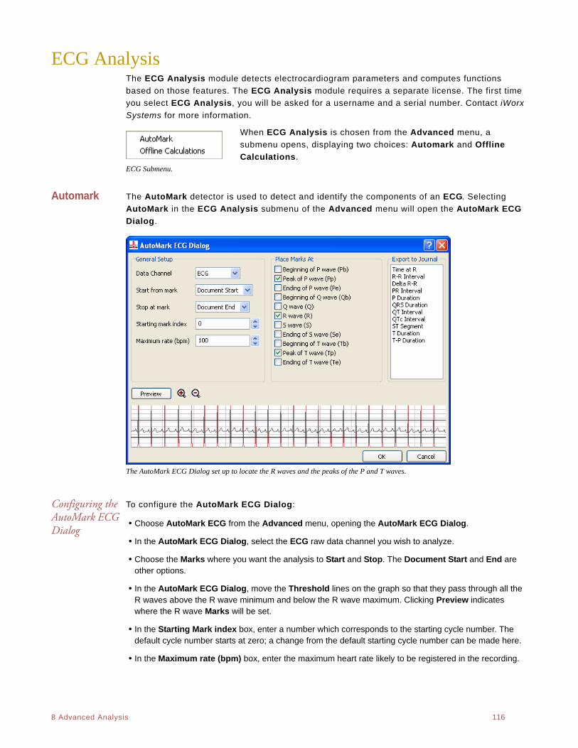
. .
8 Advanced Analysis 116
ECG AnalysisThe ECG Analysis module detects electrocardiogram parameters and computes functions
based on those features. The ECG Analysis module requires a separate license. The first time
you select ECG Analysis, you will be asked for a username and a serial number. Contact iWorx
Systems for more information.
When ECG Analysis is chosen from the Advanced menu, a
submenu opens, displaying two choices: Automark and Offline
Calculations.ECG Submenu.
Automark The AutoMark detector is used to detect and identify the components of an ECG. Selecting
AutoMark in the ECG Analysis submenu of the Advanced menu will open the AutoMark ECG
Dialog.
The AutoMark ECG Dialog set up to locate the R waves and the peaks of the P and T waves.
Configuring the AutoMark ECG Dialog
To configure the AutoMark ECG Dialog:
• Choose AutoMark ECG from the Advanced menu, opening the AutoMark ECG Dialog.
• In the AutoMark ECG Dialog, select the ECG raw data channel you wish to analyze.
• Choose the Marks where you want the analysis to Start and Stop. The Document Start and End are other options.
• In the AutoMark ECG Dialog, move the Threshold lines on the graph so that they pass through all the R waves above the R wave minimum and below the R wave maximum. Clicking Preview indicates where the R wave Marks will be set.
• In the Starting Mark index box, enter a number which corresponds to the starting cycle number. The default cycle number starts at zero; a change from the default starting cycle number can be made here.
• In the Maximum rate (bpm) box, enter the maximum heart rate likely to be registered in the recording.
. .
8 Advanced Analysis 117
• In the Place Marks at: section, select the ECG landmarks you wish to locate and mark by checking the appropriate checkboxes. These marks can be viewed and edited in the Marks window (accessed in the main Toolbar). The Marks window is organized so that the marks can be sorted by Time (ascending or descending), Channel, or Content, by clicking on the title of the appropriate column in the Marks table. Individual comments, or ranges of comments, may be selected or deselected using the SHIFT and CONTROL keys. Collections of selected comments can be exported or deleted.
• Select the calculations you wish to send to the Journal from the Export to Journal list.
• Click OK to place the Marks at the desired landmarks on the raw data channel and send the calculation results to the Journal.
The calculations that LabScribe2 can perform based on the AutoMark locations are:
Time at R: Time at the peak of the R wave.
R-R Interval: Interval between consecutive R waves.
Delta R-R: Change in the R-R Interval from the preceding interval.
PR Interval: The time from the beginning of the P wave to the peak of the R wave.
P Duration: Time from the beginning to the end of the P wave.
QRS Duration: Time from the beginning of the Q wave to the end of the S wave.
QT Interval: Time from the beginning of the Q wave to the end of the T wave.
QTc Interval: Corrected, normalized, QT Interval: QTc=QT Interval/Square root of preceding
R-R Interval.
ST Segment: Time from the end of the S wave to the beginning of the T wave.
T Duration: Time from the beginning to the end of the T wave.
TP Duration: Time from the beginning of the T wave to the end of the P wave.
These calculations can be exported to the Journal. From there, they can be exported or copied
and pasted into other applications.
Beat-by-beat ECG analysis can also be performed from the Channel menu of an ECG raw data
channel in the Analysis Window. Refer to the ECG Calculations section on page 84 of the
Analysis chapter.
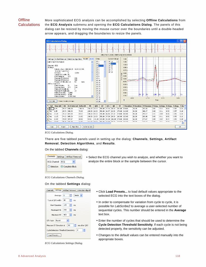
. .
8 Advanced Analysis 118
Offline Calculations
More sophisticated ECG analysis can be accomplished by selecting Offline Calculations from
the ECG Analysis submenu and opening the ECG Calculations Dialog. The panels of this
dialog can be resized by moving the mouse cursor over the boundaries until a double-headed
arrow appears, and dragging the boundaries to resize the panels.
ECG Calculations Dialog.
There are five tabbed panels used in setting up the dialog: Channels, Settings, Artifact
Removal, Detection Algorithms, and Results.
On the tabbed Channels dialog:
• Select the ECG channel you wish to analyze, and whether you want to analyze the entire block or the sample between the cursor.
ECG Calculations Channels Dialog.
On the tabbed Settings dialog:
• Click Load Presets... to load default values appropriate to the selected ECG into the text boxes of the dialog.
• In order to compensate for variation from cycle to cycle, it is possible for LabScribe2 to average a user-selected number of sequential cycles. This number should be entered in the Average text box.
• Enter the number of cycles that should be used to determine the Cycle Detection Threshold Sensitivity. If each cycle is not being detected properly, the sensitivity can be adjusted.
• Changes to the default values can be entered manually into the appropriate boxes.
ECG Calculations Settings Dialog.
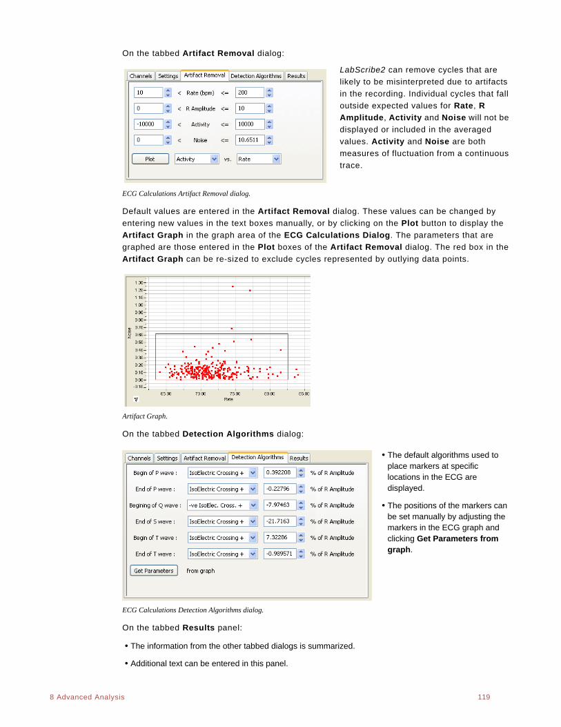
. .
8 Advanced Analysis 119
On the tabbed Artifact Removal dialog:
LabScribe2 can remove cycles that are
likely to be misinterpreted due to artifacts
in the recording. Individual cycles that fall
outside expected values for Rate, R
Amplitude, Activity and Noise will not be
displayed or included in the averaged
values. Activity and Noise are both
measures of fluctuation from a continuous
trace.
ECG Calculations Artifact Removal dialog.
Default values are entered in the Artifact Removal dialog. These values can be changed by
entering new values in the text boxes manually, or by clicking on the Plot button to display the
Artifact Graph in the graph area of the ECG Calculations Dialog. The parameters that are
graphed are those entered in the Plot boxes of the Artifact Removal dialog. The red box in the
Artifact Graph can be re-sized to exclude cycles represented by outlying data points.
Artifact Graph.
On the tabbed Detection Algorithms dialog:
• The default algorithms used to place markers at specific locations in the ECG are displayed.
• The positions of the markers can be set manually by adjusting the markers in the ECG graph and clicking Get Parameters from graph.
ECG Calculations Detection Algorithms dialog.
On the tabbed Results panel:
• The information from the other tabbed dialogs is summarized.
• Additional text can be entered in this panel.
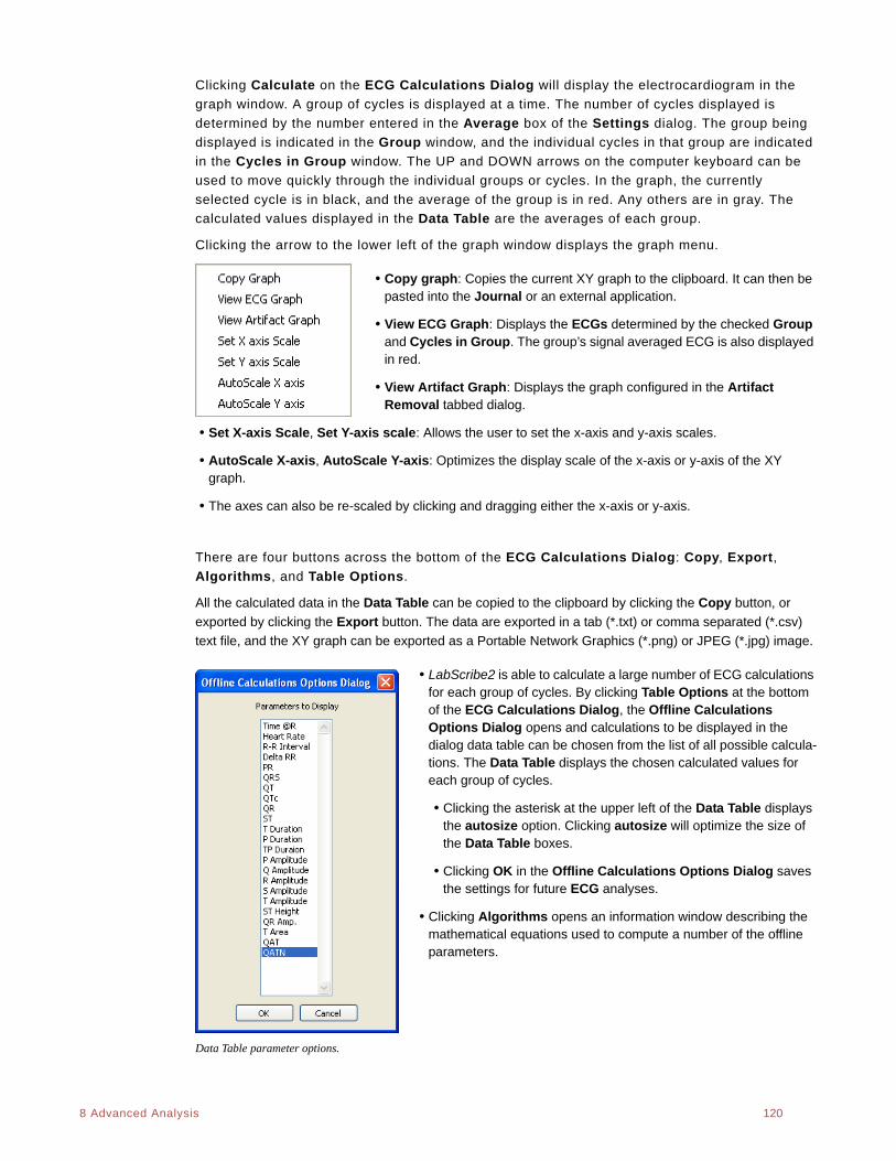
. .
8 Advanced Analysis 120
Clicking Calculate on the ECG Calculations Dialog will display the electrocardiogram in the
graph window. A group of cycles is displayed at a time. The number of cycles displayed is
determined by the number entered in the Average box of the Settings dialog. The group being
displayed is indicated in the Group window, and the individual cycles in that group are indicated
in the Cycles in Group window. The UP and DOWN arrows on the computer keyboard can be
used to move quickly through the individual groups or cycles. In the graph, the currently
selected cycle is in black, and the average of the group is in red. Any others are in gray. The
calculated values displayed in the Data Table are the averages of each group.
Clicking the arrow to the lower left of the graph window displays the graph menu.
• Copy graph: Copies the current XY graph to the clipboard. It can then be pasted into the Journal or an external application.
• View ECG Graph: Displays the ECGs determined by the checked Group and Cycles in Group. The group’s signal averaged ECG is also displayed in red.
• View Artifact Graph: Displays the graph configured in the Artifact Removal tabbed dialog.
• Set X-axis Scale, Set Y-axis scale: Allows the user to set the x-axis and y-axis scales.
• AutoScale X-axis, AutoScale Y-axis: Optimizes the display scale of the x-axis or y-axis of the XY graph.
• The axes can also be re-scaled by clicking and dragging either the x-axis or y-axis.
There are four buttons across the bottom of the ECG Calculations Dialog: Copy, Export,
Algorithms, and Table Options.
All the calculated data in the Data Table can be copied to the clipboard by clicking the Copy button, or
exported by clicking the Export button. The data are exported in a tab (*.txt) or comma separated (*.csv)
text file, and the XY graph can be exported as a Portable Network Graphics (*.png) or JPEG (*.jpg) image.
• LabScribe2 is able to calculate a large number of ECG calculations for each group of cycles. By clicking Table Options at the bottom of the ECG Calculations Dialog, the Offline Calculations Options Dialog opens and calculations to be displayed in the dialog data table can be chosen from the list of all possible calcula-tions. The Data Table displays the chosen calculated values for each group of cycles.
• Clicking the asterisk at the upper left of the Data Table displays the autosize option. Clicking autosize will optimize the size of the Data Table boxes.
• Clicking OK in the Offline Calculations Options Dialog saves the settings for future ECG analyses.
• Clicking Algorithms opens an information window describing the mathematical equations used to compute a number of the offline parameters.
Data Table parameter options.
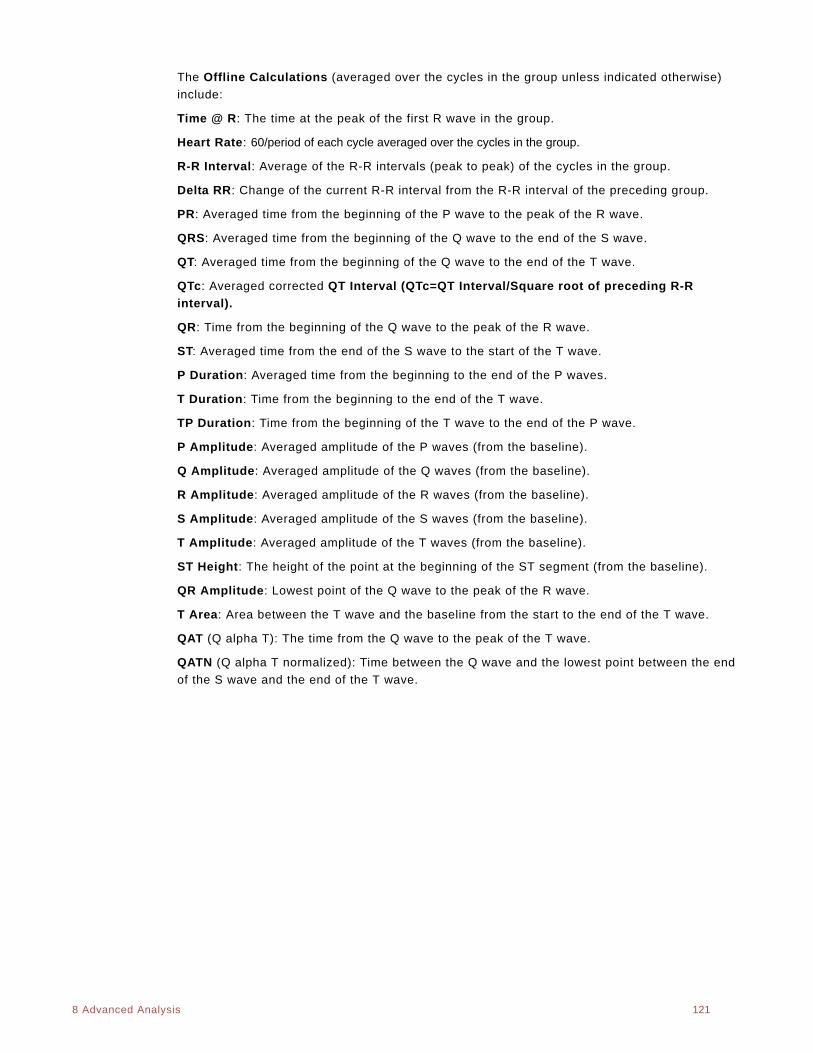
. .
8 Advanced Analysis 121
The Offline Calculations (averaged over the cycles in the group unless indicated otherwise)
include:
Time @ R: The time at the peak of the first R wave in the group.
Heart Rate: 60/period of each cycle averaged over the cycles in the group.
R-R Interval: Average of the R-R intervals (peak to peak) of the cycles in the group.
Delta RR: Change of the current R-R interval from the R-R interval of the preceding group.
PR: Averaged time from the beginning of the P wave to the peak of the R wave.
QRS: Averaged time from the beginning of the Q wave to the end of the S wave.
QT: Averaged time from the beginning of the Q wave to the end of the T wave.
QTc: Averaged corrected QT Interval (QTc=QT Interval/Square root of preceding R-R
interval).
QR: Time from the beginning of the Q wave to the peak of the R wave.
ST: Averaged time from the end of the S wave to the start of the T wave.
P Duration: Averaged time from the beginning to the end of the P waves.
T Duration: Time from the beginning to the end of the T wave.
TP Duration: Time from the beginning of the T wave to the end of the P wave.
P Amplitude: Averaged amplitude of the P waves (from the baseline).
Q Amplitude: Averaged amplitude of the Q waves (from the baseline).
R Amplitude: Averaged amplitude of the R waves (from the baseline).
S Amplitude: Averaged amplitude of the S waves (from the baseline).
T Amplitude: Averaged amplitude of the T waves (from the baseline).
ST Height: The height of the point at the beginning of the ST segment (from the baseline).
QR Amplitude: Lowest point of the Q wave to the peak of the R wave.
T Area: Area between the T wave and the baseline from the start to the end of the T wave.
QAT (Q alpha T): The time from the Q wave to the peak of the T wave.
QATN (Q alpha T normalized): Time between the Q wave and the lowest point between the end
of the S wave and the end of the T wave.
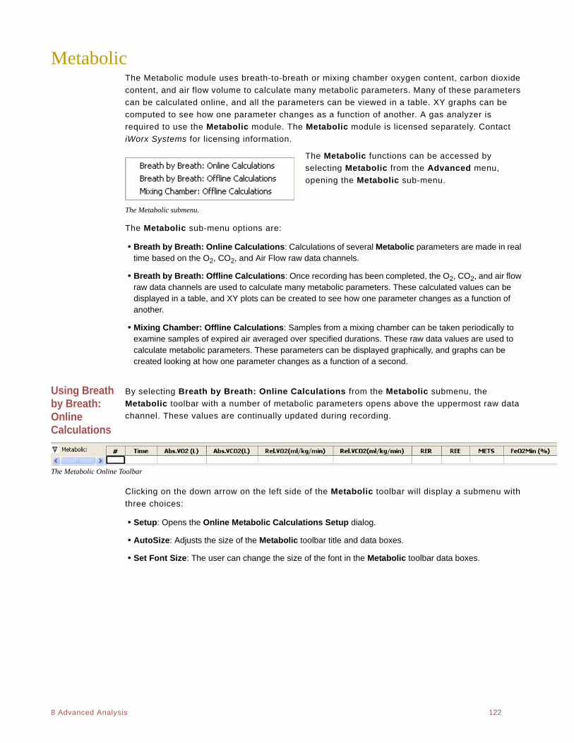
. .
8 Advanced Analysis 122
MetabolicThe Metabolic module uses breath-to-breath or mixing chamber oxygen content, carbon dioxide
content, and air flow volume to calculate many metabolic parameters. Many of these parameters
can be calculated online, and all the parameters can be viewed in a table. XY graphs can be
computed to see how one parameter changes as a function of another. A gas analyzer is
required to use the Metabolic module. The Metabolic module is licensed separately. Contact
iWorx Systems for licensing information.
The Metabolic functions can be accessed by
selecting Metabolic from the Advanced menu,
opening the Metabolic sub-menu.
The Metabolic submenu.
The Metabolic sub-menu options are:
• Breath by Breath: Online Calculations: Calculations of several Metabolic parameters are made in real time based on the O2, CO2, and Air Flow raw data channels.
• Breath by Breath: Offline Calculations: Once recording has been completed, the O2, CO2, and air flow raw data channels are used to calculate many metabolic parameters. These calculated values can be displayed in a table, and XY plots can be created to see how one parameter changes as a function of another.
• Mixing Chamber: Offline Calculations: Samples from a mixing chamber can be taken periodically to examine samples of expired air averaged over specified durations. These raw data values are used to calculate metabolic parameters. These parameters can be displayed graphically, and graphs can be created looking at how one parameter changes as a function of a second.
Using Breath by Breath: Online Calculations
By selecting Breath by Breath: Online Calculations from the Metabolic submenu, the
Metabolic toolbar with a number of metabolic parameters opens above the uppermost raw data
channel. These values are continually updated during recording.
The Metabolic Online Toolbar
Clicking on the down arrow on the left side of the Metabolic toolbar will display a submenu with
three choices:
• Setup: Opens the Online Metabolic Calculations Setup dialog.
• AutoSize: Adjusts the size of the Metabolic toolbar title and data boxes.
• Set Font Size: The user can change the size of the font in the Metabolic toolbar data boxes.
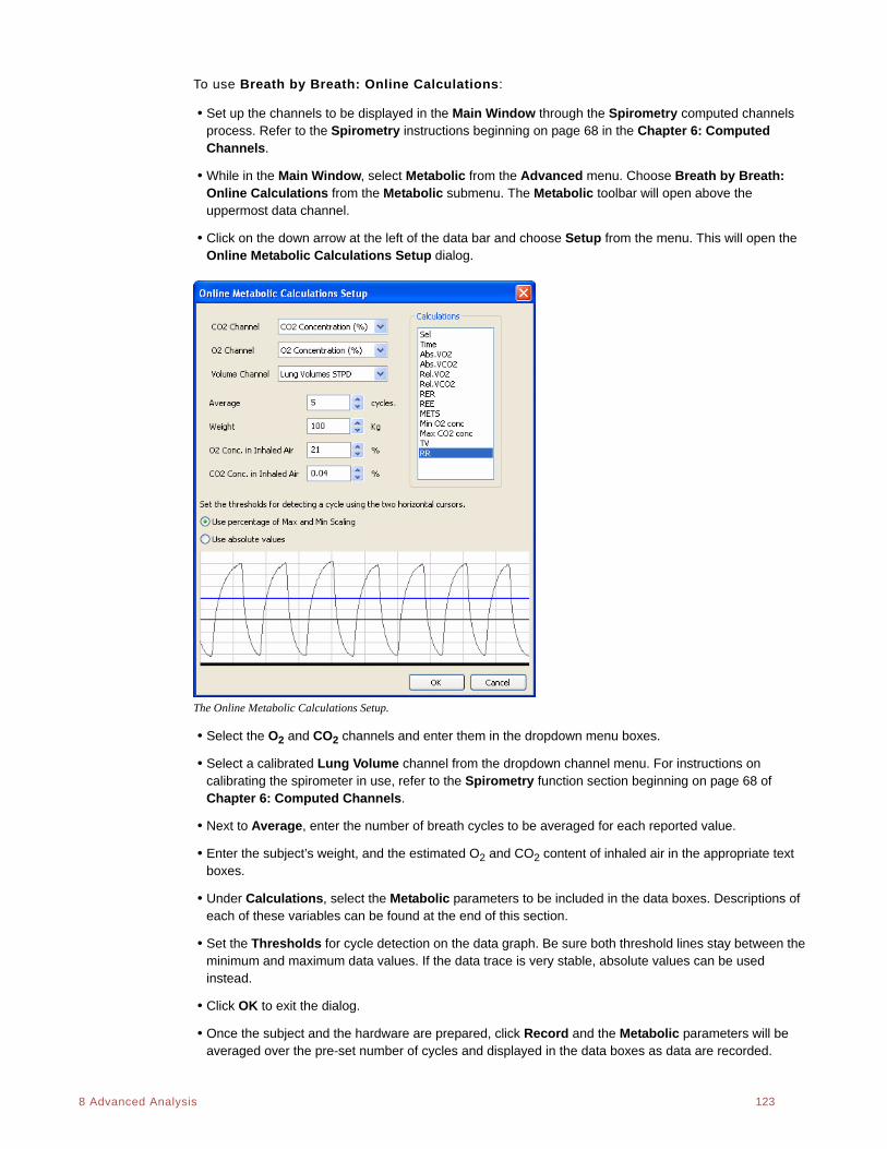
. .
8 Advanced Analysis 123
To use Breath by Breath: Online Calculations:
• Set up the channels to be displayed in the Main Window through the Spirometry computed channels process. Refer to the Spirometry instructions beginning on page 68 in the Chapter 6: Computed Channels.
• While in the Main Window, select Metabolic from the Advanced menu. Choose Breath by Breath: Online Calculations from the Metabolic submenu. The Metabolic toolbar will open above the uppermost data channel.
• Click on the down arrow at the left of the data bar and choose Setup from the menu. This will open the Online Metabolic Calculations Setup dialog.
The Online Metabolic Calculations Setup.
• Select the O2 and CO2 channels and enter them in the dropdown menu boxes.
• Select a calibrated Lung Volume channel from the dropdown channel menu. For instructions on calibrating the spirometer in use, refer to the Spirometry function section beginning on page 68 of Chapter 6: Computed Channels.
• Next to Average, enter the number of breath cycles to be averaged for each reported value.
• Enter the subject’s weight, and the estimated O2 and CO2 content of inhaled air in the appropriate text boxes.
• Under Calculations, select the Metabolic parameters to be included in the data boxes. Descriptions of each of these variables can be found at the end of this section.
• Set the Thresholds for cycle detection on the data graph. Be sure both threshold lines stay between the minimum and maximum data values. If the data trace is very stable, absolute values can be used instead.
• Click OK to exit the dialog.
• Once the subject and the hardware are prepared, click Record and the Metabolic parameters will be averaged over the pre-set number of cycles and displayed in the data boxes as data are recorded.
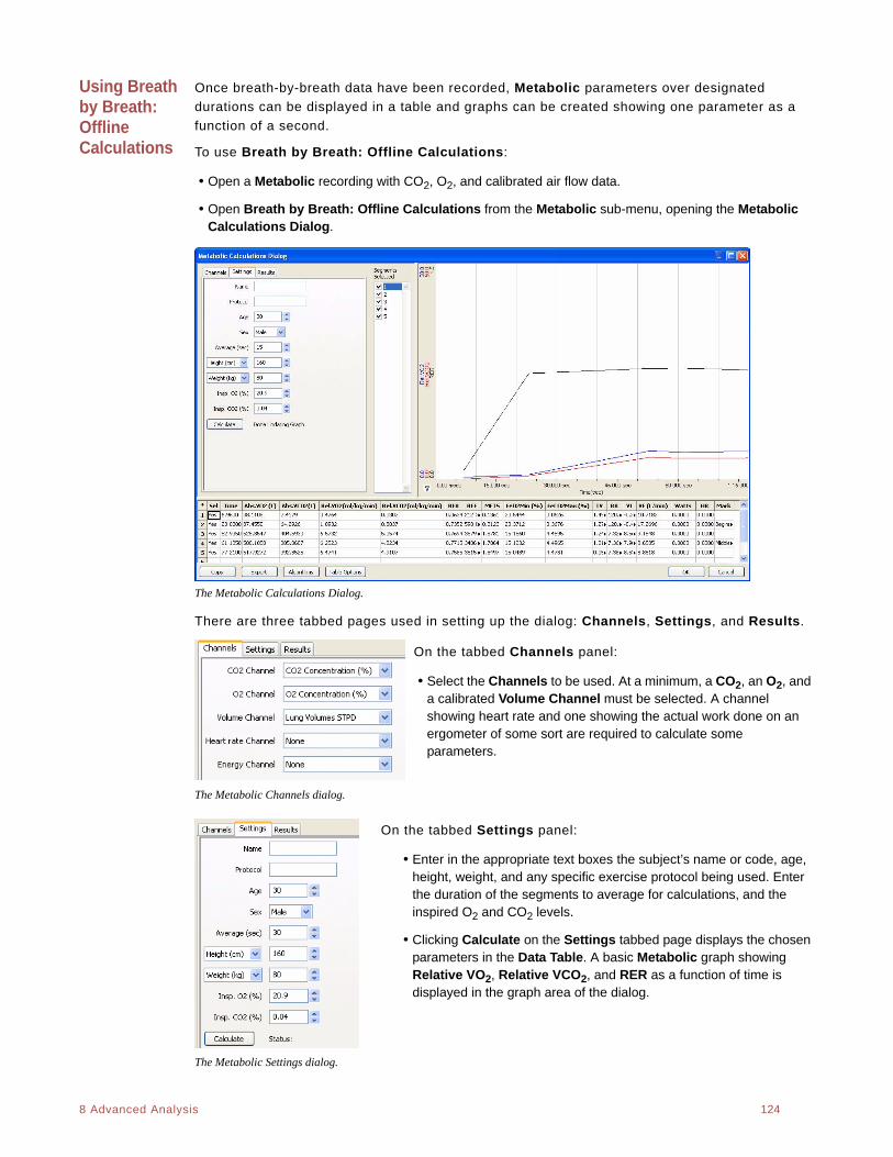
. .
8 Advanced Analysis 124
Using Breath by Breath: Offline Calculations
Once breath-by-breath data have been recorded, Metabolic parameters over designated
durations can be displayed in a table and graphs can be created showing one parameter as a
function of a second.
To use Breath by Breath: Offline Calculations:
• Open a Metabolic recording with CO2, O2, and calibrated air flow data.
• Open Breath by Breath: Offline Calculations from the Metabolic sub-menu, opening the Metabolic Calculations Dialog.
The Metabolic Calculations Dialog.
There are three tabbed pages used in setting up the dialog: Channels, Settings, and Results.
On the tabbed Channels panel:
• Select the Channels to be used. At a minimum, a CO2, an O2, and a calibrated Volume Channel must be selected. A channel showing heart rate and one showing the actual work done on an ergometer of some sort are required to calculate some parameters.
The Metabolic Channels dialog.
On the tabbed Settings panel:
• Enter in the appropriate text boxes the subject’s name or code, age, height, weight, and any specific exercise protocol being used. Enter the duration of the segments to average for calculations, and the inspired O2 and CO2 levels.
• Clicking Calculate on the Settings tabbed page displays the chosen parameters in the Data Table. A basic Metabolic graph showing Relative VO2, Relative VCO2, and RER as a function of time is displayed in the graph area of the dialog.
The Metabolic Settings dialog.
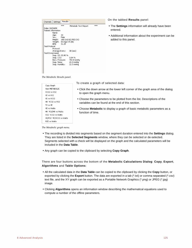
. .
8 Advanced Analysis 125
On the tabbed Results panel:
• The Settings information will already have been entered.
• Additional information about the experiment can be added to this panel.
The Metabolic Results panel.
To create a graph of selected data:
• Click the down arrow at the lower left corner of the graph area of the dialog to open the graph menu.
• Choose the parameters to be plotted from the list. Descriptions of the variables can be found at the end of this section.
• Choose Metabolic to display a graph of basic metabolic parameters as a function of time.
The Metabolic graph menu.
• The recording is divided into segments based on the segment duration entered into the Settings dialog. They are listed in the Selected Segments window, where they can be selected or de-selected. Segments selected with a check will be displayed on the graph and the calculated parameters will be included in the Data Table.
• Any graph can be copied to the clipboard by selecting Copy Graph.
There are four buttons across the bottom of the Metabolic Calculations Dialog: Copy, Export,
Algorithms and Table Options:
• All the calculated data in the Data Table can be copied to the clipboard by clicking the Copy button, or exported by clicking the Export button. The data are exported in a tab (*.txt) or comma separated (*.csv) text file, and the XY graph can be exported as a Portable Network Graphics (*.png) or JPEG (*.jpg) image.
• Clicking Algorithms opens an information window describing the mathematical equations used to compute a number of the offline parameters.
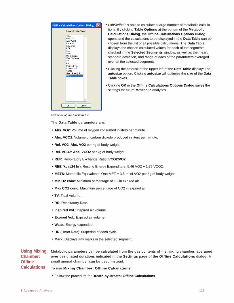
. .
8 Advanced Analysis 126
• LabScribe2 is able to calculate a large number of metabolic calcula-tions. By clicking Table Options at the bottom of the Metabolic Calculations Dialog, the Offline Calculations Options Dialog opens and the calculations to be displayed in the Data Table can be chosen from the list of all possible calculations. The Data Table displays the chosen calculated values for each of the segments checked in the Selected Segments window, as well as the mean, standard deviation, and range of each of the parameters averaged over all the selected segments.
• Clicking the asterisk at the upper left of the Data Table displays the autosize option. Clicking autosize will optimize the size of the Data Table boxes.
• Clicking OK in the Offline Calculations Options Dialog saves the settings for future Metabolic analyses.
Metabolic offline functions list.
The Data Table parameters are:
• Abs. VO2: Volume of oxygen consumed in liters per minute.
• Abs. VCO2: Volume of carbon dioxide produced in liters per minute.
• Rel. VO2: Abs. VO2 per kg of body weight.
• Rel. VCO2: Abs. VCO2 per kg of body weight.
• RER: Respiratory Exchange Ratio: VCO2/VO2.
• REE (kcal/24 hr): Resting Energy Expenditure: 5.46 VO2 + 1.75 VCO2.
• METS: Metabolic Equivalents: One MET = 3.5 ml of VO2 per kg of body weight.
• Min O2 conc: Minimum percentage of O2 in expired air.
• Max CO2 conc: Maximum percentage of CO2 in expired air.
• TV: Tidal Volume.
• RR: Respiratory Rate.
• Inspired Vol.: Inspired air volume.
• Expired Vol.: Expired air volume.
• Watts: Energy expended.
• HR (Heart Rate): 60/period of each cycle.
• Mark: Displays any marks in the selected segment.
Using Mixing Chamber: Offline Calculations
Metabolic parameters can be calculated from the gas contents of the mixing chamber, averaged
over designated durations indicated in the Settings page of the Offline Calculations dialog. A
small animal chamber can be used instead.
To use Mixing Chamber: Offline Calculations:
• Follow the procedure for Breath-by-Breath: Offline Calculations.
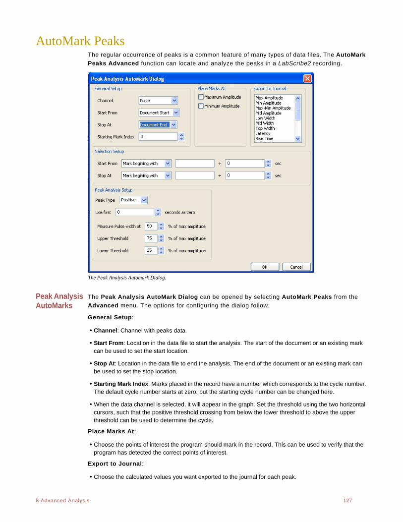
. .
8 Advanced Analysis 127
AutoMark PeaksThe regular occurrence of peaks is a common feature of many types of data files. The AutoMark
Peaks Advanced function can locate and analyze the peaks in a LabScribe2 recording.
The Peak Analysis Automark Dialog.
Peak Analysis AutoMarks
The Peak Analysis AutoMark Dialog can be opened by selecting AutoMark Peaks from the
Advanced menu. The options for configuring the dialog follow.
General Setup:
• Channel: Channel with peaks data.
• Start From: Location in the data file to start the analysis. The start of the document or an existing mark can be used to set the start location.
• Stop At: Location in the data file to end the analysis. The end of the document or an existing mark can be used to set the stop location.
• Starting Mark Index: Marks placed in the record have a number which corresponds to the cycle number. The default cycle number starts at zero, but the starting cycle number can be changed here.
• When the data channel is selected, it will appear in the graph. Set the threshold using the two horizontal cursors, such that the positive threshold crossing from below the lower threshold to above the upper threshold can be used to determine the cycle.
Place Marks At:
• Choose the points of interest the program should mark in the record. This can be used to verify that the program has detected the correct points of interest.
Export to Journal:
• Choose the calculated values you want exported to the journal for each peak.
. .
8 Advanced Analysis 128
Selection Setup:
• The start and the stop of the selection is set in this drop-down menu. To define a time location one can choose a mark identified by its starting text, the block start, or positive or negative crossing of the data. A time offset can be added to this location if desired.
Peak Analysis Setup:
• Peak type: The software will look for positive or negative peaks.
• Use first “N” seconds as zero: Used to set the offset, or the baseline.
• Measure Pulse width at: A percentage of the amplitude can be set as the location at which peak width is measured.
• Upper and Lower Thresholds: Upper and lower detection thresholds can be set in the edit boxes.
The calculated peak functions that can be exported to the Journal:
• Max: Maximum amplitude.
• Min: Minimum amplitude.
• Max-Min: Maximum amplitude - Minimum amplitude.
• Mid Amp.: Amplitude at the midpoint of the middle threshold.
• Low Width: Width of the peak as measures at the lower threshold.
• Mid Width: Width of the peak as measures at the middle threshold.
• Top Width: Width of the peak as measures at the upper threshold.
• Latency: Time from when the peak leaves the baseline to the peak.
• Rise Time: Time for the signal to travel from the lower threshold to the upper threshold.
• Fall Time: Time for the signal to travel from the upper threshold to the lower threshold.
• Leading Slope: Average slope of the signal as it travels from the lower threshold to the upper threshold.
• Trailing Slope: Average slope of the signal as it travels from the upper threshold to the lower threshold.
• Max Slope: Maximum slope.
• Min Slope: Minimum slope.
• T at Max Slope: Time at maximum slope.
• T at Min Slope: Time at minimum slope.
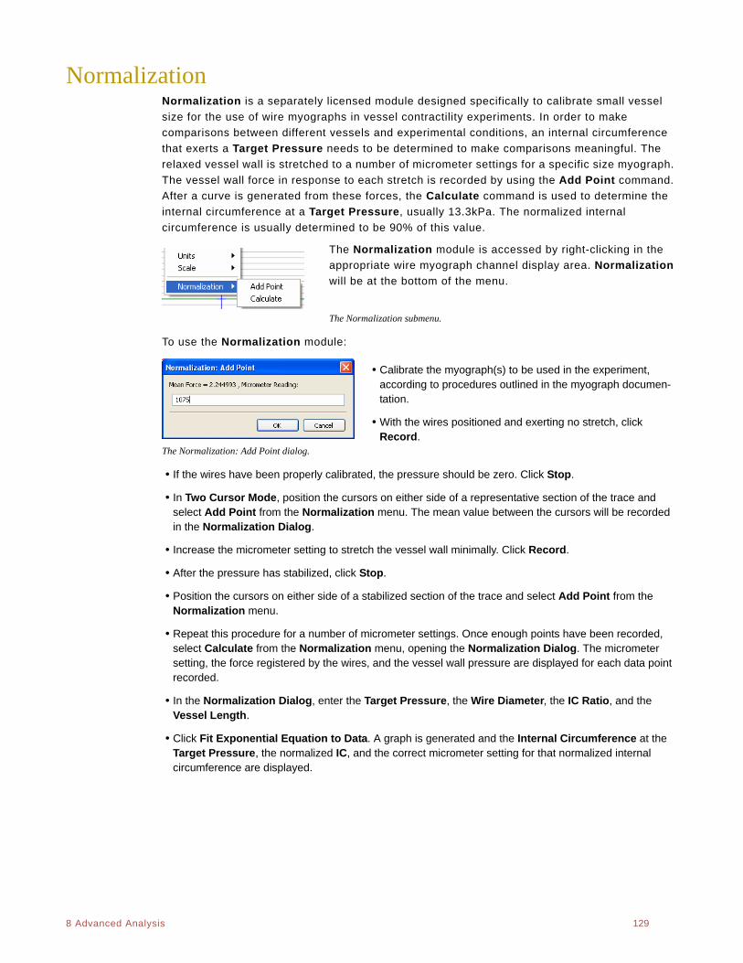
. .
8 Advanced Analysis 129
NormalizationNormalization is a separately licensed module designed specifically to calibrate small vessel
size for the use of wire myographs in vessel contractility experiments. In order to make
comparisons between different vessels and experimental conditions, an internal circumference
that exerts a Target Pressure needs to be determined to make comparisons meaningful. The
relaxed vessel wall is stretched to a number of micrometer settings for a specific size myograph.
The vessel wall force in response to each stretch is recorded by using the Add Point command.
After a curve is generated from these forces, the Calculate command is used to determine the
internal circumference at a Target Pressure, usually 13.3kPa. The normalized internal
circumference is usually determined to be 90% of this value.
The Normalization module is accessed by right-clicking in the
appropriate wire myograph channel display area. Normalization
will be at the bottom of the menu.
The Normalization submenu.
To use the Normalization module:
• Calibrate the myograph(s) to be used in the experiment, according to procedures outlined in the myograph documen-tation.
• With the wires positioned and exerting no stretch, click Record.
The Normalization: Add Point dialog.
• If the wires have been properly calibrated, the pressure should be zero. Click Stop.
• In Two Cursor Mode, position the cursors on either side of a representative section of the trace and select Add Point from the Normalization menu. The mean value between the cursors will be recorded in the Normalization Dialog.
• Increase the micrometer setting to stretch the vessel wall minimally. Click Record.
• After the pressure has stabilized, click Stop.
• Position the cursors on either side of a stabilized section of the trace and select Add Point from the Normalization menu.
• Repeat this procedure for a number of micrometer settings. Once enough points have been recorded, select Calculate from the Normalization menu, opening the Normalization Dialog. The micrometer setting, the force registered by the wires, and the vessel wall pressure are displayed for each data point recorded.
• In the Normalization Dialog, enter the Target Pressure, the Wire Diameter, the IC Ratio, and the Vessel Length.
• Click Fit Exponential Equation to Data. A graph is generated and the Internal Circumference at the Target Pressure, the normalized IC, and the correct micrometer setting for that normalized internal circumference are displayed.
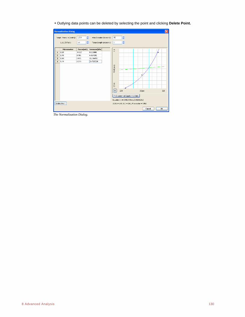
. .
8 Advanced Analysis 130
• Outlying data points can be deleted by selecting the point and clicking Delete Point.
The Normalization Dialog.
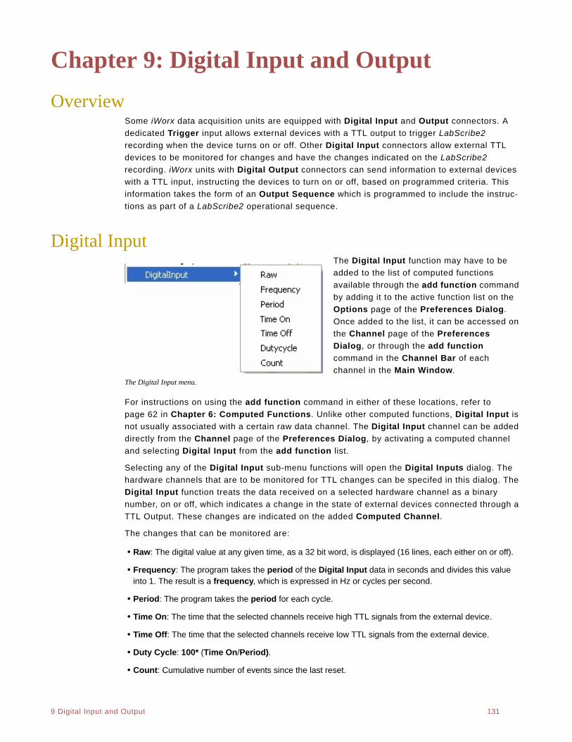
. .
9 Digital Input and Output 131
Chapter 9: Digital Input and Output
OverviewSome iWorx data acquisition units are equipped with Digital Input and Output connectors. A
dedicated Trigger input allows external devices with a TTL output to trigger LabScribe2
recording when the device turns on or off. Other Digital Input connectors allow external TTL
devices to be monitored for changes and have the changes indicated on the LabScribe2
recording. iWorx units with Digital Output connectors can send information to external devices
with a TTL input, instructing the devices to turn on or off, based on programmed criteria. This
information takes the form of an Output Sequence which is programmed to include the instruc-
tions as part of a LabScribe2 operational sequence.
Digital InputThe Digital Input function may have to be
added to the list of computed functions
available through the add function command
by adding it to the active function list on the
Options page of the Preferences Dialog.
Once added to the list, it can be accessed on
the Channel page of the Preferences
Dialog, or through the add function
command in the Channel Bar of each
channel in the Main Window. The Digital Input menu.
For instructions on using the add function command in either of these locations, refer to
page 62 in Chapter 6: Computed Functions. Unlike other computed functions, Digital Input is
not usually associated with a certain raw data channel. The Digital Input channel can be added
directly from the Channel page of the Preferences Dialog, by activating a computed channel
and selecting Digital Input from the add function list.
Selecting any of the Digital Input sub-menu functions will open the Digital Inputs dialog. The
hardware channels that are to be monitored for TTL changes can be specifed in this dialog. The
Digital Input function treats the data received on a selected hardware channel as a binary
number, on or off, which indicates a change in the state of external devices connected through a
TTL Output. These changes are indicated on the added Computed Channel.
The changes that can be monitored are:
• Raw: The digital value at any given time, as a 32 bit word, is displayed (16 lines, each either on or off).
• Frequency: The program takes the period of the Digital Input data in seconds and divides this value into 1. The result is a frequency, which is expressed in Hz or cycles per second.
• Period: The program takes the period for each cycle.
• Time On: The time that the selected channels receive high TTL signals from the external device.
• Time Off: The time that the selected channels receive low TTL signals from the external device.
• Duty Cycle: 100* (Time On/Period).
• Count: Cumulative number of events since the last reset.
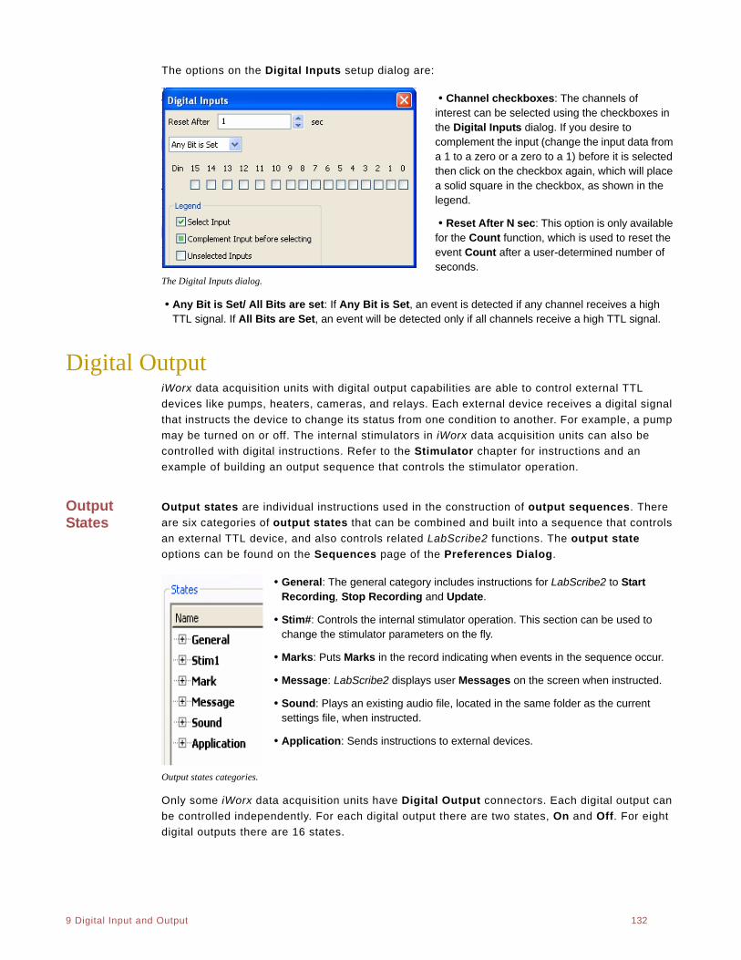
. .
9 Digital Input and Output 132
The options on the Digital Inputs setup dialog are:
• Channel checkboxes: The channels of interest can be selected using the checkboxes in the Digital Inputs dialog. If you desire to complement the input (change the input data from a 1 to a zero or a zero to a 1) before it is selected then click on the checkbox again, which will place a solid square in the checkbox, as shown in the legend.
• Reset After N sec: This option is only available for the Count function, which is used to reset the event Count after a user-determined number of seconds.
The Digital Inputs dialog.
• Any Bit is Set/ All Bits are set: If Any Bit is Set, an event is detected if any channel receives a high TTL signal. If All Bits are Set, an event will be detected only if all channels receive a high TTL signal.
Digital OutputiWorx data acquisition units with digital output capabilities are able to control external TTL
devices like pumps, heaters, cameras, and relays. Each external device receives a digital signal
that instructs the device to change its status from one condition to another. For example, a pump
may be turned on or off. The internal stimulators in iWorx data acquisition units can also be
controlled with digital instructions. Refer to the Stimulator chapter for instructions and an
example of building an output sequence that controls the stimulator operation.
Output States
Output states are individual instructions used in the construction of output sequences. There
are six categories of output states that can be combined and built into a sequence that controls
an external TTL device, and also controls related LabScribe2 functions. The output state
options can be found on the Sequences page of the Preferences Dialog.
• General: The general category includes instructions for LabScribe2 to Start Recording, Stop Recording and Update.
• Stim#: Controls the internal stimulator operation. This section can be used to change the stimulator parameters on the fly.
• Marks: Puts Marks in the record indicating when events in the sequence occur.
• Message: LabScribe2 displays user Messages on the screen when instructed.
• Sound: Plays an existing audio file, located in the same folder as the current settings file, when instructed.
• Application: Sends instructions to external devices.
Output states categories.
Only some iWorx data acquisition units have Digital Output connectors. Each digital output can
be controlled independently. For each digital output there are two states, On and Off. For eight
digital outputs there are 16 states.
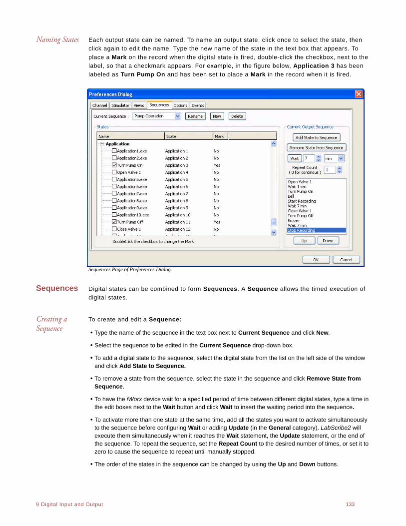
. .
9 Digital Input and Output 133
Naming States Each output state can be named. To name an output state, click once to select the state, then
click again to edit the name. Type the new name of the state in the text box that appears. To
place a Mark on the record when the digital state is fired, double-click the checkbox, next to the
label, so that a checkmark appears. For example, in the figure below, Application 3 has been
labeled as Turn Pump On and has been set to place a Mark in the record when it is fired.
Sequences Page of Preferences Dialog.
Sequences Digital states can be combined to form Sequences. A Sequence allows the timed execution of
digital states.
Creating a Sequence
To create and edit a Sequence:
• Type the name of the sequence in the text box next to Current Sequence and click New.
• Select the sequence to be edited in the Current Sequence drop-down box.
• To add a digital state to the sequence, select the digital state from the list on the left side of the window and click Add State to Sequence.
• To remove a state from the sequence, select the state in the sequence and click Remove State from Sequence.
• To have the iWorx device wait for a specified period of time between different digital states, type a time in the edit boxes next to the Wait button and click Wait to insert the waiting period into the sequence.
• To activate more than one state at the same time, add all the states you want to activate simultaneously to the sequence before configuring Wait or adding Update (in the General category). LabScribe2 will execute them simultaneously when it reaches the Wait statement, the Update statement, or the end of the sequence. To repeat the sequence, set the Repeat Count to the desired number of times, or set it to zero to cause the sequence to repeat until manually stopped.
• The order of the states in the sequence can be changed by using the Up and Down buttons.
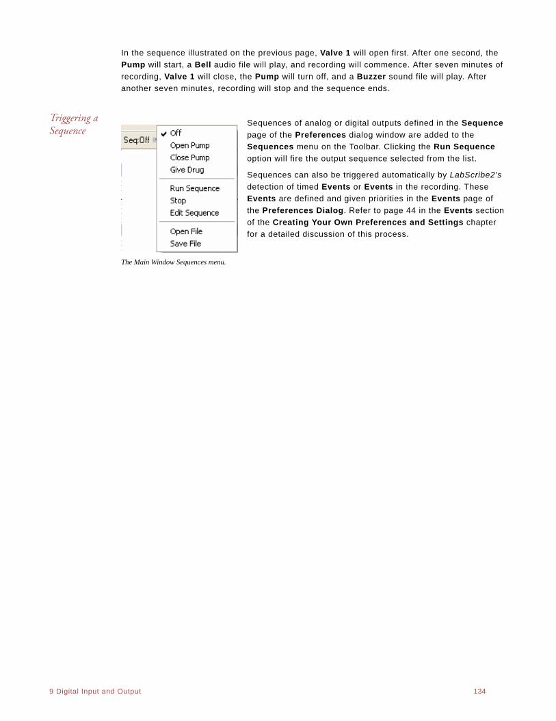
. .
9 Digital Input and Output 134
In the sequence illustrated on the previous page, Valve 1 will open first. After one second, the
Pump will start, a Bell audio file will play, and recording will commence. After seven minutes of
recording, Valve 1 will close, the Pump will turn off, and a Buzzer sound file will play. After
another seven minutes, recording will stop and the sequence ends.
Triggering a Sequence
Sequences of analog or digital outputs defined in the Sequence
page of the Preferences dialog window are added to the
Sequences menu on the Toolbar. Clicking the Run Sequence
option will fire the output sequence selected from the list.
Sequences can also be triggered automatically by LabScribe2’s
detection of timed Events or Events in the recording. These
Events are defined and given priorities in the Events page of
the Preferences Dialog. Refer to page 44 in the Events section
of the Creating Your Own Preferences and Settings chapter
for a detailed discussion of this process.
The Main Window Sequences menu.
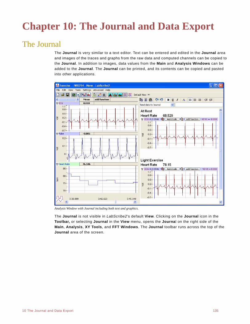
. .
10 The Journal and Data Export 135
Chapter 10: The Journal and Data Export
The JournalThe Journal is very similar to a text editor. Text can be entered and edited in the Journal area
and images of the traces and graphs from the raw data and computed channels can be copied to
the Journal. In addition to images, data values from the Main and Analysis Windows can be
added to the Journal. The Journal can be printed, and its contents can be copied and pasted
into other applications.
Analysis Window with Journal including both text and graphics.
The Journal is not visible in LabScribe2’s default View. Clicking on the Journal icon in the
Toolbar, or selecting Journal in the View menu, opens the Journal on the right side of the
Main, Analysis, XY Tools, and FFT Windows. The Journal toolbar runs across the top of the
Journal area of the screen.
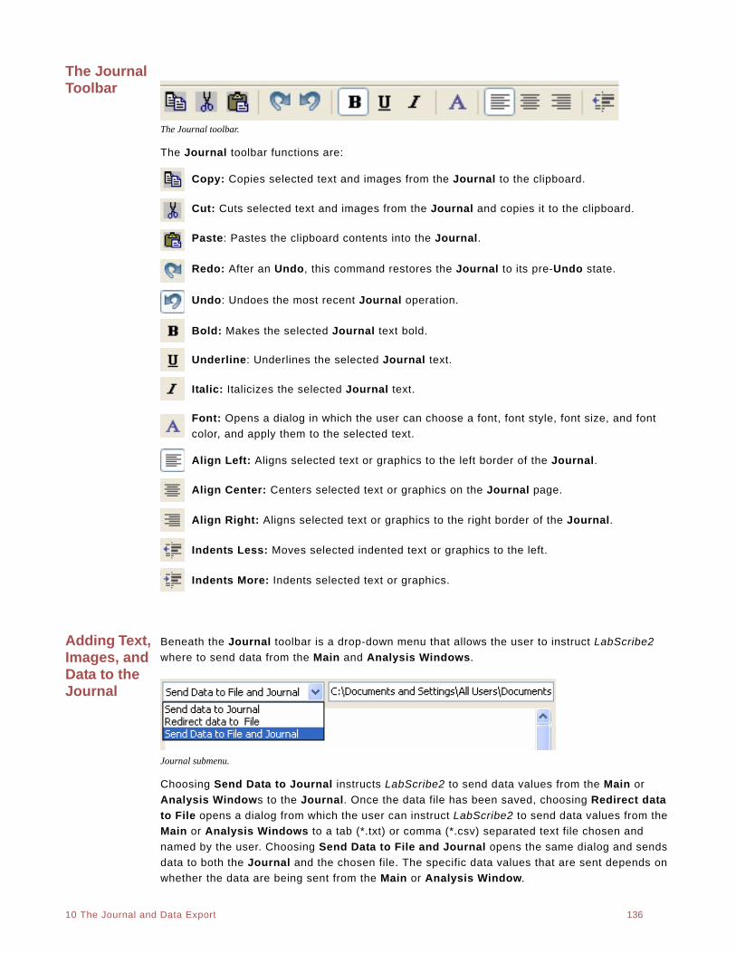
. .
10 The Journal and Data Export 136
The Journal Toolbar
The Journal toolbar.
The Journal toolbar functions are:
Copy: Copies selected text and images from the Journal to the clipboard.
Cut: Cuts selected text and images from the Journal and copies it to the clipboard.
Paste: Pastes the clipboard contents into the Journal.
Redo: After an Undo, this command restores the Journal to its pre-Undo state.
Undo: Undoes the most recent Journal operation.
Bold: Makes the selected Journal text bold.
Underline: Underlines the selected Journal text.
Italic: Italicizes the selected Journal text.
Font: Opens a dialog in which the user can choose a font, font style, font size, and font
color, and apply them to the selected text.
Align Left: Aligns selected text or graphics to the left border of the Journal.
Align Center: Centers selected text or graphics on the Journal page.
Align Right: Aligns selected text or graphics to the right border of the Journal.
Indents Less: Moves selected indented text or graphics to the left.
Indents More: Indents selected text or graphics.
Adding Text, Images, and Data to the Journal
Beneath the Journal toolbar is a drop-down menu that allows the user to instruct LabScribe2
where to send data from the Main and Analysis Windows.
Journal submenu.
Choosing Send Data to Journal instructs LabScribe2 to send data values from the Main or
Analysis Windows to the Journal. Once the data file has been saved, choosing Redirect data
to File opens a dialog from which the user can instruct LabScribe2 to send data values from the
Main or Analysis Windows to a tab (*.txt) or comma (*.csv) separated text file chosen and
named by the user. Choosing Send Data to File and Journal opens the same dialog and sends
data to both the Journal and the chosen file. The specific data values that are sent depends on
whether the data are being sent from the Main or Analysis Window.
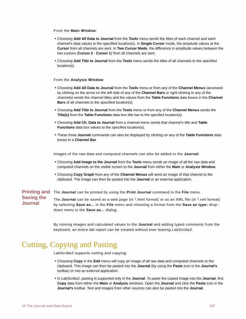
. .
10 The Journal and Data Export 137
From the Main Window:
• Choosing Add All Data to Journal from the Tools menu sends the titles of each channel and each channel’s data values to the specified location(s). In Single Cursor mode, the ampitude values at the Cursor from all channels are sent. In Two Cursor Mode, the difference in amplitude values between the two cursors (Cursor 2 - Cursor 1) from all channels are sent.
• Choosing Add Title to Journal from the Tools menu sends the titles of all channels to the specified location(s).
From the Analysis Window:
• Choosing Add All Data to Journal from the Tools menu or from any of the Channel Menus (accessed by clicking on the arrow on the left side of any of the Channel Bars or right-clicking in any of the channels) sends the channel titles and the values from the Table Functions data boxes in the Channel Bars of all channels to the specified location(s).
• Choosing Add Title to Journal from the Tools menu or from any of the Channel Menus sends the Title(s) from the Table Functions data box title bar to the specifed location(s).
• Choosing Add Ch. Data to Journal from a channel menu sends that channel’s title and Table Functions data box values to the specified location(s).
• These three Journal commands can also be displayed by clicking on any of the Table Functions data boxes in a Channel Bar.
Images of the raw data and computed channels can also be added to the Journal:
• Choosing Add Image to the Journal from the Tools menu sends an image of all the raw data and computed channels on the visible screen to the Journal from either the Main or Analysis Window.
• Choosing Copy Graph from any of the Channel Menus will send an image of that channel to the clipboard. The image can then be pasted into the Journal or an external application.
Printing and Saving the Journal
The Journal can be printed by using the Print Journal command in the File menu.
The Journal can be saved as a web page (in *.html format) or as an XML file (in *.xml format)
by selecting Save as... in the File menu and choosing a format from the Save as type: drop-
down menu in the Save as... dialog.
By moving images and calculated values to the Journal and adding typed comments from the
keyboard, an entire lab report can be created without ever leaving LabScribe2.
Cutting, Copying and PastingLabScribe2 supports cutting and copying:
• Choosing Copy in the Edit menu will copy an image of all raw data and computed channels to the clipboard. This image can then be pasted into the Journal (by using the Paste icon in the Journal’s toolbar) or into an external application.
• In LabScribe2, pasting is supported only in the Journal. To paste the copied image into the Journal, first Copy data from either the Main or Analysis windows. Open the Journal and click the Paste icon in the Journal’s toolbar. Text and images from other sources can also be pasted into the Journal.
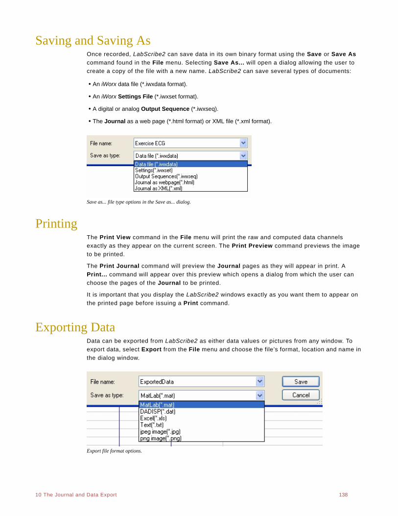
. .
10 The Journal and Data Export 138
Saving and Saving AsOnce recorded, LabScribe2 can save data in its own binary format using the Save or Save As
command found in the File menu. Selecting Save As... will open a dialog allowing the user to
create a copy of the file with a new name. LabScribe2 can save several types of documents:
• An iWorx data file (*.iwxdata format).
• An iWorx Settings File (*.iwxset format).
• A digital or analog Output Sequence (*.iwxseq).
• The Journal as a web page (*.html format) or XML file (*.xml format).
Save as... file type options in the Save as... dialog.
PrintingThe Print View command in the File menu will print the raw and computed data channels
exactly as they appear on the current screen. The Print Preview command previews the image
to be printed.
The Print Journal command will preview the Journal pages as they will appear in print. A
Print... command will appear over this preview which opens a dialog from which the user can
choose the pages of the Journal to be printed.
It is important that you display the LabScribe2 windows exactly as you want them to appear on
the printed page before issuing a Print command.
Exporting DataData can be exported from LabScribe2 as either data values or pictures from any window. To
export data, select Export from the File menu and choose the file’s format, location and name in
the dialog window.
Export file format options.
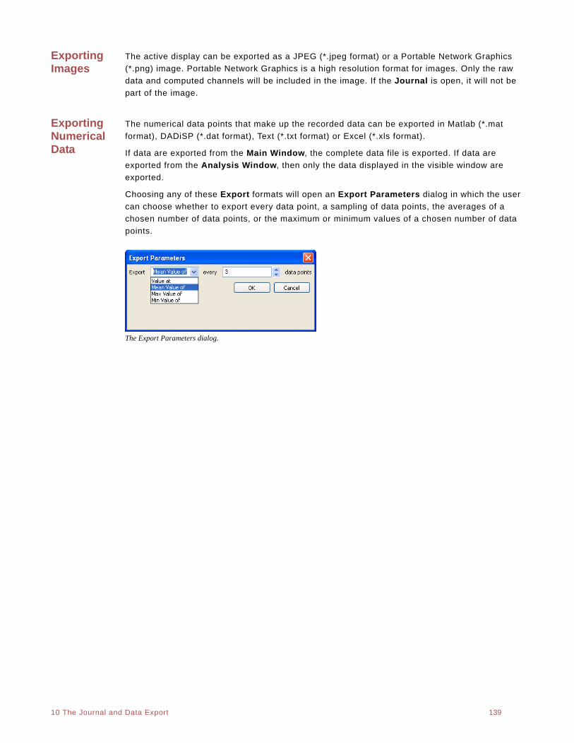
. .
10 The Journal and Data Export 139
Exporting Images
The active display can be exported as a JPEG (*.jpeg format) or a Portable Network Graphics
(*.png) image. Portable Network Graphics is a high resolution format for images. Only the raw
data and computed channels will be included in the image. If the Journal is open, it will not be
part of the image.
Exporting Numerical Data
The numerical data points that make up the recorded data can be exported in Matlab (*.mat
format), DADiSP (*.dat format), Text (*.txt format) or Excel (*.xls format).
If data are exported from the Main Window, the complete data file is exported. If data are
exported from the Analysis Window, then only the data displayed in the visible window are
exported.
Choosing any of these Export formats will open an Export Parameters dialog in which the user
can choose whether to export every data point, a sampling of data points, the averages of a
chosen number of data points, or the maximum or minimum values of a chosen number of data
points.
The Export Parameters dialog.
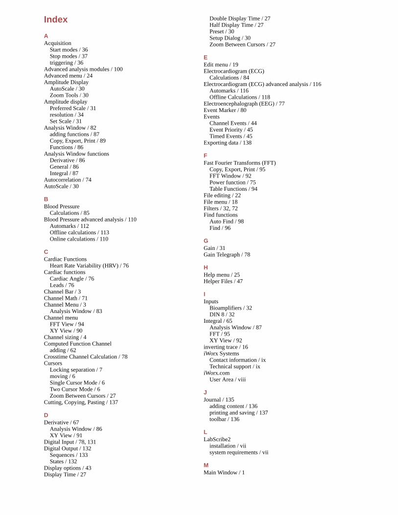
Index
AAcquisition
Start modes / 36Stop modes / 37triggering / 36
Advanced analysis modules / 100Advanced menu / 24Amplitude Display
AutoScale / 30Zoom Tools / 30
Amplitude displayPreferred Scale / 31resolution / 34Set Scale / 31
Analysis Window / 82adding functions / 87Copy, Export, Print / 89Functions / 86
Analysis Window functionsDerivative / 86General / 86Integral / 87
Autocorrelation / 74AutoScale / 30
BBlood Pressure
Calculations / 85Blood Pressure advanced analysis / 110
Automarks / 112Offline calculations / 113Online calculations / 110
CCardiac Functions
Heart Rate Variability (HRV) / 76Cardiac functions
Cardiac Angle / 76Leads / 76
Channel Bar / 3Channel Math / 71Channel Menu / 3
Analysis Window / 83Channel menu
FFT View / 94XY View / 90
Channel sizing / 4Computed Function Channel
adding / 62Crosstime Channel Calculation / 78Cursors
Locking separation / 7moving / 6Single Cursor Mode / 6Two Cursor Mode / 6Zoom Between Cursors / 27
Cutting, Copying, Pasting / 137
DDerivative / 67
Analysis Window / 86XY View / 91
Digital Input / 78, 131Digital Output / 132
Sequences / 133States / 132
Display options / 43Display Time / 27
Double Display Time / 27Half Display Time / 27Preset / 30Setup Dialog / 30Zoom Between Cursors / 27
EEdit menu / 19Electrocardiogram (ECG)
Calculations / 84Electrocardiogram (ECG) advanced analysis / 116
Automarks / 116Offline Calculations / 118
Electroencephalograph (EEG) / 77Event Marker / 80Events
Channel Events / 44Event Priority / 45Timed Events / 45
Exporting data / 138
FFast Fourier Transforms (FFT)
Copy, Export, Print / 95FFT Window / 92Power function / 75Table Functions / 94
File editing / 22File menu / 18Filters / 32, 72Find functions
Auto Find / 98Find / 96
GGain / 31Gain Telegraph / 78
HHelp menu / 25Helper Files / 47
IInputs
Bioamplifiers / 32DIN 8 / 32
Integral / 65Analysis Window / 87FFT / 95XY View / 92
inverting trace / 16iWorx Systems
Contact information / ixTechnical support / ix
iWorx.comUser Area / viii
JJournal / 135
adding content / 136printing and saving / 137toolbar / 136
LLabScribe2
installation / viisystem requirements / vii
MMain Window / 1
Markscreating, offline / 9creating, online / 7editing / 9exporting / 11position of comments / 10Preset / 7sorting / 11using marks to navigate / 9
Metabolic advanced analysis / 122Breath by breath offline calculations / 124Mixing chamber offline calculations / 126
MultiPoint Calibration / 71
NNavigating by marks / 9Normalization module / 129
OOffset / 32
PPause display / 37Peak Analysis
Calculations / 85Peaks advanced analysis / 127
Automarks / 127Periodic functions / 63Positioning trace / 31Preferences Dialog
Channel page / 41Events page / 44Options page / 43Sequences Page / 43Stimulator page / 42Views page / 42
Preview mode / 37Printing / 138PV Loops
Computed channel functions / 80PV Loops advanced analysis / 100
Automarks / 102Conductance volume / 107Offline calculations / 103Online calculations / 100
SSampling speed
choosing, Chart mode / 34choosing, Scope mode / 40
Saving data / 40Saving files / 138Scope Mode
Analysis Window options / 87Scope mode
acquiring data / 38acquisition modes / 39when to use / 38
Scripting / 99Settings files
calling a file / 26
creating / 46Settings group
loading / 26Settings Groups
creating / 46Settings menu / 23Signal Averaging / 33Smoothing / 73Sonomicrometry / 81Spirometry / 68
Calculations / 84Stimulator
Constant Voltage protocol / 53Pulse protocols / 49Ramp protocol / 56Settings / 48Step protocol / 53Train protocol / 52Triangle protocol / 56
Stimulator Control Panel / 57Consatnt voltage mode / 58Pulse mode / 57Ramp mode / 58Step mode / 58Train mode / 57Triangle mode / 59
Stimulator output sequences / 59Sweep Selection Bar / 39
TTechnical support / ixTermplate Matching / 79Tiled or Stacked Display / 87Time Shift Channel / 80Toolbar / 2Tools menu / 21Triggering / 36
Pretriggeriing / 37
UUnits Conversion / 13
Advanced / 14Advanced 2-point calibration / 14Multipoint Calibration / 71offset only / 15slope and offset method / 15
Units ConversionsSimple 2-point calibration / 13
VView menu / 20Views / 11Voltmeter / 16
XXY Plots
Copy, Export, Print / 92online / 17Table Functions / 91XY View / 89
Related Documents