Laboratory Modeling of an Axial Flow Micro Hydraulic Turbine

�����������������

Citation: Suslov, D.; Litvinov, I.;

Gorelikov, E.; Shtork, S.; Wood, D.

Laboratory Modeling of an Axial

Flow Micro Hydraulic Turbine. Appl.

Sci. 2022, 12, 573. https://doi.org/

10.3390/app12020573

Academic Editors:

Mariusz Lewandowski and

Adam Adamkowski

Received: 8 December 2021

Accepted: 5 January 2022

Published: 7 January 2022

Publisher’s Note: MDPI stays neutral

with regard to jurisdictional claims in

published maps and institutional affil-

iations.

Copyright: © 2022 by the authors.

Licensee MDPI, Basel, Switzerland.

This article is an open access article

distributed under the terms and

conditions of the Creative Commons

Attribution (CC BY) license (https://

creativecommons.org/licenses/by/

4.0/).

applied sciences

Article

Laboratory Modeling of an Axial Flow Micro Hydraulic TurbineDaniil Suslov 1,2,* , Ivan Litvinov 1,2 , Evgeny Gorelikov 1,2, Sergey Shtork 1,2 and David Wood 2,3

1 Kutateladze Institute of Thermophysics, 630090 Novosibirsk, Russia; [email protected] (I.L.);[email protected] (E.G.); [email protected] (S.S.)

2 Physics Department, Novosibirsk State University, 630090 Novosibirsk, Russia; [email protected] Department of Mechanical and Manufacturing Engineering, University of Calgary,

Calgary, AB T2N 1N4, Canada* Correspondence: [email protected]

Featured Application: The identified features of the flow for different cases are necessary forpredicting the parameters of micro hydraulic turbines and developing recommendations for ex-panding the range of regulation of turbine operating cases while maintaining high operatingefficiency.

Abstract: This article is devoted to detailed experimental studies of the flow behind the impeller ofan air model of a propeller-type microhydroturbine in a wide range of operating parameters. Themeasurements of two component distributions of averaged velocities and pulsations for conditionsfrom part load to strong overload are conducted. It is shown that the flow at the impeller outletbecomes swirled when the hydraulic turbine operating mode shifts from the optimum one. Thecharacter of the behavior of the integral swirl number, which determines the state of the swirledflow, is revealed. Information about the flow peculiarities can be used when adjusting the hydraulicunit mode to optimal conditions and developing recommendations to expand the hydraulic turbineoperation control range with preservation of high efficiency. This stage will significantly save time atthe stage of equipment design for specific field conditions of water resource.

Keywords: axial micro hydraulic turbine; swirl number; hydraulic turbine efficiency; laser-Doppleranemometer (LDA)

1. Introduction

Hydropower, being the oldest area of renewable energy, currently provides a signifi-cant contribution to world electric energy generation [1]. The basis of this production islarge-scale hydropower plants (HPP), which are built on large rivers and require heavycapital expenditures on the creation of dams. Further broadening of hydropower is limitedon the one hand because suitable water resources for the creation of large-scale hydropowersystems are already fully exploited in many countries [2]. On the other hand, the construc-tion of new big HPP in places where such resources exist is hampered by economic reasonsor safety concerns [3]. At that time, it is recommenced the attention to utilization of thehydropower potential of natural water sources in the form of small rivers and streams [4],as well as technical systems of irrigation and water supply [5]. According to the classi-fication of hydro turbines used in the literature, the class of microhydrotubines (MHT)include devices less than 100 kW, which are considered often as an off-grid technologyfor the electricity generation [6,7]. Development of MHT systems addresses the currentglobal concerns on climate change demanding decarbonization of the energy generationsector and increasing use of renewable energy sources [8–12]. Micro hydropower has beenconsidered as a reliable electricity generation technology for remote communities [11,13],living where extension of centralized power distribution networks is very expensive.

Different hydro turbine types are employed nowadays depending on parameter rangeof available water resources in terms of head and flowrate [1,11]. As moving towards

Appl. Sci. 2022, 12, 573. https://doi.org/10.3390/app12020573 https://www.mdpi.com/journal/applsci

Appl. Sci. 2022, 12, 573 2 of 18

micro hydropower applications requires reducing the scale of a power generation unit,it is important to keep low cost per kilowatts. This is becoming especially critical forpico hydroturbines with a capacity of below 5 kW for remote small communities [9,11,13].In this regard, particular attention has been given to propeller-type axial hydraulic tur-bines [9,10,14–16]. They feature a simple arrangement, moderate manufacturing costs,and high specific speed (high runner rotation speed). The high specific speed permitsapplication of cheap power generators having common shaft with the impeller [17], i.e.,avoiding use of additional transmitting gears.

The necessity of MHT price reduction requires turbines with fixed blades since mecha-nisms for adjusting the guide and impeller vanes might be expensive and complicated [18].It should be noted that propeller hydraulic turbines with fixed blade angles have a narrowrange of efficient operation [11]. The use of power sources with a stable frequency ofthe output voltage at a variable turbine speed requires significant power electronics. Thecheaper alternative is to manually adjust turbine operation to the available conditions ofhead and flow rate.

The practical use of axial hydraulic units is associated also with reducing the flowpassage size which increases the risk of clogging of blade elements with various debrisoften present in natural water bodies [10,19]. This can lead to off-design turbine operationdue to a change in flow rate with decreasing flow area or due to a deceleration of the runnerby foreign object impact.

The situation described above regarding propeller type MHTs that have favorable anddisadvantageous features holds for all hydroturbine types. Therefore, a detailed analysisis required of different structural and regime conditions for the proper choice of the mostefficient and reliable MHT technology. As for the equipment to be applied in large HPP,numerical simulation methods and model tests are employed at the hydroturbine designstage [20] with particular close attention paid to internal flow structure which determinesthe hydroturbine operation regime [21]. It should be noted that despite tremendousprogress and vast possibilities of numerical tools, experimental data is still needed forverification of calculation results.

In that context, the current work presents an experimental modeling approach, whichis based on using air as working medium and 3D printing for fabrication of model turbineelements. It is believed that this approach can provide the means for a rapid and inexpen-sive survey of detailed flow distributions in test section, characterizing the device operationmode. The obtained data can be used directly for optimization of the hydroturbine designor for a mathematical model verification.

In the following Section 2, the research methods used in the work are described. Then,Section 3 presents the results of experiments on flow characteristics downstream of apropeller-type MHT model. The operating regimes change from part load to overloadconditions. The studied range is achieved by varying the volume flow rate, Q, while theturbine shaft speed, ωn, remains constant. Emphasis is placed on the features of the flowstructure, including the generation of coherent vortex structures and their evolution alongthe length of the test section. It should be noted that for large hydraulic turbines, mostresearch has focused on underload modes [22], which are most common in practice, andmuch less attention has been paid to overload modes [23].

2. Research Methods

The experiments were carried out employing an automated experimental setup withair used as a working medium. This significantly reduced the difficulties in manufacturingexperimental sections (problems with sealing joints, structural strength, and providingoptical access) [24]. As shown in the technical reports [25,26] from the USBR group in theUSA and in the USSR energy community handbook [27], results obtained with air and watertest sections showed satisfactory correlation. The investigation of most of the hydrodynamicphenomena can be transferred from water to air [28]. This simplifies the experimentalprocedure significantly because no cavitation occurs in the flow. Nevertheless, we only

Appl. Sci. 2022, 12, 573 3 of 18

suggest a concept of the experimental finding of optimal operation of the microturbine,which should be tested on water as well. Air is supplied to the model using a blower fan.An expansion section, a settling chamber with damping screens, and a contraction produceuniform flow at the inlet to the test section. The air flow rate is changed by means of afrequency converter connected to the fan motor. The flow rate is determined by measuringthe velocity at the outlet of the contraction, i.e., in front of the test section.

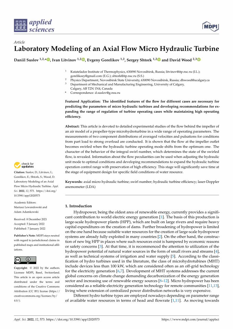
A model of propeller-type turbine (Figure 1) was chosen as a prototype of microhydro-turbine device [17,29]. The flow enters the working section through the inlet opening andpasses through the first stationary vane swirler (guide vane). It is followed by a rotatingswirler—an impeller with a streamlined body attached to it. The rotating swirler is drivenby a shaft connected to an external servo drive. The shape of the vane swirlers and theorder of their arrangement allows to simulate the velocity distribution at the outlet of areal hydraulic turbine [30]. The propeller turbine has high specific speed among othertypes of turbines. This allows high rotational speeds of the runner at low flow rates. Highturbine speeds result in faster and therefore lighter and cheaper power generators. Thehigh specific speed makes it possible to connect the turbine directly to the generator. Allparts of the model section were manufactured using rapid prototyping technology. Thediameter of the inlet part of the cone is D = 100 mm, the outlet part is1.2D. The cone lengthis H = 280 mm, the cone angle is 4◦.

Appl. Sci. 2022, 12, x FOR PEER REVIEW 3 of 19

and providing optical access) [24]. As shown in the technical reports [25,26] from the USBR group in the USA and in the USSR energy community handbook [27], results obtained with air and water test sections showed satisfactory correlation. The investigation of most of the hydrodynamic phenomena can be transferred from water to air [28]. This simplifies the experimental procedure significantly because no cavitation occurs in the flow. Nevertheless, we only suggest a concept of the experimental finding of optimal operation of the microturbine, which should be tested on water as well. Air is supplied to the model using a blower fan. An expansion section, a settling chamber with damping screens, and a contraction produce uniform flow at the inlet to the test section. The air flow rate is changed by means of a frequency converter connected to the fan motor. The flow rate is determined by measuring the velocity at the outlet of the contraction, i.e., in front of the test section.

A model of propeller-type turbine (Figure 1) was chosen as a prototype of microhydroturbine device [17,29]. The flow enters the working section through the inlet opening and passes through the first stationary vane swirler (guide vane). It is followed by a rotating swirler—an impeller with a streamlined body attached to it. The rotating swirler is driven by a shaft connected to an external servo drive. The shape of the vane swirlers and the order of their arrangement allows to simulate the velocity distribution at the outlet of a real hydraulic turbine [30]. The propeller turbine has high specific speed among other types of turbines. This allows high rotational speeds of the runner at low flow rates. High turbine speeds result in faster and therefore lighter and cheaper power generators. The high specific speed makes it possible to connect the turbine directly to the generator. All parts of the model section were manufactured using rapid prototyping technology. The diameter of the inlet part of the cone is D = 100 mm, the outlet part is1.2D. The cone length is H = 280 mm, the cone angle is 4°.

(а)

Figure 1. Cont.

Appl. Sci. 2022, 12, 573 4 of 18Appl. Sci. 2022, 12, x FOR PEER REVIEW 4 of 19

(b)

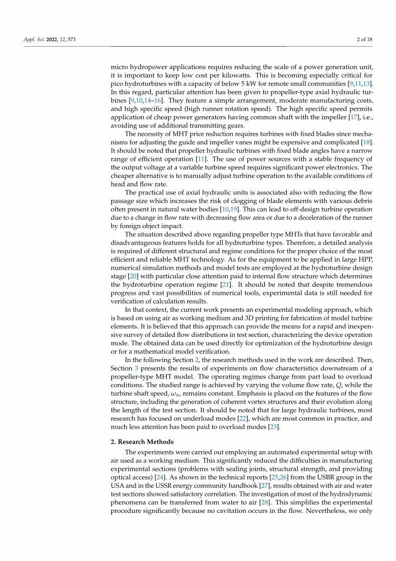
Figure 1. Air model of a micro hydraulic turbine: (a) Diagram of the experiment system; (b) Detailed diagram. 1—inlet pipe, 2—shaft, 3—servo drive, 4—guide vane (stationary swirler), 5—runner (rotating swirler), 6—streamline body, 7—conical draft tube, 8—nozzle, 9—wind tunnel.

In experiments, the Reynolds number Re = 4DQ/πν(D2 − d2) ranged from 3 × 104 to 9 × 104 (ν is the kinematic viscosity of air), which corresponds to the range of air flow rate Q from 0.02 to 0.08 m3/s, therefore, the flow was turbulent. It is supposed that the flow characteristics are unchanged when the impeller speed changes proportionally to the flow rate. The runner speed was maintained at a constant ωn = 238 rad/s. Determining the shape of the swirlers was carried out according to the method described in [30]. This computation showed that the value of ωn for a flow rate Qn = 0.049 m3/s corresponds to the point with maximum efficiency (Best Efficiency Point, BEP). The studied range of micro hydraulic turbine operation was in the range from part load (0.6Qn) to high overload (1.8Qn).

For the operation of a micro hydraulic turbine of this scale in water at the design flow rate Qn and a pressure head Hn = 2–3 m water column, the available power in the flow is Ptot = QnHn∼1.1–1.4 kW and the power developed by the turbine at a typical 70% efficiency is Pturb∼0.8–1 kW [11,16]. The design point with maximal efficiency is maintained when the velocity triangles before and after the runner are similar (ω/Q is constant). When the operating point moves along the line of constant running speed (off-design conditions), the turbine efficiency decreases. The measured velocity fields for different modes help us to understand the degree of variation in efficiency, and these velocity fields will allow the formulation of recommendations for increasing the range of efficient micro hydraulic turbine operation.

The averaged flow velocity distributions were obtained using a LAD-06I laser Doppler anemometer. Paraffin oil aerosol particles produced by a Laskin atomizer were used as tracer particles for flow seeding, which made it possible to obtain droplets with a characteristic size of 1–3 µm [22]. Part of the cone wall was replaced by a transparent film to allow the laser beams to pass into the cone. Position control of the LDA system in three axes was implemented. This provided an automated experiment to obtain an extensive amount of flow velocity data. The main errors are related to inaccuracy of flow rate setting, servo drive speed and measuring accuracy of LAD-06I system. The flow rate was controlled by IRVIS-RS4M-ULTRA flow meter with accuracy of flow measurement 1.5% (data from the instrument manual). The accuracy of setting the servo drive speed was 0.5% (data from the device manual). The LDA system measured the velocity of a single particle with an error of 0.2%. In order to measure the velocity in steady-state modes at a particular point of space, statistics of reliable flashes of at least 10,000 per point were

Figure 1. Air model of a micro hydraulic turbine: (a) Diagram of the experiment system; (b) Detaileddiagram. 1—inlet pipe, 2—shaft, 3—servo drive, 4—guide vane (stationary swirler), 5—runner(rotating swirler), 6—streamline body, 7—conical draft tube, 8—nozzle, 9—wind tunnel.

In experiments, the Reynolds number Re = 4DQ/πν(D2 − d2) ranged from 3 × 104

to 9 × 104 (ν is the kinematic viscosity of air), which corresponds to the range of air flowrate Q from 0.02 to 0.08 m3/s, therefore, the flow was turbulent. It is supposed that theflow characteristics are unchanged when the impeller speed changes proportionally to theflow rate. The runner speed was maintained at a constant ωn = 238 rad/s. Determiningthe shape of the swirlers was carried out according to the method described in [30]. Thiscomputation showed that the value of ωn for a flow rate Qn = 0.049 m3/s correspondsto the point with maximum efficiency (Best Efficiency Point, BEP). The studied range ofmicro hydraulic turbine operation was in the range from part load (0.6Qn) to high overload(1.8Qn).

For the operation of a micro hydraulic turbine of this scale in water at the design flowrate Qn and a pressure head Hn = 2–3 m water column, the available power in the flow isPtot = QnHn~1.1–1.4 kW and the power developed by the turbine at a typical 70% efficiencyis Pturb~0.8–1 kW [11,16]. The design point with maximal efficiency is maintained whenthe velocity triangles before and after the runner are similar (ω/Q is constant). When theoperating point moves along the line of constant running speed (off-design conditions),the turbine efficiency decreases. The measured velocity fields for different modes helpus to understand the degree of variation in efficiency, and these velocity fields will allowthe formulation of recommendations for increasing the range of efficient micro hydraulicturbine operation.

The averaged flow velocity distributions were obtained using a LAD-06I laser Doppleranemometer. Paraffin oil aerosol particles produced by a Laskin atomizer were usedas tracer particles for flow seeding, which made it possible to obtain droplets with acharacteristic size of 1–3 µm [22]. Part of the cone wall was replaced by a transparentfilm to allow the laser beams to pass into the cone. Position control of the LDA systemin three axes was implemented. This provided an automated experiment to obtain anextensive amount of flow velocity data. The main errors are related to inaccuracy of flowrate setting, servo drive speed and measuring accuracy of LAD-06I system. The flow ratewas controlled by IRVIS-RS4M-ULTRA flow meter with accuracy of flow measurement1.5% (data from the instrument manual). The accuracy of setting the servo drive speed was0.5% (data from the device manual). The LDA system measured the velocity of a singleparticle with an error of 0.2%. In order to measure the velocity in steady-state modes ata particular point of space, statistics of reliable flashes of at least 10,000 per point were

Appl. Sci. 2022, 12, 573 5 of 18

accumulated. This allowed the flow rate at a given point to be determined with 99.7%certainty because each velocity component at each individual point in space was averagedover at least 3000 credible bursts. The LDA system was tuned so that the signal receivedfrom the flashes was close to Gaussian, with the RMS of the velocity for both componentsnot exceeding 2–3 m/s. Based on an uncertainty analysis [31] in the present experiment, thetotal errors in the velocity measurements and their pulsations can be estimated as no morethan 5% and 2%, respectively. Using linear interpolation with the minimum interval timegiven by the average data rate, the signal with a random tracer arrival time was convertedinto an equidistant signal in the time array. The spectrum was then calculated using fastFourier transform. The maximum error for the measured fundamental frequency in theLDA spectra did not exceed 0.05 Hz.

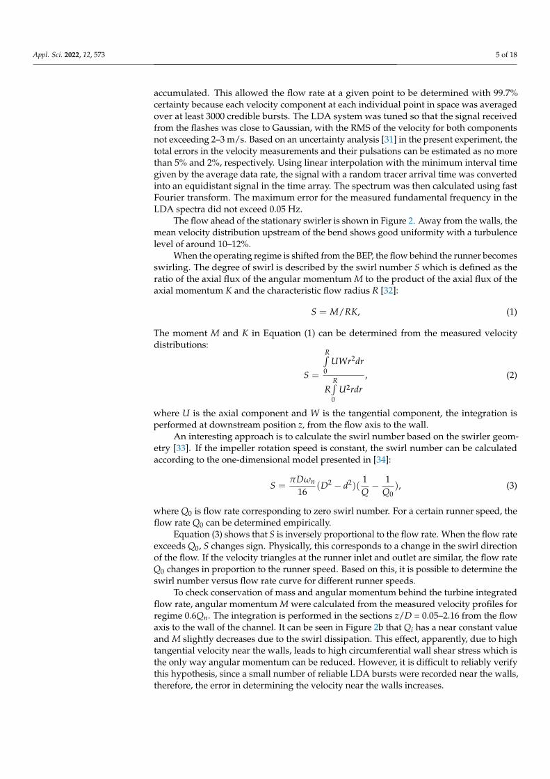
The flow ahead of the stationary swirler is shown in Figure 2. Away from the walls, themean velocity distribution upstream of the bend shows good uniformity with a turbulencelevel of around 10–12%.

When the operating regime is shifted from the BEP, the flow behind the runner becomesswirling. The degree of swirl is described by the swirl number S which is defined as theratio of the axial flux of the angular momentum M to the product of the axial flux of theaxial momentum K and the characteristic flow radius R [32]:

S = M/RK, (1)

The moment M and K in Equation (1) can be determined from the measured velocitydistributions:

S =

R∫0

UWr2dr

RR∫0

U2rdr, (2)

where U is the axial component and W is the tangential component, the integration isperformed at downstream position z, from the flow axis to the wall.

An interesting approach is to calculate the swirl number based on the swirler geom-etry [33]. If the impeller rotation speed is constant, the swirl number can be calculatedaccording to the one-dimensional model presented in [34]:

S =πDωn

16(D2 − d2)(

1Q

− 1Q0

), (3)

where Q0 is flow rate corresponding to zero swirl number. For a certain runner speed, theflow rate Q0 can be determined empirically.

Equation (3) shows that S is inversely proportional to the flow rate. When the flow rateexceeds Q0, S changes sign. Physically, this corresponds to a change in the swirl directionof the flow. If the velocity triangles at the runner inlet and outlet are similar, the flow rateQ0 changes in proportion to the runner speed. Based on this, it is possible to determine theswirl number versus flow rate curve for different runner speeds.

To check conservation of mass and angular momentum behind the turbine integratedflow rate, angular momentum M were calculated from the measured velocity profiles forregime 0.6Qn. The integration is performed in the sections z/D = 0.05–2.16 from the flowaxis to the wall of the channel. It can be seen in Figure 2b that Qi has a near constant valueand M slightly decreases due to the swirl dissipation. This effect, apparently, due to hightangential velocity near the walls, leads to high circumferential wall shear stress which isthe only way angular momentum can be reduced. However, it is difficult to reliably verifythis hypothesis, since a small number of reliable LDA bursts were recorded near the walls,therefore, the error in determining the velocity near the walls increases.

Appl. Sci. 2022, 12, 573 6 of 18

Appl. Sci. 2022, 12, x FOR PEER REVIEW 6 of 19

(a)

(b)

Figure 2. Experimental conditions: (a) Axial velocity profile (left axis—mean; right axis—RMS of velocity fluctuations) measured by LDA upstream of the bend and (b) M (left axis) and Qi/Qn (right axis) conservation as function of z/D.

3. Results and Discussion

Figure 2. Experimental conditions: (a) Axial velocity profile (left axis—mean; right axis—RMS ofvelocity fluctuations) measured by LDA upstream of the bend and (b) M (left axis) and Qi/Qn (rightaxis) conservation as function of z/D.

3. Results and Discussion

The measured velocity distributions in the conical section and their downstreamevolution are presented in Figures 3–8. Profiles of the averaged velocities and fluctuationsfor the part load regime are shown in Figures 3 and 4.

Appl. Sci. 2022, 12, 573 7 of 18

Appl. Sci. 2022, 12, x FOR PEER REVIEW 7 of 19

The measured velocity distributions in the conical section and their downstream evolution are presented in Figures 3–8. Profiles of the averaged velocities and fluctuations for the part load regime are shown in Figures 3 and 4.

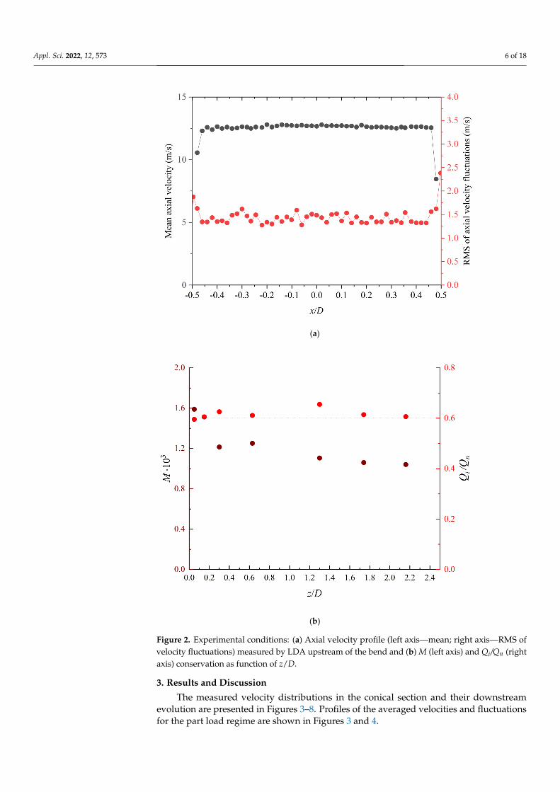
Figure 3. Time-averaged velocity profiles at different distances from the runner at a constant runner speed ωn: (a) Axial component; (b) Tangential component. Part load regime with Q = 0.6Qn. The legend indicates the distances of the measuring section from the tip of the runner cowl. In the section z/D = 1.30 the swirl number is S = 0.6.

Figure 3. Time-averaged velocity profiles at different distances from the runner at a constant runnerspeed ωn: (a) Axial component; (b) Tangential component. Part load regime with Q = 0.6Qn. Thelegend indicates the distances of the measuring section from the tip of the runner cowl. In the sectionz/D = 1.30 the swirl number is S = 0.6.

This case is characterized by high tangential velocity, which coincides in direction withthe rotation of the runner (Figure 3b). Due to intense swirling, the flow is shifted to the sidewalls of the conical channel with a corresponding reduction of the velocity along the axis,and axial reverse flow occurs. The most intense reverse flow is observed in the immediate

Appl. Sci. 2022, 12, 573 8 of 18

vicinity of the runner cowl, where it is further enhanced by the formation of a wake behindthe cowl. Further downstream, the reverse flow decreases and practically disappears incross-sections distant from the runner, where the axial velocity profile becomes muchsmoother. In this case, the swirl decays downstream, which is reflected in a decrease inthe tangential velocity (Figure 3b). At small z, the swirling of the flow by the runner cowlnear the axis leads to a pronounced peak of the tangential velocity, which flattens outdownstream and shifts toward the side wall. At larger z, the tangential velocity profilesassume a smooth shape with the tangential velocity increasing monotonically from thecenter to the side wall.

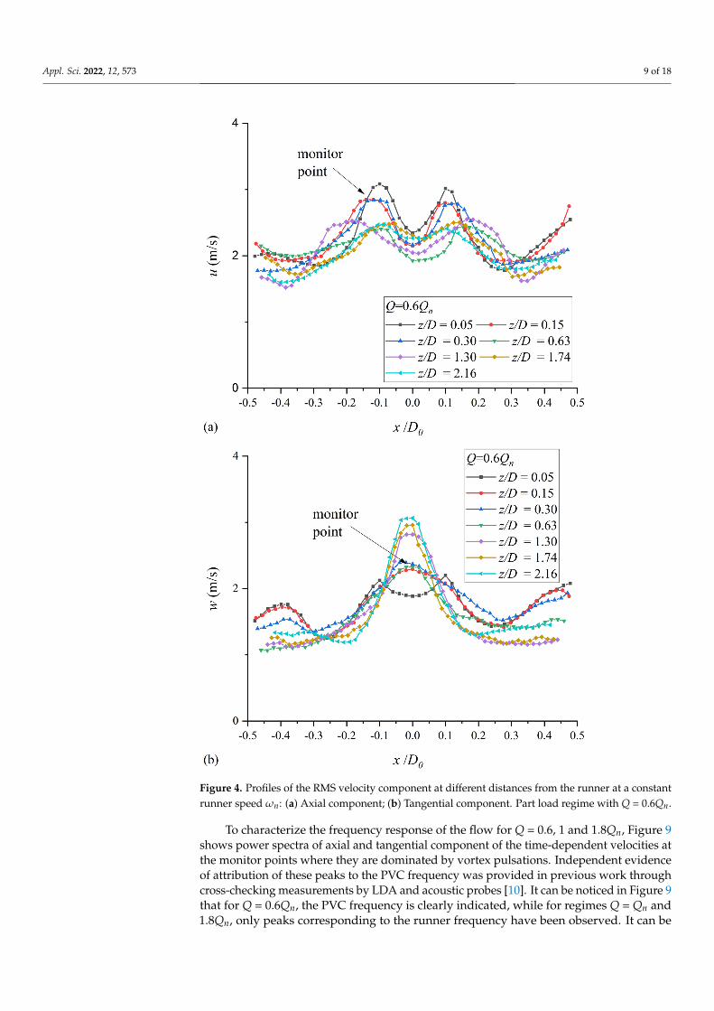
The swirling flow structure with a central recirculation zone that occurs in the part loadregime usually leads to flow instability in the form of a precessing vortex core (PVC) [35,36].The PVC generates increased flow pulsations, as can be seen from the distributions of RootMean Square (RMS) fluctuations of the axial and tangential velocity components (Figure 4).It is evident that the peaks of the RMS axial velocity are located at the boundary of thereverse flow zone which is always close to the point of maximum radial gradient of theaxial velocity (Figure 4a), whereas the peaks of the RMS tangential velocity profiles arenear the center (Figure 4b); this unambiguously indicates the precessional motion of thevortex core [22]. It should be noted that RMS distributions contain not only the stochasticturbulence fluctuations, but also the coherent pulsations due to the PVC motion, whichmay produce the major contribution to the RMS. It will be shown later that the tangentialvelocity spectra at the monitor point labeled in the figure have a distinct peak at the samefrequency of 14.5 Hz, which corresponds to the precession frequency of the coherent vortexstructure f PVC.

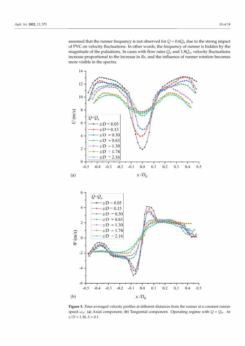
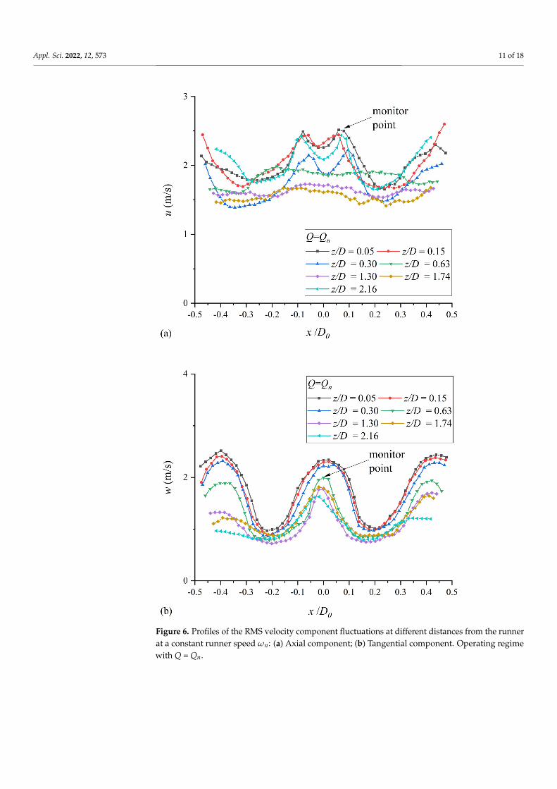
Increasing the flow rate to the level Q = Qn corresponding to the design case close tothe BEP leads to a more uniform distribution of the axial velocity along the cross-section(Figure 5a). The central dip due to the wake behind the cowl is quite pronounced at smallz, but is rapidly filled downstream. The swirl level decreases significantly, although thetangential velocity remains nonzero and coincides in direction with the rotation of therunner at all cross-sections (Figure 5b). As in the previous case, there is a region of higherswirl close to the turbine formed by the rotation of the cowl. This localized region iscompletely smoothed only after z/D = 0.30. In the design case, the velocity fluctuationsare generally significantly reduced. The RMS distributions of the axial component becomeuniform in both the radial and axial directions (Figure 6a). The corresponding profiles ofthe tangential component still have pronounced central peaks (Figure 6b), but, in contrastto the case of underload, their maxima occur immediately behind the runner cowl andthen gradually decreases toward the cone outlet. These peaks indicate a small-amplitudeprecession of the localized swirl region formed due to the rotation of the cowl.

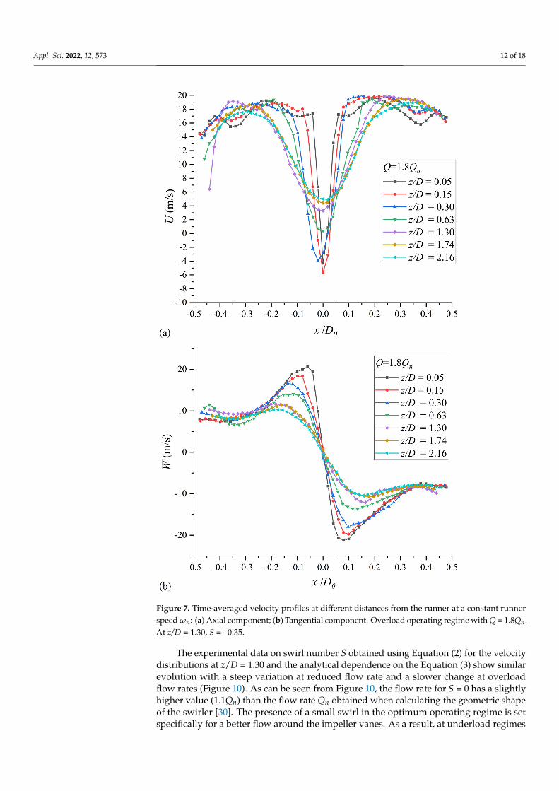
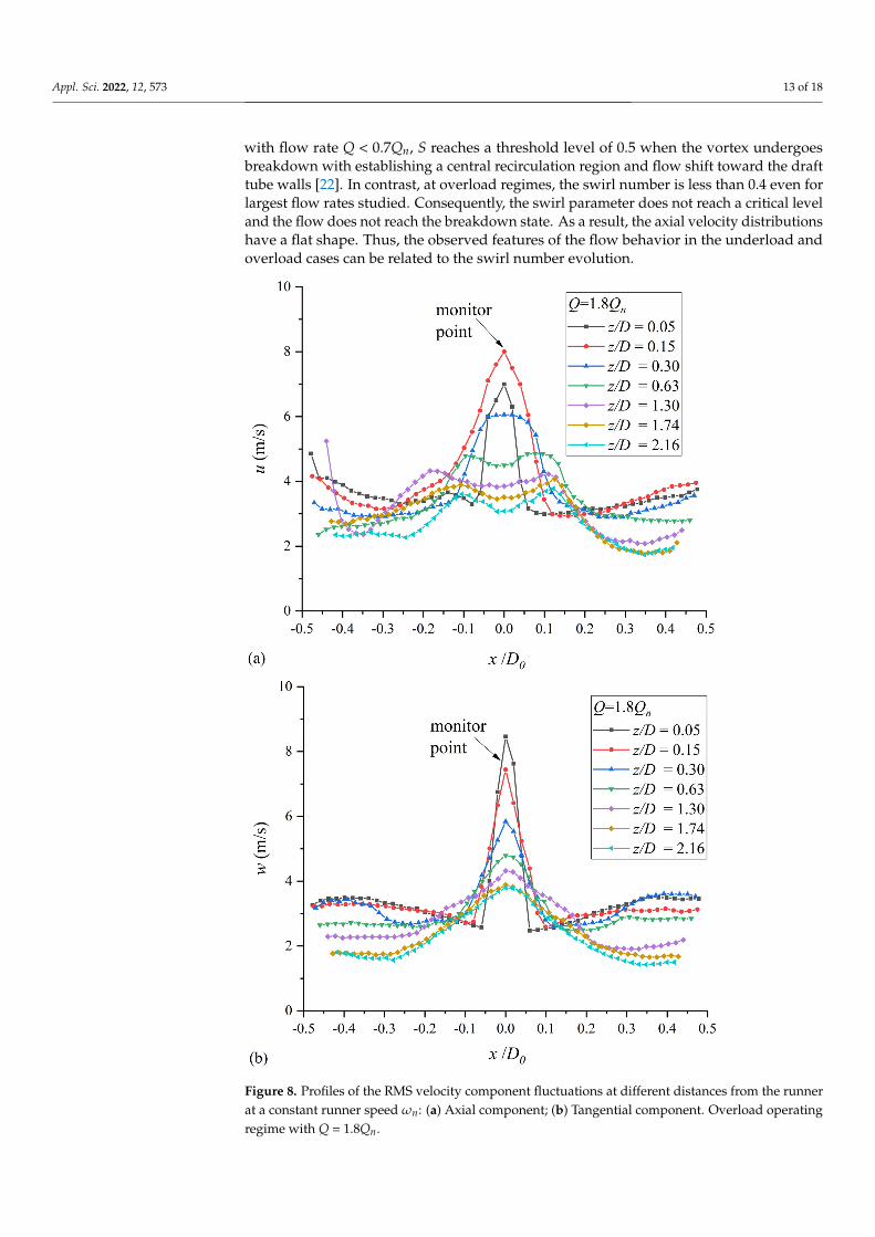
When the flow rate increases above the design value, overload occurs (Figure 7). Theswirl changes sign and the magnitude of the tangential velocity increases (Figure 7b),although S remains significantly lower in magnitude than in the underload case. As aresult, the formation of a central dip in the axial velocity profiles is observed only at largez (Figure 7a). At small z, a central peak occurs along the flow axis. In this flow structure,vorticity is localized near the flow axis, as evidenced by the proximity of the tangentialvelocity peaks to the flow axis. The tangential velocity peaks decrease in height and shiftsomewhat toward the side wall at large z, but a sharp expansion of the vortex flow, as in thecase of the underload case, does not occur. This indicates flow stabilization with formationof a vortex localized predominantly in the center. This vortex structure is in low-amplitudeprecessional motion, which is manifested in localized central peaks in the distributionsof fluctuations of the tangential velocity component (Figure 8b). Narrow central peaksalso appear in the RMS profiles of axial velocity fluctuations near the turbine (Figure 8a).With the exception of these central peaks, the RMS levels of both velocity components arerelatively low and evenly distributed over the flow cross-section.

Appl. Sci. 2022, 12, 573 9 of 18Appl. Sci. 2022, 12, x FOR PEER REVIEW 9 of 19

Figure 4. Profiles of the RMS velocity component at different distances from the runner at a constant runner speed ωn: (a) Axial component; (b) Tangential component. Part load regime with Q = 0.6Qn.

Figure 4. Profiles of the RMS velocity component at different distances from the runner at a constantrunner speed ωn: (a) Axial component; (b) Tangential component. Part load regime with Q = 0.6Qn.

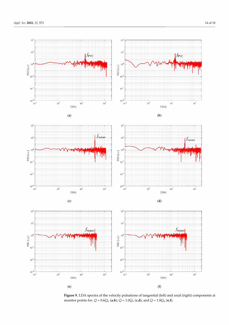
To characterize the frequency response of the flow for Q = 0.6, 1 and 1.8Qn, Figure 9shows power spectra of axial and tangential component of the time-dependent velocities atthe monitor points where they are dominated by vortex pulsations. Independent evidenceof attribution of these peaks to the PVC frequency was provided in previous work throughcross-checking measurements by LDA and acoustic probes [10]. It can be noticed in Figure 9that for Q = 0.6Qn, the PVC frequency is clearly indicated, while for regimes Q = Qn and1.8Qn, only peaks corresponding to the runner frequency have been observed. It can be

Appl. Sci. 2022, 12, 573 10 of 18

assumed that the runner frequency is not observed for Q = 0.6Qn due to the strong impactof PVC on velocity fluctuations. In other words, the frequency of runner is hidden by themagnitude of the pulsations. In cases with flow rates Qn and 1.8Qn, velocity fluctuationsincrease proportional to the increase in Re, and the influence of runner rotation becomesmore visible in the spectra.

Appl. Sci. 2022, 12, x FOR PEER REVIEW 10 of 19

Figure 5. Time-averaged velocity profiles at different distances from the runner at a constant runner speed ωn: (a) Axial component; (b) Tangential component. Operating regime with Q = Qn. At z/D = 1.30, S = 0.1.

Figure 5. Time-averaged velocity profiles at different distances from the runner at a constant runnerspeed ωn: (a) Axial component; (b) Tangential component. Operating regime with Q = Qn. Atz/D = 1.30, S = 0.1.

Appl. Sci. 2022, 12, 573 11 of 18Appl. Sci. 2022, 12, x FOR PEER REVIEW 11 of 19

Figure 6. Profiles of the RMS velocity component fluctuations at different distances from the runner at a constant runner speed ωn: (a) Axial component; (b) Tangential component. Operating regime with Q = Qn.

When the flow rate increases above the design value, overload occurs (Figure 7). The swirl changes sign and the magnitude of the tangential velocity increases (Figure 7b), although S remains significantly lower in magnitude than in the underload case. As a result, the formation of a central dip in the axial velocity profiles is observed only at large

Figure 6. Profiles of the RMS velocity component fluctuations at different distances from the runnerat a constant runner speed ωn: (a) Axial component; (b) Tangential component. Operating regimewith Q = Qn.

Appl. Sci. 2022, 12, 573 12 of 18

Appl. Sci. 2022, 12, x FOR PEER REVIEW 12 of 19

z (Figure 7a). At small z, a central peak occurs along the flow axis. In this flow structure, vorticity is localized near the flow axis, as evidenced by the proximity of the tangential velocity peaks to the flow axis. The tangential velocity peaks decrease in height and shift somewhat toward the side wall at large z, but a sharp expansion of the vortex flow, as in the case of the underload case, does not occur. This indicates flow stabilization with formation of a vortex localized predominantly in the center. This vortex structure is in low-amplitude precessional motion, which is manifested in localized central peaks in the distributions of fluctuations of the tangential velocity component (Figure 8b). Narrow central peaks also appear in the RMS profiles of axial velocity fluctuations near the turbine (Figure 8a). With the exception of these central peaks, the RMS levels of both velocity components are relatively low and evenly distributed over the flow cross-section.

Appl. Sci. 2022, 12, x FOR PEER REVIEW 13 of 19

Figure 7. Time-averaged velocity profiles at different distances from the runner at a constant runner speed ωn: (a) Axial component; (b) Tangential component. Overload operating regime with Q = 1.8Qn. At z/D = 1.30, S = –0.35.

Figure 7. Time-averaged velocity profiles at different distances from the runner at a constant runnerspeed ωn: (a) Axial component; (b) Tangential component. Overload operating regime with Q = 1.8Qn.At z/D = 1.30, S = –0.35.

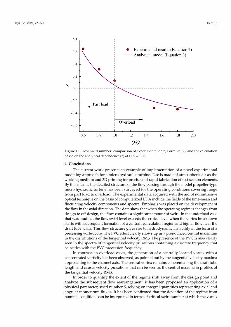
The experimental data on swirl number S obtained using Equation (2) for the velocitydistributions at z/D = 1.30 and the analytical dependence on the Equation (3) show similarevolution with a steep variation at reduced flow rate and a slower change at overloadflow rates (Figure 10). As can be seen from Figure 10, the flow rate for S = 0 has a slightlyhigher value (1.1Qn) than the flow rate Qn obtained when calculating the geometric shapeof the swirler [30]. The presence of a small swirl in the optimum operating regime is setspecifically for a better flow around the impeller vanes. As a result, at underload regimes

Appl. Sci. 2022, 12, 573 13 of 18

with flow rate Q < 0.7Qn, S reaches a threshold level of 0.5 when the vortex undergoesbreakdown with establishing a central recirculation region and flow shift toward the drafttube walls [22]. In contrast, at overload regimes, the swirl number is less than 0.4 even forlargest flow rates studied. Consequently, the swirl parameter does not reach a critical leveland the flow does not reach the breakdown state. As a result, the axial velocity distributionshave a flat shape. Thus, the observed features of the flow behavior in the underload andoverload cases can be related to the swirl number evolution.

Appl. Sci. 2022, 12, x FOR PEER REVIEW 13 of 19

Figure 7. Time-averaged velocity profiles at different distances from the runner at a constant runner speed ωn: (a) Axial component; (b) Tangential component. Overload operating regime with Q = 1.8Qn. At z/D = 1.30, S = –0.35.

Appl. Sci. 2022, 12, x FOR PEER REVIEW 14 of 19

Figure 8. Profiles of the RMS velocity component fluctuations at different distances from the runner at a constant runner speed ωn: (a) Axial component; (b) Tangential component. Overload operating regime with Q = 1.8Qn.

To characterize the frequency response of the flow for Q = 0.6, 1 and 1.8Qn, Figure 9 shows power spectra of axial and tangential component of the time-dependent velocities at the monitor points where they are dominated by vortex pulsations. Independent evidence of attribution of these peaks to the PVC frequency was provided in previous work through cross-checking measurements by LDA and acoustic probes [10]. It can be noticed in Figure 9 that for Q = 0.6Qn, the PVC frequency is clearly indicated, while for regimes Q = Qn and 1.8Qn, only peaks corresponding to the runner frequency have been observed. It can be assumed that the runner frequency is not observed for Q = 0.6Qn due to the strong impact of PVC on velocity fluctuations. In other words, the frequency of runner is hidden by the magnitude of the pulsations. In cases with flow rates Qn and 1.8Qn, velocity fluctuations increase proportional to the increase in Re, and the influence of runner rotation becomes more visible in the spectra.

The experimental data on swirl number S obtained using Equation (2) for the velocity distributions at z/D = 1.30 and the analytical dependence on the Equation (3) show similar evolution with a steep variation at reduced flow rate and a slower change at overload flow rates (Figure 10). As can be seen from Figure 10, the flow rate for S = 0 has a slightly higher value (1.1Qn) than the flow rate Qn obtained when calculating the geometric shape of the swirler [30]. The presence of a small swirl in the optimum operating regime is set specifically for a better flow around the impeller vanes. As a result, at underload regimes with flow rate Q < 0.7Qn, S reaches a threshold level of 0.5 when the vortex undergoes breakdown with establishing a central recirculation region and flow shift toward the draft tube walls [22]. In contrast, at overload regimes, the swirl number is less than 0.4 even for largest flow rates studied. Consequently, the swirl parameter does not reach a critical level and the flow does not reach the breakdown state. As a result, the axial velocity distributions have a flat shape. Thus, the observed features of the flow behavior in the underload and overload cases can be related to the swirl number evolution.

Figure 8. Profiles of the RMS velocity component fluctuations at different distances from the runnerat a constant runner speed ωn: (a) Axial component; (b) Tangential component. Overload operatingregime with Q = 1.8Qn.

Appl. Sci. 2022, 12, 573 14 of 18Appl. Sci. 2022, 12, x FOR PEER REVIEW 15 of 19

(a)

(b)

(c)

(d)

(e)

(f)

Figure 9. LDA spectra of the velocity pulsations of tangential (left) and axial (right) components atmonitor points for: Q = 0.6Qn (a,b); Q = 1.0Qn (c,d), and Q = 1.8Qn (e,f).

Appl. Sci. 2022, 12, 573 15 of 18

Appl. Sci. 2022, 12, x FOR PEER REVIEW 16 of 19

Figure 9. LDA spectra of the velocity pulsations of tangential (left) and axial (right) components at monitor points for: Q = 0.6Qn (a,b); Q = 1.0Qn (c,d), and Q = 1.8Qn (e,f).

Figure 10. Flow swirl number: comparison of experimental data, Formula (2), and the calculation based on the analytical dependence (3) at z/D = 1.30.

4. Conclusions The current work presents an example of implementation of a novel experimental

modeling approach for a micro hydraulic turbine. Use is made of atmospheric air as the working medium and 3D printing for precise and rapid fabrication of test section elements. By this means, the detailed structure of the flow passing through the model propeller-type micro hydraulic turbine has been surveyed for the operating conditions covering range from part load to overload. The experimental data acquired with the aid of nonintrusive optical technique on the basis of computerized LDA include the fields of the time-mean and fluctuating velocity components and spectra. Emphasis was placed on the development of the flow in the axial direction. The data show that when the operating regimes changes from design to off-design, the flow contains a significant amount of swirl. In the underload case that was studied, the flow swirl level exceeds the critical level when the vortex breakdown starts with subsequent formation of a central recirculation region and higher flow near the draft tube walls. This flow structure gives rise to hydrodynamic instability in the form of a precessing vortex core. The PVC effect clearly shows up as a pronounced central maximum in the distributions of the tangential velocity RMS. The presence of the PVC is also clearly seen in the spectra of tangential velocity pulsations containing a discrete frequency that coincides with the PVC precession frequency.

In contrast, in overload cases, the generation of a centrally located vortex with a concentrated vorticity has been observed, as pointed out by the tangential velocity maxima approaching to the channel axis. The central vortex remains coherent along the draft tube length and causes velocity pulsations that can be seen as the central maxima in profiles of the tangential velocity RMS.

In order to quantify the extent of the regime shift away from the design point and analyze the subsequent flow rearrangement, it has been proposed an application of a

Figure 10. Flow swirl number: comparison of experimental data, Formula (2), and the calculationbased on the analytical dependence (3) at z/D = 1.30.

4. Conclusions

The current work presents an example of implementation of a novel experimentalmodeling approach for a micro hydraulic turbine. Use is made of atmospheric air as theworking medium and 3D printing for precise and rapid fabrication of test section elements.By this means, the detailed structure of the flow passing through the model propeller-typemicro hydraulic turbine has been surveyed for the operating conditions covering rangefrom part load to overload. The experimental data acquired with the aid of nonintrusiveoptical technique on the basis of computerized LDA include the fields of the time-mean andfluctuating velocity components and spectra. Emphasis was placed on the development ofthe flow in the axial direction. The data show that when the operating regimes changes fromdesign to off-design, the flow contains a significant amount of swirl. In the underload casethat was studied, the flow swirl level exceeds the critical level when the vortex breakdownstarts with subsequent formation of a central recirculation region and higher flow near thedraft tube walls. This flow structure gives rise to hydrodynamic instability in the form of aprecessing vortex core. The PVC effect clearly shows up as a pronounced central maximumin the distributions of the tangential velocity RMS. The presence of the PVC is also clearlyseen in the spectra of tangential velocity pulsations containing a discrete frequency thatcoincides with the PVC precession frequency.

In contrast, in overload cases, the generation of a centrally located vortex with aconcentrated vorticity has been observed, as pointed out by the tangential velocity maximaapproaching to the channel axis. The central vortex remains coherent along the draft tubelength and causes velocity pulsations that can be seen as the central maxima in profiles ofthe tangential velocity RMS.

In order to quantify the extent of the regime shift away from the design point andanalyze the subsequent flow rearrangement, it has been proposed an application of aphysical parameter, swirl number S, relying on integral quantities representing axial andangular momentum fluxes. It has been confirmed that the deviation of the regime fromnominal conditions can be interpreted in terms of critical swirl number at which the vortex

Appl. Sci. 2022, 12, 573 16 of 18

breakdown occurs. This finding can assist the design of practical micro hydro turbineinstallations by determining the range of swirl number that does not lead to breakdown.

Author Contributions: Conceptualization, S.S. and D.W.; Formal analysis, E.G. and S.S.; Fundingacquisition, D.W.; Investigation, D.S.; Methodology, I.L. and D.W.; Project administration, D.W.;Resources, I.L. and S.S.; Software, I.L. and E.G.; Visualization, D.S.; Writing—original draft, D.S.and I.L.; Writing—review and editing, E.G., S.S. and D.W. All authors have read and agreed to thepublished version of the manuscript.

Funding: The work including measurements of flow characteristics and data analysis was carriedout with the state support of a contract with the Ministry of Education and Science of the RussianFederation (Agreement No. 075-15-2019-1923). The design and installation of the experimentalsetup was carried out partly within the framework of a state contract with IT SB RAS (Project No.121031800229-1).

Institutional Review Board Statement: Not applicable.

Informed Consent Statement: Not applicable.

Data Availability Statement: Not applicable.

Conflicts of Interest: The authors declare no conflict of interest.

Abbreviations

d diameter of the runner hub, 40 (mm)D, 2R diameter of the cone, 100 (mm)D0 diameter of the cross-section in which velocity measurements are made (mm)f PVC precession frequency of the PVC (Hz)f runner frequency of the impeller, 37.9 (Hz)H length of the cone, 280 (mm)K axial flux of the axial momentumM axial flux of the angular momentumQ flow rate (m3/s)Q0 flow rate corresponding to zero swirl number SQi flow rate obtained by integrating the axial velocity along the cone cross-section (m3/s)Qn flow rate for BEP regime, 0.049 (m3/s)Re Reynolds numberS swirl numberU axial averaged velocity (m/s)u root mean square (RMS) of axial velocity fluctuations (m/s)W tangential averaged velocity (m/s)w root mean square (RMS) of tangential velocity fluctuations (m/s)x, y, z Cartesian coordinatesωn runner speedBEP Best Efficiency PointLDA laser-Doppler anemometerMHT microhydrotubinesPVC precessing vortex corePSD Power Spectral Density

References1. Elbatran, A.H.; Yaakob, O.B.; Ahmed, Y.M.; Shabara, H.M. Operation, Performance and Economic Analysis of Low Head

Micro-Hydropower Turbines for Rural and Remote Areas: A Review. Renew. Sustain. Energy Rev. 2015, 43, 40–50. [CrossRef]2. Manders, T.N.; Höffken, J.I.; van der Vleuten, E.B.A. Small-Scale Hydropower in the Netherlands: Problems and Strategies of

System Builders. Renew. Sustain. Energy Rev. 2016, 59, 1493–1503. [CrossRef]3. Erinofiardi; Gokhale, P.; Date, A.; Akbarzadeh, A.; Bismantolo, P.; Suryono, A.F.; Mainil, A.K.; Nuramal, A. A Review on Micro

Hydropower in Indonesia. Energy Procedia 2017, 110, 316–321. [CrossRef]4. Punys, P.; Kvaraciejus, A.; Dumbrauskas, A.; Šilinis, L.; Popa, B. An Assessment of Micro-Hydropower Potential at Historic

Watermill, Weir, and Non-Powered Dam Sites in Selected EU Countries. Renew. Energy 2019, 133, 1108–1123. [CrossRef]

Appl. Sci. 2022, 12, 573 17 of 18

5. Berrada, A.; Bouhssine, Z.; Arechkik, A. Optimisation and Economic Modeling of Micro Hydropower Plant Integrated in WaterDistribution System. J. Clean. Prod. 2019, 232, 877–887. [CrossRef]

6. Haidar, A.M.A.; Senan, M.F.M.; Noman, A.; Radman, T. Utilization of Pico Hydro Generation in Domestic and Commercial Loads.Renew. Sustain. Energy Rev. 2012, 16, 518–524. [CrossRef]

7. Butchers, J.; Williamson, S.; Booker, J.; Tran, A.; Karki, P.B.; Gautam, B. Understanding Sustainable Operation of Micro-Hydropower: A Field Study in Nepal. Energy Sustain. Dev. 2020, 57, 12–21. [CrossRef]

8. Jawahar, C.P.; Michael, P.A. A Review on Turbines for Micro Hydro Power Plant. Renew. Sustain. Energy Rev. 2017, 72, 882–887.[CrossRef]

9. Hoghooghi, H.; Durali, M.; Kashef, A. A New Low-Cost Swirler for Axial Micro Hydro Turbines of Low Head Potential. Renew.Energy 2018, 128, 375–390. [CrossRef]

10. Druzhinin, A.A.; Orlova, E.S.; Volkov, A.V.; Parygin, A.G.; Naumov, A.V.; Ryzhenkov, A.V.; Vikhlyantsev, A.A.; Šoukal, J.; Sedlar,M.; Komárek, M.; et al. Enhancing the Efficiency of Small-Scale and Microhydroturbines Using Nature-Imitation Technologies forthe Development of Autonomous Energy Sources. Therm. Eng. 2019, 66, 944–952. [CrossRef]

11. Williamson, S.J.; Stark, B.H.; Booker, J.D. Low Head Pico Hydro Turbine Selection Using a Multi-Criteria Analysis. Renew. Energy2014, 61, 43–50. [CrossRef]

12. IEA. World Energy Outlook 2017; IEA: Paris, France, 2017.13. Lahimer, A.A.; Alghoul, M.A.; Sopian, K.; Amin, N.; Asim, N.; Fadhel, M.I. Research and Development Aspects of Pico-Hydro

Power. Renew. Sustain. Energy Rev. 2012, 16, 5861–5878. [CrossRef]14. Qian, Z.; Wang, F.; Guo, Z.; Lu, J. Performance Evaluation of an Axial-Flow Pump with Adjustable Guide Vanes in Turbine Mode.

Renew. Energy 2016, 99, 1146–1152. [CrossRef]15. Shtork, S.I.; Suslov, D.A.; Litvinov, I.V.; Gorelikov, E.Y. Analysis of the Flow Structure in the Model of a Microhydraulic Turbine. J.

Appl. Mech. Tech. Phys. 2020, 61, 807–813. [CrossRef]16. Nishi, Y.; Kobayashi, Y.; Inagaki, T.; Kikuchi, N. The Design Method of Axial Flow Runners Focusing on Axial Flow Velocity

Uniformization and Its Application to an Ultra-Small Axial Flow Hydraulic Turbine. Int. J. Rotating Mach. 2016, 2016, 5390360.[CrossRef]

17. Kaunda, C.S.; Kimambo, C.Z.; Nielsen, T.K. A Technical Discussion on Microhydropower Technology and Its Turbines. Renew.Sustain. Energy Rev. 2014, 35, 445–459. [CrossRef]

18. Chen, J.; Engeda, A. Design and Development of an Ultra Low Head Axial Hydro Turbine for Electricity Supply: Part II. InFluid Machinery; Erosion, Slurry, Sedimentation; Experimental, Multiscale, and Numerical Methods for Multiphase Flows; Gas-Liquid,Gas-Solid, and Liquid-Solid Flows; Performance of Multiphase Flow Systems; Micro/Nano-Fluidics, Proceedings of the Fluids EngineeringDivision Summer Meeting, Montreal, QC, Canada, 15 July 2018; American Society of Mechanical Engineers: New York, NY, USA,2018; Volume 3, p. V003T12A002.

19. Nishi, Y.; Kobori, T.; Kobayashi, Y.; Inagaki, T.; Kikuchi, N. Study on Foreign Body Passage in an Ultra-Small Axial Flow HydraulicTurbine. IJFMS 2020, 13, 68–78. [CrossRef]

20. Trivedi, C.; Dahlhaug, O.G. A Comprehensive Review of Verification and Validation Techniques Applied to Hydraulic Turbines.Int. J. Fluid Mach. Syst. 2019, 12, 345–367. [CrossRef]

21. Minakov, A.V.; Platonov, D.V.; Litvinov, I.V.; Shtork, S.I.; Hanjalic, K. Vortex Ropes in Draft Tube of a Laboratory KaplanHydroturbine at Low Load: An Experimental and LES Scrutiny of RANS and DES Computational Models. J. Hydraul. Res. 2017,55, 668–685. [CrossRef]

22. Litvinov, I.; Shtork, S.; Gorelikov, E.; Mitryakov, A.; Hanjalic, K. Unsteady Regimes and Pressure Pulsations in Draft Tube of aModel Hydro Turbine in a Range of Off-Design Conditions. Exp. Therm. Fluid Sci. 2018, 91, 410–422. [CrossRef]

23. Goyal, R. Vortex Core Formation in a Francis Turbine during Transient Operation from Best Efficiency Point to High Load. Phys.Fluids 2020, 32, 074109. [CrossRef]

24. Litvinov, I.; Suslov, D.; Gorelikov, E.; Shtork, S. Experimental Study of Transient Flow Regimes in a Model Hydroturbine DraftTube. Energies 2021, 14, 1240. [CrossRef]

25. Falvey, H.T. Draft Tube Surges; US Bureau of Reclamation Report, REC-ERC-71-42; Bureau of Reclamation: Washington, DC, USA,1971.

26. Palde, U.J. Influence of Draft Tube Shape on Surging Characteristics of Reaction Turbines; Hydraulics Branch, Division of GeneralResearch, Engineering and Research Center, US Department of the Interior, Bureau of Reclamation: Washington, DC, USA, 1972.

27. Povh, I.L. Aerodynamic Experiment in Machinery, 3rd ed.; Mashinostroenie: Leningrad, Russia, 1974; 479p.28. Nishi, M.; Yoshida, K.; Yano, M.; Okamoto, M.; Miyagawa, K.; Liu, S. A Preliminary Study on the Swirling Flow in a Conical

Diffuser with Jet Issued at the Center of the Inlet. In Proceedings of the 2nd IAHR International Meeting of the Workgroup onCavitation and Dynamic Problems in Hydraulic Machinery and Systems, Timisoara, Romania, 24–26 October 2007.

29. Yassi, Y.; Hashemloo, S. Improvement of the Efficiency of the Agnew Micro Hydro Turbine at Part Loads Due to Installing GuideVanes Mechanism. Energy Convers. Manag. 2010, 51, 1970–1975. [CrossRef]

30. Sonin, V.; Ustimenko, A.; Kuibin, P.; Litvinov, I.; Shtork, S. Study of the Velocity Distribution Influence upon the PressurePulsations in Draft Tube Model of Hydro-Turbine. IOP Conf. Ser. Earth Environ. Sci. 2016, 49, 082020. [CrossRef]

Appl. Sci. 2022, 12, 573 18 of 18

31. Yanta, W.; Smith, R. Measurements of Turbulence-Transport Properties with a Laser Doppler Velocimeter. In Proceedings of the11th Aerospace Sciences Meeting, Washington, DC, USA, 10 January 1973; American Institute of Aeronautics and Astronautics:Washington, DC, USA, 1973.

32. Skripkin, S.; Tsoy, M.; Kuibin, P.; Shtork, S. Swirling Flow in a Hydraulic Turbine Discharge Cone at Different Speeds andDischarge Conditions. Exp. Therm. Fluid Sci. 2019, 100, 349–359. [CrossRef]

33. Litvinov, I.V.; Sharaborin, D.K.; Shtork, S.I. Reconstructing the Structural Parameters of a Precessing Vortex by SPIV and AcousticSensors. Exp. Fluids 2019, 60, 139. [CrossRef]

34. Favrel, A.; Gomes Pereira Junior, J.; Landry, C.; Müller, A.; Nicolet, C.; Avellan, F. New Insight in Francis Turbine CavitationVortex Rope: Role of the Runner Outlet Flow Swirl Number. J. Hydraul. Res. 2018, 56, 367–379. [CrossRef]

35. Syred, N. A Review of Oscillation Mechanisms and the Role of the Precessing Vortex Core (PVC) in Swirl Combustion Systems.Prog. Energy Combust. Sci. 2006, 32, 93–161. [CrossRef]

36. Martinelli, F.; Olivani, A.; Coghe, A. Experimental Analysis of the Precessing Vortex Core in a Free Swirling Jet. Exp. Fluids 2007,42, 827–839. [CrossRef]