Technical Report Documentation Page 1. Report No. FWHA/TX-02/4240-1 2. Government Accession No. 3. Recipient’s Catalog No. 4. Title and Subtitle LABORATORY AND FIELD PROCEDURES FOR MEASURING THE SULFATE CONTENT OF TEXAS SOILS 5. Report Date October 2002 6. Performing Organization Code 7. Author(s) John Pat Harris, Tom Scullion and Stephen Sebesta 8. Performing Organization Report No. Report 4240-1 10. Work Unit No. (TRAIS) 9. Performing Organization Name and Address Texas Transportation Institute The Texas A&M University System College Station, Texas 77843-3135 11. Contract or Grant No. Project No. 0-4240 13. Type of Report and Period Covered Research: May 2001 - May 2002 12. Sponsoring Agency Name and Address Texas Department of Transportation Research and Technology Implementation Office P. O. Box 5080 Austin, Texas 78763-5080 14. Sponsoring Agency Code 15. Supplementary Notes Research performed in cooperation with the Texas Department of Transportation and the U.S. Department of Transportation, Federal Highways Administration. Research Project Title: Develop Guidelines and Procedures for Stabilization of Sulfate Soils 16. Abstract Project 0-4240 was initiated to provide guidelines on how to effectively stabilize sulfate rich soils. The first tasks in this project involved evaluating the various methods of measuring the sulfate content of soils both in the laboratory and in the field. In the laboratory, two test procedures were investigated, namely Texas Department of Transportation (TxDOT) Test Method Tex-620-J gravimetric approach and the Ion Chromatography approach. For this comparison, control samples with known sulfate contents were fabricated in the laboratory. The samples were treated with known amounts of fine-grained and coarse- grained sulfate crystals. A range of samples was sent to TxDOT and several private laboratories. In terms of both accuracy and repeatability, the researchers concluded that the Ion Chromatography approach is superior to TxDOT Test Method Tex-620-J. Recommendations are submitted to improve the Tex-620-J procedure. The main conclusion is that TxDOT should consider replacing Tex-620-J with the Ion Chromatography approach. Sulfate swell problems are frequently localized, so substantial effort was placed on evaluating rapid field tests. Four potential tests were evaluated, two were found to provide good results. Both the Colorimetric/Spectrophotometric and Conductivity tests should be considered for full-scale implementation. A survey of both automated and map systems revealed that the existing geological maps provide a good first-cut indication of locations with potentially high sulfate contents. The automated Soil Survey Geographic (SSURGO) maps hold great potential for future use, however, they are available for less than half of the Texas districts and some errors and inconsistencies were found. 17. Key Words Sulfates, Soils, Stabilization, Ion Chromatography, Field Testing, Highways, Laboratory Tests 18. Distribution Statement No restrictions. This document is available to the public through NTIS: National Technical Information Service 5285 Port Royal Road Springfield, Virginia 22161 19. Security Classif.(of this report) Unclassified 20. Security Classif.(of this page) Unclassified 21. No. of Pages 100 22. Price Form DOT F 1700.7 (8-72) Reproduction of completed page authorize

Welcome message from author
This document is posted to help you gain knowledge. Please leave a comment to let me know what you think about it! Share it to your friends and learn new things together.
Transcript

Technical Report Documentation Page 1. Report No.
FWHA/TX-02/4240-1
2. Government Accession No.
3. Recipient’s Catalog No.
4. Title and Subtitle
LABORATORY AND FIELD PROCEDURES FOR MEASURING THE SULFATE CONTENT OF TEXAS SOILS
5. Report Date
October 2002
6. Performing Organization Code
7. Author(s)
John Pat Harris, Tom Scullion and Stephen Sebesta
8. Performing Organization Report No.
Report 4240-1 10. Work Unit No. (TRAIS)
9. Performing Organization Name and Address
Texas Transportation Institute The Texas A&M University System College Station, Texas 77843-3135
11. Contract or Grant No.
Project No. 0-4240 13. Type of Report and Period Covered
Research: May 2001 - May 2002
12. Sponsoring Agency Name and Address
Texas Department of Transportation Research and Technology Implementation Office P. O. Box 5080 Austin, Texas 78763-5080
14. Sponsoring Agency Code
15. Supplementary Notes
Research performed in cooperation with the Texas Department of Transportation and the U.S. Department of Transportation, Federal Highways Administration. Research Project Title: Develop Guidelines and Procedures for Stabilization of Sulfate Soils 16. Abstract
Project 0-4240 was initiated to provide guidelines on how to effectively stabilize sulfate rich soils. The first tasks in this project involved evaluating the various methods of measuring the sulfate content of soils both in the laboratory and in the field. In the laboratory, two test procedures were investigated, namely Texas Department of Transportation (TxDOT) Test Method Tex-620-J gravimetric approach and the Ion Chromatography approach. For this comparison, control samples with known sulfate contents were fabricated in the laboratory. The samples were treated with known amounts of fine-grained and coarse-grained sulfate crystals. A range of samples was sent to TxDOT and several private laboratories. In terms of both accuracy and repeatability, the researchers concluded that the Ion Chromatography approach is superior to TxDOT Test Method Tex-620-J. Recommendations are submitted to improve the Tex-620-J procedure. The main conclusion is that TxDOT should consider replacing Tex-620-J with the Ion Chromatography approach. Sulfate swell problems are frequently localized, so substantial effort was placed on evaluating rapid field tests. Four potential tests were evaluated, two were found to provide good results. Both the Colorimetric/Spectrophotometric and Conductivity tests should be considered for full-scale implementation. A survey of both automated and map systems revealed that the existing geological maps provide a good first-cut indication of locations with potentially high sulfate contents. The automated Soil Survey Geographic (SSURGO) maps hold great potential for future use, however, they are available for less than half of the Texas districts and some errors and inconsistencies were found. 17. Key Words
Sulfates, Soils, Stabilization, Ion Chromatography, Field Testing, Highways, Laboratory Tests
18. Distribution Statement
No restrictions. This document is available to the public through NTIS: National Technical Information Service 5285 Port Royal Road Springfield, Virginia 22161
19. Security Classif.(of this report)
Unclassified
20. Security Classif.(of this page)
Unclassified
21. No. of Pages
100
22. Price
Form DOT F 1700.7 (8-72) Reproduction of completed page authorize


LABORATORY AND FIELD PROCEDURES FOR MEASURING THE SULFATE CONTENT OF TEXAS SOILS
by
John Pat Harris Associate Research Scientist
Texas Transportation Institute
Tom Scullion Research Engineer
Texas Transportation Institute
and
Stephen Sebesta Assistant Transportation Researcher
Texas Transportation Institute
Report 4240-1 Project Number 0-4240
Research Project Title: Develop Guidelines and Procedures for Stabilization of Sulfate Soils
Sponsored by the Texas Department of Transportation
In Cooperation with the U.S. Department of Transportation Federal Highway Administration
October 2002
TEXAS TRANSPORTATION INSTITUTE The Texas A&M University System College Station, Texas 77843-3135


v
DISCLAIMER
The contents of this report reflect the views of the authors, who are responsible for the
facts and the accuracy of the data presented herein. The contents do not necessarily reflect the
official view or policies of the Federal Highway Administration (FHWA) or the Texas
Department of Transportation (TxDOT). This report does not constitute a standard,
specification, or regulation. The engineer in charge was Tom Scullion, P.E. (# 62683).

vi
ACKNOWLEDGMENTS
Dr. German Claros, P.E., and Mr. Robert E. Boykin, P.E., from TxDOT are Program
Coordinator and Project Director, respectively, of this important project and have been active in
providing direction to the research team. Project Advisors, including Mr. Richard Williammee,
P.E., Mr. Mike Arellano, P.E., and Mr. Maurice Pittman, P.E., of TxDOT and Mr. Jim Cravens,
P.E., of FHWA have also been active in assisting the researchers. Both TxDOT and the FHWA
provide funds for this project.

vii
TABLE OF CONTENTS
Page List of Figures ................................................................................................................................ ix
List of Tables.................................................................................................................................. xi
Chapter 1. Introduction .................................................................................................................. 1
Chapter 2. Sulfate Content Determination - Lab Test .................................................................... 3
Background ........................................................................................................................ 3
Gravimetric Analysis .......................................................................................................... 4
Ion Chromatography Analysis ........................................................................................... 4
Testing Procedure ............................................................................................................... 5
Results with Manufactured Soils ....................................................................................... 7
Results from Field Samples .............................................................................................. 15
Discussion ........................................................................................................................ 15
Conclusions ...................................................................................................................... 19
Chapter 3. Sulfate Content Determination - Rapid Field Test ................................................... 21
Introduction ...................................................................................................................... 21
Background ...................................................................................................................... 22
Conductivity Theory ........................................................................................................ 24
Colorimetry Theory .......................................................................................................... 24
Testing Procedure ............................................................................................................. 25
Conductivity Test ............................................................................................................. 25
Acetone Test ..................................................................................................................... 28
Barium Chloride Test ....................................................................................................... 29
Colorimetry/Spectrophotometry ....................................................................................... 30
Sulfide Test ...................................................................................................................... 32
Results with Manufactured Soils ..................................................................................... 33
Results with Field Samples .............................................................................................. 39
Discussion ........................................................................................................................ 40
Conclusions ...................................................................................................................... 44
Chapter 4. Maps of Sulfate Soils .................................................................................................. 45
Use of Existing Geological Atlas of Texas ..................................................................... 46

viii
Extent of Eagle Ford Formation in Texas ........................................................................ 50
Digitized Soils Maps for Dallas and Fort Worth .............................................................. 50
Field Evaluation of Existing Digitized Maps ................................................................... 57
Conclusions ...................................................................................................................... 59
Chapter 5. Recommendations ...................................................................................................... 61
Laboratory Tests................................................................................................................ 61
Rapid Field Tests .............................................................................................................. 62
Maps ................................................................................................................................. 62
References ..................................................................................................................................... 65
Appendix A: Definition of Soil Data Elements ........................................................................... 67
Appendix B: Recommended Test Procedure for Sulfate Soils .................................................... 83

ix
LIST OF FIGURES
Figure Page
1. Known Sulfate Content vs. Laboratory Determined Sulfate Content. ................................ 9
2. Mean Error and Percent Error for Three Laboratories...................................................... 10
3. Chemical Lime Lab Results. ............................................................................................. 11
4. Lab Determined Sulfate Concentrations for Four Laboratories........................................ 13
5. Sulfate Measurements Using Tex-620-J and I.C. ............................................................. 14
6. Gypsum Filled Fractures in the Eagle Ford Formation on U.S. 82................................... 21
7. Accumet Model AR50 pH/Conductivity Meter ................................................................ 26
8. Burrell Model 75 Shaker for Conductivity Measurements ............................................... 27
9. Equipment Required for Acetone Field Test Kit ............................................................. 28
10. Filtrate of Samples from U.S. 82, Sherman, Texas........................................................... 29
11. Equipment Required for Barium Chloride Field Test Kit................................................. 30
12 Equipment Required for Colorimetry/Spectrophotometry Field Test Kit ...................... 32
13. Equipment Required for the Sulfide Test Kit.................................................................... 33
14. Conductivity vs Time Measurements for Treated Samples .............................................. 35
15. Effect of Pulverizing Coarse-Grained Gypsum ................................................................ 36
16. Effect of pH on Conductivity Measurements.................................................................... 37
17. Trends Observed Using Low and High pH Samples ........................................................ 38
18. Correlation of Experimental Soil Concentrations to a Calibration Curve ........................ 39
19. Hypothetical Curves.......................................................................................................... 41
20. Colorimetric Results with Tex-620-J Results ................................................................... 43
21. Recent Sulfate Heave Problems on Texas Highways ....................................................... 48
22. Excerpts from the Geological Atlas of Texas, Showing Locations of Failures
on the Eagle Ford Formation. Scale: 1:250,000............................................................... 49
23. Shaded Area Showing the Approximate Distribution of the High Sulfate Eagle Ford
Formation in Texas............................................................................................................ 51
24. Near Surface (0-4 feet) Sulfate Levels in Tarrant County (Cox, 2002)............................ 53
25. Sulfate Levels at Depths Greater than 4 feet in Tarrant County (Cox, 2002)................... 54
26. Near Surface (0-4 feet) Sulfate Levels in Dallas County (Cox, 2002) ............................. 55

x
27. Sulfate Levels at Depths Greater than 4 feet in Dallas County (Cox, 2002) .................... 56
28. TxDOT Developed Digital Map of FM 8 Project ............................................................ 58

xi
LIST OF TABLES
Table Page
1. Manufactured Samples Used for the Initial Comparison of
Sulfate Analysis Techniques ............................................................................................... 6
2. Description of Samples Used for the Follow-Up Sulfate Analysis Techniques ................ 7
3. Data Received from the First Round of Testing with TxDOT, TAMU
(El Paso), and Ana-Lab ....................................................................................................... 8
4. Sulfate Content and Error for Four Laboratories (Second Round Samples) .................... 12
5. Sulfate Content from U.S. 82 Field Samples ................................................................... 15
6. Number of Tests Needed for Tex-620-J vs Ion Chromatography for
Specified Allowable Error ................................................................................................ 18
7. Precision Statistics for Test Method Tex-620-J ............................................................... 19
8. Precision Statistics for Ion Chromatography ................................................................... 19
9. Comparison of Conductivity Results from TxDOT and TTI ........................................... 34
10. Rapid Field Test Results of Soils from U.S. 82 ............................................................... 40


1
CHAPTER 1
INTRODUCTION
Several TxDOT district offices have experienced problems with stabilizing soils
containing high sulfate concentrations when treated with traditional calcium-based stabilizers.
Project 0-4240 was initiated to provide guidelines to effectively treat these problem soils. This
is the first report for this on-going project, and it will cover the first three tasks in the work plan.
The main focus of this report is to recommend methods of measuring the sulfate content of soils
both in the laboratory and in the field.
In the laboratory, two test procedures were investigated: (1) TxDOT Test Method Tex-
620-J gravimetric approach, and (2) the Ion Chromatography approach. Chapter 2 of this report
describes the laboratory comparisons. For this comparison control samples with known sulfate
contents were fabricated in the laboratory. The samples were treated with fine-grained and
coarse-grained gypsum crystals. Samples with a range of concentrations were sent to TxDOT
and several private laboratories.
Many of the cases investigated in Texas revealed that sulfate problems occur in small
localized areas. It is not uncommon to have one or two sulfate-induced heaves in a project,
which may be several miles long. Currently there are no procedures in widespread use that can
be used to locate these localized problem areas prior to application of the stabilizer. Chapter 3 of
this report presents an evaluation of five rapid tests, which can be run in a matter of minutes.
The development and implementation of rapid field testing procedures is one of the major
objectives of this project and is the area where the researchers have spent most of their effort in
the first phase of this project.
Chapter 4 describes an evaluation of the usefulness of the currently available geological
and automated maps to detect high sulfate locations along Texas highways. The U.S.
Department of Agriculture (USDA) maps are widely used within TxDOT, but they provide little
information on the sulfate content of Texas soils. However, this project found that the existing
Geological Atlas of Texas can be used to detect areas which are rich in sulfates. These maps are
being used in two current forensic investigations on U.S. 82 in the Paris District and IH 40 in the
Childress District. The geological maps are known and used by engineers in both the Dallas and
Fort Worth Districts, however, they are not used in districts outside the metroplex that are known
to have similar problem soil types.


3
CHAPTER 2
SULFATE CONTENT DETERMINATION – LAB TEST
BACKGROUND
Over the past 20 years, problems with sulfate-induced heave have surfaced around the
world. This problem occurs when lime or cement is used to stabilize subgrade soils that bear
sulfate/sulfide minerals. Hunter (1989) determined that the cause of heaving is due to the
formation of two minerals that contain a large amount of water in their structure and result in a
volume increase: one is called ettringite (Ca6Al2(SO4)3(OH)12·26H2O) and the other is called
thaumasite (Ca3(SO4)(CO3)[Si(OH)6]·12H2O). Another mechanism is created by the oxidation
of iron sulfides resulting in the formation of gypsum (CaSO4·2H2O). This reaction forms a
mineral that occupies more space than the original reduced sulfide, similar to the formation of
ettringite and thaumasite, and may cause heaving due to an increase in volume as well (Dubbe et
al., 1997).
It is critical to be able to accurately determine the sulfur concentrations in soils since
sulfur is the key ingredient for forming these deleterious reaction products.
Studies of sulfate-bearing soils conducted by Texas Transportation Institute (TTI) in the
past have yielded conflicting results for the amount of sulfate present in a soil. After reviewing
TxDOT Test Method Tex-620-J some questions were raised about the technique. They are:
• How long to dry the sample in the oven?
• Does the pH of the solution need to be measured?
• Is the 1:10 dilution ratio enough for soils with high sulfate concentrations?
• Is it a valid technique to heat the sample for 24 hours since gypsum solubility is
greater at lower temperatures as with lime and calcite?
Based on this information, researchers proposed to compare results of two laboratory test
methods for quantitative determination of sulfate concentrations. The two methods proposed
were TxDOT Test Method Tex-620-J and a procedure published by the Environmental
Protection Agency (EPA) in EPA/600/2-78/054 Field and Laboratory Methods Applicable to

4
Overburdens and Minesoils. Once the project started, researchers discovered that commercial
labs had stopped using the EPA method in favor of faster techniques involving Ion
Chromatography (IC).
Therefore, a laboratory using Ion Chromatography for sulfate analysis was solicited to
participate in this study. The lab initially selected was the Texas Agricultural Experiment
Station-El Paso (TAMU-EP); later another lab Chemical Lime Lab in Fort Worth that uses Ion
Chromatography volunteered its services.
Two labs that use Test Method Tex-620-J were also solicited for this project. The
Materials and Pavement Section of the Construction Division of TxDOT agreed to test the
samples as did Ana-Lab Corporation a commercial lab located in Kilgore, Texas.
GRAVIMETRIC ANALYSIS
Test Method Tex-620-J is a gravimetric technique where the element or ion of interest
may be precipitated as a compound and weighed. From the weight of the precipitate, the
quantity of the element or ion present can be calculated. More specifically, the Tex-620-J
method involves dissolving the sulfates present in the soil with distilled water heated to near
boiling. The sample is then filtered and concentrated hydrochloric acid (HCl) is added to the
filtrate and heated to near boiling. A 10 percent barium chloride (BaCl2·2H2O) solution is added
to the mixture and heated again. The sulfate is removed from solution as barium sulfate (BaSO4)
precipitates. The precipitate is filtered and washed with water to remove chlorides, dried, and
weighed. The sulfate concentration can be calculated as a percentage of the formula weight of
the BaSO4.
ION CHROMATOGRAPHY ANALYSIS
Ion Chromatography involves dissolving the sulfate from the soil in distilled water and
adding small quantities to the IC system. The sample is injected into the system in a fixed
volume and swept through the system by an inert compound like polyetheretherketone. The
sample is transported into an ion exchange column where the different ions are attracted to the
resin in the column and released at different times by a conductivity detector. The conductivity
of each solution is measured and compared to conductivities of prepared standards to quantify
5
the concentration for the ion(s) of interest. These analyses may be performed rapidly and at low
cost with an automated system.
TESTING PROCEDURE
To test the adequacy of the two techniques for quantifying the sulfate concentrations,
samples were prepared with known concentrations of sulfate-bearing minerals. The
“manufactured soils” contained 30 percent Georgia Kaolinite and a 70 percent combination of St.
Peter Sand and various grain sizes of gypsum or anhydrite (CaSO4).
Twenty-two samples were sent to three labs. The gypsum samples had the following
concentrations of sulfate in parts per million (ppm): 0, 3000, 5000, 12,000, and 50,000. The
gypsum was also submitted in two size fractions; one passing the #200 sieve and the other
passing the #10 sieve and retained on the #40 sieve. These size fractions were chosen because
they are representative of the more reactive sulfates found in natural soils in Texas. For example,
the larger the grains, the longer it takes for them to dissolve and react (similar to powdered sugar
dissolving faster than sugar cubes in a cup of coffee). Reagent grade anhydrite was also
submitted in concentrations of 5000 and 12,000 ppm. All of the samples were submitted in
duplicate (Table 1).
In the initial testing, 600 g of each concentration were prepared and split into 50 to 100 g
subsamples and shipped to three of the four labs previously listed for analysis. The Chemical
Lime Association Lab was given different samples to test at lower sulfate levels (Table 1)
because it volunteered its services after the initial results had been evaluated from the other labs,
and the Project Monitoring Committee (PMC) decided that lower concentrations of sulfate
needed to be detected.
Because results from the initial batch received from each lab were somewhat ambiguous,
another batch of samples was sent out. The second batch was mixed at lower concentrations as
suggested by the PMC. Samples with concentrations of 0, 1000, 2000, and 3000 ppm gypsum
were submitted in duplicate, as well as two-size fractions, for a total of 14 samples to all four
labs (Table 2).
In the second round of testing, individual mixing of each sample ensured that there was
not any segregation of sulfate in the samples (to ensure that all labs received the same

6
Table 1. Manufactured Samples Used for the Initial Comparison of Sulfate Analysis Techniques.
Sample Name
Sulfate Concentration (ppm)
Description
EXP 1 3000 Reagent grade gypsum EXP 2 5000 Reagent grade gypsum EXP 3 12000 Reagent grade gypsum EXP 4 50000 Reagent grade gypsum EXP 5 0 Control sample EXP 6 5000 Reagent grade anhydrite EXP 7 12000 Reagent grade anhydrite EXP 8 5000 Gypsum large grain (<#10>#40 sieve) EXP 9 3000 Gypsum large grain (<#10>#40 sieve) EXP 10 50000 Gypsum large grain (<#10>#40 sieve) EXP 11 12000 Gypsum large grain (<#10>#40 sieve) EXP 12 0 Control sample EXP 13 5000 Reagent grade gypsum EXP 14 50000 Reagent grade gypsum EXP 15 3000 Reagent grade gypsum EXP 16 12000 Reagent grade gypsum EXP 17 5000 Reagent grade anhydrite EXP 18 12000 Reagent grade anhydrite EXP 19 50000 Gypsum large grain (<#10>#40 sieve) EXP 20 12000 Gypsum large grain (<#10>#40 sieve) EXP 21 5000 Gypsum large grain (<#10>#40 sieve) EXP 22 3000 Gypsum large grain (<#10>#40 sieve) *EX 23 12000 Reagent grade gypsum *EX 24 5000 Reagent grade gypsum *EX 25 2000 Reagent grade gypsum *EX 26 1000 Reagent grade gypsum *EX 27 500 Reagent grade gypsum *EX 28 250 Reagent grade gypsum *EX 29 100 Reagent grade gypsum *EX 30 50 Reagent grade gypsum *EX 31 0 Control sample *EX 32 0 Control sample *EX 33 12000 Gypsum large grain (<#10>#40 sieve) *EX 34 5000 Gypsum large grain (<#10>#40 sieve) *EX 35 2000 Gypsum large grain (<#10>#40 sieve) *EX 36 1000 Gypsum large grain (<#10>#40 sieve)
All labs except the Chemical Lime Association Lab received samples EXP 1 to EXP 22. The Chemical Lime Association lab received the samples labeled EX 23 to EX 36 and denoted with an asterisk(*).

7
Table 2. Description of Samples Used for the Follow-Up Sulfate Analysis Techniques.
Sample Name
Sulfate Concentration (ppm)
Description
1a 2000 Reagent grade gypsum 2a 3000 Gypsum large grain (<#10>#40sieve) 3a 1000 Reagent grade gypsum 4a 0 Control sample 5a 3000 Reagent grade gypsum 6a 1000 Gypsum large grain (<#10>#40sieve) 7a 2000 Reagent grade gypsum 8a 3000 Gypsum large grain (<#10>#40sieve) 9a 0 Control sample 10a 1000 Reagent grade gypsum 11a 2000 Gypsum large grain (<#10>#40sieve) 12a 1000 Gypsum large grain (<#10>#40sieve) 13a 3000 Reagent grade gypsum 14a 2000 Gypsum large grain (<#10>#40sieve)
concentrations of sulfates). For instance, the initial set of samples were mixed as a single batch
and divided into three equal fractions to send to each of the three labs. It is possible that a 1000
ppm sulfate sample sent to one lab could have higher or lower sulfates than the 1000 ppm sulfate
sample sent to another lab due to heterogeneous mixing.
Following testing of the “manufactured soils,” in-situ soil samples were selected from an
area on U.S. 82 in the Paris District. This area is currently under construction and has
experienced problems with sulfate heave. Researchers selected 12 samples from the westbound
lane of this new construction project. Selection was based on conductivity readings taken in the
field. Samples with high and low conductivities were delivered to the four laboratories to see
how the various techniques compared using real soils.
RESULTS WITH MANUFACTURED SOILS
Table 3 and Figures 1 and 2 are the results of the initial round of testing where samples
were submitted only to the Texas Department of Transportation, Texas Agricultural Experiment
Station-El Paso and Ana-Lab Corporation. Because the Chemical Lime Lab did not participate
in the initial testing, its results are presented separately in Figure 3. A second round

8
Table 3. Data Received from the First Round of Testing with TxDOT, TAMU (El Paso) and Ana-Lab.
This data show how the lab-determined concentrations compare with the actual concentrations. All of the concentrations are in ppm. Samples labeled Anhydrite are CaSO4. Samples labeled Coarse-Grained are gypsum (CaSO4·2H2O) that passes #10 and are retained on the #40 sieve. Fine-Grained samples are gypsum (CaSO4·2H2O) and all pass the #200 sieve. These data were used to generate the graphs in Figures 1 and 2. of testing was performed by all four labs, and results are presented in Table 4 and Figure 4.
Figure 5 is a plot of all sulfate measurements up to 12,000 ppm comparing the Texas Department
of Transportation Test Method Tex-620-J to the Ion Chromatography technique.
In Figures 1, 3, and 4, the sulfate content of the manufactured samples determined by
each lab has been divided into coarse-grained gypsum (<#10>#40 sieve) and fine-grained
gypsum (<#200 sieve) because the labs (except Ana-Lab) generally had more difficulty detecting
all of the coarse-grained sulfates. This difficulty is shown by a larger deviation from the known
Lab Sulfate Content Data (all in PPM)
DescriptionKnown
Concentration TxDOT Error % Error TAMU Error % Error AnaLab Error % Error
Anhydrite 5000 6845 1845 36.9 4431 -569 -11.38 3600 -1400 -28Anhydrite 5000 4623 -377 -7.54 4451 -549 -10.98 3000 -2000 -40Anhydrite 12000 17626 5626 46.88333 9643 -2357 -19.64167 9400 -2600 -21.66667Anhydrite 12000 11865 -135 -1.125 9022 -2978 -24.81667 9300 -2700 -22.5
Coarse-Grained 3000 1783 -1217 -40.56667 1372 -1628 -54.26667 2400 -600 -20Coarse-Grained 3000 1742 -1258 -41.93333 2812 -188 -6.266667 900 -2100 -70Coarse-Grained 5000 2291 -2709 -54.18 2703 -2297 -45.94 4900 -100 -2Coarse-Grained 5000 2922 -2078 -41.56 4654 -346 -6.92 3800 -1200 -24Coarse-Grained 12000 4033 -7967 -66.39167 6238 -5762 -48.01667 9100 -2900 -24.16667Coarse-Grained 12000 3923 -8077 -67.30833 5965 -6035 -50.29167 15000 3000 25Coarse-Grained 50000 7421 -42579 -85.158 7367 -42633 -85.266 37000 -13000 -26Coarse-Grained 50000 6598 -43402 -86.804 6925 -43075 -86.15 47000 -3000 -6
Fine-Grained 0 412 412 48 48 0 0Fine-Grained 0 604 604 41.9 41.9 0 0Fine-Grained 3000 4019 1019 33.96667 2791 -209 -6.966667 2000 -1000 -33.33333Fine-Grained 3000 3402 402 13.4 2876 -124 -4.133333 2000 -1000 -33.33333Fine-Grained 5000 8285 3285 65.7 4932 -68 -1.36 4100 -900 -18Fine-Grained 5000 3964 -1036 -20.72 4774 -226 -4.52 3300 -1700 -34Fine-Grained 12000 16570 4570 38.08333 7172 -4828 -40.23333 8500 -3500 -29.16667Fine-Grained 12000 10672 -1328 -11.06667 6982 -5018 -41.81667 9800 -2200 -18.33333Fine-Grained 50000 24333 -25667 -51.334 7019 -42981 -85.962 47200 -2800 -5.6Fine-Grained 50000 23222 -26778 -53.556 6881 -43119 -86.238 40000 -10000 -20
Mean ValuesKnown
Concentration TxDOT Error % Error TAMU Error % Error AnaLab Error % Error
Anhydrite 5000 5734 734 14.68 4441 -559 -11.18 3300 -1700 -34Anhydrite 12000 14745.5 2745.5 22.87917 9332.5 -2667.5 -22.22917 9350 -2650 -22.08333Coarse-Grained 3000 1762.5 -1237.5 -41.25 2092 -908 -30.26667 1650 -1350 -45Coarse-Grained 5000 2606.5 -2393.5 -47.87 3678.5 -1321.5 -26.43 4350 -650 -13Coarse-Grained 12000 3978 -8022 -66.85 6101.5 -5898.5 -49.15417 12050 50 0.416667Coarse-Grained 50000 7009.5 -42990.5 -85.981 7146 -42854 -85.708 42000 -8000 -16Fine-Grained 0 508 508 44.95 44.95 0 0Fine-Grained 3000 3710.5 710.5 23.68333 2833.5 -166.5 -5.55 2000 -1000 -33.33333Fine-Grained 5000 6124.5 1124.5 22.49 4853 -147 -2.94 3700 -1300 -26Fine-Grained 12000 13621 1621 13.50833 7077 -4923 -41.025 9150 -2850 -23.75Fine-Grained 50000 23777.5 -26222.5 -52.445 6950 -43050 -86.1 43600 -6400 -12.8

9
Lab Sulfate Content of Soils Treated with Coarse-Grained Gypsum
0
10000
20000
30000
40000
50000
60000
0 10000 20000 30000 40000 50000 60000
Known Sulfate Content (ppm)
Lab
Sul
fate
Con
tent
(pp
m)
TxDOT - LG TAMU - LG AnaLab - LG Perfect Fit
Lab Sulfate Content of Soils Treated with Fine-Grained Gypsum
0
10000
20000
30000
40000
50000
60000
0 5000 10000 15000 20000 25000 30000 35000 40000 45000 50000 55000
Known Sulfate Content (ppm)
Lab
Sul
fate
Con
tent
(pp
m)
TxDOT TAMU AnaLab Perfect Fit
Figure 1. Known Sulfate Content vs. Laboratory Determined Sulfate Content.

10
Mean Errors in Sulfate Content Determination for Soils Treated with Coarse-Grained and Fine-Grained Gypsum
-45000
-35000
-25000
-15000
-5000
5000
0 10000 20000 30000 40000 50000
Known Content (ppm)
Err
or (
ppm
)
TxDOT TAMU AnaLab TxDOT - LG TAMU - LG AnaLAb - LG
Mean % Error for Coarse and Fine-Grained Sulfates
-100
-80
-60
-40
-20
0
20
40
0 10000 20000 30000 40000 50000 60000
Known Content (ppm)
Mea
n %
Err
or
TxDOT-LG TxDOT TAMU-LG TAMU AnaLab-LG AnaLab
Figure 2. Mean Error and Percent Error for Three Laboratories.

11
Chemical Lime Lab Sulfate Content Results
0
2000
4000
6000
8000
10000
12000
0 2000 4000 6000 8000 10000 12000
Known Content (ppm)
Lab
Con
tent
(pp
m)
R.G. L.G. Perfect Fit
Chemical Lime Lab Measurement Error
-2500
-2000
-1500
-1000
-500
0
500
0 2000 4000 6000 8000 10000 12000 14000
Known Content (ppm)
Err
or (
ppm
)
R.G. L.G.
Figure 3. Chemical Lime Lab Results.

12
Table 4. Sulfate Content and Error for Four Laboratories (Second Round Samples).
Since duplicate samples were sent to each lab, the lower part of the table lists averages of the two samples analyzed by each lab and represented in the graphs in Figure 4. LG is the coarse-grained gypsum, and RG is the fine-grained gypsum. concentration (Figures 1, 3, and 4). Figure 2 illustrates that both coarse (LG) and fine-grained
(RG) size samples have more error at higher concentrations.
Results of samples sent to the Chemical Lime lab are given in Figure 3. The fine-grained
sulfate gave good results, but the coarse-grained material was not fully dissolved.
Based on project experience, the Dallas/Ft. Worth Districts of the Texas Department of
Transportation currently do not use calcium-based stabilizers (lime, cement) for sulfate
concentrations above 2000 ppm; therefore, the second round of testing was focused on the ability
of the labs to detect lower concentrations of sulfate in the manufactured samples.
Sample # DescriptionKnown
Concentration TxDOT Error % Error TAMU Error % Error AnaLab Error % ErrorChem Lime Error % Error
12a LG 1000 2881 1881 188.1 1227 227 22.7 1060 60 6 1141 141 14.16a LG 1000 2675 1675 167.5 893 -107 -10.7 1080 80 8 1258 258 25.8
11a LG 2000 2702 702 35.1 1496 -504 -25.2 2500 500 25 1660 -340 -1714a LG 2000 3237 1237 61.85 1689 -311 -15.55 2150 150 7.5 1585 -415 -20.752a LG 3000 3964 964 32.13333 1602 -1398 -46.6 3830 830 27.66667 2497 -503 -16.766678a LG 3000 3031 31 1.033333 1752 -1248 -41.6 2150 -850 -28.33333 2409 -591 -19.7
10a RG 1000 1852 852 85.2 1407 407 40.7 670 -330 -33 1482 482 48.23a RG 1000 1920 920 92 1608 608 60.8 860 -140 -14 1535 535 53.51a RG 2000 2414 414 20.7 2370 370 18.5 1750 -250 -12.5 2241 241 12.057a RG 2000 3442 1442 72.1 3099 1099 54.95 910 -1090 -54.5 2385 385 19.25
13a RG 3000 3566 566 18.86667 3517 517 17.23333 2330 -670 -22.33333 3228 228 7.65a RG 3000 3374 374 12.46667 1606 -1394 -46.46667 2500 -500 -16.66667 3269 269 8.9666674a 0 7133 7133 228 228 210 210 700 7009a 0 5500 5500 314 314 180 180 658 658
Mean Values
DescriptionKnown
Concentration TxDOT Error % Error TAMU Error % Error AnaLab Error % ErrorChem Lime Error % Error
LG 1000 2778 1778 177.8 1060 60 6 1070 70 7 1199.5 199.5 19.95LG 2000 2969.5 969.5 48.475 1592.5 -407.5 -20.375 2325 325 16.25 1622.5 -377.5 -18.875LG 3000 3497.5 497.5 16.58333 1677 -1323 -44.1 2990 -10 -0.333333 2453 -547 -18.23333RG 1000 1886 886 88.6 1507.5 507.5 50.75 765 -235 -23.5 1508.5 508.5 50.85RG 2000 2928 928 46.4 2734.5 734.5 36.725 1330 -670 -33.5 2313 313 15.65RG 3000 3470 470 15.66667 2561.5 -438.5 -14.61667 2415 -585 -19.5 3248.5 248.5 8.283333
0 6316.5 6316.5 271 271 195 195 679 679

13
Average Sulfate Results, Coarse-Grained Gypsum
0
500
1000
1500
2000
2500
3000
3500
4000
0 500 1000 1500 2000 2500 3000 3500
Known Content (ppm)
Lab
Con
tent
(pp
m)
TAMU AnaLab Chem Lime Perfect Fit TxDOT
Average Sulfate Results, Fine-Grained Gypsum
0
1000
2000
3000
4000
5000
6000
7000
0 500 1000 1500 2000 2500 3000 3500
Known Content (ppm)
Lab
Con
tent
(pp
m)
TAMU Analab Chem Lime Perfect Fit TxDOT
Figure 4. Lab Determined Sulfate Concentrations for Four Laboratories.

14
Tex-620-J Results
0
2000
4000
6000
8000
10000
12000
14000
16000
18000
0 2000 4000 6000 8000 10000 12000 14000
Known Sulfate Content (ppm)
Tex
-620
-J R
esul
ts
Tex-620-J Perfect Fit
Ion Chromatography Results
0
2000
4000
6000
8000
10000
12000
14000
16000
18000
0 2000 4000 6000 8000 10000 12000 14000
Known Sulfate Content (ppm)
Lab
Res
ults
(pp
m)
Ion Chromatography Perfect Fit
Note: Excludes TAMU above 5000 ppm as dilution ratio was not sufficient
Figure 5. Sulfate Measurements Using Tex-620-J and I.C.

15
RESULTS FROM FIELD SAMPLES
Twelve samples from U.S. 82 in the Paris District, east of Sherman, Texas, were sent to
all four labs for sulfate measurements. Results are given in Table 5, which shows good
correlation between low- and high-sulfate levels. Since these are field samples where the true
sulfate content is unknown, one can only speculate on the true concentration.
Table 5. Sulfate Content from U.S. 82 Field Samples.
Sample Name TxDOT Sulfates (ppm)
Ana-Lab Sulfates (ppm)
Chemical Lime Sulfates (ppm)
TAMU Sulfates (ppm)
1596R 82 330 0 33
1597R 160 90 0 28
1603L 130 260 0 30
1612R 172 150 515 61
1612L 103 150 502 60
1613R 1299 1100 2125 2079
1613L 5797 1900 1669 693
1614R 526 380 807 358
1614L 398 470 704 190
1615R 151 100 529 84
1615L 302 230 638 174
1635L 503 810 1025 559
DISCUSSION
Figures 1, 3, and 4 illustrate the difficulty in measuring all of the coarse-grained gypsum.
TAMU-EP uses a standard method endorsed by the EPA that calls for passing the sample
through a 2 mm sieve. Sulfates in that coarse-size range will not all be dissolved, which results
in low, measured concentrations. In the fine-grained sulfates with concentrations of 3000 and
5000 ppm, TAMU-EP obtained very good results. At higher concentrations, TAMU-EP results
were extremely low because a 1:5 soil to distilled water dilution ratio was used. Using the
solubility data given by Burkart et al. (1999), a saturated solution of gypsum at 25 ºC and a 1:5
dilution ratio would contain 9100 ppm sulfate. This means that 9100 ppm is the maximum

16
amount of sulfate they could detect, so at concentrations of 12,000 and 50,000 ppm, their
numbers were far too low, consistent with a saturated sulfate solution (Table 1).
The Texas Department of Transportation and Chemical Lime labs also had difficulty
detecting all of the coarse-grained sulfates due to inefficient pulverization. Ana-Lab obtained
better results with the coarse-grained sulfates by using the traditional mortar and pestle to
pulverize samples; the samples were then passed through a #50 to #100 sieve, which resulted in
more consistent fine-grained particles. This process allowed better dissolution of the sulfate
minerals.
As observed in Figure 5, there is a larger spread in the data with the Tex-620-J method
than with the Ion Chromatography technique. There are numerous factors that can contribute to
such a large variation in results, some of which are listed below:
• Use only (ultrapure) trace metal grade HCl because a sulfate contribution from the acid
may result if anything less pure is used.
• Obtaining a finely ground representative sample is critical.
• Remove all of the particulates from the solution to avoid extra weight added from clays
and other minerals remaining in the system (Mohamed, May 2002).
• The rate at which barium chloride is added to the solution is critical. It needs to be added
slowly to ensure formation of fewer, larger barium sulfate crystals and to reduce the
coprecipitation of chloride (de la Camp and Seely, 2002).
• The sample digestion period needs to be at a consistent temperature and length of time to
ensure that barium sulfate has ample time to precipitate into crystals large enough to not
pass through the filter paper.
• When washing out the salts that form, use only ice cold water because hot water may
result in peptization (part of the precipitate reverts to the colloidal form) of the barium
sulfate (TAMU, 2002).
• Care must be taken to not lose sample when burning off filter paper with the meeker
burner (Coward, 2002).
• It is critical that the analytical balances are calibrated frequently. Some private labs
calibrate balances on a daily basis (Mohamed, 2002).

17
• Foreign anions (nitrate and chlorate) and cations (ferric iron, calcium, and alkali metals)
can be coprecipitated either with the barium sulfate or as substitutional impurities within
the barium sulfate crystals. This can cause a substantial error if these ions are present in
large concentrations (de la Camp and Seely, 2002).
TAMU-EP switched from gravimetric analysis to Ion Chromatography due to the time
requirement and all of the possible sources of error with gravimetric analysis; Dr. Abdul-Mehdi
(2002) stated that there are no interferences with the Ion Chromatography technique for sulfates.
Evaluation of the Texas Department of Transportation Test Method Tex-620-J for
determining soluble sulfates has been a challenge.
Both the Tex-620-J and Ion Chromatography technique appear to give reasonably
accurate results with repeated testing; i.e., the average of multiple test results is reasonably close
to the true sulfate content (see previous Figure 5). For Tex-620-J, the average test result was
approximately 8 percent below the true value for 1000 and 2000 ppm and approximately 18
percent below the true value for 3000, 5000, and 12,000 ppm. Being a gravimetric technique,
the errors in Tex-620-J could be due to incomplete dissolution of the gypsum, loss of sample
during the test procedure, and other operational or equipment errors covered above.
Average results from Ion Chromatography were low by approximately 6 percent, 9
percent, 12 percent, 16 percent, and 18 percent for 1000, 2000, 3000, 5000, and 12,000 ppm,
respectively. This is a decent improvement in accuracy when compared to Tex-620-J. To
thoroughly evaluate Ion Chromatography versus Tex-620-J, two quantitative analyses were
performed: 1) What is the required sample size to define, within a specified range, the 95 percent
confidence interval for the true sulfate content, and 2) What are the precision (repeatability and
reproducibility) statistics for each test method?
The appropriate sample size needed to define the 95 percent confidence interval for the
true sulfate content within plus or minus a certain range, E, is defined as (Jarrell, 1994):
2
96.1
=
E
Sn
where n = sample size (number of tests required)
S = standard deviation of test results
E = specified acceptable maximum error
18
This means if n tests are conducted, there is 95 percent confidence that the true sulfate
content is within ±E ppm of the average test result. The appropriate sample size is dependent on
the expected dispersion of test outcomes and the specified allowable range, E. For this analysis,
the standard deviation of test results was the estimator for S, and values of ±10 percent, ±20
percent, and ±30 percent were used for E. Table 6 shows the needed number of samples. In
general, fewer tests are required with Ion Chromatography, and in no cases were fewer tests
required with Tex-620-J. At lower levels of allowable error (i.e., greater desired accuracy), Ion
Chromatography offers a sizeable reduction in testing requirements. At higher levels of
allowable error of ±30 percent, there is not much of an appreciable difference in testing
requirements between the two techniques until the true sulfate content is at least 5000 ppm.
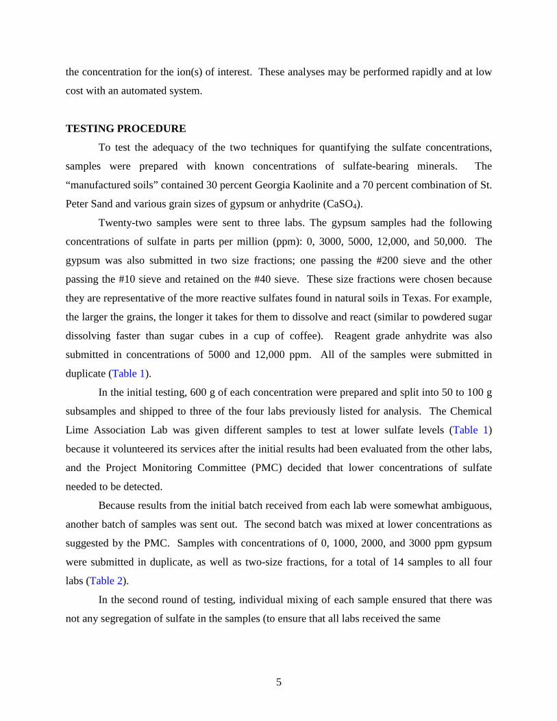
Table 6. Number of Tests Needed for Tex-620-J vs Ion Chromatography for Specified
Allowable Error. True SO4 Content (ppm)
�10% Tex-620-J
�10% Ion
Chrom.
�20% Tex-620-J
�20% Ion
Chrom.
�30% Tex-620-J
�30% Ion
Chrom. 1000 15 12 4 3 2 2 2000 45 33 11 9 5 4 3000 31 21 8 6 4 3 5000 43 14 11 4 5 2 12,000 46 7* 12 2* 6 1* * Estimate based on historic coefficient of variation due to lack of sample size at this concentration. The two sulfate test methods can also be compared by evaluating their precision.
Precision is defined as within lab repeatability and between lab reproducibility. The data
collected were processed using American Society of Testing and Materials (ASTM) E 691 to
develop the precision statistics. A more precise test method is indicated by a lower precision
statistic. The precision statistics presented in Table 7 (for Test Method Tex-620-J) and Table 8
(for Ion Chromatography) indicate that Ion Chromatography is a more precise test. For material
that is 3000 ppm, the only sulfate content at which sufficient data were available for comparison
between the test methods, the repeatability and reproducibility limits for Ion Chromatography
were approximately half that of Tex-620-J. For a given homogeneous material, the absolute
value of the difference between any two test results at the same lab is expected to be less than the

19
repeatability limit, r, for 95 percent of all observations. Similarly, the absolute value of the
difference between any two sulfate content results from different labs, on the same material, is
expected to be less than the reproducibility limit, R, for 95 percent of all observations. Further
discussion of precision is available in ASTM E 177.
Table 7. Precision Statistics for Test Method Tex-620-J.
Material X Sr SR r R 3000 ppm 2687 828 828 2318 2318 5000 ppm 4195 1617 1617 4528 4528 12,000 ppm 9700 2985 3667 8358 10,268 Note: This procedure calls for results from six labs using the same technique, however, this analysis is from only 2 labs since very few perform this test.
Table 8. Precision Statistics for Ion Chromatography. Material X Sr SR r R 1000 ppm 1319 145 169 406 473 2000 ppm 2065 273 365 764 1022 3000 ppm 2485 392 468 1098 1310 Note: This procedure calls for results from six labs using the same technique, however, this analysis is from only 2 labs. CONCLUSIONS
• Overall, Ion Chromatography is superior to the TxDOT Test Method Tex-620-J
gravimetric technique. It is more accurate and repeatable, requires less time, personnel
are not exposed to toxic chemicals, there is less interference from other constituents in
the soil, and the method is not as sensitive to individual operator biases; however, the
initial cost of the equipment is substantial.
• Detection of coarse-grained sulfates is dependent upon efficiency of pulverization.
• At higher concentrations of sulfate, a larger number of tests is required to obtain an
accurate sulfate concentration in the soil.
• The TxDOT Test Method TEX-620-J is valid, but there are multiple steps in the analysis
where error may be introduced by operation interpretation creating a large standard
deviation of test results. See recommendations in Chapter 5.


21
CHAPTER 3
SULFATE CONTENT DETERMINATION – RAPID FIELD TEST
INTRODUCTION
The purpose of this portion of the project was to pinpoint a technique that could be used
in the field to identify potential problems due to soils with high sulfate/sulfide concentrations.
Since many of the sulfate problems are localized within a small zone (Figure 6) a rapid field test
needs to be developed to identify these potential problem areas before or during construction.
The ink pen (Figure 6) is parallel to one of the filled fractures and shows how localized these
sulfate seams can be. To be useful in the field, the technique should be simple to run and yield
rapid results while the equipment should be portable and durable enough to withstand field-
operating conditions.
Figure 6. Gypsum Filled Fractures in the Eagle Ford Formation on U.S. 82.

22
An extensive literature review was performed to identify ways that sulfate and sulfide
testing is performed in soil environments. There are numerous techniques available to locate
sulfates, but most of them generally involve expensive and cumbersome equipment that is not
practical in a field environment. The researchers identified four techniques that hold promise for
working in the field. There is a scarcity of information available for sulfide determination useful
in a field environment, so only one technique was evaluated.
BACKGROUND
Bower and Huss (1948) published a paper using conductivity to measure sulfate content
in soils. Their procedure was to mix 10 to 20 g of air-dried soil with distilled water and agitate
continuously for 30 minutes, which dissolved the gypsum. Acetone was then added to re-
precipitate the gypsum. The re-precipitated gypsum was washed to remove salts (NaCl, etc.) and
then was re-dissolved in 40 ml of distilled water. The conductivity was then measured and
compared to a calibration curve to determine gypsum concentration in the soil.
The test, developed by Bower and Huss (1948), was adapted by the USDA as a
qualitative field test. It involved adding distilled water to 10 to 20 g of air-dried soil in an 8 oz
bottle and hand shaking six times at 15-minute intervals. The extract was filtered through
medium porosity filter paper. A test tube contained 5 ml of the extract, and an equal volume of
acetone was added to the extract. If a milky precipitate formed, then gypsum was present in the
soil.
The Department of Soil and Crop Sciences at Texas A&M University is also home to
many scientists with the Texas Agricultural Experiment Station (TAES), so the researchers
contacted them about how TAES analyzes for sulfates in soils. They use the Bower and Huss
(1948) technique to measure gypsum content in soils. One limitation of the technique is that it
only measures gypsum, not total sulfate, which may yield optimistic results. However, if calcite
is present in the soil then the gypsum content measured may be too high because calcite will
dissolve in distilled water and calcium ions will be available to react with other dissolved
sulfates to form gypsum. For our purposes, this limitation is actually an advantage because we
are interested in total sulfate and not just gypsum. The Eagle Ford Formation, which causes
many of Texas’ sulfate heave problems (Burkart et al., 1999), possesses abundant calcite in the
form of limestone. Therefore, other sulfate minerals that may be in the soil can form gypsum

23
when acetone is added because of the excess calcium that is supplied by the dissolution of
limestone. This will provide a better estimate of total sulfate.
Bredenkamp and Lytton (1995) proposed a simple field test to detect sulfates which
involved mixing the soil with distilled water and measuring the conductivity of the solution.
They hypothesized that high electrical conductivity would be due to the presence of soluble
sulfates. Researchers at TTI noted the following limitations:
• The current protocol calls for measurements to be taken immediately after
mixing; this could lead to underestimation of the problem with soils containing
large sulfate crystals which take longer to dissolve.
• Other salts may be present in the soil. This increases the conductivity in addition
to the sulfates, which will lead to overestimation of the problem.
• As discussed previously, sulfide minerals may be present in the soil and not be
detected by this technique, which will lead to an underestimation of the problem.
• A pH and temperature at which the test should be performed was not specified.
Gypsum is more soluble at low pH and low temperatures.
Two other rapid field techniques (colorimetric and barium chloride test) for sulfates were
identified by perusing the environmental testing and water quality sales literature. These tests
were designed for measuring sulfate concentrations in natural waters, but they may be adapted to
soils by dilution and filtration. They operate on the principles of colorimetry (measure degree of
absorption of light transmitted through the sample by human eye) or spectrophotometry (when
an instrument measures the light transmitted).
The lone sulfide technique is a “spot test” where one of the reactants is used in the form
of a solution. McClellan et al. (1998) identified one simple field test for sulfide sulfur from the
general chemical literature. The test involves adding solutions composed of sodium azide and
iodine to a sample that contains sulfides/pyrite. The sulfides do not participate in the reaction,
but they catalyze a reaction between sodium azide (NaN3) and iodine (I2) which evolves nitrogen
(N2) gas. The gas evolution can be observed as bubbles forming on the soil sample containing
sulfides (Feigl, 1958).

24
CONDUCTIVITY THEORY
The conductivity of a solution is a measure of how well a solution will carry a current
(i.e., pass electrons usually via ions). Two factors influence conductivity: first, the number of
displaceable electrons each ion carries (e.g., an anion with a –2 charge will carry twice as many
electrons as an anion with a –1 charge); second, the speed with which each ion travels through
the solution (Robinson, 1970).
Robinson (1970) lists six factors which influence the speed of the ion:
• the solvent (water or organic),
• the applied voltage,
• size of ion (larger ions less mobile),
• nature of the ion (if it becomes hydrated, then the effective size is increased),
• viscosity of solvent, and
• temperature of solvent.
The conductivity of a solution is the sum of the conductivities of the ions present;
therefore, it cannot distinguish between different types of ions. At higher concentrations the ions
may form some un-ionized molecules which will reduce the conductivity (Robinson, 1970).
COLORIMETRY THEORY
The theory behind colorimetry hinges on Beer’s law:
A = abc = log (Io/I1) A = absorbance
a = absorptivity of the sample
b = optical path length
c = concentration
Io = intensity of light entering solution
I1 = intensity of light emerging from solution
There is a linear relationship between absorbance and concentration of a solution if the
optical path length and wavelength of radiation remain constant. By measuring the ratio I1/Io
absorbance can be measured, therefore concentration can be calculated. Beer’s law usually holds
at low concentrations, but deviations are common at concentrations above �������������� ���
1970).

25
TESTING PROCEDURE
Based on the criteria of being quick, portable, and easy to perform, four rapid field sulfate
tests were identified, and one rapid field sulfide test was targeted for inclusion in this phase of
the project. The four sulfate tests include the conductivity test proposed by Bredenkamp and
Lytton (1995), the modified Bower and Huss (1948) Acetone Test proposed by the USDA, the
Barium Chloride Test, and the Colorimetry Test. The lone sulfide test that was evaluated was
one proposed by McClellan et al. (1998).
CONDUCTIVITY TEST
This phase of the research focused on answering questions regarding the conductivity test
proposed by Bredenkamp and Lytton (1995). Specific questions included:
• Was distilled water an efficient solvent for sulfates?
• Did sulfate grain size impact conductivity measurements?
• How could the test be sped up (i.e., pulverization, different solvents)?
• Was the test applicable to natural soil environments?
To answer these questions researchers developed a series of experiments using the same
lab-created “manufactured soils” samples that were shipped to the four laboratories for
quantitative sulfate analysis (Chapter 1, Tables 1 and 2).
All of the conductivity measurements performed in the lab and reported in the results
section were performed on an Accumet™ AR50 pH/Conductivity meter (Figure 7) equipped
with an Accumet (13-620-155) glass-bodied conductivity cell with a cell constant of 1.0 cm-1; an
external temperature probe was used for temperature compensation. Measurements of pH were
made using an Accu-pHast™ (13-620-296) glass-bodied combination electrode. The pH
electrode is on the left, and the conductivity cell and external temperature probe are located on
the right side of the instrument. Conductivity measurements made in the field were performed
with an Omega PHH-80™, pH/Conductivity meter.

26
Figure 7. Accumet Model AR50 pH/Conductivity Meter.
All of the samples were evaluated under identical conditions to ensure that the results
being compared were not due to procedural differences. The procedures are outlined below:
(1) Calibrate conductivity and pH meter per manufacturer’s instructions. Estimate
conductivity and pH, and calibrate with standards close to those estimates. For
example, a carbonate rich sample will be basic, so standardize pH with a pH 10
standard in addition to the pH 7 standard.
(2) Measure 5 g to the nearest 0.1 g of air-dried soil into a 125 ml (HDPE) Nalgene
brand bottle.
(3) Measure 100 g to the nearest 0.1 g of double-distilled water into the bottle.
(4) Place the samples onto a Burrell™ Model 75 wrist-action shaker (Figure 8) and
shake on the maximum setting for 1 minute.

27
(5) Remove the samples from the shaker and immediately take conductivity and pH
measurements with the Accumet Model AR50 pH/Conductivity Meter.
(6) After 50 minutes the samples were put on the wrist-action shaker for a period of 10
minutes, and were shaken at the maximum setting.
(7) Remove the samples from the shaker and immediately take conductivity and pH
measurements.
(8) This procedure was followed every hour up to 8 hours.
(9) The next day samples were placed on the wrist action shaker and shaken at the
maximum setting for 10 minutes, one time in the morning and one time in the
afternoon.
(10) Conductivity and pH were measured immediately after shaking.
(11) This procedure continued up to several days until conductivity had stabilized at a
constant value.
Figure 8. Burrell Model 75 Shaker for Conductivity Measurements.
Note: The 125 ml Nalgene Bottles Attached to the Shaker.

28
ACETONE TEST
This test was originally a quantitative technique developed by Bower and Huss (1948)
and modified by the USDA to be a rapid and inexpensive field technique for detecting sulfates
in soil (Figure 9). The procedures used for this technique are as follows:
(1) Add 10 g of air dry soil to a 250 ml (HDPE) Nalgene centrifuge bottle.
(2) Add 100 ml of double-distilled water to the 250 ml centrifuge bottle for a 1:10 ratio
of soil to solvent.
(3) Shake the sample for 15 minutes with the Burrell Model 75 wrist-action shaker at the
maximum shaking intensity.
(4) Filter the extract with a Whatman™ #42, 5-inch diameter filter paper into 250 ml
beakers. Centrifugation may be necessary with fine-grained soils to remove all
particulates from suspension.
(5) Place approximately 5 ml extract into 40 ml glass centrifuge tube (Figure 10).
(6) Add approximately 5 ml acetone to the solution in the centrifuge tube and agitate.
After 5 to 10 minutes a cloudy suspension or a white precipitate will be observed if
gypsum is present (Figure 10). This test will indicate the presence of gypsum, but it
is not quantitative. The sample on the right contains sulfate, and the sample on the
left does not.
Figure 9. Equipment Required for Acetone Field Test Kit.

29
Figure 10. Filtrate of Samples from U.S. 82, Sherman, Texas.
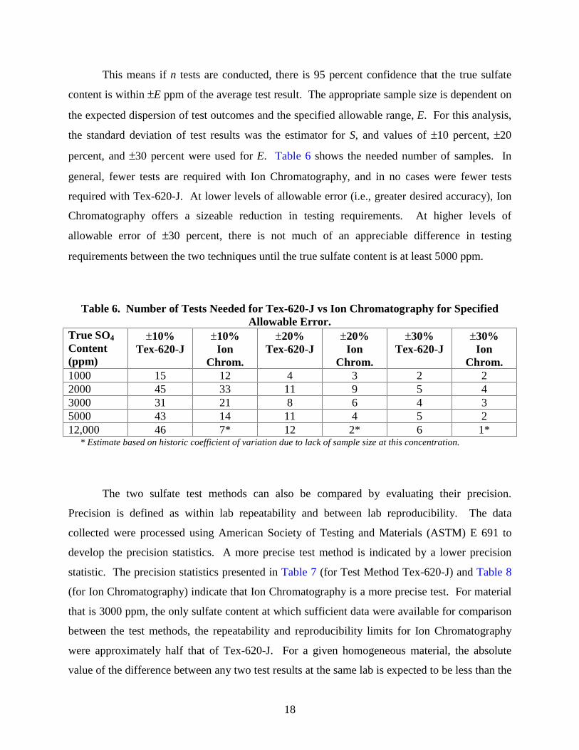
BARIUM CHLORIDE TEST
The barium chloride test is a true colorimetric technique because judgment of sulfate
concentration is based upon comparison with a chart (Figure 11). This test is somewhat
subjective since the human eye is used to judge the concentration. The procedure for this test is
written with respect to the equipment provided with the soil testing kit and is included in the kit.
The test procedure is as follows:
(1) Fill test tube to mark with Universal Extracting Solution (3 percent acetic acid and
10 percent sodium acetate with distilled water).
(2) Use orange soil measure to add one level measure of soil to test tube.
(3) Cap test tube and shake for one minute.
(4) Put filter paper in funnel and pour extract solution in funnel and collect filtrate.
(5) Use transfer pipette to add five drops of clear filtrate to turbidity vial.
(6) Add one drop of Sulfate Test Solution (0.2 percent HCl and 5 percent BaCl2·2H2O),
and gently swirl to mix.
30
(7) Lay sulfate color chart under neutral light. Hold turbidity vial 0.5 inch above black
strip in middle of chart. Look down through the turbid sample. Match sample
turbidity to a turbidity standard.
(8) Record as ppm sulfate.
Figure 11. Equipment Required for Barium Chloride Field Test Kit.
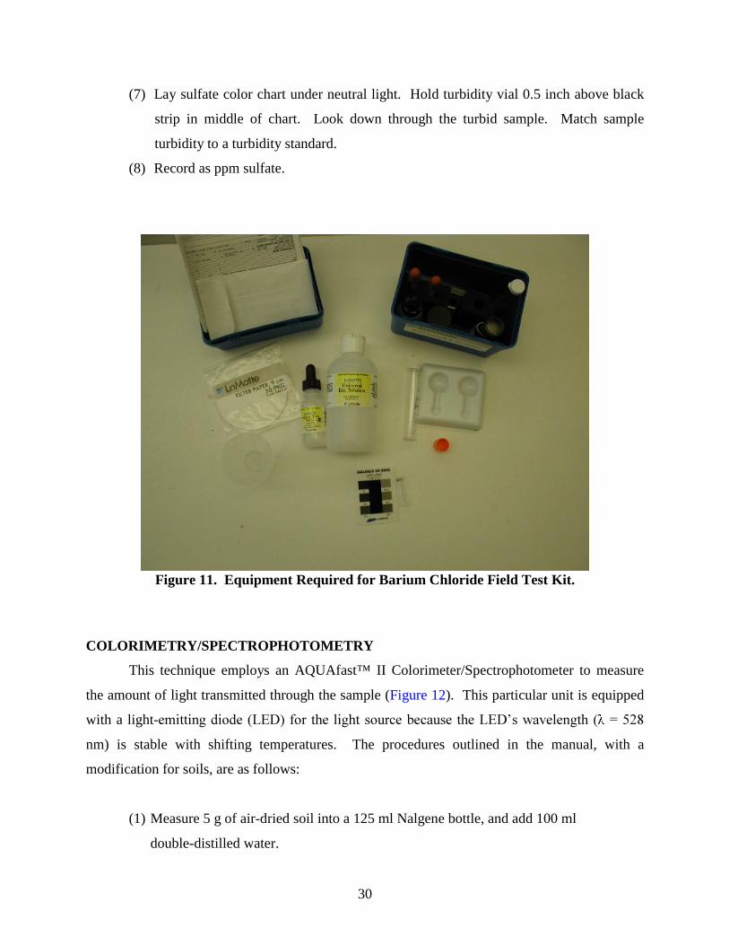
COLORIMETRY/SPECTROPHOTOMETRY
This technique employs an AQUAfast™ II Colorimeter/Spectrophotometer to measure
the amount of light transmitted through the sample (Figure 12). This particular unit is equipped
with a light-����������������������� ���������� ��������� ���������� ��� ��������� �!�"�#�
nm) is stable with shifting temperatures. The procedures outlined in the manual, with a
modification for soils, are as follows:
(1) Measure 5 g of air-dried soil into a 125 ml Nalgene bottle, and add 100 ml
double-distilled water.

31
(2) Shake on the Burrell wrist-action shaker for 15 minutes at maximum speed.
(3) Remove from shaker and filter with Whatman #42, 9.0 cm, filter paper into a 250 ml
beaker. Centrifugation may be necessary with fine-grained soils to remove all
particulates from suspension.
(4) Put on latex gloves.
(5) Fill sample vial with filtrate to the 10 ml mark and wipe vial clean with Kimwipes or
equivalent delicate task wipe.
(6) Switch the unit to “ON.”
(7) Press the MODE key until the desired method is displayed.
(8) $��������� ������ ������������ ���������������������� � �������%�����ned with the
��� �������%&
(9) Press the ZERO/TEST key. The method symbol flashes for approximately 3 seconds
and confirms zero calibration.
(10) After zero calibration, remove the vial from the sample chamber.
(11) Add sulfate tablet to vial without touching the tablet with hands and crush
immediately with white plastic rod provided. Always be consistent with the time and
amount of crushing.
(12) '��� ������������������(�������������� ���������������������� ����% ��������&
(13) Press the ZERO/TEST key. The method symbol flashes for approximately 3
seconds, and the result appears in the display. Take a minimum of three readings and
average.
• This test will only read concentrations from 5-200 mg/l. If (÷Err) message
appears, then the measuring range has been exceeded or there is excessive
turbidity. This will require diluting the sample with more double-distilled
water and measuring until the message disappears and there is a numerical
answer. If (-Err) message appears, then result is below the measuring range.

32
Figure 12. Equipment Required for Colorimetry/Spectrophotometry Field Test Kit. SULFIDE TEST
As discussed previously, sulfides weather to produce sulfate in near-surface
environments. A simple field test was described by McClellan et al. (1998), which requires
observation of gas bubbles evolved from the soil sample (Figure 13). A solution is prepared by
dissolving 3 g of NaN3 (sodium trinitride/sodium azide) in 100 ml of 0.1 N iodine solution.
Sodium azide and iodine do not react with each other under normal conditions, but when sulfide
is added to the solution, nitrogen gas is evolved. The following reaction theoretically takes
place:
2NaN3 + I2 ��)�*�+�,)2
The sulfide catalyzes the above reaction. The sodium azide reacts with the iodine, in the
presence of sulfide, to form sodium iodide and nitrogen gas (Feigl, 1958). The nitrogen gas is
observed as bubbles. This reaction does not occur if sulfides are not present in the sample.
Procedures for running this test are very simple and listed below:

33
(1) Mix sodium azide and iodine solution in the proportions listed above.
(2) Put a small sample of air-dried soil or crushed stone into porcelain spot plate
(Figure 13).
(3) Add 1 to 2 ml of iodine mix to spot plate with a disposable pipet.
(4) Look for bubbles forming in sample. If bubbles form, then there is sulfide in the
sample. A pocket magnifier or binocular microscope may be required to see the
bubbles. (Note: It takes some experience observing the evolution of N2 gas.)
Figure 13. Equipment Required for the Sulfide Test Kit. RESULTS WITH MANUFACTURED SOILS
Results were obtained from each of the four sulfate tests and the lone sulfide test using
“manufactured soil” samples, which emphasize evaluation of the conductivity test proposed by
Bredenkamp and Lytton (1995). Table 9 shows conductivity measurements performed on the
manufactured samples by TTI and TxDOT (Jim Kern, Dallas District Lab).

34
Table 9. Comparison of Conductivity Results from TxDOT and TTI.
Note: All measurements were made on unpulverized samples. Samples labeled coarse-grained are gypsum that passes #10 and are retained on the #40 sieve. Fine-grained samples are all gypsum and all pass the #200 sieve.
These samples were analyzed as received and not pulverized to evaluate the effect of
gypsum grain size on conductivity measurements. TxDOT results compared very well with TTI
initial conductivity measurements, however, there is no specification on the amount of shaking in
the procedure that TxDOT follows. The same procedure was followed at TTI, with the
exception of specifying a shaking time of 1 minute on a mechanical shaker before taking the
initial conductivity measurements. TxDOT made only initial measurements whereas TTI
performed measurements over time (Figure 14). The last column in Table 9 consists of final
conductivity measurements taken at TTI. Conductivity and pH measurements were taken every
hour for the first 8 hours followed by measurements two times a day up to 500 hours.
The top graph in Figure 14 shows how conductivity increases over time with the samples
containing coarse-grained gypsum. Note that the samples with lower concentrations of gypsum
result in lower conductivity values than samples bearing higher concentrations of gypsum. The
bottom graph illustrates how the samples bearing fine-grained gypsum reach equilibrium much
more rapidly than the coarse-grained samples.
Sample Comment
Known Sulfate Concentration
(ppm)
TxDOT Conductivity
(microsiemens)
TTI Initial Conductivity
(microsiemens)
TTI Final Conductivity
(microsiemens)
EX 5 0 11 29 123.4EX 12 0 13 26.7 112EX 9 coarse-grained 3000 38 81 409EX 22 coarse-grained 3000 44 25.4 217EX 1 fine-grained 3000 317 328 421EX 15 fine-grained 3000 325 318 375EX 6 anhydrite 5000 505 382 593EX 17 anhydrite 5000 503 517 577EX 21 coarse-grained 5000 49 48.6 499EX 8 coarse-grained 5000 38 76.8 528EX 2 fine-grained 5000 452 474 576EX 13 fine-grained 5000 459 599 666EX 7 anhydrite 12000 1029 958EX 18 anhydrite 12000 941 579 1031EX 11 coarse-grained 12000 72 140 1064EX 20 coarse-grained 12000 92 111 966EX 3 fine-grained 12000 1070 1036 1109EX 16 fine-grained 12000 950 1033 1036EX 10 coarse-grained 50000 412 338.7 2258EX 19 coarse-grained 50000 284 352 2222EX 4 fine-grained 50000 2200 2183 2311EX 14 fine-grained 50000 2400 2187 2279

35
Conductivity vs. Time for Samples Treated with Coarse-Grained Gypsum
0
500
1000
1500
2000
2500
0 100 200 300 400 500 600
Time (hours)
Con
duct
ivit
y (m
icro
siem
ens)
3000 ppm 5000 ppm 12000 jppm 50000 ppm
Conductivity vs. Time for Samples Treated with Fine-Grained and Coarse-Grained Gypsum
0
500
1000
1500
2000
2500
3000
0 5 10
Time (hours)
Con
duct
ivit
y (m
icro
siem
ens)
3000 ppm 5000 ppm 12000 ppm 50000 ppm
3000 ppm LG 5000 ppm LG 12000 ppm LG 50000 ppm LG
Figure 14. Conductivity vs Time Measurements for Treated Samples.

36
To measure the effectiveness of pulverization on reducing the time required for
conductivity to reach the maximum/equilibrium value, samples of coarse-grained gypsum at
various concentrations were pulverized with a mortar and pestle and passed through a #200 sieve
before mixing with double-distilled water and measuring conductivity. Figure 15 is a graph of
these data for gypsum retained on the #40 sieve and passing the #10 sieve at a concentration of
3000 ppm sulfate. The triangles represent the pulverized gypsum that was passed through the
#200 sieve. It is clear from this graph that pulverization helps achieve equilibrium much more
rapidly.
Coarse-Grained Gypsum (3000 ppm)
0
100
200
300
400
500
0 4 8
Time (hrs)
Con
duct
ivit
y (m
icro
siem
ens)
Gypsum (<10>40 sieve) Gypsum (<10>40 sieve) Gypsum (<200 sieve)
Figure 15. Effect of Pulverizing Coarse-Grained Gypsum.

37
To determine the effect of pH on conductivity measurements, manufactured soils with
concentrations of 0, 1000, 2000, 3000, 5000, and 12,000 ppm sulfate were treated with pyrite
(pH=4.0-4.5) or calcite (pH=8.5-9.0). Pyrite (FeS2) and calcite (CaCO3) were used because they
are natural minerals that occur in rocks from Texas and naturally make the soil more acidic and
basic, respectively. Sposito (1989) listed the pH range for naturally occurring soils between a
pH of 3 to 9.5 so our lab-generated specimens fall within the upper and lower limits of this
range. As illustrated in Figure 16, both high and low pH increase the conductivity over the
neutral pH sample (triangles). Figure 17 shows that both low and high pH samples follow the
same trend observed with the neutral pH samples. When the sulfate content increases, the
conductivity increases as well.
Calcite vs. Pyrite at 12,000 ppm Sulfate Content
600
1000
1400
1800
0 10 20 30 40 50
Time (hrs)
Con
duct
ivit
y (m
icro
siem
ens)
Calcite Pyrite Untreated
Figure 16. Effect of pH on Conductivity Measurements.

38
Pyrite (low pH)
200
600
1000
1400
1800
0 10 20 30 40 50
Time (hrs)
Con
duct
ivit
y (m
icro
siem
ens)
0 ppm Sulfate 1000 ppm 2000 ppm 3000 ppm 5000 ppm 12,000 ppm
Calcite (high pH)
200
600
1000
1400
1800
0 10 20 30 40 50
Time (hrs)
Con
duct
ivit
y (m
icro
siem
ens)
0 ppm Sulfate 1000 ppm 2000 ppm 3000 ppm 5000 ppm 12,000 ppm
Figure 17. Trends Observed Using Low and High pH Samples.

39
Conductivity of sulfate standards was measured to generate a calibration curve
(Figure 18) showing conductivity versus sulfate content. The manufactured soils correlated well
with the calibration curve.
Lab Soils Conductivity withConductivity Calibration Curve
0
200
400
600
800
1000
1200
1400
1600
1800
2000
0 5000 10000 15000 20000 25000
Sulfate Content (ppm)
Con
duct
ivit
y (m
icro
siem
ens)
Calibration Curve Experimental Soils
Figure 18. Correlation of Experimental Soil Concentrations to a Calibration Curve.
RESULTS WITH FIELD SAMPLES
Tests on natural soils from three projects in different parts of the state judged the
adequacy of the rapid field techniques. The first sample was from the Childress District on
IH40, east of Shamrock, Texas, where they experienced a heave problem (Table 10). The
second sample was from the Fort Worth District. The third sample was from a new construction
project in the Paris District on U.S. 82, east of Sherman, Texas.

40
Table 10. Rapid Field Test Results of Soils from U.S. 82.
Sample Name
Acetone (1:20 dilution)
Sulfide Colorimeter SO4
-2 (ppm) Initial Conductivity � ��
Final Conductivity � ��
1596R N.D. Very Little 0 40 55
1597R N.D. Very Little 0 40 59
1603L N.D. N.D. 160 40 53
1612R N.D. N.D. 0 40 94
1612L N.D. N.D. 180 40 61
1613R N.D. N.D. 1800 50 219
1613L Precipitate N.D. 3960 20 178
1614R N.D. N.D. 780 30 217
1614L N.D. N.D. 760 20 152
1615R N.D. Minor 100 30 76
1615L N.D. Minor 100 30 68
1635L Precipitate N.D. >4000 50 403
Note: Barium chloride test was not performed on these samples due to the high carbonate content of these soils. N.D. = not detected; Precipitate = precipitate of sulfates in the sample.
DISCUSSION
Conductivity measurements are easily performed and consistent results can be obtained
between different laboratories (Table 9). Comparison of initial conductivity measurements made
by TTI with TxDOT results show a very good correlation. As discussed in the background, all
of the factors affecting conductivity can be easily controlled so the possible error is minimal, as
long as the same techniques are followed. Conductivity measurements are affected by a dirty or
improperly calibrated cell, or a malfunctioning meter. Temperature fluctuations can also cause
conductivity measurements to drift and not yield a stable reading; therefore, this is a good reason
for not cooling the sample below ambient temperature to increase gypsum solubility. The
conductivity reading will not stabilize until the temperature of the solution reaches equilibrium
with the air temperature.
In a search for obtaining faster dissolution of sulfates for conductivity measurements, an
acidic and basic solvent was tried to enhance the sulfate solubility. A lime-saturated solution
(pH ��-�&.���������,����������(� ������������������ �������� �� ���� �����������/��������

41
pH solvents, respectively. High ionic concentrations due to the presence of hydrogen and
hydroxyl ions resulted in lower conductivity measurements because complexes formed in the
solution which decreased the conductivity. Therefore, using a high pH or low pH solvent to
enhance sulfate solubility is not advisable. The acidic and basic solvent could also lead to
solubilizing other minerals, which would contribute to the conductivity. For instance, at high
pH’s (above �� -�&"�� ��� ������ ���� �������-bearing phases are soluble (Krauskopf, 1967).
These ions are liberated from the soil and become a part of the solution which will add to the
conductivity until the concentration is high enough for molecules to start forming, thus reducing
the conductivity. The lesson learned here is that use of high and low pH solvents only
complicates conductivity determinations.
The researchers believe that conductivity measurements with double-distilled water over
an extended time period are beneficial for determining relative grain size of the soluble sulfates.
Figure 19 is a group of hypothetical curves generated showing conductivity profiles for three
different sulfate scenarios, which illustrate how conductivity measurements over time without
pulverization may give an indication of sulfate grain size and could affect how the soil is
stabilized. The upper curve is composed of fine-grained sulfates that dissolve in distilled water
rapidly and would react very quickly with lime/cement stabilization to form deleterious products.
The middle curve is representative of coarse-grained sulfates that take longer to dissolve. These
sulfates would still react with traditional stabilizers, but may take longer to show up. The lower
curve indicates that sulfates are not a problem for stabilization.
Conductivity vs Time
0500
100015002000
0 2 4 6 8 10
Time (hr)
Con
duct
ivit
y (m
icro
siem
ens)
Good Large Grained Bad Fine Grained Bad
Figure 19. Hypothetical Curves.

42
The colorimetric technique (light transmitted through a sample) should be run under
exact conditions to obtain good results and avoid some of the following sources of error:
• constant solution temperature,
• acidity of solution,
• size of BaCl2 crystals,
• amount of BaCl2 added,
• time of stirring,
• rate of stirring,
• time that the suspension stands before a measurement is taken, and
• condition of glass vials as clean and free of oils from human hands to ensure
consistent light transmittance through the sample.
In contrast to Tex-620-J and Ion Chromatography, the colorimetric technique proved to
be highly repeatable. To define the 95 percent confidence interval for true sulfate content to
within ±10 percent of the true known value for concentrations of sulfates up through 3000 ppm,
only two samples are required with this technique. At 5000 ppm and above, only one sample is
needed. This is in sharp contrast to Tex-620-J, which requires a minimum of 15 tests, and Ion
Chromatography, which requires at least seven tests to define the 95 percent confidence interval
to within ±10 percent (see previous Table 6). At lower desired accuracy levels such as ±20
percent or ±30 percent, only one test is needed with the colorimeter. The higher precision of the
spectrophotometer is graphically illustrated in Figure 20. It is clear that, with repeat testing, the
Colorimeter results are much less dispersed than Tex-620-J.
The Colorimetric technique is subject to some of the same interferences as the Tex-620-J
gravimetric technique, but since the distilled water is not boiled, only the more soluble soil
minerals will go into the solution, resulting in less interference from ferric iron, calcium, and
alkali metals.

43
0
2000
4000
6000
8000
10000
12000
14000
16000
18000
20000
0 2000 4000 6000 8000 10000 12000 14000
Known Content (ppm)
Tes
t R
esul
ts (
ppm
)
Tex-620-J Colorimetric Perfect Fit
Figure 20. Colorimetric Results with Tex-620-J Results.
The Acetone Field Test is a very good qualitative technique that can only verify the
presence of sulfates. It can be used as a screening tool by changing the dilution ratio. At the
1:20 soil-to-water dilution ratio used in this project, concentrations below approximately
2000ppm will not be detected with this technique. To detect lower concentrations one simply
reduces the dilution ratio. For example, to detect concentrations down to approximately 1000
ppm, a 1:10 soil-to-water dilution ratio would be used.
The Barium Chloride Test is somewhat more cumbersome than the Colorimetric
technique, and the results are not as good. This test, in its present form, is also difficult to run in
soils with high concentrations of carbonates because the acetic acid solvent reacts vigorously
with the carbonates, resulting in loss of much of the solution making the results erroneous.
The Sulfide Field Test is a good technique for identifying the presence of pyrite (FeS2)
but it is not quantitative. It will only detect the presence of sulfides and not actual
concentrations. It is a very quick test to perform, but a pocket magnifier or binocular microscope
(Figure 13) is useful for seeing the N2 bubbles being evolved. Using the reagent mixture
specified in the test procedure, this test only works on concentrations down to 5000 ppm.

44
CONCLUSIONS
• The Conductivity Test is a good technique for identifying possible sulfate-rich soils,
however, it will give high values in a soil containing other salts. This test is very easy
and may be rapidly performed in the field. This technique is recommended as a good
screening tool. If there are high conductivities, then perform lab testing to determine if
sulfates are causing the high conductivity readings.
• Soil pH deviations from neutral (pH = 7) cause conductivity to increase.
• Pulverizing samples prior to conductivity analysis gives a faster estimate of soluble salt
concentrations in soils.
• Performing conductivity measurements on unpulverized samples at selected intervals for
an extended period of time will give an idea about relative grain sizes of soluble salt
crystals. The researchers believe this to be invaluable in selecting a stabilization plan.
• The Barium Chloride Test for detecting sulfates works reasonably well at detecting
sulfates at low concentrations, but is difficult to perform in carbonate rich soils and
requires a longer time to run due to filtration. Barium chloride is highly toxic as well.
Therefore, this test is not recommended for use with Texas soils because many of the
sulfate-bearing soils also contain a large percentage of carbonate minerals.
• The Acetone Test works well at detecting sulfates. The time for analysis is an issue with
this test as well because the sample has to be filtered prior to analysis. The dilution ratio
can be modified to detect different concentrations of sulfates. This test is not quantitative
but will detect actual sulfates.
• The Colorimetric/Spectrophotometric Test could be used in a laboratory or field office
setting. As a lab test, it can provide accuracy approaching that of IC. Results from
Colorimetric/Spectrophotometric Testing indicate that this technique could either
augment or replace Test Method Tex-620-J. The equipment needed to perform this test
costs about $400.00 and testing can be performed in about 25 to 30 minutes.

45
CHAPTER 4
MAPS OF SULFATE SOILS
TxDOT engineers have, for many years, made use of the USDA soil series maps. The
majority of the state has been surveyed and detailed maps have been produced identifying
several key soil parameters. The TxDOT road network is superimposed on the paper copies of
these maps. Most of the data in these maps are related to crop growth potential. However, there
are several key engineering properties used by TxDOT engineers that include: the plasticity
index (PI) of the soils, Unified Soils Classification, percentage clay, etc. One example of the
utility of these maps is identifying sections of high PI soils on future full-depth recycling
projects. The Bryan District (Goehl, 2001) uses the soil maps to identify locations with potential
edge-cracking problems.
The USDA started providing automated versions of these maps in the mid 1980s. These
automated maps are called the State Soil Geographic Database (STATSGO) maps and are
available in Arc-info format. Recognizing the potential benefit to TxDOT, Mr. Bryan Stampley
and Mr. Craig Cox of the Pavement Management Information System (PMIS) section began
using these maps as the background layer for PMIS data maps. They used the Unified Soils
Classification information as a background and overlaid the existing highway system, which they
color-coded for various levels of pavement condition.
The USDA soil series maps are well known within Texas. However, another set of
geological maps is also available from the Bureau of Economic Geology at the University of
Texas in Austin (www.beg.utexas.edu). The entire state has been surveyed, and the results are
stored on 38 detailed paper maps. The information within these maps is being digitized by the
Natural Resources Conservation Service (NRCS). The digital information is stored with the Soil
Survey Geographic Maps (SSURGO) database, and they are intended as updated replacements
for the USDA maps (www.tnris.state.tx.us/stratmap/soil.htm). These maps provide a host of
more detailed information about variations in soil conditions around Texas. The elements stored
within the database are provided in Appendix A of this report. From the highway engineering
perspective, the key engineering properties stored for each soil type are as follows:
• American Association of State Highway and Transportation Officials (AASHTO)
group classification,

46
• cation exchange capacity (max and min),
• clay content,
• corrosion potential of uncoated steel,
• potential frost action,
• gypsum content (max and min),
• liquid limit,
• percent passing (max and min for 4, 10, 40 and 200 sieves),
• organic matter (max and min),
• permeability rate,
• soil pH (max and min),
• plasticity index,
• depth to bedrock (max and min),
• shrink-swell potential, and
• water table depth (max and min, seasonal variations).
For this project, clearly the item of interest is the gypsum content. However, one
limitation of the digitized maps is that they are available only for about 110 of Texas’ 254
counties. Several are under review and will be released in the near future.
In this section of the report, examples of existing paper maps (Geologic Atlas of Texas)
and how they could be used within TxDOT are correlated with the digital maps along with
results from the field soil investigation. Mr. Craig Cox from TxDOT PMIS section in Austin
developed the integrated digital maps presented in this section.
USE OF EXISTING GEOLOGICAL ATLAS OF TEXAS
Lime-induced sulfate heave problems have been reported extensively in the Dallas/Ft.
Worth Districts. As described by Burkart et al. (1999) the majority of these problems have been
associated with one geologic formation, namely the Eagle Ford Formation. Burkart et al. (1999)
described 15 failures of highway projects attributable to sudden and large increases in pavement
roughness. The swells were associated with sulfate heave in the lime-treated layer. The Eagle
Ford Formation is known to contain large percentages of gypsum near the surface. Two recent
failures on TxDOT projects are shown in Figure 21. The upper photograph shows regularly

47
spaced swells that occurred in 1999 on a section of U.S. 67 shortly after compaction and sealing
of the granular base. The swells were associated with large horizontal expansions in the lime-
treated subgrade, leading to blow-ups in the overlying pavement. The expansions were noted
just after the area experienced a heavy rainfall. The swells continued to grow and reached
maximum heights between 9 and 12 inches. To repair the section the base was removed and the
lime-stabilized layer was replaced with a select material containing little or no sulfates. The
lower figure shows a problem on U.S. 82 in the Paris District. This section was completed in
early 2002, and shortly after placement of the chip seal surface several large swells were noted in
the completed section. The cause of these swells and remedial actions are now the subject of a
forensic study being conducted by Dr. D. Chen of TxDOT.
A portion of the geological atlas of the Dallas/Fort Worth area is shown in Figure 22a.
The locations of the failed section on U.S. 67 and the major sulfate heave failure on recreational
roads near Joe Pool Lake are annotated on this map. Both failures occurred on the “blue” area,
which is the Eagle Ford Formation. The Eagle Ford Formation is described in the map notes as
“shale, medium grey, selenitic, and calcareous concretions.” While not commonly known to
highway engineers, selenite is a form of gypsum which is observed as plate-like glassy crystals.
Both the Dallas and Fort Worth districts use these maps on a regular basis to identify potential
problems in new projects. However, these maps are not widely used elsewhere in Texas. The
map in Figure 22b shows that the failure on U.S. 82, east of Sherman, also occurred in soils
developed on the Eagle Ford Formation.
It is clear that these maps should be more widely used within TxDOT. The whole state
is covered by 38 maps, and each map costs around $6. It may be advisable to review the
information contained in the geologic atlas and to classify each formation according to the three
levels of risk as follows:
• Priority A: Geologic formations producing certain types of soils rich in sulfates or
sulfides, which are known to be problematic, must be both field and laboratory
tested. The techniques developed in this study should be implemented.

48
a. U.S. 67 near Dallas/Fort Worth District Line (1999).
b. U.S. 82 Newly Constructed Section, West of Sherman (2002).
Figure 21. Recent Sulfate Heave Problems on Texas Highways.

49
a. Dallas District: Location of US 67 and Joe Pool Lake Failures.
b. Paris District: Location of Recent Failure on U.S. 82.
Figure 22. Excerpts from the Geological Atlas of Texas, Showing Locations of Failures on the Eagle Ford Formation. Scale: 1:250,000.

50
• Priority B: Geologic formations producing certain types of soils, which may be
potentially problematic, must be field tested on a limited basis before application of
any calcium-based stabilizer.
• Priority C: Geologic formations producing certain types of soils do not produce
sulfate or sulfides and do not need to be tested.
Each district should be provided with the appropriate maps and a classification of
problematic formations. If this approach is shown to be effective, then it could be expanded to
cover other problems such as soils rich in organics.
However, it must be emphasized that this approach will not eliminate the sulfate problem.
Many projects include extensive cut and fill operations, where soils are hauled to the job site.
Nevertheless, it is important to distribute this information to the districts so they are aware of
these potential problems.
EXTENT OF EAGLE FORD FORMATION IN TEXAS
From the above discussion, soils developed on the Eagle Ford Formation in the Dallas
and Fort Worth area and recent problems in the Paris District confirm that soils developed on this
formation should not be treated with lime until a thorough field and/or lab evaluation has been
performed. The extent of this formation in Texas is shown in Figure 23. This figure shows that
these rocks stretch the entire length of Texas, from Oklahoma to the Mexican border. It should
be stressed that this map only shows the rocks exposed at the surface; it may be that in some
areas the problems are buried beneath the surface deposits, which may be a problem if cut and
fill work is specified.
DIGITIZED SOILS MAPS FOR DALLAS AND FORT WORTH
The soils information from both Tarrant and Dallas Counties was downloaded from the
SSURGO databases and subsequently loaded into ARC-info by Mr. Craig Cox of TxDOT. The
standard Texas road map was then placed directly over the background soils information.
An interesting feature of this database is that any item in the database can be selected as
the background map. In addition, the information for each soil in the county is provided to
different depths below the surface. For example, for each soil type the average level of sulfates

51
Figure 23. Shaded Area Showing the Approximate Distribution of the High Sulfate Eagle Ford Formation in Texas.
is given in 2 ft intervals down to 10 ft. Therefore, it is possible to create both a surface map
showing sulfate levels in the top 48 inches and then construct a map showing sulfate levels at
greater depths. This would be beneficial in identifying potential problems in jobs where deep
cuts are made. It is well established in several soils that sulfate concentration increases with
depth.

52
The results for Tarrant County are shown in Figures 24 and 25, and the results for Dallas
County are shown in Figures 26 and 27. For Tarrant County the problem areas are in the east
where the soils are developed on the Eagle Ford Formation. One particular area of interest is in
the southeast location along State Highway (SH) 303. For large lengths of this highway the near
surface soils are shown to have sulfate levels in the 1 to 3 percent range (Figure 26) where in the
deep soils the sulfate levels are predicted to increase to over 10 percent in some areas (Figure
27). Clearly this would be a highway where careful consideration will be required prior to any
chemical stabilization with lime or cement.
The use of the SSURGO maps is now under investigation by both Dr. Andrew Wimsatt,
P.E., and Dr. Dar-Hao Chen, P.E., from TxDOT. Both have identified potential inconsistencies
in the available data. This usually occurs where in one county a particular soil series is identified
to be high in sulfates and just across the county line the sulfate values for the same soil drop to
zero. Dr. Chen evaluated these maps in investigating the failure on U.S. 82, east of Sherman.
This sulfate heave problem is shown in the geological atlas to be sitting on the Eagle Ford
Formation (Figure 22b). This is correctly reported on the Dallas map to be a high-risk area.
However, with the data provided for Grayson County, soils developed on the Eagle Ford
Formation were reported to be low in sulfates; this is clearly not the case as measurements made
on the U.S. 82 failure found sulfate levels to be in excess of 20,000 ppm.
The new maps clearly offer potential, but there appears to be some data consistency
issues. Most of the state has not been released for general use, and many of the districts have
only provisional distribution as the data consistency is still being checked. Nevertheless, these
maps offer good potential to address not only sulfate but perhaps other issues such as organics
and depth to bedrock. TxDOT and the research community should continue work in this area.

53
Figure 24. Near Surface (0-4 feet) Sulfate Levels in Tarrant County (Cox, 2002).

54
Figure 25. Sulfate Levels at Depths Greater than 4 feet in Tarrant County (Cox, 2002).

55
Figure 26. Near Surface (0-4 feet) Sulfate Levels in Dallas County (Cox, 2002).

56
Figure 27. Sulfate Levels at Depths Greater than 4 feet in Dallas County (Cox, 2002).

57
FIELD EVALUATION OF EXISTING DIGITIZED MAPS
The Fort Worth District under the direction of Materials Engineer Richard Williammee
and Pavement Engineer Andrew Wimsatt is in the process of evaluating the existing SSURGO
data. The district performs an extensive soil investigation prior to the finalization of the
pavement design. Samples are taken at approximately 0.5 mile intervals to a depth of 20 ft.
Standard tests, such as Atterburg limits, are run for the entire soil profile so that the potential
vertical rise can be calculated. However, as part of this testing the district coordinates with the
district geometric design office to locate areas where cuts are proposed. In those locations the
sulfate concentration at the level of the proposed cuts is measured in the laboratory using
TxDOT Test Method Tex-620-J. If cuts are not planned, then the sulfate content for each hole
from 0 to 4 ft depth is measured. This process is used to identify potential problem areas
requiring alternatives to calcium stabilization and will require more detailed testing during
construction prior to lime or cement stabilization.
To evaluate the usefulness of the SSURGO data, the district now produces a digitized
map showing the potential problem areas prior to drilling. One of the first tests was conducted
on a section of Farm to Market Road (FM) 8 from the Erath County Line to Lingleville. One
potential sulfate area confirmed by field drilling and lab testing (Wimsatt, 2002) is shown on
Figure 28. The gypsum data were summarized and areas where gypsum could be present at
depths down to 10 ft were identified. As shown in Figure 28, only one section near the west side
of the project was identified as a potential gypsum location; this area is color coded in green.
These data are in reasonable agreement with the soluble sulfate levels found in the TxDOT soils
report produced by TEAM Consultants Inc., who sampled soils at 22 locations. Most of the
testing was restricted to the top 5 ft because cuts were not planned for these locations.

58
Figure 28. TxDOT Developed Digital Map of FM 8 Project.

59
CONCLUSIONS
Based on the evaluation of existing maps and automated databases the following
conclusions are made:
• The Geologic Atlas of Texas works well for identifying formations which are
high in sulfates and/or sulfides.
• The SSURGO database has incorrect sulfate contents in some regions of the state
as shown on U.S. 82, East of Sherman, Texas.
• Much of the TxDOT data are incompatible with the NRCS database.


61
CHAPTER 5
RECOMMENDATIONS
Based on conclusions drawn in preceding chapters, detailed recommendations are
presented below.
LABORATORY TESTS (Chapter 2)
• TxDOT should consider adopting the Ion Chromatography test technique as the
laboratory standard.
• If TxDOT is to continue use of Test Method Tex-620-J, it is recommended that
procedural changes be made as follows:
1. $�� ���0������ ������������������������� �������� �����1"�� �� ���,��� ��&
2. Weigh out 10 to 50 g of soil and dilute in 1:10 ratio with deionized water; this
requires some knowledge of the origin of the samples because higher sulfates will
require less sample than lower sulfate contents.
3. Heat deionized water and soil mixture to near boiling for only six to eight hours.
4. After filtering with Whatman #42 filter paper, some particulate matter may
remain in the filtrate, so centrifuge it at 5000 revolutions per minute for 20 to 30
minutes.
5. Ensure the concentrated HCl is trace metal grade (ultrapure) because there can be
sulfate introduced into the sample from the HCl.
6. When the 25 ml of BaCl2 solution is added to the hot filtrate, ensure that it is
added a few drops at a time and continuously stirred to maximize crystallite size.
7. Digest the solution for a minimum of one hour instead of 10 minutes.
8. Remove from the hot plate and let cool for 24 hours instead of 15 minutes and
keep it covered.
9. Filter through a desiccated filter paper with a known mass and wash with cold
water instead of hot water to remove chlorides adsorbed to the barite.
10. Place filter paper and precipitate in weighed platinum crucible and dry in 100 ºC
oven for a minimum of one hour.
11. Do not char the filter paper with a meeker burner.

62
12. Place crucible in muffle furnace for one hour to burn off filter paper.
13. Cool in a desiccator and weigh.
14. Subtract weight of crucible from the total weight to get the R value used to
calculate sulfate content.
15. When running the test use a methods blank and a series of standards (MgSO4) in
the same concentration range suspected for the soil.
16. USE GREAT CAUTION BECAUSE BARIUM CHLORIDE IS HIGHLY
TOXIC. AVOID GETTING THIS MATERIAL ON YOUR SKIN!
RAPID FIELD TESTS (Chapter 3)
• It is recommended that the Conductivity Test be considered for full-scale
implementation. This test on unpulverized samples can provide information on both the
total sulfate content and the grain size distribution. As fine-grained gypsum crystals are
highly reactive, this may be a critical piece of information when deciding upon treatment
and construction options. A Conductivity Test Kit can be assembled for around $500.
• TxDOT should purchase the Colorimeter Test equipment to run parallel with its
laboratory test. If this is shown to be highly accurate on a range of soils, then it is
feasible to equip each district lab dealing with sulfate soils with both a Conductivity Test
Kit and a lab Colorimeter Test Kit for less than $1000.
MAPS (Chapter 4)
• TxDOT should purchase the entire Geologic Atlas of Texas and identify formations
(in addition to the Eagle Ford Formation) that are high in either sulfates or sulfides.
The three levels of risk for each formation should be implemented.
• These maps should be distributed to TxDOT districts as the first step in identifying
locations where field sulfate tests should be conducted.
• The methods used by Mr. Cox and Dr. Wimsatt to develop automated SSURGO maps
should be documented, and training should be provided to other district
materials/pavement engineers on how to use this new resource.
• Communication channels should be opened between TxDOT and the NRCS to
identify concerns about data within the existing databases.

63
• In addition to the statewide SSURGO efforts the Materials and Pavements Section of
the Construction Division should work with the PMIS group to develop the Geologic
Atlas of Texas as a base map. They should overlay all roads that have experienced
sulfate heave problems onto the base map. This will help identify formations that
have the potential for sulfate heave.


65
REFERENCES A. Abdul-Mehdi. (2002) Personal Communication with TAMU (El Paso). Ion Chromatography, April. S. Bredenkamp, and R. Lytton. (1995) Reduction of Sulfate Swell in Expansive Clay Subgrades in the Dallas District. Report 1994-5. TTI, Texas Department of Transportation. C.A. Bower, and R.B. Huss. (1948) Rapid Conductometric Method for Estimating Gypsum in Soils. B. Burkart, G.C. Goss, and J.P. Kern. (1999) The role of Gypsum in Production of Sulfate-Induced Deformation of Lime Stabilized Soils. Environmental and Engineering Geoscience, Vol. 5, No. 2, pp. 173-187. U. de la Camp, and O. Seely. (2002) Gravimetric Sulfate Determination. http://chemistry.csudh.edu/oliver/che230/labmanual/gravsulf.htm C. Coward. (2002) Personal Communication with TxDOT’s Materials and Pavements Section, March. C. Cox. (2002) Personal Communication with TxDOT’s PMIS section. Maps generated using SSURGO data. D.D. Dubbe, M.A. Usmen, and L.K. Moulton. (1997) Expansive Pyritic Shales. In Transportation Research Record 993, TRB, National Research Council, Washington, D.C., pp. 19-27. F. Feigl. (1958) Spot Tests in Inorganic Analysis. Elsevier Publishing Company, New York. D, Goehl. (2001) Presentation at the 2001 Short Course, College Station, Texas, September. D. Hunter. (1989) The Geochemistry of Lime-Induced Heave in Sulfate Bearing Clay Soils. (Dissertation) University of Nevada, Reno. S.B. Jarrell. (1994) Basic Statistics. Wm. C. Brown Publishers, Dubuque, Iowa. K.B. Krauskopf. (1967) Introduction to Geochemistry. McGraw-Hill Book Company, New York. G.H. McClellan, J.L. Eades, and N.A. Johnson. (1998) Simple Field Method to Detect Sulfide Sulfur in Rocks. Environmental and Engineering Geoscience, Vol. 4, No. 1, pp. 115-116. M. Mohamed. (2002) Personal Communication with Ana-Lab chemist. May.

66
J.W. Robinson. (1970) Undergraduate Instrumental Analysis. 2nd ed. Marcel Dekker, Inc., New York. Soil Survey Report, TxDOT, FM 8, Erath County, prepared by Team Consultants, Inc, for the Forth Worth District, Jan 3, 2002. G. Sposito. (1989) The Chemistry of Soils. Oxford University Press, New York. TAMU Chemistry Department. (2002) Gravimetric Analysis. http://www.chem.tamu.edu/class/majors/tutorialnotefiles/gravimetric.htm G.N. White. (2002) Personal Communication with Soil & Crop Sciences Dept. Texas A&M University. A. Wimsatt. (2002) Personal Communication with TxDOT’s Fort Worth District. Maps generated using SSURGO data.

67
APPENDIX A
DEFINITION OF SOIL DATA ELEMENTS


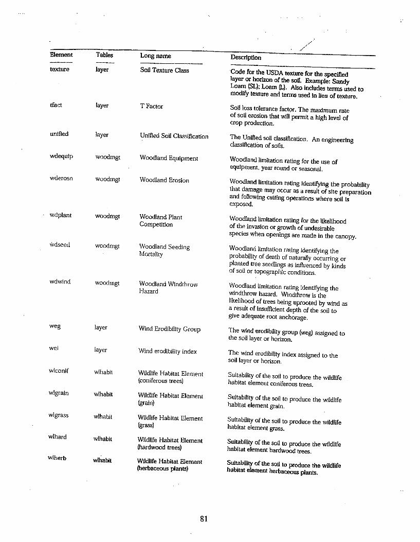


83
APPENDIX B
RECOMMENDED TEST PROCEDURE FOR SULFATE SOILS


85
Objectives: To delineate sulfate-bearing subgrade soils prior to stabilization for road
construction.
1. Collect Background.
1.1 Scope: To obtain as much information of the composition of the subgrade soils as
possible prior to construction to determine the most effective stabilization methods.
1.2 Equipment: Geologic Atlas of Texas, USDA Soil Survey for specific county where
construction is to commence and any other geologic maps or literature available for
the construction site.
1.3 Procedure: Look at the maps to determine the geologic formation and soil types on
which construction will be performed. Look for key words in geologic and soil
descriptions such as: anhydrite, gypsum (also called alabaster, satin spar,
selenite/selenitic), pyrite/pyritic, and marcasite. These are all sulfur-bearing minerals
that can cause sulfate heave.
2. Field Test.
2.1 Scope: To identify soils that may have sulfate concentrations too high for traditional
calcium-based stabilizers.
2.2 Equipment: Portable pH/conductivity meter, conductivity standards, 125 ml HDPE
Nalgene bottles (one for every sample taken in the field), portable scale, double-
distilled water, stopwatch, graduated cylinder (100 ml), 500 ml wash bottle for
double-distilled water.
2.3 Sample Preparation: Collect soil samples from subgrade to be stabilized at surface
and near base of material to be stabilized. For instance, if one is stabilizing 6 inches
of subgrade, then collect a sample from the surface to 6 inches down. Let the sample
air dry before weighing.
2.4 Procedure: Calibrate conductivity and pH meter per manufacturers’ instructions.
Estimate conductivity and pH and calibrate with standards close to those estimates.
For example, a carbonate rich sample will be basic so standardize pH with a pH 10
standard in addition to the pH 7 standard.
• Measure 5 g to the nearest 0.1 g of air-dried soil into a 125 ml (HDPE) Nalgene brand
bottle.
• Measure 100 g to the nearest 0.1 g of double-distilled water into the bottle.

86
• Shake the sample by hand for 1 minute.
• After shaking the sample, immediately take conductivity and pH measurements with
the pH/conductivity meter.
• After a minimum of 12 hours has elapsed, agitate the sample again for 1 minute.
• After shaking the sample, immediately take conductivity and pH measurements.
2.5 Interpretation of Data: Upon completion of this test, there should be two
conductivity measurements approximately 12 hours apart. Absolute conductivity
values are difficult to determine because every soil will be different, so the district
personnel will have to experiment with different soils to see what should be typical
������� ���� � ��� ������ �� &� �/�� ���� ��� ���� ����� �������� � ����� �����-��� 2�
greater than the first, then this should raise a red flag to test the sample for sulfates
��������������������������������&��3� ������������ ��(�� ������������������ 2�
test for sulfates following the procedure outlined below.
3. Field Office Test/Lab Test.
3.1 Scope: To determine the actual sulfate concentration (parts per million) in subgrade
soils.
3.2 Equipment: 2.5 cm Whatman #42 filter paper or 12.5 cm Fisher Q2 filter paper, 80 ml
Nalgene funnel, 250 ml beaker, portable colorimeter/spectrophotometer (for sulfate
analysis), sulfate reagent tablets, latex gloves, graduated cylinder (10 ml), spatula, 2
ml disposable pipettes (one for each sample), 2 pipette bulbs (an extra for breakage or
loss).
3.3 Sample Preparation: The sample produced in the field test section will be used for
this analysis.
3.4 Procedure: Shake the sample by hand for 1 minute.
• Filter with Whatman #42 or equivalent, 12.5 cm, filter paper into a 250 ml beaker.
Centrifugation may be necessary with fine-grained soils to remove all particulates
from suspension.
• Put on latex gloves.
• Fill sample vial with filtrate to the 10 ml mark; a 2 ml pipette may be necessary to fill
vial.
• Switch the unit to “ON.”

87
• Press the MODE key until the desired method is displayed.
• Wipe the sample vial with a lint-free cloth (Kimwipes) to remove any oils from the
vial to ensure repeatable results.
• $��������� ������ ������������ ���������������������� � �������%������������������
��� �������%&
• Press the ZERO/TEST key. The method symbol flashes for approximately 3 seconds
and confirms zero calibration.
• After zero calibration, remove the vial from the sample chamber.
• Add sulfate tablet to vial without touching the tablet with hands and lightly tamp the
tablet with white plastic rod until tablet starts to crumble. Tamp vigorously 20 to 30
times in a random circular motion until tablet is dispersed throughout the sample vial.
• Cap� ������������������(�������������� ���������������������� ����% ��������&
• Press the ZERO/TEST key. The method symbol flashes for approximately 3 seconds
and the result appears in the display. Take three readings and average.
• This test will only read concentrations from 5-200 mg/l. If (÷Err) message appears,
then the measuring range has been exceeded or there is excessive turbidity. This will
require diluting the sample with more double-distilled water and measuring until the
message disappears and there is a numerical answer. If (-Err) message appears, then
result is below the measuring range.
• If the measuring range has been exceeded, then measure out 5 ml of the filtrate into a
10 ml graduated cylinder and add exactly 5 ml of double-distilled water with a 2 ml
pipette. This will change the dilution ratio to 1:40 and increase the measurable range
to 8000 mg/l, or ppm.
• Calculate sulfate concentration in parts per million (ppm) by multiplying the average
of the three readings by the dilution ratio used. For example, the sample was mixed
in a 1:20 ratio of soil to water in the conductivity test. If one obtains an average
sulfate reading of 50 mg/kg, then just take 50 X 20 = 1000 ppm sulfate in the soil. If
a 1:40 dilution ratio was used, then multiply 50 by 40 to obtain 2000 ppm.

Related Documents