Labor mobility, structural change and economic growth

Labor mobility, structural change and economic growth�

Jaime Alonso-CarrerayDepartamento de Fundamentos del Análisis Económico and RGEA

Universidade de Vigo

Xavier RaurichzDepartament de Teoria Econòmica and CREB

Universitat de Barcelona

April 14, 2015

Abstract

We develop a two sector growth model where the process of structural changein the sectoral composition of both employment and GDP is jointly determined bynon-homothetic preferences and a labor mobility cost. This cost is paid by workerswhen they move to another sector and, therefore, it limits structural change. Thetwo sectors are identi�ed as the agriculture and non-agriculture sectors. We showthat this model can explain the following patterns of development of the US econ-omy in the period 1880-2000: (i) balanced growth of the aggregate variables in thesecond half of the last century; (ii) the process of structural change in the sectoralcomposition of employment; (iii) the process of structural change in the sectoralcomposition of GDP; (iv) convergence of the wages in the two sectors. We outlinethat the last two patterns can only be explained if we introduce the labor mobilitycost. We also show that this cost generates a misallocation of production factors,implying a loss of GDP. We calibrate the model and we quantify that this lossamounts more than 30% of the GDP in the initial periods. During the transition,the loss of GDP decreases and, eventually, vanishes. Therefore, the elimination ofthe misallocation explains part of the increase in the GDP. We �nally highlight thatthe misallocation introduces a mechanism through which cross-country di¤erencesin sectoral composition contribute to explain cross-country income di¤erences.JEL classi�cation codes: O41, O47.

Keywords: structural change, non-homothetic preferences, labor mobility.

�Financial support from the Spanish Ministry of Education and Science and FEDER through grantsECO2012-34046 and ECO2011-23959; and the Generalitat of Catalonia through grant SGR2014-493 isgratefully acknowledged.

y [email protected]; z [email protected]

1. Introduction

Recent multisector growth literature has built models aimed to explain both thebalanced growth of aggregate variables and the process of structural change that weobserve in most developed economies (see Acemoglu and Guerrieri, 2008; Boppart,2014; Dennis and Iscan, 2008; Melck, 2002; Foellmi and Zweimuller, 2008; Kongsamut,Rebelo and Xie, 2001; Ngai and Pissariadis, 2007). On the one hand, the balancedgrowth of aggregate variables consists of an almost constant ratio of capital to GDPand an almost constant interest rate. On the other hand, the process of structuralchange consists of a large shift of both employment and production from agricultureto other sectors. This process, that is a common characteristic of most economies, isillustrated in the �rst two columns of Table 1 for the US economy during the period1880 to 2000.

The aforementioned literature explains both balanced growth of aggregate variablesand the process of structural change in the sectoral composition of employment. Thisliterature can be divided in two lines. One line outlines that demand factors are thedriving force of structural change (Kongsamut, Rebelo and Xie, 2001). These demandfactors consist of income e¤ects generated by non-homothetic preferences that drivestructural change as the economy develops. The other line argues that supply factorsare the driving force of structural change (Acemoglu and Guerrieri, 2008; Ngai andPissariadis, 2007). These factors consist of changes in relative prices that through asubstitution e¤ect cause structural change. More recently, the literature combines bothdemand and supply factors in order to explain structural change (Boppart, 2014; Dennisand Iscan, 2008). However, none of these papers explains the magnitudes of the twopatterns of structural change, the shift in employment and production from agricultureto other sectors. Buera and Kabosky (2009) argue that this literature does not explainthese two features because it does not introduce sector speci�c factor distortions.

In this paper, we show that the two features of structural change can be explainedwhen factor distortions cause sectoral wages di¤erentials. In order to motive thisconclusion, we use the de�nition of the labor income share (LIS) at the sectoral level andwe decompose the ratio between the LIS in the agriculture sector and the LIS in the non-agriculture sector as the product of the following three ratios: the ratio between wagesin the agriculture and non-agriculture sectors, the ratio between the employment sharesin agriculture and in the non-agriculture sector and the ratio between the GDP sharesin the non-agriculture and agriculture sectors.1 If we assume that wages across sectorsare equal, the �rst ratio equals one. In this case, we can use the US data for the sectoralcomposition of employment and GDP shown in Table 1 to compute the value of the ratiobetween the two sectoral LIS that is compatible with the process of structural change inboth employment and GDP. Table 1 shows that the value of this ratio should be equalto 2.15 in the year 1880 and decreases until 1.05 in the year 2000. These values areproblematic for two reasons. First, they show a declining long run trend in the ratio of

1The LIS in sector i is de�ned as LISi = wiLi=PiYi where wi is the wage in sector i, Li is thenumber of employed workers in this sector, Pi is the relative price and Yi is the production in thissector. Using this de�nition, it is straightforward to obtain that the ratio between the LIS in sectorsa and n is LISa=LISn = (wa=wn)(ua=un)�n=�a, where ui is the employment share in sector i = a; nand �i is the share of GDP produced in sector i = a; n.

2

LIS, which can only be explained if we consider large departures from the Cobb-Douglasproduction function. These departures are not supported by empirical estimates of thelong run sectoral production functions.2 Second, the value of the ratio between thetwo sectoral LIS that is consistent with the process of structural change is completelydi¤erent from actual estimates of this ratio, which set its value approximately equal to0.68.3 This suggests that the two features of structural change cannot be explained if weassume that wages are equal across sectors. Moreover, empirical evidence clearly showsthat wages are di¤erent across sectors, specially when we consider the agriculture andnon-agriculture sectors (see Helwege, 1992; Caselli and Colleman, 2002; and Herrendorfand Schoellmany, 2014). Table 1 shows the relative wage between agriculture and non-agriculture sectors. As follows from the table, wages are lower in the agriculture sectorand during the last century there has been a clear convergence of wages. However,still wage di¤erentials across sectors are large. Using this data on relative wages, wecompute the ratio between the sectoral LIS that is consistent with the two featuresof the process of structural change when wages are not equal across sectors. The lastcolumn of Table 1 shows this ratio. Note that after 1920 the value of this ratio is close toits empirical estimates and there are not trends.4 This numerical analysis suggests thatthe introduction of sectoral wage di¤erences is necessary to explain the two features ofstructural change.

The purpose of this paper is to show that a simple multisector growth model canexplain the two features of structural change when wages do not equalize across sectors.To this end, we develop an exogenous two sector growth model with two features.First, preferences are non-homothetic due to the introduction of minimum consumptionrequirements, as in Kongsamut, et al. (2001) or Alonso-Carrera and Raurich (2014).Second, wages across sectors do not equalize. Di¤erences of wages across sectors havebeen explained as the result of (i) di¤erences in human capital across sectors (Caselli andColleman, 2002; Herrendorf and Schoellmany, 2014); (ii) barriers to mobility (Hayashiand Prescott, 2008) or (iii) labor mobility cost (Lee and Wolpin, 2006; Raurich, et. al,2014).5 In this paper, we introduce a labor mobility cost.6

The labor mobility cost amounts for any cost that workers moving to another sectormust pay. This amounts for reallocations expenses (transport and housing cost), formaltraining cost necessary to acquire the skills used in another sector or an opportunity

2Herrendorf, Herrington and Valentinyi (2014) estimate the elasticity of substitution between capitaland employment and show that it is 1.58 for the agriculture sector, 0.8 for the manufacturing sector and0.75 for the service sector. They conclude that Cobb-Douglas sectoral production functions capturethe main technological forces in the US postwar structural change.

3This value is obtained from Valentinyi and Herrendorf (2008) that use data for the US in the period1990-2000.

4Before 1920 data on relative wages is controversial as has been explained by Caselli and Colleman(2001). Therefore, meausurement errors in the value of relative wages may explain the low values ofthe ratio of LIS before 1920.

5Lee and Wolpin (2006) estimate that in the US mobility costs are substantial when mobility is acrosssectors (between 50% and 75% of average annual earnings). Artuc, et. al (2015) in a more recent paperestimate a substantially larger labor mobility cost when developing economies are considered. Theyshow that this cost is on average 370% the annual wage in developing countries.

6Gollin, Lagakos, and Waugh (2014) show that the agriculture sector has a lower labor productivityonce we control for human capital and number of hours employed. This suggests that the labor mobilitycost explains part of the wage di¤erences.

3

cost (working time lost looking for a job in a di¤erent sector). As moving out ofthe agriculture sector generally implies moving from a rural to an urban area, weassume that the relevant labor mobility cost is associated to reallocation expenses. Asa consequence, we will assume that the unitary labor mobility cost is a �x cost andthat it is only taken into account in the resource constraint of the non-agriculturesector. Artuc et al. (2015) estimate labor mobility cost for both developed anddeveloping economies and they show that this cost as a fraction of annual wage islarger in developing economies. This implies that the labor mobility cost as a fractionof GDP declines along the development process. Note that this pattern is consistentwith the assumption of a �x unitary labor mobility cost.

The introduction of the labor mobility cost divides the labor market in two sectorspeci�c labor markets. The labor supply in each market is determined by the existingnumber of workers in each sector and, thus, it is determined by the sectoral employmentshare. The labor demand in each market depends on the demand of consumptiongoods in every sector that in a model with non-homothetic preferences depends oneconomic development. In every period, market clearing determines the wages paid ineach sector. Therefore, sectoral wage di¤erences exist because the labor mobility costprevents workers from moving instantaneously to the higher wage sector. However, asthe economy develops, the labor mobility cost as a fraction of the GDP declines, whichcauses sectoral wage convergence.

The process of structural change is driven by both demand and supply factors. Onthe one hand, due to the non-homotheticity of preferences, the sectoral compositionof consumption expenditures changes as the economy develops. Obviously, this is theclassical demand factor explained in Kongsamut, et al. (2001). Economic developmentreduces the e¤ect of the minimum consumption requirement on the sectoral compositionand, eventually, this e¤ect vanishes. As a consequence, preferences are homotheticin the long run, which implies that the equilibrium converges to a balanced growthpath (BGP) in the long run. On the other hand, the supply factor is based on wageconvergence, instead of the standard mechanism in the literature, based on relative pricechanges. Wage convergence implies that wages in the agriculture sector grow faster thanwages in the non-agriculture sector. As a consequence, �rms in the agriculture sectorsubstitute labor for capital, making the technology more capital intensive and pushingworkers out of the agriculture sector. This is the supply mechanism in this paper.

We calibrate this model to explain the process of structural change in the US,during the period 1880-2000. From numerical simulations, we show that the modelexplains (i) the convergence to a BGP, while there is structural change;7 (ii) the processof structural change in the sectoral composition of employment; (iii) the process ofstructural change in the sectoral composition of GDP; and (iv) the convergence ofwages across sectors. We outline that in the absence of the labor mobility cost themodel does not explain sectoral wage convergence, nor the process of structural changein the sectoral composition of GDP.

The di¤erences in sectoral wages introduce a misallocation of production factors:the sector with larger wages has a larger capital intensity. This misallocation causes a

7We follow Acemoglu and Guerrerie (2008) and Alonso-Carrera and Raurich (2014) and we claimthat an equilibrium follows a BGP with structural change when the growth rate of capital to GDP isalmost null, whereas the growth rate of the employment share is clearly di¤erent from zero.

4

loss of GDP. This GDP loss is not due to an ine¢ ciency as in Restuccia, et. al. (2008),where barriers cause a GDP loss. Instead, it must be interpreted as the reductionin GDP with respect to the level that would be attained in the absence of the labormobility cost. Intuitively, moving a worker from a low to a high wage sector increasesthe GDP. Therefore, the GDP loss will depend on the wage gap between the two sectorsand on the size of the low wage sector (the agriculture sector). Both the wage gap andthe size of the low wage sector were large in the US in the XIX century, implying alarge GDP loss. We use the numerical simulation to account for the GDP loss and itturns out that it was about 30% of GDP in the last twenty years of the XIX century,it declines during the transition and eventually vanishes. As a consequence, part of theincrease in the GDP during the transition, specially in the initial periods, is explainedby the elimination of the misallocation.

The GDP loss introduces a mechanism through which cross-country di¤erences inthe sectoral composition of employment cause cross-country di¤erences in income percapita. This mechanism implies that those countries specialized in the low wage sector,the agriculture sector, will su¤er from a lower GDP. This conclusion is also obtained inGollin, Parente and Rogerson (2004, 2007). In these papers, the specialization in the lowwage sector is explained by home production or minimum consumption requirements.In contrast, in this paper, this specialization is explained as the result of either a largerintensity of the minimum consumption requirement or a larger labor mobility cost. Thelater can be the result of labor market regulations or larger reallocation expenses. Theformer can be explained by a lower level of development.

We measure the contribution of the misallocation in explaining cross-country incomedi¤erences. We show that this contribution is not constant through time and it cruciallydepends on the initial source of di¤erences in income per capita. We also show that thecontribution of the misallocation is sizeable. It explains up to 18% of GDP di¤erenceswhen economies are initially di¤erentiated by levels of technology and it explains upto 50% of GDP di¤erences when economies are initially di¤erentiated by the stock ofcapital.

The rest of the paper is organized as follows. Section 2 introduces the model. Section3 characterizes the equilibrium. Section 4 numerical solves the model and obtains themain results. Finally, concluding remarks are in Section 5.

2. Model

We build an exogenous two-sector growth model. We distinguish between theagriculture and the non-agriculture sector. We assume that the later is the numeraireof the economy and produces both a consumption good and an investment good. Theagriculture sector only produces a consumption good.

2.1. Household

The economy is populated by an in�nitely lived representative household, formed by acontinuum of L members. Every member inelastically supplies one unit of time and thenumber of members is assumed to be constant. Therefore, the labor supply is inelastic,constant and equal to L: The household obtains income from capital and labor. This

5

income is devoted to either consumption, investment or paying the cost of moving toanother sector. Therefore, the budget constraint of the household is

rK + [wa (1� u) + uwn]L = (pca + cn)L+ _K + � _uL; (2.1)

where r is the rental price of capital, K is the stock of capital, wa is the wage obtainedin the agriculture sector, wn is the wage obtained in the non-agriculture sector, u isthe fraction of workers employed in the non-agriculture sector, p is the relative priceof agriculture goods in units of non-agriculture goods, ca are the units consumed ofgoods produced in the agriculture sector, cn are the units consumed of goods producedin the non-agriculture sector, � is the constant unitary labor mobility cost that everyworker moving to another sector pays, and _u is the fraction of workers that move everyperiod.8 We assume that the investment good is produced in the non-agriculture sectorand, therefore, its relative price is normalized to one.

The representative households�s utility function is

U =

Z 1

0e��tL [� ln (ca � eca) + (1� �) ln cn] dt; (2.2)

where eca > 0 is the minimum consumption requirement of agriculture goods; � > 0is the subjective discount rate; and � 2 (0; 1) measures the weight of the agriculturegoods in the utility function. Note that this utility function is non-homothetic wheneca 6= 0:

The representative household chooses the sectoral composition of consumptionexpenditures, the amount of consumption expenditures and the number of workers thatevery period move to the non-agriculture sector in order to maximize the utility function(2.2) subject to the budget constraint (2.1). By standard procedure, in Appendix A we�nd the �rst order conditions and rearrange them to summarize the necessary conditionsfor optimality in the following three conditions:

v = � +eEE(1� �) ; (2.3)

_E

E=

E � eEE

!(r � �) +

eEE

!_p

p; (2.4)

andwn � wa = r�; (2.5)

where E = pca + cn is the value of consumption expenditures, v = pca=E is theexpenditure share in agriculture goods and eE = peca is the value at market prices of theminimum consumption requirement. Equation (2.3) determines the expenditure sharein agriculture goods. Note that this share would be constant and equal to � if eca = 0:In contrast, if eca > 0, preferences are non-homothetic and the sectoral compositionof consumption expenditures decreases as the economy develops and consumptionexpenditure increases. This mechanism is the classical demand factor driving structural

8We write the budget constraint assuming that workers move from the agriculture to the non-agriculture sectors. This pattern of structural change is obtained in equilibrium.

6

change. Equation (2.4) is the Euler condition governing the intertemporal decisionbetween consumption and savings. Finally, equation (2.5) is a non-arbitrage conditionbetween two investment decisions: investment in capital goods and investment inmoving out of the agriculture sector. The left hand side is the return from investing� units in moving a worker to another sector. The right hand side is the return frominvesting in capital � units. This non-arbitrage condition implicitly determines thenumber of workers moving out of the agriculture sector in every period and, thus, itdetermines the relative labor supplies in both sectors.

2.2. Firms

We assume that both sectors produce with the following constant returns to scaleCobb-Douglas technologies:

Ya = [(1� s)K]�a [Aa (1� u)L]1��a = Aa (1� u)Lz�aa ; (2.6)

andYn = (sK)

�n (AnuL)1��n = AnuLz

�nn ; (2.7)

where �a 2 (0; 1) and �n 2 (0; 1) are, respectively, the capital output elasticitiesin the agriculture and non-agriculture sector, Aa and An are e¢ ciency units oflabor, s is the fraction of capital devoted to the non-agriculture sector, and za =(1� s)K=Aa (1� u)L and zn = sK=AnuL measure, respectively, capital intensityin the agriculture and non-agriculture sectors. We assume that e¢ ciency units oflabor grow in both sectors at the exogenous growth rate ; implying that technologicalprogress is unbiased and that the long run growth rate of GDP is . Finally, perfectcompetition implies that each production factor is paid according to its marginalproduct

wi = Aipi (1� �i) z�ii ; (2.8)

andr = pi�iz

�i�1i � �; (2.9)

where � 2 [0; 1] is the depreciation rate and i = a; n.As capital can move across sectors without cost, the marginal product of capital is

identical across sectors. In contrast, the introduction of the labor mobility cost impliesthat wages can be di¤erent across sectors. We de�ne the relative wage between the twosectors by � = wa=wn: From using (2.8) and (2.9), we obtain that

za =

�� AnAa

�zn; (2.10)

and

p =

��n�a

��� AnAa

�1��azan��an ; (2.11)

where

=

��a�n

��1� �n1� �a

�:

7

Equation (2.10) shows that the relationship between the sectoral capital intensitiesdepends on the relative wage. As the economy develops, the relative wage increases,which causes an increase in the capital intensity of the agriculture sector relative tothe capital intensity of the other sector. The intuition is as follows. An increase in therelative wage implies that wages in the agriculture sector increase relative to wages inthe non-agriculture sector. As a consequence, �rms in the agriculture sector choose amore capital intensive technology, by substituting labor for capital. This mechanismdescribes the supply factor driving structural change. This supply factor is di¤erentfrom the supply mechanism proposed by the literature and based on relative pricechanges caused by either biased technological change (Ngai and Pissariadis, 2007) orcapital deepening and di¤erences in capital output elasticities (Acemoglu and Guerrieri,2008). This di¤erent supply mechanism has two relevant implications.

First, equation (2.11) shows that the relative price depends on (i) the relative wage,(ii) the ratio between the e¢ ciency units of labor in the non-agriculture sector andthe e¢ ciency units of labor in the agriculture sector, and (iii) capital deepening. Thenew supply mechanism introduced in this paper implies an increase in the relativeprice of agriculture. In contrast, both the biased technological mechanism and capitaldeepening implies a reduction in this price. On the one hand, empirical evidence onTFP growth shows that TFP growth is larger in the agriculture sector and, thus,biased technological change reduces the relative price.9 On the other hand, capitaldeepening implies a reduction in the relative price because estimates of the sectoralcapital output elasticities suggest that this magnitude is larger in the agriculture sector(See Herrendorf and Valentinyi, 2008). As a consequence, this sector bene�ts themost from capital deepening, which causes the reduction in the relative price. As inthe model we combine two di¤erent supply mechanisms, capital deepening with wageconvergence, the relative price can either increase or decrease along the developmentprocess. Interestingly, this is consistent with the observed di¤erences in the patternsof relative prices along the development process.10

Second, wage convergence implies that as the economy develops, the agriculturesector becomes a more capital intensive sector. This contributes to explain cross-country di¤erences in sectoral capital intensities that clearly show that the agriculturesector is more relatively capital intensive in developed economies (see Alvarez-Cuadrado, et al., 2013). It should be noted that a classical supply mechanism wouldnot explain this evidence. From using (2.10) and the de�nitions of zn and za; it followsthat neither di¤erent capital output elasticities, nor biased technological change canexplain cross-country di¤erences in relative capital intensities when the productionfunction is Cobb-Douglas. To the best of our knowledge, cross-country di¤erences insectoral capital intensity has only been explained by Alvarez-Cuadrado et al (2013).Using CES production functions, they explain these di¤erences as a result of di¤erentsectoral elasticities of substitution between capital and employment. We therefore o¤era complementary explanation based on wage convergence. Note that wage convergence

9Dennis and Iscan (2009) show that TFP growth in the agriculture sector is larger than TFP growthin the non-agriculture sector in the US economy after 1930.10Dennis and Iscan (2009) provide evidence that in the US relative prices of agriculture increase

during the XIX century and decrease after 1920. (Jaime, podrias mencionar como los precioshan prsentado comportamientos dispares en diferentes economías).

8

contributes to explain di¤erences in sectoral capital intensities even if the productionfunction is Cobb-Douglas.

3. Equilibrium

The non-agriculture sector produces a commodity that can be used either as aconsumption good, as an investment good or to move to a di¤erent sector and, therefore,the resource constraint in this sector is

Yn = Lcn + _K + �K + _uL�:

The agriculture sector only produces a consumption good and thus the market clearingcondition in this sector is Lca = Ya; which can be rewritten as

1� u = caAaz

�aa: (3.1)

Let z = K=AnL be the stock of aggregate capital per e¢ ciency unit of labor in theeconomy. Thus, z measures the capital intensity of the economy. Using the de�nitionof z; we obtain that

zn = sz=u (3.2)

and za = (1� s)Anz= (1� u)Aa: From the last equation and (2.10), we obtain that

zn� (1� u) = (1� s) z: (3.3)

From using the equilibrium condition in the capital market and equations (3.2) and(3.3), we obtain

z

zn= � (1� u) + u = �; (3.4)

where � measures the capital intensity of the economy relative to the capital intensityof the non-agriculture sector.

Note that without a mobility cost, wages will equalize implying that � = 1 and� = (1� u) + u � ��: However, the labor mobility cost implies that during thetransition � < 1 and then � < ��: Therefore, the introduction of the labor mobilitycost, by increasing the wages of the non-agriculture sector, increases capital intensityof this sector relative to the capital intensity of the economy. Thus, the labor mobilitycost introduces a factors�misallocation, which is measured by the gap between � and�� and it is

�� � � = (1� u) (1� �) :

The misallocation will cause a GDP loss. In order to see this, we de�ne GDP asQ = pYa + Yn. Using (2.10), (2.11) and (3.4), GDP can be rewritten as

Q = ���nK�n (AnL)1��n = ���nz�nAnL; (3.5)

where

=

��n�a

�� (1� u) + u =

��n�a

��+ u

��a � �n�a

�; (3.6)

9

and ���n measures the sectoral composition component of the total factorproductivity (TFP), which is given by ���nA1��nn :11. By de�ning by Q� the GDPlevel attained when � = 1; we measure the GDP loss as a percentage of GDP by

Q� �QQ

=

��

����

�

���n� 1;

where � is the value of when � = 1: Note that the loss of GDP depends on � andon the the employment shares in agriculture 1 � u. In the numerical simulations ofSection 4, we show that the GDP loss has declined in the US during the last centuryas a result of both wage convergence and the decline of the employment share in theagriculture sector.

An important remark that follows from the expression of the TFP is that di¤erencesin the sectoral composition of employment cause di¤erences in the TFP when eitherthere are di¤erences in capital output elasticities or there are di¤erences in wagesacross sectors. If we had assumed that �a = �n and that � = 1; then ���n = 1and di¤erences in the sectoral composition would not imply di¤erences in TFP levels.In other words, TFP increases when economies specialize in sectors with larger capitaloutput elasticities or in sectors with larger wages. In the numerical analysis, we compareeconomies with di¤erent sectoral composition and we decompose the fraction of incomedi¤erences explained by di¤erences in sectoral wages and the fraction explained bydi¤erences in capital output elasticities. From this numerical analysis, we show thatthe main mechanism explaining income di¤erences is based on di¤erences in sectoralwages.

3.1. Sectoral Composition

In this subsection, we obtain the sectoral composition of consumption expenditures andof the employment shares and the relative wage, �; as a function of the expenditure toGDP ratio, e = E=Q; the capital intensity, z = K=AnL; the intensity of the minimumconsumption requirement, measured by the ratio ee = eE=Q; and the intensity of thelabor mobility cost, measured by m = �=An. Note that as the economy develops, boththe intensity of the minimum consumption requirement and of the labor mobility costdeclines and, eventually, converge to zero.

First, we use (2.3) and the de�nitions of e and ee to obtain the expenditure sharesv = � +

eee(1� �) : (3.7)

The employment shares are obtained from combining (3.1), (2.10), (2.11) and (3.7) asfollows

1� u = v

��a�n

��E

� AnLz�nn

�:

Using (3.4) and (3.5), the previous equation simpli�es as follows

1� u = ve

��a�n

��

�

�:

11Note that the aggregate production function is not Cobb-Douglas during the transition when thereis structural change. In contrast, in the long run, when there is no structural change, it converges to aCobb-Douglas production function.

10

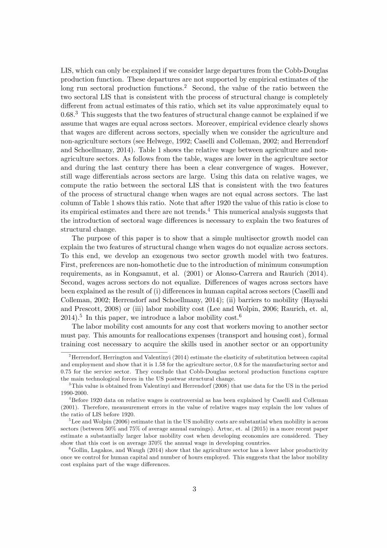
From using the previous equations and the de�nition of ; we obtain the followingexpression of the employment share in the agriculture sector:

1� u =��a�n

��veu

� (1� ve)

�; (3.8)

and =

u

1� ve: (3.9)

According to equation (3.8), sectoral change is driven by demand factors, measuredby ve, and supply factors, measured by �: Note that this equation provides a negativerelationship between the employment share in the agriculture sector and �: Thisrelationship is explained by the reduction in the demand of workers of the agriculturesector due to the increase in the relative wage.

From using (2.7), (3.4), and (3.5), we obtain

YnQ=u

: (3.10)

The variable determines the relationship between the agriculture share of GDP andthe employment share in the agriculture sector. From using (3.6), the variables canbe rewritten as

= 1 + (1� u)�1� �n1� �a

�(�� 1) + (1� u)

��a � �n1� �a

�:

Note that if there is no misallocation and there are no technological di¤erences, then = 1. In this case, the relation between the employment share and the GDP sharewill be constant and indeed these two shares will be equal. However, as follows fromTable 1, this is not consistent with actual data for the US economy. According to thisdata, the agriculture share of GDP is larger than the employment share, implying thatthe value of should be smaller than one. As follows from the previous expressionof , the misallocation reduces the value of and thus makes the model consistentwith actual data. On the contrary, technological di¤erences increase the value of ; asthe agriculture sector is more capital intensive than the non-agriculture sector.12 Thisanalysis suggests that the misallocation must be introduced in order to explain the twodimensions of structural change.

The relative wage is obtained from the market clearing in the labor market. Toobtain it, we rewrite the labor supply, (2.5), as follows

wn � �wn = �r:

12Following Herrendorf and Valentinyi (2008), �n = 0:33 and �a = 0:54: Then, = 1:2 in the USduring the period 1880-1900 when we assume that � = 1. In this period, the average value of u = 0:58and of Yn=Q = 0:75: According to these values, should be 0:75: Thus, in the absence of missallocationthe sectoral composition of both GDP and employment cannot be explained. In fact, a value of thatis consistent with the sectoral composition of employment and GDP in the period 1880-1900 is attainedwhen � = 0:31:

11

Rearranging terms and using the labor demand, (2.8), and equations (2.9) and (3.4),we obtain

� = 1�m

0B@�n�z�

��n�1� �

(1� �n)�z�

��n1CA : (3.11)

In Appendix B we use (3.11) to obtain the relative wage in equilibrium and provethe following result.

Proposition 3.1. The relative wage and the employment share satisfy

� = b� (e; z;m) ; (3.12)

and

u =� ��n�a

�(1� ve)

ve+ � ��n�a

�(1� ve)

: (3.13)

Furthermore, @� /@m < 0 and @u /@� > 0:

As follows from Proposition 3.1, � is a decreasing function of the intensity of thelabor mobility cost and u is an increasing function of �: Therefore, a large mobility costimplies that the relative wage will be smaller and the agriculture share of employmentwill be larger. Both e¤ects imply that the GDP loss increases with the labor mobilitycost.

3.2. Equilibrium Dynamics

In a supplementary appendix we obtain a full system of di¤erential equationscharacterizing the time path of the transformed variables: z; e; m and ee. Given initialconditions ee0; m0 and z0; an equilibrium is a path of fe; ee; z;m; �; v; u; �g that solves thissystem of di¤erential equations and satis�es equations (3.7), (3.12), (3.4), and (3.13),and the transversality condition lim

t!1Kcne��t = 0:Moreover, we de�ne a balanced growth

path (BGP) as an equilibrium along which both the ratio of capital to GDP and theinterest rate remain constant.

Proposition 3.2. There is an unique BGP alongwhich the variables fe; ee; z;m; �; v; u; �g remain constant and its long run value isee� = 0;m� = 0; �� = 1; v� = �;

e� =1� �n�

1 +�(�a � �n) �;

u� = �n (1� �e�)

�a�e� + �n (1� �e�);

�� = (1� u�) + u�;and

z� =

� + � + �

�n

� 1�n�1

��;

where � = (� + ) = (� + �+ ) : Furthermore, this BGP is saddle path stable. 13

13The proof is available in a supplementary appendix.

12

Note that this BGP is attained asymptotically, as ee� and m� converge to zero.Wages converge and, therefore, both the misallocation and the GDP loss disappear inthe BGP. Moreover, along the BGP there is no structural change. Thus, asymptoticallythe economy converges to an equilibrium along which the interest rate and the ratio ofcapital to GDP remain constant and there is no structural change. As this only happensasymptotically, the analysis of transitional dynamics is particularly relevant. In thefollowing section, we numerically analyze the transition and we show that aggregatevariables exhibit a period of unbalanced growth followed by a long period in which theyexhibit an almost constant time path of the interest rate and of the ratio of capital toGDP. We show that there is structural change during this period. We will then concludethat in this economy we observe (almost) balanced growth of aggregate variables andstructural change.

The equilibrium is characterized by three state variables: capital intensity, z;intensity of the minimum consumption requirements, ee; and the intensity of the labormobility cost, m: Saddle path stability implies that given initial conditions on thesethree state variables there is an unique equilibrium path converging to the steady state.In the following section, the uniqueness of the equilibrium path is used to calibrate andsimulate the economy.

4. Transitional dynamics analysis: structural change

In this section we numerically simulate the economy in order to show the e¤ects ofthe mobility cost on the process of structural change. To this end, we calibrate theparameters of the economy as follows. The parameter = 2% in order to have a longrun GDP growth rate equal to 2%; we set �a = 0:54 and �n = 0:33 as estimated byHerrendorf and Valentinyi (2008); � = 0:01 is set to �t the long run expenditure share inagriculture obtained in Herrendorf, et al. (2013); � = 0:32 so that the long run interestrate equals 5:2%; � = 5:6% in order to obtain a long run ratio of investment to capitalequal to 7:6%. We compare two di¤erent numerical simulations. In both simulationswe assume that z0 = 0:75z�: The initial value of this state variable mainly determinesthe length of the transition of aggregate variables. We choose an initial value which isconsistent with an almost constant time path of the interest rate and of the ratio ofcapital to GDP in the last 50 years of the simulation. The distinction between the twosimulations is in the labor mobility cost. In a �rst numerical simulation, we assumethat there is no mobility cost (m0 = 0) and we set the initial condition on the otherstate variable, ee0 = 0:59; to match the employment share in the US in the initial year1880. In a second simulation, we assume that there is labor mobility cost and we set theinitial conditions on the two state variables, ee0 = 0:28 and m0 = 14:3; to match boththe value of the employment share in agriculture and the share of GDP produced in theagriculture sector in the US in the year 1880. The parameters and initial conditions ofthe two simulations are summarized in Table 2.

[Insert Table 2]

Figure 1 shows the �rst numerical simulation in which we assume that there is nomobility cost. In this case, wages equalize across sectors implying that the relative

13

wage is equal to one and, thus, the simulation does not explain wage convergence. Thisimplies that there is no misallocation and thus there is no GDP loss. Panel i showsthat this simulation explains almost all the decline in the employment share in theagriculture sector. However, the model does not provide a reasonable explanation ofthe process of structural change in the sectoral composition of GDP as it overestimatesthe share agriculture in GDP during all the transition. In order to see this, we canrewrite (3.10) as = u (Q=Yn) : From Table 1, we observe that u < Yn=Q implyingthat should be substantially lower than one in order to explain the two dimensionsof structural change. Note that can be rewritten as

= 1 + (1� u)��a � �n1� �a

�+ (1� u)

�1� �n1� �a

�(�� 1) :

The second addend amounts for the e¤ect of the di¤erent capital output elasticities on; whereas the third one amounts for the e¤ect of the relative wage. In our calibration,�a > �n; implying that the second addend is positive. As a consequence, when therelative wage equals one, is larger than one and the model fails to explain the twodimensions of structural change. This explains that the �rst numerical simulationoverestimates the value of the production share and the performance of the simulationin explaining the process of structural change in the sectoral composition of GDP ispoor.

[Insert Figure 1]

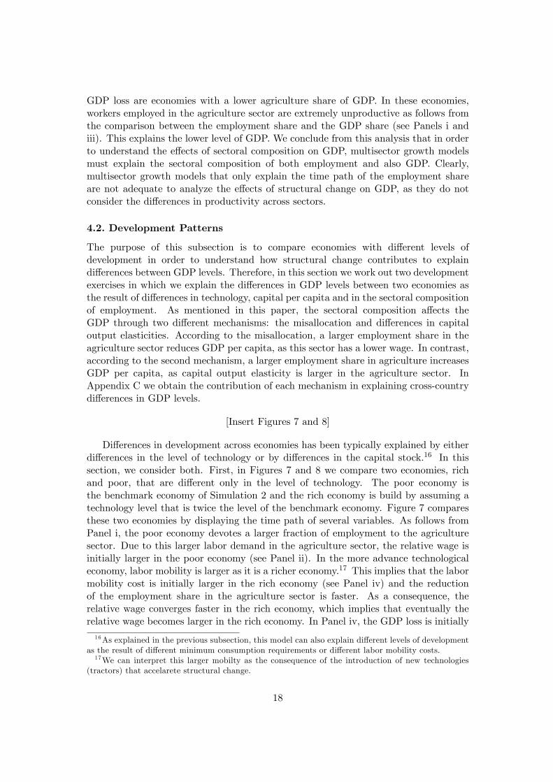
Figure 2 displays the second simulation, where a mobility cost is introduced. Thiscost, as a ratio of GDP, declines from 8% of GDP in the initial year to zero in thelong run. This ratio declines both because GDP increases and because the process ofsectoral change declines in the long run. The simulation explains the declining path ofthe employment share in the agriculture sector, the declining path of the share of GDPproduced in the agriculture sector and the process of wage convergence. Moreover,the simulation explains almost all the decline in both the employment share in theagriculture sector and the agriculture share of GDP. Regarding wage convergence, thesimulation explains the convergence of the relative wage, but it is not able to explainthe level of this relative wage. We interpret this as partial evidence that there are otherrelevant explanations of the sectoral wage di¤erences di¤erent from the mobility cost.14

Finally, the performance of this simulation in explaining the process of structural changein the sectoral composition of GDP is clearly better than the previous simulation.

[Insert Figure 2 and Table 3]

Table 3 provides three measures of performance in order to compare the twosimulations. As follows from these measures, the accuracy of both simulations in

14Candidates to explain the slow convergence in wages are metapreferences associated to working inone sector or di¤erent skills across sectors, among others. Other authors argue that wage di¤erencescan be explained by di¤erences in the cost of living between urban and rural areas (see Esteban-Preteland Sawada, 2014). Assuming that workers in urban areas are employed in the non-agriculture sector,whereas workers in rural areas can be employed in the agriculture sector, permanent sectoral wagedi¤erences are aimed to compensate for the di¤erences in the cost of living.

14

explaining the process of structural change in the sectoral composition of employmentis similar. For example, the coe¢ cient of determination is 75% in Simulation 1 and78% in Simulation 2. Thus, the performance is very similar and only slightly betterin Simulation 2. A similar conclusion is attained if we compute the fraction of thereduction in the employment share of the agriculture sector in the period 1880-2000explained by both simulations. Simulation 1 explains 96% of the reduction, whereasSimulation 2 explains 97%. The conclusion is completely di¤erent when we consider theperformance of both simulations in explaining the process of structural change in thesectoral composition of GDP. Simulation 1, based on the absence of the labor mobilitycost, has a very poor performance. In this simulation, the coe¢ cient of determinationis negative and the fraction of the reduction in the GDP share in the period 1880-2000is 197%, implying that the simulated reduction in the GDP share almost doubles thereduction in actual data. In contrast, Simulation 2, based on the introduction of thelabor mobility cost, has a very good performance. The coe¢ cient of determination is96% and the fraction of the reduction explained by this simulation is 91%. We canthen safely conclude that the model with mobility cost provides a substantially betterexplanation of the process of structural change.

As explained in the previous section, the mobility cost introduces a misallocation ofproduction factors that causes a loss of GDP. Panel (iv) in Figure 2 provides a measureof this loss as a percentage of GDP. This loss amounts initially 35% of GDP and declinesand converges to zero as both the sectoral wage di¤erences vanish and the labor share inthe agriculture sector declines. Therefore, the elimination of the misallocation explainspart of the increase in GDP during the transition.

The labor mobility cost also modi�es the time path of the growth rate of GDP. Asfollows from Panel (vi) in Figure 2 the time path of the growth rate is hump-shaped.This �nding is interesting as it is consistent with the observed development patterns.15

Christiano (1989) and, more recently, Steger (2000, 2001) explain this hump-shapedpatterns in models with minimum consumption requirements. In these models, asu¢ ciently intensive minimum consumption requirement deters initially investment,which explains the initial low growth. As the economy develops, the intensity of theminimum consumption requirement declines and both investment and growth initiallyincrease. Eventually, the interest rate declines due to diminishing returns to capitaland thus capital accumulation and the growth rate decline until they converge to itslong run value. We contribute to this literature by showing that the hump-shapedgrowth pattern can be explained by the interaction of both capital accumulation andlabor mobility. In this model, a large intensity of the labor mobility cost explains theinitial low labor mobility and also a low initial capital accumulation. As this intensitydeclines, capital accumulation increases and the GDP loss declines due to the increasein the number of workers leaving the agriculture sector. These two changes implyan increase in the growth rate of GDP. Finally, diminishing returns to capital andlabor imply that capital accumulation and labor mobility decline and �nally converge,which explains the reduction in the growth rate of GDP. Note that both mechanisms,minimum consumption requirements and labor mobility cost, introduce complementaryexplanations of the hump-shaped time path of the GDP growth rate. Interestingly,15Papageorgiou and Perez-Sebastian (2005) show that some fast growing economies exhibit a hump-

shaped transition of the GDP growth rate.

15

the calibrated economy of Simulation 1, where there is no labor mobility cost, doesnot explain the hump-shaped time path of the GDP growth rate. This outlines therelevance of the complementarity between the two mechanisms in explaining the timepath of the GDP growth rate.

[Insert Table 4]

An important stylized fact of the patterns of development in the US economy sincethe second half of the last century is the balanced growth of the aggregate variables. Inthis period, the interest rate and the ratio of capital to GDP remain almost constant,while the sectoral composition of employment and GDP change. In order to show thatour simulations are consistent with this pattern of development, we follow Acemogluand Guerrieri (2008) and we compute the average annual growth rate of the ratio ofcapital to GDP, the interest rate, the employment share in the agriculture sector andthe agriculture share of GDP during the second half of the twenty century. Results aredisplayed in Table 4. As follows from this table, in both simulations the annual growthrate of both the interest rate and of the ratio of capital to GDP is almost null, whichis consistent with the balanced growth of the aggregate variables. The annual growthrate of the employment share and of the GDP share are larger than 1% and consistentwith actual data. Thus, the calibrated model is consistent with balanced growth andstructural change.

[Insert Figure 3]

Figure 3 shows the simulated time path of the employment share when both demandand supply factors drive structural change (dashed line) and when only demand factorsdrive structural change (continuous line). The former employment share is obtainedin Simulation 2 and the later is obtained by assuming that the relative wage does notincrease. From the comparison between the two cases, it follows that demand factorsexplain most of the reduction in the employment share in the period 1880-2000. In fact,the supply factor based on wage convergence only explains 12% of the reduction in theemployment share in the whole period. In contrast, wage convergence explains a muchlarger part of the reduction during the transition. As an example, wage convergenceexplains 40% of the fall in the share during the period 1880-1920.

4.1. Sensitivity Analysis

The purpose of this subsection is to increase our understanding of the e¤ects of theminimum consumption requirement and of the labor mobility cost. To this end,we consider three exercises where we modify the value of these parameters in thebenchmark of the calibrated economy of Simulation 2.

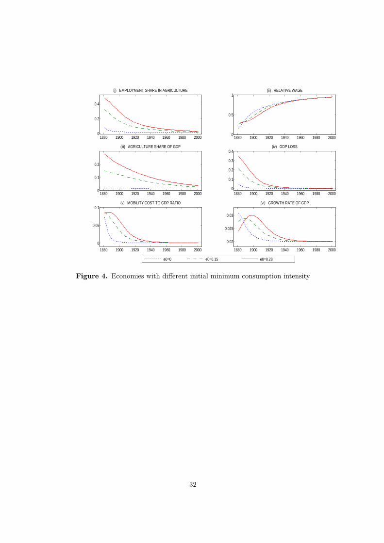
The �rst exercise is displayed in Figure 4. This �gure shows the e¤ects of changingthe initial intensity of the minimum consumption requirement by comparing threeeconomies that are di¤erentiated only by the initial value of ee0: The continuous lineshows the calibrated economy of Simulation 2. In this benchmark economy, ee0 = 0:28:The dashed line is an economy with a lower value of the initial intensity of the minimumconsumption requirement, ee0 = 0:15, and the doted line is an economy with almost zero

16

initial intensity, ee0 = 0:01: As follows from Panels i and iii of Figure 4, a larger minimumconsumption requirement implies that both the employment share and the agricultureshare of GDP are larger. This larger demand of labor in the agriculture sector impliesthat the relative wage is initially larger (see Panel ii). However, in this economy, wageconvergence is slower. This happens because a larger initial intensity of the minimumconsumption requirement reduces the willingness of agents to substitute intertemporallyand, thus, in these economies agents are less willing to reduce current consumptionto invest in either capital or in moving to a di¤erent sector. As a consequence, thereduction in the employment share of the agriculture sector is at a lower rate. Obviously,this explains the slower wage convergence.

[Insert Figures 4, 5 and 6]

Figure 5 shows the e¤ects of changing the labor mobility cost by comparing threeeconomies that have a di¤erent unitary mobility cost, �: The continuous line displaysthe benchmark economy of Simulation 2. The dashed lines displays an economy with alabor mobility cost that is 25% smaller than in the benchmark economy and the dottedline displays an economy with a mobility cost that is 75% smaller than in the benchmarkeconomy. As follows from the comparison between these economies, a lower mobilitycost implies a lower amount of workers in the agriculture sector (see Panel i), a largerrelative wage (see Panel ii), a smaller GDP loss due to the misallocation (see Panel iv)and a lower mobility cost as a percentage of GDP (see Panel v). These di¤erences inthe GDP loss will a¤ect the GDP growth rate, as shown in Panel vi. Note that thetime path of growth rate in the low mobility cost economy is not hump-shaped. Thishappens because the reduction of the GDP loss is almost null in this economy and, asmentioned before, this reduction is necessary to explain the hump-shaped time path ofthe GDP growth rate. Note also that in the economy with a low mobility cost the GDPgrowth rate converges from below, as the growth rate is below its long run value almostevery period. In the following section, we show that this low growth rate is explainedby the negative impact that the sectoral composition has on the growth rate in thoseeconomies where there is a small reduction of the GDP loss.

Figure 6 compares three economies that are di¤erent in both the initial intensity ofthe labor mobility cost and of the minimum consumption requirement. The continuousline displays the benchmark economy of Simulation 2. The dotted lines displays aneconomy without labor mobility cost and the dashed line displays an intermediatesituation with a positive but small labor mobility cost. In these economies, theinitial intensity of the minimum consumption requirement has been calibrated to havethe same initial employment share and, in fact, they exhibit a similar time path ofthe employment share (see panel i). However, there are relevant di¤erences in thetransitional dynamics of the other variables due to the fact that these economies havea di¤erent labor mobility cost. A larger mobility cost implies a smaller relative wageand, therefore, it implies a larger GDP loss (see panels ii and iv). Note that economiesexhibiting a similar process of structural change in employment will exhibit di¤erentlevels of GDP due to the di¤erences in the GDP loss generated by the misallocation.The misallocation can be observed from the comparison between the employment shareand the share of GDP produced in the agriculture sector. Those economies with a larger

17

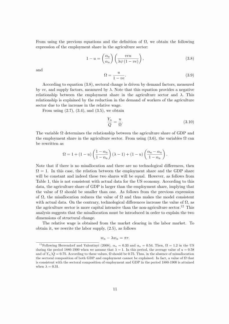
GDP loss are economies with a lower agriculture share of GDP. In these economies,workers employed in the agriculture sector are extremely unproductive as follows fromthe comparison between the employment share and the GDP share (see Panels i andiii). This explains the lower level of GDP. We conclude from this analysis that in orderto understand the e¤ects of sectoral composition on GDP, multisector growth modelsmust explain the sectoral composition of both employment and also GDP. Clearly,multisector growth models that only explain the time path of the employment shareare not adequate to analyze the e¤ects of structural change on GDP, as they do notconsider the di¤erences in productivity across sectors.

4.2. Development Patterns

The purpose of this subsection is to compare economies with di¤erent levels ofdevelopment in order to understand how structural change contributes to explaindi¤erences between GDP levels. Therefore, in this section we work out two developmentexercises in which we explain the di¤erences in GDP levels between two economies asthe result of di¤erences in technology, capital per capita and in the sectoral compositionof employment. As mentioned in this paper, the sectoral composition a¤ects theGDP through two di¤erent mechanisms: the misallocation and di¤erences in capitaloutput elasticities. According to the misallocation, a larger employment share in theagriculture sector reduces GDP per capita, as this sector has a lower wage. In contrast,according to the second mechanism, a larger employment share in agriculture increasesGDP per capita, as capital output elasticity is larger in the agriculture sector. InAppendix C we obtain the contribution of each mechanism in explaining cross-countrydi¤erences in GDP levels.

[Insert Figures 7 and 8]

Di¤erences in development across economies has been typically explained by eitherdi¤erences in the level of technology or by di¤erences in the capital stock.16 In thissection, we consider both. First, in Figures 7 and 8 we compare two economies, richand poor, that are di¤erent only in the level of technology. The poor economy isthe benchmark economy of Simulation 2 and the rich economy is build by assuming atechnology level that is twice the level of the benchmark economy. Figure 7 comparesthese two economies by displaying the time path of several variables. As follows fromPanel i, the poor economy devotes a larger fraction of employment to the agriculturesector. Due to this larger labor demand in the agriculture sector, the relative wage isinitially larger in the poor economy (see Panel ii). In the more advance technologicaleconomy, labor mobility is larger as it is a richer economy.17 This implies that the labormobility cost is initially larger in the rich economy (see Panel iv) and the reductionof the employment share in the agriculture sector is faster. As a consequence, therelative wage converges faster in the rich economy, which implies that eventually therelative wage becomes larger in the rich economy. In Panel iv, the GDP loss is initially

16As explained in the previous subsection, this model can also explain di¤erent levels of developmentas the result of di¤erent minimum consumption requirements or di¤erent labor mobility costs.17We can interpret this larger mobilty as the consequence of the introduction of new technologies

(tractors) that accelarete structural change.

18

similar in both economies. This occurs because the e¤ect on the GDP loss of a largeremployment share in the poor economy is compensated by the initially larger relativewage. However, the di¤erences in the GDP loss increase during the transition, asthe rich economy experiments a faster reduction in the GDP loss. This is driven bythe faster reduction in employment share and the faster wage convergence. Finally, thedi¤erences in the time path of the GDP loss explain the di¤erences in GDP growth rates(see Panel vi). This again outlines the importance of the reduction in the misallocationto explain the patterns of GDP growth.

Figure 8 shows the di¤erences in terms of GDP levels. Panel i displays the ratioof GDP between the rich and the poor economy. The initial GDP di¤erences areexplained only by technological di¤erences (as shown in Panel ii, the contribution oftechnology to explain GDP di¤erences is initially 100%). During the transition, thereis a period of divergence followed by a period of convergence in the levels of GDP.This transition is explained by the impact that technological di¤erences have on bothcapital accumulation and on the sectoral composition. On the one hand, the largertechnological level implies a faster capital accumulation in the rich economy, whichdrives a permanent divergence in the GDP levels. As shown in Panel iii, the contributionof capital permanently increases. On the other hand, the larger technological level alsoimplies a faster structural change in the rich economy. This faster structural changedrives an initial period of divergence which is followed by a period of convergence. Thisis illustrated in Panel iv where the time path of the contribution of sectoral compositionis hump-shaped. This hump-shaped contribution is obviously explained by the fact thateventually both economies convergence to the same sectoral composition and, thus,technological di¤erences only have temporary e¤ects on the sectoral composition (seePanel i in Figure 7). Note that the contribution of sectoral composition is sizeable,explaining up to 18% of the GDP di¤erences between the two economies. Moreover,this contribution explains the period of convergence between the two economies. Infact, in the absence of the e¤ect of sectoral composition, it would be a permanentdivergence in the levels of GDP. As mentioned before, the contribution of sectoralcomposition on GDP di¤erences is government by two di¤erent mechanisms: themisallocation and di¤erences in capital output elasticities. In Panel v we show that themisallocation channel explains slightly more than 100% of the contribution of sectoralcomposition, implying that the other mechanism slightly reduces the contribution ofsectoral composition. The reason is that capital output elasticity is larger in theagriculture sector and this reduces the GDP gap between the two economies, as thepoor economy specializes in the agriculture sector.

[Insert Figures 9 and 10]

Figures 9 and 10 compare two economies that are di¤erent only in the initial levelof capital. The rich economy has an initial capital stock that is 50% larger than thestock of capital in the poor economy. The poor economy is the benchmark economy ofSimulation 2. As follows in the �rst two panels of Figure 9, the rich economy initiallyhas a smaller employment share in the agriculture sector and a larger relative wage.This explains the initially smaller GDP loss in this economy. However, during thetransition the accumulation of capital is stronger in the poor economy, as the stock

19

of capital is initially smaller. This larger accumulation of capital requires a largernon-agriculture sector. As a consequence, the employment share in the non-agriculturesector eventually becomes slightly larger in the poor economy. It follows that theGDP loss becomes slightly smaller in the poor economy. These time paths of sectoralcomposition explain the results in Figure 10 that illustrate the contribution of capitaland sectoral composition in explaining the di¤erences in GDP levels between the twoeconomies. Panel i shows that di¤erences in GDP levels are transitory, as the di¤erencesin capital stocks vanish during the transition due to the faster accumulation of capitalin the poor economy. The initial di¤erences in GDP are explained by the contributionof capital (almost 50%) and the contribution of sectoral composition (slightly morethan 50%). However, as di¤erences in the sectoral composition of the two economiesdiminish, the contribution of sectoral composition decreases and it becomes negativewhen the employment share in the agriculture sector becomes larger in the rich economy.Obviously, the contribution of capital mirrors that of sectoral composition, implyingthat it is above 100% when the contribution of sectoral composition is negative. Finally,panels v and vi show that the mechanism through which sectoral composition a¤ectsthe level of GDP is almost entirely the misallocation.

5. Concluding Remarks

We develop a two sector growth model where structural change is driven by bothdemand and supply factors. The demand factor is an income e¤ect generated by non-homothetic preferences. The supply factor is a substitution e¤ect generated by thechange in the relative wage between the two sectors. In order to calibrate the economy,we identify the two sectors as the agriculture and non-agriculture sectors.

We show that this model can explain the following patterns of development: (i)balanced growth of the aggregate variables; (ii) structural change in the sectoralcomposition of employment; (iii) structural change in the sectoral composition of GDP;and (iv) convergence of the relative wage. We also show that in the absence of the labormobility cost the last two patterns are not explained. We then conclude that a modelof structural change should also include a theory of wage di¤erentials that is consistentwith the observed patterns of relative wages.

As wages are not equal across sectors, production factors are misallocated: theagriculture sector has smaller wages and lower capital intensity, whereas the non-agriculture sector has larger wages and a larger capital intensity. Obviously, thismisallocation causes a loss of GDP. We measure this loss and we obtain that initiallyamounts 30% of the GDP. During the transition, the loss declines and, �nally, vanishes.Therefore, the elimination of the misallocation explains part of the GDP growth,specially during the initial years of the transition, and a¤ects the patterns of GDPgrowth.

The GDP loss introduces a relevant insight on the cross-country income di¤erences:these di¤erences can be explained by di¤erences in the sectoral composition ofemployment when wages are di¤erent across sectors. In this paper, wage di¤erences areexplained by an exogenous and constant labor mobility cost. Future research shouldcontribute to the understanding of the determinants of this labor mobility cost, whichmay include labor market regulations, �scal policy, or geographical characteristics,

20

among other determinants.

21

References

[1] Acemoglu, D., and Guerrieri, V. (2008). Capital deepening and non-balancedeconomic growth. Journal of Political Economy, 116(3), 467-498.

[2] Alonso-Carrera, J. and Raurich, X. (2014). Demand-based structural change andbalanced economic growth. Working paper series University of Barcelona, E14/303.

[3] Alvarez-Cuadrado, F, Van Long, N. and Poschke, M. (2013). Capital LaborSubstitution, Structural Change and Growth, Manuscript, McGill University,Montreal.

[4] Artuc, E., Lederman, D. and Porto, G. (2015). A mapping of labor mobility costsin the developing world. Journal of International Economics, 95, 28-41.

[5] Buera, F. and Kaboski, J. (2009). Can traditional theories of structural change �tthe data? Journal of the European Economic Association, 7, 469-477.

[6] Caselli, F. and Coleman, J.W II. (2001).The U.S. structural transformation andregional convergence: A reinterpretation. Journal of Political Economy, 109, 584�616.

[7] Christiano, L (1989). Understanding Japan�s Saving Rate: The ReconstructionHypothesis. Federal Reserve Bank of Minneapolis Quarterly Review 13, 2.

[8] Dennis, B. and Iscan, T. (2009). Engel versus Baumol: accounting for sectoralchange using two centuries of US data. Explorations in Economic History, 46,186-202.

[9] Esteban-Pretel, J. and Sawada, Y. (2014). On the role of polic interventions instructural change and economic development: The case of postwar Japan. Journalof Economic Dynamics and Control, 40, 67-83.

[10] Foellmi, R. and Zweimüller, J. (2008). Structural change, Engel�s consumptioncycles and Kaldor�s facts of economic growth. Journal of Monetary Economics,55(7):1317-1328.

[11] Gollin, D., Lagakos, D. and Waugh, M. (2014). The agriculture productivity gapin developing cointries. Quarterly Journal of Economics, 129, 939-993.

[12] Gollin, D., Parente, S. and Rogerson, R. (2004). Farm work,m home work andinternational productivity di¤erences. Review of Economic Dynamics, 7, 827-850.

[13] Gollin, D., Parente, S. and Rogerson, R. (2007). The food problem and theevolution of international income levels. Journal of Monetary Economics, 54, 1230-1255.

[14] Hayashi, F. and Prescott, E. (2008) The Depressing E¤ect of AgriculturalInstitutions on the Prewar Japanese Economy. Journal of Political Economy, 116,573-632.

22

[15] Helwege, J. (1992). Sectoral Shifts and Interindustry Wage Di¤erentials. Journalof Labor Economics, 10, 55-84

[16] Herrendorf, B., Rogerson, R. and Valentinyi, Á. (2013). Two Perspectives onPreferences and Structural Transformation, American Economic Review, 103,2752-2789.

[17] Herrendorf, B., Herrington, C. and Valentinyi, Á. (2014). Sectoral technology andstructural transformation. Manuscript.

[18] Herrendorf, B and Valentinyi, Á. (2008). Measuring factor income shares at thesectoral level, Review of Economic Dynamics, 11, 820-835.

[19] Herrendorf, B. and Schoellmany, T. (2014). Wages, Human Capital, and theAllocation of Labor across Sectors. Mimeo.

[20] Kongsamunt, P., Rebelo, S., Xie, D. (2001). Beyond balanced growth. Review ofEconomic Studies, 68, 869-882.

[21] Laitner, J. (2000). Structural change and economic growth. Review of EconomicStudies, 67, 545-561.

[22] Lee, Donghoon and Kenneth I. Wolpin (2006) Intersectoral labor mobility and thegrowth of the service sector. Econometrica 74, 1-46.

[23] Melck, J. (2002). Structural Change and Generalized Balanced Growth. Journalof Economics, 77, 241-266.

[24] Ngai, R., Pissariadies, C. (2007). Structural change in a multisector model ofgrowth. American Economic Review, 97, 429-443.

[25] Papageorgiou, C. and Perez-Sebastian, F. (2006). Dynamics in a non-scale R&Dgrowth model with human capital: Explaining the Japanese and South Koreandevelopment experiences, Journal of Economic Dynamics and Control, 30, 901�930.

[26] Raurich, X., Sánchez-Losada, F. and Vilalta-Bufí, M. (2014). KnowledgeMisallocation and Growth. Macroeconomic Dynamics, forthcoming.

[27] Restuccia, D., Tao Yang, D. and Zhu, X. (2008). Agriculture and AggregateProductivity: A Quantitative Cross-Country Analysis. Journal of MonetaryEconomics, 55, 234�250.

[28] Steger, T. (2000). Economic growth with subsistence consumption. Journal ofDevelopment Economics, 62, 343�361.

[29] Steger, T.M. (2001). Stylized facts of economic growth in developing countries,Discussion Paper 08/2001.

23

Appendix

A. Solution of the representative household problem

The representative consumer maximizes the utility function (2.2) subject to the budgetconstraint (2.1). The Hamiltonian function is

H = � ln (ca � eca) + (1� �) ln cn +� frK + [wa (1� u) + uwn]L� pca � cn � 'L�g+ �'

where ' = _u: The �rst order conditions with respect to ca; cn; '; K and u are,respectively,

�

ca � eca = �p; (A.1)

1� �cn

= �; (A.2)

� = �L�; (A.3)

r � � = � _��; (A.4)

�L

�(wa � wn) =

_�

�� �: (A.5)

From combining (A.1) and (A.2), we obtain (2.3) in the main text. We log-di¤erentiate (A.1) to obtain

_caca � eca + _p

p= � _�

�=_cncn

and from (A.3) we obtain_�

�=_�

�:

Using these two equations, we rewrite (A.4) as

r � � = _caca � eca + _p

p; (A.6)

and (A.5) aswa � wn

�=_�

�� �: (A.7)

Using the de�nition of E; (A.6) can be rewritten as (2.4) in the main text. Finally,(A.7) can be rewritten as (2.5) in the main text.

B. Proof of Proposition 3.1

From combining (3.8), (3.4) and the de�nition of ; we obtain (3.13). We substitute(3.4) and (3.13) into (3.11) and we use the de�nition of m to obtain�1� ��

�z

�1� �nm

� ve1�ve +

�n�a�

ve1�ve +

�n�a

!= �n � �

�z

�

�1��n ve1�ve +

�n�a�

ve1�ve +

�n�a

!1��n:

24

This equation implicitly de�nes � = b� (e; z;m). From using the implicit functiontheorem, we obtain

@�

@m= �

�1��m2

� �ve1�ve +

�n�a� �

�1m

� h�1�

�ve1�ve + �

�n�a i+ (1� �n) �

�z�

���n ve1�ve +

�n�a�

ve1�ve +

�n�a

!��n �1�

�ve1�ve

< 0:

C. Development Accounting

The purpose of this appendix is to obtain the expression of the measures used in thedevelopment accounting exercises of Figures 8 and 10. To this end, we use (3.5) todecompose per capita GDP, q = Q=L; as q = A1��nn �k�n ;where k = K=L is capitalper capita, A1��nn � amounts for the TFP and � = ���n measures the contributionof sectoral composition to the TFP. This contribution goes through two di¤erentmechanisms: sectoral di¤erences in technologies (�a 6= �n) and misallocation due todi¤erent sectoral wages (� 6= 1) :

In what follows we explain the di¤erences in GDP per capita between two economies(Rich and Poor) as the result of di¤erences in technology, capital per capita, and sectoralcomposition. In a second step, we measure the relevance of the two mechanisms in thecontribution of sectoral composition. In order to obtain to decompose the di¤erencesin GDP levels, we compute the rewrite the ratio of per capita GDPs as follows18

log

�qR

qP

�= (1� �n) log

�ARnAPn

�+ log

��R

�P

�+ �n log

�kR

kP

�:

From this expression, we obtain the contribution to GDP of technology, capital percapita, and sectoral composition, that are, respectively,

CA =(1� �n) log

�ARnAPn

�log�qR

qP

� � 100;

C� =log��R

�P

�log�qR

qP

� � 100;and

Ck =�n log

�kR

kP

�log�qR

qP

� � 100:

These magnitudes are displayed in Panels ii, iii, and iv of Figures 8 and 10.We next measure the relevance of the two mechanisms determining the contribution

of the sectoral composition. However, this decomposition cannot be done directlyas these two mechanism generate complementaries. For our purpose, we follow thefollowing steps:18The superindex R amounts for the rich economy and the superindex P amounts for the poor

economy

25

1. First, note that if �a = �n and � = 1 then � = 1: This implies that we candecompose � as � = 1+��+�� where �� measures the contribution of sectoralcomposition to GDP through sectoral di¤erent technologies and �� measures thecontribution of sectoral composition to GDP through misallocation:

2. We obtain �� from measuring the value of � when � = 1 and u is thesectoral composition obtained when wages are di¤erent across sectors (� < 1) :We, therefore, obtain �� as follows:

�� =����n

����=1

� 1 =��

�n�a

� (1� u) + u

�[ (1� u) + u]��n :

3. We compute the contribution of sectoral composition to GDP throughmisallocation (��) by using �� and � as follows

�� = �� �� � 1:

4. We next compute the weight of the misallocation mechanism as the followingratio:

" =

�1+�R�1+�P�

���R

�P

�The numerator of this ratio measures the relative contribution of sectoralcomposition between the two countries due to the misallocation. Therefore, theratio " measures the fraction of the di¤erences between the two countries in thecontribution of the sectoral composition explained by the misallocation. We namethis measure the weight of the misallocation mechanism and we display it in Panelv of Figures 8 and 10.

5. Finally, we compute the contribution of the misallocation to GDP as C�� = "C�:This magnitude is displayed in Panel vi of Figures 8 and 10.

26

D. Figures and Tables

Table 1. Data on the US economy

Ag. sh. of GDP Employ. share Rel. wage LISa=LIS�n LISa=LIS

�n

1880-1900 0.251 0.412 0.203 2.151 0.4381900-1920 0.174 0.304 0.257 2.082 0.5351920-1940 0.117 0.222 0.333 2.169 0.7231940-1960 0.071 0.135 0.413 2.021 0.8341960-1980 0.041 0.049 0.602 1.202 0.7231980-2000 0.021 0.022 0.697 1.054 0.735Notes: Source. Historical statistics of the U.S; Caselli and Coleman (2002); Bureau of labor Statistic.

�This column shows the ratio of LIS obtained when wages are equal across sectors.��This column shows the ratio of LIS obtained when wages are not equal across sectors.

Table 2. Parameters and initial conditions

Parameters Targets = 0:02 Long run growth rate of GDP is 2%� = 0:032 Long run interest rate is 5:2%� = 0:01 Long run expenditure share in agriculture�

� = 0:056 Long run ratio of capital to GDP is 7:6%�a = 0:54 Labor income share in agriculture��

�n = 0:54 Labor income share in non-agriculture��

L = 1; Ai (0) = 1 Normalizationz0 = 0:75z

� Transition consistent with almost BGP.

Initial conditions Targets. Year 1880ee0 m0 u = 0:52 Yn=Q = 0:73

Sim. 1 0.59 0p

�Sim. 2 0.28 14:3

p p

Notes: *. Herrendorf, et al. (2013); **. Herrendorf and Valentinyi (2008).

Table 3. Performance of the simulations

Employment Share Agriculture Share of GDP

SSR U-Theil R2 SSR U-Theil R2

Sim 1 0.59 0.0636 0.758 1.097 0.2593 -0.0038Sim 2 0.54 0.0607 0.78 0.031 0.0579 0.96

27

Table 4. Average annual growth rate in the last 50 years

r K=Q 1� u pYa=Q

Model 1 -0.08% -0.04% -1.81% -1.77%Model 2 -0.009% -0.02% -1.86% -1.63%

28

1880 1900 1920 1940 1960 1980 20000

0.2

0.4

(i)   EMPLOYMENT SHARE IN AGRICULTURE

1880 1900 1920 1940 1960 1980 2000­1

­0.5

0

0.5

1(iv)   GDP LOSS

1880 1900 1920 1940 1960 1980 20000.2

0.4

0.6

0.8

1

(ii)   RELATIVE  WAGE

1880 1900 1920 1940 1960 1980 20000

0.2

0.4

0.6

0.8(iii)   AGRICULTURE SHARE OF GDP

1880 1900 1920 1940 1960 1980 2000­1

­0.5

0

0.5

1(v)   MOBILITY COST TO GDP RATIO

1880 1900 1920 1940 1960 1980 2000

0.02

0.022

0.024

0.026(vi)   GROWTH RATE OF GDP

Model 1 Data

Figure 1. Numerical simulation without labor mobility cost

29

1880 1900 1920 1940 1960 1980 20000

0.1

0.2

0.3

0.4

(i)   EMPLOYMENT SHARE IN AGRICULTURE

1880 1900 1920 1940 1960 1980 2000 20200

0.1

0.2

0.3

0.4(iv)   GDP LOSS

1880 1900 1920 1940 1960 1980 20000.2

0.4

0.6

0.8

1(ii)   RELATIVE WAGE

1880 1900 1920 1940 1960 1980 20000

0.1

0.2

(iii)   AGRICULTURE SHARE OF GDP

1880 1900 1920 1940 1960 1980 20000

0.05

0.1(v)   MOBILITY COST TO GDP RATIO

1880 1900 1920 1940 1960 1980 2000

0.02

0.025

0.03

(vi)   GROWTH RATE OF GDP

Model 2 Data

Figure 2. Numerical simulation with labor mobility cost

30

1880 1900 1920 1940 1960 1980 20000

0.05

0.1

0.15

0.2

0.25

0.3

0.35

0.4

0.45

0.5   EMPLOYMENT SHARE IN AGRICULTURE

Constant relative wage Wage convergence

Figure 3. Demand and supply factors governing structural change

31

1880 1900 1920 1940 1960 1980 20000

0.2

0.4

(i)   EMPLOYMENT SHARE IN AGRICULTURE

1880 1900 1920 1940 1960 1980 20000

0.1

0.2

0.3

0.4(iv)   GDP LOSS

1880 1900 1920 1940 1960 1980 20000

0.5

1(ii)   RELATIVE WAGE

1880 1900 1920 1940 1960 1980 20000

0.1

0.2

(iii)   AGRICULTURE SHARE OF GDP

1880 1900 1920 1940 1960 1980 20000

0.05

0.1(v)   MOBILITY COST TO GDP RATIO

1880 1900 1920 1940 1960 1980 2000

0.02

0.025

0.03

(vi)   GROWTH RATE OF GDP

e0=0 e0=0.15 e0=0.28

Figure 4. Economies with di¤erent initial minimum consumption intensity

32

1880 1900 1920 1940 1960 1980 20000

0.2

0.4

(i)   EMPLOYMENT SHARE IN AGRICULTURE

1880 1900 1920 1940 1960 1980 20000

0.1

0.2

0.3

0.4(iv)   GDP LOSS

1880 1900 1920 1940 1960 1980 20000.2

0.4

0.6

0.8

1

(ii)   RELATIVE WAGE

1880 1900 1920 1940 1960 1980 20000

0.1

0.2

0.3(iii)   SHARE OF AGRICULTURE IN GDP

1880 1900 1920 1940 1960 1980 20000

0.05

0.1(v)   MOBILITY COST TO GDP RATIO

1880 1900 1920 1940 1960 1980 2000

0.02

0.025

0.03

(vi)   GROWTH RATE OF GDP

m0=9.975 m0=13.3 m0=3.325

Figure 5. Economies with di¤erent labor mobility cost

33

1880 1900 1920 1940 1960 1980 20000

0.2

0.4

(i)   EMPLOYMENT SHARE IN AGRICULTURE

1880 1900 1920 1940 1960 1980 20000.2

0.4

0.6

0.8

1

(ii)   RELATIVE WAGE

1880 1900 1920 1940 1960 1980 20000

0.05

0.1(v)   MOBILITY COST TO GDP RATIO

1880 1900 1920 1940 1960 1980 20000

0.1

0.2

0.3

(iv)   GDP LOSS

1880 1900 1920 1940 1960 1980 20000

0.2

0.4

(iii)   AGRICULTURE SHARE OF GDP

1880 1900 1920 1940 1960 1980 2000

0.02

0.025

0.03

(vi)   GROWTH RATE OF GDP

m0=0; e0=0.59 m0=6; e0=0.415 m0=13.3; e0=0.28

Figure 6. Economies with di¤erent labor mobility cost and minimum consumption requirements.

34

1880 1900 1920 1940 1960 1980 20000

0.2

0.4

(i)   EMPLOYMENT SHARE IN AGRICULTURE

1880 1900 1920 1940 1960 1980 20000.2

0.4

0.6

0.8

1(ii)   RELATIVE WAGE

1880 1900 1920 1940 1960 1980 20000

0.05

0.1

0.15

0.2(v)   MOBILITY COST TO GDP RATIO

1880 1900 1920 1940 1960 1980 20000

0.2

0.4(iv)   GDP LOSS

1880 1900 1920 1940 1960 1980 20000

0.1

0.2

0.3

(iii)   AGRICULTURE PRODUCTION TO GDP RATIO

1880 1900 1920 1940 1960 1980 20000.02

0.04

0.06

(vi)   GROWTH RATE OF GDP

An(0)=2 An(0)=1

Figure 7 Economies with di¤erent initial technological levels.

35

1880 1900 1920 1940 1960 1980 20001.5

2

2.5(i)   RELATIVE GDP

1880 1900 1920 1940 1960 1980 2000

60

80

100

120(ii)   CONTRIBUTION OF TECHNOLOGY

1880 1900 1920 1940 1960 1980 20000

10

20

30

40(iii)  CONTRIBUTION OF CAPITAL

1880 1900 1920 1940 1960 1980 2000­10

0

10

20(iv)   CONTRIBUTION OF SECTORAL COMPOSITION

1880 1900 1920 1940 1960 1980 2000

100

100.5

101

101.5

102(v)   WEIGHT OF MISALLOCATION MECHANISM

1880 1900 1920 1940 1960 1980 2000­10

0

10

20(vi)   CONTRIBUTION OF MISALLOCATION TO GDP

Figure 8. Development accounting between two economies with di¤erent technology.

36

1880 1900 1920 1940 1960 1980 20000

0.2

0.4

0.6

(i)   EMPLOYMENT SHARE IN AGRICULTURE

1880 1900 1920 1940 1960 1980 20000.2

0.4

0.6

0.8

1(ii)   RELATIVE WAGE

1880 1900 1920 1940 1960 1980 20000

0.05

0.1(v)   MOBILITY COST TO GDP RATIO

1880 1900 1920 1940 1960 1980 2000

0

0.1

0.2

0.3

0.4(iv)   GDP LOSS

1880 1900 1920 1940 1960 1980 20000

0.1

0.2

0.3

(iii)   AGRICULTURE PRODUCTION TO GDP RATIO

1880 1900 1920 1940 1960 1980 20000.01

0.02

0.03

(vi)   GROWTH RATE OF GDP

z0=1.125z* z0=0.75z*

Figure 9 Economies with di¤erent initial capital stocks.

37

1880 1900 1920 1940 1960 1980 20001

1.1

1.2

1.3

(i)   RELATIVE GDP

1880 1900 1920 1940 1960 1980 2000­1

­0.5

0

0.5

1(ii)   CONTRIBUTION OF TECHNOLOGY

1880 1900 1920 1940 1960 1980 20000

50

100

150

200(iii)  CONTRIBUTION OF CAPITAL

1880 1900 1920 1940 1960 1980 2000­100

­50

0

50

100(iv)   CONTRIBUTION OF SECTORAL COMPOSITION

1880 1900 1920 1940 1960 1980 200099.5

100

100.5

101

101.5

102(v)   WEIGHT OF MISALLOCATION MECHANISM

1880 1900 1920 1940 1960 1980 2000­100

­50

0

50

100(vi)   CONTRIBUTION OF MISALLOCATION TO GDP

Figure 10. Development accounting between two economies with di¤erent capital stock.

38