Labor Demand Elasticities Over the Life Cycle: Evidence from ...

Labor Demand Elasticities Over the Life Cycle: Evidence from

Spain’s Payroll Tax Reforms

Ferran Elias∗

Columbia University

JOB MARKET PAPER

For the latest draft go to: http://www.columbia.edu/~fe2139/research.html

January 1, 2015

Abstract

This paper estimates the employment and wage effects of payroll tax credits at different moments of the life

cycle. In 1997, Spain reduced payroll taxes for new hires younger than 30 and older than 45. Time variation

and age discontinuities allow me to perform both a difference-in-difference analysis and a regression discontinuity

design. Using administrative data, I find that employment at age 30 increased by 2.42%. Moreover, I show

that the gains do not come at the expense of non-subsidized workers, indicating that the policy led to net job

creation. Wages of new hires are not affected by the reform. In contrast, the tax cut at 45 had no effect on

employment or wages. For prime-age workers, the lower payroll taxes can be interpreted as a transfer from

taxpayers to firms. Combining the above estimates and standard tax incidence formulas, I obtain a lower bound

labor demand elasticity of -0.63 at age 30 and zero for workers who are 45 years old. An analysis of wage densities

and other observable characteristics supports the conjecture that the elasticity decreases with age because the

quality of available workers decreases with age. I consider several alternative explanations for the results, but

none of them are consistent with the evidence. A cost-benefit analysis shows that payroll tax receipts would

increase if the tax rate for workers under 30 was reduced. The results at age 45 suggest low efficiency costs

of payroll taxes for prime-age workers. Finally, I discuss implications for payroll tax reforms, welfare-to-work

schemes, and job-search assistance.

∗I thank Ethan Kaplan, Wojciech Kopczuk and Bentley MacLeod for their help and guidance at all stages of

this paper. Elliott Ash, Chris Boone, Davide Crapis, Francois Gerard, David Lopez-Rodrıguez, David Munroe,

Olivia Nicol, Pablo Ottonello, Evan Riehl, Miikka Rokkanen, Nicolas de Roux, Bernard Salanie, Oriol Valles, and

seminar participants at Columbia University provided helpful comments. I also want to thank the Ministry of Labor

and Social Security of Spain, and specially Almudena Duran, for help accessing data. All mistakes are my own.

[email protected]

1

1 Introduction

Labor demand and labor supply elasticities are a central parameter for the design of tax systems

and welfare programs. In recent decades, major policy developments focused on encouraging labor

supply by making earnings subsidies conditional on work. Accordingly, much attention has been

devoted to measuring supply responses for men, women, and young and older workers (Blundell

and MaCurdy, 1999; Moffit, 2002). However, the employment and wage effects of these policies

also depend on labor demand. For instance, the more inelastic demand is, the less welfare-to-work

programs will increase employment and earnings. Despite that, less attention has been devoted to

estimating labor demand elasticities at different points of workers careers.1

In this paper, I exploit payroll tax cuts in Spain that affected workers younger than 30 and older

than 45 to estimate labor demand elasticities at different ages. The Spanish context is interesting

for evaluation of active labor market policies given its high and persistent level of unemployment

(Figure 1).2 Despite the relevance of understanding the effects of labor policies on employment

in dysfunctional labor markets, there is little evidence from such settings. Most evaluations have

focused on countries without sustained levels of high unemployment. (Card et al., 2010).3

The central empirical fact established in this paper is that labor demand elasticities vary over

the life cycle. Reduced form estimates show an increase of employment of 2.42% at the age of 30,

and a zero effect at 45. For both groups, wages are not affected by the reform. Combining the

employment and wage estimates with standard tax incidence formulas, I can recover a lower bound

for the structural labor demand elasticity at each age. I measure a labor demand elasticity of -0.63

for 30 year old workers, and a perfectly inelastic labor demand, or zero, for workers around the age

of 45.4 I consider several explanations for the different elasticities. The evidence is consistent with

the quality of available workers decreasing with age, such that at some point between 30 and 45

marginal workers might start facing a perfectly inelastic labor demand.

The Spanish context offers two main advantages for the study of demand elasticities over the life

cycle. First, it is difficult to find a quasi-experiment that happens during the same macroeconomic

1For evidence for young workers see Katz (1998) and Egebark and Kaunitz (2014). Huttunen et al. (2013) provide

evidence for low-wage workers older than 54. Conclusions regarding the value of labor demand elasticities over the

life cycle are complicated given the different contexts studied in each paper. For a review of the earlier literature, see

Hamermesh (1993).2In the mid-nineties, unemployment reached 25%. During the Great Recession, unemployment has been even

higher. The lowest level of unemployment during the last three decades was around 10%, a number that would be

considered high in most OECD countries.3For instance, Card et al. (2010) review the effects of active labor market policies in 26 countries. Only 3 of them

(Dominican Republic, Slovakia, and Poland) featured levels of unemployment similar to those in Spain for some years

between 1990 and 2014. The majority of the countries studied had unemployment rates between 5 and 10% between

1990 and 2014.4In the paper, I call workers aged 25-30 young workers, and those with ages around 45 prime-age workers.

2

context, within the same set of institutions, and with the same policy but at different ages. Second,

I use a rich administrative dataset that contains employment and wage records of over one million

individuals throughout their labor lives. Access to wage data is crucial to estimate the reduction

in labor costs generated by the policy. Moreover, the quality of the data allows me to analyze

potential substitution effects in “non-treated” groups (Davidson and Woodbury, 1993; Crepon et

al., 2013). This is important if one wants to understand whether the demand responses reflect net

job creation or not. In addition, I can measure the extent to which lower payroll taxes are subsidizing

employment that would have existed regardless of the policy change (Katz, 1998; Becker, 2011), a

key estimate for a cost-efficiency analysis.5

In May 1997, the Spanish government enacted a reform that allowed firms to claim payroll

tax credits only when hiring workers as new permanent employees.6 The program featured age

discontinuities that specifically targeted workers younger than 30 years old and older than 45

years old. A tax credit for the long-term unemployed, regardless of their age, was also approved. In

March 2001, the employment credit for young workers was removed, providing an additional natural

experiment. I estimate the impacts of payroll tax credits on employment, job transitions, and wages

using two empirical strategies: first, a difference-in-difference (DD) for each policy change; second,

a regression discontinuity design (RDD) based on the age thresholds.

I begin by showing how firms respond to employment credits for workers that are older than 45.

The age distribution of workers under permanent contracts has a hole or missing mass between the

ages of 44-45. These “missing” permanent workers are hoarded in temporary contracts: the age

distribution of short-term employees has an excessive mass at the same ages. Once workers reach

their 45th birthday, firms convert them to permanent employees. The RDD estimates show that

the decrease in temporary workers offsets the increase in permanent ones: firms are just arbitraging

between subsidized and non-subsidized contracts, without further effects on prime-age employment.

In other words, all subsidized contracts after 45 would have existed absent the policy. Moreover,

there is no evidence of workers capturing the tax credit in higher wages; instead, the tax credit

acts as a transfer from taxpayers to firms, a finding that is consistent with employers holding all

bargaining power. Accordingly, the tax cut is very costly for the government (4.4 billion euros of

lost revenue). The lack of an employment effect suggests low efficiency costs of payroll taxes for

prime-age workers.7

5The literature calls this effect “windfalls” (Katz, 1998). I will use this terminology throughout the paper.

Windfalls can also be understood as the effects of the policy for inframarginal workers.6The tax credits were not available for new temporary hires, the other main type of contract in Spain. The main

difference between permanent and temporary contracts is that the former does not have an agreed expiration date

and are subject to severance payments in case of dismissal. One of the objectives of the government was to reduce

the fraction of temporary workers since they are generally regarded as bad jobs. See section 2.2 for more details on

the characteristics of permanent and temporary workers.7Saez et al. (2012) reach a similar conclusion for a payroll tax reform that targeted high-wage, prime-age workers

3

I then turn to the effects on younger workers. Immediately after the 1997 policy change, both

permanent and temporary employment increase. Temporary contracts are not subsidized, but they

are also positively affected by the reform because firms are using them to screen workers and make

permanent those who perform better. Accordingly, transitions from temporary to permanent jobs

within the same firm double. Overall, employment of young workers increases by 0.84% relative to

its pre-1997 level in the DD estimate. Importantly for the cost-efficiency of the policy, half of the

employment effect comes through a reduction in unemployment insurance (UI) recipients.8 Wages

are not affected by the reform. The RDD results confirm all the DD findings, but the estimates

measure a 2.42% increase in employment. This number is significantly higher than the DD result.

Since the RDD is not based on the effects immediately after the policy change, it can be interpreted

as a long-run treatment effect. It suggests that the short-run results underestimate the effects of

the policy in the long-run due to adjustment costs (Chetty et al., 2011; Chetty, 2012; Kleven and

Waseem, 2013). I estimate that 7.6 out of 10 subsidized jobs created would have existed in any case

in 1997. This goes down to 4.6 out of 10 in 2001 due to new limitations in the use of employment

credits.9 Despite these windfalls, the program for young workers is very cost-efficient because it

decreases the number of UI recipients. I estimate an increase in net revenue of 1.4 billion euros.

The marginal efficiency cost of funds (MECF) is -0.52, indicating that the employer’s payroll tax

rate for workers under 30 is on the declining part of the Laffer curve.

The key threat to interpreting the effect on young workers as net job creation is that the

estimates might be confounding positive and negative employment effects across the threshold. I

show evidence that the estimates indeed represent net job creation. First, between 1997-2001 the

age distribution of hires features a jump at 30 years, and the removal of the threshold in March

2001 allows me to see how the jump disappears. If substitution had been ocurring, we expect to

observe that hiring above 30 jumps up. However, both visual inspection and regression results

show that the jump disappears only because hiring below 30 converges to the level of hiring above

30, and that the latter stays constant. Evidence from separations does not show any significant

change across the threshold. Second, this result might be specific to the change in 2001 and not

reflect substitution for the whole period when the policy was in place. I construct a counterfactual

based on data far away from the discontinuity (Saez, 2010; Kopczuk and Munroe, Forthcoming) and

compare it to the actual hiring distribution between 1997-2001. The assumption is that workers

close to the thresholds should suffer more from displacement because they are closer substitutes.

While this strategy detects a significant missing mass before 45, it does not for workers after 30.10

around the age of 38.8Results exploiting the 2001 removal of the credit for young employees are analogous.9Specifically, the new regulations restricted firms’ ability to fire subsidized workers and then use such contractual

arrangements again with new workers.10I perform three additional strategies to show that substitution is not a concern. All of them provide evidence

inconsistent with substitution. See section 3.3 for further details.

4

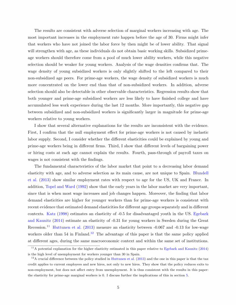
The results are consistent with adverse selection of marginal workers increasing with age. The

most important increases in the employment rate happen before the age of 30. Firms might infer

that workers who have not joined the labor force by then might be of lower ability. That signal

will strengthen with age, as these individuals do not obtain basic working skills. Subsidized prime-

age workers should therefore come from a pool of much lower ability workers, while this negative

selection should be weaker for young workers. Analysis of the wage densities confirms that. The

wage density of young subsidized workers is only slightly shifted to the left compared to their

non-subsidized age peers. For prime-age workers, the wage density of subsidized workers is much

more concentrated on the lower end than that of non-subsidized workers. In addition, adverse

selection should also be detectable in other observable characteristics. Regression results show that

both younger and prime-age subsidized workers are less likely to have finished college and have

accumulated less work experience during the last 12 months. More importantly, this negative gap

between subsidized and non-subsidized workers is significantly larger in magnitude for prime-age

workers relative to young workers.

I show that several alternative explanations for the results are inconsistent with the evidence.

First, I confirm that the null employment effect for prime-age workers is not caused by inelastic

labor supply. Second, I consider whether the different elasticities could be explained by young and

prime-age workers being in different firms. Third, I show that different levels of bargaining power

or hiring costs at each age cannot explain the results. Fourth, pass-through of payroll taxes on

wages is not consistent with the findings.

The fundamental characteristics of the labor market that point to a decreasing labor demand

elasticity with age, and to adverse selection as its main cause, are not unique to Spain. Blundell

et al. (2013) show similar employment rates with respect to age for the US, UK and France. In

addition, Topel and Ward (1992) show that the early years in the labor market are very important,

since that is when most wage increases and job changes happen. Moreover, the finding that labor

demand elasticities are higher for younger workers than for prime-age workers is consistent with

recent evidence that estimated demand elasticities for different age groups separately and in different

contexts. Katz (1998) estimates an elasticity of -0.5 for disadvantaged youth in the US. Egebark

and Kaunitz (2014) estimate an elasticity of -0.31 for young workers in Sweden during the Great

Recession.11 Huttunen et al. (2013) measure an elasticity between -0.067 and -0.13 for low-wage

workers older than 54 in Finland.12 The advantage of this paper is that the same policy applied

at different ages, during the same macroeconomic context and within the same set of institutions.

11A potential explanation for the higher elasticity estimated in this paper relative to Egebark and Kaunitz (2014)

is the high level of unemployment for workers younger than 30 in Spain.12A crucial difference between the policy studied in Huttunen et al. (2013) and the one in this paper is that the tax

credit applies to current employees and new hires, not only to new hires. They show that the policy reduces exits to

non-employment, but does not affect entry from unemployment. It is thus consistent with the results in this paper:

the elasticity for prime-age marginal workers is 0. I discuss further the implications of this in section 5.

5

Thus, we can be sure that the different elasticities are caused by changes during the life cycle and

not by other contextual factors. In light of previous evidence, the policy implications might apply

to other countries.

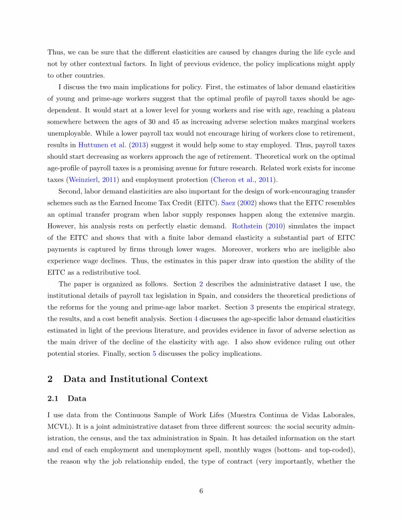
I discuss the two main implications for policy. First, the estimates of labor demand elasticities

of young and prime-age workers suggest that the optimal profile of payroll taxes should be age-

dependent. It would start at a lower level for young workers and rise with age, reaching a plateau

somewhere between the ages of 30 and 45 as increasing adverse selection makes marginal workers

unemployable. While a lower payroll tax would not encourage hiring of workers close to retirement,

results in Huttunen et al. (2013) suggest it would help some to stay employed. Thus, payroll taxes

should start decreasing as workers approach the age of retirement. Theoretical work on the optimal

age-profile of payroll taxes is a promising avenue for future research. Related work exists for income

taxes (Weinzierl, 2011) and employment protection (Cheron et al., 2011).

Second, labor demand elasticities are also important for the design of work-encouraging transfer

schemes such as the Earned Income Tax Credit (EITC). Saez (2002) shows that the EITC resembles

an optimal transfer program when labor supply responses happen along the extensive margin.

However, his analysis rests on perfectly elastic demand. Rothstein (2010) simulates the impact

of the EITC and shows that with a finite labor demand elasticity a substantial part of EITC

payments is captured by firms through lower wages. Moreover, workers who are ineligible also

experience wage declines. Thus, the estimates in this paper draw into question the ability of the

EITC as a redistributive tool.

The paper is organized as follows. Section 2 describes the administrative dataset I use, the

institutional details of payroll tax legislation in Spain, and considers the theoretical predictions of

the reforms for the young and prime-age labor market. Section 3 presents the empirical strategy,

the results, and a cost benefit analysis. Section 4 discusses the age-specific labor demand elasticities

estimated in light of the previous literature, and provides evidence in favor of adverse selection as

the main driver of the decline of the elasticity with age. I also show evidence ruling out other

potential stories. Finally, section 5 discusses the policy implications.

2 Data and Institutional Context

2.1 Data

I use data from the Continuous Sample of Work Lifes (Muestra Continua de Vidas Laborales,

MCVL). It is a joint administrative dataset from three different sources: the social security admin-

istration, the census, and the tax administration in Spain. It has detailed information on the start

and end of each employment and unemployment spell, monthly wages (bottom- and top-coded),

the reason why the job relationship ended, the type of contract (very importantly, whether the

6

contract benefited from a tax credit or not), the size of the firm, the sector, whether the job was

part-time and the number of hours, the location of the job, etc. The data also contains information

about the individual: sex, education, date of birth, province of birth, citizenship, as well as the

date of birth and sex of the members of their household.

The sample was constructed in the following way: in 2004, over 1 million of workers, or 4% of all

individuals who had some relationship with social security, were selected.13 Sampling was random,

without any kind of stratification. The data contains the labor history of each individual since he

started working, including periods when the worker was collecting UI or after he retired and started

receiving pension benefits. The same individuals selected in 2004 were followed for each edition

of the dataset between 2005 and 2012. Thus, I can reconstruct the working life of the individuals

since they started working up to 2012. In case a worker selected in 2004 leaves the sample in any

of the future years, because he stops having a relationship with social security (i.e. he is out of

employment and does not collect UI; he dies), he is replaced by another randomly selected worker

that had some relationship that year with social security. Similarly, the whole labor life of that

new worker is included in the dataset. Finally, if any of the workers is not sampled during one of

the editions of the dataset because he did not have any relationship with social security for a year

or more, but he becomes employed again, he will reappear in the dataset the year in which he had

restarted his relationship with the social security system.

The retrospective nature of the dataset raises concerns about its representativeness for the years

before 2004. This might be a problem specially for the results exploiting the policy change in 1997.

However, as shown in Bonhomme and Hospido (2012) it is only an issue when going back to the late

1980s. There are four main reasons for that. First, mortality rates are low throughout the period.

Second, attrition due to exit from the labor force because of retirement is not a problem since the

dataset includes pensioners and their previous labor histories. Third, from the mid nineties and

until the Great Recession, emigration out of Spain was very low. In fact, Spain became a host

country for immigrants. Fourth, early career interruptions are a concern for women. However, as I

show in section 4, the results are the same across genders. Thus, problems of attrition due to the

retrospective design of the sample are not a concern.

Table 1 reports summary statistics for the year 1997, when the tax credit policy was enacted.

I classify the workers in 5 year age groups and report the descriptive statistics for the main groups

of the empirical analysis: 25-30, 30-35, 40-45, and 45-50. Workers are more likely to be men for

all age groups. Most of them have achieved at most secondary education. The fraction that at

most completed primary education is increasing in age. Most of them are Spanish citizens, but

the importance of the immigrant labor force is bigger for the younger cohorts (almost 20%) than

for older cohorts (around 5%). Their real daily wage is of 37 euros for young workers, rising to

13Individuals who had some relationship with social security were either formally employed, receiving some kind

of unemployment insurance, or were perceiving a contributory pension.

7

47.26 for prime-age workers. The fraction of workers in what is considered good jobs (permanent

and public workers) is increasing in age, while the fraction of employees in short-term contracts is

decreasing. Incidence of part-time work is higher for younger workers. The mean size of the firm

is around 8-10 workers and most people work in the services sector.

2.2 Payroll Tax Legislation in Spain

Payroll tax legislation sets different payroll tax rates depending on the regime to which the worker is

affiliated. The main group, called “Regimen General”, includes most private and public employees

(13,419,951 workers or 77% of total).14 The following groups are self-employed workers (2,951,021

workers or 17% of total) and farmers (685,960 or 4% of total). There are other small schemes

for coal workers, sea workers, and housekeepers. The employment credits that are the focus of

this paper apply to all new permanent jobs, except for the sector of self-employed individuals. I

will thus focus on workers affected by the policy, but will also discuss the employment effect for

self-employed workers, since it is a common practise by firms to declare some work as carried out

by self-employed individuals to avoid paying payroll taxes and severance payments.

Payroll taxes in Spain are paid both by the employer and the employee. They are a function of

the wage of the employee and two tax rates: one that applies to employers and one that applies to

employees. There is a maximum and a minimum base for the wage depending on the occupational

category of the worker. The first two columns in table 2 show, for employees in “Regimen General”,

the minimum and maximum basis for each category of worker for 1997. The last three columns

show the tax rates for both employers (23.6%) and employees (4.7%), as well as the combined tax

rate (28.3%).15 The tax revenue collected is used to pay unemployment, workers’ accident, and

health insurance; and retirement, widow and orphan pensions. The money is also allocated to pay

for training courses and to protect the workers in case of firm’s default.

Spain’s unemployment is very high and volatile as can be seen in figure 1a. Even in the peak of

the 2000’s housing boom, unemployment was around 10%. It is also higher for younger cohorts and

women (figure 1b). In order to stimulate hiring and increase employment, the Spanish government

has implemented policies to reduce labor costs.16 Permanent and temporary contracts are the

two main types of work arrangements in Spain; the programs that reduce employers’ payroll taxes

apply only for workers hired as new permanent workers. It would have been a controversial political

decision to stimulate temporary employment. In fact, one of the objectives of the reform was to

reduce the fraction of temporary jobs. Temporary contracts are generally considered bad jobs in

14Data is for 2010. Source is Ministerio de Empleo y Seguridad Social (MESS), 2012.15 The payroll tax rate of the main group of workers has been very stable. Last reform took effect in 1995 and

decreased firms’ payroll tax rate by 3.3% and employees’ payroll tax rate by 4.1%.16 See online appendix for a full list of laws regarding payroll tax policy.

8

Spain, though it is hard to causally prove that they harm workers.17 Jimeno and Toharia (1993)

show that temporary contracts have a negative wage differential of about 10%. However, Davia and

Hernanz (2004) show that this wage differential is caused by different worker characteristics. Arranz

and Garcia-Serrano (2007) show that job stability has declined in Spain since the introduction

of temporary contracts. Regarding the effects on training of short-term contracts, Albert and

Hernanz (2005) find that workers holding temporary contracts are less likely to be employed in firms

providing training. More importantly, temporary workers employed in firms providing training are

less likely to be chosen to participate in training programs.

There are three main programs that reduce payroll tax rates: first, for workers hired before

their 30th birthday; second, for employees hired after their 45th birthday; third, for the long-term

unemployed (LTU) regardless of their age. Figure 2 displays the evolution of these programs over

time. The upper figure depicts the case of the credit for young workers and the LTU. Both tax

cuts were introduced in May 1997. At that time, the credits represented a 40% decrease of the

tax rate for the first two years of the contract. There were some changes in the generosity of the

tax credit, but they always applied for the first two years of job relationship. The main difference

between them is that the credit for young employees did not require the worker to have been at

least 1 year unemployed. Thus, they applied to a broader population. The credit for the young

was discontinued in March 2001, while the LTU credit was kept in place. After that, firms hiring

young workers with a credit could only do so if the individual fell in the category of LTU.

The lower figure depicts the case of the prime-age credit after 45 and that for the LTU. The

credit for workers older than 45 was first enacted in 1982. Until 1997, it also required that the

worker had been LTU (red dashed line). After that, it applied to all workers older than 45 (red solid

line). During the period of study, the prime-age credit after 45 suffered only small changes in its

generosity. The presence of a credit for the LTU is important because it will minimize substitution

effects across the age thresholds.

The dose of the treatment is sizable. Using the basis and tax rates for 1997 and assuming an

employee with wage equal to 2,000 euros, the monthly tax credit after 1997’s reform, for hiring a

young worker, is 2000× .236× .4 = 188.8. Thus, the subsidy represents a 7.6% saving in labor costs

during the first two years of the job relationship.18 In contrast, the monthly tax credit for workers

older than 45 years old when hired as permanent workers would have been 2000× .236× .6 = 283.2

euros each month during 2 years, and 2000 × .236 × .5 = 236 euros for the rest of the contract

duration. The savings represent 11.5% and 9.5% of the labor costs for the first two years and the

rest of the contract, respectively. Thus, the employment credits represent an important reduction

17Autor and Houseman (2010) do provide evidence that temporary job positions harm workers in a US context.18Note that this is the percentage saving for each new subsidized young hire during the first two years of job

relationship. Since currently employed workers are not subsidized, the average reduction in labor costs per worker

will be much smaller. See section 4 for more details.

9

in total labor costs.

Though the tax credits are not limited to firms that expand its workforce, its administrative

design makes them similar to a marginal employment subsidy (Johnson and Layard, 1986). There

are several limitations that limit the scope of the employment credit so that it targets only indi-

viduals with low job stability (temporary workers and unemployed).19 Most importantly, they can

only be received for workers who have not been working in a permanent contract during the last 3

months. Since on average temporary and unemployed workers have lower skills, this implies that

the program targets low-skilled individuals (Albert and Hernanz, 2005; Arranz and Garcia-Serrano,

2007; Davia and Hernanz, 2004; Jimeno and Toharia, 1993).

Two administrative details of the employment credits are important to limit the possibility of

strategic behaviors by firms, like excessive churning. The first one was introduced in 1999. Firms

who wrongfully dismissed workers with a tax cut are ineligible to hire again with a tax credit.20

The second limitation is that an employment credit contract cannot be signed with workers who

hold a permanent contract with the same firm group during the previous 24 months.21

Wage-setting in Spain is quite centralized. All collective bargaining agreements negotiated at

a level superior to the firm (i.e. national and provincial agreements; sectoral agreements) apply

to all firms that belong to the corresponding geographical or sectoral area, even if they did not

participate in the negotiation.22 In general, lower level agreements cannot modify agreements

reached at a superior level. Consequently, around 90% of workers in the private sector have their

wages fixed by collective bargaining (Izquierdo et al., 2003; OECD, 2012). The negotiated wage

is occupation specific (i.e. manager, administrative, etc.), applies to all ages, and increases with

tenure within the firm.23

Claiming a tax credit was an easy task. Figure 3 shows the back-page of a labor contract. The

employer has to fill in one of the options available in the sixth clause of the contract. Option a)

specifies the tax credit that was available between January 2000 and March 2001 for workers under

30. Option c) specifies the tax credit when the employer hires a worker over 45 years old. Finally,

19Guell and Petrongolo (2007) estimate that 86% of new entries in Spain are under short-term contracts, and that

only 5.7% of them are converted into permanent jobs.20The limitation applies either for a year since the dismissal happened or for as many workers as wrongful dismissals

happened.21Other limitations are: the tax-credited contracts cannot be used to hire relatives of the owner or of the manage-

ment chief; there are people who cannot benefit from the contract too: firms managers, home service, people in jail,

professional sportsmen, artists, and dockers working for public societies; the employers need to be current with tax

payments and must not have been excluded from the program because of any infraction they could have committed.

Finally, the tax-credited contract, combined with other programs, cannot suppose a tax credit of more than 60% of

the annual wage.22Agreements affecting most workers (50%) are negotiated at a sectoral and provincial level. 25% of workers’

conditions are negotiated at the national level. 8% are negotiated at the state level (Izquierdo et al., 2003).23Other issues negotiated are overtime hours, conversion of temporary contracts into permanent, limitations to

temporary and part-time hiring, retirement, and services to workers as provision of lunch and transport.

10

options b), d) and e) describe the tax cuts available if the firm hires employees in other situations

not only related to their age: workers registered as unemployed for at least a year, women hired

in sectors in which they are underrepresented, and unemployed people perceiving unemployment

assistance.

Finally, the age-targeted employment credits were accompanied by lower severance payments.

However, Elias (2014) explores the effects of lower severance payments for young workers during

the period 2001-2006, when no employment credits were available for that group. There are no

effects on hiring, employment or wages of reduced dismissal costs. Elias (2014) argues that the

main reason why this policy was not effective is that only firms that did not dismiss a worker in

the last 6 months could hire another worker with lower severance payments. The rationale for such

restriction was to limit excessive churning. Firms with the most turnover are likely to be the most

affected by high employment protection, but the limitation will not allow them to benefit from

lower severance payments. Such limitation was in place between 1997-2001 only to claim lower

severance payments, not the tax credit. Therefore, the main effect of the policy changes in 1997

must have been related to the employment credits. The details of severance payments regulation

are explained in the online appendix.

2.3 Theoretical Predictions and Heterogenous Responses

The standard tax incidence model, or competitive labor market, predicts that a decrease in payroll

taxes will shift demand outwards. My identification strategy thus relies on this exogenous change

in demand. The new employment and wage equilibrium will depend on the elasticities of labor

demand and supply. The more elastic is supply, the greater will be the effect on employment, and

the smaller the effect on wages. On the other hand, the more elastic is demand, the greater the

effect on both employment and wages. Figures 4a, 4b, and 4c represent the extreme cases with

perfect elastic supply, perfectly inelastic supply, and perfectly inelastic demand, respectively.24 25

But as explained in section 2.2, the labor market in Spain is not a spot market. Around 90%

of workers in the private sector have their wages determined by collective bargaining. Figure 4d

represents the equilibrium in a right-to-manage model, in which unions and employers bargain

over wages (Nickell and Andrews, 1983; Johnson and Layard, 1986; Boeri and van Ours, 2008).

24Note that supply will not shift out. In the standard tax incidence model, shifts in supply depend on changes in

the reservation wage. Its main determinant is non-wage income. Since the reform does not alter that variable, supply

does not shift out. In the case of a search model, an increase in the arrival rate of job offers increases the reservation

wage. That lowers the probability of accepting an offer and is akin to a decrease in labor supply. In that case we

expect to find increases in wages.25Models that depart from the competitive labor market framework by introducing search-and-matching frictions

also predict that an employment credit will shift demand out (Pissarides, 1998; Mortensen and Pissarides, 2001),

and that the new employment and wage equilibrium will depend on the point where the demand and wage (supply)

functions cross. I discuss further the implications of search-and-matching models in section 4.

11

Then, employers take wages as given and choose employment levels that maximize the profits of

the firm. The outcome depends on the bargaining power of unions (0 ≤ β ≤ 1; 0 is the competitive

case, and 1 the case in which the union sets wages unilaterally). The solid black line represents

the competitive equilibrium case.26 The stronger the bargaining power of unions, the higher the

equilibrium wage. The dashed black line depicts the situation when all bargaining power is on

the union-side. The exact location of the equilibrium depends on the bargaining power of unions.

The shift outward in demand will increase employment, but wages will remain the same as long

as supply constraints do not become binding. Given the level of union coverage in Spain, and the

high level of unemployment, such a representation seems realistic. Note that the predictions are

the same in a competitive market with perfectly elastic supply, and thus the standard incidence

formulas can still be applied.

A shift in demand corresponds to firms who are at the margin of hiring. The tax credit makes

some new matches productive and employment increases. However, there will also be responses by

firms that would have hired in any case, but will do now with a tax credit. This can happen through

two channels: first, firms can substitute workers above 30 (below 45) for workers below 30 (above

45) (Davidson and Woodbury, 1993). Second, firms can claim a tax credit for a worker under 30

or above 45 that would have been hired in any case, and receive the tax credit as a transfer. Such

behavioral responses will give rise to inefficiencies in the implementation of employment credits and

I will explore them too.

But transaction costs will limit the extent to which substitution and windfalls are happening.

First, as described in section 2.2, there are several limitations in the policy that will minimize

such behavior. Second, substitution across age groups depends on the extent to which workers

under 30 and above 45 are good substitutes in production for existing workers, and on the extent

that it is easy to churn employees. Given the high level of severance payments for permanent

workers, dismissing permanent workers to replace them with subsidized ones seems a rather costly

alternative.27 Third, there is also an employment credit for the long-term unemployed that can

be used regardless of the age of the worker. Thus, the hiring of the most disadvantaged workers

between 30 and 45 was also incentivized.

However, can we expect the responses to be identical in the young and prime-age labor market?

In other words, are labor demand and supply elasticities the same over the life cycle? Closer

inspection of each labor market suggests that this will not be the case. Each labor market has

very distinct features. Figure 5 contains several pictures that summarize the main differences.

26Labor supply is flat as a consequence of assuming that all workers are identical and have the same reservation

wage. While this might not be the case, it eases the graphical representation.27For dismissals considered wrongful by the courts, severance payments amount to 45 days of salary for each year

of tenure in the firm, up to 42 months of salary. 3/4 of all layoffs that go to court are considered wrongful by judges

(Bentolila, 1996). For more details on severance payments see the online appendix.

12

Figure 5a shows that the employment rate of workers younger than 30 years old is much lower than

for prime-age workers. It also shows that the most important increases in the employment rate

happen before the age of 30. Between the age of 20 and 30, the employment rate increases by 35.86

percentage points (pp). After 30, the evolution is much slower, increasing by an extra 12.95 pp

at the age of 45. The low employment rate of young workers is certainly due to these individuals

being in other activities, such as education, but it is also caused by a much higher incidence of

unemployment for young workers. As can be seen in figure 5b, the unemployment rate is around

37% for workers aged 20-25, and drops to 20% for those aged 30-35. Unemployment of prime-age

workers is much lower, being around 12.5% at ages 45-50.

Since the policy subsidizes only new permanent hires, it is important to further distinguish

between permanent workers and those in other types of contracts. Figures 5c and 5d display the

ratio of permanent and temporary workers with respect to all individuals who are working at each

age, respectively. Before the age of 30, there is an increase in the ratio of permanent workers, and

a decrease in the ratio of temporary ones. Therefore, the young labor market is characterized by

transitions to more stable jobs. Note that the ratio of permanent workers barely changes after the

age of 30. It remains constant around 50% until the ages of 55-60, when workers start retiring. In

contrast, the ratio of temporary workers after 30 is still decreasing, though at a much slower rate.

These are workers that are becoming self-employed or are finding public sector jobs, as can be seen

in figure 5 in the online appendix. Thus, there does not seem to be much room at the age of 45 to

increase permanent employment.

Figure 5e shows the starting wage of permanent workers at the age at which they are hired. It

is before the age of 30 when most wage increases happen. After 30, the wage of new permanent

hires stabilizes. Consequently, the young labor market is also characterized by transitions to better

jobs, while such dynamism halts after 30.

Finally, figure 5f shows the mean length of permanent contracts over age at hired. Job tenure

of new hires is increasing until 30, is stable until the age of 50, and then starts dropping as workers

approximate the age of retirement. Lower job tenure for young workers is important since it might

deter some firms from hiring them. If an employer has to invest in worker skills, he wants to

maximize the expected return from a job relationship. To the extent that younger workers stay

shorter in firms, that can deter hiring in the young labor market.

It is important to note that these characteristics are not unique to the Spanish labor market.

Blundell et al. (2013) plot the employment rate for the USA, UK and France in 1977 and 2007 and

find similar patterns. Topel and Ward (1992) also show, for the US, that it is during the early years

in the labor market that most wage increases and job changes happen. Finally, Murphy and Welch

(1990) show, also for the US, that the age-earnings profile is an increasing concave function, with

most wage increases happening during the early years of a worker’s career. To the extent that the

characteristics of the Spanish young and prime-age labor market are shared across countries and

13

over time, the findings of this paper will have a wider applicability for labor policy design.

3 Empirical Strategy and Results

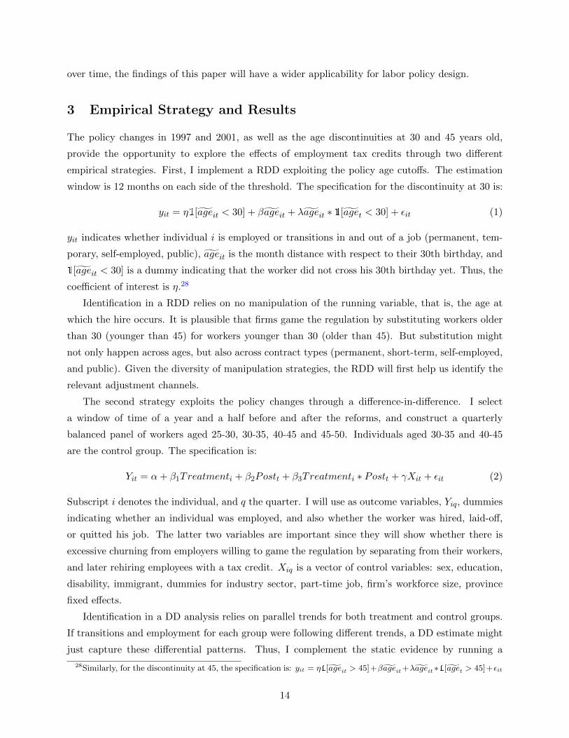
The policy changes in 1997 and 2001, as well as the age discontinuities at 30 and 45 years old,

provide the opportunity to explore the effects of employment tax credits through two different

empirical strategies. First, I implement a RDD exploiting the policy age cutoffs. The estimation

window is 12 months on each side of the threshold. The specification for the discontinuity at 30 is:

yit = η1[ageit < 30] + βageit + λageit ∗ 1[aget < 30] + εit (1)

yit indicates whether individual i is employed or transitions in and out of a job (permanent, tem-

porary, self-employed, public), ageit is the month distance with respect to their 30th birthday, and

1[ageit < 30] is a dummy indicating that the worker did not cross his 30th birthday yet. Thus, the

coefficient of interest is η.28

Identification in a RDD relies on no manipulation of the running variable, that is, the age at

which the hire occurs. It is plausible that firms game the regulation by substituting workers older

than 30 (younger than 45) for workers younger than 30 (older than 45). But substitution might

not only happen across ages, but also across contract types (permanent, short-term, self-employed,

and public). Given the diversity of manipulation strategies, the RDD will first help us identify the

relevant adjustment channels.

The second strategy exploits the policy changes through a difference-in-difference. I select

a window of time of a year and a half before and after the reforms, and construct a quarterly

balanced panel of workers aged 25-30, 30-35, 40-45 and 45-50. Individuals aged 30-35 and 40-45

are the control group. The specification is:

Yit = α+ β1Treatmenti + β2Postt + β3Treatmenti ∗ Postt + γXit + εit (2)

Subscript i denotes the individual, and q the quarter. I will use as outcome variables, Yiq, dummies

indicating whether an individual was employed, and also whether the worker was hired, laid-off,

or quitted his job. The latter two variables are important since they will show whether there is

excessive churning from employers willing to game the regulation by separating from their workers,

and later rehiring employees with a tax credit. Xiq is a vector of control variables: sex, education,

disability, immigrant, dummies for industry sector, part-time job, firm’s workforce size, province

fixed effects.

Identification in a DD analysis relies on parallel trends for both treatment and control groups.

If transitions and employment for each group were following different trends, a DD estimate might

just capture these differential patterns. Thus, I complement the static evidence by running a

28Similarly, for the discontinuity at 45, the specification is: yit = η1[ageit > 45]+βageit +λageit ∗1[aget > 45]+εit

14

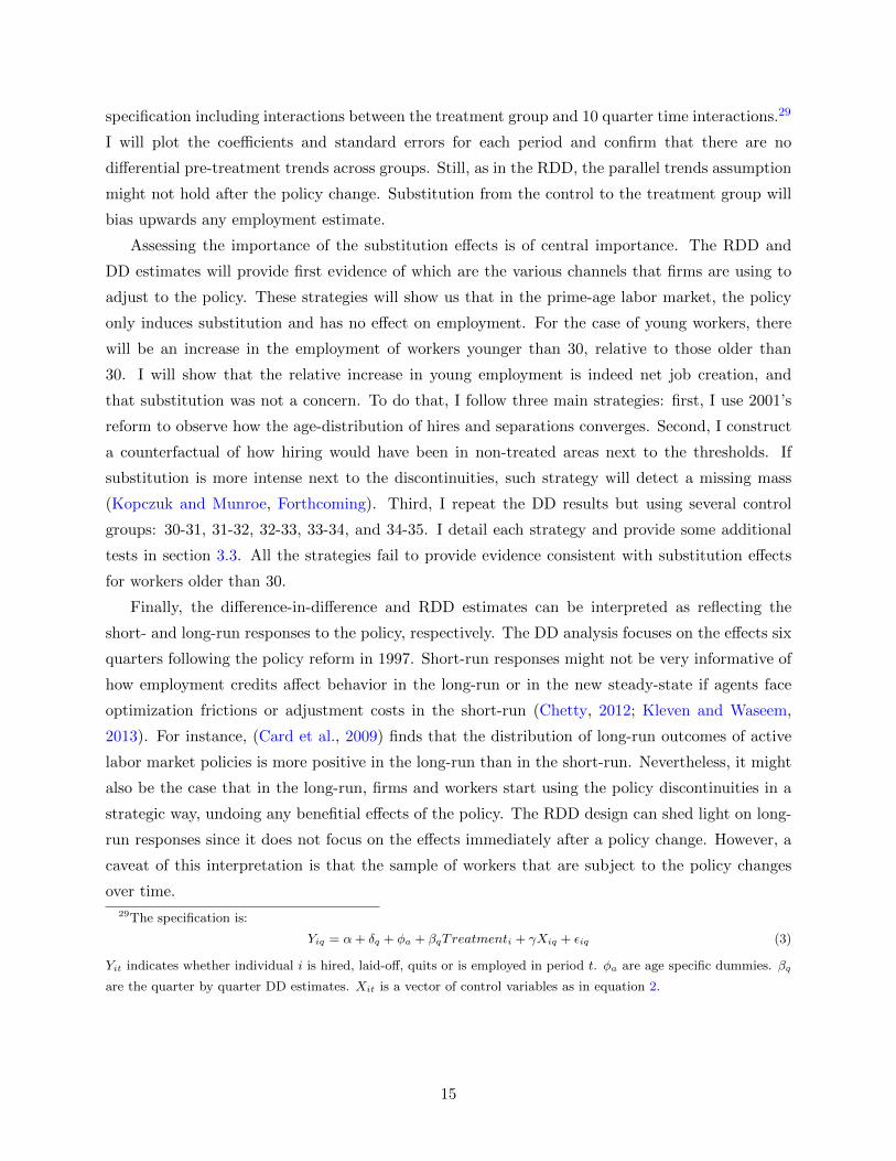
specification including interactions between the treatment group and 10 quarter time interactions.29

I will plot the coefficients and standard errors for each period and confirm that there are no

differential pre-treatment trends across groups. Still, as in the RDD, the parallel trends assumption

might not hold after the policy change. Substitution from the control to the treatment group will

bias upwards any employment estimate.

Assessing the importance of the substitution effects is of central importance. The RDD and

DD estimates will provide first evidence of which are the various channels that firms are using to

adjust to the policy. These strategies will show us that in the prime-age labor market, the policy

only induces substitution and has no effect on employment. For the case of young workers, there

will be an increase in the employment of workers younger than 30, relative to those older than

30. I will show that the relative increase in young employment is indeed net job creation, and

that substitution was not a concern. To do that, I follow three main strategies: first, I use 2001’s

reform to observe how the age-distribution of hires and separations converges. Second, I construct

a counterfactual of how hiring would have been in non-treated areas next to the thresholds. If

substitution is more intense next to the discontinuities, such strategy will detect a missing mass

(Kopczuk and Munroe, Forthcoming). Third, I repeat the DD results but using several control

groups: 30-31, 31-32, 32-33, 33-34, and 34-35. I detail each strategy and provide some additional

tests in section 3.3. All the strategies fail to provide evidence consistent with substitution effects

for workers older than 30.

Finally, the difference-in-difference and RDD estimates can be interpreted as reflecting the

short- and long-run responses to the policy, respectively. The DD analysis focuses on the effects six

quarters following the policy reform in 1997. Short-run responses might not be very informative of

how employment credits affect behavior in the long-run or in the new steady-state if agents face

optimization frictions or adjustment costs in the short-run (Chetty, 2012; Kleven and Waseem,

2013). For instance, (Card et al., 2009) finds that the distribution of long-run outcomes of active

labor market policies is more positive in the long-run than in the short-run. Nevertheless, it might

also be the case that in the long-run, firms and workers start using the policy discontinuities in a

strategic way, undoing any benefitial effects of the policy. The RDD design can shed light on long-

run responses since it does not focus on the effects immediately after a policy change. However, a

caveat of this interpretation is that the sample of workers that are subject to the policy changes

over time.

29The specification is:

Yiq = α+ δq + φa + βqTreatmenti + γXiq + εiq (3)

Yit indicates whether individual i is hired, laid-off, quits or is employed in period t. φa are age specific dummies. βq

are the quarter by quarter DD estimates. Xit is a vector of control variables as in equation 2.

15

3.1 Effects on Transitions, Employment and Wages of Prime-Age Workers

The evidence on transitions and employment of prime-age workers is the same both using the DD

and the RDD strategy. I thus discuss only the RDD here, and I relegate the DD findings to the

online appendix. Figure 6 displays the hiring flows around the 45th birthday. Figures on the left are

for the period when the policy is in place (1997-2006). Figures on the right are for a period when

the policy had an extra requirement: only workers older than 45 that had been unemployed for a

year could be hired with a tax credit. As can be seen, the policy generates a big jump in permanent

hiring at 45 between 1997-2006. Visual inspection suggests that firms are gaming the regulation.

After the 43rd birthday, the distribution features a faster decline in hiring. This suggests that

firms delay some hires until the worker’s 45th birthday. For the period 1992-1997, the distribution

of permanent hires does not display a similar distortion. There is though a jump at 45, which is

consistent with the one year of unemployment that was necessary then to claim the tax credit over

45. Thus, some workers might have waited to be hired until they fulfilled both requirements. As

can be seen from the lower figures, the policy does not affect the flows into temporary jobs. This

is consistent with the policy only subsidizing permanent jobs.

Figure 7 displays the stocks of workers within each type of job around the 45 year threshold

for the period 1997-2006. In contrast to what the flow figures suggest, the policy is affecting both

temporary and permanent workers. The stock of permanent workers decreases around the age of

44, whereas the stock of short-term workers increases around the same age. At 45, there is a jump

upwards in the stock of permanent workers, and a jump downwards in the stock of temporary

employees. The slope after 45 for permanent jobs is steeper than before the threshold. However, as

can be seen in figure 7c, this does not translate in a reduction in non-employed workers. The figures

suggests that some of these extra permanent workers after 45 would have been either temporary or

would have worked in the public sector. Overall, the figures suggest a null effect on employment of

prime-age workers.

If employers were delaying the entry into permanent contracts of temporary workers, there

should be an increase in the length of temporary contracts before 45. Consistent with that, figure

7f shows that between the ages of 41 and 44.5, temporary contracts were unusually long.

Table 3 translates the above discussion into estimates. Panel A and B analyze the effects on

hires. Panel A restricts the sample to 1 year immediately after the policy change (short-run). Panel

B is for the sample between 12 months after the policy change until 2006 (long-run). Both in the

short- and long-run, the policy only affects flows into permanent employment at the thresholds, but

not entries into short-term, self-employment, public jobs or UI. Long-run estimates of transitions

are slightly larger than short-run ones, but the estimates are not significantly different. This finding

suggests that for new hires adjustment to the policy was fast and that optimization frictions were

not very important.

16

Panel C reports the results for employment effects at the 45 years old discontinuity. There

is a positive effect on the number of people employed with permanent contracts. However, the

size of the effect is identical to the drop of people employed with short-term contracts after 45,

as column 3 indicates. There is no effect on employment of the program. Thus, the program for

workers older than 45 years just retimes conversions from short-term to permanent that would

have had happened otherwise. Note that the slope after 45 for permanent contracts is positive

and significant. The slope after 45 for short-term workers is negative and significant, and so is the

slope for non-employed workers. However, that might be caused by changes in the slope before 45

because firms and workers are delaying permanent hiring until the worker crosses the 45th birthday,

as discussed above. To test whether the change in slopes is caused by reallocation in the proximity

of the threshold, panel D reports the results of a donut RDD. I omit 1 year on each side of the

threshold. Thus, I test whether the progression of employment is the same between 12-24 months

before the discontinuity with respect to 12-24 months after the threshold. The lower panel of

table 3 reports the results of the slopes: permanent employment is still increasing faster after the

threshold, but once one accounts for the decrease in temporary employment, the slope after 45 is

no longer significant (column 3). There is a small but significant negative effect on the slope after

45 for public workers. Overall, non-employment is not decreasing faster after the discontinuity

(column 6), confirming the graphical evidence.

The results for prime-age workers show that the payroll tax credit at 45 was not successful

in stimulating prime-age employment. Firms gamed the policy by arbitraging between subsidized

contracts (permanent) and non-subsidized ones (temporary). This result is surprising in light of

a 9.5% decrease in labor costs for the whole duration of the contract. One potential reason why

the policy might fail in increasing employment is that workers were capturing the rent in terms

of higher wages. However, in section 4 I will show that that was not the case and that firms are

actually the ones receiving the transfer.

I now turn to discuss the impacts on wages. The results are based on a DD analysis exploiting

the change in 1997 and are shown in columns 1-3 in table 4. The dependent variable is the log real

daily wage and I select the sample of new permanent hires. The retiming of entry into permanent

jobs around 45 will cause compositional effects on the treatment and control groups. Better workers

should be able to avoid a delay when signing their permanent contract. Thus, the pool of permanent

hires after 45 should become relatively worse after 1997. And the pool before 45 relatively better.

Column 1 reports the results without control variables. Wages of new hires after 45 are on average

2.3% lower. However, when I include individual controls the coefficient drops to -1.8% and is only

significant at the 10% level.30 When I include occupation, cohorts, calendar quarter, and province

fixed effects the coefficient is no longer significant and drops to -0.3%. Thus, once one accounts for

compositional changes, there does not seem to be any effect on wages of prime-age workers.

30Controls are: education, experience, sex, citizenship, workers’ disability, firm size, firm sector, and part-time job.

17

3.2 Effects on Transitions, Employment and Wages of Young Workers

Difference-in-Difference Evidence . I start by exploring the effects of the employment credit

through a DD. Since permanent and temporary contracts are the most prevalent ones, I will focus

most of the discussion on them. The results for transitions in and out of these work arrangements

are in the upper panel of table 5. Permanent hires increase by 0.35 (pp). The number of permanent

lay-offs decreases by 0.046 pp. This could be caused by firms dismissing workers over 30 in order to

replace them with younger subsidized workers. In contrast, the number of quits increases by 0.082

pp. The latter effect is consistent with some young workers breaking their job matches knowing

that, thanks to the employment credit, they are more likely to receive a job offer and improve their

job situation. However, the estimates of separations are an order of magnitude smaller than those

of hires. This indicates that excessive churning is not a concern.

There is also an increase in temporary hires of 0.37 pp. This is an indirect effect of the policy,

since temporary contracts were not subsidized. However, both lay-offs and quits of temporary

workers also increase by .32 pp and .15 pp. Firms could be using temporary contracts to screen

young workers. For those who perform better, they will break the temporary contract and hire

them as permanent. Consistent with that story, transitions from temporary to permanent contracts

within the same firm also increase by 0.18 pp (column 7, panel A).

The analysis of flows suggests that the stock of young workers should increase. The lower panel of

table 5 reports the estimates for employment. The stock of young permanent and temporary workers

increases by 0.22 pp and 0.19 pp, respectively. Note that there is no evidence of crowding out of

other work arrangements like self-employment or public jobs. Thus, overall employment increases

by 0.34 pp. Very importantly too, the stock of workers receiving UI decreases by 0.17 pp. Part of

that effect can happen because temporary workers are more likely to suffer non-employment spells

because of the short-term nature of their job. Another part can come from workers unemployed

for a long time. The decrease in UI implies that subsidizing employment might be a cost-efficient

way to increase employment, since it will trigger savings from social insurance schemes.

Figure 8 displays the dynamic effect of the policy. The identification assumption of parallel

trends across treatment and control groups, before the policy change, appears to hold. The esti-

mates oscillate around zero and are not significant before the policy change. Once the policy is

enacted, the estimates jump upward and become significant.

If I compare the estimates to the mean level of transitions and employment during the year

previous to the reform in 1997, they represent an increase in permanent transitions of 57% (relative

benchmark mean is 0.61%). The increase in short-term transitions is of 15.6% (benchmark is 2.38%).

Permanent employment increases by 1.06% (benchmark is 20.85% and short-term employment by

0.97% (benchmark is 19.68%). Overall private sector employment of workers aged 25-30 increases

by 0.84% (benchmark is 40.53%) and the number of UI recipients in this age group decreases by

18

3.82% (benchmark is 4.42%).

I now turn to the effects on wages of employment credits. I repeat the difference-in-difference

analysis as in equation 2. The dependent variable is the log daily real wage of new permanent hires.

On one hand, the increase in employment of young workers might push wages up if there are supply

constraints. However, such effect is unlikely given that the wage of 90% of private sector workers are

decided by collective bargaining (see section 2.2). On the other hand, the increase in employment

under 30 might be happening through workers of lower ability or in less productive positions (and

hence, lower collectively-bargained wages). If such compositional effects are happening, we expect

to find a negative effect on the average wage. Columns 4-6 in table 4 show the results. Column

4 does not include controls, column 5 includes individual characteristics, and column 6 includes

several fixed effects.31 None of the coefficients are statistically significant. Note also that the

coefficient in the most stringent specification is very small (0.09%). In line with the institutional

details of collective bargaining, there is no evidence of supply constraints. There is no evidence

either that the increase in employment of young workers is happening mainly through an expansion

of jobs for low-wage positions.

The employment credit for young employees was discontinued in 2001. This provides and

opportunity to check the robustness of the 1997 DD. Since the tax cut had been in place for almost

4 years, it also allows to test for how persistent the effects are. The findings are in the online

appendix. All the results are analogous to those obtained with the change in 1997.

Regression Discontinuity Evidence . Figure 9 displays the hiring flows around the 30th

birthday. Figures on the left are for the period when the policy is in place (1997-2001). Figures

on the right are for a period when the credit for young workers did not exist (2001-2005). As can

be seen, the policy generates a jump in permanent hiring at 30 between 1997-2001. For the period

2001-2005, the distribution of permanent hires does not display such jump. The lower-left figure

shows the hiring distribution of temporary contracts when the credit was available. In contrast

to the DD evidence, there is not evidence of the subsidy affecting temporary hires around the

threshold. This is consistent with employers needing time to screen workers before hiring them as

permanent with the tax credit.

Table 6 reports the estimates of the jump at 30. Panel A shows the results for the first 12

months after the policy is enacted (short-run), and panel B from the 12th month and onward

(long-run). Like the results for prime-age workers, the tax credit does not affect transitions into

temporary or public jobs, self-employment, and UI. The long-run estimate is larger (.14 pp) than

the short-run one (.11 pp), but not significantly different. Like for prime-age workers, the response

in hiring was fast.

In terms of the stocks of workers, the payroll tax credit for individuals younger than 30 generates

31Individual controls are education, experience, sex, citizenship, workers’ disability, firm size, firm sector, part-time

job. Fixed effects include occupation, province, cohort, and calendar quarter.

19

kinks at the discontinuity. Figures 10 and 11 display the evolution of workers in permanent or short-

term contracts, receiving UI, or the fraction of all those who work. I restrict the treatment sample

to cohorts that were at most 29 in May 1997 (born between 05/1968 and 03/1971), so that they

could benefit from the policy for at least a year. I use as a placebo sample cohorts that could

not benefit from the employment credits during the months before becoming 30 because the policy

had been removed (born between 03/1973 and 03/1976). Cohorts crossing their 30th birthday

when the policy was in place experienced slower increases in their probability of being permanent

workers after the threshold. The fraction of them being short-term workers was decreasing before

30, and decreased at a slower pace after 30. This indicates that in the long-run, part of the effect

is shifting between subsidized and not subsidized contracts. There also seems to be a smaller slope

after 30 for the evolution of all individuals who are working, indicating that the policy is also

having employment effects. As a confirmation of that, note that the evolution of UI recipients was

decreasing before 30, and stabilizes or slightly increases after 30.32 Note that for placebo cohorts

there are not such changes in slopes centered at 30.

To translate the above discussion into estimates, I perform a RDD as in equation 1, but now the

coefficient of interest is λ, or the differential employment slope after 30 relative to the slope before

30. Table 6 reports the results. Panel C shows it for treated cohorts and panel D for the placebo

cohorts. The coefficients confirm the visual analysis. The slope after 30 for permanent workers

is significantly less positive, whereas that of short-term workers is significantly less negative. The

slope for UI is also significantly less negative after 30. Most importantly, the slope after 30 for

overall employment is significantly less positive. The coefficient indicates that the increases in

overall employment are 0.065 pp smaller every month after 30. To compare that estimate with

the difference-in-difference one, 6 quarters after overall employment would have increased by 1.17

pp more if the policy had been in place until the age of 31.5. The estimate in the long-run is

significantly larger than the short-run one, that indicated an increase of .34 pp 18 months after the

policy had been enacted. Thus, while the effects on transitions are quite immediate, the increases

in employment take more time to build up. Finally, note that none of the estimates for the slope

after 30 for the placebo cohorts are significant (panel D).

3.3 Substitution Effects

Both the DD and the RDD evidence confirm that the payroll tax credit increased employment

under 30 relative to that over 30. However, part or all the increase could be offset by a negative

effect on workers older than 30. I turn now to explore this possibility. I rely on several methods.

Convergence of the hiring distribution after 2001 . First, I consider the potential effects

that the credit for workers younger than 30 could have on hiring on each side of the threshold.

32For self-employed and public workers, see figure 4 in the online appendix .

20

Figure 12 illustrates each case. The first graph considers the situation absent any discontinuity. In

that case, the number of entries into permanent contracts would have been smooth across the 30

year threshold. The second graph represents a situation in which both job destruction and creation

are taking place around the threshold. Finally, the third graph shows the case when there is no job

destruction next to the threshold and the policy only stimulated hiring below it. Exploiting the

2001 reform, I can look at how the age-distribution of permanent hires adapts once the credit is

removed. The idea is to identify a pattern similar to the ones just described. The 2001 change is

more adequate for that purpose because the only change across the 30th threshold was the removal

of the credit for workers under 30. Inference based on the 1997 change is more complicated because

a credit for long-term unemployed workers was also introduced.33

Figure 13a shows the raw hiring data before and after each policy change. As is visually

evident, the removal of the tax credit for workers younger than 30 led to a convergence of the

hiring distribution only from below 30, as illustrated in the hypothetical figure 12c. Hiring above

30 does not show any jump upwards as expected with displacement effects. In order to translate

the discussion into numbers, I estimate difference-in-difference coefficients for each age bin. The

specification is:

yit = α+ δTreatmentt +40∑

a=20

βaAgeit +40∑

a=20

δaAgeit ∗ Treatmentt + εit (4)

The omitted group are workers 20 years old or less. The coefficient δa is a difference-in-difference

estimate of the effects of the policy for each age bin relative to the workers in the omitted group.

The age bins are 3 months wide. As can be seen in figure 13b, the policy was creating jobs below

30, but was not destroying jobs above 30, relative to workers below 20 years old. Also, the effects of

the policy are slightly stronger for workers between 25 and 30 years old than for younger workers.

Though the evidence so far suggests that there were no displacement effects, and that all the

adjustment happened through an expansion of hiring below 30, it could still be the case that workers

above 30 were more likely to separate from their employers. Figures 13c and 13d show that this

was not the case. Estimates for lay-offs and quits, with respect to the age when the separation

occurs, are not significantly different for the treatment (25-30) and the control group (30-35).

Hiring counterfactuals. A caveat with the strategy above is that it might be specific to the

period around 2001, and not reflect substitution happening during the whole period (1997-2001)

for which the policy was in place. For that reason, I construct counterfactuals of how the hiring

distribution would have looked like if the threshold had been moved to the left of 30 (i.e. at 29

years) or to the right of 45 (i.e. 46). Under the assumption that workers close to each threshold

are more substitutable than workers far away from the discontinuity, this method should detect a

missing mass of hires after 30 and before 45.

33Evidence on displacement for 1997 is in the online appendix. See figure 3. The results are consistent with those

for 2001.

21

The following is a description of the details of the estimation. I only explain the case for young

workers, but the case for the prime-age workers is symmetric. cj is the log number of individuals

in bin j in my main specification. I group individuals into age bins indexed by j. Each bin is 3

months wide. To construct the counterfactual I run the following specifications:

cj =

p∑i=0

βi(aj)i +

aU∑i≥aL

γi1[aj = i] + vj (5)

aj is the age at bin j, p is the order of the polynomial, which is 1 for the preferred specification.34 aL

and aU are the lower and upper bounds of the area that is not used to construct the counterfactual.

The counterfactual distribution is estimated as the predicted values from 5 omitting the con-

tribution of the dummies in the excluded range:

cj =

p∑i=0

βi(aj)i (6)

Missing mass is estimated as the difference between the observed and counterfactual bin counts

between the threshold (a∗) and the upper bound of the omitted area (aU ). I choose as lower and

upper bound for young workers 20 and 31.5, respectively.35 The equation for missing mass is:

M =

aU∑j=a∗

(cj − cj) (7)

The measure of the hole is:

h =M∑aUa∗ cj

(8)

Standard errors are obtained using a bootstrap procedure. I sample residuals from equation 5

with replacement to generate many age-hire distributions. The standard errors are the standard

deviation of the distribution of estimates obtained from each sample.

Results are in figure 14. As can be seen, the counterfactual between 30 and 31.5 matches very

well the actual distribution of hiring. The estimate of the missing mass has the opposite expected

sign and is not significantly different than 0. In contrast, the counterfactual between 43.5-45 is

different from the actual hiring distribution. It detects a significant missing mass of hires of 6.77%.

This evidence complements the results based on the age distribution of hires before and after the

policy change in 2001. It suggests that substitution of workers older than 30 years for younger

workers is not happenning, not only around 2001, but during the whole period when the policy was

in place.

DD changing the control group. The counterfactual strategy fails to detect a missing mass

of hires just after 30, but does so before 45. If substitution is proportionally higher next to the

34The rationale behind the election of a first-order polynomial is that the hiring distribution of workers between

30-45 years is highly linear.35The lower bound for prime-age workers is 43.5, and the upper bound is 55.

22

discontinuity, but dies away smoothly as we move to older cohorts, this strategy will fail to detect

substitution. A way to detect if that is the case is to repeat the DD estimation, but using several

control groups: 30-31, 31-32, 32-33, 33-34, and 34-35. If substitution was happenning, we would

expect to see that the estimated effects decrease as we choose as a control group older workers.

This is the same strategy as the one used in Blundell et al. (2004).

Results for both policy changes are in table 7. The estimates for new hires using different

control groups are very stable. Moreover, they are not significantly different from each other and

are not decreasing as we move away from 30. The coefficients for lay-offs and quits show a similar

picture.

Additional evidence on displacement . The evidence points to workers older than 30 not

being affected by substitution. I perform some additional robustness checks. The specifications

and results are detailed in section 5 in the online appendix. First, individuals born in March 1971

crossed their 30th birthday when the policy was removed in March 2001. Thus, those who were still

unemployed at the age of 30 cannot suffer from displacement since the policy is no longer in place.

Therefore, if displacement was an issue, the changes in slope that we have detected for cohorts

crossing their 30th birthday between May 1997 and March 2001 should be smaller for the March

1971 cohort relative to similar cohorts born in the previous year. However, the findings in tables

15-17 in the online appendix rule out that possibility.

The second strategy looks at cohorts that had already crossed the 30th birthday in March 2001.

In that case, after the removal of the policy they should benefit positively since they will not suffer

from displacement any more. Therefore, we should detect a positive change in the evolution of

their employment slope after March 2001. Results are in tables 18 and 19 in the online appendix

and I do not find evidence of a positive rebound.

Finally, I plot the flows in and out of permanent contracts around each policy change. If workers

in the control group are substituted for workers in the treatment group, we should observe that

their monthly number of hires shifts down after May 1997 (up after March 2001). The graphs are

displayed in figure 2 in the online appendix and do not show evidence consistent with substitution.

Overall, the evidence rules out the presence of substitution effects. Thus, the employment

estimates reflect net job creation, and do not confound positive and negative employment effects

on the treated and non-treated, respectively. It is important to keep in mind that there were also

non-age related employment credits targeting other disadvantaged groups such as the long-term

unemployed. Such schemes are probably the reason why the policy is successful at stimulating

employment below 30, while not creating significant negative employment effects above 30.

23

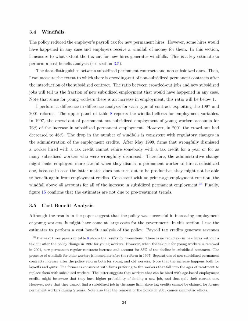
3.4 Windfalls

The policy reduced the employer’s payroll tax for new permanent hires. However, some hires would

have happened in any case and employers receive a windfall of money for them. In this section,

I measure to what extent the tax cut for new hires generates windfalls. This is a key estimate to

perform a cost-benefit analysis (see section 3.5).

The data distinguishes between subsidized permanent contracts and non-subsidized ones. Then,

I can measure the extent to which there is crowding-out of non-subsidized permanent contracts after

the introduction of the subsidized contract. The ratio between crowded-out jobs and new subsidized

jobs will tell us the fraction of new subsidized employment that would have happened in any case.

Note that since for young workers there is an increase in employment, this ratio will be below 1.

I perform a difference-in-difference analysis for each type of contract exploiting the 1997 and

2001 reforms. The upper panel of table 8 reports the windfall effects for employment variables.

In 1997, the crowd-out of permanent not subsidized employment of young workers accounts for

76% of the increase in subsidized permanent employment. However, in 2001 the crowd-out had

decreased to 46%. The drop in the number of windfalls is consistent with regulatory changes in

the administration of the employment credits. After May 1999, firms that wrongfully dismissed

a worker hired with a tax credit cannot rehire somebody with a tax credit for a year or for as

many subsidized workers who were wrongfully dismissed. Therefore, the administrative change

might make employers more careful when they dismiss a permanent worker to hire a subsidized

one, because in case the latter match does not turn out to be productive, they might not be able

to benefit again from employment credits. Consistent with no prime-age employment creation, the

windfall above 45 accounts for all of the increase in subsidized permanent employment.36 Finally,

figure 15 confirms that the estimates are not due to pre-treatment trends.

3.5 Cost Benefit Analysis

Although the results in the paper suggest that the policy was successful in increasing employment

of young workers, it might have come at large costs for the government. In this section, I use the

estimates to perform a cost benefit analysis of the policy. Payroll tax credits generate revenues

36The next three panels in table 8 shows the results for transitions. There is no reduction in new hires without a

tax cut after the policy change in 1997 for young workers. However, when the tax cut for young workers is removed

in 2001, new permanent regular contracts increase and account for 35% of the decline in subsidized contracts. The

presence of windfalls for older workers is immediate after the reform in 1997. Separations of non-subsidized permanent

contracts increase after the policy reform both for young and old workers. Note that the increase happens both for

lay-offs and quits. The former is consistent with firms prefering to fire workers that fall into the ages of treatment to

replace them with subsidized workers. The latter suggests that workers that can be hired with age-based employment

credits might be aware that they have higher probability of finding a new job, and thus quit their current one.

However, note that they cannot find a subsidized job in the same firm, since tax credits cannot be claimed for former

permanent workers during 2 years. Note also that the removal of the policy in 2001 causes symmetric effects.

24

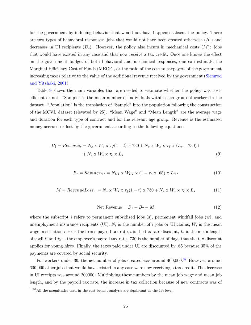
for the government by inducing behavior that would not have happened absent the policy. There

are two types of behavioral responses: jobs that would not have been created otherwise (B1) and

decreases in UI recipients (B2). However, the policy also incurs in mechanical costs (M): jobs

that would have existed in any case and that now receive a tax credit. Once one knows the effect

on the government budget of both behavioral and mechanical responses, one can estimate the

Marginal Efficiency Cost of Funds (MECF), or the ratio of the cost to taxpayers of the government

increasing taxes relative to the value of the additional revenue received by the government (Slemrod

and Yitzhaki, 2001).

Table 9 shows the main variables that are needed to estimate whether the policy was cost-

efficient or not. “Sample” is the mean number of individuals within each group of workers in the

dataset. “Population” is the translation of “Sample” into the population following the construction

of the MCVL dataset (elevated by 25). “Mean Wage” and “Mean Length” are the average wage

and duration for each type of contract and for the relevant age group. Revenue is the estimated

money accrued or lost by the government according to the following equations:

B1 = Revenues = Ns x Ws x τf (1− t) x 730 +Ns x Ws x τf x (Ls − 730)+

+Ns x Ws x τe x Ls (9)

B2 = SavingsUI = NUI x WUI x (1− τe x .65) x LUI (10)

M = RevenueLossw = Ns x Ws x τf (1− t) x 730 +Ns x Ws x τe x Ls (11)

Net Revenue = B1 +B2 −M (12)

where the subscript i refers to permanent subsidized jobs (s), permanent windfall jobs (w), and

unemployment insurance recipients (UI). Ni is the number of i jobs or UI claims, Wi is the mean

wage in situation i, τf is the firm’s payroll tax rate, t is the tax rate discount, Li is the mean length

of spell i, and τe is the employee’s payroll tax rate. 730 is the number of days that the tax discount

applies for young hires. Finally, the taxes paid under UI are discounted by .65 because 35% of the

payments are covered by social security.

For workers under 30, the net number of jobs created was around 400,000.37 However, around

600,000 other jobs that would have existed in any case were now receiving a tax credit. The decrease

in UI receipts was around 200000. Multiplying these numbers by the mean job wage and mean job

length, and by the payroll tax rate, the increase in tax collection because of new contracts was of

37All the magnitudes used in the cost benefit analysis are significant at the 1% level.

25

1220 million euros. Revenue also increased due to savings in UI by 887 million euros. Revenue lost

because of mechanical responses was of 724 million euros. Overall, for the group of workers under

30, the policy is very cost efficient and increased net government revenue by 1383 million euros.

Since for workers older than 45, the policy did not increase employment or reduced the number

of UI recipients, all we need to know are mechanical responses. Around 900,000 jobs that would have

existed in any case were now subsidized. The policy for prime-age workers is very cost-inefficient

and implied losses in revenue of 4360 million euros.

The MECF is the ratio of mechanical costs relative to the difference between behavioral re-

sponses and mechanical costs (Slemrod and Yitzhaki, 2001):

MECF =M

B1 +B2 +M(13)

The MECF measures the ratio of the cost to taxpayers of funds raised to the value of the funds

received by the government. The difference in value between the numerator and the denominator

is caused by leakages in tax collection caused by firms that are maximizing profits in the presence

of taxation. The MECF for young workers is -0.52 (.15). That implies that the payroll tax rate

for workers under 30 is on the declining portion of the Laffer curve. For the group of prime-age

workers, the MECF is 1. Thus, the efficiency costs of the current level of payroll taxes for prime-age

workers are very low.38

4 Age-Specific Labor Demand Elasticities and Explanations

4.1 Age-Specific Labor Demand Elasticities

The estimates on employment and wages can be used to recover labor demand elasticities for each

age group. In a partial equilibrium model, the impact on employment and wages depends on the

wage elasticities of labor demand and supply for the targeted group:39

d logw

dt=−εD

εS + εD(14)

d logW

dt=

εSεS + εD

(15)

−d logL

dt=

εSεDεS + εD

(16)

where w is the net wage, W is the gross wage or w(1 + t), t is the tax rate; and εD and εS are the

elasticities of labor demand and supply, respectively.

38Saez et al. (2012) reach a similar conclusion for a payroll tax reform that targeted high-wage, prime-age workers

around the age of 38.39Derivations are in appendix C. See also Salanie (2003).

26

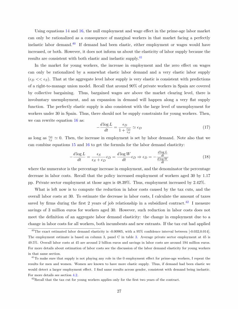
Using equations 14 and 16, the null employment and wage effect in the prime-age labor market

can only be rationalized as a consequence of marginal workers in that market facing a perfectly

inelastic labor demand.40 If demand had been elastic, either employment or wages would have

increased, or both. However, it does not inform us about the elasticity of labor supply because the

results are consistent with both elastic and inelastic supply.41

In the market for young workers, the increase in employment and the zero effect on wages

can only be rationalized by a somewhat elastic labor demand and a very elastic labor supply

(εD << εS). That at the aggregate level labor supply is very elastic is consistent with predictions

of a right-to-manage union model. Recall that around 90% of private workers in Spain are covered

by collective bargaining. Thus, bargained wages are above the market clearing level, there is

involuntary unemployment, and an expansion in demand will happen along a very flat supply

function. The perfectly elastic supply is also consistent with the large level of unemployment for

workers under 30 in Spain. Thus, there should not be supply constraints for young workers. Then,

we can rewrite equation 16 as:

−d logL

dt=

εD1 + εD

εS

' εD (17)

as long as εDεS' 0. Then, the increase in employment is set by labor demand. Note also that we

can combine equations 15 and 16 to get the formula for the labor demand elasticity:

−d logL

dt=

εSεS + εD

εD =d logW

dtεD ⇒ εD = −

d logLdt

d logWdt

(18)

where the numerator is the percentage increase in employment, and the denominator the percentage

decrease in labor costs. Recall that the policy increased employment of workers aged 30 by 1.17

pp. Private sector employment at those ages is 48.39%. Thus, employment increased by 2.42%.

What is left now is to compute the reduction in labor costs caused by the tax cuts, and the

overall labor costs at 30. To estimate the decrease in labor costs, I calculate the amount of taxes

saved by firms during the first 2 years of job relationship in a subsidized contract.42 I measure

savings of 3 million euros for workers aged 30. However, such reduction in labor costs does not

meet the definition of an aggregate labor demand elasticity: the change in employment due to a

change in labor costs for all workers, both incumbents and new entrants. If the tax cut had applied

40The exact estimated labor demand elasticity is -0.00905, with a 95% confidence interval between [-0.032,0.014].

The employment estimate is based on column 3, panel C in table 3. Average private sector employment at 45 is

49.5%. Overall labor costs at 45 are around 2 billion euros and savings in labor costs are around 194 million euros.

For more details about estimation of labor costs see the discussion of the labor demand elasticity for young workers

in that same section.41To make sure that supply is not playing any role in the 0 employment effect for prime-age workers, I repeat the

results for men and women. Women are known to have more elastic supply. Thus, if demand had been elastic we

would detect a larger employment effect. I find same results across gender, consistent with demand being inelastic.

For more details see section 4.2.42Recall that the tax cut for young workers applies only for the first two years of the contract.

27

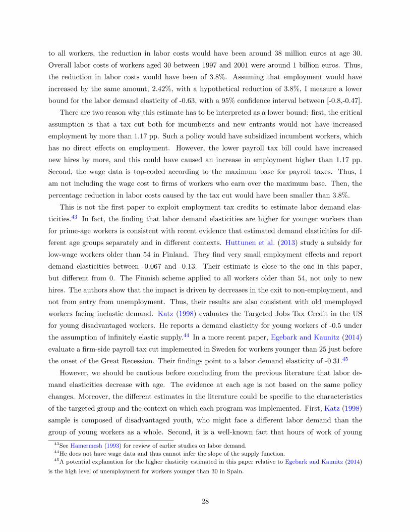
to all workers, the reduction in labor costs would have been around 38 million euros at age 30.

Overall labor costs of workers aged 30 between 1997 and 2001 were around 1 billion euros. Thus,

the reduction in labor costs would have been of 3.8%. Assuming that employment would have

increased by the same amount, 2.42%, with a hypothetical reduction of 3.8%, I measure a lower

bound for the labor demand elasticity of -0.63, with a 95% confidence interval between [-0.8,-0.47].

There are two reason why this estimate has to be interpreted as a lower bound: first, the critical

assumption is that a tax cut both for incumbents and new entrants would not have increased

employment by more than 1.17 pp. Such a policy would have subsidized incumbent workers, which

has no direct effects on employment. However, the lower payroll tax bill could have increased

new hires by more, and this could have caused an increase in employment higher than 1.17 pp.

Second, the wage data is top-coded according to the maximum base for payroll taxes. Thus, I

am not including the wage cost to firms of workers who earn over the maximum base. Then, the

percentage reduction in labor costs caused by the tax cut would have been smaller than 3.8%.

This is not the first paper to exploit employment tax credits to estimate labor demand elas-

ticities.43 In fact, the finding that labor demand elasticities are higher for younger workers than

for prime-age workers is consistent with recent evidence that estimated demand elasticities for dif-

ferent age groups separately and in different contexts. Huttunen et al. (2013) study a subsidy for

low-wage workers older than 54 in Finland. They find very small employment effects and report

demand elasticities between -0.067 and -0.13. Their estimate is close to the one in this paper,

but different from 0. The Finnish scheme applied to all workers older than 54, not only to new

hires. The authors show that the impact is driven by decreases in the exit to non-employment, and

not from entry from unemployment. Thus, their results are also consistent with old unemployed

workers facing inelastic demand. Katz (1998) evaluates the Targeted Jobs Tax Credit in the US

for young disadvantaged workers. He reports a demand elasticity for young workers of -0.5 under

the assumption of infinitely elastic supply.44 In a more recent paper, Egebark and Kaunitz (2014)

evaluate a firm-side payroll tax cut implemented in Sweden for workers younger than 25 just before

the onset of the Great Recession. Their findings point to a labor demand elasticity of -0.31.45

However, we should be cautious before concluding from the previous literature that labor de-

mand elasticities decrease with age. The evidence at each age is not based on the same policy

changes. Moreover, the different estimates in the literature could be specific to the characteristics

of the targeted group and the context on which each program was implemented. First, Katz (1998)

sample is composed of disadvantaged youth, who might face a different labor demand than the

group of young workers as a whole. Second, it is a well-known fact that hours of work of young

43See Hamermesh (1993) for review of earlier studies on labor demand.44He does not have wage data and thus cannot infer the slope of the supply function.45A potential explanation for the higher elasticity estimated in this paper relative to Egebark and Kaunitz (2014)

is the high level of unemployment for workers younger than 30 in Spain.

28

workers are more procyclical than that of prime-age men (Clark and Summers, 1981; Gomme et

al., 2004). Though this could partly be due to changes in labor supply over the cycle, it could also

be due to labor demand for young workers being more elastic during downturns. In fact, Jaimovich

et al. (2013) show in a simulation that age-specific labor supply is not enough to account for the

differential cyclicality across age groups, and that a model including age-specific labor demand

does a better job. Therefore, the estimates in Egebark and Kaunitz (2014) might reflect just re-

cessionary periods.46 Third, the estimates might be conditional on each country’s labor market

institutions. Finland and Sweden do not have minimum wage laws. Instead, minimum wages are

decided through collective bargaining.47 Then, payroll tax shifting on wages might be more likely

to happen. In such situation, employment credits do not decrease labor costs. That could explain

the null effect in Huttunen et al. (2013).

The main advantage of the quasi-experiment in this paper is that the same policy targeted

different age groups, during the same macro context, and within the same set of institutions.

Then, the potential channels that could explain the heterogeneous results in the literature are shut

off and we can be certain that the labor demand elasticity does decrease with age. But why is labor

demand elasticity decreasing with age? In the remaining of this section, I consider several channels

that could rationalize the findings.

4.2 Explanations

The decreasing demand elasticities with age are consistent with the pool of marginal workers being

more adversely selected as they age. In this section, I show evidence consistent with that. I also

consider several alternative explanations. I show that the results do not change when I separate by

gender. Then, I focus on firm characteristics, on the possibility that payroll taxes are shifted on

wages for prime-age workers, on wage capture by prime-age workers, and on hiring costs for each

age group. None of these alternative channels is consistent with the results

Adverse Selection . The evidence based on the characteristics of the young and prime-age

labor market (figure 5) is consistent with adverse selection increasing with age. The ratio of

permanent workers does not increase after 30. Firms could infer that workers who failed to have

a permanent contract before 30 are of lower ability. That signal might be strengthened over time

(Greenwald, 1986). The more a worker stays out of the permanent workforce, the more likely

he is to suffer unemployment spells that depreciate his skills. Then, firms might see prime-age

non-permanent workers as adversely selected with certainty.

In contrast, the signal will be less strong for young workers, as firms understand that is difficult

for them to land a stable job (Ryan, 2001). Younger workers might be riskier because they have

46Katz (1998) and Huttunen et al. (2013) focus on non-recessionary periods.47For more details, see Huttunen et al. (2013) and Egebark and Kaunitz (2014).

29

less history in the labor market and then greater uncertainty about their productivity. But the

average productivity of a risky young worker might be higher than that of an adversely selected

prime-age worker.

If adverse selection is increasing with age, it should be detectable in the wages. Suppose a skill

distribution for young and prime-age workers. The skill distribution should be mapped into a wage

distribution. Thus, if prime-age subsidized workers are more negatively selected than their age

peers, they should come from the lower end of the skill distribution. Then, their wages should also

be concentrated on the left-end of the distribution. In contrast, young subsidized workers are not

as negatively selected as their age peers. Therefore, their skill and wage distribution should only

be slightly shifted to the left. As can be seen, subsidized and non-subsidized prime-age workers are

very different (figure 16a). Prime-age subsidized workers are coming from a much less productive

pool of individuals. In contrast, the average subsidized young worker is not very different than

the average non-subsidized young worker (figure 16b). Thus, the analysis of the wage densities is

consistent with adverse selection increasing with age.

Adverse selection should also be detectable in other observable characteristics of these workers.

Thus, I can still provide an additional test. Note that both young and prime-age workers will

be negatively selected with respect to their age-counterparts. But the question here is whether

subsidized prime-age workers are relatively more negatively selected than young ones. To test that,

I restrict the sample to workers hired as permanent workers and run a regression with a dummy

equal to 1 if the worker was hired with a tax credit, and 0 if not, on several predictor and control

variables. The specification is as follows:

Yipct = α+ δp + φc + γt + βXipct + ψ45ipct + κ45ipctXipct + εipct (19)

Yipct is a dummy that indicates whether the individual was hired with a tax cut or not. δp, φc, and

γt are province, cohort, and year fixed effects, respectively. Xipct is a vector of characteristics of

the worker and the job: education, sex, citizenship, disability, experience, wage, industry sector,

part-time, and firm’s size. 45ipct is a dummy indicating that the worker is 45 years or older.

Table 10 reports the results. Column 1 shows them for workers under 30 years during the

period between May 1997 and March 2001 (when the tax credit for young employees was available).

Column 2 reports the estimates for prime-age workers 45-50 years old between May 1997 and June

2006. Column 3 reports the results pooling both types of workers and adding interactions for

those older than 45. The estimates are consistent with adverse selection worsening with age: both

young and prime-age subsidized workers are worse in several observable characteristics (university

education, experience during the last 12 months, firm’s size, and wage) than their counterparts.

Moreover, the interactions reveal that subsidized prime-age workers are much more negatively

selected than young employees in three dimensions: they are less likely to have finished a college

degree, they have accumulated less experience during the last 12 months, and their wages are lower.

30

However, they are more likely to work in slighty larger firms.

The above evidence, and the evolution of employment over age (figure 5), are consistent with

adverse selection increasing with age in the pool of marginal workers. However, there can be other

reasons that could explain the decreasing elasticity between the ages of 30 and 45. I turn now to

consider some of the most plausible ones.

Supply of Men and Women . I begin by showing further evidence that the elasticity of

labor supply does not play any role in explaining the results for prime-age workers. Women are

known to have more elastic labor supply (Eissa and Liebman, 1996; Blundell and MaCurdy, 1999).

Figure 1b shows the unemployment rate for men and women aged 45-50. Since unemployment is

higher among women, it suggests that female labor supply should be more elastic in Spain too.

Thus, employment responses should be higher for women, as long as demand is elastic. I repeat

the analysis for men and women separately. The evidence is presented in section 4 in the online

appendix. The results across gender are very similar and not significantly different. Therefore, it

confirms previous results that the key driver of the null employment effect in the prime-age labor

market is an inelastic demand.

Payroll taxes are shifted on wages. If workers value the benefits that are financed through

payroll taxation, they will accept a lower wage in compensation for these services. The argument

can be traced back to Summers (1989) for mandated benefits and Lazear (1990) for severance

payments. In a perfect market, any government-ordered transfer from the firm to the worker can

be offset by a voluntary transfer of the same size from the worker to the firm. Then, payroll taxes

can be fully shifted onto wages, and employment credits will not affect the level of employment.

Gruber (1997) shows that this is the case when there is full valuation of benefits financed by payroll

taxes.

However, the presence of minimum wages breaks down the argument. Firms will not be able to

fully shift payroll taxes to wages for workers who are in the proximity of the minimum wage. Thus,

a potential explanation for the results is that young workers are more likely to be at the minimum

wage than prime-age workers. If that is the case, we would expect that younger workers hired with

a tax cut are more likely to be at the minimum wage than prime-age workers. Figure 16 shows

the wage density for each age group during the period 1997-2001 for permanent and temporary

contracts (16c), for all permanent contracts (16d), and for permanent subsidized contracts (16e).

The red dashed lines represent the area of the minimum wage. Figures 16c and 16d do show that

the density of minimum wage workers is larger for younger workers. If the increases in employment

were caused by that factor we would expect that such higher mass also shows up for permanent

subsidized contracts. However, figure 16e shows that the wage density for subsidized contracts is

very similar across age groups. Thus, differential incidence of minimum wage workers does not

seem to explain the results.

31

Small v. Large Firms. One possibility is that there is no impact on prime-age workers

because they are not working in small firms. Small firms are likely to be more liquidity constrained

than large firms. Thus, they might not be able to hire workers at the occupation-specific wage

given the burden of payroll taxes. Then, the increase in demand might be driven by them. In

addition, hiring policies in large firms might be directed by a human resources department. The

age requirement of the tax credits might impose an additional transaction cost on the human

resources department that deters them from using the employment credits. In fact, Cahuc et al.

(2014) study a payroll tax credit for new hires in small French firms during the Great Recession

and find increases in employment growth.

I repeat the analysis for small and large firms. The RDD results are in table 11. For young

workers, the probability of being hired in a small firm before the threshold is significantly .28 pp

higher. In large firms, the estimate is not significant. For prime-age workers, both in small and

large firms the estimate is significant. However, note that the increase in hiring is of .37 pp for small

firms, whereas it is only of .07 pp for large firms. Then, it is mostly small firms that are delaying

the time at which they hire prime-age workers to claim the tax credit. This is not consistent with

small firms not hiring prime-age workers and cannot justifiy the inelastic labor demand for older

workers.

Another potential interpretation of this result is that informal workers are more likely to be at

small firms. However, the effects of the policy happen mostly through workers that were temporary

within the same firm before becoming permanent. If firms were trying to save taxes by keeping

workers underground, there is no rationale for hiring them as temporary before, since those contracts

are not subsidized and have to pay the standard level of payroll taxes. Therefore, this finding signals

to another relevant margin through which the policy is acting. The increases in employment happen

for young workers in small firms.

Search-and-matching . (1) Wage capture. The introduction of rigidities in the labor market

highlights some channels that could explain the differential elasticities across groups. Two of the

equations determining the equilibrium in such models are the job creation condition (Pissarides,

2000):

p− w(1 + τ)− (r + λ)pc

q(θ)= 0 (20)

and the wage function:

w = (1− β)z +βp(1 + cθ)

1 + τ(21)

where p is the productivity, w is the wage, τ is the firm’s payroll tax rate, r is the interest rate,

λ is the rate of arrival of an adverse shock that breaks the job match, c is the hiring cost; θ is

the ratio between vacancies and unemployed workers, and represents labor market tightness; q(θ)

is the rate at which vacant jobs become filled, β is the worker’s bargaining power, z is the income

that an unemployed worker receives.

32

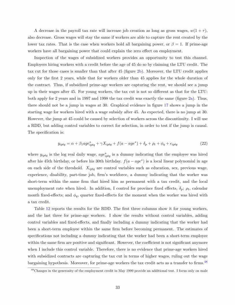
A decrease in the payroll tax rate will increase job creation as long as gross wages, w(1 + τ),

also decrease. Gross wages will stay the same if workers are able to capture the rent created by the

lower tax rates. That is the case when workers hold all bargaining power, or β = 1. If prime-age

workers have all bargaining power that could explain the zero effect on employment.

Inspection of the wages of subsidized workers provides an opportunity to test this channel.

Employers hiring workers with a credit before the age of 45 do so by claiming the LTU credit. The

tax cut for those cases is smaller than that after 45 (figure 2b). Moreover, the LTU credit applies

only for the first 2 years, while that for workers older than 45 applies for the whole duration of

the contract. Thus, if subsidized prime-age workers are capturing the rent, we should see a jump

up in their wages after 45. For young workers, the tax cut is not so different as that for the LTU:

both apply for 2 years and in 1997 and 1998 the tax credit was exactly the same (figure 2a). Thus,

there should not be a jump in wages at 30. Graphical evidence in figure 17 shows a jump in the

starting wage for workers hired with a wage subsidy after 45. As expected, there is no jump at 30.

However, the jump at 45 could be caused by selection of workers across the discontinuity. I will use

a RDD, but adding control variables to correct for selection, in order to test if the jump is causal.

The specification is:

yiptq = α+ β1age∗iptq + γXiptq + f(a− age∗) + δp + ρt + φq + εiptq (22)

where yiptq is the log real daily wage, age∗iptq is a dummy indicating that the employee was hired

after his 45th birthday, or before his 30th birthday. f(a− age∗) is a local linear polynomial in age

on each side of the threshold. Xiptq are control variables such as education, sex, previous wage,

experience, disability, part-time job, firm’s workforce, a dummy indicating that the worker was

short-term within the same firm that hired him as permanent with a tax credit, and the local

unemployment rate when hired. In addition, I control for province fixed effects, δp; ρt, calendar

month fixed-effects; and φq, quarter fixed-effects for the moment when the worker was hired with

a tax credit.

Table 12 reports the results for the RDD. The first three columns show it for young workers,

and the last three for prime-age workers. I show the results without control variables, adding

control variables and fixed-effects, and finally including a dummy indicating that the worker had

been a short-term employee within the same firm before becoming permanent. The estimates of

specifications not including a dummy indicating that the worker had been a short-term employee

within the same firm are positive and significant. However, the coefficient is not significant anymore

when I include this control variable. Therefore, there is no evidence that prime-age workers hired

with subsidized contracts are capturing the tax cut in terms of higher wages, ruling out the wage

bargaining hypothesis. Moreover, for prime-age workers the tax credit acts as a transfer to firms.48

48Changes in the generosity of the employment credit in May 1999 provide an additional test. I focus only on male

33

49

(2) Hiring costs. Another possibility is that prime-age workers were more costly to hire because

they were harder to find, given their high rates of employment. Figure 5c suggests that hiring

costs are likely to be lower for young workers as a group. However, note that the ratio of the

workforce in permanent contracts at 30 and 45 barely changes. Thus, hiring costs just before the

30th threshold and at 45 should be very similar. Then, we should not observe a positive impact just

before 30 either. Recall that the age-incidence estimates of the employment effect show a positive

and significant impact just before 30 (figure 13b). And that the effect at 30 is not significantly

different than the impact between 20 and 29 years. Then, an explanation based on hiring costs

fails to explain the results.

To sum up, the evidence is consistent with adverse selection increasing with age in the pool

of marginal workers. Thus, as adverse selection worsens over the life-cycle, the labor demand

elasticity of -0.63 for young workers decreases until reaching 0 at some point between the ages of 30

and 45. The fundamental characteristics of the labor market that point to adverse selection as the

main explanation of the results are not only characteristic of Spain. Blundell et al. (2013); Topel

and Ward (1992); Murphy and Welch (1990) document similar features in other labor markets

of developed countries. Then, the implications for labor policy design are likely to hold in other

contexts.

5 Discussion

The labor demand elasticity is a key parameter to evaluate and predict the impacts of both demand

and supply interventions in the labor market. In this section, I discuss policy implications of the

results, interpret earlier findings in light of the estimates in this paper, and suggest avenues for

future research.

Demand-Side Policies. (1) Employment Tax Credits and the Optimal Age-Profile of Payroll

Taxes. Employment tax credits have been considered as a policy to increase employment for a

long-time (Kaldor, 1936; Phelps, 1994, 1997). They are used in many countries around the world.

workers because it is for them that the generosity of the employment credit decreased unambiguously: the payroll

tax rate cut decreased from 40% to 35% for the first year, and from 40% to 25% in the second year, for male workers

under 30. For the case of male workers over 45, it decreased from a 60% tax cut for the first two years, to 45% and

40% for the first and second year, respectively. Moreover, for the remaining of the contract it decreased from 50% to

40%. I perform a DD strategy. Table 20 in the online appendix reports the results. The results are consistent with

those of the RDD: none of the estimates are significant when I include all the control variables.49It could still be the case that prime-age workers hired with a tax credit do not perceive higher wages, but firms

grant them more non-pecuniary benefits. This is unlikely for two reasons: first, non-pecuniary benefits are also

determined through collective-bargaining. Second, higher non-wage benefits for subsidized workers might undermine

the morale of non-subsidized workers who had been at the firm for a long time.

34

Most of them target either young or old workers (or both) (OECD, 2009, 2013).50 51 The demand

elasticities in this paper show that tax credits for new hires will be effective and cost-efficient for

young workers, but not for prime-age workers. That could increase employment by smoothing the

school-to-work transition period (Ryan, 2001), and by subsidizing hiring of risky young workers

with yet unknown productivity and who have to be trained. Moreover, intervention in the early

labor market years can improve employment outcomes as these workers age by reducing the pool of

adversely selected workers. More experience during the early labor market years can have positive

effects later on.

Yet, the fact that many countries target these policies to the population of older workers is

telling about the challenges that economies face in an aging society. The estimates at 45 might not

be valid for older workers who are closer to the retirement age. Blundell et al. (2013) show, for the

UK and France, that workers over 55 years play a big role in explaining reductions in employment

and hours of work during the last 30 years. Huttunen et al. (2013) study a payroll tax cut for all

low-wage workers older than 54 in Finland. Their findings show that new entries were not affected,

which is in line with the results in this paper for 45 year olds. However, they found a decrease in

exits to non-employment, with a small impact on the employment of workers older than 54. The

positive effect could be due to this population being less adversely selected since they are currently

working. Therefore, the evidence suggests that employment tax credits might also be benefitial if

targeted at workers who are much closer to retirement than those who are 45 years old. But this

is as long as the tax cuts target the currently employed and not new hires.

Perhaps a simple way to implement a reform according to the results in this paper and in

Huttunen et al. (2013), would be to make payroll taxes age-dependent. The optimal payroll tax

rate should be lower for young workers, and then increase with age. Since the labor demand

elasticity for marginal workers might reach 0 at some point between the ages of 30 and 45, the

plateau of the tax rate should be at some point between those two ages. An interesting question for

future research is where exactly the plateau should be, but this is beyond the scope of this paper.

Following the results in Huttunen et al. (2013), the payroll tax rate should start decreasing again

5012 OECD countries have provisions that target young or old workers. Belgium, France, Japan, Portugal, and the

US have specific policies both for young and old workers. Canada, Greece, Italy, South Korea, Turkey and the UK

have specific policies for young individuals. Poland has an employment credit for old workers. Neumark and Grijalva

(2013) also report that, between 1969 and 2012, US states implemented 149 employment credits.51Another common design is to focus on low-wage workers regardless of their age. Kramarz and Philippon (2001)

study payroll tax subsidies for low-wage workers in France and find a small and insignificant impact on entry from

non-employment. Crepon and Desplatz (2001) study the same policy and conclude that most employment effects

happen through substitution between treated and non-treated workers. Yet another design is to subsidize jobs in

small firms. Cahuc et al. (2014) study a payroll tax credit for new hires in small French firms during the Great

Recession. They find evidence that employment growth increased and that substitution was not happening. The

results in this paper confirm that targeting small firms is another important margin, since the employment effect for

younger workers happens only through small firms.

35

at some point before the age of retirement to prevent some of these workers from losing their jobs.

The development of the optimal age-profile of payroll taxes is an interesting avenue for future

research. There are two recent strands of literature that can shed some light to this problem. First,

there are studies on the optimal age profile of income taxes (Weinzierl, 2011) and employment

protection (Cheron et al., 2011). Second, there is research analyzing the optimal level of payroll

taxes and UI over the business cycle (Landais et al., 2014; Jung and Kuester, Forthcoming).52

While labor demand elasticities can change depending on economic conditions, the findings in this

paper show that an important factor for optimal labor policy is age. Future research can provide

theoretical fundamentals of how an age-dependent payroll tax should be. In addition, it can look

at the optimal policy mix for different age groups.

Supply-Side Labor Market Policies. (1) Earned Income Tax Credit. Given the demand

elasticities in this paper, EITC would not be an attractive work-encouraging transfer program for

neither young nor older workers. The optimal transfer program resembles the EITC when supply

responses are concentrated along the extensive margin (Saez, 2002). But most optimal tax analysis

and EITC discussions assume that labor demand is perfectly elastic and thus that the incidence

of taxes is only borne by workers. Rothstein (2010) simulates the impacts of the EITC with

different labor demand elasticities. With infinitely elastic demand, EITC is successful in raising

both employment and earnings of low-skill mothers. He estimates that incomes of low-income

mothers would rise by $1.39 for every $ spent on the program.

However, assuming more realistic labor demand elasticities of -0.3, Rothstein (2010) finds more

modest positive employment effects, and that a substantial portion of low-skill single mother’s

EITC payments is captured by employers through reduced wages: $1 in EITC spending increases

after-tax incomes by $0.73. Importantly for distributional reasons, the $0.73 estimate combines

an increase of net-of-tax incomes of women with children of $1.07 for each $ on the program,

and a decline of $0.34 in the net-of-tax income of women without children.53 The estimates of

labor demand elasticity in this paper question the ability of EITC schemes as a tool for income

redistribution. An alternative is the use of a Negative Income Tax (NIT), but the fear is that it

would strongly discourage work. Instead, payroll tax credits are at least successful in raising both

employment and earnings of young workers.

(2) Job-Search Assistance. The results in this paper show that employment tax credits can be

a more efficient way of raising both employment and earnings than job-search assistance. They

can also help us understand why job-search assistance interventions fail in general. Heckman et al.

52Landais et al. (2014) look at the optimal level of UI over the business cycle. Jung and Kuester (Forthcoming)

study the optimal mix of payroll taxes, UI and employment protection over the business cycle.53There is empirical evidence to support Rothstein (2010) analysis. Leigh (2010) exploits variation in state EITC

supplements and finds that a 10% increase in the generosity of EITC is associated with a 5% fall in the wages of high

school dropouts. This number implies a labor demand elasticity of -.3.

36

(1999) and Card et al. (2010) review the literature on active labor market policies and conclude

that these interventions (1) have, at best, very small positive effects; (2) have very heterogenous

effects depending on age and gender; (3) have no effect when targeted at young workers.54

The latter conclusion might seem puzzling in light of the findings in this paper. However,

youth unemployment is high across all OECD countries (OECD, 2002, 2013). Acting through the

supply-side might then have very small marginal effects (Michaillat, 2012). Moreover, since supply-

side policies do not alter firm’s hiring incentives, any positive estimates might only reflect partial

equilibrium changes. In a research design that can look at general equilibrium effects, Crepon et al.

(2013) find zero net employment effects of job-search assistance. In the case of prime-age workers,

lack of employment effects of these policies can be caused by them facing an inelastic demand. If

job-search assistance or training treatments are not strong enough to undo adverse selection, these

policies will fail. Moreover, participation in these programs might stigmatize workers, worsening

adverse selection.

References

Albert, C. and C. Garcia-Serrano. Hernanz, “Firm-provided Training and Temporary Con-

tracts,” Spanish Economic Review, 2005, 7, 67–88.

Arranz, J. A. and C. Garcia-Serrano, “Que ha sucedido con la estabilidad del empleo en

Espana?,” Revista de Economia Aplicada, 2007, 15, 65–98.

Autor, D. and S. Houseman, “Do Temporary-Help Jobs Improve Labor Market Outcomes

for Low-Skilled Workers? Evidence from Work First,” American Economic Journal: Applied

Economics, 2010, 2, 96–128.

Becker, G., “The Abysmal Recovery in Employment,” http://www.becker-posner-

blog.com/2011/07/the- abysmal-recovery-in-employment-becker.html 2011.

Bentolila, S., “Las decisiones judiciales sobre despidos en Espana: una perspectiva economica,”

Documento de Trabajo 9602 Programa de Investigaciones Economicas, 1996.

Blundell, R., A. Bozio, and G. Laroque, “Extensive and Intensive Margins of Labour Supply,”

Fiscal Studies, 2013, 34, 1–29.

and T. MaCurdy, “Labor Supply: A Review of Alternative Approaches,” in “Handbook of

Labor Economics,” Elsevier Science, 1999.

54Both surveys review also employment tax credits and find mostly zero effects. They argue that this is because

treated individuals are very disadvantaged.

37

, M. C. Dias, C. Meghir, and J. van Reenen, “Evaluating the Employment Impact of

a Mandatory Job Search Program,” Journal of the European Economic Association, 2004, 2,

569–606.

Boeri, T. and J. van Ours, The Economics of Imperfect Labor Markets, Princeton University

Press, 2008.

Bonhomme, S. and L. Hospido, “The Cycle of Earnings Inequality: Evidence from Spanish

Social Security Data,” IZ Discussion Paper 6669, 2012.

Cahuc, P., S. Carcillo, and T. Le Barbanchon, “Do Hiring Credits Work in Recessions?

Evidence from France,” IZA Discussion Paper No. 8330, 2014.

Card, D., J. Kluve, and A. Weber, “Active Labor Market Policy Evaluations: A Meta-

Analysis,” IZA Discussion Paper No. 4002, 2009.

, , and , “Active Labor Market Policy Evaluations: A Meta-Analysis,” Economic Journal,

2010, 120, F452–F477.

Cheron, A., J. O. Hairault, and F. Langot, “Age-Dependent Employment Protection,” Eco-

nomic Journal, 2011, 121, 1477–1504.

Chetty, R., “Bounds on Elasticities with Optimization Frictions: A Synthesis of Micro and Macro

Evidence on Labor Supply,” Econometrica, 2012, 80, 969–1018.

, J. Friedman, T. Olsen, and L. Pistaferri, “Adjustment Costs, Firm RResponse, and

Micro vs. Macro Elasticities: Evidence from Danish Tax Records,” The Quarterly Journal of

Economics, 2011, 126, 749–804.

Clark, K. B. and L. Summers, “Demographic Differences in Cyclical Employment Variation,”

Journal of Human Resources, 1981, 41, 61–79.

Crepon, B. and R. Desplatz, “Evaluation of Payroll Tax Subsidies for Low-Wage Workers,”

Working Paper INSEE, 2001.

, E. Duflo, M. Gurgand, R. Bathelot, and P. Zamora, “Do Labor Market Policies Have

Displacement Effects? Evidence from a Clustered Randomized Experiment,” Quarterly Journal

of Economics, 2013, 128, 531–580.

Davia, M. A. and V. Hernanz, “Temporary Employment and Segmentation in the Spanish

Labour Market: An Empirical Analysis through the Study of Wage Differentials,” Spanish Eco-

nomic Review, 2004, 6, 291–318.

38

Davidson, C. and S. Woodbury, “The Displacement Effect of Reemployment Bonus Programs,”

Journal of Labor Economics, 1993, 11, 575–605.

Egebark, J. and N. Kaunitz, “Do Payroll Tax Cuts Raise Youth Employment?,” 2014.

Eissa, N. and J. Liebman, “Labor Supply Response to the Earned Income Tax Credit,” The

Quarterly Journal of Economics, 1996, 111, 605–637.

Elias, F., “Do Two-Tier Reforms in Employment Protection Affect the Labor Market? Evidence

from Spain,” Columbia University Working Paper, 2014.

Gomme, P., R. Rogerson., P. Rupert, and R. Wright, “The Business Cycle and the Life

Cycle,” in “NBER Macroeconomics Annual 2004,” Vol. 19, NBER, 2004, pp. 415–592.

Greenwald, B., “Adverse Selection in the Labour Market,” Review of Economic Studies, 1986,

53, 325–347.

Gruber, J., “The Incidence of Payroll Taxation: Evidence from Chile,” Journal of Labor Eco-

nomics, 1997, 15, S72–S101.

Guell, M. and B. Petrongolo, “How Binding Are Legal Limits? Transitions from Temporary

to Permanent Work in Spain,” Labour Economics, 2007, 14, 153–183.

Hamermesh, D., Labor Demand, Princeton University Press, 1993.

Heckman, J., R. Lalonde, and J. Smith, “The Economics and Econometrics of Active Labor

Market Programs,” in “Handbook of Labor Economics,” Elsevier Science, 1999.

Huttunen, K., J. Pirttila, and R. Uusitalo, “The Employment Effects of Low-Wage Subsi-

dies,” Journal of Public Economics, 2013, 97, 49–60.

Izquierdo, M., E. Moral, and A. Urtasun, “El sistema de negociacion colectiva en Espana:

un analisis con datos individuales de convenios,” Banco de Espana. Documento Ocasional No.

0302, 2003.

Jaimovich, N., H. Siu, and S. Pruitt, “The Demand for Youth: ExpExplain Age Differences

in the Volatility of Hours,” American Economic Review, 2013, 103, 3022–3044.

Jimeno, J. F. and L. Toharia, “The Effects of Fixed-Term Employment on Wages: Theory and

Evidence from Spain,” Investigaciones Economicas, 1993, 17, 475–494.

Johnson, G. E. and P. R. G. Layard, “The Natural Rate of Unemployment: Explanation and

Policy,” in O. Ashenfelter and R. Layard, eds., Handbook of Labor Economics, Vol. II, Elsevier

Science, 1986, pp. 921–999.

39

Jung, P. and K. Kuester, “Optimal Labor Market Policy In Recessions,” American Economic

Journal: Macroeconomics, Forthcoming.

Kaldor, N., “Wage Subsidies as a Remedy for Unemployment,” Journal of Political Economy,

1936, 44, 721–742.

Katz, L., “Wage Subsidies for the Disadvantaged,” NBER Working Paper No. 5679, 1998.

Kleven, H. and M. Waseem, “Using Notches to Uncover Optimization Frictions and Structural

Elasticities,” Quarterly Journal of Economics, 2013, 128, 669–723.

Kopczuk, W. and D. Munroe, “Mansion Tax: The Effect of Transfer Taxes on the Residential

Real Estate Market,” American Economic Journal: Economic Policy, Forthcoming.

Kramarz, F. and T. Philippon, “The Impact of Differential Payroll Tax Subsidies on Minimum

Wage Employment,” Journal of Public Economics, 2001, 82, 115–146.

Landais, C., P. Michaillat., and E. Saez, “Optimal Unemployment Insurance Over the Business

Cycle,” NBER Working Paper No. 16526, 2014.

Lazear, E., “Job Security Provisions and Employment,” The Quarterly Journal of Economics,

1990, 105, 699–726.

Leigh, A., “Who Benefits from the Earned Income Tax Credit? Incidence among Recipients,

Coworkers and Firms,” The B. E. Journal of Economic Analysis and Policy, 2010, 10, 1–41.

Michaillat, P., “Do Matching Frictions Explain Unemployment? Not in Bad Times,” American

Economic Review, 2012, 102, 1721–1750.

Moffit, R., “Welfare Programs and Labor Supply,” in A. J. Auerbach and M. Feldstein, eds.,

Handbook of Public Economics, Vol. 4, Elsevier Science, 2002, pp. 2393–2430.

Mortensen, D. and C. Pissarides, “Taxes, Subsidies and Equilibrium Labor Market Outcomes,”

CEPR Discussion Papers 2989, 2001, pp. 1–32.

Murphy, K. and F. Welch, “Empirical Age-Earnings Profiles,” Journal of Labor Economics,

1990, 8, 202–229.

Neumark, D. and D. Grijalva, “The Employment Effects of State Hiring Credits During and

After the Great Recession,” NBEW Working Paper No. 18929, 2013.

Nickell, S. and M. Andrews, “Unions, Real Wages and Employment in Britain, 1951-79,”

Oxford Economic Papers, 1983, 35, 183–206.

40

OECD, “Recent Labour Market Developments and Prospects - Special Focus: a Better Start for

Youths?,” in “Employment Outlook 2002,” OECD, 2002.

, Addressing the Labour Market Challenges of the Economic Downturn: A Summary of Country

Response to the OECD-EC Questionnaire, OECD Publishing Paris, 2009.

, Economic Policy Reforms 2012. Going for Growth., OECD Publishing Paris, 2012.

, The OECD Action Plan for Youth - Giving Youth a Better Start in the Labour Market, OECD

Publishing Paris, 2013.

Phelps, E., “Low-Wage Employment Subsidies versus the Welfare State,” American Economic

Review Papers and Proceedings, 1994, 84, 54–58.

, Rewarding Work, Harvard University Press, 1997.

Pissarides, C., Equilibrium Unemployment Theory, The MIT Press, 2000.

Pissarides, C. A., “The Impact of Employment Tax Cuts on Unemployment: and Wages; The

Role of Unemployment: Benefits and Tax Structure,” European Economic Review, 1998, 42,

155–183.

Rothstein, J., “Is the EITC as Good as an NIT? Conditional Cash Transfers and Tax Incidence,”

American Economic Journal: Economic Policy, 2010, 2, 177–208.

Ryan, P., “The School-to-Work Transition: A Cross-National Perspective,” Journal of Economic

Literature, 2001, 39, 34–92.

Saez, E., “Optimal Income Transfer Programs: Intensive Versus Extensive Labor Supply Re-

sponses,” The Quarterly Journal of Economics, 2002, 117, 1039–1073.

, “Do Taxpayers Bunch at Kink Points?,” American Economic Journal: Economic Policy, 2010,

2, 180–212.

, M. Matsaganis, and P. Tsakloglou, “Earnings Determination and Taxes: Evidence from

a Cohort-Based Payroll Tax Reform in Greece,” Quarterly Journal of Economics, 2012, 127,

493–533.

Salanie, B., The Economics of Taxation, MIT Press, 2003.

Slemrod, J. and S. Yitzhaki, “Integrating Expenditure and Tax Decisions: The Marginal Cost

of Funds and the Marginal Benefit of Projects,” National Tax Journal, 2001, 54, 189–202.

Summers, L. H., “Some Simple Economics of Mandated Benefits,” American Economic Review

Papers and Proceedings, 1989, 79, 177–83.

41

Topel, R. and M. Ward, “Job Mobility and the Careers of Young Men,” Quarterly Journal of

Economics, 1992, May, 439–479.

Weinzierl, M., “The Surprising Power of Age-Dependent Taxes,” Review of Economic Studies,

2011, 78, 1490–1518.

42

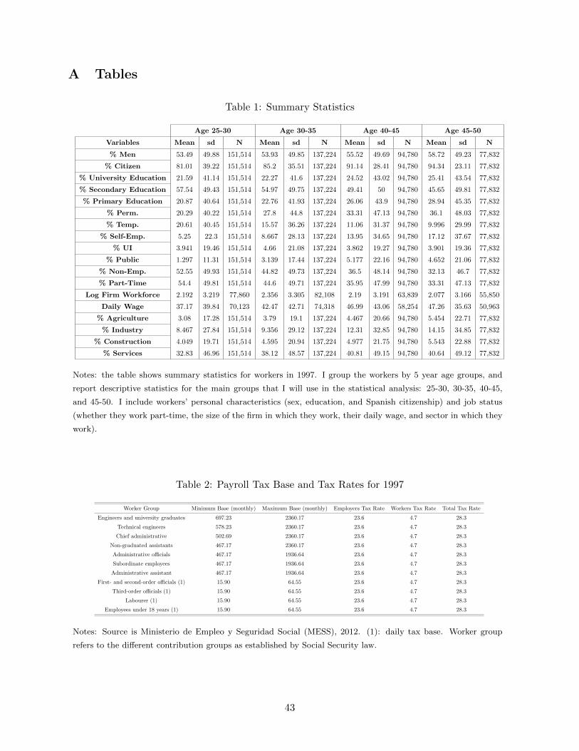
A Tables

Table 1: Summary Statistics

Age 25-30 Age 30-35 Age 40-45 Age 45-50

Variables Mean sd N Mean sd N Mean sd N Mean sd N

% Men 53.49 49.88 151,514 53.93 49.85 137,224 55.52 49.69 94,780 58.72 49.23 77,832

% Citizen 81.01 39.22 151,514 85.2 35.51 137,224 91.14 28.41 94,780 94.34 23.11 77,832

% University Education 21.59 41.14 151,514 22.27 41.6 137,224 24.52 43.02 94,780 25.41 43.54 77,832

% Secondary Education 57.54 49.43 151,514 54.97 49.75 137,224 49.41 50 94,780 45.65 49.81 77,832

% Primary Education 20.87 40.64 151,514 22.76 41.93 137,224 26.06 43.9 94,780 28.94 45.35 77,832

% Perm. 20.29 40.22 151,514 27.8 44.8 137,224 33.31 47.13 94,780 36.1 48.03 77,832

% Temp. 20.61 40.45 151,514 15.57 36.26 137,224 11.06 31.37 94,780 9.996 29.99 77,832

% Self-Emp. 5.25 22.3 151,514 8.667 28.13 137,224 13.95 34.65 94,780 17.12 37.67 77,832

% UI 3.941 19.46 151,514 4.66 21.08 137,224 3.862 19.27 94,780 3.901 19.36 77,832

% Public 1.297 11.31 151,514 3.139 17.44 137,224 5.177 22.16 94,780 4.652 21.06 77,832

% Non-Emp. 52.55 49.93 151,514 44.82 49.73 137,224 36.5 48.14 94,780 32.13 46.7 77,832

% Part-Time 54.4 49.81 151,514 44.6 49.71 137,224 35.95 47.99 94,780 33.31 47.13 77,832

Log Firm Workforce 2.192 3.219 77,860 2.356 3.305 82,108 2.19 3.191 63,839 2.077 3.166 55,850

Daily Wage 37.17 39.84 70,123 42.47 42.71 74,318 46.99 43.06 58,254 47.26 35.63 50,963

% Agriculture 3.08 17.28 151,514 3.79 19.1 137,224 4.467 20.66 94,780 5.454 22.71 77,832

% Industry 8.467 27.84 151,514 9.356 29.12 137,224 12.31 32.85 94,780 14.15 34.85 77,832

% Construction 4.049 19.71 151,514 4.595 20.94 137,224 4.977 21.75 94,780 5.543 22.88 77,832

% Services 32.83 46.96 151,514 38.12 48.57 137,224 40.81 49.15 94,780 40.64 49.12 77,832

Notes: the table shows summary statistics for workers in 1997. I group the workers by 5 year age groups, and

report descriptive statistics for the main groups that I will use in the statistical analysis: 25-30, 30-35, 40-45,

and 45-50. I include workers’ personal characteristics (sex, education, and Spanish citizenship) and job status

(whether they work part-time, the size of the firm in which they work, their daily wage, and sector in which they

work).

Table 2: Payroll Tax Base and Tax Rates for 1997

Worker Group Minimum Base (monthly) Maximum Base (monthly) Employers Tax Rate Workers Tax Rate Total Tax Rate

Engineers and university graduates 697.23 2360.17 23.6 4.7 28.3

Technical engineers 578.23 2360.17 23.6 4.7 28.3

Chief administrative 502.69 2360.17 23.6 4.7 28.3

Non-graduated assistants 467.17 2360.17 23.6 4.7 28.3

Administrative officials 467.17 1936.64 23.6 4.7 28.3

Subordinate employees 467.17 1936.64 23.6 4.7 28.3

Administrative assistant 467.17 1936.64 23.6 4.7 28.3

First- and second-order officials (1) 15.90 64.55 23.6 4.7 28.3

Third-order officials (1) 15.90 64.55 23.6 4.7 28.3

Labourer (1) 15.90 64.55 23.6 4.7 28.3

Employees under 18 years (1) 15.90 64.55 23.6 4.7 28.3

Notes: Source is Ministerio de Empleo y Seguridad Social (MESS), 2012. (1): daily tax base. Worker group

refers to the different contribution groups as established by Social Security law.

43

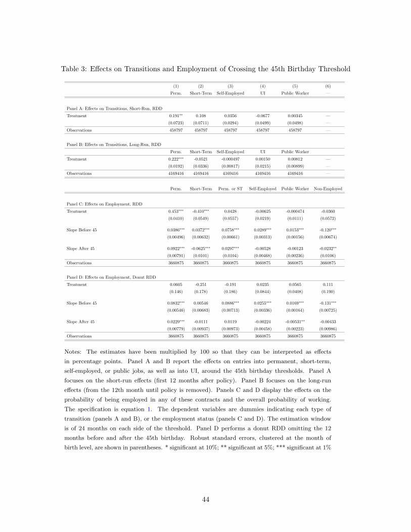
Table 3: Effects on Transitions and Employment of Crossing the 45th Birthday Threshold

(1) (2) (3) (4) (5) (6)

Perm. Short-Term Self-Employed UI Public Worker —

Panel A: Effects on Transitions, Short-Run, RDD

Treatment 0.191∗∗ 0.108 0.0356 -0.0677 0.00345 —

(0.0723) (0.0711) (0.0294) (0.0499) (0.0498) —

Observations 458797 458797 458797 458797 458797 —

Panel B: Effects on Transitions, Long-Run, RDD

Perm. Short-Term Self-Employed UI Public Worker

Treatment 0.222∗∗∗ -0.0521 -0.000497 0.00150 0.00812 —

(0.0192) (0.0336) (0.00817) (0.0215) (0.00899) —

Observations 4169416 4169416 4169416 4169416 4169416 —

Perm. Short-Term Perm. or ST Self-Employed Public Worker Non-Employed

Panel C: Effects on Employment, RDD

Treatment 0.453∗∗∗ -0.410∗∗∗ 0.0428 -0.00625 -0.000474 -0.0360

(0.0410) (0.0549) (0.0557) (0.0219) (0.0111) (0.0572)

Slope Before 45 0.0386∗∗∗ 0.0372∗∗∗ 0.0758∗∗∗ 0.0289∗∗∗ 0.0153∗∗∗ -0.120∗∗∗

(0.00496) (0.00632) (0.00661) (0.00313) (0.00156) (0.00674)

Slope After 45 0.0922∗∗∗ -0.0625∗∗∗ 0.0297∗∗∗ -0.00528 -0.00123 -0.0232∗∗

(0.00791) (0.0101) (0.0104) (0.00468) (0.00236) (0.0106)

Observations 3660875 3660875 3660875 3660875 3660875 3660875

Panel D: Effects on Employment, Donut RDD

Treatment 0.0605 -0.251 -0.191 0.0235 0.0565 0.111

(0.146) (0.178) (0.186) (0.0844) (0.0408) (0.190)

Slope Before 45 0.0832∗∗∗ 0.00546 0.0886∗∗∗ 0.0255∗∗∗ 0.0169∗∗∗ -0.131∗∗∗

(0.00546) (0.00683) (0.00713) (0.00336) (0.00164) (0.00725)

Slope After 45 0.0229∗∗∗ -0.0111 0.0119 -0.00224 -0.00531∗∗ -0.00433

(0.00779) (0.00937) (0.00973) (0.00458) (0.00223) (0.00986)

Observations 3660875 3660875 3660875 3660875 3660875 3660875

Notes: The estimates have been multiplied by 100 so that they can be interpreted as effects

in percentage points. Panel A and B report the effects on entries into permanent, short-term,

self-employed, or public jobs, as well as into UI, around the 45th birthday thresholds. Panel A

focuses on the short-run effects (first 12 months after policy). Panel B focuses on the long-run

effects (from the 12th month until policy is removed). Panels C and D display the effects on the

probability of being employed in any of these contracts and the overall probability of working.

The specification is equation 1. The dependent variables are dummies indicating each type of

transition (panels A and B), or the employment status (panels C and D). The estimation window

is of 24 months on each side of the threshold. Panel D performs a donut RDD omitting the 12

months before and after the 45th birthday. Robust standard errors, clustered at the month of

birth level, are shown in parentheses. * significant at 10%; ** significant at 5%; *** significant at 1%

44

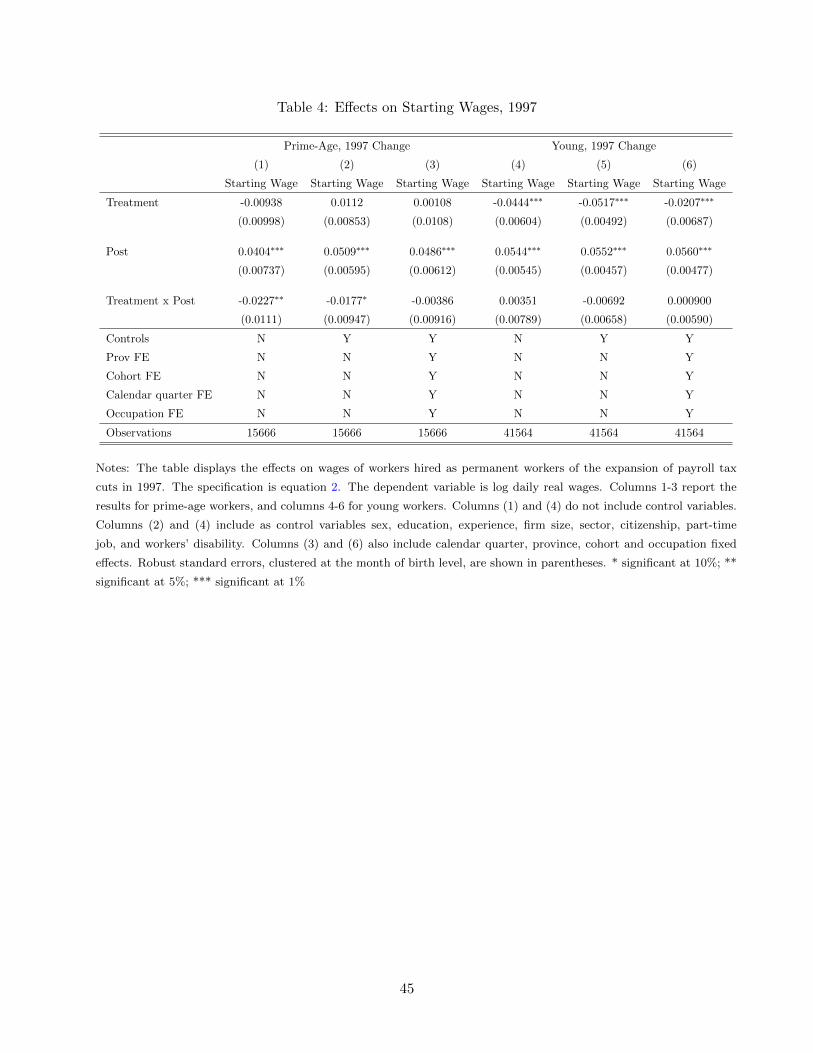
Table 4: Effects on Starting Wages, 1997

Prime-Age, 1997 Change Young, 1997 Change

(1) (2) (3) (4) (5) (6)

Starting Wage Starting Wage Starting Wage Starting Wage Starting Wage Starting Wage

Treatment -0.00938 0.0112 0.00108 -0.0444∗∗∗ -0.0517∗∗∗ -0.0207∗∗∗

(0.00998) (0.00853) (0.0108) (0.00604) (0.00492) (0.00687)

Post 0.0404∗∗∗ 0.0509∗∗∗ 0.0486∗∗∗ 0.0544∗∗∗ 0.0552∗∗∗ 0.0560∗∗∗

(0.00737) (0.00595) (0.00612) (0.00545) (0.00457) (0.00477)

Treatment x Post -0.0227∗∗ -0.0177∗ -0.00386 0.00351 -0.00692 0.000900

(0.0111) (0.00947) (0.00916) (0.00789) (0.00658) (0.00590)

Controls N Y Y N Y Y

Prov FE N N Y N N Y

Cohort FE N N Y N N Y

Calendar quarter FE N N Y N N Y

Occupation FE N N Y N N Y

Observations 15666 15666 15666 41564 41564 41564

Notes: The table displays the effects on wages of workers hired as permanent workers of the expansion of payroll tax

cuts in 1997. The specification is equation 2. The dependent variable is log daily real wages. Columns 1-3 report the

results for prime-age workers, and columns 4-6 for young workers. Columns (1) and (4) do not include control variables.

Columns (2) and (4) include as control variables sex, education, experience, firm size, sector, citizenship, part-time

job, and workers’ disability. Columns (3) and (6) also include calendar quarter, province, cohort and occupation fixed

effects. Robust standard errors, clustered at the month of birth level, are shown in parentheses. * significant at 10%; **

significant at 5%; *** significant at 1%

45

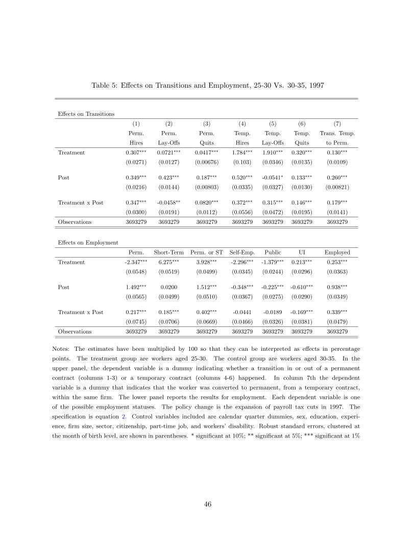
Table 5: Effects on Transitions and Employment, 25-30 Vs. 30-35, 1997

Effects on Transitions

(1) (2) (3) (4) (5) (6) (7)

Perm. Perm. Perm. Temp. Temp. Temp. Trans. Temp.

Hires Lay-Offs Quits Hires Lay-Offs Quits to Perm.

Treatment 0.307∗∗∗ 0.0721∗∗∗ 0.0417∗∗∗ 1.784∗∗∗ 1.910∗∗∗ 0.320∗∗∗ 0.130∗∗∗

(0.0271) (0.0127) (0.00676) (0.103) (0.0346) (0.0135) (0.0109)

Post 0.349∗∗∗ 0.423∗∗∗ 0.187∗∗∗ 0.520∗∗∗ -0.0541∗ 0.133∗∗∗ 0.260∗∗∗

(0.0216) (0.0144) (0.00803) (0.0335) (0.0327) (0.0130) (0.00821)

Treatment x Post 0.347∗∗∗ -0.0458∗∗ 0.0820∗∗∗ 0.372∗∗∗ 0.315∗∗∗ 0.146∗∗∗ 0.179∗∗∗

(0.0300) (0.0191) (0.0112) (0.0556) (0.0472) (0.0195) (0.0141)

Observations 3693279 3693279 3693279 3693279 3693279 3693279 3693279

Effects on Employment

Perm. Short-Term Perm. or ST Self-Emp. Public UI Employed

Treatment -2.347∗∗∗ 6.275∗∗∗ 3.928∗∗∗ -2.296∗∗∗ -1.379∗∗∗ 0.213∗∗∗ 0.253∗∗∗

(0.0548) (0.0519) (0.0499) (0.0345) (0.0244) (0.0296) (0.0363)

Post 1.492∗∗∗ 0.0200 1.512∗∗∗ -0.348∗∗∗ -0.225∗∗∗ -0.610∗∗∗ 0.938∗∗∗

(0.0565) (0.0499) (0.0510) (0.0367) (0.0275) (0.0290) (0.0349)

Treatment x Post 0.217∗∗∗ 0.185∗∗∗ 0.402∗∗∗ -0.0441 -0.0189 -0.169∗∗∗ 0.339∗∗∗

(0.0745) (0.0706) (0.0669) (0.0466) (0.0326) (0.0381) (0.0479)

Observations 3693279 3693279 3693279 3693279 3693279 3693279 3693279

Notes: The estimates have been multiplied by 100 so that they can be interpreted as effects in percentage

points. The treatment group are workers aged 25-30. The control group are workers aged 30-35. In the

upper panel, the dependent variable is a dummy indicating whether a transition in or out of a permanent

contract (columns 1-3) or a temporary contract (columns 4-6) happened. In column 7th the dependent

variable is a dummy that indicates that the worker was converted to permanent, from a temporary contract,

within the same firm. The lower panel reports the results for employment. Each dependent variable is one

of the possible employment statuses. The policy change is the expansion of payroll tax cuts in 1997. The

specification is equation 2. Control variables included are calendar quarter dummies, sex, education, experi-

ence, firm size, sector, citizenship, part-time job, and workers’ disability. Robust standard errors, clustered at

the month of birth level, are shown in parentheses. * significant at 10%; ** significant at 5%; *** significant at 1%

46

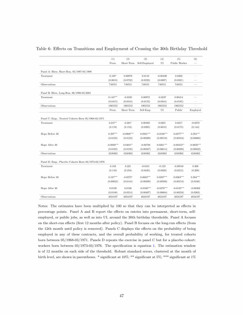
Table 6: Effects on Transitions and Employment of Crossing the 30th Birthday Threshold

(1) (2) (3) (4) (5) (6)

Perm. Short-Term Self-Employed UI Public Worker —

Panel A: Hires, Short-Run, 05/1997-05/1998

Treatment 0.108∗ 0.00978 0.0110 -0.00439 0.0202 —

(0.0618) (0.0732) (0.0228) (0.0697) (0.0331) —

Observations 748551 748551 748551 748551 748551 —

Panel B: Hires, Long-Run, 06/1998-03/2001

Treatment 0.143∗∗∗ -0.0335 0.00972 -0.0237 0.00414 —

(0.0415) (0.0544) (0.0152) (0.0344) (0.0185) —

Observations 1965552 1965552 1965552 1965552 1965552 —

Perm. Short-Term Self-Emp. UI Public Employed

Panel C: Emp., Treated Cohorts Born 05/1968-03/1971

Treatment 0.247∗∗ -0.301∗ 0.00492 0.0201 0.0217 -0.0270

(0.119) (0.153) (0.0395) (0.0618) (0.0175) (0.144)

Slope Before 30 0.297∗∗∗ -0.0908∗∗∗ 0.0501∗∗∗ -0.0186∗∗∗ 0.0277∗∗∗ 0.284∗∗∗

(0.0123) (0.0123) (0.00309) (0.00519) (0.00164) (0.00660)

Slope After 30 -0.0930∗∗∗ 0.0404∗∗ -0.00789 0.0261∗∗∗ -0.00453∗∗ -0.0650∗∗∗

(0.0192) (0.0158) (0.00567) (0.00614) (0.00208) (0.00832)

Observations 4240362 4240362 4240362 4240362 4240362 4240362

Panel D: Emp., Placebo Cohorts Born 03/1973-03/1976

Treatment 0.103 0.221 -0.0181 -0.123 -0.00548 0.300

(0.116) (0.254) (0.0435) (0.0820) (0.0212) (0.269)

Slope Before 30 0.187∗∗∗ -0.0275∗ 0.0683∗∗∗ 0.0287∗∗∗ 0.0363∗∗∗ 0.264∗∗∗

(0.00824) (0.0144) (0.00309) (0.00500) (0.00154) (0.0166)

Slope After 30 0.0139 0.0126 -0.0160∗∗∗ -0.0276∗∗∗ -0.0135∗∗∗ -0.00302

(0.0148) (0.0214) (0.00497) (0.00664) (0.00224) (0.0263)

Observations 4824197 4824197 4824197 4824197 4824197 4824197

Notes: The estimates have been multiplied by 100 so that they can be interpreted as effects in

percentage points. Panel A and B report the effects on entries into permanent, short-term, self-

employed, or public jobs, as well as into UI, around the 30th birthday thresholds. Panel A focuses

on the short-run effects (first 12 months after policy). Panel B focuses on the long-run effects (from

the 12th month until policy is removed). Panels C displays the effects on the probability of being

employed in any of these contracts, and the overall probability of working, for treated cohorts

born between 05/1968-03/1971. Panels D repeats the exercise in panel C but for a placebo cohort:

workers born between 03/1973-03/1976. The specification is equation 1. The estimation window

is of 12 months on each side of the threshold. Robust standard errors, clustered at the month of

birth level, are shown in parentheses. * significant at 10%; ** significant at 5%; *** significant at 1%

47

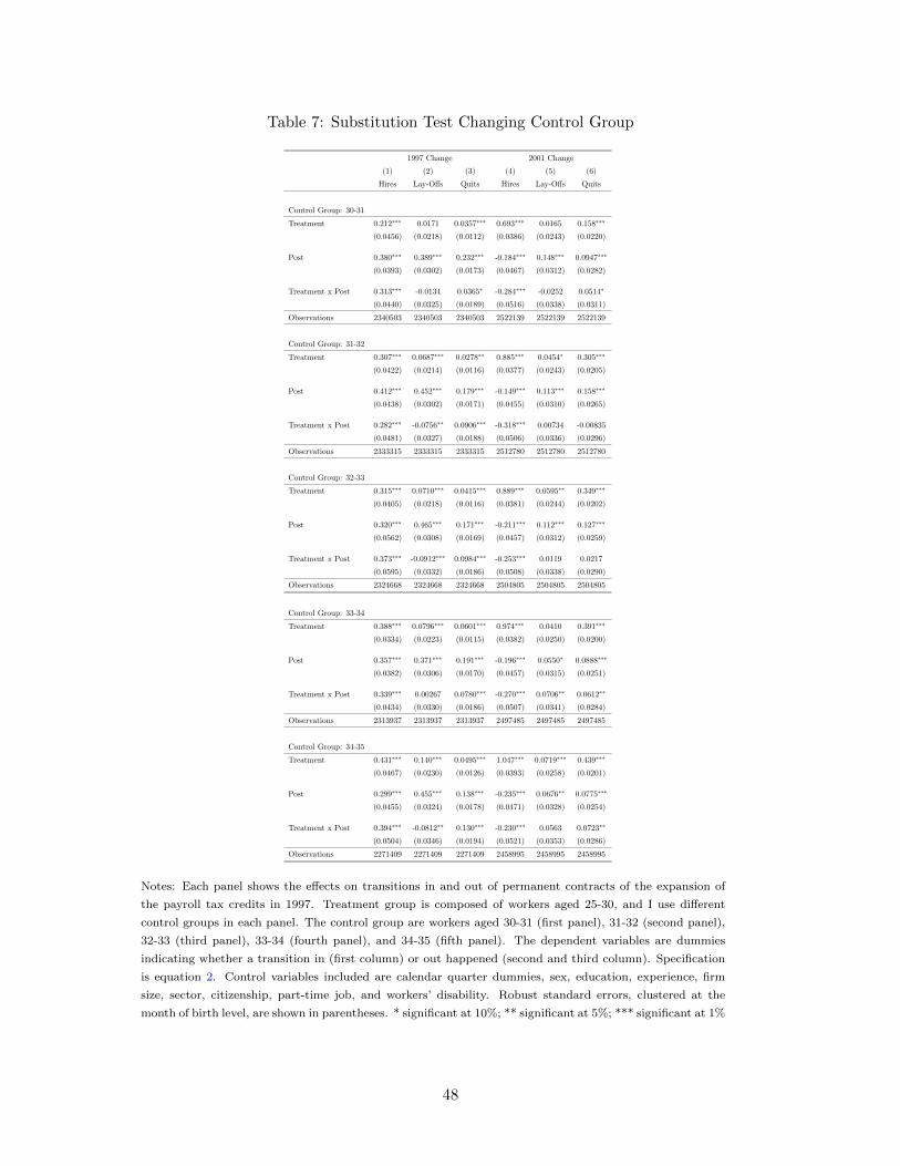
Table 7: Substitution Test Changing Control Group

1997 Change 2001 Change

(1) (2) (3) (4) (5) (6)

Hires Lay-Offs Quits Hires Lay-Offs Quits

Control Group: 30-31

Treatment 0.212∗∗∗ 0.0171 0.0357∗∗∗ 0.693∗∗∗ 0.0165 0.158∗∗∗

(0.0456) (0.0218) (0.0112) (0.0386) (0.0243) (0.0220)

Post 0.380∗∗∗ 0.389∗∗∗ 0.232∗∗∗ -0.184∗∗∗ 0.148∗∗∗ 0.0947∗∗∗

(0.0393) (0.0302) (0.0173) (0.0467) (0.0312) (0.0282)

Treatment x Post 0.313∗∗∗ -0.0134 0.0365∗ -0.284∗∗∗ -0.0252 0.0514∗

(0.0440) (0.0325) (0.0189) (0.0516) (0.0338) (0.0311)

Observations 2340503 2340503 2340503 2522139 2522139 2522139

Control Group: 31-32

Treatment 0.307∗∗∗ 0.0687∗∗∗ 0.0278∗∗ 0.885∗∗∗ 0.0454∗ 0.305∗∗∗

(0.0422) (0.0214) (0.0116) (0.0377) (0.0243) (0.0205)

Post 0.412∗∗∗ 0.452∗∗∗ 0.179∗∗∗ -0.149∗∗∗ 0.113∗∗∗ 0.158∗∗∗

(0.0438) (0.0302) (0.0171) (0.0455) (0.0310) (0.0265)

Treatment x Post 0.282∗∗∗ -0.0756∗∗ 0.0906∗∗∗ -0.318∗∗∗ 0.00734 -0.00835

(0.0481) (0.0327) (0.0188) (0.0506) (0.0336) (0.0296)

Observations 2333315 2333315 2333315 2512780 2512780 2512780

Control Group: 32-33

Treatment 0.315∗∗∗ 0.0710∗∗∗ 0.0415∗∗∗ 0.889∗∗∗ 0.0595∗∗ 0.349∗∗∗

(0.0405) (0.0218) (0.0116) (0.0381) (0.0244) (0.0202)

Post 0.320∗∗∗ 0.465∗∗∗ 0.171∗∗∗ -0.211∗∗∗ 0.112∗∗∗ 0.127∗∗∗

(0.0562) (0.0308) (0.0169) (0.0457) (0.0312) (0.0259)

Treatment x Post 0.373∗∗∗ -0.0912∗∗∗ 0.0984∗∗∗ -0.253∗∗∗ 0.0119 0.0217

(0.0595) (0.0332) (0.0186) (0.0508) (0.0338) (0.0290)

Observations 2324668 2324668 2324668 2504805 2504805 2504805

Control Group: 33-34

Treatment 0.388∗∗∗ 0.0796∗∗∗ 0.0601∗∗∗ 0.974∗∗∗ 0.0410 0.391∗∗∗

(0.0334) (0.0223) (0.0115) (0.0382) (0.0250) (0.0200)

Post 0.357∗∗∗ 0.371∗∗∗ 0.191∗∗∗ -0.196∗∗∗ 0.0550∗ 0.0888∗∗∗

(0.0382) (0.0306) (0.0170) (0.0457) (0.0315) (0.0251)

Treatment x Post 0.339∗∗∗ 0.00267 0.0780∗∗∗ -0.270∗∗∗ 0.0706∗∗ 0.0612∗∗

(0.0434) (0.0330) (0.0186) (0.0507) (0.0341) (0.0284)

Observations 2313937 2313937 2313937 2497485 2497485 2497485

Control Group: 34-35

Treatment 0.431∗∗∗ 0.140∗∗∗ 0.0495∗∗∗ 1.047∗∗∗ 0.0719∗∗∗ 0.439∗∗∗

(0.0467) (0.0230) (0.0126) (0.0393) (0.0258) (0.0201)

Post 0.299∗∗∗ 0.455∗∗∗ 0.138∗∗∗ -0.235∗∗∗ 0.0676∗∗ 0.0775∗∗∗

(0.0455) (0.0324) (0.0178) (0.0471) (0.0328) (0.0254)

Treatment x Post 0.394∗∗∗ -0.0812∗∗ 0.130∗∗∗ -0.230∗∗∗ 0.0563 0.0723∗∗

(0.0504) (0.0346) (0.0194) (0.0521) (0.0353) (0.0286)

Observations 2271409 2271409 2271409 2458995 2458995 2458995

Notes: Each panel shows the effects on transitions in and out of permanent contracts of the expansion of

the payroll tax credits in 1997. Treatment group is composed of workers aged 25-30, and I use different

control groups in each panel. The control group are workers aged 30-31 (first panel), 31-32 (second panel),

32-33 (third panel), 33-34 (fourth panel), and 34-35 (fifth panel). The dependent variables are dummies

indicating whether a transition in (first column) or out happened (second and third column). Specification

is equation 2. Control variables included are calendar quarter dummies, sex, education, experience, firm

size, sector, citizenship, part-time job, and workers’ disability. Robust standard errors, clustered at the

month of birth level, are shown in parentheses. * significant at 10%; ** significant at 5%; *** significant at 1%

48

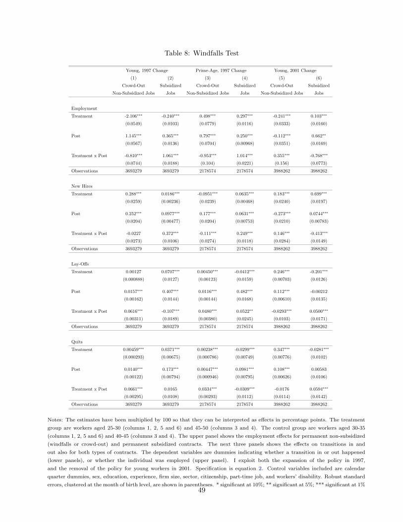
Table 8: Windfalls Test

Young, 1997 Change Prime-Age, 1997 Change Young, 2001 Change

(1) (2) (3) (4) (5) (6)

Crowd-Out Subsidized Crowd-Out Subsidized Crowd-Out Subsidized

Non-Subsidized Jobs Jobs Non-Subsidized Jobs Jobs Non-Subsidized Jobs Jobs

Employment

Treatment -2.106∗∗∗ -0.240∗∗∗ 0.498∗∗∗ 0.297∗∗∗ -0.241∗∗∗ 0.103∗∗∗

(0.0549) (0.0103) (0.0779) (0.0116) (0.0333) (0.0160)

Post 1.145∗∗∗ 0.365∗∗∗ 0.797∗∗∗ 0.250∗∗∗ -0.112∗∗∗ 0.662∗∗

(0.0567) (0.0136) (0.0704) (0.00968) (0.0351) (0.0169)

Treatment x Post -0.810∗∗∗ 1.061∗∗∗ -0.953∗∗∗ 1.014∗∗∗ 0.355∗∗∗ -0.768∗∗∗

(0.0744) (0.0188) (0.104) (0.0221) (0.156) (0.0773)

Observations 3693279 3693279 2178574 2178574 3988262 3988262

New Hires

Treatment 0.288∗∗∗ 0.0186∗∗∗ -0.0951∗∗∗ 0.0635∗∗∗ 0.183∗∗∗ 0.699∗∗∗

(0.0259) (0.00236) (0.0239) (0.00468) (0.0240) (0.0197)

Post 0.252∗∗∗ 0.0977∗∗∗ 0.177∗∗∗ 0.0631∗∗∗ -0.273∗∗∗ 0.0744∗∗∗

(0.0204) (0.00477) (0.0204) (0.00753) (0.0210) (0.00783)

Treatment x Post -0.0227 0.372∗∗∗ -0.111∗∗∗ 0.249∗∗∗ 0.146∗∗∗ -0.413∗∗∗

(0.0273) (0.0106) (0.0274) (0.0118) (0.0284) (0.0149)

Observations 3693279 3693279 2178574 2178574 3988262 3988262

Lay-Offs

Treatment 0.00127 0.0707∗∗∗ 0.00450∗∗∗ -0.0412∗∗∗ 0.246∗∗∗ -0.201∗∗∗

(0.000888) (0.0127) (0.00123) (0.0159) (0.00703) (0.0126)

Post 0.0157∗∗∗ 0.407∗∗∗ 0.0116∗∗∗ 0.482∗∗∗ 0.112∗∗∗ -0.00212

(0.00162) (0.0144) (0.00144) (0.0168) (0.00610) (0.0135)

Treatment x Post 0.0616∗∗∗ -0.107∗∗∗ 0.0480∗∗∗ 0.0522∗∗ -0.0293∗∗∗ 0.0500∗∗∗

(0.00311) (0.0189) (0.00380) (0.0245) (0.0103) (0.0171)

Observations 3693279 3693279 2178574 2178574 3988262 3988262

Quits

Treatment 0.00459∗∗∗ 0.0371∗∗∗ 0.00238∗∗∗ -0.0299∗∗∗ 0.347∗∗∗ -0.0281∗∗∗

(0.000293) (0.00675) (0.000786) (0.00749) (0.00776) (0.0102)

Post 0.0140∗∗∗ 0.173∗∗∗ 0.00447∗∗∗ 0.0981∗∗∗ 0.108∗∗∗ 0.00583

(0.00122) (0.00794) (0.000946) (0.00795) (0.00626) (0.0106)

Treatment x Post 0.0661∗∗∗ 0.0165 0.0334∗∗∗ -0.0309∗∗∗ -0.0176 0.0594∗∗∗

(0.00295) (0.0108) (0.00293) (0.0112) (0.0114) (0.0142)

Observations 3693279 3693279 2178574 2178574 3988262 3988262

Notes: The estimates have been multiplied by 100 so that they can be interpreted as effects in percentage points. The treatment

group are workers aged 25-30 (columns 1, 2, 5 and 6) and 45-50 (columns 3 and 4). The control group are workers aged 30-35

(columns 1, 2, 5 and 6) and 40-45 (columns 3 and 4). The upper panel shows the employment effects for permanent non-subsidized

(windfalls or crowd-out) and permanent subsidized contracts. The next three panels shows the effects on transitions in and

out also for both types of contracts. The dependent variables are dummies indicating whether a transition in or out happened

(lower panels), or whether the individual was employed (upper panel). I exploit both the expansion of the policy in 1997,

and the removal of the policy for young workers in 2001. Specification is equation 2. Control variables included are calendar

quarter dummies, sex, education, experience, firm size, sector, citizenship, part-time job, and workers’ disability. Robust standard

errors, clustered at the month of birth level, are shown in parentheses. * significant at 10%; ** significant at 5%; *** significant at 1%49

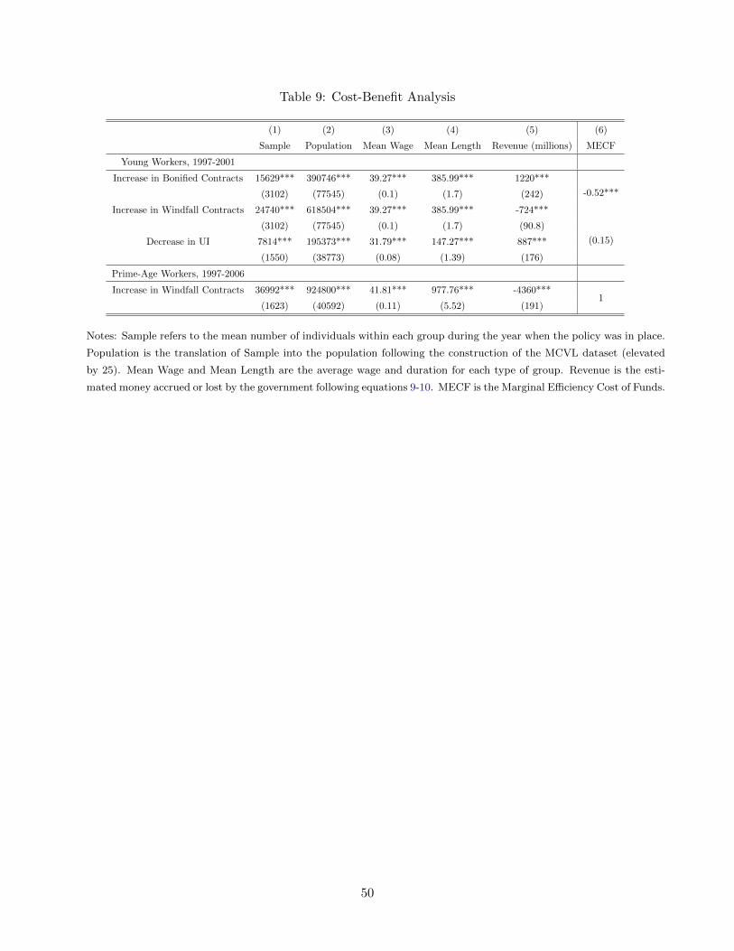
Table 9: Cost-Benefit Analysis

(1) (2) (3) (4) (5) (6)

Sample Population Mean Wage Mean Length Revenue (millions) MECF

Young Workers, 1997-2001

Increase in Bonified Contracts 15629*** 390746*** 39.27*** 385.99*** 1220***

-0.52***(3102) (77545) (0.1) (1.7) (242)

Increase in Windfall Contracts 24740*** 618504*** 39.27*** 385.99*** -724***

(3102) (77545) (0.1) (1.7) (90.8)

(0.15)Decrease in UI 7814*** 195373*** 31.79*** 147.27*** 887***

(1550) (38773) (0.08) (1.39) (176)

Prime-Age Workers, 1997-2006

Increase in Windfall Contracts 36992*** 924800*** 41.81*** 977.76*** -4360***1

(1623) (40592) (0.11) (5.52) (191)

Notes: Sample refers to the mean number of individuals within each group during the year when the policy was in place.

Population is the translation of Sample into the population following the construction of the MCVL dataset (elevated

by 25). Mean Wage and Mean Length are the average wage and duration for each type of group. Revenue is the esti-

mated money accrued or lost by the government following equations 9-10. MECF is the Marginal Efficiency Cost of Funds.

50

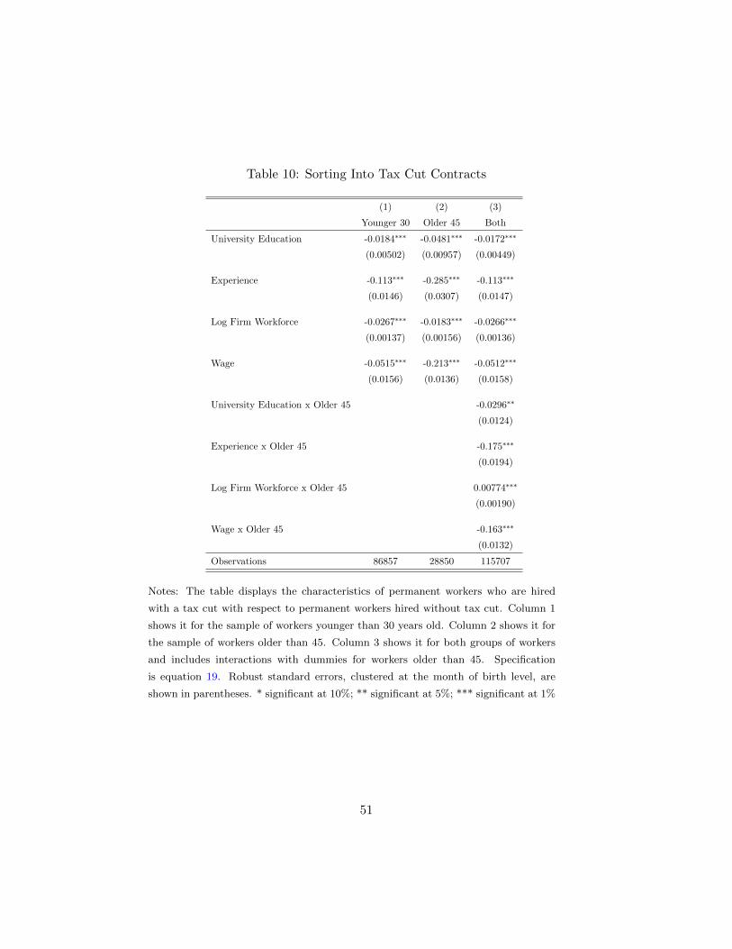
Table 10: Sorting Into Tax Cut Contracts

(1) (2) (3)

Younger 30 Older 45 Both

University Education -0.0184∗∗∗ -0.0481∗∗∗ -0.0172∗∗∗

(0.00502) (0.00957) (0.00449)

Experience -0.113∗∗∗ -0.285∗∗∗ -0.113∗∗∗

(0.0146) (0.0307) (0.0147)

Log Firm Workforce -0.0267∗∗∗ -0.0183∗∗∗ -0.0266∗∗∗

(0.00137) (0.00156) (0.00136)

Wage -0.0515∗∗∗ -0.213∗∗∗ -0.0512∗∗∗

(0.0156) (0.0136) (0.0158)

University Education x Older 45 -0.0296∗∗

(0.0124)

Experience x Older 45 -0.175∗∗∗

(0.0194)

Log Firm Workforce x Older 45 0.00774∗∗∗

(0.00190)

Wage x Older 45 -0.163∗∗∗

(0.0132)

Observations 86857 28850 115707

Notes: The table displays the characteristics of permanent workers who are hired

with a tax cut with respect to permanent workers hired without tax cut. Column 1

shows it for the sample of workers younger than 30 years old. Column 2 shows it for

the sample of workers older than 45. Column 3 shows it for both groups of workers

and includes interactions with dummies for workers older than 45. Specification

is equation 19. Robust standard errors, clustered at the month of birth level, are

shown in parentheses. * significant at 10%; ** significant at 5%; *** significant at 1%

51

Table 11: Effects on Transition of Crossing the Birthday Thresholds, Small Firms

(1) (2)

Perm. Short-Term

Young Workers, Small Firms

Treatment 0.276*** -0.0499

(0.0595) (0.0801)

Observations 1217886 1217886

Senior Workers, Small Firms

Treatment 0.374*** -0.0752

(0.0305) (0.0498)

Observations 2551782 2551782

Young Workers, Large Firms

Treatment 0.0624 0.0233

(0.0726) (0.114)

Observations 427710 427710

Senior Workers, Large Firms

Treatment 0.0679* 0.0274

(0.0384) (0.0673)

Observations 853567 853567

Notes: The estimates have been multiplied by 100 so that they can be interpreted as effects in

percentage points. The table displays the effects on entries into permanent and short-term both

for young and senior workers, and for small and large firms. The specification is equation 1. The

dependent variables are dummies indicating each type of transition. The estimation window is

of 12 months on each side of the threshold. Robust standard errors, clustered at the month of

birth level, are shown in parentheses. * significant at 10%; ** significant at 5%; *** significant at 1%

52

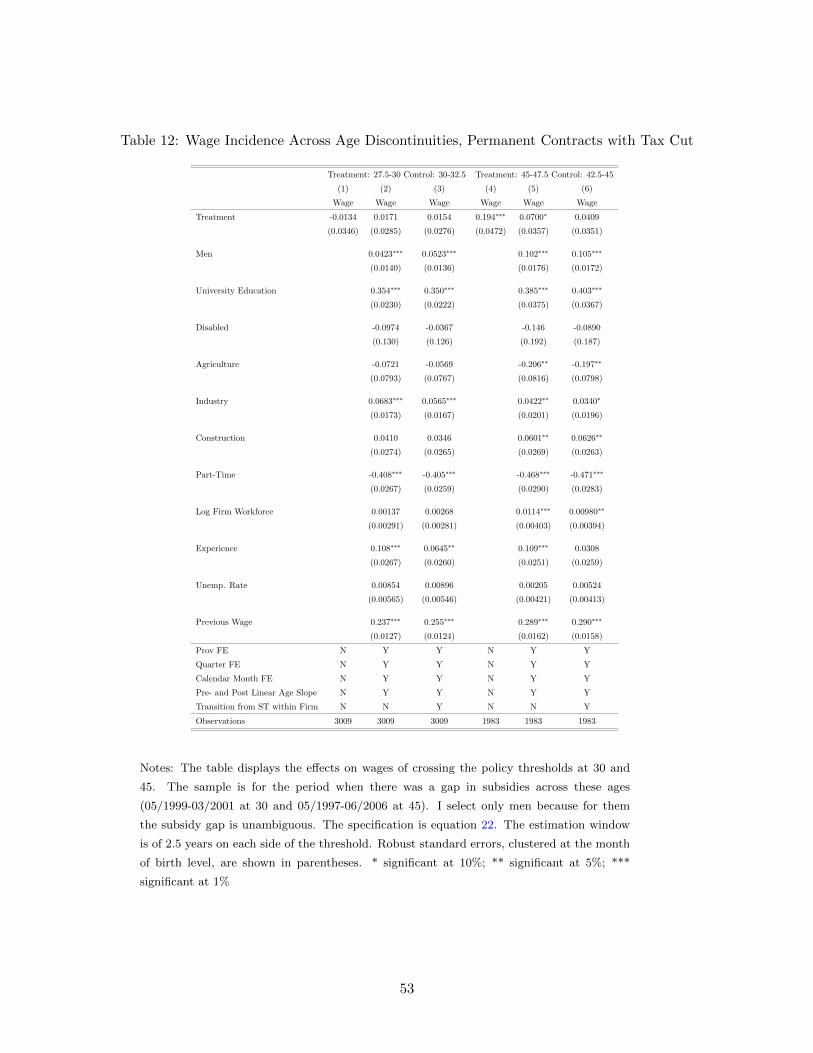
Table 12: Wage Incidence Across Age Discontinuities, Permanent Contracts with Tax Cut

Treatment: 27.5-30 Control: 30-32.5 Treatment: 45-47.5 Control: 42.5-45

(1) (2) (3) (4) (5) (6)

Wage Wage Wage Wage Wage Wage

Treatment -0.0134 0.0171 0.0154 0.194∗∗∗ 0.0700∗ 0.0409

(0.0346) (0.0285) (0.0276) (0.0472) (0.0357) (0.0351)

Men 0.0423∗∗∗ 0.0523∗∗∗ 0.102∗∗∗ 0.105∗∗∗

(0.0140) (0.0136) (0.0176) (0.0172)

University Education 0.354∗∗∗ 0.350∗∗∗ 0.385∗∗∗ 0.403∗∗∗

(0.0230) (0.0222) (0.0375) (0.0367)

Disabled -0.0974 -0.0367 -0.146 -0.0890

(0.130) (0.126) (0.192) (0.187)

Agriculture -0.0721 -0.0569 -0.206∗∗ -0.197∗∗

(0.0793) (0.0767) (0.0816) (0.0798)

Industry 0.0683∗∗∗ 0.0565∗∗∗ 0.0422∗∗ 0.0340∗

(0.0173) (0.0167) (0.0201) (0.0196)

Construction 0.0410 0.0346 0.0601∗∗ 0.0626∗∗

(0.0274) (0.0265) (0.0269) (0.0263)

Part-Time -0.408∗∗∗ -0.405∗∗∗ -0.468∗∗∗ -0.471∗∗∗

(0.0267) (0.0259) (0.0290) (0.0283)

Log Firm Workforce 0.00137 0.00268 0.0114∗∗∗ 0.00980∗∗

(0.00291) (0.00281) (0.00403) (0.00394)

Experience 0.108∗∗∗ 0.0645∗∗ 0.109∗∗∗ 0.0308

(0.0267) (0.0260) (0.0251) (0.0259)

Unemp. Rate 0.00854 0.00896 0.00205 0.00524

(0.00565) (0.00546) (0.00421) (0.00413)

Previous Wage 0.237∗∗∗ 0.255∗∗∗ 0.289∗∗∗ 0.290∗∗∗

(0.0127) (0.0124) (0.0162) (0.0158)

Prov FE N Y Y N Y Y

Quarter FE N Y Y N Y Y

Calendar Month FE N Y Y N Y Y

Pre- and Post Linear Age Slope N Y Y N Y Y

Transition from ST within Firm N N Y N N Y

Observations 3009 3009 3009 1983 1983 1983

Notes: The table displays the effects on wages of crossing the policy thresholds at 30 and

45. The sample is for the period when there was a gap in subsidies across these ages

(05/1999-03/2001 at 30 and 05/1997-06/2006 at 45). I select only men because for them

the subsidy gap is unambiguous. The specification is equation 22. The estimation window

is of 2.5 years on each side of the threshold. Robust standard errors, clustered at the month

of birth level, are shown in parentheses. * significant at 10%; ** significant at 5%; ***

significant at 1%

53

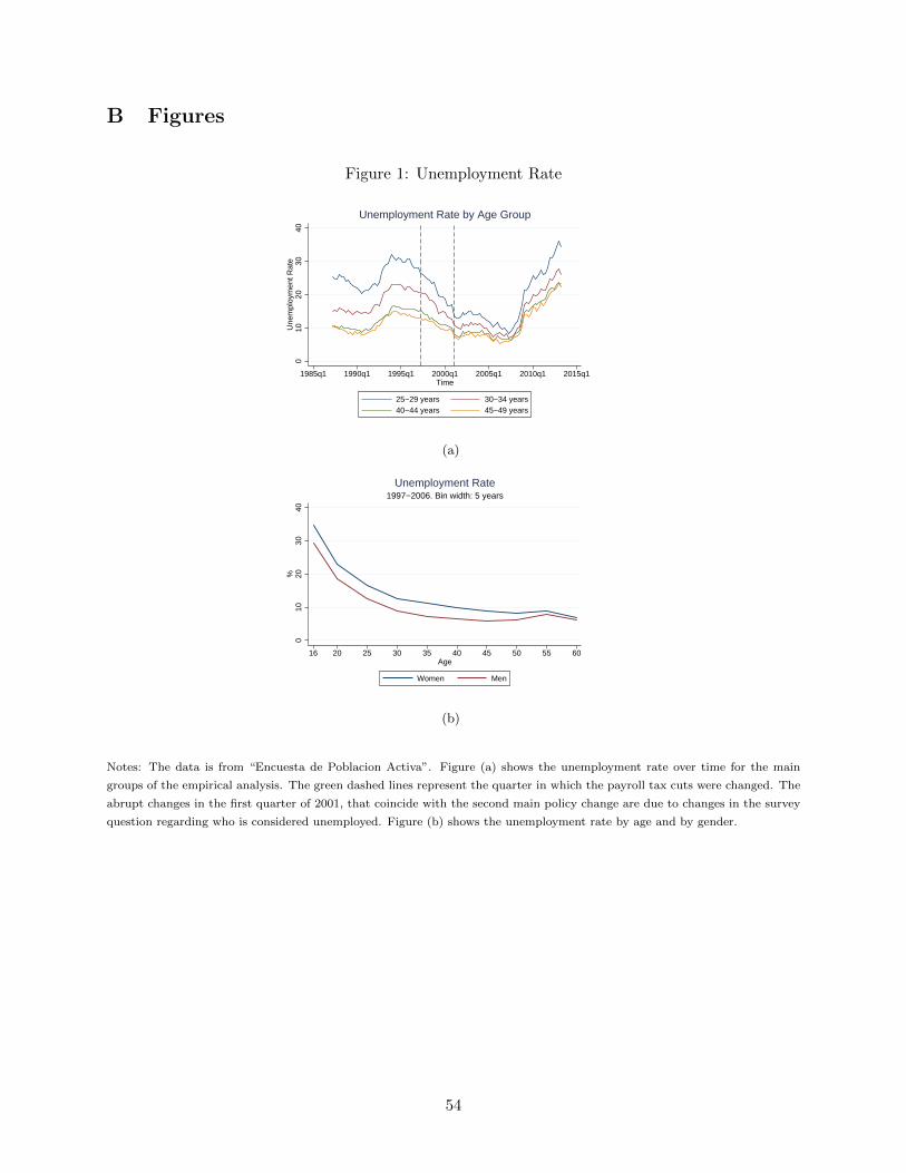
B Figures

Figure 1: Unemployment Rate

010

2030

40U

nem

ploy

men

t Rat

e

1985q1 1990q1 1995q1 2000q1 2005q1 2010q1 2015q1Time

25−29 years 30−34 years40−44 years 45−49 years

Unemployment Rate by Age Group

(a)

010

2030

40%

16 20 25 30 35 40 45 50 55 60Age

Women Men

1997−2006. Bin width: 5 yearsUnemployment Rate

(b)

Notes: The data is from “Encuesta de Poblacion Activa”. Figure (a) shows the unemployment rate over time for the main

groups of the empirical analysis. The green dashed lines represent the quarter in which the payroll tax cuts were changed. The

abrupt changes in the first quarter of 2001, that coincide with the second main policy change are due to changes in the survey

question regarding who is considered unemployed. Figure (b) shows the unemployment rate by age and by gender.

54

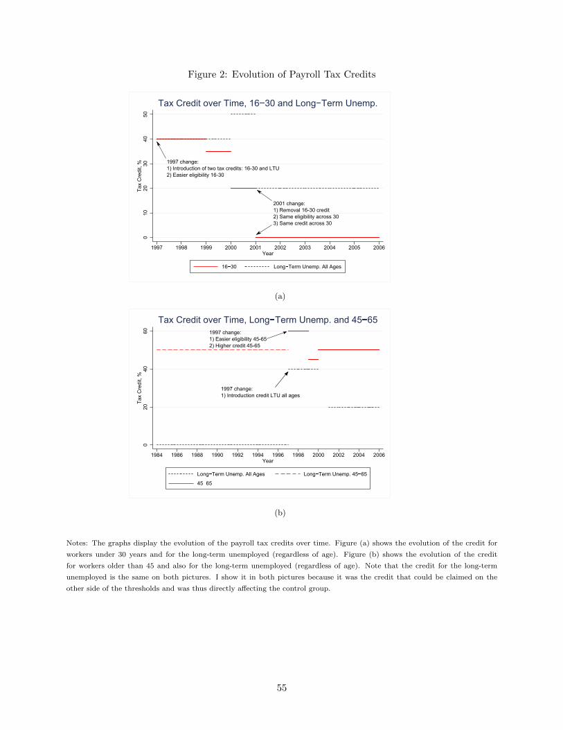
Figure 2: Evolution of Payroll Tax Credits

010

20

30

40

50

Tax C

redit,

%

1997 1998 1999 2000 2001 2002 2003 2004 2005 2006Year

16 30 Long Term Unemp. All Ages

Tax Credit over Time, 16 30 and Long Term Unemp.

2001 change:

1) Removal 16-30 credit

2) Same eligibility across 30

3) Same credit across 30

1997 change:

1) Introduction of two tax credits: 16-30 and LTU

2) Easier eligibility 16-30

(a)

020

40

60

Tax C

redit,

%

1984 1986 1988 1990 1992 1994 1996 1998 2000 2002 2004 2006Year

Long Term Unemp. All Ages Long Term Unemp. 45 65

45 65

Tax Credit over Time, Long Term Unemp. and 45 65

1997 change:

1) Easier eligibility 45-65

2) Higher credit 45-65

1997 change:

1) Introduction credit LTU all ages

(b)

Notes: The graphs display the evolution of the payroll tax credits over time. Figure (a) shows the evolution of the credit for

workers under 30 years and for the long-term unemployed (regardless of age). Figure (b) shows the evolution of the credit

for workers older than 45 and also for the long-term unemployed (regardless of age). Note that the credit for the long-term

unemployed is the same on both pictures. I show it in both pictures because it was the credit that could be claimed on the

other side of the thresholds and was thus directly affecting the control group.

55

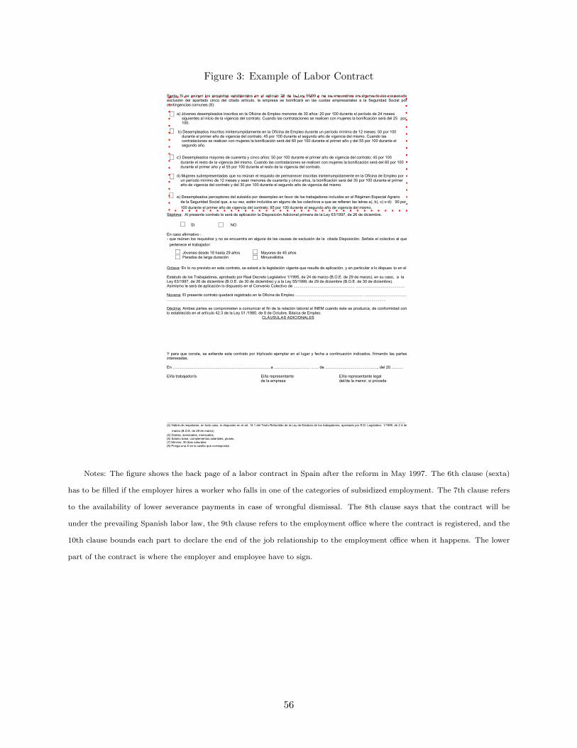
Figure 3: Example of Labor Contract

Sexta: Si se reúnen los requisitos establecidos en el artículo 28 de la Ley 55/99 y no se encuentran en alguna de las causas deexclusión del apartado cinco del citado artículo, la empresa se bonificará en las cuotas empresariales a la Seguridad Social porcontingencias comunes (8):

a) Jóvenes desempleados inscritos en la Oficina de Empleo menores de 30 años: 20 por 100 durante el período de 24 mesessiguientes al inicio de la vigencia del contrato. Cuando las contrataciones se realicen con mujeres la bonificación será del 25 por100.

b) Desempleados inscritos ininterrumpidamente en la Oficina de Empleo durante un período mínimo de 12 meses: 50 por 100durante el primer año de vigencia del contrato; 45 por 100 durante el segundo año de vigencia del mismo. Cuando lascontrataciones se realicen con mujeres la bonificación será del 60 por 100 durante el primer año y del 55 por 100 durante elsegundo año.

c) Desempleados mayores de cuarenta y cinco años: 50 por 100 durante el primer año de vigencia del contrato; 45 por 100durante el resto de la vigencia del mismo. Cuando las contrataciones se realicen con mujeres la bonificación será del 60 por 100durante el primer año y el 55 por 100 durante el resto de la vigencia del contrato.

d) Mujeres subrepresentadas que no reúnan el requisito de permanecer inscritas ininterrumpidamente en la Oficina de Empleo porun período mínimo de 12 meses y sean menores de cuarenta y cinco años, la bonificación será del 35 por 100 durante el primeraño de vigencia del contrato y del 30 por 100 durante el segundo año de vigencia del mismo.

e) Desempleados perceptores del subsidio por desempleo en favor de los trabajadores incluidos en el Régimen Especial Agrariode la Seguridad Social que, a su vez, estén incluidos en alguno de los colectivos a que se refieren las letras a), b), c) o d): 90 por

100 durante el primer año de vigencia del contrato; 85 por 100 durante el segundo año de vigencia del mismo.

Séptima: Al presente contrato le será de aplicación la Disposición Adicional primera de la Ley 63/1997, de 26 de diciembre.

SI NO

En caso afirmativo :- que reúnen los requisitos y no se encuentra en alguna de las causas de exclusión de la citada Disposición. Señale el colectivo al que

pertenece el trabajador:

Jóvenes desde 18 hasta 29 años Mayores de 45 añosParados de larga duración Minusválidos

Octava: En lo no previsto en este contrato, se estará a la legislación vigente que resulte de aplicación, y en particular a lo dispues to en el

Estatuto de los Trabajadores, aprobado por Real Decreto Legislativo 1/1995, de 24 de marzo (B.O.E. de 29 de marzo), en su caso, a laLey 63/1997, de 26 de diciembre (B.O.E. de 30 de diciembre) y a la Ley 55/1999, de 29 de diciembre (B.O.E. de 30 de diciembre).Asimismo le será de aplicación lo dispuesto en el Convenio Colectivo de ........................................................ .............................................

Novena: El presente contrato quedará registrado en la Oficina de Empleo .............................................................. ....................................................................................................................................................................... ........................................................................

Décima: Ambas partes se comprometen a comunicar el fin de la relación laboral al INEM cuando éste se produzca, de conformidad conlo establecido en el artículo 42.3 de la Ley 51 /1980, de 8 de Octubre, Básica de Empleo.

CLÁUSULAS ADICIONALES

Y para que conste, se extiende este contrato por triplicado ejemplar en el lugar y fecha a continuación indicados, firmando las partesinteresadas.

En ......................................................................................... a ................................. ....... de ................................................, del 20............

El/la trabajador/a El/la representante El/la representante legalde la empresa del/de la menor, si procede

(4) Habrá de respetarse, en todo caso, lo dispuesto en el art. 14.1 del Texto Refundido de la Ley de Estatuto de los trabajadores, aprobado por R.D. Legislativo 1/1995, de 2 4 de

marzo (B.O.E. de 29 de marzo)(5) Diarias, semanales, mensuales.(6) Salario base, complementos salariales, pluses.(7) Mínimo: 30 días naturales(8) Ponga una X en la casilla que corresponda

Notes: The figure shows the back page of a labor contract in Spain after the reform in May 1997. The 6th clause (sexta)

has to be filled if the employer hires a worker who falls in one of the categories of subsidized employment. The 7th clause refers

to the availability of lower severance payments in case of wrongful dismissal. The 8th clause says that the contract will be

under the prevailing Spanish labor law, the 9th clause refers to the employment office where the contract is registered, and the

10th clause bounds each part to declare the end of the job relationship to the employment office when it happens. The lower

part of the contract is where the employer and employee have to sign.

56

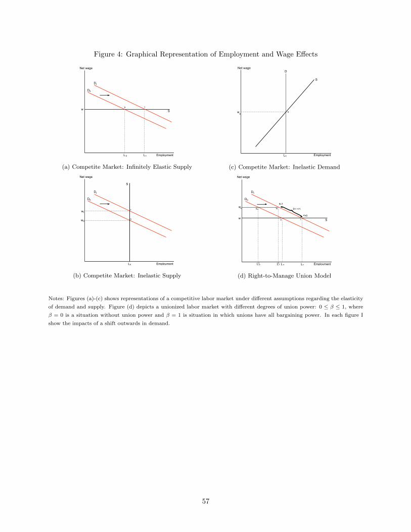
Figure 4: Graphical Representation of Employment and Wage Effects

Net wage

Employment

0 1

S

D0

D1

L L0 1

w

(a) Competite Market: Infinitely Elastic Supply

Net wage

Employment

S

D0

D1

L0

w0

w1

0

1

(b) Competite Market: Inelastic Supply

L0

w0

0

S

DNet wage

Employment

(c) Competite Market: Inelastic Demand

Net wage

Employment

0 1 S

D0

D1

0 1

L L0 1

w

wu

} =1

=0

0< <1u u

L L0 1u u

(d) Right-to-Manage Union Model

Notes: Figures (a)-(c) shows representations of a competitive labor market under different assumptions regarding the elasticity

of demand and supply. Figure (d) depicts a unionized labor market with different degrees of union power: 0 ≤ β ≤ 1, where

β = 0 is a situation without union power and β = 1 is situation in which unions have all bargaining power. In each figure I

show the impacts of a shift outwards in demand.

57

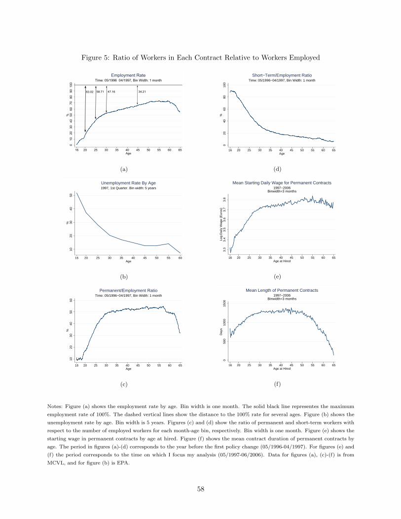
Figure 5: Ratio of Workers in Each Contract Relative to Workers Employed

010

20

30

40

50

60

70

80

90

100

%

16 20 25 30 35 40 45 50 55 60 65Age

Time: 05/1996 04/1997, Bin Width: 1 month

Employment Rate

83.02 58.71 47.16 34.21

(a)

1020

3040

50%

16 20 25 30 35 40 45 50 55 60Age

1997, 1st Quarter. Bin width: 5 yearsUnemployment Rate By Age

(b)

1020

3040

5060

%

16 20 25 30 35 40 45 50 55 60 65Age

Time: 05/1996−04/1997, Bin Width: 1 monthPermanent/Employment Ratio

(c)

020

4060

8010

0%

16 20 25 30 35 40 45 50 55 60 65Age

Time: 05/1996−04/1997, Bin Width: 1 monthShort−Term/Employment Ratio

(d)

3.3

3.4

3.5

3.6

3.7

3.8

Log

Dai

ly W

age

(Eur

os)

16 20 25 30 35 40 45 50 55 60 65Age at Hired

1997−2006Binwidth=3 months

Mean Starting Daily Wage for Permanent Contracts

(e)

050

010

0015

00D

ays

16 20 25 30 35 40 45 50 55 60 65Age at Hired

1997−2006Binwidth=3 months

Mean Length of Permanent Contracts

(f)

Notes: Figure (a) shows the employment rate by age. Bin width is one month. The solid black line representes the maximum

employment rate of 100%. The dashed vertical lines show the distance to the 100% rate for several ages. Figure (b) shows the

unemployment rate by age. Bin width is 5 years. Figures (c) and (d) show the ratio of permanent and short-term workers with

respect to the number of employed workers for each month-age bin, respectively. Bin width is one month. Figure (e) shows the

starting wage in permanent contracts by age at hired. Figure (f) shows the mean contract duration of permanent contracts by

age. The period in figures (a)-(d) corresponds to the year before the first policy change (05/1996-04/1997). For figures (e) and

(f) the period corresponds to the time on which I focus my analysis (05/1997-06/2006). Data for figures (a), (c)-(f) is from

MCVL, and for figure (b) is EPA.

58

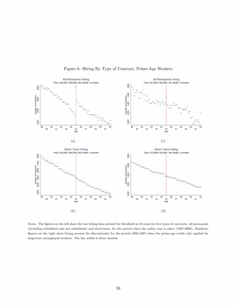
Figure 6: Hiring By Type of Contract, Prime-Age Workers

1500

2000

2500

3000

Num

ber

of C

ontr

acts

3839

4041

4243

4445

4647

4849

5051

52

Age

Time: 05/1997−06/2006, Bin Width: 3 monthsAll Permanent Hiring

(a)

3000

4000

5000

6000

7000

8000

Num

ber

of C

ontr

acts

3839

4041

4243

4445

4647

4849

5051

52

Age

Time: 05/1997−06/2006, Bin Width: 3 monthsShort−Term Hiring

(b)

1000

1200

1400

1600

1800

Num

ber

of C

ontr

acts

3839

4041

4243

4445

4647

4849

5051

52

Age

Time: 01/1992−05/1997, Bin Width: 3 monthsAll Permanent Hiring

(c)

1000

2000

3000

4000

5000

Num

ber

of C

ontr

acts

3839

4041

4243

4445

4647

4849

5051

52

Age

Time: 01/1992−05/1997, Bin Width: 3 monthsShort−Term Hiring

(d)

Notes: The figures on the left show the raw hiring data around the threshold at 45 years for two types of contracts: all permanent

(including subsidized and not subsidized) and short-term, for the period when the policy was in place (1997-2006). Similarly,

figures on the right show hiring around the discontinuity for the period 1992-1997 when the prime-age credit only applied for

long-term unemployed workers. The bin width is three months.

59

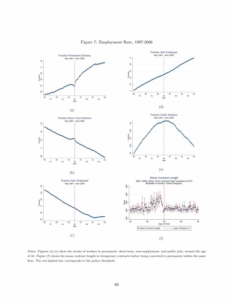
Figure 7: Employment Rate, 1997-2006.3

6.3

7.3

8.3

9.4

.41

Fra

ctio

n

3537

3941

4345

4749

5153

55

Age

May 1997− June 2006Fraction Permanent Workers

(a)

.08

.1.1

2.1

4.1

6F

ract

ion

3537

3941

4345

4749

5153

55

Age

May 1997− June 2006Fraction Short−Term Workers

(b)

.26

.28

.3.3

2.3

4.3

6F

ract

ion

3537

3941

4345

4749

5153

55

Age

May 1997− June 2006Fraction Non−Employed

(c)

.1.1

2.1

4.1

6.1

8.2

Fra

ctio

n

3537

3941

4345

4749

5153

55

Age

May 1997− June 2006Fraction Self−Employed

(d)

.04

.045

.05

.055

.06

Fra

ctio

n

3537

3941

4345

4749

5153

55

Age

May 1997− June 2006Fraction Public Workers

(e)

100

200

300

400

500

Day

s

35 40 45 50 55Age at Hired

Mean Contract Length Lower CI/Upper CI

1997−2006, Short−Term Contracts that Transition to PTCBinwidth=3 months. Same Employer.

Mean Contract Length

(f)

Notes: Figures (a)-(e) show the stocks of workers in permanent, short-term, non-employment, and public jobs, around the age

of 45. Figure (f) shows the mean contract length in termporary contracts before being converted to permanent within the same

firm. The red dashed line corresponds to the policy threshold.

60

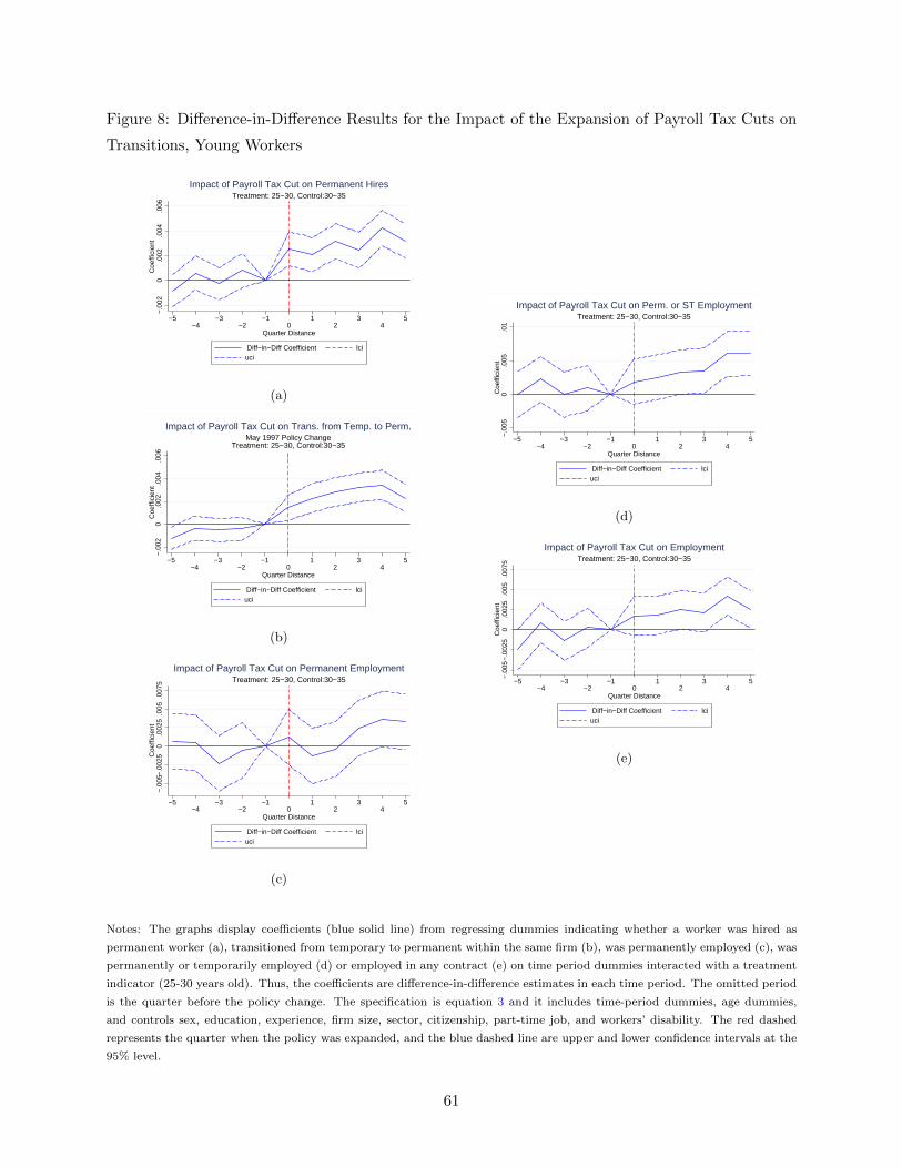
Figure 8: Difference-in-Difference Results for the Impact of the Expansion of Payroll Tax Cuts on

Transitions, Young Workers−

.002

0.0

02.0

04.0

06C

oeffi

cien

t

−5−4

−3−2

−10

12

34

5

Quarter Distance

Diff−in−Diff Coefficient lciuci

Treatment: 25−30, Control:30−35Impact of Payroll Tax Cut on Permanent Hires

(a)

−.0

020

.002

.004

.006

Coe

ffici

ent

−5−4

−3−2

−10

12

34

5

Quarter Distance

Diff−in−Diff Coefficient lciuci

May 1997 Policy ChangeTreatment: 25−30, Control:30−35

Impact of Payroll Tax Cut on Trans. from Temp. to Perm.

(b)

−.0

05−

.002

50

.002

5.0

05.0

075

Coe

ffici

ent

−5−4

−3−2

−10

12

34

5

Quarter Distance

Diff−in−Diff Coefficient lciuci

Treatment: 25−30, Control:30−35Impact of Payroll Tax Cut on Permanent Employment

(c)

−.0

050

.005

.01

Coe

ffici

ent

−5−4

−3−2

−10

12

34

5

Quarter Distance

Diff−in−Diff Coefficient lciuci

Treatment: 25−30, Control:30−35Impact of Payroll Tax Cut on Perm. or ST Employment

(d)−

.005

−.0

025

0.0

025

.005

.007

5C

oeffi

cien

t

−5−4

−3−2

−10

12

34

5

Quarter Distance

Diff−in−Diff Coefficient lciuci

Treatment: 25−30, Control:30−35Impact of Payroll Tax Cut on Employment

(e)

Notes: The graphs display coefficients (blue solid line) from regressing dummies indicating whether a worker was hired as

permanent worker (a), transitioned from temporary to permanent within the same firm (b), was permanently employed (c), was

permanently or temporarily employed (d) or employed in any contract (e) on time period dummies interacted with a treatment

indicator (25-30 years old). Thus, the coefficients are difference-in-difference estimates in each time period. The omitted period

is the quarter before the policy change. The specification is equation 3 and it includes time-period dummies, age dummies,

and controls sex, education, experience, firm size, sector, citizenship, part-time job, and workers’ disability. The red dashed

represents the quarter when the policy was expanded, and the blue dashed line are upper and lower confidence intervals at the

95% level.

61

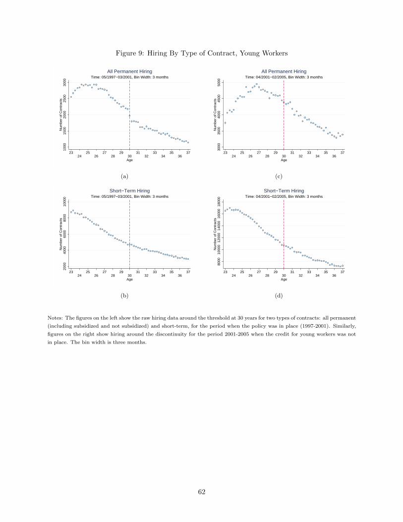
Figure 9: Hiring By Type of Contract, Young Workers

1000

1500

2000

2500

3000

Num

ber

of C

ontr

acts

2324

2526

2728

2930

3132

3334

3536

37

Age

Time: 05/1997−03/2001, Bin Width: 3 monthsAll Permanent Hiring

(a)

2000

4000

6000

8000

1000

0N

umbe

r of

Con

trac

ts

2324

2526

2728

2930

3132

3334

3536

37

Age

Time: 05/1997−03/2001, Bin Width: 3 monthsShort−Term Hiring

(b)

3000

3500

4000

4500

5000

Num

ber

of C

ontr

acts

2324

2526

2728

2930

3132

3334

3536

37

Age

Time: 04/2001−02/2005, Bin Width: 3 monthsAll Permanent Hiring

(c)

8000

1000

012

000

1400

016

000

1800

0N

umbe

r of

Con

trac

ts

2324

2526

2728

2930

3132

3334

3536

37

Age

Time: 04/2001−02/2005, Bin Width: 3 monthsShort−Term Hiring

(d)

Notes: The figures on the left show the raw hiring data around the threshold at 30 years for two types of contracts: all permanent

(including subsidized and not subsidized) and short-term, for the period when the policy was in place (1997-2001). Similarly,

figures on the right show hiring around the discontinuity for the period 2001-2005 when the credit for young workers was not

in place. The bin width is three months.

62

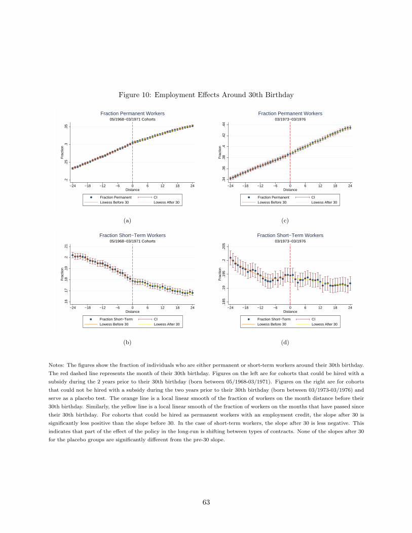
Figure 10: Employment Effects Around 30th Birthday

.2.2

5.3

.35

Fra

ctio

n

−24 −18 −12 −6 0 6 12 18 24Distance

Fraction Permanent CILowess Before 30 Lowess After 30

05/1968−03/1971 CohortsFraction Permanent Workers

(a)

.16

.17

.18

.19

.2.2

1F

ract

ion

−24 −18 −12 −6 0 6 12 18 24Distance

Fraction Short−Term CILowess Before 30 Lowess After 30

05/1968−03/1971 CohortsFraction Short−Term Workers

(b)

.34

.36

.38

.4.4

2.4

4F

ract

ion

−24 −18 −12 −6 0 6 12 18 24Distance

Fraction Permanent CILowess Before 30 Lowess After 30

03/1973−03/1976Fraction Permanent Workers

(c).1

85.1

9.1

95.2

.205

Fra

ctio

n

−24 −18 −12 −6 0 6 12 18 24Distance

Fraction Short−Term CILowess Before 30 Lowess After 30

03/1973−03/1976Fraction Short−Term Workers

(d)

Notes: The figures show the fraction of individuals who are either permanent or short-term workers around their 30th birthday.

The red dashed line represents the month of their 30th birthday. Figures on the left are for cohorts that could be hired with a

subsidy during the 2 years prior to their 30th birthday (born between 05/1968-03/1971). Figures on the right are for cohorts

that could not be hired with a subsidy during the two years prior to their 30th birthday (born between 03/1973-03/1976) and

serve as a placebo test. The orange line is a local linear smooth of the fraction of workers on the month distance before their

30th birthday. Similarly, the yellow line is a local linear smooth of the fraction of workers on the months that have passed since

their 30th birthday. For cohorts that could be hired as permanent workers with an employment credit, the slope after 30 is

significantly less positive than the slope before 30. In the case of short-term workers, the slope after 30 is less negative. This

indicates that part of the effect of the policy in the long-run is shifting between types of contracts. None of the slopes after 30

for the placebo groups are significantly different from the pre-30 slope.

63

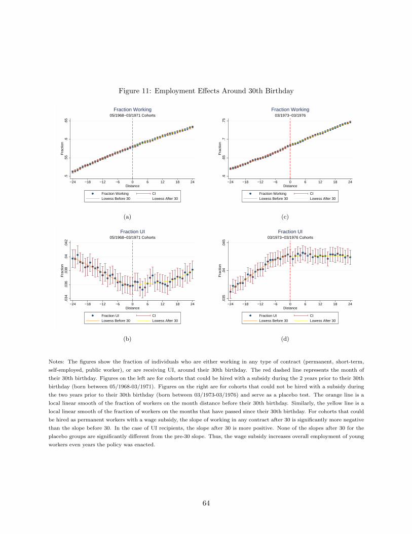
Figure 11: Employment Effects Around 30th Birthday

.5.5

5.6

.65

Fra

ctio

n

−24 −18 −12 −6 0 6 12 18 24Distance

Fraction Working CILowess Before 30 Lowess After 30

05/1968−03/1971 CohortsFraction Working

(a)

.034

.036

.038

.04

.042

Fra

ctio

n

−24 −18 −12 −6 0 6 12 18 24Distance

Fraction UI CILowess Before 30 Lowess After 30

05/1968−03/1971 CohortsFraction UI

(b)

.6.6

5.7

.75

Fra

ctio

n

−24 −18 −12 −6 0 6 12 18 24Distance

Fraction Working CILowess Before 30 Lowess After 30

03/1973−03/1976Fraction Working

(c).0

35.0

4.0

45F

ract

ion

−24 −18 −12 −6 0 6 12 18 24Distance

Fraction UI CILowess Before 30 Lowess After 30

03/1973−03/1976 CohortsFraction UI

(d)

Notes: The figures show the fraction of individuals who are either working in any type of contract (permanent, short-term,

self-employed, public worker), or are receiving UI, around their 30th birthday. The red dashed line represents the month of

their 30th birthday. Figures on the left are for cohorts that could be hired with a subsidy during the 2 years prior to their 30th

birthday (born between 05/1968-03/1971). Figures on the right are for cohorts that could not be hired with a subsidy during

the two years prior to their 30th birthday (born between 03/1973-03/1976) and serve as a placebo test. The orange line is a

local linear smooth of the fraction of workers on the month distance before their 30th birthday. Similarly, the yellow line is a

local linear smooth of the fraction of workers on the months that have passed since their 30th birthday. For cohorts that could

be hired as permanent workers with a wage subsidy, the slope of working in any contract after 30 is significantly more negative

than the slope before 30. In the case of UI recipients, the slope after 30 is more positive. None of the slopes after 30 for the

placebo groups are significantly different from the pre-30 slope. Thus, the wage subsidy increases overall employment of young

workers even years the policy was enacted.

64

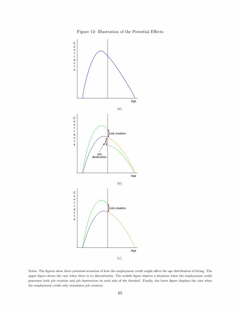
Figure 12: Illustration of the Potential Effects

Age

Contracts

(a)

Age

Contracts

}Job creation

{

Job destruction

(b)

Age

Contracts

}Job creation

(c)

Notes: The figures show three potential scenarios of how the employment credit might affect the age distribution of hiring. The

upper figure shows the case when there is no discontinuity. The middle figure depicts a situation when the employment credit

generates both job creation and job destruction on each side of the threshol. Finally, the lower figure displays the case when

the employment credit only stimulates job creation.

65

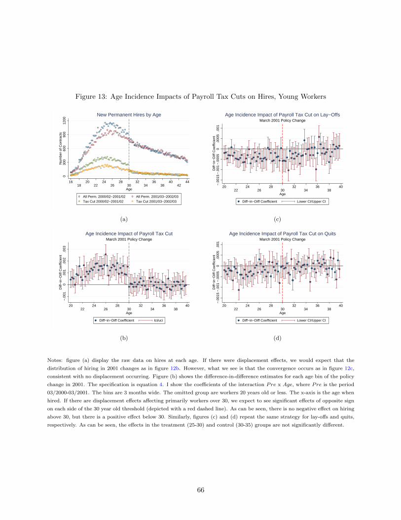
Figure 13: Age Incidence Impacts of Payroll Tax Cuts on Hires, Young Workers

030

060

090

012

00N

umbe

r of

Con

trac

ts

1618

2022

2426

2830

3234

3638

4042

44

Age

All Perm. 2000/02−2001/02 All Perm. 2001/03−2002/03 Tax Cut 2000/02−2001/02 Tax Cut 2001/03−2002/03

New Permanent Hires by Age

(a)

−.0

010

.001

.002

.003

Diff

−in

−D

iff C

oeffi

cien

t

2022

2426

2830

3234

3638

40

Age

Diff−in−Diff Coefficient lci/uci

March 2001 Policy ChangeAge Incidence Impact of Payroll Tax Cut

(b)

−.0

015

−.0

01−

.000

50

.000

5.0

01D

iff−

in−

Diff

Coe

ffici

ent

2022

2426

2830

3234

3638

40

Age

Diff−in−Diff Coefficient Lower CI/Upper CI

March 2001 Policy ChangeAge Incidence Impact of Payroll Tax Cut on Lay−Offs

(c)−

.001

5−

.001

−.0

005

0.0

005

.001

Diff

−in

−D

iff C

oeffi

cien

t

2022

2426

2830

3234

3638

40

Age

Diff−in−Diff Coefficient Lower CI/Upper CI

March 2001 Policy ChangeAge Incidence Impact of Payroll Tax Cut on Quits

(d)

Notes: figure (a) display the raw data on hires at each age. If there were displacement effects, we would expect that the

distribution of hiring in 2001 changes as in figure 12b. However, what we see is that the convergence occurs as in figure 12c,

consistent with no displacement occurring. Figure (b) shows the difference-in-difference estimates for each age bin of the policy

change in 2001. The specification is equation 4. I show the coefficients of the interaction Pre x Age, where Pre is the period

03/2000-03/2001. The bins are 3 months wide. The omitted group are workers 20 years old or less. The x-axis is the age when

hired. If there are displacement effects affecting primarily workers over 30, we expect to see significant effects of opposite sign

on each side of the 30 year old threshold (depicted with a red dashed line). As can be seen, there is no negative effect on hiring

above 30, but there is a positive effect below 30. Similarly, figures (c) and (d) repeat the same strategy for lay-offs and quits,

respectively. As can be seen, the effects in the treatment (25-30) and control (30-35) groups are not significantly different.

66

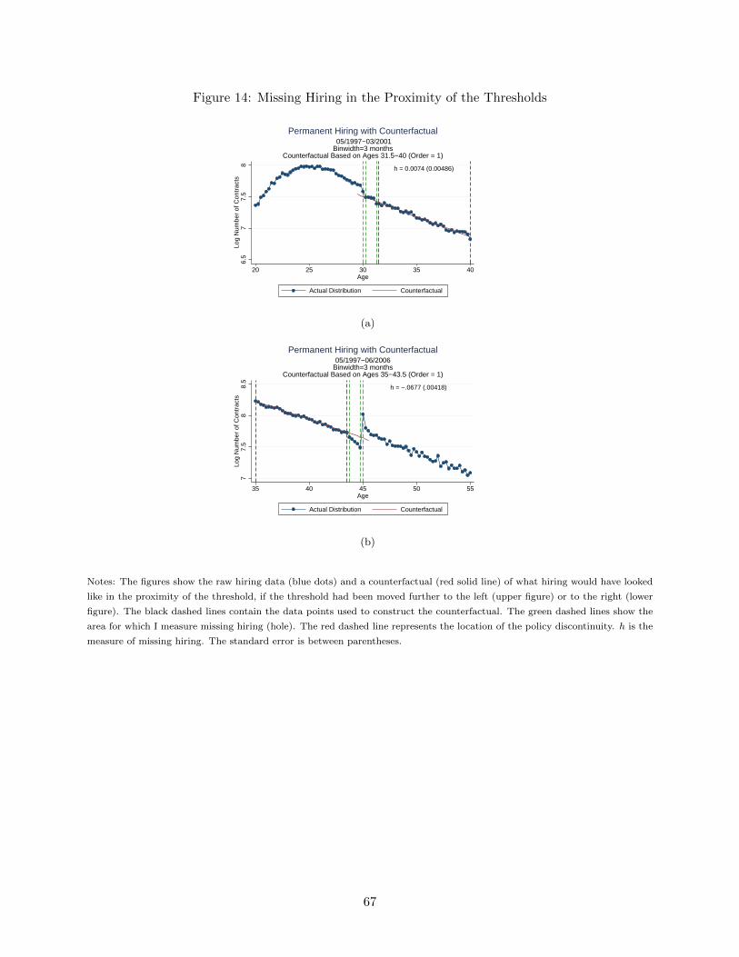
Figure 14: Missing Hiring in the Proximity of the Thresholds

h = 0.0074 (0.00486)

6.5

77.

58

Log

Num

ber

of C

ontr

acts

20 25 30 35 40Age

Actual Distribution Counterfactual

05/1997−03/2001Binwidth=3 months

Counterfactual Based on Ages 31.5−40 (Order = 1)

Permanent Hiring with Counterfactual

(a)

h = −.0677 (.00418)

77.

58

8.5

Log

Num

ber

of C

ontr

acts

35 40 45 50 55Age

Actual Distribution Counterfactual

05/1997−06/2006Binwidth=3 months

Counterfactual Based on Ages 35−43.5 (Order = 1)

Permanent Hiring with Counterfactual

(b)

Notes: The figures show the raw hiring data (blue dots) and a counterfactual (red solid line) of what hiring would have looked

like in the proximity of the threshold, if the threshold had been moved further to the left (upper figure) or to the right (lower

figure). The black dashed lines contain the data points used to construct the counterfactual. The green dashed lines show the

area for which I measure missing hiring (hole). The red dashed line represents the location of the policy discontinuity. h is the

measure of missing hiring. The standard error is between parentheses.

67

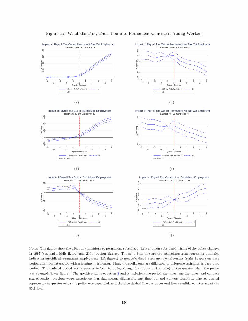
Figure 15: Windfalls Test, Transition into Permanent Contracts, Young Workers

0.0

05.0

1.0

15.0

2C

oeffi

cien

t

−5−4

−3−2

−10

12

34

5

Quarter Distance

Diff−in−Diff Coefficient lciuci

Treatment: 25−30, Control:30−35Impact of Payroll Tax Cut on Permanent Tax Cut Employment

(a)

−.0

050

.005

.01

.015

Coe

ffici

ent

−5−4

−3−2

−10

12

34

5

Quarter Distance

Diff−in−Diff Coefficient lciuci

Treatment: 45−50, Control:40−45Impact of Payroll Tax Cut on Subsidized Employment

(b)

−.0

2−

.01

0.0

1C

oeffi

cien

t

−5−4

−3−2

−10

12

34

5

Quarter Distance

Diff−in−Diff Coefficient lciuci

Treatment: 25−30, Control:30−35Impact of Payroll Tax Cut on Subsidized Employment

(c)

−.0

2−

.015

−.0

1−

.005

0.0

05C

oeffi

cien

t

−5−4

−3−2

−10

12

34

5

Quarter Distance

Diff−in−Diff Coefficient lciuci

Treatment: 25−30, Control:30−35Impact of Payroll Tax Cut on Permanent No Tax Cut Employment

(d)

−.0

2−

.01

0.0

1C

oeffi

cien

t

−5−4

−3−2

−10

12

34

5

Quarter Distance

Diff−in−Diff Coefficient lciuci

Treatment: 45−50, Control:40−45Impact of Payroll Tax Cut on Permanent No Tax Cut Employment

(e)

−.0

1−

.005

0.0

05.0

1.0

15C

oeffi

cien

t

−5−4

−3−2

−10

12

34

5

Quarter Distance

Diff−in−Diff Coefficient lciuci

Treatment: 25−30, Control:30−35Impact of Payroll Tax Cut on Non−Subsidized Employment

(f)

Notes: The figures show the effect on transitions to permanent subsidized (left) and non-subsidized (right) of the policy changes

in 1997 (top and middle figure) and 2001 (bottom figure). The solid blue line are the coefficients from regressing dummies

indicating subsidized permanent employment (left figures) or non-subsidized permanent employment (right figures) on time

period dummies interacted with a treatment indicator. Thus, the coefficients are difference-in-difference estimates in each time

period. The omitted period is the quarter before the policy change for (upper and middle) or the quarter when the policy

was changed (lower figure). The specification is equation 3 and it includes time-period dummies, age dummies, and controls

sex, education, previous wage, experience, firm size, sector, citizenship, part-time job, and workers’ disability. The red dashed

represents the quarter when the policy was expanded, and the blue dashed line are upper and lower confidence intervals at the

95% level.

68

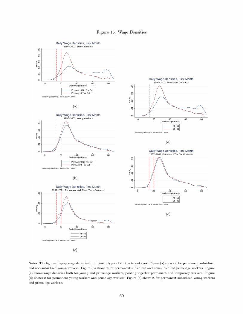
Figure 16: Wage Densities

0.0

1.0

2.0

3.0

4.0

5D

ensi

ty

0 20 40 60 80Daily Wage (Euros)

Permanent No Tax CutPermanent Tax Cut

kernel = epanechnikov, bandwidth = 3.0000

1997−2001, Senior WorkersDaily Wage Densities, First Month

(a)

0.0

1.0

2.0

3.0

4D

ensi

ty

0 20 40 60 80Daily Wage (Euros)

Permanent No Tax CutPermanent Tax Cut

kernel = epanechnikov, bandwidth = 3.0000

1997−2001, Young WorkersDaily Wage Densities, First Month

(b)

0.0

2.0

4.0

6D

ensi

ty

0 20 40 60 80Daily Wage (Euros)

45−5025−30

kernel = epanechnikov, bandwidth = 3.0000

1997−2001, Permanent and Short−Term ContractsDaily Wage Densities, First Month

(c)

0.0

1.0

2.0

3.0

4D

ensi

ty

0 20 40 60 80Daily Wage (Euros)

45−5025−30

kernel = epanechnikov, bandwidth = 3.0000

1997−2001, Permanent ContractsDaily Wage Densities, First Month

(d)

0.0

1.0

2.0

3.0

4D

ensi

ty

0 20 40 60 80Daily Wage (Euros)

45−5025−30

kernel = epanechnikov, bandwidth = 3.0000

1997−2001, Permanent Tax Cut ContractsDaily Wage Densities, First Month

(e)

Notes: The figures display wage densities for different types of contracts and ages. Figure (a) shows it for permanent subsidized

and non-subsidized young workers. Figure (b) shows it for permanent subsidized and non-subsidized prime-age workers. Figure

(c) shows wage densities both for young and prime-age workers, pooling together permanent and temporary workers. Figure

(d) shows it for permanent young workers and prime-age workers. Figure (e) shows it for permanent subsidized young workers

and prime-age workers.

69

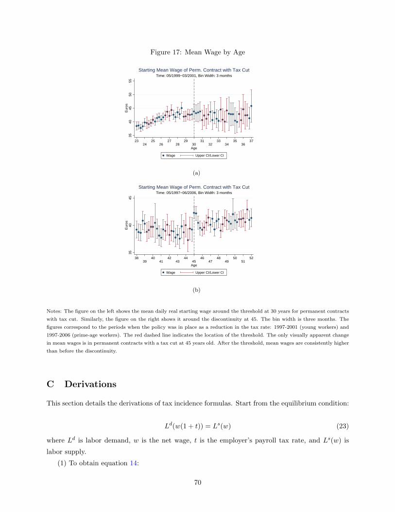
Figure 17: Mean Wage by Age

3540

4550

55E

uros

2324

2526

2728

2930

3132

3334

3536

37

Age

Wage Upper CI/Lower CI

Time: 05/1999−03/2001, Bin Width: 3 monthsStarting Mean Wage of Perm. Contract with Tax Cut

(a)

3540

45E

uros

3839

4041

4243

4445

4647

4849

5051

52

Age

Wage Upper CI/Lower CI

Time: 05/1997−06/2006, Bin Width: 3 monthsStarting Mean Wage of Perm. Contract with Tax Cut

(b)

Notes: The figure on the left shows the mean daily real starting wage around the threshold at 30 years for permanent contracts

with tax cut. Similarly, the figure on the right shows it around the discontinuity at 45. The bin width is three months. The

figures correspond to the periods when the policy was in place as a reduction in the tax rate: 1997-2001 (young workers) and

1997-2006 (prime-age workers). The red dashed line indicates the location of the threshold. The only visually apparent change

in mean wages is in permanent contracts with a tax cut at 45 years old. After the threshold, mean wages are consistently higher

than before the discontinuity.

C Derivations

This section details the derivations of tax incidence formulas. Start from the equilibrium condition:

Ld(w(1 + t)) = Ls(w) (23)

where Ld is labor demand, w is the net wage, t is the employer’s payroll tax rate, and Ls(w) is

labor supply.

(1) To obtain equation 14:

70

Suppose t = 0 and the tax rate is changed. Differentiating:

Ld′(dw + wdt) = Ls

′dw (24)

And rearranging:

dw

dt

1

w=

Ld′ wL

(Ls′+Ld′ )wL

(25)

d logw

dt=−εD

εS + εD(26)

(2) To obtain equation 15, follow the same steps as above. Suppose t = 0. Differentiating:

Ld′(dW ) = Ls

′dw (27)

Rearranging:dW

dt

1

W=Ls′

Ld′dw

dt

1

W(28)

d logW

dt=

εSεS + εD

(29)

(3) To obtain equation 16, recall L = Ld(w(1 + t)) = Ls(w). Suppose t = 0. Differentiating:

dL = Ls′dw (30)

Rearranging:dL

dt=Ls′dw

dt=Ls′w

L

dw

wdtL = εS

dw

wdtL (31)

−d logL

dt=

εSεDεS + εD

(32)

71