Lab_1

Lab 1NI ELVIS Workspace Environment

The NI ELVIS environment consists of the hardware workspace for building circuits and interfacing experiments, and the NI ELVIS software. The NI ELVIS software, all created in LabVIEW has two main types: the soft front panel (SFP) instruments and LabVIEW APIs, which are just additional LabVIEW VIs for custom control and access to the features of the NI ELVIS bench top workstation.

Goal:

This lab introduces the NI ELVIS workstation to show how electronic component properties can be measured. Circuits are then built on the protoboard and later analyzed with the NI ELVIS software suite of LabVIEW based soft front panels (SFP) or software instruments. In addition, this experiment demonstrates the use of NI ELVIS within a LabVIEW programming environment.

Soft Front Panels (SFP) Used in this LabDigital Ohmmeter DMM, Digital Capacitance meter DMM,Digital Voltmeter DMM

Components Used in this LabR1 - 1.0 kΩresistorR2 - 2.2 kΩR3 - 1.0 MΩresistorC - 1 μF capacitorLM741 Transistor

Exercise 1-1 Measurement of Component Values

Connect two banana type leads to the DMM current inputs on the workstation front panel. Connect the other ends to one of the resistors. Launch NI ELVIS. After initializing, the suite of LabVIEW software instruments pops up on the computer screen.

Select Digital Multimeter.

The Digital Multimeter SFP can be used for a variety of operations. We will use the notation DMM[X] to signify the X operation. Click on the Ohm button [] to use the Digital Ohmmeter function DMM[]. Measure R1, R2, and R3. Using the capacitor button [ ], measure the capacitor C with DMM[C] using the same leads. Fill in the following table.

R1 _______ (1.0 knominal)R2 _______ (2.2 knominal)R3 _______ (1.0 Mnominal)C* _______ (μf) (1 μF nominal)

Note If you are using an electrolytic capacitor be sure to connect the + lead of the capacitor to the DMM current +input and click on the electrolytic button of the DMM[C].

End of Exercise 1-1

Exercise 1-2 Building a Voltage Divider Circuit on the NI ELVIS Protoboard

Using the two resistors, R1 and R2, assemble the following circuit on the NI ELVIS protoboard.

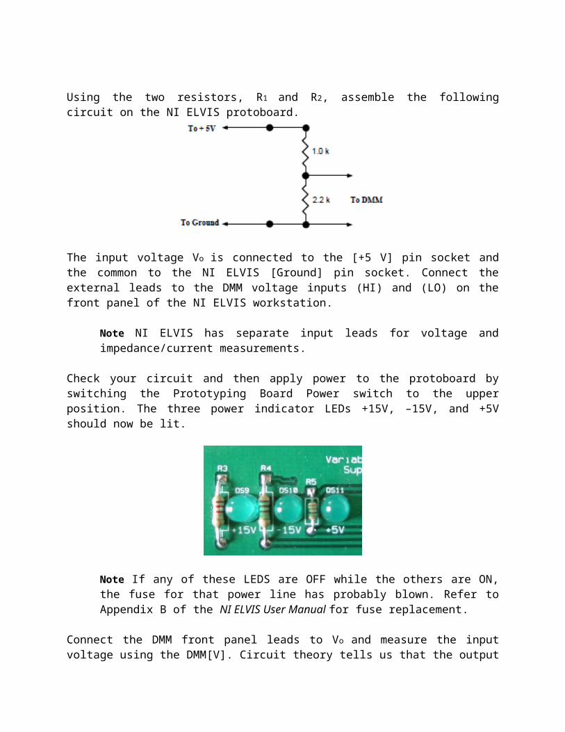
The input voltage Vo is connected to the [+5 V] pin socket and the common to the NI ELVIS [Ground] pin socket. Connect the external leads to the DMM voltage inputs (HI) and (LO) on the front panel of the NI ELVIS workstation.

Note NI ELVIS has separate input leads for voltage and impedance/current measurements.

Check your circuit and then apply power to the protoboard by switching the Prototyping Board Power switch to the upper position. The three power indicator LEDs +15V, –15V, and +5V should now be lit.

Note If any of these LEDS are OFF while the others are ON, the fuse for that power line has probably blown. Refer to Appendix B of the NI ELVIS User Manual for fuse replacement.

Connect the DMM front panel leads to Vo and measure the input voltage using the DMM[V]. Circuit theory tells us that the output voltage V1 should be R2/(R1+R2) * Vo. Using the previous measured values for R1, R2, and Vo, calculate V1. Then, use the DMM[V] to measure the actual voltage V1.

V1 (calculated) ________________ V1 (measured) ________________

How well does the measured value agree with your calculated value?

End of Exercise 1-2

Exercise 1-3 Using the DMM to Measure Current

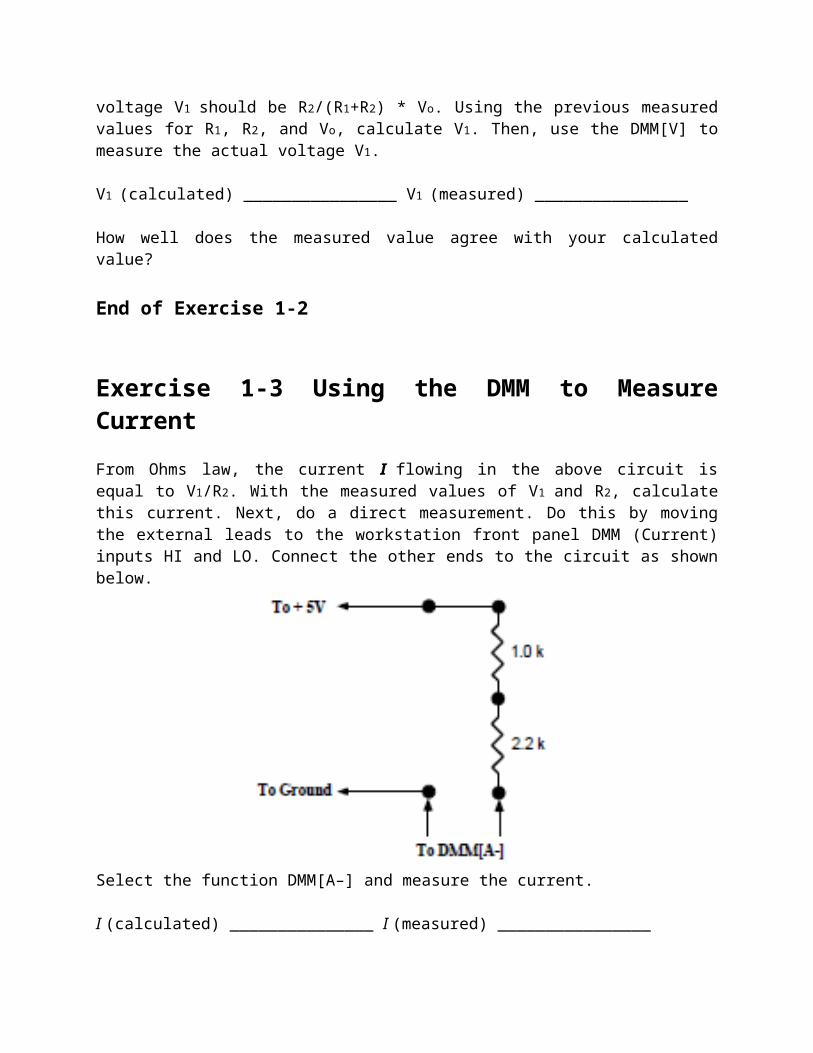
From Ohms law, the current I flowing in the above circuit is equal to V1/R2. With the measured values of V1 and R2, calculate this current. Next, do a direct measurement. Do this by moving the external leads to the workstation front panel DMM (Current) inputs HI and LO. Connect the other ends to the circuit as shown below.

Select the function DMM[A–] and measure the current.

I (calculated) _______________ I (measured) ________________

How well does the measured value agree with your calculated value?

End of Exercise 1-3

Exercise 1-4 Observing the Voltage Development of a RC Transient Circuit

Build the RC transient circuit as shown below. It uses the voltage divider circuit where R1 is now replaced with R3 (1 M resistor) and R2 is replaced with the 1 μF capacitor C. Move your front panel leads back to the DMM(VOLTAGE) inputs and select DMM[V].

Note NI ELVIS version 1 has limited input impedance (1 M) for the DMM channel.

To read the correct voltage values, you will need to buffer the input voltage for this measurement. Refer to the Limited Input Impedance Solution section for a simple solution using a unity gain circuit using a FET Op Amp. This limitation will be remedied in a future version. Also, notice that if you use the Analog Input channels of the DAQ card as in Exercise 1-5, this is not a problem.

When you power up the circuit, the voltage across the capacitor will rise exponentially. Turn on the power and watch the voltage change on the DMM display. It takes about 5 seconds to reach the steady state value of Vo. When you power off the circuit, the voltage across the capacitor will fall exponentially to 0 volts. Try it!

It would be interesting to view this transient effect on a plot of capacitor voltage versus time.

Limited Input Impedance Solution

Using an FET Op Amp such as the LM356, build a unity gain circuit and connect it as shown below. By connecting the output (pin 6) to the – input (pin 2), the gain of this circuit is set to 1. However, the + input impedance on (pin 3) is now hundreds of megaohms and the ouput voltage (pin 6) will faithfully follow the capacitor voltage allowing the DMM voltage input toread the correct values.

End of Exercise 1-4

Exercise 1-5 Visualizing the RC Transient Circuit Voltage

Remove the + 5V power lead and replace it with a wire connected to the Variable Power Supply socket pin VPS[+]. Connect the output voltage, V1, to ACH0[+] and ACH0[–].

Close the NI ELVIS software suite and launch LabVIEW. From the Hands-On NI ELVIS VI Library, select RC Transient.vi. This program uses LabVIEW APIs to turn the power supply ON for 5 seconds then OFF for 5 seconds while the voltage across the capacitor isdisplayed on a LabVIEW chart.

This type of square wave excitation dramatically shows the charging and discharging characteristics of a simple RC circuit. The circuit time constant is defined as the product of R3

and C.

From Kirchoff’s laws it is easy to show that the charging voltage VC acrossthe capacitor is given by:

VC = V0 (1-exp(- t/))

and the discharge voltage VD is given by:

VD = V0 exp(- t/)

Can you extract the time constant from the measured chart?

Take a look at the LabVIEW diagram window to see how this program works.

The VPS Initialization VI on the left starts NI ELVIS and selects the + power supply. The next VI sets the output voltage on VPS+ to 5 volts. Next, the first sequence measures 50 sequential voltage readings across the capacitor at 1/10 of a second interval. In the For Loop, the Analog Input Multiple Point VI takes 100 readings at rate of 1000 samples per second and passes the values to an array (thick orange line). The array is then passed to the Mean VI which returns the average value of the 100 readings. The average is then passed to the chart via a local variable terminal (RC Charging and Discharging). The next sequence sets the VPS+ voltage equal to 0 volts and then the last sequence measures another 50 averaged samples for the discharge cycle.

End of Exercise 1-5

Things to consider for your lab reports:

- Have you calculated all values requested in the lab? Do you have theoretical AND experimental values for all possible terms?

- Is your lab report formatted correctly? Make sure to follow the guidelines mentioned by me in class and in the lab report guide.

- Are all figures properly labeled?

- What is the significance of ?

- Did any errors come up in your results? Why are they there (basically how did they come about)? Can they be minimized?