Lab Report #3

    Student Name:    Student ID #

Laboratory  3  -­‐  Fast  Decoupled  Power  Flow  Method  

LABORATORY 3 FAST DECOUPLED POWER-FLOW METHOD

Student Name: Sanzhar Askaruly

Student ID: 201100549

Student Group: Session 1

    Student Name:    Student ID #

Laboratory  3  -­‐  Fast  Decoupled  Power  Flow  Method  

INTRODUCTION The aim of this laboratory is to investigate the affects of the fast decoupled power flow solution when compared to the Newton Raphson method performed in laboratory one. The simulator PowerWorld will be employed during the testing of the system in order to establish the bus admittance matrix and mismatch conditions of the five bus

network. The overall analysis will prove that the fast decoupled power flow solution is much more faster than the

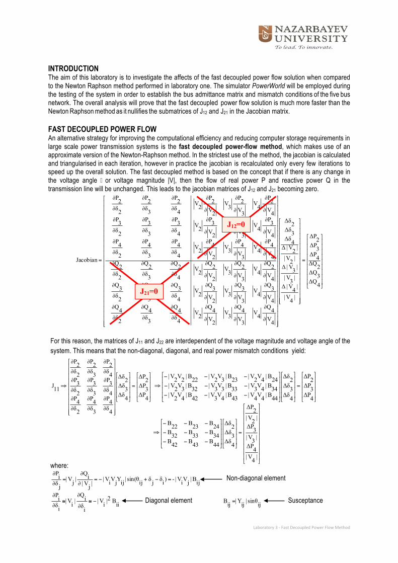
Newton Raphson method as it nullifies the submatrices of J12 and J21 in the Jacobian matrix. FAST DECOUPLED POWER FLOW An alternative strategy for improving the computational efficiency and reducing computer storage requirements in large scale power transmission systems is the fast decoupled power-flow method, which makes use of an approximate version of the Newton-Raphson method. In the strictest use of the method, the jacobian is calculated

and triangularised in each iteration, however in practice the jacobian is recalculated only every few iterations to speed up the overall solution. The fast decoupled method is based on the concept that if there is any change in the voltage angle � or voltage magnitude |V|, then the flow of real power P and reactive power Q in the transmission line will be unchanged. This leads to the jacobian matrices of J12 and J21 becoming zero.

⎥⎥⎥⎥⎥⎥⎥⎥⎥

⎦

⎤

⎢⎢⎢⎢⎢⎢⎢⎢⎢

⎣

⎡

⎥⎥⎥⎥⎥⎥⎥⎥⎥⎥⎥⎥⎥⎥⎥⎥

⎦

⎤

⎢⎢⎢⎢⎢⎢⎢⎢⎢⎢⎢⎢⎢⎢⎢⎢

⎣

⎡

⎥⎥⎥⎥⎥⎥⎥⎥⎥⎥⎥⎥⎥⎥⎥⎥⎥⎥⎥⎥⎥⎥⎥⎥⎥

⎦

⎤

⎢⎢⎢⎢⎢⎢⎢⎢⎢⎢⎢⎢⎢⎢⎢⎢⎢⎢⎢⎢⎢⎢⎢⎢⎢

⎣

⎡

=

∂

∂

∂

∂

∂

∂

∂

∂

∂

∂

∂

∂

∂

∂

∂

∂

∂

∂

∂

∂

∂

∂

∂

∂

∂

∂

∂

∂

∂

∂

∂

∂

∂

∂

∂

∂

∂

∂

∂

∂

∂

∂

∂

∂

∂

∂

∂

∂

∂

∂

∂

∂

∂

∂

∂

∂

∂

∂

∂

∂

∂

∂

∂

∂

∂

∂

∂

∂

∂

∂

∂

∂

=

4ΔQ3ΔQ2ΔQ4ΔP3ΔP2ΔP

|4V|

|4V|Δ|3V|

|3V|Δ|2V|

|2V|Δ4Δδ3Δδ2Δδ

4V4Q

4V

3V4Q

3V

2V4Q

2V4δ4Q

3δ4Q

2δ4Q

4V3Q

4V

3V3Q

3V

2V3Q

2V4δ3Q

3δ3Q

2δ3Q

4V2Q

4V

3V2Q

3V

2V2Q

2V4δ2Q

3δ2Q

2δ2Q

4V4P

4V

3V4P

3V

2V4P

2V4δ4P

3δ4P

2δ4P

4V3P

4V

3V3P

3V

2V3P

2V4δ3P

3δ3P

2δ3P

4V2P

4V

3V2P

3V

2V2P

2V4δ2P

3δ2P

2δ2P

Jacobian  

 For this reason, the matrices of J11 and J22 are interdependent of the voltage magnitude and voltage angle of the system. This means that the non-diagonal, diagonal, and real power mismatch conditions yield:

⎥⎥⎥⎥

⎦

⎤

⎢⎢⎢⎢

⎣

⎡

⎥⎥⎥⎥

⎦

⎤

⎢⎢⎢⎢

⎣

⎡

⎥⎥⎥⎥⎥⎥⎥⎥⎥⎥

⎦

⎤

⎢⎢⎢⎢⎢⎢⎢⎢⎢⎢

⎣

⎡

=

∂

∂

∂

∂

∂

∂

∂

∂

∂

∂

∂

∂

∂

∂

∂

∂

∂

∂

⇒

4ΔP3ΔP2ΔP

4Δδ3Δδ2Δδ

4δ4P

3δ4P

2δ4P

4δ3P

3δ3P

2δ3P

4δ2P

3δ2P

2δ2P

11J  ⎥⎥⎥⎥

⎦

⎤

⎢⎢⎢⎢

⎣

⎡

⎥⎥⎥⎥

⎦

⎤

⎢⎢⎢⎢

⎣

⎡

⎥⎥⎥⎥

⎦

⎤

⎢⎢⎢⎢

⎣

⎡

=

−−−

−−−

−−−

⇒

4ΔP3ΔP2ΔP

4Δδ3Δδ2Δδ

44B|4V4V|43B|4V3V|42B|4V2V|34B|4V3V|33B|3V3V|32B|3V2V|24B|4V2V|23B|3V2V|22B|2V2V|

                  where:

ijB|jViV|-)iδjδijsin(θ|ijYjViV||jV|iQ|jV|

jδiP =−+−=

∂

∂=

∂

∂                                Non-diagonal element  

iiB2|iV|

iδiQ|iV|

iδiP −≅

∂

∂≅

∂

∂                              Diagonal element                                     ijsinθ|ijY|ijB =                                Susceptance  

J12=0

J21=0

⎥⎥⎥⎥⎥⎥⎥⎥⎥⎥

⎦

⎤

⎢⎢⎢⎢⎢⎢⎢⎢⎢⎢

⎣

⎡

⎥⎥⎥⎥

⎦

⎤

⎢⎢⎢⎢

⎣

⎡

⎥⎥⎥⎥

⎦

⎤

⎢⎢⎢⎢

⎣

⎡

=

−−−

−−−

−−−

⇒

|4V|4ΔP|3V|3ΔP|2V|2ΔP

4Δδ3Δδ2Δδ

44B43B42B34B33B32B24B23B22B

    Student Name:    Student ID #

Laboratory  3  -­‐  Fast  Decoupled  Power  Flow  Method  

4Δδ24B|4V|3Δδ23B|3V|2Δδ22B|2V||2V|2ΔP −−−=  

4Δδ34B|4V|3Δδ33B|3V|2Δδ32B|2V||3V|3ΔP −−−=  

4Δδ44B|4V|3Δδ43B|3V|2Δδ42B|2V||4V|4ΔP −−−=  

⎥⎥⎥⎥

⎦

⎤

⎢⎢⎢⎢

⎣

⎡

⎥⎥⎥⎥⎥⎥⎥⎥⎥⎥

⎦

⎤

⎢⎢⎢⎢⎢⎢⎢⎢⎢⎢

⎣

⎡

⎥⎥⎥⎥

⎦

⎤

⎢⎢⎢⎢

⎣

⎡

⎥⎥⎥⎥

⎦

⎤

⎢⎢⎢⎢

⎣

⎡

⎥⎥⎥⎥⎥⎥⎥⎥⎥⎥

⎦

⎤

⎢⎢⎢⎢⎢⎢⎢⎢⎢⎢

⎣

⎡

⎥⎥⎥⎥⎥⎥⎥⎥⎥⎥⎥⎥

⎦

⎤

⎢⎢⎢⎢⎢⎢⎢⎢⎢⎢⎢⎢

⎣

⎡

=

−−−

−−−

−−−

⇒=

∂

∂

∂

∂

∂

∂

∂

∂

∂

∂

∂

∂

∂

∂

∂

∂

∂

∂

⇒

4ΔQ3ΔQ2ΔQ

|4V|

|4V|Δ|3V|

|3V|Δ|2V|

|2V|Δ

44B|4V4V|43B|4V3V|42B|4V2V|34B|4V3V|33B|3V3V|32B|3V2V|24B|4V2V|23B|3V2V|22B|2V2V|

4ΔQ3ΔQ2ΔQ

|4V|

|4V|Δ|3V|

|3V|Δ|2V|

|2V|Δ

4V4Q

4V3V4Q

3V2V4Q

2V

4V3Q

4V3V3Q

3V2V3Q

2V

4V2Q

4V3V2Q

3V2V2Q

2V

22J

           where:

ijB|jViV|-)iδjδijsin(θ|ijYjViV||jV|iQ|jV|

jδiP =−+−=

∂

∂=

∂

∂                                Non-diagonal element  

iiB2|iV|

iδiQ|iV|

iδiP −≅

∂

∂≅

∂

∂                              Diagonal element                                             ijcosθ|ijY|ijG =                          Conductance  

|4V|Δ24B|3V|Δ23B|2V|Δ22B|2V|2ΔQ

−−−=  

|4V|Δ34B|3V|Δ33B|2V|Δ32B|3V|3ΔQ

−−−=  

|4V|Δ44B|3V|Δ43B|2V|Δ42B|4V|4ΔQ

−−−=  

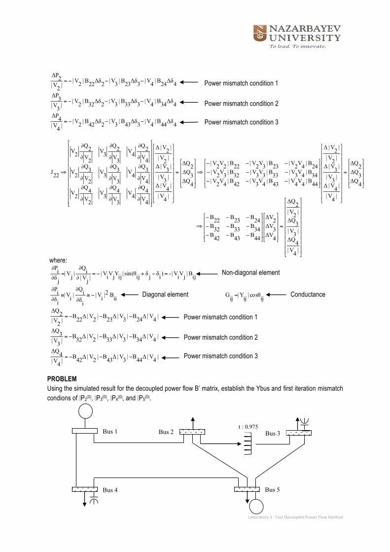
 PROBLEM Using the simulated result for the decoupled power flow B’ matrix, establish the Ybus and first iteration mismatch condions of �P2

(0), �P3(0), �P4

(0), and �P5(0).

Bus 1 Bus 2 Bus 3

Bus 4 Bus 5

t : 0.975

Power mismatch condition 1

Power mismatch condition 2

Power mismatch condition 3

⎥⎥⎥⎥⎥⎥⎥⎥⎥⎥

⎦

⎤

⎢⎢⎢⎢⎢⎢⎢⎢⎢⎢

⎣

⎡

⎥⎥⎥⎥

⎦

⎤

⎢⎢⎢⎢

⎣

⎡

⎥⎥⎥⎥

⎦

⎤

⎢⎢⎢⎢

⎣

⎡

=

−−−

−−−

−−−

⇒

|4V|4ΔQ|3V|3ΔQ|2V|2ΔQ

4ΔV3ΔV2ΔV

44B43B42B34B33B32B24B23B22B

Power mismatch condition 1

Power mismatch condition 2

Power mismatch condition 3

    Student Name:    Student ID #

Laboratory  3  -­‐  Fast  Decoupled  Power  Flow  Method  

Figure 1: One-line diagram indicating the bus names and numbers Table 1: Line data

Line

bus-to-bus

Series Z Series Y=Z-1

Charging (Mvar) R

(per unit) X

(per unit) G

(per unit) B

(per unit) 1–2 0.0108 0.0649 2.5 -15 6.6 1–4 0.0235 0.0941 2.5 -10 4.0 2–5 0.0118 0.0471 5.0 -20 7.0 3–5 0.0147 0.0588 4.0 -16 8.0 4–5 0.0118 0.0529 4.0 -18 6.0

Table 2: Bus data

Bus Generation Load V (per unit)

Remark P (MW) Q (Mvar) P (MW) Q (Mvar)

1 0 0 0 0 1.01 !0∠ Slack bus 2 0 0 60 35 1.00 !0∠ 3 0 0 70 42 1.00 !0∠ 4 0 0 80 50 1.00 !0∠ 5 190 0 65 36 1.00 !0∠ PV bus

Table 3: Transformer data

Transformer bus to bus Per unit reactance Tap settings 2 – 3 0.04 0.975

Table 4: Capacitor data

Figure 2: One-line diagram simulated in Power World

𝑌!" = −(𝐺!" + 𝑗𝐵!"), where G and B are values provided in the Table 2.

𝑌!" =  − 2.5 − 𝑗15.0 ;𝑌!" = 25𝑗  ×  0.975 = 24.375𝑗;  𝑌!" = − 5.0 − 𝑗20.0 ;  𝑌!!

= −𝑌!" + −𝑌!"  + −𝑌!" = 7.5 − 𝑗59.932;𝑌!" = 0;  

Bus Rating in Mvar 3 18 4 15

    Student Name:    Student ID #

Laboratory  3  -­‐  Fast  Decoupled  Power  Flow  Method  

𝑌!" =  0;𝑌!" =  𝑌!" = 24.375𝑗;  𝑌!" = 0;𝑌!" = −4 + 𝑗16;  𝑌!! = −𝑌!" + −𝑌!" ; 𝑌!" =  −2.5 + 𝑗10;𝑌!" =  𝑌!" = 0;𝑌!" = 𝑌!" = 0;𝑌!" =  −4 + 𝑗18;  𝑌!! = −𝑌!" + −𝑌!"

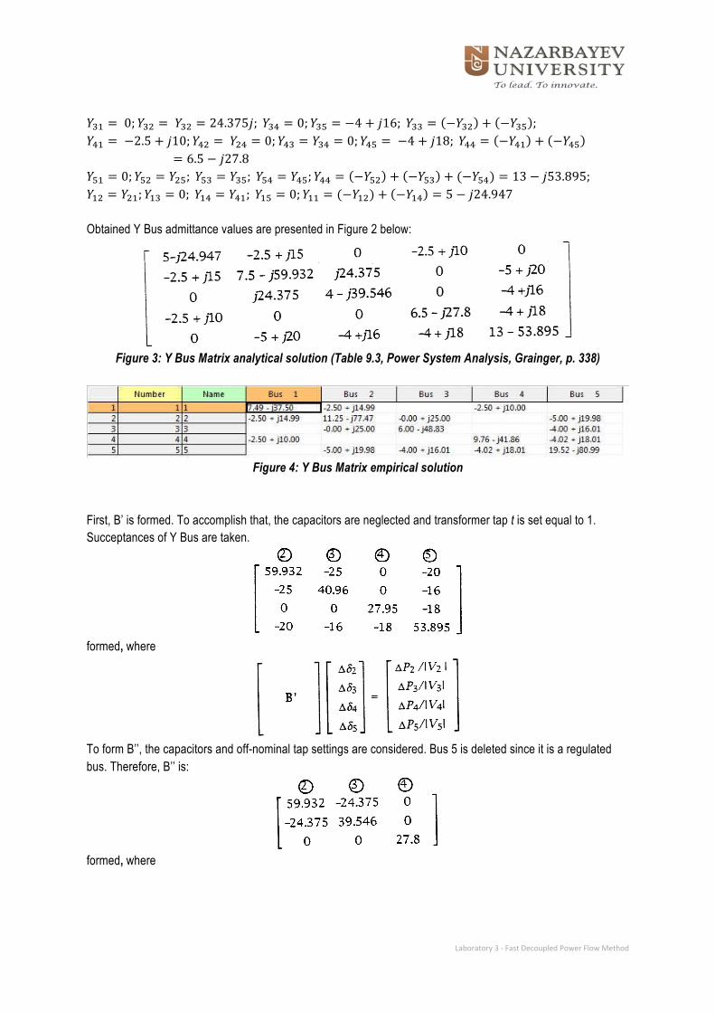
= 6.5 − 𝑗27.8 𝑌!" = 0;𝑌!" = 𝑌!";  𝑌!" = 𝑌!";  𝑌!" = 𝑌!";𝑌!! = −𝑌!" + −𝑌!" + (−𝑌!") = 13 − 𝑗53.895; 𝑌!" = 𝑌!";𝑌!" = 0;  𝑌!" = 𝑌!";  𝑌!" = 0;𝑌!! = (−𝑌!") + −𝑌!" = 5 − 𝑗24.947 Obtained Y Bus admittance values are presented in Figure 2 below:

Figure 3: Y Bus Matrix analytical solution (Table 9.3, Power System Analysis, Grainger, p. 338)

Figure 4: Y Bus Matrix empirical solution

First, B’ is formed. To accomplish that, the capacitors are neglected and transformer tap t is set equal to 1. Succeptances of Y Bus are taken.

formed, where

To form B’’, the capacitors and off-nominal tap settings are considered. Bus 5 is deleted since it is a regulated bus. Therefore, B’’ is:

formed, where

    Student Name:    Student ID #

Laboratory  3  -­‐  Fast  Decoupled  Power  Flow  Method  

𝑃!,!"#!! =   𝑉! !𝐺!! + 𝑉!𝑉!𝑉!! cos(𝜃!!

!

!

+ 𝛿! − 𝛿!)

= 6.5 + 1×1.01×10.308cos  (104.04°) + 18.439cos  (102.53°)= 6.5 − 1.01×2.5 − 4 = −0.025

𝛥𝑃!! =  𝑃!,!"! − 𝑃!,!"#!! = −0.8 − −0.025 = −0.775  𝑝. 𝑢.

𝑄!,!"#!! =   𝑉! !𝐵!! + 𝑉!𝑉!𝑉!! sin(𝜃!!

!

!

+ 𝛿! − 𝛿!)

= −(−27.8) − 1×1.01×10.308  sin(104.04°) + 18.439  sin(102.53°) == 27.8 − 1.01×10 − 18 = −0.3

𝛥𝑄!! =  𝑄!,!"! − 𝑄!,!"#!! = −0.5 − −0.3 = −0.2  𝑝. 𝑢. The P- and Q-equations at bus 4 are:

27.95𝛥𝛿! − 18𝛥𝛿! = −0.775𝑉!

= −0.775

27.8𝛥 𝑉! = −0.2𝑉!

= −0.2

Therefore, the voltage magnitude at bus 4 after the first iteration is:

𝑉!! = 𝑉!! + 𝛿 𝑉! = 1 +−0.227.8

= 0.9928

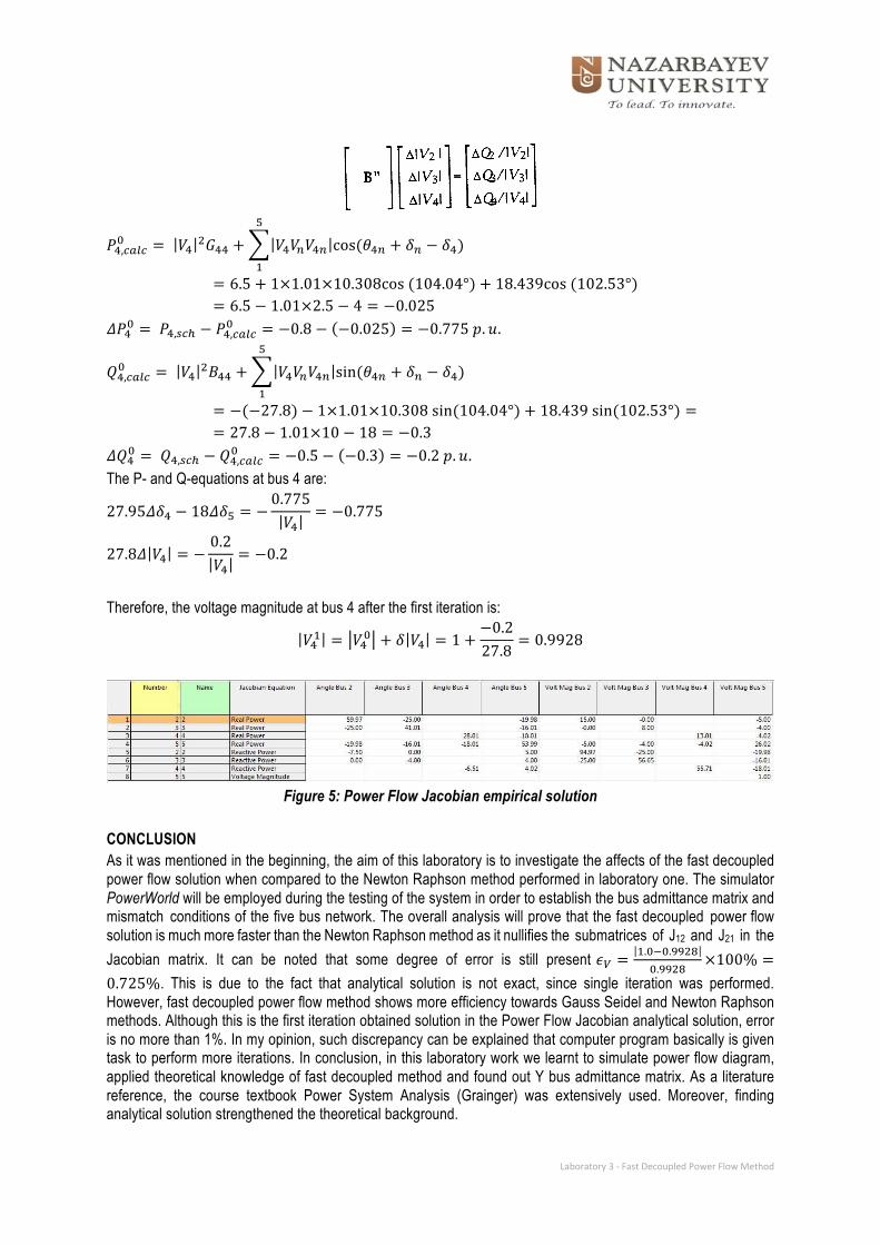
Figure 5: Power Flow Jacobian empirical solution

CONCLUSION As it was mentioned in the beginning, the aim of this laboratory is to investigate the affects of the fast decoupled power flow solution when compared to the Newton Raphson method performed in laboratory one. The simulator PowerWorld will be employed during the testing of the system in order to establish the bus admittance matrix and mismatch conditions of the five bus network. The overall analysis will prove that the fast decoupled power flow

solution is much more faster than the Newton Raphson method as it nullifies the submatrices of J12 and J21 in the

Jacobian matrix. It can be noted that some degree of error is still present 𝜖! =!.!!!.!!"#!.!!"#

×100% =0.725%. This is due to the fact that analytical solution is not exact, since single iteration was performed. However, fast decoupled power flow method shows more efficiency towards Gauss Seidel and Newton Raphson methods. Although this is the first iteration obtained solution in the Power Flow Jacobian analytical solution, error is no more than 1%. In my opinion, such discrepancy can be explained that computer program basically is given task to perform more iterations. In conclusion, in this laboratory work we learnt to simulate power flow diagram, applied theoretical knowledge of fast decoupled method and found out Y bus admittance matrix. As a literature reference, the course textbook Power System Analysis (Grainger) was extensively used. Moreover, finding analytical solution strengthened the theoretical background.