Lab Experiences for Teaching Undergraduate Dynamics by ...

Lab Experiences for Teaching Undergraduate Dynamics

by

Katherine Ann Lilienkamp

Submitted to the Department of Mechanical EngineeringFebruary 19, 2003, in partial fulfillment of the

requirements for the degree ofMaster of Science in Mechanical Engineering

Abstract

This thesis describes several projects developed to teach undergraduate dynamicsand controls. The materials were developed primarily for the class 2.003 ModelingDynamics and Control I. These include (1) a set of ActivLab modular experimentsthat illustrate the dynamics of linear time-invariant (LTI) systems and (2) a two-wheeled mobile inverted pendulum. The ActivLab equipment has been designed asshareware, and plans for it are available on the web. The inverted pendulum robotdeveloped here is largely inspired by the iBOT and Segway transportation devicesinvented by Dean Kamen.

Thesis Supervisor: David L. TrumperTitle: Associate Professor of Mechanical Engineering

1

2

Acknowledgments

First, I’d like to thank Prof. David Trumper for his support and guidance throughout

this thesis. Prof. Trumper is an incredibly knowledgable resource, and he has given

me invaluable support and advice throughout the last several years: initially as an

undergraduate, then during the consulting and masters degree work I have done with

him. He is a gifted educator and genuinely motivated to teach students how to think.

This has been inspirational both in my own choice to work on this project to develop

educational tools and in getting through a masters thesis at all.

Joe Cattell and Andrew Wilson helped design and build the first generation of

ActivLab experiments during the summer of 2001. We could not have developed

an entire set of new laboratory experiments without their devotion to the project.

Thanks particularly to Joe for the late nights spent machining in the graduate machine

shop and the missed vacation days that summer.

Joe and Andrew also worked with me as teaching assistants when the equipment

was first used (in the fall of 2001). They insured the lab sessions ran smoothly,

showing both the students and faculty how to operate the new equipment. Andrew

also put in a huge effort under the guidance of Prof. Samir Nayfeh to create the

laboratory write-ups. His patience going through multiple, last-minute iterations of

the pre-lab and lab assignment documentation was heroic, and I have included several

of his elegant pro-E drawings of the laboratory hardware in the pages of my thesis.

Willem Hijmans, an exchange student from Delft University in the Netherlands,

played a substantial role in insuring that the labs ran smoothly during this first term,

as well. He created our ActivLab website 1 and was always on hand to help set up

and calibrate equipment for class. Thanks also to Professor Jan van Eijk (also of

Delft) for arranging Mr. Hijmans internship with us at MIT and for his support and

advice throughout this project.

Special thanks to Prof. Ely Sachs for his suggestions and advice on hardware

design. Prof. Dave Gossard, Prof. Samir Nayfeh and Prof. Neville Hogan taught the

1http://web.mit.edu/2.003/www/activlab/activlab.html

3

laboratory sessions in the fall of 2001, and they provided input into the development

of the equipment, as well. Their enthusiasm and attention to detail uncovered lots of

interesting physical phenomena in the hardware. The ActivLab hardware was greatly

enhanced by the effort they provided in enouraging the students to explore.

Thanks also for the efforts spent during the second running of the class in the

spring of 2002 in maintaining and refining the laboratory projects. Prof. Gossard

organized the class; Prof. Trumper ran the lab sessions; and Marten Byl took over

the work of the previous three T.A.’s to keep the class running smoothly. Marty

also gets my love and thanks for keeping me sane and happy outside lab during

the last few months spent finishing this thesis! In subsequent terms, Xiaodong Lu,

Vijay Shilpiekandula and Yi Xie have TA’d the course, and Prof. David Hardt will

be teaching the course with Prof. Trumper in the Fall of 2003.

This project could never have happened without the funding and support of the

Department of Mechanical Engineering and its benefactors. I’d particularly like to

acknowledge the efforts and encouragement of our department head, Prof. Rohan

Abeyaratne. Thanks as well to Brit and Alex d’Arbeloff for their funding to create the

d’Arbeloff Laboratory for Information Systems at MIT, where the 2.003 laboratory

resides. Maureen DeCourcey and Maggie Beucler graciously dealt with our constant

stream of purchase orders while building the lab equipment, always expediting our

efforts to obtain parts and materials. Thanks for putting up with so many “urgent”

requests!

We are grateful to Drew Devitt of New Way Machine Components for providing air

bearings at a substantial discount. He also provided advice and enthusiastically sup-

ported our project, going so far as to deliver parts in person near the end of the term!

A few other sponsors are worth mentioning here as well. Tektronix and dSPACE each

provided equipment at a substantially discount, and the Intel Corporation donated

the computers used in the laboratory.

Finally, thanks very much to Mark Belanger, Gerry Wentworth and David Dow for

their indispensible help in the LMP (Laboratory for Manufacturing and Productivity)

machine shop and to Bob Nutall, Steve Haberek and Dick Fenner of the Pappalardo

4

machine shop. Mark and Gerry in particular have taught me most of what I know

about getting around a machine shop. They have always been generous with their

time, and I modified several designs based on their advice. They often provided more

than a little “help” in actually manufacturing specific parts, too! I believe I’m typing

this now with all ten digits, thanks in no small part to their supervision and guidance.

5

6

Contents

1 Introduction 25

1.1 Overview . . . . . . . . . . . . . . . . . . . . . . . . . . . . . . . . . . 25

1.2 General Motivations . . . . . . . . . . . . . . . . . . . . . . . . . . . 28

1.3 Goals for the ActivLab Experiments . . . . . . . . . . . . . . . . . . 29

1.3.1 Motivation for Using Low-Friction Air Bearings . . . . . . . . 30

1.3.2 Presenting Non-Ideal Real World Behaviors . . . . . . . . . . 33

1.3.3 Transparent, Hands-on Operation . . . . . . . . . . . . . . . . 36

1.3.4 Ease of Assembly . . . . . . . . . . . . . . . . . . . . . . . . . 37

1.3.5 Cost Effectiveness . . . . . . . . . . . . . . . . . . . . . . . . . 42

1.4 Summary of the Inverted Pendulum Project . . . . . . . . . . . . . . 47

1.4.1 Ideal and Actual Hardware Implementation . . . . . . . . . . 50

1.4.2 Challenges and Control Strategy . . . . . . . . . . . . . . . . . 51

1.4.3 Results . . . . . . . . . . . . . . . . . . . . . . . . . . . . . . . 54

2 Survey of Related Projects 63

2.1 Inverted Pendulum Vehicles . . . . . . . . . . . . . . . . . . . . . . . 66

2.1.1 The iBOT . . . . . . . . . . . . . . . . . . . . . . . . . . . . . 67

2.1.2 Segway Human Transport . . . . . . . . . . . . . . . . . . . . 69

2.1.3 “Joe”: An Autonomous IP Robot . . . . . . . . . . . . . . . . 74

2.1.4 “nBot”: Segway-inspired IP Robot . . . . . . . . . . . . . . . 77

2.1.5 “LegWay”: Mindstorms Robot with Single-Sensor Balancing . 80

2.1.6 “GyroBot”: IP Robot with Integral Action . . . . . . . . . . . 82

2.1.7 Robotic Unicycles . . . . . . . . . . . . . . . . . . . . . . . . . 84

7

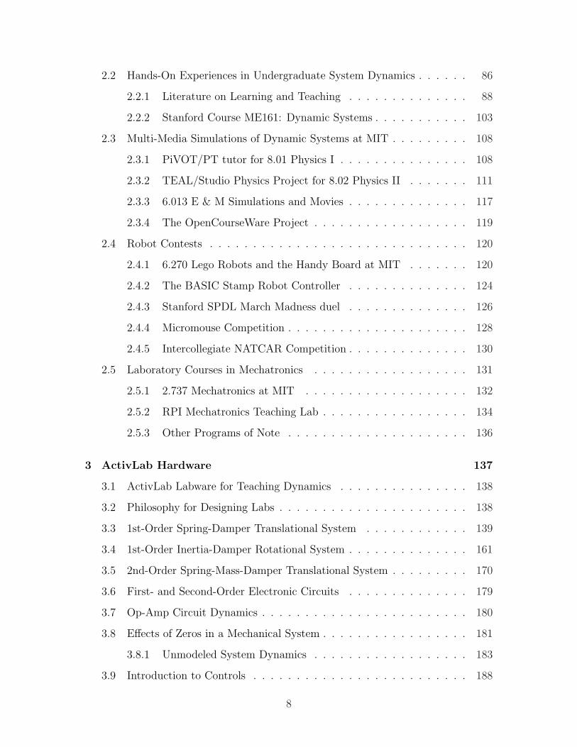
2.2 Hands-On Experiences in Undergraduate System Dynamics . . . . . . 86

2.2.1 Literature on Learning and Teaching . . . . . . . . . . . . . . 88

2.2.2 Stanford Course ME161: Dynamic Systems . . . . . . . . . . . 103

2.3 Multi-Media Simulations of Dynamic Systems at MIT . . . . . . . . . 108

2.3.1 PiVOT/PT tutor for 8.01 Physics I . . . . . . . . . . . . . . . 108

2.3.2 TEAL/Studio Physics Project for 8.02 Physics II . . . . . . . 111

2.3.3 6.013 E & M Simulations and Movies . . . . . . . . . . . . . . 117

2.3.4 The OpenCourseWare Project . . . . . . . . . . . . . . . . . . 119

2.4 Robot Contests . . . . . . . . . . . . . . . . . . . . . . . . . . . . . . 120

2.4.1 6.270 Lego Robots and the Handy Board at MIT . . . . . . . 120

2.4.2 The BASIC Stamp Robot Controller . . . . . . . . . . . . . . 124

2.4.3 Stanford SPDL March Madness duel . . . . . . . . . . . . . . 126

2.4.4 Micromouse Competition . . . . . . . . . . . . . . . . . . . . . 128

2.4.5 Intercollegiate NATCAR Competition . . . . . . . . . . . . . . 130

2.5 Laboratory Courses in Mechatronics . . . . . . . . . . . . . . . . . . 131

2.5.1 2.737 Mechatronics at MIT . . . . . . . . . . . . . . . . . . . 132

2.5.2 RPI Mechatronics Teaching Lab . . . . . . . . . . . . . . . . . 134

2.5.3 Other Programs of Note . . . . . . . . . . . . . . . . . . . . . 136

3 ActivLab Hardware 137

3.1 ActivLab Labware for Teaching Dynamics . . . . . . . . . . . . . . . 138

3.2 Philosophy for Designing Labs . . . . . . . . . . . . . . . . . . . . . . 138

3.3 1st-Order Spring-Damper Translational System . . . . . . . . . . . . 139

3.4 1st-Order Inertia-Damper Rotational System . . . . . . . . . . . . . . 161

3.5 2nd-Order Spring-Mass-Damper Translational System . . . . . . . . . 170

3.6 First- and Second-Order Electronic Circuits . . . . . . . . . . . . . . 179

3.7 Op-Amp Circuit Dynamics . . . . . . . . . . . . . . . . . . . . . . . . 180

3.8 Effects of Zeros in a Mechanical System . . . . . . . . . . . . . . . . . 181

3.8.1 Unmodeled System Dynamics . . . . . . . . . . . . . . . . . . 183

3.9 Introduction to Controls . . . . . . . . . . . . . . . . . . . . . . . . . 188

8

3.9.1 Control of Translational Spring-Mass-Damper System . . . . . 188

3.9.2 Control of DC Motor System . . . . . . . . . . . . . . . . . . 190

3.10 Web Documentation of ActivLab Projects . . . . . . . . . . . . . . . 194

4 Other Project Suggestions in Dynamics 195

4.1 Possible ActivLab Additions . . . . . . . . . . . . . . . . . . . . . . . 195

4.1.1 2nd-Order Spring-Inertia-Damping Rotational System . . . . . 196

4.1.2 Whiskered Spring Cantilever . . . . . . . . . . . . . . . . . . . 198

4.1.3 MEMS Systems . . . . . . . . . . . . . . . . . . . . . . . . . . 200

4.2 In-Lab Demos . . . . . . . . . . . . . . . . . . . . . . . . . . . . . . . 203

4.2.1 Purpose of Hands-on Demonstration Hardware . . . . . . . . . 204

4.2.2 2nd-order Translational System with No Damping . . . . . . . 205

4.2.3 Rectangular Voice Coil . . . . . . . . . . . . . . . . . . . . . . 205

4.2.4 Eddy Current Demos . . . . . . . . . . . . . . . . . . . . . . . 209

4.2.5 Demo of How an LVDT Operates . . . . . . . . . . . . . . . . 211

4.2.6 Cantilever Spring Stiffening Demonstration . . . . . . . . . . . 214

4.2.7 Floppy Disk Drive Dissection . . . . . . . . . . . . . . . . . . 219

4.3 Lecture Demonstrations . . . . . . . . . . . . . . . . . . . . . . . . . 223

4.3.1 Low-Pass and High-Pass Audio Filtering . . . . . . . . . . . . 225

4.3.2 Camera Flash Charging Circuit . . . . . . . . . . . . . . . . . 225

4.3.3 MATLAB Tools . . . . . . . . . . . . . . . . . . . . . . . . . . 231

4.3.4 Real-World Dynamic Systems . . . . . . . . . . . . . . . . . . 235

5 Driven-Cart Inverted Pendulum 243

5.1 Cart IP Hardware . . . . . . . . . . . . . . . . . . . . . . . . . . . . . 245

5.2 Equations of Motion . . . . . . . . . . . . . . . . . . . . . . . . . . . 247

5.3 Controller Dynamics . . . . . . . . . . . . . . . . . . . . . . . . . . . 249

5.4 Performance . . . . . . . . . . . . . . . . . . . . . . . . . . . . . . . . 250

6 Tilt Sensing for Inverted Pendulum Robots 257

6.1 Tilt Sensing for Segway and iBOT . . . . . . . . . . . . . . . . . . . . 257

9

6.1.1 A Brief Summary of the Use of Redundancy in FDI . . . . . . 258

6.1.2 Mathematics of FDI Using Geometric Redundancy . . . . . . 261

6.1.3 Linear Algebra for FDI . . . . . . . . . . . . . . . . . . . . . . 268

6.1.4 Advantages of Symmetry . . . . . . . . . . . . . . . . . . . . . 275

6.1.5 Suggested Geometries for Redundant Sensor Arrays . . . . . . 283

6.1.6 Redundant Gyro Sensing Array for the Segway . . . . . . . . 289

6.1.7 MEMS Gyros Used in the Segway . . . . . . . . . . . . . . . . 291

6.2 Complementary Filtering of Gyro and

Accelerometer Signals . . . . . . . . . . . . . . . . . . . . . . . . . . . 295

6.2.1 Theory of Complementary Filtering . . . . . . . . . . . . . . . 297

6.2.2 Noise Characteristics of Accelerometer and Gyro . . . . . . . . 299

6.2.3 Selecting an Appropriate Time Constant . . . . . . . . . . . . 304

6.2.4 Performance of the Complementary Filters . . . . . . . . . . . 308

6.2.5 Minimizing the Effects of the DC Bias in the Gyro . . . . . . 312

6.3 Conclusions . . . . . . . . . . . . . . . . . . . . . . . . . . . . . . . . 316

7 Demo IP Robot (DIPR) 317

7.1 Robot Hardware . . . . . . . . . . . . . . . . . . . . . . . . . . . . . 322

7.1.1 Robot Chassis and Wheels . . . . . . . . . . . . . . . . . . . . 322

7.1.2 dSPACE/Simulink Control Environment . . . . . . . . . . . . 324

7.1.3 Motors and Power Amps . . . . . . . . . . . . . . . . . . . . . 324

7.1.4 Effects of Encoder Quantization and Backlash . . . . . . . . . 328

7.1.5 Single-Axis Gyroscope . . . . . . . . . . . . . . . . . . . . . . 342

7.1.6 2-Axis Accelerometer . . . . . . . . . . . . . . . . . . . . . . . 348

7.2 Lagrangian Derivation of the Equations of Motion . . . . . . . . . . . 353

7.3 Transfer Functions and Pole Plots for Plant . . . . . . . . . . . . . . 357

7.4 System Equations in State Space . . . . . . . . . . . . . . . . . . . . 362

7.5 Mechanical Design Issues and Simulation . . . . . . . . . . . . . . . . 367

7.5.1 State Space Control . . . . . . . . . . . . . . . . . . . . . . . . 367

7.5.2 Robot Moment of Inertia Estimations and Verification . . . . 370

10

7.5.3 Matlab Simulations of Self-standing Robot . . . . . . . . . . . 372

7.5.4 Commanding Voltage vs. Current . . . . . . . . . . . . . . . . 373

7.5.5 High-pass filtering of wheel position . . . . . . . . . . . . . . . 377

7.5.6 Damage of Motor Encoder . . . . . . . . . . . . . . . . . . . . 378

7.6 Experimental Frequency Response Data . . . . . . . . . . . . . . . . 378

7.7 Controller Design . . . . . . . . . . . . . . . . . . . . . . . . . . . . . 384

7.8 Experimental Closed-loop Performance . . . . . . . . . . . . . . . . . 387

7.8.1 Time Response Data . . . . . . . . . . . . . . . . . . . . . . . 387

7.8.2 Closed-Loop Frequency Response Data . . . . . . . . . . . . . 395

7.8.3 Data Comparing Current Control and Voltage Control . . . . 395

7.9 Summary . . . . . . . . . . . . . . . . . . . . . . . . . . . . . . . . . 404

8 Conclusions and Recommendations 405

8.1 ActivLab Conclusions and Recommendation . . . . . . . . . . . . . . 406

8.1.1 Brief Evaluation of ActivLab Projects . . . . . . . . . . . . . . 406

8.1.2 Final Notes on the ActivLab Equipment and Website . . . . . 406

8.2 Inverted Pendulum Demo Summary . . . . . . . . . . . . . . . . . . . 408

A Course Catalog Descriptions for 2.003 and 2.004 411

B Programs in Mechatronics 413

C ActivLab Vendors and Prices 417

D CAD Drawing of Delrin Air Bearing Mounting Plate 419

E MATLAB Valve Flow ODE Code 421

F Motor Specifications for the Inverted Pendulum Robot 425

G MATLAB Code Simulating IP Dynamics 429

H Simulink/dSPACE Controller 433

11

12

List of Figures

1-1 Impulse response of a spring-mass system with viscous damping . . . 30

1-2 Impulse response for a spring-mass system with Coulomb friction . . 31

1-3 Porous carbon New Way air bearings . . . . . . . . . . . . . . . . . . 32

1-4 Detailed drawing of a New Way air bearing bushing . . . . . . . . . . 33

1-5 Allowable tolerances for shaft-bearing air gap . . . . . . . . . . . . . 34

1-6 Cross-sectional view of vertical bearing misalignment . . . . . . . . . 35

1-7 Generous LVDT clearance . . . . . . . . . . . . . . . . . . . . . . . . 39

1-8 Thru hole in LVDT housing aids in alignment . . . . . . . . . . . . . 40

1-9 Cantilever spring mounting with split collar clamp . . . . . . . . . . . 41

1-10 Air supply line with quick disconnect fitting . . . . . . . . . . . . . . 44

1-11 Mounting blocks for voice coil and air bearings . . . . . . . . . . . . . 46

1-12 Two types of inverted pendulums . . . . . . . . . . . . . . . . . . . . 47

1-13 IBOT and Segway Human Transports . . . . . . . . . . . . . . . . . . 49

1-14 Inverted pendulum robot set-up . . . . . . . . . . . . . . . . . . . . . 56

1-15 Impulse response of IP robot . . . . . . . . . . . . . . . . . . . . . . . 57

1-16 Loop transmission for robot and controller . . . . . . . . . . . . . . . 58

1-17 Experimental transfer function : θp(s)/Vo(s) . . . . . . . . . . . . . . 59

1-18 Impulse response of IP robots . . . . . . . . . . . . . . . . . . . . . . 60

1-19 Vibration in an early implementation of the DIPR . . . . . . . . . . . 62

2-1 DEKA control loop for inverted pendulum vehicle . . . . . . . . . . . 64

2-2 The iBOT in action . . . . . . . . . . . . . . . . . . . . . . . . . . . . 67

2-3 iBOT balancing as an inverted pendulum . . . . . . . . . . . . . . . . 68

13

2-4 iBOT climbing stairs . . . . . . . . . . . . . . . . . . . . . . . . . . . 68

2-5 The Segway human transport . . . . . . . . . . . . . . . . . . . . . . 69

2-6 Schematic of fault-tolerant motor windings in the Segway . . . . . . . 71

2-7 Harmonic (two-octave) gear meshing in the Segway . . . . . . . . . . 72

2-8 Other conceptual personal transport vehicles . . . . . . . . . . . . . . 73

2-9 “JOE” inverted pendulum robot . . . . . . . . . . . . . . . . . . . . . 75

2-10 “nBot” two-wheeled IP robot . . . . . . . . . . . . . . . . . . . . . . 77

2-11 “LegWay” LEGO MindStorms IP robot . . . . . . . . . . . . . . . . . 81

2-12 “GyroBot” two-wheeled IP platform robot . . . . . . . . . . . . . . . 83

2-13 Robotic unicycle created by David Vos . . . . . . . . . . . . . . . . . 85

2-14 Piaget, Minsky and Papert . . . . . . . . . . . . . . . . . . . . . . . . 94

2-15 Stanford haptic paddle with step response data . . . . . . . . . . . . 104

2-16 Jorge Cham’s Dashpod . . . . . . . . . . . . . . . . . . . . . . . . . . 106

2-17 Typical Dashpod data . . . . . . . . . . . . . . . . . . . . . . . . . . 107

2-18 PIVoT 8.01 torsional spring demonstration . . . . . . . . . . . . . . . 109

2-19 The TEAL/Studio Physics classroom at MIT . . . . . . . . . . . . . 111

2-20 SCALE-UP renovations of classrooms for physics . . . . . . . . . . . 115

2-21 TEAL visualizations of electrodynamic phenomena . . . . . . . . . . 116

2-22 “Edgerton’s Boomer” video demonstration for 6.013 . . . . . . . . . . 117

2-23 Time-varying current and field for Edgerton’s Boomer . . . . . . . . . 118

2-24 The Handy Board . . . . . . . . . . . . . . . . . . . . . . . . . . . . . 122

2-25 Lego ball-collecting robots from MIT 6.270 contest . . . . . . . . . . 123

2-26 The Basic Stamp . . . . . . . . . . . . . . . . . . . . . . . . . . . . . 125

2-27 Stanford March Madness duel . . . . . . . . . . . . . . . . . . . . . . 126

2-28 “Dexter” the MicroMouse . . . . . . . . . . . . . . . . . . . . . . . . 129

2-29 NATCAR autonomous robot race . . . . . . . . . . . . . . . . . . . . 131

2-30 Current controller lab for 2.737 Mechatronics . . . . . . . . . . . . . . 132

2-31 Additional projects for 2.737 Mechatronics . . . . . . . . . . . . . . . 133

2-32 The 2.737 Mechatronics laboratory . . . . . . . . . . . . . . . . . . . 133

2-33 RPI mechatronics teaching lab hardware . . . . . . . . . . . . . . . . 135

14

3-1 2.003 Lab 1 - 1st-order translational spring-damper system . . . . . . 140

3-2 Airpot dashpot . . . . . . . . . . . . . . . . . . . . . . . . . . . . . . 141

3-3 Theoretical pole-zero and step response plots for Lab 1 . . . . . . . . 142

3-4 Close-up of cantilever and Airpot in first-order lab . . . . . . . . . . . 143

3-5 Hardware details for cantilever-Airpot lab . . . . . . . . . . . . . . . 145

3-6 Cantilever-Airpot data for different final volumes in the Airpot . . . . 146

3-7 Deciphering video blurring . . . . . . . . . . . . . . . . . . . . . . . . 148

3-8 Screen shots from cantilever-Airpot lab (more damping) . . . . . . . . 149

3-9 First 5 modes for clamped-free beam . . . . . . . . . . . . . . . . . . 150

3-10 Audio indicating higher-order vibrations in the cantilever-Airpot re-

sponse . . . . . . . . . . . . . . . . . . . . . . . . . . . . . . . . . . . 151

3-11 Video camera parallax . . . . . . . . . . . . . . . . . . . . . . . . . . 152

3-12 Data measurement from camera output . . . . . . . . . . . . . . . . . 153

3-13 Screen shots from cantilever-Airpot lab (less damping) . . . . . . . . 155

3-14 Data sets 1 and 2 for cantilever-Airpot Lab . . . . . . . . . . . . . . . 156

3-15 Data sets 3 and 4 for cantilever-Airpot Lab . . . . . . . . . . . . . . . 157

3-16 Data set 5 for cantilever-Airpot Lab . . . . . . . . . . . . . . . . . . . 158

3-17 MATLAB ode cantilever-Airpot simulation vs. data set 4 . . . . . . . 159

3-18 MATLAB ode cantilever-Airpot simulation vs. data set 5 . . . . . . . 160

3-19 Lab 2 - 1st-order rotational inertia-damping system . . . . . . . . . . 162

3-20 Two discrete inertia values are possible for Lab 2 . . . . . . . . . . . 163

3-21 Video data collection for rotational 1st-order system . . . . . . . . . . 164

3-22 Experimental data for 1st-order rotational system (no honey) . . . . . 166

3-23 Experimental data for 1st-order rotational system (with honey) . . . 167

3-24 Velocity estimates for 1st-order rotational system (no honey) . . . . . 168

3-25 Schematic of the spring-mass-damper lab hardware . . . . . . . . . . 170

3-26 Idealized model of the spring-mass-damper system . . . . . . . . . . . 171

3-27 Lab 3 - 2nd-order spring-mass-damper system impulse response . . . . 172

3-28 Cantilever translation causing shaft rotation . . . . . . . . . . . . . . 173

3-29 Lab 3 - 2nd-order spring-mass-damper system impulse response . . . . 174

15

3-30 Hardware for implementing driven response of 2nd-order system . . . 175

3-31 Experimental data for 2nd-order translational system in lab 3 . . . . 176

3-32 Calculated k and c values for 2nd-order translational system . . . . . 177

3-33 Comparisons of c and k values for particular data sets . . . . . . . . . 178

3-34 RLC circuit . . . . . . . . . . . . . . . . . . . . . . . . . . . . . . . . 179

3-35 Voltage follower and RLC circuit modelling inductor resistance . . . . 179

3-36 Driven response of a second-order system . . . . . . . . . . . . . . . . 180

3-37 4th-order translational system . . . . . . . . . . . . . . . . . . . . . . 181

3-38 Schematic of the 2-mass laboratory hardware . . . . . . . . . . . . . . 182

3-39 Idealized model of the 2-mass system . . . . . . . . . . . . . . . . . . 183

3-40 Experimental Bode plot for 4th-order system . . . . . . . . . . . . . . 184

3-41 Bode plot for 4th-order system with additional pole at 30 Hz . . . . . 185

3-42 Test circuit for measuring voice coil dynamics . . . . . . . . . . . . . 186

3-43 Frequency response for voice coil in free space . . . . . . . . . . . . . 187

3-44 Frequency response for voice coil fixed in magnetic housing . . . . . . 187

3-45 Power op-amp used to drive spring-mass-damper system . . . . . . . 188

3-46 Block diagrams of proportional and lead controllers for spring-mass-

damper system . . . . . . . . . . . . . . . . . . . . . . . . . . . . . . 189

3-47 Circuit diagram for lead controller . . . . . . . . . . . . . . . . . . . . 189

3-48 DC motor hardware for introduction to controls . . . . . . . . . . . . 191

3-49 Schematic of DC motor system . . . . . . . . . . . . . . . . . . . . . 192

3-50 Block diagram of a voltage-controlled DC motor system . . . . . . . . 192

3-51 Op-amp circuit for proportional control of a DC motor . . . . . . . . 193

3-52 Op-amp circuit for PI (proportional-integral) control of a DC motor . 193

4-1 Prototype of rotational spring-inertial-damper system . . . . . . . . . 197

4-2 Concentric spring mounting in rotational spring-inertial-damper system 198

4-3 Prototype of whiskered spring for translation system . . . . . . . . . 199

4-4 Schematic of potential MEMS higher-order system . . . . . . . . . . . 201

4-5 MEMS implementation of higher-order spring-mass system . . . . . . 201

16

4-6 MEMS surface machining by release of sacrificial layers . . . . . . . . 202

4-7 2nd-order system response without eddy current damping . . . . . . . 206

4-8 Rectangular voice coil motor/generator . . . . . . . . . . . . . . . . . 207

4-9 Rectangular voice coil components . . . . . . . . . . . . . . . . . . . 208

4-10 Eddy current demonstration . . . . . . . . . . . . . . . . . . . . . . . 210

4-11 Simple LVDT Demo . . . . . . . . . . . . . . . . . . . . . . . . . . . 211

4-12 LVDT schematic with sinusoidal signals . . . . . . . . . . . . . . . . . 213

4-13 Measurement of spring displacement vs. force . . . . . . . . . . . . . 215

4-14 Data demonstrating cantilever spring stiffening . . . . . . . . . . . . . 216

4-15 Observing an increased natural frequency due to spring stiffening . . 218

4-16 Dissection of floppy disk drive . . . . . . . . . . . . . . . . . . . . . . 220

4-17 Everex hard drive dissected in Stanford ME112 . . . . . . . . . . . . 221

4-18 Diagram of flash circuit . . . . . . . . . . . . . . . . . . . . . . . . . . 226

4-19 Mechanical analogy for flash charging circuit . . . . . . . . . . . . . . 227

4-20 Digital flash camera with front panel removed . . . . . . . . . . . . . 229

4-21 Digital camera flash circuit board . . . . . . . . . . . . . . . . . . . . 230

4-22 MM-6 Stirling engine running on the heat of a hand . . . . . . . . . . 233

4-23 MATLAB animation of Stirling engine . . . . . . . . . . . . . . . . . 233

4-24 MATLAB calculation of engine cooling using ode45() . . . . . . . . . 234

4-25 Mountain bike suspension fork . . . . . . . . . . . . . . . . . . . . . . 236

4-26 Euler’s Disk and the Levitron . . . . . . . . . . . . . . . . . . . . . . 237

4-27 Viscous damping of thin oil layer between syringe walls . . . . . . . . 239

4-28 Automotive transmission . . . . . . . . . . . . . . . . . . . . . . . . . 240

4-29 Transmission details . . . . . . . . . . . . . . . . . . . . . . . . . . . 240

4-30 Disassembled motors . . . . . . . . . . . . . . . . . . . . . . . . . . . 241

5-1 Diagram of the cart-driven inverted pendulum . . . . . . . . . . . . . 245

5-2 Force and torque balances for inverted pendulum on cart . . . . . . . 247

5-3 Data showing vibration problem near 90 Hz . . . . . . . . . . . . . . 251

5-4 Steady-state IP cart response using gyro measurement of θ . . . . . . 253

17

5-5 Disturbance rejection of the IP cart system . . . . . . . . . . . . . . . 254

6-1 Schematic of skew-axis gyros in the Segway . . . . . . . . . . . . . . . 260

6-2 A 3-sensor array spanning 2-D space . . . . . . . . . . . . . . . . . . 263

6-3 A 4-sensor array spanning 2-D space . . . . . . . . . . . . . . . . . . 264

6-4 Examples of 3-sensor orientations in 2-D space . . . . . . . . . . . . . 269


6-6 More examples of 5-sensor orientations in 2-D space . . . . . . . . . . 280


6-8 The 5 Platonic solids . . . . . . . . . . . . . . . . . . . . . . . . . . . 283

6-9 Correspondence of edge and face axes for Platonic solids . . . . . . . 285

6-10 Symmetric axes associated with Platonic solids . . . . . . . . . . . . . 287

6-11 Redundant 3-axis angular velocity sensing with 5 rate gyros . . . . . 289

6-12 Silicon Sensing CRS03 rate gyro . . . . . . . . . . . . . . . . . . . . . 293

6-13 Current paths and field orientation in CRS03 gyro . . . . . . . . . . . 294

6-14 Finite DC bias in gyro causes a ramping error in angle measurement

after integration . . . . . . . . . . . . . . . . . . . . . . . . . . . . . . 296

6-15 Block diagram of gyro-accelerometer complementary filtering . . . . . 298

6-16 Drift of gyro DC bias (offset) over time . . . . . . . . . . . . . . . . . 300

6-17 Accelerometer signals before and after low-pass filtering . . . . . . . . 301

6-18 Accelerometer signals during a small step change in pendulum angle . 302

6-19 Data illustrating relative frequencies of oscillation of unfiltered gyro

and accelerometer signals . . . . . . . . . . . . . . . . . . . . . . . . . 303

6-20 Typical gyro and accelerometer noise data . . . . . . . . . . . . . . . 306

6-21 Optimal time constant for complementary filters (MMSE) . . . . . . 307

6-22 Forces on accelerometer as pendulum swings . . . . . . . . . . . . . . 308

6-23 MATLAB simulations of filter performance . . . . . . . . . . . . . . . 310

6-24 Experimental tracking data for drift-compensated gyro signal . . . . . 311

6-25 Method for resetting DC gyro offset in dSPACE/Simulink model . . . 313

6-26 Transient response during a reset of the gyro offset . . . . . . . . . . 314

18

6-27 Typical signals during reset of the gyro offset . . . . . . . . . . . . . . 315

7-1 Diagram of the inverted pendulum robot . . . . . . . . . . . . . . . . 318

7-2 Inverted pendulum robot hardware . . . . . . . . . . . . . . . . . . . 319

7-3 Two types of inverted pendulum systems . . . . . . . . . . . . . . . . 320

7-4 Maxon motor and gearhead, with detached pinion . . . . . . . . . . . 325

7-5 Significant mechanical resonance at 7.73 Hz . . . . . . . . . . . . . . 326

7-6 Response of current cut-off filter in Simulink model. . . . . . . . . . . 327

7-7 Using scaled and filtered delta encoder data for motor velocity . . . . 329

7-8 Filtered velocity estimate based on the delta encoder output . . . . . 331

7-9 Theoretical filtering of the delta encoder signal . . . . . . . . . . . . . 332

7-10 Experimental data for encoder velocity calculation and filtering . . . 334

7-11 Theoretical estimation of velocity based on the time between encoder

counts . . . . . . . . . . . . . . . . . . . . . . . . . . . . . . . . . . . 335

7-12 Theoretical filtering of time-based velocity estimate . . . . . . . . . . 336

7-13 Comparison of count- and time-based velocity estimates after filtering 337

7-14 Experimental data to test backlash and quantization effects . . . . . . 340

7-15 Time-based velocity estimates with and without backlash . . . . . . . 341

7-16 Angular measurements of motor rotation and pendulum angle . . . . 342

7-17 Primary (wine glass) modes for gyro resonator. . . . . . . . . . . . . 344

7-18 Gyroscope electrode placement . . . . . . . . . . . . . . . . . . . . . 345

7-19 Effect of rotation on mode shape. . . . . . . . . . . . . . . . . . . . . 345

7-20 First-order transient response in gyro drift during sensor warm-up . . 347

7-21 Analog Devices ADXL202 2-axis accelerometer . . . . . . . . . . . . . 349

7-22 Schematic of the ADXL202 2-axis accelerometer . . . . . . . . . . . . 349

7-23 Accelerometer calibration and resulting sine and cosine fit . . . . . . 350

7-24 ADXL202E output as tilt sensor . . . . . . . . . . . . . . . . . . . . . 351

7-25 Mass and inertia definitions for IP robot equations. . . . . . . . . . . 354

7-26 Poles for IP system near unstable and stable equilibria . . . . . . . . 361

7-27 Measured vs. theoretical plant dynamics (θp(s)/V (s)) . . . . . . . . . 368

19

7-28 Measured dynamics compared with a 7th-order stable system . . . . . 369

7-29 Pendulum near stable equilibrium. . . . . . . . . . . . . . . . . . . . 370

7-30 Pendulum oscillation at 0.62 Hz . . . . . . . . . . . . . . . . . . . . . 371

7-31 “Big DIPR” and “Little DIPR” robots . . . . . . . . . . . . . . . . . 373

7-32 Block diagrams of current and voltage control . . . . . . . . . . . . . 374

7-33 Block diagram of predicted voltage-controlled IP robot . . . . . . . . 376

7-34 Predicted TFs with current vs. voltage control (θp(s)/V (s)) . . . . . 377

7-35 High-pass filtering of wheel position . . . . . . . . . . . . . . . . . . . 378

7-36 Experimental transfer function #1: θp(s)/Vo(s) . . . . . . . . . . . . 379

7-37 Experimental transfer function #2: θp(s)/Vo(s) . . . . . . . . . . . . 380

7-38 Experimental transfer function #3: θw(s)/Vo(s) . . . . . . . . . . . . 381

7-39 Experimental transfer function #4: θw(s)/Vo(s) . . . . . . . . . . . . 382

7-40 Experimental transfer function #5: θm(s)/Vo(s) . . . . . . . . . . . . 383

7-41 Nyquist and Bode plots for robot and controller (without LP filter) . 385

7-42 Nyquist and Bode plots for robot and controller (with LP filter) . . . 386

7-43 Transient response to impulse disturbance at pendulum tip . . . . . . 388

7-44 Transient response to impulse disturbance at pendulum tip . . . . . . 389

7-45 Experimental responses to a 1-degree step in offset angle . . . . . . . 390





7-50 Experimental closed-loop transfer function for composite measurement

signal: M(s)/θdes(s) . . . . . . . . . . . . . . . . . . . . . . . . . . . 396

7-51 Experimental closed-loop transfer function #1CL: θp(s)/θdes(s) . . . . 397

7-52 Experimental closed-loop transfer function #2CL: θp(s)/θdes(s) . . . . 398

7-53 Experimental closed-loop transfer function #3CL: θw(s)/θdes(s) . . . . 399

7-54 Experimental closed-loop transfer function #4CL: θw(s)/θdes(s) . . . . 400

7-55 Experimental closed-loop transfer function #5CL: θm(s)/θdes(s) . . . 401

7-56 Current-controlled transient response to disturbance at pendulum tip 402

20

7-57 Voltage-controlled transient response to disturbance at pendulum tip 403

C-1 Spreadsheet of high-cost materials . . . . . . . . . . . . . . . . . . . . 417

D-1 CAD Drawing of Delrin adapter plate for air bearings . . . . . . . . . 419

E-1 MATLAB function airpot ode() for orifice flow damping . . . . . . . 423

F-1 Maxon RE 36 motor CAD drawing . . . . . . . . . . . . . . . . . . . 425

F-2 Maxon GP 42 C planetary gearhead CAD drawing . . . . . . . . . . 427

F-3 Maxon HEDL 55 digital encoder . . . . . . . . . . . . . . . . . . . . . 428

G-1 Pendulum stand-up simulation from MATLAB code . . . . . . . . . . 430

G-2 MATLAB simulation code . . . . . . . . . . . . . . . . . . . . . . . . 431

H-1 Simulink controller mdl-file . . . . . . . . . . . . . . . . . . . . . . . . 435

H-2 Gyro Acc Sensors subsystem of Controller mdl-file . . . . . . . . . . . 436

H-3 Gyro Acc Filtering subsystem of controller mdl-file . . . . . . . . . . 437

H-4 Motor Encoders subsystem of controller mdl-file . . . . . . . . . . . . 438

H-5 Motor Controller subsystem of controller mdl-file . . . . . . . . . . . 439

H-6 Steering Inputs subsystem of controller mdl-file . . . . . . . . . . . . 440

21

22

List of Tables

6.1 Probabilities of multi-sensor failure in a 5-sensor array . . . . . . . . 262

6.2 Geometric properties of the 5 Platonic solids . . . . . . . . . . . . . . 284

B.1 Undergraduate lab programs in mechatronics in the US . . . . . . . . 413

B.2 International undergraduate programs in mechatronics . . . . . . . . 415

F.1 Maxon RE 36 motor data . . . . . . . . . . . . . . . . . . . . . . . . 426

F.2 Maxon GP 42 C planetary gearhead data . . . . . . . . . . . . . . . . 427

23

24

Chapter 1

Introduction

1.1 Overview

The purpose of this thesis is to develop experiences for teaching undergraduates about

dynamic systems and controls. These experiences include (1) several sets of ActivLab

laboratory hardware and associated experiments investigating system dynamics and

(2) a mobile inverted pendulum to be used as a classroom demonstration in controls.

This thesis can be divided into two halves. One half focuses on learning and educa-

tion, and it includes a description of the ActivLab projects. The second half focuses

on a variety of design issues relating to the development of an inverted pendulum

system.

The half which focuses on learning and education consists of the second half of

Chapter 2, along with Chapters 3 and 4. These “two and a half” chapters together

aim to illustrate methods for implementing the following philosophy for teaching

undergraduates dynamics: that we should provide hands-on experiences that promote

critical thinking, and that “learning how to learn” is an important skill that can then

be applied more broadly in engineering specialty our students eventually gravitate

toward. This part of the thesis presents some general ideas about how to teach

problem solving skills and also describes specific laboratory hardware, demos and

other projects that all aim to establish a strong foundation for design and controls.

The second part of the thesis, consisting of the first half of Chapter 2 and Chap-

25

ters 5, 6, and 7, discusses a specific design problem: building an inverted pendulum

as a classroom demonstration illustrating modeling, dynamics and control. The in-

verted pendulum project is related to the other half of the thesis, since it focuses on

the details of designing and implementing one particular educational demo.

This introductory chapter outlines the goals in developing both the laboratory

equipment and the inverted pendulum demo. Details of the hardware developed are

also summarized, highlighting the successes and failures of attaining these motivating

goals. Below is a brief outline of the remaining chapters in this thesis.

Chapter 2 provides a survey of several other recent projects for teaching dynamics

and mechatronics. Because the basic design of my inverted pendulum robot is directly

inspired by both the iBOT and Segway human transportation devices, details and

images of each of these devices are also presented.1 The purposes of Chapter 2

are (1) to make the reader aware of related projects and ideas in teaching dynamics,

controls and mechatronics and (2) to credit work done by others which was influential

in developing this thesis.

Chapter 3 describes the hardware and experiments developed at MIT as ActivLab

projects for the class 2.003 Modeling Dynamics and Control I. Both the underlying

philosophy and specific details of the hardware and laboratory exercises are outlined.

Chapter 4 provides some additional ideas for in-class and laboratory demonstra-

tions useful in teaching undergraduate dynamics. These include both hardware we

have built, considered and/or tested in 2.003 and projects used in Prof. Trumper’s

Mechatronics course (2.737) at MIT. Chapter 4 also describes some variations of the

ActivLab experiments in Chapter 3.

An existing driven-cart inverted pendulum is discussed in Chapter 5. This demo

hardware was used to test the filtering and calibration of the gyro and accelerometer

later used in the robotic inverted pendulum. Chapter 5 also compares the utility of

1Dean Kamen and his colleagues at DEKA Research and Development Corporation invented

and developed the iBOT Mobility System, which is now a registered trademark of Independence

Technology, a Johnson & Johnson company. The Segway Human Transporter is a product of

Segway LLC. Both DEKA and Segway LLC are companies founded by Dean Kamen.

26

the cart and robotic pendulums as classroom demonstrations.

Tilt sensing for an inverted pendulum robot is a particularly interesting problem,

and Chapter 6 discusses some of the issues involved. These issues are subdivided into

two broad topics, both of which relate to the use of gyros in obtaining an absolute

measurement of the angle of tilt of the pendulum body of an IP robot. First, it

discusses redundant gyro sensor arrays. My DIPR robot, described in Chapter 7 uses

only a single gyro, but the Segway human transport (on which the DIPR is based)

uses a 5-sensor array of gyros to enable “fail-operational” performance. The design

issues involved in creating such an array are sufficiently interesting to warrant some

analysis.

The second half of Chapter 6 describes complementary filtering. If one simply

integrates the velocity measurement from a gyro to obtain a position measurement,

the DC bias in the gyro will produce a ramping error in position over time. Com-

plementary filtering can reduce the effects of this DC bias by blending a gyro signal

with a second measurement of tilt which measures angle instead of velocity, such an

accelerometer or electrolytic tilt sensor.

Chapter 7 describes a two-wheeled inverted pendulum robot which I designed as

a classroom demo. That chapter discusses the design of both the mechanical hard-

ware and control algorithms. The device is nicknamed the “demo inverted pendulum

robot” (DIPR). The specifications of the robot, langrangian equations of motion of the

system, theory and implementation of controller, and data evaluating its performance

are presented.

Finally, Chapter 8 outlines potential directions for future development of the

equipment described in this thesis. I also provide a qualitative assessment of the

effectiveness of the various hardware previously described.

The appendices include more details about 2.003, including a summary of the

course content and a list of parts and vendors used to construct the ActivLab hardware

for 2.003. Also contained in the appendices are diagrams of the Simulink models used

to implement the dSPACE controller for the inverted pendulum robot, MATLAB

code to simulate the predicted time response of the robot, and a summary of the

27

robot’s components and specifications.

1.2 General Motivations

All of the work done in this thesis is motivated by the following two principles:

First, we intend to provide a strong foundation for future study in the integration of

mechanical engineering, electrical engineering, design, controls, and other disciplines

which can be loosely categorized together as “mechatronics”. Second, we hope to

present experiences for the students which inspire interest and curiosity primarily

about investigating system dynamics but also about any scientifically explainable

phenomena in general. In short, we want to provide students with both the requisite

academic foundation and personal interest to pursue future studies in the broad range

of dynamic systems they are likely to encounter in engineering practice.

Over time, it is becoming increasingly economical to incorporate microcontrollers

into a wide variety of mechanical devices. Therefore, mechanical engineers now need

to be proficient in a variety of skills often summarized as mechatronics. The un-

dergraduate curriculum in mechanical engineering at MIT currently offers classical

controls as a (non-required) elective subject. This has typically been the point at

which many of the basic tools used in studying controls are first used in earnest.

These include Laplace notation, root locus, block diagram algebra, step and impulse

responses in the time domain, and Bode and Nyquist diagrams of frequency response.

Students will be more self-confident and productive in studying controls if they

have already become familiar with many of these basic tools. Also, since controlling a

system essentially amounts to modifying its dynamics, we believe that it is appropriate

to introduce such concepts in the study of dynamic systems. The study of controls

provides strong motivation for the study of dynamics.

The overriding objective of this thesis can thus be summarized as the creation

of hardware to make both dynamics and controls more interesting and intuitive to

students. The Laboratory exercises in 2.003 provide hands-on experience with me-

chanical and electrical systems, as discussed further in the next section. Classroom

28

demos provide an opportunity for exposure to interesting and inspirational systems

at a less-intensive level than the laboratory projects. As mentioned, the demo devel-

oped for this thesis is a robotic inverted pendulum. Inverted pendulums are familiar

demos in teaching controls, and the robotic version has a timely resemblance to the

recently developed Segway human transport.

1.3 Goals for the ActivLab Experiments

The ActivLab project is a part of the restructuring of a sophomore-level course in the

Mechanical Engineering Department at MIT: 2.003 Modeling Dynamics and Control I.

This course forms a 2-part sequence with 2.004 Modeling Dynamics and Control II.

Descriptions of each class from the MIT course catalog can be found in Appendix A.

This section provides an overview of our design philosophy in creating the labs and

describes general goals in developing the mechanical hardware. Details on the specific

laboratory projects can be found in Chapter 3.

Prior to the restructuring, the undergraduate mechanical engineering curriculum

in dynamics did not include a laboratory component. The hardware and experiments

which comprise our labware were developed during the summer of 2001. The new

labs are intended to solidify the students’ understanding of dynamic systems. A

second goal is to incorporate a mechatronics viewpoint in presenting introductory

dynamics. As previously noted, there is a growing need for work-ready mechanical

engineering graduates with expertise in electronics and controls. Many universities

have responded by offering course work and degree programs in mechatronics, but

typically such classes are not offered until the junior or senior year. To address this

need, 2.003 has been restructured to introduce controller design and basic electronics

to students at the sophomore level. By familiarizing students with Bode plots, block

diagrams, transfer functions and other tools for designing and analyzing control sys-

tems, it is hoped that students will be both better prepared and more motivated to

pursue a wide range of dynamics topics in more detail later in their education.

Mechanical systems frequently have significant non-linear effects. A challenge in

29

designing the labware was to reduce any non-linearities which might dominate the

linear behaviors we intend to demonstrate. Creating a nearly-ideal electrical circuit

is comparatively trivial. Since mechanical engineering students are typically more

comfortable with mechanical systems, however, we have elected to introduce the

less-ideal mechanical dynamic systems initially and then to present their analogous

electrical counterparts. The remainder of the section addresses several key issues

presented in trying to create the mechanical hardware.

1.3.1 Motivation for Using Low-Friction Air Bearings

One key goal in developing ActivLab labware is to provide students with hands-on

experiences to develop an intuition about the behavior of dynamic systems which can

be described by linear, constant-coefficient, differential equations. Real-world physical

systems however often exhibit significant non-linearities in response. For example,

both viscous damping and Coulomb friction act to convert mechanical energy into

waste heat, but the time response of a system dominated by each is distinctly different,

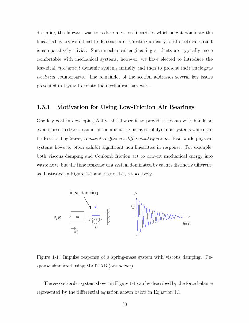
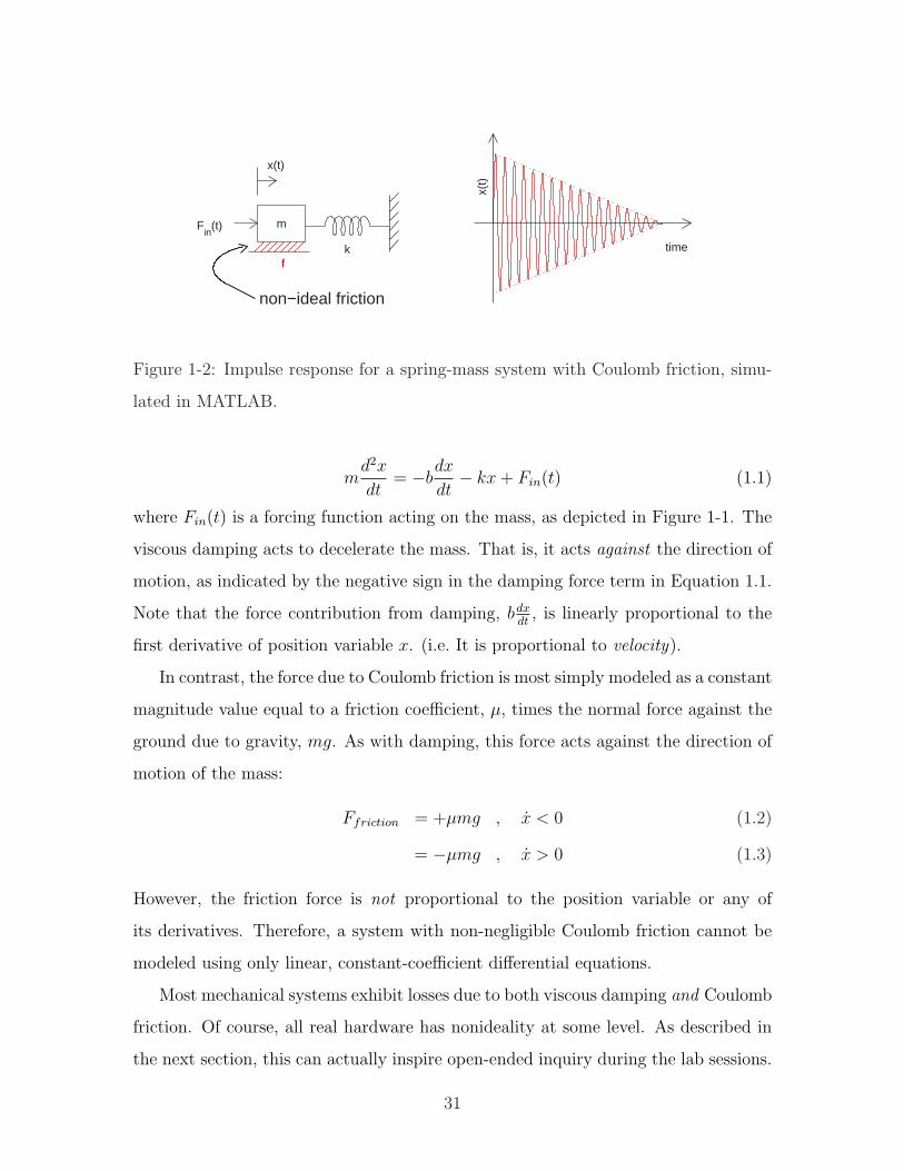
as illustrated in Figure 1-1 and Figure 1-2, respectively.

m

k

b

x(t)

Fin

(t)

time

x(t)

ideal damping

Figure 1-1: Impulse response of a spring-mass system with viscous damping. Re-

sponse simulated using MATLAB (ode solver).

The second-order system shown in Figure 1-1 can be described by the force balance

represented by the differential equation shown below in Equation 1.1,

30

m

k

x(t)

Fin

(t)

time

x(t)

non−ideal friction

f

Figure 1-2: Impulse response for a spring-mass system with Coulomb friction, simu-

lated in MATLAB.

md2x

dt= −b

dx

dt− kx + Fin(t) (1.1)

where Fin(t) is a forcing function acting on the mass, as depicted in Figure 1-1. The

viscous damping acts to decelerate the mass. That is, it acts against the direction of

motion, as indicated by the negative sign in the damping force term in Equation 1.1.

Note that the force contribution from damping, bdxdt

, is linearly proportional to the

first derivative of position variable x. (i.e. It is proportional to velocity).

In contrast, the force due to Coulomb friction is most simply modeled as a constant

magnitude value equal to a friction coefficient, µ, times the normal force against the

ground due to gravity, mg. As with damping, this force acts against the direction of

motion of the mass:

Ffriction = +µmg , x < 0 (1.2)

= −µmg , x > 0 (1.3)

However, the friction force is not proportional to the position variable or any of

its derivatives. Therefore, a system with non-negligible Coulomb friction cannot be

modeled using only linear, constant-coefficient differential equations.

Most mechanical systems exhibit losses due to both viscous damping and Coulomb

friction. Of course, all real hardware has nonideality at some level. As described in

the next section, this can actually inspire open-ended inquiry during the lab sessions.

31

However, a more fundamental goal is to foster familiarity with basic system dynamics

by allowing students to observe relatively clean first- and second- order impulse and

step responses.2 The laboratory equipment should therefore have a minimal amount of

Coulomb friction, so that the effects of loss due to viscous damping are not obfuscated

by the effects of friction. This goal is achieved in most of the mechanical ActivLab

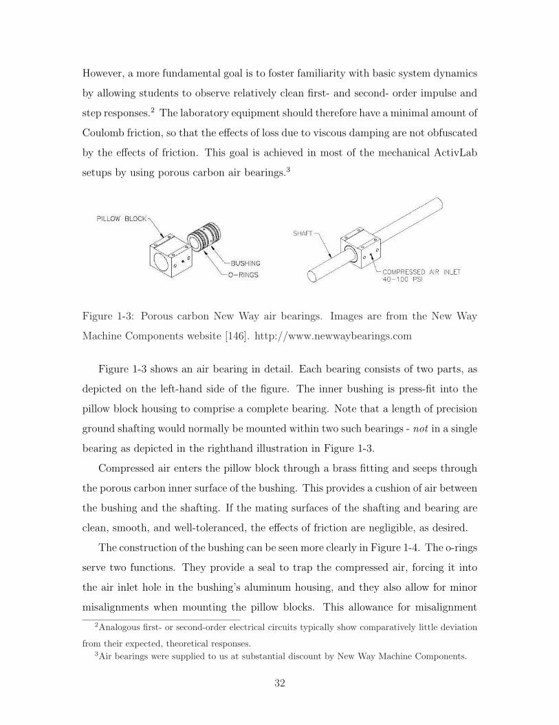
setups by using porous carbon air bearings.3

Figure 1-3: Porous carbon New Way air bearings. Images are from the New Way

Machine Components website [146]. http://www.newwaybearings.com

Figure 1-3 shows an air bearing in detail. Each bearing consists of two parts, as

depicted on the left-hand side of the figure. The inner bushing is press-fit into the

pillow block housing to comprise a complete bearing. Note that a length of precision

ground shafting would normally be mounted within two such bearings - not in a single

bearing as depicted in the righthand illustration in Figure 1-3.

Compressed air enters the pillow block through a brass fitting and seeps through

the porous carbon inner surface of the bushing. This provides a cushion of air between

the bushing and the shafting. If the mating surfaces of the shafting and bearing are

clean, smooth, and well-toleranced, the effects of friction are negligible, as desired.

The construction of the bushing can be seen more clearly in Figure 1-4. The o-rings

serve two functions. They provide a seal to trap the compressed air, forcing it into

the air inlet hole in the bushing’s aluminum housing, and they also allow for minor

misalignments when mounting the pillow blocks. This allowance for misalignment

2Analogous first- or second-order electrical circuits typically show comparatively little deviation

from their expected, theoretical responses.3Air bearings were supplied to us at substantial discount by New Way Machine Components.

32

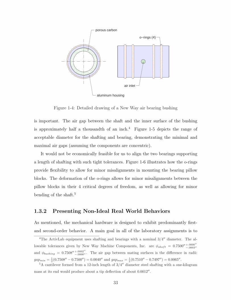
porous carbon

air inlet

aluminum housing

o−rings (4)

Figure 1-4: Detailed drawing of a New Way air bearing bushing

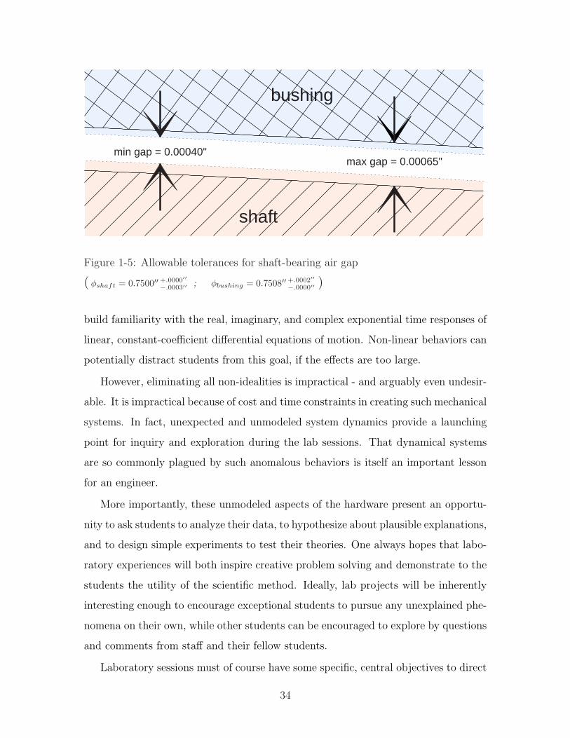
is important. The air gap between the shaft and the inner surface of the bushing

is approximately half a thousandth of an inch.4 Figure 1-5 depicts the range of

acceptable diameter for the shafting and bearing, demonstrating the minimal and

maximal air gaps (assuming the components are concentric).

It would not be economically feasible for us to align the two bearings supporting

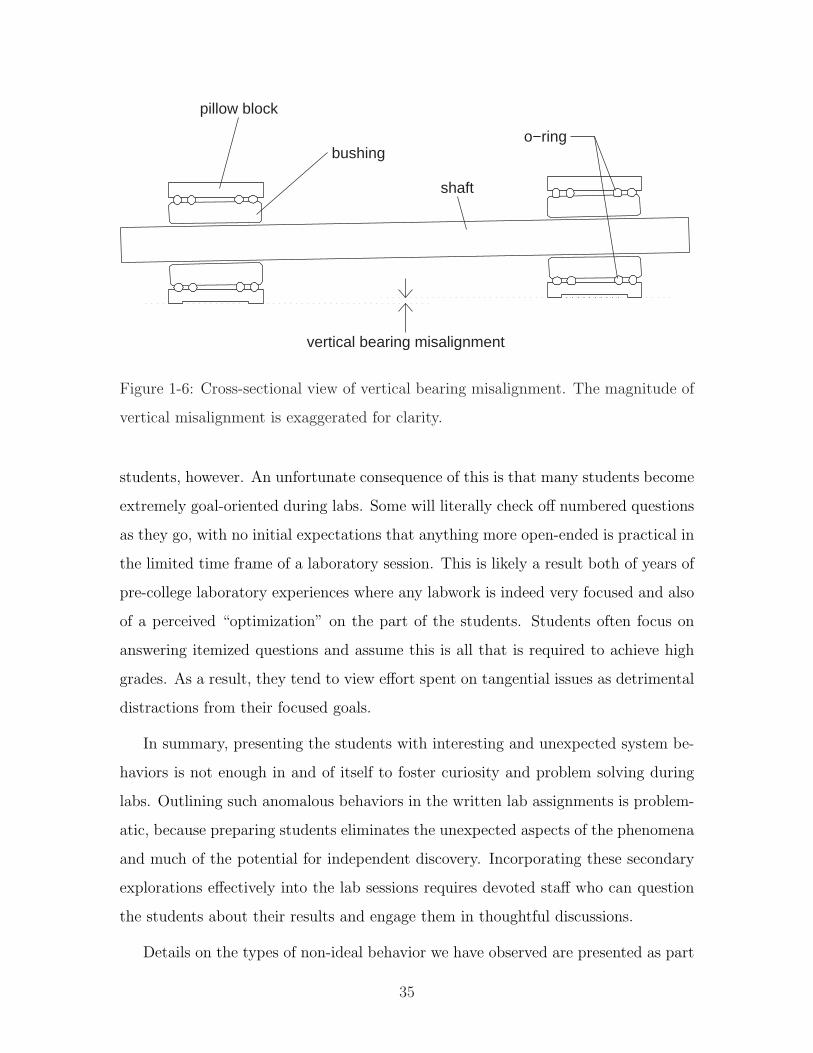
a length of shafting with such tight tolerances. Figure 1-6 illustrates how the o-rings

provide flexibility to allow for minor misalignments in mounting the bearing pillow

blocks. The deformation of the o-rings allows for minor misalignments between the

pillow blocks in their 4 critical degrees of freedom, as well as allowing for minor

bending of the shaft.5

1.3.2 Presenting Non-Ideal Real World Behaviors

As mentioned, the mechanical hardware is designed to exhibit predominantly first-

and second-order behavior. A main goal in all of the laboratory assignments is to

4The ActivLab equipment uses shafting and bearings with a nominal 3/4′′ diameter. The al-

lowable tolerances given by New Way Machine Components, Inc. are φshaft = 0.7500′′+.0000′′

−.0003′′

and φbushing = 0.7508′′+.0002′′

−.0000′′ . The air gap between mating surfaces is the difference in radii:

gapmin = 12 (0.7508′′ − 0.7500′′) = 0.0040′′ and gapmax = 1

2 (0.7510′′ − 0.7497′′) = 0.0065′′.5A cantilever formed from a 12-inch length of 3/4′′ diameter steel shafting with a one-kilogram

mass at its end would produce about a tip deflection of about 0.0012′′.

33

bushing

shaft

min gap = 0.00040"max gap = 0.00065"

Figure 1-5: Allowable tolerances for shaft-bearing air gap

( φshaft = 0.7500′′+.0000′′

−.0003′′ ; φbushing = 0.7508′′+.0002′′

−.0000′′ )

build familiarity with the real, imaginary, and complex exponential time responses of

linear, constant-coefficient differential equations of motion. Non-linear behaviors can

potentially distract students from this goal, if the effects are too large.

However, eliminating all non-idealities is impractical - and arguably even undesir-

able. It is impractical because of cost and time constraints in creating such mechanical

systems. In fact, unexpected and unmodeled system dynamics provide a launching

point for inquiry and exploration during the lab sessions. That dynamical systems

are so commonly plagued by such anomalous behaviors is itself an important lesson

for an engineer.

More importantly, these unmodeled aspects of the hardware present an opportu-

nity to ask students to analyze their data, to hypothesize about plausible explanations,

and to design simple experiments to test their theories. One always hopes that labo-

ratory experiences will both inspire creative problem solving and demonstrate to the

students the utility of the scientific method. Ideally, lab projects will be inherently

interesting enough to encourage exceptional students to pursue any unexplained phe-

nomena on their own, while other students can be encouraged to explore by questions

and comments from staff and their fellow students.

Laboratory sessions must of course have some specific, central objectives to direct

34

vertical bearing misalignment

shaft

bushing

pillow block

o−ring

Figure 1-6: Cross-sectional view of vertical bearing misalignment. The magnitude of

vertical misalignment is exaggerated for clarity.

students, however. An unfortunate consequence of this is that many students become

extremely goal-oriented during labs. Some will literally check off numbered questions

as they go, with no initial expectations that anything more open-ended is practical in

the limited time frame of a laboratory session. This is likely a result both of years of

pre-college laboratory experiences where any labwork is indeed very focused and also

of a perceived “optimization” on the part of the students. Students often focus on

answering itemized questions and assume this is all that is required to achieve high

grades. As a result, they tend to view effort spent on tangential issues as detrimental

distractions from their focused goals.

In summary, presenting the students with interesting and unexpected system be-

haviors is not enough in and of itself to foster curiosity and problem solving during

labs. Outlining such anomalous behaviors in the written lab assignments is problem-

atic, because preparing students eliminates the unexpected aspects of the phenomena

and much of the potential for independent discovery. Incorporating these secondary

explorations effectively into the lab sessions requires devoted staff who can question

the students about their results and engage them in thoughtful discussions.

Details on the types of non-ideal behavior we have observed are presented as part

35

of the relevant laboratory descriptions in Chapter 3. Briefly, some examples include

(1) an unmodeled springiness in the air-filled dashpots used in the first-order spring-

damper translational system (Section 3.3); (2) a slight “recoiling” tendency in the

1st-order inertia-damper rotational system likely caused by tilting misalignments in

the carbide flat bearing surface (Section 3.4); and (3) spring-stiffening of the cantilever

used in the 2nd-order spring-mass-damper translational system which forms the basis

for the projects described in Sections 3.5, 3.8, and 3.9.

The voice coils used in this last set-up present a couple of additional, unplanned

behaviors. When used merely to provide damping, ideally one might hope to vary the

voice coil damping from zero (when the coil circuit is open) to some maximum (when

it is short-circuited) by closing the circuit with a finite resistance value. The coils

we use are wound on aluminum cups, however, so currents flowing in the aluminum

still produce significant damping when the coil is open-circuited. Second, when the

voice coil is used as an actuator, a frequency response reveals non-finite-dimensional

dynamics.

I would once again like to acknowledge the efforts of Professors Trumper, Nayfeh,

Gossard and Hogan and all of the TA’s for 2.003 (see Acknowledgements) for prodding

the students to explore during the lab sessions. Again, such efforts from the staff are

essential in getting most students to pursue understanding in depth in their lab work.

1.3.3 Transparent, Hands-on Operation

As mentioned, the ActivLab projects should foster an intuitive understanding of

system dynamics. We intend that much of this intuition will come from encouraging

students to touch and play with the mechanical systems. Specifically, the setups have

been designed to allow students to change damping, stiffness and/or inertia in a given

system and, importantly, to feel the differences created for themselves.

Ideally, the hardware should also be transparent to both students and staff, so that

little or no instruction is necessary to figure out how the systems operate. Hopefully,

this ease-of-use will also help encourage students to play with the hardware without

fear of destroying or misaligning anything.

36

An important additional principle is that time scales at which any oscillations

and decay rates occur should be on the order of a few seconds, so that students can

observe these behaviors with their own eyes. By the same reasoning, displacements

of at least several millimeters are needed. Otherwise, students cannot relate recorded

data from sensors to their own observation to verify that calculations of displacements,

frequencies, time constants, or other system parameters actually make sense. They

are less likely to remember the lab experience if they cannot easily observe it without

sensors, too.

Finally, we would like to minimize the use of “black boxes”. To the extent practi-

cal, any actuators, sensors and passive components (e.g. springs and dampers) should

be easy to understand. We sometimes compromised this goal in favor of simplicity

and/or accuracy. For instance, a linear potentiometer is an easier displacement sen-

sor to understand than an LVDT6, but we chose to use the latter (without much

discussion of its operation) because it is frictionless. For other equipment, such as

a voice coil actuators or a viscous damper consisting of honey between concentric

cylinders, we provide basic explanations of the underlying physics. Only a few com-

ponents were straight-forward enough that we asked the students to calculate system

properties from first principles. These properties include inertia and mass of objects

with simple geometries and spring stiffness for a cantilever beam.

1.3.4 Ease of Assembly

Ease of assembly is a practical concern. The TA’s putting together the equipment

will generally not be the same from term to term, so learning any complicated pro-

cedures is not practical. Our strategy was to design each setup to be assembled on

optical breadboard. The breadboard has a grid of tapped holes, evenly spaced at one-

inch intervals.7 We designed and manufactured our own mounting blocks for various

components to make them compatible with the breadboard, so that parts could be

6“linear variable differential transformer”7Such baseplate surfaces are often used in prototyping optical systems; hence the name “optical

breadboard”.

37

assembled from photos of each setup. Generally, the parts can be set loosely in place

on the board and then screwed into place with little attention to alignment.

The greatest alignment challenges in the labs are probably in the vertical align-

ment of the rotational inertia-damping system. The shafting needs to be perpendic-

ular to the base flat, and close to concentric with a tube surrounding it that holds

viscous honey. Also, significant force is required to operate a syringe (with a small

orifice) to change the level of the honey in the tube. This creates a messy potential

failure point: the tubing that channels the honey between the syringe and tubing can

become detached from the syringe.

Alignment was also a concern for the translational spring-mass-damper system.

As mentioned, air bearings are used to minimize the effects of friction. Also, the

range of travel of the mass needed to be on the order of a half an inch (or more) total

to be clearly observable to the students. Both the voice coil actuator/damper and the

LVDT position sensor involve concentric parts which can potentially scrape against

one another as the mass moves. Thus, proper alignment of these parts is important,

as described below.

Each voice coil motor consists of a housing with an annular gap (containing a

concentrated magnetic field) and a coil assembly which moves within the gap along

the axis of the annulus. In our spring-mass-damper lab setup, the coil assembly is

mounted at one end of length of shafting. The shafting is constrained within two air

bearings to allow only rotations about and linear motion along the axis of the shaft.

The housing for the voice coil is mounted on an angle plate of the type shown at

the right in Figure 1-11. The angle plate creates a flat surface at a 90 degree angle

with the optical baseplate. This is a necessary (though not sufficient) requirement

to insure that the walls of the actuator housing remain parallel to the direction of

motion of the coil. Of course, misalignment between the housing and coil of the voice

coil motor can still occur if (1) the bottom surface of the angle plate mates with the

optical breadboard at a skew angle and/or (2) the housing is mounted too high or too

low on the vertical surface of the angle plate to allow the coil to move freely inside

within scraping. The clearance within the voice coil is sufficient that achieving such

38

alignment is relatively easy.

.50" outer dia

.25" inner dia

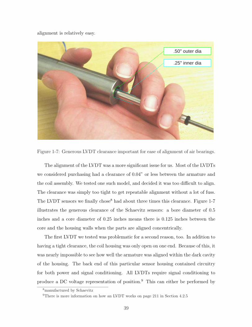
Figure 1-7: Generous LVDT clearance important for ease of alignment of air bearings.

The alignment of the LVDT was a more significant issue for us. Most of the LVDTs

we considered purchasing had a clearance of 0.04” or less between the armature and

the coil assembly. We tested one such model, and decided it was too difficult to align.

The clearance was simply too tight to get repeatable alignment without a lot of fuss.

The LVDT sensors we finally chose8 had about three times this clearance. Figure 1-7

illustrates the generous clearance of the Schaevitz sensors: a bore diameter of 0.5

inches and a core diameter of 0.25 inches means there is 0.125 inches between the

core and the housing walls when the parts are aligned concentrically.

The first LVDT we tested was problematic for a second reason, too. In addition to

having a tight clearance, the coil housing was only open on one end. Because of this, it

was nearly impossible to see how well the armature was aligned within the dark cavity

of the housing. The back end of this particular sensor housing contained circuitry

for both power and signal conditioning. All LVDTs require signal conditioning to

produce a DC voltage representation of position.9 This can either be performed by

8manufactured by Schaevitz9There is more information on how an LVDT works on page 211 in Section 4.2.5

39

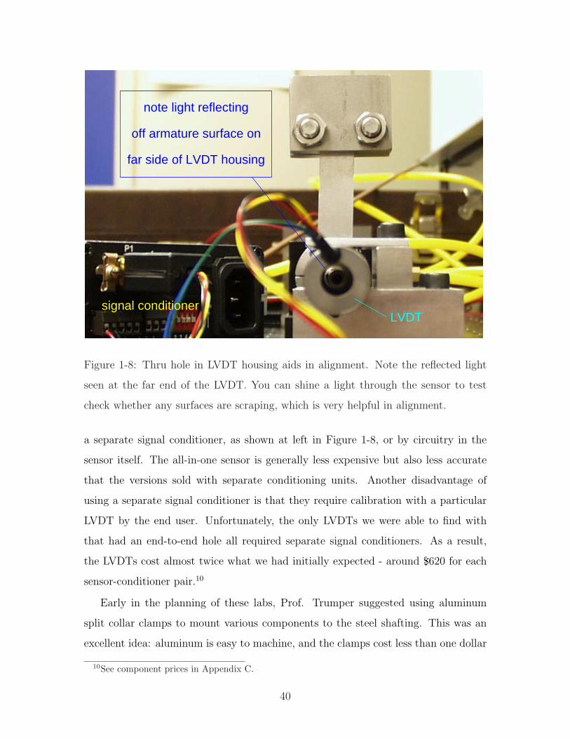
signal conditioner LVDT

note light reflecting

off armature surface on

far side of LVDT housing

Figure 1-8: Thru hole in LVDT housing aids in alignment. Note the reflected light

seen at the far end of the LVDT. You can shine a light through the sensor to test

check whether any surfaces are scraping, which is very helpful in alignment.

a separate signal conditioner, as shown at left in Figure 1-8, or by circuitry in the

sensor itself. The all-in-one sensor is generally less expensive but also less accurate

that the versions sold with separate conditioning units. Another disadvantage of

using a separate signal conditioner is that they require calibration with a particular

LVDT by the end user. Unfortunately, the only LVDTs we were able to find with

that had an end-to-end hole all required separate signal conditioners. As a result,

the LVDTs cost almost twice what we had initially expected - around $620 for each

sensor-conditioner pair.10

Early in the planning of these labs, Prof. Trumper suggested using aluminum

split collar clamps to mount various components to the steel shafting. This was an

excellent idea: aluminum is easy to machine, and the clamps cost less than one dollar

10See component prices in Appendix C.

40

each. We purchased several dozen11 from Kaman Industrial Technologies[194]. The

Kaman part number is SC-12A, and they are manufactured by Whittet-Higgins[212].

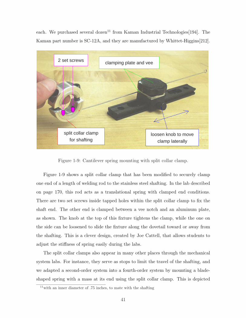
2 set screws

loosen knob to move

clamp laterally

clamping plate and vee

for shafting

split collar clamp

Figure 1-9: Cantilever spring mounting with split collar clamp.

Figure 1-9 shows a split collar clamp that has been modified to securely clamp

one end of a length of welding rod to the stainless steel shafting. In the lab described

on page 170, this rod acts as a translational spring with clamped end conditions.

There are two set screws inside tapped holes within the split collar clamp to fix the

shaft end. The other end is clamped between a vee notch and an aluminum plate,

as shown. The knob at the top of this fixture tightens the clamp, while the one on

the side can be loosened to slide the fixture along the dovetail toward or away from

the shafting. This is a clever design, created by Joe Cattell, that allows students to

adjust the stiffness of spring easily during the labs.

The split collar clamps also appear in many other places through the mechanical

system labs. For instance, they serve as stops to limit the travel of the shafting, and

we adapted a second-order system into a fourth-order system by mounting a blade-

shaped spring with a mass at its end using the split collar clamp. This is depicted

11with an inner diameter of .75 inches, to mate with the shafting

41

in Figure 1-8. In another lab (described on page 161), a collar is used to mount

a flywheel at the top end of a vertically-mounting length of shafting. Getting the

flywheel mounted so that its top surface was square and concentric with the vertical

shaft axis was time consuming, requiring some special fixtures to hold the parts in

alignment while they were screwed together tightly.

The flywheel was designed to screw into only one half of the two-piece collar. In

other words, the halfcollar-flywheel assembly can be taken off the shafting as an intact

unit. On subsequent assemblies of the lab, the flywheel will thereby fall into proper

alignment once the other half of the collar is used to clamp the structure near the

end of a length of precision shafting.

More notes on assembly occur throughout the descriptions of each lab project in

Chapter 3. As a final comment, note that considerable time was spent manufactur-

ing mounting blocks in-house, particularly for the air bearings. This was definitely

worth the effort for future ease of assembly, however. Using off-the-shelf components

whenever possible is also a good strategy, since equipment may need to be replaced

over time.

1.3.5 Cost Effectiveness

In any lab setups, cost is of course an issue. We have attempted to keep the nec-

essary components reasonably affordable to enable use by others wishing to copy or

adapt ActivLab setups. A list of components, vendors and prices12 can be found in

Appendix C. Note that we were fortunate to be able to use an existing laboratory

classroom13 with 12 lab workstations. Each workstation is equipped with a PC, a

dSPACE 1102 controller board, an oscilloscope, a function generator and a power

supply. Below is a summary of the most significant costs along with alternatives,

where applicable, and the reasoning behind our choices.

As mentioned in the previous section, each of the mechanical ActivLab setups

has been designed for assembly on an optical breadboard. We purchased anodized,

12as of summer, 200113designed for 2.737, Mechatronics

42

half-inch thick aluminum baseplates with 1/4”-20 tapped holes at one-inch spacings.

Each plate was 18” by 24” and cost about $375. The full 24 inches are required when

assembling the translational spring-mass-damper system, as you can see in Figure 3-

27.

We realized early in the development of the lab projects that the air bearings

would be a costly yet key components for attaining very low friction systems. The

bushing and pillow block which comprise each bearing14 retail for $175 and $85,

respectively, and each length of shafting requires two such bearings for support. Our

thanks to Drew Devitt of New Way Machine Components who graciously agreed to

supply these to us at a substantial discount.

Running the air bearings requires the additional complexity of supplying dry,

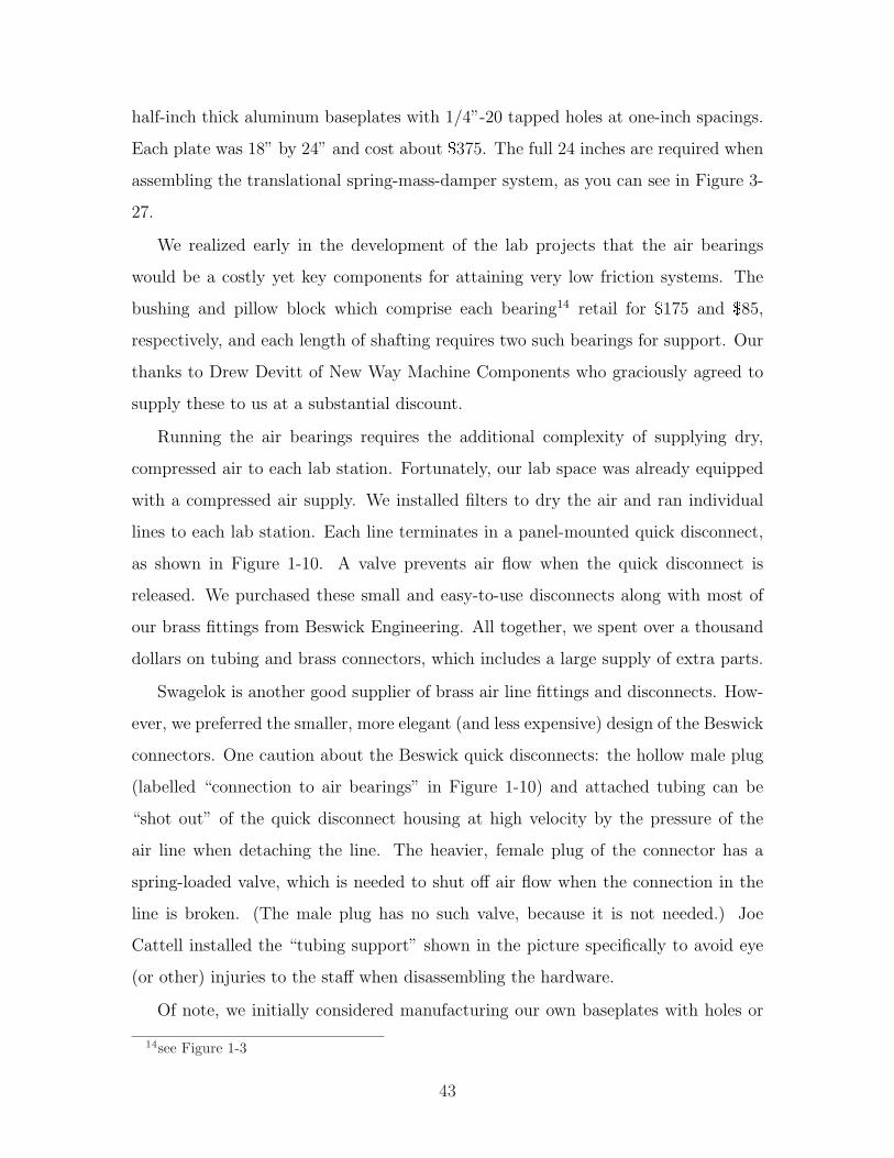
compressed air to each lab station. Fortunately, our lab space was already equipped

with a compressed air supply. We installed filters to dry the air and ran individual

lines to each lab station. Each line terminates in a panel-mounted quick disconnect,

as shown in Figure 1-10. A valve prevents air flow when the quick disconnect is

released. We purchased these small and easy-to-use disconnects along with most of

our brass fittings from Beswick Engineering. All together, we spent over a thousand

dollars on tubing and brass connectors, which includes a large supply of extra parts.

Swagelok is another good supplier of brass air line fittings and disconnects. How-

ever, we preferred the smaller, more elegant (and less expensive) design of the Beswick

connectors. One caution about the Beswick quick disconnects: the hollow male plug

(labelled “connection to air bearings” in Figure 1-10) and attached tubing can be

“shot out” of the quick disconnect housing at high velocity by the pressure of the

air line when detaching the line. The heavier, female plug of the connector has a

spring-loaded valve, which is needed to shut off air flow when the connection in the

line is broken. (The male plug has no such valve, because it is not needed.) Joe

Cattell installed the “tubing support” shown in the picture specifically to avoid eye

(or other) injuries to the staff when disassembling the hardware.

Of note, we initially considered manufacturing our own baseplates with holes or

14see Figure 1-3

43

Tubing Support

Air Supply Line

Quick Disconnect

Connection to Air Bearings

Figure 1-10: Air supply line with quick disconnect fitting.

slots spaced to accommodate the hole alignment in the pillow blocks: 1.5” by 1.562”.

Our reasoning was that the bearings were known to be constrained to this spacing,

and any additional components would either be attached to the breadboard with toe

clamps or manufactured in-house to match the unusual spacing. At the time, we

envisioned at least one of the lab systems would require two lengths of shafting and

therefore four bearings. We also planned to manufacture our own voice coil actuators,

which could easily be designed with mounting holes compatible with whatever hole

spacing we choose for the baseplates.

Purchasing pre-made breadboards with a standard spacing now seems like the

only reasonable option. Either metric or English units can be selected, as convenient.

Using toe clamps is not unreasonable, but we chose to manufacture custom mounting

blocks to allow the lab components to be linked in place easily like LEGO blocks. The

44

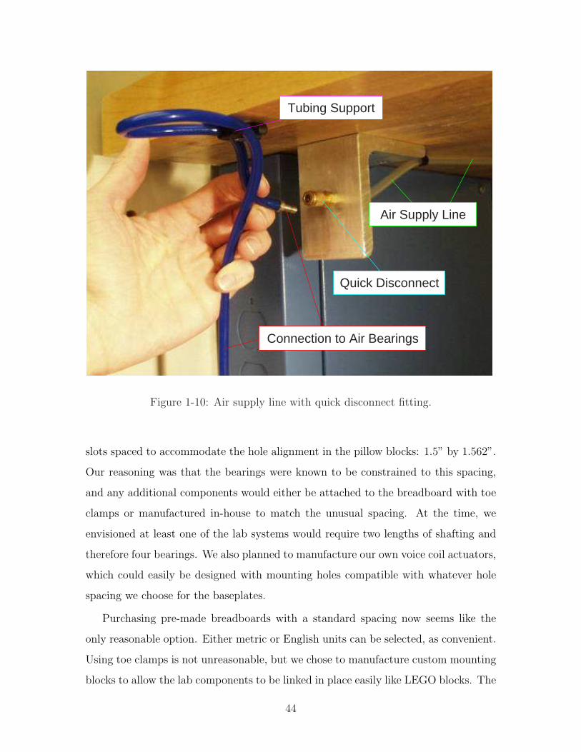
most essential mounting blocks we built were Delrin15 adaptor plates which interface

between the the pillow blocks and optical breadboard. Figure 1-11 shows adaptors

for a voice coil, air bearing and LVDT, respectively. A CAD drawing of the Delrin

adaptor plate designed for the New Way bearings is shown in Appendix D.

We have had some issues with the clearance of the bolt holes in these Delrin

adapter plates. As a result, the bearings are over-constrained when the bolts through

the plates are fully tightened into place on the breadboard. The clearance holes

themselves were drilled with appropriate clearance to provide enough slack during

alignment. However, the clearance between the counterbore for each hole and the

head of the bolt attaching the adapter plate to the breadboard is too tight. The

selection of drill diameters available in a machine shop is generally much wider than

that of end mills, and we simply chose a mill diameter that was a little too small.

We have previously addressed this over-constraint by bolting the adapter somewhat

loosely to the breadboard during labs. We have yet to modify the Delrin plates to

increase the diameter of the counterbores, which we believe will solve the problem.

We therefore cannot yet confirm that this is the sole source of over-constraint in the

hardware.

The LVDTs were the single most expensive component we used. As previously

noted, we wanted to reduce any friction to a minimum, and therefore wanted a non-

contact position sensor. We tested less-expensive LVDT’s which had built in signal

conditioning (to provide DC output of position directly), but they did not have ad-

equate clearance. The sensors we finally choose (from Shaevitz) provided ample

clearance. This clearance was only available for a two-part package including the

sensor and a separate signal conditioner16, however, which consequently meant they

were more accurate (although we did not need this accuracy) and more expensive. A

partial list of supplies and vendors appears in the appendix on page 417.

15Delrin is a registered trademark of DuPont.16The cost of the sensor and signal conditioner for one lab set-up was just over $600.

45

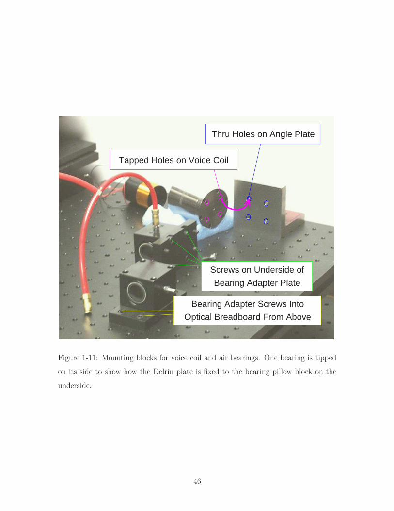
Tapped Holes on Voice Coil

Thru Holes on Angle Plate

Screws on Underside of

Bearing Adapter Plate

Optical Breadboard From Above

Bearing Adapter Screws Into

Figure 1-11: Mounting blocks for voice coil and air bearings. One bearing is tipped

on its side to show how the Delrin plate is fixed to the bearing pillow block on the

underside.

46

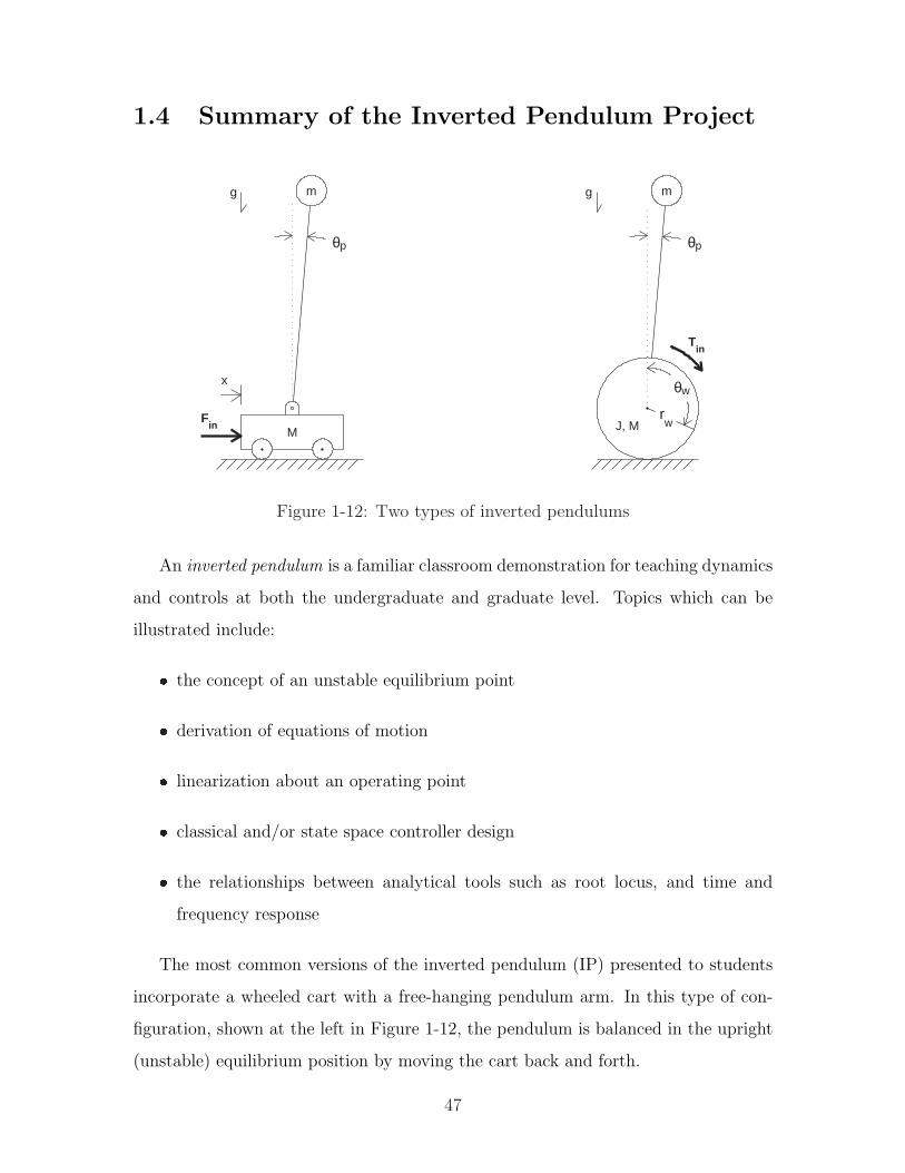
1.4 Summary of the Inverted Pendulum Project

m

M

θp θp

x

Fin

m

Tin

J, M

θw

rw

g g

Figure 1-12: Two types of inverted pendulums

An inverted pendulum is a familiar classroom demonstration for teaching dynamics

and controls at both the undergraduate and graduate level. Topics which can be

illustrated include:

the concept of an unstable equilibrium point

derivation of equations of motion

linearization about an operating point

classical and/or state space controller design

the relationships between analytical tools such as root locus, and time and

frequency response

The most common versions of the inverted pendulum (IP) presented to students

incorporate a wheeled cart with a free-hanging pendulum arm. In this type of con-

figuration, shown at the left in Figure 1-12, the pendulum is balanced in the upright

(unstable) equilibrium position by moving the cart back and forth.

47

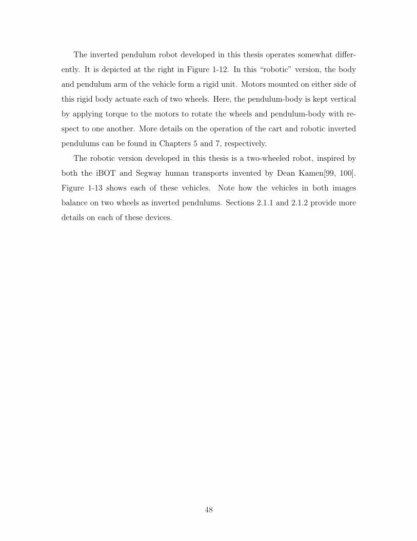
The inverted pendulum robot developed in this thesis operates somewhat differ-

ently. It is depicted at the right in Figure 1-12. In this “robotic” version, the body

and pendulum arm of the vehicle form a rigid unit. Motors mounted on either side of

this rigid body actuate each of two wheels. Here, the pendulum-body is kept vertical

by applying torque to the motors to rotate the wheels and pendulum-body with re-

spect to one another. More details on the operation of the cart and robotic inverted

pendulums can be found in Chapters 5 and 7, respectively.

The robotic version developed in this thesis is a two-wheeled robot, inspired by

both the iBOT and Segway human transports invented by Dean Kamen[99, 100].

Figure 1-13 shows each of these vehicles. Note how the vehicles in both images

balance on two wheels as inverted pendulums. Sections 2.1.1 and 2.1.2 provide more

details on each of these devices.

48

Figure 1-13: IBOT (left) and Segway Human Transports. The rendering of the

iBOT comes from a gallery of industrial designs on the “Rhinoceros NURBS modeling

for Windows” website (http://www.rhino3d.com/gallery/images/ibotchair.jpg). The

photo of the Segway transport was provided at the “Press Kit” section of the Segway

website (http://www.segway.com/aboutus/press releases/pr 062602.html).

49

1.4.1 Ideal and Actual Hardware Implementation

To function as a practical classroom demo, the IP robot should be large enough to

be clearly visible yet also reasonably portable. Since our lecture room must typically

be free for other classes before and after the lecture period, the required set-up and

disassembly times should each be less than about five minutes. Ideally, the robot

would be autonomous, carrying it’s own power, microcontroller, and a receiver to

allow remote steering.

The robot I created is not autonomous. The robot uses four power supplies:

one for each of two motors (36 volts at up to 1.5 Amps for continuous operation,

9 Amps peak), a 12-volt supply for the gyroscope (to measure the absolute pendulum

velocity), and a 5-volt supply17 for a two-axis accelerometer (used as a tilt sensor

to compensate for gyro drift). These power supplies are so heavy and bulky18, one

would need to transport them on a separate cart.

The controller is implemented on a dSPACE board, which runs on a PC. This

means the equipment cart must also carry a desktop computer (or a laptop with

a dSPACE expansion box). In addition to the inconvenience of the bulk of this

additional equipment, the lack of autonomy means the robot needs umbilical cords.

The vehicle dynamics are affected quite significantly by these cords.

I have tried two mounting schemes for the umbilical cabling. Initially, the cables

were attached about five inches directly above the wheel axis. The weight of the cords

creates a (disturbance) torque on the pendulum-body, so that its upright equilibrium

is offset from vertical (i.e. such that the torque created by the gravity at this angle

offsets the disturbance torque). Maneuvering the robot19 is difficult, both because

the cords get in the way and because shifting the position of the robot shifts the

disturbance torque.

I also tested the robot with the cables attached about four inches below the wheel

17The dSPACE controller board currently provides the 5-volt supply.18The Lambda power supplies for the motors are shown in Figure 1-14 on page 1-14. They weigh

over 50 pounds, together.19Two rotary pots provide steering inputs. One sets the forward/reverse velocity and the other

controls turning radius.

50

axis. This creates a smaller disturbance torque, since there is a much shorter length

of cable. Unfortunately, the cable helps stabilize the pendulum-body, however! This

makes it more difficult to evaluate the performance of the controller objectively (in

stabilizing the robot). The vehicle is also less responsive to commanded velocity.

For this type of inverted pendulum, a constant (linear) velocity corresponds to a

constant pendulum offset angle. Picture the cables as a “tail” dragging behind (or

ahead of) the robot. The static friction between the ground and cables allows a

range of “stable” pendulum angles, rather than a single equilibrium angle. For low

velocity commands, the robot will stabilize about an angle somewhat off of vertical,

but the static friction balances the (constant) torque to the wheels and prevents it

from rolling. The controller was designed with the umbilical in the first configuration

(mounted above the wheel axis), but the data in Chapter 7 were obtained with the

second umbilical configuration. (When operating near equilibrium and at zero forward

velocity, the response of the system in each of the two configurations did not differ

significantly.)

1.4.2 Challenges and Control Strategy

The most significant challenges in implementing the robot fall into one or more of the

following three categories: (1) the mechanical design (i.e. scaling and packaging com-

ponents appropriately); (2) filtering the sensor signals; and (3) modelling, controlling

and/or attenuating higher order dynamics (resonances) in the system.

Mechanical Design

The robot is both more visible and more impressive as a classroom demo if it stands at

least a meter or so high. The size of the robot has a huge influence on the complexity

of the design. Two extreme examples (described in more detail in Chapter 2) which

make this point are the LegWay inverted pendulum robot (described on page 80) and

the robotic unicycles described on page 84. The LegWay stands just a few inches tall.

Its low weight and inertia allow it to run with standard, Lego (9-volt) motors and to

51

carry batteries and processor onboard.

The robotic unicycles have enormous inertia by comparison.20 The motors for such

a vehicle need to provide much more torque, and this in turn significantly increases the

complexity of providing onboard power. The large inertia will also be inherently more

“sluggish” to control. Finally, the sensors for the unicycle are both more numerous

and more complex, which again adds to the hassle of packaging everthing.

I designed the chassis of the demo inverted pendulum robot (“DIPR”) to be some-

what versatile for future modifications, with the expectation that it would eventually

carry its own power and controller. As of this writing, however, the robot still uses

umbilicals. Unfortunately, the umbilical cords greatly influence the dynamics of the

robot. They are heavy and put a substantial offset torque on the pendulum (for which

one compensate reasonably well by offsetting the equilibrium angle of the pendulum

away from vertical). More importantly, when they scrape the ground, this causes sub-

stantial friction, as mentioned, and can even provide a stabilizing force against the

ground. Making the robot autonomous would also improve the steering capability.

Selecting or manufacturing appropriate wheels was (surprisingly for me) another

notable concern. One needs to keep the robot “dynamically interesting” as a control

problem. That is, if you make the wheel inertia too large, the wheels essentially be-

come fixed objects (“rocks”). Also, using wheel bearings introduces additional issues

and potential pitfalls (friction, alignment, etc), so a direct drive system (attaching

a wheel directly to the motor’s output shaft) is appealing. Each motor gearhead is

rated for 120 N radial force at 12mm from the mounting plane, or 1.44 N-m of torque.

The pendulum-body has a mass of 8 kg, divided (symmetrically) over the two wheels.

In order to meet the side-load spec, this limits the distance of the wheel from the

gearhead flange to no more than about 36mm (1.4 inches). Commercially available

wheels with a large enough diameter (12 inches) were generally too wide (2+ inches),

too heavy and too difficult to mount, so I finally decided to manufacture my own

wheels. They are cut from 1/4 inch aluminum plate and have rubber o-rings epoxied

to the circumference for traction. This is not the most elegant solution, but it works.

20See Figure 2-13 on page 85.

52

(The centerline of the wheel is about 1 inch from the flange of the gearhead.)

Sensors

Sensor issues are discussed in detail in Section 7.1. The two main challenges were: (1)

compensating for drift in the gyro (to measure pendulum angle in an inertial reference

frame), and (2) filtering the differentiated motor encoder signals to obtain a smooth

measurement of motor velocity.

The gyro signal represents angular velocity. It is accurate at high frequency, but

it has a DC bias which leads to low frequency angular errors. It is currently combined

with a 2-axis accelerometer (more accurate at low frequency) through complementary

filtering. Section 6.2 discusses complementary filtering in more detail.

Filtering the encoders to obtain velocity involved a trade-off between accuracy

and smoothness of the resulting output. Quantization of the encoder and backlash

in the gearhead are of particular concern here. Section 7.1.4 describes this in more

detail.

Controller Design

Initially, I modelled the known parameters of the robot in state space and attempted

to design an LQR (linear-quadratic regulator) controller.21 This controller did suc-

cessfully balance the robot, but it also excited a significant resonance! State-space

controller methods depend on accurate modelling of system dynamics, and there were

clearly important higher order dynamics in the system that I had not modelled.

My advisor, Prof. Trumper, suggested a different approach, which I successfully

used to control the robot (with no significant excitation of resonances). The controller

is structured with an inner loop to control wheel velocity and an outer loop to stabilize

the pendulum. The resulting controller still amounts to a state-space controller (i.e. it

multiplies some gain times the filtered signals of each of the same, four state variables

previously mentioned; then adds these four values to create a control signal). However,

21The four state variables were pendulum angle, pendulum velocity, motor position, and motor

velocity. Of these, the cost weighting on pendulum angle was clearly the greatest.

53

the methodology used to design the controller essentially involved loop-shaping (not

state-space methods).

Vibration of the pendulum arm was particularly noticeable during the LQR-

induced resonance. I therefore replaced this arm with a stiffer version. The chassis

consists largely of rectangular aluminum extrusions. These were also vibrating signif-

icantly, so I added damping layers to the rest of the structure. There is now rubber

where the pendulum arm attaches to the body and constrained-layer damping where

structural members meet in the chassis. The changes seemed to help reduce the effects

of resonances, but since all changes were made simultaneously, I am not sure which

were most useful. I still suspect it might prove difficult to create an accurate enough

state-space model of the system dynamics to design a satisfactory LQR controller,

both because the magnitude of the vibrations observed with the original LQR control

implementation were so significant, particularly along the length of the pendulum,

and also because I have subsequently found that measurements of transfer functions

for the system are not highly repeatable above 100 Hz. I choose to focus my efforts on

a loop-shaping approach instead. The initial LQR controller is not discussed further

in this thesis.

1.4.3 Results

Figure 1-14 shows the inverted pendulum robot and supporting hardware. The robot

stands about 42 inches tall and weighs just over 23 pounds. The transient response (to

a disturbance torque and/or force on the pendulum body) is somewhat underdamped,

as seen in Figure 1-15. Achieving a significantly faster response22 would be difficult,

given the large inertia of the robot. The frequency response plots and discussion in

Section 7.6 aim to explain this in more detail. Stated briefly, there are unmodelled

(and not robustly repeatable) higher-order dynamics in the transfer functions from

commanded voltage23 to the sensor outputs (i.e. to pendulum angle [and velocity]

22It takes roughly 2 seconds for the transient response to essentially die away23Note, the transfer functions obtained using current command do not differ much from those

with voltage control of the motors. The choice between voltage and current control is discussed in

54

and to motor angle [and velocity]).

Since both motors are commanded together in tandem (with a sign difference, be-

cause they are oriented in opposite directions), we can break the control loop at this

point (where we have a single, commanded output value). Figure 1-16 shows the loop

transmission.24 The peak near 50 Hz occurs in the measurement of pendulum angle

and velocity, while the peak just about 100 Hz appears only in the measurements

of motor angle and velocity. The loop transmission shown includes low-pass filter-

ing of the motor output to push these two resonances (and anything else at higher

frequencies) below unity.

Crossover for the control loop (i.e. broken at a single motor output) is at 9.2 Hz.25

The controlled robot is a multi-input multi-output system, since it acts on errors in

both pendulum angle and wheel position (and their derivatives). The state-space

controller begins to lose control authority over pendulum angle after 0.5 Hz. This can

be noted both in the transient response in Figure 1-15 and the closed-loop transfer

function to pendulum angle, shown in Figure 1-17. Figure 1-15 overlays theoretical

impulse response plots on the actual data which correspond to a second order system

with a natural frequency of 0.5 Hz, with ζ = 0.25, and the magnitude of closed-loop

transfer function from voltage to pendulum angle, shown in Figure 1-17, begins to

dip below unity after about 0.5 Hz.

The response of the DIPR to either a commanded step in pendulum angle or an

impulsive disturbance (both shown in Figure 1-15) seem qualitatively quite smooth

and stable at this bandwidth. Increasing the inertia of an inverted pendulum slows the

response of the system to imbalancing disturbances. Therefore, the larger the inertia

of the vehicle, the lower the required bandwidth necessary to maintain stability. This

is the same phenomenon which enables a man to balance more easily on a tightrope26

if he uses the large inertia of a balancing bar, or which makes it easier to balance

a vertical broomstick on the palm of the hand than than it is to balance a shorter

more detail in Sections 7.5.4 and 7.8.3.24This figure is identical to the lower half of Figure 7-42 on page 386.25The resulting closed-loop TF falls to -3dB at 7.3 Hz.26A tightrope walker is in fact an inverted pendulum system.

55

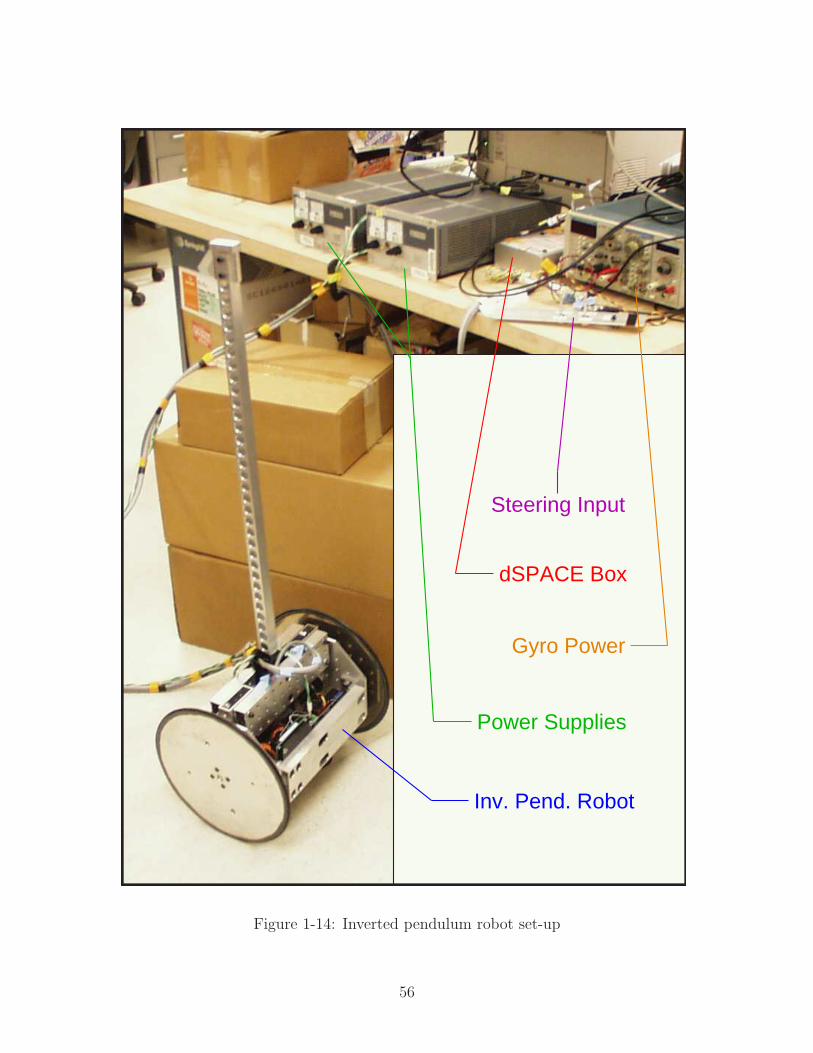
Inv. Pend. Robot

dSPACE Box

Power Supplies

Gyro Power

Steering Input

Figure 1-14: Inverted pendulum robot set-up

56

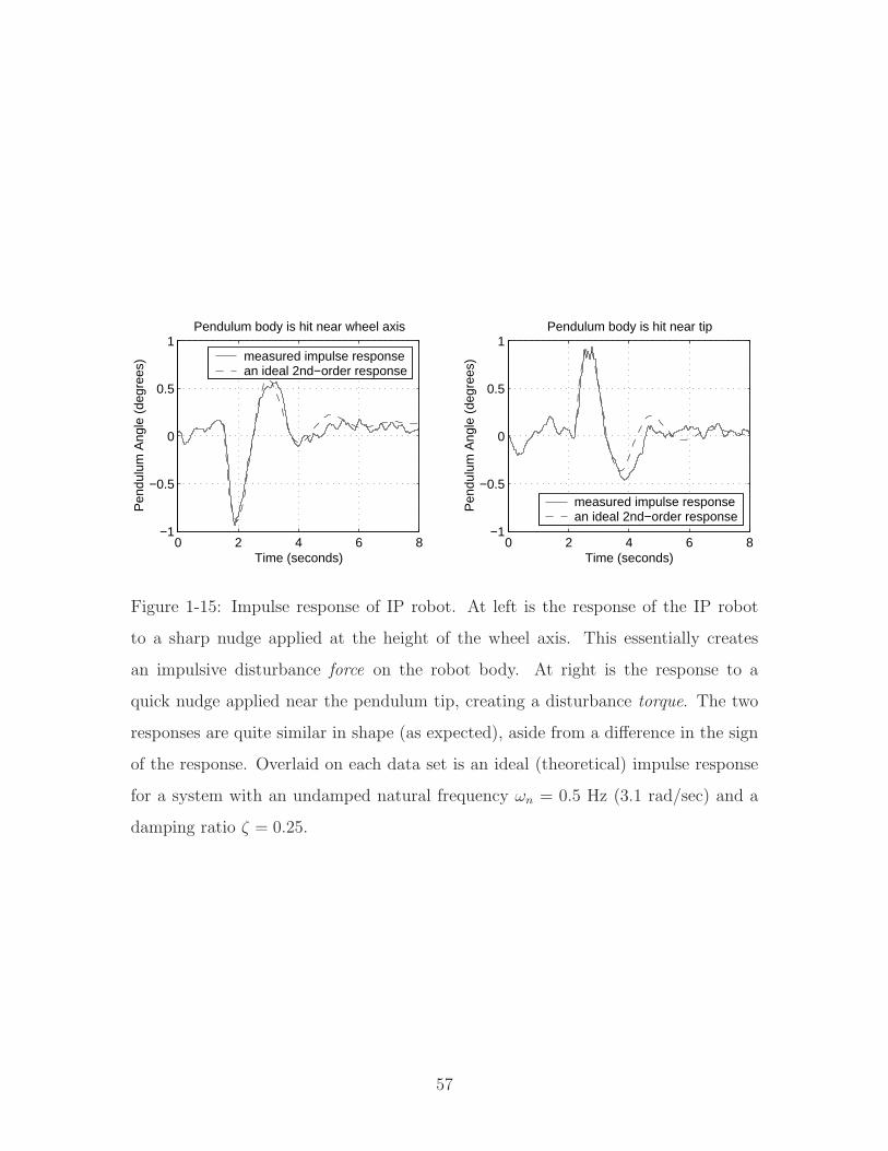
0 2 4 6 8−1

−0.5

0

0.5

1

Time (seconds)

Pen

dulu

m A

ngle

(de

gree

s)

Pendulum body is hit near wheel axis

measured impulse responsean ideal 2nd−order response

0 2 4 6 8−1

−0.5

0

0.5

1

Time (seconds)

Pen

dulu

m A

ngle

(de

gree

s)

Pendulum body is hit near tip

measured impulse responsean ideal 2nd−order response

Figure 1-15: Impulse response of IP robot. At left is the response of the IP robot

to a sharp nudge applied at the height of the wheel axis. This essentially creates

an impulsive disturbance force on the robot body. At right is the response to a

quick nudge applied near the pendulum tip, creating a disturbance torque. The two

responses are quite similar in shape (as expected), aside from a difference in the sign

of the response. Overlaid on each data set is an ideal (theoretical) impulse response

for a system with an undamped natural frequency ωn = 0.5 Hz (3.1 rad/sec) and a

damping ratio ζ = 0.25.

57

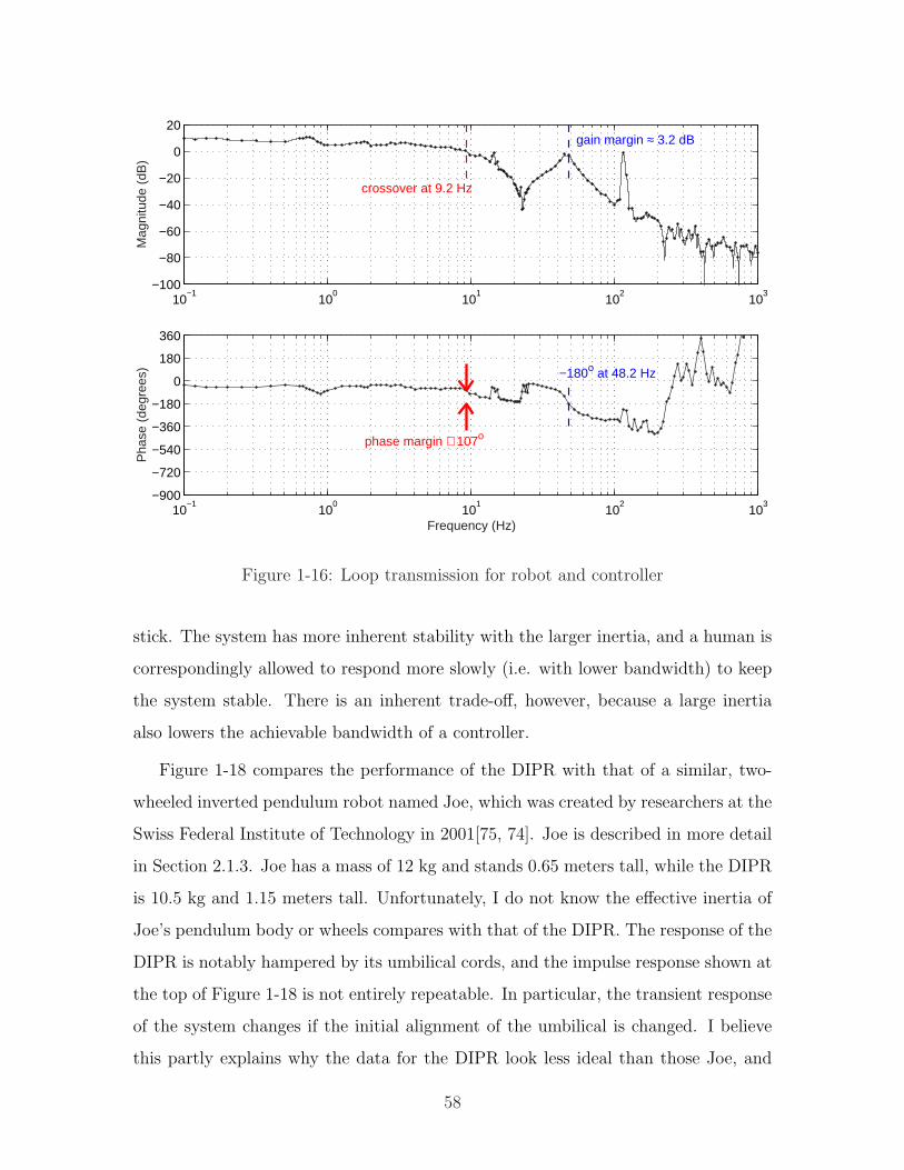
−4 −3 −2 −1 0 1 2 3 4−4

−3

−2

−1

0

1

Real

Imag

Nyquist Plot of LT (with LP filtering of commanded voltage)

phase margin ≅ 107o

gain margin ≅ 1.4

10−1

100

101

102

103

−100

−80

−60

−40

−20

0

20M

agni

tude

(dB

)

crossover at 9.2 Hz

gain margin ≈ 3.2 dB

10−1

100

101

102

103

−900

−720

−540

−360

−180

0

180

360

Frequency (Hz)

Pha

se (

degr

ees)


−180o at 48.2 Hz

Figure 1-16: Loop transmission for robot and controller

stick. The system has more inherent stability with the larger inertia, and a human is

correspondingly allowed to respond more slowly (i.e. with lower bandwidth) to keep

the system stable. There is an inherent trade-off, however, because a large inertia

also lowers the achievable bandwidth of a controller.

Figure 1-18 compares the performance of the DIPR with that of a similar, two-

wheeled inverted pendulum robot named Joe, which was created by researchers at the

Swiss Federal Institute of Technology in 2001[75, 74]. Joe is described in more detail

in Section 2.1.3. Joe has a mass of 12 kg and stands 0.65 meters tall, while the DIPR

is 10.5 kg and 1.15 meters tall. Unfortunately, I do not know the effective inertia of

Joe’s pendulum body or wheels compares with that of the DIPR. The response of the

DIPR is notably hampered by its umbilical cords, and the impulse response shown at

the top of Figure 1-18 is not entirely repeatable. In particular, the transient response

of the system changes if the initial alignment of the umbilical is changed. I believe

this partly explains why the data for the DIPR look less ideal than those Joe, and

58

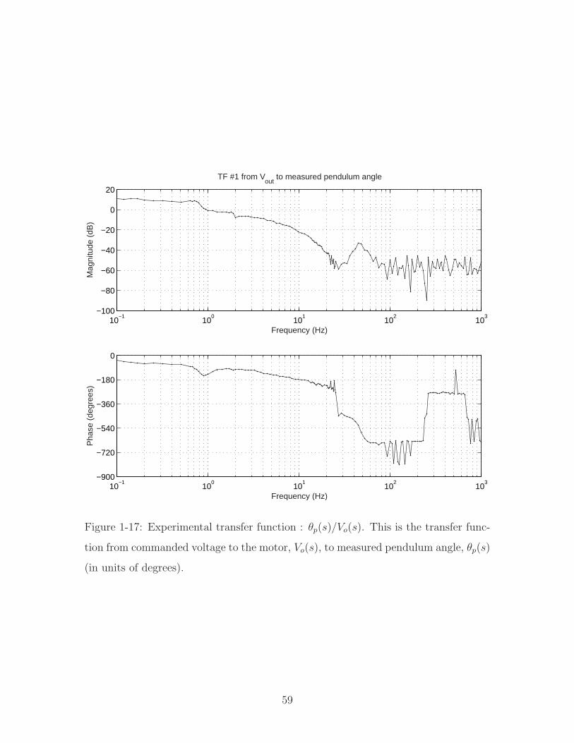
10−1

100

101

102

103

−100

−80

−60

−40

−20

0

20

TF #1 from Vout

to measured pendulum angle

Frequency (Hz)

Mag

nitu

de (

dB)

10−1

100

101

102

103

−900

−720

−540

−360

−180

0

Frequency (Hz)

Pha

se (

degr

ees)

Figure 1-17: Experimental transfer function : θp(s)/Vo(s). This is the transfer func-

tion from commanded voltage to the motor, Vo(s), to measured pendulum angle, θp(s)

(in units of degrees).

59

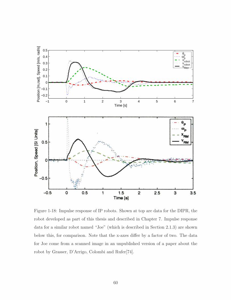
−1 0 1 2 3 4 5 6 7

−0.2

−0.1

0

0.1

0.2

0.3

0.4

0.5

Time [s]

Pos

ition

[m,r

ad],

Spe

ed [m

/s, r

ad/s

]

θpωpxrobotvrobotvfilter

Figure 1-18: Impulse response of IP robots. Shown at top are data for the DIPR, the

robot developed as part of this thesis and described in Chapter 7. Impulse response

data for a similar robot named “Joe” (which is described in Section 2.1.3) are shown

below this, for comparison. Note that the x-axes differ by a factor of two. The data

for Joe come from a scanned image in an unpublished version of a paper about the

robot by Grasser, D’Arrigo, Colombi and Rufer[74].

60

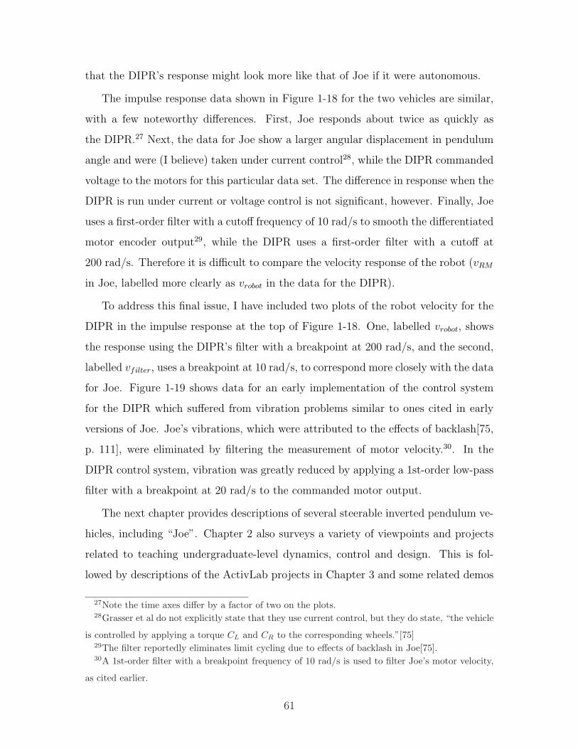
that the DIPR’s response might look more like that of Joe if it were autonomous.

The impulse response data shown in Figure 1-18 for the two vehicles are similar,

with a few noteworthy differences. First, Joe responds about twice as quickly as

the DIPR.27 Next, the data for Joe show a larger angular displacement in pendulum

angle and were (I believe) taken under current control28, while the DIPR commanded

voltage to the motors for this particular data set. The difference in response when the

DIPR is run under current or voltage control is not significant, however. Finally, Joe

uses a first-order filter with a cutoff frequency of 10 rad/s to smooth the differentiated

motor encoder output29, while the DIPR uses a first-order filter with a cutoff at

200 rad/s. Therefore it is difficult to compare the velocity response of the robot (vRM

in Joe, labelled more clearly as vrobot in the data for the DIPR).

To address this final issue, I have included two plots of the robot velocity for the

DIPR in the impulse response at the top of Figure 1-18. One, labelled vrobot, shows

the response using the DIPR’s filter with a breakpoint at 200 rad/s, and the second,

labelled vfilter, uses a breakpoint at 10 rad/s, to correspond more closely with the data

for Joe. Figure 1-19 shows data for an early implementation of the control system

for the DIPR which suffered from vibration problems similar to ones cited in early

versions of Joe. Joe’s vibrations, which were attributed to the effects of backlash[75,

p. 111], were eliminated by filtering the measurement of motor velocity.30. In the

DIPR control system, vibration was greatly reduced by applying a 1st-order low-pass

filter with a breakpoint at 20 rad/s to the commanded motor output.

The next chapter provides descriptions of several steerable inverted pendulum ve-

hicles, including “Joe”. Chapter 2 also surveys a variety of viewpoints and projects

related to teaching undergraduate-level dynamics, control and design. This is fol-

lowed by descriptions of the ActivLab projects in Chapter 3 and some related demos

27Note the time axes differ by a factor of two on the plots.28Grasser et al do not explicitly state that they use current control, but they do state, “the vehicle

is controlled by applying a torque CL and CR to the corresponding wheels.”[75]29The filter reportedly eliminates limit cycling due to effects of backlash in Joe[75].30A 1st-order filter with a breakpoint frequency of 10 rad/s is used to filter Joe’s motor velocity,

as cited earlier.

61

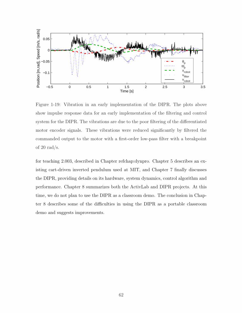
−0.5 0 0.5 1 1.5 2 2.5 3 3.5

−0.1

−0.05

0

0.05

Time [s]

Pos

ition

[m,r

ad],

Spe

ed [m

/s, r

ad/s

]

θpωpxrobotvfiltervrobot

Figure 1-19: Vibration in an early implementation of the DIPR. The plots above

show impulse response data for an early implementation of the filtering and control

system for the DIPR. The vibrations are due to the poor filtering of the differentiated

motor encoder signals. These vibrations were reduced significantly by filtered the

commanded output to the motor with a first-order low-pass filter with a breakpoint

of 20 rad/s.

for teaching 2.003, described in Chapter refchap:dynpro. Chapter 5 describes an ex-

isting cart-driven inverted pendulum used at MIT, and Chapter 7 finally discusses

the DIPR, providing details on its hardware, system dynamics, control algorithm and

performance. Chapter 8 summarizes both the ActivLab and DIPR projects. At this

time, we do not plan to use the DIPR as a classroom demo. The conclusion in Chap-

ter 8 describes some of the difficulties in using the DIPR as a portable classroom

demo and suggests improvements.

62

Chapter 2

Survey of Related Projects

This chapter reviews a variety of projects related to the demo inverted pendulum

robot (DIPR) (described in Chapter 7) and the ActivLab experiments (in Chap-

ter 3). The Segway and iBOT are both human transports which operate as inverted

pendulums. Both were direct inspirations for the design of the DIPR. In contrast,

the other projects described here were generally not direct influences. They are in-

stead included because they illustrate a variety of potential directions one can take

in accomplishing the two primary goals of this thesis: namely, (1) the creation of

an inverted pendulum robot and (2) the development of hands-on experiences that

both illustrate system dynamics and specifically provide a foundation for controls and

mechatronic design.

The control algorithms for the pendulum robots surveyed in this chapter are by

and large quite similar to one another and to the control strategy I implemented

for the robot discussed in Chapter 7. Specifically, most are essentially state-space

controllers that multiply some gain matrix, K, times the estimated state vector.

Figure 2-1, taken from a DEKA patent that appears to relate to both the Segway

and iBOT, shows a schematic of this structure.1

Paraphrasing Dean Kamen at a lecture on the iBOT at MIT in Fall of 2000,

1The patent describes several “embodiments” of inverted pendulum transportation devices, with

the passenger either seated (similar to the iBOT) or standing (as on the Segway), although none

look quite like either the Segway or iBOT.

63

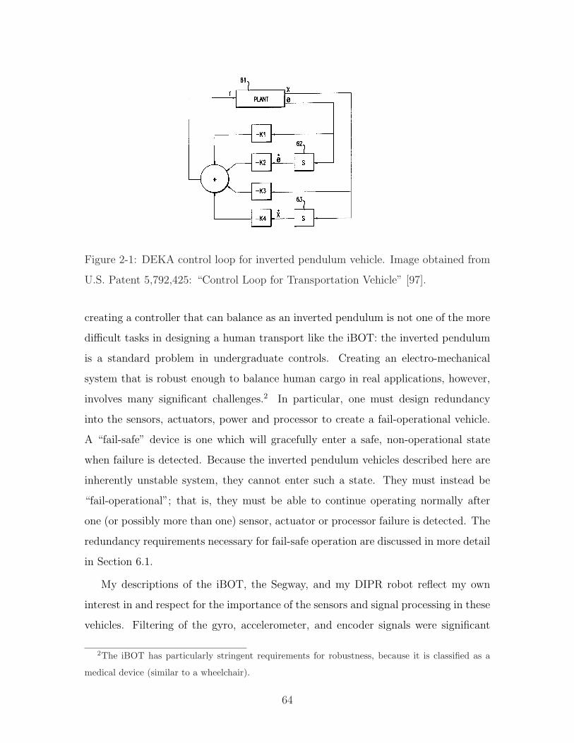
Figure 2-1: DEKA control loop for inverted pendulum vehicle. Image obtained from

U.S. Patent 5,792,425: “Control Loop for Transportation Vehicle” [97].

creating a controller that can balance as an inverted pendulum is not one of the more

difficult tasks in designing a human transport like the iBOT: the inverted pendulum

is a standard problem in undergraduate controls. Creating an electro-mechanical

system that is robust enough to balance human cargo in real applications, however,

involves many significant challenges.2 In particular, one must design redundancy

into the sensors, actuators, power and processor to create a fail-operational vehicle.

A “fail-safe” device is one which will gracefully enter a safe, non-operational state

when failure is detected. Because the inverted pendulum vehicles described here are

inherently unstable system, they cannot enter such a state. They must instead be

“fail-operational”; that is, they must be able to continue operating normally after

one (or possibly more than one) sensor, actuator or processor failure is detected. The

redundancy requirements necessary for fail-safe operation are discussed in more detail

in Section 6.1.

My descriptions of the iBOT, the Segway, and my DIPR robot reflect my own

interest in and respect for the importance of the sensors and signal processing in these

vehicles. Filtering of the gyro, accelerometer, and encoder signals were significant

2The iBOT has particularly stringent requirements for robustness, because it is classified as a

medical device (similar to a wheelchair).

64

issues in successfully controlling the DIPR, and the gyro was a substantial portion

of its total cost. MEMS gyros are beginning to provide a more affordable alternative

however. Over the past ten years, much of the research and advancement in MEMS

sensor technology has been motivated by the automotive industry, who have created

a substantial market for high-volume, low-cost accelerometers and gyros, used (for

instance) in triggering airbags and providing traction control, respectively. The iBOT

and Segway rely on rate gyros of this type.3

I discuss the current trends making MEMS gyros more accurate and cost-effective

in some detail, because the Segway and iBOT clearly demonstrate that these sensors

are an adequate alternative to the more expensive Watson VSG gyro I used. In other

words, I expect these gyros will find other applications, as they become even more

accurate. The issues involved in correction for gyro drift and failure detection are

fascinating, educational, and relevant to future technological developments. For all

these reasons, I suggest incorporating MEMS gyros into a mechatronic laboratory

project. Hopefully, the information in Sections 6.1, 6.2, and 7.1.5 makes a case for

this to the reader.

The second half of this chapter (Section 2.2) describes several projects at other

institutions which give students hands-on experiences relevant to system dynamics

and mechatronics. Note that Chapter 4 surveys a variety of potential projects tested

or considered in teaching 2.003: Modeling, Dynamics and Control I. The projects in

Chapter 4 generally consist of either alternatives to the present ActivLab laboratories

or complimentary in-class demos. In contrast, the projects described in Section 2.2

show various directions taken in teaching classes at other universities or in other

disciplines.

3The bias and rms noise figures for the CRS-03 MEMS gyro used in the Segway are roughly

25x greater (worse) than those for the Watson VSG (“vibrating structure gyro” with a cylindrical,

piezoelectric shell). The latter has a resolution of .025 o/s at a 100Hz BW and run-to-run bias

stability of 0.1 o/s. Silicon Sensing does not publicize the price for their MEMS sensor, but it is

almost certainly less than 1/25 the $1000 price of the higher-quality Watson gyro [40, 85, 19, 24].

65

2.1 Inverted Pendulum Vehicles

As mentioned in Chapter 1, the DIPR robot was inspired by the iBOT and Segway

human transports. Since both devices balance a human being in an unstable pendu-

lum equilibrium position, each must have a high level of robustness and redundancy.

Sections 2.1.1, 2.1.2 and 6.1 focus on these unique and demanding requirements.

While working on this project, I discovered a group at the Swiss Federal Insti-

tute of Technology had already built an autonomous, steerable robot (named “Joe”)

which is very similar to the one planned for my own project [75]. I include data in

Section 2.1.3 comparing the performance of Joe to that of the DIPR in Section 1.4.3

of the introduction. The umbilical cords on the DIPR affect its response significantly.

For instance, the transient response of the system changes if the initial alignment of

the umbilical is changed. I suspect making the DIPR autonomous may make help

the DIPR perform comparably. Section 2.1.3 summarizes the design of and results

for Joe.4

Many robot enthusiasts and clubs have clearly been inspired by Dean Kamen’s

Segway human transport. I learned about each of the inverted pendulum robots de-

scribed in the Sections 2.1.4, 2.1.5 and 2.1.6 while finishing my thesis in February,

2003. They are of interest because together they survey a fairly wide range of com-

plexity both in construction, sensor capabilities, and control algorithms. Finally, I

mention two robot unicycles in Section 2.1.7. A robotic unicycle is quite impressive,

since it must actively stabilize its pitch (like the Segway) and roll (i.e. lateral stability,

which is provided passively on the Segway-type vehicles by having two side-by-side

wheels) to remain upright. Each of the two unicycles described can even steer to

some extent (thereby controlling yaw) by pivoting an reaction mass mounted within

the vehicle.

4As of this writing, the Joe’s creators maintain a website with more information about their

device. This site also contains images and movies of the robot. http://leiwww.epfl.ch/joe/

66

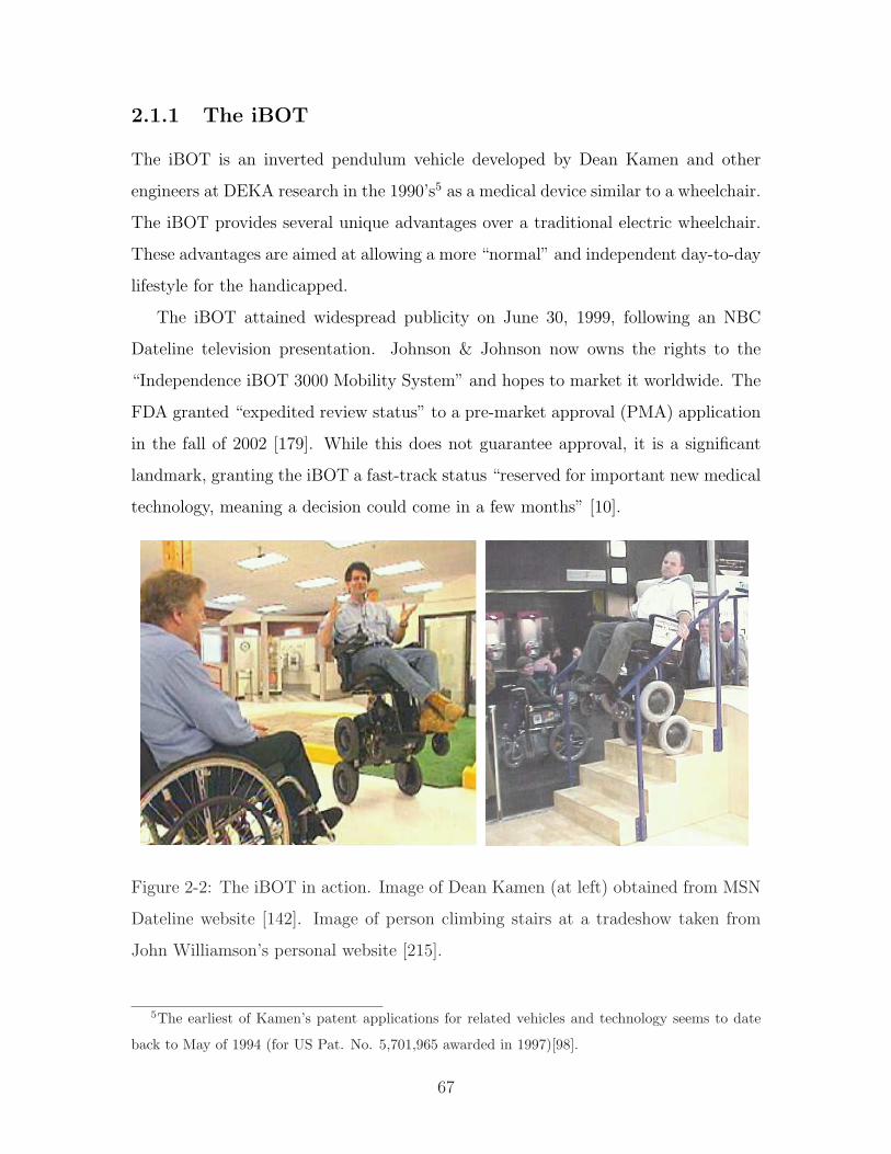
2.1.1 The iBOT

The iBOT is an inverted pendulum vehicle developed by Dean Kamen and other

engineers at DEKA research in the 1990’s5 as a medical device similar to a wheelchair.

The iBOT provides several unique advantages over a traditional electric wheelchair.

These advantages are aimed at allowing a more “normal” and independent day-to-day

lifestyle for the handicapped.

The iBOT attained widespread publicity on June 30, 1999, following an NBC

Dateline television presentation. Johnson & Johnson now owns the rights to the

“Independence iBOT 3000 Mobility System” and hopes to market it worldwide. The

FDA granted “expedited review status” to a pre-market approval (PMA) application

in the fall of 2002 [179]. While this does not guarantee approval, it is a significant

landmark, granting the iBOT a fast-track status “reserved for important new medical

technology, meaning a decision could come in a few months” [10].

Figure 2-2: The iBOT in action. Image of Dean Kamen (at left) obtained from MSN

Dateline website [142]. Image of person climbing stairs at a tradeshow taken from

John Williamson’s personal website [215].

5The earliest of Kamen’s patent applications for related vehicles and technology seems to date

back to May of 1994 (for US Pat. No. 5,701,965 awarded in 1997)[98].

67

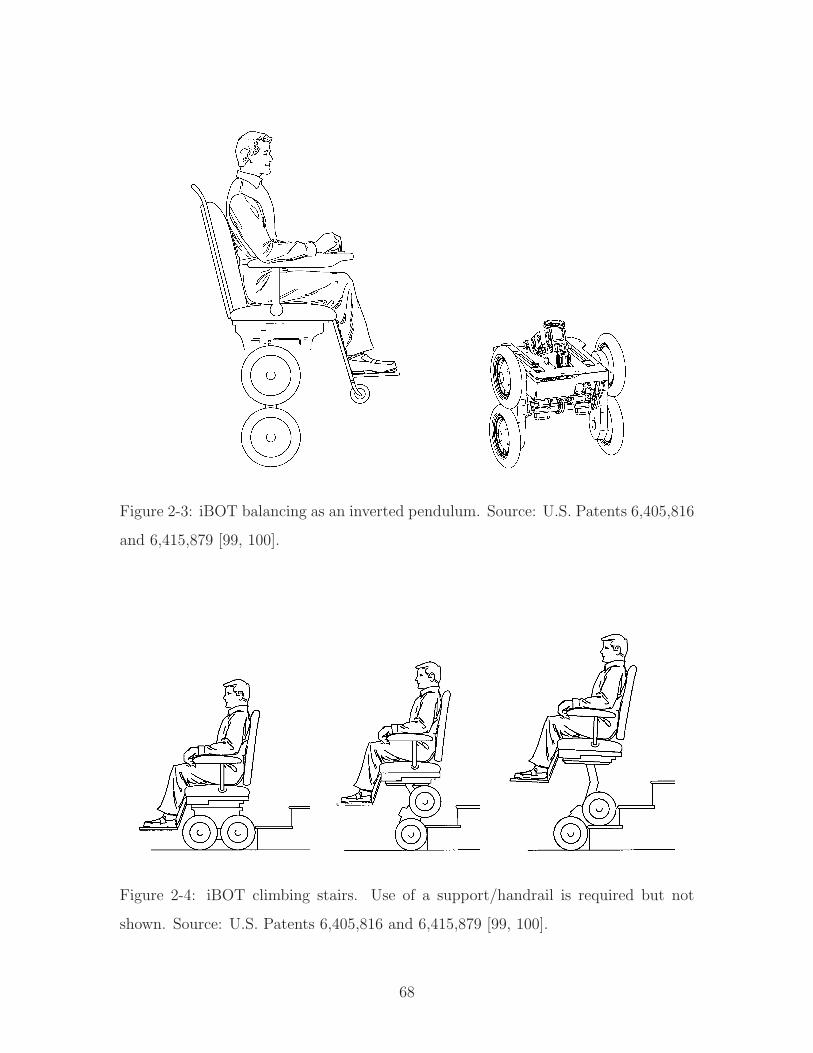
Figure 2-3: iBOT balancing as an inverted pendulum. Source: U.S. Patents 6,405,816

and 6,415,879 [99, 100].

Figure 2-4: iBOT climbing stairs. Use of a support/handrail is required but not

shown. Source: U.S. Patents 6,405,816 and 6,415,879 [99, 100].

68

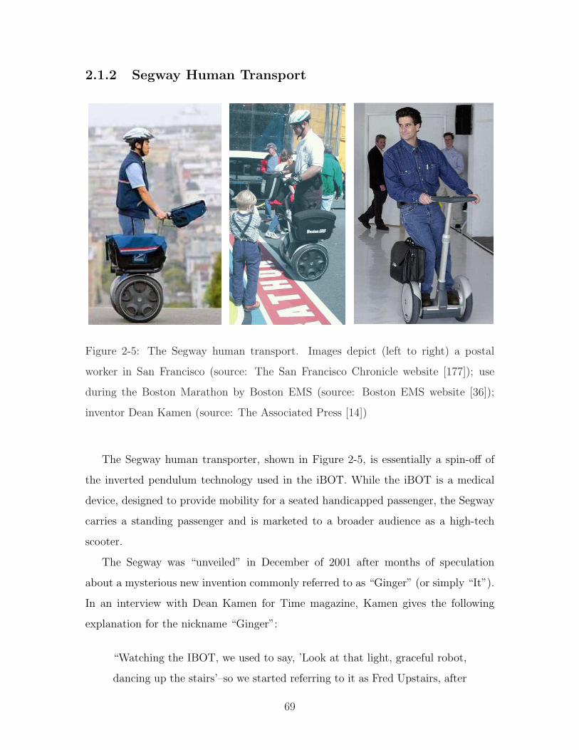
2.1.2 Segway Human Transport

Figure 2-5: The Segway human transport. Images depict (left to right) a postal

worker in San Francisco (source: The San Francisco Chronicle website [177]); use

during the Boston Marathon by Boston EMS (source: Boston EMS website [36]);

inventor Dean Kamen (source: The Associated Press [14])

The Segway human transporter, shown in Figure 2-5, is essentially a spin-off of

the inverted pendulum technology used in the iBOT. While the iBOT is a medical

device, designed to provide mobility for a seated handicapped passenger, the Segway

carries a standing passenger and is marketed to a broader audience as a high-tech

scooter.

The Segway was “unveiled” in December of 2001 after months of speculation

about a mysterious new invention commonly referred to as “Ginger” (or simply “It”).

In an interview with Dean Kamen for Time magazine, Kamen gives the following

explanation for the nickname “Ginger”:

“Watching the IBOT, we used to say, ’Look at that light, graceful robot,

dancing up the stairs’–so we started referring to it as Fred Upstairs, after

69

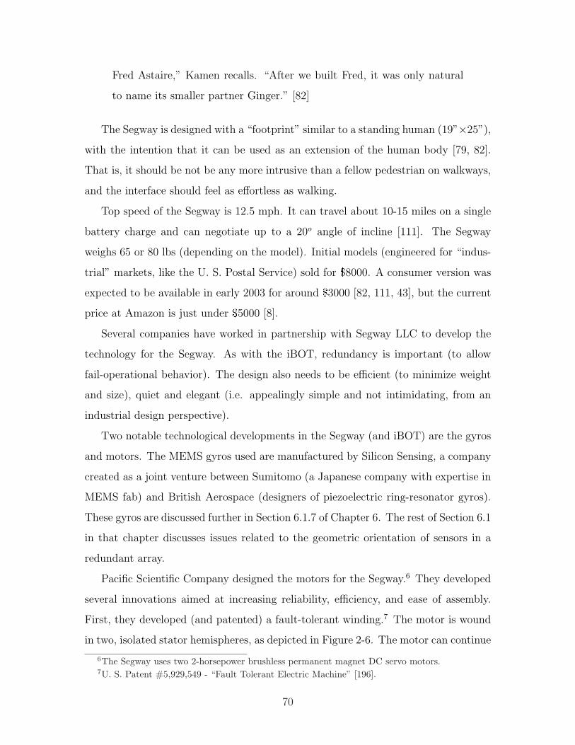
Fred Astaire,” Kamen recalls. “After we built Fred, it was only natural

to name its smaller partner Ginger.” [82]

The Segway is designed with a “footprint” similar to a standing human (19”×25”),

with the intention that it can be used as an extension of the human body [79, 82].

That is, it should be not be any more intrusive than a fellow pedestrian on walkways,

and the interface should feel as effortless as walking.

Top speed of the Segway is 12.5 mph. It can travel about 10-15 miles on a single

battery charge and can negotiate up to a 20o angle of incline [111]. The Segway

weighs 65 or 80 lbs (depending on the model). Initial models (engineered for “indus-

trial” markets, like the U. S. Postal Service) sold for $8000. A consumer version was

expected to be available in early 2003 for around $3000 [82, 111, 43], but the current

price at Amazon is just under $5000 [8].

Several companies have worked in partnership with Segway LLC to develop the

technology for the Segway. As with the iBOT, redundancy is important (to allow

fail-operational behavior). The design also needs to be efficient (to minimize weight

and size), quiet and elegant (i.e. appealingly simple and not intimidating, from an

industrial design perspective).

Two notable technological developments in the Segway (and iBOT) are the gyros

and motors. The MEMS gyros used are manufactured by Silicon Sensing, a company

created as a joint venture between Sumitomo (a Japanese company with expertise in

MEMS fab) and British Aerospace (designers of piezoelectric ring-resonator gyros).

These gyros are discussed further in Section 6.1.7 of Chapter 6. The rest of Section 6.1

in that chapter discusses issues related to the geometric orientation of sensors in a

redundant array.

Pacific Scientific Company designed the motors for the Segway.6 They developed

several innovations aimed at increasing reliability, efficiency, and ease of assembly.

First, they developed (and patented) a fault-tolerant winding.7 The motor is wound

in two, isolated stator hemispheres, as depicted in Figure 2-6. The motor can continue

6The Segway uses two 2-horsepower brushless permanent magnet DC servo motors.7U. S. Patent #5,929,549 - “Fault Tolerant Electric Machine” [196].

70

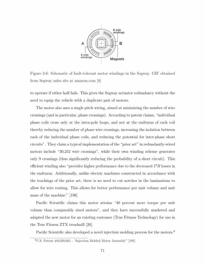
Figure 2-6: Schematic of fault-tolerant motor windings in the Segway. GIF obtained

from Segway sales site at amazon.com [8]

to operate if either half fails. This gives the Segway actuator redundancy without the

need to equip the vehicle with a duplicate pair of motors.

The motor also uses a single pitch wiring, aimed at minimizing the number of wire

crossings (and in particular, phase crossings). According to patent claims, “individual

phase coils cross only at the intra-pole loops, and not at the endturns of each coil

thereby reducing the number of phase wire crossings, increasing the isolation between

each of the individual phase coils, and reducing the potential for inter-phase short

circuits”. They claim a typical implementation of the “prior art” in redundantly-wired

motors include “30,252 wire crossings”, while their own winding scheme generates

only 9 crossings (thus significantly reducing the probability of a short circuit). This

efficient winding also “provides higher performance due to the decreased I2R losses in

the endturns. Additionally, unlike electric machines constructed in accordance with

the teachings of the prior art, there is no need to cut notches in the laminations to

allow for wire routing. This allows for better performance per unit volume and unit

mass of the machine.” [196]

Pacific Scientific claims this motor attains “40 percent more torque per unit

volume than comparably sized motors”, and they have successfully marketed and

adapted the new motor for an existing customer (True Fitness Technology) for use in

the True Fitness ZTX treadmill [20].

Pacific Scientific also developed a novel injection molding process for the motors.8

8U.S. Patent #6,020,661 - “Injection Molded Motor Assembly” [195]

71

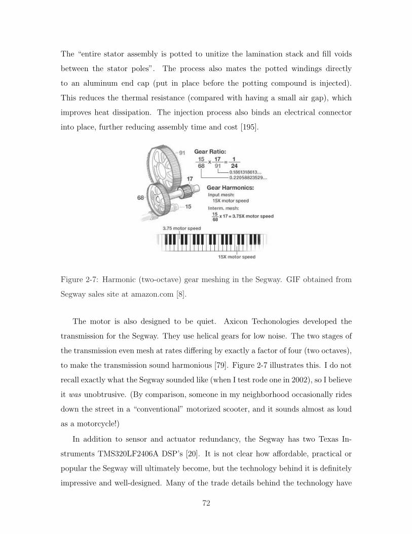
The “entire stator assembly is potted to unitize the lamination stack and fill voids

between the stator poles”. The process also mates the potted windings directly

to an aluminum end cap (put in place before the potting compound is injected).

This reduces the thermal resistance (compared with having a small air gap), which

improves heat dissipation. The injection process also binds an electrical connector

into place, further reducing assembly time and cost [195].

Figure 2-7: Harmonic (two-octave) gear meshing in the Segway. GIF obtained from

Segway sales site at amazon.com [8].

The motor is also designed to be quiet. Axicon Techonologies developed the

transmission for the Segway. They use helical gears for low noise. The two stages of

the transmission even mesh at rates differing by exactly a factor of four (two octaves),

to make the transmission sound harmonious [79]. Figure 2-7 illustrates this. I do not

recall exactly what the Segway sounded like (when I test rode one in 2002), so I believe

it was unobtrusive. (By comparison, someone in my neighborhood occasionally rides

down the street in a “conventional” motorized scooter, and it sounds almost as loud

as a motorcycle!)

In addition to sensor and actuator redundancy, the Segway has two Texas In-

struments TMS320LF2406A DSP’s [20]. It is not clear how affordable, practical or

popular the Segway will ultimately become, but the technology behind it is definitely

impressive and well-designed. Many of the trade details behind the technology have

72

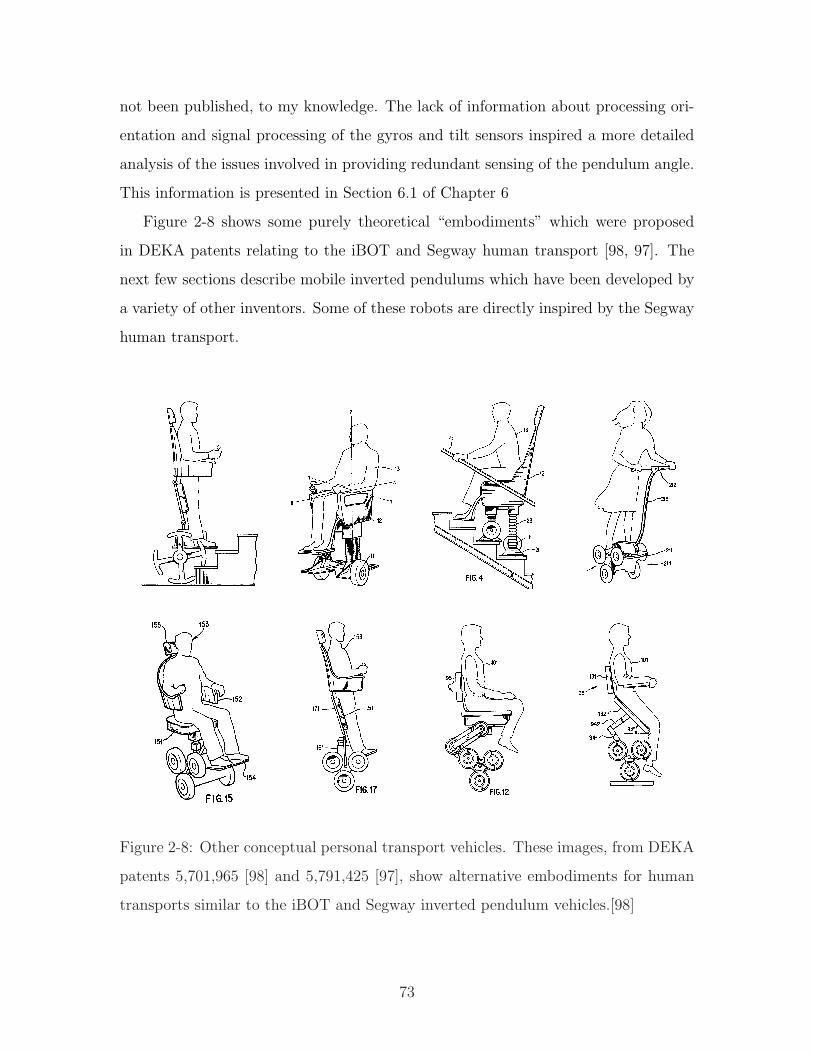
not been published, to my knowledge. The lack of information about processing ori-

entation and signal processing of the gyros and tilt sensors inspired a more detailed

analysis of the issues involved in providing redundant sensing of the pendulum angle.

This information is presented in Section 6.1 of Chapter 6

Figure 2-8 shows some purely theoretical “embodiments” which were proposed

in DEKA patents relating to the iBOT and Segway human transport [98, 97]. The

next few sections describe mobile inverted pendulums which have been developed by

a variety of other inventors. Some of these robots are directly inspired by the Segway

human transport.

Figure 2-8: Other conceptual personal transport vehicles. These images, from DEKA

patents 5,701,965 [98] and 5,791,425 [97], show alternative embodiments for human

transports similar to the iBOT and Segway inverted pendulum vehicles.[98]

73

2.1.3 “Joe”: An Autonomous IP Robot

The Industrial Electronic Laboratory at the Swiss Federal Institute of Technology

has created an autonomous inverted pendulum similar to my own “DIPR” robot,

described in Chapter 7 of this thesis. “Joe”, shown in Figure 2-9, uses two decoupled

state-space controllers to control the 3-DOF system. One controls the upright stability

(pitch of the pendulum from vertical) and the second is used to drive the vehicle

(controlling both forward velocity and yaw about the vertical axis). The vehicle is

not “self-standing”. Sensor readings are reset at each start-up, with the pendulum

arm resting on the ground. The vehicle must then be lifted close to its upright

equilibrium to begin balancing.

The upright vehicle stands just over two feet high, and weighs approximately 26

lbs. Its maximum speed is 3.4 mph, which is about human walking speed. The

controller is implemented autonomously on the robot using a DSP board designed in-

house by the Industrial Electronics Lab group. A battery is mounted on Joe’s steel

pendulum and provides enough power for about one hour of driving. The vehicle

receives steering inputs from a human via remote control.

Joe has two actuators and three sensors. Each wheel is mounted directly to the

output shaft of a planetary gearbox on each of two DC motors, powered through on-

board power amplifiers. The sensors are the two incremental encoders on the motors

and a rate gyroscope which measures the angular velocity (pitch) of the chassis. The

gyro can measure a maximum velocity of 100o/s. The encoders measure the rotation

of the motor and not of gearbox. The position of the wheel is therefore not measured

directly. Backlash in the gearbox consequently resulted in limit cycling which excited

significant mechanical resonance in initial implementations of Joe’s controller. The

Lausanne group eliminated the worst of the effects of backlash by filtering their speed

measurement with a pole at 10 rad/s.

Limit cycling was also a significant problem in the initial (state-space) control

system for the “demo inverted pendulum robot” (DIPR) presented in Chapter 7.

This problem was adequately addressed by implementing an inner, velocity loop in

74

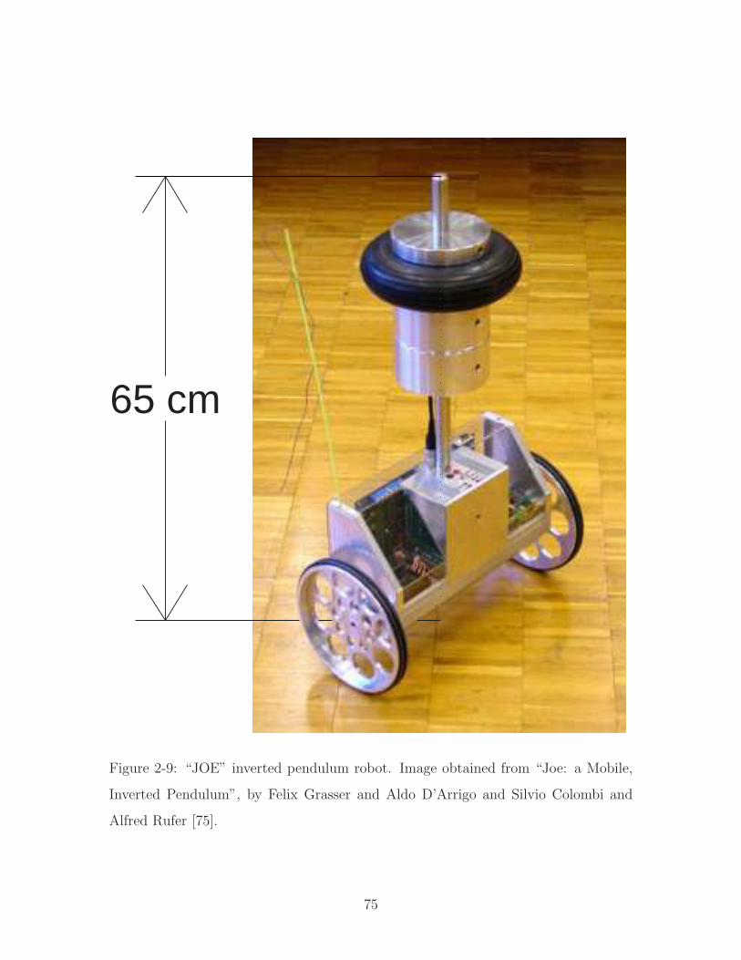
65 cm

Figure 2-9: “JOE” inverted pendulum robot. Image obtained from “Joe: a Mobile,

Inverted Pendulum”, by Felix Grasser and Aldo D’Arrigo and Silvio Colombi and

Alfred Rufer [75].

75

the controller for the robot. Section 7.7 describes these issues in controller design in

much more detail.

Drift is always an issue when obtaining angular position from a rate gyro. There

is a DC bias to the rate gyro output at zero velocity which will change due both to

environmental effects (temperature, vibration, humidity, etc) and to small changes

in the sensor itself (“aging”). This bias results in a ramping error in angle when the

velocity signal is integrated to obtain a position measurement. Drift can be elimi-

nated by blending the high frequency gyro measurement with a low frequency sensor

measurement of angle which is not prone to ramping error. Section 6.2 describes how

a 2-axis accelerometer is used to compensate for drift in the DIPR.

Joe’s creators acknowledge the problem of gyro drift briefly and seem to deal with

it in two ways. First, the gyroscope is recalibrated at each start-up, eliminating run-

to-run changes in bias at zero velocity. Day to day changes in bias will tend to be

more significant than those seen over the course of an hour or two, as illustrated in

the data in Figure 6-16 on page 300. Figure 7-20 on page 347 demonstrates how the

bias is particular apt to drift as it literally “warms up” during the first few minutes

after it is powered up.

Second, Joe’s in-run drift will have the effect of a ramping disturbance angle input

to the system. The vehicle will compensate by starting to roll forward (or backward)

as it attempts to catch itself from falling. The one-hour battery life limits the total

drift possible, and presumably, a human driver can compensate9 for the drift by

adjusting the velocity command to the robot from the remote controller.10

9Perhaps subconsciously!10No details are given to quantify the magnitude of the drift seen in the vehicle.

76

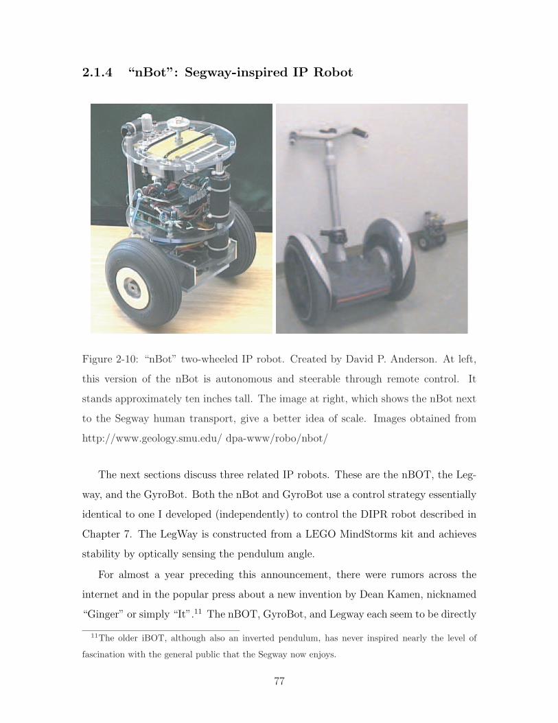
2.1.4 “nBot”: Segway-inspired IP Robot

Figure 2-10: “nBot” two-wheeled IP robot. Created by David P. Anderson. At left,

this version of the nBot is autonomous and steerable through remote control. It

stands approximately ten inches tall. The image at right, which shows the nBot next

to the Segway human transport, give a better idea of scale. Images obtained from

http://www.geology.smu.edu/ dpa-www/robo/nbot/

The next sections discuss three related IP robots. These are the nBOT, the Leg-

way, and the GyroBot. Both the nBot and GyroBot use a control strategy essentially

identical to one I developed (independently) to control the DIPR robot described in

Chapter 7. The LegWay is constructed from a LEGO MindStorms kit and achieves

stability by optically sensing the pendulum angle.

For almost a year preceding this announcement, there were rumors across the

internet and in the popular press about a new invention by Dean Kamen, nicknamed

“Ginger” or simply “It”.11 The nBOT, GyroBot, and Legway each seem to be directly

11The older iBOT, although also an inverted pendulum, has never inspired nearly the level of

fascination with the general public that the Segway now enjoys.

77

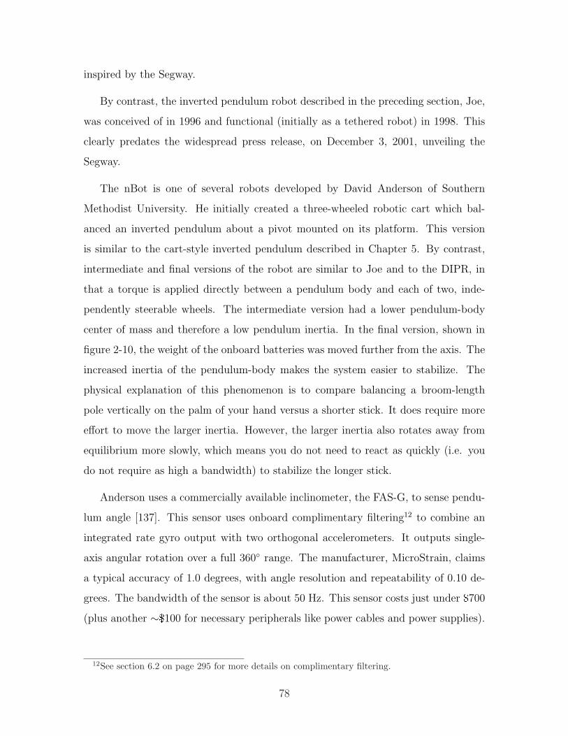
inspired by the Segway.

By contrast, the inverted pendulum robot described in the preceding section, Joe,

was conceived of in 1996 and functional (initially as a tethered robot) in 1998. This

clearly predates the widespread press release, on December 3, 2001, unveiling the

Segway.

The nBot is one of several robots developed by David Anderson of Southern

Methodist University. He initially created a three-wheeled robotic cart which bal-

anced an inverted pendulum about a pivot mounted on its platform. This version

is similar to the cart-style inverted pendulum described in Chapter 5. By contrast,

intermediate and final versions of the robot are similar to Joe and to the DIPR, in

that a torque is applied directly between a pendulum body and each of two, inde-

pendently steerable wheels. The intermediate version had a lower pendulum-body

center of mass and therefore a low pendulum inertia. In the final version, shown in

figure 2-10, the weight of the onboard batteries was moved further from the axis. The

increased inertia of the pendulum-body makes the system easier to stabilize. The

physical explanation of this phenomenon is to compare balancing a broom-length

pole vertically on the palm of your hand versus a shorter stick. It does require more

effort to move the larger inertia. However, the larger inertia also rotates away from

equilibrium more slowly, which means you do not need to react as quickly (i.e. you

do not require as high a bandwidth) to stabilize the longer stick.

Anderson uses a commercially available inclinometer, the FAS-G, to sense pendu-

lum angle [137]. This sensor uses onboard complimentary filtering12 to combine an

integrated rate gyro output with two orthogonal accelerometers. It outputs single-

axis angular rotation over a full 360 range. The manufacturer, MicroStrain, claims

a typical accuracy of 1.0 degrees, with angle resolution and repeatability of 0.10 de-

grees. The bandwidth of the sensor is about 50 Hz. This sensor costs just under $700

(plus another ∼$100 for necessary peripherals like power cables and power supplies).

12See section 6.2 on page 295 for more details on complimentary filtering.

78

The control strategy used for the nBot can be summarized as:

Vx = K1 θp,x + K2 [θp,x − θp,x−1] + K3θm,x + K4 [θm,x − θm,x−1] (2.1)

≈ K1 θp,x + K2 θp,x ·∆t + K3 θm,x + K4 θm,x ·∆t (2.2)

where θp,x and θp,x−1 are the pendulum angles away from vertical at the current

and previous algorithm step, respectively, and θm represents the averaged angle of

rotation of each of the two motors as compared with the commanded wheel rotation.

A corresponding notation is used to describe angular velocities. Here, ∆t is the

controller sampling interval. The microcontroller used is the 68HC11-based Handy

Board (described in Section 2.4.1 on page 120). The commanded voltage for each

motor is sent to an H-bridge which outputs an amplified pwm signal. Note that the

angular velocities of the pendulum (measured with the FAS-G) and motor rotation

are estimated simply by subtracting the last measured position from the current

position.13 The algorithm executes 25 times per second (i.e. a step size of ∆t =

40ms).

This control algorithm is similar to the one I use to control the DIPR inverted

pendulum robot, although the sensing is different in a few ways. First, the pendulum’s

angular rate is detected directly from the rate gyro. The rate gyro and accelerometer

signals are blended inside the Simulink controller, not onboard the sensor itself. The

DC gyro offset bias can be reset automatically at any time (when the angular velocity

of the pendulum is zero), to improve measurement of the pendulum angle. Also, the

motor encoder signals of the DIPR are filtered a bit more to provide a smoother

velocity signal. (The DIPR uses a first-order discrete-time filter with a bandwidth of

50 Hz to smooth the quantized estimate of motor velocity.)

13The FAS-G sensor can output either angle or angular rate, but surprisingly, it cannot output

both simultaneously.

79

2.1.5 “LegWay”: Mindstorms Robot with Single-Sensor Bal-

ancing

The “LegWay” inverted pendulum robot, shown in Figure 2-11, is notable because

it balances by using an optical sensor instead of a gyro [80]. The optical sensor

sends out pulses of light (directed downward, toward the floor) and outputs a value

between 0 and 100 to indicate the level of reflected light it receives. The output value

is a function of the distance, angle, color and reflectivity of the floor. The robot is

designed to operate on a flat, level, monochromatic (white) surface, however, so the

sensor works well as a distance measurement.14 For small tilt angles, the relationship

between this distance measurement and the angle of tilt will be approximately linear

(sin θ ≈ θ), and the sensor output therefore corresponds to the relative angle between

the robot axis and the normal to the floor. For a flat floor, this provides an absolute

measurement of pendulum angle without the bias issues of a gyro.

The optical sensor used in the LegWay was manufactured by a company called

“HiTechnic”, which marketed a variety of robotic sensors compatible with the Lego

MindStorms line.15 The company claims their EOPD (electro-optical proximity de-

tector) light sensor are “up to 50 times more sensitive than the standard Lego light

sensor” [84] by compensating for ambient light. (The sensors sold for about $40 each.)

Steve Hassenplug created the LegWay, and he designed it as a line-following robot.

Note in Figure 2-11 that the Legway is designed with two light sensors, side-by-side.

If one of the sensors passes over the (black) path line, its output will drop to zero (or

nearly zero). Steve’s control algorithm tests for such a “blackout” (a signal less than

3 on the 0-100 scale) of either sensor. If no blackout is detected, the robot averages

to the sensor outputs and sets both motors in unison to balance the robot at some

14One would expect the intensity of the reflected light to be inversely proportional to distance

(intensity = reflectance / distance). The sensor output is substantially linear with distance over a

limited range, however, according to the data HiTechnic provide on their website.15Apparently the market for Lego-specific sensors was not particularly profitable. HiTechnic

stopped manufacturing Lego-compatible sensors around April of 2003, saying they will now con-

centrate on “developing technology for industry” [84].

80

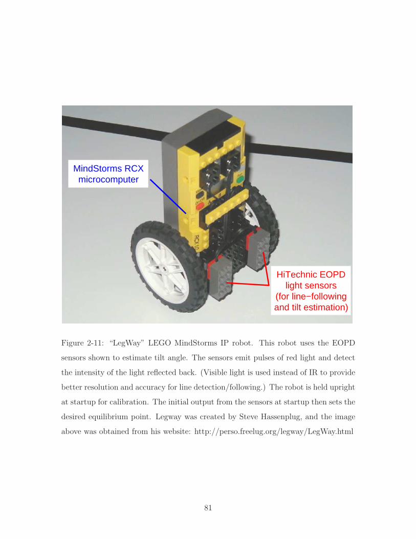
HiTechnic EOPD

microcomputer

and tilt estimation)

light sensors

MindStorms RCX

(for line−following

Figure 2-11: “LegWay” LEGO MindStorms IP robot. This robot uses the EOPD

sensors shown to estimate tilt angle. The sensors emit pulses of red light and detect

the intensity of the light reflected back. (Visible light is used instead of IR to provide

better resolution and accuracy for line detection/following.) The robot is held upright

at startup for calibration. The initial output from the sensors at startup then sets the

desired equilibrium point. Legway was created by Steve Hassenplug, and the image

above was obtained from his website: http://perso.freelug.org/legway/LegWay.html

81

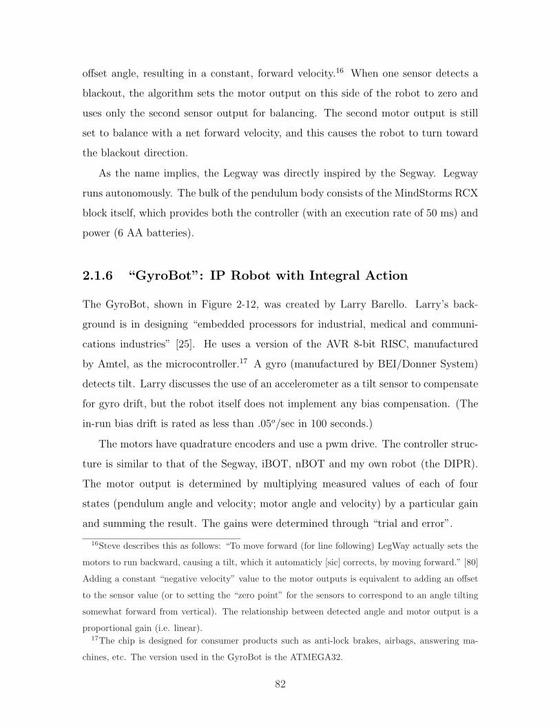
offset angle, resulting in a constant, forward velocity.16 When one sensor detects a

blackout, the algorithm sets the motor output on this side of the robot to zero and

uses only the second sensor output for balancing. The second motor output is still

set to balance with a net forward velocity, and this causes the robot to turn toward

the blackout direction.

As the name implies, the Legway was directly inspired by the Segway. Legway

runs autonomously. The bulk of the pendulum body consists of the MindStorms RCX

block itself, which provides both the controller (with an execution rate of 50 ms) and

power (6 AA batteries).

2.1.6 “GyroBot”: IP Robot with Integral Action

The GyroBot, shown in Figure 2-12, was created by Larry Barello. Larry’s back-

ground is in designing “embedded processors for industrial, medical and communi-

cations industries” [25]. He uses a version of the AVR 8-bit RISC, manufactured

by Amtel, as the microcontroller.17 A gyro (manufactured by BEI/Donner System)

detects tilt. Larry discusses the use of an accelerometer as a tilt sensor to compensate

for gyro drift, but the robot itself does not implement any bias compensation. (The

in-run bias drift is rated as less than .05o/sec in 100 seconds.)

The motors have quadrature encoders and use a pwm drive. The controller struc-

ture is similar to that of the Segway, iBOT, nBOT and my own robot (the DIPR).

The motor output is determined by multiplying measured values of each of four

states (pendulum angle and velocity; motor angle and velocity) by a particular gain

and summing the result. The gains were determined through “trial and error”.

16Steve describes this as follows: “To move forward (for line following) LegWay actually sets the

motors to run backward, causing a tilt, which it automaticly [sic] corrects, by moving forward.” [80]

Adding a constant “negative velocity” value to the motor outputs is equivalent to adding an offset

to the sensor value (or to setting the “zero point” for the sensors to correspond to an angle tilting

somewhat forward from vertical). The relationship between detected angle and motor output is a

proportional gain (i.e. linear).17The chip is designed for consumer products such as anti-lock brakes, airbags, answering ma-

chines, etc. The version used in the GyroBot is the ATMEGA32.

82

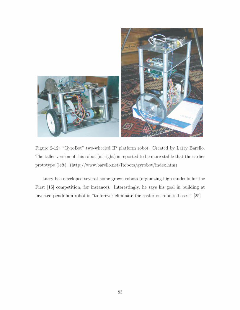
Figure 2-12: “GyroBot” two-wheeled IP platform robot. Created by Larry Barello.

The taller version of this robot (at right) is reported to be more stable that the earlier

prototype (left). (http://www.barello.net/Robots/gyrobot/index.htm)

Larry has developed several home-grown robots (organizing high students for the

First [16] competition, for instance). Interestingly, he says his goal in building at

inverted pendulum robot is “to forever eliminate the caster on robotic bases.” [25]

83

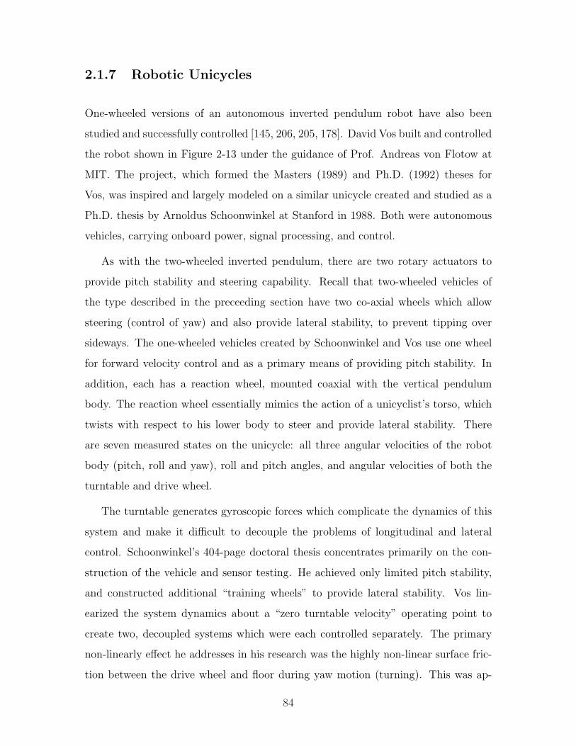
2.1.7 Robotic Unicycles

One-wheeled versions of an autonomous inverted pendulum robot have also been

studied and successfully controlled [145, 206, 205, 178]. David Vos built and controlled

the robot shown in Figure 2-13 under the guidance of Prof. Andreas von Flotow at

MIT. The project, which formed the Masters (1989) and Ph.D. (1992) theses for

Vos, was inspired and largely modeled on a similar unicycle created and studied as a

Ph.D. thesis by Arnoldus Schoonwinkel at Stanford in 1988. Both were autonomous

vehicles, carrying onboard power, signal processing, and control.

As with the two-wheeled inverted pendulum, there are two rotary actuators to

provide pitch stability and steering capability. Recall that two-wheeled vehicles of

the type described in the preceeding section have two co-axial wheels which allow

steering (control of yaw) and also provide lateral stability, to prevent tipping over

sideways. The one-wheeled vehicles created by Schoonwinkel and Vos use one wheel

for forward velocity control and as a primary means of providing pitch stability. In

addition, each has a reaction wheel, mounted coaxial with the vertical pendulum

body. The reaction wheel essentially mimics the action of a unicyclist’s torso, which

twists with respect to his lower body to steer and provide lateral stability. There

are seven measured states on the unicycle: all three angular velocities of the robot

body (pitch, roll and yaw), roll and pitch angles, and angular velocities of both the

turntable and drive wheel.

The turntable generates gyroscopic forces which complicate the dynamics of this

system and make it difficult to decouple the problems of longitudinal and lateral

control. Schoonwinkel’s 404-page doctoral thesis concentrates primarily on the con-

struction of the vehicle and sensor testing. He achieved only limited pitch stability,

and constructed additional “training wheels” to provide lateral stability. Vos lin-

earized the system dynamics about a “zero turntable velocity” operating point to

create two, decoupled systems which were each controlled separately. The primary

non-linearly effect he addresses in his research was the highly non-linear surface fric-

tion between the drive wheel and floor during yaw motion (turning). This was ap-

84

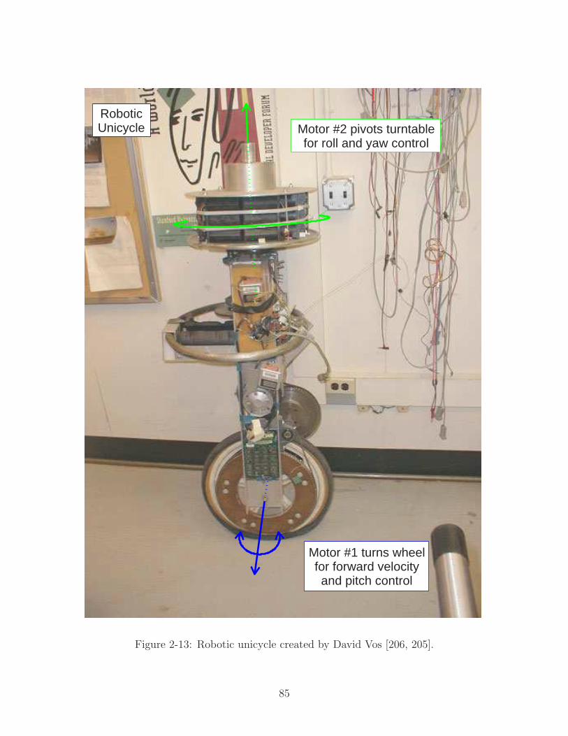
Motor #2 pivots turntablefor roll and yaw control

Unicycle

for forward velocityand pitch control

Robotic

Motor #1 turns wheel

Figure 2-13: Robotic unicycle created by David Vos [206, 205].

85

parently the most troubling aspect in control of the actual hardware. Summarizing

the one-wheeled system in the words of David Vos: “From the control point of view,

these dynamics present a particularly challenging problem in that all of the following

adjectives apply: unstable, non-minimum phase, time-varying and nonlinear” [206].

2.2 Hands-On Experiences in Undergraduate Sys-

tem Dynamics

The rest of this chapter surveys some creative approaches to undergraduate engineer-

ing education. In the paragraphs immediately following the present one, I outline

and compare the general philosophies driving the development of our ActivLab ex-

periment and the other projects described here. This is followed by a selective survey

(Section 2.2.1) of literature on learning and teaching engineering (particular dynam-

ics and design), with the goal of providing some thought-provoking perspectives on

education. Project descriptions begin in Section 2.2.2. Only the two projects de-

scribed in that section strictly involve the inclusion of a laboratory component in

an introductory dynamics course (E161 at Stanford); however, all of the remaining

programs have goals in common with our own development of the ActivLab projects

for MIT course 2.003 (Modeling Dynamics and Control I) and/or with the supple-

mentary classroom and lab demos for 2.003. The ActivLab hardware is described in

detail in Chapter 3, and that Chapter 4 includes several examples of lab and lecture

demonstrations for 2.003.

The ActivLab experiments and the related demos in dynamics we have developed

aim to reinforce students’ comprehension of dynamic systems with visual and tactile

experiences. We feel it is important to allow students to see and feel physical systems

for several reasons. First, we hope it will build a stronger intuition about dynamic

systems. For instance, students can apply forces to a system by hand and observe

first-hand the effects of varying physical properties such as viscous damping or inertia.

Such intuition is highly useful for applying knowledge in dynamics to later course work

86

in mechanical design or controls, and in engineering practice.

Hands-on laboratories and demos also promote curiosity and exploration. We

encourage students to poke and prod most of the hardware, both to lower their

inhibitions about “playing with” labware and to encourage them to explore (or at

least to note) anomalous behaviors in “real world” systems. Likewise, well-designed

classroom demos generally illustrate specific phenomena, but they are also intended

to spark broader interest in a subject.

The projects described in the remainder of this chapter aim both to reinforce an

understanding of dynamic systems and to foster interest in topics like mechatronics,

robotics and modeling of physical systems for which knowledge of dynamic systems

is critical. The examples below are certainly not comprehensive. My aim is to survey

a variety of approaches and thereby provide the reader with some reference points to

compare with our efforts in restructuring 2.003.

For instance, we felt it was particularly important to give students real labware and

to encourage them to explore and to become fully engaged in the material, but other

educators have touted other alternative to traditional laboratory sessions. Laborato-

ries are expensive, for one thing. Aside from the cost of developing and implementing

the hardware itself, including a laboratory component in a class requires additional

staff and a devoted laboratory classroom (equipped with necessary instruments, com-

puters, internet access, lab benches, etc). Similarly, live lecture demos require the

overhead of maintenance, storage and transportation.

Section 2.3 presents several projects at MIT that replace traditional lab experi-

ence or lecture demos with an “alternative media” solution. One alternative to the

conventional laboratory is a “studio” approach, which has recently been adopted in

teaching introductory physics at RPI, MIT and other universities. An MIT studio

physics program is currently used to teach second-term freshman the physics of elec-

tricity and magnetism (E&M). This program, called “TEAL”, is described in more

detail in Subsection 2.3.2. Other multi-media supplements to the standard lecture for-

mat include video recordings (used in MIT courses 8.01 and 6.013, which are described

in Subsections 2.3.1 and 2.3.3, respectively) and online materials (for instance, MIT’s

87

school-wide OpenCourseWare program, described in Subsection 2.3.4 and a physics

tutorial website for 8.01, described in Subsection 2.3.1).

I conclude this chapter by describing two other broad categories of projects. Sec-

tion 2.4 describes robot competitions that have been used as design projects in uni-

versity courses, and Section 2.5 provides examples of laboratory courses in mecha-

tronics. Robot competitions provide as inspiring way to apply and to develop skills

in modeling and designing dynamic systems. Similarly, mechatronics requires a solid

understanding of how to model and modify system dynamics.

2.2.1 Literature on Learning and Teaching

Much has been written about learning and epistemology. The goal of this section

is not to provide a comprehensive survey of the varying viewpoints. Instead, I have

compiled a selection of theories, quotations and anecdotes on learning which I find

particularly interested, enlightening and (admittedly) preferentially in agreement with

my own experiences and thoughts on engineering education. To summarize those

thoughts briefly, I have found that I only truly master some body of knowledge when

I want to create something (a computer game, or a robot, or a digital controller,

etc.) or when I try to teach it to someone else. The key factors seem to be (1) a

significantly higher motivation (i.e. trying to accomplish something, versus trying to

attain a particular grade or “learning for its own sake”) and (2) the human ability to

recall direct physical experiences more effectively than abstract ones.

Although I did not initially plan to focus so heavily on anecdotal evidence in this

section, it is, upon reflection, both appropriate and telling that my natural inclination

has led me in this direction: One common thread throughout this survey is the

importance of real experiences, as compared with a recitation or lecturing of lists of

facts, in creating intuitive (self-evident) understanding of a subject.

88

Piaget (and Papert)

I’ll begin this survey with Jean Piaget, since his work is seminal to most of the other

educational perspectives I will later discuss. Piaget was born just before the close

of the 19th century and remained engaged and influential in research until his death

in 1980. He moved to Zurich briefly to attend lectures on experimental psychology

by Carl Jung (after WWI) and soon after studied with Theodore Simon and Alfred

Binet (famous for their innovations in testing human intelligence) [155].

One of Piaget’s most influential theories is that children think differently than

adults. It is an idea that Einstein famously described as “so simple only a genius

could have thought of it.” [155] A child’s mind processes information differently than

a mature mind, and in fact observing the way her mind evolves18, according to Pi-

aget, might, logically enough, hold the key to understanding human knowledge more

generally [155]. According to Seymour Papert, “his (Piaget’s) real interest was epis-

temology - the theory of knowledge... The core of Piaget is his belief that looking

carefully at how knowledge develops in children will elucidate the nature of knowledge

in general.” [155]

Seymour Papert, mentioned above, founded the Epistemology and Learning group

(more commonly known as the “LEGO Lab” in the late 80’s and early 90’s) at MIT’s

Media Lab. Papert worked with Jean Piaget in Switzerland in the late 1950’s and

early 1960’s, which inspired his own interest in epistemology and the study of how

children learn. Piaget’s work focuses on the (famously four [155]) stages of mental

development in a child (i.e. how they think), while Papert is particularly interested

in the dynamic processes by which children progress from one stage to the next (i.e.

how they learn) [3, 154, 165]. Papert invented the “Logo” programming language,

which is designed to be compatible with LEGO robot-building and accessible to young

children. Logo is designed to foster learning from the perspective that we learn best

by doing and, more particularly, by making [154].

I have some experience with Logo. I assisted, with Fred Martin, and later taught

18Piaget received his PhD in evolutionary biology.

89

classes in LEGO/Logo robot-building intermittently for a couple of years in the early

1990’s at Boston’s Museum of Science. The kids (various levels of elementary age,

depending on the session) were always incredibly motivated and engaged, despite

the fact that classes ran up to six hours a day, in two solid, 3-hour blocks. They

could indeed pick up the Logo language rapidly, and LEGO blocks are a wonderful

medium, allowing one to begin building simple structures and yet providing a well-

planned flexibility that allows for surprisingly sophisticated or clever designs.19

The educational philosophy behind Logo is essentially Piaget’s concept of “con-

structivism” or, more precisely, what Papert has coined “constructionism” [155, 3].

So what are constructivism and constructionism? And how do they relate to our

discussion engineering education?

Constructivism: To Learn by Doing

Piaget describes constructivism as the “use of active methods” so that “every new

truth to be learned be rediscovered or at least reconstructed by the student” [165,

p. 15]. A constructivist believes, in other words, that we naturally construct our

own self-consistent frameworks (theories) to explain and to predict the world around

us. Often, the intuitions we form are incomplete or simply flawed, but they work

adequately (perhaps) to aide us in most day-to-day reasoning. Since specific fields

of study (organic chemistry, for instance) are built upon the experimentation and

observation of generations of researchers, students clearly require some level of in-

termediation to guide them toward mastery. This, Piaget argues, suggests two basic

roles for the instructor. First, writes Piaget:

The teacher as organizer remains indispensable in order to create the

situations and construct the initial devices which present useful problems

to the child. Secondly, he is needed to provide counter-examples that

19I once built a small, rubber-band-powered LEGO hopper that could perform a back flip and

land on its feet, for instance, and my 6.270 [123] partner David Hogg actually constructed a working

clock escapement as a UROP at the LEGO lab!

90

compel reflection and reconsideration of over-hasty solutions. ...his role

should be that of a mentor stimulating initiative and research [165, p. 16].

Piaget’s research focuses on childhood learning, but he and others [70, 184, 104,

68, 117, 139] postulate that further learning at the university level (and specifically

scientific and engineering education) will be most effective if we customize our style

of teaching to match the natural processes which orchestrated development of the

logical structure of our minds (as humans) in the first place. In Piaget’s words:

...if there is any area in which active methods will probably become

imperative in the full sense of the term, it is that in which experimental

procedures are learned, for an experiment not carried out by the individual

himself with all freedom of initiative is by definition not an experiment

but mere drill with no educational value: the details of the successive

steps are not adequately understood [165, p. 20].

He states later:

What is needed at both the university and secondary level are teach-

ers who indeed know their subject but who approach it from a constantly

interdisciplinary point of view... In other words, instructors should be suf-

ficiently penetrated with the spirit of epistemology to be able to make their

students constantly aware of the relations between their special province

and the sciences as a whole. Such men are rare today [165, p. 30].

All right: so from a Piagetian perspective, we should construct physical learning

environments (e.g. laboratories or design projects) where students can and will ex-

periment. But at the same time, we must take care that such an experience is not so

overly structured or “canned” that it degrades into a mechanical drill. On one hand,

an instructor must clearly design the experience with some sort of goals in mind,

and yet (s)he needs to be able to react spontaneously to (and indeed even encourage)

deviations from the “planned” path. It’s a sticky situation!

91

Constructionism: To Learn by Making

“There are two basic ideas of education,” Papert asserts. “One is instructionism;

people who subscribe to that idea look for better ways to teach. The other is con-

structionism; we look for better things for children to do, and assume that they will

learn by doing” [159].

Papert’s term “constructionism” is clearly a play on Piaget’s constructivism. The

two philosophies are similar: Essentially, constructionism accepts the constructivist

premise that we learn by building mental constructs, but it also places importance

quite literally on the construction of artifacts. “The principle of getting things done,”

Papert claims, “of making things - and of making them work - is important enough,

and different enough from any prevalent ideas about education, that it really needs

another name.” [154, p. viii] Perhaps; at any rate, any subtle linguistic distinctions

should not distract from his real point here. Design and creation are the ultimate

goals in putting knowledge to use, and I think most people would agree that the acts

of doing and building are both powerful methods for learning. We are motivated to

learn by a desire to create things, and the process of creating in turn helps us learn.

Finally, Papert feels too much of education focuses on the concepts of right or

wrong answers: it’s solutions that matter. “Discipline means commmitment to the

principle that once you start a project you sweat and slave to get it to work... Life

is not about ‘knowing the right answer’ - or at least it should not be - it is about

getting things to work!” [154].

Cautionary Advice to the Would-be Piagetian

Many people try to reduce Piaget’s ideas to create a tidy approach to learning. For

instance, an instructor may reason, “in the first lab, I will present a situation where

the students discover Principle 1-A. The second lab will then be structured such that

they discover Principle 1-B, and in the third, they will discover that two phenomena

are really instances of the same general rule...” The problem lies in the meaning of

92

“discovery”!20 How can you predict the activation energy (if you will) it will take

for a student to truly discover something? (Particularly anything worth learning.)

One may indeed create laboratories soundly based on the principles of interest, and

one may in turn guarantee that, hell or high water, the students will hear about the

relationship between the physical demonstrations and those “underlying principles”.

But there is no guarantee either that they will fully comprehend at the level we

expect or that they will have “discovered” something for themselves (which is the key

to Piaget’s ideas).

As Seymour Papert noted at a symposium on computer in education at MIT in

2002, stating:

The essence of Piaget was how much learning occurs without being

planned or organized by teachers or schools. His whole point was that

children develop intellectually without being taught! A Piagetian curricu-

lum is a contradiction in terms! [220].

Papert’s point is that many of Piaget’s observations and principles have been trivi-

alized and reduced to a point where their meaning is completely lost. Certainly, he

is not opposed to Piaget’s ideas. The following quotation (Papert writing on Logo

three years earlier) illustrates this:

Choosing constructivism as a basis for teaching traditional subjects is

a matter for professional educators to decide. I personally think that the

evidence is very strongly in favor of it, but many teachers think otherwise

and I respect their views. [154, p.viii]

Marvin Minsky on Education and Development

In his book “The Society of Mind”, Marvin Minsky provides an amusing anec-

dote which illustrates how the application of Piaget’s ideas about learning can go

wrong [139]. Minsky is perhaps most famous as the co-founder (in 1959) of the MIT

Artificial Intelligence Project (now commonly known as “the AI Lab” at MIT). He

20Or “rediscovery”, if you prefer.

93

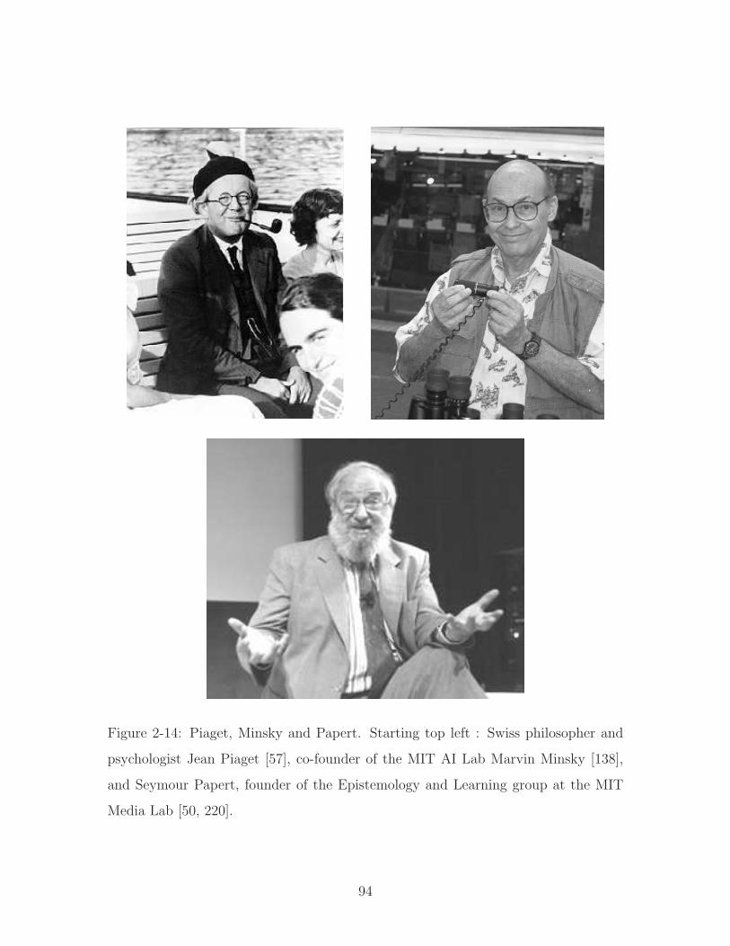
Figure 2-14: Piaget, Minsky and Papert. Starting top left : Swiss philosopher and

psychologist Jean Piaget [57], co-founder of the MIT AI Lab Marvin Minsky [138],

and Seymour Papert, founder of the Epistemology and Learning group at the MIT

Media Lab [50, 220].

94

emerged from the “golden age of mathematics at Princeton” [139, p. 323]. His teach-

ers included John Tukey (who later worked at Bell Labs and famously introduced

the fast Fourier transform) and the incomparable John von Neumann, and his fellow

students included John McCarthy (the other co-founder of the MIT AI Lab) and John

Nash [139, p. 323]. The study of machine learning (AI) is intricately entwined with

that of human learning; each provides insights on the other. Thus, like Piaget and

Papert, Minsky is also a keen theoretician on how humans (and particularly children)

learn, and in fact Seymour Papert and Marvin Minsky have collaborated in the field

of AI.

Let me introduce the anecdote with some key background on Piaget’s work. Piaget

applied a scientific approach in studying how children think. He designed a variety of

experiments to test whether a child had developed an understanding of concepts like

mass or volume conservation. A famous Piaget test for an understanding of volume

conservation, for instance, goes as follows: Present two identical (short, wide) jars of

water to children and all will agree they hold the same amount of liquid. Now, have

them watch as you pour the liquid from one of these jars into a taller, thinner jar.

A typical 5-year-old will reply that the taller jar has more that the shorter one, but

a 7-year-old is likely to reason each jar holds the same amount. “These experiments

have been repeated in many ways and in many countries - and always with the

same results: each normal child eventually acquires an adult view of quantity - and

apparently without adult help!” [139, p. 99].

Thanks to Piaget, we can identify specific stages or concepts in the development

of learning, but it is difficult to preempt (i.e. shortcut) the complete process by which

such information is ultimately absorbed. This is because we must, in the end, build

our own hierarchical structures in the mind which help us interpret the world around

us - to solve (and indeed also to formulate) problems, for instance. The development

of such structures in our minds need not be conscious, but before such a hierarchy

is fully developed, a child (and I would argue any learner) is essentially treating the

information as a set of “special rules, and so many exceptions to them” [139, p. 106].

Let me describe the dilemma (briefly) in a second way, before we launch into Minsky’s

95

story. Suppose one reasons: “If we know key benchmarks of the stages in the mental

development of a child, can’t we then focus on teaching each benchmark to accelerate

learning?” Stated in this way, perhaps it is easier to realize where this strategy may

go wrong. We may be successful in communicating a set of declarative facts to a

child, but the connections that link these facts can only be made in his own mind.

This is why, as Minsky put is:

...educational programs allegedly designed “according to Piaget” often

appear to succeed from one moment to the next, but the structures that

result from this are so fragile and specialized that children can apply them

only to contexts almost exactly like those in which they were learned [139,

p. 106].

He continues:

All this reminds me of a visit to my home from my friend Gilbert

Voyat, who was then a student of Papert and Piaget and later became a

distinguished child psychologist. On meeting our five-year-old twins, his

eyes sparkled, and he quickly improvised some experiments in the kitchen.

Gilbert engaged Julie first, planning to ask her about whether a potato

would balance best on one, two, three or four toothpicks. First, in order

to assess her general development, he began by performing the water jar

experiment. The conversation went like this:

Gilbert: “‘Is there more water in this jar or in that jar?”

Julie: “‘It looks like there’s more in that one. But you should ask my

brother, Henry. He has conservation already.”

Gilbert paled and fled. I always wondered what Henry would have said.

In any case, this anecdote illustrates how a young child may possess many

of the ingredients of perception, knowledge, and ability needed for this

kind of judgment - yet still not have suitably organized those components.

96

Herbert Simon (CMU)

Prof. Herbert Simon of the psychology department at CMU offers the anecdote below

in an essay on teaching and learning in universities. The story is about Bob Doherty,

president of CMU around 1949, when Simon came to CMU as a student. I feel this

excerpt provides a perspective for the rest of this literature survey on the higher level

thought processes educators ultimately hope their students will develop, particularly

through mentorship.

Doherty came from General Electric via Yale, and had been one of the

bright young men who were taken under the wing of the famous engineer

Stiglitz. Every Saturday, Stiglitz would hold a session with these talented

young men whom General Electric had recruited and who were trying to

learn more advanced engineering theory and problem-solving techinques.

Typically, Bob Doherty would sometimes get really stuck while working

on a problem. On those occasions, he would walk down the hall, knock on

Stiglitz’s door, talk to him - and by golly, after a few minutes or maybe a

quarter of an hour, the problem would be solved.

One morning Doherty, on his way to Stiglitz’s office, said to himself,

“Now what do we really talk about? What’s the nature of our conversa-

tion?” And his next thought was, “Well Stiglitz never says anything; he

just asks me questions. And I don’t know the answer to the problem or I

wouldn’t be down there; and yet after fifteen minutes I know the answer.”

So instead of continuing to Stiglitz’s office, he went to the nearest men’s

room and sat down for a while and asked himself, “What questions would

Stiglitz ask me about this?” And lo and behold, after ten minutes he had

the answer to the problem and went down to Stiglitz’s office and proudly

announced that he knew how to solve it. [184, p. 344]

Prof. Simon’s premise is that ”the emphasis in engineering education should not be

placed on knowledge, but should focus attention on the learning processes solving

processes of the students” [184, p. 343].

97

“Design is a special kind of problem solving...we call ill-structured” [184, p. 345],

Simon says, because “the goals are never completely defined until the design is almost

finished” [184, p. 345]. Expert designers seem to rely heavily on intuition to sort

through this cycle of defining and solving problems, and “Intuition is essentially

synonymous with recognition.” [184, p. 345] More precisely, it involves recognizing

patterns, accessing related information (in your brain), and then making decisions

about which information is most relevant and how it can be used. And the more

efficient you get at doing this, the more effortless and subconscious (“intuitive”)

the whole process becomes. Simon notes that this pattern recognition approach is

essentially the process researchers in A.I. use in algorithms for expert system and

chess-playing programs. I would make an analogy with many physical processes,

like playing tennis or sight-reading piano music, where experts are able to respond

efficiently to familiar (yet unique) situations because they have years of experience

practicing.

“Learning has to occur in the students,” Simon finally warns, and whatever ideas

you try to impart to your students, “doesn’t make a whit of difference unless it

causes a change in [their] behavior” [184, p. 346].“The beginning of the design of any

educational procedure is dreaming up experiences for students” [184, p. 346] to help

them learn. Even so, providing students with relevant demonstrations and hands-on

labs is not enough; ultimately the students have to do the work of learning.

Teaching to Match Students’ “Learning Styles” at NCSU

Richard Felder and Linda Silverman state that learning in a univerisity is a “two-step

process involving the reception and processing of information” and students ”select

the material they will process and ignore the rest” [70, p. 674]. They suggest that

instructors can be more effective by if they adopt a teaching style that is designed to

match the preferred learning styles of their students.

They have developed a set of learning traits, similar to the personality traits

(introverted vs. extroverted, etc) used in Myers-Briggs-Jung type tests. For instance:

“Sensors like solving problems by standard methods and dislike ‘surprises’; intuitors

98

like innovation and dislike repetition” and they claim that “the majority of engineering

students are sensors” [70, p. 676].

Another distinction they suggest is one between “active” and “reflective” learners.

“Active learners do not learn much in situations that require them to be passive

(such as most lectures), and reflective learners do not learn much in situations that

provide no opportunity to think about the information being presented (such as most

lectures)” [70, p. 678]. Active learners want to experience phenomena first-hand.

They “work well in groups“ and “tend to be experimentalists”. Reflective learners

want time to process new information when they encounter it. They “work better

by themselves or with at most one other person” and ”tend to be theoreticians” [70,

p. 678]. “A class in which students are always passive is a class in which neither

the active experimenter nor the reflective observer can learn effectively” [70, p. 678].

One suggestion Felder and Silverman list is to “have students organize themselves in

groups of three or four and periodically come up with collective answers to questions

posed by the instructor” [70, p. 678]. They continue:

The groups may be given from 30 seconds to five minutes to do so,

after which the answers are shared and discussed for as much or as little

time as the instructor wishes to spend on the exercise. Besides forcing

thought about the course material, such brainstorming exercises can in-

dicate material that students don’t understand; provide a more congenial

classroom environment than can be achieved with a formal lecture; and

involve even the most introverted students, who would never participate

in a full class discussion. One such exercise lasting no more than five

minutes in the midde of a lecture period can make the entire period a

stimulating and rewarding educational experience. [70, p. 678]

Engineering Dynamics at Texas A&M

Prof. Louis Everett of Texas A&M notes that “Engineering Dynamics...is neither easy

to teach nor to learn” [68]. He suggests the key is to “teach Dynamics as a problem-

solving process” and that “students tend to learn technical subjects by comparing

99

with examples” [68]. Everett believes, “The current textbooks pose a real problem.

Most texts are a collection of facts.”

The strategy he suggests for teaching dynamics is to present students with a

loosely-structured plan of attack for problem solving. His strategy attempts to provide

students with a set of general steps to aide them in approaching new problems without

prescribing specific rules.21 He also notes that the same basic skills for analysis are

essential for the design of dynamic systems, as well. The six steps he cites are:

1. “Think about the problem.” (e.g. What is being asked? What are the assump-

tions? How many degrees of freedom are there?)

2. “Choose Coordinates.” (e.g. What reference frame makes sense?)

3. “Define the System.” (e.g. free body diagram)

4. “Apply a Force-Motion Relation” (applying either Newton’s law or a work-

energy equation.)

5. “Find ’Extra’ Equations.” (e.g. kinematics, or additional assumptions that

must be made to to make the equations solvable)

6. “Solve and Interpret” (...and reflect of whether it makes sense.)

Prof. Everett cites that it takes time for most students to become comfortable

with his “process-oriented” approach. He is hopeful, however, that students can adapt

to it. For instance, he cites an example (similar to the anecdote about Bob Doherty

on page 97) where, after an exam, a student approached him to comment that he was

completely lost on a particular problem. “I didn’t have a clue,” the student said, “so

I applied the process and it worked out real easy” [68].

Everett also notes that students typically come into a dynamics class with mis-

taken intuition that needs to be addressed by investigating why students errors are

made and correcting faulty reasoning. Students can also fall into the pitfall of apply-

ing rules too blindly, when their own experience and common sense should be able to

21a tricky balance, it would seem...

100

guide them. As one example, he has shown students a car engine (running at constant

speed): Show the students a pulley running a fan or pump and another which is an

idler, and ask them to draw free body diagrams of the two pulleys. Everett’s expe-

rience is that most students will say the tension is equal on both sides of the pulley

in either case. If you ask them why, students typically respond by saying something

like, “Tension on either side of a massless frictionless pulley is the same” [68]. This

approximation may be appropriate for an idler, but it certainly will not be for the

pulley driving the pump. What is missing from the student solution is an analysis of

the equilibrium conditions necessary at the pulley which is driving the pump.

Student-designed labs at USC

Jed Lyons, Jeffrey Morehouse and Edward Young of the University of South Car-

olina have developed a capstone lab course in mechanical engineering that focuses on

the process of designing laboratory experiments focusing on thermodynamics, heat

transfer, mechanics, dynamics and control. The authors specifically cite that their

approach derives from “constructivist learning theory” [117].

They have structured laboratory experiences for the class around the analysis of a

5/8-scale replica “Legends” race car (which typically grabs student interest). Wireless

telemetry is used, so that sensors can be monitored remotely while the car is being

driven. The first weeks of the course involves more structured “learning modules”,

where students learn to use a variety of sensors and the wireless data acquisition

system and gain experience in reducing the data obtained. The course culminates

in an open-ended project, in which students spend five weeks on an experiment they

must design completely:

For example, the students may be asked to determine what effects a

steady-state turn has on the suspension and tires. The experiment they

develop could consist of using a circular or oval track to study steady

state cornering, quantified by lateral acceleration. Both lateral and front-

to-back shifts in suspension could be measured as functions of lateral

acceleration. Using wheel encoders, the difference in distance travelled

101

by each wheel could be compared to theoretical predictions, and how this

distance changes with cornering effort could be examined. The effects of

cornering on tire temperature could be correlated with different turn radii

and vehicle speeds (etc.) [117, p. 5].

Students would then need to model the system to estimate the order of magnitude of

the expected response and choose appropriate sensors22 from the stockroom for the

course and calibrate them.

Other Work of Note

A couple of other outlooks on engineering education are worth mentioning briefly.

One involves a project at the University of Alberta to create a suite of hands-on ex-

periments in fluid dynamics. The experiments are used in the recitations, which are

taught by graduate TAs, rather than in lecture. In addition to giving the students a

more intimate interaction with the demos, the demos provide a focus for the recita-

tions. As a result, “the teaching experience is a very structured one, which allows

the beginning teacher to focus on presentation, use of time, and interactions with the

students.” [104, p. 9]

In a second (remarkable) example, Professors Donald Woods & Cameron Crowe

at McMaster University actually entered their departmental programs as “freshmen”

and continued through the four-year program, observing lectures, interacting with

students, and evaluating what the strengths and pitfalls of their curriculum were.

They note that the freshmen and sophomores with whom they interacted seemed

to rely largely on “intuition” [219] rather than a self-aware problem-solving strat-

egy. Intuition may be appropriate once you have developed a high level of skill, as

described in Section 2.2.1, but to develop the right intuition requires critical think-

ing. They have found that relying so heavily on pattern matching presents potential

pitfalls for the students. “For example, they consider two problems similar if they in-

volve a ladder rather than because the problems ask about the force-mass-movement

22Sensors available in the class which are appropriate in this example include encoders, accelerom-

eters, LVDTs, infrared pyrometers, a GPS system, and load bolts [117].

102

relationship.” [219, p. 292]

In concluding this survey part of survey on how to teach engineers, I include some

remarks from Prof. James Roberge, who notes: “Many designers mention one or

two mentors...who had a major impact on their careers.” If this is so, then a good

instructor in dynamic modeling23 can clearly have a much more global impact in

a student’s education than simply building a strong foundation in dynamics alone.

Roberge continues: “The abilities required for effective design, while hard to quantify,

are common to all disciplines. I believe that a good analog circuit designer could also

become a good designer of airplane wings or steam turbines after a relatively short

internship in the new field. (It may be fortunate for frequent flyers that this hypothesis

is infrequently tested.)” [174, p. 79] With this perspective in mind, the next section

describes a variety of approaches educators have taken in teaching dynamics and the

design of dynamic systems.

2.2.2 Stanford Course ME161: Dynamic Systems

ME161 is a ten-week junior- and senior-level course in dynamics and introductory

controls with a laboratory component. The course is taught once a year at Stanford

(in the Fall) with a class size of around 60 [169]. Staff for the class have designed and

implemented two project-based themes as a focus for the lab sessions. In both cases,

students studied the same dynamic system in each of a series of separate laboratory

exercises. Both of these device-centered laboratory innovations are described briefly

below. One is a single-degree-of-freedom “haptic paddle” [169, 170], which was used

from 1996-1998, and the second (used only in the Fall of 2000) is a pneumatically-

actuated, one-legged hopping machine called the “Dashpod” [47]. These two devices

are shown in Figures 2-15 and 2-16, respectively.

103

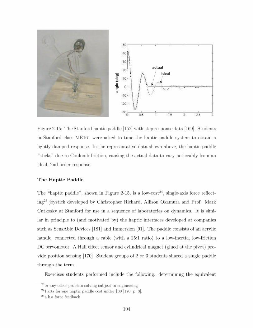
3

a simple second order system using the generalized coordinate x,to represent the horizontal movement of the joystick handle.

3.2 Electromechanical system parametersDuring the third and fourth weeks of the course the students

were introduced to electrical and electromechanical systems. Atthis time the students measured the torque and speed constants oftheir motors and estimated the maximum force (approximately7.5 N) that the devices would be able to generate at the handle.The torque and speed constants were measured using a variablevoltage power supply, ammeter, encoder, a set of weights rang-ing from 10 to 200 kg, and some 3.0 cm diameter pulleys. To ob-tain the torque constant the students attached a pulley to a motorand suspended various weights from a thread wrapped aroundthe pulley. They were told to measure the current while adjustingthe voltage so that weights appeared to be “neutrally buoyant”against gravity, when moved slowly up or down by hand. Thisprocedure allowed the small motor friction to be accounted for.To obtain the motor voltage/speed constant, they spun the motorshaft at known velocity (using another motor equipped with anencoder) and measured the voltage generated. The results wereconsistent for each of the several models of motors used in theclass.

The students also calibrated the Hall effect sensors for lateruse. The use of analog position sensing was motivated mainly bythe availability of lab stations equipped with standard A/D andD/A data acquisition cards. However, the choice of an analogsensor also gave the students some insight into the procedure ofdevice calibration, using a simple setup involving an oscillo-scope to measure the sensor voltage and a protractor to measurethe handle angle.The sensors are mounted on the base (Figs. 1and 6) and respond the changes in magnetic field of a small cy-lindrical magnet mounted at the pivot point. The output is nearlylinear for small motions, but noticeably sigmoidal over the full±35 deg. range of motion. The sensors were therefore calibratedusing a best-fit cubic. The coefficients of the cubic were enteredinto the control system in the following experiments.

3.3 Computer control and dynamic responseIn order to demonstrate how changing parameters affect sys-

tem behavior, a DOS program was written to allow the studentsto 1) modify the gains of a proportional + derivative control law,2) apply step inputs of various magnitudes and 3) record the po-

sition data. The controller ran with a sampling rate of 1000 Hz,with position data saved every 10 msec for plotting.

Students were first asked to try different positive values ofproportional feedback and observe how the stiffness of the sys-tem and the frequency of oscillations changed when the joystickwas disturbed from equilibrium. At low gains, the systems werestable without velocity feedback, due to the presence of frictionand damping in the motor and cable transmission. The studentsobserved that the kits with higher friction could accept highergains before instability appeared.

Next, the students used negative values of stiffness to observethe effect of destabilizing torques and compared this with the ef-fect of gravity on the device. The derivative feedback (obtainedby estimating the velocity from the Hall effect position data) wasalso modified. The students soon learned that for large values ofproportional feedback they needed to increase the effectivedamping to avoid instability.

Finally, students were asked to tune their system to make itrespond to step inputs like a classic lightly damped second ordersystem. From the position data taken during the response, stu-dents were asked to determine the corresponding dimensionlessdamping parameter, ζ, and resonant frequency, ω. The studentsalso observed that their plots did not precisely match those of anideal second-order system due to the presence of Coulomb fric-

ang

le (

deg

)

actual

ideal

time (s)

Fig. 4. Step response of a somewhat sticky haptic interface versus an ideal second order system

paddle ball

motion

M1 M2

spring

finger position

ground

damper

Fig. 5a. Haptic tetherball side view in XZ plane (YZ plane is equivalent)

Fig. 5b. Excite the modal frequencies (one of four sys-tems running concurrently)

Figure 2-15: The Stanford haptic paddle [152] with step response data [169]. Students

in Stanford class ME161 were asked to tune the haptic paddle system to obtain a

lightly damped response. In the representative data shown above, the haptic paddle

“sticks” due to Coulomb friction, causing the actual data to vary noticeably from an

ideal, 2nd-order response.

The Haptic Paddle

The “haptic paddle”, shown in Figure 2-15, is a low-cost24, single-axis force reflect-

ing25 joystick developed by Christopher Richard, Allison Okamura and Prof. Mark

Cutkosky at Stanford for use in a sequence of laboratories on dynamics. It is simi-

lar in principle to (and motivated by) the haptic interfaces developed at companies

such as SensAble Devices [181] and Immersion [91]. The paddle consists of an acrylic

handle, connected through a cable (with a 25:1 ratio) to a low-inertia, low-friction

DC servomotor. A Hall effect sensor and cylindrical magnet (glued at the pivot) pro-

vide position sensing [170]. Student groups of 2 or 3 students shared a single paddle

through the term.

Exercises students performed include the following: determining the equivalent

23or any other problem-solving subject in engineering24Parts for one haptic paddle cost under $30 [170, p. 3].25a.k.a force feedback

104

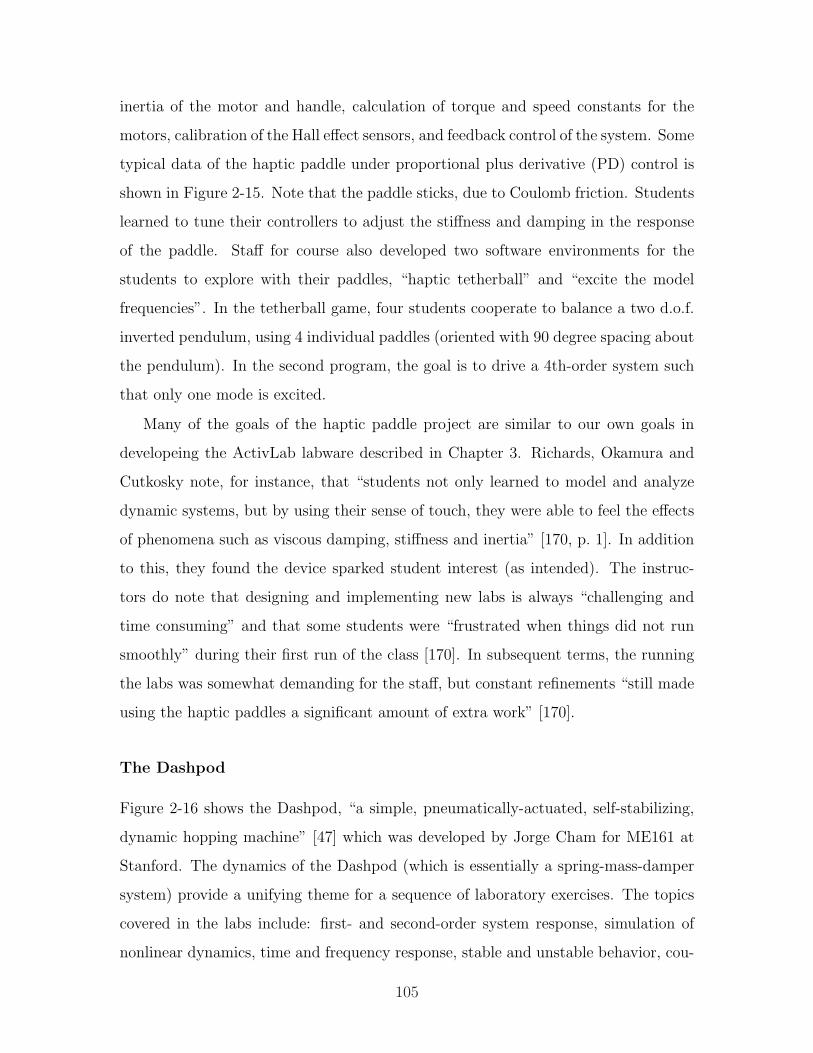
inertia of the motor and handle, calculation of torque and speed constants for the

motors, calibration of the Hall effect sensors, and feedback control of the system. Some

typical data of the haptic paddle under proportional plus derivative (PD) control is

shown in Figure 2-15. Note that the paddle sticks, due to Coulomb friction. Students

learned to tune their controllers to adjust the stiffness and damping in the response

of the paddle. Staff for course also developed two software environments for the

students to explore with their paddles, “haptic tetherball” and “excite the model

frequencies”. In the tetherball game, four students cooperate to balance a two d.o.f.

inverted pendulum, using 4 individual paddles (oriented with 90 degree spacing about

the pendulum). In the second program, the goal is to drive a 4th-order system such

that only one mode is excited.

Many of the goals of the haptic paddle project are similar to our own goals in

developeing the ActivLab labware described in Chapter 3. Richards, Okamura and

Cutkosky note, for instance, that “students not only learned to model and analyze

dynamic systems, but by using their sense of touch, they were able to feel the effects

of phenomena such as viscous damping, stiffness and inertia” [170, p. 1]. In addition

to this, they found the device sparked student interest (as intended). The instruc-

tors do note that designing and implementing new labs is always “challenging and

time consuming” and that some students were “frustrated when things did not run

smoothly” during their first run of the class [170]. In subsequent terms, the running

the labs was somewhat demanding for the staff, but constant refinements “still made

using the haptic paddles a significant amount of extra work” [170].

The Dashpod

Figure 2-16 shows the Dashpod, “a simple, pneumatically-actuated, self-stabilizing,

dynamic hopping machine” [47] which was developed by Jorge Cham for ME161 at

Stanford. The dynamics of the Dashpod (which is essentially a spring-mass-damper

system) provide a unifying theme for a sequence of laboratory exercises. The topics

covered in the labs include: first- and second-order system response, simulation of

nonlinear dynamics, time and frequency response, stable and unstable behavior, cou-

105

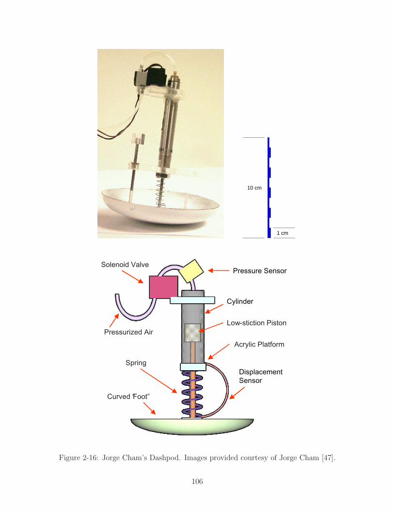
1 cm

10 cm

2 Copyright © 2001 by ASME

these concepts [see also Everett, 1997].

For example, Richard et al. [2000] introduced the “HapticPaddle,” a single-axis force-feedback joystick for undergraduatedynamic system laboratories. The Haptic Paddle was used notonly for force-feedback simulations of dynamic phenomena, butalso as a mechanical system with which class concepts such asinertia and motor equations were demonstrated. Studentsassembled the joystick from a kit and used class concepts tocreate a predictive model of the device’s dynamic behavior.This idea of centering the theme of a series of laboratoriesaround a physical, dynamic mechanical device that the studentscan assemble, touch, “play” with, re-design and modify resultsin increased student enthusiasm [Ghorbel, 1999; Lyons et al.,1998; Clark and Hake, 1997].

In this paper, we go a step further to suggest that an effectivelaboratory experience challenges the students with a design goalfor the central mechanical device. Once the students are facedwith a clear design goal, the role of the laboratories is to presentthe tools that might be used to analyze, model and design thedevice in order to meet the goal. The laboratory sessions guidestudents through the process of figuring out which tools to useand how to use them appropriately. Thus, while class conceptsare being demonstrated, their use as design tools is alsomotivated and made relevant.

In the laboratories presented here, junior- and senior-levelstudents in a mechanical engineering Dynamic Systems courseat Stanford University were challenged to improve theperformance of the “Dashpod” ( Dynamics And SystemsHopping Pod): a simple, pneumatically-actuated, self-stabilizing dynamic hopping machine (see Figure 1). In thelaboratory sessions, the students first used simple modelingconcepts learned in class to characterize the Dashpod’s dynamicbehavior and to start making predictions about the factors thataffect the machine’s hopping performance. Students then

Figure 2. Dashpod diagram. The Dashpod’s maincomponents are a solenoid valve, a pneumatic cylinderand piston, a spring and a wide curved foot.

Low-stiction Piston

Solenoid Valve

Pressurized Air

Acrylic Platform

Spring

Curved “Foot”

Pressure Sensor

DisplacementSensor

Cylinder

evaluated the limitations of these models and used appropriatelymore complex models as they were explained in class. Thus, inaddition to understanding the physical relevance of themathematical concepts given in lectures, students learned basicdynamic design methodology.

The following section describes the Dashpod, its componentsand the design goal as it was presented to the students. Next, wedescribe the laboratory sessions and how they were coordinatedwith the class syllabus. Finally, we discuss future improvementsbased upon end-of-quarter student evaluations.

2. THE DASHPOD HOPPING MACHINE

The framework discussed above for undergraduate dynamicsystems laboratories challenges the educator to find acompelling mechanical device whose components andobjectives enhance the desired course material. The Dashpodhopping machine is a simple mechanical system that integrateswell with the pedagogical goals of an undergraduate dynamicslaboratory. It is inspired by robotics and biomechanics researchon legged locomotion [Wei et al., 2000; Blickhan and Full,1993; Raibert, 1986; Cham et al. 2000]. As shown in Figure 2,the basic configuration of the Dashpod consists of a low-stictionpneumatic piston attached to a wide dish or curved “foot” onwhich it stands. A spring connects the foot to the pneumaticcylinder and platform along the piston shaft and a solenoidvalve regulates air into the cylinder’s upper chamber.Depending on the laboratory goals, a pressure sensor can beattached to measure the cylinder’s air pressure and adisplacement sensor can be used to measure the relativedistance between the platform and foot. The Appendix containsdescriptions and costs of the commercial parts used.

The machine can be made to hop vertically by supplying the

Figure 3. Dashpod hopping diagram. The solenoid valveallows pressurized air to fill the pneumatic cylinder,causing the Dashpod to push against the ground. If thevalve is activated periodically, the hopping motion isalso periodic. An off-axis center of mass will cause theDashpod to hop in a certain direction.

Hopping Sequence

Figure 2-16: Jorge Cham’s Dashpod. Images provided courtesy of Jorge Cham [47].

106

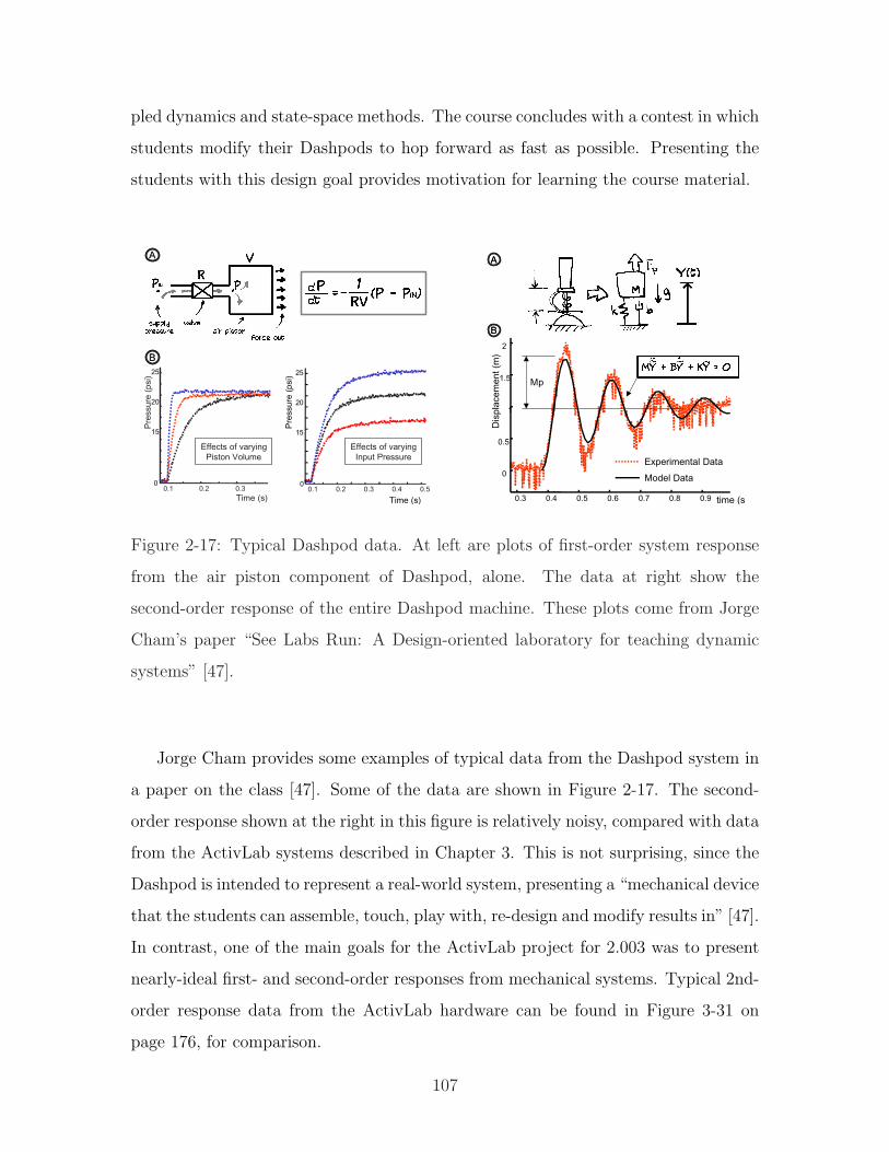
pled dynamics and state-space methods. The course concludes with a contest in which

students modify their Dashpods to hop forward as fast as possible. Presenting the

students with this design goal provides motivation for learning the course material.


valve with pressurized air (approximately 20 psi) and applyingcurrent to it, causing the valve to open. This fills the cylinder’supper chamber with pressurized air, thereby pushing theDashpod’s platform up. At some point, the Dashpod’s foot losescontact with the ground, and the machine travels ballisticallythrough the air before landing again. If the valve is turned off atthis point, the platform will compress the spring when it lands,storing energy that can be used for the next hop. If the valve isactivated at a certain frequency, the hopping motion is periodicwith a certain hopping height, as shown in Figure 3. If the centerof mass of the Dashpod is placed off-set from the piston axis,then the machine “leans” to one side. Thus, when the valve isactivated, the machine hops in a specific direction with a certainhorizontal velocity.

In essence, the Dashpod is a resonant mass-spring-dampersystem, one of the key mechanical systems in dynamic analysis.However, as described in the following sections, understandingthe basic mechanisms that affect the hopping performance ofthe Dashpod provides many good opportunities for analysis ofother simple dynamic models besides the spring-mass-damper.In addition, the Dashpod is a good vehicle for teaching basicdynamic design methodology. Like most real-life systems, theDashpod’s hopping motion is actually a non-linear, multi-variable phenomenon that is the subject of current research[Ringrose, 2000; Koditschek and Buehler, 1990]. However, theapplication of simple, fundamental models to a novel dynamicsystem before resorting to complex, multivariable models is agood approach to dynamic design. Such a methodology wouldbe difficult to teach using only demonstrations.

Students were challenged to improve the forward hoppingmotion of the Dashpod in a competitive setting between labteams of two or three students. At the end of the laboratorysequence, students raced the Dashpods under configurations orre-designs as suggested by their analysis, assuming that

Figure 4. Syllabus topics and their corresponding labsfor the Dashpod.

First-Order Systems

Second-Order Systems

System Stability

Frequency Response

Multi-variable Coupled Systems

Dynamic Simulation

What are delays in thepneumatic actuator?

How much damping in the piston and spring?

What makes the curved foot stable?

What is the “resonant” hopping frequency?

Evaluate simple models and characterize

coupled dynamics

Design and configure for optimal hopping

Lab 1

Lab 2

Lab 3

Lab 4

Lab 5

Lab 6

Class topics Dashpod design

increasing the machine’s vertical hopping also improvedforward hopping.

3. LABORATORY DESCRIPTIONS

Each laboratory session was focused on a clear question abouta component of the Dashpod as it pertained to the final designgoal. Given this question, students were guided through the useof the modeling tool given in class that was applicable in eachcase. For example, analysis of first-order, second-order systemsand their time response were first used to characterize theDashpod’s basic mechanisms in order to understand the factorsthat influence hopping. Subsequent labs focused on morecomplex models, culminating in a non-linear dynamicsimulation. Figure 4 shows the syllabus topics covered inlecture and the corresponding laboratory design question. Thefollowing sections describe each of the laboratories in moredetail.

3.1. Lab 1: First Order Systems and Actuator Delays

The first of the Dashpod’s subcomponents that the studentscharacterized was the pneumatic actuator. Since actuator delayswill determine how effectively the machine will hop, studentswere asked: “What design parameters affect the speed of theactuator?” For example, one important design decision iswhether to mount the air valve on the machine or off-board. Inthis lab, students used an electronic pressure transducer torecord the time history of the pressure inside the cylinder afterthe valve is activated. They compared this time history to asimulation of a first-order model of the pneumatic systemcomposed of an air supply, the valve, the tubing and thecylinder chamber as shown in Figure 5a along with itsdifferential equation.

Figure 5. First-order Systems. This lab illustrated thedesign impact of changing system parameters in theDashpod’s pneumatic actuator.

BB

Pre

ssur

e (p

si)

Time (s)0.1 0.2 0.3

0

15

20

25

0.1 0.2 0.3 0.4 0.5

Time (s)

Pre

ssur

e (p

si)

0

15

20

25

Effects of varying Piston Volume

AA

Effects of varying Input Pressure


The students’ task was to estimate the “time constant” (thetime it takes for the pressure to reach 63% of its steady-statevalue) for a trial run and record this value for different designparameters. Sample plots are shown in Figure 5b. The studentsfirst evaluated the linearity of the system by comparing the timeconstant for different input pressures, Pin. They found that itwas constant within reasonable bounds, as predicted by thelinear model. The students then varied the volume of thecylinder chamber by holding the piston at different positionsand recorded the time constant. This gave them an estimate ofthe range of actual delays, since this volume will be constantlychanging during actual operation. Finally, students varied thelength of tubing between the valve and the actuator and foundthat shorter tubing resulted in smaller time constants. Both theselast phenomena were compared to the model’s prediction of thetime constant being a inverse function of R, the flow resistanceof the valve and tubing (related to tubing length), and V, ameasure of the “capacitance” of the cylinder volume.

In this session, students obtained an intuitive sense of the timeconstant as a quantity inherent in a linear system and notdependent on the magnitude of the input. They observed whatphysical parameters affect it and how it impacts designdecisions.

3.2. Lab 2: Second Order Systems and Damping

The second laboratory session focused on the Dashpod’sfundamental mechanism: the interaction between the system’smass, spring and damping. Students were asked to fix thecurved foot to the ground and consider the moving mass-spring-damper system, as shown in Figure 6a. The task was to identify

Figure 6. Second Order Systems. Students identifiedthe model parameters M, B and K.

0.3 0.4 0.5 0.6 0.7 0.8 0.9

0

0.5

1

1.5

2

time (s)D

ispl

acem

ent (

m)

Experimental Data

Model Data

Mp

BB

AA

the parameters in the second-order linear model for the mass’displacement, M, B and K, and compare a simulation of thismodel with actual data. Given only this instruction and themeans to record the time history of the displacement through adisplacement sensor, students had to figure out how to estimatethe parameters.

Measuring the mass of the moving system provided a goodexercise since students had to discern which parts of theDashpod would be considered under the model and which partswere considered fixed to the ground. Estimating the springconstant provided a hands-on experience with the force-displacement relationship of a spring and a sense of how linearit actually is. To estimate a value for B, the damping constant,students recorded the time history of the mass’ motion to aninitial displacement, as shown in Figure 6b. Using the formulagiven in class for the maximum overshoot, they estimated thedamping ratio for the given configuration and then calculated avalue for B. Finally, a simulation of the model using theestimated parameters was compared with the actual data.

This session provided students with hands-on experience ofclass concepts such as a second-order underdamped response,overshoot and the damping ratio. It also familiarized studentswith the process of identifying and evaluating parameters for amodel that can be used for future re-designs.

3.3. Lab 3: Stable and Unstable Systems

A certain range of values for the curvature of the foot makesthe Dashpod self-stabilizing while standing upright. Forexample, when perturbed to one side, the Dashpod rocks backand forth, eventually returning to its upright position. In this lab,students analyzed why this happens and how it can affect the

Figure 7. Stable and Unstable Systems. Students variedthe height H of the center of mass and observed how thestability of the system changed.

Height ofMass

center

Radius of curvature

Mass, Moment of Inertia

Equation of Motion

Roots or Poles of System

Re

Im

Re

Im

Complex Plane

R=H

Increasing H

AA

BB

Figure 2-17: Typical Dashpod data. At left are plots of first-order system response

from the air piston component of Dashpod, alone. The data at right show the

second-order response of the entire Dashpod machine. These plots come from Jorge

Cham’s paper “See Labs Run: A Design-oriented laboratory for teaching dynamic

systems” [47].

Jorge Cham provides some examples of typical data from the Dashpod system in

a paper on the class [47]. Some of the data are shown in Figure 2-17. The second-

order response shown at the right in this figure is relatively noisy, compared with data

from the ActivLab systems described in Chapter 3. This is not surprising, since the

Dashpod is intended to represent a real-world system, presenting a “mechanical device

that the students can assemble, touch, play with, re-design and modify results in” [47].

In contrast, one of the main goals for the ActivLab project for 2.003 was to present

nearly-ideal first- and second-order responses from mechanical systems. Typical 2nd-

order response data from the ActivLab hardware can be found in Figure 3-31 on

page 176, for comparison.

107

2.3 Multi-Media Simulations of Dynamic Systems

at MIT

This section discusses current projects at MIT which make various educational media

(e.g. simulated demos, textbooks, and video) available to students (and typically the

general public) on the web. MIT is currently working on a project to make online

materials for virtually every course at MIT freely available to educators at other

universities and to the general public. This project, called OpenCourseWare (OCW),

is described in more detail in Section 2.3.4.

2.3.1 PiVOT/PT tutor for 8.01 Physics I

Over the last years, the physics department at MIT has spent considerable effort

revamping their introductory freshman subjects to try to improve upon the tradi-

tional lecture format. The physics department at MIT now offers several “flavors”

of its two introductory (freshman) classes. To cover classical mechanics, they offer a

traditional lecture course (8.01), a longer version which extends into the Independent

Activities Period in January26 (8.01L), a theoretical version aimed at physics majors

(8.012), and one taught in a “studio” environment (8.01T). The mainstream course

for teaching electromagnetism and electrostatics, 8.02, is now taught using this same

studio environment (described in more detail in the next section), with a minority of

students (a few dozen) taking a more theoretical option (8.022).

One notable project in the department is the “Physics Interactive Video Tutor”

(PIVoT), which currently provides an online text with links to other supplementary

materials. The PIVoT “Personal Tutor” (PT) keeps track of the topics and keywords

each student accesses most often, to suggest additional related materials. PIVoT

is not available to individuals outside of the MIT community, and students at the

university must register for a PIVoT account.27 Figure 2-18 shows a frame from one

26The MIT fall term ends before Christmas each year, and the second semester does not begin

until the first week of February.27I am not sure why it is not publicly available, but I suspect it may be because of copyright issues

108

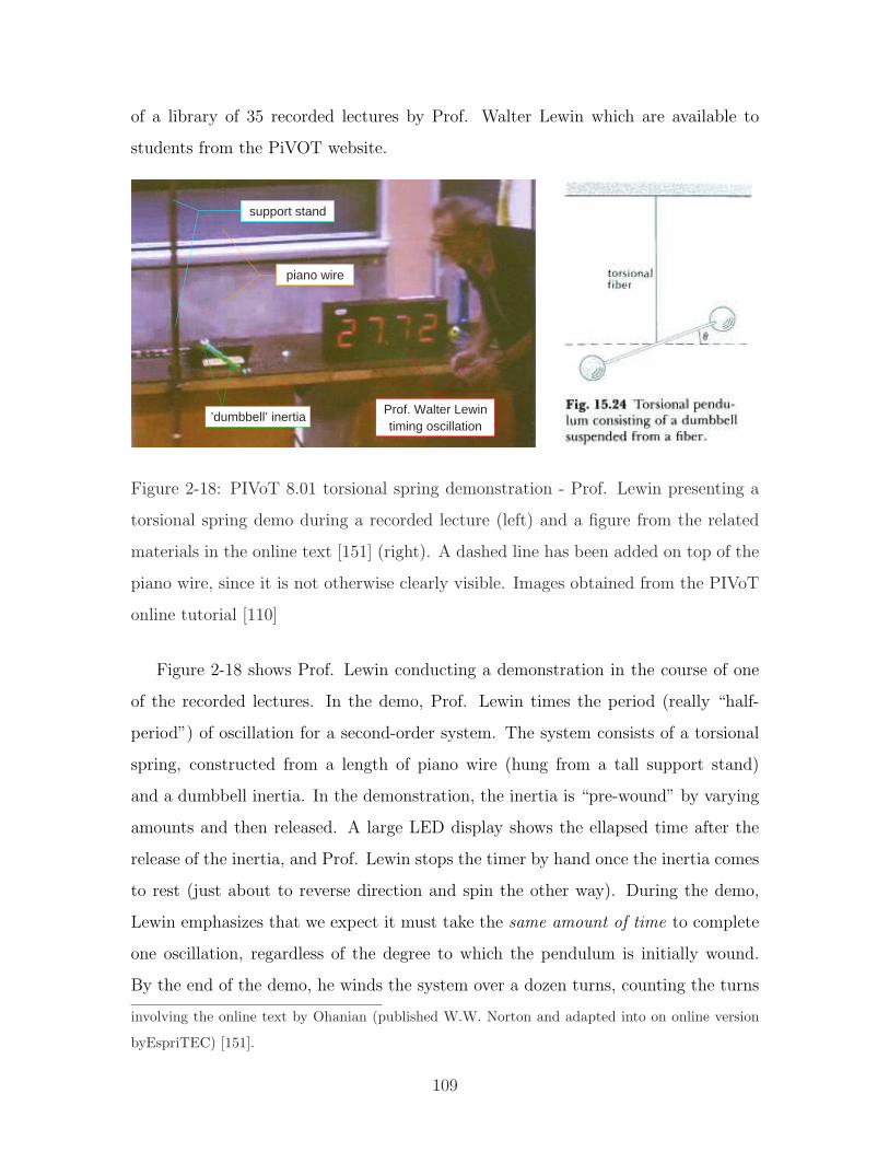
of a library of 35 recorded lectures by Prof. Walter Lewin which are available to

students from the PiVOT website.

piano wire

support stand

’dumbbell’ inertiaProf. Walter Lewintiming oscillation

Figure 2-18: PIVoT 8.01 torsional spring demonstration - Prof. Lewin presenting a

torsional spring demo during a recorded lecture (left) and a figure from the related

materials in the online text [151] (right). A dashed line has been added on top of the

piano wire, since it is not otherwise clearly visible. Images obtained from the PIVoT

online tutorial [110]

Figure 2-18 shows Prof. Lewin conducting a demonstration in the course of one

of the recorded lectures. In the demo, Prof. Lewin times the period (really “half-

period”) of oscillation for a second-order system. The system consists of a torsional

spring, constructed from a length of piano wire (hung from a tall support stand)

and a dumbbell inertia. In the demonstration, the inertia is “pre-wound” by varying

amounts and then released. A large LED display shows the ellapsed time after the

release of the inertia, and Prof. Lewin stops the timer by hand once the inertia comes

to rest (just about to reverse direction and spin the other way). During the demo,

Lewin emphasizes that we expect it must take the same amount of time to complete

one oscillation, regardless of the degree to which the pendulum is initially wound.

By the end of the demo, he winds the system over a dozen turns, counting the turns

involving the online text by Ohanian (published W.W. Norton and adapted into on online version

byEspriTEC) [151].

109

out loud. When he releases the pendulum, he comments to the student to note how

rapidly the inertia must spin - it needs to make all of those rotations in the same

span of time they have previously timed (for less aggressive windings).

The course 6.013 (“Electromagnetics and Applications”, described later in Sec-

tion 2.3.3 and page 117) has also accumulated a library of such video presentations.

Recordings like those used in both 8.01 and 6.013 reduce the overhead in providing

demos to supplement lectures or recitations (which may only have a dozen students,

each). The MIT recordings described also capture unique and inspirational people for

future generations of students. For instance Walter Lewin, who appears in the 8.01

footage, is an excellent lecturer. His enthusiasm for physics is clear, and his teaching

style has been refined over many years.

Both the PIVoT project described here and a project studio physics project called

TEAL (described in the next section) are attempts to improve the status quo in

undergraduate education by revamping or eliminating the large lecture format for

required, introductory courses. As Prof. John Belcher noted (in a department News

Letter in Fall 2001), “Even with an outstandingly effective and charismatic lecturer

like Professor Walter Lewin, lecture attendance at the end of the term in our in-

troductory courses hovers around 50%. No matter how strongly one feels about the

intrinsic worth of the lecture format, it is hard to argue that it is broadly effective

when half of the students do not attend lecture.” [29]

110

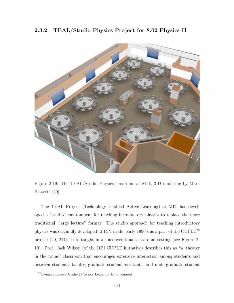
2.3.2 TEAL/Studio Physics Project for 8.02 Physics II

Fall 2001 Physics Department News Letter

3

course format below, keep in mind that one of the overall goals is to set up a structure that engages

the students more deeply, so that they come away from these introductory courses with more of an

appreciation for the beauty of physics, both conceptually and analytically.

Pedagogy

The first thing that is different in the TEAL/Studio format is that it requires very different

space for instruction. Figure 1 shows a 3D rendering (by Mark Bessette, the TEAL/Studio 3D

illustrator/animator) of the space we are using in the Fall of 2001.8

Figure 1: The TEAL/Studio Physics Classroom.

Figure 1 shows 13 tables with seven-foot diameters on fourteen-foot centers. With nine students at

a table, this room design accommodates 117 students. The instructor’s station in the center of the

room is used to present instructional material (projected on eight projection screens around the

Figure 2-19: The TEAL/Studio Physics classroom at MIT. 3-D rendering by Mark

Bessette [29].

The TEAL Project (Technology Enabled Active Learning) at MIT has devel-

oped a “studio” environment for teaching introductory physics to replace the more

traditional “large lecture” format. The studio approach for teaching introductory

physics was originally developed at RPI in the early 1990’s as a part of the CUPLE28

project [29, 217]. It is taught in a unconventional classroom setting (see Figure 2-

19). Prof. Jack Wilson (of the RPI CUPLE initiative) describes this as “a ‘theater

in the round’ classroom that encourages extensive interaction among students and

between students, faculty, graduate student assistants, and undergraduate student

28Comprehensive Unified Physics Learning Environment

111

assistants” [217]. A typical studio classroom has multiple white and/or blackboards,

overhead projector(s), and tables which seat subgroups of systems. There are laptop

computers and lab experiments on the tables, which are periodically integrated into

the studio experience. Part of the TEAL studio project at MIT involves visual sim-

ulations of electromagnetic phenomena, which students can view online. Figure 2-21

shows examples of these simulations.

Figure 2-19 show a rendering of the TEAL classroom, which is now being used

at MIT to teach introductory electromagnetism and electrostatics (8.02). Studio

physics attempts to integrate aspects from lecture, laboratory, recitation and tutorial

environments,29 and the design of the room is meant to facilitate this. The TEAL

classroom has twelve large circular tables which each seat nine students. Classes

involve a mixture of lecture and table-top experiments, which are performed in groups

of three. Each student attends two 2-hr and one 1-hr sessions each week, each in this

classroom environment.

Figure 2-20 shows similar rooms for teaching studio physics which are used at

North Carolina State University and at the University of Western Kentucky. Univer-

sities which have currently adopted the studio physics approach include: North Car-

olina State University, University of Central Florida, University of Alabama, Amer-

ican University, Coastal Carolina University, MIT, University of New Hampshire,

Rochester Institute of Technology, Wake Tech Community College and Western Ken-

tucky University [202].

The effectiveness of the program at MIT is hard to gage at this time. The TEAL

program was used on with relatively small groups of students beginning in the Fall of

2001 [29] and was tested on a large scale (with over 600 students [107]) for the first

time in the Spring of 2002. In March of 2003, over 150 students in 8.02 signed the

following petition [107]:

8.02 TEAL does not provide us with the intellectual challenge and

stimulation that can be expected from a course at MIT. We feel that

the quality of our education has been compromised for the sake of trying

29All instruction occurs in the studio; there are no additional labs or tutorials.

112

something different. We strongly advise that the traditional 8.02 course

be reinstated as soon as possible. 8.02 TEAL could remain as an option,

which will give TEAL an opportunity to evolve. However, it should not

be forced upon the majority of the student body.

Responding to questions about the student protest, Prof. Walter Lewin (mentioned

in the preceding section) is quoted as saying:

Many students are really angry. Most complain that TEAL is not

helping them to learn, so they are on their own. Without recitation, the

students are missing the ins and outs of problem solving...In a few years,

TEAL may evolve into a very wonderful program. It may turn out to be

wonderful, but right now, it is not working [107].

I do not know enough about the program to comment on its value personally. I will

note that the lecture-style freshman courses in physics at MIT traditionally contained

no laboratory component. The TEAL project at MIT provides students with hands-

on experience, and promotes interaction of the students among one another and with

staff in learning. The Physics department at MIT plans to expand the use of TEAL

in 8.01 Physics in Fall 2003 and to make it the mainstream course option in the fall

of 2005 [107]. (It is interesting to note, however, that they have no plans to convert

either 8.012 or 8.022, the versions intended for physics majors, to a studio format [29,

p. 9].)

As mentioned earlier, the studio approach is being used at several universities

now. It should be noted that “economic necessity” [28] is often cited as the driving

force for this. NCSU, for instance, reports that their program30 hopes to “provide

an economical alternative to traditional lecture-oriented instruction” [27]. Prof. Jack

Wilson also emphasizes cost savings among the motivations for originally developing

the CUPLE studio physics approach at RPI, which include the follow: “to reduce

the emphasis on the lecture, to improve the relationship between the course and

30NCSU’s studio program is part of a coalition effort called SCALE-UP (Student-Centered Activ-

ities for Large Enrollment University Physics).

113

the laboratory, to scale up the amount of doing while scaling back the watching, to

include team and cooperative learning experiences, to integrate rather than overlay

technology into all of the courses, and above all to do while reducing costs!” [217] He

notes that in the traditional introductory physics course “the lectures are team taught

by two or more faculty, labs are taught by teaching assistant, and the recitations use

a mix of faculty and teaching assistants...We have two laboratory support staff and

one lecture demonstration support person...I was surprised to see just how expensive

this course was.” [217]

In contrast, the TEAL program at MIT is expected to have “a steady state cost

that is the same at the present31 lecture/recitation mode of instruction, exclusive of

start-up costs” [29]. Then again, the traditional MIT freshman courses did not have

a laboratory component, while many of the other universities cited did. My own final

comment is that it seems a shame to destroy a traditional laboratory, like the one

shown in the lower left of Figure 2-20 in favor of what appears to be a primarily

computer-based laboratory. (The images at the bottom of this figure depict the same

room, before and after conversion to a studio classroom.)

31Note this was written in fall 2001; TEAL is now the present form in which 8.02 is taught.

114

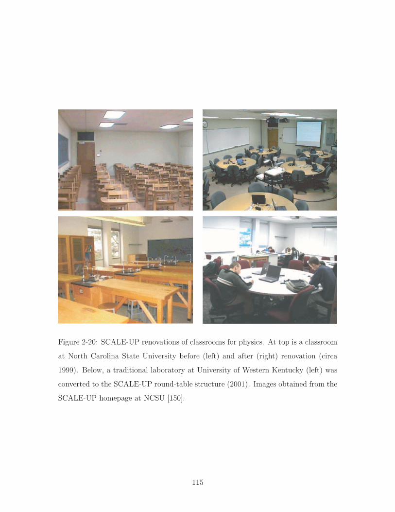
Figure 2-20: SCALE-UP renovations of classrooms for physics. At top is a classroom

at North Carolina State University before (left) and after (right) renovation (circa

1999). Below, a traditional laboratory at University of Western Kentucky (left) was

converted to the SCALE-UP round-table structure (2001). Images obtained from the

SCALE-UP homepage at NCSU [150].

115

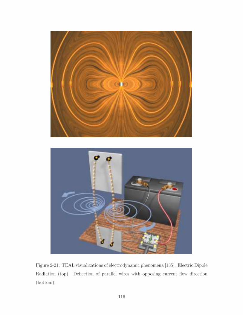
Figure 2-21: TEAL visualizations of electrodynamic phenomena [135]. Electric Dipole

Radiation (top). Deflection of parallel wires with opposing current flow direction

(bottom).

116

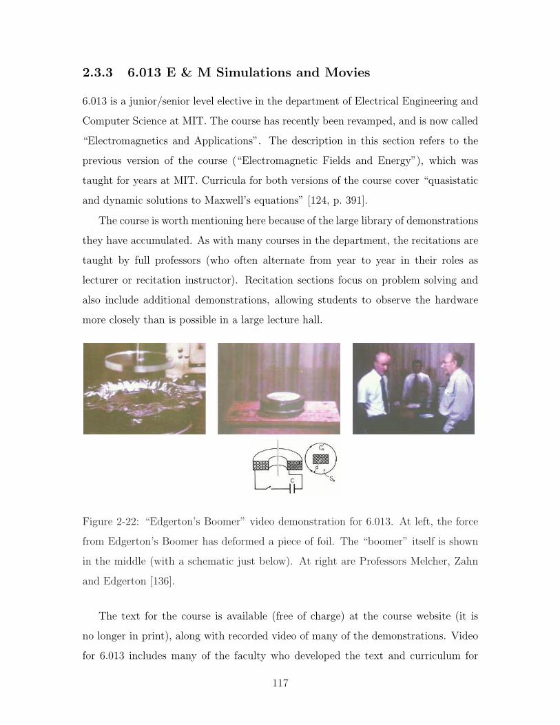
2.3.3 6.013 E & M Simulations and Movies

6.013 is a junior/senior level elective in the department of Electrical Engineering and

Computer Science at MIT. The course has recently been revamped, and is now called

“Electromagnetics and Applications”. The description in this section refers to the

previous version of the course (“Electromagnetic Fields and Energy”), which was

taught for years at MIT. Curricula for both versions of the course cover “quasistatic

and dynamic solutions to Maxwell’s equations” [124, p. 391].

The course is worth mentioning here because of the large library of demonstrations

they have accumulated. As with many courses in the department, the recitations are

taught by full professors (who often alternate from year to year in their roles as

lecturer or recitation instructor). Recitation sections focus on problem solving and

also include additional demonstrations, allowing students to observe the hardware

more closely than is possible in a large lecture hall.

Figure 2-22: “Edgerton’s Boomer” video demonstration for 6.013. At left, the force

from Edgerton’s Boomer has deformed a piece of foil. The “boomer” itself is shown

in the middle (with a schematic just below). At right are Professors Melcher, Zahn

and Edgerton [136].

The text for the course is available (free of charge) at the course website (it is

no longer in print), along with recorded video of many of the demonstrations. Video

for 6.013 includes many of the faculty who developed the text and curriculum for

117

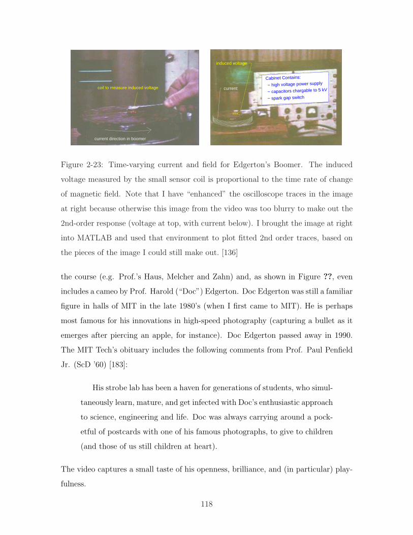
current direction in boomer

coil to measure induced voltage

induced voltage

current

− spark gap switch

Cabinet Contains:

− high voltage power supply

− capacitors chargable to 5 kV

Figure 2-23: Time-varying current and field for Edgerton’s Boomer. The induced

voltage measured by the small sensor coil is proportional to the time rate of change

of magnetic field. Note that I have “enhanced” the oscilloscope traces in the image

at right because otherwise this image from the video was too blurry to make out the

2nd-order response (voltage at top, with current below). I brought the image at right

into MATLAB and used that environment to plot fitted 2nd order traces, based on

the pieces of the image I could still make out. [136]

the course (e.g. Prof.’s Haus, Melcher and Zahn) and, as shown in Figure ??, even

includes a cameo by Prof. Harold (“Doc”) Edgerton. Doc Edgerton was still a familiar

figure in halls of MIT in the late 1980’s (when I first came to MIT). He is perhaps

most famous for his innovations in high-speed photography (capturing a bullet as it

emerges after piercing an apple, for instance). Doc Edgerton passed away in 1990.

The MIT Tech’s obituary includes the following comments from Prof. Paul Penfield

Jr. (ScD ’60) [183]:

His strobe lab has been a haven for generations of students, who simul-

taneously learn, mature, and get infected with Doc’s enthusiastic approach

to science, engineering and life. Doc was always carrying around a pock-

etful of postcards with one of his famous photographs, to give to children

(and those of us still children at heart).

The video captures a small taste of his openness, brilliance, and (in particular) play-

fulness.

118

“Edgerton’s Boomer” can essentially be modelled as a second-order LRC circuit.

The schematic at the bottom of Figure 2-22 shows a cross-section of the coil, which

can be modeled as an inductance and resistance in series. This coil is then connected

in series to a capacitor to form an LRC circuit. The scope traces in the image on

the right half of Figure 2-23 have been “touched up” to more clearly emphasize the

decaying oscillatory voltage and current responses (which are 90 degrees out of phase).

2.3.4 The OpenCourseWare Project

MIT is currently engaged in a program to make online course materials available to

the general public. This program is called “OpenCourseWare” (OCW). What the

project aims to accomplish, as cited on their website, is as follows:

1. “Provide free searchable, coherent access to MIT’s course materials for edu-

cators in the non-profit sector, students, and individual learners around the

world.” [125]

2. “Create an efficient, standards-based model that other universities may emulate

to publish their own course materials.” [125]

The project is funded by the William and Flora Hewlett Foundation, the Andrew

W. Mellon Foundation, and MIT. OCW should provide online access to materials for

nearly all of MIT’s courses (about 2000) by the summer of 2007 [125]. As of Spring

2003, OCW consists of materials from about 60 courses, including 2.003 Modeling

Dynamics and Control I. Links to descriptions of our ActivLab projects are provided

through OCW.

Much of the material at OCW will presumably consist of documentation of the

syllabus, homework and lab assignments in each class. Online (web) materials can also

include virtual laboratory experiences and demonstrations, however. For example The

videos for 8.01 and 6.013 are available as an online reference for students (independent

of the OCW project), and the TEAL simulations in Figure 2-21 are already a part of

the suite of OCW materials.

119

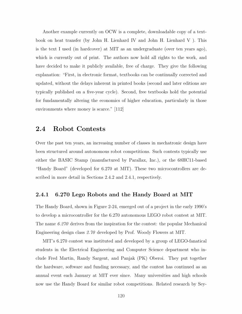
Another example currently on OCW is a complete, downloadable copy of a text-

book on heat transfer (by John H. Lienhard IV and John H. Lienhard V ). This

is the text I used (in hardcover) at MIT as an undergraduate (over ten years ago),

which is currently out of print. The authors now hold all rights to the work, and

have decided to make it publicly available, free of charge. They give the following

explanation: “First, in electronic format, textbooks can be continually corrected and

updated, without the delays inherent in printed books (second and later editions are

typically published on a five-year cycle). Second, free textbooks hold the potential

for fundamentally altering the economics of higher education, particularly in those

environments where money is scarce.” [112]

2.4 Robot Contests

Over the past ten years, an increasing number of classes in mechatronic design have

been structured around autonomous robot competitions. Such contests typically use

either the BASIC Stamp (manufactured by Parallax, Inc.), or the 68HC11-based

“Handy Board” (developed for 6.270 at MIT). These two microcontrollers are de-

scribed in more detail in Sections 2.4.2 and 2.4.1, respectively.

2.4.1 6.270 Lego Robots and the Handy Board at MIT

The Handy Board, shown in Figure 2-24, emerged out of a project in the early 1990’s

to develop a microcontroller for the 6.270 autonomous LEGO robot contest at MIT.

The name 6.270 derives from the inspiration for the contest: the popular Mechanical

Engineering design class 2.70 developed by Prof. Woody Flowers at MIT.

MIT’s 6.270 contest was instituted and developed by a group of LEGO-fanatical

students in the Electrical Engineering and Computer Science department who in-

clude Fred Martin, Randy Sargent, and Panjak (PK) Oberoi. They put together

the hardware, software and funding necessary, and the contest has continued as an

annual event each January at MIT ever since. Many universities and high schools

now use the Handy Board for similar robot competitions. Related research by Sey-

120

mour Papert’s Epistemology and Learning Group32 at the MIT Media Lab to create

the Programable LEGO Brick inspired the development of the LEGO MindStorms

robotics system [67, 109].

Handy Board specifications include 32K of static RAM. There are inputs for 7

analog and 9 digital sensors, and an expansion bus makes additional digital I/O

latches possible. The board operates on internal NiCad batteries, has a built-in

recharging circuit, and uses two L293D motor driver chips capable of driving a total

of four 9-volt DC motors.

The boards are particularly well-suited for teaching higher-level design skills due

in large part to the Interactive C (IC) programming language, developed for the

68HC11 by Randy Sargent [147]. IC compiles into pseudo-code (p-code), which is

then interpreted by the machine language. As a result, users do not need to wait

for lengthy compiles and can test code at the command line. This makes the en-

vironment particularly useful for learning higher-level skills, so that robot-builders

can focus on algorithms and good design practice rather than on details of low-level

implementation.

Figure 2-25 shows two LEGO robots built for the 6.270 autonomous robot contest

at MIT. Themes for the contest vary from year to year, and students work together

in teams of 2-4 to build their robots. The class is always over-subscribed, and par-

ticipants are chosen by lottery. The Handy Board (assembled or in parts) can be

purchased from several retailers. More details about the board can be found at the

following website: http://handyboard.com

32mentioned earlier in Section 2.2.1

121

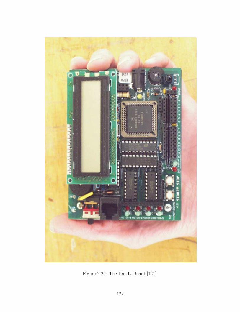
Figure 2-24: The Handy Board [121].

122

Figure 2-25: Lego ball-collecting robots from MIT 6.270 contests [123] - At top is

“Dr. Whackenscore”, created by Garrett Barter, Elie Krevat, and Dan Kwon in

2001 [26]. At bottom is “SoZoomy”, created by the Microsoft corporate sponsor

team consisting of Mike Koss, Walter vonKoch, Kevin Stoltz, Chris Koss, and Zak

Stoltzin in 2002 [103].

123

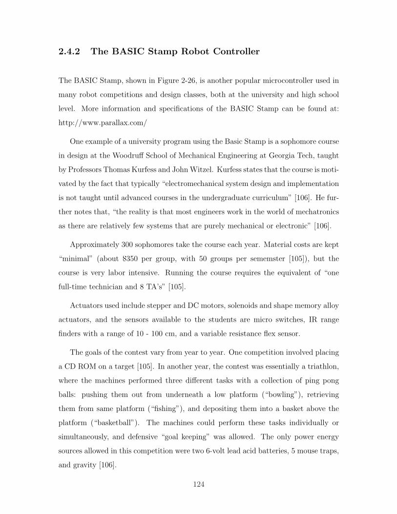
2.4.2 The BASIC Stamp Robot Controller

The BASIC Stamp, shown in Figure 2-26, is another popular microcontroller used in

many robot competitions and design classes, both at the university and high school

level. More information and specifications of the BASIC Stamp can be found at:

http://www.parallax.com/

One example of a university program using the Basic Stamp is a sophomore course

in design at the Woodruff School of Mechanical Engineering at Georgia Tech, taught

by Professors Thomas Kurfess and John Witzel. Kurfess states that the course is moti-

vated by the fact that typically “electromechanical system design and implementation

is not taught until advanced courses in the undergraduate curriculum” [106]. He fur-

ther notes that, “the reality is that most engineers work in the world of mechatronics

as there are relatively few systems that are purely mechanical or electronic” [106].

Approximately 300 sophomores take the course each year. Material costs are kept

“minimal” (about $350 per group, with 50 groups per sememster [105]), but the

course is very labor intensive. Running the course requires the equivalent of “one

full-time technician and 8 TA’s” [105].

Actuators used include stepper and DC motors, solenoids and shape memory alloy

actuators, and the sensors available to the students are micro switches, IR range

finders with a range of 10 - 100 cm, and a variable resistance flex sensor.

The goals of the contest vary from year to year. One competition involved placing

a CD ROM on a target [105]. In another year, the contest was essentially a triathlon,

where the machines performed three different tasks with a collection of ping pong

balls: pushing them out from underneath a low platform (“bowling”), retrieving

them from same platform (“fishing”), and depositing them into a basket above the

platform (“basketball”). The machines could perform these tasks individually or

simultaneously, and defensive “goal keeping” was allowed. The only power energy

sources allowed in this competition were two 6-volt lead acid batteries, 5 mouse traps,

and gravity [106].

124

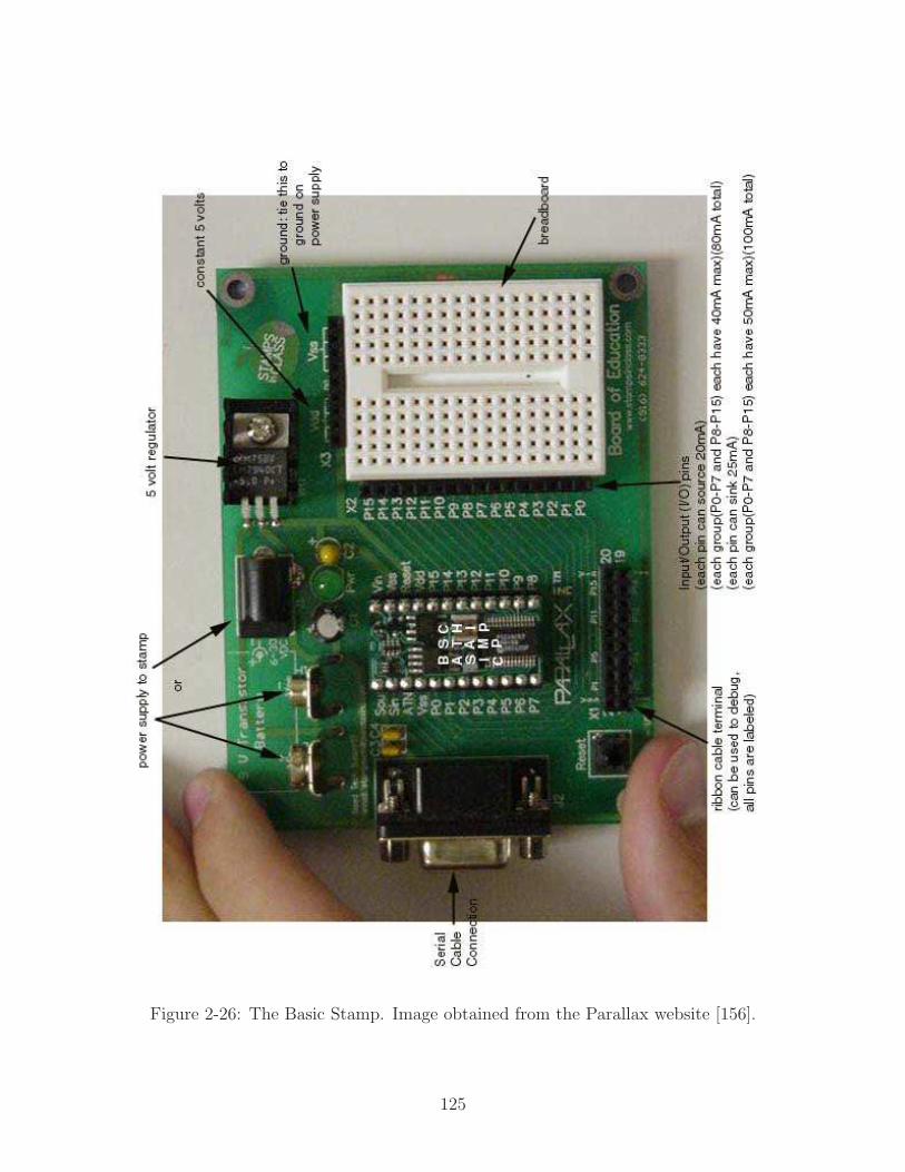
Figure 2-26: The Basic Stamp. Image obtained from the Parallax website [156].

125

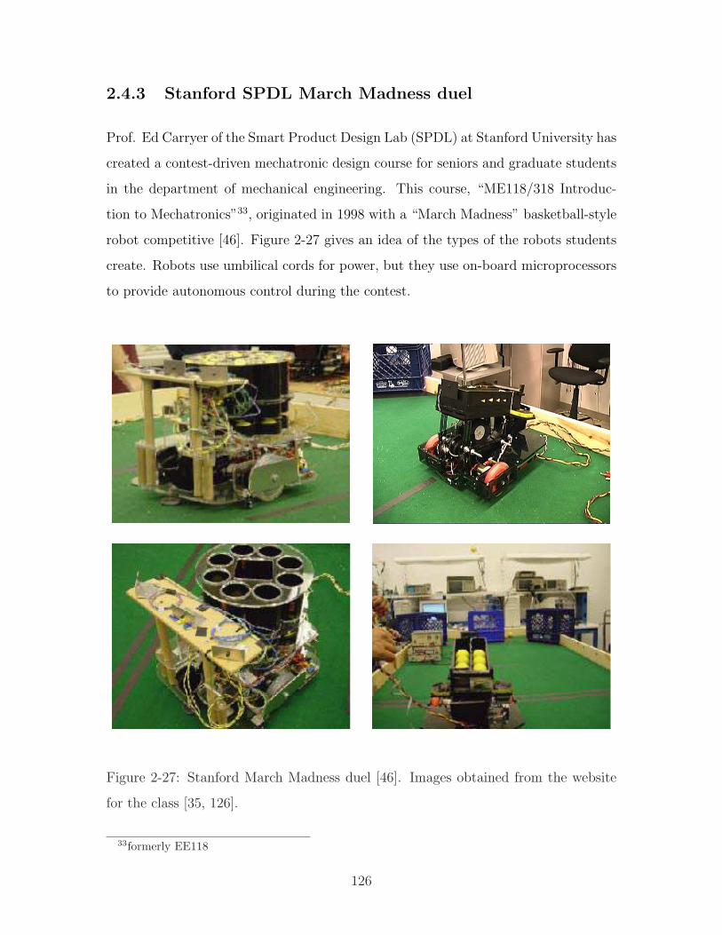
2.4.3 Stanford SPDL March Madness duel

Prof. Ed Carryer of the Smart Product Design Lab (SPDL) at Stanford University has

created a contest-driven mechatronic design course for seniors and graduate students

in the department of mechanical engineering. This course, “ME118/318 Introduc-

tion to Mechatronics”33, originated in 1998 with a “March Madness” basketball-style

robot competitive [46]. Figure 2-27 gives an idea of the types of the robots students

create. Robots use umbilical cords for power, but they use on-board microprocessors

to provide autonomous control during the contest.

Figure 2-27: Stanford March Madness duel [46]. Images obtained from the website

for the class [35, 126].

33formerly EE118

126

Over the years, the theme of the contest has varied34, but the goal of the course is

always the same: to provide students with an open-ended team project that requires

designing and building an electro-mechanical device with an embedded microproces-

sor. The class runs for ten weeks, with twice-weekly lectures on topics that include

sensors, op-amps, power drivers, solenoids and DC motors, stepper motors, A/D and

D/A, microprocessors (including both the BASIC Stamp and the 86HC11), and noise,

grounding and isolation issues. During the first four or fives weeks, there is a weekly

lab. Lab topics include programming state machines, analog signal conditioning,

mechanical prototyping with foamcore, and DC and stepper motors.

The texts for ME118/3118 are the classic “The Art of Electronics” by Horowitz

& Hill and “Mobile Robots: Inspiration to Implementation” by Joseph Jones, Bruce

Seiger and Anita Flynn. This second book “has grown out of research at the MIT

Artificial Intelligence (AI) Laboratory under Rodney Brooks and his mobile robot

group.”35 It is an excellent resource for robot builders, covering a gamut of topics

including (but not limited to) sensor and motor selection, power systems and isolation,

microprocessors, legged locomotion, and mechanical design principles. The authors

also include lists of suggested parts suppliers, data books and trade magazines.

34In 2002, the Winter Olympics inspired a contest based (loosely) on the sport of “curling”.35from the book’s Preface [96, p. xx].

127

2.4.4 Micromouse Competition

In Micromouse competitions, autonomous robots must navigate through a maze as

quickly as possible. Many Micromouse contests are held throughout the year and

across the world, involving participants from the high school students to seasoned

analog circuit designers.36 IEEE organizes regional competitions in the United States

for undergraduate students. Several universities now offer courses in which students

build a Micromouse as a capstone project. Figure 2-28 shows two views of mouse

build by students at California State University at Northridge (CSUN).

IEEE Region 6 (covering much of the south-western US and Hawaii) is particularly

active in such competitions. Participating schools in this region include the following:

Berkeley, Cal Poly Pomona, U.C. Davis, U.C. Santa Barbara, U.C.L.A., U.C. Santa

Cruz, Chico State and the University of Hawaii. The IEEE website at U.C Davis

notes: “Micromouse is an official course offered at U.C. Davis under EEC-194ABC.

It is one of the few undergraduate courses that integrates several different disciplines

of engineering, ranging from electrical to mechanical to computer science - it can offer

a valuable learning experience. In addition to various regional and national events

for Micromouse competition, one of our fondest events at U.C. Davis is the Picnic

Day competition,” held annually each Spring [93].

The EEC-194A,B,C Micromouse sequence at U.C. Davis, currently taught by Prof.

Tak Auyeung, runs through all three terms (fall, winter and spring) of the academic

year to comprise a single, 5-unit elective. The Micromouse projects are student-run.

Each team consists of approximately five students, each of whom is responsible for a

particular subsystem (electronics, power and motor, software, system integration, and

sensors). Topics covered include gears, bearings, wheels, traction, chassis construc-

tion, stepper and DC motors, differential steering, sensors, noise issues, PID control,

high level algorithms and project management [17].

36Dave Otten, who currently works a few feet away from me in the Precision Motion Control

(PMC) lab at MIT is such a “seasoned analog circuit designer” who has won accolades at several

international Micromouse competitions.

128

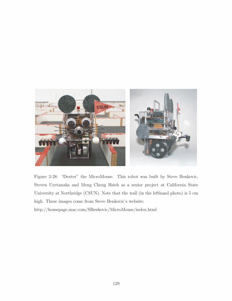
Figure 2-28: “Dexter” the MicroMouse. This robot was built by Steve Benkovic,

Steven Uyetanaka and Meng Cheng Hsieh as a senior project at California State

University at Northridge (CSUN). Note that the wall (in the lefthand photo) is 5 cm

high. These images come from Steve Benkovic’s website:

http://homepage.mac.com/SBenkovic/MicroMouse/index.html

129

2.4.5 Intercollegiate NATCAR Competition

The NATCAR race is an annual competition, sponsored by National Semiconductor,

which has involved teams of students from up to eight universities. There are typically

2-3 undergraduates per team. The five universities participating in May 2003 are

U. C. Davis, Berkeley, Stanford, San Jose State University, and Oklahoma State

University [187]. The objective of the contest is to design and build an autonomous

car that can complete a preset course in the shortest time. The race course is traced

out on black carpeting with shiny, white vinyl tape with a wire beneath it that

produces a 75 kHz signal. The curving path can cross over on itself. The smallest

allowable angle at any intersection is 60 degrees [187]. The vehicles can elect to

use either optical or magnetic sensors. Students are allowed to begin their designs

with the chassis of a radio-controlled car, but all sensing and control electronics must

be built by the students. The vehicles often achieve speeds greater than 10 mph -

significantly faster than a typical human could control an RC car over the curving

path.

Several universities incorporate the contest as the focus of a course in design.

Figure 2-29 shows two views of a U.C. Davis entry. Prof. Richard Spencer initially

organized the competition with the cooperation of engineers at National Semiconduc-

tor [175]. He now teaches “EEC195, Autonomous Race Car Project” at U.C. Davis

(where the NATCAR competition is headquartered) and coordinates the official NAT-

CAR website (outlining the rules of the competition) [187]. Berkeley offers a similar

course which focuses on the design of cars for the competition called “EE192: Mecha-

tronics Design Lab”. U.C.Davis and Berkeley are typically the strongest competitors

in NATCAR each year. NATCAR courses at other universities include “EE192G:

Electronic Dynamic Control Systems Laboratory” at Stanford, and “EEE192 Elec-

trical Engineering Design” at U.C. San Diego.

The competition forms a focal point for covering topics such as DC motor control,

analog circuitry, microcontrollers, PID control, optical and magnetic sensors, A/D’s,

noise and shielding concerns, H-bridges and PWM, and design principles [128, 69].

130

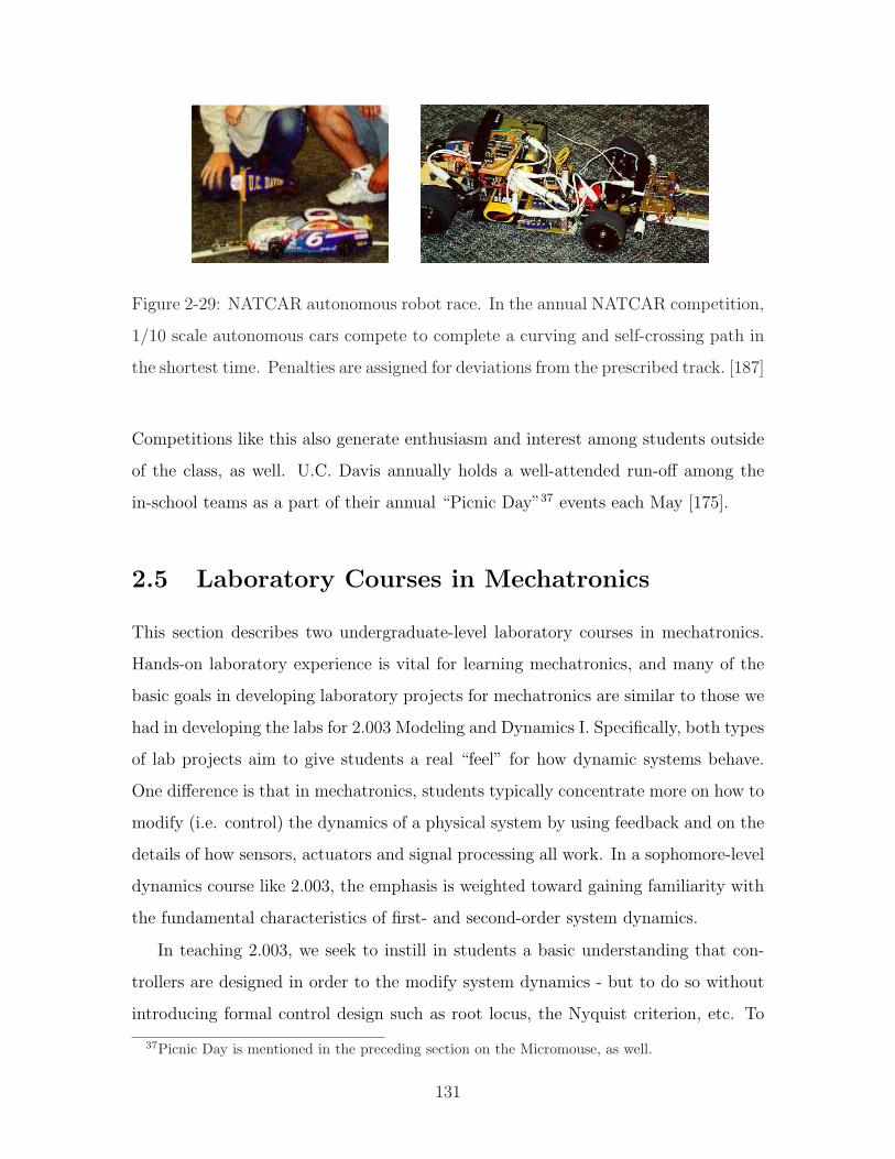
Figure 2-29: NATCAR autonomous robot race. In the annual NATCAR competition,

1/10 scale autonomous cars compete to complete a curving and self-crossing path in

the shortest time. Penalties are assigned for deviations from the prescribed track. [187]

Competitions like this also generate enthusiasm and interest among students outside

of the class, as well. U.C. Davis annually holds a well-attended run-off among the

in-school teams as a part of their annual “Picnic Day”37 events each May [175].

2.5 Laboratory Courses in Mechatronics

This section describes two undergraduate-level laboratory courses in mechatronics.

Hands-on laboratory experience is vital for learning mechatronics, and many of the

basic goals in developing laboratory projects for mechatronics are similar to those we

had in developing the labs for 2.003 Modeling and Dynamics I. Specifically, both types

of lab projects aim to give students a real “feel” for how dynamic systems behave.

One difference is that in mechatronics, students typically concentrate more on how to

modify (i.e. control) the dynamics of a physical system by using feedback and on the

details of how sensors, actuators and signal processing all work. In a sophomore-level

dynamics course like 2.003, the emphasis is weighted toward gaining familiarity with

the fundamental characteristics of first- and second-order system dynamics.

In teaching 2.003, we seek to instill in students a basic understanding that con-

trollers are designed in order to the modify system dynamics - but to do so without

introducing formal control design such as root locus, the Nyquist criterion, etc. To

37Picnic Day is mentioned in the preceding section on the Micromouse, as well.

131

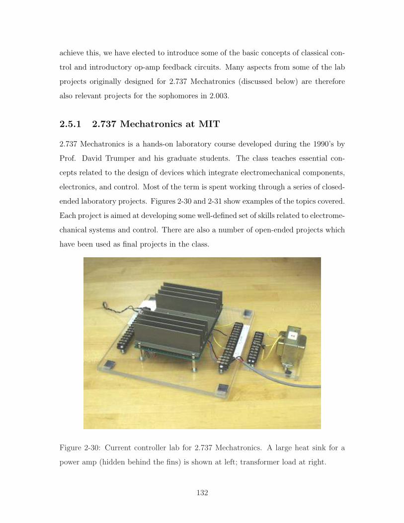
achieve this, we have elected to introduce some of the basic concepts of classical con-

trol and introductory op-amp feedback circuits. Many aspects from some of the lab

projects originally designed for 2.737 Mechatronics (discussed below) are therefore

also relevant projects for the sophomores in 2.003.

2.5.1 2.737 Mechatronics at MIT

2.737 Mechatronics is a hands-on laboratory course developed during the 1990’s by

Prof. David Trumper and his graduate students. The class teaches essential con-

cepts related to the design of devices which integrate electromechanical components,

electronics, and control. Most of the term is spent working through a series of closed-

ended laboratory projects. Figures 2-30 and 2-31 show examples of the topics covered.

Each project is aimed at developing some well-defined set of skills related to electrome-

chanical systems and control. There are also a number of open-ended projects which

have been used as final projects in the class.

Figure 2-30: Current controller lab for 2.737 Mechatronics. A large heat sink for a

power amp (hidden behind the fins) is shown at left; transformer load at right.

132

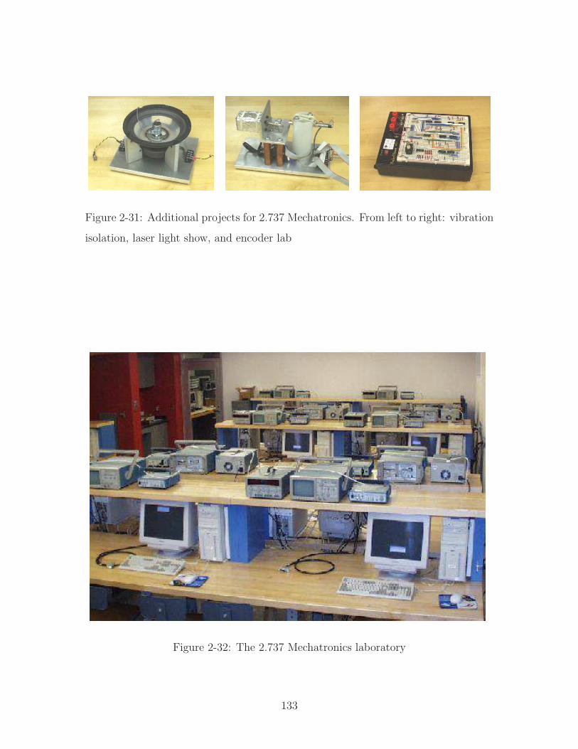
Figure 2-31: Additional projects for 2.737 Mechatronics. From left to right: vibration

isolation, laser light show, and encoder lab

Figure 2-32: The 2.737 Mechatronics laboratory

133

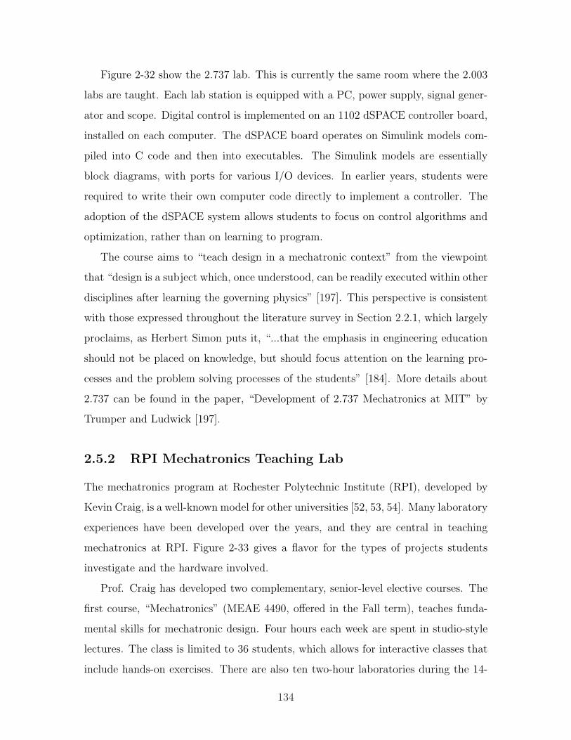
Figure 2-32 show the 2.737 lab. This is currently the same room where the 2.003

labs are taught. Each lab station is equipped with a PC, power supply, signal gener-

ator and scope. Digital control is implemented on an 1102 dSPACE controller board,

installed on each computer. The dSPACE board operates on Simulink models com-

piled into C code and then into executables. The Simulink models are essentially

block diagrams, with ports for various I/O devices. In earlier years, students were

required to write their own computer code directly to implement a controller. The

adoption of the dSPACE system allows students to focus on control algorithms and

optimization, rather than on learning to program.

The course aims to “teach design in a mechatronic context” from the viewpoint

that “design is a subject which, once understood, can be readily executed within other

disciplines after learning the governing physics” [197]. This perspective is consistent

with those expressed throughout the literature survey in Section 2.2.1, which largely

proclaims, as Herbert Simon puts it, “...that the emphasis in engineering education

should not be placed on knowledge, but should focus attention on the learning pro-

cesses and the problem solving processes of the students” [184]. More details about

2.737 can be found in the paper, “Development of 2.737 Mechatronics at MIT” by

Trumper and Ludwick [197].

2.5.2 RPI Mechatronics Teaching Lab

The mechatronics program at Rochester Polytechnic Institute (RPI), developed by

Kevin Craig, is a well-known model for other universities [52, 53, 54]. Many laboratory

experiences have been developed over the years, and they are central in teaching

mechatronics at RPI. Figure 2-33 gives a flavor for the types of projects students

investigate and the hardware involved.

Prof. Craig has developed two complementary, senior-level elective courses. The

first course, “Mechatronics” (MEAE 4490, offered in the Fall term), teaches funda-

mental skills for mechatronic design. Four hours each week are spent in studio-style

lectures. The class is limited to 36 students, which allows for interactive classes that

include hands-on exercises. There are also ten two-hour laboratories during the 14-

134

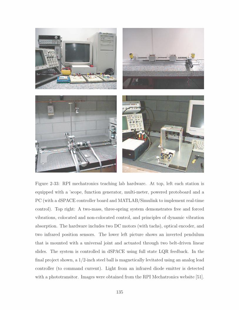
Figure 2-33: RPI mechatronics teaching lab hardware. At top, left each station is

equipped with a ’scope, function generator, multi-meter, powered protoboard and a

PC (with a dSPACE controller board and MATLAB/Simulink to implement real-time

control). Top right: A two-mass, three-spring system demonstrates free and forced

vibrations, colocated and non-colocated control, and principles of dynamic vibration

absorption. The hardware includes two DC motors (with tachs), optical encoder, and

two infrared position sensors. The lower left picture shows an inverted pendulum

that is mounted with a universal joint and actuated through two belt-driven linear

slides. The system is controlled in dSPACE using full state LQR feedback. In the

final project shown, a 1/2-inch steel ball is magnetically levitated using an analog lead

controller (to command current). Light from an infrared diode emitter is detected

with a phototransitor. Images were obtained from the RPI Mechatronics website [51].

135

week class. Both lectures and labs are held a specially-designed classroom, “The

Mechatronics Studio”, which is equipped with lab stations and multi-media capabil-

ities. Laboratory topics include the following: analog electronics, digital electronics,

A/D and D/A, stepper motor control, DC motor control, control of a thermal system,

pneumatic servomechanism, and magnetic levitation.

The Spring-term elective in mechatronics is “Mechatronic System Design” (MEAE

4250). This course is more open-ended than the former. Students work in groups of

four to complete a central term project and presentation. The project may involve

reverse engineering a mechatronic device, for instance, or creating new hardware for

the lab. The class has four hours of lecture each week and unlimited open lab access.

Both classes focus on developing essential skills in mechatronic design. As Prof.

Craig writes, “while there is certainly a need for controls experts and advanced control

techniques, most control designs used in industry today are of the classical lead-lag

type, and mechanical engineers need to know how to design and implement these

as an integral part of their design and not as after-thought add-ons.” [52, 53, 54]

Craig’s premises are that controls are taught too late (if at all) in most mechanical

engineering curricula and that mechatronic design is a relevant skill for all mechanical

engineers in today’s world.

2.5.3 Other Programs of Note

Traditionally, most mechatronics programs have been aimed at the graduate level.

This thesis is specifically concerned with undergraduate programs that give students

hands-on (laboratory) experience in dynamics and mechatronics. Over the past ten

years, many universities have begun to offer curricula and course degree programs in

mechatronics at the undergraduate level. Several such programs, both in the U.S.

and abroad, are listed in Tables B.1 and B.2 of Appendix B. I am surely not even

aware of many excellent programs worth noting. The lists in this Appendix do not

claim to be comprehensive, but they do give a survey of the current approaches used

for teaching mechatronics.

136

Chapter 3

ActivLab Hardware

This chapter describes the hardware and experiments developed for 2.003 Introduction

to Modeling, Dynamics, and Control I, which is a required undergraduate course in

the Department of Mechanical Engineering. The course focuses largely on deriving

linear constant-coefficient differential equations to model linear time-invariant (LTI)

mechanical and electrical system and then representing these differential relations

in the Laplace domain (e.g. as transfer functions). Such skills are fundamental to

controller design, and controller design is in turn an increasingly fundamental skill

for mechanical engineers.

In other words, because the goal of a control system is essentially to alter the

dynamics of a system, designers of control systems need to understand both (1) how

to model a real-world system they wish to control and (2) how they can (and should)

modify those dynamics using active control. Classical control methods have tradi-

tionally been taught as an area of specialization in mechanical engineering programs.

Even today, undergraduates do not typically encounter controls until the senior year

(if at all). Because it is becoming increasingly practical (i.e. affordable) to incorporate

microcontrollers, sensors, and actuators in a wide variety mechanical designs, many

educators now recognize that the skill set generally referred to as “mechatronics” is

relevant to all mechanical engineers [15, 31, 45, 54, 64, 71, 77, 89, 106, 115, 143, 197,

203, 221].

The lectures, coursework and laboratories in 2.003 are aimed both at teaching

137

system dynamics and at providing a solid foundation for further study in control.

We designed the ActivLab laboratory projects to provide hands-on experiences to

reinforce students’ understanding of these new concepts.

3.1 ActivLab Labware for Teaching Dynamics

Prof. David Trumper has coined the name ActivLab to refer to the set of hardware and

experiments we developed during the summer of 2001 for 2.003 Modeling Dynamics

and Control I. These lab projects have been developed as shareware, and we are in

the process of providing web-accessible documentation to allow instructors at other

universities to adapt these labs to their own efforts [83].

3.2 Philosophy for Designing Labs

The laboratories for the 2.003 class were designed with a few basic goals in mind.

One particular concern was that the students should be able to directly observe the

relevant dynamics in the mechanical systems firsthand. Thus the motions should

be tangible, and the time constants and/or oscillations should be on the order of a

second, so they are directly perceivable. In these systems, it is also important that

students are able to observe the linear effects of damping with a minimal amount

of nonlinear friction. To achieve this, we use porous carbon cylindrical air bearings

(manufactured by New Way Machine Components, Inc. [146]) to implement both

rotational and translational mechanical systems.

We also believe the laboratory hardware and data acquisition should be as trans-

parent as practical to the students. For this reason, we have avoided introducing

tachometers, encoders or other sensor technology in the first two laboratories to al-

low students to observe dynamic systems which evolve on a human-perceivable time

scale. The above ideas were catalyzed by discussions with Prof. Ely Sachs in our

Mechanical Engineering Department [176].

For these reasons the labs utilize flexures and air bearings to constrain motion,

138

as these behave in a near-ideal fashion. They allow time constants and oscillation

periods on the order of one second, and thus at a time scale directly perceivable to the

students. Finally, in the early labs, motion is measured with a video camera. Time

resolution is taken by single-stepping through the video frames, which are typically

acquired at 20 Hz.

Also, the equipment should be modular in nature, to allow extensions to the setups

to be developed with a minimum of effort and to reduce the needed investment in space

and money to develop a full set of laboratory hardware. All hardware is mounted on

an optical breadboard, which allows us to assemble the labs easily and to disassemble

the components for efficient storage.

3.3 1st-Order Spring-Damper Translational

System

The first lab in 2.003 demonstrates a first-order response with position as the variable

of interest. Student evaluations of the class report that Labs 1 and 2 are more straight-

forward (i.e. less difficult) than subsequent labs, which is not surprising. Both labs

focus on simple, first-order system dynamics, and an emphasis is placed on observing

and recording the response visually.

While the system for Lab 1 is designed to be relatively straight-forward, how-

ever, the actual system dynamics can also be modeled with much more complexity

than we expect from our sophomore-level students. Some of the phenomena we ne-

glect to incorporate in the system model are presented in this section and include

(briefly) modeling flow through an orifice, thermodynamic expansion or compression

of an ideal gas, and modal vibrations of a 4th-order Bernoulli-Euler beam. These

phenomena illustrate that the mechanical system hardware for 2.003 involves compli-

cated dynamics, just as most real-world systems do. Like many real-world systems,

however, the system response can be approximated reasonably well using low-order,

constant-coefficient linear differential equations. The main point of this lab is to study

139

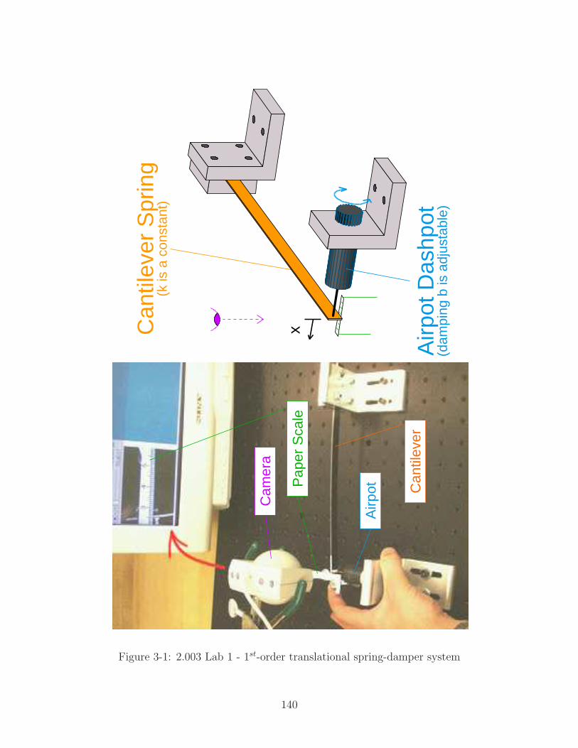
(k is

a c

onst

ant)

Can

tilev

er S

prin

g

(dam

ping

b is

adj

usta

ble)

Airp

ot D

ashp

ot

x

Cam

era

Pap

er S

cale

Airp

ot Can

tilev

er

Figure 3-1: 2.003 Lab 1 - 1st-order translational spring-damper system

140

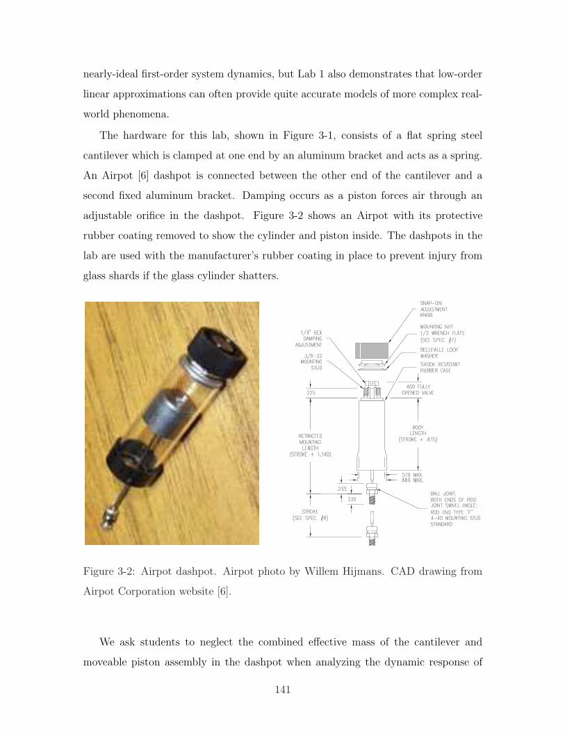
nearly-ideal first-order system dynamics, but Lab 1 also demonstrates that low-order

linear approximations can often provide quite accurate models of more complex real-

world phenomena.

The hardware for this lab, shown in Figure 3-1, consists of a flat spring steel

cantilever which is clamped at one end by an aluminum bracket and acts as a spring.

An Airpot [6] dashpot is connected between the other end of the cantilever and a

second fixed aluminum bracket. Damping occurs as a piston forces air through an

adjustable orifice in the dashpot. Figure 3-2 shows an Airpot with its protective

rubber coating removed to show the cylinder and piston inside. The dashpots in the

lab are used with the manufacturer’s rubber coating in place to prevent injury from

glass shards if the glass cylinder shatters.

!"# $ % & & & & & & & & & & & & & & & & & & & & & & & & & & & & & & & & & & & & & & & & & & & & & & & & & & & & & & & & & & & & & & & & & & & & & & & & & & & & & & & '( () !" $ % )& & & & & & & & & & & & & & & & & & & & & & & & & & & & & & & & & & & & & & & & & & & & & & & & & & & & & & & & & & & & & & & & & & & & & & & & & & & & & & & & & & & & & & & & * '$ %# !" $ % & & & & & & & & & & & & & & & & & & & & & & & & & & & & & & & & & & & & & & & & & & & & & & & & & & & & & & & & & & & & & & & & & & & & & & & & & & & & & & & & & & & & & & & & + ,& -.0/ & 1.0/ & -.)2 & 1 # 3 & 1 - 4 & $ & $ & .$ ! 5 & & & & & & & & & & & & & & & & & & & & & & & & & & & & & & & & & & & & & & & & & & & & & & & & & & & & & & & & & & & & & & & & & & & & & & & & & & & & & & & & & & & & & & & & 6 ( (0'! 7 8 5 $ ().9 9 1 %#& & & & & & & & & & & & & & & & & & & & & & & & & & & & & & & & & & & & & & & & & & & & & & & & & & & & & & & & & & & & & & & & & & & & & & & & & & & & & & & & & & & :( )# %& / - ; #5 '( !6 '$ % !"#& & & & & & & & & & & & & & & & & & & & & & & & & & & & & & & & & & & & & & & & & & & & & & & & & & & & & & & & & & & & & & & & & & & & 3

<=>?@A)B CD EGFHI BJLK M D I N O0B N CP QR S S R TVU WXZY S [ T\]Y^_X `0[ UU WXZa R b WUc#R U Wd W^R d X `0e a ^fgU WXhS R ` UYX S ^ci jk l mn o p q rVs t p o u v)wZx yz| y~

Zh h Z ¡ ¢ £¤h¤0¥¦ § ¨© ª)¨«h¬0®§¯ °²±³ ´hµ ¶ · ¸ ® ¹ ¹ ¶ º ¶ · »£ ¼ ½ ¾0¿ À Á ¡ Â Ã Á Ä ¥Å Æ Ç È Ä É Å À ¿ Ê£ ¼ £ Ë ËhÌÁ ¡ ¤h¤0Á Ä ¥

Í ° © º ÎÏ ¶ Ð Ñ ¶ · ÒÓ Ô Õ Õ Ö× Ø)Ù Ú Û Ü Ý Þ Ë¿ À¤Å ßZ¡ ½ 0Ì¥Ó Ô à áÖ× Ø)Ù Ú Û Ü Ý Þ £¿ Àh¤Å ß¡ Ë Ë ¾0Ì¥

â ° © ¶ º » ¶ ·ã ä å æ æ Ú ç Ú å Û è Ý £ ½é ä ê ç åëÚ è á ä Ô è à Ú ì åÕ ä × ì Ý í0Þ î

ï ° ª µ ³ » ¶ · ¸0ð ´hµ ³ » Ï )¨ ³ · ¸ ñ ¾ ¾ ò ó#É ôõ Þ ¾ £ ò óö ÷ ô ø Ê ù Å É Â Ã î0Å É É Ê ¤ø Ê ù Å É È ù Ê ÄÅ À ô ú Êõ û £ ò óü ø ¿ Ê Å Ä ÊÅ Æ ú Â Ä Ê÷ Å ý É ô ù þ

«#ª)ÿ ð 0Î ± ¬ ð ¬ ° «Z Ï · » ¶ · ¸ Ñ å ç è × Û Ü Ô Õ × ê Ý Þ ½ ßh û ¾ ô ù¤h¤²ßÞ £¤¤ ä Ô Û ì Ý û ¾ ô ùÞ £¤h¤ ° Ï ¸ ¸ Ò » Ð « Ï · » ¶ · ¸ ³ º » ð ¶ º · Ò Ò £ £ ¼ £ ¢ ¡ Þ ¾ ½ ¼ ½ )¤h¤¥ ° «Z Ï · » ¶ · ¸ 0Ï » ð Ï å × ì Ý Ë ¼ 0Â Ã ñ ¿ ÀZ¡ £ Ë ¾ ¼ £ ¢ £0Ì¤0¥ ä ì Û ì Ý ½ ¼ ¾0Â Ã ñ ¿ À¡ £ ½ ¼ £ ¾ 0Ì)¤0¥ ° » È ¿ ¿ Ä É ù ô ÊÂ Äô À É Å Â Ã Ê Æ)Â É hý È Ä É ô ¤Ê ù Ê ¿ Æ¤ô È Ã É Â Ã î)É ô ¿ Ê ù Å Ã ý Êô ÷ õ £ Þ ¾ ¡ £ ¤¤¥

"!#$"%&

')( * + ,

2KS95

-/. 0 0 1 2 2 34 ï 5 ¯76/8 . 9)1 Í 2 â 34 ï : 5 2 â :;6 < 5 = . > 0 ? @ . 0 < @ A). > B C D E ° F D =G6 HH/H° . > B C D E ° F D =

I JK KL M NK OP Q Q R S T/U V W S X V W S VS V Y Z U W [ V Q U W W X \ Z U ] ^ S W U W _7U Y S ` S U R

a b c d e f b g h c i j b g f i c i k f c h k i l h c m e n a b c d e f o e c d e c h f b e p q r s c i t b g h c i j b g f i c i k f c h k i l h c m e n o e c p b p j u v h g g w e c m g q a r o x y z u

| ~ ®

)) /7 /; ) ý ¿ Â ý É Ê À È É É ô Ã¿ ô ý Å É Ê ÆhÅ É É ÊÉ ô øhô ÷ É ÊÀ ù ô )Ä Ê ù )Â Ã Æ ô ü É ô0î Ê Ã Ê ù Å É Êþ ô È ù¤ô Æ Ê ¿ Ã È ¤À Ê ù

Figure 3-2: Airpot dashpot. Airpot photo by Willem Hijmans. CAD drawing from

Airpot Corporation website [6].

We ask students to neglect the combined effective mass of the cantilever and

moveable piston assembly in the dashpot when analyzing the dynamic response of

141

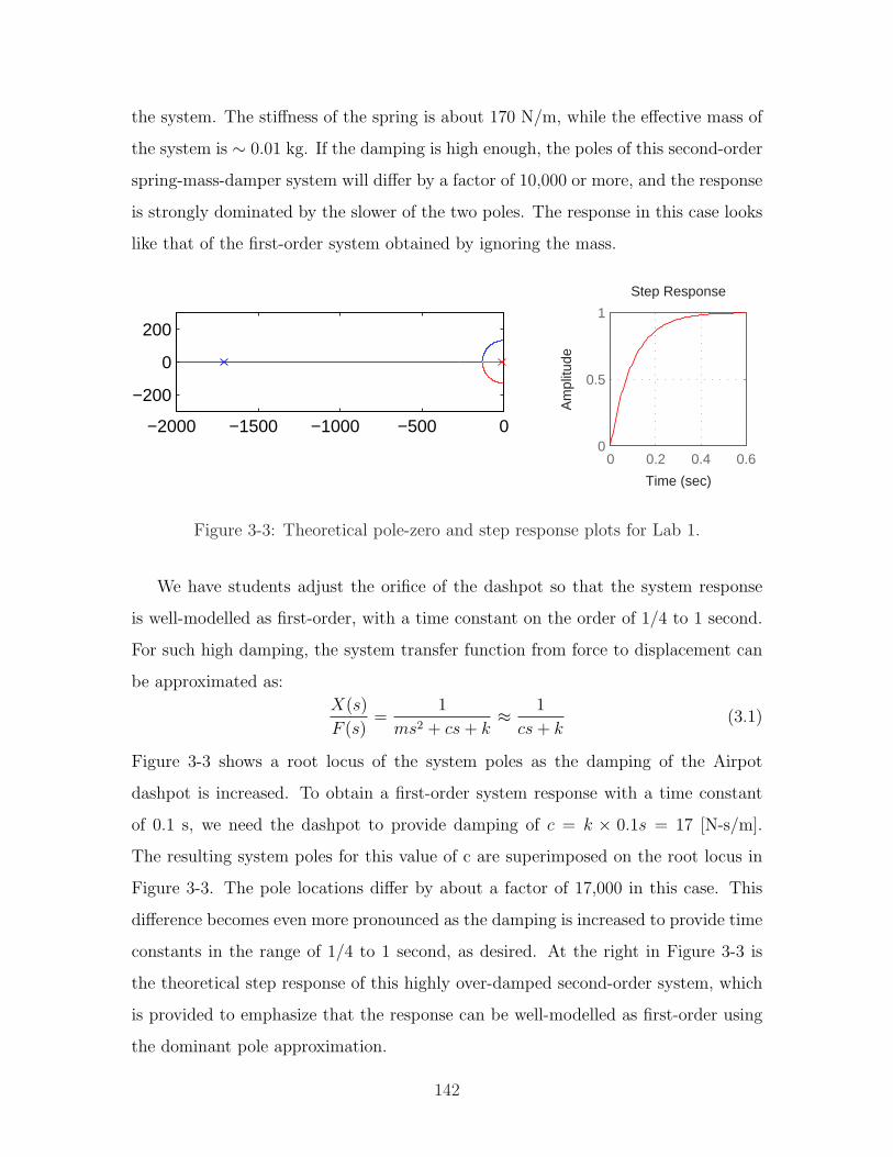
the system. The stiffness of the spring is about 170 N/m, while the effective mass of

the system is ∼ 0.01 kg. If the damping is high enough, the poles of this second-order

spring-mass-damper system will differ by a factor of 10,000 or more, and the response

is strongly dominated by the slower of the two poles. The response in this case looks

like that of the first-order system obtained by ignoring the mass.

−2000 −1500 −1000 −500 0

−200

0

200

Step Response

Time (sec)

Am

plitu

de

0 0.2 0.4 0.60

0.5

1

Figure 3-3: Theoretical pole-zero and step response plots for Lab 1.

We have students adjust the orifice of the dashpot so that the system response

is well-modelled as first-order, with a time constant on the order of 1/4 to 1 second.

For such high damping, the system transfer function from force to displacement can

be approximated as:

X(s)

F (s)=

1

ms2 + cs + k≈ 1

cs + k(3.1)

Figure 3-3 shows a root locus of the system poles as the damping of the Airpot

dashpot is increased. To obtain a first-order system response with a time constant

of 0.1 s, we need the dashpot to provide damping of c = k × 0.1s = 17 [N-s/m].

The resulting system poles for this value of c are superimposed on the root locus in

Figure 3-3. The pole locations differ by about a factor of 17,000 in this case. This

difference becomes even more pronounced as the damping is increased to provide time

constants in the range of 1/4 to 1 second, as desired. At the right in Figure 3-3 is

the theoretical step response of this highly over-damped second-order system, which

is provided to emphasize that the response can be well-modelled as first-order using

the dominant pole approximation.

142

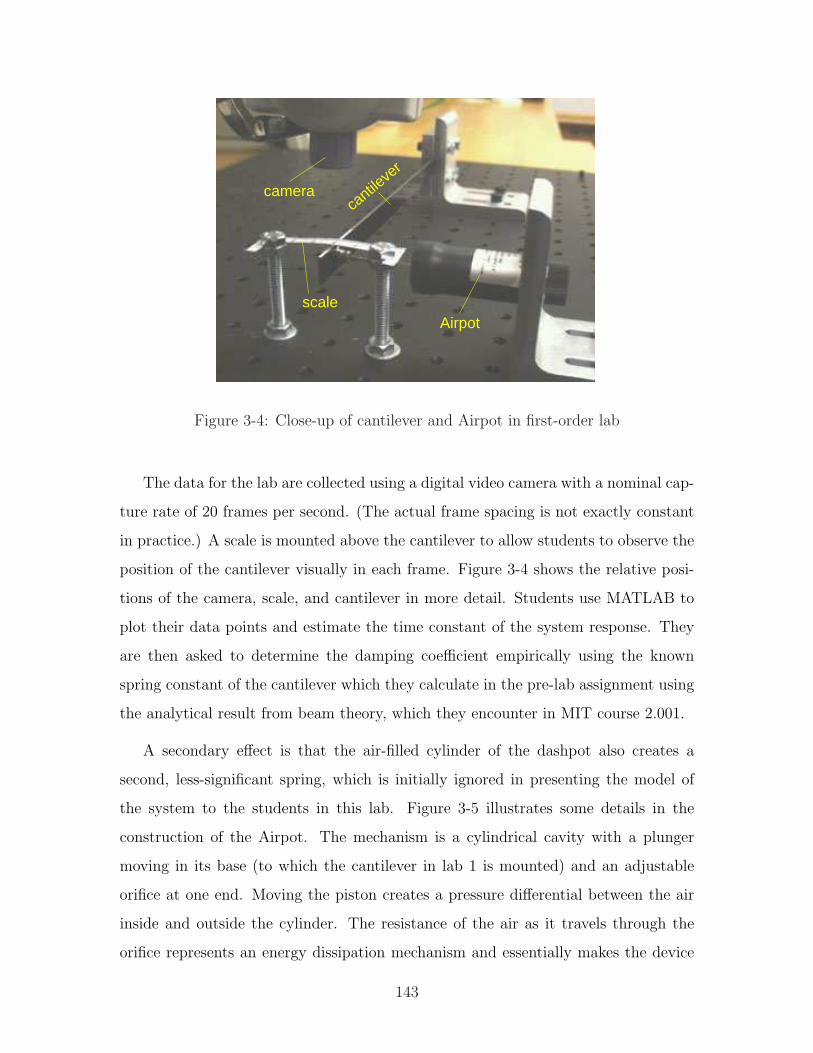
camera

scaleAirpot

cantile

ver

Figure 3-4: Close-up of cantilever and Airpot in first-order lab

The data for the lab are collected using a digital video camera with a nominal cap-

ture rate of 20 frames per second. (The actual frame spacing is not exactly constant

in practice.) A scale is mounted above the cantilever to allow students to observe the

position of the cantilever visually in each frame. Figure 3-4 shows the relative posi-

tions of the camera, scale, and cantilever in more detail. Students use MATLAB to

plot their data points and estimate the time constant of the system response. They

are then asked to determine the damping coefficient empirically using the known

spring constant of the cantilever which they calculate in the pre-lab assignment using

the analytical result from beam theory, which they encounter in MIT course 2.001.

A secondary effect is that the air-filled cylinder of the dashpot also creates a

second, less-significant spring, which is initially ignored in presenting the model of

the system to the students in this lab. Figure 3-5 illustrates some details in the

construction of the Airpot. The mechanism is a cylindrical cavity with a plunger

moving in its base (to which the cantilever in lab 1 is mounted) and an adjustable

orifice at one end. Moving the piston creates a pressure differential between the air

inside and outside the cylinder. The resistance of the air as it travels through the

orifice represents an energy dissipation mechanism and essentially makes the device

143

a damper.

The Airpot acts is primarily a dissipative device, but it also stores some energy.

Rapid movement of the piston results in a change in the stored energy of the air within

the cylinder. In other words, the Airpot also acts as a spring. Because pressure,

temperature and volume are coupled in an ideal gas, the expansion or compression

of the air inside results in a change in both the mechanical and thermal energy. The

exact relationship depends on how much heat is exchanged through the walls of the

cylinder, that is, on how closely the process comes to being adiabatic and therefore

reversible. At the end of this section, I discuss a model which approximately describes

the non-linear dynamics of both orifice flow and the energy storage relationships in

the air.

Because of the spring effect of the Airport, the relative positioning of the Airpot

and cantilever will have a minor effect on the time constant of the first-order fit to

the response. Figure 3-5 shows the L-bracket fixture which holds the Airpot in place.

This bracket is bolted down through two slots, allowing one to position the fixture

as desired. Moving the mounting for the Airpot to the left of right will change the

final volume in the Airpot, which in turn affects the time constant of the response.

Whether the piston acts to expand or compress the air in the Airpot will also affect

the time constant. The theoretical model of the system predicts that neither effect

should be significant, however, and the data in Figure 3-6 verify that this is the case.

The springiness of the Airpot becomes significant only as both the size of the

orifice is reduced to provide maximal damping and the cantilever is released such that

it compresses the air. If it is released in the other direction, the cylinder is initially

starting with virtually no air inside. The initial movement of the piston therefore

causes a large pressure differential (with nearly a vacuum inside the cylinder) and

thus the air spring is quite stiff. When the cylinder instead starts out with the piston

fully extended, and thus with a large initial volume of air in the cylinder, a much larger

displacement must occur to balance the force of the cantilever. The camera snapshots

shown in Figure 3-7 show clear evidence of these phenomena. When the cantilever

is at rest (as shown at the bottom of this figure), the image is crisp. The faster the

144

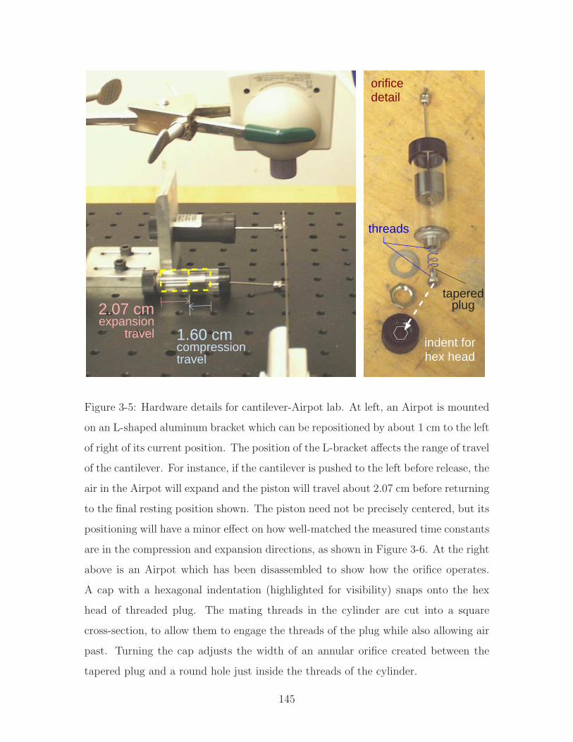
travel

2.07 cmexpansion

travel 1.60 cmcompression

detail

hex head

threads

orifice

indent for

plugtapered

Figure 3-5: Hardware details for cantilever-Airpot lab. At left, an Airpot is mounted

on an L-shaped aluminum bracket which can be repositioned by about 1 cm to the left

of right of its current position. The position of the L-bracket affects the range of travel

of the cantilever. For instance, if the cantilever is pushed to the left before release, the

air in the Airpot will expand and the piston will travel about 2.07 cm before returning

to the final resting position shown. The piston need not be precisely centered, but its

positioning will have a minor effect on how well-matched the measured time constants

are in the compression and expansion directions, as shown in Figure 3-6. At the right

above is an Airpot which has been disassembled to show how the orifice operates.

A cap with a hexagonal indentation (highlighted for visibility) snaps onto the hex

head of threaded plug. The mating threads in the cylinder are cut into a square

cross-section, to allow them to engage the threads of the plug while also allowing air

past. Turning the cap adjusts the width of an annular orifice created between the

tapered plug and a round hole just inside the threads of the cylinder.

145

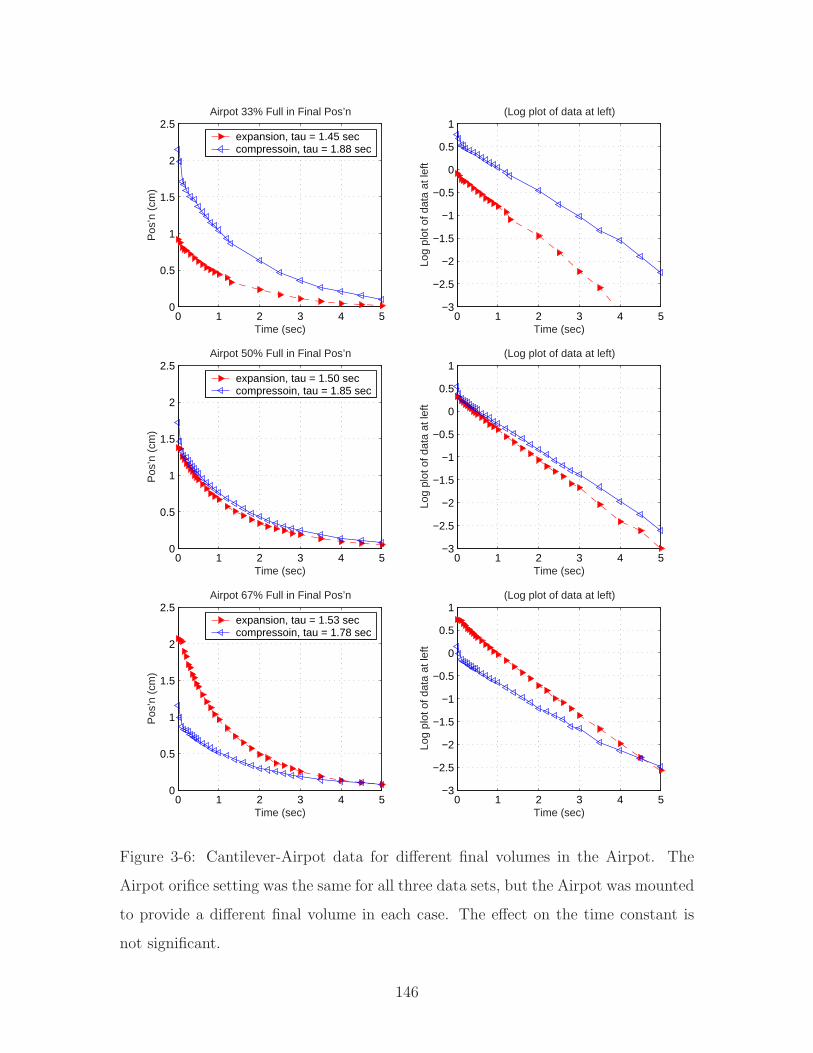
0 1 2 3 4 50

0.5

1

1.5

2

2.5Airpot 50% Full in Final Pos’n

Time (sec)

Pos

’n (

cm)

expansion, tau = 1.50 seccompressoin, tau = 1.85 sec

0 1 2 3 4 5−3

−2.5

−2

−1.5

−1

−0.5

0

0.5

1

Time (sec)

Log

plot

of d

ata

at le

ft

(Log plot of data at left)

0 1 2 3 4 50

0.5

1

1.5

2


Time (sec)

Pos

’n (

cm)


0 1 2 3 4 5−3

−2.5

−2

−1.5

−1

−0.5

0

0.5

1

Time (sec)

Log

plot

of d

ata

at le

ft


0 1 2 3 4 50

0.5

1

1.5

2


Time (sec)

Pos

’n (

cm)


0 1 2 3 4 5−3

−2.5

−2

−1.5

−1

−0.5

0

0.5

1

Time (sec)

Log

plot

of d

ata

at le

ft


Figure 3-6: Cantilever-Airpot data for different final volumes in the Airpot. The

Airpot orifice setting was the same for all three data sets, but the Airpot was mounted

to provide a different final volume in each case. The effect on the time constant is

not significant.

146

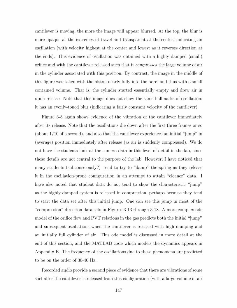
cantilever is moving, the more the image will appear blurred. At the top, the blur is

more opaque at the extremes of travel and transparent at the center, indicating an

oscillation (with velocity highest at the center and lowest as it reverses direction at

the ends). This evidence of oscillation was obtained with a highly damped (small)

orifice and with the cantilever released such that it compresses the large volume of air

in the cylinder associated with this position. By contrast, the image in the middle of

this figure was taken with the piston nearly fully into the bore, and thus with a small

contained volume. That is, the cylinder started essentially empty and drew air in

upon release. Note that this image does not show the same hallmarks of oscillation;

it has an evenly-toned blur (indicating a fairly constant velocity of the cantilever).

Figure 3-8 again shows evidence of the vibration of the cantilever immediately

after its release. Note that the oscillations die down after the first three frames or so

(about 1/10 of a second), and also that the cantilever experiences an initial “jump” in

(average) position immediately after release (as air is suddenly compressed). We do

not have the students look at the camera data in this level of detail in the lab, since

these details are not central to the purpose of the lab. However, I have noticed that

many students (subconsciously?) tend to try to “damp” the spring as they release

it in the oscillation-prone configuration in an attempt to attain “cleaner” data. I

have also noted that student data do not tend to show the characteristic “jump”

as the highly-damped system is released in compression, perhaps because they tend

to start the data set after this initial jump. One can see this jump in most of the

“compression” direction data sets in Figures 3-13 through 3-18. A more complex ode

model of the orifice flow and PVT relations in the gas predicts both the initial “jump”

and subsequent oscillations when the cantilever is released with high damping and

an initially full cylinder of air. This ode model is discussed in more detail at the

end of this section, and the MATLAB code which models the dynamics appears in

Appendix E. The frequency of the oscillations due to these phenomena are predicted

to be on the order of 30-40 Hz.

Recorded audio provide a second piece of evidence that there are vibrations of some

sort after the cantilever is released from this configuration (with a large volume of air

147

Figure 3-7: Deciphering video blurring. Above are three video frames of the cantilever.

1: The topmost frame has captured the cantilever during vibration. The image is most

opaque at the extremes of oscillation, where the velocity was the slowest, but it is

virtually transparent in the center, where the velocity was much faster. This frame

was captured after the cantilever was released from the righthand side of the image,

resulting in rapid compression of the air within the Airpot. Vibrations at 30-40 Hertz

are predicted by the MATLAB ode model of the system presented in Appendix E.

2: The middle frame captures the cantilever soon after its release from the lefthand

side. The evenly-toned blur is caused by the high velocity of the system, which just

been adjusted for low damping. 3: The crisp image at the bottom (of the cantilever

at rest) is included for comparison.

148

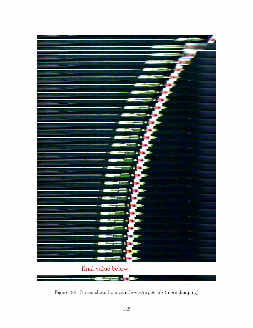
final value below:

Figure 3-8: Screen shots from cantilever-Airpot lab (more damping)

149

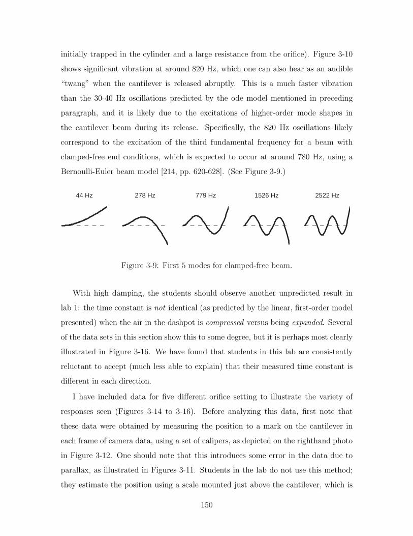
initially trapped in the cylinder and a large resistance from the orifice). Figure 3-10

shows significant vibration at around 820 Hz, which one can also hear as an audible

“twang” when the cantilever is released abruptly. This is a much faster vibration

than the 30-40 Hz oscillations predicted by the ode model mentioned in preceding

paragraph, and it is likely due to the excitations of higher-order mode shapes in

the cantilever beam during its release. Specifically, the 820 Hz oscillations likely

correspond to the excitation of the third fundamental frequency for a beam with

clamped-free end conditions, which is expected to occur at around 780 Hz, using a

Bernoulli-Euler beam model [214, pp. 620-628]. (See Figure 3-9.)

44 Hz 278 Hz 779 Hz 1526 Hz 2522 Hz

Figure 3-9: First 5 modes for clamped-free beam.

With high damping, the students should observe another unpredicted result in

lab 1: the time constant is not identical (as predicted by the linear, first-order model

presented) when the air in the dashpot is compressed versus being expanded. Several

of the data sets in this section show this to some degree, but it is perhaps most clearly

illustrated in Figure 3-16. We have found that students in this lab are consistently

reluctant to accept (much less able to explain) that their measured time constant is

different in each direction.

I have included data for five different orifice setting to illustrate the variety of

responses seen (Figures 3-14 to 3-16). Before analyzing this data, first note that

these data were obtained by measuring the position to a mark on the cantilever in

each frame of camera data, using a set of calipers, as depicted on the righthand photo

in Figure 3-12. One should note that this introduces some error in the data due to

parallax, as illustrated in Figures 3-11. Students in the lab do not use this method;

they estimate the position using a scale mounted just above the cantilever, which is

150

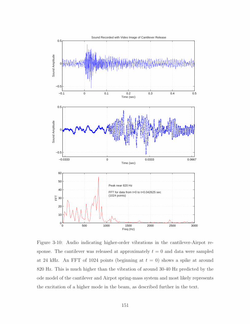
−0.1 0 0.1 0.2 0.3 0.4 0.5

−0.5

0

0.5

Time (sec)

Sou

nd A

mpl

itude

Sound Recorded with Video Image of Cantilever Release

−0.0333 0 0.0333 0.0667

−0.5

0

0.5

Time (sec)

Sou

nd A

mpl

itude

0 500 1000 1500 2000 2500 30000

10

20

30

40

50

60

Peak near 820 Hz

Freq (Hz)

FF

T

FFT for data from t=0 to t=0.042625 sec(1024 points)

Figure 3-10: Audio indicating higher-order vibrations in the cantilever-Airpot re-

sponse. The cantilever was released at approximately t = 0 and data were sampled

at 24 kHz. An FFT of 1024 points (beginning at t = 0) shows a spike at around

820 Hz. This is much higher than the vibration of around 30-40 Hz predicted by the

ode model of the cantilever and Airpot spring-mass system and most likely represents

the excitation of a higher mode in the beam, as described further in the text.

151

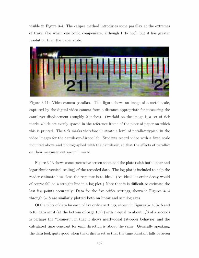
visible in Figure 3-4. The caliper method introduces some parallax at the extremes

of travel (for which one could compensate, although I do not), but it has greater

resolution than the paper scale.

Figure 3-11: Video camera parallax. This figure shows an image of a metal scale,

captured by the digital video camera from a distance appropriate for measuring the

cantilever displacement (roughly 2 inches). Overlaid on the image is a set of tick

marks which are evenly spaced in the reference frame of the piece of paper on which

this is printed. The tick marks therefore illustrate a level of parallax typical in the

video images for the cantilever-Airpot lab. Students record video with a fixed scale

mounted above and photographed with the cantilever, so that the effects of parallax

on their measurement are minimized.

Figure 3-13 shows some successive screen shots and the plots (with both linear and

logarithmic vertical scaling) of the recorded data. The log plot is included to help the

reader estimate how close the response is to ideal. (An ideal 1st-order decay would

of course fall on a straight line in a log plot.) Note that it is difficult to estimate the

last few points accurately. Data for the five orifice settings, shown in Figures 3-14

through 3-18 are similarly plotted both on linear and semilog axes.

Of the plots of data for each of five orifice settings, shown in Figures 3-14, 3-15 and

3-16, data set 4 (at the bottom of page 157) (with τ equal to about 1/3 of a second)

is perhaps the “cleanest”, in that it shows nearly-ideal 1st-order behavior, and the

calculated time constant for each direction is about the same. Generally speaking,

the data look quite good when the orifice is set so that the time constant falls between

152

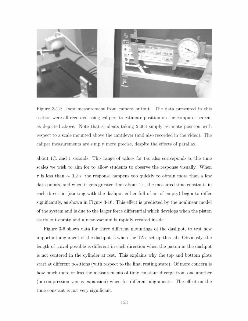
Figure 3-12: Data measurement from camera output. The data presented in this

section were all recorded using calipers to estimate position on the computer screen,

as depicted above. Note that students taking 2.003 simply estimate position with

respect to a scale mounted above the cantilever (and also recorded in the video). The

caliper measurements are simply more precise, despite the effects of parallax.

about 1/5 and 1 seconds. This range of values for tau also corresponds to the time

scales we wish to aim for to allow students to observe the response visually. When

τ is less than ∼ 0.2 s, the response happens too quickly to obtain more than a few

data points, and when it gets greater than about 1 s, the measured time constants in

each direction (starting with the dashpot either full of air of empty) begin to differ

significantly, as shown in Figure 3-16. This effect is predicted by the nonlinear model

of the system and is due to the larger force differential which develops when the piston

starts out empty and a near-vacuum is rapidly created inside.

Figure 3-6 shows data for three different mountings of the dashpot, to test how

important alignment of the dashpot is when the TA’s set up this lab. Obviously, the

length of travel possible is different in each direction when the piston in the dashpot

is not centered in the cylinder at rest. This explains why the top and bottom plots

start at different positions (with respect to the final resting state). Of more concern is

how much more or less the measurements of time constant diverge from one another

(in compression versus expansion) when for different alignments. The effect on the

time constant is not very significant.

153

Finally, one can provide students with a more complicated model of the dynamics

in the system which helps explain some of the unexpected behavior observed in this

lab. Specifically, if one both models the PVT (pressure-volume-temperature) relations

of the air in the cylinder and uses the equation governing flow through an orifice,

the predicted response shows both the initial jump and transient oscillations during

compression, as well as deviations from the ideal exponential decay. The model also

predicts the small deviations observed in the time constant, depending on whether the

piston is released in compression or expansion. This deviation is apparently caused

by the asymmetry of the spring effect of the air for the two directions of travel (i.e.

with the chamber starting out empty and rapidly forming a near-vacuum vs. starting

out full.).

Appendix E provides more details on modeling flow through an orifice and in-

cludes a MATLAB function (to be use with one of MATLAB’s ode solvers, such as

“ode45()”) which simulates the dynamics of the Airpot. Plots of simulations using

this code are shown along with experimental data sets 4 and 5 in Figures 3-17 and

3-18. In the plots, the valve coefficient for the orifice was selected (“tweaked”) by

hand until reasonable fits were obtained. I find it satisfying that the model predicts

both transient oscillations and the initial “jump” of the cantilever that occur in the

compression direction. We would not expect nor wish the students (sophomores) to

be able to model such dynamics, but it may be worth presenting the model cursorily

to demonstrate that despite the complexity of the full non-linear dynamics, the es-

sential features of the response can be captured quite well using a low-order, linear

model.

154

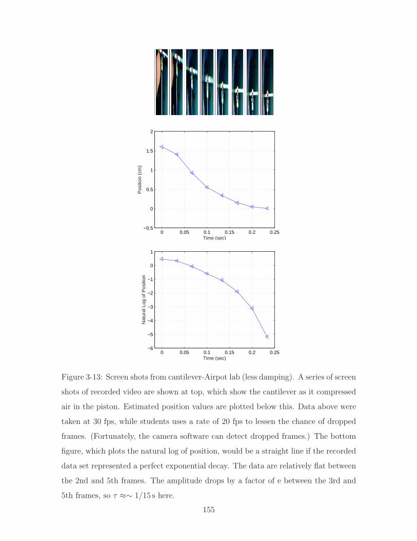
0 0.05 0.1 0.15 0.2 0.25−0.5

0

0.5

1

1.5

2

Time (sec)

Pos

ition

(cm

)

0 0.05 0.1 0.15 0.2 0.25−6

−5

−4

−3

−2

−1

0

1

Time (sec)

Nat

ural

Log

of P

ositi

on

0 0.05 0.1 0.15 0.2 0.25−0.5

0

0.5

1

1.5

2

Time (sec)

Pos

ition

(cm

)

0 0.05 0.1 0.15 0.2 0.25−6

−5

−4

−3

−2

−1

0

1

Time (sec)

Nat

ural

Log

of P

ositi

on

Figure 3-13: Screen shots from cantilever-Airpot lab (less damping). A series of screen

shots of recorded video are shown at top, which show the cantilever as it compressed

air in the piston. Estimated position values are plotted below this. Data above were

taken at 30 fps, while students uses a rate of 20 fps to lessen the chance of dropped

frames. (Fortunately, the camera software can detect dropped frames.) The bottom

figure, which plots the natural log of position, would be a straight line if the recorded

data set represented a perfect exponential decay. The data are relatively flat between

the 2nd and 5th frames. The amplitude drops by a factor of e between the 3rd and

5th frames, so τ ≈∼ 1/15 s here.

155

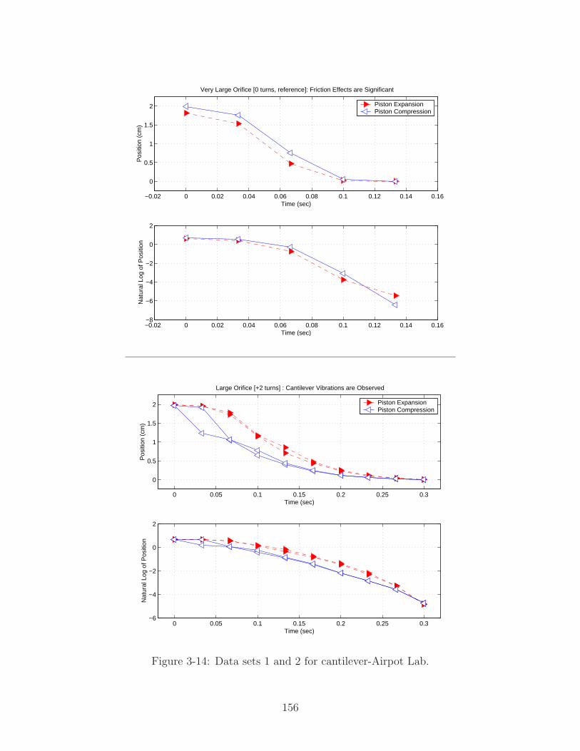
−0.02 0 0.02 0.04 0.06 0.08 0.1 0.12 0.14 0.16

0

0.5

1

1.5

2

Time (sec)

Pos

ition

(cm

)

Very Large Orifice [0 turns, reference]: Friction Effects are Significant

Piston ExpansionPiston Compression

−0.02 0 0.02 0.04 0.06 0.08 0.1 0.12 0.14 0.16−8

−6

−4

−2

0

2

Time (sec)

Nat

ural

Log

of P

ositi

on

0 0.05 0.1 0.15 0.2 0.25 0.3

0

0.5

1

1.5

2

Time (sec)

Pos

ition

(cm

)

Large Orifice [+2 turns] : Cantilever Vibrations are Observed


0 0.05 0.1 0.15 0.2 0.25 0.3−6

−4

−2

0

2

Time (sec)

Nat

ural

Log

of P

ositi

on

Figure 3-14: Data sets 1 and 2 for cantilever-Airpot Lab.

156

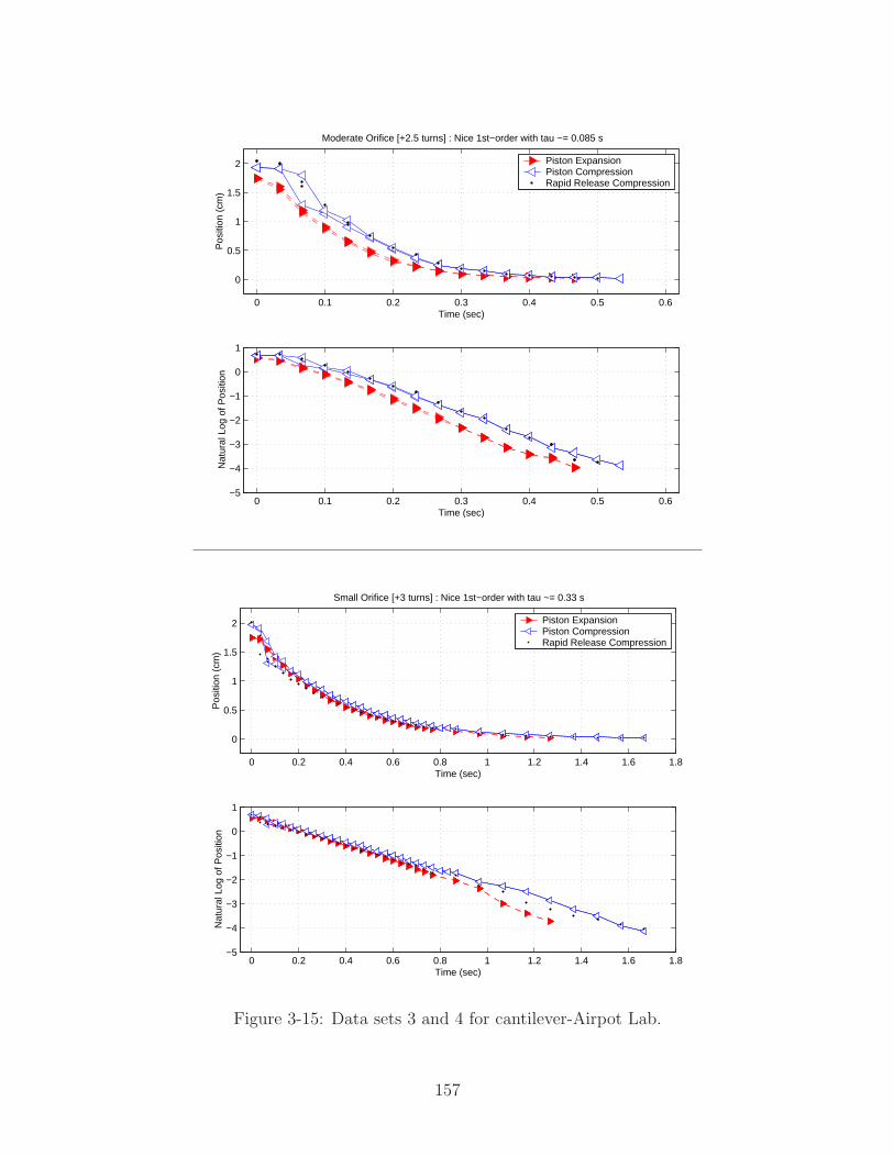
0 0.1 0.2 0.3 0.4 0.5 0.6

0

0.5

1

1.5

2

Time (sec)

Pos

ition

(cm

)

Moderate Orifice [+2.5 turns] : Nice 1st−order with tau ~= 0.085 s

Piston ExpansionPiston CompressionRapid Release Compression

0 0.1 0.2 0.3 0.4 0.5 0.6−5

−4

−3

−2

−1

0

1

Time (sec)

Nat

ural

Log

of P

ositi

on

0 0.2 0.4 0.6 0.8 1 1.2 1.4 1.6 1.8

0

0.5

1

1.5

2

Time (sec)

Pos

ition

(cm

)

Small Orifice [+3 turns] : Nice 1st−order with tau ~= 0.33 s

Piston ExpansionPiston CompressionRapid Release Compression

0 0.2 0.4 0.6 0.8 1 1.2 1.4 1.6 1.8−5

−4

−3

−2

−1

0

1

Time (sec)

Nat

ural

Log

of P

ositi

on

Figure 3-15: Data sets 3 and 4 for cantilever-Airpot Lab.

157

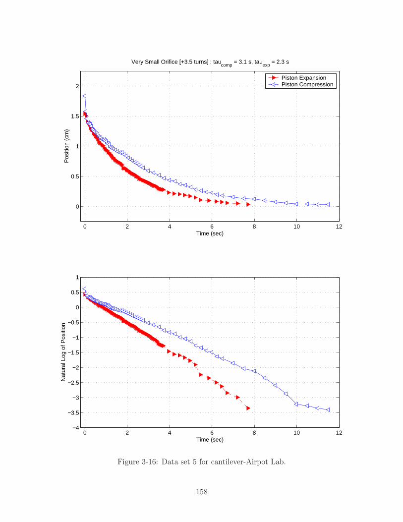
0 2 4 6 8 10 12

0

0.5

1

1.5

2

Time (sec)

Pos

ition

(cm

)Very Small Orifice [+3.5 turns] : tau

comp = 3.1 s, tau

exp = 2.3 s


0 2 4 6 8 10 12−4

−3.5

−3

−2.5

−2

−1.5

−1

−0.5

0

0.5

1

Time (sec)

Nat

ural

Log

of P

ositi

on

Figure 3-16: Data set 5 for cantilever-Airpot Lab.

158

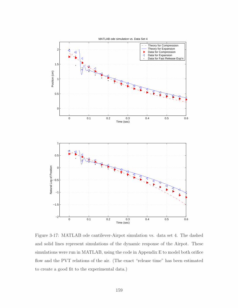
0 0.1 0.2 0.3 0.4 0.5 0.6

0

0.5

1

1.5

2

Time (sec)

Pos

ition

(cm

)

MATLAB ode simulation vs. Data Set 4

Theory for CompressionTheory for ExpansionData for CompressionData for ExpansionData for Fast Release Exp’n

0 0.1 0.2 0.3 0.4 0.5 0.6−2

−1.5

−1

−0.5

0

0.5

1

Time (sec)

Nat

ural

Log

of P

ositi

on

Figure 3-17: MATLAB ode cantilever-Airpot simulation vs. data set 4. The dashed

and solid lines represent simulations of the dynamic response of the Airpot. These

simulations were run in MATLAB, using the code in Appendix E to model both orifice

flow and the PVT relations of the air. (The exact “release time” has been estimated

to create a good fit to the experimental data.)

159

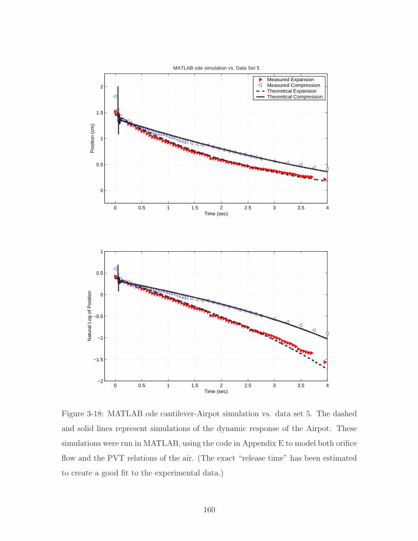
0 0.5 1 1.5 2 2.5 3 3.5 4

0

0.5

1

1.5

2

Time (sec)

Pos

ition

(cm

)

MATLAB ode simulation vs. Data Set 5

Measured ExpansionMeasured CompressionTheoretical ExpansionTheoretical Compression

0 0.5 1 1.5 2 2.5 3 3.5 4−2

−1.5

−1

−0.5

0

0.5

1

Time (sec)

Nat

ural

Log

of P

ositi

on

Figure 3-18: MATLAB ode cantilever-Airpot simulation vs. data set 5. The dashed

and solid lines represent simulations of the dynamic response of the Airpot. These

simulations were run in MATLAB, using the code in Appendix E to model both orifice

flow and the PVT relations of the air. (The exact “release time” has been estimated

to create a good fit to the experimental data.)

160

3.4 1st-Order Inertia-Damper Rotational System

In Lab 2, students explore the dynamics of a rotational 1st-order system. Figure 3-19

shows the setup for this lab. A 12-inch length of shafting is mounted vertically within

a pair of air bearings, and a ball bearing set into the bottom end of the shaft rests

on a tungsten carbide flat, providing a low-friction pivot. A cup at the base of the

shaft holds honey to provide damping to the system. We use honey both because of

its high viscosity and because it is environmentally benign. The level of the honey is

adjusted during the lab exercises with a syringe attached at the base of the cup. An

aluminum hub is mounted at the top of the shaft, and a brass ring can be put on or

taken off to vary the inertia, as shown in Figure 3-20.

As in Lab 1, students again use the digital cameras to record data. We have placed

a radial line at the top of the hub (see Figure 3-20) to allow the students to record the

angle at each frame in the recorded data. A clear plastic sheet with angular markings

is taped to the computer screen during this lab to provide a scale for angle, as shown

in Figure 3-21.

The students record data for two or three levels of honey both with and without

the additional inertia of the brass ring. They then use MATLAB to plot their data

and use these plots to determine the time constant for each set of system parameters.

As part of the pre-lab handout, we present the following equation relating Tviscous,

the viscous torque retarding the rotating shaft in an annulus of fluid, to the viscosity

of the fluid (µ), the diameter of the shaft (D), the height of the fluid level (L), and

the gap in the annulus (ε) [153, p. 263] :

Tviscous =πD3Lµ

4εω = c ω (3.2)

As the students generally have not yet taken a formal course in fluid dynamics, we

do not present the derivation of this model. We present students with Equation 3.2

primarily to emphasize that the viscous damping coefficient (c) should be proportional

to the height of the honey surrounding the base of the shaft. The lab focuses on the

system effects of changing both the viscosity (damping) and inertia of the system.

We feel it is important students both see and feel these effects (i.e. of changing

161

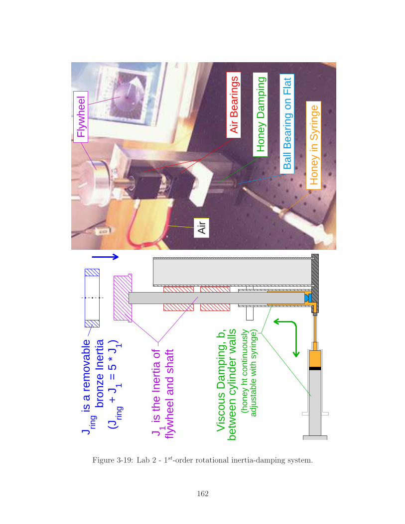
Air

Fly

whe

el

Hon

ey D

ampi

ng

Bal

l Bea

ring

on F

lat

Hon

ey in

Syr

inge

Air

Bea

rings

bron

ze In

ertia

(Jrin

g + J

1 = 5

* J

1)

J 1 is th

e In

ertia

of

flyw

heel

and

sha

ft

Vis

cous

Dam

ping

, b,

betw

een

cylin

der

wal

ls(h

oney

ht c

ontin

uous

lyad

just

able

with

syr

inge

)

J ring is

a r

emov

able

Figure 3-19: Lab 2 - 1st-order rotational inertia-damping system.

162

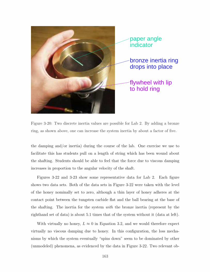
to hold ring

drops into place

paper angleindicator

flywheel with lip

bronze inertia ring

Figure 3-20: Two discrete inertia values are possible for Lab 2. By adding a bronze

ring, as shown above, one can increase the system inertia by about a factor of five.

the damping and/or inertia) during the course of the lab. One exercise we use to

facilitate this has students pull on a length of string which has been wound about

the shafting. Students should be able to feel that the force due to viscous damping

increases in proportion to the angular velocity of the shaft.

Figures 3-22 and 3-23 show some representative data for Lab 2. Each figure

shows two data sets. Both of the data sets in Figure 3-22 were taken with the level

of the honey nominally set to zero, although a thin layer of honey adheres at the

contact point between the tungsten carbide flat and the ball bearing at the base of

the shafting. The inertia for the system with the bronze inertia (represent by the

righthand set of data) is about 5.1 times that of the system without it (data at left).

With virtually no honey, L ≈ 0 in Equation 3.2, and we would therefore expect

virtually no viscous damping due to honey. In this configuration, the loss mecha-

nisms by which the system eventually “spins down” seem to be dominated by other

(unmodeled) phenomena, as evidenced by the data in Figure 3-22. Two relevant ob-

163

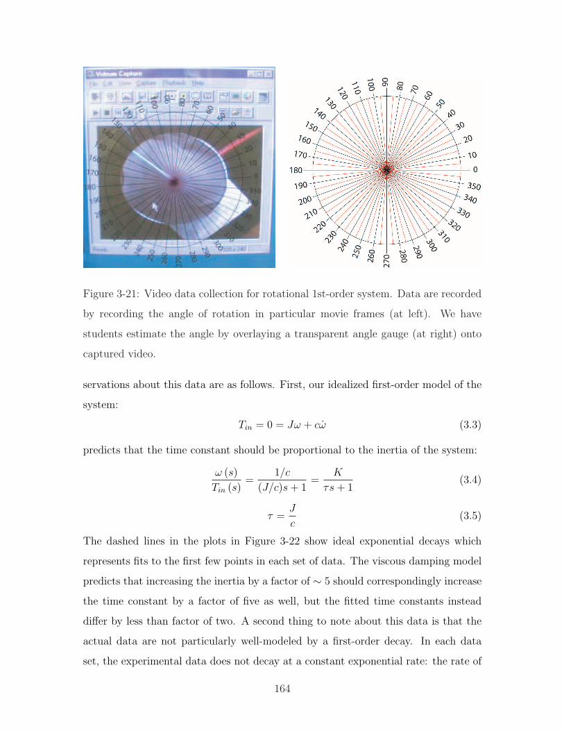
Figure 3-21: Video data collection for rotational 1st-order system. Data are recorded

by recording the angle of rotation in particular movie frames (at left). We have

students estimate the angle by overlaying a transparent angle gauge (at right) onto

captured video.

servations about this data are as follows. First, our idealized first-order model of the

system:

Tin = 0 = Jω + cω (3.3)

predicts that the time constant should be proportional to the inertia of the system:

ω (s)

Tin (s)=

1/c

(J/c)s + 1=

K

τs + 1(3.4)

τ =J

c(3.5)

The dashed lines in the plots in Figure 3-22 show ideal exponential decays which

represents fits to the first few points in each set of data. The viscous damping model

predicts that increasing the inertia by a factor of ∼ 5 should correspondingly increase

the time constant by a factor of five as well, but the fitted time constants instead

differ by less than factor of two. A second thing to note about this data is that the

actual data are not particularly well-modeled by a first-order decay. In each data

set, the experimental data does not decay at a constant exponential rate: the rate of

164

decay becomes greater as the velocity goes to zero. This is consistent with non-linear

effects that would result from Coulomb friction losses.

The dominant loss mechanisms when there is no honey are not well-understood,

but they likely include some viscous damping (perhaps from shear in the surrounding

air and/or from the residual honey at the bearing interface) and Coulomb friction

(predominantly where the ball bearing glued to the shaft end rests on a carbide

flat). A more detailed analysis at the end of this section provides further evidence to

support this conclusion. In summary, data taken with no honey are not particularly

well-modeled as a first-order inertia-damper system.

In contrast, the data taken with honey strongly support the system model students

develop in the pre-lab assignment. We model the system during rundown as a first-

order system with no external applied forces: Jθ + cθ = 0. If the damping is a

function of the height of the honey, as predicted by Equation 3.2, then “c” is the

same in each data set shown in Figure 3-23, and the time constant, τ = J/c, should

increase by a factor of 5.1 when the inertia (J) is increased by a factor of 5.1. The

data in Figure 3-23 have been carefully plotted to illustrate that they come quite

close to this ideal. The axes on which the data have been plotted have been scaled to

emphasize that the shape of the decay is essentially the same in both plots: the time

axes for the righthand plot span a range five times greater than that of the lefthand

plot.

It would probably be desirably to have the students obtain data with viscous

damping from the honey first, since it supports their first-order model of the dynamics.

Unfortunately however, it is a lot easier to push honey into the reservoir than it is to

pull it out again! The high viscosity that makes honey such a desirable fluid for the

lab (i.e. to get time constants on the order of one second) makes it a real pain when it

comes to emptying the reservoirs. Note in Figure 3-19 that the honey must be pulled

through a length of narrow tubing (with an orifice connection at either end). If you

pull too hard, bubbles are generated or the plunger pulls free of the rubber seal.

There are two issues which make it more difficult to pull honey out than it is to

push it in. First, one can at best obtain a vacuum inside the syringe, which limits

165

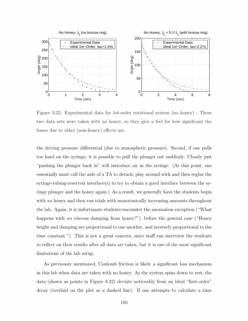
0 1 2 3 40

50

100

150

200

250

300

No Honey; J1 (no bronze ring)

Time (sec)

Ang

le (

deg)

Experimental DataIdeal 1st−Order, tau=1.24s

0 2 4 6 80

50

100

150

200

No Honey; J2 = 5.1*J

1 (with bronze ring)

Time (sec)

Ang

le (

deg)


Figure 3-22: Experimental data for 1st-order rotational system (no honey) - These

two data sets were taken with no honey, so they give a feel for how significant the

losses due to other (non-honey) effects are.

the driving pressure differential (due to atmospheric pressure). Second, if one pulls

too hard on the syringe, it is possible to pull the plunger out suddenly. Clearly just

“pushing the plunger back in” will introduce air in the syringe. (At this point, one

essentially must call the aide of a TA to detach, play around with and then reglue the

syringe-tubing-reservoir interface(s) to try to obtain a good interface between the sy-

ringe plunger and the honey again.) As a result, we generally have the students begin

with no honey and then run trials with monotonically increasing amounts throughout

the lab. Again, it is unfortunate students encounter the anomalous exception (“What

happens with no viscous damping from honey?”) before the general case (“Honey

height and damping are proportional to one another, and inversely proportional to the

time constant.”). This is not a great concern, since staff can interview the students

to reflect on their results after all data are taken, but it is one of the most significant

limitations of the lab setup.

As previously mentioned, Coulomb friction is likely a significant loss mechanism

in this lab when data are taken with no honey. As the system spins down to rest, the

data (shown as points in Figure 3-22) deviate noticeably from an ideal “first-order”

decay (overlaid on the plot as a dashed line). If one attempts to calculate a time

166

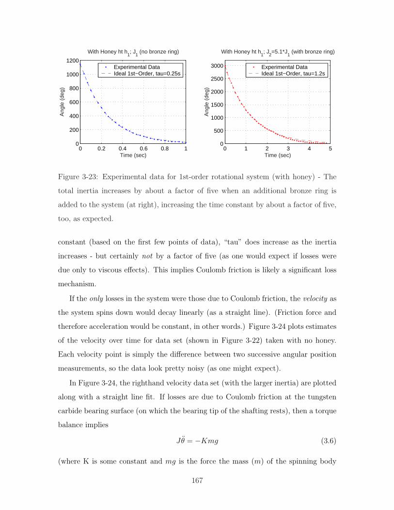
0 1 2 3 4 50

500

1000

1500

2000

2500

3000

Time (sec)

Ang

le (

deg)

With Honey ht h1; J

2=5.1*J



0 0.2 0.4 0.6 0.8 10

200

400

600

800

1000

1200

Time (sec)

Ang

le (

deg)

With Honey ht h1; J

1 (no bronze ring)


Figure 3-23: Experimental data for 1st-order rotational system (with honey) - The

total inertia increases by about a factor of five when an additional bronze ring is

added to the system (at right), increasing the time constant by about a factor of five,

too, as expected.

constant (based on the first few points of data), “tau” does increase as the inertia

increases - but certainly not by a factor of five (as one would expect if losses were

due only to viscous effects). This implies Coulomb friction is likely a significant loss

mechanism.

If the only losses in the system were those due to Coulomb friction, the velocity as

the system spins down would decay linearly (as a straight line). (Friction force and

therefore acceleration would be constant, in other words.) Figure 3-24 plots estimates

of the velocity over time for data set (shown in Figure 3-22) taken with no honey.

Each velocity point is simply the difference between two successive angular position

measurements, so the data look pretty noisy (as one might expect).

In Figure 3-24, the righthand velocity data set (with the larger inertia) are plotted

along with a straight line fit. If losses are due to Coulomb friction at the tungsten

carbide bearing surface (on which the bearing tip of the shafting rests), then a torque

balance implies

Jθ = −Kmg (3.6)

(where K is some constant and mg is the force the mass (m) of the spinning body

167

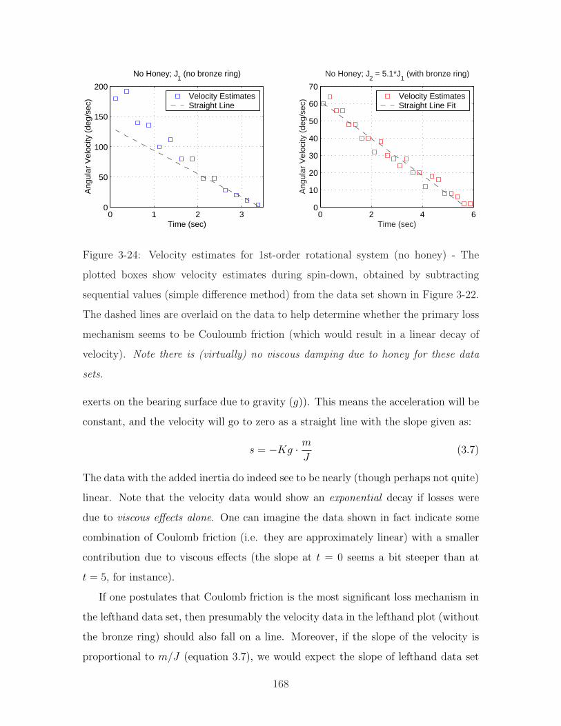
0 1 2 30

50

100

150

200

Time (sec)

Ang

ular

Vel

ocity

(de

g/se

c)

No Honey; J1 (no bronze ring)

Velocity EstimatesStraight Line

0 2 4 60

10

20

30

40

50

60

70

Time (sec)

Ang

ular

Vel

ocity

(de

g/se

c)

No Honey; J2 = 5.1*J


Velocity EstimatesStraight Line Fit

Figure 3-24: Velocity estimates for 1st-order rotational system (no honey) - The

plotted boxes show velocity estimates during spin-down, obtained by subtracting

sequential values (simple difference method) from the data set shown in Figure 3-22.

The dashed lines are overlaid on the data to help determine whether the primary loss

mechanism seems to be Couloumb friction (which would result in a linear decay of

velocity). Note there is (virtually) no viscous damping due to honey for these data

sets.

exerts on the bearing surface due to gravity (g)). This means the acceleration will be

constant, and the velocity will go to zero as a straight line with the slope given as:

s = −Kg · m

J(3.7)

The data with the added inertia do indeed see to be nearly (though perhaps not quite)

linear. Note that the velocity data would show an exponential decay if losses were

due to viscous effects alone. One can imagine the data shown in fact indicate some

combination of Coulomb friction (i.e. they are approximately linear) with a smaller

contribution due to viscous effects (the slope at t = 0 seems a bit steeper than at

t = 5, for instance).

If one postulates that Coulomb friction is the most significant loss mechanism in

the lefthand data set, then presumably the velocity data in the lefthand plot (without

the bronze ring) should also fall on a line. Moreover, if the slope of the velocity is

proportional to m/J (equation 3.7), we would expect the slope of lefthand data set

168

(sL) to be related to that of the righthand set (sR) as:

sL =mL

JL

· sRJR

mR

= sR · mLJr

mRJL

(3.8)

Adding the bronze ring increases the inertia by a factor of 5.1 (JR/JL = 5.1), as

mentioned, and increases the mass by a factor of about 1.5 (mR/mL = 1.5). The

slope of the fitted line in the righthand plot is sR = −10.8 (deg/s2). Thus, we would

expect:

sL = sR · JR/JL

mR/mL

= −10.8 · 5.1

1.5= −37 (deg/s2) (3.9)

The dashed line plotted with the velocity data at the left of Figure 3-24 is a fit to

the last 6 data points, only. The slope is -38 (deg/s2); close to our expected value of

-37.

My own conclusion is that we are seeing both viscous damping and Coulomb fric-

tion in the data with no bronze ring. Note that the velocities are all substantially lower

in the plot with the inertia. Viscous effects seem to be noticeable in the data without

the bronze ring only for velocities above around θLc = 40-50 (deg/s2). Whatever the

relationship between the torque due to viscous damping (B · θ) and the Coulomb fric-

tion (Kg ·m) is in this range (when Coulomb friction becomes notably dominant), the

velocity at which we expect a similar relation between the two contributing torques

to exist in the other data set should be roughly θRc = θLc ·mR/ML, or in the range

of θRc = 60-75 (deg/s2). At any rate, it is not at all surprising that we the data

in the righthand plot seem to be dominated more significantly by Coulomb friction.

We do not ask students to go into this level of analysis in investigating the effects

of Coulomb friction. The labs were in fact designed (as mentioned in the discussion

of our use of air bearings on page 30 of the Introduction) to minimize the effects

of Coulomb friction, so students could focus on nearly-ideal first- and second-order

system behaviors. Because we have students take data for Lab 2 with essentially no

honey in the reservoir (except for that which adheres at the bearing interface at the

base of the shafting), it is useful to address the effect of Coulomb friction to some

extent, however, especially for the most highly motivated students.

169

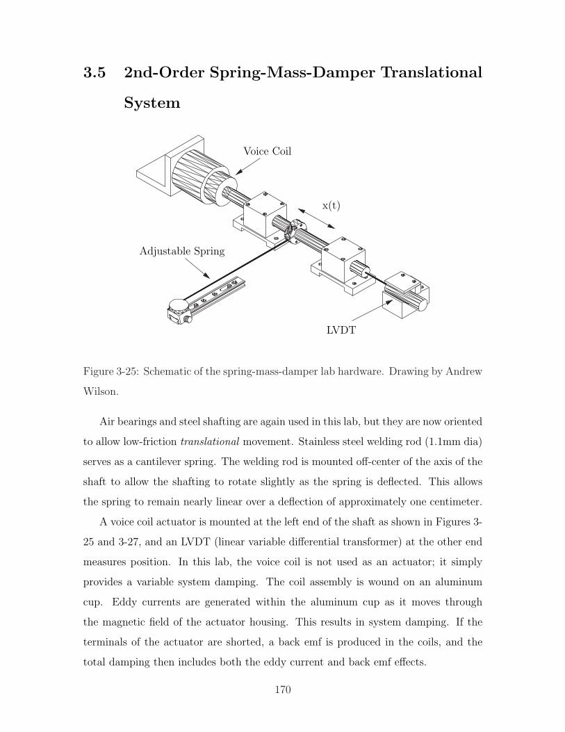
3.5 2nd-Order Spring-Mass-Damper Translational

System

LVDT

Voice Coil

x(t)

Adjustable Spring

Figure 3-25: Schematic of the spring-mass-damper lab hardware. Drawing by Andrew

Wilson.

Air bearings and steel shafting are again used in this lab, but they are now oriented

to allow low-friction translational movement. Stainless steel welding rod (1.1mm dia)

serves as a cantilever spring. The welding rod is mounted off-center of the axis of the

shaft to allow the shafting to rotate slightly as the spring is deflected. This allows

the spring to remain nearly linear over a deflection of approximately one centimeter.

A voice coil actuator is mounted at the left end of the shaft as shown in Figures 3-

25 and 3-27, and an LVDT (linear variable differential transformer) at the other end

measures position. In this lab, the voice coil is not used as an actuator; it simply

provides a variable system damping. The coil assembly is wound on an aluminum

cup. Eddy currents are generated within the aluminum cup as it moves through

the magnetic field of the actuator housing. This results in system damping. If the

terminals of the actuator are shorted, a back emf is produced in the coils, and the

total damping then includes both the eddy current and back emf effects.

170

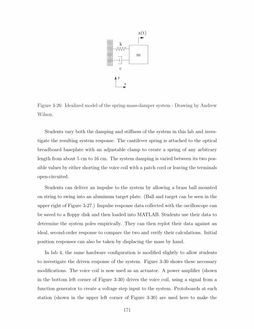
y

x

k

x(t)

m

c

Figure 3-26: Idealized model of the spring-mass-damper system - Drawing by Andrew

Wilson.

Students vary both the damping and stiffness of the system in this lab and inves-

tigate the resulting system response. The cantilever spring is attached to the optical

breadboard baseplate with an adjustable clamp to create a spring of any arbitrary

length from about 5 cm to 16 cm. The system damping is varied between its two pos-

sible values by either shorting the voice coil with a patch cord or leaving the terminals

open-circuited.

Students can deliver an impulse to the system by allowing a brass ball mounted

on string to swing into an aluminum target plate. (Ball and target can be seen in the

upper right of Figure 3-27.) Impulse response data collected with the oscilloscope can

be saved to a floppy disk and then loaded into MATLAB. Students use their data to

determine the system poles empirically. They can then replot their data against an

ideal, second-order response to compare the two and verify their calculations. Initial

position responses can also be taken by displacing the mass by hand.

In lab 4, the same hardware configuration is modified slightly to allow students

to investigate the driven response of the system. Figure 3-30 shows these necessary

modifications. The voice coil is now used as an actuator. A power amplifier (shown

in the bottom left corner of Figure 3-30) drives the voice coil, using a signal from a

function generator to create a voltage step input to the system. Protoboards at each

station (shown in the upper left corner of Figure 3-30) are used here to make the

171

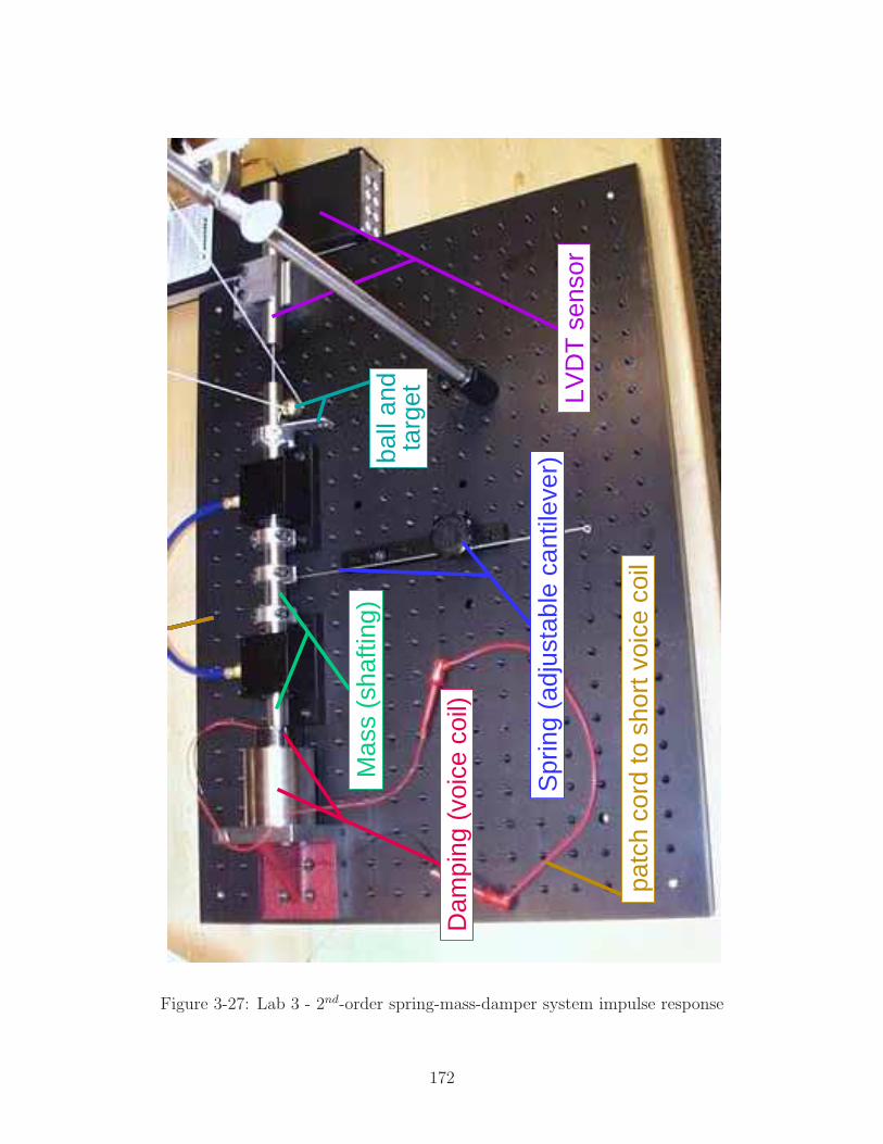
Dam

ping

(vo

ice

coil)

Mas

s (s

hafti

ng)

Spr

ing

(adj

usta

ble

cant

ileve

r)ball

and

targ

et LVD

T s

enso

r

patc

h co

rd to

sho

rt v

oice

coi

l

Figure 3-27: Lab 3 - 2nd-order spring-mass-damper system impulse response

172

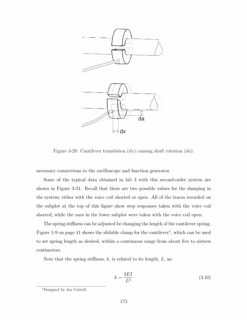
da

dx

Figure 3-28: Cantilever translation (dx) causing shaft rotation (da).

necessary connections to the oscilloscope and function generator.

Some of the typical data obtained in lab 3 with this second-order system are

shown in Figure 3-31. Recall that there are two possible values for the damping in

the system; either with the voice coil shorted or open. All of the traces recorded on

the subplot at the top of this figure show step responses taken with the voice coil

shorted, while the ones in the lower subplot were taken with the voice coil open.

The spring stiffness can be adjusted be changing the length of the cantilever spring.

Figure 1-9 on page 41 shows the slidable clamp for the cantilever1, which can be used

to set spring length as desired, within a continuous range from about five to sixteen

centimeters.

Note that the spring stiffness, k, is related to its length, L, as:

k =3EI

L3(3.10)

1Designed by Joe Cattell.

173

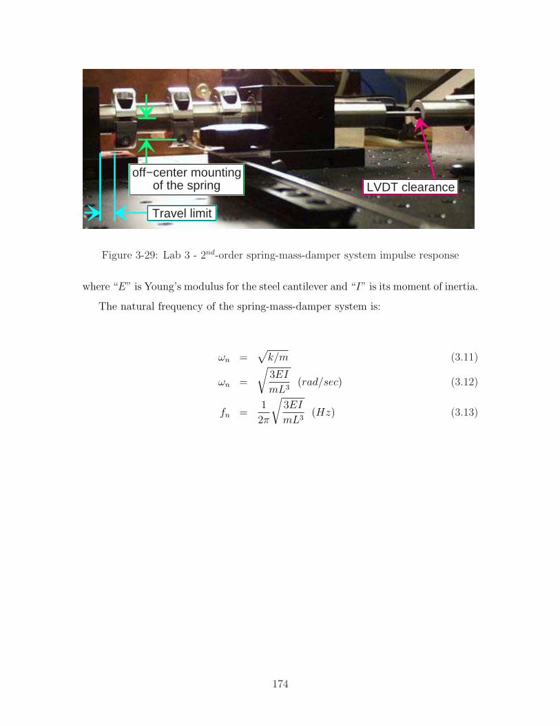
off−center mountingof the spring LVDT clearance

Travel limit

Figure 3-29: Lab 3 - 2nd-order spring-mass-damper system impulse response

where “E” is Young’s modulus for the steel cantilever and “I” is its moment of inertia.

The natural frequency of the spring-mass-damper system is:

ωn =√

k/m (3.11)

ωn =

√3EI

mL3(rad/sec) (3.12)

fn =1

2π

√3EI

mL3(Hz) (3.13)

174

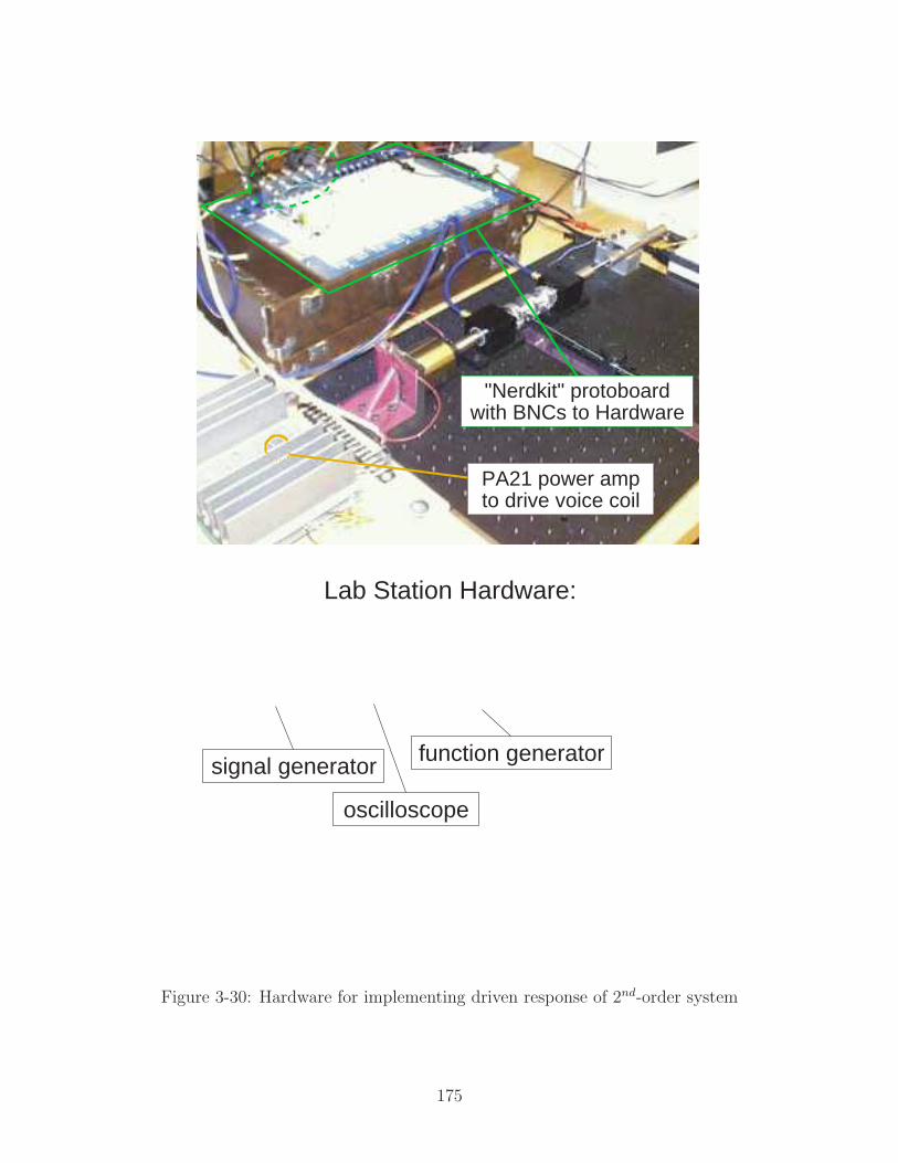
PA21 power ampto drive voice coil

"Nerdkit" protoboardwith BNCs to Hardware

signal generator

Lab Station Hardware:

function generator

oscilloscope

Figure 3-30: Hardware for implementing driven response of 2nd-order system

175

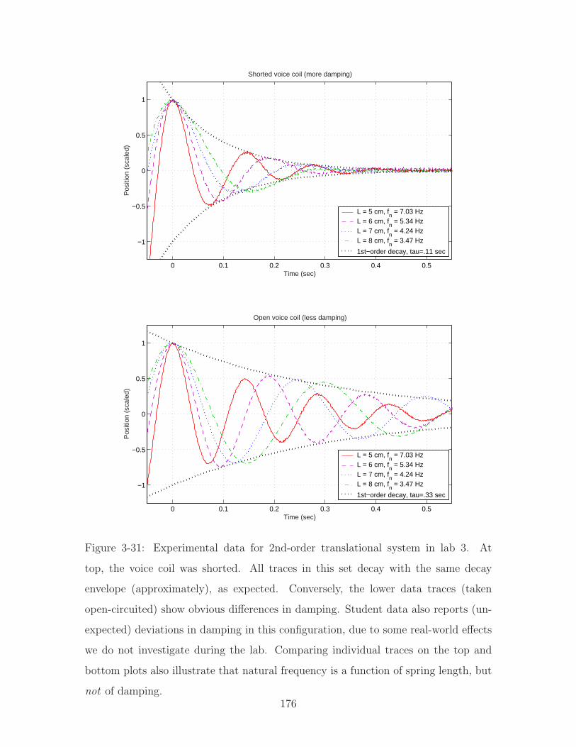
0 0.1 0.2 0.3 0.4 0.5

−1

−0.5

0

0.5

1

Time (sec)

Pos

ition

(sc

aled

)

Shorted voice coil (more damping)

L = 5 cm, fn = 7.03 Hz

L = 6 cm, fn = 5.34 Hz

L = 7 cm, fn = 4.24 Hz

L = 8 cm, fn = 3.47 Hz

1st−order decay, tau=.11 sec

0 0.1 0.2 0.3 0.4 0.5

−1

−0.5

0

0.5

1

Time (sec)

Pos

ition

(sc

aled

)

Open voice coil (less damping)

L = 5 cm, fn = 7.03 Hz

L = 6 cm, fn = 5.34 Hz

L = 7 cm, fn = 4.24 Hz

L = 8 cm, fn = 3.47 Hz

1st−order decay, tau=.33 sec

Figure 3-31: Experimental data for 2nd-order translational system in lab 3. At

top, the voice coil was shorted. All traces in this set decay with the same decay

envelope (approximately), as expected. Conversely, the lower data traces (taken

open-circuited) show obvious differences in damping. Student data also reports (un-

expected) deviations in damping in this configuration, due to some real-world effects

we do not investigate during the lab. Comparing individual traces on the top and

bottom plots also illustrate that natural frequency is a function of spring length, but

not of damping.176

0.04 0.06 0.08 0.1 0.12 0.14 0.160

200

400

600

800

1000

1200

1400

1600

1800

2000

valu

es o

f k (

N/m

)

spring length (m)

Experimental data for Lab 3

k theory, for r=.575mmk measured (closed)k measured (open)

0.04 0.06 0.08 0.1 0.12 0.14 0.164

6

8

10

12

14

16

18

20

22

expe

rimen

tal v

alue

s of

c (

N−

s/m

)

spring length (m)

c measured (closed)c measured (open)

Figure 3-32: Calculated k and c values for 2nd-order translational system. The two

plots above show values of k and c as a function of spring length. These values were

obtained by fitting successive data sets (including those shown in Figure 3-31). The

values of k obtained are all very close to the ideal relationship one would expect. The

data in the lower plot are less ideal. One would expect the same damping coefficient

for each trial run open-circuit and a second (but consistent) value for all close-circuit

data (i.e. Each plot should be a flat, horizontal line). We do not attempt to explain

the non-ideality.

177

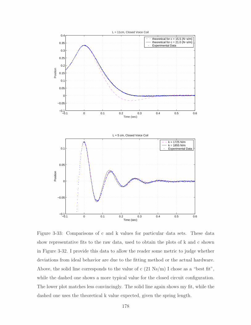
−0.1 0 0.1 0.2 0.3 0.4 0.5 0.6−0.1

−0.05

0

0.05

0.1

0.15

0.2

0.25

0.3

0.35

0.4L = 11cm, Closed Voice Coil

Time (sec)

Pos

ition

theoretical for c = 15.5 (N−s/m)theoretical for c = 21.0 (N−s/m)Experimental Data

−0.1 0 0.1 0.2 0.3 0.4 0.5 0.6−0.1

−0.05

0

0.05

0.1

L = 5 cm, Closed Voice Coil

Time (sec)

Pos

ition

k = 1725 N/mk = 1855 N/mExperimental Data

Figure 3-33: Comparisons of c and k values for particular data sets. These data

show representative fits to the raw data, used to obtain the plots of k and c shown

in Figure 3-32. I provide this data to allow the reader some metric to judge whether

deviations from ideal behavior are due to the fitting method or the actual hardware.

Above, the solid line corresponds to the value of c (21 Ns/m) I chose as a “best fit”,

while the dashed one shows a more typical value for the closed circuit configuration.

The lower plot matches less convincingly. The solid line again shows my fit, while the

dashed one uses the theoretical k value expected, given the spring length.

178

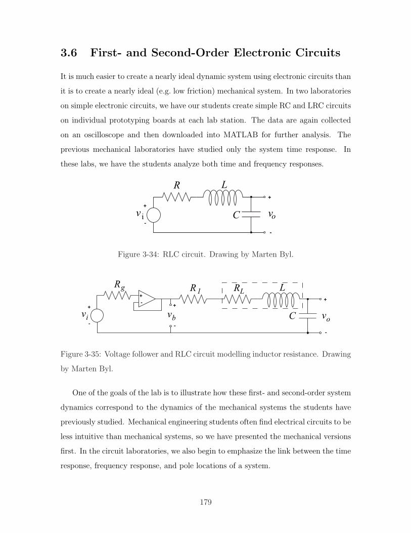
3.6 First- and Second-Order Electronic Circuits

It is much easier to create a nearly ideal dynamic system using electronic circuits than

it is to create a nearly ideal (e.g. low friction) mechanical system. In two laboratories

on simple electronic circuits, we have our students create simple RC and LRC circuits

on individual prototyping boards at each lab station. The data are again collected

on an oscilloscope and then downloaded into MATLAB for further analysis. The

previous mechanical laboratories have studied only the system time response. In

these labs, we have the students analyze both time and frequency responses.

-

+

+

-

Figure 3-34: RLC circuit. Drawing by Marten Byl.

-

+

+

-

+

-

-+

Figure 3-35: Voltage follower and RLC circuit modelling inductor resistance. Drawing

by Marten Byl.

One of the goals of the lab is to illustrate how these first- and second-order system

dynamics correspond to the dynamics of the mechanical systems the students have

previously studied. Mechanical engineering students often find electrical circuits to be

less intuitive than mechanical systems, so we have presented the mechanical versions

first. In the circuit laboratories, we also begin to emphasize the link between the time

response, frequency response, and pole locations of a system.

179

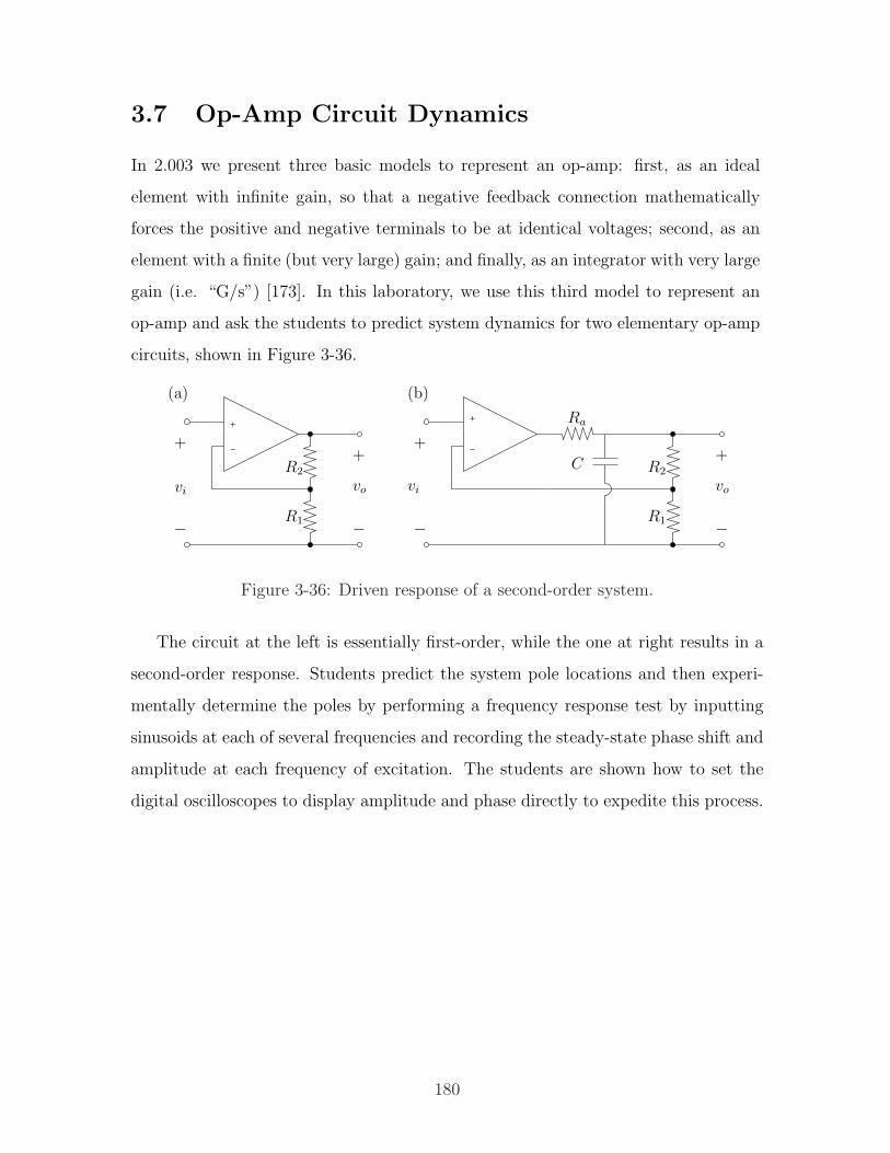
3.7 Op-Amp Circuit Dynamics

In 2.003 we present three basic models to represent an op-amp: first, as an ideal

element with infinite gain, so that a negative feedback connection mathematically

forces the positive and negative terminals to be at identical voltages; second, as an

element with a finite (but very large) gain; and finally, as an integrator with very large

gain (i.e. “G/s”) [173]. In this laboratory, we use this third model to represent an

op-amp and ask the students to predict system dynamics for two elementary op-amp

circuits, shown in Figure 3-36.

−

+

R2

R1

vo

+

−

+

−

vi

(a)

−

+

−

R2

R1

vo

+

vi

+

−

C

Ra

(b)

Figure 3-36: Driven response of a second-order system.

The circuit at the left is essentially first-order, while the one at right results in a

second-order response. Students predict the system pole locations and then experi-

mentally determine the poles by performing a frequency response test by inputting

sinusoids at each of several frequencies and recording the steady-state phase shift and

amplitude at each frequency of excitation. The students are shown how to set the

digital oscilloscopes to display amplitude and phase directly to expedite this process.

180

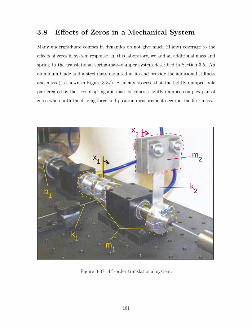
3.8 Effects of Zeros in a Mechanical System

Many undergraduate courses in dynamics do not give much (if any) coverage to the

effects of zeros in system response. In this laboratory, we add an additional mass and

spring to the translational spring-mass-damper system described in Section 3.5. An

aluminum blade and a steel mass mounted at its end provide the additional stiffness

and mass (as shown in Figure 3-37). Students observe that the lightly-damped pole

pair created by the second spring and mass becomes a lightly-damped complex pair of

zeros when both the driving force and position measurement occur at the first mass.

x2

x1

x1

m2

k1

b1

m1

k2

Figure 3-37: 4th-order translational system.

181

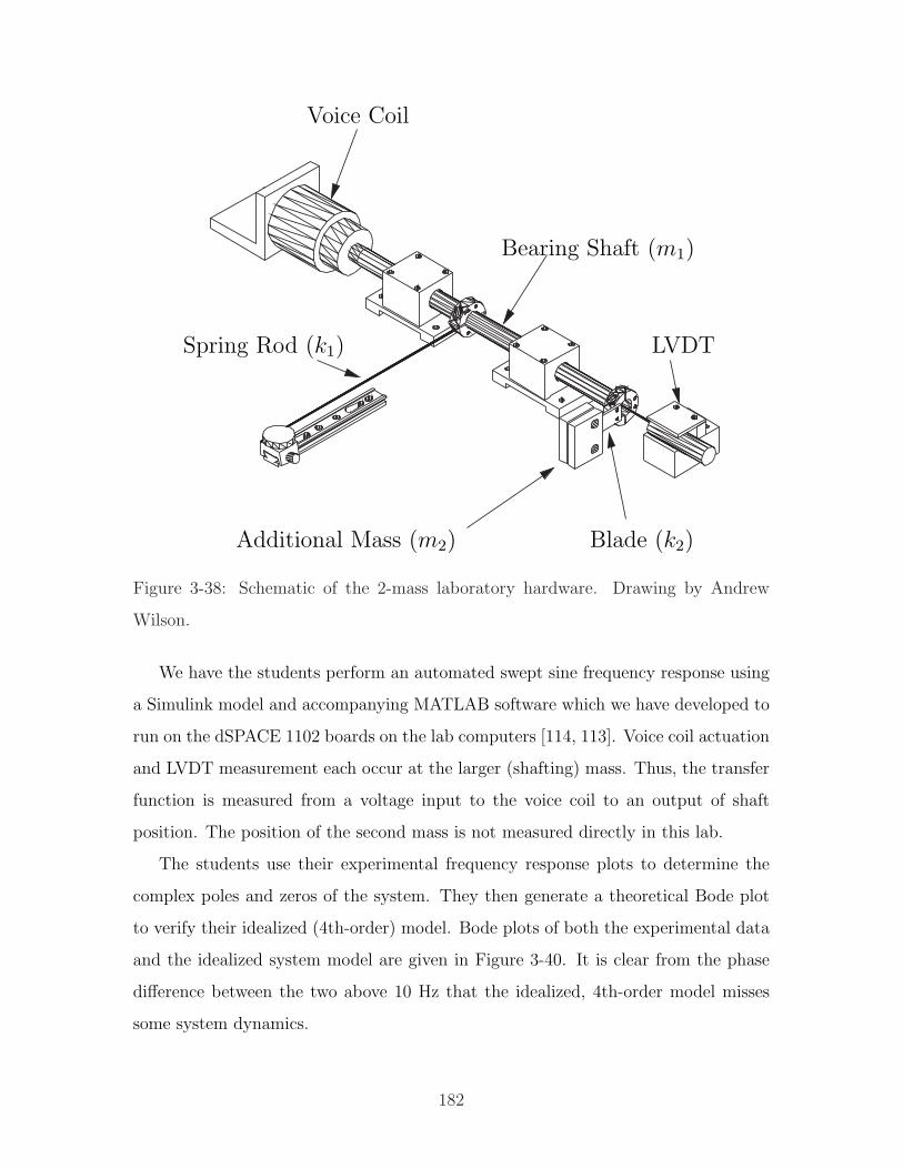
Voice Coil

Bearing Shaft (m1)

LVDTSpring Rod (k1)

Additional Mass (m2) Blade (k2)

Figure 3-38: Schematic of the 2-mass laboratory hardware. Drawing by Andrew

Wilson.

We have the students perform an automated swept sine frequency response using

a Simulink model and accompanying MATLAB software which we have developed to

run on the dSPACE 1102 boards on the lab computers [114, 113]. Voice coil actuation

and LVDT measurement each occur at the larger (shafting) mass. Thus, the transfer

function is measured from a voltage input to the voice coil to an output of shaft

position. The position of the second mass is not measured directly in this lab.

The students use their experimental frequency response plots to determine the

complex poles and zeros of the system. They then generate a theoretical Bode plot

to verify their idealized (4th-order) model. Bode plots of both the experimental data

and the idealized system model are given in Figure 3-40. It is clear from the phase

difference between the two above 10 Hz that the idealized, 4th-order model misses

some system dynamics.

182

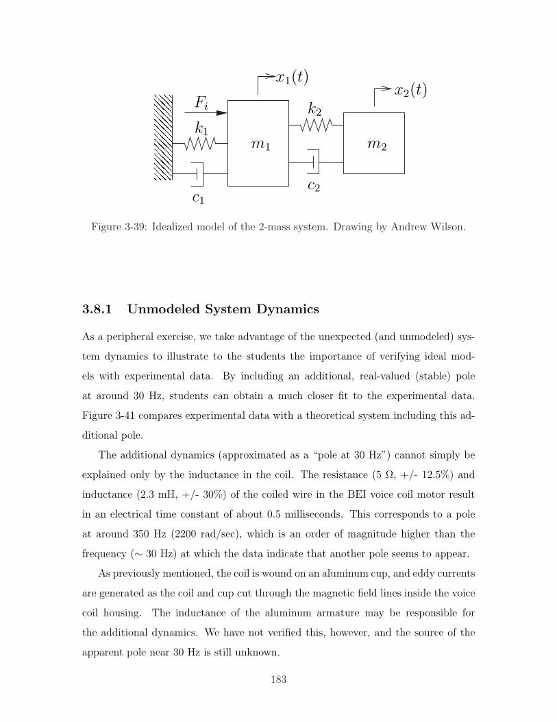
m2m1

x1(t)x2(t)

k2

c1

c2

k1

Fi

Figure 3-39: Idealized model of the 2-mass system. Drawing by Andrew Wilson.

3.8.1 Unmodeled System Dynamics

As a peripheral exercise, we take advantage of the unexpected (and unmodeled) sys-

tem dynamics to illustrate to the students the importance of verifying ideal mod-

els with experimental data. By including an additional, real-valued (stable) pole

at around 30 Hz, students can obtain a much closer fit to the experimental data.

Figure 3-41 compares experimental data with a theoretical system including this ad-

ditional pole.

The additional dynamics (approximated as a “pole at 30 Hz”) cannot simply be

explained only by the inductance in the coil. The resistance (5 Ω, +/- 12.5%) and

inductance (2.3 mH, +/- 30%) of the coiled wire in the BEI voice coil motor result

in an electrical time constant of about 0.5 milliseconds. This corresponds to a pole

at around 350 Hz (2200 rad/sec), which is an order of magnitude higher than the

frequency (∼ 30 Hz) at which the data indicate that another pole seems to appear.

As previously mentioned, the coil is wound on an aluminum cup, and eddy currents

are generated as the coil and cup cut through the magnetic field lines inside the voice

coil housing. The inductance of the aluminum armature may be responsible for

the additional dynamics. We have not verified this, however, and the source of the

apparent pole near 30 Hz is still unknown.

183

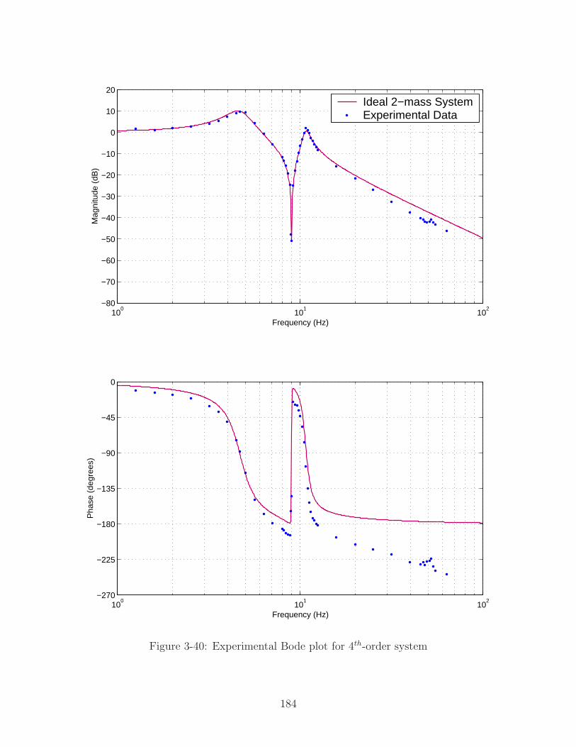
100

101

102

−80

−70

−60

−50

−40

−30

−20

−10

0

10

20

Frequency (Hz)

Mag

nitu

de (

dB)

Ideal 2−mass SystemExperimental Data

100

101

102

−270

−225

−180

−135

−90

−45

0

Frequency (Hz)

Pha

se (

degr

ees)

Figure 3-40: Experimental Bode plot for 4th-order system

184

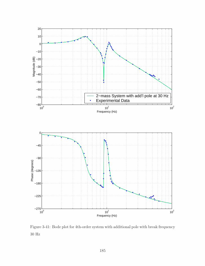
100

101

102

−80

−70

−60

−50

−40

−30

−20

−10

0

10

20

Frequency (Hz)

Mag

nitu

de (

dB)

2−mass System with add’l pole at 30 HzExperimental Data

100

101

102

−270

−225

−180

−135

−90

−45

0

Frequency (Hz)

Pha

se (

degr

ees)

Figure 3-41: Bode plot for 4th-order system with additional pole with break frequency

30 Hz

185

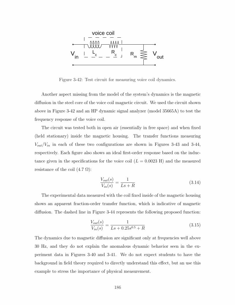
Vin

Vout

Lc

Rc

voice coil

Rm

Figure 3-42: Test circuit for measuring voice coil dynamics.

Another aspect missing from the model of the system’s dynamics is the magnetic

diffusion in the steel core of the voice coil magnetic circuit. We used the circuit shown

above in Figure 3-42 and an HP dynamic signal analyzer (model 35665A) to test the

frequency response of the voice coil.

The circuit was tested both in open air (essentially in free space) and when fixed

(held stationary) inside the magnetic housing. The transfer functions measuring

Vout/Vin in each of these two configurations are shown in Figures 3-43 and 3-44,

respectively. Each figure also shows an ideal first-order response based on the induc-

tance given in the specifications for the voice coil (L = 0.0023 H) and the measured

resistance of the coil (4.7 Ω):

Vout(s)

Vin(s)=

1

Ls + R(3.14)

The experimental data measured with the coil fixed inside of the magnetic housing

shows an apparent fraction-order transfer function, which is indicative of magnetic

diffusion. The dashed line in Figure 3-44 represents the following proposed function:

Vout(s)

Vin(s)=

1

Ls + 0.25s0.5 + R(3.15)

The dynamics due to magnetic diffusion are significant only at frequencies well above

30 Hz, and they do not explain the anomalous dynamic behavior seen in the ex-

periment data in Figures 3-40 and 3-41. We do not expect students to have the

background in field theory required to directly understand this effect, but an use this

example to stress the importance of physical measurement.

186

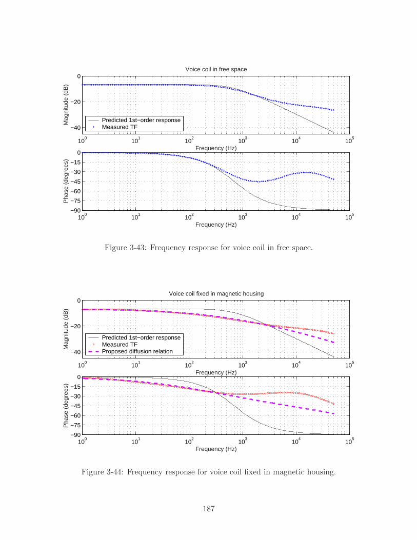
100

101

102

103

104

105

−40

−20

0

Frequency (Hz)

Mag

nitu

de (

dB)

Voice coil in free space

Predicted 1st−order responseMeasured TF

100

101

102

103

104

105

−90

−75

−60

−45

−30

−15

0

Frequency (Hz)

Pha

se (

degr

ees)

Figure 3-43: Frequency response for voice coil in free space.

100

101

102

103

104

105

−40

−20

0

Frequency (Hz)

Mag

nitu

de (

dB)

Voice coil fixed in magnetic housing

Predicted 1st−order responseMeasured TFProposed diffusion relation

100

101

102

103

104

105

−90

−75

−60

−45

−30

−15

0

Frequency (Hz)

Pha

se (

degr

ees)

Figure 3-44: Frequency response for voice coil fixed in magnetic housing.

187

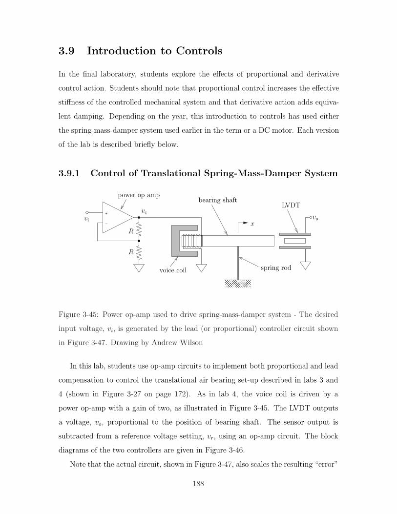
3.9 Introduction to Controls

In the final laboratory, students explore the effects of proportional and derivative

control action. Students should note that proportional control increases the effective

stiffness of the controlled mechanical system and that derivative action adds equiva-

lent damping. Depending on the year, this introduction to controls has used either

the spring-mass-damper system used earlier in the term or a DC motor. Each version

of the lab is described briefly below.

3.9.1 Control of Translational Spring-Mass-Damper System

−

+

power op amp

voice coil

LVDT

spring rod

bearing shaft

xvi

R

R

vo

vc

Figure 3-45: Power op-amp used to drive spring-mass-damper system - The desired

input voltage, vi, is generated by the lead (or proportional) controller circuit shown

in Figure 3-47. Drawing by Andrew Wilson

In this lab, students use op-amp circuits to implement both proportional and lead

compensation to control the translational air bearing set-up described in labs 3 and

4 (shown in Figure 3-27 on page 172). As in lab 4, the voice coil is driven by a

power op-amp with a gain of two, as illustrated in Figure 3-45. The LVDT outputs

a voltage, vo, proportional to the position of bearing shaft. The sensor output is

subtracted from a reference voltage setting, vr, using an op-amp circuit. The block

diagrams of the two controllers are given in Figure 3-46.

Note that the actual circuit, shown in Figure 3-47, also scales the resulting “error”

188

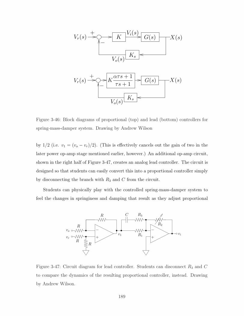
G(s)−

+K

KsVo(s)

X(s)Vi(s)

Vr(s)

−+

KsVo(s)

G(s) X(s)Vr(s) Kατs + 1

τs + 1

Figure 3-46: Block diagrams of proportional (top) and lead (bottom) controllers for

spring-mass-damper system. Drawing by Andrew Wilson

by 1/2 (i.e. v1 = (vo − vr)/2). (This is effectively cancels out the gain of two in the

later power op-amp stage mentioned earlier, however.) An additional op-amp circuit,

shown in the right half of Figure 3-47, creates an analog lead controller. The circuit is

designed so that students can easily convert this into a proportional controller simply

by disconnecting the branch with R3 and C from the circuit.

Students can physically play with the controlled spring-mass-damper system to

feel the changes in springiness and damping that result as they adjust proportional

− −++

vi

vo

vr

C

R1

R

R

RR

R2

R3

v1

Figure 3-47: Circuit diagram for lead controller. Students can disconnect R3 and C

to compare the dynamics of the resulting proportional controller, instead. Drawing

by Andrew Wilson.

189

and derivative gains. They can disconnect the mechanical spring, for instance, to

feel that the controlled system still provides a very similar stiffness. The reference

voltage come from a signal generator. Students can set different DC values and

watch the equilibrium position of the mass change as a result. They can also drive

the system with step or sinusoidal waveforms to analyze transient and frequency

response (respectively).

Controller design is often an intimidating subject for undergraduates, and we hope

this early hands-on experience will be an aid in developing an intuitive understanding

for later courses in control. The lab also provides some introductory circuit experi-

ence. Although the students are not asked to design the control circuits used in the

actual lab, we do require them to analyze and design op-amp circuits in the pre-lab

assignment. Perhaps the most central point we hope students will take away with

them is the basic concept that design of a control system essentially amounts to the

modification of a system to obtain desired changes in the dynamics.

3.9.2 Control of DC Motor System

The project described in this section has been used to introduce to controls as an

alternative to the laboratory just described (in Section 3.9.1). This control lab uses

a DC motor setup originally created as a laboratory project for 2.737 Mechatronics.2

A picture of the motor hardware is shown in Figure 3-48. The motor is mounted for

2.737 so that it drives a potentiometer (shown in the foreground), but this (position)

output in not used in 2.003. Instead, students use the tach output to command the

voltage signal driving the motor.

Figure 3-49 shows a schematic of the DC motor, and Figure 3-50 represents the

feedback due to back emf which occurs when one commands voltage (as opposed to

current) to drive the motor. Note that the gain of two (at the left in both figures)

occurs in the power op-amp stage, as illustrated earlier in Figure 3-47 on page 189.

As configured in Figure 3-50, the controller outputs a command voltage proportional

2More information on other projects for 2.737 can be found on page 132 of Chapter 2

190

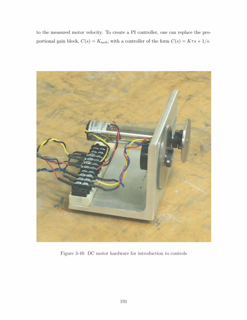
to the measured motor velocity. To create a PI controller, one can replace the pro-

portional gain block, C(s) = Ktach, with a controller of the form C(s) = Kτs + 1/s.

Figure 3-48: DC motor hardware for introduction to controls

191

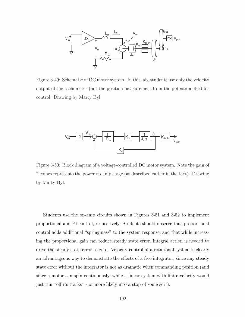
-e

m L

Rm

m

++

-

Vm

Jm

.m

Jf

PotKtach

nd

np

Kpot2XVin+

-

m I Km

Figure 3-49: Schematic of DC motor system. In this lab, students use only the velocity

output of the tachometer (not the position measurement from the potentiometer) for

control. Drawing by Marty Byl.

Vm

-1Rm

1J s t

Km

Km

2Vin K tach

v tach

Figure 3-50: Block diagram of a voltage-controlled DC motor system. Note the gain of

2 comes represents the power op-amp stage (as described earlier in the text). Drawing

by Marty Byl.

Students use the op-amp circuits shown in Figures 3-51 and 3-52 to implement

proportional and PI control, respectively. Students should observe that proportional

control adds additional “springiness” to the system response, and that while increas-

ing the proportional gain can reduce steady state error, integral action is needed to

drive the steady state error to zero. Velocity control of a rotational system is clearly

an advantageous way to demonstrate the effects of a free integrator, since any steady

state error without the integrator is not as dramatic when commanding position (and

since a motor can spin continuously, while a linear system with finite velocity would

just run “off its tracks” - or more likely into a stop of some sort).

192

-+

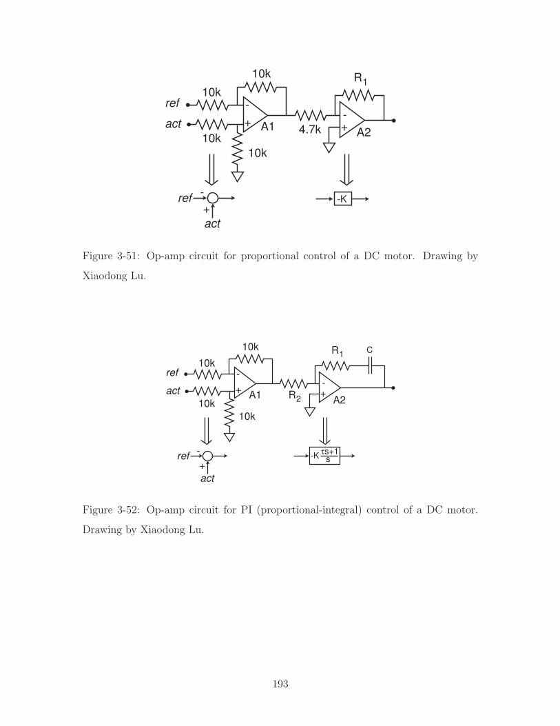
ref

act

10k

10k10k

+-

10k

4.7k

R1

act

ref -+

-K

A1 A2

Figure 3-51: Op-amp circuit for proportional control of a DC motor. Drawing by

Xiaodong Lu.

-+

ref

act

10k

10k10k

+-

10k R1

act

ref -+

-K

C

R2

τs+1s

A1 A2

Figure 3-52: Op-amp circuit for PI (proportional-integral) control of a DC motor.

Drawing by Xiaodong Lu.

193

Teaching the controls laboratory with a new set of hardware (i.e. not yet seen by

the students in the class in previous labs) also allows us to introduce new concepts.

Students can note how the back emf for the rotational motor (more commonly mod-

eled in similar classes) is analogous to that in the linear voice coil motor used in labs

3 and 4. They are also exposed to new sensors (the tach).

Finally, as in the previous control laboratory described, we hope students will

begin to appreciate how controllers modify system dynamics. Design of mechatronic

devices would corresponding therefore involve design of the combined mechanical,

electrical and control system dynamics, together.

3.10 Web Documentation of ActivLab Projects

We have documented each of the ActivLab projects on the class website for 2.003

Modeling Dynamics and Control I. Others are welcome to use any of the concepts

presented in this thesis or on the ActivLab website, which is currently located here:

http://web.mit.edu/2.003/www/activlab/activlab.html

Web addresses are prone to change, however, and a more reliable method of accessing

our site on the web is through the homepage for MIT’s OpenCourseWare (OCW)

program, which was described on page 119. OCW will eventually document materials

for virtually every class offered at MIT. One can presently access the OCW database

from the following address:

http://ocw.mit.edu/index.html

2.003 should be listed among the course offered by the Department of Mechanical

Engineering.

194

Chapter 4

Other Project Suggestions in

Dynamics

Chapter 3 reviewed the ActivLab experiments we developed and have been used in

teaching 2.003 since the Fall of 2001. Chapter 4 describes other projects which may

also be useful for teaching dynamics. These are distributed into three categories: (1)

additional laboratory projects or variations of existing labs which could be added

to the ActivLab curriculum, (2) In-lab demos of phenomena or technology (sensors,

actuators, bearings, etc) that are relevant to particular labs, and (3) formal lecture

demonstrations (i.e. of the type often seen in introductory college physics). Compared

with the survey in Chapter 2, Chapter 4 presents ideas which have been developed at

MIT1 specifically for 2.003, while the Chapter 2 surveys the work of others, including

various hands-on projects and demos for teaching dynamics and related disciplines

(e.g. mechatronics, robots and physics).

4.1 Possible ActivLab Additions

The next three sections briefly describe some ideas for additional laboratory projects

in dynamics. Sections 4.1.1 and 4.1.2 each describe prototypes of rotational and

translational 2nd-order systems we built as possible alternatives to the translational

1by Prof. Trumper and other staff

195

2nd-order system described in Section 3.5, and Section 4.1.3 discusses the possibility

of manufacturing a higher-order dynamic system at the MEMS scale.

4.1.1 2nd-Order Spring-Inertia-Damping Rotational System

We considered including an ActivLab project with a rotational system analogous to

the second-order translational system described in Section 3.5 (page 170). Figure 4-1

shows a prototype of the system. The torsional spring is a length of the same stainless

steel welding rod used to create the linear spring in the translational second-order

system. One end of the spring is clamped to a fixture and the other is attached at

the center of the shaft end.

It was quite difficult mounting the spring along the axis of the shaft in the proto-

type, which involved intermediate fixturing to align everything carefully. Figure 4-2

shows the prototype clamp at the shaft end of the spring. The split collar clamp

holding the fixture to the shafting can be taken off and replaced without loosening

the clamp on the torsional spring. Once the spring is successfully mounted on center,

in other words, it can be reused from term to term (until it fails) without realignment.

We originally intended to notch a vee in one half of the clamp to hold the spring

at three points. It proved to be much easier to align the spring if the two clamping

surface were simply flat, however. For a prototype showing proof of concept, the

clamp was adequate, and the spring is remarkably close to being perfectly concentric.

The aluminum flywheel shown in Figure 4-1 serves two purposes. First, it makes

the total inertia of the system approximately three times that of shaft alone. Second,

eddy currents generated on the surface of the disk as it moves inside the field of the

magnets create damping. The magnet fixture (shown at left in the bottom photo-

graph in Figure 4-1) can be loosened from its mounting and slid into a new position,

providing a continuous range of possible damping values for the system. Also, when

the magnets are moved away from the shaft to their full extent, the resulting system

has an very low damping coefficient (ζ < .005).

Recall that the translation lab system has only two possible damping values which

differ by about a factor of two. In that lab project, the students can not observe a

196

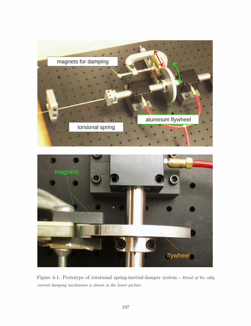
magnets for damping

aluminum flywheeltorsional spring

flywheel

magnets

Figure 4-1: Prototype of rotational spring-inertial-damper system - Detail of the eddy

current damping mechanism is shown in the lower picture.

197

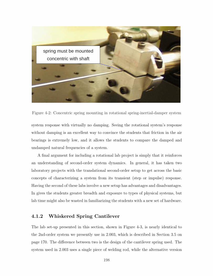
concentric with shaft

spring must be mounted

Figure 4-2: Concentric spring mounting in rotational spring-inertial-damper system

system response with virtually no damping. Seeing the rotational system’s response

without damping is an excellent way to convince the students that friction in the air

bearings is extremely low, and it allows the students to compare the damped and

undamped natural frequencies of a system.

A final argument for including a rotational lab project is simply that it reinforces

an understanding of second-order system dynamics. In general, it has taken two

laboratory projects with the translational second-order setup to get across the basic

concepts of characterizing a system from its transient (step or impulse) response.

Having the second of these labs involve a new setup has advantages and disadvantages.

In gives the students greater breadth and exposure to types of physical systems, but

lab time might also be wasted in familiarizing the students with a new set of hardware.

4.1.2 Whiskered Spring Cantilever

The lab set-up presented in this section, shown in Figure 4-3, is nearly identical to

the 2nd-order system we presently use in 2.003, which is described in Section 3.5 on

page 170. The difference between two is the design of the cantilever spring used. The

system used in 2.003 uses a single piece of welding rod, while the alternative version

198

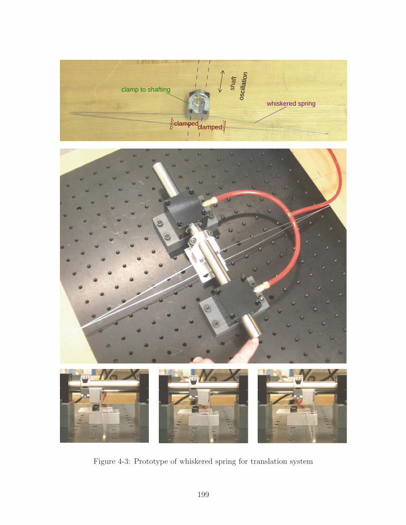
clamped

clamp to shafting

clamped

osci

llatio

n

whiskered spring

shaf

t

Figure 4-3: Prototype of whiskered spring for translation system

199

described here would use two lengths of rod, each doubled over into a “whiskered”

configuration.

The motivation for the whiskered configuration is to create a more ideal spring

which is more nearly linear. The spring we currently use in 2.003 is substantially

linear for small displacement, but it stiffens noticeably for larger travel (on the order

of a centimeter or so). Section 4.2.6 on page 214 describes this spring stiffening in

more detail. The whiskered spring also eliminates rotational coupling of the shaft

with translational movement. With the single-rod cantilever we settled on for the

labs, the shaft rotates somewhat as it moves back and forth, due to the geometric

constraints of the design.

There are several disadvantages of the whiskered spring, however. It would not be

as simple to make the spring adjustable. In contrast, the single-cantilever construction

now used in 2.003 can be set to different lengths easily by students during the lab.

It would also be more difficult for the TA’s to align and assemble, and it is not as

compact an elegant (so that one can easy picture students bumping into and bending

the long whiskers).

4.1.3 MEMS Systems

We have also considered designing and manufacturing MEMS devices which illustrate

higher-order system dynamics. Numerous researcher have developed spring-mass sys-

tems at the MEMS scale which are driven by parallel-plate capacitors, particularly

in developing accelerometers. Many companies (including Analog Devices, Motorola,

and Delphi Automotive Systems) currently sell a large volume of MEMS devices to

the automotive industry, for instance, and MEMS accelerometers are also being de-

veloped as an alternative to using geophones for seismic measurements [130]. Higher-

order spring-mass structures have also been designed and tested at a few research

labs, including Sandia [62], the University of Michigan [148], and National Tsing Hua

University in Taiwan [88].2

2Sandia and U. Mich. have designed translational systems, while those developed at the Tsing

Hua involve torsional modes.

200

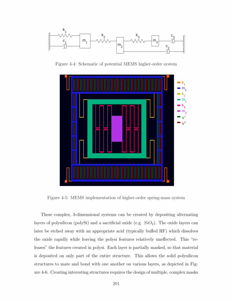
m1

m2

m3

k1

k2

k3

c1

c2

c3

Figure 4-4: Schematic of potential MEMS higher-order system

k1

k2

k3

m1

m2

m3

V−

V+

Figure 4-5: MEMS implementation of higher-order spring-mass system

These complex, 3-dimensional systems can be created by depositing alternating

layers of polysilicon (polySi) and a sacrificial oxide (e.g. SiO2). The oxide layers can

later be etched away with an appropriate acid (typically buffed HF) which dissolves

the oxide rapidly while leaving the polysi features relatively uneffected. This “re-

leases” the features created in polysi. Each layer is partially masked, so that material

is deposited on only part of the entire structure. This allows the solid polysilicon

structures to mate and bond with one another on various layers, as depicted in Fig-

ure 4-6. Creating interesting structures requires the design of multiple, complex masks

201

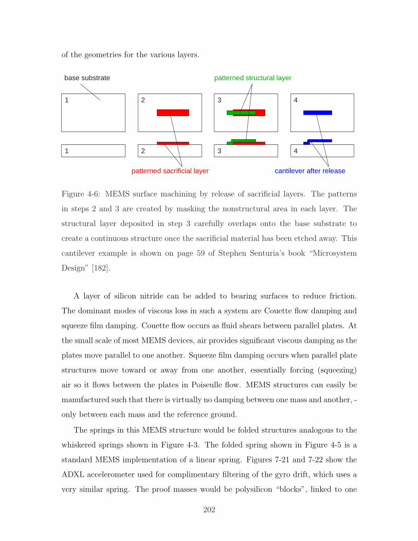
of the geometries for the various layers.

1

1

base substrate

2

2

patterned sacrificial layer

3

3

patterned structural layer

cantilever after release

4

4

Figure 4-6: MEMS surface machining by release of sacrificial layers. The patterns

in steps 2 and 3 are created by masking the nonstructural area in each layer. The

structural layer deposited in step 3 carefully overlaps onto the base substrate to

create a continuous structure once the sacrificial material has been etched away. This

cantilever example is shown on page 59 of Stephen Senturia’s book “Microsystem

Design” [182].

A layer of silicon nitride can be added to bearing surfaces to reduce friction.

The dominant modes of viscous loss in such a system are Couette flow damping and

squeeze film damping. Couette flow occurs as fluid shears between parallel plates. At

the small scale of most MEMS devices, air provides significant viscous damping as the

plates move parallel to one another. Squeeze film damping occurs when parallel plate

structures move toward or away from one another, essentially forcing (squeezing)

air so it flows between the plates in Poiseulle flow. MEMS structures can easily be

manufactured such that there is virtually no damping between one mass and another, -

only between each mass and the reference ground.

The springs in this MEMS structure would be folded structures analogous to the

whiskered springs shown in Figure 4-3. The folded spring shown in Figure 4-5 is a

standard MEMS implementation of a linear spring. Figures 7-21 and 7-22 show the

ADXL accelerometer used for complimentary filtering of the gyro drift, which uses a

very similar spring. The proof masses would be polysilicon “blocks”, linked to one

202

another and the base substrate through the folded springs.

Many MEMS devices are actuated using capacitive, electrostatic actuators. One

type, called a “comb drive”, consists of two sets of interlaced combs which pull toward

one another when the charges on the two plates are opposite in sign and push away

from one another when the plates have the same sign charge. As the interdigitated

fingers move parallel to one another, the gap between fingers remains essentially

constant; only the amount by which they overlap changes.

The capacitive actuator shown in Figure 4-5 is not a comb drive but a parallel plate

electrostatic actuator. The parallel plates are simply attracted or repelled, so that

here the gap between the plates does change. Consequently, this type of actuator

is quite nonlinear (compared with the comb drive). The parallel plate actuator is

generally capable of higher forces per unit area than the comb actuator, and is easier

to manufacture, but it has a very short stroke length.

One could look at the static structure using a low-power microscope, but both the

time and geometric scale would clearly make the dynamics of this device unobservable

to the naked eye. (The frequencies would be on the order of kiloHertz, with maximum

displacements of roughly a micron or so.) MEMS devices supply a host of dynamic

effects of interesting dynamics to analyze in class, bringing together many disciplines

(fluids, dynamics, thermodynamics, materials, design, etc) for analysis. The higher-

order MEMS system described here would also present both an additional example

of a dynamic system and a useful introduction to field of microsystem design, which

now seems certain to grow in significance over the next couple of decades. Mechanical

engineers are particularly well-suited for understanding MEMS design, because it

requires expertise in so many engineering disciplines, and a lab project such as this

could serve as a useful introduction to interest our students in this growing field.

4.2 In-Lab Demos

The remainder of this chapter documents some demostrations which have been used in

teaching 2.003 over the past few terms. While there are multiple sets of hardware for

203

each of the laboratory projects (described in Chapter 3), each piece of demonstration

hardware is typically a one-of-kind apparatus. In general, these demos are designed

to further illustrate some particular aspects in one of more of the laboratory projects.

I have made a loose distinction between “laboratory” and “lecture” demonstra-

tions. The first group presented attempt to demonstrate some physical phenomena

relating to the laboratory projects that may not be obvious during the course of the

lab. These include such things as how a voice coil motor or LVDT sensor works,

the viscous damping created by eddy currents, and spring stiffening effects in our

cantilever. A critical component in all these demonstrations is that students have the

ability to touch and play with the hardware individually - something not typically

possible in a large, lecture demo setting. We have set up some of these demonstra-

tions during labs and encouraged students to come over individually at some point

during the 3-hour lab to look at them.

The remaining group of “lecture” demonstrations described after this are gener-

ally appropriate for demos in a larger, in-class setting, but again, the distinction is

very loose! Some of the lecture materials could certainly be used in exercises in lab-

oratory or recitation section, and the lab demos still have use an non-tactile (visual)

demonstrations during a lecture.

4.2.1 Purpose of Hands-on Demonstration Hardware

The main purpose of the laboratory demos described here is to isolate particular

details and physical phenomena relevant to the lab projects in order to focus student

attention to them more clearly. There are many details that become obfuscated (or

unobservable) in the fully-assembled hardware for a particular lab.

For instance, when asked about potential sources of error or non-ideality in the

equipment, students will often cite the air bearings as a likely source of error. Our

purpose in using air bearings was to insure any such issues are miniscule. We find

this is not at all obvious to the students, however, because the voice coils in the trans-

lational spring-mass-dampers always always provide some viscous damping (whether

shorted or left open-circuit, because eddy currents are free to flow in the aluminum

204

housing for the coil). The first demo described below addresses this issue by show-

ing the system response when the voice coil is completely removed from the set-up.

Other demonstrations similarly aim to focus attention on particular details about the

hardware used in the labs.

4.2.2 2nd-order Translational System with No Damping

As mentioned above, it can be useful to demonstrate that the viscous damping in the

2nd-order system due to the air bearings is small, and any Coulomb friction (from

imperfections or dirt along the shaft-bearing interface) is truly miniscule. The data

in Figure 4-7 show that the viscous damping for such a system is on the order of

1/100 that of the system with the voice coil mounted, even when it is open-circuit.

If students then disconnect the spring from the damper-less system and either tap

or spin the shafting of this system, it becomes viscerally clear that any losses from

damping or Couloumb are low. We have also left some unused bearings in the lab. We

have allowed curious students to run a finger along the porous carbon surface while

it is connected to an air supply, to feel how “slick” the interface feels for themselves,

and we have left some bearings disassembled (i.e. the separate pillow block housing

and cylindrical core) to show students how they work.

4.2.3 Rectangular Voice Coil

During the development of the ActivLab projects, we considered manufacturing our

own voice coil motors. The prototype we developed is shown in Figures 4-8 and 4-9.

Ultimately, we were instead able to find a commercially available circular voice coil

with a large stroke at a reasonable price from BEI (a little over $300 a piece, in

quantity of 30). The circular geometry also allows the shaft to rotate as it translates

back and forth, and this in turn allows us to use a simpler cantilever (as illustrated

in Figure 3-28 on page 173).

The prototypes of the rectangular voice coil make useful in-lab demos for several

reasons. First, students can see the magnets and coil more easily, since the sides of

205

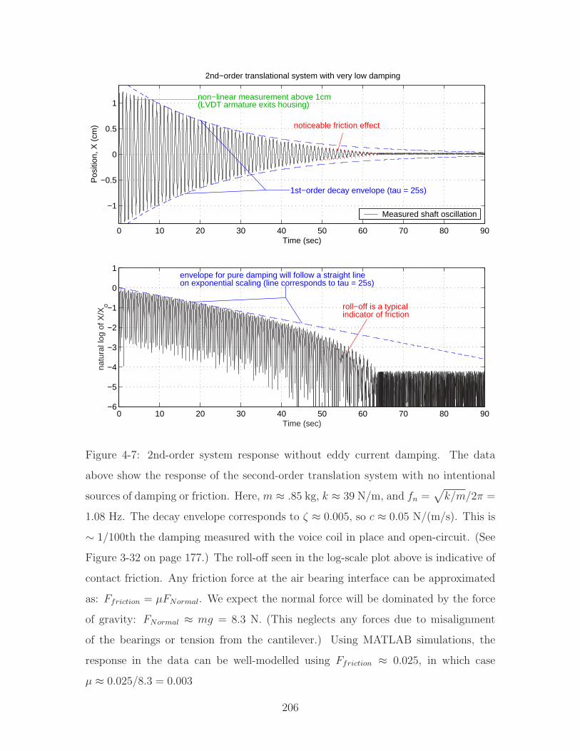
0 10 20 30 40 50 60 70 80 90

−1

−0.5

0

0.5

1non−linear measurement above 1cm(LVDT armature exits housing)

Time (sec)

Pos

ition

, X (

cm)

2nd−order translational system with very low damping

1st−order decay envelope (tau = 25s)

noticeable friction effect

Measured shaft oscillation

0 10 20 30 40 50 60 70 80 90−6

−5

−4

−3

−2

−1

0

1

Time (sec)

natu

ral l

og o

f X/X

o

envelope for pure damping will follow a straight lineon exponential scaling (line corresponds to tau = 25s)

roll−off is a typicalindicator of friction

Figure 4-7: 2nd-order system response without eddy current damping. The data

above show the response of the second-order translation system with no intentional

sources of damping or friction. Here, m ≈ .85 kg, k ≈ 39 N/m, and fn =√

k/m/2π =

1.08 Hz. The decay envelope corresponds to ζ ≈ 0.005, so c ≈ 0.05 N/(m/s). This is

∼ 1/100th the damping measured with the voice coil in place and open-circuit. (See

Figure 3-32 on page 177.) The roll-off seen in the log-scale plot above is indicative of

contact friction. Any friction force at the air bearing interface can be approximated

as: Ffriction = µFNormal. We expect the normal force will be dominated by the force

of gravity: FNormal ≈ mg = 8.3 N. (This neglects any forces due to misalignment

of the bearings or tension from the cantilever.) Using MATLAB simulations, the

response in the data can be well-modelled using Ffriction ≈ 0.025, in which case

µ ≈ 0.025/8.3 = 0.003

206

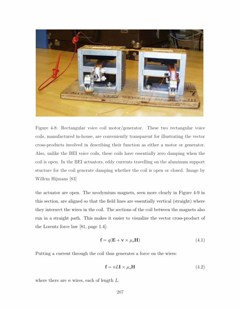
Figure 4-8: Rectangular voice coil motor/generator. These two rectangular voice

coils, manufactured in-house, are conveniently transparent for illustrating the vector

cross-products involved in describing their function as either a motor or generator.

Also, unlike the BEI voice coils, these coils have essentially zero damping when the

coil is open. In the BEI actuators, eddy currents travelling on the aluminum support

stucture for the coil generate damping whether the coil is open or closed. Image by

Willem Hijmans [83]

the actuator are open. The neodymium magnets, seen more clearly in Figure 4-9 in

this section, are aligned so that the field lines are essentially vertical (straight) where

they intersect the wires in the coil. The sections of the coil between the magnets also

run in a straight path. This makes it easier to visualize the vector cross-product of

the Lorentz force law [81, page 1.4]:

f = q(E + v× µoH) (4.1)

Putting a current through the coil thus generates a force on the wires:

f = nLI× µoH (4.2)

where there are n wires, each of length L.

207

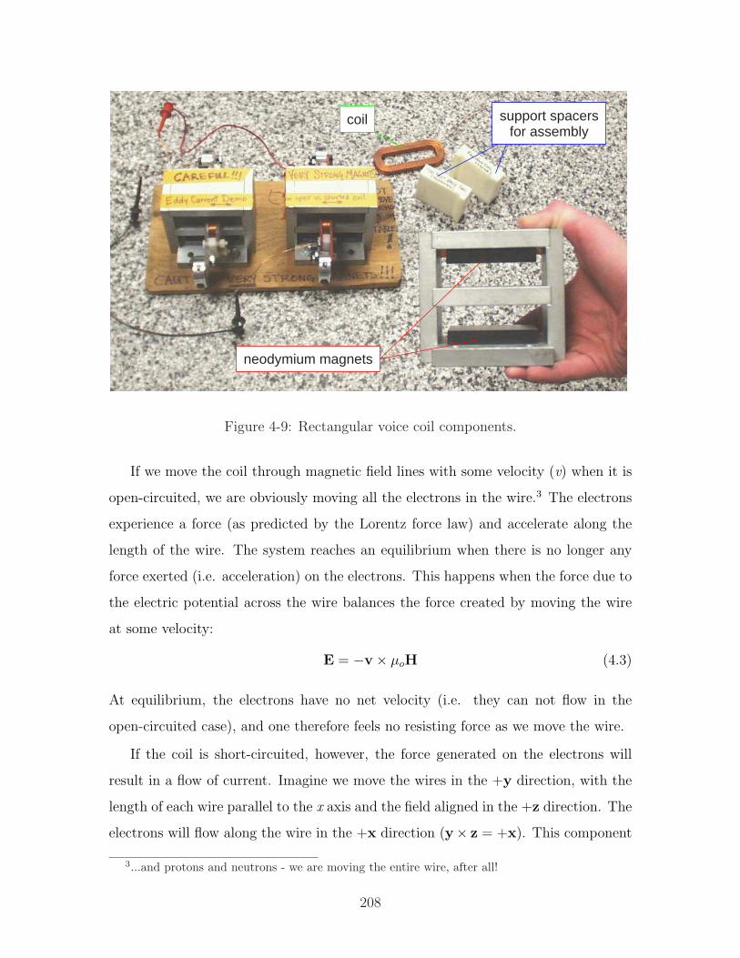
for assembly

neodymium magnets

coil support spacers

Figure 4-9: Rectangular voice coil components.

If we move the coil through magnetic field lines with some velocity (v) when it is

open-circuited, we are obviously moving all the electrons in the wire.3 The electrons

experience a force (as predicted by the Lorentz force law) and accelerate along the

length of the wire. The system reaches an equilibrium when there is no longer any

force exerted (i.e. acceleration) on the electrons. This happens when the force due to

the electric potential across the wire balances the force created by moving the wire

at some velocity:

E = −v× µoH (4.3)

At equilibrium, the electrons have no net velocity (i.e. they can not flow in the

open-circuited case), and one therefore feels no resisting force as we move the wire.

If the coil is short-circuited, however, the force generated on the electrons will

result in a flow of current. Imagine we move the wires in the +y direction, with the

length of each wire parallel to the x axis and the field aligned in the +z direction. The

electrons will flow along the wire in the +x direction (y× z = +x). This component

3...and protons and neutrons - we are moving the entire wire, after all!

208

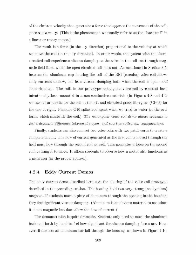
of the electron velocity then generates a force that opposes the movement of the coil,

since x× z = −y. (This is the phenomenon we usually refer to as the “back emf” in

a linear or rotary motor.)

The result is a force (in the −y direction) proportional to the velocity at which

we move the coil (in the +y direction). In other words, the system with the short-

circuited coil experiences viscous damping as the wires in the coil cut through mag-

netic field lines, while the open-circuited coil does not. As mentioned in Section 3.5,

because the aluminum cup housing the coil of the BEI (circular) voice coil allows

eddy currents to flow, one feels viscous damping both when the coil is open- and

short-circuited. The coils in our prototype rectangular voice coil by contrast have

intentionally been mounted in a non-conductive material. (In Figures 4-8 and 4-9,

we used clear acrylic for the coil at the left and electrical-grade fiberglass (GP03) for

the one at right. Phenolic G10 splintered apart when we tried to water-jet the oval

forms which sandwich the coil.) The rectangular voice coil demo allows students to

feel a dramatic difference between the open- and short-circuited coil configurations.

Finally, students can also connect two voice coils with two patch cords to create a

complete circuit. The flow of current generated as the first coil is moved through the

field must flow through the second coil as well. This generates a force on the second

coil, causing it to move. It allows students to observe how a motor also functions as

a generator (in the proper context).

4.2.4 Eddy Current Demos

The eddy current demo described here uses the housing of the voice coil prototype

described in the preceding section. The housing hold two very strong (neodymium)

magnets. If students move a piece of aluminum through the opening in the housing,

they feel significant viscous damping. (Aluminum is an obvious material to use, since

it is not magnetic but does allow the flow of current.)

The demonstration is quite dramatic. Students only need to move the aluminum

back and forth by hand to feel how significant the viscous damping forces are. How-

ever, if one lets an aluminum bar fall through the housing, as shown in Figure 4-10,

209

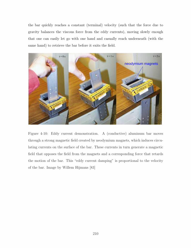
the bar quickly reaches a constant (terminal) velocity (such that the force due to

gravity balances the viscous force from the eddy currents), moving slowly enough

that one can easily let go with one hand and casually reach underneath (with the

same hand) to retrieve the bar before it exits the field.

neodymium magnets

Figure 4-10: Eddy current demonstration. A (conductive) aluminum bar moves

through a strong magnetic field created by neodymium magnets, which induces circu-

lating currents on the surface of the bar. These currents in turn generate a magnetic

field that opposes the field from the magnets and a corresponding force that retards

the motion of the bar. This “eddy current damping” is proportional to the velocity

of the bar. Image by Willem Hijmans [83]

210

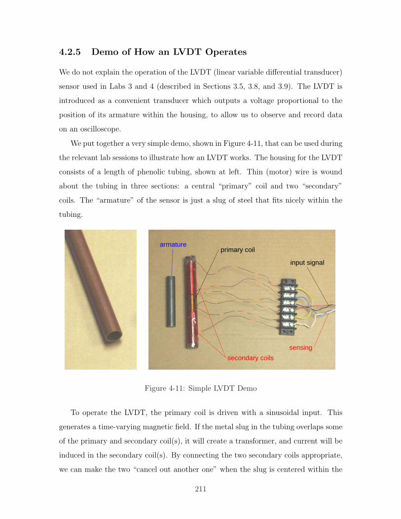
4.2.5 Demo of How an LVDT Operates

We do not explain the operation of the LVDT (linear variable differential transducer)

sensor used in Labs 3 and 4 (described in Sections 3.5, 3.8, and 3.9). The LVDT is

introduced as a convenient transducer which outputs a voltage proportional to the

position of its armature within the housing, to allow us to observe and record data

on an oscilloscope.

We put together a very simple demo, shown in Figure 4-11, that can be used during

the relevant lab sessions to illustrate how an LVDT works. The housing for the LVDT

consists of a length of phenolic tubing, shown at left. Thin (motor) wire is wound

about the tubing in three sections: a central “primary” coil and two “secondary”

coils. The “armature” of the sensor is just a slug of steel that fits nicely within the

tubing.

armature

secondary coils

sensing

input signal

primary coil

Figure 4-11: Simple LVDT Demo

To operate the LVDT, the primary coil is driven with a sinusoidal input. This

generates a time-varying magnetic field. If the metal slug in the tubing overlaps some

of the primary and secondary coil(s), it will create a transformer, and current will be

induced in the secondary coil(s). By connecting the two secondary coils appropriate,

we can make the two “cancel out another one” when the slug is centered within the

211

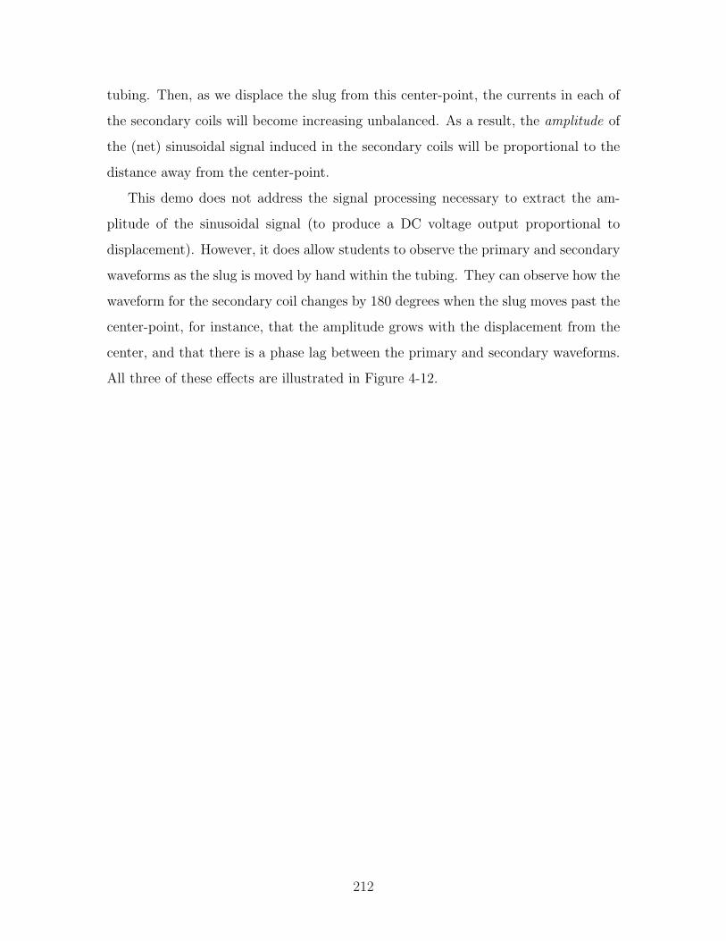
tubing. Then, as we displace the slug from this center-point, the currents in each of

the secondary coils will become increasing unbalanced. As a result, the amplitude of

the (net) sinusoidal signal induced in the secondary coils will be proportional to the

distance away from the center-point.

This demo does not address the signal processing necessary to extract the am-

plitude of the sinusoidal signal (to produce a DC voltage output proportional to

displacement). However, it does allow students to observe the primary and secondary

waveforms as the slug is moved by hand within the tubing. They can observe how the

waveform for the secondary coil changes by 180 degrees when the slug moves past the

center-point, for instance, that the amplitude grows with the displacement from the

center, and that there is a phase lag between the primary and secondary waveforms.

All three of these effects are illustrated in Figure 4-12.

212

secondary coils

primary coil

primarysecondary

Figure 4-12: LVDT schematic with sinusoidal signals. The primary coil is driven with

a sinusoidal excitation of constant amplitude. A time-varying magnetic field is thereby

created in a metal slug within the coils. If the slug is perfectly centered, the equal and

opposite signals in the secondary coils cancel one another. The differential amplitude

of the induced signals in the two secondary coils varies linearly with displacement

from the null (centered) position, as shown at right. The sensor (secondary) signal

is somewhat delayed with respect to the waveform in the primary coil. The signal

conditioner is adjusted to account for this phase lag during calibration to maximize

the sensitivity of the LVDT.

213

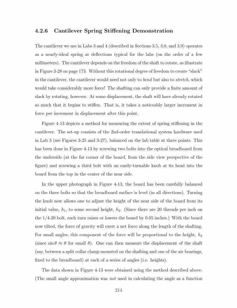
4.2.6 Cantilever Spring Stiffening Demonstration

The cantilever we use in Labs 3 and 4 (described in Sections 3.5, 3.8, and 3.9) operates

as a nearly-ideal spring at deflections typical for the labs (on the order of a few

millimeters). The cantilever depends on the freedom of the shaft to rotate, as illustrate

in Figure 3-28 on page 173. Without this rotational degree of freedom to create “slack”

in the cantilever, the cantilever would need not only to bend but also to stretch, which

would take considerably more force! The shafting can only provide a finite amount of

slack by rotating, however. At some displacement, the shaft will have already rotated

so much that it begins to stiffen. That is, it takes a noticeably larger increment in

force per increment in displacement after this point.

Figure 4-13 depicts a method for measuring the extent of spring stiffening in the

cantilever. The set-up consists of the 2nd-order translational system hardware used

in Lab 3 (see Figures 3-25 and 3-27), balanced on the lab table at three points. This

has been done in Figure 4-13 by screwing two bolts into the optical breadboard from

the underside (at the far corner of the board, from the side view perspective of the

figure) and screwing a third bolt with an easily-turnable knob at its head into the

board from the top in the center of the near side.

In the upper photograph in Figure 4-13, the board has been carefully balanced

on the three bolts so that the breadboard surface is level (in all directions). Turning

the knob now allows one to adjust the height of the near side of the board from its

initial value, h1, to some second height, h2. (Since there are 20 threads per inch on

the 1/4-20 bolt, each turn raises or lowers the board by 0.05 inches.) With the board

now tilted, the force of gravity will exert a net force along the length of the shafting.

For small angles, this component of the force will be proportional to the height, h2

(since sin θ ≈ θ for small θ). One can then measure the displacement of the shaft

(say, between a split collar clamp mounted on the shafting and one of the air bearings,

fixed to the breadboard) at each of a series of angles (i.e. heights).

The data shown in Figure 4-13 were obtained using the method described above.

(The small angle approximation was not used in calculating the angle as a function

214

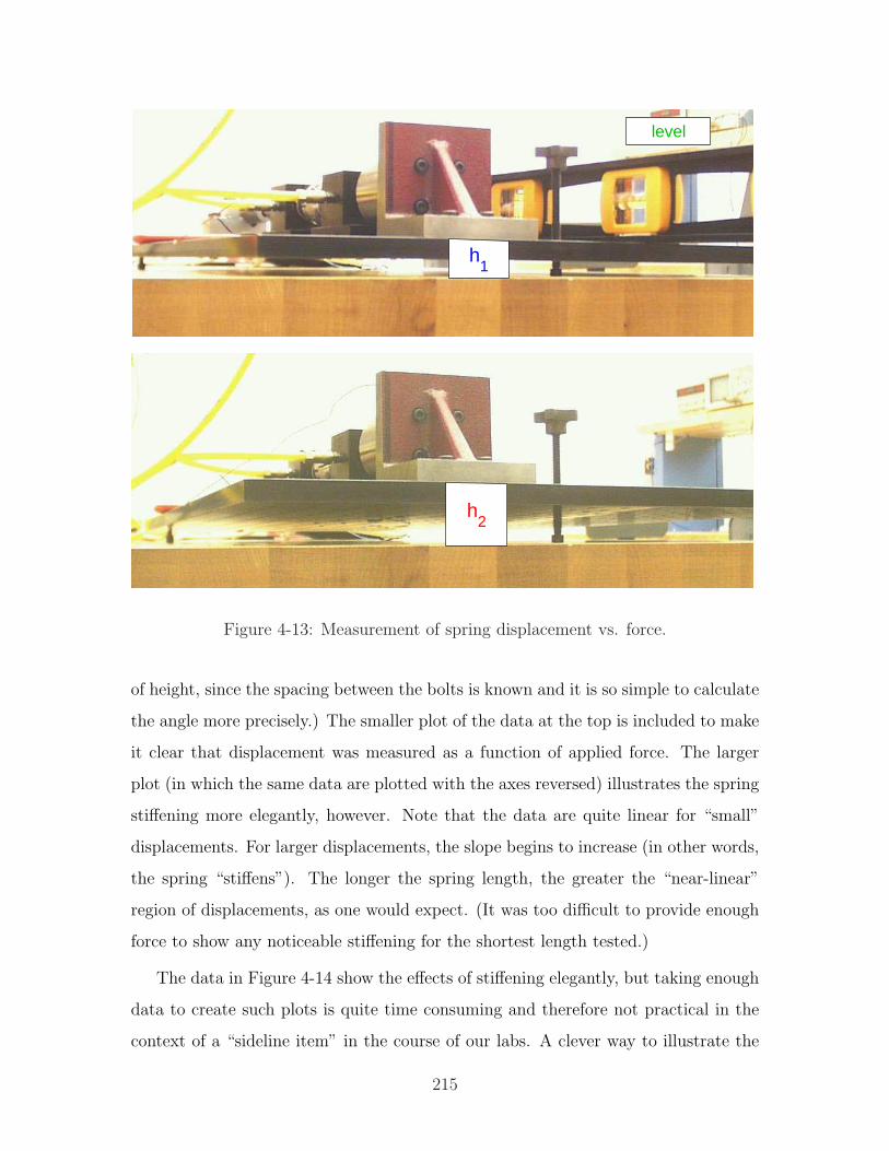
h1

level

h2

Figure 4-13: Measurement of spring displacement vs. force.

of height, since the spacing between the bolts is known and it is so simple to calculate

the angle more precisely.) The smaller plot of the data at the top is included to make

it clear that displacement was measured as a function of applied force. The larger

plot (in which the same data are plotted with the axes reversed) illustrates the spring

stiffening more elegantly, however. Note that the data are quite linear for “small”

displacements. For larger displacements, the slope begins to increase (in other words,

the spring “stiffens”). The longer the spring length, the greater the “near-linear”

region of displacements, as one would expect. (It was too difficult to provide enough

force to show any noticeable stiffening for the shortest length tested.)

The data in Figure 4-14 show the effects of stiffening elegantly, but taking enough

data to create such plots is quite time consuming and therefore not practical in the

context of a “sideline item” in the course of our labs. A clever way to illustrate the

215

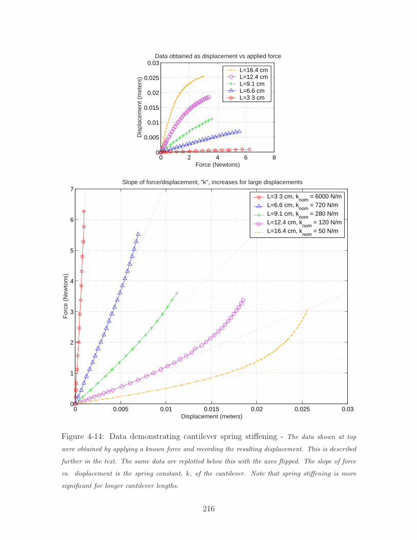
0 2 4 6 80

0.005

0.01

0.015

0.02

0.025

0.03

Force (Newtons)

Dis

plac

emen

t (m

eter

s)

Data obtained as displacement vs applied force

L=16.4 cmL=12.4 cmL=9.1 cmL=6.6 cmL=3 3 cm

0 0.005 0.01 0.015 0.02 0.025 0.030

1

2

3

4

5

6

7

For

ce (

New

tons

)

Displacement (meters)

Slope of force/displacement, "k", increases for large displacements

L=3 3 cm, knom

= 6000 N/mL=6.6 cm, k

nom = 720 N/m

L=9.1 cm, knom

= 280 N/mL=12.4 cm, k

nom = 120 N/m

L=16.4 cm, knom

= 50 N/m

Figure 4-14: Data demonstrating cantilever spring stiffening - The data shown at top

were obtained by applying a known force and recording the resulting displacement. This is described

further in the text. The same data are replotted below this with the axes flipped. The slope of force

vs. displacement is the spring constant, k, of the cantilever. Note that spring stiffening is more

significant for longer cantilever lengths.

216

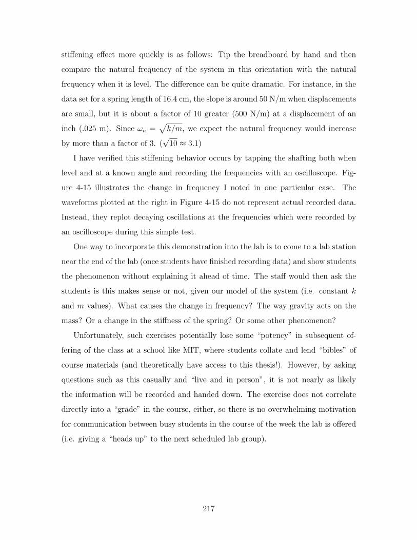
stiffening effect more quickly is as follows: Tip the breadboard by hand and then

compare the natural frequency of the system in this orientation with the natural

frequency when it is level. The difference can be quite dramatic. For instance, in the

data set for a spring length of 16.4 cm, the slope is around 50 N/m when displacements

are small, but it is about a factor of 10 greater (500 N/m) at a displacement of an

inch (.025 m). Since ωn =√

k/m, we expect the natural frequency would increase

by more than a factor of 3. (√

10 ≈ 3.1)

I have verified this stiffening behavior occurs by tapping the shafting both when

level and at a known angle and recording the frequencies with an oscilloscope. Fig-

ure 4-15 illustrates the change in frequency I noted in one particular case. The

waveforms plotted at the right in Figure 4-15 do not represent actual recorded data.

Instead, they replot decaying oscillations at the frequencies which were recorded by

an oscilloscope during this simple test.

One way to incorporate this demonstration into the lab is to come to a lab station

near the end of the lab (once students have finished recording data) and show students

the phenomenon without explaining it ahead of time. The staff would then ask the

students is this makes sense or not, given our model of the system (i.e. constant k

and m values). What causes the change in frequency? The way gravity acts on the

mass? Or a change in the stiffness of the spring? Or some other phenomenon?

Unfortunately, such exercises potentially lose some “potency” in subsequent of-

fering of the class at a school like MIT, where students collate and lend “bibles” of

course materials (and theoretically have access to this thesis!). However, by asking

questions such as this casually and “live and in person”, it is not nearly as likely

the information will be recorded and handed down. The exercise does not correlate

directly into a “grade” in the course, either, so there is no overwhelming motivation

for communication between busy students in the course of the week the lab is offered

(i.e. giving a “heads up” to the next scheduled lab group).

217

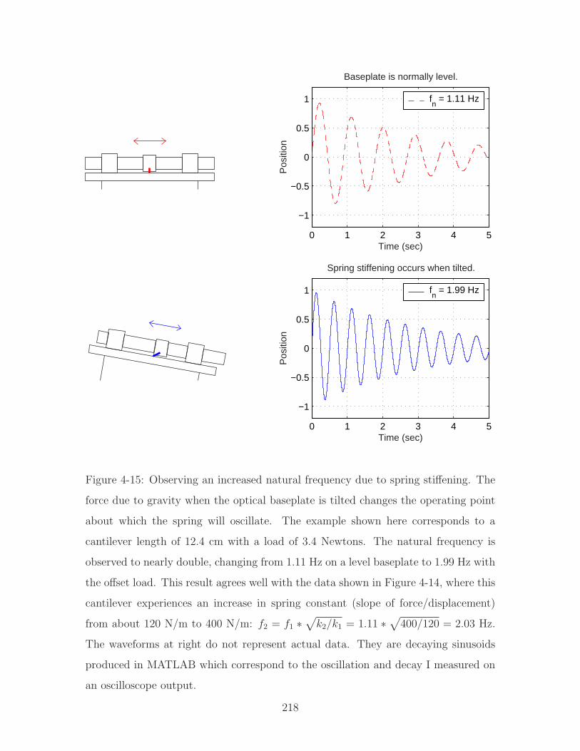
0 1 2 3 4 5

−1

−0.5

0

0.5

1

Baseplate is normally level.

Time (sec)

Pos

ition

fn = 1.11 Hz

0 1 2 3 4 5

−1

−0.5

0

0.5

1

Spring stiffening occurs when tilted.

Time (sec)

Pos

ition

fn = 1.99 Hz

Figure 4-15: Observing an increased natural frequency due to spring stiffening. The

force due to gravity when the optical baseplate is tilted changes the operating point

about which the spring will oscillate. The example shown here corresponds to a

cantilever length of 12.4 cm with a load of 3.4 Newtons. The natural frequency is

observed to nearly double, changing from 1.11 Hz on a level baseplate to 1.99 Hz with

the offset load. This result agrees well with the data shown in Figure 4-14, where this

cantilever experiences an increase in spring constant (slope of force/displacement)

from about 120 N/m to 400 N/m: f2 = f1 ∗√

k2/k1 = 1.11 ∗√

400/120 = 2.03 Hz.

The waveforms at right do not represent actual data. They are decaying sinusoids

produced in MATLAB which correspond to the oscillation and decay I measured on

an oscilloscope output.

218

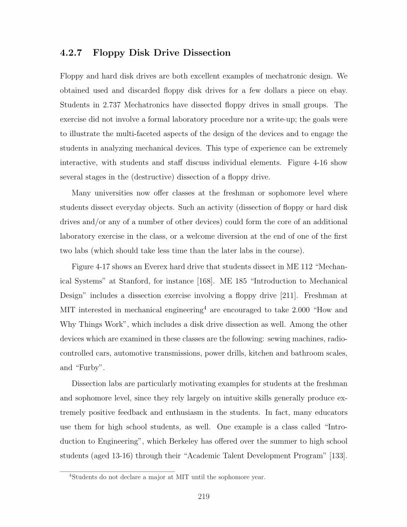
4.2.7 Floppy Disk Drive Dissection

Floppy and hard disk drives are both excellent examples of mechatronic design. We

obtained used and discarded floppy disk drives for a few dollars a piece on ebay.

Students in 2.737 Mechatronics have dissected floppy drives in small groups. The

exercise did not involve a formal laboratory procedure nor a write-up; the goals were

to illustrate the multi-faceted aspects of the design of the devices and to engage the

students in analyzing mechanical devices. This type of experience can be extremely

interactive, with students and staff discuss individual elements. Figure 4-16 show

several stages in the (destructive) dissection of a floppy drive.

Many universities now offer classes at the freshman or sophomore level where

students dissect everyday objects. Such an activity (dissection of floppy or hard disk

drives and/or any of a number of other devices) could form the core of an additional

laboratory exercise in the class, or a welcome diversion at the end of one of the first

two labs (which should take less time than the later labs in the course).

Figure 4-17 shows an Everex hard drive that students dissect in ME 112 “Mechan-

ical Systems” at Stanford, for instance [168]. ME 185 “Introduction to Mechanical

Design” includes a dissection exercise involving a floppy drive [211]. Freshman at

MIT interested in mechanical engineering4 are encouraged to take 2.000 “How and

Why Things Work”, which includes a disk drive dissection as well. Among the other

devices which are examined in these classes are the following: sewing machines, radio-

controlled cars, automotive transmissions, power drills, kitchen and bathroom scales,

and “Furby”.

Dissection labs are particularly motivating examples for students at the freshman

and sophomore level, since they rely largely on intuitive skills generally produce ex-

tremely positive feedback and enthusiasm in the students. In fact, many educators

use them for high school students, as well. One example is a class called “Intro-

duction to Engineering”, which Berkeley has offered over the summer to high school

students (aged 13-16) through their “Academic Talent Development Program” [133].

4Students do not declare a major at MIT until the sophomore year.

219

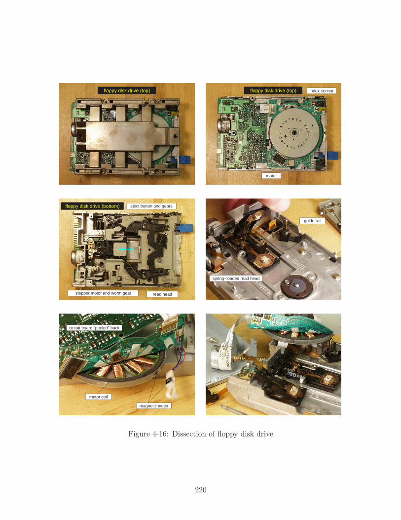
floppy disk drive (top) floppy disk drive (top) index sensor

motor

floppy disk drive (bottom)

stepper motor and worm gear

eject button and gears

read head

spring−loaded read head

guide rail

magnetic index

circuit board "peeled" back

motor coil

Figure 4-16: Dissection of floppy disk drive

220

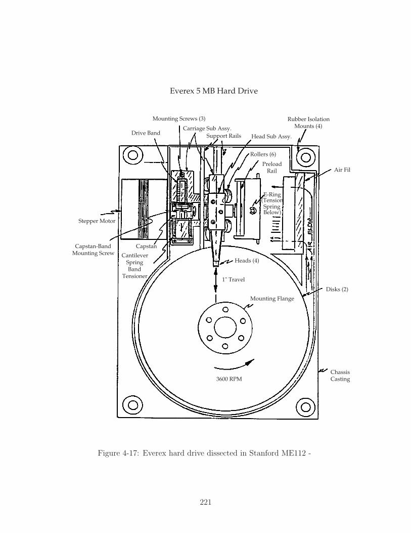
3600 RPM

Mounting Flange

ChassisCasting

Disks (2)

Air Filter

Rubber IsolationMounts (4)

Head Sub Assy.

Rollers (6)

PreloadRail

Carriage Sub Assy.Support Rails

Mounting Screws (3)

Drive Band

Stepper Motor

Capstan-BandMounting Screw

Capstan

CantileverSpringBand

Tensioner

E-Ring(TensionSpringBelow)

1" Travel

Heads (4)

Everex 5 MB Hard Drive

Figure 1: Sketch of major compenents of Everex 5MB Hard Drive.

Figure 4-17: Everex hard drive dissected in Stanford ME112 -

221

The course includes the dissection of an actual disk drive, and the activity is supple-

mented with a virtual exploration on an interactive CD-ROM that helps describe the

various parts and their function [171]. Students can reference the CD-ROM as they

take apart the real disk drive in front of them (working in teams of two). This sounds

like a great use of technology to me. (I am heartened they did not try to replace a

real-life dissection with a purely simulated one!)

My own experience indicates that students respond enthusiastically to dissection

exercises. I taught a “How Thing Work” class during the January term at an all-girl

high school near Boston (The Windsor School). The students seemed mildly receptive

to various demos and short lectures I gave in class during first couple of days, but

when I began to bring things to us to take apart in class, they became genuinely eager

and excited.

The first device we dissected was a broken toaster. The students were interested

in exploring how it worked, but their primary “thrill” came from the fact that we

were actually able to fix it ! We just needed to reposition the bimetallic strip so it

would properly trigger and release the spring. After this, they began bringing in a

variety of broken appliances from home.5 I don’t recall being able to fix any of the

rest of the lot, but the students were still excited just to solve the mystery of “what

was wrong” (and in the process, learned a bit about mechanical design, I hope).

5Apparently, I’m not the only one in the world reluctant to throw things out...

222

4.3 Lecture Demonstrations

This section briefly documents some of the lecture demonstrations Prof. Trumper

has used in 2.003. Other potential demos can be found in the survey in Chapter 2.

Lecture demos are typically quite popular events in classes. Jack Wilson, professor

of physics and dean for Undergraduate and Continuing Education at RPI, gives the

following warning that “enjoyable” does not necessarily equate with “educational”,

however:

Each meeting of the American Association of Physics Teachers is filled

with ideas for how to improve the lecture. One recurring them is the use

of lecture demonstrations that range from the spectacular to the humor-

ous. Faculty, students, and even the general public love and remember the

best demonstrations and the best demonstrators. Over the years, we have

turned to audio, video, and now computers to make lectures more inter-

esting and more instructive. Unfortunately, later interviews with

the students often reveal that the memory of the the demon-

stration is often not accompanied by an understanding of the

physics of the demonstration.6 [218]

This last sentence is an excellent comment and a genuine concern. I will, however,

rebut the point with the following three points. (1) When lecture demonstrations

incite enthusiasm and interest in a class, they are potentially planting seeds of cu-

riosity in the students which may inspire them to pursue a particular discipline (e.g.

mechatronic design, biomechanical engineerings, etc) and answer the motivational

question, “when would I ever actually use this stuff?” (“Stuff” potentially meaning

the entire course curriculum!) (2) There is no indication that those students who do

not recall and/or understand the details behind their favorite physics demonstrations

would in fact actually happen to recall and/or understand very much from the rest of

6The italic emphasis is mine, not Prof. Wilson’s.

223

the course.7 One can argue the demonstration may still be generating a substantially

larger “bang for the buck” that an equivalent amount of time spent in typical lecture.

(3) Finally, instructors who wish to avoid this potential pitfall should incorporate

complementary exercises (in-class problem solving and/or homework assignments) to

reinforce the concepts covered !

In-class exercises might, for instance, ask that students work with 2 or 3 of their

neighbors in class to perform some calculation, develop a model, or answer particular

questions that probe their understanding. This gives slower students the opportunity

to learn from watching peers solve problems, and it gives the brighter students an

opportunity to try to explain phenomena to others. (Everyone knows you learn a

subject “best” when you try to teach it to others!)

Homework assignments give students the opportunity to think about the physical

phenomena at their own pace (and a graded assignment somehow always seems to

provide the most-reliable motivation for learning in our students). When presenting

a demo to a large class, it is usually not possible to set a pace which is appropriate

for everyone. Supplementary materials can be provided to address this issue, giving

the students a reference they can study outside of class and freeing the from the

distraction of note taking during the demo. These additional hand-outs (providing

equations and text reviewing the concepts covered by the demonstration) “bridge the

gap” for students who do not fully comprehend a demo and consequently struggle

through the related homework. (TA’s can also clearly help to bridge this gap.)

And so, with a mixture of optimism and caution, we proceed to the survey of demos

that follows. Note that most of the demonstrations have been used in previous terms

by Prof. David Trumper in teaching either 2.003 Modeling Dynamics and Control I

or 2.737 Mechatronics.

7Those principles they do recall have likely been repeated many times throughout the course,

too, unlike a demo which they have only seen once and which lasted for perhaps 20 minutes.

224

4.3.1 Low-Pass and High-Pass Audio Filtering

Everyone has played with the bass and treble adjustments on their home stereos, but

students may not have thought about what happens in the system when they tweak

those settings. One can demonstrate low- and high-pass filtering in front of the class

with simple RC circuits. This is an appropriate demonstration after students have

analyzed and experimented with simple first-order circuits in the labs. (The relevant

ActivLab experiments can be found in Section 3.6 on page 179.) The analysis of

the circuits is straight-forward and should be familiar to the students at this point.

(Repetition is still a useful teaching tool, though.)

The circuit can then be used to filter music (e.g. from a CD or MP3 player). The

output should be both played aloud for students to hear and shown visually at the

front of the room on a scope (preferably projected, so it can be seen easily). Most

music conveniently provides components over large spectrum of frequencies (treble

and bass), so that students can see and hear significant effects when either a high- or

low-pass filter is applied to the waveform.

4.3.2 Camera Flash Charging Circuit

We spend considerable time in the lab sessions8 investigating the dynamics of a me-

chanical 2nd-order system. The camera flash demo described here presents a 2nd-

order electrical (LRC) circuit and provides a context in which such a thing is useful.

The circuit charges a capacitor to a high voltage (up to 300 volts). When triggered,

the capacitor then discharges at the center of xenon flash tube, generating the “flash”

for the camera.

Figure 4-18 shows the simplified model for the circuit which we use in class. With

the transistor in position “A”, current flows continuously through the inductor. When

the transistor is then switched to position “B”, the current can not instantaneously

stop flowing through the inductor, even if the voltage potential across the capacitor

already exceeds that of the battery (1.5 volts). Thus, electrons continue to flow, and

8typically 3 lab sessions, as described in Sections 3.5,3.8, and 3.9

225

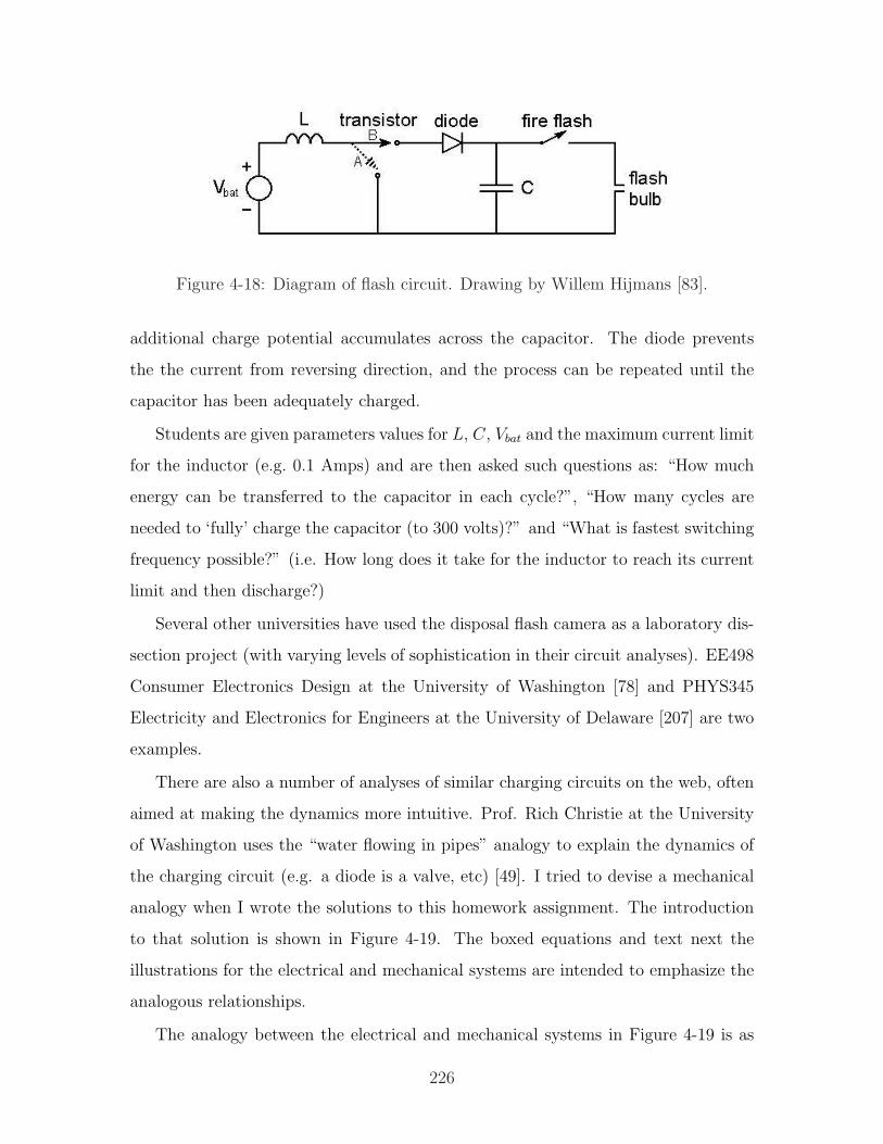
Figure 4-18: Diagram of flash circuit. Drawing by Willem Hijmans [83].

additional charge potential accumulates across the capacitor. The diode prevents

the the current from reversing direction, and the process can be repeated until the

capacitor has been adequately charged.

Students are given parameters values for L, C, Vbat and the maximum current limit

for the inductor (e.g. 0.1 Amps) and are then asked such questions as: “How much

energy can be transferred to the capacitor in each cycle?”, “How many cycles are

needed to ‘fully’ charge the capacitor (to 300 volts)?” and “What is fastest switching

frequency possible?” (i.e. How long does it take for the inductor to reach its current

limit and then discharge?)

Several other universities have used the disposal flash camera as a laboratory dis-

section project (with varying levels of sophistication in their circuit analyses). EE498

Consumer Electronics Design at the University of Washington [78] and PHYS345

Electricity and Electronics for Engineers at the University of Delaware [207] are two

examples.

There are also a number of analyses of similar charging circuits on the web, often

aimed at making the dynamics more intuitive. Prof. Rich Christie at the University

of Washington uses the “water flowing in pipes” analogy to explain the dynamics of

the charging circuit (e.g. a diode is a valve, etc) [49]. I tried to devise a mechanical

analogy when I wrote the solutions to this homework assignment. The introduction

to that solution is shown in Figure 4-19. The boxed equations and text next the

illustrations for the electrical and mechanical systems are intended to emphasize the

analogous relationships.

The analogy between the electrical and mechanical systems in Figure 4-19 is as

226

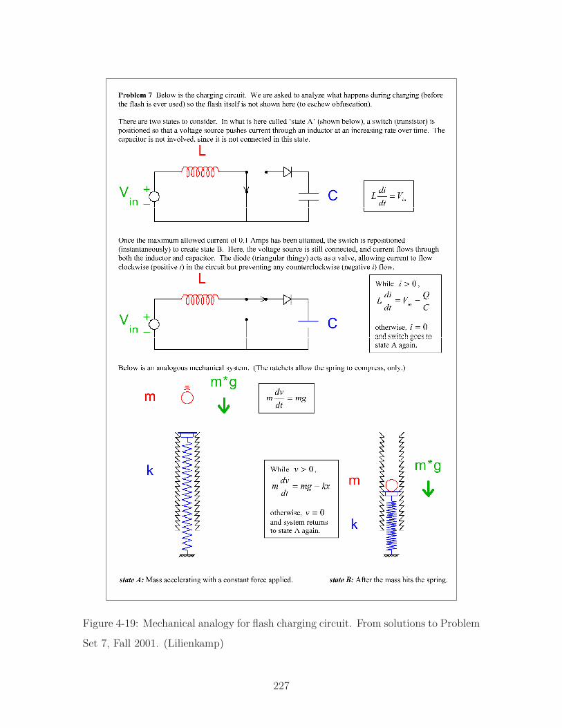
Figure 4-19: Mechanical analogy for flash charging circuit. From solutions to Problem

Set 7, Fall 2001. (Lilienkamp)

227

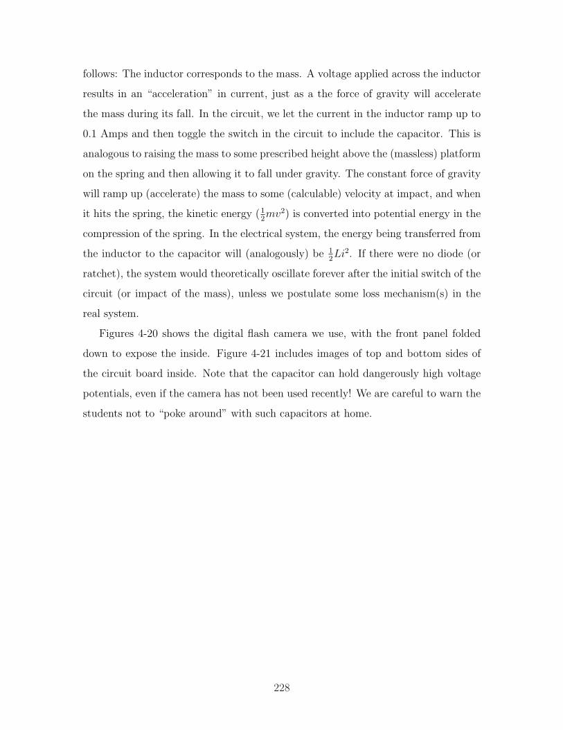
follows: The inductor corresponds to the mass. A voltage applied across the inductor

results in an “acceleration” in current, just as a the force of gravity will accelerate

the mass during its fall. In the circuit, we let the current in the inductor ramp up to

0.1 Amps and then toggle the switch in the circuit to include the capacitor. This is

analogous to raising the mass to some prescribed height above the (massless) platform

on the spring and then allowing it to fall under gravity. The constant force of gravity

will ramp up (accelerate) the mass to some (calculable) velocity at impact, and when

it hits the spring, the kinetic energy (12mv2) is converted into potential energy in the

compression of the spring. In the electrical system, the energy being transferred from

the inductor to the capacitor will (analogously) be 12Li2. If there were no diode (or

ratchet), the system would theoretically oscillate forever after the initial switch of the

circuit (or impact of the mass), unless we postulate some loss mechanism(s) in the

real system.

Figures 4-20 shows the digital flash camera we use, with the front panel folded

down to expose the inside. Figure 4-21 includes images of top and bottom sides of

the circuit board inside. Note that the capacitor can hold dangerously high voltage

potentials, even if the camera has not been used recently! We are careful to warn the

students not to “poke around” with such capacitors at home.

228

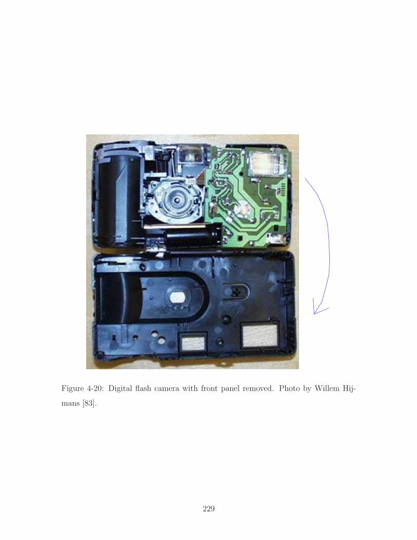
Figure 4-20: Digital flash camera with front panel removed. Photo by Willem Hij-

mans [83].

229

Figure 4-21: Digital camera flash circuit board. Photos taken by Willem Hijmans [83].

230

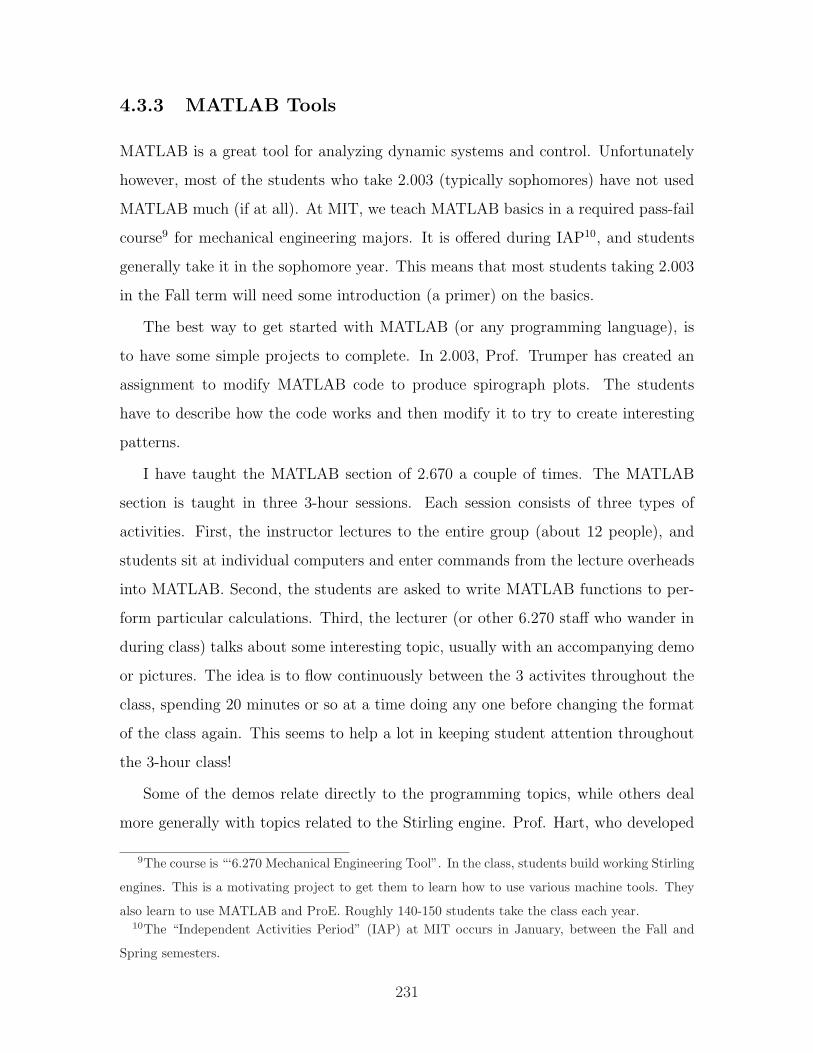
4.3.3 MATLAB Tools

MATLAB is a great tool for analyzing dynamic systems and control. Unfortunately

however, most of the students who take 2.003 (typically sophomores) have not used

MATLAB much (if at all). At MIT, we teach MATLAB basics in a required pass-fail

course9 for mechanical engineering majors. It is offered during IAP10, and students

generally take it in the sophomore year. This means that most students taking 2.003

in the Fall term will need some introduction (a primer) on the basics.

The best way to get started with MATLAB (or any programming language), is

to have some simple projects to complete. In 2.003, Prof. Trumper has created an

assignment to modify MATLAB code to produce spirograph plots. The students

have to describe how the code works and then modify it to try to create interesting

patterns.

I have taught the MATLAB section of 2.670 a couple of times. The MATLAB

section is taught in three 3-hour sessions. Each session consists of three types of

activities. First, the instructor lectures to the entire group (about 12 people), and

students sit at individual computers and enter commands from the lecture overheads

into MATLAB. Second, the students are asked to write MATLAB functions to per-

form particular calculations. Third, the lecturer (or other 6.270 staff who wander in

during class) talks about some interesting topic, usually with an accompanying demo

or pictures. The idea is to flow continuously between the 3 activites throughout the

class, spending 20 minutes or so at a time doing any one before changing the format

of the class again. This seems to help a lot in keeping student attention throughout

the 3-hour class!

Some of the demos relate directly to the programming topics, while others deal

more generally with topics related to the Stirling engine. Prof. Hart, who developed

9The course is “‘6.270 Mechanical Engineering Tool”. In the class, students build working Stirling

engines. This is a motivating project to get them to learn how to use various machine tools. They

also learn to use MATLAB and ProE. Roughly 140-150 students take the class each year.10The “Independent Activities Period” (IAP) at MIT occurs in January, between the Fall and

Spring semesters.

231

the class around building a Stirling engine, has purchased several novel toy Stirling

engines over the years. Several operate from the heat of a lamp and there is even one

that runs from the heat of your hand as you hold it (see Figure 4-22). These are great

demos to pass around the classroom. We also teach the students how their Stirling

engines work. I’ve taught the fundamentals of how a standard internal combustion

engine and the Wankel engine each work, too. I even created an animation of the

engine, drawn entirely with MATLAB as an inspiration (I hope) at how much it can

do. A frame from this animation is shown in Figure 4-23.

Many of the MATLAB projects involve implementing some simple numerical

method techniques. We also have the students use MATLAB’s ordinary differen-

tial equation solving functions ode45 and ode23. One project involves predicting

how rapidly the heat transfer cylinder of the engine will cool off, once the flame has

been extinguished.11 We brought in an actual engine and used a thermocouple and

timer to record it cooling in room temperature air. The resulting data are shown in

Figure 4-24, plotted against a theoretical cooling profile calculated with MATLAB’s

ordinary differential equation solver “ode45()”. This figure also includes the m-file

“tempdot.m” which provides ode45() with the differential relationship between the

current temperature and rate of cooling.

In summary, keeping variety in the class was extremely helpful in turning a rather

dull subject into a bearable class.12 Guided exercises are an efficient way to learn the

necessary skills to begin using MATLAB (or similar numerical software).

11This problem was developed by Prof. Doug Hart and Prof. Kevin Otto. When students bring

their engines to the staff to ask for help in adjusting them to run, they almost invariably hand the

hot end of the engine to the instructor. Thus the inspiration for the problem.12Class evaluations for the sections were quite positive.

232

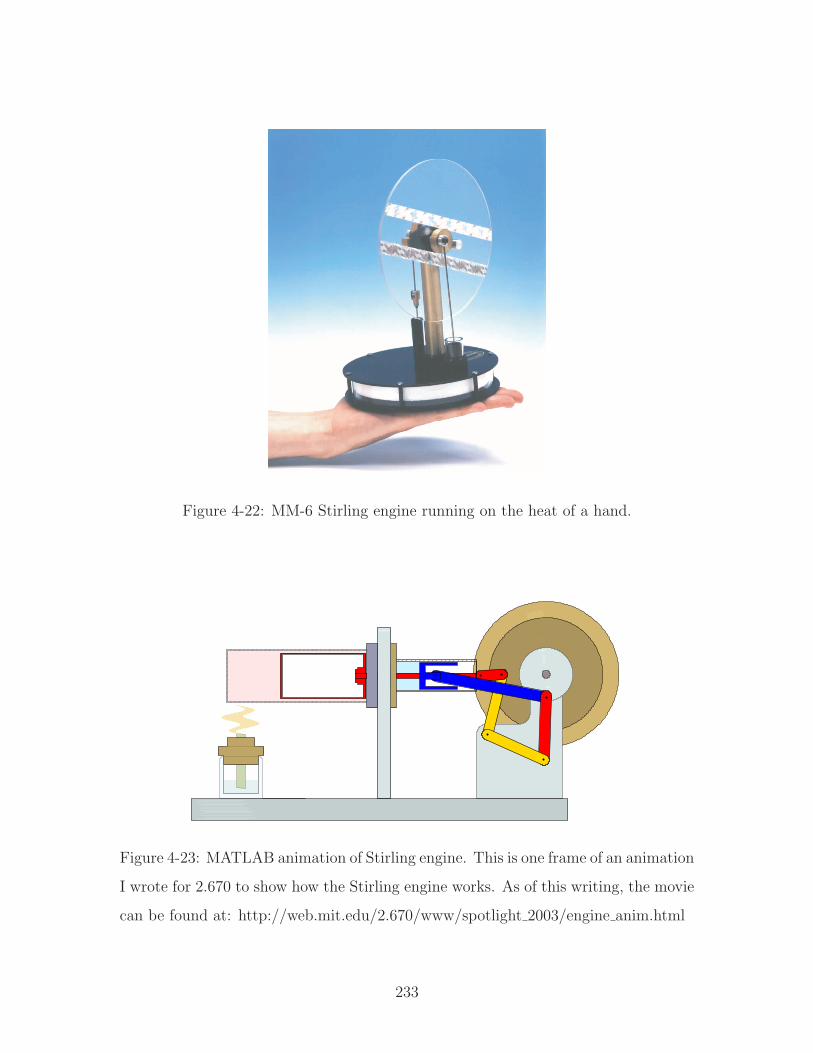
Figure 4-22: MM-6 Stirling engine running on the heat of a hand.

Figure 4-23: MATLAB animation of Stirling engine. This is one frame of an animation

I wrote for 2.670 to show how the Stirling engine works. As of this writing, the movie

can be found at: http://web.mit.edu/2.670/www/spotlight 2003/engine anim.html

233

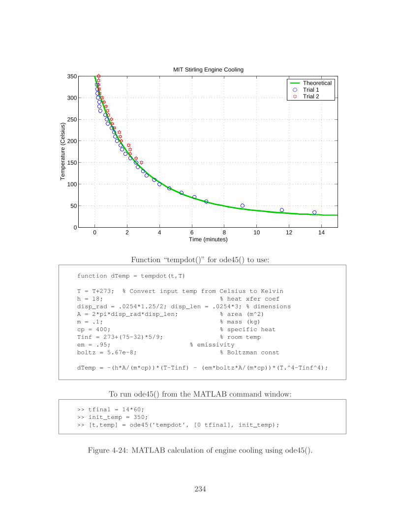
0 2 4 6 8 10 12 140

50

100

150

200

250

300

350

Time (minutes)

Tem

pera

ture

(C

elsi

us)

MIT Stirling Engine Cooling

TheoreticalTrial 1Trial 2

Function “tempdot()” for ode45() to use:

G:\thesis_katie\camera_pics\tempdot.mJanuary 29, 2003

Page 18:22:01 PM

function dTemp = tempdot(t,T)

T = T+273; % Convert input temp from Celsius to Kelvinh = 18; % heat xfer coefdisp_rad = .0254*1.25/2; disp_len = .0254*3; % dimensionsA = 2*pi*disp_rad*disp_len; % area (m^2)m = .1; % mass (kg)cp = 400; % specific heatTinf = 273+(75-32)*5/9; % room tempem = .95; % emissivityboltz = 5.67e-8; % Boltzman const

dTemp = -(h*A/(m*cp))*(T-Tinf) - (em*boltz*A/(m*cp))*(T.^4-Tinf^4);

To run ode45() from the MATLAB command window:

Untitled13January 29, 2003

Page 18:28:32 PM

>> tfinal = 14*60;>> init_temp = 350;>> [t,temp] = ode45(’tempdot’, [0 tfinal], init_temp);

Figure 4-24: MATLAB calculation of engine cooling using ode45().

234

4.3.4 Real-World Dynamic Systems

Real-world systems are a great way to motivate students, who will naturally be cu-

rious about how things work. There are many resources in print and on the web

which explain the way everyday objects work. Two particularly popular and well-

crafted examples worth note are David McCaulay’s famous book “The Way Things

Work”13 [118] and the website “howstuffworks.com” [87].

Mountain bike front suspension

A car suspension is a popular system to model in mechanical engineering courses and

texts in dynamics. A modern mountain bike fork provides a more modern version of

the shock absorber, which is likely to be of interest to many students. As an added

bonus, a suspension fork can easily be brought into the classroom, too.

Prof. Trumper has brought such a mountain bike fork into class as a demo in 2.003.

Students can put their full weight on the suspension to feel the dynamic response.

This system is an excellent candidate for a text or course note example, which can be

coupled with a hands-on classroom demonstration. Dorf and Bishop [60] now include

such an example in ”Modern Control Systems”, as shown in Figure 4-25.14 In this

model, the damping (b) can be adjusted by biker to improve performance based on

the terrain.

In the description of the demos for 6.013 in Section 2.3.3 (page 117), I described

how physical hardware in class can be enhanced by documenting each of a suite of

demonstration examples in clear presentations in the course text. Such text descrip-

tions would typically include some information of the how the object or system is

used, the essential principles being illustrated, and a derivation of the theoretical

equations describing the dynamics. Homework problems can and should be devel-

oped which require the students to understand the text example and then extend the

principles involved in some way.

13...and also his 1998 book “The New Way Things Work” [119].14This mountain bike suspension model appears as AP3.4 in the “Advanced Problems” section at

the end of Chapter 3 (pp. 165-166).

235

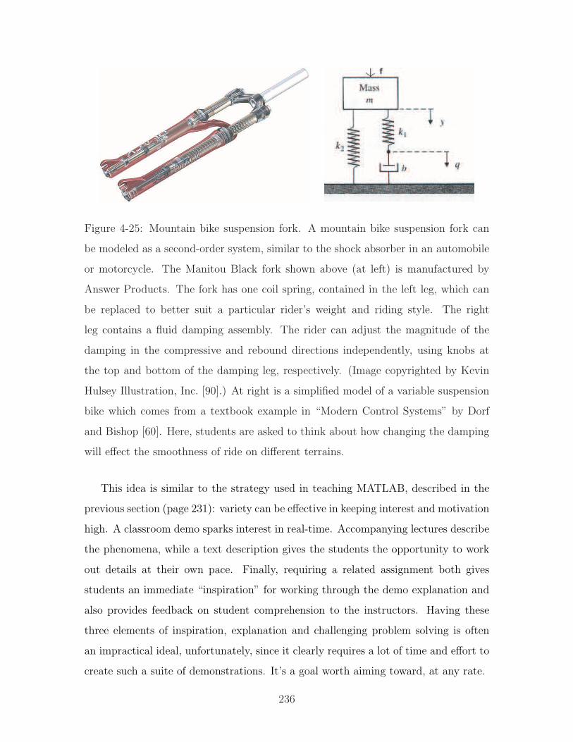
Figure 4-25: Mountain bike suspension fork. A mountain bike suspension fork can

be modeled as a second-order system, similar to the shock absorber in an automobile

or motorcycle. The Manitou Black fork shown above (at left) is manufactured by

Answer Products. The fork has one coil spring, contained in the left leg, which can

be replaced to better suit a particular rider’s weight and riding style. The right

leg contains a fluid damping assembly. The rider can adjust the magnitude of the

damping in the compressive and rebound directions independently, using knobs at

the top and bottom of the damping leg, respectively. (Image copyrighted by Kevin

Hulsey Illustration, Inc. [90].) At right is a simplified model of a variable suspension

bike which comes from a textbook example in “Modern Control Systems” by Dorf

and Bishop [60]. Here, students are asked to think about how changing the damping

will effect the smoothness of ride on different terrains.

This idea is similar to the strategy used in teaching MATLAB, described in the

previous section (page 231): variety can be effective in keeping interest and motivation

high. A classroom demo sparks interest in real-time. Accompanying lectures describe

the phenomena, while a text description gives the students the opportunity to work

out details at their own pace. Finally, requiring a related assignment both gives

students an immediate “inspiration” for working through the demo explanation and

also provides feedback on student comprehension to the instructors. Having these

three elements of inspiration, explanation and challenging problem solving is often

an impractical ideal, unfortunately, since it clearly requires a lot of time and effort to

create such a suite of demonstrations. It’s a goal worth aiming toward, at any rate.

236

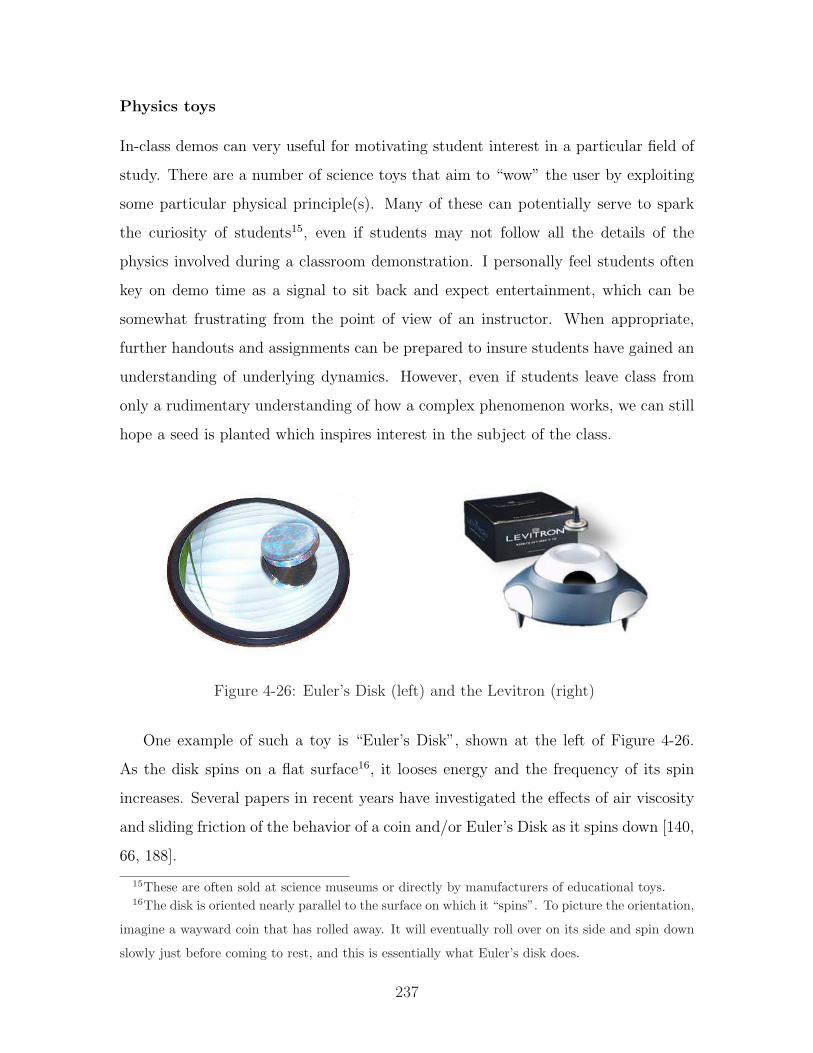
Physics toys

In-class demos can very useful for motivating student interest in a particular field of

study. There are a number of science toys that aim to “wow” the user by exploiting

some particular physical principle(s). Many of these can potentially serve to spark

the curiosity of students15, even if students may not follow all the details of the

physics involved during a classroom demonstration. I personally feel students often

key on demo time as a signal to sit back and expect entertainment, which can be

somewhat frustrating from the point of view of an instructor. When appropriate,

further handouts and assignments can be prepared to insure students have gained an

understanding of underlying dynamics. However, even if students leave class from

only a rudimentary understanding of how a complex phenomenon works, we can still

hope a seed is planted which inspires interest in the subject of the class.

Figure 4-26: Euler’s Disk (left) and the Levitron (right)

One example of such a toy is “Euler’s Disk”, shown at the left of Figure 4-26.

As the disk spins on a flat surface16, it looses energy and the frequency of its spin

increases. Several papers in recent years have investigated the effects of air viscosity

and sliding friction of the behavior of a coin and/or Euler’s Disk as it spins down [140,

66, 188].

15These are often sold at science museums or directly by manufacturers of educational toys.16The disk is oriented nearly parallel to the surface on which it “spins”. To picture the orientation,

imagine a wayward coin that has rolled away. It will eventually roll over on its side and spin down

slowly just before coming to rest, and this is essentially what Euler’s disk does.

237

The Levitron©, shown at right in Figure 4-26, is another intriguing toy that can

be used to illustrate that real dynamic system can indeed require more sophistication

than the typical first- and second-order models we study throughout the class. The

device consists of a magnetic spinning top which levitates over a magnetic base.

Magnetostatic theory predicts that two repellent magnets cannot remain balanced

(one above the other), because the equilibrium point is unstable (like an inverted

pendulum). The reasoning can be summarized as follows: First, we will model the

levitating magnet (the spinning top) as a magnetic dipole with vector moment µ and

mass m. The potential energy of the dipole due to the gravitational and magnetic

fields is then:

V (r, z) = mgz − µ ·B(r, z) (4.4)

We can then form Lagrange’s equation to produce a force balance equation axis the

z axis:

Fz = −∂V (0, z)

∂z= −mg + µ · ∂B(0, z)

∂z(4.5)

The dipole is in equilibrium when the net force Fz is zero, meaning we require that

mg = µ · ∂B/∂z. Now imagine that magnetic field is in the positive z direction, i.e.

Bz > 0 and therefore ∂Bz/∂z < 0. This means µ must align antiparallel to B [132,

33]. Our intuition supports this: the two magnets must be aligned “north-to-north” or

”south-to-south” in order for them to provide a repellent force to counteract gravity.

However, our intuition (and magnetostatics) also tells us that the dipole µ will align

itself with B. Stability requires that any small perturbation away from equilibrium

be opposed by a restoring force (tending to push it back toward equilibrium), and

we sense from experience17 that this is not the case. Earnshaw’s Theorem [63] states

this more rigorously.

Prof. Kirk McDonald of Princeton University provides analyses of both Euler’s

Disk and the Levitron at a website which includes numerous other interesting prob-

lems and phenomena in physics [132].18 The most commonly cited paper explaining

the physics of the Levitron is by Dr. Michael Berry [33].

17(and can prove by applying Gauss’ Integral Theorem [81]18http://www.hep.princeton.edu/˜mcdonald/examples/

238

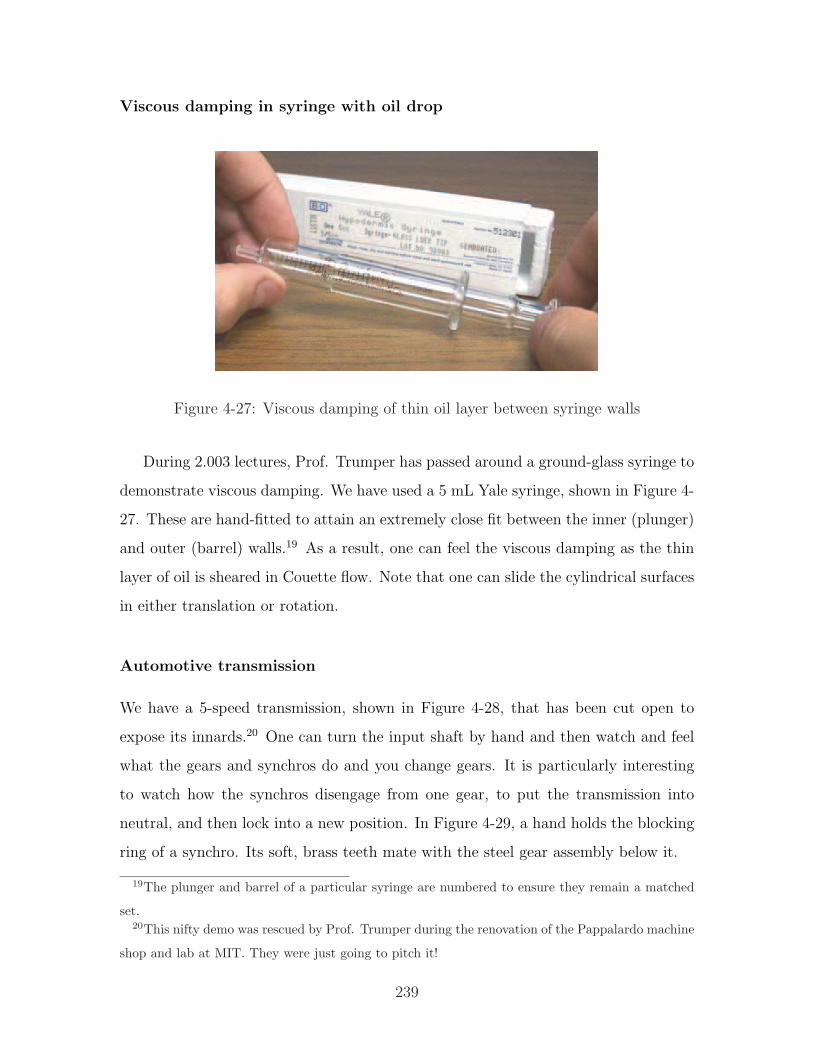
Viscous damping in syringe with oil drop

Figure 4-27: Viscous damping of thin oil layer between syringe walls

During 2.003 lectures, Prof. Trumper has passed around a ground-glass syringe to

demonstrate viscous damping. We have used a 5 mL Yale syringe, shown in Figure 4-

27. These are hand-fitted to attain an extremely close fit between the inner (plunger)

and outer (barrel) walls.19 As a result, one can feel the viscous damping as the thin

layer of oil is sheared in Couette flow. Note that one can slide the cylindrical surfaces

in either translation or rotation.

Automotive transmission

We have a 5-speed transmission, shown in Figure 4-28, that has been cut open to

expose its innards.20 One can turn the input shaft by hand and then watch and feel

what the gears and synchros do and you change gears. It is particularly interesting

to watch how the synchros disengage from one gear, to put the transmission into

neutral, and then lock into a new position. In Figure 4-29, a hand holds the blocking

ring of a synchro. Its soft, brass teeth mate with the steel gear assembly below it.

19The plunger and barrel of a particular syringe are numbered to ensure they remain a matched

set.20This nifty demo was rescued by Prof. Trumper during the renovation of the Pappalardo machine

shop and lab at MIT. They were just going to pitch it!

239

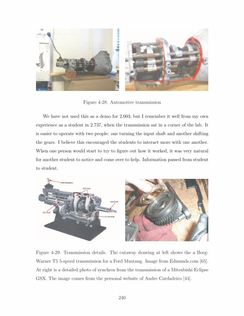
Figure 4-28: Automotive transmission

We have not used this as a demo for 2.003, but I remember it well from my own

experience as a student in 2.737, when the transmission sat in a corner of the lab. It

is easier to operate with two people: one turning the input shaft and another shifting

the gears. I believe this encouraged the students to interact more with one another.

When one person would start to try to figure out how it worked, it was very natural

for another student to notice and come over to help. Information passed from student

to student.

Figure 4-29: Transmission details. The cutaway drawing at left shows the a Borg-

Warner T5 5-speed transmission for a Ford Mustang. Image from Edmunds.com [65].

At right is a detailed photo of synchros from the transmission of a Mitsubishi Eclipse

GSX. The image comes from the personal website of Andre Cardadeiro [44].

240

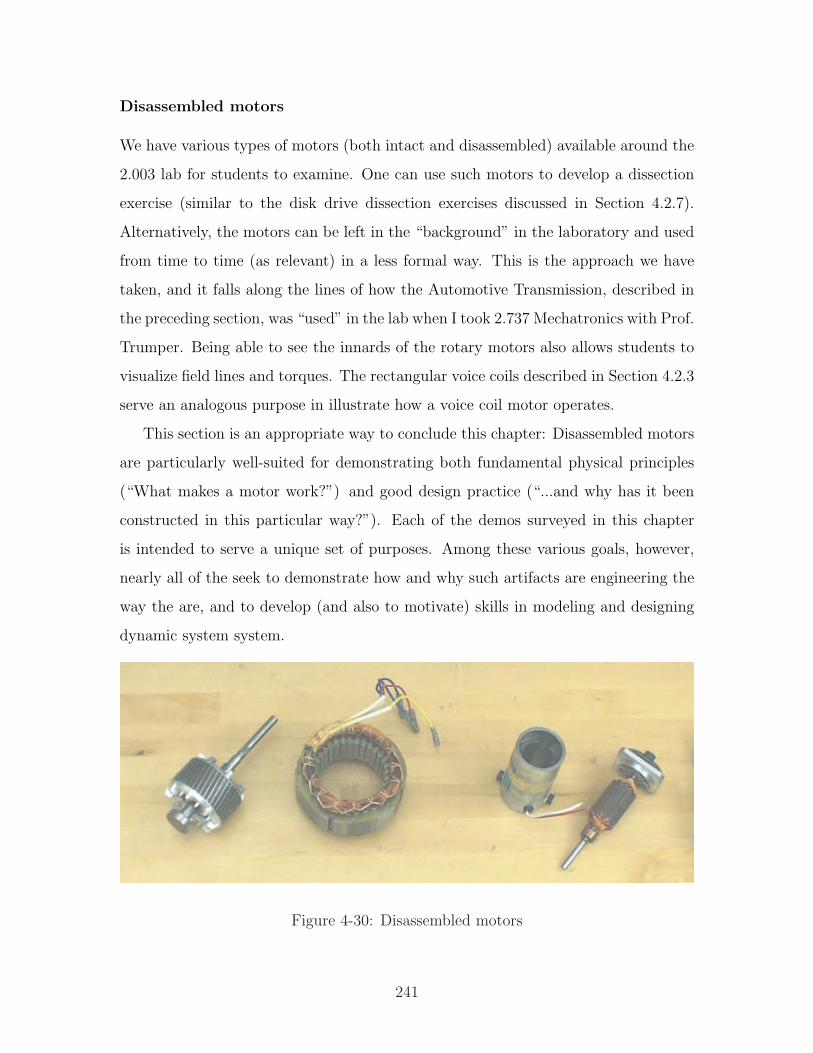
Disassembled motors

We have various types of motors (both intact and disassembled) available around the

2.003 lab for students to examine. One can use such motors to develop a dissection

exercise (similar to the disk drive dissection exercises discussed in Section 4.2.7).

Alternatively, the motors can be left in the “background” in the laboratory and used

from time to time (as relevant) in a less formal way. This is the approach we have

taken, and it falls along the lines of how the Automotive Transmission, described in

the preceding section, was “used” in the lab when I took 2.737 Mechatronics with Prof.

Trumper. Being able to see the innards of the rotary motors also allows students to

visualize field lines and torques. The rectangular voice coils described in Section 4.2.3

serve an analogous purpose in illustrate how a voice coil motor operates.

This section is an appropriate way to conclude this chapter: Disassembled motors

are particularly well-suited for demonstrating both fundamental physical principles

(“What makes a motor work?”) and good design practice (“...and why has it been

constructed in this particular way?”). Each of the demos surveyed in this chapter

is intended to serve a unique set of purposes. Among these various goals, however,

nearly all of the seek to demonstrate how and why such artifacts are engineering the

way the are, and to develop (and also to motivate) skills in modeling and designing

dynamic system system.

Figure 4-30: Disassembled motors

241

242

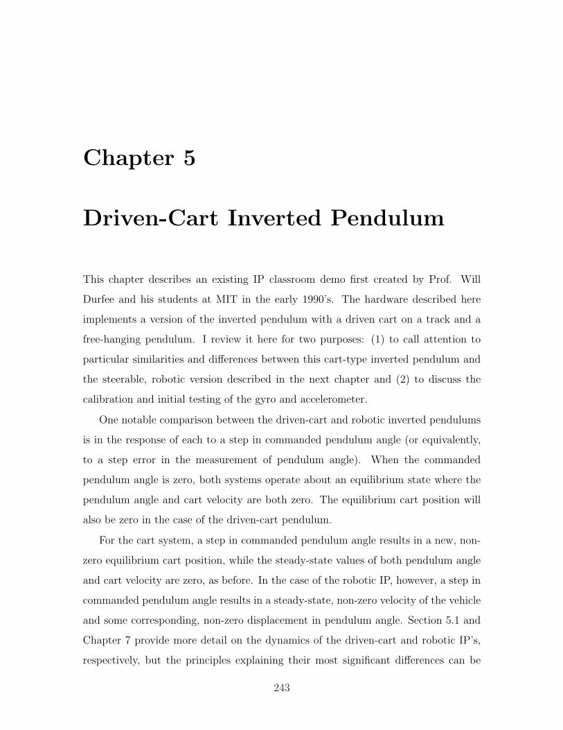
Chapter 5

Driven-Cart Inverted Pendulum

This chapter describes an existing IP classroom demo first created by Prof. Will

Durfee and his students at MIT in the early 1990’s. The hardware described here

implements a version of the inverted pendulum with a driven cart on a track and a

free-hanging pendulum. I review it here for two purposes: (1) to call attention to

particular similarities and differences between this cart-type inverted pendulum and

the steerable, robotic version described in the next chapter and (2) to discuss the

calibration and initial testing of the gyro and accelerometer.

One notable comparison between the driven-cart and robotic inverted pendulums

is in the response of each to a step in commanded pendulum angle (or equivalently,

to a step error in the measurement of pendulum angle). When the commanded

pendulum angle is zero, both systems operate about an equilibrium state where the

pendulum angle and cart velocity are both zero. The equilibrium cart position will

also be zero in the case of the driven-cart pendulum.

For the cart system, a step in commanded pendulum angle results in a new, non-

zero equilibrium cart position, while the steady-state values of both pendulum angle

and cart velocity are zero, as before. In the case of the robotic IP, however, a step in

commanded pendulum angle results in a steady-state, non-zero velocity of the vehicle

and some corresponding, non-zero displacement in pendulum angle. Section 5.1 and

Chapter 7 provide more detail on the dynamics of the driven-cart and robotic IP’s,

respectively, but the principles explaining their most significant differences can be

243

summarized briefly and are outlined in the next two paragraphs.

The robotic IP is driven by motors which apply torque directly between the pen-

dulum body and the wheels of the vehicle. Consequently, an equilibrium state can

exist such that the pendulum angle is non-zero, with the motors providing a constant

torque to balance the torque on the pendulum from gravity. With the steady-state

motor torque at a constant, non-zero value, the steady-state velocity of the wheels is

also constant and non-zero. A step in reference angle therefore results in both some

steady-state velocity of the vehicle and a steady-state change in pendulum angle.

In a driven-cart inverted pendulum of the type described in this chapter, however,

the pendulum hangs freely from a pivot on the cart. No actuator applies a torque

directly at the pendulum pivot axis. Therefore, unlike the robotic system, the cart-

mounted pendulum cannot find equilibrium states where the pendulum angle is non-

zero. Consider a case where the cart moves with a constant velocity, for instance.

This provides no torque on pendulum, because there is no acceleration of the cart

to produce a force at the pivot. If the pendulum is not exactly vertical, the torque

created by gravity will accelerate the pendulum, and it will begin to fall. If this

system can find an equilibrium state in response to a commanded step in pendulum

angle, the actual pendulum angle in this state must be zero. Section 5.3 explains

why the system can in fact find such an equilibrium state (for small values of θref )

and also why the relationship between the equilibrium position of the cart and the

commanded angle, θref , is linear.

The second purpose of this chapter is to discuss the initial testing of the calibration

and filtering used for the gyro and accelerometer. Together, these two sensors provide

tilt sensing which is essential in controlling the free-standing robot. Section 6.2 in

the next chapter describes the complementary filtering used to blend the two sensor

outputs to measure the pendulum angle.

The gyro and accelerometer were initially tested with the cart setup described

in this chapter, which greatly facilitated the development of sensor calibration and

filtering. In previous controllers for the cart demo, the pendulum’s angular velocity

had been obtained by differentiating an encoder signal. Using the gyro to measure

244

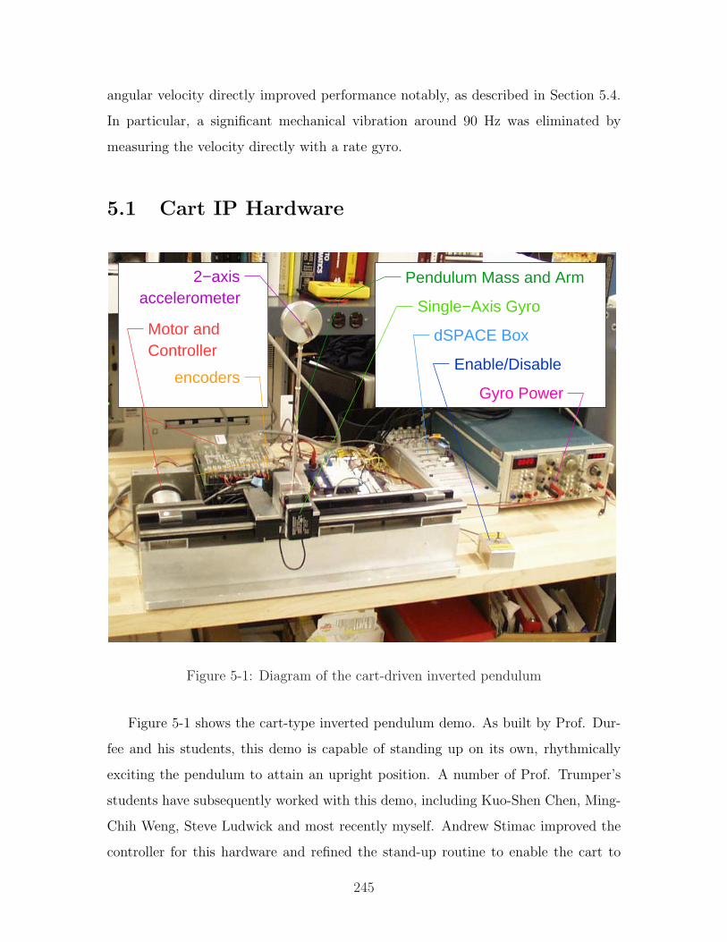
angular velocity directly improved performance notably, as described in Section 5.4.

In particular, a significant mechanical vibration around 90 Hz was eliminated by

measuring the velocity directly with a rate gyro.

5.1 Cart IP Hardware

Motor and Controller

2−axis accelerometer Single−Axis Gyro

encoders

Pendulum Mass and Arm

dSPACE Box

Gyro Power

Enable/Disable

Figure 5-1: Diagram of the cart-driven inverted pendulum

Figure 5-1 shows the cart-type inverted pendulum demo. As built by Prof. Dur-

fee and his students, this demo is capable of standing up on its own, rhythmically

exciting the pendulum to attain an upright position. A number of Prof. Trumper’s

students have subsequently worked with this demo, including Kuo-Shen Chen, Ming-

Chih Weng, Steve Ludwick and most recently myself. Andrew Stimac improved the

controller for this hardware and refined the stand-up routine to enable the cart to

245

swing the pendulum from an initial state at rest into the upright equilibrium position

more reliably [189].

In this system, the inverted pendulum is stabilized about its vertical equilibrium

through the control effort of a single actuator: a current-driven DC servo motor.1

Force is transmitted from the motor to a cart through a chain drive. The cart rides

on two parallel rails and supports the pendulum at one end with a free pivot.

In the original design of the hardware, three sensors are used to estimate four

states. An encoder at the back of the motor (hidden behind an aluminum mounting

plate in Figure 5-1) gives an output proportional to the cart position, and a second

encoder mounted at the pivot of the pendulum measures the pendulum angle. The

motor velocity (which is proportional to cart velocity) is measured directly with a

tachometer. The angular velocity of the pendulum is estimated by differentiating the

pendulum encoder and filtering this output with a first-order low-pass filter with a

time constant of 0.005 seconds (∼32 Hz).

I used this system to help design and verify the filtering of the gyro and to calibrate

the accelerometers later used in measuring the absolute pendulum angle and angular

velocity for the inverted pendulum robot (nicknamed the “DIPR”) described in the

next chapter. The velocity measurement from the gyro improved the performance

of the cart system, eliminating a significant resonance. This is described in more

detail in Section 5.4. The next two sections first develop some theory to describe the

dynamics of the controlled system adequately enough to compare its behavior with

that of the robotic IP in Chapter 7.

One final note on the hardware: Andrew Stimac implemented his controller on the

now-outdated DS1102 board which has since been replaced by the DS1104, and there

are a few differences between the two boards. In particular, the encoder input on

the DS1102 increments by one bit (2−23) for each quadrature count. The advantage

of this was that it was easy to tell how close an encoder channel was to overflowing,

because the encoder value was always between -1 and +1. The DS1104 has opted

for a more intuitive counting scheme. Each quadrature pulse increments the encoder

1Aerotech Permanent Magnet DC Servo Motor, Model 1135 [189]

246

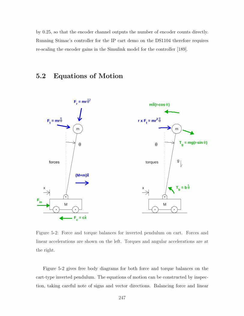
by 0.25, so that the encoder channel outputs the number of encoder counts directly.

Running Stimac’s controller for the IP cart demo on the DS1104 therefore requires

re-scaling the encoder gains in the Simulink model for the controller [189].

5.2 Equations of Motion

m

M

θ

x

Fin

forces

Fc = cx

Ft = mrθ

Fr = mrθ2

(M+m)x

m

M

θ

x

gtorques

Tb = b θ

r x Ft = mr2 θ

mx(r cos )θ

Tg = mg(r sin )θ

Figure 5-2: Force and torque balances for inverted pendulum on cart. Forces and

linear accelerations are shown on the left. Torques and angular accelerations are at

the right.

Figure 5-2 gives free body diagrams for both force and torque balances on the

cart-type inverted pendulum. The equations of motion can be constructed by inspec-

tion, taking careful note of signs and vector directions. Balancing force and linear

247

acceleration terms in the x direction yields:

ΣF =dP

dt

Fin − cx = (M + m)x + mrθ cos θ −mrθ2 sin θ (5.1)

where P =∑

mx is the total (linear) momentum of the system. Equation 5.2 can

be obtained similarly, by balancing the net torque on the system with the change in

its angular momentum, L:

ΣT =dL

dt

mgr sin θ − bθ −mrx cos θ = mr2θ (5.2)

where L =∑

J θ. Note that it is assumed here that the moment of inertia of the

pendulum neglects any distributed mass along the length of the arm. The mass is

modeled as though it is entirely concentrated at a radius, r, from the pivot, so that

Jp = mr2.

When the pendulum is balancing upright near its unstable equilibrium position,

these equations can be linearized using the approximations sin θ ≈ θ and cos θ ≈ 1.

Rearranging equations 5.1 and 5.2, the linearized equations of motion become:

Fin = cx + mrθ + (M + m)x− [mrθ2θ][H.O.T.]

Fin ≈ cx + mrθ + (M + m)x (5.3)

0 = mgrθ − bθ −mr2θ −mrx (5.4)

When the pendulum is near its stable equilibrium, θ is close to 180 (as defined in

Figure 5-2). To write the equations of motion more clearly, we will first define an

angle φ which is offset from θ by 180 (φ = θ + 180) and measures the displacement

of the pendulum from the down-pointing equilibrium position.

Since sin(θ + 180) = −sinθ and cos(θ + 180) = −cosθ, the linearized equations

of motion for the stable equilibrium case are:

Fin ≈ cx−mrφ + (M + m)x (5.5)

0 = −mgrφ− bφ−mr2φ + mrx (5.6)

248

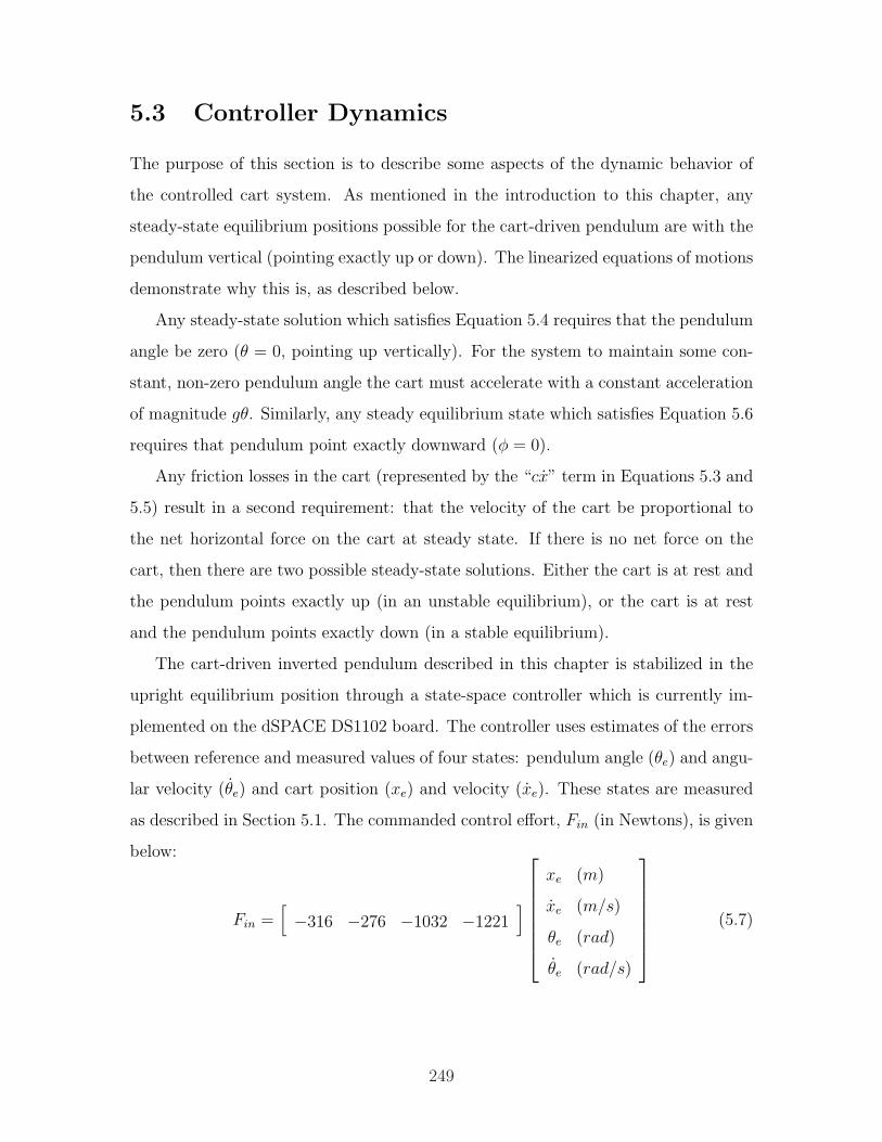
5.3 Controller Dynamics

The purpose of this section is to describe some aspects of the dynamic behavior of

the controlled cart system. As mentioned in the introduction to this chapter, any

steady-state equilibrium positions possible for the cart-driven pendulum are with the

pendulum vertical (pointing exactly up or down). The linearized equations of motions

demonstrate why this is, as described below.

Any steady-state solution which satisfies Equation 5.4 requires that the pendulum

angle be zero (θ = 0, pointing up vertically). For the system to maintain some con-

stant, non-zero pendulum angle the cart must accelerate with a constant acceleration

of magnitude gθ. Similarly, any steady equilibrium state which satisfies Equation 5.6

requires that pendulum point exactly downward (φ = 0).

Any friction losses in the cart (represented by the “cx” term in Equations 5.3 and

5.5) result in a second requirement: that the velocity of the cart be proportional to

the net horizontal force on the cart at steady state. If there is no net force on the

cart, then there are two possible steady-state solutions. Either the cart is at rest and

the pendulum points exactly up (in an unstable equilibrium), or the cart is at rest

and the pendulum points exactly down (in a stable equilibrium).

The cart-driven inverted pendulum described in this chapter is stabilized in the

upright equilibrium position through a state-space controller which is currently im-

plemented on the dSPACE DS1102 board. The controller uses estimates of the errors

between reference and measured values of four states: pendulum angle (θe) and angu-

lar velocity (θe) and cart position (xe) and velocity (xe). These states are measured

as described in Section 5.1. The commanded control effort, Fin (in Newtons), is given

below:

Fin =[−316 −276 −1032 −1221

]

xe (m)

xe (m/s)

θe (rad)

θe (rad/s)

(5.7)

249

Using Equations 5.3, 5.4 and 5.7, we can make some predictions about the dynamic

behavior of this upright driven-cart pendulum system. For instance, if we request an

angle of one degree (θref = 0.017 rad), the controlled cart system will still operate

about an equilibrium state where the actual pendulum angle is precisely vertical

(pointing up), as required by Equation 5.4. Now suppose that there are no external

disturbance forces exerted on the cart or pendulum. In this case, the cart will operate

about an equilibrium position such that the θe and xe terms in Equation 5.7 result in

zero net commanded force. The steady-state equilibrium cart position will therefore

be proportional to requested reference pendulum angle. Specifically,

xe = θe · −1032

316

(m)

(rad)= θe · −3.27(m/rad) (5.8)

Since the pendulum continues to operate about vertical, a requested displacement in

pendulum angle of 0.017 rad (1 clockwise, as defined in Figure 5-2) will result in

a steady-state error in pendulum angle of θe = −0.017 rad. The cart position will

correspondingly operate about a location 0.057 meters to the right of whatever point

is defined as “zero”.2 In other words, the cart’s equilibrium position shifts by about

2.2 inches (0.057 m) for each degree change in reference angle for the pendulum.

5.4 Performance

This section briefly discusses some aspects of the dynamic response of the cart-driven.

First, it provides data showing improved performance when gyro was used to measure

the angular velocity of the pendulum instead of a differentiated encoder signal. Fig-

ure 5-3 shows typical data for system demonstrating a significant resonance around

90 Hz which appears when the differentiated encoder signal is used. In Figures 5-4

and 5-5, taken when the gyro was used for control instead, this vibration problem is

no longer evident.

2The encoders are not indexed and reset to zero when the controller is downloaded to the dSPACE

board. Therefore, a position of “zero” for the cart corresponds to wherever the cart was resting on

the track when the code was generated.

250

0 0.01 0.02 0.03 0.04 0.05 0.06 0.07 0.08 0.09 0.10.05

0.1

0.15

0.2

0.25

0.3

Time (seconds)

The

ta (

degr

ees)

Vibration at 90.15 Hz

Encoder Angle

0 0.01 0.02 0.03 0.04 0.05 0.06 0.07 0.08 0.09 0.1−20

−10

0

10

20

30

Time (seconds)

Ang

. Vel

. (de

g/s)

differentiated encoderfiltered gyro (BW is 75 Hz)

0 0.01 0.02 0.03 0.04 0.05 0.06 0.07 0.08 0.09 0.1−15

−10

−5

0

5

10

15

20

Time (seconds)

Con

trol

For

ce (

N)

Commanded Force (N)

Figure 5-3: Data showing vibration problem near 90 Hz. The differentiated encoder

signal was used to estimate pendulum velocity when the data above were collected.

Angular velocity data from the gyro was also recorded for comparison, however, and

is shown in the middle plot.

251

Figure 5-4 shows data characterizing the steady-state behavior of the cart-driven

pendulum system as it balances upright. The top portion of Figure 5-4 provides data

comparing the encoder measurements of pendulum angle to those obtained from com-

plementary filtering of the gyro and accelerometer signals. The encoder measurement

in this plot has been offset slightly so that the two measurements line up more closely

and can therefore be compared more easily. Below this is data of the cart position,

taken during the same time period. The cart has a characteristic oscillation (at a

frequency of roughly 0.2 Hz) about its equilibrium position.

The accelerometer provides a low-frequency measurement of the angle of the pen-

dulum with respect to gravity. The 2-axis accelerometer was glued onto the mass

at the end of the pendulum by hand, so its alignment was not precise! Any mis-

alignment can be adjusted by adding an offset angle to the pendulum measurement.

The locations of both the accelerometer (at the free end of the pendulum) and the

gyro (near the pendulum pivot) can be seen in Figure 5-1. The measured equilibrium

pendulum angle in the top plot of Figure 5-4 is not zero, although presumably the

actual equilibrium angle must be zero, for reasons discussed in the previous section.

The offset in the measurement appears to be approximately −1.6. The cart position,

shown in the lower plot, is offset from zero by about 0.085 meters. This works out

to roughly 0.053 meters in the offset of the equilibrium cart position for each degree

offset in reference pendulum angle, compared with the predicted ratio of 0.057 m/deg

(3.27 m/rad) calculated and the end of the previous section.

Finally, Figure 5-5 shows the transient response of both the cart-driven inverted

pendulum and the robotic inverted pendulum (the DIPR) described in Chapter 7.

The inertia of the DIPR is much larger than that of the pendulum on the cart-driven

system, and the response of the DIPR is correspondingly much slower than the cart

system.

The inertia of the pendulum on the cart is primarily due to the 0.15 kg mass,

which is mounted 0.314 m from the pivot. The inertia of the cart’s pendulum, Jc is

therefore approximately:

Jc ≈ mL2 = 0.015 (kg m2) (5.9)

252

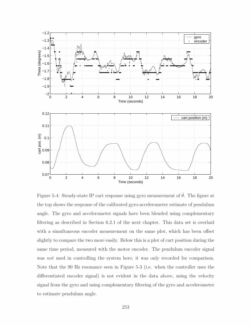
0 2 4 6 8 10 12 14 16 18 20−2

−1.9

−1.8

−1.7

−1.6

−1.5

−1.4

−1.3

−1.2

Time (seconds)

The

ta (

degr

ees)

gyroencoder

0 2 4 6 8 10 12 14 16 18 200.07

0.08

0.09

0.1

0.11

0.12

Time (seconds)

cart

pos

. (m

)

cart position (m)

Figure 5-4: Steady-state IP cart response using gyro measurement of θ. The figure at

the top shows the response of the calibrated gyro-accelerometer estimate of pendulum

angle. The gyro and accelerometer signals have been blended using complementary

filtering as described in Section 6.2.1 of the next chapter. This data set is overlaid

with a simultaneous encoder measurement on the same plot, which has been offset

slightly to compare the two more easily. Below this is a plot of cart position during the

same time period, measured with the motor encoder. The pendulum encoder signal

was not used in controlling the system here; it was only recorded for comparison.

Note that the 90 Hz resonance seen in Figure 5-3 (i.e. when the controller uses the

differentiated encoder signal) is not evident in the data above, using the velocity

signal from the gyro and using complementary filtering of the gyro and accelerometer

to estimate pendulum angle.

253

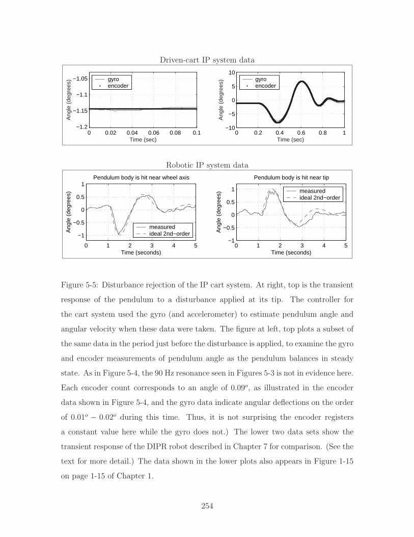
Driven-cart IP system data

0 0.02 0.04 0.06 0.08 0.1−1.2

−1.15

−1.1

−1.05

Time (sec)

Ang

le (

degr

ees) gyro

encoder

0 0.2 0.4 0.6 0.8 1−10

−5

0

5

10

Time (sec)

Ang

le (

degr

ees) gyro

encoder

Robotic IP system data

0 1 2 3 4 5

−1

−0.5

0

0.5

1

Time (seconds)

Ang

le (

degr

ees)

Pendulum body is hit near wheel axis

measuredideal 2nd−order

0 1 2 3 4 5−1

−0.5

0

0.5

1

Time (seconds)

Ang

le (

degr

ees)

Pendulum body is hit near tip

measuredideal 2nd−order

Figure 5-5: Disturbance rejection of the IP cart system. At right, top is the transient

response of the pendulum to a disturbance applied at its tip. The controller for

the cart system used the gyro (and accelerometer) to estimate pendulum angle and

angular velocity when these data were taken. The figure at left, top plots a subset of

the same data in the period just before the disturbance is applied, to examine the gyro

and encoder measurements of pendulum angle as the pendulum balances in steady

state. As in Figure 5-4, the 90 Hz resonance seen in Figures 5-3 is not in evidence here.

Each encoder count corresponds to an angle of 0.09o, as illustrated in the encoder

data shown in Figure 5-4, and the gyro data indicate angular deflections on the order

of 0.01o − 0.02o during this time. Thus, it is not surprising the encoder registers

a constant value here while the gyro does not.) The lower two data sets show the

transient response of the DIPR robot described in Chapter 7 for comparison. (See the

text for more detail.) The data shown in the lower plots also appears in Figure 1-15

on page 1-15 of Chapter 1.

254

The inertia of the “pendulum” in the IP robot is much larger, since it consists

of the entire chassis between its two wheels and also the extended pendulum arm.

These components are all connected together as a rigid unit and can be seen in the

photo which appears on both pages 56 and 319. The total inertia, Jr, of the rigid

pendulum-body of the robot (detailed in Section 7.5.2 on page 370) is approximately:

Jr = Jp + Jb + mL2 ≈ 0.05 + 0.05 + 1 · 0.42 = 0.26 (kg m2) (5.10)

This is about 17.6 times larger than the inertia of the pendulum in the cart-based

system. The response of the robot is roughly 5 times slower than that of the cart, as

shown in the right-hand plots of Figure 5-5.

For the data in Figure 5-5, the disturbances applied to the cart-driven and robotic

systems (by tapping each system by hand) were of approximately the same magni-

tude. One would expect the smaller inertia in the cart-based system would therefore

experience a greater deflection, and this is in fact the case. The deflection of cart-

driven pendulum is about five times greater than that of the robot.

The next chapter provides more details on the use of gyroscopes in implementing

tilt sensing. In particular, Section 6.2 describes a method called complementary

filtering in which multiple types of sensors can by blended to provide a single estimate

of some desired output. In the case of an inverted pendulum robot, simply integrating

the signal from a gyro would result in a ramping error because the gyro has a finite

DC bias. To improve the measurement, a gyroscope can be blended with a sensor

which measures tilt directly, such as an accelerometer or a tilt sensor which uses

electrolytic fluid which has better performance at low frequencies. The “gyro” data

shown in the top portions of Figures 5-4 and 5-5 for instance has been blended with

an accelerometer signal to create a more accurate estimate of pendulum angle than

would obtain by integrating the gyro alone.

255

256

Chapter 6

Tilt Sensing for Inverted

Pendulum Robots

The cart-driven pendulum system described in Chapter 5 uses an encoder to measure

the angle between the pendulum and the cart on which it is mounted. Since the cart

rides on a level track, it too remains level, and the encoder therefore provides an

absolute measure of the pendulum angle with respect to gravity.

In a robotic inverted pendulum system like the DIPR described in Chapter 7,

encoders can measure the relative angle between the body of the robot and each

wheel, but the wheels will rotate in inertial space as the vehicle moves. For this

reason, such an encoder can not provide an absolute angle of the pendulum body

with respect to gravity. This absolute angle measurement is achieved in the DIPR by

using gyroscopes.

This chapter describes several issues which relate to the use of gyroscopes for tilt

sensing in a two-wheeled inverted pendulum vehicle.

6.1 Tilt Sensing for Segway and iBOT

The implementation of tilt sensing for the Segway is an interesting topic, since cost-

effective MEMS sensors will probably make redundant sensing much more widespread

in the future. Their low price makes MEMS sensors practical for undergraduate labs,

257

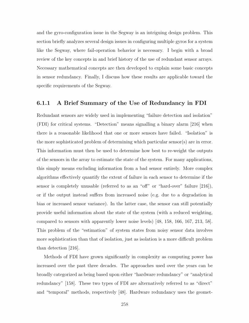
and the gyro-configuration issue in the Segway is an intriguing design problem. This

section briefly analyzes several design issues in configuring multiple gyros for a system

like the Segway, where fail-operation behavior is necessary. I begin with a broad

review of the key concepts in and brief history of the use of redundant sensor arrays.

Necessary mathematical concepts are then developed to explain some basic concepts

in sensor redundancy. Finally, I discuss how these results are applicable toward the

specific requirements of the Segway.

6.1.1 A Brief Summary of the Use of Redundancy in FDI

Redundant sensors are widely used in implementing “failure detection and isolation”

(FDI) for critical systems. “Detection” means signalling a binary alarm [216] when

there is a reasonable likelihood that one or more sensors have failed. “Isolation” is

the more sophisticated problem of determining which particular sensor(s) are in error.

This information must then be used to determine how best to re-weight the outputs

of the sensors in the array to estimate the state of the system. For many applications,

this simply means excluding information from a bad sensor entirely. More complex

algorithms effectively quantify the extent of failure in each sensor to determine if the

sensor is completely unusable (referred to as an “off” or “hard-over” failure [216]),

or if the output instead suffers from increased noise (e.g. due to a degradation in

bias or increased sensor variance). In the latter case, the sensor can still potentially

provide useful information about the state of the system (with a reduced weighting,

compared to sensors with apparently lower noise levels) [48, 158, 166, 167, 213, 58].

This problem of the “estimation” of system states from noisy sensor data involves

more sophistication than that of isolation, just as isolation is a more difficult problem

than detection [216].

Methods of FDI have grown significantly in complexity as computing power has

increased over the past three decades. The approaches used over the years can be

broadly categorized as being based upon either “hardware redundancy” or “analytical

redundancy” [158]. These two types of FDI are alternatively referred to as “direct”

and “temporal” methods, respectively [48]. Hardware redundancy uses the geomet-

258

ric relationships between the sensors in a fixed array to recognize at any particular

moment whether their outputs are mathematically compatible (within given noise

thresholds) and, if not, to isolate which sensor(s) disagree with the others. Analytical

redundancy, on the other hand, incorporates a model of the dynamics of the system

being sensed and analyzes whether the changes in state variables over time are com-

patible. I prefer using the phrase “geometric redundancy” when discussing hardware

redundancy because I believe this more clearly distinguishes it from temporal FDI of

a sensor in an array.

The mathematical theory behind geometrical redundancy developed hand-in-hand

with the space program in the 1960’s and essentially involves creating parity vectors

to detect incompatibility in sensor outputs [158, 73, 160]. Parity vectors will be

discussed in detail in the next subsection, as they are a central mathematical concept

in hardware redundancy systems, and most of this section will focus on geometric

(not temporal) FDI.

Once computational power became more available in the 1970’s, the state of the

art in FDI became much more sophisticated, involving (often complex) state-space

models of system dynamics. Based on such models, analytic FDI algorithms analyze

and compare the likelihoods of redundant sensor measurements over time. “Fly-

by-wire” (FBW) technology strongly motivated the development of this state-space

approach. One early example of this type of sensor FDI system was developed at

Draper Lab in the 1970’s for the F-8 and incorporates data from eleven pairs of

sensors [58].1 The resulting “dual-mode FDI system” evaluates and compares the

measurements of both sensors in each pair based on a sequential probability ratio test

(SPRT) [58]. A more recent example of temporal analytical redundancy (described

in a paper from 1994) is based upon a simplified linearization of a “fully nonlinear

thermodynamic” model of a gas turbine jet engine which uses “17 state variables

including pressures, air and gas mass flow rates, shaft speeds, absolute temperature,

1The 11 instrument types includes the following: “longitudinal accelerometer, lateral accelerom-

eter, normal accelerometer, roll rate gyro, pitch rate gyro, yaw rate gyro, vertical gyro, directional

gyro, altimeter, Mach meter, and alpha vane” [58].

259

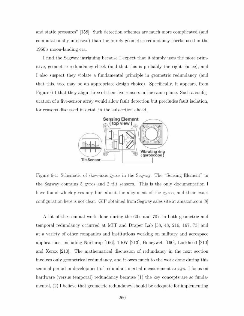
and static pressures” [158]. Such detection schemes are much more complicated (and

computationally intensive) than the purely geometric redundancy checks used in the

1960’s moon-landing era.

I find the Segway intriguing because I expect that it simply uses the more prim-

itive, geometric redundancy check (and that this is probably the right choice), and

I also suspect they violate a fundamental principle in geometric redundancy (and

that this, too, may be an appropriate design choice). Specifically, it appears, from

Figure 6-1 that they align three of their five sensors in the same plane. Such a config-

uration of a five-sensor array would allow fault detection but precludes fault isolation,

for reasons discussed in detail in the subsection ahead.

Figure 6-1: Schematic of skew-axis gyros in the Segway. The “Sensing Element” in

the Segway contains 5 gyros and 2 tilt sensors. This is the only documentation I

have found which gives any hint about the alignment of the gyros, and their exact

configuration here is not clear. GIF obtained from Segway sales site at amazon.com [8]

A lot of the seminal work done during the 60’s and 70’s in both geometric and

temporal redundancy occurred at MIT and Draper Lab [58, 48, 216, 167, 73] and

at a variety of other companies and institutions working on military and aerospace

applications, including Northrop [166], TRW [213], Honeywell [160], Lockheed [210]

and Xerox [210]. The mathematical discussion of redundancy in the next section

involves only geometrical redundancy, and it owes much to the work done during this

seminal period in development of redundant inertial measurement arrays. I focus on

hardware (versus temporal) redundancy because (1) the key concepts are so funda-

mental, (2) I believe that geometric redundancy should be adequate for implementing

260

fault-operational FDI for the Segway, and (3) I wish to compare the redundancy re-

quirements of the Segway with those of the space program to discuss how applicable

such fundamental principles are in this application.

6.1.2 Mathematics of FDI Using Geometric Redundancy

This subsection explains some fundamental mathematical concepts in using geometric

redundancy for failure detection and isolation. Summarizing briefly, failure detection

is typically accomplished through the use of “parity vectors”. Isolation can be ac-

complished by creating various subsets from groups of sensors whose axes form a set

of linearly dependent vectors and then performing a series of parity checks on each

of these subsets to identify the faulty sensor(s) through a process of elimination. The

discussion ahead will explain this approach to FDI in detail.

Throughout the analysis that follows, we will be concerned with the case of FDI

for a single sensor failure. The principles outlined can certainly be expanded to

permit FDI in cases with two or more simultaneous sensors faults, but our analysis

will be more straight-forward if we limit FDI to single-sensor failure initially. In many

hardware situations, single-sensor failure detection is quite sufficient, as well, since

the probability of a simultaneous failure of two (or more) sensors will generally be

very small.

For instance, suppose we have an array of five sensors which each have an expected

average failure rate of once every 10 years, and that we model the failure mechanism

of each sensor as a Poisson process (which seem sensible) and assume that failure

of one sensor is uncorrelated to that of any other (which may be less likely, but it

makes the problem tractable). There is a probability of 39.25% that at least one of

the five sensors will fail in a given year (which is quite high). However, the chance

of two sensors failing within an hour of one another in a given year is approximately

1 in 88,000, and the odds against any two sensors failing within five minutes of one

another in a particular year are roughly 10,500,000 to 1. Table 6.1 shows what these

odds are if we assume other failure rates.

We will also assume throughout this and subsequent discussions that each indi-

261

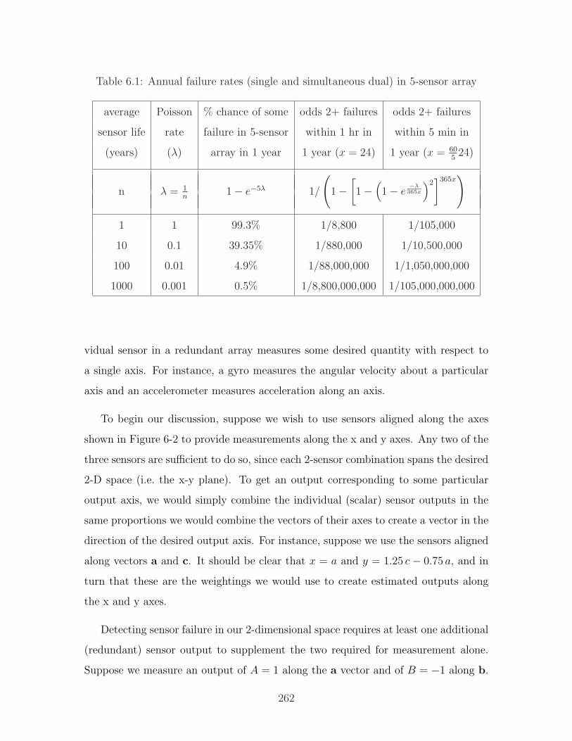
Table 6.1: Annual failure rates (single and simultaneous dual) in 5-sensor array

average Poisson % chance of some odds 2+ failures odds 2+ failures

sensor life rate failure in 5-sensor within 1 hr in within 5 min in

(years) (λ) array in 1 year 1 year (x = 24) 1 year (x = 60524)

n λ = 1n

1− e−5λ

(1/

(1−

[1−

(1− e

−λ365x

)2]365x

))

1 1 99.3% 1/8,800 1/105,000

10 0.1 39.35% 1/880,000 1/10,500,000

100 0.01 4.9% 1/88,000,000 1/1,050,000,000

1000 0.001 0.5% 1/8,800,000,000 1/105,000,000,000

vidual sensor in a redundant array measures some desired quantity with respect to

a single axis. For instance, a gyro measures the angular velocity about a particular

axis and an accelerometer measures acceleration along an axis.

To begin our discussion, suppose we wish to use sensors aligned along the axes

shown in Figure 6-2 to provide measurements along the x and y axes. Any two of the

three sensors are sufficient to do so, since each 2-sensor combination spans the desired

2-D space (i.e. the x-y plane). To get an output corresponding to some particular

output axis, we would simply combine the individual (scalar) sensor outputs in the

same proportions we would combine the vectors of their axes to create a vector in the

direction of the desired output axis. For instance, suppose we use the sensors aligned

along vectors a and c. It should be clear that x = a and y = 1.25 c − 0.75 a, and in

turn that these are the weightings we would use to create estimated outputs along

the x and y axes.

Detecting sensor failure in our 2-dimensional space requires at least one additional

(redundant) sensor output to supplement the two required for measurement alone.

Suppose we measure an output of A = 1 along the a vector and of B = −1 along b.

262

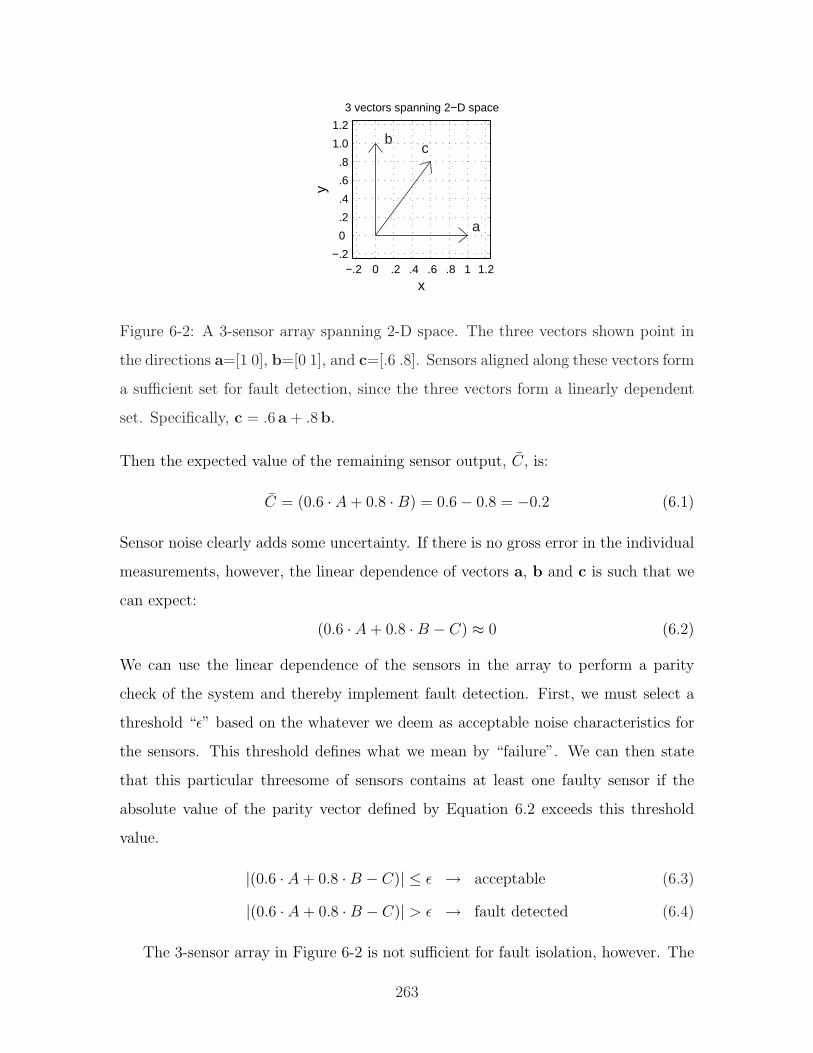
−.2 0 .2 .4 .6 .8 1 1.2−.2

0

.2

.4

.6

.8

1.0

1.2

x

y

3 vectors spanning 2−D space

b

a

c

Figure 6-2: A 3-sensor array spanning 2-D space. The three vectors shown point in

the directions a=[1 0], b=[0 1], and c=[.6 .8]. Sensors aligned along these vectors form

a sufficient set for fault detection, since the three vectors form a linearly dependent

set. Specifically, c = .6 a + .8b.

Then the expected value of the remaining sensor output, C, is:

C = (0.6 · A + 0.8 ·B) = 0.6− 0.8 = −0.2 (6.1)

Sensor noise clearly adds some uncertainty. If there is no gross error in the individual

measurements, however, the linear dependence of vectors a, b and c is such that we

can expect:

(0.6 · A + 0.8 ·B − C) ≈ 0 (6.2)

We can use the linear dependence of the sensors in the array to perform a parity

check of the system and thereby implement fault detection. First, we must select a

threshold “ε” based on the whatever we deem as acceptable noise characteristics for

the sensors. This threshold defines what we mean by “failure”. We can then state

that this particular threesome of sensors contains at least one faulty sensor if the

absolute value of the parity vector defined by Equation 6.2 exceeds this threshold

value.

|(0.6 · A + 0.8 ·B − C)| ≤ ε → acceptable (6.3)

|(0.6 · A + 0.8 ·B − C)| > ε → fault detected (6.4)

The 3-sensor array in Figure 6-2 is not sufficient for fault isolation, however. The

263

method described above can identify when a problem exists within an entire array, but

it gives no information about which sensor(s) are broken. Isolation requires at least

two redundant sensors (beyond the two required for measurement in a 2-dimensional

space). Figure 6-3 shows one of an infinite number of acceptable sets of vectors for

isolation in a 2-D sensor array.

−.2 0 .2 .4 .6 .8 1 1.2−.2

0

.2

.4

.6

.8

1.0

1.2

x

y

4 vectors spanning 2−D space

b

a

c

d

Figure 6-3: A 4-sensor array spanning 2-D space. The four vectors shown point

in the directions a=[1 0], b=[0 1], c=[.6 .8], and d=[.8 .6]. Sensors aligned along

these vectors form a sufficient set for fault isolation. This can be accomplished by

performing parity checks on each of the four possible triads of sensors from this set.

To identify a faulty sensor, we can perform a parity check on each of the four

possible triads of sensors. If none of the parity vectors exceed our error threshold, all

of the sensors are (probably) fine. If one sensor is bad, it should generally2 push three

of the four triads beyond the acceptable threshold, because it is a member of three of

the four triads being tested. Let us suppose we have already detected a sensor fault

exists. In this case, we can conclude that the sensor which was excluded from the one

2Of course technically speaking, there is always a finite probability that a bad sensor will “just

happen” to output a value which still satisfies the parity check at a particular instant in time! (“Even

a broken clock is right twice a day...”)

264

non-faulty triad must be bad one:

|(0.6 · A + 0.8 ·B − C)| ≤ ε → D is bad (6.5)

|(0.8 · A + 0.6 ·B −D)| ≤ ε → C is bad (6.6)

1.09 · |(0.35 · A + 0.75 · C −D)| ≤ ε → B is bad (6.7)

1.09 · |(0.35 ·B − C + 0.75 ·D)| ≤ ε → A is bad (6.8)

The parity vectors above are scaled appropriately so that the same value of ε is appro-

priate as the threshold in each check, assuming the acceptable noise characteristics

for all four sensors are the same.

Before proceeding to a more formal discussion about parity vectors I will call

attention to some additional details which the 2-dimensional examples above can

illustrate. First, simply having four sensors is not sufficient for the 2-D fault isolation

method above. We also need to make sure the array contains at least one set of four

of the sensors no two of which provide outputs along the same axis. Referring to the

vectors shown in Figures 6-2 and 6-3 again, suppose we use two measurements which

point in the direction of vector c, C1 and C2, along with measurements A and B (in

the directions of vectors a and b respectively, as previously defined). Then we can

only create the following three parity checks:

|(0.6 · A + 0.8 ·B − C1)| ≤ ε → C2 is bad (6.9)

|(0.6 · A + 0.8 ·B − C2)| ≤ ε → C1 is bad (6.10)

|(C1 − C2)| ≤ ε → either A or B is bad (6.11)

This means if either A or B fails, we can detect that either sensor A or B is at fault ,

but we can not isolate which of the two sensors is the cause. (We can isolate a fault

of either C1 or C2, however.)

The problem in this example is that A and B are the only two sensors which

provide any sensitivity along the axis perpendicular to the line on which both C1 and

C2 lie. Any parity check equation can not exclude either A or B without excluding

them both, because these are the only two sensors which include vector components

orthogonal to the space spanned by all the remaining sensors (i.e. orthogonal to vector

265

c). As a result, our method of “isolation through a process of elimination” can no

longer distinguish a failure in sensor A from a failure in B. Expanding this concept

more broadly, if any sensor in an array has some sensitivity along a particular axis in

space, the isolation method presented here requires that at least three sensors in the

entire array must have some sensitivity along that axis.

We can now begin to generalize some geometric principles for sensor arrays. To

create a sensor array whose outputs span an n-dimensional space, there needs to

be at least one (uniaxial) sensor which is aligned at least partially along (i.e. with a

non-zero dot product with) each existing vector in the measured n-dimensional space.

Stated differently, we can not allow a direction in the n-dimensional space to exist

which is not measured with at least some degree of sensitivity by at least one sensor.

To provide fault detection, there must be at least two sensors so aligned to provide

some sensitivity in each possible direction, and for fault isolation, one must have have

three such sensors which provide some level of sensitivity in each possible direction

of sensing.

One way of achieving the requirements above for the tasks of measurement, fault

detection, and fault isolation is to arrange one, two or three sensors along each of n

mutually-orthogonal axes in the n-dimensional space. Detection then involves com-

paring the outputs of the two sensors along each orthogonal axis. When a discrepancy

between two co-linear sensors occurs, we know one of the two is at fault. Isolating

which sensor is at fault requires at least three sensors along each of the mutually-

orthogonal axes in order to create a majority of “good” sensors to “out-vote” a bad

one.

For the 2-d case we have discussed so far, this method (i.e. using a set of mutually-

orthogonal axes) requires 2 sensors for measurement, 4 sensors for detection, and 6

for isolation, but as we have already seen, skew-axis orientations allow us to accom-

plish these tasks with 2, 3, and 4 total sensors, respectively, if such axes are chosen

appropriately. For a sensor array whose output spans an n-dimensional space, we can

state more generally that:

1. When the sensors in an array are aligned along a set of n mutually orthogonal

266

axes which span the n-dimensional space of interest, we need to have n, 2n and

3n sensors for measurement, detection and isolation, respectively.

2. The minimum numbers of measurements required for measurement, detection

and isolation are n, n + 1, and n + 2 (respectively).

3. If we use the minimum numbers of measurements given above, however, we can

only be sure of being able to isolate a single sensor failure if each n-sensor subset

of sensors spans the full n-dimension space of the sensor array.

As an example, consider the Segway, which uses the a 5-sensor array [180, 8].

This is the minimum number of sensors required for fault isolation in a 3-D sensor

array. Complete fault isolation also requires that no three of these five sensors lie in

the same plane, however. Otherwise, if either of the non-coplanar sensors fails, we

will not be able to distinguish which of the two is bad. At this point, it is useful to

remind ourselves that the real point of isolating a bad sensor is to be able to exclude it

so that we can continue to obtain useful output from our sensor array. If we can not

distinguish which of two sensors is bad, we must disregard both of them in our array.

For a 3-d sensor array, such as the one used by the Segway, if three of five sensors

are oriented within some particular plane (“P”), this means that if either of the non-

coplanar sensors fails, the entire array can no longer provide a useful measurement

for the axis perpendicular to the plane P .

We will consider the specific case of the Segway in more detail later. In the next

section, I will summarize the results we have obtained so far more formally and outline

some simple relationships (i.e. linear algebra) one can use to implement this method

of FDI. After this, I will discuss sensor alignment. It should be clear by now (and

agrees with our intuition) that the alignment of the sensors can affect the sensitivity

along each of the output axes of a sensor array. (As an extreme example, aligning all

sensors along a single axis clearly provides no information about any other directions

in space.) Symmetric orientations are of particular interest. Finally, I will apply all

of the concepts covered in this discussion of FDI to the design problem of creating a

redundant sensor array for the Segway.

267

6.1.3 Linear Algebra for FDI

This subsection presents some simple algebraic methods for implementing a parity

check on a redundant array of sensors. The method summarized here is sometimes

referred to as a “voting scheme” [48, 213, 41]. The linear algebra here simply codifies

the general approach discussed over the past several pages for testing whether any

of the sensors’ outputs violates the geometric requirements defined by its alignment

(with respect to the other sensors in the array). The notation used over the years

by different authors to describe this method (for the vectors and matrices involved)

varies, but the essence of the method is straight-forward [48, 213, 166, 190, 94]. The

description below summarizes the goals of the approach and then outlines equations

which implement it.

To implement a direct (geometric) redundancy check for the detection and isola-

tion of a single sensor failure in a sensor array, we can create a set of parity equations

(i.e. parity checks). To detect every possible failure, we need to insure that each

sensor is included in at least one parity equation. To isolate which sensor has failed,

we must also insure that each sensor is excluded in at least one parity equation, and

additionally, we must insure that there is a unique (i.e. two-way) functional mapping

between the failure of each individual sensor and the resulting set of (binary) alarm

statuses produced by the parity checks. This last point was emphasized in the discus-

sion of Equation 6.11 at the end of the preceding subsection. For that configuration

of sensors, it was not possible to create a set of parity relations whose statuses could

unambiguously identify which particular sensor was bad.

If we have a set of m sensors which span an n-dimensional space, then there

exists an space of parity vectors of dimension m − n. In the direct (geometric) FDI

approach, the extent to which the sensor outputs lie in this (m− n) dimension space

is directly related to the incompatibility (i.e. error) in the sensor outputs. Another

way to describe this is as follows. Let us consider each sensor output as containing

both a dependent component (signal) and an independent component (noise). Then

in a worst-case scenario (i.e. with a lot of noise), a set of m sensors will fully span

268

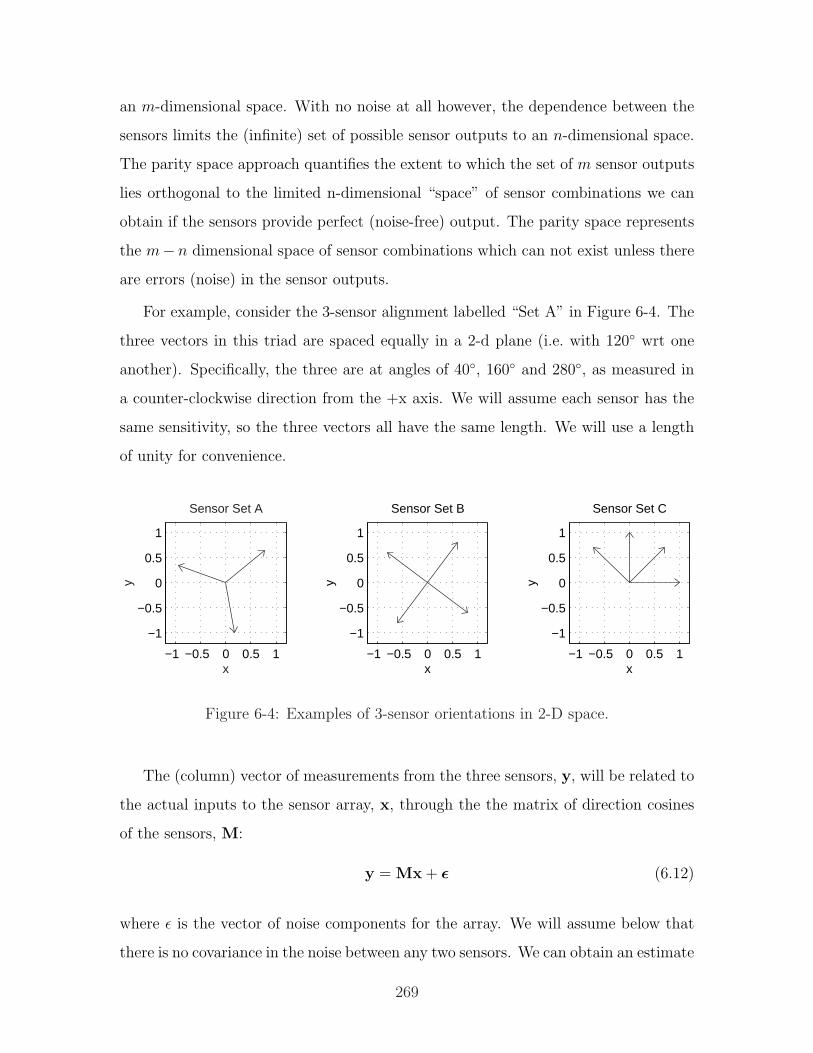
an m-dimensional space. With no noise at all however, the dependence between the

sensors limits the (infinite) set of possible sensor outputs to an n-dimensional space.

The parity space approach quantifies the extent to which the set of m sensor outputs

lies orthogonal to the limited n-dimensional “space” of sensor combinations we can

obtain if the sensors provide perfect (noise-free) output. The parity space represents

the m− n dimensional space of sensor combinations which can not exist unless there

are errors (noise) in the sensor outputs.

For example, consider the 3-sensor alignment labelled “Set A” in Figure 6-4. The

three vectors in this triad are spaced equally in a 2-d plane (i.e. with 120 wrt one

another). Specifically, the three are at angles of 40, 160 and 280, as measured in

a counter-clockwise direction from the +x axis. We will assume each sensor has the

same sensitivity, so the three vectors all have the same length. We will use a length

of unity for convenience.

−1 −0.5 0 0.5 1

−1

−0.5

0

0.5

1

x

y

Sensor Set A

−1 −0.5 0 0.5 1

−1

−0.5

0

0.5

1

x

y

Sensor Set B

−1 −0.5 0 0.5 1

−1

−0.5

0

0.5

1

x

y

Sensor Set C

Figure 6-4: Examples of 3-sensor orientations in 2-D space.

The (column) vector of measurements from the three sensors, y, will be related to

the actual inputs to the sensor array, x, through the the matrix of direction cosines

of the sensors, M:

y = Mx + ε (6.12)

where ε is the vector of noise components for the array. We will assume below that

there is no covariance in the noise between any two sensors. We can obtain an estimate

269

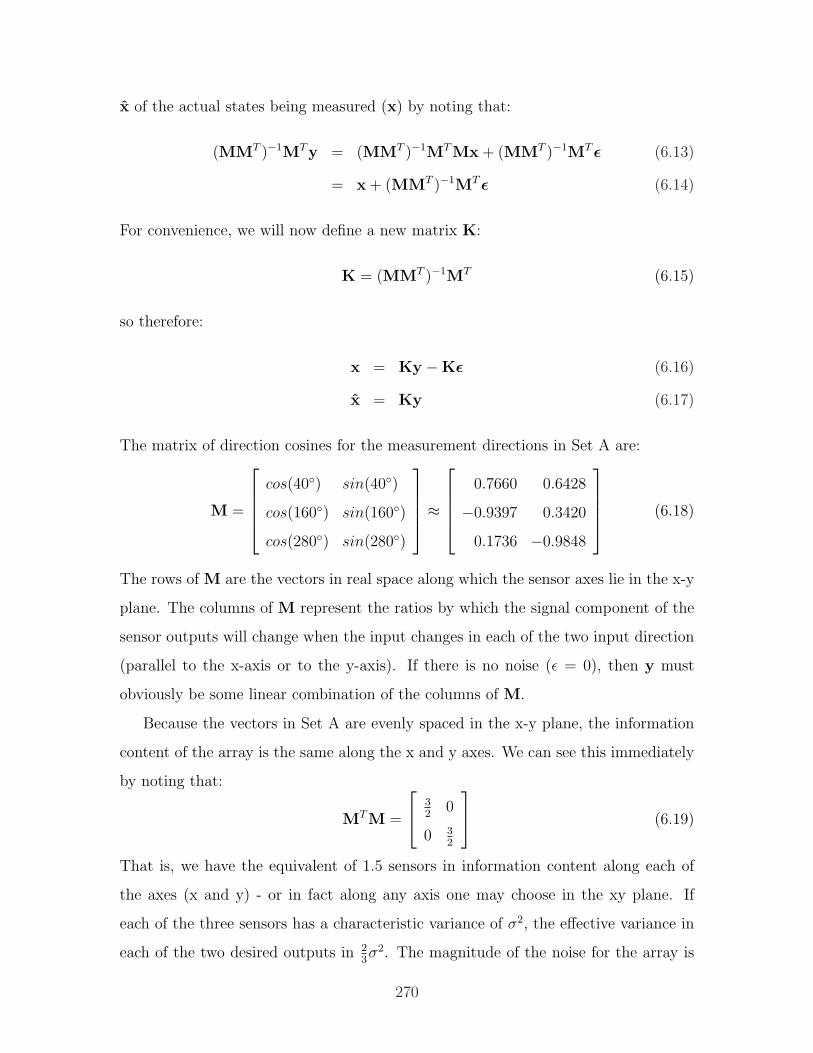
x of the actual states being measured (x) by noting that:

(MMT )−1MTy = (MMT )−1MTMx + (MMT )−1MT ε (6.13)

= x + (MMT )−1MT ε (6.14)

For convenience, we will now define a new matrix K:

K = (MMT )−1MT (6.15)

so therefore:

x = Ky −Kε (6.16)

x = Ky (6.17)

The matrix of direction cosines for the measurement directions in Set A are:

M =

cos(40) sin(40)

cos(160) sin(160)

cos(280) sin(280)

≈

0.7660 0.6428

−0.9397 0.3420

0.1736 −0.9848

(6.18)

The rows of M are the vectors in real space along which the sensor axes lie in the x-y

plane. The columns of M represent the ratios by which the signal component of the

sensor outputs will change when the input changes in each of the two input direction

(parallel to the x-axis or to the y-axis). If there is no noise (ε = 0), then y must

obviously be some linear combination of the columns of M.

Because the vectors in Set A are evenly spaced in the x-y plane, the information

content of the array is the same along the x and y axes. We can see this immediately

by noting that:

MTM =

32

0

0 32

(6.19)

That is, we have the equivalent of 1.5 sensors in information content along each of

the axes (x and y) - or in fact along any axis one may choose in the xy plane. If

each of the three sensors has a characteristic variance of σ2, the effective variance in

each of the two desired outputs in 23σ2. The magnitude of the noise for the array is

270

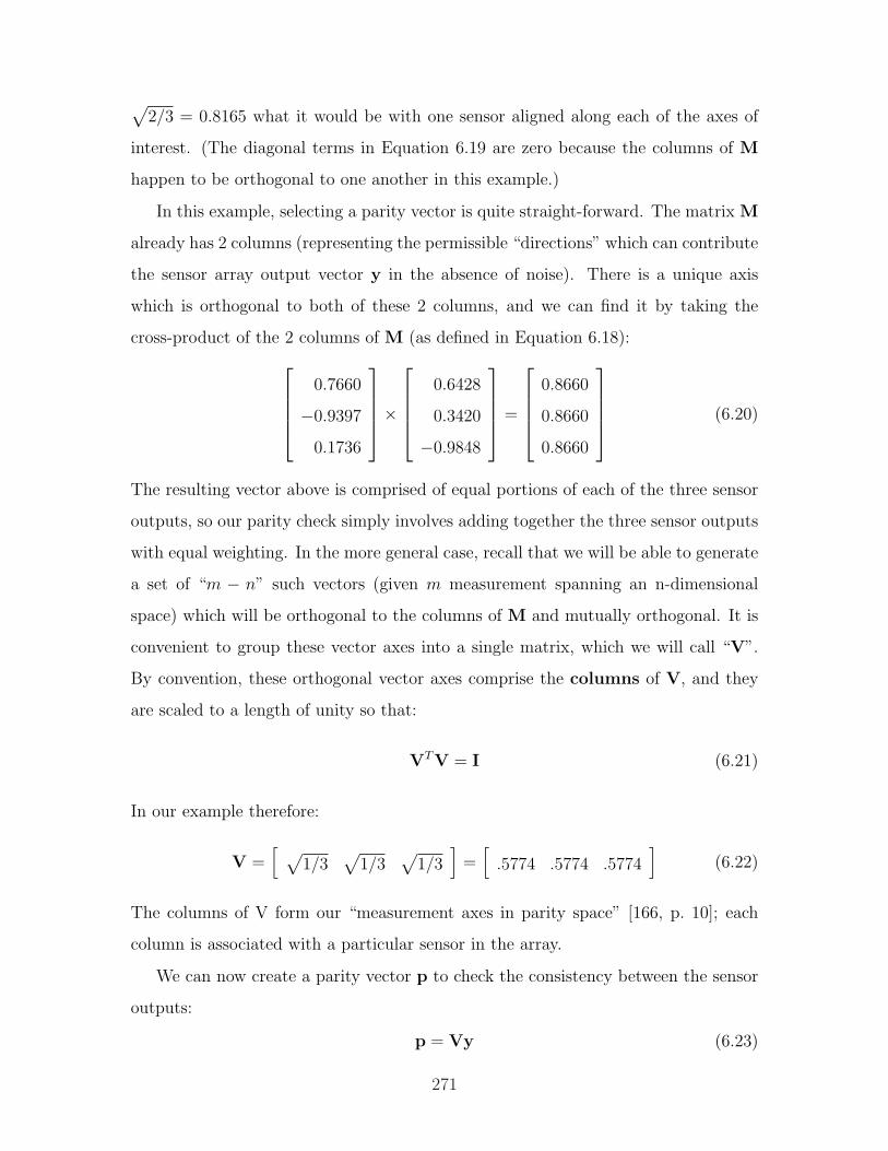
√2/3 = 0.8165 what it would be with one sensor aligned along each of the axes of

interest. (The diagonal terms in Equation 6.19 are zero because the columns of M

happen to be orthogonal to one another in this example.)

In this example, selecting a parity vector is quite straight-forward. The matrix M

already has 2 columns (representing the permissible “directions” which can contribute

the sensor array output vector y in the absence of noise). There is a unique axis

which is orthogonal to both of these 2 columns, and we can find it by taking the

cross-product of the 2 columns of M (as defined in Equation 6.18):

0.7660

−0.9397

0.1736

×

0.6428

0.3420

−0.9848

=

0.8660

0.8660

0.8660

(6.20)

The resulting vector above is comprised of equal portions of each of the three sensor

outputs, so our parity check simply involves adding together the three sensor outputs

with equal weighting. In the more general case, recall that we will be able to generate

a set of “m − n” such vectors (given m measurement spanning an n-dimensional

space) which will be orthogonal to the columns of M and mutually orthogonal. It is

convenient to group these vector axes into a single matrix, which we will call “V”.

By convention, these orthogonal vector axes comprise the columns of V, and they

are scaled to a length of unity so that:

VTV = I (6.21)

In our example therefore:

V =[ √

1/3√

1/3√

1/3]

=[

.5774 .5774 .5774]

(6.22)

The columns of V form our “measurement axes in parity space” [166, p. 10]; each

column is associated with a particular sensor in the array.

We can now create a parity vector p to check the consistency between the sensor

outputs:

p = Vy (6.23)

271

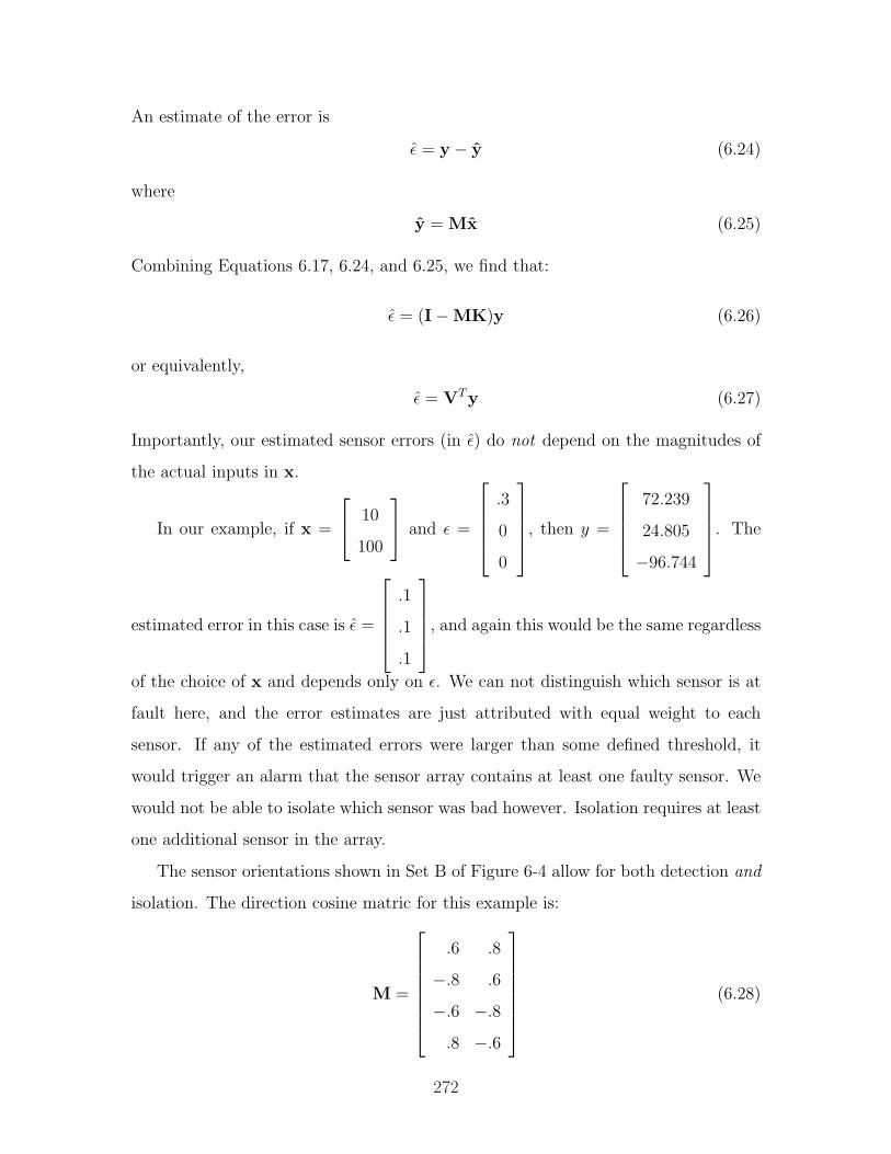
An estimate of the error is

ε = y − y (6.24)

where

y = Mx (6.25)

Combining Equations 6.17, 6.24, and 6.25, we find that:

ε = (I−MK)y (6.26)

or equivalently,

ε = VTy (6.27)

Importantly, our estimated sensor errors (in ε) do not depend on the magnitudes of

the actual inputs in x.

In our example, if x =

10

100

and ε =

.3

0

0

, then y =

72.239

24.805

−96.744

. The

estimated error in this case is ε =

.1

.1

.1

, and again this would be the same regardless

of the choice of x and depends only on ε. We can not distinguish which sensor is at

fault here, and the error estimates are just attributed with equal weight to each

sensor. If any of the estimated errors were larger than some defined threshold, it

would trigger an alarm that the sensor array contains at least one faulty sensor. We

would not be able to isolate which sensor was bad however. Isolation requires at least

one additional sensor in the array.

The sensor orientations shown in Set B of Figure 6-4 allow for both detection and

isolation. The direction cosine matric for this example is:

M =

.6 .8

−.8 .6

−.6 −.8

.8 −.6

(6.28)

272

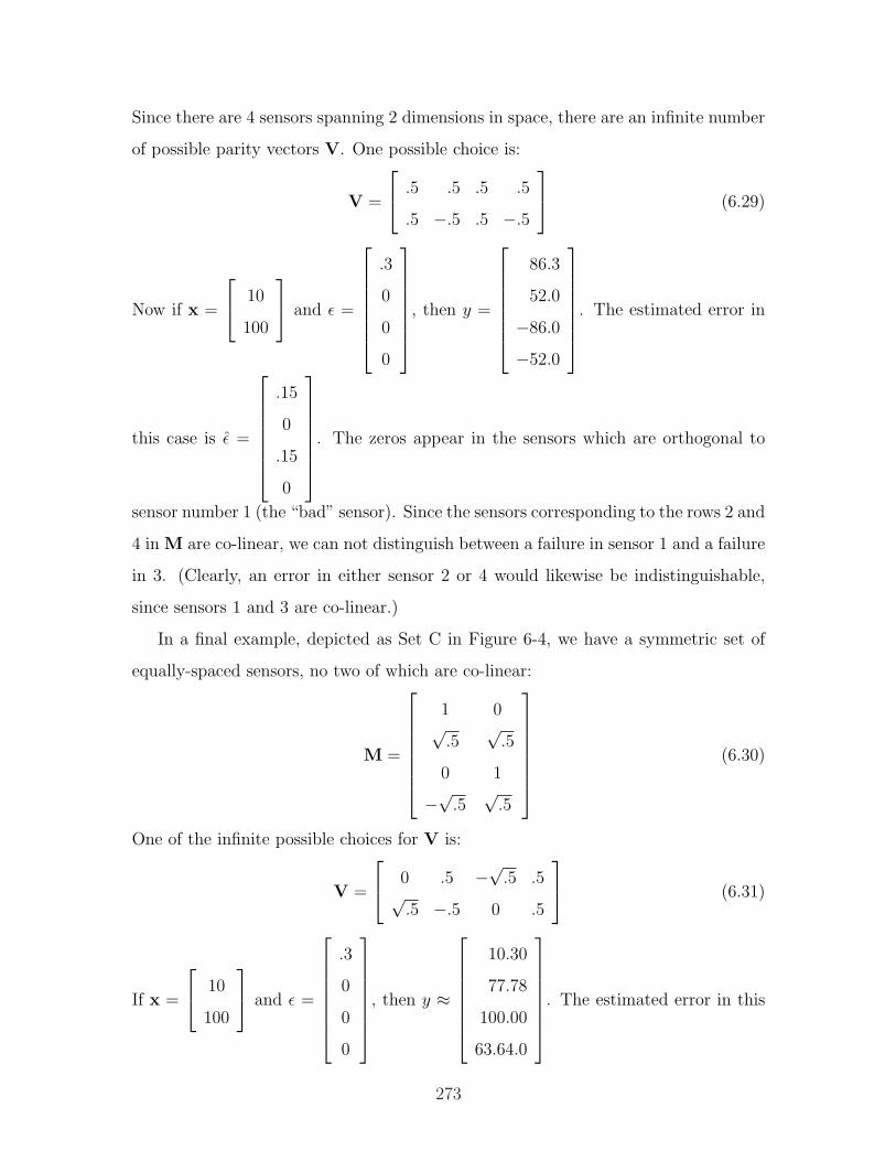
Since there are 4 sensors spanning 2 dimensions in space, there are an infinite number

of possible parity vectors V. One possible choice is:

V =

.5 .5 .5 .5

.5 −.5 .5 −.5

(6.29)

Now if x =

10

100

and ε =

.3

0

0

0

, then y =

86.3

52.0

−86.0

−52.0

. The estimated error in

this case is ε =

.15

0

.15

0

. The zeros appear in the sensors which are orthogonal to

sensor number 1 (the “bad” sensor). Since the sensors corresponding to the rows 2 and

4 in M are co-linear, we can not distinguish between a failure in sensor 1 and a failure

in 3. (Clearly, an error in either sensor 2 or 4 would likewise be indistinguishable,

since sensors 1 and 3 are co-linear.)

In a final example, depicted as Set C in Figure 6-4, we have a symmetric set of

equally-spaced sensors, no two of which are co-linear:

M =

1 0√

.5√

.5

0 1

−√.5√

.5

(6.30)

One of the infinite possible choices for V is:

V =

0 .5 −√.5 .5√

.5 −.5 0 .5

(6.31)

If x =

10

100

and ε =

.3

0

0

0

, then y ≈

10.30

77.78

100.00

63.64.0

. The estimated error in this

273

case is ε =

.150

−0.106

0

0.106

. Unlike the 4-sensor array in Set B, we can isolate the fault

within the sensor in Set C. To do so, we would systematically exclude a single sensor

at a time by setting the corresponding column in V to zero. Here, we will use the

notation Vi to denote a matrix identical to V, except that all elements in the ith

column of Vi are set to zero. Similarly, we will define a parity vector pi associated

with each Vi:

pi = Viy (6.32)

We can now perform individual parity checks to identify the faulty sensor through

a process of elimination. We find that V1Tp1 =

0

0

0

0

, V2Tp2 ≈

0.15

0

0

0.10607

,

V3Tp3 ≈

0.15

−0.10607

0

0.10607

, and V4Tp4 ≈

0.15

−0.10607

0

0

. The one parity check which

“passes” in this case is the one in which we have excluded any contribution from

sensor 1; therefore, we can isolate the error as being due to sensor 1.

Of course, in a real sensor array, each sensor will have some finite error, and we

must set an appropriate threshold which distinguishes a failure from the allowable

noise which will exist in the measurements. I will not discuss setting such thresholds,

except to say that they clearly depend on the noise characteristics of the sensors

and amount to a trade-off, weighing both the probability and cost of triggering false

alarms against those of failing to identify actual faults.

To give the reader some feel for the effectiveness of this method, however, consider

the sensor alignments in Set C once again. Suppose we instead have errors in all the

sensor measurements, with the error in sensor 1 outweighing the others by a factor

274

of 3. Specifically, let us say that ε =

.3

.1

.1

.1

. In this case, the parity relations

will produce the following: V1Tp1 ≈

0

0.01464

−0.02071

0.01464

, V2Tp2 ≈

0.18535

0

0.01464

0.12071

,

V3Tp3 ≈

0.15

−0.05607

0

0.15607

, and V4Tp4 ≈

0.11464

−0.09142

0.01464

0

. The vector first vector,

corresponding to the exclusion of sensor 1, is not of zero length now, but it is still

substantially smaller in magnitude than any of the other three vectors.

Symmetry of the sensor array is not required for this FDI method to work, but

there are some advantages of choosing axes which are symmetric. In particular, we are

often interesting in selecting axes which collectively span each direction in space with

equal sensitivity. The next section discusses issues involved in selecting symmetric

axes in a 3-dimensional space.

6.1.4 Advantages of Symmetry

There are several considerations when selecting the orientations of the individual

sensors in a redundant array. This section focuses on three issues and explains why

symmetric configurations are often advantageous. These issues are: (1) Adjusting the

relative noise sensitivities of a sensor array in each direction in space, (2) minimizing

the overall noise of the array, and (3) minimizing the reduction in performance of the

array given the exclusion of any sensor (due to a fault).

First, the alignment of the sensor axes will certainly affect the sensitivity of the

sensor array to each direction in space. We have already seen in previous section,

for instance, that one can position 3 sensors in a 2-d array to get the equivalent

275

information of 1.5 sensors in each of 2 orthogonal measurement directions. Suppose

more generally that we have m sensors spanning n dimensions. We can position the

m sensors to obtain the equivalent of xi sensors of information in each ith out of n

orthogonal measurement directions. Of particular interest, we can define “optimal”

configurations as those which satisfy the following restrictions:

n∑i=1

xi = m, (xi >= 0, ∀i) (6.33)

The equality in the equation above with “m” becomes an inequality in suboptimal

configurations, as we will see later.

In some applications, one may wish to distribute the information content of the

array equally in each direction in space, although there are other applications where

sensitivity is more (or less) critical along a particular axis. For instance, the devel-

opment of early inertial navigation systems (INS) in the 1960’s centered on space

(zero-g) navigation, and a lot of emphasis was therefore placed on obtaining equal

sensitivity along each direction in 3-d space [210, 166, 213, 73].

The development of Earth-bound INS systems gained importance by the early- to

mid-1970’s, and this redefined the problem of optimal sensor configuration in at least

two significant ways: (1) Azimuthal errors will generally have a lesser importance

than those in the horizontal directions (latitude and longitude), and (2) rotating

gyros generally have both g-insensitive and g-sensitive noise characteristics in drift

rate, and the standard deviation of the gravity-dependent noise term “varies with

the cosine of the elevation angle of the output axis” [160]. The configuration of the

rate gyros for the Segway is another application where one would probably not assign

equal importance to every axis in our 3-space. The most critical axis for the Segway

is the rotation of the body of the device about the wheel axis (i.e. pitch).

A second consideration is insuring that sensors are distributed so that we take

full advantage of the noise-reducing potential of the m sensors in an array. I noted

above that we can configure m sensors such that their information content is effi-

ciently divvied up (in whatever proportions we wish) among n dimensions in space,

as described by Equation 6.33. However, it is possible to configure them inefficiently

276

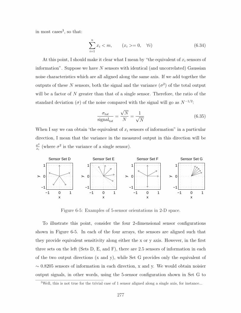
in most cases3, so that:

n∑i=1

xi < m, (xi >= 0, ∀i) (6.34)

At this point, I should make it clear what I mean by “the equivalent of xi sensors of

information”. Suppose we have N sensors with identical (and uncorrelated) Gaussian

noise characteristics which are all aligned along the same axis. If we add together the

outputs of these N sensors, both the signal and the variance (σ2) of the total output

will be a factor of N greater than that of a single sensor. Therefore, the ratio of the

standard deviation (σ) of the noise compared with the signal will go as N−1/2:

σtot

signaltot

=

√N

N=

1√N

(6.35)

When I say we can obtain ‘the equivalent of xi sensors of information” in a particular

direction, I mean that the variance in the measured output in this direction will be

σ2

xi(where σ2 is the variance of a single sensor).

−1 0 1−1

0

1

x

y

Sensor Set F

−1 0 1−1

0

1

x

y

Sensor Set G

−1 0 1−1

0

1

x

y

Sensor Set D

−1 0 1−1

0

1

x

y

Sensor Set E


To illustrate this point, consider the four 2-dimensional sensor configurations

shown in Figure 6-5. In each of the four arrays, the sensors are aligned such that

they provide equivalent sensitivity along either the x or y axis. However, in the first

three sets on the left (Sets D, E, and F), there are 2.5 sensors of information in each

of the two output directions (x and y), while Set G provides only the equivalent of

∼ 0.8205 sensors of information in each direction, x and y. We would obtain noisier

output signals, in other words, using the 5-sensor configuration shown in Set G to

3Well, this is not true for the trivial case of 1 sensor aligned along a single axis, for instance...

277

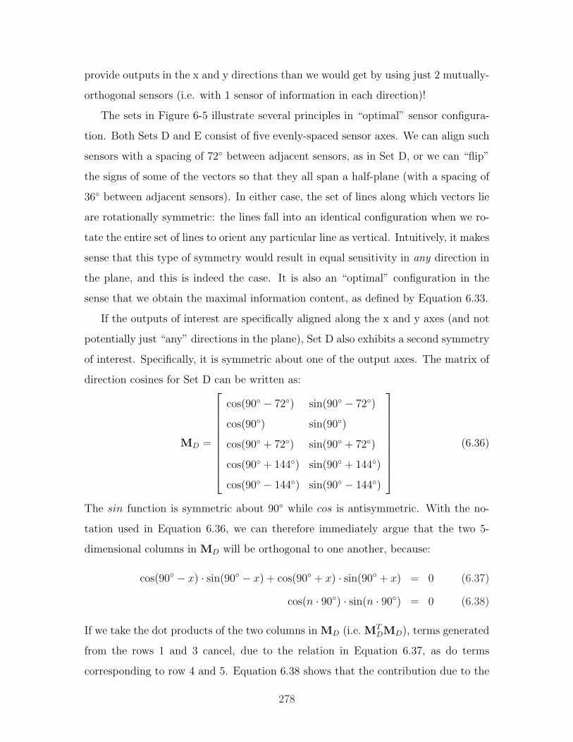
provide outputs in the x and y directions than we would get by using just 2 mutually-

orthogonal sensors (i.e. with 1 sensor of information in each direction)!

The sets in Figure 6-5 illustrate several principles in “optimal” sensor configura-

tion. Both Sets D and E consist of five evenly-spaced sensor axes. We can align such

sensors with a spacing of 72 between adjacent sensors, as in Set D, or we can “flip”

the signs of some of the vectors so that they all span a half-plane (with a spacing of

36 between adjacent sensors). In either case, the set of lines along which vectors lie

are rotationally symmetric: the lines fall into an identical configuration when we ro-

tate the entire set of lines to orient any particular line as vertical. Intuitively, it makes

sense that this type of symmetry would result in equal sensitivity in any direction in

the plane, and this is indeed the case. It is also an “optimal” configuration in the

sense that we obtain the maximal information content, as defined by Equation 6.33.

If the outputs of interest are specifically aligned along the x and y axes (and not

potentially just “any” directions in the plane), Set D also exhibits a second symmetry

of interest. Specifically, it is symmetric about one of the output axes. The matrix of

direction cosines for Set D can be written as:

MD =

cos(90 − 72) sin(90 − 72)

cos(90) sin(90)

cos(90 + 72) sin(90 + 72)

cos(90 + 144) sin(90 + 144)

cos(90 − 144) sin(90 − 144)

(6.36)

The sin function is symmetric about 90 while cos is antisymmetric. With the no-

tation used in Equation 6.36, we can therefore immediately argue that the two 5-

dimensional columns in MD will be orthogonal to one another, because:

cos(90 − x) · sin(90 − x) + cos(90 + x) · sin(90 + x) = 0 (6.37)

cos(n · 90) · sin(n · 90) = 0 (6.38)

If we take the dot products of the two columns in MD (i.e. MTDMD), terms generated

from the rows 1 and 3 cancel, due to the relation in Equation 6.37, as do terms

corresponding to row 4 and 5. Equation 6.38 shows that the contribution due to the

278

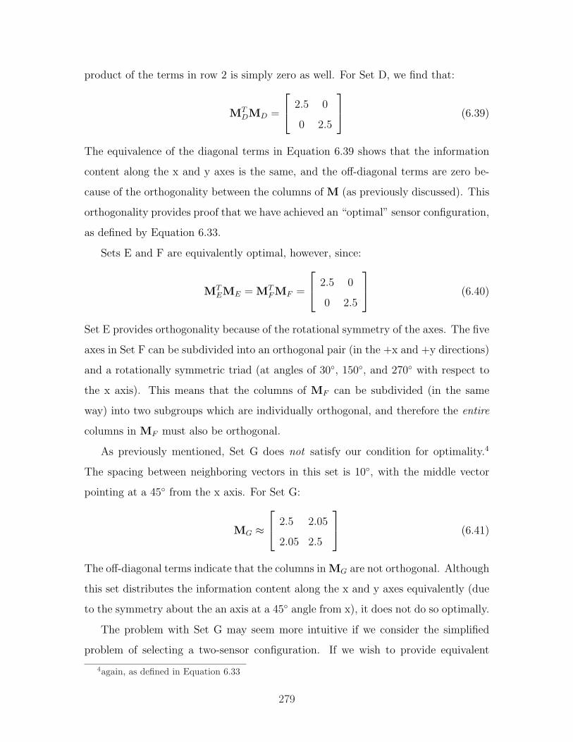
product of the terms in row 2 is simply zero as well. For Set D, we find that:

MTDMD =

2.5 0

0 2.5

(6.39)

The equivalence of the diagonal terms in Equation 6.39 shows that the information

content along the x and y axes is the same, and the off-diagonal terms are zero be-

cause of the orthogonality between the columns of M (as previously discussed). This

orthogonality provides proof that we have achieved an “optimal” sensor configuration,

as defined by Equation 6.33.

Sets E and F are equivalently optimal, however, since:

MTEME = MT

FMF =

2.5 0

0 2.5

(6.40)

Set E provides orthogonality because of the rotational symmetry of the axes. The five

axes in Set F can be subdivided into an orthogonal pair (in the +x and +y directions)

and a rotationally symmetric triad (at angles of 30, 150, and 270 with respect to

the x axis). This means that the columns of MF can be subdivided (in the same

way) into two subgroups which are individually orthogonal, and therefore the entire

columns in MF must also be orthogonal.

As previously mentioned, Set G does not satisfy our condition for optimality.4

The spacing between neighboring vectors in this set is 10, with the middle vector

pointing at a 45 from the x axis. For Set G:

MG ≈ 2.5 2.05

2.05 2.5

(6.41)

The off-diagonal terms indicate that the columns in MG are not orthogonal. Although

this set distributes the information content along the x and y axes equivalently (due

to the symmetry about the an axis at a 45 angle from x), it does not do so optimally.

The problem with Set G may seem more intuitive if we consider the simplified

problem of selecting a two-sensor configuration. If we wish to provide equivalent

4again, as defined in Equation 6.33

279

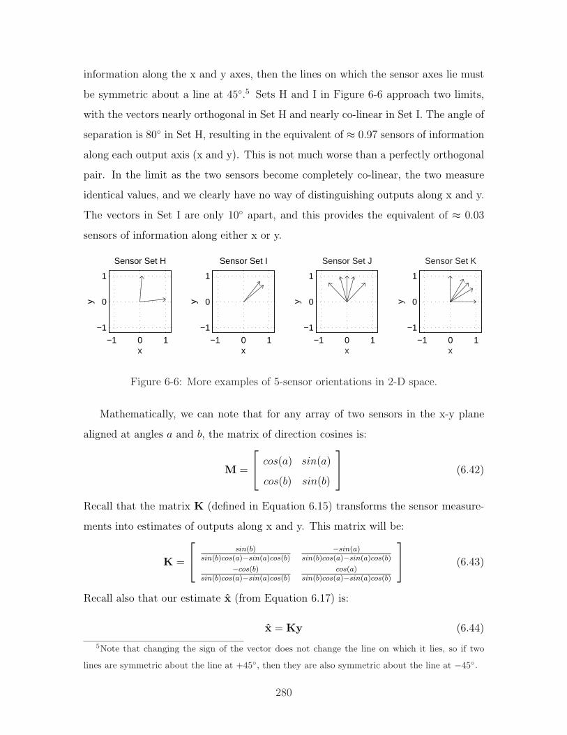
information along the x and y axes, then the lines on which the sensor axes lie must

be symmetric about a line at 45.5 Sets H and I in Figure 6-6 approach two limits,

with the vectors nearly orthogonal in Set H and nearly co-linear in Set I. The angle of

separation is 80 in Set H, resulting in the equivalent of ≈ 0.97 sensors of information

along each output axis (x and y). This is not much worse than a perfectly orthogonal

pair. In the limit as the two sensors become completely co-linear, the two measure

identical values, and we clearly have no way of distinguishing outputs along x and y.

The vectors in Set I are only 10 apart, and this provides the equivalent of ≈ 0.03

sensors of information along either x or y.

−1 0 1−1

0

1

x

y

Sensor Set H

−1 0 1−1

0

1

x

y

Sensor Set I

−1 0 1−1

0

1

x

y

Sensor Set J

−1 0 1−1

0

1

x

y

Sensor Set K

Figure 6-6: More examples of 5-sensor orientations in 2-D space.

Mathematically, we can note that for any array of two sensors in the x-y plane

aligned at angles a and b, the matrix of direction cosines is:

M =

cos(a) sin(a)

cos(b) sin(b)

(6.42)

Recall that the matrix K (defined in Equation 6.15) transforms the sensor measure-

ments into estimates of outputs along x and y. This matrix will be:

K =

sin(b)sin(b)cos(a)−sin(a)cos(b)

−sin(a)sin(b)cos(a)−sin(a)cos(b)

−cos(b)sin(b)cos(a)−sin(a)cos(b)

cos(a)sin(b)cos(a)−sin(a)cos(b)

(6.43)

Recall also that our estimate x (from Equation 6.17) is:

x = Ky (6.44)

5Note that changing the sign of the vector does not change the line on which it lies, so if two

lines are symmetric about the line at +45, then they are also symmetric about the line at −45.

280

which differs from the actual value of x by some noise component, given by Equa-

tion 6.16:

x = Ky −Kε (6.45)

x− x = Kε (6.46)

If the sensors each have (uncorrelated) Gaussian noise with a standard deviation of

σs, the standard deviation of the noise in our estimates along the x and y axes will

each be:

σx =

sin2(a)+sin2(b)(sin(b)cos(a)−sin(a)cos(b))2

cos2(a)+cos2(b)(sin(b)cos(a)−sin(a)cos(b))2

· σs (6.47)

When the angles are equal (a = b), the denominator (which is the same in the terms

corresponding to the x and y directions) goes to zero, and we have infinite noise. If

the angles differ by 90 (either a = b + 90 or a = b − 90), both the numerator

and denominator in each of the two noise components equal unity, and we obtain the

equivalent noise of an orthogonal alignment where one sensor is specifically oriented

along the x axis and the second lies along y.

We can expand this last principle to the more broad case of m sensors distributed

evenly (with equivalent angles separating them) in n dimensions, in which case we

will obtain an “optimal” configuration with mn

sensors of information in each of n

directions. (The proof of this is not provided here, but will hopefully make intuitive

sense to the reader at this point.) This will be an important concept when we expand

this analysis (shortly) to consider 3-dimensional sensor arrays.

Sets J and K in Figure 6-6 show symmetric 5-sensor arrays which can be used to

reemphasize some of the points covered in the last few pages. Each set consists of

a central axis with two axes at ±10 and two more at ±45. As before, suppose we

are concerned with obtaining outputs along the x and y axes. In Set J, the axis of

symmetry coincides with an output axis (the y axis), so the columns of MJ will be

orthogonal:

MTJ M ≈

1.06 0

0 3.94

(6.48)

281

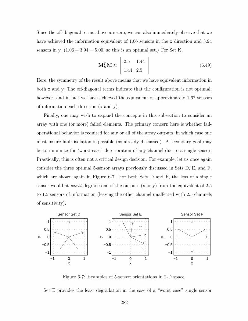
Since the off-diagonal terms above are zero, we can also immediately observe that we

have achieved the information equivalent of 1.06 sensors in the x direction and 3.94

sensors in y. (1.06 + 3.94 = 5.00, so this is an optimal set.) For Set K,

MTKM ≈

2.5 1.44

1.44 2.5

(6.49)

Here, the symmetry of the result above means that we have equivalent information in

both x and y. The off-diagonal terms indicate that the configuration is not optimal,

however, and in fact we have achieved the equivalent of approximately 1.67 sensors

of information each direction (x and y).

Finally, one may wish to expand the concepts in this subsection to consider an

array with one (or more) failed elements. The primary concern here is whether fail-

operational behavior is required for any or all of the array outputs, in which case one

must insure fault isolation is possible (as already discussed). A secondary goal may

be to minimize the ‘worst-case” deterioration of any channel due to a single sensor.

Practically, this is often not a critical design decision. For example, let us once again

consider the three optimal 5-sensor arrays previously discussed in Sets D, E, and F,

which are shown again in Figure 6-7. For both Sets D and F, the loss of a single

sensor would at worst degrade one of the outputs (x or y) from the equivalent of 2.5

to 1.5 sensors of information (leaving the other channel unaffected with 2.5 channels

of sensitivity).

−1 0 1

−1

−0.5

0

0.5

1

x

y

Sensor Set D

−1 0 1

−1

−0.5

0

0.5

1

x

y

Sensor Set E

−1 0 1

−1

−0.5

0

0.5

1

x

y

Sensor Set F


Set E provides the least degradation in the case of a “worst case” single sensor

282

failure (of any optimal 5-sensor array in 2-D), but it is really not much of an improve-

ment over the other two. If either of the two sensors which are closest to the x and

y axes were to fail, that nearest output axis would then operate with the equivalent

sensitivity of 1.5148 sensors. This is less than 1% greater that the “equivalent sensor

value” for the worst case scenarios for Set D and F, and it corresponds to an increase

in the standard deviation of the noise on that output of less than 0.5%.

6.1.5 Suggested Geometries for Redundant Sensor Arrays

As outlined in the preceding section, symmetric configurations can be used both to

equalize the sensitivities along the desired output axes and to maximize the overall

effectiveness of the sensors being used. In 2-dimensional arrays (like the ones shown

so far), it is relatively straightforward to identify optimal sensor orientations. The

problem is less intuitive for a 3-d array, but it is tractable once one defines optimality

for the array. This was defined at length in the preceding subsection and can be

summarized as (1) obtaining the desired ratios of sensitivities along the output axes

(e.g. equal sensitivity in each direction) and (2) making full, efficient use of all sensors.

One way of achieving symmetric configurations in three dimensions is to use ge-

ometric features of the Platonic solids. The Platonic solids are the five regular poly-

hedra. They are the only convex solids whose faces are comprised of identical regular

polygons. Figure 6-8 shows the five Platonic solids.

Figure 6-8: The 5 Platonic solids. A Platonic solid is a polyhedron whose faces are

congruent regular polygons that meet at equal angles. Only five such solids are geo-

metrically possibly. They are (as depicted from left to right above) the tetrahedron,

octahedron, icosahedron, hexahedron (aka cube), and dodecahedron.

We can create a symmetric set of axes for a sensor array by drawing vectors from

283

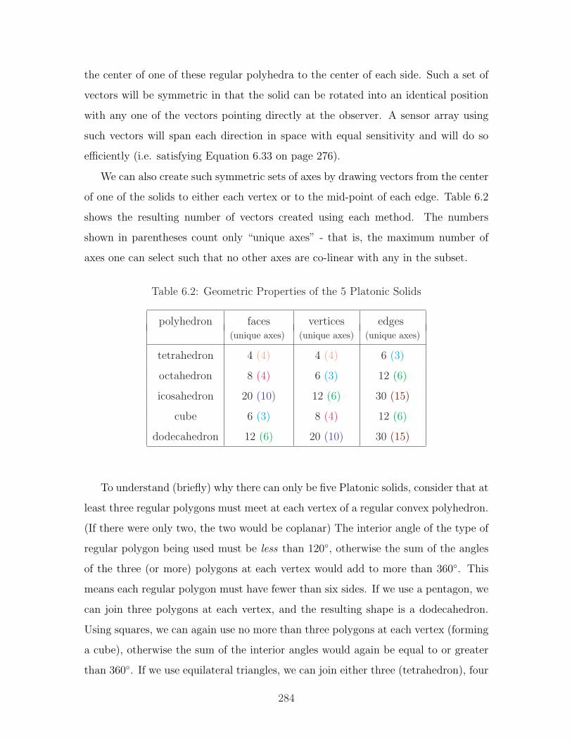
the center of one of these regular polyhedra to the center of each side. Such a set of

vectors will be symmetric in that the solid can be rotated into an identical position

with any one of the vectors pointing directly at the observer. A sensor array using

such vectors will span each direction in space with equal sensitivity and will do so

efficiently (i.e. satisfying Equation 6.33 on page 276).

We can also create such symmetric sets of axes by drawing vectors from the center

of one of the solids to either each vertex or to the mid-point of each edge. Table 6.2

shows the resulting number of vectors created using each method. The numbers

shown in parentheses count only “unique axes” - that is, the maximum number of

axes one can select such that no other axes are co-linear with any in the subset.

Table 6.2: Geometric Properties of the 5 Platonic Solids

polyhedron faces vertices edges(unique axes) (unique axes) (unique axes)

tetrahedron 4 (4) 4 (4) 6 (3)

octahedron 8 (4) 6 (3) 12 (6)

icosahedron 20 (10) 12 (6) 30 (15)

cube 6 (3) 8 (4) 12 (6)

dodecahedron 12 (6) 20 (10) 30 (15)

To understand (briefly) why there can only be five Platonic solids, consider that at

least three regular polygons must meet at each vertex of a regular convex polyhedron.

(If there were only two, the two would be coplanar) The interior angle of the type of

regular polygon being used must be less than 120, otherwise the sum of the angles

of the three (or more) polygons at each vertex would add to more than 360. This

means each regular polygon must have fewer than six sides. If we use a pentagon, we

can join three polygons at each vertex, and the resulting shape is a dodecahedron.

Using squares, we can again use no more than three polygons at each vertex (forming

a cube), otherwise the sum of the interior angles would again be equal to or greater

than 360. If we use equilateral triangles, we can join either three (tetrahedron), four

284

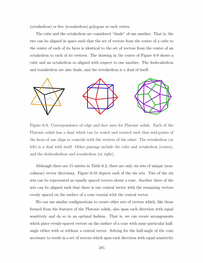
(octahedron) or five (icosahedron) polygons at each vertex.

The cube and the octahedron are considered “duals” of one another. That is, the

two can be aligned in space such that the set of vectors from the center of a cube to

the center of each of its faces is identical to the set of vectors from the center of an

octahedron to each of its vertices. The drawing in the center of Figure 6-9 shows a

cube and an octahedron so aligned with respect to one another. The dodecahedron

and icosahedron are also duals, and the tetrahedron is a dual of itself.

Figure 6-9: Correspondence of edge and face axes for Platonic solids. Each of the

Platonic solids has a dual which can be scaled and rotated such that mid-points of

the faces of one align to coincide with the vertices of the other. The tetrahedron (at

left) is a dual with itself. Other pairings include the cube and octahedron (center),

and the dodecahedron and icosahedron (at right).

Although there are 15 entries in Table 6.2, there are only six sets of unique (non-

colinear) vector directions. Figure 6-10 depicts each of the six sets. Two of the six

sets can be represented as equally spaced vectors about a cone. Another three of the

sets can be aligned such that there is one central vector with the remaining vectors

evenly spaced on the surface of a cone coaxial with the central vector.

We can use similar configurations to create other sets of vectors which, like those

formed from the features of the Platonic solids, also span each direction with equal

sensitivity and do so in an optimal fashion. That is, we can create arrangements

which place evenly-spaced vectors on the surface of a cone with some particular half-

angle either with or without a central vector. Solving for the half-angle of the cone

necessary to result in a set of vectors which span each direction with equal sensitivity

285

is fairly straight-forward.

Consider the first and fourth configurations shown in Figure 6-10, in which there

are three vectors about a cone either with or without an additional central vector

along the axis of the cone (respectively). The matrix of direction cosines for the “1–

3” case, in which there are one central vector and three about a cone with half-angle

β, can be written as:

M1–3 =

0 0 1

cos(0 · 360/3) · sin(β) sin(0 · 360/3) · sin(β) cos(β)



(6.50)

Each row vector above is of length unity, and therefore the sum of the squares of any

single row will be one. The sum of the squares of all the elements of all the rows

must therefore be equal to the number of rows in M1–3, which is 4. To span each

direction in space equally requires that each column vector in M1–3 have identical

length. To do so efficiently requires that the column vectors in Equation 6.50 be

orthogonal to one another, and therefore that the squares of their lengths will each

add to (n + 1)/3, where n + 1 is the total number of rows in M1–n. The first and

second columns will automatically be equal in length if we space the vectors equally

about a cone (as done in Equation 6.50). Applying the necessary restrictions on the

length of the third column of Equation 6.50, we require that:

12 + 3 · (cos(β1–3))2 =

4

3(6.51)

Therefore:

cos(β1–3) =

√4

3 · 3 −1

3(6.52)

β1–3 = 70.529 (6.53)

More generally, to generate a set of n + 1 vectors arranged with 1 central and n

peripheral vectors equally spaced about a cone with half-angle β1–n such that they

span each direction in space equally and optimally, the half-angle β1–n must be given

286

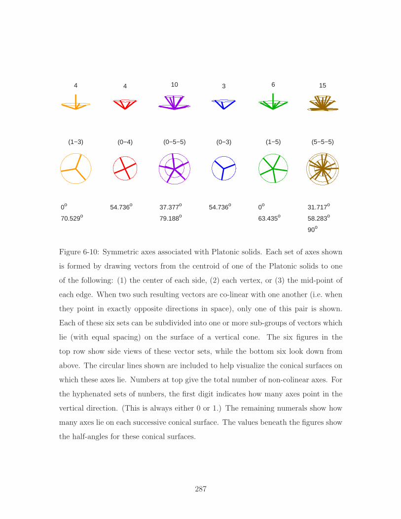
4 4 10 3 6 15

(1−3) (0−4) (0−5−5) (0−3) (1−5) (5−5−5)

0o

70.529o

54.736o 37.377o

79.188o

54.736o 0o

63.435o

31.717o

58.283o

90o

Figure 6-10: Symmetric axes associated with Platonic solids. Each set of axes shown

is formed by drawing vectors from the centroid of one of the Platonic solids to one

of the following: (1) the center of each side, (2) each vertex, or (3) the mid-point of

each edge. When two such resulting vectors are co-linear with one another (i.e. when

they point in exactly opposite directions in space), only one of this pair is shown.

Each of these six sets can be subdivided into one or more sub-groups of vectors which

lie (with equal spacing) on the surface of a vertical cone. The six figures in the

top row show side views of these vector sets, while the bottom six look down from

above. The circular lines shown are included to help visualize the conical surfaces on

which these axes lie. Numbers at top give the total number of non-colinear axes. For

the hyphenated sets of nunbers, the first digit indicates how many axes point in the

vertical direction. (This is always either 0 or 1.) The remaining numerals show how

many axes lie on each successive conical surface. The values beneath the figures show

the half-angles for these conical surfaces.

287

as:

cos(β1–n) =

√n + 1

3n− 1

n(6.54)

β1–n = cos−1

(√(n + 1)− 3

3n

)(6.55)

Some of the resulting “optimal” half-angle values are:

β1–3 = 70.529 (6.56)

β1–4 = 65.905 (6.57)

β1–5 = 63.435 (6.58)

β1–6 = 61.874 (6.59)

β1–7 = 60.794 (6.60)

We can similarly analyze the case with no central angle by first writing the matrix

of direction cosines for the “0-3” case (with three vectors equally spaced about a cone

but no central vector):

M0–3 =




(6.61)

This geometric configuration corresponds to a set of non-colinear vectors drawn from

the center of a cube to centers of three of its faces and is depicted in the fourth image

from the left in Figure 6-10.

From the form of Equation 6.61 and our previous reasoning, it follows that in the

general “0–n” case, with equal and optimal sensitivity along all axes, we require that

the sum of the squares of the elements in the n rows of the third column must add

to n/3:

n · (cos(β0–3))2 =

n

3(6.62)

And therefore:

cos(β0–n) =

√1

3(6.63)

β0–n = 54.736 (6.64)

288

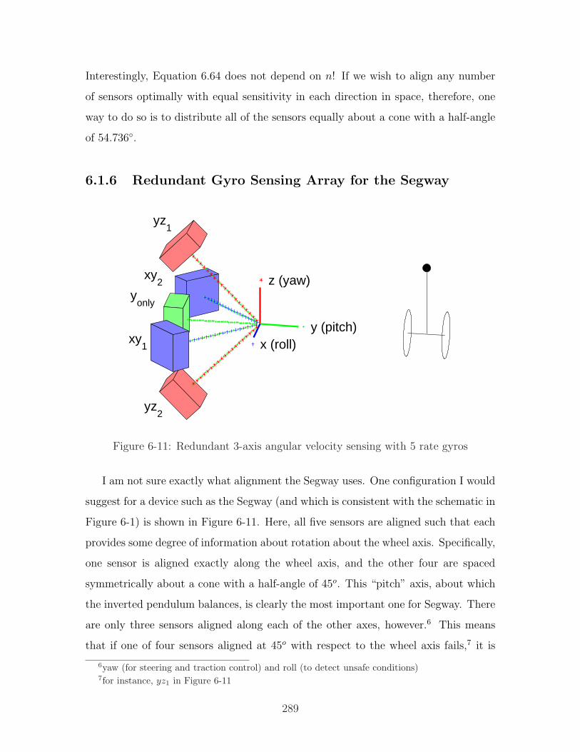
Interestingly, Equation 6.64 does not depend on n! If we wish to align any number

of sensors optimally with equal sensitivity in each direction in space, therefore, one

way to do so is to distribute all of the sensors equally about a cone with a half-angle

of 54.736.

6.1.6 Redundant Gyro Sensing Array for the Segway

y (pitch)

z (yaw)

x (roll)

yz1

yz2

xy2

yonly

xy1

Figure 6-11: Redundant 3-axis angular velocity sensing with 5 rate gyros

I am not sure exactly what alignment the Segway uses. One configuration I would

suggest for a device such as the Segway (and which is consistent with the schematic in

Figure 6-1) is shown in Figure 6-11. Here, all five sensors are aligned such that each

provides some degree of information about rotation about the wheel axis. Specifically,

one sensor is aligned exactly along the wheel axis, and the other four are spaced

symmetrically about a cone with a half-angle of 45o. This “pitch” axis, about which

the inverted pendulum balances, is clearly the most important one for Segway. There

are only three sensors aligned along each of the other axes, however.6 This means

that if one of four sensors aligned at 45o with respect to the wheel axis fails,7 it is

6yaw (for steering and traction control) and roll (to detect unsafe conditions)7for instance, yz1 in Figure 6-11

289

not possible to isolate whether it was in fact this sensor which is faulty or the one

aligned 90o to it (one the opposite side of the central cone axis).8 If the sensor along

the wheel axis fails, in contrast, it can be precisely isolated.

The result of not being able to precisely isolate every sensor failure is as follows:

First, if the sensor along the wheel axis fails, it can be isolated and normal operation

can continue, with the remaining four sensors providing information about the wheel

axis, and two sensors each aligned at 45o to each of the other axes. Moreover, the four

sensors used in estimating pitch, each 45o off the wheel axis, provide the equivalent

information content (with respect to noise) as two aligned exactly along the axis, and

therefore result in an output with somewhat lower noise9 than a single on-axis sensor.

For each of the other orthogonal axes, the two remaining sensor outputs provide the

equivalent SNR of a single on-axis sensor.

By contrast, if one of the other four sensors fails, we are left with only three usable

sensor outputs. As a result, we can only sense rotation about two of the three axes -

but importantly, the pitch axis is always one of these two sensed directions. If sensor

yz1 in Figure 6-11 fails, for instance, then we can no longer sense roll. There are

still one on-axis and two off-axis sensors giving the equivalent of two on-axis sensors’

data for pitch (just as in the on-axis failure case), and there are two off-axis sensors

for estimating roll (providing the equivalent of a single on-axis sensor, just as in the

on-axis failure case).

As a consequence, this alignment allows the Segway to balance given the failure of

any gyro in the assembly. However, 4/5 of the possible failures will make it impossible

to measure either roll or yaw. Balance is critical for insuring the Segway is “fail-

operational”, but traction control and roll information is not.10 If a gyro fails in this

configuration, the Segway can warn the user that maintenance is required, yet still

remain quite operational. Also, the alignment improves sensitivity along the pitch

axis (over the sensitivity of a single gyro) and provides an equivalent SNR along the

8i.e. yz2 in Figure 6-119by a factor of sqrt.5 = 0.7

10The gyros are necessary to maintain stability about an axis of pitch, but there is no active

stabilization in the lateral direction.

290

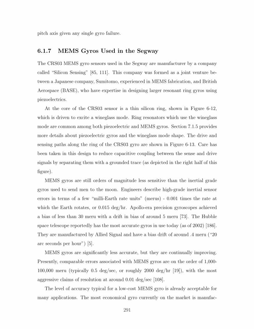
pitch axis given any single gyro failure.

6.1.7 MEMS Gyros Used in the Segway

The CRS03 MEMS gyro sensors used in the Segway are manufacturer by a company

called “Silicon Sensing” [85, 111]. This company was formed as a joint venture be-

tween a Japanese company, Sumitomo, experienced in MEMS fabrication, and British

Aerospace (BASE), who have expertise in designing larger resonant ring gyros using

piezoelectrics.

At the core of the CRS03 sensor is a thin silicon ring, shown in Figure 6-12,

which is driven to excite a wineglass mode. Ring resonators which use the wineglass

mode are common among both piezoelectric and MEMS gyros. Section 7.1.5 provides

more details about piezoelectric gyros and the wineglass mode shape. The drive and

sensing paths along the ring of the CRS03 gyro are shown in Figure 6-13. Care has

been taken in this design to reduce capacitive coupling between the sense and drive

signals by separating them with a grounded trace (as depicted in the right half of this

figure).

MEMS gyros are still orders of magnitude less sensitive than the inertial grade

gyros used to send men to the moon. Engineers describe high-grade inertial sensor

errors in terms of a few “milli-Earth rate units” (merus) - 0.001 times the rate at

which the Earth rotates, or 0.015 deg/hr. Apollo-era precision gyroscopes achieved

a bias of less than 30 meru with a drift in bias of around 5 meru [73]. The Hubble

space telescope reportedly has the most accurate gyros in use today (as of 2002) [186].

They are manufactured by Allied Signal and have a bias drift of around .4 meru (“20

arc seconds per hour”) [5].

MEMS gyros are significantly less accurate, but they are continually improving.

Presently, comparable errors associated with MEMS gyros are on the order of 1,000-

100,000 meru (typically 0.5 deg/sec, or roughly 2000 deg/hr [19]), with the most

aggressive claims of resolution at around 0.01 deg/sec [108].

The level of accuracy typical for a low-cost MEMS gyro is already acceptable for

many applications. The most economical gyro currently on the market is manufac-

291

tured by Analog Devices. Analog Devices currently sells their ADXRS150 for $30,

and the price is expected to drop to around $10 in the future [101]. The auto-

motive industry is now the largest market for such devices, which provide feedback

for traction control, sensing rollover or spin-out to deploy airbags, and enhancing

GPS navigation in tunnels or other areas where satellite communication may be lost

temporarily [101].

The issues relating to practical implementation of redundant gyro arrays which

have been discussed so far in this chapter seem likely to become more relevant in

the future as MEMS technology is making gyros smaller, more accurate and more

affordable [223, 18, 19, 191, 86, 85, 32, 137, 108].

292

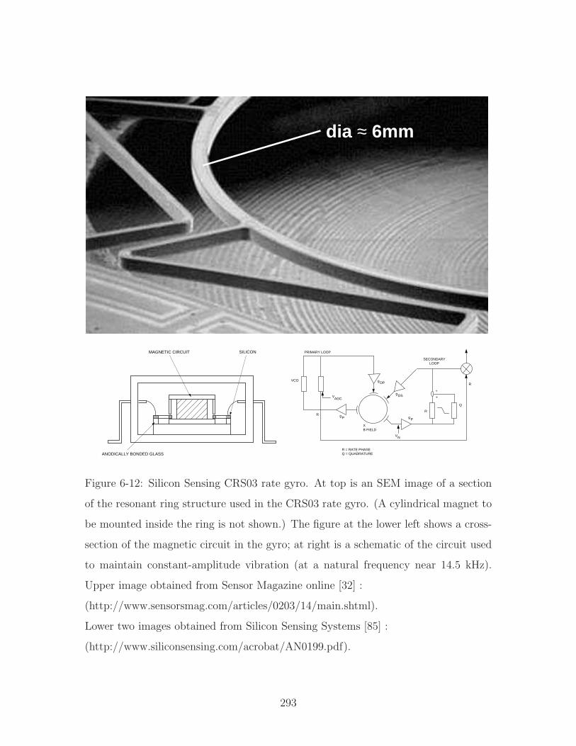
dia ≈ 6mm

Silicon Sensing Systems Application Note 3

The force developed by each drive transducerwith a voltage VD applied is given by:

F K V gr D D=

where:

K B Rr = 0 25. πand gD is the amps/volt gain of the current

amplifier, B is the magnetic field and R is theradius of the ring.

The signal developed by a pick-off transducer,which is a velocity detector, is given by:

V a KP P= ωa is the amplitude of the vibration at an angular

frequency ω and:

K B RP = 0 25. πThis signal is applied to an integrating amplifier

to give a signal VPO proportional to amplitude.

It can be shown that the transfer function of thehead on resonance is given by:

V

V

g g B Q R

h tPO

D

p D

r r

=2

8

πρ ω

where Q is the Quality factor of the resonance, hr

the width of the ring, tr the thickness of the of ring,ρ the density of silicon and gp is the volt/volt gainof the pick-off amp (note this is an integrator so gp

α 1/ω).

MAGNETIC CIRCUIT

ANODICALLY BONDED GLASS

SILICON

C.G. 15894

Figure 3. Hermetic Metal IC Can Package

ELECTRONIC CONTROL

Thusfar this paper has described the Siliconsensing element, which is the heart of thegyroscope. This obviously needs to be integratedwith control electronics in order to produce a fullyfunctional sensor. While it may be possible tooperate a gyro in an open-loop mode,considerable performance advantages are gainedby operating closed loop. Reference is made toFigure 4. The primary mode is controlled by the

primary loop which comprises both a VCO loop, tomaintain the vibration on resonance, and an AGCloop which maintains constant amplitude ofmotion. Under applied rotation, energy is coupledfrom the primary mode to the secondary mode. Itis possible to measure the amount of vibration onthe secondary pick-off as a measure of rate.However, in this implementation a secondary loopis used to maintain the secondary vibration at zero,and the amount of drive required to do this is ameasure of the applied rate. By maintaining aconstant modal pattern on the resonator thelinearity and bias of the system is improved. Thecombination of the AGC loop and the secondaryloop also serves to remove Q from the scalefactor.A fully open loop system would have a Q²dependence. The secondary loop comprises twoparts, a rate loop and a quadrature loop. The useof a quadrature loop to null quadrature motionsignificantly reduces errors due to frequencydifferences between the primary and secondarymodes.

C.G. 15895

R = RATE PHASEQ = QUADRATURE

R

R

Q

+

+

RATE OUT

SECONDARYLOOP

PRIMARY LOOP

VCO

AGCV

R

XB FIELD

NV

DSg

DPg

PgPg

Figure 4. Closed Loop Control Electronics

In order to understand the details of the closedloop electronics then a comprehensive error modelis required. Such a model has been developedwhich includes physical errors such as frequencysplit, delta Q, electrode misalignment and modemisalignment to electrode pattern, together withelectronic gain, phase and crosstalk errors. Thismodel is beyond the scope of this paper.

With reference to the closed loop scheme inFigure 4, and the drive and pick-off termsdescribed earlier, it is possible to examine the keyerror drivers to scale factor. These can besummarised as:

SFV

g g BAGC

DS p

α2

Where VAGC is the demand level of the AGC loopand gDS is amps/volt gain of the secondary driver

Silicon Sensing Systems Application Note 3

The force developed by each drive transducerwith a voltage VD applied is given by:

F K V gr D D=

where:

K B Rr = 0 25. πand gD is the amps/volt gain of the current

amplifier, B is the magnetic field and R is theradius of the ring.

The signal developed by a pick-off transducer,which is a velocity detector, is given by:

V a KP P= ωa is the amplitude of the vibration at an angular

frequency ω and:

K B RP = 0 25. πThis signal is applied to an integrating amplifier

to give a signal VPO proportional to amplitude.

It can be shown that the transfer function of thehead on resonance is given by:

V

V

g g B Q R

h tPO

D

p D

r r

=2

8

πρ ω

where Q is the Quality factor of the resonance, hr

the width of the ring, tr the thickness of the of ring,ρ the density of silicon and gp is the volt/volt gainof the pick-off amp (note this is an integrator so gp

α 1/ω).

MAGNETIC CIRCUIT

ANODICALLY BONDED GLASS

SILICON

C.G. 15894

Figure 3. Hermetic Metal IC Can Package

ELECTRONIC CONTROL

Thusfar this paper has described the Siliconsensing element, which is the heart of thegyroscope. This obviously needs to be integratedwith control electronics in order to produce a fullyfunctional sensor. While it may be possible tooperate a gyro in an open-loop mode,considerable performance advantages are gainedby operating closed loop. Reference is made toFigure 4. The primary mode is controlled by the

primary loop which comprises both a VCO loop, tomaintain the vibration on resonance, and an AGCloop which maintains constant amplitude ofmotion. Under applied rotation, energy is coupledfrom the primary mode to the secondary mode. Itis possible to measure the amount of vibration onthe secondary pick-off as a measure of rate.However, in this implementation a secondary loopis used to maintain the secondary vibration at zero,and the amount of drive required to do this is ameasure of the applied rate. By maintaining aconstant modal pattern on the resonator thelinearity and bias of the system is improved. Thecombination of the AGC loop and the secondaryloop also serves to remove Q from the scalefactor.A fully open loop system would have a Q²dependence. The secondary loop comprises twoparts, a rate loop and a quadrature loop. The useof a quadrature loop to null quadrature motionsignificantly reduces errors due to frequencydifferences between the primary and secondarymodes.

C.G. 15895

R = RATE PHASEQ = QUADRATURE

R

R

Q

+

+

RATE OUT

SECONDARYLOOP

PRIMARY LOOP

VCO

AGCV

R

XB FIELD

NV

DSg

DPg

PgPg

Figure 4. Closed Loop Control Electronics

In order to understand the details of the closedloop electronics then a comprehensive error modelis required. Such a model has been developedwhich includes physical errors such as frequencysplit, delta Q, electrode misalignment and modemisalignment to electrode pattern, together withelectronic gain, phase and crosstalk errors. Thismodel is beyond the scope of this paper.

With reference to the closed loop scheme inFigure 4, and the drive and pick-off termsdescribed earlier, it is possible to examine the keyerror drivers to scale factor. These can besummarised as:

SFV

g g BAGC

DS p

α2

Where VAGC is the demand level of the AGC loopand gDS is amps/volt gain of the secondary driver

Figure 6-12: Silicon Sensing CRS03 rate gyro. At top is an SEM image of a section

of the resonant ring structure used in the CRS03 rate gyro. (A cylindrical magnet to

be mounted inside the ring is not shown.) The figure at the lower left shows a cross-

section of the magnetic circuit in the gyro; at right is a schematic of the circuit used

to maintain constant-amplitude vibration (at a natural frequency near 14.5 kHz).

Upper image obtained from Sensor Magazine online [32] :

(http://www.sensorsmag.com/articles/0203/14/main.shtml).

Lower two images obtained from Silicon Sensing Systems [85] :

(http://www.siliconsensing.com/acrobat/AN0199.pdf).

293

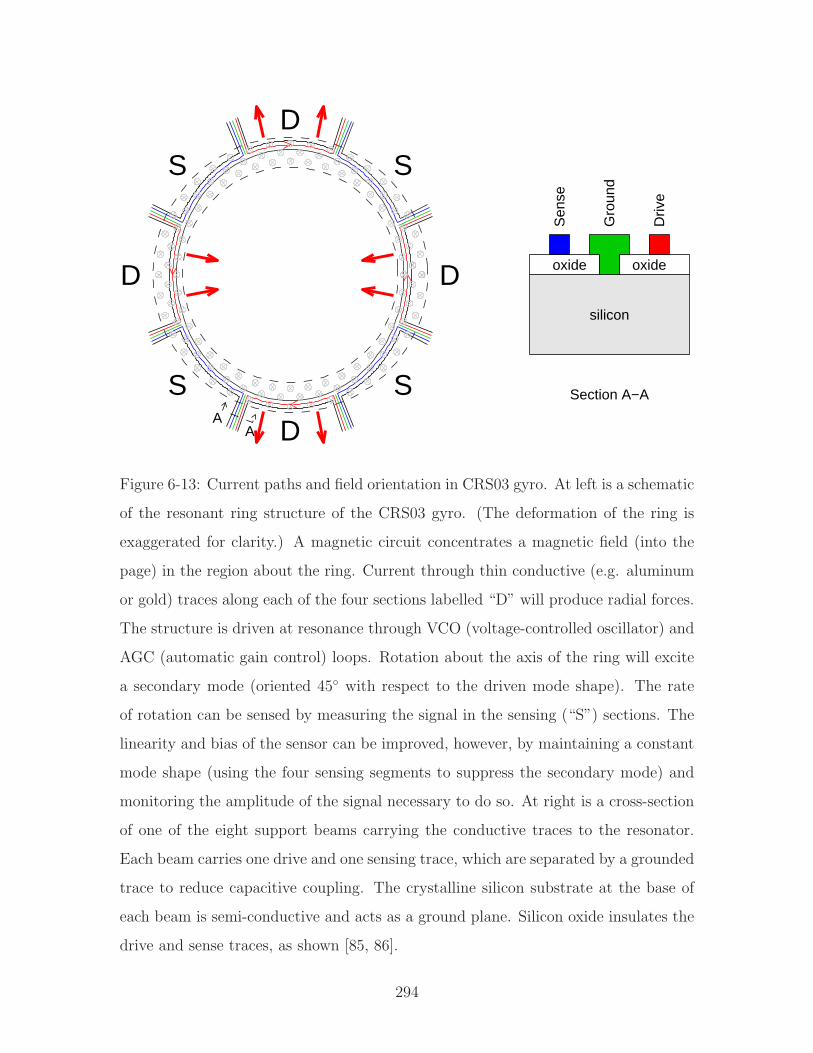
D

S

D

S

D

S

D

S

oxide oxide

silicon

Sen

se

Driv

e

Gro

und

Section A−A

AA

Figure 6-13: Current paths and field orientation in CRS03 gyro. At left is a schematic

of the resonant ring structure of the CRS03 gyro. (The deformation of the ring is

exaggerated for clarity.) A magnetic circuit concentrates a magnetic field (into the

page) in the region about the ring. Current through thin conductive (e.g. aluminum

or gold) traces along each of the four sections labelled “D” will produce radial forces.

The structure is driven at resonance through VCO (voltage-controlled oscillator) and

AGC (automatic gain control) loops. Rotation about the axis of the ring will excite

a secondary mode (oriented 45 with respect to the driven mode shape). The rate

of rotation can be sensed by measuring the signal in the sensing (“S”) sections. The

linearity and bias of the sensor can be improved, however, by maintaining a constant

mode shape (using the four sensing segments to suppress the secondary mode) and

monitoring the amplitude of the signal necessary to do so. At right is a cross-section

of one of the eight support beams carrying the conductive traces to the resonator.

Each beam carries one drive and one sensing trace, which are separated by a grounded

trace to reduce capacitive coupling. The crystalline silicon substrate at the base of

each beam is semi-conductive and acts as a ground plane. Silicon oxide insulates the

drive and sense traces, as shown [85, 86].

294

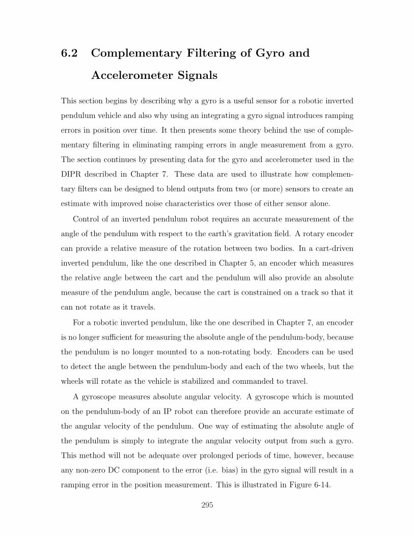
6.2 Complementary Filtering of Gyro and

Accelerometer Signals

This section begins by describing why a gyro is a useful sensor for a robotic inverted

pendulum vehicle and also why using an integrating a gyro signal introduces ramping

errors in position over time. It then presents some theory behind the use of comple-

mentary filtering in eliminating ramping errors in angle measurement from a gyro.

The section continues by presenting data for the gyro and accelerometer used in the

DIPR described in Chapter 7. These data are used to illustrate how complemen-

tary filters can be designed to blend outputs from two (or more) sensors to create an

estimate with improved noise characteristics over those of either sensor alone.

Control of an inverted pendulum robot requires an accurate measurement of the

angle of the pendulum with respect to the earth’s gravitation field. A rotary encoder

can provide a relative measure of the rotation between two bodies. In a cart-driven

inverted pendulum, like the one described in Chapter 5, an encoder which measures

the relative angle between the cart and the pendulum will also provide an absolute

measure of the pendulum angle, because the cart is constrained on a track so that it

can not rotate as it travels.

For a robotic inverted pendulum, like the one described in Chapter 7, an encoder

is no longer sufficient for measuring the absolute angle of the pendulum-body, because

the pendulum is no longer mounted to a non-rotating body. Encoders can be used

to detect the angle between the pendulum-body and each of the two wheels, but the

wheels will rotate as the vehicle is stabilized and commanded to travel.

A gyroscope measures absolute angular velocity. A gyroscope which is mounted

on the pendulum-body of an IP robot can therefore provide an accurate estimate of

the angular velocity of the pendulum. One way of estimating the absolute angle of

the pendulum is simply to integrate the angular velocity output from such a gyro.

This method will not be adequate over prolonged periods of time, however, because

any non-zero DC component to the error (i.e. bias) in the gyro signal will result in a

ramping error in the position measurement. This is illustrated in Figure 6-14.

295

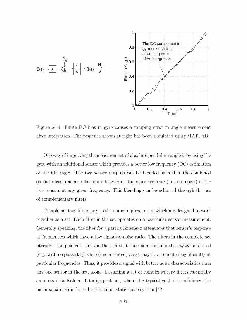
θ(s) s Σ 1s

Ng

θ(s) + N

g

s

0 0.2 0.4 0.6 0.8 10

0.2

0.4

0.6

0.8

1

Time

Err

or in

Ang

le

The DC component ingyro noise yieldsa ramping errorafter intergration

Figure 6-14: Finite DC bias in gyro causes a ramping error in angle measurement

after integration. The response shown at right has been simulated using MATLAB.

One way of improving the measurement of absolute pendulum angle is by using the

gyro with an additional sensor which provides a better low frequency (DC) estimation

of the tilt angle. The two sensor outputs can be blended such that the combined

output measurement relies more heavily on the more accurate (i.e. less noisy) of the

two sensors at any given frequency. This blending can be achieved through the use

of complementary filters.

Complementary filters are, as the name implies, filters which are designed to work

together as a set. Each filter in the set operates on a particular sensor measurement.

Generally speaking, the filter for a particular sensor attenuates that sensor’s response

at frequencies which have a low signal-to-noise ratio. The filters in the complete set

literally “complement” one another, in that their sum outputs the signal unaltered

(e.g. with no phase lag) while (uncorrelated) noise may be attenuated significantly at

particular frequencies. Thus, it provides a signal with better noise characteristics than

any one sensor in the set, alone. Designing a set of complementary filters essentially

amounts to a Kalman filtering problem, where the typical goal is to minimize the

mean-square error for a discrete-time, state-space system [42].

296

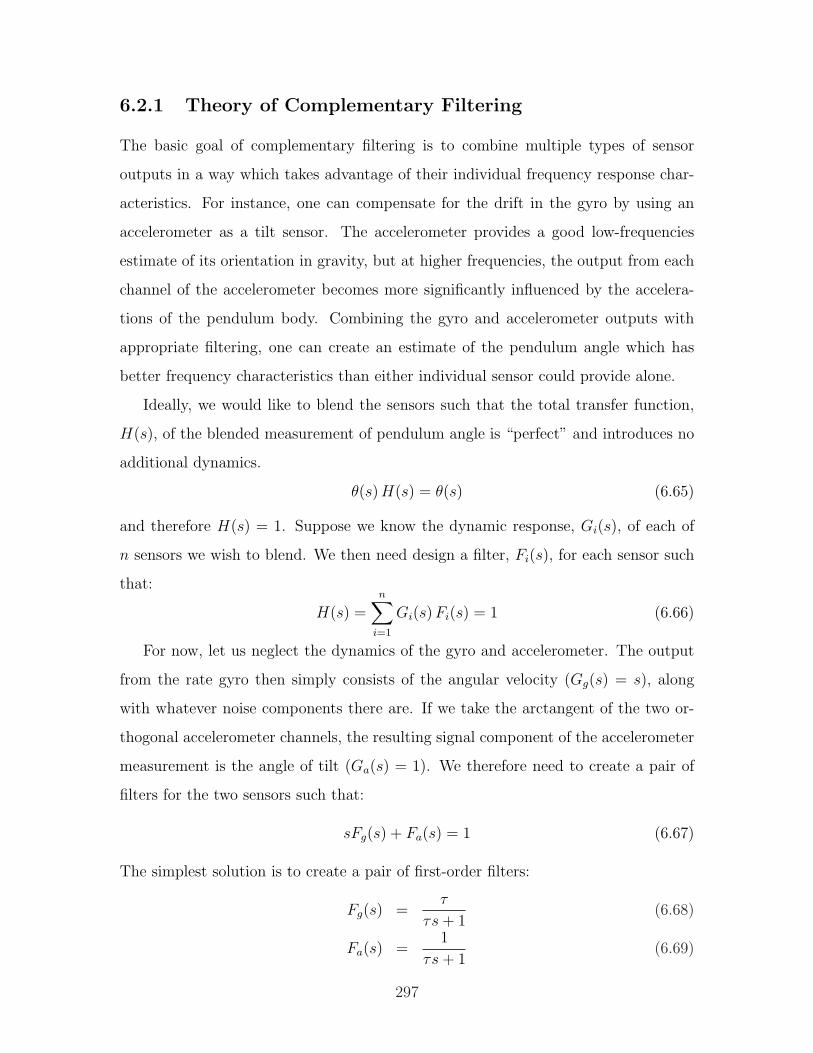
6.2.1 Theory of Complementary Filtering

The basic goal of complementary filtering is to combine multiple types of sensor

outputs in a way which takes advantage of their individual frequency response char-

acteristics. For instance, one can compensate for the drift in the gyro by using an

accelerometer as a tilt sensor. The accelerometer provides a good low-frequencies

estimate of its orientation in gravity, but at higher frequencies, the output from each

channel of the accelerometer becomes more significantly influenced by the accelera-

tions of the pendulum body. Combining the gyro and accelerometer outputs with

appropriate filtering, one can create an estimate of the pendulum angle which has

better frequency characteristics than either individual sensor could provide alone.

Ideally, we would like to blend the sensors such that the total transfer function,

H(s), of the blended measurement of pendulum angle is “perfect” and introduces no

additional dynamics.

θ(s) H(s) = θ(s) (6.65)

and therefore H(s) = 1. Suppose we know the dynamic response, Gi(s), of each of

n sensors we wish to blend. We then need design a filter, Fi(s), for each sensor such

that:

H(s) =n∑

i=1

Gi(s) Fi(s) = 1 (6.66)

For now, let us neglect the dynamics of the gyro and accelerometer. The output

from the rate gyro then simply consists of the angular velocity (Gg(s) = s), along

with whatever noise components there are. If we take the arctangent of the two or-

thogonal accelerometer channels, the resulting signal component of the accelerometer

measurement is the angle of tilt (Ga(s) = 1). We therefore need to create a pair of

filters for the two sensors such that:

sFg(s) + Fa(s) = 1 (6.67)

The simplest solution is to create a pair of first-order filters:

Fg(s) =τ

τs + 1(6.68)

Fa(s) =1

τs + 1(6.69)

297

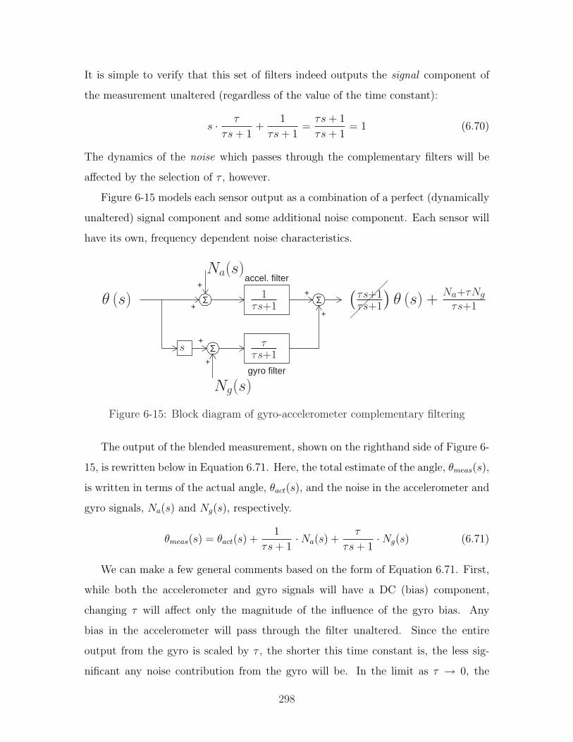
It is simple to verify that this set of filters indeed outputs the signal component of

the measurement unaltered (regardless of the value of the time constant):

s · τ

τs + 1+

1

τs + 1=

τs + 1

τs + 1= 1 (6.70)

The dynamics of the noise which passes through the complementary filters will be

affected by the selection of τ , however.

Figure 6-15 models each sensor output as a combination of a perfect (dynamically

unaltered) signal component and some additional noise component. Each sensor will

have its own, frequency dependent noise characteristics.

Σ

Σ

accel. filter

gyro filter

Σ

+

+

+

+

+

+

(τs+1τs+1

)θ (s) +

Na+τNg

τs+1θ (s) 1τs+1

ττs+1

Na(s)

Ng(s)

s

¡¡

¡¡

Figure 6-15: Block diagram of gyro-accelerometer complementary filtering

The output of the blended measurement, shown on the righthand side of Figure 6-

15, is rewritten below in Equation 6.71. Here, the total estimate of the angle, θmeas(s),

is written in terms of the actual angle, θact(s), and the noise in the accelerometer and

gyro signals, Na(s) and Ng(s), respectively.

θmeas(s) = θact(s) +1

τs + 1·Na(s) +

τ

τs + 1·Ng(s) (6.71)

We can make a few general comments based on the form of Equation 6.71. First,

while both the accelerometer and gyro signals will have a DC (bias) component,

changing τ will affect only the magnitude of the influence of the gyro bias. Any

bias in the accelerometer will pass through the filter unaltered. Since the entire

output from the gyro is scaled by τ , the shorter this time constant is, the less sig-

nificant any noise contribution from the gyro will be. In the limit as τ → 0, the

298

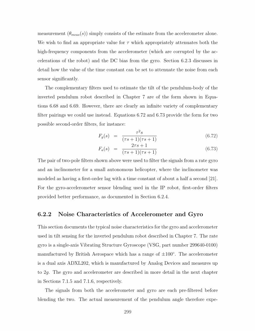
measurement (θmeas(s)) simply consists of the estimate from the accelerometer alone.

We wish to find an appropriate value for τ which appropriately attenuates both the

high-frequency components from the accelerometer (which are corrupted by the ac-

celerations of the robot) and the DC bias from the gyro. Section 6.2.3 discusses in

detail how the value of the time constant can be set to attenuate the noise from each

sensor significantly.

The complementary filters used to estimate the tilt of the pendulum-body of the

inverted pendulum robot described in Chapter 7 are of the form shown in Equa-

tions 6.68 and 6.69. However, there are clearly an infinite variety of complementary

filter pairings we could use instead. Equations 6.72 and 6.73 provide the form for two

possible second-order filters, for instance:

Fg(s) =τ 2s

(τs + 1)(τs + 1)(6.72)

Fa(s) =2τs + 1

(τs + 1)(τs + 1)(6.73)

The pair of two-pole filters shown above were used to filter the signals from a rate gyro

and an inclinometer for a small autonomous helicopter, where the inclinometer was

modeled as having a first-order lag with a time constant of about a half a second [21].

For the gyro-accelerometer sensor blending used in the IP robot, first-order filters

provided better performance, as documented in Section 6.2.4.

6.2.2 Noise Characteristics of Accelerometer and Gyro

This section documents the typical noise characteristics for the gyro and accelerometer

used in tilt sensing for the inverted pendulum robot described in Chapter 7. The rate

gyro is a single-axis Vibrating Structure Gyroscope (VSG, part number 299640-0100)

manufactured by British Aerospace which has a range of ±100. The accelerometer

is a dual axis ADXL202, which is manufactured by Analog Devices and measures up

to 2g. The gyro and accelerometer are described in more detail in the next chapter

in Sections 7.1.5 and 7.1.6, respectively.

The signals from both the accelerometer and gyro are each pre-filtered before

blending the two. The actual measurement of the pendulum angle therefore expe-

299

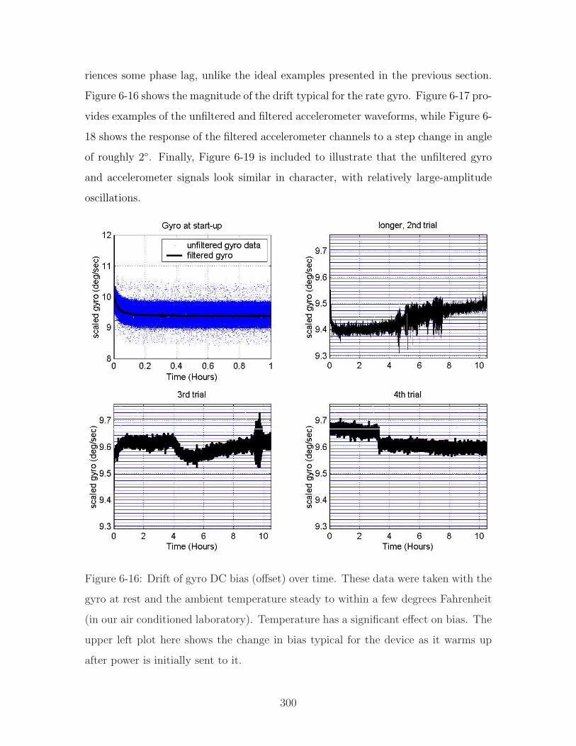
riences some phase lag, unlike the ideal examples presented in the previous section.

Figure 6-16 shows the magnitude of the drift typical for the rate gyro. Figure 6-17 pro-

vides examples of the unfiltered and filtered accelerometer waveforms, while Figure 6-

18 shows the response of the filtered accelerometer channels to a step change in angle

of roughly 2. Finally, Figure 6-19 is included to illustrate that the unfiltered gyro

and accelerometer signals look similar in character, with relatively large-amplitude

oscillations.

Figure 6-16: Drift of gyro DC bias (offset) over time. These data were taken with the

gyro at rest and the ambient temperature steady to within a few degrees Fahrenheit

(in our air conditioned laboratory). Temperature has a significant effect on bias. The

upper left plot here shows the change in bias typical for the device as it warms up

after power is initially sent to it.

300

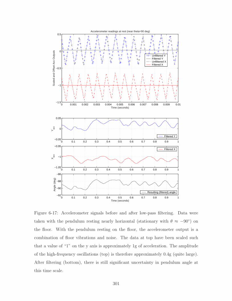
0 0.001 0.002 0.003 0.004 0.005 0.006 0.007 0.008 0.009 0.01−1.5

−1

−0.5

0

0.5

Time (seconds)

Sca

led

and

Offs

et A

cc O

utpu

ts

Accelerometer readings at rest (near theta=90 deg)

Unfiltered YFiltered YUnfilitered XFiltered X

0 0.1 0.2 0.3 0.4 0.5 0.6 0.7 0.8 0.9 1−0.05

0

0.05

Yac

c

Filtered Y

0 0.1 0.2 0.3 0.4 0.5 0.6 0.7 0.8 0.9 1−1.05

−1

−0.95

Xac

c

Filtered X

0 0.1 0.2 0.3 0.4 0.5 0.6 0.7 0.8 0.9 1−92

−90

−88

−86

Time (seconds)

Ang

le (

deg)

Resulting (filtered) angle

Figure 6-17: Accelerometer signals before and after low-pass filtering. Data were

taken with the pendulum resting nearly horizontal (stationary with θ ≈ −90) on

the floor. With the pendulum resting on the floor, the accelerometer output is a

combination of floor vibrations and noise. The data at top have been scaled such

that a value of “1” on the y axis is approximately 1g of acceleration. The amplitude

of the high-frequency oscillations (top) is therefore approximately 0.4g (quite large).

After filtering (bottom), there is still significant uncertainty in pendulum angle at

this time scale.

301

0 0.5 1 1.5 2 2.5 3

0.05

0.1

Yac

cAccelerometer response to small step change in angle

Filtered Y

0 0.5 1 1.5 2 2.5 3

−1.04

−1.02

−1

−0.98

Xac

c

Filtered X

0 0.5 1 1.5 2 2.5 3−88

−86

−84

−82

Time (seconds)

Ang

le (

deg)

Resulting (filtered) angle

Figure 6-18: Accelerometer signals during a small step change in pendulum angle.

The pendulum angle changed by two degrees at t ≈ 1.8 seconds in the traces shown

above. Note the magnitude of the “noise” (consisting of seismic or other vibrations of

the floor and any sensor noise) in the accelerometer measurement of pendulum angle

at this time scale, as compared with the gyro measurement (with low frequency drift

compensation from the accelerometers). The accelerometer is not accurate enough

to be used in measuring the pendulum angle directly. Also note that the top and

bottom plots are almost identical (through a scaling factor). When the pendulum is

within a few degrees of being vertical or horizontal, the output angle is essentially

a scaled version of the output of just one of the accelerometer axes, while the other

signal essentially serves as a sign bit.

302

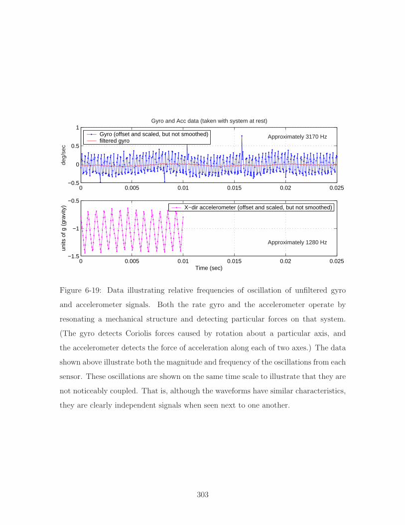
0 0.005 0.01 0.015 0.02 0.025−0.5

0

0.5

1Gyro and Acc data (taken with system at rest)

deg/

sec

Approximately 3170 HzGyro (offset and scaled, but not smoothed)filtered gyro

0 0.005 0.01 0.015 0.02 0.025−1.5

−1

−0.5

Time (sec)

units

of g

(gr

avity

)

Approximately 1280 Hz

X−dir accelerometer (offset and scaled, but not smoothed)

Figure 6-19: Data illustrating relative frequencies of oscillation of unfiltered gyro

and accelerometer signals. Both the rate gyro and the accelerometer operate by

resonating a mechanical structure and detecting particular forces on that system.

(The gyro detects Coriolis forces caused by rotation about a particular axis, and

the accelerometer detects the force of acceleration along each of two axes.) The data

shown above illustrate both the magnitude and frequency of the oscillations from each

sensor. These oscillations are shown on the same time scale to illustrate that they are

not noticeably coupled. That is, although the waveforms have similar characteristics,

they are clearly independent signals when seen next to one another.

303

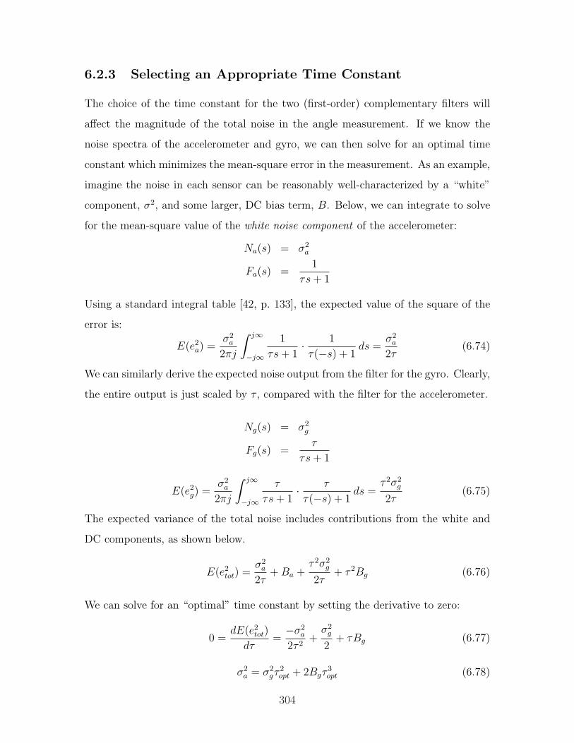
6.2.3 Selecting an Appropriate Time Constant

The choice of the time constant for the two (first-order) complementary filters will

affect the magnitude of the total noise in the angle measurement. If we know the

noise spectra of the accelerometer and gyro, we can then solve for an optimal time

constant which minimizes the mean-square error in the measurement. As an example,

imagine the noise in each sensor can be reasonably well-characterized by a “white”

component, σ2, and some larger, DC bias term, B. Below, we can integrate to solve

for the mean-square value of the white noise component of the accelerometer:

Na(s) = σ2a

Fa(s) =1

τs + 1

Using a standard integral table [42, p. 133], the expected value of the square of the

error is:

E(e2a) =

σ2a

2πj

∫ j∞

−j∞

1

τs + 1· 1

τ(−s) + 1ds =

σ2a

2τ(6.74)

We can similarly derive the expected noise output from the filter for the gyro. Clearly,

the entire output is just scaled by τ , compared with the filter for the accelerometer.

Ng(s) = σ2g

Fg(s) =τ

τs + 1

E(e2g) =

σ2a

2πj

∫ j∞

−j∞

τ

τs + 1· τ

τ(−s) + 1ds =

τ 2σ2g

2τ(6.75)

The expected variance of the total noise includes contributions from the white and

DC components, as shown below.

E(e2tot) =

σ2a

2τ+ Ba +

τ 2σ2g

2τ+ τ 2Bg (6.76)

We can solve for an “optimal” time constant by setting the derivative to zero:

0 =dE(e2

tot)

dτ=−σ2

a

2τ 2+

σ2g

2+ τBg (6.77)

σ2a = σ2

gτ2opt + 2Bgτ

3opt (6.78)

304

If the gyro and accelerometer noise are both truly white (in particular, if there is

no predominant DC bias component in the gyro), then τopt = σa/σg. In the limit as

σg → 0 (or as σa → ∞), then τopt → ∞. That is, as the gyro noise gets vanishingly

small, there is no longer any reason to compensate with the accelerometer, and we

would simply use the integrated gyro signal to estimate the tilt angle. In the other

extreme where the accelerometer signal is far superior to the gyro (as σg →∞, or as

σa → 0), then τopt → 0, and we would use the unfiltered accelerometer signal, alone.

The piezoelectric shell-type resonator used in the BASE gyro is plagued by sig-

nificant, temperature-dependent bias. There is an (unused) temperature output for

the gyro. I have chosen not to use the temperature output, and the measurement of

pendulum angle is in fact adequate without it. This temperature effect will have an

influence on the noise characteristics of the robot, however, particularly if it is not

run in an air-conditioned environment (like out lab). Figure 6-16 shows the drift in

bias over a long (10-hr) time scale. For an hour-long run, the magnitude of the drift

in bias can be on the order of two or three times the magnitude of the white noise or

more, depending on ambient temperature changes - the temperature-dependent drift

in bias is on the order of .01 deg/sec/oF of temperature change.

The complementary filters for the DIPR currently use τ = 1 s. The noise data and

captions in Figures 6-20 and 6-21 are included to justify this choice. Both the gyro

and accelerometer outputs are pre-filtered in addition to the complementary filtering

performed on each signal. The BASE gyro is pre-filtered with a single-pole low-pass

filter which matches the bandwidth of 75 Hz of the device. The accelerometer channels

are pre-filtered before taking an arctangent to estimate tilt angle.

The accelerometer compensates for the DC bias in the gyro, and the bandwidth

of the pre-filtered accelerometer is only a few Hertz. At the lower right of Figure 6-20

is the noise spectrum of the pre-filtered angle measurement from the accelerometer

(taken with the pendulum at rest). If this were reasonably flat, one could solve

Equation 6.77 explicitly to find the optimal time constant. I have instead used actual

data to calculate the magnitude of various noise components as a function of τ . This

data is shown in Figure 6-21.

305

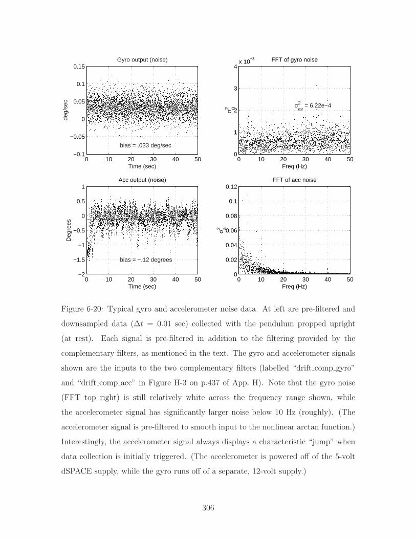
0 10 20 30 40 50−0.1

−0.05

0

0.05

0.1

0.15

Time (sec)

deg/

sec

Gyro output (noise)

bias = .033 deg/sec

0 10 20 30 40 500

1

2

3

4x 10

−3 FFT of gyro noise

Freq (Hz)

σ g2 σav2 = 6.22e−4

0 10 20 30 40 50−2

−1.5

−1

−0.5

0

0.5

1

Time (sec)

Deg

rees

Acc output (noise)

bias = −.12 degrees

0 10 20 30 40 500

0.02

0.04

0.06

0.08

0.1

0.12

Freq (Hz)

FFT of acc noise

σ a2

Figure 6-20: Typical gyro and accelerometer noise data. At left are pre-filtered and

downsampled data (∆t = 0.01 sec) collected with the pendulum propped upright

(at rest). Each signal is pre-filtered in addition to the filtering provided by the

complementary filters, as mentioned in the text. The gyro and accelerometer signals

shown are the inputs to the two complementary filters (labelled “drift comp gyro”

and “drift comp acc” in Figure H-3 on p.437 of App. H). Note that the gyro noise

(FFT top right) is still relatively white across the frequency range shown, while

the accelerometer signal has significantly larger noise below 10 Hz (roughly). (The

accelerometer signal is pre-filtered to smooth input to the nonlinear arctan function.)

Interestingly, the accelerometer signal always displays a characteristic “jump” when

data collection is initially triggered. (The accelerometer is powered off of the 5-volt

dSPACE supply, while the gyro runs off of a separate, 12-volt supply.)

306

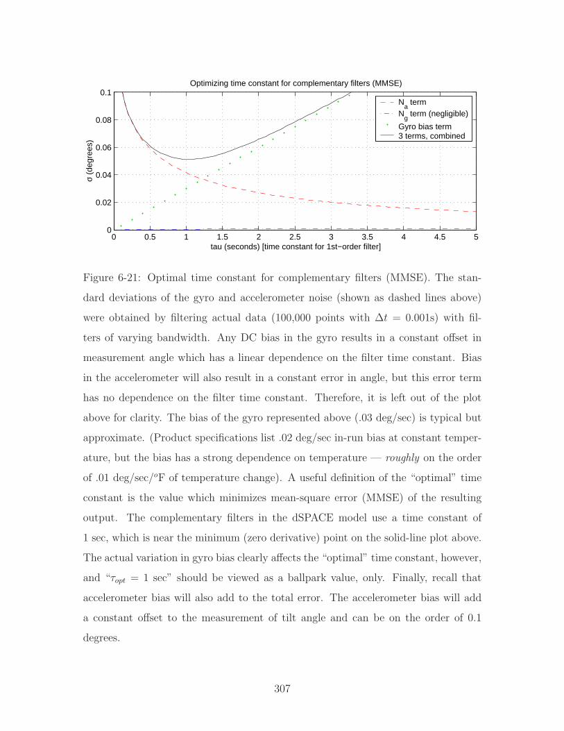
0 0.5 1 1.5 2 2.5 3 3.5 4 4.5 50

0.02

0.04

0.06

0.08

0.1

tau (seconds) [time constant for 1st−order filter]

σ (d

egre

es)

Optimizing time constant for complementary filters (MMSE)

Na term

Ng term (negligible)

Gyro bias term3 terms, combined

Figure 6-21: Optimal time constant for complementary filters (MMSE). The stan-

dard deviations of the gyro and accelerometer noise (shown as dashed lines above)

were obtained by filtering actual data (100,000 points with ∆t = 0.001s) with fil-

ters of varying bandwidth. Any DC bias in the gyro results in a constant offset in

measurement angle which has a linear dependence on the filter time constant. Bias

in the accelerometer will also result in a constant error in angle, but this error term

has no dependence on the filter time constant. Therefore, it is left out of the plot

above for clarity. The bias of the gyro represented above (.03 deg/sec) is typical but

approximate. (Product specifications list .02 deg/sec in-run bias at constant temper-

ature, but the bias has a strong dependence on temperature — roughly on the order

of .01 deg/sec/oF of temperature change). A useful definition of the “optimal” time

constant is the value which minimizes mean-square error (MMSE) of the resulting

output. The complementary filters in the dSPACE model use a time constant of

1 sec, which is near the minimum (zero derivative) point on the solid-line plot above.

The actual variation in gyro bias clearly affects the “optimal” time constant, however,

and “τopt = 1 sec” should be viewed as a ballpark value, only. Finally, recall that

accelerometer bias will also add to the total error. The accelerometer bias will add

a constant offset to the measurement of tilt angle and can be on the order of 0.1

degrees.

307

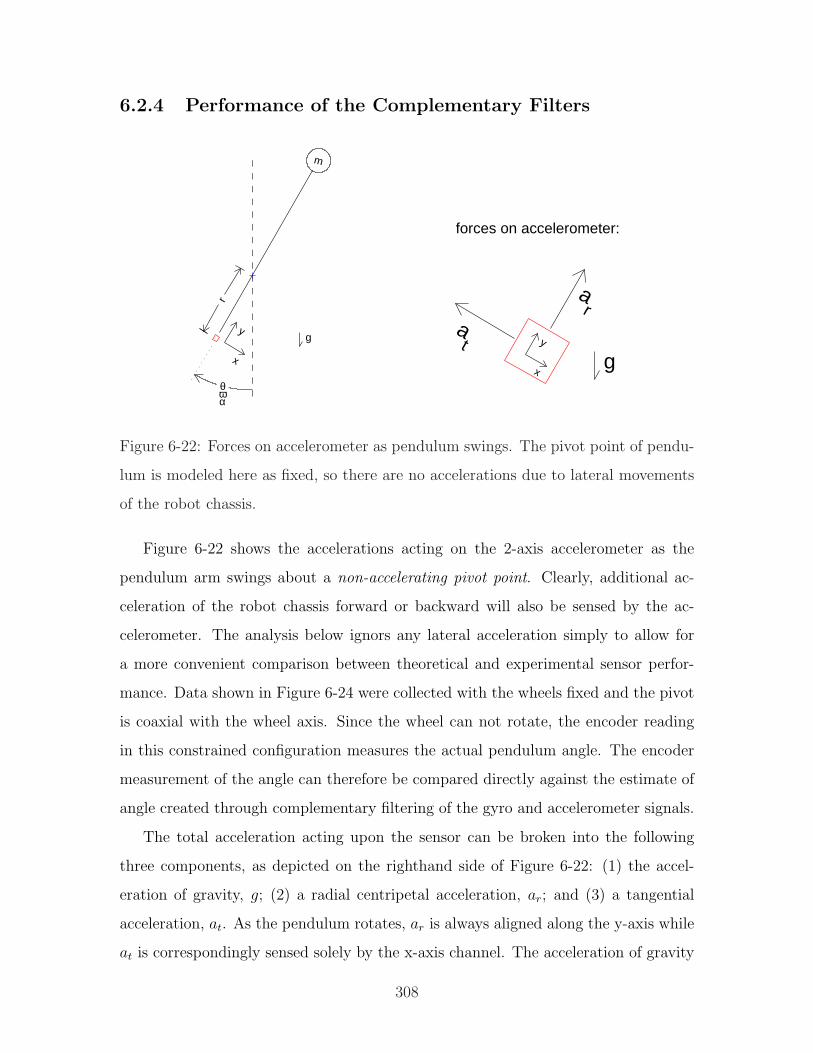
6.2.4 Performance of the Complementary Filters

m

θωα

x

yg

r

x

y

ar

at

forces on accelerometer:

g

Figure 6-22: Forces on accelerometer as pendulum swings. The pivot point of pendu-

lum is modeled here as fixed, so there are no accelerations due to lateral movements

of the robot chassis.

Figure 6-22 shows the accelerations acting on the 2-axis accelerometer as the

pendulum arm swings about a non-accelerating pivot point. Clearly, additional ac-

celeration of the robot chassis forward or backward will also be sensed by the ac-

celerometer. The analysis below ignors any lateral acceleration simply to allow for

a more convenient comparison between theoretical and experimental sensor perfor-

mance. Data shown in Figure 6-24 were collected with the wheels fixed and the pivot

is coaxial with the wheel axis. Since the wheel can not rotate, the encoder reading

in this constrained configuration measures the actual pendulum angle. The encoder

measurement of the angle can therefore be compared directly against the estimate of

angle created through complementary filtering of the gyro and accelerometer signals.

The total acceleration acting upon the sensor can be broken into the following

three components, as depicted on the righthand side of Figure 6-22: (1) the accel-

eration of gravity, g; (2) a radial centripetal acceleration, ar; and (3) a tangential

acceleration, at. As the pendulum rotates, ar is always aligned along the y-axis while

at is correspondingly sensed solely by the x-axis channel. The acceleration of gravity

308

is sensed by each axis as the cosine or sine of the pendulum angle:

ay = −ar − g · cos(θ) (6.79)

ax = at + g · sin(θ) (6.80)

The centripetal acceleration, ar, is proportional to the square of the angular ve-

locity. The sign of this component and of gravity will both be negative, with respect

to the axis orientation shown in Figure 6-22. If the pendulum is not rotating at a con-

stant angular velocity, then its angular acceleration will be sensed along the x-axis.

Equations 6.81 and 6.82 summarize these forces.

ar = rω2 = r

(dθ

dt

)2

(6.81)

at = rα = rd2θ

dt2(6.82)

Recall that the entire point of using the accelerometer is to detect the direction of

gravity. Therefore, we would like to minimize the detection of any other accelerations

and should therefore locate the accelerometer as close as practical to the pendulum

pivot (so that r ≈ 0). The robot has been tested with the ADXL202 located coaxial

with the wheel axis. The accelerometer is currently mounted approximately 3” below

the pivot point of the pendulum, however, to make the wiring and debugging of

the robot more accessible. Any difference in performance between the coaxial and

off-center the accelerometer positions was not noticeable. The simulations and data

shown here all correspond to an accelerometer mounted 3” below the pivot point.

Figure 6-23 shows simulated estimates of the pendulum angle, while Figure 6-

24 provides actual data taken with the wheels of the DIPR fixed in place and the

pendulum moved rapidly by hand. Complementary filtering in the DIPR currently

uses the single-pole filters shown in Equations 6.68 and 6.69 with a time constant,

τ , of one second. This value was determined to be close to “optimal” as defined in

the previous section. The lower half of Figure 6-23 compares theoretical outputs with

values of τ a factor of four faster and slower than this.

309

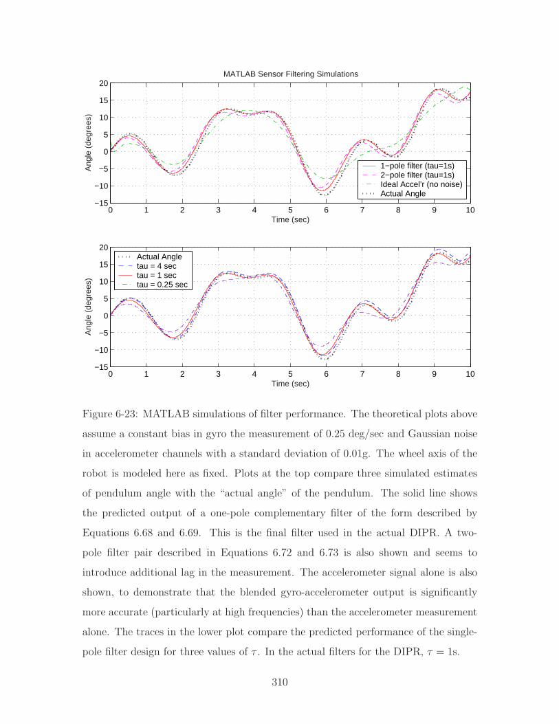
0 1 2 3 4 5 6 7 8 9 10−15

−10

−5

0

5

10

15

20MATLAB Sensor Filtering Simulations

Time (sec)

Ang

le (

degr

ees)

1−pole filter (tau=1s)2−pole filter (tau=1s)Ideal Accel’r (no noise)Actual Angle

0 1 2 3 4 5 6 7 8 9 10−15

−10

−5

0

5

10

15

20

Time (sec)

Ang

le (

degr

ees)

Actual Angletau = 4 sectau = 1 sectau = 0.25 sec

Figure 6-23: MATLAB simulations of filter performance. The theoretical plots above

assume a constant bias in gyro the measurement of 0.25 deg/sec and Gaussian noise

in accelerometer channels with a standard deviation of 0.01g. The wheel axis of the

robot is modeled here as fixed. Plots at the top compare three simulated estimates

of pendulum angle with the “actual angle” of the pendulum. The solid line shows

the predicted output of a one-pole complementary filter of the form described by

Equations 6.68 and 6.69. This is the final filter used in the actual DIPR. A two-

pole filter pair described in Equations 6.72 and 6.73 is also shown and seems to

introduce additional lag in the measurement. The accelerometer signal alone is also

shown, to demonstrate that the blended gyro-accelerometer output is significantly

more accurate (particularly at high frequencies) than the accelerometer measurement

alone. The traces in the lower plot compare the predicted performance of the single-

pole filter design for three values of τ . In the actual filters for the DIPR, τ = 1s.

310

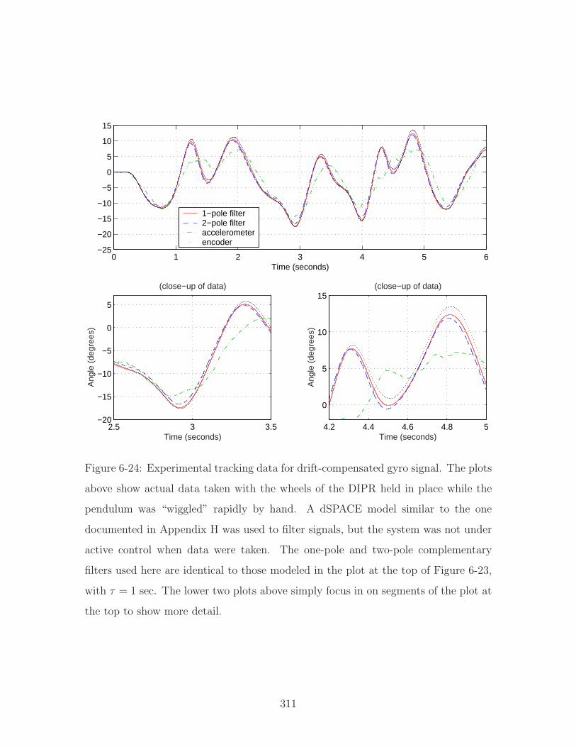
0 1 2 3 4 5 6−25

−20

−15

−10

−5

0

5

10

15

Time (seconds)

1−pole filter2−pole filteraccelerometerencoder

2.5 3 3.5−20

−15

−10

−5

0

5

Time (seconds)

Ang

le (

degr

ees)

(close−up of data)

4.2 4.4 4.6 4.8 5

0

5

10

15

Time (seconds)

Ang

le (

degr

ees)

(close−up of data)

Figure 6-24: Experimental tracking data for drift-compensated gyro signal. The plots

above show actual data taken with the wheels of the DIPR held in place while the

pendulum was “wiggled” rapidly by hand. A dSPACE model similar to the one

documented in Appendix H was used to filter signals, but the system was not under

active control when data were taken. The one-pole and two-pole complementary

filters used here are identical to those modeled in the plot at the top of Figure 6-23,

with τ = 1 sec. The lower two plots above simply focus in on segments of the plot at

the top to show more detail.

311

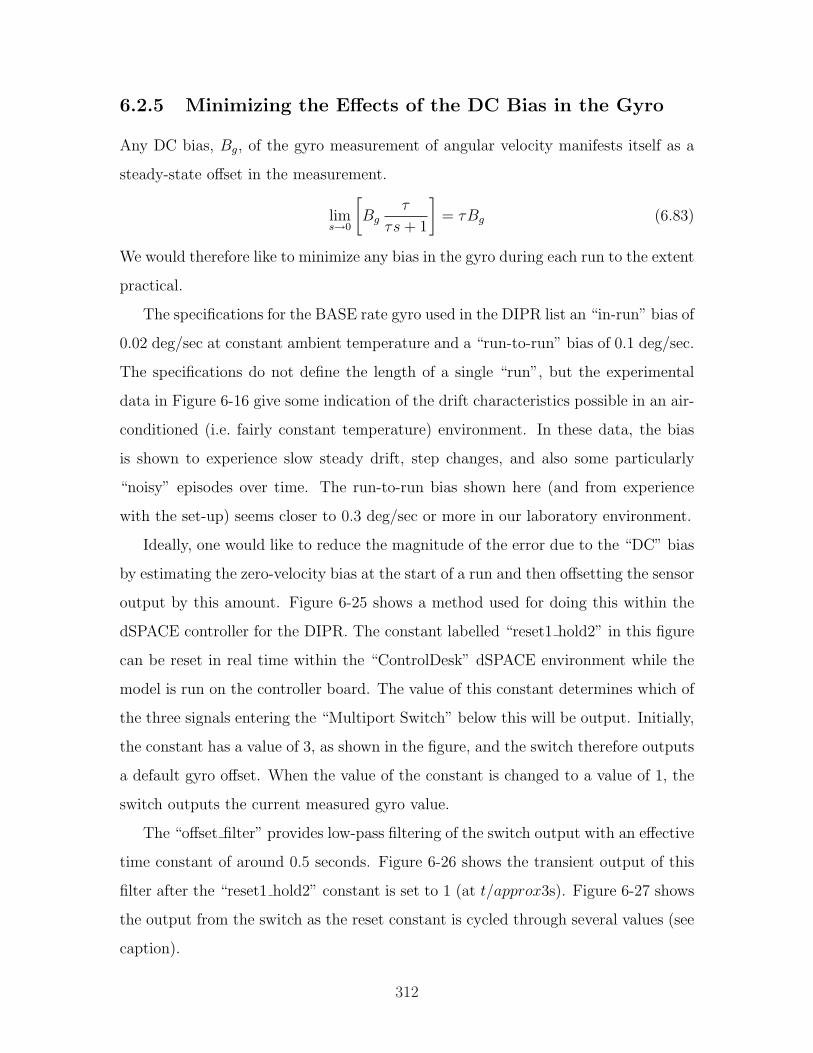
6.2.5 Minimizing the Effects of the DC Bias in the Gyro

Any DC bias, Bg, of the gyro measurement of angular velocity manifests itself as a

steady-state offset in the measurement.

lims→0

[Bg

τ

τs + 1

]= τBg (6.83)

We would therefore like to minimize any bias in the gyro during each run to the extent

practical.

The specifications for the BASE rate gyro used in the DIPR list an “in-run” bias of

0.02 deg/sec at constant ambient temperature and a “run-to-run” bias of 0.1 deg/sec.

The specifications do not define the length of a single “run”, but the experimental

data in Figure 6-16 give some indication of the drift characteristics possible in an air-

conditioned (i.e. fairly constant temperature) environment. In these data, the bias

is shown to experience slow steady drift, step changes, and also some particularly

“noisy” episodes over time. The run-to-run bias shown here (and from experience

with the set-up) seems closer to 0.3 deg/sec or more in our laboratory environment.

Ideally, one would like to reduce the magnitude of the error due to the “DC” bias

by estimating the zero-velocity bias at the start of a run and then offsetting the sensor

output by this amount. Figure 6-25 shows a method used for doing this within the

dSPACE controller for the DIPR. The constant labelled “reset1 hold2” in this figure

can be reset in real time within the “ControlDesk” dSPACE environment while the

model is run on the controller board. The value of this constant determines which of

the three signals entering the “Multiport Switch” below this will be output. Initially,

the constant has a value of 3, as shown in the figure, and the switch therefore outputs

a default gyro offset. When the value of the constant is changed to a value of 1, the

switch outputs the current measured gyro value.

The “offset filter” provides low-pass filtering of the switch output with an effective

time constant of around 0.5 seconds. Figure 6-26 shows the transient output of this

filter after the “reset1 hold2” constant is set to 1 (at t/approx3s). Figure 6-27 shows

the output from the switch as the reset constant is cycled through several values (see

caption).

312

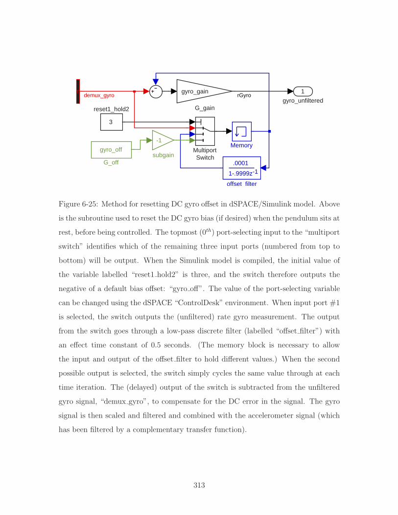
1

gyro_unfiltered

-1

subgain

3

reset1_hold2

.0001

1-.9999z -1

offset_filter

MultiportSwitch

Memorygyro_off

G_off

gyro_gain

G_gain

DemuxrGyrodemux_gyro

Figure 6-25: Method for resetting DC gyro offset in dSPACE/Simulink model. Above

is the subroutine used to reset the DC gyro bias (if desired) when the pendulum sits at

rest, before being controlled. The topmost (0th) port-selecting input to the “multiport

switch” identifies which of the remaining three input ports (numbered from top to

bottom) will be output. When the Simulink model is compiled, the initial value of

the variable labelled “reset1 hold2” is three, and the switch therefore outputs the

negative of a default bias offset: “gyro off”. The value of the port-selecting variable

can be changed using the dSPACE “ControlDesk” environment. When input port #1

is selected, the switch outputs the (unfiltered) rate gyro measurement. The output

from the switch goes through a low-pass discrete filter (labelled “offset filter”) with

an effect time constant of 0.5 seconds. (The memory block is necessary to allow

the input and output of the offset filter to hold different values.) When the second

possible output is selected, the switch simply cycles the same value through at each

time iteration. The (delayed) output of the switch is subtracted from the unfiltered

gyro signal, “demux gyro”, to compensate for the DC error in the signal. The gyro

signal is then scaled and filtered and combined with the accelerometer signal (which

has been filtered by a complementary transfer function).

313

3 3.5 4 4.5 5 5.5 6 6.5 7 7.5

−.08

−.06

−.04

−.02

.00

What happens during a gyro offset reset

Time (seconds)

Gyr

o D

C O

ffset

(de

g/se

c)

Filtered Gyro Offset

13 13.5 14 14.5 15 15.5 16 16.5 17 17.5 18

−.08

−.06

−.04

−.02

.00

Time (seconds)

Gyr

o D

C O

ffset

(de

g/se

c)

Figure 6-26: Transient response during a reset of the gyro offset. This figure shows

data (taken while the pendulum was at rest) of a transition from the default gyro offset

to the measured DC bias. The time constant to reach a steady-state measurement of

the bias is 0.5 seconds. The output above is scaled to correspond to angular velocity

units of degrees per second. The DC offset in the measured pendulum angle will

be proportional to the DC bias in the gyro measurement: θe = τcf · θbias, where τcf

is the time constant used in the complementary filters. For the inverted pendulum

robot, τcf = 1.0 sec. In other words, since the initial bias shown at the lefthand side

of this plot is approximately -.065 deg/s, these data indicate the DC error in the

measurement of the pendulum angle would be about 1.0[s]·0.065[deg/s]= 0.065 [deg]

(quite small) if the default bias value were used.

314

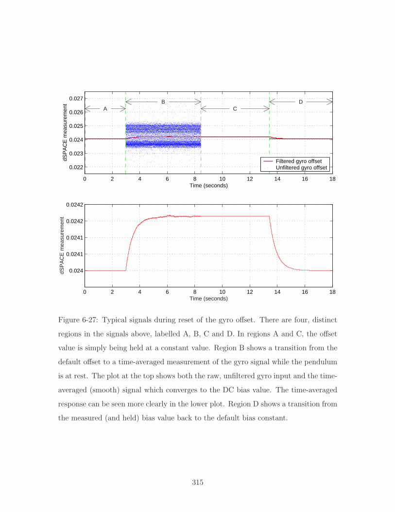
0 2 4 6 8 10 12 14 16 18

0.022

0.023

0.024

0.025

0.026

0.027

Time (seconds)

dSP

AC

E m

easu

rem

ent

AB

CD

Filtered gyro offsetUnfiltered gyro offset

0 2 4 6 8 10 12 14 16 18

0.024

0.0241

0.0241

0.0242

0.0242

dSP

AC

E m

easu

rem

ent

Time (seconds)

Figure 6-27: Typical signals during reset of the gyro offset. There are four, distinct

regions in the signals above, labelled A, B, C and D. In regions A and C, the offset

value is simply being held at a constant value. Region B shows a transition from the

default offset to a time-averaged measurement of the gyro signal while the pendulum

is at rest. The plot at the top shows both the raw, unfiltered gyro input and the time-

averaged (smooth) signal which converges to the DC bias value. The time-averaged

response can be seen more clearly in the lower plot. Region D shows a transition from

the measured (and held) bias value back to the default bias constant.

315

This simple reset method significantly reduces the bias during a typical run of

the DIPR. The inverted pendulum robot named “Joe” which is described on page 74

of Chapter 2 also uses a compensation scheme which measures the initial gyro bias

with the system at rest just before running the controller. For Joe, the subsequent

in-run bias is small enough that the robot can operate for several minutes without

any additional compensation for drift. Joe operates without using a low-frequency

tilt sensor (e.g. an accelerometer) or complementary filtering.

6.3 Conclusions

A gyroscope is a key sensor for obtaining an absolute measure of pendulum angle in

a robotic inverted pendulum vehicle. Of the inverted pendulum vehicles described

in the first half of Chapter 2 for instance, only one - the Legway, described in more

detail in Section 2.1.5 on page 80 - does not use a gyroscope to detect pendulum angle.

Since the Legway instead depends on the intensity of light reflected from the surface

beneath it, however, it is limited to operation on a relatively flat and monochromatic

surface. A gyro allows for more robustness to environmental conditions.

This chapter discusses several of the issues involved in optimizing the performance

of one or more gyros in a tilt sensing application. Specifically, it describes the design

of redundant sensor arrays for fail operational devices like the Segway and iBOT, and

it reviews complementary filtering to reduce the errors introduced by integrating a

velocity sensor to obtain an estimate of position.

Section 6.1.7 also describes some of the advances in MEMS gyro design. As the

performance of low cost gyros improves, the issues covered in this chapter may become

relevant for a wider variety of devices. The inverted pendulum robot described in

the next chapter (the DIPR) uses a gyro based on a piezoelectric shell resonator.

The operating principles of both types of gyros are similar, but the piezo device

is both more expensive and more accurate than the MEMS gyros described here.

Sections 7.1.5 and 7.1.6 of the next chapter describe this piezo gyro and the Analog

Devices accelerometer which are used together for tilt sensing in the DIPR.

316

Chapter 7

Demo IP Robot (DIPR)

This chapter describes a two-wheeled “demo inverted pendulum robot” (DIPR) that

was originally designed as a demo for 2.003 Modeling Dynamics and Control I. Fig-

ure 7-1 shows a diagram of the robot, and Figure 7-2 provides a photo of the actual

hardware.1 This two-wheeled design is inspired by the iBOT and Segway human

transports reviewed in Sections 2.1.1 and 2.1.2 of Chapter 2. A brief outline of the

chapter is given below.

The sensors and actuators for the robot are described in Section 7.1. Section 6.2

in the preceding chapter provides more detail on sensor issues relating to the com-

plementary filtering of the gyro and accelerometer signals to provide tilt sensing and

has a more general, theoretical focus. In contrast, the sensor discussion in 7.1 relates

more directly to the specifications of the devices actually used in the DIPR.

Section 7.2 derives of the equations of motion for the system. Sections 7.3 and 7.4

and then present these equations in both transfer function and state space format for

completeness. Section 7.5 discusses some issues related to the sizing of robot and its

motors and the choice between current and voltage control of the motors. Section 7.6

provides experimental transfer functions characterizing the plant. Section 7.7 out-

lines the control loop used, and Section 7.8 gives time and frequency response data

which illustrate the performance of the closed-loop system. Finally, the project is

summarized briefly in Section 7.9 and in Chapter 8.

1Figure 7-2 uses the same photo of the robot hardware previously shown in Figure 1-14 on page 56.

317

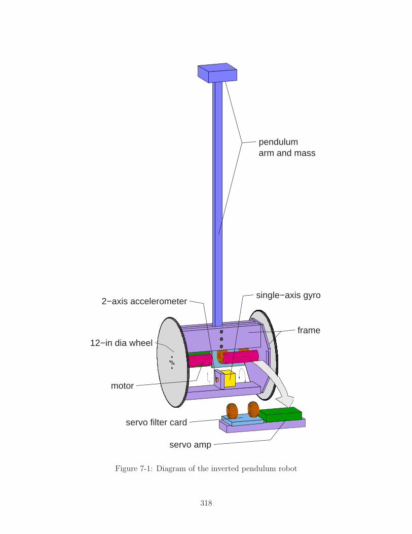
frame

arm and mass pendulum

single−axis gyro

servo amp

servo filter card

2−axis accelerometer

12−in dia wheel

motor

Figure 7-1: Diagram of the inverted pendulum robot

318

Inv. Pend. Robot

dSPACE Box

Power Supplies

Gyro Power

Steering Input

Figure 7-2: Inverted pendulum robot hardware

319

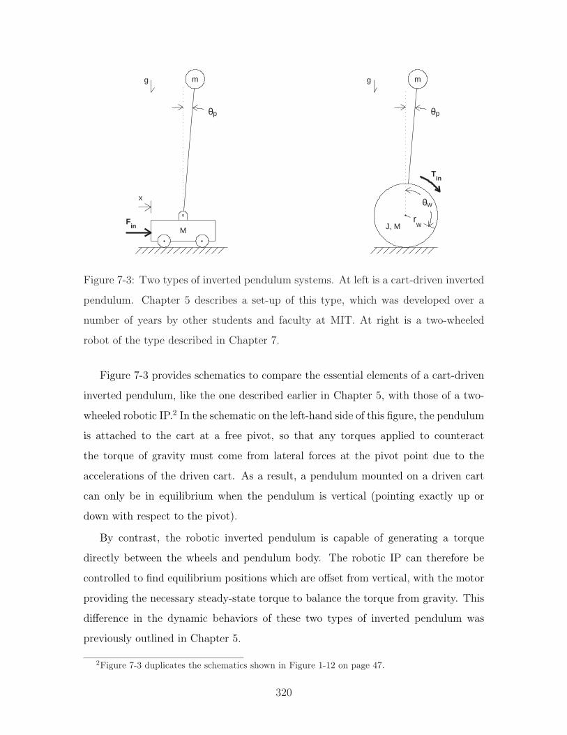
m

M

θp θp

x

Fin

m

Tin

J, M

θw

rw

g g

Figure 7-3: Two types of inverted pendulum systems. At left is a cart-driven inverted

pendulum. Chapter 5 describes a set-up of this type, which was developed over a

number of years by other students and faculty at MIT. At right is a two-wheeled

robot of the type described in Chapter 7.

Figure 7-3 provides schematics to compare the essential elements of a cart-driven

inverted pendulum, like the one described earlier in Chapter 5, with those of a two-

wheeled robotic IP.2 In the schematic on the left-hand side of this figure, the pendulum

is attached to the cart at a free pivot, so that any torques applied to counteract

the torque of gravity must come from lateral forces at the pivot point due to the

accelerations of the driven cart. As a result, a pendulum mounted on a driven cart

can only be in equilibrium when the pendulum is vertical (pointing exactly up or

down with respect to the pivot).

By contrast, the robotic inverted pendulum is capable of generating a torque

directly between the wheels and pendulum body. The robotic IP can therefore be

controlled to find equilibrium positions which are offset from vertical, with the motor

providing the necessary steady-state torque to balance the torque from gravity. This

difference in the dynamic behaviors of these two types of inverted pendulum was

previously outlined in Chapter 5.

2Figure 7-3 duplicates the schematics shown in Figure 1-12 on page 47.

320

A constant motor torque in the robotic IP corresponds to a constant steady-state

vehicle speed. Since a given motor torque corresponds both to a particular equilibrium

pendulum angle and a particular forward velocity for the robot, there is a direct

correspondence between commanded pendulum angle and robot velocity. In other

words, one can command a particular robot speed by commanding the appropriate

desired pendulum angle (or equivalently by offsetting the measurement of pendulum

angle by this amount).

Each of the two wheels of the DIPR is controlled by a separate motor. One

can therefore steer the robot by offsetting the command signal to each motor by

equal and opposite amounts. Technically, they are in fact offset by equal and “same-

sign” amounts, because the motor output shafts are aligned 180 with respect to one

another. However, it makes more sense semantically to consider each motor as having

a “forward” and “reverse” direction. Commanding both motors to move “forward”

results in the robot moving forward in a (theoretically) straight line, and adding

oppositely-signed outputs causes the vehicle to turn.

As of this writing, the DIPR is not autonomous, and the umbilical cords required

to transmit power, sensor measurements and command signals have several disadvan-

tages which do not make the robot practical as a classroom demo. First, the umbilical

cords significantly affect the dynamics of the system. They damp the movement of

the pendulum, and they also create significant drag on the ground which essentially

anchors the wheels of the robot in place to some extent. This drag inhibits the robot

from moving forward as the robot tilts forward or backward and allows the robot to

balance with moderate offset angles (away from vertical).

The non-autonomous design also reduces the ease with which the equipment can

be transported to and set up in a classroom for a demo. The robot requires multiple

power supplies: the two servo amps driving the motors each require a power supply,

and separate 5- and 12-volt supplies power the accelerometer and gyro, respectively.

Redesigning the robot to make it autonomous would require substantial effort, and

there are no plans to implement an autonomous version of the robot nor to use the

current version as a classroom demo at this time.

321

7.1 Robot Hardware

Figure 7-1 shows a diagram of the key components of the robotic inverted pendulum

developed in this thesis. The vehicle weighs approximately 26 lbs, has two 12-inch

diameter wheels which are spaced 14 inches apart, and stands about 44 inches high

when balancing upright. Umbilical cords carry power and sensor/actuator signals.

Two potentiometers provide steering inputs to command the desired forward velocity

and turning rate. The controller for the robot is implemented digitally on a dSPACE

1103 board using an execution step size of 50 microseconds.

The sensors, actuators and robot chassis are described in more detail below. This

section also outlines specifications on and advantages of using dSPACE and Con-

trolDesk in implementing the controller. Sections 7.7 and 7.8 present the controller

design and performance in detail. Section 6.2 of the previous chapter describes com-

plementary filtering of the gyro and accelerometer and provides data showing the

noise characteristics of each of these sensors and of the overall estimate of pendulum

tilt angle produced through filtering.

Estimates of the actual robot specifications are used in modeling through the rest

of this chapter. Calculating (or simply measuring) the mass of the robot pendulum-

body is more straight-forward than estimating its moment of inertia. One simple way

to test calculated inertia of the robot chassis (i.e. the rigid structure that forms both

the body and extended pendulum arm) is to measure the frequency of oscillation of

the pendulum in the downward (stable) configuration, assuming the wheels are fixed.

This was done and is described in Section 7.5.2.

7.1.1 Robot Chassis and Wheels

An aluminum frame, shown in Figures 7-1 and 7-2, forms the basis of the robot

chassis. The frame is essentially an open box: two 14” thick octagonal plates form the

sides and are bolted through a set of aluminum L-brackets to five extruded aluminum

tubes which run parallel to the wheel axis.

This design was intended to facilitate prototyping during the planned evolution of

322

the robot into a fully autonomous device, with additional components being bolted

along the aluminum extrusion as necessary. The aluminum tubes also provide some

heat dissipation for the motor servo amps. Figure 7-1 is drawn with one extrusion

pulled away from the robot, so one can see the component lay-out within the robot

more clearly. The DIPR still requires the use of umbilical cords at this time, however,

and in retrospect, the chassis design seems unnecessarily inelegant.

The pendulum arm is bolted between two extrusions at the top of the frame,

so that the robot chassis and pendulum together form a rigid. A 116

-inch layer of

rubber was added at the interface between the frame and arm to attenuate significant

vibration in the pendulum observed in early versions of the robot. This seemed to

reduce vibration along the pendulum, but the chassis was still prone to resonances

during development and testing of the control system. I added constrained layer

damping (∼ 15 mil thick) at most of the aluminum-aluminum joints in the robot

after the pinions on both motors came unglued at a significant resonance near 8 Hz

(see Section 7.1.3 and Figure 7-5 on page 326).

Finding appropriate off-the-shelf wheels proved difficult, and I finally decided to

manufacture the wheels for the robot myself. There were two key features I wanted

for the wheels. First, I wanted thin wheels to keep the torque due to the radial

force from the weight of the robot on the output shaft of the motor gearbox within

specifications. Commercial wheels of this diameter (12”) are typically 3 or 4 inches

wide and would therefore necessitate a transmission with additional wheel bearings.

The thin wheels allow the robot to operate with a direct drive transmission.

The second feature I wanted for the wheels was a convenient method for attaching

them to the motor shaft. The wheel are cut from 14-inch thick aluminum plate. Four

bolts near the center attach each wheel connect it to a 2-inch diameter inner aluminum

hub. The hub has a keyway which mates with the output shaft of the motor gearbox

and is held in place with a set screw. Four additional holes further out on the wheel

surface are simply a by-product of manufacturing the wheels (allowing it to be bolted

down during machining).

Inertia and traction of the wheels were additional concerns. O-rings are epoxied

323

at the circumference of each wheel and provide adequate traction. The inertia of the

wheels affects the dynamics of the system. Balancing the pendulum become a less

interesting problem if the inertia of the wheel gets too large. In an extreme case where

the wheels are virtually immovable objects, one is essentially just commanding the

motors to remain at a fixed position, and the robot loses (virtually) all of its mobility.

7.1.2 dSPACE/Simulink Control Environment

The controller for the robot is implemented on a dSPACE 1103 board, using an exe-

cution step size of 100 ms. The dSPACE environment provides several features which

facilitate the development of control systems. Algorithms can be created intuitively

using the graphical “block diagram style” Simulink/MATLAB environment. Addi-

tional Simulink blocks specific to the dSPACE board enable communication with a

set of A/D, DAC and encoder channels. Appendix H shows the Simulink model (with

subsystems) used to control the DIPR.

Another feature is the dSPACE ContolDesk environment, which allows users to

view data and change variable parameters in real time as the controller runs. One can

also access data streams and write to variable addresses directly through a special-

ized MATLAB function called “mlib()”. The experimental transfer functions shown

in Sections 7.6 and 7.8 were obtained using a Simulink-driven dynamic signal ana-

lyzer based on this mlib() function. The analyzer uses mlib() both to command the

frequency and amplitude of a sinusoidal signal generator within the Simulink model

and to collect relevant system response(s)[113, 114].

7.1.3 Motors and Power Amps

The DIPR has two 18-volt DC Maxon RE 36 motors, each equipped with a planetary

gearhead with a ratio of 13:3 and a 500-count quadrature digital encoder. Figure 7-

4 show the motor (left) with the gearhead (right) detached. Appendix F on page

425 provides data sheets for the motor, gearhead and encoder. The motor has a stall

torque of .73 Nm (at 27.8 Amps), corresponding to about 2.8 Nm after gear reduction

324

(assuming 90% efficiency), and its continuous torque rating is 0.082 Nm (at 3.1 Amps;

0.31 Nm at gearhead output).

detached pinionplanetary gear

Figure 7-4: Maxon motor and gearhead, with detached pinion. This figure shows one

of the Maxon motors used in the DIPR (at left) with the gearhead (at right) removed.

The pinion (shown at center) became unglued from the smooth output shaft of the

motor during vibration.

Each motor is powered through a model 413 DC Brush Servo Amplifier manu-

factured by Copley Controls Corporation, which requires a 24-90 VDC single-ended

(unregulated) power supply and can supply a peak output of 30 Amps (15 Amps, con-

tinuously). I used Lambda LK 343A power supplies capable of outputting 36 Volts

and up to 9 Amps of current. Each servo amp was supplied the full 36 Volts but

power output was limited to about 2 Amps output during most testing of the robot.

This corresponds to a maximum current of about 3.8 Amps to the 18-volt motor

325

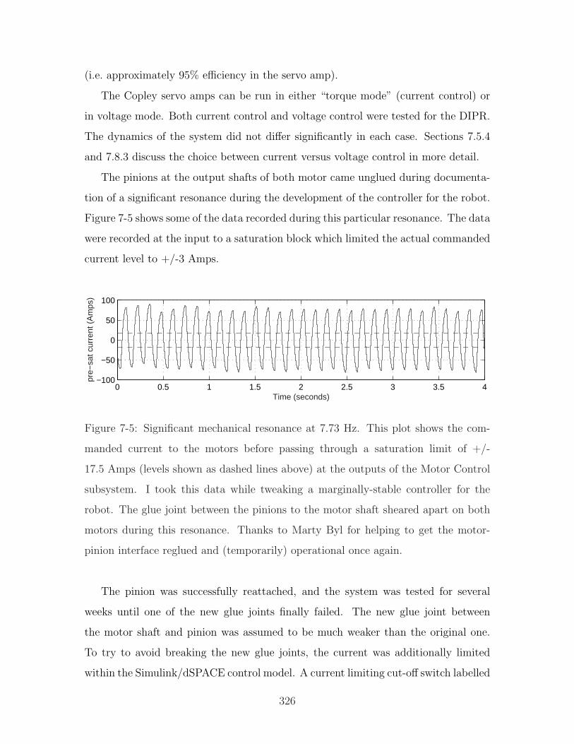
(i.e. approximately 95% efficiency in the servo amp).

The Copley servo amps can be run in either “torque mode” (current control) or

in voltage mode. Both current control and voltage control were tested for the DIPR.

The dynamics of the system did not differ significantly in each case. Sections 7.5.4

and 7.8.3 discuss the choice between current versus voltage control in more detail.

The pinions at the output shafts of both motor came unglued during documenta-

tion of a significant resonance during the development of the controller for the robot.

Figure 7-5 shows some of the data recorded during this particular resonance. The data

were recorded at the input to a saturation block which limited the actual commanded

current level to +/-3 Amps.

0 0.5 1 1.5 2 2.5 3 3.5 4−100

−50

0

50

100

Time (seconds)

pre−

sat c

urre

nt (

Am

ps)

Figure 7-5: Significant mechanical resonance at 7.73 Hz. This plot shows the com-

manded current to the motors before passing through a saturation limit of +/-

17.5 Amps (levels shown as dashed lines above) at the outputs of the Motor Control

subsystem. I took this data while tweaking a marginally-stable controller for the

robot. The glue joint between the pinions to the motor shaft sheared apart on both

motors during this resonance. Thanks to Marty Byl for helping to get the motor-

pinion interface reglued and (temporarily) operational once again.

The pinion was successfully reattached, and the system was tested for several

weeks until one of the new glue joints finally failed. The new glue joint between

the motor shaft and pinion was assumed to be much weaker than the original one.

To try to avoid breaking the new glue joints, the current was additionally limited

within the Simulink/dSPACE control model. A current limiting cut-off switch labelled

326

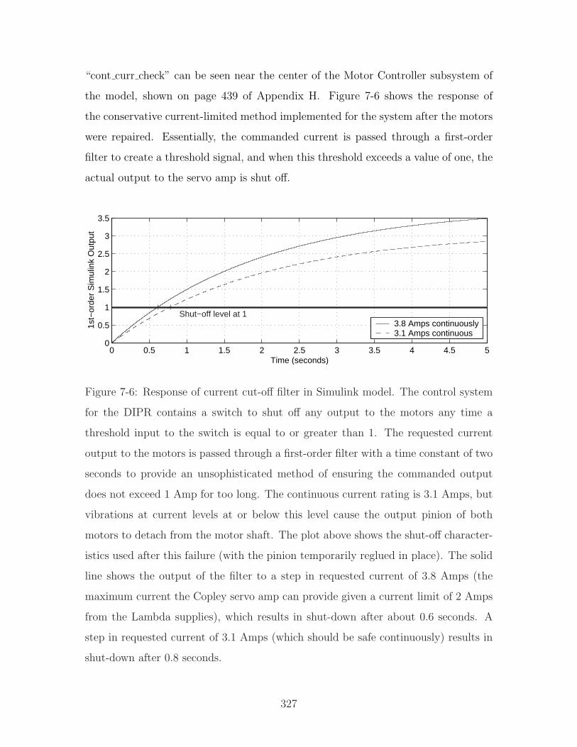
“cont curr check” can be seen near the center of the Motor Controller subsystem of

the model, shown on page 439 of Appendix H. Figure 7-6 shows the response of

the conservative current-limited method implemented for the system after the motors

were repaired. Essentially, the commanded current is passed through a first-order

filter to create a threshold signal, and when this threshold exceeds a value of one, the

actual output to the servo amp is shut off.

0 0.5 1 1.5 2 2.5 3 3.5 4 4.5 50

0.5

1

1.5

2

2.5

3

3.5

Time (seconds)

1st−

orde

r S

imul

ink

Out

put

Shut−off level at 13.8 Amps continuously3.1 Amps continuous

Figure 7-6: Response of current cut-off filter in Simulink model. The control system

for the DIPR contains a switch to shut off any output to the motors any time a

threshold input to the switch is equal to or greater than 1. The requested current

output to the motors is passed through a first-order filter with a time constant of two

seconds to provide an unsophisticated method of ensuring the commanded output

does not exceed 1 Amp for too long. The continuous current rating is 3.1 Amps, but

vibrations at current levels at or below this level cause the output pinion of both

motors to detach from the motor shaft. The plot above shows the shut-off character-

istics used after this failure (with the pinion temporarily reglued in place). The solid

line shows the output of the filter to a step in requested current of 3.8 Amps (the

maximum current the Copley servo amp can provide given a current limit of 2 Amps

from the Lambda supplies), which results in shut-down after about 0.6 seconds. A

step in requested current of 3.1 Amps (which should be safe continuously) results in

shut-down after 0.8 seconds.

327

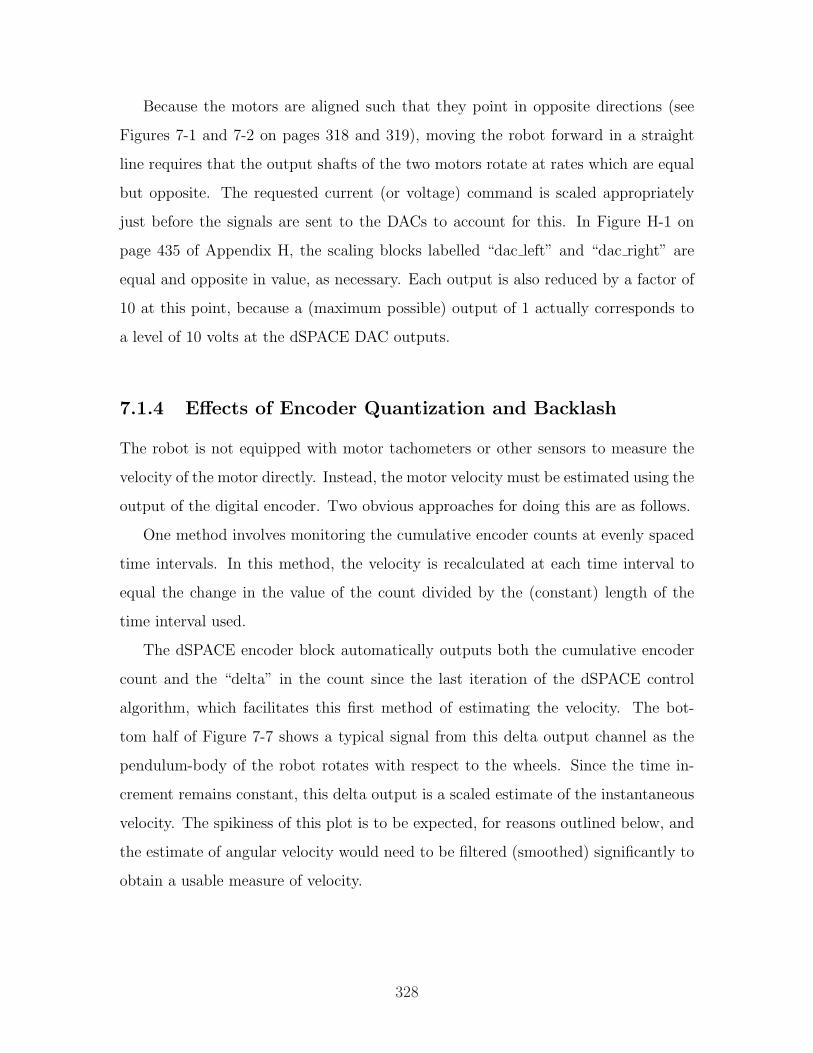
Because the motors are aligned such that they point in opposite directions (see

Figures 7-1 and 7-2 on pages 318 and 319), moving the robot forward in a straight

line requires that the output shafts of the two motors rotate at rates which are equal

but opposite. The requested current (or voltage) command is scaled appropriately

just before the signals are sent to the DACs to account for this. In Figure H-1 on

page 435 of Appendix H, the scaling blocks labelled “dac left” and “dac right” are

equal and opposite in value, as necessary. Each output is also reduced by a factor of

10 at this point, because a (maximum possible) output of 1 actually corresponds to

a level of 10 volts at the dSPACE DAC outputs.

7.1.4 Effects of Encoder Quantization and Backlash

The robot is not equipped with motor tachometers or other sensors to measure the

velocity of the motor directly. Instead, the motor velocity must be estimated using the

output of the digital encoder. Two obvious approaches for doing this are as follows.

One method involves monitoring the cumulative encoder counts at evenly spaced

time intervals. In this method, the velocity is recalculated at each time interval to

equal the change in the value of the count divided by the (constant) length of the

time interval used.

The dSPACE encoder block automatically outputs both the cumulative encoder

count and the “delta” in the count since the last iteration of the dSPACE control

algorithm, which facilitates this first method of estimating the velocity. The bot-

tom half of Figure 7-7 shows a typical signal from this delta output channel as the

pendulum-body of the robot rotates with respect to the wheels. Since the time in-

crement remains constant, this delta output is a scaled estimate of the instantaneous

velocity. The spikiness of this plot is to be expected, for reasons outlined below, and

the estimate of angular velocity would need to be filtered (smoothed) significantly to

obtain a usable measure of velocity.

328

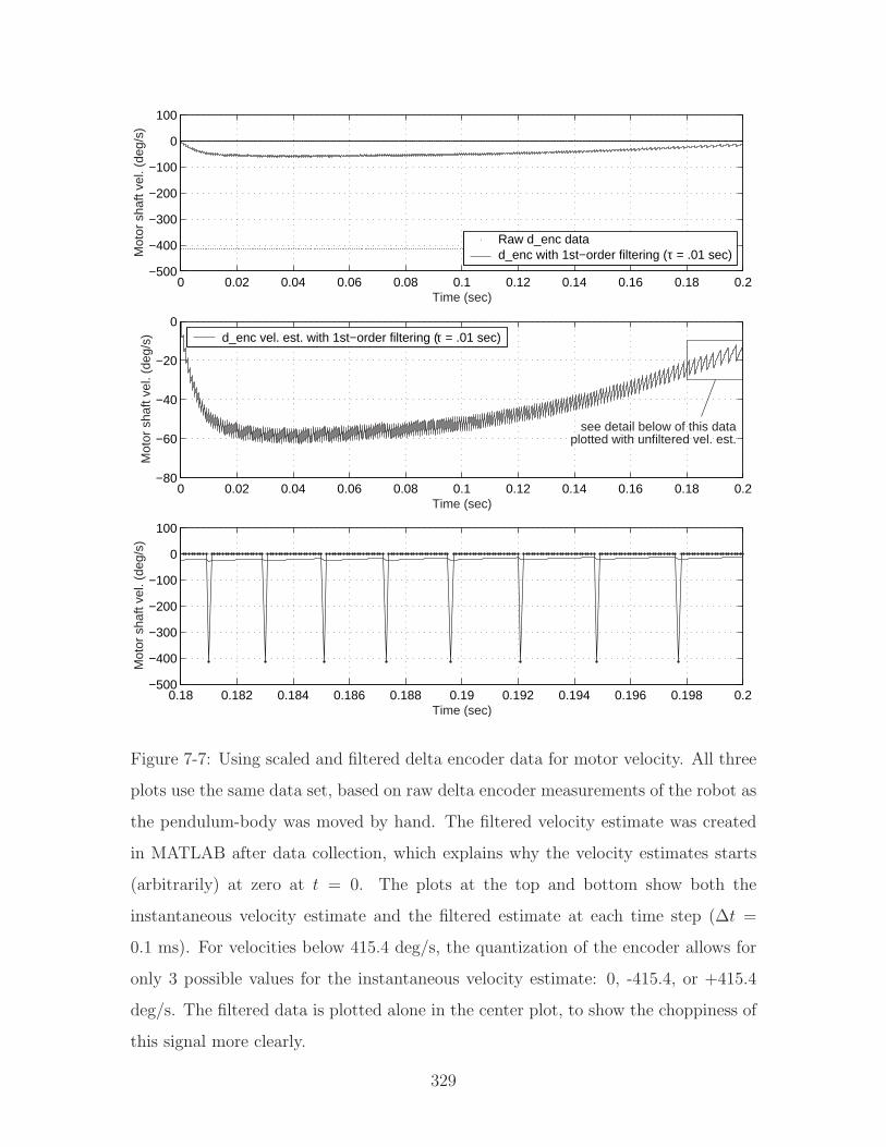
0 0.02 0.04 0.06 0.08 0.1 0.12 0.14 0.16 0.18 0.2−500

−400

−300

−200

−100

0

100

Time (sec)

Mot

or s

haft

vel.

(deg

/s)

Raw d_enc datad_enc with 1st−order filtering (τ = .01 sec)

0 0.02 0.04 0.06 0.08 0.1 0.12 0.14 0.16 0.18 0.2−80

−60

−40

−20

0

Time (sec)

Mot

or s

haft

vel.

(deg

/s)

see detail below of this dataplotted with unfiltered vel. est.

d_enc vel. est. with 1st−order filtering (τ = .01 sec)

0.18 0.182 0.184 0.186 0.188 0.19 0.192 0.194 0.196 0.198 0.2−500

−400

−300

−200

−100

0

100

Time (sec)

Mot

or s

haft

vel.

(deg

/s)

Figure 7-7: Using scaled and filtered delta encoder data for motor velocity. All three

plots use the same data set, based on raw delta encoder measurements of the robot as

the pendulum-body was moved by hand. The filtered velocity estimate was created

in MATLAB after data collection, which explains why the velocity estimates starts

(arbitrarily) at zero at t = 0. The plots at the top and bottom show both the

instantaneous velocity estimate and the filtered estimate at each time step (∆t =

0.1 ms). For velocities below 415.4 deg/s, the quantization of the encoder allows for

only 3 possible values for the instantaneous velocity estimate: 0, -415.4, or +415.4

deg/s. The filtered data is plotted alone in the center plot, to show the choppiness of

this signal more clearly.

329

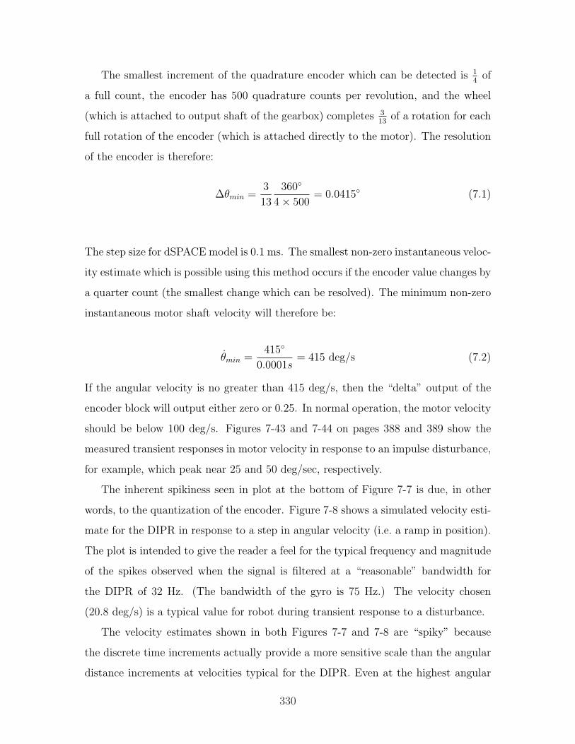
The smallest increment of the quadrature encoder which can be detected is 14

of

a full count, the encoder has 500 quadrature counts per revolution, and the wheel

(which is attached to output shaft of the gearbox) completes 313

of a rotation for each

full rotation of the encoder (which is attached directly to the motor). The resolution

of the encoder is therefore:

∆θmin =3

13

360

4× 500= 0.0415 (7.1)

The step size for dSPACE model is 0.1 ms. The smallest non-zero instantaneous veloc-

ity estimate which is possible using this method occurs if the encoder value changes by

a quarter count (the smallest change which can be resolved). The minimum non-zero

instantaneous motor shaft velocity will therefore be:

θmin =415

0.0001s= 415 deg/s (7.2)

If the angular velocity is no greater than 415 deg/s, then the “delta” output of the

encoder block will output either zero or 0.25. In normal operation, the motor velocity

should be below 100 deg/s. Figures 7-43 and 7-44 on pages 388 and 389 show the

measured transient responses in motor velocity in response to an impulse disturbance,

for example, which peak near 25 and 50 deg/sec, respectively.

The inherent spikiness seen in plot at the bottom of Figure 7-7 is due, in other

words, to the quantization of the encoder. Figure 7-8 shows a simulated velocity esti-

mate for the DIPR in response to a step in angular velocity (i.e. a ramp in position).

The plot is intended to give the reader a feel for the typical frequency and magnitude

of the spikes observed when the signal is filtered at a “reasonable” bandwidth for

the DIPR of 32 Hz. (The bandwidth of the gyro is 75 Hz.) The velocity chosen

(20.8 deg/s) is a typical value for robot during transient response to a disturbance.

The velocity estimates shown in both Figures 7-7 and 7-8 are “spiky” because

the discrete time increments actually provide a more sensitive scale than the angular

distance increments at velocities typical for the DIPR. Even at the highest angular

330

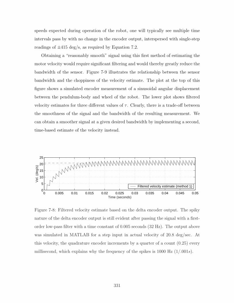
speeds expected during operation of the robot, one will typically see multiple time

intervals pass by with no change in the encoder output, interspersed with single-step

readings of ±415 deg/s, as required by Equation 7.2.

Obtaining a “reasonably smooth” signal using this first method of estimating the

motor velocity would require significant filtering and would thereby greatly reduce the

bandwidth of the sensor. Figure 7-9 illustrates the relationship between the sensor

bandwidth and the choppiness of the velocity estimate. The plot at the top of this

figure shows a simulated encoder measurement of a sinusoidal angular displacement

between the pendulum-body and wheel of the robot. The lower plot shows filtered

velocity estimates for three different values of τ . Clearly, there is a trade-off between

the smoothness of the signal and the bandwidth of the resulting measurement. We

can obtain a smoother signal at a given desired bandwidth by implementing a second,

time-based estimate of the velocity instead.

0 0.005 0.01 0.015 0.02 0.025 0.03 0.035 0.04 0.045 0.050

5

10

15

20

25

Time (seconds)

Vel

. (de

g/s)

Filtered velocity estimate (method 1)

Figure 7-8: Filtered velocity estimate based on the delta encoder output. The spiky

nature of the delta encoder output is still evident after passing the signal with a first-

order low-pass filter with a time constant of 0.005 seconds (32 Hz). The output above

was simulated in MATLAB for a step input in actual velocity of 20.8 deg/sec. At

this velocity, the quadrature encoder increments by a quarter of a count (0.25) every

millisecond, which explains why the frequency of the spikes is 1000 Hz (1/.001s).

331

0 0.02 0.04 0.06 0.08 0.1 0.12 0.14 0.16 0.18 0.2

−1

−0.5

0

0.5

1

Time (seconds)

Enc

oder

out

put (

deg)

0 0.02 0.04 0.06 0.08 0.1 0.12 0.14 0.16 0.18 0.2−80

−60

−40

−20

0

20

40

60

80

Time (seconds)

Mot

or v

eloc

ity (

deg/

s)

exact velocity τ=.02s (32 Hz)

τ=.005s (8 Hz)

τ=.001s (1.6 Hz)

Figure 7-9: Theoretical filtering of the delta encoder signal. The data shown represent

simulations of a “count-based” velocity estimation method in which the instantaneous

velocity is recalculated at each time step as being equal to the change in measured

position from the encoder reading at the last time step divided by the (constant)

time step. In other words, the instantaneous velocity estimate is a scaled version of

the delta encoder signal. The upper plot shows a quantized encoder measurement

of a 10 Hz sinusoidal waveform. The lower plots shows low-pass filtered versions of

the count-based velocity estimate for three values of τ . The exact (non-measured,

non-quantized) velocity is also shown on this plot, for comparison.

332

The second method for estimating velocity from an encoder measurement essen-

tially uses a filtered zero-order-hold estimate based on the time between successive

encoder counts. The (pre-filtered) zero-order-hold estimate is created by updating

the velocity only when the encoder registers a new value. The new velocity estimate

is then equal to the change in the encoder signal divided by the time elapsed since

the previous change in encoder value.

Both the first (count-based) velocity estimation method and this second (time-

based) zero-order-hold estimate produce inherently quantized signals, due to the dis-

crete nature both of the encoder measurement and of the constant time increments

of the digital controller. As before, this quantization can be smoothed significantly

by passing the signal through a low-pass filter.

This time-based method is more practical than the first (count-based) method

when the angular velocities are slow enough that encoder typically registers the same

value for multiple time steps in row during typical operation. For the combina-

tion of encoder (2000 quadrature counts per revolution), gearhead (3 encoder turns

correspond to 13 rotations of the vehicles wheel) and discrete time step (0.1 ms),

this threshold velocity of one quarter-count per time step works out to 415 deg/s.

( 3604×2000

× 133÷0.0001 s ≈ 415 deg/s) As previously mentioned, the data shown later in

this chapter (specifically, Figures 7-43 and 7-44 on pages 388 and 389) show typical

velocities in response to an impulse disturbance are not likely to exceed the measure-

ment limit of the gyro, which is 200 deg/s, much less twice this value. Therefore, the

second, time-based method of calculating the velocity is more appropriate.

Figure 7-10 shows actual data obtained by moving the robot pendulum by hand

with the wheels fixed. The plot at the top shows both the quantized zero-order-hold

estimate and the smoother signal which results from low-pass filtering of this estimate.

Below this plot is a close-up of part of the delta encoder signal used to create the

time-based estimate. Figure 7-11 shows simulated data for the robot. This plot

also illustrates the significant “steps” in the signal when the encoder measurement

reverses direction (and the velocity therefore crosses zero) and shows the results of a

“smoothing” technique described next.

333

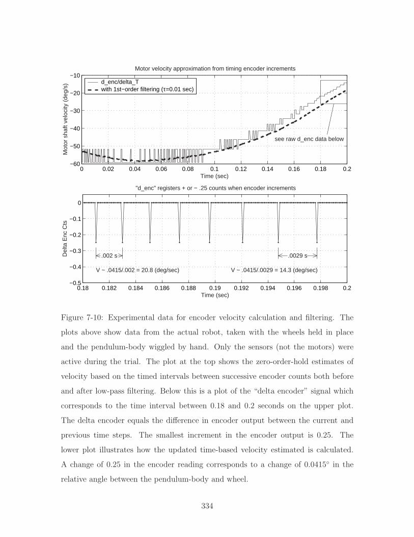
0 0.02 0.04 0.06 0.08 0.1 0.12 0.14 0.16 0.18 0.2−60

−50

−40

−30

−20

−10

Time (sec)

Mot

or s

haft

velo

city

(de

g/s)

Motor velocity approximation from timing encoder increments

see raw d_enc data below

d_enc/delta_Twith 1st−order filtering (τ=0.01 sec)

0 0.02 0.04 0.06 0.08 0.1 0.12 0.14 0.16 0.18 0.20

10

20

30

40

50

60

70

Time (sec)

Mot

or O

utpu

t Sha

ft V

eloc

ity (

deg/

sec)

Motor velocity approximation from encoder output

d_enc/delta_Twith add’l filtering (tau=.01 sec)close−up (subplot below) in these regions

0.18 0.182 0.184 0.186 0.188 0.19 0.192 0.194 0.196 0.198 0.2−0.5

−0.4

−0.3

−0.2

−0.1

0

Time (sec)

Del

ta E

nc C

ts

.002 s .0029 s

"d_enc" registers + or − .25 counts when encoder increments

V ~ .0415/.002 = 20.8 (deg/sec) V ~ .0415/.0029 = 14.3 (deg/sec)

Figure 7-10: Experimental data for encoder velocity calculation and filtering. The

plots above show data from the actual robot, taken with the wheels held in place

and the pendulum-body wiggled by hand. Only the sensors (not the motors) were

active during the trial. The plot at the top shows the zero-order-hold estimates of

velocity based on the timed intervals between successive encoder counts both before

and after low-pass filtering. Below this is a plot of the “delta encoder” signal which

corresponds to the time interval between 0.18 and 0.2 seconds on the upper plot.

The delta encoder equals the difference in encoder output between the current and

previous time steps. The smallest increment in the encoder output is 0.25. The

lower plot illustrates how the updated time-based velocity estimated is calculated.

A change of 0.25 in the encoder reading corresponds to a change of 0.0415 in the

relative angle between the pendulum-body and wheel.

334

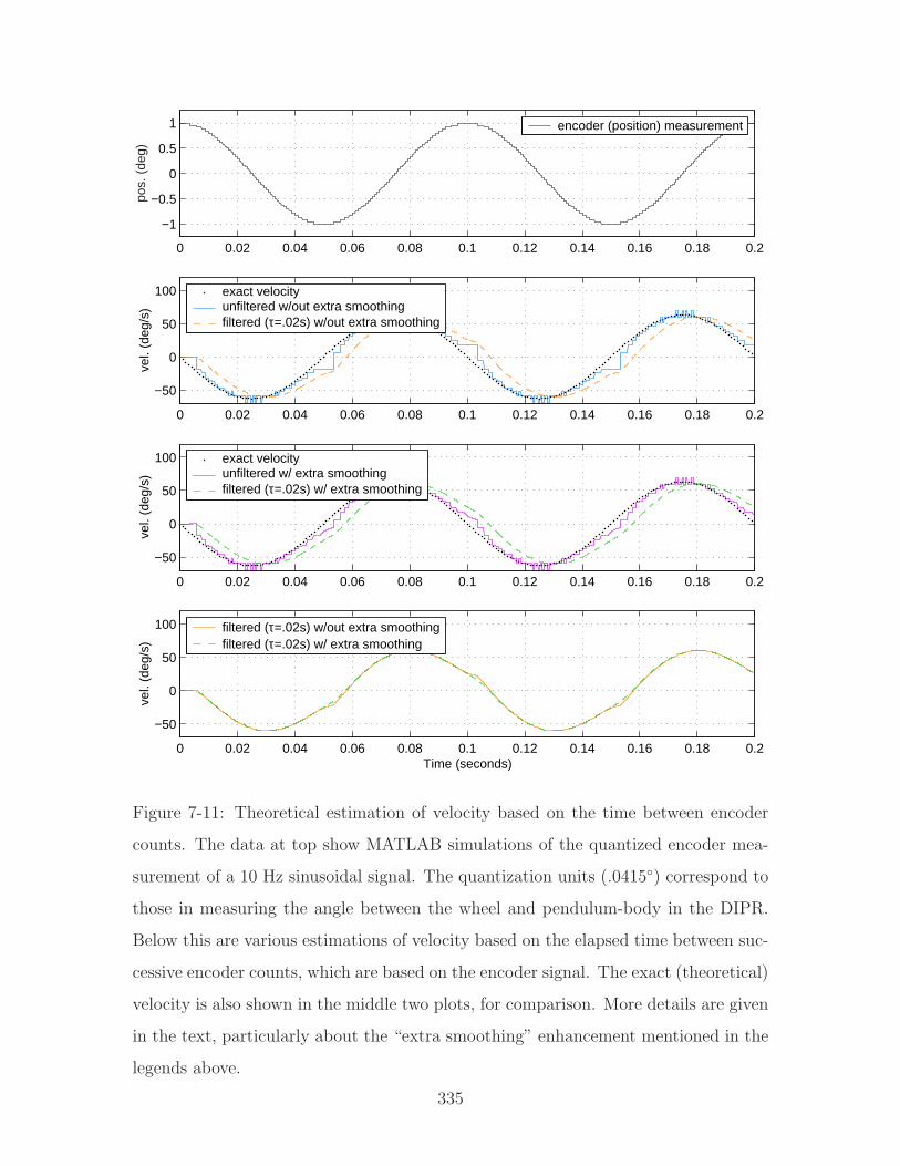
0 0.02 0.04 0.06 0.08 0.1 0.12 0.14 0.16 0.18 0.2

−1

−0.5

0

0.5

1po

s. (

deg)

encoder (position) measurement

0 0.02 0.04 0.06 0.08 0.1 0.12 0.14 0.16 0.18 0.2

−50

0

50

100

vel.

(deg

/s)

exact velocityunfiltered w/out extra smoothingfiltered (τ=.02s) w/out extra smoothing

0 0.02 0.04 0.06 0.08 0.1 0.12 0.14 0.16 0.18 0.2

−50

0

50

100

vel.

(deg

/s)

exact velocityunfiltered w/ extra smoothingfiltered (τ=.02s) w/ extra smoothing

0 0.02 0.04 0.06 0.08 0.1 0.12 0.14 0.16 0.18 0.2

−50

0

50

100

Time (seconds)

vel.

(deg

/s)

filtered (τ=.02s) w/out extra smoothingfiltered (τ=.02s) w/ extra smoothing

Figure 7-11: Theoretical estimation of velocity based on the time between encoder

counts. The data at top show MATLAB simulations of the quantized encoder mea-

surement of a 10 Hz sinusoidal signal. The quantization units (.0415) correspond to

those in measuring the angle between the wheel and pendulum-body in the DIPR.

Below this are various estimations of velocity based on the elapsed time between suc-

cessive encoder counts, which are based on the encoder signal. The exact (theoretical)

velocity is also shown in the middle two plots, for comparison. More details are given

in the text, particularly about the “extra smoothing” enhancement mentioned in the

legends above.

335

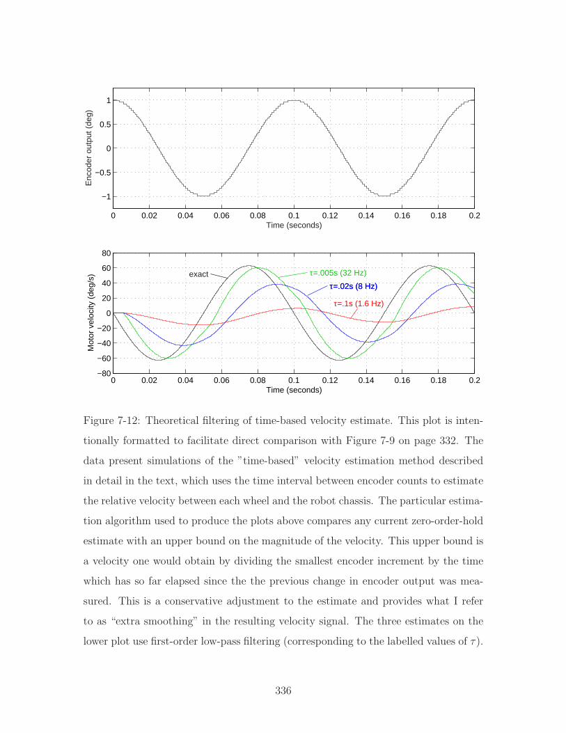
0 0.02 0.04 0.06 0.08 0.1 0.12 0.14 0.16 0.18 0.2

−1

−0.5

0

0.5

1

Time (seconds)

Enc

oder

out

put (

deg)

0 0.02 0.04 0.06 0.08 0.1 0.12 0.14 0.16 0.18 0.2−80

−60

−40

−20

0

20

40

60

80

exact τ=.005s (32 Hz)

τ=.02s (8 Hz) τ=.02s (8 Hz)

τ=.1s (1.6 Hz)

Time (seconds)

Mot

or v

eloc

ity (

deg/

s)

Figure 7-12: Theoretical filtering of time-based velocity estimate. This plot is inten-

tionally formatted to facilitate direct comparison with Figure 7-9 on page 332. The

data present simulations of the ”time-based” velocity estimation method described

in detail in the text, which uses the time interval between encoder counts to estimate

the relative velocity between each wheel and the robot chassis. The particular estima-

tion algorithm used to produce the plots above compares any current zero-order-hold

estimate with an upper bound on the magnitude of the velocity. This upper bound is

a velocity one would obtain by dividing the smallest encoder increment by the time

which has so far elapsed since the the previous change in encoder output was mea-

sured. This is a conservative adjustment to the estimate and provides what I refer

to as “extra smoothing” in the resulting velocity signal. The three estimates on the

lower plot use first-order low-pass filtering (corresponding to the labelled values of τ).

336

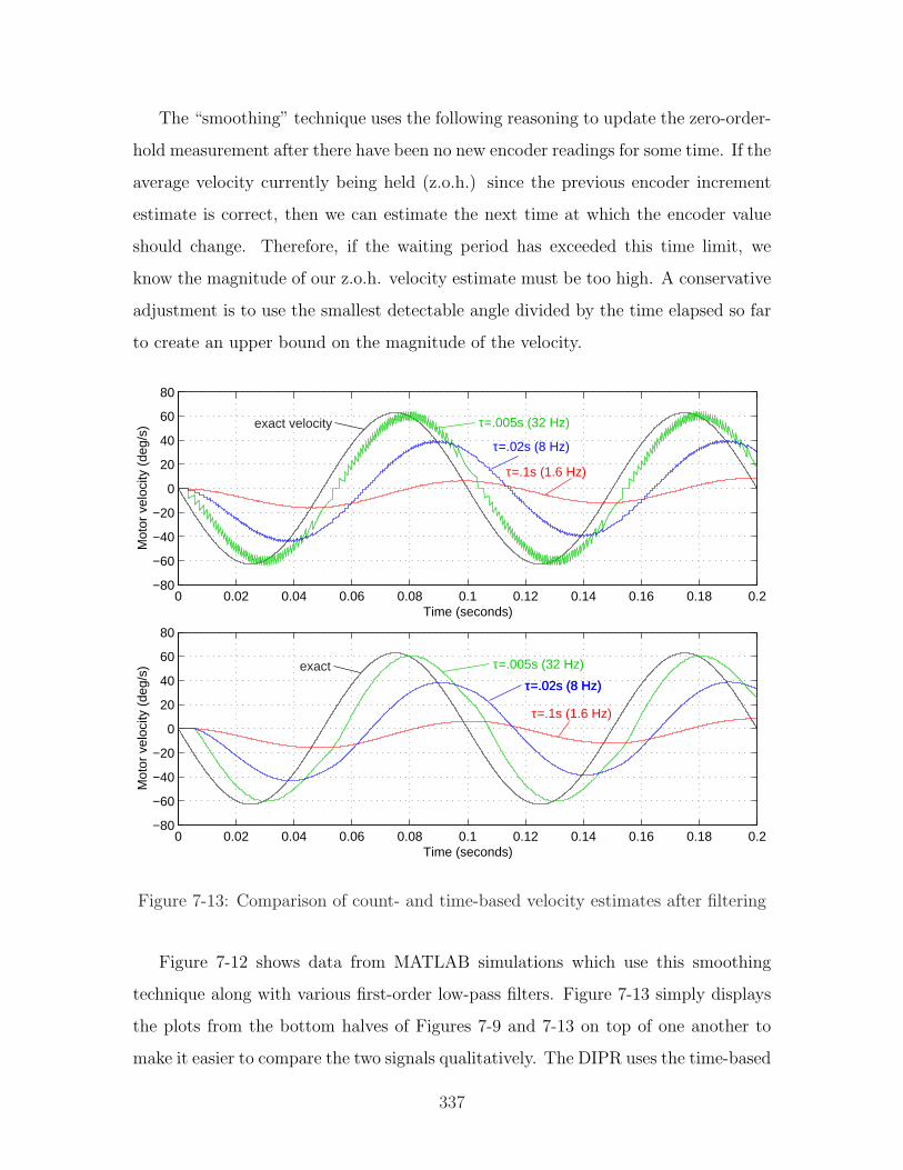
The “smoothing” technique uses the following reasoning to update the zero-order-

hold measurement after there have been no new encoder readings for some time. If the

average velocity currently being held (z.o.h.) since the previous encoder increment

estimate is correct, then we can estimate the next time at which the encoder value

should change. Therefore, if the waiting period has exceeded this time limit, we

know the magnitude of our z.o.h. velocity estimate must be too high. A conservative

adjustment is to use the smallest detectable angle divided by the time elapsed so far

to create an upper bound on the magnitude of the velocity.

0 0.02 0.04 0.06 0.08 0.1 0.12 0.14 0.16 0.18 0.2−80

−60

−40

−20

0

20

40

60

80

Time (seconds)

Mot

or v

eloc

ity (

deg/

s)

exact velocity τ=.005s (32 Hz)

τ=.02s (8 Hz)

τ=.1s (1.6 Hz)

0 0.02 0.04 0.06 0.08 0.1 0.12 0.14 0.16 0.18 0.2−80

−60

−40

−20

0

20

40

60

80

exact τ=.005s (32 Hz)

τ=.02s (8 Hz) τ=.02s (8 Hz)

τ=.1s (1.6 Hz)

Time (seconds)

Mot

or v

eloc

ity (

deg/

s)

Figure 7-13: Comparison of count- and time-based velocity estimates after filtering

Figure 7-12 shows data from MATLAB simulations which use this smoothing

technique along with various first-order low-pass filters. Figure 7-13 simply displays

the plots from the bottom halves of Figures 7-9 and 7-13 on top of one another to

make it easier to compare the two signals qualitatively. The DIPR uses the time-based

337

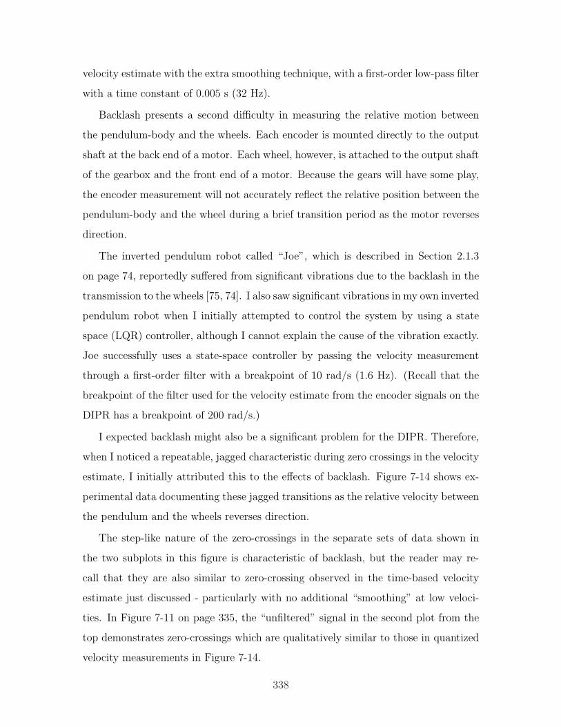
velocity estimate with the extra smoothing technique, with a first-order low-pass filter

with a time constant of 0.005 s (32 Hz).

Backlash presents a second difficulty in measuring the relative motion between

the pendulum-body and the wheels. Each encoder is mounted directly to the output

shaft at the back end of a motor. Each wheel, however, is attached to the output shaft

of the gearbox and the front end of a motor. Because the gears will have some play,

the encoder measurement will not accurately reflect the relative position between the

pendulum-body and the wheel during a brief transition period as the motor reverses

direction.

The inverted pendulum robot called “Joe”, which is described in Section 2.1.3

on page 74, reportedly suffered from significant vibrations due to the backlash in the

transmission to the wheels [75, 74]. I also saw significant vibrations in my own inverted

pendulum robot when I initially attempted to control the system by using a state

space (LQR) controller, although I cannot explain the cause of the vibration exactly.

Joe successfully uses a state-space controller by passing the velocity measurement

through a first-order filter with a breakpoint of 10 rad/s (1.6 Hz). (Recall that the

breakpoint of the filter used for the velocity estimate from the encoder signals on the

DIPR has a breakpoint of 200 rad/s.)

I expected backlash might also be a significant problem for the DIPR. Therefore,

when I noticed a repeatable, jagged characteristic during zero crossings in the velocity

estimate, I initially attributed this to the effects of backlash. Figure 7-14 shows ex-

perimental data documenting these jagged transitions as the relative velocity between

the pendulum and the wheels reverses direction.

The step-like nature of the zero-crossings in the separate sets of data shown in

the two subplots in this figure is characteristic of backlash, but the reader may re-

call that they are also similar to zero-crossing observed in the time-based velocity

estimate just discussed - particularly with no additional “smoothing” at low veloci-

ties. In Figure 7-11 on page 335, the “unfiltered” signal in the second plot from the

top demonstrates zero-crossings which are qualitatively similar to those in quantized

velocity measurements in Figure 7-14.

338

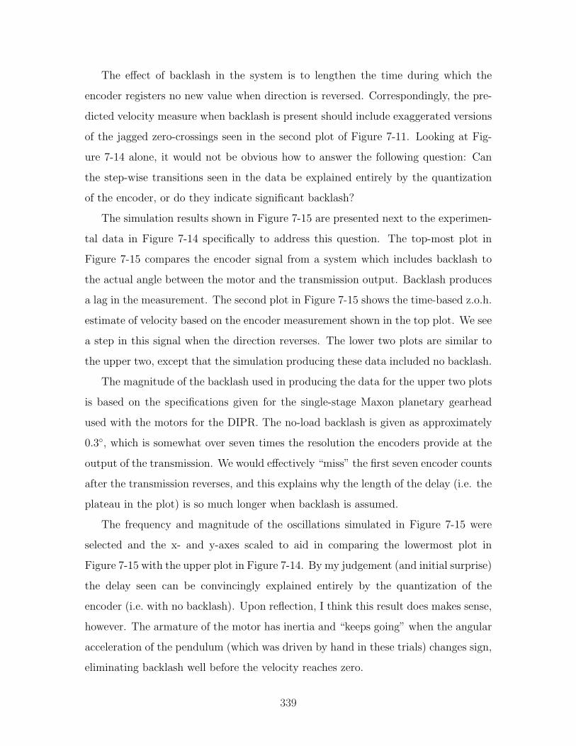
The effect of backlash in the system is to lengthen the time during which the

encoder registers no new value when direction is reversed. Correspondingly, the pre-

dicted velocity measure when backlash is present should include exaggerated versions

of the jagged zero-crossings seen in the second plot of Figure 7-11. Looking at Fig-

ure 7-14 alone, it would not be obvious how to answer the following question: Can

the step-wise transitions seen in the data be explained entirely by the quantization

of the encoder, or do they indicate significant backlash?

The simulation results shown in Figure 7-15 are presented next to the experimen-

tal data in Figure 7-14 specifically to address this question. The top-most plot in

Figure 7-15 compares the encoder signal from a system which includes backlash to

the actual angle between the motor and the transmission output. Backlash produces

a lag in the measurement. The second plot in Figure 7-15 shows the time-based z.o.h.

estimate of velocity based on the encoder measurement shown in the top plot. We see

a step in this signal when the direction reverses. The lower two plots are similar to

the upper two, except that the simulation producing these data included no backlash.

The magnitude of the backlash used in producing the data for the upper two plots

is based on the specifications given for the single-stage Maxon planetary gearhead

used with the motors for the DIPR. The no-load backlash is given as approximately

0.3, which is somewhat over seven times the resolution the encoders provide at the

output of the transmission. We would effectively “miss” the first seven encoder counts

after the transmission reverses, and this explains why the length of the delay (i.e. the

plateau in the plot) is so much longer when backlash is assumed.

The frequency and magnitude of the oscillations simulated in Figure 7-15 were

selected and the x- and y-axes scaled to aid in comparing the lowermost plot in

Figure 7-15 with the upper plot in Figure 7-14. By my judgement (and initial surprise)

the delay seen can be convincingly explained entirely by the quantization of the

encoder (i.e. with no backlash). Upon reflection, I think this result does makes sense,

however. The armature of the motor has inertia and “keeps going” when the angular

acceleration of the pendulum (which was driven by hand in these trials) changes sign,

eliminating backlash well before the velocity reaches zero.

339

0 0.02 0.04 0.06 0.08 0.1 0.12 0.14 0.16 0.18 0.2−60

−40

−20

0

20

40

60

Time (sec)

Ang

ular

Vel

ocity

(de

g/se

c)Filtering encoder for velocity measurement: Data set #1 − note effects of backlash

Backlash effect (when velocity changes sign)

filtered enc motor vel (tau = 0.01s)quantized enc motor velfiltered gyro pend vel

0 0.02 0.04 0.06 0.08 0.1 0.12 0.14 0.16 0.18 0.2−60

−40

−20

0

20

40

60

Time (sec)

Ang

ular

Vel

ocity

(de

g/se

c)

Filtering encoder for velocity measurement: Data set #2 − with "backlash reset"

Here, velocity is reset when sign change is detected

Figure 7-14: Experimental data to test backlash and quantization effects. The plots

above show actual data obtained by wiggling the pendulum-body of the DIPR rapidly

by hand with the wheels held in place. With the wheels stationary, the encoder

measures an absolute angle, which allows one to compare the estimations of velocity

from the encoder and from the gyro. Initially, I assumed the jagged delays indicated

with the three arrows above were primarily due to the effects of backlash. The no load

backlash for the single-stage planetary gearbox at the output of the Maxon motor is

specified as approximately 0.3. This should be quite noticeable if there were play

before the gears when the pendulum reversed direction, as Figure 7-15 indicates. The

fact that backlash does not seem to be a factor in the data above is most likely an

artifact of the limitations of the test environment and does not mean that backlash

is insignificant in normal operation of the robot. (See text for more details.)

340

0 0.02 0.04 0.06 0.08 0.1 0.12 0.14 0.16 0.18 0.2

−2

0

2

Time (seconds)

angl

e (d

egre

es)

exact angleencoder with backlash

0 0.02 0.04 0.06 0.08 0.1 0.12 0.14 0.16 0.18 0.2−60

−40

−20

0

20

40

60

Time (seconds)

velo

city

(de

g/s)

velocity with time lagvelocity from encoder with backlash

0 0.02 0.04 0.06 0.08 0.1 0.12 0.14 0.16 0.18 0.2

−2

0

2

Time (seconds)

angl

e (d

egre

es)

exact angleencoder without backlash

0 0.02 0.04 0.06 0.08 0.1 0.12 0.14 0.16 0.18 0.2−60

−40

−20

0

20

40

60

Time (seconds)

velo

city

(de

g/s)

velocity with time lagvelocity from encoder without backlash

Figure 7-15: Time-based velocity estimates with and without backlash. The plots

above are theoretical MATLAB simulations. The bottommost plot above (simulating

a system with no backlash) appears more similar to actual data in the upper plot in

Figure 7-14 than the plot with backlash (second from top above). (See text for more

detail.)

341

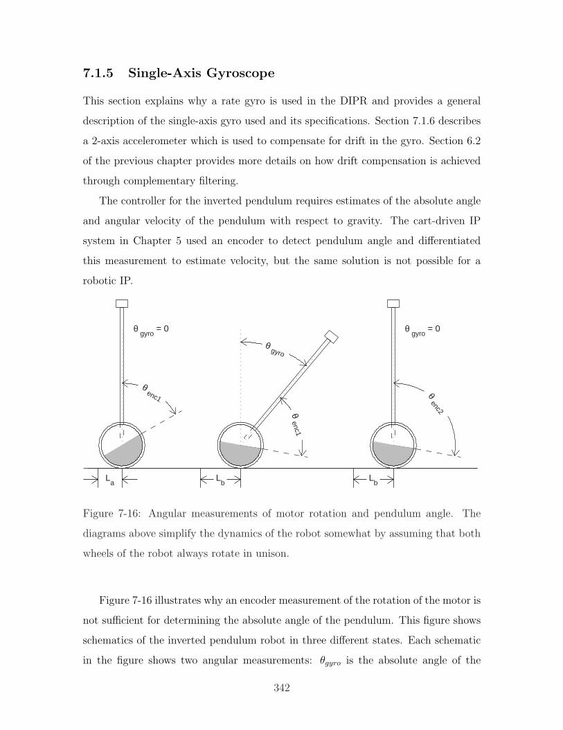
7.1.5 Single-Axis Gyroscope

This section explains why a rate gyro is used in the DIPR and provides a general

description of the single-axis gyro used and its specifications. Section 7.1.6 describes

a 2-axis accelerometer which is used to compensate for drift in the gyro. Section 6.2

of the previous chapter provides more details on how drift compensation is achieved

through complementary filtering.

The controller for the inverted pendulum requires estimates of the absolute angle

and angular velocity of the pendulum with respect to gravity. The cart-driven IP

system in Chapter 5 used an encoder to detect pendulum angle and differentiated

this measurement to estimate velocity, but the same solution is not possible for a

robotic IP.

θ enc1

La

θ enc1

Lb

θ gyro

θ enc2

Lb

θ gyro

= 0 θ gyro

= 0

Figure 7-16: Angular measurements of motor rotation and pendulum angle. The

diagrams above simplify the dynamics of the robot somewhat by assuming that both

wheels of the robot always rotate in unison.

Figure 7-16 illustrates why an encoder measurement of the rotation of the motor is

not sufficient for determining the absolute angle of the pendulum. This figure shows

schematics of the inverted pendulum robot in three different states. Each schematic

in the figure shows two angular measurements: θgyro is the absolute angle of the

342

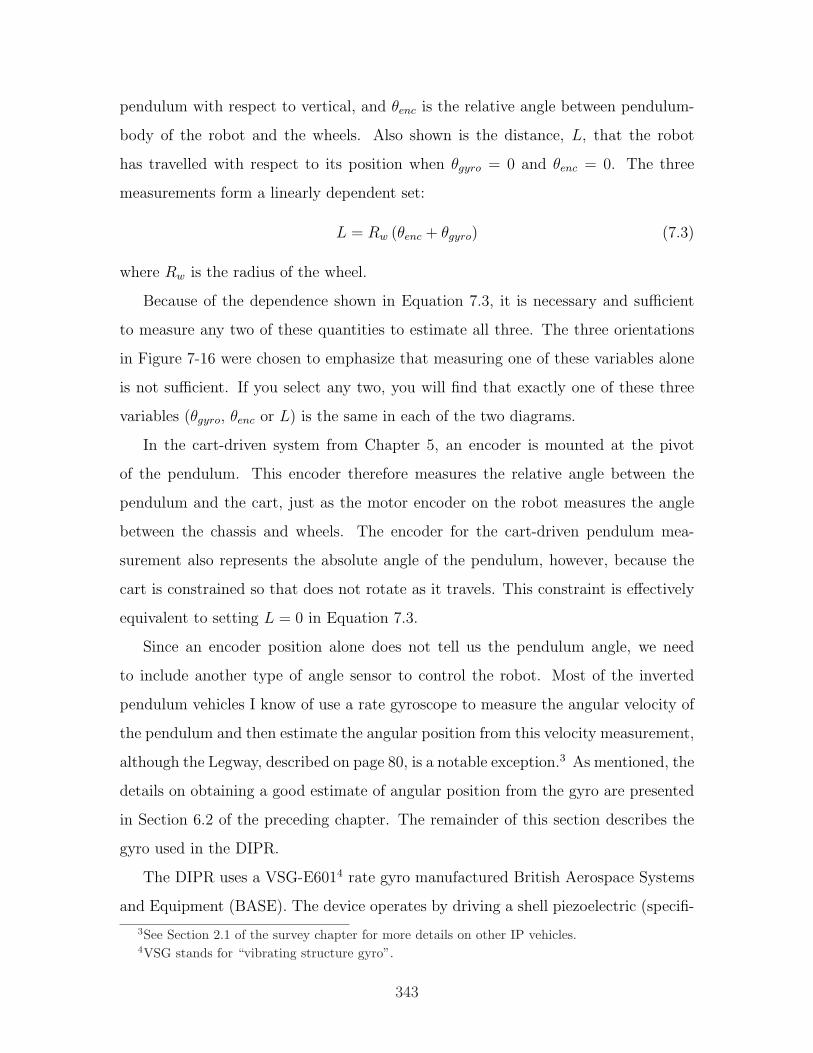
pendulum with respect to vertical, and θenc is the relative angle between pendulum-

body of the robot and the wheels. Also shown is the distance, L, that the robot

has travelled with respect to its position when θgyro = 0 and θenc = 0. The three

measurements form a linearly dependent set:

L = Rw (θenc + θgyro) (7.3)

where Rw is the radius of the wheel.

Because of the dependence shown in Equation 7.3, it is necessary and sufficient

to measure any two of these quantities to estimate all three. The three orientations

in Figure 7-16 were chosen to emphasize that measuring one of these variables alone

is not sufficient. If you select any two, you will find that exactly one of these three

variables (θgyro, θenc or L) is the same in each of the two diagrams.

In the cart-driven system from Chapter 5, an encoder is mounted at the pivot

of the pendulum. This encoder therefore measures the relative angle between the

pendulum and the cart, just as the motor encoder on the robot measures the angle

between the chassis and wheels. The encoder for the cart-driven pendulum mea-

surement also represents the absolute angle of the pendulum, however, because the

cart is constrained so that does not rotate as it travels. This constraint is effectively

equivalent to setting L = 0 in Equation 7.3.

Since an encoder position alone does not tell us the pendulum angle, we need

to include another type of angle sensor to control the robot. Most of the inverted

pendulum vehicles I know of use a rate gyroscope to measure the angular velocity of

the pendulum and then estimate the angular position from this velocity measurement,

although the Legway, described on page 80, is a notable exception.3 As mentioned, the

details on obtaining a good estimate of angular position from the gyro are presented

in Section 6.2 of the preceding chapter. The remainder of this section describes the

gyro used in the DIPR.

The DIPR uses a VSG-E6014 rate gyro manufactured British Aerospace Systems

and Equipment (BASE). The device operates by driving a shell piezoelectric (specifi-

3See Section 2.1 of the survey chapter for more details on other IP vehicles.4VSG stands for “vibrating structure gyro”.

343

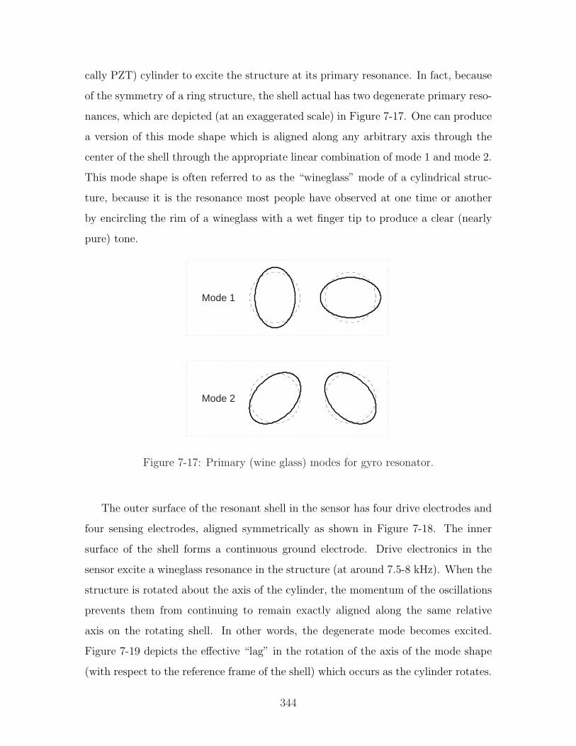
cally PZT) cylinder to excite the structure at its primary resonance. In fact, because

of the symmetry of a ring structure, the shell actual has two degenerate primary reso-

nances, which are depicted (at an exaggerated scale) in Figure 7-17. One can produce

a version of this mode shape which is aligned along any arbitrary axis through the

center of the shell through the appropriate linear combination of mode 1 and mode 2.

This mode shape is often referred to as the “wineglass” mode of a cylindrical struc-

ture, because it is the resonance most people have observed at one time or another

by encircling the rim of a wineglass with a wet finger tip to produce a clear (nearly

pure) tone.

Mode 1

Mode 2

Figure 7-17: Primary (wine glass) modes for gyro resonator.

The outer surface of the resonant shell in the sensor has four drive electrodes and

four sensing electrodes, aligned symmetrically as shown in Figure 7-18. The inner

surface of the shell forms a continuous ground electrode. Drive electronics in the

sensor excite a wineglass resonance in the structure (at around 7.5-8 kHz). When the

structure is rotated about the axis of the cylinder, the momentum of the oscillations

prevents them from continuing to remain exactly aligned along the same relative

axis on the rotating shell. In other words, the degenerate mode becomes excited.

Figure 7-19 depicts the effective “lag” in the rotation of the axis of the mode shape

(with respect to the reference frame of the shell) which occurs as the cylinder rotates.

344

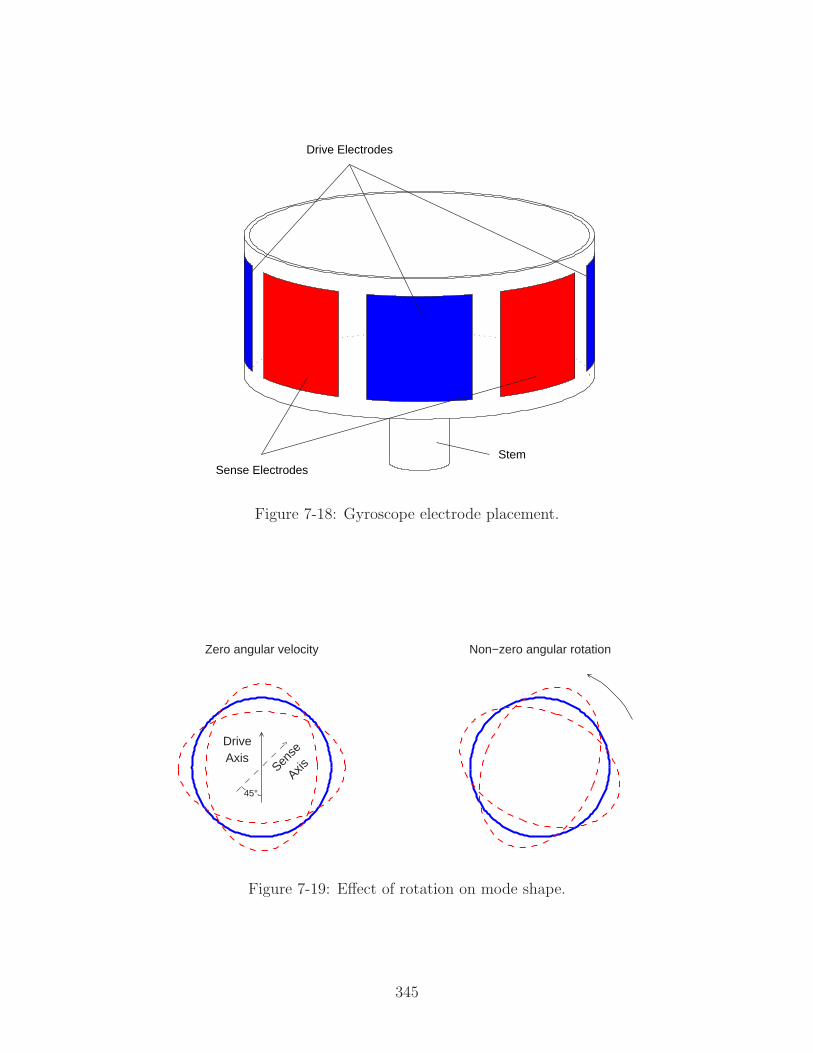
Drive Electrodes

Sense ElectrodesStem

Figure 7-18: Gyroscope electrode placement.

DriveAxis

Sense

Axis

45°

Zero angular velocity Non−zero angular rotation

Figure 7-19: Effect of rotation on mode shape.

345

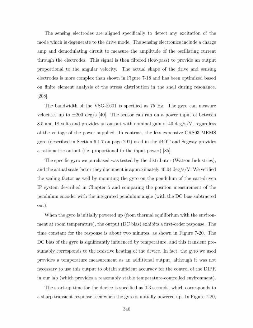
The sensing electrodes are aligned specifically to detect any excitation of the

mode which is degenerate to the drive mode. The sensing electronics include a charge

amp and demodulating circuit to measure the amplitude of the oscillating current

through the electrodes. This signal is then filtered (low-pass) to provide an output

proportional to the angular velocity. The actual shape of the drive and sensing

electrodes is more complex than shown in Figure 7-18 and has been optimized based

on finite element analysis of the stress distribution in the shell during resonance.

[208].

The bandwidth of the VSG-E601 is specified as 75 Hz. The gyro can measure

velocities up to ±200 deg/s [40]. The sensor can run on a power input of between

8.5 and 18 volts and provides an output with nominal gain of 40 deg/s/V, regardless

of the voltage of the power supplied. In contrast, the less-expensive CRS03 MEMS

gyro (described in Section 6.1.7 on page 291) used in the iBOT and Segway provides

a ratiometric output (i.e. proportional to the input power) [85].

The specific gyro we purchased was tested by the distributor (Watson Industries),

and the actual scale factor they document is approximately 40.04 deg/s/V. We verified

the scaling factor as well by mounting the gyro on the pendulum of the cart-driven

IP system described in Chapter 5 and comparing the position measurement of the

pendulum encoder with the integrated pendulum angle (with the DC bias subtracted

out).

When the gyro is initially powered up (from thermal equilibrium with the environ-

ment at room temperature), the output (DC bias) exhibits a first-order response. The

time constant for the response is about two minutes, as shown in Figure 7-20. The

DC bias of the gyro is significantly influenced by temperature, and this transient pre-

sumably corresponds to the resistive heating of the device. In fact, the gyro we used

provides a temperature measurement as an additional output, although it was not

necessary to use this output to obtain sufficient accuracy for the control of the DIPR

in our lab (which provides a reasonably stable temperature-controlled environment).

The start-up time for the device is specified as 0.3 seconds, which corresponds to

a sharp transient response seen when the gyro is initially powered up. In Figure 7-20,

346

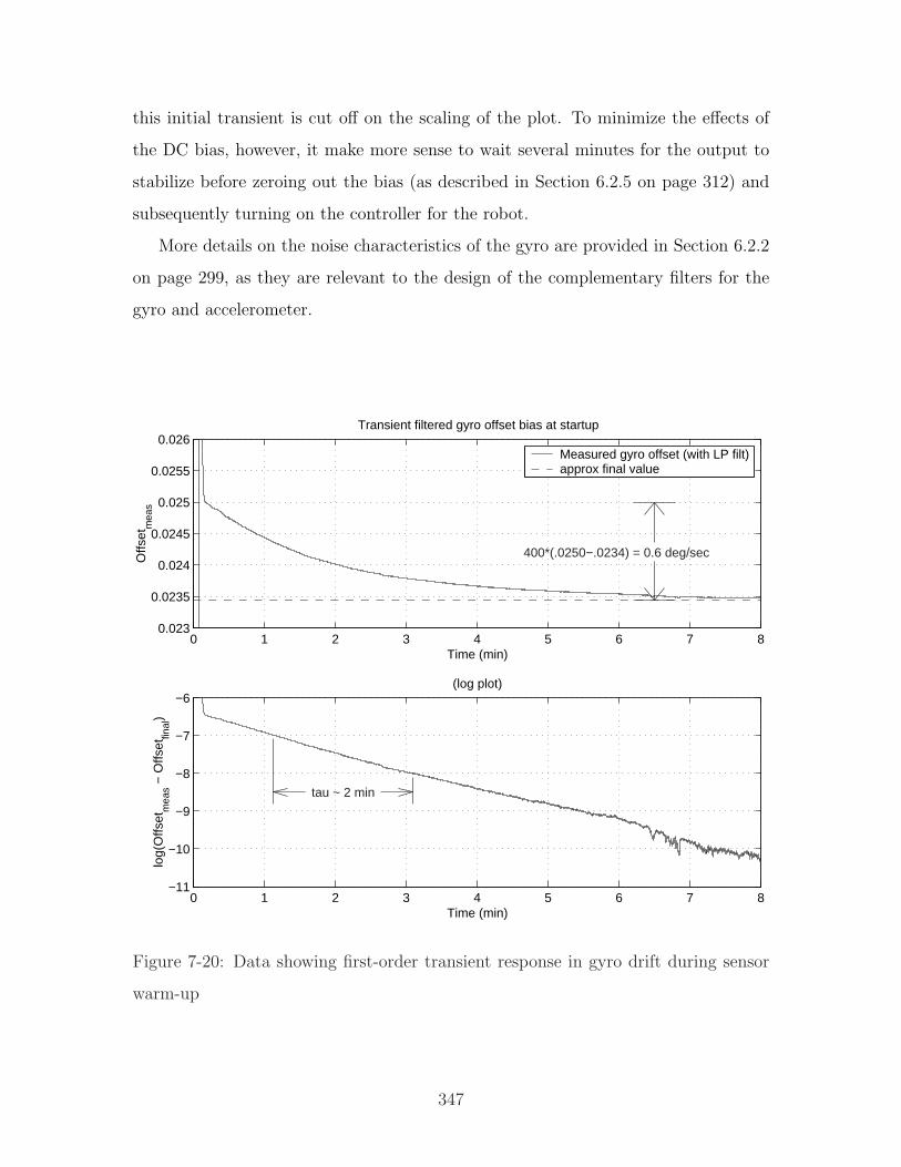
this initial transient is cut off on the scaling of the plot. To minimize the effects of

the DC bias, however, it make more sense to wait several minutes for the output to

stabilize before zeroing out the bias (as described in Section 6.2.5 on page 312) and

subsequently turning on the controller for the robot.

More details on the noise characteristics of the gyro are provided in Section 6.2.2

on page 299, as they are relevant to the design of the complementary filters for the

gyro and accelerometer.

0 1 2 3 4 5 6 7 80.023

0.0235

0.024

0.0245

0.025

0.0255

0.026

Time (min)

Offs

etm

eas

Transient filtered gyro offset bias at startup

400*(.0250−.0234) = 0.6 deg/sec

Measured gyro offset (with LP filt)approx final value

0 1 2 3 4 5 6 7 8−11

−10

−9

−8

−7

−6

Time (min)

log(

Offs

etm

eas −

Offs

etfin

al)

(log plot)

tau ~ 2 min

Figure 7-20: Data showing first-order transient response in gyro drift during sensor

warm-up

347

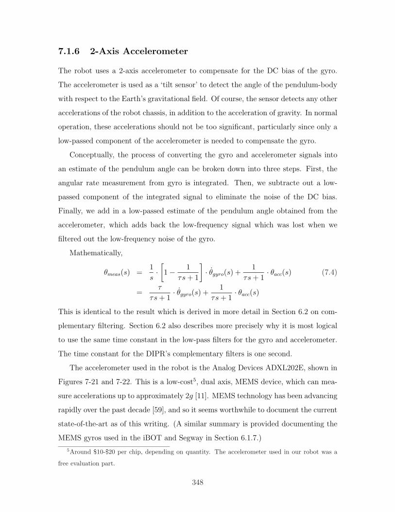
7.1.6 2-Axis Accelerometer

The robot uses a 2-axis accelerometer to compensate for the DC bias of the gyro.

The accelerometer is used as a ‘tilt sensor’ to detect the angle of the pendulum-body

with respect to the Earth’s gravitational field. Of course, the sensor detects any other

accelerations of the robot chassis, in addition to the acceleration of gravity. In normal

operation, these accelerations should not be too significant, particularly since only a

low-passed component of the accelerometer is needed to compensate the gyro.

Conceptually, the process of converting the gyro and accelerometer signals into

an estimate of the pendulum angle can be broken down into three steps. First, the

angular rate measurement from gyro is integrated. Then, we subtracte out a low-

passed component of the integrated signal to eliminate the noise of the DC bias.

Finally, we add in a low-passed estimate of the pendulum angle obtained from the

accelerometer, which adds back the low-frequency signal which was lost when we

filtered out the low-frequency noise of the gyro.

Mathematically,

θmeas(s) =1

s·[1− 1

τs + 1

]· θgyro(s) +

1

τs + 1· θacc(s) (7.4)

=τ

τs + 1· θgyro(s) +

1

τs + 1· θacc(s)

This is identical to the result which is derived in more detail in Section 6.2 on com-

plementary filtering. Section 6.2 also describes more precisely why it is most logical

to use the same time constant in the low-pass filters for the gyro and accelerometer.

The time constant for the DIPR’s complementary filters is one second.

The accelerometer used in the robot is the Analog Devices ADXL202E, shown in

Figures 7-21 and 7-22. This is a low-cost5, dual axis, MEMS device, which can mea-

sure accelerations up to approximately 2g [11]. MEMS technology has been advancing

rapidly over the past decade [59], and so it seems worthwhile to document the current

state-of-the-art as of this writing. (A similar summary is provided documenting the

MEMS gyros used in the iBOT and Segway in Section 6.1.7.)

5Around $10-$20 per chip, depending on quantity. The accelerometer used in our robot was a

free evaluation part.

348

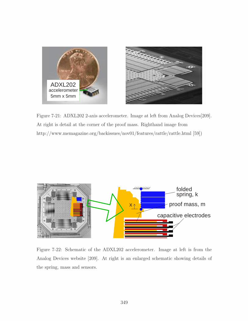
accelerometer5mm x 5mm

ADXL202

Figure 7-21: ADXL202 2-axis accelerometer. Image at left from Analog Devices[209].

At right is detail at the corner of the proof mass. Righthand image from

http://www.memagazine.org/backissues/nov01/features/rattle/rattle.html [59])

proof mass, m

spring, k folded

x

capacitive electrodes

Figure 7-22: Schematic of the ADXL202 accelerometer. Image at left is from the

Analog Devices website [209]. At right is an enlarged schematic showing details of

the spring, mass and sensors.

349

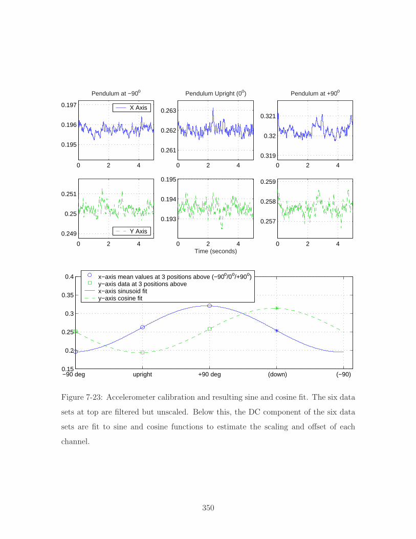
0 2 4

0.195

0.196

0.197

Pendulum at −90o

X Axis

0 2 4

0.261

0.262

0.263

Pendulum Upright (0o)

0 2 4

0.319

0.32

0.321

Pendulum at +90o

0 2 4

0.193

0.194

0.195

Time (seconds)0 2 4

0.249

0.25

0.251

Y Axis

0 2 4

0.257

0.258

0.259

−90 deg upright +90 deg (down) (−90) 0.15

0.2

0.25

0.3

0.35

0.4 x−axis mean values at 3 positions above (−90o/0o/+90o)y−axis data at 3 positions abovex−axis sinusoid fity−axis cosine fit

Figure 7-23: Accelerometer calibration and resulting sine and cosine fit. The six data

sets at top are filtered but unscaled. Below this, the DC component of the six data

sets are fit to sine and cosine functions to estimate the scaling and offset of each

channel.

350

yx

xy x

yg

(ADXL202AE top view)

Output at +90o tilt

Xnom

= 62.5% duty cycle= 0.3125 A/D input

Xmeas

= 0.3203 A/D input

Ynom


Ymeas

= 0.2576 A/D input

Output when pendulum upright

Xnom


Xmeas

= 0.2620 A/D input

Ynom


Ymeas

= 0.1935 A/D input

Output at −90o tilt

Xnom


Xmeas

= 0.1957 A/D input

Ynom


Ymeas

= 0.2503 A/D input

Figure 7-24: ADXL202AE output as tilt sensor. This figure is included to explain how

data for Figure 7-23 were obtained and to illustrate more clearly how the measured

values from the data in that figure compare with nominal outputs specified for the

sensor, as described further in the text.

The ADXL202 is a monolithic device, with all mechanical elements and accom-

panying electronics integrated onto a single chip. It is essentially just a spring-mass

system. The force in the spring (F = kx) balances the acceleration of the mass

(F = ma), and therefore the position of the mass is proportional to the accelera-

tion (x = mka). Folded polysilicon beams form the springs which are attached at the

corners of a thin square proof mass to minimize cross-coupling of the x- and y-axis

measurements. A series of fingers extend from the periphery of the mass. Each finger

is surround by two stationary plates which are fixed to the support structure and

driven by square waves which are 180 out of face. These interdigitated plates form

a differential capacitor, so that the amplitude of the resulting square wave output is

proportional to the displacement of the mass and therefore also to the acceleration

on the body [209, 11].

351

The DIPR uses the two PWM outputs of the ADXL202 which are thenfiltered

by a passive low-pass RC circuit with a bandwidth of 50 Hz. At 0 g, the duty cycle

should nominally be 50%, or 2.5 V after low-pass filtering. The nominal scaling factor

is 12.5% duty cycle change per g. The variance in the device can be huge, however.

The zero g bias level is given specified to fall within the range between 25% and 75%

duty cycle, and the specified tolerance on the scaling factor goes from 10% duty cycle

per g to 15% per g.

Figures 7-23 and 7-24 on previous two pages document the measured zero-g offset

and scaling factor for each of the two axes on the accelerometer. The values did not

vary significantly on a run-to-run basis.

Figure 7-23 on the left-hand page (p. 350) shows partial segments of six longer

streams of data each recorded while the robot was at rest with the pendulum pointing

either vertically or horizontally (as indicated on the figure). When the pendulum is

at rest, the acceleration of gravity should be the only force or acceleration acting on

the sensor. The three data sets shown at the top come from the x-axis channel of the

gyro and should therefore correspond to accelerations of -1g, 0g and +1g (going from

left to right). The y-axis data below this should ideally correspond to accelerations

of 0g, -1g (due to the orientation of the sensor) and 0g.

Because the accelerometer is not aligned perfectly on the robot, the actual angle

at which accelerometer is oriented is likely off by a couple of degrees (consistently)

from the angle of the pendulum. If you look closely at Figure 7-23, you may note

that the sine and cosine fits have been shifted somewhat to the left to take this into

account. The data seem to indicate that the alignment error of the accelerometer

mounting is approximately 2.

The figure on the righthand leaf (page 351) summarizes the expected and measured

DC outputs in each of the three configurations. Additional information on the noise

characteristics for the ADXL202 is given in Section 6.2.2 on page 299.

352

7.2 Lagrangian Derivation of the Equations of

Motion

The equations of motion for the inverted pendulum robot are derived below using

the indirect approach (i.e. “variational dynamics”). First, the lagrangian function,

L, is formed by subtracting the potential energy, V , from the kinetic coenergy, T ∗,

as shown in equation 7.5 below:

L = T ∗ − V (7.5)

where T ∗ and V are written in terms of a set of generalized variables. For the

derivation that follows, there are two generalized variables: θw, the rotation of the

wheels, and θp, the angle of the pendulum with respect to vertical.6 The generalized

forces acting on the system are denoted as “Ξj”. Lagrange’s equations, shown in

equation 7.6, provide a systematic way to balance the systems dynamics with these

external forces to form the equations of motion of the system.

d

dt

(∂L∂ξj

)− ∂L

∂ξj

= Ξj (j = 1, 2, . . . , n) (7.6)

The kinetic coenergy of a particle is 12mivi ·vi. For a rigid body, the total coenergy

of all particles in the body can be represented as:

T ∗body =

1

2mbvb · vb +

1

2Jbθb · θb (7.7)

where mb and Jb are the mass and moment of inertia of the body, respectively. Cor-

respondingly, for a system of rigid bodies:

T ∗system =

n∑i=1

1

2mivi · vi +

n∑i=1

1

2Jiθi · θi (7.8)

For the inverted pendulum robot, we will consider four rigid bodies in constructing

the langrangian. These are illustrated in Figure 7-25. It is a reasonable approximation

to assume that the centers of mass of the wheels (Mw), chassis (Mb), and motor

6Note that this analysis has been simplified by lumping both wheels together, so that they always

rotate in unison.

353

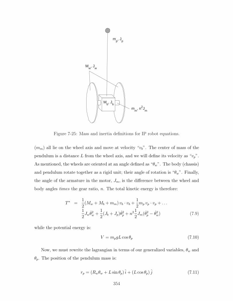
mp, J

p

Mw

, Jw

Mb, J

b

mm

, n2Jm

Figure 7-25: Mass and inertia definitions for IP robot equations.

(mm) all lie on the wheel axis and move at velocity “vb”. The center of mass of the

pendulum is a distance L from the wheel axis, and we will define its velocity as “vp”.

As mentioned, the wheels are oriented at an angle defined as “θw”. The body (chassis)

and pendulum rotate together as a rigid unit; their angle of rotation is “θw”. Finally,

the angle of the armature in the motor, Jm, is the difference between the wheel and

body angles times the gear ratio, n. The total kinetic energy is therefore:

T ∗ =1

2(Mw + Mb + mm) vb · vb +

1

2mp vp · vp + . . .

1

2Jwθ2

w +1

2(Jb + Jp)θ

2p + n2 1

2Jm(θ2

p − θ2w) (7.9)

while the potential energy is:

V = mpgL cos θp (7.10)

Now, we must rewrite the lagrangian in terms of our generalized variables, θw and

θp. The position of the pendulum mass is:

rp = (Rwθw + L sin θp) i + (L cos θp) j (7.11)

354

therefore its velocity is:

vp =drp

dt=

(Rwθw + θpL cos θp

)i +

(−θpL sin θp

)j (7.12)

and so:

1

2mp vp · vp =

1

2mp

[R2

wθ2w + 2RwLθwθp cos θp + L2θ2

pcos2θp + L2θ2psin

2θp

]

=1

2mp

[R2


p

](7.13)

Collecting terms:

T ∗ =1

2MR2

wθ2w +

1

2mp

(R2


p

)+

1

2Jwθ2

w + . . .

1

2n2Jm

(θ2

p − 2θpθw + θ2w

)+

1

2(Jp + Jb) θ2

p (7.14)

L =1

2MR2

wθ2w +

1

2mp

(R2


p

)+

1

2Jwθ2

w + . . .

1

2n2Jm

(θ2

p − 2θpθw + θ2w

)+

1

2(Jp + Jb) θ2

p −mpgL cos θp (7.15)

where M = Mb + Mw + mm. We can now derive the two equations of motion. First,

with respect to the wheel angle,

d

dt

(∂L

∂θw

)− ∂L

∂θw

= Ξθw (7.16)

The torques acting to accelerate the wheel angle include the motor torque, nKti,

friction, ffric

(θp − θw

), and any external disturbance force applied at (or near) the

motor, Fm ·Rm:

Ξθw = nKti + bfric

(θp − θw

)+ Fm ·Rm (7.17)

∂L

∂θw

= MR2wθw + mpR

2wθw + mpRwLθp cos θp + n2Jm

(θw − θp

)+ Jwθw (7.18)

d

dt

(∂L

∂θw

)= MR2

wθw + mpR2wθw + mpRwLθp cos θp −mpRwLθ2

p sin θp + . . .

n2Jm

(θw − θp

)+ Jwθw (7.19)

∂L

∂θw

= 0 (7.20)

355

Combining all these terms and applying equation 7.16, we obtain the first equation

of motion, shown in equation 7.21:

[(M + mp) R2w + n2Jm + Jw] θw + [mpRwL cos θp − n2Jm] θp = . . .

mpRwLθ2p sin θp + nKti + bfric

(θp − θw

)+ Fm ·Rw

(7.21)

The second equation of motion is derived (below) in the same manner. Again, we

begin with the definition of the lagrangian, now with respect to the pendulum angle.

d

dt

(∂L

∂θp

)− ∂L

∂θp

= Ξθp (7.22)

The torque contributions from the motor and friction are equal but opposite to those

in the previous derivation, and we will now include a disturbance torce applied to the

pendulum-body unit.

Ξθp = −nKti− bfric

(θp − θw

)+ τp (7.23)

∂L

∂θp

= mpL2θp + mpRwLθw cos θp + (Jp + Jb) θp + n2Jm

(θp − θw

)(7.24)

d

dt

(∂L

∂θp

)= mpL

2θp + mpRwLθw cos θp−mpRwLθwθp sin θp + Jpθp + n2Jm

(θp − θw

)

(7.25)∂L

∂θp

= −mpRwθwθpL sin θp + mpgL sin θp (7.26)

The second equation of motion is shown in equation 7.27:

[mpL2 + Jp + Jb + n2Jm] θp + [mpRwL cos θp − n2Jm] θw = . . .

mgL sin θp − nKti− bfric

(θp − θw

)+ τp

(7.27)

To linearize the equations of motions about the unstable (upright) equilibrium

point, we will make the standard small-angle assumptions that θp << 1 and θp << 1.

Therefore, sin θp ≈ 0, cos θp ≈ 1, and θ2p ≈ 0. Applying these approximation to

equations 7.21 and 7.27 we get the following two linearized equations of motion:

[(M + mp) R2w + Jw + n2Jm] θw + [mpRwL− n2Jm] θp = . . .

nKti + bfric

(θp − θw

)+ Fm ·Rw

(7.28)

356

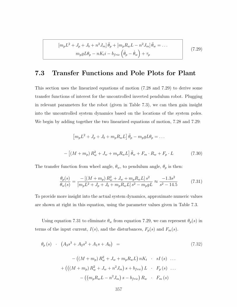
[mpL2 + Jp + Jb + n2Jm] θp + [mpRwL− n2Jm] θw = . . .

mpgLθp − nKti− bfric

(θp − θw

)+ τp

(7.29)

7.3 Transfer Functions and Pole Plots for Plant

This section uses the linearized equations of motion (7.28 and 7.29) to derive some

transfer functions of interest for the uncontrolled inverted pendulum robot. Plugging

in relevant parameters for the robot (given in Table 7.3), we can then gain insight

into the uncontrolled system dynamics based on the locations of the system poles.

We begin by adding together the two linearized equations of motion, 7.28 and 7.29:

[mpL

2 + Jp + Jb + mpRwL]θp −mpgLθp = . . .

− [(M + mp) R2

w + Jw + mpRwL]θw + Fm ·Rw + Fp · L (7.30)

The transfer function from wheel angle, θw, to pendulum angle, θp is then:

θp(s)

θw(s)=

− [(M + mp) R2w + Jw + mpRwL] s2

[mpL2 + Jp + Jb + mpRwL] s2 −mpgL≈ −1.3s2

s2 − 14.5(7.31)

To provide more insight into the actual system dynamics, approximate numeric values

are shown at right in this equation, using the parameter values given in Table 7.3.

Using equation 7.31 to eliminate θw from equation 7.29, we can represent θp(s) in

terms of the input current, I(s), and the disturbances, Fp(s) and Fm(s).

θp (s) · (A3s

3 + A2s2 + A1s + A0

)= (7.32)

− ((M + mp) R2

w + Jw + mpRwL)nKt · sI (s) . . .

+((

(M + mp) R2w + Jw + n2Jm

)s + bfric

)L · Fp (s) . . .

− ((mpRwL− n2Jm

)s− bfric

)Rw · Fm (s)

357

The new variables defined in this equation are:

A3 = mpML2R2w + (M + mp) R2

w (Jp + Jb) + mpL2Jw + Jw (Jp + Jb) + . . .

. . . + n2Jm

[mp

(L + R2

w

)2+ MR2

w + Jw + Jp + Jb

](7.33)

≈ mpML2R2w + (M + mp) R2

w (Jp + Jb) + mpL2Jw + Jw (Jp + Jb)

≈ 0.0718

A2 =(mp(L + Rw)2 + MR2

w + Jw + Jp + Jb

)bfric (7.34)

≈ 0.00034

A1 = −mpgL((M + mp) R2

w + Jw + n2Jm

)(7.35)

≈ −mpgL((M + mp) R2

w + Jw

)

≈ −1.14

A0 = −mpgLbfric (7.36)

≈ −0.002

The transfer functions from each input to θp are:

θp(s)

I(s)=

− ((M + mp) R2w + Jw + mpRwL) nKts

A3s3 + A2s2 + A1s + A0

(7.37)

≈ −0.039s

0.072s3 + 0.00034s2 − 1.14s− 0.002

=−0.33

(s− 4.0)(s + 4.0)

θp(s)

Fm(s)=

−Rw ((mpRwL− n2Jm) s− bfric)

A3s3 + A2s2 + A1s + A0

(7.38)

≈ −0.0090s + 0.000075

0.072s3 + 0.00034s2 − 1.14s− 0.002

≈ −0.125

(s− 4.0)(s + 4.0)

(7.39)

358

θp(s)

Fp(s)=

L (((M + mp) R2w + Jw) s + bfric)

A3s3 + A2s2 + A1s + A0

(7.40)

≈ 0.12

0.072s2 + 0.00034s− 1.14

≈ 1.67

(s− 4.0)(s + 4.0)

Estimated Parameter Values for Inverted Pendulum Robot. Note that each inertia

value are taken with respect to the center of mass of that object.

Final Smaller

Var. robot prototype

mp = 1.0 [kg] 0.2 [kg]

Mw = 2.6 [kg] 2 [kg]

Mb = 6.5 [kg] 2 [kg]

mm = 1.3 [kg] (same)

M = 10.6 [kg] ∼ 5.5 [kg]

Jp = 0.05 [kg m2] 0.02 [kg m2]

Jw = 0.029 [kg m2] 0.009 [kg m2]

Jb = 0.05 [kg m2] 0.016 [kg m2]

Jm = 0.000012 [kg m2] (same)

n = 13/3 (same)

n2Jm = 0.00023 [kg m2] (same)

Rw = 0.15 [m] 0.10 [m]

Leff = 0.4 [m] 0.5 [m]

bfric ≈ 0.0005 ? [Nms/rad] (same)

Kt = 0.026 [Nm/A] (same)

359

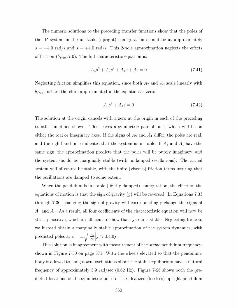
The numeric solutions to the preceding transfer functions show that the poles of

the IP system in the unstable (upright) configuration should be at approximately

s = −4.0 rad/s and s = +4.0 rad/s. This 2-pole approximation neglects the effects

of friction (bfric ≈ 0). The full characteristic equation is:

A3s3 + A2s

2 + A1s + A0 = 0 (7.41)

Neglecting friction simplifies this equation, since both A2 and A0 scale linearly with

bfric and are therefore approximated in the equation as zero:

A3s3 + A1s = 0 (7.42)

The solution at the origin cancels with a zero at the origin in each of the preceding

transfer functions shown. This leaves a symmetric pair of poles which will lie on

either the real or imaginary axes. If the signs of A3 and A1 differ, the poles are real,

and the righthand pole indicates that the system is unstable. If A3 and A1 have the

same sign, the approximation predicts that the poles will be purely imaginary, and

the system should be marginally stable (with undamped oscillations). The actual

system will of course be stable, with the finite (viscous) friction terms insuring that

the oscillations are damped to some extent.

When the pendulum is in stable (lightly damped) configuration, the effect on the

equations of motion is that the sign of gravity (g) will be reversed. In Equations 7.33

through 7.36, changing the sign of gravity will correspondingly change the signs of

A1 and A0. As a result, all four coefficients of the characteristic equation will now be

strictly positive, which is sufficient to show that system is stable. Neglecting friction,

we instead obtain a marginally stable approximation of the system dynamics, with

predicted poles at s = ±√∣∣∣A1

A3

∣∣∣j ≈ ±4.0j.

This solution is in agreement with measurement of the stable pendulum frequency,

shown in Figure 7-30 on page 371. With the wheels elevated so that the pendulum-

body is allowed to hang down, oscillations about the stable equilibrium have a natural

frequency of approximately 3.9 rad/sec (0.62 Hz). Figure 7-26 shows both the pre-

dicted locations of the symmetric poles of the idealized (lossless) upright pendulum

360

vehicle (at left) and (at right) the measured complex pole pair corresponding to the

stable pendulum. The magnitude of the distance of each pole from the origin is the

same (approximately), as expected.

In fact, the frequency of the oscillations in the stable configuration was used

to help determine the inertia of the chassis more precisely (as described further in

Section 7.5.2), so it is no accident that the agreement is so close!

−6 −4 −2 0 2 4 6−6

−4

−2

0

2

4

6

Real

Imag

Predicted Unstable Poles

−3.980 +3.978

−6 −4 −2 0 2 4 6−6

−4

−2

0

2

4

6

Real

Imag

Observed Stable Poles

−.136+3.90j

−.136−3.90j

Figure 7-26: Poles for IP system near unstable and stable equilibria. The unstable

pole locations at left are those predicted by the transfer functions derived in this

section. The stable poles shown are right were obtained from encoder measurements

of the pendulum oscillations near its stable equilibrium. These pole plots show that

that two results are in agreement. Because the system has little damping, we would

expect mathematically that changing the sign of gravity would effectively just change

the signs of some terms in the characteristic polynomial for the system and would

correspondingly “swap” the axes (Real vs. Imag) on which the poles are located. The

distance of the poles from the origin should not change, however.

361

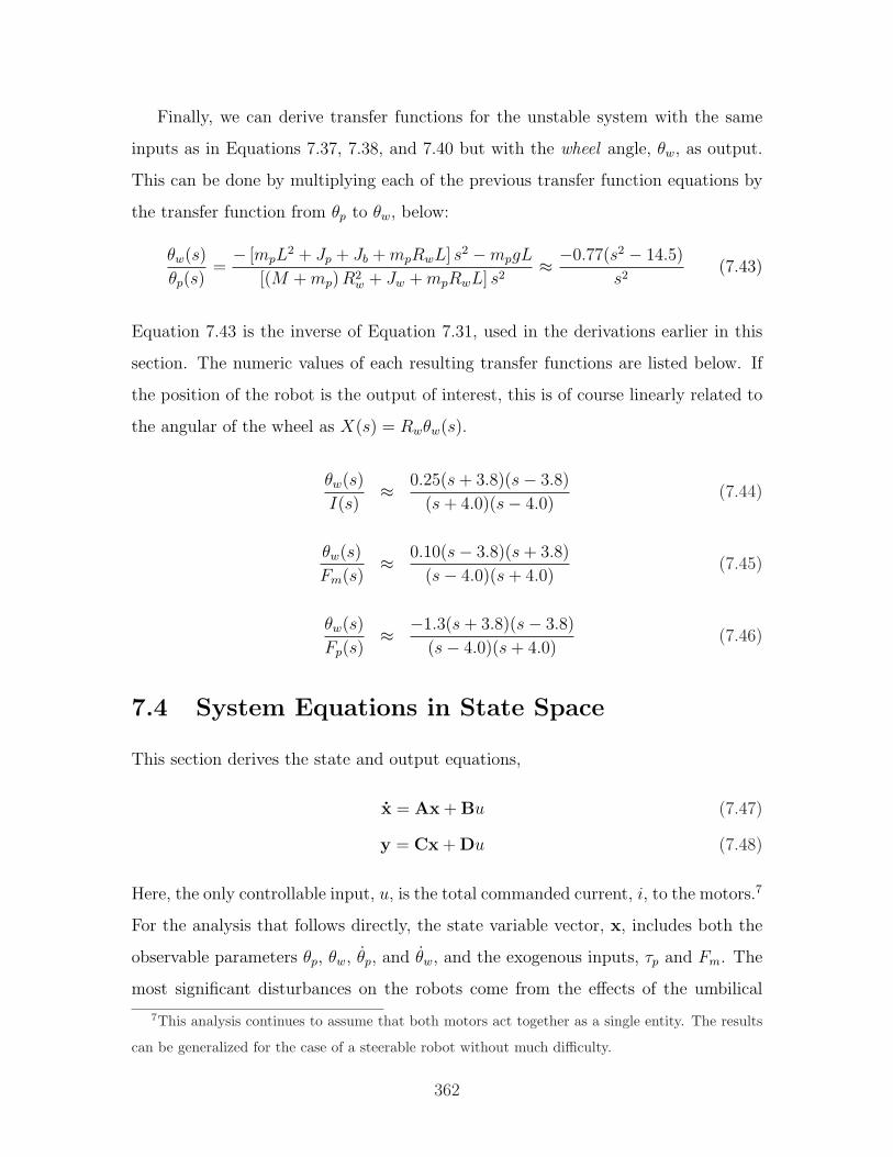
Finally, we can derive transfer functions for the unstable system with the same

inputs as in Equations 7.37, 7.38, and 7.40 but with the wheel angle, θw, as output.

This can be done by multiplying each of the previous transfer function equations by

the transfer function from θp to θw, below:

θw(s)

θp(s)=− [mpL

2 + Jp + Jb + mpRwL] s2 −mpgL

[(M + mp) R2w + Jw + mpRwL] s2

≈ −0.77(s2 − 14.5)

s2(7.43)

Equation 7.43 is the inverse of Equation 7.31, used in the derivations earlier in this

section. The numeric values of each resulting transfer functions are listed below. If

the position of the robot is the output of interest, this is of course linearly related to

the angular of the wheel as X(s) = Rwθw(s).

θw(s)

I(s)≈ 0.25(s + 3.8)(s− 3.8)

(s + 4.0)(s− 4.0)(7.44)

θw(s)

Fm(s)≈ 0.10(s− 3.8)(s + 3.8)

(s− 4.0)(s + 4.0)(7.45)

θw(s)

Fp(s)≈ −1.3(s + 3.8)(s− 3.8)

(s− 4.0)(s + 4.0)(7.46)

7.4 System Equations in State Space

This section derives the state and output equations,

x = Ax + Bu (7.47)

y = Cx + Du (7.48)

Here, the only controllable input, u, is the total commanded current, i, to the motors.7

For the analysis that follows directly, the state variable vector, x, includes both the

observable parameters θp, θw, θp, and θw, and the exogenous inputs, τp and Fm. The

most significant disturbances on the robots come from the effects of the umbilical

7This analysis continues to assume that both motors act together as a single entity. The results

can be generalized for the case of a steerable robot without much difficulty.

362

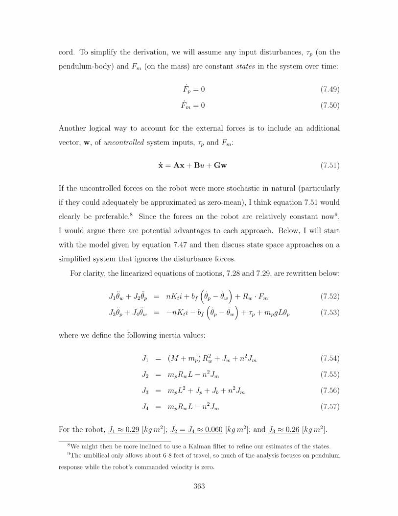
cord. To simplify the derivation, we will assume any input disturbances, τp (on the

pendulum-body) and Fm (on the mass) are constant states in the system over time:

Fp = 0 (7.49)

Fm = 0 (7.50)

Another logical way to account for the external forces is to include an additional

vector, w, of uncontrolled system inputs, τp and Fm:

x = Ax + Bu + Gw (7.51)

If the uncontrolled forces on the robot were more stochastic in natural (particularly

if they could adequately be approximated as zero-mean), I think equation 7.51 would

clearly be preferable.8 Since the forces on the robot are relatively constant now9,

I would argue there are potential advantages to each approach. Below, I will start

with the model given by equation 7.47 and then discuss state space approaches on a

simplified system that ignores the disturbance forces.

For clarity, the linearized equations of motions, 7.28 and 7.29, are rewritten below:

J1θw + J2θp = nKti + bf

(θp − θw

)+ Rw · Fm (7.52)

J3θp + J4θw = −nKti− bf

(θp − θw

)+ τp + mpgLθp (7.53)

where we define the following inertia values:

J1 = (M + mp) R2w + Jw + n2Jm (7.54)

J2 = mpRwL− n2Jm (7.55)

J3 = mpL2 + Jp + Jb + n2Jm (7.56)

J4 = mpRwL− n2Jm (7.57)

For the robot, J1 ≈ 0.29 [kg m2]; J2 = J4 ≈ 0.060 [kg m2]; and J3 ≈ 0.26 [kg m2].

8We might then be more inclined to use a Kalman filter to refine our estimates of the states.9The umbilical only allows about 6-8 feet of travel, so much of the analysis focuses on pendulum

response while the robot’s commanded velocity is zero.

363

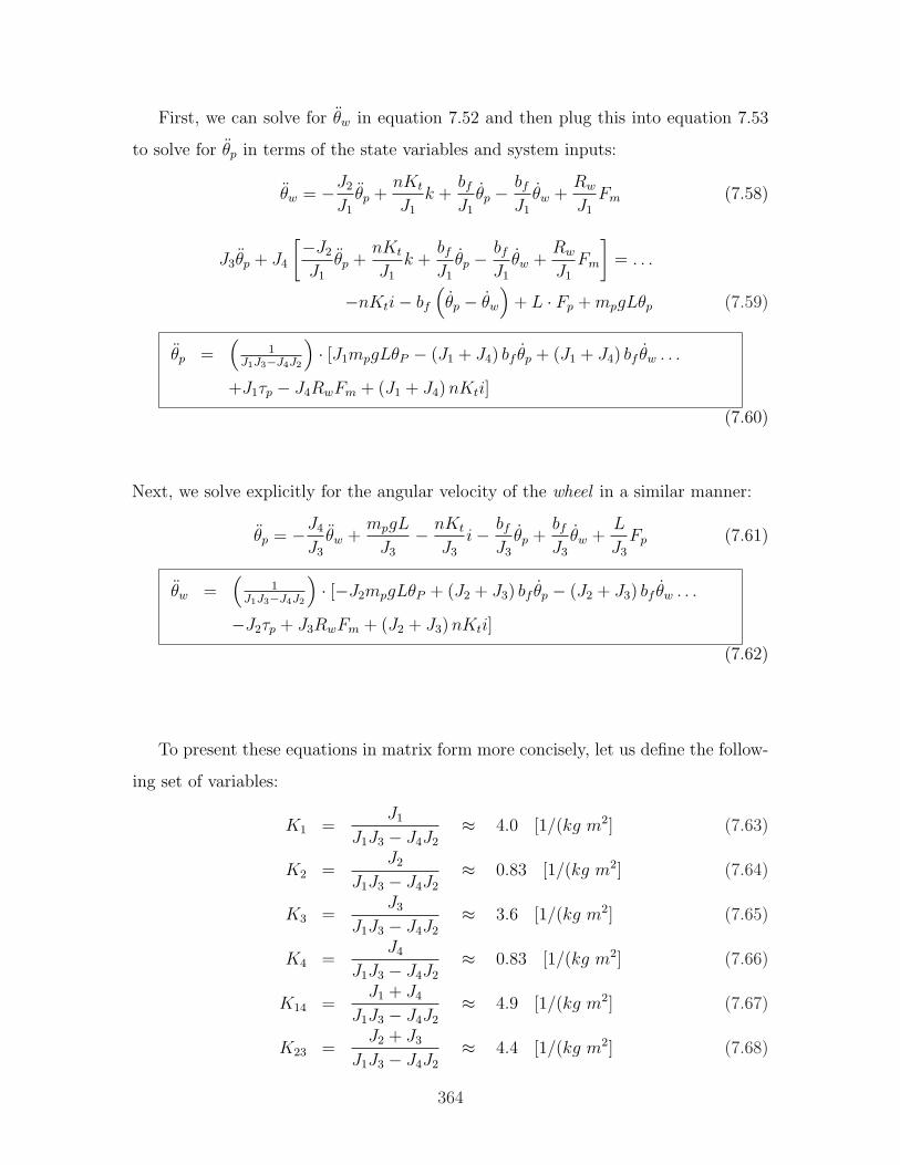
First, we can solve for θw in equation 7.52 and then plug this into equation 7.53

to solve for θp in terms of the state variables and system inputs:

θw = −J2

J1

θp +nKt

J1

k +bf

J1

θp − bf

J1

θw +Rw

J1

Fm (7.58)

J3θp + J4

[−J2

J1

θp +nKt

J1

k +bf

J1

θp − bf

J1

θw +Rw

J1

Fm

]= . . .

−nKti− bf

(θp − θw

)+ L · Fp + mpgLθp (7.59)

θp =(

1J1J3−J4J2

)· [J1mpgLθP − (J1 + J4) bf θp + (J1 + J4) bf θw . . .

+J1τp − J4RwFm + (J1 + J4) nKti]

(7.60)

Next, we solve explicitly for the angular velocity of the wheel in a similar manner:

θp = −J4

J3

θw +mpgL

J3

− nKt

J3

i− bf

J3

θp +bf

J3

θw +L

J3

Fp (7.61)

θw =(

1J1J3−J4J2

)· [−J2mpgLθP + (J2 + J3) bf θp − (J2 + J3) bf θw . . .

−J2τp + J3RwFm + (J2 + J3) nKti]

(7.62)

To present these equations in matrix form more concisely, let us define the follow-

ing set of variables:

K1 =J1

J1J3 − J4J2

≈ 4.0 [1/(kg m2] (7.63)

K2 =J2

J1J3 − J4J2

≈ 0.83 [1/(kg m2] (7.64)

K3 =J3

J1J3 − J4J2

≈ 3.6 [1/(kg m2] (7.65)

K4 =J4

J1J3 − J4J2

≈ 0.83 [1/(kg m2] (7.66)

K14 =J1 + J4

J1J3 − J4J2

≈ 4.9 [1/(kg m2] (7.67)

K23 =J2 + J3

J1J3 − J4J2

≈ 4.4 [1/(kg m2] (7.68)

364

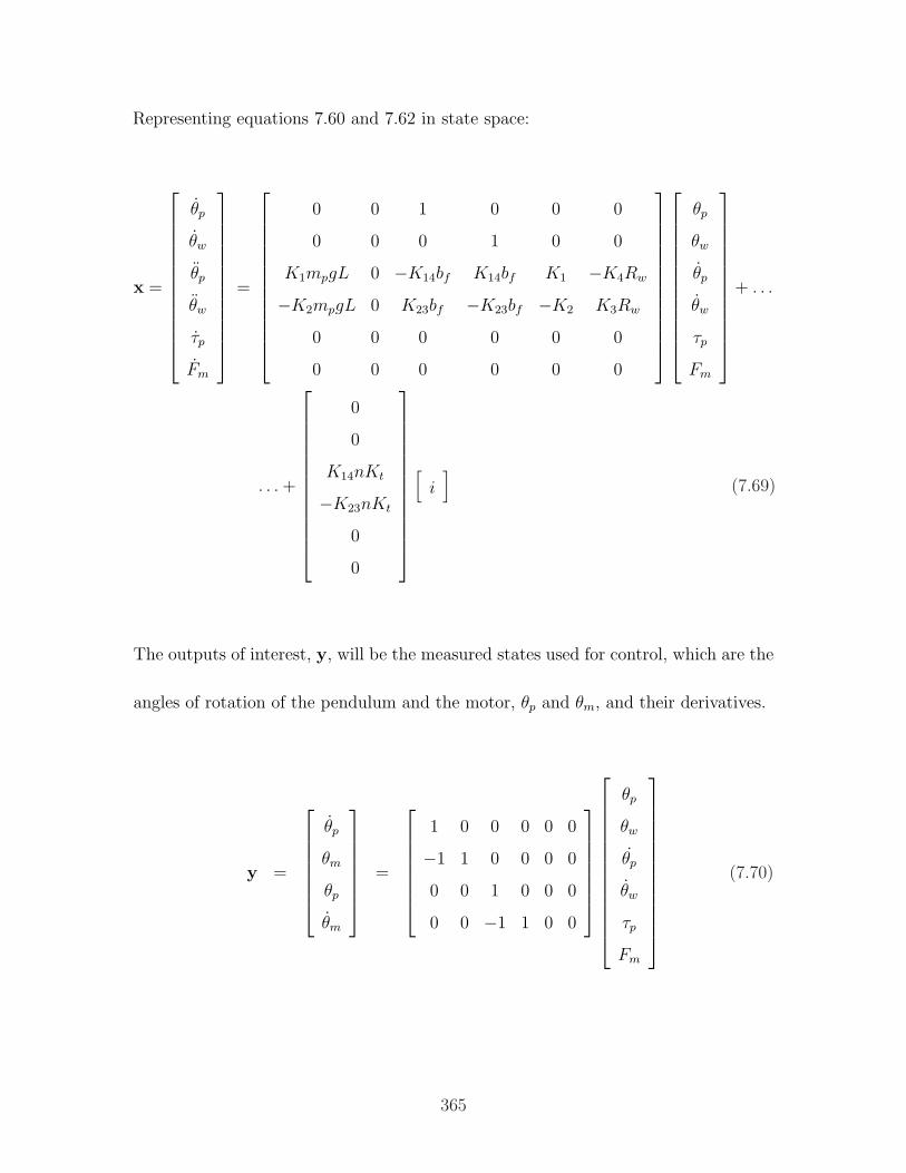
Representing equations 7.60 and 7.62 in state space:

x =

θp

θw

θp

θw

τp

Fm

=

0 0 1 0 0 0

0 0 0 1 0 0

K1mpgL 0 −K14bf K14bf K1 −K4Rw

−K2mpgL 0 K23bf −K23bf −K2 K3Rw

0 0 0 0 0 0

0 0 0 0 0 0

θp

θw

θp

θw

τp

Fm

+ . . .

. . . +

0

0

K14nKt

−K23nKt

0

0

[i

](7.69)

The outputs of interest, y, will be the measured states used for control, which are the

angles of rotation of the pendulum and the motor, θp and θm, and their derivatives.

y =

θp

θm

θp

θm

=

1 0 0 0 0 0

−1 1 0 0 0 0

0 0 1 0 0 0

0 0 −1 1 0 0

θp

θw

θp

θw

τp

Fm

(7.70)

365

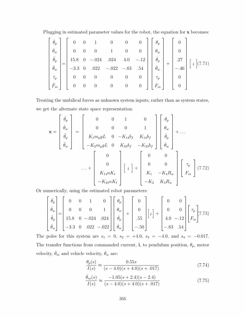
Plugging in estimated parameter values for the robot, the equation for x becomes:

θp

θw

θp

θw

τp

Fm

=

0 0 1 0 0 0

0 0 0 1 0 0

15.8 0 −.024 .024 4.0 −.12

−3.3 0 .022 −.022 −.83 .54

0 0 0 0 0 0

0 0 0 0 0 0

θp

θw

θp

θw

τp

Fm

+

0

0

.27

−.46

0

0

[i](7.71)

Treating the umbilical forces as unknown system inputs, rather than as system states,

we get the alternate state space representation:

x =

θp

θw

θp

θw

=

0 0 1 0

0 0 0 1

K1mpgL 0 −K14bf K14bf

−K2mpgL 0 K23bf −K23bf

θp

θw

θp

θw

+ . . .

. . . +

0

0

K14nKt

−K23nKt

[i

]+

0 0

0 0

K1 −K4Rw

−K2 K3Rw

τp

Fm

(7.72)

Or numerically, using the estimated robot parameters:

θp

θw

θp

θw

=

0 0 1 0

0 0 0 1

15.8 0 −.024 .024

−3.3 0 .022 −.022

θp

θw

θp

θw

+

0

0

.55

−.50

[i]

+

0 0

0 0

4.0 −.12

−.83 .54

τp

Fm

(7.73)

The poles for this system are s1 = 0, s2 = +4.0, s3 = −4.0, and s4 = −0.017.

The transfer functions from commanded current, i, to pendulum position, θp, motor

velocity, θm and vehicle velocity, θw are:

θp(s)

I(s)≈ 0.55s

(s− 4.0)(s + 4.0)(s + .017)(7.74)

θm(s)

I(s)≈ −1.05(s + 2.4)(s− 2.4)

(s− 4.0)(s + 4.0)(s + .017)(7.75)

366

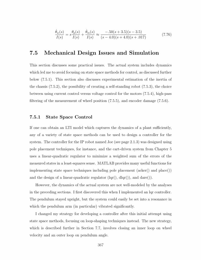
θw(s)

I(s)= s

θp(s)

I(s)+

θm(s)

I(s)≈ −.50(s + 3.5)(s− 3.5)

(s− 4.0)(s + 4.0)(s + .017)(7.76)

7.5 Mechanical Design Issues and Simulation

This section discusses some practical issues. The actual system includes dynamics

which led me to avoid focusing on state space methods for control, as discussed further

below (7.5.1). This section also discusses experimental estimation of the inertia of

the chassis (7.5.2), the possibility of creating a self-standing robot (7.5.3), the choice

between using current control versus voltage control for the motors (7.5.4), high-pass

filtering of the measurement of wheel position (7.5.5), and encoder damage (7.5.6).

7.5.1 State Space Control

If one can obtain an LTI model which captures the dynamics of a plant sufficiently,

any of a variety of state space methods can be used to design a controller for the

system. The controller for the IP robot named Joe (see page 2.1.3) was designed using

pole placement techniques, for instance, and the cart-driven system from Chapter 5

uses a linear-quadratic regulator to minimize a weighted sum of the errors of the

measured states in a least-squares sense. MATLAB provides many useful functions for

implementing state space techniques including pole placement (acker() and place())

and the design of a linear-quadratic regulator (lqr(), dlqr()), and dare()).

However, the dynamics of the actual system are not well-modeled by the analyses

in the preceding sections. I first discovered this when I implemented an lqr controller.

The pendulum stayed upright, but the system could easily be set into a resonance in

which the pendulum arm (in particular) vibrated significantly.

I changed my strategy for developing a controller after this initial attempt using

state space methods, focusing on loop-shaping techniques instead. The new strategy,

which is described further in Section 7.7, involves closing an inner loop on wheel

velocity and an outer loop on pendulum angle.

367

The transfer functions in Section 7.6 document the measured plant dynamics.

Figure 7-27 shows an example of the measured plant data, which is identical to the

data presented in Figure 7-37 on page 380.

10−1

100

101

102

103

−40

−20

0

20

Mag

n. (

dB)

MeasuredTheory

10−1

100

101

102

103

−360

−180 0

180

360

540

Pha

se (

deg.

)

Frequency (Hz)

MeasuredTheory

Figure 7-27: Measured plant compared with theoretical TF (θp(s)/V (s)). The pre-

dicted transfer function from voltage to pendulum angle is very close to the TF from

current to θp, which is given in Equation 7.37. (Section 7.5.4 discusses the differences

between current and voltage control.)

Both the theoretical and measured systems have a zero at or near the original and

a pair of poles near 4 rad/s. Aside from this, however, the two systems show quite

significant disparity! Mostly particularly, the expected dynamics include an unstable

pole at +4 rad/s, while there seems to be a complex pole pair rather than a real pole

pair in the measured transfer function. Moreover, the actual poles seem to lie entirely

in the left-half plane, so the pendulum is theoretically stable in upright position, even

without control.

Figure 7-28 compares the same measured data shown in Figure 7-27 with a 7th-

order plant. This higher-order system was selected to match the general characteris-

tics of the experimental data, but it is not intended to be a close fit. The 7th-order

system contains a lightly damped pole pair at around 4.3 rad/s (0.68 Hz) with ζ ≈ 0.1.

368

10−1

100

101

102

103

−40

−20

0

20

Mag

n. (

dB)

Measured7th−order system

10−1

100

101

102

103

−360

−180 0

180

360

540

Frequency (Hz)

Pha

se (

deg.

)

Measured7th−order system

Figure 7-28: Measured dynamics compared with a 7th-order stable system. The

measured data, which are identical to those shown in Figure 7-27, represent the

transfer function from voltage to pendulum angle (θp(s)/V (s)). The dashed line

represents a stable 7th-order system. The 7th-order system is not meant to match

the data as a convincing fit, but it does seem to indicate that the actual plant can

be modeled more closely as a stable 7th-order system than as the unstable 2nd-order

plant predicted (which was shown in Figure 7-27).

Also of interest are the lightly damped pair of zeros near 22 Hz (140 rad/sec)

and the resonant pole pair at about twice this frequency (45 Hz), which present a

potential obstacle to attaining high bandwidth. The data above about 100 Hz look

largely erroneous. Any controller should roll off significantly by this frequency.

The best possible explanation I have for the unpredicted system dynamics is that

the umbilical supports the structure. The measured data shown here were obtained

with the umbilical attached at the base of the robot. In the original robot, these cords

were attached near the top of the chassis. The robot has been successfully stabilized

(with similar resulting dynamics) in both configurations. Each has its own drawbacks

and affect the uncontrolled plant dynamics significantly.

369

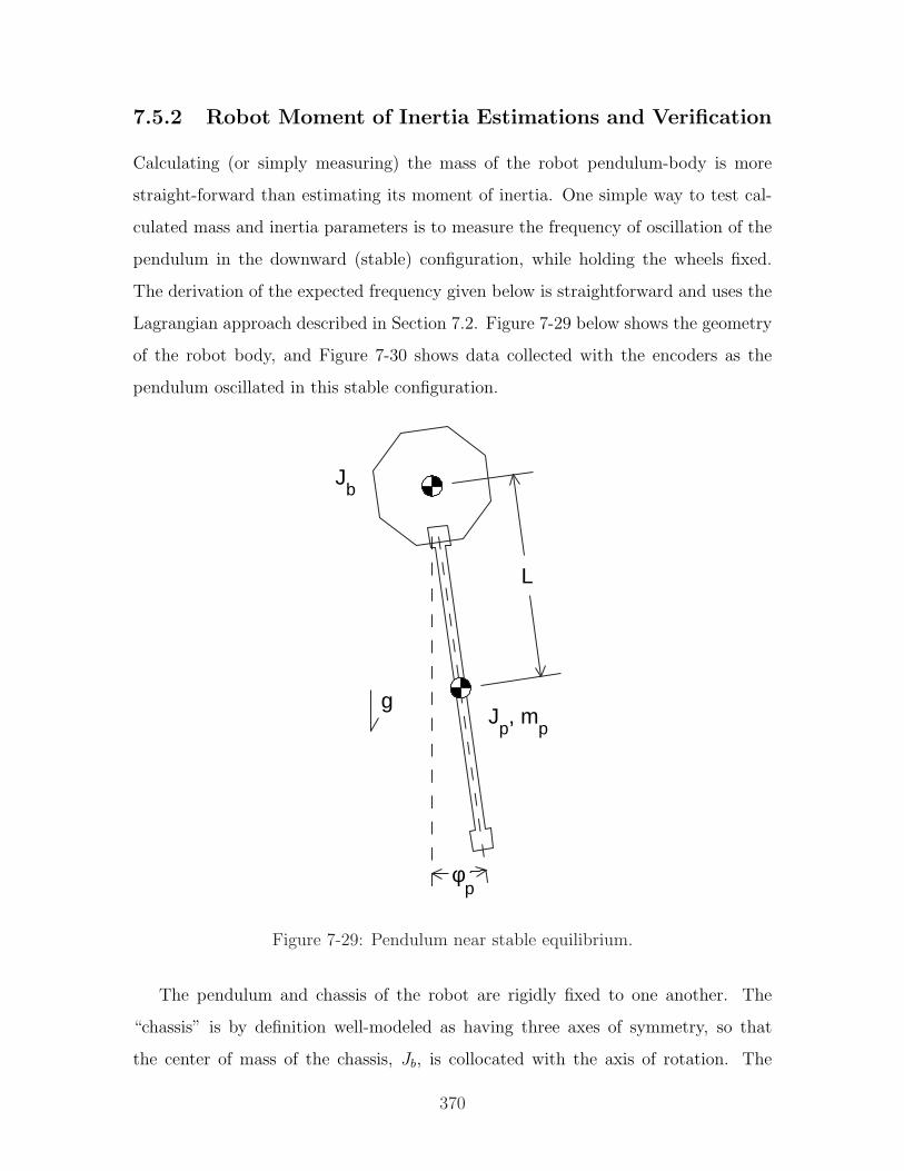
7.5.2 Robot Moment of Inertia Estimations and Verification

Calculating (or simply measuring) the mass of the robot pendulum-body is more

straight-forward than estimating its moment of inertia. One simple way to test cal-

culated mass and inertia parameters is to measure the frequency of oscillation of the

pendulum in the downward (stable) configuration, while holding the wheels fixed.

The derivation of the expected frequency given below is straightforward and uses the

Lagrangian approach described in Section 7.2. Figure 7-29 below shows the geometry

of the robot body, and Figure 7-30 shows data collected with the encoders as the

pendulum oscillated in this stable configuration.

L

Jb

Jp, m

p

φp

g

Figure 7-29: Pendulum near stable equilibrium.

The pendulum and chassis of the robot are rigidly fixed to one another. The

“chassis” is by definition well-modeled as having three axes of symmetry, so that

the center of mass of the chassis, Jb, is collocated with the axis of rotation. The

370

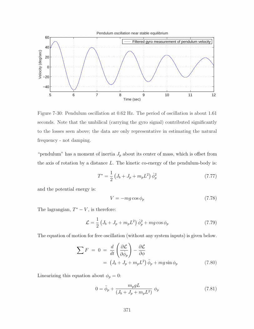
5 6 7 8 9 10 11 12

−40

−20

0

20

40

60

Time (sec)

Vel

ocity

(de

g/se

c)

Pendulum oscillation near stable equilibrium

Filtered gyro measurement of pendulum velocity

Figure 7-30: Pendulum oscillation at 0.62 Hz. The period of oscillation is about 1.61

seconds. Note that the umbilical (carrying the gyro signal) contributed significantly

to the losses seen above; the data are only representative in estimating the natural

frequency - not damping.

“pendulum” has a moment of inertia Jp about its center of mass, which is offset from

the axis of rotation by a distance L. The kinetic co-energy of the pendulum-body is:

T ∗ =1

2

(Jb + Jp + mpL

2)φ2

p (7.77)

and the potential energy is:

V = −mg cos φp (7.78)

The lagrangian, T ∗ − V , is therefore:

L =1

2

(Jb + Jp + mpL

2)φ2

p + mg cos φp (7.79)

The equation of motion for free oscillation (without any system inputs) is given below.

∑F = 0 =

d

dt

(∂L∂φp

)− ∂L

∂φ

=(Jb + Jp + mpL

2)φp + mg sin φp (7.80)

Linearizing this equation about φp = 0:

0 = φp +mpgL

(Jb + Jp + mpL2)φp (7.81)

371

Therefore, the natural frequency is:

ωn =

√mpgL

(Jb + Jp + mpL2)[rad/sec] (7.82)

The moment of inertia of the body is the most difficult parameter to estimate. Based

on my accounting of the geometry and density of the various components of the

chassis, I calculated its inertia should be in the range of 0.053± .005 [kg m2]. We can

use the measured natural frequency of approximately 0.62 Hertz (see Figure 7-30)

to refine this estimate. A value of Jb = 0.050 [kg m2] yields a predicted frequency

of 0.62 Hertz, as shown below. Plugging in estimated parameters values (listed in

Table 7.3 on page 359), we find:

ωn =

√(1.0 [kg])(9.8 [m/s2])(0.4 [m])

(0.05 + 0.05 + (1.0)(0.4)2) [kg m2]= 3.9 [rad/sec] = 0.62 [Hz] (7.83)

The other system parameters for the larger robot in Table 7.3 should be accurate to

within ±5%.

7.5.3 Matlab Simulations of Self-standing Robot

I created several MATLAB m-files before the IP robot was built to simulate the

dynamic response of the robot. Of particular interest at the time were the torque

requirements for achieving a self-standing robot which can begin at rest with the

pendulum horizontal and lift itself to a stable upright position.

The MATLAB simulations animate the expected response of the robot, assuming

perfect sensor data and a discrete execution step size equivalent to that of the dSPACE

controller (i.e. 0.1 ms steps). This allowed me to test the feasibility of particular

combinations of variables including motor specs, gear ratio, and mass and moment

of inertia of both the robot body and wheels.

The initial prototype for the robot, shown on the left-hand side of Figure 7-31

(and in all of the earlier photos of the robot appearing in this chapter), is too large

to be self-standing. The large size facilitated prototyping, however.

A smaller prototype, shown at the right of Figure 7-31, was also developed and

stabilized. The chassis of this robot is not large enough to hold the servo amps and

372

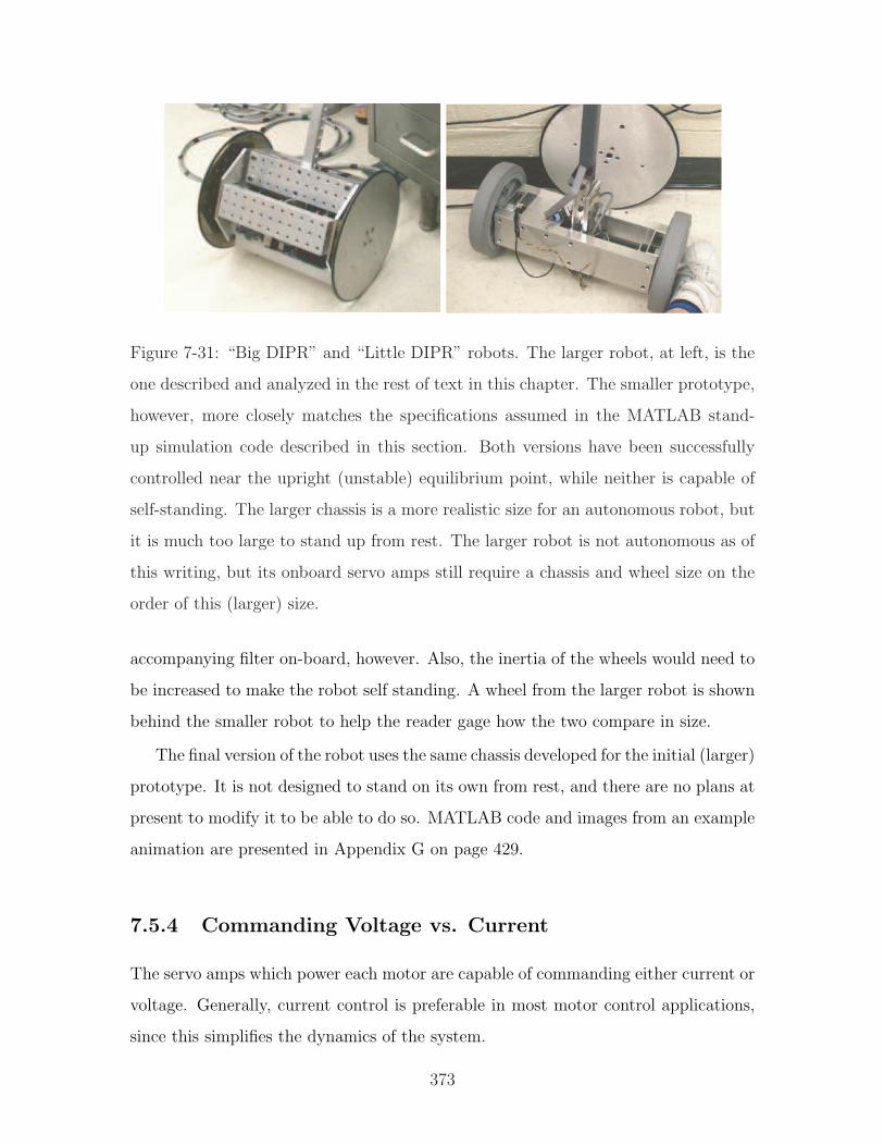
Figure 7-31: “Big DIPR” and “Little DIPR” robots. The larger robot, at left, is the

one described and analyzed in the rest of text in this chapter. The smaller prototype,

however, more closely matches the specifications assumed in the MATLAB stand-

up simulation code described in this section. Both versions have been successfully

controlled near the upright (unstable) equilibrium point, while neither is capable of

self-standing. The larger chassis is a more realistic size for an autonomous robot, but

it is much too large to stand up from rest. The larger robot is not autonomous as of

this writing, but its onboard servo amps still require a chassis and wheel size on the

order of this (larger) size.

accompanying filter on-board, however. Also, the inertia of the wheels would need to

be increased to make the robot self standing. A wheel from the larger robot is shown

behind the smaller robot to help the reader gage how the two compare in size.

The final version of the robot uses the same chassis developed for the initial (larger)

prototype. It is not designed to stand on its own from rest, and there are no plans at

present to modify it to be able to do so. MATLAB code and images from an example

animation are presented in Appendix G on page 429.

7.5.4 Commanding Voltage vs. Current

The servo amps which power each motor are capable of commanding either current or

voltage. Generally, current control is preferable in most motor control applications,

since this simplifies the dynamics of the system.

373

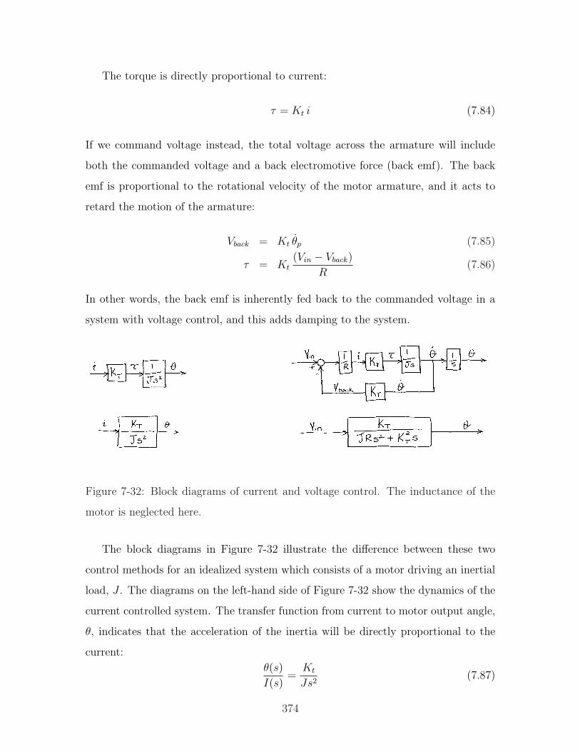
The torque is directly proportional to current:

τ = Kt i (7.84)

If we command voltage instead, the total voltage across the armature will include

both the commanded voltage and a back electromotive force (back emf). The back

emf is proportional to the rotational velocity of the motor armature, and it acts to

retard the motion of the armature:

Vback = Kt θp (7.85)

τ = Kt(Vin − Vback)

R(7.86)

In other words, the back emf is inherently fed back to the commanded voltage in a

system with voltage control, and this adds damping to the system.

Figure 7-32: Block diagrams of current and voltage control. The inductance of the

motor is neglected here.

The block diagrams in Figure 7-32 illustrate the difference between these two

control methods for an idealized system which consists of a motor driving an inertial

load, J . The diagrams on the left-hand side of Figure 7-32 show the dynamics of the

current controlled system. The transfer function from current to motor output angle,

θ, indicates that the acceleration of the inertia will be directly proportional to the

current:

θ(s)

I(s)=

Kt

Js2(7.87)

374

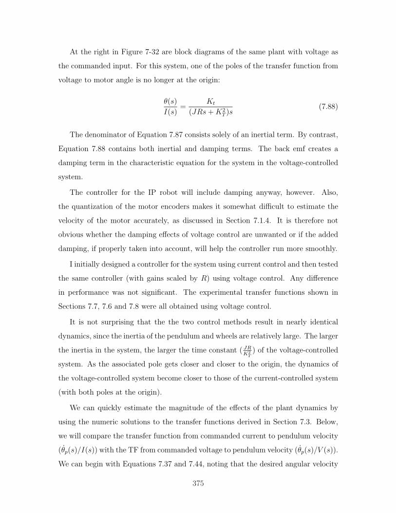
At the right in Figure 7-32 are block diagrams of the same plant with voltage as

the commanded input. For this system, one of the poles of the transfer function from

voltage to motor angle is no longer at the origin:

θ(s)

I(s)=

Kt

(JRs + K2T )s

(7.88)

The denominator of Equation 7.87 consists solely of an inertial term. By contrast,

Equation 7.88 contains both inertial and damping terms. The back emf creates a

damping term in the characteristic equation for the system in the voltage-controlled

system.

The controller for the IP robot will include damping anyway, however. Also,

the quantization of the motor encoders makes it somewhat difficult to estimate the

velocity of the motor accurately, as discussed in Section 7.1.4. It is therefore not

obvious whether the damping effects of voltage control are unwanted or if the added

damping, if properly taken into account, will help the controller run more smoothly.

I initially designed a controller for the system using current control and then tested

the same controller (with gains scaled by R) using voltage control. Any difference

in performance was not significant. The experimental transfer functions shown in

Sections 7.7, 7.6 and 7.8 were all obtained using voltage control.

It is not surprising that the the two control methods result in nearly identical

dynamics, since the inertia of the pendulum and wheels are relatively large. The larger

the inertia in the system, the larger the time constant ( JRK2

T) of the voltage-controlled

system. As the associated pole gets closer and closer to the origin, the dynamics of

the voltage-controlled system become closer to those of the current-controlled system

(with both poles at the origin).

We can quickly estimate the magnitude of the effects of the plant dynamics by

using the numeric solutions to the transfer functions derived in Section 7.3. Below,

we will compare the transfer function from commanded current to pendulum velocity

(θp(s)/I(s)) with the TF from commanded voltage to pendulum velocity (θp(s)/V (s)).

We can begin with Equations 7.37 and 7.44, noting that the desired angular velocity

375

output is just the derivative of angular position:

θp(s)

I(s)≈ −0.33s

(s2 − 16.0)(7.89)

θw(s)

I(s)≈ +0.25(s2 − 14.5)s

(s2 − 16.0)(7.90)

Combining these two equations,

θw(s)

θp(s)≈ −0.77(s2 − 14.5)

s2(7.91)

Recall that the back emf will be proportional to the motor velocity, θm:

θm = θw − θp (7.92)

=

(θw(s)

θp(s)− 1

)θp (7.93)

=

(−0.77(s2 − 14.5)

s2− 1

)θp (7.94)

=−1.77(s2 − 6.72)

s2(7.95)

Combining the preceding equations, we derive the block diagram for this system which

is shown in Figure 7-33.

Figure 7-33: Block diagram of predicted voltage-controlled IP robot.

The resistance of the Maxon motor used in the robot is R = 0.647 Ω, and the back

emf constant is KT = 0.0263 Volt/rad/s. (Motor parameters are listed in Appendix F

on page 425.) The block diagram above simplifies to the following transfer function:

θp(s)

Vin(s)=

−0.51s2

s3 + 0.056s2 − 16.0s− 0.378(7.96)

The poles for this system are at -4.02 rad/s, +3.98 rad/s and 0.02 rad/s. Over the

frequency range in which the transfer function was measured (see Figures 7-27 and

376

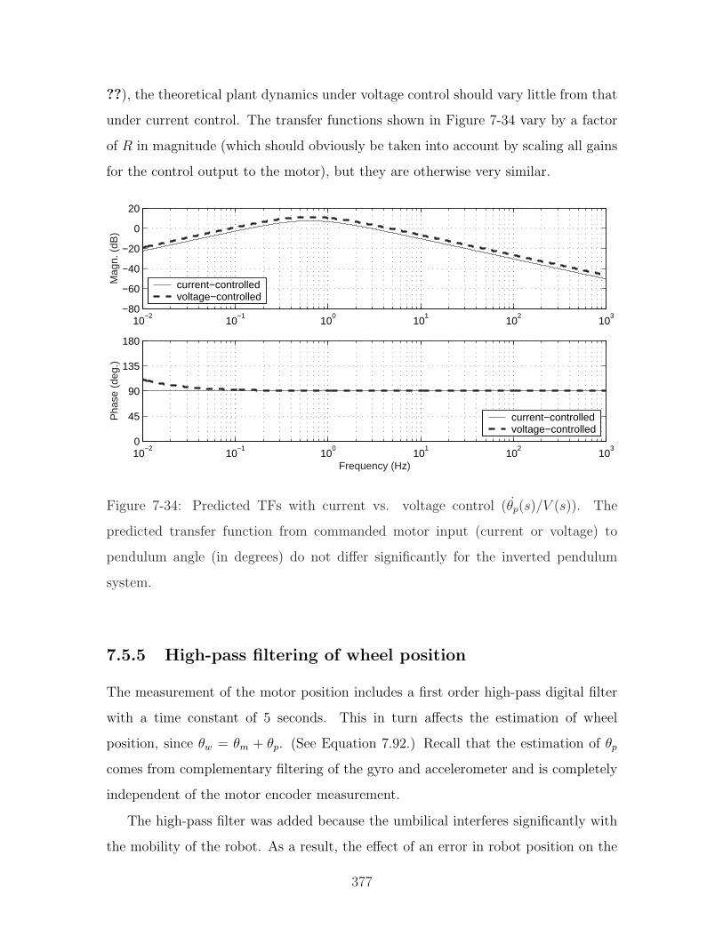
??), the theoretical plant dynamics under voltage control should vary little from that

under current control. The transfer functions shown in Figure 7-34 vary by a factor

of R in magnitude (which should obviously be taken into account by scaling all gains

for the control output to the motor), but they are otherwise very similar.

10−2

10−1

100

101

102

103

−80

−60

−40

−20

0

20

Mag

n. (

dB)

current−controlledvoltage−controlled

10−2

10−1

100

101

102

103

0

45

90

135

180

Pha

se (

deg.

)

Frequency (Hz)

current−controlledvoltage−controlled

Figure 7-34: Predicted TFs with current vs. voltage control (θp(s)/V (s)). The

predicted transfer function from commanded motor input (current or voltage) to

pendulum angle (in degrees) do not differ significantly for the inverted pendulum

system.

7.5.5 High-pass filtering of wheel position

The measurement of the motor position includes a first order high-pass digital filter

with a time constant of 5 seconds. This in turn affects the estimation of wheel

position, since θw = θm + θp. (See Equation 7.92.) Recall that the estimation of θp

comes from complementary filtering of the gyro and accelerometer and is completely

independent of the motor encoder measurement.

The high-pass filter was added because the umbilical interferes significantly with

the mobility of the robot. As a result, the effect of an error in robot position on the

377

control effort is that of a spring and dashpot in series, rather than that of a spring

alone. This effect is described further in the caption for the transfer function from

voltage to wheel position on page 382.

1

Enc2_pos

1-(1-dt/5)z -1dt/5(z)

recent_pos

-2

enc2_sign

enc_k

enc2_deg

Enc position

Enc delta position

DS1104ENC_POS_C2

E2deg

Figure 7-35: High-pass filtering of wheel position.

Figure 7-35 shows the Simulink blocks which implement this filtering in the control

model. The entire encoder-filtering subsystem is shown on page 438 of Appendix H.

7.5.6 Damage of Motor Encoder

In the process of repairing the motors, one of the encoders was damaged. As a result,

the final version of the controller uses a single encoder to estimate motor position and

velocity. The robot has been tested using both encoders, which allows for steering

from a potentiometer input. The loss of an encoder has not had a significant effect

on performance, although both motors must now be controlled in tandem.

7.6 Experimental Frequency Response Data

The next five pages shows experimental Bode plots for the robot. Data were obtained

using a Simulink-driven dynamic signal analyzer within the dSPACE model [114, 113].

The step size for the Simulink model was 0.1 ms, which causes a half-sample delay of

0.05 ms in both the measured transfer functions shown and in the actual dynamics

of the system under digital control.

The controller was initially developed without access to such data. The data

were all obtained while the plant was controlled, so the system would remain stable.

Subsequent fine-tuning was then done once the actual dynamics had been measured.

378

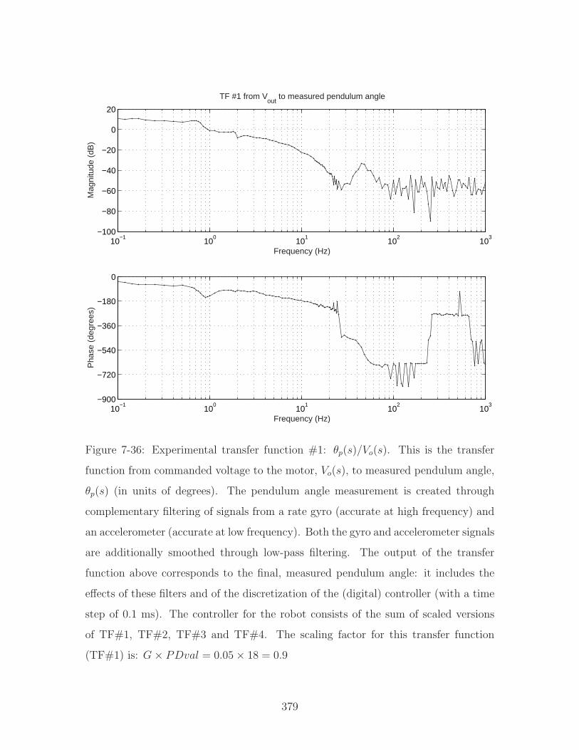
10−1

100

101

102

103

−100

−80

−60

−40

−20

0

20

TF #1 from Vout


Frequency (Hz)

Mag

nitu

de (

dB)

10−1

100

101

102

103

−900

−720

−540

−360

−180

0

Frequency (Hz)

Pha

se (

degr

ees)

Figure 7-36: Experimental transfer function #1: θp(s)/Vo(s). This is the transfer

function from commanded voltage to the motor, Vo(s), to measured pendulum angle,

θp(s) (in units of degrees). The pendulum angle measurement is created through

complementary filtering of signals from a rate gyro (accurate at high frequency) and

an accelerometer (accurate at low frequency). Both the gyro and accelerometer signals

are additionally smoothed through low-pass filtering. The output of the transfer

function above corresponds to the final, measured pendulum angle: it includes the

effects of these filters and of the discretization of the (digital) controller (with a time

step of 0.1 ms). The controller for the robot consists of the sum of scaled versions

of TF#1, TF#2, TF#3 and TF#4. The scaling factor for this transfer function

(TF#1) is: G× PDval = 0.05× 18 = 0.9

379

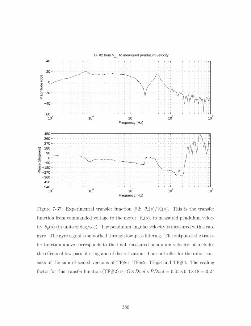
10−1

100

101

102

103

−60

−40

−20

0

20

40

Frequency (Hz)

Mag

nitu

de (

dB)

TF #2 from Vout

to measured pendulum velocity

10−1

100

101

102

103

−540−450−360−270−180

−900

90180270360450

Frequency (Hz)

Pha

se (

degr

ees)

Figure 7-37: Experimental transfer function #2: θp(s)/Vo(s). This is the transfer

function from commanded voltage to the motor, Vo(s), to measured pendulum veloc-

ity, θp(s) (in units of deg/sec). The pendulum angular velocity is measured with a rate

gyro. The gyro signal is smoothed through low-pass filtering. The output of the trans-

fer function above corresponds to the final, measured pendulum velocity: it includes

the effects of low-pass filtering and of discretization. The controller for the robot con-

sists of the sum of scaled versions of TF#1, TF#2, TF#3 and TF#4. The scaling

factor for this transfer function (TF#2) is: G×Dval×PDval = 0.05×0.3×18 = 0.27

380

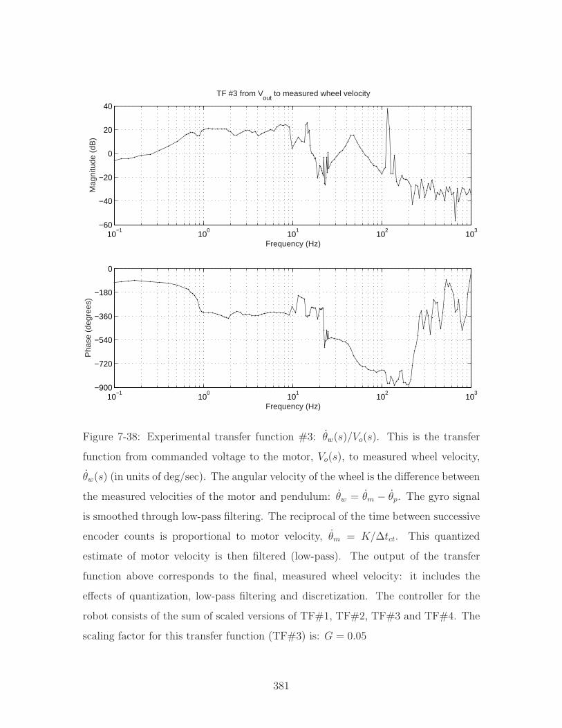
10−1

100

101

102

103

−60

−40

−20

0

20

40

TF #3 from Vout

to measured wheel velocity

Frequency (Hz)

Mag

nitu

de (

dB)

10−1

100

101

102

103

−900

−720

−540

−360

−180

0

Frequency (Hz)

Pha

se (

degr

ees)

Figure 7-38: Experimental transfer function #3: θw(s)/Vo(s). This is the transfer

function from commanded voltage to the motor, Vo(s), to measured wheel velocity,

θw(s) (in units of deg/sec). The angular velocity of the wheel is the difference between

the measured velocities of the motor and pendulum: θw = θm − θp. The gyro signal

is smoothed through low-pass filtering. The reciprocal of the time between successive

encoder counts is proportional to motor velocity, θm = K/∆tct. This quantized

estimate of motor velocity is then filtered (low-pass). The output of the transfer

function above corresponds to the final, measured wheel velocity: it includes the

effects of quantization, low-pass filtering and discretization. The controller for the

robot consists of the sum of scaled versions of TF#1, TF#2, TF#3 and TF#4. The

scaling factor for this transfer function (TF#3) is: G = 0.05

381

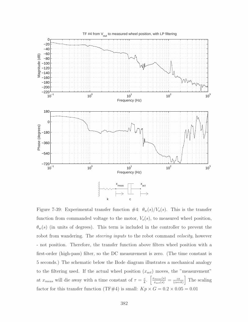
10−1

100

101

102

103

−220−200−180−160−140−120−100

−80−60−40−20

0

Frequency (Hz)

Mag

nitu

de (

dB)

TF #4 from Vout

to measured wheel position, with LP filtering

10−1

100

101

102

103

−720

−540

−360

−180

0

180

Frequency (Hz)

Pha

se (

degr

ees)

xmeas

xact

k c

Figure 7-39: Experimental transfer function #4: θw(s)/Vo(s). This is the transfer

function from commanded voltage to the motor, Vo(s), to measured wheel position,

θw(s) (in units of degrees). This term is included in the controller to prevent the

robot from wandering. The steering inputs to the robot command velocity, however

- not position. Therefore, the transfer function above filters wheel position with a

first-order (high-pass) filter, so the DC measurement is zero. (The time constant is

5 seconds.) The schematic below the Bode diagram illustrates a mechanical analogy

to the filtering used. If the actual wheel position (xact) moves, the ”measurement”

at xmeas will die away with a time constant of τ = ck.

[xmeas(s)xact(s)

= cs(cs+k)

]The scaling

factor for this transfer function (TF#4) is small: Kp×G = 0.2× 0.05 = 0.01

382

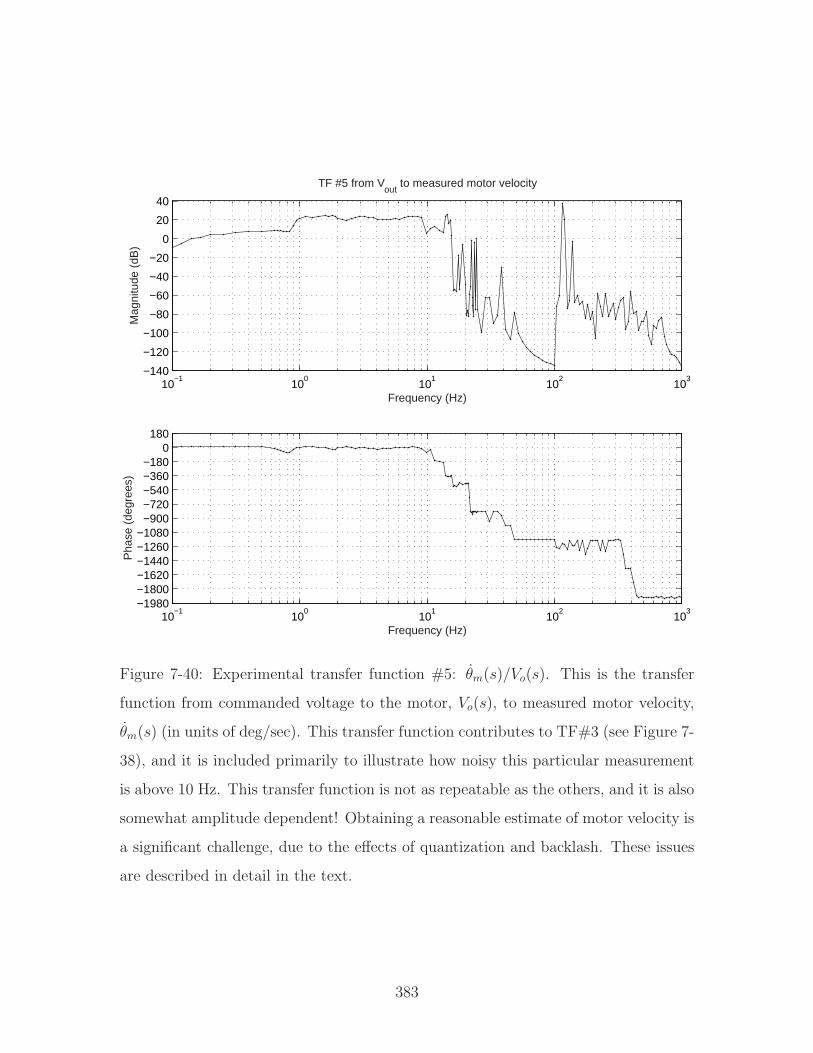
10−1

100

101

102

103

−140

−120

−100

−80

−60

−40

−20

0

20

40

Frequency (Hz)

Mag

nitu

de (

dB)

TF #5 from Vout

to measured motor velocity

10−1

100

101

102

103

−1980−1800−1620−1440−1260−1080−900−720−540−360−180

0180

Frequency (Hz)

Pha

se (

degr

ees)

Figure 7-40: Experimental transfer function #5: θm(s)/Vo(s). This is the transfer

function from commanded voltage to the motor, Vo(s), to measured motor velocity,

θm(s) (in units of deg/sec). This transfer function contributes to TF#3 (see Figure 7-

38), and it is included primarily to illustrate how noisy this particular measurement

is above 10 Hz. This transfer function is not as repeatable as the others, and it is also

somewhat amplitude dependent! Obtaining a reasonable estimate of motor velocity is

a significant challenge, due to the effects of quantization and backlash. These issues

are described in detail in the text.

383

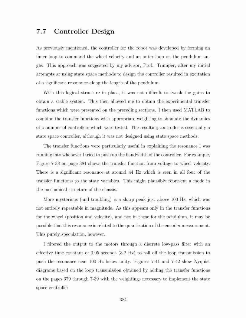
7.7 Controller Design

As previously mentioned, the controller for the robot was developed by forming an

inner loop to command the wheel velocity and an outer loop on the pendulum an-

gle. This approach was suggested by my advisor, Prof. Trumper, after my initial

attempts at using state space methods to design the controller resulted in excitation

of a significant resonance along the length of the pendulum.

With this logical structure in place, it was not difficult to tweak the gains to

obtain a stable system. This then allowed me to obtain the experimental transfer

functions which were presented on the preceding sections. I then used MATLAB to

combine the transfer functions with appropriate weighting to simulate the dynamics

of a number of controllers which were tested. The resulting controller is essentially a

state space controller, although it was not designed using state space methods.

The transfer functions were particularly useful in explaining the resonance I was

running into whenever I tried to push up the bandwidth of the controller. For example,

Figure 7-38 on page 381 shows the transfer function from voltage to wheel velocity.

There is a significant resonance at around 44 Hz which is seen in all four of the

transfer functions to the state variables. This might plausibly represent a mode in

the mechanical structure of the chassis.

More mysterious (and troubling) is a sharp peak just above 100 Hz, which was

not entirely repeatable in magnitude. As this appears only in the transfer functions

for the wheel (position and velocity), and not in those for the pendulum, it may be

possible that this resonance is related to the quantization of the encoder measurement.

This purely speculation, however.

I filtered the output to the motors through a discrete low-pass filter with an

effective time constant of 0.05 seconds (3.2 Hz) to roll off the loop transmission to

push the resonance near 100 Hz below unity. Figures 7-41 and 7-42 show Nyquist

diagrams based on the loop transmission obtained by adding the transfer functions

on the pages 379 through 7-39 with the weightings necessary to implement the state

space controller.

384

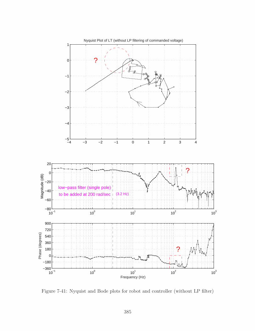
−4 −3 −2 −1 0 1 2 3 4−5

−4

−3

−2

−1

0

1Nyquist Plot of LT (without LP filtering of commanded voltage)

?

10−1

100

101

102

103

−80

−60

−40

−20

0

20

?

Mag

nitu

de (

dB)

low−pass filter (single pole)

to be added at 200 rad/sec (3.2 Hz)

10−1

100

101

102

103

−360

−180

0

180

360

540

720

900

Frequency (Hz)

Pha

se (

degr

ees)

?

Figure 7-41: Nyquist and Bode plots for robot and controller (without LP filter)

385

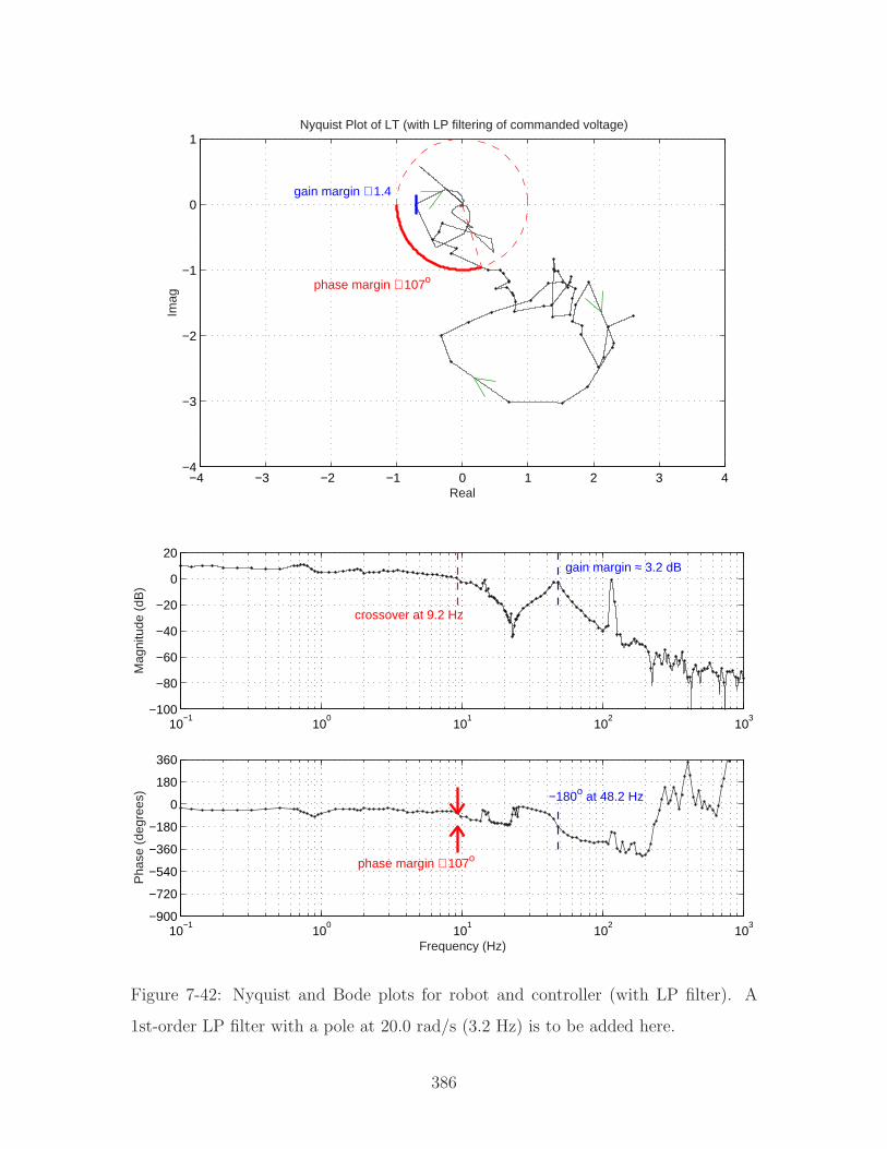
−4 −3 −2 −1 0 1 2 3 4−4

−3

−2

−1

0

1

Real

Imag

Nyquist Plot of LT (with LP filtering of commanded voltage)


gain margin ≅ 1.4

10−1

100

101

102

103

−100

−80

−60

−40

−20

0

20

Mag

nitu

de (

dB)

crossover at 9.2 Hz

gain margin ≈ 3.2 dB

10−1

100

101

102

103

−900

−720

−540

−360

−180

0

180

360

Frequency (Hz)

Pha

se (

degr

ees)


−180o at 48.2 Hz

Figure 7-42: Nyquist and Bode plots for robot and controller (with LP filter). A

1st-order LP filter with a pole at 20.0 rad/s (3.2 Hz) is to be added here.

386

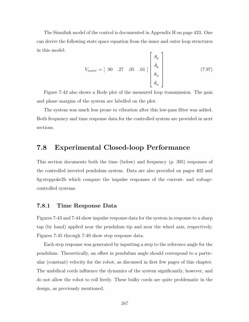
The Simulink model of the control is documented in Appendix H on page 433. One

can derive the following state space equation from the inner and outer loop structures

in this model:

Vmotor = [ .90 .27 .05 .01 ]

θp

θp

θw

θw

(7.97)

Figure 7-42 also shows a Bode plot of the measured loop transmission. The gain

and phase margins of the system are labelled on the plot.

The system was much less prone to vibration after this low-pass filter was added.

Both frequency and time response data for the controlled system are provided in next

sections.

7.8 Experimental Closed-loop Performance

This section documents both the time (below) and frequency (p. 395) responses of

the controlled inverted pendulum system. Data are also provided on pages 402 and

fig:steppoke2b which compare the impulse responses of the current- and voltage-

controlled systems.

7.8.1 Time Response Data

Figures 7-43 and 7-44 show impulse response data for the system in response to a sharp

tap (by hand) applied near the pendulum tip and near the wheel axis, respectively.

Figures 7-45 through 7-49 show step response data.

Each step response was generated by inputting a step to the reference angle for the

pendulum. Theoretically, an offset in pendulum angle should correspond to a partic-

ular (constant) velocity for the robot, as discussed in first few pages of this chapter.

The umbilical cords influence the dynamics of the system significantly, however, and

do not allow the robot to roll freely. These bulky cords are quite problematic in the

design, as previously mentioned.

387

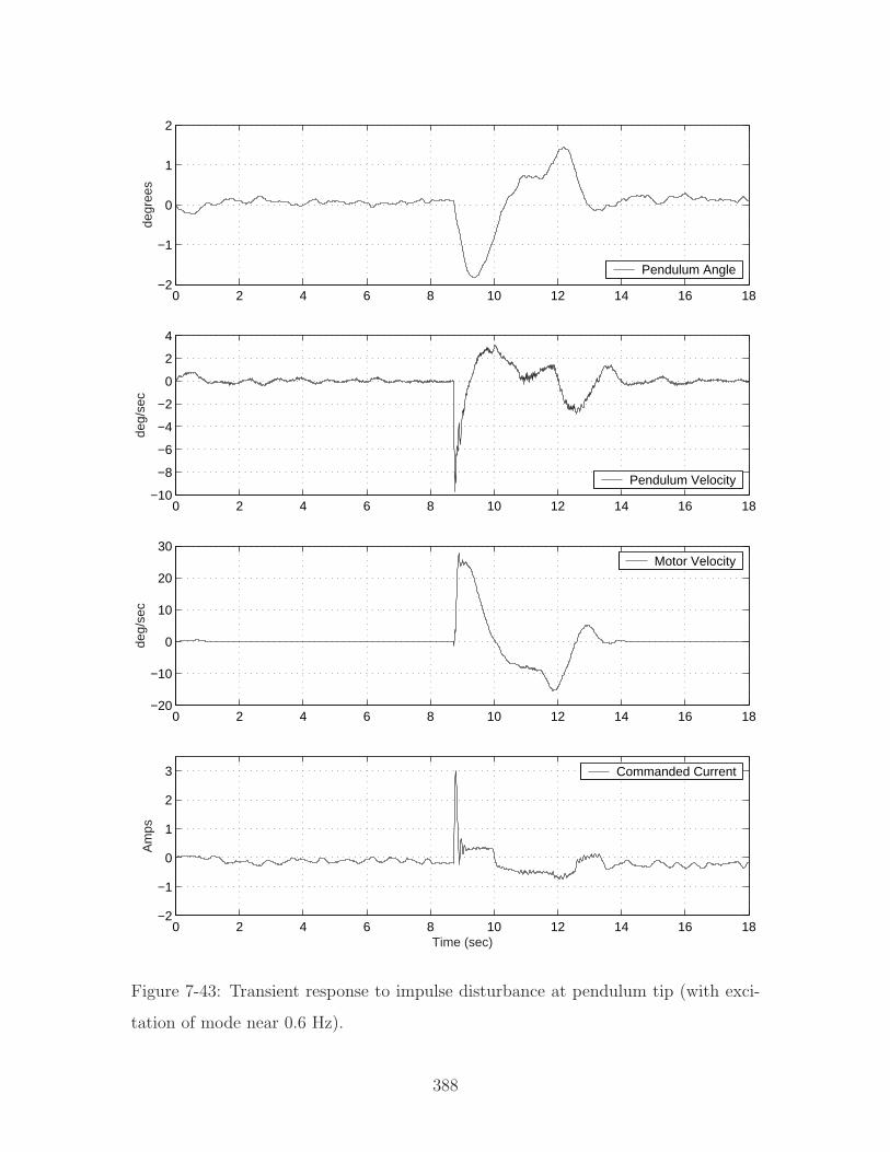
0 2 4 6 8 10 12 14 16 18−2

−1

0

1

2

degr

ees

Step response to disturbance at pendulum tip

Pendulum Angle

0 2 4 6 8 10 12 14 16 18−10

−8

−6

−4

−2

0

2

4

deg/

sec

Pendulum Velocity

0 2 4 6 8 10 12 14 16 18−20

−10

0

10

20

30

deg/

sec

Motor Velocity

0 2 4 6 8 10 12 14 16 18−2

−1

0

1

2

3

Am

ps

Time (sec)

Commanded Current

Figure 7-43: Transient response to impulse disturbance at pendulum tip (with exci-

tation of mode near 0.6 Hz).

388

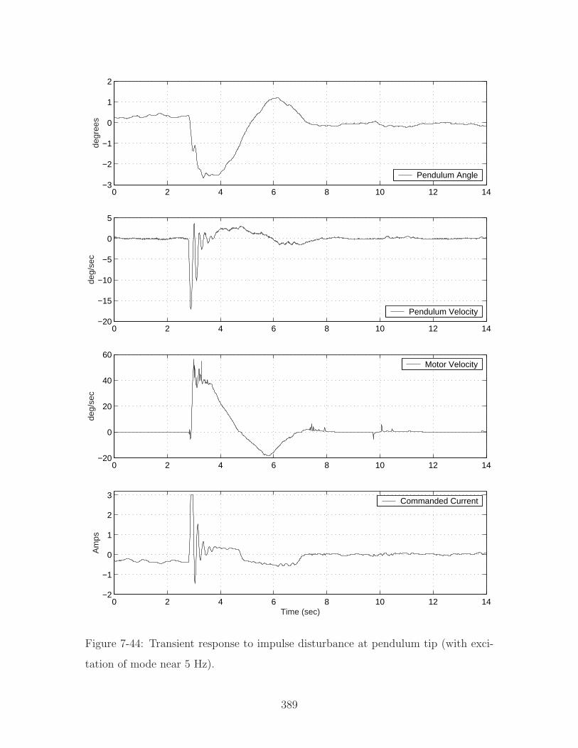
0 2 4 6 8 10 12 14−3

−2

−1

0

1

2

degr

ees


Pendulum Angle

0 2 4 6 8 10 12 14−20

−15

−10

−5

0

5

deg/

sec

Pendulum Velocity

0 2 4 6 8 10 12 14−20

0

20

40

60

deg/

sec

Motor Velocity

0 2 4 6 8 10 12 14−2

−1

0

1

2

3

Am

ps

Time (sec)

Commanded Current

Figure 7-44: Transient response to impulse disturbance at pendulum tip (with exci-

tation of mode near 5 Hz).

389

0 2 4 6 8 10 12 14 16 18−5

−4

−3

−2

−1de

gree

sResponse to step in angle offset (1 degree stepsizes)

Pendulum Angle

0 2 4 6 8 10 12 14 16 18−5

0

5

deg/

sec

Pendulum Velocity

0 2 4 6 8 10 12 14 16 18

−5

0

5

deg/

sec

Motor Velocity

0 2 4 6 8 10 12 14 16 18

−0.5

0

0.5

Vol

ts

Time (sec)

Commanded Voltage

Figure 7-45: Experimental responses to a 1-degree step in offset angle.

390

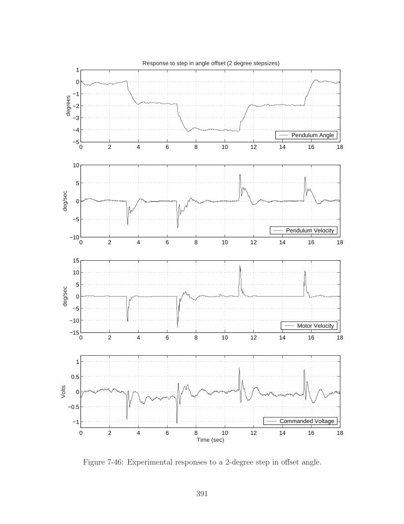
0 2 4 6 8 10 12 14 16 18−5

−4

−3

−2

−1

0

1de

gree


Pendulum Angle

0 2 4 6 8 10 12 14 16 18−10

−5

0

5

10

deg/

sec

Pendulum Velocity

0 2 4 6 8 10 12 14 16 18−15

−10

−5

0

5

10

15

deg/

sec

Motor Velocity

0 2 4 6 8 10 12 14 16 18

−1

−0.5

0

0.5

1

Vol

ts

Time (sec)

Commanded Voltage


391

0 2 4 6 8 10 12 14 16 18−8

−6

−4

−2

0

2de

gree


Pendulum Angle

0 2 4 6 8 10 12 14 16 18

−10

−5

0

5

10

deg/

sec

Pendulum Velocity

0 2 4 6 8 10 12 14 16 18

−20

−10

0

10

20

deg/

sec

Motor Velocity

0 2 4 6 8 10 12 14 16 18−1.5

−1

−0.5

0

0.5

1

1.5

Vol

ts

Time (sec)

Commanded Voltage


392

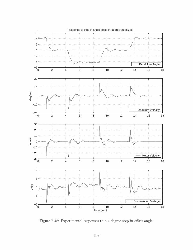
0 2 4 6 8 10 12 14 16 18−6

−4

−2

0

2

4

6Response to step in angle offset (4 degree stepsizes)

Pendulum Angle

0 2 4 6 8 10 12 14 16 18−20

−10

0

10

20

deg/

sec

Pendulum Velocity

0 2 4 6 8 10 12 14 16 18−30

−20

−10

0

10

20

30

deg/

sec

Motor Velocity

0 2 4 6 8 10 12 14 16 18−2

−1

0

1

2

Vol

ts

Time (sec)

Commanded Voltage


393

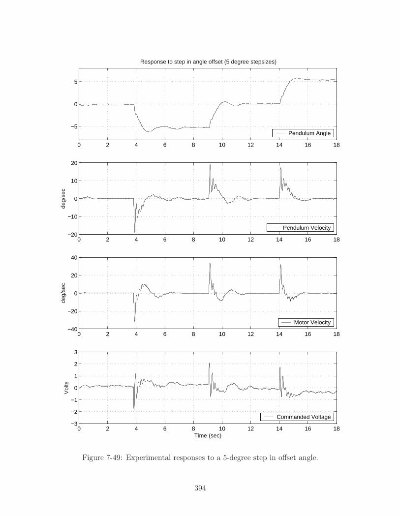
0 2 4 6 8 10 12 14 16 18

−5

0

5

Response to step in angle offset (5 degree stepsizes)

Pendulum Angle

0 2 4 6 8 10 12 14 16 18−20

−10

0

10

20

deg/

sec

Pendulum Velocity

0 2 4 6 8 10 12 14 16 18−40

−20

0

20

40

deg/

sec

Motor Velocity

0 2 4 6 8 10 12 14 16 18−3

−2

−1

0

1

2

3

Vol

ts

Time (sec)

Commanded Voltage


394

7.8.2 Closed-Loop Frequency Response Data

The next few pages provide measured transfer functions of the controlled plant. This

system has multiple outputs of interest, namely both pendulum angle and wheel

velocity. The pendulum angle is of more importance in maintaining stability, and

the controller begins to lose authority over the pendulum angle after about 0.5 Hz.

(i.e. near the natural frequency of the free pendulum) Crossover for the loop trans-

mission occurs near 7.5 Hz.

7.8.3 Data Comparing Current Control and Voltage Control

As mentioned in Section 7.5.4, the inertias involved in the system are large enough

that one would expect little difference in performance when the system is run under

current control rather than voltage control. Figure 7-56 on page 402 shows the tran-

sient response to a disturbance applied at the tip of the pendulum. Figure 7-57 on

page 403 provides similar data for the voltage-controlled system.

395

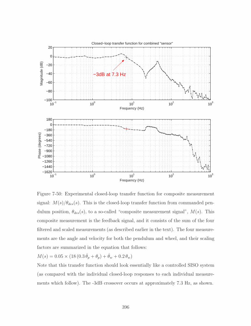
10−1

100

101

102

103

−100

−80

−60

−40

−20

0

20

Frequency (Hz)

Mag

nitu

de (

dB)

Closed−loop transfer function for combined "sensor"

−3dB at 7.3 Hz

10−1

100

101

102

103

−1620

−1440

−1260

−1080

−900

−720

−540

−360

−180

0

180

Frequency (Hz)

Pha

se (

degr

ees)

Figure 7-50: Experimental closed-loop transfer function for composite measurement

signal: M(s)/θdes(s). This is the closed-loop transfer function from commanded pen-

dulum position, θdes(s), to a so-called “composite measurement signal”, M(s). This

composite measurement is the feedback signal, and it consists of the sum of the four

filtered and scaled measurements (as described earlier in the text). The four measure-

ments are the angle and velocity for both the pendulum and wheel, and their scaling

factors are summarized in the equation that follows:

M(s) = 0.05× (18 (0.3 θp + θp) + θw + 0.2 θw)

Note that this transfer function should look essentially like a controlled SISO system

(as compared with the individual closed-loop responses to each individual measure-

ments which follow). The -3dB crossover occurs at approximately 7.3 Hz, as shown.

396

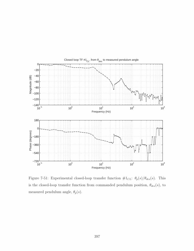
10−1

100

101

102

103

−140

−120

−100

−80

−60

−40

−20

0

Frequency (Hz)

Mag

nitu

de (

dB)

Closed loop TF #1CL

, from θdes


10−1

100

101

102

103

−720

−540

−360

−180

0

180

Frequency (Hz)

Pha

se (

degr

ees)

Figure 7-51: Experimental closed-loop transfer function #1CL: θp(s)/θdes(s). This

is the closed-loop transfer function from commanded pendulum position, θdes(s), to

measured pendulum angle, θp(s).

397

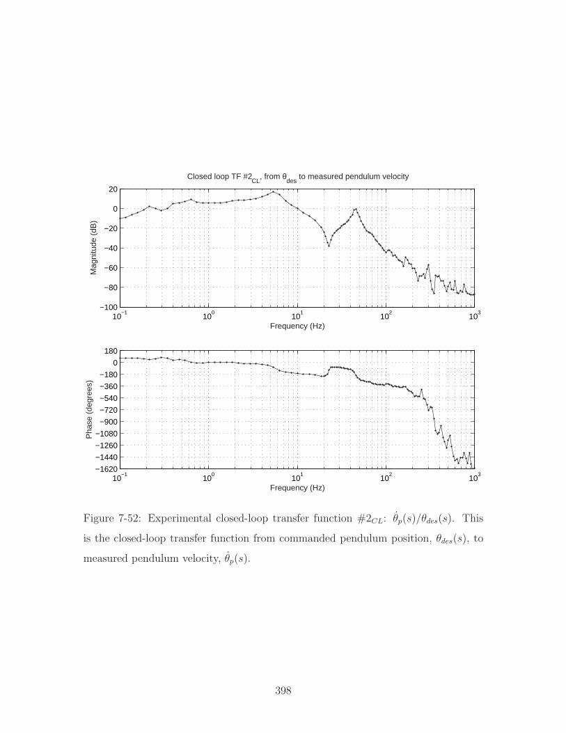
10−1

100

101

102

103

−100

−80

−60

−40

−20

0

20

Frequency (Hz)

Mag

nitu

de (

dB)

Closed loop TF #2CL

, from θdes

to measured pendulum velocity

10−1

100

101

102

103

−1620

−1440

−1260

−1080

−900

−720

−540

−360

−180

0

180

Frequency (Hz)

Pha

se (

degr

ees)

Figure 7-52: Experimental closed-loop transfer function #2CL: θp(s)/θdes(s). This

is the closed-loop transfer function from commanded pendulum position, θdes(s), to

measured pendulum velocity, θp(s).

398

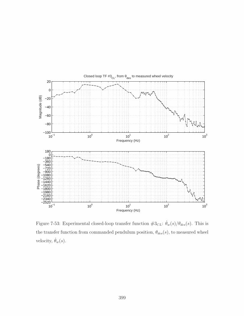
10−1

100

101

102

103

−100

−80

−60

−40

−20

0

20

Frequency (Hz)

Mag

nitu

de (

dB)

Closed loop TF #3CL

, from θdes

to measured wheel velocity

10−1

100

101

102

103

−2520−2340−2160−1980−1800−1620−1440−1260−1080−900−720−540−360−180

0180

Frequency (Hz)

Pha

se (

degr

ees)

Figure 7-53: Experimental closed-loop transfer function #3CL: θw(s)/θdes(s). This is

the transfer function from commanded pendulum position, θdes(s), to measured wheel

velocity, θw(s).

399

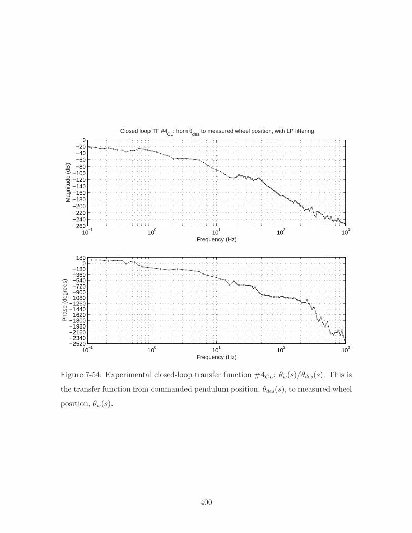
10−1

100

101

102

103

−260−240−220−200−180−160−140−120−100

−80−60−40−20

0

Frequency (Hz)

Mag

nitu

de (

dB)

Closed loop TF #4CL

: from θdes

to measured wheel position, with LP filtering

10−1

100

101

102

103

−2520−2340−2160−1980−1800−1620−1440−1260−1080−900−720−540−360−180

0180

Frequency (Hz)

Pha

se (

degr

ees)

Figure 7-54: Experimental closed-loop transfer function #4CL: θw(s)/θdes(s). This is

the transfer function from commanded pendulum position, θdes(s), to measured wheel

position, θw(s).

400

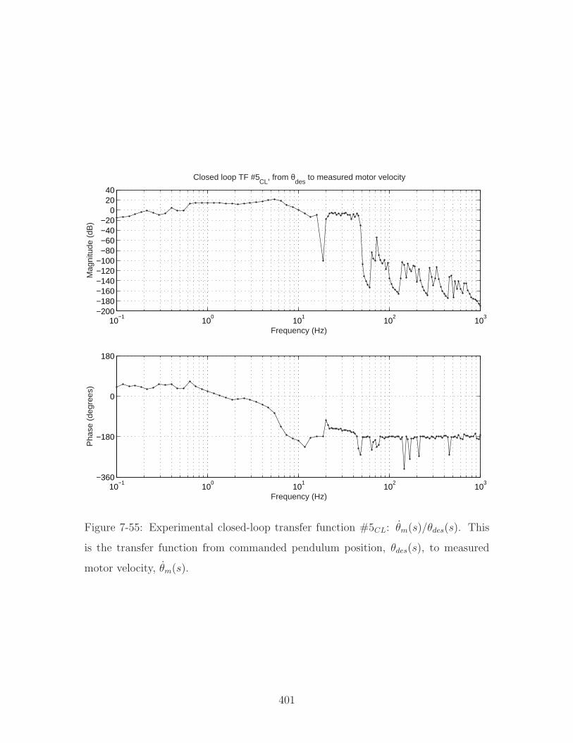
10−1

100

101

102

103

−200−180−160−140−120−100

−80−60−40−20

02040

Frequency (Hz)

Mag

nitu

de (

dB)

Closed loop TF #5CL

, from θdes

to measured motor velocity

10−1

100

101

102

103

−360

−180

0

180

Frequency (Hz)

Pha

se (

degr

ees)

Figure 7-55: Experimental closed-loop transfer function #5CL: θm(s)/θdes(s). This

is the transfer function from commanded pendulum position, θdes(s), to measured

motor velocity, θm(s).

401

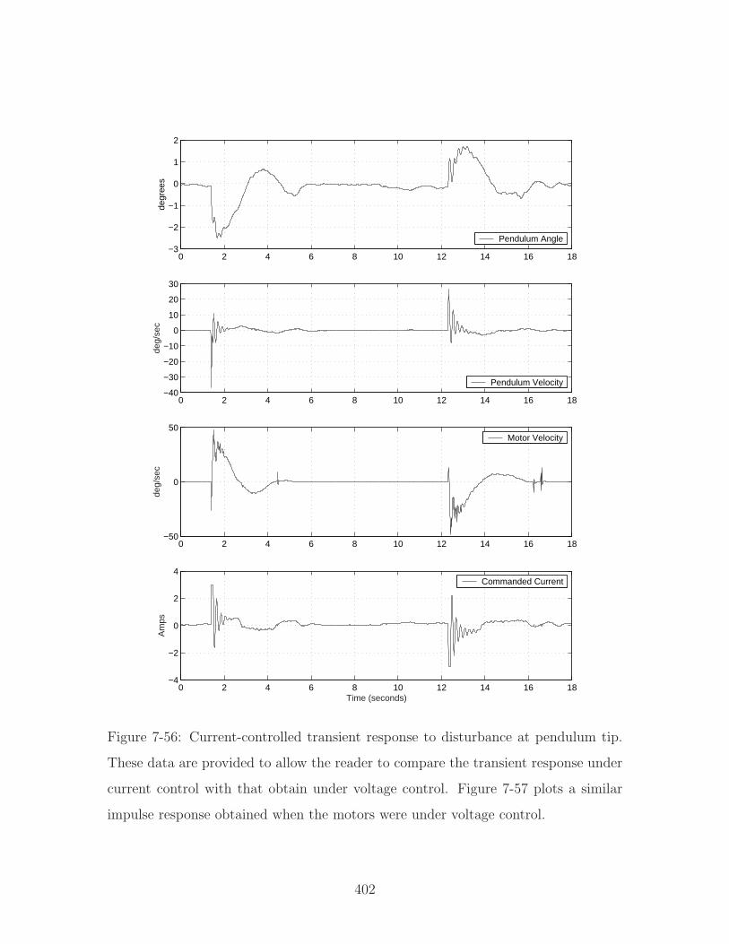
0 2 4 6 8 10 12 14 16 18−3

−2

−1

0

1

2

degr

ees

Pendulum Angle

0 2 4 6 8 10 12 14 16 18−40

−30

−20

−10

0

10

20

30

deg/

sec

Pendulum Velocity

0 2 4 6 8 10 12 14 16 18−50

0

50

deg/

sec

Motor Velocity

0 2 4 6 8 10 12 14 16 18−4

−2

0

2

4

Am

ps

Time (seconds)

Commanded Current

Figure 7-56: Current-controlled transient response to disturbance at pendulum tip.

These data are provided to allow the reader to compare the transient response under

current control with that obtain under voltage control. Figure 7-57 plots a similar

impulse response obtained when the motors were under voltage control.

402

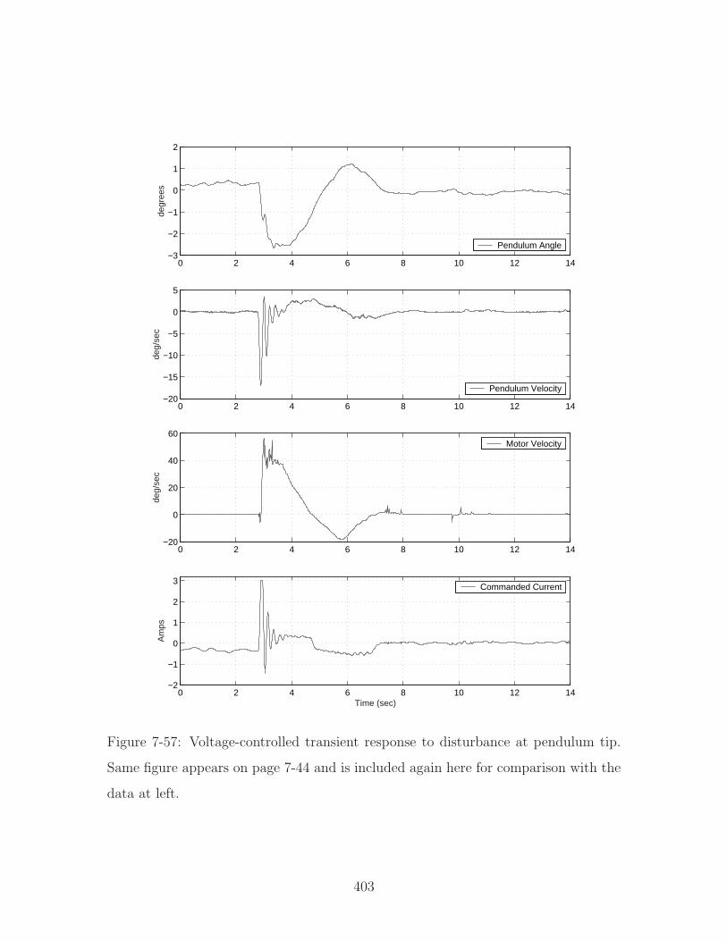
0 2 4 6 8 10 12 14−3

−2

−1

0

1

2

degr

ees


Pendulum Angle

0 2 4 6 8 10 12 14−20

−15

−10

−5

0

5

deg/

sec

Pendulum Velocity

0 2 4 6 8 10 12 14−20

0

20

40

60

deg/

sec

Motor Velocity

0 2 4 6 8 10 12 14−2

−1

0

1

2

3

Am

ps

Time (sec)

Commanded Current

Figure 7-57: Voltage-controlled transient response to disturbance at pendulum tip.

Same figure appears on page 7-44 and is included again here for comparison with the

data at left.

403

7.9 Summary

The inverted pendulum robot discussed in this chapter was originally intended as an

autonomous classroom demo for 2.003. It is not autonomous at this time, and the

umbilical cords interfere significantly with the desired dynamics of the uncontrolled

plant.

Most of the effort in creating the robot involved the design and manufacture

of the hardware and appropriate sensor selection and filtering. Two sensor issues

are of particular interest. The first is complementary filtering, which combines the

measurements from a gyro and an accelerometer in order to compensate for drift, and

the second is the estimation of motor velocity from the quantized encoder output.

We do not currently plan to use the robot as an in-class demo. The theoretical

differences in dynamics between the cart-driven and Segway-type inverted pendulums

are interesting, however, and might be presented in a recitation or lecture for the class.

404

Chapter 8

Conclusions and Recommendations

This thesis has two central goals, each of which relates to laboratory projects and/or

classroom demos which demonstrate dynamics and introductory control. This work

was all inspired by the recent revision of the sophomore-level course “2.003 Model-

ing Dynamics and Control I”, which is a required course for undergraduates in the

Department of Mechanical Engineering at MIT. The three central parts of this thesis

are: (1) a description of a set of ActivLab experiments which we have designed to cre-

ate weekly laboratory experiences, and (2) the development of an inverted pendulum

robot (named the DIPR) intended as a classroom demo in dynamics and control.

To provide background for these two goals (the ActivLab projects and the IP

robot), I have also compiled a survey of other projects which provide undergraduates

with experiences in dynamics, controls and design. The survey covers a variety of

laboratory projects, lecture demos, capstone projects, robot contests and other ac-

tivities, described in Chapter 2, created by educators at MIT and other universities.

Chapter 4 forms a second part of the survey, which focuses on additional laboratories

and demos which are specifically appropriate for 2.003. The remainder of this chap-

ter summarizes current status of and provides suggestion for future work on both the

ActivLab project and the inverted pendulum robot.

405

8.1 ActivLab Conclusions and Recommendation

8.1.1 Brief Evaluation of ActivLab Projects

As of this writing, the ActivLab hardware has completed its fourth term in use.

The equipment is designed to demonstrate first-, second- and higher-order system

responses and to introduce controls. Much care has been taken to create systems

which demonstrate nearly ideal first- and second-order responses. In particular, much

of the hardware uses air bearings to virtually eliminate any Coulomb friction in the

mechanical systems.

We have still observed a variety of anomalous behaviors in the course of teaching

the class however, many of which are documented in Chapter 3. We feel it is im-

portant that any non-ideal behaviors are not “swept under the carpet” during the

labs. Unexpected system behaviors can, in moderation, present an opportunity for

students. During the labs, we encourage curiosity in the students. We hope that

students will explore, experiment, and also propose and test hypotheses during lab

sessions. The ability to engage hardware with an open-minded yet scientific outlook

is a necessity for successful independent research.

8.1.2 Final Notes on the ActivLab Equipment and Website

The ActivLab projects are documented on the website for course 2.003 Modeling

Dynamics and Control I at MIT. The current address for the ActivLab site is:

http://web.mit.edu/2.003/www/activlab/activlab.html

This website is also accessible through MIT’s growing “OpenCourseWare” (OCW)

project, which is described in Section 2.3.4 on page 119. The link to 2.003 can be

found among the courses offered by the Department of Mechanical Engineering which

currently participate in OCW. The OCW homepage is currently located at:

http://ocw.mit.edu/index.html

406

We encourage others to use or adapt any of the ideas we have documented in this

thesis and on the ActivLab website.

The ActivLab hardware was designed to be robust, easy to assemble, and relatively

transparent in operation. The equipment has proved to be fairly robust so far, and we

have not experienced any significant hardware failures. The most notable issue with

wear involves the cantilevers used in the second-order translational system described

in Section 3.5 (page 170). We use lengths of thin welding rod, and these have a

tendency to fatigue after a couple of terms of use because the second-order system is

driven. The welding rod is cheap and easy to replace, however. (We got a few lengths

for free from welders at MIT’s Central Machine Shop.)

We have been particularly pleased with the decision to design the mechanical hard-

ware in the ActivLab projects so that labs can be assembled on optical breadboard

and then stored efficiently after disassembly. The Delrin adapter plates we man-

ufactured which interface between the air bearings and the breadboard have been

particularly useful in this respect. The design of this adapter plate is documented in

Appendix D on page 419.

Overall, we have been pleased with the laboratories for 2.003, and there are no

plans to modify the ActivLab projects significantly in the near future. We do hope to

create some supplementary material for the class over the summer of 2003, however,

primarily through the efforts of undergraduate (UROP) students who have previously

taken the class.

Ross Hatton will be creating online materials which will describe a magnetic ball

levitation demo. This demo was originally created by Prof. Trumper and has been

subsequently modified to run under the dSPACE environment by Yi Xie as part of

her MEng thesis. Ross is also creating an online tutorial explaining many of the key

electromechanical components of a disk drive, and he will also be helping to format

Prof. Trumper’s course notes for the class with LATEX.

Larry Hawe II will be creating additional documentation for the cart-driven in-

verted pendulum demo described in Chapter 5. He also plans to add storage shelves

beneath the laboratory benches which will help us store the optical breadboard out

407

of the way during the weeks when they are not used.

We may also create some additional hands-on projects and exercises for a weekly

one-hour recitation session for the class. The recitations, if added to the class content,

could provide tutorial coverage of topics such as: drawing and using free body dia-

grams, the fundamentals of Bode diagrams, introduction to MATLAB, and a review

of complex exponentials. A particular recitation session might also present a more in

depth examination of demos presented in lecture, or it could focus on problem solving

and involve hardware exercises which are more loosely-structured that the three-hour

weekly labs.

8.2 Inverted Pendulum Demo Summary

The inverted pendulum robot I designed which is described in Chapter 7 (the DIPR)

is not practical as a classroom demo in its current state. The robot requires umbilical

cords to carry power, sensor signals, and control commands for the robot. These cords

interfere with the operation of the inverted pendulum, and the entire demo is quite

bulky since it must include the off-board power supplies and a computer equipped

with a dSPACE controller board.

At this time, there are no plans to adapt the DIPR into a fully autonomous robot,

and we will instead continue to use the cart-driven inverted pendulum hardware

described in Chapter 5 as a lecture demo for 2.003. The operation of the cart-driven

system is documented in Andrew Stimac’s bachelor thesis: “Standup and Stabilization

of the Inverted Pendulum”[189]. As mentioned in the previous section, Larry Hawe

plans to document this demo further over the summer of 2003.

One suggestion for future work is the development of a smaller, autonomous in-

verted pendulum robot, similar in scale and complexity to the Legway described

on page 2.1.5, as a lecture demo. Another possible project is the development of

a low-cost kit of parts which each student could assemble to create his or her own

inverted pendulum. The device would more likely be a fixed base design instead of

a two-wheeled robot, and it would be small enough to sit in the corner of a desktop.

408

Students would then be asked to complete a design project at home to stabilize the

inverted pendulum with their own analog control circuits.

This type of project would give each student the opportunity to work on a design

project and gain some experience in introductory controls. They would also have

much more opportunity to interact with this demo than with a lecture demo version

of an inverted pendulum demo and would be encouraged to explore the effects of

“tweaking” the controller.

The actual hardware could also involve some other system, such a magnetic ball

levitator, instead of an inverted pendulum. Hopefully, students would be inspired by

the opportunity to build their own working desktop toy to keep at the end of the

term, and this might also generate more interest in the content of the class. A design

project of this type could also be useful for a class which focuses more directly on

introductory control theory, such as 2.14 or 6.302.

409

410

Appendix A

Course Catalog Descriptions for

2.003 and 2.004

Below are the text descriptions of 2.003 and 2.004 from the MIT Bulletin (course

catalog). Also included is a brief paragraph clarifying some details about 2.003.

2.003 Modeling Dynamics and Control I

Undergraduate Subject

Prereq.: 8.01, 8.02, 18.02, 18.03

Units: 4-3-8

URL: http://web.mit.edu/2.003/www/

First of two-term sequence on modeling, analysis and control of dynamic systems.

Mechanical translation, uniaxial rotation, electrical circuits and their coupling via

levers, gears and electro-mechanical devices. Analytical and computational solution of

linear differential equations and state-determined systems. Laplace transforms, trans-

fer functions. Frequency response, Bode plots. Vibrations, modal analysis. Open-

and closed-loop control, instability. Time-domain controller design, introduction to

frequency-domain control design techniques. Case studies of engineering applications.

D. Trumper, D. Gossard, N. Hogan

411

Additional details about 2.003

Most subjects at MIT are 12-unit courses. 2.003 is a 15-unit class, meaning students

should typically spend approximately 15 hours per week on their combined prepara-

tory and in-class efforts. Each week, students are expected to attend two one-hour

lectures, two one-hour recitations and a three-hour laboratory session. 2.003 is a

required, sophomore-level course for mechanical engineering majors. The workload

and content are by design similar to the EECS course 6.003 Signals and Systems.

Course prerequisites include classical mechanics (8.01), electricity and magnetism

(8.02), multi-variate calculus (18.02), and differential equations (18.03).

2.004 Modeling Dynamics and Control II

Undergraduate Subject

Prereq.: 2.003, 18.03

Units: 4-3-8

Second subject of two-term sequence on modeling, analysis and control of dynamic

systems. Kinematics and dynamics of mechanical systems including rigid bodies in

plane motion. Linear and angular momentum principles. Impact and collision prob-

lems. Linearization about equilibrium. Free and forced vibrations. Sensors and

actuators. Control of mechanical systems. Integral and derivative action, lead and

lag compensators. Root-locus design methods. Frequency-domain design methods.

Applications to case-studies of multi-domain systems.

T. R. Akylas, S. H. Crandall, N. Hogan

412

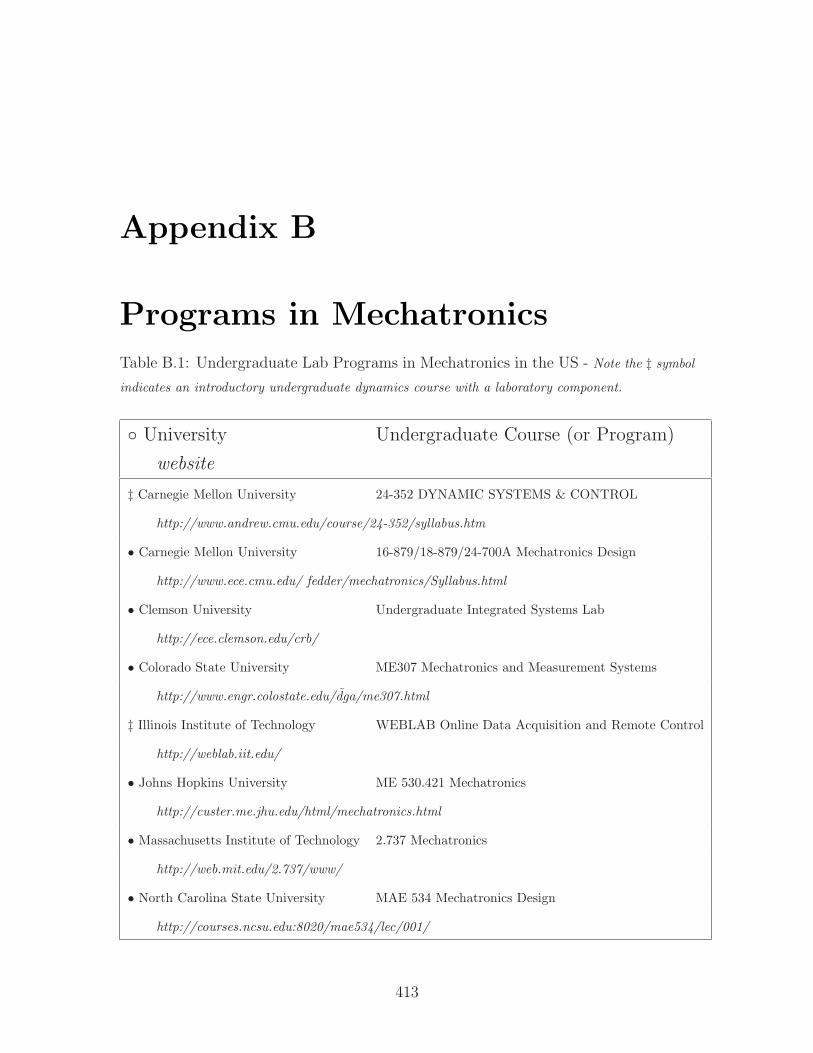
Appendix B

Programs in Mechatronics

Table B.1: Undergraduate Lab Programs in Mechatronics in the US - Note the ‡ symbol

indicates an introductory undergraduate dynamics course with a laboratory component.

University Undergraduate Course (or Program)

website

‡ Carnegie Mellon University 24-352 DYNAMIC SYSTEMS & CONTROL

http://www.andrew.cmu.edu/course/24-352/syllabus.htm

• Carnegie Mellon University 16-879/18-879/24-700A Mechatronics Design

http://www.ece.cmu.edu/ fedder/mechatronics/Syllabus.html

• Clemson University Undergraduate Integrated Systems Lab

http://ece.clemson.edu/crb/

• Colorado State University ME307 Mechatronics and Measurement Systems

http://www.engr.colostate.edu/dga/me307.html

‡ Illinois Institute of Technology WEBLAB Online Data Acquisition and Remote Control

http://weblab.iit.edu/

• Johns Hopkins University ME 530.421 Mechatronics

http://custer.me.jhu.edu/html/mechatronics.html

• Massachusetts Institute of Technology 2.737 Mechatronics

http://web.mit.edu/2.737/www/

• North Carolina State University MAE 534 Mechatronics Design

http://courses.ncsu.edu:8020/mae534/lec/001/

413


website

• Rensselaer Polytechnic Institute MEAE-4490 Mechatronics

http://www.rpi.edu/ craigk/mech2002.html

• Rice University ELEC 201 Introduction to Engineering

http://www-ece.rice.edu/Courses/201/

• San Jose State University ME 106 Fundamentals of Mechatronics

http://www.engr.sjsu.edu/bjfurman/courses/ME106/ME106courseinfo.htm

• Stanford University SPDL Lab Courses

http://design.stanford.edu/spdl/

• SUNY University at Buffalo MAE 476/576: Mechatronics

http://www.eng.buffalo.edu/Courses/mae576/CourseInformation.html

• University of California Berkeley EE192 Mechatronics Design Lab

http://www-inst.eecs.berkeley.edu/ee192/

• University of California Davis EEC 194 MicroMouse Competition

http://www.ece.ucdavis.edu/umouse/

• University of Illinois and Urbana-Champaign UIUC College of Engineering Mechatronics Lab

http://robot0.ge.uiuc.edu/ spong/deere/

‡ The University of Texas at Austin ME 244L Dynamic Systems and Controls Lab

http://www.me.utexas.edu/ lotario/me244L/labs/ufresp/

• University of Utah ME3200/ME3210 Mechatronics

http://www.mech.utah.edu/ me3200/

• University of Washington Mechatronics Project

http://www.me.washington.edu/ dig/medesign/Mechatronics.htm

• Virginia Tech ME/ECpE 4734 Mechatronics

http://mechatronics.me.vt.edu/home.html

• Wellesley College CS115/PHYS115 Robotic Design Studio

http://nike.wellesley.edu/ rds/rds01/index.html

414

Table B.2: International Undergraduate Programs in Mechatronics


website

• Chemnitz University of Technology Institute of Mechatronics

http://www.tu-chemnitz.de/ifm/english/index.htm

• City University of Hong Kong Bachelor of Engineering in Mechatronic Engineering

http://www.cityu.edu.hk/me/bengmte.htm

• Griffith University (Australia) School of Microelectronic Engineering

http://www.gu.edu.au/school/mee/home.html

• Indian Institute of Technology Kanpur (India) Center for Mechatronics

http://www.iitk.ac.in/robotics/general/about.html

• James Cook University (Australia)

http://www.eng.jcu.edu.au/mech/info/mechatronics.html

• Johannes Kepler University of Linz (Austria) Mechatronics Course Curriculum

http://www.mechatronik.uni-linz.ac.at/index.en.html

• Loughborough University (UK) Mechatronics Teaching Laboratory

http://www.lboro.ac.uk/research/mechatronics/

• McGill (Canada) Mechatronic Option for Undergrads

http://www.mcgill.ca/mecheng/undergrad/curriculum/mechatronics/

• National University of Singapore (Singapore) Mechatronics Electives for Undergrads

http://www.eng.nus.edu.sg/mpe/courses/me4244.html

• Singapore Polytechnic (Singapore) Full-time diploma in Mechatronics

http://sspwb100.sp.edu.sg/schools/mm/courses/cm ftdmec.htm

• The University of Adelaide (Australia) Bachelor of Engineering (Mechatronics)

http://www.mecheng.adelaide.edu.au/Courses/Bachelors/structure.html

• University of Delft (Netherlands) Advanced Mechatronics group

http://dutera.et.tudelft.nl/Delft Control/

415


website

• University of Hannover (Germany) Hanover Center of Mechatronics

http://www.mzh.uni-hannover.de/lehre e.htm

• University of Twente (Netherlands) The Mechatronic Design Group

http://www.rt.el.utwente.nl/mechatronics/

• The University of Waikato (New Zealand) 0773.415 Mechatronics

http://www.phys.waikato.ac.nz/

• University of Waterloo (Canada) Engineering Mechatronics Option for Undergrads

http://www.me.uwaterloo.ca/ mechatro/

• University of Wollongong (Australia) Bachelor of Engineering (Mechatronics)

http://www.uow.edu.au/ friso/mechatronics.htm

Note that the lists in Tables B.1 and B.2 only sample a few particular types of

programs in mechatronics. The emphasis is on courses and degree programs which (1)

provide undergraduate preparation for design in mechatronics and (2) have publicly

accessible materials from which others may survey the types of course work available.

Even under these guideline, there are clearly a large number of notable programs

left off of this list (because of time and space constraints or my own ignorance) that

deserve note.

416

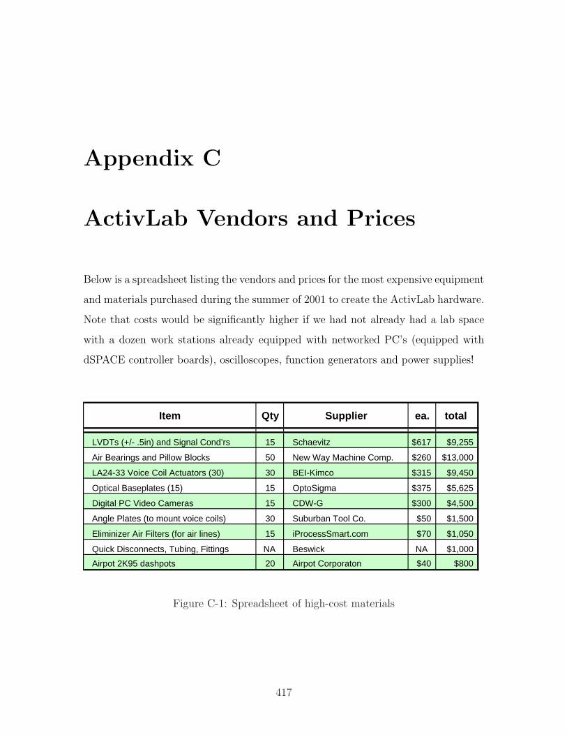
Appendix C

ActivLab Vendors and Prices

Below is a spreadsheet listing the vendors and prices for the most expensive equipment

and materials purchased during the summer of 2001 to create the ActivLab hardware.

Note that costs would be significantly higher if we had not already had a lab space

with a dozen work stations already equipped with networked PC’s (equipped with

dSPACE controller boards), oscilloscopes, function generators and power supplies!

Item Qty Supplier ea. total

LVDTs (+/- .5in) and Signal Cond’rs 15 Schaevitz $617 $9,255

Air Bearings and Pillow Blocks 50 New Way Machine Comp. $260 $13,000

LA24-33 Voice Coil Actuators (30) 30 BEI-Kimco $315 $9,450

Optical Baseplates (15) 15 OptoSigma $375 $5,625

Digital PC Video Cameras 15 CDW-G $300 $4,500

Angle Plates (to mount voice coils) 30 Suburban Tool Co. $50 $1,500

Eliminizer Air Filters (for air lines) 15 iProcessSmart.com $70 $1,050

Quick Disconnects, Tubing, Fittings NA Beswick NA $1,000

Airpot 2K95 dashpots 20 Airpot Corporaton $40 $800

Figure C-1: Spreadsheet of high-cost materials

417

418

Appendix D

CAD Drawing of Delrin Air

Bearing Mounting Plate

Figure D-1: CAD Drawing of Delrin adapter plate for air bearings.

419

420

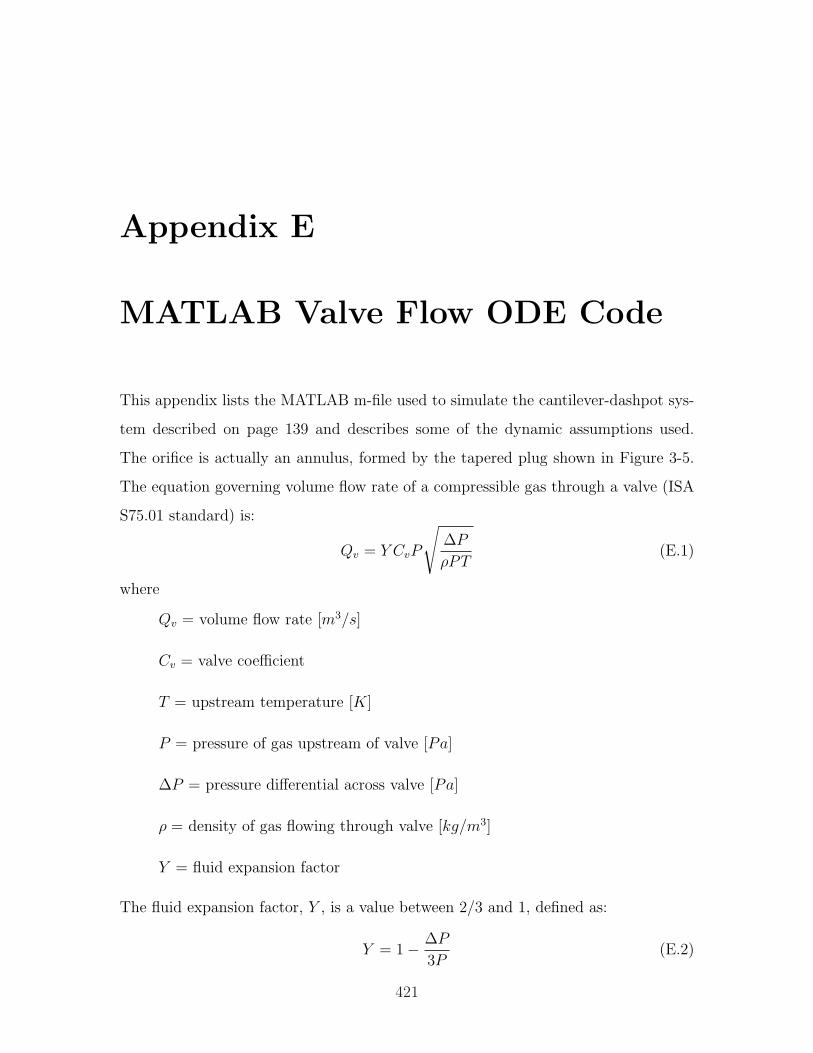
Appendix E

MATLAB Valve Flow ODE Code

This appendix lists the MATLAB m-file used to simulate the cantilever-dashpot sys-

tem described on page 139 and describes some of the dynamic assumptions used.

The orifice is actually an annulus, formed by the tapered plug shown in Figure 3-5.

The equation governing volume flow rate of a compressible gas through a valve (ISA

S75.01 standard) is:

Qv = Y CvP

√∆P

ρPT(E.1)

where

Qv = volume flow rate [m3/s]

Cv = valve coefficient

T = upstream temperature [K]

P = pressure of gas upstream of valve [Pa]

∆P = pressure differential across valve [Pa]

ρ = density of gas flowing through valve [kg/m3]

Y = fluid expansion factor

The fluid expansion factor, Y , is a value between 2/3 and 1, defined as:

Y = 1− ∆P

3P(E.2)

421

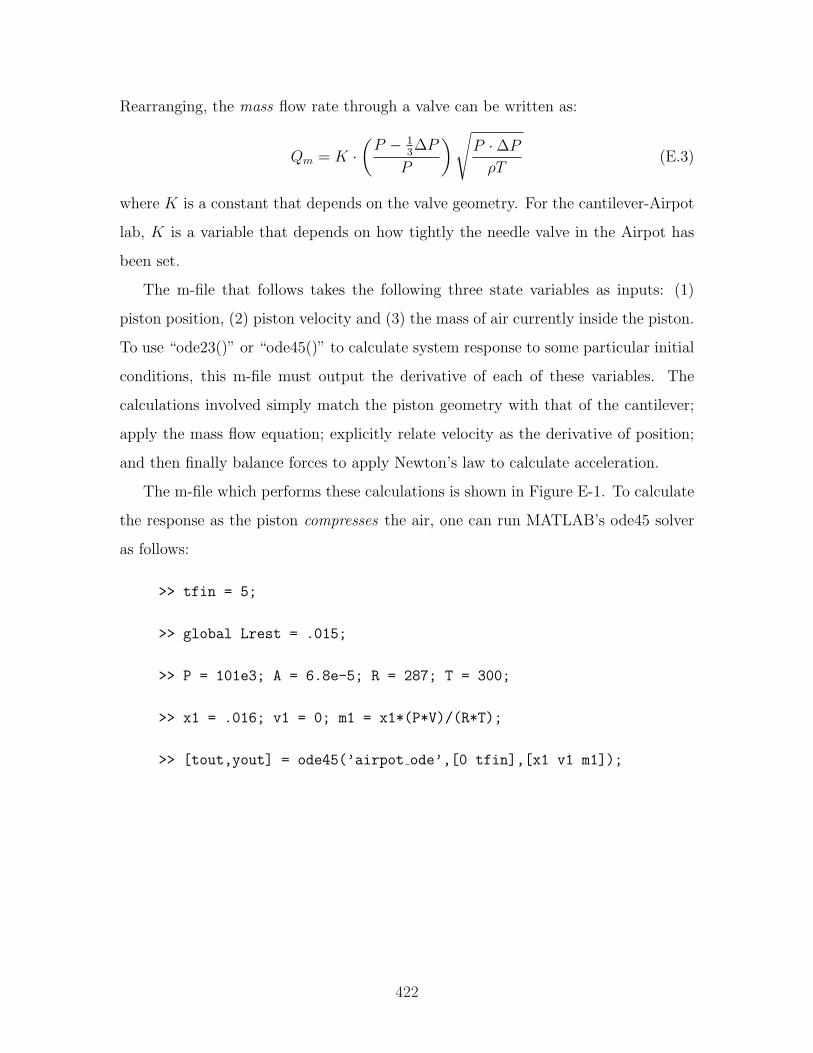
Rearranging, the mass flow rate through a valve can be written as:

Qm = K ·(

P − 13∆P

P

) √P ·∆P

ρT(E.3)

where K is a constant that depends on the valve geometry. For the cantilever-Airpot

lab, K is a variable that depends on how tightly the needle valve in the Airpot has

been set.

The m-file that follows takes the following three state variables as inputs: (1)

piston position, (2) piston velocity and (3) the mass of air currently inside the piston.

To use “ode23()” or “ode45()” to calculate system response to some particular initial

conditions, this m-file must output the derivative of each of these variables. The

calculations involved simply match the piston geometry with that of the cantilever;

apply the mass flow equation; explicitly relate velocity as the derivative of position;

and then finally balance forces to apply Newton’s law to calculate acceleration.

The m-file which performs these calculations is shown in Figure E-1. To calculate

the response as the piston compresses the air, one can run MATLAB’s ode45 solver

as follows:

>> tfin = 5;

>> global Lrest = .015;

>> P = 101e3; A = 6.8e-5; R = 287; T = 300;

>> x1 = .016; v1 = 0; m1 = x1*(P*V)/(R*T);

>> [tout,yout] = ode45(’airpot ode’,[0 tfin],[x1 v1 m1]);

422

G:\thesis_katie\test_dir\airpot_ode.mFebruary 4, 2003

Page 16:13:05 AM

function [dy] = airpot_ode(t,y)% function [dy] = airpot_ode(t,y)% input variables defined by "y":% y(1): x, position in m% y(2): v, velocity in m/s% y(2): m_air, mass of air inside

global Lrest; %x position of cantilever at rest

isentropic=1; % (set to 0 for isothermal limit)b=.0127; h=.00127; L=.205; % cantilever dimensionsE=210e9; I=b*h^3/12; % cantilever propertiesk=3*E*I/(L*L*L); % cantilever spring constantPout=101e3; % Pa, atmospheric pressureTout=300; % room temp of air outside, KelvinR=287; % gas constant for airmpot=1.8e-3; % mass of airpot pistonm=mpot+.24*b*h*L*8000; % ..with effective mass of cantileverx=y(1); v=y(2); m_air=y(3);A=6.8e-5; % piston areaV_air=(Lrest+x)*A; % volume now inside pistonif isentropic V1=m_air*R*Tout/Pout; % volume this mass at STP Pin=Pout*(V_air/V1)^-1.4; % isentropic relationship Tin=Pin*V_air/(R*m_air);else % assume isothermal limit Pin=(m_air*R*Tout)/V_air;% pressure in piston given T=Tout Tin=Tout;endK=.000000000005; % scaling coefficient for orifice sizedP=Pout-Pin; % driving pressure differentialif sign(dP)>0 % check air flow direction... rho=Pout/(R*Tout); % use density of air going thru orifice! Tair=Tout;else rho=m_air/V_air; % density of air in piston Tair=Tin; end

q = sign(dP)*K*((Pin-.33*dP)/Pin)*sqrt(Pin^2*abs(dP)*rho/Tin);

fr=.05*sign(v); % friction in piston, .002 to .1c=1.5; % damping in pistonFnet = -k*x - dP*A -fr -c*v;dv = Fnet/m; % F = m*ady=[v; dv; q]; % output all derivatives% --- EOF ---

Figure E-1: MATLAB function airpot ode() for orifice flow damping

423

424

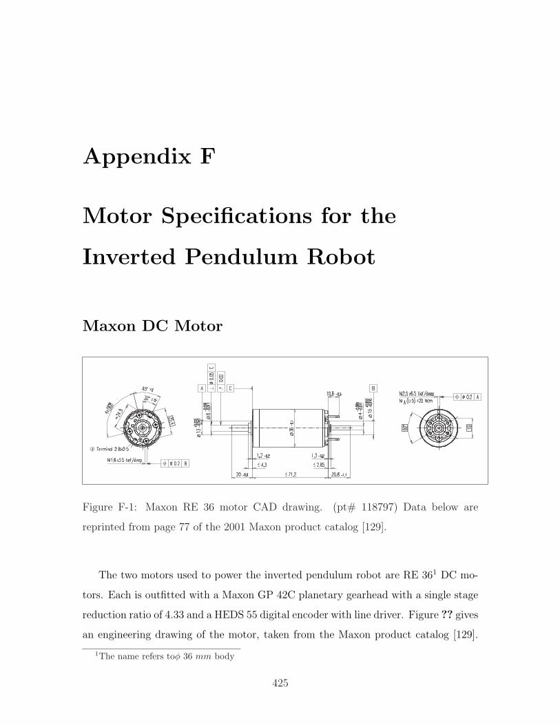
Appendix F

Motor Specifications for the

Inverted Pendulum Robot

Maxon DC Motor

Operating Range Comments Details on page 49

Recommended operating range

Continuous operationIn observation of above listed thermal resistances (li-nes 19 and 20) the maximum permissible rotor tem-perature will be reached during continuous operationat 25°C ambient.= Thermal limit.

Short term operationThe motor may be briefly overloaded (recurring).

Motor with high resistance winding

Motor with low resistance winding

n [rpm]

maxon Modular System

maxo

nD

Cm

oto

r

Specifications

April 2001 edition / subject to change maxon DC motor 77

Stock programStandard program

Special program (on request!)

Order Number

118804

118797

Axial play 0.05 - 0.15 mm Max. ball bearing loads

axial (dynamic)not preloaded 5.6 Npreloaded 2.4 N

radial (5 mm from flange) 28 NPress-fit force (static) 110 N(static, shaft supported) 1200 N

Radial play ball bearings 0.025 mm Ambient temperature range -20/+100°C Max. rotor temperature +125°C

Number of commutator segments 13

Weight of motor 350 g

Values listed in the table are nominal.For applicable tolerances (see page 43)and additional details please requestout of the maxon selection program on thesettled CD-Rom.

Tolerances may vary from the standardspecification.

100 200 300

9000

7000

5000

3000

1000

70 Watt

0.5 1.0 1.5 2.0 2.5 3.0

2 4 6 8 10 12

M [mNm]I [A]

I [A]

Planetary Gearhead32 mm0.75-4.5 NmDetails page 188


Planetary Gearhead42 mm3-15 NmDetails page 195

DC-Tacho22 mm0.52 VDetails page 200

Digital EncoderHP HEDS 5540500 CPT, 3 channelsDetails page 204

Digital EncoderHP HEDL 5540500 CPT, 3 channelsDetails page 206

118797 118798 118799 118800 118801 118802 118803 118804 118805 118806 118807 118808 118809 118810

Motor Data1 Assigned power rating W 70 70 70 70 70 70 70 70 70 70 70 70 70 70

2 Nominal voltage Volt 18.0 24.0 32.0 42.0 42.0 48.0 48.0 48.0 48.0 48.0 48.0 48.0 48.0 48.03 No load speed rpm 6410 6210 6790 7020 6340 6420 5220 4320 3450 2830 2280 1780 1420 1180

4 Stall torque mNm 730 783 832 865 786 785 627 504 403 326 258 198 158 127

5 Speed/torque gradient rpm/mNm 8.96 8.05 8.27 8.19 8.14 8.25 8.41 8.65 8.67 8.80 8.96 9.17 9.21 9.516 No load current mA 147 105 89 70 61 55 42 33 25 20 15 12 9 7

7 Starting current A 27.8 21.5 18.7 15.3 12.6 11.1 7.22 4.80 3.06 2.04 1.30 0.784 0.501 0.334

8 Terminal resistance Ohm 0.647 1.11 1.71 2.75 3.35 4.32 6.65 10.00 15.7 23.5 36.8 61.3 95.8 144

9 Max. permissible speed rpm 8200 8200 8200 8200 8200 8200 8200 8200 8200 8200 8200 8200 8200 820010 Max. continuous current A 3.14 2.44 1.99 1.59 1.44 1.27 1.03 0.847 0.679 0.556 0.445 0.346 0.277 0.226

11 Max. continuous torque mNm 82.4 88.8 88.5 89.8 90.4 90.1 89.8 89.0 89.2 88.8 88.1 87.3 87.2 85.8

12 Max. power output at nominal voltage W 119 125 146 157 129 131 84.9 56.4 36.0 23.9 15.2 9.09 5.78 3.82

13 Max. efficiency % 84 85 86 86 86 86 85 84 82 81 79 77 75 7214 Torque constant mNm/A 26.3 36.4 44.5 56.6 62.6 70.7 86.9 105 131 160 198 253 315 380

15 Speed constant rpm/V 364 263 215 169 152 135 110 90.9 72.7 59.8 48.2 37.8 30.3 25.1

16 Mechanical time constant ms 6 6 6 6 6 6 6 6 6 6 6 6 6 617 Rotor inertia gcm2 62.0 67.7 65.2 65.4 65.6 64.6 63.3 61.5 61.3 60.3 59.2 57.8 57.5 55.7

18 Terminal inductance mH 0.10 0.20 0.30 0.49 0.60 0.76 1.15 1.68 2.62 3.87 5.96 9.70 15.10 21.90

19 Thermal resistance housing-ambient K/W 6.4 6.4 6.4 6.4 6.4 6.4 6.4 6.4 6.4 6.4 6.4 6.4 6.4 6.4

20 Thermal resistance rotor-housing K/W 3.4 3.4 3.4 3.4 3.4 3.4 3.4 3.4 3.4 3.4 3.4 3.4 3.4 3.421 Thermal time constant winding s 39 43 41 41 41 41 40 39 39 38 37 36 36 35


Figure F-1: Maxon RE 36 motor CAD drawing. (pt# 118797) Data below are

reprinted from page 77 of the 2001 Maxon product catalog [129].

The two motors used to power the inverted pendulum robot are RE 361 DC mo-

tors. Each is outfitted with a Maxon GP 42C planetary gearhead with a single stage

reduction ratio of 4.33 and a HEDS 55 digital encoder with line driver. Figure ?? gives

an engineering drawing of the motor, taken from the Maxon product catalog [129].

1The name refers toφ 36 mm body

425

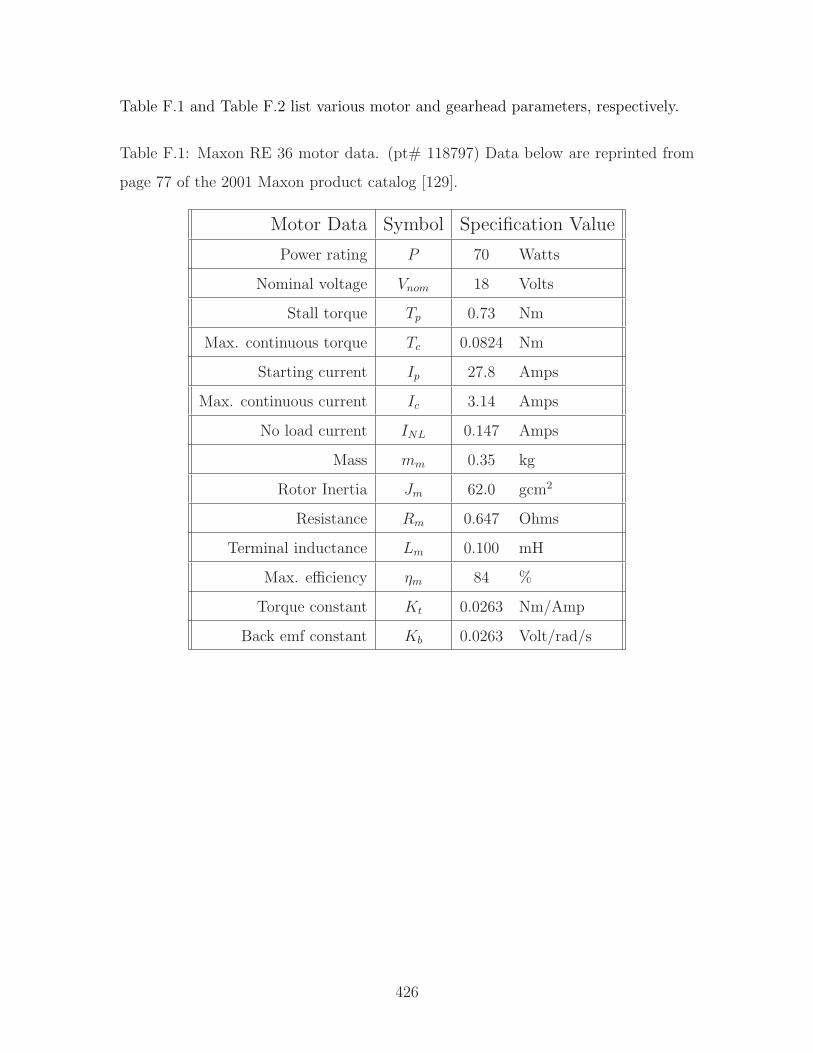
Table F.1 and Table F.2 list various motor and gearhead parameters, respectively.

Table F.1: Maxon RE 36 motor data. (pt# 118797) Data below are reprinted from

page 77 of the 2001 Maxon product catalog [129].

Motor Data Symbol Specification Value

Power rating P 70 Watts

Nominal voltage Vnom 18 Volts

Stall torque Tp 0.73 Nm

Max. continuous torque Tc 0.0824 Nm

Starting current Ip 27.8 Amps

Max. continuous current Ic 3.14 Amps

No load current INL 0.147 Amps

Mass mm 0.35 kg

Rotor Inertia Jm 62.0 gcm2

Resistance Rm 0.647 Ohms

Terminal inductance Lm 0.100 mH

Max. efficiency ηm 84 %

Torque constant Kt 0.0263 Nm/Amp

Back emf constant Kb 0.0263 Volt/rad/s

426

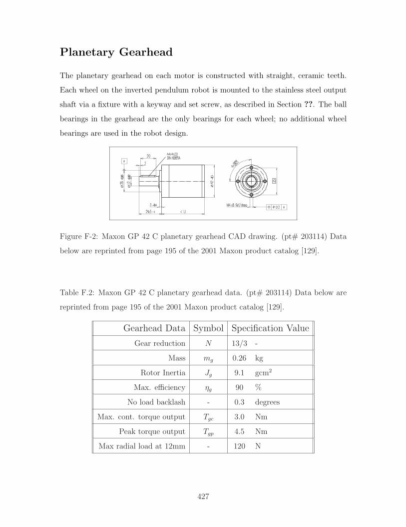
Planetary Gearhead

The planetary gearhead on each motor is constructed with straight, ceramic teeth.

Each wheel on the inverted pendulum robot is mounted to the stainless steel output

shaft via a fixture with a keyway and set screw, as described in Section ??. The ball

bearings in the gearhead are the only bearings for each wheel; no additional wheel

bearings are used in the robot design.

April 2001 edition / subject to change maxon gear 195

Stock programStandard programSpecial program (on request!)

Combination:

max

onge

ar

overall length overall length

Ceramicversion

Order Number

203113 203115 203120 203125 203128 203134 203139Gearhead Data

1 Reduction 3.5 : 1 12 : 1 43 : 1 91 : 1 150 : 1 319 : 1 546 : 12 Reduction absolute 7/2 49/4 343/8 91 2401 /16

637/2 5463 Mass inertia gcm2 14 15 15 15 15 15 14

203114 203116 203121 203126 203130 203135 2031401 Reduction 4.3 : 1 15 : 1 53 : 1 113 : 1 186 : 1 353 :1 676 : 12 Reduction absolute 13/3 91/6 637/12

338/3 4459 /2428561/81 676

3 Mass inertia gcm2 9.1 15 15 9.4 15 9.4 9.1203117 203122 203127 203131 203136 203141

1 Reduction 19 : 1 66 : 1 126 : 1 230 : 1 394 : 1 756 : 12 Reduction absolute 169/9 1183/18 126 8281 /36

1183/3 7563 Mass inertia gcm2 9.4 15 14 15 15 14

203118 203123 203129 203132 203137 2031421 Reduction 21 : 1 74 : 1 156 : 1 257 : 1 441 : 1 936 : 12 Reduction absolute 21 147/2 156 1029/4 441 9363 Mass inertia gcm2 14 15 9.1 15 14 9.1

203119 203124 203133 2031381 Reduction 26 : 1 81 : 1 285 : 1 488 : 12 Reduction absolute 26 2197/27

15379/544394/9

3 Mass inertia gcm2 9.1 9.4 15 9.4

4 Number of stages 1 2 3 3 4 4 45 Max. continuous torque at gear output Nm 3.0 7.5 15 15 15 15 156 Intermittently permissible torque at gear output Nm 4.5 11.3 22.5 22.5 22.5 22.5 22.57 Max. efficiency % 90 81 72 72 64 64 648 Weight g 260 360 460 460 560 560 5609 Average backlash no load ° 0.3 0.4 0.5 0.5 0.5 0.5 0.5

10 Gearhead length L1 mm 41.0 55.5 70.0 70.0 84.5 84.5 84.5

+ Motor Page + Tacho Page + Brake Page Overall length [mm]RE 35, 90 W 76 112.0 126.5 141.0 141.0 155.5 155.5 155.5RE 35, 90 W 76 DC-Tacho 22 200 130.1 144.6 159.1 159.1 173.6 173.6 173.6RE 35, 90 W 76 Digital Encoder HED_ 55_ 204/206 133.0 147.5 162.0 162.0 176.5 176.5 176.5RE 35, 90 W 76 Brake 40 232 148.0 162.5 177.0 177.0 191.5 191.5 191.5RE 36, 70 W 77 112.3 126.8 141.3 141.3 155.8 155.8 155.8RE 36, 70 W 77 DC-Tacho 22 200 130.4 144.9 159.4 159.4 173.9 173.9 173.9RE 36, 70 W 77 Digital Encoder HED_ 55_ 204/206 132.3 146.8 161.3 161.3 175.8 175.8 175.8RE 40, 150 W 78 112.1 126.6 141.1 141.1 155.6 155.6 155.6RE 40, 150 W 78 Digital Encoder HED_ 55_ 204/206 132.8 147.3 161.8 161.8 176.3 176.3 176.3RE 40, 150 W 78 Brake 40 232 148.1 162.6 177.1 177.1 191.6 191.6 191.6RE 40, 150 W 78 Digital Encoder HEDL 9140 208 158.9 173.4 187.9 187.9 202.4 202.4 202.4RE 40, 150 W 78 Brake 28 233 158.9 173.4 187.9 187.9 202.4 202.4 202.4RE 40, 150 W 78 Digital Encoder HEDL 9140 208 Brake 28 233 174.5 189.0 203.5 203.5 218.0 218.0 218.0EC 40, 120 W 157 111.1 125.6 140.1 140.1 154.6 154.6 154.6EC 40, 120 W 157 Digital Encoder HED_ 55_ 205/207 129.5 144.0 158.5 158.5 173.0 173.0 173.0EC 40, 120 W 157 Resolver 26 213 137.7 152.2 166.7 166.7 181.2 181.2 181.2EC 40. 120 W 157 Brake 40 232 144.6 159.1 173.6 173.6 188.1 188.1 188.1EC 45, 150 W 158 152.3 166.8 181.3 181.3 195.8 195.8 195.8EC 45, 150 W 158 Digital Encoder HEDL 9140 208 167.9 182.4 196.9 196.9 211.4 211.4 211.4EC 45, 150 W 158 Digital Encoder HEDL 9140 208 Brake 28 233 167.9 182.4 196.9 196.9 211.4 211.4 211.4EC 45, 150 W 158 Resolver 26 213 152.3 166.8 181.3 181.3 195.8 195.8 195.8EC 45, 150 W 158 Brake 28 233 167.9 182.4 196.9 196.9 211.4 211.4 211.4EC 45, 250 W 159 185.1 199.6 214.1 214.1 228.6 228.6 228.6EC 45, 250 W 159 Digital Encoder HEDL 9140 208 200.7 215.2 229.7 229.7 244.2 244.2 244.2EC 45, 250 W 159 Digital Encoder HEDL 9140 208 Brake 28 233 200.7 215.2 229.7 229.7 244.2 244.2 244.2EC 45, 250 W 159 Resolver 26 213 185.1 199.6 214.1 214.1 228.6 228.6 228.6EC 45, 250 W 159 Brake 28 233 200.7 215.2 229.7 229.7 244.2 244.2 244.2

Technical Data

Planetary Gearhead straight teethOutput shaft stainless steelBearing at output ball bearingsRadial play, 12 mm from flange preloadedAxial play preloadedMax. permissible axial load 150 NMax. permissible force for press fits 300 NRecommended input speed < 8000 rpmRecommended temperature range -20/+100°C

Number of stages 1 2 3 4 5Max. perm. radial load12 mm from flange 120 N 150 N 150 N 150 N 150 N

Figure F-2: Maxon GP 42 C planetary gearhead CAD drawing. (pt# 203114) Data

below are reprinted from page 195 of the 2001 Maxon product catalog [129].

Table F.2: Maxon GP 42 C planetary gearhead data. (pt# 203114) Data below are

reprinted from page 195 of the 2001 Maxon product catalog [129].

Gearhead Data Symbol Specification Value

Gear reduction N 13/3 -

Mass mg 0.26 kg

Rotor Inertia Jg 9.1 gcm2

Max. efficiency ηg 90 %

No load backlash - 0.3 degrees

Max. cont. torque output Tgc 3.0 Nm

Peak torque output Tgp 4.5 Nm

Max radial load at 12mm - 120 N

427

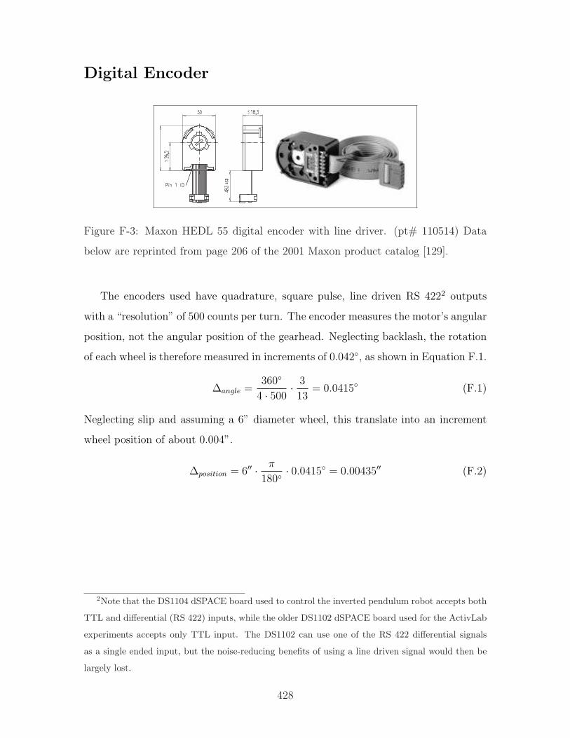
Digital Encoder

206 maxon tacho April 2001 edition / subject to change

overall length overall length

Stock programStandard programSpecial program (on request!)

max

onta

cho

Technical Data Pin Allocation Test CircuitSupply voltage 5 V 10%

Type No. designation1 N.C.2 Vcc3 Gnd4 N.C.5 Channel A6 Channel A7 Channel B8 Channel B9 Channel I (Index)

10 Channel I (Index)

Output signal EIA Standard RS 422drivers used: DS26LS31

Number of channels (not at 1000 Imp.)

Counts per turnPhase shift (nominal) 90°eLogic state width s min. 45°eSignal rise time(typical at CL = 25 pF, R L = 2.7 k, 25°C) 180 nsSignal fall time(typical at CL = 25 pF, R L = 2.7 k, 25°C) 40 nsIndex pulse width (nominal) Option 90°eOperating temperature range 0/+70°CMoment of inertia of code wheel 0.6 gcm2

Max. acceleration 250’000 rad s-2

Output current per channel min. -1 mA, max. 20 mAMax. operating frequency 100 kHz

5002+1 Index channel

1000 1

9

2

10

Combination+ Motor Page + Gearhead Page + Brake Page Overall length [mm] / see: + GearheadRE 25, 10 W 73 75.3RE 25, 10 W 73 GP 26, 0.2-2.0 Nm 184/185

RE 25, 10 W 73 GP 32, 0.75-6.0 Nm 187/190

RE 25, 10 W 73 GP 32, 0.4-2.0 Nm 193

RE 25, 20 W 74 75.3RE 25, 20 W 74 GP 26, 0.2-2.0 Nm 184/185

RE 25, 20 W 74 GP 32, 0.75-6.0 Nm 187/190

RE 25, 20 W 74 GP 32, 0.4-2.0 Nm 193

RE 26, 18 W 75 77.2RE 26, 18 W 75 GP 26, 0.2-2.0 Nm 184/185

RE 26, 18 W 75 GP 32, 0.75-6.0 Nm 187/190

RE 26, 18 W 75 GP 32, 0.4-2.0 Nm 193

RE 35, 90 W 76 91.9RE 35, 90 W 76 GP 32, 0.75-6.0 Nm 188/191

RE 35, 90 W 76 GP 42, 3.0-15 Nm 195

RE 36, 70 W 77 92.2RE 36, 70 W 77 GP 32, 0.75-6.0 Nm 188/191

RE 36, 70 W 77 GP 32, 0.4-2.0 Nm 193

RE 36, 70 W 77 GP 42, 3.0-15 Nm 195

RE 40, 150 W 78 91.7RE 40, 150 W 78 GP 42, 3.0-15 Nm 195

RE 40, 150 W 78 GP 42, 3.0-15 Nm 195 Brake 40 232

RE 40, 150 W 78 Brake 40 232 107.1RE 75, 250 W 79 241.5RE 75, 250 W 79 GP 81, 20-120 Nm 197

RE 75, 250 W 79 Brake 75 234 281.4RE 75, 250 W 79 GP 81, 20-120 Nm 197 Brake 75 234

S 2322, 6 W 82 68.8S 2322, 6 W 82 GP 22, 0.5-2.0 Nm 181/182

S 2322, 6 W 82 GP 26, 0.2-2.0 Nm 184/185

S 2326, 6 W 85 64.5S 2326, 6 W 85 GP 26, 0.2-1.8 Nm 184

S 2326, 6 W 85 GS 38, 0.1-0.6 Nm 194

Order Number

110510 110512 110514 110516 137398Type

Shaft diameter mm 2 3 4 6 8

Figure F-3: Maxon HEDL 55 digital encoder with line driver. (pt# 110514) Data

below are reprinted from page 206 of the 2001 Maxon product catalog [129].

The encoders used have quadrature, square pulse, line driven RS 4222 outputs

with a “resolution” of 500 counts per turn. The encoder measures the motor’s angular

position, not the angular position of the gearhead. Neglecting backlash, the rotation

of each wheel is therefore measured in increments of 0.042, as shown in Equation F.1.

∆angle =360

4 · 500· 3

13= 0.0415 (F.1)

Neglecting slip and assuming a 6” diameter wheel, this translate into an increment

wheel position of about 0.004”.

∆position = 6′′ · π

180· 0.0415 = 0.00435′′ (F.2)

2Note that the DS1104 dSPACE board used to control the inverted pendulum robot accepts both

TTL and differential (RS 422) inputs, while the older DS1102 dSPACE board used for the ActivLab

experiments accepts only TTL input. The DS1102 can use one of the RS 422 differential signals

as a single ended input, but the noise-reducing benefits of using a line driven signal would then be

largely lost.

428

Appendix G

MATLAB Code Simulating IP

Dynamics

This appendix contains MATLAB code that simulates an initial “stand-up” of the

robotic inverted pendulum (described in Chapter 7). Figure G-1 shows the calcu-

lated performance for the robot as originally planned. Note this simulated robot is

substantially smaller that the one actually built.

429

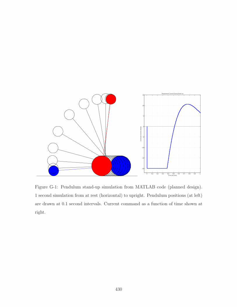
0 0.1 0.2 0.3 0.4 0.5 0.6 0.7 0.8 0.9 1

−20

−15

−10

−5

0

5

10

15

Time (seconds)

Com

man

d C

urre

nt (

Am

ps)

Requirement Current During Stand−up

Figure G-1: Pendulum stand-up simulation from MATLAB code (planned design).

1 second simulation from at rest (horizontal) to upright. Pendulum positions (at left)

are drawn at 0.1 second intervals. Current command as a function of time shown at

right.

430

C:\katie\mat_dir\standup_maxon7_draw.mFebruary 5, 2003

Page 11:57:03 AM

nmotor=2; mmotor=.35; mgears=.26;m_stuff= 7; % extra mass of batteries, wheel, et almp=.2; mw=nmotor*(mmotor+mgears)+m_stuff; % kg L=1; n=13/3; % gear ratio Jp=1e-3; Jbody=.14; Jm=nmotor*6.2e-6; %kg-m^2 mass_one_wheel=1.25; R=.15; % 15 cm wheel radius Jw=nmotor*.5*mass_one_wheel*R*R; % m_wheel= 1 kg Kt=nmotor*.0263; % Nm/A , 18 volt ref...fr=5e-4; eff=.75; % friction, gear train efficiency

theta_p=zeros(10100,1); theta_w=theta_p; thetad_p=theta_p; thetad_w=theta_p; thetad2_p=theta_p; thetad2_w=theta_p; torque_val=theta_p; u_was=theta_p;theta_p(1)=-pi/2-atan2(.5*R,L); theta_w(1)=-pi/2-atan2(.5*R,L); dt=1e-4; A=mp*L*L+Jp+Jbody+n*n*Jm; g=9.8; ustall=27.75; % stall current no_load_speed=671; % rad/secFe=0; K=-10; sum_pos=0; K_control=40; %20;for i=2:length(theta_p) u=K_control*(theta_p(i-1)+thetad_p(i-1)*.2)-0*sum_pos; % u is current umax=ustall*(1-abs(thetad_p(i-1)/no_load_speed)); if abs(umax)>20 umax=sign(umax)*20; end if abs(u)>umax u=sign(u)*umax; end u_was(i)=u; B=mp*R*L*cos(theta_p(i-1))-n*n*Jm; C=-mp*g*L*sin(theta_p(i-1)); D=fr*(thetad_p(i-1)-thetad_w(i-1)); E=(mp+mw)*R*R+Jw+n*n*Jw; F=-mp*R*L*sin(theta_p(i-1))*(thetad_p(i-1)^2); thetad2_w(i)=(A/(E*A-B*B))*((B*D+B*C+B*n*Kt*u)/A+D-F+n*Kt*u+Fe*R); thetad2_p(i)=(-1/A)*(n*Kt*u+B*thetad2_w(i)+C+D); thetad_w(i)=thetad_w(i-1)+dt*thetad2_w(i); thetad_p(i)=thetad_p(i-1)+dt*thetad2_p(i); theta_w(i)=theta_w(i-1)+dt*thetad_w(i); theta_p(i)=theta_p(i-1)+dt*thetad_p(i); sum_pos=sum_pos+theta_w(i)*R*dt; end t=dt*[1:length(theta_p)]; base_pos=R*theta_w; pend_posx=base_pos+L*sin(theta_p); pend_posy=R+L*cos(theta_p); figure(1); clf; a=2*pi*[0:.01:1]; i=1; nframe=11;plot([-2 1],[0 0],’k’); hold on;for j=1:nframe; if j==1 plot(base_pos(i)+[R (-.5*R+L)]*sin(theta_p(i)),R+[R (-.5*R+L)]*cos(theta_p(i)),’b’) patch(base_pos(i)+R*cos(a),R+R*sin(a),’b’) patch(pend_posx(i)+.5*R*cos(a),pend_posy(i)+.5*R*sin(a),’b’) elseif j==nframe plot(base_pos(i)+[R (-.5*R+L)]*sin(theta_p(i)),R+[R (-.5*R+L)]*cos(theta_p(i)),’r’) patch(base_pos(i)+R*cos(a),R+R*sin(a),’r’); patch(pend_posx(i)+.5*R*cos(a),pend_posy(i)+.5*R*sin(a),’r’) else plot(base_pos(i)+[R (-.5*R+L)]*sin(theta_p(i)),R+[R (-.5*R+L)]*cos(theta_p(i)),’k’) plot(base_pos(i)+R*cos(a),R+R*sin(a),’k’); plot(pend_posx(i)+.5*R*cos(a),pend_posy(i)+.5*R*sin(a),’k’) end i=i+1000; end axis image; axis([-1.5 0 -.05 1.5]); axis off% --- EOF ---

Figure G-2: MATLAB simulation code.

431

432

Appendix H

Simulink/dSPACE Controller

This appendix documents the main Simulink/dSPACE model used to control the

inverted pendulum robot. There is a separate figure for each subsystem in the model.

Table H lists the MATLAB variables used for the controller.

433

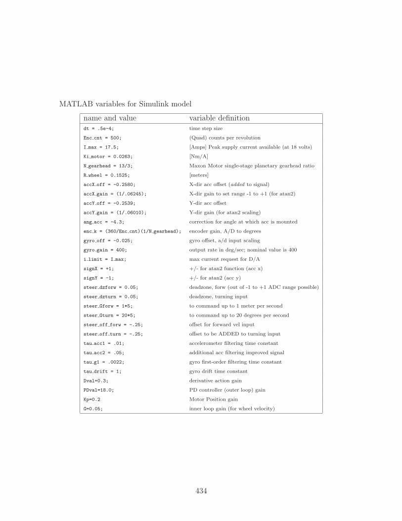
MATLAB variables for Simulink model

name and value variable definitiondt = .5e-4; time step size

Enc cnt = 500; (Quad) counts per revolution

I max = 17.5; [Amps] Peak supply current available (at 18 volts)

Ki motor = 0.0263; [Nm/A]

N gearhead = 13/3; Maxon Motor single-stage planetary gearhead ratio

R wheel = 0.1525; [meters]

accX off = -0.2580; X-dir acc offset (added to signal)

accX gain = (1/.06245); X-dir gain to set range -1 to +1 (for atan2)

accY off = -0.2539; Y-dir acc offset

accY gain = (1/.06010); Y-dir gain (for atan2 scaling)

ang acc = -4.3; correction for angle at which acc is mounted

enc k = (360/Enc cnt)(1/N gearhead); encoder gain, A/D to degrees

gyro off = -0.025; gyro offset, a/d input scaling

gyro gain = 400; output rate in deg/sec; nominal value is 400

i limit = I max; max current request for D/A

signX = +1; +/- for atan2 function (acc x)

signY = -1; +/- for atan2 (acc y)

steer dzforw = 0.05; deadzone, forw (out of -1 to +1 ADC range possible)

steer dzturn = 0.05; deadzone, turning input

steer Gforw = 1*5; to command up to 1 meter per second

steer Gturn = 20*5; to command up to 20 degrees per second

steer off forw = -.25; offset for forward vel input

steer off turn = -.25; offset to be ADDED to turning input

tau acc1 = .01; accelerometer filtering time constant

tau acc2 = .05; additional acc filtering improved signal

tau g1 = .0022; gyro first-order filtering time constant

tau drift = 1; gyro drift time constant

Dval=0.3; derivative action gain

PDval=18.0; PD controller (outer loop) gain

Kp=0.2 Motor Position gain

G=0.05; inner loop gain (for wheel velocity)

434

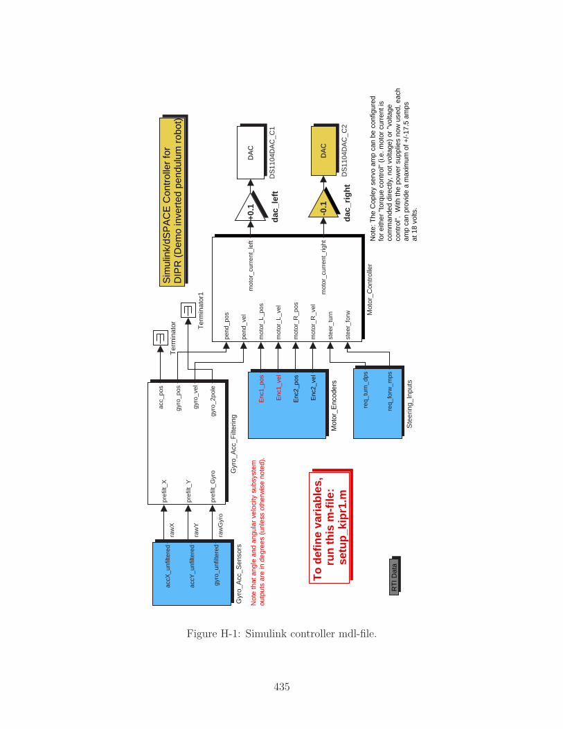
Sim

ulin

k/dS

PA

CE

Con

trol

ler

for

DIP

R (

Dem

o in

vert

ed p

endu

lum

rob

ot)

Not

e th

at a

ngle

and

ang

ular

vel

ocity

sub

syst

emou

tput

s ar

e in

deg

rees

(un

less

oth

erw

ise

note

d).

To

def

ine

vari

able

s,

run

th

is m

-file

:se

tup

_kip

r1.m

Not

e: T

he C

ople

y se

rvo

amp

can

be c

onfig

ured

fo

r ei

ther

"to

rque

con

trol

" (i.

e. m

otor

cur

rent

isco

mm

ande

d di

rect

ly, n

ot v

olta

ge)

or "

volta

geco

ntro

l". W

ith th

e po

wer

sup

plie

s no

w u

sed,

eac

h am

p ca

n pr

ovid

e a

max

imum

of +

/-17

.5 a

mps

at

18

volts

.

-0.1

dac

_rig

ht

+0.1

dac

_lef

t

Ter

min

ator

1

Ter

min

ator

req_

turn

_dps

req_

forw

_mps

Ste

erin

g_In

puts

RT

I Dat

a

Enc

1_po

s

Enc

1_ve

l

Enc

2_po

s

Enc

2_ve

l

Mot

or_E

ncod

ers

pend

_pos

pend

_vel

mot

or_L

_pos

mot

or_L

_vel

mot

or_R

_pos

mot

or_R

_vel

stee

r_tu

rn

stee

r_fo

rw

mot

or_c

urre

nt_l

eft

mot

or_c

urre

nt_r

ight

Mot

or_C

ontr

olle

r

accX

_unf

ilter

ed

accY

_unf

ilter

ed

gyro

_unf

ilter

ed

Gyr

o_A

cc_S

enso

rs

pref

ilt_X

pref

ilt_Y

pref

ilt_G

yro

acc_

pos

gyro

_pos

gyro

_vel

gyro

_2po

le

Gyr

o_A

cc_F

ilter

ing

DA

C

DS

1104

DA

C_C

2

DA

C

DS

1104

DA

C_C

1

raw

Y

raw

Gyr

o

raw

X

Figure H-1: Simulink controller mdl-file.

435

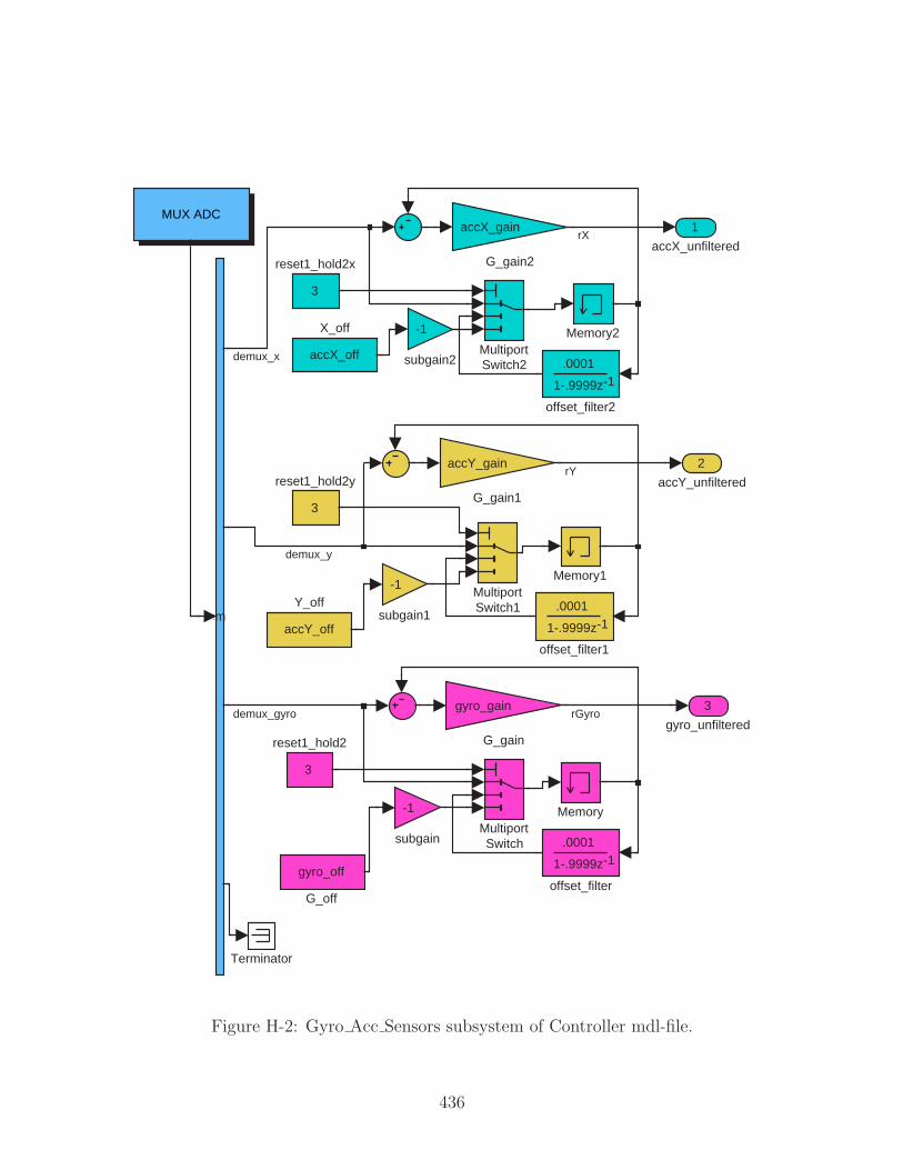
3

gyro_unfiltered

2

accY_unfiltered

1

accX_unfiltered

-1

subgain2

-1

subgain1

-1

subgain

3

reset1_hold2y

3

reset1_hold2x

3

reset1_hold2

.0001

1-.9999z -1

offset_filter2

.0001

1-.9999z -1

offset_filter1

.0001

1-.9999z -1

offset_filter

accY_off

Y_off

accX_off

X_off

Terminator

MultiportSwitch2

MultiportSwitch1

MultiportSwitch

Memory2

Memory1

Memory

gyro_off

G_off

accX_gain

G_gain2

accY_gain

G_gain1

gyro_gain

G_gain

Demux

MUX ADC

demux_y

demux_gyro rGyro

rY

demux_x

rX

Figure H-2: Gyro Acc Sensors subsystem of Controller mdl-file.

436

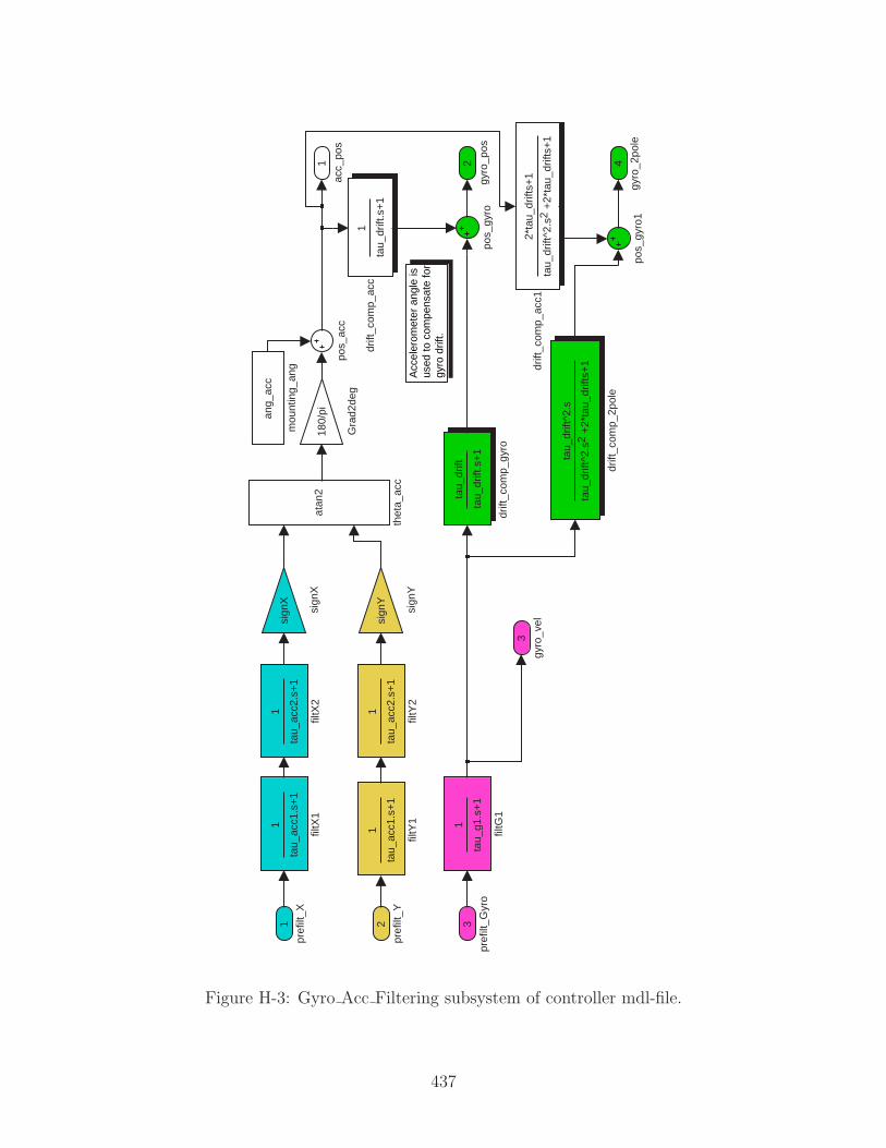
Acc

eler

omet

er a

ngle

isus

ed to

com

pens

ate

for

gyro

drif

t.

4

gyro

_2po

le

3

gyro

_vel

2

gyro

_pos

1

acc_

pos

atan

2

thet

a_ac

c

sign

Y

sign

Y

sign

X

sign

X

pos_

gyro

1

pos_

gyro

pos_

acc

ang_

acc

mou

ntin

g_an

g

1

tau_

acc2

.s+

1

filtY

2

1

tau_

acc1

.s+

1

filtY

1

1

tau_

acc2

.s+

1

filtX

2

1

tau_

acc1

.s+

1

filtX

1

1

tau_

g1.s

+1

filtG

1

tau_

drift

tau_

drift

.s+

1

drift

_com

p_gy

ro

2*ta

u_dr

ifts+

1

tau_

drift

^2.s

+

2*ta

u_dr

ifts+

12

drift

_com

p_ac

c1

1

tau_

drift

.s+

1dr

ift_c

omp_

acc

tau_

drift

^2.s

tau_

drift

^2.s

+

2*ta

u_dr

ifts+

12

drift

_com

p_2p

ole

180/

pi

Gra

d2de

g

3

pref

ilt_G

yro

2

pref

ilt_Y

1

pref

ilt_X

Figure H-3: Gyro Acc Filtering subsystem of controller mdl-file.

437

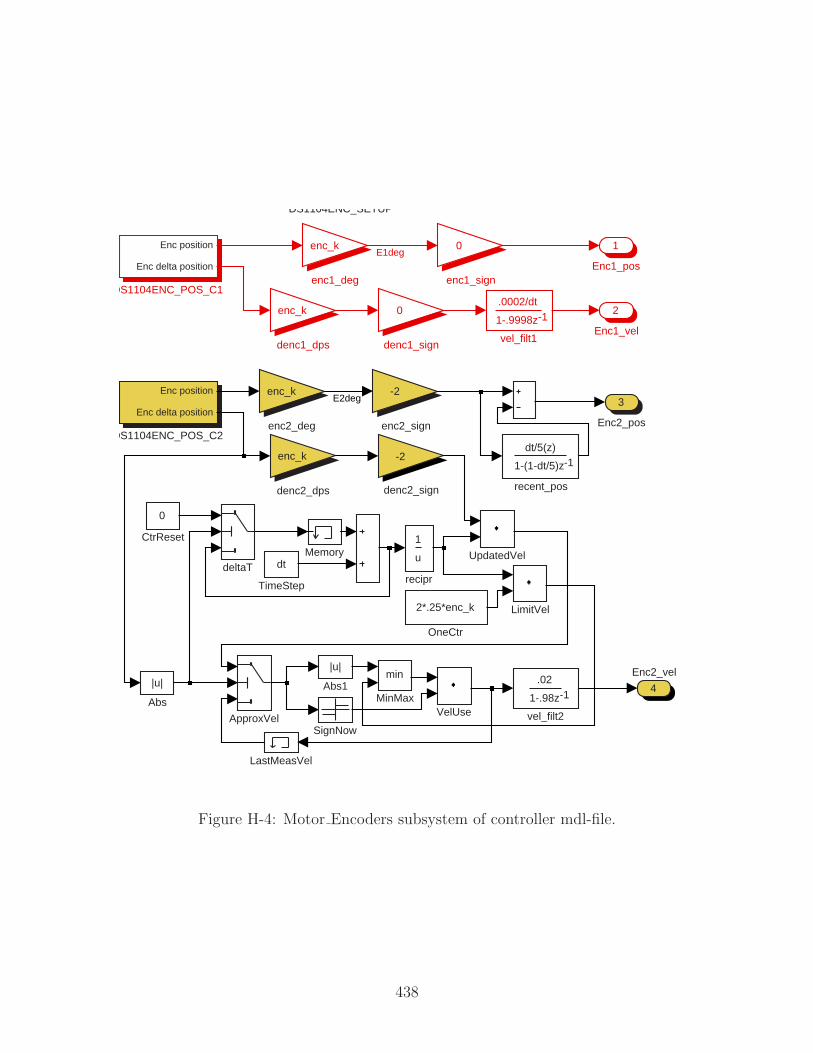
Note: Maxon Encoders areRS 422 line driven Note: not using dysfunctional

encoder on motor 1!!!

4

Enc2_vel

3

Enc2_pos

2

Enc1_vel

1

Enc1_pos

.02

1-.98z -1

vel_filt2

.0002/dt

1-.9998z -1

vel_filt1

1

u

recipr

1-(1-dt/5)z -1dt/5(z)

recent_pos

-2

enc2_sign

enc_k

enc2_deg

0

enc1_sign

enc_k

enc1_deg

-2

denc2_sign

enc_k

denc2_dps

0

denc1_sign

enc_k

denc1_dps

deltaT

VelUse

UpdatedVeldt

TimeStep

SignNow

2*.25*enc_k

OneCtr

min

MinMax

Memory

LimitVel

LastMeasVel

ENCODERMASTER SETUP

DS1104ENC_SETUP

Enc position

Enc delta position

DS1104ENC_POS_C2

Enc position

Enc delta position

DS1104ENC_POS_C1

0

CtrReset

ApproxVel

|u|

Abs1|u|

Abs

E1deg

E2deg

Figure H-4: Motor Encoders subsystem of controller mdl-file.

438

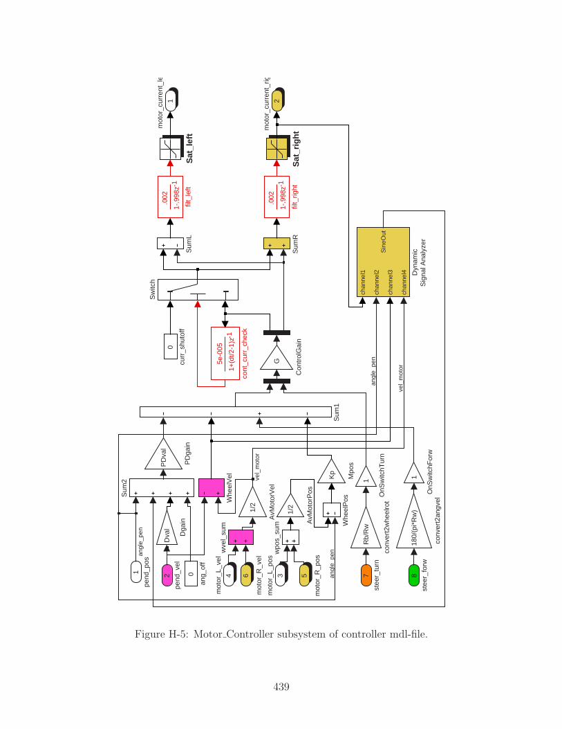
2

mot

or_c

urre

nt_r

ight

1

mot

or_c

urre

nt_l

eft

wve

l_su

m

wpo

s_su

m.0

02

1-.9

98z -

1

filt_

right

.002

1-.9

98z -

1

filt_

left

0

curr

_shu

toff

Rb/

Rw

conv

ert2

whe

elro

t

180/

(pi*

Rw

)

conv

ert2

angv

el

1+(d

t/2-1

)z -1

5e-0

05

cont

_cur

r_ch

eck

0

ang_

off

Whe

elV

el

Whe

elP

os

Sw

itch

Sum

R

Sum

L

Sum

2

Sum

1

Sat

_rig

ht

Sat

_lef

t

PD

val

PD

gain

1

OnS

witc

hTur

n

1

OnS

witc

hFor

w

Kp

Mpo

s

chan

nel1

chan

nel2

chan

nel3

chan

nel4

Sin

eOut

Dyn

amic

Sig

nal A

naly

zer

Dva

l

Dga

in

Dem

uxG

Con

trol

Gai

n

1/2

AvM

otor

Vel

1/2

AvM

otor

Pos

8

stee

r_fo

rw

7

stee

r_tu

rn

6

mot

or_R

_vel

5

mot

or_R

_pos

4

mot

or_L

_vel

3

mot

or_L

_pos

2

pend

_vel

1

pend

_pos

vel_

mot

or

vel_

mot

or

angl

e_pe

n

angl

e_pe

n

angl

e_pe

n

Figure H-5: Motor Controller subsystem of controller mdl-file.

439

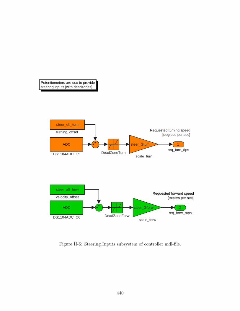
Requested turning speed[degrees per sec]

Requested forward speed[meters per sec]

Potentiometers are use to providesteering inputs [with deadzones].

2

req_forw_mps

1

req_turn_dps

steer_off_forw

velocity_offset

steer_off_turn

turning_offset

steer_Gturn

scale_turn

steer_Gforw

scale_forw

DeadZoneTurn

DeadZoneForw

ADC

DS1104ADC_C6

ADC

DS1104ADC_C5

Figure H-6: Steering Inputs subsystem of controller mdl-file.

440

Bibliography

[1] M. Acar. Mechatronics challenge for the higher education world. IEEE Trans-

actions on Components, Packaging, and Manufacturing Technology - Part C,

20(1):14–20, 1997.

[2] M. Acar and R. M. Parkin. Engineering education for mechatronics. IEEE

Transactions on Industrial Electronics, 43(1):106–112, February, 1996.

[3] Edith Ackermann. Piaget’s constructivism, papert’s constructionism: What’s

the difference? (publication in progress, 2001).

http://learning.media.mit.edu/content/publications/EA.Piaget%20 %20Papert.pdf.

[4] National Aeronautics and Space Administration. Hubble facts: Hubble space

telescope servicing mission 3A (Gyroscopes), 1999. Fact sheet.

http://www.gsfc.nasa.gov/gsfc/service/gallery/fact sheets/spacesci/hst3-

01/hst gyros.pdf.

[5] National Aeronautics and Space Administration. The Hubble project: Servicing

mission 3B, 2002. Mission Update.

http://sm3b.gsfc.nasa.gov/mission-updates/mission/mar9.html.

[6] The Airpot Corporation. Airpot corporation home page. website, accessed July

2001. http://www.airpot.com.

[7] D. G. Alciatore and M. B. Histand. Integrating mechatronics into a mechanical

engineering curriculum. IEEE Robotics and Automation Magazine, pages 35–38,

June, 2001.

441

[8] Amazon.com. The science behind the segway. Amazon.com: Electronics -

Segway Human Transporter, accessed March 2003.

http://www.amazon.com/exec/obidos/tg/detail/-/B00007EPJ6/ref=segway tn left/104-

4673826-9915947.

[9] American stirling company. mm-6 stirling engine. website, accessed January,

2003. http://www.stirlingengine.com/ecommerce/product.tcl?product id=31.

[10] American Association of People with Disabilities. FDA backs stair-climbing

wheelchair, Dec. 2002. http://www.aapd.com/docs/stairclimbwheelchair.html.

[11] Analog Devices, Inc. Low cost +/-2 g / +/-10 g dual axis iMEMS accelerometers

with digital output. Product Specification Sheet, 1999.

[12] David P. Anderson. nBOT balancing robot. website, accessed February 2003.

http://www.geology.smu.edu/ dpa-www/robo/nbot/.

[13] R. C. Arkin, K. Lee, L. F. McGinner, and C. Zhoe. The development of a shared

interdisciplinary intelligent mechatronics laboratory. Journal of Engineering

Education, pages 113–118, April, 1997.

[14] The Associated Press. The Associated Press photo archive. website, accessed

August, 2002.

http://photoarchive.ap.org/apdbs/Intl Photos/views/mini/6068/6068441.jpg.

[15] D. M. Auslander. Meeting industrial needs in mechatronics and control. Pro-

ceeding of the ASME Dynamic Systems and Control Division, DCS-64:383–387,

1998.

[16] Autodesk. FIRST. website - Site design courtesy of Autodesk, accessed Febru-

ary, 2003. http://www.usfirst.org/.

[17] Tak Auyeung. Micromouse handbook, April 6, 2003.

http://www.mobots.com/EeC194/book/book/.

442

[18] Farrokh Ayazi and Khalil Najafi. Design and fabrication of a high-performance

polysilicon vibrating ring gyroscope. Eleventh IEEE/ASME Intervational

Workshop on Micro Electro Mechanical Systems, Heidelburg, Germany, Jan-

uary 25-29 1998.

[19] Farrokh Ayazi and Khalil Najafi. A HARPSS polysilicon vibrating ring gyro-

scope. Journal of Microelectromechanical Systems, 10(2):169–179, June 2001.

[20] Richard Babyak. Servo surprise. Appliance Manufacturer Magazine, March

2002. http://www.ammagazine.com/CDA/ArticleInformation/features/

BNP Features Item/0,2606,72638,00.html - Note the underscores (“ ”) are

two “ ” wide, each.

[21] A.J. Baerveldt and R. Klang. A low-cost and low-weight attitude estimation

system for an autonomous helicopter. Proc. of the IEEE Int. Conf. on Intelligent

Engineering Systems, INES ’97, September 1997.

[22] Albert-Jan Baerveldt and Robert Klang. A low-cost and low-weight attitude

estimation system for an autonomous helicopter. Proc. of the IEEE Int. Conf.

on Intelligent Engineering Systems, INES 97, Budapest, Hungary, Sep 1997.

online at: http://www.geology.smu.edu/ dpa-www/robo/balance/inertial.pdf.

[23] Jens G. Balchen and Kenneth I. Mumme. Process Control: Structures and

Applications. Van Nostrand Reinhold Company, New York, 1988.

[24] Neil Barbour and George Schmidt. Inertial sensor technology trends. Proceed-

ings of the 1998 Workshop on Autonomous Underwater Vehicles, Cambridge,

MA:55–62, August 20-21 1998.

[25] Larry Barello. Gyrobot - a balancing robotic platform. website, accessed Febru-

ary, 2003. http://www.barello.net/Robots/gyrobot/index.htm.

[26] Garrett Barter, Elie Krevat, and Dan Kwon. Team 33 - Dr. Whackenscore.

MIT website, accessed January 2003, 6.270, January, 2001.

http://robots6270.mit.edu/contests/2001/robots/33/www/.

443

[27] Robert J. Beichner. SCALE-UP project summary, 1999. online at the North

Carolina State University website http://www.ncsu.edu/PER/SUPFIPSE.pdf.

[28] Robert J. Beichner, Jeffrey M. Saul, Rhett J. Allain, Duane L. Deardorff, and

David S. Abbott. Introduction to SCALE-UP: Student-centered activities for

large enrollment university physics. Proceedings of the 2000 Annual meeting of

the American Society for Engineering Education., 2000.

[29] John W. Belcher. Studio physics at MIT, Fall 2001. Physics Department News

Letter.

[30] Steve Benkovic, Steven Uyetanaka, and Meng Cheng Hsieh. Micromouse - hints,

ideas, inspiration. Personal website, accessed January, 2003.

http://homepage.mac.com/SBenkovic/MicroMouse/index.html.

[31] C. F. Bergh, A. Kita, and C. Ume. Development of mechatronics course in

the school of mechanical engineering at Georgia Tech. Proceeding of the 1999

IEEE/ASME International Conference on Advanced Intelligent Mechatronics,

pages 459–465, September, 1999.

[32] Jonathan Bernstein. MEMS inertial sensing technology. Sensors Magazine

Online, Feb. 2003. http://www.sensorsmag.com/articles/0203/14/main.shtml.

[33] Michael V. Berry. The levitronTM : an adiabatic trap for spins. Proceedings of

the Royal Society of London: Mathematical, Physical and Engineering Sciences,

452(1948):1207–1220, May 8, 1996.

[34] Beswick Engineering. Beswick engineering home page. website, accessed Jan-

uary 2003. http://www.beswick.com.

[35] David Black-Schaffer, Dave Chisholm, Ramji Srinivasan, and Tenbite Ermias.

The Yellow Jacket robot project report. Stanford website, accessed May 2002,

EE118, Winter, 2001. http://design.stanford.edu/spdl/EE118/YellowJacket/.

444

[36] Boston EMS. Technology at 106th Boston marathon. website, accessed July

2002. http://www.bostonems.com/GalSegway.htm.

[37] R. S. Bradbeer. An integrated studio approach to teaching basic electronics

to first year mechatronics degree students. 2001 IEEE/ASME International

Conference on Advanced intelligent Mechatronics Proceedings, pages 1118–1123,

July, 2001.

[38] E. Douglas Bradbury. Suspension fork for bicycles. U.S. Patent 5,445,401 -

assigned to Manitou Mountain Bikes, Inc., August 29, 1995.

[39] E. Douglas Bradbury. Suspension fork for bicycles with dual, fluid-based

dampers. U.S. Patent 5,509,677 - assigned to Manitou Mountain Bikes, Inc.,

April 23, 1996.

[40] British Aerospace Engineering Systems. VSG typical performance guide, 2001.

http://www.baesystems-gyro.com/PDF/Vsg.pdf.

[41] Alison K. Brown, Mark A. Sturza, Franco DeAngelis, and David A.

Lukaszewski. Fault tolerant GPS/inertial syste design. ION Satellite Division

3rd International Technical Meeting, pages 495–504, September 1990.

[42] Robert Grover Brown. Introduction to Random Signals and Applied Kalman

Filtering: with MATLAB exercises and solution. John Wiley & Sons, 1997.

[43] Vic Caleca. Under wraps: How they kept the Segway secret. USA Today online,

February 2002.

http://www.usatoday.com/tech/techreviews/2002/1/30/segway-secret.htm.

[44] Andre Cardadeiro. Dre’s 99gsx master tranny rebuild vfaq. Personal website, ac-

cessed January 2003. http://www.twingles.com/ideck/rebuild3/dretranny.htm.

[45] J. E. Carryer. Controller and components: Deciding what (and what not) to

teach in mechatronics courses. Proceeding of the ASME Dynamic Systems and

Control Division, DSC-64:377–382, 1998.

445

[46] J. E. Carryer. March madness: A mechatronics project theme. Proceeding of

the 7th Mechatronics Forum International Conference: Mechatronics Education

VI session, September, 2000.

[47] J. F. Cham, B. Stafford, and M. R. Curkosky. See labs run: A design-oriented

laboratory for teaching dynamic systems. Proceedings of 2001 ASME Interna-

tional Mechanical Engineering Congress and Exposition, November 11-16 2001.

[48] Edward Y. Chow and Alan S. Willsky. Analytical redundancy and the design

of robust failure detection systems. IEEE Transactions on Automatic Control,

AC-29(7):603–614, July 1984.

[49] Richard D. Christie. The disposable camera, June 1996.

http://www.ee.washington.edu/conselec/CE/kuhn/labs/camera/fl.htm.

[50] Donna Coveney. Photo of seymour papert from mit’s tech talk. copyright 2002.

http://www.davidsonfilms.com/piafot01.htm.

[51] Kevin Craig. Mechatronics facilities at rensselaer. RPI website.

http://www.rpi.edu/sincraigk.

[52] Kevin Craig. Mechatronics in university and professional education: Is there

anything really new here? Proceedings of the ASME Dynamic Systems and

Control Division, DSC-64:369–375, 1998.

[53] Kevin Craig. Mechatronics at rensselaer: a two-course senior-elective sequence

in mechanical engineering. Proceedings of the 1999 IEEE/ASME International

Conference on Advanced Intelligent Mechatronics, pages 452–458, September,

1999.

[54] Kevin Craig. Is anything really new in mechatronics education? IEEE Robotics

and Automation Magazine, pages 12–19, June, 2001.

[55] Edward F. Crawley, Kenneth B. Lazarus, Jeffrey W. Moore, Douglas A. Simp-

son, Gerald F. Caron, and Farla M. Russo. Damper and valve. U.S. Patent

6,193,029 - assigned to Active Control eXperts, Inc., February 27, 2001.

446

[56] Martin L. Culpepper. 2.000 How and why things work - labs (MIT).

http://psdam.mit.edu/2.000/lab.html.

[57] Davidson Films. Piaget, middle age, boating with friends. website copyright

1998-2002.

http://www.davidsonfilms.com/piafot01.htm.

[58] James C. Deckert, Mukund N. Desai, John J. Deyst, and Alan S. Willsky. F-8

DFBW sensor failure identification using analytic redundancy. IEEE Transac-

tions on Automatic Control, AC-22(5):795–803, October 1977.

[59] John DeGaspari. Shake, rattle and roll - thanks to the airbag, MEMS accelerom-

eters are getting to explore new territory. Mechanical Engineering Magazine

[online], 2001. Published by the American Society of Mechanical Engineers.

http://www.memagazine.org/backissues/nov01/features/rattle/rattle.html.

[60] Richard C. Dorf and Robert H. Bishop. Modern control systems. Prentice Hall,

Upper Saddle River, NJ, seventh edition, 1995.

[61] The dSPACE Corporation. dSPACE - solutions for control. website, accessed

March 2002. http://www.dspaceinc.com.

[62] Christopher W. Dyck, James J. Allen, and Robert J. Huber. Parallel-plate

electrostatic dual-mass oscillator. Presented at the Society of Photo-Optical

Instrumentation Engineers (SPIE) Micromachining and Microfabrication Sym-

posium, Santa Clara, California, Septempber 20-22, 1999. available online at

http://www.sandia.gov/mstc/technologies/micromachines/biblog summit.html.

[63] Samuel Earnshaw. On the nature of the molecular forces which regulate the con-

stitution of the luminiferous ether. Transactions of the Cambridge Philosophical

Society, 7:97–112, 1842.

[64] Imme Ebert-Uphoff, John F. Gardner, William R. Murray, and Ronald

Perez. Preparing for the next century: The state of mechatronics education.

IEEE/ASME Transactions on Mechatronics, 5(2):226–227, 2000.

447

[65] Edmunds.com, inc. manual transmission basics. website, accessed Jan. 2003.

http://www.edmunds.com/ownership/techcenter/articles/46029/article.html.

[66] G. Engh, P. Nelson, and N. J. Roach. Numismatic gyrations. Nature, 408:540,

2000.

[67] Epistemology and Learning Group MIT Media Lab. The programmable brick

FAQ. website, accessed March, 2002.

http://el.www.media.mit.edu/groups/el/projects/programmable-brick/more.html.

[68] Louis J. Everett. Dynamics as a process, helping undergraduates understand

design and analysis of dynamic systems. 1997 ASEE National Conference,

Session 2666, 1997.

[69] Ron Fearing. Ee192 mechatronics design lab, 2003.

http://www-inst.eecs.berkeley.edu/ee192/.

[70] Richard M. Felder and Linda K. Silverman. Learning and teaching styles. En-

gineering Education, 78(7):674–681, April 1988.

[71] S. Field, S. Meek, and S. Devasia. Mechatronics education in the department of

mechanical engineering at the University of Utah. Proceedings of the 7th Mecha-

tronics Forum International Conference: Mechatronics Education IV session,

September, 2000.

[72] J. F. Gardner. Two projects for undergraduate mechatronics class: Success and

failure. Proceedings of the 7th Mechatronics Forum International Conference:

Mechatronic Education VI session, September, 2000.

[73] Jerold P. Gilmore and Richard A. McKern. A redundant strapdown inertial

system mechanization - SIRU. Charles Stark Draper Laboratory publication,

pages 899–902, August 17-19 1970. Presented at the AIAA Guidance, Control

and Flight Mechanics Conference, Santa Barbara, California.

448

[74] Felix Grasser, Aldo D’Arrigo, Silvio Colombi, and Alfred Rufer. JOE: A mobile,

inverted pendulum, 2001. Unpublished paper, available online.

http://leiwww.epfl.ch/publications/grasser darrigo colombi rufer mic 01.pdf.

[75] Felix Grasser, Aldo D’Arrigo, Silvio Colombi, and Alfred Rufer. JOE: A mobile,

inverted pendulum. IEEE Transactions on Industrial Electronics, 49(1):107–

114, February 2002.

[76] Donald E. Grove. The vertical integration of mechatronics at Virginia Tech.

Master’s thesis, Virginia Tech, Mechanical Engineering Department, February

2001.

[77] T. G. Habetler, J. Meisel, G. H. Ronald, and H. B. Puttgen. A new undergradu-

ate course in energy conversion and mechatronics at Georgia Tech. Proceedings

of the 7th Mechatronics Forum International Conference: Mechatronics Educa-

tion I session, September, 2000.

[78] Blake Hannaford. Robust electronic circuits: The disposable camera flash,

March 2001. Lab assignment for EE498 Consumer Electronics Design at the

University of Washington.

http://www-brl.ee.washington.edu/Education/EE498/labs/lab cam 1-2.html.

[79] Tom Harris. HowStuffWorks, Inc. Howstuffworks - how segways work. website,

accessed August 2002. Copyright 1998-2003, HowStuffWorks, Inc.

http://www.howstuffworks.com/ginger.htm.

[80] Steve Hassenplug. Steve’s LegWay. website, accessed February 2003.

http://perso.freelug.org/legway/LegWay.html.

[81] H. A. Haus and J. R. Melcher. Electromagnetic Fields and Energy. electronic

text rights reserved by HTF (Hypermedia Teaching Facility) at MIT, online

text edition, 1998. http://web.mit.edu/6.013 book/www/book.html.

[82] John Heilemann. Reinventing the wheel. Time online edition, December 2 2001.

http://www.time.com/time/business/article/0,8599,186660-2,00.html.

449

[83] Willem M. Hijmans. ActivLab. website, accessed August 2002.

http://web.mit.edu/2.003/www/activlab/activlab.html.

[84] HiTechnic Products. HiTechnic products and accessories. website, accessed

February 2003. http://www.hitechnic.com/products.htm.

[85] Ian D. Hopkins. Performance and design of a silicon micromachined gyro. Rate

Sensor Application Note, 2001. Silicon Sensing Systems

http://www.siliconsensing.com/acrobat/AN0199.pdf.

[86] Ian David Hopkins, Christopher Paul Fell, Kevin Townsend, and Timo-

thy Robert Mason. Vibrating structure gyroscope. U.S. Patent 5,932,804 -

assigned to British Aerospace Public Limited Company, August 3, 1999.

[87] HowStuffWorks, Inc. HowStuffWorks - learn how everything works! website.

Copyright 1998-2003, HowStuffWorks, Inc. http://www.howstuffworks.com.

[88] Jerwei Hsieh and Weileum Fang. A boron etch-stop assisted lateral etching pro-

cess for improved high-aspect-ratio silicon micro-machining and its applications.

Journal of Micromechanics and icroengineering, 12:574–581, June 2002.

[89] T. Hsu and J. Wang. A mechatronics curriculum stem for undergraduate

mechanical engineering education. Proceedings of the 1999 IEEE/ASME In-

ternational Conference on Advanced Intelligent Mechatronics, pages 577–584,

September, 1999.

[90] Kevin Hulsey. Mountain bike suspension fork. website, accessed January, 2003.

Copyright Kevin Hulsey Illustration, Inc.

http://www.khulsey.com/bikefork.jpeg.

[91] Immersion Corporation. Immersion Corporation homepage, copyright 2002.

http://www.immersion.com/.

[92] Fascinations Incorporated. Levitron - the amazing anti-gravity top. website,

accessed March, 2002. http://www.levitron.com.

450

[93] Institute of Electrical and Electronic Engineers (IEEE) U.C. Davis. What is

Micromouse? http://www.ece.ucdavis.edu/∼ieee/umouse/umouse.html.

[94] Hong Jin and Hong Yue Zhang. Optimal parity vector sensitive to desig-

nated sensor fault. IEEE Transactions of Aerospace and Electronic Systems,

35(4):1122–1128, October 1999.

[95] Johnson & Johnson and DEKA. Independence Technology, a Johnson & John-

son company - iBOT(TM). website, accessed August 2002.

http://www.independencenow-europe.com/ibot/index.html.

[96] Joseph L. Jones, Bruce A. Seiger, and Anita Flynn. Mobile Robots: Inspiration

to Implementation. A K Peters, Ltd., Natick, Massachusetts, second edition,

1999.

[97] Dean L. Kamen, Robert R. Ambrogi, Robert J. Duggan, Richard K. Heinzman,

Brian R. Key, and Susan D. Dastous. Control loop for transportation vehicles.

U.S. Patent 5,791,425, August 11, 1998.

[98] Dean L. Kamen, Robert R. Ambrogi, Robert J. Duggan, Richard K. Heinzman,

Brian R. Key, Andrzej Skoskiewicz, and Phyllis K. Kristal. Human transporter.

U.S. Patent 5,701,965, Deceber 30, 1997.

[99] Dean L. Kamen, Robert R. Ambrogi, Richard Kurt Heinzman, Christopher C.

Langenfeld, Marc A. Nisbet, Stanley B. Smith (III), and Thomas Alan Brindley.

Mechanical improvements to a personal vehicle. U.S. Patent 6,405,816, June

18, 2002.

[100] Dean L. Kamen, Robert R. Ambrogi, John David Heinzmann, Richard Kurt

Heinzmann, David Herr, and John B. Morrell. Control inputs for a balancing

personal vehicle. U.S. Patent 6,415,879, July 9, 2002.

[101] Matt Kelly. MEMS for everyman? Analog gyro puts a new spin on price, Octo-

ber 1 2002. http://smalltimes.com/document display.cfm?document id=4732.

451

[102] Clive William Kilmister. Lagrangian Dynamics: An introduction for students.

Plenum Press, New York, 1967.

[103] Mike Koss. Home page for mike koss. Personal website, accessed January 2003,

6.270, January, 2002. http://mckoss.com/6270/sozoomy.htm.

[104] Suzanne M. Kresta. Hands-on demonstrations: An alternative to full scale lab

experiments. Journal of Engineering Education, 87(1):7–9, January 1998.

[105] T. Kurfess and J. G. Witzel. Using mechatronics in early design. Proceedings of

the 7th Mechatronics Forum International Conference: Mechatronics Education

III session, September, 2000.

[106] Thomas R. Kurfess. Mechatronics and early mechanical design. IEEE/ASME

International Conference on Advanced Intelligent Mechatronics Proceedings,

pages 990–993, July 8-12, 2001.

[107] Lauren E. LeBon. Students petition against TEAL. The Tech, 123(14), March

21 2003. http://www-tech.mit.edu/V123/N14/14802T.14n.html.

[108] Sangwoo Lee, Sangjun Park, Jongpal Kim, Sangchul Lee, and Dong

il (Dan) Cho. Surface/bulk micromachined single-crystalline-silicon icro-

gyroscope. TJournal Of Microelectromechanical Systems, 9(4):557–567, De-

cember 2000.

[109] The LEGO Group. LEGO Mindstorms Robotics Invention System 2.0. website,

last accessed February 2003.

http://mindstorms.lego.com/eng/products/ris/risdetails.asp.

[110] Walter Lewin. 8.01 fall 1999 lecture 30: Simple harmonic oscillations - en-

ergy considerations - torsional pendulum. MIT PIVoT online study materials,

Recorded Nov. 24, 1999. (limited website access)

https://curricula2.mit.edu/servlet/pivot.pvservlet.Home?acode=0x0008000.

452

[111] John Lewis and Karen Auguston Field. An exclusive look at the engineering

behind the Segway HT, with some never-before-published technical details. De-

sign News - Product Design and Development (online), March 25, 2002.

http://www.manufacturing.net/dn/index.asp?layout=articleWebzine&articleid=CA200964.

[112] John H. Lienhard V. A heat transfer textbook: A free electronic textbook.

Online letter to the public.

http://web.mit.edu/lienhard/www/ahttproject.pdf.

[113] Katherine A. Lilienkamp. A simulink-driven dynamic signal analyzer. Bache-

lor’s thesis, MIT, Mechanical Engineering Department, February, 1999.

[114] Katherine A. Lilienkamp and David L. Trumper. Dynamic signal analyzer for

dSPACE. http://web.mit.edu/pmc/www/Links/dsa paper.pdf, 1999.

[115] G. R. Luecke. “Muscletronics”: Teaching mechatronics with fluid power sys-

tems. Proceedings of the 1999 IEEE/ASME International Conference on Ad-

vanced Intelligent Mechatronics, pages 466–471, September, 1999.

[116] Howard Lundberh. Linear dual inverted pendulum control. Master’s thesis,

MIT, Electrical Engineering Department, 1997.

[117] Jed S. Lyons, Jeffrey H. Morehouse, and Edward F. Young. Design of a labora-

tory to teach design of experiments. Proceedings of the 1999 ASME Education

Annual Conference, Session 2566, June 20-23 1999.

[118] David Macaulay. The Way Things Work. Houghton Mifflin Company, 1988.

[119] David Macaulay and Neil Ardley. The New Way Things Work: From Levers

to Lasers, Windmills to Web Sites, a Visual Guide to the World of Machines.

Houghton Mifflin Company, 1998.

[120] R. Manseur. Development of an undergraduate robotics course. 1997 Frontiers

in Education Conference, Session F1C:610–612, 1997.

453

[121] Fred Martin. The handy board technical reference, accessed March, 2002. avail-

able online at http://handyboard.com.

[122] Fred Martin. Mindstorms information. website, accessed March, 2002.

http://fredm.www.media.mit.edu/people/fredm/mindstorms/.

[123] Massachusetts Institure of Technology website. 6.270 - MIT’s autonomous robot

design competition. website. http://web.mit.edu/6.270/.

[124] Massachusetts Institute of Technology. Bulletin, volume 138. MIT, Cambridge,

MA, 2002.

[125] Massachusetts Institute of Technology. OpenCourseWare -About OCW.

http://ocw.mit.edu/global/about-ocw.html.

[126] Ben Massawir, Aren Sandersen, and Tenbite Ermias. Wilt - introduction. Stan-

ford website, accessed May 2002, EE118, Winter, 2001.

http://design.stanford.edu/spdl/EE118/Wilt/.

[127] The MathWorks, Inc. The MathWorks: Developers of MATLAB and Simulink

for technical computing. website, accessed March, 2002.

http://www.mathworks.com.

[128] Oliver Max. Ee192 stanford natcar, 2003.

http://www.stanford.edu/group/natcar/index.html.

[129] Maxon Precision Motors, Inc. Maxon motor 2001: High precision drives and

systems. Product Catalog, 2001. pp. 77, 195, and 206.

[130] Peter Maxwell, Jon Tessman, and Bruce Reichert. Design through to production

of a MEMS accelerometer for seismic acquisition. First Break, 19(3):141–144,

March 2001. published by the European Association of Geoscientists & Engi-

neers. www.firstbreak.nl.

[131] S. W. McCuskey. An Introduction to Advanced Dynamics. Addison Wesley

Publishing Company, Inc., Reading, Massachusetts, 1959.

454

[132] K. T. McDonald. Mcdonald’s physics examples. website, accessed March 2002.

http://www.hep.princeton.edu/˜mcdonald/examples/.

[133] Ann McKenna and Alice Agogino. Integrating design, analysis, and problem

solving in an introduction to engineering curriculum to high school students.

Engineering Education: Contributing to U.S. Competitiveness; Proceedings of

ASEE ’98, Session 1280:1–14, June 28-July 1 1988. CD ROM.

[134] Ann McKenna and Alice Agogino. Integrating design, analysis, and problem

solving in an introduction to engineering curriculum for high school students.

ASEE Annual Conference and Exposition, Charlotte, NC, June 20-23, 1999.

http://www.asee.org/conferences/annual99/assets/images/00308.pdf.

[135] Andrew McKinney and Mark Bessette, et al. MIT TEAL/Studio Physics

Project. MIT TEAL tutorial visualizations, 2002. available through the MIT

OpenCourseWare project at http://ocw.mit.edu/8/8.02/f02/index.html.

[136] James R. Melcher, Mark Zahn, and Harold Edgerton. “Edgerton’s Boomer”

Demonstration 10.2.1 for 6.013. electronic text rights reserved by HTF (Hy-

permedia Teaching Facility) at MIT, online video demonstration and numeric

calculations edition, 1998. See Section 10.2 at

http://web.mit.edu/6.013 book/www/book.html.

[137] MicroStrain, Inc. MicroStrain microminiature sensors: FAS-G inclinometer.

website, accessed February 2003. http://www.microstrain.com/FAS-G.htm.

[138] Henry Minsky. Photo of marvin minsky from personal website. copyright 2002.

http://www.ai.mit.edu/people/hqm/marvin1.gif.

[139] Marvin Minsky. The Society of Mind. Simon & Schuster, New York, 2nd edition

edition, 1988.

[140] H. K. Moffat. Euler’s disk and its finite-time singularity. Nature, 404:833–834,

2000.

455

[141] Francis C. Moon. Applied dynamics with application to multibody and mecha-

tronic systems. John Wiley & Sons, Inc., New York, 1st edition edition, 1998.

[142] MSNBC Dateline. A revolutionary new wheelchair. website, accessed August

2002. http://www.msnbc.com/news/285231.asp.

[143] W. R. Murray and J. L. Garbini. Mechatronics: A thread in the mechanial engi-

neering undergraduate curriculum. Proceedings of the ASME Dynami Systems

and Control Division, DSC-Vol. 64:397–404, 1998.

[144] W. R. Murray and J. L. Garbini. Mechatronics capstone design projects at the

University of Washington. Proceedings of the 1999 IEEE/ASME International

Conference on Advanced Intelligent Mechatronics, pages 598–604, September,

1999.

[145] Yoav Naveh, Pinhas Z. Bar-Yoseph, and Yoram Halevi. Nonlinear modeling

and control of a unicycle. Dynamics and Control, 9(4):279–296, Oct 1999.

[146] New Way Machine Components, Inc. Air bearings. website, accessed August

2001. http://newwaybearings.com.

[147] Newton Research Labs, Inc. Interactive C (IC). website, accessed February 2002.

http://www.newtonlabs.com/ic/.

[148] Clark T.-C. Nguyen. Frequency-selective MEMS for miniaturized communiza-

tion devices. Proceedings of the 1998 IEEE Aerospace Conference (Snowass,

Colorado), 1:445–460, March 21-28 1998.

[149] Steven Niemczyk. An Adaptive Domain-Independent Agents-Based Tutor for

Web-Based Supplemental Learning Environments. PhD thesis, MIT, Depart-

ment of Civil and Environmental Engineering, February, 2003.

[150] North Carolina State University. about the SCALE-UP project... Website ac-

cessed March 2003. http://www.ncsu.edu/per/scaleup.html.

456

[151] Hans Ohanian. Physics. W. W. Norton Publishing Co., 2nd edition edition,

1989. online text adapted by EspriTEC (not publically available) included on

PIVoT website.

[152] Allison Okamura. The haptic paddle. website, copyright 1998.

http://www-cdr.stanford.edu/Touch/previous projects/paddle/.

[153] William J. Palm III. Modeling, Analysis, and Control of Dynamic Systems.

John Wiley & Sons, Inc., New York, 2nd edition edition, 1999.

[154] Seymour Papert. Logo Philosophy and Implementation - Introduction: What is

Logo? Who needs it? Logo Computer Systems, Inc, 1999.

[155] Seymour Papert. Papert on piaget. Time Magazine: “The Century’s Greatest

Minds”, page 105, March 29 1999.

[156] Parallax, Inc. Parallax: BASIC stamp microcontrollers. website, accessed

March 2002. http://www.parallaxinc.com/.

[157] Antoonio M. Pascoal, Isaac Kaminer, and Paulo Oliveira. Navigation system de-

sign using time-varying complementary filters. IEEE Transactions on Aerospace

and Electronic Systems, 36(4):1099–1114, Oct 2000.

[158] R. J. Patton and J. Chen. Review of parity space approaches to fault diagnosis

for aerospace systems. Journal of Guidance, Control and Dynamics, 17(2):278–

285, March-April 1994.

[159] Theresa M. Pease. Papert describes his philosophy of education. Tech Talk,

May 16 1990. http://web.mit.edu/newsoffice/tt/1990/may16/23181.html.

[160] Arthur J. Pejsa. Optimum skewed redundant inertial navigators. AIAA Journal,

12(7):899–902, July 1974.

[161] A. J. Peyton, J. R. Burch, A. Bradshaw, and A. P. Dorey. The teaching of

sensors and instrumentation to second year electronics/mechatronics students.

457

Technical report, Engineering Dept., Lancaster UK, 1996. (published by the

Institution of Electrical Engineers).

[162] H. A. Pham, Y. S. Kua, and K. Salem. Having fun with muscle wires. Pro-

ceedings of the 7th Mechatronics Forum International Conference: Mechatronic

Education II session, September 2000.

[163] Philips Electronics N. V. Philips employee appointed advanced mechatronics

professor at Delft University of Technology. news release, accessed online March

2001. http://www.cft.philips.com/newscenter/newscenter copy(3).htm.

[164] Lara C. Phillips. Control of a dual inverted pendulum system using linear-

quadratic and H-infinity methods. Master’s thesis, MIT, Electrical Engineering

Department, 1994.

[165] Jean Piaget. To understand is to invent: the future of education. [English

translation by George-Anne Roberts]. Grossman Publishers, New York, 1973.

[166] J. E. Potter and M. C. Suman. Thresholdless redundancy management with

arrays of skewed instruments. Integrity in Electronic Flight Control Systems,

NATO Agardograph(225):15:1–25, April 1977.

[167] James E. Potter and James C. Deckert. Minimax failure detection and identifi-

cation in redundant gyro and accelerometer systems. Journal of Spacecraft and

Rockets, 10(4):236–243, April 1973.

[168] Derek Reamon. Mechanical dissection labs. Stanford University.

http://www-adl.stanford.edu/labs.html.

[169] Christopher Richard, Allison M. Okamura, and Mark R. Cutkosky. Getting

a feel for dynamics: Using haptic interface kits for teaching dynamics and

controls. ASME IMECE 6th Annual Symposium on Haptic Interfaces (Dallas,

Texas), November 15-21 1997.

458

[170] Christopher Richard, Allison M. Okamura, and Mark R. Cutkosky. Feeling is

believing: Using a force-feedback joystick to teach dynamic systes. Proceedings

of the 2000 ASEE Annual Conference and Exposition, Session 3668, 2000.

[171] Rebecca Richkus, Alice Agogino, David Yu, and David Tang. Virtual disk

drive design game with links to math, physics and dissection activities. 29th

ASEE/IEEE Frontiers in Education Conference, San Juan, Puerto Rico, Ses-

sion 12c3:1–5, November 10-13 1999.

[172] Rebecca Richkus, Alice M. Agogino, David Yu, and David Tang. Virtual disk

drive design game with links to math, physics and dissection activities. 29th

ASEE/IEEE Frontiers in Education Conference, San Juan, Puerto Rico, Nov.

10-13, 1999. http://best.me.berkeley.edu/aagogino/papers/VIRTUAL.PDF.

[173] James K. Roberge. Operational Amplifiers: Theory and Practice. John Wiley

and Sons, New York, 1975.

[174] James K. Roberge. Propogation of the race (of analog circuit designers). In

Jim Williams, editor, Analog Circuit Design: Art, Science, and Personalities,

pages 79–88. Butterworth-Heinemann, Boston, Massachusetts, 1991.

[175] Suzanne Rockwell. Eight more seated at the endowed ‘table’. Dateline U.C.

Davis, February 25, 2000.

http://www-dateline.ucdavis.edu/022500/Dl chairs.html.

[176] Ely Sachs. personal communication, 2001.

[177] San Francisco Chronicle [online]. Dashing new device for delivering mail / postal

service tries scooter on s.f. hills. website, accessed July 2002.

http://sfgate.com/cgi-bin/article.cgi?f=/c/a/2002/07/16/BA232425.DTL&type=news.

[178] Arnoldus Schoonwinkel. Design and Test of a Computer-Stabilized Unicycle.

Ph.d. thesis, Stanford University, 1988. (Abstract only.).

459

[179] Marie A. Schroeder. Memorandum containing the review of p020033 - indepen-

dence ibot 3000 mobility system by independence technology, l.l.c., October 24

2002. FDA document obtained online at:

http://www.fda.gov/ohrms/dockets/ac/02/briefing/3910b1 03 P020033.clinical.doc.

[180] Segway LLC. Segway. website, accessed August 2002. http://www.segway.com.

[181] SensAble Technologies. SensAble Technologies homepage, copyright 1996-2003.

http://www.sensable.com/.

[182] Stephen D. Senturia. Microsystem Design. Kluwer Academic Publishers,

Boston, Massachusetts, first edition, 2001.

[183] Katherine Shim. Edgerton, inventor, professor, dies at 86. The Tech, 109(58),

January 10 1990. http://the-tech.mit.edu/V109/N58/edge.58n.html.

[184] Herbert A. Simon. What we know about learning. Journal of Engineering

Education, 87(4):343–348, October 1998.

[185] Philip L. Skousen. Valve Handbook. McGraw-Hill, New York, 4th edition edi-

tion, 1998.

[186] Daniel Sorid. Hubble plagued by old, broken gyroscopes. space.com, November

15, 1999.

http://www.space.com/scienceastronomy/astronomy/hubble gyroold 991115.html.

[187] Richard Spencer. Natcar homepage. http://www.ece.ucdavis.edu/natcar/.

[188] A. A. Stanislavsky and K. Weron. Nonlinear oscillations in the rolling motion

of euler’s disk. Physica D, 156:247–259, 2001.

[189] Andrew K. Stimac. Standup and stabilization of the inverted pendulum. Bach-

elor’s thesis, MIT, Mechanical Engineering Department, June, 1999.

[190] Mark A. Sturza. Navigation system integrity monitoring using redundant mea-

surements. Navigation: Journal of The Institute of Navigation, 35(4):69–87,

Winter 1988-89.

460

[191] Salah Sukkarieh, Peter Gibbens, Ben Grocholsky, Keith Willis, and Hugh F.

Durrant-Whyte. A low-cost, redundant inertial measurement unit for unmanned

air vehicles. The International Journal of Robotics Research, 19(11):1089–1103,

2000.

[192] Swagelok Company. Swagelok home page. website, accessed June 2001.

http://www.swagelok.com.

[193] Keith R. Symon. Mechanics. Addison Wesley Publishing Company, Inc., Read-

ing, Massachusetts, third edition, 1971.

[194] Kaman Industrial Technologies. Kamandirect.com: Welcome. website, accessed

January 2003. http://www.kamandirect.com/.

[195] Bradley A. Trago, Edward J. Byrnes, and Griff D. Neal. Injection molded

motor assembly. U.S. Patent 6,020,661 - assigned to Pacific Scientific Company,

February 1, 2000.

[196] Bradley A. Trago and Robert E. Lordo. Fault tolerant electric machine. U.S.

Patent 5,929,549 - assigned to Pacific Scientific Company, July 27, 1999.

[197] David L. Trumper and Steven J. Ludwick. Development of 2.737 mechatronics

at MIT. In Development Conference on Advanced Intelligent Mechatronics,

pages 446–451, 1999. invited paper.

[198] David L. Trumper and Tsuyoshi Sato. A vibration isolation platform. Mecha-

tronics, 12:281–294, 2002.

[199] Chin S. Tsai. Bicycle shock-absorbing apparatus. U.S. Patent 5,088,705 -

assigned to Dan Ken Industrial Co., Ltd., February 18, 1992.

[200] Chin S. Tsai. Compression-adjustable bicycle shock-absorbing apparatus. U.S.

Patent 5,284,352, February 8, 1994.

[201] Paul H. Turner. Bicycle with improved front fork wheel suspension. U.S. Patent

5,186,481 - assigned to Rockshox, Inc., February 16, 1993.

461

[202] University of Central Florida. The Student Centered Activities for Large En-

rollment Undergraduate Programs (SCALE-UP) project. Website accessed May

2003. http://www.physics.ucf.edu/ peg/SCALE-UP/.

[203] H. M. J. van Brussel. Mechatronics - a powerful conurrent engineering frame-

work. IEEE/ASME Transactions on Mechatronics, 1(2):127–136, June, 1996.

[204] Jesco von Puttkamer. Space flight 1999 - space sciences and astronomy.

http://www.hq.nasa.gov/osf/1999/yearinrev/99science.html.

[205] David William Vos. Dynamics and nonlinear, adaptive control of an autonomous

unicycle. Master’s thesis, MIT, Department of Aeronautics and Astronautics,

1989.

[206] David William Vos. Nonlinear control of an autonomous unicycle robot: prac-

tical issues. PhD thesis, MIT, Department of Aeronautics and Astronautics,

1992.

[207] George Watson. Phys345 laboratory: Camera flash and transients in circuits,

1999. Lab assignent for PHYS345 Electricity and Electronics for Engineers at

the University of Delaware.

http://www.physics.udel.edu/watson/phys345/lab/camera.htm.

[208] William S. Watson. Vibrating structure gyro performacne improvements. Prod-

uct Report Paper, September, 2001. Watson Industries, Inc.

http://www.watson-gyro.com/company info/vsgrpt.pdf.

[209] Harvey Weinberg. Dual axis, low g, fully integrated accelerometers. Analog

Dialogue 33-1, 1999.

[210] R. Weiss and I. Nathan. An ultrareliable sensing system for vehicles with limited

sparing capability. Journal of Spacecraft, 4(9):1151–1158, September 1967.

[211] Glenn Weston-Murphy. Floppy drive dissection (Yale University).

http://www.eng.yale.edu/me185/floppy dissection.htm.

462

[212] Whittet-Higgins company. Whittet-Higgins Company home page. website, ac-

cessed January 2003. http://www.whittet-higgins.com/.

[213] James C. Wilcox. Competitive evaluation of failure detection algorithms for

strapdown redundant inertial instruments. Journal of Spacecraft and Rockets,

11(7):525–530, July 1974.

[214] James H. Williams. Fundamentals of Applied Dynamics. John Wiley and Sons,

New York, 1996.

[215] John Williamson. Latest news! iBOT 3000 stair climbing balancing wheelchair!

website, accessed August 2002.

http://www.dynopower.freeserve.co.uk/homepages/ibot3000/stairs.jpg.

[216] Alan S. Willsky. A survey of design methods for failure detection in

dynamic systems. Integrity in Electronic Flight Control Systems, NATO

Agardograph(225):5:1–14, April 1977.

[217] Jack M. Wilson. The CUPLE physics studio. The Physics Teacher, 32(9):518–

523, December 1994.

[218] Jack M. Wilson. The CUPLE Physics Studio. The Physics Teacher, 32(9):518–

523, December 1994.

[219] Donald R. Woods and Cameron M. Crowe. Characteristics of engineering stu-

dents in their first two years. Engineering Education, 74(5):289–295, February

1984.

[220] Sarah Wright. Papert misses big ideas of the good old days in AI. Tech Talk,

July 10 2002. http://web.mit.edu/newsoffice/nr/2002/papert.html.

[221] K. Yamazaki and S. Miyazawa. A development of courseware for mechatronics

education. International Journal of Engineering Education, 8(1):61–70, 1992.

463

[222] S. Yurkovitch, U. Ozguner, and K. M. Passino. Control system testbeds and

toys: Serendipitous or suspect. In Proceedings of the 1997 American Control

Conference, pages 2692–2696, Albuquerque, NM, June, 1998.

[223] S. Zarabadi, T. Vas, D. Sparks, J. Johnson, Q. Jiang, M. Chia, and E. Borz-

abadi. A resonating comb/ring angular rate sensor vaccum packaged via wafer

bonding. SAE Technical Paper Series, 199-01-1043, March 1-4 1999.

464

Lab Experiences for Teaching Undergraduate Dynamics by ...

Documents