Lab 9 First-Order Circuits and Oscilloscopes - Tom Reboldtomrebold.com/engr12lab/Labs/Lab-09-First-Order-Circ… ·  · 2017-03-281 Lab 9 First-Order Circuits and Oscilloscopes Objectives

1

Lab 9

First-Order Circuits and Oscilloscopes

Objectives

concepts

1. oscilloscopes

2. trigger modes

3. step response and natural response

skills

1. measure signal characteristics with an oscilloscope

2. experimentally determine the time constant of a first-order circuit

Key Prerequisites

Chapter 7 (First-Order Circuits)

Required Resources

Laptop, Circuit Kits, DMM, Digilent Analog Discovery (USB Oscilloscope)

Getting Started Video for Digilent’s Analog Discovery

WaveForms Software for Digilent Analog Discovery

Getting Started with WaveForms

Previously, we have utilized a multimeter to measure voltage, current, and resistance in electrical

circuits. The oscilloscope is another basic instrument used to measure electrical quantities in a

system and is an indispensable tool for electrical, computer, or wireless engineers. An

oscilloscope receives an electrical signal and converts it to a waveform that is displayed on a

screen as shown in Figure 1. Engineers employ oscilloscopes as a diagnostic tool to determine if

a system is working properly or not. As an example, a computer engineer could utilize an

oscilloscope to examine the signals from a USB port to determine if it is functioning properly.

Lab 9: First-Order Circuits

2

Fig 1: An oscilloscope connected to a function generator, from a tutorial on oscilloscopes

A sample (more modern) oscilloscope display is shown in Figure 2. The waveform in the display

shows the variation in voltage with time and is plotted on a graphical grid called a graticule. The

vertical or y-axis of the graticule typically represents voltage, while the horizontal or x-axis

typically represents time. Various buttons or knobs allow one to modify the view of the

waveform being studied.

Fig 2: A typical oscilloscope found in an electronics lab.

Oscilloscopes are essential tools, but can be costly and awkward to ship for online labs.

Fortunately, cheaper and smaller options exist. In this lab, we will use the Digilent Analog

DiscoveryTM Portable Analog Circuit Design Kit, which includes a USB oscilloscope and a

waveform generator to perform signal measurements in this and subsequent labs.

An image of this device in action, with the WaveForms software that runs it, is shown in Fig 3.

Lab 9: First-Order Circuits

3

Fig 3. Analog DiscoveryTM connected to breadboard, with WaveFormsTM software display

The Analog Discovery is more than just a USB oscilloscope. The device combines the following

instruments into one low cost package ($99 for students):

2 channel DC Power Supply (limited to +/- 5V and 50 mA each – we won’t be using this)

Voltmeter

2 channel Function Generator

2 channel Oscilloscope

16 channel Digital Pattern Generator

16 channel Logic Analyzer

Network Analyzer

Spectrum Analyzer

Normally, the physical version of these devices would go for many tens of thousands of dollars if

purchased separately.

Discussion and Procedure

Part 1: Oscilloscope Basics

1) Before you can use the Analog Discovery, your computer will need a copy of WaveForms

2015, installed on it. Visit the link below and start the download process, selecting all the

standard choices unless you have a good reason to customize them.

http://store.digilentinc.com/waveforms-2015-download-only/

2) For reference, the following diagram identifies all of the wires on the Analog Discovery

Adapter box:

Lab 9: First-Order Circuits

4

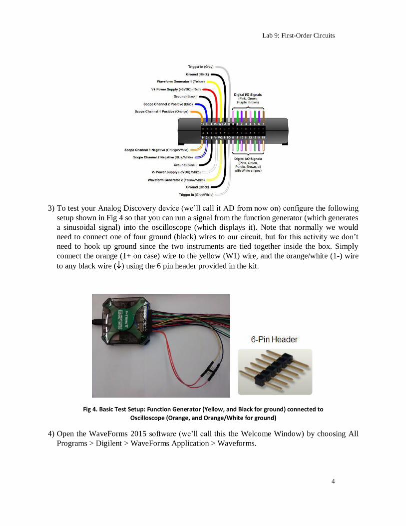
3) To test your Analog Discovery device (we’ll call it AD from now on) configure the following

setup shown in Fig 4 so that you can run a signal from the function generator (which generates

a sinusoidal signal) into the oscilloscope (which displays it). Note that normally we would

need to connect one of four ground (black) wires to our circuit, but for this activity we don’t

need to hook up ground since the two instruments are tied together inside the box. Simply

connect the orange (1+ on case) wire to the yellow (W1) wire, and the orange/white (1-) wire

to any black wire () using the 6 pin header provided in the kit.

Fig 4. Basic Test Setup: Function Generator (Yellow, and Black for ground) connected to

Oscilloscope (Orange, and Orange/White for ground)

4) Open the WaveForms 2015 software (we’ll call this the Welcome Window) by choosing All

Programs > Digilent > WaveForms Application > Waveforms.

Lab 9: First-Order Circuits

5

Fig 5. WaveForms 2015 Instrument Selection Window

5) Click on the WaveGen Icon to bring up the Arbitrary Waveform Generator (aka Function

Generator). This is the part of the Analog Discovery that generates sinewaves and other types

of signals.

6) Using the pulldown menus configure the generator to produce a 1 kHz sinewave, with an

amplitude of 1V and a DC offset of 0V, as shown below. These happen to be the default

settings, so you don’t have to change anything, although you can try modifying the settings

and changing them back again for practice. Click the Run button and in a moment your

display will look like the following.

Fig 6a. WaveGen set for a 1 kHz sinewave with a 1V amplitude.

To change from the default BLACK background, choose

Settings > Options > Analog Color and change from Dark to Light

Lab 9: First-Order Circuits

6

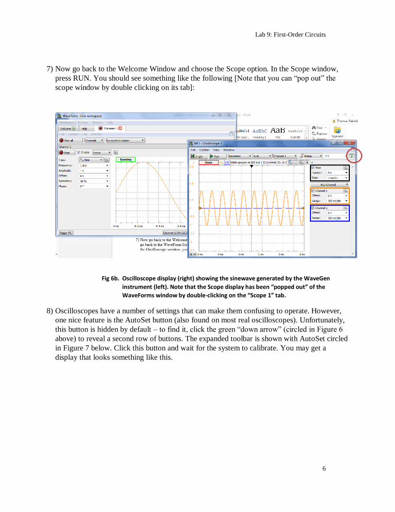
7) Now go back to the Welcome Window and choose the Scope option. In the Scope window,

press RUN. You should see something like the following [Note that you can “pop out” the

scope window by double clicking on its tab]:

Fig 6b. Oscilloscope display (right) showing the sinewave generated by the WaveGen

instrument (left). Note that the Scope display has been “popped out” of the

WaveForms window by double-clicking on the “Scope 1” tab.

8) Oscilloscopes have a number of settings that can make them confusing to operate. However,

one nice feature is the AutoSet button (also found on most real oscilloscopes). Unfortunately,

this button is hidden by default – to find it, click the green “down arrow” (circled in Figure 6

above) to reveal a second row of buttons. The expanded toolbar is shown with AutoSet circled

in Figure 7 below. Click this button and wait for the system to calibrate. You may get a

display that looks something like this.

Lab 9: First-Order Circuits

7

Fig 7. Oscilloscope display after AutoSet. To deactivate Channel 2, uncheck the box circled.

9) The following skills are essential to modifying a signal display so you can inspect and

measure various properties of any dynamic signal:

a. Change the vertical scale

b. Change the vertical offset

c. Measure the peak-to-peak amplitude

d. Change the horizontal scale (time base)

e. Change the trigger modes

f. Change the trigger threshold

g. Measure the period (time between positive zero crossings)

We are now going to experiment with each of these skills. Check out the video tutorial linked in

your datasheet for help with these steps, which are fairly complex.

10) Change the Vertical Scale and Offset – There is a box to the right of the display with a

Channel 1 checkbox. This is the channel 1 vertical control box. Change the range to several

different values, like 10 mV/div and 5 V/div. Change the offset to several different values,

such as 200 mV and 1 V. You can also change the vertical offset by grabbing the triangle on

the left side of display and dragging it up and down. Now press AutoSet and notice the

offset changes back to 0V and the range to 1 V/div.

11) Change the Horizontal Scale (time base) and Offset– Locate the Time checkbox above

Channel 1. Change the base to 100 μsec/div. You should have exactly one period of the

sinewave in the window. Now change it to something else. You can change the time offset

by modifying the “Position” value under Time, or grab the downward pointing black

triangle at the top of the display and drag it left or right.

12) Change the Trigger Mode and Level – this controls what triggers the sampling so that the

signal appears frozen on the display. Locate the box that says “Auto” and change it to

Lab 9: First-Order Circuits

8

“None.” You’ll notice the signal bouncing around the display randomly. This is what you

get when no triggering is enabled. Change Mode to Normal. Notice that the signal is frozen

again. Make sure you observe the timestamp increasing rapidly at the top of the display.

This means the signal is being updated and synchronized so it appears stationary.

If you now change the trigger “Level” to 5V, the timestamp will appear frozen at the last

valid sampling. This is because “Normal” only updates the signal when a trigger event

occurs. If you change the mode back to “Auto” you will see the signal jumping around

again. This is because “Auto” shows the signal whether it is triggering or not. Set the

“Level” to 1 V. You may notice the signal now appears frozen but vibrates a small amount.

This is because the trigger value takes place at the top of a sinewave, which is susceptible to

noise. Set the level back to 0V and the signal should appear stable again.

Leaving the trigger mode in Auto is the best way to make sure you are seeing the signal,

even if it is not triggering properly. Note that you can change the trigger level graphically by

dragging the triangle up or down on the right side of the display (the color of that triangle

will reflect which input is being used for triggering).

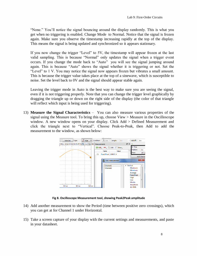
13) Measure the Signal Characteristics – You can also measure various properties of the

signal using the Measure tool. To bring this up, choose View > Measure in the Oscilloscope

window. A new window opens on your display. Click Add > Defined Measurement and

click the triangle next to “Vertical”. Choose Peak-to-Peak, then Add to add the

measurement to the window, as shown below:

Fig 8. Oscilloscope Measurement tool, showing Peak2Peak amplitude

14) Add another measurement to show the Period (time between positive zero crossings), which

you can get at for Channel 1 under Horizontal.

15) Take a screen capture of your display with the current settings and measurements, and paste

in your datasheet.

Lab 9: First-Order Circuits

9

We are now going to build a switched first-order capacitor circuit and measure its time constant.

Part 2: Measuring the Time Constant of a First Order Circuit

Parts List

10 uF Capacitor (1) Push-button switch (1) Resistors (1K, 100K (2) )

WARNING – the 10 uF Capacitor is an electrolytic capacitor, which requires insertion into the

circuit with the correct polarity. Placing an electrolytic capacitor in the circuit backwards could

cause the capacitor to “pop” and render it unusable.

16) Measure and record the resistance of your resistors in your datasheet.

17) Construct the circuit shown in Figure 8. Note the placement of the 6 pin header on the

breadboard, which is where we can attach the properly colored leads from the Analog

Discovery. Also note that for improved noise reduction, we are connecting a black (ground)

Analog Discovery wire to our breadboard as well.

Fig 9. Test circuit #1

What follows is a general description of how to measure the RC time constant of your circuit.

This is a very compliated task, so you are encouraged to watch the instruction provided in the

video playlist, which is linked from the datasheet.

18) On the Analog Discovery (AD) start the oscilloscope running, but DO NOT press AutoSet

Lab 9: First-Order Circuits

10

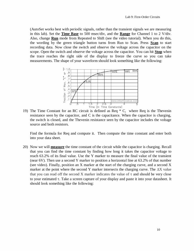
(AutoSet works best with periodic signals, rather than the transient signals we are measuring

in this lab). Set the Time Base to 500 msec/div, and the Range for Channel 1 to 2 V/div.

Also, change Run mode from Repeated to Shift (see the video tutorial). When you do this,

the wording by the green triangle button turns from Run to Scan. Press Scan to start

recording data. Now close the switch and observe the voltage across the capacitor on the

scope. Open the switch and observe the voltage across the capacitor. You can hit Stop when

the trace reaches the right side of the display to freeze the curve so you can take

measurements. The shape of your waveform should look something like the following:

19) The Time Constant for an RC circuit is defined as Req * C, where Req is the Thevenin

resistance seen by the capacitor, and C is the capacitance. When the capacitor is charging,

the switch is closed, and the Thevenin resistance seen by the capacitor includes the voltage

source and both resistors.

Find the formula for Req and compute it. Then compute the time constant and enter both

into your data sheet.

20) Now we will measure the time constant of the circuit while the capacitor is charging. Recall

that you can find the time constant by finding how long it takes the capacitor voltage to

reach 63.2% of its final value. Use the Y marker to measure the final value of the transient

(near 6V). Then use a second Y marker to position a horizontal line at 63.2% of that number

(see video). Finally, position an X marker at the start of the charging curve, and a second X

marker at the point where the second Y marker intersects the charging curve. The ΔX value

that you can read off the second X marker indicates the value of and should be very close

to your estimated . Take a screen capture of your display and paste it into your datasheet. It

should look something like the following:

Lab 9: First-Order Circuits

11

21) Add your scope measurements and theoretical calculations of the charging time constant to

Table 1 in your datasheet.

22) Now repeat to find the time constant while the capacitor is discharging. Note that this is a

“source-free” response, so the Req needs to be recalculated for your theoretical estimate. To

measure for the discharge curve, hold the switch down and wait for it to charge, then

release the switch and capture the capacitor voltage while the capacitor is discharging. Use

the markers to measure the time constant again, similar to the method of the previous step.

In this case, the time constant can determined by locating the time required for the capacitor

voltage to reach 36.8% of its initial value. Your display should looks something like the

following.

Insert a screen capture of your display of the discharge curve, including the markers

measuring the time constant, in your datasheet.

23) Repeat parts 18 through 22 for the following modified circuit.

Lab 9: First-Order Circuits

12

Part 3 - Creative Challenge (Optional – 10% extra credit)

The speaker we have in our kit can be modelled as an inductor (a coil) in series with an internal

resistance. We can measure the resistance of the speaker with an ohmmeter. But how can we

measure the inductance?

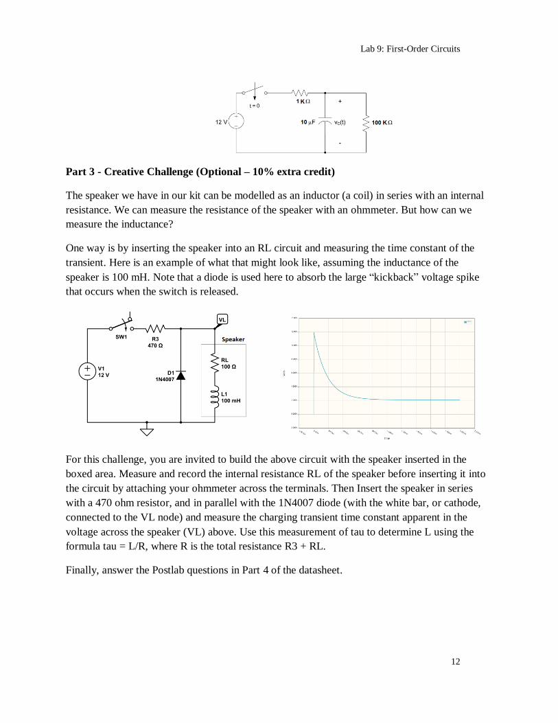
One way is by inserting the speaker into an RL circuit and measuring the time constant of the

transient. Here is an example of what that might look like, assuming the inductance of the

speaker is 100 mH. Note that a diode is used here to absorb the large “kickback” voltage spike

that occurs when the switch is released.

For this challenge, you are invited to build the above circuit with the speaker inserted in the

boxed area. Measure and record the internal resistance RL of the speaker before inserting it into

the circuit by attaching your ohmmeter across the terminals. Then Insert the speaker in series

with a 470 ohm resistor, and in parallel with the 1N4007 diode (with the white bar, or cathode,

connected to the VL node) and measure the charging transient time constant apparent in the

voltage across the speaker (VL) above. Use this measurement of tau to determine L using the

formula tau = L/R, where R is the total resistance R3 + RL.

Finally, answer the Postlab questions in Part 4 of the datasheet.