LAB 1 – The Scientific Method and Metric System Overview In this laboratory you will first watch a brief video on the importance of laboratory safety, organization and cleanliness. You will then focus on principles relating to the scientific method and the presentation of experimental data after which you will perform an experiment applying these principles. In the second part of this laboratory you will make a variety of measurements in metric units, and practice converting units within the metric system. Part 1: The Scientific Method The field of science is based on observation and measurement. If a scientist cannot observe and measure something that can be described and repeated by others, then it is not considered to be objective and scientific. In general, the scientific method is a process composed of several steps: 1. observation – a certain pattern or phenomenon of interest is observed which leads to a question such as “What could explain this observation?” 2. hypothesis – an educated guess is formulated to explain what might be happening 3. experiment – an experiment or study is carefully designed to test the hypothesis, and the resulting data are presented in an appropriate form 4. conclusion – the data is concluded to “support” or “not support” the hypothesis To illustrate the scientific method, let’s consider the following observation: A scientist observes that Compound X appears to increase plant growth, which leads to the question: “Does Compound X really increase plant growth?” Hypotheses The next step in applying the scientific method to a question such as the one above would be to formulate a hypothesis. For a hypothesis to be a good hypothesis it should be a statement of prediction that: a) uses objective, clearly defined terms b) can be tested experimentally

Welcome message from author
This document is posted to help you gain knowledge. Please leave a comment to let me know what you think about it! Share it to your friends and learn new things together.
Transcript

LAB 1 – The Scientific Method and Metric System
Overview
In this laboratory you will first watch a brief video on the importance of laboratory safety,
organization and cleanliness. You will then focus on principles relating to the scientific
method and the presentation of experimental data after which you will perform an experiment
applying these principles. In the second part of this laboratory you will make a variety of
measurements in metric units, and practice converting units within the metric system.
Part 1: The Scientific Method
The field of science is based on observation and measurement. If a scientist cannot observe
and measure something that can be described and repeated by others, then it is not considered
to be objective and scientific.
In general, the scientific method is a process composed of several steps:
1. observation – a certain pattern or phenomenon of interest is observed which leads
to a question such as “What could explain this observation?”
2. hypothesis – an educated guess is formulated to explain what might be happening
3. experiment – an experiment or study is carefully designed to test the hypothesis,
and the resulting data are presented in an appropriate form
4. conclusion – the data is concluded to “support” or “not support” the hypothesis
To illustrate the scientific method, let’s consider the following observation:
A scientist observes that Compound X appears to increase plant growth, which leads
to the question: “Does Compound X really increase plant growth?”
Hypotheses
The next step in applying the scientific method to a question such as the one above would be
to formulate a hypothesis. For a hypothesis to be a good hypothesis it should be a statement
of prediction that:
a) uses objective, clearly defined terms
b) can be tested experimentally

2
A reasonable hypothesis regarding the observation on the previous page would be:
Increasing amounts of compound X correlate with increased plant height.
In this case there is nothing vague or subjective in the terminology of the hypothesis, and it
can easily be tested experimentally, so it’s a good hypothesis. Keep in mind that a good
hypothesis is not necessarily correct. If a hypothesis is clear and testable and experimentation
disproves it, valuable information has been gained nonetheless. For example, if testing the
hypothesis “supplement Y is safe for human consumption”, it would be very valuable to
know if experimental data does not support this hypothesis.
Exercise 1A – Good vs bad hypotheses
Indicate whether or not you think each hypothesis listed on your worksheet is “good” or “bad”.
Experimentation
Experiments are designed to test hypotheses. A simple test of the hypothesis on the previous
page would be to plant the seeds of identical pea plants in pots containing the same type of
soil, being sure that each pot is exposed to the same temperature, pH, amount of sunlight,
water, etc, and measure their height after a 5 week period. The only difference between these
plants will be amounts of Compound X given to the plants each day, which are as follows:
Pea Plant Compound X per Day (grams)
1 0
2 1
3 3
4 5
5 7
6 9
In testing the effects of Compound X on pea plant growth, it is common sense that you should
devise an experiment in which multiple pea plants are grown under identical conditions
except for 1 difference or variable, the amount of Compound X given to each plant. In this
way any differences in plant height should be due to the only condition that varies among the
plants, the amount of Compound X.
When you design an experiment or a study such as this, it is important to consider all of its
components. Even though we design the experiment to contain only 1 variable component,
we need to consider all other components including the outcome of the experiment and any

3
control experiments that are done. Thus, when designing an experiment you need to account
for the following:
independent variable the treatment or condition that VARIES among the groups
dependent variable the MEASUREMENTS or outcomes recorded at the end of the experiment
standardized variables all other factors or conditions in the experiment that must be kept the same
(e.g., type of soil, amount of water, amount of sunlight) so their influence on
the dependent variable remains constant (i.e., we want to measure the effect of
the independent variable only)
experimental groups/treatments the subjects (e.g., plants) that receive the different treatments
control group/treatment the subjects that receive NO treatment, i.e., the independent variable is
eliminated (set to “zero”) or set to a background or default level
(NOTE: control treatments for independent variables such as temperature and
pH that cannot be eliminated are generally at a “background” level such as
room temperature or pH = 7)
Repetition is also important for an experimental result to be convincing. There needs to be a
sufficient number of subjects and repetitions of the experiment. For example, to make this
experiment more convincing multiple plants would be tested at each level of the independent
variable and it would be repeated multiple times.
Data Collection & Presentation
Upon completion of an experiment, the results need to be collected or measured, and
presented in an appropriate format. For our sample experiment, after 5 weeks the height of
the pea plants is measured and the following data are collected:
Pea Plant Compound X per Day (grams) Height of Plant (centimeters)
1 0 4.0
2 1 9.9
3 3 13.2
4 5 15.1
5 7 16.8
6 9 17.0

4
Now that you have the raw data for the experiment, it is important to present it in a form that
is easy to interpret. Frequently this will be in the form of a table, chart or graph. The data
above are presented in a table, however the overall results will be easier to interpret if
presented in a graph.
There are many ways to present data graphically, but the two most common types of graphs
are line graphs and bar graphs. When graphing data in this way, it is customary to place the
independent variable on the X-axis (horizontal) and the dependent variable on the Y-axis
(vertical). The independent variable in this experiment is the “amount of Compound X
added” and the dependent variable is the height of pea plants after 5 weeks. Below are the
Compound X data presented in a line graph on the left and a bar graph on the right:
Which type of graph is best for this data? It depends on the nature of the independent
variable on the X-axis. If the independent variable is continuous (i.e., there are values for the
independent variable that fall between those actually tested), then a line graph would be
appropriate. This would be the case if the independent variable covered a range of values for
time, temperature, distance, weight, or volume for example. In our example, the “grams of
Compound X” is clearly a continuous variable for which there are values in between those
tested, therefore a line graph is appropriate. By drawing a line or curve through the points,
you can clearly estimate what the “in between” values are likely to be, something you cannot
do as easily with a bar graph.
If the independent variable is discontinuous (i.e., there are no values between those tested),
then a bar graph would be appropriate. If you wanted to graph the average height of students
at each table in the lab (tables 1 through 6), the independent variable is the “specific table”.
Even though we label each table with a number, there are no “in between” values, there are
only tables 1, 2, 3, 4, 5 and 6, that’s it! So in this case a bar graph would be appropriate.
14
6
0
2
4
8
10
12
5 6 7 8 9 101 2 3 40
pla
nt
hei
gh
t (c
m)
grams of Compound X
added
16
18
14
6
0
2
4
8
10
12
5 7 91 3
pla
nt
hei
gh
t (c
m)
grams of Compound X
added
16
18
14
6
0
2
4
8
10
12
5 6 7 8 9 101 2 3 40
pla
nt
hei
gh
t (c
m)
grams of Compound X
added
16
18
14
6
0
2
4
8
10
12
5 6 7 8 9 101 2 3 40
pla
nt
hei
gh
t (c
m)
grams of Compound X
added
16
18
14
6
0
2
4
8
10
12
5 7 91 3
pla
nt
hei
gh
t (c
m)
grams of Compound X
added
16
18
14
6
0
2
4
8
10
12
5 7 91 3
pla
nt
hei
gh
t (c
m)
grams of Compound X
added
16
18

5
When you’re ready to create a graph, you need to determine the range of values for each axis
and to scale and label each axis properly. Notice that the range of values on the axes of these
graphs are just a little bit larger than the range of values for each variable. As a result there is
little wasted space and the graph is well spread out and easy to interpret. It is also essential
that the units (e.g., grams or centimeters) for each axis be clearly indicated, and that each
interval on the scale represents the same quantity. By scaling each axis regularly and evenly,
each value plotted on the graph will be accurately represented in relation to the other values.
Conclusions
Once the data from an experiment are collected and presented, a conclusion is made with
regard to the original hypothesis. Based on the graph on the previous page it is clear that all
of the plants that received Compound X grew taller than the control plant which received no
Compound X. In fact, there is a general trend that increasing amounts of Compound X cause
the pea plant to grow taller (except for plants 5 and 6 which are very close).
These data clearly support the hypothesis, but they by no means prove it. In reality, you can
never prove a hypothesis with absolute certainty, you can only accumulate experimental data
that support it. However if you consistently produce experimental data that do not support a
hypothesis, you should discard it and come up with a new hypothesis to test.
Exercise 1B – Effect of distance on making baskets
In this exercise, you will design an experiment to determine the effect of distance on the
accuracy of shooting paper balls into a beaker (and also determine which person in your
group is the best shot!). Each student will attempt to throw small paper balls into a large
beaker at 3 different distances in addition to the control (which should be 0 cm, i.e., a slam
dunk!). You will measure each distance using the metric system and determine how many
attempts are made out of 10 total attempts at each distance.
1. State your hypothesis and identify your independent and dependent variables.
2. Place the large beaker on your lab table at each test distance and record how many
attempts out of 10 you make.
3. Graph the data for each member of your group on a single graph (use different curves
for each person) and answer the corresponding questions on your worksheet.
4. Conclude whether or not the data support your hypothesis and answer any other
associated questions on your worksheet.
6
Part 2: The Metric System of Measurement
The English system of measurement is what we are all most familiar with (e.g., pounds,
inches, gallons), very few countries still use it to any significant degree (United States,
Myanmar and Liberia). Not even England still uses it! The problem is converting units
within the English system, which is rather awkward since there is no consistent pattern in the
relationship of one unit to another (12 inches per foot, 16 ounces per pound, four quarts per
gallon, etc…). Most countries in the world, including the entire scientific community, have
adopted a much easier system to work with called the Metric System of Measurement.
The advantage of the metric system of measurement is twofold: 1) there is a single, basic unit
for each type of measurement (meter, liter, gram, ºC) and 2) each basic unit can use prefixes
that are based on powers of 10 making conversions much easier. Once you learn the basic
units and the multiples of 10 associated with each prefix, you will have the entire system
mastered.
Basic Units of the Metric System
LENGTH - The basic unit of length in the metric system is the meter, abbreviated by
the single letter m. A meter was originally calculated to be one ten-millionth of the
distance from the north pole to the equator, and is ~3 inches longer than a yard.
VOLUME – The basic unit of volume in the metric system is the liter, abbreviated by
the single letter l or L. A liter is defined as the volume of a box that is 1/10 of a meter
on each side. A liter is just a little bit larger than a quart (1 liter = 1.057 quarts)
MASS – The basic unit of mass in the metric system is the gram, abbreviated by the
single letter g. A gram is defined as the mass of a volume of water that is 1/1000th
of a
liter. [Note: 1/1000th
of a liter = 1 milliliter = 1 cubic centimeter = 1 cm3 = 1 cc).
TEMPERATURE – The basic unit of temperature in the metric system is a degree
Celsius (ºC). Water freezes at 0 ºC and boils at 100 ºC.
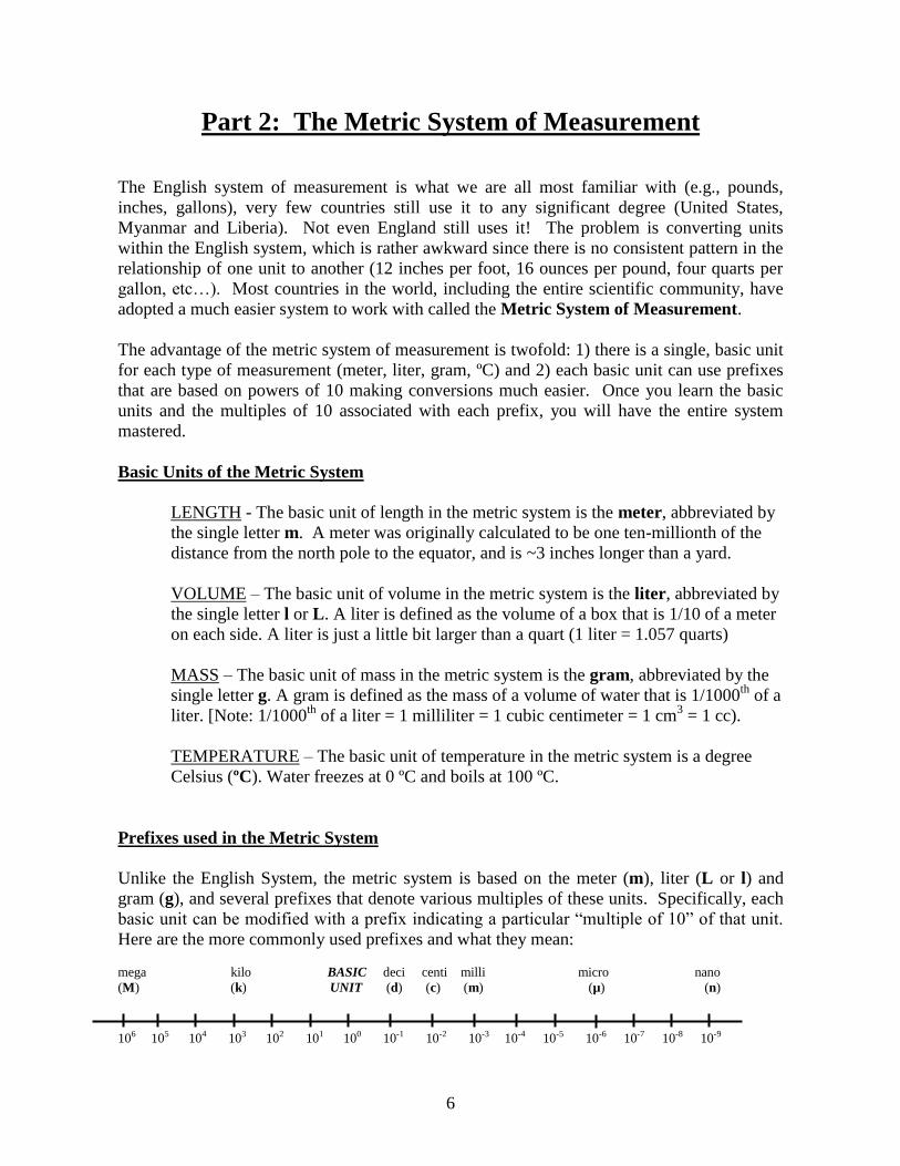
Prefixes used in the Metric System
Unlike the English System, the metric system is based on the meter (m), liter (L or l) and
gram (g), and several prefixes that denote various multiples of these units. Specifically, each
basic unit can be modified with a prefix indicating a particular “multiple of 10” of that unit.
Here are the more commonly used prefixes and what they mean:
mega kilo BASIC deci centi milli micro nano
(M) (k) UNIT (d) (c) (m) (µ) (n)
106 105 104 103 102 101 100 10-1 10-2 10-3 10-4 10-5 10-6 10-7 10-8 10-9

7
Mega (M) = 106 = 1,000,000
kilo (k) = 103 = 1,000
no prefix = 100 = 1
deci (d) = 10-1
= 1/10 (or 0.1)
centi (c) = 10-2
= 1/100 (or 0.01)
milli (m) = 10-3
= 1/1,000 (or 0.001)
micro (µ) = 10-6
= 1/1,000,000 (or 0.000001)
nano (n) = 10-9
= 1/1,000,000,000 (or 0.000000001)
Here is how simple the metric system is using the basic units and the prefixes:
What is one thousandth of a meter? a millimeter (mm)
What is one one-millionth of a liter? a microliter (l)
What is 1,000 grams? a kilogram (kg)
Let us now examine these units more closely by using them to make actual measurements and
converting from one metric unit to another.
Exercise 2A – Measuring distance
1. Obtain a wooden meter stick. If you look on the back of the meter stick, one meter is
approximately 39 inches or about 3 inches longer than one yard (36 inches). Using the meter stick,
estimate the size of the laboratory by measuring its width and length to the nearest meter.
2. Observe that the meter is divided into 100 equal units called centimeters. A centimeter is about the
width of a small finger. Using the meter stick, estimate the dimensions of a regular piece of notebook
paper to the nearest centimeter.
3. How tall are you? Go over to the medical weight and height scale to measure how tall you are to
the nearest centimeter.
4. Next, obtain a small plastic metric rule. Observe that each centimeter is divided into 10 small units
called millimeters. A millimeter is about the thickness of a fingernail. Using the small plastic ruler,
estimate the diameter of a hole on a regular piece of notebook paper to the nearest millimeter.
What are some other real-world examples of metric units of length?
One micrometer (µm) is 1/1,000th
the size of a millimeter or 1/1,000,000th
of a meter. When
you observe a cheek cell under the microscope in a future lab, it is about 40 µm in diameter.
Typical bacteria are about 5-10 µm in diameter.
One nanometer (nm) is 1/1,000th
the size of a micrometer or 1/1,000,000,000th
of a meter.
Objects this small are far too tiny to observe even in a light microscope. If you line up five
water molecules side-by-side, the length would be about 1 nanometer.

8
Exercise 2B – Measuring volume
1. Obtain a one liter (L or l) beaker. One liter is equal to 1,000 cubic centimeters (cc = cm
3 =
milliliter = ml). Fill the beaker with one liter of water. To do this, add water until the meniscus (top
level of the water) reaches the 1 liter marker on the beaker. Pour the water into a 2 liter soda bottle.
Once again, fill the beaker with one liter of water by adding water until the meniscus reaches the 1
liter mark. Pour the water into the 2 liter soda bottle.
Once again, fill the beaker with one liter of water by adding water until the meniscus reaches the 1
liter mark. Over the sink, add the 1 liter of water to the 1 quart container provided. Notice that 1 liter
is just a little bit more than 1 quart. In fact, 1 liter = 1.057 quarts.
2. One way to measure the volume of a fluid in a laboratory is to use a graduated cylinder. Whereas
beakers are generally used to hold fluids, graduated cylinders are used to accurately measure volumes.
Obtain a 50 milliliter (ml) graduated cylinder. Fill the graduated cylinder with water until the
meniscus reaches the 50 ml mark. Add the water to a 1 liter (1,000 ml) beaker. Notice that 50 ml is
equal to 1/20th of a liter. Next, measure the fluid in the flask labeled “A” to the nearest 0.1 ml.
3. Pipettes are used to measure smaller liquid volumes whereas graduated cylinders are used to
measure larger volumes. Obtain a 10 ml glass pipette and attach it snugly to a pipette pump.
Notice whether or not the pipette is a delivery or blowout pipette. Blowout pipettes are designed for
measuring fluids all the way to the end of the pipette so that the liquid measured can be completely
“blown out” of the pipette. Delivery pipettes have a gap at the end of the pipette and are designed to
“deliver” the liquid down to the desired marking only. The remainder is discarded or returned to the
original container. (NOTE: blowing out a delivery pipette will give a wrong volume)
Using the roller on the pipette pump, gradually suck up some water until the meniscus reaches the 0
ml mark. Measure 10 ml of the water into the sink by rolling the roller in the opposite direction. Next,
measure the amount of fluid in the test tube labeled B to the nearest 0.1 ml using the 10 ml pipette.

9
Exercise 2C – Measuring mass
A balance scale is used to measure the mass of a sample in grams (g).
1. Place an empty 50 ml graduated cylinder on the balance and determine its mass in grams.
2. Next, fill the graduated cylinder with 50 ml of water and measure the mass of both the cylinder
and the water. From this value subtract the mass of the cylinder to get the mass of the water.
By definition, one gram is the mass of exactly 1.0 ml of water, thus 50 ml of water has a mass of 50.0
grams. How far off was your measured mass from the true mass of 50 ml of water?
3. Next, take a large paper clip and place it on the balance and determine its mass in grams.
Exercise 2D – Measuring temperature
The metric unit for temperature is ºCelsius (ºC). Water freezes at 0 ºC and boils at 100 ºC. Note that
this is much easier to remember than the corresponding values of 32 ºF and 212 ºF.
1. Use a thermometer to measure the following in degrees Celsius:
A) the ambient temperature of the lab B) a bucket of ice water C) a beaker of boiling water
2. Convert the temperatures on your worksheet from ºC to ºF or ºF to ºC with the following formulas:
ºC = 5/9 x (ºF - 32)
ºF = (9/5 x ºC) + 32

10
Converting Units within the Metric System
Once you are familiar with the units and prefixes in the metric system, converting from one
unit to another requires two simple steps:
1) divide the value associated with the prefix of the original unit by the prefix of the
unit you are converting to
2) multiply this value by the number in front of the original unit
To illustrate this let’s look at an example:
2.4 kg = _____ mg
In this case you’re converting from kilograms to milligrams. Since the prefix kilo- refers to
1000 and the prefix milli- refers to 1/1000 or 0.001 (see page 7), divide 1000 by 0.001. This
gives a value of 1,000,000 which is multiplied by 2.4 to get the mass in milligrams:
2.4 kg = 2.4 x 1,000,000 mg = 2,400,000 mg
You may find it simpler to associate each metric prefix with an exponential number. With
this approach kilo- refers to 103 and milli- refers to 10
-3, so 10
3/10
-3 equals 10
6 (when
dividing exponential numbers simply subtract the first exponent minus the second), and thus:
2.4 kg = 2.4 x 10⁶ mg = 2,400,000 mg
Whether or not you represent your answer as an exponential number is up to you, either way
the values are the same. To ensure that you’ve done the problem correctly, remember that
any given distance, mass or volume should contain more of a smaller unit and less of a
larger unit. This is simply common sense if you think about it. As you can see in the
example above, there are a lot more of the smaller milligrams than there are the larger
kilograms, even though both represent the exact same mass. So each time you do a metric
conversion look at your answer to be sure that you have more of the smaller unit and less of
the larger unit.
One more thing to remember is that a basic unit without a prefix (m, g or l) is one or 100 of
that unit. Here are a couple more examples just to be sure everything is clear:
643 m = _____ km 1 divided by 1000 (kilo-) = 0.001 x 643 = 0.643 km
50 ml = _____ l 10-3
(milli-) divided by 100 = 10
-3 x 50 = 5.0 x 10
-2 l
Exercise 2E – Metric Conversions
Complete the metric conversions on your worksheet.

LABORATORY 1 WORKSHEET Name ________________________
Section_______________________
Exercise 1A – Good vs bad hypotheses
Circle good or bad for each hypothesis, and underline any terms that make a hypothesis bad:
1. Students who own laptops have higher GPAs. Good or Bad
2. Murders occur more often during a full moon. Good or Bad
3. Cats are happier when you pet them. Good or Bad
4. Orangutans are smarter than gorillas. Good or Bad
5. Sea level will be higher in 100 years than it is today. Good or Bad
Exercise 1B – Paper basketball experiment
State your hypothesis:
In the table below, record the number of shots made at each distance (out of 10) for each person:
Name 0 cm ____ cm ____ cm ____ cm
Graph the data for each member of your group below (use a different curve for each person):

What is your control in this experiment?
What is the independent variable?
What is the dependent variable?
State your conclusion addressing whether or not the data support your original hypothesis:
Exercise 2A – Measurement of distance
Laboratory width: _________ m Laboratory length: _________ m
Calculate approximate area: width _____ m x length _____ m = _________ m2
Paper width: _______ cm Paper length: _______ cm
Calculate approximate area: width _____ cm x length _____ cm = _________ cm2
Paper hole diameter: ________ mm
Your height: _______ cm, which is equal to _______ m
Indicate which metric unit of length you would use to measure the following:
length of a fork __________ width of a plant cell __________
size of a small pea __________ length of your car __________
height of a refrigerator __________ distance to the beach __________
diameter of an apple __________ size of a dust particle __________
Exercise 2B – Measurement of volume
Volume of fluid in Beaker A = ____________ ml
Volume of fluid in Test Tube B = ____________ ml

Exercise 2C – Measurement of mass
Mass of Graduated Cylinder = _____________ g
Mass of Graduated Cylinder with 50 ml of water = _____________ g
Mass of 50 ml of water: ________________ g
Difference between calculated and actual mass of 50 ml of water: ______________
Mass of 1 ml of water based on your measurements: _________ g/50 ml = _________ g/ml
Mass of Large Paper Clip = ____________ g
Exercise 2D – Measurement of temperature
Ambient temperature in lab ______ºC ice water ______ºC boiling water ______ ºC
Convert the following temperatures using the formulas on page 10 of the lab exercises:
Mild temperature: 72 ºF = ________ ºC Body temperature 98.6 ºF = ________ ºC
Cold day 10 ºC = ________ ºF Very hot day 34 ºC = ________ ºF
Exercise 2E – Metric conversions
Convert the following measurements to the indicated unit:
335.9 g = _________________ kg __________________ m = 0.0886 km
0.00939 μl = __________________ ml __________________ kg = 89 mg
456.82 ng = _________________ μg __________________dl = 900.5 cl
20 megabytes = __________ kilobytes __________________ μm = 0.37 mm
8 megabase pairs (mbp) = __________ kbp __________________ mm = 11.5 nm
95 ºC = _____________ ºF __________________ ºC = 100 ºF
Related Documents