Lab-01

[Spring 2012] [INTRODUCTION TO MATLAB] Signals and Systems

1 | Ali Waqar Azim

Lab 01-Introduction to MATLAB and Basic Commands Once MATLAB® is installed; it is time to start using it. MATLAB is best understood by entering the instructions in your computer one at a time and by observing and studying the responses. Learning by doing is probably the most effective way to maximize retention. ______________________________________________________________________________________________ I hear and I forget I see and I remember I do and I understand

Confucius ______________________________________________________________________________________________

1.1 MATLAB MATLAB (short for MATrix LABoratory) is a platform (program) organized for optimized engineering programming and scientific calculations. The MATLAB program implements the MATLAB programming language and provides an extensive library of predefined functions and make technical programming tasks easier and more efficient. MATLAB has incredibly large variety of functions and toolkits with more functions and various specialties. 1.1.1 The Advantage of MATLAB

Some of the advantages of MATLAB are: 1. Ease of Use. 2. Platform Independence. 3. Predefined Functions 4. Device independent plotting. 5. Graphical User Interface.

1.1.2 The disadvantages of MATLAB

The only disadvantage of MATLAB is that it is an interpreted language rather than complied language. Because of the same reason the it executes more slowly than compiled languages such as C, C++.

1.2 Getting Started with MATLAB Open MATLAB through the start menu or from the desktop icon. The interface will be like this

Fig.1. MATLAB Interface

Current Directory: Shows the current folder of MATLAB. Workspace: Shows the size of variables which are initiated on the command window. Command History: Shows the history of commands used previously on command window. Command Window: Command are written in command windows.


2 | Ali Waqar Azim

1.3 Working with Variables The fundamental unit of data in MATLAB is array. A common programming mistake is to use a variable without declaring it first. This is not a problem in MATLAB. In fact, MATLAB is very flexible about variables and data types. MATLAB variable is automatically created when they are initialized. There are three common ways to initialize a variable in MATLAB:

1. Assign data to the variable in the assignment statement. 2. Input data into the variable from the keyboard. 3. Read data from a file.

The first way will be defined here and the remaining two approached will be discussed in later labs if time permits.

1.3.1 Initializing variables in Assignments Statements:

The simplest way to create a variable is to assign it one or more values in an assignment statement. An assignment statement has the general form.

var = expression where var is the name of the variable, and the expression is a scalar constant, an array, or combination of constants, vectors or matrix.

1.3.2 Variable Initialization:

If an undefined variable is assigned a value, for example: a = 1;

MATLAB will assume that the variable a should be created, and that the value 1 should be stored in it. If the variable already exists, then it will have the number 1 replace its previous value. This works with scalars, vectors, and matrices. The numbers stored in variables can be integers (e.g., 3), floating-points (e.g., 3.1), or even complex (e.g., 3.1+5.2j). a = 3; b = 3.1; c = 3.1+5.2j;

1.3.3 Semicolon Operator:

A semicolon “;" is often put at the end of a command. This has the effect of suppressing the output of the resulting values. Leaving of the semicolon does not affect the program, just what is printed to the screen, though printing to the screen can make a program run slowly. If a variable name is typed on a line by itself, then the value(s) stored for that variable will be printed. This also works inside a function or a program. A variable on a line by itself (without a semicolon) will be displayed. >> a a = 3 >> b b = 3.1000 >> c c = 3.1000 + 5.2000i


3 | Ali Waqar Azim

1.3.4 Complex Variable:

MATLAB shows the complex value stored in c with i representing the complex part (the square root of -1). In the above example of complex number j is used for indicating the square root of -1, instead of j, i can also be used to indicate the square root of -1.

1.4 MATLAB Programming Basics This section covers the main things that you need to know to work with MATLAB.

1.4.1 How to clear command screen:

The command clc clears the command window, and is similar to the clear command in the Unix or Dos environments.

1.4.2 How to get rid of variables:

The command clear, by the way, tells MATLAB to get rid of all variables, or can be used to get rid of a specific variable, such as clear a.

1.4.3 Information about variables:

To see a list of the variables in memory, type who. The similar command whos gives the same list, but with more information.

>> who Your variables are: a b c >> whos Name Size Bytes Class Attributes a 1x1 8 double b 1x1 8 double c 1x1 16 double complex >> clear >> who >> whos

In the example above, we see that the variable a, b and c are defined, and the difference between who and whos. After the clear statement, the who and whos command returns nothing since we got rid of the variables.


4 | Ali Waqar Azim

1.5 Scalars, Vectors, and Matrices 1.5.1 Scalar Declaration:

A variable can be given a “normal" (scalar) value, such as b=3 or b=3.1, but it is also easy to give a variable several values at once, making it a vector, or even a matrix.

1.5.2 Vector Declaration:

For example, c=[1 2] stores both numbers in variable c.

1.5.3 Matrix Declaration:

To make a matrix, use a semicolon (“;") to separate the rows, such as:

d=[1 2; 3 4; 5 6]

This makes d a matrix of 3 rows and 2 columns. Please note that

d(row specifier, column specifier)

is the correct version of to access the element at specified row and specific column.

>> d=[1 2; 3 4; 5 6] d =

1 2 3 4 5 6

1.5.3.1 How to add a row in matrix:

What if you want to add another row onto d? This is easy, just give it a value: d(4,:)=[7 8]. Notice the colon “:” in the place of the column specifier. This is intentional; it is a little trick to specify the whole range. We could have used the command d(4,1:2)=[7 8] to say the same thing, but the first version is easier (and less typing).

>> d(4,:)=[7 8] d =

1 2 3 4 5 6 7 8

1.5.3.2 How to delete a Column from a matrix: You can delete rows and columns from a matrix using just a pair of square brackets. Start with

>> A = [16 3 2 13; 5 10 11 8; 9 6 7 12;4 15 14 1]

>> X = A;

Then, to delete the second column of X, use


5 | Ali Waqar Azim

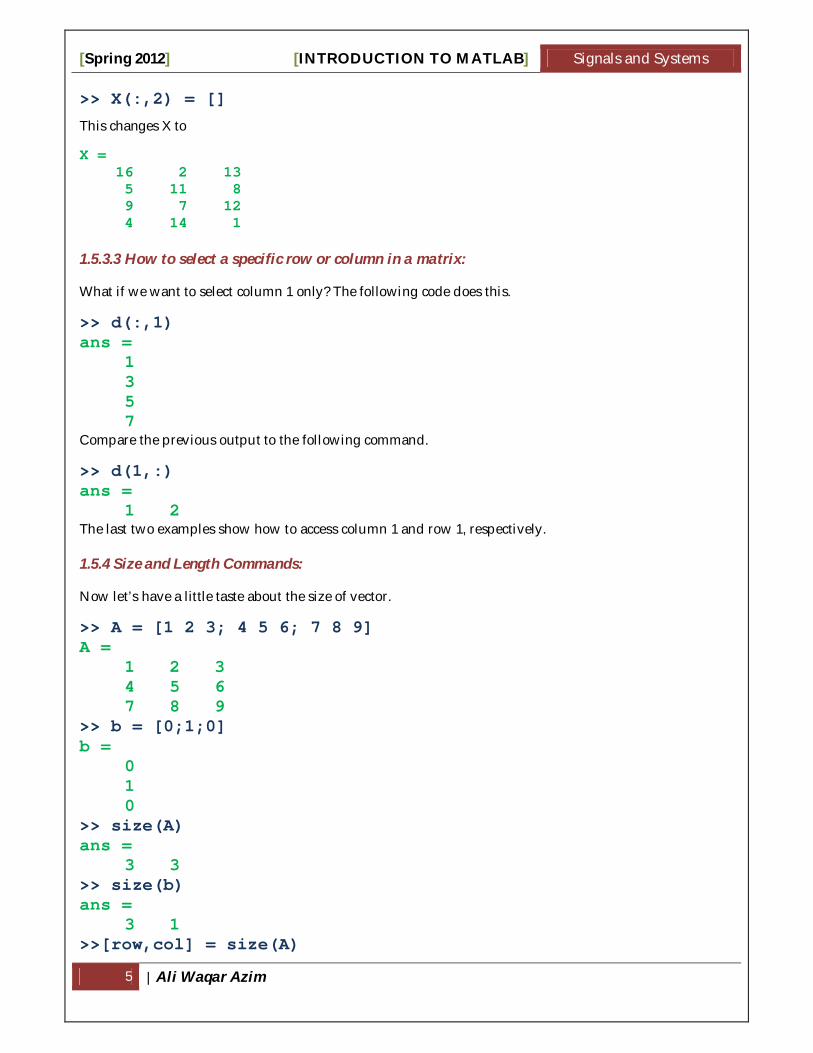
>> X(:,2) = []

This changes X to

X = 16 2 13 5 11 8 9 7 12 4 14 1 1.5.3.3 How to select a specific row or column in a matrix:

What if we want to select column 1 only? The following code does this.

>> d(:,1) ans =

1 3 5 7

Compare the previous output to the following command.

>> d(1,:) ans =

1 2 The last two examples show how to access column 1 and row 1, respectively. 1.5.4 Size and Length Commands:

Now let’s have a little taste about the size of vector.

>> A = [1 2 3; 4 5 6; 7 8 9] A =

1 2 3 4 5 6 7 8 9

>> b = [0;1;0] b =

0 1 0

>> size(A) ans =

3 3 >> size(b) ans =

3 1 >>[row,col] = size(A)


6 | Ali Waqar Azim

row = 3

col = 2

>>[row,column]=size(b) row = 3 column = 1 >>length (A) ans =

3 >>length (b) ans =

3

The command length(A) returns the number of elements of A, if A is a vector, or the largest value of either n or m, if it is an n × m matrix. The MATLAB command size(A) returns the size of the matrix A (number of rows by the number of column), and the command [row, col] = size(A) returns the number of rows assigned to the variable row and the number of columns of A assigned to the variable col.

1.5.5 Concatenation:

Arrays can be built out of other arrays, as long as the sizes are compatible:

>> [A b] ans =

1 2 3 0 4 5 6 1 7 8 9 0

>> [A;b] ??? Error using ==> vertcat CAT arguments dimensions are not consistent. >> B = [[1 2;3 4] [5;6]] B =

1 2 5 3 4 6


7 | Ali Waqar Azim

1.6 Number Ranges A variable can hold a range of numbers. For example, imagine that variable N should hold all numbers 1, 2, 3, 4, etc., up to the number 100. Here is one way to create N: for index=1:100 N(index)=index; end

1.6.1 The Colon Operator:

This does the job, but there is a faster and simpler way to say the same thing. Below, we set N equal to a range, specified with a colon “:” symbol between the starting and ending values.

N=Start: Increment/Decrement: End N=1:100; If a third number is specified, then the second one will be used as the increment. For example, M=0:0.4:2 would assign the sequence {0, 0.4, 0.8, 1.2, 1.6, 2} to variable M. The following example shows all numbers between 8 and 20, with an increment of 2.

>> 8:2:20 ans =

8 10 12 14 16 18 20

1.6.2 The linspace Command:

The linspace command do more or less the same thing as done by colon operator. This command provides the user with more flexibility in such a way that we can get the exact number of elements in a row vector we want.

>> linspace(1,2,9)


8 | Ali Waqar Azim

In the above statement, a row vector would be formed such that it contains 9 entries equally spaced between 1 and 2. Now, in certain case if number of entries of the vector is not defined, the command will automatically generate a row vector which will contain 100 entries equally spaced between 1 and 2.

>> linspace(1,2)

1.7 Referencing Elements It is frequently necessary to access one or more of the elements of a matrix. Each dimension is given a single index or vector of indices. The result is a block extracted from the matrix. The colon is often a useful way to construct array indices. Here are some examples, consider the following matrix

>> A = [1 2 3; 4 5 6; 7 8 9] A =

1 2 3 4 5 6 7 8 9

>> b = [0;1;0] b =

0 1 0

>> A(2,3) % single element ans =

6 >> b(2) % one index for a vector ans =

1 >> b([1 3]) % multiple elements ans =

0 0

>> A(1:2,2:3) % a submatrix ans =

2 3 5 6

>> A(1:end-1,end) % all but last row, last column ans =

3 6

>> b(:,[1 1 1 1]) % multiple copies of a column ans =

0 0 0 0 1 1 1 1 0 0 0 0


9 | Ali Waqar Azim

1.8 Arithmetic Operations 1.8.1 Scalar Mathematics:

Scalar mathematics involves operations on single-valued variables. MATLAB provides support for scalar mathematics similar to that provided by a calculator. 1.8.1.1 Numbers:

MATLAB represents numbers in two form, fixed point and floating point. Fixed point: Decimal form, with an optional decimal point. For example:2.6349, -381, 0.00023

Floating point: Scientific notation, representing m × 10e. For example: 2.6349 × 105 is represented as 2.6349e5. It is called floating point because the decimal point is allowed to move. The number has two parts: • mantissa m: fixed point number (signed or unsigned), with an optional decimal point (2.6349 in the example above) • exponent e: an integer exponent (signed or unsigned) (5 in the example). • Mantissa and exponent must be separated by the letter e (or E). Scientific notation is used when the numbers are very small or very large. For example, it is easier to represent 0.000000001 as 1e-9. 1.8.1.2 Operators

The evaluation of expressions is achieved with arithmetic operators, shown in the table below.

Table 1: Mathematical Operators in MATLAB Operation Algebraic Form MATLAB Expression Addition a+b a+b 5+3

Multiplication axb a*b 23-12 Subtraction a-b a-b 3.14*0.85

Right Division a/b a/b 56/8 Left Division b/a a\b 8/56

Exponentiation ab a^b 2^3

Operators operate on operands (a and b in the table).

Examples of expressions constructed from numbers and operators, processed by MATLAB:

>> 3 + 4 ans =

7 >> 3 - 3 ans =

0


10 | Ali Waqar Azim

>> 4/5 ans =

0.8000

Operations may be chained together. For example:

>> 3 + 5 + 2 ans =

10 >> 4*22 + 6*48 + 2*82 ans =

540 >> 4 * 4 * 4 ans =

64

Instead of repeating the multiplication, the MATLAB exponentiation or power operator can be used to write the last expression above as

>> 4^3 ans =

64

Left division may seem strange: divide the right operand by the left operand. For scalar operands the expressions 56/8 and 8\56 produce the same numerical result.

>> 56/8 ans =

7 >> 8\56 ans =

7

1.8.1.3 Syntax:

MATLAB cannot make sense out of just any command; commands must be written using the correct syntax (rules for forming commands). Compare the interaction above with

>> 4 + 6 + ??? 4 + 6 + | Missing operator, comma, or semi-colon.

Here, MATLAB is indicating that we have made a syntax error, which is comparable to a misspelled word or a grammatical mistake in English. Instead of answering our question, MATLAB tells us that we’ve made a mistake and tries its best to tell us what the error is.


11 | Ali Waqar Azim

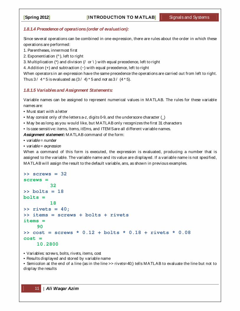
1.8.1.4 Precedence of operations (order of evaluation):

Since several operations can be combined in one expression, there are rules about the order in which these operations are performed: 1. Parentheses, innermost first 2. Exponentiation (^), left to right 3. Multiplication (*) and division (/ or \) with equal precedence, left to right 4. Addition (+) and subtraction (−) with equal precedence, left to right When operators in an expression have the same precedence the operations are carried out from left to right. Thus 3 / 4 * 5 is evaluated as (3 / 4) * 5 and not as 3 / (4 * 5). 1.8.1.5 Variables and Assignment Statements:

Variable names can be assigned to represent numerical values in MATLAB. The rules for these variable names are: • Must start with a letter • May consist only of the letters a-z, digits 0-9, and the underscore character (_) • May be as long as you would like, but MATLAB only recognizes the first 31 characters • Is case sensitive: items, Items, itEms, and ITEMS are all different variable names. Assignment statement: MATLAB command of the form: • variable = number • variable = expression When a command of this form is executed, the expression is evaluated, producing a number that is assigned to the variable. The variable name and its value are displayed. If a variable name is not specified, MATLAB will assign the result to the default variable, ans, as shown in previous examples.

>> screws = 32 screws =

32 >> bolts = 18 bolts =

18 >> rivets = 40; >> items = screws + bolts + rivets items =

90 >> cost = screws * 0.12 + bolts * 0.18 + rivets * 0.08 cost =

10.2800

• Variables: screws, bolts, rivets, items, cost • Results displayed and stored by variable name • Semicolon at the end of a line (as in the line >> rivets=40;) tells MATLAB to evaluate the line but not to display the results


12 | Ali Waqar Azim

1.8.2 Vector and Matrix Arithmetic:

First thing to learn in arithmetic operations is to learn how to do element wise operations. For element wise operation you will have to use .,.*, ./, .^. In order to use these operators the dimensions of both the vectors should be same.

>> a=[1 2 3];b=[4;2;1]; >> a.*b, a./b, a.^b -> all errors

>> a.*b', a./b’, a.^(b’) all valid

Here are some examples of common arithmetic operations in MATLAB. First, we will define some variables to work with.

>> A = [20 1 9 16] A =

20 1 9 16 >> A2 = [20, 1, 9, 16] % Commas can separate entries A2 =

20 1 9 16 As we see above, adding commas after each element also works, and is a bit clearer. >> B = [5 4 3 2] B =

5 4 3 2 >> C = [0 1 2 3; 4 5 6 7; 8 9 10 11] C =

0 1 2 3


13 | Ali Waqar Azim

4 5 6 7 8 9 10 11

>> D = [8; 12; 0; 6] % Semicolons separate rows D =

8 12 0 6

>> F = [31 30 29 28; 27 26 25 24; 23 22 21 20] F =

31 30 29 28 27 26 25 24 23 22 21 20

Semicolons can be used to separate rows of a matrix, as seen above, where all of the operations are assignment statements. Most of the examples below are not assignment statements; that is, the results are just printed to the screen and do not affect the above matrices. A variable followed by a period then the single-quote character indicates the transpose of that variable. The notation: A.’ simply represents the transpose of the array A. We can obtain the same effect by using transpose(A) instead. The example below shows the transpose of A, that is, views it as a 4 by 1 matrix instead of a 1 by 4 matrix. We can verify this with the size function. On a matrix like C, the result is to swap the rows with the columns. Similarly, we see that C is a 3 by 4 matrix, while the transpose of C is 4 by 3.

>> A.’ % transpose A ans =

20 1 9 16

>> size(A.’) ans =

4 1 >> size(A) ans =

1 4 >> C.’ % transpose C ans =

0 4 8 1 5 9 2 6 10 3 7 11

>> size(C.’) ans =

4 3


14 | Ali Waqar Azim

>> size(C) ans =

3 4 Addition and subtraction can be carried out as expected. Below, we see that a constant can be added to every element of a matrix, e.g., A+7. We can add every element of two matrices together, as in A+B. Subtraction is easily done with A-B and B-A.

>> A+7 ans =

27 8 16 23 >> A+B % Note that A and B must be the same size. ans =

25 5 12 18 >> A-B ans =

15 -3 6 14 >> B-A ans =

-15 3 -6 -14

To find the summation of an array, use the sum function. It also works with two dimensional matrices, though it will add all of the numbers along the columns and return an array. Notice below that there are two ways of expressing the same thing. The command sum(A+B) says to add matrix A to matrix B, then find the sum of the result. The second way to do this, sum(A)+sum(B) says to find the sum of A and the sum of B, then add the two sums together. As in any programming language, there are often multiple ways to do the same thing. This becomes important when performance is poor; it may be possible to restate the operations in a more efficient way.

>> sum(A) ans =

46 >> sum(B) ans =

14 >> % Add A to B, then find their sum >> sum(A+B) ans =

60 >> % find sum of A and sum of B, then add >> sum(A) + sum(B) ans =

60 The next examples are of multiplication operations. Multiplication can be a bit tricky, since there are several similar operations. First, let us start by trying to multiply A with B.


15 | Ali Waqar Azim

>> A*B ??? Error using ==> * Inner matrix dimensions must agree.

We cannot multiply a 4X1 matrix with a 4 x1 matrix! If we want to multiply two matrices together, we must make sure that the first matrix has as many columns as the second matrix has rows. In this case, we must transpose either A or B in order to multiply it by the other. Note that when we multiply A by the transpose of B, we are multiplying the nth elements together, and adding the results.

>> A.’*B % Multiply transpose(A) by B ans =

100 80 60 40 5 4 3 2 45 36 27 18 80 64 48 32

>> A*B.’ % Multiply A by transpose(B). ans =

163 >> A(1)*B(1) + A(2)*B(2) + A(3)*B(3) + A(4)*B(4) ans =

163

What if we want to multiply the nth elements together, but not add the results? This can be accomplished by putting a period before the multiplication sign, to say that we want to multiply the individual elements together. Notice that now we do not have to transpose either array.

>> A.*B % ans = [A(1)*B(1) A(2)*B(2) A(3)*B(3) A(4)*B(4)] ans =

100 4 27 32

We can multiply an array by a scalar value, as seen below. Also, we can take the results of such an operation and add them together with the sum function.

>> A*4 % multiply all values of A by 4 ans =

80 4 36 64 >> sum(A*4) ans =

184 When it comes to multiplying matrices with arrays, the results are as one would expect from linear algebra.

>> [1 2 3]*C % Multiply row vector [1 2 3] by C % result(1) = 0*1 + 4*2 + 8*3 % result(2) = 1*1 + 5*2 + 9*3 % result(3) = 2*1 + 6*2 + 10*3 % result(4) = 3*1 + 7*2 + 11*3


16 | Ali Waqar Azim

% Results are all in 1 row. ans =

32 38 44 50 >> C*[1 2 3 4] % Multiply C by [1 2 3 4] as a column vector % result(1) = 0*1 + 1*2 + 2*3 + 3*4 % result(2) = 4*1 + 5*2 + 6*3 + 7*4 % result(3) = 8*1 + 9*2 + 10*3 + 11*4 % Results are all in 1 column. ans =

20 60 100

There are several different ways to multiply F and C. Trying F*C does not work, because the dimensions are not correct. If F or C is transposed, then there is no problem. The numbers from these two matrices are shown multiplied and added in the variable result, showing that the multiplication result is what we should expect. We use the three dots (ellipsis) after result below to continue on the next line; this makes the lines fit.

>> F.’*C % transpose(F) * C ans =

292 373 454 535 280 358 436 514 268 343 418 493 256 328 400 472

>> result = ... [31*0+27*4+23*8, 31*1+27*5+23*9, 31*2+27*6+23*10, 31*3+27*7+23*11; 30*0+26*4+22*8, 30*1+26*5+22*9, 30*2+26*6+22*10, 30*3+26*7+22*11; 29*0+25*4+21*8, 29*1+25*5+21*9, 29*2+25*6+21*10, 29*3+25*7+21*11; 28*0+24*4+20*8, 28*1+24*5+20*9, 28*2+24*6+20*10, 28*3+24*7+20*11] result =

292 373 454 535 280 358 436 514 268 343 418 493 256 328 400 472

>> F*C.’ ans =

172 644 1116 148 556 964 124 468 812

>> result = ... [31*0+30*1+29*2+28*3, 31*4+30*5+29*6+28*7, 31*8+30*9+29*10+28*11; 27*0+26*1+25*2+24*3, 27*4+26*5+25*6+24*7, 27*8+26*9+25*10+24*11; 23*0+22*1+21*2+20*3, 23*4+22*5+21*6+20*7, 23*8+22*9+21*10+20*11]


17 | Ali Waqar Azim

result = 172 644 1116 148 556 964 124 468 812

We can change the order of the matrices, and find that we get the same results as above, except transposed. An easy way to verify this is to subtract one (transposed) result from the other, to see that all subtraction results are zero.

>> C.’*F % gives same answer as F.’*C, except transposed. ans =

292 280 268 256 373 358 343 328 454 436 418 400 535 514 493 472

>> (F.’*C).’- C.’*F ans =

0 0 0 0 0 0 0 0 0 0 0 0 0 0 0 0

>> C*F.’ % gives same answer as F*C.’, except transposed. ans =

172 148 124 644 556 468 1116 964 812

>> (F*C.’).’- C*F.’ ans =

0 0 0 0 0 0 0 0 0

Suppose we want to multiply every element of C with the corresponding element of F. We can do this with the .* operator, as we did before. Incidentally, reversing the order of operands produces the same result.

>> C.*F ans =

0 30 58 84 108 130 150 168 184 198 210 220

>> result = [0*31, 1*30, 2*29, 3*28; 4*27, 5*26, 6*25, 7*24; 8*23, 9*22, 10*21, 11*20] result =

0 30 58 84


18 | Ali Waqar Azim

108 130 150 168 184 198 210 220

Like multiplication, division has a couple of different interpretations, depending on whether ./ or / is specified. For example, A./B specifies that elements of A should be divided by corresponding elements of B.

>> A = [20 1 9 16]; >> B = [5 4 3 2]; >> A./B ans =

4.0000 0.2500 3.0000 8.0000 >> result = [ 20/5, 1/4, 9/3, 16/2 ] result =

4.0000 0.2500 3.0000 8.0000

We can specify that elements of B should be divided by corresponding elements of A, in two different ways: using the backslash A.\B or the forward slash A./B. Referring to the values of result from above, we can divide the value 1 by each element. Also shown below is that we can divide each element of matrix C by the value 5.

>> A.\B ans =

0.2500 4.0000 0.3333 0.1250 >> B./A ans =

0.2500 4.0000 0.3333 0.1250 >> 1./result ans =

0.2500 4.0000 0.3333 0.1250 >> C/5 ans =

0 0.2000 0.4000 0.6000 0.8000 1.0000 1.2000 1.4000 1.6000 1.8000 2.0000 2.2000

Next, we divide the elements of matrix C by the corresponding elements of F. The very first result is 0. If we switched the two matrices, i.e., using F's elements for nominators (the top part of the fractions) while C's elements are used for denominators (the bottom part of the fractions), it would still work, but the division by zero would cause the first result to be Inf (infinity).

>> C./F ans =

0 0.0333 0.0690 0.1071 0.1481 0.1923 0.2400 0.2917


19 | Ali Waqar Azim

0.3478 0.4091 0.4762 0.5500 >> result = [ 0/31, 1/30, 2/29, 3/28; 4/27, 5/26, 6/25, 7/24; 8/23, 9/22, 10/21, 11/20] result =

0 0.0333 0.0690 0.1071 0.1481 0.1923 0.2400 0.2917 0.3478 0.4091 0.4762 0.5500

Finally, we can divide one matrix by another. Here is an example, which uses “nice” values for the second matrix. The inv function returns the matrix's inverse. We expect the result of matrix division to be the same as multiplication of the first matrix by the inverse of the second. In other words, M/N = M N-1, just as it works with scalar values. The code below verifies that our results are as we expect them.

M = [1 2 3; 4 5 6; 7 8 9] M =

1 2 3 4 5 6 7 8 9

>> N = [1 2 0; 3 0 4; 0 5 6] N =

1 2 0 3 0 4 0 5 6

>> inv(N) ans =

0.3571 0.2143 -0.1429 0.3214 -0.1071 0.0714 -0.2679 0.0893 0.1071

>> M/N % This is the same as M*inv(N) ans =

0.1964 0.2679 0.3214 1.4286 0.8571 0.4286 2.6607 1.4464 0.5357

>> M*inv(N) ans =

0.1964 0.2679 0.3214 1.4286 0.8571 0.4286 2.6607 1.4464 0.5357

There are many other operators in MATLAB. For a list, type help , that is the word help followed by a space then a period. Let us have a look at the following table which in fact summarizes the arithmetic operations in MATLAB.


20 | Ali Waqar Azim

Table 1.2: Matlab Operations Symbol Operation Example Answer

+ Addition z=4+2 z=6 - Subtraction z=4-2 z=2 / Right Division z=4/2 z=2 \ Left Division z=2\4 z=2 * Multiplication z=4*2 z=8 ^ Exponentiation z=4^2 z=16

Functions such as: sqrt, log

Square root, log2 z=sqrt(4) z=log2(4)

z=2 z=2

Then the hierarchy of operations is as follows: i. Functions such as sqrt(x), log(x), and exp(x) ii. Exponentiation (^) iii. Products and division (*, /) iv. Addition and subtraction (+, −)

1.9 Some other basic commands Empty Vector

>> Y = [] Y =

[]

Zeros Matrix >> M = zeros(2,3) % 1st parameter is row, 2nd parameter is col. M =

0 0 0 0 0 0

Ones Matrix >> m = ones(2,3) m =

1 1 1 1 1 1

Identity Matrix >> I = eye(3) I =

1 0 0 0 1 0 0 0 1


21 | Ali Waqar Azim

Random Number Generation

>> R = rand(1,3) R =

0.9501 0.2311 0.6068 Round

>> round([1.5 2; 2.2 3.1]) % round command rounds to nearest 1. ans =

2 2 2 3

Mean Suppose a is a vector >> a=[1 4 6 3] a =

1 4 6 3

>> mean(a) ans =

3.5000

Maximum >> max(a) ans =

6


22 | Ali Waqar Azim

Tasks Task 01: Are the following true or false? Assume A is a generic n×n matrix. Please provide a proper reasoning for your answer. (a) Aˆ(-1) equals 1/A (b) A.ˆ(-1) equals 1./A Task 02: Vector Generation (a) Generate the following vectors: A = [1 0 4 5 3 9 0 2] a = [4 5 0 2 0 0 7 1] Note: Be aware that MATLAB are case sensitive. Vector A and a have different values. (b) Generate the following vectors: B = [A a] C = [a, A] (c) Generate the following vectors using function zeros and ones: D = [0 0 0 . . . 0] with fifty 0’s. E = [1 1 1 . . . 1] with a hundred 1’s. (d) Generate the following vectors using the colon operator F = [1 2 3 4 . . . 30] G = [25 22 19 16 13 10 7 4 1] H = [0 0.2 0.4 0.6 . . . 2.0] Task 03: Operate with the vectors V1 = [1 2 3 4 5 6 7 8 9 0] V2 = [0.3 1.2 0.5 2.1 0.1 0.4 3.6 4.2 1.7 0.9] V3 = [4 4 4 4 3 3 2 2 2 1] (a) Calculate, respectively, the sum of all the elements in vectors V1, V2, and V3. (b) How to get the value of the fifth element of each vector? What happens if we execute the command

V1(0) and V1(11)? Remember if a vector has N elements, their subscripts are from 1 to N. (c) Generate a new vector V4 from V2, which is composed of the first five elements of V2. Generate a new

vector V5 from V2, which is composed of the last five elements of V2. (d) Derive a new vector V6 from V2, with its 6th element omitted. Derive a new vector V7 from V2, with its

7th element changed to 1.4. Derive a new vector V8 from V2, whose elements are the 1st, 3rd, 5th, 7th, and 9th elements of V2.

(e) What are the results of 9-V1, V1*5, V1+V2, V1-V3, V1.*V2, V1*V2, V1.^2, V1.^V3, V1^V3

Task 04: Suppose p is a row vector such that p=[4 2 3 1]. What does this line do? Please provide a detailed answer stepwise

[length(p)-1:-1:0] .* p

Task 05: Suppose A is any matrix. What does this statement do? Please provide a reasonable reason. A(1:size(A,1)+1:end)


23 | Ali Waqar Azim

Task 06: Try to avoid using unnecessary brackets in an expression. Can you spot the errors in the following expression? (Test your corrected version with MATLAB.)

(2(3+4)/(5*(6+1))ˆ2

Task 07: Set up a vector n with elements 1, 2, 3, 4, 5. Use MATLAB array operations on it to set up the following four vectors, each with five elements: (a) 2, 4, 6, 8, 10 (b) 1/2, 1, 3/2, 2, 5/2 (c) 1, 1/2, 1/3, 1/4, 1/5

Task 08: Suppose vectors a and b are defined as follows: a = [2 –1 5 0]; b = [3 2 –1 4]; Evaluate by hand the vector c in the following statements. Check your answers with MATLAB. (a) c = a – b; (b) c = b + a – 3; (c) c = 2 * a + a .ˆ b; (d) c = b ./ a; (e) c = b . a; (f) c = a .ˆ b; (g) c = 2.ˆb+a; (h) c = 2*b/3.*a; (i) c = b*2.*a;

Task 09: Make a vector v=[1 2 3 4 5 6 7 8 9 10], develop an algorithm such that the first element of the vector is multiplied by length(v), second element by length(v)-1and similarly the last element i.e. 10 is multiplied by length(v)-9. The final vector should be f=[10 18 24 28 30 30 28 24 18 10]. The algorithm devised should only use the length of vector v to achieve vector f.

Task 10: (a) Make a matrix M1 which consists of two rows and three columns and all the entries in the matrix are ones. (b) Make a vector V1 consisting of three ones. (c) Make a 3x3 matrix M2 in which the diagonal entries are all fives. (d) Now make a matrix M3 from M1, M2 and V1 which look like the matrix given below

1 1 1 5 0 03 1 1 1 0 5 0

0 0 0 0 0 5M

(e) Now use the referencing element concept to make three vectors V2, V3 and V4 such that V2 consists of first row of M3, V3 consists of second row of M3 and V4 consists of third row of M3. (f) Now alter the fourth entry of vectors V2, fifth entry of V3 and sixth entry of V4 to 1.4 and make a new vector M4 which looks like the matrix given below.

1 1 1 1.4 0 04 1 1 1 0 1.4 0

0 0 0 0 0 1.4M

Lab-01

Documents

matlab variable

matlab matlab short

matlab open matlab

matlab signals

disadvantage of matlab

disadvantages of matlab

matlab programming language

current folder of matlab