L7 uhc-inequality-jk

Under JPG Teaching Fellowship

Permission from JPGSPH

CoE-UHC

2

Equity in Healthcare Financing: Principals and Measurements

Jahangir A. M. Khan, PhD

Head, Health Economics Unit, icddr,b

Associate Professor, JPGSPH, BRAC University

3

What is equity?

Principle of being fair to all, with reference

to a defined and recognized set of values.

4

Equity concepts

Market mechanism is considered fair/Nozick.

Maximising greatest happiness for greatest numbers, but ignores distributional aspects /Utilitarianism.

Goods are distributed so that the position of the least

well off in society is maximized/ Rawls

Equal shares of a distribution of a commodity which means equality in health and health care/ Egalitarianism

5

Equity in what ?

Health

Health care delivery

Health care utilization

Health care financing

6

Dimensions in Equity

Vertical equity

The principle that says that those who are in different

circumstances should be treated differently.

Horizontal equity

The principle that says that those who are in identical or

similar circumstances should be treated equally.

7

Measurements

The range

The index of dissimilarity

The slope and relative indices of inequality

The Gini-coefficient

The concentration index

8

Criteria to be a good measurement of inequality in health

1. It reflects the experiences of the entire population. 2. It reflects the socioeconomic dimension of health. 3. It is sensitive to changes in the distribution of the population across the socioeconomic groups. The objective of the study determines which measurement of inequality is best.

9

GINI-COEFFICIENT

10

Lorenz Curve

Lorenz curve plots cumulative proportion population (ranked from the sickest to the healthiest one) in x-axel against cumulative poportion payments in y-axel.

11

Equal distribution of healthcare payments

EXCEL EXAMPLE

12

Lorenz curve with perfect equality

Cumulative proportion population

Cu

mu

lati

ve p

rop

ort

ion

Pay

men

ts

20%

40%

60%

80%

100%

20% 40% 60% 80% 100% O

B

C

13

Inequal distribution of payments

EXCEL EXAMPLE

14

Gini-Coefficient

2 * (Area under diagonal – area under lorenz curve)

15

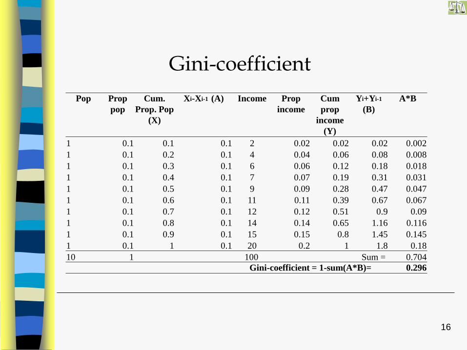
Calculating Gini-Coefficient

Brown’s formula

Index =

Y = Cumulative proportion population

X = Cumulative proportion health or ill-health

k = Number of individuals

i = Individual and corresponding health in specific position

16

Gini-coefficient

Pop Prop

pop

Cum.

Prop. Pop

(X)

Xi-Xi-1 (A) Income Prop

income

Cum

prop

income

(Y)

Yi+Yi-1

(B)

A*B

1 0.1 0.1 0.1 2 0.02 0.02 0.02 0.002

1 0.1 0.2 0.1 4 0.04 0.06 0.08 0.008

1 0.1 0.3 0.1 6 0.06 0.12 0.18 0.018

1 0.1 0.4 0.1 7 0.07 0.19 0.31 0.031

1 0.1 0.5 0.1 9 0.09 0.28 0.47 0.047

1 0.1 0.6 0.1 11 0.11 0.39 0.67 0.067

1 0.1 0.7 0.1 12 0.12 0.51 0.9 0.09

1 0.1 0.8 0.1 14 0.14 0.65 1.16 0.116

1 0.1 0.9 0.1 15 0.15 0.8 1.45 0.145

1 0.1 1 0.1 20 0.2 1 1.8 0.18

10 1 100 Sum = 0.704

Gini-coefficient = 1-sum(A*B)= 0.296

17

CONCENTRATION INDEX

18

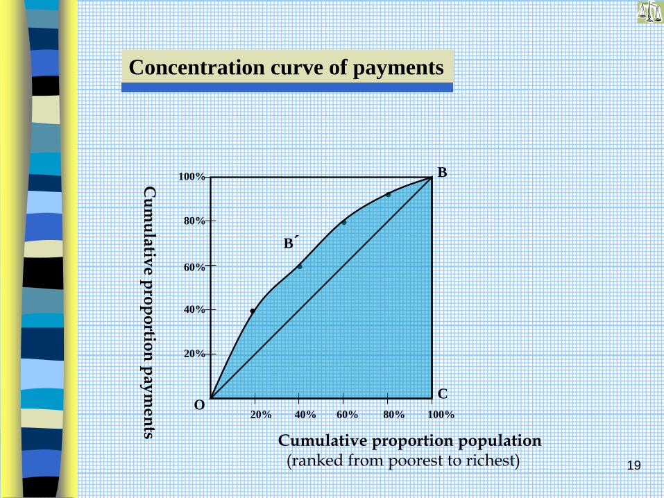
A variant of Lorenz curve. Socioeconomic dimension of health is included in the concentration curve. Concentration curve plots cumulative proportion population (ranked from the poorest to the richest socioeconomic condition) in x-axel against cumulative poportion payments in y-axel.

Concentration curve

19

Cumulative proportion population (ranked from poorest to richest)

Cu

mu

lativ

e p

rop

ortio

n p

ay

men

ts

Concentration curve of payments

20%

40%

60%

80%

100%

20% 40% 60% 80% 100%

O

B´

B

C

20

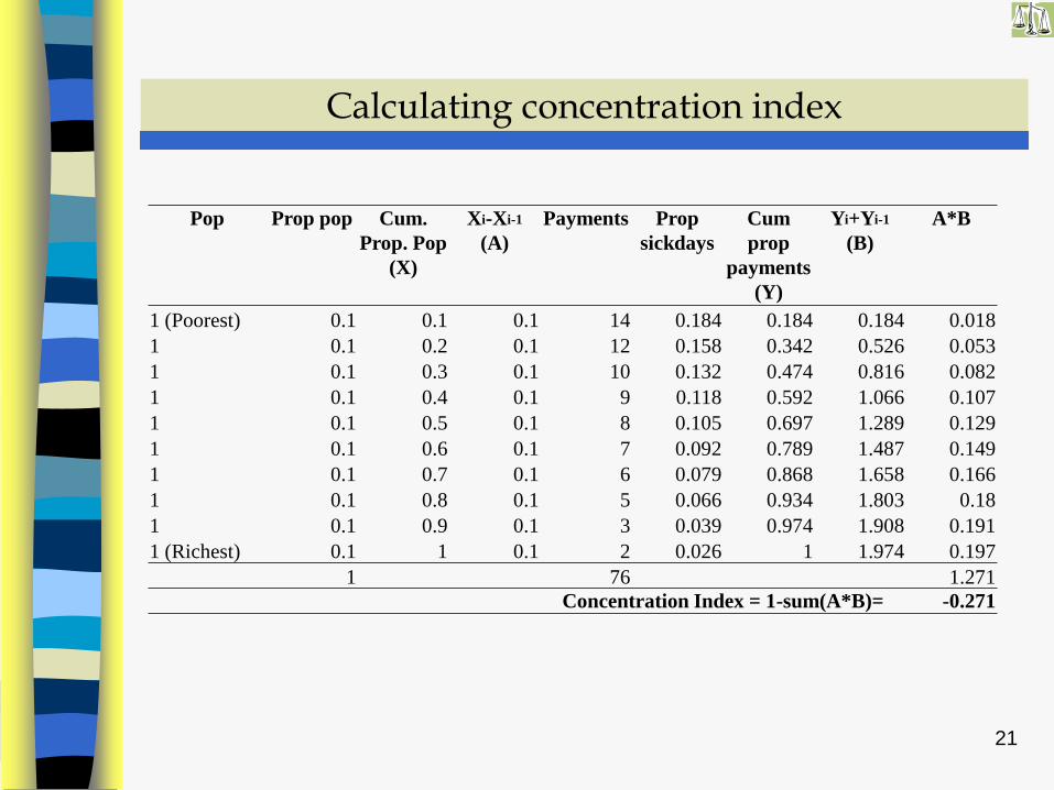
Concentration Index

2*(area under diagonal – area under concentration curve)

21

Calculating concentration index

Pop Prop pop Cum.

Prop. Pop

(X)

Xi-Xi-1

(A)

Payments Prop

sickdays

Cum

prop

payments

(Y)

Yi+Yi-1

(B)

A*B

1 (Poorest) 0.1 0.1 0.1 14 0.184 0.184 0.184 0.018

1 0.1 0.2 0.1 12 0.158 0.342 0.526 0.053

1 0.1 0.3 0.1 10 0.132 0.474 0.816 0.082

1 0.1 0.4 0.1 9 0.118 0.592 1.066 0.107

1 0.1 0.5 0.1 8 0.105 0.697 1.289 0.129

1 0.1 0.6 0.1 7 0.092 0.789 1.487 0.149

1 0.1 0.7 0.1 6 0.079 0.868 1.658 0.166

1 0.1 0.8 0.1 5 0.066 0.934 1.803 0.18

1 0.1 0.9 0.1 3 0.039 0.974 1.908 0.191

1 (Richest) 0.1 1 0.1 2 0.026 1 1.974 0.197

1 76 1.271

Concentration Index = 1-sum(A*B)= -0.271

22

Measuring progressivity

Kakwani Index = Concentration index of payments

minus Gini- coefficient of income

Kakwani Index ranges between -2 and +1

(-) Regressive

(0) Proportional

(+) Progressive

23

1. It reflects the experiences of the entire population.

2. It reflects the socioeconomic dimension of health.

3. It is sensitive to changes in the distribution of the population across the socioeconomic groups.

Check if Gini-coefficient and concentration index satisfy

the following criteria.

24

Application of Gini coefficient and concentration index

Redistributive Effects of the Swedish Social Insuarnce System

European Journal of Public Health 2002; 12: 273-278.

Jahangir Khan, MSc Bjarne Jansson, PhD

Ulf-G Gerdtham, PhD

25

Background Four principles are used to distribute payments via the Swedish social-insurance system in cases of temporary or permanent illness and death. This paper studies the redistributive effects on income of these four principles.

26

Types of payment and the payment principles No Insurance Principle Coverage Regulation Expected distribution

1 Sickness allowance (SA) Compensates lost income Universal Insured persons

earning at least

897 US$ during the

year and on sick leave

longer than 14 days

CI < 0

2 Cash benefit to closely

related persons (CBR)

Compensates lost income Universal Payments for 30 days

per year per person

CI (?)

3 Rehabilitation benefit (RB) Compensates lost income Universal Workplace-related CI < 0

4 Survivor’s pension (SP) Compensates lost income Universal CI < 0

5 Occupational injury (OI) Compensates lost income Gainful

workers

CI < 0

6 Child care allowance (CC) Flat-rate Universal CI (?)

7 Municipal housing

supplement (MHS)

Means-tested Universal CI < 0

8 Handicap allowance (HA) Need-based Universal CI < 0

9 Disability pension (DP) Compensates lost income

and flat-rate

Universal CI < 0

27

Methods The analysis is based on aggregate social-insurance data from the 25 municipalities that comprise Stockholm County in Sweden. For nine different types of social-insurance payments based on the four principles, the degree of income redistribution is measured according to concentration indexes and differences between Gini coefficients with social-insurance payments excluded and included.

28

Municipalities IGW SA CBR RB SP OI CC MHS HA DP TP

Norrtälje 20269 614.60 0.46 94.08 338.67 57.43 40.28 110.64 26.43 1000.47 2283.06

Södertälje 22182 658.81 0.49 114.78 280.38 48.00 29.89 140.98 26.54 1080.21 2380.07

Botkyrka 22227 670.95 0.56 100.03 161.33 39.63 28.47 108.36 18.57 842.29 1970.21

Nynäshamn 22706 557.73 0.73 83.73 260.24 20.24 22.41 64.31 20.65 776.94 1806.98

Sundbyberg 23004 515.96 0.36 95.86 343.79 31.75 16.51 111.37 27.46 946.78 2089.84

Haninge 23423 510.84 0.41 88.16 170.18 65.92 30.06 98.40 19.07 796.77 1779.79

Upplands-Bro 23438 512.78 0.29 78.65 155.53 21.08 23.10 79.67 21.88 634.01 1526.99

Sigtuna 23946 565.62 0.12 88.60 200.00 31.88 24.70 65.88 21.98 641.60 1640.35

Solna 24051 498.61 0.28 73.04 384.39 16.96 18.82 93.66 27.49 910.69 2023.94

Huddinge 24215 555.35 0.39 96.88 198.35 66.29 26.90 82.59 19.87 789.34 1835.95

Värmdö 24230 549.88 0.19 84.03 179.15 40.94 29.26 42.72 25.18 765.31 1716.66

Upplands-Väsby

24380 559.82 0.27 45.30 171.12 46.63 28.91 67.06 21.14 619.01 1559.27

Vallentuna 24649 371.92 0.67 26.74 200.37 24.45 38.76 58.78 17.31 503.26 1242.26

Salem 24768 529.30 0.35 109.82 166.27 28.90 30.46 60.75 22.74 510.31 1458.89

Stockholm 24813 524.72 0.38 104.94 371.25 39.96 25.91 130.82 29.02 882.18 2109.19

Vaxholm 24873 565.13 0.90 76.93 293.26 38.54 48.69 38.37 17.75 551.33 1630.91

Österåker 24963 439.10 0.39 84.16 167.65 64.93 32.97 69.49 16.59 532.49 1407.77

Tyresö 25321 518.50 0.44 89.99 179.61 47.19 29.16 73.25 19.06 683.13 1640.32

Järfälla 25904 425.17 0.36 74.43 207.30 36.13 23.67 78.08 22.85 685.33 1553.32

Ekerö 26054 420.28 0.83 87.39 189.02 26.19 28.34 44.84 19.76 408.98 1225.63

Sollentuna 27145 433.23 0.36 68.80 224.68 35.63 28.62 71.31 19.85 591.91 1474.39

Nacka 27309 520.77 0.40 88.45 263.03 31.07 23.80 69.87 19.02 653.20 1669.60

Täby 29731 343.85 0.46 49.26 241.25 13.95 25.95 44.76 19.08 483.43 1221.99

Lidingö 31016 452.72 0.64 62.63 402.43 17.34 25.37 51.81 22.13 507.29 1542.36

Danderyd 35291 323.14 0.71 45.31 381.37 9.27 25.37 34.40 21.06 426.42 1267.04

Mean 24963 518.66 0.41 90.83 289.79 39.31 26.87 100.33 24.39 785.09 1875.69

CI (t-value)

-0.0587 (-5.330)

0.0184 (0.546)

- 0.0390 (-1.650)

0.0334 (0.974)

-0.0787 (-2.182)

-0.0158 (-0.910)

- 0.0598 (-1.695)

-0.0089 (-0.420)

- 0.0686 (-3.556)

- 0.0469 (-2.773)

p-value 0.000 0.590 0.113 0.340 0.040 0.372 0.104 0.678 0.002 0.011

Weight 0.2765 0.0002 0.0484 0.1545 0.0210 0.0143 0.0535 0.0130 0.4186 1.000

Absolute -0.0162 0.0000 - 0.0019 0.0052 -0.0016 -0.0002 - 0.0032 -0.0001 - 0.0287 - 0.0469

Relative (%) 34.65 - 0.01 4.03 -11.00 3.52 0.48 6.83 0.25 61.26 100.00

IGW IGW+SA IGW+CBR IGW+RB IGW+SP IGW+OI IGW+CC IGW+MHS IGW+HA IGW+DP IGW+TP

Gini coefficient (t-value)

0.0437 (7.387)

0.0416 (7.299)

0.0437 (7.387)

0.043 (7.419)

0.0442 (7.160)

0.0435 (7.398)

0.0436 (7.388)

0.0433 (7.432)

0.0436* (7.392)

0.0405 (7.448)

0.0379 (7.624)

p value 0.000 0.000 0.000 0.000 0.000 0.000 0.000 0.000 0.000 0.000 0.000

Results

29

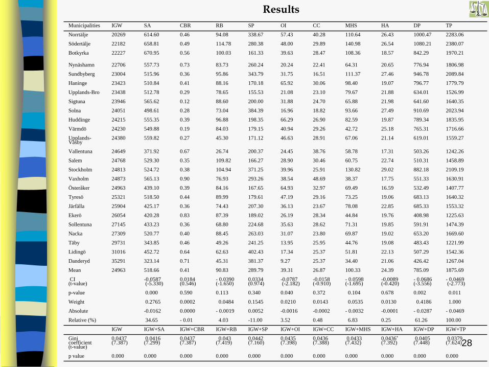
Results The concentration indexes for payments from the nine social-insurance schemes in total is –0.0469. The Gini coefficient falls from 0.0437 excluding insurance payments (i.e. for income only from gainful work, IGW) to 0.0379 when including insurance payments with income from gainful work (IGW+TP). That is, the Gini coefficient is 15% lower when insurance payments are included. Decomposition by payment shows that the largest redistribution effect on income inequality is made by disability pension.

30

Conclusions

Municipalities with low average income are favoured by the

Swedish social-insurance system. Payment principles can be

ranked according to their redistributive capacity: mix of

compensating-lost-income and flat-rate, compensating-lost-

income, means-testing, flat-rate, and need-based respectively.

The nine social-insurance schemes contribute very differently

to income redistribution. Disability pension and sickness

allowance contribute most to income redistribution and

reducing income inequality.