L4 Dynamics of the current account in a small open … · Dynamics of the current account in a small open economy microfounded model Lecture 4, MSc Open Economy Macroeconomics Birmingham,

Dynamics of the current account in a small open economy microfounded

modelLecture 4, MSc Open Economy 

MacroeconomicsBirmingham, Autumn 2015

Tony Yates

Main features of the model.

• Small open economy.• Our economy is too small for outcomes to affect world variables like the real rate.– Used by central banks like Sweden, Norway.– Used in study of small emerging economies.

• But world variables affect us.• Endowment economy, so we don’t model production.

Punchlines of the lecture

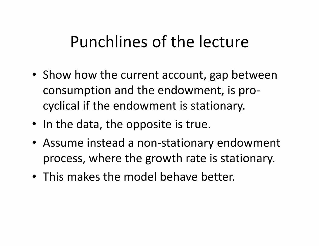
• Show how the current account, gap between consumption and the endowment, is pro‐cyclical if the endowment is stationary.

• In the data, the opposite is true.• Assume instead a non‐stationary endowment process, where the growth rate is stationary.

• This makes the model behave better.

Points to note about our SOE model

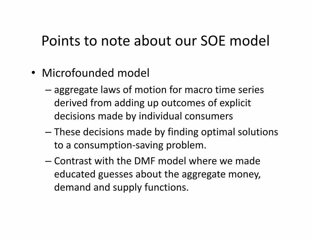
• Microfounded model– aggregate laws of motion for macro time series derived from adding up outcomes of explicit decisions made by individual consumers

– These decisions made by finding optimal solutions to a consumption‐saving problem.

– Contrast with the DMF model where we made educated guesses about the aggregate money, demand and supply functions. 

Representative consumer

• Our model is one of infinitely many and infinitely ‘small’ identical consumers.

• Known as the ‘representative agent’ paradigm.

• Obviously, since everyone is different, counter‐factual.

• Various arguments for pursuing it…..

On the rep agent paradigm

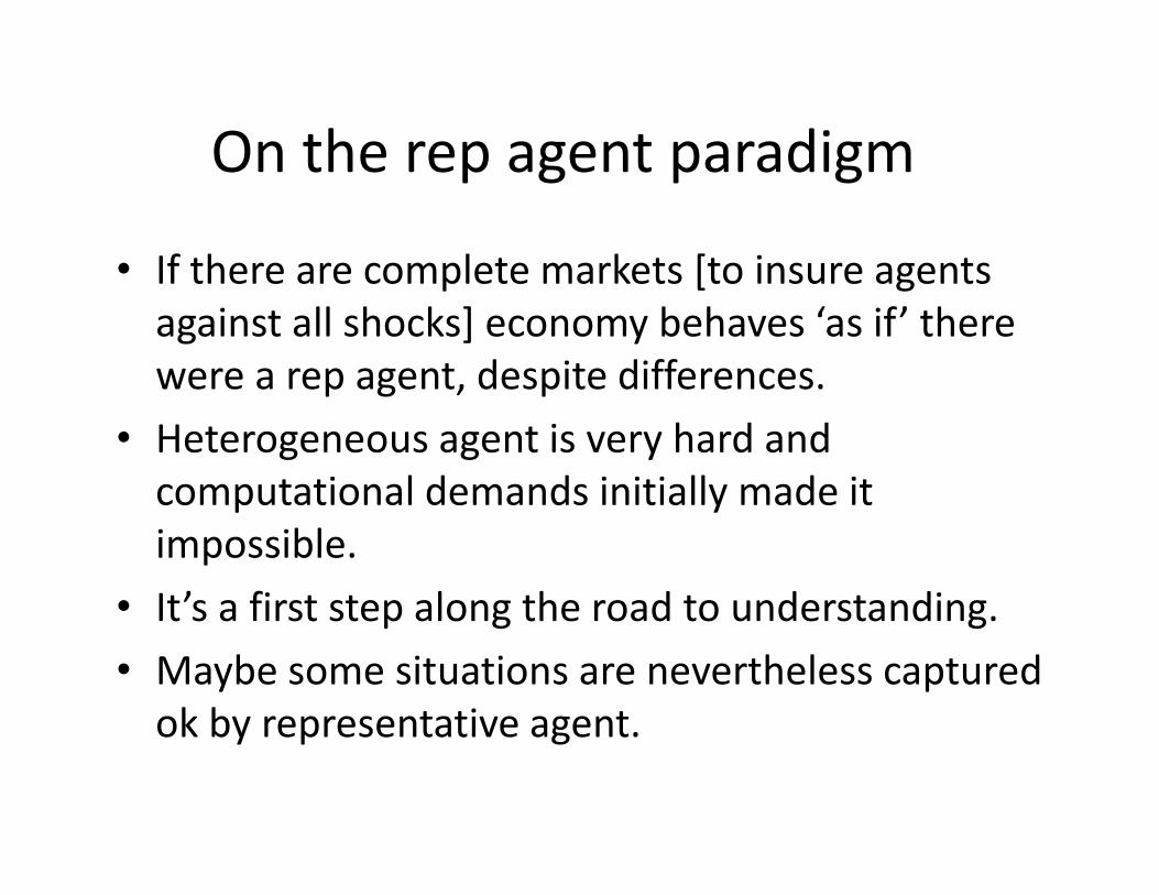
• If there are complete markets [to insure agents against all shocks] economy behaves ‘as if’ there were a rep agent, despite differences.

• Heterogeneous agent is very hard and computational demands initially made it impossible.

• It’s a first step along the road to understanding.• Maybe some situations are nevertheless captured ok by representative agent.

Current account expresses flow of saving and borrowing

• Common in popular discourse for gap between consumption and income, current account, to be viewed as ‘bad’ if there is a negative number.

• Translates into protectionist and ‘pro‐export’ policies.

• Or, Polonius, Hamlet: ‘neither a borrower nor a lender be’.

• In this model, borrowing and saving are devices for consumption smoothing and beneficial intertemporal trade.

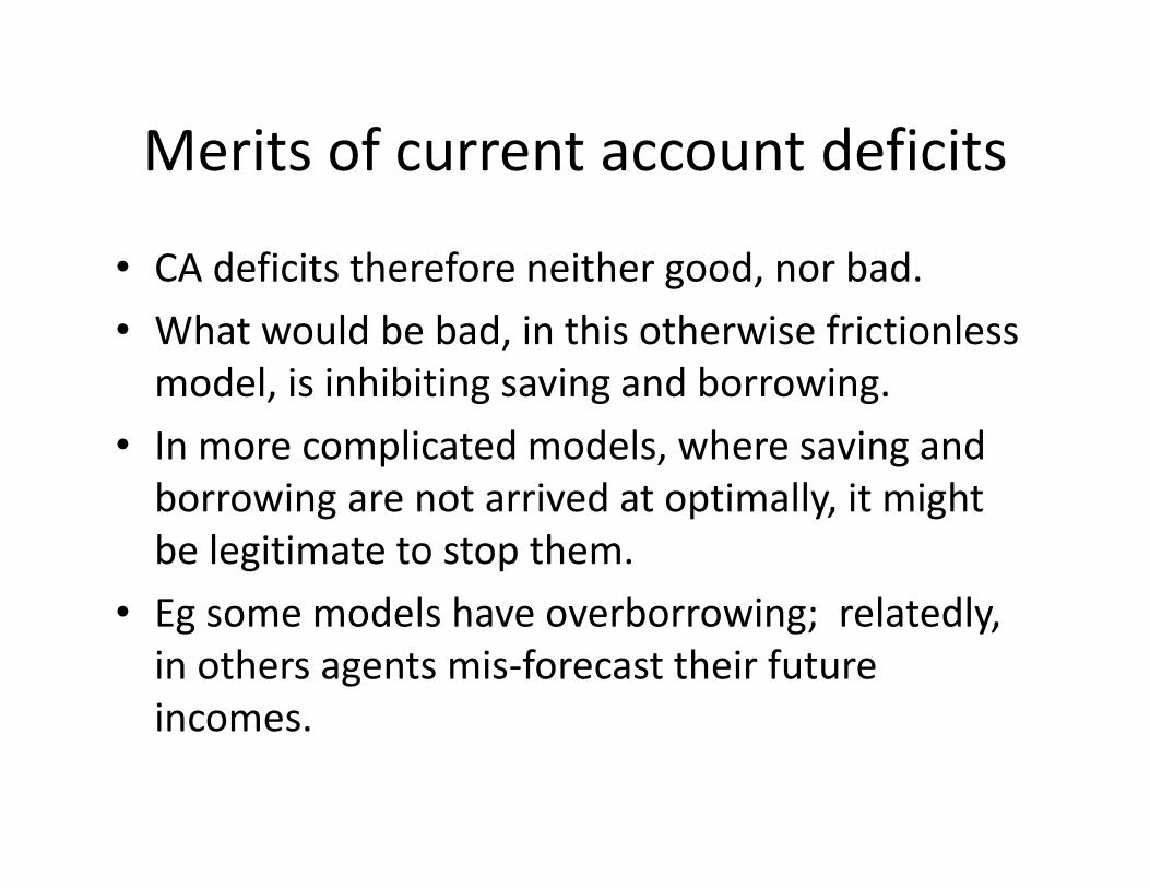
Merits of current account deficits

• CA deficits therefore neither good, nor bad.• What would be bad, in this otherwise frictionless model, is inhibiting saving and borrowing.

• In more complicated models, where saving and borrowing are not arrived at optimally, it might be legitimate to stop them.

• Eg some models have overborrowing;  relatedly, in others agents mis‐forecast their future incomes.

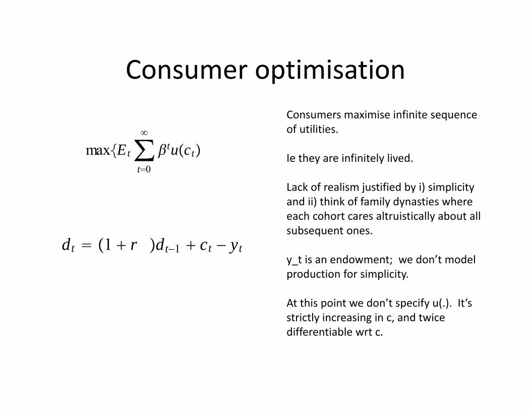
Consumer optimisation

maxEt∑t0

tuct

dt 1 r dt−1 ct − yt

Consumers maximise infinite sequence of utilities.

Ie they are infinitely lived.

Lack of realism justified by i) simplicity and ii) think of family dynasties where each cohort cares altruistically about all subsequent ones.

y_t is an endowment;  we don’t model production for simplicity.

At this point we don’t specify u(.).  It’s strictly increasing in c, and twice differentiable wrt c.

No Ponzi Games Condition

limj→ Etd tj

1rj ≤ 0

Can’t continually run up debts;  d>0 means ‘I owe someone’.

If stream of consumption set optimally, will mean that expect to make sure debts=0.

If you have any positive assets left over ‘at the end of time’, better to eat them.

Dynamic optimisation using the Lagrangian, again….

L E0∑t0

tuct − tdt − 1 r dt−1 yt − ct

Form the Lagrangian, made from i) period utility, and ii) the LM times the budget constraint set=0.

Differentiate wrt choice variables d_t,c_t, and set=0.

Eliminate LM’s to get, in this case, the Euler equation.

Here we have uncertainty, so take care with the expectations operator, which, remember, is just a way of averaging over future possible outcomes.

u ′ct 1 r Etu ′ct1

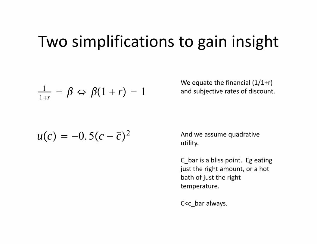
Two simplifications to gain insight

11r 1 r 1

uc −0.5c − c2

We equate the financial (1/1+r) and subjective rates of discount.

And we assume quadrative utility.

C_bar is a bliss point.  Eg eating just the right amount, or a hot bath of just the right temperature.

C<c_bar always.

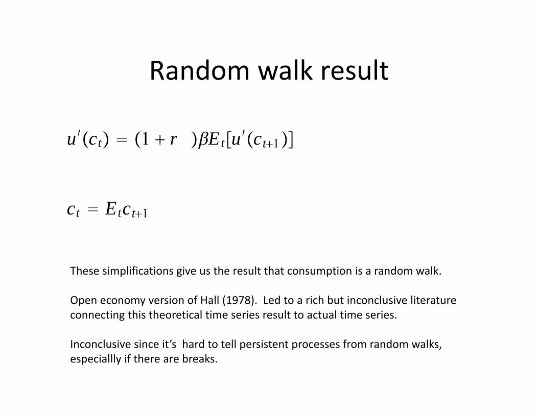
Random walk result

ct Etct1

u ′ct 1 r Etu ′ct1

These simplifications give us the result that consumption is a random walk.

Open economy version of Hall (1978).  Led to a rich but inconclusive literature connecting this theoretical time series result to actual time series.

Inconclusive since it’s  hard to tell persistent processes from random walks, especiallly if there are breaks.

What it means to solve the model

• This is not yet the solution to the model.• We have found the consumers’ first order condition, which the solution must obey.

• Solution to model usually refers to deriving expression for endogenous variable consumption [eg] in terms of primitive parameters and exogenous driver, in this case the output endowment.

Plan for analysis

• Derive an ‘infinite period budget constraint’, by repeated substitution of the period budget constraint into itself.

• Use the random walk assumption to substitute out for the infinite period ahead forecasts.

• This gives us our relationship between c, ca and y.

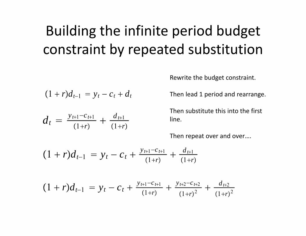
Building the infinite period budget constraint by repeated substitution

1 rdt−1 yt − ct dt

dt yt1−ct1

1r d t11r

1 rdt−1 yt − ct yt1−ct1

1r d t11r

1 rdt−1 yt − ct yt1−ct1

1r yt2−ct2

1r2 d t2

1r2

Rewrite the budget constraint.

Then lead 1 period and rearrange.

Then substitute this into the first line.

Then repeat over and over….

Getting rid of the last d_t+n term using the No Ponzi Games condition.

1 rdt−1 Et∑j0

sytj−ctj

1rj d ts

1rs

limj→ Etd tj

1rj ≤ 0

1 rdt−1 Et∑j0

ytj−ctj

1rj

This is what we get eventually.

NPG holds with equality at an optimum.

So the ‘last’ d_t term disappears.

Recap on our goal….

1 rdt−1 Et∑j0

ytj−ctj

1rj

Now we have the infinite period budget constraint.

Remember that the purpose was to get an expression for c_t[actually the current account, defined later] in terms of the exogenous endowment y_t.

To do this we have to turn the infinite sequence forecast on the RHS into terms involving only c_t and y_t…..

This is what we do next.  Starting with c……

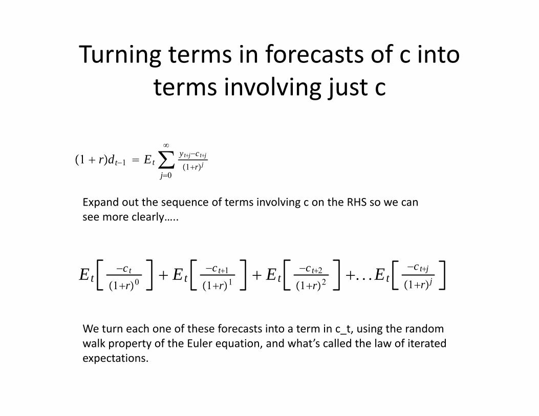
Turning terms in forecasts of c into terms involving just c

1 rdt−1 Et∑j0

ytj−ctj

1rj

Et−ct

1r0 Et

−ct1

1r1 Et

−ct2

1r2. . .Et

−ctj

1rj

Expand out the sequence of terms involving c on the RHS so we can see more clearly…..

We turn each one of these forecasts into a term in c_t, using the random walk property of the Euler equation, and what’s called the law of iterated expectations.

From c_t+j to c_t….

Et−ct

1r0

Etct ct

Et−ct1

1r1

ct Etct1

First term involves only c_t anyway.

Expectation at t of something at t is just that thing at t.

Second term involves c_t+1.

We can use the Euler Equation directly to substitute out for this

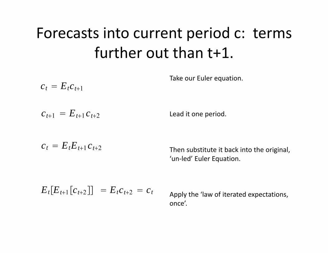
Forecasts into current period c:  terms further out than t+1.

ct Etct1

ct1 Et1ct2

ct EtEt1ct2

Take our Euler equation.

Lead it one period.

Then substitute it back into the original, ‘un‐led’ Euler Equation.

Apply the ‘law of iterated expectations, once’.

EtEt1ct2 Etct2 ct

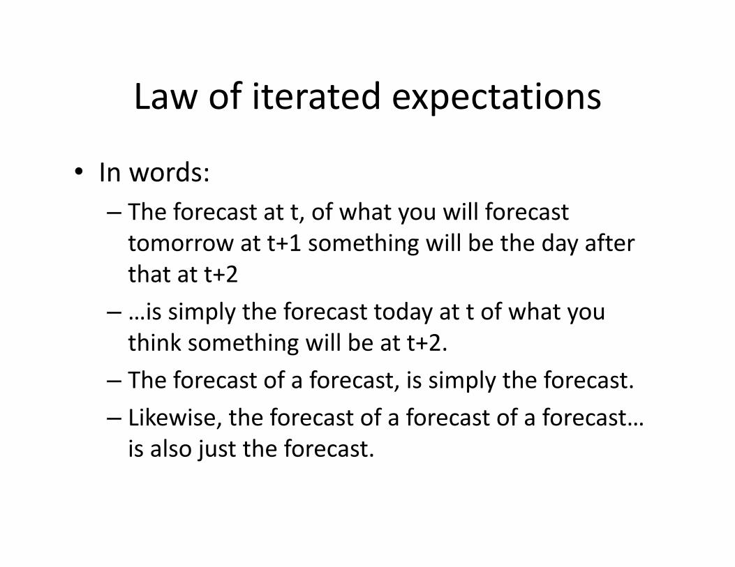
Law of iterated expectations

• In words:– The forecast at t, of what you will forecast tomorrow at t+1 something will be the day after that at t+2

– …is simply the forecast today at t of what you think something will be at t+2.

– The forecast of a forecast, is simply the forecast.– Likewise, the forecast of a forecast of a forecast… is also just the forecast.

LOIE again

• Not special to economics.  It’s a property of integration [which is what an expectation, or a forecast is] and time series processes.

• Some conditions required, that we won’t go into.

• Satisfied here.

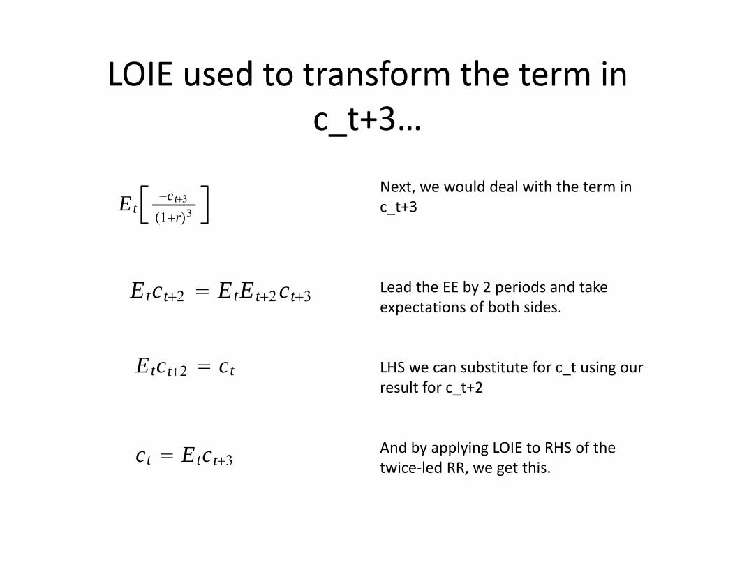
LOIE used to transform the term in c_t+3…

Et−ct3

1r3

Etct2 EtEt2ct3

Etct2 ct

ct Etct3

Next, we would deal with the term in c_t+3

Lead the EE by 2 periods and take expectations of both sides.

LHS we can substitute for c_t using our result for c_t+2

And by applying LOIE to RHS of the twice‐led RR, we get this.

Concluding process of dealing with the stream of E_t[c_t+j]’s

1 rdt−1 Et∑j0

ytj−ctj

1rj

ct Etctj

1 rdt−1 ∑j0

Etytj

1rj − ct

1rj

rdt−1 ct r1r Et∑

j0

ty tj

1rj

Recall this was the infinite period budget constraint of the SOE consumer….

We find that all of the future c’s=c_t

Hence take out of the expectation.

And with algebra of infinite sequence sum, can write like this.

Now need to deal with y’s.

SOE and permanent income hypothesis

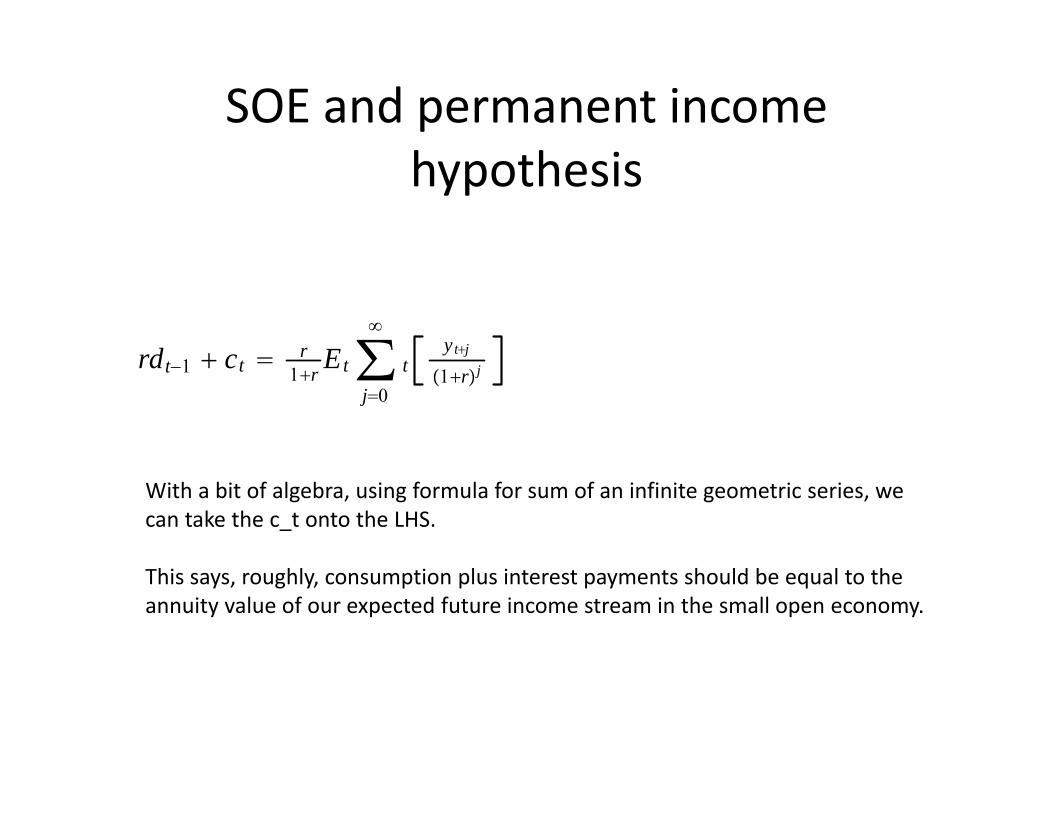
rdt−1 ct r1r Et∑

j0

ty tj

1rj

With a bit of algebra, using formula for sum of an infinite geometric series, we can take the c_t onto the LHS.

This says, roughly, consumption plus interest payments should be equal to the annuity value of our expected future income stream in the small open economy.

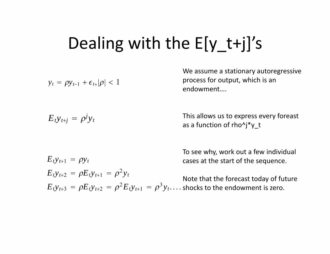
Dealing with the E[y_t+j]’s

yt yt−1 t, || 1

Etytj jyt

Etyt1 yt

Etyt2 Etyt1 2yt

Etyt3 Etyt2 2Etyt1 3yt. . . .

We assume a stationary autoregressive process for output, which is an endowment….

This allows us to express every foreastas a function of rho^j*y_t

To see why, work out a few individual cases at the start of the sequence.

Note that the forecast today of future shocks to the endowment is zero.

Converting the stream of expected future y_t’s into y_t’s…

Et∑j0

ty tj

1rj yt∑j0

j

1rj 1r1r− yt

First substitute in the result we had using the autoregressive process assumption….

Then use our high school formula for the sum of an infinite geometric series….

And we are done.  So we have converted the infinite sequence of ever far ahead forecasts into a set of terms in today’s endowment.

How consumption responds to the endowment

rdt−1 ct r1 r

1 r1 r − yt

r1 r − yt

ct r1 r − yt − rdt−1

Consumption responds less than one for one with the endowment.

Since the shock is temporary, consumers save some of it to consume later.

Utility quadratic, so benefit of small increments in later period very large, hence don’t eat it all at once.

Towards the relationship between the current account and y

tbt yt − ct

cat −rdt−1 tbt

tbt yt − r1 r − yt rdt−1

yt 1 − r1 r − rdt−1

tbt 1 −

1 r − yt rdt−1

cat 1−1r− yt

Trade balance=endowment less consumption.

Current account=balance between funds used to pay foreign debtors, and trade balance

Substituting in, we can get the relationship between the trade balance and the endowment y….

And between the current account and the endowment y……

The model and the data

• Model predicts current account is pro‐cyclical.• But the data says the opposite!• Many assumptions made along the way.  Which one could be the cause of this problem?

• We’ll show that assuming non‐stationary endowment [stationary growth] can fix it.

A hint from our stationary endowment results

ct r1r− yt − rdt−1

yt yt−1 t, || 1

This was our expression for consumption.

This is the stationary assumption we made about the endowment.

As rho goes towards 1, consumers spend more and more of the change in y.

They know the change is longer lived, so don’t have to share the current change in y out over many periods.

Tendency for current account to respond positively [ie for saving to rise] with endowment falls….    A clue to saving the model.

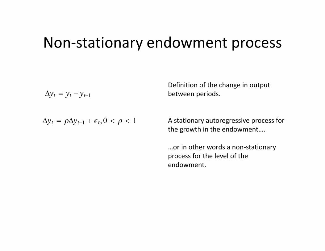
Non‐stationary endowment process

Δyt yt − yt−1

Δyt Δyt−1 t, 0 1

Definition of the change in output between periods.

A stationary autoregressive process for the growth in the endowment….

…or in other words a non‐stationary process for the level of the endowment.

Recap on what we need to do• Take our infinite period budget constraint.• That involves expressions in infinite sequence of expectations of income and consumption.

• Use the EE and LOIE to substitute out for the expected consumption terms

• Use the endowment process to try to turn the expected endowment terms into current endowment terms.

• Then we have an equation relating consumption to the endowment.

• [And therefore the current account, which is ‘saving’, related to the endowment]

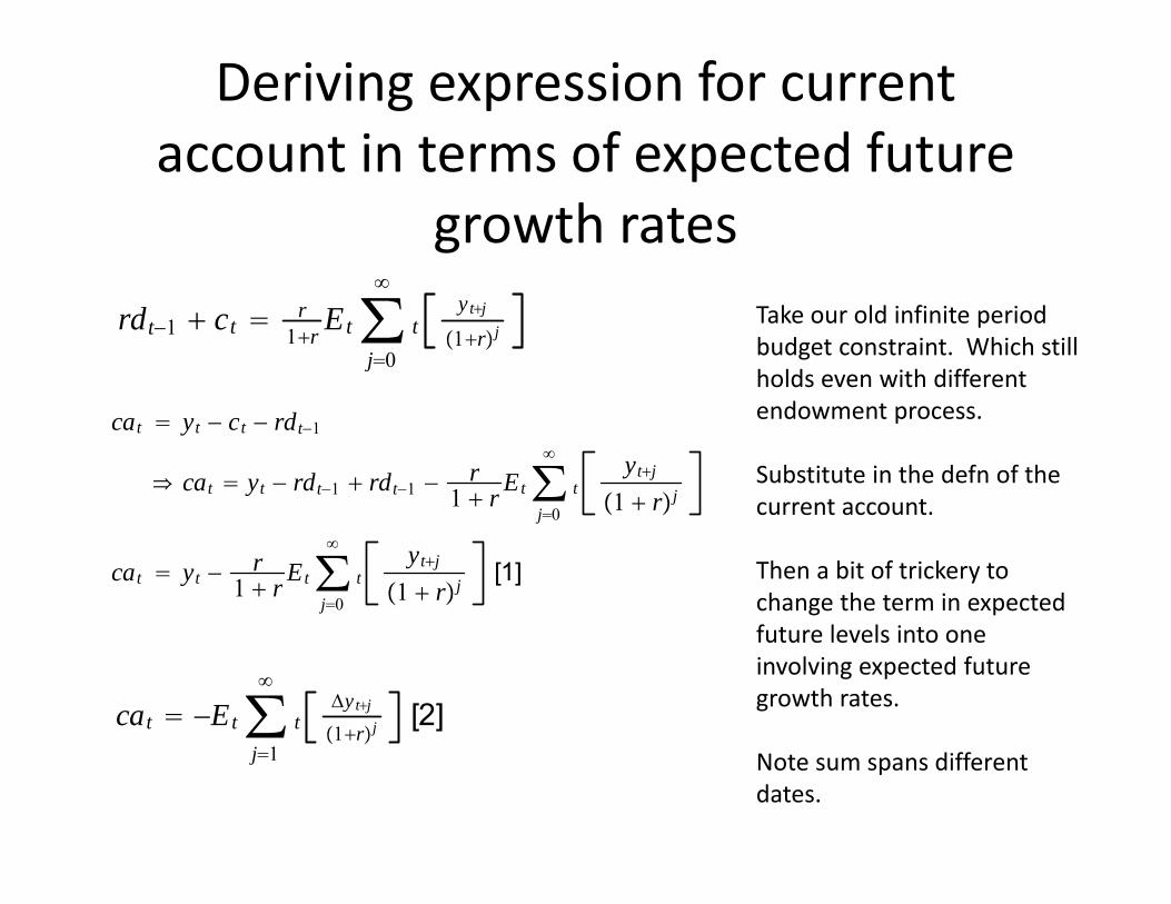
Deriving expression for current account in terms of expected future 

growth ratesrdt−1 ct r

1r Et∑j0

ty tj

1rj

cat yt − ct − rdt−1

cat yt − rdt−1 rdt−1 − r1 r Et∑

j0

tytj

1 rj

cat yt − r1 r Et∑

j0

tytj

1 rj [1]

cat −Et∑j1

tΔytj

1rj [2]

Take our old infinite period budget constraint.  Which still holds even with different endowment process.

Substitute in the defn of the current account.

Then a bit of trickery to change the term in expected future levels into one involving expected future growth rates.

Note sum spans different dates.

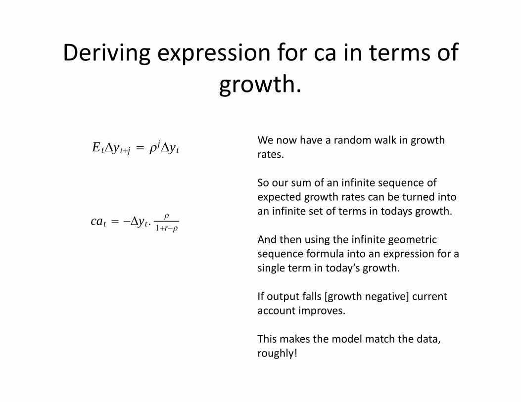
Deriving expression for ca in terms of growth.

EtΔytj jΔyt

cat −Δyt. 1r−

We now have a random walk in growth rates.

So our sum of an infinite sequence of expected growth rates can be turned into an infinite set of terms in todays growth.

And then using the infinite geometric sequence formula into an expression for a single term in today’s growth.

If output falls [growth negative] current account improves.

This makes the model match the data, roughly!

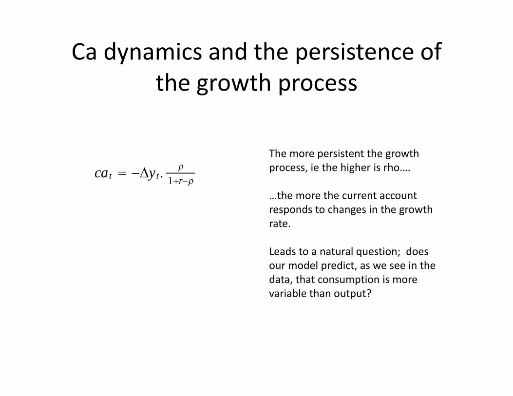
Ca dynamics and the persistence of the growth process

cat −Δyt. 1r−

The more persistent the growth process, ie the higher is rho….

…the more the current account responds to changes in the growth rate.

Leads to a natural question;  does our model predict, as we see in the data, that consumption is more variable than output?

Variability of consumption and output

• Plan for the next lot of algebra [!!]– Find the variability of output as a function of the variability of the endowment shock

– Do the same for consumption.– Then figure out [for you in an exercise] what conditions lead to consumption variance being larger.

– Uses result about the variance of an AR(1).

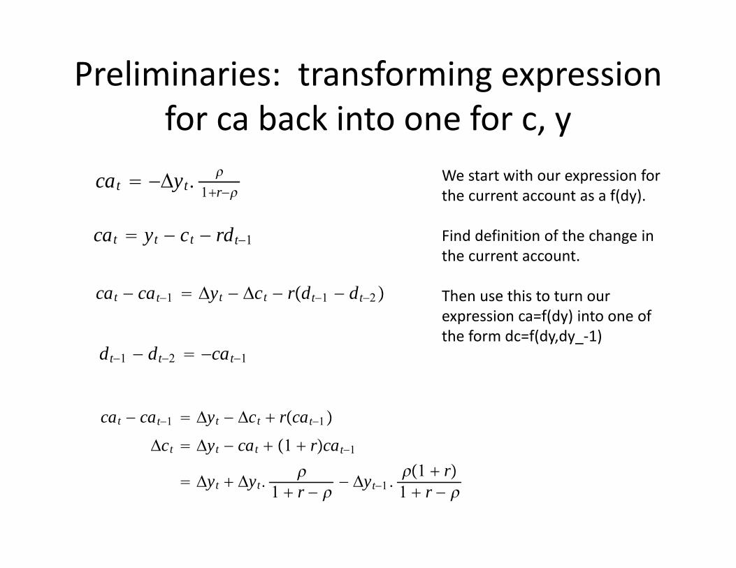
Preliminaries:  transforming expression for ca back into one for c, y

cat −Δyt. 1r−

cat yt − ct − rdt−1

cat − cat−1 Δyt − Δct − rdt−1 − dt−2

dt−1 − dt−2 −cat−1

cat − cat−1 Δyt − Δct rcat−1

Δct Δyt − cat 1 rcat−1

Δyt Δyt.

1 r − − Δyt−1 .1 r1 r −

We start with our expression for the current account as a f(dy).

Find definition of the change in the current account.  

Then use this to turn our expression ca=f(dy) into one of the form dc=f(dy,dy_‐1) 

Deriving the variance of consumption growth

Δct 1r1r−Δyt −

1r1r− Δyt−1

Δyt Δyt−1 t

Δct 1r1r− t

Δct2 1r

1r−

22

This comes from collecting terms in y from last expression on previous slide.

Now substitute in our AR(1) for endowment.

Our expression for dc=f(shock)

Using classic formula for variances of functions of random variables,  we get this formula for the variance of dc.

Now for the variance out output.

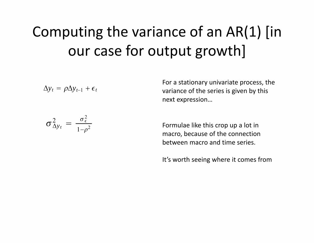
Computing the variance of an AR(1) [in our case for output growth]

Δyt Δyt−1 t

Δyt2 2

1−2

For a stationary univariate process, the variance of the series is given by this next expression…

Formulae like this crop up a lot in macro, because of the connection between macro and time series.

It’s worth seeing where it comes from

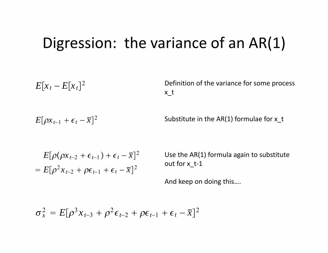
Digression:  the variance of an AR(1)

Ex t − Ex t2

Ex t−1 t − x2

Ex t−2 t−1 t − x2

E2x t−2 t−1 t − x2

Definition of the variance for some process x_t

Substitute in the AR(1) formulae for x_t

Use the AR(1) formula again to substitute out for x_t‐1

And keep on doing this….

x2 E3x t−3 2t−2 t−1 t − x2

Computing the variance of an AR(1)/ctd…

x2 Ent−n . . .2t−2 t−1 t − x2

Ett Et−nt−n 2 ,∀j

Ex t x 0

We assert that errors in different time periods are uncorrelated;

That the variance of the shock does not change over time.

And that the expected value of x is zero.  [we’ll justify this in a moment]. 

Ets 0, s ≠ t

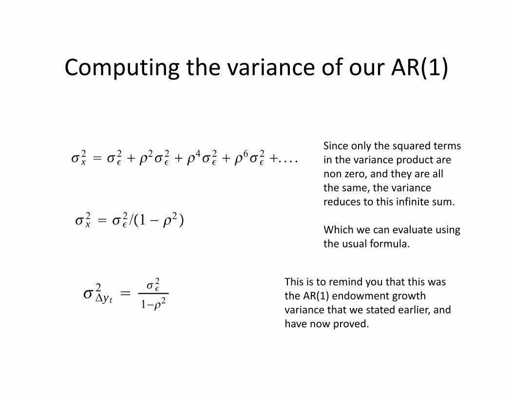
Computing the variance of our AR(1)

x2

2 22 4

2 62 . . . .

x2

2 /1 − 2

Since only the squared terms in the variance product are non zero, and they are all the same, the variance reduces to this infinite sum.

Which we can evaluate using the usual formula.

Δyt2 2

1−2This is to remind you that this was the AR(1) endowment growth variance that we stated earlier, and have now proved.

Justifying the assertion that the mean of the AR(1) was zero…

Ex t Ex t−1 t

Ex t Ex t−1 t

Ent−n . . .2t−2 t−1 t

Substitute in the expression for the AR(1) repeatedly…..

And we see that we are taking an expectation of an infinite sequence of errors.

But we assume that the shock at each point in time is mean zero.

Hence the expectation, or mean of x_t is 0 too.

Et−j 0,∀j

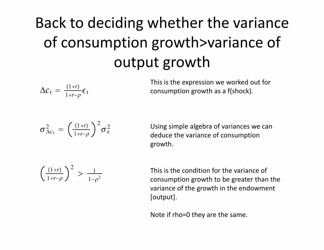
Back to deciding whether the variance of consumption growth>variance of 

output growth

Δct 1r1r− t

Δct2 1r

1r−

22

1r1r−

2 1

1−2

This is the expression we worked out for consumption growth as a f(shock).

Using simple algebra of variances we can deduce the variance of consumption growth.

This is the condition for the variance of consumption growth to be greater than the variance of the growth in the endowment [output].

Note if rho=0 they are the same.

Recap

• We wrote down a small open economy endowment model.

• We derived the representative agent consumer euler equation

• We used an assumption about quadratic utility to get that this EE implies a random walk.

• We derived an infinite period budget constraint from the ‘each period’ one.

• We then used the RW for consumption, and the law of iterated expectations….

• …to turn the infinite period budget constraint into an expression for c or the ca in terms of the exogenous endowment y.

• We saw that with a stationary y, the ca was procyclical, which is counterfactual.

• Re‐deriving using a stationary dy, we got a countercyclical current account.

Recap 3

• Finally, we worked out conditions under which the variance of consumption growth > variance of output growth.

• [Noting that in the data this tends to be true for SOEs.]

• To do this, we used time series econometrics, and the algebra of variances to derive the variance of an AR(1) process, and its mean.

Key assumptions

• Quadratic utility, and the bliss point.• Rational expectations.• Complete markets and representative agent.• Optimising consumers.• Endowment economy, no production.• SOE is too small to affect rest of the world.• Flexible prices.  No money, or monetary policy.

Comments comparing this to Eggertson Krugman

• EK we also began with flexible prices, but later introduced sticky prices.  And we had an endowment economy.

• But there we considered two ‘large’ economies, one borrowing and one lending.

• The shock to the borrowers did affect the lenders, because it drove down the real rate.

• In our SOE model, what happens to our SOE agents does not matter for the real rate or the rest of the world in any way.

• Note here there was no frictions on borrowing by or lending into the SOE.