CSCE 666 Pattern Analysis | Ricardo Gutierrez-Osuna | CSE@TAMU 1 L2: Review of probability and statistics • Probability – Definition of probability – Axioms and properties – Conditional probability – Bayes theorem • Random variables – Definition of a random variable – Cumulative distribution function – Probability density function – Statistical characterization of random variables • Random vectors – Mean vector – Covariance matrix • The Gaussian random variable

Welcome message from author
This document is posted to help you gain knowledge. Please leave a comment to let me know what you think about it! Share it to your friends and learn new things together.
Transcript
CSCE 666 Pattern Analysis | Ricardo Gutierrez-Osuna | CSE@TAMU 1
L2: Review of probability and statistics
• Probability
– Definition of probability
– Axioms and properties
– Conditional probability
– Bayes theorem
• Random variables
– Definition of a random variable
– Cumulative distribution function
– Probability density function
– Statistical characterization of random variables
• Random vectors
– Mean vector
– Covariance matrix
• The Gaussian random variable
CSCE 666 Pattern Analysis | Ricardo Gutierrez-Osuna | CSE@TAMU 2
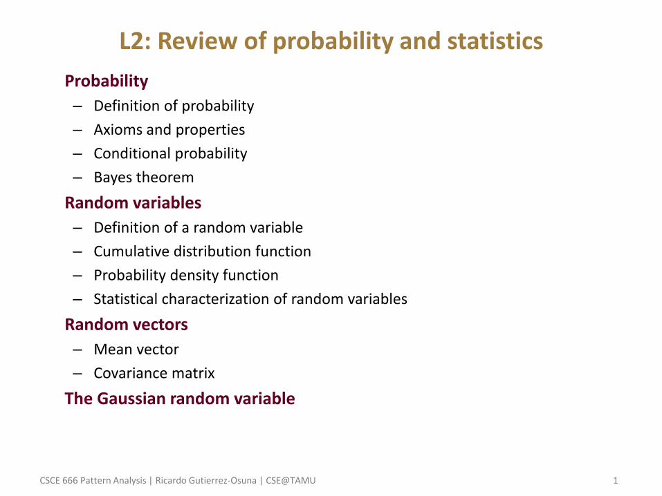
Review of probability theory
• Definitions (informal) – Probabilities are numbers assigned to events that
indicate “how likely” it is that the event will occur when a random experiment is performed
– A probability law for a random experiment is a rule that assigns probabilities to the events in the experiment
– The sample space S of a random experiment is the set of all possible outcomes
• Axioms of probability – Axiom I: 𝑃 𝐴𝑖 ≥ 0
– Axiom II: 𝑃 𝑆 = 1
– Axiom III: 𝐴𝑖 ∩ 𝐴𝑗 = ∅ ⇒ 𝑃 𝐴𝑖⋃𝐴𝑗 = 𝑃 𝐴𝑖 + 𝑃 𝐴𝑗
A1
A2
A3 A4
event
pro
bab
ility
A1 A2 A3 A4
Sample space
Probability law
CSCE 666 Pattern Analysis | Ricardo Gutierrez-Osuna | CSE@TAMU 3
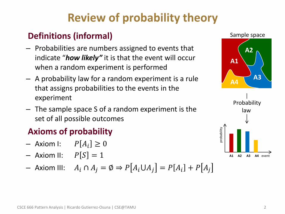
• Warm-up exercise – I show you three colored cards
• One BLUE on both sides • One RED on both sides • One BLUE on one side, RED on the other
– I shuffle the three cards, then pick one and show you one side only. The side visible to you is RED • Obviously, the card has to be either A or C, right?
– I am willing to bet $1 that the other side of the card has the same color, and need someone in class to bet another $1 that it is the other color • On the average we will end up even, right? • Let’s try it!
A B C
CSCE 666 Pattern Analysis | Ricardo Gutierrez-Osuna | CSE@TAMU 4
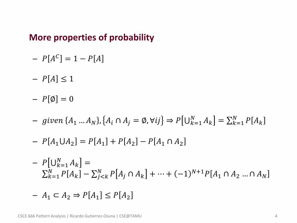
• More properties of probability
– 𝑃 𝐴𝐶 = 1 − 𝑃 𝐴
– 𝑃 𝐴 ≤ 1
– 𝑃 ∅ = 0
– 𝑔𝑖𝑣𝑒𝑛 𝐴1…𝐴𝑁 , 𝐴𝑖 ∩ 𝐴𝑗 = ∅,∀𝑖𝑗 ⇒ 𝑃 ⋃ 𝐴𝑘𝑁𝑘=1 = 𝑃 𝐴𝑘
𝑁𝑘=1
– 𝑃 𝐴1⋃𝐴2 = 𝑃 𝐴1 + 𝑃 𝐴2 − 𝑃 𝐴1 ∩ 𝐴2
– 𝑃 ⋃ 𝐴𝑘𝑁𝑘=1 =
𝑃 𝐴𝑘 − 𝑃 𝐴𝑗 ∩ 𝐴𝑘 +⋯+ −1 𝑁+1𝑃 𝐴1 ∩ 𝐴2 …∩ 𝐴𝑁𝑁𝑗<𝑘
𝑁𝑘=1
– 𝐴1 ⊂ 𝐴2 ⇒ 𝑃 𝐴1 ≤ 𝑃 𝐴2
CSCE 666 Pattern Analysis | Ricardo Gutierrez-Osuna | CSE@TAMU 5
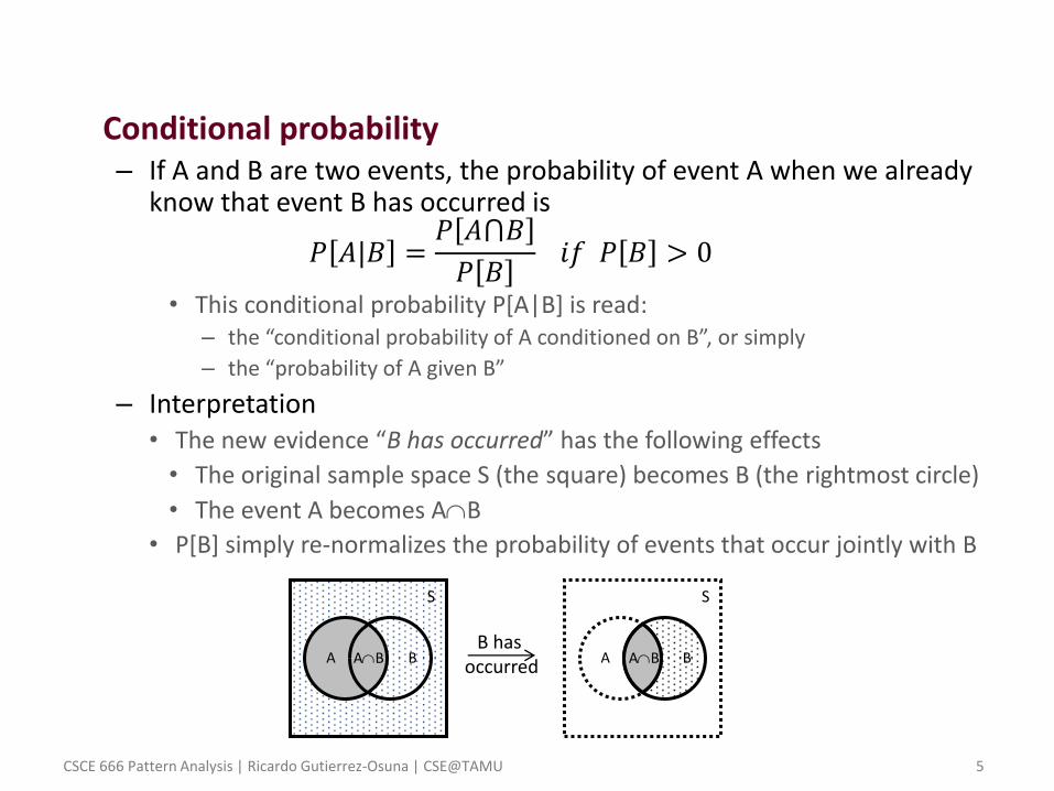
• Conditional probability – If A and B are two events, the probability of event A when we already
know that event B has occurred is
𝑃 𝐴|𝐵 =𝑃 𝐴⋂𝐵
𝑃 𝐵 𝑖𝑓 𝑃 𝐵 > 0
• This conditional probability P[A|B] is read: – the “conditional probability of A conditioned on B”, or simply
– the “probability of A given B”
– Interpretation • The new evidence “B has occurred” has the following effects
• The original sample space S (the square) becomes B (the rightmost circle)
• The event A becomes AB
• P[B] simply re-normalizes the probability of events that occur jointly with B
S S
A AB B A AB B B has
occurred
CSCE 666 Pattern Analysis | Ricardo Gutierrez-Osuna | CSE@TAMU 6
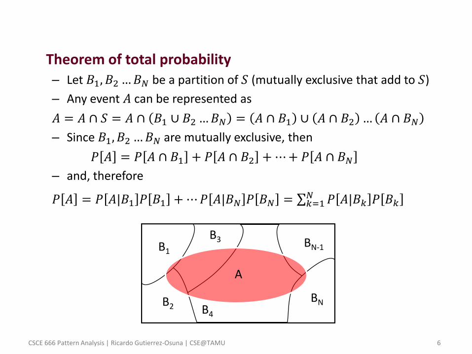
• Theorem of total probability – Let 𝐵1, 𝐵2…𝐵𝑁 be a partition of 𝑆 (mutually exclusive that add to 𝑆)
– Any event 𝐴 can be represented as
𝐴 = 𝐴 ∩ 𝑆 = 𝐴 ∩ 𝐵1 ∪ 𝐵2…𝐵𝑁 = 𝐴 ∩ 𝐵1 ∪ 𝐴 ∩ 𝐵2 … 𝐴 ∩ 𝐵𝑁
– Since 𝐵1, 𝐵2…𝐵𝑁 are mutually exclusive, then
𝑃 𝐴 = 𝑃 𝐴 ∩ 𝐵1 + 𝑃 𝐴 ∩ 𝐵2 +⋯+ 𝑃 𝐴 ∩ 𝐵𝑁
– and, therefore
𝑃 𝐴 = 𝑃 𝐴|𝐵1 𝑃 𝐵1 +⋯𝑃 𝐴|𝐵𝑁 𝑃 𝐵𝑁 = 𝑃 𝐴|𝐵𝑘 𝑃 𝐵𝑘𝑁𝑘=1
B1
B2
B3 BN-1
BN
A
B4
CSCE 666 Pattern Analysis | Ricardo Gutierrez-Osuna | CSE@TAMU 7
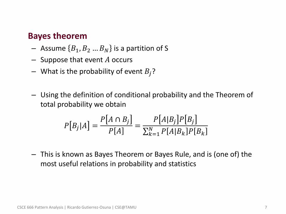
• Bayes theorem – Assume 𝐵1, 𝐵2…𝐵𝑁 is a partition of S
– Suppose that event 𝐴 occurs
– What is the probability of event 𝐵𝑗?
– Using the definition of conditional probability and the Theorem of total probability we obtain
𝑃 𝐵𝑗|𝐴 =𝑃 𝐴 ∩ 𝐵𝑗
𝑃 𝐴=
𝑃 𝐴|𝐵𝑗 𝑃 𝐵𝑗
𝑃 𝐴|𝐵𝑘 𝑃 𝐵𝑘𝑁𝑘=1
– This is known as Bayes Theorem or Bayes Rule, and is (one of) the most useful relations in probability and statistics
CSCE 666 Pattern Analysis | Ricardo Gutierrez-Osuna | CSE@TAMU 8
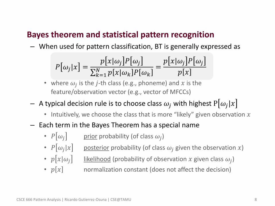
• Bayes theorem and statistical pattern recognition – When used for pattern classification, BT is generally expressed as
𝑃 𝜔𝑗|𝑥 =𝑝 𝑥|𝜔𝑗 𝑃 𝜔𝑗
𝑝 𝑥|𝜔𝑘 𝑃 𝜔𝑘𝑁𝑘=1
=𝑝 𝑥|𝜔𝑗 𝑃 𝜔𝑗
𝑝 𝑥
• where 𝜔𝑗 is the 𝑗-th class (e.g., phoneme) and 𝑥 is the
feature/observation vector (e.g., vector of MFCCs)
– A typical decision rule is to choose class 𝜔𝑗 with highest P 𝜔𝑗|𝑥
• Intuitively, we choose the class that is more “likely” given observation 𝑥
– Each term in the Bayes Theorem has a special name
• 𝑃 𝜔𝑗 prior probability (of class 𝜔𝑗)
• 𝑃 𝜔𝑗|𝑥 posterior probability (of class 𝜔𝑗 given the observation 𝑥)
• 𝑝 𝑥|𝜔𝑗 likelihood (probability of observation 𝑥 given class 𝜔𝑗)
• 𝑝 𝑥 normalization constant (does not affect the decision)
CSCE 666 Pattern Analysis | Ricardo Gutierrez-Osuna | CSE@TAMU 9
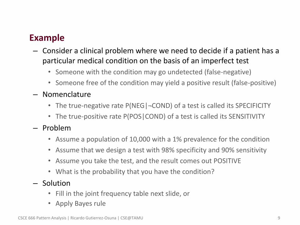
• Example – Consider a clinical problem where we need to decide if a patient has a
particular medical condition on the basis of an imperfect test
• Someone with the condition may go undetected (false-negative)
• Someone free of the condition may yield a positive result (false-positive)
– Nomenclature
• The true-negative rate P(NEG|¬COND) of a test is called its SPECIFICITY
• The true-positive rate P(POS|COND) of a test is called its SENSITIVITY
– Problem
• Assume a population of 10,000 with a 1% prevalence for the condition
• Assume that we design a test with 98% specificity and 90% sensitivity
• Assume you take the test, and the result comes out POSITIVE
• What is the probability that you have the condition?
– Solution • Fill in the joint frequency table next slide, or
• Apply Bayes rule
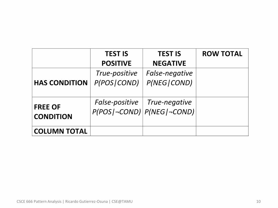
CSCE 666 Pattern Analysis | Ricardo Gutierrez-Osuna | CSE@TAMU 10
TEST IS POSITIVE
TEST IS NEGATIVE
ROW TOTAL
HAS CONDITION True-positive P(POS|COND)
100×0.90
False-negative P(NEG|COND) 100×(1-0.90)
100
FREE OF CONDITION
False-positive P(POS|¬COND) 9,900×(1-0.98)
True-negative P(NEG|¬COND)
9,900×0.98
9,900 COLUMN TOTAL 288 9,712 10,000
CSCE 666 Pattern Analysis | Ricardo Gutierrez-Osuna | CSE@TAMU 11
TEST IS POSITIVE
TEST IS NEGATIVE
ROW TOTAL
HAS CONDITION True-positive P(POS|COND)
100×0.90
False-negative P(NEG|COND) 100×(1-0.90)
100
FREE OF CONDITION
False-positive P(POS|¬COND) 9,900×(1-0.98)
True-negative P(NEG|¬COND)
9,900×0.98
9,900 COLUMN TOTAL 288 9,712 10,000
CSCE 666 Pattern Analysis | Ricardo Gutierrez-Osuna | CSE@TAMU 12
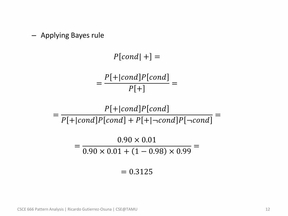
– Applying Bayes rule
𝑃 𝑐𝑜𝑛𝑑| + =
=𝑃 +|𝑐𝑜𝑛𝑑 𝑃 𝑐𝑜𝑛𝑑
𝑃 +=
=𝑃 +|𝑐𝑜𝑛𝑑 𝑃 𝑐𝑜𝑛𝑑
𝑃 +|𝑐𝑜𝑛𝑑 𝑃 𝑐𝑜𝑛𝑑 + 𝑃 +|¬𝑐𝑜𝑛𝑑 𝑃 ¬𝑐𝑜𝑛𝑑=
=0.90 × 0.01
0.90 × 0.01 + 1 − 0.98 × 0.99=
= 0.3125
CSCE 666 Pattern Analysis | Ricardo Gutierrez-Osuna | CSE@TAMU 13
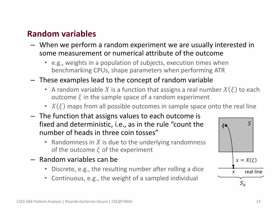
• Random variables – When we perform a random experiment we are usually interested in
some measurement or numerical attribute of the outcome • e.g., weights in a population of subjects, execution times when
benchmarking CPUs, shape parameters when performing ATR
– These examples lead to the concept of random variable • A random variable 𝑋 is a function that assigns a real number 𝑋 𝜉 to each
outcome 𝜉 in the sample space of a random experiment
• 𝑋 𝜉 maps from all possible outcomes in sample space onto the real line
– The function that assigns values to each outcome is fixed and deterministic, i.e., as in the rule “count the number of heads in three coin tosses” • Randomness in 𝑋 is due to the underlying randomness
of the outcome 𝜉 of the experiment
– Random variables can be • Discrete, e.g., the resulting number after rolling a dice
• Continuous, e.g., the weight of a sampled individual
𝝃
𝑥 = 𝑋 𝜉
𝑥
𝑆𝑥
real line
𝑆
CSCE 666 Pattern Analysis | Ricardo Gutierrez-Osuna | CSE@TAMU 14
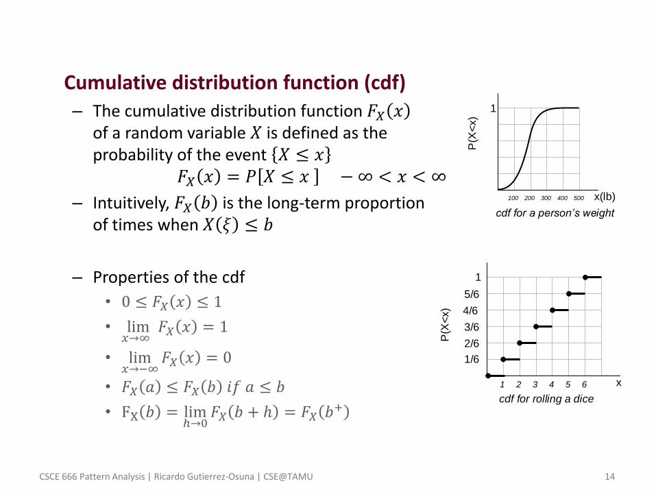
• Cumulative distribution function (cdf) – The cumulative distribution function 𝐹𝑋 𝑥
of a random variable 𝑋 is defined as the probability of the event 𝑋 ≤ 𝑥
𝐹𝑋 𝑥 = 𝑃 𝑋 ≤ 𝑥 − ∞ < 𝑥 < ∞
– Intuitively, 𝐹𝑋 𝑏 is the long-term proportion of times when 𝑋 𝜉 ≤ 𝑏
– Properties of the cdf
• 0 ≤ 𝐹𝑋 𝑥 ≤ 1
• lim𝑥→∞
𝐹𝑋 𝑥 = 1
• lim𝑥→−∞
𝐹𝑋 𝑥 = 0
• 𝐹𝑋 𝑎 ≤ 𝐹𝑋 𝑏 𝑖𝑓 𝑎 ≤ 𝑏
• FX 𝑏 = limℎ→0
𝐹𝑋 𝑏 + ℎ = 𝐹𝑋 𝑏+
1 2 3 4 5 6
P(X
<x)
x
cdf for rolling a dice
1
5/6
4/6
3/6
2/6
1/6
P(X
<x)
100 200 300 400 500 x(lb)
cdf for a person’s weight
1
CSCE 666 Pattern Analysis | Ricardo Gutierrez-Osuna | CSE@TAMU 15
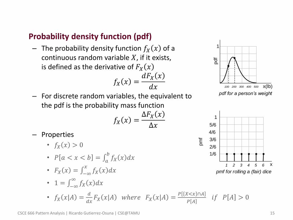
• Probability density function (pdf)
– The probability density function 𝑓𝑋 𝑥 of a continuous random variable 𝑋, if it exists, is defined as the derivative of 𝐹𝑋 𝑥
𝑓𝑋 𝑥 =𝑑𝐹𝑋 𝑥
𝑑𝑥
– For discrete random variables, the equivalent to the pdf is the probability mass function
𝑓𝑋 𝑥 =Δ𝐹𝑋 𝑥
Δ𝑥
– Properties
• 𝑓𝑋 𝑥 > 0
• 𝑃 𝑎 < 𝑥 < 𝑏 = 𝑓𝑋 𝑥 𝑑𝑥𝑏
𝑎
• 𝐹𝑋 𝑥 = 𝑓𝑋 𝑥 𝑑𝑥𝑥
−∞
• 1 = 𝑓𝑋 𝑥 𝑑𝑥∞
−∞
• 𝑓𝑋 𝑥|𝐴 =𝑑
𝑑𝑥𝐹𝑋 𝑥|𝐴 𝑤ℎ𝑒𝑟𝑒 𝐹𝑋 𝑥|𝐴 =
𝑃 𝑋<𝑥 ∩𝐴
𝑃 𝐴 𝑖𝑓 𝑃 𝐴 > 0
100 200 300 400 500
pd
f
x(lb)
pdf for a person’s weight
1
1 2 3 4 5 6
pm
f
x
pmf for rolling a (fair) dice
1
5/6
4/6
3/6
2/6
1/6

CSCE 666 Pattern Analysis | Ricardo Gutierrez-Osuna | CSE@TAMU 16
• What is the probability of somebody weighting 200 lb? • According to the pdf, this is about 0.62 • This number seems reasonable, right?
• Now, what is the probability of somebody weighting 124.876 lb?
• According to the pdf, this is about 0.43 • But, intuitively, we know that the probability should be zero (or very,
very small)
• How do we explain this paradox? • The pdf DOES NOT define a probability, but a probability DENSITY! • To obtain the actual probability we must integrate the pdf in an interval • So we should have asked the question: what is the probability of
somebody weighting 124.876 lb plus or minus 2 lb?
1 2 3 4 5 6
pm
f
x
pmf for rolling a (fair) dice
1
5/6
4/6
3/6
2/6
1/6
100 200 300 400 500
pd
f
x(lb)
pdf for a person’s weight
1
• The probability mass function is a ‘true’ probability (reason why we call it a ‘mass’ as opposed to a ‘density’)
• The pmf is indicating that the probability of any number when rolling a fair dice is the same for all numbers, and equal to 1/6, a very legitimate answer
• The pmf DOES NOT need to be integrated to obtain the probability (it cannot be integrated in the first place)

CSCE 666 Pattern Analysis | Ricardo Gutierrez-Osuna | CSE@TAMU 17
• Statistical characterization of random variables – The cdf or the pdf are SUFFICIENT to fully characterize a r.v.
– However, a r.v. can be PARTIALLY characterized with other measures
– Expectation (center of mass of a density)
𝐸 𝑋 = 𝜇 = 𝑥𝑓𝑋 𝑥 𝑑𝑥∞
−∞
– Variance (spread about the mean)
𝑣𝑎𝑟 𝑋 = 𝜎2 = 𝐸 𝑋 − 𝐸 𝑋 2 = 𝑥 − 𝜇 2𝑓𝑋 𝑥 𝑑𝑥∞
−∞
– Standard deviation 𝑠𝑡𝑑 𝑋 = 𝜎 = 𝑣𝑎𝑟 𝑋 1/2
– N-th moment
𝐸 𝑋𝑁 = 𝑥𝑁𝑓𝑋 𝑥 𝑑𝑥∞
−∞
CSCE 666 Pattern Analysis | Ricardo Gutierrez-Osuna | CSE@TAMU 18
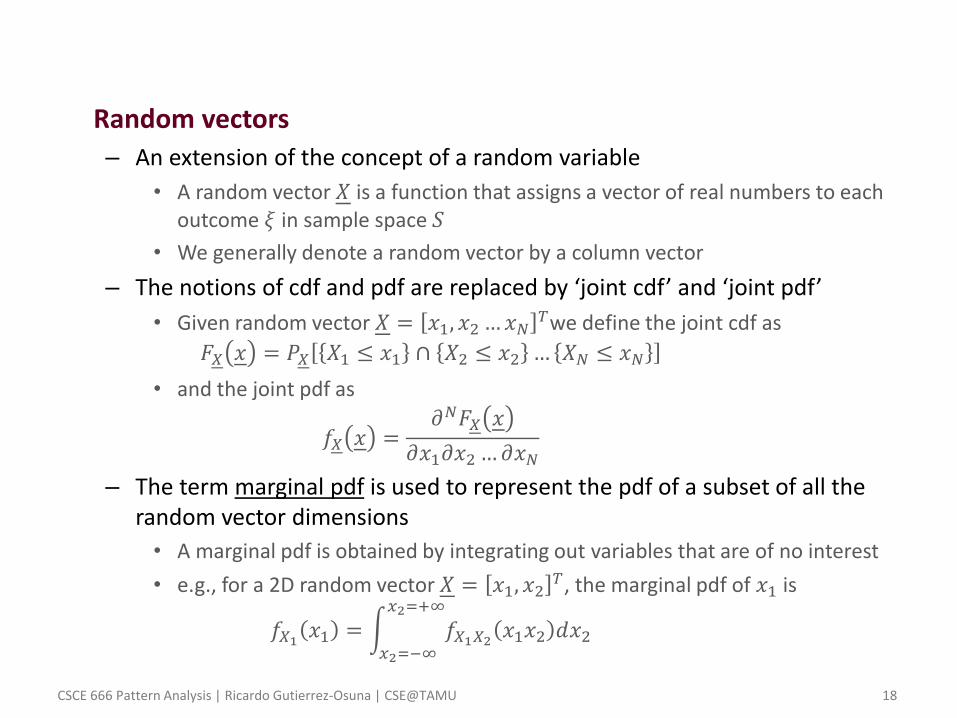
• Random vectors
– An extension of the concept of a random variable
• A random vector 𝑋 is a function that assigns a vector of real numbers to each outcome 𝜉 in sample space 𝑆
• We generally denote a random vector by a column vector
– The notions of cdf and pdf are replaced by ‘joint cdf’ and ‘joint pdf’
• Given random vector 𝑋 = 𝑥1, 𝑥2…𝑥𝑁𝑇we define the joint cdf as
𝐹𝑋 𝑥 = 𝑃𝑋 𝑋1 ≤ 𝑥1 ∩ 𝑋2 ≤ 𝑥2 … 𝑋𝑁 ≤ 𝑥𝑁
• and the joint pdf as
𝑓𝑋 𝑥 =𝜕𝑁𝐹𝑋 𝑥
𝜕𝑥1𝜕𝑥2…𝜕𝑥𝑁
– The term marginal pdf is used to represent the pdf of a subset of all the random vector dimensions
• A marginal pdf is obtained by integrating out variables that are of no interest
• e.g., for a 2D random vector 𝑋 = 𝑥1, 𝑥2𝑇, the marginal pdf of 𝑥1 is
𝑓𝑋1 𝑥1 = 𝑓𝑋1𝑋2 𝑥1𝑥2 𝑑𝑥2
𝑥2=+∞
𝑥2=−∞
CSCE 666 Pattern Analysis | Ricardo Gutierrez-Osuna | CSE@TAMU 19
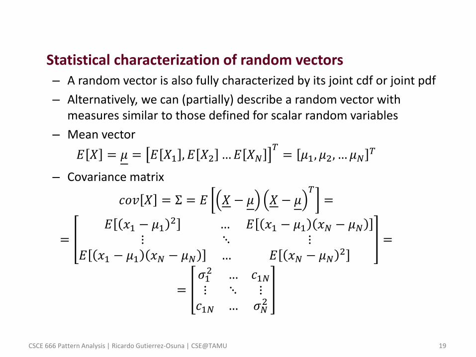
• Statistical characterization of random vectors – A random vector is also fully characterized by its joint cdf or joint pdf
– Alternatively, we can (partially) describe a random vector with measures similar to those defined for scalar random variables
– Mean vector
𝐸 𝑋 = 𝜇 = 𝐸 𝑋1 , 𝐸 𝑋2 …𝐸 𝑋𝑁𝑇= 𝜇1, 𝜇2, … 𝜇𝑁
𝑇
– Covariance matrix
𝑐𝑜𝑣 𝑋 = Σ = 𝐸 𝑋 − 𝜇 𝑋 − 𝜇𝑇=
=𝐸 𝑥1 − 𝜇1
2 … 𝐸 𝑥1 − 𝜇1 𝑥𝑁 − 𝜇𝑁⋮ ⋱ ⋮
𝐸 𝑥1 − 𝜇1 𝑥𝑁 − 𝜇𝑁 … 𝐸 𝑥𝑁 − 𝜇𝑁2
=
=𝜎12 … 𝑐1𝑁⋮ ⋱ ⋮𝑐1𝑁 … 𝜎𝑁
2
CSCE 666 Pattern Analysis | Ricardo Gutierrez-Osuna | CSE@TAMU 20
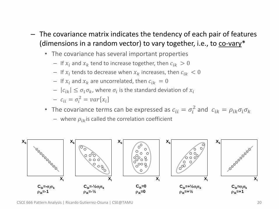
– The covariance matrix indicates the tendency of each pair of features (dimensions in a random vector) to vary together, i.e., to co-vary*
• The covariance has several important properties
– If 𝑥𝑖 and 𝑥𝑘 tend to increase together, then 𝑐𝑖𝑘 > 0
– If 𝑥𝑖 tends to decrease when 𝑥𝑘 increases, then 𝑐𝑖𝑘 < 0
– If 𝑥𝑖 and 𝑥𝑘 are uncorrelated, then 𝑐𝑖𝑘 = 0
– 𝑐𝑖𝑘 ≤ 𝜎1𝜎𝑘, where 𝜎𝑖 is the standard deviation of 𝑥𝑖
– 𝑐𝑖𝑖 = 𝜎𝑖2 = 𝑣𝑎𝑟 𝑥𝑖
• The covariance terms can be expressed as 𝑐𝑖𝑖 = 𝜎𝑖2 and 𝑐𝑖𝑘 = 𝜌𝑖𝑘𝜎𝑖𝜎𝑘
– where 𝜌𝑖𝑘 is called the correlation coefficient
Xi
Xk
Cik=-sisk
rik=-1
Xi
Xk
Cik=-½sisk
rik=-½
Xi
Xk
Cik=0
rik=0
Xi
Xk
Cik=+½sisk
rik=+½
Xi
Xk
Cik=sisk
rik=+1
CSCE 666 Pattern Analysis | Ricardo Gutierrez-Osuna | CSE@TAMU 21
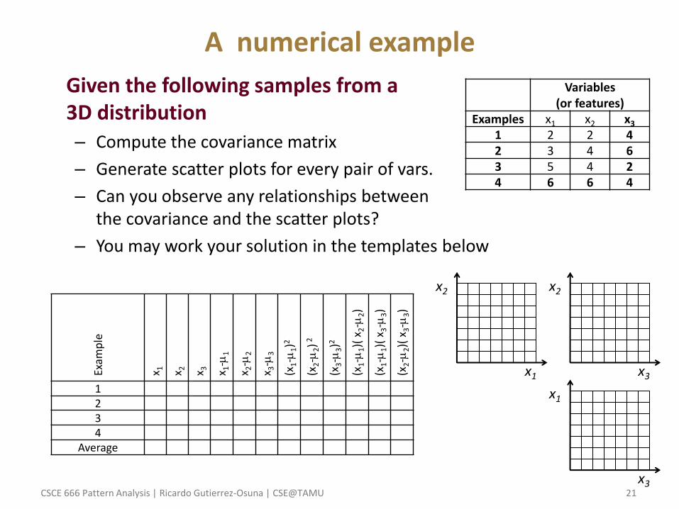
A numerical example
• Given the following samples from a 3D distribution – Compute the covariance matrix
– Generate scatter plots for every pair of vars.
– Can you observe any relationships between the covariance and the scatter plots?
– You may work your solution in the templates below
Exam
ple
x 1
x 2
x 3
x 1-
1
x 2-
2
x 3-
3
(x1-
1)2
(x2-
2) 2
(x3-
3)2
(x1-
1)(
x2-
2)
(x1-
1)(
x3-
3)
(x2-
2)(
x3-
3)
1 2 3 4
Average
Variables (or features)
Examples x1 x2 x3
1 2 2 4
2 3 4 6
3 5 4 2
4 6 6 4
x1
x2
x3
x2
x3
x1
CSCE 666 Pattern Analysis | Ricardo Gutierrez-Osuna | CSE@TAMU 22
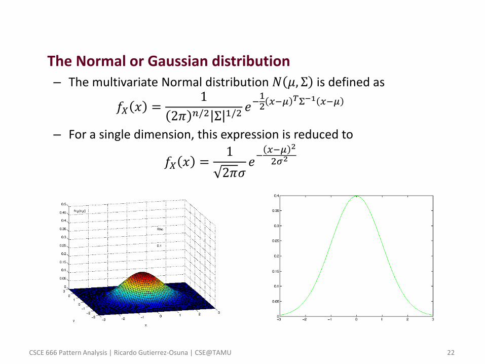
• The Normal or Gaussian distribution – The multivariate Normal distribution 𝑁 𝜇, Σ is defined as
𝑓𝑋 𝑥 =1
2𝜋 𝑛/2 Σ 1/2𝑒−12 𝑥−𝜇
𝑇Σ−1 𝑥−𝜇
– For a single dimension, this expression is reduced to
𝑓𝑋 𝑥 =1
2𝜋𝜎𝑒−𝑥−𝜇 2
2𝜎2
CSCE 666 Pattern Analysis | Ricardo Gutierrez-Osuna | CSE@TAMU 23
– Gaussian distributions are very popular since
• Parameters 𝜇, Σ uniquely characterize the normal distribution
• If all variables 𝑥𝑖 are uncorrelated 𝐸 𝑥𝑖𝑥𝑘 = 𝐸 𝑥𝑖 𝐸 𝑥𝑘 , then
– Variables are also independent 𝑃 𝑥𝑖𝑥𝑘 = 𝑃 𝑥𝑖 𝑃 𝑥𝑘 , and
– Σ is diagonal, with the individual variances in the main diagonal
• Central Limit Theorem (next slide)
• The marginal and conditional densities are also Gaussian
• Any linear transformation of any 𝑁 jointly Gaussian rv’s results in 𝑁 rv’s that are also Gaussian
– For 𝑋 = 𝑋1𝑋2…𝑋𝑁𝑇jointly Gaussian, and 𝐴𝑁×𝑁 invertible, then 𝑌 = 𝐴𝑋 is
also jointly Gaussian
𝑓𝑌 𝑦 =𝑓𝑋 𝐴
−1𝑦
𝐴
CSCE 666 Pattern Analysis | Ricardo Gutierrez-Osuna | CSE@TAMU 24
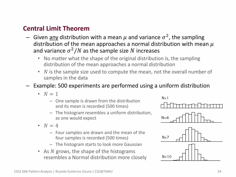
• Central Limit Theorem – Given any distribution with a mean 𝜇 and variance 𝜎2, the sampling
distribution of the mean approaches a normal distribution with mean 𝜇 and variance 𝜎2/𝑁 as the sample size 𝑁 increases • No matter what the shape of the original distribution is, the sampling
distribution of the mean approaches a normal distribution
• 𝑁 is the sample size used to compute the mean, not the overall number of samples in the data
– Example: 500 experiments are performed using a uniform distribution
• 𝑁 = 1 – One sample is drawn from the distribution
and its mean is recorded (500 times)
– The histogram resembles a uniform distribution, as one would expect
• 𝑁 = 4 – Four samples are drawn and the mean of the
four samples is recorded (500 times)
– The histogram starts to look more Gaussian
• As 𝑁 grows, the shape of the histograms resembles a Normal distribution more closely
Related Documents