METHODS ARTICLE published: 29 May 2012 doi: 10.3389/fpls.2012.00076 L-Py: an L-system simulation framework for modeling plant architecture development based on a dynamic language Frédéric Boudon 1 *, Christophe Pradal 1 ,Thomas Cokelaer 2 , Przemyslaw Prusinkiewicz 3 and Christophe Godin 2 * 1 CIRAD, Virtual Plants INRIATeam, Montpellier, France 2 INRIA, Virtual Plants INRIATeam, Montpellier, France 3 Department of Computer Science, University of Calgary, Calgary, AB, Canada Edited by: Basil Nikolau, Iowa State University, USA Reviewed by: Roeland Merks, Centrum Wiskunde & Informatica, Netherlands Haiquan Li, National University of Singapore, Singapore *Correspondence: Frédéric Boudon and Christophe Godin, INRIATeam Virtual Plants, UMR AGAP,TA A-108/02, Avenue Agropolis, 34398 Montpellier Cedex 5, France. e-mail: [email protected]; [email protected] The study of plant development requires increasingly powerful modeling tools to help under- stand and simulate the growth and functioning of plants. In the last decade, the formalism of L-systems has emerged as a major paradigm for modeling plant development. Previous implementations of this formalism were made based on static languages, i.e., languages that require explicit definition of variable types before using them. These languages are often efficient but involve quite a lot of syntactic overhead, thus restricting the flexibility of use for modelers. In this work, we present an adaptation of L-systems to the Python language, a popular and powerful open-license dynamic language. We show that the use of dynamic language properties makes it possible to enhance the development of plant growth models: (i) by keeping a simple syntax while allowing for high-level programming constructs, (ii) by making code execution easy and avoiding compilation overhead, (iii) by allowing a high-level of model reusability and the building of complex modular models, and (iv) by providing powerful solutions to integrate MTG data-structures (that are a common way to represent plants at several scales) into L-systems and thus enabling to use a wide spectrum of computer tools based on MTGs developed for plant architecture. We then illustrate the use of L-Py in real applications to build complex models or to teach plant modeling in the classroom. Keywords: L-system, Python language, plant modeling, MTG, development, environment, FSPM INTRODUCTION In the last two decades, the study of plant functioning and develop- ment has been accompanied and supported by the development of a new family of models called functional–structural models (FSPMs, Sievänen et al., 1997; Godin and Sinoquet, 2005; Hanan and Prusinkiewicz, 2008). These computational models use 3D representations of plant architecture to simulate different types of physical, physiological, or ecophysiological processes in plants, and make it possible to assess the effects of these processes on plant functioning, development, and form. The formalism of L-systems has emerged as the major par- adigm for constructing FSPMs (c.f. FSPM Special Issue, 2005, 2008, 2011). Introduced in the late 1960s by A. Lindenmayer as a formalism for describing developmental processes in biology (Lindenmayer, 1968), L-systems proved well suited to describe models of plant development (Prusinkiewicz and Lindenmayer, 1990; Prusinkiewicz, 1998, 1999). In L-systems, the plant is rep- resented by a bracketed string, whose elements, called modules, represent the plant’s components (metamers, meristems, flowers, etc.). Modules consist of a symbolic name and an optional set of parameters. Modules with the same name represent the same type of component (e.g., I for internode, M for meristem, etc.). A set of rules (also called productions) then defines how each module transforms over time. In particular, a module can pro- duce one or more new modules, thus giving a possibility of adding new components to the structure. Brackets are used to delimit the branches. When using L-systems, the modeler designs a set of L-system rules which, when applied step after step to the initial string (representing the initial state of the plant), will simulate its development. During the past 20 years, several implementations of L-systems have been designed. The main ones used in plant modeling have been cpfg (Prusinkiewicz and Lindenmayer, 1990; Hanan, 1992; Prusinkiewicz et al., 1999a), lpfg (Prusinkiewicz et al., 2007; Karwowski and Prusinkiewicz, 2003), and XL (Kniemeyer and Kurth, 2008). Cpfg introduced a dedicated modeling lan- guage, in which L-system rules are written using a mathemati- cal notation based on formal language theory. This notation is extended with C-like statements for specifying changes in para- meters values. In the early 2000s, cpfg was completely reengi- neered to address the needs of building more complex functional– structural models. This gave rise to a new modeling program lpfg and the modeling language L + C. L + C extends C++ with the notion of L-system productions. XL relies on a simi- lar approach, but is based on a different support language, Java, usually considered as a bit less efficient than C++ but which offers at no cost portability between the different operating sys- tems on which it runs. XL manipulates dynamic structures made of modules that fully support object-oriented definition and extends the L-systems paradigm by making it possible to define www.frontiersin.org May 2012 |Volume 3 | Article 76 | 1

Welcome message from author
This document is posted to help you gain knowledge. Please leave a comment to let me know what you think about it! Share it to your friends and learn new things together.
Transcript
METHODS ARTICLEpublished: 29 May 2012
doi: 10.3389/fpls.2012.00076
L-Py: an L-system simulation framework for modeling plantarchitecture development based on a dynamic languageFrédéric Boudon1*, Christophe Pradal 1,Thomas Cokelaer 2, Przemyslaw Prusinkiewicz 3 and
Christophe Godin2*
1 CIRAD, Virtual Plants INRIA Team, Montpellier, France2 INRIA, Virtual Plants INRIA Team, Montpellier, France3 Department of Computer Science, University of Calgary, Calgary, AB, Canada
Edited by:
Basil Nikolau, Iowa State University,USA
Reviewed by:
Roeland Merks, Centrum Wiskunde &Informatica, NetherlandsHaiquan Li, National University ofSingapore, Singapore
*Correspondence:
Frédéric Boudon andChristophe Godin, INRIA Team VirtualPlants, UMR AGAP, TA A-108/02,Avenue Agropolis, 34398 MontpellierCedex 5, France.e-mail: [email protected];[email protected]
The study of plant development requires increasingly powerful modeling tools to help under-stand and simulate the growth and functioning of plants. In the last decade, the formalismof L-systems has emerged as a major paradigm for modeling plant development. Previousimplementations of this formalism were made based on static languages, i.e., languagesthat require explicit definition of variable types before using them. These languages areoften efficient but involve quite a lot of syntactic overhead, thus restricting the flexibilityof use for modelers. In this work, we present an adaptation of L-systems to the Pythonlanguage, a popular and powerful open-license dynamic language. We show that the useof dynamic language properties makes it possible to enhance the development of plantgrowth models: (i) by keeping a simple syntax while allowing for high-level programmingconstructs, (ii) by making code execution easy and avoiding compilation overhead, (iii) byallowing a high-level of model reusability and the building of complex modular models, and(iv) by providing powerful solutions to integrate MTG data-structures (that are a commonway to represent plants at several scales) into L-systems and thus enabling to use a widespectrum of computer tools based on MTGs developed for plant architecture. We thenillustrate the use of L-Py in real applications to build complex models or to teach plantmodeling in the classroom.
Keywords: L-system, Python language, plant modeling, MTG, development, environment, FSPM
INTRODUCTIONIn the last two decades, the study of plant functioning and develop-ment has been accompanied and supported by the developmentof a new family of models called functional–structural models(FSPMs, Sievänen et al., 1997; Godin and Sinoquet, 2005; Hananand Prusinkiewicz, 2008). These computational models use 3Drepresentations of plant architecture to simulate different typesof physical, physiological, or ecophysiological processes in plants,and make it possible to assess the effects of these processes on plantfunctioning, development, and form.
The formalism of L-systems has emerged as the major par-adigm for constructing FSPMs (c.f. FSPM Special Issue, 2005,2008, 2011). Introduced in the late 1960s by A. Lindenmayer asa formalism for describing developmental processes in biology(Lindenmayer, 1968), L-systems proved well suited to describemodels of plant development (Prusinkiewicz and Lindenmayer,1990; Prusinkiewicz, 1998, 1999). In L-systems, the plant is rep-resented by a bracketed string, whose elements, called modules,represent the plant’s components (metamers, meristems, flowers,etc.). Modules consist of a symbolic name and an optional setof parameters. Modules with the same name represent the sametype of component (e.g., I for internode, M for meristem, etc.).A set of rules (also called productions) then defines how eachmodule transforms over time. In particular, a module can pro-duce one or more new modules, thus giving a possibility of adding
new components to the structure. Brackets are used to delimitthe branches. When using L-systems, the modeler designs a set ofL-system rules which, when applied step after step to the initialstring (representing the initial state of the plant), will simulate itsdevelopment.
During the past 20 years, several implementations of L-systemshave been designed. The main ones used in plant modelinghave been cpfg (Prusinkiewicz and Lindenmayer, 1990; Hanan,1992; Prusinkiewicz et al., 1999a), lpfg (Prusinkiewicz et al.,2007; Karwowski and Prusinkiewicz, 2003), and XL (Kniemeyerand Kurth, 2008). Cpfg introduced a dedicated modeling lan-guage, in which L-system rules are written using a mathemati-cal notation based on formal language theory. This notation isextended with C-like statements for specifying changes in para-meters values. In the early 2000s, cpfg was completely reengi-neered to address the needs of building more complex functional–structural models. This gave rise to a new modeling programlpfg and the modeling language L + C. L + C extends C++with the notion of L-system productions. XL relies on a simi-lar approach, but is based on a different support language, Java,usually considered as a bit less efficient than C++ but whichoffers at no cost portability between the different operating sys-tems on which it runs. XL manipulates dynamic structures madeof modules that fully support object-oriented definition andextends the L-systems paradigm by making it possible to define
www.frontiersin.org May 2012 | Volume 3 | Article 76 | 1
Boudon et al. L-Py, L-systems in Python
production rules on structures more general than trees, such asgraphs.
Despite the language difference, both L + C and XL, share thecommon feature of being based on languages that are staticallytyped. By making it mandatory to define the exact type of variablesthat are manipulated in every part of the programs, statically typedlanguages can optimize the handling of data-structures, efficiencyof computation, and early detection of errors (at compilationtime, before execution). On the other hand, they constrain theuser to strictly respect typing rules during programming, whichinvolves high-level of programming expertize for users and, as aconsequence, requires a steep learning curve (Ousterhout, 1998;Prechelt, 2000; Tratt, 2009). In contrast, dynamic languages areless exigent and do not require the specification of variable typesin the code. They do manipulate types, but the correctness ofvariable types in expressions is mainly checked during execution.This involves an extra burden in program execution, resulting ina loss of overall efficiency with respect to statically typed lan-guages, as many optimization schemes cannot be applied. Onthe positive side, the programming is more intuitive, the syn-tax is less austere, and the learning curve is much more shallowthan for static languages (Tratt, 2009). Ousterhout (1998) illus-trates this difference by pointing out that a typical statement in adynamic language is equivalent to 100–1000 elementary instruc-tions of the target machine while, in similar conditions, a typicalstatement in a static language corresponds to 1–10 elementaryinstructions. A higher level of abstraction is thus enabled bydynamic languages. Consequently, dynamic languages are fre-quently used as scripting languages, i.e., languages that allowfast prototyping both by fostering interactivity between program-mers and their programs during development and by makingit possible to glue together macroscopic software componentseasily.
The difference between static and dynamic languages canappear at first sight to be of a technical nature and of lit-tle interest to biologists. However, we suggest here that theuse of dynamic languages is particularly well adapted to thebuilding of simulation systems in developmental biology. Inmany modeling applications, the advantages of dynamic lan-guages over static ones make the former an attractive choicedespite their relative lower computational efficiency. They aremore intuitive for users with a limited background in com-puter science, while offering recent, powerful object-orientedprogramming constructs for more computationally orientedusers.
In this work, we explored the adaptation of dynamic lan-guages to the modeling of plant growth. For this, we designed anew open-source L-system-based modeling environment based onPython, a popular and powerful dynamic language. An overviewof the resulting language, L-Py, and its programming environ-ment is presented in Section “L-Py Overview.” Then we describehow L-Py can be used to model plant development at sev-eral scales. For topology, we extend classical L-strings to rep-resent MTGs (formalism to represent the multiscale nature ofplants), which makes it possible to seamlessly integrate a wideset of model components and tools already designed for MTGs
into L-Py programs. For geometry, new primitives have beenintroduced in the language to describe plant components in ahigh-level manner and at different scales. Finally, we illustrate theuse of L-Py in real modeling applications, composed of multi-ple modeling components and for developing training programson modeling in the classroom (see Example of FSPM Appli-cations in L-Py). All the code excerpts given in the paper areactual L-Py code. The corresponding example files can be down-loaded together with the L-Py software through the OpenAleadistribution (http://openalea.gforge.inria.fr).
L-Py OVERVIEWEmbedding L-systems into a dynamic language such as Python hasa number of consequences on the language syntax, its interpreter,the programming environment, and the openness of the system(i.e., its ability to interact with external components).
A SIMPLE SYNTAX OWING TO DYNAMIC TYPINGTo integrate L-systems into Python, we followed a methodologysimilar to that used by Karwowski and Prusinkiewicz (2003) todesign and implement L + C. L-system constructs were thus addedto the syntax of Python, following the syntax of cpfg and L + Cas closely as possible for compatibility between L + C and L-Py.However, some constructs inherit specifically from the Python lan-guage syntax. Compared to L + C, the L-Py syntax is simplified byavoiding type declaration of parameters and variables. A simpleexample of L-Py code is given below.
Lsystem1:1 module Apex(age), Internode(length, radius)2 MAX_AGE, dr = 10, 0.02 # constants3 Axiom: Apex(0)4 production:5 Internode(l,r) --> Internode(l,r + dr)6 Apex(age):7 if age < MAX_AGE:8 produce Internode(1,0.05)/(137.5)[+(40)Apex(age+1)]
Apex(age+1)
The main components of this code are as follows.
ModulesIn L-systems, plant structures are decomposed into physical unitscalled modules. The set of modules forms a branching structurethat is represented by a bracketed string of modules (Linden-mayer, 1968; Prusinkiewicz and Lindenmayer, 1990; Hanan, 1992),here that we call here L-string. By default, any character can be avalid module name. Modules containing more than one charac-ter must be declared. Module parameters may also be declaredto make explicit their role (although this is not mandatory), e.g.,Apex(age) may represent an apex characterized by its age, asin line 1 of the above example. In this case, if Apex is found in astring, it will be interpreted as one module instead of four differ-ent modules, namely A, p, e, and x. Module parameters (such asage) are Python objects and can be of any type.
AxiomA specific string of modules, called the axiom, defines the ini-tial state of the simulation. This string is declared by using the
Frontiers in Plant Science | Technical Advances in Plant Science May 2012 | Volume 3 | Article 76 | 2
Boudon et al. L-Py, L-systems in Python
keyword Axiom. In the example, the axiom is a string made of asingle module Apex(0), representing the initial structure of theplant.
RulesThe keyword production indicates the beginning of ruledeclarations. As in cpfg, rules may have the syntax:
Predecessor --> Successor
or, more generally
LeftContext < Predecessor > RightContext --> Successor
where Predecessor and Successor are strings of modules,and both LeftContext and RightContext are optionalstrings of modules. The rules can be expressed using two conven-tions. Simple rules can be written in a compact mathematical stylesimilar to cpfg (Prusinkiewicz and Lindenmayer, 1990; Hanan,1992), e.g., line 5. Alternatively, for more complex rules, succes-sor specifications are declared as in L + C using the producestatement (instead of the arrow -->) embedded into regularPython code, e.g., line 8. In this case, predecessors are separatedfrom the right-hand side of the rules by a colon (line 6) con-sistently with the syntax of Python functions. For example, therule of lines (6–8) replaces every Apex with parameter age infe-rior to MAX_AGE (line 7) with an Internode module followedby a lateral Apex and the main Apex. Lateral Apex is includedin brackets. Two geometric symbols, / and +, make it possibleto specify phyllotactic and insertion angles for the interpreta-tion, respectively. The strings generated by this simple L-systemin the first three simulation steps (starting with the axiom w0)will be:
w0:Apex(0)w1:Internode(1,0.05)/(137.5)[+(40)Apex(1)]Apex(1)w2:Internode(1,0.07)/(137.5)[+(40)Internode(1,0.05)/(137.5)[+(40)Apex(2)]Apex(2)]Internode(1,0.05)/(137.5)[+(40)Apex(2)]Apex(2)
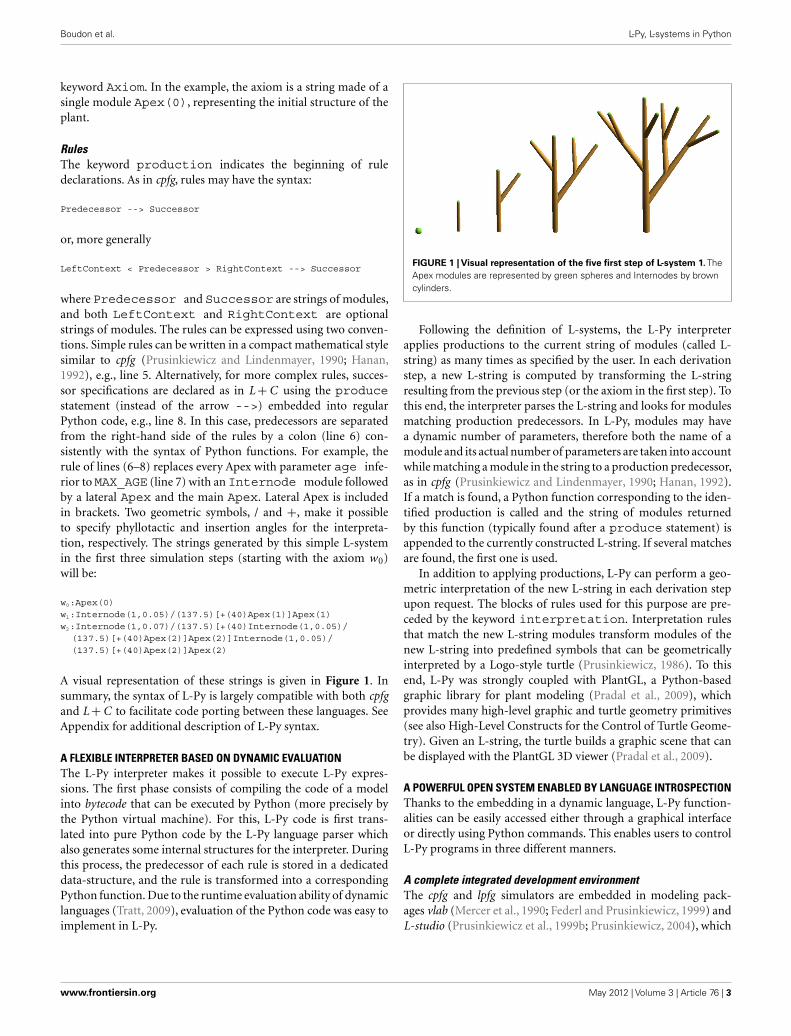
A visual representation of these strings is given in Figure 1. Insummary, the syntax of L-Py is largely compatible with both cpfgand L + C to facilitate code porting between these languages. SeeAppendix for additional description of L-Py syntax.
A FLEXIBLE INTERPRETER BASED ON DYNAMIC EVALUATIONThe L-Py interpreter makes it possible to execute L-Py expres-sions. The first phase consists of compiling the code of a modelinto bytecode that can be executed by Python (more precisely bythe Python virtual machine). For this, L-Py code is first trans-lated into pure Python code by the L-Py language parser whichalso generates some internal structures for the interpreter. Duringthis process, the predecessor of each rule is stored in a dedicateddata-structure, and the rule is transformed into a correspondingPython function. Due to the runtime evaluation ability of dynamiclanguages (Tratt, 2009), evaluation of the Python code was easy toimplement in L-Py.
FIGURE 1 | Visual representation of the five first step of L-system 1. TheApex modules are represented by green spheres and Internodes by browncylinders.
Following the definition of L-systems, the L-Py interpreterapplies productions to the current string of modules (called L-string) as many times as specified by the user. In each derivationstep, a new L-string is computed by transforming the L-stringresulting from the previous step (or the axiom in the first step). Tothis end, the interpreter parses the L-string and looks for modulesmatching production predecessors. In L-Py, modules may havea dynamic number of parameters, therefore both the name of amodule and its actual number of parameters are taken into accountwhile matching a module in the string to a production predecessor,as in cpfg (Prusinkiewicz and Lindenmayer, 1990; Hanan, 1992).If a match is found, a Python function corresponding to the iden-tified production is called and the string of modules returnedby this function (typically found after a produce statement) isappended to the currently constructed L-string. If several matchesare found, the first one is used.
In addition to applying productions, L-Py can perform a geo-metric interpretation of the new L-string in each derivation stepupon request. The blocks of rules used for this purpose are pre-ceded by the keyword interpretation. Interpretation rulesthat match the new L-string modules transform modules of thenew L-string into predefined symbols that can be geometricallyinterpreted by a Logo-style turtle (Prusinkiewicz, 1986). To thisend, L-Py was strongly coupled with PlantGL, a Python-basedgraphic library for plant modeling (Pradal et al., 2009), whichprovides many high-level graphic and turtle geometry primitives(see also High-Level Constructs for the Control of Turtle Geome-try). Given an L-string, the turtle builds a graphic scene that canbe displayed with the PlantGL 3D viewer (Pradal et al., 2009).
A POWERFUL OPEN SYSTEM ENABLED BY LANGUAGE INTROSPECTIONThanks to the embedding in a dynamic language, L-Py function-alities can be easily accessed either through a graphical interfaceor directly using Python commands. This enables users to controlL-Py programs in three different manners.
A complete integrated development environmentThe cpfg and lpfg simulators are embedded in modeling pack-ages vlab (Mercer et al., 1990; Federl and Prusinkiewicz, 1999) andL-studio (Prusinkiewicz et al., 1999b; Prusinkiewicz, 2004), which
www.frontiersin.org May 2012 | Volume 3 | Article 76 | 3
Boudon et al. L-Py, L-systems in Python
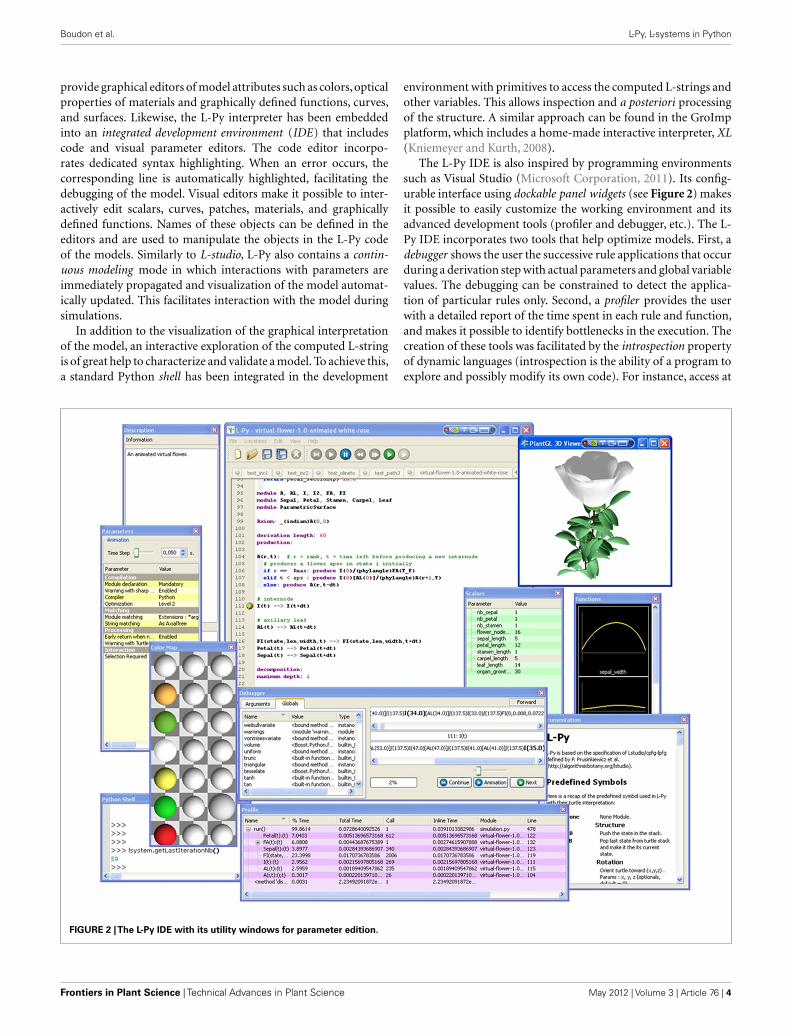
provide graphical editors of model attributes such as colors, opticalproperties of materials and graphically defined functions, curves,and surfaces. Likewise, the L-Py interpreter has been embeddedinto an integrated development environment (IDE) that includescode and visual parameter editors. The code editor incorpo-rates dedicated syntax highlighting. When an error occurs, thecorresponding line is automatically highlighted, facilitating thedebugging of the model. Visual editors make it possible to inter-actively edit scalars, curves, patches, materials, and graphicallydefined functions. Names of these objects can be defined in theeditors and are used to manipulate the objects in the L-Py codeof the models. Similarly to L-studio, L-Py also contains a contin-uous modeling mode in which interactions with parameters areimmediately propagated and visualization of the model automat-ically updated. This facilitates interaction with the model duringsimulations.
In addition to the visualization of the graphical interpretationof the model, an interactive exploration of the computed L-stringis of great help to characterize and validate a model. To achieve this,a standard Python shell has been integrated in the development
environment with primitives to access the computed L-strings andother variables. This allows inspection and a posteriori processingof the structure. A similar approach can be found in the GroImpplatform, which includes a home-made interactive interpreter, XL(Kniemeyer and Kurth, 2008).
The L-Py IDE is also inspired by programming environmentssuch as Visual Studio (Microsoft Corporation, 2011). Its config-urable interface using dockable panel widgets (see Figure 2) makesit possible to easily customize the working environment and itsadvanced development tools (profiler and debugger, etc.). The L-Py IDE incorporates two tools that help optimize models. First, adebugger shows the user the successive rule applications that occurduring a derivation step with actual parameters and global variablevalues. The debugging can be constrained to detect the applica-tion of particular rules only. Second, a profiler provides the userwith a detailed report of the time spent in each rule and function,and makes it possible to identify bottlenecks in the execution. Thecreation of these tools was facilitated by the introspection propertyof dynamic languages (introspection is the ability of a program toexplore and possibly modify its own code). For instance, access at
FIGURE 2 |The L-Py IDE with its utility windows for parameter edition.
Frontiers in Plant Science | Technical Advances in Plant Science May 2012 | Volume 3 | Article 76 | 4

Boudon et al. L-Py, L-systems in Python
runtime to the names and values of the different variables involvedin a procedure is simple in a dynamic language and facilitates, forinstance, the creation of the debugger.
L-Py as a component library: controlling L-systems execution fromPythonL-Py has been developed as a C++ library embedded in Pythonthat can thus be integrated into any Python-compatible appli-cation. For this, the L-Py library defines a number of structures(module, L-string, rule, L-system, etc.) that can be accessed fromPython in an object-oriented manner. As a result, an L-systemmodel can easily be manipulated by an external process. Such aprocess typically creates an L-system object, executes it for a num-ber of specified steps, possibly changes its parameters, resumesthe execution, and finally gets the computed L-string. In this way,L-Py can be encapsulated as a simple component of a more com-plex modeling pipeline that integrates other components, possiblyusing formalisms different from L-systems.
The central issue of such an encapsulation strategy is to controlthe execution of L-Py models. An L-Py program contains globalvariables, functions, rules, and configuration/execution variablessuch as the number of derivation steps. From an external process, auser may want to access and change any of these elements. In L-Py,this can be done by using the Python/L-Py introspection mecha-nism or by using dedicated primitives implemented in L-Py. Forinstance, to explore a large parameter space for a given L-system,a user may want to vary parameters (e.g., global variables) of anL-system model after each execution. Such exploration cannot bemade easily manually. The use of the introspection property of L-Pymakes it possible to resolve this issue elegantly: a process that usesL-Py as a component can inquire about the internal variables ofthe L-Py model (global and configuration/execution variable) anddirectly access and modify them in memory. Global variables ofthe model become automatically and dynamically attributes of theL-system structure that contains the model, and can be modified aseasily as any attribute of a Python object. Execution variables canalso be modified with predefined L-Py functions. For example, tooverwrite the axiom of an existing L-system object, an L-string canbe built from a specified string of characters with the Lstringconstruct and then used to overwrite the contents of the L-systemaxiom. More generally, L-strings can be built from modules con-taining objects of any complex type as parameter values. Thanksto the dynamic typing of the language, parameters of any typecan be introduced into the L-string and passed to an L-system.For example, the following program creates and runs iterativelyLsystem1 using an increasing value of the global variable dr,incremented externally in each step.
Code2:1 lsys = Lsystem(‘Lsystem1.lpy’)2 print lsys.dr # This would print 0.023 axiom = Lstring(‘Apex(2)’,lsys)4 for i in range(10):5 lsys.dr += 0.026 lstring = lsys.derive(axiom,5)7 interpretedstring = lsys.interpret(lstring)8 scene = lsys.turtle_interpretation(interpretedstring)9 Viewer.display(scene)
Line 1 reads in and creates an L-system structure from theLsystem1 code. The second line requests and prints the value
of the internal variable dr from the model lsys. Note that theglobal variables such as dr are automatically considered as attrib-utes of the L-system object. Line 3 creates an L-system string froma text string, using lsys module definition to interpret correctlythe module names. This L-string will be used subsequently as theL-system axiom. Line 4 initiates a loop that will perform parame-ter space exploration for ten values of the dr parameter. At eachiteration step, Line 5 changes the value of dr before performing5 Lsystem derivation steps starting from the axiom (line 6) andassigns the resulting string to lstring. Note that in this case,only the production rules and the global variables of the L-systemare used in the object, while the initial string (axiom) can be con-sidered as a variable (notion of L-system scheme, Herman andRozenberg, 1975). The function derive can also be called withno argument and will use in this case the values of the axiom andthe number of derivation to perform declared in the L-system.Finally, lines 7–9 interpret the resulting string geometrically usingthe turtle interpretation, and display the result in the viewer. Theselines can also be summarized into one (more efficient) com-mand lsys.plot (lstring). However, they are given here toshow that a user can finely control the execution of an L-system.Importantly, entire functions and productions of complex modelscan be changed similarly to the simple variable dr in the aboveexample.
Creation and manipulation of an L-system object have alsobeen encapsulated into OpenAlea (Pradal et al., 2008) as compu-tational nodes. Similarly to the example provided here, these nodescan be created with L-Py code and parameterized with a dictionarycontaining the names and new values of the variables. Examplesof such use are given in Section “L-Py as Growth Component forSimulating an FSPM.”
The L-Py introspection mechanism: controlling L-system executionfrom L-Py programsL-Py makes it also possible to control its execution, vari-ables, and rules from within L-Py models. For instance,the ExecutionContext object is accessible through theexecContext() function and makes it possible to ask andmodify the values of the L-Py model configuration/execution vari-ables. These variables control the number of derivation steps, thecurrently used group, etc. (a complete list is given in the onlinehelp; see also Standard L-Systems Features of L-Py in Appen-dix). After each iteration modelers also have access, through theEndEach function, to the resulting L-string and the correspond-ing scene graph. This enables global post-processing of the mod-eled structure using regular Python code and external modulesfrom within a model. In this way, an L-Py model can also actas an integrative framework for different modeling components(see for instance section “Minimizing Measurements in 3D PlantArchitecture Reconstruction”). For example,
Lsystem3:1 Axiom: A2 production:3 A--> B4 B--> AB
produces a sequence of strings whose lengths follow the Fibonacciseries. It can also be shown that the string produced in step t is the
www.frontiersin.org May 2012 | Volume 3 | Article 76 | 5

Boudon et al. L-Py, L-systems in Python
concatenation of the strings produced in steps t-2 and t-1. Check-ing visually these properties with L-Py is easy and requires onlyadding two lines of code:
Lsystem3 (continued):5 def EndEach(lstring):6 print len(lstring), lstring
These lines print the length and the value of the current L-stringand are called after each derivation step. The output exhibits theFibonacci properties of the model:
Lsystem3 (output):1 A1 B2 AB3 BAB5 ABBAB8 BABABBAB
Modification to the string can be made in a similar way from withina L-Py model. Likewise, thanks to the dynamic language evalua-tion, it is possible to add or remove a rule during the execution ofan L-system.
MODULAR L-SYSTEMS IN L-PyCode modularity is the key to build complex and reusable mod-els. In our context, this raises the question of building reusableblocks based on L-systems that can subsequently be assembled.Modularity of the model may result from the decomposition ofthe structure into components such as internodes or leaves, whichcan be processed and defined independently (Hanan, 1992; Godinet al., 1998; Prusinkiewicz et al., 1999a) or from the decompositionof the model into of component aspects such as growth, photo-synthesis, and hormone transport (Cieslak et al., 2011). In thissection, we discuss the support for decomposition into aspects,offered by L-Py.
One technique supporting such decomposition was proposedby Federl and Prusinkiewicz (2004), based on the concept of con-trolled derivations in L-systems. Different groups of productionrules are identified by group Ids. Only one group is active inany derivation step. However, another group may be activated inthe next derivation step, and so on. The selection of the appro-priate group can be conveniently made before each derivationstep using the StartEach statement. Within a static language,however, parameters of the modules are declared at the begin-ning of the model and their declaration should take into accountall parameters required for all groups. This limits the indepen-dence of the groups and thus the modularity of the compositeL-system.
More recently, Cieslak et al. (2011) proposed another strategyto develop modular L-systems, based on the use of separate mod-ules to represent different aspects of the model. These modulescan be combined such that one organ of the plant is representedby a list of modules, each reflecting a different aspect of the model.The rules related to the different aspects are described in differentgroups and are invoked sequentially. While this makes it possibleto have separate definition of each group with their own modulesand rules, a given element is modeled in this approach with severalmodules, which blurs its identity.
In L-Py, we elaborated on the approach of Federl andPrusinkiewicz (2004) and extended it with the use of a dynamiclanguage to reinforce the decoupling of the different L-systems toassemble. The goal is to combine several independent L-systems,typically written by different persons, in different files (say forexample files A.lpy, B.lpy, C.lpy). Each L-system can beconsidered as a processing unit dealing with an aspect of sim-ulation, for example substance transport, branch mechanics, orgrowth. An order may have to be respected in the application ofthe corresponding L-systems, as some of them may update L-stringparameters subsequently used by other L-systems. We assume thatthe different L-systems operate on the same or closely related setsof plant components, e.g., apices, growth units, or internodes. Assimilar components in different L-systems may be identified by dif-ferent module names, a mapping between these names is definedin the third “translation” L-system. For instance, if the modulerepresenting an internode is named I in L-system A and S in L-system B, a ruleI-->Swill be created in the translation L-systemA2B.Module parameters must also be translated. Detailed exam-ples of how this is done are given in Section “Managing L-SystemModularity” in Appendix.
Different L-systems and their translations can be chainedby the programmer to make up a unique compound L-system. To easily handle such chaining, a generic Python classComposedLsystem is provided in L-Py. It takes two arguments:a list of L-systems to be chained (including translation schemes)and a list of interpretation schemes to be chained. A sketch of atypical code that must be defined to combine different L-systemsfollows.
Code4:1 a,b,c = Lsystem(‘A.lpy’),Lsystem(‘B.lpy’),Lsystem(‘C.lpy’)
2 a2b, b2a, a2c = Lsystem(‘A2B.lpy’),Lsystem(‘B2A.lpy’),Lsystem(‘A2C.lpy’)
3 clsystem = ComposedLsystem([a,a2b,b,b2a],[a2c,c])4 lstring = clsystem.axiom5 for i in xrange(K):6 lstring = clsystem.derive(lstring)7 clsystem.plot(lstring)
The first two lines create the different L-systems required for themodel. The third line gathers them into a ComposedLsystem struc-ture. As arguments, two lists of L-systems are given. The first listcontains the set of L-systems responsible for the production rulesand the second list for the interpretation, given in the order inwhich they should be called. In the first list, the target L-system ofthe last translation (the “a” in b2a in the example below) mustbe identical to the first L-system of this list, while in the secondlist, the source L-system of the first translation (“a” in a2c) mustbe identical to the last L-system of the first list (i.e., “a” also). Thenext four lines simply run and plot the ComposedLsystem for anumber K of iterations as if it were a simple L-system. In this casethe chaining of L-systems is controlled by the ComposedLsystemprimitive, but the modeler still has the possibility to write codethat calls each Lsystem one after another a number of times (forinstance to handle different time units in the different L-systems).
This approach shows a great flexibility in assembling com-ponents by transforming L-strings expressed in the alphabet of
Frontiers in Plant Science | Technical Advances in Plant Science May 2012 | Volume 3 | Article 76 | 6
Boudon et al. L-Py, L-systems in Python
one L-system to that of another one. This approach may be com-bined with sub-Lsystems or other aspect-oriented approaches intoa completely flexible and modular L-system framework.
MODELING PLANT GROWTH AT DIFFERENT SCALES IN L-PyThe embedding of L-Py in a dynamic language has a number ofconsequences on the modeling possibilities themselves. Due to thenon-strict typing system, connection with external modules andmodels is much simpler than with static languages. Here, we inves-tigate the consequences of this language specificity to key aspectsof plant modeling.
SEAMLESSLY COMBINING L-SYSTEMS AND MTGsIn the late 1990s, Godin and Caraglio (1998) introduced a formalmodel called Multiscale Tree Graph (MTG) to represent a widerange of plant architectures, at varying scales of description, in aflexible and unified way. Since then, MTGs have been used widelyto encode various types of plant architectures at varying scales(e.g., Godin et al., 1999; Mündermann et al., 2005; Teobaldelliet al., 2008) and to analyze the resulting data with dedicated soft-ware such as AMAPmod (Godin and Guédon,1997) and OpenAlea(Pradal et al., 2008). Today, in OpenAlea, MTG is the central data-structure that different modeling packages use as a standardizedway to represent plants.
In order to exploit the large library of algorithms and mod-els built for MTGs in L-Py, we designed bidirectional translationand mapping mechanisms between L-strings and MTGs. Conver-sion between these structures is possible as they both representa particular type of labeled tree graphs. L-strings represent axialtree graphs (Prusinkiewicz and Lindenmayer, 1990) while MTGsmay integrate tree graph descriptions at several scales (Godin andCaraglio, 1998). Fortunately, it has been shown that, similarlyto simple tree graphs, multiscale tree graphs can be encoded asstrings (Godin et al., 1999). L-strings corresponding to MTGs canbe defined using this property (Godin et al., 1999; Ferraro andGodin, 2000).
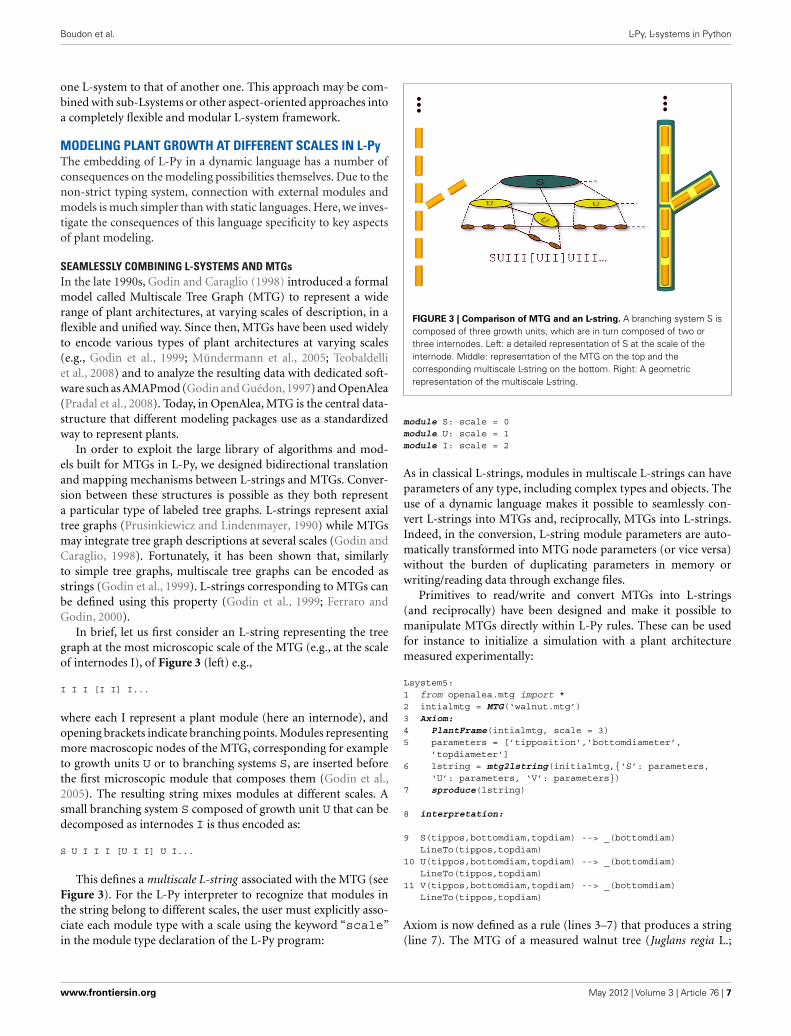
In brief, let us first consider an L-string representing the treegraph at the most microscopic scale of the MTG (e.g., at the scaleof internodes I), of Figure 3 (left) e.g.,
I I I [I I] I...
where each I represent a plant module (here an internode), andopening brackets indicate branching points. Modules representingmore macroscopic nodes of the MTG, corresponding for exampleto growth units U or to branching systems S, are inserted beforethe first microscopic module that composes them (Godin et al.,2005). The resulting string mixes modules at different scales. Asmall branching system S composed of growth unit U that can bedecomposed as internodes I is thus encoded as:
S U I I I [U I I] U I...
This defines a multiscale L-string associated with the MTG (seeFigure 3). For the L-Py interpreter to recognize that modules inthe string belong to different scales, the user must explicitly asso-ciate each module type with a scale using the keyword “scale”in the module type declaration of the L-Py program:
FIGURE 3 | Comparison of MTG and an L-string. A branching system S iscomposed of three growth units, which are in turn composed of two orthree internodes. Left: a detailed representation of S at the scale of theinternode. Middle: representation of the MTG on the top and thecorresponding multiscale L-string on the bottom. Right: A geometricrepresentation of the multiscale L-string.
module S: scale = 0module U: scale = 1module I: scale = 2
As in classical L-strings, modules in multiscale L-strings can haveparameters of any type, including complex types and objects. Theuse of a dynamic language makes it possible to seamlessly con-vert L-strings into MTGs and, reciprocally, MTGs into L-strings.Indeed, in the conversion, L-string module parameters are auto-matically transformed into MTG node parameters (or vice versa)without the burden of duplicating parameters in memory orwriting/reading data through exchange files.
Primitives to read/write and convert MTGs into L-strings(and reciprocally) have been designed and make it possible tomanipulate MTGs directly within L-Py rules. These can be usedfor instance to initialize a simulation with a plant architecturemeasured experimentally:
Lsystem5:1 from openalea.mtg import *2 intialmtg = MTG(‘walnut.mtg’)3 Axiom:4 PlantFrame(intialmtg, scale = 3)5 parameters = [’tipposition’,’bottomdiameter’,
’topdiameter’]6 lstring = mtg2lstring(initialmtg,{‘S’: parameters,
‘U’: parameters, ‘V’: parameters})7 sproduce(lstring)
8 interpretation:
9 S(tippos,bottomdiam,topdiam) --> _(bottomdiam)LineTo(tippos,topdiam)
10 U(tippos,bottomdiam,topdiam) --> _(bottomdiam)LineTo(tippos,topdiam)
11 V(tippos,bottomdiam,topdiam) --> _(bottomdiam)LineTo(tippos,topdiam)
Axiom is now defined as a rule (lines 3–7) that produces a string(line 7). The MTG of a measured walnut tree (Juglans regia L.;
www.frontiersin.org May 2012 | Volume 3 | Article 76 | 7
Boudon et al. L-Py, L-systems in Python
Sinoquet et al., 1997) is first loaded (line 2, note that the func-tions for manipulating MTGs, such as MTG and PlantFrameused here, are independently provided by the MTG package ofOpenAlea). This file contains the information related to the topol-ogy of the plant at three different scales (axis segments, axes,and plant). In addition, for some plant segments, it containskey information about their geometry, called “frame” informa-tion (this information was not systematically measured for allplant segments in the field). The frame information consists ofthe spatial location of the segment tip in a reference coordinatesystem originating at the basis of the plant, together with theirbottom and top diameters. Based on the frame information avail-able for some segments in the MTG, the PlantFrame functionmakes it possible to compute the frame information for all theplant segments where it is missing, using predefined inferencerules (Godin et al., 1999). As a result, the frame attributes (’tipposition’,’bottomdiameter’,’topdiameter’) ofthe segments of the MTG are updated with the computed infor-mation. The MTG is then transformed into a multiscale L-string(lines 5–6), where the different modules corresponding to theplant segments (here labeled S, U, V) are given parameterscorresponding to their frame information in the MTG. Finally,the sproduce statement of line 7 produces the multiscale L-string corresponding to the MTG (one can note the differencebetween produce and sproduce: produce creates a suc-cessor L-string from a list of modules, while sproduce createsa successor L-string from an already built L-string structure). Theaxiom defined by this string has thus been procedurally evaluated.Finally, to plot a graphical representation of the axiom, a simpleinterpretation rule is defined for each type of module (line 9–11)that uses the turtle to draw the complete plant structure by exploit-ing the frame data of the successive plant segments along the plantaxes (Figure 9, left).
HIGH-LEVEL CONSTRUCTS FOR THE CONTROL OF TURTLE GEOMETRYAs illustrated in the previous sections, the use of a dynamic lan-guage such as Python favors the openness of the modeling language(i.e., its ability to be extended) and its simplicity of use by pro-viding high-level constructs in the language. Both characteristicswere considered as key guiding principles throughout the designof L-Py. In this section, we show how these principles were usedto simplify the modeling of plant geometry by introducing newconstructs to manipulate turtle geometry at high abstraction level.
Custom geometric primitives for plant representation at differentscalesWhen representing plant architecture, most simulation systemsuse an explicit geometric representation of plant organs: intern-odes are represented by cylinders, leaves by small parametricsurfaces, fruits by volumetric models, roots by generalized cylin-ders, etc. In recent years, however, abstract geometric models ofplant organs have been introduced to represent plant architecturesat more macroscopic scales in simulation models (e.g., Cescatti,1997; Boudon, 2004; Pradal et al., 2009; Livny et al., 2011). Theseapproaches are based on the use of either volume or envelopemodels that represent groups of organs instead of individualorgans. Such models can be readily designed in L-Py thanks to
the tight coupling with the PlantGL library (Pradal et al., 2009). Ageneric primitive, @g(geometry), allows the modeler to posi-tion any PlantGL model in space using the current turtle locationand orientation. In this way, coarse geometric representations ofplant architecture can be defined where parts of the tree crown arerepresented by parametric envelopes. The resulting architecturemay then be used in conjunction with ecophysiological modelsthat take a 3D scene as an input. Here we illustrate this possibilityby computing the direct illumination of each crownlet in the plantusing the Fractalysis library (Da Silva et al., 2008) from OpenAlea:
Lsystem6:1 from openalea.plantgl.all import AsymmetricHull2 from openalea.fractalysis.ligth import
diffuseInterception3 def EndEach(lstring,lscene):4 lighting = diffuseInterception(lscene)5 for id, light in lighting.iteritems():6 if lstring[id].name == ‘Crownlet’:7 lstring[id].light = light89 module Crownlet(height,radii,light)10 production:11 ... # generation of the tree containing Crownlet12 interpretation:13 Crownlet(height,radii,light)-->; (colormap(light))
@g(AsymmetricHull(height,radii))
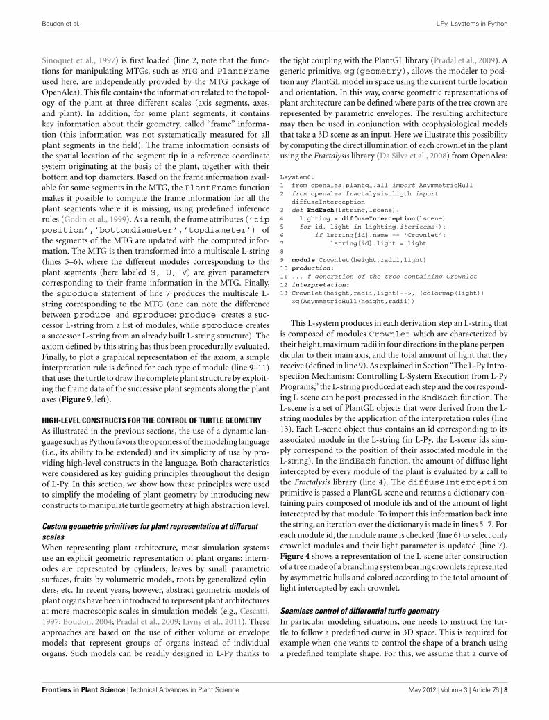
This L-system produces in each derivation step an L-string thatis composed of modules Crownlet which are characterized bytheir height,maximum radii in four directions in the plane perpen-dicular to their main axis, and the total amount of light that theyreceive (defined in line 9). As explained in Section“The L-Py Intro-spection Mechanism: Controlling L-System Execution from L-PyPrograms,” the L-string produced at each step and the correspond-ing L-scene can be post-processed in the EndEach function. TheL-scene is a set of PlantGL objects that were derived from the L-string modules by the application of the interpretation rules (line13). Each L-scene object thus contains an id corresponding to itsassociated module in the L-string (in L-Py, the L-scene ids sim-ply correspond to the position of their associated module in theL-string). In the EndEach function, the amount of diffuse lightintercepted by every module of the plant is evaluated by a call tothe Fractalysis library (line 4). The diffuseInterceptionprimitive is passed a PlantGL scene and returns a dictionary con-taining pairs composed of module ids and of the amount of lightintercepted by that module. To import this information back intothe string, an iteration over the dictionary is made in lines 5–7. Foreach module id, the module name is checked (line 6) to select onlycrownlet modules and their light parameter is updated (line 7).Figure 4 shows a representation of the L-scene after constructionof a tree made of a branching system bearing crownlets representedby asymmetric hulls and colored according to the total amount oflight intercepted by each crownlet.
Seamless control of differential turtle geometryIn particular modeling situations, one needs to instruct the tur-tle to follow a predefined curve in 3D space. This is required forexample when one wants to control the shape of a branch usinga predefined template shape. For this, we assume that a curve of
Frontiers in Plant Science | Technical Advances in Plant Science May 2012 | Volume 3 | Article 76 | 8
Boudon et al. L-Py, L-systems in Python
length L is defined that represents the shape of a particular branch.In the 3D scene, at the position of the branch insertion on the par-ent branch, we then need to instruct the turtle to move along thiscurve from its current position. To achieve this, Prusinkiewicz et al.(2001) designed an algorithm to move the turtle in the 3D spacebased on differential geometry and using quantities such as localtangent, curvature, and step size. The following L-Py code gives asimple 2D version inspired from this algorithm.
Lsystem7:1 length = 12.42 dl = 0.013 Axiom: FFF [+M(0)] FF4 production:5 M(l):6 if l < length:7 u, nextu = l/length, (l + dl)/length8 tgt = curve.getTangent(u)9 nexttgt = curve.getTangent(nextu)10 rotangle = degrees(atan2(cross(tgt,nexttgt),
dot(tgt,nexttg)))11 produce +(rotangle) F(dl) M(l + dl)
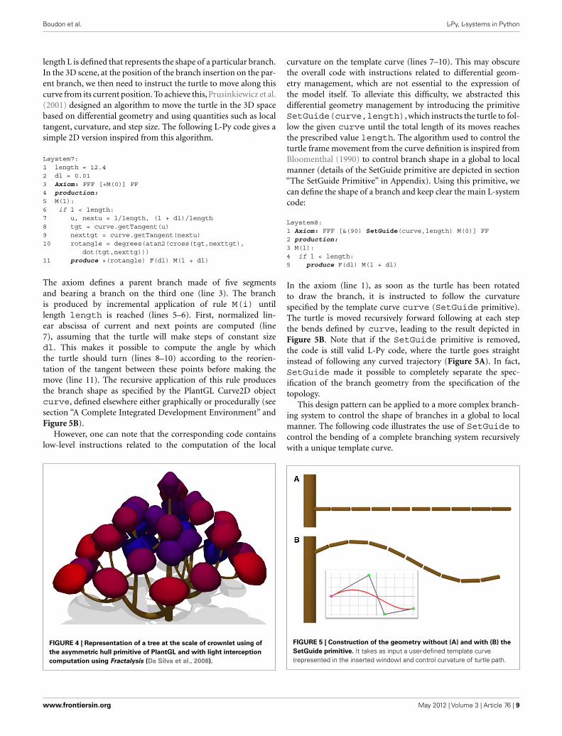
The axiom defines a parent branch made of five segmentsand bearing a branch on the third one (line 3). The branchis produced by incremental application of rule M(i) untillength length is reached (lines 5–6). First, normalized lin-ear abscissa of current and next points are computed (line7), assuming that the turtle will make steps of constant sizedl. This makes it possible to compute the angle by whichthe turtle should turn (lines 8–10) according to the reorien-tation of the tangent between these points before making themove (line 11). The recursive application of this rule producesthe branch shape as specified by the PlantGL Curve2D objectcurve, defined elsewhere either graphically or procedurally (seesection “A Complete Integrated Development Environment” andFigure 5B).
However, one can note that the corresponding code containslow-level instructions related to the computation of the local
FIGURE 4 | Representation of a tree at the scale of crownlet using of
the asymmetric hull primitive of PlantGL and with light interception
computation using Fractalysis (Da Silva et al., 2008).
curvature on the template curve (lines 7–10). This may obscurethe overall code with instructions related to differential geom-etry management, which are not essential to the expression ofthe model itself. To alleviate this difficulty, we abstracted thisdifferential geometry management by introducing the primitiveSetGuide(curve,length), which instructs the turtle to fol-low the given curve until the total length of its moves reachesthe prescribed value length. The algorithm used to control theturtle frame movement from the curve definition is inspired fromBloomenthal (1990) to control branch shape in a global to localmanner (details of the SetGuide primitive are depicted in section“The SetGuide Primitive” in Appendix). Using this primitive, wecan define the shape of a branch and keep clear the main L-systemcode:
Lsystem8:1 Axiom: FFF [&(90) SetGuide(curve,length) M(0)] FF2 production:3 M(l):4 if l < length:5 produce F(dl) M(l + dl)
In the axiom (line 1), as soon as the turtle has been rotatedto draw the branch, it is instructed to follow the curvaturespecified by the template curve curve (SetGuide primitive).The turtle is moved recursively forward following at each stepthe bends defined by curve, leading to the result depicted inFigure 5B. Note that if the SetGuide primitive is removed,the code is still valid L-Py code, where the turtle goes straightinstead of following any curved trajectory (Figure 5A). In fact,SetGuide made it possible to completely separate the spec-ification of the branch geometry from the specification of thetopology.
This design pattern can be applied to a more complex branch-ing system to control the shape of branches in a global to localmanner. The following code illustrates the use of SetGuide tocontrol the bending of a complete branching system recursivelywith a unique template curve.
FIGURE 5 | Construction of the geometry without (A) and with (B) the
SetGuide primitive. It takes as input a user-defined template curve(represented in the inserted window) and control curvature of turtle path.
www.frontiersin.org May 2012 | Volume 3 | Article 76 | 9
Boudon et al. L-Py, L-systems in Python
Lsystem9:1 Axiom: M(0,0)2 production:3 M(l,order):4 if order < MAXORDER and l < length:5 produce F(dl) iRoll(phi)[ˆ(60)SetGuide(curve,
length-l)M(l,order+1)]M(l+dl, order)6 else: produce
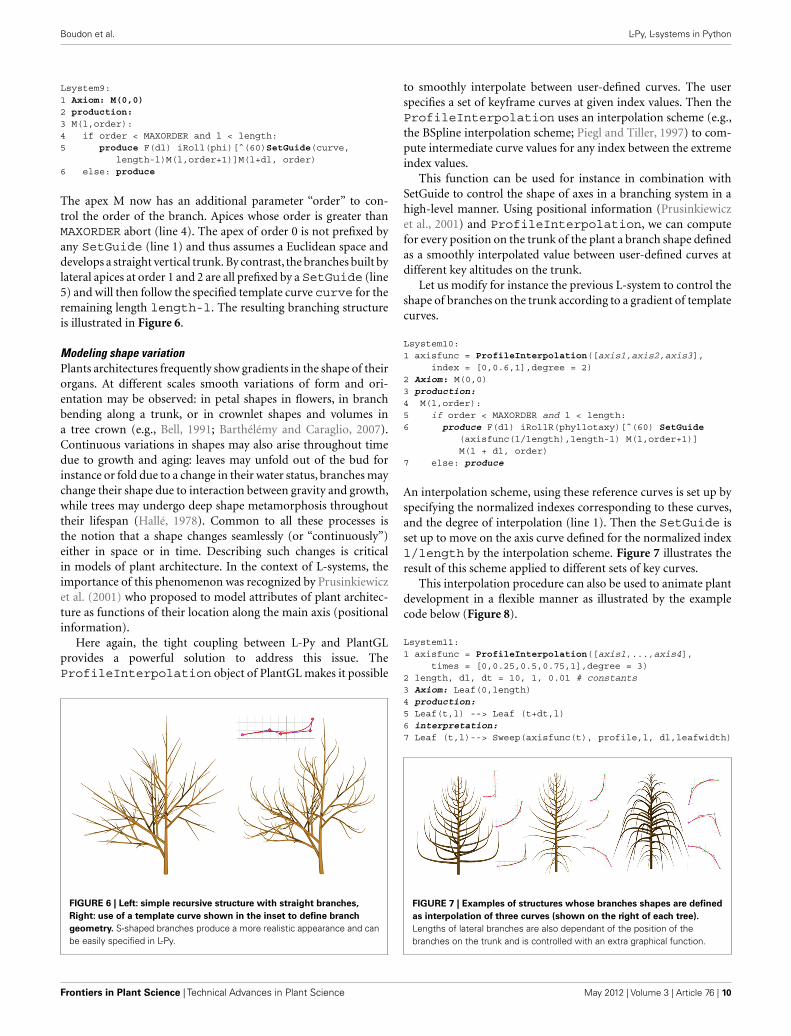
The apex M now has an additional parameter “order” to con-trol the order of the branch. Apices whose order is greater thanMAXORDER abort (line 4). The apex of order 0 is not prefixed byany SetGuide (line 1) and thus assumes a Euclidean space anddevelops a straight vertical trunk. By contrast, the branches built bylateral apices at order 1 and 2 are all prefixed by a SetGuide (line5) and will then follow the specified template curve curve for theremaining length length-l. The resulting branching structureis illustrated in Figure 6.
Modeling shape variationPlants architectures frequently show gradients in the shape of theirorgans. At different scales smooth variations of form and ori-entation may be observed: in petal shapes in flowers, in branchbending along a trunk, or in crownlet shapes and volumes ina tree crown (e.g., Bell, 1991; Barthélémy and Caraglio, 2007).Continuous variations in shapes may also arise throughout timedue to growth and aging: leaves may unfold out of the bud forinstance or fold due to a change in their water status, branches maychange their shape due to interaction between gravity and growth,while trees may undergo deep shape metamorphosis throughouttheir lifespan (Hallé, 1978). Common to all these processes isthe notion that a shape changes seamlessly (or “continuously”)either in space or in time. Describing such changes is criticalin models of plant architecture. In the context of L-systems, theimportance of this phenomenon was recognized by Prusinkiewiczet al. (2001) who proposed to model attributes of plant architec-ture as functions of their location along the main axis (positionalinformation).
Here again, the tight coupling between L-Py and PlantGLprovides a powerful solution to address this issue. TheProfileInterpolation object of PlantGL makes it possible
FIGURE 6 | Left: simple recursive structure with straight branches,
Right: use of a template curve shown in the inset to define branch
geometry. S-shaped branches produce a more realistic appearance and canbe easily specified in L-Py.
to smoothly interpolate between user-defined curves. The userspecifies a set of keyframe curves at given index values. Then theProfileInterpolation uses an interpolation scheme (e.g.,the BSpline interpolation scheme; Piegl and Tiller, 1997) to com-pute intermediate curve values for any index between the extremeindex values.
This function can be used for instance in combination withSetGuide to control the shape of axes in a branching system in ahigh-level manner. Using positional information (Prusinkiewiczet al., 2001) and ProfileInterpolation, we can computefor every position on the trunk of the plant a branch shape definedas a smoothly interpolated value between user-defined curves atdifferent key altitudes on the trunk.
Let us modify for instance the previous L-system to control theshape of branches on the trunk according to a gradient of templatecurves.
Lsystem10:1 axisfunc = ProfileInterpolation([axis1,axis2,axis3],
index = [0,0.6,1],degree = 2)2 Axiom: M(0,0)3 production:4 M(l,order):5 if order < MAXORDER and l < length:6 produce F(dl) iRollR(phyllotaxy)[ˆ(60) SetGuide
(axisfunc(l/length),length-l) M(l,order+1)]M(l + dl, order)
7 else: produce
An interpolation scheme, using these reference curves is set up byspecifying the normalized indexes corresponding to these curves,and the degree of interpolation (line 1). Then the SetGuide isset up to move on the axis curve defined for the normalized indexl/length by the interpolation scheme. Figure 7 illustrates theresult of this scheme applied to different sets of key curves.
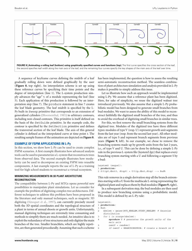
This interpolation procedure can also be used to animate plantdevelopment in a flexible manner as illustrated by the examplecode below (Figure 8).
Lsystem11:1 axisfunc = ProfileInterpolation([axis1,...,axis4],
times = [0,0.25,0.5,0.75,1],degree = 3)2 length, dl, dt = 10, 1, 0.01 # constants3 Axiom: Leaf(0,length)4 production:5 Leaf(t,l) --> Leaf (t+dt,l)6 interpretation:7 Leaf (t,l)--> Sweep(axisfunc(t), profile,l, dl,leafwidth)
FIGURE 7 | Examples of structures whose branches shapes are defined
as interpolation of three curves (shown on the right of each tree).
Lengths of lateral branches are also dependant of the position of thebranches on the trunk and is controlled with an extra graphical function.
Frontiers in Plant Science | Technical Advances in Plant Science May 2012 | Volume 3 | Article 76 | 10
Boudon et al. L-Py, L-systems in Python
FIGURE 8 | Animating a rolling leaf (bottom) using graphically specified curves and functions (top). The first curve specifies the cross section of the leaf,the second specifies leaf width along the main axis of the leaf, and the remaining four curves specify the key shapes of the main axis of the leaf over time.
A sequence of keyframe curves defining the midrib of a leafgradually rolling down were defined graphically by the user(Figure 8, top right). An interpolation scheme is set up usingthese reference curves by specifying their time points and thedegree of interpolation (line 1). The L-system production sim-ply advances the “age” t of a module representing the leaf (line5). Each application of this production is followed by an inter-pretation step (line 7). The produce statement in line 7 createsthe leaf blade geometry. The leaf midrib is specified by the L-Py built-in Sweep primitive that corresponds to an extension ofgeneralized cylinders (Bloomenthal, 1985) to arbitrary contours,including non-closed contours. This primitive is itself defined onthe basis of the SetGuide primitive. In the example code, thecontour is specified by the SetSection primitive and definesthe transversal section of the leaf blade. The axis of this generalcylinder is defined as the interpolated curve at time point t. Theresulting sample frames of the animation are depicted on Figure 8.
EXAMPLE OF FSPM APPLICATIONS IN L-PyIn this section, we show how L-Py can be used to create complexFSPM scenarios. A first example illustrates how advanced analysistools can be used to parameterize a L-system that reconstructs treesfrom observed data. The second example illustrates how modu-larity can be used to decompose an existing FSPM into reusablecomponents. A last example reports the use of L-Py as a trainingtool for high school students to reconstruct a virtual ecosystem.
MINIMIZING MEASUREMENTS IN 3D PLANT ARCHITECTURERECONSTRUCTIONThe compatibility between L-Py and MTGs opens powerful newpossibilities to manipulate plant simulations. Let us consider forexample the problem of digitizing complex tree architectures. Dif-ferent techniques to address this problem have been proposed inthe literature and only manual techniques, such as magnetic 3Ddigitizing (Sinoquet et al., 1997), can currently precisely recordboth the 3D spatial coordinates and the topological structure ofa plant in terms of annual shoots or growth units. Unfortunately,manual digitizing techniques are extremely time consuming andmethods to simplify them are much needed. An intuitive idea is toexploit the redundancy of tree structures and only digitize the mainbranches of the tree. Smaller branchlets, which are highly repeti-tive, are then generated procedurally. Assuming that such a scheme
has been implemented, the question is how to assess the resultingsemi-automatic reconstruction method. The seamless combina-tion of plant architecture simulation and analysis provided in L-Pymakes it possible to simply address this issue.
Let us illustrate how such an approach would be implementedusing L-Py. We assume that a reference plant has been digitized.Here, for sake of simplicity, we reuse the digitized walnut treeintroduced previously. We also assume that a simple L-Py proba-bilistic model has been designed to generate small branches frombud modules. We want to assess the ability of this model to recon-struct faithfully the digitized small branches of the tree, and thusto avoid the overhead of digitizing small branches in similar trees.
For this, we first remove the small branching systems from thedigitized tree. Modules of the digitized tree have three differenttypes: modules of type V (resp. U) represent growth unit segmentsfrom the last year (resp. from the second last year). All other mod-ules are of type S and represent branch segments from previousyears (Figure 9, left). In our example, we chose to remove thebranching systems made up by growth units from the last 2 years,i.e., of type V and U. This can be done by defining a simple L-Pyrule in the previous L-system file (lsystem5.lpy) that replaces everybranching system starting with a U and following a segment S bya bud:
Lsystem5 (sequel):1 production:2 S(tip0,dbot0, dtop0) < U(tip,dbot,dtop) --> Bud%
This rule removes in a single derivation step all the branch extrem-ities starting with a U from the multiscale L-string representing thedigitized plant and replaces them by Bud modules (Figure 9, right).
In a subsequent derivation step, the bud modules are then usedto produce new branching systems using a probabilistic model.This model is defined by an L-Py rule:
Lsystem12:1 production:1 Bud:2 nbelem = gauss(AVG_NBELEM,STDEV_NBELEM) # Gaussian
distribution3 for i in xrange(nbelem):4 nproduce U # generates the growth units of the
main axis5 ramif = random()6 if ramif < BRANCHINGPROB: # create a branch on U
www.frontiersin.org May 2012 | Volume 3 | Article 76 | 11

Boudon et al. L-Py, L-systems in Python
(with fixed probability)7 nproduce [V]8 nproduce V
This rule specifies that a bud is replaced by a shoot made of a ran-domly chosen number of segments U that can each bear (or not) asegment V and that terminate by a segment V. Note that we omit-ted to show the computation of the branch geometry to keep theexample simple. As a result, all the removed digitized branches arereplaced by artificially generated small branches, thus providing apartially digitized and partially simulated tree.
Then, to assess the quality of the resulting semi-simulated tree,we make use of the plant structural comparison primitive avail-able in the VPlants package of OpenAlea (Ferraro and Godin,2000). This function compares the structures of two plants (herethe digitized and semi-simulated trees) and returns a list of pairs
FIGURE 9 | Use of a digitized 20-year-old walnut tree (Juglans regia L.)
as the axiom of a simulation. Right, shoots produced during the last2 years are removed. Simulation process will use this structure as newaxiom and produce algorithmically new shoots. Generated shoots will becompared with measured ones. Bottom, a detail view of the process: fromtop to bottom, original branching system, pruned system with insertion ofBud represented as red sphere, and example of regenerated structure.
of plant segments from both plants that were found to match eachother. The more matching segments are found in both trees, thebetter the reconstruction. The normalized length of the returnedlist, Q = 2 × L/(L1 + L2), L being the size of the returned list andL1 and L2 respectively the sizes of the compared trees, can thusbe used as an indicator of the faithfulness of the model. If Q isgreater than a specified threshold, the simulated tree is consideredas a faithful reconstruction and the list contains pairs referring tomost of the components of both plants. In the opposite case, thelist is close to being empty and the reconstruction is consideredpoor. The following function illustrates how such a comparisoncan be carried out in L-Py:
Code13:1 from openalea.treematching import *2 def compare(lstring, initialmtg):3 reconsmtg = lstring2mtg(lstring)4 m = Matching(reconsmtg,initialmtg)5 return 2 * len(m.getMatchingList())/(len(reconsmtg)+
len(initialmtg))
The compare function takes as arguments the current L-stringrepresenting the reconstructed plant and an MTG representing theinitial digitized tree. It first transforms the L-string into an MTGand then compares the two MTG structures using a primitive fromthe treematching module of OpenAlea. As a result, it returnsthe estimated value of Q for this comparison.
This function can then be used to explore the parameter spaceof the probabilistic branching model (here through varying thebranching probability) so as to find those parameters that make itpossible to reconstruct trees faithfully with respect to the originaldigitized tree. This is done in the following function that assemblesthe different components of this pipeline:
Code13 (sequel):6 def optimize_reconstruction (minv,maxv,vstep):7 l = Lsystem(‘lsystem5.lpy’)
FIGURE 10 | Result of the comparison between regenerated structures
and the measured one. The scores of the different branching systems aregiven by the colored curves and the average value by the black curve.Maximum average score is reached with a probability of 0.77 and gives ascore of 0.8.
Frontiers in Plant Science | Technical Advances in Plant Science May 2012 | Volume 3 | Article 76 | 12
Boudon et al. L-Py, L-systems in Python
8 initialmtg = l.initialmtg9 prunedstring = l.derive()10 Q = zeros((maxv-minv)/vstep)11 for i, branchingprob in enumerate (arange(minv,
maxv,vstep)):12 l = Lsystem(‘lsystem12.lpy’)13 l.BRANCHINGPROB = branchingprob14 lstring = l.derive(prunedstring,1)15 Q[i] = compare(lstring,initialmtg)16 plot(arange(minv,maxv,vstep),Q)
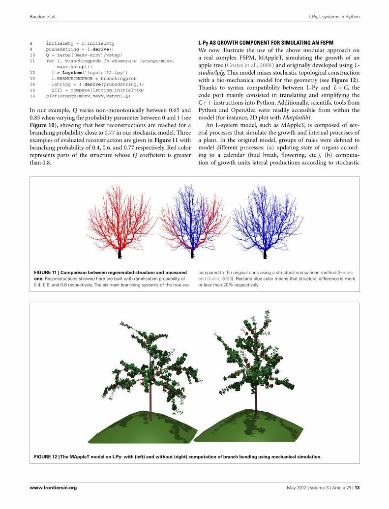
In our example, Q varies non-monotonically between 0.65 and0.85 when varying the probability parameter between 0 and 1 (seeFigure 10), showing that best reconstructions are reached for abranching probability close to 0.77 in our stochastic model. Threeexamples of evaluated reconstruction are given in Figure 11 withbranching probability of 0.4, 0.6, and 0.77 respectively. Red colorrepresents parts of the structure whose Q coefficient is greaterthan 0.8.
L-Py AS GROWTH COMPONENT FOR SIMULATING AN FSPMWe now illustrate the use of the above modular approach ona real complex FSPM, MAppleT, simulating the growth of anapple tree (Costes et al., 2008) and originally developed using L-studio/lpfg. This model mixes stochastic topological constructionwith a bio-mechanical model for the geometry (see Figure 12).Thanks to syntax compatibility between L-Py and L + C, thecode port mainly consisted in translating and simplifying theC++ instructions into Python. Additionally, scientific tools fromPython and OpenAlea were readily accessible from within themodel (for instance, 2D plot with Matplotlib).
An L-system model, such as MAppleT, is composed of sev-eral processes that simulate the growth and internal processes ofa plant. In the original model, groups of rules were defined tomodel different processes: (a) updating state of organs accord-ing to a calendar (bud break, flowering, etc.), (b) computa-tion of growth units lateral productions according to stochastic
FIGURE 11 | Comparison between regenerated structure and measured
one. Reconstructions showed here are built with ramification probability of0.4, 0.6, and 0.8 respectively. The six main branching systems of the tree are
compared to the original ones using a structural comparison method (Ferraroand Godin, 2000). Red and blue color means that structural difference is moreor less than 20% respectively.
FIGURE 12 |The MAppleT model on L-Py: with (left) and without (right) computation of branch bending using mechanical simulation.
www.frontiersin.org May 2012 | Volume 3 | Article 76 | 13

Boudon et al. L-Py, L-systems in Python
models, (c) growth process, (d) biomechanics. During refactor-ing, the code was divided into distinct L-systems correspond-ing to these different groups of rule to achieve modularity.Because they came from a single original L-system code, theseL-systems components used similar module naming conventionand thus were readily compatible with each other (see ModularL-Systems in L-Py). The parameters of the modules were storedin a generic container object whose contents can be updatedby each L-system component. Parameters used by different L-system components were given a unique name in all of these.For instance, the growth process component (c) requires infor-mation on the number and types of components to create ateach time step. This information is provided by the stochasticprocess component (b) using a consistent naming convention inboth components.
Usually the different processes also rely on a number of globalvariables. To change their values, a dictionary containing the
names and values of global variables can be passed to the L-systemsand can be applied using the introspection mechanism presentedin Section “L-Py as a Component Library: Controlling L-SystemsExecution from Python.” In this way, the global variables can bepassed from one process to the next one. Each process can thusupdate these settings to inform the other processes if needed.
To better demonstrate the modularity of the code resultingfrom this decomposition of MAppleT, the L-system compo-nents were assembled graphically using a dataflow in OpenAlea(Figure 13). As opposed to code representation, dataflows give avisual representation of the logical dependency structure of theFSPM. The composition of the components can be made graphi-cally by the modeler by linking input and output of the differentL-systems components and making it possible for the system topass on the L-string and the dictionary of global parameters. Theresulting graph (dataflow) can be executed and runs the pipelinethroughout.
FIGURE 13 | Data flow of the MAppleT simulation. The model has been decomposed into several independent processes that can be combined andparameterized by user to drive the simulation graphically.
Frontiers in Plant Science | Technical Advances in Plant Science May 2012 | Volume 3 | Article 76 | 14
Boudon et al. L-Py, L-systems in Python
Thanks to this modular decomposition, interesting manipula-tion of the assembled models can be made. For example, the userhas the possibility to enable/disable some of them upon request.Figure 12 right illustrates for example the result of the model inwhich the Biomechanics component has been disabled.
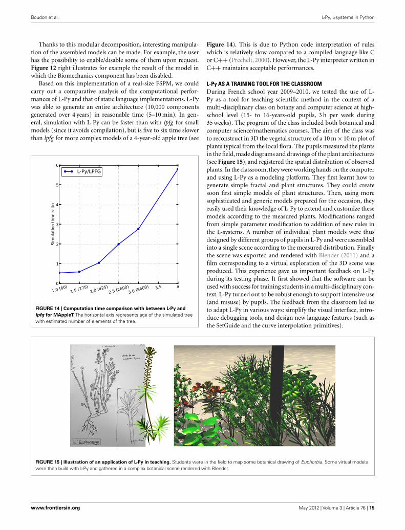
Based on this implementation of a real-size FSPM, we couldcarry out a comparative analysis of the computational perfor-mances of L-Py and that of static language implementations. L-Pywas able to generate an entire architecture (10,000 componentsgenerated over 4 years) in reasonable time (5–10 min). In gen-eral, simulation with L-Py can be faster than with lpfg for smallmodels (since it avoids compilation), but is five to six time slowerthan lpfg for more complex models of a 4-year-old apple tree (see
FIGURE 14 | Computation time comparison with between L-Py and
lpfg for MAppleT. The horizontal axis represents age of the simulated treewith estimated number of elements of the tree.
Figure 14). This is due to Python code interpretation of ruleswhich is relatively slow compared to a compiled language like Cor C++ (Prechelt, 2000). However, the L-Py interpreter written inC++ maintains acceptable performances.
L-Py AS A TRAINING TOOL FOR THE CLASSROOMDuring French school year 2009–2010, we tested the use of L-Py as a tool for teaching scientific method in the context of amulti-disciplinary class on botany and computer science at high-school level (15- to 16-years-old pupils, 3 h per week during35 weeks). The program of the class included both botanical andcomputer science/mathematics courses. The aim of the class wasto reconstruct in 3D the vegetal structure of a 10 m × 10 m plot ofplants typical from the local flora. The pupils measured the plantsin the field, made diagrams and drawings of the plant architectures(see Figure 15), and registered the spatial distribution of observedplants. In the classroom, they were working hands on the computerand using L-Py as a modeling platform. They first learnt how togenerate simple fractal and plant structures. They could createsoon first simple models of plant structures. Then, using moresophisticated and generic models prepared for the occasion, theyeasily used their knowledge of L-Py to extend and customize thesemodels according to the measured plants. Modifications rangedfrom simple parameter modification to addition of new rules inthe L-systems. A number of individual plant models were thusdesigned by different groups of pupils in L-Py and were assembledinto a single scene according to the measured distribution. Finallythe scene was exported and rendered with Blender (2011) and afilm corresponding to a virtual exploration of the 3D scene wasproduced. This experience gave us important feedback on L-Pyduring its testing phase. It first showed that the software can beused with success for training students in a multi-disciplinary con-text. L-Py turned out to be robust enough to support intensive use(and misuse) by pupils. The feedback from the classroom led usto adapt L-Py in various ways: simplify the visual interface, intro-duce debugging tools, and design new language features (such asthe SetGuide and the curve interpolation primitives).
FIGURE 15 | Illustration of an application of L-Py in teaching. Students were in the field to map some botanical drawing of Euphorbia. Some virtual modelswere then build with L-Py and gathered in a complex botanical scene rendered with Blender.
www.frontiersin.org May 2012 | Volume 3 | Article 76 | 15

Boudon et al. L-Py, L-systems in Python
CONCLUSIONIn this paper, we presented L-Py, an open-source software platformfor L-system simulation based on Python. Compared to previousL-system simulation software packages, L-Py makes intensive useof Python’s property of being a dynamic language to achieve flex-ibility in modeling and high-level programming. Inherited fromPython, the L-Py language syntax remains simple, with no or min-imal bracketing of expressions, and very clear block structures.L-Py was designed as both an integrative framework and a libraryof L-system constructs that can be called from Python. Owing toits dynamic language structure, L-Py facilitates the design of mod-ular models by assembling elementary models without modifyingtheir code, provided they respect minimal specifications. For thedesign of plant models, special language constructs were intro-duced for compliance with MTG data-structures, for which largelibraries of computational models and tools already exist (e.g.,OpenAlea software platform and its packages). Likewise, for geom-etry, constructs were introduced to reuse any model from PlantGL,
a library of geometric primitives dedicated to plant representationat different scales, and to simplify the specification of complex geo-metric models with the L-system turtle. To illustrate the flexibilityand power of L-Py, we presented its application to real modelingsituations. The problem of optimizing plant digitizing strategyillustrated the benefit of using jointly L-systems and MTGs in amodeling application. MappleT was used to illustrate the possi-bility to design complex simulation systems in a modular way.The last example illustrated the pedagogic value of L-Py basedon a real experiment carried out with high-school students inFrance.
ACKNOWLEDGMENTSThe authors are grateful to M. Beziz, E. Farcot, Y. Caraglio, D.Lacour, L. Comte, and J. Chopard who were involved in thehigh-school classes. This project is partially supported by Agropo-lis Foundation and the INRIA VPlants-BMV associated teamproject.
REFERENCESBarthélémy, D., and Caraglio, Y. (2007).
Plant architecture: a dynamic, mul-tilevel and comprehensive appro-ach to plant form, structure andontogeny. Ann. Bot. 99, 375–407.
Bell, A. D. (1991). Plant Form: An Illus-trated Guide to Flowering Plant Mor-phology. Oxford: Oxford UniversityPress.
Blender. (2011). The Blender Foun-dation. Amsterdam. Available at:http://www.blender.org
Bloomenthal, J. (1985). “Modeling themighty maple,” in Proceedings of the12th Annual Conference on ComputerGraphics and Interactive Techniques,SIGGRAPH ‘85 (New York: ACM).
Bloomenthal, J. (1990). “Calculationof reference frames along a spacecurve,” in Graphics Gems, ed A. S.Glassner (Boston: Academic Press),567–571.
Boudon, F. (2004). ReprésentationGéométrique de L’architecture desPlantes. Ph.D. thesis, University ofMontpellier II, Montpellier.
Cescatti, A. (1997). Modelling theradiative transfer in discontinuouscanopies of asymmetric crowns. I.Model structure and algorithms.Ecol. Modell. 101, 263–274.
Cieslak, M., Seleznyova, A. N., Prusin-kiewicz, P., and Hanan, J. (2011).Towards aspect-oriented functional-structural plant modelling. Ann. Bot.108, 1025–1041.
Costes, E., Smith, C., Renton, M.,Guédon, Y., Prusinkiewicz, P., andGodin, C. (2008). MAppleT: simula-tion of apple tree development usingmixed stochastic and biomechani-cal models. Funct. Plant Biol. 35,936–950.
Da Silva, D., Boudon, F., Godin, C.,and Sinoquet, H. (2008). Multiscaleframework for modeling and ana-lyzing light interception by trees.Multiscale Model. Simul. 7, 910–933.
Federl, P., and Prusinkiewicz, P. (1999).“Virtual laboratory: an interactivesoftware environment for computergraphics,” in Proceedings of Com-puter Graphics International, Can-more: Alberta. ’99, 93–100.
Federl, P., and Prusinkiewicz, P. (2004).“Solving differential equations indevelopmental models of mul-ticellular structures expressedusing L-systems,” in Proceedingsof Computational Science. ICCS2004 (Krakow, Poland, June 6–9,2004), Part II, Lecture Notes inComputer Science 3037, eds M.Bubak, G. van Albada, P. Sloot,and J. Dongarra (Berlin: Springer),65–72.
Ferraro, P., and Godin, C. (2000). A dis-tance measure between plant archi-tecture. Ann. For. Sci. 57, 445–461.
FSPM Special Issue. (2005). New Phy-tologist. Blackwell Publishing. 166,771–894.
FSPM Special Issue. (2008). FunctionalPlant Biology. Eds J. Hanan andP. Prusinkiewicz, CSIRO Publishing,35, 739–1090.
FSPM Special Issue. (2011). Annals ofBotany. Eds T. de Jong and D. DaSilva (Oxford: Oxford University),108, 987–1223,
Godin, C., and Caraglio, Y. (1998). Amultiscale model of plant topolog-ical structures. J. Theor. Biol. 191,1–46.
Godin, C., Costes, C., and Caraglio,Y. (1998). Exploring plant topolog-ical structure with the AMAPmod
software; an outline. Silva Fennica31, 357–368.
Godin, C., Costes, E., and Sinoquet,H. (1999). A method for describingplant architecture which integratestopology and geometry. Ann. Bot. 84,343–357.
Godin, C., Costes, E., and Sinoquet,H. (2005). “Plant architecture mod-elling – virtual plants and com-plex systems,” in Plant Architectureand its Manipulation, Vol. 17, ed C.G. N. Turnbull (Oxford: Blackwell)238–287.
Godin, C., and Guédon, Y. (1997).AMAPmod v1.8. Introduction andReference Manual. CIRAD Report,Montpellier.
Godin, C., and Sinoquet, H. (2005).Functional–structural plant model-ling. New Phytol. 166, 705–708.
Hallé, F. (1978). “Architectural vari-ation at specific level of tropi-cal trees,” in Tropical Trees as Liv-ing Systems, eds P. B. Tomlinsonand M. H. Zimmermann (Cam-bridge: Cambridge University Press),209–221.
Hanan, J. (1992). Parametric L-Systemsand their Application to the Model-ing and Visualization of Plants. Ph.D.dissertation, University of Regina,Regina, Saskatchewan.
Hanan, J., and Prusinkiewicz, P. (2008).Foreword: studying plants withfunctional–structural models.Funct. Plant Biol. 35, vi–viii.
Herman, G. T., and Rozenberg, G.(1975). Developmental systems andlanguages. North-Holland: Amster-dam.
Karwowski, R., and Prusinkiewicz, P.(2003). Design and implementa-tion of the L+C modeling language.
Electron. Notes Theor. Comput. Sci.86, 134–152.
Kniemeyer, O., and Kurth, W. (2008).“The modelling platform GroIMPand the programming language XL,”in Applications of Graph Trans-formations with Industrial Rele-vance: Third International Sympo-sium, AGTIVE 2007, Kassel, Ger-many, October 10-12, 2007, RevisedSelected and Invited Papers, LectureNotes In Computer Science, 5088,eds A. Schürr, M. Nagl, and A.Zündorf (Kassel: Springer-Verlag),570–572.
Lindenmayer, A. (1968). Mathematicalmodels for cellular interaction indevelopment, Parts I and II. J. Theor.Biol. 18, 280–315.
Livny, Y., Pirk, S., Cheng, Z., Yan,F., Deussen, O., Cohen-Or, D., andChen, B. (2011). Texture-lobes fortree modelling. ACM Trans. Graph.30, 53.
Mercer, L., Prusinkiewicz, P., andHanan, J. (1990). “The concept anddesign of a virtual laboratory,” inProceedings of Graphics Interface.Halifax, Nova Scotia. ‘90, 149–155.
Microsoft Corporation. (2011). TheVisual Studio. Available at: http://www.microsoft.com/visualstudio/
Mündermann, L., Erasmus, Y., Lane,B., Coen, E., and Prusinkiewicz,P. (2005). Quantitative modelingof Arabidopsis development. PlantPhysiol. 139, 960–968.
Ousterhout, J. K. (1998). Scripting:higher-level programming for the21st century. IEEE Comput. 31,23–30.
Piegl, L. A., and Tiller, W. (1997).The Nurbs Book, 2nd Edn. Berlin:Springer.
Frontiers in Plant Science | Technical Advances in Plant Science May 2012 | Volume 3 | Article 76 | 16
Boudon et al. L-Py, L-systems in Python
Pradal, C., Boudon, F., Nouguier, C.,Chopard, J., and Godin, C. (2009).PlantGL: a Python-based geometriclibrary for 3D plant modelling atdifferent scales. Graph. Models 71,1–21.
Pradal, C., Dufour-Kowalski, S.,Boudon, F., Fournier, C., and Godin,C. (2008). OpenAlea: a visualprogramming and component-based software platform for plantmodeling. Funct. Plant Biol. 35,751–760.
Prechelt, L. (2000). An empirical com-parison of seven programming lan-guages. IEEE Comput. 33, 23–29.
Prusinkiewicz, P. (1986). “Graphicalapplications of L-systems,” in Pro-ceedings of Graphics Interface ‘86,247–253.
Prusinkiewicz, P. (1998). Modeling ofspatial structure and development ofplants. Sci. Hortic. 74, 113–149.
Prusinkiewicz, P. (1999). A look at thevisual modeling of plants using L-systems. Agron. Agric. Environ. 19,211–224.
Prusinkiewicz, P. (2004). “Art and sci-ence for life: designing and grow-ing virtual plants with L-systems,” inNursery Crops: Development, Evalu-ation, Production and Use: Proceed-ings of the XXVI International Horti-cultural Congress, Acta Horticulturae
630, eds C. Davidson and T. Fernan-dez, (ISHS: Toronto), 15–28.
Prusinkiewicz, P., Hanan, J., and Mech,R. (1999a). “An L-system-basedplant modeling language,” in Appli-cations of Graph Transformationswith Industrial Relevance. Proceed-ings of the International WorkshopAGTIVE ‘99, Lecture Notes in Com-puter Science 1779, eds M. Nagl, A.Schuerr, and M. Muench (Berlin:Springer), 395–410.
Prusinkiewicz, P., Karwowski, R., Mech,R., and Hanan, J. (1999b). “L-studio/cpfg: A software system formodeling plants,” in Applications ofGraph Transformations with Indus-trial Relevance. Proceedings of theInternational Workshop AGTIVE ’99,Lecture Notes in Computer Science1779, eds M. Nagl,A. Schuerr, and M.Muench (Berlin: Springer),457–464.
Prusinkiewicz, P., James, M., and Mech,R. (1994). “Synthetic topiary,” inProceedings of SIGGRAPH Orlando,Florida. ‘94, 351–358.
Prusinkiewicz, P., Karwowski, R., andLane, B. (2007). “The L+C plantmodeling language,” in Functional-Structural Plant Modeling in CropProduction, eds. J. Vos, L. F. M.Marcelis, P. H. B. de Visser, P. C.Struik, J. B. Evers and R. J. Bogers,(Wageningen: Springer), 27–42.
Prusinkiewicz, P., and Lindenmayer, A.(1990). The Algorithmic Beauty ofPlants. New York: Springer.
Prusinkiewicz, P., Lindenmayer, A., andHanan, J. (1988). Developmentalmodels of herbaceous plants forcomputer imagery purposes. Com-put. Graph. 22, 141–150.
Prusinkiewicz, P., Mündermann, L.,Karwowski, R., and Lane, B. (2001).“The use of positional informationin the modeling of plants,” in Pro-ceedings of SIGGRAPH ‘2001, LosAngeles, 289–300.
Sievänen, R., Mäkelä, A., Nikinmaa,E., and Korpilahti, E. (1997), Spe-cial issue on functional-structuraltree models. Silva Fennica 31,237–238.
Sinoquet, H., Rivet, P., and Godin, C.(1997). Assessment of the three-dimensional architecture of walnuttrees using digitising. Silva Fennica31, 265–273.
Teobaldelli, M., Puig, A. D., Zenone,T., Matteucci, M., Seufert, G., andSequeira, V. (2008). Building atopological and geometrical modelof poplar tree using portable on-ground scanning LIDAR. Funct.Plant Biol. 35, 1080–1090.
Tratt, L. (2009). Dynamically typedlanguages. Adv. Comput. 77,149–184.
Wang, W., Jüttler, B., Zheng, D., andLiu, Y. (2008). Computation of rota-tion minimizing frame. ACM Trans.Graph. 27, 18.
Conflict of Interest Statement: Theauthors declare that the research wasconducted in the absence of any com-mercial or financial relationships thatcould be construed as a potential con-flict of interest.
Received: 16 December 2011; accepted:04 April 2012; published online: 29 May2012.Citation: Boudon F, Pradal C, Coke-laer T, Prusinkiewicz P and Godin C(2012) L-Py: an L-system simulationframework for modeling plant architec-ture development based on a dynamiclanguage. Front. Plant Sci. 3:76. doi:10.3389/fpls.2012.00076This article was submitted to Frontiersin Technical Advances in Plant Science,a specialty of Frontiers in Plant Science.Copyright © 2012 Boudon, Pradal, Coke-laer , Prusinkiewicz and Godin. This is anopen-access article distributed under theterms of the Creative Commons Attribu-tion Non Commercial License, which per-mits non-commercial use, distribution,and reproduction in other forums, pro-vided the original authors and source arecredited.
www.frontiersin.org May 2012 | Volume 3 | Article 76 | 17
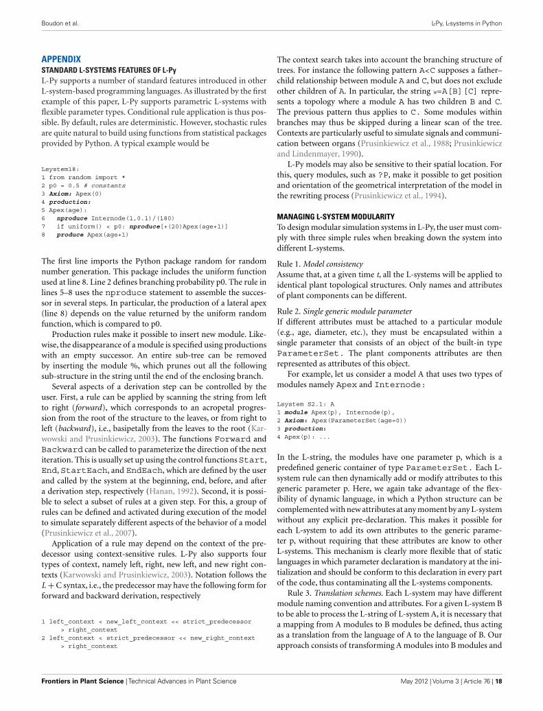
Boudon et al. L-Py, L-systems in Python
APPENDIXSTANDARD L-SYSTEMS FEATURES OF L-PyL-Py supports a number of standard features introduced in otherL-system-based programming languages. As illustrated by the firstexample of this paper, L-Py supports parametric L-systems withflexible parameter types. Conditional rule application is thus pos-sible. By default, rules are deterministic. However, stochastic rulesare quite natural to build using functions from statistical packagesprovided by Python. A typical example would be
Lsystem18:1 from random import *2 p0 = 0.5 # constants3 Axiom: Apex(0)4 production:5 Apex(age):6 nproduce Internode(1,0.1)/(180)7 if uniform() < p0: nproduce[+(20)Apex(age+1)]8 produce Apex(age+1)
The first line imports the Python package random for randomnumber generation. This package includes the uniform functionused at line 8. Line 2 defines branching probability p0. The rule inlines 5–8 uses the nproduce statement to assemble the succes-sor in several steps. In particular, the production of a lateral apex(line 8) depends on the value returned by the uniform randomfunction, which is compared to p0.
Production rules make it possible to insert new module. Like-wise, the disappearance of a module is specified using productionswith an empty successor. An entire sub-tree can be removedby inserting the module %, which prunes out all the followingsub-structure in the string until the end of the enclosing branch.
Several aspects of a derivation step can be controlled by theuser. First, a rule can be applied by scanning the string from leftto right (forward), which corresponds to an acropetal progres-sion from the root of the structure to the leaves, or from right toleft (backward), i.e., basipetally from the leaves to the root (Kar-wowski and Prusinkiewicz, 2003). The functions Forward andBackward can be called to parameterize the direction of the nextiteration. This is usually set up using the control functionsStart,End, StartEach, and EndEach, which are defined by the userand called by the system at the beginning, end, before, and aftera derivation step, respectively (Hanan, 1992). Second, it is possi-ble to select a subset of rules at a given step. For this, a group ofrules can be defined and activated during execution of the modelto simulate separately different aspects of the behavior of a model(Prusinkiewicz et al., 2007).
Application of a rule may depend on the context of the pre-decessor using context-sensitive rules. L-Py also supports fourtypes of context, namely left, right, new left, and new right con-texts (Karwowski and Prusinkiewicz, 2003). Notation follows theL + C syntax, i.e., the predecessor may have the following form forforward and backward derivation, respectively
1 left_context < new_left_context << strict_predecessor> right_context
2 left_context < strict_predecessor << new_right_context> right_context
The context search takes into account the branching structure oftrees. For instance the following pattern A<C supposes a father–child relationship between module A and C, but does not excludeother children of A. In particular, the string w=A[B][C] repre-sents a topology where a module A has two children B and C.The previous pattern thus applies to C. Some modules withinbranches may thus be skipped during a linear scan of the tree.Contexts are particularly useful to simulate signals and communi-cation between organs (Prusinkiewicz et al., 1988; Prusinkiewiczand Lindenmayer, 1990).
L-Py models may also be sensitive to their spatial location. Forthis, query modules, such as ?P, make it possible to get positionand orientation of the geometrical interpretation of the model inthe rewriting process (Prusinkiewicz et al., 1994).
MANAGING L-SYSTEM MODULARITYTo design modular simulation systems in L-Py, the user must com-ply with three simple rules when breaking down the system intodifferent L-systems.
Rule 1. Model consistencyAssume that, at a given time t, all the L-systems will be applied toidentical plant topological structures. Only names and attributesof plant components can be different.
Rule 2. Single generic module parameterIf different attributes must be attached to a particular module(e.g., age, diameter, etc.), they must be encapsulated within asingle parameter that consists of an object of the built-in typeParameterSet. The plant components attributes are thenrepresented as attributes of this object.
For example, let us consider a model A that uses two types ofmodules namely Apex and Internode:
Lsystem S2.1: A1 module Apex(p), Internode(p),2 Axiom: Apex(ParameterSet(age=0))3 production:4 Apex(p): ...
In the L-string, the modules have one parameter p, which is apredefined generic container of type ParameterSet. Each L-system rule can then dynamically add or modify attributes to thisgeneric parameter p. Here, we again take advantage of the flex-ibility of dynamic language, in which a Python structure can becomplemented with new attributes at any moment by any L-systemwithout any explicit pre-declaration. This makes it possible foreach L-system to add its own attributes to the generic parame-ter p, without requiring that these attributes are know to otherL-systems. This mechanism is clearly more flexible that of staticlanguages in which parameter declaration is mandatory at the ini-tialization and should be conform to this declaration in every partof the code, thus contaminating all the L-systems components.
Rule 3. Translation schemes. Each L-system may have differentmodule naming convention and attributes. For a given L-system Bto be able to process the L-string of L-system A, it is necessary thata mapping from A modules to B modules be defined, thus actingas a translation from the language of A to the language of B. Ourapproach consists of transforming A modules into B modules and
Frontiers in Plant Science | Technical Advances in Plant Science May 2012 | Volume 3 | Article 76 | 18

Boudon et al. L-Py, L-systems in Python
back using L-system rules. Module name translation can easily beexpressed with L-system rules as illustrated by the Lsystem A2Bbelow that transforms A modules into corresponding B ones.
Lsystem S2.2: B1 module A(param), I(param),2 production:3 A(param): ...
Lsystem S2.3: A2B1 module Apex(p), A(p), Internode(p), I(p)23 production:4 Apex(p) --> A(p)5 Internode(p) --> I(p)
Symmetric rules may be required to translate back from the lan-guage of B into the language of A, in particular if one wants toiteratively apply L-systems A, B several times consecutively. Such abidirectional translation requires that mapping from the alphabetof A to the alphabet of B is one to one. This is done by defining anew L-system:
Lsystem S2.4: B2A1 module Apex(p), A(p), Internode(p), I(p)23 production:4 A(p) --> Apex(p)5 I(p) --> Internode(p)
Similarly, attribute names used in the parameter container shouldbe consistent between different L-systems. If, for instance, twoprocesses rely on similar attributes but use different naming con-vention, attributes will also have to be renamed during translationstep. Conversely, if two processes use the same attribute name fordifferent things, attributes will also have to be renamed to avoid aconflict.
Then, at a given time step, starting from an A L-string, the userapplies L-system A which computes a new A L-string. Then this AL-string is translated into a B L-string with L-system B2A so thatthe L-system B can be applied. Then B is applied and finally, theresulting B string is translated back into A L-string to come backto the initial A L-system and continue the simulation. The proce-dure can be readily extended to the combination of any numberof L-systems.
The L-systems can then be assembled into a super-L-systemusing the built-in ComposedLsystem primitive described in themain text.
THE SetGuide PRIMITIVEA turtle is associated with a position P and frame F T composedof three orientation vectors mutually perpendicular that indicatesits heading H, up U, and left directions L (Prusinkiewicz et al.,2001). The turtle can perform a number of geometric operations.In particular, it can step forward in its heading direction or canrotate along its three orientation axis. Following a predefined pathwith turtle geometry was described in Prusinkiewicz et al. (2001)and consists of adjusting orientation of the turtle before each stepto fit the heading vector to the local path tangent T.
Similarly, the SetGuidemakes it possible that steps of a turtlefollow the path of a user-defined curve C, scaled to reach a length
L also specified by the user. The turtle steps are not supposed inthis case to be small. The curve is supposed to be positioned andoriented in the initial location of the turtle. It is also supposed tobe parameterized with curvilinear abscissa u.
To compute orientations along a curve, a frame can be com-puted at each point of C. A frame is made of three vector (r, s,t ) with t representing the tangent to the curve. Classical solu-tion relies on the Frenet frame. However, it produces importanttwist of the frame at inflection point of the curve. Some meth-ods make it possible to compute frame with minimized rotation(Bloomenthal, 1990; Wang et al., 2008). In our approach, we adaptthe method described in Prusinkiewicz et al. (2001). It starts froma frame F(r, s, t ) at C(u). To compute F ′(r ′, s ′, t ′) at C(u + du),the tangent t ′ of the curve is first estimated. Then the rotation Rthat maps t to t ′ is computed. This rotation can then be applied tos and r of F to have r ′ and s ′ values. The advantage of this methodis that it is consistent (no twist) and iterative with only the valueof the previous step needed to compute the next one.
To follow the path of the curve, rotations of the turtle will beperformed before and after each step to orient it in a directiongiven by the curve C. The step forward command (F) with a para-meter du representing step length is thus decomposed into threesteps: adjust orientation to reach C(u + du), move the turtle for-ward, and adjust the orientation of the turtle to fit tangent of Cat u + du (see Figure A1). The first and last operations are turtleorientation performed using the method presented previously. Inthe first case, the new tangent direction is approximated with thevector d = C(u + du) − C(u).
One problem comes from the fact that the rotation is com-puted in the coordinate system of the curve. To adapt it forthe turtle frame, the axis A of rotation R is translated from thereference frame F(u) of the curve to the frame F T of the turtle:A′ = F T × F(u)−1 × A. The transformation R′(A′, α) can then beapplied to the vectors H, L, and U of the turtle frame to expressthe reorientation of the turtle. Note that R(A, α) is still used tocomputed the new frame of the curve at C(u + du). Finally whenmoving the turtle forward, the length of the step has to be adapted.
FIGURE A1 | A step with the SetGuide command. On the left,computation on the guide curve. On the right, the application of thecommand for the turtle. Three steps are made for the step forward: first areorientation R(A1, α1) in the direction of C (u + du), a move forward oflength ||C (u + du) − C (u)||, and a reorientation R(A2, α2) in the direction ofthe tangent at C (u + du). A1 and A2 have to be translated first in the localcoordinate system of the turtle to be applied on the turtle.
www.frontiersin.org May 2012 | Volume 3 | Article 76 | 19
Boudon et al. L-Py, L-systems in Python
Indeed, the length of the curve between C(u) and C(u + du) isdu but the curve between this two points is approximated with astraight segment by the turtle. Thus the length of turtle step shouldbe changed for ||C(u + du) − C(u)||.
The turtle will thus produce a path with curvature similar to thecurve C when moving forward. Additionally, some rotations canalso be explicitly asked by the user to the turtle between each step.By default, these rotations will provide additional curvature to theturtle path. For instance, trunk and main branches can be builtusing the same SetGuide command except that at the begin-ning of branches an additional rotation is made to have lateraldirection. In this case, guide and turtle are rigidly linked since the
rotation of the turtle will also change the guide curve referenceframe.
It is also possible to apply similar rotations of the turtle to theframe along the guide. For instance, the Roll operation consistsin turning around the heading H of the turtle. Its counterpartconsists in turning the reference frame F(r, s, t ) of the curve Cat C(u) around its tangent t. Both operations can be made at thesame time when turtle is requested to turn. In this case, guide andturtle are non-rigidly linked since a turtle rotation will change thecorresponding position and orientation on the curve C. Such oper-ations are made possible in L-Py with special command iRollRand iRollL.
Frontiers in Plant Science | Technical Advances in Plant Science May 2012 | Volume 3 | Article 76 | 20
Related Documents