CERN 94-01 26 January 1994 Vol. I ORGANISATION EUROPÉENNE POUR LA RECHERCHE NUCLÉAIRE CERN EUROPEAN ORGANIZATION FOR NUCLEAR RESEARCH LnrlO CERN ACCELERATOR SCHOOL FIFTH GENERAL ACCELERATOR PHYSICS COURSE University of Jyvàskylà, Finland 7-18 September 1992 PROCEEDINGS Editor: S. Turner Vol.1 GENEVA 1994

Welcome message from author
This document is posted to help you gain knowledge. Please leave a comment to let me know what you think about it! Share it to your friends and learn new things together.
Transcript
CERN 94-01 26 January 1994 Vol. I
ORGANISATION EUROPÉENNE POUR LA RECHERCHE NUCLÉAIRE
CERN EUROPEAN ORGANIZATION FOR NUCLEAR RESEARCH
L n r l O CERN ACCELERATOR SCHOOL
FIFTH GENERAL ACCELERATOR PHYSICS COURSE
University of Jyvàskylà, Finland 7-18 September 1992
PROCEEDINGS Editor: S. Turner
Vol.1
GENEVA 1994

© Copyright CERN, Genève, 1994
Propriété littéraire et scientifique réservée
pour tous les pays du monde. Ce document ne
peut être reproduit ou traduit en tout ou en
partie sans l'autorisation écrite du Directeur
général du CERN, titulaire du droit d'auteur.
Dans les cas appropriés, et s'il s'agit d'utiliser
le document à des fins non commerciales, cette
autorisation sera volontiers accordée.
Le CERN ne revendique pas la propriété des
inventions brevetables et dessins ou modèles
susceptibles de dépôt qui pourraient être
décrits dans le présent document; ceux-ci peu
vent être librement utilisés par les instituts de
recherche, les industriels et autres intéressés.
Cependant, le CERN se réserve le droit de
s'opposer à toute revendication qu'un usager
pourrait faire de la propriété scientifique ou
industrielle de toute invention et tout dessin
ou modèle décrits dans le présent document.
Literary and scientific copyrights reserved in
all countries of the world. This report, or
any part of it, may not be reprinted or trans
lated without written permission of the copy
right holder, the Director-General of CERN.
However, permission will be freely granted for
appropriate non-commercial use.
If any patentable invention or registrable
design is described in the report, CERN makes
no claim to property rights in it but offers it
for the free use of research institutions, man
ufacturers and others. CERN, however, may
oppose any attempt by a user to claim any
proprietary or patent rights in such inventions
or designs as may be described in the present
document.
ISSN 0007-8328
ISBN 92-9083-057-3
CERN 94-01 26 January 1994 Vol. I
ORGANISATION EUROPÉENNE POUR LA RECHERCHE NUCLÉAIRE
CERN EUROPEAN ORGANIZATION FOR NUCLEAR RESEARCH
4 # # 4 % ^ CERN ACCELERATOR SCHOOL
FIFTH GENERAL ACCELERATOR PHYSICS COURSE
University of Jyvaskylâ, Finland 7-18 September 1992
PROCEEDINGS Editor: S. Turner
Vol. I
GENEVA 1994

CERN-Service d'information sciendfique-RD/920-5000-janvicr 1994
ABSTRACT
The fifth CERN Accelerator School (CAS) basic course on General Accelerator Physics was given at the University of Jyvaskylâ, Finland, from 7 to 18 September 1992. Its syllabus was based on the previous similar courses held at Gif-sur-Yvette in 1984, Aarhus 1986, Salamanca 1988 and Jiilich 1990, and whose proceedings were published as CERN Reports 85-19, 87-10, 89-05 and 91-04, respectively. However, certain topics were treated in a different way, improved or extended, while new subjects were introduced. As far as the proceedings of this school are concerned the opportunity was taken not only to include the lectures presented but also to select and revise the most appropriate chapters from the previous similar schools. In this way the present volumes constitute a rather complete introduction to all aspects of the design and construction of particle accelerators, including optics, emittance, luminosity, longitudinal and transverse beam dynamics, insertions, chromaticity, transfer lines, resonances, accelerating structures, tune shifts, coasting beams, lifetime, synchrotron radiation, radiation damping, beam-beam effects, diagnostics, cooling, ion and positron sources, RF and vacuum systems, injection and extraction, conventional, permanent and superconducting magnets, cyclotrons, RF linear accelerators, microtrons, as well as applications of particle accelerators (including therapy) and the history of accelerators.
iii

^ « t f * ^
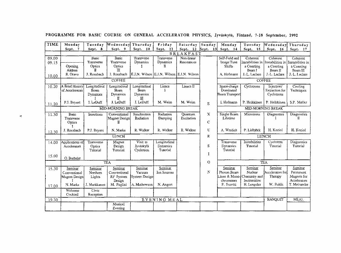
PROGRAMME FOR BASIC COURSE ON GENERAL ACCELERATOR PHYSICS, Jyväskylä, Finland, 7-18 September, 1992
TIME Monday Sept. 7
T u e s d a y Sept. 8
W e d n e s d a y Sept. 9
T h u r s d a y Sept. 10
F r i d a y Sept. 11
Saturday Sept. 12
S u n d a y Sept. 13
Monday Sept. 14
T u e s d a y Sept. 15
W e d n e s d a y Sept. 16
T h u r s d a y Sept. 17
B R E A K F A S T 09.00 09.15
10.00
Basic Transverse
Optics n
J. Rossbach
Basic Transverse
Optics m
J. Rossbach
Transverse Dynamics
I
E.J.N. Wilson
Transverse Dynamics
n
EJ.N. Wilson
Non-linear Resonances
EJ.N. Wilson
E
X
c
u R
S
I
0
N
Self-Field and Image Tune
Shifts
A. Hofmann
Coherent Instabilities in
a Coasting Beam I
J.-L. Laclare
Coherent Instabilities in
a Coasting Beam H
J.-L. Laclare
Coherent Instabilities in
a Coasting Beam HI
J.-L. Laclare
09.00 09.15
10.00
Opening Address
R. Orava
Basic Transverse
Optics n
J. Rossbach
Basic Transverse
Optics m
J. Rossbach
Transverse Dynamics
I
E.J.N. Wilson
Transverse Dynamics
n
EJ.N. Wilson
Non-linear Resonances
EJ.N. Wilson
E
X
c
u R
S
I
0
N
Self-Field and Image Tune
Shifts
A. Hofmann
Coherent Instabilities in
a Coasting Beam I
J.-L. Laclare
Coherent Instabilities in
a Coasting Beam H
J.-L. Laclare
Coherent Instabilities in
a Coasting Beam HI
J.-L. Laclare
COFFEE
E
X
c
u R
S
I
0
N
COFFEE
10.20
11.20
A Brief History of Accelerators
PJ . Bryant
Longitudinal Beam
Dynamics I
I LeDuff
Longitudinal Beam
Dvnamics H
J. LeDuff
Longitudinal Beam
Dynamics m
I LeDuff
Linacs I
M. Weiss
Linacs IE
M. Weiss E
X
c
u R
S
I
0
N
Space-charge Dominated
Beam Transport
I. Hofmann
Cyclotrons
P. Heikkinen
Injection/ Extraction for
Cyclotrons
P. Heikkinen
Cooling Techniques
S.P. M0lkr
MID-MORNING BREAK E
X
c
u R
S
I
0
N
MID-MORNING BREAK
11.30
12.30
Basic Transverse
Optics I
J. Rossbach
Insertions
P.J. Bryant
Conventional Magnet Design
H
N. Marks
Synchrotron Radiation
R.Walker
Radiation Damping
R.Walker
Quantum Excitation
R.Walker
E
X
c
u R
S
I
0
N
Single Beam Lifetime
A. Wrulich
Microtrons
P. Lidbjörk
Diagnostics I
H. Kozioï
Diagnostics
n
H. Koziol
LUNCH
E
X
c
u R
S
I
0
N
LUNCH
14.00
15.00
Applications of Accelerators
O. Barbalat
Transverse Optics
Tutorial
Magnet Design Tutorial
Visit to Jyväskylä Cyclotron
Longitudinal Dynamics Tutorial
E
X
c
u R
S
I
0
N
Transverse Dynamics Tutorial
Instabilities Tutorial
Cyclotron Tutorial
Diagnostics Tutorial
TEA
E
X
c
u R
S
I
0
N
TEA
15.30
17.00
Seminar Conventional
Magnet Design I
N. Marks
Seminar Northern Lights
J. Markkanen
Seminar Conventional RF System
Design M. Puglisi
Seminar Vacuum
System Design
A. Mathewson
Seminar Ion Sources
N. Angert
E
X
c
u R
S
I
0
N Seminar
Photon Beam Lines & Mono
chromators P. Suoriti
Seminar Nuclear
Chemistry and Incineration H. Lengeler
Seminar Accelerators for
Therapy
W. Pohlit
Seminar Permanent
Magnets for Accelerators T. Meinander
Welcome Cocktail
Civic Reception
E
X
c
u R
S
I
0
N
19.30 E V E N I N G M E A L BANQUET MEAL Musical Evening
BANQUET
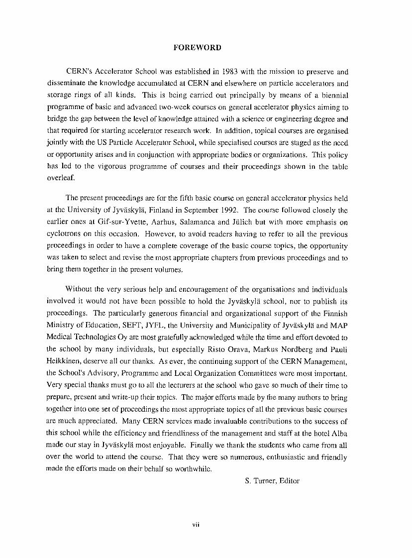
FOREWORD
CERN's Accelerator School was established in 1983 with the mission to preserve and disseminate the knowledge accumulated at CERN and elsewhere on particle accelerators and storage rings of all kinds. This is being carried out principally by means of a biennial programme of basic and advanced two-week courses on general accelerator physics aiming to bridge the gap between the level of knowledge attained with a science or engineering degree and that required for starting accelerator research work. In addition, topical courses are organised jointly with the US Particle Accelerator School, while specialised courses are staged as the need or opportunity arises and in conjunction with appropriate bodies or organizations. This policy has led to the vigorous programme of courses and their proceedings shown in the table overleaf.
The present proceedings are for the fifth basic course on general accelerator physics held at the University of Jyvaskyla, Finland in September 1992. The course followed closely the earlier ones at Gif-sur-Yvette, Aarhus, Salamanca and Jiilich but with more emphasis on cyclotrons on this occasion. However, to avoid readers having to refer to all the previous proceedings in order to have a complete coverage of the basic course topics, the opportunity was taken to select and revise the most appropriate chapters from previous proceedings and to bring them together in the present volumes.
Without the very serious help and encouragement of the organisations and individuals involved it would not have been possible to hold the Jyvaskyla school, nor to publish its proceedings. The particularly generous financial and organizational support of the Finnish Ministry of Education, SEFT, JYFL, the University and Municipality of Jyvaskyla and MAP Medical Technologies Oy are most gratefully acknowledged while the time and effort devoted to the school by many individuals, but especially Risto Orava, Markus Nordberg and Pauli Heikkinen, deserve all our thanks. As ever, the continuing support of the CERN Management, the School's Advisory, Programme and Local Organization Committees were most important. Very special thanks must go to all the lecturers at the school who gave so much of their time to prepare, present and write-up their topics. The major efforts made by the many authors to bring together into one set of proceedings the most appropriate topics of all the previous basic courses are much appreciated. Many CERN services made invaluable contributions to the success of this school while the efficiency and friendliness of the management and staff at the hotel Alba made our stay in Jyvaskyla most enjoyable. Finally we thank the students who came from all over the world to attend the course. That they were so numerous, enthusiastic and friendly made the efforts made on their behalf so worthwhile.
S. Turner, Editor
vu
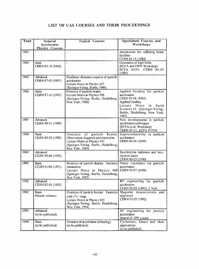
LIST OF CAS COURSES AND THEIR PROCEEDINGS
Year General Accelerator
Physics Courses
Topical Courses Specialised Courses and Workshops
1983 '
Antiprotons for colliding beam facilities CERN 84-15 (1984)
1984 Basic CERN 85-19 (1985)
Generation of high fields (ECFA and INFN Workshop) ECFA 85/91, CERN 85-07 (1985)
1985 Advanced CERN 87-03 (1987)
Nonlinear dynamics aspects of particle accelerators Lecture Notes in Physics 247 (Springer- Verlag, Berlin, 1986)
1986 Basic CERN 87-10 (1987)
Frontiers of particle beams Lecture Notes in Physics 296 (Springer-Vcrlag, Berlin, Heidelberg, New York, 1988)
Applied Geodesy for particle accelerators CERN 87-01 (1987) Applied Geodesy Lecture Notes in Earth Sciences 12 (Springer-Verlag, Berlin, Heidelberg, New York, 1987)
1987 Advanced CERN 89-01 (1989)
New developments in particle acceleration techniques (ECFA et al. Workshop) CERN 87-11, ECFA 87/110
1988 Basic CERN 89-05 (1989)
Frontiers of particle beams; Observation, diagnosis and correction Lecture Notes in Physics 343 (Springer-Verlag, Berlin, Heidelberg, New York, 1989)
Superconductivity in particle accelerators CERN 89-04 (1989)
1989 Advanced CERN 90-04 (1990)
Synchrotron radiation and free-electron lasers CERN 90-03 (1990)
1990 Basic CERN 91-04 (1991)
Frontiers of particle beams: Intensity limitations Lecture Notes in Physics 400 (Springer-Verlag, Berlin, Heidelberg, New York, 1992)
Power converters for particle accelerators CERN 90-07 (1990)
1991 Advanced CERN 92-01 (1992)
RF engineering for particle accelerators CERN 92-03 (1992), 2 Vols.
1992 Basic Present volumes
Frontiers of particle beams: Factories with e +e" rings Lecture Notes in Physics 425 (Springer-Verlag, Berlin, Heidelberg, New York, 1994)
Magnetic measurements and alignment CERN 92-05 (1992)
1993 Advanced (to be published)
RF engineering for particle accelerators Repeat of 1991 course
1994 Basic (to be published)
Frontiers of accelerator technology (to be published)
Cyclotrons, linacs and their applications (to be published)
V l l l
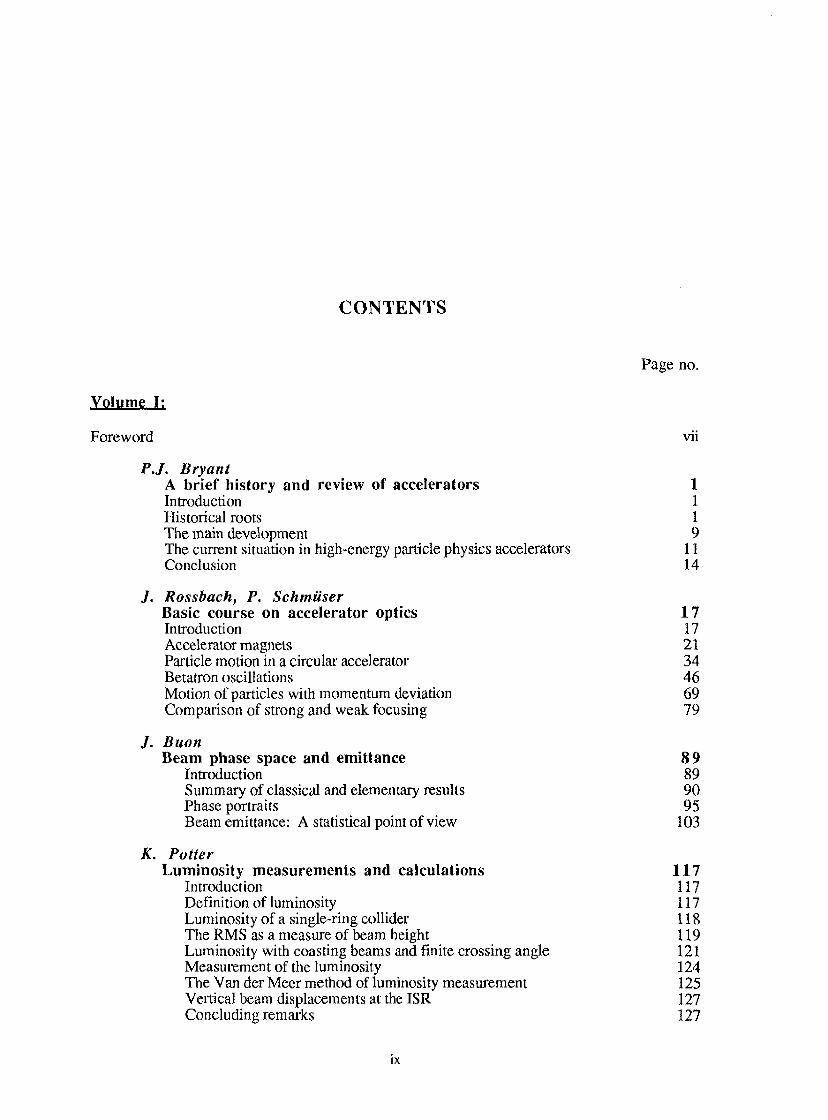
CONTENTS
Page no.
Volume I:
Foreword vii
PJ. Bryant A brief history and review of accelerators 1 Introduction 1 Historical roots 1 The main development 9 The current situation in high-energy particle physics accelerators 11 Conclusion 14
/ . Rossbach, P. Schmuser Basic course on accelerator optics 17 Introduction 17 Accelerator magnets 21 Particle motion in a circular accelerator 34 Betatron oscillations 46 Motion of particles with momentum deviation 69 Comparison of strong and weak focusing 79
J. Buon Beam phase space and emittance 89
Introduction 89 Summary of classical and elementary results 90 Phase portraits 95 Beam emittance: A statistical point of view 103
K. Potter Luminosity measurements and calculations 117
Introduction 117 Definition of luminosity 117 Luminosity of a single-ring collider 118 The RMS as a measure of beam height 119 Luminosity with coasting beams and finite crossing angle 121 Measurement of the luminosity 124 The Van der Meer method of luminosity measurement 125 Vertical beam displacements at the ISR 127 Concluding remarks 127
IX
E. Wilson Transverse beam dynamics 131
Introduction 131 Liouville's theorem 132 A simplified treatment of betatron motion 139 The Q values 141 Closed-orbit distortion 143 Gradient errors 151 The working diagram 153 Chromaticity 154 Conclusions 157
P.J. Bryant Insertions 159
Introduction 159 Matching 160 Dispersion suppressors embedded in a FODO lattice 167 Low-p insertions 171 Extraction and injection 173 Collimation insertions 174 More exotic insertions 187
S. Guiducci Chromaticity 191
Introduction 191 Quadrupole 192 Sextupole 194 Chromaticity correction 195 General bending magnet 197 End-field effects 201
P.J. Bryant A simple theory for weak betatron coupling 207
Introduction 207 Coupling in uniform skew quadrupole and axial fields 208 Observations 214 Results of the exact analysis 216
P.J. Bryant Beam transfer lines 219
Distinctions between transfer lines and periodic circular machines 219 Orbit correction in transfer lines 221 Matching transfer lines 225 Emittance and mismatch measurement in a dispersion-free region 225 Small misalignments and field ripple errors in dipoles
and quadrupoles 227 Emittance blow-up due to thin windows in transfer lines 231 Emittance dilution from betatron mismatch 232 Emittance exchange insertion 235
E. Wilson Non-linearities and resonances 239
Introduction 239 Multipole fields 241 Second-order resonance 242 The third-integer resonance 246 General numerology of resonances 249 Slow extraction using the third-order resonance 249 Landau damping with octupoles 250
X
J. Le Duff Dynamics and acceleration in linear structures 253
Basic methods of linear acceleration 253 Fundamental parameters of accelerating structures 259 Energy gain in linear accelerating structures 273 Particle dynamics in linear accelerators 277
/ . Le Duff Longitudinal beam dynamics in circular accelerators 289
Acceleration by time varying fields 289 Dispersion effects due to the guide field in a synchrotron 296 Synchrotron oscillation in adiabatic limit 299 Adiabatic damping of synchrotron oscillations 306 Trapping, matching, accumulating and accelerating processes 309
T. Risselada Gamma transition jump schemes 313
Introduction 313 Effect of quadrupoles on yi 316 Zero tune shift and non-zero àijt) 318 Cells, superperiods and families 321 Conclusion 325
A. Hofmann Tune shifts from self-fields and images 329
Introduction 329 Direct incoherent tune shifts 330 Effects of the walls on the incoherent tune shift 336 Coherent tune shifts 340 Comments 344 Practical examples 346
J.-L. Laclare Coasting beam longitudinal coherent instabilities 349
Introduction 349 Single-particle motion 351 Longitudinal signal of a single particle 353 Distribution function 356 Electromagnetic field induced by the beam 360 Negative mass instability 363 Introduction of the longitudinal coupling impedance Z//(co) 364 Longitudinal coupling impedance Z//(CÙ) of an accelerator ring 366 Vlasov's equation and dispersion relation 371 Monochromatic beam 375 Coasting beam with momentum spread 378 Landau damping by momentum spread 380 Limits of the theory 382
J.-L. Laclare Coasting beam transverse coherent instabilities 385
Introduction 385 Single-particle transverse motion 386 Transverse signal of a single particle 387 Distribution function 390 Total beam signal 390 Definition of transverse coupling impedance 391 Transverse coupling impedance Z//(co) of an accelerator ring 393 Dispersion relation for coherent motion 395 Beam without tune spread 397 Landau damping by momentum spread 401 Landau damping by amplitude dependent tune 405
XI
A. Wrulich Single-beam lifetime 409
Introduction 409 Lifetime due to quantum fluctuation and radiation damping 412 Lifetime for statistical fluctuations without damping 414 Lifetime due to beam-gas scattering 416 Lifetime due to Touschek scattering 424 Intrabeam scattering 428 Lifetime due to resonance crossing 432 Lifetime measurement 433
R.P. Walker Synchrotron radiation 437
Introduction 437 Basic properties 438 S pectral an d an gu lar properties 442 Photon distribution 449 Synchrotron radiation aspects in electron accelerator design 451 Synchrotron radiation sources 453 Synchrotron radiation from protons 454
R.P. Walker Radiation damping 461
Introduction 461 Energy oscillations 462 Betatron oscillations 466 Damping partition and the Robinson theorem 470 Radiation damping aspects in various lattice designs 471 Modification of damping rates 475 Measurement of damping rates 477
R.P. Walker Quantum excitation and equilibrium beam properties 481
Introduction 481 Energy oscillations 481 Betatron oscillations 486 Synchrotron radiation integrals 489 Quantum lifetime 490 Low emittance lattices 493 Changes in beam properties due to insertion devices 494
Volume II:
H. Mais, C. Mari Introduction to beam-beam effects 499
Introduction 499 Basic facts 500 Linear beam-beam models 504 Experimental facts and results for lepton and hadron colliders 510 Theoretical tools and methods 515 Summary and conclusions 520
Y. Baconnier, A. Poncet, P.F. Tavares Neutralisation of accelerator beams by
ionisation of the residual gas 525 Neutralisation of abeam: a simple description 525 The ionisation process 527 The ion or electron motion 530 A few examples of ion or electron motion 537
Xll
Bunched beams 539 Clearing electrodes 541 The limit of accumulation 541 The effects of neutralisation 541 Diagnostics and phenomenology 549
H. Koziol Beam diagnostics for accelerators 565
Introduction 565 Description of diagnos tic devices 5 67 Concluding remarks 590
S.P. M0ller Cooling techniques 601
Introduction 601 Stochastic cooling 602 Electron cooling 607 Laser cooling 613 Other cooling methods 615 Conclusion and comparisons 616
JV. Angert Ion sources 619
Introduction 619 Principles 619 Ion sources for positive ions 624 Ion sources for negative ions 633 Beam formation 637
R. Chehab Positron sources 643
Physical processes associated with positron production 643 Presentation of some positron sources 655 Positron collection: The matching system 661 Emittance transformation and preservation 674 Comparison of positron sources 674 Summary and conclusions 675
M. Puglisi Conventional RF system design 679
Introduction 679 The accelerating gap 679 The drift tube 680 Cavity resonators 682 The cylindrical cavity 684 TEM cavities 686 m cavity 688 Re -entrant cavi ty 689 Common RF accelerating structures 691 Coupling to the cavities 693 Shunt impedance 695 RF power amplifiers 696 RF generators 696
A.G, Mathewson Vacuum system design 717
Introduction 717 Basic formulae 717 Conductance 718 Monolayer 719
X l l l
Pumping systems Cleaning methods 720 Thermal outgassing 722 Bakeout 723 Synchrotron radiation induced gas desorption 724 Simple machine 726 Proton storage rings 727 Cold proton storage rings 729
G.H. Rees Injection 731
Introduction 731 Single-turn injection 732 Multi-turn injection 734 H" charge-exchange injection 737 Injection from a cyclotron into a synchrotron 742 Novel injection schemes 742
G.H. Rees Extraction 745
Introduction 745 Fast extraction 746 Slow extraction 747 Septum units 751
S. Wolff Superconducting accelerator magnet design 755
Introduction 755 Superconducting magnet configurations 755 Field analysis 757 Examples of existing magnet designs 765 Design details 767 Test results at HERA mass production magnets 783 Conclusions 788
H. Lengeler Modern technologies in RF superconductivity 791
Limitations of SC cavity performances 792 Nb material 794 Surface diagnostics, inspection and repair methods 794 Shaping and welding of SC cavities 797 Surface treatments 799 Cavities coated with thin superconducting layers 801
P. Heikkinen Cyclotrons 805
Introduction 805 Operation principle 805 Isochronous cyclotron 807 Cyclotron hardware 815
P. Heikkinen Injection and extraction for cyclotrons 819
Introduction to injection systems 819 Neutral beam injection 820 Axial injection 820 Radial injection 826 Longitudinal matching 830 Introduction to extraction schemes 830 Extraction systems for cyclotrons 831
xiv
Stability of vertical motion in extraction 836 Extraction elements 836 Conclusions 838
O. Barbalat Applications of particle accelerators 841
Introduction and overview 841 Research applications 842 Element analysis 846 Medicine 846 Industrial processing 848 Power engineering 851 Conclusion 852
W. Pohlit Accelerators for therapy 855
Introduction 855 Development of present tumor therapy 855 Developments for future radiation therapy of tumors 860
N. Marks Conventional magnets - I 867
Introduction 867 Magneto-static theory 867 Practical aspects of magnet design 875
N. Marks Conventional Magnets - II 891
Introduction to AC effects 891 Low frequency systems 892 High frequency magnets 901 Conclusion 910
M. Weiss Introduction to RF linear accelerators 913
Introduction 913 Electromagnetic waves and cavities 914 Wave equation and slowing down of waves 917 Travelling and standing wave linear accelerators 921 Electromagnetic forces and their action 928 Phase stability and acceptance of an accelerator 932 Handling of intense beams 939 Various structures of linear accelerators 941 Conclusion 951
P. Suortti Photon beamtines and monochromators 955
Introduction 955 X-ray optics 956 Constructions 964 Experimental stations 968
P. Lidbjork Microtrons 971
Introduction 971 The circular or classical microtron 972 The racetrack microtron 977
XV
T. Meinander Generation of magnetic fields for accelerators
with permanent magnets 983 Introduction 983 Permanent magnet materials 983 Calculation of permanent magnet fields 985 Electromagnets versus permanent magnets 986 Multipole magnets 990 Insertion devices 994
H. Lengeler Nuclear waste transmutation using high-intensity
proton linear accelerators 999 Introduction 999 The nuclear waste problem 999 Earlier transmutation studies 1001 A new Los Alamos proposal 1001 State of the art of high-power proton and deuteron linear accelerators 1004 Two design aspects of a high-intensity proton-linac 1006 A possible layout 1009 Superconducting (S.C.) cavities 1012 Conclusion 1016
List of participants 1021
xvi
INTRODUCTION TO BEAM-BEAM EFFECTS
H. Mais, DESY, Hamburg, FRG
C. Mari, ENEA, Frascati, Italy
ABSTRACT An introduction is given to beam-beam effects in lepton and hadron colliders. The experimental results and facts are summarized and some theoretical tools and methods are explained.
1. INTRODUCTION Lepton and hadron storage rings have become one of the most important tools in high
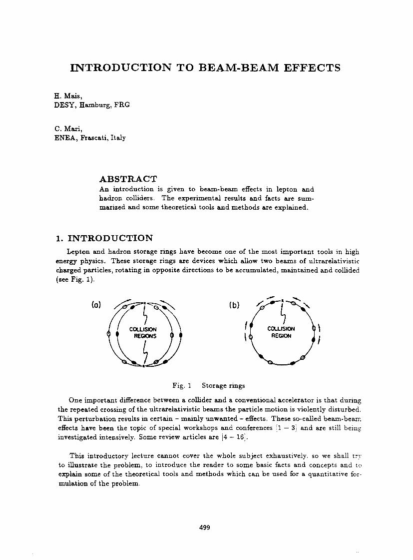
energy physics. These storage rings are devices which allow two beams of ultrarelativistic charged particles, rotating in opposite directions to be accumulated, maintained and collided (see Fig. 1).
Fig. 1 Storage rings
One important difference between a collider and a conventional accelerator is that during the repeated crossing of the ultrarelativistic beams the particle motion is violently disturbed. This perturbation results in certain - mainly unwanted - effects. These so-called beam-beam effects have been the topic of special workshops and conferences [1 — 3] and are still being investigated intensively. Some review articles are [4 — 16].
This introductory lecture cannot cover the whole subject exhaustively, so we shall try to illustrate the problem, to introduce the reader to some basic facts and concepts and to explain some of the theoretical tools and methods which can be used for a quantitative formulation of the problem.
499
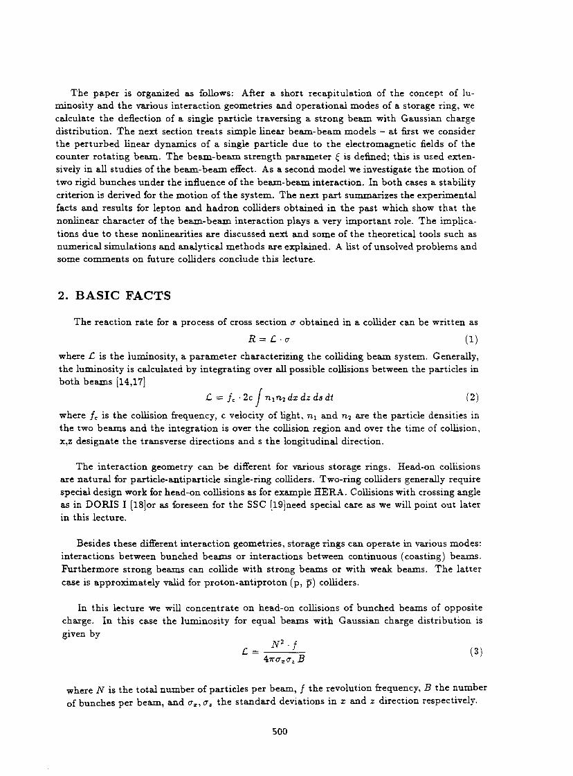
The paper is organized as follows: After a short recapitulation of the concept of luminosity and the various interaction geometries and operational modes of a storage ring, we calculate the deflection of a single particle traversing a strong beam with Gaussian charge distribution. The next section treats simple linear beam-beam models - at first we consider the perturbed linear dynamics of a single particle due to the electromagnetic fields of the counter rotating beam. The beam-beam strength parameter £ is defined; this is used extensively in all studies of the beam-beam effect. As a second model we investigate the motion of two rigid bunches under the influence of the beam-beam interaction. In both cases a stability criterion is derived for the motion of the system. The next part summarizes the experimental facts and results for lepton and hadron colliders obtained in the past which show that the nonlinear character of the beam-beam interaction plays a very important role. The implications due to these nonlinearities are discussed next and some of the theoretical tools such as numerical simulations and analytical methods are explained. A list of unsolved problems and some comments on future colliders conclude this lecture.
2. BASIC FACTS
The reaction rate for a process of cross section a obtained in a collider can be written as
R = C-<r (1)
where £ is the luminosity, a parameter characterizing the colliding beam system. Generally, the luminosity is calculated by integrating over all possible collisions between the particles in both beams [14,17]
C = fc • 2c / Tiin2 dx dz ds dt (2)
where fc is the collision frequency, c velocity of light, nj and n 2 are the particle densities in the two beams and the integration is over the collision region and over the time of collision, x,z designate the transverse directions and s the longitudinal direction.
The interaction geometry can be different for various storage rings. Head-on collisions are natural for particle-antiparticle single-ring colliders. Two-ring colliders generally require special design work for head-on collisions as for example HERA. Collisions with crossing angle as in DORIS I [l8]or as foreseen for the SSC [I9]need special care as we will point out later in this lecture.
Besides these different interaction geometries, storage rings can operate in various modes: interactions between bunched beams or interactions between continuous (coasting) beams. Furthermore strong beams can collide with strong beams or with weak beams. The latter case is approximately valid for proton-antiproton (p, p) colliders.
In this lecture we will concentrate on head-on collisions of bunched beams of opposite charge. In this case the luminosity for equal beams with Gaussian charge distribution is given by
N2 • f £ = — -* (3)
Ait<rxcz B
where N is the total number of particles per beam, / the revolution frequency, B the number of bunches per beam, and <JX, az the standard deviations in x and z direction respectively.
500
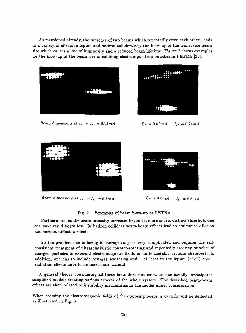
As mentioned already, the presence of two beams which repeatedly cross each other, leads to a variety of effects in lepton and hadron colliders e.g. t h e blow-up of the transverse beam size which causes a loss of luminosity and a reduced b e a m lifetime. Figure 2 shows examples for the blow-up of the beam size of colliding electron-positron bunches in P E T R A [20].
Beam dimensions at /,+ = It- = 0.15mA I e + = 0.52mA Ie- = 0.74mA
Beam dimensions at 7 C + = 7 t_ = 0.3mA ^ + = 0.6mA It. = 0.6mA
Fig. 2 Examples of beam blow-up at P E T R A
Fur thermore , as the b e a m intensity increases beyond a more or less distinct threshold one can have rapid beam loss. In hadron colliders beam-beam effects lead to emit tance dilation and various diffusion effects.
So the problem one is facing in storage rings is very complicated and requires the self-consistent t rea tment of ultrarelativist ic counter-rotat ing and repeatedly crossing bunches of charged particles in external electromagnetic fields in finite metallic vacuum chambers . In addit ion, one has to include rest-gas scattering and - at least in the lepton ( e + e ~ ) case -radiat ion effects have to be taken into account.
A general theory considering all these facts does not exist, so one usually investigates simplified models t reat ing various aspects of the whole system. The described beam-beam effects are then related to instability mechanisms in the mode l under consideration.
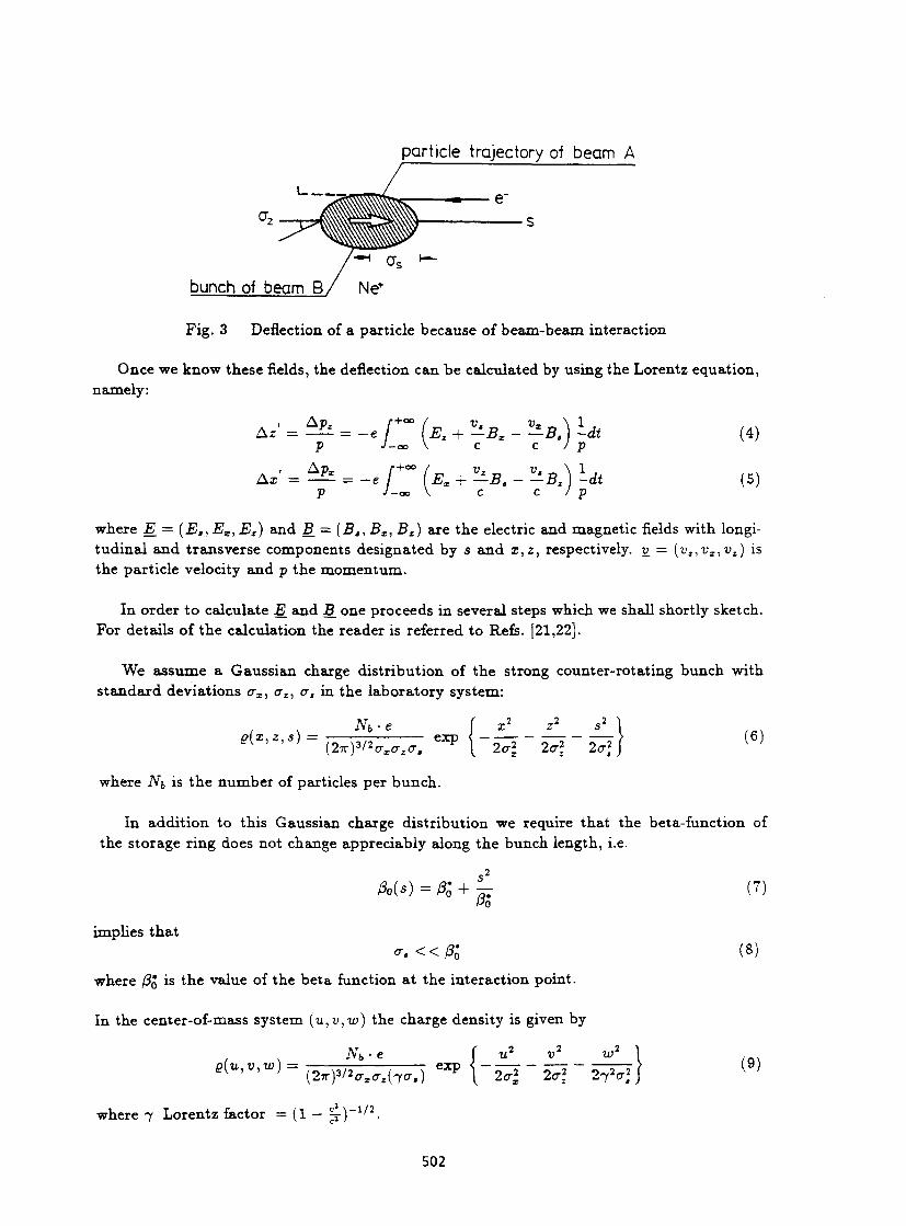
When crossing the electromagnetic fields of the opposing beam, a particle will be deflected as i l lustrated in Fig. 3.
501
< • • • • • iw. "••
particle trajectory of beam A
bunch of beam B / Ne+
Fig. 3 Deflection of a particle because of beam-beam interaction
Once we know these fields, the deflection can be calculated by using the Lorentz equation, namely:
A z < = ^ = _e r~ (Ez + ^Bm _ ^ \ i d t ( 4 ) P J-oo \ C C ) p
* * ' = * * = _ e T~ U +
vJLBt _ ^ B z ) ldt ( 5 ) P J-oo \ C C J p
where E_ = (E,,EX,EZ) and B_ — (B,,BX,BZ) are the electric and magnetic fields with longitudinal and transverse components designated by s and x,z, respectively. v_ — [va,vx,vz) is the particle velocity and p the momentum.
In order to calculate E_ and B_ one proceeds in several steps which we shall shortly sketch. For details of the calculation the reader is referred to Refs. [21,22].
We assume a Gaussian charge distribution of the strong counter-rotating bunch with standard deviations crx, <rz, <r, in the laboratory system:
g{x,z,s) = exp i - — = • - r - r - T-Z> (6) (2ir)3'2(Txazcr, { 1a\ 2o\ 2a] J
where Nb is the number of particles per bunch.
In addition to this Gaussian charge distribution we require that the beta-function of the storage ring does not change appreciably along the bunch length, i.e.
&(*)=# + £- (7) Po
implies that a, <<&* (8)
where /% is the value of the beta function at the interaction point.
In the center-of-mass system (u,v,w) the charge density is given by
( \ N»-e \ u 2 v 2 w* \ (to
where 7 Lorentz factor = (1 — \) -1/2
502
The potential corresponding to this charge distribution can be calculated and the electric field of the Gaussian bunch is obtained in the center-of-mass system. Transforming the field back to the laboratory system using the well-known transformation rules
Ex = 7 Eu Ez = 7EV E, = EV
(10) Bx = ^Ev BZ = -V-7EU B, = 0
and taking into account (4) and (5) one finally gets for short bunches
, _ 2Nbrez r°° exp { - ^ - ^ } 7 Jo {2er\ + q)3'2 {2a\ + ç ) 1 / 2 9
Az = -
- _ 2Nbr,x /•«» exp { ~ a f e ? ~ 2 ^ } A x = —•
7 I {2<r\ + ç)VJ {2<r\ + q)*/* dq
(ID
(12)
with r. = m j t 2 classical particle radius.
Remark i: The kicks experienced by the test particle can be derived from a potential U(x,z)
' Az' ••
Ax
au(x,z) 8i
dU(x,z) ax
™ f *2
U { x : ) = ^ f l - e x p { - s ^ - s ^ } { ' > j Jo (2tr* + q)V* (2<rl + q)V* 9 "
(13)
(14)
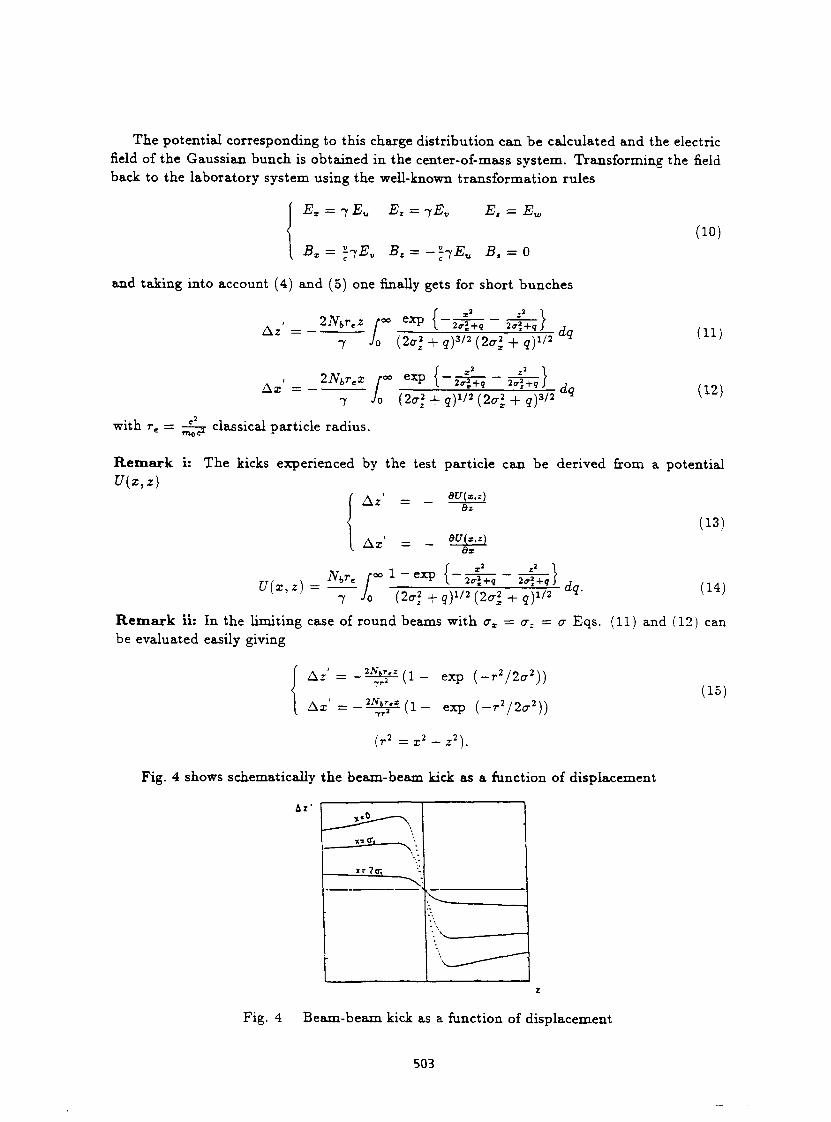
Remark ii: In the limiting case of round beams with crx = cr. = <r Eqs. (11) and (12) can be evaluated easily giving
Az' = - ^ ( 1 - exp ( - r 2 / 2 a 2 ) )
A x ' = - ^ ( 1 - exp (-r 2 /2<7 2 ))
^ 2 - ~ 2
(15)
x' + z'
Fig. 4 shows schematically the beam-beam kick as a function of displacement
Az'
XT ?q; 1
Fig. 4 Beam-beam kick as a function of displacement
503
For small values x < < crx,z << az the behaviour is l inear. Using (11) and (12) one obtains
2Nbrez 1 A* =
A i = —
f(ax + az)az fz
2Nbrtx 1
with
j(ax + <Jz)crx fx
2Nbre
fz f{<rx + <rz)o-z
1 2Nbrt
fx f{crx + CT2)CTX'
(16)
(17)
(18)
(19)
3. LINEAR BEAM-BEAM MODELS As a simple mode l we now study the dynamics of a test part icle which is per turbed
by the linear b e a m - b e a m kicks. The interaction point Sip is specified by (y = x or z)
y(*ip + 0 =y{sip - e)
or m m a t r i x no ta t ion :
y'{siP + 0 = 2 / ( s . p - 0 y{sir
(20)
(21)
(22)
The 2 x 2 m a t r i x describing the beam-beam interact ion in this linear model is equivalent to the transfer m a t r i x of a th in lens quadrupole of focal length fy [23]. The influence of this addit ional pe r t u rba t i on on the particle motion can be calculated in the usual way (231.
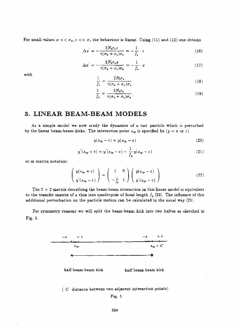
For symmet ry reasons we will split the beam-beam kick in to two halves as sketched in
Fig. 5.
— £ -+- £
-1 « / < « >
-£ + £
•Sip + C"
half beam-beam kick half beam-beam kick
( C dis tance between two adjacent interact ion points)
Fig. 5
504
The transfer ma t r i x from one interaction point to the next in teract ion point is then given
by:
' co s (^ y + Afiy) /3* sin(^xv -f Afiy) ^
\ -jzsm{^y + Aiiy) cos(My + A ^ v ) / 2 / »
cos^v / ? ô v
s i n ^ v
— ^ " S i n fly COS fly
o\
(23)
(y,y + Afiy), (3* are the pe r tu rbed lattice functions (phase advance between interact ion points
and be ta function). As usual we assume tha t 8 vanishes at the in teract ion point .
A\iy is calculated from 8:
(24) Ply • cos(^i y -i- Aj i y ) = cos fiy — sin fiy
2, J y
— cos fiy — 2-7T • £ y sin fiy
where we have introduced the beam-beam st rength parameter
£y = 27r •yay(crx 4- az
(25)
£ y plays a fundamenta l role in t he investigations of the beam- beam interact ion. It character
izes the s t rength of t he interact ion and for small Afiy it gives the tune shift of the system
due to the pe r tu rb ing beam-beam kick
«, = £ = **. (26)
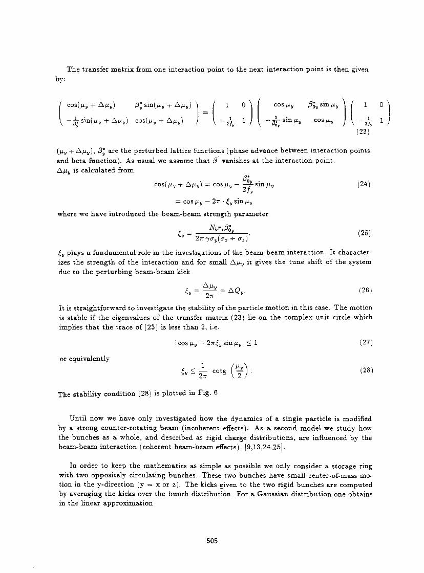
It is s traightforward to investigate the stability of the particle mot ion in this case. The motion
is stable if the eigenvalues of the transfer mat r ix (23) he on the complex unit circle which
implies t ha t the t race of (23) is less than 2, i.e.
or equivalently
cos \iy — 27r£y sin \iy \ < 1
<• <- h -* (y
(27)
(28)
The stabil i ty condition (28) is p lot ted in Fig. 6
Until now we have only investigated how the dynamics of a single part icle is modified by a s t rong counter - ro ta t ing b e a m (incoherent effects). As a second model we s tudy how the bunches as a whole, and described as rigid charge dis t r ibut ions , are influenced by the beam-beam interact ion (coherent beam-beam effects) [9,13,24,25].
In order to keep the mathemat ics as simple as possible we only consider a storage ring with two oppositely circulating bunches. These two bunches have small center-of-mass motion in the y-direction (y = x or z). The kicks given to the two rigid bunches are computed by averaging the kicks over the bunch distr ibution. For a Gauss ian dis t r ibut ion one obtains in the linear approximat ion
505
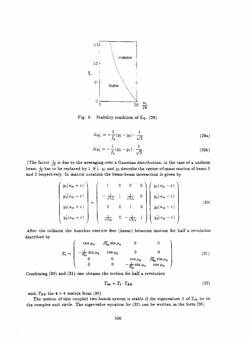
Fig. 6 Stabili ty condition of Eq. (28)
(29a)
(29b)
(The factor -j- is due to the averaging over a Gaussian d is t r ibut ion; in the case of a uniform
beam 4= has to be replaced by 1 [9]). j/i and 3/2 describe the center-of-mass motion of beam 1
and 2 respectively. In m a t r i x no ta t ion the beam-beam interact ion is given by
/
V
y[(sip +e)
V2{sip + e)
/ 1 0
1 V 2 / v
1
0 0
1 0
V V2/,
1 N/2/S
1
0
0
0
1
/
/ V
2/I(-S.P - e)
y'i(*ip-£)
yi(sip - e)
y 2 ( 5 > P - £ )
\
(30)
/
After the collision the bunches execute free (linear) be ta t ron mot ion for half a revolution
described by
cos /xv fay s i n My /
To = - â ï - s in M V
0 0
cos^xv
0 0
0 0
0 0
cos ny fay sin /z y
\
(31)
— jp- sin fj.y cos /z v /
Combining (30) and (31) one obta ins the motion for half a revolution
Ttot — TQ -TBB (32)
with TBB the 4 x 4 m a t r i x from (30). T h e motion of this coupled two-bunch system is stable if the eigenvalues A of Ttot lie on
the complex unit circle. The eigenvalue equation for (32) can be wr i t ten in the form [26]:
506
A 2 - A(4 cos My - 2£/3*v sin M V ) + (2 cos M V - e&'y sin My)2 - £ 2/?ô v
2 sin 2
M y = 0 (33)
where we have used t h e abbreviat ions
1 £ =
%/2/ v
A = A + - .
A
The solution of (33) gives four eigenvalues:
A/.// = e ± l ^ (34a)
A///./V = e ± i <"» + A " ' )
where A/x v is de termined by
4?r cos(/x v + A^y) = c o s ^ v 7=^ v sin/x y .
v 2
(34b)
(35)
The motion belonging to (34a) is always stable and is called the cr-mode. In this mode the bunches oscillate in phase moving up and down together at the collision point . The motion corresponding to (34b) is s table if
COS / i y 4TT£V
sin M V | < 1
or equivalently 1 ,M U l
Î36)
(37)
In this case the bunches oscillate out of phase, colliding at an offset changing from collision to collision. This mode is called 7r-mode. This behaviour is similar to the mot ion of two coupled linear oscillators in classical mechanics. Figure 7 shows the stability condition (37) which is more str ingent t h a n in the incoherent case (28).
03 -
Fig. 7 Stability region for two strong rigid beams executing small center of mass oscillations as a function of the to t a l tune Qy of the storage ring. The dashed line shows the strong-weak stability limit of Eq. (28).
507
R e m a r k i: For a uniform charge dis t r ibut ion the stability is given by
i v < h cotg ^ and the tune shift for small A/iy is given by
2TT
[381
(39)
(twice the incoherent tune shift).
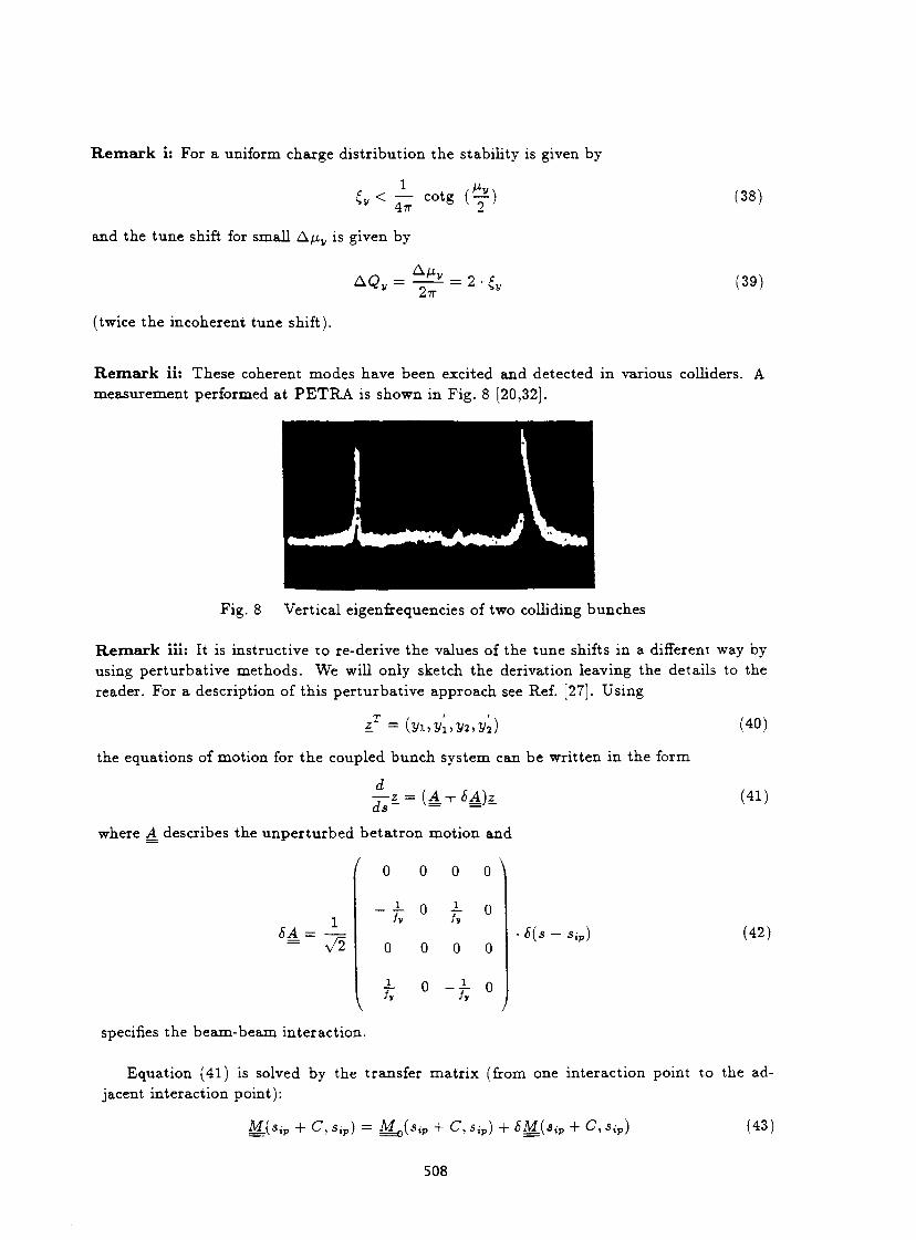
R e m a r k ii: These coherent modes have been excited and detected in various colliders. A measurement performed at P E T R A is shown in Fig. 8 [20,32].
Fig. 8 Vertical eigenfrequencies of two colliding bunches
R e m a r k Hi: It is instructive to re-derive the values of the tune shifts in a different way by using per turbat ive methods . We will only sketch the derivation leaving the details to the reader. For a description of this per tu rba t ive approach see Ref. [27]. Using
* = (yi ,2/ i ,y2,y 2 )
the equations of motion for the coupled bunch system can be wri t ten in the form
as — —
where A_ describes the unpe r tu rbed be t a t r on motion and
I n n n n '
(40)
(41)
SA = V2
0 0 0
f ° f 0
0
0 0 0
V T °
• S(s - sip) (42)
specifies the beam-beam interact ion.
Equat ion (41) is solved by the transfer ma t r ix (from one interaction point to the adjacent interaction point):
M{sip + C, sxp) = M^is,,, + C, 5,p) + 6M{sir, + C, sip) (43)
508
with tK{sir + C,3ip) = M^i-ip + C,sip)x
x f"P+ ^'Mo~V,s, P)<$â( 5')-Mo(^ P)- ( 4 4 ) In order to calculate the eigenvalues of M we need to know the unper tu rbed eigenvalues of M0 where the two bunches are uncoupled. It is easy to verify tha t
A/i = ^iv = A* (451
with the corresponding eigenvectors
/fo,\ Vj = fifc. Oy
0 (46a)
VJII =
\ o ;
t ° \ 0
2/30* ov A* \
Oy i I
and
are solutions to
or explicitly:
VJI = V.i, liv = VJII
Mol-Sip + C, J t p M a i p ) = Xvisip)
(46b)
(47)
(48)
COS My / ? ô y s i l l M y 0 0 \
• g!- sin My cos My 0 0
0 0
v(sip) = A r ( s i p ) . 0 0
cos My /?5y sin / i y
V U U — ^ - sin My cos My /
The eigenvectors (46a) and (46b) satisfy the following normalisation condition [28]
i
where -+- means Hermitean conjugation and S is denned by
/ 0 - 1 0 0 \ 1 0 0 0 0 0 0 - 1
\ 0 0 1 0 J
(49)
5 = (50)
Prom (45) it follows tha t t he unpe r tu rbed spectrum of M^ is degenerate a n d therefore the tune shifts are calculated according to the well-known quan tum mechanical expressions
SX=\ [6MU + 6 M 3 3 ] ± \yJ{8M11-6M33y + A6Mh (51)
509
where
i J»,r
(52)
Substituting (46a), (46b), (47), (42) into (52) and solving (51) we get the results
6\ = 0
8\ = ^-SL-• V2fy
(531
or equivalently
8Q = 0
flï, (54)
in accordance with (36).
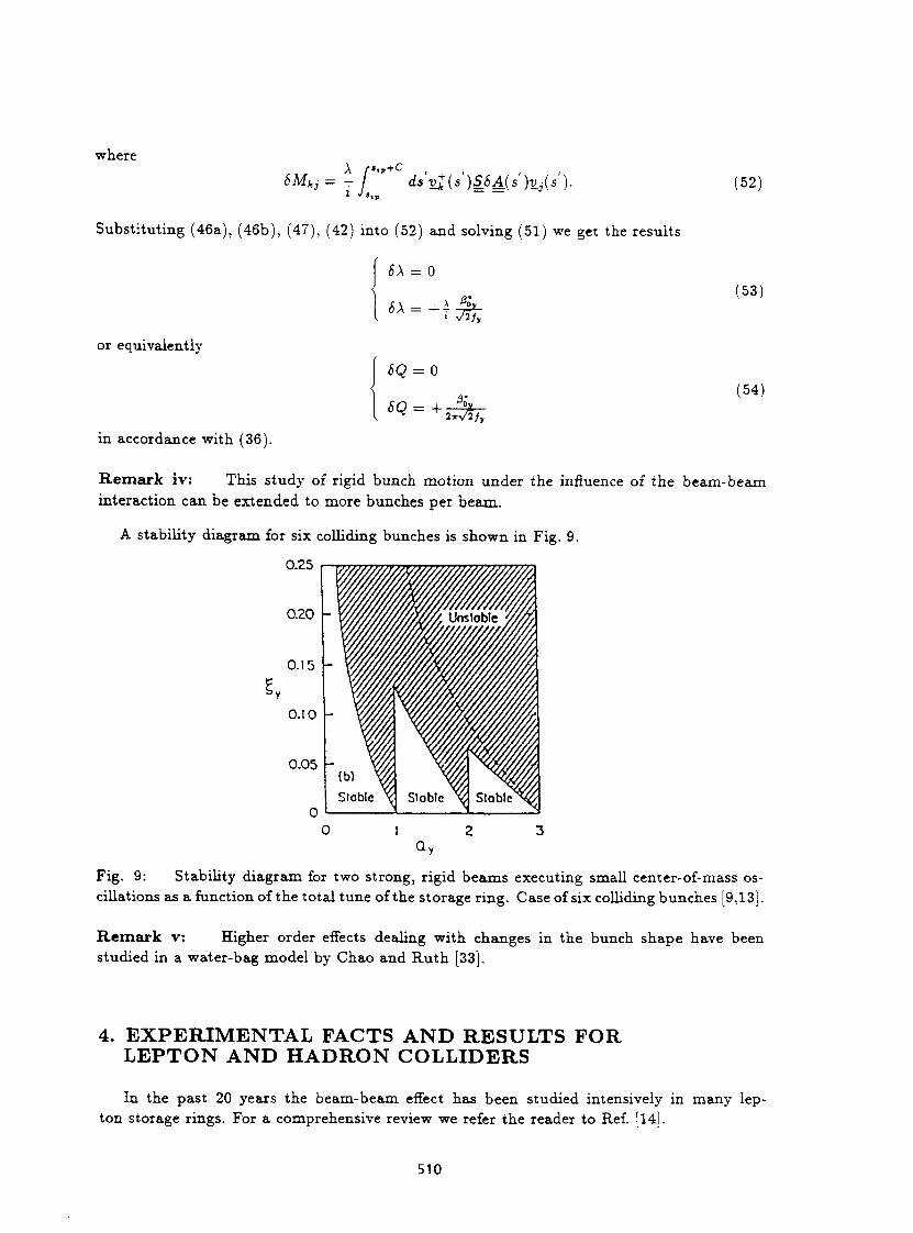
Remark iv: This study of rigid bunch motion under the influence of the beam-beam interaction can be extended to more bunches per beam.
A stability diagram for six colliding bunches is shown in Fig. 9.
0.25
0.20 -
0.15 -
0.10 -
0.05 -
Fig. 9: Stability diagram for two strong, rigid beams executing small center-of-mass oscillations as a function of the total tune of the storage ring. Case of six colliding bunches [9,13].
Remark v: Higher order effects dealing with changes in the bunch shape have been studied in a water-bag model by Chao and Ruth [33].
4. EXPERIMENTAL FACTS AND RESULTS FOR LEPTON AND HADRON COLLIDERS
In the past 20 years the beam-beam effect has been studied intensively in many lep-ton storage rings. For a comprehensive review we refer the reader to Ref. [14].
510
In order to investigate the pa rame te r dependence of the luminosity of a collider, we rewri te
£ as: I2 IiL
£ =
where we have used
and
47re2/-BCTxcT: 2ere(3'0z
I = N -ef = Nb-ef B
( total cur rent )
r(i-r) (55)
(56)
(25) 2Tr-yBefcr:{ax + <r.)
In all lepton colliders az < < ax therefore one can neglect (crz/ax) in (55).
The current I of a collider depends on single-beam instabilities and coupled-bunch instabilities. Due to the chromatici ty compensa t ing sextupoles the value of /?Ô2 is limited by aper ture considerat ions and because of (8) by the bunch length. £z depends on various operating condit ions such as energy, tune of the machine , coupling, dispersion, radiat ion damping and all kinds of per tu rba t ions . Some impor t an t facts which have been found experimentally are listed below:
Fact i: For a b e a m current smaller t h a n a characterist ic threshold current Ith, the luminosity £ is propor t iona l to I2 which implies
i,~I. (57)
For currents of t h e order of Ith, £ varies linearly wi th I implying a sa tura t ion of fz. This sa tura t ion is due to a linear increase of the beam size with current . For all existing lepton colliders
£, < 0.07 (58)
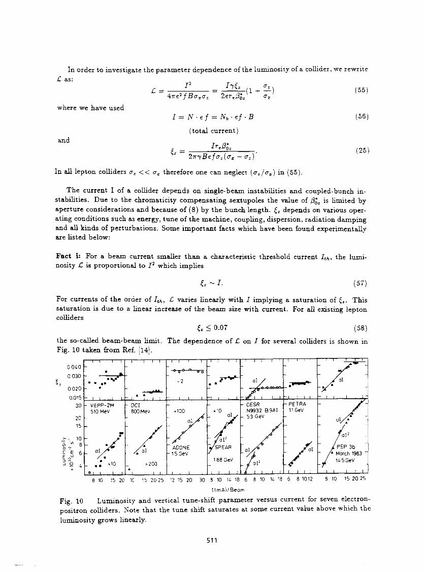
the so-called b e a m - b e a m limit. The dependence of £ on J for several colliders is shown in Fig. 10 taken from Ref. [14].
1 1 ' I I T
OOiO
0 030 -
0020
0015
30
20 15
^ - 10 S , J > 8 o "v £ E, 6
- 1 2 L
^
J I I L VEPP-2M 510 MeV
aï
«10
_L_J L
J L DCI 800 MeV
1Z
ADONE - 15 GeV
J L_J L
1 1 — I 1 r
% a agon. - *
J L - CESR
N9932 B.9AI 53 GeV
PETRA 11 GeV
I . I l _ l _ J I I I L 10 15 20 10 15 20 25 12 15 20 30 8 10 U 18 6 8 10 U 18 6 8 1012 8 10 15 20 25
KmAI/Beam
Fig. 10 Luminosi ty and vertical tune-shift pa ramete r versus current for seven electron-
positron colliders. Note tha t the t u n e shift sa tura tes at some current value above which the
luminosity grows linearly.
511
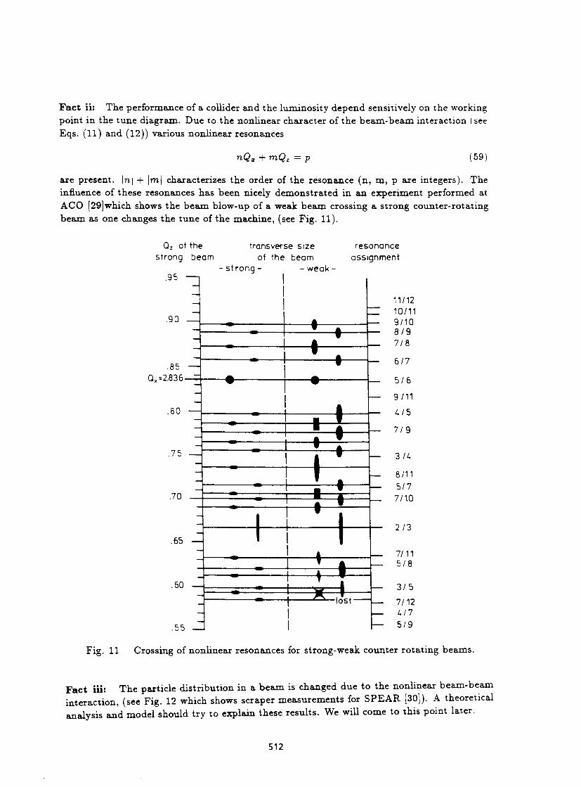
Fact ii: The performance of a collider and the luminosity depend sensitively on the working point in the tune diagram. Due to the nonlinear character of the beam- beam interaction ( see Eqs. (11) and (12)) various nonlinear resonances
nQx + mQz = p (59)
are present . \n\ + \m\ characterizes the order of the resonance (n, m , p are integers). The influence of these resonances has been nicely demonst ra ted in an experiment performed at ACO [29]which shows the b e a m blow-up of a weak b e a m crossing a s t rong counter-rotat ing beam as one changes the tune of the machine, (see Fig. 11).
Qz of the transverse size resonance strong beam of the beam assignment
- s t r o n g - - w e a k -.95 -
.90
.85 Q =2.836-
.80 —
.75
.70
.65 —
* .60 — .
2 / 3
7/11 5 /8
3 / 5
7/12 Lil
.55 - J I r - 5 /9
Fig. 11 Crossing of nonlinear resonances for strong-weak counter ro ta t ing beams.
+
i
T
11/12 10/11 9/10 8 / 9 7 /8
6 /7
5 / 6
9/11
A/5
7 / 9
— 3 IL
. 8/11 - 5 /7 . 7/10
XïM— - ^ — lost
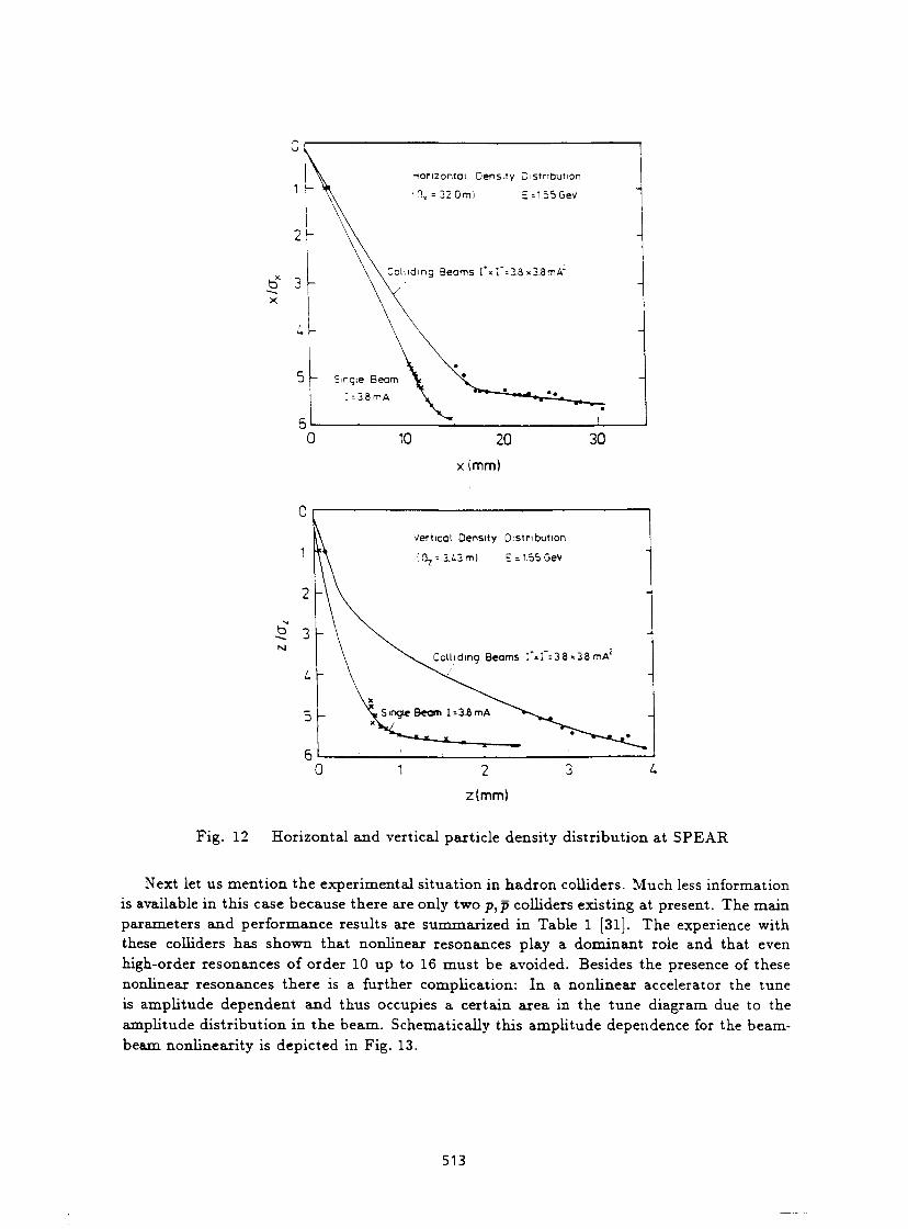
Fact iii: T h e particle distr ibution in a b e a m is changed due to the nonlinear beam-beam interact ion, (see Fig. 12 which shows scraper measurements for S P E A R [30]). A theoretical analysis and model should t ry to explain these results . We will come to this point later.
512
x(mm)
Fig. 12 Horizontal and vertical particle density distribution at SPEAR
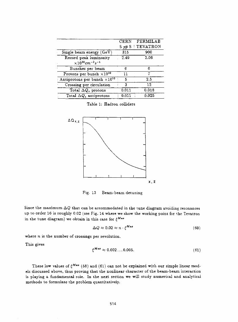
Next let us mention the experimental situation in hadron colliders. Much less information is available in this case because there are only two p, p colliders existing at present. The main parameters and performance results are summarized in Table 1 [31]. The experience with these colliders has shown that nonlinear resonances play a dominant role and that even high-order resonances of order 10 up to 16 must be avoided. Besides the presence of these nonlinear resonances there is a further complication: In a nonlinear accelerator the tune is amplitude dependent and thus occupies a certain area in the tune diagram due to the amplitude distribution in the beam. Schematically this amplitude dependence for the beam-beam nonlinearity is depicted in Fig. 13.
513
CERN S pp S
FERMILAB TEVATRON
Single beam energy (GeV) 315 900 Record peak luminosity
x l O ^ c m - 2 * - 1
2.49 2.06
Bunches per beam 6 6 Pro tons per bunch x l O 1 0 11 7
; Ant iprotons per bunch x l O 1 0 5 2.5 Crossing per circulation 3 12
Total AQZ protons 0.011 0.018 Total AQZ ant iprotons o.oii ; 0.025
Table 1: Hadron colliders
ACL,
x,z
Fig. 13 Beam-beam detuning
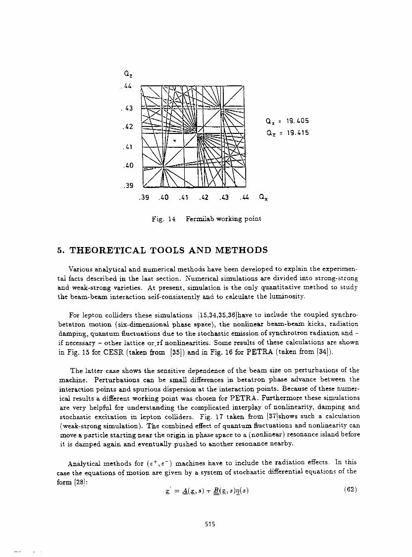
Since the m a x i m u m A Q tha t can be accommodated in the tune d iagram avoiding resonances up to order 16 is roughly 0.02 (see Fig. 14 where we show the working point for the Tevatron in the tune d iagram) we obta in in this case for £Max
A Q % 0.02 « n • £
where n is the number of crossings per revolution
This gives
Max
i M a s « 0 . 0 0 2 . . . 0.005.
(60)
(61)
These low values of £Max (58) and (61) can not be explained wi th our simple linear models discussed above, thus proving tha t the nonlinear character of the b e a m - b e a m interaction is playing a fundamental role. In the next section we will s tudy numerical and analytical methods to formulate the problem quantitatively.
514
Q x = 19.405
Ou = 19.415
.39 .40 .41 .42 .43 .44 Q,
Fig. 14 Fermilab working point
5. THEORETICAL TOOLS AND METHODS Various analytical and numerical methods have been developed to explain the experimen
tal facts described in the last section. Numerical simulations are divided into strong-strong and weak-strong varieties. At present, simulation is the only quantitative method to study the beam-beam interaction self-consistently and to calculate the luminosity.
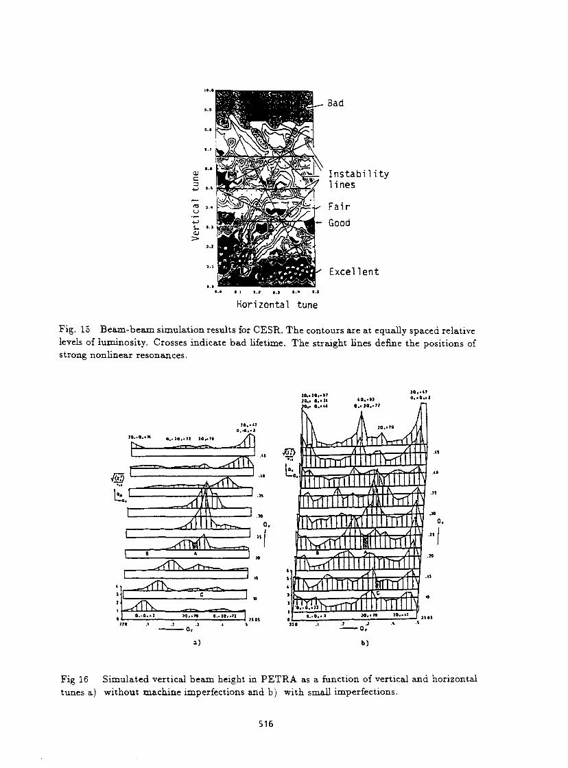
For lepton colliders these simulations [I5,34,35,36]have to include the coupled synchro-betatron motion (six-dimensional phase space), the nonlinear beam-beam kicks, radiation damping, quantum fluctuations due to the stochastic emission of synchrotron radiation and -if necessary - other lattice or.rf nonlinearities. Some results of these calculations are shown in Fig. 15 for CESR (taken from [35]) and in Fig. 16 for PETRA (taken from [34]).
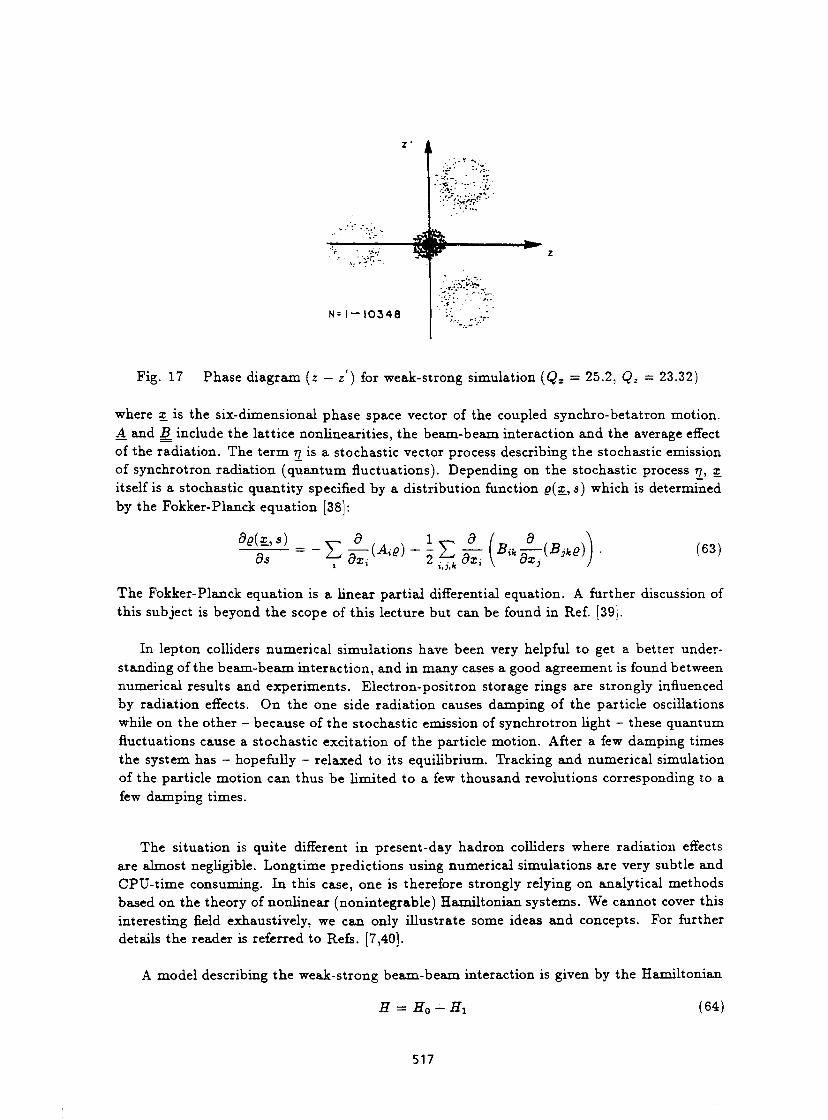
The latter case shows the sensitive dependence of the beam size on perturbations of the machine. Perturbations can be small differences in betatron phase advance between the interaction points and spurious dispersion at the interaction points. Because of these numerical results a different working point was chosen for PETRA. Furthermore these simulations are very helpful for understanding the complicated interplay of nonlinearity, damping and stochastic excitation in lepton colliders. Fig. 17 taken from [37]shows such a calculation (weak-strong simulation). The combined effect of quantum fluctuations and nonlinearity can move a particle starting near the origin in phase space to a (nonlinear) resonance island before it is damped again and eventually pushed to another resonance nearby.
Analytical methods for ( e + , e~ ) machines have to include the radiation effects. In this case the equations of motion are given by a system of stochastic differential equations of the form [28]:
x =A{X,3) + BS{X,S)JL(S) (62)
515
Bad
I n s t a b i l i t y l ines
Fair r Good
Excellent
• • • ! i . i i . i • » M
Horizontal tune
Fig. 15 Beam-beaxa simulation results for CESR. The contours are at equally spaced relative levels of luminosity. Crosses indicate bad lifetime. The straight lines define the positions of strong nonlinear resonances.
fc a., t o . - l l )0, . i»
> a . . « o.-a>*>
m * '•' i i4y<Tl I rs—
^TiK^rVi-Y—
^rnv, -~~rv*—
^ T K io . •?» 0 . .10 . . J :
» • .i
' t e i W r T T f f l H l l r r ! M . i » 70..11
n 3 )
• 0 .
Fig 16 Simulated vertical beam height in PETRA as a function of vertical and horizontal tunes a) without machine imperfections and b) with small imperfections.
516
N= 1 - 1 0 3 4 8
Fig. 17 Phase diagram (z — z) for weak-strong simulation (Qx = 25.2, Qz = 23.32)
where x is the six-dimensional phase space vector of the coupled synchro-betatron motion. A and B_ include the lattice nonlinearities, the beam-beam interaction and the average effect of the radiation. The term 77 is a stochastic vector process describing the stochastic emission of synchrotron radiation (quantum fluctuations). Depending on the stochastic process 77, x itself is a stochastic quantity specified by a distribution function g(x_, s) which is determined by the Fokker-Planck equation [38]:
9Q{X,S)
ds (63)
The Fokker-Planck equation is a linear partial differential equation. A further discussion of this subject is beyond the scope of this lecture but can be found in Ref. [39].
In lepton colliders numerical simulations have been very helpful to get a better understanding of the beam-beam interaction, and in many cases a good agreement is found between numerical results and experiments. Electron-positron storage rings are strongly influenced by radiation effects. On the one side radiation causes damping of the particle oscillations while on the other - because of the stochastic emission of synchrotron light - these quantum fluctuations cause a stochastic excitation of the particle motion. After a few damping times the system has - hopefully - relaxed to its equilibrium. Tracking and numerical simulation of the particle motion can thus be limited to a few thousand revolutions corresponding to a few damping times.
The situation is quite different in present-day hadron colliders where radiation effects are almost negligible. Longtime predictions using numerical simulations are very subtle and CPU-time consuming. In this case, one is therefore strongly relying on analytical methods based on the theory of nonlinear (nonintegrable) Hamiltonian systems. We cannot cover this interesting field exhaustively, we can only illustrate some ideas and concepts. For further details the reader is referred to Refs. [7,40].
A model describing the weak-strong beam-beam interaction is given by the Hamiltonian
H = Ho + H1 (64)
517

where D 2 X2 V2 Z2
Ho = f + kx(s)- + ^ + kz(s)j (65) describes the transverse linear betatron motion in an ideal uncoupled machine [28], and kx, kz
are the horizontal and vertical focusing strength.
H1 = U{x,z)-6p{s) (66)
describes the nonlinear kick a test particle is experiencing when crossing the strong counter-rotating beam at the interaction point.
m , Nbre / • » ! - exp { - ^ - ^ } U{x,z)= / ' , ' ' dq (14)
7 Jo (2cr2 + q)i /2(2<72-t-g)V2
£p(s) is the periodic delta function
6P(s) = Y,&(*-(*i, + n-C)) (67) n
(si p designates the interaction and C is the distance between adjacent interaction points). The corresponding equations of motion read:
, dH x = —- = px (68a)
dpx
dH , dU(x,z) px = -— = -kxx L-L-L.6p{s) (68b)
ox ox
, dH z = —- = P z (68c)
dpz
dH dU(x,z) P x = -—— = -kt-z 8p{s). (68d)
OZ OZ
In order to find the solution to (68 a-d) from sip — e to Sip + C — e (see Fig. 18) we proceed as follows:
- e + £ -e + e H 1 1 , , • _
Sip Sip + C
Fig. 18
518
The motion from sip — e to Sip -r e is just given by (kick)
\
x(sip + e)
P*(siP + £ )
z(sip + e)
Pz(s>P + e)
\ (
I
x(stp - e)
P*(sip - e ) - %{x{sip - e), z(sip - e))
z(sip-e)
\ Pz{sip - e ) - ^j{x(sip - e),z{sip - c))
(69)
or in shor thand no ta t ion y(sip + e)=N_(y(sip-e)) (70)
where N_ is a nonl inear four-dimensional m a p . From Sip + e to stp -f C - s the part icle performs free (linear) be t a t ron oscillations described by:
/
x ( S i p + C-e) \
px{sip + C - e)
z{sxp + C - e )
p z ( s i p + C - e) V
/ COS iZj. /?5i s i n
= - -±- sin txx
0 COS i i
0
\ 0 0
0 0 cos nz (3QZ sin i i z
• -±r sin t i 2 cos ^ z p0t
x(Sip-f e)
Px{siP + e)
z{stp + e)
V (71)
or y_(sip + C - e) = L{y{sip + e)) (72)
where L is a l inear m a p (see Eq. (71)). The combined mot ion is given by insert ing (69) into the right hand side of Eq. (71) or:
y_(sip + C - e) = LoN_{y{sxp - e)). (73)
Analysing the b e a m - b e a m interact ion means investigating the nonl inear four-dimensional mapping (73) and its consequences for the particle mot ion. Numerical and per turba t ive methods have been developed to s tudy these mappings , and it has t u r n e d out tha t these systems contain extremely complicated dynamics. In order to i l lustrate the problem and to demonstra te some of the unexpected features contained in
y(n + 1) = T(y(n)) (74)
we make a further approximat ion . Since it is very difficult to visualize four-dimensional quantities we restrict ourselves to the two-dimensional case. This case describes, for example, the horizontal mot ion of a test part icle which repeatedly crosses a r o u n d counter-rota t ing beam [41]:
x(n + 1) = x(n) cos iz + (5 • p(n) • sin/z + j3f(x(n)) • sinzz (75a)
p(n + 1) = — — x(n) sin ii + p(n) cos /x + f(x(n)) cos ix (75b)
with
519
,. . 4TT£ 1 - exp (- i 2 /2<7 2 ) / (*) = --j-x p - :
(see Eq. (15)).
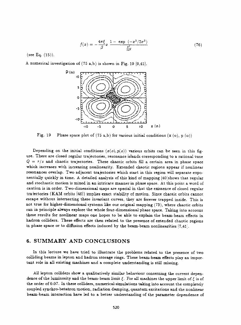
A numerical investigation of (75 a,b) is shown in Fig. 19 [9,41].
P ( n ) 10
5
0
-5
-10
-10 -5 0 5 10 X (n)
Fig. 19 Phase space plot of (75 a,b) for various initial conditions (x (o), p (o))
Depending on the initial conditions (x(o),p(o)) various orbits can be seen in this figure. There are closed regular trajectories, resonance islands corresponding to a rational tune Q = r/s and chaotic trajectories. These chaotic orbits fill a certain area in phase space which increases with increasing nonlinearity. Extended chaotic regions appear if nonlinear resonances overlap. Two adjacent trajectories which start in this region will separate exponentially quickly in time. A detailed analysis of this kind of mapping [40]shows that regular and stochastic motion is mixed in an intricate manner in phase space. At this point a word of caution is in order. Two-dimensional maps are special in that the existence of closed regular trajectories (KAM orbits [40]) implies exact stability of motion. Since chaotic orbits cannot escape without intersecting these invariant curves, they are forever trapped inside. This is not true for higher-dimensional systems like our original mapping (73), where chaotic orbits can in principle always explore the whole four-dimensional phase space. Taking into account these results for nonlinear maps one hopes to be able to explain the beam-beam effects in hadron colliders. These effects are then related to the presence of extended chaotic regions in phase space or to diffusion effects induced by the beam-beam nonlinearities [7,41].
6. SUMMARY AND CONCLUSIONS
In this lecture we have tried to illustrate the problems related to the presence of two colliding beams in lepton and hadron storage rings. These beam-beam effects play an important role in all existing machines and a complete understanding is still missing.
All lepton colliders show a qualitatively similar behaviour concerning the current dependence of the luminosity and the beam-beam limit £. For all machines the upper limit of £ is of the order of 0.07. In these colliders, numerical simulations taking into account the completely coupled synchro-betatron motion, radiation damping, quantum excitations and the nonlinear beam-beam interaction have led to a better understanding of the parameter dependence of
i I i i . " i T ï i i • I •••• t i I . I . . < i i I i
520
the system. In many cases, a good agreement is found between numerical calculations and experiments. Furthermore these simulations are the only method of treating the beam-beam interaction in a self-consistent manner so far, because the bunches will influence each other in a very complicated way. Analytical methods using concepts from the theory of stochastic differential equations are very difficult and are only at the beginning of their development.
In proton colliders nonlinear resonances play the dominant role in determining the luminosity. Even high-order nonlinear resonances must be avoided. Numerical simulations are very CPU-time consuming and subtle because of the lack of radiation damping. The longtime dynamics under the influence of the (nonlinear) beam-beam interaction can not be extrapolated easily from tracking the particles a few thousand revolutions. Therefore, in the hadron case one relies strongly on analytic (perturbative) methods of nonlinear (noninte-grable) Hamiltonian systems. The dynamics contained in these models shows a very rich and complicated structure: regular and chaotic regions are intricately mixed in phase space. In higher-dimensional systems (e.g. four-dimensional maps) various diffusion processes induced by the nonlinear character of the beam-beam interaction are possible. These include Arnold diffusion and various kinds of modulations! diffusion [7,40]. The hope is that these concepts will explain the beam-beam effects in hadron colliders.
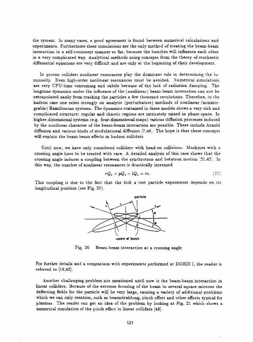
Until now, we have only considered colliders with head-on collisions. Machines with a crossing angle have to be treated with care. A detailed analysis of this case shows that the crossing angle induces a coupling between the synchrotron and betatron motion [21,42!. In this way, the number of nonlinear resonances is drastically increased
TQX + pQz + IQ, = m. (77)
This coupling is due to the fact that the kick a test particle experiences depends on its longitudinal position (see Fig. 20).
centre of bunch
Fig. 20 Beam-beam interaction at a crossing angle
For further details and a comparison with experiments performed at DORIS I, the reader is referred to [18,42].
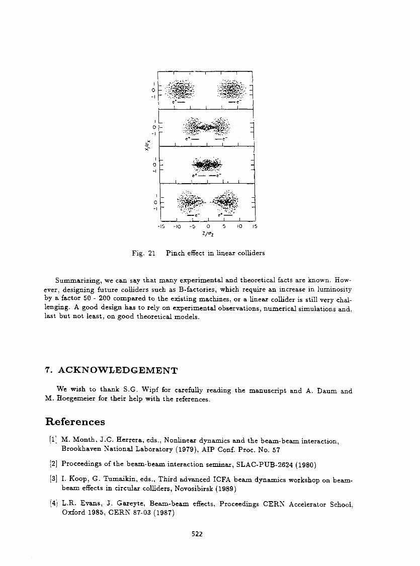
Another challenging problem not mentioned until now is the beam-beam interaction in linear colliders. Because of the extreme focusing of the beam to several square microns the deflecting fields for the particle will be very large, causing a variety of additional problems which we can only mention, such as beamstrahlung, pinch effect and other effects typical for plasmas. The reader can get an idea of the problem by looking at Fig. 21 which shows a numerical simulation of the pinch effect in linear colliders [43].
521
1 1 1 1 !
0 -1
i i i 1
te — c"
1
-
.*-... : • • - ' .
0 - •M&&SÊ9; -
c* — 1 !
— e~ i 1
1
0 - "HHriS JPV*^ --1
c*'— 1 1
— e" 1 - 1
1 .*4i .•"'T>'cl
0 -1
— '30$*-•*m -. *'•* • * "
. . + •
-e" J L
15 -10 -5 0 Z/crz
10 15
Fig. 21 Pinch effect in linear colliders
Summarizing, we can say that many experimental and theoretical facts are known. However, designing future colliders such as B-factories, which require an increase in luminosity by a factor 50 - 200 compared to the existing machines, or a linear collider is still very challenging. A good design has to rely on experimental observations, numerical simulations and, last but not least, on good theoretical models.
7. ACKNOWLEDGEMENT
We wish to thank S.G. Wipf for carefully reading the manuscript and A. Daum and M. Hoegemeier for their help with the references.
References
[1] M. Month, J.C. Herrera, eds., Nonlinear dynamics and the beam-beam interaction, Brookhaven National Laboratory (1979), AIP Conf. Proc. No. 57
[2] Proceedings of the beam-beam interaction seminar, SLAC-PUB-2624 (1980)
[3] I. Koop, G. Tumaikin, eds., Third advanced ICFA beam dynamics workshop on beam-beam effects in circular colliders, Novosibirsk (1989)
[4] L.R. Evans, J. Gareyte, Beam-beam effects, Proceedings CERN Accelerator School. Oxford 1985, CERN 87-03 (1987)
522

[5] P. Bambade , Effets faisceau-faisceau dans les annaux de stockage e / e à haute
énergie: grossissement résonant des dimensions verticales dans le cas de faisceaux plats .
LAL 84/21 (1984)
[6] J . F . Schonfeld, Beam-beam interaction, AIP Conf. Proc . No. 87
[7] J .L. Tennyson, The dynamics of the beam-beam interact ion, AIP Conf. Proc . No. 87
[8] J . F . Schonfeld, The effects of beam-beam collisions on storage ring performance - a
pedagogical review AIP Conf. Proc . No. 105
[9] A.W. Chao , Beam-beam instability, AIP Conf. P roc . No. 127
[10] E. Keil, Beam-beam interactions in p-p storage rings, CERN 77-13 (1977)
[ i l ] G.H. Rees, Beam-beam interactions in e-p storage rings, ibid. [10]
[12] J . Le Duff, Beam-beam interactions in e+e~ storage r ings, ibid. [10]
[13] A.W. Chao, P. Bambade , W.T . Weng, Nonlinear beam-beam resonances,
Lect. Notes in Physics Vol. 247, Springer (1986)
[14] J . T . Seeman, Observations of the beam-beam interact ion, ibid. [13]
[15] S. Myers, Review of beam-beam simulations, ibid. [13]
[16] E. Keil, Beam-beam effects in electron and proton colliders,
P a r t . Ace. 27, 165 (1990)
[17] J .R. Boyce, S. Heifets, G.A. Krafft, Simulations of high disruption colliding beams, C E B A F PR-90-013 (1990)
[18] A. Piwinski , Limitations of the luminosity by satellite resonances, DESY 77/18 (1977)
[19] A. Piwinski , Computer simulation of satellite resonances caused by the beam-beam interact ion at a crossing angle in the SSC, SSC-57 (1986)
[20] A. Piwinski , Recent results from DORIS and P E T R A in [l]
[21] A. Piwinski , Der Raumladungseffekt bei vertikalem oder
horizontalem Kreuzungswinkel, DESY E l / 1 (1969)
[22] J . Kewisch, Depolarisation der Elektronenspins in Speicherringen durch nichtlineare Spin-Bahn-Kopplung, DESY 85-109 (1985)
[23] P. Schmûser, Basic course on acclerator optics, Proceedings CERN Accelerator School, Aarhus , 1986, CERN 87-10 (1987)
[24] A. Piwinski , Coherent beam break-up due to space charge, Proc. 8 th Intern. Conf. High Energy Accelerators, CERN (1971)
[25] A. Piwinski , Einstellung der Kreuzung der beiden Strahlen mit Hilfe des Raumladungsef-fekts, DESY H2-75/3 (1975)
[26] E. Couran t , H. Snyder, Theory of the al ternating gradient synchrotrons, Ann . Phys . 3, 1 (1958)
523
[27] G. Ripken, F . Willeke, On the impact of linear coupling on nonlinear dynamics. DESY 90-001 (1990)
[28] H. Mais, G. Ripken, Theory of coupled synchro-betat ron oscillations (I), DESY M-82-05 (1982)
[29] H. Zyngier, Beam-beam effect - A review of the observations made at Orsay in [1]
130] H. Wiedemann , Exper iments on the beam-beam effect in e+e~ storage rings in [l]
[31] D.A. Finley, Observations of beam-beam effects in proton-ant iproton colliders in [3]
[32] A. Piwinski, Observation of beam-beam effects in P E T R A , DESY M-79/11 (1979)
[33] A.W. Chao, R.D. Ru th , Coherent beam-beam instabili ty in colliding-beam storage rings, Pa r t . Accel. 16, 201 (1985)
[34] A. Piwinski, Computer simulation of beam-beam interaction for various be ta t ron frequencies, DESY M-81/31 (1981)
[35] S. Peggs, R. Ta lman, Beam-beam luminosity l imitat ion in electron-positron colliding rings, Phys . Rev. D24, 2379 (1981)
[36] S. Myers, Simulation of the beam-beam effect for e T e ~ storage rings, Nucl. Ins t r . Meth . 2 U , 263 (1983)
[37] A. Piwinski , Dependence of the luminosity on various machine parameters and their opt imizat ion at P E T R A , DESY 83-028 (1983)
[38] C.W. Gardiner , Handbook of stochastic methods , Springer (1985)
[39] A.L. Gerasimov, Phase convection and dis t r ibut ion "tails" in periodically driven Brow-nian mot ion, Physica D41, 89 (1990)
[40] A.J . Lichtenberg, M.A. Lieberman, Regular and stochastic motion, Springer (1983)
[41] F .M. Izraelev, Nearly linear mappings and their applications, Physica D l , 243 (1980)
[42] A. Piwinski , Synchro-beta t ron resonances in [4]
[43] R. Hollebeek, Disrupt ion limits for linear colliders, in [2]
524
NEUTRALISATION OF ACCELERATOR BEAMS BY IONISATION OF T H E RESIDUAL GAS Y. Baconnier, A. Poncet, and P.F. Tavares*
CERN, Geneva, Switzerland
Introduction This note was first written on the occasion of a lecture. It is a review paper as shown by the long reference list. We have classified the references under various headings, which should provide a useful guide for the reader.
The present note is a revised version of a note written ten years ago (CERN/PS/PSR 84-24) for the CERN Accelerator School. A considerable amount of work has been done in the mean time. We have tried to integrate the important advances while keeping the simple and elementary approach of the first version. The emphasis has been placed on electron and antiproton beams rather than coasting proton beams (since the closing of the ISR collider, no machine with coasting proton beams has been built).
1 Neutralisation of a beam: a simple description The circulating particles in a stored beam collide with residual gas molecules producing positive ions and electrons. A negatively charged beam (e.g., electrons or antiprotons) captures the ions and repels the electrons towards the vacuum chamber walls 1. If other possible natural or artificial clearing mechanisms are not present, the neutralising ions accumulate up to the point where the remaining trapping potential is effectively zero, i.e., until the number of static neutralising particles is equal to the number of beam particles. The beam is then fully neutralised. The average neutralisation factor is defined by
>? = - , (1) ne
where n; is the total neutralising charge measured in units of the electronic charge and ne is the number of stored beam particles. The neutralisation is often not homogeneous along the machine azimuth s, and we define a local neutralisation factor by
2irRdni . , Vis) = - j - , (2)
ne as where 2irR is the machine circumference and is a local linear neutralising charge density (measured in units of electronic charge per meter) 2 .
"On leave from Laboratôrio Nacional de Luz Sincrotron, Campinas,Brazil. 1 Positively charged coasting beams trap electrons, and this effect has been extensively studied in
the CERN ISR (see references). Bunched proton or positron beams do not suffer from neutralisation problems because the electrons are not stably trapped (cf section 5).
2Some authors define an average neutralisation factor for bunched beams as a ratio of the average neutralising charge density to the bunch charge density. This is related to our definition through the bunching factor B — ^ where Nb is the number of bunches and Lb is the bunch length. This definition is useful when one compares the incoherent space-charge tune shift with the neutralisation induced tune shift.
525
In order to get a feeling for the orders of magnitude involved in neutralisation problems, we consider a set of machine parameters corresponding to typical values for the CERN electron-positron accumulator (EPA). We disregard, for the time being, the fact that the EPA electron beam is bunched and only calculate longitudinally averaged values. Also, for the sake of simplicity, we assume a round beam with a homogeneous transverse charge distribution. The beam current is 7 = 100 mA, the energy is E = 500 MeV and the beam radius is 0.5 mm. The corresponding linear particle density is
A = 4 - i = -— = 2 x 10⁹ particles /m. (3) as epc
The electric field at the beam edge is obtained via Gauss's law.
S = -^— = 1.2 x 10⁴ volt/m. (4)
The magnetic field at the edge is obtained via Ampere's law:
B = ^ = 4 x l 0 " 5 T . (5) Z7ra
The total direct space-charge force on a circulating electron is F = e(£ + v x B) = Fe + Fm = F e - ^ , (6)
T where 7 is the total relativistic beam energy in units of the rest energy and Fe is the electrostatic force. The fact that the two forces counteract results in the so-called relativistic cancellation. With neutralisation, the electrostatic force is changed from Fe to Fe(l — 7?) and the magnetic force is unchanged. Then
F = F<(±-,y (7)
The force which we have calculated at the edge of the beam is in fact proportional to the distance to the centre of the beam. The corresponding local quadrupole has a strength (with the Courant and Snyder definition [1])
We simplify the formulae by introducing the classical electron radius
= 2.82 x 10- 1 5 m. (9) e 2
4:7rtomec2
and the local beam volume density
de = ~^— = 2.7 x 10 5particles/m 3 (10) as ira1
so that, with eqs. (4), (7), (8), (9), and (10),
k { s ) = _rlred(l_ _ A (H)
526
and the corresponding tune shift is
AQ = ^-J/3(s)k(s)ds, (12)
where fl(s) is the usual Twiss parameter and the integration is done along the machine azimuth. Instead of calculating the integral, we use average values for all quantities involved 3 :
A Q „ - i | M 4 , . ( 1 3 )
For j3 = 4 m and 2TTR = 126m, we find
AQ % 27/ (14)
and machine performance will be limited for values of rj above a few percent.
2 The ionisation process The circulating beam interacts with the electrons of the molecules of the residual gas and with the ions t rapped in the beam. In turn the trapped ions interact with the molecules in many different ways. In the following sections, we briefly review these phenomena.
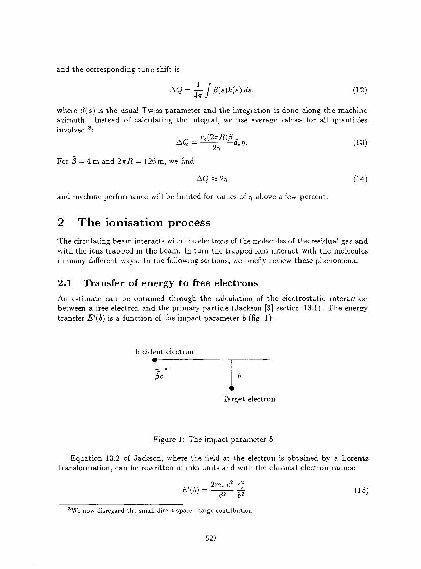
2.1 Transfer of energy to free electrons An estimate can be obtained through the calculation of the electrostatic interaction between a free electron and the primary particle (Jackson [3] section 13.1). The energy transfer E'(b) is a function of the impact parameter b (fig. 1).
Incident electron
Pc
Target electron
Figure 1: The impact parameter b
Equation 13.2 of Jackson, where the field at the electron is obtained by a Lorentz transformation, can be rewritten in mks units and with the classical electron radius:
3We now disregard the small direct space charge contribution.
527
or
where fie is the velocity of the primary particle and E'(b) is the transferred energy. The cross-section da for energy transfer between E' and E' + dE' is
da = 2x6 db
or da = 2ir
me c2
2dE'
(16)
(17)
(18) / ? 2 e E12 " One sees immediately an unphysical situation for E' — 0 (b large, distant collisions) and E' — oo (b small, close collisions). The difficulty is solved by the definition of a minimum energy E^n and a maximum energy E ^ . The maximum energy E ^ can be obtained from pure kinematic considerations, 4 whereas the minimum energy requires a detailed analysis of the medium in which the interaction takes place.
The above formulae cannot be used to compute the exact ionisation cross-section, as we shall see below, but they give a fair description of the phenomenon.
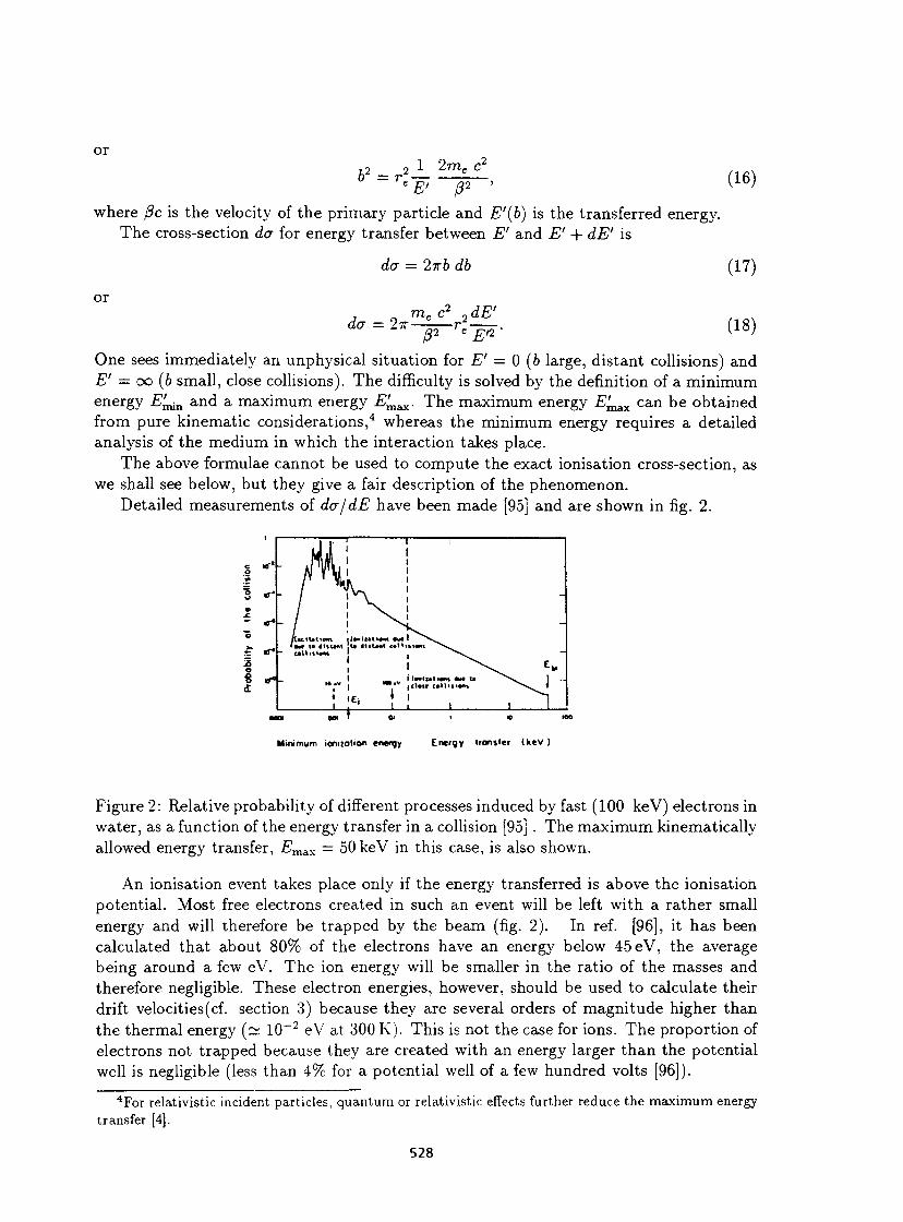
Detailed measurements of da/dE have been made [95] and are shown in fig. 2.
*
Minimum ionization enengy Energy transfer (kev )
Figure 2: Relative probability of different processes induced by fast (100 keV) electrons in water, as a function of the energy transfer in a collision [95] . The maximum kinematically allowed energy transfer, £ m ax = 50 keV in this case, is also shown.
An ionisation event takes place only if the energy transferred is above the ionisation potential. Most free electrons created in such an event will be left with a rather small energy and will therefore be trapped by the beam (fig. 2). In ref. [96], it has been calculated that about 80% of the electrons have an energy below 45 eV, the average being around a few eV. The ion energy will be smaller in the ratio of the masses and therefore negligible. These electron energies, however, should be used to calculate their drift velocities(cf. section 3) because they are several orders of magnitude higher than the thermal energy (~ 1 0 - 2 eV at 300 K). This is not the case for ions. The proportion of electrons not trapped because they are created with an energy larger than the potential well is negligible (less than 4% for a potential well of a few hundred volts [96]).
4For relativistic incident particles, quantum or relativistic effects further reduce the maximum energy transfer [4].
528
2.2 Ionisation cross-section The ionisation cross-section depends on the molecule of the residual gas and on the velocity of the ionising particle but neither on its charge nor on its mass 5 . Measurements have been made [98] for various incident electron energies and the results were fitted to the theoretical expression by Bethe (see [4], p. 45):
a% = AT h M 2
0 In 0 l - #
- 1 + /3?
where
4TT I — ] = 1.87 x l ( T 2 4 m 2
mc,
(19)
(20)
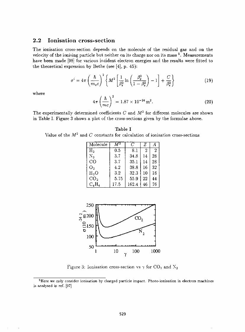
The experimentally determined coefficients C and M2 for different molecules are shown in Table I. Figure 3 shows a plot of the cross-sections given by the formulae above.
Table I Value of the M2 and C constants for calculation of ionisation cross-sections
Molecule M2 C Z A H 2
0.5 8.1 2 2 N 2
3.7 34.8 14 28 CO 3.7 35.1 14 28 o 2
4.2 38.8 16 32 H 2 0 3.2 32.3 10 18 C 0 2 5.75 55.9 22 44 C4H4 17.5 162.4 46 76
250
10 100 1000 y
Figure 3: Ionisation cross-section vs 7 for CO2 and N2
5Here we only consider ionisation by charged particle impact. Photo-ionisation in electron machines is analysed in ref. [97]
529
2.3 Heating and cooling Trapped ions are continually bombarded by the circulating beam particles and gain energy from these collisions. If the energy gained is larger than the depth of the potential well in which they oscillate, they will be lost on the wall. Small impact parameter collisions in which a trapped ion or electron is immediately lost are very rare and provide a negligible clearing rate. The average effect of a large number of large impact parameter collisions is to increase the temperature of the trapped particles continuously; on the other hand, the ions collide with residual gas molecules (which have only thermal energy) and lose energy. Resonant charge exchange may also play an important role in the cooling mechanism, with cross section about 100 times larger than typical kinetical cross- sections. Heating favours the accumulation of light ion species in negative beams and is particularly important in antiproton machines, where cooling is negligible due to the very low pressure.
2.4 Ionisation rate The time it takes for one circulating particle to create one ion is given by:
1 dm <7m /3c
(21)
where dm is the molecular density ( m - 3 ) ; am is the ionisation cross-section for molecule m (m 2 ) ; /3c is the velocity of the circulating beam (m • s _ 1 ) .
The molecular density dm is related to the partial pressure Pm in torr by the relation (valid at 20 °C)
dm = 3.3 x 1 0 2 2 P m . (22)
If there are several types of molecules in the residual gas then the total ionisation time Ti is given by the relation
T *-* T '» m ' m
3 The ion or electron motion The temperature of the molecules of the residual gas will be slightly increased by the interactions with the beam. However, the reservoir of molecules is so big that the energy in the gas will be the energy related to the temperature of the vacuum chamber walls, usually 300 K. The energy of the electrons acquired through momentum transfer from the circulating beam in the ionisation process will be of a few eV and the energy of the ions lower by the mass ratio
A m p '
where Amp is the mass of the ion, and me the mass of the electron. The electrons and the ions created inside the beam will either be chased out or oscillate
in its potential well. Their motion will be influenced by magnetic fields. The analysis of these different energies and motions is the object of this section.
530
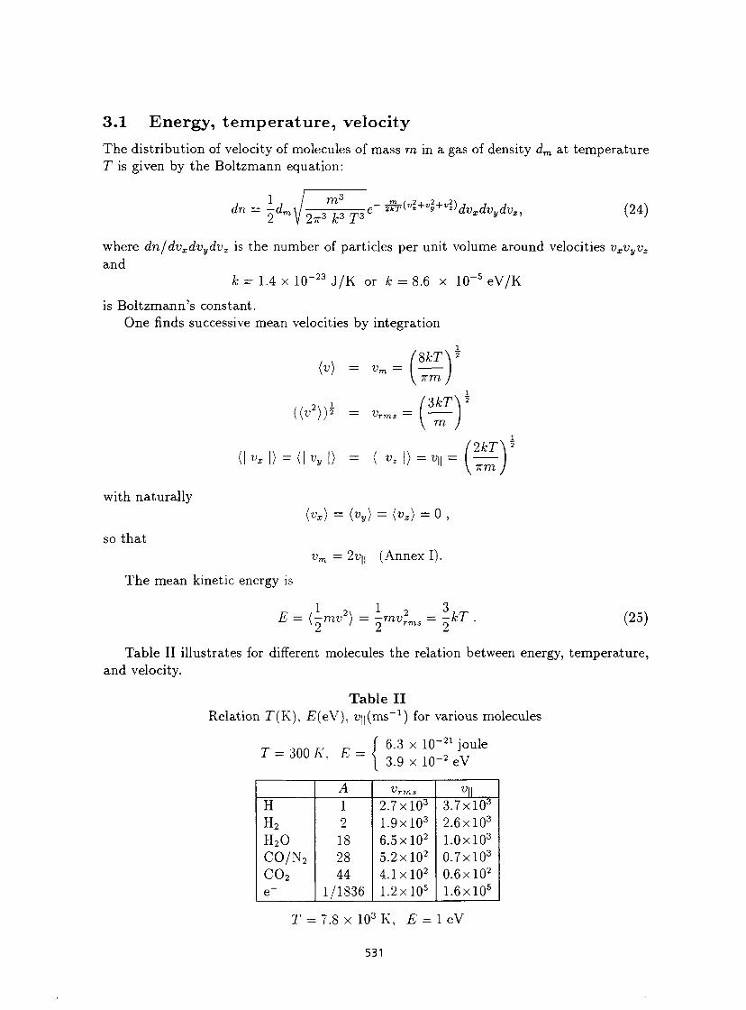
3.1 Energy, temperature, velocity The distribution of velocity of molecules of mass raina gas of density dm at temperature T is given by the Boltzmann equation:
dU = W 2 ^ W e " ^{vlW»W^dvydvz, (24)
where dn/dvxdvydvz is the number of particles per unit volume around velocities vxvyvz
and k = 1.4 x 1 (T 2 3 J / K or U 8.6 x 1 0 - 5 eV/K
is Boltzmann's constant. One finds successive mean velocities by integration
'SkT\ (v) = vm = \ —^ I
irm
( ( t ; 2 } ) 2 = U r m s = 'ZkT'
m
VX l) = ( | Vy | ) = (| ^ | ) = U | | = (2kT\ \ itm
with naturally
so that
The mean kinetic energy is
(VX) = (Vy) = (VZ) = 0 ,
vm = 2u|| (Annex I).
E = (-mv2) = -mv2
Tms = -kT . (25)
Table II illustrates for different molecules the relation between energy, temperature, and velocity.
Table II Relation T(K), E(e\f), U| |(ms _ 1 ) for various molecules
' 6.3 x 10~ 2 1 joule T = 300 K. E = 3.9 x 10~ 2 eV
A " r a s v\\ H 1 2.7xl0 3 3.7xl0 3
H 2 2 1.9xl0 3 2.6 xlO 3
H 2 0 18 6.5xl0 2 l.OxlO 3
CO/N 2 28 5.2xl0 2 0.7xl0 3
C 0 2 44 4.1xl0 2 0.6xl0 2
e~ 1/1836 1.2xl0 5 1.6xl0 5
T = 7.8 x 10 3 K, E = 1 eV
531
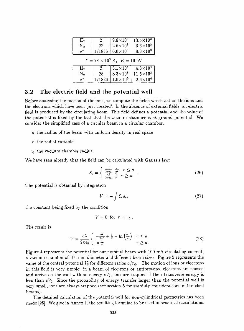
H 2 2 9.8 xlO 3 13.5xl0 3
N 2 28 2.6 xlO 3 3.6xl0 3
e~ 1/1836 6.0 xlO 3 8.3 xlO 3
T = 78 x 10 3 K, E = 10 eV
H 2 2 3.1 xlO 4 4.3xl0 4
N 2 28 8.3 xlO 3 11.5xl0 3
e~ 1/1836 1.9xl0 6 2.6 xlO 4
3.2 The electric field and the potential well Before analysing the motion of the ions, we compute the fields which act on the ions and the electrons which have been 'just created'. In the absence of external fields, an electric field is produced by the circulating beam. This field defines a potential and the value of the potential is fixed by the fact that the vacuum chamber is at ground potential. We consider the simplified case of a circular beam in a circular chamber.
a the radius of the beam with uniform density in real space
r the radial variable
r 0 the vacuum chamber radius.
We have seen already that the field can be calculated with Gauss's law:
The potential is obtained by integration
v = -Jsrdr, the constant being fixed by the condition
V = 0 for r — r0 .
The result is
V = jL[-e + \ + H?) r^a (28) 27re0 I In a r>a.
Figure 4 represents the potential for our nominal beam with 100 mA circulating current, a vacuum chamber of 100 mm diameter and different beam sizes. Figure 5 represents the value of the central potential Vo for different ratios a/r0. The motion of ions or electrons in this field is very simple: in a beam of electrons or antiprotons, electrons are chased and arrive on the wall with an energy eV0, ions are trapped if their transverse energy is less than eV0. Since the probability of energy transfer larger than the potential well is very small, ions are always trapped (see section 5 for stability considerations in bunched beams).
The detailed calculation of the potential well for non-cylindrical geometries has been made [26]. We give in Annex II the resulting formulae to be used in practical calculations.
532
(26)
(27)
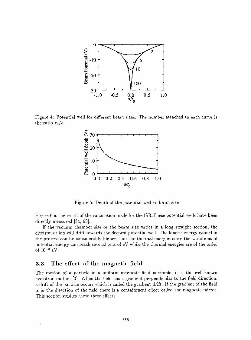
Figure 4: Potential well for different beam sizes. The number attached to each curve is the ratio r0/a
1 — > — i — • — i — ' — i — r -
J i i i i_
0.0 0.2 0.4 0.6 0.8 1.0
Figure 5: Depth of the potential well vs beam size
Figure 6 is the result of the calculation made for the ISR.These potential wells have been directly measured [34, 83].
If the vacuum chamber size or the beam size varies in a long straight section, the electron or ion will drift towards the deepest potential well. The kinetic energy gained in the process can be considerably higher than the thermal energies since the variations of potential energy can reach several tens of eV while the thermal energies are of the order of I t )" 2 eV.
3.3 The effect of the magnetic field The motion of a particle in a uniform magnetic field is simple, it is the well-known cyclotron motion [3]. When the field has a gradient perpendicular to the field direction, a drift of the particle occurs which is called the gradient drift. If the gradient of the field is in the direction of the field there is a containment effect called the magnetic mirror. This section studies these three effects.
533
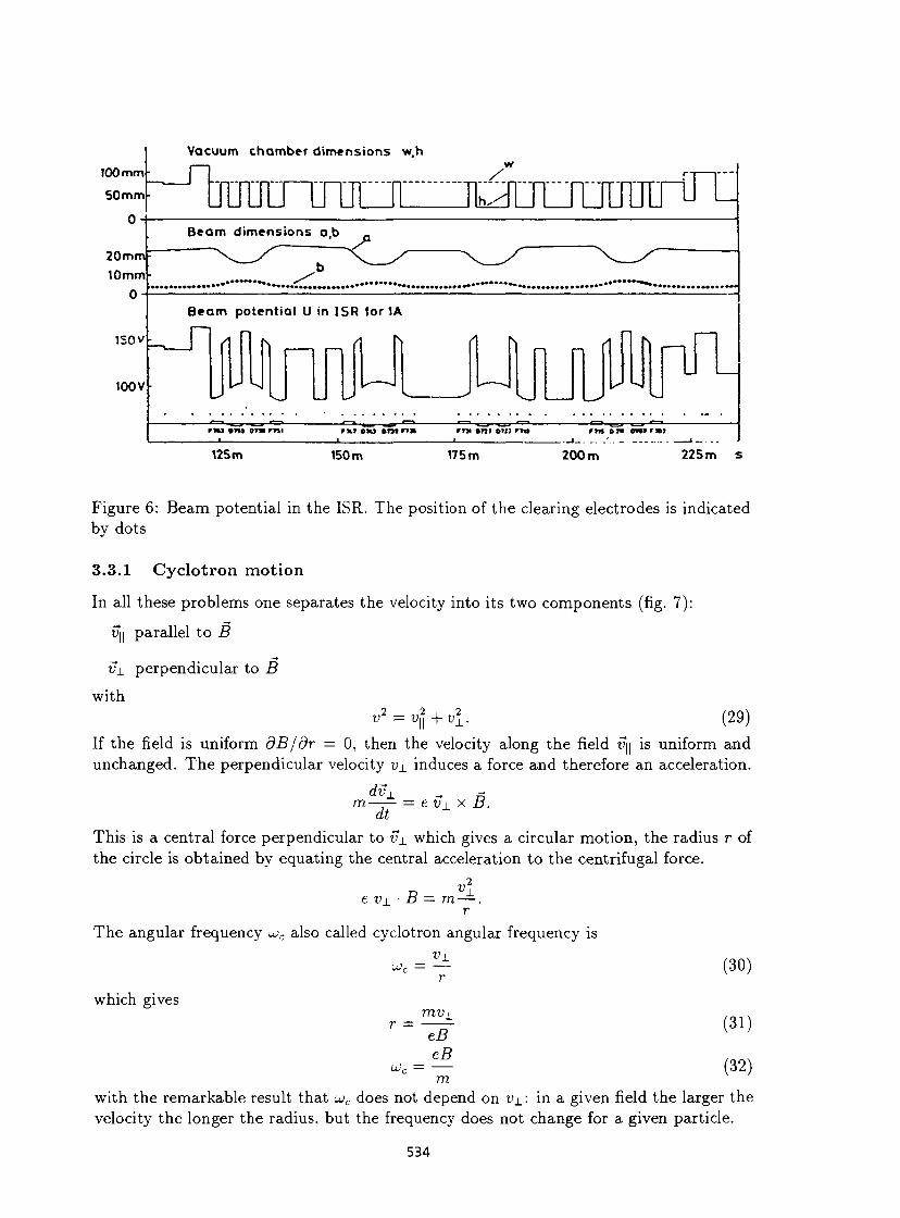
100 mm
50 mm
0
Vacuum chamber dimensions w.h
JljmErinja[zzjtkji 20mm 10mm
0
Beam dimensions a.b
1S0V
100V
Beam potential U in ISR (or 1A
A r\
Ukl
A h A N A IS
\S N
riu ont am mi
125m F U oto vntmk m »m »»H «w rm on omf rw
150m 175m 200m 225m s
Figure 6: Beam potential in the ISR. The position of the clearing electrodes is indicated by dots
3.3.1 C y c l o t r o n m o t i o n
In all these problems one separates the velocity into its two components (fig. 7):
ujl parallel to B
v±_ perpendicular to B
with v2 = vf\+vl. (29)
If the field is uniform dB/dr = 0, then the velocity along the field v\\ is uniform and unchanged. The perpendicular velocity u x induces a force and therefore an acceleration.
dv± m- dt = e vL x B.
This is a central force perpendicular to v± which gives a circular motion, the radius r of the circle is obtained by equating the central acceleration to the centrifugal force.
tv^-B — m—. r
The angular frequency uc also called cyclotron angular frequency is v±
which gives
Mr.
mvj_ ~7B
_eB_ m
(30)
(31)
(32)
with the remarkable result that uc does not depend on v±: in a given field the larger the velocity the longer the radius, but the frequency does not change for a given particle.
534
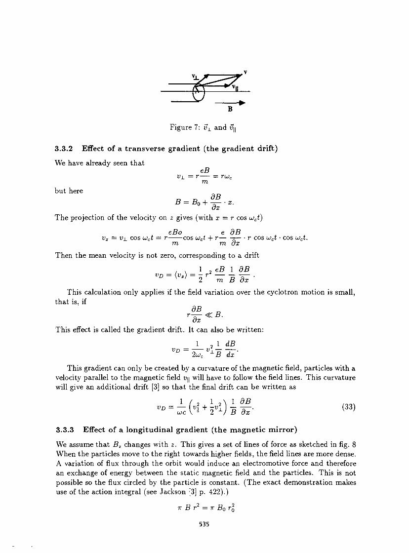
K' B
Figure 7: vL and uj|
3.3.2 Effect of a transverse gradient (the gradient drift)
We have already seen that eB
vj_ = i = ruc
m but here
R - R + d B . ti = B0 + -7T— • X.
OX The projection of the velocity on z gives (with x — r cos u>ct)
eBo e dB vz = v_i cos u>ct = i cos ujct + r -— • r cos u;cï • cos u>ct.
m m ox
Then the mean velocity is not zero, corresponding to a drift
. . 1 2 eB 1 dB
2 m B ox
This calculation only applies if the field variation over the cyclotron motion is small, that is, if
r—<£B. ox
This effect is called the gradient drift. It can also be written:
_ 1 2 1 dB V D ~ 2uc
V±B dx'
This gradient can only be created by a curvature of the magnetic field, particles with a velocity parallel to the magnetic field U|| will have to follow the field lines. This curvature will give an additional drift [3] so that the final drift can be written as
1 / 2 1 2 \ 1 dB VD = ~c ^1 + 2V-J B -dx- ( 3 3 )
3.3.3 Effect of a longitudinal gradient (the magnet i c mirror)
We assume that Bz changes with z. This gives a set of lines of force as sketched in fig. 8 When the particles move to the right towards higher fields, the field lines are more dense. A variation of flux through the orbit would induce an electromotive force and therefore an exchange of energy between the static magnetic field and the particles. This is not possible so the flux circled by the particle is constant. (The exact demonstration makes use of the action integral (see Jackson [3] p. 422).)
7T B r2 = 7T BQ 7*0
535
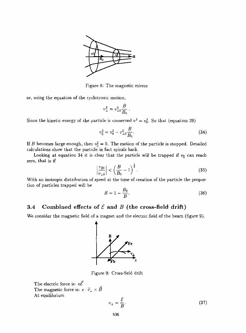
*-B
Figure 8: The magnetic mirror
or, using the equation of the cyclotronic motion,
B 2 2
Bo
Since the kinetic energy of the particle is conserved v2 = v$. SO that (equation 29)
o o o -D v\\ = vo~ v±o Bo'
(34)
If B becomes large enough, then v?< = 0. The motion of the particle is stopped. Detailed calculations show that the particle in fact spirals back.
Looking at equation 34 it is clear that the particle will be trapped if v\\ can reach zero, that is if
B \ * (35)
v\\o V\.Q
< 1
With an isotropic distribution of speed at the time of creation of the particle the proportion of particles trapped will be
(36)
3.4 Combined effects of £ and B (the cross-field drift) We consider the magnetic field of a magnet and the electric field of the beam (figure 9).
Figure 9: Cross-field drift
The electric force is: e£ The magnetic force is: e • v± x B At equilibrium
U - L = - ^ E_ B'
(37)
536
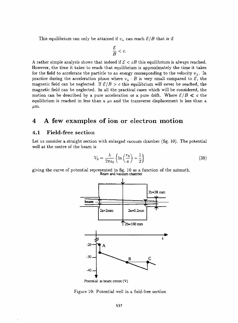
This equilibrium can only be attained if v± can reach £/B tha t is if
S B < C -
A rather simple analysis shows that indeed if S < cB this equilibrium is always reached. However, the time it takes to reach that equilibrium is approximately the time it takes for the field to accelerate the particle to an energy corresponding to the velocity v±. In practice during the acceleration phase where v± • B is very small compared to £, the magnetic field can be neglected. If €/B > c this equilibrium will never be reached, the magnetic field can be neglected. In all the practical cases which will be considered, the motion can be described by a pure acceleration or a pure drift. Where £/B <C c the equilibrium is reached in less than a fis and the transverse displacement is less than a fj,m.
4 A few examples of ion or electron motion
4.1 Field-free section Let us consider a straight section with enlarged vacuum chamber (fig. 10). The potential well at the centre of the beam is
ro\ , 1 *-£M?)+5} (38)
giving the curve of potential represented in fig. 10 as a function of the azimuth. Beam and vacuum chamber
beam
2a=2mm
2b=38 mm *i*
•$x-2a=0.2mm
2b=100mm
-20 — 1 A
s
-30 — ^ . B C
-40 —
1 ' Potential at beam centre (V)
Figure 10: Potential well in a field-free section
537
In this example the ions created between B and C will be trapped, the ions created between A and B will drift towards C and continue to the right with an energy between 0 and 6 eV.
4.2 Pure dipole field With our nominal beam parameters (section 1), the electric field at the edge of the beam is 1.2 x 10⁴ V m _ 1 so that the cross-field drift velocity varies from zero at the centre to 8.6 x 10³ m s ' 1 at the edge of the beam. The corresponding energies are 2 x 1 0 - 4 eV for electrons and 11 eV for N 2 ions. The cyclotron radius for electrons in the centre with energy about 1 eV is 2.4 \i m (0.6 mm for ions).
Particles with the same charge as the beam are chased out of the potential well in the vertical plane. Particles with opposite charge drift towards the end of the magnet, but are contained in the potential well in the vertical plane.
4.3 Combined function magnet Let us consider a magnet like the EPA magnet with a field of 1.4 T on the central orbit and a gradient of 1 T/m on the central orbit.
We have seen that the typical energy of particles created in the potential well is a few electron volts, the corresponding velocities are (section 3.1):
for ions ~ 2.6 x 10 3 m s - 1 . for electrons ~ 6 x 10⁵ ms" 1 .
The cyclotron radii in the centre are very small. The gradient drift for ions or electrons of 1 eV is of the order of 0.5 ms" 1 and therefore negligible with respect to the cross-field drift.
4.4 The quadrupole field If the beam is centred in a quadrupole with gradient 3 T m - 1 , the cross-field drift at the edge of the beam will be (37)
vc = 8 x 10⁶ m s" 1
corresponding to an energy for ions of 9 MeV. This energy would have to be provided by the potential well, which is of only a few tens of volts, so that the equilibrium required for the cross-field drift will never be reached. The electric field of the potential well dominates the ion motion.
The gradient drift does not take place because the field is too small. Particles with the same charge as the circulating beam are chased toward the poles
of the quadrupole. In some cases a magnetic mirror effect could ensure the containment of these particles.
4.5 Undulator The field of an undulator is dipolar but with alternatively positive and negative polarity along the azimuth. The main effect in the horizontal plane is the cross-field drift but the fact that the field is alternated gives a possibility of containment. In the vertical plane the field is concentrated in the poles so that a magnetic mirror effect can develop.
538
This mechanism can be effective for electrons or ions depending on the geometry and the beam polarity.
Since the potential well is not required to achieve containment, it is not easy to find the mechanism which limits the accumulation of ions in an undulator.
5 Bunched beams All previous studies are in principle valid only for unbunched circulating beams. In fact the bunching only introduces additional effects.
In refs. [7, 14, 57, 75], one finds a study of the stability of ions in single-beam and colliding-beam machines. We shall only summarise the results of this study in the case of single-beam machines.
Here, we have changed the definition of the neutralisation factor r\ from the local definition used in ref. [14] to the average definition given above (equation 1). This explains the difference between our formulae and those of ref. [14].
At a given azimuth, an ion sees successively the focusing (or defocusing) forces induced by the bunch passage, followed by a drift time between bunches. If a vertical dipole magnetic field is applied, the horizontal transverse and longitudinal motions will be coupled, the vertical motion however is independent of the magnetic field. The horizontal motion will not be studied here [83]. It gives similar results in drift space; in a bending magnet the horizontal motion is usually stable. The present study is therefore limited to the vertical motion.
The forces induced by the passage of a bunch have been studied by several au-thors(e.g. [8, 14]). With the time as independent variable the bunch passage is similar to a focusing (or defocusing) lens; if the bunch is short the effect on the ion can be described by a matrix equivalent to a thin lens. The non-linear effects are not considered here.
Let y and dy/dt = y be the position and speed of the ion. Then the passage of a bunch is described by
U A U 1JU/0 with
where ne/n is the charge per bunch n is the number of bunches r p is the classical proton radius a, b is the beam size, horizontal resp. vertical A is the atomic weight of the ion /?c is the velocity of the circulating beam.
In between bunches the ion drifts freely during the time t = T/n. Where T is the revolution time, corresponding to the matrix transformation
(ii)-539
One period of the forces applied is described by the matrix product.
The stability is insured if the trace of the matrix satisfies
- 2 < Tr{M) < +2
that is for
- K ( 1 ± 0 5 ) < + 1 -The -+• sign is to be selected for cases where the beam and the ion are of the same sign. Electron beams therefore cannot accumulate electrons, and proton beams cannot accumulate positive ions, which is obvious.
For the opposite sign, the requirement is:
T
If A • mp is the mass of the ion, one can express the above formulae by the following criterion: all ionic masses larger than a critical mass Ac will be accumulated.
n i r £ _ 2 ^ R n n ^ - 62 (l + f )
In most practical cases the critical mass varies between 0.1 and 100. This explains why electrons (A ~ 1/2000) never accumulate in bunched beams of positrons or protons.
In bunched beams of electrons with a large number of bunches (e.g. synchrotron radiation sources) the critical mass can be very small ~ 1 0 - 2 . Then the ion accumulation can be treated as in D.C. beams: the ions are too heavy to 'see' that the beam is bunched.
When the critical mass is above 44, the ions usually found in vacuum systems cannot accumulate.
Intermediate cases: 1 < Ac < 44
require a detailed analysis [14]. Note:
There is some confusion on the values to be used for a and b after a real measurement of particle distributions. They are related to the central density of the transverse distribution of particles. If the measured distributions were rectangular then a and b would be the measure of the real half width of the distributions. If the distributions are Gaussian, a simple calculation shows that
a = axV2 b = crvy/2.
540
6 Clearing electrodes As we have seen in section 4, ions created in some point will drift around the circumference of the machine and will accumulate to a certain level of neutralisation. The clearing can be done if required by installing in selected places, electrodes with a potential sufficient to suppress the potential well. If one wants to avoid neutralisation pockets, the electrodes should be placed at convenient places around the ring. In the example of Section 4.1 (fig. 10) an electrode placed in A or B will not clear the neutralisation pocket BC.
The location of the clearing electrodes in the ISR fig. 6 has been selected to avoid these neutralisation pockets. The large list of references on this subject (refs. [59, 61, 63, 64, 70, 74]) can be used as a guide to the design of clearing electrodes. The design should be made such as to avoid the introduction of parasitic impedances especially in electron rings [44].
Clearing electrodes placed in magnetic fields must be calculated to avoid the cross-field drift.
7 The limit of accumulation The containment of particles is in general due to the potential well. When charges start to accumulate, they diminish the depth of the potential well. The limit is reached when the density of accumulated charges is equal and opposite to the density of circulating charges so that the net resulting charge is null.
0 = di- dp.
The neutralisation factor rj is then, at most, equal to 1. The beam is fully neutralised. Clearly the same limitation of neutralisation exists in bunched beams.
As we have seen, several clearing effects due to various drifts will limit the local neutralisation factor to less than 1. If required, clearing electrodes will collect electrons and reduce the neutralisation in appropriate places.
However, in some extreme cases the trapping of the ions or electrons is not due to the potential well, so that one could have local accumulation of charges to neutralisation levels higher than 1. We have seen that the undulators are probably very efficient in accumulating ions. Detailed calculations should be made in this particular case. It is not excluded that similar situations be found in the combination of end-fields of conventional magnets or quadrupoles.
8 The effects of neutralisation There are several effects of neutralisation. The particles (ions or electrons) chased from the beam and hitting the wall with the energy of the potential well can create desorption. The ions stored in the beam modify the local pressure and therefore the life-time of stored beams.
The most important effects come from the electric field of the ion (or electron) cloud. This induces a shift and a spread of betatron oscillation frequencies and a coupling of horizontal and vertical motion.
Finally, the ion cloud can interact as a whole with the beam and induce instabilities.
541
8.1 The pressure bump The mechanism of the pressure bump is rather simple. In a beam of protons the ions are chased out of the potential well and hit the wall with enough energy to induce desorption of 7/ molecules per ion (here 77 is the desorption factor and not the neutralisation factor). If the rate of filling the vacuum vessel with these molecules is higher than the pumping speed, the pressure will increase.
The exact treatment is given in refs. [62, 65]. It is however possible to obtain a first indication and order of magnitude by equating the pumping speeds to the desorption rate.
The equation of pumping of a vacuum vessel is in the absence of desorption [2]
dP__ _SP_ dt V
where
P is the pressure (torr)
S is the pumping speed (m 3 • s _ 1 )
V is the volume (m 3 ) .
In terms of molecular density dm and linear pumping speed s, this can be written as
jtdm = - ^dm (41)
where A is the cross-sectional area of the vessel (and not a molecular mass). The rate of production of ions is (I/e)dma ions per second and per metre (I/e is the
number of protons per second and dma is the probability of ion production per metre). The desorption rate is therefore
Combining the two effects gives
dt A \ e leading to an exponential increase of density or pressure if
d , 1 / , -j-dm = ??• — • -dma. (42) at A e
d d m = ^ ( v l ° - s ) (43)
e
Ex: the ISR pressure bump at the beginning of operation
rj - i I = 4
•ql— > s. (44)
a 6.25 x 10 - 4
gives r\l{aft) = l ( T 2 m 2 • s" 1 .
If in some place the effective local pumping speed is reduced below 10 1 s _ 1 m _ 1 the pressure bump can develop.
542
- The rise time of the pressure is of the order of A/s which is, for standard vacuum chambers, a few seconds. This could explain the oscillation of the vacuum pressure observed in a slow cycling machine with high currents like the PS.
- The desorption coefficient rj depends on the energy of the ion striking the wall and therefore on the potential well depth: Vo. It also depends on the cleanliness of the vacuum chamber.
8.2 Pressure increase due to ions
The residual gas density and composition enter in the calculations of beam lifetime due to scattering of particles of the beam by the residual gas or of beam emittance growth due to multiple scattering.
The effective density to be considered is the sum of molecular and ionic densities. We have seen (eqs. 3 and 10) that the circulating beam density is
I I I e PC 7TÛ2
The neutralisation factor rj gives the ion density
d{ = r)de.
The molecular density is dm = 3.3 x 10 2 2 Pm.
If we use the data of our nominal beam
d e = 2.7 x 10 1 5 m~ 3.
With 10% neutralisation di = 2.7 x 10 1 4 m - 3
corresponding to a 'partial pressure'
P,: = 8 x 1 0 - 9 torr.
In ultra-high vacuum systems, the pressure increase due to ions can be equal to the residual gas pressure [43, 67, 72].
8.3 Tune shifts
The problem of tune shifts induced by neutralisation is similar to the problem of tune shifts induced by space charge. One assumes that the transverse distributions of ions are the same as the distributions of circulating particles 6 . The calculations are made with constant real space density [7] for a beam of width 2a and height 2b. The ion density is (77 is the neutralisation factor)
1 1 dx = —r —-r, n e . (46) 2irR irao
6 This assumption is made for the sake of simplicity. In fact, calculations [19] based on a one-dimensional linear model of the ion cloud motion show that this is not true. In that model, the width of the ion distribution is much smaller than the width of the electron beam distribution.
543
The electric field of this distribution has been calculated by several authors [7]; It can be written for the horizontal plane as (mks units)
dS e di
~fc = 70 Î T f ' ( 4 7 )
The local quadrupole strength as defined in [1] is
c d€ k=ETx < 4 8 >
where E is the energy of the circulating particle. The corresponding tune shifts are obtained using
AQ = ±- [ (3(s) k(s) ds.
The tradition is to introduce the classical electron (or proton) radius
(49) e 2
E0 47re 0 '
where Eo is the rest mass of the electron. The integration is made around the circumference of the machine where /?, a, b vary as a function of s. One usually replaces the quantities by their average around the machine (/? = R/Q). This averaging is partly justified by the fact that the quantity 7ra2//? is an emittance.
AQX = re~ 77 • ne (50) 7 Qx Tra(a + 0)
. „ 1 i? 1 , . AQy = re~ — ———— T] • ne. 51)
7 Qy 7r6(a + 6) The values AQX and AQy are in fact tune spreads as well as tune shifts because the
distribution of ions is not uniform in the beam, so that the fields are strongly non-linear. The non-linearities of the field produced by the ion cloud introduce coupling effects 7 .
This is particularly visible in e + e ~ machines [8, 12, 78]. These effects have been directly measured [66, 69].
8.4 Instabilities in proton beams The motion of the electrons (or ions) in the potential well of the circulating beam and of the motion of the circulating beam in the electron cloud provides a feedback mechanism which can drive beam instabilities. Two such instabilities have been detected in proton machines. They received the name of ionic oscillations [110] and of electron instabilities [113]. The detailed theory of these instabilities does not have its place here. The mechanisms however are rather simple, and simplified formulae can be derived to obtain orders of magnitude.
7Recent calculations [18] show that the coupling produced by an ion cloud whose transverse distribution is a replica of the distribution of a symmetrical bi-gaussian flat beam is much smaller than what is observed experimentally [89]. This suggests that, either asymmetric ion distributions are present, creating stronger linear coupling or that other (possibly coherent) effects play a role in the phenomenon.
544
8.4.1 T h e ionic oscil lations
The proton bunches leave ion-electron pairs after their passage. With a bunched beam the light weight electrons are so stirred up in the ionisation process that they are lost to the wall almost immediately.
The heavy positive ions, even though they are of the same polarity as the beam, will stay longer in the vacuum chamber because they are created with thermal energies and are more difficult to move [110].
The detailed calculations go through the following steps:
- a closed pattern of oscillation of the beam around the machine is defined:
x(9, t) = a cos(Q — n)Qt + n9
which implies that at a given time (e.g. t — 0) the centre of gravity of the beam is distributed along n oscillations around the machine and that a given particle (9 = 8o + tit) oscillates with the betatron frequency Qfl. For simplicity we define
u — (Q — n)Q.
then x — a cos(ut + n9). (52)
- The corresponding pattern of ions will have the same aspect but with a phase shift due to the ion motion in the beam field.
xt — B0 cos(ut + n$) + B\ sin(w< + nO).
We shall skip the difficult calculation of B0 and B\.
- The presence of these ions will induce a force on the proton beam to be inserted in the equation of motion of the proton.
x + (QQ)2x = K • xt. (53)
- The definition of x (eq. 52) no longer satisfies this equation of motion. The technique is to let the two constants a and u vary slightly to take into account the small extra force introduced.
a —* a + àt
UJ —> LO + du.
Then x ~ — a(uj + du)2 cos(ut + n9) — au sm(ut + h9) (54)
can be introduced in eq. (53).
- The resolution of the cosine terms gives a negligible change in the tune shift. The resolution of the sine terms leads to the rate of rise of the instability
1 _ à TT a
where rr is given as a function of BQ and B\.
545
- For TT > 0 the amplitude is unstable. This is only obtained for Q — n negative which means that only patterns with n > Q will be unstable. This is a good signature of the instability.
- The final result [110] is remarkably simple for the dense beams which are common in present accelerators
Tr~ (n-Q)ATi
where r, is the ionisation time, A the atomic mass number of the ion. For example at low energy (7 ~ 1) in the CERN PS (Q = 6.25, n = 7) with a pressure of 10" 7 torr of N 2 (A = 28) one finds
Ti — 10 ms r r = 20 ms
8.4.2 Electron-proton instabilities
This instability was first observed in the ISR. The field of the electrons accumulated in a proton beam induces a tune shift AQ. This effect can be introduced in the equation of motion of the protons [70, 113] (we have selected the vertical motion)
zp + Q2n2zp = Q2
pn2(ze - Zp) (55) where zp and ze are the transverse positions of the centre of gravity of the beam and of the electron cloud and Q2 is given by (Section 8.3)
Ql = 2QAQ = ^-R- \ • ne. (56) y 7 7ro(a + 0)
In a similar way the equation of motion of the centre of gravity of the electron cloud can be written as
ze = Q2
en2(zp - ze) (57)
with _ 2 re Rnp
•K a(a + b) As in the previous case we can define a pattern of oscillation of the proton beam
zp = Ap e'("*-"<). (58)
Note that the introduction of the complex exponential will simplify the calculation of the phase shift and of the rate of rise that was treated with real sine and cosine functions in the previous example.
The electrons have only a local oscillation:
ze = Ae e'"1. (59)
The substitution of (58) and (59) in (55) and (57) gives two homogeneous equations in Ae and Ap. Ae and Ap can be eliminated with the result that the defined quantities must satisfy the resulting equation where the reduced frequency x = (UJ/CI) has been introduced:
(Ql - x2)[Q2 + G} - (n - x)2) = Q2
eQ2
p. (60)
546
In this equation Qe, Qp , Q and n are the parameters and x is the unknown. If x is real it means that there exists a real frequency of oscillation of the system of
two beams. The system is stable. If x is complex the solutions come by pairs; one with a positive imaginary part corre
sponding to a damping of the pattern; one with a negative imaginary part corresponding to an anti-damping of the pattern.
A detailed examination of equation (60) shows that for large values of Qp the solutions become complex.
The threshold value of Qp is
Qf = ( " 7 ^ - g 2 (61) ' 2jQ<(n - Q.)
and defines the threshold of the instability. Above this threshold the imaginary part of the complex conjugate solutions x is
The growth is
- = ft I m £ . (63) Tr il
For example, consider the case of the ISR where this instability was first discovered [113].
13
a = 3 x 10~ 2 m Np = 6 x 10
b = 1 0 _ 2 m
7 = 16 Q = 8.75
Then Qe = 200 (Eq. 57).
The most dangerous mode n will give the smaller threshold Qx
p
h . This is obtained for n = 209 (Eq. 61)
Qv
h = 0.052. Equation (56) gives the corresponding average neutralisation required
v = ^- = 2x lO" 3
np
and equations (62) and (63) give the growth rate
r r = 8T
where T is the revolution period of the ISR
TV = 25^ s .
The instability is extremely fast and the frequency observed is, in general, above the bandwidth of pick-up electrodes
— Qen = 64 MHz. 2TT
547
8.4.3 Landau damping
In reality these instabilities are much less predictable than in the above simplified picture. The complexity comes when, instead of analysing the behaviour of the beam or of the ion cloud as a whole, one analyses the behaviour of each individual particle or ion before averaging the displacements. The fact that neutralisation forces are very non-linear, that the frequency of oscillation of electrons depends on the azimuth as well as the number of electrons trapped still complicates the picture. The calculations cannot be made on a single frequency but rather on a distribution of frequencies. It is far easier to explain why a given instability occurs in a given machine than why it does not occur in another machine.
8.5 Instabilities in antiproton beams 8.5.1 Coherent instabil it ies
Transverse coherent instabilities where collective oscillations of the beam centre or the beam shape grow exponentially due to the interaction with trapped ions have been identified in antiproton accumulators (coasting beams with negative space charge) at CERN and FNAL. These "two beams" instabilities have represented severe intensity limiting mechanisms for these machines, where they have been studied in detail [111].
For dipole instabilities, the theory outlined in 8.4.2 applies. The essential difference with proton machines trapping electrons is that the ionic oscillation frequencies in the beam potential well are much lower than with electrons (typically 1 to 2 MHz for H + and H j , versus 20 to 80 MHz for electrons). The lowest transverse beam modes (n — Q)Q. are thus excited. These low frequency modes are the most unstable because of their low frequency spreads, resulting in loss of Landau damping.
For this reason, dipole instabilities driven by ions(H + , H j ) occur at very low neutralisation levels (< 0.01), lower than in proton beams. The neutralisation resulting from a single neutralisation pocket around the ring created for instance by a localised vacuum chamber enlargement, may be sufficient to drive an instability [116].
Dipole instabilities can be effectively damped by a transverse feedback system using a high sensitivity resonant pick-up tuned at the frequency of the single unstable mode [108].
Quadrupole instabilities caused by ions, whereby the beam transverse shape or envelope oscillates, have also been identified in the CERN AA. This instability manifests itself as a kind of 'breathing' mode or fast emittance blow up phenomenon causing eventually beam loss at a quadrupolar frequency (n — 2Q)Q which can be as low as 400 kHz in the CERN AA.
The theory for this instability, similar to the dipolar one, is also well developed [117]. The threshold neutralisation at which this instability occurs is higher than the one for a dipole instability by a factor 2 to 4 depending on the type of quadrupole instability, for which four breathing modes exist. The required frequency spreads in ionic oscillations and beam mode frequencies for Landau damping to be effective are also lower by the same factors. In the CERN AA this instability appeared only after the dipole modes had been cured by transverse feedback damping.
548
8.6 Incoherent effects These are single-particle phenomena, by comparison to coherent effects where the beam oscillates as a whole.
Tune shifts due to the space charge field created by trapped ions cause particles to cross resonance lines in the tune diagram:
nQx + mQy = integer (64) n,m = 0 , ± 1 , ± 2 . (65)
Very similarly to the excitation of non-linear resonances by the beam-beam interaction in colliding beam machines, the electrostatic field of ion clouds in neutralisation pockets causes non-linear detuning, and its uneven distribution may excite very high order resonances (up to 15th order in the CERN AA) [109].
This effect, still present at low neutralisation levels of a fraction of a percent, is very detrimental to antiproton accumulators which have low transverse emittance cooling rates.
8.7 Instabilities in electron beams In electron storage rings which trap ions, the emission of synchrotron radiation by the circulating particles results in high damping rates of their transverse motion. It is unlikely that high order resonances can be harmful, since their strength decreases as their order increases. Otherwise, the physics of ion-beam interactions is similar to antiproton accumulators or proton machines. Coupling resonances excited by ions yield spectacular emittance effects, in particular in the vertical plane, where normally the beam size is naturally very small [78].
Transverse coherent instabilities may induce pulsations of the beam size. This occurs when the emittance growth rate due to an ion-induced instability is larger, and the neutralisation rate smaller than the natural damping rate. As the beam inflates ions are chased away by the instability, the beam then shrinks, neutralisation builds up again and the process repeats itself in a sort of relaxation mechanism [13].
Experience on modern machines shows that ion-induced tune shifts of a few 10~ 3
caused by neutralisation levels of a few percent or less, already present annoying emittance effects.
9 Diagnostics and phenomenology As described in the preceding sections, the presence of trapped species in a beam is diagnosed qualitatively by observation of the beam behaviour : intensity limitations, reduced particle lifetime, emittance blow up, coupling and coherent beam instabilities. To assess semi-quantitatively an effective degree of neutralisation is very difficult. The experimenter has essentially three possible means at his disposal, namely tune-shift measurements, ion clearing current recordings and Bremsstrahlung diagnostics. None of these means is always applicable or absolutely rigorous. Nevertheless they can be powerful tools in understanding the rich phenomenology of ion-trapping physics.
549
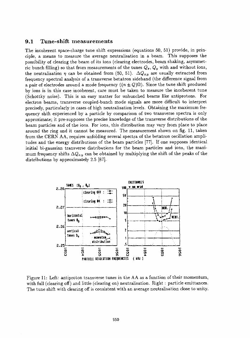
9.1 Tune-shift measurements The incoherent space-charge tune shift expressions (equations 50, 51) provide, in principle, a means to measure the average neutralisation in a beam. This supposes the possibility of clearing the beam of its ions (clearing electrodes, beam shaking, asymmetric bunch filling) so that from measurements of the tunes Qx, Qy with and without ions, the neutralisation rj can be obtained from (50, 51). AQx,y are usually extracted from frequency spectral analysis of a transverse betatron sideband (the difference signal from a pair of electrodes around a mode frequency ((n ± Q)Cl). Since the tune shift produced by ions is in this case incoherent, care must be taken to measure the incoherent tune (Schottky noise). This is an easy matter for unbunched beams like antiprotons. For electron beams, transverse coupled-bunch mode signals are more difficult to interpret precisely, particularly in cases of high neutralisation levels. Obtaining the maximum frequency shift experienced by a particle by comparison of two transverse spectra is only approximate; it pre-supposes the precise knowledge of the transverse distributions of the beam particles and of the ions. For ions, this distribution may vary from place to place around the ring and it cannot be measured. The measurement shown on fig. 11, taken from the CERN AA, requires unfolding several spectra of the betatron oscillation amplitudes and the energy distributions of the beam particles [77]. If one supposes identical initial bi-gaussian transverse distributions for the beam particles and ions, the maximum frequency shifts AQXiy can be obtained by multiplying the shift of the peaks of the distributions by approximately 2.5 [87].
2.28
2.27
2.26
2 .25
T«*S (0 h , »v)
clejrinj OFF : Z^Z
clearing IN : I g ^
horizontal tunes %
vertical tones Qu
-4-, horizontal tunes %
vertical tones Qu
M«entu«^» distribution
EHITTAHCES m w MI wad
SI
21
I I
5
i Jk
!I0I.
'HI VERT.
CO œ CO co CO CO CO CO UI en Ul Ul ut u IA Ul u A U) «n ( j À W m
PARI I CLE REUOlimOH FREQUENCIES ( kHz )
Figure 11: Left: antiproton transverse tunes in the A A as a function of their momentum, with full (clearing off) and little (clearing on) neutralisation. Right : particle emittances. The tune shift with clearing off is consistent with an average neutralisation close to unity.
550
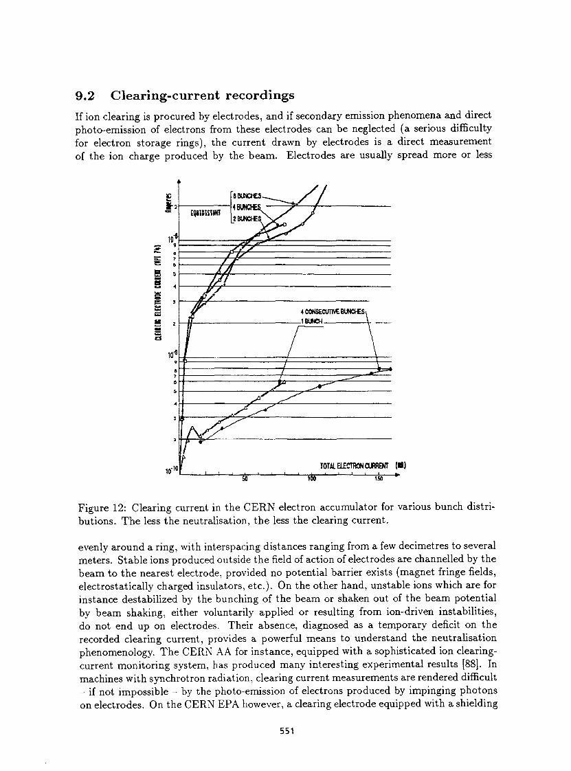
9.2 Clearing-current recordings If ion clearing is procured by electrodes, and if secondary emission phenomena and direct photo-emission of electrons from these electrodes can be neglected (a serious difficulty for electron storage rings), the current drawn by electrodes is a direct measurement of the ion charge produced by the beam. Electrodes are usually spread more or less
Figure 12: Clearing current in the CERN electron accumulator for various bunch distributions. The less the neutralisation, the less the clearing current.
evenly around a ring, with interspacing distances ranging from a few decimetres to several meters. Stable ions produced outside the field of action of electrodes are channelled by the beam to the nearest electrode, provided no potential barrier exists (magnet fringe fields, electrostatically charged insulators, etc.). On the other hand, unstable ions which are for instance destabilized by the bunching of the beam or shaken out of the beam potential by beam shaking, either voluntarily applied or resulting from ion-driven instabilities, do not end up on electrodes. Their absence, diagnosed as a temporary deficit on the recorded clearing current, provides a powerful means to understand the neutralisation phenomenology. The CERN AA for instance, equipped with a sophisticated ion clearing-current monitoring system, has produced many interesting experimental results [88]. In machines with synchrotron radiation, clearing current measurements are rendered difficult - if not impossible - by the photo-emission of electrons produced by impinging photons on electrodes. On the CERN EPA however, a clearing electrode equipped with a shielding
551
mask against synchrotron radiation and located at the end of a long straight section, has yielded some interesting measurements of the relative neutralisation levels for various bunch distributions (see fig. 12), thus confirming theoretical predictions qualitatively [89].
9.3 Bremsstrahlung measurements High energy photons (gamma rays) are produced when the electrons of a circulating beam collide with the nuclei of ions trapped in the beam. By counting the number of these bremsstrahlung photons produced per second, one can estimate the density of target ions along the beam path seen by the detection system. This is a Cerenkov (lead-glass) or scintillator counter of dimensions large enough to contain the electromagnetic shower produced by the gammas. The whole system is aligned with the beam, looking through a metallic window in a bending magnet vacuum chamber at a straight section or a section of the beam orbit inside the dipole magnet.
The bremsstrahlung radiation covers a wide spectrum with energies extending up to the kinetic energy of the primary electron and has a very sharp collimation with a characteristic opening angle given by - , where 7 is the relativistic energy of the stored beam in units of the rest energy. This allows the use of lead collimation to prevent gamma rays from other sources (mainly shower debris from lost beam electrons) from reaching the detector.
An important advantage of this technique with respect to the more conventional tune-shift measurements described above is that it allows the measurement of the local neutralisation rather than the average over the whole machine. However, since many different ion species may be trapped, some assumption must be made concerning the trapped-ion composition. In fact, since the total bremsstrahlung yield is proportional to the square of the atomic number of the target atom, the count rates are proportional to a weighted average of the ion densities, each ion species contributing with a weight Z2. Also, collisions with the neutral residual gas molecules produce an additional bremsstrahlung yield which one must either evaluate theoretically from the known residual gas composition or experimentally, e.g., by running the machine with positrons or comparing different machine conditions (e.g. clearing electrodes on/off).
The first observations [90] were made in the KEK Photon Factory storage ring in the form of a correlation between sudden changes in lifetime with bursts of bremsstrahlung events.
Later [91], bremsstrahlung count rates were registered in synchronism with a vertical blow-up caused by the accumulation of ions. The count rates as a function of t ime showed a rapid decrease at the time of the blow-up, followed by a slow increase which was attributed to the creation of new ions. The time constant for this slow rise was found to be in good agreement with the expected ionisation time for CO.
In [92, 93], a vertical blow-up was artificially produced by means of an external resonant excitation and the variation of the bremsstrahlung count rates was observed in both a uniform filling and partial filling modes of operation. Since the bremsstrahlung yield from the neutral residual gas molecules is expected to be independent of the beam dimensions, a decrease in the count rates during the blow-up was interpreted as a sign of the presence of trapped ions, and the comparison between the uniform filling and the partial filling confirms the theoretical prediction that fewer ions are present in the partial filling.
552
In [94], a study of the longitudinal motion of trapped ions is presented. Several gamma-ray counters were aimed at successive straight sections of the UVSOR storage ring. By looking at the time response of the count rates in these counters to a pulsed high voltage applied to a clearing electrode, the authors arrive at a spread in longitudinal ion velocities substantially larger than that expected from thermal considerations only.
553
References A considerable number of papers on the subject of neutralisation has been published in recent years. An at tempt has been made to classify the large number of useful references.
[1] E.D. Courant and H. Snyder, "Theory of the alternating gradient synchrotron", Ann. Phys. (N.Y.) vol. 3, p. 1 (1958).
[2] J. Delafosse, G. Mongodin, 'Les calculs de la technique du vide', Société Française des ingénieurs et techniciens du vide, 1961.
[3] J .D. Jackson, "Classical electrodynamics", John Wiley & Sons, New York, 1962.
[4] B. Rossi, "High energy particles", Prentice-Hall, Inc., Englewood Cliffs, N.J., U.S.A., 1956.
[5] L. Spitzer, Jr., "Physics of fully ionized gases", Interscience Publishers, Inc., New York, 1956.
Reviews, early papers
[6] B. Angerth, "Review of studies on beam neutralization in storage rings", CERN AR/Int .SG/65-1 (1965).
[7] R. Jolivot, "Anneaux de Stockage. Le piégeage des ions dans ACO et leur balayage", Rapport technique 75-63 /RJ- FB, Ecole Normale Supérieure — Faculté des Sciences, Orsay, Laboratoire de l'Accélérateur Linéaire (1963).
[8] R.D. Kohaupt, "Ion clearing mechanism in the electron-positron storage ring DORIS", DESY Ml-71/2 (1971).
[9] R. Alves Pires, J. Marriner, W. Marsh, A. Poncet, J. Rosensweig, and P. Zhou, Fermilab III Instabilities Workshop, Saint Charles, Illinois (1990).
[10] A. Poncet, "Ion trapping and clearing", CERN/MT 90-1 (ES). Course given at the the CAS, Uppsala, Sweden (October 1989) CERN 90-04 (1990).
[11] A. Poncet, "Ions and neutralization", CERN/MT 91-01. Talk given at the joint CERN/US particle accelerator school,Hilton Head Island, South Carolina, USA (November 1990) Springer Verlag, Lecture notes in Physics, n.400 (1992).
[12] D. Poteaux, "Piégeage des ions dans un anneau e + e ~ " , Rapport technique 29-69 D P / L N Laboratoire de l'Accélérateur Linéaire, Orsay (1969).
[13] E.M. Rowe, "Trapped ion effects and their treatment in electron storage rings.", American Vacuum Society Series 5, AIP conf. proceedings No.171, p.193, New York (1988).
554
Trapped ion dynamics
[14] Y. Baconnier and G. Brianti, "The stability of ions in bunched beam machines", CERN/SPS/80-2 (1980).
[15] C. Bernardini , "Space-charge effects in electron- synchrotrons", Nuovo Cimento, Vol X, N.5, p.804 (1988).
[16] L. Evans and D.J. Warner, "Space-charge neutralization of intense charged particle beams: some theoretical considerations", CERN MPS/LIN 71-2 (1971).
[17] E. Fischer, "Space charges in electron storage rings and the removal of positive ions by a D.C. clearing field", PS/Int . AR/60- 14 (1960).
[18] P.F. Tavares, "Betatron coupling in ion loaded electron beams", CERN PS/92-54 (LP) (1992).
[19] P.F. Tavares, "Transverse distribution of ions trapped in an electron beam", CERN PS/92-55 (LP) (1992).
Partial filling, gaps
[20] M. Barton,"Ion trapping with asymmetric bunch filling of the NSLS VUV ring", Nucl. Instrum. Methods, A243 p.278 (1986).
[21] D. Douglas, "Ion stability in bunched electron beams", IEEE Trans. Nucl. Sci. Vol. Ns-32, No.5 p.2294 (1985).
[22] S. Sakanaka, "The stability of ions in partially filled mode operation in the electron storage ring", KEK 86-17 (1986).
Longitudinal motion
[23] Y. Miyahara, K. Takayama, and G. Horikoshi, "Dynamical analysis of the longitudinal motion of trapped ions in an electron storage ring", Nucl. Instrum. Methods, A270 p.217 (1988).
[24] D. Sagan, "Some aspects of the longitudinal motion of ions in electron storage rings", Nucl. Instrum. Methods, A307 p.171 (1991).
Beam potential calculations and measurements
[25] M. Bassetti and G.A. Erskine, "Closed expressions for the electrical field of a two dimensional Gaussian charge", CERN-ISR-TH/80-06 (1980).
[26] O. Grôbner and K. Hiibner, "Computation of the electrostatic beam potential in vacuum chambers of rectangular cross-section", CERN/ISR-VA/75-27 (May 1975).
555
[27] M. Gygi-Hanney and B. Zotter, "Field strength in a bigaussian beam", LEP theory note 44 (1987).
[28] L.J. Laslett, "Potential of a uniformly charged beam with an elliptical cross-section", ERAN-44 (November 1969).
[29] L.J. Laslett, "Image field of a straight beam of elliptical cross-section", ERAN-49 (1970).
[30] R. Alves-Pires, "Beam dimensions and beam potential in the CERN Antiproton Accumulator complex", CERN PS/87-70 AA (1987).
[31] R. Alves-Pires, "Conformai mapping for two-dimensional electrostatic beam potential calculations", CERN PS/87-66 (1987).
[32] E. Regenstreif, "Potential and field created by an elliptic beam inside an infinite cylindrical vacuum chamber of circular cross-section", CERN/PS/DL 77-37 (1977).
[33] E. Regenstreif, "Potential and field created by a rectangular beam inside an infinite cylindrical vacuum chamber of circular cross section", CERN PS/DL 77-31 (1977).
[34] P. Strubin, "ISR Performance Report—Run 750, 7 July 1976, 26 GeV-Measure of the beam potential as a function of beam current", ISR-VA- ISR-VA-PS/sm (24th August, 1976).
Dust trapping
[35] P. Marin, "Microlosses of beam current in Super-ACO operated with electrons", Lure RT/90-01 (1990).
[36] P. Marin, "Longitudinal motion of a dust particle along a beam of electrons in a storage ring", Lure RT/90-06 (1990).
[37] P. Marin, "Observation of bremsstrahlung on dust particles trapped in electron beams at DCI and Super-ACO", Lure RT/91-03 (1991).
[38] F. Pedersen, "Effects of highly charged, solid macroparticles in negatively charged circulating beams", CERN PS/87-25 (1987).
[39] H. Saeki, T. Momose, and H. Ishimaru, "Observations of dust trapping phenomena in the Tristan accumulation ring and a study of dust removal in a beam chamber", Rev.Sci.Instrum. Vol.62 No.4 p.874 (1991).
[40] D. Sagan, "Mass and charge measurement of trapped dust in the CESR storage rings", Cornell CBN 92-12 (1992).
556
Papers describing specific machines
[41] C.J. Bochetta and A. Wrulich, "The trapping and clearing of ions in ELETTRA", Sincrotrone Trieste ST/M-88/26 (1988).
[42] E. Bozoki and H. Halama, "Ion related problems for the XLS ring", Nucl. Instrum. Methods, A307 p.156 (1991) .
[43] G. Brianti, "Upper limits of the average luminosity in the SPS p-p collider", CERN/SPS/DI /80-1 (20th February, 1980).
[44] F. Caspers, J.P. Delahaye, J.C. Godot, K. Hubner, and A. Poncet, " EPA beam-vacuum interaction and ion-clearing system", EPAC p. 1324, Rome (1988).
[45] S. Chattopadhyay, "Coherent instability and ion trapping considerations for Alladin lattices", LBL-19281 (1985).
[46] R.C. Gluckstern and A.G. Ruggiero, "Ion production and trapping in electron rings", BNL-26585 (1979).
[47] J. Herrera and B. Zotter, "Average neutralisation and transverse stability in Isabelle", BNL 50980 UC-28 (1978).
[48] T. Kasuga, "Ion clearing system for the UVSOR storage ring", Jpn. J. Appl. Phys. Vol.2 No . l l , p . l 711 (1986).
[49] R.Z. Liu, "Considerations on ion accumulation and clearing in Spear", SSRL ACD-Note 25 (1984).
[50] F. Pedersen, A. Poncet, and L. Soby, "The CERN Antiproton Accumulator clearing system with ion current as a residual neutralization diagnostic", CERN PS/89-17 ML (1989).
[51] A. Poncet, "Ion clearing in EPA", PS/ML/Note 83-1 (1983).
[52] A. Poncet, "Quel vide pour l 'EPA?", PS/ML/Note 83-3 (1983).
[53] D. Sagan, "Ion trapping in the CESR B-Factory", Cornell, CBN 91-2, (May 1990).
[54] Y. Sun, "A preliminary report on ion clearing in Spear", SSRL ACD-note 83 (may 1990).
[55] P.F. Tavares, "The ion clearing system of the UVX-2 synchrotron radiation source", Proceedings 3rd EPAC, p. 1647, Berlin (1992).
[56] E.J.N. Wilson, "Does ion trapping produce a large space charge AQ in the LEP injector chain?", CERN/SPS-DI LTD (1980).
[57] Workshop on pp in the SPS. (Theoretical aspects of machine design, March 1980), S P S - p p - l , 9 t h M a y , 1980.
[58] P. Zhou and J.B. Rosenzweig, "Ion trapping in Tevatron with separated orbits", Fermilab III Instabilities Workshop, Saint Charles, Illinois (1990).
557
Neutralisation in the ISR
[59] B. Angerth, E. Fischer, and 0 . Grôbner, "The clearing fields of the ISR", CERN-ISR-VA/71-47 (1971).
[60] R. Calder, E. Fischer, 0 . Grôbner, and E. Jones, "Vacuum conditions for proton storage rings", CERN/ISR-VA/74-26 (1974).
[61] E. Fischer, "Clearing fields for the ISR", ISR-VAC/66-15, 3e (1966).
[62] E. Fischer and K. Zankel, "The stability of the residual gas density in the ISR in presence of high intensity proton beams". CERN-ISR-VA/ 73-52 (1973).
[63] 0 . Grôbner, "ISR Performance Report- Clearing studies using Langmuir probe technique Run 139, 22 GeV, 20 bunches", ISR-VA/OG/ss (1972).
[64] 0 . Grôbner, "ISR Performance Report— Run 142 , 26 GeV, 20 bunches, Ring 1, 26 FC, Beam Decay as Function of Clearing Voltage", ISR-VA/OG/ss , (1972).
[65] 0 . Grôbner and R.S. Calder, "Beam induced gas desorption in the CERN intersecting storage rings", IEEE Trans.Nucl.Sci. , Vol. NS-20, No 3 p.760 (1973).
[66] O. Grôbner, 'ISR Performance Report— Attempt to measure neutralisation Q shifts', ISR-VA/OG/sm (1974).
[67] 0 . Grôbner, P. Strubin, "ISR Performance Report —Decay rate due to nuclear scattering pressure as determined from the clearing currents", ISR-VA/OG/sm, 11th July, 1974.
[68] O. Grôbner, "ISR Performance Report— Clearing, Pressure Bump, Beam Behaviour", ISR-VA/OG/sm (1975).
[69] 0 . Grôbner, "Performance study on proton- proton storage rings at several hundred GeV/c. Neutralization and vacuum requirements in ISR". CERN/ISR-AS/74-67 (1974).
[70] O. Grôbner, "ISR Performance Report R F - RF Clearing, e~p lines and electron noise", ISR-VA/OG/sm (1975).
[71] O. Grôbner, "An estimate of the rate of electron removal by RF-clearing". ISR-VA/OG (1975).
[72] 0 . Grôbner, "ISR Performance Report- -Run 904, 26 GeV, 6.12.77. Observation of beam blow-up by multiple scattering on neutralising electrons", ISR-VA/OG/sm (1978).
[73] O. Grôbner, "Ion clearing of anti-proton beams in the ISR". CERN ISR-VA/OG/sm (1978).
[74] 0 . Grôbner, "ISR Performance Report-Run 389, Ring 1, 5C26, Dependence of clearing current on neutralisation", ISR-VA/OG/sm (1984).
558
[75] Technical Note - ISR Vacuum Group, "The behaviour of ions in presence of a bunched antiproton beam in the ISR', ISR-VA/EF-sm, 7th November 1978.
[76] D. G. Koshkarev, "Concerning a new way of removing electrons from an unbunched electron beam", ISR-DI/DGK (1974).
[77] S. Van der Meer, "Measurement of transverse stack emittances from Schottky scans", PS/AA/Note 84-11 (1984).
Neutralisation experiments [78] M.F. Biagini et al., "Observation of ion trapping at Adone", 11th International
conference on high energy accelerators,p. 687, Geneva (1980).
[79] E.V. Bulyak and V.I. Kurilko, "Low frequency transverse charge oscillations in and electron storage ring", J E T P Letters Vol.34, No. 9 p.471 (1981).
[80] E.V. Bulyak and V.I. Kurilko, "Space charge neutralization of a beam in high current electron storage rings", Sov. Phys. Tech. Phys. Vol.27, No.2 p.194 (1982).
[81] T.S. Chou and H.J. Halama, "Trapped ions and beam lifetime in the NSLS storage rings", Proceedings of the EPAC, p.1773, Rome (1988).
[82] R. Cappi and J.P. Riunaud, "Trapped ion effects with electron beams in the CERN PS" , CERN/PS 90-17 PA (1990).
[83] 0 . Grôbner, "ISR Performance Report— Measurement of the self-clearing ra te as function of beam current", ISR- VA/OG/sm, 27th March, 1975.
[84] H. Halama and E. Bozoki, "Ion clearing and photoelectron production in the 200 MeV SXLS ring", BNL-46471 (1991).
[85] T. Kasuga, H. Yonehara, T. Kinoshita, and M. Hasumoto, "Ion trapping effect in the UVSOR storage ring", Jpn. J. Appl. Phys. Vol.24, No.9 p.1212 (1985).
[86] P. Marin, "Positron versus electron behaviour in Super- ACO", Lure RT/Anneaux/90-03 (1990).
[87] W. Marsh, "How to measure beam neutralization in the accumulator", Fermilab III Instabilities Workshop, Saint Charles, Illinois (1990). (unpublished)
[88] F. Pedersen et al, "The CERN Antiproton Accumulator clearing system with ion current measurements as a residual neutralisation diagnostic", CERN PS/89-17 (ML) (1989).
[89] A. Poncet, "Trapping of ions in the EPA electron beam : Stability conditions and diagnosis", CERN PS 88-14 [ML] (1988).
559
Bremsstrahlung experiments
[90] M. Kobayashi et al, "Observations of bremsstrahlung caused by ion trapping", Proceedings of the 5th Symposium of Accelerator Science and Technology, KEK (1984).
[91] H. Kobayakawa et al, "Observation of the ion trapping phenomenon with bremsstrahlung", Nucl. Instrum. Methods, A248 p. 565 (1986).
[92] S. Sakanaka et al, "Observation of ion trapping in single bunch operation at the Photon Factory storage ring", KEK 87-168 (1987).
[93] S. Sakanaka et al, "Differences in ion trapping between uniform and partial filling", Nucl. Instrum. Methods, A256 p.184 (1987).
[94] K. Watanabe et al., "Drift velocity and pulse response of trapped ions in a circulating electron beam", Jpn. J .Appl. Phys., Vol.26, No.12 , L1964 (1987).
Ionisation, heating, cooling
[95] U. Amaldi, "Fisica delle radiazioni", Boringhieri, Torino (1971).
[96] F. Lapique and F. Piuz, "Simulation of the measurement by primary cluster counting of the energy lost by a relativistic ionizing particle in argon", Nucl. Instrum. Methods, 175 p. 297 (1980).
[97] Y. Miyahara, "Photoionization of residual gas in electron storage ring", Jpn. J. Appl. Phys., Vol. 26, No. 9, p. 1544
[98] F . Rieke and W. Prepjchal, "Ionisation cross-section of gaseous atoms and molecules for high-energy electrons and positrons" , Phys.Rev. A Vol. 6, No. 4 , p.1507 (1972).
[99] F . Sauli, "Principles of operation of multiwire proportional drift chambers", CERN 77-09 (1977).
[100] K. Symon, "Are clearing electrodes really necessary?", Private Comunication (1964).
Beam shaking
[101] E. Bozoki, "Ion shaking in the 200 MeV XLS-ring". Proceedings 3rd EPAC, p.789, Berlin (1992).
[102] J. Marriner, D. Môhl, Y. Orlov, A. Poncet and S. Van der Meer, "Experiments and practice in beam shaking", CERN/PS/89-48 AR (1989).
[103] Y. Orlov, "The suppresion of transverse instabilities caused by trapped ions in the AA by shaking the pp beam", CERN/PS/89-01 (1989).
560
[104] R. Alves-Pires, "Beam shaking for the Fermilab Antiproton Accumulator", Fermi-lab III Instabilities Workshop, Saint Charles, Illinois (1990).
[105] A. Poncet and Y. Orlov, "EPA machine experiment note - ion shaking tests", PS/ML/Note 89-1 (1989).
[106] J.B. Rosenzweig, "Beam-ion cyclotron resonance instability", Fermilab III Instabilities Workshop, Saint Charles, Illinois (1990).
[107] P. Zhou and J.B. Rosenzweig, "Ion clearing using Cyclotron shaking", Fermilab III Instabilities Workshop, Saint Charles, Illinois (1990).
Instabilities
[108] G. Carron et al, "Observation of transverse quadrupole instabilities in intense cooled antiproton beams in the AA ", CERN/PS/89-18 (AR), Proceedings PAC, p.803, Chicago (1989).
[109] A. Dainelli, "Antiproton-positive ion transverse instabilities in the CERN AA". A tune modulated direct map simulation", CERN/PS/87-13 (AA) (1987).
[110] H.G. Hereward, "The instability of radial betatron oscillations in the CPS", CERN MPS/Int. DL 64-8 (1964).
[Ill] E. Jones et al, "Transverse instabilities due to beam trapped ions and charged matter in the CERN AA", IEEE Trans.Nucl.Sci., Vol. NS -32, p. 2218 (1985).
[112] Y. Kamiya, M. Yzawa, T. Katsura, and M. Kihara, "Vertical instability caused by ion trapping in KEK-Photon factory storage ring", Proc. of 5th Symp. Ace. Sci. Tech. p. 148 (1984).
[113] E. Keil, B. Zotter, "Landau-damping of coupled electron-proton oscillations", CERN-ISR-TH/71-58 (1971).
[114] D.G. Koshkarev and P.R. Zenkevich, "Resonance of coupled transverse oscillations in two circular beams", Part.Ace. Vol.3 p.l (1972).
[115] L.J. Laslett, A. Sessler, and D. Môhl, "Transverse two-stream instability in the presence: of strong species-species and image forces", Nucl. Instrum. Methods, Vol. 121 p.517 (1974).
[116] F. Pedersen, A. Poncet,"Proton- antiproton instability in the CERN AA", CERN PS/AA/MENoteSl , 1981
[117] R. Alves-Pires et al, "On the theory of coherent instabilities due to coupling between a dense cooled beam and charged particles from the residual gas", CERN/PS/89-14 (AR), PAC p.800 Chicago (1989).
[118] R. Alves-Pires and D. Môhl, "Landau damping of coupled quadrupole modes", PS/AR/Note 90-09 (1990).
561
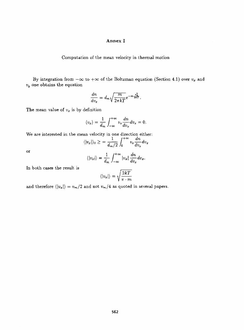
A n n e x I
Computation of the mean velocity in thermal motion
By integration from —oo to +00 of the Boltzman equation (Section 4.1) over vx and vy one obtains the equation
dn I m _mA.
The mean value of vx is by definition
1 f+0° dn . , 1 / + ° ° dn , [Vx) = ~r / vx-—dvx = 0.
" m J-00 dVx
We are interested in the mean velocity in one direction either: .. .. 1 f+°° dn
{ M o - = dj2Jo VxdVx
dv* or
1 f+°°, . dn 1 f-r00 an
(\vx\) = -r- / \vx\-r-dvx. am J-00 avx i m «'—OO
In both cases the result is
/I l\ l 2 k T
/ 7T • m
and therefore ( |v x | ) = vm/2 and not vm/4 as quoted in several papers.
562
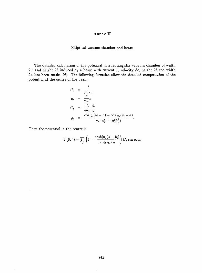
A n n e x I I
Elliptical vacuum chamber and beam
The detailed calculation of the potential in a rectangular vacuum chamber of width 2w and height 2h induced by a beam with current / , velocity /3c, height 26 and width 2a has been made [26]. The following formulae allow the detailed computation of the potential at the centre of the beam:
Uo - /3ce0
•K
V» = -—5 2w
cs = <ibw rjs
cos rjs(w --a) — cos TJS(W + a) 9s — Vs • a ( l - n 2 4 )
Then the potential in the centre is
T/ n n\ V- (i cosh[ns{h - b))\ .
563
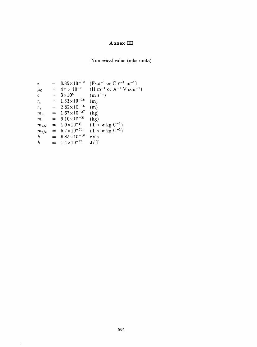
Annex III
Numerical value (mks units)
e = 8.85xl0~ 1 2 (F-m- 1 or C v" 1 m" 1 ) /*o = 4TT x 10~7 (H-m- 1 or A" 1 Vs-m" 1 ) c = 3 x l 0 8 ( m s - 1 ) rp = 1.53xl0" 1 8 (m) re = 2.82xl0" 1 5 (m) mp = 1.67xl0~ 2 7 (kg) me = 9.10xl0" 3 1 (kg) mp/e = l .OxKT 8 (T-s or kg C- 1 ) me/e = 5 .7x l0 - 2 3 (T-s or kg C ' 1 ) h = 6.85xl0- 1 6 eV-s k = 1.4xlO- 2 3 J/K
564

BEAM DIAGNOSTICS FOR ACCELERATORS H. Koziol CERN, Geneva, Switzerland
Abstract This introductory course aims at a reasonably complete coverage of beam diagnostic devices used in linear and circular accelerators and in primary beam lines. The weight is on the concepts and the indication of variants, while for technical details the reader is referred to the literature.
1 . INTRODUCTION Beam diagnostics is an essential consti tuent of any accelerator. These systems are our organs of sense that let us perceive what propert ies a beam has and how it behaves in a machine. W i thou t diagnost ics, we wou ld b l ind ly grope around in the dark and the achievem ent of a beam for physics-use wou ld be a m atter of sheer luck (some accelerators have at some t ime been close to such a si tuat ion!) . As the saying goes: an accelerator is just as good as its diagnostics.
Beam diagnostics is a rich field. A great variety of physical effects are made use of, imagination and inventiveness find a wide playground. Therefore, there exists today a vast choice of different types of diagnostic devices, each usually in many variants.
Two hours of lecture time do not permit an in-depth coverage of all devices on the market, but to present only a selection would not fulfill the purpose of this course. The choice I have made is to aim for a reasonably complete coverage of diagnostic devices currently used, at the expense of detail. We will thus concentrate on the concepts and indicate the variants that exist and refer to the literature for details.
Also, we will limit ourselves to diagnostics used on accelerators and on ejected primary beams and leave aside detectors for secondary beams, downstream from a target, on their transport to an experimental set-up. As a further economy measure, we will also leave aside associated electronics, analogue signal treatment and digital data treatment, although these are subjects of great importance to beam diagnostics.
There are subjects which have been treated in other lectures, e.g. synchrotron radiation, which permits us to be briefer on those. Very specialized measurements, such as that of beam polarization or those at the final focus of colliding linacs, are beyond the aim of an introductory course and will be just mentioned for completeness.
When setting out to describe a large number of diagnostic devices, one first tries to establish a systematic order. One could proceed according to the properties measured (intensity, position, etc.). Or one could class the devices as electromagnetic, using secondary emission, etc, or as destructive and non-destructive. However, none of that makes much sense. Many devices can measure more than one property, their variants may make use of different physical principles and the distinction between destructive and non-destructive often depends on circumstances.
I have therefore drawn up a matrix (see Table 1) listing the devices to be discussed and the properties they can measure. And now we will forget about classification and get on with the description in a sequence that is didactically convenient.
Table 1
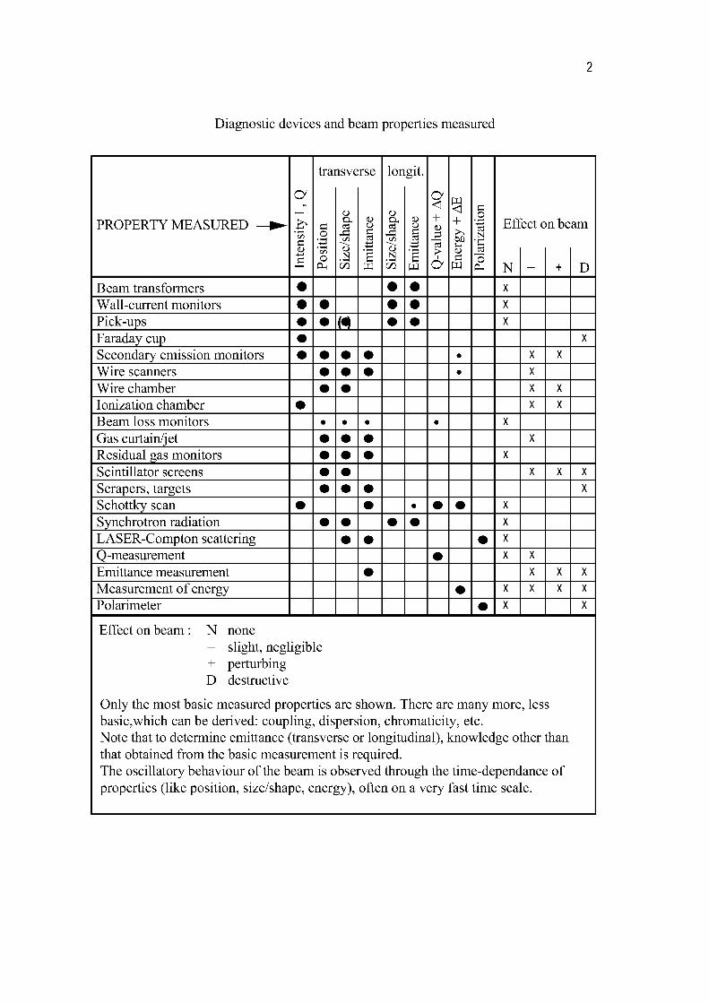
2
Diagnostic devices and beam properties measured
PROPERTY MEASURED — •
Inte
nsity
I, Q
trai
«
'co O
P* Size
/shap
e %
m
rse
i W Si
ze/sh
ape
o"
git-
i W Q
-val
ue +
AQ
En
ergy
+ A
E Po
lariz
atio
n
Eff
N
ectc nbe
+
am
D Beam transformers • • X
Wall-current monitors • • • X
Pick-ups • « • • X Faraday cup X
Secondary emission monitors • • • • X X
Wire scanners • • • • X Wire chamber • • X X
Ionization chamber • X X
Beam loss monitors • • • • X Gas curtain/jet • • • X
Residual gas monitors • • • X
Scintillator screens • • X X X
Scrapers, targets • • • X
Schottky scan • • • • • X
Synchrotron radiation • • • • X LASER-Compton scattering • • • X
Q-measurement • X X
Emittance measurement • X X X
Measurement of energy • X X X X
Polarimeter • X X
Effect on beam : N none - slight, negligible + perturbing D destructive
Only the most basic measured properties are shown. There are many more, less basic,which can be derived: coupling, dispersion, chromaticity, etc. Note that to determine emittance (transverse or longitudinal), knowledge other than that obtained from the basic measurement is required. The oscillatory behaviour of the beam is observed through the time-dependance of properties (like position, size/shape, energy), often on a very fast time scale.
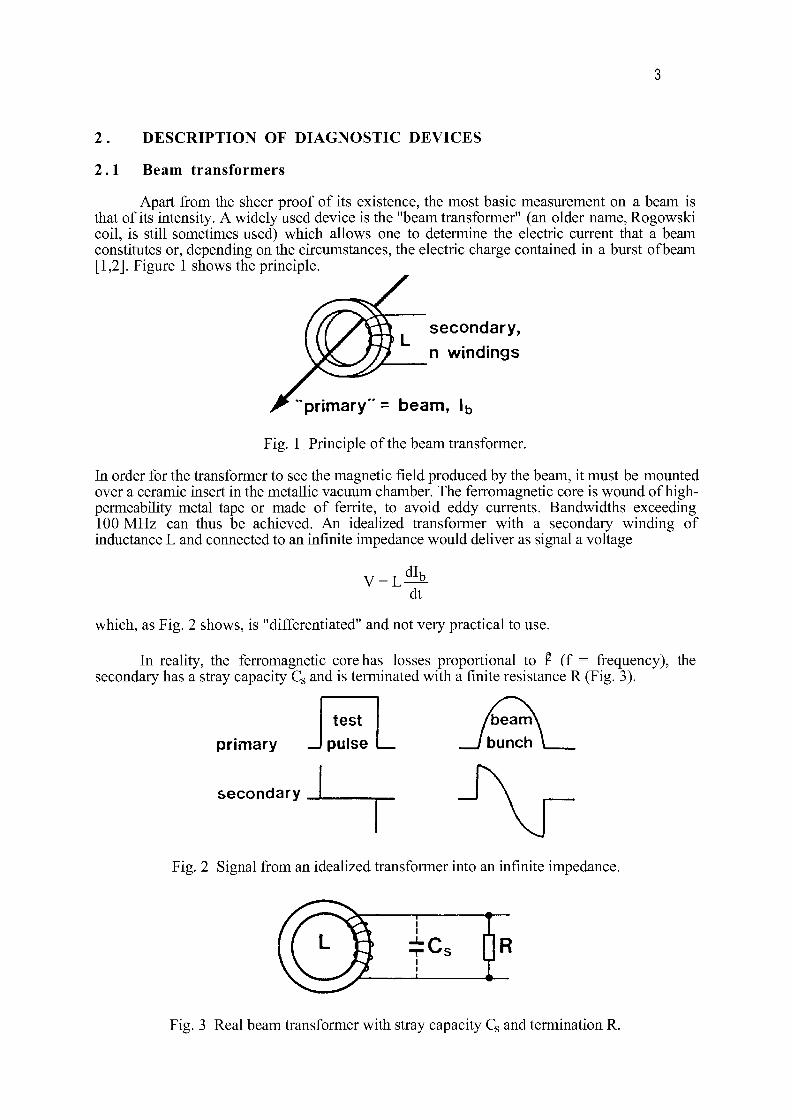
3
2 . DESCRIPTION OF DIAGNOSTIC DEVICES
2.1 Beam transformers
Apart from the sheer proof of its existence, the most basic measurement on a beam is that of its intensity. A widely used device is the "beam transformer" (an older name, Rogowski coil, is still sometimes used) which allows one to determine the electric current that a beam constitutes or, depending on the circumstances, the electric charge contained in a burst ofbeam [1,2]. Figure 1 shows the principle.
secondary, n windings
pr imary" = beam, l b
Fig. 1 Principle of the beam transformer.
In order for the transformer to see the magnetic field produced by the beam, it must be mounted over a ceramic insert in the metallic vacuum chamber. The ferromagnetic core is wound of high-permeability metal tape or made of ferrite, to avoid eddy currents. Bandwidths exceeding 100 MHz can thus be achieved. An idealized transformer with a secondary winding of inductance L and connected to an infinite impedance would deliver as signal a voltage
V = L dlb dt
which, as Fig. 2 shows, is "differentiated" and not very practical to use.
In reality, the ferromagnetic core has losses proportional to f- (f = frequency), the secondary has a stray capacity Q and is terminated with a finite resistance R (Fig. 3).
primary _J
secondary
test pulse
Fig. 2 Signal from an idealized transformer into an infinite impedance.
Fig. 3 Real beam transformer with stray capacity Q and termination R.

4
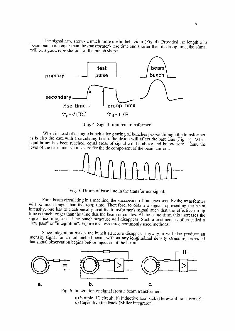
5
The signal now shows a much more useful behaviour (Fig. 4). Provided the length of a beam bunch is longer than the transformer's rise time and shorter than its droop time, the signal will be a good reproduction of the bunch shape.
primary
secondary
rise t ime- 1
Tr~\/Tcr
L droop time
T d ~ L / R
Fig. 4 Signal from real transformer.
When instead of a single bunch a long string of bunches passes through the transformer, as is also the case with a circulating beam, the droop will affect the base line (Fig. 5). When equilibrium has been reached, equal areas of signal will be above and below zero. Thus, the level of the base line is a measure for the dc component of the beam current.
Fig. 5 Droop of base line in the transformer signal.
For a beam circulating in a machine, the succession of bunches seen by the transformer will be much longer than its droop time. Therefore, to obtain a signal representing the beam intensity, one has to electronically treat the transformer's signal such that the effective droop time is much longer than the time that the beam circulates. At the same time, this increases the signal rise time, so that the bunch structure will disappear. Such a treatment is often called a "low pass" or "integration". Figure 6 shows three commonly used methods.
Since integration makes the bunch structure disappear anyway, it will also produce an intensity signal for an unbunched beam, without any longitudinal density structure, provided that signal observation begins before injection of the beam.
-rzn-
a. b. c. Fig. 6 Integration of signal from a beam transformer.
a) Simple RC circuit, b) Inductive feedback (Hereward transformer), c) Capacitive feedback (Miller integrator).
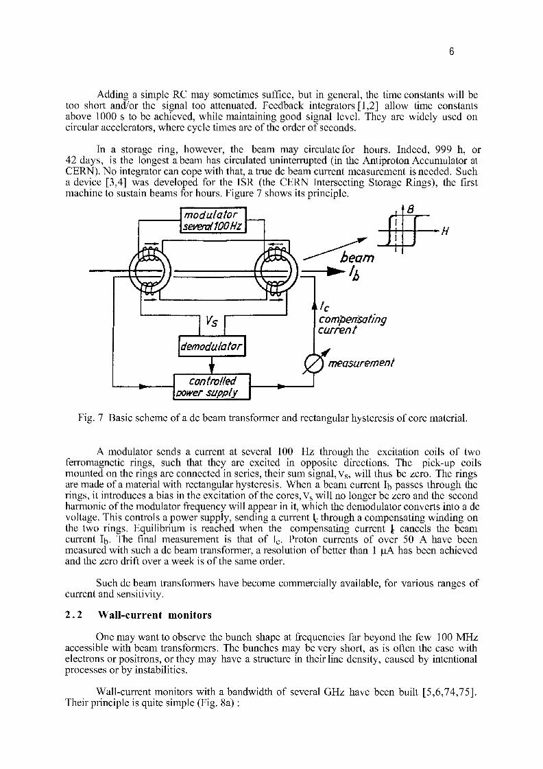
6
Adding a simple RC may sometimes suffice, but in general, the time constants will be too short and/or the signal too attenuated. Feedback integrators [1,2] allow time constants above 1000 s to be achieved, while maintaining good signal level. They are widely used on circular accelerators, where cycle times are of the order of seconds.
In a storage ring, however, the beam may circulate for hours. Indeed, 999 h, or 42 days, is the longest abeam has circulated uninterrupted (in the Antiproton Accumulator at CERN). No integrator can cope with that, a true dc beam current measurement is needed. Such a device [3,4] was developed for the ISR (the CERN Intersecting Storage Rings), the first machine to sustain beams for hours. Figure 7 shows its principle.
modulator severvilOQHz
Vs
demodulator
I
He compensating current
controlled power supply
» measurement
Fig. 7 Basic scheme of a dc beam transformer and rectangular hysteresis of core material.
A modulator sends a current at several 100 Hz through the excitation coils of two ferromagnetic rings, such that they are excited in opposite directions. The pick-up coils mounted on the rings are connected in series, their sum signal, Vs, will thus be zero. The rings are made of a material with rectangular hysteresis. When a beam current lb passes through the rings, it introduces a bias in the excitation of the cores, Vs will no longer be zero and the second harmonic of the modulator frequency will appear in it, which the demodulator converts into a dc voltage. This controls a power supply, sending a current \ through a compensating winding on the two rings. Equilibrium is reached when the compensating current \ cancels the beam current lb. The final measurement is that of I c. Proton currents of over 50 A have been measured with such a dc beam transformer, a resolution of better than 1 |uA has been achieved and the zero drift over a week is of the same order.
Such dc beam transformers have become commercially available, for various ranges of current and sensitivity.
2.2 Wall-current monitors
One may want to observe the bunch shape at frequencies far beyond the few 100 MHz accessible with beam transformers. The bunches may be very short, as is often the case with electrons or positrons, or they may have a structure in their line density, caused by intentional processes or by instabilities.
Wall-current monitors with a bandwidth of several GHz have been built [5,6,74,75]. Their principle is quite simple (Fig. 8a) :
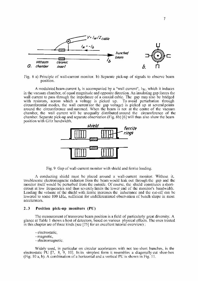
7
V: /w/Zcable
-V777Z
vacuum Q. chamber
—V77A— ceramic insert
/A
bunched beam
Fig. 8 a) Principle of wall-current monitor, b) Separate pick-up of signals to observe beam position.
A modulated beam current lb is accompanied by a "wall current", I\y, which it induces in the vacuum chamber, of equal magnitude and opposite direction. An insulating gap forces the wall current to pass through the impedance of a coaxial cable. The gap may also be bridged with resistors, across which a voltage is picked up. To avoid perturbation through circumferential modes, the wall current (or the gap voltage) is picked up at several points around the circumference and summed. When the beam is not at the centre of the vacuum chamber, the wall current will be unequally distributed around the circumference of the chamber. Separate pick-up and separate observation (Fig. 8b) [6] will thus also show the beam position with GHz bandwidth.
shield
i -^3-
l •E2& r ferrite rings
Fig. 9 Gap of wall-current monitor with shield and ferrite loading.
A conducting shield must be placed around a wall-current monitor. Without it, troublesome electromagnetic radiation from the beam would leak out through the gap and the monitor itself would be perturbed from the outside. Of course, the shield constitutes a short-circuit at low frequencies and thus severely limits the lower end of the monitor's bandwidth. Loading the volume of the shield with ferrite increases the inductance and the cut-off can be lowered to some 100 kHz, sufficient for undifferentiated observation of bunch shape in most accelerators.
2.3 Position pick-up monitors (PU)
The measurement of transverse beam position is a field of particularly great diversity. A glance at Table 1 shows a host of detectors, based on various physical effects. The ones treated in this chapter are of three kinds (see [75] for an excellent tutorial overview) :
- electrostatic, - magnetic, - electromagnetic.
Widely used, in particular on circular accelerators with not too short bunches, is the electrostatic PU [7, 8, 9, 10]. In its simplest form it resembles a diagonally cut shoe-box (Fig. 10 a, b). A combination of a horizontal and a vertical PU is shown in Fig. 11.
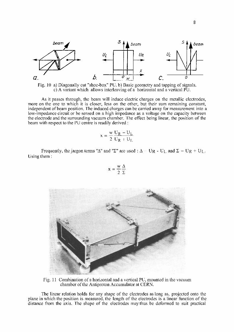
beam
b.
n k beam
UL UR
X c i V _ c.
Fig. 10 a) Diagonally cut "shoe-box" PU. b) Basic geometry and tapping of signals, c) A variant which allows interleaving of a horizontal and a vertical PU.
As it passes through, the beam will induce electric charges on the metallic electrodes, more on the one to which it is closer, less on the other, but their sum remaining constant, independent of beam position. The induced charges can be carried away for measurement into a low-impedance circuit or be sensed on a high impedance as a voltage on the capacity between the electrode and the surrounding vacuum chamber. The effect being linear, the position of the beam with respect to the PU centre is readily derived :
x = w U R UT
2 U B + U T ; R
Frequently, the jargon terms "A" and "S" are used : A Using them :
U R - U L and S = U R + U L .
_ w A
2"ï
Fig. 11 Combination of a horizontal and a vertical PU, mounted in the vacuum chamber of the Antiproton Accumulator at CERN.
The linear relation holds for any shape of the electrodes as long as, projected onto the plane in which the position is measured, the length of the electrodes is a linear function of the distance from the axis. The shape of the electrodes may thus be deformed to suit practical
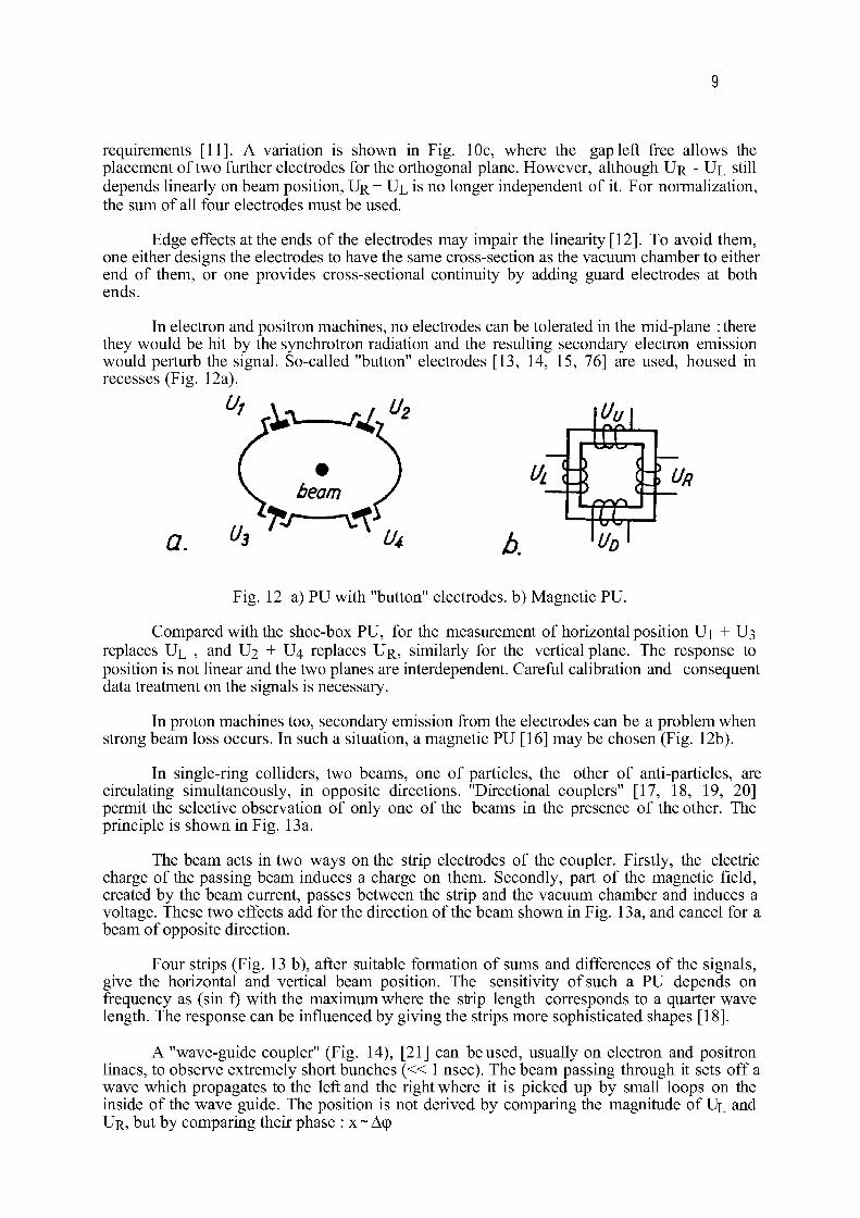
9
requirements [11]. A variation is shown in Fig. 10c, where the gap left free allows the placement of two further electrodes for the orthogonal plane. However, although U R - U L still depends linearly on beam position, UR + UL is no longer independent of it. For normalization, the sum of all four electrodes must be used.
Edge effects at the ends of the electrodes may impair the linearity [12]. To avoid them, one either designs the electrodes to have the same cross-section as the vacuum chamber to either end of them, or one provides cross-sectional continuity by adding guard electrodes at both ends.
In electron and positron machines, no electrodes can be tolerated in the mid-plane : there they would be hit by the synchrotron radiation and the resulting secondary electron emission would perturb the signal. So-called "button" electrodes [13, 14, 15, 76] are used, housed in recesses (Fig. 12a).
a. beam
Fig. 12 a) PU with "button" electrodes, b) Magnetic PU.
Compared with the shoe-box PU, for the measurement of horizontal position Ui + U3 replaces UL , and U2 + U4 replaces UR, similarly for the vertical plane. The response to position is not linear and the two planes are interdependent. Careful calibration and consequent data treatment on the signals is necessary.
In proton machines too, secondary emission from the electrodes can be a problem when strong beam loss occurs. In such a situation, a magnetic PU [16] may be chosen (Fig. 12b).
In single-ring colliders, two beams, one of particles, the other of anti-particles, are circulating simultaneously, in opposite directions. "Directional couplers" [17, 18, 19, 20] permit the selective observation of only one of the beams in the presence of the other. The principle is shown in Fig. 13a.
The beam acts in two ways on the strip electrodes of the coupler. Firstly, the electric charge of the passing beam induces a charge on them. Secondly, part of the magnetic field, created by the beam current, passes between the strip and the vacuum chamber and induces a voltage. These two effects add for the direction of the beam shown in Fig. 13a, and cancel for a beam of opposite direction.
Four strips (Fig. 13 b), after suitable formation of sums and differences of the signals, give the horizontal and vertical beam position. The sensitivity of such a PU depends on frequency as (sin f) with the maximum where the strip length corresponds to a quarter wave length. The response can be influenced by giving the strips more sophisticated shapes [18].
A "wave-guide coupler" (Fig. 14), [21] can be used, usually on electron and positron linacs, to observe extremely short bunches ( « 1 nsec). The beam passing through it sets off a wave which propagates to the left and the right where it is picked up by small loops on the inside of the wave guide. The position is not derived by comparing the magnitude of UL and UR, but by comparing their phase : x ~ Acp
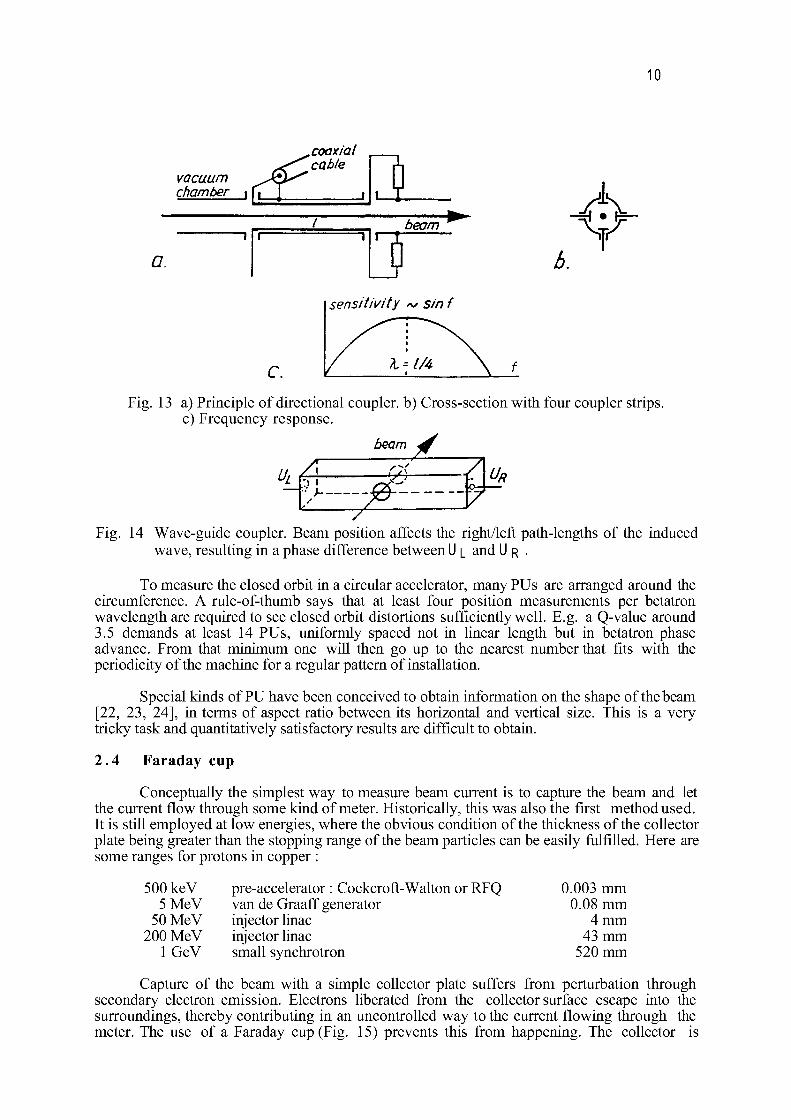
10
vacuum chamber \ rrf
coaxial
1 <) vacuum chamber \
I beam m
i
J. « 1
t) 4i\
sensitivity ~ sin f
C. Fig. 13 a) Principle of directional coupler, b) Cross-section with four coupler strips,
c) Frequency response. beam £.
«m — "••• J--
71 ^
UR
Fig. 14 Wave-guide coupler. Beam position affects the right/left path-lengths of the induced wave, resulting in a phase difference between U |_ and U R .
To measure the closed orbit in a circular accelerator, many PUs are arranged around the circumference. A rule-of-thumb says that at least four position measurements per betatron wavelength are required to see closed orbit distortions sufficiently well. E.g. a Q-value around 3.5 demands at least 14 PUs, uniformly spaced not in linear length but in betatron phase advance. From that minimum one will then go up to the nearest number that fits with the periodicity of the machine for a regular pattern of installation.
Special kinds of PU have been conceived to obtain information on the shape of the beam [22, 23, 24], in terms of aspect ratio between its horizontal and vertical size. This is a very tricky task and quantitatively satisfactory results are difficult to obtain.
2.4 Faraday cup
Conceptually the simplest way to measure beam current is to capture the beam and let the current flow through some kind of meter. Historically, this was also the first method used. It is still employed at low energies, where the obvious condition of the thickness of the collector plate being greater than the stopping range of the beam particles can be easily fulfilled. Here are some ranges for protons in copper :
500 keV pre-accelerator : Cockcroft-Walton or RFQ 5 MeV van de Graaff generator
50 MeV injector linac 200 MeV injector linac
1 GeV small synchrotron
0.003 mm 0.08 mm
4 mm 43 mm
520 mm
Capture of the beam with a simple collector plate suffers from perturbation through secondary electron emission. Electrons liberated from the collector surface escape into the surroundings, thereby contributing in an uncontrolled way to the current flowing through the meter. The use of a Faraday cup (Fig. 15) prevents this from happening. The collector is
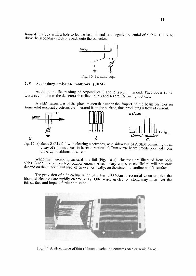
11
housed in a box with a hole to let the beam in and at a negative potential of a few 100 V to drive the secondary electrons back onto the collector.
Fig. 15 Faraday cup.
2.5 Secondary-emission monitors (SEM)
At this point, the reading of Appendices 1 and 2 is recommended. They cover some features common to the detectors described in this and several following sections.
A SEM makes use of the phenomenon that under the impact of the beam particles on some solid material electrons are liberated from the surface, thus producing a flow of current.
- o f beam
a. Fig. 16
f i i signal
1 , channel number D. C.
a) Basic SEM : foil with clearing electrodes, seen sideways, b) A SEM consisting of an array of ribbons , seen in beam direction, c) Transverse beam profile obtained from an array of ribbons or wires.
When the intercepting material is a foil (Fig. 16 a), electrons are liberated from both sides. Since this is a surface phenomenon, the secondary emission coefficient will not only depend on the material but also, often even critically, on the state of cleanliness of its surface.
The provision of a "clearing field" of a few 100 V/cm is essential to ensure that the liberated electrons are rapidly cleared away. Otherwise, an electron cloud may form over the foil surface and impede further emission.
Fig. 17 A SEM made of thin ribbons attached to contacts on a ceramic frame.
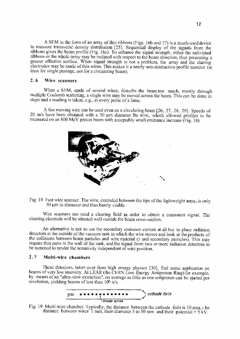
12
A SEM in the form of an array of thin ribbons (Figs. 16b and 17) is a much-used device to measure transverse density distribution [25]. Sequential display of the signals from the ribbons gives the beam profile (Fig. 16c). To enhance the signal strength, either the individual ribbons or the whole array may be inclined with respect to the beam direction, thus presenting a greater effective surface. When signal strength is not a problem, the array and the cletring electrodes may be made of thin wires. This makes it a nearly non-destructive profile monitor (at least for single passage, not for a circulating beam).
2.6 Wire scanners
When a SEM, made of several wires, disturbs the beam too much, mostly through multiple Coulomb scattering, a single wire may be moved across the beam. This can be done in steps and a reading is taken, e.g., at every pulse of a linac.
A fast moving wire can be used even on a circulating beam [26, 27, 28, 29]. Speeds of 20 m/s have been obtained with a 50 urn diameter Be wire, which allowed profiles to be measured on an 800 MeV proton beam with acceptably small emittance increase (Fig. 18).
Fig. 18 Fast wire scanner. The wire, extended between the tips of the lightweight arms, is only 50 |um in diameter and thus barely visible.
Wire scanners too need a clearing field in order to obtain a consistent signal. The clearing electrode will be situated well outside the beam cross-section.
An alternative is not to use the secondary emission current at all but to place radiation detectors at the outside of the vacuum tank in which the wire moves and look at the products of the collisions between beam particles and wire material (y and secondary particles). This may require thin parts in the wall of the tank, and the signal from two or more radiation detectors to be summed to render the sensitivity independent of wire position.
2.7 Multi-wire chambers
These detectors, taken over from high energy physics [30], find some application on beams of very low intensity. At LEAR (the CERN Low Energy Antiproton Ring) for example, by means of an "ultra-slow extraction", on average as little as one antiproton can be ejœted per revolution, yielding beams of less than 106 Jt/s.
9aS 1 • V annr1c> us/rpç
^ cathode foils
' anode wires
Fig. 19 Multi-wire chamber. Typically, the distance between the cathode foils is 10 mm, t he distance between wires 1 mm, their diameter 5 to 50 mm and their potential + 5 kV.
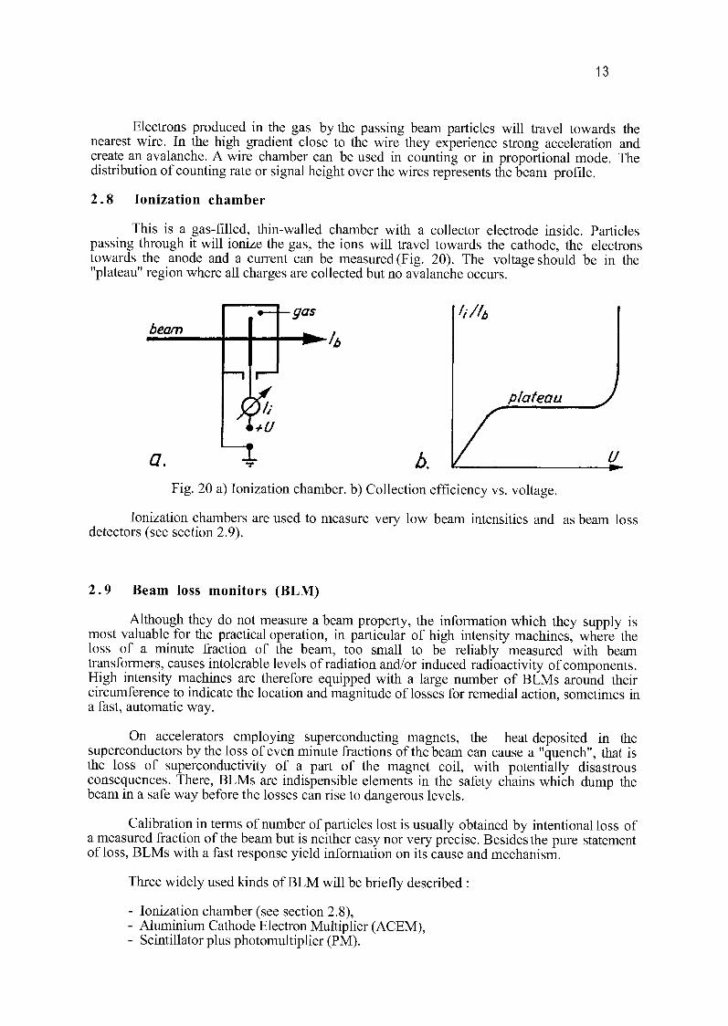
13
Electrons produced in the gas by the passing beam particles will travel towards the nearest wire. In the high gradient close to the wire they experience strong acceleration and create an avalanche. A wire chamber can be used in counting or in proportional mode. The distribution of counting rate or signal height over the wires represents the beam profile.
2.8 Ionization chamber
This is a gas-filled, thin-walled chamber with a collector electrode inside. Particles passing through it will ionize the gas, the ions will travel towards the cathode, the electrons towards the anode and a current can be measured (Fig. 20). The voltage should be in the "plateau" region where all charges are collected but no avalanche occurs.
beam •gas
•k
+U
a. b.
h/lt
plateau
U
Fig. 20 a) Ionization chamber, b) Collection efficiency vs. voltage.
Ionization chambers are used to measure very low beam intensities and as beam loss detectors (see section 2.9).
2.9 Beam loss monitors (BLM)
Although they do not measure a beam property, the information which they supply is most valuable for the practical operation, in particular of high intensity machines, where the loss of a minute fraction of the beam, too small to be reliably measured with beam transformers, causes intolerable levels of radiation and/or induced radioactivity of components. High intensity machines are therefore equipped with a large number of BLMs around their circumference to indicate the location and magnitude of losses for remedial action, sometimes in a fast, automatic way.
On accelerators employing superconducting magnets, the heat deposited in the superconductors by the loss of even minute fractions of the beam can cause a "quench", that is the loss of superconductivity of a part of the magnet coil, with potentially disastrous consequences. There, BLMs are indispensible elements in the safety chains which dump the beam in a safe way before the losses can rise to dangerous levels.
Calibration in terms of number of particles lost is usually obtained by intentional loss of a measured fraction of the beam but is neither easy nor very precise. Besides the pure statement of loss, BLMs with a fast response yield information on its cause and mechanism.
Three widely used kinds of BLM will be briefly described :
- Ionization chamber (see section 2.8), - Aluminium Cathode Electron Multiplier (ACEM), - Scintillator plus photomultiplier (PM).
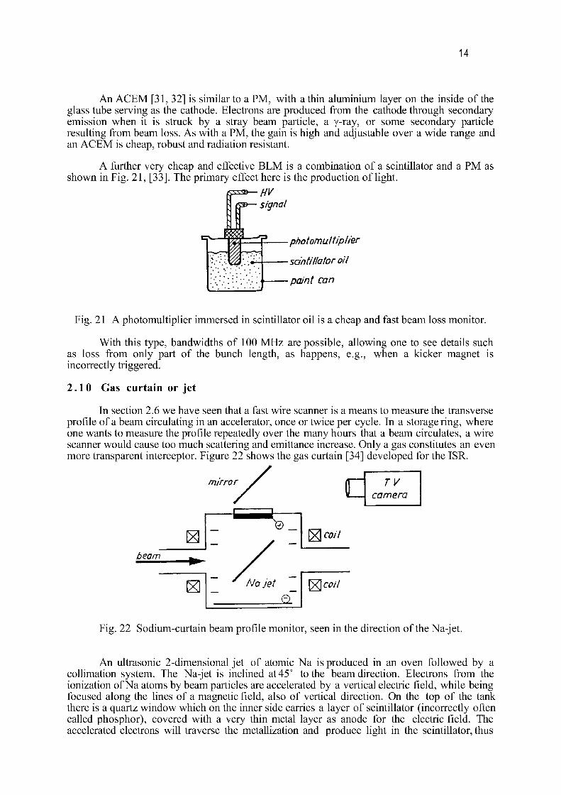
14
An ACEM [31, 32] is similar to a PM, with a thin aluminium layer on the inside of the glass tube serving as the cathode. Electrons are produced from the cathode through secondary emission when it is struck by a stray beam particle, a y-ray, or some secondary particle resulting from beam loss. As with a PM, the gain is high and adjustable over a wide range and an ACEM is cheap, robust and radiation resistant.
A further very cheap and effective BLM is a combination of a scintillator and a PM as shown in Fig. 21, [33]. The primary effect here is the production of light.
photomultiplier
scintillator oil
paint can
Fig. 21 A photomultiplier immersed in scintillator oil is a cheap and fast beam loss monitor.
With this type, bandwidths of 100 MHz are possible, allowing one to see details such as loss from only part of the bunch length, as happens, e.g., when a kicker magnet is incorrectly triggered.
2.10 Gas curtain or jet
In section 2.6 we have seen that a fast wire scanner is a means to measure the transverse profile of a beam circulating in an accelerator, once or twice per cycle. In a storage ring, where one wants to measure the profile repeatedly over the many hours that a beam circulates, a wire scanner would cause too much scattering and emittance increase. Only a gas constitutes an even more transparent interceptor. Figure 22 shows the gas curtain [34] developed for the ISR.
Fig. 22 Sodium-curtain beam profile monitor, seen in the direction of the Na-jet.
An ultrasonic 2-dimensional jet of atomic Na is produced in an oven followed by a collimation system. The Na-jet is inclined at 45° to the beam direction. Electrons from the ionization of Na atoms by beam particles are accelerated by a vertical electric field, while being focused along the lines of a magnetic field, also of vertical direction. On the top of the tank there is a quartz window which on the inner side carries a layer of scintillator (incorrectly often called phosphor), covered with a very thin metal layer as anode for the electric field. The accelerated electrons will traverse the metallization and produce light in the scintillator, thus
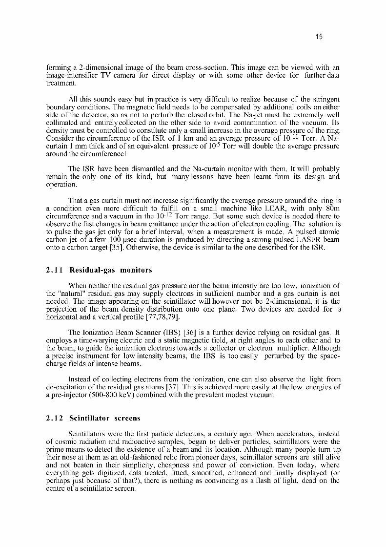
15
forming a 2-dimensional image of the beam cross-section. This image can be viewed with an image-intensifier TV camera for direct display or with some other device for further data treatment.
All this sounds easy but in practice is very difficult to realize because of the stringent boundary conditions. The magnetic field needs to be compensated by additional coils on either side of the detector, so as not to perturb the closed orbit. The Na-jet must be extremely well collimated and entirely collected on the other side to avoid contamination of the vacuum. Its density must be controlled to constitute only a small increase in the average pressure of the ring. Consider the circumference of the ISR of 1 km and an average pressure of 10"11 Torr. A Na-curtain 1 mm thick and of an equivalent pressure of 10"5 Torr will double the average pressure around the circumference!
The ISR have been dismantled and the Na-curtain monitor with them. It will probably remain the only one of its kind, but many lessons have been learnt from its design and operation.
That a gas curtain must not increase significantly the average pressure around the ring is a condition even more difficult to fulfill on a small machine like LEAR, with only 80m circumference and a vacuum in the 10~12 Torr range. But some such device is needed there to observe the fast changes in beam emittance under the action of electron cooling. The solution is to pulse the gas jet only for a brief interval, when a measurement is made. A pulsed atomic carbon jet of a few 100 |usec duration is produced by directing a strong pulsed LASER beam onto a carbon target [35]. Otherwise, the device is similar to the one described for the ISR.
2.11 Residual-gas monitors
When neither the residual gas pressure nor the beam intensity are too low, ionization of the "natural" residual gas may supply electrons in sufficient number and a gas curtain is not needed. The image appearing on the scintillator will however not be 2-dimensional, it is the projection of the beam density distribution onto one plane. Two devices are needed for a horizontal and a vertical profile [77,78,79].
The Ionization Beam Scanner (IBS) [36] is a further device relying on residual gas. It employs a time-varying electric and a static magnetic field, at right angles to each other and to the beam, to guide the ionization electrons towards a collector or electron multiplier. Although a precise instrument for low intensity beams, the IBS is too easily perturbed by the space-charge fields of intense beams.
Instead of collecting electrons from the ionization, one can also observe the light from de-excitation of the residual gas atoms [37]. This is achieved more easily at the low energies of a pre-injector (500-800 keV) combined with the prevalent modest vacuum.
2.12 Scintillator screens
Scintillators were the first particle detectors, a century ago. When accelerators, instead of cosmic radiation and radioactive samples, began to deliver particles, scintillators were the prime means to detect the existence of a beam and its location. Although many people turn up their nose at them as an old-fashioned relic from pioneer days, scintillator screens are still alive and not beaten in their simplicity, cheapness and power of conviction. Even today, where everything gets digitized, data treated, fitted, smoothed, enhanced and finally displayed (or perhaps just because of that?), there is nothing as convincing as a flash of light, dead on the centre of a scintillator screen.
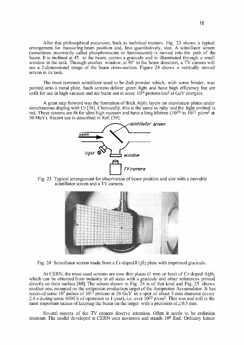
16
After that philosophical excursion, back to technical matters. Fig. 23 shows a typical arrangement for measuring beam position and, less quantitatively, size. A scintillator screen (sometimes incorrectly called phosphorescent or luminescent) is moved into the path of the beam. It is inclined at 45 to the beam, carries a graticule and is illuminated through a small window in the tank. Through another window, at 90° to the beam direction, a TV camera will see a 2-dimensional image of the beam cross-section. Figure 24 shows a vertically moved screen in its tank.
The most common scintillator used to be ZnS powder which, with some binder, was painted onto a metal plate. Such screens deliver green light and have high efficiency but are unfit for use in high vacuum and are burnt out at some 10 1 4 protons/cm2 at GeV energies.
A great step forward was the formation of thick AI2O3 layers on aluminium plates under simultaneous doping with Cr [38]. Chemically, this is the same as ruby and the light emitted is red. These screens are fit for ultra high vacuum and have a long lifetime (10 2 0 to 10 2 1 p/cm2 at 50 MeV). Recent use is described in Ref. [391.
'Scintillator screen
window
TVcamera
Fig. 23 Typical arrangement for observation of beam position and size with a movable scintillator screen and a TV camera.
Fig. 24 Scintillator screen made from a Cr-dopedA I2O3 plate with imprinted graticule.
At CERN, the most-used screens are now thin plates (1 mm or less) of Cr-doped Ab.03 which can be obtained from industry in all sizes with a graticule and other references printed directly on their surface [80]. The screen shown in Fig. 24 is of that kind and Fig. 25 shows another one, mounted on the antiproton production target of the Antiproton Accumulator. It has received some 107 pulses of lO1^ protons at 26 GeV in a spot of about 3 mm diameter (every 2.4 s during some 6000 h of operation in 1 year), i.e. over 10 2 0 p/cm2. This was and still is the most important means of keeping the beam on the target with a precision ofZ0.5 mm.
Several aspects of the TV camera deserve attention. Often it needs to be radiation resistant. The model developed at CERN uses nuvistors and stands 108 Rad. Ordinary lenses
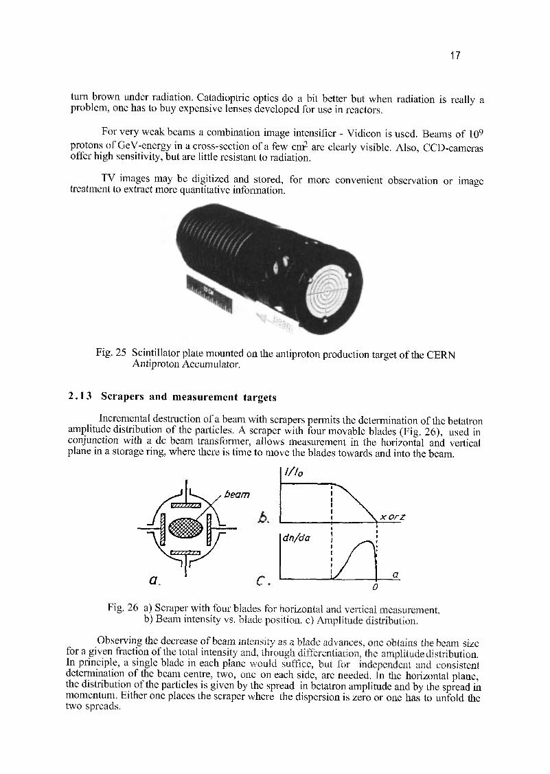
17
turn brown under radiation. Catadioptric optics do a bit better but when radiation is really a problem, one has to buy expensive lenses developed for use in reactors.
For very weak beams a combination image intensifier - Vidicon is used. Beams of 109
protons of GeV-energy in a cross-section of a few cm2 are clearly visible. Also, CCD-cameras offer high sensitivity, but are little resistant to radiation.
TV images may be digitized and stored, for more convenient observation or image treatment to extract more quantitative information.
Fig. 25 Scintillator plate mounted on the antiproton production target of the CERN Antiproton Accumulator.
2.13 Scrapers and measurement targets
Incremental destruction of a beam with scrapers permits the determination of the betatron amplitude distribution of the particles. A scraper with four movable blades (Fig. 26), used in conjunction with a dc beam transformer, allows measurement in the horizontal and vertical plane in a storage ring, where there is time to move the blades towards and into the beam.
beam
xorz
C
Fig. 26 a) Scraper with four blades for horizontal and vertical measurement, b) Beam intensity vs. blade position, c) Amplitude distribution.
Observing the decrease of beam intensity as a blade advances, one obtains the beam size for a given fraction of the total intensity and, through differentiation, the amplitude distribution. In principle, a single blade in each plane would suffice, but for independent and consistent determination of the beam centre, two, one on each side, are needed. In the horizontal plane, the distribution of the particles is given by the spread in betatron amplitude and by the spread in momentum. Either one places the scraper where the dispersion is zero or one has to unfold the two spreads.
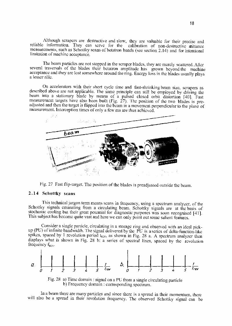
18
Although scrapers are destructive and slow, they are valuable for their precise and reliable information. They can serve for the calibration of non-destructive mittance measurements, such as Schottky scans of betatron bands (see section 2.14) and for intentional limitation of machine acceptance.
The beam particles are not stopped in the scraper blades, they are merely scattered. After several traversais of the blades their betatron amplitude has grown beyond the machine acceptance and they are lost somewhere around the ring. Energy loss in the blades usually plays a lesser rôle.
On accelerators with their short cycle time and fast-shrinking beam size, scrapers as described above are not applicable. The same principle can still be employed by driving the beam into a stationary blade by means of a pulsed closed orbit distortion [40]. Fast measurement targets have also been built (Fig. 27). The position of the two blades is pre-adjusted and then the target is flipped into the beam in a movement perpendicular to the plane of measurement. Interception times of only a few ms are thus achieved.
Fig. 27 Fast flip-target. The position of the blades is preadjusted outside the beam.
2.14 Schottky scans
This technical jargon term means scans in frequency, using a spectrum analyzer, of the Schottky signals emanating from a circulating beam. Schottky signals are at the basis of stochastic cooling but their great potential for diagnostic purposes was soon recognised [41]. This subject has become quite vast and here we can only point out some salient features.
Consider a single particle, circulating in a storage ring and observed with an ideal pickup (PU) of infinite bandwidth. The signal delivered by the PU is a series of delta-function-like spikes, spaced by 1 revolution period t r e v , as shown in Fig. 28 a. A spectrum analyzer then displays what is shown in Fig. 28 b: a series of spectral lines, spaced by the revolution frequency frev.
1 I t b.
| f
0 1 t 7 i ? 4 i - trev c i J 2 z » 4 i ; frev
Fig. 28 a) Time domain : signal on a PU from a single circulating particle b) Frequency domain : corresponding spectrum.
In a beam there are many particles and since there is a spread in their momentum, there will also be a spread in their revolution frequency. The observed Schottky signal can be
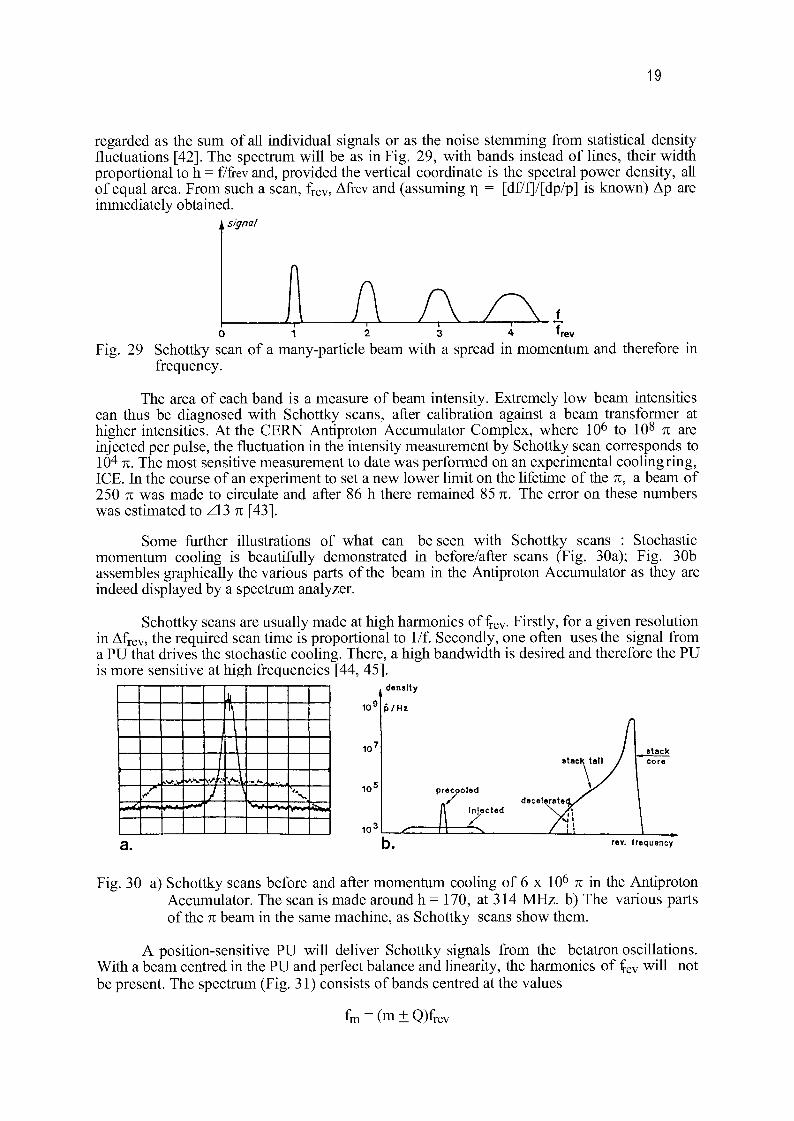
19
regarded as the sum of all individual signals or as the noise stemming from statistical density fluctuations [42]. The spectrum will be as in Fig. 29, with bands instead of lines, their width proportional to h = f/frev and, provided the vertical coordinate is the spectral power density, all of equal area. From such a scan, frev, Afrev and (assuming r) = [df/fj/[dp/p] is known) Ap are immediately obtained.
i signal
Fig. 29 Schottky scan of a many-particle beam with a spread in momentum and therefore in frequency.
The area of each band is a measure of beam intensity. Extremely low beam intensities can thus be diagnosed with Schottky scans, after calibration against a beam transformer at higher intensities. At the CERN Antiproton Accumulator Complex, where 106 to 108 n are injected per pulse, the fluctuation in the intensity measurement by Schottky scan corresponds to 104 7i. The most sensitive measurement to date was performed on an experimental cooling ring, ICE. In the course of an experiment to set a new lower limit on the lifetime of the n, a beam of 250 7i was made to circulate and after 86 h there remained 85 n. The error on these numbers was estimated to Z13 n [43].
Some further illustrations of what can be seen with Schottky scans : Stochastic momentum cooling is beautifully demonstrated in before/after scans (Fig. 30a); Fig. 30b assembles graphically the various parts of the beam in the Antiproton Accumulator as they are indeed displayed by a spectrum analyzer.
Schottky scans are usually made at high harmonics of frev. Firstly, for a given resolution in Afrev, the required scan time is proportional to 1/f. Secondly, one often uses the signal from a PU that drives the stochastic cooling. There, a high bandwidth is desired and therefore the PU is more sensitive at high frequencies [44, 45].
density k \
•.V.V *>->v- S-4- V--1 *
' - * - < £ 7 «-*"
10 =
10'
10-
p/Hz
precooled recp' MS decelerate'
acted A Injec
rev. frequency
Fig. 30 a) Schottky scans before and after momentum cooling of 6 x 10⁶ n in the Antiproton Accumulator. The scan is made around h = 170, at 314 MHz. b) The various parts of the n beam in the same machine, as Schottky scans show them.
A position-sensitive PU will deliver Schottky signals from the betatron oscillations. With a beam centred in the PU and perfect balance and linearity, the harmonics of f e v will not be present. The spectrum (Fig. 31) consists of bands centred at the values
(m±Q)f„
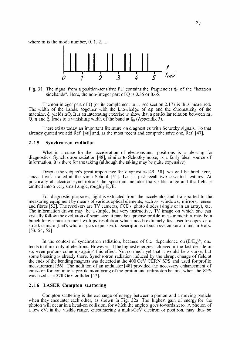
20
where m is the mode number, 0, 1,2, ....
f — — j — — ! — |— — | — — J 7
0 1 2 3 4 5 f r e y
Fig. 31 The signal from a position-sensitive PU contains the frequencies fm of the "betatron sidebands". Here, the non-integer part of Q is 0.35 or 0.65.
The non-integer part of Q (or its complement to 1, see section 2.17) is thus measured. The width of the bands, together with the knowledge of Ap and the chromaticity of the machine, ^, yields AQ. It is an interesting exercise to show that a particular relation between m, Q, r\ and ^, leads to a vanishing width of the band at fm (Appendix 3).
There exists today an important literature on diagnostics with Schottky signals. To that already quoted we add Ref. [46] and, as the most recent and comprehensive one, Ref. [47].
2.15 Synchrotron radiation
What is a curse for the acceleration of electrons and positrons is a blessing for diagnostics. Synchrotron radiation [48], similar to Schottky noise, is a fairly ideal source of information, it is there for the taking (although the taking may be quite expensive).
Despite the subject's great importance for diagnostics [49, 50], we will be brief here, since it was treated at the same School [51]. Let us just recall two essential features: At practically all electron synchrotrons the spectrum includes the visible range and the light is emitted into a very small angle, roughly EQ/E.
For diagnostic purposes, light is extracted from the accelerator and transported to the measuring equipment by means of various optical elements, such as windows, mirrors, lenses and fibres [52]. The receivers are TV cameras, CCDs, photo diodes (single or in an array), etc. The information drawn may be a simple, but very instructive, TV image on which one can visually follow the evolution of beam size; it may be a precise profile measurement; it may be a bunch length measurement with ps resolution which needs extremely fast oscilloscopes or a streak camera (that's where it gets expensive). Descriptions of such systems are found in Refs. [53, 54, 55]
In the context of synchrotron radiation, because of the dependence on (E/E 0) 4, one tends to think only of electrons. However, at the highest energies achieved in the last decade or so, even protons come up against this effect. Not so much yet that it would be a curse, but some blessing is already there. Synchrotron radiation induced by the abrupt change of field at the ends of the bending magnets was detected at the 400 GeV CERN SPS and used for profile measurement [56]. The addition of an undulator [48] provided the necessary enhancement of emission for continuous profile monitoring of the proton and antiproton beams, when the SPS was used as a 270 GeV collider [57].
2.16 LASER Compton scattering
Compton scattering is the exchange of energy between a photon and a moving particle when they encounter each other, as shown in Fig. 32a. The highest gain of energy for the photon will occur in a head-on collision, for which the angle a goes towards zero. A photon of a few eV, in the visible range, encountering a multi-GeV electron or positron, may thus be
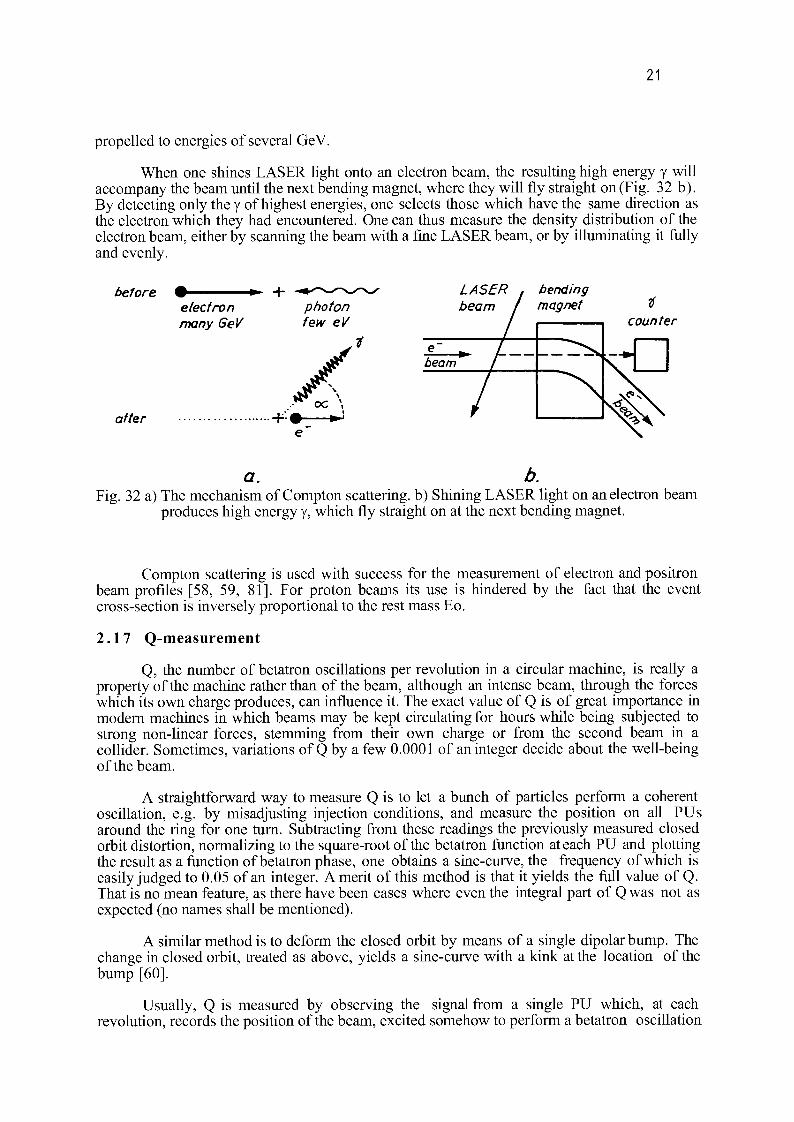
21
propelled to energies of several GeV.
When one shines LASER light onto an electron beam, the resulting high energy y will accompany the beam until the next bending magnet, where they will fly straight on (Fig. 32 b). By detecting only they of highest energies, one selects those which have the same direction as the electron which they had encountered. One can thus measure the density distribution of the electron beam, either by scanning the beam with a fine LASER beam, or by illuminating it fully and evenly.
before • • + electron photon many GeV few eV
LASER beam
bending magnet
after
I e~ m
beam " 1 1 counter
a. b. Fig. 32 a) The mechanism of Compton scattering, b) Shining LASER light on an electron beam
produces high energy y, which fly straight on at the next bending magnet.
Compton scattering is used with success for the measurement of electron and positron beam profiles [58, 59, 81]. For proton beams its use is hindered by the fact that the event cross-section is inversely proportional to the rest mass Eo.
2.17 Q-measurement
Q, the number of betatron oscillations per revolution in a circular machine, is really a property of the machine rather than of the beam, although an intense beam, through the forces which its own charge produces, can influence it. The exact value of Q is of great importance in modern machines in which beams may be kept circulating for hours while being subjected to strong non-linear forces, stemming from their own charge or from the second beam in a collider. Sometimes, variations of Q by a few 0.0001 of an integer decide about the well-being of the beam.
A straightforward way to measure Q is to let a bunch of particles perform a coherent oscillation, e.g. by misadjusting injection conditions, and measure the position on all PUs around the ring for one turn. Subtracting from these readings the previously measured closed orbit distortion, normalizing to the square-root of the betatron function at each PU and plotting the result as a function of betatron phase, one obtains a sine-curve, the frequency of which is easily judged to 0.05 of an integer. A merit of this method is that it yields the full value of Q. That is no mean feature, as there have been cases where even the integral part of Q was not as expected (no names shall be mentioned).
A similar method is to deform the closed orbit by means of a single dipolar bump. The change in closed orbit, treated as above, yields a sine-curve with a kink at the location of the bump [60].
Usually, Q is measured by observing the signal from a single PU which, at each revolution, records the position of the beam, excited somehow to perform a betatron oscillation
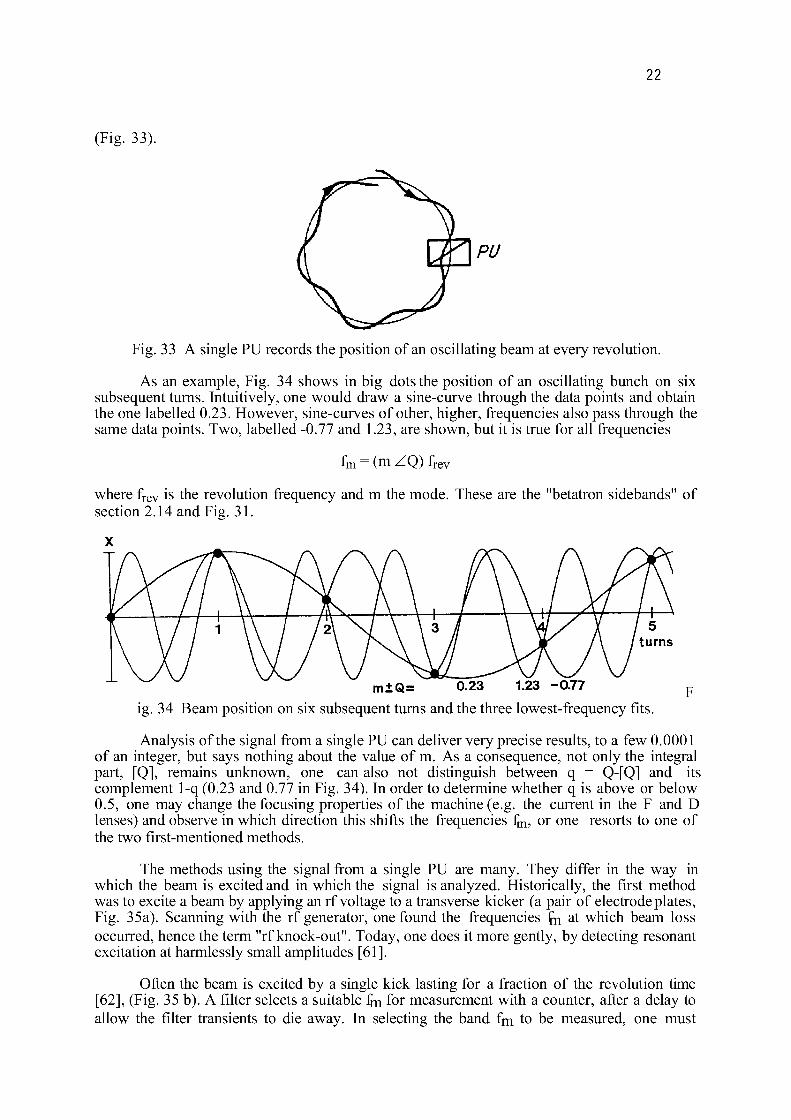
22
(Fig. 33).
Fig. 33 A single PU records the position of an oscillating beam at every revolution.
As an example, Fig. 34 shows in big dots the position of an oscillating bunch on six subsequent turns. Intuitively, one would draw a sine-curve through the data points and obtain the one labelled 0.23. However, sine-curves of other, higher, frequencies also pass through the same data points. Two, labelled -0.77 and 1.23, are shown, but it is true for all frequencies
fm = (m ZQ) frev
where frev is the revolution frequency and m the mode. These are the "betatron sidebands" of section 2.14 and Fig. 31.
ig. 34 Beam position on six subsequent turns and the three lowest-frequency fits.
Analysis of the signal from a single PU can deliver very precise results, to a few 0.0001 of an integer, but says nothing about the value of m. As a consequence, not only the integral part, [Q], remains unknown, one can also not distinguish between q = Q-[Q] and its complement 1-q (0.23 and 0.77 in Fig. 34). In order to determine whether q is above or below 0.5, one may change the focusing properties of the machine (e.g. the current in the F and D lenses) and observe in which direction this shifts the frequencies fm, or one resorts to one of the two first-mentioned methods.
The methods using the signal from a single PU are many. They differ in the way in which the beam is excited and in which the signal is analyzed. Historically, the first method was to excite a beam by applying an rf voltage to a transverse kicker (a pair of electrode plates, Fig. 35a). Scanning with the rf generator, one found the frequencies £n at which beam loss occurred, hence the term "rf knock-out". Today, one does it more gently, by detecting resonant excitation at harmlessly small amplitudes [61].
Often the beam is excited by a single kick lasting for a fraction of the revolution time [62], (Fig. 35 b). A filter selects a suitable fm for measurement with a counter, after a delay to allow the filter transients to die away. In selecting the band fm to be measured, one must
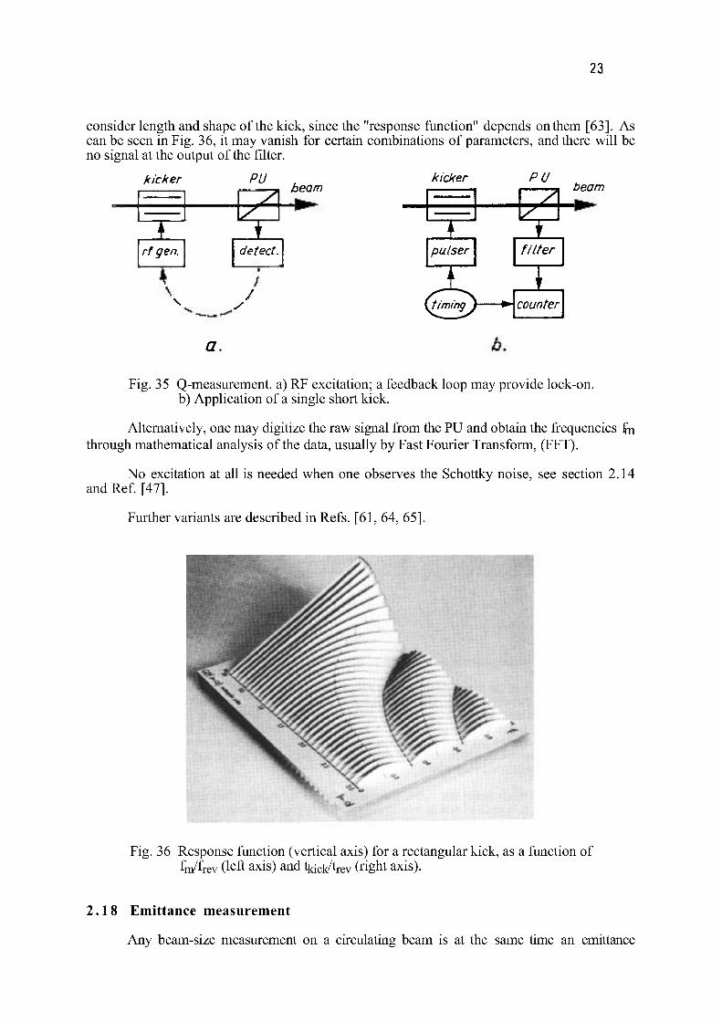
23
consider length and shape of the kick, since the "response function" depends on them [63]. As can be seen in Fig. 36, it may vanish for certain combinations of parameters, and there will be no signal at the output of the filter.
kicker PU
Ï ~A
LZ:
rfgen. T
beam
detect.
\ y /
kicker PU beam
a. Fig. 35 Q-measurement. a) RF excitation; a feedback loop may provide lock-on.
b) Application of a single short kick.
Alternatively, one may digitize the raw signal from the PU and obtain the frequencies fn through mathematical analysis of the data, usually by Fast Fourier Transform, (FFT).
No excitation at all is needed when one observes the Schottky noise, see section 2.14 and Ref. [47].
Further variants are described in Refs. [61, 64, 65].
Fig. 36 Response function (vertical axis) for a rectangular kick, as a function of Wfrev (left axis) and tki ck/t r e v (right axis).
2.18 Emittance measurement
Any beam-size measurement on a circulating beam is at the same time an emittance
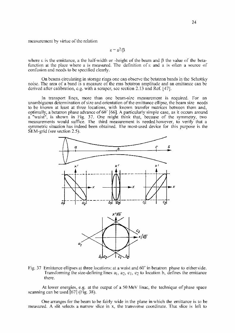
24
measurement by virtue of the relation
i2/p
where s is the emittance, a the half-width or -height of the beam and P the value of the beta-function at the place where a is measured. The definition of s and a is often a source of confusion and needs to be specified clearly.
On beams circulating in storage rings one can observe the betatron bands in the Schottky noise. The area of a band is a measure of the rms betatron amplitude and an emittance can be derived after calibration, e.g. with a scraper, see section 2.13 and Ref. [47].
In transport lines, more than one beam-size measurement is required. For an unambiguous determination of size and orientation of the emittance ellipse, the beam size needs to be known at least at three locations, with known transfer matrices between them and, optimally, a betatron phase advance of 60° [66]. A particularly simple case, as it occurs around a "waist", is shown in Fig. 37. One might think that, because of the symmetry, two measurements would suffice. The third measurement is needed however, to verify that a symmetric situation has indeed been obtained. The most-used device for this purpose is the SEM-grid (see section 2.5).
Fig. 37 Emittance ellipses at three locations: at a waist and 60° in betatron phase to eitherside. Transforming the size-defining lines a\, &2, c\, C2 to location b, defines the emittance there.
At lower energies, e.g. at the output of a 50 MeV linac, the technique of phase space scanning can be used [67] (Fig. 38).
One arranges for the beam to be fairly wide in the plane in which the emittance is to be measured. A slit selects a narrow slice in x, the transverse coordinate. That slice is left to
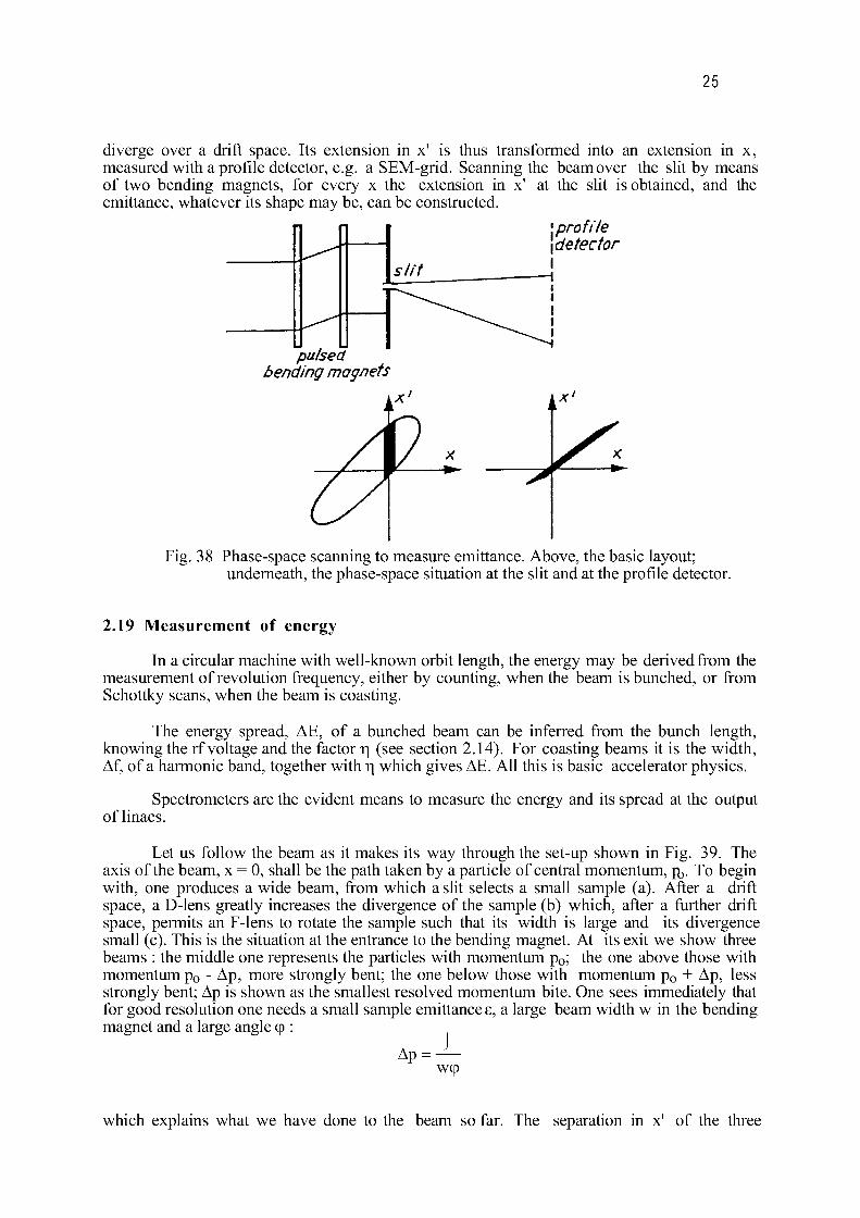
25
diverge over a drift space. Its extension in x' is thus transformed into an extension in x, measured with a profile detector, e.g. a SEM-grid. Scanning the beam over the slit by means of two bending magnets, for every x the extension in x' at the slit is obtained, and the emittance, whatever its shape may be, can be constructed.
[profite detector
pulsed bending magnets
Fig. 38 Phase-space scanning to measure emittance. Above, the basic layout; underneath, the phase-space situation at the slit and at the profile detector.
2.19 Measurement of energy
In a circular machine with well-known orbit length, the energy may be derived from the measurement of revolution frequency, either by counting, when the beam is bunched, or from Schottky scans, when the beam is coasting.
The energy spread, ÀE, of a bunched beam can be inferred from the bunch length, knowing the rf voltage and the factor r\ (see section 2.14). For coasting beams it is the width, Af, of a harmonic band, together withr) which gives AE. All this is basic accelerator physics.
Spectrometers are the evident means to measure the energy and its spread at the output of linacs.
Let us follow the beam as it makes its way through the set-up shown in Fig. 39. The axis of the beam, x = 0, shall be the path taken by a particle of central momentum, pj. To begin with, one produces a wide beam, from which a slit selects a small sample (a). After a drift space, a D-lens greatly increases the divergence of the sample (b) which, after a further drift space, permits an F-lens to rotate the sample such that its width is large and its divergence small (c). This is the situation at the entrance to the bending magnet. At its exit we show three beams : the middle one represents the particles with momentum p 0 ; the one above those with momentum p 0 - Ap, more strongly bent; the one below those with momentum p 0 + Ap, less strongly bent; Ap is shown as the smallest resolved momentum bite. One sees immediately that for good resolution one needs a small sample emittance s, a large beam width w in the bending magnet and a large angle cp :
Ap = ^ wcp
which explains what we have done to the beam so far. The separation in x' of the three
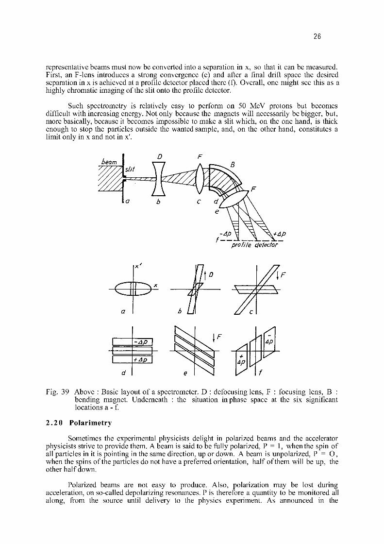
26
representative beams must now be converted into a separation in x, so that it can be measured. First, an F-lens introduces a strong convergence (e) and after a final drift space the desired separation in x is achieved at a profile detector placed there (f). Overall, one might see this as a highly chromatic imaging of the slit onto the profile detector.
Such spectrometry is relatively easy to perform on 50 MeV protons but becomes difficult with increasing energy. Not only because the magnets will necessarily be bigger, but, more basically, because it becomes impossible to make a slit which, on the one hand, is thick enough to stop the particles outside the wanted sample, and, on the other hand, constitutes a limit only in x and not in x'.
profile detector
<3B^
-_AR_
+Ap I
Fig. 39 Above : Basic layout of a spectrometer. D : defocusing lens, F : focusing lens, B : bending magnet. Underneath : the situation in phase space at the six significant locations a - f.
2.20 Polarimetry
Sometimes the experimental physicists delight in polarized beams and the accelerator physicists strive to provide them. A beam is said to be fully polarized, P = 1, when the spin of all particles in it is pointing in the same direction, up or down. A beam is unpolarized, P = O, when the spins of the particles do not have a preferred orientation, half of them will be up, the other half down.
Polarized beams are not easy to produce. Also, polarization may be lost during acceleration, on so-called depolarizing resonances. P is therefore a quantity to be monitored all along, from the source until delivery to the physics experiment. As announced in the
27
introduction, this is too specialized a subject for an introductory course. We will just mention three kinds of methods and refer to the literature.
Firstly, P can be measured in the physics experiment itself, through the asymmetry in the scattering of the beam particles or in the products of their collisions with target nucléons [68, 69]. This accurate determination can serve as a calibration for other methods.
Secondly, a thin fibre can be brought into the beam, even into the fringe of a circulating beam, and the asymmetry in the scattered particles observed (Mott scattering) [69, 70].
Thirdly, the cross section for Compton scattering depends on the polarization of both the particles and the photons. By shining polarized LASER light onto a circulating beam, P can be determined [58, 71, 72, 73].
3 . CONCLUDING REMARKS
I would like to conclude with some advice, first on the technical-operational level.
It is important that calibration, automatic or on demand, can be performed remotely and without interruption to the operation of the accelerator. This applies particularly to beam transformers and position pick-ups.
Status signals must indicate the good order of a device and permit remote fault diagnosis.
Diagnostic systems usually rely for data processing and display of results on a small local computer or are linked to a larger central controls computer. I consider it important that the software, which contains the understanding of the measurement and determines the way in which the desired information is extracted, be conceived, if not written, by the person who has conceived the diagnostic device.
Lastly, and this is true for all components of a machine: good documentation is indispensable for efficient use of the systems and for their maintenance.
In a more general vein, it is no idle advice that before designing the diagnostic equipment for a machine, one should first acquaint oneself with the machine and its possible modes of operation and with the properties and behaviour the beam may show under various conditions. One will take into account not only the "nominal" beam, but also what it might be like in an early stage, the running-in, of the machine and under abnormal conditions, when one is particularly dependent on diagnostics.
One will think of tricky measurements the machine experimenters will want to carry out in order to further performance and basic knowledge, but equally consider the need for precise, unfailing and easily perceived information during routine operation.
Often diagnostic equipment is added on at an advanced state in the design of an accelerator. That is wrong. Diagnostic systems must be included in the design at an early stage, otherwise only too often one finds that no space is left at the best suited locations, or even none at all.
Another important aim, when building a new accelerator, is to have a complete set of diagnostic systems tested and ready for use on the day of first beam. Not only is adequate equipment with diagnostics essential for an efficient running-in of the accelerator, it is also an economic investment in terms of time, pain and simply cost of electricity that it helps to save.

28
4 . ACKNOWLEDGEMENTS
My thanks go to those students of this course, in Salamanca in 1988 and in Jyvâskylâ in 1992, who have helped me by pointing out the weak spots, and to Mrs. L. Ghilardi for her patient and careful preparation of this paper.
29
5 . LITERATURE
Part I : Previous CAS lectures on beam diagnostics.
ANTIPROTONS FOR COLLIDING BEAM FACILITIES
CERN, Geneva, 11-21 October 1983, Yellow Report CERN 84-15
J. Borer and R. Jung, Diagnostics, p.385, vast list of references.
GENERAL ACCELERATOR PHYSICS Gif-sur-Yvette, Paris, 3-14 September 1984, Yellow Report CERN 85-19 K. Potter, Beam Profiles, p.301 K. Potter, Luminosity Measurements, p.318 P. Wolstenholme, Control Systems of Accelerators, par.6: Beam Instrumentation, p.519
ADVANCED ACCELERATOR PHYSICS
The Queen's College, Oxford, 16-27 September 1985, Yellow Report CERN 87-03
D. Boussard, Schottky Noise and Beam Transfer Function Diagnostics, p.416
SECOND GENERAL ACCELERATOR PHYSICS COURSE Scanticon Conference Centre, Aarhus, 15-26 September 1986, Yellow Report CERN 87-10 P. Strehl, Beam Diagnostics, p.99 K. Potter, Luminosity Monitoring at LEP, p. 153
SECOND ADVANCED ACCELERATOR PHYSICS COURSE Berlin, 14-25 September 1987, Yellow Report CERN 89-01
D. Boussard, Schottky Noise and Beam Transfer Function Diagnostics
JOINT US-CERN SCHOOL ON PARTICLE ACCELERATORS: FRONTIERS OF PARTICLE BEAMS, OBSERVATION, DIAGNOSIS AND CORRECTION Capri, 20-26 October 1988, Lecture Notes in Physics, No. 343, Springer, Heidelberg, 1989.
FOURTH GENERAL ACCELERATOR PHYSICS COURSE KFA, Julich, 17-28 September 1990, Yellow Report CERN 91-04
M. Serio, Tune Measurements, p. 136
Part II : References
[1] S. Battisti, CERN/MPS/CO 69-15, 1969.
[2] F. Loyer, T. André, B. Ducoudret, J.P. Rataud, Part. Ace. Conf, Vancouver, 1985. IEEE Trans. Nucl. Sci., NS-32, No. 5.
[3] K. Unser, Part. Ace. Conf., Washington, 1981. IEEE Trans. Nucl. Sci., NS-28, No.3. Also: CERN-ISR-OP/81-14, 1981.
[4] G. Burtin, R.J. Colchester, C. Fischer, J.Y. Hemery, R. Jung, M. Vanden Eynden, J.M. Voillot, 2nd Europ. Part. Ace. Conf, (EPAC 90), Nice, 1990. Also : CERN/SL/90-30 (BI).
30
[5] R.T. Avery, A. Faltens, E.C. Hartwig, Part. Ace. Conf., Chicago, 1971. IEEE Trans. Nucl. Sci, NS-18, No. 3. Also : UCRL-20166, 1971.
[6] G. Schneider, IEEE Part. Ace. Conf., Washington, 1987. Also: CERN/PS 87-44 (BT), 1987.
[7] G. Schneider, Thesis, Technical University of Hannover, 1971.
[8] M. Rabany, Part. Ace. Conf., San Francisco, 1973. IEEE Trans. Nucl. Sci., NS-20, No.3. Also: CERN/MPS/Int.BR/73-4, 1973.
[9] G. Gelato, H. Koziol, M. Le Gras, D.J. Williams, Part. Ace. Conf., Washington, 1981. IEEE Trans. Nucl. Sci., NS-28, No.3. Also: CERN/PS/AA/BR/81-19, 1981.
[10] J. Durand, J. Gonzalez, E. Schulte, M. Thivent, 1st European Part. Ace. Conf. (EPAC 88), Rome, 1988. Also: CERN/PS 88-42 (PA), 1988.
[11] G. Nassibian, M. Rabany, CERN/SI/Int.EL/71-2, 1971.
[12] J. Cuperus, Nucl. Instr. Meth., 145, 1977.
[13] T. Katsura, S. Shibata, KEK-79-27, 1979.
[14] J. Borer, C. Bovet, D. Cocq, H. Kropf, A. Manarin, C. Paillard, M. Rabany, G. Vismara, IEEE Part. Accel. Conf., Washington, 1987. Also: CERN/LEP-BI/87-06, 1987.
[15] A. Aragona, C. Biscari, S. De Simone, E. Gianfelice, S. Guiducci, V. Lollo, S. Prella, M. Preger, M. Serio, IEEE Part. Accel. Conf, Washington, 1987.
[16] S. Battisti, M. Le Gras, J.M. Roux, B. Szeless, D.J. Williams, IEEE Part. Ace. Conf., Washington, 1987. Also: CERN/PS 87-37 (BR), 1987.
[17] J.H. Cuperus, Nucl. Instr. Meth., 145, 1977.
[18] W. Barry, CEBAF-PR-89-003, 1989.
[19] J.-C. Denard, G.B. Bowden, G.J. Oxby, J.-L. Pellegrins, M.C. Ross, IEEE Part. Ace. Conf. Washington, 1987. Also : SLAC-PUB-4267, 1987.
[20] R. Bossart, 1st European Part. Ace. Conf. (EPAC 88), Rome, 1988.
[21] Z.D. Farkas, H.A. Hogg, H.L. Martin, A.R. Wilmunder, Proton Lin. Ace. Conf., Chalk River, 1976, Proa: AECL-5677. Also: SLAC-PUB-1823, 1976.
[22] G. Nassibian, Si/Note EL/70-13, CERN, 1970.
[23] R.H. Miller, J.E. Clendenin, M.B. James, J.C. Sheppard, Xllth Int. Conf. High-En. Ace, FNAL, 1983. Also: SLAC-PUB-3186, 1983.
[24] V. Chohan, F. Pedersen, S. van der Meer, D.J. Williams, 2nd Europ. Part. Ace. Conf. (EPAC 90), Nice, 1990. Also : CERN PS/AR/90-31.
[25] L. Bernard, C. Dutriat, J. Gabardo, M. Le Gras, U. Tallgren, P.Têtu, D.J. Williams, Part. Ace. Conf., Santa Fe, 1983, IEEE Trans. Nucl. Sci., NS-30, No.4. Also: CERN/PS/LEAR/83-15, 1983.
31
Ch. Steinbach, M. van Rooij,Part. Ace. Conf., Vancouver, 1985. IEEE Trans. Nucl. Sci., NS-32, No.5. Also: CERN/PS 85-33 (OP), 1985.
J. Bosser, J. Camas, L. Evans, G. Ferioli, R. Hopkins, J. Mann, O. Olsen, Nucl. Instr Meth. A235, 1985. Also: CERN SPS/84-11 (DI/MST), 1984.
S. Hancock, M. Martini, M. van Rooij, Ch. Steinbach, Workshop Adv. Beam Instr., KEK, Tsukuba, 1991. Also : CERN/PS/91-12 (OP).
C. Fischer, G. Burtin, R. Colchester, B. Halvarson, R. Jung, J.M. Vouillot, 1st European Part. Ace. Conf. (EPAC 88), Rome, 1988. Also: CERN/LEP-BI/88-12, 1988.
C.W. Fabjan, H.G. Fischer, Reports on Progress in Physics, 43, 1003, The Institute of Physics, 1980.
V. Agoritsas, C. Johnson, CERN-MPS/CO Note 71-51, 1971.
V. Agoritsas, F. Beck, G.P. Benincasa, J.P. Bovigny, Nucl. Instr. Meth., A247, 1986. Also: CERN/PS/85-60 (CO), 1985.
M. Awschalom, H. Howe, R. Shafer, D. Theriot, NAL, TM-274, Batavia, 1970.
B. Vosicki, K. Zankel, Part. Ace. Conf., Washington, 1975. IEEE Trans. Nucl. Sci., NS-22,No.3. Also: CERN-ISR-VA/75-11, 1975.
R. Galiana, D. Manglunki, C. Mazeline, CERN/PS 91-29 (OP), 1991.
CD. Johnson, L. Thorndahl, Part. Ace. Conf., Washington, 1969. IEEE Trans. Nucl. Sci., NS-16, No.3.
F. Hornstra, DESY HERA 89-04, 1989.
R.W. Allison, R.W. Brokloff, R.L. McLaughlin, R.M. Richter, M. Tekawa, J.R. Woodyard, UCRL-19270, Berkeley, 1969.
S. Yencho, D.R. Walz, Part. Ace. Conf., Vancouver, 1985. IEEE Trans. Nucl. Sci., NS-32, No.5.
H. Schônauer, Workshop Adv. Beam Instr., KEK, Tsukuba, 1991. Also : CERN/PS 92-10 (HI)
J. Borer, P. Bramham, H.G. Hereward, K. Hubner, W. Schnell, L. Thorndahl, IXth Int. Conf. High En. Ace, SLAC, Stanford, 1974. Also: CERN/ISR-DI/RF/74-23, 1974.
F. Sacherer, CERN-ISR-TH/78-ll, 1978.
G. Carron, H. Herr, G. Lebée, H. Koziol, F. Krienen, D. Môhl, G. Petrucci, C. Rubbia, F. Sacherer, B. Sadoulet, G. Stefanini, L. Thorndahl, S. van der Meer, T. Wikberg, Part. Ace. Conf., San Francisco, 1979. IEEE Trans. Nucl. Sci., NS-26, No.3.
S. van der Meer, Nobel Lecture in Physics, 1984. Also: CERN/PS/84-32, 1984.
L. Faltin, Nucl. Instr. Meth., 148, 1978.
32
[46] D. Boussard, T. Linnecar, W. Scandale, Part. Ace. Conf., Vancouver, 1985. IEEE Trans. Nucl. Sci., NS-32, No.5. Also: CERN SPS/85-30 (ARF), 1985.
[47] S. van der Meer, Joint US-CERN School on Beam Observation, Diagnosis and Correction, Capri, 1988, Proa: Lecture Notes in Physics No. 343, Springer, Heidelberg, 1989. Also : CERN/PS/88-60 (AR), 1988.
[48] H. Winick, Scientific American, Nov. 1987.
[49] A. Hofmann, Part. Ace. Conf., Washington, 1981. IEEE Trans. Nucl. Sci., NS-28, No.3. Also: CERN-ISR-TH/81-10, 1981.
[50] A. Hofmann, F. Méot, Nucl. Instr. Meth., 203, 1982. Also: CERN/ISR-TH/82-04, 1982.
[51] R. Walker, these proceedings.
[52] M.R. Howells, LBL-20833 Rev., -20834 Rev., -20835 Rev., Berkeley, 1986.
[53] C. Bovet, E. Rossa, Workshop Adv. Beam Instr., KEK, Tsukuba, 1991. Also: CERN SL/91-18 (BI).
[54] C. Bovet, G. Burtin, R.J. Colchester, B. Halvarsson, R. Jung, S. Levitt, J.M. Vouillot, IEEE Part. Ace. Conf, San Francisco, 1991. Also : CERN SL/91-25 (BI).
[55] S. Battisti, J.F. Bottollier, B. Frammery, E. Marcarini, CERN, PS/LPI/Note 87-13, 1987.
[56] R. Bossart, J. Bosser, L. Burnod, R. Coisson, E. dAmico, G. Ferioli, J. Mann, F. Méot, Nucl. Instr. Meth., 184, 1981. Also: CERN SPS/80-8 (ABM), 1980.
[57] J. Bosser, L. Burnod, R. Coisson, E. dAmico, G. Ferioli, J. Mann, F. Méot, Part. Ace. Conf, Santa Fe, 1983. IEEE Trans. Nucl. Sci., NS-30, No.4. Also: CERN SPS/ABM/83-15, 1983.
[58] R. Rossmanith, R. Schmidt, Int. Laser Conf, Munchen, 1981. Also: Internal Report DESY M-81/24, Hamburg, 1981.
[59] K. Wittenburg, DESY-HERA 1986-06, 1986.
[60] M.Q. Barton, R. Frankel, M. Month, Rev. Sci. Instr., Vol.40, No.11, 1969.
[61] I. Farago, K.D. Lohmann, M. Placidi, H. Schmickler, 2nd Europ. Part. Ace. Conf. (EPAC 90), Nice, 1990. Also : CERN/SL/90-40 (BI).
[62] H. Koziol, CERN-MPS/Int. BR/74-14, 1974.
[63] K. Hùbner, CERN-ISR-TH/69-17, 1969.
[64] J.P. Potier, G.C. Schneider, E. Schulte, Part. Ace. Conf, San Francisco, 1973. IEEE Trans. Nucl. Sci., NS-20, No.3. Also: CERN/MPS/SR 73-1, 1973.
[65] R. Bossart, A. Chapmann-Hatchett, I. Gjerpe, H.K. Kuhn, T. Linnecar, G. Paillard, C. Saltmarsh, W. Scandale, R. Schmidt, I. Wilkie, Part. Ace. Conf, Vancouver, 1985. IEEE Trans. Nucl. Sci., NS-32, No.5. Also: CERN SPS/85-22 (DI-MST), 1985.
[66] M. Arruat, M. Martini, CERN/PS 92-59 (PA), 1992.
33
[67] P. Têtu, CERN/PS/LR 79-33, 1979.
[68] T. Khoe, R.L. Kustom, R.L. Martin, E.F. Parker, C.W. Potts, L.G. Ratner, R.E. Timm, Particle Accelerators, Vol.6, 1975.
[69] A.D. Krisch, Journal de Physique, Tome 46, Colloque C2, supplément no.2, 1985.
[70] T. Dorenbos, CD. Johnson, Conference on High Energy Physics with Polarized Beams and Targets, Argonne, 1976. American Institute of Physics, AIP Conf. Proc. No. 35, Particles and Fields, Subseries No. 12, 1976.
[71] R. Schmidt, Workshop Ace. Instr., CEBAF, Newport News, 1991, AIP Conf. Proc, 252, 1992. Also : CERN SL/91-51 (BI).
[72] M. Placidi, R. Rossmanith, Nucl. Instr. Meth., A274, 1989. Also: CERN/LEP-BI/86-25 Rev., 1988.
[73] D.P. Barber et al, DESY 92-136, 1992.
[74] T. Naito, H. Akiyama, J. Urakawa, T. Shintake, M. Yoshioka, 8th Symp. on Ace. Science and Technology, Wako, Saitama, 1991. Also : KEK Preprint 91-134.
[75] D.A. Goldberg, G.R. Lambertson, US Part. Ace. School , 1991. AIP Conf. Proc., 249, 1992. Also : LBL-31664, 1991.
[76] J. Hinkson, Workshop Ace. Instr., CEBAF, Newport News, 1991, AIP Conf. Proc., 252, 1992. Also : LBL-31526, 1991.
[77] F. Hornstra, 1st Europ. Conf. Part. Ace. (EPAC 88), Rome, 1988.
[78] T. Kawakubo, T. Adachi, E. Kadokura, H. Nakagawa, Y. Ajima, T. Ishida, XIV Int. Conf. High En. Ace, Tsukuba, 1989. Also : KEK Preprint 89-71.
[79] J. M. Schippers, H.H. Kiewiet, J. Zijlsta, Nucl. Instr. Meth., A310, 1991.
[80] CD. Johnson, CERN/PS/90-42 (AR), 1990.
[81] T. Shintake, H. Hayano, A. Hayakawa, Y. Ozaki, M. Ohashi, K. Yasuda, D. Waltz, S. Wagner, D. Burke, XV Int. Conf. High En. Ace, Hamburg, 1992. Also : KEK Preprint 92-65.
[82] K. Wittenburg, 3rd Europ. Conf. Part. Ace. (EPAC 92), Berlin 1992. Also : DESY HERA 92-12.
[83] J.D. Jackson, Classical Electrodynamics, 2nd ed. J. Wiley & Sons, 1975.
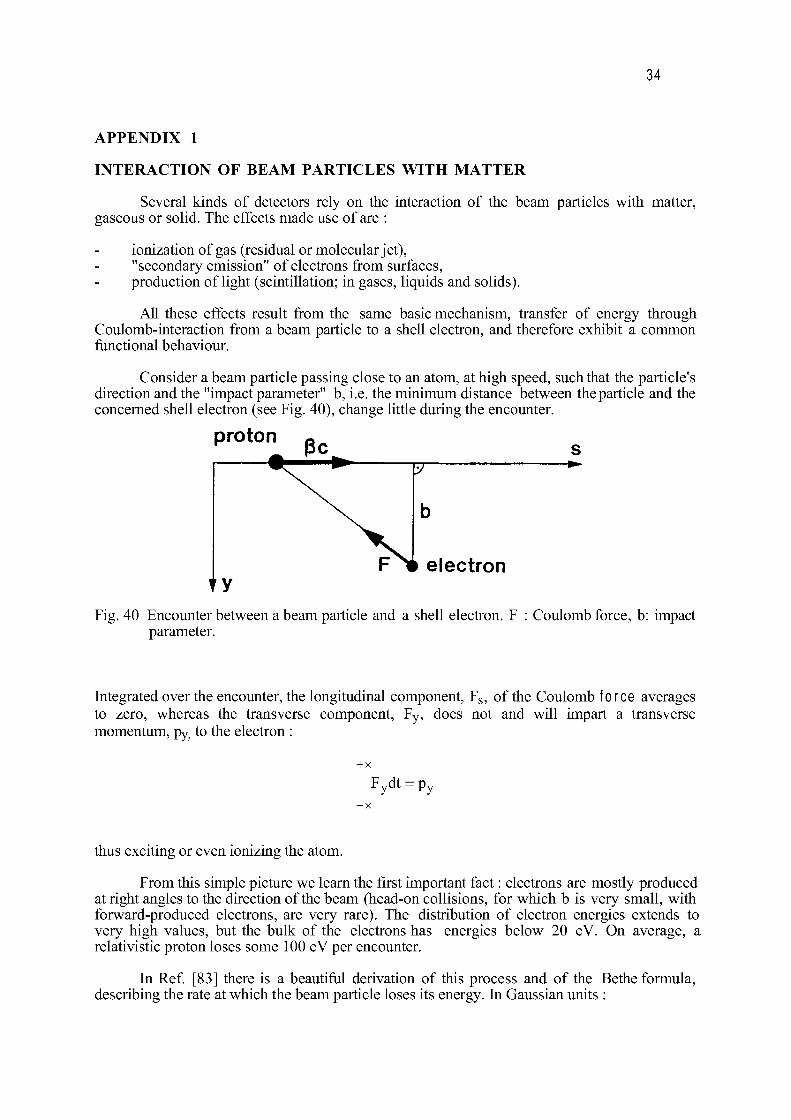
34
APPENDIX 1
INTERACTION OF BEAM PARTICLES WITH MATTER
Several kinds of detectors rely on the interaction of the beam particles with matter, gaseous or solid. The effects made use of are :
ionization of gas (residual or molecular jet), "secondary emission" of electrons from surfaces, production of light (scintillation; in gases, liquids and solids).
All these effects result from the same basic mechanism, transfer of energy through Coulomb-interaction from a beam particle to a shell electron, and therefore exhibit a common functional behaviour.
Consider a beam particle passing close to an atom, at high speed, such that the particle's direction and the "impact parameter" b, i.e. the minimum distance between the particle and the concerned shell electron (see Fig. 40), change little during the encounter.
proton
electron
Fig. 40 Encounter between a beam particle and a shell electron. F : Coulomb force, b: impact parameter.
Integrated over the encounter, the longitudinal component, F s , of the Coulomb force averages to zero, whereas the transverse component, F y , does not and will impart a transverse momentum, py: to the electron :
+ x F vdt - p.
thus exciting or even ionizing the atom.
From this simple picture we learn the first important fact : electrons are mostly produced at right angles to the direction of the beam (head-on collisions, for which b is very small, with forward-produced electrons, are very rare). The distribution of electron energies extends to very high values, but the bulk of the electrons has energies below 20 eV. On average, a relativistic proton loses some 100 eV per encounter.
In Ref. [83] there is a beautiful derivation of this process and of the Bethe formula, describing the rate at which the beam particle loses its energy. In Gaussian units :
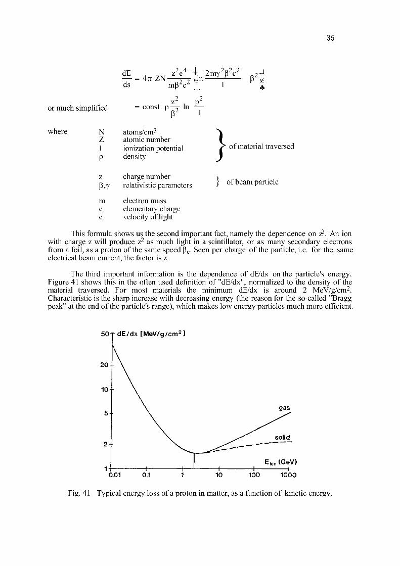
35
or much simplified
where N Z I P
— - 4TI ZN ~ I 9 dn ds mpV
2 2 = const, p—~- In —
p 2 I
atoms/cm3
atomic number ionization potential density
z 2 e 4 \ 2 m y 2 p 2 c 2
Q 2
J
VU
} of material traversed
} of beam particle z charge number P, y relativistic parameters
m electron mass e elementary charge c velocity of light
This formula shows us the second important fact, namely the dependence on z2. An ion with charge z will produce z 2 as much light in a scintillator, or as many secondary electrons from a foil, as a proton of the same speed p c . Seen per charge of the particle, i.e. for the same electrical beam current, the factor is z.
The third important information is the dependence of dE/ds on the particle's energy. Figure 41 shows this in the often used definition of "dE/dx", normalized to the density of the material traversed. For most materials the minimum dE/dx is around 2 MeV/g/cm2. Characteristic is the sharp increase with decreasing energy (the reason for the so-called "Bragg peak" at the end of the particle's range), which makes low energy particles much more efficient.
5 0 T dE/dx [MeV/g /cm 2 ]
20-
10-
0.01 0.1
Ekin (GeV) ^
1000
Fig. 41 Typical energy loss of a proton in matter, as a function of kinetic energy.
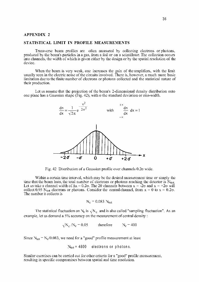
36
APPENDIX 2
STATISTICAL LIMIT IN PROFILE MEASUREMENTS
Transverse beam profiles are often measured by collecting electrons or photons, produced by the beam's particles in a gas, from a foil or on a scintillator. The collection occurs into channels, the width of which is given either by the design or by the spatial resolution of the device.
When the beam is very weak, one increases the gain of the amplifiers, with the limit usually seen in the electric noise of the circuits involved. There is, however, a much more basic limitation due to the finite number of electrons or photons collected and the statistical nature of their production.
Let us assume that the projection of the beam's 2-dimensional density distribution onto one plane has a Gaussian shape (Fig. 42), with a the standard deviation or rms-width.
dn dx 2K
2a' + x
with — dx = 1 dx
Fig. 42 Distribution of a Gaussian profile over channels 0.2a wide.
Within a certain time interval, which may be the desired measurement time or simply the time that the beam lasts, the total number of electrons or photons reaching the detector is Nt0t. Let us take a channel width of Ax = 0.2a. The 20 channels between x = -2a and x = +2a will collect 0.95 Ntot electrons or photons. Consider the central channel, from x = 0 to x = 0.2a. The number it collects is
N c = 0.083 Ntot
The statistical fluctuation onN c is -\/Nc and is also called "sampling fluctuation". As an example, let us demand a 5% accuracy on the measurement of central density :
sl%/Nc = 0.05 therefore N c = 400
Since Ntot = Nc/0.083, we need for a "good" profile measurement at least
N t o t=4800 electrons or photons.
Similar exercises can be carried out for other criteria for a "good" profile measurement, resulting in specific compromises between spatial and time resolution.
37
APPENDIX 3
SCHOTTKY SIDE BANDS OF VANISHING WIDTH
In paragraph 2.14, on Schottky scans, we saw that the spectrum of the signal from a position-sensitive PU contains the frequencies
fm = (m ZQ)frev mode number : m = 0, 1, 2, ... (1)
These are not lines but rather bands of a certain width Afm, because the beam particles do not all have the same momentum and both fi-ev and Q depend on momentum. With Ap the momentum spread of the particles :
A f m = A p ^ L dp
We mentioned the interesting fact that under certain conditions the width of these bands may shrink to very small values, indeed vanish. This happens when the dependence of fev and the dependence of Q on momentum (the chromaticity) just cancel each other, so that dfm/dp = 0. Differentiating Eq. (1) with respect to momentum p :
dp dp dp
= ( m Z Q ) ^ Z f r e v ^ (4) dp dp
We introduce the chromaticity £, = (5) d p / p
and the relation r| = d f r e v ' f r e v (6) d p / p
T) is a function of energy, y = E/Eo, and of the transition energy ytr, a property of the machine lattice :
1 1 ™ T l = — - — ( 7)
Y Ytr Inserting Eqs. (5) and (6) into Eq. (4) :
df m [(m/Qh4] (8)
dp
which will be 0 when (m ZQ) r\ = + £, (9)
or (m-Q)Ti = Ç. (10)
When condition (10) is fulfilled, the width Afm of the betatron band will vanish. Looking for that line in the spectrum and knowing r\, one obtains the chromaticity £, (or vice versa).
COOLING TECHNIQUES
S.P. M0ller Institute for Synchrotron Radiation, University of Aarhus, DK — 8000 Aarhus C, Denmark
Abstract After an introduction to the general concepts of cooling of charged particle beams, some specific cooling methods are discussed, namely stochastic, electron and laser cooling. The treatment concentrates on the physical ideas of the cooling methods and only very crude derivations of cooling times are given. At the end three other proposed cooling schemes are briefly discussed.
1. INTRODUCTION
The subject of the present lecture is cooling of charged particle beams in storage rings. The lecture is intended to be a general introduction to "all" methods of cooling with emphasis on a physical description and understanding. Detailed theoretical derivations can be found in the referenced literature. Concerning the cooling hardware, no details will be given.
The terms beam temperature and beam cooling have been taken over from kinetic gas theory. As in the case of a gas, the temperature T is given by the kinetic energy of the ions,
IkT = lm<v2> , (1) 2 2
where k is the Boltzmann constant and m the particle mass. Traditionally, the average kinetic energy is also called temperature, and a commonly used unit for temperature is eV. The velocity v entering the right-hand side of Eq. (1) is the rms value of the ion velocities relative to the average ion velocity, which in a storage ring is non-zero. In this way the temperature is a measure of the disordered motion. Very often the ion beam is not isotropic and one has to specify the longitudinal T« and the transverse temperature T,, defined by Eq. (1) and the longitudinal and transverse velocity components, respectively. Furthermore, the definition of temperature is only meaningful for a system in equilibrium. Cooling is then a reduction of the beam temperature.
In practice, the transverse emittance e [1] and the longitudinal momentum spread Ap/p are used as measures of the transverse and longitudinal temperature, respectively, since these quantities are directly extracted from measurements. The temperature is related to these quantities by the following expressions
3 , x 2o2J> f 1 1 } — kT, = mc p r e +
1<P*> <Pv>J 2 * 7 , =mc2p2(Ap/p>2
where (3 and y are the relativistic quantities and (3W and P v the horizontal and vertical betatron amplitude functions.
601
The cooling process is characterized by two quantities, namely the cooling time and the final temperature. We shall mainly discuss the cooling times, since the final temperature of the cooled beam is usually determined by an equilibrium between the cooling process and various heating processes. This brings us to the next point, namely why do cooling? The answer is to improve the beam quality. Beam quality is here used in the broad sense of lifetime, transverse and longitudinal emittance and intensity. Furthermore, cooling may counteract heating processes, e.g., intrabeam scattering, multiple scattering on residual gas (and internal targets) and slow instabilities. The intensity increase by alternately cooling and injection is called accumulation or stacking. It is obtained by adding new particles in regions of phase space cleared of previously injected particles by the cooling system.
If a cooling method is going to be useful, the cooling time must be small and the final temperature low. Furthermore, large beam losses due to the cooling and connected processes are clearly not acceptable, since cooling aims at increasing the particle density.
The Liouville theorem [1] states that for a continuous fluid under the influence of conservative forces, the phase space density is invariant. The cooling methods circumvent the Liouville theorem in two different ways. The stochastic cooling relies on the fact that a beam of charged particles is not a continuous fluid but consists of many point-like particles. By detection of the phase-space coordinates of samples consisting of a finite number of particles and subsequent correction, the beam can be cooled using conservative forces. Electron cooling, on the other hand, cools the beam with non-conservative forces stemming from collisions between the beam particles and an electron beam.
Synchrotron radiation cooling, or radiation damping, has already been treated in this school by R. Walker [2]. Here we only remind the reader that radiation damping is a very efficient cooling mechanism for electron and positron beams functioning without any cooling hardware. Although synchrotron radiation has been observed from protons in e.g., the CERN SPS, the cooling times for protons are very long, even at the next generation of accelerators, LHC and SSC, to have much significance.
We begin by discussing stochastic cooling and electron cooling in Sections 2 and 3, respectively. These cooling methods have already been shown to be valuable tools in storage rings. The next cooling method, laser cooling, has been extensively used in traps, to achieve very cold samples of ions or atoms. Laser cooling, presently being investigated on ion beams held in a storage ring, will be discussed in Section 4. In Section 5 some more speculative cooling mechanisms will be discussed, and we will compare the different cooling methods and conclude in Section 6.
2. STOCHASTIC COOLING
From the invention of stochastic cooling in 1968 to the pay-off with the discovery of the intermediate vector bosons nearly 15 years passed. The father of stochastic cooling, S. van der Meer, was subsequently awarded the Nobel Prize together with C. Rubbia. One of the reasons for this relatively long ripening period was undoubtedly people's blind belief in Liouville. It is also surprising, at first sight, that one can increase the phase-space density by observing, and correcting, the chance variations in the phase-space coordinates of samples of beam particles.
In the following we shall develop the ideas of stochastic cooling and "derive" an expression for the cooling time. For a more complete and rigorous treatment see Ref. [3], in which an extensive list of references and the history of stochastic cooling is to be found. An introduction to stochastic cooling hardware is given in Ref. [4].
602
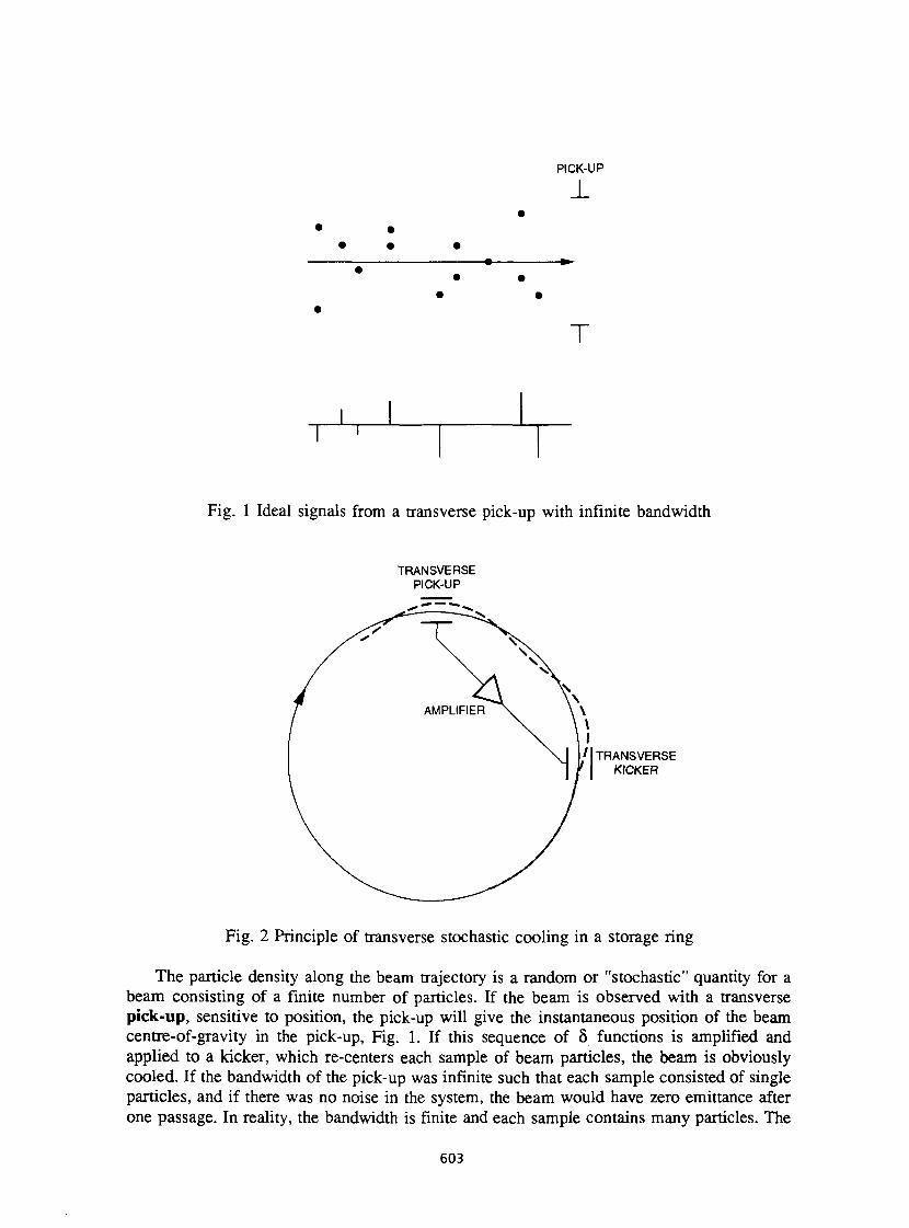
PICK-UP
T
Fig. 1 Ideal signals from a transverse pick-up with infinite bandwidth
TRANSVERSE PICK-UP
\ I ' I TRANSVERSE
| KICKER
Fig. 2 Principle of transverse stochastic cooling in a storage ring
The particle density along die beam trajectory is a random or "stochastic" quantity for a beam consisting of a finite number of particles. If the beam is observed with a transverse pick-up, sensitive to position, the pick-up will give the instantaneous position of the beam centre-of-gravity in the pick-up, Fig. 1. If this sequence of 8 functions is amplified and applied to a kicker, which re-centers each sample of beam particles, the beam is obviously cooled. If the bandwidth of the pick-up was infinite such that each sample consisted of single particles, and if there was no noise in the system, the beam would have zero emittance after one passage. In reality, the bandwidth is finite and each sample contains many particles. The
603
situation for transverse stochastic cooling in a storage ring is given in Fig. 2. Because the kicker corrects the angle to the axis, the kicker should be placed an odd number of quarter betatron wavelengths after the pick-up. The situation in Fig. 2 is clearly optimal, since the indicated particle passes the pick-up at the crest of its betatron oscillation. A particle with an additional phase of 90° will not be corrected at all, whereas particles with phases in between will be only partially corrected. Since a storage ring is always designed to have an irrational number of betatron wavelengths per circumference, particles with an unfavourable phase will soon pass the pick-up with a more favourable phase.
Let us now define the term "sample" used above. An off-axis particle passing through a pick-up will give a kicker signal of length Ts = 1/2W, where W is the bandwidth of the pickup-kicker cooling system (Kupfmuller-Nyquist relation). In the same way, a particle passing through the kicker will be influenced by all particles passing the pick-up during a time interval of width Ts. Consequently, the number of particles in a sample, defined by the smallest fraction of the beam observable by the system, is given by
Ns = N/2WT , (2)
where T is the revolution time.
Exercise 1. What is the number of particles per sample in a situation where N=109, W=100 MHz, and 7=1 \is (typical numbers)? (Central limit theorem). What is the RMS value of the centre-of-gravity of one sample if the sample is rerandomized from passage to passage? Assume a beam with size a=5 mm.
Exercise 2 (due to C.S. Taylor). 1) Ask for N random numbers from a normal distribution with zero mean and RMS-value a=l. 2) Find the actual mean value (in general *0). 3) Subtract error in mean value from each number to restore mean to zero. 4) Calculate new a'. 5) Go to step one, replace a=l with a=&, and continue. 6) Watch the progress of a.
Try different values of N, e.g., 5, 50. The evolution of a can be very irregular, but in the long term the "beam" is cooled. Use either your pocket calculator or your personal computer. How is the cooling time and the number of particles N connected?
We are now ready to "derive" the cooling time. Assume that the error at the pick-up of some test particle is x and the applied correction is Xx. In general, X*l. The corrected position of the test particle will then be given by
xc =x -he- £*.*,. , ( 3 )
s'
where the last term corresponds to the kicks from the other particles in the sample. The kick from the test particle itself is called the coherent term and the sum of kicks from the other particles in the sample is called the incoherent term. These two terms can be added by including in the sum all particles in the sample
604
xc=x-Xj^Xi. (4) s
The sum can now be expressed by the average error of the particles in the sample
<x>s=^rExi (« s s
as x = x - XN <x> = x - g <x>„ , (6)
where g=XNs is the fractional correction usually called the gain. Accepting, intuitively, that it is unhealthy to correct more than the observed error of the sample, g < 1, we assume g = 1. Let us furthermore neglect the incoherent term in Eq. (3), which should give a best performance estimate. We then get the single passage correction
Ax = x. - x = - — x , (7) Ns
giving us the cooling rate per turn
1 x„ x dn x N 1 1 dx Ax 1 / o x - — = — per turn . (8)
s
The cooling rate per second can now be obtained by multiplication of Eq. (8) with the revolution frequency. Substituting Eq. (2) for Ns, we get
1_ _ J_ J_ _ 2W_ x T Ns N
Surprisingly, this expression only overestimates the optimal cooling time by a factor of 2. (Compare Eq. (9) to the cooling time seen in Exercise 2.)
It is a matter of taste whether one likes the manipulations in the above derivation. Clearly, one has to justify the assumptions. Much more rigorous derivations can be found in Ref. [3] both in time domain and in frequency domain. The general expression for the cooling rate reads
1 _ 2WL, 2
x N 2g - g 2 (M + [/)] . (10)
The first term is identified as the coherent terms and the second is the incoherent term due to the other particles in the sample (M) and due to the noise in the system (U). Actually, U is the noise-to-signal ratio, which increases as the cooling proceeds. The quantity M> 1 is also called the mixing factor. The reason why M> 1, is that there is no complete rerandomization from the kicker to the pick-up. In other words, the samples are not random samples. Actually, there is also a small mixing term, which decreases the coherent term, due to the mixing between the pick-up and the kicker. The mixing is mainly due to the momentum spread in the
605
beam, and by a clever design of the cooling ring it is possible to minimize the mixing between the pick-up and the kicker while having a strong mixing between the kicker and the pick-up. There are, however, many other restrictions on the lattice. The optimum cooling time is given by
x = JL (M + U) (11) 2W
obtained for
g = — L _ • (12) M + U
Exercise 3. Verify this (by differentiation)!
From Eqs. (11) and (12) we see that the cooling time increases as the cooling proceeds, due to the increasing influence of the noise. We also see that optimally the gain has to be reduced during the progress of the cooling, but the cooling never stops even for very small signal-to-noise ratios. The cooling time is proportional to the number of stored particles, and stochastic cooling favours low-intensity and hot beams. The last and most important quantity in Eq. (11) is the bandwidth which has to be as large as possible. For the Fermilab antiproton collector and the ACOL at CERN, W is up to several GHz. For W= 1 GHz and the ideal situation C/=0 and M= 1 we have x = Is for N = 10 9 . In practice, x is around an order of magnitude larger.
Exercise 4. Include noise in the computer model from Exercise 2 by adding some random number to the "observed" mean value.
The cooling system described above is directly applicable for horizontal and vertical betatron cooling. Two ways of momentum cooling have been suggested. In both cases the transverse kicker is replaced by a longitudinal acceleration/deceleration gap. In the Palmer method the momentum deviation from the nominal is detected by a transverse pick-up placed in a high dispersion region. Remember Ax/x=DxAp/p. Inevitably, there will also be an influence from the betatron motion to the detected signal. In the same way, momentum cooling may lead to transverse heating. The other method detects the momentum by sensing the revolution frequency, Af/f=r\Ap/p. One big advantage of this method is that the pick-up is a sum pick-up, giving a much larger signal than a transverse difference pick-up. This filter method of Thorn-dahl transforms the detected signal to a correction signal by placing a so-called notch filter between the preamplifier and the power amplifier.
Stochastic cooling was first investigated at ISR and ICE at CERN, and is now routinely used at the antiproton rings LEAR, AA, and ACOL at CERN, and the antiproton collector at Fermilab in USA. The cooling times have constantly been decreasing by utilizing pick-up-am-plifier-kicker systems of larger and larger bandwidths and less noise. Stochastic momentum cooling has also been tested at TARN in Japan, and stochastic cooling is also going to be used at the heavy-ion storage rings COSY and ESR in Germany.
606
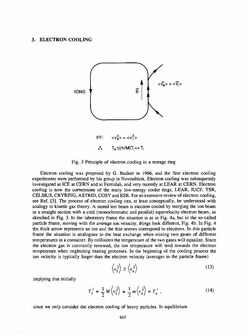
3. ELECTRON COOLING
IONS
< V e > = <Vi>
PF: < V | > = < V | >
T e<(m/M)Ti«Ti
Fig. 3 Principle of electron cooling in a storage ring
Electron cooling was proposed by G. Budker in 1966, and the first electron cooling experiments were performed by his group in Novosibirsk. Electron cooling was subsequently investigated at ICE at CERN and at Fermilab, and very recently at LEAR at CERN. Electron cooling is now the cornerstone of the many low-energy cooler rings, LEAR, IUCF, TSR, CELSIUS, CRYRING, ASTRID, COSY and ESR. For an extensive review of electron cooling, see Ref. [5]. The process of electron cooling can, at least conceptually, be understood with analogy to kinetic gas theory. A stored ion beam is electron cooled by merging the ion beam in a straight section with a cold (monochromatic and parallel) equivelocity electron beam, as sketched in Fig. 3. In the laboratory frame the situation is as in Fig. 4a, but in the so-called particle frame, moving with the average ion velocity, things look different, Fig. 4b. In Fig. 4 the thick arrow represents an ion and the thin arrows correspond to electrons. In this particle frame the situation is analogous to the heat exchange when mixing two gases of different temperatures in a container. By collisions the temperature of the two gases will equalize. Since the electron gas is constantly renewed, the ion temperature will tend towards the electron temperature when neglecting heating processes. In the beginning of the cooling process the ion velocity is typically larger than the electron velocity (averages in the particle frame)
v,2) > ( v 2 (13)
implying that initially
77 s _ M > — m 2
= r„ (14)
since we only consider the electron cooling of heavy particles. In equilibrium
607
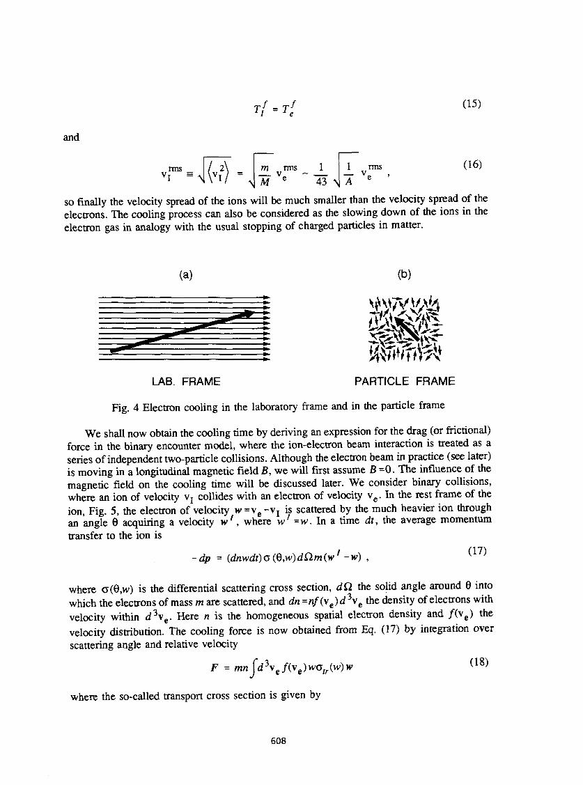
Tf = Tf (15)
and
rms \
m rms 1 ~43 N
1 rms (16)
so finally the velocity spread of the ions will be much smaller than the velocity spread of the electrons. The cooling process can also be considered as the slowing down of the ions in the electron gas in analogy with the usual stopping of charged particles in matter.
(a) (b)
LAB. FRAME PARTICLE FRAME
Fig. 4 Electron cooling in the laboratory frame and in the particle frame
We shall now obtain the cooling time by deriving an expression for the drag (or frictional) force in the binary encounter model, where the ion-electron beam interaction is treated as a series of independent two-particle collisions. Although the electron beam in practice (see later) is moving in a longitudinal magnetic field B, we will first assume B =0. The influence of the magnetic field on the cooling time will be discussed later. We consider binary collisions, where an ion of velocity v x collides with an electron of velocity v e . In the rest frame of the ion, Fig. 5, the electron of velocity w =v e -Vj is scattered by the much heavier ion through an angle 6 acquiring a velocity w', where w' =w. In a time dt, the average momentum transfer to the ion is
-dp = (dnwdt)a(Q,w)dQm(wf-w) , ( 1 7 )
where o(B,w) is the differential scattering cross section, dQ the solid angle around 6 into which the electrons of mass m are scattered, and dn = / i / (v e )d 3 v e the density of electrons with velocity within d3\e. Here n is the homogeneous spatial electron density and / ( v e ) the velocity distribution. The cooling force is now obtained from Eq. (17) by integration over scattering angle and relative velocity
F = mnjd\ef(ve)w<5tr(w)w <18>
where the so-called transport cross section is given by
608
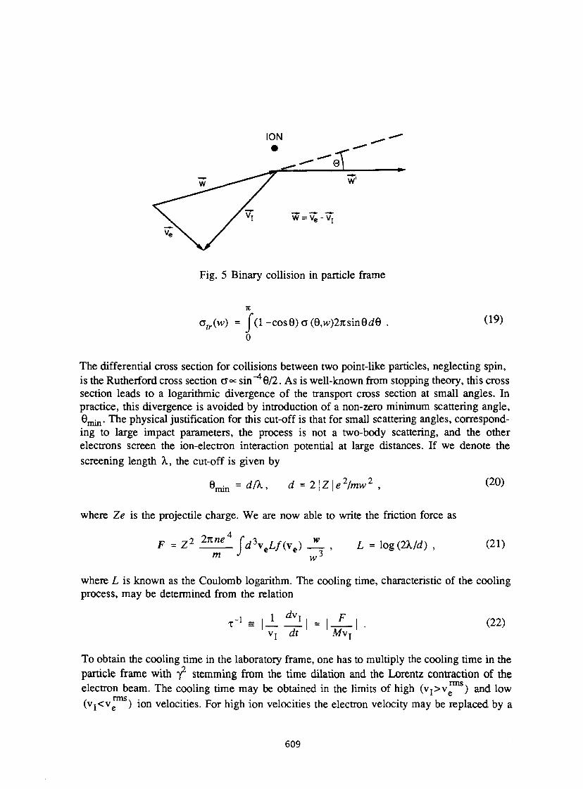
ION
w
W = V e - Vj
Fig. 5 Binary collision in particle frame
Gtr(w) = f(l-cose)a(0,w)27isinede . ( 1 9 )
The differential cross section for collisions between two point-like particles, neglecting spin, is the Rutherford cross section o « sin" 46/2. As is well-known from stopping theory, this cross section leads to a logarithmic divergence of the transport cross section at small angles. In practice, this divergence is avoided by introduction of a non-zero minimum scattering angle, Qn^n- The physical justification for this cut-off is that for small scattering angles, corresponding to large impact parameters, the process is not a two-body scattering, and the other electrons screen the ion-electron interaction potential at large distances. If we denote the screening length X, the cut-off is given by
6 m i T 1 = dfk, d = 2 \Z\e2/mw2 , (20) nun
where Ze is the projectile charge. We are now able to write the friction force as
F = Z 2 2 l t n e 4 f d 3 v e L / ( v e ) _^L , L = Iog(2X/d) , (21) m J ...3 m - w
where L is known as the Coulomb logarithm. The cooling time, characteristic of the cooling process, may be determined from the relation
t- 1^ \±^1\ = | _ L | . (22) Vj dt Mvj
To obtain the cooling time in the laboratory frame, one has to multiply the cooling time in the particle frame with T 2 stemming from the time dilation and the Lorentz contraction of the electron beam. The cooling time may be obtained in the limits of high (vj>v e ) and low (vj<v e ) ion velocities. For high ion velocities the electron velocity may be replaced by a
609
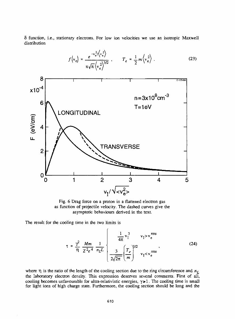
8 function, i.e., stationary electrons. For low ion velocities we use an isotropic Maxwell distribution
/W -- V e 2 / ( v e
2 )
* \ / K \ v e 2 / V3/2
= T m W - (23)
8
x10" n=3x108cm"3
T=1eV LONGITUDINAL
Vj/V 2 < V g >
Fig. 6 Drag force on a proton in a flattened electron gas as function of projectile velocity. The dashed curves give the
asymptotic behaviours derived in the text.
The result for the cooling time in the two limits is
T = y 2 Mm 1 •n z V nLL
1 3 4 ^ '
v I > v
e
rms
ly/liT
( ^3/2
V W y v I < v e
rms
(24)
where TJ is the ratio of the length of the cooling section due to the ring circumference and «^ the laboratory electron density. This expression deserves several comments. First of all, cooling becomes unfavourable for ultra-relativistic energies, y > l . The cooling time is small for light ions of high charge state. Furthermore, the cooling section should be long and the
610
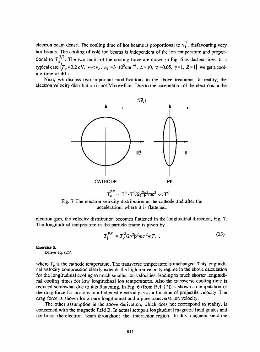
electron beam dense. The cooling time of hot beams is proportional to Vj , disfavouring very hot beams. The cooling of cold ion beams is independent of the ion temperature and propor-
3/2 tional to Te . The two limits of the cooling force are drawn in Fig. 6 as dashed lines. In a typical case ( r c =0.2 eV, Vj<v e, n L =3-10 8 cm " 3 , L = 10, rj=0.05, y=l , Z = l) wegetacool-ing time of 40 s.
Next, we discuss two important modifications to the above treatment. In reality, the electron velocity distribution is not Maxwellian. Due to the acceleration of the electrons in the
f(ve)
CATHODE PF
T,f = T c . T c / 2 Y
2 p 2 m c 2 « T c
Fig. 7 The electron velocity distribution at the cathode and after the acceleration, where it is flattened.
electron gun, the velocity distribution becomes flattened in the longitudinal direction, Fig. 7. The longitudinal temperature in the particle frame is given by
r, = rwp^c^r (25)
Exercise 5. Derive eq. (25).
where Tc is the cathode temperature. The transverse temperature is unchanged. This longitudinal velocity compression clearly extends the high ion velocity regime in the above calculation for the longitudinal cooling to much smaller ion velocities, leading to much shorter longitudinal cooling times for low longitudinal ion temperatures. Also the transverse cooling time is reduced somewhat due to this flattening. In Fig. 6 (from Ref. [7]) is shown a computation of the drag force for protons in a flattened electron gas as a function of projectile velocity. The drag force is shown for a pure longitudinal and a pure transverse ion velocity.
The other assumption in the above derivation, which does not correspond to reality, is concerned with the magnetic field B. In actual setups a longitudinal magnetic field guides and confines the electron beam throughout the interaction region. In this magnetic field the
611
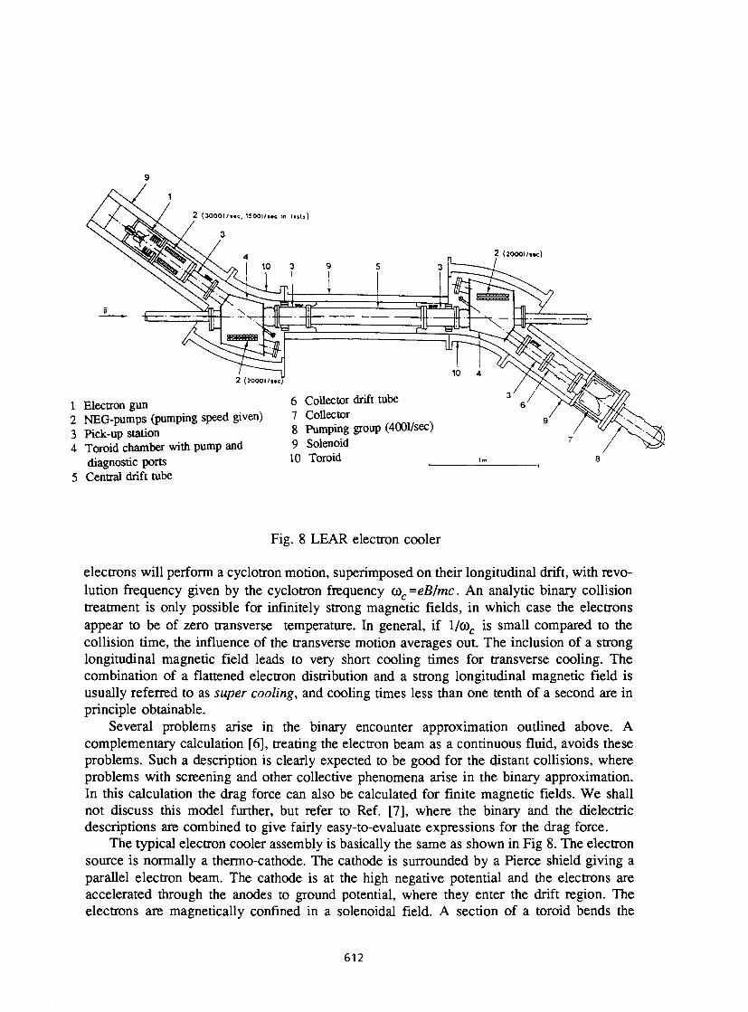
9
2 (20O0I/IK)
1 Electron gun 2 NEG-pumps (pumping speed given) 3 Pick-up station 4 Toroid chamber with pump and
diagnostic ports 5 Central drift tube
6 Collector drift tube 7 Collector 8 Pumping group (4001/sec) 9 Solenoid 10 Toroid
Fig. 8 LEAR electron cooler
electrons will perform a cyclotron motion, superimposed on their longitudinal drift, with revolution frequency given by the cyclotron frequency (ûc=eB/mc. An analytic binary collision treatment is only possible for infinitely strong magnetic fields, in which case the electrons appear to be of zero transverse temperature. In general, if l/û)c is small compared to the collision time, the influence of the transverse motion averages out. The inclusion of a strong longitudinal magnetic field leads to very short cooling times for transverse cooling. The combination of a flattened electron distribution and a strong longitudinal magnetic field is usually referred to as super cooling, and cooling times less than one tenth of a second are in principle obtainable.
Several problems arise in the binary encounter approximation outlined above. A complementary calculation [6], treating the electron beam as a continuous fluid, avoids these problems. Such a description is clearly expected to be good for the distant collisions, where problems with screening and other collective phenomena arise in the binary approximation. In this calculation the drag force can also be calculated for finite magnetic fields. We shall not discuss this model further, but refer to Ref. [7], where the binary and the dielectric descriptions are combined to give fairly easy-to-evaluate expressions for the drag force.
The typical electron cooler assembly is basically the same as shown in Fig 8. The electron source is normally a thermo-cathode. The cathode is surrounded by a Pierce shield giving a parallel electron beam. The cathode is at the high negative potential and the electrons are accelerated through the anodes to ground potential, where they enter the drift region. The electrons are magnetically confined in a solenoidal field. A section of a toroid bends the
612
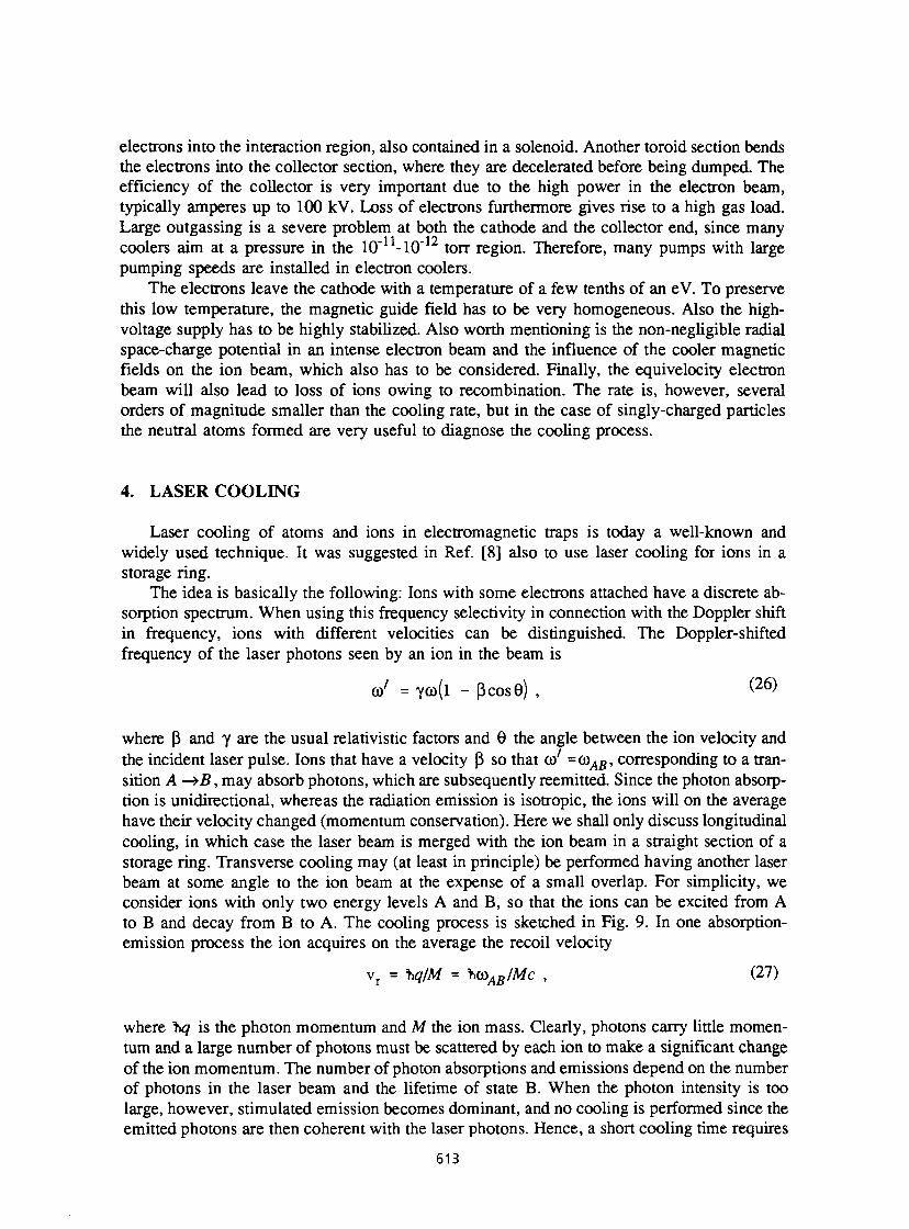
electrons into the interaction region, also contained in a solenoid. Another toroid section bends the electrons into the collector section, where they are decelerated before being dumped. The efficiency of the collector is very important due to the high power in the electron beam, typically amperes up to 100 kV. Loss of electrons furthermore gives rise to a high gas load. Large outgassing is a severe problem at both the cathode and the collector end, since many coolers aim at a pressure in the ÎO'^-IO torr region. Therefore, many pumps with large pumping speeds are installed in electron coolers.
The electrons leave the cathode with a temperature of a few tenths of an eV. To preserve this low temperature, the magnetic guide field has to be very homogeneous. Also the high-voltage supply has to be highly stabilized. Also worth mentioning is the non-negligible radial space-charge potential in an intense electron beam and the influence of the cooler magnetic fields on the ion beam, which also has to be considered. Finally, the equivelocity electron beam will also lead to loss of ions owing to recombination. The rate is, however, several orders of magnitude smaller than the cooling rate, but in the case of singly-charged particles the neutral atoms formed are very useful to diagnose the cooling process.
4. LASER COOLING
Laser cooling of atoms and ions in electromagnetic traps is today a well-known and widely used technique. It was suggested in Ref. [8] also to use laser cooling for ions in a storage ring.
The idea is basically the following: Ions with some electrons attached have a discrete absorption spectrum. When using this frequency selectivity in connection with the Doppler shift in frequency, ions with different velocities can be distinguished. The Doppler-shifted frequency of the laser photons seen by an ion in the beam is
<o' = Y©(l - pcosG) , < 2 6 )
where P and y are the usual relativistic factors and 6 the angle between the ion velocity and the incident laser pulse. Ions that have a velocity (3 so that a/ =0)45, corresponding to a transition A —>B, may absorb photons, which are subsequently reemitted. Since the photon absorption is unidirectional, whereas the radiation emission is isotropic, the ions will on the average have their velocity changed (momentum conservation). Here we shall only discuss longitudinal cooling, in which case the laser beam is merged with the ion beam in a straight section of a storage ring. Transverse cooling may (at least in principle) be performed having another laser beam at some angle to the ion beam at the expense of a small overlap. For simplicity, we consider ions with only two energy levels A and B, so that the ions can be excited from A to B and decay from B to A. The cooling process is sketched in Fig. 9. In one absorption-emission process the ion acquires on the average the recoil velocity
v r = ^q/M = ï(ùAB/Mc , (27)
where ^q is the photon momentum and M the ion mass. Clearly, photons carry little momentum and a large number of photons must be scattered by each ion to make a significant change of the ion momentum. The number of photon absorptions and emissions depend on the number of photons in the laser beam and the lifetime of state B. When the photon intensity is too large, however, stimulated emission becomes dominant, and no cooling is performed since the emitted photons are then coherent with the laser photons. Hence, a short cooling time requires
613
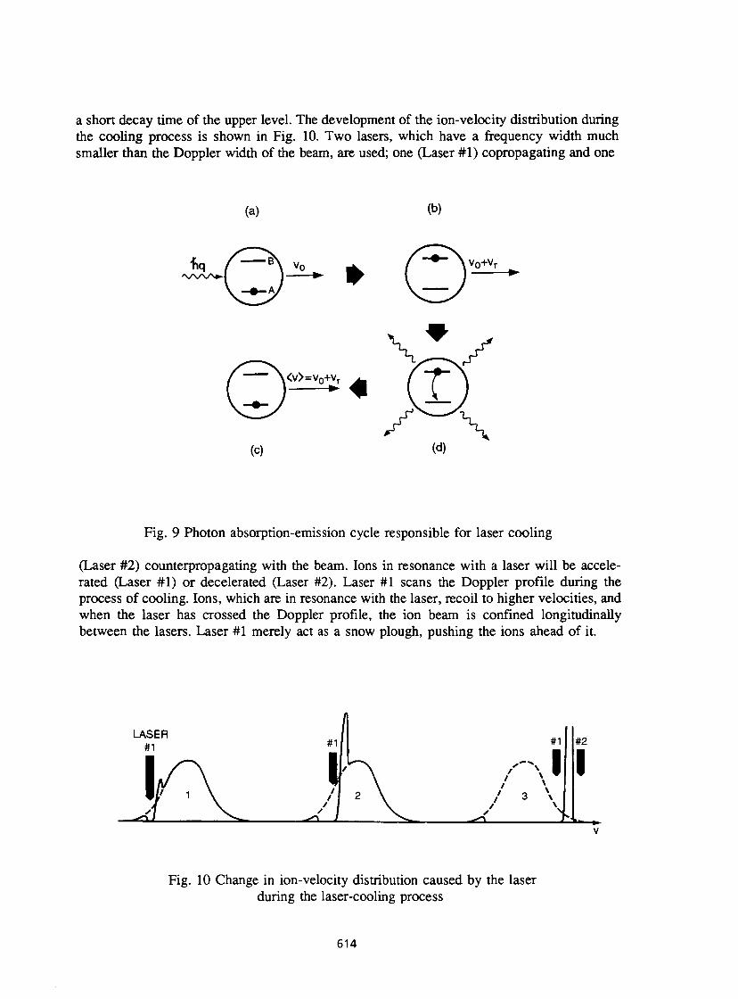
a short decay time of the upper level. The development of the ion-velocity distribution during the cooling process is shown in Fig. 10. Two lasers, which have a frequency width much smaller than the Doppler width of the beam, are used; one (Laser #1) copropagating and one
(a) (b)
'V\/\/\»-l j • | V o ( \<v>=v0+vr M
(c)
Fig. 9 Photon absorption-emission cycle responsible for laser cooling
(Laser #2) counterpropagating with the beam. Ions in resonance with a laser will be accelerated (Laser #1) or decelerated (Laser #2). Laser #1 scans the Doppler profile during the process of cooling. Ions, which are in resonance with the laser, recoil to higher velocities, and when the laser has crossed the Doppler profile, the ion beam is confined longitudinally between the lasers. Laser #1 merely act as a snow plough, pushing the ions ahead of it.
_-£L
#1
I -eO_ 1
#2
I i « _
Fig. 10 Change in ion-velocity distribution caused by the laser during the laser-cooling process
614
As an example, let us consider the case of a 100-keV Li + beam. The ion has a closed transition from the metastable 3S(ls2s) to the 3P(ls2p) of 5485Â, which can be reached by CW dye lasers. The lifetime of the upper state is 43 ns. The change in energy of an ion from one photon absorption-emission corresponds to AE=12 meV. If we choose a laser power so that the stimulated emission rate equals the spontaneous emission, we have a spontaneous rate of 1.2'107/s. This corresponds to a few mW in a beam spot of 5 mm, which is a moderate power density. Then, we have approximately 15 photon absorption emission cycles in an interaction region of 2m, corresponding to a change in energy of 0.2 eV. An ion beam from a well-stabilized separator has an energy spread of one eV, so the cooling time will correspond to a few revolution times, typically a few tenths of (is. The ultimate temperature corresponds to a single recoil kick of 12 meV.
We have seen above that laser cooling has the potential of a very fast cooling process, and that very low temperatures can, in principle, be reached. The main problem with laser cooling is that it is not universal. Few ion species with appropriate energy-level schemes exist that can be reached by tunable lasers. The only (?) known species are Li + (ls2s), 9 Be + , ^Mg"1", and 1 6 6 E r + .
Laser cooling has recently been demonstrated at TSR and ASTRID on Li + [9], Be + and I66£r+ Momentum spreads of less than 10"6 have been obtained for dilute Li + beams. Also transverse cooling is being investigated.
5. OTHER COOLING METHODS
Several other cooling methods have been proposed, but the question is whether these cooling methods are useful, because — although the beam is cooled — an appreciable fraction of the beam may be lost due to competing processes. More than 20 years ago Kolomensky suggested the so-called ionization cooling [10]. The method is equivalent to electron cooling but the electron beam is replaced by a foil. The problem is clearly that ions are lost or acquire very large momentum changes due to electron capture and large-angle scattering on nuclei. Kilian has proposed a radiative cooling of ions [11]. The idea is that intrabeam scattering [12] excites ions, which subsequently de-excite radiatively. In this way, internal energy in the circulating beam is emitted as photons, and the relative motion of the ions is damped. A strong bunching is needed to provide sufficient collision energy to excite ions. On the other hand, charge-changing collisions should be avoided. The principle of this cooling method is very attractive, since the beam is cooled in all directions, since no cooling hardware is needed and since it gets better the denser the beam is. However, the method still has to be demonstrated both theoretically and experimentally. Finally we mention dielectronic cooling, which was recently proposed by Schuch [13]. Dielectronic recombination is the process of electron capture, where the energy gained in the capture process is spent to excite another electron. The final state is thus a doubly excited ion with a charge one unit higher than the original one. If the ion auto-ionizes before the first magnetic element, on the average the ion has gained the momentum of the captured electron, since the electron emission process is isotropic. The process is a kind of resonant electron scattering, similar to the 'resonant photon scattering' in laser cooling. Also the feasibility of this cooling method has to be proven. Other cooling methods can still be invented, but they will probably not be as universal as stochastic and electron cooling.
615
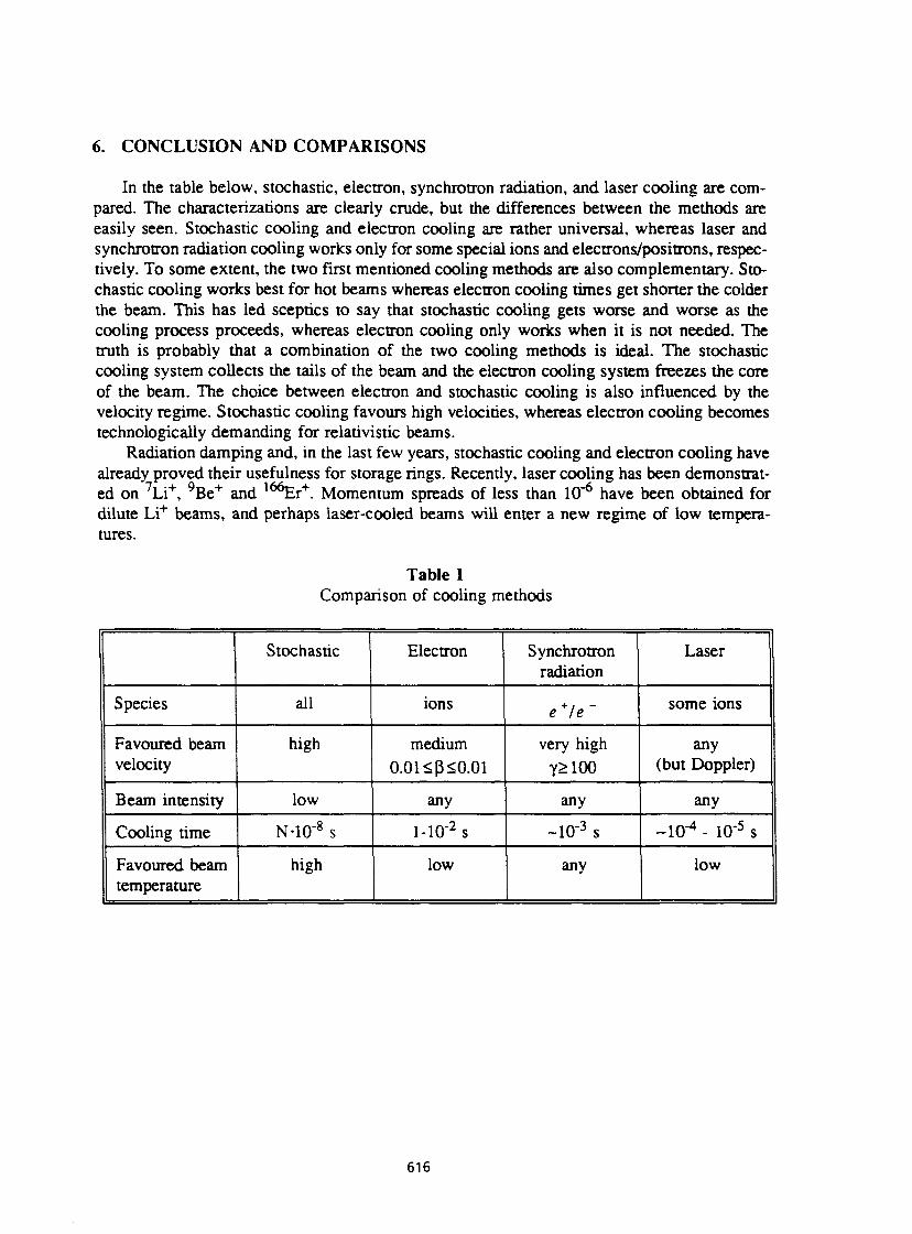
6. CONCLUSION AND COMPARISONS
In the table below, stochastic, electron, synchrotron radiation, and laser cooling are compared. The characterizations are clearly crude, but the differences between the methods are easily seen. Stochastic cooling and electron cooling are rather universal, whereas laser and synchrotron radiation cooling works only for some special ions and electrons/positrons, respectively. To some extent, the two first mentioned cooling methods are also complementary. Stochastic cooling works best for hot beams whereas electron cooling times get shorter the colder the beam. This has led sceptics to say that stochastic cooling gets worse and worse as the cooling process proceeds, whereas electron cooling only works when it is not needed. The truth is probably that a combination of the two cooling methods is ideal. The stochastic cooling system collects the tails of the beam and the electron cooling system freezes the core of the beam. The choice between electron and stochastic cooling is also influenced by the velocity regime. Stochastic cooling favours high velocities, whereas electron cooling becomes technologically demanding for relativistic beams.
Radiation damping and, in the last few years, stochastic cooling and electron cooling have already proved their usefulness for storage rings. Recently, laser cooling has been demonstrated on Li+, 9 Be + and 1 ^Er + . Momentum spreads of less than 10 - 6 have been obtained for dilute Li+ beams, and perhaps laser-cooled beams will enter a new regime of low temperatures.
Table 1 Comparison of cooling methods
Stochastic Electron Synchrotron radiation
Laser
Species all ions e le some ions
Favoured beam velocity
high medium 0.01<(3<0.01
very high Y>100
any (but Doppler)
Beam intensity low any any any
Cooling time N-10"8 s MO" 2 s -IO- 3 s -10- 4 - lO-5 s
Favoured beam temperature
high low any low
616
REFERENCES
[I] A.H. S0rensen, 3rd General Accelerator Physics Course, Proc. 1988 CERN Accelerator School, Ed. S. Turner, CERN 89-05 (1989) 18, and J. Buon, 4th General Accelerator Physics Course, Proc. 1990 CERN Accelerator School, Ed. S. Turner, CERN 91-04 (1991) 30.
[2] R. Walker, Present proceedings. [3] D. Môhl, Advanced Accelerator Physics Course, Proc. 1985 CERN Accelerator School,
Ed. S. Turner, CERN 87-03 (1986) 453 ff. [4] C.S. Taylor, Antiprotons for Colliding Beam Facilities, Proc. 1983 CERN Accelerator
School, CERN 84-15 (1984) 163 ff. [5] J. Bosser, 4th Advanced Accelerator Physics Course, Proc. 1991 CERN Accelerator
School, Ed. S. Turner, CERN 92-01 (1992) 147. [6] A.H. Sorensen and E. Bonderup, Nucl. Instrum. Methods 215 (1983) 27. [7] A.H. S0rensen, ECOL 1984, Ed. H. Poth, Karlsruhe, Germany. [8] PJ. Channell, J. Appl. Phys. £2 (1981) 3791. [9] S. Schroder et al., Phys. Rev. Lett. 64 (1990) 2901.
J.S. Hangst et al., Phys. Rev. Lett. 67 (1991) 1238. [10] A.N. Skrinsky and V.V. Parkhomchuck, Sov. J. Part. Nucl. 12 (1981) 223. [II] K. Kilian, CERN EP 84-05, unpublished. [12] A.H. S0rensen, General Accelerator Physics Course, Proc. 1986 CERN Accelerator
School, Ed. S. Turner, CERN 87-10 (1987) 135 ff. [13] R. Schuch, Symp. Ion Cooler Ring Experiments, Abisko, Sweden, May 4-5, 1988,
unpublished.
617

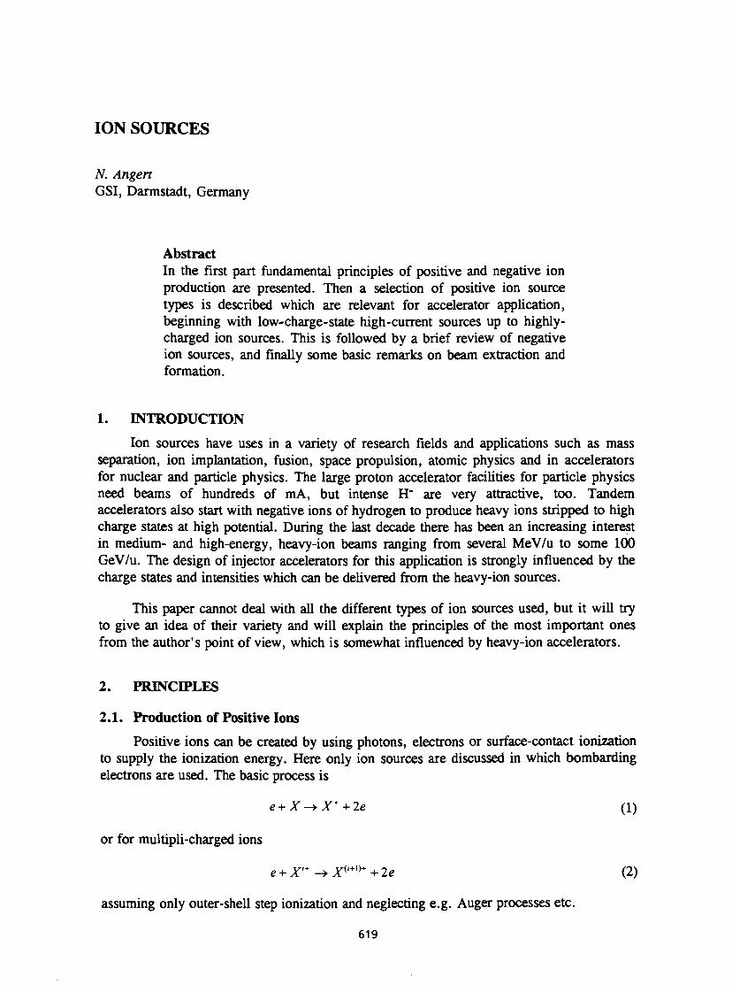
ION SOURCES
N. Angert GSI, Darmstadt, Germany
Abstract In the first part fundamental principles of positive and negative ion production are presented. Then a selection of positive ion source types is described which are relevant for accelerator application, beginning with low-charge-state high-current sources up to highly-charged ion sources. This is followed by a brief review of negative ion sources, and finally some basic remarks on beam extraction and formation.
1. INTRODUCTION Ion sources have uses in a variety of research fields and applications such as mass
separation, ion implantation, fusion, space propulsion, atomic physics and in accelerators for nuclear and particle physics. The large proton accelerator facilities for particle physics need beams of hundreds of mA, but intense H" are very attractive, too. Tandem accelerators also start with negative ions of hydrogen to produce heavy ions stripped to high charge states at high potential. During the last decade there has been an increasing interest in medium- and high-energy, heavy-ion beams ranging from several MeV/u to some 100 GeV/u. The design of injector accelerators for this application is strongly influenced by the charge states and intensities which can be delivered from the heavy-ion sources.
This paper cannot deal with all the different types of ion sources used, but it will try to give an idea of their variety and will explain the principles of the most important ones from the author's point of view, which is somewhat influenced by heavy-ion accelerators.
2. PRINCIPLES
2.1. Production of Positive Ions Positive ions can be created by using photons, electrons or surface-contact ionization
to supply the ionization energy. Here only ion sources are discussed in which bombarding electrons are used. The basic process is
e + X^>X+ +2e (1)
or for multipli-charged ions
e + X'+ -+X0+l)++2e (2)
assuming only outer-shell step ionization and neglecting e.g. Auger processes etc.
619
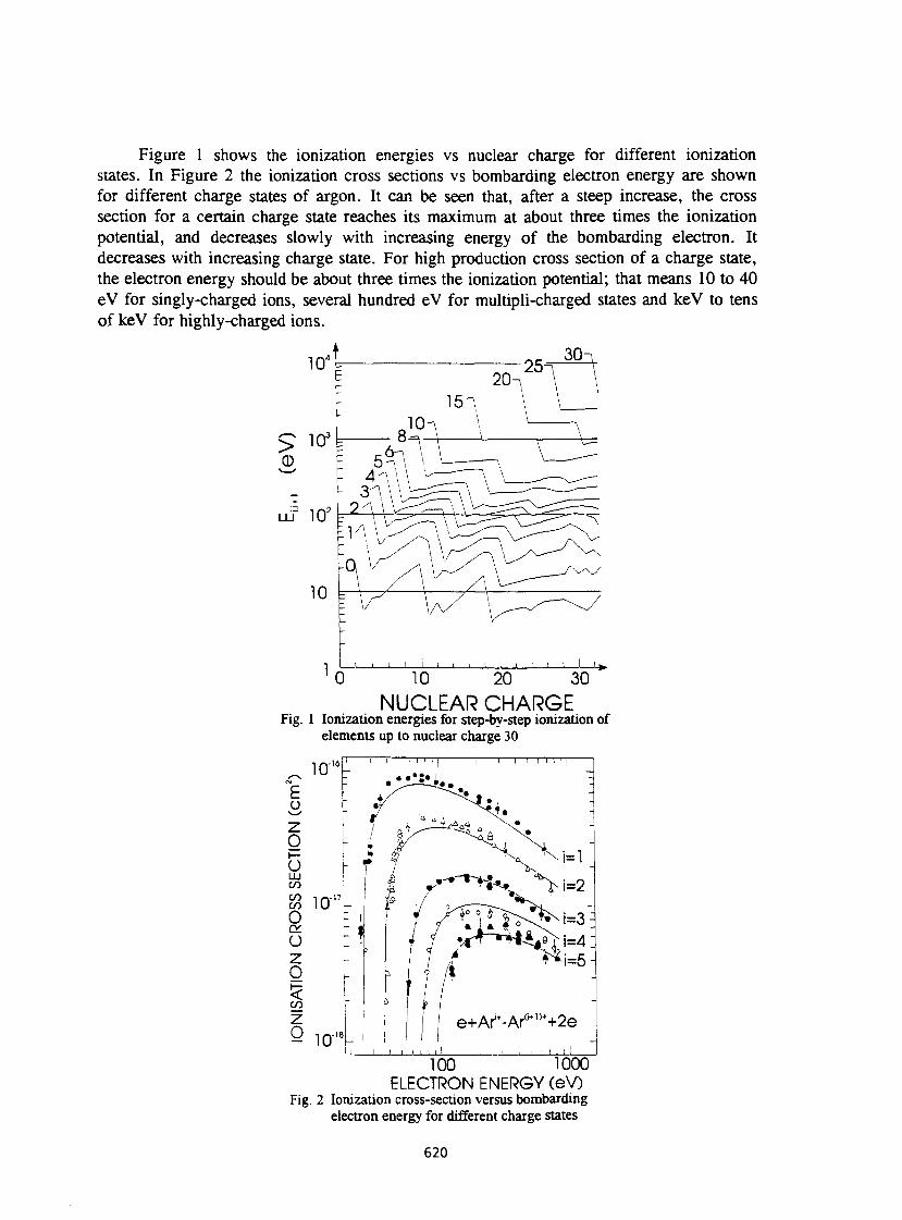
Figure 1 shows the ionization energies vs nuclear charge for different ionization states. In Figure 2 the ionization cross sections vs bombarding electron energy are shown for different charge states of argon. It can be seen that, after a steep increase, the cross section for a certain charge state reaches its maximum at about three times the ionization potential, and decreases slowly with increasing energy of the bombarding electron. It decreases with increasing charge state. For high production cross section of a charge state, the electron energy should be about three times the ionization potential; that means 10 to 40 eV for singly-charged ions, several hundred eV for multipli-charged states and keV to tens of keV for highly-charged ions.
> CD
ni icr =
0 10 20 30 NUCLEAR CHARGE
Fig. 1 Ionization energies for step-by-step ionization of elements up to nuclear charge 30
10' 6 -£ o
O i—
u LU CO % I f f" o O z O CO
S iff»
=3: =4: =5
e+AT-Ar"*+2e .i i i < ' n i
100 1000 ELECTRON ENERGY (eV)
Fig. 2 Ionization cross-section versus bombarding electron energy for different charge states
620

The time necessary for an atom to reach a certain charge state depends on the cross section and the electron current density. In competition with the ionization are the loss processes, diffusion out of the ionization volume or charge exchange processes with neutral atoms. Taking this into account the time evolution of the charge state distribution can be calculated from the following simplified differential equation [1]
dn01 dt = n0aQJe (3a)
and
dnt I dt = »,., o-_, J e - nt oiMje - n, I xc(i) (3b)
where:
n0 is the neutral particle density
rt; is the ion density in charge state i
oiml ; is the cross section for single step ionization into charge state i
j e is the electron current density
zc(J) is t n e u r e time of ion in charge state i (containment time) without ionization
The charge state distribution is mainly determined by a, i.e. by the energy of the electrons, and jeic, the product of electron current density and containment time. The diffusion time out of the ionization volume without any confinement is in the range of |is. By special magnetic and electric fields containment times up to s can be achieved if charge exchange is negligible. The dominant charge exchange process is with neutral atoms. The charge exchange between ions is much smaller because of Coulomb repulsion. The life-time is in the range of tens of ms for a residual gas pressure in the range of 10" 6—10 7 torr [2]. From Eq. (3) one can draw the following conclusions:
a) h igh/ , and n0 lead to high current, but not to high charge states because of short xc
b) high electron energy, low pressure and long containment is needed for high charge states.
This leads to the schematic diagram shown in Figure 3, where nexc = jerj ve, (ve
electron velocity) is taken for the abscissa. nexc is a figure of merit as used in fusion reactors.
621
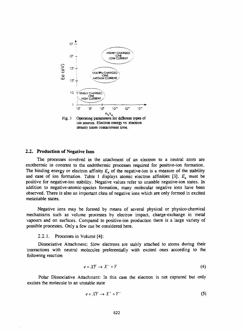
i 10* +
> CD
104
1 0 5 '
10= +
HIGHLY CHARGED IONS
LOW CURRENT
MULT1PU CHARGED \ IONS ;
\MEDIUM CURRENT,
10 -7 SINGLY CHARGED \ IONS
HIGH CURRENT
10" 10" 10' 10'°
Fig. 3 Operating parameters for different types of ion sources. Electron energy vs. electron density times containment time.
2.2. Production of Negative Ions
The processes involved in the attachment of an electron to a neutral atom are exothermic in contrast to the endothermic processes required for positive-ion formation. The binding energy or electron affinity EA of the negative-ion is a measure of the stability and ease of ion formation. Table 1 displays atomic electron affinities [3]. EA must be positive for negative-ion stability. Negative values refer to unstable negative-ion states. In addition to negative-atomic-species formation, many molecular negative ions have been observed. There is also an important class of negative ions which are only formed in excited metastable states.
Negative ions may be formed by means of several physical or physico-chemical mechanisms such as volume processes by electron impact, charge-exchange in metal vapours and on surfaces. Compared to positive-ion production there is a large variety of possible processes. Only a few can be considered here.
2.2.1. Processes in Volume [4] :
Dissociative Attachment: Slow electrons are stably attached to atoms during their interactions with neutral molecules preferentially with excited ones according to the following reaction
e + XY^X'+Y (4)
Polar Dissociative Attachment: In this case the electron is not captured but only excites the molecule to an unstable state
e + XY ->X++Y~ (5)
622
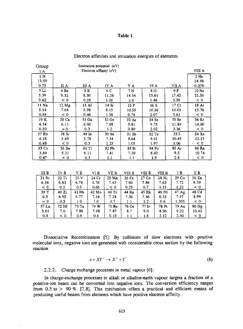
Table 1
Electron affinities and ionization energies of elements
Group Ionization potential (eV) I A " Electron affinity (eV) VIIIA 1H 2 He
13.59 24.58 0.75 II A III A IV A VA VIA VII A 0.078 3 Li 4 Be 5 B 6 C 7 N 8 0 9 F 10 Ne 3.39 9.32 8.30 11.26 14.54 13.61 17.42 21.56 0.62 < 0 0.28 1.26 <0 1.46 3.39 < 0 11 Na 12 Mg 13 Al 14 Si 15 P 16 S 17 Cl 18 AT 5.14 7.64 5.98 8.15 10.55 10.36 13.01 15.76 0.54 < 0 0.46 1.38 0.74 2.07 3.61 < 0 19 K 20 Ca 31 Ga 32 Ge 33 As 34 Se 35 Br 36 Kr 4.34 6.11 6.00 7.88 9.81 9.75 11.84 14.00 0.50 * 0 0.3 1.2 0.80 2.02 3.36 < 0
37 Rb 38 Sr 49 In 50 Sn 51 Sb 52 Te 53 1 54 Xe 4.18 5.69 5.78 7.34 8.64 9.01 10.45 12.13 0.48 < 0 0.3 1.25 1.05 1.97 3.06 < 0 55 Cs 56 Ba 81 Tl 82 Pb 83 Bi 84 Po 85 AT 86 Rn 3.89 5.21 6.11 7.41 7.29 8.43 9.5 10.74
1 0.47 < 0 0.3 1.1 1.1 1.9 2.8 < 0
III B IV B VB VIB VIIB VIIIB VIIIB VIIIB IB IIB 21 Sc 6.56 < 0
22 Ti 6.83 0.2
23 V 6.74 0.5
24 Cr 6.76 0.66
25 Mn 7.43 < 0
26 Fe 7.90 0.25
27 Co 7.86 0.7
28 Ni 7.63 1.15
29 Cu 7.72 1.22
30 Zn 9.39 < 0
39 Y 6.5 = 0
40 Zr 6.95 0.5
41 Nb 6.77 1.0
42 Mo 7.18 1.0
43 Tc 7.28 0.7
44 Ru 7.36 1.1
45 Rh 7.46 1.2
46 Pd 8.33 0.6
47 Ag 7.57 1.303
48 Cd 8.99 < 0
57 La 5.61 0.5
72 Hf 7.0 < 0
73 Ta 7.88 0.6
74 W 7.98 0.6
75 Re 7.87 0.15
76 0s 8.7 1.1
77 Ir 9.0 1.6
78 Pt 8.96 2.12
79 Au 9.22 2.30
80 Hg 10.43 < 0
Dissociative Recombination [5]: By collisions of slow electrons with positive molecular ions, negative ions are generated with considerable cross section by the following reaction
e+XY+ - > X + + r (6)
2.2.2. Charge exchange processes in metal vapour [6]: In charge-exchange processes in alkali or alkaline-earth vapour targets a fraction of a
positive-ion beam can be converted into negative ions. The conversion efficiency ranges from 0.5 to > 90 % [7,8]. This mechanism offers a practical and efficient means of producing useful beams from elements which have positive electron affinity.
623
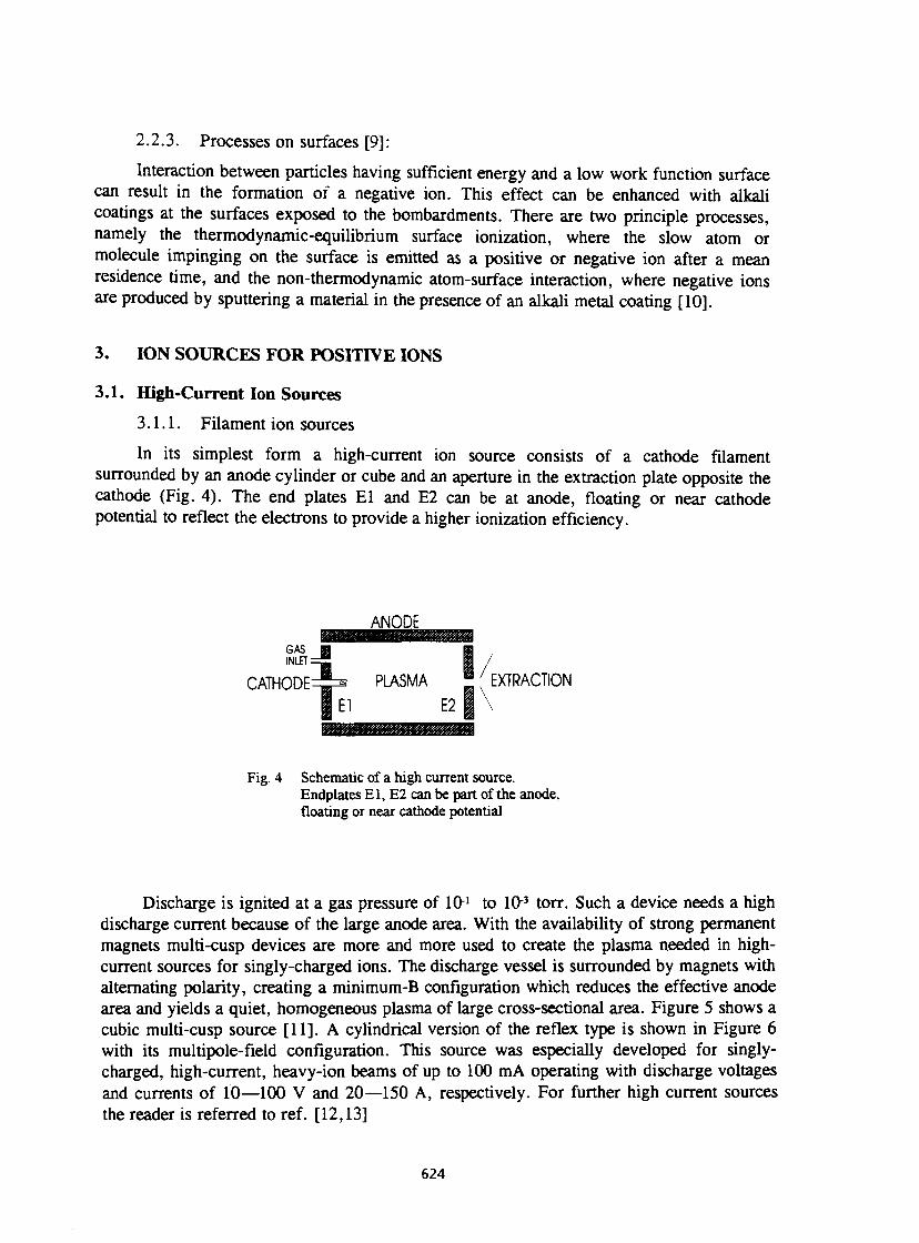
2.2.3. Processes on surfaces [9]: Interaction between particles having sufficient energy and a low work function surface
can result in the formation of a negative ion. This effect can be enhanced with alkali coatings at the surfaces exposed to the bombardments. There are two principle processes, namely the thermodynamic-equilibrium surface ionization, where the slow atom or molecule impinging on the surface is emitted as a positive or negative ion after a mean residence time, and the non-thermodynamic atom-surface interaction, where negative ions are produced by sputtering a material in the presence of an alkali metal coating [10].
3. ION SOURCES FOR POSITIVE IONS
3.1. High-Current Ion Sources 3.1.1. Filament ion sources In its simplest form a high-current ion source consists of a cathode filament
surrounded by an anode cylinder or cube and an aperture in the extraction plate opposite the cathode (Fig. 4). The end plates El and E2 can be at anode, floating or near cathode potential to reflect the electrons to provide a higher ionization efficiency.
Fig. 4 Schematic of a high current source. Endplates El, E2 can be part of the anode, floating or near cathode potential
Discharge is ignited at a gas pressure of 101 to 103 torr. Such a device needs a high discharge current because of the large anode area. With the availability of strong permanent magnets multi-cusp devices are more and more used to create the plasma needed in high-current sources for singly-charged ions. The discharge vessel is surrounded by magnets with alternating polarity, creating a minimum-B configuration which reduces the effective anode area and yields a quiet, homogeneous plasma of large cross-sectional area. Figure 5 shows a cubic multi-cusp source [11]. A cylindrical version of the reflex type is shown in Figure 6 with its multipole-field configuration. This source was especially developed for singly-charged, high-current, heavy-ion beams of up to 100 mA operating with discharge voltages and currents of 10—100 V and 20—150 A, respectively. For further high current sources the reader is referred to ref. [12,13]
624
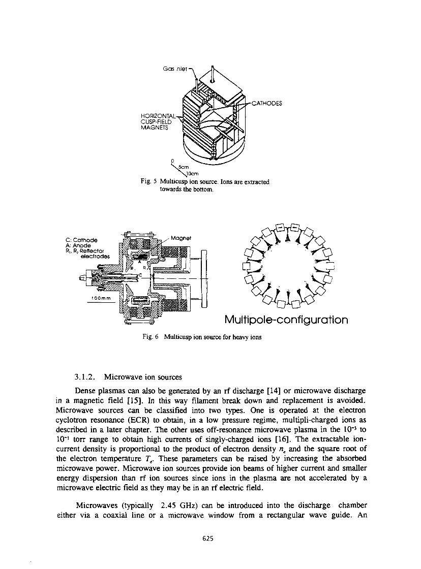
Fig. 6 Multicusp ion source for heavy ions
3.1.2. Microwave ion sources Dense plasmas can also be generated by an rf discharge [14] or microwave discharge
in a magnetic field [15]. In this way filament break down and replacement is avoided. Microwave sources can be classified into two types. One is operated at the electron cyclotron resonance (ECR) to obtain, in a low pressure regime, multipli-charged ions as described in a later chapter. The other uses off-resonance microwave plasma in the 10"3 to 10"1 torr range to obtain high currents of singly-charged ions [16]. The extractable ion-current density is proportional to the product of electron density ne and the square root of the electron temperature Te. These parameters can be raised by increasing the absorbed microwave power. Microwave ion sources provide ion beams of higher current and smaller energy dispersion than rf ion sources since ions in the plasma are not accelerated by a microwave electric field as they may be in an rf electric field.
Microwaves (typically 2.45 GHz) can be introduced into the discharge chamber either via a coaxial line or a microwave window from a rectangular wave guide. An
625
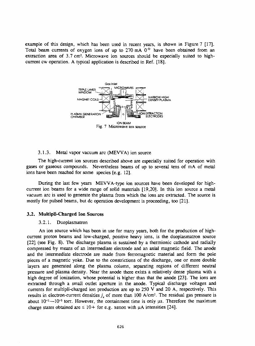
example of this design, which has been used in recent years, is shown in Figure 7 [17]. Total beam currents of oxygen ions of up to 270 m A 0 + have been obtained from an extraction area of 3.7 cm2. Microwave ion sources should be especially suited to high-current cw operation. A typical application is described in Ref. [18].
Gas inlet
ION BEAM Fig. 7 Microwave ion source
3.1.3. Metal vapor vacuum arc (MEWA) ion source The high-current ion sources described above are especially suited for operation with
gases or gaseous compounds. Nevertheless beams of up to several tens of m A of metal ions have been reached for some species [e.g. 12].
During the last few years MEVVA-type ion sources have been developed for high-current ion beams for a wide range of solid materials [19,20]. In this ion source a metal vacuum arc is used to generate the plasma from which the ions are extracted. The source is mostly for pulsed beams, but dc operation development is proceeding, too [21].
3.2. Multipli-Charged Ion Sources 3.2.1. Duoplasmatron An ion source which has been in use for many years, both for the production of high-
current proton beams and low-charged, positive heavy ions, is the duoplasmatron source [22] (see Fig. 8). The discharge plasma is sustained by a thermionic cathode and radially compressed by means of an intermediate electrode and an axial magnetic field. The anode and the intermediate electrode are made from ferromagnetic material and form the pole pieces of a magnetic yoke. Due to the constrictions of the discharge, one or more double layers are generated along the plasma column, separating regions of different neutral pressure and plasma density. Near the anode there exists a relatively dense plasma with a high degree of ionization, whose potential is higher than that the anode [23]. The ions are extracted through a small outlet aperture in the anode. Typical discharge voltages and currents for multipli-charged ion production are up to 250 V and 20 A, respectively. This results in electron-current densities j e of more than 100 A/cm2. The residual gas pressure is about 10"2—10"3 torr. However, the containment time is only (is. Therefore the maximum charge states obtained are < 10+ for e.g. xenon with uA intensities [24].
626
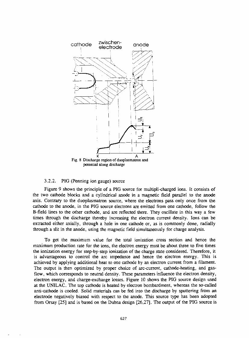
Fig. 8 Discharge region of duoplasmatron and potential along discharge
3.2.2. PIG (Penning ion gauge) source Figure 9 shows the principle of a PIG source for multipli-charged ions. It consists of
the two cathode blocks and a cylindrical anode in a magnetic field parallel to the anode axis. Contrary to the duoplasmatron source, where the electrons pass only once from the cathode to the anode, in the PIG source electrons are emitted from one cathode, follow the B-field lines to the other cathode, and are reflected there. They oscillate in this way a few times through the discharge thereby increasing the electron current density. Ions can be extracted either axially, through a hole in one cathode or, as is commonly done, radially through a slit in the anode, using the magnetic field simultaneously for charge analysis.
To get the maximum value for the total ionization cross section and hence the maximum production rate for the ions, the electron energy must be about three to five times the ionization energy for step-by-step ionization of the charge state considered. Therefore, it is advantageous to control the arc impedance and hence the electron energy. This is achieved by applying additional heat to one cathode by an electron current from a filament. The output is then optimized by proper choice of arc-current, cathode-heating, and gas-flow, which corresponds to neutral density. These parameters influence the electron density, electron energy, and charge-exchange losses. Figure 10 shows the PIG source design used at the UNILAC. The top cathode is heated by electron bombardment, whereas the so-called anti-cathode is cooled. Solid materials can be fed into the discharge by sputtering from an electrode negatively biased with respect to the anode. This source type has been adopted from Orsay [25] and is based on the Dubna design [26,27]. The output of the PIG source is
627
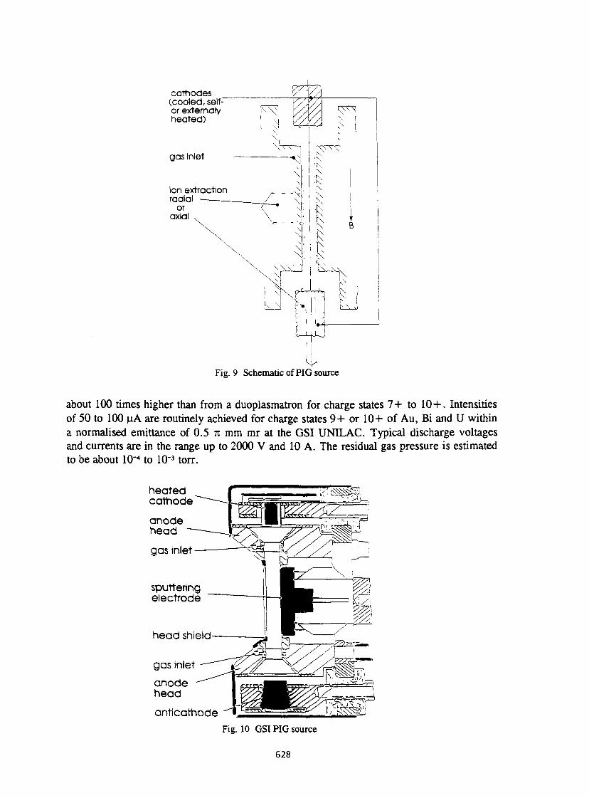
cathodes (cooled, self or externaly heated)
gas inlet
ion extraction radial
Fig. 9 Schematic of PIG source
about 100 times higher than from a duoplasmatron for charge states 7+ to 10+. Intensities of 50 to 100 nA are routinely achieved for charge states 9+ or 10+ of Au, Bi and U within a normalised emittance of 0.5 7t mm mr at the GSI UNILAC. Typical discharge voltages and currents are in the range up to 2000 V and 10 A. The residual gas pressure is estimated to be about 10 -4 to 10"3 torr.
heated cathode
anode head
gas inlet
sputtering electrode
head shield
gas inlet anode head anticathode ~"< C g / | V " > ^z^^ h £&>'}
Fig. 10 GSI PIG source
628
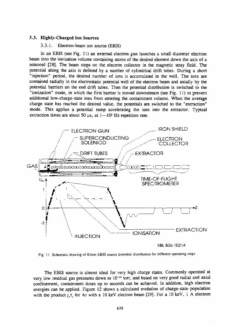
3.3. Highly-Charged Ion Sources 3.3.1. Electron-beam ion source (EBIS) In an EBIS (see Fig. 11) an external electron gun launches a small diameter electron
beam into the ionization volume containing atoms of the desired element down the axis of a solenoid [28]. The beam stops on the electron collector in the magnetic stray field. The potential along the axis is defined by a number of cylindrical drift tubes. During a short "injection" period, the desired number of ions is accumulated in the well. The ions are contained radially in the electrostatic potential well of the electron beam and axially by the potential barriers on the end drift tubes. Then the potential distribution is switched to the "ionization" mode, in which the first barrier is moved downstream (see Fig. 11) to prevent additional low-charge-state ions from entering the containment volume. When the average charge state has reached the desired value, the potentials are switched to the "extraction" mode. This applies a potential ramp accelerating the ions into the extractor. Typical extraction times are about 50 ^s, at 1—103 Hz repetition rate.
XBL836-10214
Fig. 11 Schematic drawing of Krion EBIS source potential distribution for different operating steps
The EBIS source is almost ideal for very high charge states. Commonly operated at very low residual gas pressures down to 10"10 torr, and based on very good radial and axial confinement, containment times up to seconds can be achieved. In addition, high electron energies can be applied. Figure 12 shows a calculated evolution of charge-state population with the product jxc for Ar with a 10 keV electron beam [29]. For a 10 keV, 1 A electron
629
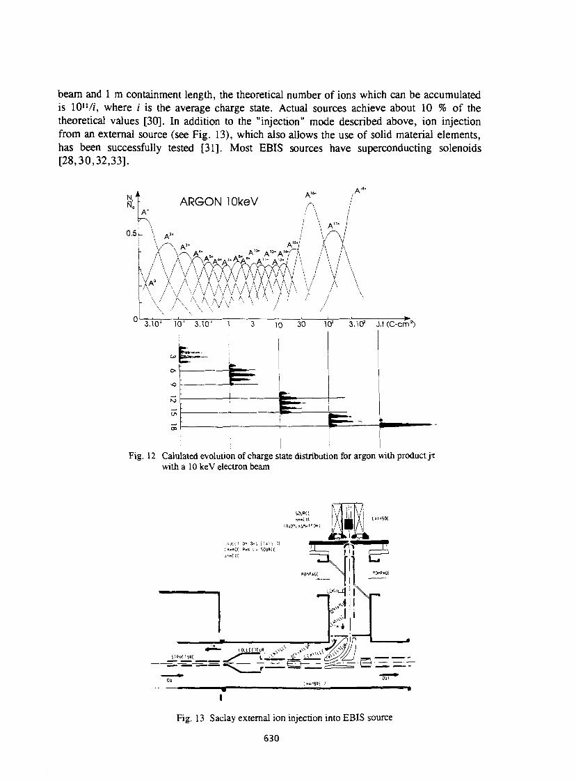
beam and 1 m containment length, the theoretical number of ions which can be accumulated is 10"//, where / is the average charge state. Actual sources achieve about 10 % of the theoretical values [30]. In addition to the "injection" mode described above, ion injection from an external source (see Fig. 13), which also allows the use of solid material elements, has been successfully tested [31]. Most EBIS sources have superconducting solenoids [28,30,32,33].
3.10"' 10"' 3.10"' 1 10 30 l t f 3.Iff J.tCC-cm2)
Fig. 12 Calulated evolution of charge state distribution for argon with product jx with a 10 keV electron beam
I
Fig. 13 Saclay external ion injection into EBIS source
630
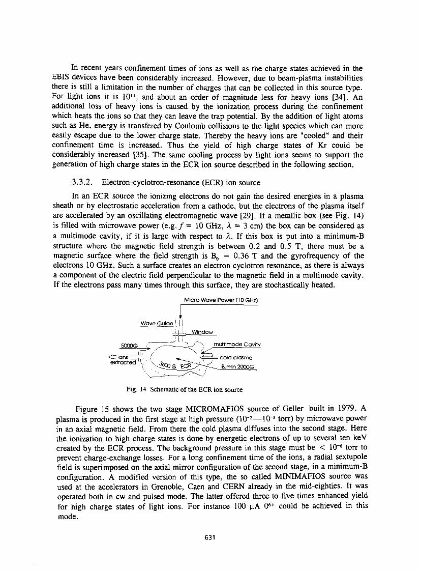
In recent years confinement times of ions as well as the charge states achieved in the EBIS devices have been considerably increased. However, due to beam-plasma instabilities there is still a limitation in the number of charges that can be collected in this source type. For light ions it is 10", and about an order of magnitude less for heavy ions [34]. An additional loss of heavy ions is caused by the ionization process during the confinement which heats the ions so that they can leave the trap potential. By the addition of light atoms such as He, energy is transfered by Coulomb collisions to the light species which can more easily escape due to the lower charge state. Thereby the heavy ions are "cooled" and their confinement time is increased. Thus the yield of high charge states of Kr could be considerably increased [35]. The same cooling process by light ions seems to support the generation of high charge states in the ECR ion source described in the following section.
3.3.2. Electron-cyclotron-resonance (ECR) ion source In an ECR source the ionizing electrons do not gain the desired energies in a plasma
sheath or by electrostatic acceleration from a cathode, but the electrons of the plasma itself are accelerated by an oscillating electromagnetic wave [29]. If a metallic box (see Fig. 14) is filled with microwave power (e.g./ = 10 GHz, A = 3 cm) the box can be considered as a multimode cavity, if it is large with respect to A. If this box is put into a minimum-B structure where the magnetic field strength is between 0.2 and 0.5 T, there must be a magnetic surface where the field strength is B0 = 0.36 T and the gyrofrequency of the electrons 10 GHz. Such a surface creates an electron cyclotron resonance, as there is always a component of the electric field perpendicular to the magnetic field in a multimode cavity. If the electrons pass many times through this surface, they are stochastically heated.
Micro Wave Power (10 GHz)
extracted V \ ^ O G ^ R
muttimode Cavity
cold plasma B.mln 20006
Fig. 14 Schematic of the ECR ion source
Figure 15 shows the two stage MICROMAFIOS source of Geller built in 1979. A plasma is produced in the first stage at high pressure (10"2—10"3 torr) by microwave power in an axial magnetic field. From there the cold plasma diffuses into the second stage. Here the ionization to high charge states is done by energetic electrons of up to several ten keV created by the ECR process. The background pressure in this stage must be < 10"s torr to prevent charge-exchange losses. For a long confinement time of the ions, a radial sextupole field is superimposed on the axial mirror configuration of the second stage, in a minimum-B configuration. A modified version of this type, the so called MINIMAFIOS source was used at the accelerators in Grenoble, Caen and CERN already in the mid-eighties. It was operated both in cw and pulsed mode. The latter offered three to five times enhanced yield for high charge states of light ions. For instance 100 |iA 06* could be achieved in this mode.
631
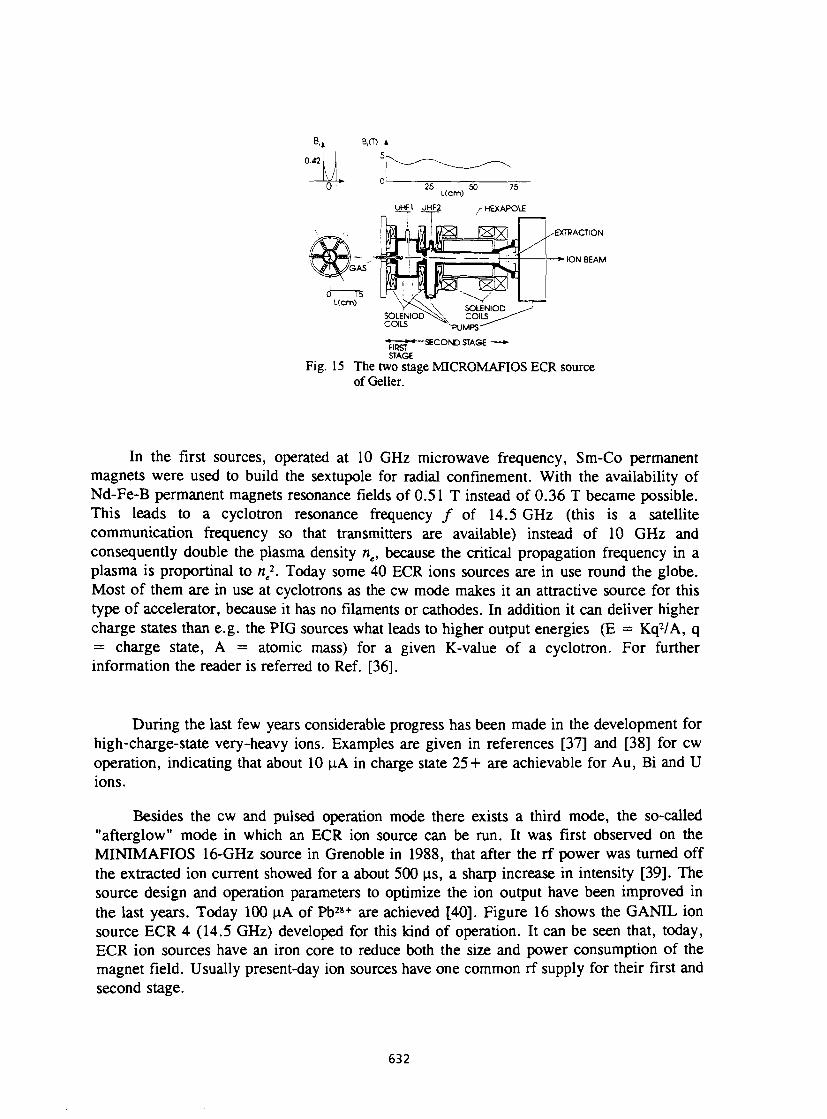
B,. B,(T) *
UHF) UHF? /-HEXAPOŒ
• — - S E C O M J S W S E — STAGE
Fig. 15 The two stage MICROMAFIOS ECR source ofGeller.
In the first sources, operated at 10 GHz microwave frequency, Sm-Co permanent magnets were used to build the sextupole for radial confinement. With the availability of Nd-Fe-B permanent magnets resonance fields of 0.51 T instead of 0.36 T became possible. This leads to a cyclotron resonance frequency / of 14.5 GHz (this is a satellite communication frequency so that transmitters are available) instead of 10 GHz and consequently double the plasma density ne, because the critical propagation frequency in a plasma is proportinal to ne
2. Today some 40 ECR ions sources are in use round the globe. Most of them are in use at cyclotrons as the cw mode makes it an attractive source for this type of accelerator, because it has no filaments or cathodes. In addition it can deliver higher charge states than e.g. the PIG sources what leads to higher output energies (E = Kq2/A, q = charge state, A = atomic mass) for a given K-value of a cyclotron. For further information the reader is referred to Ref. [36].
During the last few years considerable progress has been made in the development for high-charge-state very-heavy ions. Examples are given in references [37] and [38] for cw operation, indicating that about 10 (iA in charge state 25+ are achievable for Au, Bi and U ions.
Besides the cw and pulsed operation mode there exists a third mode, the so-called "afterglow" mode in which an ECR ion source can be run. It was first observed on the MINIMAFIOS 16-GHz source in Grenoble in 1988, that after the rf power was turned off the extracted ion current showed for a about 500 (is, a sharp increase in intensity [39]. The source design and operation parameters to optimize the ion output have been improved in the last years. Today 100 |iA of Pb 2 8 + are achieved [40]. Figure 16 shows the GANIL ion source ECR 4 (14.5 GHz) developed for this kind of operation. It can be seen that, today, ECR ion sources have an iron core to reduce both the size and power consumption of the magnet field. Usually present-day ion sources have one common rf supply for their first and second stage.
632
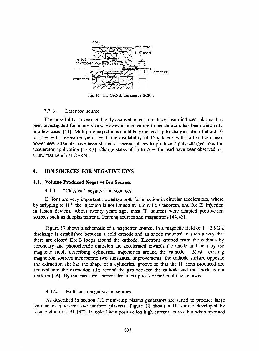
Fig. 16 The GANIL ion source ECR4.
3.3.3. Laser ion source The possibility to extract highly-charged ions from laser-beam-induced plasma has
been investigated for many years. However, application to accelerators has been tried only in a few cases [41]. Multipli-charged ions could be produced up to charge states of about 10 to 15+ with resonable yield. With the availability of C0 2 lasers with rather high peak power new attempts have been started at several places to produce highly-charged ions for accelerator application [42,43]. Charge states of up to 26+ for lead have been observed on a new test bench at CERN.
4. ION SOURCES FOR NEGATIVE IONS
4.1. Volume Produced Negative Ion Sources 4.1.1. "Classical" negative ion soources H" ions are very important nowadays both for injection in circular accelerators, where
by stripping to H+ the injection is not limited by Liouville's theorem, and for H° injection in fusion devices. About twenty years ago, most H" sources were adapted positive-ion sources such as duoplasmatrons, Penning sources and magnetrons [44,45].
Figure 17 shows a schematic of a magnetron source. In a magnetic field of 1—2 kG a discharge is established between a cold cathode and an anode mounted in such a way that there are closed E x B loops around the cathode. Electrons emitted from the cathode by secondary and photoelectric emission are accelerated towards the anode and bent by the magnetic field, describing cylindrical trajectories around the cathode. Most existing magnetron sources incorporate two substantial improvements: the cathode surface opposite the extraction slit has the shape of a cylindrical groove so that the H" ions produced are focused into the extraction slit; second the gap between the cathode and the anode is not uniform [46]. By that measure current densities up to 3 A/cm2 could be achieved.
4.1.2. Multi-cusp negative ion sources As described in section 3.1 multi-cusp plasma generators are suited to produce large
volume of quiescent and uniform plasmas. Figure 18 shows a H" source developed by Leung et.al at LBL [47]. It looks like a positive ion high-current source, but when operated
633
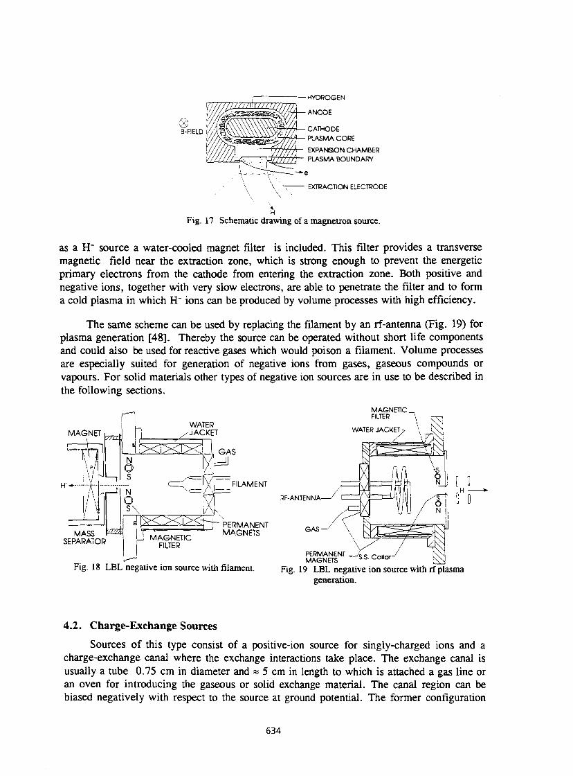
Fig. 17 Schematic drawing of a magnetron source.
as a H" source a water-cooled magnet filter is included. This filter provides a transverse magnetic field near the extraction zone, which is strong enough to prevent the energetic primary electrons from the cathode from entering the extraction zone. Both positive and negative ions, together with very slow electrons, are able to penetrate the filter and to form a cold plasma in which H" ions can be produced by volume processes with high efficiency.
The same scheme can be used by replacing the filament by an rf-antenna (Fig. 19) for plasma generation [48]. Thereby the source can be operated without short life components and could also be used for reactive gases which would poison a filament. Volume processes are especially suited for generation of negative ions from gases, gaseous compounds or vapours. For solid materials other types of negative ion sources are in use to be described in the following sections.
Fig. 18 LBL negative ion source with filament. Fig. 19 LBL negative ion source with rf plasma generation.
4.2. Charge-Exchange Sources Sources of this type consist of a positive-ion source for singly-charged ions and a
charge-exchange canal where the exchange interactions take place. The exchange canal is usually a tube 0.75 cm in diameter and « 5 cm in length to which is attached a gas line or an oven for introducing the gaseous or solid exchange material. The canal region can be biased negatively with respect to the source at ground potential. The former configuration
634
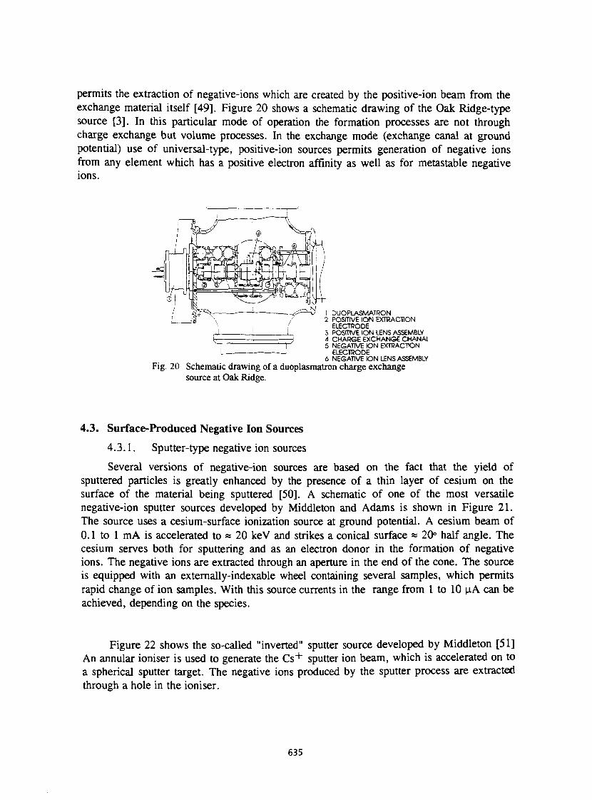
permits the extraction of negative-ions which are created by the positive-ion beam from the exchange material itself [49]. Figure 20 shows a schematic drawing of the Oak Ridge-type source [3]. In this particular mode of operation the formation processes are not through charge exchange but volume processes. In the exchange mode (exchange canal at ground potential) use of universal-type, positive-ion sources permits generation of negative ions from any element which has a positive electron affinity as well as for metastable negative ions.
1 DUOPLASMATRON 2 POSITIVE ION EXTRACTION
ELECTRODE 3 POSITIVE ION LENS ASSEMBLY 4 CHARGE EXCHANGE CHANAt 5 NEGATIVE ION EXTRACTION
ELECTRODE 6 NEGATIVE ION LENS ASSEMBLY
Fig. 20 Schematic drawing of a duoplasmatron charge exchange source at Oak Ridge.
4.3. Surface-Produced Negative Ion Sources 4.3.1. Sputter-type negative ion sources Several versions of negative-ion sources are based on the fact that the yield of
sputtered particles is greatly enhanced by the presence of a thin layer of cesium on the surface of the material being sputtered [50]. A schematic of one of the most versatile negative-ion sputter sources developed by Middleton and Adams is shown in Figure 21. The source uses a cesium-surface ionization source at ground potential. A cesium beam of 0.1 to 1 mA is accelerated to « 20 keV and strikes a conical surface « 20° half angle. The cesium serves both for sputtering and as an electron donor in the formation of negative ions. The negative ions are extracted through an aperture in the end of the cone. The source is equipped with an externally-indexable wheel containing several samples, which permits rapid change of ion samples. With this source currents in the range from 1 to 10 uA c a n ^ e
achieved, depending on the species.
Figure 22 shows the so-called "inverted" sputter source developed by Middleton [51] An annular ioniser is used to generate the C s + sputter ion beam, which is accelerated on to a spherical sputter target. The negative ions produced by the sputter process are extracted through a hole in the ioniser.
635
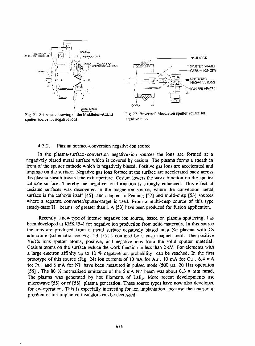
' Sputter Surface Element A
Fig. 21 Schematic drawing of the Middleton-Adams sputter source for negative ions
4.3.2. Plasma-surface-conversion negative-ion source In the plasma-surface-conversion negative-ion sources the ions are formed at a
negatively biased metal surface which is covered by cesium. The plasma forms a sheath in front of the sputter cathode which is negatively biased. Positive gas ions are accelerated and impinge on the surface. Negative gas ions formed at the surface are accelerated back across the plasma sheath toward the exit aperture. Cesium lowers the work function on the sputter cathode surface. Thereby the negative ion formation is strongly enhanced. This effect at cesiated surfaces was discovered in the magnetron source, where the conversion metal surface is the cathode itself [45], and adapted to Penning [52] and multi-cusp [53] sources where a separate converter/sputter-target is used. From a multi-cusp source of this type steady-state H" beams of greater than 1 A [53] have been produced for fusion application.
Recently a new type of intense negative-ion source, based on plasma sputtering, has been developed at KEK [54] for negative ion production from solid materials. In this source the ions are produced from a metal surface negatively biased in,a Xe plasma with Cs admixture (schematic see Fig. 23 [55] ) confined by a cusp magnet field. The positive Xe/Cs ions sputter atoms, positive, and negative ions from the solid sputter material. Cesium atoms on the surface reduce the work function to less than 2 eV. For elements with a large electron affinity up to 10 % negative ion probability can be reached. In the first prototype of this source (Fig. 24) ion currents of 10 m A for Au", 10 mA for Cu", 6.4 mA for Pt", and 6 mA for Ni" have been measured in pulsed mode (500 us, 20 Hz) operation [55] . The 80 % normalized emittance of the 6 mA Ni" beam was about 0.3 n mm mrad. The plasma was generated by hot filaments of LaB6. More recent developments use microwave [55] or rf [56] plasma generation. These source types have now also developed for cw-operation. This is especially interesting for ion implantation, because the charge-up problem of ion-implanted insulators can be decreased.
INSULATOR
SPUTTER TARGET CESIUM IONIZER
SPUTTERED NEGATIVE IONS
-IONIZER HEATER
-{ViAO
Fig. 22 "Inverted" Middleton sputter source for negative ions.
636
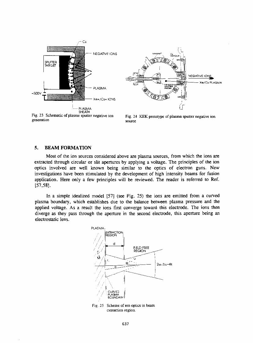
•Cs
L-^ I \ \ - J NEGATIVE IONS
SPUTTER TARGET I T^&T ' — PIASMA
-500V _
Fig. 23 generat
i rrr -500V _
Fig. 23 generat
' — PLASMA SHEATH
Schematic of plasme sputter negative ion ion
Xe/Cs PLASMA
Fig. 24 KEK prototype of plasma sputter negative ion source
5. BEAM FORMATION Most of the ion sources considered above are plasma sources, from which the ions are
extracted through circular or slit apertures by applying a voltage. The principles of the ion optics involved are well known being similar to the optics of electron guns. New investigations have been stimulated by the development of high intensity beams for fusion application. Here only a few principles will be reviewed. The reader is referred to Ref. [57,58].
In a simple idealized model [57] (see Fig. 25) the ions are emitted from a curved plasma boundary, which establishes due to the balance between plasma pressure and the applied voltage. As a result the ions first converge toward this electrode. The ions then diverge as they pass through the aperture in the second electrode, this aperture being an electrostatic lens.
PLASMA,
/ / ,
' n /
EXTRACTION i REGION
d J / / ,
' n / FIELD FREE REGION ^^-^~"
M / r •~\Lr--'^ \ / / e \ " ' - - . 2o=2|v-0| ~ 7 / _ _ - R — — 7 7 ^ " -
2o=2|v-0|
. / M \ ^ ^ ^ ^ ^ • / / \
•' / II CURVED / / !l PLASMA
BOUNDARY
Fig. 25 Scheme of ion optics in beam extraction region.
637
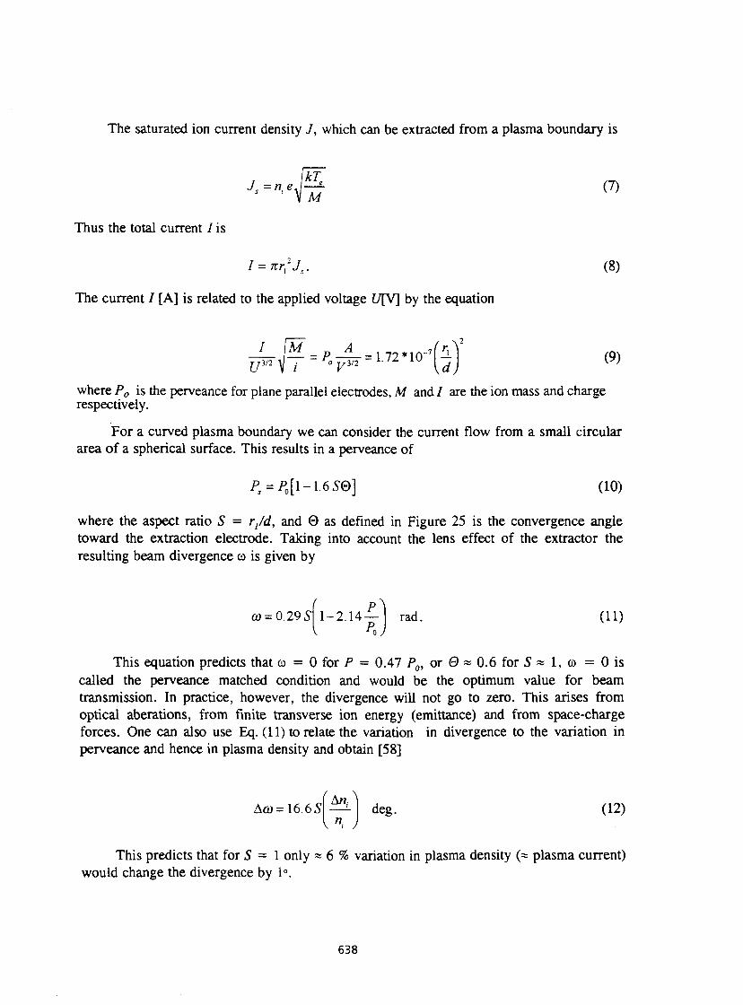
The saturated ion current density J, which can be extracted from a plasma boundary is
Js = ", e
M (7)
Thus the total current / is
I = nr;Js.
The current / [A] is related to the applied voltage U[V] by the equation
(8)
U 3/2 V • ro ym l- I A 1 U
r, Kd (9)
where P0 is the perveance for plane parallel electrodes, M and / are the ion mass and charge respectively.
For a curved plasma boundary we can consider the current flow from a small circular area of a spherical surface. This results in a perveance of
Ps = P0[\-16 SQ] (10)
where the aspect ratio 5 = rjd, and 0 as defined in Figure 25 is the convergence angle toward the extraction electrode. Taking into account the lens effect of the extractor the resulting beam divergence co is given by
CO = 0.29 S P\ 1-2.14 —
V rad. (11)
roJ
This equation predicts that co = 0 for P = 0.47 P0, or 0 « 0.6 for S ~ 1, co = 0 is called the perveance matched condition and would be the optimum value for beam transmission. In practice, however, the divergence will not go to zero. This arises from optical aberations, from finite transverse ion energy (emittance) and from space-charge forces. One can also use Eq. (11) to relate the variation in divergence to the variation in perveance and hence in plasma density and obtain [58]
Aco=16.6S AH,
V ni deg. (12)
This predicts that for S = 1 only « 6 % variation in plasma density (« plasma current) would change the divergence by 1°.
638
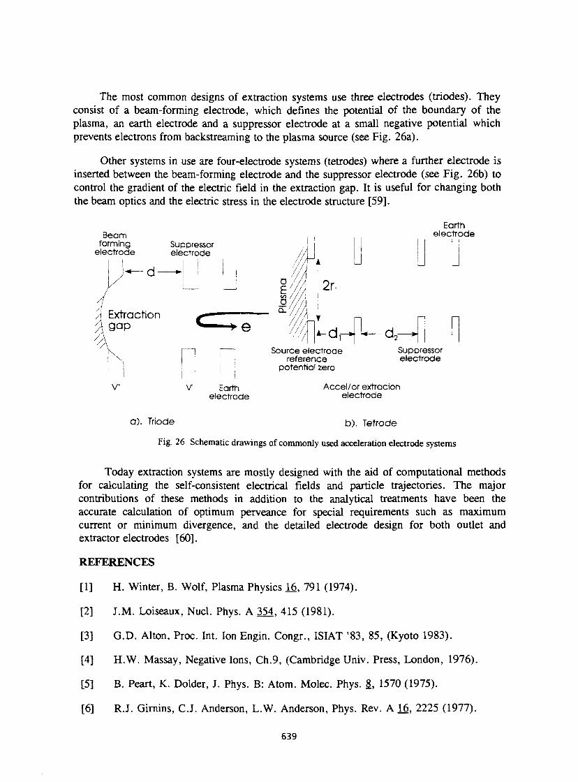
The most common designs of extraction systems use three electrodes (triodes). They consist of a beam-forming electrode, which defines the potential of the boundary of the plasma, an earth electrode and a suppressor electrode at a small negative potential which prevents electrons from backstreaming to the plasma source (see Fig. 26a).
Other systems in use are four-electrode systems (tetrodes) where a further electrode is inserted between the beam-forming electrode and the suppressor electrode (see Fig. 26b) to control the gradient of the electric field in the extraction gap. It is useful for changing both the beam optics and the electric stress in the electrode structure [59].
Beam forming
electrode Suppressor electrode
A Extraction gap
v* V" Earth electrode
Earth electrode
d,—*-Source electrode
reference potential zero
Suppressor electrode
Accel/or extracion electrode
a) . Triode b) . Tetrode
Fig. 26 Schematic drawings of commonly used acceleration electrode systems
Today extraction systems are mostly designed with the aid of computational methods for calculating the self-consistent electrical fields and particle trajectories. The major contributions of these methods in addition to the analytical treatments have been the accurate calculation of optimum perveance for special requirements such as maximum current or minimum divergence, and the detailed electrode design for both outlet and extractor electrodes [60].
REFERENCES
[1] H. Winter, B. Wolf, Plasma Physics 16, 791 (1974).
[2] J.M. Loiseaux, Nucl. Phys. A 354, 415 (1981).
[3] G.D. Alton, Proc. Int. Ion Engin. Congr., ISIAT '83, 85, (Kyoto 1983).
[4] H.W. Massay, Negative Ions, Ch.9, (Cambridge Univ. Press, London, 1976).
[5] B. Peart, K. Dolder, J. Phys. B: Atom. Molec. Phys. 8, 1570 (1975).
[6] R.J. Girnins, C.J. Anderson, L.W. Anderson, Phys. Rev. A 16, 2225 (1977).
639
[7] J. Heinemeier, P. Hvelplund, Nucl. Instr. & Meth. 148, 65 (1975).
[8] J. Heinemeier, P. Hvelplund, Nucl. Instr. & Meth. 148, 425 (1975).
[9] M. Kaminsky, Atomic and Ionic Impact Phenomena on Metal Surfaces (Springer Verlag, New York, 1965).
[10] V.E. Krohn, J. Appl. Phys. 33, 3523 (1962).
[11] J.D. Schneider et al., BNL-51134, 457 (Brookhaven 1979).
[12] R. Keller, Proc. 1984 Lin. Ace. Conf., GSI-84-11, 19 (1984).
[13] I.G. Brown, The Physics and Technology of Ion Sources, Ch. 7, 151, R. Keller, High-Current Gaseous Ion Sources, J. Wiley & Sons (1989).
[14] K.N. Leung, D.A. Bachmann, D.D. Mc Donald, Proc. 1992 Europ. Part. Ace. Conf., Berlin March 24-28, (1992).
[15] N. Sakudo, K. Tokiguchi, H. Koike, I. Kanomata, Rev. Sci. Instr. 48, 762 (1977).
[16] N. Sakudo, Microwave Ion Sources, in Ref. [13], Ch 11, p. 229.
[17] Y. Torii, M. Shimada, I. Watanabe, J. Hippie, C. Hayden, G. Dionne, Rev. Sci. Instr. èl, 253 (1990).
[18] T. Taylor, J.S.C. Wills, Nucl. Instr. Meth. A 309, 37 (1991).
[19] I.G. Brown, J.E. Garvin, B.F. Gavin, R.A. MacGill, Rev. Sci. Instr. 57, 1069 (1986).
[20] I.G. Brown, The Metal Vacuum Vapor Arc Ion Source, in Ref. [13], Ch 16, p. 331.
[21] I.G. Brown, M.R. Dickinson, J.E. Galvin, R.A. MacGill, Rev. Sci. Instr. 63, 2417 (1992).
[22] R.A. Demirkanov, H. Frôhlich, Proc. Int. Conf. on High-Energy. Ace, Brookhaven, p.224 (1962).
[23] C. Lejeune, Nucl. Instr. Meth. 116, 417 (1974).
[24] R. Keller, M. Muller, IEEE Trans. Nucl. Sci. NS-23, 1049 (1976).
[25] C. Bieth et al., IEEE Trans. Nucl. Sci. NS-19, 2 (1972).
[26] P.M. Mozorov et al., Atomnaya Energiya 3, 272 (1957).
[27] A.S. Pasyuk et al., Prib. Tekh. Eksp. 5, 23 (1963).
640
[28] E.D. Donets, IEEE Trans. Nucl. Sci. NS-23, 897 (1976).
[29] J. Arianer, R. Geller, Ann. Rev. Nucl. Part. Sci. 31, 19 (1981).
[30] J. Faure, Proc. 1984 Lin. Ace. Conf., GSI-84-11, p. 103, Darmstadt (1984).
[31] J. Faure, Proc. Int. Conf. on High-Energy Ace, Batavia p. 206 (1983).
[32] R. Becker, M. Kleinod, H. Klein, 2nd EBIS Workshop Saclay-Orsay (1981).
[33] T. Iwai et al., Phys. Rev. A 26, p. 105 (1982).
[34] E.D. Donets, Electron Beam Ion Sources, in Ref. [13], Ch 7, p. 245.
[35] A. Courtois, J. Faure, R. Gobin, P.A. Leroy, B. Visentin, P. Zupranski, Rev. Sci. Instr. 63, 2815 (1992).
[36] Y. Jongen, CM. Lyneis, Electron Cyclotron Resonance Ion Sources, in Ref [13], Ch 10, p. 207.
[37] R. Geller, P. Ludwig, G. Melin, Ref. Sci. Instr. 63, 2795 (1992).
[38] M.P. Bourgarel, M. Bisch, J. Bony, P. Leherissier, J.Y. Pacquet, J.P. Rataud, Ch. Ricaud, Rev. Sci. Instr. 63, 2851 (1992).
[39] G. Melin et al., Rev. Sci. Instr. 61, 236 (1990).
[40] P. Sortais, Rev. Sci. Instr. 63, 2801 (1992).
[41] B.Yu. Sharkov, A.V. Shumshurov, V.B. Dubenkov, O.B. Sharmaev, A.A. Golubev, Rev. Sci. Instr. 63, 2841 (1992).
[42] T. Henkelmann, G. Korschinek, G. Belayev, V. Dubenkov, A. Golubev, S. Latyshev, B. Sharkov, A. Shumshurov, B. Wolf, Rev. Sci. Instr. 63, 2828 (1992).
[43] Y. Amdidouche, H. Haseroth, A. Kuttenberger, K. Langbein, J. Sellmair, T.R. Sherwood, B. Williams, B. Sharkov, O. Sharmaev, Rev. Sci. Instr. 63, 2838 (1992).
[44] K. Prelec, Th. Sluyters, Rev. Sci. Instr. 44, 1451 (1973).
[45] Yu.I. Belchenko, G.I Dimov, V.G. Dudnikov, Bull, Akad. Sci. USSR Phys. Ser. 39, 91 (1973).
[46] J.G. Alessi, Th. Slyuters, Rev. Sci. Instr. 5_i, 1630 (1980).
[47] K.N.Leung, C.A. Hauck, W.B.Kunkel, S.R. Walther, Rev. Sci. Instr. 60, 531 (1989).
[48] K.N. Leung, G.J. DeVries, W.F. DiVergilio, R.W. Hamm, C.A. Hauck, W.B. Kunkel, D.S. McDonald, M.D. Williams, Rev. Sci. Instr. 62, 100 (1991).
641
[49] W. Gentner, G. Hortig, Z. Phys. 172, 357 (1963).
[50] R. Middleton, C.T. Adams, Nucl. Instr. Meth. H8, 329 (1974).
[51] R. Middelton, IEEE Trans. Nucl. Sci. NS-23, 1098 (1976).
[52] K. Prelec, Nucl. Instr. Meth. 144, 413 (1977).
[53] K.N. Leung, K.W. Ehlers, Rev. Sci. Instr. 53, 803 (1982).
[54] G.D. Alton, Y. Mori, A. Takagi, A. Ueno, S. Fukumoto, Nucl. Instr. Meth. A 270. 194 (1988).
[55] Y. Mori, Rev. Sci. Instr. 63, 2357 (1992).
[56] J. Ishikawa, Rev. Sci. Instr. 63, 2368 (1992).
[57] J.R. Coupland, R.S. Green, D.P. Hammond, A.C. Riviere, Rev. Sci. Instr. 44, 1258 (1973).
[58] E. Thompson, Physica 104c, 199 (1981).
[59] T.S. Green, ISIAT '83 & IPAT '83, p. 13 (Kyoto 1983).
[60] P. Spàdtke, GSI Int. Rep., GSI-83-9 (Darmstadt 1983).
642
POSITRON SOURCES
R. Chehab
Laboratoire de l'Accélérateur Linéaire, IN2P3-CNRS et Université de Paris-Sud, 91405 Orsay Cedex, France
Abstract A tentative survey of positron sources is given. Physical processes on which positron generation is based are indicated and analyzed. Explanation of the general features of electromagnetic interactions and nuclear P + decay makes it possible to predict the yield and emittance for a given optical matching system between the positron source and the accelerator. Some kinds of matching systems commonly used - mainly working with solenoidal field - are studied and the acceptance volume calculated. Such knowledge is helpful in comparing different matching systems. Since for large machines, a significant distance exists between the positron source and the experimental facility, positron emittance has to be preserved during beam transfer over large distances and methods used for that purpose are indicated. Comparison of existing positron sources leads to extrapolation to sources for future linear colliders. Some new ideas associated with these sources are also presented.
INTRODUCTION
In recent years, there has been increasing interest in the use of high intensity positron beams in storage and collider rings. With the advent of linear colliders such as SLC or others presently under study, more stringent conditions are imposed on positron intensity and emittance.
Positron beam intensity and emittance are strongly related to the methods of production and collection. Positron generation by electromagnetic interaction or nuclear P + decay present different features which will be analyzed. Thermic processes in the target have also to be considered. However, knowledge of the positron production rate is insufficient to calculate the actual beam intensity which is also dependent on collection devices and, obviously, on linac acceptance. Positron emittance is mainly determined by the converter and the matching system. Very often, longitudinal (À0, ÀE/E) and transverse (x,x?; y, y') emittances have to be reduced to deal with storage ring injection requirements or linear collider interaction point conditions. Beam transport and trajectory control are of particular importance in ensuring that the intensity and emittance of the beam are protected from the effects of wakefields. Some comparisons between existing e + sources will lead to predictions of yields, emittance and the feasibility of positron sources for linear colliders.
1 . PHYSICAL PROCESSES ASSOCIATED WITH POSITRON PRODUCTION
Two kinds of physical processes are generally considered for positron production: the electromagnetic interaction of a photon with the Coulomb field of the nucleus with consequent pair production, and the weak interaction occuring in nuclear P + decay. Coherent pair production in a strong electromagnetic field using a very high energy electron beam could also be foreseen in some particular cases (cf. 2).
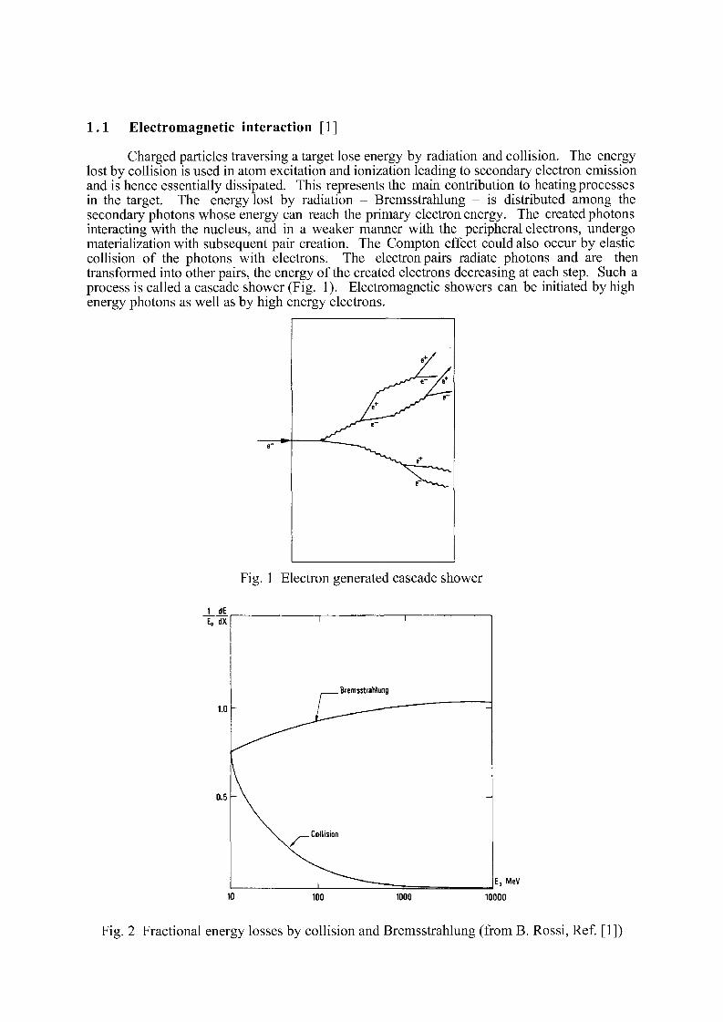
1.1 Electromagnetic interaction [1]
Charged particles traversing a target lose energy by radiation and collision. The energy lost by collision is used in atom excitation and ionization leading to secondary electron emission and is hence essentially dissipated. This represents the main contribution to heating processes in the target. The energy lost by radiation - Bremsstrahlung - is distributed among the secondary photons whose energy can reach the primary electron energy. The created photons interacting with the nucleus, and in a weaker manner with the peripheral electrons, undergo materialization with subsequent pair creation. The Compton effect could also occur by elastic collision of the photons with electrons. The electron pairs radiate photons and are then transformed into other pairs, the energy of the created electrons decreasing at each step. Such a process is called a cascade shower (Fig. 1). Electromagnetic showers can be initiated by high energy photons as well as by high energy electrons.
Fig. 1 Electron generated cascade shower
1 dE E, dX 1
Bremsstrahlung
1
1.0
1
Bremsstrahlung
0.5 -
N. Collision
I • — I — E0 MeV
100 1000 10000
Fig. 2 Fractional energy losses by collision and Bremsstrahlung (from B. Rossi, Ref [1])
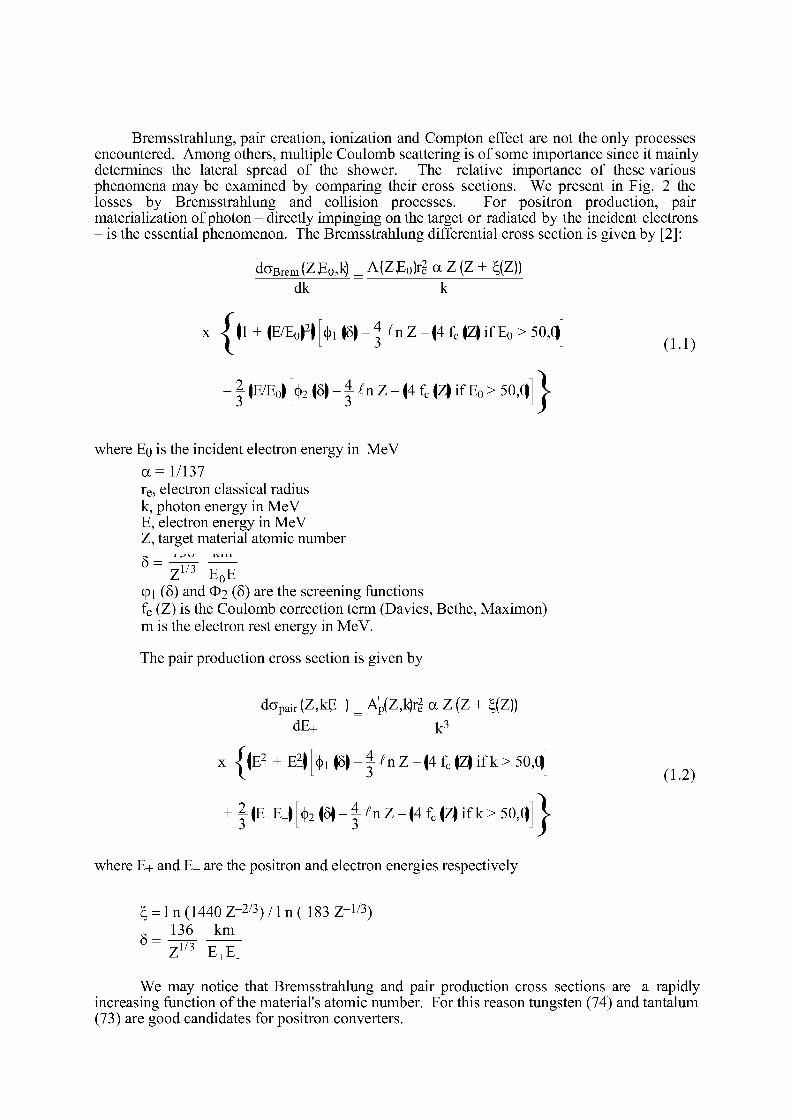
Bremsstrahlung, pair creation, ionization and Compton effect are not the only processes encountered. Among others, multiple Coulomb scattering is of some importance since it mainly determines the lateral spread of the shower. The relative importance of these various phenomena may be examined by comparing their cross sections. We present in Fig. 2 the losses by Bremsstrahlung and collision processes. For positron production, pair materialization of photon- directly impinging on the target or radiated by the incident electrons - is the essential phenomenon. The Bremsstrahlung differential cross section is given by [2]:
dGBrem(ZE0,k) _ A(ZE 0)r| a Z (Z + Ç(Z)) dk k
x | | l + (E /Eop}^ i (ô | - ^nZ- (4 f c (Z | i fE 0 >50 ,C | j
- 1 (E/Eoj [fa (ô| - Un Z - (4 fc (ZJ if E 0 > 50,0)] |
where Eo is the incident electron energy in MeV a =1/137 r e, electron classical radius k, photon energy in MeV E, electron energy in MeV Z, target material atomic number L ^J \J 1V111
Z 1 / 3 E 0 E cpi (ô) and ©2 ($) a r e the screening functions fc (Z) is the Coulomb correction term (Davies, Bethe, Maximon) m is the electron rest energy in MeV.
The pair production cross section is given by
d a p a i r (Z,kE+) _ Ap(Z,k)rj a Z (Z + Ç(Z)) dE + k 3
x | | E Î + E2} [fa (8\-UnZ- (4 fc (Zj if k > 50,0)
+ | ( E + E_| [fa (5)-UnZ- (4 fc (Z| if k > 50,()] i
where E+ and E_ are the positron and electron energies respectively
Ç = 1 n (1440 Z" 2 / 3 ) / 1 n ( 183 Z" 1 / 3 ) 136 km
8 = Z 1 / 3 E,E.
(1.2)
We may notice that Bremsstrahlung and pair production cross sections are a rapidly increasing function of the material's atomic number. For this reason tungsten (74) and tantalum (73) are good candidates for positron converters.
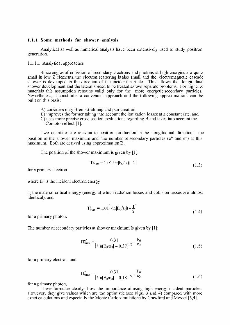
1.1.1 Some methods for shower analysis
Analytical as well as numerical analysis have been extensively used to study positron generation.
1.1.1.1 Analytical approaches
Since angles of emission of secondary electrons and photons at high energies are quite small in low Z elements, the electron scattering is also small and the electromagnetic cascade shower is developed in the direction of the incident particle. This allows the longitudinal shower development and the lateral spread to be treated as two separate problems. For higher Z materials this assumption remains valid only for the more energetic secondary particles. Nevertheless, it constitutes a convenient approach and the following approximations can be built on this basis:
A) considers only Bremsstrahlung and pair creation. B) improves the former taking into account the ionization losses at a constant rate, and C) uses more precise cross section evaluations regarding B and takes into account the
Compton effect [1].
Two quantities are relevant to positron production in the longitudinal direction: the position of the shower maximum and the number of secondary particles (e + and e~) at this maximum. Both are derived using approximation B.
The position of the shower maximum is given by [1]:
T W = 1 . 0 1 M E 0 / S 0 | - 1 ] (1.3) for a primary electron
where Eo is the incident electron energy
so the material critical energy (energy at which radiation losses and collision losses are almost identical), and
TU = 1.0l[HEo/so}-[] for a primary photon.
The number of secondary particles at shower maximum is given by [1]:
ne- 0.31 Ik n(E 0 /s 0 | -0 .37] 1 / 2 S ° (1.5)
xmax
for a primary electron, and
nY 0.31 Eo m a X ^ n ( E 0 / s 0 } - 0 . 1 8 ] 1 / 2 ' S o (1-6)
for a primary photon. These formulae clearly show the importance of using high energy incident particles.
However, they give values which are too optimistic (see Figs. 3 and 4) compared with more exact calculations and especially the Monte Carlo simulations by Crawford and Messel [3,4].
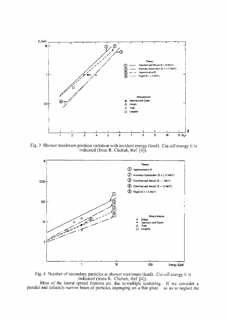
E„(GeV)
10
1 -
0.1 -
— 1 1 1 1 1
(T) .
/ /
i
s
I T i l l 1 1 1 1 1
(T) .
/ /
Theory /s/
m Crawford and Mcsscl <E = 10 McV)
jy' ' (?) Ivanenlco-Samosudov (E = 1.13 McV)
jy' ' (TÏ Approximation B
/ ' /
/ D /
? y/
© Nagcl(E=1.5McV)
Measurements
®-?f • j&keways and Calder
'/ A
0
Nelson
Yuda
i i i i i \
D Lengeler
1 1 1 I 1
10 " ix„
Fig. 3 Shower maximum position variation with incident energy (lead). Cut-off energy E is indicated (from R. Chehab, Ref. [4]).
N Theory
© Approximation B
® Ivanenko-Samosudov (E = 1.13 MeV)
1000 ® Crawford and Messel (E = 1 MeV)
® Crawford and Messel (E = 10 MeV)
P ® N a g e l ( E = 1 . 5 M e V )
100 I ^ i &
10
Measurements
X Drikcy • Jakeways and Calder A Yuda Q Lengeler
1
1 1 i
10 100 Energy (GeV)
Fig. 4 Number of secondary particles at shower maximum (lead). Cut-off energy E is indicated (from R. Chehab, Ref. [4]).
Most of the lateral spread features are due to multiple scattering. If we consider a parallel and infinitely narrow beam of particles impinging on a thin plate - so as to neglect the
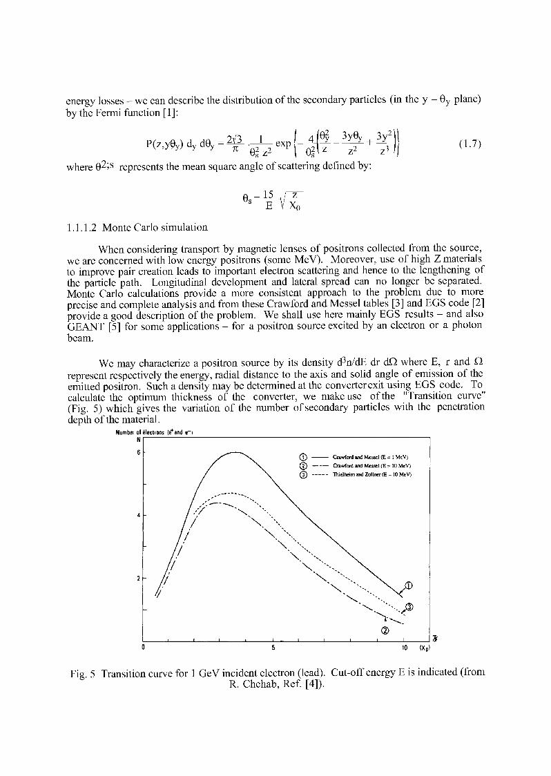
energy losses - we can describe the distribution of the secondary particles (in the y - 9 y plane) by the Fermi function [1]:
P ( z ^ ) d y d ^2fi^exp{- | ( f -^ + | - )J (,.7) where &2;s represents the mean square angle of scattering defined by:
1.1.1.2 Monte Carlo simulation
When considering transport by magnetic lenses of positrons collected from the source, we are concerned with low energy positrons (some MeV). Moreover, use of high Z materials to improve pair creation leads to important electron scattering and hence to the lengthening of the particle path. Longitudinal development and lateral spread can no longer be separated. Monte Carlo calculations provide a more consistent approach to the problem due to more precise and complete analysis and from these Crawford and Messel tables [3] and EGS code [2] provide a good description of the problem. We shall use here mainly EGS results - and also GEANT [5] for some applications - for a positron source excited by an electron or a photon beam.
We may characterize a positron source by its density d3n/dE dr dQ where E, r and Q represent respectively the energy, radial distance to the axis and solid angle of emission of the emitted positron. Such a density may be determined at the converter exit using EGS code. To calculate the optimum thickness of the converter, we make use of the "Transition curve" (Fig. 5) which gives the variation of the number of secondary particles with the penetration depth of the material.
Number of électrons le*and e"t
Fig. 5 Transition curve for 1 GeV incident electron (lead). Cut-off energy E is indicated (from R. Chehab, Ref. [4]).
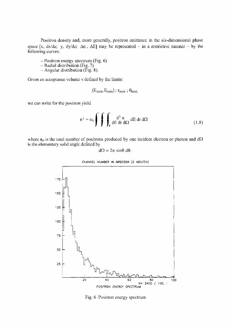
Positron density and, more generally, positron emittance in the six-dimensional phase space [x, dx/dz; y, dy/dz; A§ , AE] may be represented - in a restrictive manner - by the following curves:
- Positron energy spectrum (Fig. 6) - Radial distribution (Fig. 7) - Angular distribution (Fig. 8).
Given an acceptance volume v defined by the limits:
axj
we can write for the positron yield
n T = n 0
I I d 3 n J J dEdrdQ
dEdrdQ (1.8)
where rio is the total number of positrons produced by one incident electron or photon and dQ is the elementary solid angle defined by
dQ - 2TI sin9 d9.
CHANNEL NUMBER IN ABSCISSA (2 MEV/CH)
175. -•
150 -L
125 • 1 100 -
75 -f
\
50 -
\ 25 -
! I U IW^ lk^ lT l _ n -r J-TL _ P-_ r-i_ H 20 4-0 60 80 100
N= 2400 / 100, I POSITRON ENERGY SPECTRUM
Fig. 6 Positron energy spectrum
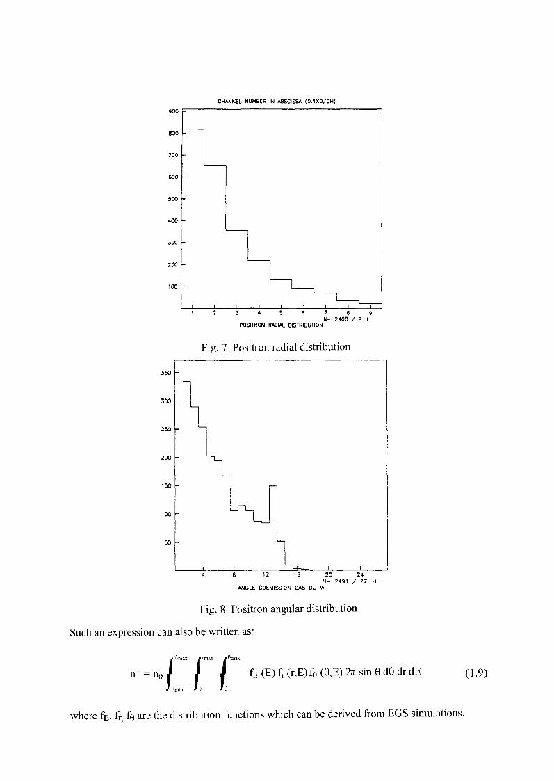
CHANNEL NUMBER N ABSCISSA (0.1XO/CH)
900
800
700
1 I
1 1
1 1
1 1
600
500
400
1 I
1 1
1 1
1 1
300
1 I
1 1
1 1
1 1
200
1 I
1 1
1 1
1 1
100 1 I
1 1
1 1
1 1
| 1 I
1 1
1 1
1 1
1
1 I
1 1
1 1
1 1
1
1 I
1 1
1 1
1 1
1 I
1 1
1 1
1 1
1 1 1 1 1 1 ! 1 1 2 3 4 5 6 7 8 9
N= 2408 / 9. II POSITRON RADIAL DISTRIBUTION
Fig. 7 Positron radial distribution
350
300
250
200
" S 150 -
100 -
50
I 1 I H - i — i i 8 12 16 20 24
N= 2491 / 27, H-ANGLE D9EMISSI0N CAS DU W
Fig. 8 Positron angular distribution
Such an expression can also be written as:
n + = n 0
* Emax / rmax £ Sm
/ E m m *0 / 0
fE (E) fr (r,E) fe (9,E) 2re sin 9 d9 dr dE (1
where fE, fr fe are the distribution functions which can be derived from EGS simulations.
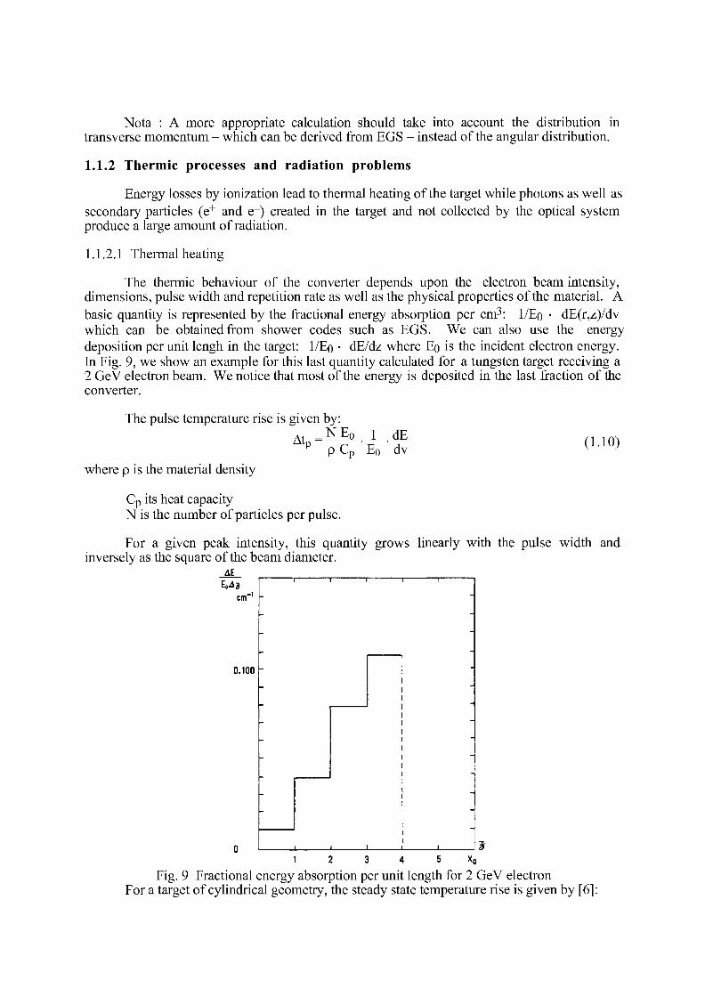
Nota : A more appropriate calculation should take into account the distribution in transverse momentum - which can be derived from EGS - instead of the angular distribution.
1.1.2 Thermic processes and radiation problems
Energy losses by ionization lead to thermal heating of the target while photons as well as secondary particles (e + and e~) created in the target and not collected by the optical system produce a large amount of radiation.
1.1.2.1 Thermal heating
The thermic behaviour of the converter depends upon the electron beam intensity, dimensions, pulse width and repetition rate as well as the physical properties of the material. A basic quantity is represented by the fractional energy absorption per cm3: 1/Eo • dE(r,z)/dv which can be obtained from shower codes such as EGS. We can also use the energy deposition per unit lengh in the target: 1/Eo • dE/dz where Eo is the incident electron energy. In Fig. 9, we show an example for this last quantity calculated for a tungsten target receiving a 2 GeV electron beam. We notice that most of the energy is deposited in the last fraction of the converter.
The pulse temperature rise is given by: . N E 0 Atr p C F Eo
dE dv (1.10)
where p is the material density
Cp its heat capacity N is the number of particles per pulse.
For a given peak intensity, this quantity grows linearly with the pulse width and inversely as the square of the beam diameter.
AE E 043
0.100
1 2 3 4 5 X„
Fig. 9 Fractional energy absorption per unit length for 2 GeV electron For a target of cylindrical geometry, the steady state temperature rise is given by [6]:
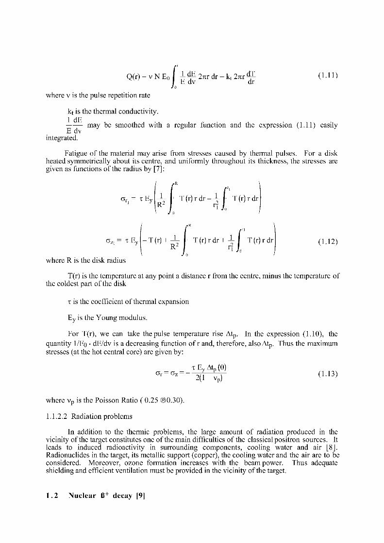
Q(r) = v N E 0 I -L^2;irdr = k t 27irÇ (LU) | E dv dr Jo
where v is the pulse repetition rate
kt is the thermal conductivity. 1 dE
may be smoothed with a regular function and the expression (1.11) easily E dv
integrated. Fatigue of the material may arise from stresses caused by thermal pulses. For a disk
heated symmetrically about its centre, and uniformly throughout its thickness, the stresses are given as functions of the radius by [7]:
I f J- l T(r)rdr-J-
J 0
aIt= T E y Mt- J1 T ( r ) r d r - - L | ' T(r)rdr R 2
/ r n
T(r) + J - ' T ( r ) r d r + J - | T(r)rdr
where R is the disk radius
CTZl = X E y (1.12)
T(r) is the temperature at any point a distance r from the centre, minus the temperature of the coldest part of the disk
x is the coefficient of thermal expansion
Ey is the Young modulus.
For T(r), we can take the pulse temperature rise Atp. In the expression (1.10), the quantity 1/Eo • dE/dv is a decreasing function of r and, therefore, alsoAtp. Thus the maximum stresses (at the hot central core) are given by:
x E y Atp (0)
where v p is the Poisson Ratio ( 0.25 ®0.30).
1.1.2.2 Radiation problems
In addition to the thermic problems, the large amount of radiation produced in the vicinity of the target constitutes one of the main difficulties of the classical positron sources. It leads to induced radioactivity in surrounding components, cooling water and air [8]. Radionuclides in the target, its metallic support (copper), the cooling water and the air are to be considered. Moreover, ozone formation increases with the beam power. Thus adequate shielding and efficient ventilation must be provided in the vicinity of the target.
1.2 Nuclear B+ decay [9]
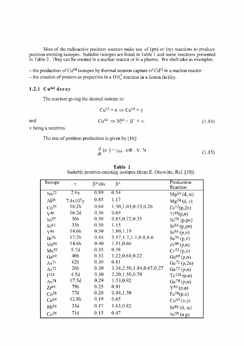
Most of the radioactive positron sources make use of (pn) or (ny) reactions to produce positron emitting isotopes. Suitable isotopes are listed in Table 1 and some reactions presented in Table 2. They can be created in a nuclear reactor or in a plasma. We shall take as examples:
- the production of Cu 6 4 isotopes by thermal neutron capture of Cu 6 3 in a nuclear reactor - the creation of protons as projectiles in a DH e reaction in a fusion facility.
1.2.1 C u 6 4 decay
The reaction giving the desired isotope is:
Cu 6 3 + n => Cu 6 4 + y
and Cu 6 4 => N^ 4 + p + + v : (1.14) v being a neutrino.
The rate of positron production is given by [10]:
^ ( n + ) = Y 6 4 . o ô . V . N ( 1 1 5 )
Table 1 Suitable positron-emitting isotopes (from E. Ottewitte, Ref. [10])
Isotope x R+/dis B+ Production Reaction
° - 5 4 Mg2 4 (d, a) 1 1 7 Mg 2 4 (d ,y) 1.50,1.03,0.53,0.26 Fe 1 2(p,2n) 0.69 Ti 4 8(p,n) 0.85,0.72,0.35 N i 5 8 (p , p n ) !-!5 Sr 8 4(p,pn) 1.80,1.19 Sr86 ( p ,n) 3.57,1.7,1.1,0.8,0.6 Se76 (p,n) 1.51,0.66 Zr90(p,n) 0-58 Cr52(p,n) 1.22,0.61,0.22 Ga69(p,n) 0-81 Ge 7 2(p,2n) 3.34,2.50,1.84,0.67,0.27 G e 7 2 (p^) 2.20,1.50,0.70 Tel2 4(p,n) 1.53,0.92 Ge 7 4 (p,n) 0.91 Y89(p, n) 0.44,1.50 Fe 5 6(p,n) 0.65 C u 6 3 ( n > y ) 1.63,0.82 Sr86(d, a) ° - 4 7 Ni 5 8(np)
Na 2 2 2.6y 0.89 A 126 7.4xl0 5y 0.85
Co 5 5 18.2h 0.60 V48 16.2d 0.56 N i 5 7 36h 0.50 Sr83 33h 0.50 y86 14.6h 0.50 B r 76 17.2h 0.44 Nb90 14.6h 0.40 Mn 5 2 5.7d 0.35 Ge69 40h 0.33 As71 62h 0.30 As 7 2 26h 0.30 J124 4.5d 0.30 A s 7 4 17.5d 0.29 Zr89 79h 0.25 Co 5 6 77d 0.20 Cu64 12.8h 0.19 R b 8 4 33d 0.17
Co 5 8 71d 0.15
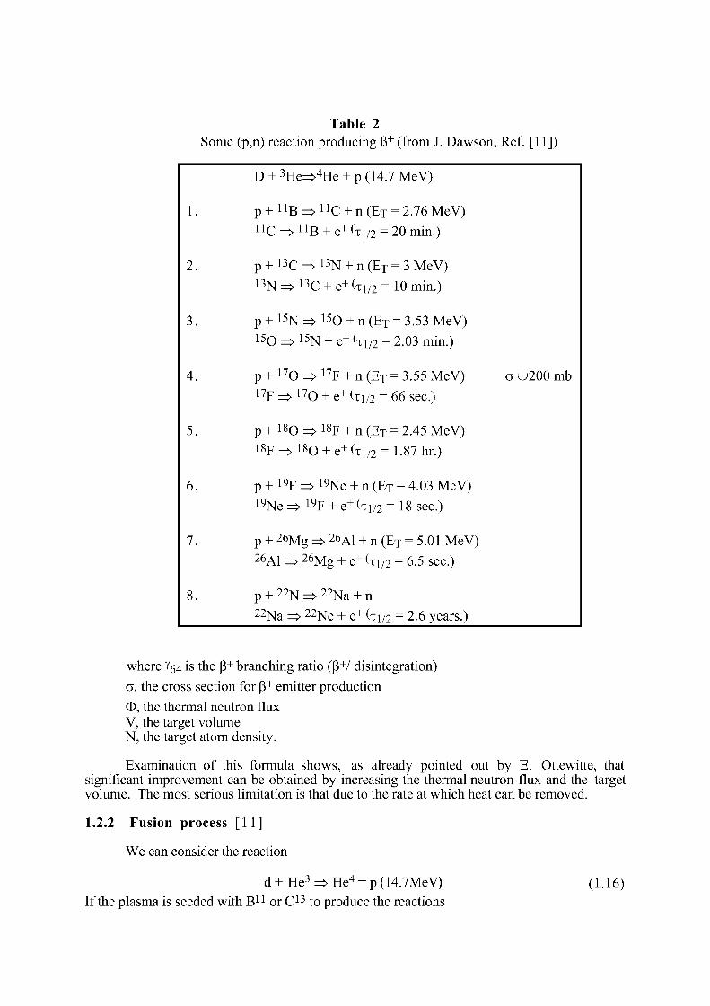
Table 2 Some (p,n) reaction producing R+ (from J. Dawson, Ref. [11])
D + 3 H e ^ 4 H e + p (14.7 MeV)
1. p + llB => n C + n (E T = 2.76 MeV) n C => n B + e+ (xi/2 = 20 min.)
2. p + 13C => 1 3 N + n (E T = 3 MeV) 13 N _> 13c + e+ (xi/2 = 10 min.)
3. p + 15N => 150 + n (E T = 3.53 MeV) 150 => 1 5 N + e+ (xi/2 = 2.03 min.)
4. p + 170 => i 7 F + n (E T = 3.55 MeV) 17F => l7o + e+ (xi/2 = 66 sec.)
a u200 mb
5. p + 180 => i 8 F + n (E T = 2.45 MeV) 1 8 F ^ 1 8 0 + e+(xi/2 = 1.87hr.)
6. p + 19F => 19Ne + n (E T = 4.03 MeV) l9Ne => i 9 F + e+ (xi/2 = 18 sec.)
7. p + 2 6 Mg => 2 6A1 + n (E T = 5.01 MeV) 26Al ^> 26Mg + e + (xi/2 = 6.5 sec.)
8. p + 22N => 22^ a + n 22Na ^> 22^e + e + (xi/2 = 2.6 years.)
where Y(>4 is the P + branching ratio (P +/ disintegration) a, the cross section for P+ emitter production O, the thermal neutron flux V, the target volume N, the target atom density.
Examination of this formula shows, as already pointed out by E. Ottewitte, that significant improvement can be obtained by increasing the thermal neutron flux and the target volume. The most serious limitation is that due to the rate at which heat can be removed.
1.2.2 Fusion process [11]
We can consider the reaction
d + H e 3 ^ H e 4 = p(14.7MeV) (1.16) If the plasma is seeded with B 1 1 or C i 3 to produce the reactions
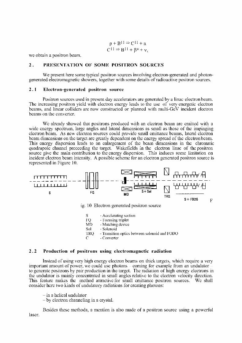
p + B 1 1 = > C n + n C n ^ B n + p+ + v,
we obtain a positron beam.
2 . PRESENTATION OF SOME POSITRON SOURCES
We present here some typical positron sources involving electron-generated and photon-generated electromagnetic showers, together with some details of radioactive positron sources.
2.1 Electron-generated positron source
Positron sources used in present day accelerators are generated by a linac electron beam. The increasing positron yield with electron energy leads to the use of very energetic electron beams, and linear colliders are now constructed or planned with multi-GeV incident electron beams on the converter.
We already showed that positrons produced with an electron beam are emitted with a wide energy spectrum, large angles and lateral dimensions as small as those of the impinging electron beam. As new electron sources could provide small emittance beams, lateral electron beam dimensions on the target are greatly dependent on the energy spread of the electronbeam. This energy dispersion leads to an enlargement of the beam dimensions in the chromatic quadrupole channel preceeding the target. Wakefields in the electron linac of the positron source give the main contribution to the energy dispersion. This induces some limitation on incident electron beam intensity. A possible scheme for an electron generated positron source is represented in Figure 10.
I I I I I I I I I I I
' ' ' ' I
s
ISI H ffiffliWfl
FQ S+Sol ^ 'iV'iV'iV/ti TRQ
S+F0D0
ig. 10 Electron generated positron source
S - Accelerating section FQ - Focusing triplet MD - Matching device Sol - Solenoid TRQ - Transition optics between solenoid and FODO C - Converter
2.2 Production of positrons using electromagnetic radiation
Instead of using very high energy electron beams on thick targets, which require a very important amount of power, we could use photons - coming for example from an undulator -to generate positrons by pair production in the target. The radiation of high energy electrons in the undulator is mainly concentrated in small angles relative to the electron velocity direction. This feature makes the method attractive for small emittance positron sources. We shall consider here two kinds of undulatory radiations for creating photons:
- in a helical undulator - by electron channeling in a crystal.
Besides these methods, a mention is also made of a positron source using a powerful laser.
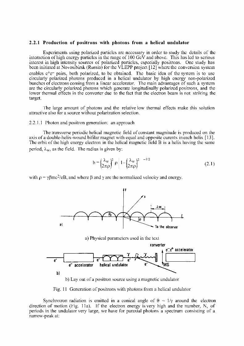
2.2.1 Production of positrons with photons from a helical undulator
Experiments using polarized particles are necessary in order to study the details of the interaction of high energy particles in the range of 100 GeV and above. This has led to serious interest in high intensity sources of polarized particles, especially positrons. One study has been initiated at Novosibirsk (Russia) for the VLEPP project [12] where the conversion system enables e+e~ pairs, both polarized, to be obtained. The basic idea of the system is to use circularly polarized photons produced in a helical undulator by high energy non-polarized bunches of electrons coming from a linear accelerator. The main advantages of such a system are the circularly polarized photons which generate longitudinally polarized positrons, and the lower thermal effects in the converter due to the fact that the electron beam is not striking the target.
The large amount of photons and the relative low thermal effects make this solution attractive also for a source without polarization selection.
2.2.1.1 Photon and positron generation: an approach
The transverse periodic helical magnetic field of constant magnitude is produced on the axis of a double-helix-wound bifilar magnet with equal and opposite curents in each helix [13]. The orbit of the high energy electron in the helical magnetic field B is a helix having the same period, Xw, as the field. The radius is given by:
- f e l 2
P \27ip
-1/2 (2.1)
with p = y[3mc2/eB, and where P and y are the normalized velocity and energy.
To the observer
a) Physical parameters used in the text converter
i e"7e+ accelerator
e~ accelerator helical undulator
b)
rTTY)
b) Lay out of a positron source using a magnetic undulator
Fig. 11 Generation of positrons with photons from a helical undulator
Synchrotron radiation is emitted in a conical angle of 9 ~ 1/y around the electron direction of motion (Fig. 11a). If the electron energy is very high and the number, N, of periods in the undulator very large, we have for paraxial photons a spectrum consisting of a narrow-peak at:
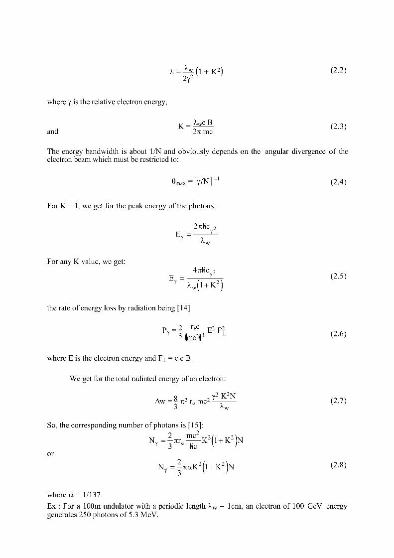
À,, X = A W ( I + K 2 ) (2-2) 2y2
where y is the relative electron energy,
and 27i me
The energy bandwidth is about 1/N and obviously depends on the angular divergence of the electron beam which must be restricted to:
e m a x = [yVN] - 1 (2.4)
For K = 1, we get for the peak energy of the photons:
27lhc 2 E = y—
w
For any K value, we get: 47ihc 2
the rate of energy loss by radiation being [14]
p = 2 _ T e C _ E 2 F 2 Y 3(m c2}3 ± (2.6)
where E is the electron energy and F^ = e c B.
We get for the total radiated energy of an electron:
. 8 . 2 y 2 K 2 N Aw = 5- 7i2 r e mc 2 - ^ (2.7) 3 Aw
So, the corresponding number of photons is [15]:
N = ^ r e - ^ K 2 ( l + K 2)N Y 3 e he v '
or N y = - T U X K 2 ( I + K 2 ) N (2-8)
where a = 1/137. Ex : For a 100m undulator with a periodic length Xw = 1cm, an electron of 100 GeV energy generates 250 photons of 5.3 MeV.
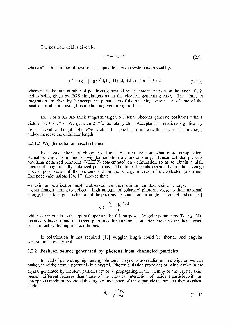
The positron yield is given by :
Tf = NY n+ (2.9)
where n + is the number of positrons accepted by a given system expressed by:
n+ = n 0 (H fE (E) fr (r,E) fe (9,E) dE dr 2% sin 9 d9 (2.10)
where no is the total number of positrons generated by an incident photon on the target, fj? fe and fr being given by EGS simulations as in the electron generating case. The limits of integration are given by the acceptance parameters of the matching system. A scheme of the positron production using this method is given in Figure 1 lb.
Ex : For a 0.2 Xo thick tungsten target, 5.3 MeV photons generate positrons with a yield of 8.10"3 e+/y. We get then 2 e+/e~ as total yield. Acceptance limitations significantly lower this value. To get higher e+/e~ yield values one has to increase the electron beam energy and/or increase the undulator length.
2.2.1.2 Wiggler radiation based schemes
Exact calculations of photon yield and spectrum are somewhat more complicated. Actual schemes using intense wiggler radiation are under study. Linear collider projects requiring polarized positrons (VLEPP) concentrated on optimization so as to obtain a high degree of longitudinally polarized positrons. The latter depends essentially on the average circular polarization of the photons and on the energy interval of the collected positrons. Extended calculations [16, 17] showed that:
- maximum polarization must be observed near the maximum emitted positron energy, - optimization aiming to collect a high amount of polarized photons, close to their maximal energy, leads to angular selection of the photons. A characteristic angle is then defined as: [16]
T 9 - ( ' + K 2 ) " 2
' 3 which corresponds to the optimal aperture for this purpose. Wiggler parameters (B, Xw ,N), distance between it and the target, photon collimation and converter thickness are then chosen so as to realize the required conditions.
If polarization is not required [18] wiggler length could be shorter and angular separation is less critical.
2.2.2 Positron source generated by photons from channeled particles
Instead of generating high energy photons by synchrotron radiation in a wiggler, we can make use of the atomic potentials in a crystal. Photon emission processes or pair creation in the crystal generated by incident particles (e~ or y) propagating in the vicinity of the crystal axis, present different features than those of the classical interaction of incident particles with an amorphous medium, provided the angle of incidence of these particles is smaller than a critical angle:
° c V Eo (2-11)
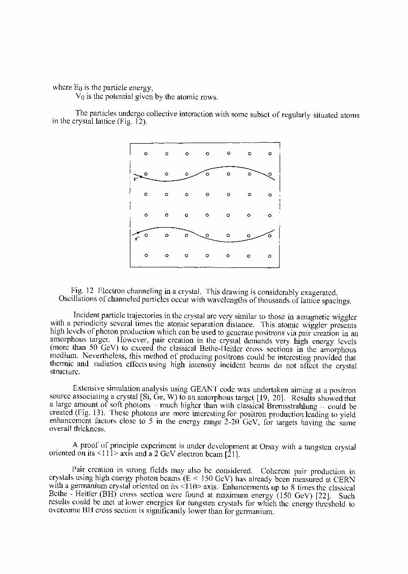
where Eo is the particle energy, Vo is the potential given by the atomic rows.
The particles undergo collective interaction with some subset of regularly situated atoms in the crystal lattice (Fig. 12).
Fig. 12 Electron channeling in a crystal. This drawing is considerably exagerated. Oscillations of channeled particles occur with wavelengths of thousands of lattice spacings.
Incident particle trajectories in the crystal are very similar to those in a magnetic wiggler with a periodicity several times the atomic separation distance. This atomic wiggler presents high levels of photon production which can be used to generate positrons via pair creation in an amorphous target. However, pair creation in the crystal demands very high energy levels (more than 50 GeV) to exceed the classical Bethe-Heitler cross sections in the amorphous medium. Nevertheless, this method of producing positrons could be interesting provided that thermic and radiation effects using high intensity incident beams do not affect the crystal structure.
Extensive simulation analysis using GEANT code was undertaken aiming at a positron source associating a crystal [Si, Ge, W) to an amorphous target [19, 20]. Results showed that a large amount of soft photons - much higher than with classical Bremsstrahlung - could be created (Fig. 13). These photons are more interesting for positron production leading to yield enhancement factors close to 5 in the energy range 2-20 GeV, for targets having the same overall thickness.
A proof of principle experiment is under development at Orsay with a tungsten crystal oriented on its <111> axis and a 2 GeV electron beam [21].
Pair creation in strong fields may also be considered. Coherent pair production in crystals using high energy photon beams (E < 150 GeV) has already been measured at CERN with a germanium crystal oriented on its <110> axis. Enhancements up to 8 times the classical Bethe - Heitler (BH) cross section were found at maximum energy (150 GeV) [22]. Such results could be met at lower energies for tungsten crystals for which the energy threshold to overcome BH cross section is significantly lower than for germanium.
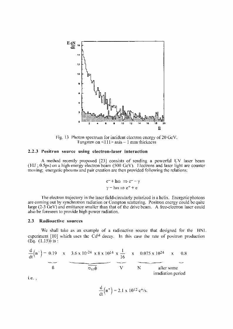
EdN dE
10 12 14 16 IS 20
Fig. 13 Photon spectrum for incident electron energy of 20 GeV. Tungsten on <111> axis - 1 mm thickness
2.2.3 Positron source using electron-laser interaction
A method recently proposed [23] consists of sending a powerful UV laser beam (10J ; 0.5ps) on a high energy electron beam (500 GeV). Electrons and laser light are counter moving; energetic photons and pair creation are then provided following the relations:
e~ + hco => e~ + y y + hco => e + + e~
The electron trajectory in the laser field-circularly polarized is a helix. Energetic photons are coming out by synchrotron radiation or Compton scattering. Positron energy could be quite large (2-3 GeV) and emittance smaller than that of the drive beam. A free-electron laser could also be foreseen to provide high power radiation.
2.3 Radioactive sources
We shall take as an example of a radioactive source that designed for the BNL experiment [10] which uses the Ci£4 decay. In this case the rate of positron production (Eq. (1.15)) is :
_d_ dt M 0.19 x 3 .6x l0 - 2 4 x 8 x l 0 1 4 x — x 0.075 x 10 2 4 x 0.8
16
R+
i.e.
°63^ V N after some irradiation period
— ( n + ) = 2 . 1 x l 0 1 2 e + / s . dt' /

Higher e + fluxes have been obtained by test reactors e.g. INEL/ATR (Idaho National Engineering Laboratory, US Navy) with more than 10 1 7 e +/s. These reactors require large irradiation volumes to perform multi-magnitude increase in positron production. Thus, the INEL/ATR has nine large channels presenting a total irradiation volume of 2.6 x 10* cm3: such a facility allows more than a factor of 5 in magnitude improvement of the positron production.
As mentioned before, e + rate improvement using larger source volumes poses two difficult problem :
- how to transform from a large, voluminous positron source into a compact beam - increasing the volume may lead to self absorption, so a limitation on thickness exists.
3 . POSITRON COLLECTION: THE MATCHING SYSTEM
The characteristic emittance of the positron source at the converter - large angles, small lateral dimensions - has to be transformed into small angles, large lateral dimensions, so as to fit with the accelerator acceptance. The choice of the matching device is therefore dependent on:
- the expected positron yield
- the allowed energy dispersion.
Two kinds of matching devices are now mainly used on positron accelerators:
- narrow-band systems such as the quarter-wave transformer
- large-band systems such as the adiabatic device.
Other kinds of matching devices such as the lithium and plasma lens may also be used.
3.1 Matching devices using a solenoidal magnetic field [4, 24]
3.1.1 The solenoidal magnetic field Due to the cylindrical symmetry of the solenoid about the z axis, the only non-zero
component of the potential vector A in cylindrical coordinates (r, o, z) is: A - - 2 B W - W ' 3 ^ ( 3 ' 1 )
The Lagrangian,
L = - m 0 c 2 V l - v 2 / c 2 - { V - A . v )
may be expressed in these coordinates as;
L - m o r f - / 7 ^ 3 ^ - e ( v - * a ) . (3.2)
Conjugate variables (q, p) are defined by:
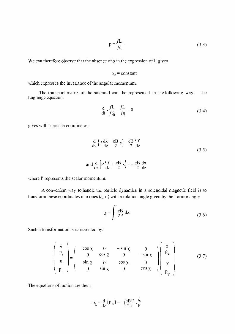
./L /q
(3.3)
We can therefore observe that the absence of § in the expression of L gives
P(|) = constant
which expresses the invariance of the angular momentum.
The transport matrix of the solenoid can be represented in the following way. The Lagrange equation:
A Ik_fk = 0
dt'/qj /q (3.4)
gives with cartesian coordinates:
j L ( p d x _ e B v \ = eB dy dzV dz 2 y! 2 dz
(3.5)
a n d f ( p ^ + e & x dz \ dz 2 eBdx 2 dz
where P represents the scalar momentum.
A convenient way to handle the particle dynamics in a solenoidal magnetic field is to transform these coordinates into ones ( , r\) with a rotation angle given by the Larmor angle
Y = j eB d z 1 2P
Jo (3.6)
Such a transformation is represented by:
/ 4 \
n
cosx 0 -s inx 0 0 cosx 0 -s inx
sinx 0 cosx 0 0 sinx 0 cosx
X
p x
y
p.
(3.7)
\ P v /
The equations of motion are then:
p5=^')=-(fM
P T I d z t P T l j "IT/ 'p
(3.8)
Motions for £, and r\ are decoupled and can be handled separately. The equations (3.8) may be written:
"+ £ E + ( # F S = 0
V+ fî,'+ fêgVo (3.9)
For a constant field B, and in the absence of an accelerating field, these equations are those of a classical harmonic oscillator of constant frequency eB/2P. The transformation matrix is then, in the ( , p £ ) plane for example,
cosx
eB
2 • \ ~"êr sin y eB K
\ - ^ s i n x cosx / (3.10)
We can associate with the variables ( , p^) and (r\ p^), the Hamiltonians:
u , = eBc \eB %2 + 2 n 2 H l 4P I 2 ^ eB J
H = eBc feB_ _2 + _2_ «2 4P L 2 eB
(3.11)
If we define a frequency co ebc 4TTP
, the quantity:
H 71 eB %2 i 2 n 2 2 ^ eB P ^
(3.12)
is an adiabatic invariant of the motion. So, we can write:
jeJij2 (ç2 + ^2) + Jp2 + p 2j = constant
Coming back to the variables [x px ; y p y ] , we may writ :
feR)2 (X2 + y2) + (p2 + p2) = constant (3.13)
This relation holds everywhere in the ©lenoid. It represents the equation of a hyperellipsoid in the phase space [x px ; y p y ] . The volume comprised in this hyperellipsoid is constant [Liouville Theorem].
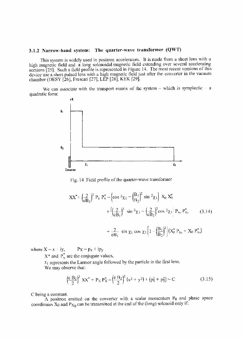
3.1.2 Narrow-band system: The quarter-wave transformer (QWT)
This system is widely used in positron accelerators. It is made from a short lens with a high magnetic field and a long solenoidal magnetic field extending over several accelerating sections [25]. Such a field profile is represented in Figure 14. The most recent versions of this device use a short pulsed lens with a high magnetic field just after the converter in the vacuum chamber (DESY [26], Frascati [27], LEP [28], KEK [29].
We can associate with the transport matrix of the system - which is symplectic - a quadratic form:
Zi Converter
Fig. 14 Field profile of the quarter-wave transformer
XX*+ ( J - ) 2 P x P* = (cos 2 Xi + (§^f sin hi) Xo XS
+ m2
leBii s in 2 xi + L U 2
leBJ cos 2 x i P P r x o r x 0
(3.14)
+ - ^ - sin xi cos xi eBi
BiF B,
(XS P X 0 + Xo P*0)
where X = x + iy, Px = Px + ipy X* and P* are the conjugate values, 1\ represents the Larmor angle followed by the particle in the first lens. We may observe that:
(ef^) 2 XX* + P X P i = ("fj (x2 + y2) + (pi + P2) = c. (3.15)
C being a constant. A positron emitted on the converter with a scalar momentum Po and phase space
coordinates Xo and Px 0 can be transmitted at the end of the (long) solenoid only if:
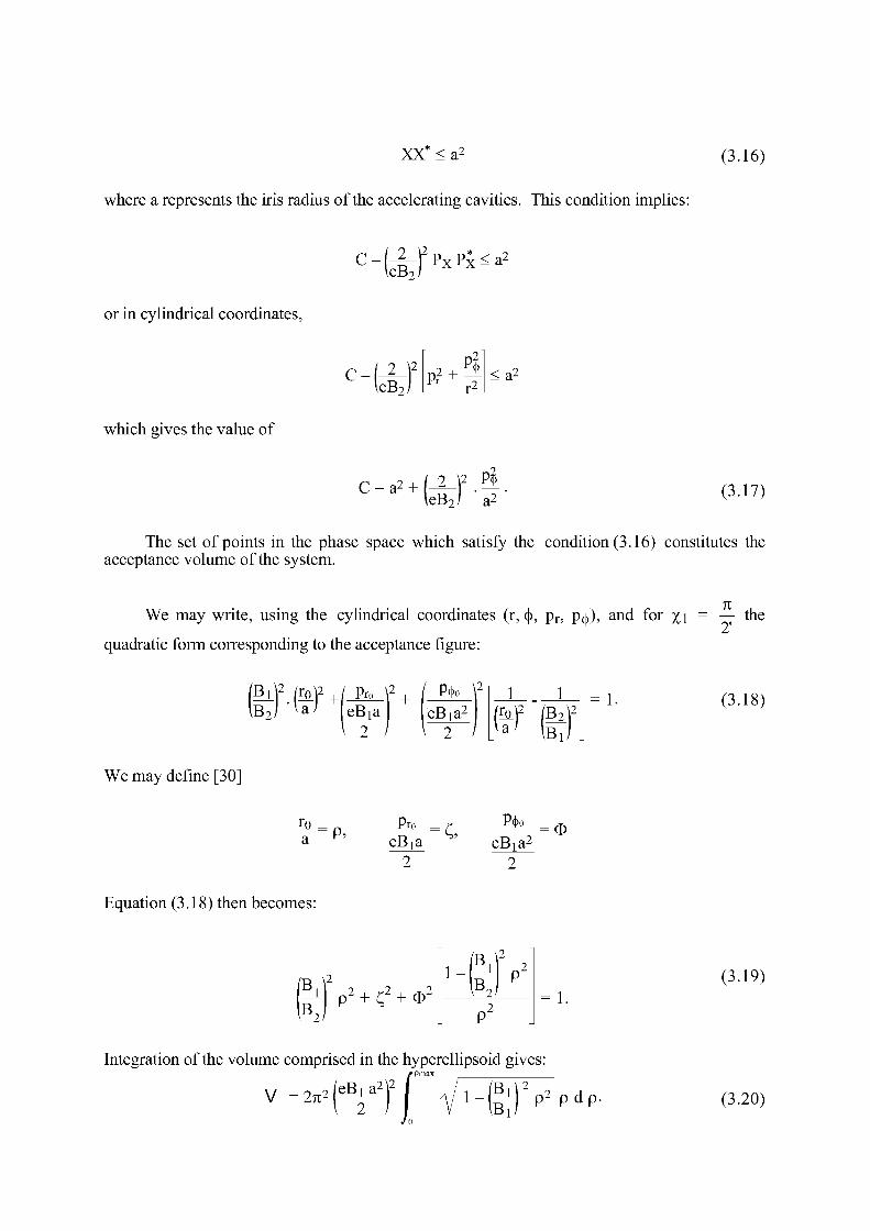
XX* < a 2
(3.16)
where a represents the iris radius of the accelerating cavities. This condition implies:
or in cylindrical coordinates,
c - ( 4 F P x P ^ a 2
c 2 V eB,
P? + ^ < a 2
which gives the value of
c=a 2
+ m2 . p i
leB2j a2
(3.17)
The set of points in the phase space which satisfy the condition (3.16) constitutes the acceptance volume of the system.
71 We may write, using the cylindrical coordinates (r, §, p r , p^), and for xi = — the
quadratic form corresponding to the acceptance figure:
Btï-m+IP ro \ 2
+ / P*o Y eBjji
2 > eBia2
\ 2 /
1 1
tf B ^ 2
Bi
(3.18)
We may define [30]
ro Pro _ £ eBia. S '
2
P«|>0
e B ^ 2
2
O
Equation (3.18) then becomes:
B„ p 2 + Ç2 + O 2
/B
B„ 1 ~ 2
(3.19)
Integration of the volume comprised in the hyperellipsoid gives: y»Pmax
Jo
(3.20)
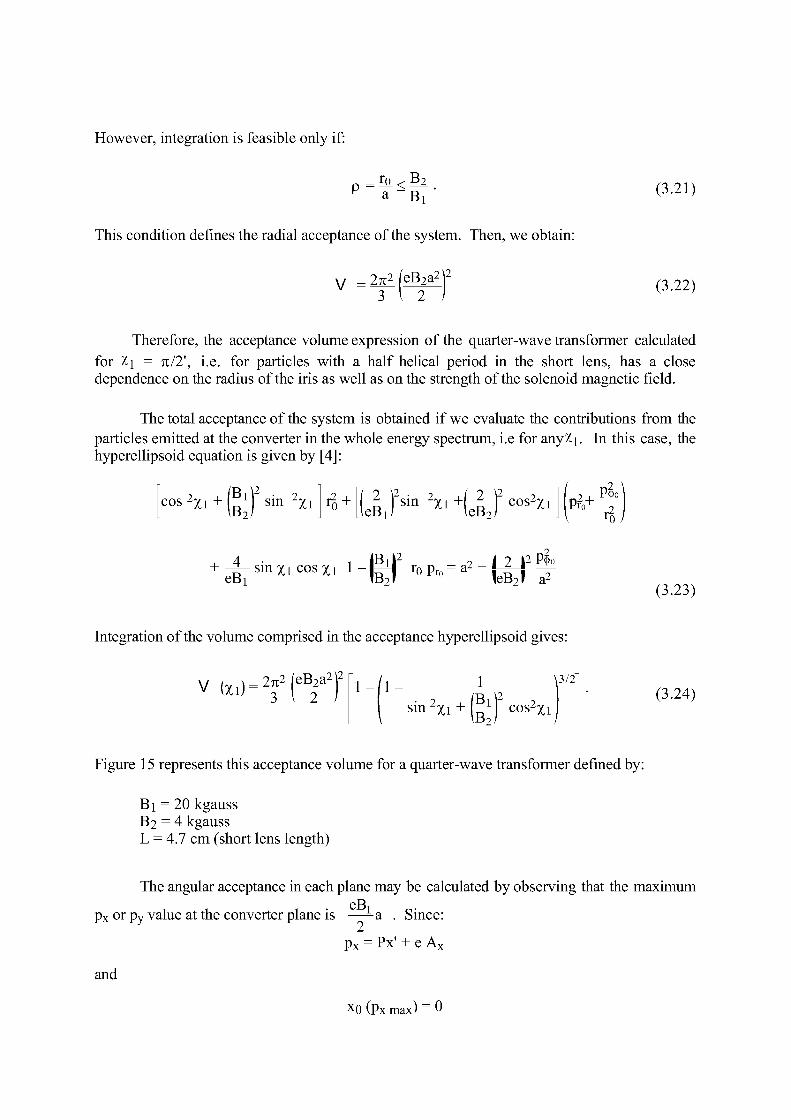
However, integration is feasible only if:
p = r o < I k p a Bi (3.21)
This condition defines the radial acceptance of the system. Then, we obtain:
v -27i 2 [eB 2 a2j 2
(3.22)
Therefore, the acceptance volume expression of the quarter-wave transformer calculated for %i = 7i/2', i.e. for particles with a half helical period in the short lens, has a close dependence on the radius of the iris as well as on the strength of the solenoid magnetic field.
The total acceptance of the system is obtained if we evaluate the contributions from the particles emitted at the converter in the whole energy spectrum, i.e for any%i. In this case, the hyperellipsoid equation is given by [4]:
cos 2 xi + l^j sin 2 xi r2, + y ^ s i n 2Xi + ( e B ^ f c o s 2 X i W Â
+ - S - s i n x i c o s x i 1 - b H ro Pro = a 2 + h ^ H —, eBi L !B2r J !eB2r a2
(3.23)
Integration of the volume comprised in the acceptance hyperellipsoid gives:
v ( X l ) - ^ ( ^ 1 V 2 1-/1 X \3/2
I s i n ^ i + l^ 1 ) cos 2xil (3.24)
Figure 15 represents this acceptance volume for a quarter-wave transformer defined by:
Bi = 20 kgauss B2 = 4 kgauss L = 4.7 cm (short lens length)
The angular acceptance in each plane may be calculated by observing that the maximum eB p x or p y value at the converter plane is —-a . Since:
p x = Px' + e A x
and
X0 (Px max) = 0
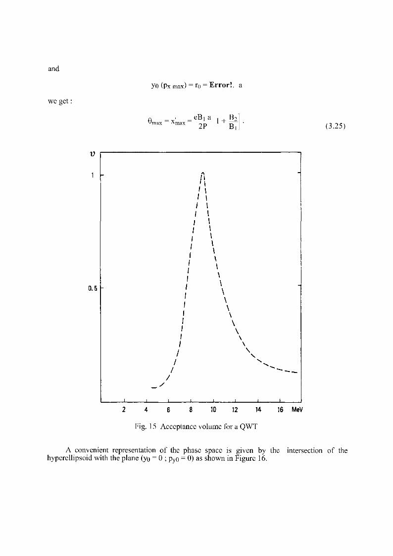
and
we get :
yo (p x max) = ro = Error!, a
A - _eBi a [ 1 B2_ '-'max A m a I I T -'max A max (3.25)
16 MeV
Fig. 15 Acceptance volume for a QWT
A convenient representation of the phase space is given by the intersection of the hyperellipsoid with the plane (yo = 0 ; pyo = 0) as shown in Figure 16.
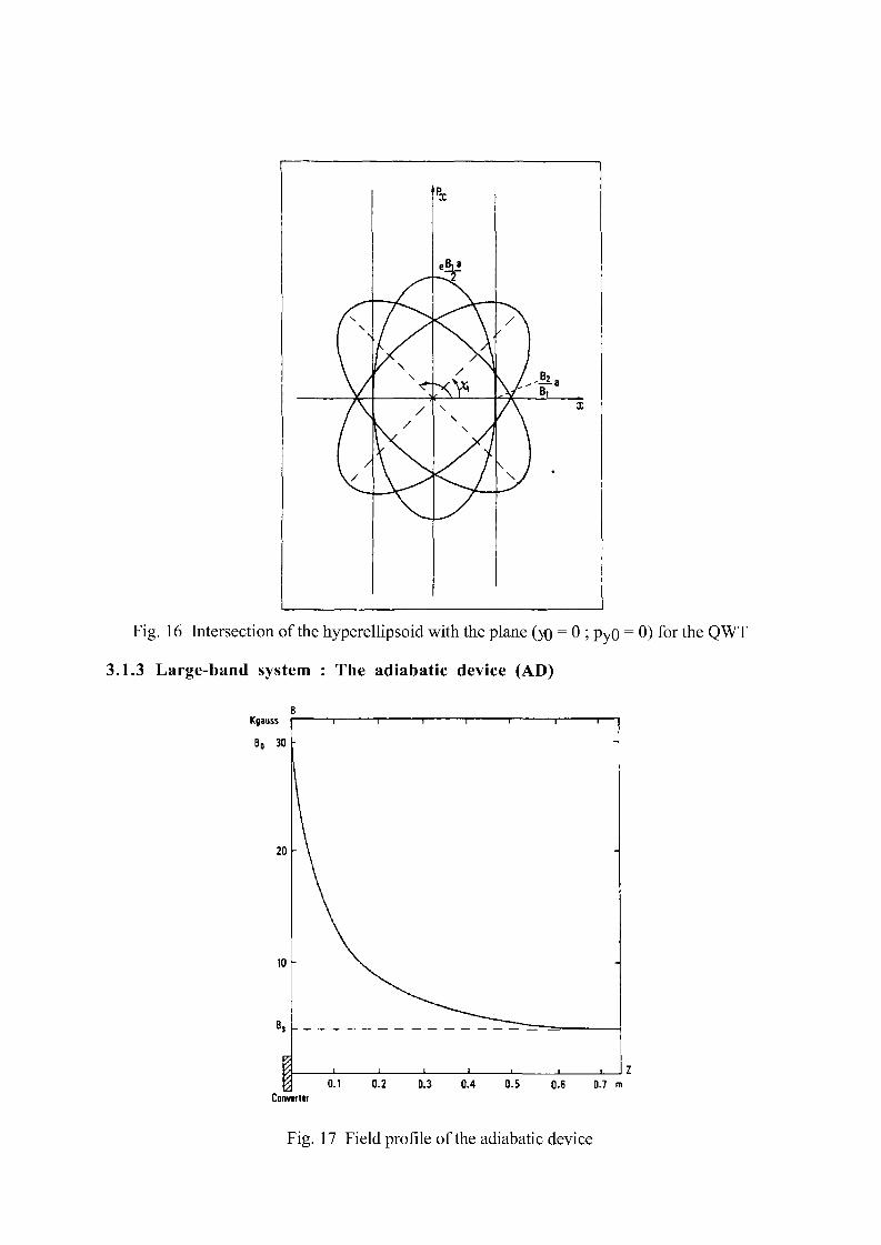
P
- v 2
/ x / \ 1 •*. ' \
If \ rsY \ / - ^ -V Bt
/ \ \ / \ ^ \ / \ /
1 / \ / \ v V '
Fig. 16 Intersection of the hyperellipsoid with the plane (K) = 0 ; pyO = 0) for the QWT
3.1.3 Large-band system : The adiabatic device (AD)
0.1 0.2 0.3 0.4 0.5 0.6 0.7 m Converter
Fig. 17 Field profile of the adiabatic device
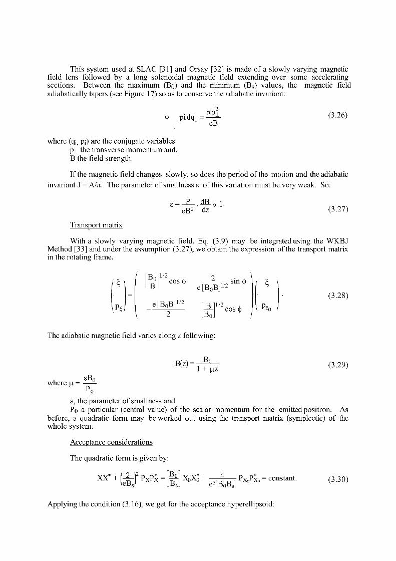
This system used at SLAC [31] and Orsay [32] is made of a slowly varying magnetic field lens followed by a long solenoidal magnetic field extending over some accelerating sections. Between the maximum (Bo) and the minimum (Bs) values, the magnetic field adiabatically tapers (see Figure 17) so as to conserve the adiabatic invariant:
o pidqi -eB
(3.26)
where (qi: pi) are the conjugate variables p i the transverse momentum and, B the field strength.
If the magnetic field changes slowly, so does the period of the motion and the adiabatic invariant J = A/71. The parameter of smallness s of this variation must be very weak. So:
P eB 2
< P - « 1 . dz (3.27)
Transport matrix
With a slowly varying magnetic field, Eq. (3.9) may be integrated using the WKBJ Method [33] and under the assumption (3.27), we obtain the expression of the transport matrix in the rotating frame.
/ ? \
m
Bo B
1/2 COS ())
e[B 0 B] 1 / 2
efBoBF2 sin (j)
B B oJ
1/2 COS ())
/ \ P < 3 /
(3.28)
The adiabatic magnetic field varies along z following:
B(Z): Bo 1 + |uz (3.29)
where \x - sB n
s, the parameter of smallness and Po a particular (central value) of the scalar momentum for the emitted positron. As
before, a quadratic form may be worked out using the transport matrix (symplectic) of the whole system.
Acceptance considerations
The quadratic form is given by:
XX + J^\2
eB, PxP x^x Br BQ
XQXO + e 2[B 0Bj
PXQPXO = constant. (3.30)
Applying the condition (3.16), we get for the acceptance hyperellipsoid:
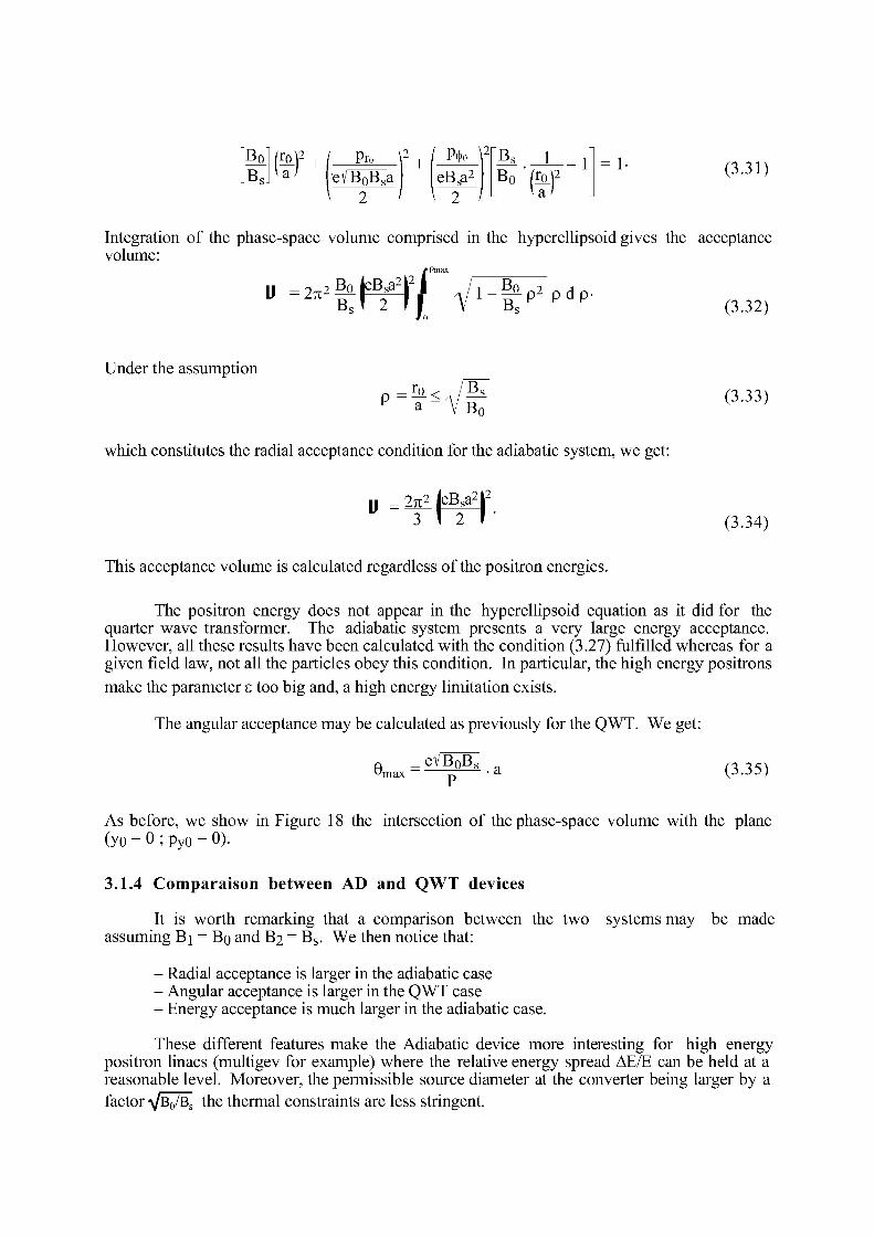
Bs\'a + Bol feP + / PQ \2
eVB0Bsa \ 2
&r + \ 2
foW"^1- (3-31) a
> . w
Integration of the phase-space volume comprised in the hyperellipsoid gives the acceptance volume:
fPmax
»=^Btmi v ^ ^ J V E ^ P U P ' (3.32)
p = 5 L < . / | ^ (3.33) Under the assumption
n ~ a " V B„
which constitutes the radial acceptance condition for the adiabatic system, we get:
U _ 2n2 jeB s a 2 j 2
(3.34)
This acceptance volume is calculated regardless of the positron energies.
The positron energy does not appear in the hyperellipsoid equation as it did for the quarter wave transformer. The adiabatic system presents a very large energy acceptance. However, all these results have been calculated with the condition (3.27) fulfilled whereas for a given field law, not all the particles obey this condition. In particular, the high energy positrons make the parameter s too big and, a high energy limitation exists.
The angular acceptance may be calculated as previously for the QWT. We get:
em a x = ^ f ^ - a (3.35)
As before, we show in Figure 18 the intersection of the phase-space volume with the plane (yo = 0 ; p yo = 0).
3.1.4 Comparaison between AD and QWT devices
It is worth remarking that a comparison between the two systems may be made assuming Bi = Bo and B2 = B s . We then notice that:
- Radial acceptance is larger in the adiabatic case - Angular acceptance is larger in the QWT case - Energy acceptance is much larger in the adiabatic case.
These different features make the Adiabatic device more interesting for high energy positron linacs (multigev for example) where the relative energy spread AE/E can be held at a reasonable level. Moreover, the permissible source diameter at the converter being larger by a factor -\/B0/Bs the thermal constraints are less stringent.
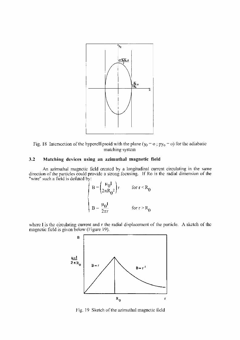
Pi
—^2
A' X
Fig. 18 Intersection of the hyperellipsoid with the plane (y0 = o ; py 0 = o) for the adiabatic matching system
3.2 Matching devices using an azimuthal magnetic field
An azimuthal magnetic field created by a longitudinal current circulating in the same direction of the particles could provide a strong focusing. If Ro is the radial dimension of the "wire" such a field is defined by:
B = L ^ ° r fo r r<R n
\2nRQ2l 0
B ^ O 1
27ir for r > R, 0
where I is the circulating current and r the radial displacement of the particle. A sketch of the magnetic field is given below (Figure 19).
2 K R „
Fig. 19 Sketch of the azimuthal magnetic field
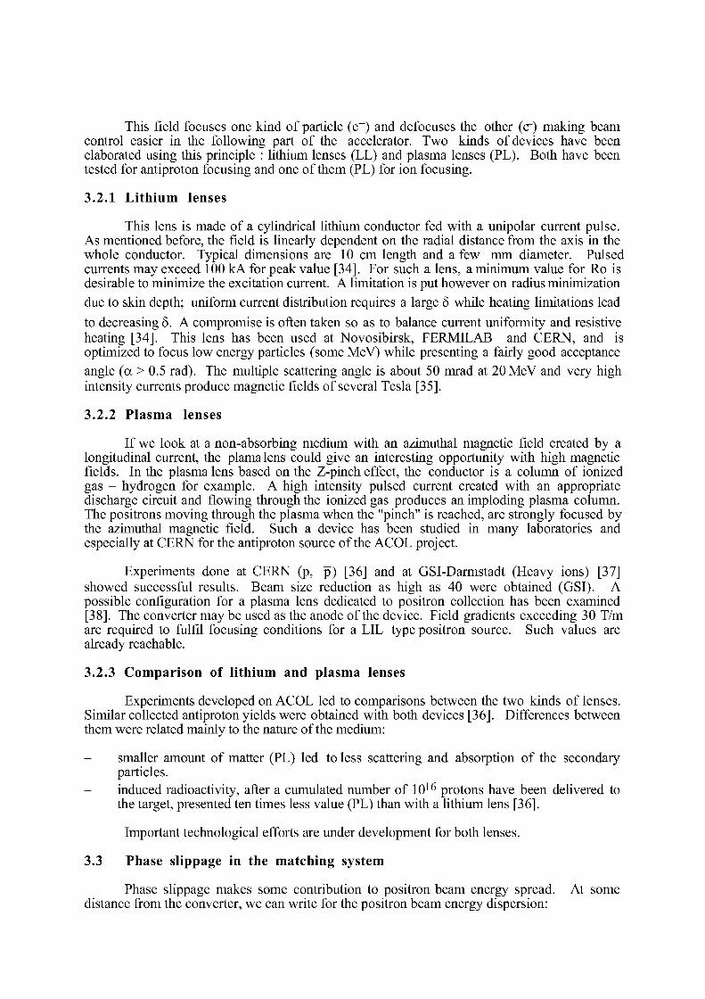
This field focuses one kind of particle (e+) and defocuses the other (e~) making beam control easier in the following part of the accelerator. Two kinds of devices have been elaborated using this principle : lithium lenses (LL) and plasma lenses (PL). Both have been tested for antiproton focusing and one of them (PL) for ion focusing.
3.2.1 Lithium lenses
This lens is made of a cylindrical lithium conductor fed with a unipolar current pulse. As mentioned before, the field is linearly dependent on the radial distance from the axis in the whole conductor. Typical dimensions are 10 cm length and a few mm diameter. Pulsed currents may exceed 100 kA for peak value [34]. For such a lens, a minimum value for Ro is desirable to minimize the excitation current. A limitation is put however on radius minimization due to skin depth; uniform current distribution requires a large ô while heating limitations lead to decreasing ô. A compromise is often taken so as to balance current uniformity and resistive heating [34]. This lens has been used at Novosibirsk, FERMILAB and CERN, and is optimized to focus low energy particles (some MeV) while presenting a fairly good acceptance angle (a > 0.5 rad). The multiple scattering angle is about 50 mrad at 20 MeV and very high intensity currents produce magnetic fields of several Tesla [35].
3.2.2 Plasma lenses
If we look at a non-absorbing medium with an azimuthal magnetic field created by a longitudinal current, the plamalens could give an interesting opportunity with high magnetic fields. In the plasma lens based on the Z-pinch effect, the conductor is a column of ionized gas - hydrogen for example. A high intensity pulsed current created with an appropriate discharge circuit and flowing through the ionized gas produces an imploding plasma column. The positrons moving through the plasma when the "pinch" is reached, are strongly focused by the azimuthal magnetic field. Such a device has been studied in many laboratories and especially at CERN for the antiproton source of the ACOL project.
Experiments done at CERN (p, p) [36] and at GSI-Darmstadt (Heavy ions) [37] showed successful results. Beam size reduction as high as 40 were obtained (GSI). A possible configuration for a plasma lens dedicated to positron collection has been examined [38]. The converter may be used as the anode of the device. Field gradients exceeding 30 T/m are required to fulfil focusing conditions for a LIL type positron source. Such values are already reachable.
3.2.3 Comparison of lithium and plasma lenses
Experiments developed on ACOL led to comparisons between the two kinds of lenses. Similar collected antiproton yields were obtained with both devices [36]. Differences between them were related mainly to the nature of the medium:
- smaller amount of matter (PL) led to less scattering and absorption of the secondary particles.
- induced radioactivity, after a cumulated number of 10 1 6 protons have been delivered to the target, presented ten times less value (PL) than with a lithium lens [36].
Important technological efforts are under development for both lenses.
3.3 Phase slippage in the matching system
Phase slippage makes some contribution to positron beam energy spread. At some distance from the converter, we can write for the positron beam energy dispersion:
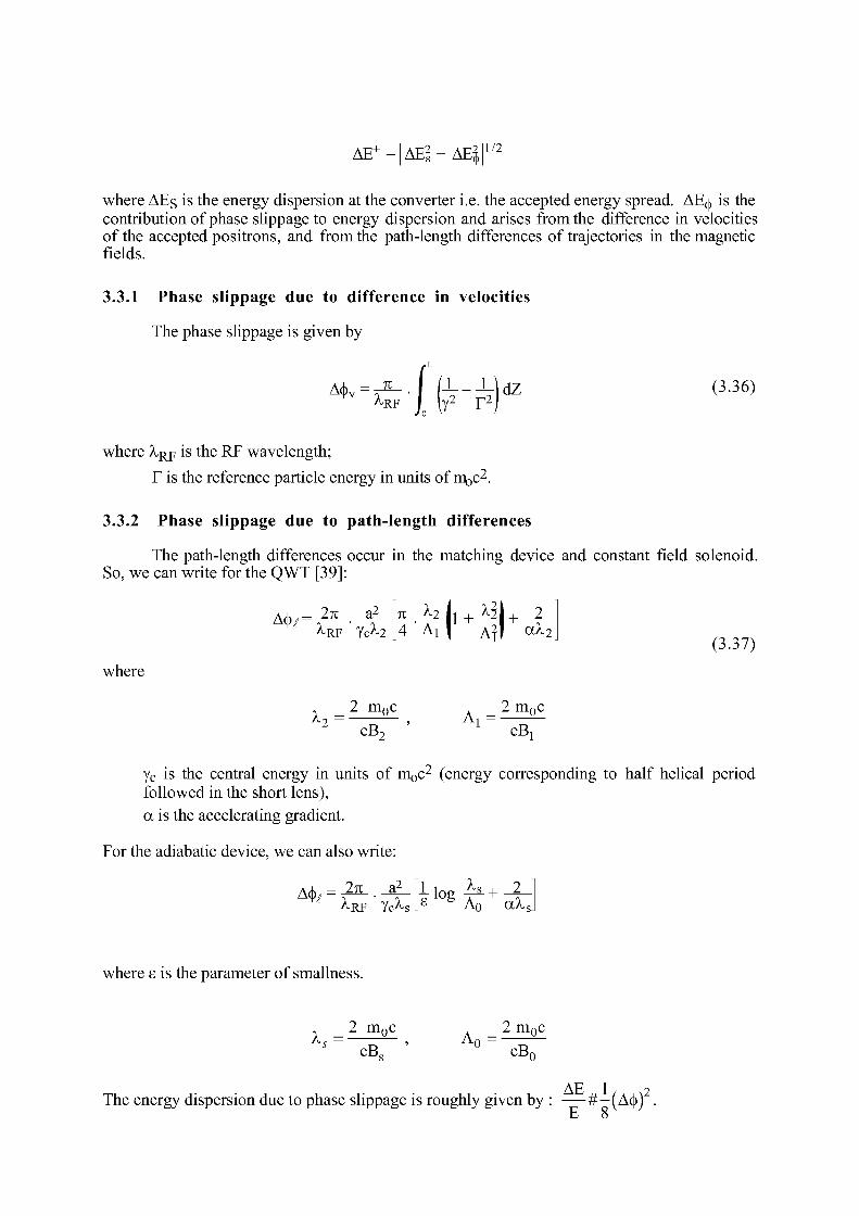
AE + = [ A E ! + A E | 1/2
where AE§ is the energy dispersion at the converter i.e. the accepted energy spread. AE^ is the contribution of phase slippage to energy dispersion and arises from the difference in velocities of the accepted positrons, and from the path-length differences of trajectories in the magnetic fields.
3.3.1 Phase sl ippage due to difference in velocities
The phase slippage is given by
*--&•{(£-£ dZ (3.36)
where X R F is the RF wavelength; r is the reference particle energy in units of moC2.
3.3.2 Phase sl ippage due to path-length differences
The path-length differences occur in the matching device and constant field solenoid. So, we can write for the QWT [39]:
A(|>i 2TI a2 7L h i M ^ L 2 ^RF Yc 2 ^4 Al | A?| a ^ 2 1 + +
(3.37)
where
Ai 2 m 0 c A,
2 m 0c e B 2 eB 1
y c is the central energy in units of rrioC2 (energy corresponding to half helical period followed in the short lens), a is the accelerating gradient.
For the adiabatic device, we can also write:
Afa 2% _ a 2 l l o „ K + ^_ £ g Ao alt
where s is the parameter of smallness.
K = 2 m 0 c
A o -2 m 0c
e B s e B 0
The energy dispersion due to phase slippage is roughly given by : #—(A§) . E 8

4 . EMITTANCE TRANSFORMATION AND PRESERVATION
The solenoidal magnet system which is used after the matching system requires high power. A quadrupole focusing system is generally inserted some distance after the solenoid, typically when positrons have an energy of about 100 MeV. The transition between solenoidal and quadrupoles focusing is made as soon as the spacing between the quadrupoles allows this. The quadrupoles are thus put on the accelerating sections with aFODO sequence. A matching device is generally inserted between the solenoid and the quadrupole systems to transform the axisymmetric beam coming from the solenoid into the well known elliptical shape of the FODO system. The positron beam transverse emittance is quite large, 2 to 5 MeV/c mm or,
s n = 4.10~3 to 10~2 mmmrad.
This emittance has to be reduced before the interaction point in damping rings (DR) producing synchrotron radiation. Damping and excitation due to quantized emission of photons provide an equilibrium beam size which is smaller than that entering the DR.
Since the required positron bunch length is usually shorter than that delivered by the DR, bunch length compression, has to be applied. This is done in a two-stage process:
- acceleration of the bunch in a RF cavity: the phase of the bunch centre is at 0 so as to accelerate the particles ahead of this point and decelerate those behind
- non isochronous transport of the bunch: the higher energy particles travel on a longer path than those of lower energy.
As a result, all the positrons arrive at the linac entrance at almost the same time so that the bunch length is shortened while the energy spread is increased.
Geometrical misalignments in a linac cause perturbations of the beam trajectory. Since the positron beam emittance before damping is relatively large, accurate steering to avoid beam losses in the accelerating sections is required. Trajectory perturbations can be caused by quadrupole misalignments (displacements and rotation of the quadrupole axis), accelerating-section misalignments and gradient errors. Analytical evaluations have shown that the lateral quadrupole displacement is the most critical misalignment while tilt around one of their transverse axes is the effect next in importance. Trajectory control using beam-position monitors associated with steering dipoles allows the beam lateral displacements to be minimized and hence prevents significant wake field perturbations for high intensity positron beams [40].
5 . COMPARISON OF POSITRON SOURCES
A comparison of positron sources - existing or starting - is presented in Table 3. The two parameters associated with the incident electron beam, peak intensity I~ or number of electrons per bunch N~ and energy E~, are represented by their values at the converter location. Target material and matching device are also indicated. The two magnetic field values represent (Bi, B2) and (Bo B s) for the quarter-wave transformer and the adiabatic device respectively. Positron yield normalized to 1 GeV incident electron beam is reported for three corresponding measurements:
- as close as possible to the target (total yield) - at the linac output - in the beam switchyard ; slit width is indicated in % of the final energy.
Emittance measurements are also reported.
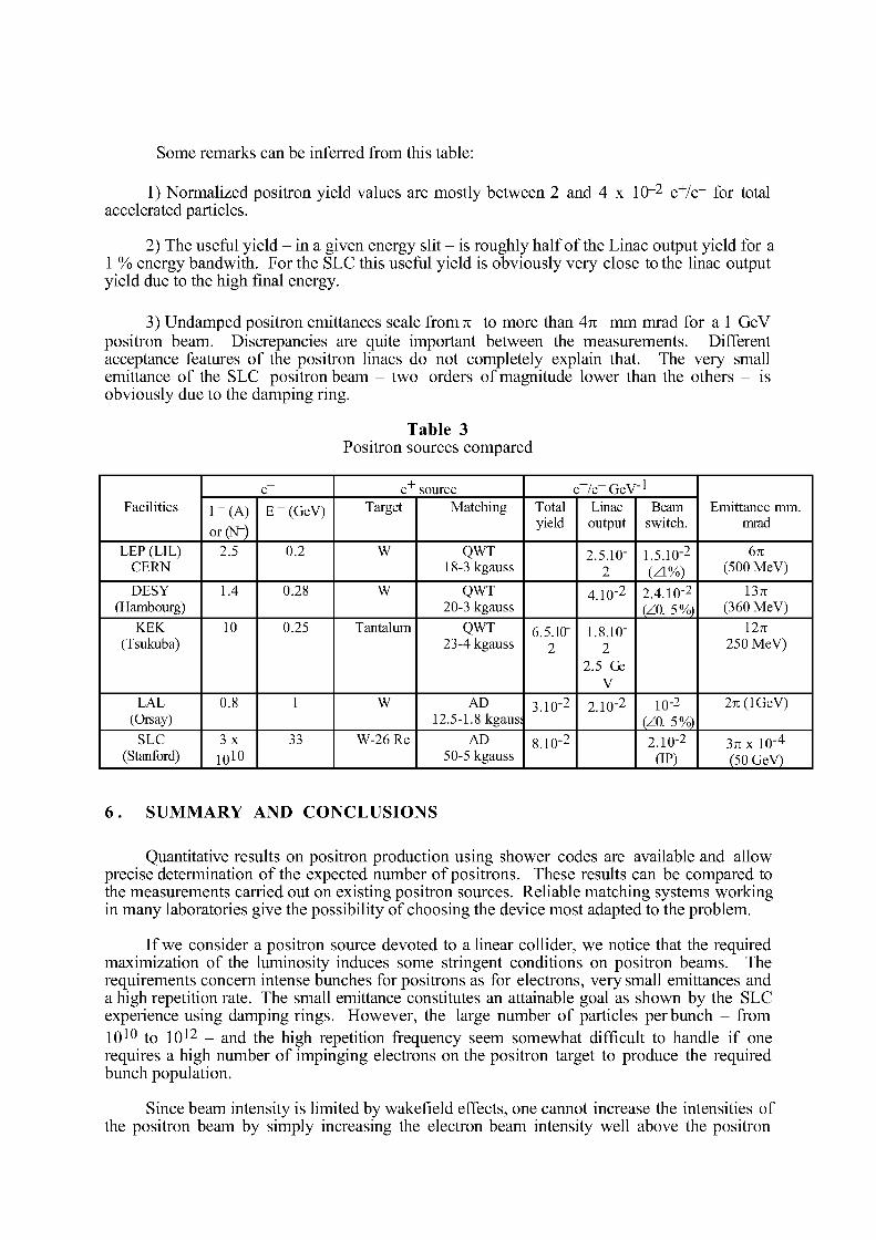
Some remarks can be inferred from this table:
1) Normalized positron yield values are mostly between 2 and 4 x 10~2 e+/e~ for total accelerated particles.
2) The useful yield - in a given energy slit - is roughly half of the Linac output yield for a 1 % energy bandwith. For the SLC this useful yield is obviously very close to the linac output yield due to the high final energy.
3) Undamped positron emittances scale from7i to more than 4n mm mrad for a 1 GeV positron beam. Discrepancies are quite important between the measurements. Different acceptance features of the positron linacs do not completely explain that. The very small emittance of the SLC positron beam - two orders of magnitude lower than the others - is obviously due to the damping ring.
Table 3 Positron sources compared
Facilities e e + source e+ArGeV 1
Emittance mm. mrad
Facilities I "(A) or (NT)
E-(GeV) Target Matching Total yield
Linac output
Beam switch.
Emittance mm. mrad
LEP (LIL) CERN
2.5 0.2 W QWT 18-3 kgauss
2.5.10" 2
1.5.10-2 (Zl%)
6JI (500 MeV)
DESY (Hambourg)
1.4 0.28 W QWT 20-3 kgauss
4.10-2 2.4.10"2
(Z0. 5%) 13JI
(360 MeV) KEK
(Tsukuba) 10 0.25 Tantalum QWT
23-4 kgauss 6.5.10"
2 1.8.10"
2 2.5 Ge
V
12JI 250 MeV)
LAL (Qrsay)
0.8 1 W AD 12.5-1.8 kgauss
3.10-2 2.10-2 10"2
(Z0. 5%) 2JI (lGeV)
SLC (Stanford)
3x îoio
33 W-26 Re AD 50-5 kgauss
8.10-2 2.10- 2
(IP) 3JIX lO" 4
(50 GeV
6. SUMMARY AND CONCLUSIONS
Quantitative results on positron production using shower codes are available and allow precise determination of the expected number of positrons. These results can be compared to the measurements carried out on existing positron sources. Reliable matching systems working in many laboratories give the possibility of choosing the device most adapted to the problem.
If we consider a positron source devoted to a linear collider, we notice that the required maximization of the luminosity induces some stringent conditions on positron beams. The requirements concern intense bunches for positrons as for electrons, very small emittances and a high repetition rate. The small emittance constitutes an attainable goal as shown by the SLC experience using damping rings. However, the large number of particles per bunch - from 10 1 0 to 10 1 2 - and the high repetition frequency seem somewhat difficult to handle if one requires a high number of impinging electrons on the positron target to produce the required bunch population.
Since beam intensity is limited by wakefield effects, one cannot increase the intensities of the positron beam by simply increasing the electron beam intensity well above the positron
intensity needed. So we are led to a yield of 1 e+/e~, at least concerning the accepted positrons. Moreover, thermic and radiation problems in the target limit the incident electron power. If the interest associated with high energy electron beams is clearly demonstrated, one has to consider the effects of a large number of particles impinging on a small area of the target. Rotating targets could be a solution.
Semi-classical methods using photons instead of electrons on amorphous targets may offer attractive alternatives for future e + sources while radioactive sources, though offering the possibility of large number of e + as in the test reactors, present too many difficulties.
Positron sources generated by photons from undulators are nowadays under intense analysis and considered in almost half of the linear collider projects as the desirable issue for the positron source. More recent ideas are under consideration (laser) or under theoretical and experimental investigation (channeling).
REFERENCES
[ 1] B. Rossi, High energy particles, Prentice Hall, Ed. (1956)
[ 2] W.R. Nelson, R.L Ford, The EGS code system, SLAC 210 (1978)
[ 3] A. Crawford, M. Messel, Electron-photon shower distribution function tables for lead, copper and air absorbers, Pergamon Press, Oxford (1970)
[ 4] R. Chehab, Etude de la production et du confinement d'un faisceau de positrons. Application à lAccélérateur Linéaire d'Orsay, RI/75-4 (Avril 75)
[ 5] R. Brun et al, GEANT 3, CERN - DD/EE 84 - 1
[ 6] H. De Staebler, More calculations for positron target test in ESA, Internal memo CN-24 (Avril 1980)
[7] S. Ecklund, Positrons for linear colliders, SLAC Pub 4484 (Nov. 87)
[ 8] P. Sievers, M. Hôfert, Radiological problems at high energy, high intensity electron-positron converters, CLIC note 71 (July 1988)
[ 9] K.G. Lynn, W.E. Frieze, Intense positron beams and possible experiments in "Positron scattering in Gases", J. Humberton & M.R. McDowell Ed., Nato ASI Series
[10] E. Ottewitte, Large scale positron production for physics needs via fission reactors, Proc. of the Advanced Accelerator concepts Conference, Madison, WI 1986
[11] J. Dawson, A positron factory. Proceedings of the Workshop "Critical issues in the development of new linear colliders", Madison, Wisconsin (August 1986)
[12] V. Balakin, A. Mikhailichenko, The conversion system for obtaining highly polarized electrons and positrons, Preprint INP 79 - 85 Novosibirsk
[13] B. Kincaid, Journal of Applied Physics Vol. 48, n 7 (July 1977)
[14] M. Sands, in "Physics with intersecting storage rings" (1971) Academic Press, B. Toushek, Ed.
[15] H. Wiedemann, SLAC Pub 2849 (November 1981)
[16] E.G. Bessonov, A.A. Mikhailichenko, Some aspects of undulator radiation forming for conversion system of the linear accelerator, Preprint Budker INP 92-43
[17] A.D. Bukin, A.A. Mikhailichenko, Optimized target strategy for polarized electrons and positrons production for linear colliders, Preprint Budker INP 92-76
[18] K. Flottman, J. Rossbach, A high intensity positron source for linear collider, DESY M-91-11, October 91
[19] R. Chehab et al, Proc. of IEEE Particle Accelerator Conference, Chicago, IL, March 20-23, 1989
[20] X. Artru et al, Proc. of IEEE Particle Accelerator Conference, San-Francisco, CA, May 6-9, 1991
[21] R. Chehab, Proc.of the Linear Collider 92 Workshop, July 92, Garmisch
[22] A. Belkacem et al, Nucl. Instr. & Meth. B13 (1986) 9
[23] P. Chen, R. Palmer, Positron production by electron-laser interaction, Proc. of the Linear Collider 92 Workshop, July 92, Garmisch
[24] R. Helm et al, The positron source in "The Stanford Two Mile Accelerator", R. Neal Editor, W.A. Benjamin Inc (1968).
[25] J. Ha'issinski, Nucl. Instr. & Meth. 51 (1967) 181.
[26] G. Stange, IEEE Trans. Nucl. Science, NS-26 n 3 (June 1979)
[27] R. Boni, S. Guiducci, M. Vescovi, A new system for positron focusing at the Frascati Linac,LNF-81/6(R)(1981)
[28] R. Belbeoch et al., Rapport d'études sur le projet des linacs injecteurs de LEP (LIL), LAL PI 82-01/T, LAL Orsay
[29] A. Enomoto and al, Proc. of the 1986 Linac Conference, Stanford (June 1986)
[30] R. Helm, SLAC - 4, Stanford Linear Accelerator Center, Stanford (August 1962)
[31] F. Bulos et al, IEEE Transactions on Nuclear Science, NS-32 n5 (October 1985) also: J.E. Clendenin et al, SLAC Pub 4704 (September 1988)
[32] R. Chehab et al, IEEE Transactions on Nuclear Science, NS-30 n 4 (August 1983)
[33] J. Heading, An introduction to Phase Integral Methods, London: Methuen, New York: John Wiley (1962)
[34] B.F. Bayanov et al, Nucl. Instr. & Meth. 190 (1981)9
[35] G.I. Silvestrov Problems of intense secondary particle beam production, Preprint INP 86-163 Novosibirsk (1986)
[36] R. Kowalewicz et al, Performance of the CERN plasma lens in laboratory and beam tests at the antiproton source, Proc. 1991 IEEE PAC, San-Francisco, May 91
[37] E. Boggasch et al, Plasma lens fine focusing of heavy ion beams, Appl. Phys. Letters 60 (20) 1992, p. 2475
[38] H. Braun et al, Application of plasma lenses in positron sources, Proc. of the 1992 EPAC, Berlin, March, 1992

[39] F. Amman, Positron accelerators in "Linear Accelerators", P. Lapostolle, A. Septier Editors, North-Holland Pub. Co (1970)
[40] R. Chehab, Y. Thiery, K. Hubner, Proc. of the 1986 Linear Accelerator Conference, June 1986, Stanford.
WATCH ALPHABETIC SYMBOLS! ! ! ! ! CONVENTIONAL RF SYSTEM DESIGN
M. Puglisi Sincrotrone Trieste, Italy
Abstract The design of a conventional RF system is always complex and must fit the needs of the particular machine for which it is planned. It follows that many different design criteria should be considered and analyzed, thus exceeding the narrow limits of a lecture. For this reason only the fundamental components of an RF system, including the generators, are considered in this short seminar. The most common formulas are simply presented in the text, while their derivations are shown in the appendices to facilitate, if desired, a more advanced level of understanding.
1. INTRODUCTION
In dynamic machines the charged particles exchange energy with the electric field (positive or negative acceleration). The acceleration can be:
a) along a straight path - linear accelerators, (single-pass acceleration); b) along a closed orbit - cyclic accelerators, (many-pass acceleration).
In both cases, because the curl of the electric field cannot be zero, it follows that a static
field cannot be used. In fact we know that: — x E = . ft
In principle any non-constant E.M. field could be used, but due to the huge amount of technology derived from radio communications, sinusoidal radio-frequency fields are used. The equipments, which create and apply the field to the charged particles, are known as the RF-systems or, more simply, the RF.
2. THE ACCELERATING GAP
Basically RF acceleration is obtained by creating a suitable RF field inside one or more gaps of the vacuum chamber which is supposed to be metallic. These accelerating gaps can be obtained using two conceptually different devices:
drift tubes; cavity resonators.
First of all we study the behaviour of a gap (no matter how it is made). We make the hypothesis that the field Ez is uniform along the axis of the gap and depends sinusoidally upon the time:
Ez =EQ COS (wt +j).
Phase y is referred to the particle which for t = 0 is in the middle of the gap (z = 0). The voltage gain is then:
+ G/2 V - E0 E0 cos (cot + <p) dz . (1)
-G/2
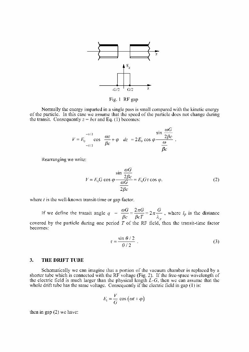
& ^ | E 7
-G/2 G/2
Fig. 1 RF gap
Normally the energy imparted in a single pass is small compared with the kinetic energy of the particle. In this case we assume that the speed of the particle does not change during the transit. Consequently z = bet and Eq. (1) becomes:
vGll sin V = En cos
- G / 2
(OZ + (p dz = 2E0 c o s <p -
<x>G
2/3c CO
Jc Rearranging we write:
sin coG 2j5c
V = E0G cos (p p— = EQGx COS q>
2~pc
where t is the well-known transit-time or gap factor.
coG 2KG
(2)
If we define the transit angle q = 2n— , where L is the distance Pc PcT A p
covered by the particle during one period T of the RF field, then the transit-time factor becomes:
x = • sin 612
012 (3)
3. THE DRIFT TUBE
Schematically we can imagine that a portion of the vacuum chamber is replaced by a shorter tube which is connected with the RF voltage (Fig. 2). If the free-space wavelength of the electric field is much larger than the physical length L-G, then we can assume that the whole drift tube has the same voltage. Consequently if the electric field in gap (1) is:
E = V cos (cot + cp)
then in gap (2) we have:
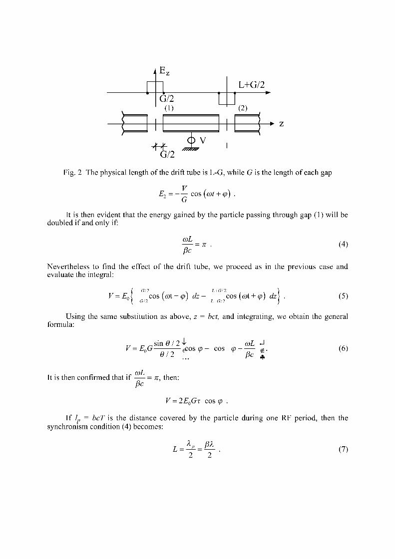
i E z
L+G/2 G/2
(1) (2) ,
•>• z
I
Fig. 2 The physical length of the drift tube is L-G, while G is the length of each gap
V , v is 2 = cos (cttf + cp) .
G
It is then evident that the energy gained by the particle passing through gap (1) will be doubled if and only if:
coL = n (4)
Nevertheless to find the effect of the drift tube, we proceed as in the previous case and evaluate the integral:
+ G/2 L + G/2 V = EA cos (cot + cp) dz- cos (cot + cp) dz
u _G/2 \ T ) L-G It V ' (5)
Using the same substitution as above, z = bet, and integrating, we obtain the general formula:
„ r^sm9/2J ^coL J V=EnG—: gos cp - cos cp-i g. "0 V
6/2 (3c (6)
It is then confirmed that if = TC, then: Pc
V = 2E0GT COS cp .
If lp = bcT is the distance covered by the particle during one RF period, then the synchronism condition (4) becomes:
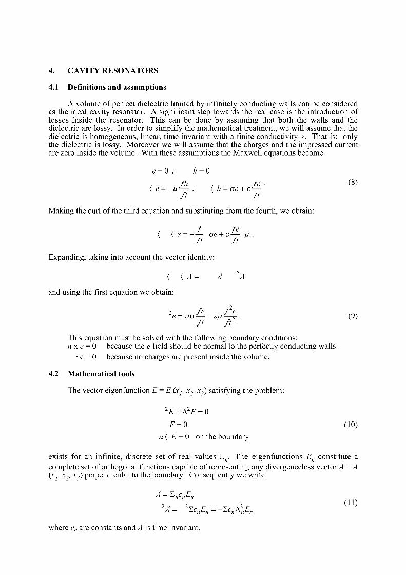
4. CAVITY RESONATORS
4.1 Definitions and assumptions
A volume of perfect dielectric limited by infinitely conducting walls can be considered as the ideal cavity resonator. A significant step towards the real case is the introduction of losses inside the resonator. This can be done by assuming that both the walls and the dielectric are lossy. In order to simplify the mathematical treatment, we will assume that the dielectric is homogeneous, linear, time invariant with a finite conductivity s. That is: only the dielectric is lossy. Moreover we will assume that the charges and the impressed current are zero inside the volume. With these assumptions the Maxwell equations become:
e = 0 ; h = 0 fh fe • (8)
( e = - « — ; (h = ae + s — ft ft
Making the curl of the third equation and substituting from the fourth, we obtain:
i i f fe
ft ft Expanding, taking into account the vector identity:
< (A= A- 2A
and using the first equation we obtain:
7 fe fe e = ao— + su J—^r . (9)
This equation must be solved with the following boundary conditions: nx e = 0 because the e field should be normal to the perfectly conducting walls.
• e = 0 because no charges are present inside the volume.
4.2 Mathematical tools
The vector eigenfunction E = E (xj, x2, x3) satisfying the problem: 2E + A2E - 0
E = 0 (10) n ( E - 0 on the boundary
exists for an infinite, discrete set of real values L . The eigenfunctions E constitute a complete set of orthogonal functions capable of representing any divergenceless vector A= A (xj, x2, x3) perpendicular to the boundary. Consequently we write:
^ = ^ncn^n 2 _ 2 2 O 1 ) A - ^cnEn - LcnAnEn
where c„ are constants and A is time invariant.
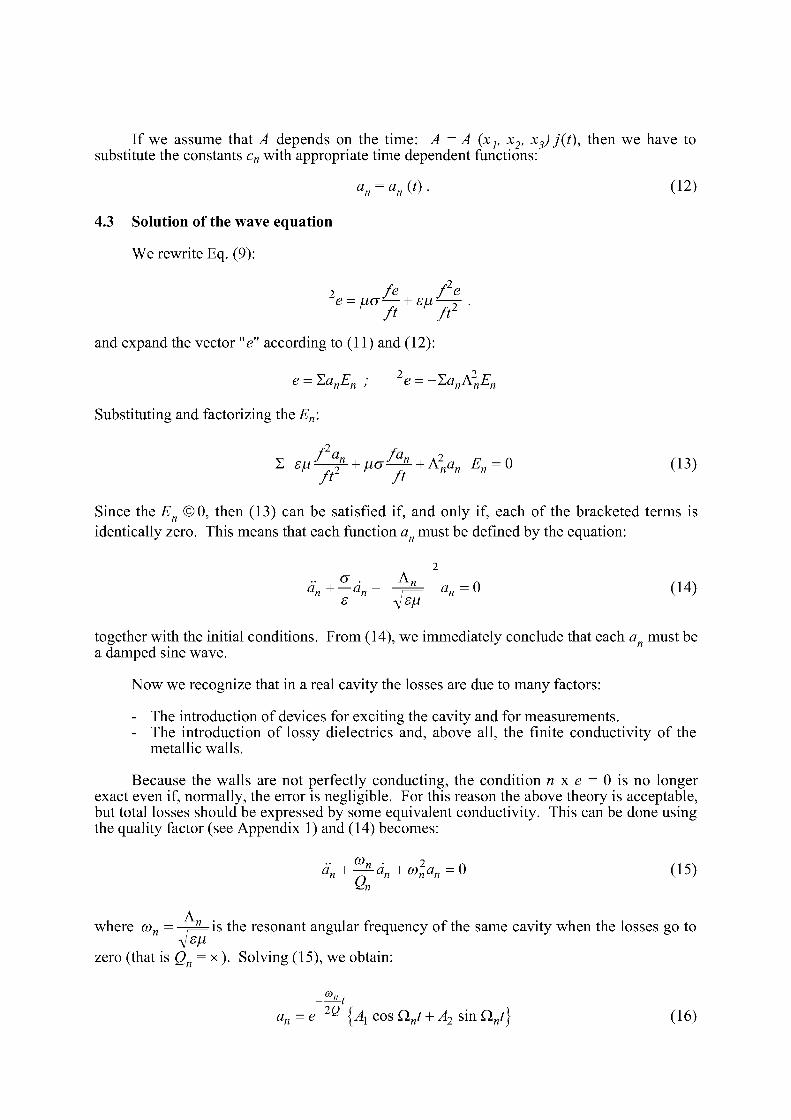
If we assume that A depends on the time: A = A (xj, x2, x3)j(t), then we have to substitute the constants cn with appropriate time dependent functions:
an = an(t). (12)
4.3 Solution of the wave equation
We rewrite Eq. (9):
2 fe f e e - u<j-—h su ^r .
" ft ** ft2
and expand the vector "e" according to (11) and (12):
e = ZanEn ; 2e =-ZanA2
nEn
Substituting and factorizing the En:
S S L t ^ + Ltcj^ + A 2 ^ En = 0 (13)
Since the En ©0, then (13) can be satisfied if, and only if, each of the bracketed terms is identically zero. This means that each function an must be defined by the equation:
2
à„+-ân+ -j^ an=0 (14) S slSLl
together with the initial conditions. From (14), we immediately conclude that each an must be a damped sine wave.
Now we recognize that in a real cavity the losses are due to many factors:
- The introduction of devices for exciting the cavity and for measurements. - The introduction of lossy dielectrics and, above all, the finite conductivity of the
metallic walls.
Because the walls are not perfectly conducting, the condition n x e = 0 is no longer exact even if, normally, the error is negligible. For this reason the above theory is acceptable, but total losses should be expressed by some equivalent conductivity. This can be done using the quality factor (see Appendix 1) and (14) becomes:
CO i an+yran+(onan=0 ( 1 5 )
sen
where con - J1- is the resonant angular frequency of the same cavity when the losses go to
zero (that is Qn = x ). Solving (15), we obtain:
a n = e 2 Q {A C O S ^ V + ^2 s m ^V} (16)
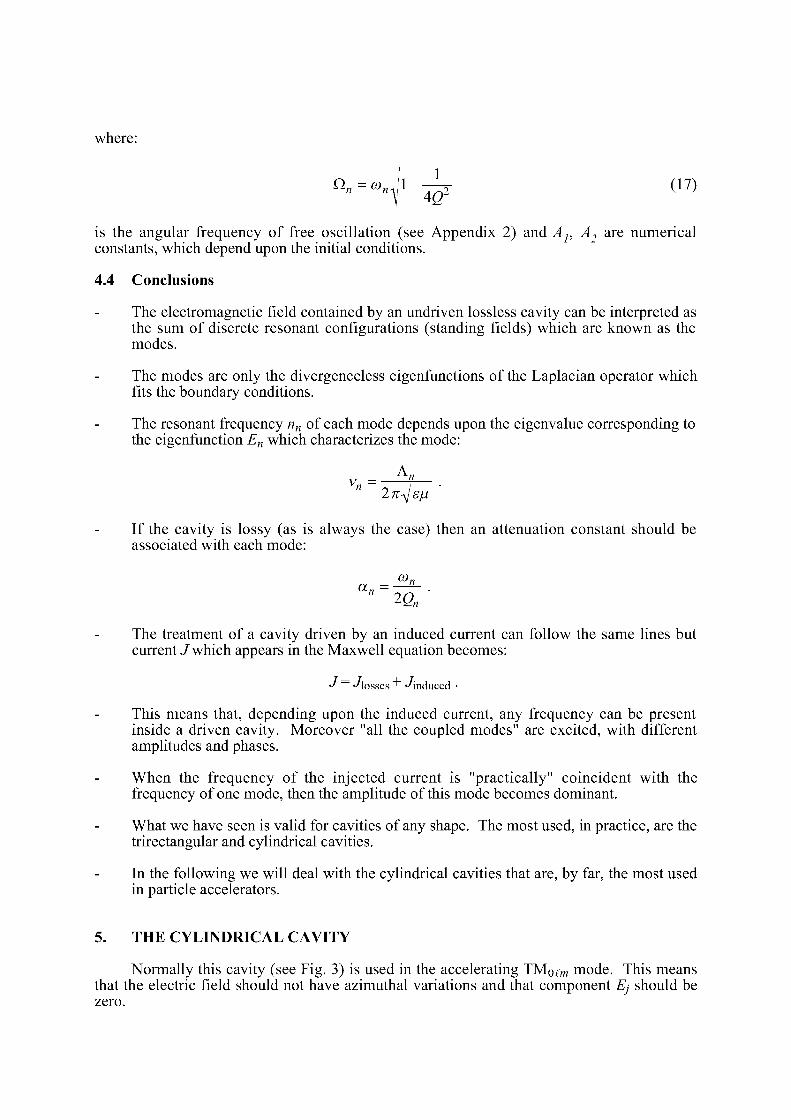
where:
Çln=an^--^î ( 1 7 >
is the angular frequency of free oscillation (see Appendix 2) and Aj, A2 are numerical constants, which depend upon the initial conditions.
4.4 Conclusions
The electromagnetic field contained by an undriven lossless cavity can be interpreted as the sum of discrete resonant configurations (standing fields) which are known as the modes.
The modes are only the divergenceless eigenfunctions of the Laplacian operator which fits the boundary conditions.
The resonant frequency nn of each mode depends upon the eigenvalue corresponding to the eigenfunction En which characterizes the mode:
If the cavity is lossy (as is always the case) then an attenuation constant should be associated with each mode:
The treatment of a cavity driven by an induced current can follow the same lines but current J which appears in the Maxwell equation becomes:
•J ~ •'losses ~"~ •'induced •
This means that, depending upon the induced current, any frequency can be present inside a driven cavity. Moreover "all the coupled modes" are excited, with different amplitudes and phases.
When the frequency of the injected current is "practically" coincident with the frequency of one mode, then the amplitude of this mode becomes dominant.
What we have seen is valid for cavities of any shape. The most used, in practice, are the trirectangular and cylindrical cavities.
In the following we will deal with the cylindrical cavities that are, by far, the most used in particle accelerators.
5. THE CYLINDRICAL CAVITY
Normally this cavity (see Fig. 3) is used in the accelerating TMo^m mode. This means that the electric field should not have azimuthal variations and that component Ej should be zero.
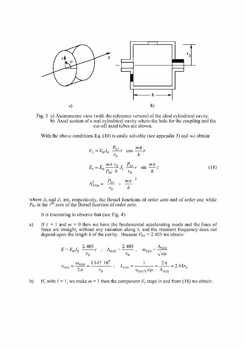
a)
• •
b)
Fig. 3 a) Axonometric view (with the reference versors) of the ideal cylindrical cavity. b) Axial section of a real cylindrical cavity where the hole for the coupling and the
cut-off axial tubes are shown.
With the above conditions Eq. (10) is easily solvable (see appendix 3) and we obtain:
P0i mn Ez = EQJQ -^-r cos _
'o h
Er=E0 mn r. PM h
J, 0£ r sin mn (18) Of
A' 0 Cm 01 mn
where JQ and J\ are, respectively, the Bessel functions of order zero and of order one while /fth PQII is the v zero of the Bessel function of order zero.
It is interesting to observe that (see Fig. 4):
a) If i = 1 and m = 0 then we have the fundamental accelerating mode and the lines of force are straight, without any variation along z, and the resonant frequency does not depend upon the length h of the cavity. Because PQI = 2.405 we obtain:
E = E0J0
2.405 A-oio _
2.405 CO 010
_ A-oio
CO "010
010 1.147 10-2n
X 1 2n
010 VoioV6/* A o
2.61r n
10
b) If, with £ = 1, we make m = 1 then the component Er steps in and from (18) we obtain:
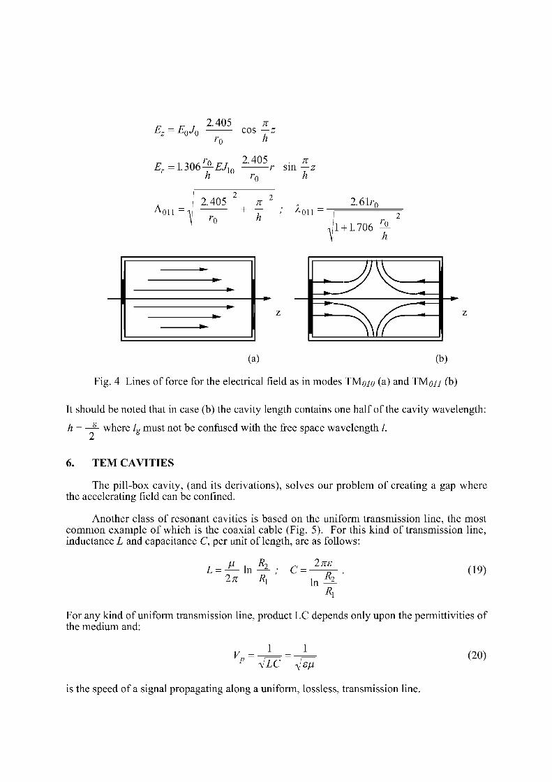
_. _. , 1405 n Ez = EoJo c o s T z
rn h 'o
Er = L306%-EJla ^ ^ h r0
. % r sin — z
h
A on 2.405 K
)' o h X on
2.61rn
1 + 1.706 ^
(a) (b)
Fig. 4 Lines of force for the electrical field as in modes TMoio (a) and TMou (b)
It should be noted that in case (b) the cavity length contains one half of the cavity wavelength:
h = — where lg must not be confused with the free space wavelength /.
6. TEM CAVITIES
The pill-box cavity, (and its derivations), solves our problem of creating a gap where the accelerating field can be confined.
Another class of resonant cavities is based on the uniform transmission line, the most common example of which is the coaxial cable (Fig. 5). For this kind of transmission line, inductance L and capacitance C, per unit of length, are as follows:
L ^ l n ^ 2 71 i?i
C = 2ns
h 7 ^ (19)
For any kind of uniform transmission line, product LC depends only upon the permittivities of the medium and:
VP = 1 1
•sjLC -sjeiÀ (20)
is the speed of a signal propagating along a uniform, lossless, transmission line.
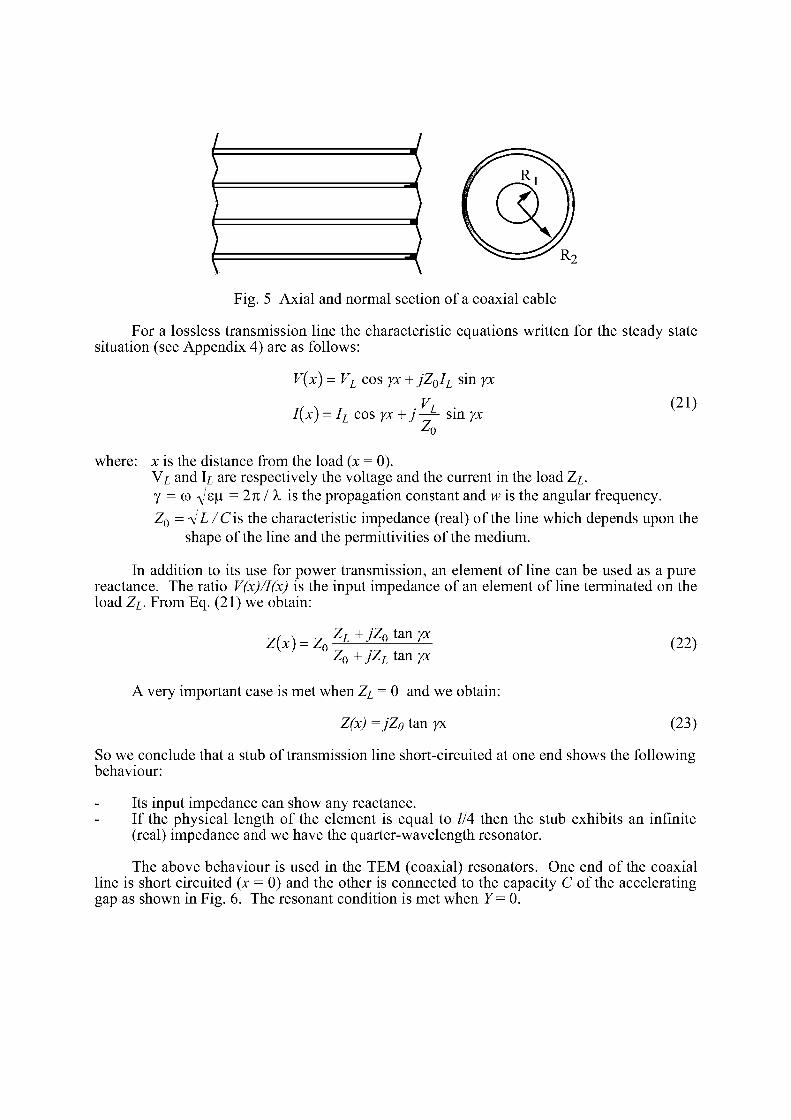
Fig. 5 Axial and normal section of a coaxial cable
For a lossless transmission line the characteristic equations written for the steady state situation (see Appendix 4) are as follows:
V(x) = VL cos yx+jZ0IL sin yx Vj . (21)
I\x) = IL cos yx +j—^- sin yx
where: x is the distance from the load (x = 0). \L and \i are respectively the voltage and the current in the load Z^. y = co -sj&\i = 2n I X is the propagation constant and w is the angular frequency. Z 0 = VXTC is the characteristic impedance (real) of the line which depends upon the
shape of the line and the permittivities of the medium.
In addition to its use for power transmission, an element of line can be used as a pure reactance. The ratio V(x)/I(x) is the input impedance of an element of line terminated on the load Zi. From Eq. (21) we obtain:
Z(x) = Z 0
Z L + J Z ° t m y X (22) Z 0 + jZL tan yx
A very important case is met when Zi = 0 and we obtain:
Z(x) =jZo tan yx (23)
So we conclude that a stub of transmission line short-circuited at one end shows the following behaviour:
Its input impedance can show any reactance. If the physical length of the element is equal to 1/4 then the stub exhibits an infinite (real) impedance and we have the quarter-wavelength resonator.
The above behaviour is used in the TEM (coaxial) resonators. One end of the coaxial line is short circuited (x = 0) and the other is connected to the capacity C of the accelerating gap as shown in Fig. 6. The resonant condition is met when 7 = 0 .
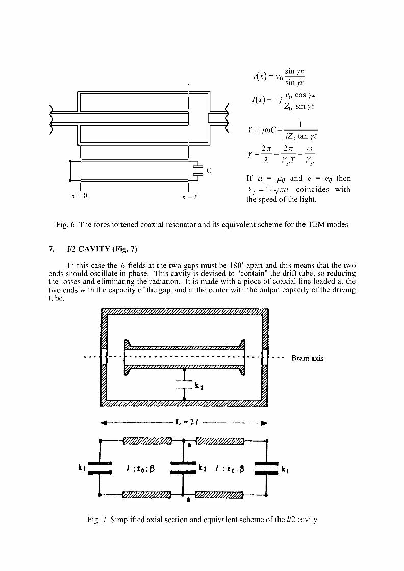
c
x = 0
sin yx
K*) = -J
sin y£
. v 0 cos yx Z 0 sin yt
Y = jcoC + -1
jZ0 tan 7^
_ 27T _ 27T ft)
If [d = fio and e = eo then Vp — l /«Jëfi coincides with the speed of the light.
Fig. 6 The foreshortened coaxial resonator and its equivalent scheme for the TEM modes
7. Ill CAVITY (Fig. 7)
In this case the E fields at the two gaps must be 180° apart and this means that the two ends should oscillate in phase. This cavity is devised to "contain" the drift tube, so reducing the losses and eliminating the radiation. It is made with a piece of coaxial line loaded at the two ends with the capacity of the gap, and at the center with the output capacity of the driving tube.
mmzm&^^s^zmzzmmzMzm
i Hmzzzzœzzœœmzœmzzzmzzzzzaà \
r//*rt*r*r**tffS******W******ftW*JJ*rr*t*/.
mM^Mmzz^^mmzmzsmm. L - 2 /
X
Beam axis
Fig. 7 Simplified axial section and equivalent scheme of the 111 cavity
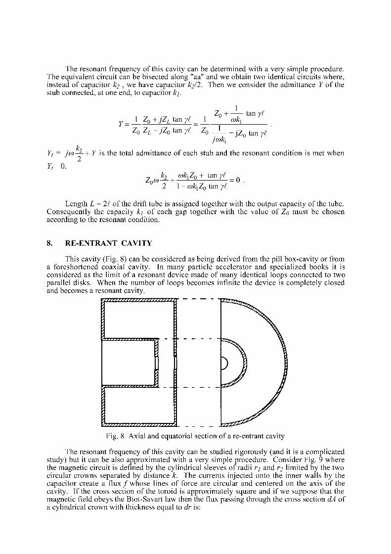
The resonant frequency of this cavity can be determined with a very simple procedure. The equivalent circuit can be bisected along "aa" and we obtain two identical circuits where, instead of capacitor £2 , we have capacitor k^l. Then we consider the admittance Y of the stub connected, at one end, to capacitor kj.
Y = 1 Z 0 + jZL tan yl _ 1
Z 0 + 1 <x>kx
tan y I
Z0 ZL + jZ0 tan yl Z0 _ L _ + J Z Q t a n y i
jcokx
Yt = JCO — +Y is the total admittance of each stub and the resonant condition is met when J 2
Yt 0. k2 CD^ZQ + tan yl
Z 0 f t ) 1 = U . 2 1 - CO^ZQ tan y I
Length L = 21 of the drift tube is assigned together with the output capacity of the tube. Consequently the capacity kj of each gap together with the value of ZQ must be chosen according to the resonant condition.
8. RE-ENTRANT CAVITY
This cavity (Fig. 8) can be considered as being derived from the pill box-cavity or from a foreshortened coaxial cavity. In many particle accelerator and specialized books it is considered as the limit of a resonant device made of many identical loops connected to two parallel disks. When the number of loops becomes infinite the device is completely closed and becomes a resonant cavity.
vs/r/f/////////;;j/jjsrsssr
11 J t y 11} t J
TTTTTr-rrn J I m l
Fig. 8 Axial and equatorial section of a re-entrant cavity
The resonant frequency of this cavity can be studied rigorously (and it is a complicated study) but it can be also approximated with a very simple procedure. Consider Fig. 9 where the magnetic circuit is defined by the cylindrical sleeves of radii r\ and r2 limited by the two circular crowns separated by distance k. The currents injected onto the inner walls by the capacitor create a flux/whose lines of force are circular and centered on the axis of the cavity. If the cross section of the toroid is approximately square and if we suppose that the magnetic field obeys the Biot-Savart law then the flux passing through the cross section dA of a cylindrical crown with thickness equal to dr is:
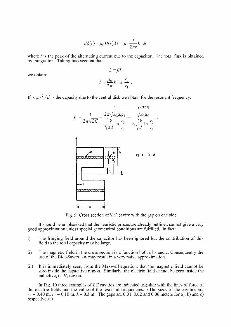
d(f)(r) - jjLQH{r)dA - JJLQ k dr 2nr
where / is the peak of the alternating current due to the capacitor. The total flux is obtained by integration. Taking into account that:
L=fll
L = ^ k In ^ - . we obtain:
L = 2n rx
If £ 0
7 r r i / ^ is the capacity due to the central disk we obtain for the resonant frequency:
1 0.225
/ o 1 2 ^ 5 0 ^ 0 ^ _ ygp/ip
In^LC k . r7 \k . r ?
— In — rx \— In — \ 2d r1 \i' J r 1
i '
E -f|;
zz:tL.
r j r i - k - d
ZZZZZZZZZZ2227Z
L Fig. 9 Cross section of XC cavity with the gap on one side
It should be emphasized that the heuristic procedure already outlined cannot give a very good approximation unless special geometrical conditions are fulfilled. In fact:
i) The fringing field around the capacitor has been ignored but the contribution of this field to the total capacity may be large.
ii) The magnetic field in the cross section is a function both of r and z. Consequently the use of the Biot-Savart law may result in a very naive approximation.
iii) It is immediately seen, from the Maxwell equation, that the magnetic field cannot be zero inside the capacitive region. Similarly, the electric field cannot be zero inside the inductive, or H, region.
In Fig. 10 three examples of LC cavities are indicated together with the lines of force of the electric fields and the value of the resonant frequencies. (The sizes of the cavities are V2 = 0.40 m, rj = 0.10 m, k = 0.3 m. The gaps are 0.01, 0.02 and 0.06 meters for a), b) and c) respectively.)
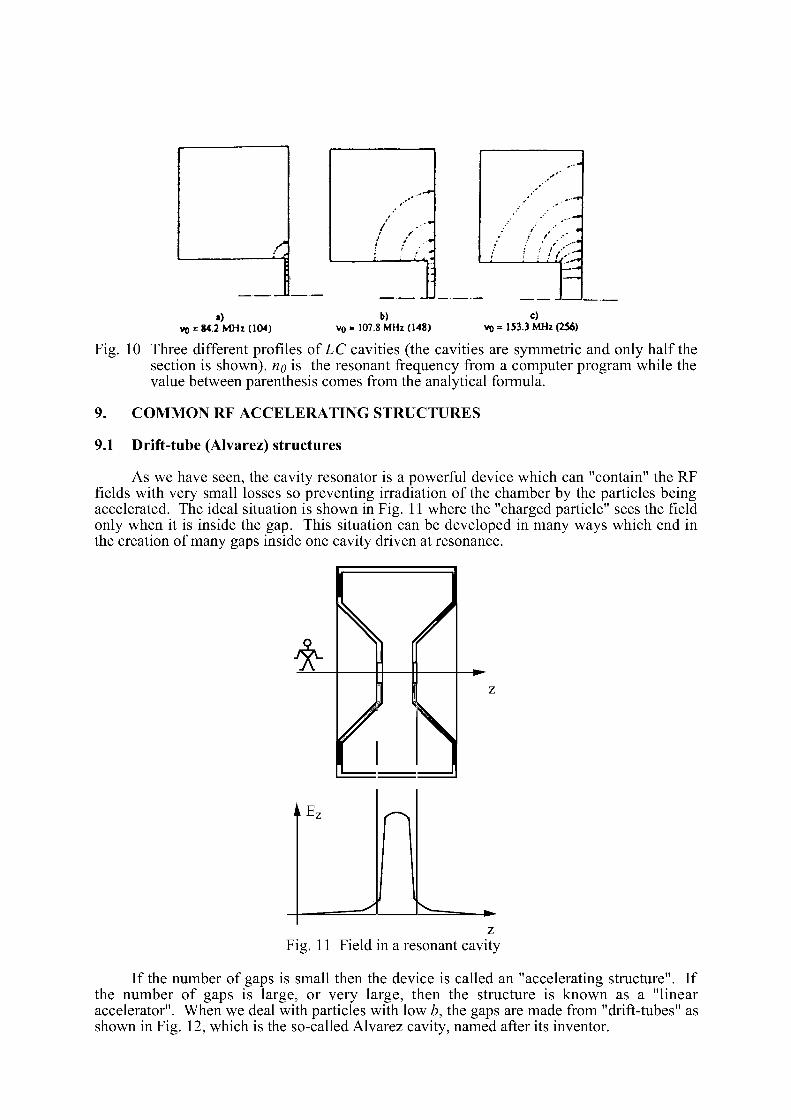
i) b) c) vo = 84.2 MHz (104) v 0 = 107.8 MHz (148) VQ = 153.3 MHz (256)
Fig. 10 Three different profiles of LC cavities (the cavities are symmetric and only half the section is shown), no is the resonant frequency from a computer program while the value between parenthesis comes from the analytical formula.
9. COMMON RF ACCELERATING STRUCTURES
9.1 Drift-tube (Alvarez) structures
As we have seen, the cavity resonator is a powerful device which can "contain" the RF fields with very small losses so preventing irradiation of the chamber by the particles being accelerated. The ideal situation is shown in Fig. 11 where the "charged particle" sees the field only when it is inside the gap. This situation can be developed in many ways which end in the creation of many gaps inside one cavity driven at resonance.
Fig. 11 Field in a resonant cavity
If the number of gaps is small then the device is called an "accelerating structure". If the number of gaps is large, or very large, then the structure is known as a "linear accelerator". When we deal with particles with low b, the gaps are made from "drift-tubes" as shown in Fig. 12, which is the so-called Alvarez cavity, named after its inventor.
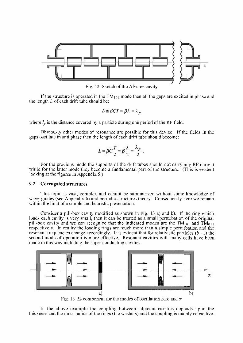
Fig. 12 Sketch of the Alvarez cavity
If the structure is operated in the TM101 mode then all the gaps are excited in phase and the length L of each drift tube should be:
L = pCT = pA=Xp
where lp is the distance covered by a particle during one period of the RF field.
Obviously other modes of resonance are possible for this device. If the fields in the gaps oscillate in anti phase then the length of each drift tube should become:
2 2 2
For the previous mode the supports of the drift tubes should not carry any RF current while for the latter mode they become a fundamental part of the structure. (This is evident looking at the figures in Appendix 5.)
9.2 Corrugated structures
This topic is vast, complex and cannot be summarized without some knowledge of wave-guides (see Appendix 6) and periodic-structures theory. Consequently here we remain within the limit of a simple and heuristic presentation.
Consider a pill-box cavity modified as shown in Fig. 13 a) and b). If the ring which loads each cavity is very small, then it can be treated as a small perturbation of the original pill-box cavity and we can recognize that the indicated modes are the TMioi and TMon respectively. In reality the loading rings are much more than a simple perturbation and the resonant frequencies change accordingly. It is evident that for relativistic particles (b ~1) the second mode of operation is more effective. Resonant cavities with many cells have been made in this way including the super conducting cavities.
D n
\
j
o n
a) b) Fig. 13 Ez component for the modes of oscillation zero and n
In the above example the coupling between adjacent cavities depends upon the thickness and the inner radius of the rings (the washers) and the coupling is mainly capacitive.
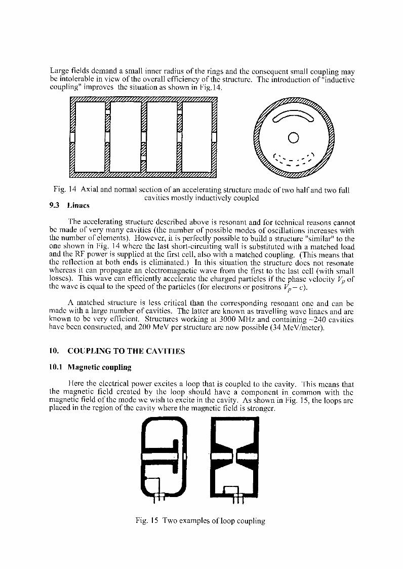
Large fields demand a small inner radius of the rings and the consequent small coupling may be intolerable in view of the overall efficiency of the structure. The introduction of "inductive coupling" improves the situation as shown in Fig. 14.
V////////////^//////////^//////J^//////////^
Z 9/;;/;;;/;//^/;//;/;M/;/////;/s>^ Z
Fig. 14 Axial and normal section of an accelerating structure made of two half and two full cavities mostly inductively coupled
9.3 Linacs
The accelerating structure described above is resonant and for technical reasons cannot be made of very many cavities (the number of possible modes of oscillations increases with the number of elements). However, it is perfectly possible to build a structure "similar" to the one shown in Fig. 14 where the last short-circuiting wall is substituted with a matched load and the RF power is supplied at the first cell, also with a matched coupling. (This means that the reflection at both ends is eliminated.) In this situation the structure does not resonate whereas it can propagate an electromagnetic wave from the first to the last cell (with small losses). This wave can efficiently accelerate the charged particles if the phase velocity Vp of the wave is equal to the speed of the particles (for electrons or positrons Vp = c).
A matched structure is less critical than the corresponding resonant one and can be made with a large number of cavities. The latter are known as travelling wave linacs and are known to be very efficient. Structures working at 3000 MHz and containing -240 cavities have been constructed, and 200 MeV per structure are now possible (34 MeV/meter).
10. COUPLING TO THE CAVITIES
10.1 Magnetic coupling
Here the electrical power excites a loop that is coupled to the cavity. This means that the magnetic field created by the loop should have a component in common with the magnetic field of the mode we wish to excite in the cavity. As shown in Fig. 15, the loops are placed in the region of the cavity where the magnetic field is stronger.
Fig. 15 Two examples of loop coupling
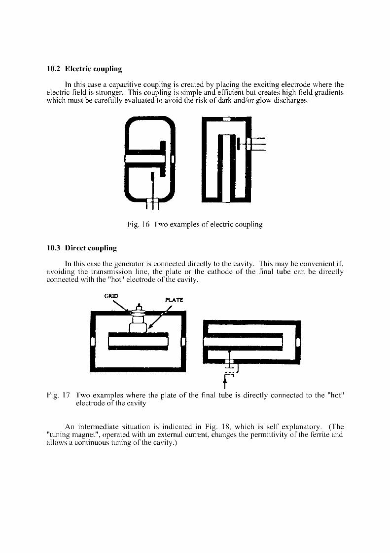
10.2 Electric coupling
In this case a capacitive coupling is created by placing the exciting electrode where the electric field is stronger. This coupling is simple and efficient but creates high field gradients which must be carefully evaluated to avoid the risk of dark and/or glow discharges.
Fig. 16 Two examples of electric coupling
10.3 Direct coupling
In this case the generator is connected directly to the cavity. This may be convenient if, avoiding the transmission line, the plate or the cathode of the final tube can be directly connected with the "hot" electrode of the cavity.
GRID PLATE
Fig. 17 Two examples where the plate of the final tube is directly connected to the "hot" electrode of the cavity
An intermediate situation is indicated in Fig. 18, which is self explanatory. (The "tuning magnet", operated with an external current, changes the permittivity of the ferrite and allows a continuous tuning of the cavity.)
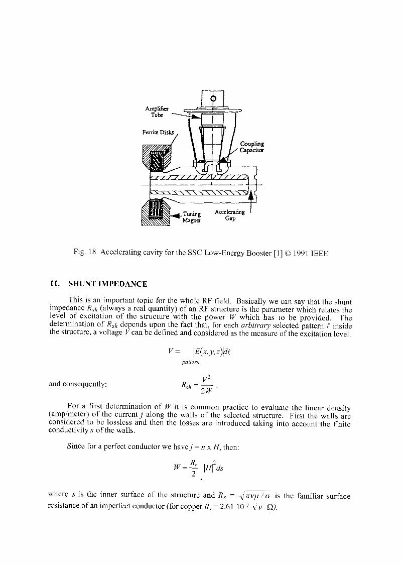
Amplifier Tube
Coupling Capacitor
Tuning Accelerating Magnet G a P
Fig. 18 Accelerating cavity for the SSC Low-Energy Booster [1] © 1991 IEEE
11. SHUNT IMPEDANCE This is an important topic for the whole RF field. Basically we can say that the shunt
impedance Rsh (always a real quantity) of an RF structure is the parameter which relates the level of excitation of the structure with the power W which has to be provided. The determination of Rsh depends upon the fact that, for each arbitrary selected pattern £ inside the structure, a voltage F can be defined and considered as the measure of the excitation level.
V= \E{x,y,zjftt pattern
and consequently: R sh XL 2W
For a first determination of W it is common practice to evaluate the linear density (amp/meter) of the current j along the walls of the selected structure. First the walls are considered to be lossless and then the losses are introduced taking into account the finite conductivity s of the walls.
Since for a perfect conductor we have y = nxH, then:
W = ^- \H^ds s
where s is the inner surface of the structure and Rs = ^nv^i / a is the familiar surface resistance of an imperfect conductor (for copper^ = 2.61 10"7 Vv Q.).

12. RF POWER AMPLIFIERS
1) The power needed to drive the accelerating structures ranges between a few kilowatts and a few megawatts (c.w.).
2) The wave shape is always sinusoidal. Amplitude and frequency modulation may be requested.
3) Due to these facts tuned amplifiers are always used (both for narrow and broad band operation).
4) The tuned amplifier is used because it has high efficiency and allows the generation of sinusoidal carriers independently upon the shape of the current inside the tube.
5) In a tuned amplifier both the input and the output circuits should be resonant (tuned).
6) Sometimes the RF output circuit is the accelerating structure (resonant).
The basic elements of most RF power amplifiers are the triode or the tetrode with which it is possible to cover a frequency range from a few to a few hundred megahertz. At higher frequencies another device is preferred: the klystron. As will be shown later, this is an electron device which, by its own nature, is an amplifier. Both the electron tube and the klystron are considered as RF generators.
13. RF GENERATORS
13.1 Introduction
RF generators constitute a "universe" similar to our own in that it is expanding and contains galaxies. In fact it contains very many groups of elements with something in common but, on the other hand, far apart from each other technically speaking.
The dawn of the modern RF generators started with the invention of the triode by L. de Forest in 1906, a discovery of so great practical importance that it made the electronic industry possible. The actual industrial frontier is represented by the Gyrotron which is a powerful generator in the range of the millimetric waves while the very promising free electron laser is still under laboratory development.
It is important to notice that each new class of generators does not render the previous ones obsolete. This is due to the different applications for which the generator is required. For instance, triodes are still commonly manufactured together with other more modern devices.
13.2 Triode amplifier
It is well known that in a triode, the current Ia depends upon the plate and the grid voltages referred to the cathode. Let Vpk and Vgk be those voltages. Roughly the anode current obeys the "adapted" Langmuir-Cfnld law:
Ia=k{vpk+iiVgkf2 (24)
where k is the perveance of the tube and /J its amplification factor. Unfortunately these parameters are not constant (because they depend upon the current) and should be considered as average values. For this reason the characteristics of each tube provided by the manufacturers should be carefully studied for each application.
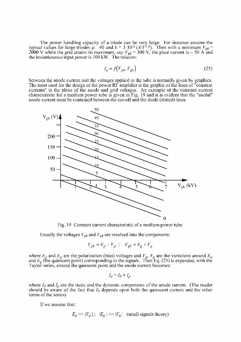
The power handling capacity of a triode can be very large. For instance assume the typical values for large triodes JÂ 40 and k = 3 10"5 (A/V1-5). Then with a minimum Vpi = 2000 V while the grid attains its maximum, say Vgi = 300 V, the plate current is ~ 50 A and the instantaneous input power is 100 kW. The relation:
ia=f{vpk,vgk) (25)
between the anode current and the voltages applied to the tube is normally given by graphics. The most used for the design of the power RF amplifier is the graphic of the lines of "constant currents" in the plane of the anode and grid voltages. An example of the constant current characteristic for a medium power tube is given in Fig. 19 and it is evident that the "useful" anode current must be contained between the cut-off and the diode (dotted) lines.
V p k (kV)
Fig. 19 Constant current characteristic of a medium-power tube
Usually the voltages Vpk and Vgk are resolved into the components:
Vpk=Ep + Vp V, gk En + Vn
where E„ and Eg are the polarization (bias) voltages and Vp, Vg are the variations around Ep
and Eg (the quiescent point) corresponding to the signals. Then Eq. (25) is expanded, with the Taylor series, around the quiescent point and the anode current becomes:
Ia=I()+Ip
where IQ and Ip are the static and the dynamic components of the anode current. (The reader should be aware of the fact that IQ depends upon both the quiescent current and the other terms of the series).
If we assume that:
Ep»\Vp K » I Vg | (small signals theory)
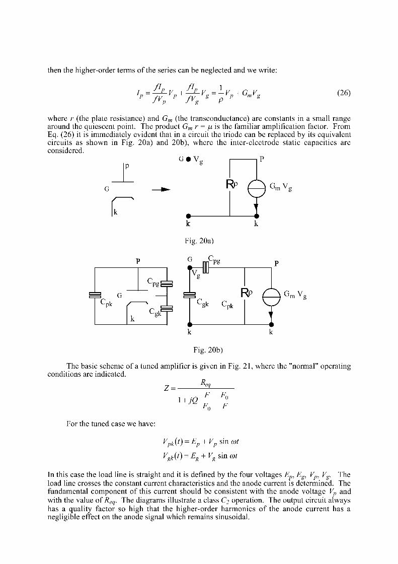
then the higher-order terms of the series can be neglected and we write:
fl I =—^
P fVt
p -r v„ — V +G V p F 6
(26)
where r (the plate resistance) and Gm (the transeonductance) are constants in a small range around the quiescent point. The product Gm r = /j is the familiar amplification factor. From Eq. (26) it is immediately evident that in a circuit the triode can be replaced by its equivalent circuits as shown in Fig. 20a) and 20b), where the inter-electrode static capacities are considered.
G # V
Fig. 20a)
G __C
= G C p k
= G C p k
k C g k =
v„ pg
c
k
RP gk C pk
G m V ,
Fig. 20b)
The basic scheme of a tuned amplifier is given in Fig. 21, where the "normal" operating conditions are indicated.
Z = R -eq
l + / g - - ^ ^o F
For the tuned case we have:
v
Pkif) = Ep + Vp s i n m t
Vgk(t) = Eg + Vg sin cot
In this case the load line is straight and it is defined by the four voltages Ep, Eg
load line crosses the constant current characteristics and the anode current is determined. V V The
The fundamental component of this current should be consistent with the anode voltage Vp and with the value of Req. The diagrams illustrate a class C2 operation. The output circuit always has a quality factor so high that the higher-order harmonics of the anode current has a negligible effect on the anode signal which remains sinusoidal.
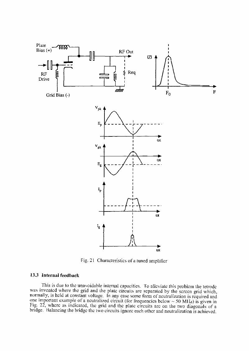
Bias (+) RFOut IZI 4
Grid Bias (-)
ox
hi
tot
Fig. 21 Characteristics of a tuned amplifier
13.3 Internal feedback
This is due to the unavoidable internal capacities. To alleviate this problem the tetrode was invented where the grid and the plate circuits are separated by the screen grid which, normally, is held at constant voltage. In any case some form of neutralization is required and one important example of a neutralized circuit (for frequencies below ~ 50 MHz) is given in Fig. 22, where as indicated, the grid and the plate circuits are on the two diagonals of a bridge. Balancing the bridge the two circuits ignore each other and neutralization is achieved.
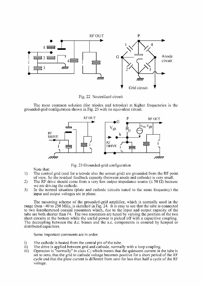
RFOUT •
7177777
1777771 7177777
• Grid circuit
Anode circuit
Fig. 22 Neutralized circuit
The most common solution (for triodes and tetrodes) at higher frequencies is the grounded-grid configuration shown in Fig. 23 with its equivalent circuit.
RFOUT
RF DRIVE
i i
* J i
Ï T T\ r
P RFOUT
I — # G t 1 i—*
"• %k j I J DRIVE ; cztz, ^ P
///// /////
Fig. 23 Grounded-grid configuration Note that:
1) The control grid (and for a tetrode also the screen grid) are grounded from the RF point of view. So the residual feedback capacity (between anode and cathode) is very small.
2) The RF drive should come from a very low output impedance source (< 50 Q) because we are driving the cathode.
3) In the normal situation (plate and cathode circuits tuned to the same frequency) the input and output voltages are in phase.
The mounting scheme of the grounded-grid amplifier, which is normally used in the range from -40 to 250 MHz, is sketched in Fig. 24. It is easy to see that the tube is connected to two foreshortened coaxial resonators which, due to the input and output capacity of the tube are both shorter than IIA. The two resonators are tuned by varying the position of the two short circuits at the bottom while the useful power is picked off with a capacitive coupling. The decoupling between the d.c. biases and the a.c. components is ensured by lumped or distributed capacitors.
Some important comments are in order:
i) The cathode is heated from the central pin of the tube. ii) The drive is applied between grid and cathode, normally with a loop coupling. iii) Operation is "normally" in class C2 which means that the quiescent current in the tube is
set to zero, that the grid to cathode voltage becomes positive for a short period of the RF cycle and that the plate current is different from zero for less than half a cycle of the RF voltage.
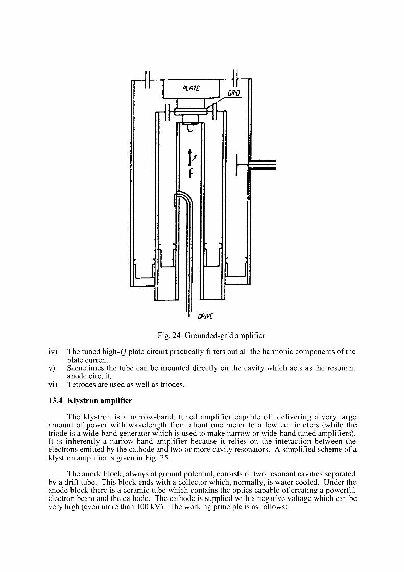
Hl- h
U
J-
(h
U U
h
U
Fig. 24 Grounded-grid amplifier
iv) The tuned high- Q plate circuit practically filters out all the harmonic components of the plate current.
v) Sometimes the tube can be mounted directly on the cavity which acts as the resonant anode circuit,
vi) Tetrodes are used as well as triodes.
13.4 Klystron amplifier
The klystron is a narrow-band, tuned amplifier capable of delivering a very large amount of power with wavelength from about one meter to a few centimeters (while the triode is a wide-band generator which is used to make narrow or wide-band tuned amplifiers). It is inherently a narrow-band amplifier because it relies on the interaction between the electrons emitted by the cathode and two or more cavity resonators. A simplified scheme of a klystron amplifier is given in Fig. 25.
The anode block, always at ground potential, consists of two resonant cavities separated by a drift tube. This block ends with a collector which, normally, is water cooled. Under the anode block there is a ceramic tube which contains the optics capable of creating a powerful electron beam and the cathode. The cathode is supplied with a negative voltage which can be very high (even more than 100 kV). The working principle is as follows:
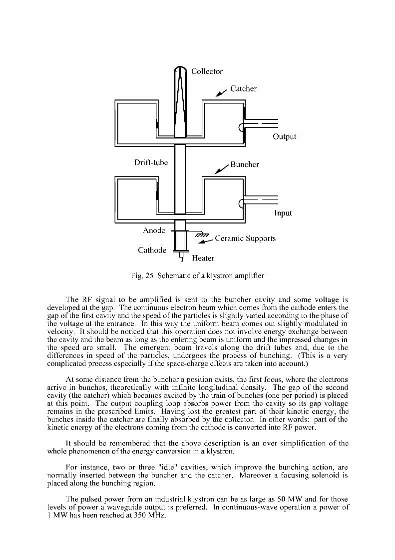
Collector
y Catcher
Output
Drift-tube V Buncher
c Anode
Cathode
Input
//)// Ceramic Supports
T Heater
Fig. 25 Schematic of a klystron amplifier
The RF signal to be amplified is sent to the buncher cavity and some voltage is developed at the gap. The continuous electron beam which comes from the cathode enters the gap of the first cavity and the speed of the particles is slightly varied according to the phase of the voltage at the entrance. In this way the uniform beam comes out slightly modulated in velocity. It should be noticed that this operation does not involve energy exchange between the cavity and the beam as long as the entering beam is uniform and the impressed changes in the speed are small. The emergent beam travels along the drift tubes and, due to the differences in speed of the particles, undergoes the process of bunching. (This is a very complicated process especially if the space-charge effects are taken into account.)
At some distance from the buncher a position exists, the first focus, where the electrons arrive in bunches, theoretically with infinite longitudinal density. The gap of the second cavity (the catcher) which becomes excited by the train of bunches (one per period) is placed at this point. The output coupling loop absorbs power from the cavity so its gap voltage remains in the prescribed limits. Having lost the greatest part of their kinetic energy, the bunches inside the catcher are finally absorbed by the collector. In other words: part of the kinetic energy of the electrons coming from the cathode is converted into RF power.
It should be remembered that the above description is an over simplification of the whole phenomenon of the energy conversion in a klystron.
For instance, two or three "idle" cavities, which improve the bunching action, are normally inserted between the buncher and the catcher. Moreover a focusing solenoid is placed along the bunching region.
The pulsed power from an industrial klystron can be as large as 50 MW and for those levels of power a waveguide output is preferred. In continuous-wave operation a power of 1 MW has been reached at 350 MHz.
REFERENCE
[1] C.C. Friedricks, L. Walling and B.M. Campbell, Design of an accelerating cavity for the Superconducting Super Collider Low-Energy Booster, Proc. Particle Accelerator Conference, May 6-9, 1991 in California.
BIBLIOGRAPHY
1) R.E. Collin, Field Theory of Guided Waves, McGraw Hill, New York (1961).
2) C.G. Montgomery, R.H. Dike and E.M. Purcell, Principles of Microwave Circuits, M.I.T. Radiation Lab. Series, Mc Graw Hill, (1948).
3) T. Moreno, Microwave Transmission Design Data, Dover Pub. Inc., (1958).
4) J.C. Slater, Microwave Electronics, Dover Pub. Inc., (1969).
5) S. Ramo, J.R. Whinnery and T. van Duzer, Fields and Waves in Communication Electronics, John Wiley & Sons, (1984).
6) E.T. Whittaker and G.N. Watson, A Course of Modern Analysis, 4th éd., Cambridge Univ. Press, Cambridge, England, (1952).
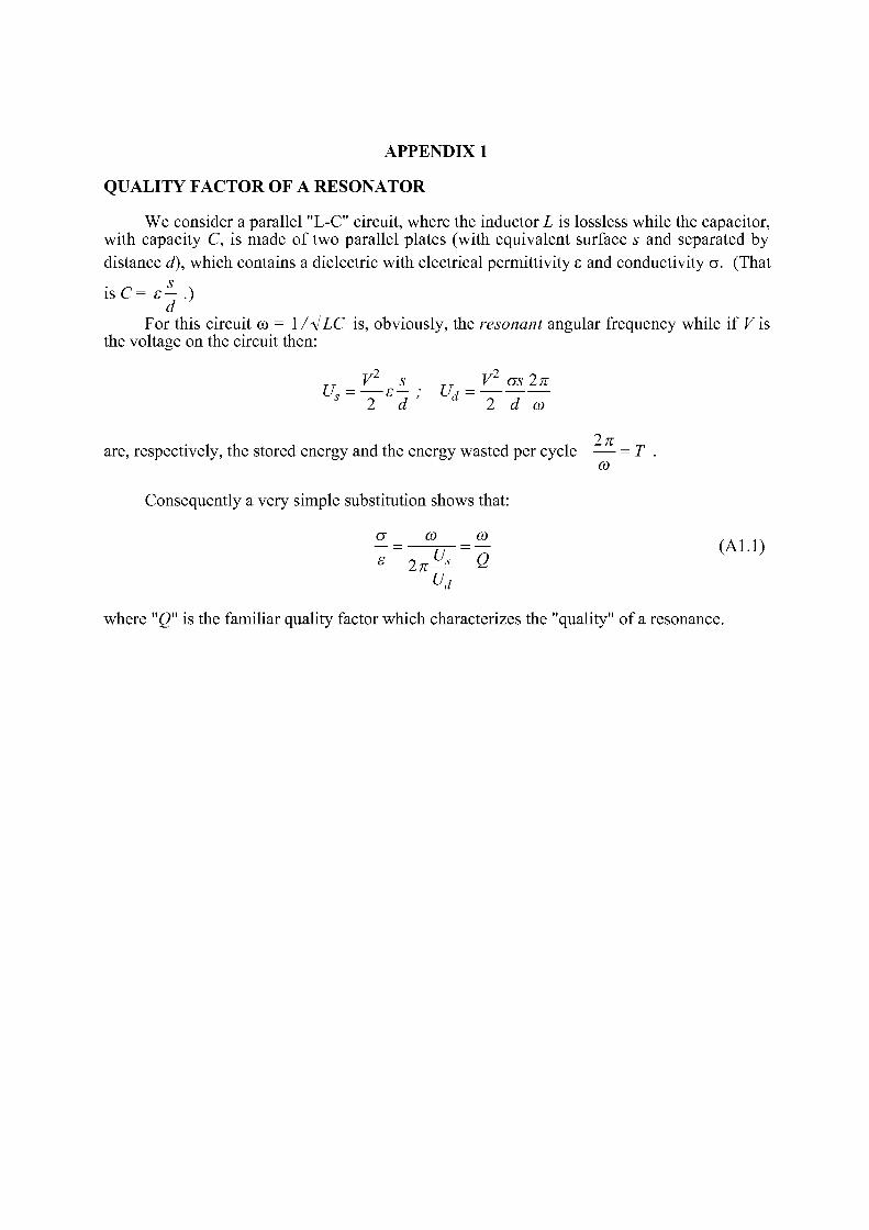
APPENDIX 1
QUALITY FACTOR OF A RESONATOR
We consider a parallel "L-C" circuit, where the inductor L is lossless while the capacitor, with capacity C, is made of two parallel plates (with equivalent surface s and separated by distance d), which contains a dielectric with electrical permittivity s and conductivity a. (That
i sC= e- .)
For this circuit co = 1/^lLC is, obviously, the resonant angular frequency while if Fis the voltage on the circuit then:
V s T r V as 2n U, - — s — ; Uj ' s 2 d 2 d (ù
2n are, respectively, the stored energy and the energy wasted per cycle — = T
co
Consequently a very simple substitution shows that:
a co co *~2nl^~Q
Ud
(AU)
where "Q" is the familiar quality factor which characterizes the "quality" of a resonance.
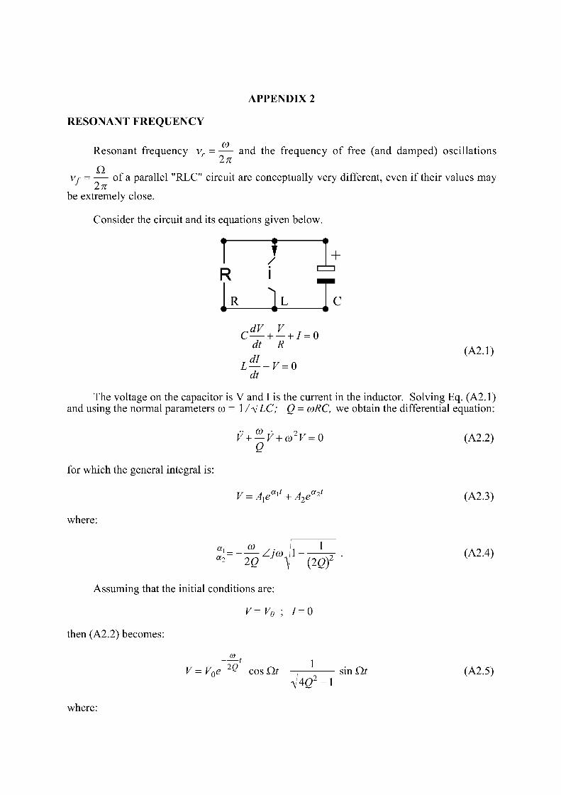
APPENDIX 2 RESONANT FREQUENCY
Resonant frequency vr = — and the frequency of free (and damped) oscillations 2n
Q Vf = — of a parallel "RLC" circuit are conceptually very different, even if their values may
2 n be extremely close.
Consider the circuit and its equations given below.
c ^ + ^ + / = o
dt R
dt
(A2.1)
The voltage on the capacitor is V and I is the current in the inductor. Solving Eq. (A2.1) and using the normal parameters co = 1 /^jLC; Q = coRC, we obtain the differential equation:
V + — V+co2V=0 Q
for which the general integral is:
V = Axeait + A2eait
where:
co a, "J , • -, (X-y /-\ s~\ J 1 I
1 a 2 2Q J f (2Q)2
Assuming that the initial conditions are:
V=V0 ; 7=0
then (A2.2) becomes:
(A2.2)
(A2.3)
(A2.4)
V = Vne 2 Q cos Qt - sin Qt oL
V 4 g z - 1 (A2.5)
where:
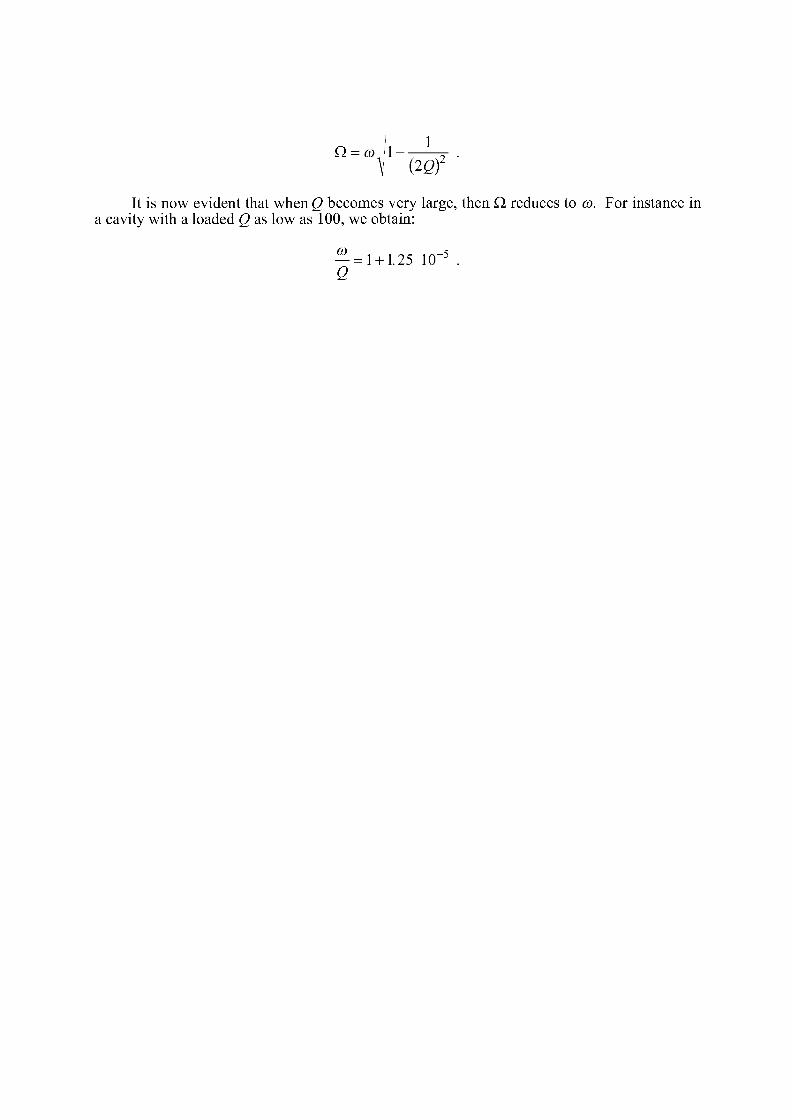
Q,- co 1 ~- . K (2Ô) 2
It is now evident that when Q becomes very large, then Q reduces to co. For instance in a cavity with a loaded Q as low as 100, we obtain:
^ = 1 + 1.25 10"5 . Q
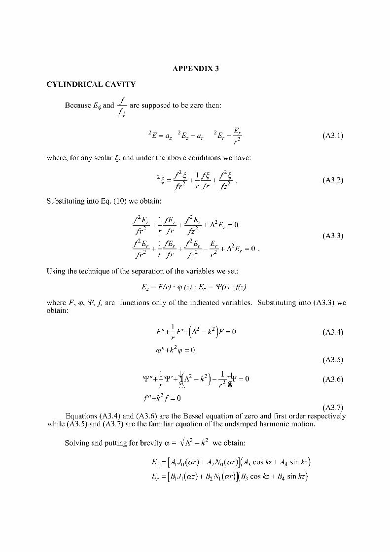
APPENDIX 3
CYLINDRICAL CAVITY
/ Because E^ and J— are supposed to be zero then:
2E = az
2Ez+ar
2 E r - \ (A3.1) r
where, for any scalar £, and under the above conditions we have:
S=-^T + —T + -TT- ( A 3 - 2 ) fr r fr fz
Substituting into Eq. (10) we obtain:
^ + ±& + & + A2Ez=0 fr2 r fr fz2
f Er , l f E r , f Er Er , A 2 F _ n
—— + — + — 2 j " + A Er - 0 / r r / r / z r
(A3.3)
Using the technique of the separation of the variables we set:
Ez = F(r)-<p(z);Er=W(r)-f(z)
where F, cp, W, f, are functions only of the indicated variables. Substituting into (A3.3) we obtain:
F"+-F '+(A 2 - k2y = 0 (A3.4)
(p"+k2(p = 0 (A3.5)
V F " + - V F ' + J A 2 - Â : 2 ) - \*^ = 0 (A3.6)
f"+k2f = 0 (A3.7)
Equations (A3.4) and (A3.6) are the Bessel equation of zero and first order respectively while (A3.5) and (A3.7) are the familiar equation of the undamped harmonic motion.
Solving and putting for brevity a = A / A 2 - * 2 we obtain:
Ez = [A^Q^ar) + A2N0(ar)](A3 cos kz + A4 sin kz)
Er = [BiJi(az) + B2Ni(ar)^B3 cos kz + B4 sin kz)
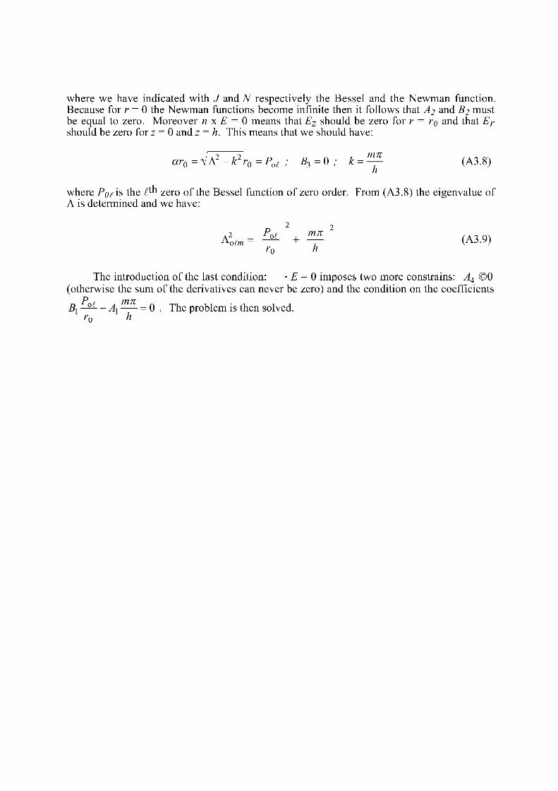
where we have indicated with J and N respectively the Bessel and the Newman function. Because for r = 0 the Newman functions become infinite then it follows that A2 and B2 must be equal to zero. Moreover n x E = 0 means thatis z should be zero for r = ro and that Er
should be zero for z = 0 and z = h. This means that we should have:
ar0 = ^A2-k2r0 = Pof ; B3 = 0 ; k = — (A3.8) h
where PQ£ is the ^ m
z e r o 0 f the Bessel function of zero order. From (A3.8) the eigenvalue of A is determined and we have:
At*,, = Z*- 2 + ^ 2 (A3.9) r 0 h
The introduction of the last condition: • E = 0 imposes two more constrains: A4 ©0 (otherwise the sum of the derivatives can never be zero) and the condition on the coefficients
Bl —^- - Ax = 0 . The problem is then solved. rn h
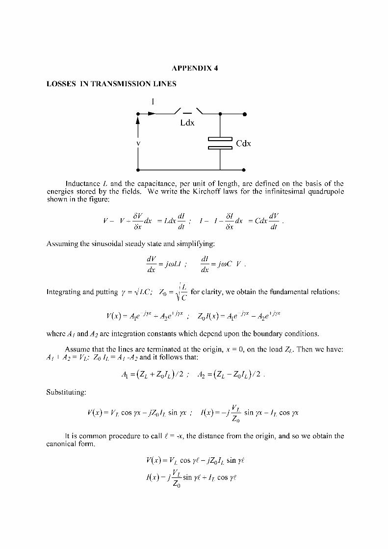
APPENDIX 4
LOSSES IN TRANSMISSION LINES
I
A
V
y— v. Ldx
Cdx
Inductance L and the capacitance, per unit of length, are defined on the basis of the energies stored by the fields. We write the Kirchoff laws for the infinitesimal quadrupole shown in the figure:
J , J , Ô V J TJ d I T T Ô I J ™ dV
V — V H dx = Lax — ; 1 — 1 -\ ax - Lax — . ôx dt ôx dt
Assuming the sinusoidal steady state and simplifying:
dV . TJ dl .
dx dx
Integrating and putting y - -sjLC; Z 0 = J— for clarity, we obtain the fundamental relations:
V{x) = Aie-jïX + A2e
+jyx ; Z0l(x) - Axe~iyx - A2e+jyx
where A] and A2 are integration constants which depend upon the boundary conditions.
Assume that the lines are terminated at the origin, x = 0, on the load Zi. Then we have: A] + A2 = Vi; ZQ h = A] -A2 and it follows that:
Al=(ZL+Z0IL)/2 ; A2=(ZL-Z0IL)/2
Substituting:
VT V(x) - VL cos yx -jZ0IL sin yx ; l(x) - -j— sin yx + IL cos yx
It is common procedure to call £ = -x, the distance from the origin, and so we obtain the canonical form.
V(x) = VL cos y£ +jZ0IL sin y£
l(x) = j —^sin y£ + IL cos y£
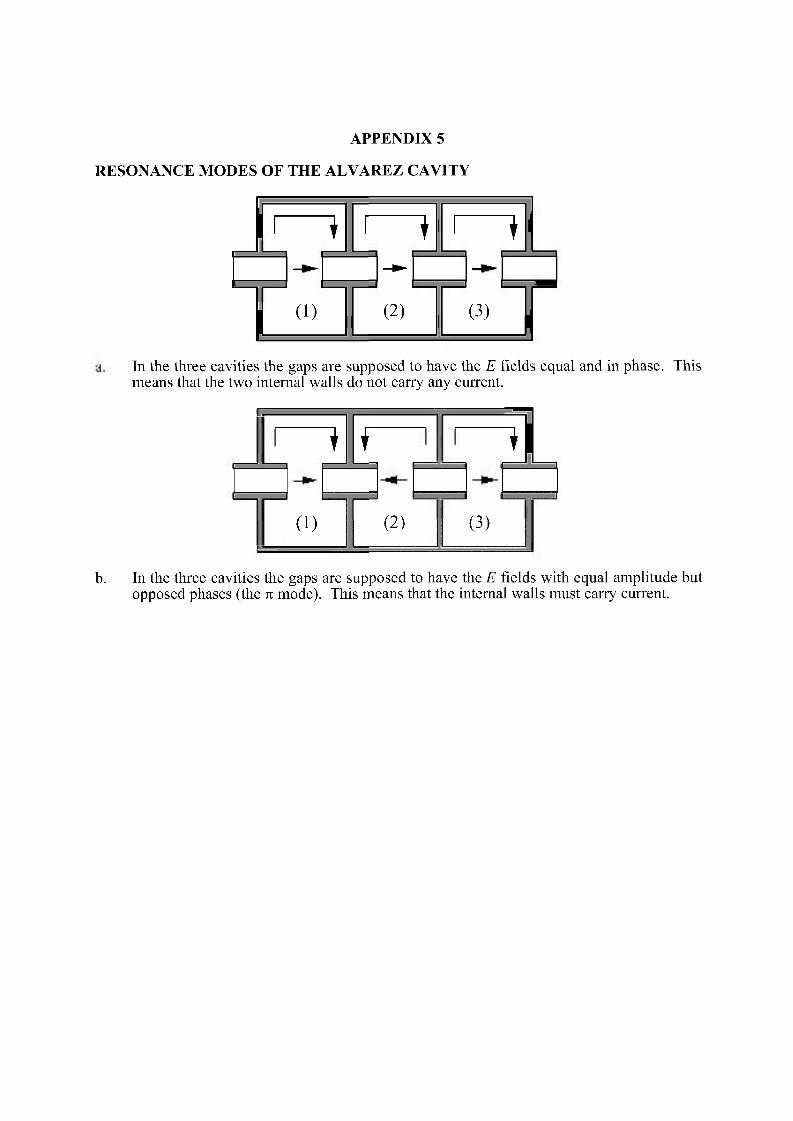
APPENDIX 5
RESONANCE MODES OF THE ALVAREZ CAVITY
Il 1
Jh i 1 1 1 1 - •
i
\\ ( 1 )
(2) (3)
In the three cavities the gaps are supposed to have the E fields equal and in phase. This means that the two internal walls do not carry any current.
1 f a (i) (2) (3)
b. In the three cavities the gaps are supposed to have the E fields with equal amplitude but opposed phases (the n mode). This means that the internal walls must carry current.
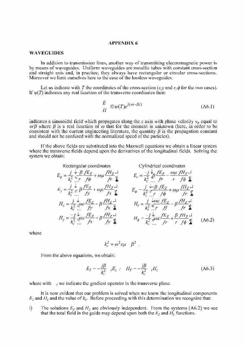
APPENDIX 6
WAVEGUIDES
In addition to transmission lines, another way of transmitting electromagnetic power is by means of waveguides. Uniform waveguides are metallic tubes with constant cross-section and straight axis and, in practice, they always have rectangular or circular cross-sections. Moreover we limit ourselves here to the case of the lossless waveguides.
Let us indicate with T the coordinates of the cross-section (x,y and r, <f) for the two cases). If i//(Z) indicates any real function of the transverse coordinates then:
E ©¥(T)Amt-pz) (A6.1)
indicates a sinusoidal field which propagates along the z axis with phase velocity vp equal to co/(5 where (5 is a real function of co that for the moment is unknown (here, in order to be consistent with the current engineering literature, the quantity (5 is the propagation constant and should not be confused with the normalized speed of the particles).
If the above fields are substituted into the Maxwell equations we obtain a linear system where the transverse fields depend upon the derivatives of the longitudinal fields. Solving the system we obtain:
Rectangular coordinates Cylindrical coordinates _ j ^P/Ez /HZJ _-ji /Ez coM/HzJ
K T.r ft fr % K 1 fr r f<f> *
E -±i_B& + C0UfE^J
F _ J ^PfEz fHzJ y - * > ? . p fy M A I 0 " ? f 7 7 ^ + ^ 7 ^ *
J K... fy fx % kz
c Zr ff fr %
y-*>^A P fy I 0 " ? ^ ~fr~ + ~r~fi% ( A 6 - 2 )
where
k2
c - (Ù2SJI -fi2 .
From the above equations, we obtain:
ET = -J4 tEz; HT = -J-£ tHz (A6.3) k c
where with t we indicate the gradient operator in the transverse plane.
It is now evident that our problem is solved when we know the longitudinal components Ez and Hz and the value of kc. Before proceeding with this determination we recognize that:
i) The solutions Ez and Hz are obviously independent. From the systems (A6.2) we see that the total field in the guide may depend upon both the Ez and Hz functions.
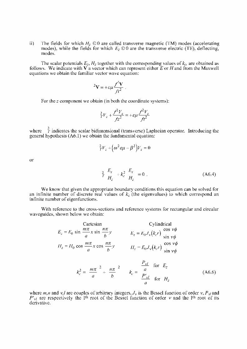
ii) The fields for which Hz © 0 are called transverse magnetic (TM) modes (accelerating modes), while the fields for which Ez © 0 are the transverse electric (TE), deflecting, modes.
The scalar potentials Ez, Hz together with the corresponding values of kc, are obtained as follows. We indicate with V a vector which can represent either E or H and from the Maxwell equations we obtain the familiar vector wave equation:
2 / V ft2
For the z component we obtain (in both the coordinate systems):
7 f2V f2V A ft
2 where T indicates the scalar bidimensional (transverse) Laplacian operator. Introducing the general hypothesis (A6.1) we obtain the fundamental equation:
2
TVz+(co2s^-l32)vz = 0
or
T ** +k2 f" = 0 . (A6.4) tiz nz
We know that given the appropriate boundary conditions this equation can be solved for an infinite number of discrete real values of kc (the eigenvalues) to which correspond an infinite number of eigenfunctions.
With reference to the cross-sections and reference systems for rectangular and circular waveguides, shown below we obtain:
Cartesian Cylindrical mn . nn , cos vé Ez = E0 sin —x sin —y ^ = E0Jv(kcr)
I sin v(j)
sin v(j) TT TT mn nn cos vé Hz=H0cos—xcos—y H E0Jv(kcr) .
2 2 — for Ez
,2 Mn nn , a K= — + — K= Z (A6.6) for H7
a b c P'vi
where m,n and v,l are couples of arbitrary integers, Jv is the Bessel function of order v, P^ and P'vi are respectively the 1 t h root of the Bessel function of order v and the 1 t h root of its derivative.
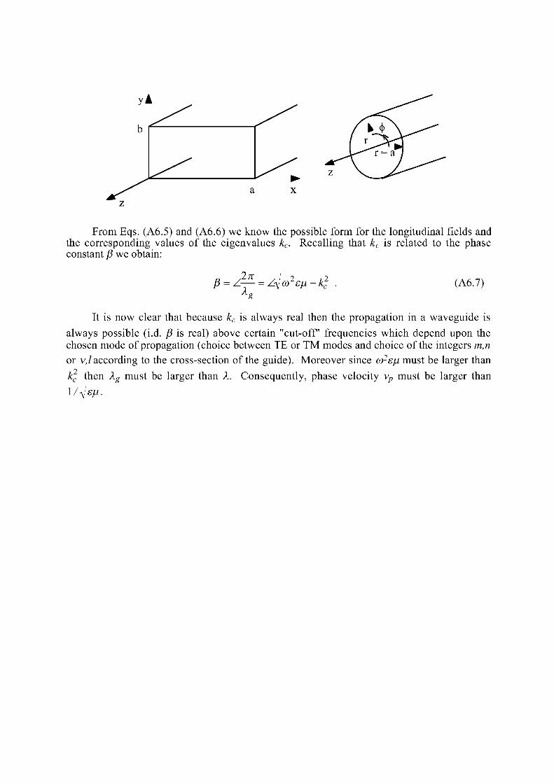
From Eqs. (A6.5) and (A6.6) we know the possible form for the longitudinal fields and the corresponding values of the eigenvalues kc. Recalling that kc is related to the phase constant (3 we obtain:
p = Z— = AJœ2en-kc . (A6.7) Xg
It is now clear that because kc is always real then the propagation in a waveguide is
always possible (i.d. ft is real) above certain "cut-off frequencies which depend upon the chosen mode of propagation (choice between TE or TM modes and choice of the integers m,n or v,l according to the cross-section of the guide). Moreover since (ù2e\x must be larger than
kc then Xg must be larger than X. Consequently, phase velocity vp must be larger than
1 /^fs/u.
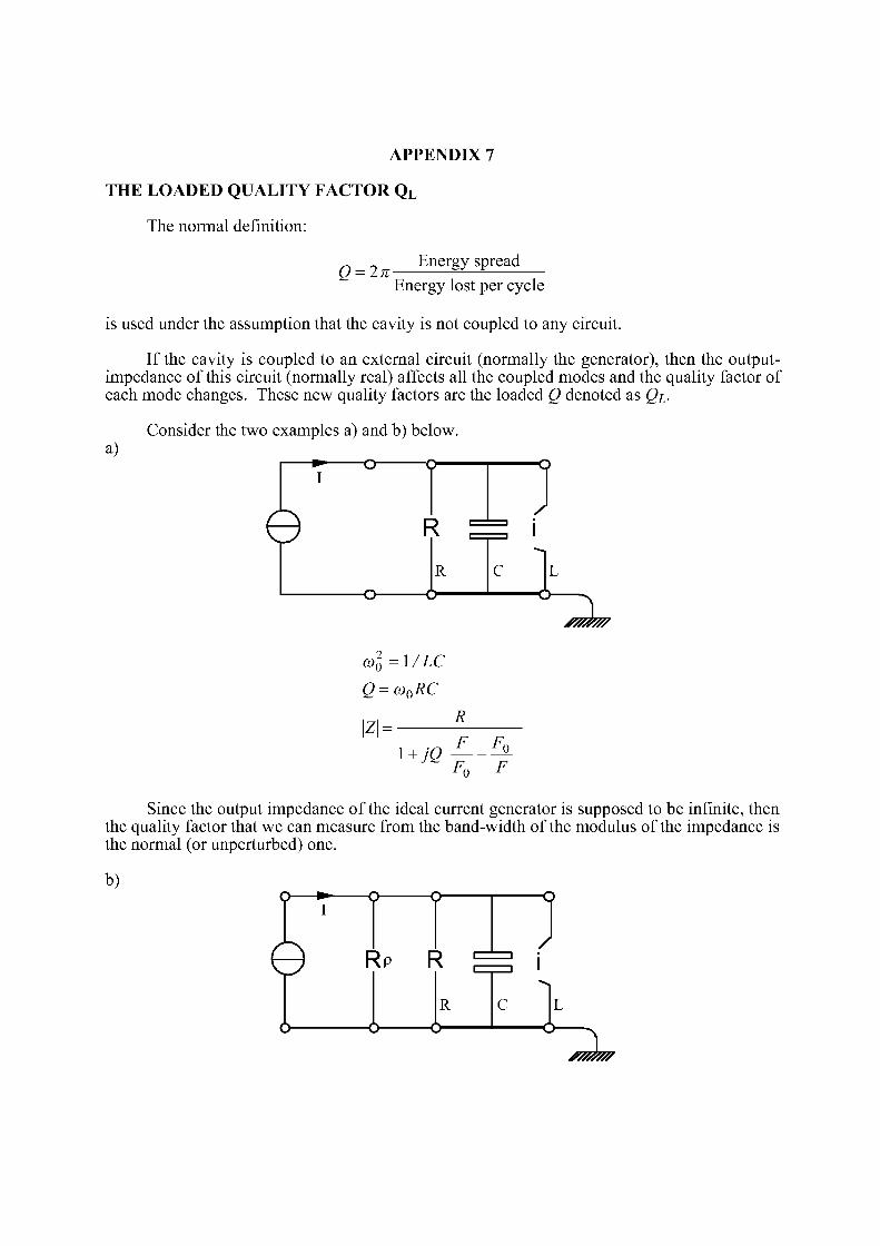
APPENDIX 7
THE LOADED QUALITY FACTOR Q L
The normal definition:
Energy spread Q = 2n-
Energy lost per cycle
is used under the assumption that the cavity is not coupled to any circuit.
If the cavity is coupled to an external circuit (normally the generator), then the output-impedance of this circuit (normally real) affects all the coupled modes and the quality factor of each mode changes. These new quality factors are the loaded Q denoted as Qi.
a) Consider the two examples a) and b) below.
—*• o o — I
e R /
R C
o>l=\/LC Q = (o0RC
R
1+jQ F F Fn
0 F
Since the output impedance of the ideal current generator is supposed to be infinite, then the quality factor that we can measure from the band-width of the modulus of the impedance is the normal (or unperturbed) one.
b)
G RP R
R
/
' . '
C
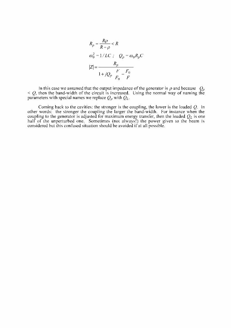
RP = J£-<R p R + p
a>l=\/LC ; Q =G)0RC
\Z\ Rp
Fn F F_ Fn
7o
In this case we assumed that the output impedance of the generator is p and because Qp
< Q, then the band-width of the circuit is increased. Using the normal way of naming the parameters with special names we replace Qp with Qi.
Coming back to the cavities: the stronger is the coupling, the lower is the loaded Q. In other words: the stronger the coupling the larger the band-width. For instance when the coupling to the generator is adjusted for maximum energy transfer, then the loaded Qi is one half of the unperturbed one. Sometimes (not always!) the power given to the beam is considered but this confused situation should be avoided if at all possible.

VACUUM SYSTEM DESIGN
A.G. Mathewson CERN. Geneva, Switzerland
1 . INTRODUCTION
In this paper the basic terms used by the vacuum engineer are presented and some useful formulae are also given. The concept of bakeout is introduced and the physics behind it explained. However we will not dwell on the very basics of vacuum system design but concentrate on the effects in electron and proton storage rings which are due to energetic particle bombardment of the vacuum system walls and the ensuing gas desorption which may detrimentally affect the running of the machine. In addition, the problems associated with proton storage rings where the vacuum chamber is at cryogenic temperature are described.
2 . BASIC FORMULAE
What interests the electron or proton storage ring vacuum system builder is the molecular density encountered by the circulating particles since it is these residual gas molecules which scatter the circulating particles and, with time, gradually reduce the beam intensity.
Although most vacuum gauges measure the molecular density, conventionally we always refer to pressure, which is a force per unit area. The pressure/5 is given by:
P = const n M <v2>
where n is the number of molecules/cm3
Mis the mass of the molecule
and <v2> is the mean square velocity of the molecule
In the MKS system the unit of pressure is the Pascal (Pa) and
1 Pa = 1 N m"2
The relation between pressure and molecular density is derived from Avogadro's number and the definition of the gram molecular volume i.e. 22.414 1 of gas at 1.013 105 Pa (1 atmosphere) and 273 K contain 6.023 10 2 3 molecules. Or 1 Pa 1 of gas contains 2.65 10 1 7
molecules at 273 K.
Other units of pressure used very frequently are Torr and millibar where
1 Torr = 133.33 Pa
and 1 millibar = 100 Pa
At lower temperatures, for a given pressure, the number density of molecules increases since the kinetic energy of the molecule is proportional to the temperature and it is the mean square velocity of the molecule which enters in the expression for the pressure.
Pressures in storage rings are typically below 1 10~9 Torr.
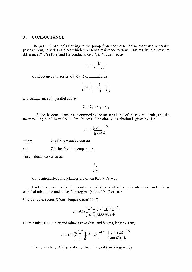
3 . CONDUCTANCE
The gas Q (Torr Is" 1) flowing to the pump from the vessel being evacuated generally passes through a series of pipes which represent a resistance to flow. This results in a pressure difference P1-P2 (Torr) and the conductance C (1 s_1) is defined as:
c- e Pi-Pi
Conductances in series C\, C2, C3, add as
_L-_L _L _L C Q C2 C3
and conductances in parallel add as
C = CX + C2+CT,
Since the conductance is determined by the mean velocity of the gas molecule, and the mean velocity v of the molecule for a Maxwellian velocity distribution is given by [1]:
- A kT } / 2
v - 4 „
where k is Boltzmann's constant
and T is the absolute temperature
the conductance varies as:
Conventionally, conductances are given for N2, M= 28.
Useful expressions for the conductance C (1 s _ 1) of a long circular tube and a long elliptical tube in the molecular flow regime (below 10 3 Torr) are:
Circular tube, radius R (cm), length L (cm) » R
C = 9 2 . 8 ^ ^ ^ 1 / 2
Elliptic tube, semi major and minor axes a (cm) and b (cm), lengths (cm)
C = 130 ia2b2 4 1 s : L #
2 , L 2
a + b -1/2 i T j | 28 j 1/2
9oo stmt The conductance C (1 s_1) of an orifice of area A (cm2) is given by
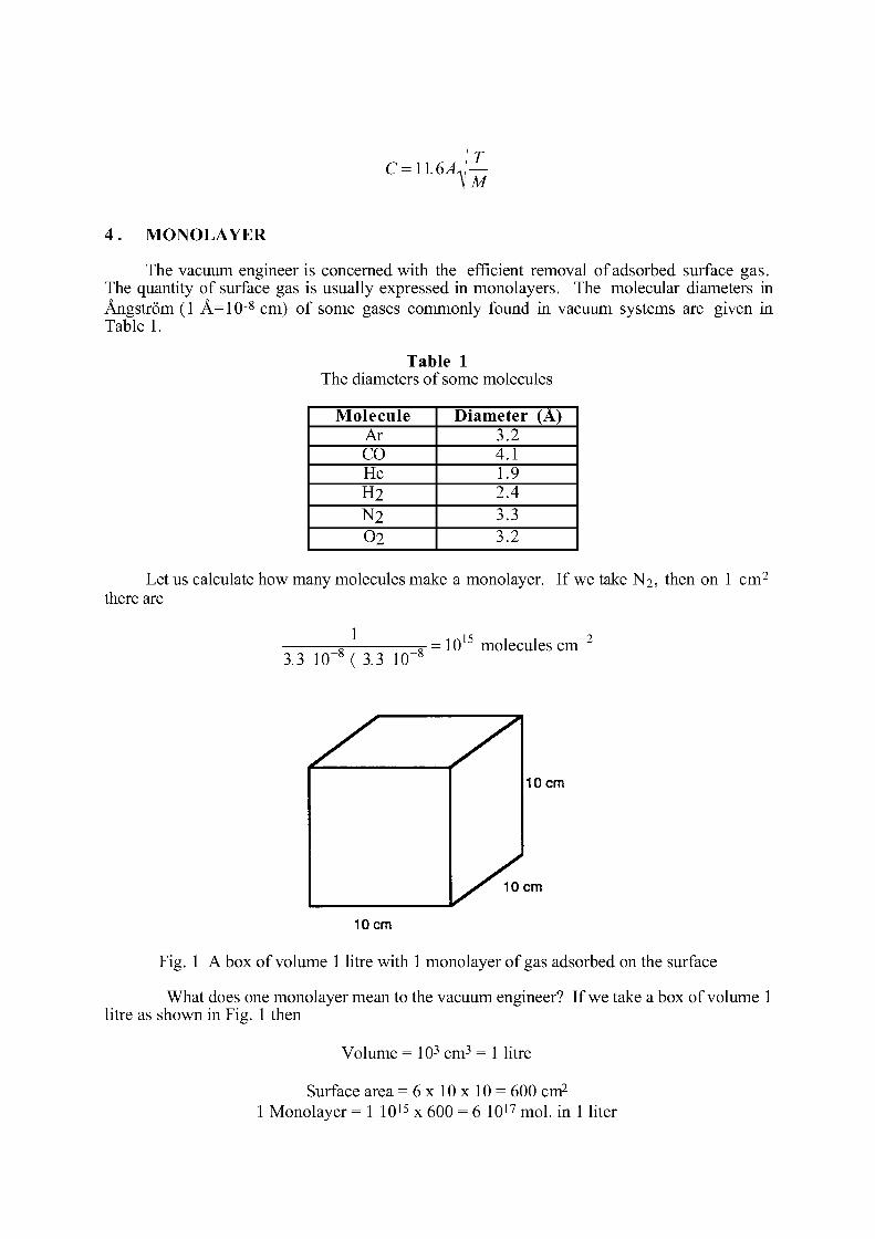
C = 1L6AJ—
MONOLAYER
The vacuum engineer is concerned with the efficient removal of adsorbed surface gas. The quantity of surface gas is usually expressed in monolayers. The molecular diameters in Angstrom (1 Â=10"8 cm) of some gases commonly found in vacuum systems are given in Table 1.
Table 1 The diameters of some molecules
Molecule Diameter (A) Ar 3.2 CO 4.1 He 1.9 H2 2.4 N2 3.3 02 3.2
Let us calculate how many molecules make a monolayer. If we take N2, then on 1 cm 2
there are
1 3.3 10"8< 3.3 10"
1 c >-\
10 molecules cm
10 cm
10 cm
10 cm
Fig. 1 A box of volume 1 litre with 1 monolayer of gas adsorbed on the surface
What does one monolayer mean to the vacuum engineer? If we take a box of volume 1 litre as shown in Fig. 1 then
Volume = 103 cm3 = 1 litre
Surface area = 6 x 1 0 x 1 0 = 600 cm2
1 Monolayer =1 10 1 5 x 600 = 6 10 1 7 mol. in 1 liter
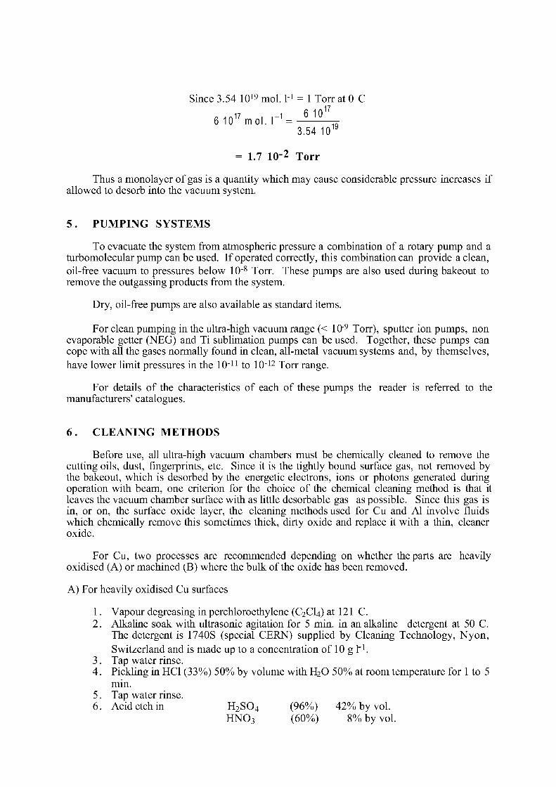
Since 3.54 10 1 9 mol. F = 1 Torr at 0 C ,17 , ,-1 6 10 1 7
6 10" mol. P = 3.54 10 1 9
= 1.7 10-2 Torr
Thus a monolayer of gas is a quantity which may cause considerable pressure increases if allowed to desorb into the vacuum system.
5. PUMPING SYSTEMS
To evacuate the system from atmospheric pressure a combination of a rotary pump and a turbomolecular pump can be used. If operated correctly, this combination can provide a clean, oil-free vacuum to pressures below 10~8 Torr. These pumps are also used during bakeout to remove the outgassing products from the system.
Dry, oil-free pumps are also available as standard items.
For clean pumping in the ultra-high vacuum range (< 10"9 Torr), sputter ion pumps, non evaporable getter (NEG) and Ti sublimation pumps can be used. Together, these pumps can cope with all the gases normally found in clean, all-metal vacuum systems and, by themselves, have lower limit pressures in the 10"11 to 10"12 Torr range.
For details of the characteristics of each of these pumps the reader is referred to the manufacturers' catalogues.
6. CLEANING METHODS
Before use, all ultra-high vacuum chambers must be chemically cleaned to remove the cutting oils, dust, fingerprints, etc. Since it is the tightly bound surface gas, not removed by the bakeout, which is desorbed by the energetic electrons, ions or photons generated during operation with beam, one criterion for the choice of the chemical cleaning method is that it leaves the vacuum chamber surface with as little desorbable gas as possible. Since this gas is in, or on, the surface oxide layer, the cleaning methods used for Cu and Al involve fluids which chemically remove this sometimes thick, dirty oxide and replace it with a thin, cleaner oxide.
For Cu, two processes are recommended depending on whether the parts are heavily oxidised (A) or machined (B) where the bulk of the oxide has been removed.
A) For heavily oxidised Cu surfaces
1. Vapour degreasing in perchloroethylene (C2CI4) at 121 C. 2. Alkaline soak with ultrasonic agitation for 5 min. in an alkaline detergent at 50 C.
The detergent is 1740S (special CERN) supplied by Cleaning Technology, Nyon, Switzerland and is made up to a concentration of 10 g 1"1.
3. Tap water rinse. 4. Pickling in HC1 (33%) 50% by volume with H 2 0 50% at room temperature for 1 to 5
min. 5. Tap water rinse. 6. Acid etch in H 2 S 0 4 (96%) 42% by vol.
HNO3 (60%) 8% by vol.
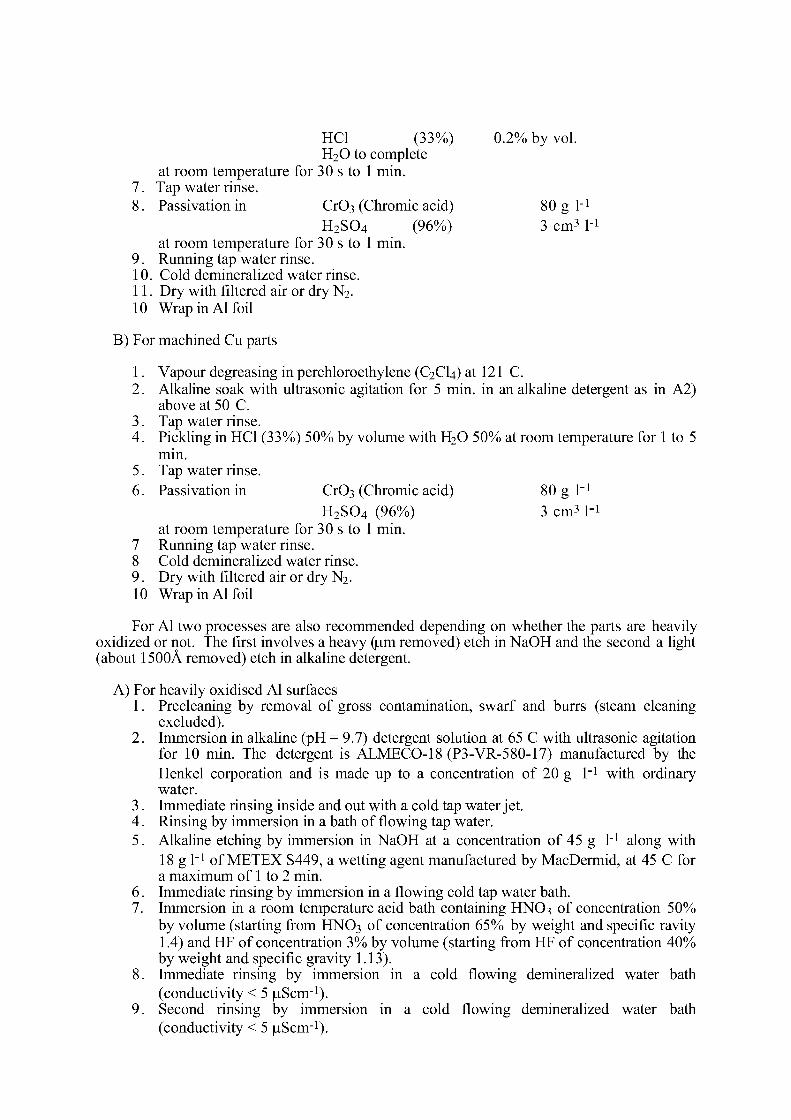
HC1 (33%) 0.2% by vol. H 2 0 to complete
at room temperature for 30 s to 1 min. 7. Tap water rinse. 8. Passivation in CrÛ3 (Chromic acid) 80 g I"1
H 2 S 0 4 (96%) 3 cm 3 F at room temperature for 30 s to 1 min.
9. Running tap water rinse. 10. Cold demineralized water rinse. 11. Dry with filtered air or dry N 2. 10 Wrap in Al foil
B) For machined Cu parts
1. Vapour degreasing in perchloroethylene (C2CI4) at 121 C. 2. Alkaline soak with ultrasonic agitation for 5 min. in an alkaline detergent as in A2)
above at 50 C. 3. Tap water rinse. 4. Pickling in HC1 (33%) 50% by volume with H 2 0 50% at room temperature for 1 to 5
min. 5. Tap water rinse. 6. Passivation in CrÛ3 (Chromic acid) 80 g H
H 2 S 0 4 (96%) 3 cm 3 H at room temperature for 30 s to 1 min.
7 Running tap water rinse. 8 Cold demineralized water rinse. 9. Dry with filtered air or dry N 2. 10 Wrap in Al foil
For Al two processes are also recommended depending on whether the parts are heavily oxidized or not. The first involves a heavy (jum removed) etch in NaOH and the second a light (about 1500Â removed) etch in alkaline detergent.
A) For heavily oxidised Al surfaces 1. Precleaning by removal of gross contamination, swarf and burrs (steam cleaning
excluded). 2. Immersion in alkaline (pH = 9.7) detergent solution at 65 C with ultrasonic agitation
for 10 min. The detergent is ALMECO-18 (P3-VR-580-17) manufactured by the Henkel corporation and is made up to a concentration of 20 g H with ordinary water.
3. Immediate rinsing inside and out with a cold tap water jet. 4. Rinsing by immersion in a bath of flowing tap water. 5. Alkaline etching by immersion in NaOH at a concentration of 45 g H along with
18 g F of METEX S449, a wetting agent manufactured by MacDermid, at 45 C for a maximum of 1 to 2 min.
6. Immediate rinsing by immersion in a flowing cold tap water bath. 7. Immersion in a room temperature acid bath containing HNO3 of concentration 50%
by volume (starting from FINO3 of concentration 65% by weight and specific ravity 1.4) and HF of concentration 3% by volume (starting from HF of concentration 40% by weight and specific gravity 1.13).
8. Immediate rinsing by immersion in a cold flowing demineralized water bath (conductivity < 5 n-Scnr1).
9. Second rinsing by immersion in a cold flowing demineralized water bath (conductivity < 5 n-Scnr1).

10.Drying in a hot air oven at about 80 C. Care must be taken to drain all excess water from the tubes before drying as the combination of water and high temperature can form thick oxide layers on the surface.
A) For lightly oxidised Al surfaces
1. Precleaning by removal of gross contamination, swarf and burrs (steam cleaning excluded).
2. Immersion in alkaline (pH = 9.7) detergent solution at 65 C with ultrasonic agitation for 10 min. The detergent is ALMECO-18(=P3-VR-580-17) manufactured by the Henkel corporation and is made up to a concentration of 20 g H with ordinary water.
3. Immediate rinsing inside and out with a cold demineralized water water jet. 4. Rinsing by immersion in a bath of cold flowing demineralized water (conductivity
< 5 luScnr1). 5. Drying in a hot air oven at about 80 C. Care must be taken to drain all excess water
from the tubes before drying as the combination of water and high temperature can form thick oxide layers on the surface.
The above processes have been found to be effective in cleaning the 128 Cu RF cavity units and the 27 km of Al vacuum chambers in the CERN Large Electron Positron (LEP) storage ring [2,3]- However, it must be remembered that chemical cleaning procedures will never provide atomically clean surfaces since traces of the cleaning solutions will always remain and exposure to air results in adsorption of water vapour, CO2, etc.
7. THERMAL OUTGASSING
The vacuum pumps have to cope with a molecular flux Q from the surface. The units of Q are molecules s _ 1 or Torr I s - 1 . The equilibrium pressure P (Torr) obtained when one has a pumping speed S (1 s - 1) and an outgassing rate Q (Torr 1 s"1) is given by:
s Molecules are bound to the surface with a certain binding energy E (eV) and the rate at
which the surface coverage N (molecules cm"2) is reduced is given by:
d N . *r ~ E
— = - const N exp
dt kT
where k is Boltzmann's constant
and T is the absolute temperature dN The thermal outgassing rate Q is simply —r-
Typical values of outgassing rates for clean, baked stainless steel, Cu or Al are around 1 10"12 (Torr 1 s _ 1 cm - 2) and that is mostly H2.
For unbaked surfaces the outgassing rates are roughly 10 times higher and contain other gases apart from H 2 such as CH4, H 2 0 , CO and CO2 and take longer to pump down to the equilibrium pressure. Figure 2 shows how the outgassing rate depends on the pumping time.
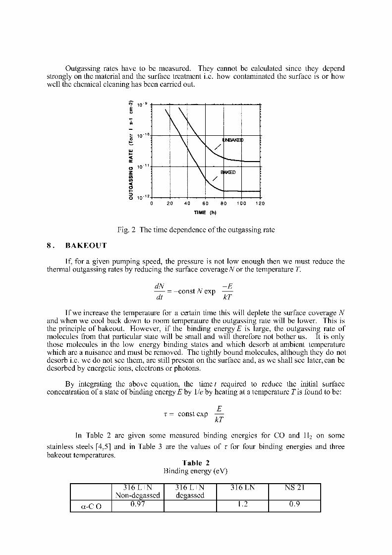
Outgassing rates have to be measured. They cannot be calculated since they depend strongly on the material and the surface treatment i.e. how contaminated the surface is or how well the chemical cleaning has been carried out.
o
10 ' s
10"
< E (3 Z CO CO < a 3 o
10- 1
10'
: •
•
IJNBAKE )
•
IJNBAKE
: B WED ;
: B
20 40 60 80
TIME (h)
100 120
Fig. 2 The time dependence of the outgassing rate
8 . BAKEOUT
If, for a given pumping speed, the pressure is not low enough then we must reduce the thermal outgassing rates by reducing the surface coverage TV or the temperature T.
d N . *r ~ E
= -const N exp dt kT
If we increase the temperature for a certain time this will deplete the surface coverage N and when we cool back down to room temperature the outgassing rate will be lower. This is the principle of bakeout. However, if the binding energy E is large, the outgassing rate of molecules from that particular state will be small and will therefore not bother us. It is only those molecules in the low energy binding states and which desorb at ambient temperature which are a nuisance and must be removed. The tightly bound molecules, although they do not desorb i.e. we do not see them, are still present on the surface and, as we shall see later, can be desorbed by energetic ions, electrons or photons.
By integrating the above equation, the time t required to reduce the initial surface concentration of a state of binding energy E by lie by heating at a temperature r i s found to be:
x - const exp kT
In Table 2 are given some measured binding energies for CO and H 2 on some stainless steels [4,5] and in Table 3 are the values of T for four binding energies and three bakeout temperatures.
Table 2 Binding energy (eV)
316 L+N Non-degassed
316 L+N degassed
316 LN NS21
a-CO 0.97 1.2 0.9
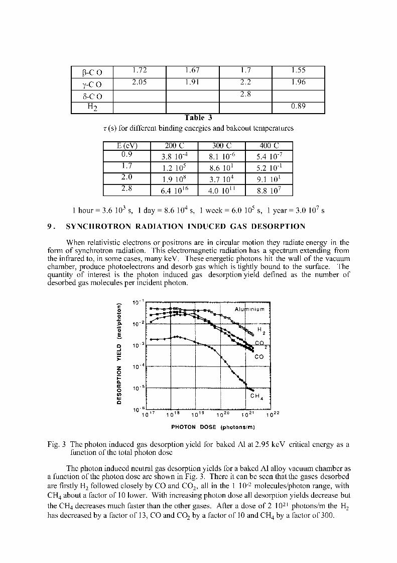
9
p-co 1.72 1.67 1.7 1.55 Y-CO 2.05 1.91 2.2 1.96 Ô-CO 2.8 H 2 0.89
Table 3 T (s) for different binding energies and bakeout temperatures
E(eV) 200 C 300 C 400 C 0.9 3.8 10"4 8.1 10"6 5.4 10"7
1.7 1.2 105 8.6 101 5.2 10"1
2.0 1.9 108 3.7 104 9.1 101
2.8 6.4 10 1 6 4.0 10 1 1 8.8 107
1 hour = 3.6 103 s, 1 day = 8.6 104 s, 1 week = 6.0 105 s, 1 year = 3.0 107 s
SYNCHROTRON RADIATION INDUCED GAS DESORPTION
When relativistic electrons or positrons are in circular motion they radiate energy in the form of synchrotron radiation. This electromagnetic radiation has a spectrum extending from the infrared to, in some cases, many keV. These energetic photons hit the wall of the vacuum chamber, produce photoelectrons and desorb gas which is tightly bound to the surface. The quantity of interest is the photon induced gas desorption yield defined as the number of desorbed gas molecules per incident photon.
c o Ô c Q.
"5 E
UJ
>-z o a. oc o v> UJ
a
PHOTON DOSE (photons/m)
Fig. 3 The photon induced gas desorption yield for baked Al at 2.95 keV critical energy as a function of the total photon dose
The photon induced neutral gas desorption yields for a baked Al alloy vacuum chamber as a function of the photon dose are shown in Fig. 3. There it can be seen that the gases desorbed are firstly H 2 followed closely by CO and C0 2 , all in the 1 10"2 molecules/photon range, with CH4 about a factor of 10 lower. With increasing photon dose all desorption yields decrease but the CH4 decreases much faster than the other gases. After a dose of 2 10 2 1 photons/m the H 2
has decreased by a factor of 13, CO and C0 2 by a factor of 10 and CH4 by a factor of 300.
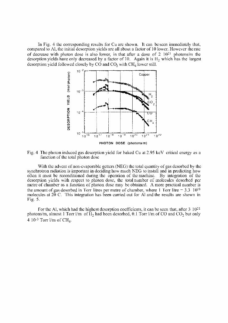
In Fig. 4 the corresponding results for Cu are shown. It can be seen immediately that, compared to Al, the initial desorption yields are all about a factor of 10 lower. However the rate of decrease with photon dose is also lower, in that after a dose of 2 10 2 1 photons/m the desorption yields have only decreased by a factor of 10. Again it is H 2 which has the largest desorption yield followed closely by CO and C0 2 with CH4 lower still.
c o o
I "5 _§_ Q _J UJ
z o I -o. cc o en UJ Q
PHOTON DOSE (photons/m)
Fig. 4 The photon induced gas desorption yield for baked Cu at 2.95 keV critical energy as a function of the total photon dose
With the advent of non-evaporable getters (NEG) the total quantity of gas desorbed by the synchrotron radiation is important in deciding how much NEG to install and in predicting how often it must be reconditioned during the operation of the machine. By integration of the desorption yields with respect to photon dose, the total number of molecules desorbed per metre of chamber as a function of photon dose may be obtained. A more practical number is the amount of gas desorbed in Torr litres per metre of chamber, where 1 Torr litre = 3.3 10 1 9
molecules at 20 C. This integration has been carried out for Al and the results are shown in Fig. 5.
For the Al, which had the highest desorption coefficients, it can be seen that, after 3 10 2 1
photons/m, almost 1 Torr 1/m of H 2 had been desorbed, 0.1 Torr 1/m of CO and C 0 2 but only 4 10- 3Torrl/mofCH 4 .
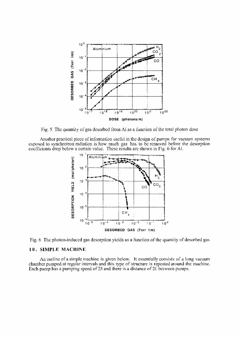
1 0 l
E - 10" 1
tn <
10"
S 1er3
m ce O Î2 i o - 4
Q
10"
Alum nium CO
: CO i
" T H 4 : J ï y :
/
1 0 ' 1 0 ' 1 0 I S 1 0 " 10
DOSE (photons/m)
21 10 22
Fig. 5 The quantity of gas desorbed from Al as a function of the total photon dose
Another practical piece of information useful in the design of pumps for vacuum systems exposed to synchrotron radiation is how much gas has to be removed before the desorption coefficients drop below a certain value. These results are shown in Fig. 6 for Al.
c o Ô a. "5 E
UJ
CL CE o (/) UJ a
10
10'
10"
10"
10
10
; A l u m i n i i _
?
; A l u m i n i i _
3
H \ : 2
4
CO C 0 2 ;
S
i
6
C H 4
1 0 " 3 10 10 J 10"^ 1 0 ' 1
DESORBED GAS (Torr l/m)
1 0 l
Fig. 6 The photon-induced gas desorption yields as a function of the quantity of desorbed gas
10 . SIMPLE MACHINE
An outline of a simple machine is given below. It essentially consists of a long vacuum chamber pumped at regular intervals and this type of structure is repeated around the machine. Each pump has a pumping speed of 25* and there is a distance of IL between pumps.
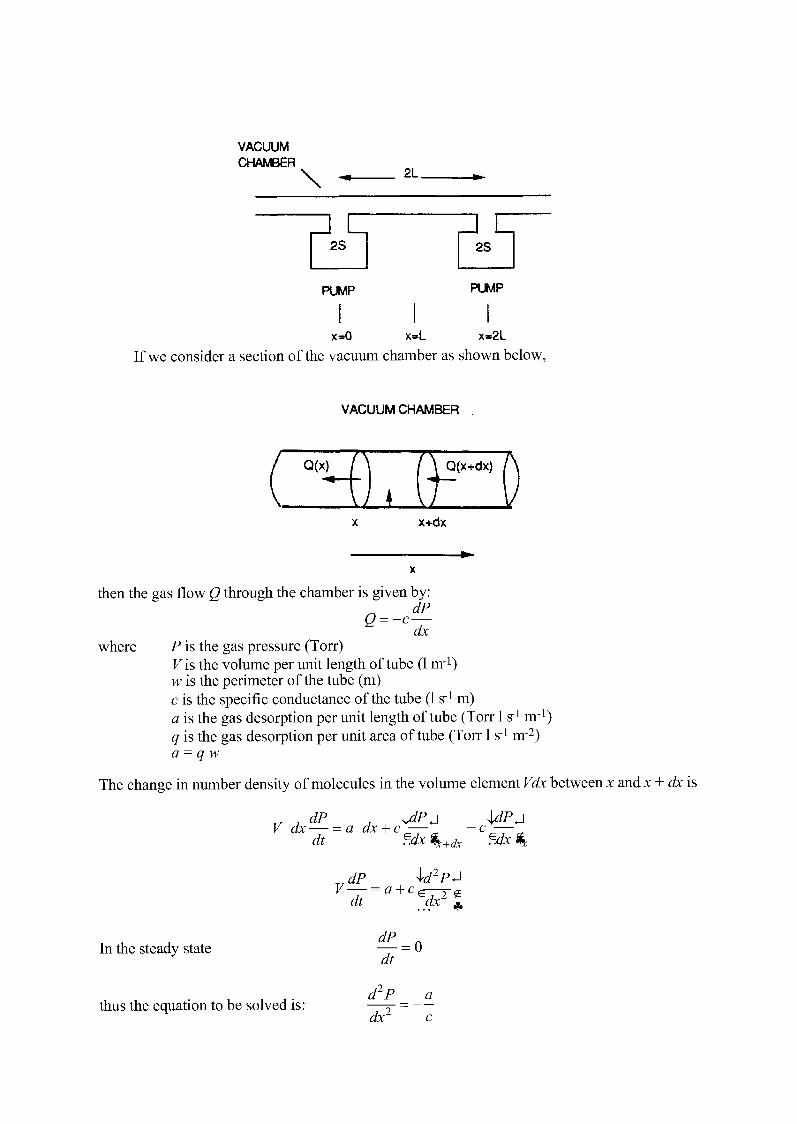
VACUUM CHAMBER
\ 2L_
2S 2S
PUMP PUMP
x=0 x=L x=2L If we consider a section of the vacuum chamber as shown below,
VACUUM CHAMBER
Q(x) Q(x+dx)
x+dx
then the gas flow Q through the chamber is given by: dP
Q = -c— dx
where P is the gas pressure (Torr) Fis the volume per unit length of tube (1 nr 1 ) w is the perimeter of the tube (m) c is the specific conductance of the tube (1 s - 1 m) a is the gas desorption per unit length of tube (Torr 1 s - 1 n r 1 ) q is the gas desorption per unit area of tube (Torr 1 s _ 1 n r 2 ) a = q w
The change in number density of molecules in the volume element Vdx between x and x + dx is
T / dP UP J V dx — -a dx + c —
Clt . MX ^+dx
TdP id2P^ V— = a + c.
\dP_j
dt dx T£
In the steady state
thus the equation to be solved is:
^ = 0 dt
d2P dx
a c
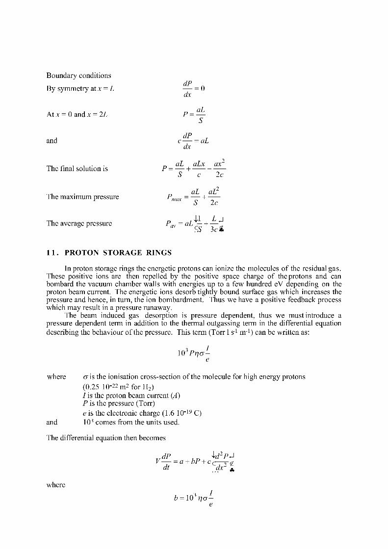
Boundary conditions By symmetry at x = L
At x = 0 and x = 2L
and
The final solution is
The maximum pressure
The average pressure Pav - aL c— + —
1 1 . PROTON STORAGE RINGS
dx = 0
P = aL
dP c —
dx - aL
p = aL — + S
aLx c
ax 2c
p =-A max
iL — + S
aL2
2c
In proton storage rings the energetic protons can ionize the molecules of the residual gas. These positive ions are then repelled by the positive space charge of the protons and can bombard the vacuum chamber walls with energies up to a few hundred eV depending on the proton beam current. The energetic ions desorb tightly bound surface gas which increases the pressure and hence, in turn, the ion bombardment. Thus we have a positive feedback process which may result in a pressure runaway.
The beam induced gas desorption is pressure dependent, thus we must introduce a pressure dependent term in addition to the thermal outgassing term in the differential equation describing the behaviour of the pressure. This term (Torr 1 s - 1 nr 1 ) can be written as:
l O 3 / 5 ^ -e
where a is the ionisation cross-section of the molecule for high energy protons (0.25 10- 2 2 m 2 forH 2 ) / is the proton beam current (A) P is the pressure (Torr) e is the electronic charge (1.6 10"19 C)
and 103 comes from the units used.
The differential equation then becomes
dP ,_ id2PJ V— = a + bP + C£—Y<£
dt dx jf.
where
e
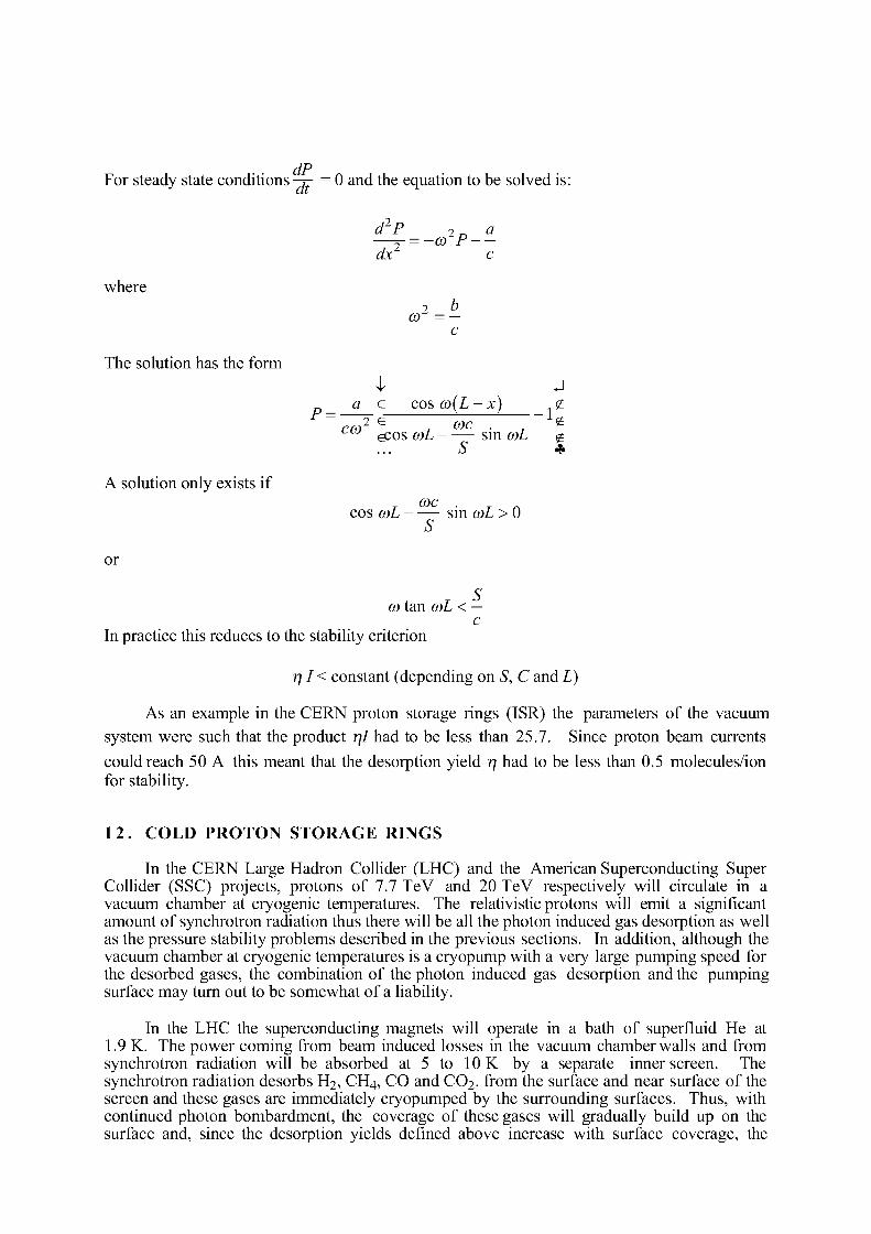
dP For steady state conditions-r- = 0 and the equation to be solved is:
where
The solution has the form
A solution only exists if
d2P 2„ a — Y = -G> P- — dx c
2 b CO - —
c
I J a e cos co(L - x)
<
* c c o e^os coL sin coL
S
<
*
T ( O C • T A
cos coL sin coL > 0 S
or
T S
co tan COL < — c
In practice this reduces to the stability criterion
rj I < constant (depending on S, C and L)
As an example in the CERN proton storage rings (ISR) the parameters of the vacuum system were such that the product rjl had to be less than 25.7. Since proton beam currents could reach 50 A this meant that the desorption yield rj had to be less than 0.5 molecules/ion for stability.
12. COLD PROTON STORAGE RINGS
In the CERN Large Hadron Collider (LHC) and the American Superconducting Super Collider (SSC) projects, protons of 7.7 TeV and 20 TeV respectively will circulate in a vacuum chamber at cryogenic temperatures. The relativistic protons will emit a significant amount of synchrotron radiation thus there will be all the photon induced gas desorption as well as the pressure stability problems described in the previous sections. In addition, although the vacuum chamber at cryogenic temperatures is a cryopump with a very large pumping speed for the desorbed gases, the combination of the photon induced gas desorption and the pumping surface may turn out to be somewhat of a liability.
In the LHC the superconducting magnets will operate in a bath of superfluid He at 1.9 K. The power coming from beam induced losses in the vacuum chamber walls and from synchrotron radiation will be absorbed at 5 to 10 K by a separate inner screen. The synchrotron radiation desorbs H 2, CH4, CO and CO2. from the surface and near surface of the screen and these gases are immediately cryopumped by the surrounding surfaces. Thus, with continued photon bombardment, the coverage of these gases will gradually build up on the surface and, since the desorption yields defined above increase with surface coverage, the
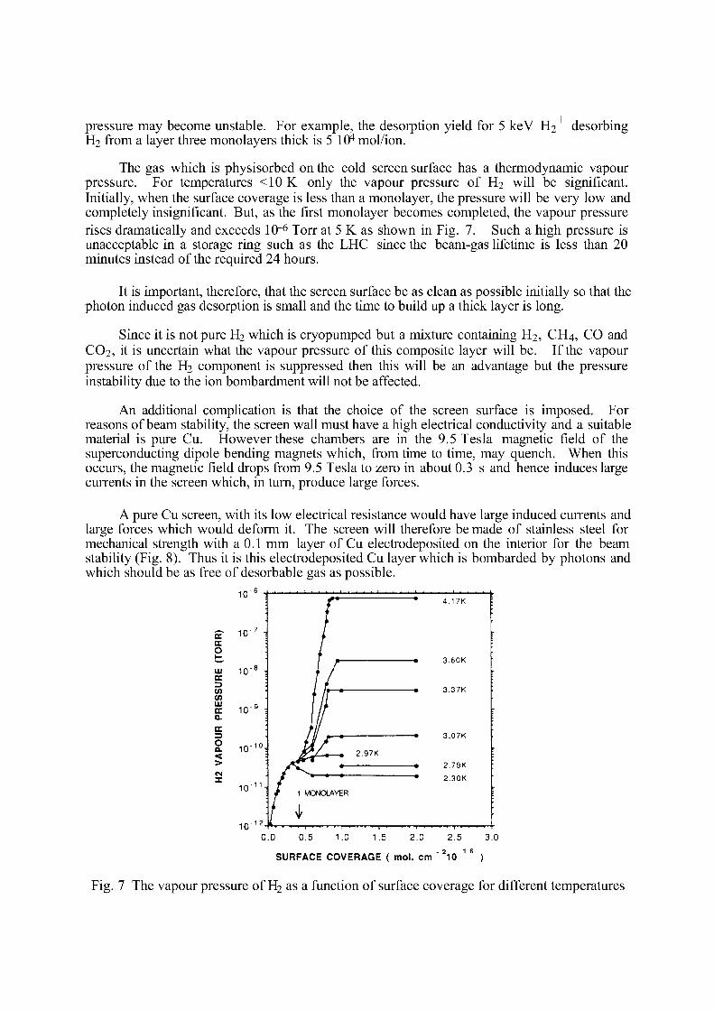
pressure may become unstable. For example, the desorption yield for 5 keV H2 H2 from a layer three monolayers thick is 5 10* mol/ion.
+ desorbing
The gas which is physisorbed on the cold screen surface has a thermodynamic vapour pressure. For temperatures <10 K only the vapour pressure of H2 will be significant. Initially, when the surface coverage is less than a monolayer, the pressure will be very low and completely insignificant. But, as the first monolayer becomes completed, the vapour pressure rises dramatically and exceeds 10"6 Torr at 5 K as shown in Fig. 7. Such a high pressure is unacceptable in a storage ring such as the LHC since the beam-gas lifetime is less than 20 minutes instead of the required 24 hours.
It is important, therefore, that the screen surface be as clean as possible initially so that the photon induced gas desorption is small and the time to build up a thick layer is long.
Since it is not pure H 2 which is cryopumped but a mixture containing H 2 , CH4, CO and CO2, it is uncertain what the vapour pressure of this composite layer will be. If the vapour pressure of the H 2 component is suppressed then this will be an advantage but the pressure instability due to the ion bombardment will not be affected.
An additional complication is that the choice of the screen surface is imposed. For reasons of beam stability, the screen wall must have a high electrical conductivity and a suitable material is pure Cu. However these chambers are in the 9.5 Tesla magnetic field of the superconducting dipole bending magnets which, from time to time, may quench. When this occurs, the magnetic field drops from 9.5 Tesla to zero in about 0.3 s and hence induces large currents in the screen which, in turn, produce large forces.
A pure Cu screen, with its low electrical resistance would have large induced currents and large forces which would deform it. The screen will therefore be made of stainless steel for mechanical strength with a 0.1 mm layer of Cu electrodeposited on the interior for the beam stability (Fig. 8). Thus it is this electrodeposited Cu layer which is bombarded by photons and which should be as free of desorbable gas as possible.
0.0
10"° 1 4.17K
10"° 1 4.17K
OR
R) 1er 7 • :
3.60K
3.37K
3.07K
UJ OC Z3
10" 8 1
1er9 :
10- 1 0 ^
3.60K
3.37K
3.07K
:
VAPO
UR
PRES
S
10" 8 1
1er9 :
10- 1 0 ^
3.60K
3.37K
3.07K
VAPO
UR
PRES
S
10" 8 1
1er9 :
10- 1 0 ^ 2.97K
3.60K
3.37K
3.07K
VAPO
UR
PRES
S
•— • • 2.79K CM
X 1 0 - 1 1 l
i o - 1 2 -
f 1 "»—•—«—
MONOLAYER
• 2.30K •
0.5 1.0 1.5 2.0 2.5 3.0
SURFACE COVERAGE ( mol. cm ' 210 1 6 )
Fig. 7 The vapour pressure of H2 as a function of surface coverage for different temperatures
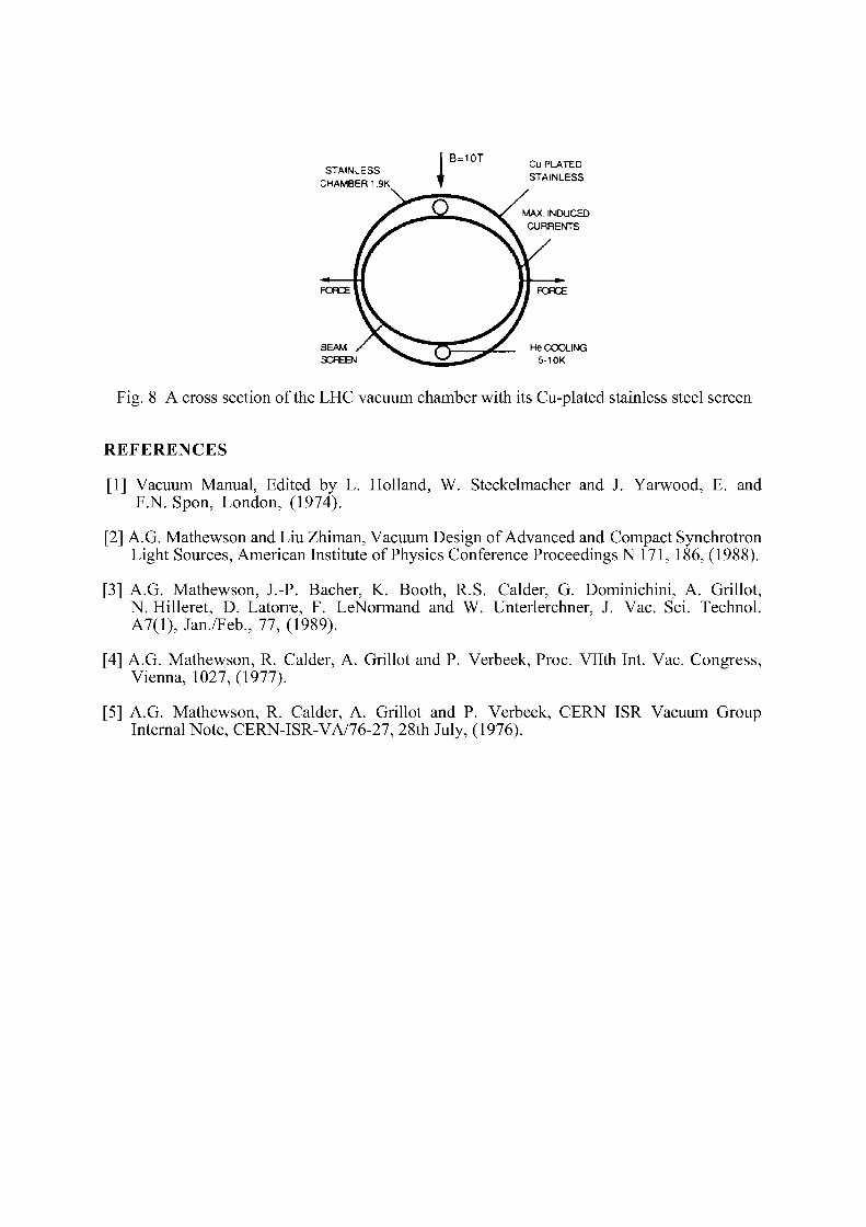
STAINLESS CHAMBER 1.9K
BEAM / > ^ /^> JT He COOLING SCREEN ^ 5-1 OK
Fig. 8 A cross section of the LHC vacuum chamber with its Cu-plated stainless steel screen
REFERENCES
[1] Vacuum Manual, Edited by L. Holland, W. Steckelmacher and J. Yarwood, E. and F.N. Spon, London, (1974).
[2] A.G. Mathewson and Liu Zhiman, Vacuum Design of Advanced and Compact Synchrotron Light Sources, American Institute of Physics Conference Proceedings N 171, 186, (1988).
[3] A.G. Mathewson, J.-P. Bâcher, K. Booth, R.S. Calder, G. Dominichini, A. Grillot, N. Hilleret, D. Latorre, F. LeNormand and W. Unterlerchner, J. Vac. Sci. Technol. A7(l), Jan./Feb., 77, (1989).
[4] A.G. Mathewson, R. Calder, A. Grillot and P. Verbeek, Proc. Vllth Int. Vac. Congress, Vienna, 1027, (1977).
[5] A.G. Mathewson, R. Calder, A. Grillot and P. Verbeek, CERN ISR Vacuum Group Internal Note, CERN-ISR-VA/76-27, 28th July, (1976).

INJECTION
G.H. Rees Rutherford Appleton Laboratory, UK.
1 . INTRODUCTION
Injection covers the final stage of transfer of beam from one accelerator to another, either from a linear to a circular machine or from one circular machine to another. The design aims are to achieve the transfer with little beam loss and with a minimum or a defined dilution of the beam emittances.
Single-turn injection schemes are relatively straightforward; beam is injected onto a central orbit via a septum unit and a fast kicker element, with appropriate matching arranged in the transverse and longitudinal planes. There should be no beam loss and very little emittance dilution, only that associated with transfer errors. For the longitudinal plane, the momentum spread (Ap/p) and phase (À0) parameters of the incoming bunch must be matched to those of the partial 'bucket' defined by the radio frequency fields of the ring. Successful single-turn injection requires that:
i) the stray field of the septum unit is at an acceptable level,
ii) the kicker field is reduced to zero in a time less than a defined fraction of the revolution period and,
iii) the RF system is capable of containing the transient beam loading introduced at the instant of injection.
Multi-turn injection involves more complex processes and is significantly different for electron accelerators than for proton or heavy-ion machines. The electron rings are often able to take advantage of radiation damping effects to increase the brightness of the resulting beam. Proton and heavy-ion machines generally operate at a beam brightness that is set by space-charge effects. The final particle distributions are very different in the two cases. The electron beams reach a near equilibrium state where there are Gaussian particle distributions in both transverse and longitudinal planes. The proton and heavy-ion distributions are functions of the details of the multi-turn process and of the space-charge levels achieved. In recent years, proton machines have utilised a type of multi-turn scheme known as charge-exchange injection. An injector linac accelerates H" particles which are subsequently stripped to protons in the ring to be filled. This allows considerable flexibility in the injection process; below the space-charge limit, the beam brightness may be increased by large factors, while at the space-charge limit there is better control of the final beam distributions.
The hardware needed for multi-turn injection is not greatly different from that for single-turn injection but the role of the fast kicker element is replaced by that of programmed orbit bump magnets. The particular case of charge exchange injection also requires the provision of micron or sub-micron stripping foils.
Historically, multi-turn injection first occurred [1] in weak-focusing synchrotrons, with filling of the horizontal betatron acceptance of the ring. Subsequently, energy-ramping systems were included in the injection beam line to allow simultaneous filling of the longitudinal acceptance. Most alternating-gradient machines have used multi-turn injection in the horizontal betatron plane alone; injection in both the horizontal and vertical planes has often been discussed but never utilised in practice except recently in the charge-exchange injection schemes.

Finally, mention should be made of some novel injection schemes:
i) the resonant injection scheme into the Argonne zero-gradient synchrotron [2],
ii) the radio-frequency stacking schemes of the MURA machines [3] and subsequently the ISR,
iii) the pion-decay scheme for injecting into muon storage rings [4] and
iv) the combined cooling and stacking process for the antiproton accumulator ring at CERN [5].
2 . SINGLE-TURN INJECTION
The first requirement for the injected beam is that it be matched at the entry point to the ring. This means that, at the exit from the septum unit, the betatron and dispersion function,
Py> ay, Px> ax> Dx> D'x> Dy a n d D'y »
must be identical with the machine lattice parameters at that point. Also the phase-space contours containing defined percentages of beam must approximate the elliptical contours in transverse phase space given by:
f+(ayy + py)?) =pysy (1)
x2 + (axx+(3xx'f =fixsx (2)
where ney, nex are un-normalised emittance values. Similar contours exist in longitudinal space but are somewhat more complex as the synchrotron motion is non-linear.
For horizontal, single-turn injection, the centre of the injected beam must be at a distance x from the centre of the machine aperture at the exit of the septum, where:
x _ , „ , , „ , , „ . , ,. AP , AP [K{-l£i+4£x^) + Dx — + — +xco+xs (3) P i P x
where net and nex are the un-normalised horizontal emittances in the injected beam line and the ring respectively, (Ap I p). and (Ap I p) are the momentum spread of the beam in the injection line and the ring respectively, xco is an allowance for closed-orbit deviations and clearances and xs is the effective thickness of the septum unit. Note that ex may be somewhat larger than ei due to transfer errors and
Ap Ap — > — due to subsequent adjustments of the radio-frequency fields. P x Pi
Horizontal single-turn injection is shown schematically in Fig. 1. It is assumed that the fast kicker is located at a point downstream from the septum unit with a phase shift of the horizontal betatron motion, JUX , between the two positions. The injected beam must move to the centre of the aperture by the time it reaches the kicker and, for this to occur, the input beam divergence at the exit of the septum is required to be:
x' = -(ccx+ cot jujx/ px (4)
The angular deflection that the kicker must then impart to the beam for it to move subsequently on the central equilibrium orbit is:
0 = * / A/AÂ sin nx (5)
where (5X is the horizontal ^-function at the kicker position.
From (5) it may be seen that a high value of J5X is advantageous to reduce the kick angle. Also, a high value of ftx helps in reducing the relative contribution to 6 due to the septum thickness.
For injection into a FODO lattice, as shown in Fig. 1, the septum and kicker units are placed just downstream of the F quadrupoles, with the kicker one cell downstream from the septum. px and ftx are nearly equal to the maximum ftx value of the cell and ax is positive. In the particular case when the phase shift per cell is n/2:
Vx = nl2 x1 - -axx / Px
e = xi{pjx (6)
Septum units may be dc septum magnets or dc electrostatic wire septa. Magnetic septa are the more rugged but electrostatic septa are used when it is necessary to reduce the fast kicker requirements. The components between the septum and kicker must have an adequate aperture for the transit of the incoming beam. If the injection energy is relatively low, it is important that there be adequate shielding of the beam from the septum leakage field. The sources of this stray (fringing) field for a magnetic septum are the magnetomotive loss field from the yoke, the gap between the yoke and the septum, the gaps between the septum turns and, finally, the cooling channels in the septum conductors. Techniques used to reduce the leakage field include the use of a mild steel vacuum chamber for the region between the septum conductors and the beam, the use of septum magnet field clamps and the use of powered anti-reluctance field windings.
Fast kicker magnets require to be switched off in times typically of 50 to 150 ns. The kickers are powered from pulse-forming networks which are charged in the off-time of the machine cycle and rapidly discharged via thyratron switches when needed. The rise and fall times of the pulse are functions of the thyratron characteristics and the kicker design. Originally, the kickers have been built in the form of lumped delay lines which are then terminated by the characteristic impedance of the line. This is adequate unless undesirable beam coupling impedances are introduced above the cut-off frequency of the line. For a high intensity machine it is simpler to use a lumped kicker element fed via high-voltage cables, terminated suitably at the end of the line as sketched in Fig. 2. Typical voltage and current levels during the pulse are 40 to 80 kV and 2000 to 5000 A, with magnetic field levels 250 to 500 gauss. Frequently it is necessary to use ferrites to contain the field and the usual material is a nickel-zinc ferrite. If the ferrites are contained within the vacuum chamber of the machine, the out-gassing properties must be acceptable. The density of the ferrite must be such that its water absorbent characteristics are not too high and care is needed in the grinding process that no undesirable lubricants are used. Sometimes a ceramic vacuum chamber is inserted between the ferrite and the beam, with a thin conducting layer deposited on the inner wall of the ceramic.
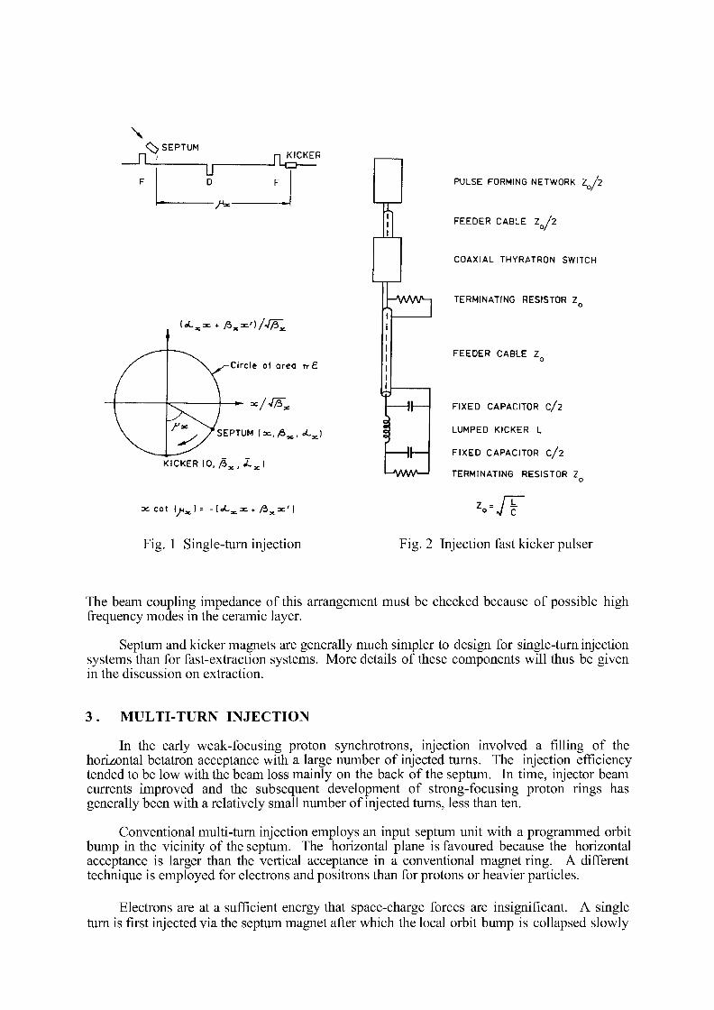
\ <N SEPTUM
n i KICKER _ri^i f
-S*-
i ^ x ^ ^ ' i / ^ ;
Circle of area TT-£
'SEPTUM (x.,/=>x, oC„
KICKER (0, P>x, j l ^ l
•x. > x.'
JhWWH
M A W - l
PULSE FORMING NETWORK Z h
FEEDER CABLE Z / 2 / 2
COAXIAL THYRATRON SWITCH
TERMINATING RESISTOR Z o
FEEDER CABLE Z o
FIXED CAPACITOR C/2
LUMPED KICKER L
FIXED CAPACITOR c /2
TERMINATING RESISTOR Z
3C COt </•*>= -l<*~xx-* frx*')
Fig. 1 Single-turn injection Fig. 2 Injection fast kicker puiser
The beam coupling impedance of this arrangement must be checked because of possible high frequency modes in the ceramic layer.
Septum and kicker magnets are generally much simpler to design for single-turn injection systems than for fast-extraction systems. More details of these components will thus be given in the discussion on extraction.
3 . MULTI-TURN INJECTION
In the early weak-focusing proton synchrotrons, injection involved a filling of the horizontal betatron acceptance with a large number of injected turns. The injection efficiency tended to be low with the beam loss mainly on the back of the septum. In time, injector beam currents improved and the subsequent development of strong-focusing proton rings has generally been with a relatively small number of injected turns, less than ten.
Conventional multi-turn injection employs an input septum unit with a programmed orbit bump in the vicinity of the septum. The horizontal plane is favoured because the horizontal acceptance is larger than the vertical acceptance in a conventional magnet ring. A different technique is employed for electrons and positrons than for protons or heavier particles.
Electrons are at a sufficient energy that space-charge forces are insignificant. A single turn is first injected via the septum magnet after which the local orbit bump is collapsed slowly
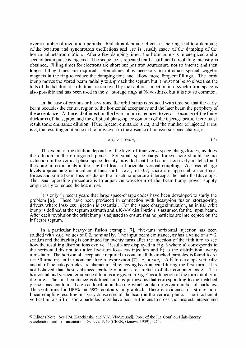
over a number of revolution periods. Radiation damping effects in the ring lead to a damping of the betatron and synchrotron oscillations and use is usually made of the damping of the horizontal betatron motion. After a few damping times, the beam bump is re-energized and a second beam pulse is injected. The sequence is repeated until a sufficient circulating intensity is obtained. Filling times for electrons are short but positron sources are not so intense and then longer filling times are required. Sometimes it is necessary to introduce special wiggler magnets in the ring to reduce the damping time and allow more frequent fillings. The orbit bump moves the stored beam radially to approach the septum but it must not be so close that the tails of the betatron distribution are removed by the septum. Injection into synchrotron space is also possible and has been used in the e storage rings at Novosibirsk but it is not so common.
In the case of protons or heavy ions, the orbit bump is reduced with time so that the early beam occupies the central region of the horizontal acceptance and the later beam the periphery of the acceptance. At the end of injection the beam bump is reduced to zero. Because of the finite thickness of the septum and the elliptical phase-space contours of the injected beam, there must result some emittance dilution. If the injector emittance is net and the number of injected turns is n, the resulting emittance in the ring, even in the absence of transverse space charge, is:
nsx > \.57mSi . (7)
The extent of the dilution depends on the level of transverse space-charge forces, as does the dilution in the orthogonal plane. For small space-charge forces there should be no reduction in the vertical phase-space density provided that the beam is correctly matched and there are no error fields in the ring that lead to horizontal-vertical coupling. At space-charge levels approaching an incoherent tune shift, zxy' , of 0.2, there are appreciable non-linear forces and some beam loss results as the machine aperture intercepts the halo that develops. The usual operating procedure is to adjust the waveform of the beam bump power supply empirically to reduce the beam loss.
It is only in recent years that large space-charge codes have been developed to study the problem [6]. These have been produced in connection with heavy-ion fusion storage-ring drivers where loss-less injection is essential. For the space charge simulation, an initial orbit bump is defined at the septum azimuth and a K-Va) distribution is assumed for the input beam. After each revolution the orbit bump is adjusted to ensure that no particles are intercepted on the inflector septum.
In a particular heavy-ion fusion example [7], five-turn horizontal injection has been studied with I\IJ values of 0.2, nominally. The input beam emittance, ne has a value of e = 2 /jrad.m and the tracking is continued for twenty turns after the injection of the fifth turn to see how the resulting distributions evolve. Results are displayed in Fig. 3 where a) corresponds to the horizontal distribution after five-turn loss-less injection and b) to the distribution twenty turns later. The horizontal acceptance required to contain all the tracked particles is found to be £=30 |urad.m; in the nomenclature of expression (7), sx - 5nst. A halo develops vertically and all of the halo particles are characterised by having been injected during the first turn. It is not believed that these enhanced particle motions are artefacts of the computer code. The horizontal and vertical emittance dilutions are given in Fig. 4 as a function of the turn number in the ring. The final emittance is defined for this purpose as that corresponding to the matched phase-space contours at a given location in the ring which contain a given number of particles. Thus solutions for 100% and 98% contours are graphed. There is evidence for strong nonlinear coupling resulting in a very dense core of the beam in the vertical plane. The incoherent vertical tune shift of some particles must have been sufficient to cross the nearest integer and
a) Editor's Note. See I.M. Kapchinskij and V.V. Vladimirskij, Proc. of the Int. Conf. on High-Energy Accelerators and Instrumentation, Geneva, 1959 (CERN, Geneva, 1959) p.274.
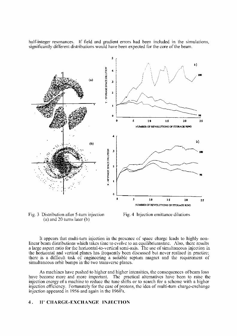
half-integer resonances. If field and gradient errors had been included in the simulations, significantly different distributions would have been expected for the core of the beam.
NUMBER OF REVOLUTIONS OF STORAGE RING
Fig. 3 Distribution after 5-turn injection Fig. 4 Injection emittance dilutions (a) and 20 turns later (b)
It appears that multi-turn injection in the presence of space charge leads to highly nonlinear beam distributions which takes time to evolve to an equilibrium state. Also, there results a large aspect ratio for the horizontal-to-vertical semi-axis. The use of simultaneous injection in the horizontal and vertical planes has frequently been discussed but never realised in practice; there is a difficult task of engineering a suitable septum magnet and the requirement of simultaneous orbit bumps in the two transverse planes.
As machines have pushed to higher and higher intensities, the consequences of beam loss have become more and more important. The practical alternatives have been to raise the injection energy of a machine to reduce the tune shifts or to search for a scheme with a higher injection efficiency. Fortunately for the case of protons, the idea of multi-turn charge-exchange injection appeared in 1956 and again in the 1960's.
4 . H" CHARGE-EXCHANGE INJECTION
The development of intense H" ion sources together with the concept of H" charge-exchange injection of protons came from Novosibirsk [8]. ANL adopted the idea and converted the ZGS accelerator for such a scheme [9]. Following their success, H" injection has become the preferred scheme for most high-intensity proton machines.
The constraints imposed by Liouville's Theorem on conventional multi-turn injection do not apply to charge-exchange injection since the stripping of H" ions to protons occurs within the acceptance of the ring. Because of this, it is generally possible to inject a large number of turns.
Though it is possible to inject into a restricted area of the acceptance and allow the proton density to increase with each succeeding turn, this method is not adopted (except in the case when a small beam emittance is required). For a high intensity machine, the aim of the injection process is to fill prescribed emittances in the longitudinal and both transverse phase planes in such a way that the resulting beam distributions do not lead to excessive space-charge forces. Uniform 2-dimensional density distributions are impractical to achieve, but elliptical 2-D distributions are considered acceptable as a design aim. A variety of injection schemes has now been tried or proposed to approximate such a distribution, and the resultant filling schemes have come to be referred to as injection painting.
The earlier schemes involved painting only in the transverse planes. For example, in the high-intensity synchrotron at the SNS facility [10], (Fig. 5), vertical painting has been achieved by a programmed vertical steering of the H" beam in the injection line, and the horizontal painting by the use of a fixed horizontal bump during the injection interval, while the synchrotron sinusoidal guide field approaches its minimum value. An additional feature is a correlation of the proton oscillation amplitudes in the two transverse planes; small horizontal amplitudes may be linked to large vertical ones or vice-versa or a range of correlated intermediate amplitudes obtained. Various distributions may then be devised, and the filling of the phase space is more gradual than for conventional multi-turn injection, with improved use of the phase space and more diffuse boundaries between successive turns. After the injection interval in SNS and while trapping is being established, the horizontal orbit bump is reduced to zero within 100 |us to reduce the number of subsequent proton foil traversais.
Later schemes have proposed combined longitudinal and transverse painting, and the most advanced of these has been proposed for the TR1UMF KAON Factory Project Definition Study [11]. Some details are given here and in the following section and, though devised for injection from a H" cyclotron to a proton accumulator ring, the scheme may also be adapted for the case of a H" linac and a proton synchrotron. The best arrangement for longitudinal painting is when the injector provides only one or two microbunches per rf bucket per turn in the ring. Often this is impractical to arrange, and the longitudinal painting must then allow for a much larger number of microbunches per rf bucket.
At high intensity it is important to minimise the number of proton foil traversais during and after the filling process. This objective guided the KAON study, and the solution proposed has come to be referred to as 'optimised H" injection'. There is simultaneous painting of al 1 three phase planes, commencing with small synchrotron, large horizontal and small vertical betatron oscillations, and ending with the reverse correlations. To achieve this optimally requires:
- momentum ramping of the injected beam; - shaping of the input beam phase space areas at the stripping foil; - use of a long-life foil with two free, unsupported edges; - removing from the ring unstripped H" and H particles; - providing appropriate lattice parameters at the foil;
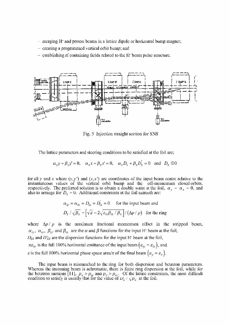
merging H" and proton beams in a lattice dipole or horizontal bump magnet; creating a programmed vertical orbit bump; and establishing rf containing fields related to the H" beam pulse structure.
ir s a ,-i f- ' • - • ^ fCZUT/O, L
J.OIP. I 1.DIP2 I, DIPS ! 1 r I t D IP U. I !
— h - J — f - i .
Fig. 5 Injection straight section for SNS
The lattice parameters and steering conditions to be satisfied at the foil are;
ayy + Pyy' = 0, axx + pxx' = 0, axDx + pxDx = 0 and Dx ©0
for all y and x where (y,yf) and (x,x') are coordinates of the input beam centre relative to the instantaneous values of the vertical orbit bump and the off-momentum closed orbits, respectively. The preferred solution is to obtain a double waist at the foil, ay = ax = 0, and also to arrange for Dx - U. Additional constraints at the foil azimuth are:
a,- a; Dix - Dix - 0 for the input beam and
Dx I iPx = [Ve - 2^]six(5ix /pxy(Ap/ p) for the ring
where Ap I p is the maximum fractional momentum offset in the stripped beam, aiy, aix, Pty and /3ix are the a and /3 functions for the input H" beam at the foil,
Dix sndD'ix are the dispersion functions for the input H" beam at the foil, nsix is the full 100% horizontal emittance of the input beam I siy = six\, and
a is the full 100% horizontal phase space area/^ of the final beam is = sx I.
The input beam is mismatched to the ring for both dispersion and betatron parameters. Whereas the incoming beam is achromatic, there is finite ring dispersion at the foil, while for the betatron motions [11], px > pix ana p > pi . Of the lattice constraints, the most difficult condition to satisfy is usually that for the value of ux I ^px at the foil.
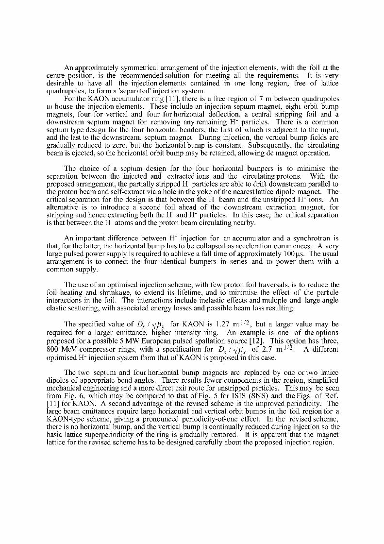
An approximately symmetrical arrangement of the injection elements, with the foil at the centre position, is the recommended solution for meeting all the requirements. It is very desirable to have all the injection elements contained in one long region, free of lattice quadrupoles, to form a 'separated' injection system.
For the KAON accumulator ring [11], there is a free region of 7 m between quadrupoles to house the injection elements. These include an injection septum magnet, eight orbit bump magnets, four for vertical and four for horizontal deflection, a central stripping foil and a downstream septum magnet for removing any remaining H" particles. There is a common septum type design for the four horizontal benders, the first of which is adjacent to the input, and the last to the downstream, septum magnet. During injection, the vertical bump fields are gradually reduced to zero, but the horizontal bump is constant. Subsequently, the circulating beam is ejected, so the horizontal orbit bump may be retained, allowing dc magnet operation.
The choice of a septum design for the four horizontal bumpers is to minimise the separation between the injected and extracted ions and the circulating protons. With the proposed arrangement, the partially stripped H particles are able to drift downstream parallel to the proton beam and self-extract via a hole in the yoke of the nearest lattice dipole magnet. The critical separation for the design is that between the H beam and the unstripped H" ions. An alternative is to introduce a second foil ahead of the downstream extraction magnet, for stripping and hence extracting both the H and H" particles. In this case, the critical separation is that between the H atoms and the proton beam circulating nearby.
An important difference between H" injection for an accumulator and a synchrotron is that, for the latter, the horizontal bump has to be collapsed as acceleration commences. A very large pulsed power supply is required to achieve a fall time of approximately 100 |us. The usual arrangement is to connect the four identical bumpers in series and to power them with a common supply.
The use of an optimised injection scheme, with few proton foil traversais, is to reduce the foil heating and shrinkage, to extend its lifetime, and to minimise the effect of the particle interactions in the foil. The interactions include inelastic effects and multiple and large angle elastic scattering, with associated energy losses and possible beam loss resulting.
The specified value of Dx I ftx for KAON is 1.27 m 1 / 2 , but a larger value may be required for a larger emittance, higher intensity ring. An example is one of the options proposed for a possible 5 MW European pulsed spallation source [12]. This option has three, 800 MeV compressor rings, with a specification for Dx I fjx of 2.7 m 1 / 2 . A different optimised H" injection system from that of KAON is proposed in this case.
The two septum and four horizontal bump magnets are replaced by one or two lattice dipoles of appropriate bend angles. There results fewer components in the region, simplified mechanical engineering and a more direct exit route for unstripped particles. This may be seen from Fig. 6, which may be compared to that of Fig. 5 for ISIS (SNS) and the Figs, of Ref. [11] for KAON. A second advantage of the revised scheme is the improved periodicity. The large beam emittances require large horizontal and vertical orbit bumps in the foil region for a KAON-type scheme, giving a pronounced periodicity-of-one effect. In the revised scheme, there is no horizontal bump, and the vertical bump is continually reduced during injection so the basic lattice superperiodicity of the ring is gradually restored. It is apparent that the magnet lattice for the revised scheme has to be designed carefully about the proposed injection region.
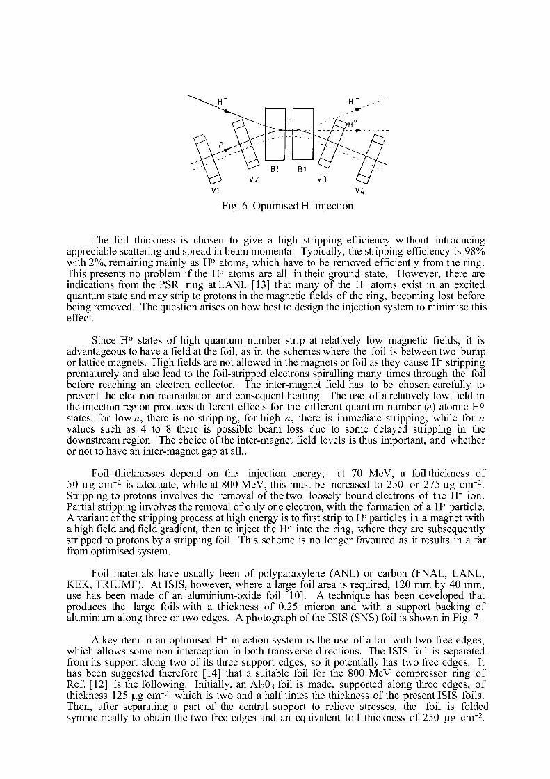
B1 B1 V2 V3
VI V4
Fig. 6 Optimised H" injection
The foil thickness is chosen to give a high stripping efficiency without introducing appreciable scattering and spread in beam momenta. Typically, the stripping efficiency is 98% with 2%, remaining mainly as H° atoms, which have to be removed efficiently from the ring. This presents no problem if the H° atoms are all in their ground state. However, there are indications from the PSR ring atLAKL [13] that many of the H atoms exist in an excited quantum state and may strip to protons in the magnetic fields of the ring, becoming lost before being removed. The question arises on how best to design the injection system to minimise this effect.
Since H° states of high quantum number strip at relatively low magnetic fields, it is advantageous to have a field at the foil, as in the schemes where the foil is between two bump or lattice magnets. High fields are not allowed in the magnets or foil as they cause H" stripping prematurely and also lead to the foil-stripped electrons spiralling many times through the foil before reaching an electron collector. The inter-magnet field has to be chosen carefully to prevent the electron recirculation and consequent heating. The use of a relatively low field in the injection region produces different effects for the different quantum number (n) atomic H° states; for lown, there is no stripping, for high n, there is immediate stripping, while for n values such as 4 to 8 there is possible beam loss due to some delayed stripping in the downstream region. The choice of the inter-magnet field levels is thus important, and whether or not to have an inter-magnet gap at all.
Foil thicknesses depend on the injection energy; at 70 MeV, a foil thickness of 50 [4,g cm" 2 is adequate, while at 800 MeV, this must be increased to 250 or 275 |ug cm"2. Stripping to protons involves the removal of the two loosely bound electrons of the H" ion. Partial stripping involves the removal of only one electron, with the formation of a H° particle. A variant of the stripping process at high energy is to first strip to H° particles in a magnet with a high field and field gradient, then to inject the H° into the ring, where they are subsequently stripped to protons by a stripping foil. This scheme is no longer favoured as it results in a far from optimised system.
Foil materials have usually been of polyparaxylene (ANL) or carbon (FNAL, LANL, KEK, TRIUMF). At ISIS, however, where a large foil area is required, 120 mm by 40 mm, use has been made of an aluminium-oxide foil [10]. A technique has been developed that produces the large foils with a thickness of 0.25 micron and with a support backing of aluminium along three or two edges. A photograph of the ISIS (SNS) foil is shown in Fig. 7.
A key item in an optimised H" injection system is the use of a foil with two free edges, which allows some non-interception in both transverse directions. The ISIS foil is separated from its support along two of its three support edges, so it potentially has two free edges. It has been suggested therefore [14] that a suitable foil for the 800 MeV compressor ring of Ref. [12] is the following. Initially, an AI2O3 foil is made, supported along three edges, of thickness 125 |ug cm"2' which is two and a half times the thickness of the present ISIS foils. Then, after separating a part of the central support to relieve stresses, the foil is folded symmetrically to obtain the two free edges and an equivalent foil thickness of 250 |ug cm"2.
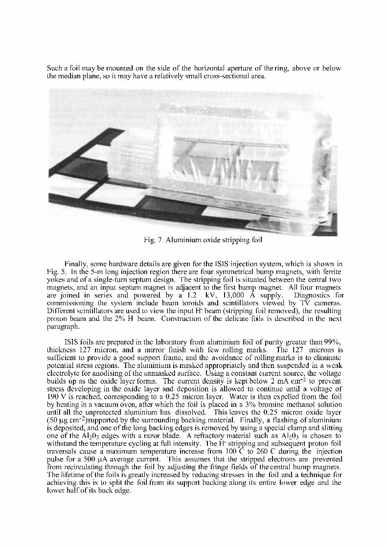
Such a foil may be mounted on the side of the horizontal aperture of the ring, above or below the median plane, so it may have a relatively small cross-sectional area.
Fig. 7 Aluminium oxide stripping foil
Finally, some hardware details are given for the ISIS injection system, which is shown in Fig. 5. In the 5-m long injection region there are four symmetrical bump magnets, with ferrite yokes and of a single-turn septum design. The stripping foil is situated between the certral two magnets, and an input septum magnet is adjacent to the first bump magnet. All four magnets are joined in series and powered by a 1.2 kV, 13,000 A supply. Diagnostics for commissioning the system include beam toroids and scintillators viewed by TV cameras. Different scintillators are used to view the input H" beam (stripping foil removed), the resulting proton beam and the 2% H beam. Construction of the delicate foils is described in the next paragraph.
ISIS foils are prepared in the laboratory from aluminium foil of purity greater than 99%, thickness 127 micron, and a mirror finish with few rolling marks. The 127 microns is sufficient to provide a good support frame, and the avoidance of rolling marks is to eliminate potential stress regions. The aluminium is masked appropriately and then suspended in a weak electrolyte for anodising of the unmasked surface. Using a constant current source, the voltage builds up as the oxide layer forms. The current density is kept below 2 mA cm"2 to prevent stress developing in the oxide layer and deposition is allowed to continue until a voltage of 190 V is reached, corresponding to a 0.25 micron layer. Water is then expelled from the foil by heating in a vacuum oven, after which the foil is placed in a 3% bromine methanol solution until all the unprotected aluminium has dissolved. This leaves the 0.25 micron oxide layer (50 |ug cm"2)supported by the surrounding backing material. Finally, a flashing of aluminium is deposited, and one of the long backing edges is removed by using a special clamp and slitting one of the AI2O3 edges with a razor blade. A refractory material such as AI2O3 is chosen to withstand the temperature cycling at full intensity. The H" stripping and subsequent proton foil traversais cause a maximum temperature increase from 100 C to 260 C during the injection pulse for a 500 |uA average current. This assumes that the stripped electrons are prevented from recirculating through the foil by adjusting the fringe fields of the central bump magnets. The lifetime of the foils is greatly increased by reducing stresses in the foil and a technique for achieving this is to split the foil from its support backing along its entire lower edge and the lower half of its back edge.
5. INJECTION FROM A CYCLOTRON INTO A SYNCHROTRON
A basic requirement is that the cyclotron is able to accelerate and extract H" ions. For the KAON Project Definition Study [11] at TRIUMF, a cyclotron transfers 452 MeV H" ions into an accumulator ring which is filled over ~ 15 000 turns, during most of the period of repeated 50 Hz cycles. The long injection interval puts severe demands on the injection system design, the basis of which has been described in section 4.
There is simultaneous injection painting in the longitudinal and both transverse phase planes. Vertical painting is obtained with the aid of a vertical bump magnet system, and the horizontal and longitudinal painting by a ramping of the momentum of the input H" beam. There is an appropriate choice of lattice parameters at the stripping foil which is to be made with two free unsupported edges, as has been discussed.
The average beam current to be accumulated is 100 |uA corresponding to 1.25 10 1 3
protons per cycle. Computer simulations show that the average number of foil traversais is reduced to about 50 by the use of the optimised injection scheme, assuming input and final transverse emittances of aproximately 2.5 and 50 n |urad m, respectively.
6 . NOVEL INJECTION SCHEMES
These are mentioned only briefly:
i) The ZGS type of resonant injection scheme [2] employs a fast kicker plus bumper magnets with dipole, quadrupole and octupole fields. A separatrix results with two stable regions, separated by an unstable fixed point; into one stable region beam is injected, in the other are the previously injected pulses. The fields are adjusted to merge the beams after which the injection condition is re-established. In principle there should be no dilution of the betatron phase-space density.
ii) Stacking by means of radio-frequency fields [3] provides filling of the longitudinal phase space. The scheme has been used routinely at the ISR. On successive cycles, bunches are deposited at the stacking radius; particles already stacked are displaced to make room in phase space for the newly arriving particles.
iii) Injection into muon storage rings [4] is envisaged as following pion-muon decay. The pion decay may occur in the injection channel or within one turn in the storage ring. For the decay to occur within the ring, the momentum acceptance should be greater than the pion decay width and be matched to that of the injection channel. A lithium lens and matching elements are required. Muons are stored for the muon lifetime after which they decay to provide neutrinos.
iv) For the antiproton accumulator [5], each injected antiproton pulse is first subjected to fast longitudinal cooling. Then it is deposited by the RF system at the high momentum edge of the stacked beam after which it undergoes stochastic cooling to make phase space available for the next injected pulse. In this manner 36,000 pulses are injected over a 24-hour period. Also required are two horizontal and two vertical betatron cooling systems.
REFERENCES
[1] M.H. Blewett, The Cosmotron - A Review, Rev. Sc. Inst. Vol 24, No.9., September 1953, p. 725.

[2] T.K. Khoe and R.J. Lari, Proc. Conf. on High-Energy Accelerators, Geneva, 1971, (CERN, Geneva, 1971), p. 98.
[3] K.R. Symon and A.M. Sessler, Proc. of the CERN Symposium on High Energy Accelerators, (CERN, Geneva, 1956) p. 44.
[4] D. Neuffer, Design of Muon Storage Rings for Neutrino Oscillation Experiments, IEEE Trans, on Nucl. Sci., Vol NS-28, No. 3, June 1981, p. 2034.
[5] S. van der Meer, Stochastic Cooling in the CERN Antiproton Accumulator, IEEE Trans, on Nucl. Sci., Vol NS-28, No. 3, June 1981, p. 1994.
[6] C.R. Prior, Multiturn Injection for Heavy Ion Fusion, Proc. Symposium on Accelerator Aspects of HIF, GSI-82-8, 1982, p. 290.
[7] C.R. Prior, Private Communication, briefly reported by: G. H. Rees, Storage Ring Studies and Simulations, Proc. International Symposium on Heavy Ion Accelerators and their Applications for Inertial Fusion, INS, Tokyo, 1984, p. 253.
[8] G.I. Budker and G.I. Dimov, Proc. Int. Conf. on High-Energy Accelerators, Dubna, 1963, CONF. 114, (USAEC, TID-4500, 1965), p. 1372-1377.
[9] C.W. Potts, Negative Hydrogen Injection into the Zero Gradient Synchrotron, IEEE Trans, on Nucl. Sci., Vol NS-24, No. 3, June 1977, p. 1385.
[10] V.C. Kempson, C.W. Planner and V.T. Pugh, Injection Dynamics and Multiturn Charge Exchange Injection into the Fast Cycling Synchrotron for the SNS, IEEE Trans, on Nucl. Sci., Vol NS-28, No. 3, June 1981, p. 3085.
[11] TRIUMF KAON FACTORY Project Definition Study, 1990; C.W. Planner, G.H. Rees and G.H. Mackenzie, A Separated H" Injection System in a Modified Accumulator Lattice for the TRIUMF KAON FACTORY, TRI-DN-89-K98, 1989. TRIUMF DESIGN NOTES, TRI-DN-84-63 and TRI-DN-88-K9.
[12] G.H. Rees, European Spallation Neutron Source Notes, Rutherford Appleton Laboratory, EPNS/RAL/A4/92 and EPNS/RAL/A2/91.
[13] R. Hutson, First-turn Losses in the PSR, LANL MP-5 Note, 1992.
[14] C.W. Planner, RAL, Private Communication, 1991.
EXTRACTION
G.H. Rees Rutherford Appleton Laboratory, UK.
1 . INTRODUCTION
Extraction is the mechanism used to remove beam from an accelerator. Beam emerges automatically from linear accelerators but a number of different techniques are employed to eject beam from circular machines.
The simplest technique is where the charge state is changed so the beam is bent directly out of the ring. Such a technique is confined to low-energy machines; an example is H acceleration in a cyclotron followed by foil stripping to protons at the extraction radius. Another simple method is the use of internal targets to scatter beam, either directly out of a ring or via a septum extraction magnet. The early weak-focusing proton synchrotrons made use of this last scheme in Piccioni extraction systems [1]. The loss of particle energy in the scattering target led to an induced radial betatron oscillation which allowed beam to jump the septum. Modern accelerators avoid the use of such internal targets because of the associated activation; clean extraction has become a necessity as particle energies and intensities have increased. Typical ejection efficiencies now achieved are 100% for carefully designed cyclotrons, 100% for fast extraction from synchrotrons and 99% for slow resonant schemes from synchrotrons and stretcher rings.
Fast one-turn extraction is employed in the transfer of beam from one circular machine to another. An example is in the box-car stacking of a main ring from a booster injector. Sometimes bunch-by-bunch transfers are made and then the fields of the fast kicker magnets must have both rapid rise and fall times.
Experimental facilities generally use slow-extracted beams though exceptions are to be found in the fast-extracted beams for pulsed neutron sources and neutrino factories. An optimum slow extracted beam has a smooth, uniform spill and such a beam may be provided by controlled excitation of a non-linear betatron resonance in the ring.
Many features of extraction are the reverse process of injection. However, one difference between the two systems is that injection is usually dominated by space-charge effects whereas extraction occurs at higher energies so that space charge is unimportant. The higher energy may lead to more complex hardware development.
Extraction systems often influence strongly the overall design of a machine. There must be sufficient straight section space for the system components and adequate apertures for the perturbed beam. The magnet lattice may include special insertions to house the extraction elements. It is also possible to design high-/? insertions that magnify the betatron motion in the vicinity of the first extraction septum. This improves the extraction efficiency for it is equivalent to reducing the effective thickness of the first septum which is a thin-wire electrostatic unit. The extraction channel contains one or more septum magnets downstream of the electrostatic septum, providing enhanced deflections. A machine may adapt its extraction channel for both slow and fast extracted beams.
In a conventional magnet ring it is more common that slow extraction is in the horizontal plane. In a superconducting ring the alternative of vertical extraction merits equal consideration.
2 . FAST EXTRACTION
The first stage of fast extraction is the powering of orbit bump magnets to steer the beam slowly to lie adjacent to the first of the extraction septum elements. This is followed by the energising of a fast kicker magnet in the time interval between two successive circulating bunches, typically 50 to 150 ns. The duration and switch-off time of the kicker pulse depend on the mode of fast extraction. For one-turn extraction, the pulse duration is the revolution period and the switch-off time is arbitrary. For bunch-by-bunch extraction, the pulse duration is the bunch repetition period and the fall time of the pulse has to be as rapid as the rise time. The kicker field deflects the beam into the extraction channel where it receives a sufficient angular deflection to leave the machine.
As for fast injection, the kicker must deflect the beam by:
# = *A7U^sin/ix (1) where, /3X, /3X are the lattice j8-functions at the kicker and first septum unit respectively,
JUX is the betatron phase shift between the kicker and septum and, x is the displacement required at the septum.
The initial slow orbit bump is used to reduce the value forx
In a FODO lattice the kicker is positioned just upstream of an F quadrupole and the first septum is one cell downstream from this point. The optimum phase shift per cell is then^/2.
The simplest fast kicker conceptually is a pair of metal plates, one on each side of the beam, all contained in a grounded enclosure and with the two plates fed by push-pull voltage pulses formed from pulse forming networks and switches. If each plate is terminated by its characteristic impedance, Z 0 , there will be no reflected pulses and the time to establish the full deflecting field is the time taken to fully close the switches plus the transit time down the system, of assumed length, 1. The system is fully defined by the following expressions:
F = eV(\Zj5)/h
e = Fi/Ppc (2)
T = £/c
I=V/2ZQ
where, F is the sum of the electric and magnetic deflecting forces, Z V/2 are the pulsed voltages on the plates, h is the plate separation, p is the particle momentum, mocfiy, and T is the transit time down the line.
The positive sign in the term (1 Z (J) applies to the case of particles travelling in the opposite direction to that of the voltage pulses. The electric and magnetic forces are essentially equal for relativistic particles. In general, such a system requires large values of V and / to provide adequate deflections, 6.
Most operating systems employ a ferrite yoke for the fast kicker to enhance the magnetic deflection. In this case the relevant formulae are, for a single-turn, push-pull kicker of length 1, width w and gap g, fed with voltage pulses Z V/2 through cables of impedance Z 0 :
F=Ql/3^oc/g
L - ^ocol/g (3)
Tr = L/ZQ
I=V/Z0
When the pulses are reflected at the kicker, the voltage levels first double to m F and then decay with the time constant Tr. After a time of approximately 4Tr the voltage falls below m F/50 and the kicker current rises to above 0.98 V/ZQ. Then the magnetic field should be constant to better than m 1% for the remainder of the pulse. A lumped kicker system of this type is used at the SNS synchrotron [2] with 4Tr = 200 ns. The pulsing system is shown in Fig. 1 and includes a pulse forming network with resonant charging system, a coaxial switch employing a double-ended deuterium thyratron, the CX 1168B, the feeder cable Z 0 and a terminating resistor Z$ at the sending end of the cable. During acceleration in the SNS, the switch is open so that each kicker plate is in parallel with a matched cable. The yoke of the ferrite kicker has a window-frame design but is separated at the mid-plane by a copper ground plane which extends for the full length of the unit. This arrangement provides a very low longitudinal coupling impedance for the circulating beam [3]. In practice the output stages of the pulse-forming network are modified to enhance the overall system rise time. Figure 2 shows the SNS coaxial switch housing.
The SNS type kicker is not suitable for bunch-by-bunch extraction as there are some small reflected pulses after the main pulse. In this case, a matched kicker system must be used, with the kicker inductance forming one element of a low-pass filter which is terminated by its characteristic impedance. A pulse forming network charged to a voltage V, when discharged into a matched load, provides a voltage pulse V/2 for a time equal to twice the transit time of the network. The impedance of the PFN is made equal to that of the kicker system so that the kicker excitation current is V/2Z0.
If very fast rise and fall times are a requirement it may prove necessary to replace the thyratron switch by a triggered spark gap and to subdivide the kicker into shorter length sections. Each individual kicker may also be modified to form a delay-line unit with lumped capacitors introduced between the short ferrite sections. Many kickers have adopted this design; for example, the proposed beam abort system for ISABELLE [4]. Care must be taken with the high-frequency performance of delay-line kickers for above the cut-off frequency of the line the kicker may present an undesirable transverse beam coupling impedance. Such a design led to transverse instability in the KEK booster [5].
3 . SLOW EXTRACTION
Slow extraction is achieved by controlled excitation of a non-linear betatron resonance of the ring, often a third-integer resonance. An alternative is the choice of a linear second-order resonance but with some non-linearity introduced by the inclusion of magnetic octupoles.
The efficiency of slow extraction depends on the thickness of the first ejection septum as compared to the growth of the resonant betatron amplitudes in the final few turns before extraction. The first septum is thus made as thin as possible and is aligned very carefully whereas the maximumgrowth per turn is obtained for the available aperture and for the actual beam emittance. The larger horizontal than vertical aperture of a conventional magnet ring favours the choice of a horizontal slow extraction system.
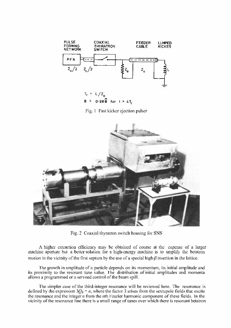
PULSE COAXIAL FEEDER LUMPED FORMING THYRATRON CABLE KICKER NETWORK SWITCH
Z o / 2 Z 0 / 2
T r = L / Z Q
B > 0 9 8 B for t > C\
Fig. 1 Fast kicker ejection puiser
Fig. 2 Coaxial thyratron switch housing for SNS
A higher extraction efficiency may be obtained of course at the expense of a larger machine aperture but a better solution for a high-energy machine is to amplify the betatron motion in the vicinity of the first septum by the use of a special high-/? insertion in the lattice.
The growth in amplitude of a particle depends on its momentum, its initial amplitude and its proximity to the resonant tune value. The distribution of initial amplitudes and momenta allows a programmed or a servoed control of the beam spill.
The simpler case of the third-integer resonance will be reviewed here. The resonance is defined by the expression 3Qh = n, where the factor 3 arises from the sextupole fields that excite the resonance and the integers from the nth Fourier harmonic component of these fields. In the vicinity of the resonance line there is a small range of tunes over which there is resonant betatron
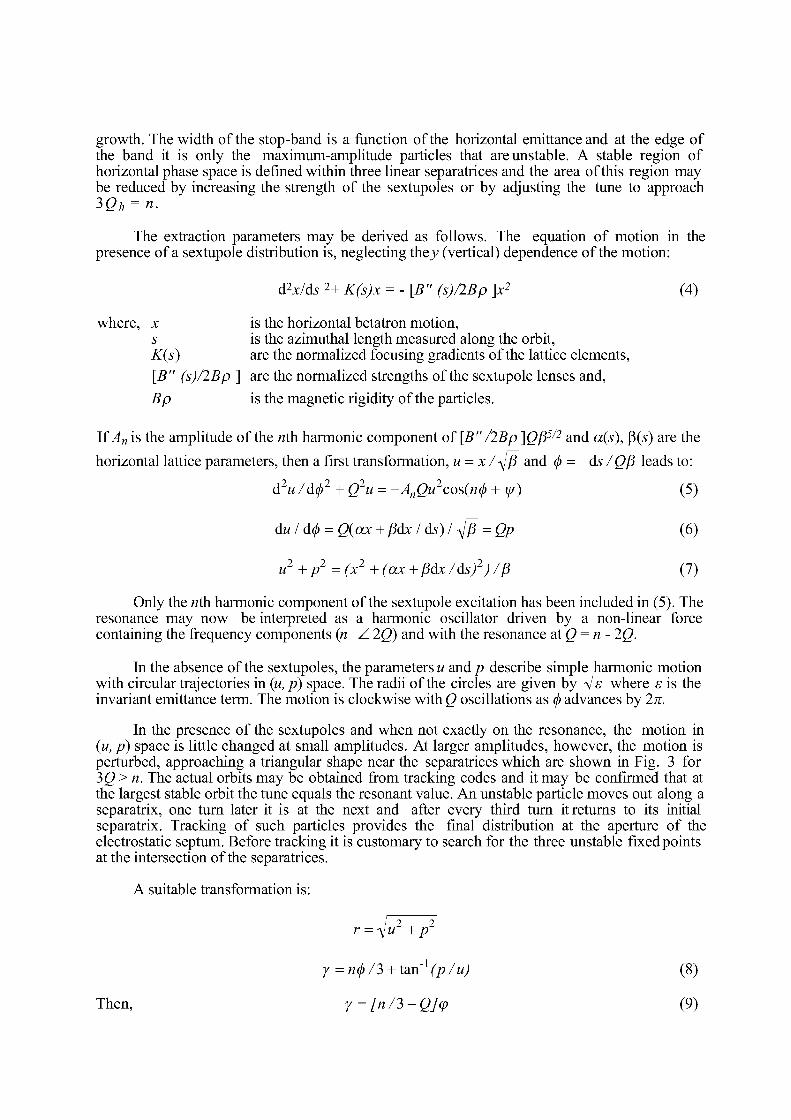
growth. The width of the stop-band is a function of the horizontal emittanceand at the edge of the band it is only the maximum-amplitude particles that are unstable. A stable region of horizontal phase space is defined within three linear séparatrices and the area of this region may be reduced by increasing the strength of the sextupoles or by adjusting the tune to approach 3Qh = n.
The extraction parameters may be derived as follows. The equation of motion in the presence of a sextupole distribution is, neglecting they (vertical) dependence of the motion:
d2x/ds 2+ K(s)x = -[B" (s)/2Bp ]x2 (4)
where, x is the horizontal betatron motion, s is the azimuthal length measured along the orbit, K(s) are the normalized focusing gradients of the lattice elements, [B" (s)/2Bp ] are the normalized strengths of the sextupole lenses and, Bp is the magnetic rigidity of the particles.
If An is the amplitude of the nth harmonic component of [B" /2Bp ]Q(55/2 and a(s), P(s) are the horizontal lattice parameters, then a first transformation, u = x /yj5 and (f> = ds /Q/3 leads to:
d2u/d<j)2 + Q2u = -AnQu2cos(n(/) + y/) (5)
du I d<j> = Q(ax + pdx I ds) 14P = Qp (6)
u2 +p2 =(x
2 +(ax+pdx/ds)2)/(3 (7)
Only the nth harmonic component of the sextupole excitation has been included in (5). The resonance may now be interpreted as a harmonic oscillator driven by a non-linear force containing the frequency components (n Z. 2Q) and with the resonance at Q = n - 2Q.
In the absence of the sextupoles, the parameters M and/? describe simple harmonic motion with circular trajectories in (u, p) space. The radii of the circles are given by Vs where e is the invariant emittance term. The motion is clockwise with Q oscillations as 0 advances by 2n.
In the presence of the sextupoles and when not exactly on the resonance, the motion in (u, p) space is little changed at small amplitudes. At larger amplitudes, however, the motion is perturbed, approaching a triangular shape near the séparatrices which are shown in Fig. 3 for 3Q> n. The actual orbits may be obtained from tracking codes and it may be confirmed that at the largest stable orbit the tune equals the resonant value. An unstable particle moves out along a separatrix, one turn later it is at the next and after every third turn it returns to its initial separatrix. Tracking of such particles provides the final distribution at the aperture of the electrostatic septum. Before tracking it is customary to search for the three unstable fixed points at the intersection of the séparatrices.
A suitable transformation is:
2 . 2
r - -y u + p
y = n<j)/3 +tan1 (p/u) (8) Then, y = [n/3-Q]<p (9)
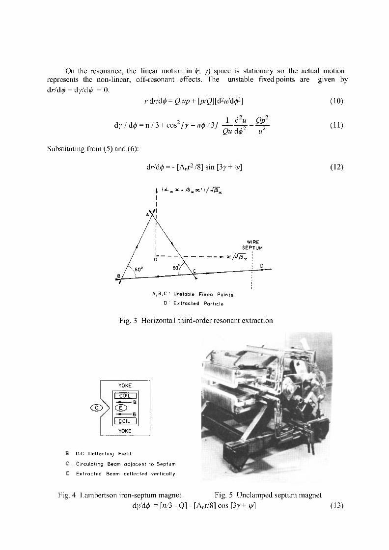
On the resonance, the linear motion in ((, y) space is stationary so the actual motion represents the non-linear, off-resonant effects. The unstable fixed points are given by dr/d(j) = d//d0 = 0.
r dr/d0 =Qup+ \p/Q\ [d2u/df] ( 10)
dy/d<t) = n/3 +cos2 fy-n(j)/3J — ^ - % - (H) Qu d(j> u
Substituting from (5) and (6):
dr/d0 = -[A nr 2 /8]sin[37+i// | (12)
| l i . ^ / i . x ' l / J ^
WIRE SEPTUM
A,B,C : Unstable F ixed Poin ts
D : E x t r a c t e d Par t ic le
Fig. 3 Horizontal third-order resonant extraction
CD
YOKE
I COIL
CD I COIL
YOKE
DC. Def lect ing F ie ld
Circulat ing Beam ad jacen t to Septum
E x t r a c t e d Beam def lec ted ve r t i ca l l y
Fig. 4 Lambertson iron-septum magnet Fig. 5 Undamped septum magnet d//d0 = [n/3 - Q] - [Anr/8] cos [3/+ y/] (13)
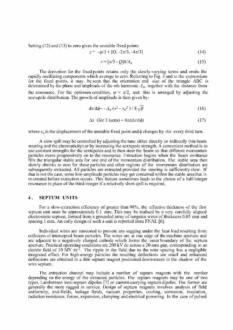
Setting (12) and (13) to zero gives the unstable fixed points: Y= -y//3 + [O, -2K/3, -4K/3] (14)
r=[n/3-Q]8/An (15)
The derivation for the fixed points retains only the slowly-varying terms and omits the rapidly oscillating components which average to zero. Referring to Fig. 3 and to the expressions for the fixed points, it may be seen that the orientation and size of the triangle ABC is determined by the phase and amplitude of the nth harmonic An, together with the distance from the resonance. For the optimum condition, y/ = nil, and this is arranged by adjusting the sextupole distribution. The growth of amplitude is then given by:
dx/d<t>=-An(x2-xu2)/84p (16)
Ax (for 3 turns) = 67i(dx/d0) (17)
where xu is the displacement of the unstable fixed point and § changes by -6n every third turn.
A slow spill may be controlled by adjusting the tune either directly or indirectly (via beam steering and the chromaticity) or by increasing the sextupole strength. A convenient method is to use constant strengths for the sextupoles and to then steer the beam so that different momentum particles move progressively on to the resonance. Extraction begins when the beam emittance fills the triangular stable area for one end of the momentum distribution. The stable area then slowly shrinks to zero for these particles and other regions of the momentum distribution are subsequently extracted. All particles are extracted provided the steering is sufficiently slow. If that is not the case, some low-amplitude particles may get contained within the stable area that is re-created before extraction occurs. This feature sometimes leads to the choice of a half-integer resonance in place of the third-integer if a relatively short spill is required.
4 . SEPTUM UNITS
For a slow-extraction efficiency of greater than 98%, the effective thickness of the first septum unit must be approximately 0.1 mm. This may be realised by a very carefully aligned electrostatic septum, formed from a grounded array of tungsten wires of thickness 0.05 mm and spacing 1 mm. An early design of such a unit is reported from FNAL [6].
Individual wires are tensioned to prevent any sagging under the heat load resulting from collisions of intercepted beam particles. The wires are at one edge of the machine aperture and are adjacent to a negatively charged cathode which forms the outer boundary of the septum aperture. Practical operating conditions are 200 kV dc across a 20-mm gap, corresponding to an electric field of 10 MV m - 1 . The ripple in the field due to the wire spacing has a negligible integrated effect. For high-energy particles the resulting deflections are small and enhanced deflections are obtained in a thin septum magnet positioned downstream in the shadow of the wire septum.
The extraction channel may include a number of septum magnets with the number depending on the energy of the extracted particles. The septum magnets may be one of two types, Lambertson iron-septum dipoles [7] or current-carrying septum dipoles. The former are generally the more rugged in service. Design of septum magnets involves analysis of field uniformity, end-fields, leakage fields, vacuum properties, cooling, corrosion, insulation, radiation resistance, forces, expansion, clamping and electrical powering. In the case of pulsed
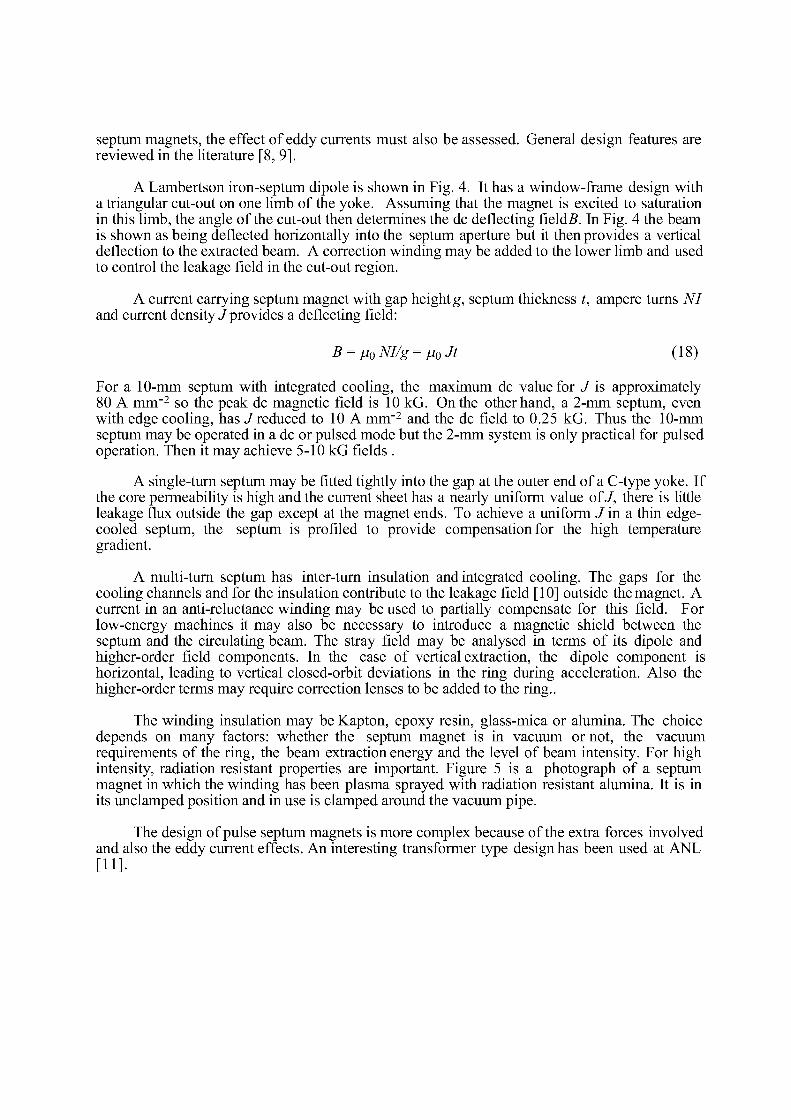
septum magnets, the effect of eddy currents must also be assessed. General design features are reviewed in the literature [8, 9].
A Lambertson iron-septum dipole is shown in Fig. 4. It has a window-frame design with a triangular cut-out on one limb of the yoke. Assuming that the magnet is excited to saturation in this limb, the angle of the cut-out then determines the dc deflecting fields. In Fig. 4 the beam is shown as being deflected horizontally into the septum aperture but it then provides a vertical deflection to the extracted beam. A correction winding may be added to the lower limb and used to control the leakage field in the cut-out region.
A current carrying septum magnet with gap height g, septum thickness t, ampere turns NI and current density/provides a deflecting field:
B = / j 0 Nl/g = / j 0 Jt (18)
For a 10-mm septum with integrated cooling, the maximum dc value for J is approximately 80 A mm"2 so the peak dc magnetic field is 10 kG. On the other hand, a 2-mm septum, even with edge cooling, has /reduced to 10 A mm"2 and the dc field to 0.25 kG. Thus the 10-mm septum may be operated in a dc or pulsed mode but the 2-mm system is only practical for pulsed operation. Then it may achieve 5-10 kG fields .
A single-turn septum may be fitted tightly into the gap at the outer end of a C-type yoke. If the core permeability is high and the current sheet has a nearly uniform value of J, there is little leakage flux outside the gap except at the magnet ends. To achieve a uniform J in a thin edge-cooled septum, the septum is profiled to provide compensation for the high temperature gradient.
A multi-turn septum has inter-turn insulation and integrated cooling. The gaps for the cooling channels and for the insulation contribute to the leakage field [10] outside the magnet. A current in an anti-reluctance winding may be used to partially compensate for this field. For low-energy machines it may also be necessary to introduce a magnetic shield between the septum and the circulating beam. The stray field may be analysed in terms of its dipole and higher-order field components. In the case of vertical extraction, the dipole component is horizontal, leading to vertical closed-orbit deviations in the ring during acceleration. Also the higher-order terms may require correction lenses to be added to the ring..
The winding insulation may be Kapton, epoxy resin, glass-mica or alumina. The choice depends on many factors: whether the septum magnet is in vacuum or not, the vacuum requirements of the ring, the beam extraction energy and the level of beam intensity. For high intensity, radiation resistant properties are important. Figure 5 is a photograph of a septum magnet in which the winding has been plasma sprayed with radiation resistant alumina. It is in its undamped position and in use is clamped around the vacuum pipe.
The design of pulse septum magnets is more complex because of the extra forces involved and also the eddy current effects. An interesting transformer type design has been used at ANL [11].
REFERENCES
[I] O. Piccioni, D. Clark, R. Cool, G. Friedlander and D. Kassner, External Proton Beam of the Cosmotron, Rev. Sci. Inst., Vol 26, No.2, February 1965, p. 232.
[2] E.G. Sandels, Notes on the Design of the SNS Extraction Kicker Magnets, RAL Internal Note, SNS/MAG/N2/83, September 1983.
[3] A. Faltens, ISABELLE Kicker Magnets, Septa and Scrapers, Proc. of ISABELLE Summer Study, BNL 20550, July 1975, p. 476.
[4] R.J. Nawrocky, P.A. Montemurro and J. Baron, On the Design of Fast Kickers for the ISABELLE Beam Abort System, IEEE Trans, on Nucl. Sci., Vol NS-28, No.3, June 1981, p. 921.
[5] Y.Miyahara, Head-Tail Instability Induced by a Matched Kicker Magnet, Particle Accelerators, Vol II, No. 4, 1981, p. 201.
[6] C.H. Rode, R.A. Andrews, A.M. Maschke and R.M. Mobley, Design of the 500 GeV Slow Extracted Beam and Proton Beam Lines, IEEE Trans, on Nucl. Sci., Vol NS-16, No. 3, June 1971, p. 984.
[7] L.W. Olesiuk, R.A. Andrews, E.J. Bleser and C.H. Rode, The NAL Beam-Splitting System, IEEE Trans, on Nucl. Sci., Vol NS-20, No. 3, June 1973, p. 428.
[8] J.J. Grisoli and H.C.H. Hsieh, Septum Magnets, Proc. Third Int. Conf. on Magnet Technology, Hamburg, 1970, (DESY, Hamburg, 1972) p. 1501.
[9] R.L. Keizer, Dipole Septum Magnets, CERN 74-13, May 1974.
[10] A.J.T. Holmes, private communication, Calculation and Optimization of Septum Dipole Stray Fields, CERN Lab II Internal Report/BT/75-2, April 1975.
[II] M. Foss, K. Thompson and W. Praeg, A Transformer Septum Magnet, IEEE Trans, on Nucl Sci., Vol NS-26, No. 3, June 1979, p. 4024.
SUPERCONDUCTING ACCELERATOR MAGNET DESIGN
S. Wolff DESY, Hamburg, Germany
Abstract Superconducting dipoles, quadrupoles and correction magnets are necessary to achieve the high magnetic fields required for big accelerators presently in construction or in the design phase. Different designs of superconducting accelerator magnets are described and the designs chosen at the big accelerator laboratories are presented. The most frequently used cosG coil configuration is discussed in detail. Approaches for calculating the magnetic field quality including coil end fields are presented. Design details of the cables, coils, mechanical structures, yokes, helium vessels and cryostats including thermal radiation shields and support structures used in superconducting magnets are given. Necessary material properties are mentioned. Finally, the main results of magnetic field measurements and quench statistics are presented.
1. INTRODUCTION Superconducting accelerator magnets are being used world-wide in the new generation
of big particle accelerators. The goal of higher and higher energies in synchrotrons and storage rings can be reached only if the bending fields or the diameters of these rings, or even both, are increased to the upper limits. Sometimes ring diameters are limited by local boundary conditions or even by the fact that existing tunnels should be used. In this case increasing the magnetic fields is the only way to reach higher energies. In standard normal conducting magnets the field strength and quality are determined by the gap width and the shape of the magnetic steel poles. However, because of saturation already below 2.0 Tesla, the use of these magnets is rather limited. For higher fields yokeless magnets could be used but they are normally not economical due to their big volume and high energy consumption. Superconducting magnets are, therefore, the only reasonable solution to this problem in spite of their greater technical complexity.
A large series of superconducting accelerator magnets was built for the TEVATRON at Fermilab from 1979 to 1980. Industrial mass production of such magnets occurred for the first time from 1988 to 1990 for HERA. Other accelerators under construction or in the planning phase making use of superconducting accelerator magnets are UNK at Serpukhov, RHIC at BNL, SSC in Texas and LHC at CERN.
2. SUPERCONDUCTING MAGNET CONFIGURATIONS Superconductivity can be used in accelerator magnets to save electrical energy or to in
crease the field strength or to do both. Several different approaches have been made so far to reach the desired goals including:
755
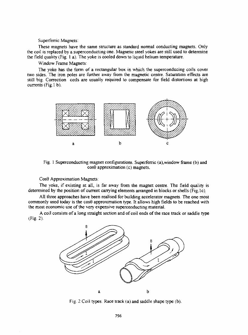
Superferric Magnets: These magnets have the same structure as standard normal conducting magnets. Only
the coil is replaced by a superconducting one. Magnetic steel yokes are still used to determine the field quality (Fig. 1 a). The yoke is cooled down to liquid helium temperature.
Window Frame Magnets: The yoke has the form of a rectangular box in which the superconducing coils cover
two sides. The iron poles are further away from the magnetic centre. Saturation effects are still big. Correction coils are usually required to compensate for field distortions at high currents (Fig. 1 b).
Fig. 1 Superconducting magnet configurations. Superferric (a),window frame (b) and cos0 approximation (c) magnets.
CosG Approximation Magnets: The yoke, if existing at all, is far away from the magnet centre. The field quality is
determined by the position of current carrying elements arranged in blocks or shells (Fig.lc). All three approaches have been realised for building accelerator magnets. The one most
commonly used today is the cosG approximation type. It allows high fields to be reached with the most economic use of the very expensive superconducting material.
A coil consists of a long straight section and of coil ends of the race track or saddle type (Fig. 2).
Fig. 2 Coil types. Race track (a) and saddle shape type (b).
756
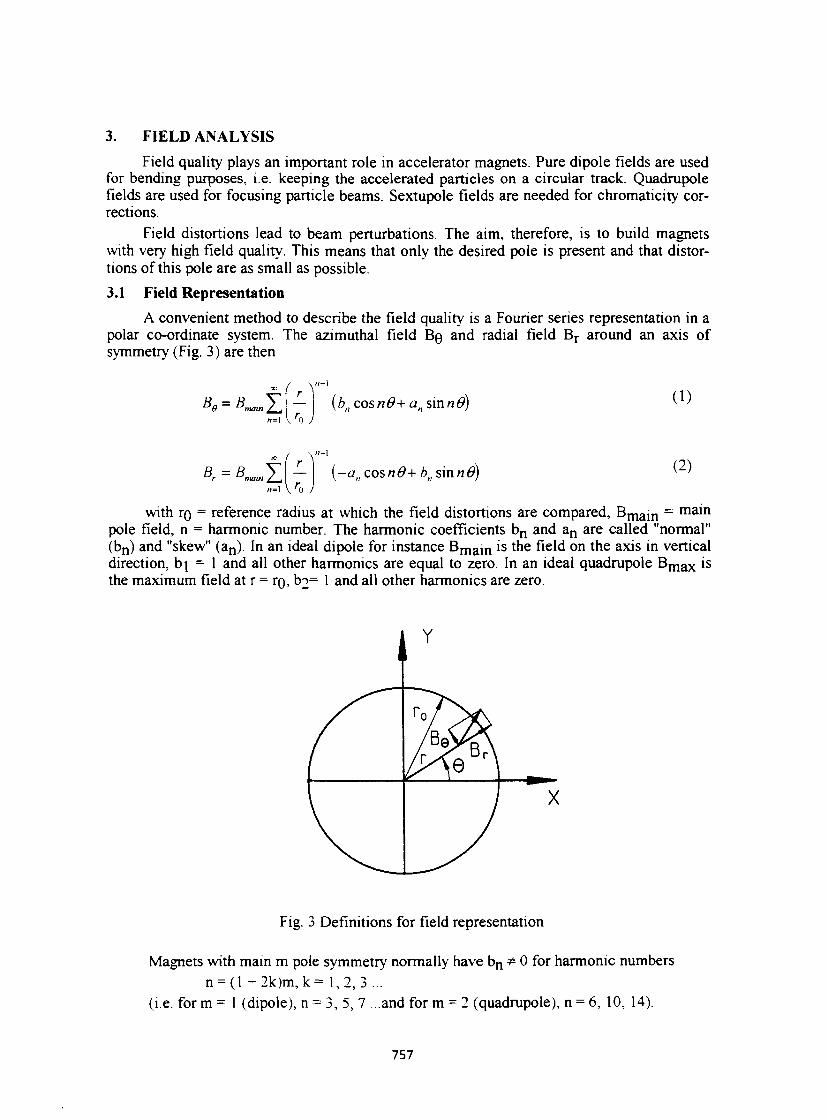
3. FIELD ANALYSIS Field quality plays an important role in accelerator magnets. Pure dipole fields are used
for bending purposes, i.e. keeping the accelerated particles on a circular track. Quadrupole fields are used for focusing particle beams. Sextupole fields are needed for chromaticity corrections.
Field distortions lead to beam perturbations. The aim, therefore, is to build magnets with very high field quality. This means that only the desired pole is present and that distortions of this pole are as small as possible. 3.1 Field Representation
A convenient method to describe the field quality is a Fourier series representation in a polar co-ordinate system. The azimuthal field BQ and radial field B r around an axis of symmetry (Fig. 3) are then
B9= Bmam^j
( Y'~' r (btl cosn0+ an sinn#) (1)
M=l V ' 0 J
B. = B. fr\ ,1 (-an cosn0+ bn sinnO) (2)
with ro = reference radius at which the field distortions are compared, B m a m = main pole field, n = harmonic number. The harmonic coefficients b n and a n are called "normal" (b n) and "skew" (a n). In an ideal dipole for instance B m a m is the field on the axis in vertical direction, b\ = 1 and all other harmonics are equal to zero. In an ideal quadrupole B m a x is the maximum field at r = rg, b2= 1 and all other harmonics are zero.
X
Fig. 3 Definitions for field representation
Magnets with main m pole symmetry normally have b n * 0 for harmonic numbers n = (l +2k)m, k= 1,2,3...
(i.e. for m = 1 (dipole), n = 3, 5, 7 ...and for m = 2 (quadrupole), n = 6, 10, 14).
757
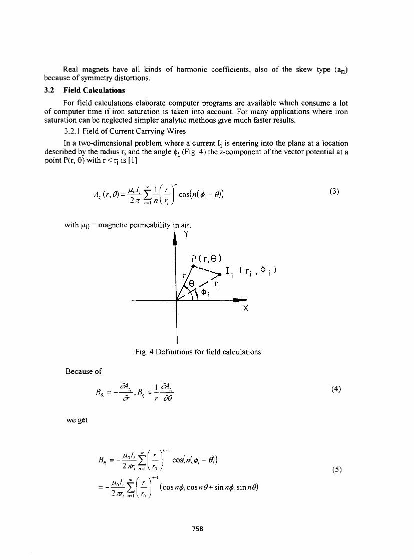
Real magnets have all kinds of harmonic coefficients, also of the skew type (a n ) because of symmetry distortions. 3.2 Field Calculations
For field calculations elaborate computer programs are available which consume a lot of computer time if iron saturation is taken into account. For many applications where iron saturation can be neglected simpler analytic methods give much faster results.
3.2.1 Field of Current Carrying Wires In a two-dimensional problem where a current Ij is entering into the plane at a location
described by the radius q and the angle ^ (Fig. 4) the z-component of the vector potential at a point P(r, 6) with r < q is [1]
A:(r,0) = ^ ± U ^ \ cos(n(<f>, - 0)) 2/r „=1 n\r; )
(3)
with UQ = magnetic permeability in air. Y
Because of
I P ( r , 9 )
Fig. 4 Definitions for field calculations
Bo = dA_
cr • - B , =
1 ÔA.
r 09 (4)
we get
Mol, 2 TTT ,
( r \
n-i V 'o J
Mo1, 7 irr .
f r \ ,t-\
liur..
cos(«(^ - 0))
(cosnfij cosn0+smruf>i sinnd) M=l V '<) J
(5)
758
and with Eq. (1)
b.. = (r \
\r, J cos ncj). (6)
(r\ o., - sin n<j)l
(7)
If there are m wires, the field of the individual wires is superposed. Therefore, we get
*.=i*. (8)
— {cosnef)t cos n(f)+smn(f)j sin né). n J
As the main pole of order p at a reference radius TQ is given by
we get
£_.„.„ --m V \p']
r
, A'i f cospfr (9)
m j
if ^ v -COSW0,
b..= '=i '. v '- y (10) \p-i
cos / ^ ,
«.. =
m r 'r.^
\ r , J sin «0,
(ID
if f.. A'" 1
cos p<f>i
\ r , \ r , J
3.2.2 Field of Current Distribution
Assuming the current carrying elements are all at a constant radius "a" (Fig. 5) with the current varying according to a simple function
/ ( $ = I0cosp<j> (12)
759
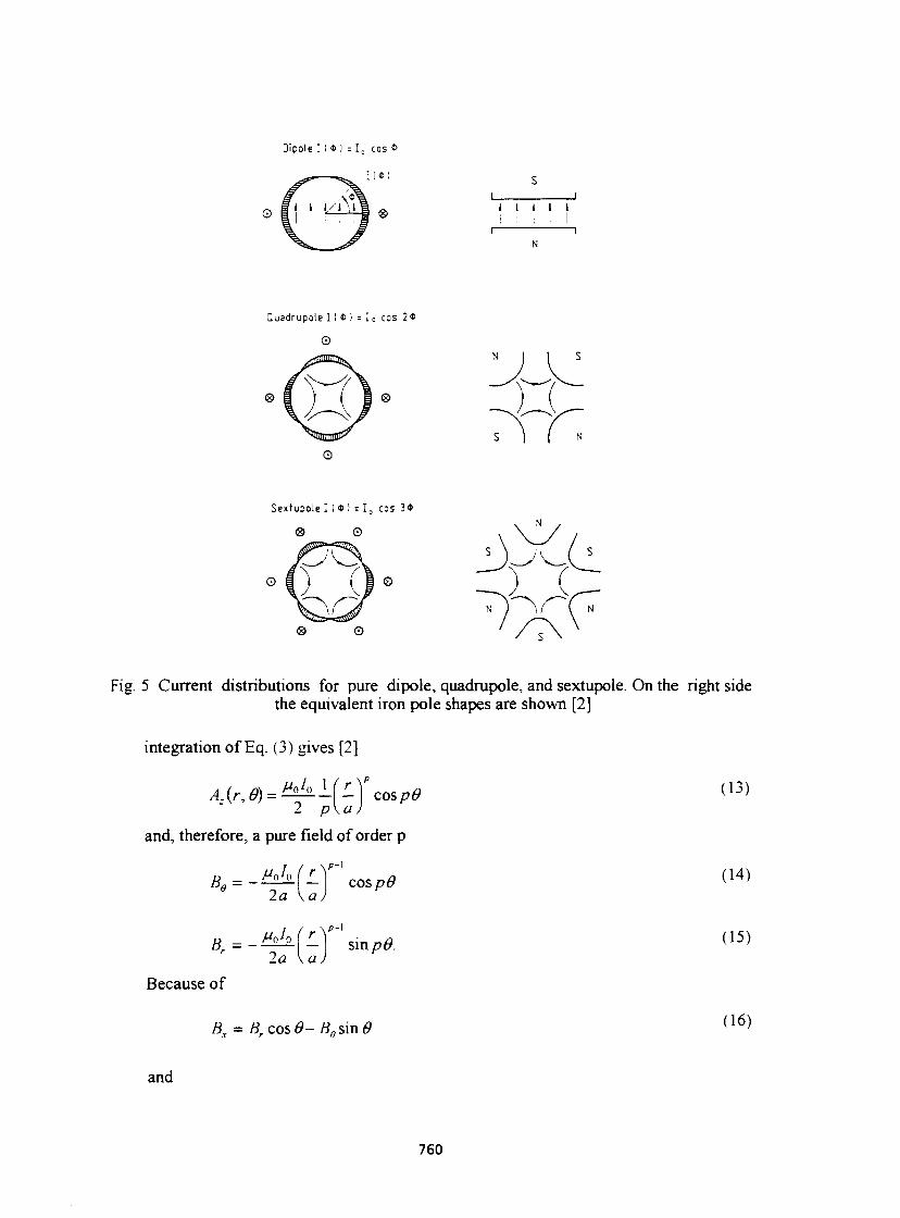
Oipole I ( « ) = I 0 cos 0
i l * :
0 I t I I I
Quadrupole I ( « ) = I 0 cos 2*
0
Sextupole I I * I = I 0 cos 3*
® ©
©
© ©
N ) \[ K N
S
Fig. 5 Current distributions for pure dipole, quadrupole, and sextupole. On the right side the equivalent iron pole shapes are shown [2]
integration of Eq. (3) gives [2]
2 p\a
and, therefore, a pure field of order p
ft, • i^ r - " /"oA> ( r
la \a Br = -!2&L\-\ sin pO.
P-\
Because of
B= Bcosû-8nsmÛ
(13)
(14)
(15)
(16) .T r
and
760
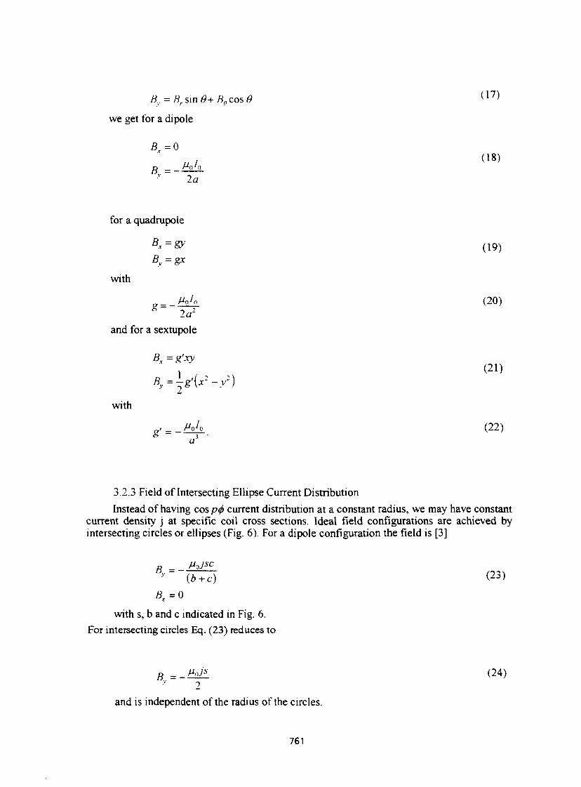
Bv = BrsmÛ+B9cosû ( 1 7 )
we get for a dipole
a I ( 1 8 )
2 a
for a quadrupole
0, = gy
£ , = g *
with
2a"
and for a sextupole
5, = £ , J ^
fi,=^2- -y2)
with
g a 3 •
(19)
(20)
(21)
(22)
3.2.3 Field of Intersecting Ellipse Current Distribution
Instead of having cos p<j> current distribution at a constant radius, we may have constant current density j at specific coil cross sections. Ideal field configurations are achieved by intersecting circles or ellipses (Fig. 6). For a dipole configuration the field is [3]
B = MoJSC
Xb^c) (23) Bx=0
with s, b and c indicated in Fig. 6. For intersecting circles Eq. (23) reduces to
B = - B l l (24)
and is independent of the radius of the circles.
761
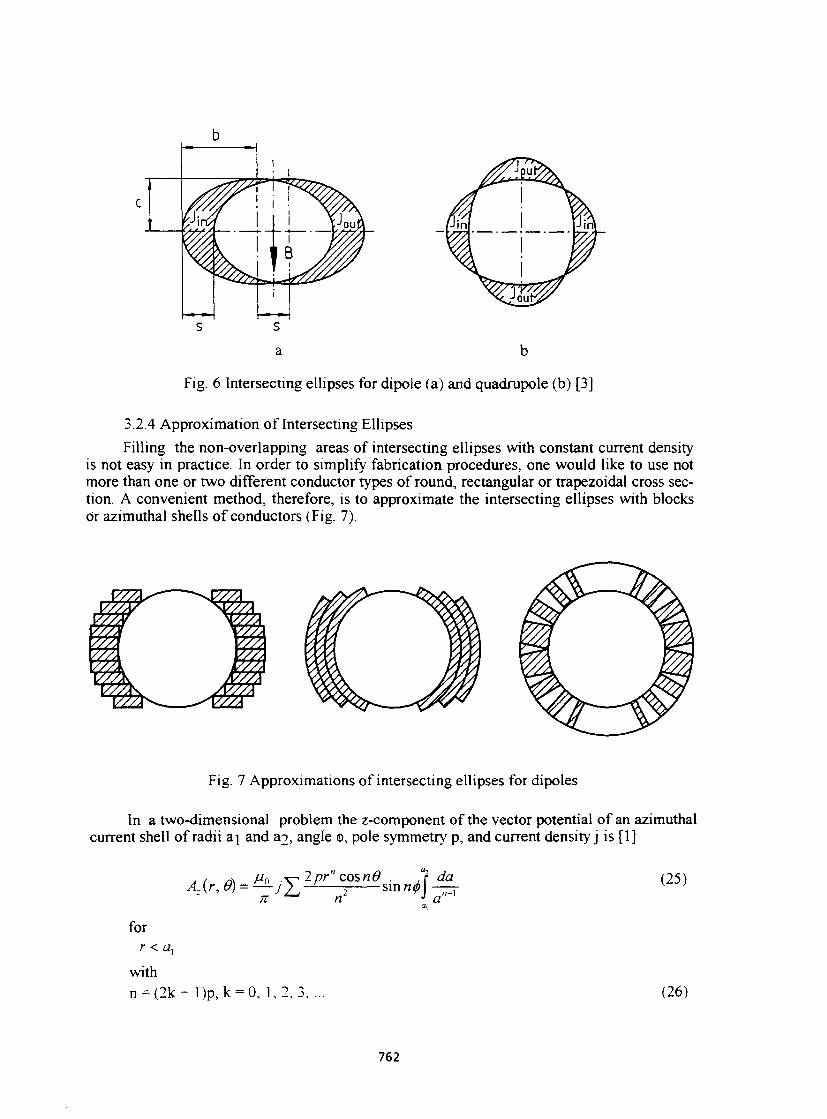
b
Fig. 6 Intersecting ellipses for dipole (a) and quadrupole (b) [3]
3.2.4 Approximation of Intersecting Ellipses Filling the non-overlapping areas of intersecting ellipses with constant current density
is not easy in practice. In order to simplify fabrication procedures, one would like to use not more than one or two different conductor types of round, rectangular or trapezoidal cross section. A convenient method, therefore, is to approximate the intersecting ellipses with blocks or azimuthal shells of conductors (Fig. 7).
Fig. 7 Approximations of intersecting ellipses for dipoles
In a two-dimensional problem the z-component of the vector potential of an azimuthal current shell of radii a] and a2, angle <j), pole symmetry p, and current density j is [1]
da A__(r, 9) = —j^— -2 sin/i^l — K n J a
(25)
for r < a.
with n = (2k+ l)p,k = 0, 1,2,3, (26)
762
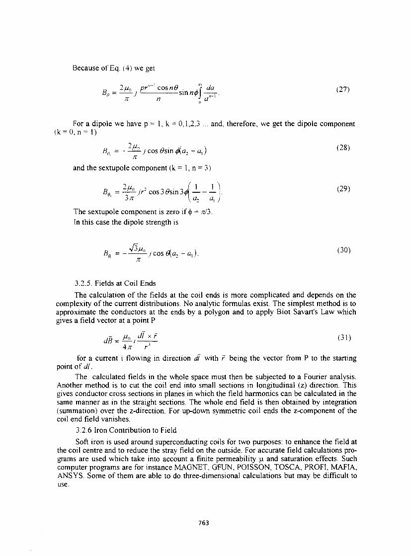
Because of Eq. (4) we get
2/4, pr" ' cosnG . /f da nj)
n " a " '
For a dipole we have p = 1, k = 0,1,2,3 ... and, therefore, we get the dipole component (k = 0 , n = l )
B0 = - ^ 2 - / cos Osm j(a, - a, ) ^ 2 8 )
and the sextupole component (k = 1, n = 3)
" > , >u ( 1 \ \ Bg^ ==p^jr2 cos30sm3<j>
' ^ K \az ax j
The sextupole component is zero if <t> = nJ2>. In this case the dipole strength is
(29)
^L.r^àn -n) (30) B0 = / cos 6{a-, - a, ).
3.2.5. Fields at Coil Ends
The calculation of the fields at the coil ends is more complicated and depends on the complexity of the current distributions. No analytic formulas exist. The simplest method is to approximate the conductors at the ends by a polygon and to apply Biot Savart's Law which gives a field vector at a point P
jB = £Lii^L (3D
for a current 1 flowing in direction dl with r being the vector from P to the starting point of dl.
The calculated fields in the whole space must then be subjected to a Fourier analysis. Another method is to cut the coil end into small sections in longitudinal (z) direction. This gives conductor cross sections in planes in which the field harmonics can be calculated in the same manner as in the straight sections. The whole end field is then obtained by integration (summation) over the z-direction. For up-down symmetric coil ends the z-component of the coil end field vanishes.
3.2.6 Iron Contribution to Field
Soft iron is used around superconducting coils for two purposes: to enhance the field at the coil centre and to reduce the stray field on the outside. For accurate field calculations programs are used which take into account a finite permeability u and saturation effects. Such computer programs are for instance MAGNET, GFUN, POISSON, TOSCA, PROFI, MAPIA, ANSYS. Some of them are able to do three-dimensional calculations but may be difficult to use.
763
As saturation in superconducting magnets of the cos9 type starts at high currents only a much simpler calculation method can be used for quick analysis. In this case /u = oo is assumed and the iron boundary is treated as an ideal mirror. The field on the axis is then obtained from a superposition of the fields from the real coils and from the image coils.
With a circular iron boundary of radius b we get the following parameters of the image currents (Fig. 8):
For individual wires (radii, angles and currents):
r,'=b-/r,
4 = 4 l\ = A •
For coil segments (radii, angle and current density):
(32)
< = b2 la2
a'l = b2 la,
<t>' = <P •r . a \~a2~
(33)
Fig. 8 Current images from a circular yoke boundary
The dipole field component for the coil segments of Section 3.2.4 and yoke radius b is, therefore.
764
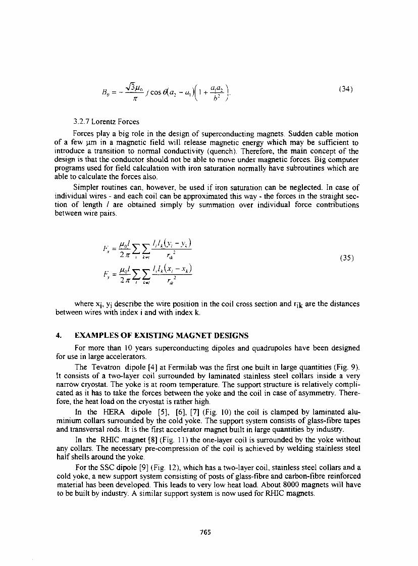
Bg = - ^ j cos d,az-ax)[x + ^ \ ^4 )
3.2.7 Lorentz Forces Forces play a big role in the design of superconducting magnets. Sudden cable motion
of a few urn in a magnetic field will release magnetic energy which may be sufficient to introduce a transition to normal conductivity (quench). Therefore, the main concept of the design is that the conductor should not be able to move under magnetic forces. Big computer programs used for field calculation with iron saturation normally have subroutines which are able to calculate the forces also.
Simpler routines can, however, be used if iron saturation can be neglected. In case of individual wires - and each coil can be approximated this way - the forces in the straight section of length / are obtained simply by summation over individual force contributions between wire pairs.
F = y0iyyiiik{y,-yk) IK T""' r.} k*i
y 2x^£; rit
2
(35)
where XJ, yj describe the wire position in the coil cross section and r ^ are the distances between wires with index i and with index k.
4. EXAMPLES OF EXISTING MAGNET DESIGNS For more than 10 years superconducting dipoles and quadrupoles have been designed
for use in large accelerators. The Tevatron dipole [4] at Fermilab was the first one built in large quantities (Fig. 9).
It consists of a two-layer coil surrounded by laminated stainless steel collars inside a very narrow cryostat. The yoke is at room temperature. The support structure is relatively complicated as it has to take the forces between the yoke and the coil in case of asymmetry. Therefore, the heat load on the cryostat is rather high.
In the ITERA dipole [5], [6], [7] (Fig. 10) the coil is clamped by laminated aluminium collars surrounded by the cold yoke. The support system consists of glass-fibre tapes and transversal rods. It is the first accelerator magnet built in large quantities by industry.
In the RHIC magnet [8] (Fig. 11 ) the one-layer coil is surrounded by the yoke without any collars. The necessary pre-compression of the coil is achieved by welding stainless steel half shells around the yoke.
For the SSC dipole [9] (Fig. 12), which has a two-layer coil, stainless steel collars and a cold yoke, a new support system consisting of posts of glass-fibre and carbon-fibre reinforced material has been developed. This leads to very low heat load. About 8000 magnets will have to be built by industry. A similar support system is now used for RHIC magnets.
765
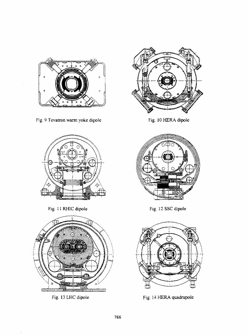
Fig. 9 Tevatron warm yoke dipole Fig. 10 HERA dipole
Fig. 11 RHIC dipole Fig. 12 SSC dipole
Fig. 13 LHC dipole Fig. 14 HERA quadrupole
766
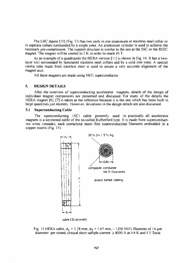
The LHC dipole [10] (Fig. 13) has two coils in one aluminium or stainless steel collar or in separate collars surrounded by a single yoke. An aluminium cylinder is used to achieve the necessary pre-compression. The support structure is similar to the one at the SSC or the RHIC magnet. The magnet will be cooled to 2 K in order to reach 10 T.
As an example of a quadrupole the HERA version [11] is shown in Fig. 14. It has a two-layer coil surrounded by laminated stainless steel collars and by a cold iron yoke. A special inertia tube made from stainless steel is used to assure a very accurate alignment of the magnet axis.
All these magnets are made using NbTi superconductor.
5. DESIGN DETAILS After the overview of superconducting accelerator magnets, details of the design of
individual magnet components are presented and discussed. For many of the details the HERA magnet [6], [7] is taken as the reference because it is the one which has been built in large quantities just recently. However, deviations in the design details are also discussed. 5.1 Superconducting Cable
The superconducting (SC) cable presently used in practically all accelerator magnets is a keystoned cable of the so-called Rutherford type. It is made from superconducting wires (strands), each containing manv fine superconducting filaments embedded in a copper matrix (Fig. 15).
-d 2—1
m
%
95 7. Sn / 5 7. Ag.
composite conductor NbTi f i laments
strand before cabling
cable (24 strands)
Fig. 15 HERA cable, d, = 1.28 mm, d 2 = 1.67 mm, - 1200 NbTi filaments of 14 u,m diameter per strand, critical short sample current > 8000 A at 4.6 K and 5.5 Tesla
767
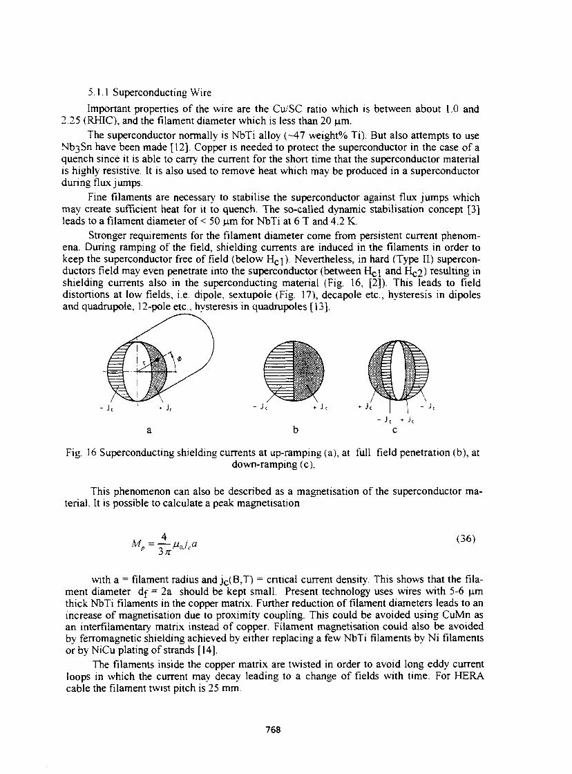
5.1.1 Superconducting Wire Important properties of the wire are the Cu/SC ratio which is between about 1.0 and
2.25 (RHIC), and the filament diameter which is less than 20 jam. The superconductor normally is NbTi alloy (-47 weight% Ti). But also attempts to use
Nb3Sn have been made [12]. Copper is needed to protect the superconductor in the case of a quench since it is able to carry the current for the short time that the superconductor material is highly resistive. It is also used to remove heat which may be produced in a superconductor during flux jumps.
Fine filaments are necessary to stabilise the superconductor against flux jumps which may create sufficient heat for it to quench. The so-called dynamic stabilisation concept [3] leads to a filament diameter of < 50 jam for NbTi at 6 T and 4.2 K.
Stronger requirements for the filament diameter come from persistent current phenomena. During ramping of the field, shielding currents are induced in the filaments in order to keep the superconductor free of field (below H cj). Nevertheless, in hard (Type II) superconductors field may even penetrate into the superconductor (between HQ\ and H c2) resulting in shielding currents also in the superconducting material (Fig. 16, [2]). This leads to field distortions at low fields, i.e. dipole, sextupole (Fig. 17), decapole etc., hysteresis in dipoles and quadrupole, 12-pole etc., hysteresis in quadrupoles [13].
- J c • h a b e
Fig. 16 Superconducting shielding currents at up-ramping (a), at full field penetration (b), at down-ramping (c).
This phenomenon can also be described as a magnetisation of the superconductor material. It is possible to calculate a peak magnetisation
3/r
with a = filament radius and j c(B,T) = critical current density. This shows that the filament diameter df = 2a should be kept small. Present technology uses wires with 5-6 urn thick NbTi filaments in the copper matrix. Further reduction of filament diameters leads to an increase of magnetisation due to proximity coupling. This could be avoided using CuMn as an interfilamentary matrix instead of copper. Filament magnetisation could also be avoided by ferromagnetic shielding achieved by either replacing a few NbTi filaments by Ni filaments or by NiCu plating of strands [14].
The filaments inside the copper matrix are twisted in order to avoid long eddy current loops in which the current may decay leading to a change of fields with time. For HERA cable the filament twist pitch is 25 mm.
768
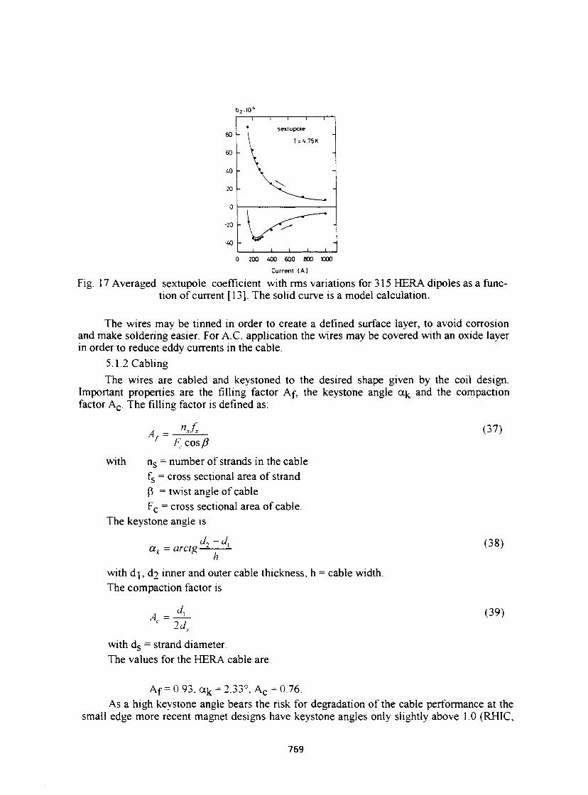
b 3 1 0 '
80
1 1 1 1 i
• sexlupole
\ T = 4.75K
50 V 40 \
20 \ \
0
•20
* 0
•20 _ \ x < r ^ '
-40 - \?
( ) 200 400 600 800 KX»
Current 1A]
Fig. 17 Averaged sextupole coefficient with rms variations for 315 HERA dipoles as a function of current [13]. The solid curve is a model calculation.
The wires may be tinned in order to create a defined surface layer, to avoid corrosion and make soldering easier. For A.C. application the wires may be covered with an oxide layer in order to reduce eddy currents in the cable.
5.1.2 Cabling The wires are cabled and keystoned to the desired shape given by the coil design.
Important properties are the filling factor Af, the keystone angle a^ and the compaction factor A c . The filling factor is defined as:
Af = n,L
Fccosp (37)
with n s = number of strands in the cable fs = cross sectional area of strand p = twist angle of cable F c = cross sectional area of cable.
The keystone angle is
a, arctg-• < / , (38)
h with d] , d2 inner and outer cable thickness, h = cable width. The compaction factor is
2d. (39)
with d s = strand diameter. The values for the HERA cable are
O J A c = 0.76. Af=0.93,afc = ^ As a high keystone angle bears the risk for degradation of the cable performance at the
small edge more recent magnet designs have keystone angles only slightly above 1.0 (RHIC,
769
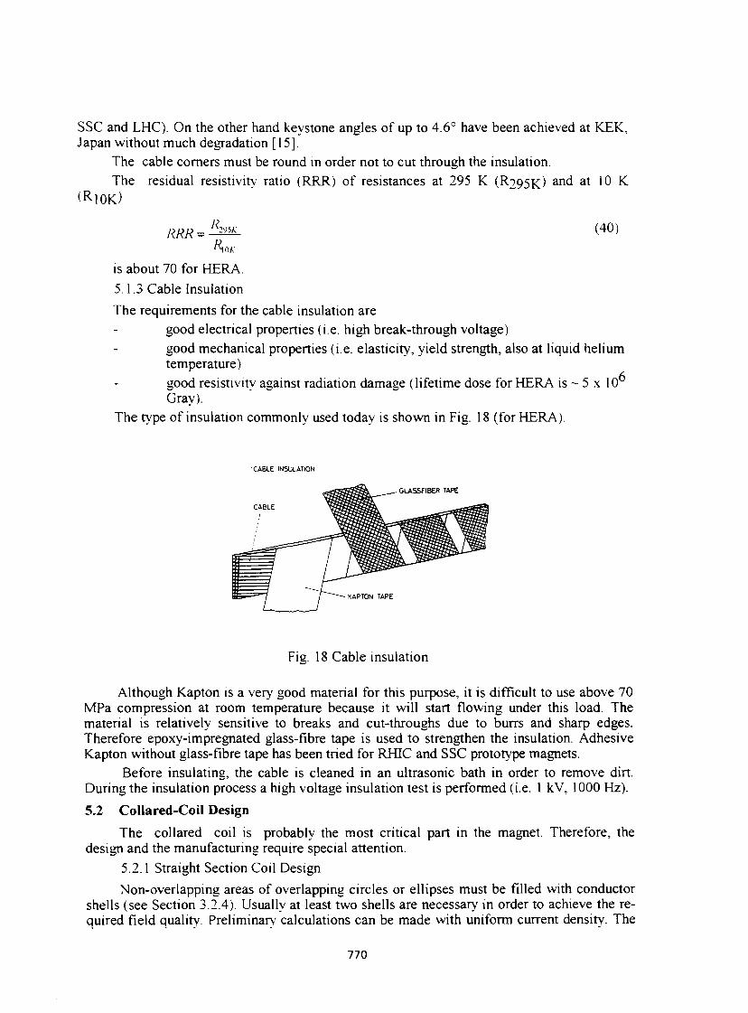
SSC and LHC). On the other hand keystone angles of up to 4.6° have been achieved at KEK, Japan without much degradation [15].
The cable corners must be round in order not to cut through the insulation. The residual resistivitv ratio (RRR) of resistances at 295 K ( R ? 9 5 K ) a n d at 10 K
<RlOK)
^cuis about 70 for HERA. 5.1.3 Cable Insulation The requirements for the cable insulation are
good electrical properties (i.e. high break-through voltage) good mechanical properties (i.e. elasticity, yield strength, also at liquid helium temperature) good resistivity against radiation damage (lifetime dose for HERA is ~ 5 x 10 Gray).
The type of insulation commonly used today is shown in Fig. 18 (for HERA).
CABLE INSULATION
" " . GLASSFIBER TAPE
KAPTON TAPE
Fig. 18 Cable insulation
Although Kapton is a very good material for this purpose, it is difficult to use above 70 MPa compression at room temperature because it will start flowing under this load. The material is relatively sensitive to breaks and cut-throughs due to burrs and sharp edges. Therefore epoxy-impregnated glass-fibre tape is used to strengthen the insulation. Adhesive Kapton without glass-fibre tape has been tried for RHIC and SSC prototype magnets.
Before insulating, the cable is cleaned in an ultrasonic bath in order to remove dirt. During the insulation process a high voltage insulation test is performed (i.e. 1 kV, 1000 Hz). 5.2 Collared-Coil Design
The collared coil is probably the most critical part in the magnet. Therefore, the design and the manufacturing require special attention.
5.2.1 Straight Section Coil Design Non-overlapping areas of overlapping circles or ellipses must be filled with conductor
shells (see Section 3.2.4). Usually at least two shells are necessary in order to achieve the required field quality. Preliminary calculations can be made with uniform current density. The
770
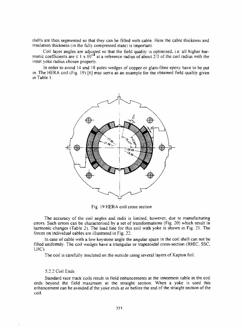
shells are then segmented so that they can be filled with cable. Here the cable thickness and insulation thickness (in the fully compressed state) is important.
Coil layer angles are adjusted so that the field quality is optimised, i.e. all higher harmonic coefficients are < 1 x 10 at a reference radius of about 2/3 of the coil radius with the inner yoke radius chosen properly.
In order to avoid 14 and 18 poles wedges of copper or glass-fibre epoxy have to be put in. The HERA coil (Fig. 19) [6] may serve as an example for the obtained field quality given in Table 1.
Fig. 19 HERA coil cross section
The accuracy of the coil angles and radii is limited, however, due to manufacturing errors. Such errors can be characterised by a set of transformations (Fig. 20) which result in harmonic changes (Table 2). The load line for this coil with yoke is shown in Fig. 21. The forces on individual cables are illustrated in Fig. 22.
In case of cable with a low keystone angle the angular space in the coil shell can not be filled uniformly. The coil wedges have a triangular or trapezoidal cross-section (RHIC, SSC, LHC).
The coil is carefully insulated on the outside using several layers of Kapton foil.
5.2.2 Coil Ends Standard race track coils result in field enhancements at the innermost cable in the coil
ends beyond the field maximum in the straight section. When a yoke is used this enhancement can be avoided if the yoke ends at or before the end of the straight section of the coil.
771
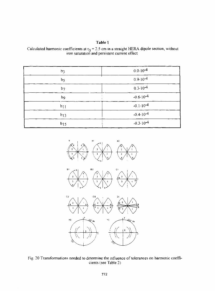
Table 1 Calculated harmonic coefficients at TQ = 2.5 cm in a straight HERA dipole section, without
iron saturation and persistent current effect
b3 0.0-10"4
b5 0.9-lO-4
b 7 0.3-10"4
b 9 -0.6-lO"4
bll -O.I-IO-4
bis -0.4-lO-4
bis -0.3-lO"4
Fig. 20 Transformations needed to determine the influence of tolerances on harmonic coefficients (see Table 2)
772
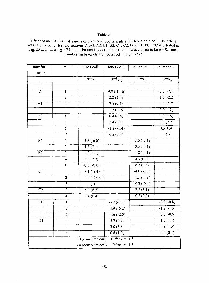
Table 2 Effect of mechanical tolerances on harmonic coefficients at HERA dipole coil. The effect
was calculated for transformations R, Al, A2, Bl, B2, Cl, C2, DO, Dl, XO, YO illustrated in Fig. 20 at a radius TQ = 25 mm. The amplitude of deformation was chosen to be Ô = 0.1 mm.
Numbers in brackets are for a coil without yoke.
transformation
n inner coil inner coil outer coil outer coil
' 0 - 4 a n 10-4bn 10"% lo-X
R 1 -9.0 (-14.6) -3.5 (-7.1) 3 2.2(2.0) -1.7 (-2.2)
Al 2 7.5(9.1) 2.4(2.7) 4 -1.2 (-1.5) 0.9(1.2)
A2 1 6.4(6.8) 1.7(1.6) 2.4(3.1) 1.7(2.2)
5 -1.1 (-1.4) 0.3 (0.4) 7 0.3 (0.4) - ( - )
Bl 1 -5.8 (-6.0) -3.6 (-3.4) 4.3(5.4) -0.3 (-0.4)
B2 2 1.2(1.4) -1.8 (-2.1) 4 2.3(2.9) 0.3 (0.3) 6 -0.5 (-0.6) 0.2 (0.3)
CI 1 -8.1 (-8.4) -4.0 (-3.7) -2.0 (-2.6) -1.5 (-1.8)
5 - ( - ) -0.3 (-0.4) C2 2 5.3(6.5) 2.7(3.1)
4 0.4(0.4) 0.7(0.9) DO 1 -3.7 (-3.7) -0.8 (-0.8)
3 -4.9 (-6.2) -1.2 (-1.3) 5 -1.6 (-2.0) -0.5 (-0.6)
Dl 2 5.7(6.9) 1.3(1.4) 4 3.0(3.8) 0.8(1.0) 6 0.8(1.0) 0.3 (0.3)
XO (complete coil) l O " ^ = YO (complete coil) 10-4a2 =
.5 1.3
773
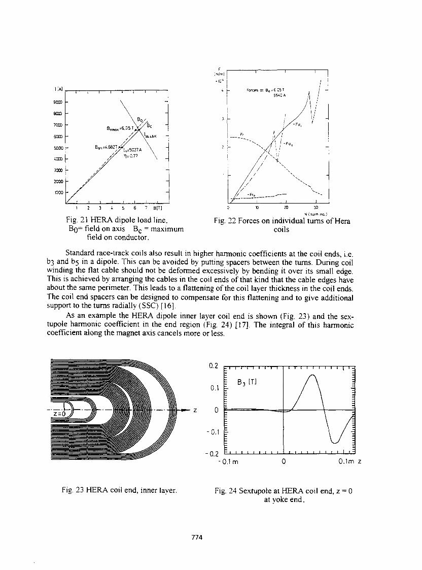
1 [Al
9000
8000
7000
6000
5000
iOOO
3000
2000
1000
I • 1 1 1 1 I I I
-
-\ °//
-
• "
°onwx * 6 . 0 S T \ ^ & C ~ - /7\\
// VLS.4.6K / / \
// \ - Bon=i.682T> ln=5027A \ -
-
// // // // // // AS
T) = 0.77 \
1 1
1
- > 1 i 1 1 1 1 1
-
1 2 3 4 5 6 7 B[T]
Fig. 21 HERA dipole load line, BQ= field on axis B c = maximum
field on conductor.
20 30 N ( turn no.)
Fig. 22 Forces on individual turns of Hera coils
Standard race-track coils also result in higher harmonic coefficients at the coil ends, i.e. b3 and D5 in a dipole. This can be avoided by putting spacers between the turns. During coil winding the flat cable should not be deformed excessively by bending it over its small edge. This is achieved by arranging the cables in the coil ends of that kind that the cable edges have about the same perimeter. This leads to a flattening of the coil layer thickness in the coil ends. The coil end spacers can be designed to compensate for this flattening and to give additional support to the turns radially (SSC) [16].
As an example the HERA dipole inner layer coil end is shown (Fig. 23) and the sex-tupole harmonic coefficient in the end region (Fig. 24) [17]. The integral of this harmonic coefficient along the magnet axis cancels more or less.
Fig. 23 HERA coil end, inner layer. Fig. 24 Sextupole at HERA coil end, z = 0 at vokeend.
774
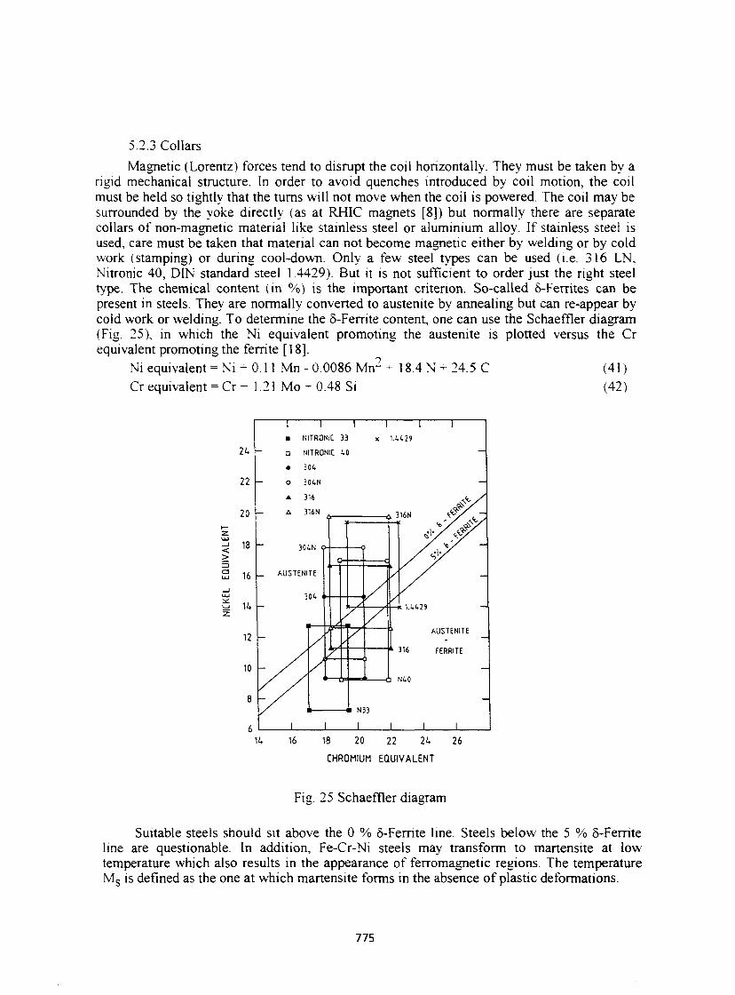
5.2.3 Collars Magnetic (Lorentz) forces tend to disrupt the coil horizontally. They must be taken by a
rigid mechanical structure. In order to avoid quenches introduced by coil motion, the coil must be held so tightly that the turns will not move when the coil is powered. The coil may be surrounded by the yoke directly (as at RHIC magnets [8]) but normally there are separate collars of non-magnetic material like stainless steel or aluminium alloy. If stainless steel is used, care must be taken that material can not become magnetic either by welding or by cold work (stamping) or during cool-down. Only a few steel types can be used (i.e. 316 LN, Nitronic 40, DIN standard steel 1.4429). But it is not sufficient to order just the right steel type. The chemical content (in %) is the important criterion. So-called 6-Ferrites can be present in steels. They are normally converted to austenite by annealing but can re-appear by cold work or welding. To determine the 5-Fernte content, one can use the Schaeffler diagram (Fig. 25), in which the Ni equivalent promoting the austenite is plotted versus the Cr equivalent promoting the ferrite [18].
Ni equivalent = Ni - 0.11 Mn - 0.0086 Mn 2 + 18.4 N-24 .5 C (41) Cr equivalent = Cr - 1.21 Mo ^ 0.48 Si (42)
< >
x 1.i.(.29
18 20 22 24
CHROMIUM EQUIVALENT
26
Fig. 25 Schaeffler diagram
Suitable steels should sit above the 0 % 5-Ferrite line. Steels below the 5 % 5-Ferrite line are questionable. In addition, Fe-Cr-Ni steels may transform to martensite at low temperature which also results in the appearance of ferromagnetic regions. The temperature M s is defined as the one at which martensite forms in the absence of plastic deformations.
775
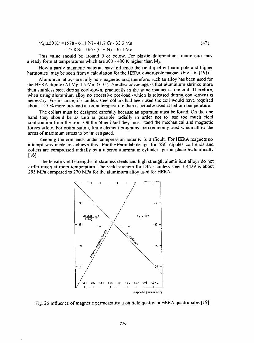
MS(±50K) =1578-61.1 Ni - 41.7 Cr - 33.3 Mn (43) -27.8 Si- 1667 (C + N)- 36.1 Mo
This value should be around 0 or below. For plastic deformations martensite may already form at temperatures which are 300 - 400 K higher than M s.
How a partly magnetic material may influence the field quality (main pole and higher harmonics) may be seen from a calculation for the HERA quadrupole magnet (Fig. 26, [19]).
Aluminium alloys are fully non-magnetic and, therefore, such an alloy has been used for the HERA dipole (Al Mg 4.5 Mn, G 35). Another advantage is that aluminium shrinks more than stainless steel during cool-down, practically in the same manner as the coil. Therefore, when using aluminium alloy no excessive pre-load (which is released during cool-down) is necessary. For instance, if stainless steel collars had been used the coil would have required about 12.5 % more pre-load at room temperature than is actually used at helium temperature.
The collars must be designed carefully because an optimum must be found. On the one hand they should be as thin as possible radially in order not to lose too much field contribution from the iron. On the other hand they must stand the mechanical and magnetic forces safely. For optimisation, finite element programs are commonly used which allow the areas of maximum stress to be investigated.
Keeping the coil ends under compression radially is difficult. For HERA magnets no attempt was made to achieve this. For the Fermilab design for SSC dipoles coil ends and collets are compressed radially by a tapered aluminium cylinder put in place hydraulically [16].
The tensile yield strengths of stainless steels and high strength aluminium alloys do not differ much at room temperature. The yield strength for DIN stainless steel 1.4429 is about 295 MPa compared to 270 MPa for the aluminium alloy used for HERA.
magnetic permeability
Fig. 26 Influence of magnetic permeability JJ. on field quality in HERA quadrupoles [19]
776
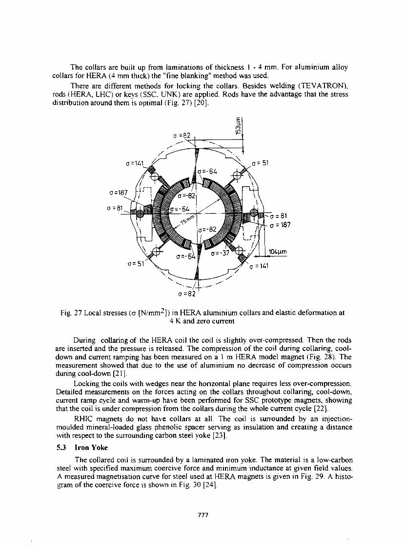
The collars are built up from laminations of thickness 1 - 4 mm. For aluminium alloy collars for HERA (4 mm thick) the "fine blanking" method was used.
There are different methods for locking the collars. Besides welding (TEVATRON), rods (HERA, LHC) or keys (SSC, UNK) are applied. Rods have the advantage that the stress distribution around them is optimal (Fig. 27) [20].
Fig. 27 Local stresses (a [N/mm^]) in HERA aluminium collars and elastic deformation at 4 K and zero current
During collaring of the HERA coil the coil is slightly over-compressed. Then the rods are inserted and the pressure is released. The compression of the coil during collaring, cool-down and current ramping has been measured on a 1 m HERA model magnet (Fig. 28). The measurement showed that due to the use of aluminium no decrease of compression occurs during cool-down [21].
Locking the coils with wedges near the horizontal plane requires less over-compression. Detailed measurements on the forces acting on the collars throughout collaring, cool-down, current ramp cycle and warm-up have been performed for SSC prototype magnets, showing that the coil is under compression from the collars during the whole current cycle [22].
RHIC magnets do not have collars at all. The coil is surrounded by an injection-moulded mineral-loaded glass phenolic spacer serving as insulation and creating a distance with respect to the surrounding carbon steel yoke [23]. 5.3 Iron Yoke
The collared coil is surrounded by a laminated iron yoke. The material is a low-carbon steel with specified maximum coercive force and minimum inductance at given field values. A measured magnetisation curve for steel used at HERA magnets is given in Fig. 29. A histogram of the coercive force is shown in Fig. 30 [24].
777
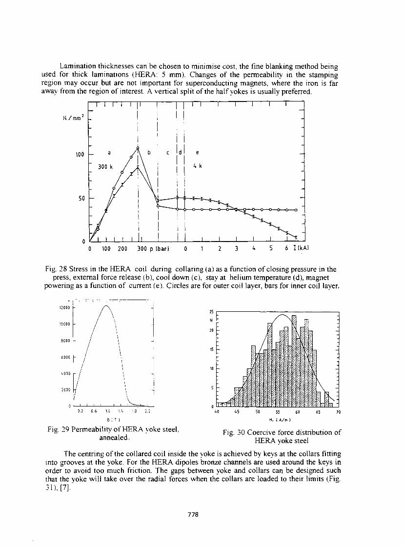
Lamination thicknesses can be chosen to minimise cost, the fine blanking method being used for thick laminations (HERA: 5 mm). Changes of the permeability in the stamping region may occur but are not important for superconducting magnets, where the iron is far away from the region of interest. A vertical split of the half yokes is usually preferred.
N/mnT
100
50 -
1 1 1 , 1 1 1 1
— a y\ k c
300 k / J \ |
• y i \ i
: / ! !
M 1 1 t 1 1
1 \
d
1 1 1 1 1 1 1
e _
4 k
1 1 1 1 1 1 s *
0 100 200 300 p [bar] 6 I lkAI
Fig. 28 Stress in the HERA coil during collaring (a) as a function of closing pressure in the press, external force release (b), cool down (c), stay at helium temperature (d), magnet
powering as a function of current (e). Circles are for outer coil layer, bars for inner coil layer.
* • . 1 1
12000 -
10000 / \ \ -
8000 / \ -
6000 " / \ -
1.000 \ -
2000
a 1 1 I I I 1 1 1
0.2 0.6 1.0 l.i. 1.8 2.2
B I T ]
Fig. 29 Permeability of HERA yoke steel, annealed.
H, [ A/m ]
Fig. 30 Coercive force distribution of HERA yoke steel
The centring of the collared coil inside the yoke is achieved by keys at the collars fitting into grooves at the yoke. For the HERA dipoles bronze channels are used around the keys in order to avoid too much friction. The gaps between yoke and collars can be designed such that the yoke will take over the radial forces when the collars are loaded to their limits (Fig. 31), [7].
778
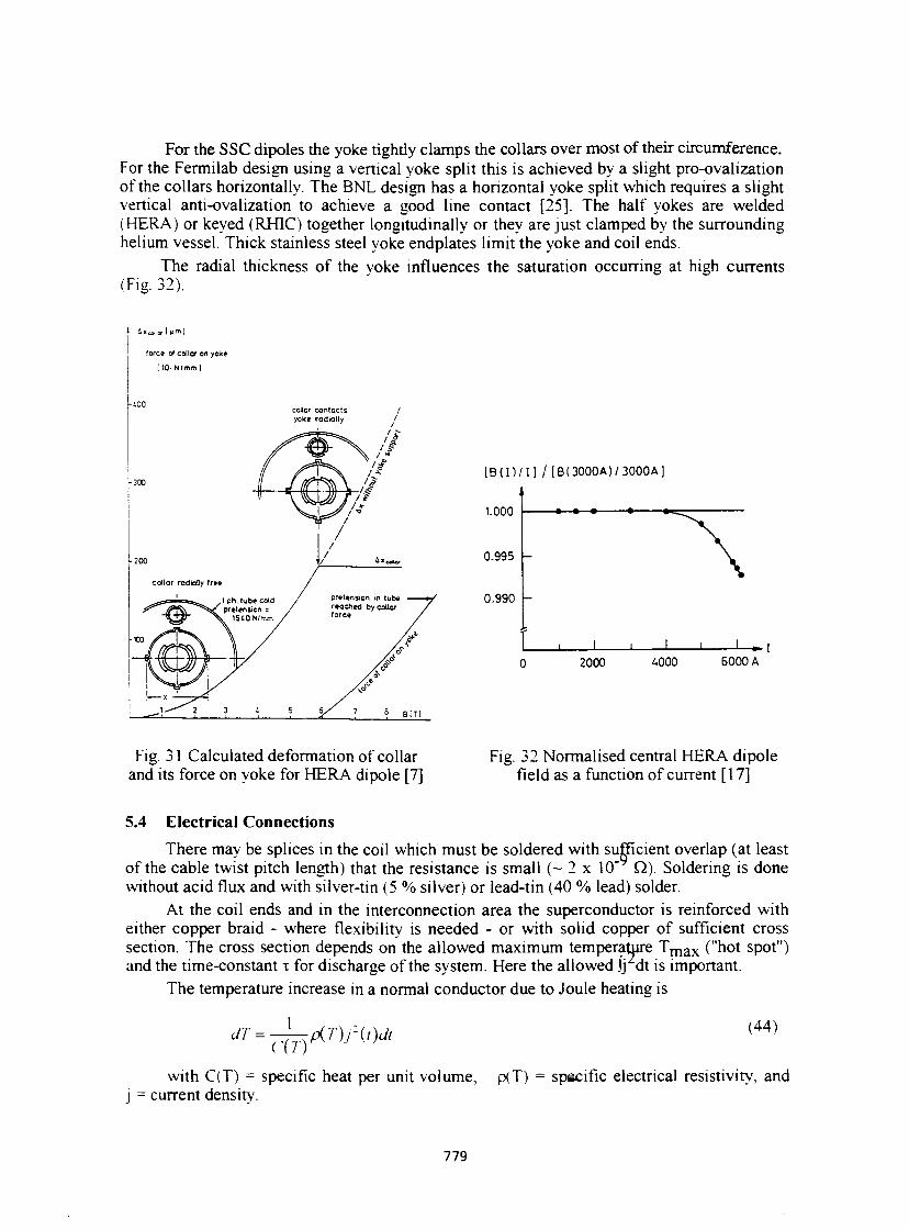
For the SSC dipoles the yoke tightly clamps the collars over most of their circumference. For the Fermilab design using a vertical yoke split this is achieved by a slight pro-ovalization of the collars horizontally. The BNL design has a horizontal yoke split which requires a slight vertical anti-ovalization to achieve a good line contact [25]. The half yokes are welded (HERA) or keyed (RH1C) together longitudinally or they are just clamped by the surrounding helium vessel. Thick stainless steel yoke endplates limit the yoke and coil ends.
The radial thickness of the voke influences the saturation occurring at high currents (Fig. 32).
force of colter on yoke
M O - N / m m ]
coilor contacts yoke rodial ly
[ B ( I ) / I ] /[B(3OOOA)/3OO0A]
1.000
0.995
0.990
-•—» • •»
- * - I 2000 4000 6000 A
Fig. 31 Calculated deformation of collar and its force on yoke for HERA dipole [7]
Fig. 32 Normalised central HERA dipole field as a function of current [17]
5.4 Electrical Connections There may be splices in the coil which must be soldered with sufficient overlap (at least
of the cable twist pitch length) that the resistance is small (~ 2 x 10 Q). Soldering is done without acid flux and with silver-tin (5 % silver) or lead-tin (40 % lead) solder.
At the coil ends and in the interconnection area the superconductor is reinforced with either copper braid - where flexibility is needed - or with solid copper of sufficient cross section. The cross section depends on the allowed maximum temperature T m a x ("hot spot") and the time-constant x for discharge of the system. Here the allowed Jfj dt is important.
The temperature increase in a normal conductor due to Joule heating is
JT = 1 C(T)
p{T)f{()dt (44)
with C(T) = specific heat per unit volume, p(T) = specific electrical resistivity, and j = current density.
779
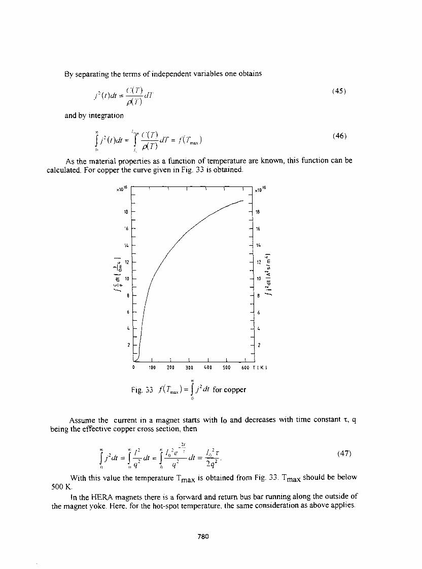
By separating the terms of independent variables one obtains
and by integration
(45)
l^Jjm.r-.f^J (46)
As the material properties as a function of temperature are known, this function can be calculated. For copper the curve given in Fig. 33 is obtained.
«10 " «10
18
14
12 E IA
< 10 — 5
0 100 200 300 400 500 600 T I K I
•3Z,
Fig. 33 f{TmJ = \/dt for copper
Assume the current in a magnet starts with Io and decreases with time constant x, q being the effective copper cross section, then
x T2 X I 2 /o 2r (47)
With this value the temperature T m a x is obtained from Fig. 33. T m a x should be below 500 K.
In the HERA magnets there is a forward and return bus bar running along the outside of the magnet yoke. Here, for the hot-spot temperature, the same consideration as above applies.
780
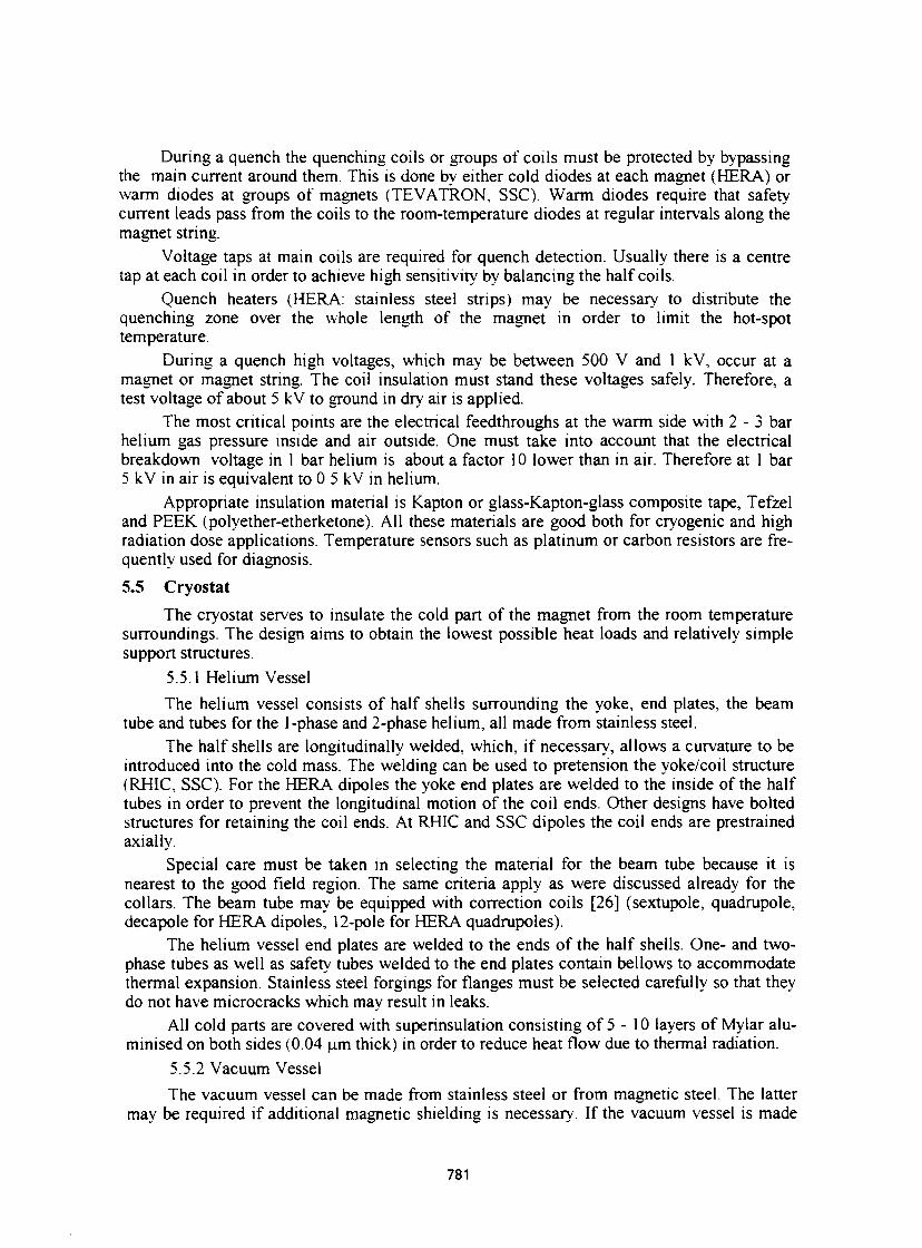
During a quench the quenching coils or groups of coils must be protected by bypassing the main current around them. This is done by either cold diodes at each magnet (HERA) or warm diodes at groups of magnets (TEVATRON, SSC). Warm diodes require that safety current leads pass from the coils to the room-temperature diodes at regular intervals along the magnet string.
Voltage taps at main coils are required for quench detection. Usually there is a centre tap at each coil in order to achieve high sensitivity by balancing the half coils.
Quench heaters (HERA: stainless steel strips) may be necessary to distribute the quenching zone over the whole length of the magnet in order to limit the hot-spot temperature.
During a quench high voltages, which may be between 500 V and 1 kV, occur at a magnet or magnet string. The coil insulation must stand these voltages safely. Therefore, a test voltage of about 5 kV to ground in dry air is applied.
The most critical points are the electrical feedthroughs at the warm side with 2 - 3 bar helium gas pressure inside and air outside. One must take into account that the electrical breakdown voltage in 1 bar helium is about a factor 10 lower than in air. Therefore at 1 bar 5 kV in air is equivalent to 0.5 kV in helium.
Appropriate insulation material is Kapton or glass-Kapton-glass composite tape, Tefzel and PEEK (polyether-etherketone). All these materials are good both for cryogenic and high radiation dose applications. Temperature sensors such as platinum or carbon resistors are frequently used for diagnosis. 5.5 Cryostat
The cryostat serves to insulate the cold part of the magnet from the room temperature surroundings. The design aims to obtain the lowest possible heat loads and relatively simple support structures.
5.5.1 Helium Vessel The helium vessel consists of half shells surrounding the yoke, end plates, the beam
tube and tubes for the 1-phase and 2-phase helium, all made from stainless steel. The half shells are longitudinally welded, which, if necessary, allows a curvature to be
introduced into the cold mass. The welding can be used to pretension the yoke/coil structure (RHIC, SSC). For the HERA dipoles the yoke end plates are welded to the inside of the half tubes in order to prevent the longitudinal motion of the coil ends. Other designs have bolted structures for retaining the coil ends. At RHIC and SSC dipoles the coil ends are prestrained axially.
Special care must be taken in selecting the material for the beam tube because it is nearest to the good field region. The same criteria apply as were discussed already for the collars. The beam tube may be equipped with correction coils [26] (sextupole, quadrupole, decapole for HERA dipoles, 12-pole for HERA quadrupoles).
The helium vessel end plates are welded to the ends of the half shells. One- and two-phase tubes as well as safety tubes welded to the end plates contain bellows to accommodate thermal expansion. Stainless steel forgings for flanges must be selected carefully so that they do not have microcracks which may result in leaks.
All cold parts are covered with superinsulation consisting of 5 - 10 layers of Mylar alu-minised on both sides (0.04 urn thick) in order to reduce heat flow due to thermal radiation.
5.5.2 Vacuum Vessel The vacuum vessel can be made from stainless steel or from magnetic steel. The latter
may be required if additional magnetic shielding is necessary. If the vacuum vessel is made
781
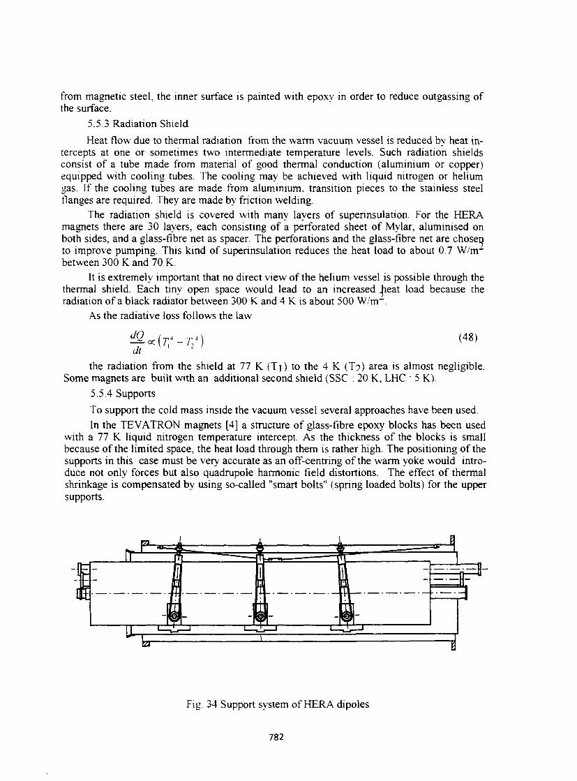
from magnetic steel, the inner surface is painted with epoxy in order to reduce outgassing of the surface.
5.5.3 Radiation Shield Heat flow due to thermal radiation from the warm vacuum vessel is reduced by heat in
tercepts at one or sometimes two intermediate temperature levels. Such radiation shields consist of a tube made from material of good thermal conduction (aluminium or copper) equipped with cooling tubes. The cooling may be achieved with liquid nitrogen or helium gas. If the cooling tubes are made from aluminium, transition pieces to the stainless steel flanges are required. They are made by friction welding.
The radiation shield is covered with many layers of superinsulation. For the HERA magnets there are 30 layers, each consisting of a perforated sheet of Mylar, aluminised on both sides, and a glass-fibre net as spacer. The perforations and the glass-fibre net are chosen to improve pumping. This kind of supennsulation reduces the heat load to about 0.7 W/m~ between 300 K and 70 K.
It is extremely important that no direct view of the helium vessel is possible through the thermal shield. Each tiny open space would lead to an increased Jieat load because the radiation of a black radiator between 300 K and 4 K is about 500 W/m~.
As the radiative loss follows the law
^ c c ( 7 î < - 7 - ) at
(48)
the radiation from the shield at 77 K (Ti) to the 4 K (T?) area is almost negligible. Some magnets are built with an additional second shield (SSC : 20 K, LHC : 5 K).
5.5.4 Supports To support the cold mass inside the vacuum vessel several approaches have been used. In the TEVATRON magnets [4] a structure of glass-fibre epoxy blocks has been used
with a 77 K liquid nitrogen temperature intercept. As the thickness of the blocks is small because of the limited space, the heat load through them is rather high. The positioning of the supports in this case must be very accurate as an off-centring of the warm yoke would introduce not only forces but also quadrupole harmonic field distortions. The effect of thermal shrinkage is compensated by using so-called "smart bolts" (spring loaded bolts) for the upper supports.
Fig. 34 Support system of HERA dipoles
782
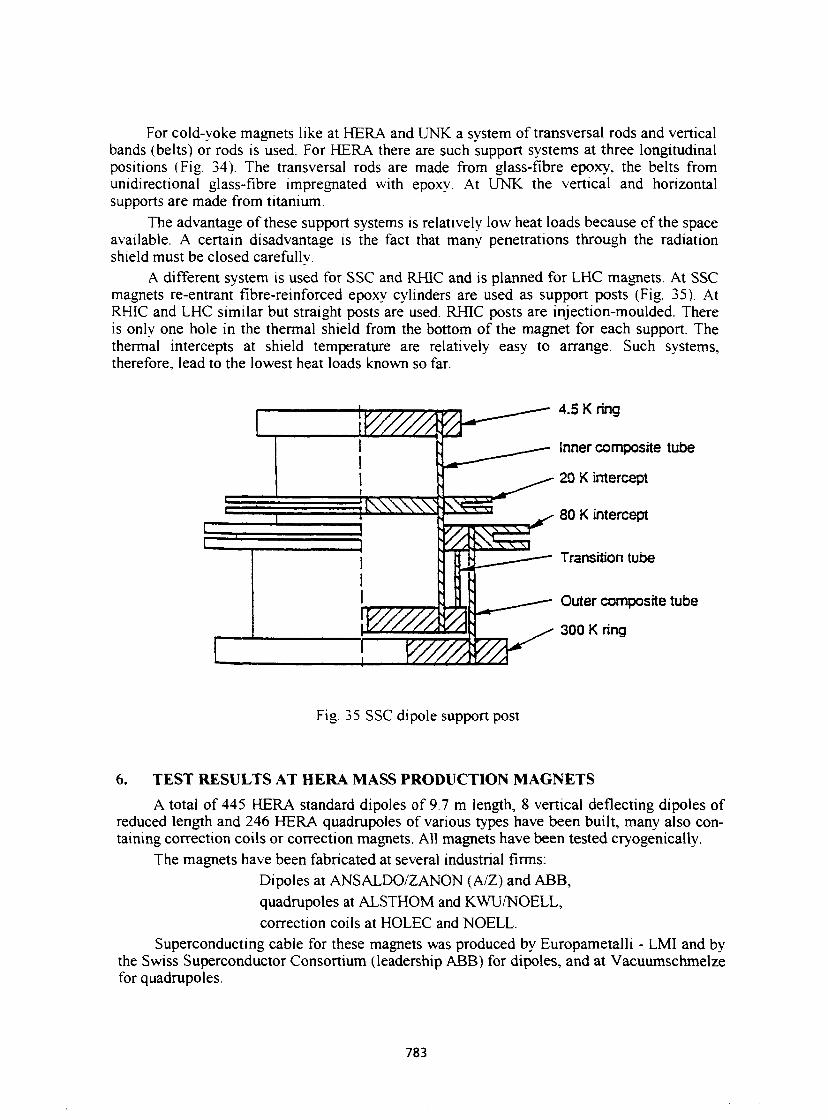
For cold-yoke magnets like at HERA and UNK a system of transversal rods and vertical bands (belts) or rods is used. For HERA there are such support systems at three longitudinal positions (Fig. 34). The transversal rods are made from glass-fibre epoxy, the belts from unidirectional glass-fibre impregnated with epoxy. At UNK the vertical and horizontal supports are made from titanium.
The advantage of these support systems is relatively low heat loads because of the space available. A certain disadvantage is the fact that many penetrations through the radiation shield must be closed carefully.
A different system is used for SSC and RHIC and is planned for LHC magnets. At SSC magnets re-entrant fibre-reinforced epoxy cylinders are used as support posts (Fig. 35). At RHIC and LHC similar but straight posts are used. RHIC posts are injection-moulded. There is only one hole in the thermal shield from the bottom of the magnet for each support. The thermal intercepts at shield temperature are relatively easy to arrange. Such systems, therefore, lead to the lowest heat loads known so far.
wvzm
4.5 K ring
Inner composite tube
20 K intercept
80 K intercept
Transition tube
Outer composite tube
300 K ring
Fig. 35 SSC dipole support post
6. TEST RESULTS AT HERA MASS PRODUCTION MAGNETS A total of 445 HERA standard dipoles of 9.7 m length, 8 vertical deflecting dipoles of
reduced length and 246 HERA quadrupoles of various types have been built, many also containing correction coils or correction magnets. AH magnets have been tested cryogenically.
The magnets have been fabricated at several industrial firms: Dipoles at ANSALDO/ZANON (A/Z) and ABB, quadrupoles at ALSTHOM and KWU/NOELL, correction coils at HOLEC and NOELL.
Superconducting cable for these magnets was produced by Europametalli - LMI and by the Swiss Superconductor Consortium (leadership ABB) for dipoles, and at Vacuumschmelze for quadrupoles.
783
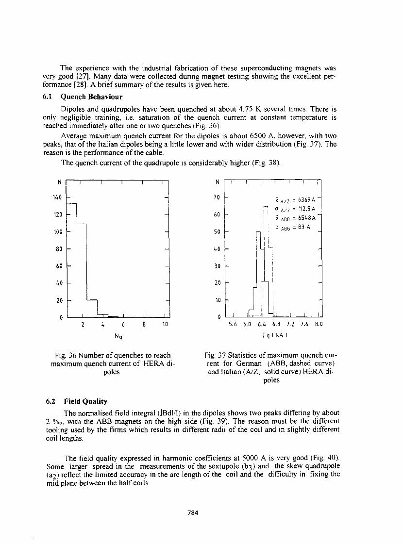
The experience with the industrial fabrication of these superconducting magnets was very good [27]. Many data were collected during magnet testing showing the excellent performance [28]. A brief summary of the results is given here. 6.1 Quench Behaviour
Dipoles and quadrupoles have been quenched at about 4.75 K several times. There is only negligible training, i.e. saturation of the quench current at constant temperature is reached immediately after one or two quenches (Fig. 36).
Average maximum quench current for the dipoles is about 6500 A, however, with two peaks, that of the Italian dipoles being a little lower and with wider distribution (Fig. 37). The reason is the performance of the cable.
The quench current of the quadrupole is considerably higher (Fig. 38).
N
70
60
50
A0
30
20
10
rJ, k,
x A / z = 6369 A
A/Z 112.5 A x A B B = 6548A a A B B = 83 A
5.6 6.0 6.L 6.8 7.2 7.6
I q [ kA 1
8.0
Fig. 36 Number of quenches to reach maximum quench current of HERA di
poles
Fig. 37 Statistics of maximum quench current for German (ABB, dashed curve) and Italian (A/Z, solid curve) HERA di
poles
6.2 Field Quality The normalised field integral (JBdl/I) in the dipoles shows two peaks differing by about
2 %o, with the ABB magnets on the high side (Fig. 39). The reason must be the different tooling used by the firms which results in different radii of the coil and in slightly different coil lengths.
The field quality expressed in harmonic coefficients at 5000 A is very good (Fig. 40). Some larger spread in the measurements of the sextupole (b3) and the skew quadrupole (a?) reflect the limited accuracy in the arc length of the coil and the difficulty in fixing the mid plane between the half coils.
784
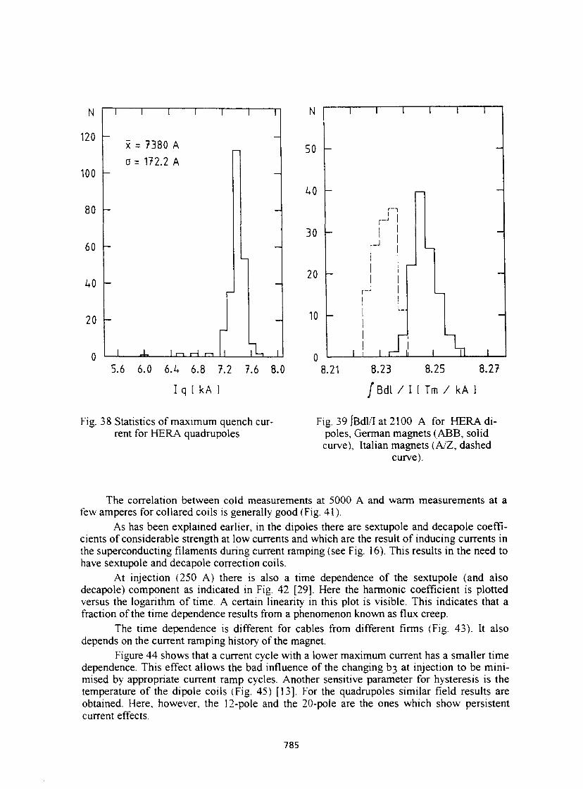
N i i i i I I I N I I I I I I
120 x = 7380 A 50 a =172.2 A
100 -
40 -
80 — -r—'
30 r I -
60 r-J
I —
U0 ^ 20 I
I _ j
—
20 - 10 -L_.
-
0 I -L I i — i i — l i — i l \u i 0 3 8
i I r- i il i 0 5.6 6.0 6A 6.8 7.2 7.6 8.
0 3 8 .21 8.23 8.25 8.27
I q I kA ] /Bd l / I ( Tm / kA 1
Fig. 38 Statistics of maximum quench current for HERA quadrupoles
Fig. 39jBdl/Iat2100 A for HERA di-poles, German magnets (ABB, solid curve), Italian magnets (A/Z, dashed
curve).
The correlation between cold measurements at 5000 A and warm measurements at a few amperes for collared coils is generally good (Fig. 41).
As has been explained earlier, in the dipoles there are sextupole and decapole coefficients of considerable strength at low currents and which are the result of inducing currents in the superconducting filaments during current ramping (see Fig. 16). This results in the need to have sextupole and decapole correction coils.
At injection (250 A) there is also a time dependence of the sextupole (and also decapole) component as indicated in Fig. 42 [29]. Here the harmonic coefficient is plotted versus the logarithm of time. A certain linearity in this plot is visible. This indicates that a fraction of the time dependence results from a phenomenon known as flux creep.
The time dependence is different for cables from different firms (Fig. 43). It also depends on the current ramping history of the magnet.
Figure 44 shows that a current cycle with a lower maximum current has a smaller time dependence. This effect allows the bad influence of the changing b3 at injection to be minimised by appropriate current ramp cycles. Another sensitive parameter for hysteresis is the temperature of the dipole coils (Fig. 45) [13]. For the quadrupoles similar field results are obtained. Here, however, the 12-pole and the 20-pole are the ones which show persistent current effects.
785
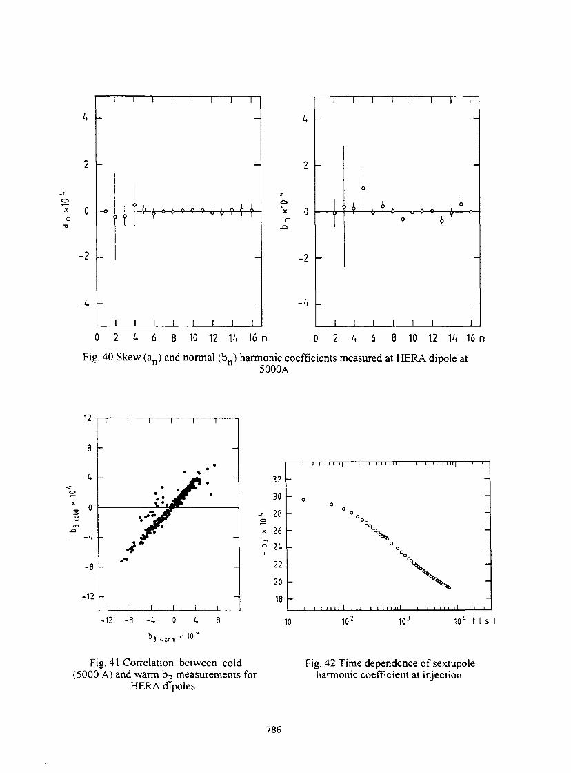
o
c ru
4
1 1 1 1 1 1 1 1
2
o ^ 0
c
1 1
>
. T A . X A l 1 _
2
o ^ 0
c ^r • < , - ' • ^
-2 - -
-4
i i i i i i i i
0 2 4 6 8 10 12 14 16 n 0 2 4 6 8 10 12 14 16 n
Fig. 40 Skew (a ) and normal (b ) harmonie coefficients measured at HERA dipole at 5000A
i i 1 1 1 1 II 1 1 I I TTT I I | 1 1 1 1 I I 111 1 1
32 -
30 — o -
- 28 o o o —
<=> \ x 26 % ^ —
1 - O
o
V -
22 - \ h. -
20 - V -
18 1 1 i i i i M I I i i i i i n i i 1 1 1 1 1 I I I 1 1
10 10' 10 : t0u t [ s ]
3 warm
Fig. 41 Correlation between cold (5000 A) and warm b^ measurements for
HERA dipoles
Fig. 42 Time dependence of sextupole harmonic coefficient at injection
786
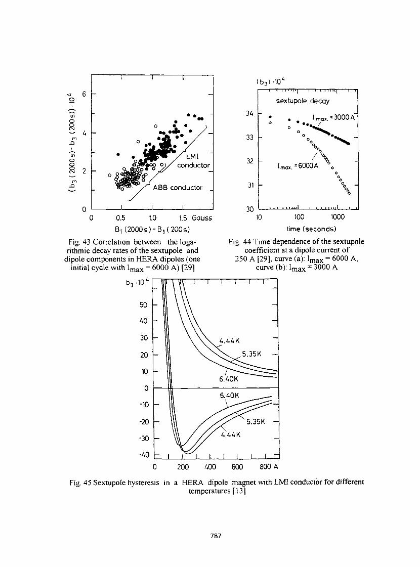
o
O o CM
6 -
— 4 -
en o o o CM
<•»•>
2 -
0
-
1 1 1
- ° v • ; •A • /
JLSL* Y •
# A # P ^ / L M I
-
°û frJïto °/y c o r | ductor
- «0*
1
® / ABB conductor
1 1
l b 3 M 0 4
1— 1 I I I l i lt I 1- I T T I lly' " T—r
sextupole decay
34 • I max. =3000 A" o
33
32 Im a x.=6000A \
o o o
31
1
o
\
_ l l i I J J J I I i i m i l l i ,
0.5 1.0 1.5 Gauss
B, (2000s ) -B , ( 200s)
Fig. 43 Correlation between the logarithmic decay rates of the sextupole and
dipole components in HERA dipoles (one initial cycle with I m a x = 6000 A) [29]
b 3 -10'
50
40
30
20
10
0
-10
-20
-30
-40
10 100 1000
time (seconds)
Fig. 44 Time dependence of the sextupole coefficient at a dipole current of
250 A [29], curve (a): I m a x = 6000 A, curve (b): I m a x = 3000 A
1 1
1 1 1 1 1 1
:
— Ill \ \ \ A . A 4 K
—
- Ill \ ^ X V ^ 5 . 3 5 K —
" 6 . 4 0 K ' "~"
6.40K ^ ,
— U\ / / ^ < ^ 5 , 3 5 K
—
- y\ , / / / 4.44 K —
- 1 1 y \ I 1 1 1 1 —
0 200 400 600 800 A
Fig. 45 Sextupole hysteresis in a HERA dipole magnet with LMI conductor for different temperatures [13]
787
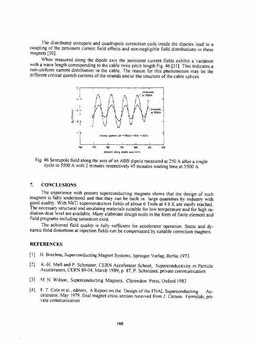
The distributed sextupole and quadrupole correction coils inside the dipoles lead to a coupling of the persistent current field effects and non-negligible field distributions in these magnets [30].
When measured along the dipole axis the persistent current fields exhibit a variation with a wave length corresponding to the cable twist pitch length Fig. 46 [31]. This indicates a non-uniform current distribution in the cable. The reason for this phenomenon mav be the different critical quench currents of the strands and/or the structure of the cable splices.
( history : quench. 0A -> 5500A -> 50 A -> 250A )
_ 1 _ 760 780 790 800
position along dipole oxis (cm]
820
Fig. 46 Sextupole field along the axis of an ABB dipole measured at 250 A after a single cycle to 5500 A with 2 minutes respectively 45 minutes waiting time at 5500 A
7. CONCLUSIONS
The experience with present superconducting magnets shows that the design of such magnets is fully understood and that they can be built in large quantities by industry with good quality. With NbTi superconductors fields of about 6 Tesla at 4.6 K are easily reached. The necessary structural and insulating materials suitable for low temperature and for high radiation dose level are available. Many elaborate design tools in the form of finite element and field programs including saturation exist.
The achieved field quality is fully sufficient for accelerator operation. Static and dynamic field distortions at injection fields can be compensated by suitable correction magnets.
REFERENCES
[1] H. Brechna, Superconducting Magnet Systems, Springer Verlag, Berlin 1973
[2] K.-H. MeB and P. Schmuser, CERN Accelerator School, Superconductivity in Particle Accelerators, CERN 89-04, March 1989, p. 87, P. Schmuser, private communication
[3] M.N.Wilson, Superconducting Magnets, Clarendon Press, Oxford 1983
[4] F T . Cole et a l , editors, A Report on the Design of the FNAL Superconducting Accelerator, May 1979, final magnet cross section received from J. Carson, FermTlab, private communication
788
[5] HERA, A Proposal for a Large Electron-Proton Colliding Beam Facility at DESY, DESY HERA 81-10, 1981
[6] S. Wolff, Superconducting Magnets for HERA, Proceedings of the XIII International Conference on High Energy Particle Accelerators, Novosibirsk, Aug. 1986, Vol. 2, p. 29, DESY HERA 1986-12
[7] H. Kaiser, Design of Superconducting Dipole for HERA, Proceedings of the XIII International Conference on High Energy Particle Accelerators, Novosibirsk, Aug. 1986, Vol. 2, p. 49. DESY HERA 1986-14
[8] Conceptual Design of the Relativistic Heavy Ion Collider, RHIC, Report No. BNL51932, Brookhaven National Laboratory, Upton N Y . 1986, latest version of magnet design received from A. Greene, BNL, private communication
[9] Conceptual Design of the Superconducting Supercollider, SSC Central Design Group, Lawrence Berkeley Laboratory, CDG SSC-SR-2020, March 1986, and, Superconducting Super Collider Site-Specific Conceptual Design, SSC Laboratory, SSC-SR-1051, June 1990, latest version of magnet design received from C. L. Goodzeit, SSCL, private communication
[10] G. Brianti and K. Hubner (Eds), The Large Hadron Collider in the LEP Tunnel, CERN-87-05, May 1987, latest version of magnet design received from R. Perrin, CERN, private communication
[11] R. Auzolle et al., First Industry Made Superconducting Quadrupoles for HERA, Proceedings of the Applied Superconductivity Conference, San Francisco, 1988, IEEE Transactions on Magnetics, Vol.25, 1989, p. 1660
[12] A. Asner, R. Perrin, S. Wenger, F. Zerobin, First Nb3Sn 1 m Long Superconducting Dipole Model Magnets for LHC Break the 10 Tesla Field Threshold, Proceedings of the 1 l t n International Conference on Magnet Technology, Tsukuba, Japan, 1989, p. 36
[13] H. Briick et al., Persistent Current Effects in the Superconducting HERA Magnets and Correction Coils, Proceedings of 2 n (* European Particle Accelerator Conference, Nice, June 1990, Vol. 2, p. 1160
[14] E. W. Collings, M. D. Sumption, Innovative Strand Design for Accelerator Magnets, XV™ International Conference on High Energy Accelerators, Hamburg, July 1992
[15] H. Hirabayashi, et. al., Design Study of a Superconducting Dipole Model Magnet for the Large Hadron Collider, IEEE Transactions on Magnetics, Vol. 27, No. 2, 1991, p. 2004
[16] J. Strait, SSCL, private communication
[17] K. Balewski, Untersuchung der Feldqualitât supraleitender Dipolmagnete, Diplomarbeit, Hamburg University 1985
[18] D. Larbalestier, Selection of Stainless Steel for the Fermilab Energy Doubler/Saver Magnets, TM-745 1630.000, Fermilab, October 1977
[19] J. Perot, CEN-Saclay, private communication
789
[20] G. Meyer, DES Y, private communication
[21] M. D. Anarella, R. Jackimowicz, The Application of Strain Gauges for Measuring Coil Stresses in HERA Dipole Magnets at DESY/Results of Coil Stress Measurements on a 1 m HERA Magnet at DESY. AD/SSC/Techn. No. 63 SSC-N-378, Brookhaven National Laboratory, August 20, 1987
[22] T. Ogitsu, et. al., Mechanical Performance of 5-cm-Aperture, 15-m-Long SSC Dipole Magnet Prototypes, Proceedings of the 1992 Applied Superconducting Conference, Chicago
[23] A. F. Greene and E. Willen, private communication
[24] K. Sinram, The Influence of Fine Blanking on the Magnetic Properties of Soft Magnetic Steel, Proceedings of the 10 t n International Conference on Magnet Technology, Boston, September 1987, IEEE Transactions on Magnetics, Vol. 24, 1988, p. 839
[25] C. L. Goodzeit, private communication
[26] C. Daum et al., The Superconducting Quadrupole and Sextupole Correction Coils for the HERA Proton Ring, DESY HERA 89-09, Feb. 1989
[27] E. Apostolescu, et. al., Summary of Experience with Industrial Superconducting Magnet Production for HERA, IEEE Transactions on Magnetics, Vol. 28, No. 2, 1992, p. 689
[28] H. R. Barton et al., Performance of the Superconducting Magnets for the HERA Accelerator. Proceedings of the 1 1 m International Conference on Magnet Technology, Tsukuba, Japan, 1989, p. 147
R. Meinke, Superconducting Magnet System for HERA, IEEE Transactions on Magnetics, Vol. 27, No. 2, 1991, p. 1728
P. Schmuser, Field Qualitv Issues in Superconductinc Magnets, Conference Record of the 1991 IEEE Particle Accelerator Conference, Vol. T, 1991, p. 37
P. Schmuser, Magnetic Measurements of Superconducting Magnets and Analysis of Systematic Errors. CERN Accelerator School, Montreux, March 1992, CERN'92-05, p. 240
[29] H. Briick et al., Time Dependence of Persistent Current Field Distortions in the Superconducting HERA Magnets, Proceedings of 2 n c* European Particle Accelerator Conference, Nice, June 1990, Vol. 1, p. 329
[30] M. Pekeler, et. al., Coupled Persistent Current Effects in the HERA Dipoles and Beam Pipe Correction Coils, Proceedings of the 3 r c* European Particle Accelerator Conference, Berlin, 1992
[31] H. Brùck, et. al., Observation of a Periodic Pattern in the Persistent-Current Fields of the Superconducting HERA Dipole Magnets, DESY HERA 91-01 (1991)
790
MODERN TECHNOLOGIES IN RF SUPERCONDUCTIVITY
H. Lengeler CERN, Geneva, Switzerland
Abstract The development and application of superconducting rf cavities in particle accelerators is a fine example of advanced technology and of close cooperation with industry. This contribution examines the theoretical and present-day practical limitations of sc cavities and describes some advanced technologies needed for their large scale applications.
INTRODUCTION
Since more than 20 years superconducting (sc) rf-cavities have been used with increasing success in particle accelerators [1-5].
In 1972, the first electron-beam was accelerated in the sc recirculating linear accelerator at HEPL, Stanford University [6]. In 1977, routine operation of the CERN/Karlsruhe sc particle separator started at CERN [7]. The first regular operation of a heavy ion booster took place at Argonne [8] in 1978 followed subsequently by a few others and a considerable operational experience of more than 100 000 hours has been accumulated since then in heavy ion linacs [9].
In 1988, 16 sc cavities started routine operation in the TRISTAN e* storage ring at KEK [10], followed later on by sc cavities in LEP, CERN [11] and HERA, DESY[12]. Most of the sc cavities were already produced by industry. In the United States at CEBAF, Newport News, a 4 GeV, sc recirculating linac for electrons with a 100% duty cycle is under construction [13,14].
At present, the use of sc cavities is considered for high intensity e* colliders (i.e. T-charm and beauty factories), for linear colliders in the energy range well above 100 GeV and for the planned large p-p colliders LHC and SSC.
Projects of this kind do not only need an adequate production technology with a very high degree of reliability but also economic fabrication methods, surface treatments and assemblies. These arguments apply even more to sc cavities for large linear colliders [15] which are today under active discussion and for which another considerable increase in cavity performance will be essential.
Although a substantial increase of field levels and quality factors in sc cavities has been achieved we are still far away from the performance limits set by theory, especially in multicell cavities. Today it is commonly agreed that further progress will be mainly linked to developments in technologies of sc metallurgy, cavity fabrication and surface treatments. We do not expect that a single factor will increase performances dramatically and progress will be presumably bound to a whole bundle of improvements.
Up to now by far the largest effort has been applied for two superconductors: Pb and Nb. In future we cannot ignore the potential of superconductors such as A 15-alloys or the very recently developed high T c oxide-based superconductors whose application to sc cavities will require even more complex material and surface treatment technologies.
The application of rf superconductivity makes use of a number of advanced technologies. High purity superconducting materials with very homogeneous and clean surfaces are
791
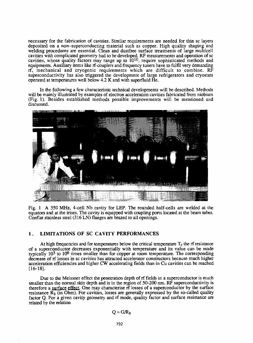
necessary for the fabrication of cavities. Similar requirements are needed for thin sc layers deposited on a non-superconducting material such as copper. High quality shaping and welding procedures are essential. Clean and dustfree surface treatments of large multicell cavities with complicated geometry had to be developed. RF measurements and operation of sc cavities, whose quality factors may range up to 10 1 0 , require sophisticated methods and equipments. Auxiliary items like rf-couplers and frequency tuners have to fulfil very demanding rf, mechanical and cryogenic requirements which are difficult to combine. RF superconductivity has also triggered the development of large refrigerators and cryostats operated at temperatures well below 4.2 K and with superfluid He.
In the following a few characteristic technical developments will be described. Methods will be mainly illustrated by examples of electron acceleration cavities fabricated from niobium (Fig. 1). Besides established methods possible improvements will be mentioned and discussed.
Fig. 1 A 350 MHz, 4-cell Nb cavity for LEP. The rounded half-cells are welded at the equators and at the irises. The cavity is equipped with coupling ports located at the beam tubes. Confiât stainless steel (316 LN) flanges are brazed to all openings.
1 . LIMITATIONS OF SC CAVITY PERFORMANCES
At high frequencies and for temperatures below the critical temperature T c the rf resistance of a superconductor decreases exponentially with temperature and its value can be made typically 10 5 to 10 6 times smaller than for copper at room temperature. The corresponding decrease of rf losses in sc cavities has attracted accelerator constructors because much higher acceleration efficiencies and higher CW accelerating fields than in Cu cavities can be reached [16-18].
Due to the Meissner effect the penetration depth of rf fields in a superconductor is much smaller than the normal skin depth and is in the region of 50-200 nm. RF superconductivity is therefore a surface effect. One may characterise rf losses of a superconductor by the surface resistance R§ (in Ohm). For cavities, losses are generally expressed by the so-called quality factor Q. For a given cavity geometry and rf mode, quality factor and surface resistance are related by the relation
Q = G/RS
792
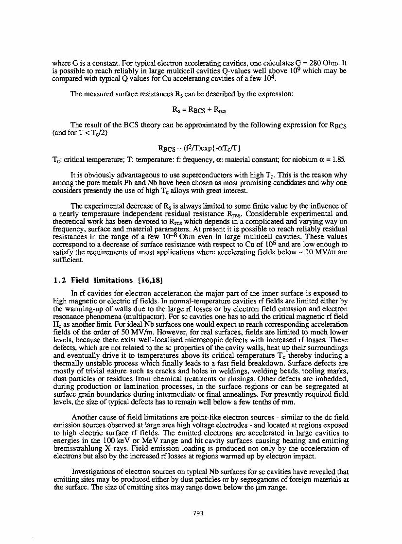
where G is a constant. For typical electron accelerating cavities, one calculates G = 280 Ohm. It is possible to reach reliably in large multicell cavities Q-values well above 109 which may be compared with typical Q values for Cu accelerating cavities of a few 104.
The measured surface resistances R s can be described by the expression:
Rs = RBCS + Rres
The result of the BCS theory can be approximated by the following expression for RBCS (andforT<Tc/2)
RBCS-^/TOexpf-aTc/T} T c: critical temperature; T: temperature: f: frequency, a: material constant; for niobium a = 1.85.
It is obviously advantageous to use superconductors with high T c . This is the reason why among the pure metals Pb and Nb have been chosen as most promising candidates and why one considers presently the use of high T c alloys with great interest.
The experimental decrease of R s is always limited to some finite value by the influence of a nearly temperature independent residual resistance R r e s . Considerable experimental and theoretical work has been devoted to Rres which depends in a complicated and varying way on frequency, surface and material parameters. At present it is possible to reach reliably residual resistances in the range of a few 10~8 Ohm even in large multicell cavities. These values correspond to a decrease of surface resistance with respect to Cu of 10 6 and are low enough to satisfy the requirements of most applications where accelerating fields below - 1 0 MV/m are sufficient
1.2 Field limitations [16,18] In rf cavities for electron acceleration the major part of the inner surface is exposed to
high magnetic or electric rf fields. In normal-temperature cavities rf fields are limited either by the warming-up of walls due to the large rf losses or by electron field emission and electron resonance phenomena (multipactor). For sc cavities one has to add the critical magnetic rf field He as another limit For ideal Nb surfaces one would expect to reach corresponding acceleration fields of the order of 50 MV/m. However, for real surfaces, fields are limited to much lower levels, because there exist well-localised microscopic defects with increased rf losses. These defects, which are not related to the sc properties of the cavity walls, heat up their surroundings and eventually drive it to temperatures above its critical temperature T c thereby inducing a thermally unstable process which finally leads to a fast field breakdown. Surface defects are mostly of trivial nature such as cracks and holes in weldings, welding beads, tooling marks, dust particles or residues from chemical treatments or rinsings. Other defects are imbedded, during production or lamination processes, in the surface regions or can be segregated at surface grain boundaries during intermediate or final annealings. For presendy required field levels, the size of typical defects has to remain well below a few tenths of mm.
Another cause of field limitations are point-like electron sources - similar to the dc field emission sources observed at large area high voltage electrodes - and located at regions exposed to high electric surface rf fields. The emitted electrons are accelerated in large cavities to energies in the 100 keV or MeV range and hit cavity surfaces causing heating and emitting bremsstrahlung X-rays. Field emission loading is produced not only by the acceleration of electrons but also by the increased rf losses at regions warmed up by electron impact.
Investigations of electron sources on typical Nb surfaces for sc cavities have revealed that emitting sites may be produced either by dust particles or by segregations of foreign materials at the surface. The size of emitting sites may range down below the Jim range.
793
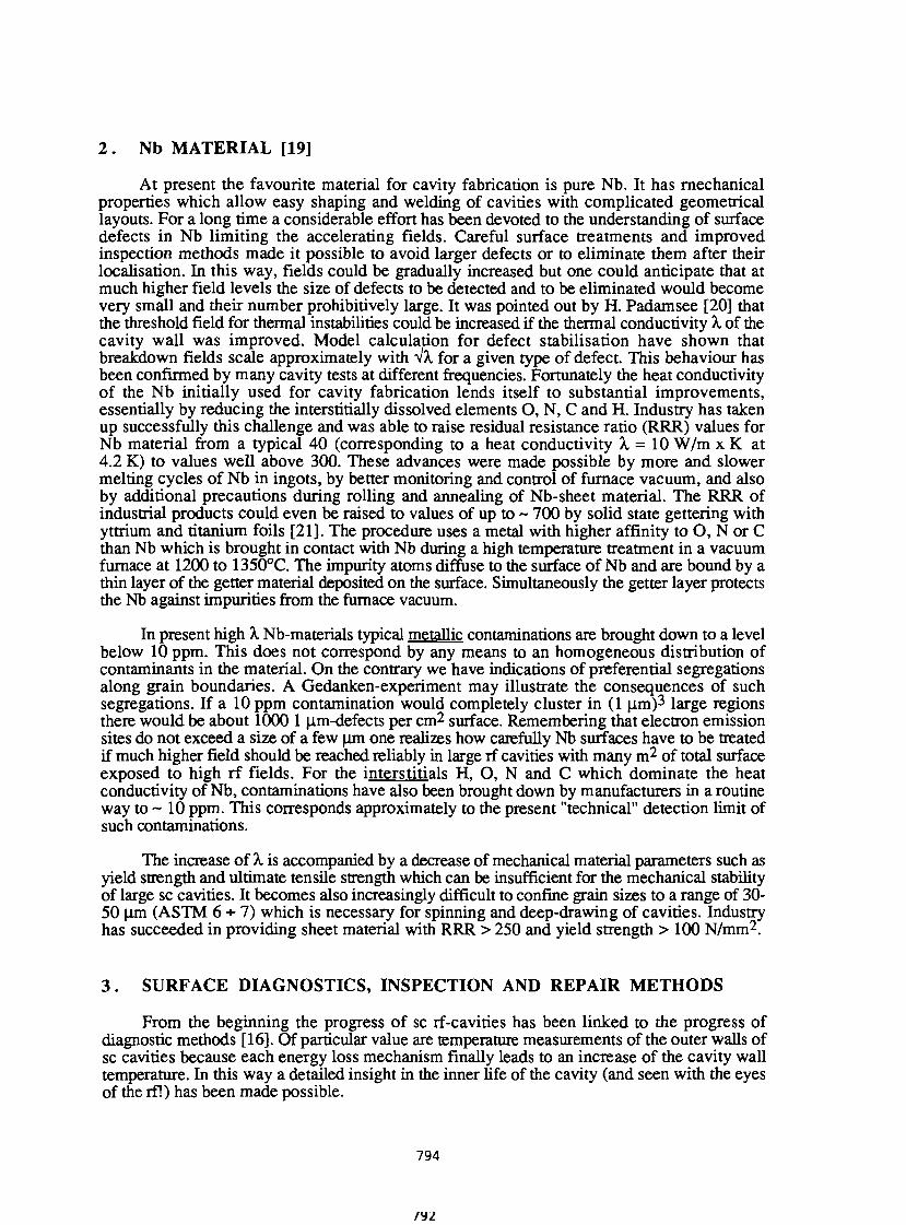
2 . Nb MATERIAL [19]
At present the favourite material for cavity fabrication is pure Nb. It has mechanical properties which allow easy shaping and welding of cavities with complicated geometrical layouts. For a long time a considerable effort has been devoted to the understanding of surface defects in Nb limiting the accelerating fields. Careful surface treatments and improved inspection methods made it possible to avoid larger defects or to eliminate them after their localisation. In this way, fields could be gradually increased but one could anticipate that at much higher field levels the size of defects to be detected and to be eliminated would become very small and their number prohibitively large. It was pointed out by H. Padamsee [20] that the threshold field for thermal instabilities could be increased if the thermal conductivity X of the cavity wall was improved. Model calculation for defect stabilisation have shown that breakdown fields scale approximately with VA. for a given type of defect. This behaviour has been confirmed by many cavity tests at different frequencies. Fortunately the heat conductivity of the Nb initially used for cavity fabrication lends itself to substantial improvements, essentially by reducing the interstitially dissolved elements O, N, C and H. Industry has taken up successfully this challenge and was able to raise residual resistance ratio (RRR) values for Nb material from a typical 40 (corresponding to a heat conductivity X = 10 W/m x K at 4.2 K) to values well above 300. These advances were made possible by more and slower melting cycles of Nb in ingots, by better monitoring and control of furnace vacuum, and also by additional precautions during rolling and annealing of Nb-sheet material. The RRR of industrial products could even be raised to values of up to ~ 700 by solid state gettering with yttrium and titanium foils [21]. The procedure uses a metal with higher affinity to O, Nor C than Nb which is brought in contact with Nb during a high temperature treatment in a vacuum furnace at 1200 to 1350°C. The impurity atoms diffuse to the surface of Nb and are bound by a thin layer of the getter material deposited on the surface. Simultaneously the getter layer protects the Nb against impurities from the furnace vacuum.
In present high X Nb-materials typical metallic contaminations are brought down to a level below 10 ppm. This does not correspond by any means to an homogeneous distribution of contaminants in the material. On the contrary we have indications of preferential segregations along grain boundaries. A Gedanken-experiment may illustrate the consequences of such segregations. If a 10 ppm contamination would completely cluster in (1 | im) 3 large regions there would be about 1000 1 |im-defects per cm 2 surface. Remembering that electron emission sites do not exceed a size of a few |im one realizes how carefully Nb surfaces have to be treated if much higher field should be reached reliably in large rf cavities with many m 2 of total surface exposed to high rf fields. For the interstitials H, O, N and C which dominate the heat conductivity of Nb, contaminations have also been brought down by manufacturers in a routine way to ~ 10 ppm. This corresponds approximately to the present "technical" detection limit of such contaminations.
The increase of X is accompanied by a decrease of mechanical material parameters such as yield strength and ultimate tensile strength which can be insufficient for the mechanical stability of large sc cavities. It becomes also increasingly difficult to confine grain sizes to a range of 30-50 M-m (ASTM 6^-7) which is necessary for spinning and deep-drawing of cavities. Industry has succeeded in providing sheet material with RRR > 250 and yield strength > 100 N/mm2.
3 . SURFACE DIAGNOSTICS, INSPECTION AND REPAIR METHODS
From the beginning the progress of sc rf-cavities has been linked to the progress of diagnostic methods [16]. Of particular value are temperature measurements of the outer walls of sc cavities because each energy loss mechanism finally leads to an increase of the cavity wall temperature. In this way a detailed insight in the inner fife of the cavity (and seen with the eyes of the rf!) has been made possible.
794
792
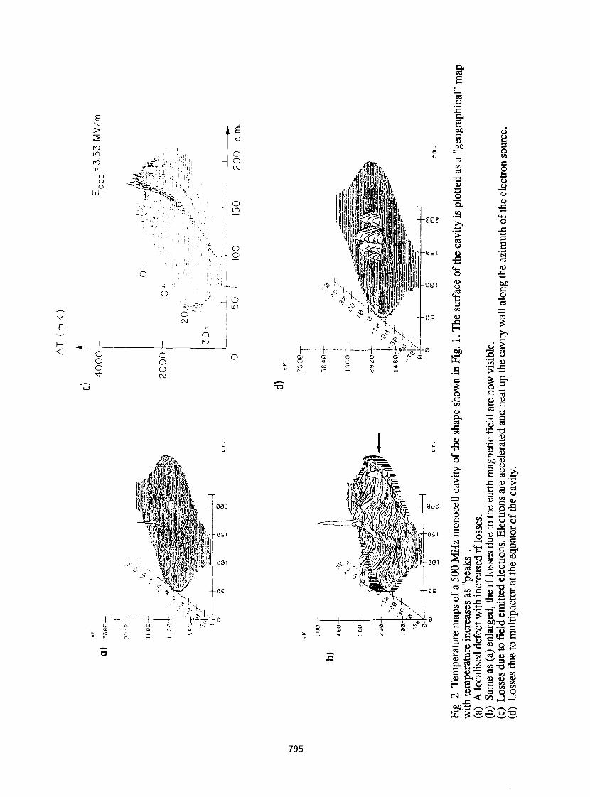
e es
£ >
ro ro ro
o o Ld
O o o <3"
E o
O O c\J
O m
O O
o
d "" " CM
! m
O ro 1
O o o CM
O
iilp i, MM
1, - - 0 S
si u U w 3.3
W M 22 <u u o g „ «
795
Temperature mapping [16] with sliding sensor (temperature dependent resistor) systems located at the outer cavity walls and immersed in a bath of subcooled helium have made it possible to detect, visualize and measure quantitatively the various loss mechanisms (Fig. 2). Its role in the understanding of these losses, their nature and distributions, of defect classification and of electron emission has been invaluable. It can be foreseen that refined temperature mapping layouts will continue to play a decisive role for a further increase of cavity fields and quality factors. On a more practical side temperature mapping has been used to localise surface defects, an essential requirement for eliminating them afterwards by mechanical or chemical treatments.
During the last years efforts have been directed towards a better insulation of the temperatue sensing elements against the surrounding LHe bath. In this way a higher temperature sensitivity (AT < 0.1 mK) and work in superfluid He was made possible. Systems using smaller sensors and faster read-out have also been developed [22,23].
Already at an early stage attempts were made to combine T-mapping with X-ray mapping for the study of field emission. Small solid state X-ray detectors operating at LHe temperatures have been used.
However, one should keep in mind that temperature mapping needs very complex and sophisticated equipments and that it can only be applied to cavities operating in a liquid helium-bath. In addition some cavity shapes (especially the ones needed for heavy-ion acceleration) do not lend themselves easily to temperature mapping. Therefore inspection methods which can be applied to wall materials and cavities at room temperature (and before the first cold measurements) are highly desirable, especially for large scale applications.
At present direct visual inspection of Nb sheet material, of cavity half-cells and of complete cavities after welding is almost exclusively the method used. Present equipments using the naked eye or a telescope (Fig. 3) allow one to detect surface and welding defects down to about 50 |im diameter. This is sufficient to reach in a reliable way accelerating fields of the order of 10 MV/m in high-A. Nb material. Systems allowing an inspection of cavities with a "microscope" located near the inner cavity surface, preferably with stereoscopic view and with adequate illumination could increase the detection limits considerably. Optical equipment with CCD devices would offer the flexibility and compactness necessary for this task especially in smaller cavities. Modern image processing such as fast Fourier transforms and the use of TV-screens for display and storage would be highly desirable. Any mechanical contact with inspection devices and the inner surfaces of a cavity has to be carefully avoided, therefore the inspection system should include computerized support.
A non-destructive inspection method for sheet material used for fabrication of cavities is at hand with the Scanning Laser Acoustic Microscope (SLAM) [24], an acoustic microscope with ultrasonic visualisation and a scanning laser beam as a point ultrasonic wave detector. Prototypes have already been developed and tested on flat Nb-sheets. It is hoped that a spatial resolution of 25-50 ^m can be realized. Scanning speeds allowing inspection of ~ 1 m 2 within 5 min. have already been attained. Defects can be detected at the surface and in the bulk. The method can also be used to characterize general material properties like RRR, grain size or nonuniform recrystallisation. More experience has still to be gained for detecting small isolated defects rapidly and safely.
It is tempting to combine inspection devices for complete cavities of the kind described above with repair devices. Repairs of localised defects have been made by mechanical methods such as grinding and milling, and by local chemical treatments such as chemical polishing or electropolishing [25]. Reliable repairs become extremely difficult in long multicell cavities and are nearly impossible to do in high frequency cavities where iris openings are small. Laser devices [26] may provide a more elegant solution for evaporating or "spreading" out localised defects. It is known that short, high power pulses can produce a plasma of the surface which can be heated up and cooled down so fast that oxidation of Nb under air (or under a protective
796
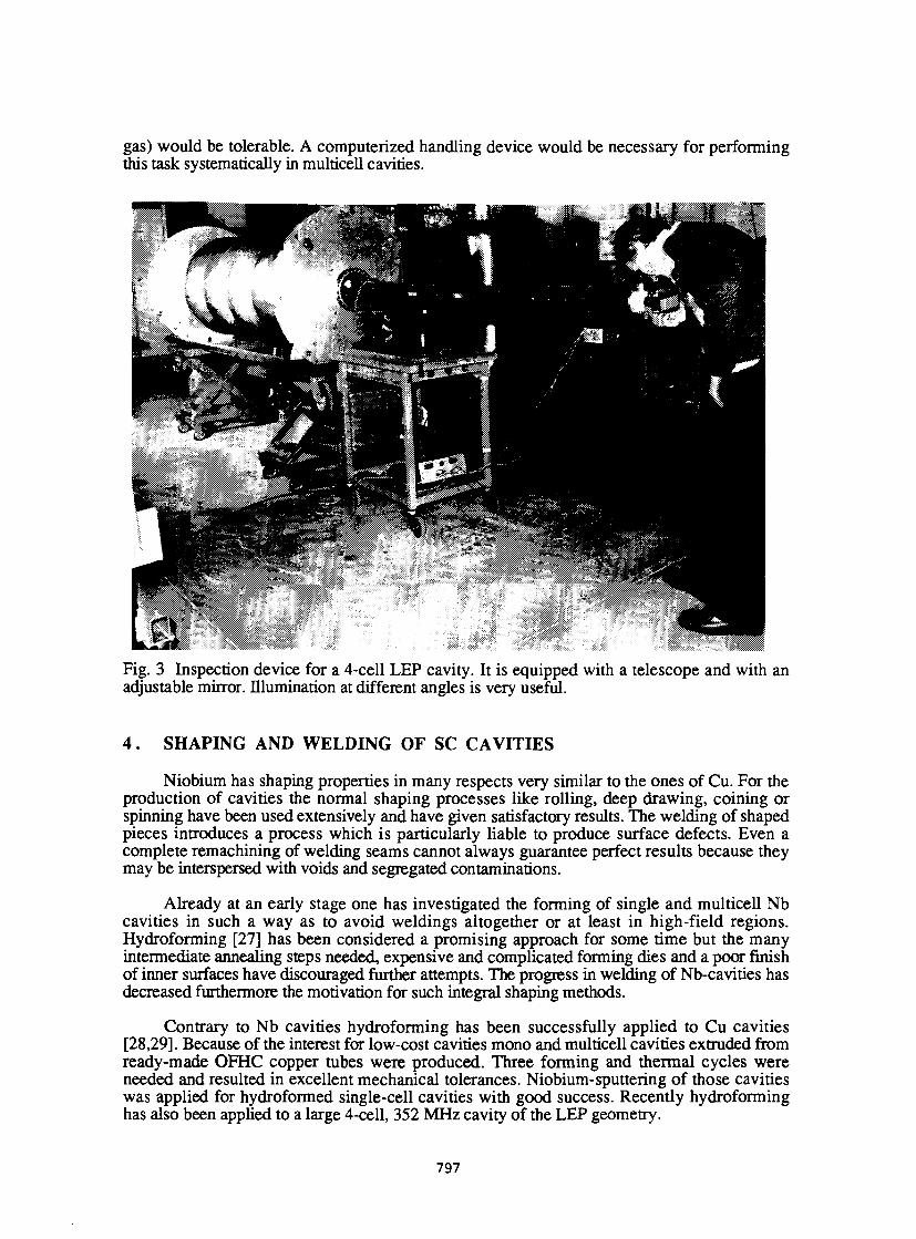
gas) would be tolerable. A computerized handling device would be necessary for performing this task systematically in multicell cavities.
Fig. 3 Inspection device for a 4-cell LEP cavity. It is equipped with a telescope and with an adjustable mirror. Illumination at different angles is very useful.
4 . SHAPING AND WELDING OF SC CAVITIES
Niobium has shaping properties in many respects very similar to the ones of Cu. For the production of cavities the normal shaping processes like rolling, deep drawing, coining or spinning have been used extensively and have given satisfactory results. The welding of shaped pieces introduces a process which is particularly liable to produce surface defects. Even a complete remachining of welding seams cannot always guarantee perfect results because they may be interspersed with voids and segregated contaminations.
Already at an early stage one has investigated the forming of single and multicell Nb cavities in such a way as to avoid weldings altogether or at least in high-field regions. Hydroforming [27] has been considered a promising approach for some time but the many intermediate annealing steps needed, expensive and complicated forming dies and a poor finish of inner surfaces have discouraged further attempts. The progress in welding of Nb-cavities has decreased furthermore the motivation for such integral shaping methods.
Contrary to Nb cavities hydroforming has been successfully applied to Cu cavities [28,29]. Because of the interest for low-cost cavities mono and multicell cavities extruded from ready-made OFHC copper tubes were produced. Three forming and thermal cycles were needed and resulted in excellent mechanical tolerances. Niobium-sputtering of those cavities was applied for hydroformed single-cell cavities with good success. Recently hydroforming has also been applied to a large 4-cell, 352 MHz cavity of the LEP geometry.
797
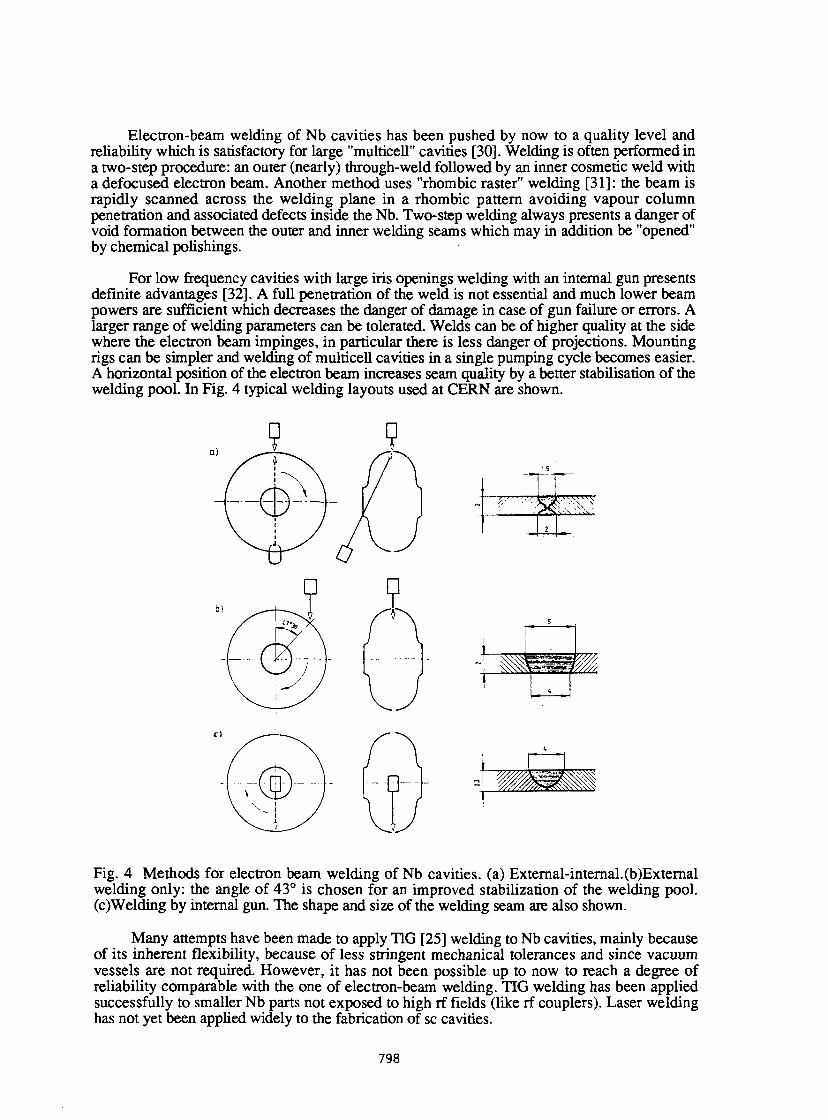
Electron-beam welding of Nb cavities has been pushed by now to a quality level and reliability which is satisfactory for large "multicell" cavities [30]. Welding is often performed in a two-step procedure: an outer (nearly) through-weld followed by an inner cosmetic weld with a defocused electron beam. Another method uses "rhombic raster" welding [31]: the beam is rapidly scanned across the welding plane in a rhombic pattern avoiding vapour column penetration and associated defects inside the Nb. Two-step welding always presents a danger of void formation between the outer and inner welding seams which may in addition be "opened" by chemical polishings.
For low frequency cavities with large iris openings welding with an internal gun presents definite advantages [32]. A full penetration of the weld is not essential and much lower beam powers are sufficient which decreases the danger of damage in case of gun failure or errors. A larger range of welding parameters can be tolerated. Welds can be of higher quality at the side where the electron beam impinges, in particular there is less danger of projections. Mounting rigs can be simpler and welding of multicell cavities in a single pumping cycle becomes easier. A horizontal position of the electron beam increases seam quality by a better stabilisation of the welding pool. In Fig. 4 typical welding layouts used at CERN are shown.
Fig. 4 Methods for electron beam welding of Nb cavities, (a) External-internal.(b)External welding only: the angle of 43° is chosen for an improved stabilization of the welding pool. (c)Welding by internal gun. The shape and size of the welding seam are also shown.
Many attempts have been made to apply TIG [25] welding to Nb cavities, mainly because of its inherent flexibility, because of less stringent mechanical tolerances and since vacuum vessels are not required. However, it has not been possible up to now to reach a degree of reliability comparable with the one of electron-beam welding. TIG welding has been applied successfully to smaller Nb parts not exposed to high rf fields (like rf couplers). Laser welding has not yet been applied widely to the fabrication of sc cavities.
798

Joining of Nb parts with other materials like stainless steel and Cu is extensively used and can considerably facilitate construction problems. Typical examples are vacuum flanges and waveguide flanges for main and higher-order mode couplers. Besides the normal UHV properties, flanges have to withstand low-temperature operation, repeated thermal cyclings from hundreds of °C to a few K and they must not develop magnetic fields above a few mG which may influence the rf losses of adjacent Nb surfaces. Joining of Nb with stainless steel flanges has been achieved by brazing in vacuum furnaces with Cu-Au and Cu alloys [32]. With adequate preparation and a furnace vacuum better than 10"4 mbar at 960°C very reliable joints have been produced. Explosive bonding of Nb to stainless steel is another method which has been used e.g. for the fabrication of waveguide flanges [25]. For the joining of Nb to Cu, electron beam welding has been successfully applied [32].
We also mention the joining of Nb, stainless steel or Cu parts to (ceramic) windows for coaxial and waveguide couplers and feedthroughs. Such elements are omnipresent in all warm and cold tests of sc cavities and in the past their reliability has often been insufficient. The development of economic, reliable rf windows and feedthroughs using AI2O3 and withstanding temperature shocks, operation at LHe temperatures and fulfilling the requirements of UHV, is now well mastered.
5 . SURFACE TREATMENTS [33,31]
In addition to the cavity material and welds, treatments of all inner surfaces exposed to high rf fields are of prime importance for obtaining good cavity performances. Requirements for high fields and low rf losses require different surface characteristics: fields are mostly limited by well-localised defects or electron emitters whereas rf losses are more influenced by the overall nature of surface and/or by many small defects.
Surface treatments of cavities start generally by die removal of damage layers (50-100 jxm) due to shaping, machining and welding. For the following surface treatments there exists today general agreement but procedures may vary from one laboratory to die odier and from one cavity size and geometry to the odier. Furthermore, technical feasibility questions of reliability, security and economics have to be taken into account, particularly for large scale applications.
For Nb cavities a chemical polishing in a bath of concentrated HF, HNO3 and H3PO4 followed by a thorough rinsing with demineralised water, alcohol etc. and by a drying under dust-free conditions is considered necessary. Dedicated installations are essential and the trend goes to automatic installations where large numbers of cavities can be prepared and treated in a way largely independent of human interventions and under reasonably clean conditions (Fig. 5). The number of parameters governing such treatments is considerable and requires a very careful planning and testing of large installations. We mention the purity of bath constituents (very often p.a. quality is recommended), bath composition, bath temperature and saturation, flow rates and agitation (influencing the formation of viscous layers at the surfaces), removal of gases produced during treatments and avoidance of gas pockets, filling and emptying times, fast neutralisation of acids at inner surfaces, final pH of rinsing waters, etc. Security aspects like overflow facilities and emergency drains have to be integrated in die system. Non-Nb parts have to be protected carefully from the very agressive acids used. In general these operations are not attempted under dust-free conditions.A major concern is a rapid emptying and neutralisation of acids at the cavity walls. Already contact widi air for a few seconds can lead to the formation of non-soluble Nb salts which are hard to remove by subsequent rinsings.
The importance of adequate rinsing and drying cannot be overstated. Dust-free conditions (class 100) are of utmost importance. Great care has also to be taken for the rinsing liquid quality and cleanliness. At present dust-free ultrapure water (p = 18 MOhm x cm, standard
799
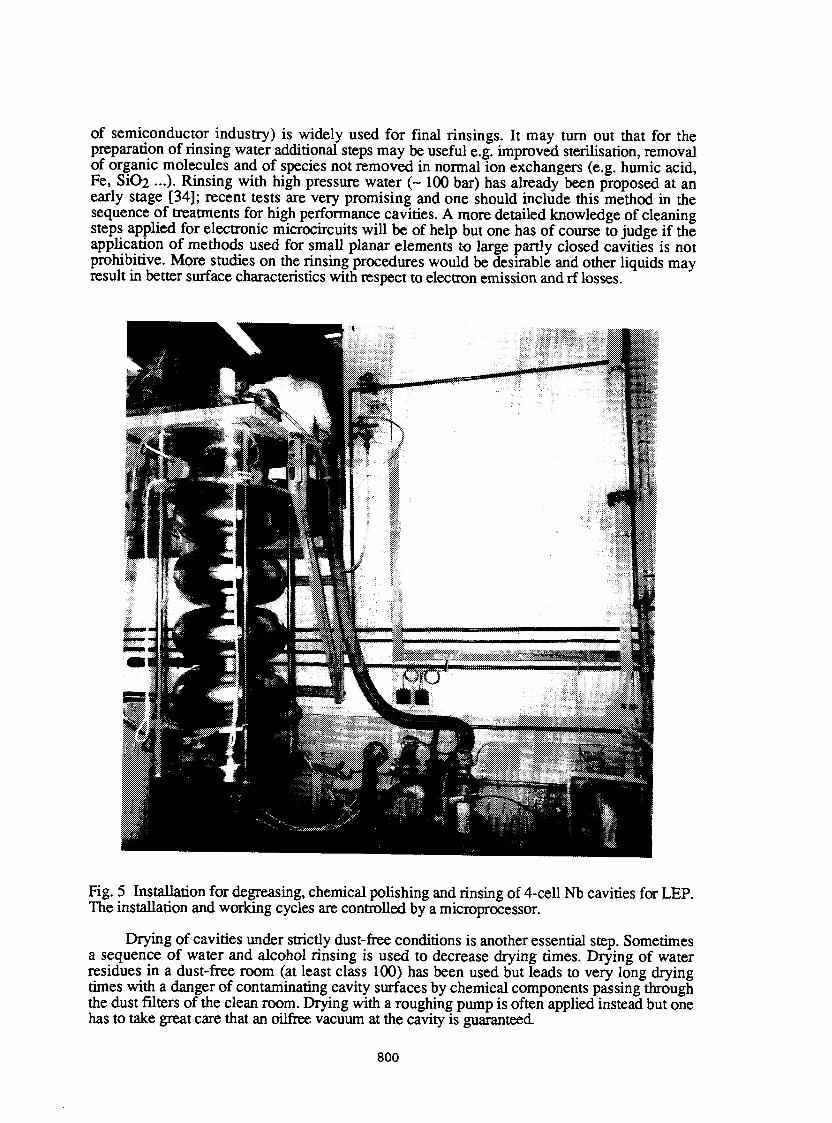
of semiconductor industry) is widely used for final rinsings. It may turn out that for the preparation of rinsing water additional steps may be useful e.g. improved sterilisation, removal of organic molecules and of species not removed in normal ion exchangers (e.g. humic acid, Fe, SiÛ2 ...). Rinsing with high pressure water (~ 100 bar) has already been proposed at an early stage [34]; recent tests are very promising and one should include this method in the sequence of treatments for high performance cavities. A more detailed knowledge of cleaning steps applied for electronic microcircuits will be of help but one has of course to judge if the application of methods used for small planar elements to large partly closed cavities is not prohibitive. More studies on the rinsing procedures would be desirable and other liquids may result in better surface characteristics with respect to electron emission and rf losses.
Fig. 5 Installation for degreasing, chemical polishing and rinsing of 4-cell Nb cavities for LEP. The installation and working cycles are controlled by a microprocessor.
Drying of cavities under strictly dust-free conditions is another essential step. Sometimes a sequence of water and alcohol rinsing is used to decrease drying times. Drying of water residues in a dust-free room (at least class 100) has been used but leads to very long drying times with a danger of contaminating cavity surfaces by chemical components passing through the dust filters of the clean room. Drying with a roughing pump is often applied instead but one has to take great care that an oilfree vacuum at the cavity is guaranteed.
800
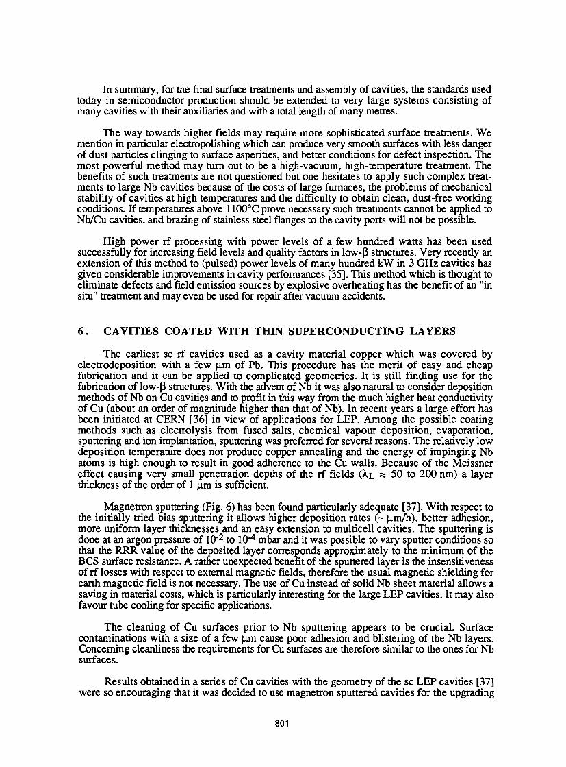
In summary, for the final surface treatments and assembly of cavities, the standards used today in semiconductor production should be extended to very large systems consisting of many cavities with their auxiliaries and with a total length of many metres.
The way towards higher fields may require more sophisticated surface treatments. We mention in particular electropolishing which can produce very smooth surfaces with less danger of dust particles clinging to surface asperities, and better conditions for defect inspection. The most powerful method may turn out to be a high-vacuum, high-temperature treatment. The benefits of such treatments are not questioned but one hesitates to apply such complex treatments to large Nb cavities because of the costs of large furnaces, the problems of mechanical stability of cavities at high temperatures and the difficulty to obtain clean, dust-free working conditions. If temperatures above 1100°C prove necessary such treatments cannot be applied to Nb/Cu cavities, and brazing of stainless steel flanges to the cavity ports will not be possible.
High power rf processing with power levels of a few hundred watts has been used successfully for increasing field levels and quality factors in low-(3 structures. Very recently an extension of this method to (pulsed) power levels of many hundred kW in 3 GHz cavities has given considerable improvements in cavity performances [35]. This method which is thought to eliminate defects and field emission sources by explosive overheating has the benefit of an "in situ" treatment and may even be used for repair after vacuum accidents.
6. CAVITIES COATED WITH THIN SUPERCONDUCTING LAYERS
The earliest sc rf cavities used as a cavity material copper which was covered by electrodeposition with a few u.m of Pb. This procedure has the merit of easy and cheap fabrication and it can be applied to complicated geometries. It is still finding use for the fabrication of low-|3 structures. With the advent of Nb it was also natural to consider deposition mediods of Nb on Cu cavities and to profit in this way from the much higher heat conductivity of Cu (about an order of magnitude higher than that of Nb). In recent years a large effort has been initiated at CERN [36] in view of applications for LEP. Among the possible coating methods such as electrolysis from fused salts, chemical vapour deposition, evaporation, sputtering and ion implantation, sputtering was preferred for several reasons. The relatively low deposition temperature does not produce copper annealing and the energy of impinging Nb atoms is high enough to result in good adherence to the Cu walls. Because of the Meissner effect causing very small penetration depths of the rf fields (X,L »J 50 to 200 nm) a layer thickness of the order of 1 |im is sufficient.
Magnetron sputtering (Fig. 6) has been found particularly adequate [37]. With respect to the initially tried bias sputtering it allows higher deposition rates (~ |j.m/h), better adhesion, more uniform layer thicknesses and an easy extension to multicell cavities. The sputtering is done at an argon pressure of 10~2 to 10"4 mbar and it was possible to vary sputter conditions so that the RRR value of the deposited layer corresponds approximately to the minimum of the BCS surface resistance. A rather unexpected benefit of the sputtered layer is the insensitiveness of rf losses with respect to external magnetic fields, therefore the usual magnetic shielding for earth magnetic field is not necessary. The use of Cu instead of solid Nb sheet material allows a saving in material costs, which is particularly interesting for the large LEP cavities. It may also favour tube cooling for specific applications.
The cleaning of Cu surfaces prior to Nb sputtering appears to be crucial. Surface contaminations with a size of a few \xm cause poor adhesion and blistering of the Nb layers. Concerning cleanliness the requirements for Cu surfaces are therefore similar to the ones for Nb surfaces.
Results obtained in a series of Cu cavities with the geometry of the sc LEP cavities [37] were so encouraging that it was decided to use magnetron sputtered cavities for the upgrading
801
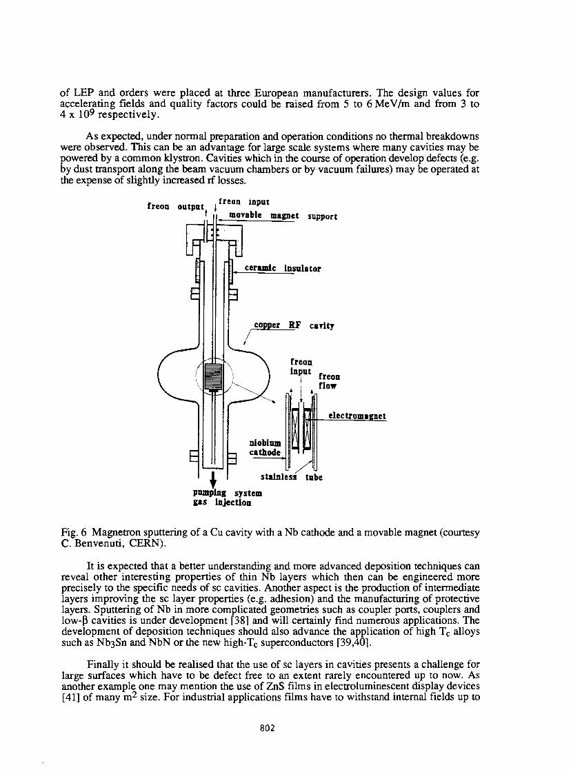
of LEP and orders were placed at three European manufacturers. The design values for accelerating fields and quality factors could be raised from 5 to 6 MeV/m and from 3 to 4 x 10 9 respectively.
As expected, under normal preparation and operation conditions no thermal breakdowns were observed. This can be an advantage for large scale systems where many cavities may be powered by a common klystron. Cavities which in the course of operation develop defects (e.g. by dust transport along the beam vacuum chambers or by vacuum failures) may be operated at the expense of slightly increased rf losses.
freon output freon input movable magnet support
ceramic insulator
copper RF cavity
freon i n i m t freon
flow
electromagnet
stainless tnbe pumping system gas injection
Fig. 6 Magnetron sputtering of a Cu cavity with a Nb cathode and a movable magnet (courtesy C. Benvenuti, CERN).
It is expected that a better understanding and more advanced deposition techniques can reveal other interesting properties of thin Nb layers which then can be engineered more precisely to the specific needs of sc cavities. Another aspect is the production of intermediate layers improving the sc layer properties (e.g. adhesion) and the manufacturing of protective layers. Sputtering of Nb in more complicated geometries such as coupler ports, couplers and low-P cavities is under development [38] and will certainly find numerous applications. The development of deposition techniques should also advance the application of high T c alloys such as Nb3Sn and NbN or the new high-Tc superconductors [39,40].
Finally it should be realised that the use of sc layers in cavities presents a challenge for large surfaces which have to be defect free to an extent rarely encountered up to now. As another example one may mention the use of ZnS films in electroluminescent display devices [41] of many m 2 size. For industrial applications films have to withstand internal fields up to
802
150 MV/m. The number of defects (pin holes) with a diameter exceeding 30 |im can be kept below one defect per m 2 . These defect numbers are comparable to the ones we would like to achieve in large, high performance cavities.
ACKNOWLEDGEMENTS
I would like to thank my colleagues from CERN for many fruitful discussions and for information, in particular, D. Bloess on inspection methods and surface treatments and E. Chiaveri on fabrication methods.
* * * * * *
REFERENCES
[I] M. Kuntze, éd., Proceedings of the First Workshop on RF Superconductivity, Karlsruhe (1980), KfK Report 3019.
[2] H. Lengeler, éd., Proceedings of the Second Workshop on RF Superconductivity, CERN, Geneva, (1984).
[3] K. Shepard, éd., Proceedings of the Third Workshop on RF Superconductivity, Argonne (1987), ANL-PHY 88-1.
[4] Y. Kojima, éd., Proceedings of the Fourth Workshop on RF Superconductivity, KEK, Japan (1989), KEK Report 89-21.
[5] D. Proch, éd., Proceedings of the Fifth Workshop on RF Superconductivity, DESY, Hamburg (1991).
[6] M.S. McAshan, K. Mittag, H.A. Schwettman, L.R. Suelze and J.-P. Turneaure, Appl. Phys. Lett. 22 (1973) 605.
[7] A. Citron et al., Nucl. Instr. & Meth. 164 (1979) 31.
[8] J. Aron et al., Proceedings of the 1984 Linear Ace. Conf. Seeheim, FRG (1984), report GSI-84-11 (1984) 132.
[9] J.R. Delayen in Ref. [4], 249.
[10] Y. Kojima et al., Proceedings of the 1989 IEEE Part. Ace. Conf., Chicago (1989) 1789.
[II] C. Arnaud et al.in EPAC 90, Nice (1990). eds P. Marin and P. Mandrillon, 152.
[12] B. Dwersteg et al. in Proceedings of the 1991 IEEE Particle Ace. Conf. San Francisco (1991) 2429.
[13] P. Kneisel et al. in Ref. [11] (1990) 2384.
[14] K. Jordan et a l , ibidem, 2381.
[15] See Ref. [5], 75-104.
[16] H. Piel, CAS proceedings of the School on Superconductivity in Particle Accelerators, Hamburg, FRG, CERN 89-04 (1989) 149.
[17] H. Lengeler, ibidem 197.
803
[18] W. Weingarten, CAS proceedings of the School on RF Engineering for Particle Accelerators, Oxford, UK, CERN 92-03 (1992) 318.
[19] H. Padamsee, Proc. Conf. Electron Beam Melting and Refining, Reno (1987) 241.
[20] H. Padamsee, IEEE Trans. MAG-19 (1983) 1322.
[21] H. Padamsee, IEEE Trans. MAG-21 (1985) 1007.
[22] M. Fouaidy, T. Junquera and A. Carutte in Ref. [5], 547.
[23] R.W. Rôth et al. in Ref. [5], 599.
[24] N.C. Oravecz, I.W. Kessler and H. Padamsee, Ultrasonic Symposium, IEEE (1985) 547.
[25] J. Susta in Ref. [4], 597.
[26] See e.g. J. Longellow, Lasers in Industry, ed. S.S. Charschan, Van Nostrand Comp, New York (1972).
D. Bloess, CERN, private communication.
[27] J. Kirchgessner et al., IEEE NS-30 (1983) 3351.
[28] C. Hauviller, Proceedings of the 1989 IEEE Particle Ace. Conf, Chicago (1989) 1485.
[29] S. Dujardin et al., in Ref. [11], 1100.
[30] E. Chiaveri et H. Lengeler in Ref. [2], 611.
[31] P. Kneisel in Ref. [5], 163.
[32] E. Chiaveri, CERN, private communication.
[33] D. Bloess in Ref. [2], 409.
[34] D. Bloess in ref. 3, 359 and private communication.
[35] J. Graber et al. in Ref. [5], 758.
[36] C. Benvenuti et al., Ref. [2], 627.
[37] C. Benvenuti in Ref. [5], 758.
[38] V. Palmieri in Ref. [5], 473.
[39] P. Bosland et al. in Ref. [5], 497.
[40] C. Benvenuti et al. in Ref. [5], 518.
[41] T. Sutela, Displays, April 1984, 73.
804
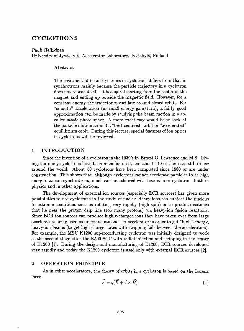
CYCLOTRONS Pauli Heikkinen University of Jyvàskylâ, Accelerator Laboratory, Jyvàskylâ, Finland
Abstract
The treatment of beam dynamics in cyclotrons differs from that in synchrotrons mainly because the particle trajectory in a cyclotron does not repeat itself - it is a spiral starting from the center of the magnet and ending up outside the magnetic field. However, for a constant energy the trajectories oscillate around closed orbits. For "smooth" acceleration (or small energy gain/turn), a fairly good approximation can be made by studying the beam motion in a so-called static phase space. A more exact way would be to look at the particle motion around a "best-centered" orbit or "accelerated" equilibrium orbit. During this lecture, special features of ion optics in cyclotrons will be reviewed.
1 I N T R O D U C T I O N
Since the invention of a cyclotron in the 1930's by Ernest 0 . Lawrence and M.S. Livingston many cyclotrons have been manufactured, and about 140 of them are still in use around the world. About 50 cyclotrons have been completed since 1980 or are under construction. This shows that , although cyclotrons cannot accelerate particles to as high energies as can synchrotrons, much can be achieved with beams from cyclotrons both in physics and in other applications.
The development of external ion sources (especially ECR sources) has given more possibilities to use cyclotrons in the study of nuclei: Heavy ions can subject the nucleus to extreme conditions such as rotating very rapidly (high spin) or to produce isotopes that lie near the proton drip line (too many protons) via heavy-ion fusion reactions. Since ECR ion sources can produce highly-charged ions they have taken over from large accelerators being used as injectors into another accelerator in order to get "high"-energy, heavy-ion beams (to get high charge states with stripping foils between the accelerators). For example, the MSU K1200 superconducting cyclotron was initially designed to work as the second stage after the K500 SCC with radial injection and stripping in the center of K1200 [1]. During the design and manufacturing of K1200, ECR sources developed very rapidly and today the K1200 cyclotron is used only with external ECR sources [2].
2 O P E R A T I O N P R I N C I P L E
As in other accelerators, the theory of orbits in a cyclotron is based on the Lorenz force
F = q(E + vxB). (1)
805
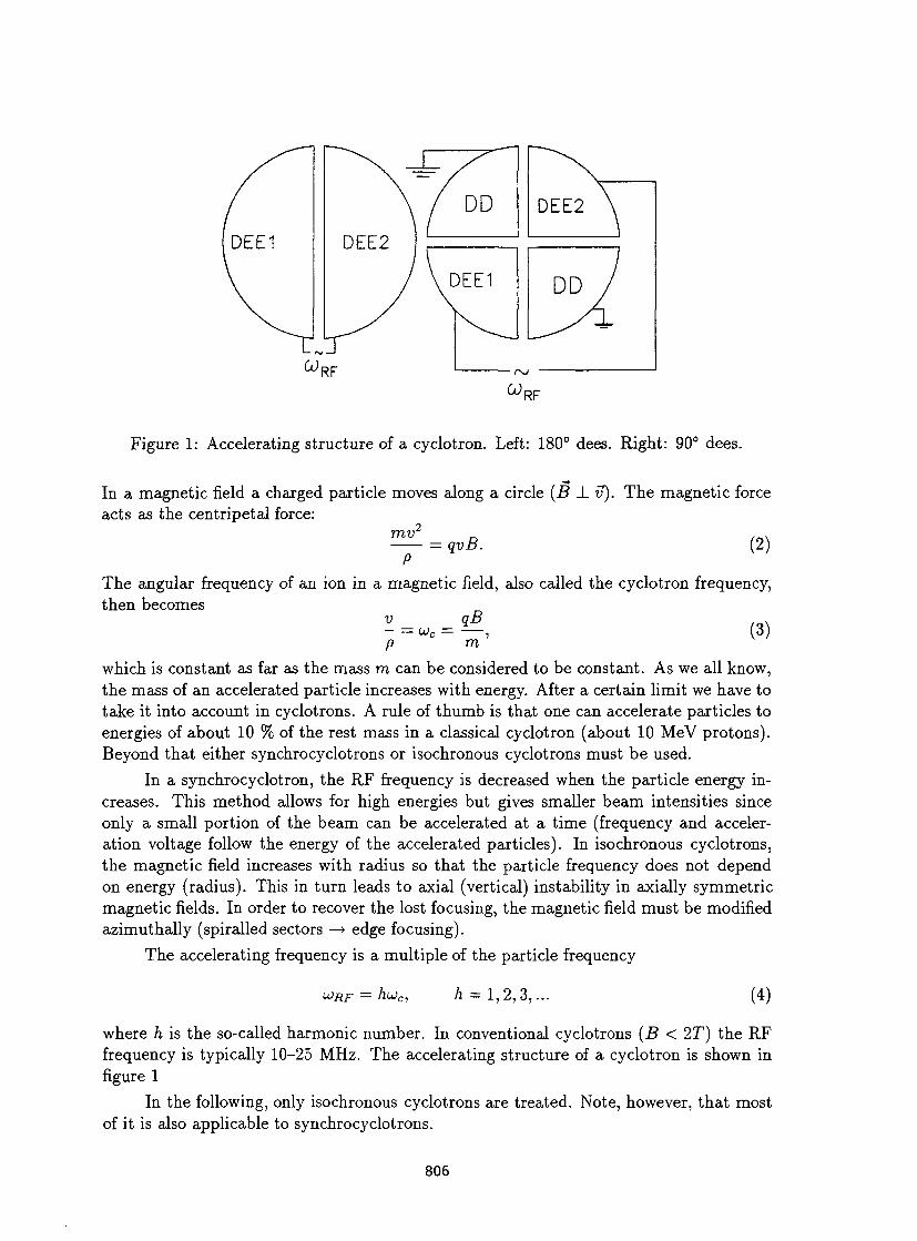
Figure 1: Accelerating structure of a cyclotron. Left: 180° dees. Right: 90° dees.
In a magnetic field a charged particle moves along a circle (B JL v). The magnetic force acts as the centripetal force:
mv qvB. (2)
(3)
The angular frequency of an ion in a magnetic field, also called the cyclotron frequency, then becomes
v qB p c m '
which is constant as far as the mass m can be considered to be constant. As we all know, the mass of an accelerated particle increases with energy. After a certain limit we have to take it into account in cyclotrons. A rule of thumb is that one can accelerate particles to energies of about 10 % of the rest mass in a classical cyclotron (about 10 MeV protons). Beyond that either synchrocyclotrons or isochronous cyclotrons must be used.
In a synchrocyclotron, the RF frequency is decreased when the particle energy increases. This method allows for high energies but gives smaller beam intensities since only a small portion of the beam can be accelerated at a time (frequency and acceleration voltage follow the energy of the accelerated particles). In isochronous cyclotrons, the magnetic field increases with radius so that the particle frequency does not depend on energy (radius). This in turn leads to axial (vertical) instability in axially symmetric magnetic fields. In order to recover the lost focusing, the magnetic field must be modified azimuthally (spiralled sectors —• edge focusing).
The accelerating frequency is a multiple of the particle frequency
u)RF = hu>c, h = 1,2,3,... (4)
where h is the so-called harmonic number. In conventional cyclotrons (B < IT) the RF frequency is typically 10-25 MHz. The accelerating structure of a cyclotron is shown in figure 1
In the following, only isochronous cyclotrons are treated. Note, however, that most of it is also applicable to synchrocyclotrons.
806
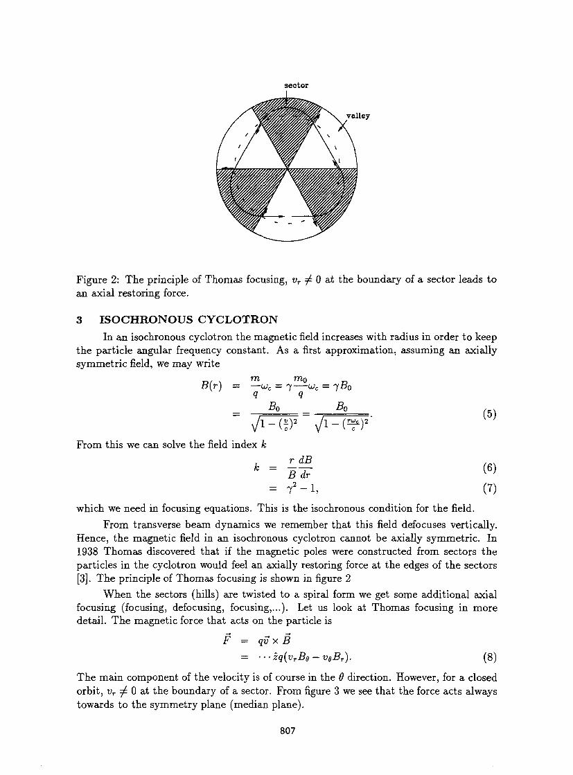
sector
valley
Figure 2: The principle of Thomas focusing, vr ^ 0 at the boundary of a sector leads to an axial restoring force.
3 ISOCHRONOUS CYCLOTRON In an isochronous cyclotron the magnetic field increases with radius in order to keep
the particle angular frequency constant. As a first approximation, assuming an axially symmetric field, we may write
(5)
(6)
(7) which we need in focusing equations. This is the isochronous condition for the field.
From transverse beam dynamics we remember that this field defocuses vertically. Hence, the magnetic field in an isochronous cyclotron cannot be axially symmetric. In 1938 Thomas discovered that if the magnetic poles were constructed from sectors the particles in the cyclotron would feel an axially restoring force at the edges of the sectors [3]. The principle of Thomas focusing is shown in figure 2
When the sectors (hills) are twisted to a spiral form we get some additional axial focusing (focusing, defocusing, focusing,...). Let us look at Thomas focusing in more detail. The magnetic force that acts on the particle is
F = qv x B = •••zq(vrBe-veBT). (8)
The main component of the velocity is of course in the 6 direction. However, for a closed orbit, vT ^ 0 at the boundary of a sector. From figure 3 we see that the force acts always towards to the symmetry plane (median plane).
B(r) m q
m 0
= 7 — ^ c = 7#o
B 0 Bo
fi- (;)2 A - i T J f ) 2
From this we can solve the field index k
II II
r dB B dr 7 2 " 1 ,
807
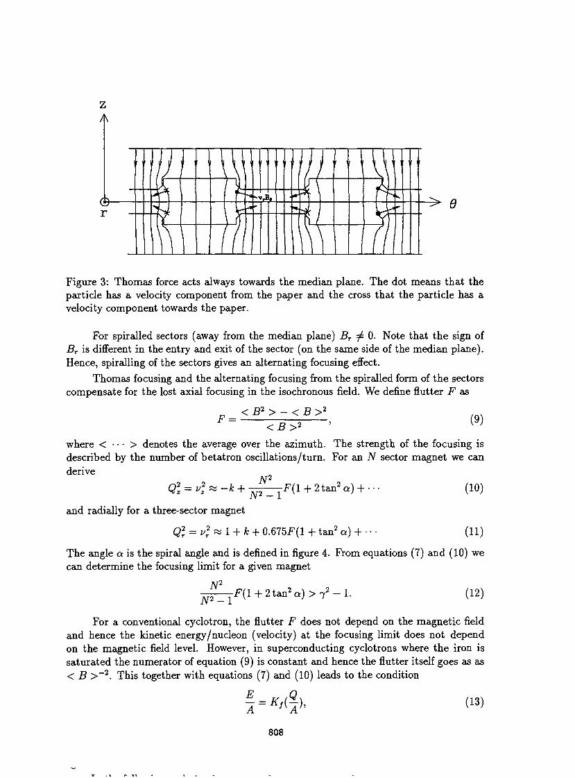
> e
Figure 3: Thomas force acts always towards the median plane. The dot means that the particle has a velocity component from the paper and the cross that the particle has a velocity component towards the paper.
For spiralled sectors (away from the median plane) BT ^ 0. Note that the sign of Br is different in the entry and exit of the sector (on the same side of the median plane). Hence, spiralling of the sectors gives an alternating focusing effect.
Thomas focusing and the alternating focusing from the spiralled form of the sectors compensate for the lost axial focusing in the isochronous field. We define flutter F as
< B ' > - < B > ' <B>' ( l
where < • • • > denotes the average over the azimuth. The strength of the focusing is described by the number of betatron oscillations/turn. For an N sector magnet we can derive
N2
Q " . « - * + ]vr -F(l + 2tan J a) + (10)
and radially for a three-sector magnet
Ql = v
2 « 1 + k + 0.675F(1 + tan 2 a) + • • • (11)
The angle a is the spiral angle and is defined in figure 4. From equations (7) and (10) we can determine the focusing limit for a given magnet
N2
N2-l F( l + 2 t an 2 a ) > 7 ' - 1. (12)
For a conventional cyclotron, the flutter F does not depend on the magnetic field and hence the kinetic energy/nucleon (velocity) at the focusing limit does not depend on the magnetic field level. However, in superconducting cyclotrons where the iron is saturated the numerator of equation (9) is constant and hence the flutter itself goes as as < B >~2. This together with equations (7) and (10) leads to the condition
E -K (Q\ (13)
808
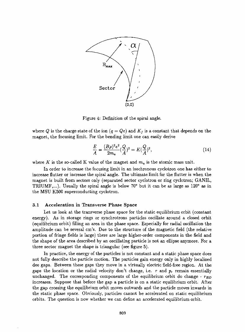
(o.o)
Figure 4: Definition of the spiral angle.
where Q is the chaxge state of the ion (q = Qe) and Kj is a constant that depends on the magnet, the focusing limit. For the bending limit one can easily derive
E _ (Bp)V Q _ Q 2
where K is the so-called K value of the magnet and mu is the atomic mass unit. In order to increase the focusing limit in an isochronous cyclotron one has either to
increase flutter or increase the spiral angle. The ultimate limit for the flutter is when the magnet is built from sectors only (separated sector cyclotron or ring cyclotron; GANIL, TRIUMF,...). Usually the spiral angle is below 70° but it can be as large as 120° as in the MSU K500 superconducting cyclotron.
3.1 Acceleration in Transverse Phase Space Let us look at the transverse phase space for the static equilibrium orbit (constant
energy). As in storage rings or synchrotrons particles oscillate around a closed orbit (equilibrium orbit) filling an area in the phase space. Especially for radial oscillation the amplitude can be several em's. Due to the structure of the magnetic field (the relative portion of fringe fields is large) there are large higher-order components in the field and the shape of the area described by an oscillating particle is not an ellipse anymore. For a three sector magnet the shape is triangular (see figure 5).
In practice, the energy of the particles is not constant and a static phase space does not fully describe the particle motion. The particles gain energy only in highly localized dee gaps. Between these gaps they move in a virtually electric field-free region. At the gaps the location or the radial velocity don't change, i.e. r and pr remain essentially unchanged. The corresponding components of the equilibrium orbit do change - TEO increases. Suppose that before the gap a particle is on a static equilibrium orbit. After the gap crossing the equilibrium orbit moves outwards and the particle moves inwards in the static phase space. Obviously, particles cannot be accelerated on static equilibrium orbits. The question is now whether we can define an accelerated equilibrium orbit.
809
(14)
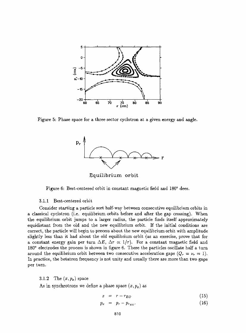
Figure 5: Phase space for a three sector cyclotron at a given energy and angle.
E q u i l i b r i u m o r b i t
Figure 6: Best-centered orbit in constant magnetic field and 180° dees.
3.1.1 Best-centered orbit Consider starting a particle sort half-way between consecutive equilibrium orbits in
a classical cyclotron (i.e. equilibrium orbits before and after the gap crossing). When the equilibrium orbit jumps to a larger radius, the particle finds itself approximately equidistant from the old and the new equilibrium orbit. If the initial conditions are correct, the particle will begin to precess about the new equilibrium orbit with amplitude slightly less than it had about the old equilibrium orbit (as an exercise, prove that for a constant energy gain per turn AE, Ar oc 1/r). For a constant magnetic field and 180° electrodes the process is shown in figure 6. There the particles oscillate half a turn around the equilibrium orbit between two consecutive acceleration gaps (Qr = vT — 1). In practice, the betatron frequency is not unity and usually there are more than two gaps per turn.
3.1.2 The (x,px) space As in synchrotrons we define a phase space (x,px) as
x = r — rEO
Px — Pr ~~ PTEO '
(15) (16)
810
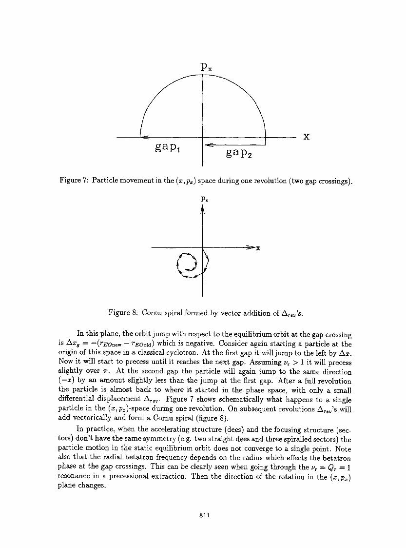
p
X
Figure 7: Particle movement in the (x,px) space during one revolution (two gap crossings).
Px
Figure 8: Cornu spiral formed by vector addition of AT
In this plane, the orbit jump with respect to the equilibrium orbit at the gap crossing is Axg = —(rEOnev — rEOo\d) which is negative. Consider again starting a particle at the origin of this space in a classical cyclotron. At the first gap it will jump to the left by Ax. Now it will start to precess until it reaches the next gap. Assuming vT > 1 it will precess slightly over -IT. At the second gap the particle will again jump to the same direction (—x) by an amount slightly less than the jump at the first gap. After a full revolution the particle is almost back to where it started in the phase space, with only a small differential displacement ATev. Figure 7 shows schematically what happens to a single particle in the (x^^-space during one revolution. On subsequent revolutions A r e„'s will add vectorically and form a Cornu spiral (figure 8).
In practice, when the accelerating structure (dees) and the focusing structure (sectors) don't have the same symmetry (e.g. two straight dees and three spiralled sectors) the particle motion in the static equilibrium orbit does not converge to a single point. Note also that the radial betatron frequency depends on the radius which effects the betatron phase at the gap crossings. This can be clearly seen when going through the uT = Qr = 1 resonance in a precessional extraction. Then the direction of the rotation in the (x,px) plane changes.
811
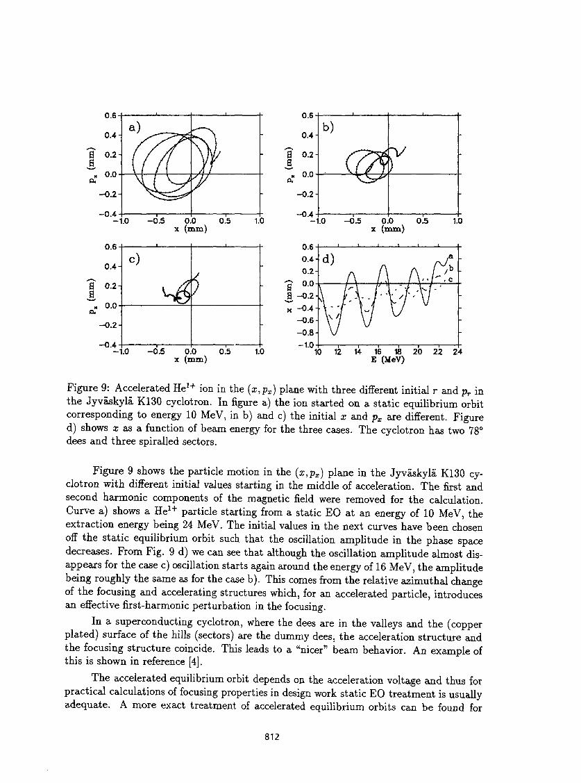
0.6
0.4
I" N 0.0
- 0 . 2 -
- 0 . 4
1
1 1
^vss=^ s * ' 1
-1.0 -0.5 0.0 0.5 x (mm)
1.0
0.6
0.4-
"? 0.2-
"H 0.0
-0 .2 -
-0.4
c)
^
-1.0 - 0 5 0.0 0.5 x (mm)
1.0
0.6
0.4
S 0.2 J, ~ 0.0
-0 .2-
-0.4
. b )
' <(3 •
1 — • !
-1.0 -0.5 0.0 0.5 x (mm)
1.0
10 12 14 16 18 20 22 24 E (MeV)
Figure 9: Accelerated He 1 + ion in the (x,px) plane with three different initial r and pr in the Jyvaskylâ K130 cyclotron. In figure a) the ion started on a static equilibrium orbit corresponding to energy 10 MeV, in b) and c) the initial x and px are different. Figure d) shows a; as a function of beam energy for the three cases. The cyclotron has two 78° dees and three spiralled sectors.
Figure 9 shows the particle motion in the (x,px) plane in the Jyvâskylâ K130 cyclotron with different initial values starting in the middle of acceleration. The first and second harmonic components of the magnetic field were removed for the calculation. Curve a) shows a H e 1 + particle starting from a static EO at an energy of 10 MeV, the extraction energy being 24 MeV. The initial values in the next curves have been chosen off the static equilibrium orbit such that the oscillation amplitude in the phase space decreases. From Fig. 9 d) we can see that although the oscillation amplitude almost disappears for the case c) oscillation starts again around the energy of 16 MeV, the amplitude being roughly the same as for the case b). This comes from the relative azimuthal change of the focusing and accelerating structures which, for an accelerated particle, introduces an effective first-harmonic perturbation in the focusing.
In a superconducting cyclotron, where the dees are in the valleys and the (copper plated) surface of the hills (sectors) are the dummy dees, the acceleration structure and the focusing structure coincide. This leads to a "nicer" beam behavior. An example of this is shown in reference [4].
The accelerated equilibrium orbit depends on the acceleration voltage and thus for practical calculations of focusing properties in design work static EO treatment is usually adequate. A more exact treatment of accelerated equilibrium orbits can be found for
812
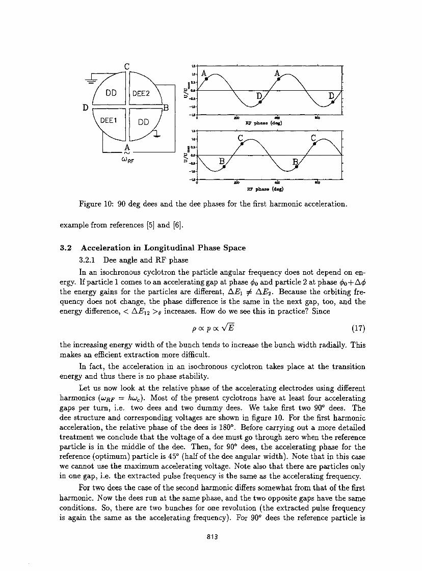
RF phase (deg)
Figure 10: 90 deg dees and the dee phases for the first harmonic acceleration,
example from references [5] and [6].
3.2 Acceleration in Longitudinal Phase Space 3.2.1 Dee angle and RF phase
In an isochronous cyclotron the particle angular frequency does not depend on energy. If particle 1 comes to an accelerating gap at phase (j>o and particle 2 at phase (f>o + A(j> the energy gains for the particles are different, A^i ^ AEÏ. Because the orbiting frequency does not change, the phase difference is the same in the next gap, too, and the energy difference, < AE-^ >g increases. How do we see this in practice? Since
p oc p ex Vf (17)
the increasing energy width of the bunch tends to increase the bunch width radially. This makes an efficient extraction more difficult.
In fact, the acceleration in an isochronous cyclotron takes place at the transition energy and thus there is no phase stability.
Let us now look at the relative phase of the accelerating electrodes using different harmonics (U>RF = hwc)- Most of the present cyclotrons have at least four accelerating gaps per turn, i.e. two dees and two dummy dees. We take first two 90° dees. The dee structure and corresponding voltages are shown in figure 10. For the first harmonic acceleration, the relative phase of the dees is 180°. Before carrying out a more detailed treatment we conclude that the voltage of a dee must go through zero when the reference particle is in the middle of the dee. Then, for 90° dees, the accelerating phase for the reference (optimum) particle is 45° (half of the dee angular width). Note that in this case we cannot use the maximum accelerating voltage. Note also that there are particles only in one gap, i.e. the extracted pulse frequency is the same as the accelerating frequency.
For two dees the case of the second harmonic differs somewhat from that of the first harmonic. Now the dees run at the same phase, and the two opposite gaps have the same conditions. So, there are two bunches for one revolution (the extracted pulse frequency is again the same as the accelerating frequency). For 90° dees the reference particle is
813
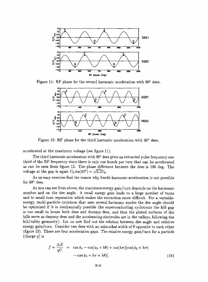
DEE1
DEE2
"UÔ ~7& 900
RF phase (deg)
MéO CÈ0
Figure 11: RF phase for the second harmonic acceleration with 90° dees.
2160
DEE1
DEE2
"35 ' iôSô ' ' 5ô 2«o RF phase (deg)
Figure 12: RF phase for the third harmonic acceleration with 90° dees.
accelerated at the maximum voltage (see figure 11).
The third harmonic acceleration with 90° dees gives an extracted pulse frequency one third of the RF frequency since there is only one bunch per turn that can be accelerated as can be seen from figure 12. The phase difference between the dees is 180 deg. The voltage at the gap is again £/osin(45°) = VoliUo.
As an easy exercise find the reason why fourth harmonic acceleration is not possible for 90° dees.
As you can see from above, the maximum energy gain/turn depends on the harmonic number and on the dee angle. A small energy gain leads to a large number of turns and to small turn separation which makes the extraction more difficult. For a variable-energy, multi-particle cyclotron that uses several harmonic modes the dee angle should be optimized if it is mechanically possible (for superconducting cyclotrons the hill gap is too small to house both dees and dummy dees, and thus the plated surfaces of the hills serve as dummy dees and the accelerating electrodes are in the valleys, following the hill/valley geometry). Let us now find out the relation between dee angle and relative energy gain/turn. Consider two dees with an azimuthal width of 9 opposite to each other (figure 13). There are four acceleration gaps. The relative energy gain/turn for a particle (charge q) is
AE —— = cos <f>Q — cos(<?!>o + h6) + cos(/i7r)[cos(<£0 + hir)
— cos(<^o + hit + hO)]. (18)
814
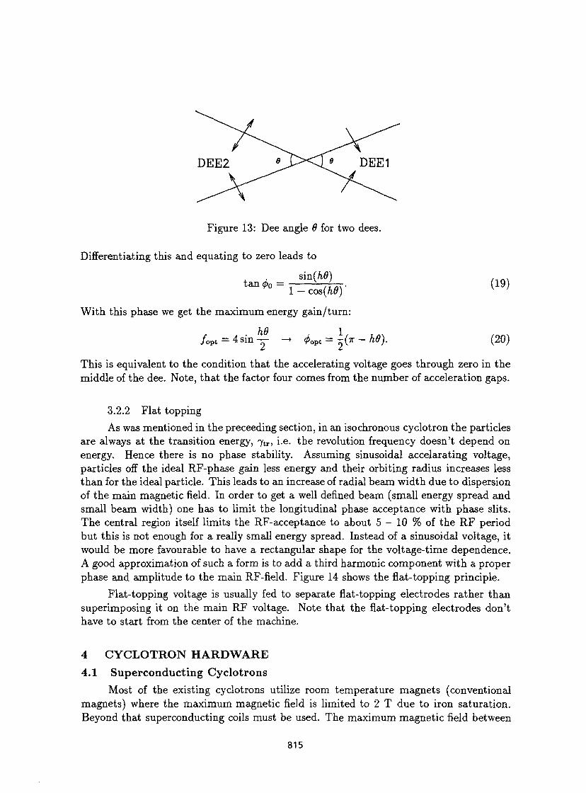
Figure 13: Dee angle 6 for two dees.
Differentiating this and equating to zero leads to
sm(h$) ,„_ tan^ 0 = 1 ^Tlâv 1 9
1 — cos(hd) With this phase we get the maximum energy gain/turn:
/ o p t = 4 s i n y - 4>ovt = l(ir-h0). (20)
This is equivalent to the condition that the accelerating voltage goes through zero in the middle of the dee. Note, that the factor four comes from the number of acceleration gaps.
3.2.2 Flat topping As was mentioned in the preceeding section, in an isochronous cyclotron the particles
are always at the transition energy, 7 t r , i.e. the revolution frequency doesn't depend on energy. Hence there is no phase stability. Assuming sinusoidal accelarating voltage, particles off the ideal RF-phase gain less energy and their orbiting radius increases less than for the ideal particle. This leads to an increase of radial beam width due to dispersion of the main magnetic field. In order to get a well defined beam (small energy spread and small beam width) one has to limit the longitudinal phase acceptance with phase slits. The central region itself limits the RF-acceptance to about 5 - 10 % of the RF period but this is not enough for a really small energy spread. Instead of a sinusoidal voltage, it would be more favourable to have a rectangular shape for the voltage-time dependence. A good approximation of such a form is to add a third harmonic component with a proper phase and amplitude to the main RF-field. Figure 14 shows the flat-topping principle.
Flat-topping voltage is usually fed to separate flat-topping electrodes rather than superimposing it on the main RF voltage. Note that the flat-topping electrodes don't have to start from the center of the machine.
4 CYCLOTRON HARDWARE 4.1 Superconducting Cyclotrons
Most of the existing cyclotrons utilize room temperature magnets (conventional magnets) where the maximum magnetic field is limited to 2 T due to iron saturation. Beyond that superconducting coils must be used. The maximum magnetic field between
815
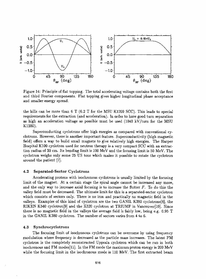
1.0: r
^ •
i
0.5: / *"v \ "
U.U / ;
0.5- ' -
-1.0: Vu,/ '•_
C ) 45 90 135 18(
1.0:
0.5:
0.0:
- 0 . 5 :
-1 .0 : C
U, + 0.15xU3
•
unit
s)
1.0:
0.5:
0.0:
- 0 . 5 :
-1 .0 : C
U (a
rb
1.0:
0.5:
0.0:
- 0 . 5 :
-1 .0 : C
1.0:
0.5:
0.0:
- 0 . 5 :
-1 .0 : C ) 45 90 135 180
0„ (deg) * R F (deg)
Figure 14: Principle of flat topping. The total accelerating voltage contains both the first and third Fourier components. Flat topping gives higher longitudinal phase acceptance and smaller energy spread.
the hills can be more than 6 T (6.2 T for the MSU K1200 SCC). This leads to special requirements for the extraction (and acceleration). In order to have good turn separation as high an acceleration voltage as possible must be used (1040 kV/turn for the MSU K1200).
Superconducting cyclotrons offer high energies as compared with conventional cyclotrons. However, there is another important feature. Superconductivity (high magnetic field) offers a way to build small magnets to give relatively high energies. The Harper Hospital K100 cyclotron used for neutron therapy is a very compact SCC with an extraction radius of 30 cm. Its bending limit is 100 MeV and the focusing limit is 50 MeV. The cyclotron weighs only some 25 US tons which makes it possible to rotate the cyclotron around the patient [7].
4.2 Separated-Sector Cyclotrons Accelerating protons with isochronous cyclotrons is usually limited by the focusing
limit of the magnet. At a certain stage the spiral angle cannot be increased any more, and the only way to increase axial focusing is to increase the flutter F. To do this the valley field must be decreased. The ultimate limit for this is a separated-sector cyclotron which consists of sectors only. There is no iron and practically no magnetic field in the valleys. Examples of this kind of cyclotron are the two G ANIL K380 cyclotrons[8], the RIKEN K540 cyclotron[9] and the K520 cyclotron at TRIUMF in Vancouver[10]. Since there is no magnetic field in the valleys the average field is fairly low, being e.g. 0.95 T in the GANIL K380 cyclotron. The number of sectors varies from 4 to 6.
4.3 Synchrocyclotrons The focusing limit of isochronous cyclotrons can be overcome by using frequency
modulation where frequency is decreased as the particle mass increases. The latest FM cyclotron is the completely reconstructed Uppsala cyclotron which can be run in both isochronous and FM modes[ll]. In the FM mode the maximum proton energy is 200 MeV while the focusing limit in the isochronous mode is 110 MeV. The first extracted beam
816
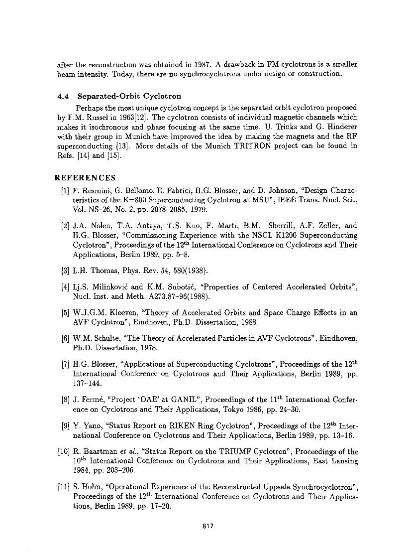
after the reconstruction was obtained in 1987. A drawback in FM cyclotrons is a smaller beam intensity. Today, there are no synchrocyclotrons under design or construction.
4.4 Separated-Orbit Cyclotron Perhaps the most unique cyclotron concept is the separated orbit cyclotron proposed
by F.M. Russel in 1963[12]. The cyclotron consists of individual magnetic channels which makes it isochronous and phase focusing at the same time. U. Trinks and G. Hinderer with their group in Munich have improved the idea by making the magnets and the RF superconducting [13]. More details of the Munich TRITRON project can be found in Refs. [14] and [15].
REFERENCES [1] F. Resmini, G. Bellomo, E. Fabrici, H.G. Blosser, and D. Johnson, "Design Charac
teristics of the K=800 Superconducting Cyclotron at MSU", IEEE Trans. Nucl. Sci., Vol. NS-26, No. 2, pp. 2078-2085, 1979.
[2] J.A. Nolen, T.A. Antaya, T.S. Kuo, F. Marti, B.M. Sherrill, A.F. Zeller, and H.G. Blosser, "Commissioning Experience with the NSCL K1200 Superconducting Cyclotron", Proceedings of the 12 t h International Conference on Cyclotrons and Their Applications, Berlin 1989, pp. 5-8.
[3] L.H. Thomas, Phys. Rev. 54, 580(1938).
[4] Lj.S. Milinkovic and K.M. Subotic, "Properties of Centered Accelerated Orbits", Nucl. Inst, and Meth. A273,87-96(1988).
[5] W.J.G.M. Kleeven, "Theory of Accelerated Orbits and Space Charge Effects in an AVF Cyclotron", Eindhoven, Ph.D. Dissertation, 1988.
[6] W.M. Schulte, "The Theory of Accelerated Particles in AVF Cyclotrons", Eindhoven, Ph.D. Dissertation, 1978.
[7] H.G. Blosser, "Applications of Superconducting Cyclotrons", Proceedings of the 12 t h
International Conference on Cyclotrons and Their Applications, Berlin 1989, pp. 137-144.
[8] J. Fermé, "Project 'OAE' at GANIL", Proceedings of the 11 t h International Conference on Cyclotrons and Their Applications, Tokyo 1986, pp. 24-30.
[9] Y. Yano, "Status Report on RIKEN Ring Cyclotron", Proceedings of the 12 t h International Conference on Cyclotrons and Their Applications, Berlin 1989, pp. 13-16.
[10] R. Baartman et al, "Status Report on the TRIUMF Cyclotron", Proceedings of the 10 t h International Conference on Cyclotrons and Their Applications, East Lansing 1984, pp. 203-206.
[11] S. Holm, "Operational Experience of the Reconstructed Uppsala Synchrocyclotron", Proceedings of the 12 t h International Conference on Cyclotrons and Their Applications, Berlin 1989, pp. 17-20.
817

[12] F.M. Russel, Nucl. Inst, and Meth. A23, 229(1963).
[13] U. Trinks et al., IEEE Trans. Nucl. Science NS-32, 2721(1985).
[14] W. Assmann et al., "TRITRON Progress Report", Proceedings of the 12 t h International Conference on Cyclotrons and Their Applications, Berlin 1989. pp. 47-50.
[15] U. Trinks, "The Superconducting Separated Orbit Cyclotron Tritron", Presented at the 12 t h International Conference on Cyclotrons and Their Applications, Vancouver 1992.
818
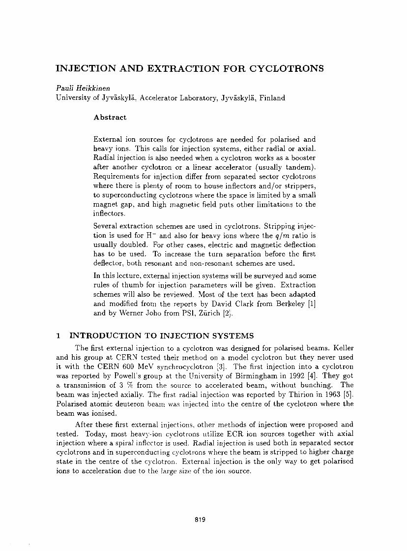
INJECTION AND EXTRACTION FOR CYCLOTRONS
Pauli Heikkinen University of Jyvàskylà, Accelerator Laboratory, Jyvàskylâ, Finland
Abstract
External ion sources for cyclotrons are needed for polarised and heavy ions. This calls for injection systems, either radial or axial. Radial injection is also needed when a cyclotron works as a booster after another cyclotron or a linear accelerator (usually tandem). Requirements for injection differ from separated sector cyclotrons where there is plenty of room to house inflectors and/or strippers, to superconducting cyclotrons where the space is limited by a small magnet gap, and high magnetic field puts other limitations to the infiectors.
Several extraction schemes are used in cyclotrons. Stripping injection is used for H~ and also for heavy ions where the q/m ratio is usually doubled. For other cases, electric and magnetic deflection has to be used. To increase the turn separation before the first deflector, both resonant and non-resonant schemes are used.
In this lecture, external injection systems will be surveyed and some rules of thumb for injection parameters will be given. Extraction schemes will also be reviewed. Most of the text has been adapted and modified from the reports by David Clark from Berkeley [1] and by Werner Joho from PSI, Zurich [2].
1 I N T R O D U C T I O N TO I N J E C T I O N S Y S T E M S
The first external injection to a cyclotron was designed for polarised beams. Keller and his group at CERN tested their method on a model cyclotron but they never used it with the CERN 600 MeV synchrocyclotron [3]. The first injection into a cyclotron was reported by Powell's group at the University of Birmingham in 1992 [4]. They got a transmission of 3 % from the source to accelerated beam, without bunching. The beam was injected axially. The first radial injection was reported by Thirion in 1963 [5]. Polarised atomic deuteron beam was injected into the centre of the cyclotron where the beam was ionised.
After these first external injections, other methods of injection were proposed and tested. Today, most heavy-ion cyclotrons utilize ECR ion sources together with axial injection where a spiral inflector is used. Radial injection is used both in separated sector cyclotrons and in superconducting cyclotrons where the beam is stripped to higher charge state in the centre of the cyclotron. External injection is the only way to get polarised ions to acceleration due to the large size of the ion source.
819
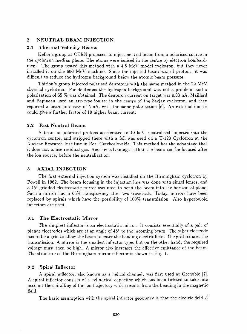
2 N E U T R A L B E A M I N J E C T I O N
2.1 Thermal Veloc i ty Beams Keller's group at CERN proposed to inject neutral beam from a polarised source in
the cyclotron median plane. The atoms were ionised in the centre by electron bombardment. The group tested this method with a 4.5 MeV model cyclotron, but they never installed it on the 600 MeV machine. Since the injected beam was of protons, it was difficult to reduce the hydrogen background below the atomic beam pressure.
Thirion's group injected polarised deuterons with the same method in the 22 MeV classical cyclotron. For deuterons the hydrogen background was not a problem, and a polarisation of 55 % was obtained. The deuteron current on target was 0.03 nA. Maillard and Papineau used an arc-type ioniser in the centre of the Saclay cyclotron, and they reported a beam intensity of 5 nA, with the same polarisation [6]. An external ioniser could give a further factor of 10 higher beam current.
2.2 Fast Neutra l B e a m s A beam of polarised protons accelerated to 40 keV, neutralised, injected into the
cyclotron centre, and stripped there with a foil was used on a U-120 Cyclotron at the Nuclear Research Institute in Rez, Czechoslovakia. This method has the advantage that it does not ionise residual gas. Another advantage is that the beam can be focused after the ion source, before the neutralisation.
3 A X I A L I N J E C T I O N
The first external injection system was installed on the Birmingham cyclotron by Powell in 1962. The beam focusing in the injection line was done with einzel lenses, and a 45° gridded electrostatic mirror was used to bend the beam into the horizontal plane. Such a mirror had a 65% transparency after two traversais. Today, mirrors have been replaced by spirals which have the possibility of 100% transmission. Also hyperboloid inflectors are used.
3.1 T h e Electrostat ic Mirror The simplest inflector is an electrostatic mirror. It consists essentially of a pair of
planar electrodes which are at an angle of 45° to the incoming beam. The other electrode has to be a grid to allow the beam to enter the bending electric field. The grid reduces the transmission. A mirror is the smallest inflector type, but on the other hand, the required voltage must then be high. A mirror also increases the effective emittance of the beam. The structure of the Birmingham mirror inflector is shown in Fig. 1.
3.2 Spiral Inflector A spiral inflector, also known as a helical channel, was first used at Grenoble [7].
A spiral inflector consists of a cylindrical capacitor which has been twisted to take into account the spiralling of the ion trajectory which results from the bending in the magnetic field.
The basic assumption with the spiral inflector geometry is that the electric field E
820
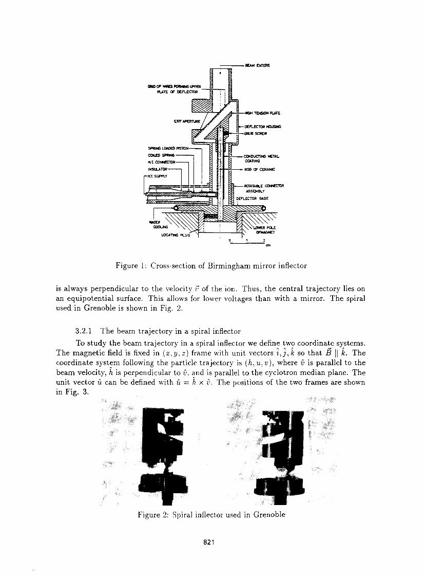
BEAM ENTERS
(MO OF WIRES FOBMWG UPPER
PLATE OF DeFLECTDR
«GH TENSION PLATE
LOCATING PLUG
Figure 1: Cross-section of Birmingham mirror inflector
is always perpendicular to the velocity v of the ion. Thus, the central trajectory lies on an equipotential surface. This allows for lower voltages than with a mirror. The spiral used in Grenoble is shown in Fig. 2.
3.2.1 The beam trajectory in a spiral inflector
To study the beam trajectory in a spiral inflector we define two coordinate systems. The magnetic field is fixed in (x,y,z) frame with unit vectors i,j,k so that B || k. The coordinate system following the particle trajectory is (h,u,v), where v is parallel to the beam velocity, h is perpendicular to v, and is parallel to the cyclotron median plane. The unit vector û can be defined with û — h x v. The positions of the two frames are shown in Fig. 3.
Figure 2: Spiral inflector used in Grenoble
821
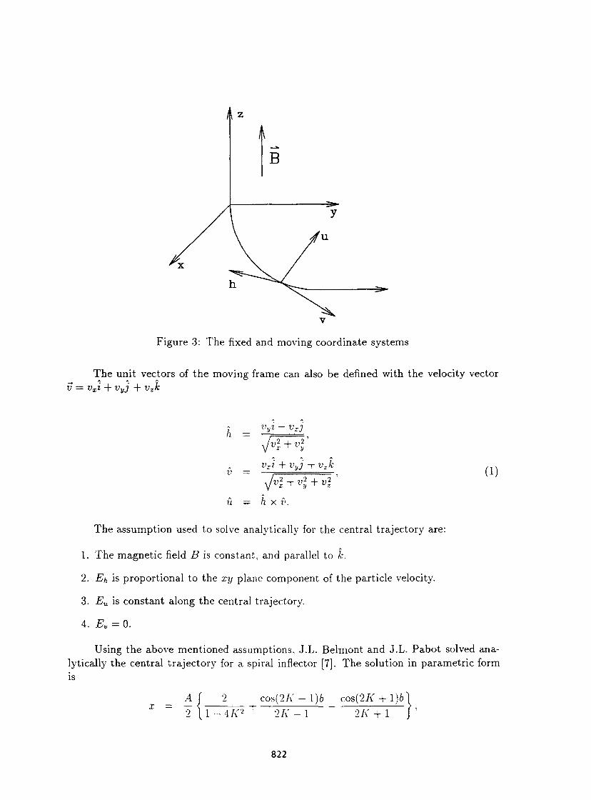
Az
B
Figure 3: The fixed and moving coordinate systems
The unit vectors of the moving frame can also be defined with the velocity vector v — vxi + vyj + v2k
u
Vyl -vxj
J: vxi
2 + v2' x ' wy
vzk M + vi + vl (1)
h x v.
The assumption used to solve analytically for the central trajectory are:
1. The magnetic field B is constant, and parallel to k.
2. Eh is proportional to the xy plane component of the particle velocity.
3. Eu is constant along the central trajectory.
4. Ev = 0.
Using the above mentioned assumptions, J.L. Belmont and J.L. Pabot solved analytically the central trajectory for a spiral inflector [7]. The solution in parametric form is
A\ 2 c o s ( 2 A ' - l ) 6 cos(2/C + l ) 6 \ j ^ _ _ ^ _ _ _ _ _ _ _ _ j _
2 1 - 4 A' 2 A' - 1 IK + 1
822
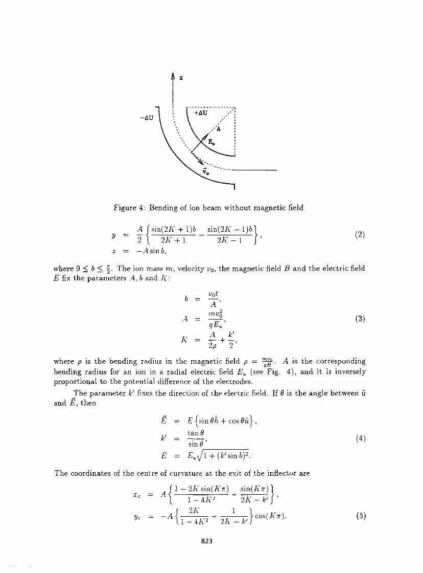
Figure 4: Bending of ion beam without magnetic field
V = A \sm{2K + l)b sin(2A - 1)6'
2 [ 2A' + 1
z = —A sin 6.
2/v - 1 (2)
where 0 < b < | . The ion mass m, velocity i>o, the magnetic field B and the electric field E fix the parameters A, 6 and K:
(3)
where /> is the bending radius in the magnetic field p = 2 2 ^-. A is the corresponding bending radius for an ion in a radial electric field Eu (see Fig. 4), and it is inversely proportional to the potential difference of the electrodes.
The parameter k' fixes the direction of the electric field. If 9 is the angle between û and E, then
b = vQt
A = qEu'
K = A k'
2p 2
E — E I sin 6h + cos 9û>,
tan (9 fc' =
sin0 ' (4)
E = Eu^Jl + (k'smby.
The coordinates of the centre of curvature at the exit of the inflector are
1 — 2A'sin(A'7r) sin(A'7r)l X c — r\
Vc - -A
1 - 4 A 2
2A 2A"
1 - 4A ô + 2A COs(A'7r). (5)
823
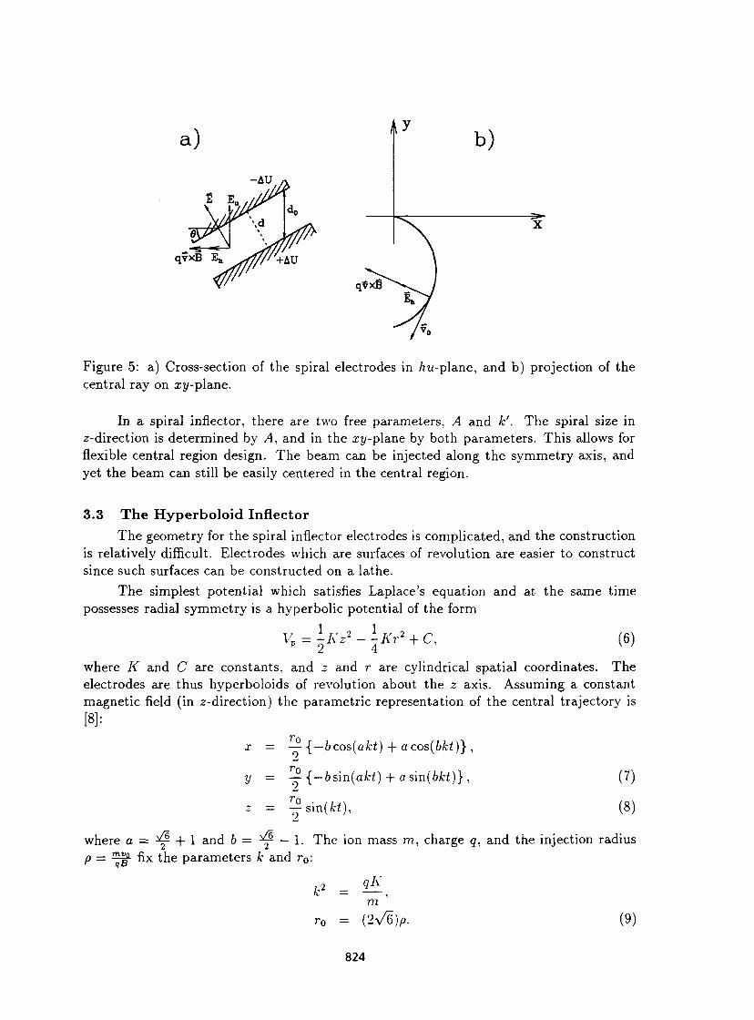
a) A?
-AU
qvxB 1^
b)
qvxB
Figure 5: a) Cross-section of the spiral electrodes in /?u-plane, and b) projection of the central ray on xy-p\a.ne.
In a spiral inflector, there are two free parameters, A and k!. The spiral size in z-direction is determined by A, and in the xy-plane by both parameters. This allows for flexible central region design. The beam can be injected along the symmetry axis, and yet the beam can still be easily centered in the central region.
3.3 T h e Hyperbo lo id Inflector The geometry for the spiral inflector electrodes is complicated, and the construction
is relatively difficult. Electrodes which are surfaces of revolution are easier to construct since such surfaces can be constructed on a lathe.
The simplest potential which satisfies Laplace's equation and at the same time possesses radial symmetry is a hyperbolic potential of the form
Vp=l-Kz2-l-Kr2 + C, 2 4 (6)
where K and C are constants, and z and r are cylindrical spatial coordinates. The electrodes are thus hyperboloids of revolution about the z axis. Assuming a constant magnetic field (in z-direction) the parametric representation of the central trajectory is [8]:
y =
— { — bcos(akt) + a cos(bkt)} ,
— { — bsm(akt) + a s'm(bkt)} ,
— sin(fci),
(7)
(8)
where 0 = ^ + 1 and b = ^ — 1. The ion mass m, charge ç, and the injection radius p = z^ fix the parameters k and r 0 :
, 2 <? A '
m r0 = (2y/6)p. (9)
824
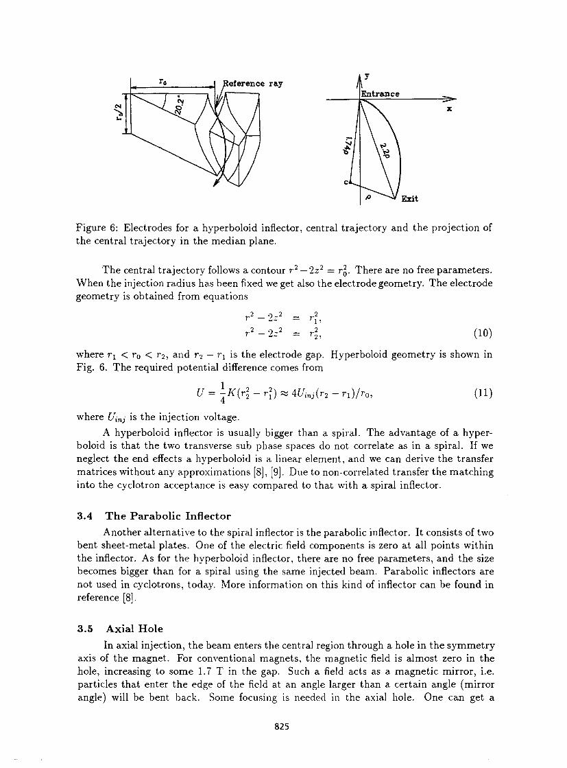
eference ray
Figure 6: Electrodes for a hyperboloid inflector, central trajectory and the projection of the central trajectory in the median plane.
The central trajectory follows a contour r 2 — 2z2 = TQ. There are no free parameters. When the injection radius has been fixed we get also the electrode geometry. The electrode geometry is obtained from equations
-2 - 0 r 2
_ 9-1'
(10)
where rx < r0 < r 2 , and r 2 — r x is the electrode gap. Hyperboloid geometry is shown in Fig. 6. The required potential difference comes from
U -K(r. 4 v r 2 ) w4J7 i n j ( r 2 - r i ) / r 0 , (H )
where Uinj is the injection voltage. A hyperboloid inflector is usually bigger than a spiral. The advantage of a hyper
boloid is that the two transverse sub phase spaces do not correlate as in a spiral. If we neglect the end effects a hyperboloid is a linear element, and we can derive the transfer matrices without any approximations [8], [9]. Due to non-correlated transfer the matching into the cyclotron acceptance is easy compared to that with a spiral inflector.
3.4 T h e Parabol ic Inflector Another alternative to the spiral inflector is the parabolic inflector. It consists of two
bent sheet-metal plates. One of the electric field components is zero at all points within the inflector. As for the hyperboloid inflector, there are no free parameters, and the size becomes bigger than for a spiral using the same injected beam. Parabolic inflectors are not used in cyclotrons, today. More information on this kind of inflector can be found in reference [8].
3.5 Axial Hole In axial injection, the beam enters the central region through a hole in the symmetry
axis of the magnet. For conventional magnets, the magnetic field is almost zero in the hole, increasing to some 1.7 T in the gap. Such a field acts as a magnetic mirror, i.e. particles that enter the edge of the field at an angle larger than a certain angle (mirror angle) will be bent back. Some focusing is needed in the axial hole. One can get a
825
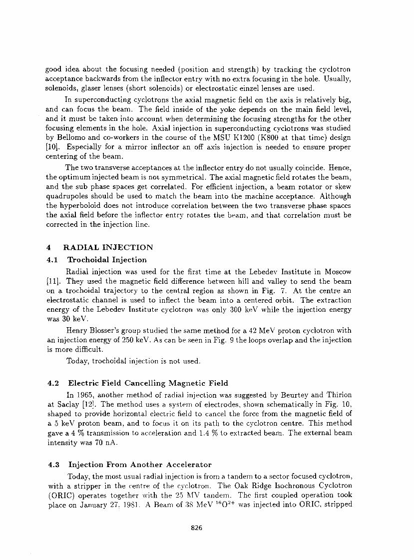
good idea about the focusing needed (position and strength) by tracking the cyclotron acceptance backwards from the inflector entry with no extra focusing in the hole. Usually, solenoids, glaser lenses (short solenoids) or electrostatic einzel lenses are used.
In superconducting cyclotrons the axial magnetic field on the axis is relatively big, and can focus the beam. The field inside of the yoke depends on the main field level, and it must be taken into account when determining the focusing strengths for the other focusing elements in the hole. Axial injection in superconducting cyclotrons was studied by Bellomo and co-workers in the course of the MSU K1200 (K800 at that time) design [10]. Especially for a mirror inflector an off axis injection is needed to ensure proper centering of the beam.
The two transverse acceptances at the inflector entry do not usually coincide. Hence, the optimum injected beam is not symmetrical. The axial magnetic field rotates the beam, and the sub phase spaces get correlated. For efficient injection, a beam rotator or skew quadrupoles should be used to match the beam into the machine acceptance. Although the hyperboloid does not introduce correlation between the two transverse phase spaces the axial field before the inflector entry rotates the beam, and that correlation must be corrected in the injection line.
4 R A D I A L I N J E C T I O N
4.1 Trochoidal Injection Radial injection was used for the first time at the Lebedev Institute in Moscow
[11]. They used the magnetic field difference between hill and valley to send the beam on a trochoidal trajectory to the central region as shown in Fig. 7. At the centre an electrostatic channel is used to inflect the beam into a centered orbit. The extraction energy of the Lebedev Institute cyclotron was only 300 keV while the injection energy was 30 keV.
Henry Blosser's group studied the same method for a 42 MeV proton cyclotron with an injection energy of 250 keV. As can be seen in Fig. 9 the loops overlap and the injection is more difficult.
Today, trochoidal injection is not used.
4.2 Electric Fie ld Cancel l ing Magne t i c Field In 1965, another method of radial injection was suggested by Beurtey and Thirion
at Saclay [12]. The method uses a system of electrodes, shown schematically in Fig. 10, shaped to provide horizontal electric field to cancel the force from the magnetic field of a 5 keV proton beam, and to focus it on its path to the cyclotron centre. This method gave a 4 % transmission to acceleration and 1.4 % to extracted beam. The external beam intensity was 70 nA.
4.3 Inject ion From A n o t h e r A c c e l e r a t o r Today, the most usual radial injection is from a tandem to a sector focused cyclotron,
with a stripper in the centre of the cyclotron. The Oak Ridge Isochronous Cyclotron (ORIC) operates together with the 25 MV tandem. The first coupled operation took place on January 27. 1981. A Beam of 38 MeV 1 6 0 2 + was injected into ORIC, stripped
826
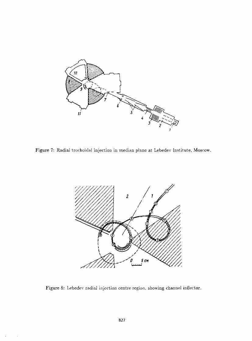
Figure 7: Radial trochoidal injection in median plane at Lebedev Institute, Moscow.
Figure 8: Lebedev radial injection centre region, showing channel inflector.
827
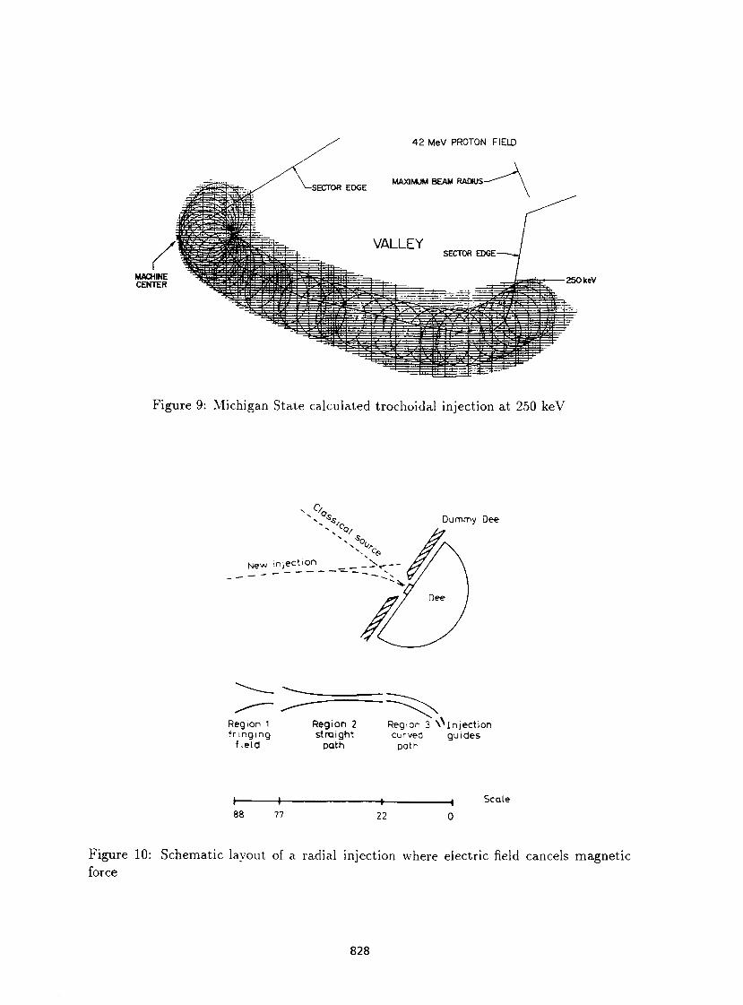
4 2 MeV PROTON FIELD
250 keV
Figure 9: Michigan State calculated trochoidal injection at 250 keV
vOv
* > /
N e w inject ion \ ^ _
Dummy Dee
Region 1 Region 2 Region 3 \Mn jec t i on fr i ngmg straight curved guides
field path oath
88 77
Scale 22
Figure 10: Schematic layout of a radial injection where electric field cancels magnetic force
828
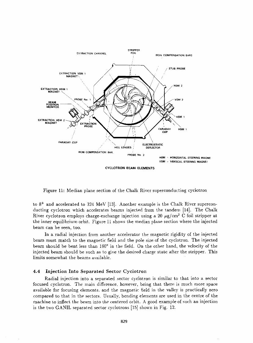
EXTRACTION CHANNEL STRIPPER
FOIL IRON COMPENSATION BARS
EXTRACTION VSM 1 MAGNET \
STUB PROBE
HSM 2 EXTRACTION HSM 1
MAGNET
VSM 2
EXTRACTION HSM 2 MAGNET
VSM 1
FARADAY HSM 1 CUP
FARADAY -CUP ELECTROSTATIC
DEFLECTOR
IRON COMPENSATION BAR. PROBE No. 2
HSM = HORIZONTAL STEERING MAGNE VSM = VERTICAL STEERING MAGNET
CYCLOTRON BEAM ELEMENTS
Figure 11: Median plane section of the Chalk River superconducting cyclotron
to 8 + and accelerated to 324 MeV [13]. Another example is the Chalk River superconducting cyclotron which accelerates beams injected from the tandem [14]. The Chalk River cyclotron employs charge-exchange injection using a 20 /zg/cm 2 C foil stripper at the inner equilibrium orbit. Figure 11 shows the median plane section where the injected beam can be seen, too.
In a radial injection from another accelerator the magnetic rigidity of the injected beam must match to the magnetic field and the pole size of the cyclotron. The injected beam should be bent less than 180° in the field. On the other hand, the velocity of the injected beam should be such as to give the desired charge state after the stripper. This limits somewhat the beams available.
4.4 Inject ion Into Separated Sector Cyclotron Radial injection into a separated sector cyclotron is similar to that into a sector
focused cyclotron. The main difference, however, being that there is much more space available for focusing elements, and the magnetic field in the valley is practically zero compared to that in the sectors. Usually, bending elements are used in the centre of the machine to inflect the beam into the centered orbit. A good example of such an injection is the two GANIL separated sector cyclotrons [15] shown in Fig. 12.
829
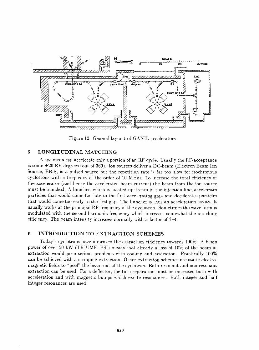
V////////////////////7//M//7,
SCALE
l\l I I II 11 II 11 I
30 meter
< i /i111/1
V </////////////////J^~* e2%= Figure 12: General lay-out of GANIL accelerators
5 L O N G I T U D I N A L M A T C H I N G
A cyclotron can accelerate only a portion of an RF cycle. Usually the RF-acceptance is some ±20 RF-degrees (out of 360). Ion sources deliver a DC-beam (Electron Beam Ion Source, EBIS, is a pulsed source but the repetition rate is far too slow for isochronous cyclotrons with a frequency of the order of 10 MHz). To increase the total efficiency of the accelerator (and hence the accelerated beam current) the beam from the ion source must be bunched. A buncher. which is located upstream in the injection line, accelerates particles that would come too late to the first accelerating gap, and decelerates particles that would come too early to the first gap. The buncher is thus an acceleration cavity. It usually works at the principal RF-frequency of the cyclotron. Sometimes the wave form is modulated with the second harmonic frequency which increases somewhat the bunching efficiency. The beam intensity increases normally with a factor of 3-4.
6 I N T R O D U C T I O N TO E X T R A C T I O N S C H E M E S
Today's cyclotrons have improved the extraction efficiency towards 100%. A beam power of over 50 kW (TRIUMF, PSI) means that already a loss of 10% of the beam at extraction would pose serious problems with cooling and activation. Practically 100% can be achieved with a stripping extraction. Other extraction schemes use static electromagnetic fields to "peel" the beam out of the cyclotron. Both resonant and non-resonant extraction can be used. For a deflector, the turn separation must be increased both with acceleration and with magnetic bumps which excite resonances. Both integer and half integer resonances are used.
830
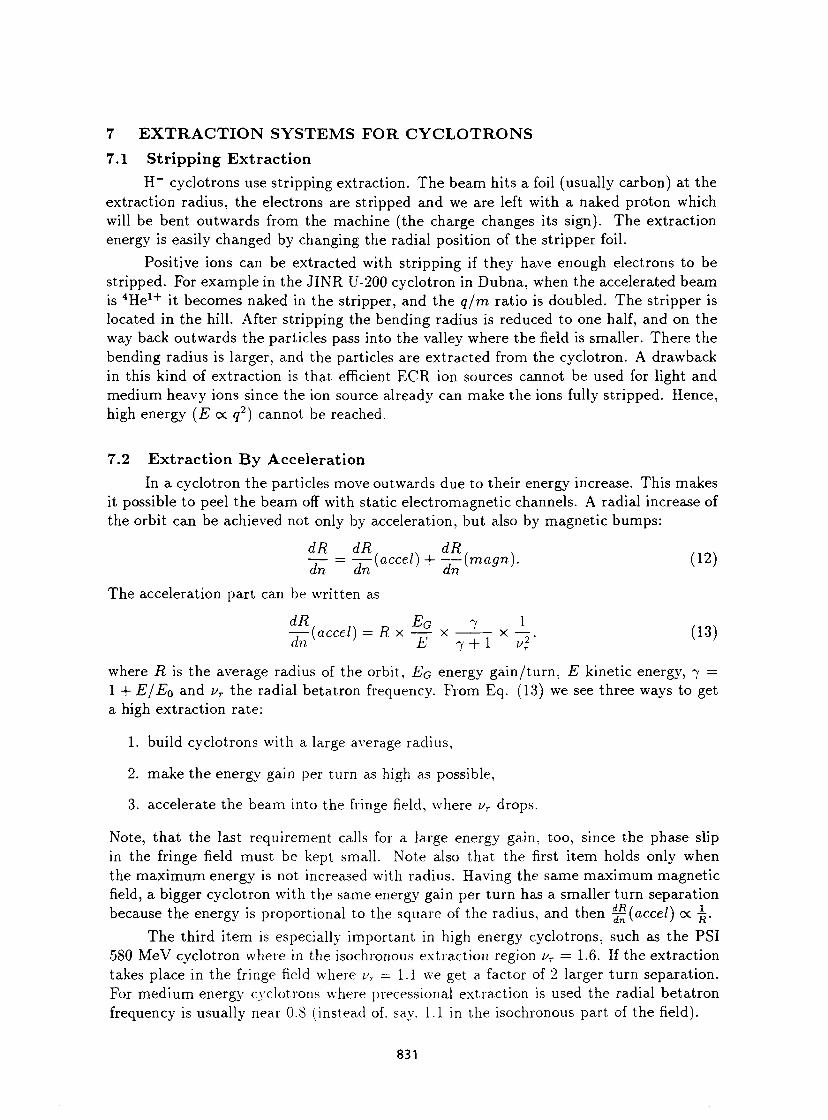
7 E X T R A C T I O N S Y S T E M S FOR C Y C L O T R O N S
7.1 Str ipping Extract ion H - cyclotrons use stripping extraction. The beam hits a foil (usually carbon) at the
extraction radius, the electrons are stripped and we are left with a naked proton which will be bent outwards from the machine (the charge changes its sign). The extraction energy is easily changed by changing the radial position of the stripper foil.
Positive ions can be extracted with stripping if they have enough electrons to be stripped. For example in the JINR U-200 cyclotron in Dubna, when the accelerated beam is 4 H e 1 + it becomes naked in the stripper, and the q/m ratio is doubled. The stripper is located in the hill. After stripping the bending radius is reduced to one half, and on the way back outwards the particles pass into the valley where the field is smaller. There the bending radius is larger, and the particles are extracted from the cyclotron. A drawback in this kind of extraction is that efficient ECR ion sources cannot be used for light and medium heavy ions since the ion source already can make the ions fully stripped. Hence, high energy (E oc q2) cannot be reached.
7.2 Extrac t ion B y Accelerat ion In a cyclotron the particles move outwards due to their energy increase. This makes
it possible to peel the beam off with static electromagnetic channels. A radial increase of the orbit can be achieved not only by acceleration, but also by magnetic bumps:
dR dR, dR. . / 1 0 . — = ——{accelj H——(magn). ( lz) dn dn dn
The acceleration part can be written as
— (accel) = R x -£- x — I - x —, (13) dn E 7 -f 1 v;
where R is the average radius of the orbit, EG energy gain/ turn, E kinetic energy, 7 = 1 + E/Eo and vT the radial betatron frequency. From Eq. (13) we see three ways to get a high extraction rate:
1. build cyclotrons with a large average radius,
2. make the energy gain per turn as high as possible,
3. accelerate the beam into the fringe field, where vT drops.
Note, that the last requirement calls for a large energy gain, too, since the phase slip in the fringe field must be kept small. Note also that the first item holds only when the maximum energy is not increased with radius. Having the same maximum magnetic field, a bigger cyclotron with the same energy gain per turn has a smaller turn separation because the energy is proportional to the square of the radius, and then ^(accel) oc -5.
The third item is especially important in high energy cyclotrons, such as the PSI 580 MeV cyclotron where in the isochronous extraction region vT = 1.6. If the extraction takes place in the fringe field where vr — 1.1 we get a factor of 2 larger turn separation. For medium energy cyclotrons where precessional extraction is used the radial betatron frequency is usually near 0.8 (instead of. say. 1.1 in the isochronous part of the field).
831
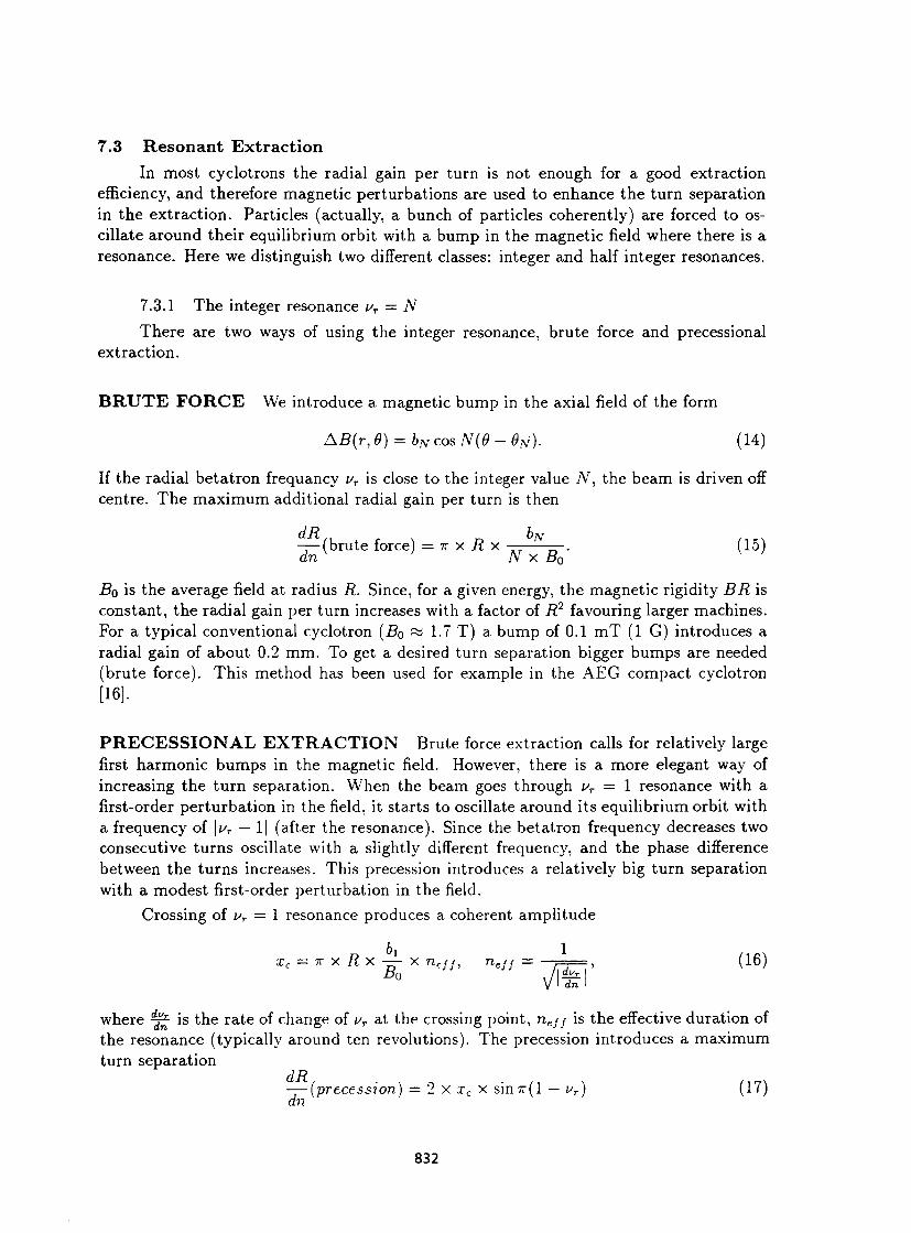
7.3 Resonant Extract ion In most cyclotrons the radial gain per turn is not enough for a good extraction
efficiency, and therefore magnetic perturbations are used to enhance the turn separation in the extraction. Particles (actually, a bunch of particles coherently) are forced to oscillate around their equilibrium orbit with a bump in the magnetic field where there is a resonance. Here we distinguish two different classes: integer and half integer resonances.
7.3.1 The integer resonance vr = N There are two ways of using the integer resonance, brute force and precessional
extraction.
B R U T E F O R C E We introduce a magnetic bump in the axial field of the form
AB(r,6) = bNcosN(9-6N). (14)
If the radial betatron frequancy vr is close to the integer value N, the beam is driven off centre. The maximum additional radial gain per turn is then
- ^ ( b r u t e force) = i x i ? x — —. (15) dnx ' N x Bo v '
Bo is the average field at radius R. Since, for a given energy, the magnetic rigidity BR is constant, the radial gain per turn increases with a factor of R2 favouring larger machines. For a typical conventional cyclotron (Bo ~ 1.7 T) a. bump of 0.1 m T (1 G) introduces a radial gain of about 0.2 mm. To get a desired turn separation bigger bumps are needed (brute force). This method has been used for example in the AEG compact cyclotron [16].
P R E C E S S I O N A L E X T R A C T I O N Brute force extraction calls for relatively large first harmonic bumps in the magnetic field. However, there is a more elegant way of increasing the turn separation. When the beam goes through vT = 1 resonance with a first-order perturbation in the field, it starts to oscillate around its equilibrium orbit with a frequency of \vr — 1| (after the resonance). Since the betatron frequency decreases two consecutive turns oscillate with a slightly different frequency, and the phase difference between the turns increases. This precession introduces a relatively big turn separation with a modest first-order perturbation in the field.
Crossing of vT = 1 resonance produces a coherent amplitude
XC = 7 T X / 2 X - ^ - X nejJ, ne}f = ——, (16)
where ^p- is the rate of change of vr at the crossing point, nejj is the effective duration of the resonance (typically around ten revolutions). The precession introduces a maximum turn separation
—— (precession) — 2 x x c x sin7r(l — i/r) (17) an
832
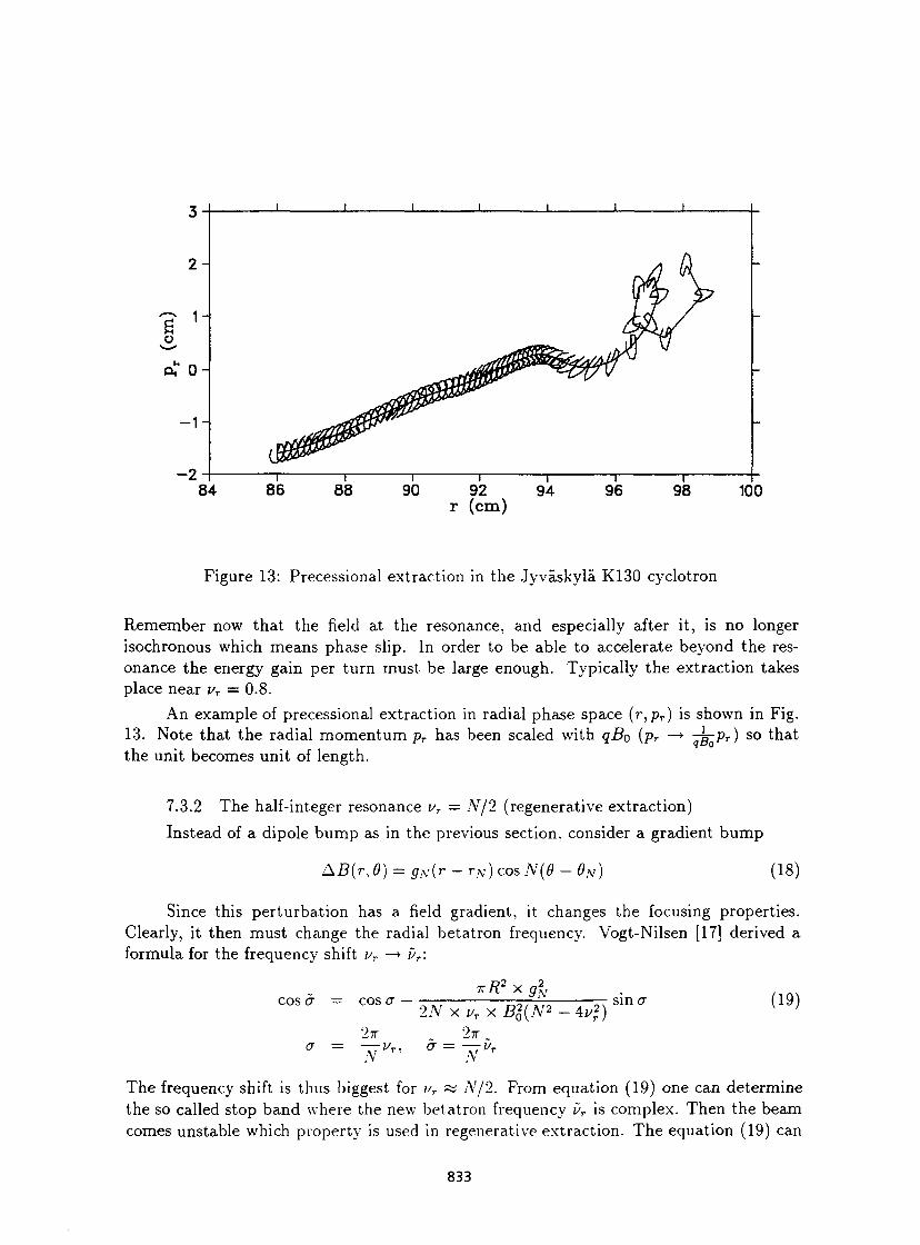
100
Figure 13: Precessional extraction in the Jyvàskylâ K130 cyclotron
Remember now that the field at the resonance, and especially after it, is no longer isochronous which means phase slip. In order to be able to accelerate beyond the resonance the energy gain per turn must be large enough. Typically the extraction takes place near vT = 0.8.
An example of precessional extraction in radial phase space (r ,p r ) is shown in Fig. 13. Note that the radial momentum pT has been scaled with qBo (pT —• rg-Pr) so that the unit becomes unit of length.
7.3.2 The half-integer resonance vr — N/2 (regenerative extraction) Instead of a dipole bump as in the previous section, consider a gradient bump
AB{r, 9) = gN(r - rN) cos N(9 - 0N) (18)
Since this perturbation has a field gradient, it changes the focusing properties. Clearly, it then must change the radial betatron frequency. Vogt-Nilsen [17] derived a formula for the frequency shift vT —> vT:
cos a — cos <T TTR2 X g2
N
a Z7T
7v Vr,
•2N xvrx Bl{N2 - 4i/2)
a = l v I / r
sin a- (19)
The frequency shift is thus biggest for ur ~ N/2. From equation (19) one can determine the so called stop band where the new betatron frequency vr is complex. Then the beam comes unstable which property is used in regenerative extraction. The equation (19) can
833
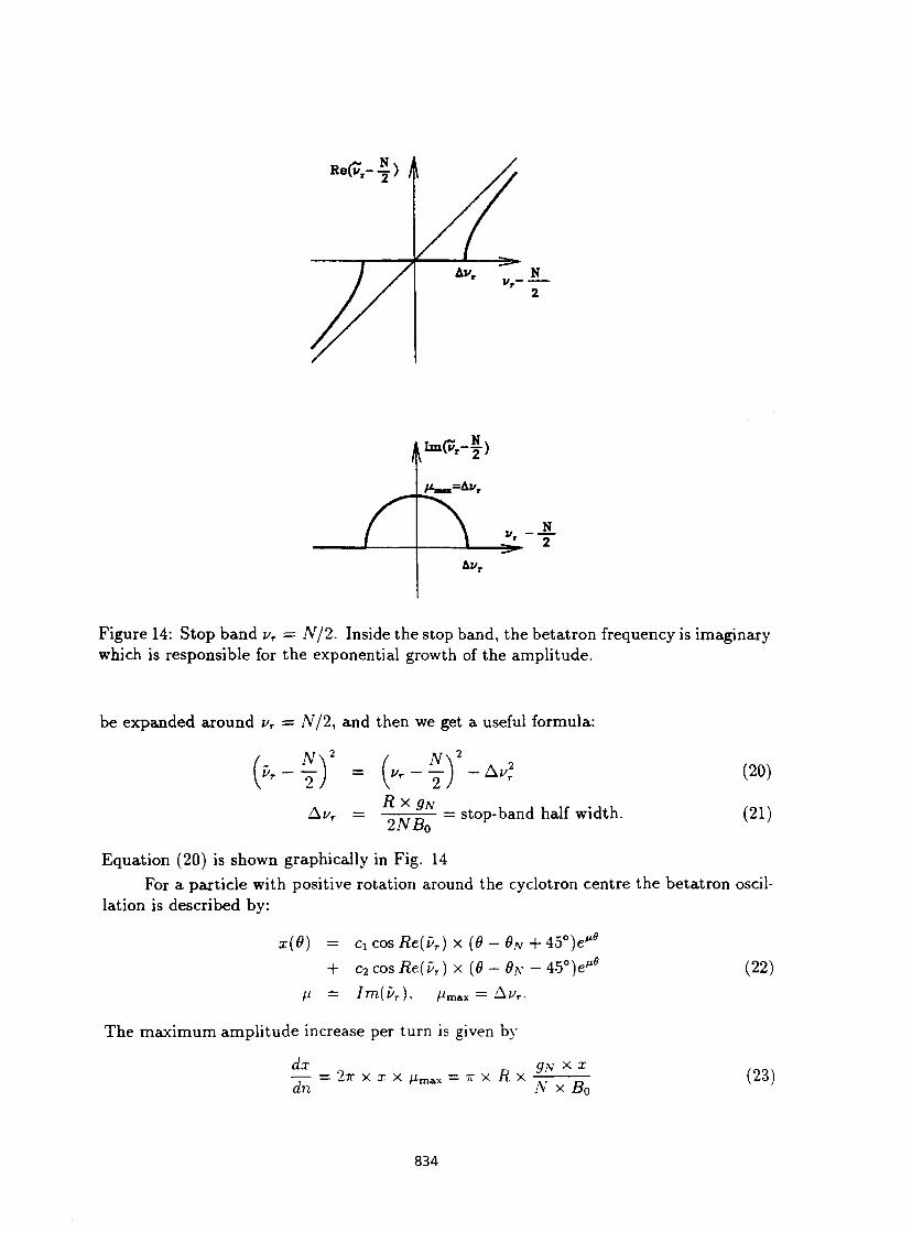
R e & - | ) A
Figure 14: Stop band vT — N/2. Inside the stop band, the betatron frequency is imaginary which is responsible for the exponential growth of the amplitude.
be expanded around vT = N/2, and then we get a useful formula:
( * - * ) " " *-*)" - (,-fV-A, ^ V r =
0 » r p = stop-band half width. 2N BQ
(20)
(21)
Equation (20) is shown graphically in Fig. 14
For a particle with positive rotation around the cyclotron centre the betatron oscillation is described by:
x{0) = CïCosReiÛr) x (0 - 0 * + 45°)e"«
+ c 2 cos Re{ûr )x(0-ON- 45°)e"'
/i = Im{vT), / x m a x = A i v
The maximum amplitude increase per turn is given by
dx gN x x —- = 2TT x x x j i m a x = x x R. x — — dn A x B0
(22)
(23)
834
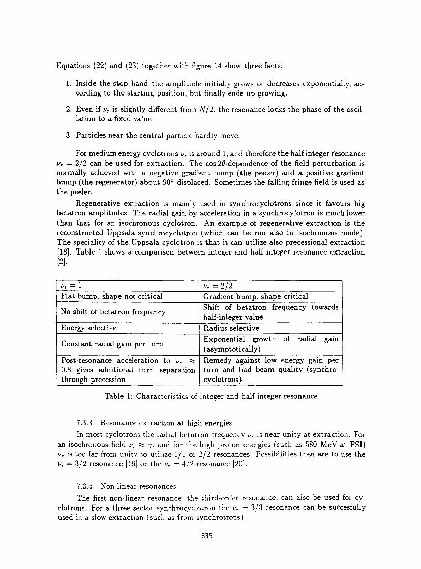
Equations (22) and (23) together with figure 14 show three facts:
1. Inside the stop band the amplitude initially grows or decreases exponentially, according to the starting position, but finally ends up growing.
2. Even if vT is slightly different from N/2, the resonance locks the phase of the oscillation to a fixed value.
3. Particles near the central particle hardly move.
For medium energy cyclotrons vT is around 1, and therefore the half integer resonance vT = 2/2 can be used for extraction. The cos 20-dependence of the field perturbation is normally achieved with a negative gradient bump (the peeler) and a positive gradient bump (the regenerator) about 90° displaced. Sometimes the falling fringe field is used as the peeler.
Regenerative extraction is mainly used in synchrocyclotrons since it favours big betatron amplitudes. The radial gain by acceleration in a synchrocylotron is much lower than that for an isochronous cyclotron. An example of regenerative extraction is the reconstructed Uppsala synchrocyclotron (which can be run also in isochronous mode). The speciality of the Uppsala cyclotron is that it can utilize also precessional extraction [18]. Table 1 shows a comparison between integer and half integer resonance extraction [2]-
I/ r = 1 ur = 2/2 Flat bump, shape not critical Gradient bump, shape critical
No shift of betatron frequency Shift of betatron frequency towards half-integer value
Energy selective Radius selective
Constant radial gain per turn Exponential growth of radial gain (asymptotically)
Post-resonance acceleration to uT as 0.8 gives additional turn separation through precession
Remedy against low energy gain per turn and bad beam quality (synchrocyclotrons)
Table 1: Characteristics of integer and half-integer resonance
7.3.3 Resonance extraction at high energies In most cyclotrons the radial betatron frequency vT is near unity at extraction. For
an isochronous field vT % -y, and for the high proton energies (such as 580 MeV at PSI) vT is too far from unity to utilize 1/1 or 2/2 resonances. Possibilities then are to use the vr — 3/2 resonance [19] or the vr = 4/2 resonance [20].
7.3.4 Non-linear resonances The first non-linear resonance, the third-order resonance, can also be used for cy
clotrons. For a three sector synchrocyclotron the vr = 3/3 resonance can be succesfully used in a slow extraction (such as from synchrotrons).
835
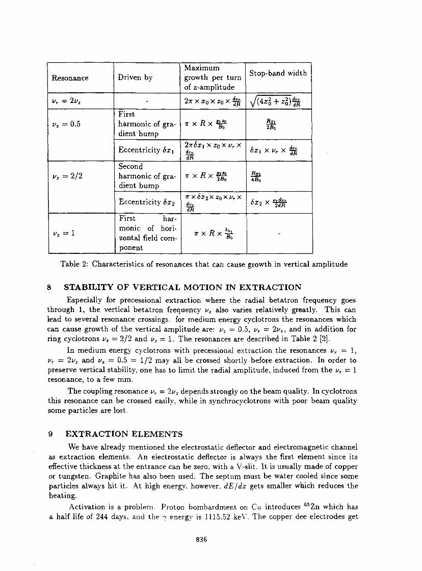
Resonance Driven by Maximum growth per turn of z-amplitude
Stop-band width
vT — 2vz - 2x x i 0 x zo x ^ V(4x§ + zg)ft
vz = 0.5 First harmonic of gradient bump
i x R x ^ Rax 2B 0
vz = 0.5
Eccentricity 6x\ 2x6xi x z0 x vT x
dR 6x1 x i / r x |
vz = 2/2 Second harmonic of gradient bump
irxRx®^ 522 4B 0
vz = 2/2
Eccentricity 6x2
•K X 6X2 X Zo X i/ r X bx* x isf
!/, = !
First harmonic of horizontal field component
7T X R X -Ê1- -
Table 2: Characteristics of resonances that can cause growth in vertical amplitude
8 S T A B I L I T Y OF V E R T I C A L M O T I O N IN E X T R A C T I O N
Especially for precessional extraction where the radial betatron frequency goes through 1, the vertical betatron frequency vz also varies relatively greatly. This can lead to several resonance crossings, for medium energy cyclotrons the resonances which can cause growth of the vertical amplitude are: vz = 0.5, vr = 2i/ 2, and in addition for ring cyclotrons i/z = 2/2 and vz = 1. The resonances are described in Table 2 [2].
In medium energy cyclotrons with precessional extraction the resonances vT — 1, vT = 2vz and vz = 0.5 = 1/2 may all be crossed shortly before extraction. In order to preserve vertical stability, one has to limit the radial amplitude, induced from the vT = 1 resonance, to a few mm.
The coupling resonance vT = 1vz depends strongly on the beam quality. In cyclotrons this resonance can be crossed easily, while in synchrocyclotrons with poor beam quality some particles are lost.
9 E X T R A C T I O N E L E M E N T S
We have already mentioned the electrostatic deflector and electromagnetic channel as extraction elements. An electrostatic deflector is always the first element since its effective thickness at the entrance can be zero, with a V-slit. It is usually made of copper or tungsten. Graphite has also been used. The septum must be water cooled since some particles always hit it. At high energy, however, dE/dx gets smaller which reduces the heating.
Activation is a problem. Proton bombardment on Cu introduces 6 5 Z n which has a half life of 244 days, and the 7 energy is 1115.52 keV. The copper dee electrodes get
836
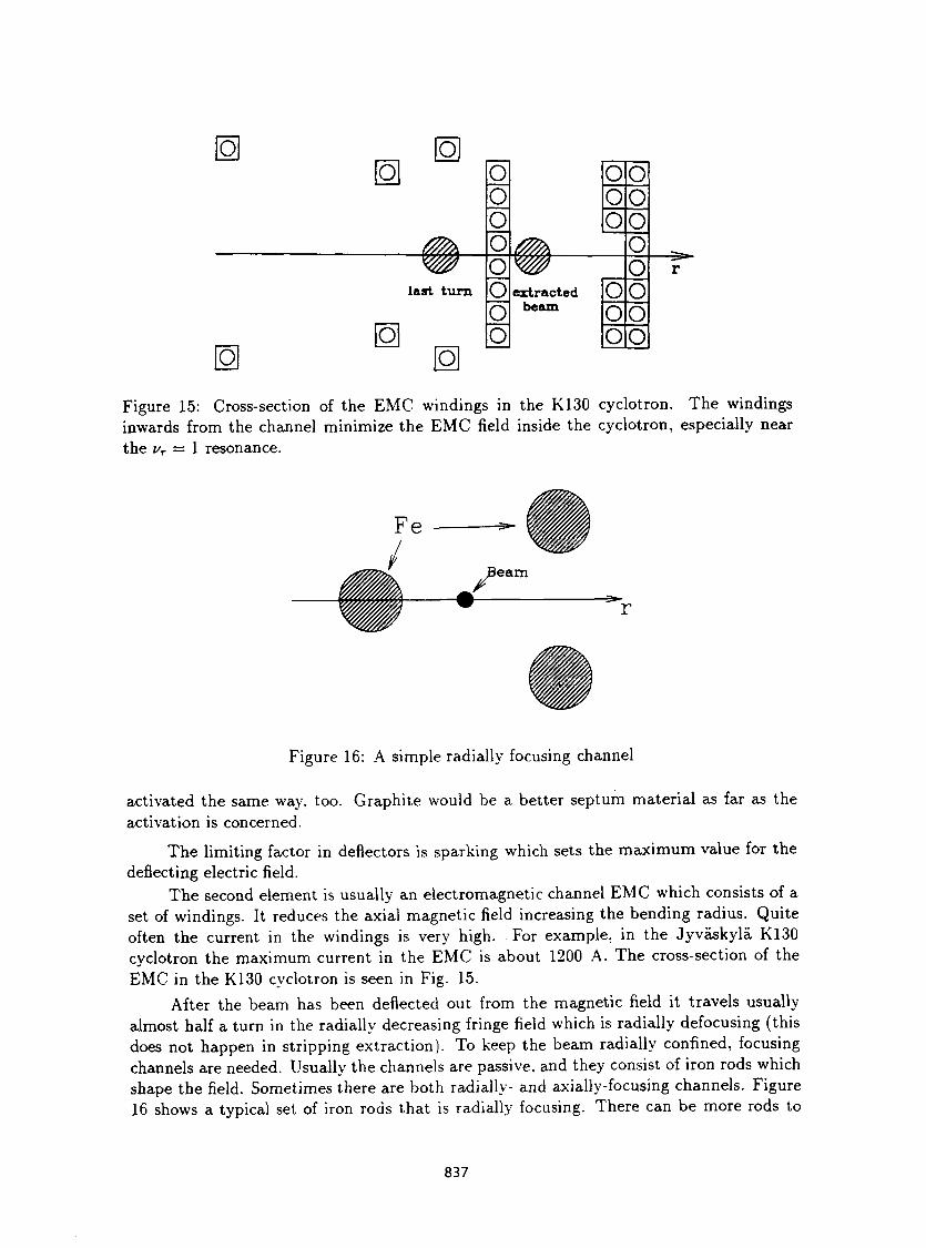
o
o
o o o
o o
0%\ o *w o
last turn o o o o
o
o o o
extracted beam
o o o
o o o o o o o o
Figure 15: Cross-section of the EMC windings in the K130 cyclotron. The windings inwards from the channel minimize the EMC field inside the cyclotron, especially near the vT — 1 resonance.
Figure 16: A simple radially focusing channel
activated the same way. too. Graphite would be a better septum material as far as the activation is concerned.
The limiting factor in deflectors is sparking which sets the maximum value for the deflecting electric field.
The second element is usually an electromagnetic channel EMC which consists of a set of windings. It reduces the axial magnetic field increasing the bending radius. Quite often the current in the windings is very high. For example, in the Jyvâskylâ K130 cyclotron the maximum current in the EMC is about 1200 A. The cross-section of the EMC in the K130 cyclotron is seen in Fig. 15.
After the beam has been deflected out from the magnetic field it travels usually almost half a turn in the radially decreasing fringe field which is radially defocusing (this does not happen in stripping extraction). To keep the beam radially confined, focusing channels are needed. Usually the channels are passive, and they consist of iron rods which shape the field. Sometimes there are both radially- and axially-focusing channels. Figure 16 shows a typical set of iron rods that is radially focusing. There can be more rods to
837
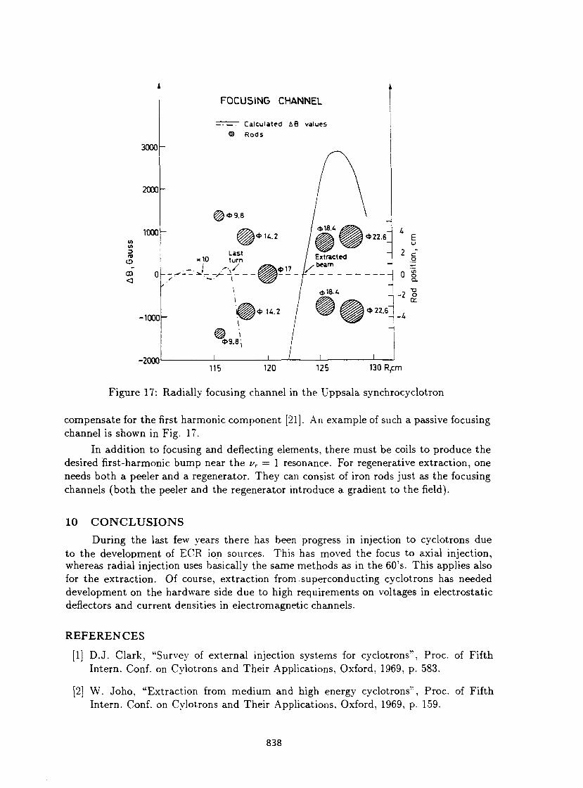
3000
2000
1000 m m D ID O
m o
-1000
-2000 115 120 125 130R,cm
Figure 17: Radially focusing channel in the Uppsala synchrocyclotron
compensate for the first harmonic component [21]. An example of such a passive focusing channel is shown in Fig. 17.
In addition to focusing and deflecting elements, there must be coils to produce the desired first-harmonic bump near the vT = 1 resonance. For regenerative extraction, one needs both a peeler and a regenerator. They can consist of iron rods just as the focusing channels (both the peeler and the regenerator introduce a. gradient to the field).
10 C O N C L U S I O N S
During the last few years there has been progress in injection to cyclotrons due to the development of ECR ion sources. This has moved the focus to axial injection, whereas radial injection uses basically the same methods as in the 60's. This applies also for the extraction. Of course, extraction from superconducting cyclotrons has needed development on the hardware side due to high requirements on voltages in electrostatic deflectors and current densities in electromagnetic channels.
R E F E R E N C E S
[1] D.J. Clark, "Survey of external injection systems for cyclotrons", Proc. of Fifth Intern. Conf. on Cylotrons and Their Applications, Oxford, 1969, p. 583.
[2] W. Joho, "Extraction from medium and high energy cyclotrons' 1, Proc. of Fifth Intern. Conf. on Cylotrons and Their Applications, Oxford, 1969, p. 159.
838
FOCUSING CHANNEL
: " = - Calculated ÛB values © Rods
x10
— J
I «9.8
Last turn
-y
}4>H.2
V * > 1 7
<*22.6
2 c o
[3] R. Keller, et al., CERN 60-2 (1960)
[4] A.J. Cox, et al., Nucl. Instr. Meth. 18-19,118(1962).
[5] CEA-N 621,76(1966).
[6] R. Maillard, et al., CEA-N 1032,67(196S).
[7] J.L. Belmont and J.L. Pabot, "Study of axial injection for the Grenoble cyclotron", IEEE Trans. Nucl. Sci. N S - 1 3 No. 4,191-193(1966).
[8] R.W. Muller, "Novel inflectors for cyclic accelerators", Nucl. Instr. and Meth. 54,29-41(1967).
[9] J.I.M. Botman, J. Reich, P. Wucherer and H.L. Hagedoorn, "Analytical t reatment of ion inflectors". Eleventh Intern. Conf. on Cyclotrons, 1987, Tokyo, ed. M. Sekiguchi, Y. Yano and K. Hataka, 263-266.
[10] G. Bellomo, D. Johnson. F. Marti and F.G. Resmini, "On the feasibility of axial injection in superconducting cyclotrons", Nucl. Instr. Meth. 206,19-46(1983).
[11] V.A. Gladyshev, et al.. Sov. Atom. Ener. (Transi.) 18, 3,268(1965).
[12] R. Beurtey, et al., Nucl. Instr. Meth. 33,338(1965).
[13] R.S. Lord, et al., "Coupled operation of the Oak Ridge Isochronous Cyclotron and the 25 MV Tandem", IEEE Trans. Nucl. Sci. N S - 2 8 , No. 3,2083(1981).
[14] W.G. Davies and A.R. Rutledge, "Design of the injection system for the Chalk River superconducting cyclotron project". IEEE Trans. Nucl. Sci. N S - 2 6 , No. 2,2086(1979).
[15] J. Ferme, "Project "OAE" at Ganil. a project for increasing the heavy iorf energies", Proceedings of the 11th International Conference on Cyclotrons and Their Applications, Tokyo, 1987, p. 24.
[16] R. Mahrt and 0 . Bôttger, Nucl. Instr. Meth. 71,45(1969).
[17] N. Vogt-Nilsen, MURA-118(1956).
[18] S. Holm, "Operational experience of the reconstructed Uppsala synchrocyclotron", Proc. of the Twelfth Intern. Conf. on Cyclotrons and Their Applications, Berlin, 1989, p. 17.
[19] D.I. Hopp and J.R. Richardson, Nucl. Instr. Meth. 44,277(1966).
[20] D.I. Dmitrievsky et al., IEEE Trans. Nucl. Sci. N S - 1 3 No.4,84(1966).
[21] S. Holm, R. Peterson, P.U. Renberg and 0 . Sunberg, "Design of passive beam extraction elements for the GWI cyclotron", GWI-PH 1/84.
839

APPLICATIONS OF PARTICLE ACCELERATORS O.Barbalat CERN, Geneva, Switzerland
ABSTRACT Particle accelerators are now widely used in a variety of applications for scientific research, applied physics, medicine, industrial processing, while possible utilisation in power engineering is envisaged. Earlier presentations of this subject, given at previous CERN Accelerator School sessions have been updated with papers contributed to the first European Conference on Accelerators in Applied Research and Technology (ECAART) held in September 1989 in Frankfurt and to the Second European Particle Accelerator Conference in Nice in June 1990.
1. INTRODUCTION AND OVERVIEW
Particle accelerators are one of the most versatile instruments designed by physicists. From its inception, as the cathode ray tube by J.J. Thomson who used it to discover the electron, to the present giant colliders, it is intimately associated with the major milestones of nuclear and particle physics.
Today it is widely used in nearly every field of physics from elementary particles to solid state. It is also an essential instrument in many other areas of research to study structures in chemistry and biology or to perform sensitive trace element analysis. Its range of application is being considerably extended by its capability of generating synchrotron radiation. Progress in nuclear and particle physics originated from studies with accelerators is playing now a determining role in astrophysics and cosmology.
Industrial applications cover a broad range such as ion implantation in the semiconductor industry but also the modification of surface properties of many materials. A particularly promising application is microlithography with synchrotron radiation for high density integrated electronic circuits.
Radiation is being used in a variety of processes to preserve food, sterilize toxic waste or polymerize plastics. Activation methods with compact-accelerator-produced neutrons are applied in geophysics and are being developed for the detection of explosives.
It is probably in medicine that accelerators have found their wider field of applications, either for isotope production in view of diagnosis or treatment, or for therapy with gamma rays and, more recendy, with neutrons and heavy charged particles.
Accelerators may also play a key role in power engineering. Studies of inertial confinement fusion by heavy ions are actively pursued in several countries. Accelerators are an essential ingredient to provide the additional heating needed for plasma ignition in magnetically confined tokomaks. Finally research is also going on to use accelerators to incinerate long-life nuclear waste which could lead to an acceptable long-term disposal solution.
When discussing the application of particle accelerators one should also mention the technical and industrial evolution induced by these applications. Whereas the front line machines are usually general purpose facilities designed for fundamental physics research, such as particle or nuclear physics, these machines may later find a new life in more applied research fields such as solid state or material science. They are then followed by dedicated facilities for a more specialised type of research or process (synchrotron radiation, isotope production) and finally by single purpose optimized devices such as soft X-ray generators for microlithography,
841
compact cyclotrons for positron emitting isotope production, ion implanters or radiotherapy electron accelerators. They are then produced on an industrial basis rather than designed and built by or for a research laboratory.
2. RESEARCH APPLICATIONS
2 .1 Particle physics
The development of particle physics has been directly determined by the progress achieved in building accelerators of ever increasing energy. One can easily recall examples, such as the discovery of the antiproton at the Berkeley Bevatron in the mid-fifties, the two neutrinos with the Brookhaven AGS machine in the early sixties, neutral currents with the CERN PS, the J/<|> with the AGS and the Stanford Linear Accelerator in the seventies. More recently, the W and Z particles with die CERN Spp-S collider and the number of neutrinos with CERN's LEP are a clear demonstration of the continuing importance of accelerators to get a better and deeper insight in the structure and properties of the building blocks of matter, quarks and leptons, and in the forces by which they interact
In about forty years, from 1959 to 1990, accelerators and colliders have allowed physicists to gain three orders of magnitude from 10"^ to 10"^ m (corresponding to 100 GeV for the constituents in the centre-of-mass reference frame) in their quest for probing matter at an increasingly finer scale. They can describe our complicated world with only three families of particles, each being constituted of two quarks and two leptons characterized by the properties of charge, flavour and colour which are responsible for the electromagnetic, the weak and the strong interactions. Accelerators of the present generation have led to the discovery of the carriers of these interactions, the gluons and the intermediate vector boson better known as W and Z particles.
A new generation of very high energy machines (the large hadron collider (LHC) and the super superconducting collider (SSC)) are now under design in the hope of elucidating some of the many questions which are still open, while lower energy specialized devices such as t-charm and B-factories are envisaged to study more specific areas.
2.2 Nuclear physics
Accelerators are the essential tool by which physicists have been able to probe the nucleus and to determine its structure and behaviour. Depending on the properties of interest, one is using electron, proton and more recently heavy ion beams. The increase of available energy and intensity is also opening new opportunities.
In the past nuclear physics research has been devoted to the study of the structure of individual nuclei, their excited states and the associated spectroscopy. Present areas of interest are for instance super-deformed nuclei with extremely high angular momenta or exotic nuclei far from the line of stability produced by facilities such as Isolde at CERN or GANIL in France. The availability of heavy ion machines allows the dynamics of nucleus-nucleus collisions and the fragmentation of nuclei to be studied. Subnucleonic degrees of freedom of nuclei such as meson exchange currents are investigated with both electron and hadronic probes, hence the interest for the Kaon project in Canada. The study of nuclear matter under extreme conditions allows phenomena related to the composite nature of nucléons to be investigated. It is, in particular, hoped to reach the phase transition from nucleous to quarks and gluons by accelerating lead ions in the CERN SPS.
Electromagnetic properties of nuclei are best studied with electron beams of high energy (-10 GeV) to reach spatial resolution of 0.1 fm.
842
A new generation of high intensity electron accelerators will allow the quark structure of nucléons and how they combine into hadrons to be investigated. A 4 GeV machine (CEBAF) is under construction in the U.S.A. and a 10 GeV version is planned in France.
Beam cooling developed for the pp" collider is opening up many possibilities in nuclear physics on machines like LEAR at CERN and on dedicated-heavy ion storage rings under construction in Germany and Scandinavia.
2.3 Cosmology and astrophysics
Accelerators are now becoming more and more complementary to telescopes. The universe originated in a hot Big Bang. Temperature decreased with time and the increasing energy of accelerators and colliders allows the physicist to study experimentally processes closer to the origin of the universe. At temperatures equivalent to an energy of 100 GeV, which is where present machines allow observations, one is 10" 10 second from this origin and it is possible to study the moment when W and Z particles acquired their mass and disappeared from the scene. Results obtained with accelerators have made it possible to explain cosmic observations such as the hydrogen/helium ratio, and to determine the number of neutrino families.
Astrophysics issues can also be settled with accelerators. For example the understanding of the synthesis of elements in stars (nucleo-synthesis) requires the determination of the rate and cross sections of nuclear reactions. A recent development is the need to use radioactive particle beams which are necessary to investigate some reactions. Their understanding could explain some not yet understood features of stellar burning and, in particular, aspects of the sun's behaviour such as the 11-year solar cycle.
2.4 Atomic physics
The detailed behaviour of the complex multiparticle systems which constitute atoms and ions is still far from being understood and computable. A large amount of research is conducted in many institutions, although the total number of facilities has probably decreased from the 850 positive-ion accelerators with energies below 33 MeV reported to exist in the early 1970's.
The following topics discussed at recent conferences illustrates this type of research:
- Mechanisms of atomic collisions and ionization processes (charge distribution and rotational properties of electron clouds during collisions).
- Correlation effects in atomic collisions. - Study of highly excited atomic states produced during atomic collisions. - Physics of highly-ionized ions and of bare atoms. - Charge exchange cross sections of high velocity or even relativistic ions (electron capture
and electron losses). - X-rays produced by relativistic ion collisions. - Quasi-molecular states produced by nearly symmetric ion-atom collisions. - Electron impact ionization processes and electron ion collisions (of particular interest for
the study of both laboratory and astrophysical plasmas). - Electron emission following fast ion impact on thin solid targets (in view of quantitative
analysis of surface contamination). - Resonant transfer and excitation (RTE) in ion-atom collisions (effect due to the resonant
capture of a target electron by the projectile ion and the subsequent excitation of that ion). - Production of convoy electrons. (This term refers to the electrons ejected in ion-atom and
ion-solid collisions closely matched in vector velocity to that of the incident ions). - Precision ion energy loss in solids. - Precision range distribution and electronic stopping power in solids. - S tudy of molecular ion s.
843
2.5 Condensed matter physics and material science
The main tools used by physicists to probe the structure and properties of matter in the solid state have for a long time been X-rays produced by conventional sources and neutrons generated by nuclear reactors.
This picture has changed dramatically over the last few years with the advent of new accelerator derived radiation sources, synchrotron radiation now produced by dedicated electron machines, and neutrons from spallation neutron sources. In addition ion beams are used in a variety of ways.
Many research fields have been opened up or offered new prospects by the availability of synchrotron radiation with its brightness and tunability. The latter makes it possible to exploit the fact that each element exhibits a sharp increase in absorption at certain wave-lengths called absorption edges. This is used to obtain information on the local or long range structure of material. The technique called EXAFS (Extended X-ray Absorption Fine Structure) gives information on the atomic environment around a particular elemental constituent of a complex material. This is used to study atomic arrangements in many condensed matter systems such as catalysts, crystals, glasses and other amorphous materials, polymers, surface layers, thin films, etc.
Because of their absence of charge and their penetration ability, neutrons make excellent probes for the study of condensed matter. Neutron scattering has made it possible to understand the bonding and cohesion of metals, semiconductors and insulators. Neutron diffraction is concerned with the structural arrangement of atomic particles in a material and the relation of this arrangement to its physical and chemical properties.
Energetic (500 MeV to 1 GeV) protons produce intense bursts of neutrons by spallation in a target which allows a substantial intensity improvement compared with nuclear reactors. Furthermore, the time structure of the beam provides the added advantage of low background because the source is off most of the time. Studies with spallation neutrons are complementary to those carried out with synchrotron radiation on topics like crystallography, in particular for powders when single crystals cannot be grown, liquids and amorphous materials, surfaces and intermaterial interfaces (air-liquid, liquid-liquid and liquid-solid), polymers, thin films, membranes, measurements under shear flow, magnetic and electrical fields.
Ion beams are utilized in many complementary processes to determine the elemental composition of samples. The main techniques are:
- Rutherford Backscattering (RBS) - Proton Induced X-ray Emission (PIXE) - Charged Particle Activation Analysis (CPAA) or Nuclear Reaction Analysis (NRA) - Secondary Ionisation Mass Spectrometry (SIMS) - Particle Desorption Mass Spectrometry (PDMS).
RBS and PIXE are well-established techniques, CPAA and NRA are newer. While RBS is well adapted to the study of heavy elements in a light substrate which is the case of semiconductor research (Si substrate), NRA is better adapted to studies of the behaviour of light elements in heavy substrates (metals) and finds, therefore, a natural field of application in metallurgy. It is being used in particular for understanding the structure and features of high-Tc
superconductors. It makes it possible to characterize unambiguously what a sample really looks like and not what it was intended to be before the constituents were made to react.
Charged Particle Activation finds its field of application in two areas: ultra-low concentrations and wear studies. It is applicable to most elements and allows trace elements to be identified at the ppb (parts per billion i.e. 10"9) level. One can determine the effect of
844
impurities such as C, N or O in metals, monitor the elaboration process and detect low-level contaminants. Ion beams are used in a wide energy range (1 to 45 MeV) allowing depth analysis ranging from microns to millimetres.
CPAA is also a sensitive and fast technique for wear studies (corrosion, erosion). One activates a thin surface layer and for suitable isotopes, the loss of activity will correspond to the loss of matter. The method was reported to be used to monitor on-line industrial processes. It has also been applied to study die effect of pH on the corrosion rate in nuclear reactors.
The utilisation of small-spot-size ion beams, also called nuclear microprobes, in the scanning mode has transformed the PIXE technique from an analytical tool into an imaging device. It permits a map of the elements and their distribution in the studied sample to be obtained so that die device could be described as being a nuclear microscope.
The elemental map can be compared with the structure given by optical or electron microscopes. A compromise must be found between resolution requiring a small spot size and sensitivity which is direcdy related to beam intensity. Hence the requirement of high brightness (which is however limited by die need not to destroy the sample). Recent progress has allowed the spot size to be reduced to die micron level.
Reported applications of this technique include the mapping of structures in multilayer semiconductor devices to monitor the manufacturing process, the study of high-T c
superconductor compound structures, the analysis of weld failures,....
The combination of RBS (Rutherford BackScattering) which allows the depth profile to be determined with PDΠcan give a three dimensional picture of the element distribution in the sample.
Whereas with ion beam analysis, the accelerator is used to bombard the sample witii ions and detect die induced atomic or nuclear processes, in accelerator mass spectrometry (AMS) the constituents of the sample are ionized, accelerated and identified by mass spectrometry.
The high sensitivity of AMS finds applications in the semiconductor industry. Semiconductor devices are rapidly degraded by even a small concentration of some impurities which can be readily detected by AMS. Up to now this was essentially studied by SIMS (Secondary Ion Mass Spectrometry). AMS gives a dramatic improvement of two orders of magnitude in sensitivity. The sample is ionized by a cesium beam. Scanning of die sample by die cesium beam allows imaging.
Anodier application of accelerators in material science is for radiation damage. It is of particular interest in studies of structural material for a future fusion power generator or for satellites and space systems.
2.6 Chemistry and biology
Accelerators are a source of radiation, in particular synchrotron light allows unique information on the chemical state to be obtained (e.g. oxidation of molecules, the chemical bonding in solids, gases and absorbed layers, structure of complex molecules and dieir dynamics, kinetics of chemical reactions).
Electron accelerators with energies up to a few MeV are used in radiation chemistry studies, for instance the radiation-enhanced chemical reactions of die highly active intermediate chemical states produced by the electron beam.
Radiation biology studies using accelerators have mainly been aimed at understanding the molecular pathways of radiation damage and with related cancer therapy.
845

Synchrotron light has revolutionized many fields of biology. It is now possible, because of the brightness and tunalibility of this source, to study the crystallography of proteins and solve large structures like viruses, and to follow the structural changes of a molecule binding to an enzyme. It is possible to study the dynamics of biological processes, for instance muscles under contraction with time frames of 10 ms.
The nuclear microprobes mentioned in the previous section also find applications in life science studies. Reported examples are the metal uptake of organisms, biomineralisation in teeth and bones, metal-related diseases, element gradient in membranes, trace elements in neurological disorders (Alzheimer disease), etc.
3 . ELEMENT ANALYSIS
The various accelerator laboratory techniques mentioned in the previous section for sample composition analysis and trace element detection are now extensively used in applied science, archeology, art or even for air travel security.
In geology and mineralogy one can proceed to element zoning in rocks and minerals, determine the composition of inclusions and analyze grain boundaries. These techniques have also been used in the analysis of the structure of lunar material and meteorites.
Progress in geology has direct application to oil exploration and mineral research. A widely used technique in the oil industry is neutron well logging. Neutrons produced by the bombardment of a tritium target by deuterons activate the surrounding rocks. The gamma ray spectrum of the activated nuclei allows the rock composition along the well to be determined and to 'log' its profile.
For acheological dating with carbon 14, accelerator mass spectrometry is used more and more instead of beta decay counting because of its much greater sensitivity. A noteworthy case has been the successful dating of the Turin Shroud with comparable results obtained in three different laboratories with a sample of only a few milligrams.
PIXE or Nuclear Reaction Activation Analysis is non-destructive and is used for studies of precious art objects. One has in this way been able to determine the composition of ancient jewels or of the pigment layers in old paintings. Pigment composition is a way to detect forgeries or additions to art-work, as old masters could not use the yet undiscovered organic compounds used in modern dies.
A recent application is the possibility to detect concealed explosives. These substances are nitrogen rich and can therefore be detected by neutron activation. Compact accelerators for use in airports have been designed for this application.
4 . MEDICINE
Accelerators are used in two broad ways in medicine for diagnostics and for therapy.
4.1 Medical diagnostics
Radio-isotopes have proved that they can give unique biochemical and physiological information when injected into living organisms. The possibility of external detection offers a non-invasive way to follow changes in the distribution of tagged atoms, observe anomalies of metabolism (changes in blood flow, oxygen utilization, glucose metabolism) or detect tumours.
846

Recently accelerator produced positron emitting radio-isotopes have been found to respond better to the needs of nuclear medicine than traditional gamma emitting nuclides, in particular the widely used technetium-99 (produced in nuclear reactors).
The annihilation radiation of positrons is easily detected and localized and has given rise to the growing field of Positron Emission Tomography (PET). They are short-lived and can be injected into human beings without giving rise to high radiation doses.
The production of these positron emitters is achieved by cyclotrons accelerating protons or deuterons in the 10 to 40 MeV range. The short half-life of these nuclei requires them to be produced and utilized on the same site by dedicated facilities. Special purpose cyclotrons are now manufactured by industry and commercially available (Ion Beam Applications in Belgium or Scanditronix in Sweden).
Another technique is based on the high X-ray flux available from synchrotron radiation. The sensitivity to contrast agents such as iodine can be enhanced by two or more orders of magnitude by taking the difference between a pair of exposures with monochromatic X-ray beams, one just above, the other below the agent absorption edge. The increased sensitivity makes it possible to detect restrictions in arteries by angiography without the invasive procedure of inserting a catheter in a major artery.
Finally one should mention the application of accelerator derived superconducting magnets to the fastly growing field of nuclear magnetic resonance (NMR) imaging, a device which has become a powerful diagnostic tool superior in many respects to X-rays scanners. The availability of reliable and powerful magnets with small energy requirements and an already proven technology has been a decisive factor.
4.2 Radiotherapy
It is estimated that 25 to 30% of the population of industrial countries will contract cancer in their life-time and that about half of mese will receive some form of radiation therapy. The aim of radiotherapy is to destroy the malignant cells without damaging the healthy tissues. Unfortunately radiation travels in straight lines through the body and destroys cells in the entrance region between the surface and the tumour and most kinds of radiation also have effects downstream before exiting the body. Unwanted damage to normal tissues are minimized by delivering the radiation from different directions crossing at the location of the tumour.
The vast majority of present facilities use X or gamma rays, or photons produced by 60Co or by linear electron accelerators. Accelerators are more versatile and can provide deeper penetration when necessary. Machines of 5 to 20 or even 40 MeV are constructed industrially by several manufacturers: Siemens in Germany, CGR-MeV in France and Philips Medical Systems in Great Britain.
Major progress in cancer therapy is being achieved by improvement in the local control of the tumour. This is the result both of improved diagnostics tools which allow a better localisation of the malignant tissues and of the use of particle beams which permit a higher energy deposition (the characteristic parameter is the LET : Linear Energy Transfer) and a more accurate range.
Because of their high penetration and their biological effectiveness, neutrons are, for some cases, more advantageous than photons. Neutrons are generated by the reaction of 200/300 keV deuterons on a tritium target. Large deuteron currents are needed to obtain sufficient fluxes resulting in rather short target life-times. Furthermore, the neutron energy obtained in this way does not allow to treat deep seated tumours. One is therefore using
847
classical cyclotrons with energies from 30 to 65 MeV to produce fast neutrons by reaction on a beryllium target
Pions, protons and heavier ions offer the possibility of improving the damage ratio between malignant tumours and healthy tissues. With heavy charged particles one can achieve a highly localized distribution. The so-called Bragg peak (region of maximum energy deposition) is only a few millimetres wide near the end of the range, which allows a high dose to be delivered with less damage to die overlaying tissues. The required penetration depths make it necessary to use machines capable of producing particles in the several hundreds of MeV range. Present installations have still an experimental character and are located near accelerators built for another purpose (SIN, Bevalac, TRIUMF, Dubna,...) but dedicated therapeutical facilities are under design or construction. One should in particular mention here the European Light Ion Medical Accelerator (EULEMA) proposal. Heavy ions combine the advantages of high LET and precision penetration depth. Another feature is the possibility to combine therapy with treatment monitoring with the use of positron emitting ions which allow the adjustment of the beam to be checked by tomography.
The improvements in tumour control, reduction in mortality and restoration of individual quality of life reported at the recent EPAC Conference is a testimony of the contribution of accelerator technology to medicine.
In contrast with radiotherapy proper which involves radiation dose delivery to a substantial volume of tissue by a large number of daily treatments spread over several weeks, charged particle radiosurgery is the treatment of a well defined target, such as an intracranial lesion, with a narrow particle beam delivered in one or a few fractions. Various ions in the 100 to 500 MeV range are being used for that application.
5 . INDUSTRIAL PROCESSING
5.1 Ion implantation
Ion implantation for manufacturing semiconductors is one of the major present industrial applications of particle accelerators. This process allows the introduction of ions of a specific type at the desired depth to dope in the appropriate way the semiconductor substrate to achieve the required circuit pattern. This technique has replaced the traditional ion diffusion used previously. It allows accurate and reproducible manufacturing of all the present compact micro-circuits.
The present generation of low and medium current implanters derive from physics laboratory devices with current of a few mA and voltages of a few hundred kV generated by multistage voltage multipliers. High current machines (say 300 mA) derive from the wartime Calutron isotope separator. A major technical issue is the scanning either of the beam or of the target to achieve a tight control of the implant angle variations across the semiconductor wafer to achieve consistent electrical characteristics.
The present trend is in the direction of higher energies produced either by electrostatic belt generators, RF linacs or RF quadrupoles to achieve penetration depths exceeding one micron. This gives the possibility to modify bulk rather than only surface properties or to produce buried patterns, or to synthesize local and in depth oxides or silicides, so as to achieve truly tfiree-dimensional semiconductor circuits.
Ion implantation can also be used to modify other properties than just electrical conductivity, surface hardness, corrosion resistance, friction coefficient, fatigue behaviour, adhesive properties or catalytic behaviour. Applications have been found in the automotive industry to improve the performance of highly-stressed components (ball bearings, crankshafts, helicopter rotor shafts, ...). Other applications have been found in the medical field where
848

spectacular increase in the lifetime of artificial joints (hip, knee,...) have been achieved and are now commercially successful.
5.2 Radiation processing
When passing across matter, particle beams cause excitation and ionization of the material. Charged and uncharged fragments of molecules, resulting from bond breaking, have high chemical activity and tend to react quickly with one another or with other molecules. This opens the possibility to perform a variety of chemical processes.
Examples are:
- Polymerisation of low molecular components (monomers). The rate of polymerisation can be enhanced by a factor 100 compared with the process in an untreated monomer.
- Radiation modification of wood to improve mechanical, fire or biological resistance. - Radiation cross-linking of polymers to create three-dimensional structures to achieve, for
instance, insolubility in organic solvents. This process is most extensively used with polyethylene pipes and insulated wires and cables operating in hard environmental conditions (high temperature, aggressive chemical media, irradiation,...).
- Polyethylene cross-linking to achieve a 'memory' effect and so obtain a thermo-shrinkable material used for tight packing of goods.
- Radiation vulcanisation of rubber to improve heat resistance and resistance to ageing and deformation at high temperature. The effect is again obtained by cross-linking.
- Curing of varnish and paint coatings. Radiation processing acts in three ways by polymerisation of the monomers, cross-linking of the produced polymeric molecules and the development of chemical bonding between polymer and substrate.
- Fabrication of crease-resistant, fireproof and hydrophobic textiles. This is the result of inducing polymerisation and cross-links and grafting water repellent compounds such as fluorinated acrylates or siloxanes on cotton or viscose rayon fibres.
- Destruction of" noxious material by causing scission of unwanted molecules. The industrial and domestic utilisation of surface-active synthetic agents (such as detergents) creates a serious sewage treatment problem since these products feature a high chemical stability. Radiation promotes their breaking into lighter and more easily removable substances. In the presence of oxygen, organic compounds are oxidized, which enhances the treatment effect.
- Purification of industrial gases. To clean gas containing sulphur or nitrogenous impurities one adds ammonia (NH3). Irradiation initiates reactions of N O x and SO2 with NH3. The resulting ammonia salts can then be trapped with an electrical precipitator.
5.3 Food preservation
Radiation sterilisation of foodstuff has a great economic potential. It allows one to avoid the chemical additives now used for food preservation and which are meeting increasing objections in view of their potential carcinogenic effects or to avoid the need to maintain at low temperature ready-to-serve meals.
One of the most promising applications of radiation technology is sterilisation of culinary processed foodstuff which can after suitable packaging be stored at room temperature for several months. Successful tests have been carried out with a large variety of foods such as smoked and fried sausages, ham, roasted potatoes, meat, chicken, filleted fish
Another use of radiation is to suppress the activity of micro-organisms in fresh perishable food stuffs. Storage life of strawberries, cherries, peaches, grapes, tomatoes,... can be extended by 1 or 2 weeks. Unwanted germination of agricultural crops like potatoes or onions can also be prevented by radiation.
849
Radiation is also used in storehouses for crop protection against insects. The main method of insect control at present consists of treating grain with chemicals, like methyl bromide or chloropicrin. This has the disadvantage, besides the high cost, of leaving toxic substances in the products. It has been demonstrated that with radiation doses of 100 to 200 Gy most insects become sterile and die within 2 or 3 weeks while there is no measurable deterioration of wheat, maize, peas, rice or dried fruit
Insect sterilisation by radiation is not only appropriate for food preservation in storerooms but has also been used for suppression of pests in natural conditions by releasing sterile insects over large areas. Successful operation against certain types of flies have been reported in the United States and in Japan.
5 .4 Sterilisation
Industrial and domestic sewage sludge contains useful organic and inorganic substances which may be used as fertilizer in agriculture or as a nourishing addition to fodder. Special treatment for killing pathogenic micro-organisms is however required beforehand and can be achieved by moderate radiation doses (30 Gy). This treatment can be combined with the destruction by radiation of harmful chemicals mentioned in a previous section.
Radiation is also employed to sterilize medical products (garments, gloves,...) and to treat hospital waste products to ensure safe disposal.
5.5 Ion-beam processing
Heavy-ion accelerators are used to produce microporous membranes in thin film materials. One can make holes ranging in diameter from 0.05 to 1 mm in membranes having a thickness of several tens of microns. The main applications are filters for the food industry and porous substrates for growing cells or micro-organisms for biology or medical research. Commercial companies have been set up and buy beam time on research accelerator to produce these membranes (GANTL, Louvain-la Neuve).
5.6 Microlithography
X-ray lithography with synchrotron radiation produced by electron accelerator is considered a very strong contender for the production of the next generation of integrated circuits.
Present mass produced circuits are made by the photo-lithography process by which a master mask is projected onto the surface of a silicon wafer coated with a 'photoresist'. Present technology uses visible light which limits the resolution to around 1 micron. Resolution of 0.7 to 0.5 (im can be reached with strong lenses, but at the expense of depth of focus which raises serious problems of process control and yield. This is adequate for the present 4 MBit memories, but it reaches its limit with 16 MBit memories which require a ~ 0.5 ^m line-width. However 64 MBit will require 0.35 UJÏI and 256 MBit will need 0.2 |im.
The most promising technique is to use X-ray lithography which allows a 0.1 u,m resolution. Synchrotron radiation, because of its brightness, good collimation and capability to deliver the required power of the order of a kilowatt, appears well suited for this application. Some ten machines in the 500 to 1000 MeV range, of which six in Japan, are under various design stages in the world.
850

6. POWER ENGINEERING
6.1 Heavy ion fusion
The acceleration of heavy ions for fusion is one of the great challenges of accelerator physicists. Heavy ions to achieve inertial confinement offer several advantages over lasers which are currently studied for the same goal. The acceleration of ions can be achieved with a higher efficiency than for the corresponding laser beam and with a higher repetition rate.
Heavy ions have a high specific deposition power in matter and the beam can easily be transported and focused. A major problem is to achieve a symmetric implosion and one is therefore led to consider the so-called indirect drive whereby the kinetic energy of the beam is converted into radiation before imploding the pellet of material to be fused. Requirements for inertial confinement fusion are pulses of 10 MJ of 10 ns duration, with therefore instantaneous power of 10*5 W over areas of the order of one cm^.
To achieve these values a considerable amount of R&D work is still necessary, but steady progress is reported at accelerator conferences.
6.2 Plasma heating
It now appears that to achieve the required ignition temperatures and obtain an appreciable level of commercial power from a magnetically confined plasma, new methods of heating must be developed. One of the most attractive sources of additional power is the use of a multi-megawatt ion accelerator. The accelerator generates a negative ion beam which is neutralized in a gas or by photo-detachment, before crossing the confining magnetic field. It seems possible to reach the desired performance (~ 1 MeV/1-2 A) with an RFQ. Initially deuterium had been proposed, but heavier ions like oxygen appear more suitable.
6.3 Radioactive waste incineration
The possibility of using high energy accelerators for transmuting long-life-time radioactive waste from fission reactors into stable or short-life isotopes is under investigation in several laboratories. Studies have been carried out at CERN in die early eighties with ^ S r and 137 C s using the 600 MeV beam of the synchro-cyclotron.
An ambitious Japanese project for the incineration of transuranium waste using a high energy proton induced spallation reaction was presented at the last European Particle Accelerator Conference in Nice. One of the major problems of these incineration schemes has always been the energy balance. The process must not require a disproportionate amount of energy compared with the reactor production. The Japanese proposal is based on a 1.5 GeV proton linac with an average current of 10 mA.
The actinides transmutation target would be a subcritical sodium-cooled assembly. The generated reaction energy would be recovered through a heat exchanger and a power plant to drive the accelerator. The facility could handle some 200 kg of actinide waste per year, corresponding to the production of about eight reactors of a nominal capacity of 1000 MW with an efficiency of 50%, requiring therefore 30 MW. The proposed facility could generate excess energy for the electrical network. Another accelerator based incineration scheme is under study at Los Alamos
6.4 Other
The possibility of using muons, a type of heavy electrons produced by accelerators, has at one time been envisaged to catalyze thermonuclear fusion. Muonic atoms, because of the large muon mass, have smaller radii than normal atoms. Their probability to fuse is therefore higher
851

and the conditions for ignition easier to achieve. Unfortunately more detailed calculations have shown that the muon life-time is too short to achieve an overall positive energy balance.
Accelerator derived technologies, in particular in the field of superconductivity, may have a major impact in power engineering in the coming decades. Superconductors developed for high field accelerator magnets could be used for large scale magnetic energy storage of electricity. Superconductors have the potential of transporting large quantities of electricity in a compact cable compared with overhead lines. Superconducting alternators are under development. Commercial magneto-hydrodynamic or magnetically confined fusion generators would require efficient magnets and therefore have to use similar technologies.
7 . CONCLUSION
In the hundred years following their first use to discover the electron, particle accelerators have evolved into a wide variety of devices up to the giant colliders of particle physics. They have given rise to a multitude of applications, the most widespread of which is the television picture tube which is too familar to be even worth mentioning. They now encompass most of the fields of physics research, play an essential role in medicine for both diagnostics and therapy, are used for many industrial processes and may, in the next century, offer possible technical answers to the energy problems of mankind.
Accelerator derived technologies are even more diverse, ranging from the already well established NMR imaging to novel methods of electricity generation, transport and large scale storage.
BIBLIOGRAPHY
• Applications of particle accelerators to particle physics as well as the corresponding physics results are regularly reported in the CERN Courrier.
• Applications to physics in general together with discussion of new facilities and their research programmes are a regular feature of Europhysics News, the journal of the European Physics Society.
• Interaction between particle physics, astronomy and cosmology is the subject of the series of ESO-CERN Symposia.
• Applications in research and industry are extensively covered in the proceedings of the series of International Conferences on Applications of Accelerators in Research and Industry organized every second year in Denton, Texas, edited by J.L. Duggan and I.L. Morgan and published by North Holland. (The 10th Conf. took place in November 1988 and one was scheduled for 1990).
• A first European Conference on Accelerators in Applied Research and Technology (ECAART) was organized in Frankfurt-am-Main in September 1989 and its proceedings edited by K. Bethge, F. Rausch and P. Misaelides have recently been published by North Holland. A second conference is planned for 1991.
• Invited review papers on the applications of accelerators to industry and medicine have been prepared by K. Bethge and Y. Jongens respectively for the first European Particle Accelerator Conference (EPAC) held in Rome in June 1988 and are included in the proceedings published by World Scientific.
852
Several papers on a variety of applications (synchrotron radiation for microlithography, radiotherapy, nuclear waste incineration, heavy ion fusion) were presented at the June 1990 EPAC, held in Nice.
Information on medical applications of ion beams can be found in the proceedings of the Eulima Workshop on the Potential Value of Light Ion Therapy held in November 1988 in Nice, edited by P. Chauvel and A. Wambersie and published by the Centre Antoine Lacassagne of Nice.
Industrial Electron Accelerators and Applications are the subject of a book by E.A. Abramyan and published in 1988 by the Hemisphere Publishing Corporation.
Particle accelerator applications are also well described in Particle Accelerators and their Uses by W. Scharf edited in 1986 by Harwood Academic Publishers.
853

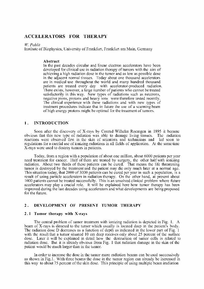
ACCELERATORS FOR THERAPY
W. Pohlit Institute of Biophysics, University of Frankfurt, Frankfurt am Main, Germany
Abstract In the past decades circular and linear electron accelerators have been developed for clinical use in radiation therapy of tumors with the aim of achieving a high radiation dose in the tumor and as low as possible dose in the adjacent normal tissues. Today about one thousand accelerators are in medical use throughout the world and many hundred thousand patients are treated every day with accelerator-produced radiation. There exists, however, a large number of patients who cannot be treated satisfactorily in this way. New types of radiations such as neutrons, negative pions, protons and heavy ions were therefore tested recently. The clinical experience with these radiations and with new types of treatment procedures indicate that in future the use of a scanning beam of high energy protons might be optimal for the treatment of tumors.
1 . INTRODUCTION
Soon after the discovery of X-rays by Conrad Wilhelm Roentgen in 1895 it became obvious that this new type of radiation was able to damage living tissues. The radiation reactions were observed first in the skin of scientists and technicians and led soon to regulations for a careful use of ionizing radiations in all fields of application. At the same time X-rays were used to destroy tumors in patients.
Today, from a region with a population of about one million, about 6000 patients per year need treatment for cancer. Half of them are treated by surgery, the other half with ionizing radiation. About two thirds of these patients can be cured. That means the life threatening tumor is destroyed by the treatment and the patient may die only much later at a normal age. This situation today, that 2000 of 3000 patients can be cured per year in such a population, is a result of using particle accelerators in radiation therapy. On the other hand, at present about 1000 patients cannot be treated successfully. This is an unsolved clinical problem where future accelerators may play a crucial role. It will be explained here how tumor therapy has been improved during the last decades using accelerators and what developments are being proposed for the future.
2 . DEVELOPMENT OF PRESENT TUMOR THERAPY
2.1 Tumor therapy with X-rays
The central problem of tumor treatment with ionizing radiation is depicted in Fig. 1. A beam of X-rays is directed to the tumor which usually is located deep in the patient's body. The radiation dose D decreases as a function of depth as indicated in the lower part of Fig. 1 with the result that a tumor situated 10 cm deep receives only about 25 percent of the surface dose. Later it will be explained in detail how the destruction of tumor cells is related to radiation dose. But it is already obvious from Fig. 1 that radiation damage in the skin of the patient would be much larger than in the tumor.
In order to increase the dose in the tumor more radiation beams can be used successively as shown in Fig. 1. With three beams the dose in the tumor region can already be increased in this way to about 75 percent of the skin dose. This principle of using multiple beam iradiation
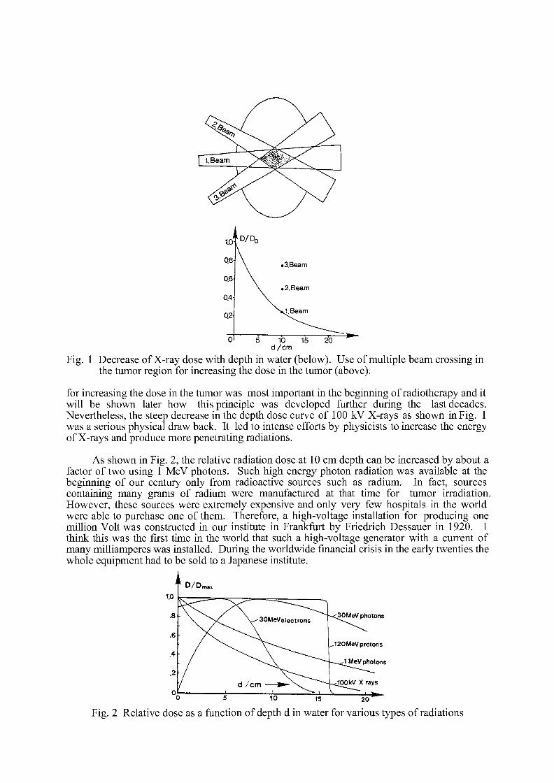
J l D / D 0
Q8- •3Beam
0.6-.2.Beam
0.4-
Q2- VIBeam
0 5 10 15 2'0 d/cm
Fig. 1 Decrease of X-ray dose with depth in water (below). Use of multiple beam crossing in the tumor region for increasing the dose in the tumor (above).
for increasing the dose in the tumor was most important in the beginning of radiotherapy and it will be shown later how this principle was developed further during the last decades. Nevertheless, the steep decrease in the depth dose curve of 100 kV X-rays as shown in Fig. 1 was a serious physical draw back. It led to intense efforts by physicists to increase the energy of X-rays and produce more penetrating radiations.
As shown in Fig. 2, the relative radiation dose at 10 cm depth can be increased by about a factor of two using 1 MeV photons. Such high energy photon radiation was available at the beginning of our century only from radioactive sources such as radium. In fact, sources containing many grams of radium were manufactured at that time for tumor irradiation. However, these sources were extremely expensive and only very few hospitals in the world were able to purchase one of them. Therefore, a high-voltage installation for producing one million Volt was constructed in our institute in Frankfurt by Friedrich Dessauer in 1920. I think this was the first time in the world that such a high-voltage generator with a current of many milliamperes was installed. During the worldwide financial crisis in the early twenties the whole equipment had to be sold to a Japanese institute.
30MeV photons
Fig. 2 Relative dose as a function of depth d in water for various types of radiations
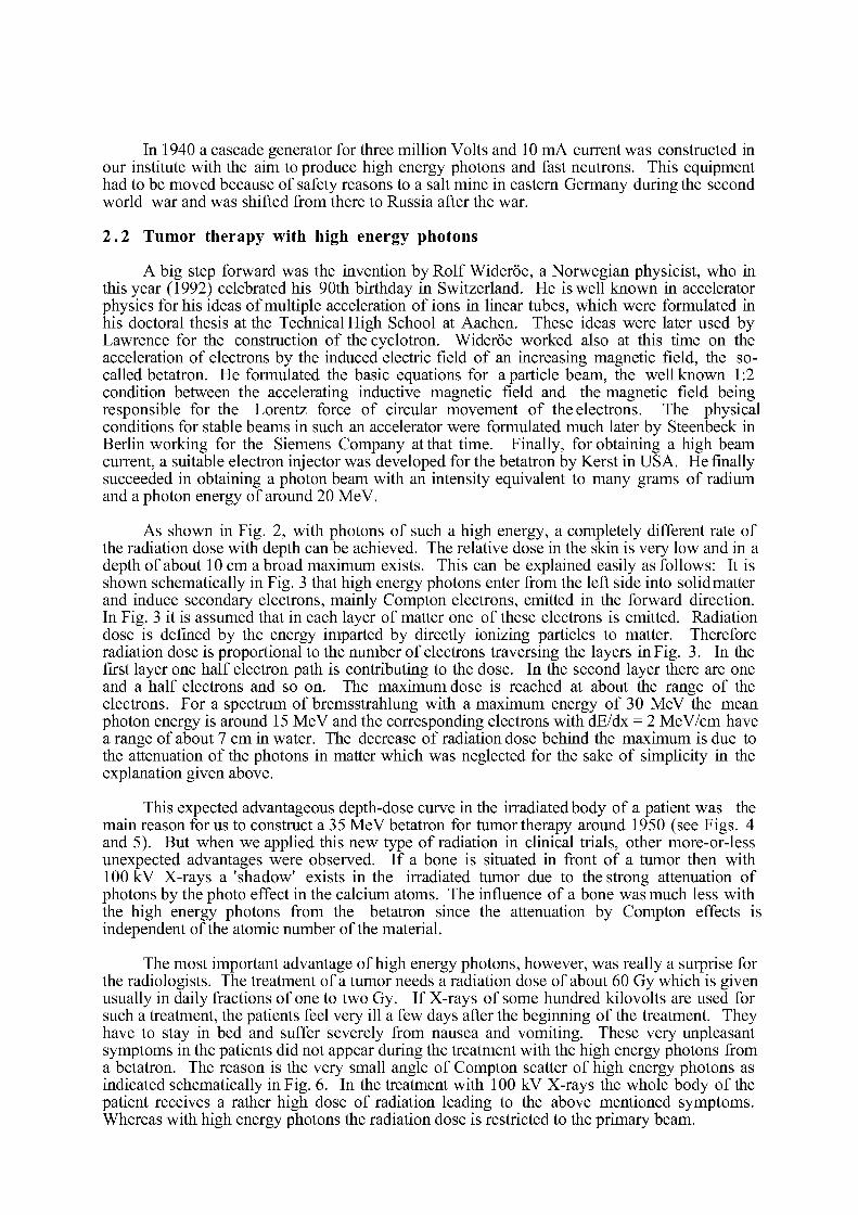
In 1940 a cascade generator for three million Volts and 10 mA current was constructed in our institute with the aim to produce high energy photons and fast neutrons. This equipment had to be moved because of safety reasons to a salt mine in eastern Germany during the second world war and was shifted from there to Russia after the war.
2.2 Tumor therapy with high energy photons
A big step forward was the invention by Rolf Widerôe, a Norwegian physicist, who in this year (1992) celebrated his 90th birthday in Switzerland. He is well known in accelerator physics for his ideas of multiple acceleration of ions in linear tubes, which were formulated in his doctoral thesis at the Technical High School at Aachen. These ideas were later used by Lawrence for the construction of the cyclotron. Widerôe worked also at this time on the acceleration of electrons by the induced electric field of an increasing magnetic field, the so-called betatron. He formulated the basic equations for a particle beam, the well known 1:2 condition between the accelerating inductive magnetic field and the magnetic field being responsible for the Lorentz force of circular movement of the electrons. The physical conditions for stable beams in such an accelerator were formulated much later by Steenbeck in Berlin working for the Siemens Company at that time. Finally, for obtaining a high beam current, a suitable electron injector was developed for the betatron by Kerst in USA. He finally succeeded in obtaining a photon beam with an intensity equivalent to many grams of radium and a photon energy of around 20 MeV.
As shown in Fig. 2, with photons of such a high energy, a completely different rate of the radiation dose with depth can be achieved. The relative dose in the skin is very low and in a depth of about 10 cm a broad maximum exists. This can be explained easily as follows: It is shown schematically in Fig. 3 that high energy photons enter from the left side into solidmatter and induce secondary electrons, mainly Compton electrons, emitted in the forward direction. In Fig. 3 it is assumed that in each layer of matter one of these electrons is emitted. Radiation dose is defined by the energy imparted by directly ionizing particles to matter. Therefore radiation dose is proportional to the number of electrons traversing the layers in Fig. 3. In the first layer one half electron path is contributing to the dose. In the second layer there are one and a half electrons and so on. The maximum dose is reached at about the range of the electrons. For a spectrum of bremsstrahlung with a maximum energy of 30 MeV the mean photon energy is around 15 MeV and the corresponding electrons with dE/dx = 2 MeV/cm have a range of about 7 cm in water. The decrease of radiation dose behind the maximum is due to the attenuation of the photons in matter which was neglected for the sake of simplicity in the explanation given above.
This expected advantageous depth-dose curve in the irradiated body of a patient was the main reason for us to construct a 35 MeV betatron for tumor therapy around 1950 (see Figs. 4 and 5). But when we applied this new type of radiation in clinical trials, other more-or-less unexpected advantages were observed. If a bone is situated in front of a tumor then with 100 kV X-rays a 'shadow' exists in the irradiated tumor due to the strong attenuation of photons by the photo effect in the calcium atoms. The influence of a bone was much less with the high energy photons from the betatron since the attenuation by Compton effects is independent of the atomic number of the material.
The most important advantage of high energy photons, however, was really a surprise for the radiologists. The treatment of a tumor needs a radiation dose of about 60 Gy which is given usually in daily fractions of one to two Gy. If X-rays of some hundred kilovolts are used for such a treatment, the patients feel very ill a few days after the beginning of the treatment. They have to stay in bed and suffer severely from nausea and vomiting. These very unpleasant symptoms in the patients did not appear during the treatment with the high energy photons from a betatron. The reason is the very small angle of Compton scatter of high energy photons as indicated schematically in Fig. 6. In the treatment with 100 kV X-rays the whole body of the patient receives a rather high dose of radiation leading to the above mentioned symptoms. Whereas with high energy photons the radiation dose is restricted to the primary beam.
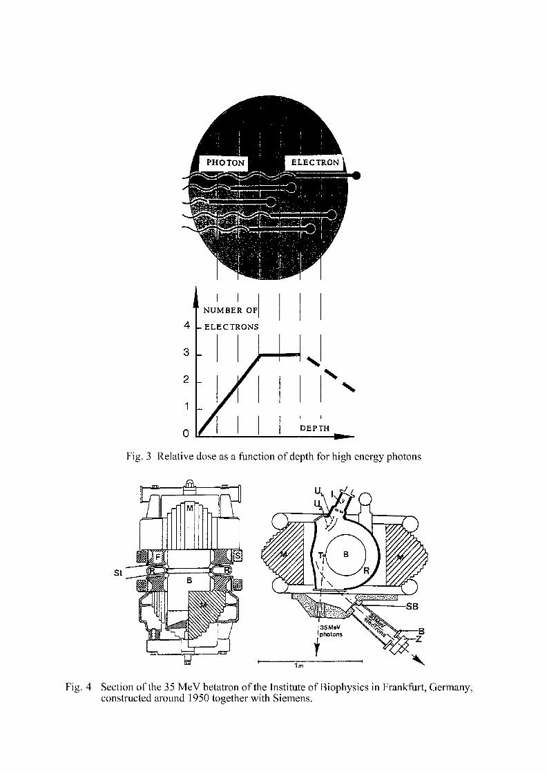
1 NUMBER OF
4 -ELECTRONS
3
;
/ { N
2 ;
/ { • N
V
1 J /
n A DEPTH
Fig. 3 Relative dose as a function of depth for high energy photons
Fig. 4 Section of the 35 MeV betatron of the Institute of Biophysics in Frankfurt, Germany, constructed around 1950 together with Siemens.
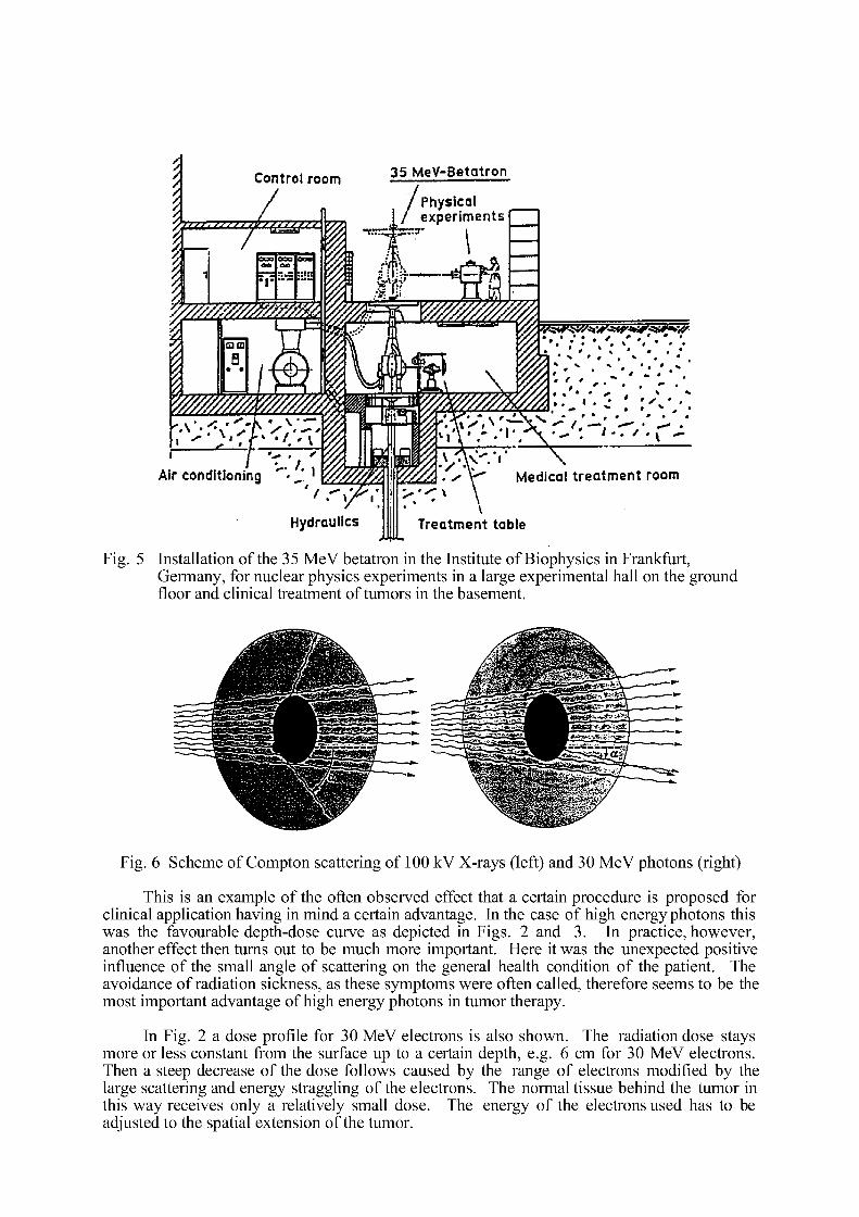
35 MeV-Betatron
Air conditioning
Hydraulics
WJ '• ; : \ • » v • • •
sp% , . - .. .. .:--'-Ar-- '-.'-r-. ^
Medical treatment room
Treatment table
Fig. 5 Installation of the 35 MeV betatron in the Institute of Biophysics in Frankfurt, Germany, for nuclear physics experiments in a large experimental hall on the ground floor and clinical treatment of tumors in the basement.
Fig. 6 Scheme of Compton scattering of 100 kV X-rays (left) and 30 MeV photons (right)
This is an example of the often observed effect that a certain procedure is proposed for clinical application having in mind a certain advantage. In the case of high energy photons this was the favourable depth-dose curve as depicted in Figs. 2 and 3. In practice, however, another effect then turns out to be much more important. Here it was the unexpected positive influence of the small angle of scattering on the general health condition of the patient. The avoidance of radiation sickness, as these symptoms were often called, therefore seems to be the most important advantage of high energy photons in tumor therapy.
In Fig. 2 a dose profile for 30 MeV electrons is also shown. The radiation dose stays more or less constant from the surface up to a certain depth, e.g. 6 cm for 30 MeV electrons. Then a steep decrease of the dose follows caused by the range of electrons modified by the large scattering and energy straggling of the electrons. The normal tissue behind the tumor in this way receives only a relatively small dose. The energy of the electrons used has to be adjusted to the spatial extension of the tumor.
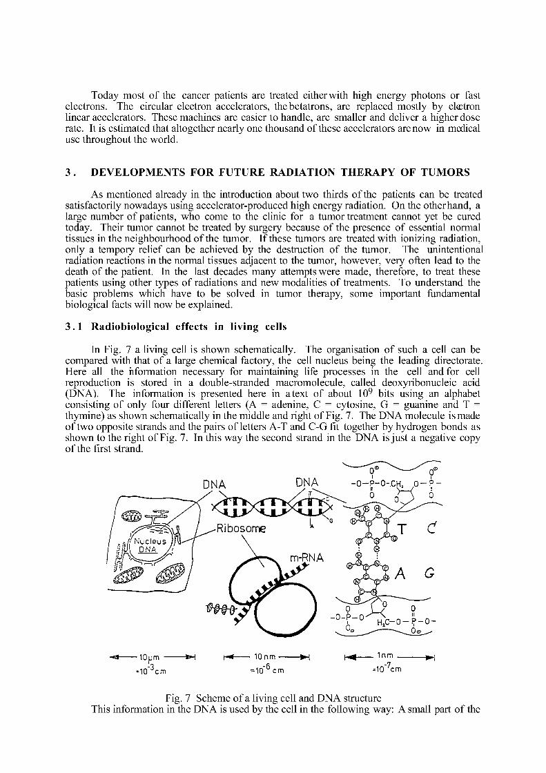
Today most of the cancer patients are treated either with high energy photons or fast electrons. The circular electron accelerators, the betatrons, are replaced mostly by elœtron linear accelerators. These machines are easier to handle, are smaller and deliver a higher dose rate. It is estimated that altogether nearly one thousand of these accelerators are now in medical use throughout the world.
3 . DEVELOPMENTS FOR FUTURE RADIATION THERAPY OF TUMORS
As mentioned already in the introduction about two thirds of the patients can be treated satisfactorily nowadays using accelerator-produced high energy radiation. On the other hand, a large number of patients, who come to the clinic for a tumor treatment cannot yet be cured today. Their tumor cannot be treated by surgery because of the presence of essential normal tissues in the neighbourhood of the tumor. If these tumors are treated with ionizing radiation, only a tempory relief can be achieved by the destruction of the tumor. The unintentional radiation reactions in the normal tissues adjacent to the tumor, however, very often lead to the death of the patient. In the last decades many attempts were made, therefore, to treat these patients using other types of radiations and new modalities of treatments. To understand the basic problems which have to be solved in tumor therapy, some important fundamental biological facts will now be explained.
3 .1 Radiobiological effects in living cells
In Fig. 7 a living cell is shown schematically. The organisation of such a cell can be compared with that of a large chemical factory, the cell nucleus being the leading directorate. Here all the hformation necessary for maintaining life processes in the cell and for cell reproduction is stored in a double-stranded macromolecule, called deoxyribonucleic acid (DNA). The information is presented here in a text of about 109 bits using an alphabet consisting of only four different letters (A = adenine, C = cytosine, G = guanine and T = thymine) as shown schematically in the middle and right of Fig. 7. The DNA molecule is made of two opposite strands and the pairs of letters A-T and C-G fit together by hydrogen bonds as shown to the right of Fig. 7. In this way the second strand in the DNA is just a negative copy of the first strand.
-<s 10pm *H h * 10nm • < H< 1 n m ^\
=10"3cm =10" 6cm --10"7cm
Fig. 7 Scheme of a living cell and DNA structure This information in the DNA is used by the cell in the following way: A small part of the

DNA of about 300 to 500 letters is copied by the cell from the DNA. This molecule is called messenger-RNA since it leaves the cell nucleus and transports information to the cytoplasm of the cell. There, this text is translated into a sequence of amino acids, called a protein or an enzyme. The living cell is using an alphabet of 20 different amino acids for this purpose. Therefore a triplet of RNA letters is always coding for one amino acid in the enzyme molecule. There is much redundancy in this genetic code of a living cell. But in general, one letter in the DNA decides on a certain amino acid being put in a distinct position in an enzyme.
Due to the specific sequence of the amino acids in the enzyme this molecule gets a special spatial structure. It is then able to recognize and bind selected substrates, e.g. a glucose molecule. Another part of this enzyme may, for example, bind an energetic molecule with a phosphorus group, such as adenosine triphosphate (ATP). Both reactive partners have lost by this binding most of their freedom of statistical movement in space and consequently the entropy is reduced in this system. In this way the enzymes in a living cell act like the well known 'Maxwellian demons' reducing the entropy of the system. In a next step, the enzyme brings together both reactants and in this way the biochemical reaction of this binding procedure is accelerated by a factor of 106 to 108. Each biochemical reaction in the living cell is catalysed by a special specific enzyme and it is obvious that destroying one letter in the DNA may lead to the death or inactivation of a complete cell.
In experiments measuring the inactivation of living cells by irradiation with ionizing particles a very important discovery was made: If the cells were tested for their vitality immediately after irradiation, a large number of dead cells was registered at a certain radiation dose. If this test of vitality was done, however, several hours later, a smaller number of cells suffered from the irradiation and most were vital as if unirradiated. This was an indication of the repair of radiation damage in living cells. The biochemical mechanism of repair of radiation damage should be explained here briefly using a simple example (see Fig. 8).
1 Ligase
Fig. 8 Repair of a single base damage in the DNA by four different repair enzymes
If a letter in the DNA is destroyed by the passage of an ionizing particle, this can be recognized by a special enzyme molecule which moves up and down the DNA. This enzyme makes a cut into the backbone of the DNA at the position of the damage and is called therefore 'endonuclease'. Then a second enzyme cuts out the damaged DNA letter and some more adjacent letters. It is called therefore 'exonuclease'. A third enzyme, the DNA polymerase, fills the existing gap with new DNA letters using the opposite strand of the DNA as a template.
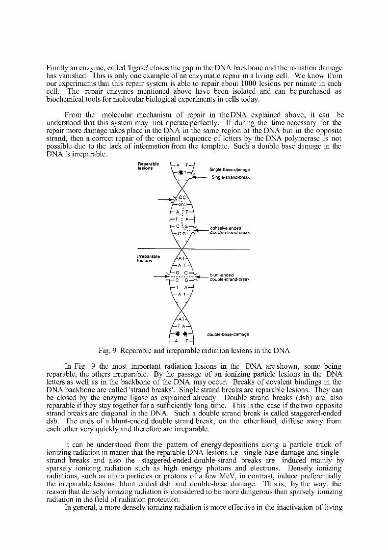
Finally an enzyme, called 'ligase' closes the gap in the DNA backbone and the radiation damage has vanished. This is only one example of an enzymatic repair in a living cell. We know from our experiments that this repair system is able to repair about 1000 lesions per minute in each cell. The repair enzymes mentioned above have been isolated and can be purchased as biochemical tools for molecular biological experiments in cells today.
From the molecular mechanism of repair in the DNA explained above, it can be understood that this system may not operate perfectly. If during the time necessary for the repair more damage takes place in the DNA in the same region of the DNA but in the opposite strand, then a correct repair of the original sequence of letters by the DNA polymerase is not possible due to the lack of information from the template. Such a double base damage in the DNA is irreparable.
Reparable \ _ A 7 / Single-base-damage
— Single-strand-break
cohesive ended double-strand-break
double-base-damage
Fig. 9 Reparable and irreparable radiation lesions in the DNA
In Fig. 9 the most important radiation lesions in the DNA are shown, some being reparable, the others irreparable. By the passage of an ionizing particle lesions in the DNA letters as well as in the backbone of the DNA may occur. Breaks of covalent bindings in the DNA backbone are called 'strand breaks'. Single strand breaks are reparable lesions. They can be closed by the enzyme ligase as explained already. Double strand breaks (dsb) are also reparable if they stay together for a sufficiently long time. This is the case if the two opposite strand breaks are diagonal in the DNA. Such a double strand break is called staggered-ended dsb. The ends of a blunt-ended double strand break, on the other hand, diffuse away from each other very quickly and therefore are irreparable.
It can be understood from the pattern of energy depositions along a particle track of ionizing radiation in matter that the reparable DNA lesions i.e. single-base damage and single-strand breaks and also the staggered-ended double-strand breaks are induced mainly by sparsely ionizing radiation such as high energy photons and electrons. Densely ionizing radiations, such as alpha particles or protons of a few MeV, in contrast, induce preferentially the irreparable lesions: blunt ended dsb and double-base damage. This is, by the way, the reason that densely ionizing radiation is considered to be more dangerous than sparsely ionizing radiation in the field of radiation protection.
In general, a more densely ionizing radiation is more effective in the inactivation of living
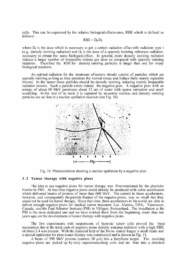
cells. This can be expressed by the relative biological effectivenes, RBE which is defined as follows:
RBE = Dr/Di
where Dj is the dose which is necessary to get a certain radiation effect with radiation type i (e.g. densely ionizing radiation) and Dr is the dose of a sparsely ionizing reference radiation, necessary to obtain the same biological effect. In general, more densely ionizing radiation induces a larger number of irreparable lesions per dose as compared with sparsely ionizing radiation. Therefore the RBE for densely ionizing particles is larger than one for many biological reactions.
An optimal radiation for the treatment of tumors should consist of particles which are sparsely ionizing as long as they penetrate the normal tissue and induce there mainly reparable lesions. In the tumor these particles should be densely ionizing inducing mainly irreparable radiation lesions. Such a particle exists indeed: the negative pion. A negative pion with an energy of about 80 MeV penetrates about 12 cm of water with sparse ionization and small scattering. At the end of its track it is captured by an atomic nucleus and densely ionizing particles are set free in a nuclear spallation reaction (see Fig. 10).
Fig. 10 Photoemulsion showing a nuclear spallation by a negative pion
3 .2 Tumor therapy with negative pions
The idea to use negative pions for tumor therapy was first mentioned by the physicist Fowler in 1961. At that time negative pions could already be produced with some accelerators which delivered beams of protons of more than 600 MeV. The current in these accelerators, however, and consequently the particle fluence of the negative pions, was so small that they could not be used for tumor therapy. Since that time, three accelerators in the world are able to deliver enough negative pions for medical tumor treatment: Los Alamos, USA; Vancouver, Canada; and the Paul Scherrer Institute (PSI) in Villigen, Switzerland. The installation at the PSI is the most dedicated one and we have worked there from the beginning, more than ten years ago, on the development of tumor therapy with negative pions.
The first experiments with suspensions of hypoxic tumor cells proved the basic assumption that at the track ends of negative pions densely ionizing radiation with a high RBE of about 2.4 was present. With the financial help of the Swiss cancer league a small clinic and a special applicator for pion tumor therapy was constructed and is shown in Fig. 11.
A beam of 590 MeV protons (current 20 |uA) hits a beryllium target. The resulting negative pions are picked up by sixty superconductiing coils and are bent into a direction
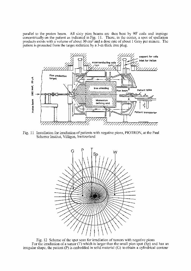
parallel to the proton beam. All sixty pion beams are then bent by 90° coils and impinge concentrically on the patient as indicated in Fig. 11. There, in the center, a spot of spallation products exists with a volume of about 30 cm3 and a dose rate of about 1 Gray per minute. The patient is protected from the target radiation by a 3-m thick iron plug.
'//////////
[/ support for colls Inlet for Helium
V///////,
> a 2
in
E
I
v/////?///////////////. /////////y?////////;////, Fig. 11 Installation for irradiation of patients with negative pions, PIOTRON, at the Paul
Scherrer Institut, Villigen, Switzerland
Fig. 12 Scheme of the spot scan for irradiation of tumors with negative pions For the irradiation of a tumor (T) which is larger than the small pion spot (Sp) and has an
irregular shape, the patient (P) is embedded in solid material (G) to obtain a cylindrical contour

as shown in Fig. 12. With this cylinder the patient is inserted into a circular water filledring (W) with rubber side walls. The patient can be moved by computer control relative to the spot of stopped pions which stays always at the same fixed position in space. In this way the radiation dose can be distributed homogeneously in the irregularly shaped tumor and the adjacent normal tissues can be spared. A few hundred patients have been treated in this way during the last years with negative pions at the PSI. The clinical experience can be summarized as follows:
a) Negative pions were thought to be advantageous due to the induction of a large fraction of irreparable radiation lesions in the tumor. This advantage is reduced, however, by the fact that the tumors are much larger than the small spot of densely ionizing spallation products and must be treated by the scanning procedure explained above. As a consequence, each part of the tumor is irradiated for a certain time with densely ionizing radiation from the spot and the rest of the irradiation time with sparsely ionizing radiation from the pions in flight. Instead of an RBE of 2.4 as determined from cell suspensions and from irradiation of small mouse tumors, an RBE of only 1.7 can be achieved in large tumors in the patients.
b) The clinical trials indicated that the most important advantage of the pion treatment is related to the scanning procedure taking into account the unregular shape of the tumor and sparing as much as possible the adjacent normal tissue. This important advantage, however, is reduced by the fact that neutrons are produced also by nuclear spallation and are scattered out of the treatment volume. The RBE of this densely ionizing radiation is high and this is in contrast with the initially expected advantage of negative pions that they would traverse normal tissue with sparse ionisation.
This clinical experience which has been proven by further systematic and more precise experiments led to the proposal to use protons in radiation therapy. The disadvantages of negative pions mentioned above can be avoided and all important advantages can be used with even higher efficiency.
3 .3 Tumor therapy with high energy protons
With high energy protons a high dose rate can be achieved easily with a relatively small proton current. With a current of one nanoampere a volume of one liter can be irradiated with a dose of one Gray in about one minute. Therefore a single beam of protons can be used for tumor therapy. For reaching every point in the human body a proton energy of about 200 MeV is neccessary. As was shown in the previous chapter, the most important advantage in the clinical use of negative pions was the conformai irradiation of the tumor with the spot scan method. With high energy protons the irregular shape of the tumor can also be taken into consideration as is explained in Fig. 13. A proton beam with a small diameter of about 5 mm is scanned over the tumor and the energy is continuously modulated by absorbers in such a way that the proton range coincides with the edge of the tumor. The first irradiation would be done e.g. from the direction indicated with (a) in Fig. 13. The next day the irradiation is given from direction (b) and so on. In this way the tumor can be irradiated with a homogeneous distributed dose. By selecting a suitable set of beam directions a very sensitive and essential normal tissue, indicated by "S" in Fig. 13 can be spared completely. It should be mentioned that such a sharp dose gradient from the tumor (T) to an essential senisitive normal tissue (S) can only be obtained with protons. Other types of particles, such as light or heavy ions would always result in a considerable dose behind the range of these particles due to densely ionizing secondary particles from nuclear reactions.
The development of a suitable scanning procedure for a 200 MeV proton beam is very advanced at the PSI. The construction of a small proton accelerator dedicated to medical use, however, still is an open technical problem to be solved in the near future. It seems that the use
of high energy protons will be a big step forward in tumor therapy, comparable with that of using high energy photons and fast electrons thirty years ago.
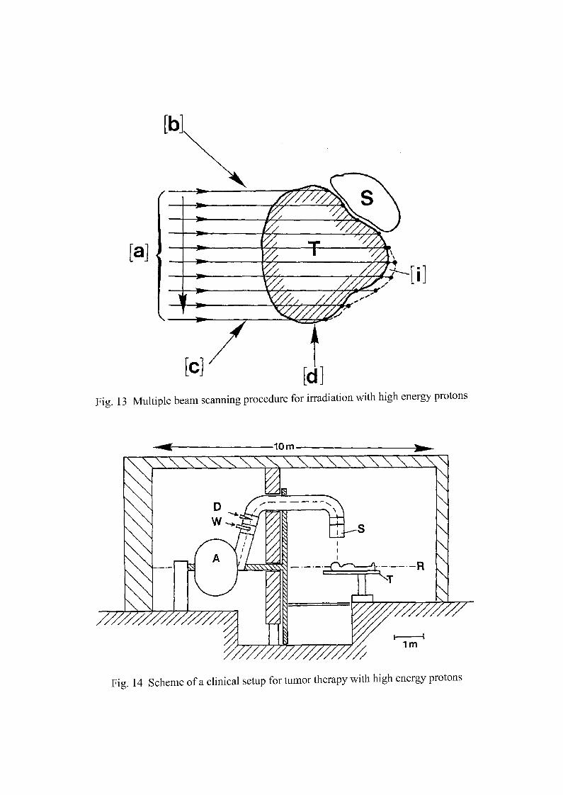
[a]
[ C ] [d] Fig. 13 Multiple beam scanning procedure for irradiation with high energy protons
-10m-
//////////////////A
Fig. 14 Scheme of a clinical setup for tumor therapy with high energy protoi
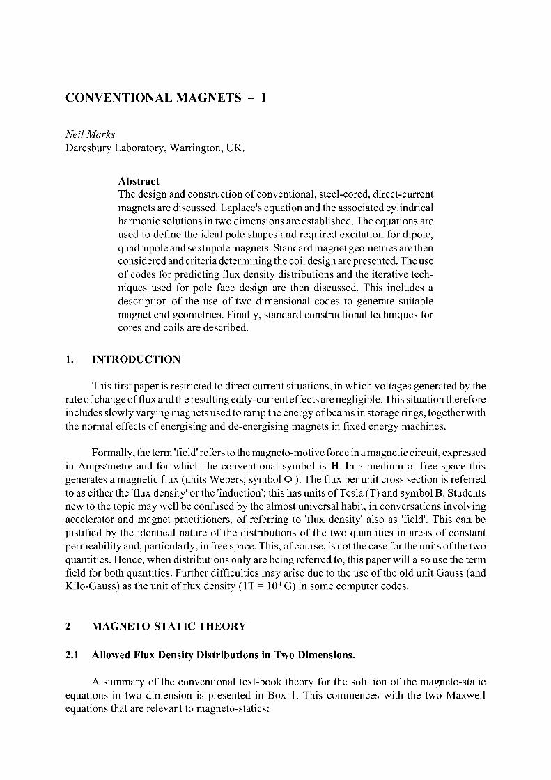
CONVENTIONAL MAGNETS - I
Neil Marks. Daresbury Laboratory, Warrington, UK.
Abstract The design and construction of conventional, steel-cored, direct-current magnets are discussed. Laplace's equation and the associated cylindrical harmonic solutions in two dimensions are established. The equations are used to define the ideal pole shapes and required excitation for dipole, quadrupole and sextupole magnets. Standard magnet geometries are then considered and criteria determining the coil design are presented. The use of codes for predicting flux density distributions and the iterative techniques used for pole face design are then discussed. This includes a description of the use of two-dimensional codes to generate suitable magnet end geometries. Finally, standard constructional techniques for cores and coils are described.
1. INTRODUCTION
This first paper is restricted to direct current situations, in which voltages generated by the rate of change of flux and the resulting eddy-current effects are negligible. This situation therefore includes slowly varying magnets used to ramp the energy of beams in storage rings, together with the normal effects of energising and de-energising magnets in fixed energy machines.
Formally, the term 'field' refers to the magneto-motive force in a magnetic circuit, expressed in Amps/metre and for which the conventional symbol is H. In a medium or free space this generates a magnetic flux (units Webers, symbol O ). The flux per unit cross section is referred to as either the 'flux density' or the 'induction'; this has units of Tesla (T) and symbol B. Students new to the topic may well be confused by the almost universal habit, in conversations involving accelerator and magnet practitioners, of referring to 'flux density' also as 'field'. This can be justified by the identical nature of the distributions of the two quantities in areas of constant permeability and, particularly, in free space. This, of course, is not the case for the units of the two quantities. Hence, when distributions only are being referred to, this paper will also use the term field for both quantities. Further difficulties may arise due to the use of the old unit Gauss (and Kilo-Gauss) as the unit of flux density (IT = 104 G) in some computer codes.
2 MAGNETO-STATIC THEORY
2.1 Allowed Flux Density Distributions in Two Dimensions.
A summary of the conventional text-book theory for the solution of the magneto-static equations in two dimension is presented in Box 1. This commences with the two Maxwell equations that are relevant to magneto-statics:
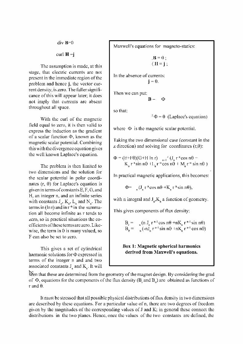
Maxwell's equations for magneto-statics:
.B = 0; (H = j ;
In the absence of currents: j = 0 .
Then we can put:
so that:
B= O
' 0 = 0 (Laplace's equation)
div B=0
curl H =j
The assumption is made, at this stage, that electric currents are not present in the immediate region of the problem and hence j , the vector current density, is zero. The fuller significance of this will appear later; it does not imply that currents are absent throughout all space.
With the curl of the magnetic field equal to zero, it is then valid to express the induction as the gradient of a scalar function O, known as the magnetic scalar potential. Combining this with the divergence equation gives the well known Laplace's equation.
The problem is then limited to two dimensions and the solution for the scalar potential in polar coordinates (r, 9) for Laplace's equation is given in terms of constants E, F, G, and H, an integer n, and an infinite series with constants J , K , L and N . The
n' n' n n
terms in (In r) and in r ~n in the summation all become infinite as r tends to zero, so in practical situations the coefficients of these terms are zero. Likewise, the term in 9 is many valued, so F can also be set to zero.
This gives a set of cylindrical harmonic solutions for O expressed in terms of the integer n and and two associated constants J and K . It will
n n
seen that these are determined from the geometry of the magnet design. By considering the grad of O, equations for the components of the flux density (Br and B e) are obtained as functions of r and 9.
It must be stressed that all possible physical distributions of flux density in two dimensions are described by these equations. For a particular value of n, there are two degrees of freedom given by the magnitudes of the corresponding values of J and K; in general these connect the distributions in the two planes. Hence, once the values of the two constants are defined, the
where O is the magnetic scalar potential.
Taking the two dimensional case (constant in the z direction) and solving for coordinates (r,9):
O = (E+F9)(G+H In r) n = 1
x (Jn r n cos n9 + K r nsin n9 +L r n cos n9 + M r n sin n9 )
n n n 7
In practical magnetic applications, this becomes:
<D= (J r n cos n9 +K r n sin n9), n v n n -"
with n integral and Jn,Kn a function of geometry.
This gives components of flux density: B r = n (n Jn r n l cos n9 +nKn r n l sin n9) BI = " (-nJ r n l sin n9 +nK° r n l cos n9)
6 n v n n '
Box 1: Magnetic spherical harmonics derived from Maxwell's equations.
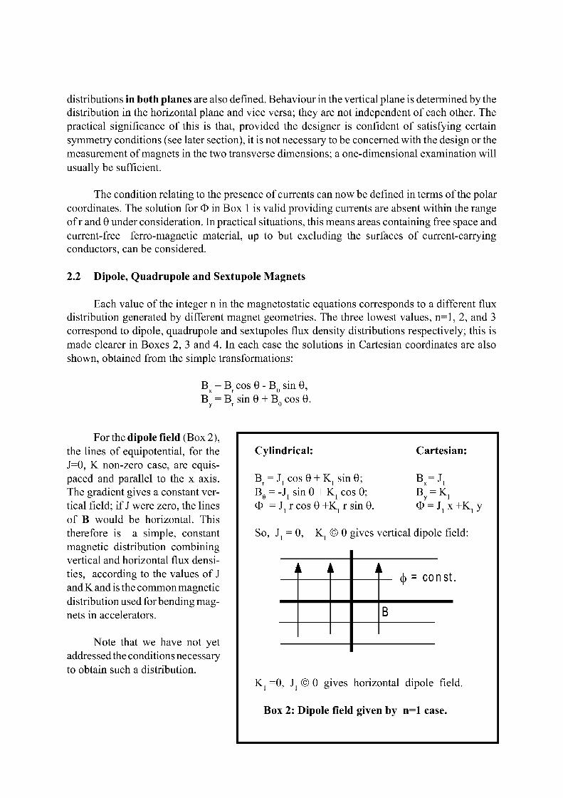
distributions in both planes are also defined. Behaviour in the vertical plane is determined by the distribution in the horizontal plane and vice versa; they are not independent of each other. The practical significance of this is that, provided the designer is confident of satisfying certain symmetry conditions (see later section), it is not necessary to be concerned with the design or the measurement of magnets in the two transverse dimensions; a one-dimensional examination will usually be sufficient.
The condition relating to the presence of currents can now be defined in terms of the polar coordinates. The solution for O in Box 1 is valid providing currents are absent within the range of r and 6 under consideration. In practical situations, this means areas containing free space and current-free ferro-magnetic material, up to but excluding the surfaces of current-carrying conductors, can be considered.
2.2 Dipole, Quadrupole and Sextupole Magnets
Each value of the integer n in the magnetostatic equations corresponds to a different flux distribution generated by different magnet geometries. The three lowest values, n=l, 2, and 3 correspond to dipole, quadrupole and sextupoles flux density distributions respectively; this is made clearer in Boxes 2, 3 and 4. In each case the solutions in Cartesian coordinates are also shown, obtained from the simple transformations:
B x = B r cos 9 - B e sin 9, BX = B' sin 9 + B n cos 9.
y r 0
For the dipole field (Box 2), the lines of equipotential, for the J=0, K non-zero case, are equis-paced and parallel to the x axis. The gradient gives a constant vertical field; if J were zero, the lines of B would be horizontal. This therefore is a simple, constant magnetic distribution combining vertical and horizontal flux densities, according to the values of J and K and is the common magnetic distribution used for bending magnets in accelerators.
Note that we have not yet addressed the conditions necessary to obtain such a distribution.
Cylindrical: Cartesian:
B = J, cos 9 + K, sin 0; r 1 1 '
B e = -Jj sin 9 + Kj cos 9; O = Jj r cos 9 +Kj r sin 9.
B =J, X 1
B y = Kj O = Jj x +K, y
So, J = 0, K © 0 gives vertical dipole field:
i k i k i k
rh = con st
B
Kj =0, Jj © 0 gives horizontal dipole field.
Box 2: Dipole field given by n=l case.
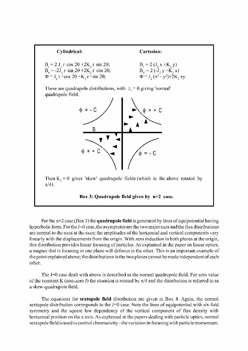
For the n=2 case (Box 3) the quadrupole field is generated by lines of equipotential having hyperbolic form. For the J=0 case, the asymptotes are the two major axes and the flux distributions are normal to the axes at the axes; the amplitudes of the horizontal and vertical components vary linearly with the displacements from the origin. With zero induction in both planes at the origin, this distribution provides linear focusing of particles. As explained in the paper on linear optics, a magnet that is focusing in one plane will defocus in the other. This is an important example of the point explained above; the distributions in the two planes cannot be made independent of each other.
The J=0 case dealt with above is described as the normal quadrupole field. For zero value of the constant K (non-zero J) the situation is rotated by n/4 and the distribution is referred to as a skew quadrupole field.
The equations for sextupole field distribution are given in Box 4. Again, the normal sextupole distribution corresponds to the J=0 case. Note the lines of equipotential with six-fold symmetry and the square law dependency of the vertical component of flux density with horizontal position on the x axis. As explained in the papers dealing with particle optics, normal sextupole field is used to control chromaticity - the variation in focusing with particle momentum.
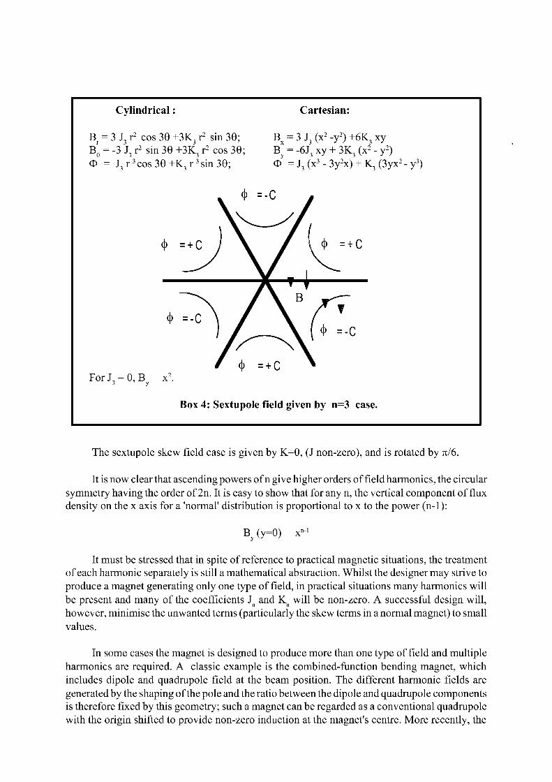
Cylindrical : Cartesian:
B = 3 J, r2 cos 39 +3K, r2 sin 39; r 3 3
B x = 3 J3 (x2 -y2) +6K3 xy B e = -3 J3 r2 sin 39 +3K3 r2 cos 39; B = -6J3 xy + 3K3 (x2 - y2) O = J 3 r 3 c o s 3 9 + K 3 r 3 s i n 3 9 ; O = J3 (x3 - 3y2x) + K, (3yx2 - y3)
v * : = -C M
* = + C / \ / I 4> = + c
- ^ y / T ! V
* =-<A / \ B -^— \ / ?
_ ^ \ ( * =-C
/ <|> : For J = 0, B x2.
3 ' y
=+c ^
Box 4: Sextupole field given by n=3 case.
The sextupole skew field case is given by K=0, (J non-zero), and is rotated by 7t/6.
It is now clear that ascending powers of n give higher orders of field harmonics, the circular symmetry having the order of 2n. It is easy to show that for any n, the vertical component of flux density on the x axis for a 'normal' distribution is proportional to x to the power (n-1):
By(y=0) x"1
It must be stressed that in spite of reference to practical magnetic situations, the treatment of each harmonic separately is still a mathematical abstraction. Whilst the designer may strive to produce a magnet generating only one type of field, in practical situations many harmonics will be present and many of the coefficients J and K will be non-zero. A successful design will, however, minimise the unwanted terms (particularly the skew terms in a normal magnet) to small values.
In some cases the magnet is designed to produce more than one type of field and multiple harmonics are required. A classic example is the combined-function bending magnet, which includes dipole and quadrupole field at the beam position. The different harmonic fields are generated by the shaping of the pole and the ratio between the dipole and quadrupole components is therefore fixed by this geometry; such a magnet can be regarded as a conventional quadrupole with the origin shifted to provide non-zero induction at the magnet's centre. More recently, the
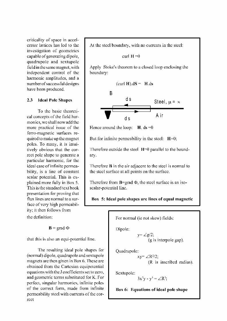
criticality of space in accelerator lattices has led to the investigation of geometries capable of generating dipole, quadrupole and sextupole field in the same magnet, with independent control of the harmonic amplitudes, and a number of successful designs have been produced.
2.3 Ideal Pole Shapes
To the basic theoretical concepts of the field harmonics, we shall now add the more practical issue of the ferro-magnetic surfaces required to make up the magnet poles. To many, it is intuitively obvious that the correct pole shape to generate a particular harmonic, for the ideal case of infinite permeability, is a line of constant scalar potential. This is explained more fully in Box 5. This is the standard text book presentation for proving that flux lines are normal to a surface of very high permeability; it then follows from the definition:
B = grad O
that this is also an equi-potential line.
The resulting ideal pole shapes for (normal) dipole, quadrupole and sextupole magnets are then given in Box 6. These are obtained from the Cartesian equipotential equations with the J coefficients set to zero, and geometric terms substituted for K. For perfect, singular harmonics, infinite poles of the correct form, made from infinite permeability steel with currents of the correct
At the steel boundary, with no currents in the steel:
curl H =0
Apply Stake's theorem to a closed loop enclosing the boundary:
(curlH).dS= H.ds
ds Steel, |_i = x
* ds Hence around the loop: H. ds =0
Air
But for infinite permeability in the steel: H=0;
Therefore outside the steel H=0 parallel to the boundary.
Therefore B in the air adjacent to the steel is normal to the steel surface at all points on the surface.
Therefore from B=grad O, the steel surface is an iso-scalar-potential line.
Box 5: Ideal pole shapes are lines of equal magnetic
For normal (ie not skew) fields:
Dipole: y= ^g/2;
(g is interpole gap).
Quadrupole: xy= ZR2/2;
(R is inscribed radius).
Sextupole: 3x2y - y 3 = ZR 3;
Box 6: Equations of ideal pole shape
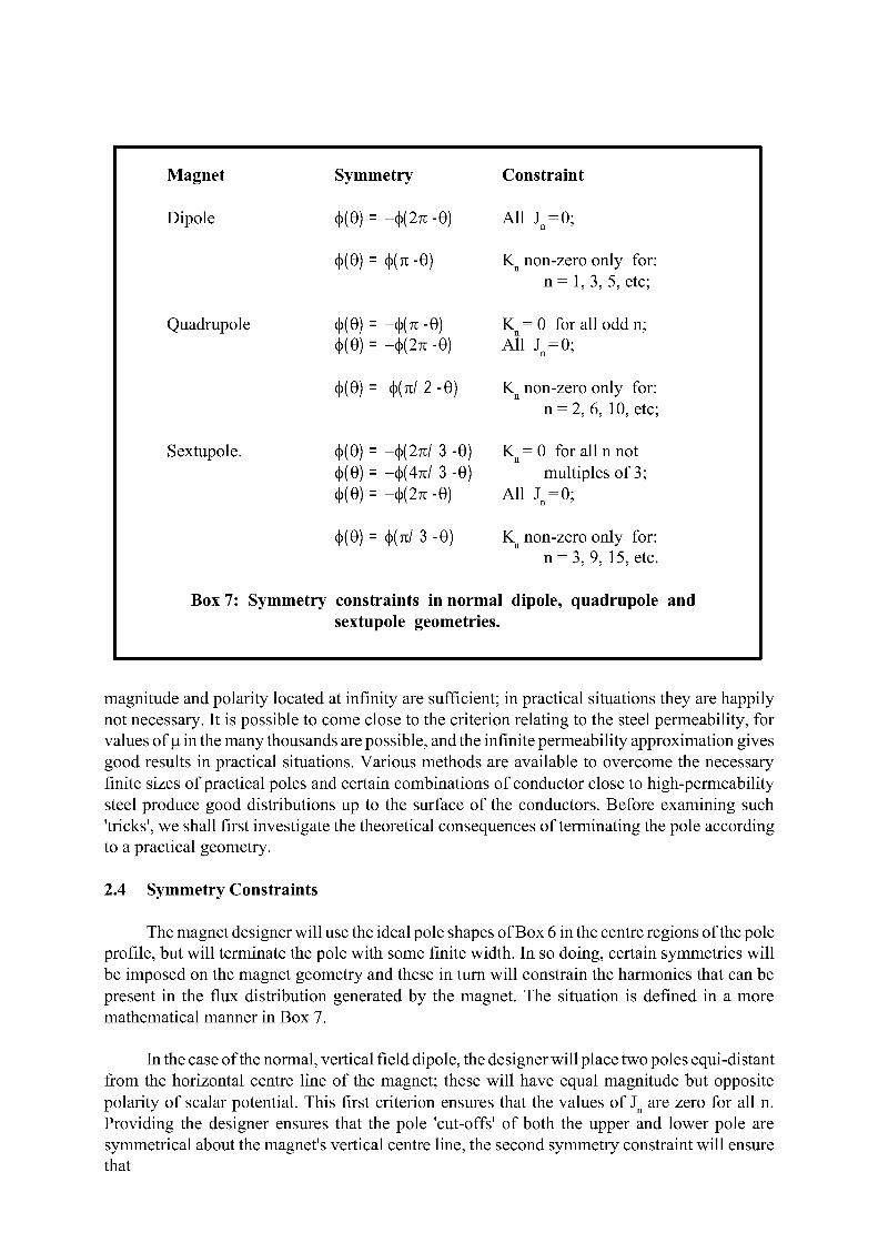
Magnet Symmetry Constraint
Dipole 4>(0) = -i>{2n -9) AU J =0; n '
4>(e) = ^(71-e) K n non-zero only for: n = 1, 3, 5, etc;
Quadrupole -<K7C -9) —<P(2TC -9)
K n = 0 for all odd n; AU J =0;
n '
4>(e) = (|)(7i/ 2 -9) K non-zero only for: n = 2, 6, 10, etc;
Sextupole. -i>{2nl 3 -9) -(|)(47i/ 3 -9) —<P(2TC -9)
K = 0 for all n not n
multiples of 3; AU J =0;
n ' m = (|)(7i/ 3 -9) K non-zero only for: n = 3, 9, 15, etc.
Box 7: Symmetry constraints in normal dipole, quadrupole and sextupole geometries.
magnitude and polarity located at infinity are sufficient; in practical situations they are happily not necessary. It is possible to come close to the criterion relating to the steel permeability, for values of [4, in the many thousands are possible, and the infinite permeability approximation gives good results in practical situations. Various methods are available to overcome the necessary finite sizes of practical poles and certain combinations of conductor close to high-permeability steel produce good distributions up to the surface of the conductors. Before examining such 'tricks', we shall first investigate the theoretical consequences of terminating the pole according to a practical geometry.
2.4 Symmetry Constraints
The magnet designer will use the ideal pole shapes of Box 6 in the centre regions of the pole profile, but will terminate the pole with some finite width. In so doing, certain symmetries will be imposed on the magnet geometry and these in turn will constrain the harmonics that can be present in the flux distribution generated by the magnet. The situation is defined in a more mathematical manner in Box 7.
In the case of the normal, vertical field dipole, the designer will place two poles equi-distant from the horizontal centre line of the magnet; these will have equal magnitude but opposite polarity of scalar potential. This first criterion ensures that the values of J n are zero for all n. Providing the designer ensures that the pole 'cut-offs' of both the upper and lower pole are symmetrical about the magnet's vertical centre line, the second symmetry constraint will ensure that

all Kn values are zero for even n. Thus, with two simple symmetry criteria, the designer has ensured that the error fields that can be present in the dipole are limited to sextupole, decapole, fourteen-pole, etc.
In the case of the quadrupole, the basic four-fold symmetry about the horizontal and vertical axes (the first two criteria) render all values of Jn and the values of Kn for all odd n equal to zero. The third constraint concerns the eight-fold symmetry ie the pole cut-offs being symmetrical about the 7i/4 axes. This makes all values of K zero, with the exception of the coefficients that correspond to n=2 (fundamental quadrupole), 6, 10, etc. Thus in a fully symmetric quadrupole magnet, the lowest-order allowed field error is twelve pole (duodecapole), followed by twenty pole, etc.
Box 7 also defines the allowed error harmonics in a sextupole and shows that with the basic sextupole symmetry, eighteen pole is the lowest allowed harmonic error; the next is thirty pole. Higher order field errors are therefore usually not of high priority in the design of a sextupole magnet.
Given the above limitations on the possible error fields that can be present in a magnet, the magnet designer has additional techniques that can be used to reduce further the errors in the distribution; these usually take the form of small adjustments to the pole profile close to the cutoff points.
It must be appreciated that the symmetry constraints described in this section apply to magnet geometries as designed. Construction should closely follow the design but small tolerance errors will always be present in the magnet when it is finally assembled and these will break the symmetries described above. Thus, a physical magnet will have non-zero values of all J and K coefficients. It is the task of the magnet engineer to predict the distortions resulting from manufacturing and assembly tolerances; this information then becomes the basis for the specification covering the magnet manufacture, so ensuring that the completed magnet will meet its design criteria.
Before leaving the topic of magnetic cylindrical harmonics, it is necessary to put this concept into the wider context of the interaction of beams with magnetic fields. Particles are not able to carry out a cylindrical harmonic analysis and are therefore not sensitive to the amplitude or phase of a particular harmonic in a magnet. They see flux densities B and, in resonance type phenomena, the spatial differentials of B, sometimes to high orders. It is a mistake, therefore, to associate a certain order of differential with one particular harmonic, as all the higher harmonic terms will contribute to the derivative; the magnet designer may well have balanced the amplitudes and polarities of a number of quite high harmonics to meet successfully a stringent flux density criterion within the defined good field region of the magnet.
The two-dimensional cylindrical harmonics are therefore a useful theoretical tool and give a valuable insight into the allowed spatial distributions of magnetic fields. However, when judging the viability of a design or the measurements from a completed magnet, always reassemble the harmonic series and examine the flux density or its derivatives. These are the quantities corresponding to the physical situation in an accelerator magnet.
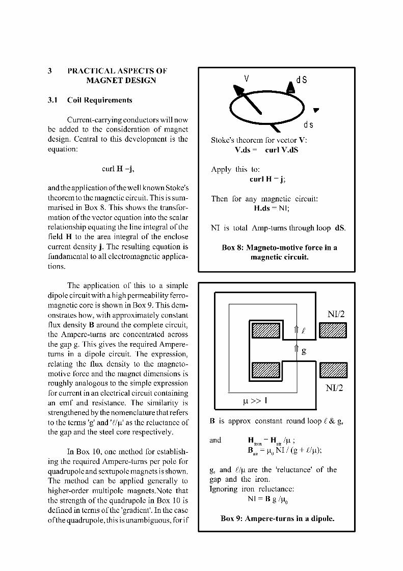
3 PRACTICAL ASPECTS OF MAGNET DESIGN
3.1 Coil Requirements
Current-carrying conductors will now be added to the consideration of magnet design. Central to this development is the equation:
curl H =j,
and the application of the well known Stoke's theorem to the magnetic circuit. This is summarised in Box 8. This shows the transformation of the vector equation into the scalar relationship equating the line integral of the field H to the area integral of the enclose current density j . The resulting equation is fundamental to all electromagnetic applications.
The application of this to a simple dipole circuit with a high permeability ferromagnetic core is shown in Box 9. This demonstrates how, with approximately constant flux density B around the complete circuit, the Ampere-turns are concentrated across the gap g. This gives the required Ampere-turns in a dipole circuit. The expression, relating the flux density to the magnetomotive force and the magnet dimensions is roughly analogous to the simple expression for current in an electrical circuit containing an emf and resistance. The similarity is strengthened by the nomenclature that refers to the terms 'g' and 7/|u' as the reluctance of the gap and the steel core respectively.
In Box 10, one method for establishing the required Ampere-turns per pole for quadrupole and sextupole magnets is shown. The method can be applied generally to higher-order multipole magnets.Note that the strength of the quadrupole in Box 10 is defined in terms of the 'gradient'. In the case of the quadrupole, this is unambiguous, for if
V _dS
Stake's theorem for vector V: V.ds = curl V.dS
Apply this to: curl H = j ;
Then for any magnetic circuit: H.ds = NI;
NI is total Amp-turns through loop dS.
Box 8: Magneto-motive force in a magnetic circuit.
\i
NI/2
Bi î \i WÊ< î r g
ill WÊ< NI/2
I_l» 1
B is approx constant round loop £ & g,
iron air ^ '
B a i r = ^ 0 N I / ( g + ^ ) ;
g, and il\x, are the 'reluctance' of the gap and the iron. Ignoring iron reluctance:
NI = B g X
Box 9: Ampere-turns in a dipole.
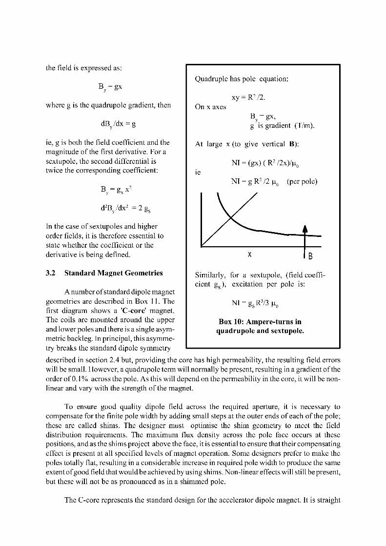
the field is expressed as:
B =gx
where g is the quadrupole gradient, then
dB /dx = g y &
ie, g is both the field coefficient and the magnitude of the first derivative. For a sextupole, the second differential is twice the corresponding coefficient:
Quadruple has pole equation:
xy = R212.
B y = gx, On x axes
g is gradient (T/m).
At large x (to give vertical B):
îe
NI = (gx)(R 2/2x)/u,
NI = g R212 \i0 (per pole) B
y = es * 2
d 2B y/dx 2 = 2 g s
In the case of sextupoles and higher order fields, it is therefore essential to state whether the coefficient or the derivative is being defined.
3.2 Standard Magnet Geometries
A number of standard dipole magnet geometries are described in Box 11. The first diagram shows a 'C-core' magnet. The coils are mounted around the upper and lower poles and there is a single asymmetric backleg. In principal, this asymmetry breaks the standard dipole symmetry described in section 2.4 but, providing the core has high permeability, the resulting field errors will be small. However, a quadrupole term will normally be present, resulting in a gradient of the order of 0.1% across the pole. As this will depend on the permeability in the core, it will be nonlinear and vary with the strength of the magnet.
To ensure good quality dipole field across the required aperture, it is necessary to compensate for the finite pole width by adding small steps at the outer ends of each of the pole; these are called shims. The designer must optimise the shim geometry to meet the field distribution requirements. The maximum flux density across the pole face occurs at these positions, and as the shims project above the face, it is essential to ensure that their compensating effect is present at all specified levels of magnet operation. Some designers prefer to make the poles totally flat, resulting in a considerable increase in required pole width to produce the same extent of good field that would be achieved by using shims. Non-linear effects will still be present, but these will not be as pronounced as in a shimmed pole.
B
Similarly, for a sextupole, (field coefficient g s ) , excitation per pole is:
NI = g s R 3 / 3 ^ 0
Box 10: Ampere-turns in quadrupole and sextupole.
The C-core represents the standard design for the accelerator dipole magnet. It is straight
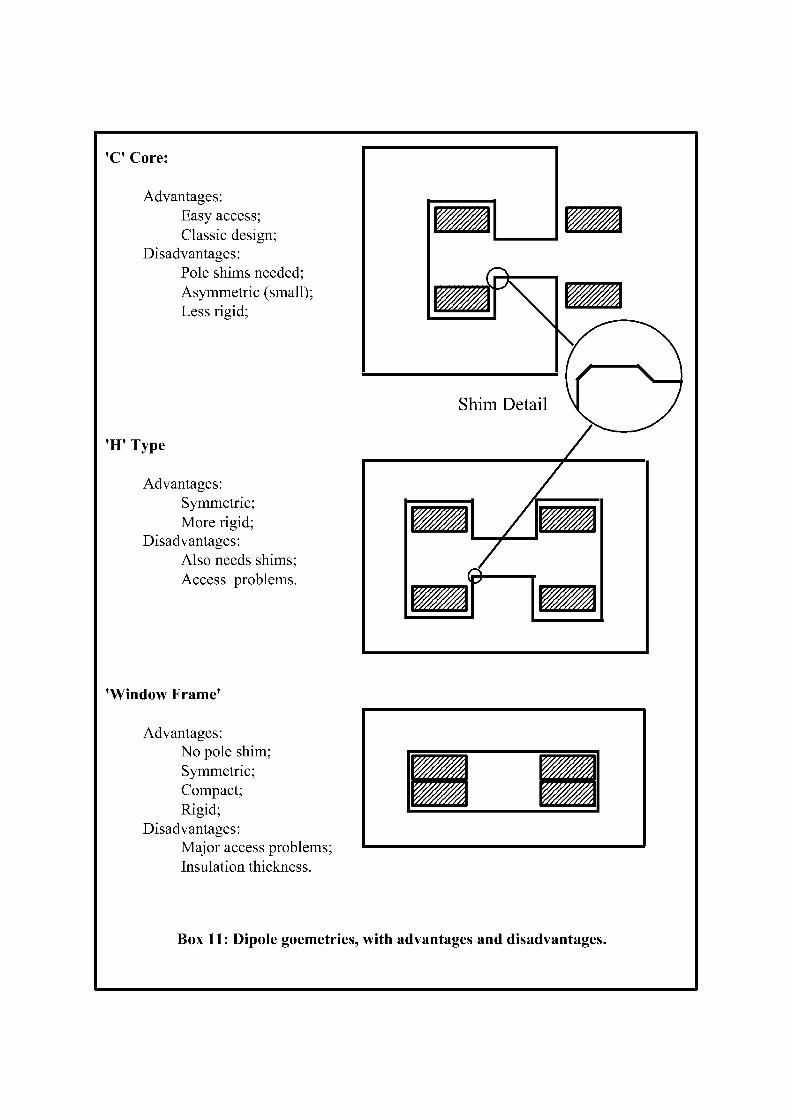
'C Core:
Advantages: Easy access; Classic design;
Disadvantages: Pole shims needed; Asymmetric (small); Less rigid;
'H' Type
Advantages: Symmetric; More rigid;
Disadvantages: Also needs shims; Access problems.
'Window Frame'
Advantages: No pole shim; Symmetric; Compact; Rigid;
Disadvantages: Major access problems; Insulation thickness.
Box 11: Dipole goemetries, with advantages and disadvantages.
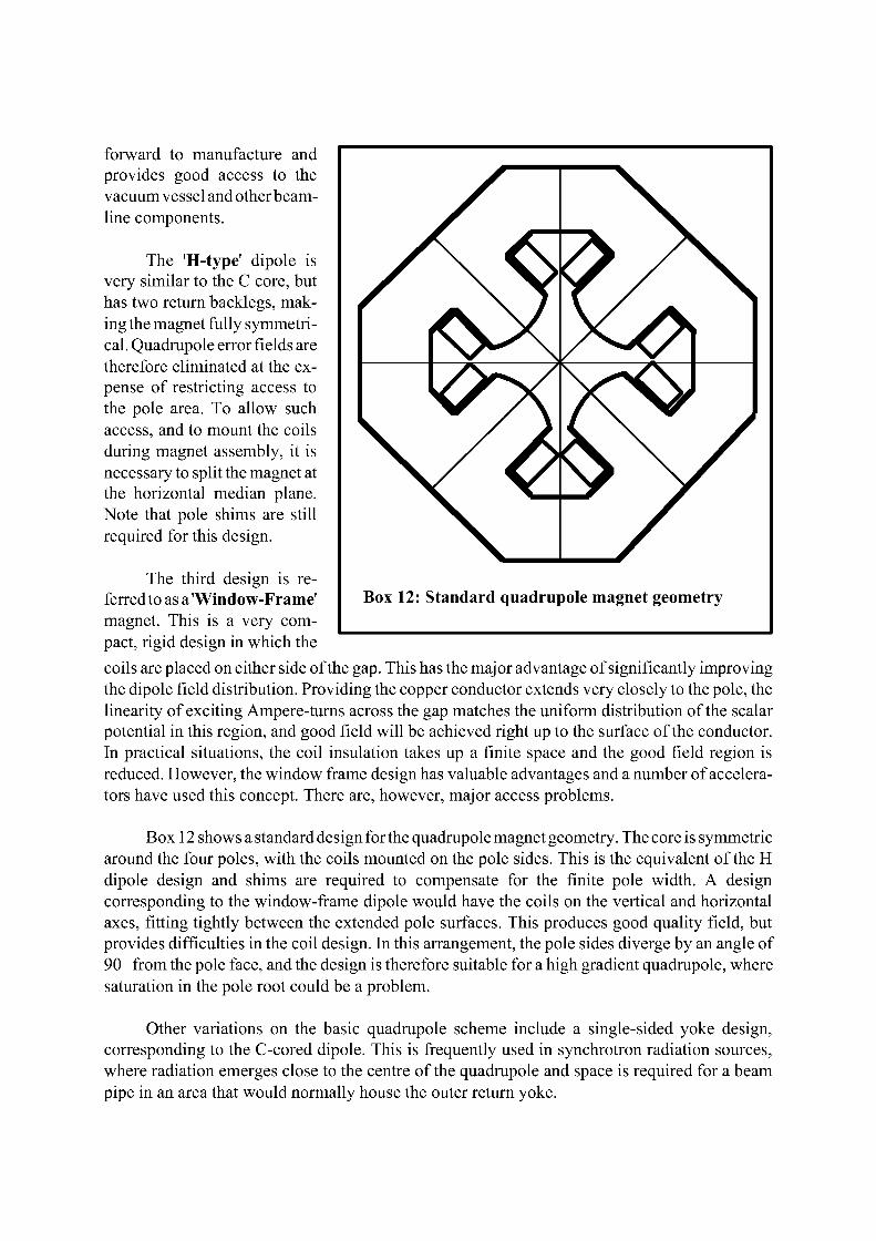
forward to manufacture and provides good access to the vacuum vessel and other beam-line components.
The 'H-type' dipole is very similar to the C core, but has two return backlegs, making the magnet fully symmetrical. Quadrupole error fields are therefore eliminated at the expense of restricting access to the pole area. To allow such access, and to mount the coils during magnet assembly, it is necessary to split the magnet at the horizontal median plane. Note that pole shims are still required for this design.
The third design is referred to as a 'Window-Frame' magnet. This is a very compact, rigid design in which the coils are placed on either side of the gap. This has the major advantage of significantly improving the dipole field distribution. Providing the copper conductor extends very closely to the pole, the linearity of exciting Ampere-turns across the gap matches the uniform distribution of the scalar potential in this region, and good field will be achieved right up to the surface of the conductor. In practical situations, the coil insulation takes up a finite space and the good field region is reduced. However, the window frame design has valuable advantages and a number of accelerators have used this concept. There are, however, major access problems.
Box 12 shows a standard design for the quadrupole magnet geometry. The core is symmetric around the four poles, with the coils mounted on the pole sides. This is the equivalent of the H dipole design and shims are required to compensate for the finite pole width. A design corresponding to the window-frame dipole would have the coils on the vertical and horizontal axes, fitting tightly between the extended pole surfaces. This produces good quality field, but provides difficulties in the coil design. In this arrangement, the pole sides diverge by an angle of 90 from the pole face, and the design is therefore suitable for a high gradient quadrupole, where saturation in the pole root could be a problem.
Other variations on the basic quadrupole scheme include a single-sided yoke design, corresponding to the C-cored dipole. This is frequently used in synchrotron radiation sources, where radiation emerges close to the centre of the quadrupole and space is required for a beam pipe in an area that would normally house the outer return yoke.
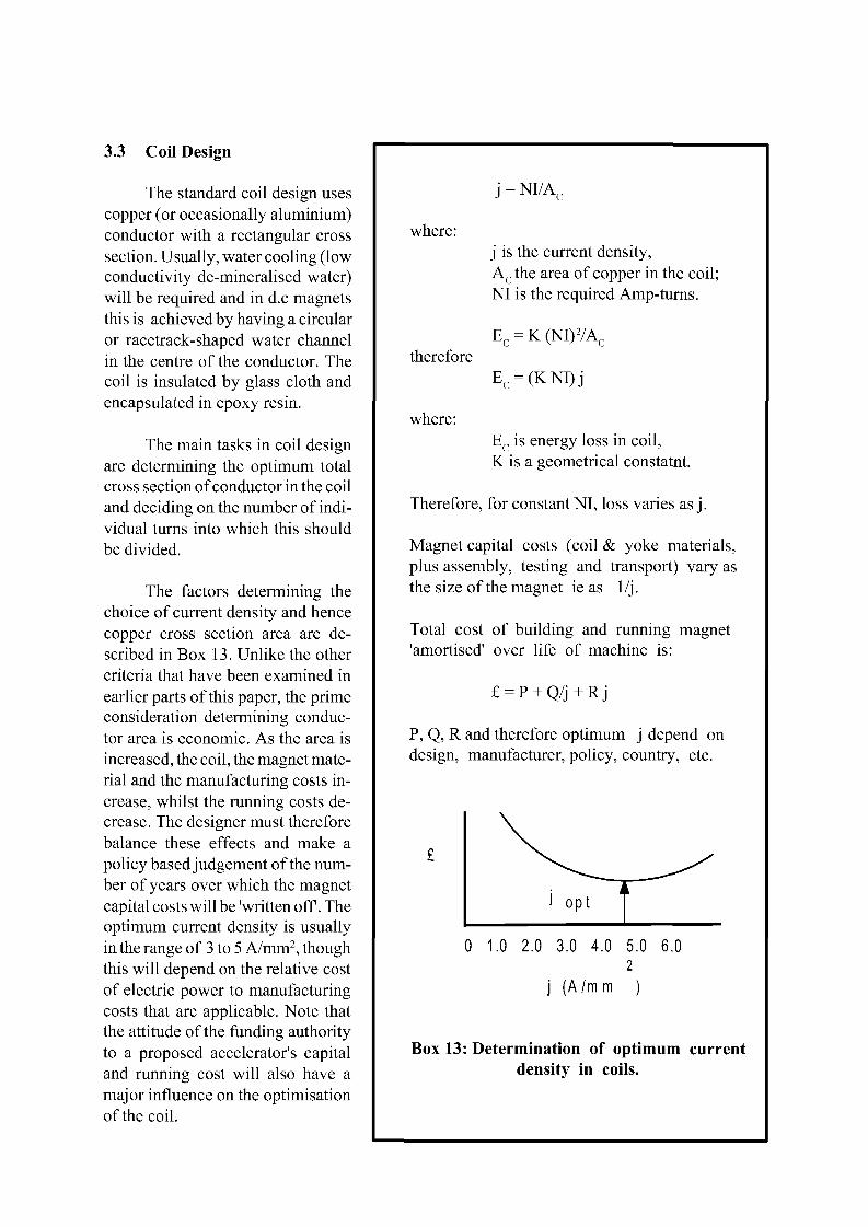
3.3 Coil Design
The standard coil design uses copper (or occasionally aluminium) conductor with a rectangular cross section. Usually, water cooling (low conductivity de-mineralised water) will be required and in d.c magnets this is achieved by having a circular or racetrack-shaped water channel in the centre of the conductor. The coil is insulated by glass cloth and encapsulated in epoxy resin.
The main tasks in coil design are determining the optimum total cross section of conductor in the coil and deciding on the number of individual turns into which this should be divided.
The factors determining the choice of current density and hence copper cross section area are described in Box 13. Unlike the other criteria that have been examined in earlier parts of this paper, the prime consideration determining conductor area is economic. As the area is increased, the coil, the magnet material and the manufacturing costs increase, whilst the running costs decrease. The designer must therefore balance these effects and make a policy based judgement of the number of years over which the magnet capital costs will be 'written off. The optimum current density is usually in the range of 3 to 5 A/mm2, though this will depend on the relative cost of electric power to manufacturing costs that are applicable. Note that the attitude of the funding authority to a proposed accelerator's capital and running cost will also have a major influence on the optimisation of the coil.
where:
therefore
where:
j=NI /A r
j is the current density, A c the area of copper in the coil; NI is the required Amp-turns.
E c = K (NI)2/AC
E =(KNI)j
E is energy loss in coil, K is a geometrical constatnt.
Therefore, for constant NI, loss varies as j .
Magnet capital costs (coil & yoke materials, plus assembly, testing and transport) vary as the size of the magnet ie as 1/j.
Total cost of building and running magnet 'amortised' over life of machine is:
£ = P + Q/j+Rj
P, Q, R and therefore optimum j depend on design, manufacturer, policy, country, etc.
opt
0 1.0 2.0 3.0 4.0 5.0 6.0 2
j (A/mm )
Box 13: Determination of optimum current density in coils.
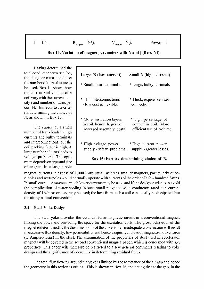
I 1/N, R t N 2 j , V t Ni , Power j ' magnet J ' magnet J ' J
Box 14: Variation of magnet parameters with N and j (fixed NI).
Large N (low current)
* Small, neat terminals.
* Thin interconnections - low cost & flexible.
* More insulation layers in coil, hence larger coil, increased assembly costs.
* High voltage power supply - safety problems.
Small N (high current)
* Large, bulky terminals
* Thick, expensive interconnection.
* High percentage of copper in coil. More efficient use of volume.
* High current power supply - greater losses.
Having determined the total conductor cross section, the designer must decide on the number of turns that are to be used. Box 14 shows how the current and voltage of a coil vary with the current density j and number of turns per coil, N. This leads to the criteria determining the choice of N, as shown in Box 15.
The choice of a small number of turns leads to high currents and bulky terminals and interconnections, but the coil packing factor is high. A large number of turns leads to voltage problems. The optimum depends on type and size of magnet. In a large dipole magnet, currents in excess of 1,000A are usual, whereas smaller magnets, particularly quad-rupoles and sextupoles would normally operate with currents of the order of a few hundred Amps. In small corrector magnets, much lower currents may be used and if the designer wishes to avoid the complication of water cooling in such small magnets, solid conductor, rated at a current density of 1 A/mm2 or less, may be used; the heat from such a coil can usually be dissipated into the air by natural convection.
3.4 Steel Yoke Design
The steel yoke provides the essential ferro-magnetic circuit in a conventional magnet, linking the poles and providing the space for the excitation coils. The gross behaviour of the magnet is determined by the the dimensions of the yoke, for an inadequate cross section will result in excessive flux density, low permeability and hence a significant loss of magneto-motive force (ie Ampere-turns) in the steel. The examination of the properties of steel used in accelerator magnets will be covered in the second conventional magnet paper, which is concerned with a.c. properties. This paper will therefore be restricted to a few general comments relating to yoke design and the significance of coercivity in determining residual fields.
Box 15: Factors determining choice of N.
The total flux flowing around the yoke is limited by the reluctance of the air gap and hence the geometry in this region is critical. This is shown in Box 16, indicating that at the gap, in the
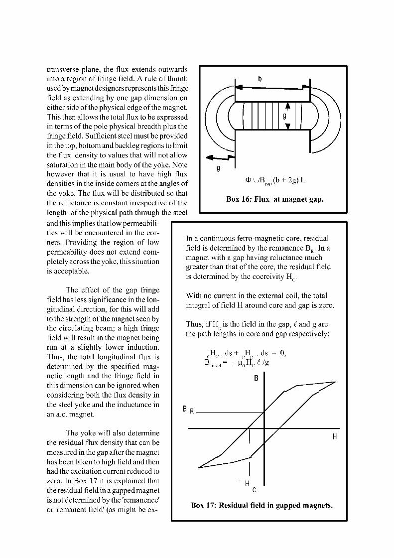
transverse plane, the flux extends outwards into a region of fringe field. A rule of thumb used by magnet designers represents this fringe field as extending by one gap dimension on either side of the physical edge of the magnet. This then allows the total flux to be expressed in terms of the pole physical breadth plus the fringe field. Sufficient steel must be provided in the top, bottom and backleg regions to limit the flux density to values that will not allow saturation in the main body of the yoke. Note however that it is usual to have high flux densities in the inside corners at the angles of the yoke. The flux will be distributed so that the reluctance is constant irrespective of the length of the physical path through the steel and this implies that low permeabilities will be encountered in the corners. Providing the region of low permeability does not extend completely across the yoke, this situation is acceptable.
T
* u B „ ( b + 2g)l. gap
Box 16: Flux at magnet gap.
The effect of the gap fringe field has less significance in the longitudinal direction, for this will add to the strength of the magnet seen by the circulating beam; a high fringe field will result in the magnet being run at a slightly lower induction. Thus, the total longitudinal flux is determined by the specified magnetic length and the fringe field in this dimension can be ignored when considering both the flux density in the steel yoke and the inductance in an a.c. magnet.
The yoke will also determine the residual flux density that can be measured in the gap after the magnet has been taken to high field and then had the excitation current reduced to zero. In Box 17 it is explained that the residual field in a gapped magnet is not determined by the 'remanence' or 'remanent field' (as might be ex-
In a continuous ferro-magnetic core, residual field is determined by the remanence B R . In a magnet with a gap having reluctance much greater than that of the core, the residual field is determined by the coercivity H c .
With no current in the external coil, the total integral of field H around core and gap is zero.
Thus, if H is the field in the gap, i and g are the path lengths in core and gap respectively:
Box 17: Residual field in gapped magnets.
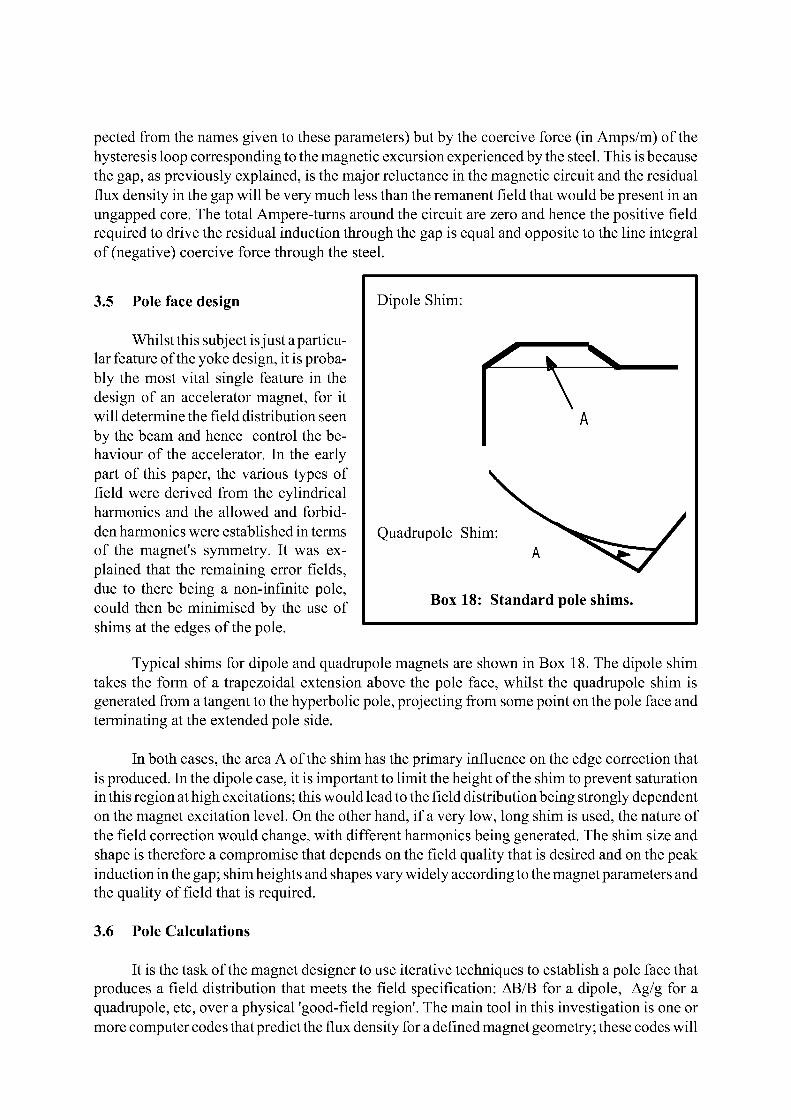
pected from the names given to these parameters) but by the coercive force (in Amps/m) of the hysteresis loop corresponding to the magnetic excursion experienced by the steel. This is because the gap, as previously explained, is the major reluctance in the magnetic circuit and the residual flux density in the gap will be very much less than the remanent field that would be present in an ungapped core. The total Ampere-turns around the circuit are zero and hence the positive field required to drive the residual induction through the gap is equal and opposite to the line integral of (negative) coercive force through the steel.
3.5 Pole face design
Whilst this subject is just a particular feature of the yoke design, it is probably the most vital single feature in the design of an accelerator magnet, for it will determine the field distribution seen by the beam and hence control the behaviour of the accelerator. In the early part of this paper, the various types of field were derived from the cylindrical harmonics and the allowed and forbidden harmonics were established in terms of the magnet's symmetry. It was explained that the remaining error fields, due to there being a non-infinite pole, could then be minimised by the use of shims at the edges of the pole.
Typical shims for dipole and quadrupole magnets are shown in Box 18. The dipole shim takes the form of a trapezoidal extension above the pole face, whilst the quadrupole shim is generated from a tangent to the hyperbolic pole, projecting from some point on the pole face and terminating at the extended pole side.
In both cases, the area A of the shim has the primary influence on the edge correction that is produced. In the dipole case, it is important to limit the height of the shim to prevent saturation in this region at high excitations; this would lead to the field distribution being strongly dependent on the magnet excitation level. On the other hand, if a very low, long shim is used, the nature of the field correction would change, with different harmonics being generated. The shim size and shape is therefore a compromise that depends on the field quality that is desired and on the peak induction in the gap; shim heights and shapes vary widely according to the magnet parameters and the quality of field that is required.
3.6 Pole Calculations
It is the task of the magnet designer to use iterative techniques to establish a pole face that produces a field distribution that meets the field specification: AB/B for a dipole, Ag/g for a quadrupole, etc, over a physical 'good-field region'. The main tool in this investigation is one or more computer codes that predict the flux density for a defined magnet geometry; these codes will
Dipole Shim:
Quadrupole Shim:
Box 18: Standard pole shims.
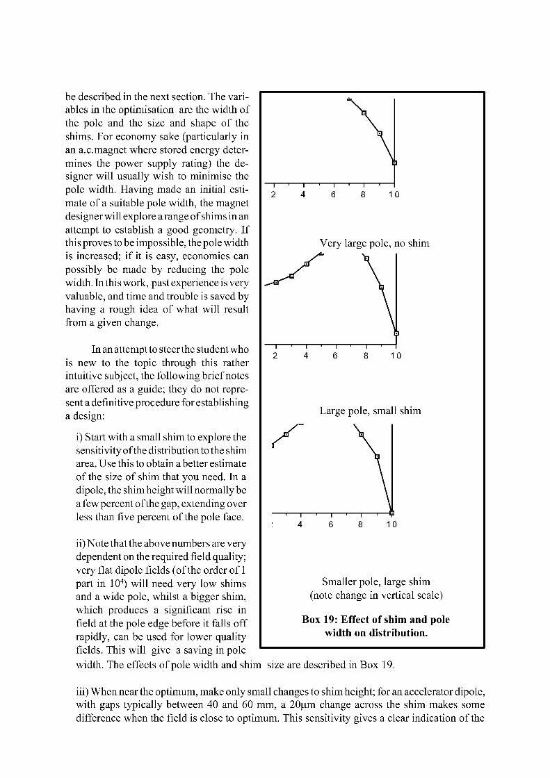
be described in the next section. The variables in the optimisation are the width of the pole and the size and shape of the shims. For economy sake (particularly in an a.c.magnet where stored energy determines the power supply rating) the designer will usually wish to minimise the pole width. Having made an initial estimate of a suitable pole width, the magnet designer will explore a range of shims in an attempt to establish a good geometry. If this proves to be impossible, the pole width is increased; if it is easy, economies can possibly be made by reducing the pole width. In this work, past experience is very valuable, and time and trouble is saved by having a rough idea of what will result from a given change.
In an attempt to steer the student who is new to the topic through this rather intuitive subject, the following brief notes are offered as a guide; they do not represent a definitive procedure for establishing a design:
i) Start with a small shim to explore the sensitivity of the distribution to the shim area. Use this to obtain a better estimate of the size of shim that you need. In a dipole, the shim height will normally be a few percent of the gap, extending over less than five percent of the pole face.
ii) Note that the above numbers are very dependent on the required field quality; very flat dipole fields (of the order of 1 part in 104) will need very low shims and a wide pole, whilst a bigger shim, which produces a significant rise in field at the pole edge before it falls off rapidly, can be used for lower quality fields. This will give a saving in pole
Very large pole, no shim
- r 2
- r 4
Large pole, small shim
- r 4
Smaller pole, large shim (note change in vertical scale)
Box 19: Effect of shim and pole width on distribution.
width. The effects of pole width and shim size are described in Box 19.
iii) When near the optimum, make only small changes to shim height; for an accelerator dipole, with gaps typically between 40 and 60 mm, a 20|um change across the shim makes some difference when the field is close to optimum. This sensitivity gives a clear indication of the
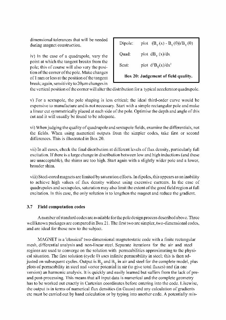
dimensional tolerances that will be needed during magnet construction.
iv) In the case of a quadrupole, vary the point at which the tangent breaks from the pole; this of course will also vary the position of the corner of the pole. Make changes of 1 mm or less at the position of the tangent break; again, sensitivity to 20|um changes in the vertical position of the corner will alter the distribution for a typical accelerator quadrupole.
v) For a sextupole, the pole shaping is less critical; the ideal third-order curve would be expensive to manufacture and is not necessary. Start with a simple rectangular pole and make a linear cut symmetrically placed at each side of the pole. Optimise the depth and angle of this cut and it will usually be found to be adequate.
vi) When judging the quality of quadrupole and sextupole fields, examine the differentials, not the fields. When using numerical outputs from the simpler codes, take first or second differences. This is illustrated in Box 20.
vii) In all cases, check the final distribution at different levels of flux density, particularly full excitation. If there is a large change in distribution between low and high inductions (and these are unacceptable), the shims are too high. Start again with a slightly wider pole and a lower, broader shim.
viii) Steel-cored magnets are limited by saturation effects. In dipoles, this appears as an inability to achieve high values of flux density without using excessive currents. In the case of quadrupoles and sextupoles, saturation may also limit the extent of the good field region at full excitation. In this case, the only solution is to lengthen the magnet and reduce the gradient.
3.7 Field computation codes
A number of standard codes are available for the pole design process described above. Three well known packages are compared in Box 21. The first two are simpler, two-dimensional codes, and are ideal for those new to the subject.
MAGNET is a 'classical' two-dimensional magnetostatic code with a finite rectangular mesh, differential analysis and non-linear steel. Separate iterations for the air and steel regions are used to converge on the solution with permeabilities approximating to the physical situation. The first solution (cycle 0) uses infinite permeability in steel; this is then adjusted on subsequent cycles. Output is B x and B Y in air and steel for the complete model, plus plots of permeability in steel and vector potential in air (to give total fluxes) and (in one version) an harmonic analysis. It is quickly and easily learned but suffers from the lack of pre-and post-processing. This means that all input data is numerical and the complete geometry has to be worked out exactly in Cartesian coordinates before entering into the code. Likewise, the output is in terms of numerical flux densities (in Gauss) and any calculation of gradients etc must be carried out by hand calculation or by typing into another code. A potentially mis-
Dipole: plot (BY(x)-BY(0))/BY(0)
Quad: plot dBY(x)/dx
Sext: plot d2BY(x)/dx2
Box 20 Judgement of field quality.
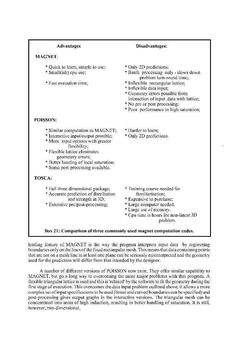
Advantages Disadvantages:
MAGNET:
* Quick to learn, simple to use; * Only 2D predictions; * Small(ish) cpu use; * Batch processing only - slows down
problem turn-round time; * Fast execution time; * Inflexible rectangular lattice;
* Inflexible data input; * Geometry errors possible from
interaction of input data with lattice; * No pre or post processing; * Poor performance in high saturation;
POISSON:
* Similar computation as MAGNET; * Harder to learn; * Interactive input/output possible; * Only 2D predictions. * More input options with greater
flexibility; * Flexible lattice eliminates
geometery errors; * Better handing of local saturation; * Some post processing available.
TOSCA:
* Full three dimensional package; * Training course needed for * Accurate prediction of distribution familiarisation;
and strength in 3D; * Expensive to purchase; * Extensive pre/post-processing; * Large computer needed.
* Large use of memory. * Cpu time is hours for non-linear 3D
problem.
Box 21: Comparison of three commonly used magnet computation codes.
leading feature of MAGNET is the way the program interprets input data by registering boundaries only on the lines of the fixed rectangular mesh. This means that data containing points that are not on a mesh line in at least one plane can be seriously misinterpreted and the geometry used for the prediction will differ from that intended by the designer.
A number of different versions of POISSON now exist. They offer similar capability to MAGNET, but go a long way to overcoming the more major problems with that program. A flexible triangular lattice is used and this is 'relaxed' by the software to fit the geometry during the first stage of execution. This overcomes the data input problem outlined above, it allows a more complex set of input specifications to be used (linear and curved boundaries can be specified) and post-processing gives output graphs in the interactive versions. The triangular mesh can be concentrated into areas of high induction, resulting in better handling of saturation. It is still, however, two dimensional.
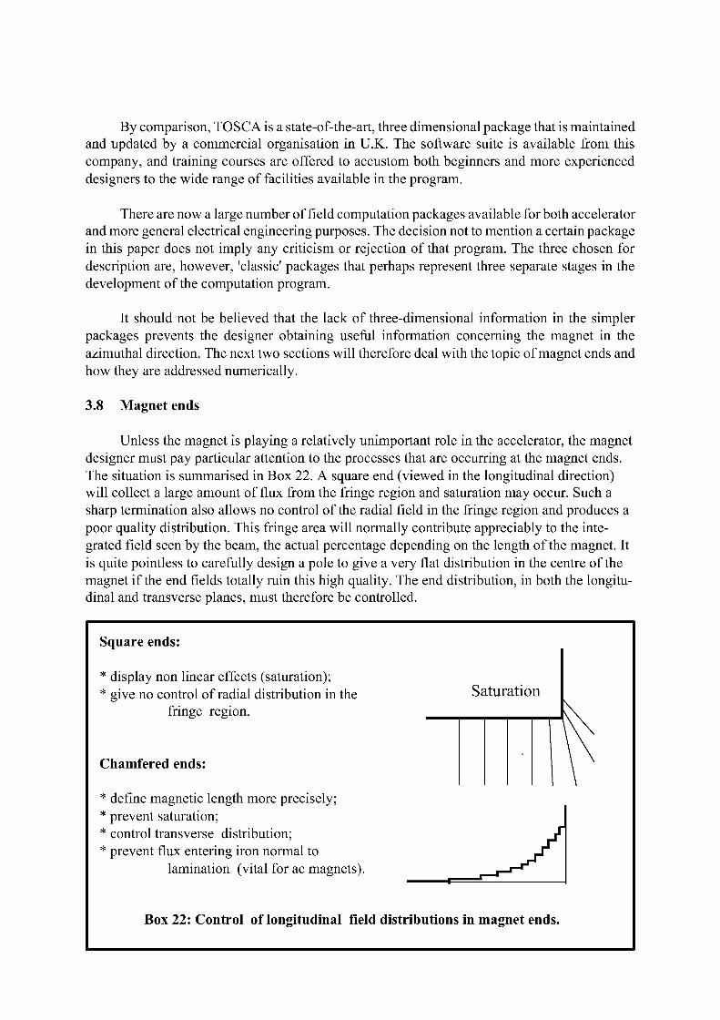
By comparison, TOSCA is a state-of-the-art, three dimensional package that is maintained and updated by a commercial organisation in U.K. The software suite is available from this company, and training courses are offered to accustom both beginners and more experienced designers to the wide range of facilities available in the program.
There are now a large number of field computation packages available for both accelerator and more general electrical engineering purposes. The decision not to mention a certain package in this paper does not imply any criticism or rejection of that program. The three chosen for description are, however, 'classic' packages that perhaps represent three separate stages in the development of the computation program.
It should not be believed that the lack of three-dimensional information in the simpler packages prevents the designer obtaining useful information concerning the magnet in the azimuthal direction. The next two sections will therefore deal with the topic of magnet ends and how they are addressed numerically.
3.8 Magnet ends
Unless the magnet is playing a relatively unimportant role in the accelerator, the magnet designer must pay particular attention to the processes that are occurring at the magnet ends. The situation is summarised in Box 22. A square end (viewed in the longitudinal direction) will collect a large amount of flux from the fringe region and saturation may occur. Such a sharp termination also allows no control of the radial field in the fringe region and produces a poor quality distribution. This fringe area will normally contribute appreciably to the integrated field seen by the beam, the actual percentage depending on the length of the magnet. It is quite pointless to carefully design a pole to give a very flat distribution in the centre of the magnet if the end fields totally ruin this high quality. The end distribution, in both the longitudinal and transverse planes, must therefore be controlled.
Square ends:
* display non linear effects (saturation); * give no control of radial distribution in the
fringe region.
Chamfered ends:
* define magnetic length more precisely; * prevent saturation; * control transverse distribution; * prevent flux entering iron normal to
lamination (vital for ac magnets).
Box 22: Control of longitudinal field distributions in magnet ends.
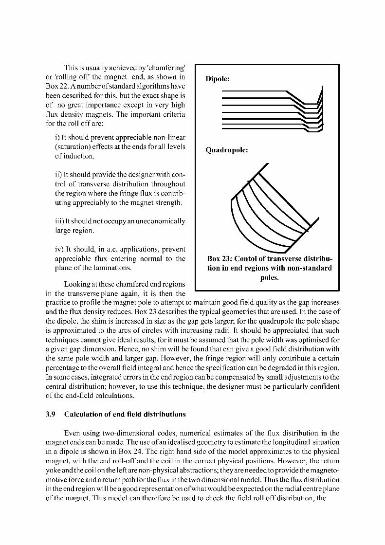
This is usually achieved by 'chamfering' or 'rolling off the magnet end, as shown in Box 22. A number of standard algorithms have been described for this, but the exact shape is of no great importance except in very high flux density magnets. The important criteria for the roll off are:
i) It should prevent appreciable non-linear (saturation) effects at the ends for all levels of induction.
ii) It should provide the designer with control of transverse distribution throughout the region where the fringe flux is contributing appreciably to the magnet strength.
iii) It should not occupy an uneconomically large region.
iv) It should, in a.c. applications, prevent appreciable flux entering normal to the plane of the laminations.
Looking at these chamfered end regions in the transverse plane again, it is then the practice to profile the magnet pole to attempt to maintain good field quality as the gap increases and the flux density reduces. Box 23 describes the typical geometries that are used. In the case of the dipole, the shim is increased in size as the gap gets larger; for the quadrupole the pole shape is approximated to the arcs of circles with increasing radii. It should be appreciated that such techniques cannot give ideal results, for it must be assumed that the pole width was optimised for a given gap dimension. Hence, no shim will be found that can give a good field distribution with the same pole width and larger gap. However, the fringe region will only contribute a certain percentage to the overall field integral and hence the specification can be degraded in this region. In some cases, integrated errors in the end region can be compensated by small adjustments to the central distribution; however, to use this technique, the designer must be particularly confident of the end-field calculations.
3.9 Calculation of end field distributions
Even using two-dimensional codes, numerical estimates of the flux distribution in the magnet ends can be made. The use of an idealised geometry to estimate the longitudinal situation in a dipole is shown in Box 24. The right hand side of the model approximates to the physical magnet, with the end roll-off and the coil in the correct physical positions. However, the return yoke and the coil on the left are non-physical abstractions; they are needed to provide the magnetomotive force and a return path for the flux in the two dimensional model. Thus the flux distribution in the end region will be a good representation of what would be expected on the radial centre plane of the magnet. This model can therefore be used to check the field roll off distribution, the
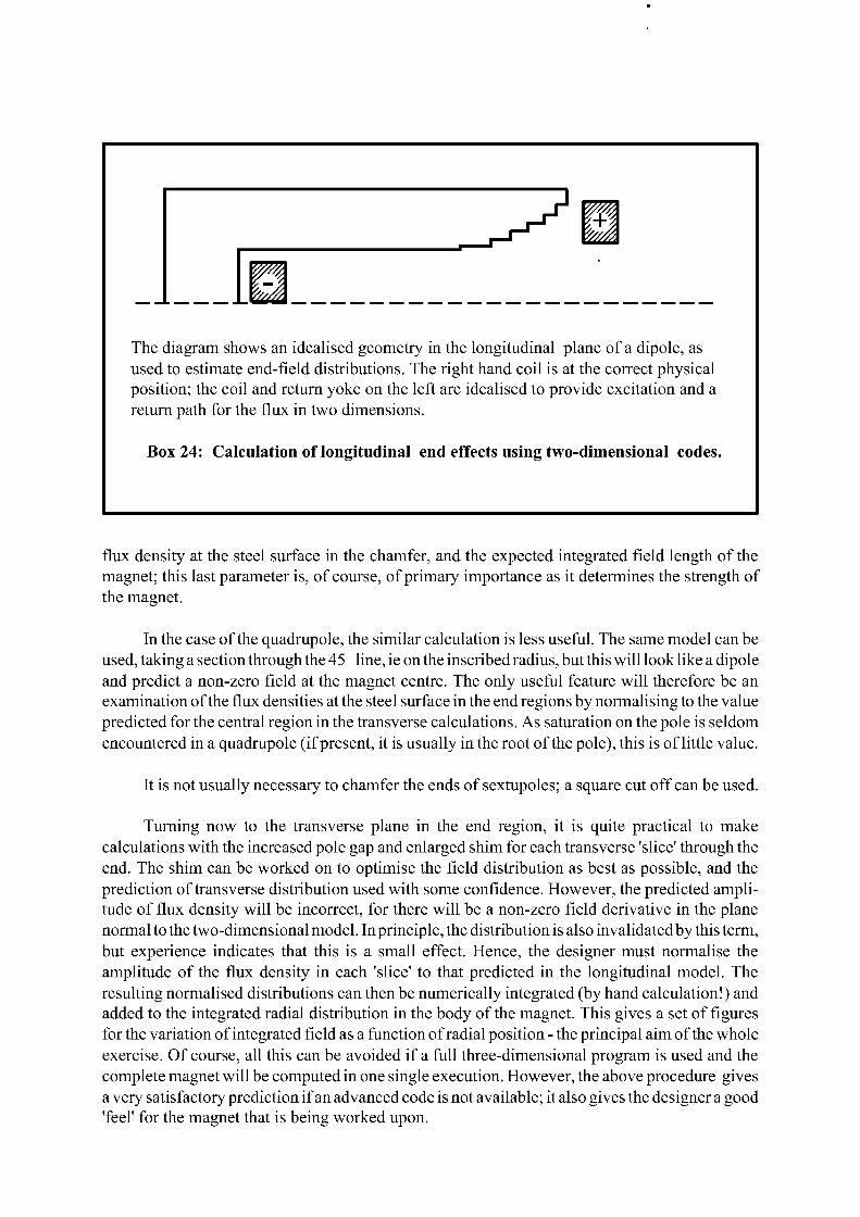
m
The diagram shows an idealised geometry in the longitudinal plane of a dipole, as used to estimate end-field distributions. The right hand coil is at the correct physical position; the coil and return yoke on the left are idealised to provide excitation and a return path for the flux in two dimensions.
Box 24: Calculation of longitudinal end effects using two-dimensional codes.
flux density at the steel surface in the chamfer, and the expected integrated field length of the magnet; this last parameter is, of course, of primary importance as it determines the strength of the magnet.
In the case of the quadrupole, the similar calculation is less useful. The same model can be used, taking a section through the 45 line, ie on the inscribed radius, but this will look like a dipole and predict a non-zero field at the magnet centre. The only useful feature will therefore be an examination of the flux densities at the steel surface in the end regions by normalising to the value predicted for the central region in the transverse calculations. As saturation on the pole is seldom encountered in a quadrupole (if present, it is usually in the root of the pole), this is of little value.
It is not usually necessary to chamfer the ends of sextupoles; a square cut off can be used.
Turning now to the transverse plane in the end region, it is quite practical to make calculations with the increased pole gap and enlarged shim for each transverse 'slice' through the end. The shim can be worked on to optimise the field distribution as best as possible, and the prediction of transverse distribution used with some confidence. However, the predicted amplitude of flux density will be incorrect, for there will be a non-zero field derivative in the plane normal to the two-dimensional model. In principle, the distribution is also invalidated by this term, but experience indicates that this is a small effect. Hence, the designer must normalise the amplitude of the flux density in each 'slice' to that predicted in the longitudinal model. The resulting normalised distributions can then be numerically integrated (by hand calculation!) and added to the integrated radial distribution in the body of the magnet. This gives a set of figures for the variation of integrated field as a function of radial position - the principal aim of the whole exercise. Of course, all this can be avoided if a full three-dimensional program is used and the complete magnet will be computed in one single execution. However, the above procedure gives a very satisfactory prediction if an advanced code is not available; it also gives the designer a good 'feel' for the magnet that is being worked upon.
3.10 Magnet manufacture
This is a specialised topic, the details of which are perhaps best left to the various manufacturers that make their living by supplying accelerator laboratories. However, a few comments should help the designer when preparing for this exercise.
For d.c. accelerator magnets, yokes are usually laminated. This allows the 'shuffling' of steel to randomise the magnetic properties. Laminations also prevent eddy current effects which, even in d.c. magnets, can cause problems with decay time constants of the order of minutes. Laminations are therefore be regarded as essential in storage rings which are ramped between injection and full energy.
The laminations are 'stamped' using a 'stamping tool'. This must have very high precision and reproducibility (~20|um). Manufacturers involved in standard electrical engineering production will regard this figure as stringent but possible. The dimensions of the lamination must be checked on an optical microscope every five to eight thousand laminations.
Assembly of the laminations is in a fixture; the number of laminations in each stack is determined by weight and hydraulic pressure is used to define the length. At one time, the stacked laminations were glued together, but now it is more usual to weld externally whilst the stack is firmly held in the fixture. If a.c. magnets are being assembled the welding must not produce shorted turns.
Coils are wound using glass insulation wrapped onto the copper or aluminium conductor before receiving an 'outerground' insulation of (thicker) glass cloth. The assembly is then placed in a mould and heated under vacuum to dry and outgas. The mould is subsequently flooded with liquid epoxy resin that has been mixed with the catalyst under vacuum. The vacuum tank is let up to atmosphere, forcing the resin deep into the coil to produce full impregnation. 'Curing' of the resin then occurs at high temperature. Total cleanliness is essential during all stages of this process!
Rigorous testing of coils, including water pressure, water flow, thermal cycling and 'flash' testing at high voltage whilst the body of the coil is immersed in water (terminals only clear) is strongly recommended. This will pay dividends in reliability of the magnets in the operational environment of the accelerator.
BIBLIOGRAPHY
Many text-books provide a sound theoretical description of fundamental magneto-statics as described in this paper, but for a clear and easily understood presentation see:
B.I. Bleaney and B. Bleaney, Electricity and Magnetism, (Oxford University Press, 1959)
For a more advanced presentation, see:
W.K.H. Panofsky and M. Phillips, Classical Electricity and Magnetism, (Addison - Wesley Publishing Co., 1956).

Many magnet designs for accelerator applications have been described in detail in the series of International Conferences on Magnet Technology. Given below are the dates and venues of these conferences; the proceedings of these Conferences provide many examples of d.c, a.c. and pulsed magnet design:
1965 Stanford Ca, USA; 1967 Oxford, UK; 1970 Hamburg, Germany; 1972 BrookhavenN.Y.,USA; 1975 Rome, Italy; 1977 Bratislava, Czechoslovakia 1981 Karlsruhe, Germany; 1983 Grenoble, France; 1985 Zurich, Switzerland; 1989 Boston, USA.
CONVENTIONAL MAGNETS - II
Neil Marks. Daresbury Laboratory, Warrington, U.K.
Abstract
This second paper covers the wide range of techniques associated with a.c. and pulsed magnets and associated power supplies. The necessary changes in magnet design to minimise eddy losses in low frequency magnets are first considered and this leads to a broader discussion of the different types of steel used in magnet yokes. Inductance is then considered and the traditional power supply circuit used for a.c. magnets is described. The paper then presents a simple description of the higher frequency pulsed magnets and supply circuits used for injection and extraction and contrasts a number of different design concepts for both kicker and septum systems. In conclusion, the relevant properties of high frequency magnetic materials are briefly reviewed.
1. INTRODUCTION TO AC EFFECTS
The paper resulting from the first seminar dealt exclusively with the design of accelerator magnets generating d.c. or what was referred to as 'slowly varying' fields. This second paper will mainly concentrate on magnet systems with time varying fields and will separately discuss 'low-frequency' and pulsed or 'higher-frequency' devices. It is therefore useful to give some definition to further clarify the arbitrary distinction between these three separate classifications, as used in this paper.
A convenient, though not rigorous, criterion relates to eddy current effects. These are the currents that are induced in any conducting material by the emf generated by a rate of change of magnetic flux cutting the material, as given by the Maxwell equation for electromagnetic induction:
curlE =-dB/dt
The d.c. or slowly varying magnet can therefore be regarded as one in which eddy currents have a negligible effect on the performance of the magnet and its power losses. It will be seen that this definition includes laminated magnets with excitations having Fourier components extending from d.c. to one or two Hertz. It should be noted, however, that if solid steel is used in the yoke, eddy effects are produced by very much lower frequency fields, oscillating at 0.1 Hertz or less. The first seminar was devoted to d.c. systems, though much of the physics was quite general.
In a low-frequency magnet, the eddy currents will increase, perhaps appreciably, the power losses in the coil. However, their potential for influencing the magnetic field distribution
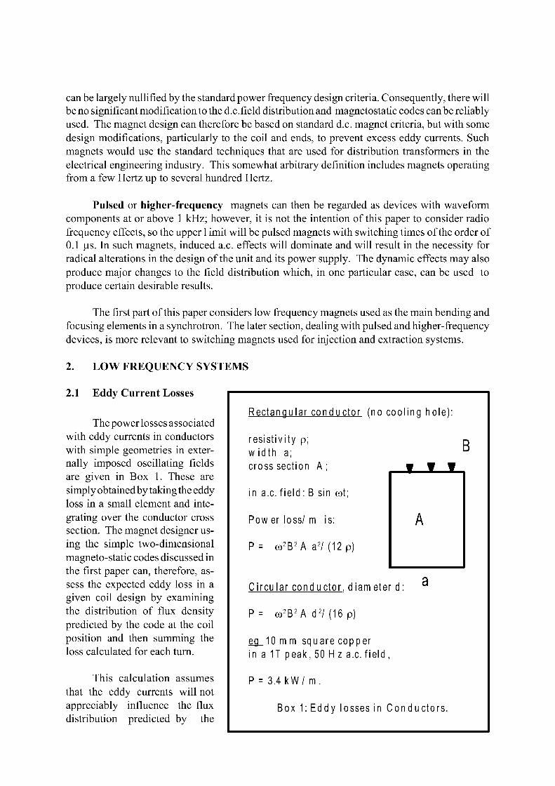
can be largely nullified by the standard power frequency design criteria. Consequently, there will be no significant modification to the d.c.field distribution and magnetostatic codes canbe reliably used. The magnet design can therefore be based on standard d.c. magnet criteria, but with some design modifications, particularly to the coil and ends, to prevent excess eddy currents. Such magnets would use the standard techniques that are used for distribution transformers in the electrical engineering industry. This somewhat arbitrary definition includes magnets operating from a few Hertz up to several hundred Hertz.
Pulsed or higher-frequency magnets can then be regarded as devices with waveform components at or above 1 kHz; however, it is not the intention of this paper to consider radio frequency effects, so the upper 1 imit will be pulsed magnets with switching times of the order of 0.1 |us. In such magnets, induced a.c. effects will dominate and will result in the necessity for radical alterations in the design of the unit and its power supply. The dynamic effects may also produce major changes to the field distribution which, in one particular case, can be used to produce certain desirable results.
The first part of this paper considers low frequency magnets used as the main bending and focusing elements in a synchrotron. The later section, dealing with pulsed and higher-frequency devices, is more relevant to switching magnets used for injection and extraction systems.
2. LOW FREQUENCY SYSTEMS
2.1 Eddy Current Losses
The power losses associated with eddy currents in conductors with simple geometries in externally imposed oscillating fields are given in Box 1. These are simply obtained by taking the eddy loss in a small element and integrating over the conductor cross section. The magnet designer using the simple two-dimensional magneto-static codes discussed in the first paper can, therefore, assess the expected eddy loss in a given coil design by examining the distribution of flux density predicted by the code at the coil position and then summing the loss calculated for each turn.
This calculation assumes that the eddy currents will not appreciably influence the flux distribution predicted by the
Rectangular conductor (no cooling hole):
resistivity p; w id th a; cross section A ;
in a.c. f ie ld : B sin cot;
Pow er loss/ m is:
P= co 2B 2A a 2/ (12 p)
B f f f
A
Circular conductor, diameter d:
P= co 2B 2A d 2 / (16 p)
eg 10 m m square copper in a 1T peak, 50 H z a.c. f ie ld ,
P = 3 .4kW/ m.
Box 1: Eddy losses in Conductors.
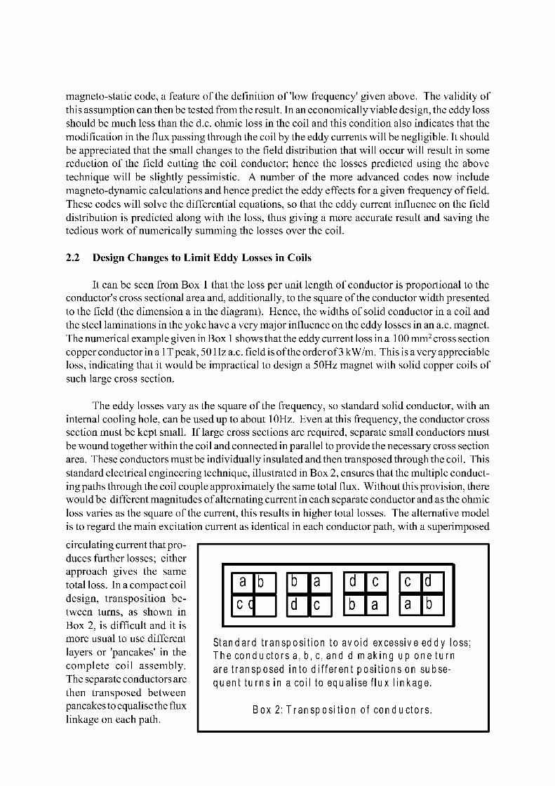
magneto-static code, a feature of the definition of'low frequency' given above. The validity of this assumption can then be tested from the result. In an economically viable design, the eddy loss should be much less than the d.c. ohmic loss in the coil and this condition also indicates that the modification in the flux passing through the coil by the eddy currents will be negligible. It should be appreciated that the small changes to the field distribution that will occur will result in some reduction of the field cutting the coil conductor; hence the losses predicted using the above technique will be slightly pessimistic. A number of the more advanced codes now include magneto-dynamic calculations and hence predict the eddy effects for a given frequency of field. These codes will solve the differential equations, so that the eddy current influence on the field distribution is predicted along with the loss, thus giving a more accurate result and saving the tedious work of numerically summing the losses over the coil.
2.2 Design Changes to Limit Eddy Losses in Coils
It can be seen from Box 1 that the loss per unit length of conductor is proportional to the conductor's cross sectional area and, additionally, to the square of the conductor width presented to the field (the dimension a in the diagram). Hence, the widths of solid conductor in a coil and the steel laminations in the yoke have a very major influence on the eddy losses in an a.c. magnet. The numerical example given in Box 1 shows that the eddy current loss in a 100 mm2 cross section copper conductor in a lTpeak, 50 Hz a.c. fieldisoftheorderof3kW/m. This is a very appreciable loss, indicating that it would be impractical to design a 50Hz magnet with solid copper coils of such large cross section.
The eddy losses vary as the square of the frequency, so standard solid conductor, with an internal cooling hole, can be used up to about 10Hz. Even at this frequency, the conductor cross section must be kept small. If large cross sections are required, separate small conductors must be wound together within the coil and connected in parallel to provide the necessary cross section area. These conductors must be individually insulated and then transposed through the coil. This standard electrical engineering technique, illustrated in Box 2, ensures that the multiple conducting paths through the coil couple approximately the same total flux. Without this provision, there would be different magnitudes of alternating current in each separate conductor and as the ohmic loss varies as the square of the current, this results in higher total losses. The alternative model is to regard the main excitation current as identical in each conductor path, with a superimposed
circulating current that produces further losses; either approach gives the same total loss. In a compact coil design, transposition between turns, as shown in Box 2, is difficult and it is more usual to use different layers or 'pancakes' in the complete coil assembly. The separate conductors are then transposed between pancakes to equalise the flux linkage on each path.
Standard transposit ion to avoid excessive eddy loss; T h e c o n d u c t o r s a , b , c , a n d d making up one tu rn are transposed into different posit ions on subsequent turns in a coil to equalise f lux l inkage.
Box 2: Transposi t ion of conductors.
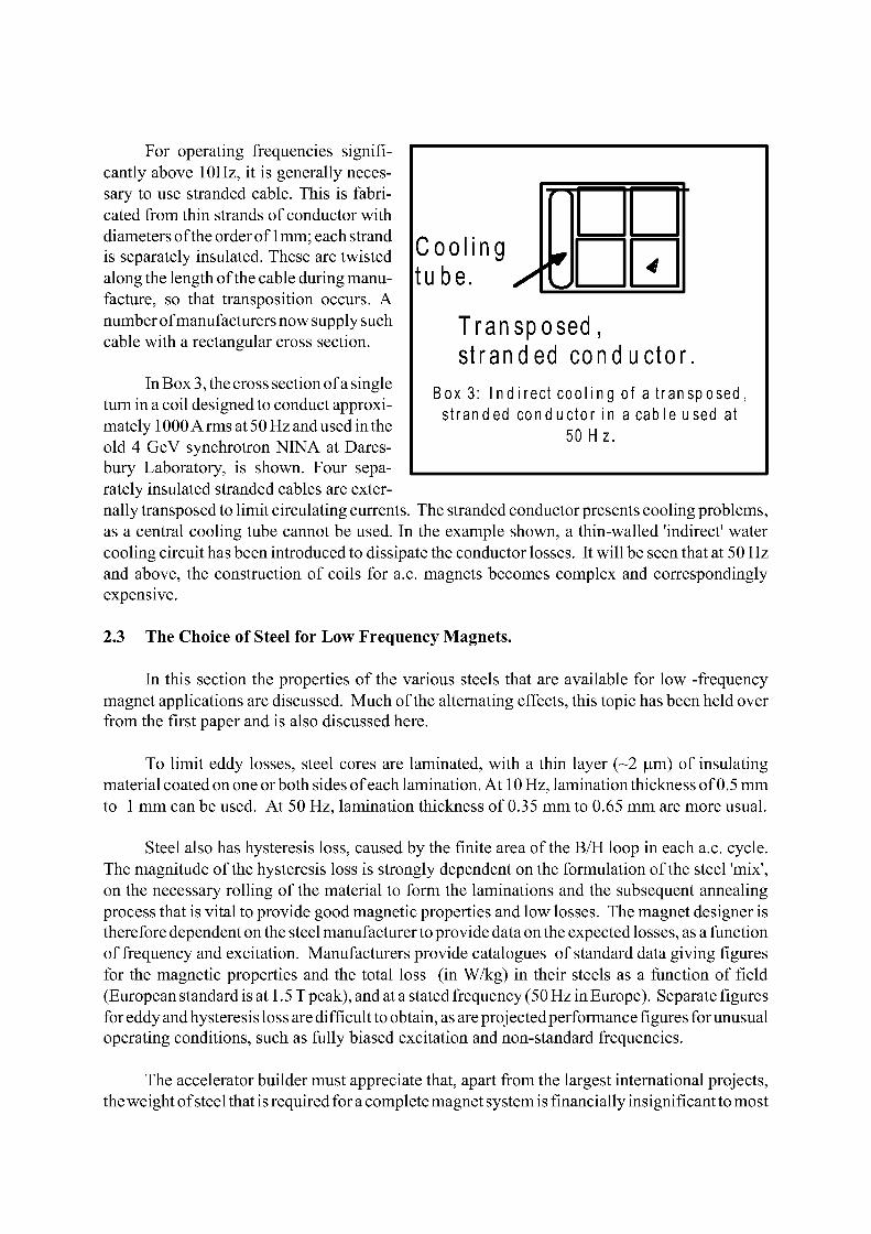
For operating frequencies significantly above 10Hz, it is generally necessary to use stranded cable. This is fabricated from thin strands of conductor with diameters of the order of 1 mm; each strand is separately insulated. These are twisted along the length of the cable during manufacture, so that transposition occurs. A number of manufacturers now supply such cable with a rectangular cross section.
In Box 3, the cross section of a single turn in a coil designed to conduct approximately 1000 A rms at 5 0 Hz and used in the old 4 GeV synchrotron NINA at Dares-bury Laboratory, is shown. Four separately insulated stranded cables are externally transposed to limit circulating currents. The stranded conductor presents cooling problems, as a central cooling tube cannot be used. In the example shown, a thin-walled 'indirect' water cooling circuit has been introduced to dissipate the conductor losses. It will be seen that at 50 Hz and above, the construction of coils for a.c. magnets becomes complex and correspondingly expensive.
2.3 The Choice of Steel for Low Frequency Magnets.
In this section the properties of the various steels that are available for low -frequency magnet applications are discussed. Much of the alternating effects, this topic has been held over from the first paper and is also discussed here.
To limit eddy losses, steel cores are laminated, with a thin layer (~2 |um) of insulating material coated on one or both sides of each lamination. At 10 Hz, lamination thickness of 0.5 mm to 1 mm can be used. At 50 Hz, lamination thickness of 0.35 mm to 0.65 mm are more usual.
Steel also has hysteresis loss, caused by the finite area of the B/H loop in each a.c. cycle. The magnitude of the hysteresis loss is strongly dependent on the formulation of the steel 'mix', on the necessary rolling of the material to form the laminations and the subsequent annealing process that is vital to provide good magnetic properties and low losses. The magnet designer is therefore dependent on the steel manufacturer to provide data on the expected losses, as a function of frequency and excitation. Manufacturers provide catalogues of standard data giving figures for the magnetic properties and the total loss (in W/kg) in their steels as a function of field (European standard is at 1.5 T peak), and at a stated frequency (50 Hz in Europe). Separate figures for eddy and hysteresis loss are difficult to obtain, as are projected performance figures for unusual operating conditions, such as fully biased excitation and non-standard frequencies.
The accelerator builder must appreciate that, apart from the largest international projects, the weight of steel that is required for a complete magnet system is financially insignificant to most
Cooling tube, y <~>
Cooling tube, y <~>
4
Transposed, stranded conductor.
Box 3: Indi rect cool ing of a t ransposed, stranded conductor in a cable used at
50 Hz.
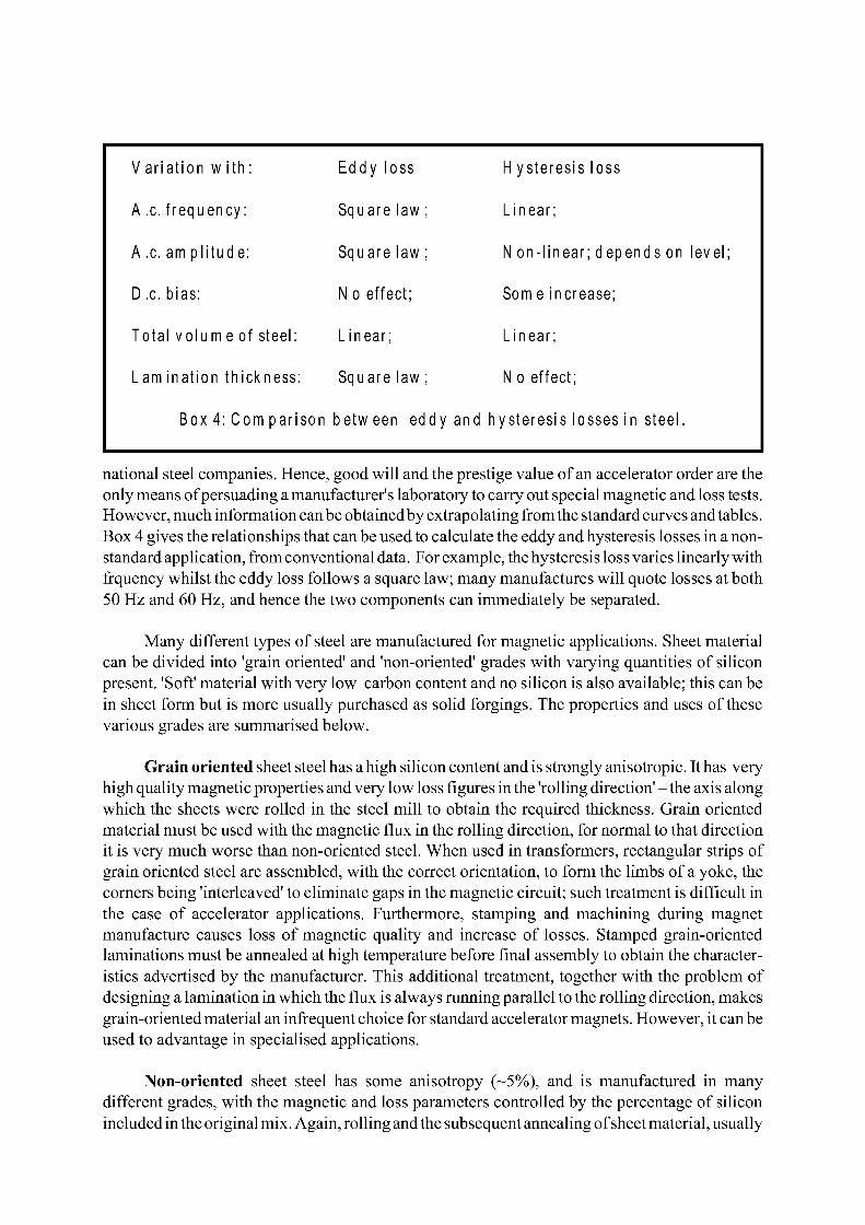
V ariat ion w ith : Eddy loss H ysteresis loss
A .c. frequency: Square law ; Linear;
A .c. am p l i tude: Square law ; N on-l inear; depends on level;
D .c. bias: N o effect; Some increase;
Total volum e of steel: Linear; Linear;
Lam ination thickness: Square law ; N o effect;
Box 4: Com parison between eddy an d h ysteresis losses in steel.
national steel companies. Hence, good will and the prestige value of an accelerator order are the only means of persuading a manufacturer's laboratory to carry out special magnetic and loss tests. However, much information can be obtained by extrapolating from the standard curves and tables. Box 4 gives the relationships that can be used to calculate the eddy and hysteresis losses in a nonstandard application, from conventional data. For example, the hysteresis loss varies linearly with frquency whilst the eddy loss follows a square law; many manufactures will quote losses at both 50 Hz and 60 Hz, and hence the two components can immediately be separated.
Many different types of steel are manufactured for magnetic applications. Sheet material can be divided into 'grain oriented' and 'non-oriented' grades with varying quantities of silicon present. 'Soft' material with very low carbon content and no silicon is also available; this can be in sheet form but is more usually purchased as solid forgings. The properties and uses of these various grades are summarised below.
Grain oriented sheet steel has a high silicon content and is strongly anisotropic. It has very high quality magnetic properties and very low loss figures in the 'rolling direction' - the axis along which the sheets were rolled in the steel mill to obtain the required thickness. Grain oriented material must be used with the magnetic flux in the rolling direction, for normal to that direction it is very much worse than non-oriented steel. When used in transformers, rectangular strips of grain oriented steel are assembled, with the correct orientation, to form the limbs of a yoke, the corners being 'interleaved' to eliminate gaps in the magnetic circuit; such treatment is difficult in the case of accelerator applications. Furthermore, stamping and machining during magnet manufacture causes loss of magnetic quality and increase of losses. Stamped grain-oriented laminations must be annealed at high temperature before final assembly to obtain the characteristics advertised by the manufacturer. This additional treatment, together with the problem of designing a lamination in which the flux is always running parallel to the rolling direction, makes grain-oriented material an infrequent choice for standard accelerator magnets. However, it can be used to advantage in specialised applications.
Non-oriented sheet steel has some anisotropy (~5%), and is manufactured in many different grades, with the magnetic and loss parameters controlled by the percentage of silicon included in the original mix. Again, rolling and the subsequent annealing of sheet material, usually
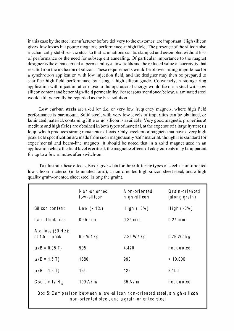
in this case by the steel manufacturer before delivery to the customer, are important. High silicon gives low losses but poorer magnetic performance at high field. The presence of the silicon also mechanically stabilises the steel so that laminations can be stamped and assembled without loss of performance or the need for subsequent annealing. Of particular importance to the magnet designer is the enhancement of permeability at low fields and the reduced value of coercivity that results from the inclusion of silicon. These requirements would be of over-riding importance for a synchrotron application with low injection field, and the designer may then be prepared to sacrifice high-field performance by using a high-silicon grade. Conversely, a storage ring application with injection at or close to the operational energy would favour a steel with low silicon content and better high-field permeability. For reasons mentioned below, a laminated steel would still generally be regarded as the best solution.
Low carbon steels are used for d.c. or very low frequency magnets, where high field performance is paramount. Solid steel, with very low levels of impurities can be obtained, or laminated material, containing little or no silicon is available. Very good magnetic properties at medium and high fields are obtained in both types of material, at the expense of a large hysteresis loop, which produces strong remanence effects. Only accelerator magnets that have a very high peak field specification are made from such magnetically 'soft' material, though it is standard for experimental and beam-line magnets. It should be noted that in a solid magnet used in an application where the field level is critical, the magnetic effects of eddy currents may be apparent for up to a few minutes after switch-on.
To illustrate these effects, Box 5 gives data for three differing types of steel: a non-oriented low-silicon material (in laminated form), a non-oriented high-silicon sheet steel, and a high quality grain-oriented sheet steel (along the grain).
N on-or iented N on-or iented G rain-or iented low -si l icon h igh-s i l icon (along grain)
Silicon content Low (~ 1%) High (-3%) High (-3%)
Lam. thickness 0.65 m m 0.35 mm 0.27 mm
A.c. loss (50 Hz) at 1.5 T peak 6.9 W/ kg 2.25W/ kg 0.79W/ kg
H(B = 0.05 T) 995 4,420 not quoted
H ( B = 1.5T) 1680 990 > 10,000
H ( B = 1.8 T) 184 122 3,100
Coercivity H c 100 A/ m 35 A/ m not quoted
Box 5: Com parison betw een a low -si icon non-or iented stee , a h igh-s i l icon non -oriented steel, an d a grain-or iented steel
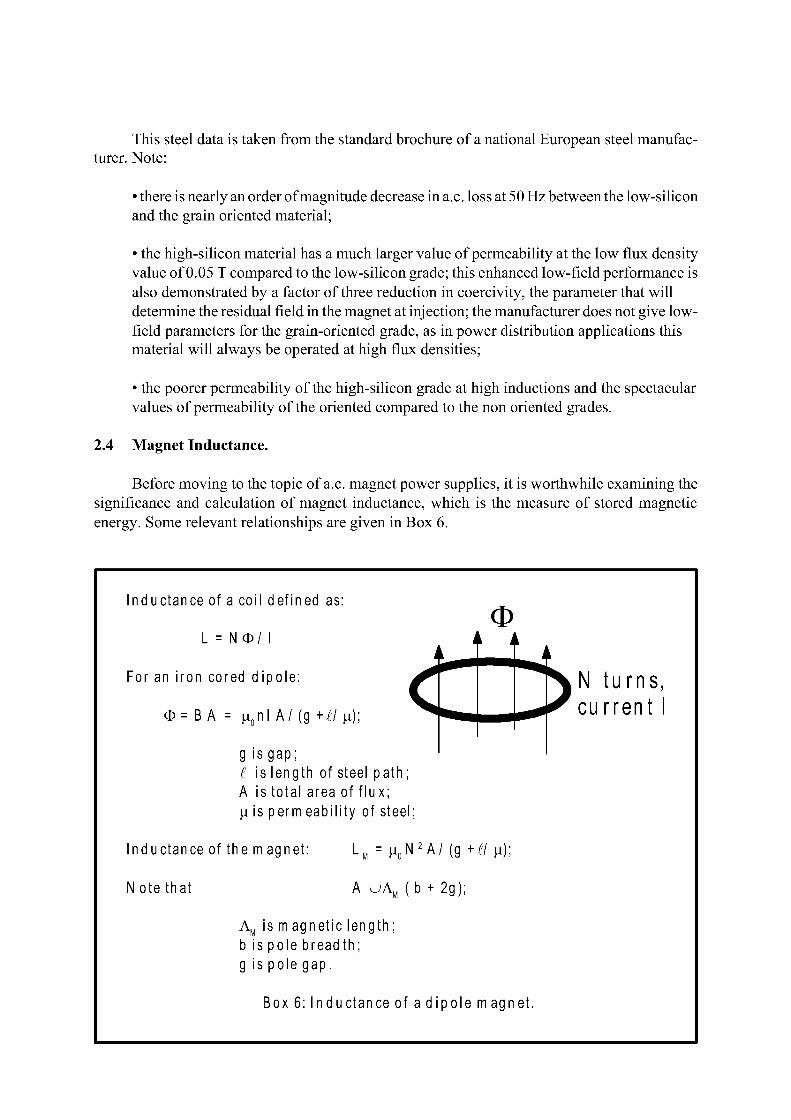
This steel data is taken from the standard brochure of a national European steel manufacturer. Note:
• there is nearly an order of magnitude decrease in a.c. loss at 50 Hz between the low-silicon and the grain oriented material;
• the high-silicon material has a much larger value of permeability at the low flux density value of 0.05 T compared to the low-silicon grade; this enhanced low-field performance is also demonstrated by a factor of three reduction in coercivity, the parameter that will determine the residual field in the magnet at injection; the manufacturer does not give low-field parameters for the grain-oriented grade, as in power distribution applications this material will always be operated at high flux densities;
• the poorer permeability of the high-silicon grade at high inductions and the spectacular values of permeability of the oriented compared to the non oriented grades.
2.4 Magnet Inductance.
Before moving to the topic of a.c. magnet power supplies, it is worthwhile examining the significance and calculation of magnet inductance, which is the measure of stored magnetic energy. Some relevant relationships are given in Box 6.
Inductance of a coil defined as:
L = N O / 1 i
i i k
For an iron cored d ipole: f \ N turns, 0 = B A = n 0 n l A / (g +11 \x); ^ ^cu r ren t 1
g i sgap ; £ is length of steel path; A is total area of f lux; |uis permeabi l i ty of steel;
Inductance of the magnet: L M = j u 0 N 2 A/ (g +^/ |u);
Note that A u A M ( b + 2g);
A M is m agnetic length; b is pole breadth; g is pole gap.
Box 6: Inductance of a d ipo le m agnet.
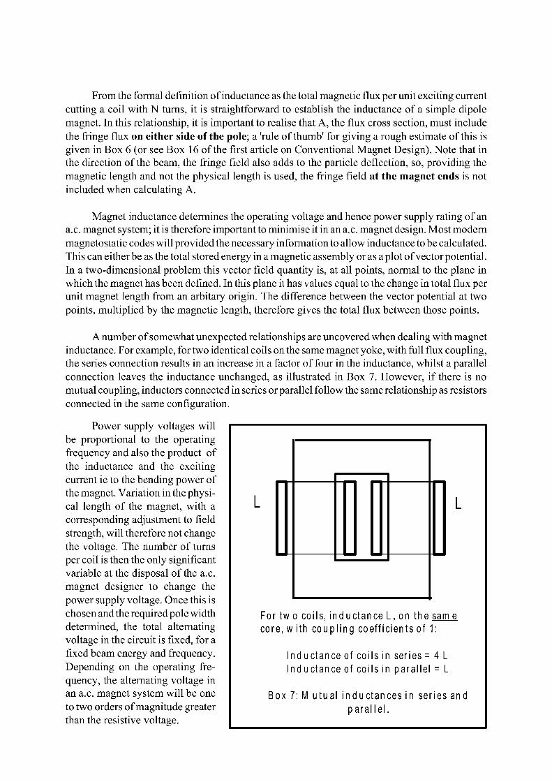
From the formal definition of inductance as the total magnetic flux per unit exciting current cutting a coil with N turns, it is straightforward to establish the inductance of a simple dipole magnet. In this relationship, it is important to realise that A, the flux cross section, must include the fringe flux on either side of the pole; a 'rule of thumb' for giving a rough estimate of this is given in Box 6 (or see Box 16 of the first article on Conventional Magnet Design). Note that in the direction of the beam, the fringe field also adds to the particle deflection, so, providing the magnetic length and not the physical length is used, the fringe field at the magnet ends is not included when calculating A.
Magnet inductance determines the operating voltage and hence power supply rating of an a.c. magnet system; it is therefore important to minimise it in an a.c. magnet design. Most modern magnetostatic codes will provided the necessary information to allow inductance to be calculated. This can either be as the total stored energy in a magnetic assembly or as a plot of vector potential. In a two-dimensional problem this vector field quantity is, at all points, normal to the plane in which the magnet has been defined. In this plane it has values equal to the change in total flux per unit magnet length from an arbitary origin. The difference between the vector potential at two points, multiplied by the magnetic length, therefore gives the total flux between those points.
A number of somewhat unexpected relationships are uncovered when dealing with magnet inductance. For example, for two identical coils on the same magnet yoke, with full flux coupling, the series connection results in an increase in a factor of four in the inductance, whilst a parallel connection leaves the inductance unchanged, as illustrated in Box 7. However, if there is no mutual coupling, inductors connected in series or parallel follow the same relationship as resistors connected in the same configuration.
Power supply voltages will be proportional to the operating frequency and also the product of the inductance and the exciting current ie to the bending power of the magnet. Variation in the physical length of the magnet, with a corresponding adjustment to field strength, will therefore not change the voltage. The number of turns per coil is then the only significant variable at the disposal of the a.c. magnet designer to change the power supply voltage. Once this is chosen and the required pole width determined, the total alternating voltage in the circuit is fixed, for a fixed beam energy and frequency. Depending on the operating frequency, the alternating voltage in an a.c. magnet system will be one to two orders of magnitude greater than the resistive voltage.
L L
For two coils, inductance L, on the same core, w ith coupl ing coefficients of 1:
Inductance of coils in series = 4 L Inductance of coils in parallel = L
Box 7: M u tu al inductances in series and para l le l .
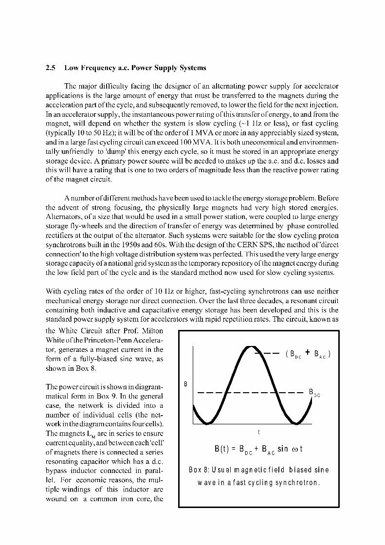
2.5 Low Frequency a.c. Power Supply Systems
The major difficulty facing the designer of an alternating power supply for accelerator applications is the large amount of energy that must be transferred to the magnets during the acceleration part of the cycle, and subsequently removed, to lower the field for the next injection. In an accelerator supply, the instantaneous power rating of this transfer of energy, to and from the magnet, will depend on whether the system is slow cycling (~1 Hz or less), or fast cycling (typically 10 to 50 Hz); it will be of the order of 1 MVA or more in any appreciably sized system, and in a large fast cycling circuit can exceed 100 MVA. It is both uneconomical and environmentally unfriendly to 'dump' this energy each cycle, so it must be stored in an appropriate energy storage device. A primary power source will be needed to makes up the a.c. and d.c. losses and this will have a rating that is one to two orders of magnitude less than the reactive power rating of the magnet circuit.
A number of different methods have been used to tackle the energy storage problem. Before the advent of strong focusing, the physically large magnets had very high stored energies. Alternators, of a size that would be used in a small power station, were coupled to large energy storage fly-wheels and the direction of transfer of energy was determined by phase controlled rectifiers at the output of the alternator. Such systems were suitable for the slow cycling proton synchrotrons built in the 1950s and 60s. With the design of the CERN SPS, the method of'direct connection' to the high voltage distribution system was perfected. This used the very large energy storage capacity of a national grid system as the temporary repository of the magnet energy during the low field part of the cycle and is the standard method now used for slow cycling systems.
With cycling rates of the order of 10 Hz or higher, fast-cycling synchrotrons can use neither mechanical energy storage nor direct connection. Over the last three decades, a resonant circuit containing both inductive and capacitative energy storage has been developed and this is the standard power supply system for accelerators with rapid repetition rates. The circuit, known as the White Circuit after Prof. Milton White of the Princeton-Penn Accelerator, generates a magnet current in the form of a fully-biased sine wave, as shown in Box 8.
The power circuit is shown in diagrammatical form in Box 9. In the general case, the network is divided into a number of individual cells (the network in the diagram contains four cells). The magnets L., are in series to ensure current equality, and between each 'cell' of magnets there is connected a series resonating capacitor which has a d.c. bypass inductor connected in parallel. For economic reasons, the multiple windings of this inductor are wound on a common iron core, the
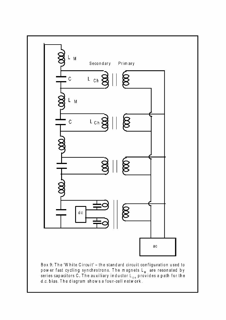
Secondary Primary
ac
Box 9: The 'W hite C i rcu i t ' - the standard circui t conf igurat ion used to power fast cycl ing synchrot rons. The magnets L M are resonated by series capacitors C. The auxi l iary inductor L C H prov ides a path for the d.c. bias. The diagram show s a four-cel l netw ork.

resulting device being referred to as the 'energy storage choke'. Note that each capacitance C must be adequate to resonate both one cell of magnets in series and one choke winding in parallel; ie
C = l/(co2LM) +l/(co2LCH)
where co is the oscillation frequency of the power supply system.
The required direct current bias is introduced by connecting a rectifier set at the mid point of a special split winding of the energy storage choke; this is usually the position of the network earth. A.c. power is generated by an alternating power source, usually an invertor, connected to a further set of windings also wound on the yoke of the energy storage choke. These additional coils are usually referred to as the 'primary' windings, and are magnetically closely coupled to the main choke coils, which are therefore referred to as the 'secondary' windings. The device is therefore both an inductor and a transformer.
The important features of this circuit, that make it well suited for powering fast-cycling synchrotrons, are:
* the magnet waveform is close to ideal;
* the a.c. and d.c. power sources are electrically isolated from each other;
* the magnet voltages are not cumulative, for the alternating voltage across the capacitor and choke winding is n out of phase with the magnet voltage; whilst the total magnet voltage may be in excess of 100 kV, the voltage to earth can be kept an order of magnitude lower by dividing into larger numbers of cells;
* the power drawn from the public supply system represents an almost steady load, with a power factor close to one;
* in addition to feeding power to the network, the primary windings on the energy storage choke also balance the network voltages and stabilise the oscillations at the required fundamental frequency.
3. HIGH FREQUENCY MAGNETS
3.1 Magnets used in Injection and Extraction Systems
In general, the injection and extraction systems of accelerators require two types of magnet systems - called 'kicker' and 'septum' magnets.
The kickers are used for the temporary, very rapid displacement of the closed orbit that is needed, either to accept a newly injected beam into a stable, unobstructed orbit, or to move the beam close to the final extraction element at the end of the acceleration process, prior to extraction. In either case, the kicker magnets in an accelerator (for usually more than one is needed) are required to have waveforms that provide a constant deflection for some period of time with a very rapid switch-on and/or switch-off, depending on the beam orbit dynamics that are required. Pulse
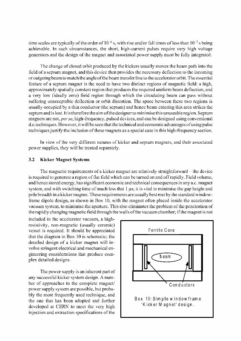
time scales are typically of the order of 10 "6 s, with rise and/or fall times of less than 10 "7 s being achievable. In such circumstances, the short, high-current pulses require very high voltage generators and the design of the magnet and associated power supply must be fully integrated.
The change of closed orbit produced by the kickers usually moves the beam path into the field of a septum magnet, and this device then provides the necessary deflection to the incoming or outgoing beam to match the angle of the beam transfer line to the accelerator orbit. The essential feature of a septum magnet is the need to have two distinct regions of magnetic field: a high, approximately spatially constant region that produces the required uniform beam deflection, and a very low (ideally zero) field region through which the circulating beam can pass without suffering unacceptable deflection or orbit distortion. The space between these two regions is usually occupied by a thin conductor (the septum) and hence beam entering this area strikes the septum and is lost. It is therefore the aim of the designer to minimise this unuseable region. Septum magnets are not, per se, high-frequency, pulsed devices, and can be designed using conventional d.c.techniques. However, it will be seen that the technical and economic advantages of using pulse techniques justify the inclusion of these magnets as a special case in this high-frequency section.
In view of the very different natures of kicker and septum magnets, and their associated power supplies, they will be treated separately.
3.2 Kicker Magnet Systems
The magnetic requirements of a kicker magnet are relatively straightforward - the device is required to generate a region of flat field which can be turned on and off rapidly. Field volume, and hence stored energy, has significant economic and technical consequences in any a.c. magnet system, and with switching time of much less that 1 |us, it is vital to minimise the gap height and pole breadth in a kicker magnet. These requirements are usually best met by the standard window-frame dipole design, as shown in Box 10, with the magnet often placed inside the accelerator vacuum system, to minimise the aperture. This also eliminates the problem of the penetration of the rapidly changing magnetic field through the walls of the vacuum chamber; if the magnet is not included in the accelerator vacuum, a high-resistivity, non-magnetic (usually ceramic) vessel is required. It should be appreciated that the diagram in Box 10 is schematic; the detailed design of a kicker magnet will involve stringent electrical and mechanical engineering considerations that produce complex detailed designs.
The power supply is an inherent part of any successful kicker system design. A number of approaches to the complete magnet/ power supply system are possible, but probably the most frequently used technique, and the one that has been adopted and further developed at CERN to meet the very high injection and extraction specifications of the
Ferrite Core
y\ X Conductors
Box 10: Sim pie w indow fram e 'K icker M agnet' design.
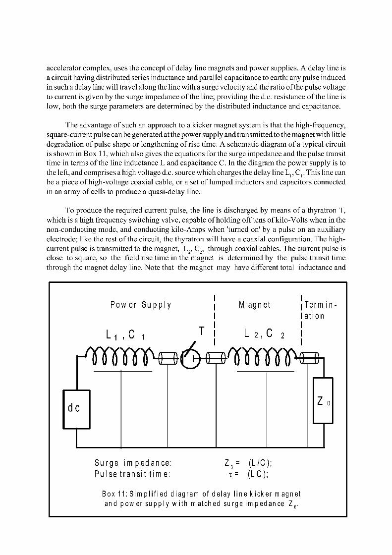
accelerator complex, uses the concept of delay line magnets and power supplies. A delay line is a circuit having distributed series inductance and parallel capacitance to earth; any pulse induced in such a delay line will travel along the line with a surge velocity and the ratio of the pulse voltage to current is given by the surge impedance of the line; providing the d.c. resistance of the line is low, both the surge parameters are determined by the distributed inductance and capacitance.
The advantage of such an approach to a kicker magnet system is that the high-frequency, square-current pulse can be generated at the power supply and transmitted to the magnet with little degradation of pulse shape or lengthening of rise time. A schematic diagram of a typical circuit is shown in Box 11, which also gives the equations for the surge impedance and the pulse transit time in terms of the line inductance L and capacitance C. In the diagram the power supply is to the left, and comprises a high voltage d.c. source which charges the delay line L , C t. This line can be a piece of high-voltage coaxial cable, or a set of lumped inductors and capacitors connected in an array of cells to produce a quasi-delay line.
To produce the required current pulse, the line is discharged by means of a thyratron T, which is a high frequency switching valve, capable of holding off tens of kilo-Volts when in the non-conducting mode, and conducting kilo-Amps when 'turned on' by a pulse on an auxiliary electrode; like the rest of the circuit, the thyratron will have a coaxial configuration. The high-current pulse is transmitted to the magnet, L2, C2, through coaxial cables. The current pulse is close to square, so the field rise time in the magnet is determined by the pulse transit time through the magnet delay line. Note that the magnet may have different total inductance and
Pow er Supply
Li ,C T
agnet
L 2 , C 2 I
j Term in I ation
rwnnnte(Winnnnnte dc
Surge im pedance: Pulse transit tim e:
V (L/C); * = (LC);
Box 11: Sim p l i f ied diagram of delay l ine k icker m agnet and power supply w i th matched surge imp ed an ce Z 0 .

capacitance to the power supply line but the surge impedances of the complete system must be the same to avoid unwanted reflections of the pulse and give optimum transfer of energy. The inductance L 2 will be the inherent self inductance of the magnet, but the capacitance to earth, C2, is built into the magnet as an additional design requirement. The magnet is terminated by a matching resistor, shown as Z 0 in the diagram. This element is, ideally, a pure resistance, with a value equal to the surge impedance of the system, also to prevent reflection of the pulse.
The delay line magnet is often mechanically and electrically very complex, for the designer must incorporate the distributed capacitors by including conducting plates, connected to the high-voltage magnet winding, interleaved with a corresponding set of plates at earth potential, with a thin dielectric separating layer. The magnet core will be assembled from a high-frequency ferrite material (see later section) which usually will not tolerate high-voltage stress. Hence, ceramic insulators are needed to locate and restrain the magnet conductors. The whole assembly is mounted in the accelerator vacuum so that stringent vacuum specifications must be met; long term reliability is essential, as access to the magnet will be both difficult and costly in terms of accelerator down-time.
It should be understood that kicker-magnet power supplies are also highly detailed and complex; the description given here is of a simplified nature. Alternative configurations, with different behavioural characteristics, have been developed for specialised applications and in practice the circuits can be further modified by small trimming elements that sculptor a required pulse waveform. The theory and practice of kicker magnet power systems are closely related to the modulator technology that is used in radar and other pulsed r.f. systems and there is an extensive body of literature and conference proceedings covering the topic.
The delay line method of generating high-current pulses has a number of advantages and disadvantages, as summarised in Box 12. Perhaps the most important advantage is the possibility of locating the power supply remotely from the magnet, using up to ten meters of interconnect-
Advantages: D isadvantages:
Very rapid rise times (<0.1 JAS); Volts on pow er supply are tw ice the pulse voltage;
Good quali ty flat top on square Pulse voltage (10 s of kV) present on current pulse; m agnet throughout pulse;
M atched connection allow s supply to Com plex and expensive m agnet; be rem ote from m agnet;
Reverse volts on valve are not large; Di f f icul ty wi th terminat ing resistor m anufacture;
Box 12: Advantages and di sad van tag es of using m atched 'del ay- l ine ' type k icker m agnet and p ow er supply c i rcui t .
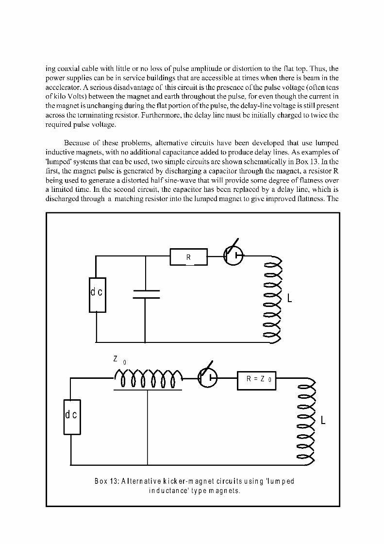
ing coaxial cable with little or no loss of pulse amplitude or distortion to the flat top. Thus, the power supplies can be in service buildings that are accessible at times when there is beam in the accelerator. A serious disadvantage of this circuit is the presence of the pulse voltage (often tens of kilo Volts) between the magnet and earth throughout the pulse, for even though the current in the magnet is unchanging during the flat portion of the pulse, the delay-line voltage is still present across the terminating resistor. Furthermore, the delay line must be initially charged to twice the required pulse voltage.
Because of these problems, alternative circuits have been developed that use lumped inductive magnets, with no additional capacitance added to produce delay lines. As examples of 'lumped' systems that can be used, two simple circuits are shown schematically in Box 13. In the first, the magnet pulse is generated by discharging a capacitor through the magnet, a resistor R being used to generate a distorted half sine-wave that will provide some degree of flatness over a limited time. In the second circuit, the capacitor has been replaced by a delay line, which is discharged through a matching resistor into the lumped magnet to give improved flattness. The
dc
R H 6 ^
L
=5
• W ï ï F é de
R = Z o ^
L
^
Box 13: A I tern a t i ve k i ck er-m ag net c i r c u i t s u s i n g ' lu m ped
i n d u c t a n c e ' t y p e m agne ts .
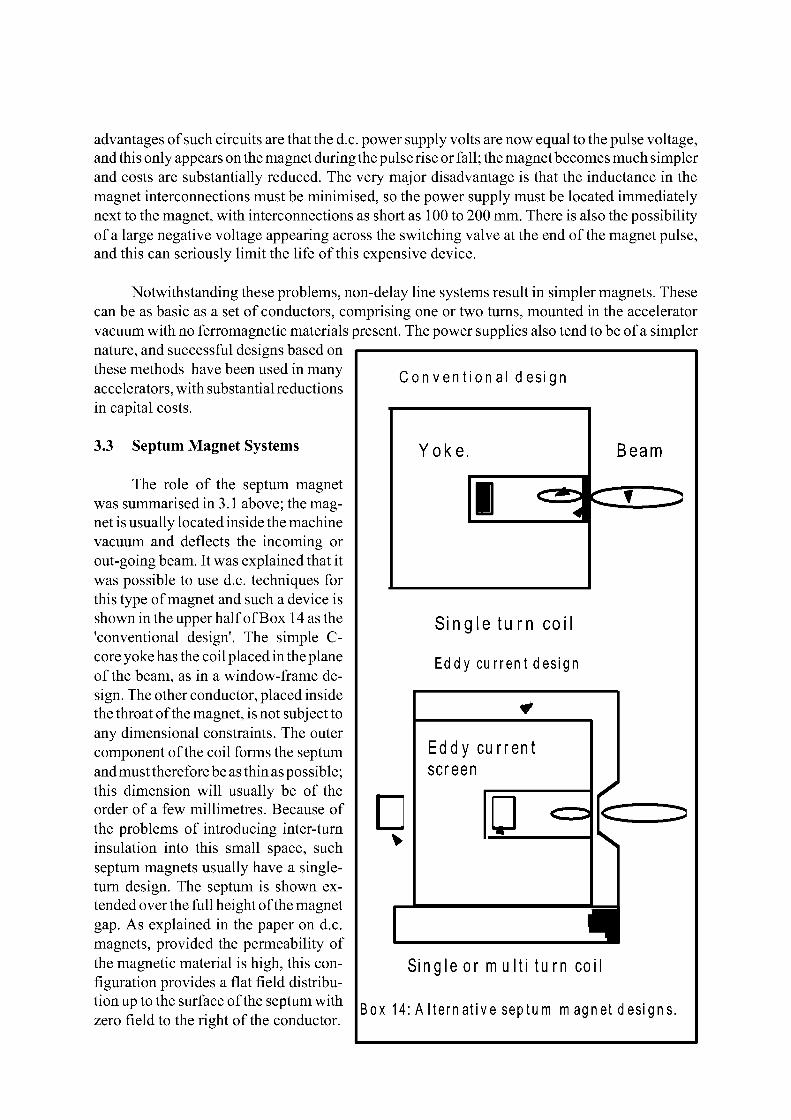
advantages of such circuits are that the d.c. power supply volts are now equal to the pulse voltage, and this only appears on the magnet during the pulse rise or fall; the magnetbecomes much simpler and costs are substantially reduced. The very major disadvantage is that the inductance in the magnet interconnections must be minimised, so the power supply must be located immediately next to the magnet, with interconnections as short as 100 to 200 mm. There is also the possibility of a large negative voltage appearing across the switching valve at the end of the magnet pulse, and this can seriously limit the life of this expensive device.
Notwithstanding these problems, non-delay line systems result in simpler magnets. These can be as basic as a set of conductors, comprising one or two turns, mounted in the accelerator vacuum with no ferromagnetic materials present. The power supplies also tend to be of a simpler nature, and successful designs based on these methods have been used in many accelerators, with substantial reductions in capital costs.
3.3 Septum Magnet Systems
The role of the septum magnet was summarised in 3.1 above; the magnet is usually located inside the machine vacuum and deflects the incoming or out-going beam. It was explained that it was possible to use d.c. techniques for this type of magnet and such a device is shown in the upper half of Box 14 as the 'conventional design'. The simple C-core yoke has the coil placed in the plane of the beam, as in a window-frame design. The other conductor, placed inside the throat of the magnet, is not subject to any dimensional constraints. The outer component of the coil forms the septum and must therefore be as thin as possible; this dimension will usually be of the order of a few millimetres. Because of the problems of introducing inter-turn insulation into this small space, such septum magnets usually have a single-turn design. The septum is shown extended over the full height of the magnet gap. As explained in the paper on d.c. magnets, provided the permeability of the magnetic material is high, this configuration provides a flat field distribution up to the surface of the septum with zero field to the right of the conductor.
C o n v e n t i o n a l d es ign
Yoke.
D <4 Beam
Single tu rn coil
Eddy current design
• Eddy current screen
• j
Single or m ulti turn coil
Box 14: A I ternat ive septum m agnet designs.
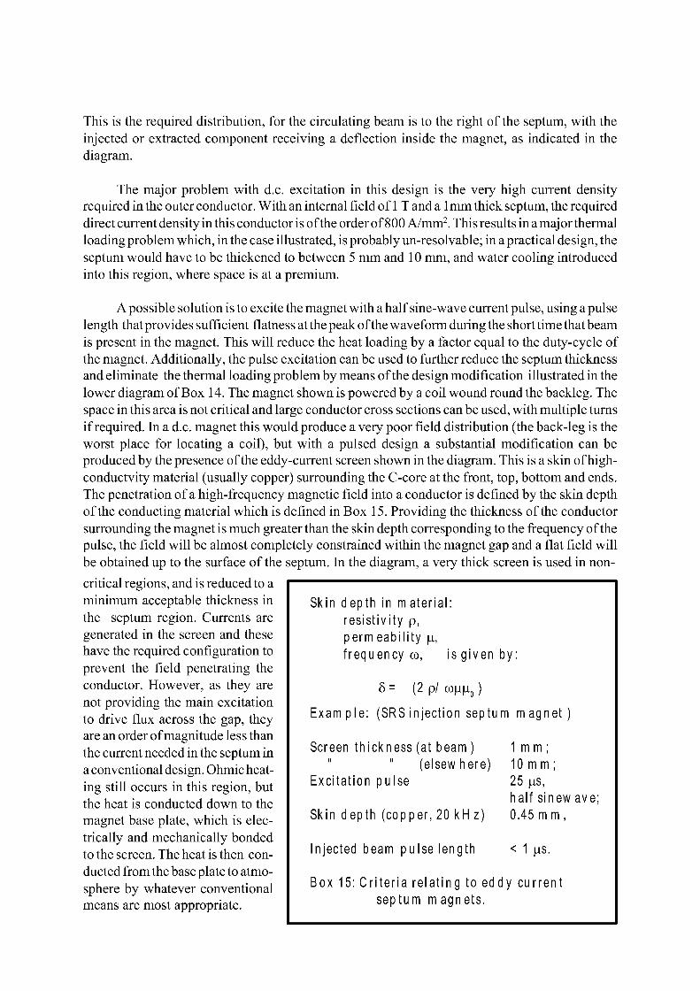
This is the required distribution, for the circulating beam is to the right of the septum, with the injected or extracted component receiving a deflection inside the magnet, as indicated in the diagram.
The major problem with d.c. excitation in this design is the very high current density required in the outer conductor. With an internal field of 1 T and a 1 mm thick septum, the required direct current density in this conductor is of the order of 800 A/mm2. This results in a major thermal loading problem which, in the case illustrated, is probably un-resolvable; in a practical design, the septum would have to be thickened to between 5 mm and 10 mm, and water cooling introduced into this region, where space is at a premium.
A possible solution is to excite the magnet with a half sine-wave current pulse, using a pulse length that provides sufficient flatness at the peak of the waveform during the short time that beam is present in the magnet. This will reduce the heat loading by a factor equal to the duty-cycle of the magnet. Additionally, the pulse excitation can be used to further reduce the septum thickness and eliminate the thermal loading problem by means of the design modification illustrated in the lower diagram of Box 14. The magnet shown is powered by a coil wound round the backleg. The space in this area is not critical and large conductor cross sections can be used, with multiple turns if required. In a d.c. magnet this would produce a very poor field distribution (the back-leg is the worst place for locating a coil), but with a pulsed design a substantial modification can be produced by the presence of the eddy-current screen shown in the diagram. This is a skin of high-conductvity material (usually copper) surrounding the C-core at the front, top, bottom and ends. The penetration of a high-frequency magnetic field into a conductor is defined by the skin depth of the conducting material which is defined in Box 15. Providing the thickness of the conductor surrounding the magnet is much greater than the skin depth corresponding to the frequency of the pulse, the field will be almost completely constrained within the magnet gap and a flat field will be obtained up to the surface of the septum. In the diagram, a very thick screen is used in non-critical regions, and is reduced to a minimum acceptable thickness in the septum region. Currents are generated in the screen and these have the required configuration to prevent the field penetrating the conductor. However, as they are not providing the main excitation to drive flux across the gap, they are an order of magnitude less than the current needed in the septum in a conventional design. Ohmic heating still occurs in this region, but the heat is conducted down to the magnet base plate, which is electrically and mechanically bonded to the screen. The heat is then conducted from the base plate to atmosphere by whatever conventional means are most appropriate.
Skin depth in mater ial : resistivity p, permeabil i ty |u, frequency co, is given by:
8 = (2 p/ a\i\i0 )
Example: (SRS injection septum magnet
Screen thickness (at beam ) (elsewhere)
Excitation pulse
Skin depth (copper,20 kHz)
Injected beam pulse length
1 m m ; 10 m m ; 25 |us, half sinew ave; 0.45 m m,
< 1 us.
Box 15: Cr i ter ia relat ing to eddy current septum m agnets.
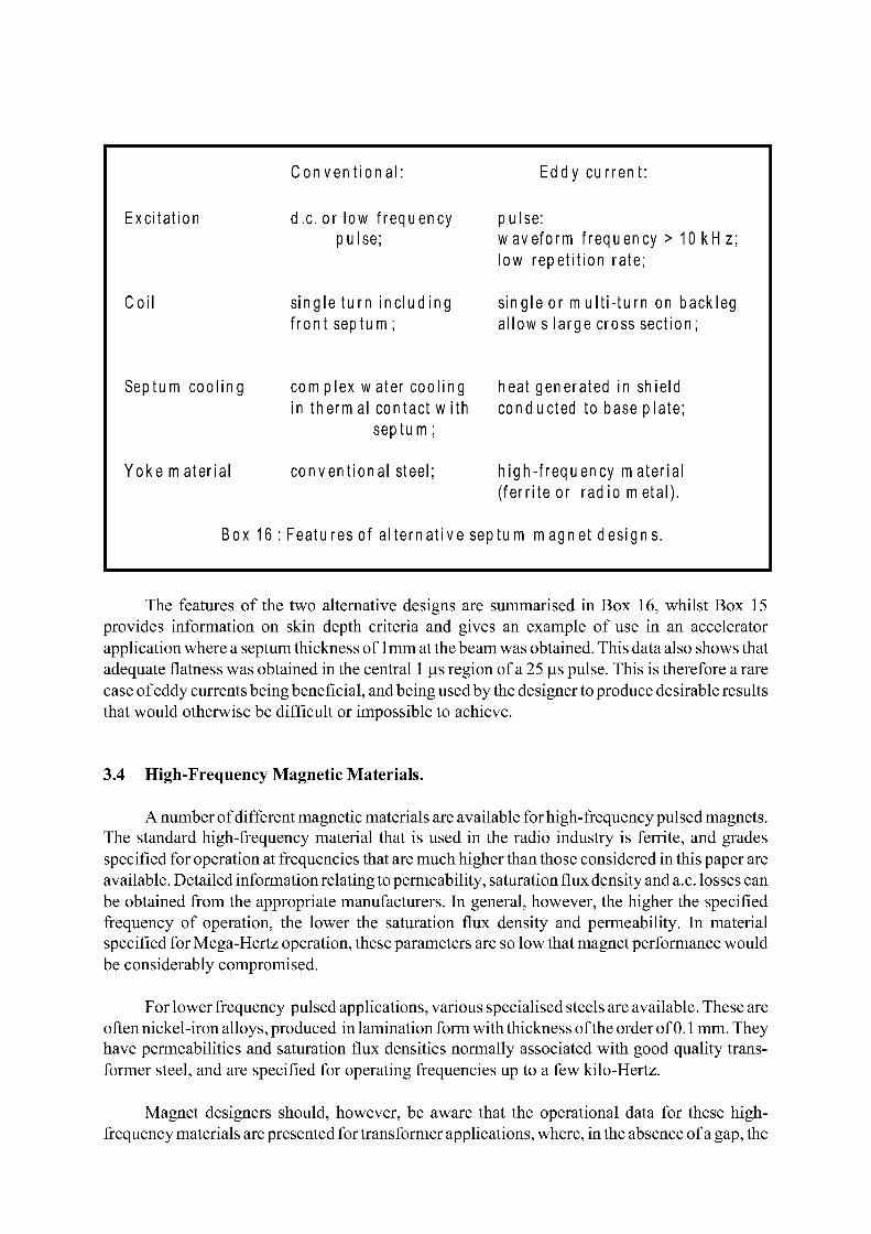
Conven t iona l : Eddy current:
Excitation d x . or low frequency pulse: pulse; waveform frequency > 10 kHz ;
low repetit ion rate;
Coil single turn inc luding single or m ul t i - turn on back leg front septum ; allow s large cross section;
Septum cooling com plex w ater cooling heat generated in shield in therm al contact w ith
septum ; conducted to base plate;
Yoke m aterial conventional steel; high-frequency m aterial (ferrite or radio m étal).
Box 16 Features of a l ternat ive se ) tum m agnet designs.
The features of the two alternative designs are summarised in Box 16, whilst Box 15 provides information on skin depth criteria and gives an example of use in an accelerator application where a septum thickness of 1 mm at the beam was obtained. This data also shows that adequate flatness was obtained in the central 1 |us region of a 25 |us pulse. This is therefore a rare case of eddy currents being beneficial, and being used by the designer to produce desirable results that would otherwise be difficult or impossible to achieve.
3.4 High-Frequency Magnetic Materials.
A number of different magnetic materials are available for high-frequency pulsed magnets. The standard high-frequency material that is used in the radio industry is ferrite, and grades specified for operation at frequencies that are much higher than those considered in this paper are available. Detailed information relating to permeability, saturation flux density and a.c. losses can be obtained from the appropriate manufacturers. In general, however, the higher the specified frequency of operation, the lower the saturation flux density and permeability. In material specified for Mega-Hertz operation, these parameters are so low that magnet performance would be considerably compromised.
For lower frequency pulsed applications, various specialised steels are available. These are often nickel-iron alloys, produced in lamination form with thickness of the order of 0.1 mm. They have permeabilities and saturation flux densities normally associated with good quality transformer steel, and are specified for operating frequencies up to a few kilo-Hertz.
Magnet designers should, however, be aware that the operational data for these high-frequency materials are presented for transformer applications, where, in the absence of a gap, the
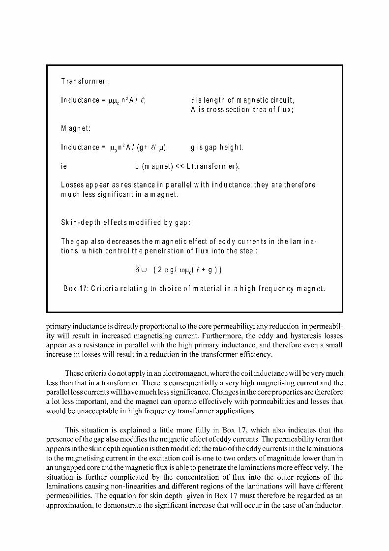
Transform er:
Inductance = \i\i0 n 2 A / 1 , i is length of magnetic circuit,
A is cross section area of f lux;
M agnet:
Inductance = |u 0 n 2 A/ (g+ il \x)\ g is gap height.
ie L (magnet) << L(transformer).
Losses appear as resistance in parallel w ith inductance; they are therefore m uch less signif icant in a m agnet.
Sk in-depth effects m od i f ied by gap:
Thegap also decreases the m agnet ic effect of eddy currents in the lam in a-tions, w hich control the penetration of f lux into the steel:
o u { 2 p g / o ^ 0 U + g ) }
Box 17: Cr i ter ia relat ing to choice of material in a h i g h f requency m agnet.
primary inductance is directly proportional to the core permeability; any reduction in permeability will result in increased magnetising current. Furthermore, the eddy and hysteresis losses appear as a resistance in parallel with the high primary inductance, and therefore even a small increase in losses will result in a reduction in the transformer efficiency.
These criteria do not apply in an electromagnet, where the coil inductance will be very much less than that in a transformer. There is consequentially a very high magnetising current and the parallel loss currents will have much less significance. Changes in the core properties are therefore a lot less important, and the magnet can operate effectively with permeabilities and losses that would be unacceptable in high frequency transformer applications.
This situation is explained a little more fully in Box 17, which also indicates that the presence of the gap also modifies the magnetic effect of eddy currents. The permeability term that appears in the skin depth equation is then modified; the ratio of the eddy currents in the laminations to the magnetising current in the excitation coil is one to two orders of magnitude lower than in an ungapped core and the magnetic flux is able to penetrate the laminations more effectively. The situation is further complicated by the concentration of flux into the outer regions of the laminations causing non-linearities and different regions of the laminations will have different permeabilities. The equation for skin depth given in Box 17 must therefore be regarded as an approximation, to demonstrate the significant increase that will occur in the case of an inductor.
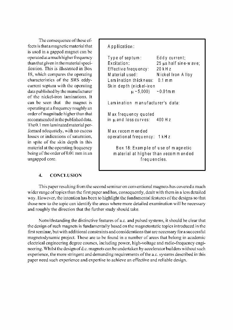
The consequence of these effects is that a magnetic material that is used in a gapped magnet can be operated at a much higher frequency than that given in the material specification. This is illustrated in Box 18, which compares the operating characteristics of the SRS eddy-current septum with the operating data published by the manufacturer of the nickel-iron laminations. It can be seen that the magnet is operating at a frequency roughly an order of magnitude higher than that recommended in the published data. The 0.1 mm laminated material performed adequately, with no excess losses or indications of saturation, in spite of the skin depth in this material at the operating frequency being of the order of 0.01 mm in an ungapped core.
CONCLUSION
A pp l i ca t ion :
Type of septum : Excitat ion: Effective frequency: M aterial used: Lam ination thickness: Skin depth (nickel- iron
JU~5 ,000 )
Eddy current; 25 |us half sine-w ave; 2 0 k H z N ickel Iron A l loy 0.1 m m
~0.01mm
Laminat ion m anufacturer 's data:
M ax frequency quoted in |uand loss curves: 400 H z
M ax recom m ended operational frequency: 1 k H z
Box 18: Example of use of magnet ic m aterial at higher than recom m ended
f requencies.
This paper resulting from the second seminar on conventional magnets has covered a much wider range of topics than the first paper and has, consequently, dealt with them in a less detailed way. However, the intention has been to highlight the fundamental features of the designs so that those new to the topic can identify the areas where more detailed examination will be necessary and roughly the direction that the further study should take.
Notwithstanding the distinctive features of a.c. and pulsed systems, it should be clear that the design of such magnets is fundamentally based on the magnetostatic topics introduced in the first seminar, but with additional constraints and considerations that are necessary for a successful magnetodynamic project. These are to be found in a number of areas that belong in academic electrical engineering degree courses, including power, high-voltage and radio-frequency engineering. Whilst the design of d.c. magnets can be undertaken by accelerator builders without such experience, the more stringent and demanding requirements of the a.c. systems described in this paper need such experience and expertise to achieve an effective and reliable design.

BIBLIOGRAPHY
Many examples of the design of a.c. and pulsed magnets together with suitable power supplies are given in the proceedings of the series of International Conferences on Magnet Technology. Given below are the dates and venues of these conferences:
1965 Stanford Ca, USA; 1967 Oxford, UK; 1970 Hamburg, Germany; 1972 BrookhavenN.Y.,USA; 1975 Rome, Italy; 1977 Bratislava, Czechoslovakia 1981 Karlsruhe, Germany; 1983 Grenoble, France; 1985 Zurich, Switzerland; 1989 Boston, USA.

M agnet M easurem ent Techniques P.C. M agnets
Travers ing m e thods :
The probe is t raversed in the m agnet. Its posi t ion is contrôlée] and m oni tored to high prec is ion; a m ap of f ield in tw o (or three) dim ensions is generated. Th is can take ( m a n y ) h o u r s t o m easure a m agnet - best used for d ipo les . Probe types:
N M R probes:
Very high accuracy and sensi t iv i ty (parts in 10 6 or better) ;
On ly poss ib le in very horn ogeneous f i e l d ; Large probe ( -10 m m cube); Lim ited range of f i e l d ; Best used as absolute s tanda rd .
H all probes:
N eed tern pera ture s tab i l i sa t ion / com pensat ion Accura te to better than 1 0 4 T; Cover a large range of f i e l d ; Sm all com pact p robe; N o range lim i ta t ion .
Flip coi ls: Usual ly used as transfer s tandard between
N M R and H all probes.
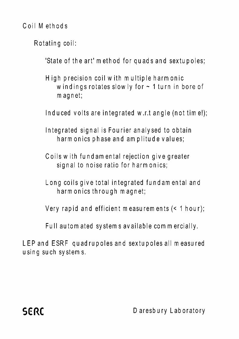
Coi l M e thods
Rotat ing co i l :
'State of the art ' m et hod for quads and sex tu poles;
H igh precision coil w ith m u l t i p le ha rmon i c w i n d i n g s rotates slow Iy for ~ 1 turn in bore of m agnet;
Induced vo l ts are integrated w.r.t angle (not tim e!);
Integrated signal is Four ier analysed to obtain harm onics phase and am p l i t ude valu es;
C o i l s w i t h f u n d a m e n t a l rejection g i veg rea te r signal to noise ratio for harm onics;
Long coi ls g ive total integrated f u n d a m e n t a l and harm onics th rough m agnet;
Very rapid and eff ic ient m easurem ents (< 1 hour ) ;
Ful l au torn ated system s a v a i l a b l e c o m m erci al ly.
L E P a n d E S R F quad rupo les and sextupoles all m easured using such system s.
5 C R C Daresbu ry Labora to ry
A .C. M easurem ents .
Co i ls :
T h e i n d u c e d v o l t a g e i n a coil m a k e s t h i s m e t h o d very prac t ica l . A var ie ty of techn iques are ava i lab le using either sm all t ravers ing coi ls (for spot m easurem ents) or long coi ls for in tegrated m easurem ents.
Peaking s t r ips :
Sm all th in pieces of ferrom agnet ic m aterial w ith square hysteresis l o o p . T h e y a r e w o u n d w i t h coi ls of very f ine w ire w hich p roduce a short pu lse w hen H in the ferrom agnet passes t h rough zero. Cal ibrated bias coi ls can be added to p roduce the pulse at a predeterm ined level of B.
These devices are also very useful for contro l pu rposes in a.c. m achines. In a 50H z f ield rise tim es are < 1(is and can therefore be used for synch ron i sa t i on , tim ing and sw i t ch ing purposes .
SCRC D aresbury Labo ra to ry
INTRODUCTION TO RF LINEAR ACCELERATORS
Mario Weiss CERN, Geneva, Switzerland
ABSTRACT The basic features of RF linear accelerators are described. The concept of the 'loaded cavity', essential for the synchronism wave-particle, is introduced, and formulae describing the action of electromagnetic fields on the beam are given. The treatment of intense beams is mentioned, and various existing linear accelerators are presented as examples.
1 INTRODUCTION Under the name 'linear accelerators', a great number of devices can be included,
having in common the acceleration of particles on a linear path. If we only consider devices which operate with time-varying electric fields, all the d.c. devices are excluded. In fact, we wish to be even more restrictive and only consider devices which operate with sinusoidally varying electromagnetic fields. Such devices are very important and are called RF linear accelerators or RF linacs. These operate either as waveguides or resonators. We shall concentrate our study on them, leaving out devices such as induction linacs which operate in a pulsed manner: a current pulse passes through a magnetic torroid, producing a rapidly changing magnetic field, which by Faraday's law induces a voltage across an accelerating gap.
RF linear accelerators usually operate in the frequency range from 100 MHz up to several GHz. They produce intense beams of very good quality and are applied to scientific research (elementary particle physics), as well as industry or medicine. They can be used at lower energies as injectors into synchrotrons (typically several tens or hundred MeV), or at high energies, e.g. as colliders, accelerating electrons and positrons to 50 GeV, as at the Stanford Linear Accelerator Center (SLAC).
The history of linear accelerators starts with G. Ising, who in 1924 proposed a system of sequentially-pulsed drift tubes, where the particles would be accelerated in gaps between them. In 1928, R. Widerôe suggested the use of RF voltage between successive drift tubes, and successfully tested such a device. He was followed in 1931 by D.H. Sloan and E.O. Lawrence who constructed an improved version of Widerôe's accelerator. It was, however, not until the end of the Second World War that the development of linear accelerators really started. The availability of RF power sources in the MW range and at frequencies of hundreds of MHz, developed for radar purposes, was a great asset. In 1946, L. Alvarez built in Berkeley his famous proton drift tube linac of 32 MeV, operating at 200 MHz. At the same time the development of a 3 GHz election linear accelerator at SLAC was under way. Since then, many linear accelerator structures have been developed and built, and
913
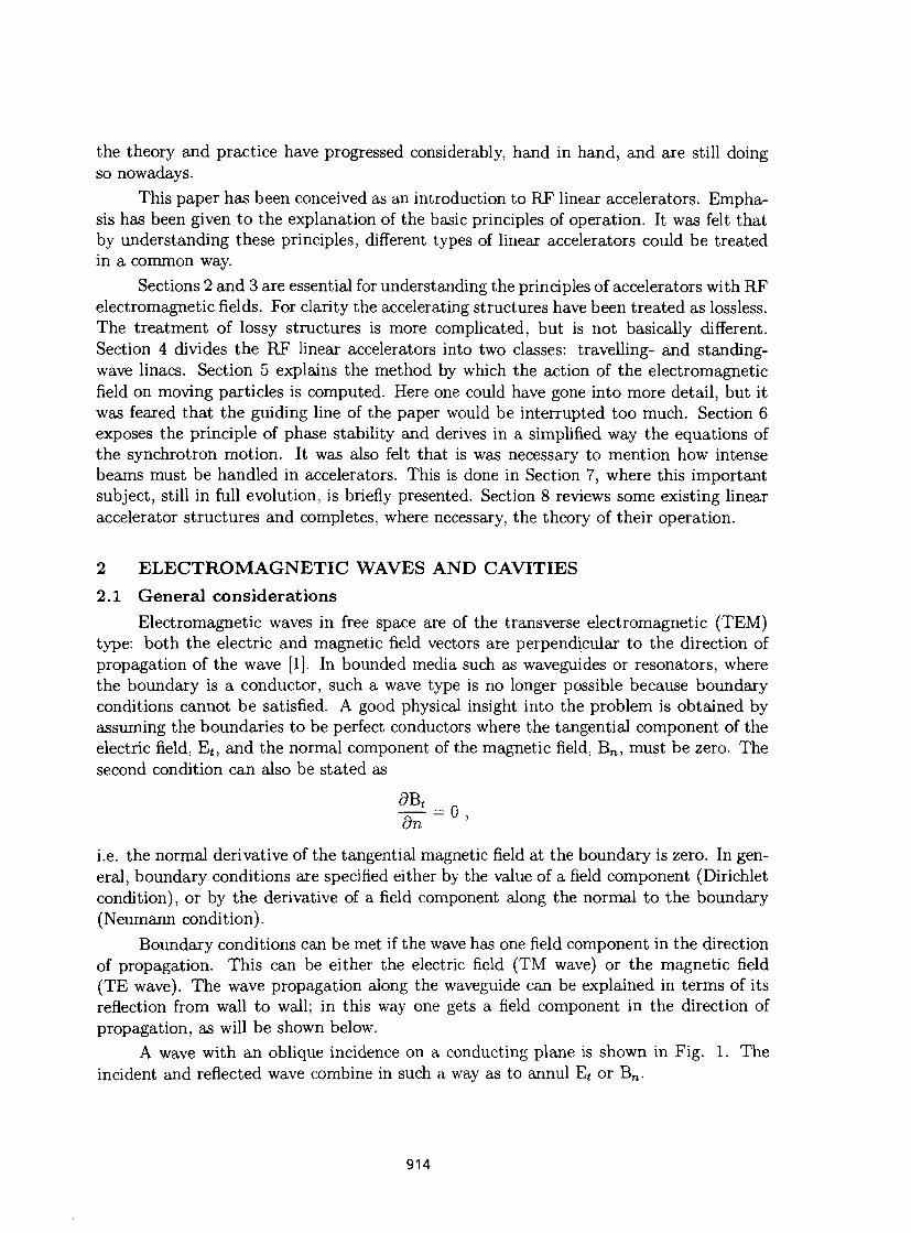
the theory and practice have progressed considerably, hand in hand, and are still doing so nowadays.
This paper has been conceived as an introduction to RF linear accelerators. Emphasis has been given to the explanation of the basic principles of operation. It was felt that by understanding these principles, different types of linear accelerators could be treated in a common way.
Sections 2 and 3 are essential for understanding the principles of accelerators with RF electromagnetic fields. For clarity the accelerating structures have been treated as lossless. The treatment of lossy structures is more complicated, but is not basically different. Section 4 divides the RF linear accelerators into two classes: travelling- and standing-wave linacs. Section 5 explains the method by which the action of the electromagnetic field on moving particles is computed. Here one could have gone into more detail, but it was feared that the guiding line of the paper would be interrupted too much. Section 6 exposes the principle of phase stability and derives in a simplified way the equations of the synchrotron motion. It was also felt that is was necessary to mention how intense beams must be handled in accelerators. This is done in Section 7, where this important subject, still in full evolution, is briefly presented. Section 8 reviews some existing linear accelerator structures and completes, where necessary, the theory of their operation.
2 ELECTROMAGNETIC WAVES AND CAVITIES 2.1 General considerations
Electromagnetic waves in free space are of the transverse electromagnetic (TEM) type: both the electric and magnetic field vectors are perpendicular to the direction of propagation of the wave [1]. In bounded media such as waveguides or resonators, where the boundary is a conductor, such a wave type is no longer possible because boundary conditions cannot be satisfied. A good physical insight into the problem is obtained by assuming the boundaries to be perfect conductors where the tangential component of the electric field, E t , and the normal component of the magnetic field, B n , must be zero. The second condition can also be stated as
i.e. the normal derivative of the tangential magnetic field at the boundary is zero. In general, boundary conditions are specified either by the value of a field component (Dirichlet condition), or by the derivative of a field component along the normal to the boundary (Neumann condition).
Boundary conditions can be met if the wave has one field component in the direction of propagation. This can be either the electric field (TM wave) or the magnetic field (TE wave). The wave propagation along the waveguide can be explained in terms of its reflection from wall to wall; in this way one gets a field component in the direction of propagation, as will be shown below.
A wave with an oblique incidence on a conducting plane is shown in Fig. 1. The incident and reflected wave combine in such a way as to annul E t or B n .
914
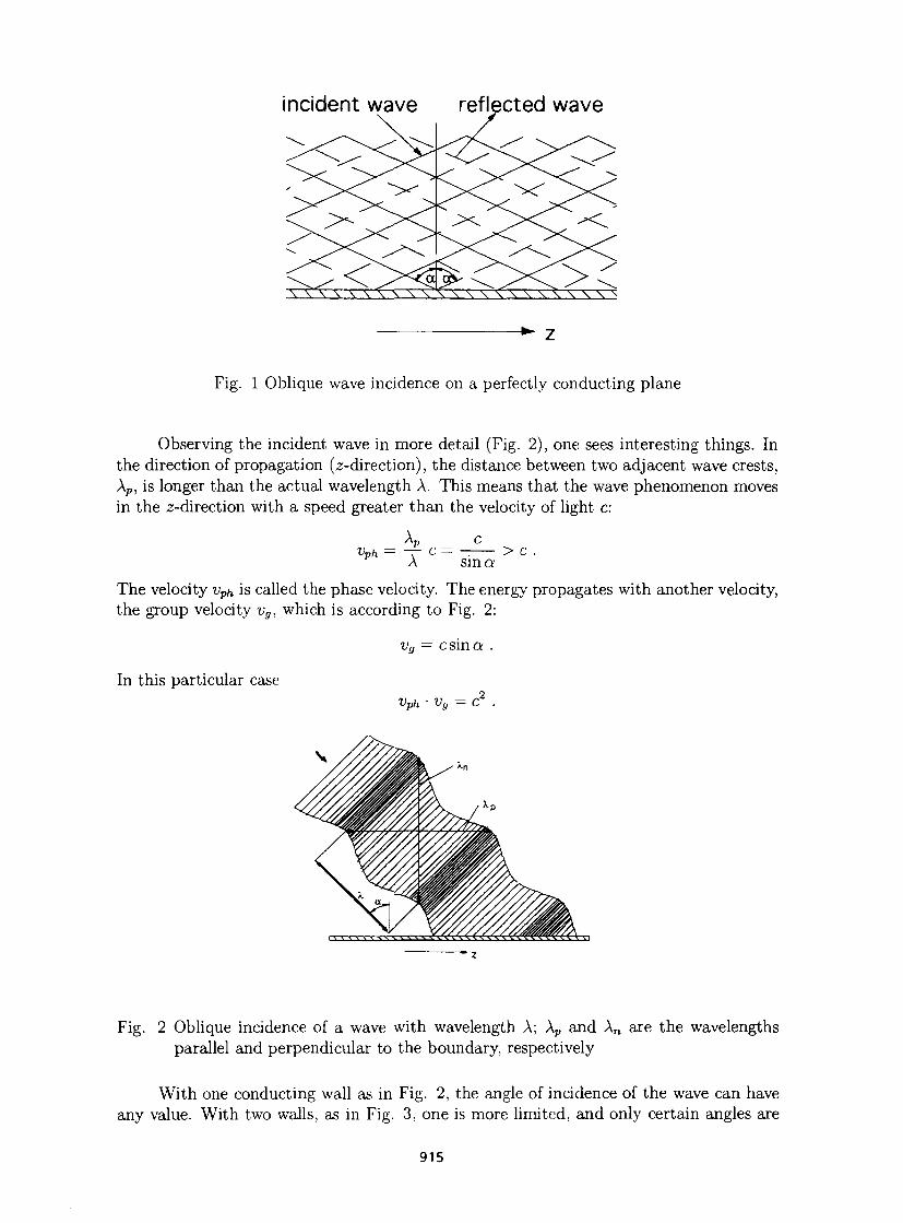
incident wave reflected wave
Fig. 1 Oblique wave incidence on a perfectly conducting plane
Observing the incident wave in more detail (Fig. 2), one sees interesting things. In the direction of propagation (^-direction), the distance between two adjacent wave crests, Xp, is longer than the actual wavelength A. This means that the wave phenomenon moves in the z-direction with a speed greater than the velocity of light c:
Ap C
vph= -r c-A sina
> c .
The velocity vvh is called the phase velocity. The energy propagates with another velocity, the group velocity vg, which is according to Fig. 2:
In this particular case Vph • Vy — C
Fig. 2 Oblique incidence of a wave with wavelength A; \ v and A„ are the wavelengths parallel and perpendicular to the boundary, respectively
With one conducting wall as in Fig. 2, the angle of incidence of the wave can have any value. With two walls, as in Fig. 3, one is more limited, and only certain angles are
915
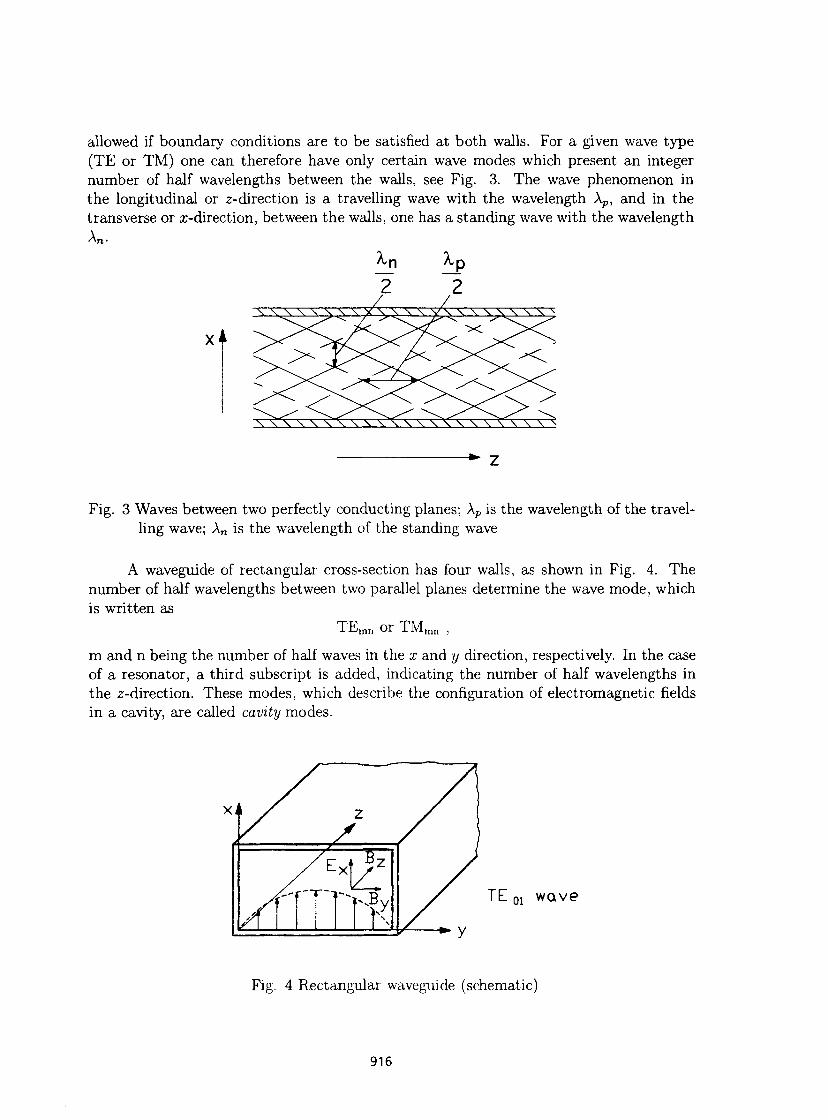
allowed if boundary conditions are to be satisfied at both walls. For a given wave type (TE or TM) one can therefore have only certain wave modes which present an integer number of half wavelengths between the walls, see Fig. 3. The wave phenomenon in the longitudinal or z-direction is a travelling wave with the wavelength Ap, and in the transverse or x-direction, between the walls, one has a standing wave with the wavelength An-
~2 ~2
x^
Fig. 3 Waves between two perfectly conducting planes; Ap is the wavelength of the travelling wave; An is the wavelength of the standing wave
A waveguide of rectangular cross-section has four walls, as shown in Fig. 4. The number of half wavelengths between two parallel planes determine the wave mode, which is written as
TE m I I or T M m n ,
m and n being the number of half waves in the x and y direction, respectively. In the case of a resonator, a third subscript is added, indicating the number of half wavelengths in the ^-direction. These modes, which describe the configuration of electromagnetic fields in a cavity, are called cavity modes.
X i i
TE 0 1 wave
Fig. 4 Rectangular waveguide (schematic)
916
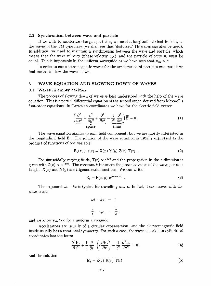
2.2 Synchronism between wave and particle
If we wish to accelerate charged particles, we need a longitudinal electric field, as the waves of the TM type have (we shall see that 'distorted' TE waves can also be used). In addition, we need to maintain a synchronism between the wave and particle, which means that the wave velocity (phase velocity vph), and the particle velocity vp must be equal. This is impossible in the uniform waveguide as we have seen that vph > c.
In order to use electromagnetic waves for the acceleration of particles one must first find means to slow the waves down.
3 WAVE EQUATION AND SLOWING DOWN OF WAVES
3.1 Waves in empty cavities
The process of slowing down of waves is best understood with the help of the wave equation. This is a partial differential equation of the second order, derived from Maxwell's first-order equations. In Cartesian coordinates we have for the electric field vector
' * + £ + £_i£W=„. (1) \dx2 dy2 dz2
^ v ' space time
The wave equation applies to each field component, but we are mostly interested in the longitudinal field E 2 . The solution of the wave equation is usually expressed as the product of functions of one variable:
E2(x,y,z,t) = X(x)Y(y)Z(z)T(t). (2)
For sinusoidally varying fields, T(r) ex ç?wt and the propagation in the z-direction is given with Z(z) ex e~jkz. The constant k indicates the phase advance of the wave per unit length. X(x) and Y(y) are trigonometric functions. We can write:
E 2 = F ( x - , y ) e ^ - f c z ) . (3)
The exponent ut — kz is typical for travelling waves. In fact, if one moves with the wave crest:
ut — kz = 0
Z ijj
and we know vph > c for a uniform waveguide.
Accelerators are usually of a circular cross-section, and the electromagnetic field inside usually has a rotational symmetry. For such a case, the wave equation in cylindrical coordinates has the form:
d2Ez \ d ( dEz\ 1 d2Ez ... + - s- [ r^r~ ~ -? -S3- = ° > ( 4) dz2 r dr \ dr } c2 dt2
and the solution E 2 = Z(z) R(r) T(i) . (5)
917
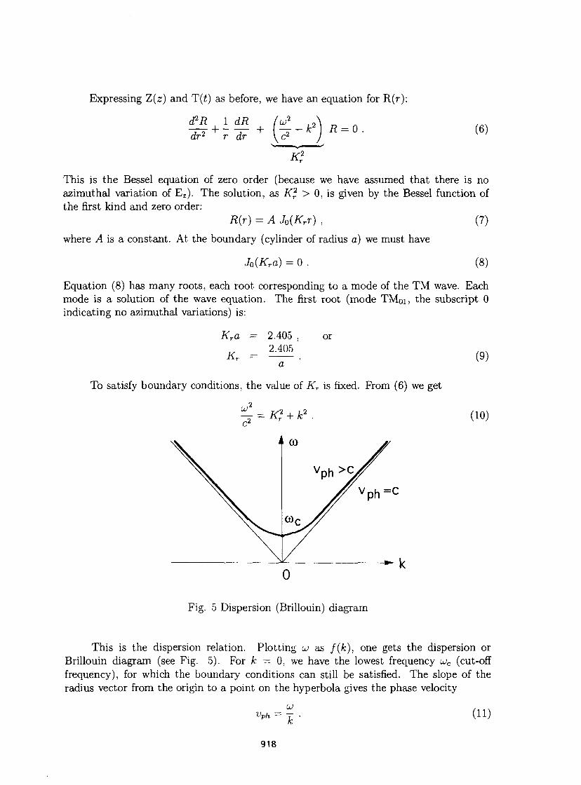
Expressing Z(z) and T(t) as before, we have an equation for R(r):
(PR ldR dr2 r dr
UJ -k2] R = 0 . (6)
K
This is the Bessel equation of zero order (because we have assumed that there is no azimuthal variation of E z ) . The solution, as K2 > 0, is given by the Bessel function of the first kind and zero order:
R(r) = A J0(Krr) , (7)
where A is a constant. At the boundary (cylinder of radius a) we must have
Jo(Kra) = 0 . (8)
Equation (8) has many roots, each root corresponding to a mode of the TM wave. Each mode is a solution of the wave equation. The first root (mode TMoi, the subscript 0 indicating no azimuthal variations) is:
Kra = 2.405 = ^ 0 5
or (9)
To satisfy boundary conditions, the value of KT is fixed. From (6) we get
UJ ^r = K? + k*. (10)
^ k
Fig. 5 Dispersion (Brillouin) diagram
This is the dispersion relation. Plotting u as f{k), one gets the dispersion or Brillouin diagram (see Fig. 5). For k = 0, we have the lowest frequency uc (cut-off frequency), for which the boundary conditions can still be satisfied. The slope of the radius vector from the origin to a point on the hyperbola gives the phase velocity
Vph ~k (11)
918
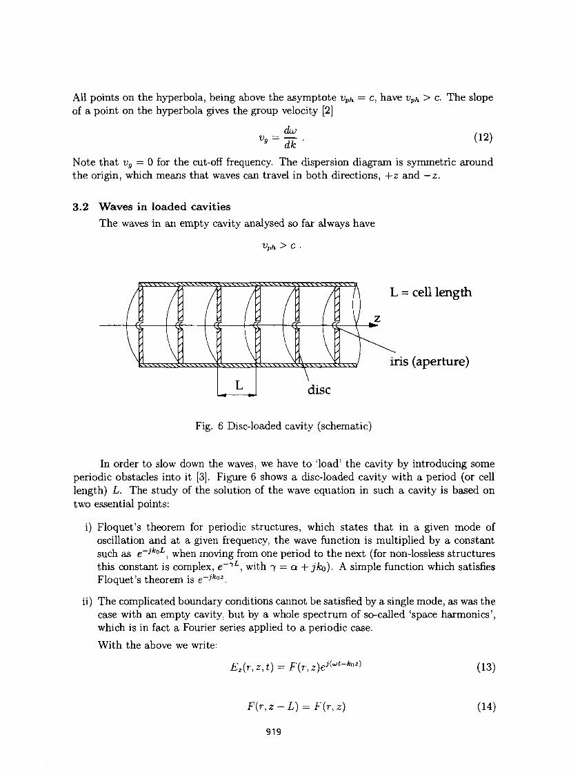
AU points on the hyperbola, being above the asymptote vph = c, have vvh > c. The slope of a point on the hyperbola gives the group velocity [2]
dw Ik (12)
Note that vg — 0 for the cut-off frequency. The dispersion diagram is symmetric around the origin, which means that waves can travel in both directions, +z and —z.
3.2 Waves in loaded cavities The waves in an empty cavity analysed so far always have
Vph> C .
L = cell length
iris (aperture)
Fig. 6 Disc-loaded cavity (schematic)
In order to slow down the waves, we have to 'load' the cavity by introducing some periodic obstacles into it [3]. Figure 6 shows a disc-loaded cavity with a period (or cell length) L. The study of the solution of the wave equation in such a cavity is based on two essential points:
i) Floquet's theorem for periodic structures, which states that in a given mode of oscillation and at a given frequency, the wave function is multiplied by a constant such as e~jk°L, when moving from one period to the next (for non-lossless structures this constant is complex, e - 7 L , with 7 = a + jko). A simple function which satisfies Floquet's theorem is e~jkoz.
ii) The complicated boundary conditions cannot be satisfied by a single mode, as was the case with an empty cavity, but by a whole spectrum of so-called 'space harmonics', which is in fact a Fourier series applied to a periodic case. With the above we write:
Ez(r,z,t) = F(r,z)e j(u>t-k0z) (13)
F(r,z + L) = F{r,z) (14)
919
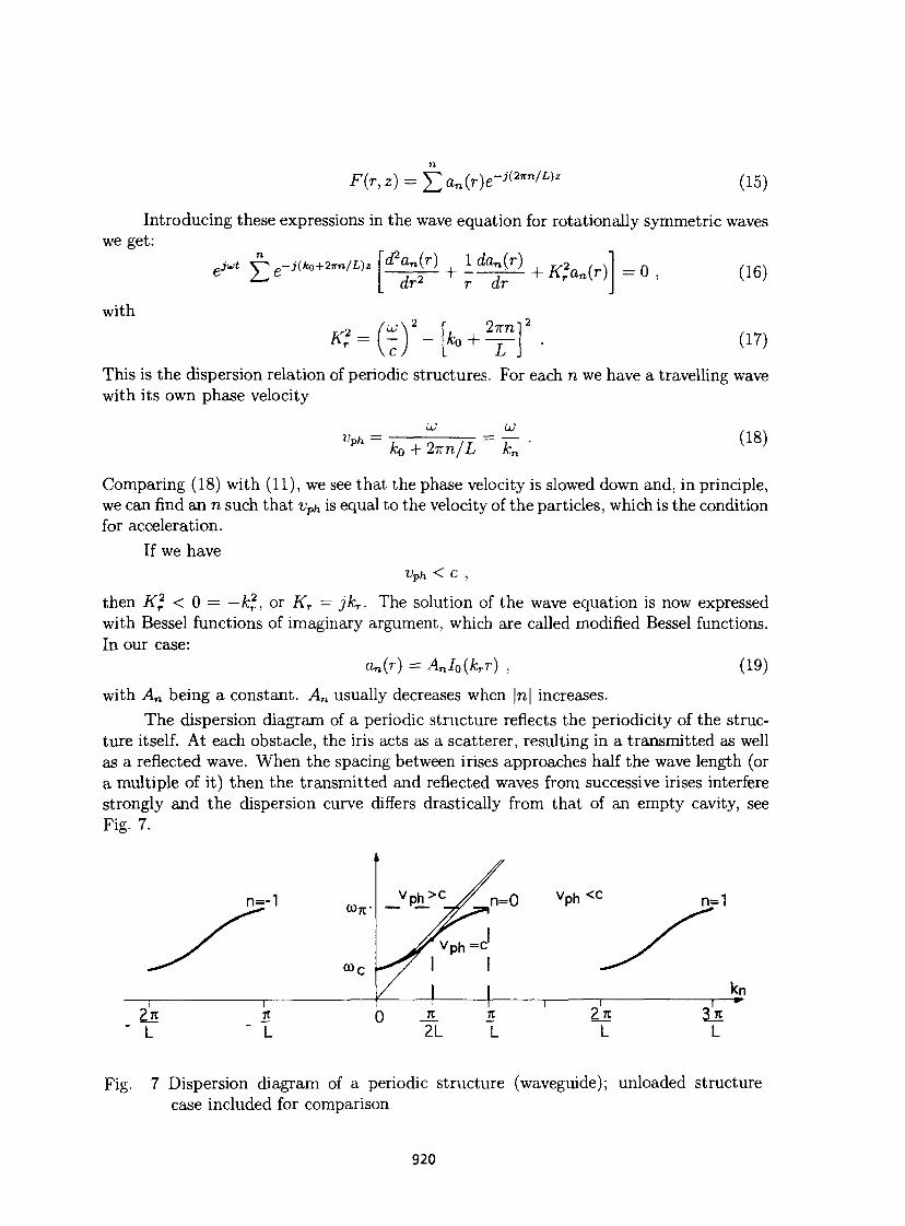
F(r,z) = -£an(r)e-j{2™/L)z (15)
Introducing these expressions in the wave equation for rotationally symmetric waves we get:
with
-jujt £ • j(ko+2irn/L)z '(Pan(r) dr2
K = ;?r-
1 dan(r) _ _2 . , + ^ - + K2
ran{r) r dr
ko + 2irn -\2
(16)
(17)
This is the dispersion relation of periodic structures. For each n we have a travelling wave with its own phase velocity
u Vph
UJ
k® 4- 2im/L kn
(18)
Comparing (18) with (11), we see that the phase velocity is slowed down and, in principle, we can find an n such that vph is equal to the velocity of the particles, which is the condition for acceleration.
If we have Vph < C ,
then K? < 0 = — k2, or Kr = jkr. The solution of the wave equation is now expressed with Bessel functions of imaginary argument, which are called modified Bessel functions. In our case:
dnir) = AnI0(krr) , (19)
with An being a constant. An usually decreases when |n| increases. The dispersion diagram of a periodic structure reflects the periodicity of the struc
ture itself. At each obstacle, the iris acts as a scatterer, resulting in a transmitted as well as a reflected wave. When the spacing between irises approaches half the wave length (or a multiple of it) then the transmitted and reflected waves from successive irises interfere strongly and the dispersion curve differs drastically from that of an empty cavity, see Fig. 7.
Fig. 7 Dispersion diagram of a periodic structure (waveguide); unloaded structure case included for comparison
920
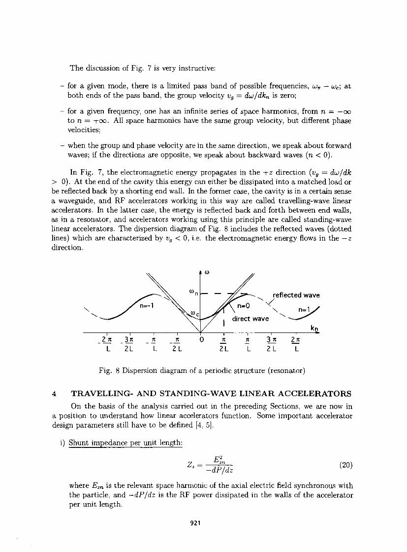
The discussion of Fig. 7 is very instructive:
- for a given mode, there is a limited pass band of possible frequencies, un — u>c; at both ends of the pass band, the group velocity vg = duj/dkn is zero;
- for a given frequency, one has an infinite series of space harmonics, from n — — oo to n = +00. All space harmonics have the same group velocity, but different phase velocities;
- when the group and phase velocity are in the same direction, we speak about forward waves; if the directions are opposite, we speak about backward waves (n < 0).
In Fig. 7, the electromagnetic energy propagates in the +z direction (vg = duj/dk > 0). At the end of the cavity this energy can either be dissipated into a matched load or be reflected back by a shorting end wall. In the former case, the cavity is in a certain sense a waveguide, and RF accelerators working in this way are called travelling-wave linear accelerators. In the latter case, the energy is reflected back and forth between end walls, as in a resonator, and accelerators working using this principle are called standing-wave linear accelerators. The dispersion diagram of Fig. 8 includes the reflected waves (dotted lines) which are characterized by vg < 0, i.e. the electromagnetic energy flows in the — z direction.
reflected wave
\ n=1
Fig. 8 Dispersion diagram of a periodic structure (resonator)
4 TRAVELLING- AND STANDING-WAVE LINEAR ACCELERATORS On the basis of the analysis carried out in the preceding Sections, we are now in
a position to understand how linear accelerators function. Some important accelerator design parameters still have to be defined [4, 5].
i) Shunt impedance per unit length:
Z,= -dP/dz
(20)
where Ezn is the relevant space harmonic of the axial electric field synchronous with the particle, and —dP/dz is the RF power dissipated in the walls of the accelerator per unit length.
921
The shunt impedance is a measure of the excellence of a structure to accelerate particles. Note that some authors include a factor of one half in Eq. (20) to be consistent with the standard circuit theory. A high Z3 means an efficient acceleration for a given dissipated RF power. The Z„ is usually expressed in MÇlrrT1.
ii) Quality factor: Q=»-^m (21)
where u is the RF angular frequency, and w is the stored energy per unit length,
iii) Ratio Z,/Q: § = ; (22) Q u>w
This ratio depends only on the structure geometry and not on the quality of the surface of the cavity walls. It tells us how much accelerating field one has for a given stored energy per unit length.
iv) Frequency: the choice of the frequency of an accelerator depends on many factors. For relativistic particles, such as electrons above 10 MeV, the frequency is usually in the range of several GHz, whilst for protons it is of several hundred MHz. One can also show that
Zs oc u1/2 ,
so higher frequencies are more efficient for acceleration. The breakdown problems due to high electric surface fields, are also diminished at higher frequencies, as indicated by the Kilpatrick law (see Section 8.1). However, as structures at high frequency are smaller, they might not have a sufficient aperture for intense particle beams.
v) Group velocity: v»=5; (23)
where P is the power flowing in the structure.
This definition of the group velocity is obvious. Since the stored energy per unit length is proportional to E\n, a small vg, usually 0.01 c to 0.02 c, is preferred for better acceleration efficiency, keeping the accelerator filling time still in reasonable limits, see Eq. (35).
4.1 Travelling-wave accelerators There is no firm rule with which to decide whether a travelling-wave or a standing-
wave accelerator is to be chosen. However, travelling-wave accelerators are usually used when dealing with short beam pulses and when particle velocities approach the velocity of light, as is the case with electrons. One should distinguish between a constant impedance and a constant gradient travelling-wave accelerator [6].
A travelling-wave accelerator operates with the n = 0 space harmonic, as the wave amplitude is largest in this case. The structure is usually designed so that the dispersion
922
curve crosses the vph = c line for a phase advance per period of 7r/2 to 27r/3 (approximately in the middle of the pass band) or
IT 2n
(see Fig. 7). Note that 10 MeV electrons already have a relativistic f3T of 0.999, whilst that of protons is only 0.145. Therefore, the structure with VPH < c is only used for very low electron energies.
Along the accelerator, a certain power is dissipated in the cavity walls and the electric field is attenuated:
dEz0(z) —-£•— = -a{z)E20{z) , (24)
where a(z) is the attenuation constant.
We have correspondingly
^ = -2a(z)P(z) . (25)
Using the definitions of Q and w, we also have
dP(z) _ u P{z) dz Q vg(z)
It follows that
(26)
a ( 2 ) = wkîT) • ( 2 7 )
A constant-impedance accelerator has a uniform structure:
a(z) = const = a
Ez0(z) = Ez0(0) e~az .
The energy gain of a particle of charge q, sitting on the crest of the wave in a constant-impedance accelerator of length £ is
qV = q t EzO(0) e~az dz Jo
1 - t~at
= qEzO(0)£—^. (28)
This expression is maximum for at — 1.26 and
gV i n a x = 0.57q E*W . (29)
At the end of the accelerator in the optimized case one has:
EzQ(£) = O.28£20(0) , (30)
P(£) = 0.08P(0) . (31)
923
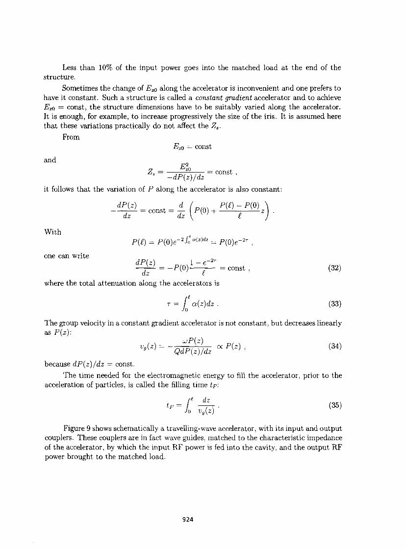
Less than 10% of the input power goes into the matched load at the end of the structure.
Sometimes the change of Ez0 along the accelerator is inconvenient and one prefers to have it constant. Such a structure is called a constant gradient accelerator and to achieve Ezo = const, the structure dimensions have to be suitably varied along the accelerator. It is enough, for example, to increase progressively the size of the iris. It is assumed here that these variations practically do not affect the Zs.
From Ezo = const
and E2zo 2 0 - const
* -dP(z)/dz it follows that the variation of P along the accelerator is also constant:
dP{z) d / / m P{£)-P(0) \ v ' = const = — P(0) + v ;
n——z .
With
one can write
dz dz \ £
P{£) = P{0)e-2i'oa(z)dz = P(0)e-2r ,
dP(z) = _ P { 0 )
l - e ~ 2 T
= c o n s t ( 3 2 )
dz where the total attenuation along the accelerators is
T = / a(z)dz . (33) Jo
The group velocity in a constant gradient accelerator is not constant, but decreases linearly as P(z):
^ = -Qimr, a p ( z ) • ( 3 4 )
because dP(z)/dz = const. The time needed for the electromagnetic energy to fill the accelerator, prior to the
acceleration of particles, is called the filling time if:
r e dz
tF = / —— . (35)
Figure 9 shows schematically a travelling-wave accelerator, with its input and output couplers. These couplers are in fact wave guides, matched to the characteristic impedance of the accelerator, by which the input RF power is fed into the cavity, and the output RF power brought to the matched load.
924
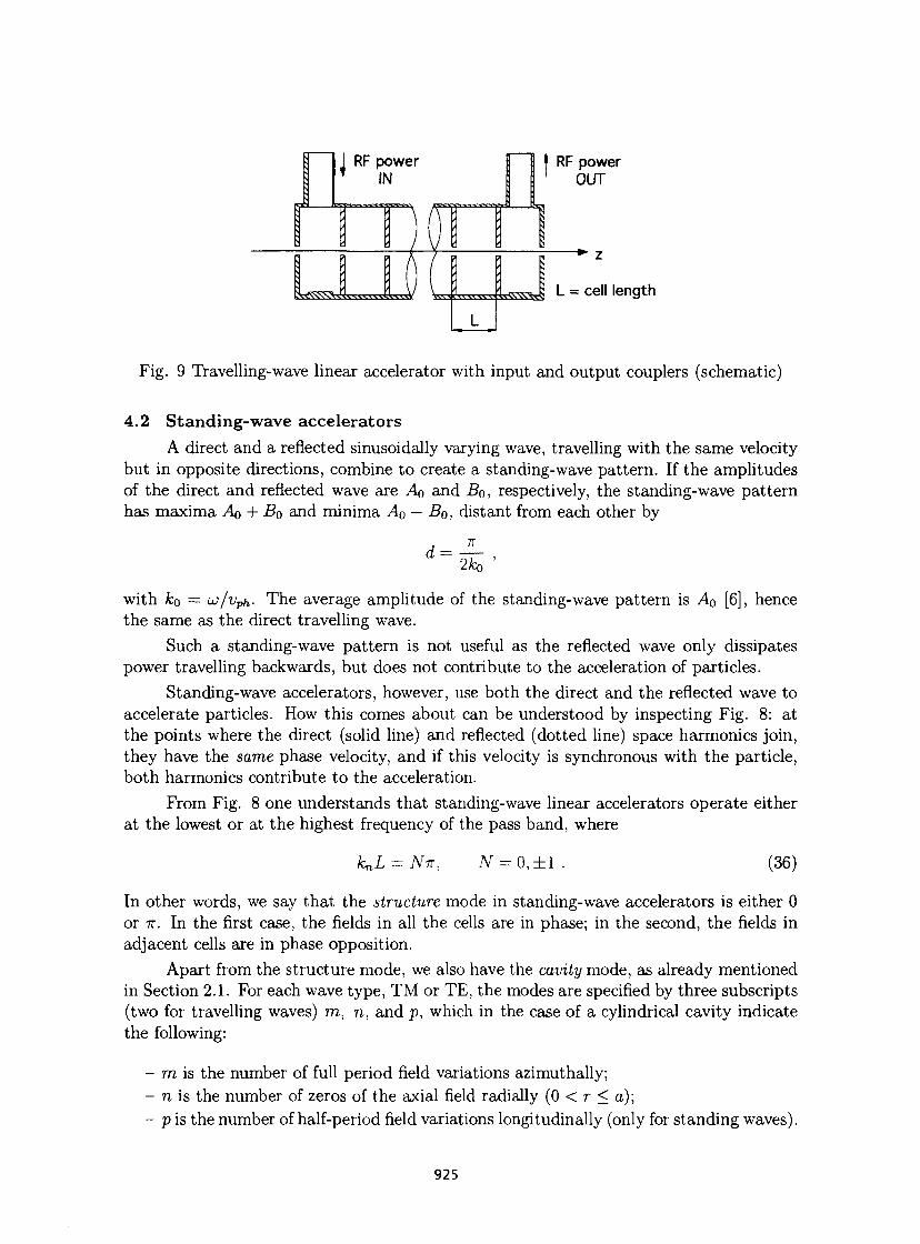
RF power IN
RF power OUT
acsssc ssssssssa ^ S W 3 L = cell length
Fig. 9 Travelling-wave linear accelerator with input and output couplers (schematic)
4.2 Standing-wave accelerators A direct and a reflected sinusoidally varying wave, travelling with the same velocity
but in opposite directions, combine to create a standing-wave pattern. If the amplitudes of the direct and reflected wave are AQ and Bo, respectively, the standing-wave pattern has maxima AQ + B0 and minima A0 — B0, distant from each other by
d = IT
2ko
with ko = uj/vph- The average amplitude of the standing-wave pattern is AQ [6], hence the same as the direct travelling wave.
Such a standing-wave pattern is not useful as the reflected wave only dissipates power travelling backwards, but does not contribute to the acceleration of particles.
Standing-wave accelerators, however, use both the direct and the reflected wave to accelerate particles. How this comes about can be understood by inspecting Fig. 8: at the points where the direct (solid line) and reflected (dotted line) space harmonics join, they have the same phase velocity, and if this velocity is synchronous with the particle, both harmonics contribute to the acceleration.
From Fig. 8 one understands that standing-wave linear accelerators operate either at the lowest or at the highest frequency of the pass band, where
knL — NTT, N = 0,±1 (36)
In other words, we say that the structure mode in standing-wave accelerators is either 0 or 7T. In the first case, the fields in all the cells are in phase; in the second, the fields in adjacent cells are in phase opposition.
Apart from the structure mode, we also have the cavity mode, as already mentioned in Section 2.1. For each wave type, TM or TE, the modes are specified by three subscripts (two for travelling waves) m, n, and p, which in the case of a cylindrical cavity indicate the following:
- m is the number of full period field variations azimuthally; - n is the number of zeros of the axial field radially (0 < r < a); -pis the number of half-period field variations longitudinally (only for standing waves).
925
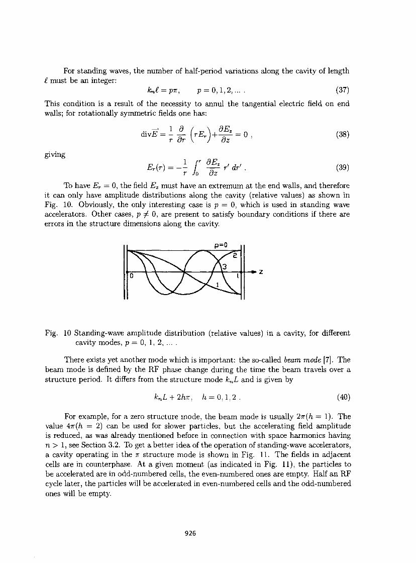
For standing waves, the number of half-period variations along the cavity of length t must be an integer:
kni^jm, p = 0,1,2, . . . . (37)
This condition is a result of the necessity to annul the tangential electric field on end walls; for rotationally symmetric fields one has:
divE == - | - ( rEr r or dEz
' dz 0 ,
giving Er(r)
r Jo dEz
dz r' dr'
(38)
(39)
To have Er = 0, the field Ez must have an extremum at the end walls, and therefore it can only have amplitude distributions along the cavity (relative values) as shown in Fig. 10. Obviously, the only interesting case is p = 0, which is used in standing wave accelerators. Other cases, p ^ 0, are present to satisfy boundary conditions if there are errors in the structure dimensions along the cavity.
*• z
Fig. 10 Standing-wave amplitude distribution (relative values) in a cavity, for different cavity modes, p — 0, 1, 2, ... .
There exists yet another mode which is important: the so-called beam mode [7]. The beam mode is defined by the RF phase change during the time the beam travels over a structure period. It differs from the structure mode knL and is given by
knL + 2hK, h = 0,1,2 (40)
For example, for a zero structure mode, the beam mode is usually 2-n(h— 1). The value 47r(/i = 2) can be used for slower particles, but the accelerating field amplitude is reduced, as was already mentioned before in connection with space harmonics having n > 1, see Section 3.2. To get a better idea of the operation of standing-wave accelerators, a cavity operating in the re structure mode is shown in Fig. 11. The fields in adjacent cells are in counterphase. At a given moment (as indicated in Fig. 11), the particles to be accelerated are in odd-numbered cells, the even-numbered ones are empty. Half an RF cycle later, the particles will be accelerated in even-numbered cells and the odd-numbered ones will be empty.
926
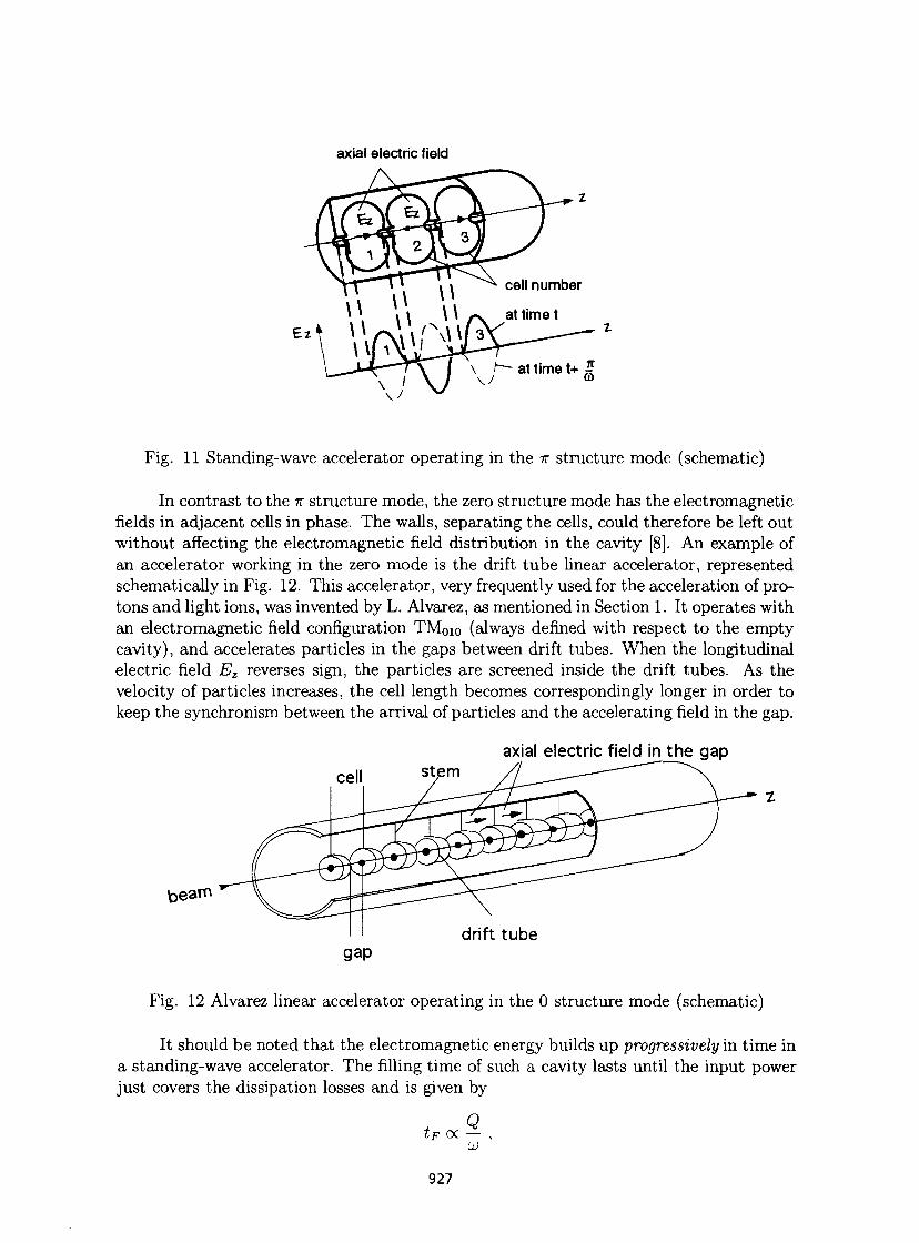
axial electric field
Fig. 11 Standing-wave accelerator operating in the IT structure mode (schematic)
In contrast to the IT structure mode, the zero structure mode has the electromagnetic fields in adjacent cells in phase. The walls, separating the cells, could therefore be left out without affecting the electromagnetic field distribution in the cavity [8]. An example of an accelerator working in the zero mode is the drift tube linear accelerator, represented schematically in Fig. 12. This accelerator, very frequently used for the acceleration of protons and light ions, was invented by L. Alvarez, as mentioned in Section 1. It operates with an electromagnetic field configuration TM0io (always defined with respect to the empty cavity), and accelerates particles in the gaps between drift tubes. When the longitudinal electric field Ez reverses sign, the particles are screened inside the drift tubes. As the velocity of particles increases, the cell length becomes correspondingly longer in order to keep the synchronism between the arrival of particles and the accelerating field in the gap.
axial electric field in the gap
drift tube gap
Fig. 12 Alvarez linear accelerator operating in the 0 structure mode (schematic)
It should be noted that the electromagnetic energy builds up progressively in time in a standing-wave accelerator. The filling time of such a cavity lasts until the input power just covers the dissipation losses and is given by
Q t f OC — ,
927
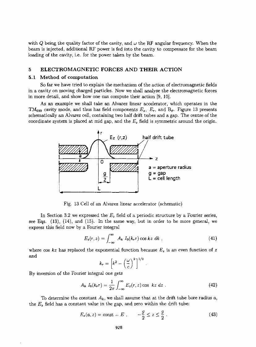
with Q being the quality factor of the cavity, and u the RF angular frequency. When the beam is injected, additional RF power is fed into the cavity to compensate for the beam loading of the cavity, i.e. for the power taken by the beam.
5 ELECTROMAGNETIC FORCES A N D THEIR ACTION 5.1 Method of computation
So far we have tried to explain the mechanism of the action of electromagnetic fields in a cavity on moving charged particles. Now we shall analyse the electromagnetic forces in more detail, and show how one can compute their action [9, 10].
As an example we shall take an Alvarez linear accelerator, which operates in the TMoio cavity mode, and thus has field components Ez, ET, and B#. Figure 13 presents schematically an Alvarez cell, containing two half drift tubes and a gap. The centre of the coordinate system is placed at mid gap, and the Ez field is symmetric around the origin.
half drift tube
*- z a = aperture radius 9 = gap L = cell length
Fig. 13 Cell of an Alvarez linear accelerator (schematic)
In Section 3.2 we expressed the Ez field of a periodic structure by a Fourier series, see Eqs. (13), (14), and (15). In the same way, but in order to be more general, we express this field now by a Fourier integral
/
CO
Ak Io(krr) cos kz dk , -oo
(41)
where cos kz has replaced the exponential function because Ez is an even function of z and
rVy k* ~c) By inversion of the Fourier integral one gets
1 r°° Ak Zo(M*) = 7T- / Ez(r, z) cos kz dz
Z7T J - c o (42)
To determine the constant Ak, we shall assume that at the drift tube bore radius a, the Ez field has a constant value in the gap, and zero within the drift tube:
Ez(a, z) = const = E ,
928
•— < z < — 2 ~ - 2
(43)
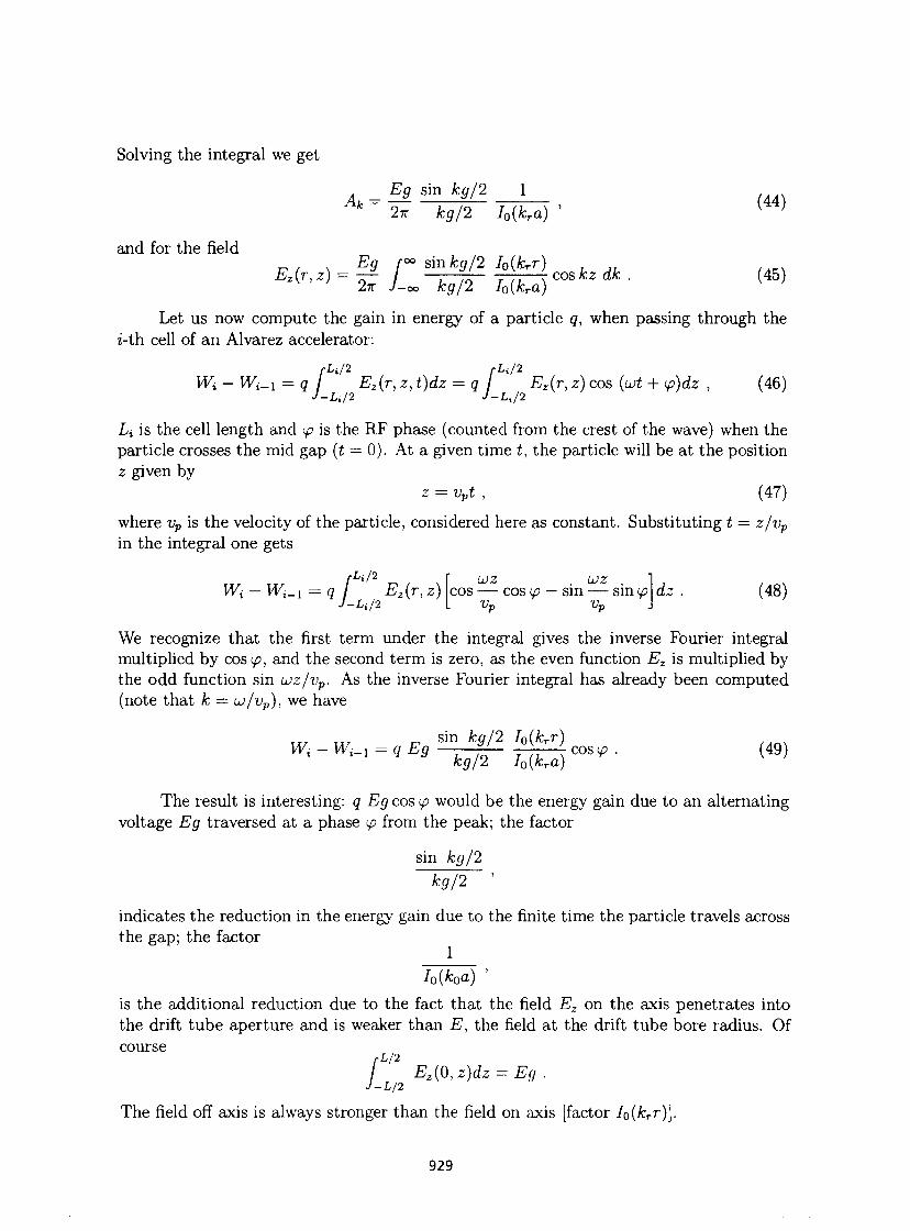
Solving the integral we get
Eg_ sin kg/2 1 k 2TT kg/2 I0(kra) ' K '
and for the field „ , , Eg r00 sinkg/2 I0(krr) , „ Ez(r, z = - * / -rrrr TTT^ c o s k z d k • 4 5
27T 7-oo fcp/2 Ioykra) Let us now compute the gain in energy of a particle q, when passing through the
z-th cell of an Alvarez accelerator: fLi/2 ,L 4 /2
/» - Wi-i = g / Ez(r,z,t)dz = q Ez(r, z) cos (ut + >p)dz , (46) J-LJ2 J-U12
Li is the cell length and <p is the RF phase (counted from the crest of the wave) when the particle crosses the mid gap (t — 0). At a given time i, the particle will be at the position z given by
z = vpt , (47)
where vp is the velocity of the particle, considered here as constant. Substituting t = z/vp
in the integral one gets L i / / 2 „ , A cuz . LOZ
/
Uil* UOZ LOZ
Ez (r, z) cos — cos <p — sin — sin <p -Li/2 I Vp Vp
dz . (48)
We recognize that the first term under the integral gives the inverse Fourier integral multiplied by cos <p, and the second term is zero, as the even function Ez is multiplied by the odd function sin uz/vp. As the inverse Fourier integral has already been computed (note that k = UJ/VP), we have
r-, s m kg/2 IoiKr) . A .
The result is interesting: q Eg cos <p would be the energy gain due to an alternating voltage Eg traversed at a phase ip from the peak; the factor
sin kg/2 kg/2 '
indicates the reduction in the energy gain due to the finite time the particle travels across the gap; the factor
1 h{k0a)
is the additional reduction due to the fact that the field Ez on the axis penetrates into the drift tube aperture and is weaker than E, the field at the drift tube bore radius. Of course
rL/2 / EJ0.z)dz = Eq .
J-L/2 The field off axis is always stronger than the field on axis [factor I0(krr)}.
929
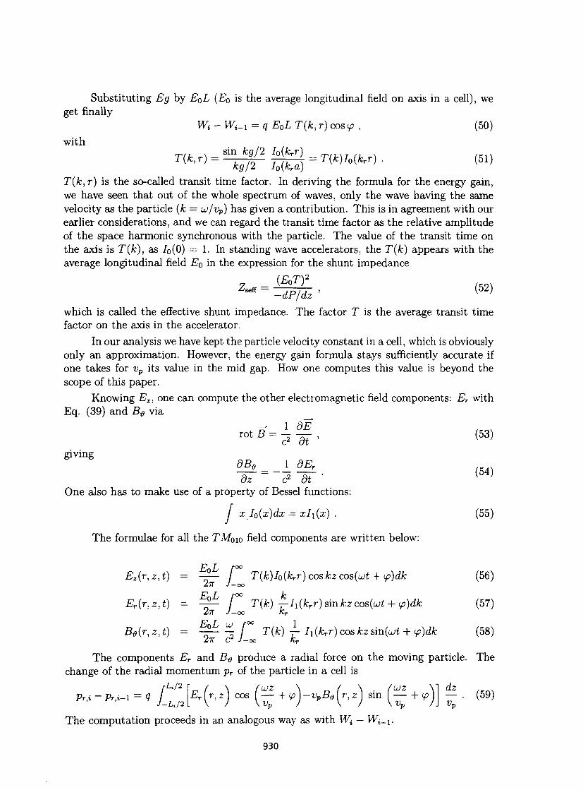
Substituting Eg by E0L (E0 is the average longitudinal field on axis in a cell), we get finally
Wi - V i_i = q E0L T{k, r) cos y? , (50) with
T(fc, r) is the so-called transit time factor. In deriving the formula for the energy gain, we have seen that out of the whole spectrum of waves, only the wave having the same velocity as the particle (fc = ui/vp) has given a contribution. This is in agreement with our earlier considerations, and we can regard the transit time factor as the relative amplitude of the space harmonic synchronous with the particle. The value of the transit time on the axis is T(k), as Io(0) = 1. In standing wave accelerators, the T(k) appears with the average longitudinal field E0 in the expression for the shunt impedance
(EoT) 2
Z s e f f ~ ^dPjTz ' ( 5 2 )
which is called the effective shunt impedance. The factor T is the average transit time factor on the axis in the accelerator.
In our analysis we have kept the particle velocity constant in a cell, which is obviously only an approximation. However, the energy gain formula stays sufficiently accurate if one takes for vp its value in the mid gap. How one computes this value is beyond the scope of this paper.
Knowing Ez, one can compute the other electromagnetic field components: Er with Eq. (39) and B# via
r o t B = ? 3 T - ( 5 3 )
giving dB& 1 dEr
dz c2 dt One also has to make use of a property of Bessel functions:
(54)
/ xJ0(x)dx = xl\(x) . (55)
The formulae for all the TM0W field components are written below:
JP T roc Ez(r,z,t) = —— / T(k)Io(krr) cos kz cosfat + <p)dh (56)
E L r°° k Er(r,z,t) = -£— / T(k) — h(krr)smkzcos(ujt + ifi)dk (57)
Z7T J-oo kr
B#(r,z,t) = - 7 - % i°° T(k) — Il(kTr)coskzsm{ut + ip)dk (58) Z7T C J J-oo Kr
The components Er and B# produce a radial force on the moving particle. The change of the radial momentum pr of the particle in a cell is
Pr,< ~ P,i-i = q / _ W 2 [Er (r, z) cos ( ^ + * ) -vpB, (r, z) sin ( ^ + <p)] ^ • (59)
The computation proceeds in an analogous way as with W^ — W^.
930
5.2 Actual computations The method of computation presented in the preceding paragraph has given us a
physical insight into the problem. It was shown that in standing-wave accelerators the action of the electromagnetic field on a particle is not computed point by point, but given by means of integral expressions. Such integrals are usually computed in programs which analyse the structure of linear accelerators.
The sequence of computer programs used in the design of standing-wave accelerators is the following:
i) A structure program, such as SUPERFISH [11], URMEL [12] or MAFIA [13] (in earlier days CLAS [14]) solves the wave equation in a cell of the structure and determines the cell dimensions corresponding to a given RF frequency. All important structure parameters such as Zs^,Q, dP/dz etc. are computed, as well as various integrals of the electromagnetic field analogous to (42). These integrals are called transit-time coefficients and are used for beam dynamics calculations, in particular to determine the exact energy and phase of the synchronous particle at mid gap [10, 15, 16]. One of them, which we already know, is called the transit time factor and is computed with
S-L/2 Ez(0,z)cos u>z/vpdz 1% E2(0>Z)dz T(k) = j-L/2zr:z:. • (60)
ii) Having computed a certain number of structure cells corresponding to different particle velocities, an accelerator is generated using a program such as GENLIN [16] or PARI [17]. Such a program interpolates between precalculated structure cells to determine all the cells in a certain energy (velocity) range. Then, with the help of transit-time coefficients, exact energies and phases of the synchronous particle in all the cells are computed, and the accelerator- is thus progressively determined.
iii) An accelerator has to accept and accelerate particles which lie in a certain range around the synchronous particle. This range is called the acceptance of the accelerator, and the beam has to be matched to it. The calculation of the acceptance, beam matching parameters and, if required, an external transverse focusing is done with programs like ADAPT [18], where the influence of beam space charge forces is also included.
iv) As a final step, the accelerator designed with the above procedure is tested by simulating a beam through it. Simulation programs, such as PARMILA [19] represent the beam with up to several thousands of macro-particles (their number is limited by the required computer time) and follow them through the accelerator. The number of particles at the output and their distribution is a measure of the quality of the designed accelerator.
A travelling-wave linear accelerator structure is designed in a similar way. One can also use SUPERFISH to determine the structure, although this program computes only standing-wave fields. With a 'trick' it is possible to obtain a travelling-wave by conveniently adding two standing waves [20]. In fact, only one standing wave is computed by
931
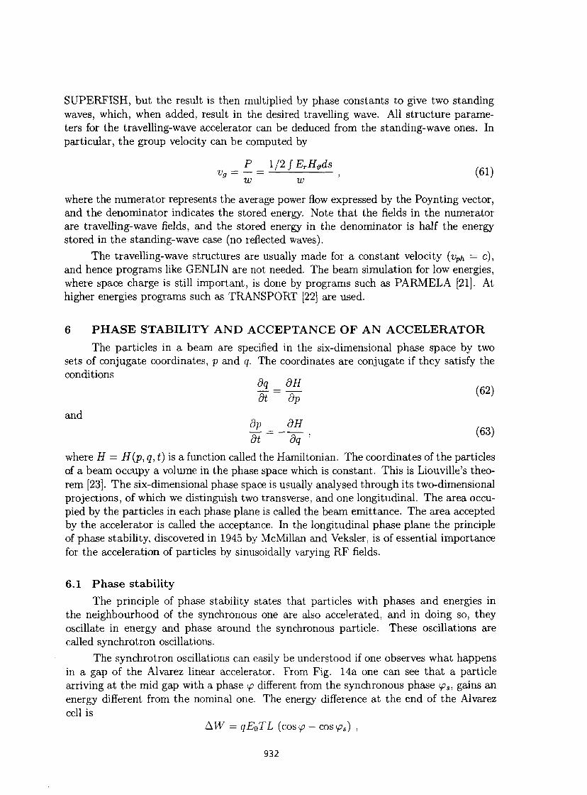
SUPERFISH, but the result is then multiplied by phase constants to give two standing waves, which, when added, result in the desired travelling wave. All structure parameters for the travelling-wave accelerator can be deduced from the standing-wave ones. In particular, the group velocity can be computed by
P 1/2 JErHyds Vg = — = , (61)
w w where the numerator represents the average power flow expressed by the Poynting vector, and the denominator indicates the stored energy. Note that the fields in the numerator are travelling-wave fields, and the stored energy in the denominator is half the energy stored in the standing-wave case (no reflected waves).
The travelling-wave structures are usually made for a constant velocity {vph = c), and hence programs like GENLIN are not needed. The beam simulation for low energies, where space charge is still important, is done by programs such as PARMELA [21]. At higher energies programs such as TRANSPORT [22] are used.
6 PHASE STABILITY A N D ACCEPTANCE OF A N ACCELERATOR The particles in a beam are specified in the six-dimensional phase space by two
sets of conjugate coordinates, p and q. The coordinates are conjugate if they satisfy the conditions
¥ = ^ ( 6 2 )
and
di = ' W ( 6 3 )
where H = H(p, q, t) is a function called the Hamiltonian. The coordinates of the particles of a beam occupy a volume in the phase space which is constant. This is Liouville's theorem [23]. The six-dimensional phase space is usually analysed through its two-dimensional projections, of which we distinguish two transverse, and one longitudinal. The area occupied by the particles in each phase plane is called the beam emittance. The area accepted by the accelerator is called the acceptance. In the longitudinal phase plane the principle of phase stability, discovered in 1945 by McMillan and Veksler, is of essential importance for the acceleration of particles by sinusoidally varying RF fields.
6.1 Phase stability The principle of phase stability states that particles with phases and energies in
the neighbourhood of the synchronous one are also accelerated, and in doing so, they oscillate in energy and phase around the synchronous particle. These oscillations are called synchrotron oscillations.
The synchrotron oscillations can easily be understood if one observes what happens in a gap of the Alvarez linear accelerator. From Fig. 14a one can see that a particle arriving at the mid gap with a phase y? different from the synchronous phase <ps, gains an energy different from the nominal one. The energy difference at the end of the Alvarez cell is
Al^ = qE0TL (cosy? — cos^ps) ,
932
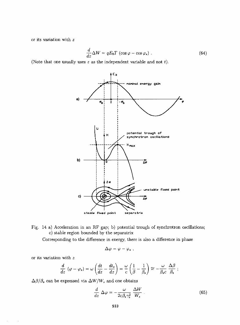
or its variation with z
—AW = qE0T (cos <p — cos <pa) . dz (Note that one usually uses z as the independent variable and not t).
(64)
a)
b)
c)
— noninal energy gain
potential t rough of synchrotron oscillations
unstable fixed point
stable fixed point separatrlx
Fig. 14 a) Acceleration in an RF gap; b) potential trough of synchrotron oscillations; c) stable region bounded by the separatrix
Corresponding to the difference in energy, there is also a difference in phase
Ay = <p - ips ,
or its variation with z
dz {if - <ps) - u y— - ^ j - c y- - ^
A(3/fis can be expressed via AW/WS and one obtains
d_ u AW dz *~~ 2c0rf Ws '
w A(3 PsC 0,
(65)
933
The set of first-order differential equations, (64) and (65), describes the synchrotron oscillations. If the frequency is constant, the variables AW and A<p are canonically conjugate, and they describe the longitudinal phase plane.
Figure 14b shows the potential trough of synchrotron oscillations. The trough is asymmetric as the set of equations is not linear. To obtain a solution, one assumes adia-baticity (/3S, % = const), and transformes the first-order set into a second-order differential equation:
COS {(fig + Apt) — COS ipa I?A^K = 0 (66)
with
K ujqEoT
2 c & 7
2 Ws •
The equation (66) is transformed in the usual way by considering the second term as dU/dAip and multiplying all by dAp/dz
A. dz \(Ti^ = o (67)
The expression in the bracket is constant and it represents the total energy of oscillation, usually denoted by H. All particles with H < Hmax will remain in the potential trough (see Fig. 14b). The potential function U(Aip) has two points where the first derivative (with respect to Ap>) is zero: one is a minimum (stable point), and the other a maximum (unstable point). At both points, the velocity in the phase plane is zero, and therefore they are called fixed points.
The bracket of (67) can be written as
u IJO
2cPs-Y2sWsUcPsy>Ws V (AWM +q EQT sini <ps +A<p)—A<pcos<p3 — sin ip3 >= H (68)
where one has used (65) and expressed U(Ap) in order for it to be zero for Ap> = 0. For each H, one has a trajectory in the Aip, AW phase plane (see Fig. 14c). For i ïm a x [equal to U(—2ys)], we get the separatrix, dividing the stable from the unstable region:
uj (AW\ +q EQT sin(ips + Aif) + sin ips — (2<ps + Aip) cos <p>$ = 0 . 4 c & 7 s
2 w8 v ; The separatrix is shown in Fig. 14c. The maximum allowed AW is found for Aip — 0:
(69)
A W m a x = ±2 2q E0T c0sj1Ws(ps cos >ps - sin (ps)
UJ
1/2
(70)
The area inside the separatrix is called the bucket. Note that the oscillations are stable only for tps < 0.
To analyse the motion around the stable phase, one can linearize (64) by cos ip — cos ips = — sin <psAip, and thus obtain a linear set of equations of the form
-^Ap = -b\z)AW . (71) dz
934
dz AW = a2(z)A<p (72)
with a2(z) and b2(z) being slowly varying functions of z. Eliminating dz and integrating, one obtains the equation of an ellipse
(A^) 2 (AW)2
5 1 TT> = C 0 I 1 S t >
(see Fig. 14c). The linearized system (71), (72) can be solved without the assumption of adiabatic-
ity. The second-order differential equation is
^(«^J.^-^o, mc°
(73)
m being the rest mass of the particle. Multiplying (73) by 01"/* and substituting
d d 0hs — = — ,
dz du one gets an equation of the form
d?_ du2 A<p + K(u)A<p (74)
where K(u) is a slowly varying function of u. This equation is solved by the usual BKW (Brillouin, Kramer, Wenzel) method, which assumes solutions of the form
w(u)eJ^u) .
Transforming the solution back to the independent variable z, we have
Aip(z) = C Aip(z) sin ( j Qs(z)dz' + v?o
with C and </>o being integration constants and
Aip(z) -mc uqEoT sin ps0sl. 3-,3
1/4
—uqEoT sin <ps
ma 01^1
1/2
(75)
(76)
Equations (75) and (76) give the amplitude and frequency of small phase oscillations. In the course of acceleration, Aip becomes smaller
Aip « ( & 7 * r 3 / 4 • (77)
This is called phase damping. If the area in the phase plane is conserved, the energy spread in the beam is increased correspondingly
AW oc ( /3 s 7 , ) 3 / 4
935
(78)
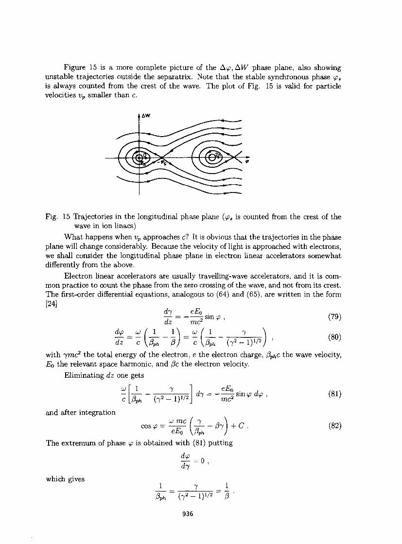
Figure 15 is a more complete picture of the Aip, AW phase plane, also showing unstable trajectories outside the separatrix. Note that the stable synchronous phase <pa
is always counted from the crest of the wave. The plot of Fig. 15 is valid for particle velocities vP smaller than c.
Fig. 15 Trajectories in the longitudinal phase plane (tps is counted from the crest of the wave in ion linacs)
What happens when vp approaches c? It is obvious that the trajectories in the phase plane will change considerably. Because the velocity of light is approached with electrons, we shall consider the longitudinal phase plane in electron linear accelerators somewhat differently from the above.
Electron linear accelerators are usually travelling-wave accelerators, and it is common practice to count the phase from the zero crossing of the wave, and not from its crest. The first-order differential equations, analogous to (64) and (65), are written in the form [24]
dj eE0 . dz mc2
dip UJ I \ 1 \ ui ( I 7 dz
(79)
(80) M PJ CVA* ( 7 2 - l ) 1 / 2 ,
with 7771c2 the total energy of the electron, e the electron charge, (3phC the wave velocity, Eo the relevant space harmonic, and /3c the electron velocity.
Eliminating dz one gets
1 c
7 A* ( 7 2 - i ) 1 / 2 J
d-y = sin ip dip , mo-
and after integration
COS<£> UJ mc + C
(81)
(82)
The extremum of phase <p is obtained with (81) putting
d<p d'y
which gives 1
0ph
= 0
7 ( 7 2 _ 1)1/2
1_
936
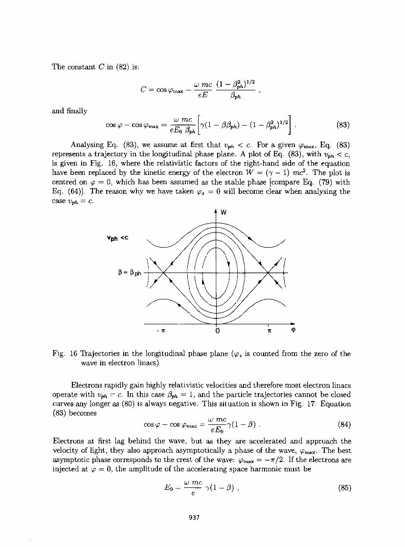
The constant C in (82) is:
C = cos </?„ umc (1- %hy/2
eE pph
and finally
COS <f — COS <£>maX = u mc
eE0 (3ph _ 7 ( l - / 5 ^ ) - ( l - / 3 p \ ) 1 / 2 (83)
Analysing Eq. (83), we assume at first that vpu < c. For a given </?max, Eq. (83) represents a trajectory in the longitudinal phase plane. A plot of Eq. (83), with vph < c, is given in Fig. 16, where the relativistic factors of the right-hand side of the equation have been replaced by the kinetic energy of the electron W = (7 — 1) mc2. The plot is centred on tp = 0, which has been assumed as the stable phase [compare Eq. (79) with Eq. (64)]. The reason why we have taken ps = 0 will become clear when analysing the case Vph = c.
4 W
Vph <c
p=p p h
Fig. 16 Trajectories in the longitudinal phase plane (</?5 is counted from the zero of the wave in electron linacs)
Electrons rapidly gain highly relativistic velocities and therefore most electron linacs operate with Vph = c. In this case fiph = 1, and the particle trajectories cannot be closed curves any longer as (80) is always negative. This situation is shown in Fig. 17. Equation (83) becomes
COS ip — COS < / ? m a x
u> mc eE0
7 ( 1 - / 5 ) - (84)
Electrons at first lag behind the wave, but as they are accelerated and approach the velocity of light, they also approach asymptotically a phase of the wave, cpmax- The best asymptotic phase corresponds to the crest of the wave: </?max = — 7r/2. If the electrons are injected at (p = 0, the amplitude of the accelerating space harmonic must be
Eo uj 'mc 7(1 - /5 ) (85)
937
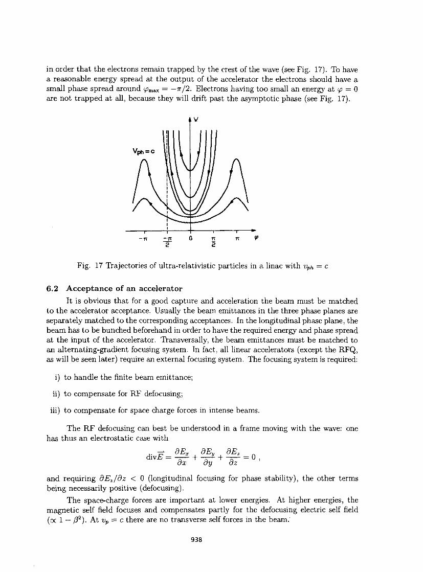
in order that the electrons remain trapped by the crest of the wave (see Fig. 17). To have a reasonable energy spread at the output of the accelerator the electrons should have a small phase spread around <pmax = — ir/2. Electrons having too small an energy at p = 0 are not trapped at all, because they will drift past the asymptotic phase (see Fig. 17).
Fig. 17 Trajectories of ultra-relativistic particles in a linac with vph = c
6.2 Acceptance of an accelerator It is obvious that for a good capture and acceleration the beam must be matched
to the accelerator acceptance. Usually the beam emittances in the three phase planes are separately matched to the corresponding acceptances. In the longitudinal phase plane, the beam has to be bunched beforehand in order to have the required energy and phase spread at the input of the accelerator. Transversally, the beam emittances must be matched to an alternating-gradient focusing system. In fact, all linear accelerators (except the RFQ, as will be seen later) require an external focusing system. The focusing system is required:
i) to handle the finite beam emittance;
ii) to compensate for RF defocusing;
iii) to compensate for space charge forces in intense beams.
The RF defocusing can best be understood in a frame moving with the wave: one has thus an electrostatic case with
divE = dET dEv dEz
dx dy + dz = 0
and requiring dEz/dz < 0 (longitudinal focusing for phase stability), the other terms being necessarily positive (defocusing).
The space-charge forces are important at lower energies. At higher energies, the magnetic self field focuses and compensates partly for the defocusing electric self field (oc 1 — P2). At vp = c there are no transverse self forces in the beam.
938
The acceptance of a linear accelerator in all phase planes is computed as if it had a periodic focusing system. Note that ion linear accelerators, where the cell length increases, are periodic if one considers t and not z as the independent variable. For intense beams, space-charge forces must somehow be included when quoting the acceptances. There are computer programs which compute the beam matching parameters and the accelerator acceptances in the presence of beam self forces.
7 HANDLING OF INTENSE BEAMS
In Section 6.1 we saw that with linear equations of motion the particle trajectories are ellipses. In the longitudinal plane the linear region is limited to the neighbourhood of the synchronous phase. In the transverse planes the external focusing forces are essentially linear.
The beam emittances in the phase planes are also specified by ellipses. To match a beam to the accelerator, the beam emittances must have the same shape as the trajectories and lie inside them.
If one deals with intense beams, space-charge forces must be taken into account. The charge density distribution in the beam is usually non-uniform, giving rise to non-linear self forces. The question now is the following: how can a non-uniform beam be matched to a structure with predominently linear forces?
It can be done. Sacherer [25] has demonstrated that the evolution of the root-mean-square (r.m.s) beam size essentially depends on the linearized part of the self forces. This is valid for beams of any charge distribution, provided they are of the ellipsoidal type, i.e. the isodensity curves are concentric ellipses. Hence, the r.m.s beam sizes and an emittance defined with r.m.s values can be matched. All beams having the same intensity, and the same r.m.s values behave in the same way. Therefore, once we know the r.m.s values of a real beam it can be replaced by an 'equivalent' one having the same r.m.s sizes, but a uniform density distribution.
The r.m.s beam sizes are computed via the second momenta of a normalized density distribution function /
x = fê)1/2 = J ... J(x - xf f(x, x', y, y', z, z')dx dy dz dx' dy' dz' , (86)
where x is the first moment (average value), usually zero. The same is valid for other phase space coordinates. Note that in Eq. (86) the longitudinal phase plane is described with z and z', replacing A<p and AV^. The important r.m.s envelope equation is
x" + K(s)x - -^- - = J i = 0 , (87) X3 X
where primes indicate the derivative with respect to the indépendant variable s (which indicates the position on the longitudinal axis) and
r n 1/2 trms XX yXX ) ,
is the r.m.s emittance ellipse and Fs the non-linear self force. Sacherer has shown that
x F s x = Ksc(s)x , (88) x2
939
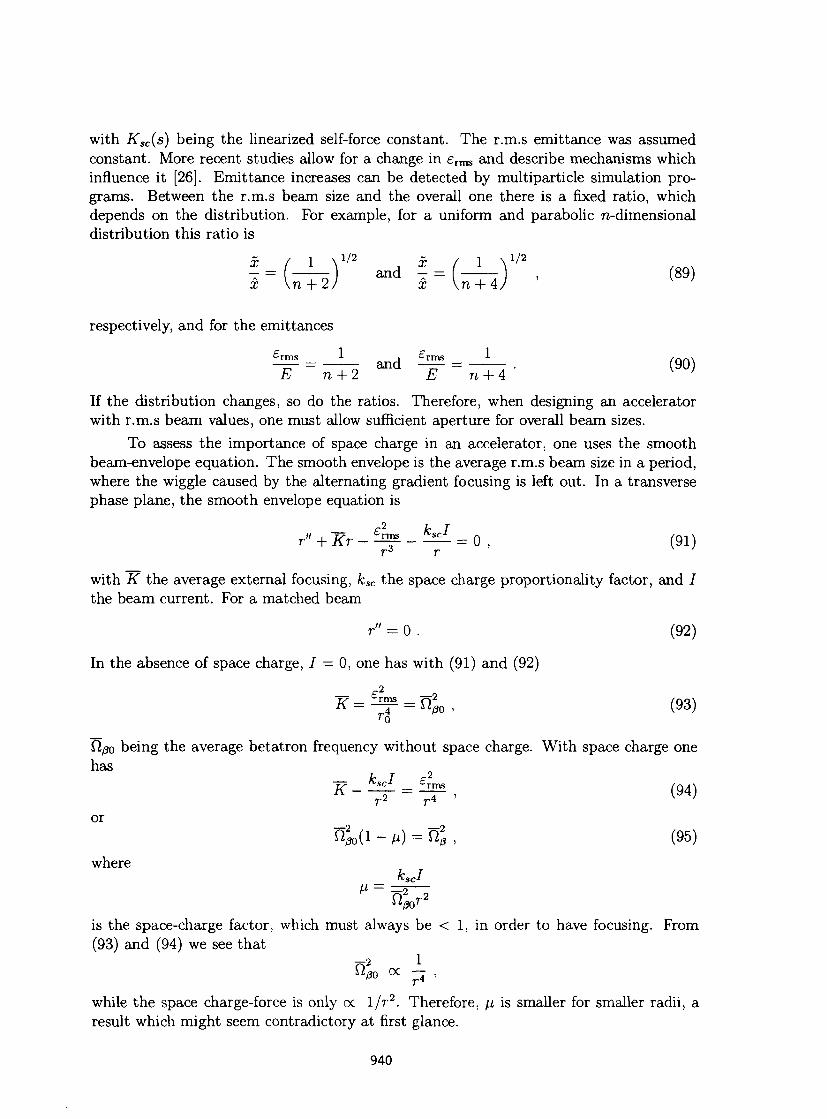
with Ksc(s) being the linearized self-force constant. The r.m.s emittance was assumed constant. More recent studies allow for a change in £ r m s and describe mechanisms which influence it [26]. Emittance increases can be detected by multiparticle simulation programs. Between the r.m.s beam size and the overall one there is a fixed ratio, which depends on the distribution. For example, for a uniform and parabolic n-dimensional distribution this ratio is
x ( 1 \ ^ 2
J x ( 1 \ 1 / 2
and - = , (89) x \n + 2/ x \n + 4
respectively, and for the emittances
—pr = T: and ~ r r = r • (90)
E n+2 E n+4 K ' If the distribution changes, so do the ratios. Therefore, when designing an accelerator with r.m.s beam values, one must allow sufficient aperture for overall beam sizes.
To assess the importance of space charge in an accelerator, one uses the smooth beam-envelope equation. The smooth envelope is the average r.m.s beam size in a period, where the wiggle caused by the alternating gradient focusing is left out. In a transverse phase plane, the smooth envelope equation is
F2 k T r" + K r - ^ - ^ - = 0 , (91)
with K the average external focusing, fcsc the space charge proportionality factor, and I the beam current. For a matched beam
r" = 0 . (92)
In the absence of space charge, 7 = 0, one has with (91) and (92)
7f = % = n^0, ( 9 3 ) TO
Qpo being the average betatron frequency without space charge. With space charge one has
^ " 7 ^ = ^ . (94) or
njo(i - n) = r ç , (95) where
Kscl V = =2
O r 2
is the space-charge factor, which must always be < 1, in order to have focusing. From (93) and (94) we see that
ô 2 l
while the space charge-force is only a 1/r2. Therefore, n is smaller for smaller radii, a result which might seem contradictory at first glance.
940
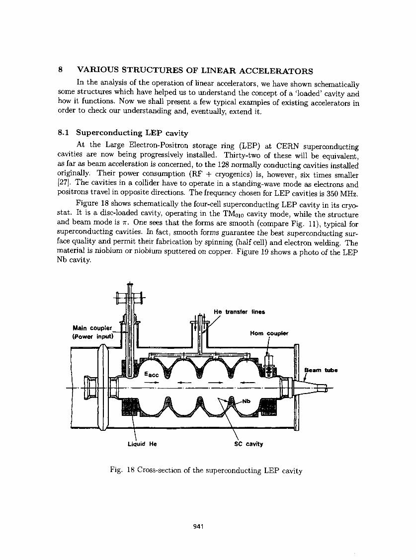
8 VARIOUS STRUCTURES OF LINEAR ACCELERATORS In the analysis of the operation of linear accelerators, we have shown schematically
some structures which have helped us to understand the concept of a 'loaded' cavity and how it functions. Now we shall present a few typical examples of existing accelerators in order to check our understanding and, eventually, extend it.
8.1 Superconducting LEP cavity At the Large Electron-Positron storage ring (LEP) at CERN superconducting
cavities are now being progressively installed. Thirty-two of these will be equivalent, as far as beam acceleration is concerned, to the 128 normally conducting cavities installed originally. Their power consumption (RF + cryogenics) is, however, six times smaller [27]. The cavities in a collider have to operate in a standing-wave mode as electrons and positrons travel in opposite directions. The frequency chosen for LEP cavities is 350 MHz.
Figure 18 shows schematically the four-cell superconducting LEP cavity in its cryostat. It is a disc-loaded cavity, operating in the T M 0 1 0 cavity mode, while the structure and beam mode is ir. One sees that the forms are smooth (compare Fig. 11), typical for superconducting cavities. In fact, smooth forms guarantee the best superconducting surface quality and permit their fabrication by spinning (half cell) and electron welding. The material is niobium or niobium sputtered on copper. Figure 19 shows a photo of the LEP Nb cavity.
Liquid He SC cavity
Fig. 18 Cross-section of the superconducting LEP cavity
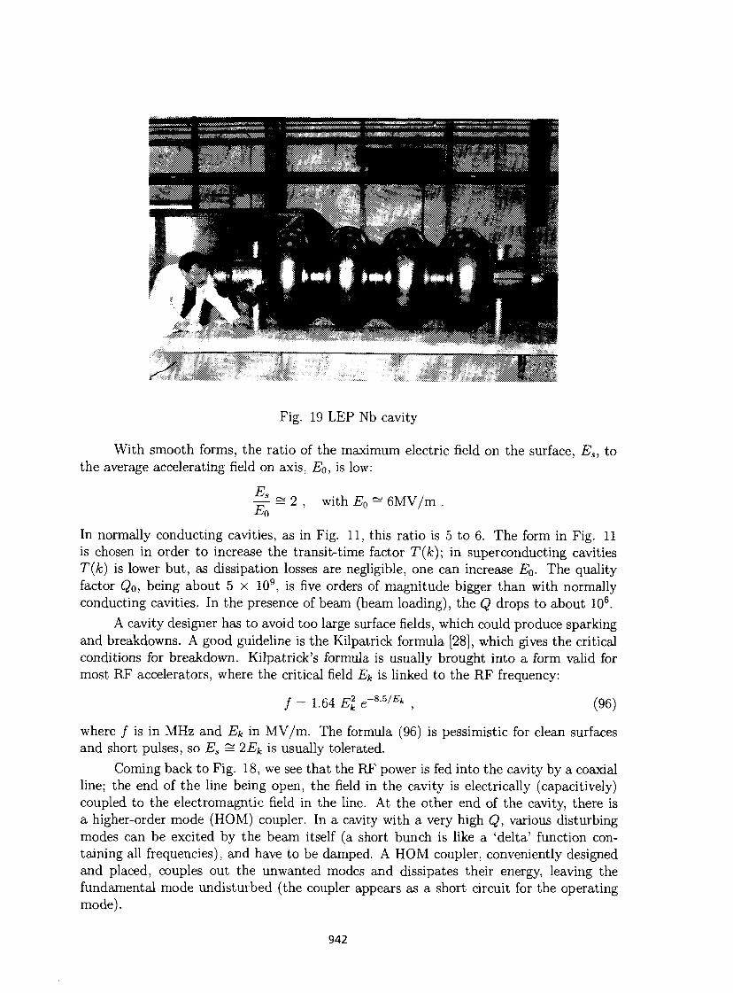
Fig. 19 LEP Nb cavity
With smooth forms, the ratio of the maximum electric field on the surface, Es, to the average accelerating field on axis, Eo, is low:
E 7 f s 2 , with E0 =* 6MV/m . Eo
In normally conducting cavities, as in Fig. 11, this ratio is 5 to 6. The form in Fig. 11 is chosen in order to increase the transit-time factor T(k); in superconducting cavities T(k) is lower but, as dissipation losses are negligible, one can increase E0. The quality factor Qo, being about 5 x 10⁹, is five orders of magnitude bigger than with normally conducting cavities. In the presence of beam (beam loading), the Q drops to about 106.
A cavity designer has to avoid too large surface fields, which could produce sparking and breakdowns. A good guideline is the Kilpatrick formula [28], which gives the critical conditions for breakdown. Kilpatrick's formula is usually brought into a form valid for most RF accelerators, where the critical field Ek is linked to the RF frequency:
/ = 1.64 E2
k e~8-5/Ek , (96)
where / is in MHz and Ek in MV/m. The formula (96) is pessimistic for clean surfaces and short pulses, so Es = 2Ek is usually tolerated.
Coming back to Fig. 18, we see that the RF power is fed into the cavity by a coaxial line; the end of the line being open, the field in the cavity is electrically (capacitively) coupled to the electromagntic field in the line. At the other end of the cavity, there is a higher-order mode (HOM) coupler. In a cavity with a very high Q, various disturbing modes can be excited by the beam itself (a short bunch is like a 'delta' function containing all frequencies), and have to be damped. A HOM coupler, conveniently designed and placed, couples out the unwanted modes and dissipates their energy, leaving the fundamental mode undisturbed (the coupler appears as a short circuit for the operating mode).
942
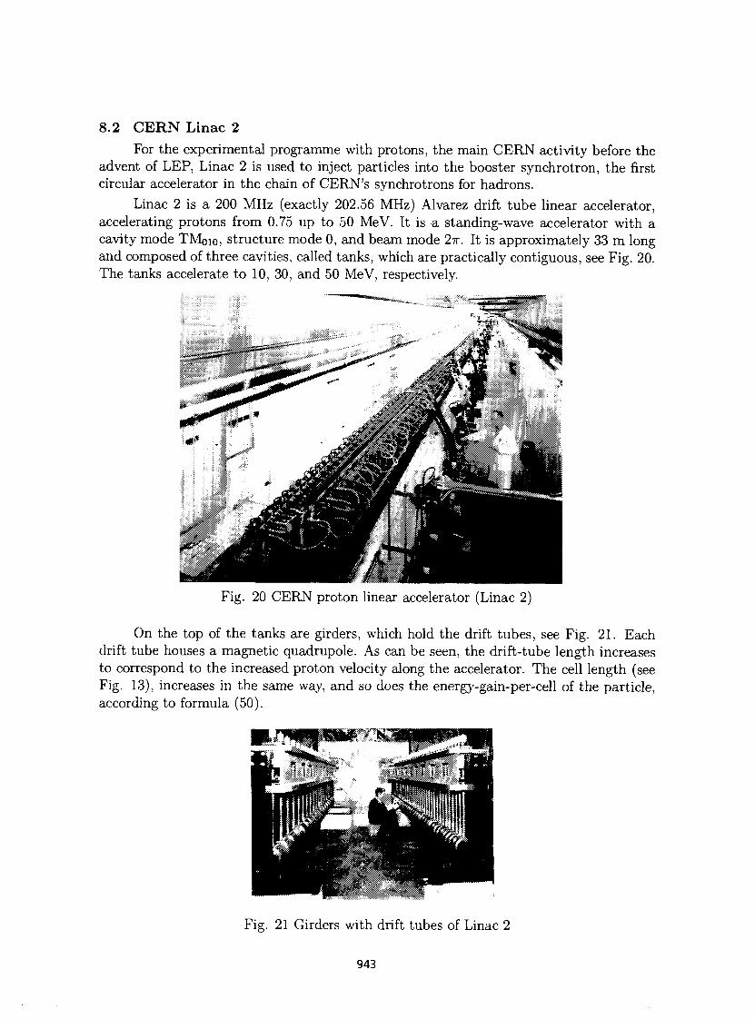
8.2 CERN Linac 2 For the experimental programme with protons, the main CERN activity before the
advent of LEP, Linac 2 is used to inject particles into the booster synchrotron, the first circular accelerator in the chain of CERN's synchrotrons for hadrons.
Linac 2 is a 200 MHz (exactly 202.56 MHz) Alvarez drift tube linear accelerator, accelerating protons from 0.75 up to 50 MeV. It is a standing-wave accelerator with a cavity mode TM0io, structure mode 0, and beam mode 2ir. It is approximately 33 m long and composed of three cavities, called tanks, which are practically contiguous, see Fig. 20. The tanks accelerate to 10, 30, and 50 MeV, respectively.
Fig. 20 CERN proton linear accelerator (Linac 2)
On the top of the tanks are girders, which hold the drift tubes, see Fig. 21. Each drift tube houses a magnetic quadrupole. As can be seen, the drift-tube length increases to correspond to the increased proton velocity along the accelerator. The cell length (see Fig. 13), increases in the same way, and so does the energy-gain-per-cell of the particle, according to formula (50).
Fig. 21 Girders with drift tubes of Linac 2
943
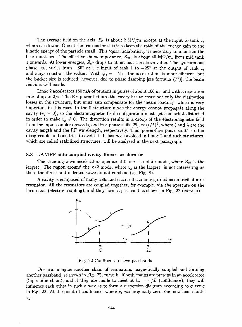
The average field on the axis, E0, is about 2 MV/m, except at the input to tank 1, where it is lower. One of the reasons for this is to keep the ratio of the energy gain to the kinetic energy of the particle small. This 'quasi adiabaticity' is necessary to maintain the beam matched. The effective shunt impedance, Z e f f , is about 40 Mft/m, from mid tank 1 onwards. At lower energies, Zen drops to about half the above value. The synchronous phase, (pa, varies from —35° at the input of tank 1 to —25° at the output of tank 1, and stays constant thereafter. With <ps = —25°, the acceleration is more efficient, but the bucket size is reduced; however, due to phase damping [see formula (77)], the beam remains well inside.
Linac 2 accelerates 150 mA of protons in pulses of about 100 /zs, and with a repetition rate of up to 2/s. The RF power fed into the cavity has to cover not only the dissipation losses in the structure, but must also compensate for the 'beam loading', which is very important in this case. In the 0 structure mode the energy cannot propagate along the cavity (vg = 0), so the electromagnetic field configuration must get somewhat distorted in order to make vg ^ 0. The distortion results in a droop of the electromagnetic field from the input coupler onwards, and in a phase shift [29], oc (£/X)2, where t and A are the cavity length and the RF wavelength, respectively. This 'power-flow phase shift' is often disagreeable and one tries to avoid it. It has been avoided in Linac 2 and such structures, which are called stabilized structures, will be analysed in the next paragraph.
8.3 LAMPF side-coupled cavity linear accelerator The standing-wave accelerators operate at 0 or TT structure mode, where Zeff is the
largest. The region around the 7r/2 mode, where vg is the largest, is not interesting as there the direct and reflected wave do not combine (see Fig. 8).
A cavity is composed of many cells and each cell can be regarded as an oscillator or resonator. All the resonators are coupled together, for example, via the aperture on the beam axis (electric coupling), and they form a passband as shown in Fig. 22 (curve a).
K K
L 2L
Fig. 22 Confluence of two passbands
One can imagine another chain of resonators, magnetically coupled and forming another passband, as shown in Fig. 22, curve b. If both chains are present in an accelerator (biperiodic chain), and if they are made to meet at kn = -n/L (confluence), they will influence each other in such a way as to form a dispersion diagram according to curve c in Fig. 22. At the point of confluence, where vg was originally zero, one now has a finite vg.
944
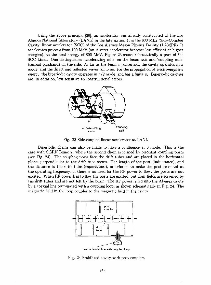
Using the above principle [30], an accelerator was already constructed at the Los Alamos National Laboratory (LANL) in the late sixties. It is the 800 MHz 'Side-Coupled Cavity' linear accelerator (SCC) of the Los Alamos Meson Physics Facility (LAMPF). It accelerates protons from 100 MeV (an Alvarez accelerator becomes less efficient at higher energies), to the final energy of 800 MeV. Figure 23 shows schematically a part of the SCC Linac. One distinguishes 'accelerating cells' on the beam axis and 'coupling cells' (second passband) on the side. As far as the beam is concerned, the cavity operates in % mode, and the direct and reflected waves combine. For the propagation of electromagnetic energy, the biperiodic cavity operates in TT/2 mode, and has a finite vg. Biperiodic cavities are, in addition, less sensitive to constructional errors.
acce le ra t ing cells
coupling cell
Fig. 23 Side-coupled linear accelerator at LANL
Biperiodic chains can also be made to have a confluence at 0 mode. This is the case with CERN Linac 2, where the second chain is formed by resonant coupling posts (see Fig. 24). The coupling posts face the drift tubes and are placed in the horizontal plane, perpendicular to the drift tube stems. The length of the post (inductance), and the distance to the drift tube (capacitance), are chosen to make the post resonant at the operating frequency. If there is no need for the RF power to flow, the posts are not excited. When RF power has to flow the posts are excited, but their fields are screened by the drift tubes and are not felt by the beam. The RF power is fed into the Alvarez cavity by a coaxial line terminated with a coupling loop, as shown schematically in Fig. 24. The magnetic field in the loop couples to the magnetic field in the cavity.
post coupler
7 3&BB0Q& drift tube
—777771 lil zzs I coaxial feeder line with coupling loop
Fig. 24 Stabilized cavity with post couplers
945
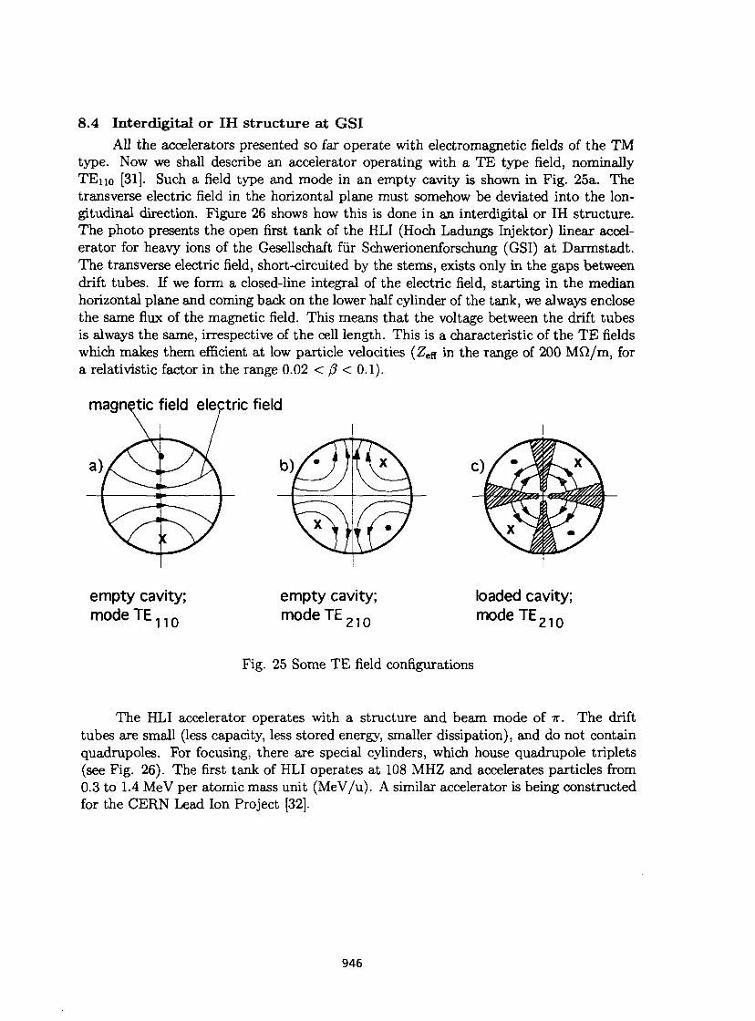
8.4 Interdigital or IH structure a t GSI All the accelerators presented so far operate with electromagnetic fields of the TM
type. Now we shall describe an accelerator operating with a TE type field, nominally TEno [31]. Such a field type and mode in an empty cavity is shown in Fig. 25a. The transverse electric field in the horizontal plane must somehow be deviated into the longitudinal direction. Figure 26 shows how this is done in an interdigital or IH structure. The photo presents the open first tank of the HLI (Hoch Ladungs Injektor) linear accelerator for heavy ions of the Gesellschaft fur Schwerionenforschung (GSI) at Darmstadt. The transverse electric field, short-circuited by the stems, exists only in the gaps between drift tubes. If we form a closed-line integral of the electric field, starting in the median horizontal plane and coming back on the lower half cylinder of the tank, we always enclose the same flux of the magnetic field. This means that the voltage between the drift tubes is always the same, irrespective of the cell length. This is a characteristic of the TE fields which makes them efficient at low particle velocities (Zeff in the range of 200 MQ/m, for a relativistic factor in the range 0.02 < 0 < 0.1).
empty cavity; empty cavity; loaded cavity; modeTE 1 1 0 modeTE 2 1 0 modeTE 2 1 0
Fig. 25 Some TE field configurations
The HLI accelerator operates with a structure and beam mode of -K. The drift tubes are small (less capacity, less stored energy, smaller dissipation), and do not contain quadrupoles. For focusing, there are special cylinders, which house quadrupole triplets (see Fig. 26). The first tank of HLI operates at 108 MHZ and accelerates particles from 0.3 to 1.4 MeV per atomic mass unit (MeV/u). A similar accelerator is being constructed for the CERN Lead Ion Project [32].
946
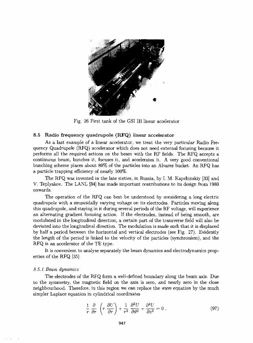
Fig. 26 First tank of the GSI IH linear accelerator
8.5 Radio frequency quadrupole (RFQ) linear accelerator As a last example of a linear accelerator, we treat the very particular Radio Fre
quency Quadrupole (RFQ) accelerator which does not need external focusing because it performs all the required actions on the beam with the RF fields. The RFQ accepts a continuous beam, bunches it, focuses it, and accelerates it. A very good conventional bunching scheme places about 80% of the particles into an Alvarez bucket. An RFQ has a particle trapping efficiency of nearly 100%.
The RFQ was invented in the late sixties, in Russia, by I. M. Kapchinskiy [33] and V. Teplyakov. The LANL [34] has made important contributions to its design from 1980 onwards.
The operation of the RFQ can best be understood by considering a long electric quadrupole with a sinusoidally varying voltage on its electrodes. Particles moving along this quadrupole, and staying in it during several periods of the RF voltage, will experience an alternating gradient focusing action. If the electrodes, instead of being smooth, are modulated in the longitudinal direction, a certain part of the transverse field will also be deviated into the longitudinal direction. The modulation is made such that it is displaced by half a period between the horizontal and vertical electrodes (see Fig. 27). Evidently the length of the period is linked to the velocity of the particles (synchronism), and the RFQ is an accelerator of the TE type.
It is convenient to analyse separately the beam dynamics and electrodynamics properties of the RFQ [35].
8.5.1 Beam dynamics The electrodes of the RFQ form a well-defined boundary along the beam axis. Due
to the symmetry, the magnetic field on the axis is zero, and nearly zero in the close neighbourhood. Therefore, in this region we can replace the wave equation by the much simpler Laplace equation in cylindrical coordinates
r dr V dr ) + r 2 dW + dz1 ~ ' { }
947
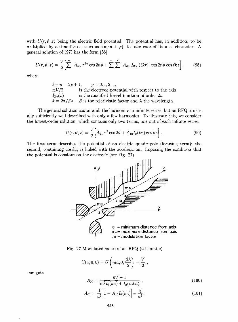
with U{r,d,z) being the electric field potential. The potential has, in addition, to be multiplied by a time factor, such as sin(u>£ + f), to take care of its a.c. character. A general solution of (97) has the form [36]
U(r,0,z) = V_
~2~l Y^ Aonr2ncos2ri'd + Y2J2 Aen hn {tkr) cos2m?cos£kz (98)
where
£ + n = 2p+l, p=0,l,2,... ±V/2 is the electrode potential with respect to the axis hnipc) is the modified Bessel function of order 2n k = 2ir/(3\, 0 is the relativistic factor and À the wavelength.
The general solution contains all the harmonics in infinite series, but an RFQ is usually sufficiently well described with only a few harmonics. To illustrate this, we consider the lowest-order solution, which contains only two terms, one out of each infinite series:
CM,*) = ! AQI r 2 cos 2d + AwIo(kr) cos kz (99)
The first term describes the potential of an electric quadrupole (focusing term); the second, containing coskz, is linked with the acceleration. Imposing the condition that the potential is constant on the electrode (see Fig. 27)
a = minimum distance from axis ma= maximum distance from axis m = modulation factor
Fig. 27 Modulated vanes of an RFQ (schematic)
px\ v U(a, 0,0) = U ma,0,
2 '
one gets
Aio = m2 - 1
m2Io(ka) + I0(mka)
4)1= -5 a2
1 - i4io/o(fca)
948
X
a 2 "
(100)
(101)
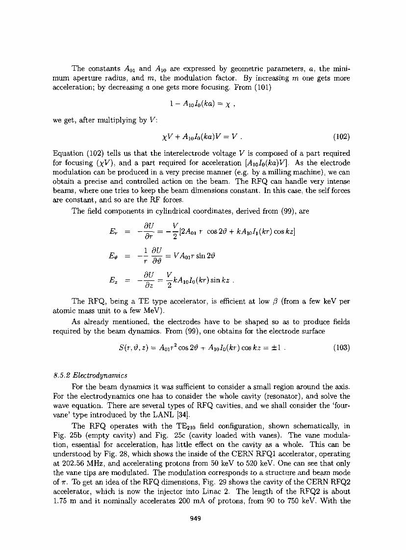
The constants A 0i and A 1 0 are expressed by geometric parameters, a, the minimum aperture radius, and m, the modulation factor. By increasing m one gets more acceleration; by decreasing a one gets more focusing. From (101)
1 - Aiolo(ka) = x >
we get, after multiplying by V:
XV + A10I0(ka)V = V . (102)
Equation (102) tells us that the interelectrode voltage V is composed of a part required for focusing (x^)> and a part required for acceleration [.Aioio^a)^. As the electrode modulation can be produced in a very precise manner (e.g. by a milling machine), we can obtain a precise and controlled action on the beam. The RFQ can handle very intense beams, where one tries to keep the beam dimensions constant. In this case, the self forces are constant, and so are the RF forces.
The field components in cylindrical coordinates, derived from (99), are
Er = — £ - = -—[2A 0i T cos2t9 + kAwIi(kr) cos kz} or 2
E# = - - ^ r = VA0ir sin2tf r ov
Ez = -— =—kAl0I0(kr) sin kz .
The RFQ, being a TE type accelerator, is efficient at low j3 (from a few keV per atomic mass unit to a few MeV).
As already mentioned, the electrodes have to be shaped so as to produce fields required by the beam dynamics. From (99), one obtains for the electrode surface
S(r, tf, z) = A01r2 cos 2d + Al0I0(kr) cos kz = ±1 . (103)
8.5.2 Electrodynamics For the beam dynamics it was sufficient to consider a small region around the axis.
For the electrodynamics one has to consider the whole cavity (resonator), and solve the wave equation. There are several types of RFQ cavities, and we shall consider the 'four-vane' type introduced by the LANL [34].
The RFQ operates with the TE2io field configuration, shown schematically, in Fig. 25b (empty cavity) and Fig. 25c (cavity loaded with vanes). The vane modulation, essential for acceleration, has little effect on the cavity as a whole. This can be understood by Fig. 28, which shows the inside of the CERN RFQ1 accelerator, operating at 202.56 MHz, and accelerating protons from 50 keV to 520 keV. One can see that only the vane tips are modulated. The modulation corresponds to a structure and beam mode of 7T. To get an idea of the RFQ dimensions, Fig. 29 shows the cavity of the CERN RFQ2 accelerator, which is now the injector into Linac 2. The length of the RFQ2 is about 1.75 m and it nominally accelerates 200 mA of protons, from 90 to 750 keV. With the
949
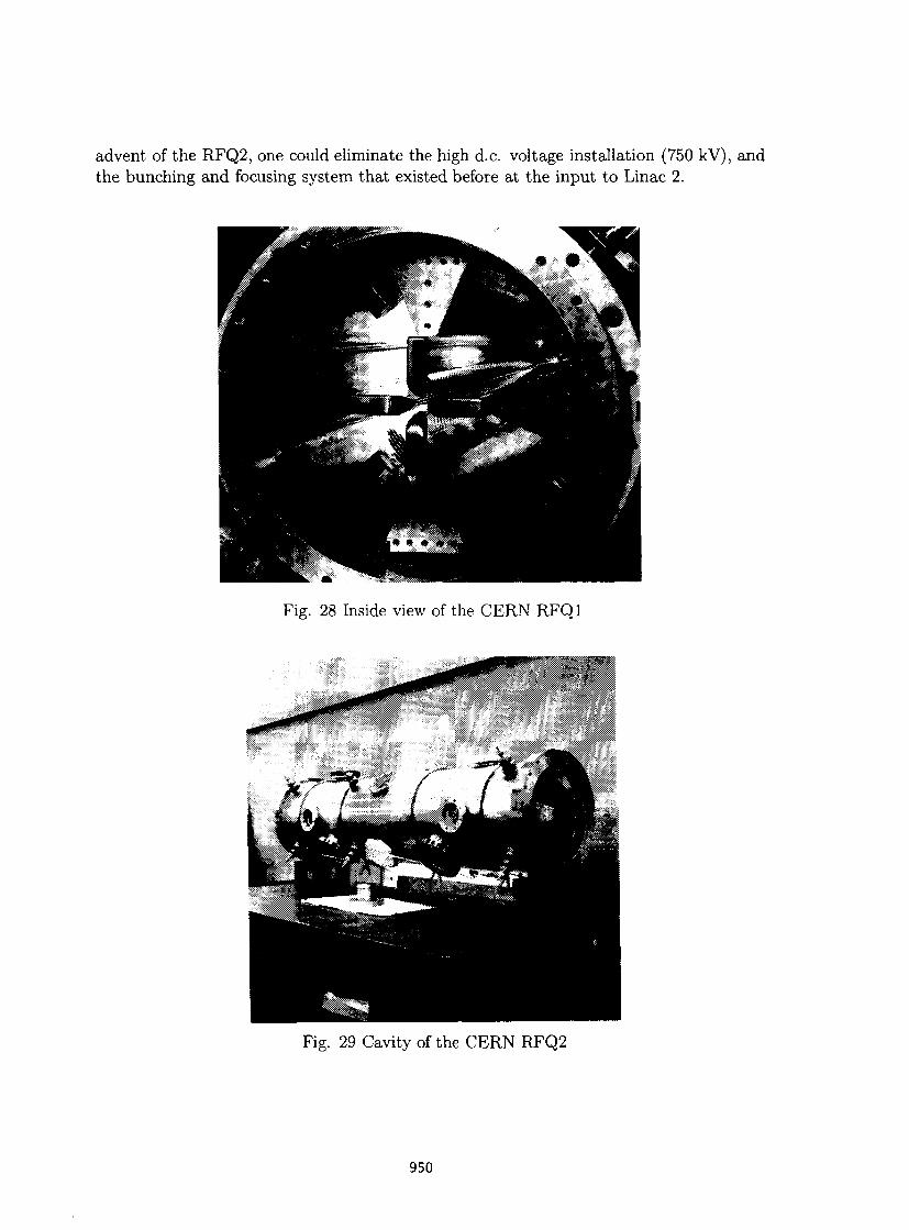
advent of the RFQ2, one could eliminate the high d.c. voltage installation (750 kV), and the bunching and focusing system that existed before at the input to Linac 2.
Fig. 28 Inside view of the CERN RFQl
Fig. 29 Cavity of the CERN RFQ2
950
9 CONCLUSION The basic concepts underlying how RF linear accelerators function have been pre
sented. This paper, as the title indicates, is only an introduction, where the subjects have been treated to facilitate further study. The beam dynamics equations in cavities have been dealt with in the correct way, but with some simplifications, as have the theories of coupled oscillators and intense beams. By including design principles and examples of existing linear accelerators in this paper, it is hoped that enough material is presented in order to understand what is involved when dealing with linacs.
ACKNOWLEDGEMENTS This paper has profited from discussions with G. Dôme, T.P. Wangler and in par
ticular P.M. Lapostolle. D.J. Warner has read and commented on the manuscript. To all of them go my thanks.
References [1] C. Ramo, J.R. Whinnery and T. van Duzer, Fields and waves in communication
electronics (John Wiley, New York, 1965).
[2] J.C. Slater, Microwave electronics (D. van Nostrand, New York, 1951), p. 395.
[3] Ibid., pp. 169-177.
[4] G.A. Loew and R.B. Neal, Accelerating structures, in Linear Accelerators, by P.M. Lapostolle and A.L. Septier (North Holland, Amsterdam 1970), pp. 47-52.
[5] G. Dôme, Review and survey of accelerating structures, in Linear Accelerators (see Ref. [4]).
[6] G.A. Loew and R.B. Neal, Accelerating Structures, in Linear Accelerators (see Ref. [4]), pp. 52-65.
[7] P. Lapostolle, Introduction à la théorie des accélérateurs linéaires, CERN 87-09 (1987), pp. 43-44.
[8] J. Le Duff, Dynamics and acceleration in linear structures, Proc. CER.N Accelerator School, Gif-sur-Yvette, 1984, CERN 85-19 (1985), p. 146.
[9] P.M. Lapostolle, Introduction à l'étude des accélérateurs linéaires, CERN 66-20 (1966).
[10] RM. Lapostolle, Equations de la dynamique des particules dans un accélérateur linéaire à protons, Int. Rep. CERN AR/Int. SG/65-11.
[11] K. Halbach and R.F. Holsinger, SUPERFISH-A computer program, Part. Accel. 7 (4), pp. 213-222 (1976).
[12] T. Weiland, On the computation of resonant modes in cylindrically symmetric cavities, Nucl. Instrum. Methods 216, pp. 329-248 (1983).
951
[13] R. Klatt et al., MAFIA-A three dimensional electromagnetic CAD system, Proc. Linear Accelerator Conference, 1986, SLAC report 303, pp. 276-278.
[14] M. Martini and D.J. Warner, Numerical calculations of linear accelerator cavities, CERN 68-11 (1968).
[15] B. Schnizer, General properties of fields and beam dynamics in a linac gap, CERN 69-3 (1969).
[16] M. Promé, Effets de la charge d'espace dans les accélérateurs linéaires à protons, Thèse, Orsay No. 761 (1971).
[17] K. Crandall, Documentation for PARMULT, Memo AT-1: 92-151, LANL, Los Alamos.
[18] B. Bru, Calcul de la focalisation quadripolaire d'un linac et de l'adaptation du faisceau en présence de charge d'espace, Int. Rep. MPS/LIN 70-10 (1970).
[19] G.P. Boicourt and J. Merson, PARMILA Users and Reference Manual, LA-UR-90-127, LANL, Los Alamos.
[20] G.A. Loew, R.H. Miller and R.A. Early, Computer calculations of travelling wave periodic structure properties, IEEE Trans. Nucl. Sci., NS-26, pp. 3701-3704 (1979).
[21] K. Crandall, PARMELA, Computer code available from AT-6, H829, LANL, Los Alamos.
[22] K.L. Brown et al., Transport - A computer program for designing charged particle beam transport systems, CERN 80-04.
[23] M. Weiss, A short demonstration of Liouville's Theorem, Proc. CERN Accelerator School, Aarhus, Denmark 1986, CERN 87-10 (1987).
[24] R.H. Helm and R. Miller, Particle dynamics, in Linear Accelerators (see Ref. [4]), pp. 115-120.
[25] F. Sacherer, RMS envelope equation with space charge, Int. Rep. CERN/SI/Int. DL/70-12.
[26] T.P. Wangler, K.R. Crandall, R.S. Mills and M. Reiser, Field energy and r.m.s. emittance in intense particle beams, Workshop on High Brightness, San Diego, AIP Conf. Proc. 139 (1986), p. 133.
[27] Ph. Bernard, CERN, private communication.
[28] W.D. Kilpatrick, Criterion for vacuum sparking designed to include both RF and d.c, Rev. Sci. Instrum., 28 (1957).
[29] H.G. Hereward, Some examples of energy flow in the Alvarez structure, Int. Rep. CERN MPS/DL Int. 65-1 (1965).
[30] E.A. Knapp, High energy structures, in Linear Accelerators (see Ref. [4]), pp. 601-616.
952
[31] U. Ratzinger et al., The Upgraded Munich Linear Heavy Ion Postaccelerator, Nucl. Instrum. Methods A263 pp. 261-270 (1988).
[32] D.J. Warner (éd.), CERN Heavy-Ion Facility Design Report, CERN 93-01 (1993).
[33] I.M. Kapchinskiy, Strahldynamik in den Sektionen mit Raumlich Uniformer Fokussierung, GSI-tr-14/76 (Translation from Russian).
[34] R.H. Stokes et al., The radio frequency quadrupole, Proc. of 11th Int. Conf. on High Energy Accelerators, Geneva, 1980 (Birkhauser, Basle, 1980).
[35] M. Weiss, Radio frequency quadrupole, CERN Accelerator School, Aarhus, Denmark, 1986, CERN 87-10 (1987), pp. 196-230.
[36] C. Biscari, Computer programs and methods for the design of high intensity RFQs, Int. Rep. CERN/PS 85-67 (Li).
953

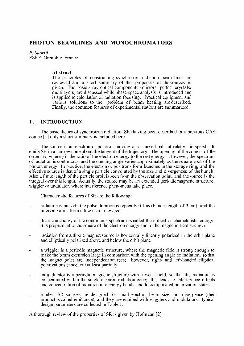
PHOTON BEAMLINES AND MONOCHROMATORS
P. Suortti ESRF, Grenoble, France
Abstract The principles of constructing synchrotron radiation beam lines are reviewed and a short summary of the properties of the sources is given. The basic x-ray optical components (mirrors, perfect crystals, multilayers) are discussed while phase-space analysis is introduced and is applied to calculation of radiation focusing. Practical equipment and various solutions to the problem of beam heating are described. Finally, the common features of experimental stations are summarized.
1 . INTRODUCTION
The basic theory of synchrotron radiation (SR) having been described in a previous CAS course [1] only a short summary is included here.
The source is an electron or positron moving on a curved path at relativistic speed. It emits SR in a narrow cone about the tangent of the trajectory. The opening of the cone is of the order \ly, where y is the ratio of the electron energy to the rest energy. However, the spectrum of radiation is continuous, and the opening angle varies approximately as the square root of the photon energy. In practice, the electron or positrons form bunches in the storage ring, and the effective source is that of a single particle convoluted by the size and divergences of the bunch. Also a finite length of the particle orbit is seen from the observation point, and the source is the integral over this length. Actually, the source may be an extended periodic magnetic structure, wiggler or undulator, where interference phenomena take place.
Characteristic features of SR are the following:
radiation is pulsed; the pulse duration is typically 0.1 ns (bunch length of 3 cm), and the interval varies from a few ns to a few /JS
the mean energy of the continuous spectrum is called the critical or characteristic energy, it is proprtional to the square of the electron energy and to the magnetic field strength
radiation from a dipole magnet source is horizontally linearly polarized in the orbit plane and elliptically polarized above and below the orbit plane
a wiggler is a periodic magnetic structure, where the magnetic field is strong enough to make the beam excursion large in comparison with the opening angle of radiation, so that the magnet poles are independent sources; however, right- and left-handed elliptical polarizations cancel out at least partially
an undulator is a periodic magnetic structure with a weak field, so that the radiation is concentrated within the single electron radiation cone; this leads to interference effects and concentration of radiation into energy bands, and to complicated polarization states
modern SR sources are designed for small electron beam size and divergence (their product is called emittance), and they are equiped with wigglers and undulators; typical design parameters are collected in Table 1.
A thorough review of the properties of SR is given by Hofmann [2].
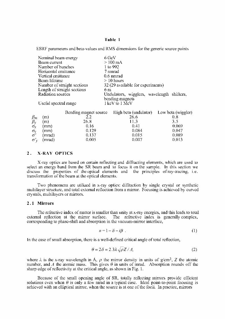
Table 1
ESRF parameters and beta-values and RMS dimensions for the generic source points
Nominal beam energy 6 GeV Beam current > 100 mA Number of bunches 1 to 992 Horizontal emittance 7 nmrad Vertical emittance 0.6 nmrad Beam lifetime > 10 hours Number of straight sections 32 (29 available for experiments) Length of straight sections 6 m Radiation sources Undulators, wigglers, wavelength shifters,
bending magnets Useful spectral range 1 keV to 1 MeV
Bending magnet source High beta (undulator) p m (m) 2.2 26.6 Py (m) 26.8 11.3 c>x (mm) 0.16 0.41 cry (mm) 0.129 0.084 a' (mrad) 0.137 0.015 a'y (mrad) 0.005 0.007
2 . X-RAY OPTICS
X-ray optics are based on certain reflecting and diffracting elements, which are used to select an energy band from the SR beam and to focus it on the sample. In this section we discuss the properties of the optical elements and the principles of ray-tracing, i.e. transformation of the beam at the optical elements.
Two phenomena are utilized in x-ray optics: diffraction by single crystal or synthetic multilayer structure, and total external reflection from a mirror. Focusing is achieved by curved crystals, multilayers or mirrors.
2 . 1 Mirrors
The refractive index of matter is smaller than unity at x-ray energies, and this leads to total external reflection at the mirror surface. The refractive index is generally complex, corresponding to phase-shift and absorption in the vacuum-mirror interface,
n = \-5-ij5 . (1)
In the case of small absorption, there is a well-defined critical angle of total reflection,
e = 28 = 2.3XsJpZ/A, (2)
where X is the x-ray wavelength in Â, p the mirror density in units of g/cm3, Z the atomic number, and A the atomic mass. This gives 6 in units of mrad. Absorption rounds off the sharp edge of reflectivity at the critical angle, as shown in Fig. 1.
Because of the small opening angle of SR, totally reflecting mirrors provide efficient solutions even when 0 is only a few mrad in a typical case. Ideal point-to-point focusing is achieved with an elliptical mirror, when the source is at one of the focii. In practice, mirrors
Low beta (wiggler) 0.8 3.5 0.069 0.047 0.089 0.013
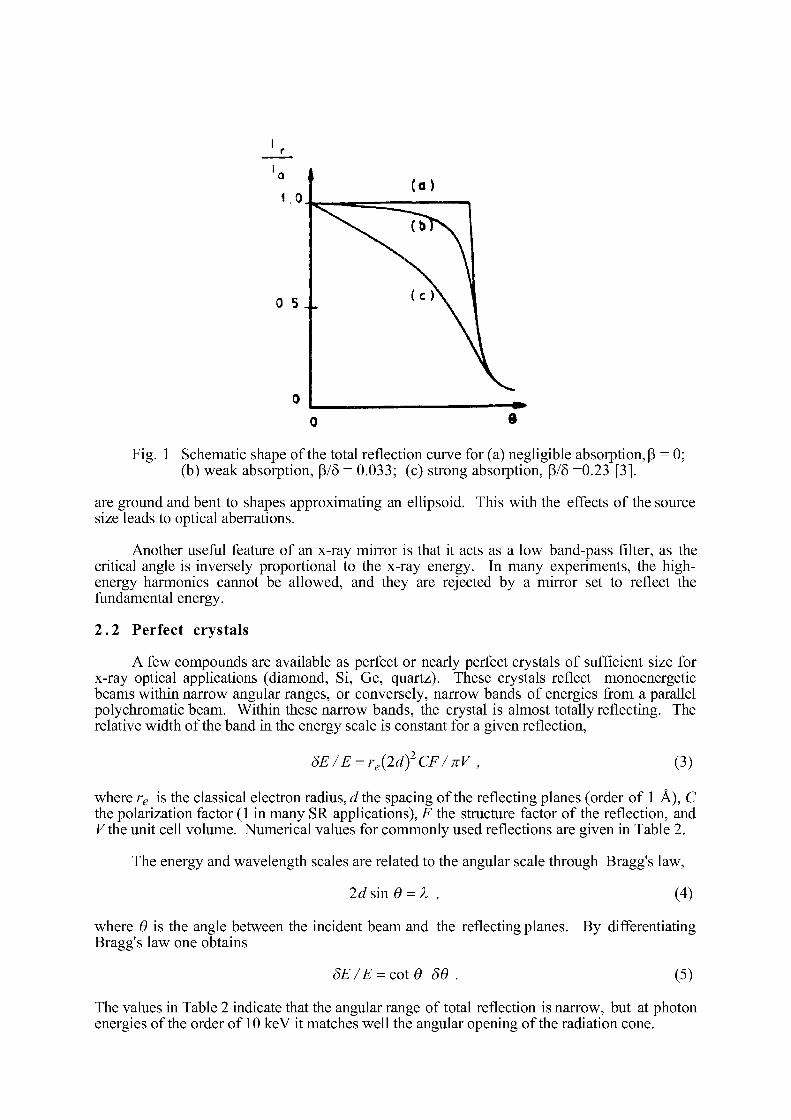
0 5
0 0 »
Fig. 1 Schematic shape of the total reflection curve for (a) negligible absorption, P = 0; (b) weak absorption, p/ô = 0.033; (c) strong absorption, p/ô =0.23 [3].
are ground and bent to shapes approximating an ellipsoid. This with the effects of the source size leads to optical aberrations.
Another useful feature of an x-ray mirror is that it acts as a low band-pass filter, as the critical angle is inversely proportional to the x-ray energy. In many experiments, the high-energy harmonics cannot be allowed, and they are rejected by a mirror set to reflect the fundamental energy.
2.2 Perfect crystals
A few compounds are available as perfect or nearly perfect crystals of sufficient size for x-ray optical applications (diamond, Si, Ge, quartz). These crystals reflect monoenergetic beams within narrow angular ranges, or conversely, narrow bands of energies from a parallel polychromatic beam. Within these narrow bands, the crystal is almost totally reflecting. The relative width of the band in the energy scale is constant for a given reflection,
ÔE/E = re(2df CF/nV , (3)
where re is the classical electron radius, d the spacing of the reflecting planes (order of 1 Â), C the polarization factor (1 in many SR applications), F the structure factor of the reflection, and F the unit cell volume. Numerical values for commonly used reflections are given in Table 2.
The energy and wavelength scales are related to the angular scale through Bragg's law,
2 d sin 6 = X , (4)
where 6 is the angle between the incident beam and the reflecting planes. By differentiating Bragg's law one obtains
5E/E = cote 56 . (5)
The values in Table 2 indicate that the angular range of total reflection is narrow, but at photon energies of the order of 10 keV it matches well the angular opening of the radiation cone.
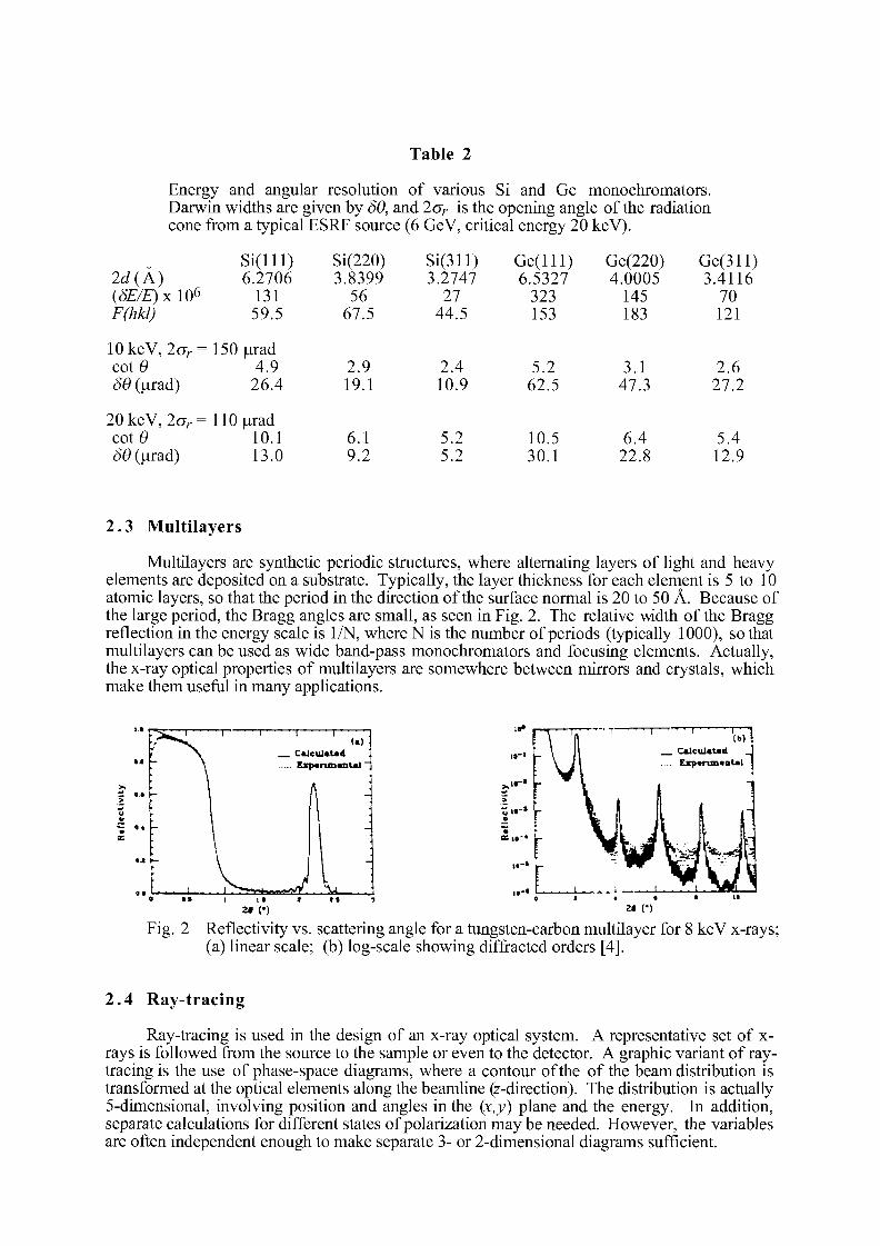
Table 2
Energy and angular resolution of various Si and Ge monochromators. Darwin widths are given by 89, and 2crr is the opening angle of the radiation cone from a typical ESRF source (6 GeV, critical energy 20 keV).
Si(ll l) 2d (A) 6.2706 (<5£/E)xl06 131 F(hkl) 59.5
Si(220) 3.8399
56 67.5
Si(311) 3.2747
27 44.5
Ge(ll l) 6.5327
323 153
Ge(220) 4.0005
145 183
Ge(311) 3.4116
70 121
1 0 k e V , 2 a r = 1 5 0 ^ a d cot 0 4.9 <50(^rad) 26.4
2.9 19.1
2.4 10.9
5.2 62.5
3.1 47.3
2.6 27.2
20keV, 2ar= 110 ^rad cot0 10.1 <50(>ad) 13.0
6.1 9.2
5.2 5.2
10.5 30.1
6.4 22.8
5.4 12.9
2.3 Multilayers
Multilayers are synthetic periodic structures, where alternating layers of light and heavy elements are deposited on a substrate. Typically, the layer thickness for each element is 5 to 10 atomic layers, so that the period in the direction of the surface normal is 20 to 50 Â. Because of the large period, the Bragg angles are small, as seen in Fig. 2. The relative width of the Bragg reflection in the energy scale is 1/N, where N is the number of periods (typically 1000), so that multilayers can be used as wide band-pass monochromators and focusing elements. Actually, the x-ray optical properties of multilayers are somewhere between mirrors and crystals, which make them useful in many applications.
2» (•) 2» (•)
Fig. 2 Reflectivity vs. scattering angle for a tungsten-carbon multilayer for 8 keV x-rays; (a) linear scale; (b) log-scale showing diffracted orders [4].
2.4 Ray-tracing
Ray-tracing is used in the design of an x-ray optical system. A representative set of x-rays is followed from the source to the sample or even to the detector. A graphic variant of ray-tracing is the use of phase-space diagrams, where a contour of the of the beam distribution is transformed at the optical elements along the beamline (z-direction). The distribution is actually 5-dimensional, involving position and angles in the (x,y) plane and the energy. In addition, separate calculations for different states of polarization may be needed. However, the variables are often independent enough to make separate 3- or 2-dimensional diagrams sufficient.
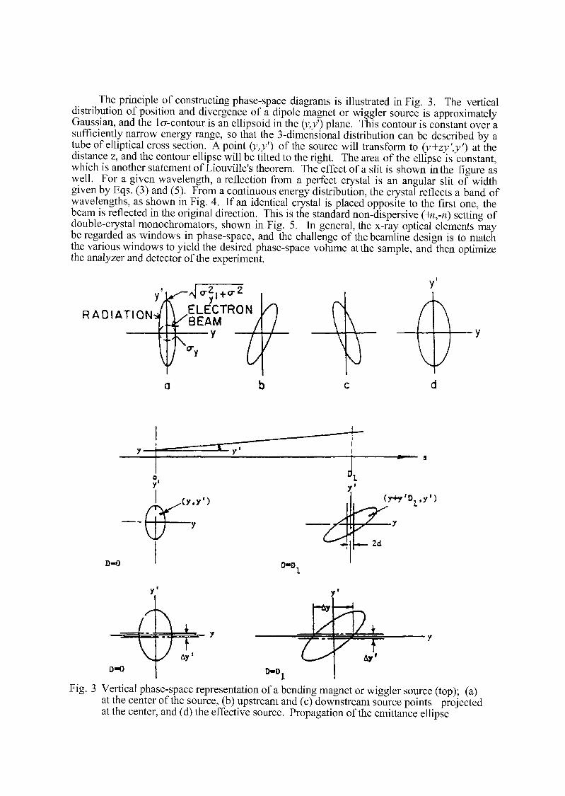
The principle of constructing phase-space diagrams is illustrated in Fig. 3. The vertical distribution of position and divergence of a dipole magnet or wiggler source is approximately Gaussian, and the la-contour is an ellipsoid in the (y,yf) plane. This contour is constant over a sufficiently narrow energy range, so that the 3-dimensional distribution can be described by a tube of elliptical cross section. A point fy,y') of the source will transform to (y+zy',y') at the distance z, and the contour ellipse will be tilted to the right. The area of the ellipse is constant, which is another statement of Liouville's theorem. The effect of a slit is shown in the figure as well. For a given wavelength, a reflection from a perfect crystal is an angular slit of width given by Eqs. (3) and (5). From a continuous energy distribution, the crystal reflects a band of wavelengths, as shown in Fig. 4. If an identical crystal is placed opposite to the first one, the beam is reflected in the original direction. This is the standard non-dispersive (-\n,-ri) setting of double-crystal monochromators, shown in Fig. 5. In general, the x-ray optical elements may be regarded as windows in phase-space, and the challenge of thebeamline design is to match the various windows to yield the desired phase-space volume at the sample, and then optimize the analyzer and detector of the experiment.
RADIATION
4 °ii+°-2
, ELECTRON i ^BEAM
—y
D-0
( y + y ' D ^ y ' )
D-D,
D-0
-Ar ^ n
/ 2±. z '7 \ Ay'
D-D
Fig. 3 Vertical phase-space representation of a bending magnet or wiggler source (top); (a) at the center of the source, (b) upstream and (c) downstream source points projected at the center, and (d) the effective source. Propagation of the emittance ellipse
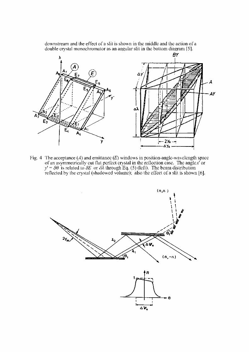
downstream and the effect of a slit is shown in the middle and the action of a double crystal monochromator as an angular slit in the bottom diagram [51.
Fig. 4 The acceptance (A) and emittance (£) windows in position-angle-wavelength space of an asymmetrically cut flat perfect crystal in the reflection case. The anglex' or y = 86 is related to 8E or 8X through Eq. (5) (left). The beam distribution reflected by the crystal (shadowed volume); also the effect of a slit is shown [6].
(n,n )
AV Q
- 6
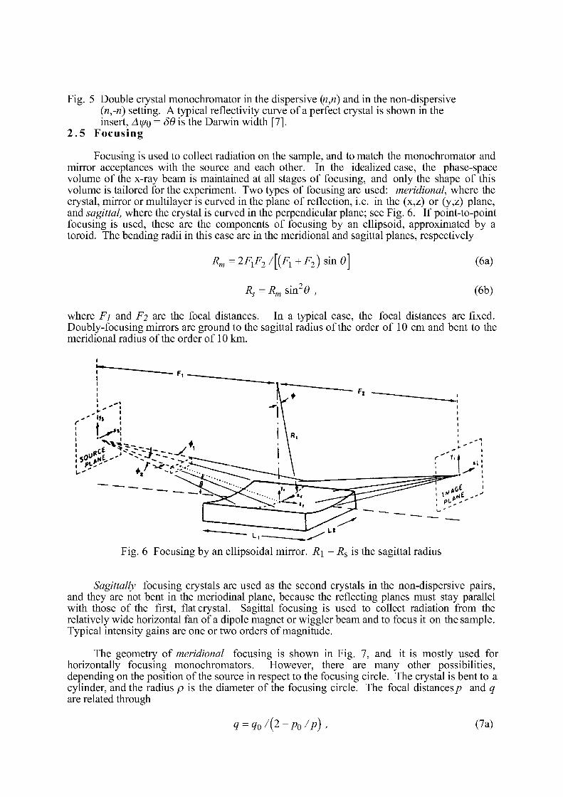
Fig. 5 Double crystal monochromator in the dispersive (n,n) and in the non-dispersive (n,-n) setting. A typical reflectivity curve of a perfect crystal is shown in the insert, Ay/Q = 56 is the Darwin width [7].
2.5 Focusing
Focusing is used to collect radiation on the sample, and to match the monochromator and mirror acceptances with the source and each other. In the idealized case, the phase-space volume of the x-ray beam is maintained at all stages of focusing, and only the shape of this volume is tailored for the experiment. Two types of focusing are used: meridional, where the crystal, mirror or multilayer is curved in the plane of reflection, i.e. in the (x,z) or (y,z) plane, and sagittal, where the crystal is curved in the perpendicular plane; see Fig. 6. If point-to-point focusing is used, these are the components of focusing by an ellipsoid, approximated by a toroid. The bending radii in this case are in the meridional and sagittal planes, respectively
Rm=2FlF2/[(Fl+F2)sm6] (6a)
Rs = Rm sin2 6 , (6b)
where Fj and F2 are the focal distances. In a typical case, the focal distances are fixed. Doubly-focusing mirrors are ground to the sagittal radius of the order of 10 cm and bent to the meridional radius of the order of 10 km.
Fig. 6 Focusing by an ellipsoidal mirror. R\ = Rs is the sagittal radius
Sagittally focusing crystals are used as the second crystals in the non-dispersive pairs, and they are not bent in the meriodinal plane, because the reflecting planes must stay parallel with those of the first, flat crystal. Sagittal focusing is used to collect radiation from the relatively wide horizontal fan of a dipole magnet or wiggler beam and to focus it on the sample. Typical intensity gains are one or two orders of magnitude.
The geometry of meridional focusing is shown in Fig. 7, and it is mostly used for horizontally focusing monochromators. However, there are many other possibilities, depending on the position of the source in respect to the focusing circle. The crystal is bent to a cylinder, and the radius p is the diameter of the focusing circle. The focal distances/? and q are related through
q = q0/(2-p0/p) , (7a)
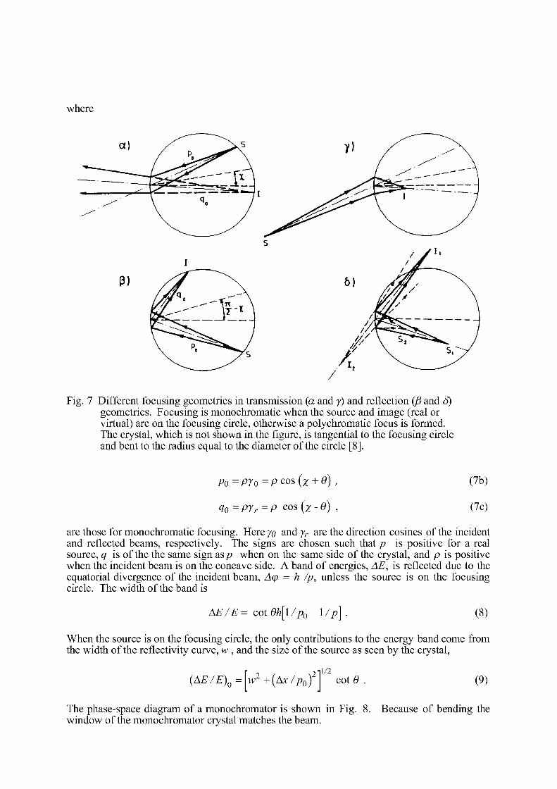
where
a) y)
:IL
P)
Fig. 7 Different focusing geometries in transmission (a and y) and reflection (fi and <5) geometries. Focusing is monochromatic when the source and image (real or virtual) are on the focusing circle, otherwise a polychromatic focus is formed. The crystal, which is not shown in the figure, is tangential to the focusing circle and bent to the radius equal to the diameter of the circle [8].
A> = PYo=P cos (x + 9) ,
qQ =pïr=p c o s (x-o) »
(7b)
(7c)
are those for monochromatic focusing. Here yo and yr are the direction cosines of the incident and reflected beams, respectively. The signs are chosen such that p is positive for a real source, q is of the the same sign as/? when on the same side of the crystal, and p is positive when the incident beam is on the concave side. A band of energies, AE, is reflected due to the equatorial divergence of the incident beam, Aq> = h /p, unless the source is on the focusing circle. The width of the band is
AE/E= cot0h[l/po-l/p] . (8)
When the source is on the focusing circle, the only contributions to the energy band come from the width of the reflectivity curve, w , and the size of the source as seen by the crystal,
(AE/E)Q w + (Ax/p0) i l l / 2
COt0 . (9)
The phase-space diagram of a monochromator is shown in Fig. 8. Because of bending the window of the monochromator crystal matches the beam.
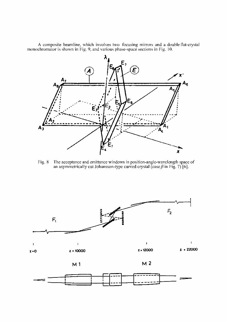
A composite beamline, which involves two focusing mirrors and a double flat-crystal monochromator is shown in Fig. 9, and various phase-space sections in Fig. 10.
Fig. 8 The acceptance and emittance windows in position-angle-wavelength space of an asymmetrically cut Johansson-type curved crystal (case (5 in Fig. 7) [6].
Fi
• V
- V
2 - 0 z . 10000 z . 12000 Z « 22000
M 1 M 2
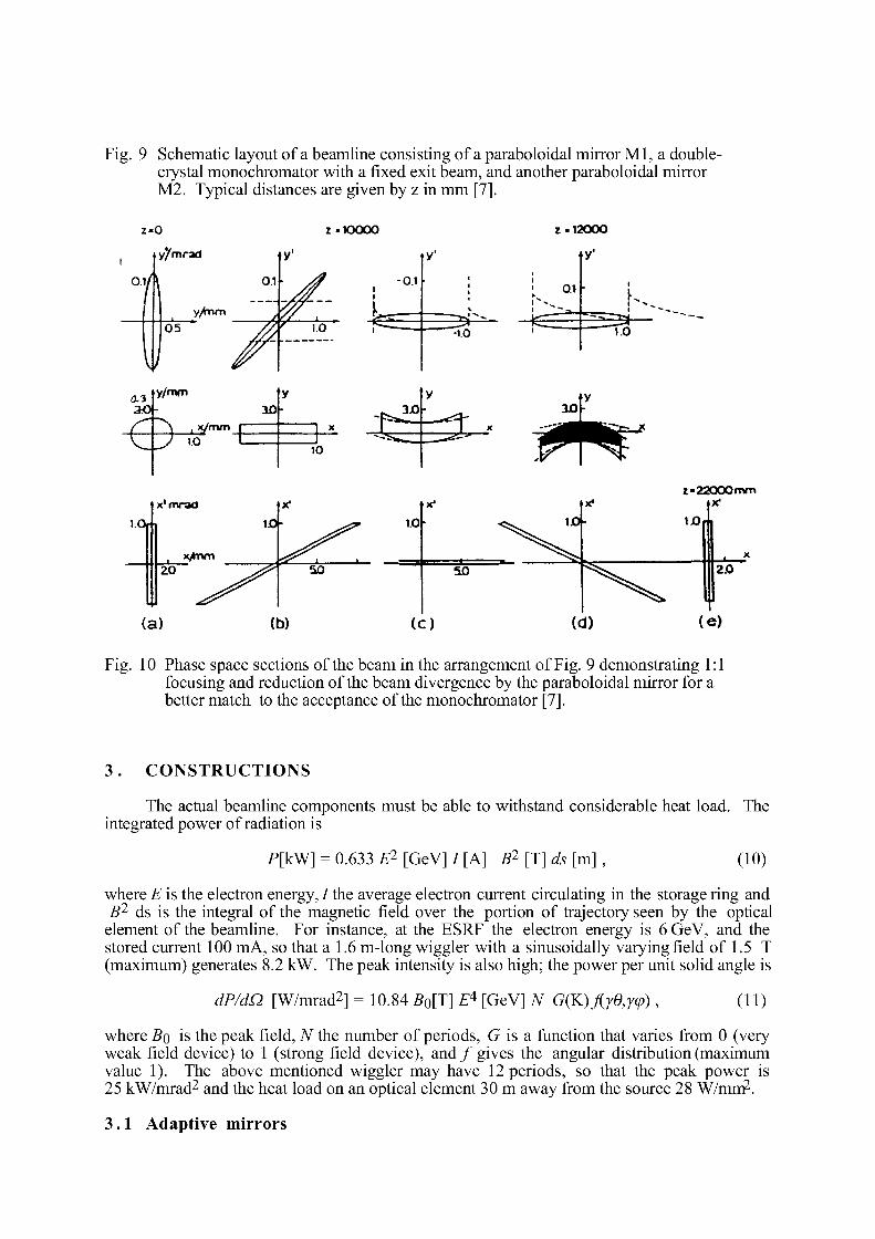
Fig. 9 Schematic layout of a beamline consisting of a paraboloidal mirror Ml, a double-crystal monochromator with a fixed exit beam, and another paraboloidal mirror M2. Typical distances are given by z in mm [7].
z - 0
y'/mrad
y/"nm
0.3 - 3 0 -
y/nvn
l .Ori
1.0
x 'mrad
i x/mm
x/tnm ZO
(a)
3Û
*x"
1.0-
2 * 1 0 0 0 0
-0.1
1 ^
y"
I.12000
4 /
S I v . ^
-1.0
10
1.0
50 5 0
(b) (c)
Ql -i *.„
sa-1.0
1J0-
I « 2 2 0 0 0 m m x-
I j O r i
2.0
(d) (e)
Fig. 10 Phase space sections of the beam in the arrangement of Fig. 9 demonstrating 1:1 focusing and reduction of the beam divergence by the paraboloidal mirror for a better match to the acceptance of the monochromator [7].
3 . CONSTRUCTIONS
The actual beamline components must be able to withstand considerable heat load. The integrated power of radiation is
P[kW] = 0.633 E2 [GeV] / [A] B2 [T] ds [m] (10)
where E is the electron energy, / the average electron current circulating in the storage ring and B2 ds is the integral of the magnetic field over the portion of trajectory seen by the optical element of the beamline. For instance, at the ESRF the electron energy is 6 GeV, and the stored current 100 mA, so that a 1.6 m-long wiggler with a sinusoidally varying field of 1.5 T (maximum) generates 8.2 kW. The peak intensity is also high; the power per unit solid angle is
dP/dQ [W/mrad2] = 10.84 B0[T] E4 [GeV] N G(K) J(y6,y(p) (11)
where BQ is the peak field, TV the number of periods, G is a function that varies from 0 (very weak field device) to 1 (strong field device), and / gives the angular distribution (maximum value 1). The above mentioned wiggler may have 12 periods, so that the peak power is 25 kW/mrad2 and the heat load on an optical element 30 m away from the source 28 W/mm2.
3 .1 Adaptive mirrors
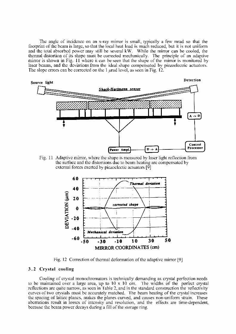
The angle of incidence on an x-ray mirror is small, typically a few mrad so that the footprint of the beam is large, so that the local heat load is much reduced, but it is not uniform and the total absorbed power may still be several kW. While the mirror can be cooled, the thermal distortion of its shape must be corrected mechanically. The principle of an adaptive mirror is shown in Fig. 11 where it can be seen that the shape of the mirror is monitored by laser beams, and the deviations from the ideal shape compensated by piezoelectric actuators. The slope errors can be corrected on the 1 /jrad level, as seen in Fig. 12.
Source light Detection
[Power Ampl.l
Fig. 11 Adaptive mirror, where the shape is measured by laser light reflection from the surface and the distortions due to beam heating are compensated by external forces exerted by piezoelectic actuators [9]
60
£ a 20 z o E
Q
0
20
40
•60
Thermal déviation
40 —
Mechanical deriation
SO -30 -10 10 30 50 MIRROR COORDINATES (cm)
Fig. 12 Correction of thermal deformation of the adaptive mirror [9]
3.2 Crystal cooling
Cooling of crystal monochromators is technically demanding as crystal perfection needs to be maintained over a large area, up to 10 x 10 cm. The widths of the perfect crystal reflections are quite narrow, as seen in Table 2, and in the standard construction the reflectivity curves of two crystals must be accurately matched. The beam heating of the crystal increases the spacing of lattice planes, makes the planes curved, and causes non-uniform strain. These aberrations result in losses of intensity and resolution, and the effects are time-dependent, because the beam power decays during a fill of the storage ring.
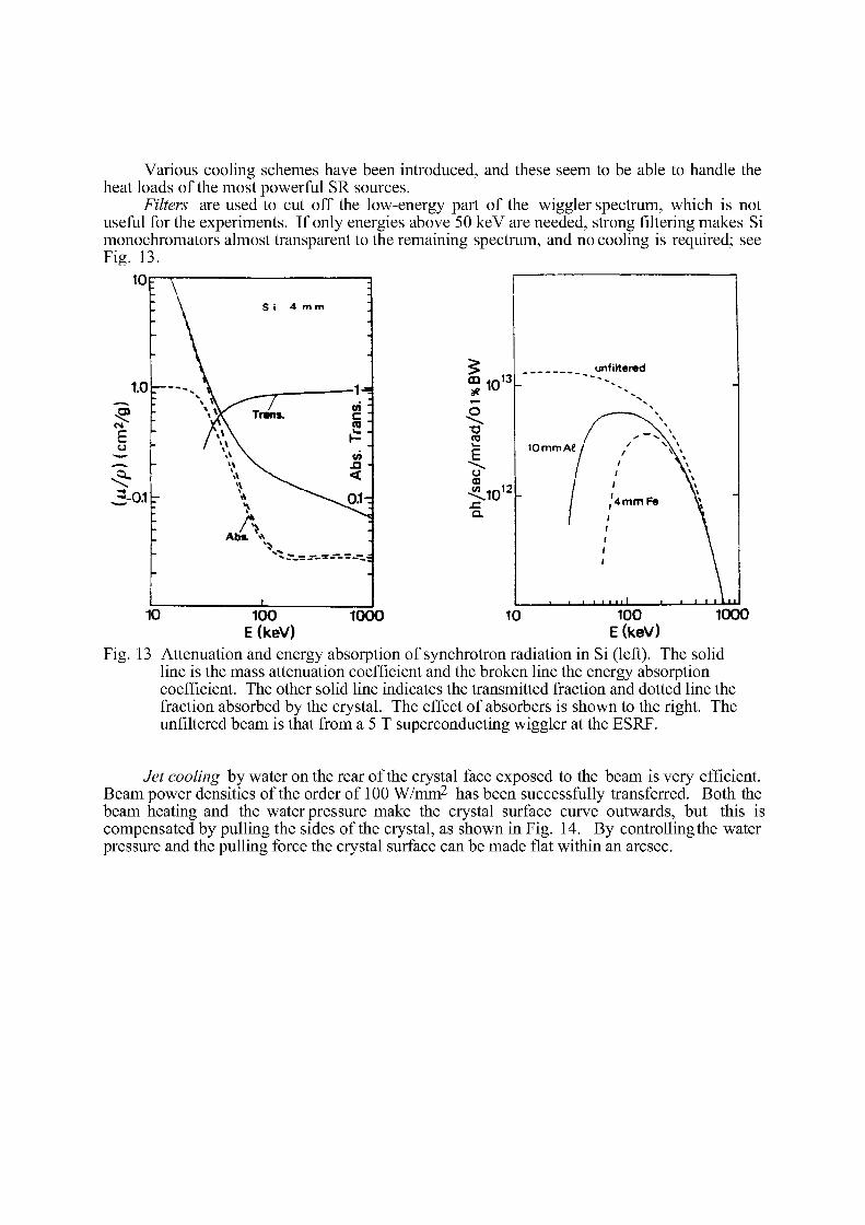
Various cooling schemes have been introduced, and these seem to be able to handle the heat loads of the most powerful SR sources.
Filters are used to cut off the low-energy part of the wiggler spectrum, which is not useful for the experiments. If only energies above 50 keV are needed, strong filtering makes Si monochromators almost transparent to the remaining spectrum, and no cooling is required; see Fig. 13.
S unfiltered
£io 1 3 " • - ^ -
o X3 / X V
« j / -' v \ * E
lOmmAÉ f / \ \ u 03
^ 1 0 1 2
' V u 03
^ 1 0 1 2 / ' V i Y
r 4mm Fe V, -Q.
, i i i n i i i i i dLu. 100
E (keV) 1000 10 100
E (keV) 1000
Fig. 13 Attenuation and energy absorption of synchrotron radiation in Si (left). The solid line is the mass attenuation coefficient and the broken line the energy absorption coefficient. The other solid line indicates the transmitted fraction and dotted line the fraction absorbed by the crystal. The effect of absorbers is shown to the right. The unfiltered beam is that from a 5 T superconducting wiggler at the ESRF.
Jet cooling by water on the rear of the crystal face exposed to the beam is very efficient. Beam power densities of the order of 100 W/mm2 has been successfully transferred. Both the beam heating and the water pressure make the crystal surface curve outwards, but this is compensated by pulling the sides of the crystal, as shown in Fig. 14. By controlling the water pressure and the pulling force the crystal surface can be made flat within an arcsec.
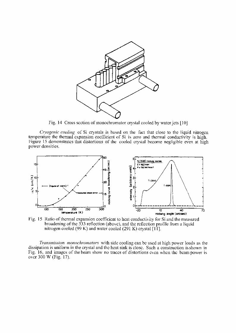
Fig. 14 Cross section of monochromator crystal cooled by water jets [10]
Cryogenic cooling of Si crystals is based on the fact that close to the liquid nitrogen temperature the thermal expansion coefficient of Si is zero and thermal conductivity is high. Figure 15 demonstrates that distortions of the cooled crystal become negligible even at high power densities.
100 150 200 250 300 _ 2 Q 1 0 40 temperature (K) ^ ^ a n g ) e ( a r e s e c )
Fig. 15 Ratio of thermal expansion coefficient to heat conductivity for Si and the measured broadening of the 333 reflection (above), and the reflection profile from a liquid nitrogen cooled (99 K) and water cooled (291 K) crystal [11].
Transmission monochromators with side cooling can be used at high power loads as the dissipation is uniform in the crystal and the heat sink is close. Such a construction is shown in Fig. 16, and images of the beam show no traces of distortions even when the beam power is over 300 W (Fig. 17).
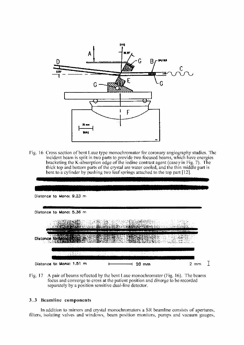
V. F .
«MI
**
Fig. 16 Cross section of bent Laue type monochromator for coronary angiography studies. The incident beam is split in two parts to provide two focused beams, which have energies bracketing the K-absorption edge of the iodine contrast agent (case y in Fig. 7). The thick top and bottom parts of the crystal are water cooled, and the thin middle part is bent to a cylinder by pushing two leaf springs attached to the top part [12].
Distance to Mono: 9.23 m
Distance t o Mono: 5.36 m
= É É mw^a »*<r v ^ fe* ~V*V^, ^
lata n M t°l l l i i mW^-S^ ^ _ v -
• . '. -• r?m
Distance to Mono: 1.51 m H 20 mm 2 mm I
Fig. 17 A pair of beams reflected by the bent Laue monochromator (Fig. 16). The beams focus and converge to cross at the patient position and diverge to be recorded separately by a position sensitive dual-line detector.
3.3 Beamline components
In addition to mirrors and crystal monochromators a SR beamline consists of apertures, filters, isolating valves and windows, beam position monitors, pumps and vacuum gauges,
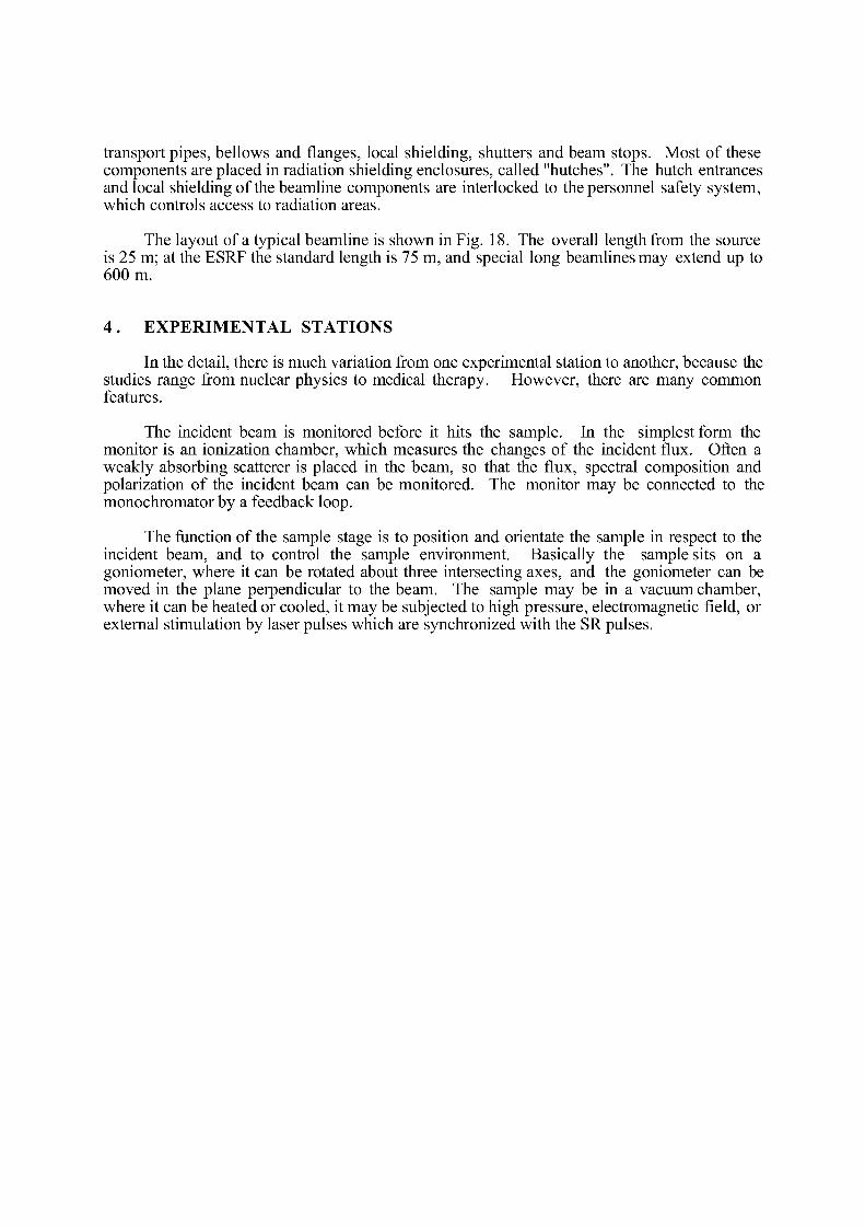
transport pipes, bellows and flanges, local shielding, shutters and beam stops. Most of these components are placed in radiation shielding enclosures, called "hutches". The hutch entrances and local shielding of the beamline components are interlocked to the personnel safety system, which controls access to radiation areas.
The layout of a typical beamline is shown in Fig. 18. The overall length from the source is 25 m; at the ESRF the standard length is 75 m, and special long beamlines may extend up to 600 m.
4 . EXPERIMENTAL STATIONS
In the detail, there is much variation from one experimental station to another, because the studies range from nuclear physics to medical therapy. However, there are many common features.
The incident beam is monitored before it hits the sample. In the simplest form the monitor is an ionization chamber, which measures the changes of the incident flux. Often a weakly absorbing scatterer is placed in the beam, so that the flux, spectral composition and polarization of the incident beam can be monitored. The monitor may be connected to the monochromator by a feedback loop.
The function of the sample stage is to position and orientate the sample in respect to the incident beam, and to control the sample environment. Basically the sample sits on a goniometer, where it can be rotated about three intersecting axes, and the goniometer can be moved in the plane perpendicular to the beam. The sample may be in a vacuum chamber, where it can be heated or cooled, it may be subjected to high pressure, electromagnetic field, or external stimulation by laser pulses which are synchronized with the SR pulses.
Fig. 18 Perspective view of a beamline at the ESRF. The components after the shield wall are primary slits, selective filters, mirror, secondary slits, monochromator, slits, mirror, beam position monitor, collimator slits, beam shutter, intenmsity monitor and diffractometer
The scattered or transmitted radiation is observed through an analyzer-detector combination. The intensity and sometimes the state of polarization is measured varying the scattering angles, and this may be combined with a spectral analysis. In time resolved experiments, the time interval between the stimulating pulse and the probing SR pulse is varied, or the decay of an excited state is followed by a time-resolving detector. The analyzer may be a single crystal that is tuned to reflect only a narrow energy band, or the crystal may disperse the scattered radiation which is analyzed by a position sensitive detector, or the detector itself is energy dispersive. Large area detectors are becoming more and more common in SR experiments, particularly in protein crystallography, where a diffraction pattern consisting of thousands of reflections has to be recorded in a short time.
* * *
REFERENCES
[I] R. Maier, Proceedings of the Fourth General Accelerator Physics School, Julich, 1990, CERN 91-04 (1991).
[2] A. Hofmann, SSRL ADC-Note 38 (1986).
[3] G. Raunio and O. Svensson, Arkiv Fys. 35, 149 (1967).
[4] B.W. Batterman and D.H. Bilderback, "Handbook of Synchrotron Radiation" ed. E-E. Koch, Vol. 3, 105, Elsevier Science Publ. (1991).
[5] G.K. Green, "National Synchrotron Light Source" ed. J.P. Blewett, Brookhaven National Laboratory Report 50595, Vol. II, 1-35 (1977).
[6] T. Matsushita and H. Hashizume, "Handbook of Synchrotron Radiation"ed. E-E. Koch, Vol la, 261, North Holland Publ. Co. (1983).
[7] P. Suortti, Brookhaven National Laboratory Informal Report 29180 (1980).
[8] P. Suortti and A.K. Freund, Rev. Sci. Instrum. 60, 2579 (1989).
[9] J. Susini, G. Fôrstner, L. Zhang, G. Boyer and R. Ravalet, Rev. Sci. Instrum. 63, 423 (1992).
[10] L.E. Berman, M. Hart and S. Sharma, Nucl. Instr. and Meth. A321, 617 (1992).
[II] A.K. Freund, Rev. Sci. Instrum. 63, 413 (1992).
[12] P. Suortti, W. Thomlinson, D. Chapman, N. Gmûr, C. Schulze, P. Siddons (in preparation).
MICROTRONS
Per Lidbjôrk Scanditronix AB, Uppsala, Sweden.
Abstract Microtrons are accelerators for low to intermediate energy electrons. The operating principles for both circular (classical) and racetrack microtrons are described. Longitudinal and transverse stability is discussed and some examples of applications are given.
1. INTRODUCTION
The microtron is a cyclic particle accelerator for low to intermediate energies (up to some tens of MeV in circular microtrons and up to a few hundred MeV in racetrack microtrons). The particles are accelerated by a high frequency electric field in a resonant cavity or a linac, and are recirculated by a homogeneous, constant magnetic field. This resemblance to the classical cyclotron has resulted in the microtron being sometimes referred to as an "electron cyclotron". The microtron is however restricted to accelerating particles whose kinetic energy can be increased by an amount comparable to their rest energy during one single pass through the accelerating cavity, and the only particles in question are therefore electrons and positrons. Microtrons offer a combination of high beam currents, with small emittance and very good energy resolution.
The microtron was first proposed by Veksler in 1944 [1], and the first working microtron was constructed a few years later, in Ottawa, Canada in 1948 [2]. Mainly due to inefficient injection methods, resulting in very low beam currents, the microtron more or less disappeared from the scene in Western Europe and North America for about a decade. After the war, in the Soviet Union however, the microtron was studied theoretically, and by the 1960's it was highly developed and extensively used. A new injection method was developed by Wernholm in Stockholm in 1964 [3], by which the beam current could be increased an order of magnitude. During this period of time research and development programs were carried out in for example Sweden, Italy, Canada, England and USA.
The sector-focused, single-cavity, racetrack microtron (RTM) at the University of Western Ontario was the first practical machine of this type to be built, in 1961 [4]. Due to beam optical stability, sector-focused racetrack microtrons are limited to a few accelerating cavities. The first multi-cavity standard RTM was built at the University of Illinois at Urbana-Champaign in the mid 70's, and is described by Hanson et al. [5]. Other notable racetrack microtron projects are e.g. the University of Mainz 180 MeV RTM [6], the 50 MeV machine in Stockholm, which has been operational since 1974 [7], the 100 MeV injector RTM at the University of Wisconsin [8] and the 100 MeV racetrack microtron at the University of Lund, also used as a storage ring injector [9]. In this context the Scanditronix commercially available RTM50 and RTM100, developed from the accelerator concepts at Lund and Stockholm should be mentioned.
971
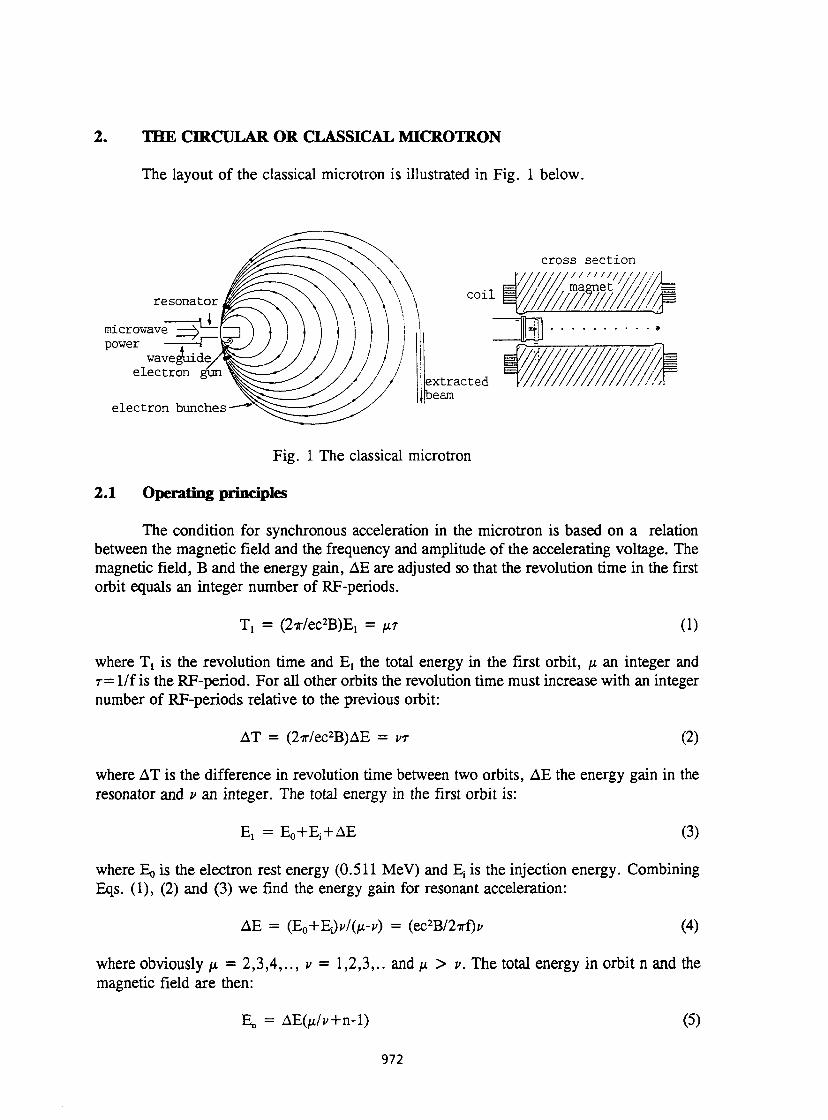
2. THE CIRCULAR OR CLASSICAL MICROTRON
The layout of the classical microtron is illustrated in Fig. 1 below.
Fig. 1 The classical microtron
2.1 Operating principles
The condition for synchronous acceleration in the microtron is based on a relation between the magnetic field and the frequency and amplitude of the accelerating voltage. The magnetic field, B and the energy gain, AE are adjusted so that the revolution time in the first orbit equals an integer number of RF-periods.
Tj = (2T/ec2B)E! = M r (1)
where T t is the revolution time and Ex the total energy in the first orbit, y. an integer and T= 1/f is the RF-period. For all other orbits the revolution time must increase with an integer number of RF-periods relative to the previous orbit:
AT = (27r/ec2B)AE = VT (2)
where AT is the difference in revolution time between two orbits, AE the energy gain in the resonator and v an integer. The total energy in the first orbit is:
Ej = EQ+EJ+AE (3)
where EQ is the electron rest energy (0.511 MeV) and E; is the injection energy. Combining Eqs. (1), (2) and (3) we find the energy gain for resonant acceleration:
AE = ( E 0 + E > / ( M - 0 = (ec2B/2irf> (4)
where obviously n = 2,3,4,.., v = 1,2,3,.. and /x > v. The total energy in orbit n and the magnetic field are then:
E» = AEG*/i/+n-l) (5)
972
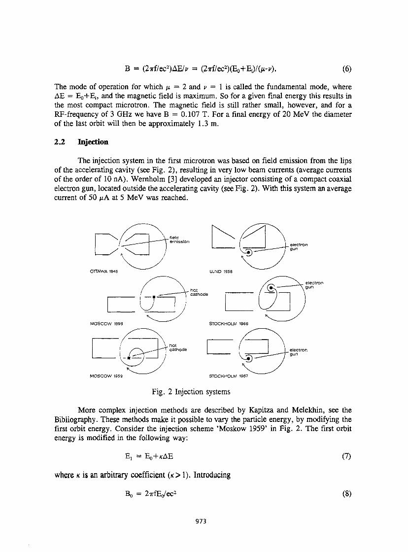
B = (2wf/ec2)AE/p = (2irf/ec2)(E0+Ei)/(/i-i'). (6)
The mode of operation for which /* = 2 and v — 1 is called the fundamental mode, where AE = E 0+E ;, and the magnetic field is maximum. So for a given final energy this results in the most compact microtron. The magnetic field is still rather small, however, and for a RF-frequency of 3 GHz we have B = 0.107 T. For a final energy of 20 MeV the diameter of the last orbit will then be approximately 1.3 m.
2.2 Injection
The injection system in the first microtron was based on field emission from the lips of the accelerating cavity (see Fig. 2), resulting in very low beam currents (average currents of the order of 10 nA). Wernholm [3] developed an injector consisting of a compact coaxial electron gun, located outside the accelerating cavity (see Fig. 2). With this system an average current of 50 /xA at 5 MeV was reached.
MOSCOW 19S9 STOCKHOLM 1967
Fig. 2 Injection systems
More complex injection methods are described by Kapitza and Melekhin, see the Bibliography. These methods make it possible to vary the particle energy, by modifying the first orbit energy. Consider the injection scheme 'Moskow 1959' in Fig. 2. The first orbit energy is modified in the following way:
Ei = Eo+/cAE (7)
where K is an arbitrary coefficient (K> 1). Introducing
B 0 = 2xfEo/ec2 (8)
973
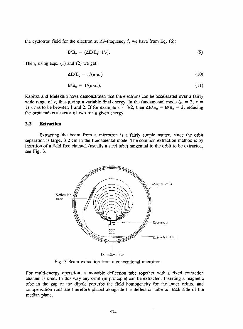
the cyclotron field for the electron at RF-frequency f, we have from Eq. (6):
B/B0 = (AE/E0)(1/?).
Then, using Eqs. (1) and (2) we get:
AE/E0 = vl(y.-Kv)
B/B0 = VQI-KP).
(9)
(10)
(11)
Kapitza and Melekhin have demonstrated that the electrons can be accelerated over a fairly wide range of K, thus giving a variable final energy. In the fundamental mode (/x = 2, v = 1) K has to be between 1 and 2. If for example K = 3/2, then AE/E0 = B/B0 = 2, reducing the orbit radius a factor of two for a given energy.
2.3 Extraction
Extracting the beam from a microtron is a fairly simple matter, since the orbit separation is large, 3.2 cm in the fundamental mode. The common extraction method is by insertion of a field-free channel (usually a steel tube) tangential to the orbit to be extracted, see Fig. 3.
Deflection tube
Magnet coils
•Resonator
Extracted beam
Extraction tube
Fig. 3 Beam extraction from a conventional microtron
For multi-energy operation, a movable deflection tube together with a fixed extraction channel is used. In this way any orbit (in principle) can be extracted. Inserting a magnetic tube in the gap of the dipole perturbs the field homogeneity for the inner orbits, and compensation rods are therefore placed alongside the deflection tube on each side of the median plane.
974
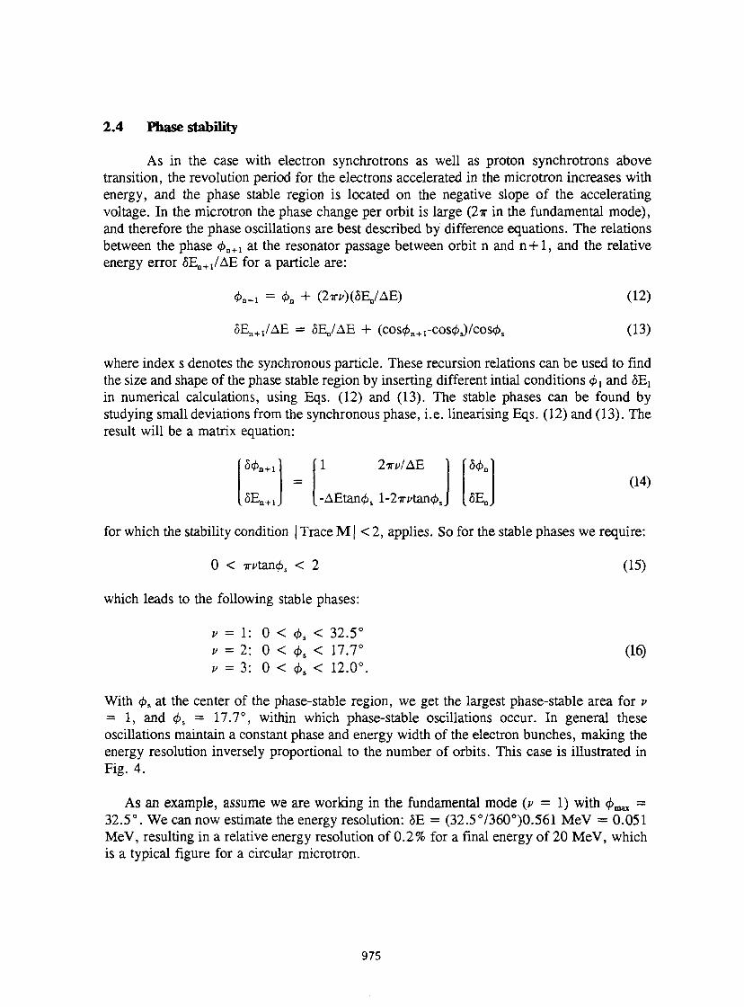
2.4 Phase stability
As in the case with electron synchrotrons as well as proton synchrotrons above transition, the revolution period for the electrons accelerated in the microtron increases with energy, and the phase stable region is located on the negative slope of the accelerating voltage. In the microtron the phase change per orbit is large (2T in the fundamental mode), and therefore the phase oscillations are best described by difference equations. The relations between the phase <£n+1 at the resonator passage between orbit n and n+1, and the relative energy error ôE^/AE for a particle are:
<5En+1/AE = ôEj/AE 4- (cos<£n+1-cos<£s)/cos</>s
(12)
(13)
where index s denotes the synchronous particle. These recursion relations can be used to find the size and shape of the phase stable region by inserting different intial conditions 4>\ and $EX
in numerical calculations, using Eqs. (12) and (13). The stable phases can be found by studying small deviations from the synchronous phase, i.e. linearising Eqs. (12) and (13). The result will be a matrix equation:
(14) ^n+il [1 2ITP/AE ] fô<£n
ôE n + 1J [-AEtan$s l-2-7r*'tan<£j [ôE,,
for which the stability condition | Trace M | < 2, applies. So for the stable phases we require:
0 < 7nnan4>s < 2 (15)
which leads to the following stable phases:
o
(16)
With 4>s at the center of the phase-stable region, we get the largest phase-stable area for v = 1, and <$>% = 17.7°, within which phase-stable oscillations occur. In general these oscillations maintain a constant phase and energy width of the electron bunches, making the energy resolution inversely proportional to the number of orbits. This case is illustrated in Fig. 4.
As an example, assume we are working in the fundamental mode (J> = 1) with 4 ^ = 32.5°. We can now estimate the energy resolution: ÔE = (32.5°/360°)0.561 MeV = 0.051 MeV, resulting in a relative energy resolution of 0.2% for a final energy of 20 MeV, which is a typical figure for a circular microtron.
V r= 1: 0 < 4>s < 32.5°
V = 2: 0 < 4>s < 17.7° V = 3: 0 < 4>s
< 12.0°
975
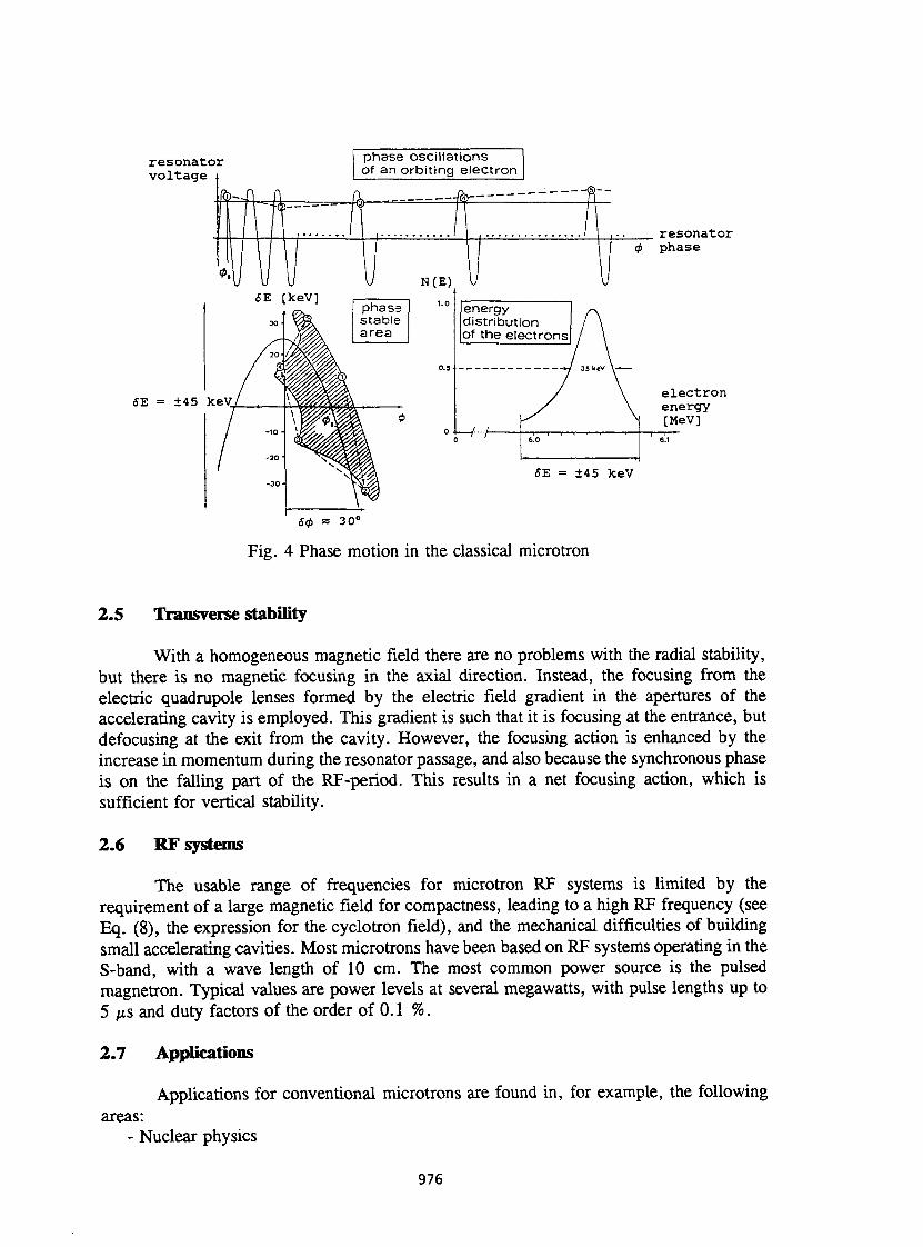
r phase oscil lat ions of an orbit ing electron
SE [keV] r— .
Fig. 4 Phase motion in the classical microtron
2.5 Transverse stability
With a homogeneous magnetic field there are no problems with the radial stability, but there is no magnetic focusing in the axial direction. Instead, the focusing from the electric quadrupole lenses formed by the electric field gradient in the apertures of the accelerating cavity is employed. This gradient is such that it is focusing at the entrance, but defocusing at the exit from the cavity. However, the focusing action is enhanced by the increase in momentum during the resonator passage, and also because the synchronous phase is on the falling part of the RF-period. This results in a net focusing action, which is sufficient for vertical stability.
2.6 RF systems
The usable range of frequencies for microtron RF systems is limited by the requirement of a large magnetic field for compactness, leading to a high RF frequency (see Eq. (8), the expression for the cyclotron field), and the mechanical difficulties of building small accelerating cavities. Most microtrons have been based on RF systems operating in the S-band, with a wave length of 10 cm. The most common power source is the pulsed magnetron. Typical values are power levels at several megawatts, with pulse lengths up to 5 /xs and duty factors of the order of 0.1 %.
2.7 Applications
Applications for conventional microtrons are found in, for example, the following areas:
- Nuclear physics
976
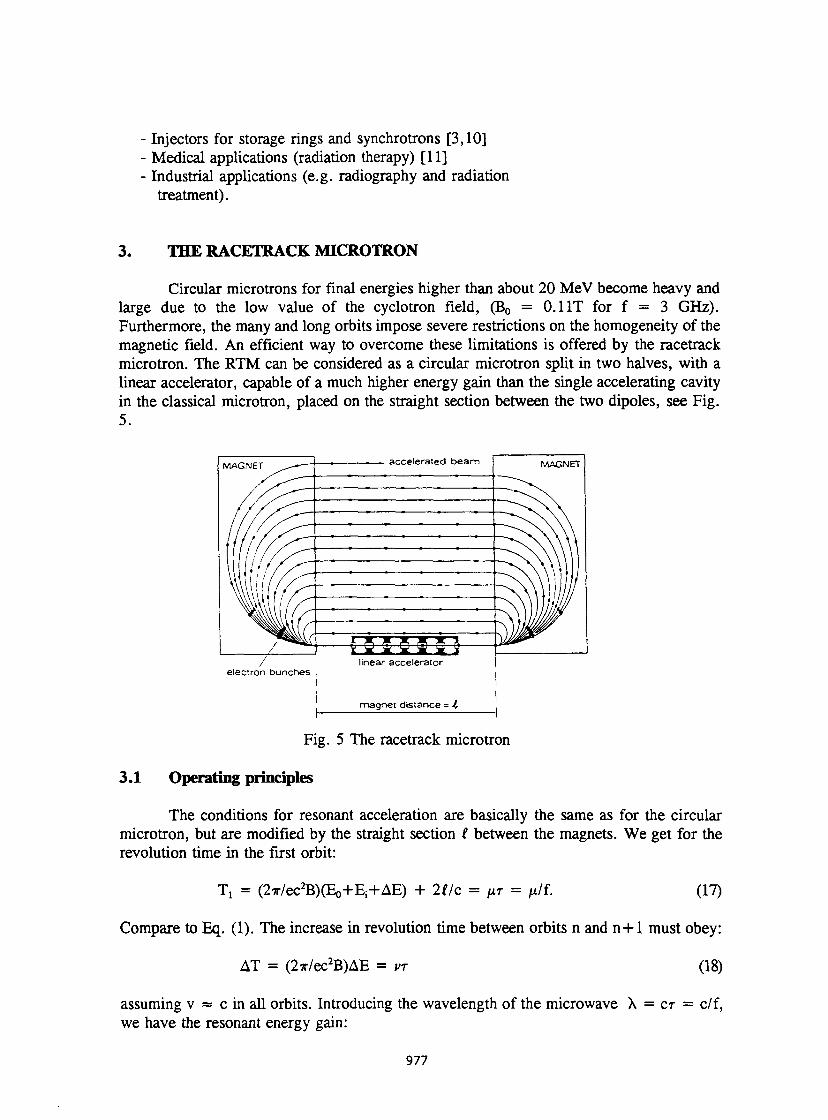
- Injectors for storage rings and synchrotrons [3,10] - Medical applications (radiation therapy) [11] - Industrial applications (e.g. radiography and radiation
treatment).
3. THE RACETRACK MICROTRON
Circular microtrons for final energies higher than about 20 MeV become heavy and large due to the low value of the cyclotron field, (B0 = 0.1 IT for f = 3 GHz). Furthermore, the many and long orbits impose severe restrictions on the homogeneity of the magnetic field. An efficient way to overcome these limitations is offered by the racetrack microtron. The RTM can be considered as a circular microtron split in two halves, with a linear accelerator, capable of a much higher energy gain than the single accelerating cavity in the classical microtron, placed on the straight section between the two dipoles, see Fig. 5.
Fig. 5 The racetrack microtron
3.1 Operating principles
The conditions for resonant acceleration are basically the same as for the circular microtron, but are modified by the straight section I between the magnets. We get for the revolution time in the first orbit:
Tx = (2x/ec2B)(E0+Ei+AE) + 21/c = HT = \xlî. (17)
Compare to Eq. (1). The increase in revolution time between orbits n and n+1 must obey:
AT = (2x/ec2B)AE = VT (18)
assuming v = c in all orbits. Introducing the wavelength of the microwave X = cr = c/f, we have the resonant energy gain:
977
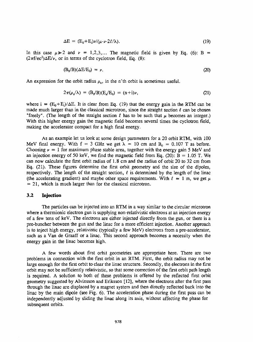
AE = (Eo+E>/0t-j/-2£/X). (19)
In this case n>2 and v = 1,2,3,... The magnetic field is given by Eq. (6): B = (2irf/ec2)AE/j/, or in terms of the cyclotron field, Eq. (8):
(Bo/B)(AE/E0) = v. (20)
An expression for the orbit radius p n, in the n'th orbit is sometimes useful.
2x(pn/X) = (Bo/B)(En/E0) = (n+i>, (21)
where i = (EQ+E^/AE. It is clear from Eq. (19) that the energy gain in the RTM can be made much larger than in the classical microtron, since the straight section 2 can be chosen "freely". (The length of the straight section 2 has to be such that y. becomes an integer.) With this higher energy gain the magnetic field becomes several times the cyclotron field, making the accelerator compact for a high final energy.
As an example let us look at some design parameters for a 20 orbit RTM, with 100 MeV final energy. With f = 3 GHz we get X = 10 cm and B 0 = 0.107 T as before. Choosing v = 1 for maximum phase stable area, together with the energy gain 5 MeV and an injection energy of 50 keV, we find the magnetic field from Eq. (20): B = 1.05 T. We can now calculate the first orbit radius of 1.8 cm and the radius of orbit 20 to 32 cm from Eq. (21). These figures determine the first orbit geometry and the size of the dipoles, respectively. The length of the straight section, 2 is determined by the length of the linac (the accelerating gradient) and maybe other space requirements. With 2 « 1 m, we get /x = 21, which is much larger than for the classical microtron.
3.2 Injection
The particles can be injected into an RTM in a way similar to the circular microtron where a thermionic electron gun is supplying non-relativistic electrons at an injection energy of a few tens of keV. The electrons are either injected directly from the gun, or there is a pre-buncher between the gun and the linac for a more efficient injection. Another approach is to inject high energy, relativistic (typically a few MeV) electrons from a pre-accelerator, such as a Van de Graaff or a linac. This second approach becomes a necessity when the energy gain in the linac becomes high.
A few words about first orbit geometries are appropriate here. There are two problems in connection with the first orbit in an RTM. First, the orbit radius may not be large enough for the first orbit to clear the linac structure. Secondly, the electrons in the first orbit may not be sufficiently relativistic, so that some correction of the first orbit path length is required. A solution to both of these problems is offered by the reflected first orbit geometry suggested by Alvinsson and Eriksson [12], where the electrons after the first pass through the linac are displaced by a magnet system and then directly reflected back into the linac by the main dipole (see Fig. 6). The acceleration phase during the first pass can be independently adjusted by sliding the linac along its axis, without affecting the phase for subsequent orbits.
978
Displacing Accelerator Electron Magnets (Linac) Gun
Fig. 6 A racetrack microtron layout illustrated by the Scanditronix RTM50
3.3 Extraction
The orbits are well separated also in the RTM, making the extraction of any orbit uncomplicated. The extraction is usually carried out with a small magnet deflecting the orbit to be extracted into an extraction channel. For multi-energy operation, when several orbits are to be extracted, the magnet is made movable or extraction magnets are placed in each orbit (see Fig. 6).
3.4 Phase stability
The relations for the phase motion in the classical microtron, i.e. Eqs. (12) and (13), are valid also for the RTM, with the energy resolution inversely proportional to the orbit number. It must be emphasized however, that Eqs. (12) and (13) are derived under the assumption of extreme relativistic particles and that there is no focusing of the particles. In a practical case the focusing modifies the phase motion and the conditions for extreme relativistic particles may not be fulfilled for the first few orbits. Performing numerical calculations with these factors taken into account is therefore the best approach to study the phase stability in the racetrack microtron.
3.5 Transverse stability
The transverse stability in the RTM is completely different from the conventional, circular microtron due to the main dipole geometry, and a separated-function solution to the transverse stability problem is usually employed. Characteristic for racetrack microtrons is also that the beam optics has to focus over a large dynamic range.
There are two different approaches to arrange the beam optics in an RTM. One solution is placing focusing elements in the drift section of each orbit, and in this way the betatron phase advance can be kept constant for all orbits. The other approach is to put the focusing
979
elements on the linac axis. In order to avoid overfocusing in the first orbits, the focusing in the last orbits becomes weak. The beam optics will therefore be working close to integer resonances, with high sensitivity to dipole errors. This is however not so serious here as in synchrotrons, because these errors can easily be corrected by small dipoles in each orbit.
A problem common to all RTM's is the vertical defocusing effect from the fringe fields of the dipoles, with a focal length of the same order of magnitude as the bending radius in the magnet. This can be solved by the reversed field from active field clamps suggested by Babic and Sedlacek in 1967 [13], and now used in most RTM's. If the fringe field is symmetric about the median plane the vertical focal length due to the fringe field is given by:
fv = P 2
d d d J (B/B0)dz - J (B/Bo)2dz - 2(y2/3) \ (B7B0)2dz +
0 0 0 (2)
where d is the nominal extent of the fringe field, p is the orbit radius in the uniform field B0 and B' = dB/dz. From this it is evident that for small values of y, when the y2-term is negligible, a fringe field distribution can be found for which fy is infinite.
The vertical focusing from the reversed field is only important for the first orbits, since fy ~ p 2. However, it can be improved by introducing a small gradient in the main dipoles. This will give a focal length f « B/2g, where g is the gradient, independent of energy.
3.6 RF systems
All racetrack microtrons operate in the L-band (~ 1.3 GHz) or the S-band (~3GHz), using klystrons as the RF-power source, due to the higher power levels needed compared to conventional microtrons. Pulse lengths from less than 1 jus up to around 5 fis are typical, with duty factors from approximately 0.1 to several percent. Most RTM's employ standing wave linacs, with accelerating gradients in the range 2-15 MV/ra, and energy gains per pass of typically 1 to 5 MeV. Average beam currents are typically between 1 and 100 jxA.
3.7 Applications
Racetrack microtrons find applications in various areas of science and technology. For example:
- Injectors to storage rings and synchrotrons, where their excellent momentum spread and small emittance simplify multi-turn injection [9].
- Nuclear physics. - Industrial applications, e.g. radiography and electron radiation treatment. - Medical applications: radiation therapy, where the high energy and good beam quality
is employed for scanned beam techniques [14]. The high energy available also makes production of short-lived isotopes from photonuclear reactions possible.
- Free-electron laser applications.
980
REFERENCES
[I] V.I. Veksler, Proc. USSR Acad. Sci. 43 (1944) 346 and J. Phys. USSR 9 (1945) 153.
[2] W.J. Henderson, H. Le Caine and R. Montalbetti, Nature 162 (1948) 699.
[3] O. Wernholm, Arkiv. Fys. 26 (1964) 527.
[4] E. Brannen and H. Froelich, J. Appl. Phys. 32 (1961) 1179.
[5] A.O. Hanson, J.R. Harlan, R.A. Hoffswell, D. Jamnik, and L.M. Young, SLAC Conf. (1974) 151.
[6] H. Herminghaus, B. Dreher, H. Euteneuer, K.H. Kaiser, M. Kelliher, R. Klein, H.J. Kreidel, M. Loch, U. Ludwig-Mertin, K. Merle, H. Schoeler, R. Schulze, P. Semmel and G. Stephan, IEEE Trans. NS-30. No. 4 (1983) 3274.
[7] S. Rosander, M. Sedlacek and O. Wernholm, Nucl. Instrum. Methods 204 (1982) 1.
[8] M. A. Green, E.M. Rowe, W.S. Trzeciak and W.R. Winter, IEEE Trans. NS-28.
No. 3 (1981) 2074.
[9] M. Eriksson, IEEE Trans. NS-30. No. 4 (1983) 2070.
[10] G.v. Egan-Krieger, D. Einfeld, W.-D. Klotz, H. Lehr, R. Maier, G. Mùlhaupt,
R. Richter and E. Weihreter, IEEE Trans. NS-30. No. 4 (1983) 3103.
[II] A. Brahme and H. Svensson, Acta Rad. One. 18 (1979) 244.
[12] R. Alvinsson and M. Eriksson, Royal Inst, of Tech., Stockholm, Report TRITA-
EPP-76-07 (1976).
[13] H. Babic and M. Sedlacek, Nucl. Instrum. Methods 56 (1967) 170.
[14] M. Karlsson, H. Nystrôm and H. Svensson, Med. Phys. 19 (1992) 307. BIBLIOGRAPHY P. Kapitza and V.N. Melekhin, The Microtron (Harwood Academic Publishers, London, 1978).
R.E. Rand, Recirculating electron accelerators (Harwood Academic Publishers, 1984).
981

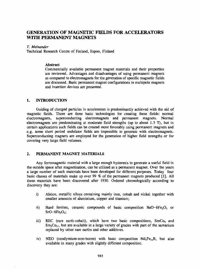
GENERATION OF MAGNETIC FIELDS FOR ACCELERATORS WITH PERMANENT MAGNETS
T. Meinander Technical Research Centre of Finland, Espoo, Finland
Abstract Commercially available permanent magnet materials and their properties are reviewed. Advantages and disadvantages of using permanent magnets as compared to electromagnets for the generation of specific magnetic fields are discussed. Basic permanent magnet configurations in multipole magnets and insertion devices are presented.
1. INTRODUCTION
Guiding of charged particles in accelerators is predominantly achieved with the aid of magnetic fields. There are three basic technologies for creating these fields: normal electromagnets, superconducting electromagnets and permanent magnets. Normal electromagnets are predominating at moderate field strengths (up to about 1.5 T), but in certain applications such fields can be created more favorably using permanent magnets and e.g. some short period undulator fields are impossible to generate with electromagnets. Superconducting magnets are employed for the generation of higher field strengths or for covering very large field volumes.
2. PERMANENT MAGNET MATERIALS
Any ferromagnetic material with a large enough hysteresis to generate a useful field in the outside space after magnetization, can be utilized as a permanent magnet. Over the years a large number of such materials have been developed for different purposes. Today four basic classes of materials make up over 99 % of the permanent magnets produced [1]. All these materials have been discovered after 1930. Ordered chronologically according to discovery they are:
i) Alnico, metallic alloys containing mainly iron, cobalt and nickel together with smaller amounts of aluminium, copper and titanium;
ii) Hard ferrites, ceramic compounds of basic composition BaO'ôFejOj or SrO-6Fe203;
iii) REC (rare earth-cobalt), which have two basic compositions, SmCo5 and Sm2Con, but are available in a large variety of grades with part of the samarium replaced by other rare earths and other additives.
iv) NEO (neodymium-iron-boron) with basic composition Nd2Fe14B, but also available in many grades with slightly different composition.
983
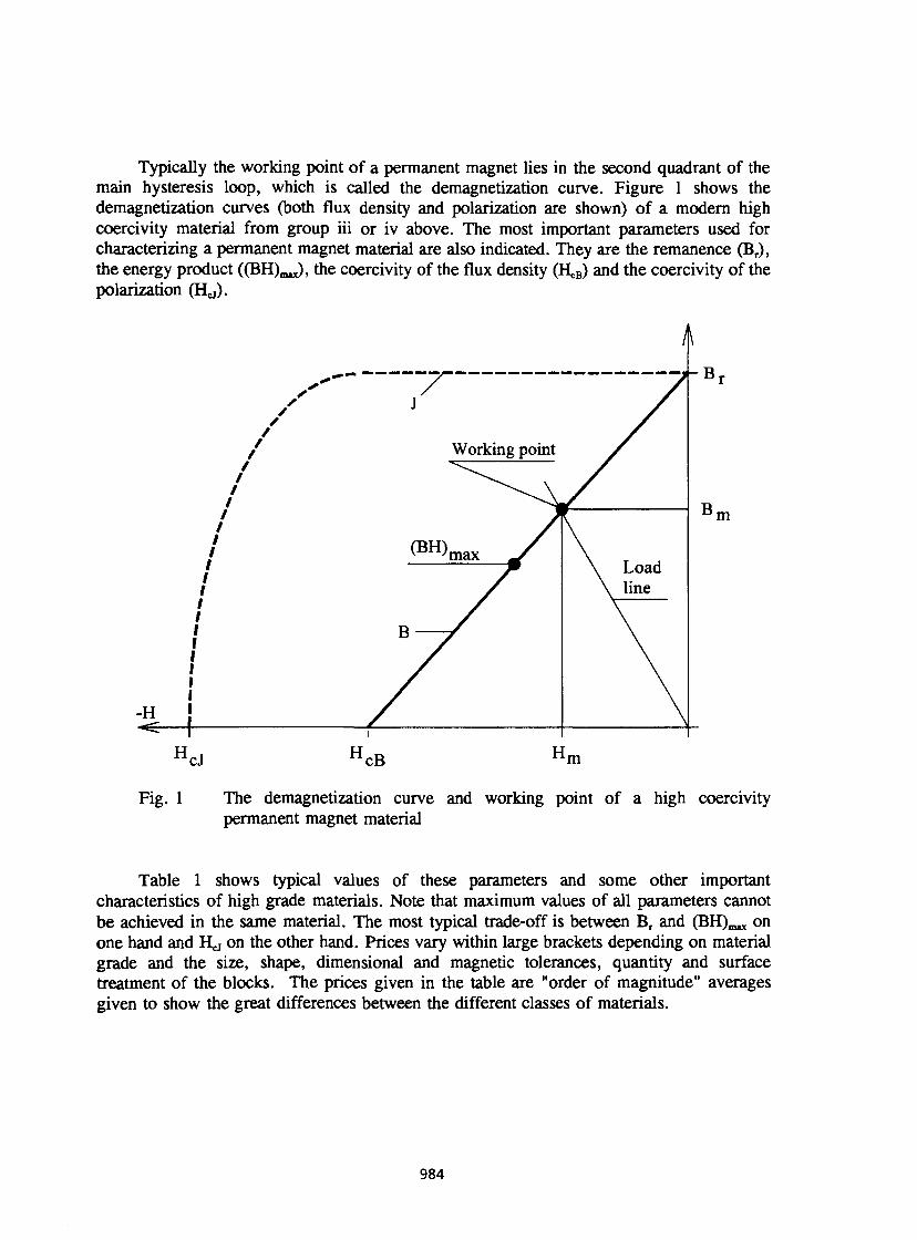
Typically the working point of a permanent magnet lies in the second quadrant of the main hysteresis loop, which is called the demagnetization curve. Figure 1 shows the demagnetization curves (both flux density and polarization are shown) of a modern high coercivity material from group iii or iv above. The most important parameters used for characterizing a permanent magnet material are also indicated. They are the remanence (Br), the energy product ((BH),,,,,), the coercivity of the flux density (H,,B) and the coercivity of the polarization (H^).
Fig. 1 The demagnetization curve and working point of a high coercivity permanent magnet material
Table 1 shows typical values of these parameters and some other important characteristics of high grade materials. Note that maximum values of all parameters cannot be achieved in the same material. The most typical trade-off is between B r and (BH)^ on one hand and H^ on the other hand. Prices vary within large brackets depending on material grade and the size, shape, dimensional and magnetic tolerances, quantity and surface treatment of the blocks. The prices given in the table are "order of magnitude" averages given to show the great differences between the different classes of materials.
984
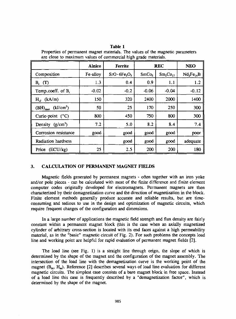
Table 1 Properties of permanent magnet materials. The values of the magnetic parameters are close to maximum values of commercial high grade materials.
Alnico Ferrite REC NEO
Composition Fe-alloy SrO-ôFeA SmCoj Sm2Coi7 Nd 2Fe 1 4B
B r (T) 1.3 0.4 0.9 1.1 1.2
Temp.coeff. of B r -0.02 -0.2 -0.06 -0.04 -0.12
H j (kA/m) 150 320 2400 2000 1400
( B H ) ^ (kJ/cm3) 50 25 170 250 300
Curie-point (°C) 800 450 750 800 300
Density (g/cm3) 7.2 5.0 8.2 8.4 7.4
Corrosion resistance good good good good poor
Radiation hardness good good good adequate
Price (ECU/kg) 25 2.5 200 200 180
3. CALCULATION OF PERMANENT MAGNET FIELDS
Magnetic fields generated by permanent magnets - often together with an iron yoke and/or pole pieces - can be calculated with most of the finite difference and finite element computer codes originally developed for electromagnets. Permanent magnets are then characterized by their demagnetization curve and the direction of magnetization in the block. Finite element methods generally produce accurate and reliable results, but are time-consuming and tedious to use in the design and optimization of magnetic circuits, which require frequent changes of the configuration and dimensions.
In a large number of applications the magnetic field strength and flux density are fairly constant within a permanent magnet block (this is the case when an axially magnetized cylinder of arbitrary cross-section is located with its end faces against a high permeability material, as in the "basic" magnetic circuit of Fig. 2). For such problems the concepts load line and working point are helpful for rapid evaluation of permanent magnet fields [2].
The load line (see Fig. 1) is a straight line through origo, the slope of which is determined by the shape of the magnet and the configuration of the magnet assembly. The intersection of the load line with the demagnetization curve is the working point of the magnet (Bm, ILJ. Reference [2] describes several ways of load line evaluation for different magnetic circuits. The simplest case consists of a bare magnet block in free space. Instead of a load line this case is frequently described by a "demagnetization factor", which is determined by the shape of the magnet.
985
In many cases the utilization of permanent magnet material is optimized if the working point coincides with (BH),^. The potential energy of the field outside the magnet is then maximized. This can be seen from the general expression of the magnetic energy:
w = %/S-fldv - -vi/S.-a.dv (i) v„ v„
o m
In Eq. (1) V 0 is the field space outside the magnet and Vm is the magnet volume. The maximum magnetic energy of the outside field, which can be generated by a permanent magnet is thus simply:
W = i/2 Vm- (BH)^ (2)
The demagnetization curves of modern high coercivity materials are close to straight lines with the slope /*0. In such materials the magnetic polarization is rigid and close to B r in the whole third quadrant and the magnetic field can often be calculated by integrating the dipole fields generated by volume elements of the magnet. The dipole strength (magnetic moment) of a volume element is then simply
dM = — B r dV (3)
In this case the field can also be calculated from an equivalent surface current or charge at the surface of the magnet [3]. This approach is especially favourable in the case of an axially magnetized straight cylinder, which is the preferred shape of magnet blocks in many applications. The equivalent "magnetic charge" density at the end surfaces is then simply = B r. Alternatively a current of surface density BJ/j.0on the mantle surface generates the same field. Note that while both methods yields the correct field outside the magnet, only the equivalent charge gives the correct field strength inside the magnet and correspondingly the equivalent current sheet gives the correct interior flux density. When such high coercivity magnets are used together with yokes or poles of high permeability, many methods originally developed for the calculation of electrostatic fields (images, conformai mapping, variable separation and series approximations) can be utilized [4].
4. ELECTROMAGNETS VERSUS PERMANENT MAGNETS
In principle most static or quasistatic fields required in accelerators can be generated either by electromagnets or permanent magnets. There are a number of factors influencing the choice, the most important of which are examined in some detail below.
4.1 Field control
Field control of electromagnets is easily and effectively achieved by the use of variable current power supplies. With proper design of coils and power supplies a wide range from fast pulsed to stationary magnetic fields can be covered. In this respect permanent magnets are at a disadvantage. They are basically suited only for fixed field applications.
986
Field control of permanent magnet systems is, however, in many cases possible by moving iron or magnet parts with respect to each other. Such mechanical field control is necessarily always fairly slow and can be very complicated to implement. Further difficulties are generated by the magnetic forces between the moving parts, which can be very large. In planar insertion devices (see Section 6) peak field control is as a rule achieved by moving two magnet arrays symmetrically with respect to the field axis. In high field wigglers the magnetic force between these magnet arrays can reach several tens of tons.
4.2 Field stability
The field stability of an electromagnet is generally related directly to the current stability of the power supply. The stability of modern magnet power supplies are typically better than 0.01 % and stabilities down to 1 ppm over an operating temperature range of 20 °C are available.
In permanent magnet systems the field stability is generally limited by the temperature coefficient of the remanence. As can be seen from Table 1 a temperature stability of 0.02 %/°C is the best that can be achieved and for the nowadays preferred NEO-materials the temperature stability is worse than 0.1 %/°C. This limits the use of permanent magnets to applications where stability is not critical. It is generally not feasible to stabilize the temperature of the magnets to better than about 0.5 °C, which results in a limit of 0.01 % for the field stability.
There are two ways in which the temperature stability of a permanent magnet assembly can be improved. One is based on combinations of soft magnetic materials and permanent magnets with temperature coefficients of different sign. This is a delicate procedure, which as a rule is feasible only in small systems such as instruments and not when fields must be generated in larger volumes, which is generally the case in accelerator magnets. Another possibility is the incorporation of a small correction electromagnet into the permanent magnet circuit. By controlling the current of this electromagnet with the aid of one or several temperature sensors mounted on the permanent magnet blocks, an improvement of the temperature stability of the field by up to a factor ten can be achieved, but only at the price of a much more complicated system.
4.3 Power consumption
The great advantage of using permanent magnets is of course that they can sustain a static field without any power consumption. The power consumption of accelerator electromagnets can be considerable, but the power costs themselves are generally marginal. The power supplies and cooling systems of electromagnets do, however add a lot to the capital costs, space requirements and complexity of a complete electromagnetic setup. Cooling requirements also set a limit to the generation of certain spatially rapidly varying fields (e.g. in insertion devices, see Section 6) and in such cases permanent magnets offer the only solution.
987
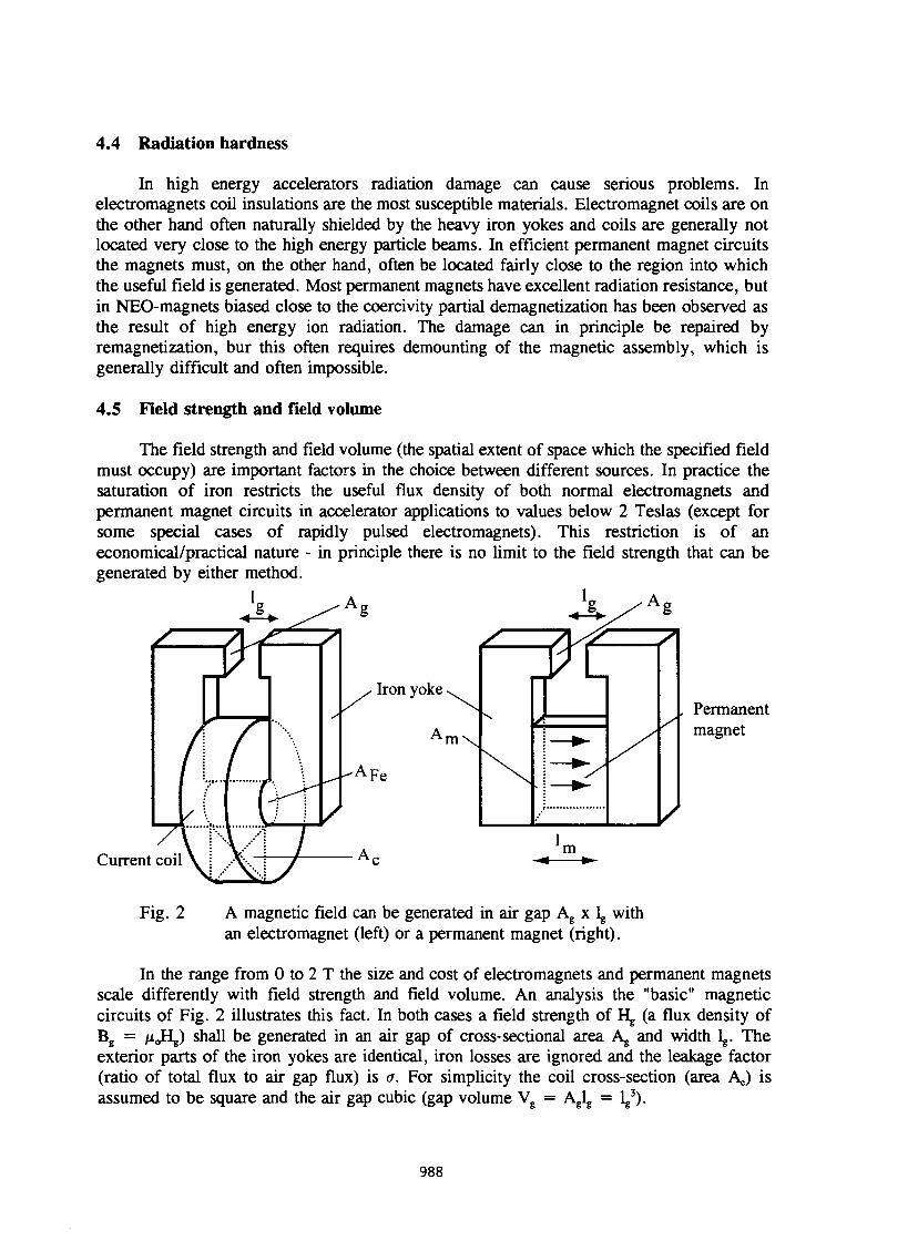
4.4 Radiation hardness
In high energy accelerators radiation damage can cause serious problems. In electromagnets coil insulations are the most susceptible materials. Electromagnet coils are on the other hand often naturally shielded by the heavy iron yokes and coils are generally not located very close to the high energy particle beams. In efficient permanent magnet circuits the magnets must, on the other hand, often be located fairly close to the region into which the useful field is generated. Most permanent magnets have excellent radiation resistance, but in NEO-magnets biased close to the coercivity partial demagnetization has been observed as the result of high energy ion radiation. The damage can in principle be repaired by remagnetization, bur this often requires demounting of the magnetic assembly, which is generally difficult and often impossible.
4.5 Field strength and field volume
The field strength and field volume (the spatial extent of space which the specified field must occupy) are important factors in the choice between different sources. In practice the saturation of iron restricts the useful flux density of both normal electromagnets and permanent magnet circuits in accelerator applications to values below 2 Teslas (except for some special cases of rapidly pulsed electromagnets). This restriction is of an economical/practical nature - in principle there is no limit to the field strength that can be generated by either method.
Fig. 2 A magnetic field can be generated in air gap Ag x lg with an electromagnet (left) or a permanent magnet (right).
In the range from 0 to 2 T the size and cost of electromagnets and permanent magnets scale differently with field strength and field volume. An analysis the "basic" magnetic circuits of Fig. 2 illustrates this fact. In both cases a field strength of Hg (a flux density of Bg = M<>Hg) shall be generated in an air gap of cross-sectional area Ag and width lg. The exterior parts of the iron yokes are identical, iron losses are ignored and the leakage factor (ratio of total flux to air gap flux) is a. For simplicity the coil cross-section (area A,.) is assumed to be square and the air gap cubic (gap volume Vg = Aglg = lg
3).
988
If the circular coil aperture (cross-sectional area of the iron yoke at the coil location) is denoted AF e, it is easy to show that the volume of the ring-shaped coil can be expressed as
V, = TIA„ V^ &
(4)
By definition the coil flux (BFeAFe) is equal to the air gap flux (BgAg) multiplied by the leakage factor. This determines the required coil aperture:
vFe ° B A
B* (5)
B F e denotes the maximum flux density allowed in the iron. The magnetomotive force of the coil (ampereturns), is equal to the potential drop across the air gap (NI = Hglg). The maximum ampereturns that the coil can sustain are basically proportional to the cross-sectional area (NI = Ac). The maximum current density (a) in the coil depends on the resistivity of the coil wire, the filling factor of the winding and the cooling method, but once these are fixed it tends to be fairly constant. The required coil cross-section is then:
K " Si a
(6)
By substituting Eqs. (5) and (6) into Eq. (4) an expression for the coil volume required to generate the gap field is obtained:
JLy~> + 1 i t
or
n ° ^ o „ I «N «Be
H (7)
The total power consumption of the coil is also proportional to the volume.
The volume of the permanent magnet is simply A ^ . A,,, is again determined by equating the magnet flux B , , ^ with the gap flux multiplied by the leakage factor:
g 8 B_
(8)
The magnetomotive force of the magnet is HJn, and again by equating this to the potential drop across the air gap lm is obtained:
1. (9)
989
By multiplying Eqs. (8) and (9) the amount of permanent magnet material needed to generate the gap field is found to be:
V m = - ^ 2 _ V HÏ (10)
BA g
From Eq. (10) it is immediately obvious that the magnet volume is minimized if the magnet is shaped so that the working point (B^H^ coincides with (BH),^.
Comparison between Eqs. (7) and (10) shows the different scaling with size and field strength for electromagnets and permanent magnets. The amount of permanent magnet material needed to produce the specified field increases linearly with field volume and with the square of the field strength, while the coil size and power consumption of the electromagnet increases more slowly with both variables. It is consequently natural that permanent magnet applications become economically disadvantageous at high field strengths and volumes. The critical values at which permanent magnet solutions become uneconomical vary largely with the application. As a rule of thumb it can, however, be stated that permanent magnets are seldom economical for field volumes above a few dm3.
Another important consequence of the different scaling laws follows directly from Eqs. (6) and (9). If all dimensions of a magnet assembly are scaled by the same factor, the field strength remains constant in the permanent magnet case, while at constant current density it scales proportionally to the dimensions in electromagnets. Small field volumes or spatially rapidly varying fields, can thus be very inconvenient to excite by electromagnets, because the size of the coils becomes excessive as compared to the field volume.
5. MULTIPOLE MAGNETS
The majority of all accelerator magnets fall into the category of "multipole magnets", the integrated fields of which have certain electron optical bending or focussing properties. Field control and stability criteria as a rule require that they are realized as electromagnets. In many cases field volumes are also too large for permanent magnet solutions. Nevertheless, permanent magnet multipoles have been implemented in accelerators in considerable quantities [5,6] in less demanding locations. Especially where small beam apertures suffice considerable space and cost savings can be possible.
Multipole magnets can be constructed with permanent magnets in much the same way as the traditional electromagnets, in which the field shape is determined by an iron yoke. There is, however, a much more efficient way to generate these fields with permanent magnets. Consider the ring-shaped area (r, < r < r2) in Fig. 3, which represents the cross-section of a hollow permanent magnet cylinder. The magnetic polarization of this high coercivity magnet has a fixed amplitude (Br), but its direction varies in the x-y plane according to:
J = B ^ W » (11)
990
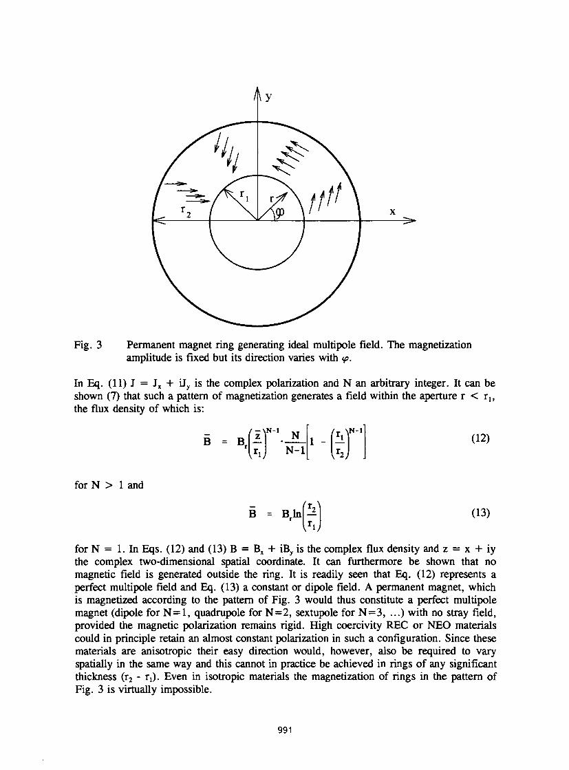
Fig. 3 Permanent magnet ring generating ideal multipole field. The magnetization amplitude is fixed but its direction varies with <p.
In Eq. (11) J = Jx + LFy is the complex polarization and N an arbitrary integer. It can be shown (7) that such a pattern of magnetization generates a field within the aperture r < r,, the flux density of which is:
B = B. / jVK-l
v r i ; N
N-l 1 -
fr \N-1
L 2 /
(12)
for N > 1 and
B = Brln (13)
for N = 1. In Eqs. (12) and (13) B = Bx + iBy is the complex flux density and z = x + iy the complex two-dimensional spatial coordinate. It can furthermore be shown that no magnetic field is generated outside the ring. It is readily seen that Eq. (12) represents a perfect multipole field and Eq. (13) a constant or dipole field. A permanent magnet, which is magnetized according to the pattern of Fig. 3 would thus constitute a perfect multipole magnet (dipole for N=l , quadrupole for N=2, sextupole for N=3, ...) with no stray field, provided the magnetic polarization remains rigid. High coercivity REC or NEO materials could in principle retain an almost constant polarization in such a configuration. Since these materials are anisotropic their easy direction would, however, also be required to vary spatially in the same way and this cannot in practice be achieved in rings of any significant thickness (r2 - r^. Even in isotropic materials the magnetization of rings in the pattern of Fig. 3 is virtually impossible.
991
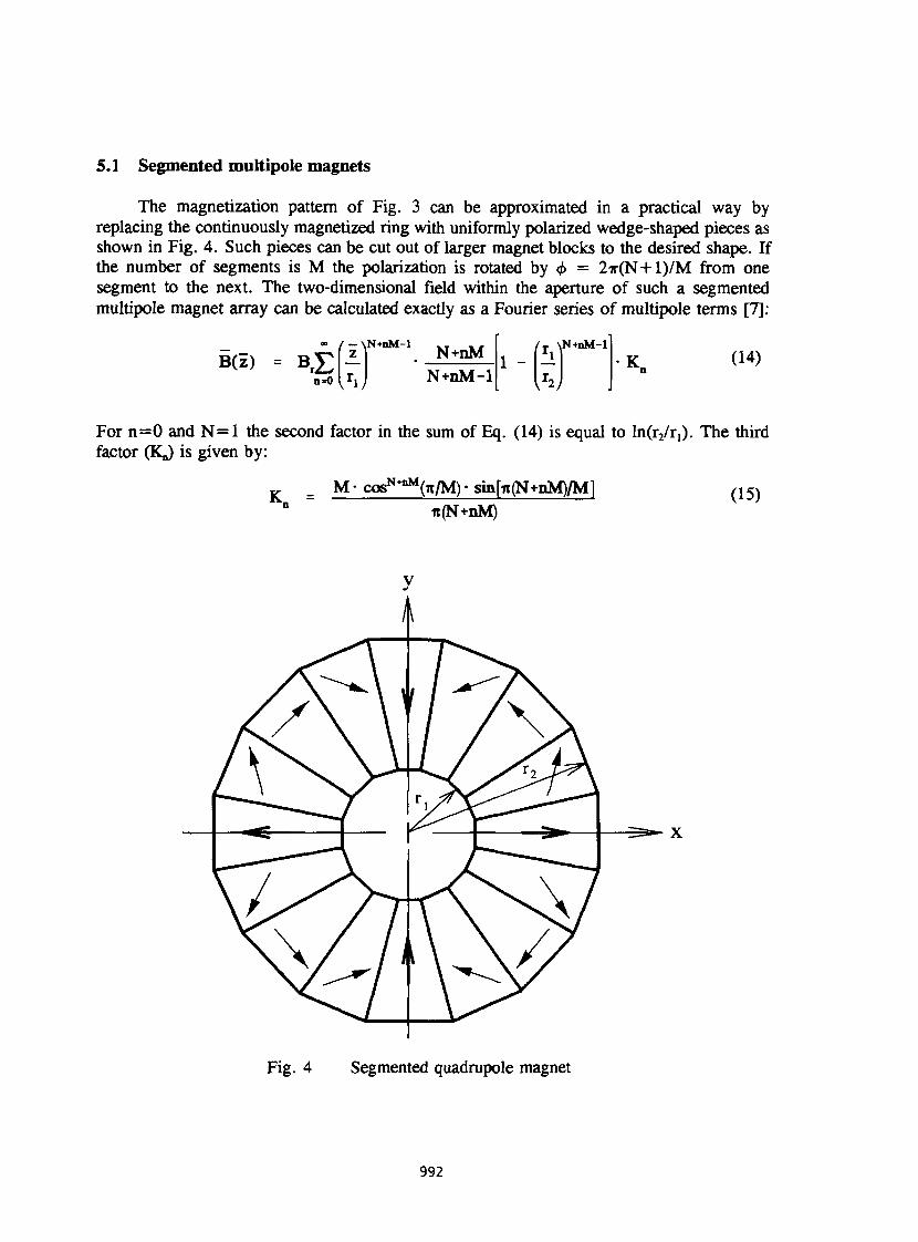
5.1 Segmented multipole magnets
The magnetization pattern of Fig. 3 can be approximated in a practical way by replacing the continuously magnetized ring with uniformly polarized wedge-shaped pieces as shown in Fig. 4. Such pieces can be cut out of larger magnet blocks to the desired shape. If the number of segments is M the polarization is rotated by <j> = 2 T ( N + 1 ) / M from one segment to the next. The two-dimensional field within the aperture of such a segmented multipole magnet array can be calculated exactly as a Fourier series of multipole terms [7]:
n=0
N+nM _ - / - \N+nM-l
B(z) = B j -r^rJ N+nM-1 Uy
r \N+nM-l
K. (14)
For n=0 and N = l the second factor in the sum of Eq. (14) is equal to ln(r2/ri). The third factor (KJ is given by:
K = M- cos^'Hn/M)- sin[n(N+nM)/Ml 7i(N+nM)
(15)
Fig. 4 Segmented quadrupole magnet
992
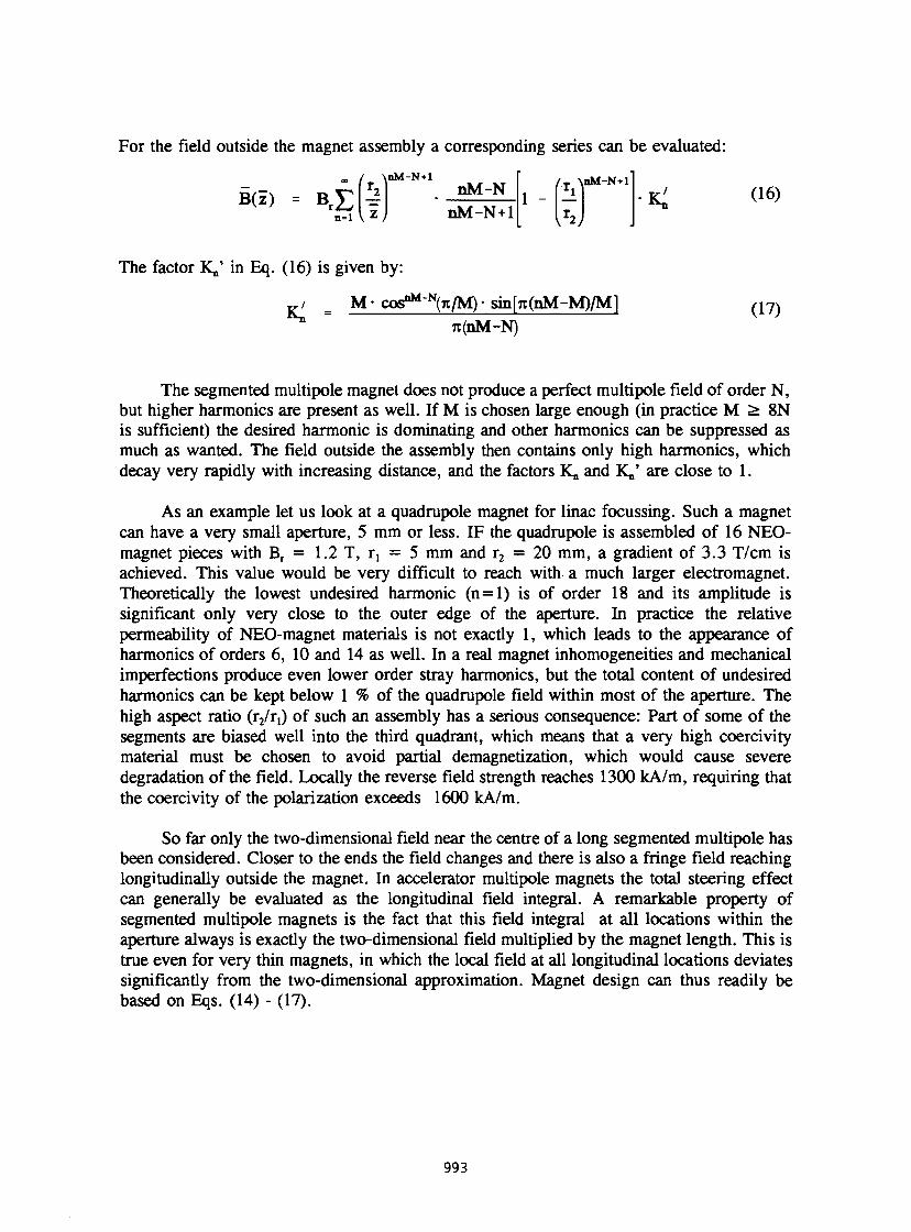
For the field outside the magnet assembly a corresponding series can be evaluated:
B(i) = B r £ n=l
/ \nM-N+l
\ * l
nM-N nM-N+1
fr \nM-N+l r l
\ \ •K (16)
The factor K„' in Eq. (16) is given by:
„ / = M- cos^-Nfo/M)- sin[7t(nM-M)/M] 7t(nM-N)
(17)
The segmented multipole magnet does not produce a perfect multipole field of order N, but higher harmonics are present as well. If M is chosen large enough (in practice M > 8N is sufficient) the desired harmonic is dominating and other harmonics can be suppressed as much as wanted. The field outside the assembly then contains only high harmonics, which decay very rapidly with increasing distance, and the factors K„ and K„' are close to 1.
As an example let us look at a quadrupole magnet for linac focussing. Such a magnet can have a very small aperture, 5 mm or less. IF the quadrupole is assembled of 16 NEO-magnet pieces with Br = 1.2 T, rj = 5 mm and r2 = 20 mm, a gradient of 3.3 T/cm is achieved. This value would be very difficult to reach with a much larger electromagnet. Theoretically the lowest undesired harmonic (n = l) is of order 18 and its amplitude is significant only very close to the outer edge of the aperture. In practice the relative permeability of NEO-magnet materials is not exactly 1, which leads to the appearance of harmonics of orders 6, 10 and 14 as well. In a real magnet inhomogeneities and mechanical imperfections produce even lower order stray harmonics, but the total content of undesired harmonics can be kept below 1 % of the quadrupole field within most of the aperture. The high aspect ratio (x2/xi) of such an assembly has a serious consequence: Part of some of the segments are biased well into the third quadrant, which means that a very high coercivity material must be chosen to avoid partial demagnetization, which would cause severe degradation of the field. Locally the reverse field strength reaches 1300 kA/m, requiring that the coercivity of the polarization exceeds 1600 kA/m.
So far only the two-dimensional field near the centre of a long segmented multipole has been considered. Closer to the ends the field changes and there is also a fringe field reaching longitudinally outside the magnet. In accelerator multipole magnets the total steering effect can generally be evaluated as the longitudinal field integral. A remarkable property of segmented multipole magnets is the fact that this field integral at all locations within the aperture always is exactly the two-dimensional field multiplied by the magnet length. This is true even for very thin magnets, in which the local field at all longitudinal locations deviates significantly from the two-dimensional approximation. Magnet design can thus readily be based on Eqs. (14) - (17).
993
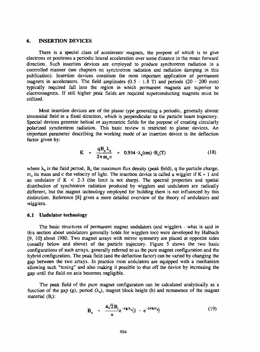
6. INSERTION DEVICES
There is a special class of accelerator magnets, the purpose of which is to give electrons or positrons a periodic lateral acceleration over some distance in the mean forward direction. Such insertion devices are employed to produce synchrotron radiation in a controlled manner (see chapters on synchrotron radiation and radiation damping in this publication). Insertion devices constitute the most important application of permanent magnets in accelerators. The field amplitudes (0.5 - 1.8 T) and periods (20 - 200 mm) typically required fall into the region in which permanent magnets are superior to electromagnets. If still higher peak fields are required superconducting magnets must be utilized.
Most insertion devices are of the planar type generating a periodic, generally almost sinusoidal field in a fixed direction, which is perpendicular to the particle beam trajectory. Special devices generate helical or asymmetric fields for the purpose of creating circularly polarized synchrotron radiation. This basic review is restricted to planar devices. An important parameter describing the working mode of an insertion device is the deflection factor given by:
K = q ° " * 0.934-X (cm)-Bm (18) 2itm 0 c n °
where X„ is the field period, B 0 the maximum flux density (peak field), q the particle charge, m0 its mass and c the velocity of light. The insertion device is called a wiggler if K » 1 and an undulator if K < 2-3 (the limit is not sharp). The spectral properties and spatial distribution of synchrotron radiation produced by wigglers and undulators are radically different, but the magnet technology employed for building them is not influenced by this distinction. Reference [8] gives a more detailed overview of the theory of undulators and wigglers.
6.1 Undulator technology
The basic structures of permanent magnet undulators (and wigglers - what is said in this section about undulators generally holds for wigglers too) were developed by Halbach [9, 10] about 1980. Two magnet arrays with mirror symmetry are placed at opposite sides (usually below and above) of the particle trajectory. Figure 5 shows the two basic configurations of such arrays, generally referred to as the pure magnet configuration and the hybrid configuration. The peak field (and the deflection factor) can be varied by changing the gap between the two arrays. In practice most undulators are equipped with a mechanism allowing such "tuning" and also making it possible to shut off the device by increasing the gap until the field on axis becomes negligible.
The peak field of the pure magnet configuration can be calculated analytically as a function of the gap (g), period (XJ, magnet block height (h) and remanence of the magnet material (Br):
B = 4^Ble~Kilx-(i - e'2nh,xA ( 1 9 )
994
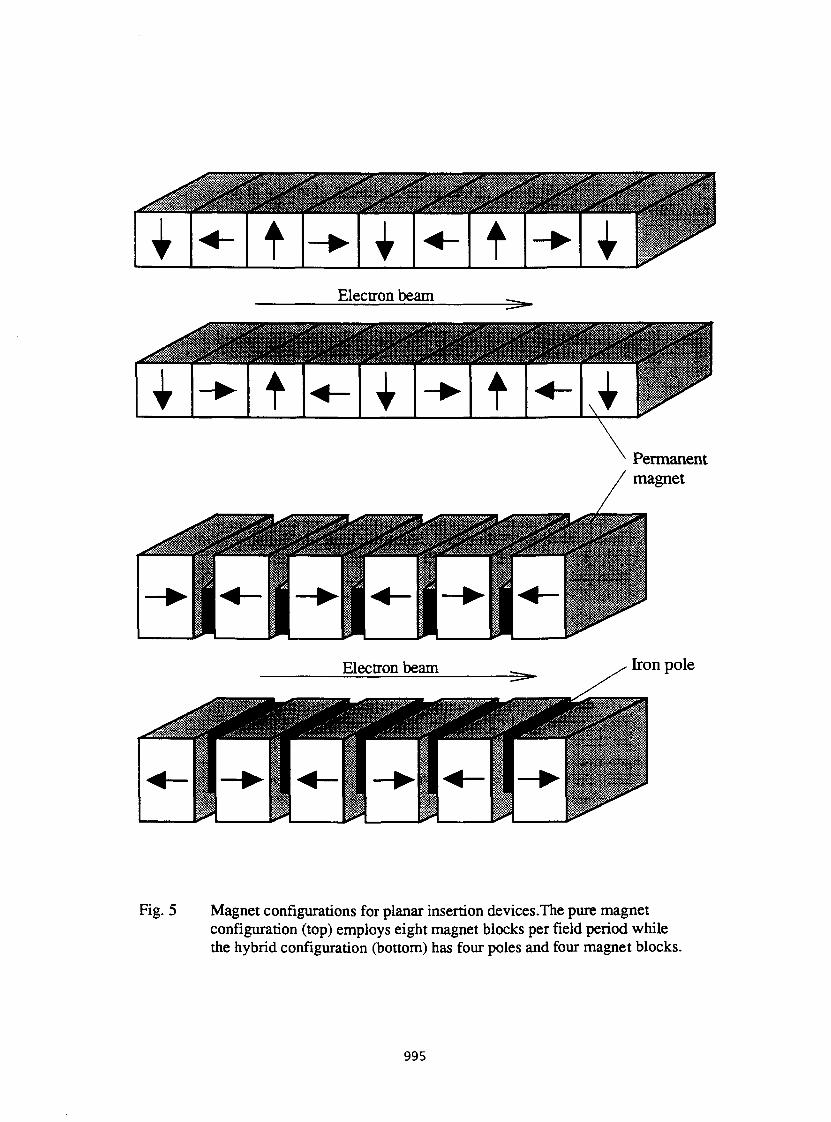
Electron beam
Permanent magnet
rlfir*TV * 'Jfrfj^z-tt
K^H
i l W' m
fl m
Electron beam
•TBI
Iron pole
Fig. 5 Magnet configurations for planar insertion devices.The pure magnet configuration (top) employs eight magnet blocks per field period while the hybrid configuration (bottom) has four poles and four magnet blocks.
995
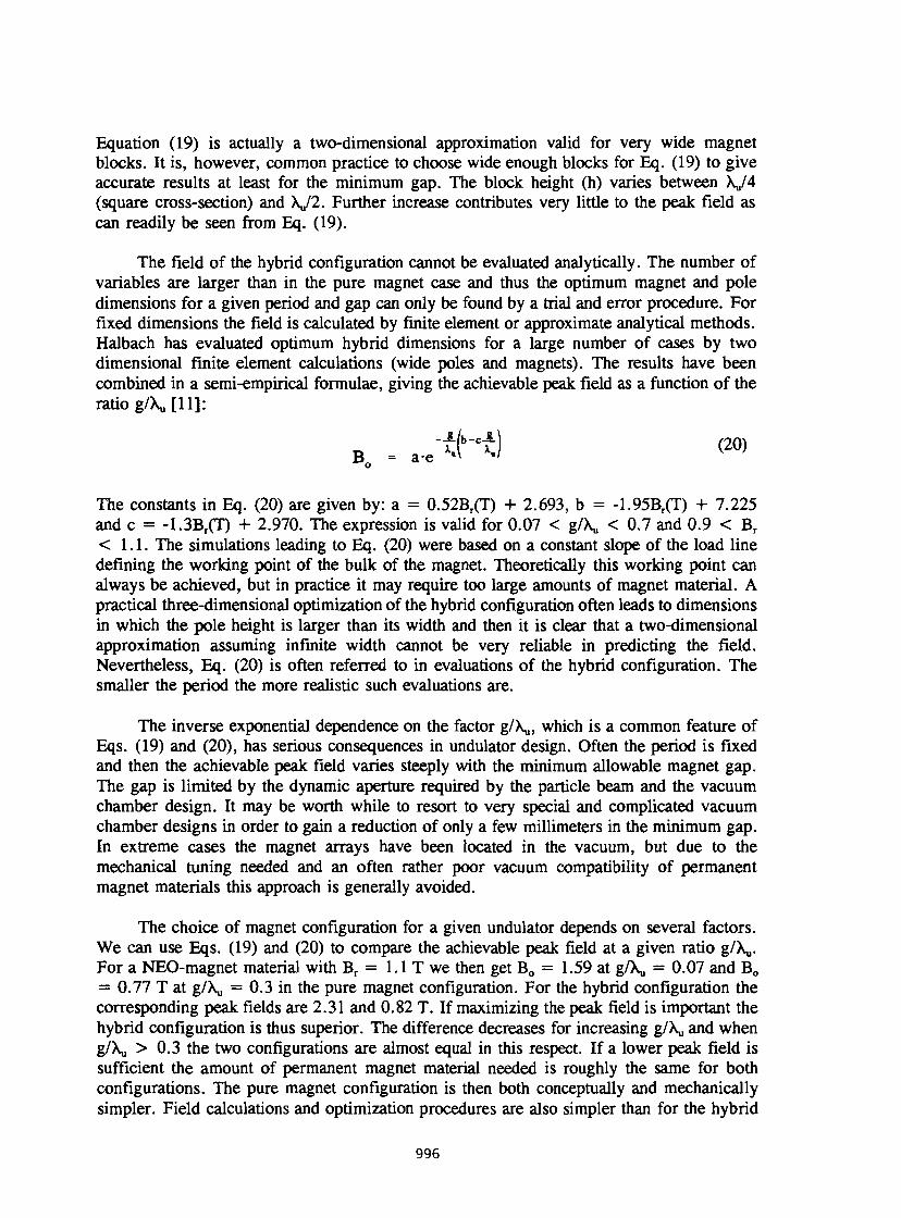
Equation (19) is actually a two-dimensional approximation valid for very wide magnet blocks. It is, however, common practice to choose wide enough blocks for Eq. (19) to give accurate results at least for the minimum gap. The block height (h) varies between \,/4 (square cross-section) and \/2. Further increase contributes very little to the peak field as can readily be seen from Eq. (19).
The field of the hybrid configuration cannot be evaluated analytically. The number of variables are larger than in the pure magnet case and thus the optimum magnet and pole dimensions for a given period and gap can only be found by a trial and error procedure. For fixed dimensions the field is calculated by finite element or approximate analytical methods. Halbach has evaluated optimum hybrid dimensions for a large number of cases by two dimensional finite element calculations (wide poles and magnets). The results have been combined in a semi-empirical formulae, giving the achievable peak field as a function of the ratio g/\ [11]:
"^ ( b " c t ) (20) B = a*e *v "'
o
The constants in Eq. (20) are given by: a = 0.52Br(T) + 2.693, b = -1.95Br(T) + 7.225 and c = -1.3Br(T) + 2.970. The expression is valid for 0.07 < g/\, < 0.7 and 0.9 < B r
< 1.1. The simulations leading to Eq. (20) were based on a constant slope of the load line defining the working point of the bulk of the magnet. Theoretically this working point can always be achieved, but in practice it may require too large amounts of magnet material. A practical three-dimensional optimization of the hybrid configuration often leads to dimensions in which the pole height is larger than its width and then it is clear that a two-dimensional approximation assuming infinite width cannot be very reliable in predicting the field. Nevertheless, Eq. (20) is often referred to in evaluations of the hybrid configuration. The smaller the period the more realistic such evaluations are.
The inverse exponential dependence on the factor g/\, which is a common feature of Eqs. (19) and (20), has serious consequences in undulator design. Often the period is fixed and then the achievable peak field varies steeply with the minimum allowable magnet gap. The gap is limited by the dynamic aperture required by the particle beam and the vacuum chamber design. It may be worth while to resort to very special and complicated vacuum chamber designs in order to gain a reduction of only a few millimeters in the minimum gap. In extreme cases the magnet arrays have been located in the vacuum, but due to the mechanical tuning needed and an often rather poor vacuum compatibility of permanent magnet materials this approach is generally avoided.
The choice of magnet configuration for a given undulator depends on several factors. We can use Eqs. (19) and (20) to compare the achievable peak field at a given ratio g/X„. For a NEO-magnet material with Br = 1.1 T we then get B 0 = 1.59 at g/\, = 0.07 and B 0
= 0.77 T at g/X,, = 0.3 in the pure magnet configuration. For the hybrid configuration the corresponding peak fields are 2.31 and 0.82 T. If maximizing the peak field is important the hybrid configuration is thus superior. The difference decreases for increasing g/X„ and when g/Xu > 0.3 the two configurations are almost equal in this respect. If a lower peak field is sufficient the amount of permanent magnet material needed is roughly the same for both configurations. The pure magnet configuration is then both conceptually and mechanically simpler. Field calculations and optimization procedures are also simpler than for the hybrid
996
configuration. On the other hand the high permeability poles of the hybrid configuration have a screening effect which reduces field errors on axis caused by inhomogeneities in the magnetization of the magnets. If a very high uniformity of the undulator field is required the hybrid configuration thus offers a better starting point. In many practical cases the choice of magnet configuration is, however, a marginal one, which tends to be resolved by institutional traditions and personal experience of the designer.
A more extensive review of undulator design and technology can be found in reference [12]. References [13] and [14] contain in depth treatment of many important aspects of undulator design and also a number of practical examples of constructed devices.
REFERENCES
[I] K.J. Strnat, Proc. IEEE 78 (1990) 923.
[2] R.J. Parker, Advances in permanent magnetism (John Wiley & Sons, 1990).
[3] J.A. Stratton, Electromagnetic theory (McGraw-Hill, 1941).
[4] K.J. Binns and P.J. Lawrenson, Analysis and computation of electric and magnetic field problems (Pergamon press, 1973).
[5] K. Halbach, Nucl. Instr. and Meth. 187 (1981) 109.
[6] R.F. Holsinger, Proc. 1979 Lin. Accel. Conf. Brookhaven BNL-51134 (1980) 373.
[7] K. Halbach, Nucl. Inst, and Meth. 169 (1980) 1.
[8] P. Elleaume, Proc. CAS Synchrotron Radiation and Free Electron Lasers CERN 90-03 (1990) 142.
[9] K. Halbach, Journal de Physique 44 (1983) Cl-211.
[10] G. Brown et al., Nucl. Instr. and Meth. 208 (1983) 65.
[II] E.S.R.F. Foundation Phase Report (1987) 314.
[12] M. Poole, Proc. CAS Synchrotron Radiation and Free Electron Lasers CERN 90-03 (1990) 195.
[13] R Tatchyn and I. Lindau éd., Proc. International Conference on Insertion Devices for Synchrotron Sources SPIE 582 (186).
[14] I.H. Munro and D.J. Thomson ed., Proc. 4th International Conference on Synchrotron Radiation Instrumentation Rev. Sci. Instr. 63 (1992).
997


NUCLEAR WASTE TRANSMUTATION USING HIGH-INTENSITY PROTON LINEAR ACCELERATORS
H. Lengeler CERN, Geneva, Switzerland
Abstract Long-term nuclear waste disposal is one of the most serious problems of the nuclear power industry. In order to alleviate the problem of geological or sea-bed disposal the transmutation of long half-time nuclides has been considered. Recently this method has received renewed attention by a Los Alamos proposal involving the use of a high-intensity linear proton accelerator for transmuting long-lived actinides and fission products in a high flux of thermal neutrons. A possible layout of such an accelerator is discussed by taking into account the specific problems of high efficiency and low beam losses. The possible advantages of superconducting cavities are considered.
1 . INTRODUCTION
Four decades of civilian and military nuclear power [1] and material production has left us with large quantities of radioactive wastes the safe disposal of which poses not only considerable technical problems but also increasing political concern. At present about 400 GW, corresponding to about 17% of the world electricity consumption is produced by nuclear reactors and will add large amounts of nuclear wastes to the already existing quantities.
Geological and sea-bed disposal of long-lived and highly concentrated waste is under active study in a number of countries. Many experts consider that geological storage will be an unescapable issue but the task may be alleviated by nuclear transmutation, i.e. the transformation in an intense neutron flux of long-lived radioactive species to isotopes with shorter half-life.
The idea of using high-intensity accelerators to produce fissionable material by transmutation was already advanced around 1950 by E.O. Lawrence and others at Berkeley [2] and its seems a natural idea to extend transmutation to unwanted radioactive species. Today accelerator technology has been developed to a level of sophistication and reliability where a new approach to its role for waste transmutation seems justified.
2. THE NUCLEAR WASTE PROBLEM [1,3,4] It is customary to classify nuclear waste according to its nature [3] as:
actinides,
fission products,
activated reactor material.
2 . 1 Actinides Actinides (belonging to the 7th period of elements) exist naturally as Ac, Th, Pa and U;
higher actinides with Z > 92 are produced by n-capture in nuclear reactors. The isotopes
999
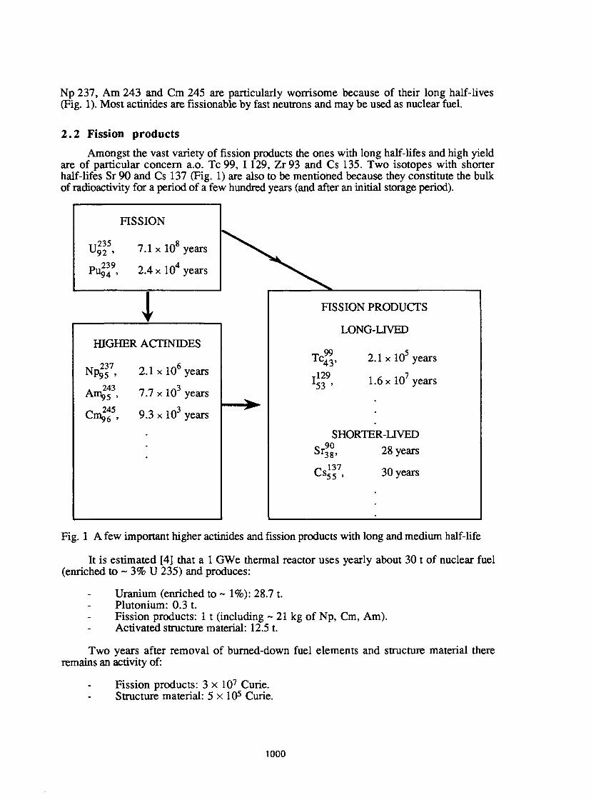
Np 237, Am 243 and Cm 245 are particularly worrisome because of their long half-lives (Fig. 1). Most actinides are fissionable by fast neutrons and may be used as nuclear fuel.
2.2 Fission products Amongst the vast variety of fission products the ones with long half-lifes and high yield
are of particular concern a.o. Tc 99, 1129, Zr 93 and Cs 135. Two isotopes with shorter half-lifes Sr 90 and Cs 137 (Fig. 1) are also to be mentioned because they constitute the bulk of radioactivity for a period of a few hundred years (and after an initial storage period).
FISSION
u 2 3 5
u 9 2 ' 7.1x 10⁸ years
n 239 P u 9 4 ' 2.4 x 10 4 years
1 HIGHER ACTTNIDES
Np 9 5 , 2.1 x 10 years A 243 Amps • 7.7 x 10 years
Cmç6 , 9.3 x 10 years
FISSION PRODUCTS
LONG-LJVED
Tc^, 2.1 xlO 5 years u 4 3 ' r129 l 53 '
7 1.6 x 10 years
Sr;
Cs
SHORTER-LIVED ,90 38' 137 55 '
28 years
30 years
Fig. 1 A few important higher actinides and fission products witii long and medium half-life
It is estimated [4] that a 1 GWe thermal reactor uses yearly about 301 of nuclear fuel (enriched to ~ 3% U 235) and produces:
Uranium (enriched to ~ 1%): 28.7 t. Plutonium: 0.3 t. Fission products: 1 t (including ~ 21 kg of Np, Cm, Am). Activated structure material: 12.5 t.
Two years after removal of burned-down fuel elements and structure material there remains an activity of:
Fission products: 3 x 10⁷ Curie. Structure material: 5 x 10⁵ Curie.
1000
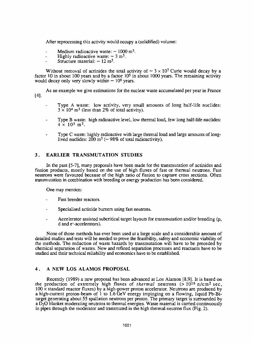
After reprocessing this activity would occupy a (solidified) volume:
Medium radioactive waste: ~ 1000 m 3. Highly radioactive waste: ~ 3 m 3 . Structure material: ~ 12 m 3 .
Without removal of actinides the total activity of ~ 3 x 10 7 Curie would decay by a factor 10 in about 100 years and by a factor 105 in about 1000 years. The remaining activity would decay only very slowly within ~ 106 years.
As an example we give estimations for the nuclear waste accumulated per year in France [4].
Type A waste: low activity, very small amounts of long half-life nuclides: 3 x 10 4 m 3 (less than 2% of total activity).
Type B waste: high radioactive level, low thermal load, few long half-life nuclides: 4 x 10 3 m 3 .
Type C waste: highly radioactive with large thermal load and large amounts of long-lived nuclides: 200 m 3 (~ 98% of total radioactivity).
3 . EARLIER TRANSMUTATION STUDIES
In the past [5-7], many proposals have been made for the transmutation of actinides and fission products, mostly based on the use of high fluxes of fast or thermal neutrons. Fast neutrons were favoured because of the high ratio of fission to capture cross sections. Often transmutation in combination with breeding or energy production has been considered.
One may mention:
Fast breeder reactors.
Specialised actinide burners using fast neutrons.
Accelerator assisted subcritical target layouts for transmutation and/or breeding (p, d and e"-accelerators).
None of those methods has ever been used at a large scale and a considerable amount of detailed studies and tests will be needed to prove the feasibility, safety and economic viability of the methods. The reduction of waste hazards by transmutation will have to be preceded by chemical separation of wastes. New and refined separation processes and reactants have to be studied and their technical reliability and economics have to be established.
4 . A NEW LOS ALAMOS PROPOSAL
Recently (1989) a new proposal has been advanced at Los Alamos [8,9]. It is based on the production of extremely high fluxes of thermal neutrons (> 1 0 1 6 n / cm 2 sec, 100 x standard reactor fluxes) by a high-power proton accelerator. Neutrons are produced by a high-current proton-beam of 1 to 1.6 GeV energy impinging on a flowing, liquid Pb-Bi-target generating about 55 spallation neutrons per proton. The primary target is surrounded by a D2O blanket moderating neutrons to thermal energies. Waste material is carried continuously in pipes through the moderator and transmuted in the high thermal neutron flux (Fig. 2).
1001
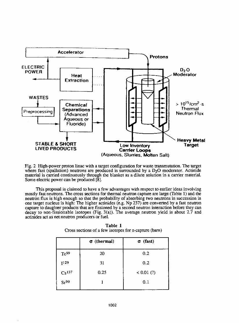
ELECTRIC POWER
WASTES i Preprocessing
Chemical Separations (Advanced Aqueous or
Fluoride)
T STABLE & SHORT LIVED PRODUCTS
"*\ Protons
0 2 O Moderator
VI > Wi5fcm?-s
Thermal Neutron Flux
Low Inventory Carrier Loops
(Aqueous. Slurries. Morten Salt)
Heavy Metal Target
Fig. 2 High-power proton linac with a target configuration for waste transmutation. The target where fast (spallation) neutrons are produced is surrounded by a D2O moderator. Actinide material is carried continuously through the blanket as a dilute solution in a carrier material. Some electric power can be produced [8].
This proposal is claimed to have a few advantages with respect to earlier ideas involving mostly fast neutrons. The cross sections for thermal neutron capture are large (Table 1) and the neutron flux is high enough so that the probability of absorbing two neutrons in succession in one target nucleus is high: The higher actinides (e.g. Np 237) are converted by a fast neutron capture to daughter products that are fissioned by a second neutron interaction before they can decay to non-fissionable isotopes (Fig. 3(a)). The average neutron yield is about 2.7 and actinides act as net neutron producers or fuel.
Table 1 Cross sections of a few isotopes for n-capture (barn)
0 (thermal) 0 (fast)
T c 9 9 20 0.2
1129 31 0.2
C s 1 3 7 0.25 < 0.01 (?)
Sr90 1 0.1
1002
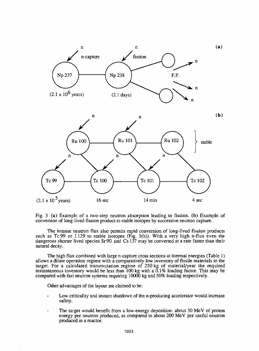
n n (a)
(2.1 x 10 years) 16 sec 14min 4 sec
Fig. 3 (a) Example of a two-step neutron absorption leading to fission, (b) Example of conversion of long-lived fission product to stable isotopes by successive neutron capture.
The intense neutron flux also permits rapid conversion of long-lived fission products such as Tc99 or 1129 to stable isotopes (Fig. 3(b)). With a very high n-flux even the dangerous shorter lived species Sr 90 and Cs 137 may be converted at a rate faster than their natural decay.
The high flux combined with large n-capture cross sections at thermal energies (Table 1) allows a dilute operation regime with a comparatively low inventory of fissile materials in the target. For a calculated transmutation regime of 250 kg of material/year the required instantaneous inventory would be less than 100 kg with a 0.1% loading factor. This may be compared with fast neutron systems requiring 10000 kg and 50% loading respectively.
Other advantages of the layout are claimed to be:
Low criticality and instant shutdown of the n-producing accelerator would increase safety.
The target would benefit from a low-energy deposition: about 30 MeV of proton energy per neutron produced, as compared to about 200 MeV per useful neutron produced in a reactor.
1003
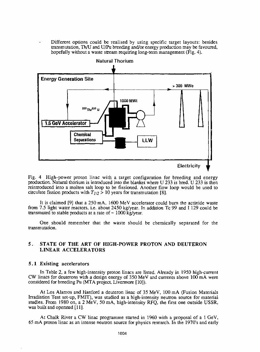
Different options could be realised by using specific target layouts: besides transmutation, Th/U and U/Pu breeding and/or energy production may be favoured, hopefully without a waste stream requiring long-term management (Fig. 4).
Natural Thorium
i Energy Generation Site
232 XhP3
> 300 MWe
1000 M Wt
1,6 GeV Accelerator
Chemical Separations LLW
Electricity
Fig. 4 High-power proton linac with a target configuration for breeding and energy production. Natural thorium is introduced into the blanket where U 233 is bred. U 233 is then reintroduced into a molten salt loop to be fissioned. Another flow loop would be used to circulate fission products with Tj/2 > 10 years for transmutation [8].
It is claimed [9] that a 250 m A, 1600 MeV accelerator could burn the actinide waste from 7.5 light water reactors, i.e. about 2450 kg/year. In addition Tc 99 and 1129 could be transmuted to stable products at a rate of ~ 1000 kg/year.
One should remember that the waste should be chemically separated for the transmutation.
5 . STATE OF THE ART OF HIGH-POWER PROTON AND DEUTERON LINEAR ACCELERATORS
5.1 Existing accelerators In Table 2, a few high-intensity proton linacs are listed. Already in 1950 high-current
CW linacs for deuterons with a design energy of 350 MeV and currents above 100 raA were considered for breeding Pu (MTA project, Livermore [10]).
At Los Alamos and Hanford a deuteron linac of 35 MeV, 100 mA (Fusion Materials Irradiation Test set-up, FMIT), was studied as a high-intensity neutron source for material studies. From 1980 on, a 2 MeV, 50 mA, high-intensity RFQ, the first one outside USSR, was built and operated [11].
At Chalk River a CW linac programme started in 1960 with a proposal of a 1 GeV, 65 mA proton linac as an intense neutron source for physics research. In the 1970's and early
1004
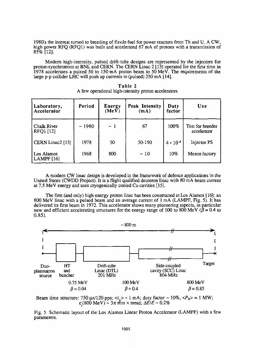
1980's the interest turned to breeding of fissile fuel for power reactors from Th and U. A CW, high power RFQ (RFQ1) was built and accelerated 67 m A of protons with a transmission of 85% [12].
Modern high-intensity, pulsed drift-tube designs are represented by the injectors for proton-synchrotrons at BNL and CERN. The CERN Linac 2 [13] operated for the first time in 1978 accelerates a pulsed 50 to 150 mA proton beam to 50 MeV. The requirements of the large p-p collider LHC will push up currents to (pulsed) 250 m A [14].
Table 2 A few operational high-intensity proton accelerators
Laboratory, Accelerator
Period Energy (MeV)
Peak Intensity (mA)
Duty factor
Use
Chalk River RFQ1 [12]
- 1980 ~ 1 67 100% Test for breeder accelerator
CERNLinac2[13] 1978 50 50-150 4« 10^ Injector PS
Los Alamos LAMPF [16]
1968 800 ~ 10 10% Meson factory
A modern CW linac design is developed in the framework of defence applications in the United States (CWDD Project). It is a flight qualified deuteron linac with 80 mA beam current at 7.5 MeV energy and uses cryogenically cooled Cu-cavities [15].
The first (and only) high-energy proton linac has been constructed at Los Alamos [16]: an 800 MeV linac with a pulsed beam and an average current of 1 mA (LAMPF, Fig. 5). It has delivered its first beam in 1972. This accelerator shows many pioneering aspects, in particular new and efficient accelerating structures for the energy range of 100 to 800 MeV (j3 = 0.4 to 0.85).
~800m I< 0 >i
Duo-plasmatron
source
HT and
buncher
Drift-tube Linac (DTL)
201MHz
Side-coupled cavity (SCC) Linac
804 MHz
Target
0.75 MeV 0 = 0.04
100 MeV 0 = 0.4
800 MeV 0 = 0.85
Beam time structure: 750 us/120 pps; <i > ~ 1 mA; duty factor ~ 10%, <Py> = 1 MW; e (800 MeV) ~ 3TT rftm x mrad; AEIE ~ 0.2%
Fig. 5 Schematic layout of the Los Alamos Linear Proton Accelerator (LAMPF) with a few parameters.
1005
5.2 Plans for high-intensity, high-energy proton linacs In the past design studies for proton linacs with high beam intensity have been made for
various applications. A few typical projects with design values are given in Table 3.
Spallation sources [17] for material studies with neutrons operate at an energy range of 1 GeV. Because of the need for time of flight measurements the beams are pulsed e.g. with 500 //s pulses at 100 Hz and average currents of 5 to 10 m A. The beam power can reach many MW and needs already an elaborate target layout and cooling system.
During the last years interest in tritium production by accelerators has grown. As an example one may mention an accelerator studied at Los Alamos and Brookhaven (APT [18]). A reference design of a proton accelerator with 1.6 GeV, 250 mA beam current (CW) and 400 MW beam power has been considered. This design has already many similarities with accelerators proposed for nuclear waste transmutation.
Accelerators for waste transmutation have been proposed in USA, CIS and Japan [6,7,19].
It should be stressed that none of these machines has yet been built and that the beam currents and beam powers considered correspond to an increase with respect to the largest existing proton linac, LAMPF, by two orders of magnitude. It reminds one of the present situation in e* colliders where particle factories (r-charm, beauty) are considered with beam currents of ~ 1 A, corresponding to a hundredfold increase as compared to existing colliders.
Table 3 A few planned high-intensity proton-linacs (typical parameters)
Type Energy (MeV) Average
Intensity (mA)
Spallation source
CERN Linac 2 for LHC (1993)
Tritium production
Waste incineration
- 1000
50
~ 1000
800-1600
5 (pulsed)
0.1 (pulsed)
2 0 - 100
100 + 300
For comparison
Kaon factory [20] LHC [21] Pulsed spallation source "Austron" [22]
30 GeV 7.7 TeV
0.8 + 5 GeV
~ 1 mA 800 m A per beam
63-125 M (pulsed)
Synchrotron p-p collider synchrotron Linac followed by rapid cycling synchrotron
6 . TWO DESIGN ASPECTS OF A HIGH-INTENSITY PROTON-LINAC
The optimization of a high-intensity proton-linac involves a large number of parameters. Besides the usual accelerator parameters for injection, acceleration and beam optics, safety
1006
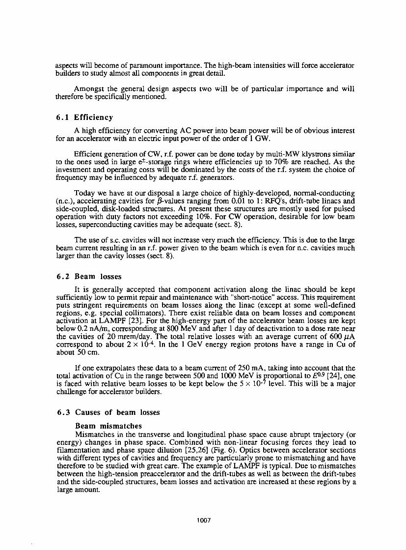
aspects will become of paramount importance. The high-beam intensities will force accelerator builders to study almost all components in great detail.
Amongst the general design aspects two will be of particular importance and will therefore be specifically mentioned.
6.1 Efficiency A high efficiency for converting AC power into beam power will be of obvious interest
for an accelerator with an electric input power of the order of 1 GW.
Efficient generation of CW, r.f. power can be done today by multi-MW klystrons similar to the ones used in large ei-storage rings where efficiencies up to 70% are reached. As the investment and operating costs will be dominated by the costs of the r.f. system the choice of frequency may be influenced by adequate r.f. generators.
Today we have at our disposal a large choice of highly-developed, normal-conducting (n.c), accelerating cavities for /?-values ranging from 0.01 to 1 : RFQ's, drift-tube linacs and side-coupled, disk-loaded structures. At present these structures are mostly used for pulsed operation with duty factors not exceeding 10%. For CW operation, desirable for low beam losses, superconducting cavities may be adequate (sect. 8).
The use of s.c. cavities will not increase very much the efficiency. This is due to the large beam current resulting in an r.f. power given to the beam which is even for n.c. cavities much larger than the cavity losses (sect. 8).
6.2 Beam losses It is generally accepted that component activation along the linac should be kept
sufficiently low to permit repair and maintenance with "short-notice" access. This requirement puts stringent requirements on beam losses along the linac (except at some well-defined regions, e.g. special collimators). There exist reliable data on beam losses and component activation at LAMPF [23]. For the high-energy part of the accelerator beam losses are kept below 0.2 nA/m, corresponding at 800 MeV and after 1 day of deactivation to a dose rate near the cavities of 20 mrem/day. The total relative losses with an average current of 600 fiA correspond to about 2 x 10 4 . In the 1 GeV energy region protons have a range in Cu of about 50 cm.
If one extrapolates these data to a beam current of 250 mA, taking into account that the total activation of Cu in the range between 500 and 1000 MeV is proportional to E0-9 [24], one is faced with relative beam losses to be kept below the 5 x 10-' level. This will be a major challenge for accelerator builders.
6.3 Causes of beam losses
Beam mismatches Mismatches in the transverse and longitudinal phase space cause abrupt trajectory (or
energy) changes in phase space. Combined with non-linear focusing forces they lead to filamentation and phase space dilution [25,26] (Fig. 6). Optics between accelerator sections with different types of cavities and frequency are particularly prone to mismatching and have therefore to be studied with great care. The example of LAMPF is typical. Due to mismatches between the high-tension preaccelerator and the drift-tubes as well as between the drift-tubes and the side-coupled structures, beam losses and activation are increased at these regions by a large amount.
1007
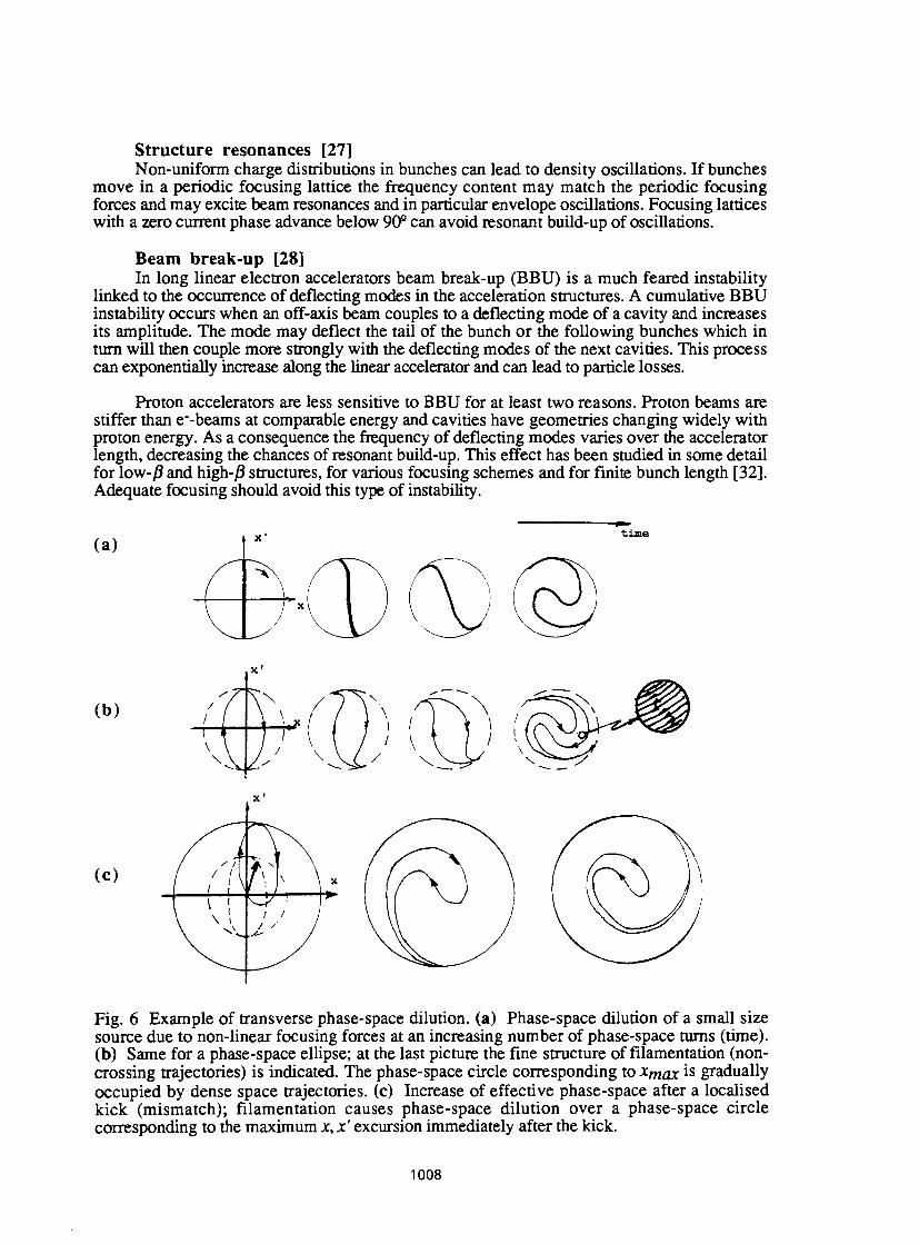
Structure resonances [27] Non-uniform charge distributions in bunches can lead to density oscillations. If bunches
move in a periodic focusing lattice the frequency content may match the periodic focusing forces and may excite beam resonances and in particular envelope oscillations. Focusing lattices with a zero current phase advance below 90 e can avoid resonant build-up of oscillations.
Beam break-up [28] In long linear electron accelerators beam break-up (BBU) is a much feared instability
linked to the occurrence of deflecting modes in die acceleration structures. A cumulative BBU instability occurs when an off-axis beam couples to a deflecting mode of a cavity and increases its amplitude. The mode may deflect the tail of the bunch or the following bunches which in turn will then couple more strongly with the deflecting modes of the next cavities. This process can exponentially increase along the linear accelerator and can lead to particle losses.
Proton accelerators are less sensitive to BBU for at least two reasons. Proton beams are stiffer than e"-beams at comparable energy and cavities have geometries changing widely with proton energy. As a consequence the frequency of deflecting modes varies over the accelerator length, decreasing the chances of resonant build-up. This effect has been studied in some detail for low-/? and high-/3 structures, for various focusing schemes and for finite bunch length [32]. Adequate focusing should avoid this type of instability.
Fig. 6 Example of transverse phase-space dilution, (a) Phase-space dilution of a small size source due to non-linear focusing forces at an increasing number of phase-space turns (time). (b) Same for a phase-space ellipse; at the last picture the fine structure of filamentation (non-crossing trajectories) is indicated. The phase-space circle corresponding to x m a x is gradually occupied by dense space trajectories, (c) Increase of effective phase-space after a localised kick (mismatch); filamentation causes phase-space dilution over a phase-space circle corresponding to the maximum x, x' excursion immediately after the kick.
1008
Emittance growth [27] The problem of emittance growth in high-intensity p-accelerators attracted the attention of
accelerator builders already in 1968 when the injector linacs at CERN and BNL were designed.
For the high-intensity proton-linacs considered, the bunch charge density lies in a range where the effect of space-charge forces exceeds largely the effect of individual particle scattering and where space-charge forces becomes comparable to the focusing forces, especially at low energies (space-charge dominated beam dynamics).
For the treatment of emittance growth it has been found fruitful to consider the beam in its rest system as a (non-relativistic) plasma for which the role of opposite charges is taken over by the external focusing forces.
Particles adjust their position to shield external fields. At the same time the charge distribution tends towards uniformity corresponding to a minimum of self-energy. The energy gained by this uniformisation increases the thermal energy of particles and results in an emittance growth. If the thermal energy is not the same in all degrees of freedom it will tend towards equality (equipartition) and increase the emittance in the degree of freedom with low thermal energy.
The thermalisation is a fast process with a typical time constant of l/coc (coc: plasma frequency). For the high intensities considered this corresponds to trajectory distances smaller than one focusing cell. The equipartitioning is mainly obtained by density oscillations of the bunch charge and occurs in a few plasma periods.
This model has been well confirmed by analytical calculations and by computer simulations for different types of optics. However, more work will be needed for extending results to a range of relative beam losses < 10"6 and where the beam halo will make non-negligeable contributions to beam losses.
7. A POSSIBLE LAYOUT
From the arguments given above one can already give a few design guidelines for a high intensity proton-linac (Fig. 7).
At injection a charge distribution should be provided which is as uniform as possible, equipartitioned and matched in all degrees of freedom to the front-end acceleration. An RFQ for efficient bunching and small emittance is an obvious choice [29,30].
CW operation can keep bunch populations low. Despite the high CW beam current the bucket population could be kept small corresponding to only 4 to 5 times the one of LAMPF. CW operation would also avoid transient beam loading effects which are considerable at high beam currents and can lead to additional beam losses and to increased r.f. power requirements. Funnelling behind the injection would be a possibility for keeping not only bunch charges small during the critical low-energy (low frequency) acceleration but also for filling all buckets of the (high-frequency) high-energy acceleration.
Beam containment would be used as a basic design principle: the optics should be as smooth as possible with an extremely careful matching of transitions between different accelerator sections. Transitions should be made at the lowest possible energy.
1009
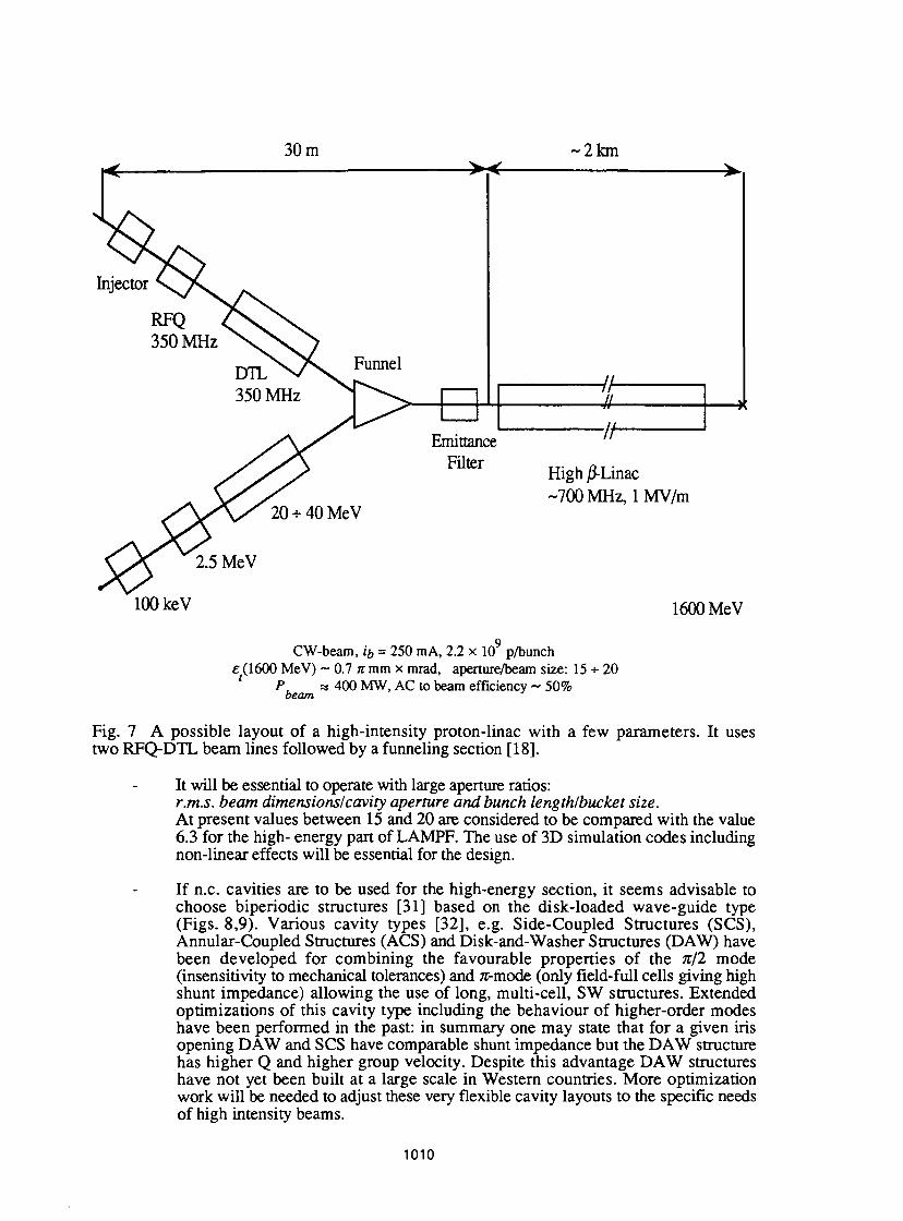
30 m 2km
High j3-Linac -700 MHz, 1 MV/m
100 keV 1600 MeV
CW-beam, ib - 250 mA, 2.2 x 10 p/bunch e (1600 MeV) ~ 0.7 imm x mrad, aperture/beam size: 15 ' / \ « 400 MW, AC to beam efficiency ~ 50% beam
20
Fig. 7 A possible layout of a high-intensity proton-linac with a few parameters. It uses two RFQ-DTL beam lines followed by a funneling section [18].
It will be essential to operate with large aperture ratios: r.m.s. beam dimensions/cavity aperture and bunch length/bucket size. At present values between 15 and 20 are considered to be compared with the value 6.3 for the high- energy part of LAMPF. The use of 3D simulation codes including non-linear effects will be essential for the design.
If n.c. cavities are to be used for the high-energy section, it seems advisable to choose biperiodic structures [31] based on the disk-loaded wave-guide type (Figs. 8,9). Various cavity types [32], e.g. Side-Coupled Structures (SCS), Annular-Coupled Structures (ACS) and Disk-and-Washer Structures (DAW) have been developed for combining the favourable properties of the nil mode (insensitivity to mechanical tolerances) and 7T-mode (only field-full cells giving high shunt impedance) allowing the use of long, multi-cell, SW structures. Extended optimizations of this cavity type including the behaviour of higher-order modes have been performed in the past: in summary one may state that for a given iris opening DAW and SCS have comparable shunt impedance but the DAW structure has higher Q and higher group velocity. Despite this advantage DAW structures have not yet been built at a large scale in Western countries. More optimization work will be needed to adjust these very flexible cavity layouts to the specific needs of high intensity beams.
1010
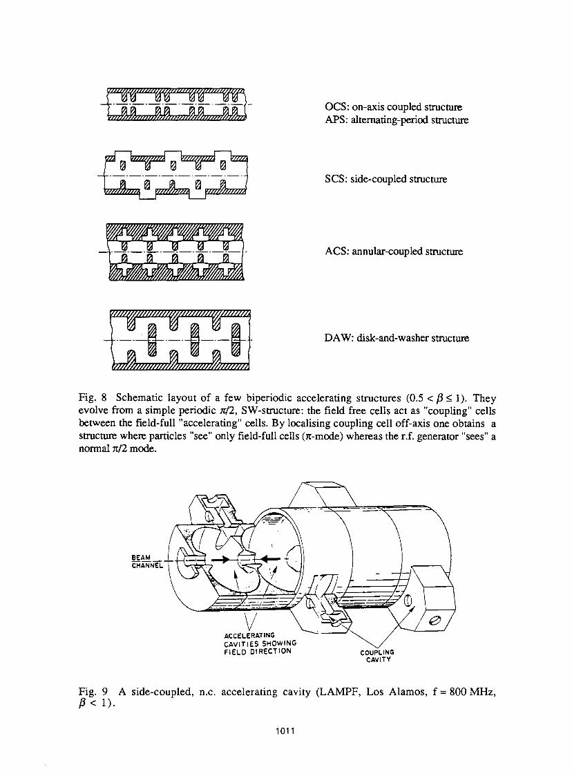
OCS: on-axis coupled structure APS: alternating-period structure
/w/A/m^ ® Y77™7777^ ^mrnnmA SCS: side-coupled structure
ACS: annular-coupled structure
mMMWMWUty//MtMK PfT? to/M/M////WWM/M/M/»A
DAW: disk-and-washer structure
Fig. 8 Schematic layout of a few biperiodic accelerating structures (0.5 </3< 1). They evolve from a simple periodic Till, SW-structure: the field free cells act as "coupling" cells between the field-full "accelerating" cells. By localising coupling cell off-axis one obtains a structure where particles "see" only field-full cells (rc-mode) whereas the r.f. generator "sees" a normal 7t/2 mode.
BEAM CHANNEL
ACCELERATING CAVITIES SHOWING FIELD DIRECTION COUPLING
CAVITY
Fig. 9 A side-coupled, n.c. accelerating cavity (LAMPF, Los Alamos, f = 800 MHz, P< 1).
1011
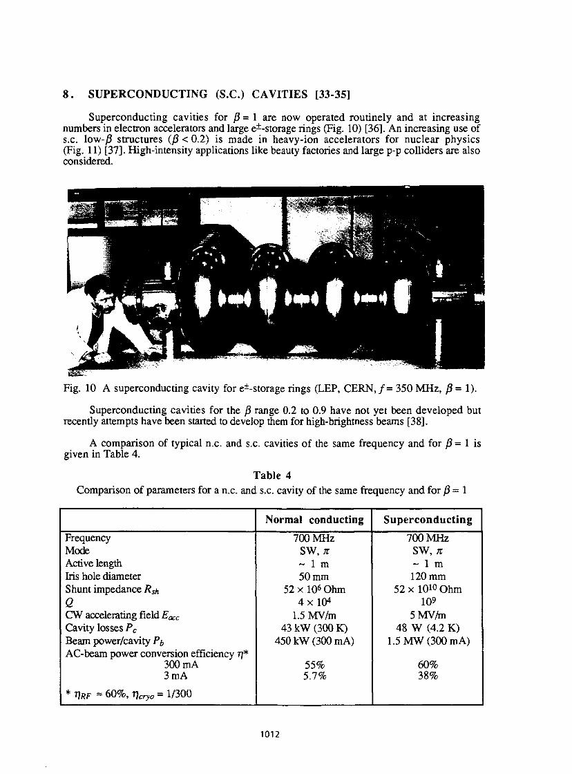
8. SUPERCONDUCTING (S.C.) CAVITIES [33-35]
Superconducting cavities for /? = 1 are now operated routinely and at increasing numbers in electron accelerators and large e—storage rings (Fig. 10) [36]. An increasing use of s.c. low-/? structures (/? < 0.2) is made in heavy-ion accelerators for nuclear physics (Fig. 11) [37]. High-intensity applications like beauty factories and large p-p colliders are also considered.
Fig. 10 A superconducting cavity for ei-storage rings (LEP, CERN, / = 350 MHz, /? = 1).
Superconducting cavities for the /? range 0.2 to 0.9 have not yet been developed but recently attempts have been started to develop mem for high-brightness beams [38].
A comparison of typical n.c. and s.c. cavities of the same frequency and for /? = 1 is given in Table 4.
Table 4 Comparison of parameters for a n.c. and s.c. cavity of the same frequency and for j3 - 1
Normal conducting Superconducting Frequency 700 MHz 700 MHz Mode SW, n SW, it Active length ~ 1 m ~ 1 m Iris hole diameter 50 mm 120 mm Shunt impedance RSh 52 x 106 Ohm 52 x 10 1 0 Ohm Q 4 x 10⁴ 109 CW accelerating field EacC 1.5 MV/m 5 MV/m Cavity losses Pc 43 kW (300 K) 48 W (4.2 K) Beam power/cavity Pb 450 kW (300 mA) 1.5 MW (300 m A) AC-beam power conversion efficiency r\*
300 mA 55% 60% 3 mA 5.7% 38%
* T)RF » 60%, 7]cryo = 1/300
1012
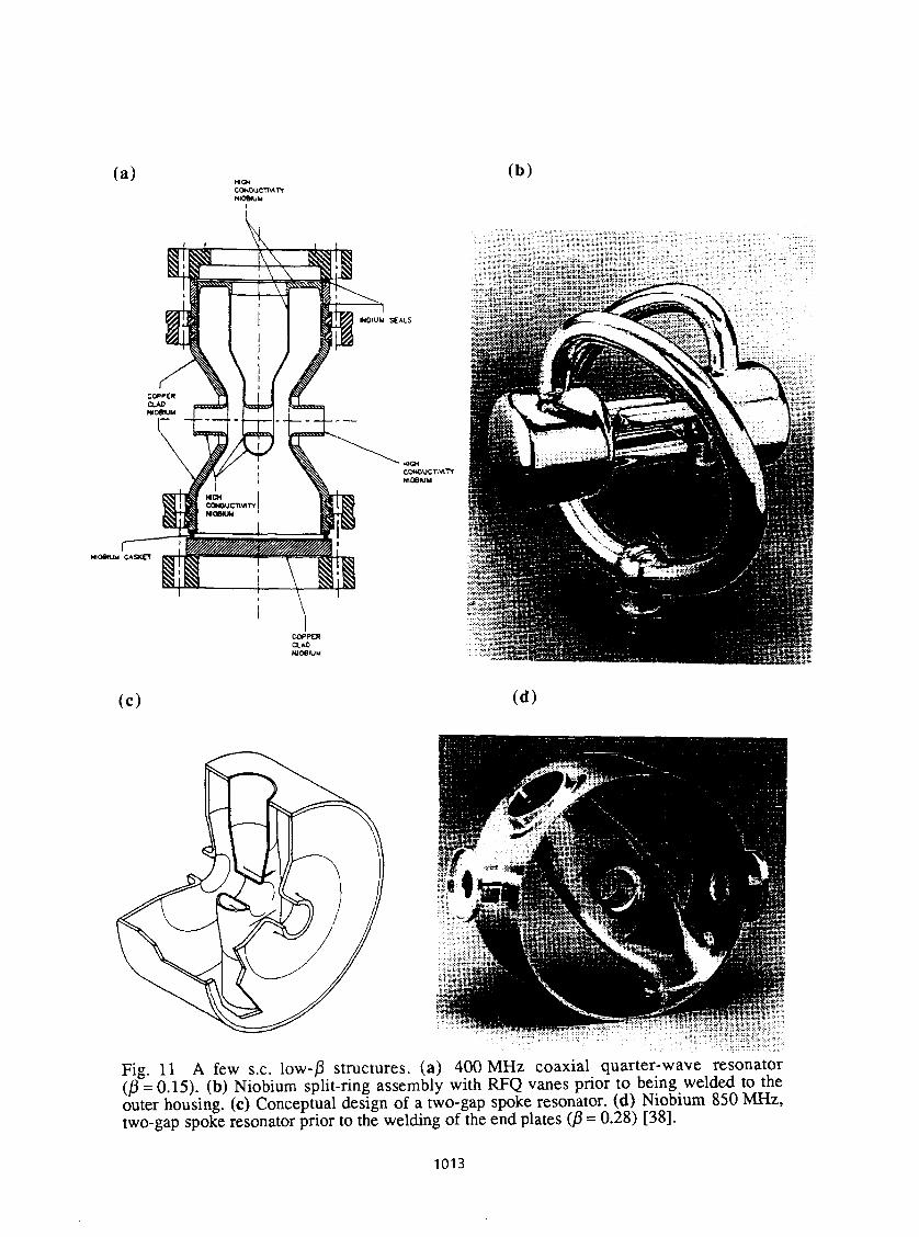
(a) HIGH CONDUCTIVITY Nioeiuu
(b)
NOIUW S£ALS
NIOetUU CASKCT
MICH CONDUCTIVITY Ntoeiuu
(C) (d)
Fig. 11 A few s.c. low-/3 structures, (a) 400 MHz coaxial quarter-wave resonator (j3 = 0.15). (b) Niobium split-ring assembly with RFQ vanes prior to being welded to the outer housing, (c) Conceptual design of a two-gap spoke resonator, (d) Niobium 850 MHz, two-gap spoke resonator prior to the welding of the end plates 03 = 0.28) [38].
1013
We have scaled the cavity geometry from the n.c. [39] and s.c. [40] LEP cavities (which correspond to an advanced design for large e* storage rings) to a frequency of 700 MHz. Although this frequency choice is by no means supported by a detailed optimization study it appears to be a possible compromise between many conflicting arguments for the high-energy part of a proton linac a.o. frequency doubling with respect to a 350 MHz, low-energy acceleration and funnelling, and an iris of 120 mm diameter. An important argument for s.c. cavities is to use a frequency well below 1000 MHz; in this range one may use Nb cavities at the normal operating temperature for He (4.2 K) and still have sufficiently high Q-values of about 10 9 [33].
8.1 AC power to beam power conversion efficiency (for n.c. and s.c. cavities)
We define the efficiency by
77 = beam power/mains power
and may transform it to the following expressions for n.c. and s.c. cavities.
n . c . s .c .
77 = ^ n = 5> (f6 + Pc)hRF PbMRF + PcryolVcryo
P> b
— ^IRF 9—7 lb * Vacc + Vacc/Rsh
ace
Pb/riRF+{Pc + Pst)/ri cryo
kVacc = ibiYt
k * Vacc VRF +
(Pc « Pb) V Rsh J)
with:
Pb'. Power given to the beam by the cavity, Pt, = i},. Vacc.
if. (average) beam current.
y ace- Cavity voltage.
Pc: Cavity r.f. losses; Pc = V^JRsh (1 inac definition).
RSh'- Shunt impedance; because of the low r.f. losses of s.c. cavities, Rsh is about a factor 105 higher for s.c. cavities than for n.c. cavities (Table 4). For s.c. cavities one has Pc « Pb but the losses have to be evacuated at 4.2 K.
Pst' Static losses of cryostat (at 4.2 K). We assume Pst <10W/m.
Icryo- overall efficiency for evacuating the losses Pc + Pst = PCryo- At 4.2 K and for a large system one may assume rjcry0 = 1/300.
T\RF'- Efficiency for r.f. production and transmission; for large CW klystron systems we estimate T)RF ~ 60%.
1014
Obviously r] depends on the accelerating voltage and the beam current. In Table 4 77 is given for two values of current and for a typical V a c c ; one sees that for large beam currents Pc « Pb even for n.c. cavities. The efficiency can therefore only be increased in a high-current proton linac from 55% to 60% (as opposed to storage rings or linear accelerators with a typical beam current of a few raA).
8.2 CW accelerating fields
Because of the low r.f. losses of s.c. cavities much higher CW accelerating fields than in n.c. cavities can be reached.
In disk-loaded multicell cavities (350 MHz to 3000 MHz) for e* storage rings and electron accelerators, gradients well above 5 MV/m are reached and much higher fields are considered for s.c. linear colliders. However in high-intensity accelerators the gradients will not be limited by the cavities but presumably by the input couplers. With a 250 raA current, Eacc = 4 MV/m and a i m cavity, it has to handle 1 MW, almost an order of magnitude more than is used today [41].
A key design principle of s.c. cavities, to be operated at high CW accelerating fields, is a simple geometrical shape with small ratios EplE^ and HplEacc (Ep, Hp : maximum electric and magnetic surface fields respectively). Easy machining and welding and shapes which can be thoroughly cleaned are of primordial importance. Rounded cells for avoiding multipactoring and efficient cooling by LHe of all s.c. parts would be essential. One would therefore probably not use a variant of biperiodic structures but simple SW, 7r-mode periodic structures with rounded cells as used universally in e* storage rings and electron accelerators (Fig. 10). Large iris openings will provide sufficient coupling between cells, so that extra coupling slots can be avoided.
It should be however stressed again, that up to now s.c. cavities have not been developed and optimised for the velocity range j3 = 0.3 to 0.9.
RFQ's and low-/? cavities have much more complex geometries than simply periodic, iris-loaded cavities. This results in a very high ratio of maximum electric surface fields Ep to accelerating fields exceeding greatly the typical EpIEacC = 2 value for disk-loaded waveguide cavities and may lead to a limitation of E^c by field emitted electrons. Typical Eacc reached in low-/? structures under CW conditions range up to 5 MV/m.
Recently a very interesting test has been made with a s.c. RFQ: In a short RFQ model gradients of 128 MV/m over 10 cm 2 (vane voltage ~ 300 kV) have been achieved [38]. If these gradients could be sustained over longer RFQ very compact designs may be possible and maximum CW currents (believed to be proportional to the vane voltage) could be increased.
Funnelling of two low-energy beams into one high-energy section (Fig. 7) could be obtained by deflector cavities operated in a dipole (deflecting) mode. Superconducting deflector cavities have been developed and operated in high-energy r.f. particle separators [42] under CW conditions at 3 GHz (p = 1). They have to be developed for lower particle velocities and lower frequencies (e.g. p = 0 .4 , /= 350 MHz).
8.3 Iris openings A dominant merit factor for n.c. cavities is a high shunt impedance requiring small iris
openings. Because of the low r.f. losses this requirement is much less stringent for s.c. cavities and very large iris openings are possible (Table 4). This will be a considerable bonus for s.c. cavities because a large aperture ratio can be obtained, resulting in reduced beam losses and activation. Large iris openings go hand in hand with a reduction of cavity impedances for fundamental and higher-order mode resonances excited by the beam. Although this will not be
1015
as crucial as for beauty factory applications [43], it may be helpful for decreasing beam instabilities and beam losses. With respect to n.c. cavities total impedances will be further reduced by the higher accelerating fields resulting in a shorter linac.
The attenuation of higher-order modes in s.c. cavities by dedicated couplers has been pushed to a high degree of perfection and Qext values well below 105 for the most dangerous (deflecting) modes are routinely reached [41]. Delayen et al. [44] have made beam break up calculations for a few model high-intensity linacs. Their conclusion is that for strong focusing and sufficient damping of dangerous deflecting modes (Qext < 5 x 10⁶) BBU should not be a major problem.
8.4 Beam losses and s.c. cavities
In a s.c. cavity beam losses can have at least three effects:
Power absorption at LHe temperatures.
A few W/m would probably be tolerable compared to r.f. losses which are of the order of 20 to 50 W/m.
Activation:
Similar limits (0.2 nA/m) as for n.c. cavities would be necessary and would correspond to losses far below a few W/m.
Degradation of cavity performances in fields and Q-values.
In the past [45] measurements have been performed showing that total proton doses (at 180 MeV) of ~ 2 x 10 1 5 p/cm2 start to degrade Q-values of Nb-cavities. A first estimation for Nb cavities has shown that present LAMPF losses of 0.2 nA/m would allow a total operating time of about 20000 h without an intolerable degradation.
Activation and Q-degradation would thus put a lower limit to beam losses for s.c. cavities.
9. CONCLUSION
The new Los Alamos approach for nuclear waste transmutation looks promising. It may allow flexible options between waste transmutation, breeding and energy production.
For this approach high-intensity proton linear accelerators in the energy range of GeV are considered. With respect to existing high energy linacs (e.g. LAMPF), beam currents and beam powers would have to be increased by 2 orders of magnitude. Among the design guidelines high efficiency for converting electric power to beam power and safety aspects will be primordial. The request for "hands-on" maintainance and repair will require relative beam losses at a level below 10~6, far smaller than presently achieved values.
The present state of the art of high-intensity proton accelerators and, in particular, injectors seems to be a sound basis for the development of high-intensity, CW proton linear accelerators. No basic objections have been identified but a large study effort for space-charge dominated beam transports backed up by 3D beam simulations will be needed. The large beam intensities will ask for detailed tests of all beam components. A linear accelerator for spallation sources could be a very useful intermediate step towards this goal.
1016
The use of superconducting accelerator cavities should be considered. They may favour the option for higher beam energies with a concomitant reduction of beam current. A definite advantage would be that much larger iris openings could be afforded as compared to normal conducting cavities of the same frequency. Cavity development, particularly in the region of low /?, would be needed.
Considering that a geological disposal of long-lived wastes is studied in many countries and will need a multi-billion US$ budget, it seems sensible to foresee a small part of this sum for the study of accelerator-supported transmutation of long-lived nuclei.
Today there exists worldwide a number of accelerator teams with an excellent competence in high-power accelerators which could participate in this effort. A vigorous international collaboration not only in the field of accelerators but also for chemical separation of wastes targeting technology and safety aspects would be highly desirable.
ACKNOWLEDGEMENTS
I would like to thank my colleagues from CERN for many instructive discussions, in particular G. Dôme, E. Haebel, D. Warner and M. Weiss. I. Hofmann (GSI) and T. Wangler (Los Alamos) supplied me with much information on space charge dominated beams and particle losses.
* * *
REFERENCES
[1] A general presentation of nuclear technology can be found in:
S. Glasstone, Principles of Nuclear Reactor Engineering, D. Van Nostrand Comp., Princeton (1955).
W. Marshall, Editor, Nuclear Power Technology, Clarendon Press, Oxford (1983).
[2] See e.g. M. Steinberg, Editor Proc. Inform. Meeting Accelerator Breeding, BNL Report Conf. 770107 (1977).
[3] J. Keen in [1], vol. 2, p. 282.
[4] J.Y. Barré in Scientific Basis for Nuclear Waste Management XV, ed. C.G. Sombret, Strasbourg (1991) 7, Materials Research Society, Pittsburgh, Pennsylvania (1992).
[5] See e.g. Proc. Int. Conf. on Nuclear Waste Transmutation, Austin, Texas (July 1980).
[6] Specialists Meeting on Accelerator-Driven Transmutation Technology for Rad Waste and other Applications, Stockholm 1991, ed. R.A. Jameson, Los Alamos report LA-12205-C.
[7] Specialists Meeting on Accelerator Based Transmutation, PSI Villigen, Switzerland 1992, ed. H.W. Wenger, PSI Proc. 92-02, September 1992.
[8] R.A. Jameson, G.P. Lawrence and C D . Bowman, 2nd European Conf. on Accelerators in Applied Research and Technology, Frankfurt-am-Main (1991) 474.
[9] R.A. Jameson, G.P. Lawrence and S.O. Schriber, 3rd European Ace. Conf., Berlin (1992) 230.
1017
[10] P.V. Livdahl, Proc. 1981 Linac Conf., Los Alamos Report LA-9234 (1982) 5.
[11] W.D. Cornelius, Nucl. Instr. & Meth. B10/11 (1985) 859.
[12] G.M. Arbigue et al., Proc. 1988 Linac Conf., CEBAF Report 89-001 (1989) 91.
[13] E. Boltezar et al., 1979 Linear Ace. Conf., Montauk, BNL Report 5113A.
[14] M. Weiss, 3rd European Particle Ace. Conf, Berlin (1992) 539.
[15] See e.g. G.E. McMichael, Linear Ace. Conf., Los Alamos Report LA-12004-C (1991) 515.
[16] Catalogue of High-Energy Accelerators, XI Int. Conf. on High Energy Ace., Geneva (1980).
[17] See e.g. G.S. Bauer and J.E. Vetter in Nuclear Technologies in a Sustainable Energy System, G.S. Bauer and A. McDonald eds, Springer Verlag (1983) 237.
[18] T.P. Wangler et al., réf. [15], p. 548.
[19] The 2nd Int. Symposium on Advanced Nucl. Energy Research Evolution by Accelerators, Mito, Japan (January 1990).
[20] F. Bradamante, Europhysics News 23 (1992) 7.
[21] Design Study of the Large Hadron Collider (LHC), CERN 91-03 (1991).
[22] H. Aiginger et al., 3rd European Particle Ace. Conf., Berlin (1992) 432.
[23] R.W. Garnett, R.S. Mills and T.P. Wangler, ref. [15], p. 347 and
T.P. Wangler, Los Alamos, private communication.
[24] J. Sullivan, CERN, private communication.
[25] A.H. Sorensen, CAS, Salamanca 1988, CERN 89-05 (1989) 18.
[26] P.J. Bryant, ibidem p. 37.
[27] For a more detailed treatment and a bibliography of structure resonances and space-charge dominated beams, see I. Hofmann, these CAS proceedings.
[28] J. Le Duff, CAS, Oxford 1985, CERN 87-03 (1987) 610.
[29] A. Schempp, CAS, Oxford 1991, CERN 92-03 (1992) 522.
[30] M. Weiss, these CAS proceedings.
[31] D.E. Nagle, E.A. Knapp and B.C. Knapp, Rev. Scient. Instr. 38 (1967) 1583.
[32] T. Kageyama et al., Particle Ace. 32 (1990) 33.
[33] H. Piel, Proc. CAS, Hamburg 1988, CERN 89-04 (1989) 149.
[34] H. Lengeler, ibidem p. 197.
[35] W. Weingarten, Proceedings CAS, Oxford 1991, CERN 92-03 (1992) 318.
[36] J. Tiickmantel, 3rd European Ace. Conf. EPAC92, Berlin (1992) 279.
1018
[37] J.R. Delayen, Proc. 4th Workshop on RF Superconductivity, ed. Y. Kojima KEK (1989) 249.
[38] J.R. Delayen et al., Proc. 5th Workshop on RF Superconductivity, ed. D. Proch, DESY (1991) 376.
[39] I. Wilson and H. Henke, CERN 89-09 (1989). [40] E. Haebel, P. Marchand and J. Tiickmantel, Proc. 2nd Workshop on RF
Superconductivity, CERN, ed. H. Lengeler (1984) 281. [41] E. Haebel in ref. [38], p. 334.
[42] A. Citron et al., Nucl. Instr. & Meth. 164 (1979) 31. [43] H. Lengeler, to be published in Proc. SLAC B-Factory Conf. Stanford (1992). [44] C.L. Bohn and J.R. Delayen, Phys. Rev. A45, 8 (1992) 5964. [45] HJ. Halama, Appl. Phys. Lett. 19, 4 (1971) 90.
1019

Related Documents


