Kuno_2013_Prey survey_report full

Citation:

Bipin C.M., Bhattacharjee S., Shah S., Sharma V.S., Mishra R.K., Ghose D., & Jhala Y.V. (2013). Status of prey in Kuno Wildlife Sanctuary, Madhya Pradesh. Wildlife Institute of India, Dehradun.

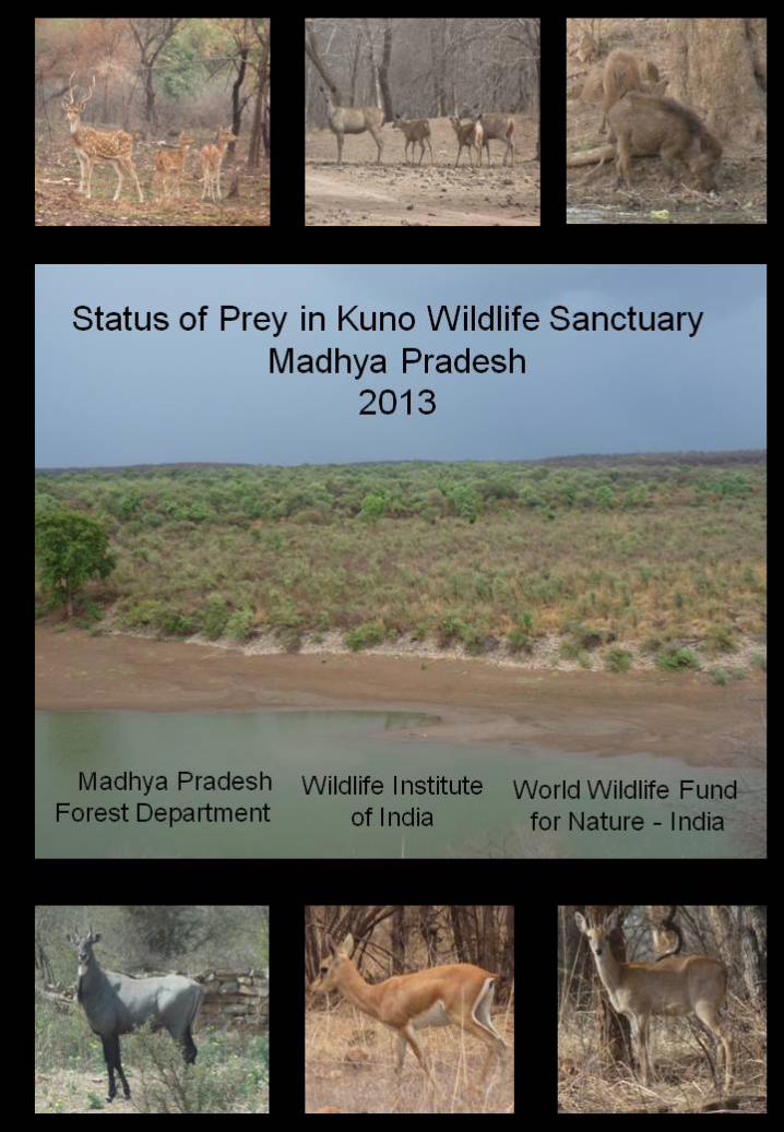
Cover page photo credits:

Bipin.C.M

Status of Prey in Kuno Wildlife Sanctuary

Madhya Pradesh

2013

Madhya Pradesh Forest Department

Team

V.S. Sharma, IFS

- Chief Conservator of Forests, Lion Project

R.K. Mishra, IFS

- Division Forest Officer Kuno Wildlfe Division

Wildlife Institute of India Team

Y.V. Jhala, Ph.D.

Scientist- G - Head of Department

Animal Ecology & Conservation Biology

Bipin C.M.

World Wildlife Fund for Nature (WWF), India

Team

Dipankar Ghose, Ph.D.

- Director, Species & Landscapes Division

Sunny Shah

Subhadeep Bhattacharjee

Contents

Page No.

Introduction 01

Prey base Estimation 03

Methods 03

Analysis 04

Results 05

Discussion 06

Literature Cited 07

Annexure 1

Summary of Prey Species Abundance Estimation Model 08

Parameters in DISTANCE

Annexure 2

Detection Function Curves for Prey Species Abundance Estimation

2.01: Chital in Kuno WLS 09

2.02: Sambar in Kuno WLS 09

2.03: Nilgai in Kuno WLS 10

2.04: Wild pig in Kuno WLS 10

2.05: Chinkara in Kuno WLS 11

2.06: Four-horned antelope in Kuno WLS 11

2.07: Gray langur in Kuno WLS 12

2.08: Peafowl in Kuno WLS 12

2.09: Feral cattle in Kuno WLS 13

1

Status of Prey in Kuno Wildlife Sanctuary, Madhya Pradesh

2013

Introduction: - Kuno Wildlife Sanctuary (WLS) is spread over an area of 344.68 km2 and is

situated in Sheopur district of Madhya Pradesh. The Sanctuary is part of the Kuno wildlife

division which covers an area of 1235.39 km2. Kuno River, one of the major tributaries of

Chambal River flows through the entire length bisecting the wildlife division. The division

comprises of eight ranges, with Palpur west and Palpur east ranges forming the Sanctuary. The

six ranges in the buffer area are Moravan east and west, Sironi north and south, Agara west

and east (See Fig.1) The area is classified as Semi-arid zone (4b), Gujarat- Rajputana

biogeographic region (Rodgers et al. 2002). The elevation ranges from 238m to 498m above

msl. The south-western portion of this landscape is patchily connected to Panna Tiger Reserve

through Shivpuri forest area. On the north-western side, this forest region is contiguous with

Ranthambhore Tiger Reserve across the river Chambal.

Fig 1: Kuno wildlife division

2

Temperature and Rainfall: During the months of April and May, the maximum summer

temperature ranges between 38°C - 47.4°C and the minimum winter temperature through the

months of December to February ranges between 0.6°C - 12.4°C .The average annual rainfall is

760mm.

Vegetation: According to the revised classification of forest types of India (Champion & Seth

1968) the forest types found in this region are:

Northern tropical dry deciduous forest

Southern tropical dry deciduous forest

Anogeissus pendula forest & scrub

Boswellia forest

Butea forest

Dry savannah forest & grassland

Tropical riverine forest

The dominant tree species that occur in the division are Acacia catechu (Khair), Anogeissus

pendula (Kardhai), Boswellia serrata (Salai), Diospyros melanoxylon (Tendu), Butea

monosperma (Palash), Anogeissus latifolia (Dhok), Acacia leucophlea (Remja), Zizyphus

mauritiana (Ber) and Zizyphus xylopyrus (Ghont).

Prominent shrub species include Grewia flavescens, Helicteres isora, Dodonoea viscosa, Vitex

nigundo. Some of the grass species found are Heteropogon contortus, Apluda mutica, Aristida

hystrix, Themeda quadrivalvis, Cenchrus ciliaris and Desmostachya bipinnata. Commonly found

weeds in this area include Cassia tora and Argemone mexicana.

Wildlife: The herbivores found in this area are Axis axis (Chital), Rusa unicolor (Sambar),

Boselaphus tragocamelus (Nilgai), Sus scrofa (Wild pig), Gazella bennetii (Chinkara),

Tetracerus quadricornis (Chousingha or Four-horned antelope), Antilope cervicapra

(Blackbuck), Semnopethicus dussumieri (Southern plains gray langur), Hystrix indica (Indian

crested porcupine) and Lepus nigricollis (Indian hare).

Carnivores include the Panthera pardus (Leopard), Ursus melursinus (Sloth bear), Hyaena

hyaena (Striped hyaena), Canis lupus (Gray wolf), Canis aureus (Golden jackal), Vulpes

bengalensis (Indian fox) and Mellivora capensis (Ratel). One male Panthera tigris (Tiger) which

has migrated from Ranthambhore Tiger Reserve is seen moving in and around the Sanctuary

3

since December 2010. Small carnivores such as the Felis chaus (Jungle cat), Herpestes

edwardsii (Indian grey mongoose), Herpestes smithii (Ruddy mongoose) and Herpestes

javanicus (Small Asian mongoose) are found here.

Some of the bird species that occur here are Sarcogyps calvus (Red headed vulture) , Gyps

indicus (Indian vulture), Neophron percnopterus (Egyptian vulture), Pernis ptilorhyncus (Oriental

honey- buzzard), Elanus caeruleus (Black shouldered kite), Ketupa zeylonensis (Brown fish

owl), Caprimulgus europaeus (Eurasian nightjar), Caprimulgus asiaticus (Indian nightjar) , Pavo

cristatus (Indian peafowl), Pterocles indicus (Painted sandgrouse), Ciconia episcopus (Woolly-

necked stork), Esacusre curvirostris (Great thick-knee)Phaenicophaeus leschenaultia (Sirkeer

malkoha), Oriolus kundoo (Indian golden oriole), Dinopium benghalense (Black-rumped

flameback), Lanius vittatus (Bay- backed shrike) & Terpsiphone paradise (Asian paradise

flycatcher). A few of the reptiles found in the sanctuary are Crocodylus palustris (Mugger),

Nilssonia gangetica (Ganges softshell turtle) & Varanus bengalensis (Bengal monitor lizard).

Occasionally, Gavialis gangeticus (Gharial) is also sighted in Kuno River.

To assess the prey base in Kuno WLS, Wildlife Institute of India (WII) and World Wildlife Fund

for Nature (WWF) – India was requested to conduct a survey in June 2013 by the Madhya

Pradesh Forest Department (MPFD).The survey was jointly carried out by WII, WWF and

MPFD. On 16th June, training was imparted to the forest department staff about the protocols to

be followed and the equipments to be used during the survey. The prey assessment survey in

Kuno WLS was carried out from 17th to 19th June 2013. The data was collected by the forest

department staff. A total of 48 people were involved in the survey.

Prey base estimation

Methods:-

Field methods;

To assess the prey density, the sampling protocol designed for monitoring tigers, co-predators,

prey and their habitat (Jhala et al., 2009) was used.

Prey base density estimation: Distance sampling on systematic line transect method was

used (Buckland et al. 2001) to estimate population density of prey. Fixed line transects

distributed across Kuno WLS, of length ranging from 2-3 km were sampled (Fig. 2). A total of 24

line transects in the Sanctuary were sampled. All the line transects were walked three times. On

every walk, prey species (chital, sambar, nilgai, chinkara, four-horned antelope, blackbuck, wild

pig, gray langur, Indian hare, peafowl and feral cattle) observed along with their group sizes was

4

recorded. Sighting distance and sighting angle to the prey was measured using a laser range

finder (Bushnell pro800) and handheld compass (Suunto) respectively. The total sampling effort

was 211.05 km and 144 man-days.

Fig. 2: Map of 24 transect lines sampled to estimate prey population density in Kuno WLS

Analysis;

Using the software DISTANCE 6.0 (Thomas et al. 2009), the density of prey species which

include chital, sambar, nilgai, wild pig, chinkara, four-horned antelope, gray langur, peafowl and

feral cattle were estimated. DISTANCE enables the computation of detection probability for the

sightings of prey species obtained during transect walks (Buckland 1985; Buckland et al. 1993;

Karanth & Nichols 2002). This detection probability enables estimation of animal abundances by

correcting for the biases in detection of animals.

Model selection: In DISTANCE analysis, several models were used with varying group

intervals and truncations to select a model that best fit the data. Detection function was usually

fitted using half normal or hazard rate or uniform models as key functions with cosine or simple

polynomial series expansion. Outliers from the data were truncated. AIC values, goodness of fit

5

tests, visual inspection of the detection function and variances associated with the density

estimates obtained were used to select the most appropriate model for each prey species

(Buckland et al. 2001). Due to low observations for wild pig, chinkara, four-horned antelope and

feral cattle, data of 2012 and 2013 were pooled together to model the detection functions for

each species. Since the transect lines, habitat and season of the survey conducted in 2012 and

2013 were the same, pooling of data to obtain statistical rigor was warranted. Based on the

selected model for the above mentioned species using the detection function and post

stratification, individual density (Di), group density (Ds) and average cluster size for the

surveyed year for each of the species were estimated.

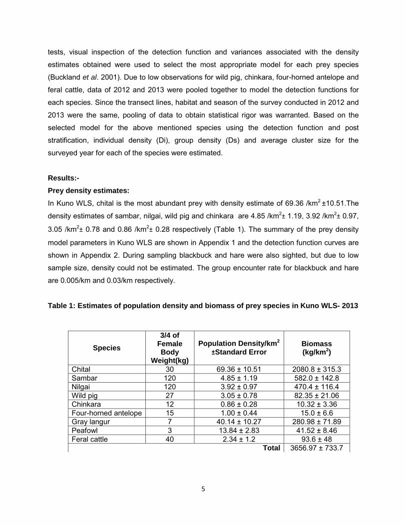
Results:-

Prey density estimates:

In Kuno WLS, chital is the most abundant prey with density estimate of 69.36 /km2 ±10.51.The

density estimates of sambar, nilgai, wild pig and chinkara are 4.85 /km2± 1.19, 3.92 /km2± 0.97,

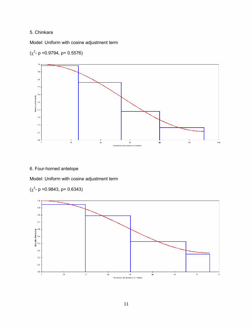
3.05 /km2± 0.78 and 0.86 /km2± 0.28 respectively (Table 1). The summary of the prey density

model parameters in Kuno WLS are shown in Appendix 1 and the detection function curves are

shown in Appendix 2. During sampling blackbuck and hare were also sighted, but due to low

sample size, density could not be estimated. The group encounter rate for blackbuck and hare

are 0.005/km and 0.03/km respectively.

Table 1: Estimates of population density and biomass of prey species in Kuno WLS- 2013

Species

3/4 of Female Body

Weight(kg)

Population Density/km2

±Standard Error Biomass (kg/km2)

Chital 30 69.36 ± 10.51 2080.8 ± 315.3 Sambar 120 4.85 ± 1.19 582.0 ± 142.8 Nilgai 120 3.92 ± 0.97 470.4 ± 116.4 Wild pig 27 3.05 ± 0.78 82.35 ± 21.06 Chinkara 12 0.86 ± 0.28 10.32 ± 3.36 Four-horned antelope 15 1.00 ± 0.44 15.0 ± 6.6 Gray langur 7 40.14 ± 10.27 280.98 ± 71.89 Peafowl 3 13.84 ± 2.83 41.52 ± 8.46 Feral cattle 40 2.34 ± 1.2 93.6 ± 48

Total 3656.97 ± 733.7

6

Biomass estimate: Using 3/4 of the adult body female body weight and density estimates of

prey species, the biomass in Kuno WLS for the year 2013 was estimated as 3657.97 kg /km2 ±

733.7 (Table 1).

Discussion: - Since 2005, WII has been conducting population estimation in Kuno WLS and

the data suggests an exponential increase in chital population (Table 2). The natural log

transformed population density estimates when regressed against time provide an estimate of

the realized rate of increase - r (Caughley, 1977). Chital population grew at a realized growth

rate (r) =0.35 (Fig.3) and finite rate of population change (λ) =1.42, where λ=er.

Table 2: Chital Population in Kuno WLS since 2005

S.no

Year

Chital population density/km2± Standard Error

1 2005 4.63 ± 1.03 (Banerjee, K. 2005) 2 2006 5.3 ± 1.78 (Jhala & Qureshi, 2006. Unpub.) 3 2011 35.87 ± 11.7 (Jhala et al., 2011) 4 2012 51.59 ± 8.84 (Jhala et al., 2012) 5 2013 69.36 ± 10.51 (Present survey)

The observed r is exceptionally high suggesting a growth rate close to intrinsic growth rate (rm).

The intrinsic growth rate for chital population is 0.44 using the equation rm=1.5W-0.36 (Caughley

and Krebs, 1983) where W is 3/4 of the adult body female body weight. The recovery of chital

population could be attributed to the good management practices and protection measures

implemented by the forest department in Kuno WLS.

Fig. 3: Chital Population in Kuno WLS since 2005

Chital density/km2 = 2.948e0.353Year

R² = 0.996

0

10

20

30

40

50

60

70

80

Po

pu

lati

on

De

nsi

ty/k

m2

Chital

2005 2006 2007 2008 2009 2010 2011 2012 2013 (1) (2) (3) (4) (5) (6) (7) (8) (9) Year

7

Literature cited:- Banerjee, K. (2005). Estimating the ungulate abundance and developing the habitat specific effective strip width models in Kuno Wildlife Sanctuary, Madhya Pradesh. Dissertation submitted in partial fulfillment of the degree of M.Sc. Forestry, Forest Research Institute, Dehradun. pp.170. Buckland S.T. (1985). Perpendicular distance models for line transect sampling. Biometrics. 41: 177-195. Buckland, S.T., Anderson, D.R., Burnham, K.P. and Laake, J.L. (1993) Distance Sampling: Estimating Abundance of Biological Populations. Chapman & Hall, London. Buckland, S.T., Anderson, D.R., Burnham, K.P., Laake, J.L., Borchers, D.L. and Thomas, L. (2001). Introduction to distance sampling: Estimating abundance of biological populations. Oxford University Press, New York. Caughley, G. (1977). Analysis of vertebrate populations. Wiley. 234p. New York. Caughley, G. & Krebs, C. (1983) Are big mammals simply little mammals writ large? Oecologia, 59, 7–17. Champion, H.G. and Seth, S.K. (1968). A revised survey of the forest types of India, Manager of publications, Government of India, New Delhi. Jhala, Y.V., Ranjitsinh, M. K. and Pabla, H.S, (2011). Action plan for the reintroduction of the cheetah (Acinonyx jubatus) in Kuno-Palpur Wildlife Sanctuary, Madhya Pradesh. Wildlife Institute of India, Dehradun. Karanth, K.U. and Nichols, J (Eds.). (2002). Monitoring tigers and their prey: A manual for researchers, managers and conservationists in tropical Asia. Centre for Wildlife Studies, Bangalore. Rodger, W.A., Panwar, H.S. and Mathur, V.B (2002). Wildlife Protected Area network in India: A reiew (Executive summary). Wildlife Institute of India, Dehradun. Thomas, L., Laake, J.L., Rexstad, E., Strindberg, S., Marques, F.F.C., Buckland, S.T., Borchers, D.L., Anderson, D.R., Burnham, K.P., Burt, M.L., Hedley, S.L., Pollard, J.H., Bishop, J.R.B., and Marques, T.A. (2009). Distance 6.0. Release 2. Research Unit for Wildlife Population Assessment, University of St. Andrews, UK.

8

Annexure 1: Summary of Prey Species Abundance Estimation Model Parameters in DISTANCE

Category Chital Sambar Nilgai

Wild

pig Chinkara

Four-

horned

antelope

Gray

Langur Peafowl

Feral

cattle

Number of Replicates 24 24 24 24 24 24 24 24 24 Number of Observations (n) 172 42 47 27 10 11 68 45 21 Effort (L) km 211.05 211.05 211.05 211.05 211.05 211.05 211.05 211.05 211.05

Density (Di) / km2

± Standard Error (S.E)

69.36

± 10.51

4.85

± 1.19

3.92

± 0.97

3.05

± 0.78

0.86

± 0.28

1.00

± 0.44

40.14

± 10.27

13.84

± 2.83

2.34

± 1.2

Di Coefficient of Variation (% CV) 15.15 24.54 24.66 25.55 32.19 43.74 25.58 20.46 51.1

Di - 95% Confidence Interval

51.44 -93.53

2.99 -7.86

2.42 - 6.35

1.85 -5.03

0.45 - 1.62

0.43 - 2.33

24.29 -66.32

9.19 -20.84

0.89 -6.18

Group Density(Ds)/km2 ± S.E

7.21 ± 0.85

2.3 ± 0.53

1.72 ± 0.39

1.23 ± 0.25

0.39 ± 0.12

0.54 ± 0.22

2.98 ± 0.67

4.6 ± 0.87

0.59 ± 0.22

Ds Coefficient of Variation (% CV) 11.86 22.93 22.52 20.51 30.07 40.33 22.58 18.87 37.51

Probability of Detection (p) 0.29 0.42 0.27 0.26 0.56 0.63 0.35 0.38 0.56 Goodness of Fit (Chi2-p) 0.96 0.87 0.92 0.99 0.96 0.98 0.98 0.9 0.96 Effective Strip Width (ESW) m 56.55 43.26 64.92 52.11 61.33 48.02 54.05 54.64 84.63

Group Encounter Rate 0.81 0.2 0.22 0.13 0.05 0.05 0.32 0.59 0.1

Model Half Normal Uniform Hazard

Rate Hazard Rate Uniform Uniform Hazard

Rate Half

Normal Uniform

Model Adjustment Term Cosine Cosine

Simple Polynomial Cosine Cosine Cosine Cosine Cosine Cosine

9

Annexure 2:

Detection Function Curves for Prey Species Abundance Estimation

1. Chital

Model: Half normal with cosine adjustment term

( 2- p =0.9649, p=0.2857 )

2. Sambar

Model: Uniform with cosine adjustment term

( 2- p =0.8682, p= 0.4184)

10

3. Nilgai

Model: Hazard rate with simple polynomial adjustment term

( 2- p =0.9211, p=0.2677 )

4. Wild pig

Model: Hazard rate with cosine adjustment term

( 2- p =0. 9889, p= 0. 0.2641)

11

5. Chinkara

Model: Uniform with cosine adjustment term

( 2- p =0.9794, p= 0.5576)

6. Four-horned antelope

Model: Uniform with cosine adjustment term

( 2- p =0.9843, p= 0.6343)

12

7. Gray langur:

Model: Hazard rate with cosine adjustment term

( 2- p =0.9819, p= 0. 3528)

8. Peafowl:

Model: Half normal with cosine adjustment term

( 2- p =0.9037, p= 0.383)

13

9. Feral cattle

Model: Uniform with cosine adjustment term

( 2- p =0.9591, p= 0. 5642)