ktiml.mff.cuni.czfink/teaching/optimization...Optimization methods NOPT048 Jirka Fink œfink/ Department of Theoretical Computer Science and Mathematical Logic Faculty of …

Optimization methodsNOPT048

Jirka Finkhttps://ktiml.mff.cuni.cz/˜fink/

Department of Theoretical Computer Science and Mathematical LogicFaculty of Mathematics and Physics

Charles University in Prague

Summer semester 2017/18Last change on May 22, 2018

License: Creative Commons BY-NC-SA 4.0

Jirka Fink Optimization methods 1

Jirka Fink: Optimization methods

Plan of the lectureLinear and integer optimization

Convex sets and Minkowski-Weyl theorem

Simplex methods

Duality of linear programming

Ellipsoid method

Unimodularity

Minimal weight maximal matching

Matroid

Cut and bound method



General informationE-mail [email protected]

Homepage https://ktiml.mff.cuni.cz/˜fink/

Consultations Individual schedule

ExaminationTutorial conditions

TestsTheoretical homeworksPractical homeworks

Pass the exam



LiteratureA. Schrijver: Theory of linear and integer programming, John Wiley, 1986

W. J .Cook, W. H. Cunningham, W. R. Pulleyblank, A. Schrijver: CombinatorialOptimization, John Wiley, 1997

J. Matousek, B. Gartner: Understanding and using linear programming, Springer,2006.

J. Matousek: Introduction to Discrete Geometry. ITI Series 2003-150, MFF UK,2003


Outline

1 Linear programming

2 Linear, affine and convex sets

3 Convex polyhedron

4 Simplex method

5 Duality of linear programming

6 Ellipsoid method

7 Matching


Example of linear programming: Optimized diet

Express using linear programming the following problemFind the cheapest vegetable salad from carrots, white cabbage and cucumberscontaining required amount the vitamins A and C and dietary fiber.

Food Carrot White cabbage Cucumber Required per mealVitamin A [mg/kg] 35 0.5 0.5 0.5 mgVitamin C [mg/kg] 60 300 10 15 mgDietary fiber [g/kg] 30 20 10 4 gPrice [EUR/kg] 0.75 0.5 0.15

Formulation using linear programming

Carrot White cabbage CucumberMinimize 0.75xxx1 + 0.5xxx2 + 0.15xxx3 Costsubject to 35xxx1 + 0.5xxx2 + 0.5xxx3 ≥ 0.5 Vitamin A

60xxx1 + 300xxx2 + 10xxx3 ≥ 15 Vitamin C30xxx1 + 20xxx2 + 10xxx3 ≥ 4 Dietary fiber

xxx1,xxx2,xxx3 ≥ 0


Matrix notation of the linear programming problem

Formulation using linear programming

Minimize 0.75xxx1 + 0.5xxx2 + 0.15xxx3

subject to 35xxx1 + 0.5xxx2 + 0.5xxx3 ≥ 0.560xxx1 + 300xxx2 + 10xxx3 ≥ 1530xxx1 + 20xxx2 + 10xxx3 ≥ 4

xxx1,xxx2,xxx3 ≥ 0

Matrix notationMinimize 0.75

0.50.15

T xxx1

xxx2

xxx3

Subject to 35 0.5 0.5

60 300 1030 20 10

xxx1

xxx2

xxx3

≥0.5

154

and xxx1,xxx2,xxx3 ≥ 0


Notation: Vector and matrix

ScalarA scalar is a real number. Scalars are written as a, b, c, etc.

VectorA vector is an n-tuple of real numbers. Vectors are written as ccc, xxx , yyy , etc. Usually,vectors are column matrices of type n × 1.

MatrixA matrix of type m × n is a rectangular array of m rows and n columns of real numbers.Matrices are written as A, B, C, etc.

Special vectors000 and 111 are vectors of zeros and ones, respectively.

Transpose

The transpose of a matrix A is matrix AT created by reflecting A over its main diagonal.The transpose of a column vector xxx is the row vector xxxT.


https://ktiml.mff.cuni.cz/~fink/

https://creativecommons.org/licenses/by-nc-sa/4.0/

Notation: Matrix product

Elements of a vector and a matrixThe i-th element of a vector xxx is denoted by xxx i .

The (i , j)-th element of a matrix A is denoted by Ai,j .

The i-th row of a matrix A is denoted by Ai,?.

The j-th column of a matrix A is denoted by A?,j .

Dot product of vectors

The dot product (also called inner product or scalar product) of vectors xxx ,yyy ∈ Rn is thescalar xxxTyyy =

∑ni=1 xxx iyyy i .

Product of a matrix and a vector

The product Axxx of a matrix A ∈ Rm×n of type m × n and a vector xxx ∈ Rn is a vectoryyy ∈ Rm such that yyy i = Ai,?xxx for all i = 1, . . . ,m.

Product of two matrices

The product AB of a matrix A ∈ Rm×n and a matrix B ∈ Rn×k a matrix C ∈ Rm×k suchthat C?,j = AB?,j for all j = 1, . . . , k .


Notation: System of linear equations and inequalities

Equality and inequality of two vectors

For vectors xxx ,yyy ∈ Rn we denote

xxx = yyy if xxx i = yyy i for every i = 1, . . . , n and

xxx ≤ yyy if xxx i ≤ yyy i for every i = 1, . . . , n.

System of linear equations

Given a matrix A ∈ Rm×n of type m × n and a vector bbb ∈ Rm, the formula Axxx = bbbmeans a system of m linear equations where xxx is a vector of n real variables.

System of linear inequalities

Given a matrix A ∈ Rm×n of type and a vector bbb ∈ Rm, the formula Axxx ≤ bbb means asystem of m linear inequalities where xxx is a vector of n real variables.

Example: System of linear inequalities in two different notations

2xxx1 + xxx2 + xxx3 ≤ 142xxx1 + 5xxx2 + 5xxx3 ≤ 30

(2 1 12 5 5

)xxx1

xxx2

xxx3

≤ (1430

)


Optimization

Mathematical optimizationMathematical optimization is the selection of a best element (with regard to somecriteria) from some set of available alternatives.

Examples

Minimize x2 + y2 where (x , y) ∈ R2

Maximal matching in a graph

Minimal spanning tree

Shortest path between given two vertices

Optimization problemGiven a set of solutions M and an objective function f : M → R, optimization problem isfinding a solution x ∈ M with the maximal (or minimal) objective value f (x) among allsolutions of M.

Duality between minimization and maximizationIf minx∈M f (x) exists, then also maxx∈M −f (x) exists and−minx∈M f (x) = maxx∈M −f (x).


Linear Programming

Linear programming problemA linear program is the problem of maximizing (or minimizing) a given linear functionover the set of all vectors that satisfy a given system of linear equations andinequalities.

Equation form: mincccTxxx subject to Axxx = bbb,xxx ≥ 000

Canonical form: maxcccTxxx subject to Axxx ≤ bbb,

where ccc ∈ Rn, bbb ∈ Rm, A ∈ Rm×n a xxx ∈ Rn.

Conversion from the equation form to the canonical form

max−cccTxxx subject to Axxx ≤ bbb,−Axxx ≤ −bbb,−xxx ≤ 000

Conversion from the canonical form to the equation form

min−cccTxxx ′ + cccTxxx ′′ subject to Axxx ′ − Axxx ′′ + Ixxx ′′′ = bbb, xxx ′,xxx ′′,xxx ′′′ ≥ 000


Terminology

Basic terminologyNumber of variables: n

Number of constrains: m

Solution: an arbritrary vector xxx of Rn

Objective function: a function to be minimized or maximized, e.g. maxcccTxxx

Feasible solution: a solution satisfying all constrains, e.g. Axxx ≤ bbb

Optimal solution: a feasible solution maximizing cccTxxx

Infeasible problem: a problem having no feasible solution

Unbounded problem: a problem having a feasible solution with arbitrary largevalue of given objective function

Polyhedron: a set of points xxx ∈ Rn satisfying Axxx ≤ bbb for some A ∈ Rm×n andbbb ∈ Rm

Polytope: a bounded polyhedron


Example of linear programming: Network flow

Network flow problem

Given a direct graph (V ,E) with capacities ccc ∈ RE and a source s ∈ V and a sinkt ∈ V , find the maximal flow from s to t satisfying the flow conservation and capacityconstrains.

Formulation using linear programmingVariables: Flow xxxe for every edge e ∈ E

Capacity constrains: 000 ≤ xxx ≤ ccc

Flow conservation:∑

uv∈E xxxuv =∑

vw∈E xxxvw for every v ∈ V \ {s, t}Objective function: Maximize

∑sw∈E xxxsw −

∑us∈E xxxus

Matrix notation• Add an auxiliary edge xxx ts with a sufficiently large capacity cccts

Objective function: maxxxx ts

Flow conservation: Axxx = 000 where A is the incidence matrix

Capacity constrains: xxx ≤ ccc and xxx ≥ 0


Graphical method: Set of feasible solutions

ExampleDraw the set of all feasible solutions (xxx1,xxx2) satisfying the following conditions.

xxx1 + 6xxx2 ≤ 154xxx1 − xxx2 ≤ 10−xxx1 + xxx2 ≤ 1

xxx1,xxx2 ≥ 0

Solution

xxx1 ≥ 0 xxx2 − xxx1 ≤ 1

xxx1 + 6xxx2 ≤ 15

4xxx1 − xxx2 ≤ 10

xxx2 ≥ 0

(0, 0)


Graphical method: Optimal solution

ExampleFind the optimal solution of the following problem.

Maximize xxx1 + xxx2


xxx1,xxx2 ≥ 0

Solution

(0, 0)

(3, 2)

(1, 1)

cccTxxx = 0

cccTxxx = 1

cccTxxx = 2

cccTxxx = 5


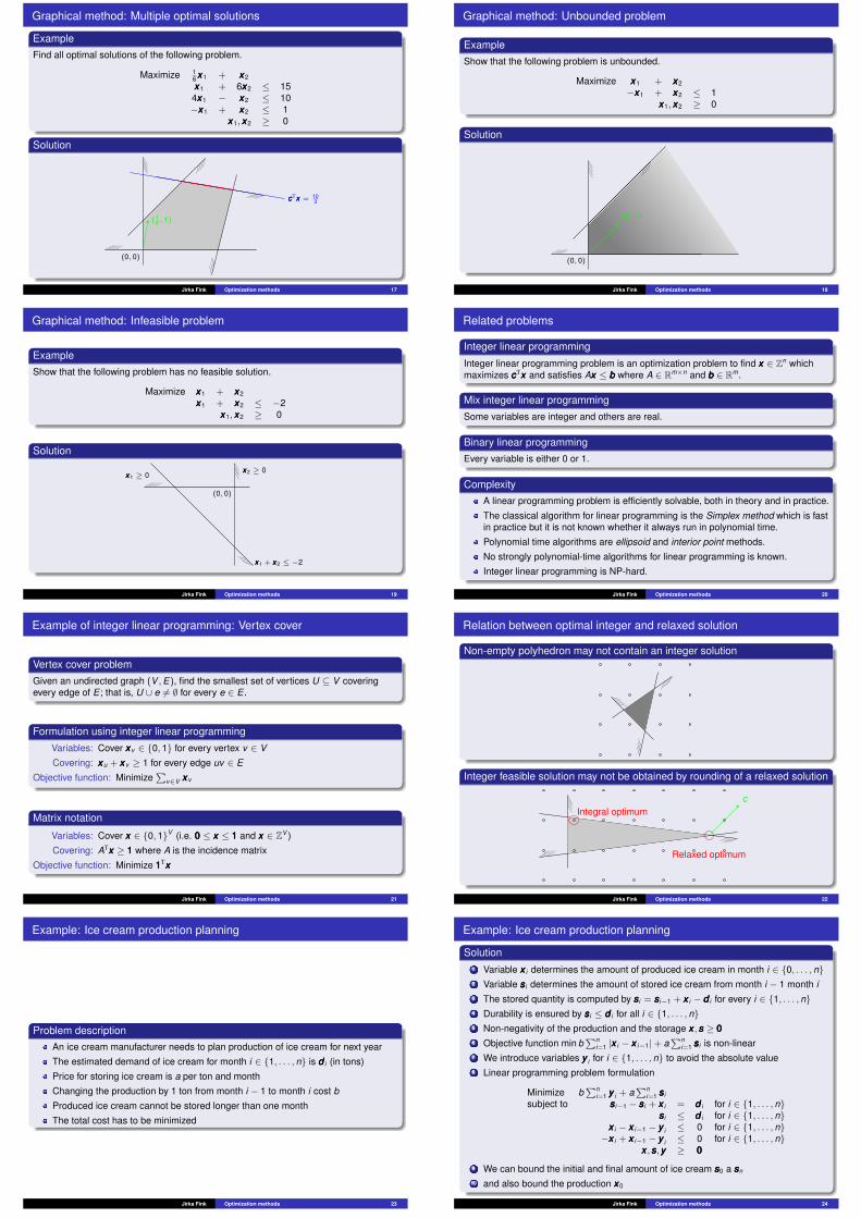
Graphical method: Multiple optimal solutions

ExampleFind all optimal solutions of the following problem.

Maximize 16xxx1 + xxx2


xxx1,xxx2 ≥ 0

Solution

(0, 0)

( 16 , 1)

cccTxxx = 103


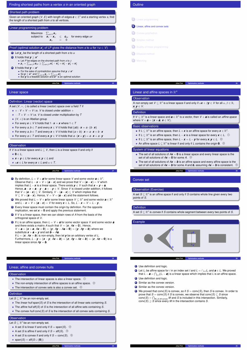
Graphical method: Unbounded problem

ExampleShow that the following problem is unbounded.


−xxx1 + xxx2 ≤ 1xxx1,xxx2 ≥ 0

Solution

(0, 0)

(1, 1)


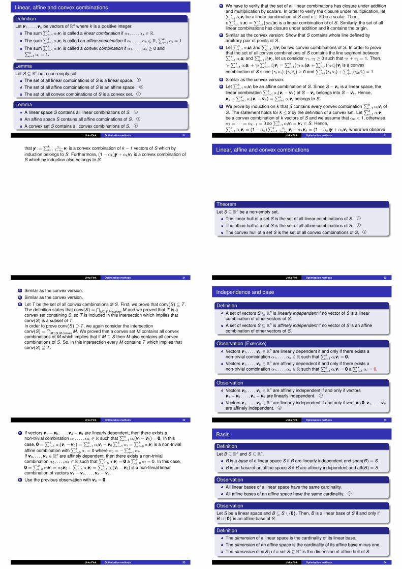
Graphical method: Infeasible problem

ExampleShow that the following problem has no feasible solution.


xxx1 + xxx2 ≤ −2xxx1,xxx2 ≥ 0

Solution

xxx2 ≥ 0xxx1 ≥ 0

xxx1 + xxx2 ≤ −2

(0, 0)


Related problems

Integer linear programming

Integer linear programming problem is an optimization problem to find xxx ∈ Zn whichmaximizes cccTxxx and satisfies Axxx ≤ bbb where A ∈ Rm×n and bbb ∈ Rm.

Mix integer linear programmingSome variables are integer and others are real.

Binary linear programmingEvery variable is either 0 or 1.

ComplexityA linear programming problem is efficiently solvable, both in theory and in practice.

The classical algorithm for linear programming is the Simplex method which is fastin practice but it is not known whether it always run in polynomial time.

Polynomial time algorithms are ellipsoid and interior point methods.

No strongly polynomial-time algorithms for linear programming is known.

Integer linear programming is NP-hard.


Example of integer linear programming: Vertex cover

Vertex cover problemGiven an undirected graph (V ,E), find the smallest set of vertices U ⊆ V coveringevery edge of E ; that is, U ∪ e 6= ∅ for every e ∈ E .

Formulation using integer linear programmingVariables: Cover xxxv ∈ {0, 1} for every vertex v ∈ V

Covering: xxxu + xxxv ≥ 1 for every edge uv ∈ E

Objective function: Minimize∑

v∈V xxxv

Matrix notation

Variables: Cover xxx ∈ {0, 1}V (i.e. 000 ≤ xxx ≤ 111 and xxx ∈ ZV )

Covering: ATxxx ≥ 111 where A is the incidence matrix

Objective function: Minimize 111Txxx


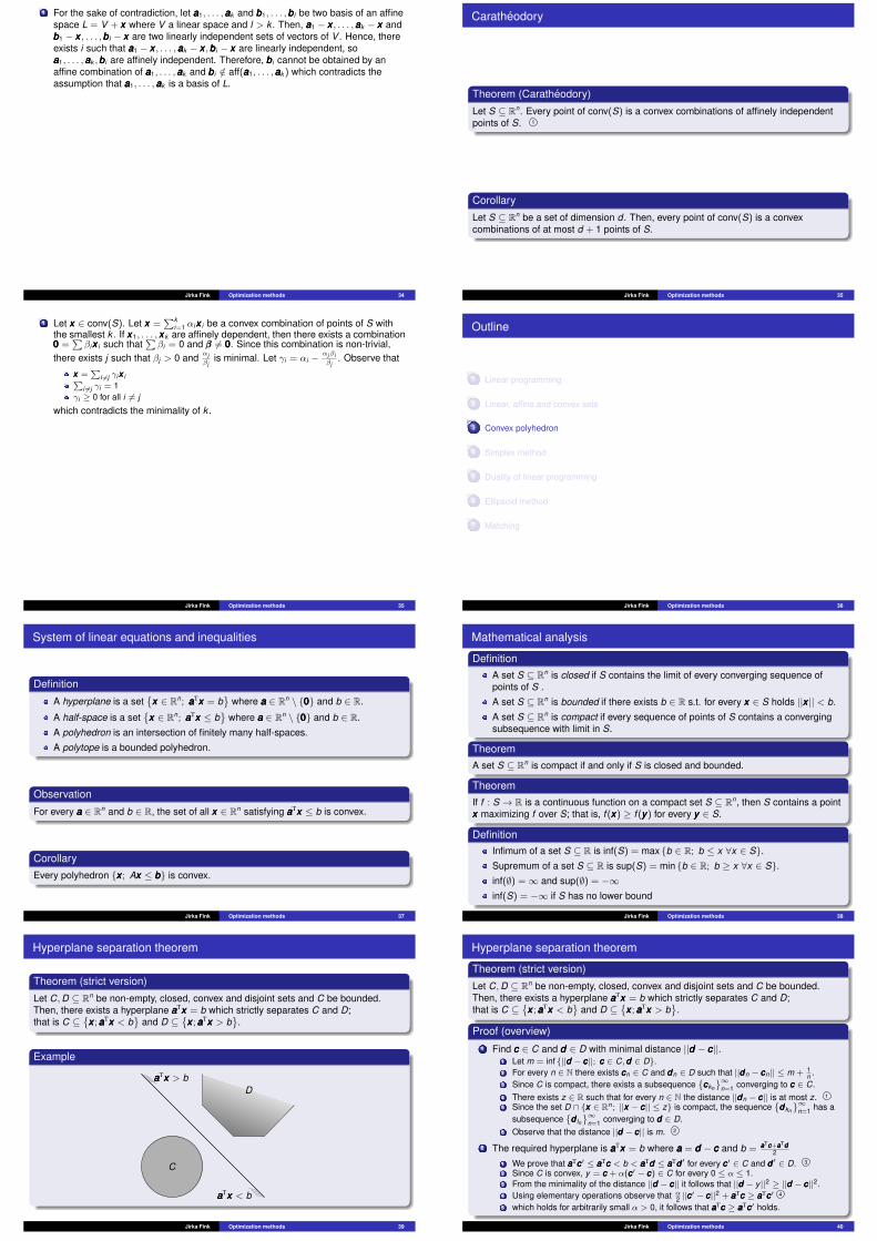
Relation between optimal integer and relaxed solution

Non-empty polyhedron may not contain an integer solution

Integer feasible solution may not be obtained by rounding of a relaxed solution

c

Relaxed optimum

Integral optimum


Example: Ice cream production planning

Problem descriptionAn ice cream manufacturer needs to plan production of ice cream for next year

The estimated demand of ice cream for month i ∈ {1, . . . , n} is ddd i (in tons)

Price for storing ice cream is a per ton and month

Changing the production by 1 ton from month i − 1 to month i cost b

Produced ice cream cannot be stored longer than one month

The total cost has to be minimized


Example: Ice cream production planning

Solution1 Variable xxx i determines the amount of produced ice cream in month i ∈ {0, . . . , n}2 Variable sssi determines the amount of stored ice cream from month i − 1 month i3 The stored quantity is computed by sssi = sssi−1 + xxx i − ddd i for every i ∈ {1, . . . , n}4 Durability is ensured by sssi ≤ ddd i for all i ∈ {1, . . . , n}5 Non-negativity of the production and the storage xxx ,sss ≥ 0006 Objective function min b

∑ni=1 |xxx i − xxx i−1|+ a

∑ni=1 sssi is non-linear

7 We introduce variables yyy i for i ∈ {1, . . . , n} to avoid the absolute value8 Linear programming problem formulation

Minimize b∑n

i=1 yyy i + a∑n

i=1 sssi

subject to sssi−1 − sssi + xxx i = ddd i for i ∈ {1, . . . , n}sssi ≤ ddd i for i ∈ {1, . . . , n}

xxx i − xxx i−1 − yyy i ≤ 0 for i ∈ {1, . . . , n}−xxx i + xxx i−1 − yyy i ≤ 0 for i ∈ {1, . . . , n}

xxx ,sss,yyy ≥ 000

9 We can bound the initial and final amount of ice cream sss0 a sssn

10 and also bound the production xxx0


Finding shortest paths from a vertex s in an oriented graph

Shortest path problem

Given an oriented graph (V ,E) with length of edges ccc ∈ Zn and a starting vertex s, findthe length of a shortest path from s to all vertices.

Linear programming problem

Maximize∑

u∈V xxxu

subject to xxxv − xxxu ≤ cccuv for every edge uvxxxs = 0

Proof (optimal solution xxx?u of LP gives the distance from s to u for ∀u ∈ V )1 Let yyyu be the length of a shortest path from s to u2 It holds that yyy ≥ xxx?

Let P be edges on the shortest path from s to zyyyz =

∑uv∈P cccuv ≥

∑uv∈P xxx?v − xxx?u = xxx?z − yyy?s = xxx?z

3 It holds that yyy = xxx?

For the sake of contradiction assume that yyy 6= xxx?So yyy ≥ xxx? and

∑u∈V yyyu >

∑u∈V xxx?u

But yyy is a feasible solution and xxx? is an optimal solution


Outline



3 Convex polyhedron

4 Simplex method


6 Ellipsoid method

7 Matching


Linear space

Definition: Linear (vector) spaceA set (V ,+, ·) is called a linear (vector) space over a field T if

+ : V × V → V i.e. V is closed under addition +

· : T × V → V i.e. V is closed under multiplication by T

(V ,+) is an Abelian group

For every xxx ∈ V it holds that 1 · xxx = xxx where 1 ∈ T

For every a, b ∈ T and every xxx ∈ V it holds that (ab) · xxx = a · (b · xxx)

For every a, b ∈ T and every xxx ∈ V it holds that (a + b) · xxx = a · xxx + b · xxxFor every a ∈ T and every xxx ,yyy ∈ V it holds that a · (xxx + yyy) = a · xxx + a · yyy

ObservationIf V is a linear space and L ⊆ V , then L is a linear space if and only if

000 ∈ L,

xxx + yyy ∈ L for every xxx ,yyy ∈ L and

αxxx ∈ L for every xxx ∈ L and α ∈ T .


Linear and affine spaces in Rn

ObservationA non-empty set V ⊆ Rn is a linear space if and only if αxxx + βyyy ∈ V for all α, β ∈ R,xxx ,yyy ∈ V .

DefinitionIf V ⊆ Rn is a linear space and aaa ∈ Rn is a vector, then V + aaa is called an affine spacewhere V + aaa = {xxx + aaa; xxx ∈ V}.

Basic observationsIf L ⊆ Rn is an affine space, then L + xxx is an affine space for every xxx ∈ Rn.

If L ⊆ Rn is an affine space, then L− xxx is a linear space for every xxx ∈ L. 1

If L ⊆ Rn is an affine space, then L− xxx = L− yyy for every xxx ,yyy ∈ L. 2

An affine space L ⊆ Rn is linear if and only if L contains the origin 000. 3

System of linear equationsThe set of all solutions of Axxx = 000 is a linear space and every linear space is theset of all solutions of Axxx = 000 for some A. 4

The set of all solutions of Axxx = bbb is an affine space and every affine space is theset of all solutions of Axxx = bbb for some A and bbb, assuming Axxx = bbb is consistent. 5


1 By definition, L = V + aaa for some linear space V and some vector aaa ∈ Rn.Observe that L− xxx = V + (aaa− xxx) and we prove that V + (aaa− xxx) = V whichimplies that L− xxx is a linear space. There exists yyy ∈ V such that xxx = yyy + aaa.Hence, aaa− xxx = aaa− yyy − aaa = −yyy ∈ V . Since V is closed under addition, it followsthat V + (aaa− xxx) ⊆ V . Similarly, V − (aaa− xxx) ⊆ V which implies thatV ⊆ V + (aaa− xxx). Hence, V = V + (aaa− xxx) and the statement follows.

2 We proved that L = V + aaa for some linear space V ⊆ Rn and some vector aaa ∈ Rn

and L− xxx = V + (aaa− xxx) = V for every xxx ∈ L. So, L− xxx = V = L− yyy .3 Every linear space must contain the origin by definition. For the opposite

implication, we set xxx = 000 and apply the previous statement.4 If V is a linear space, then we can obtain rows of A from the basis of the

orthogonal space of V .5 If L is an affine space, then L = V + aaa for some vector space V and some vector aaa

and there exists a matrix A such that V = {xxx ; Axxx = 000}. Hence,V + aaa = {xxx + aaa; Axxx = 000} = {yyy ; Ayyy − Aaaa = 000} = {yyy ; Ayyy = bbb} where wesubstitute xxx + aaa = yyy and set bbb = Aaaa.If L = {xxx ; Axxx = bbb} is non-empty, then let yyy be an arbitrary vertex of L.Furthermore, L− yyy = {xxx − yyy ; Axxx = bbb} = {zzz; Ayyy + Azzz = bbb} = {zzz; Azzz = 000} is alinear space since Ayyy = bbb.


Convex set

Observation (Exercise)

A set S ⊆ Rn is an affine space if and only if S contains whole line given every twopoints of S.

DefinitionA set S ⊆ Rn is convex if S contains whole segment between every two points of S.

Example

a

b

u

v


Linear, affine and convex hulls

Observation

The intersection of linear spaces is also a linear space. 1

The non-empty intersection of affine spaces is an affine space. 2

The intersection of convex sets is also a convex set. 3

DefinitionLet S ⊆ Rn be an non-empty set.

The linear hull span(S) of S is the intersection of all linear sets containing S.

The affine hull aff(S) of S is the intersection of all affine sets containing S.

The convex hull conv(S) of S is the intersection of all convex sets containing S.

ObservationLet S ⊆ Rn be an non-empty set.

A set S is linear if and only if S = span(S). 4

A set S is affine if and only if S = aff(S). 5

A set S is convex if and only if S = conv(S). 6

span(S) = aff(S ∪ {000})


1 Use definition and logic.2 Let Li be affine space for i in an index set I and L = ∩i∈ILi and aaa ∈ L. We proved

that L− aaa =⋂

i∈I(Li − aaa) is a linear space which implies that L is an affine space.3 Use definition and logic.4 Similar as the convex version.5 Similar as the convex version.6 We proved that conv(S) is convex, so if S = conv(S), then S is convex. In order to

prove that S = conv(S) if S is convex, we observe that conv(S) ⊆ S sinceconv(S) =

⋂M⊇S,M convex M and S is included in this intersection. Similarly,

conv(S) ⊇ S since every M in the intersection contains S.


Linear, affine and convex combinations

DefinitionLet vvv1, . . . ,vvv k be vectors of Rn where k is a positive integer.

The sum∑k

i=1 αivvv i is called a linear combination if α1, . . . , αk ∈ R.

The sum∑k

i=1 αivvv i is called an affine combination if α1, . . . , αk ∈ R,∑k

i=1 αi = 1.

The sum∑k

i=1 αivvv i is called a convex combination if α1, . . . , αk ≥ 0 and∑ki=1 αi = 1.

LemmaLet S ⊆ Rn be a non-empty set.

The set of all linear combinations of S is a linear space. 1

The set of all affine combinations of S is an affine space. 2

The set of all convex combinations of S is a convex set. 3

Lemma

A linear space S contains all linear combinations of S. 4

An affine space S contains all affine combinations of S. 5

A convex set S contains all convex combinations of S. 6


1 We have to verify that the set of all linear combinations has closure under additionand multiplication by scalars. In order to verify the closure under multiplication, let∑k

i=1 αivvv i be a linear combination of S and c ∈ R be a scalar. Then,c∑k

i=1 αivvv i =∑k

i=1(cαi )vvv i is a linear combination of of S. Similarly, the set of alllinear combinations has closure under addition and it contains the origin.

2 Similar as the convex version: Show that S contains whole line defined byarbitrary pair of points of S.

3 Let∑k

i=1 αiuuu i and∑l

j=1 βjvvv j be two convex combinations of S. In order to provethat the set of all convex combinations of S contains the line segment between∑k

i=1 αiuuu i and∑l

j=1 βjvvv j , let us consider γ1, γ2 ≥ 0 such that γ1 + γ2 = 1. Then,γ1∑k

i=1 αiuuu i + γ2∑l

j=1 βjvvv j =∑k

i=1(γ1αi )uuu i +∑l

j=1(γ2βj )vvv j is a convexcombination of S since (γ1αi ), (γ2βj ) ≥ 0 and

∑ki=1(γ1αi ) +

∑lj=1(γ2βj ) = 1.

4 Similar as the convex version.5 Let

∑ki=1 αivvv i be an affine combination of S. Since S − vvv k is a linear space, the

linear combination∑k

i=1 αi (vvv i − vvv k ) of S − vvv k belongs into S − vvv k . Hence,vvv k +

∑ki=1 αi (vvv i − vvv k ) =

∑ki=1 αivvv i belongs to S.

6 We prove by induction on k that S contains every convex combination∑k

i=1 αivvv i ofS. The statement holds for k ≤ 2 by the definition of a convex set. Let

∑ki=1 αivvv i

be a convex combination of k vectors of S and we assume that αk < 1, otherwiseα1 = · · · = αk−1 = 0 so

∑ki=1 αivvv i = vvv k ∈ S. Hence,∑k

i=1 αivvv i = (1− αk )∑k

i=1αi

1−αkvvv i + αkvvv k = (1− αk )yyy + αkvvv k where we observe


that yyy :=∑k

i=1αi

1−αkvvv i is a convex combination of k − 1 vectors of S which by

induction belongs to S. Furthermore, (1− αk )yyy + αkvvv k is a convex combination ofS which by induction also belongs to S.


Linear, affine and convex combinations

TheoremLet S ⊆ Rn be a non-empty set.

The linear hull of a set S is the set of all linear combinations of S. 1

The affine hull of a set S is the set of all affine combinations of S. 2

The convex hull of a set S is the set of all convex combinations of S. 3


1 Similar as the convex version.2 Similar as the convex version.3 Let T be the set of all convex combinations of S. First, we prove that conv(S) ⊆ T .

The definition states that conv(S) =⋂

M⊇S,M convex M and we proved that T is aconvex set containing S, so T is included in this intersection which implies thatconv(S) is a subset of T .In order to prove conv(S) ⊇ T , we again consider the intersectionconv(S) =

⋂M⊇S,M convex M. We proved that a convex set M contains all convex

combinations of M which implies that if M ⊇ S then M also contains all convexcombinations of S. So, in this intersection every M contains T which implies thatconv(S) ⊇ T .


Independence and base

DefinitionA set of vectors S ⊆ Rn is linearly independent if no vector of S is a linearcombination of other vectors of S.

A set of vectors S ⊆ Rn is affinely independent if no vector of S is an affinecombination of other vectors of S.


Vectors vvv1, . . . ,vvv k ∈ Rn are linearly dependent if and only if there exists anon-trivial combination α1, . . . , αk ∈ R such that

∑ki=1 αivvv i = 000.

Vectors vvv1, . . . ,vvv k ∈ Rn are affinely dependent if and only if there exists anon-trivial combination α1, . . . , αk ∈ R such that

∑ki=1 αivvv i = 000 a

∑ki=1 αi = 0.

ObservationVectors vvv0, . . . ,vvv k ∈ Rn are affinely independent if and only if vectorsvvv1 − vvv0, . . . ,vvv k − vvv0 are linearly independent. 1

Vectors vvv1, . . . ,vvv k ∈ Rn are linearly independent if and only if vectors 000,vvv1, . . . ,vvv k

are affinely independent. 2


1 If vectors vvv1 − vvv0, . . . ,vvv k − vvv0 are linearly dependent, then there exists anon-trivial combination α1, . . . , αk ∈ R such that

∑ki=1 αi (vvv i − vvv0) = 000. In this

case, 000 =∑k

i=1 αi (vvv i − vvv0) =∑k

i=1 αivvv i − vvv0∑k

i=1 αi =∑k

i=0 αivvv i is a non-trivialaffine combination with

∑ki=0 αi = 0 where α0 = −

∑ki=1 αi .

If vvv0, . . . ,vvv k ∈ Rn are affinely dependent, then there exists a non-trivialcombination α0, . . . , αk ∈ R such that

∑ki=0 αivvv i = 000 a

∑ki=0 αi = 0. In this case,

000 =∑k

i=0 αivvv i = α0vvv0 +∑k

i=1 αivvv i =∑k

i=1 αi (vvv i − vvv0) is a non-trivial linearcombination of vectors vvv1 − vvv0, . . . ,vvv k − vvv0.

2 Use the previous observation with vvv0 = 000.


Basis

DefinitionLet B ⊆ Rn and S ⊆ Rn.

B is a base of a linear space S if B are linearly independent and span(B) = S.

B is an base of an affine space S if B are affinely independent and aff(B) = S.

ObservationAll linear bases of a linear space have the same cardinality.

All affine bases of an affine space have the same cardinality. 1

ObservationLet S be a linear space and B ⊆ S \ {000}. Then, B is a linear base of S if and only ifB ∪ {000} is an affine base of S.

DefinitionThe dimension of a linear space is the cardinality of its linear base.

The dimension of an affine space is the cardinality of its affine base minus one.

The dimension dim(S) of a set S ⊆ Rn is the dimension of affine hull of S.


1 For the sake of contradiction, let aaa1, . . . ,aaak and bbb1, . . . ,bbbl be two basis of an affinespace L = V + xxx where V a linear space and l > k . Then, aaa1 − xxx , . . . ,aaak − xxx andbbb1 − xxx , . . . ,bbbl − xxx are two linearly independent sets of vectors of V . Hence, thereexists i such that aaa1 − xxx , . . . ,aaak − xxx ,bbbi − xxx are linearly independent, soaaa1, . . . ,aaak ,bbbi are affinely independent. Therefore, bbbi cannot be obtained by anaffine combination of aaa1, . . . ,aaak and bbbi /∈ aff(aaa1, . . . ,aaak ) which contradicts theassumption that aaa1, . . . ,aaak is a basis of L.


Caratheodory

Theorem (Caratheodory)

Let S ⊆ Rn. Every point of conv(S) is a convex combinations of affinely independentpoints of S. 1

Corollary

Let S ⊆ Rn be a set of dimension d . Then, every point of conv(S) is a convexcombinations of at most d + 1 points of S.


1 Let xxx ∈ conv(S). Let xxx =∑k

i=1 αixxx i be a convex combination of points of S withthe smallest k . If xxx1, . . . ,xxxk are affinely dependent, then there exists a combination000 =

∑βixxx i such that

∑βi = 0 and βββ 6= 000. Since this combination is non-trivial,

there exists j such that βj > 0 and αjβj

is minimal. Let γi = αi −αjβiβj

. Observe that

xxx =∑

i 6=j γixxx i∑i 6=j γi = 1

γi ≥ 0 for all i 6= j

which contradicts the minimality of k .


Outline



3 Convex polyhedron

4 Simplex method


6 Ellipsoid method

7 Matching


System of linear equations and inequalities

Definition

A hyperplane is a set{xxx ∈ Rn; aaaTxxx = b

}where aaa ∈ Rn \ {000} and b ∈ R.

A half-space is a set{xxx ∈ Rn; aaaTxxx ≤ b

}where aaa ∈ Rn \ {000} and b ∈ R.

A polyhedron is an intersection of finitely many half-spaces.

A polytope is a bounded polyhedron.

Observation

For every aaa ∈ Rn and b ∈ R, the set of all xxx ∈ Rn satisfying aaaTxxx ≤ b is convex.

CorollaryEvery polyhedron {xxx ; Axxx ≤ bbb} is convex.


Mathematical analysis

DefinitionA set S ⊆ Rn is closed if S contains the limit of every converging sequence ofpoints of S .

A set S ⊆ Rn is bounded if there exists b ∈ R s.t. for every xxx ∈ S holds ||xxx || < b.

A set S ⊆ Rn is compact if every sequence of points of S contains a convergingsubsequence with limit in S.

TheoremA set S ⊆ Rn is compact if and only if S is closed and bounded.

TheoremIf f : S → R is a continuous function on a compact set S ⊆ Rn, then S contains a pointxxx maximizing f over S; that is, f (xxx) ≥ f (yyy) for every yyy ∈ S.

DefinitionInfimum of a set S ⊆ R is inf(S) = max {b ∈ R; b ≤ x ∀x ∈ S}.Supremum of a set S ⊆ R is sup(S) = min {b ∈ R; b ≥ x ∀x ∈ S}.inf(∅) =∞ and sup(∅) = −∞inf(S) = −∞ if S has no lower bound


Hyperplane separation theorem

Theorem (strict version)

Let C,D ⊆ Rn be non-empty, closed, convex and disjoint sets and C be bounded.Then, there exists a hyperplane aaaTxxx = b which strictly separates C and D;that is C ⊆

{xxx ;aaaTxxx < b

}and D ⊆

{xxx ;aaaTxxx > b

}.

Example

aaaTxxx > b

aaaTxxx < b

D

C


Hyperplane separation theorem

Theorem (strict version)

Let C,D ⊆ Rn be non-empty, closed, convex and disjoint sets and C be bounded.Then, there exists a hyperplane aaaTxxx = b which strictly separates C and D;that is C ⊆

{xxx ;aaaTxxx < b

}and D ⊆

{xxx ;aaaTxxx > b

}.

Proof (overview)1 Find ccc ∈ C and ddd ∈ D with minimal distance ||ddd − ccc||.

1 Let m = inf {||ddd − ccc||; ccc ∈ C,ddd ∈ D}.2 For every n ∈ N there exists cccn ∈ C and dddn ∈ D such that ||dddn − cccn|| ≤ m + 1

n .3 Since C is compact, there exists a subsequence

{ccckn

}∞n=1 converging to ccc ∈ C.

4 There exists z ∈ R such that for every n ∈ N the distance ||dddn − ccc|| is at most z. 1

5 Since the set D ∩ {xxx ∈ Rn; ||xxx − ccc|| ≤ z} is compact, the sequence{

dddkn

}∞n=1 has a

subsequence{

ddd ln}∞

n=1 converging to ddd ∈ D.6 Observe that the distance ||ddd − ccc|| is m. 2

2 The required hyperplane is aaaTxxx = b where aaa = ddd − ccc and b = aaaTccc+aaaTddd2

1 We prove that aaaTccc′ ≤ aaaTccc < b < aaaTddd ≤ aaaTddd ′ for every ccc′ ∈ C and ddd ′ ∈ D. 3

2 Since C is convex, y = ccc + α(ccc′ − ccc) ∈ C for every 0 ≤ α ≤ 1.3 From the minimality of the distance ||ddd − ccc|| it follows that ||ddd − y ||2 ≥ ||ddd − ccc||2.4 Using elementary operations observe that α2 ||ccc

′ − ccc||2 + aaaTccc ≥ aaaTccc′ 4

5 which holds for arbitrarily small α > 0, it follows that aaaTccc ≥ aaaTccc′ holds.


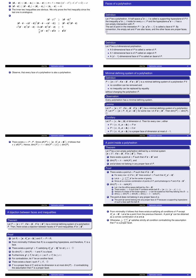
1 ||dddn − ccc|| ≤ ||dddn − cccn||+ ||cccn − ccc|| ≤ m + 1 + max {||c′ − c′′||; c′, c′′ ∈ C} = z2 ||ddd − ccc|| ≤ ||ddd − ddd ln ||+ ||ddd ln − ccc ln ||+ ||ccc ln − ccc|| → m3 The inner two inequalities are obvious. We only prove the first inequality since the

last one is analogous.4

||ddd − y ||2 ≥ ||ddd − ccc||2

(ddd − ccc − α(ccc′ − ccc))T(ddd − ccc − α(ccc′ − ccc)) ≥ (ddd − ccc)T(ddd − ccc)

α2(ccc′ − ccc)T(ccc′ − ccc)− 2α(ddd − ccc)T(ccc′ − ccc) ≥ 0

α

2||ccc′ − ccc||2 + aaaTccc ≥ aaaTccc′


Faces of a polyhedron

Definition

Let P be a polyhedron. A half-space αααTxxx ≤ β is called a supporting hyperplane of P ifthe inequality αααTxxx ≤ β holds for every x ∈ P and the hyperplane αααTxxx = β has anon-empty intersection with P.The set of point in the intersetion P ∩

{xxx ; αααTxxx = β

}is called a face of P. By

convention, the empty set and P are also faces, and the other faces are proper faces.1

DefinitionLet P be a d-dimensional polyhedron.

A 0-dimensional face of P is called a vertex of P.

A 1-dimensional face is of P called an edge of P.

A (d − 1)-dimensional face of P is called an facet of P.


1 Observe, that every face of a polyhedron is also a polyhedron.


Minimal defining system of a polyhedron

Definition

P ={xxx ∈ Rn; A′xxx = bbb′, A′′xxx ≤ bbb′′

}is a minimal defining system of a polyherdon P if

no condition can be removed and

no inequality can be replaced by equality

without changing the polyhedron P.

ObservationEvery polyhedron has a minimal defining system.

Lemma

Let P ={xxx ∈ Rn; A′xxx = bbb′, A′′xxx ≤ bbb′′

}be a minimal defining system of a polyherdon

P. Let P′ ={xxx ∈ P; A′′i,?xxx = bbb′′i

}for some row i of A′′xxx ≤ bbb′′. Then dim(P′) < dim(P).

1

CorollaryLet P = {x ; Axxx ≤ bbb} of dimension d . Then for every row i , either

P ∩ {x ; Ai,?xxx = bbbi} = P or

P ∩ {x ; Ai,?xxx = bbbi} = ∅ or

P ∩ {x ; Ai,?xxx = bbbi} is a proper face of dimension at most d − 1.


1 There exists x ∈ P \ P′. Since aff(P′) ⊆{xxx ; A′′i,?xxx = bbb′′i

}, it follows that

x /∈ aff(P′). Hence, dim(P′) + 1 = dim(P′ ∪ {x}) ≤ dim(P).


A point inside a polyhedron

TheoremLet P be a non-empty polyhedron defined by a minimal system{xxx ∈ Rn; A′xxx = bbb′, A′′xxx ≤ bbb′′

}. Then,

1 there exists a point zzz ∈ P such that A′′zzz < bbb′′ and2 dim(P) = n − rank(A′), and3 and zzz does not belong in any proper face of P.

Proof1 There exists a point zzz ∈ P such that A′′zzz < bbb′′.

1 For every row i of A′′xxx ≤ bbb′′ there exists zzz i ∈ P such that A′′i,?zzzi < bbb′′i .

2 Let zzz = 1m′′∑m′′

i=1 zzz i be the center of gravity.3 Since zzz is a convex combination of points of P, point zzz belongs to P and A′′zzz < bbb′′.

2 dim(P) = n − rank(A′)1 Let L be the affine space defined by A′xxx = bbb′.2 There exists ε > 0 such that P contains whole ball B = {xxx ∈ L; ||x − z|| ≤ ε}.3 Vectors of a base of the linear space L− z can be scaled so that they belong into B− z.4 dim(L) ≥ dim(P) ≥ dim(B) ≥ dim(L) = n − rank(A′).

3 The point zzz does not belong in any proper face of p.1 The point zzz cannot belong into any proper face of P because a supporting hyperplane

of such a face split the ball B.


A bijection between faces and inequalities

Theorem

Let P ={xxx ∈ Rn; A′xxx = bbb′, A′′xxx ≤ bbb′′

}be a minimal defining system of a polyhedron

P. Then, there exists a bijection between facets of P and inequalities A′′xxx ≤ bbb′′.

Proof1 Let Ri =

{xxx ; A′′i,?xxx = bbbi

}and Fi = P ∩ Ri .

2 From minimality if follows that Ri is a supporting hyperplane, and therefore, Fi is aface.

3 There exists a point yyy i ∈ Fi satisfying A′′j,?yyyi < bbb′′j for all j 6= i . 1

4 So dim(Fi ) = dim(P)− 1 and Fi is a facet.5 Furthermore, yyy i /∈ Fj for all j 6= i , so Fi 6= Fj for j 6= i .6 For contradiction, let F be an another facet.7 There exists a facet i such F ⊆ Fi . 2

8 F is a proper face of Fi and so its dimension is at most dim(P)− 2 contradictingthe assumption that F is a proper facet.


1 From minimality it follows that there exists xxx satifying all conditions of P exceptA′′i,?xxx < bbb′′i . Let zzz be a point from the previous theorem. A point yyy i can be obtainedas a convex combination of xxx and zzz.

2 Otherwise 1m′′∑m′′

i=1 yyy i satisfies strictly all condition contradicting the assumptionthat F is a proper facet.


Fully dimensional polyhedron

DefinitionA polyhedron P ⊆ Rn is of full-dimension if dim(P) = n.

CorollaryIf P is a full-dimensional polyhedron, then P has exactly one minimal defining systemup-to multiplying conditions by constants. 1


1 Affine space of dimension n − 1 is determined by a unique condition.


Minkowski-Weyl

Theorem (Minkowski-Weyl)

A set S ⊆ Rn is a polytope if and only if there exists a finite set V ⊆ Rn such thatS = conv(V ).

Illustration

A1,?xxx ≤ bbb1

A2,?xxx ≤ bbb2

A3,?xxx ≤ bbb3

A4,?xxx ≤ bbb4

A5,?xxx ≤ bbb5

vvv1

vvv2

vvv3

vvv4

vvv5

{xxx ; Axxx ≤ bbb}=

conv({vvv1, . . . ,vvv5})


Minkowski-Weyl



Proof of the implication ⇒ (main steps) by induction on dim(S)

For dim(S) = 0 the size of S is 1 and the statement holds. Assume that dim(S) > 0.1 Let S =

{xxx ∈ Rn; A′xxx = bbb′, A′′xxx ≤ bbb′′

}be a minimal defining system.

2 Let Si ={xxx ∈ S; A′′i,?xxx = bbb′′i

}where i is a row of A′′xxx ≤ bbb′′.

3 Since dim(Si ) < dim(S), there exists a finite set Vi ⊆ Rn such that Si = conv(Vi ).4 Let V =

⋃i Vi . We prove that conv(V ) = S.

⊆ Follows from Vi ⊆ Si ⊆ S and convexity of S.⊇ Let xxx ∈ S. Let L be a line containing xxx .

S ∩ L is a line segment with end-vertices uuu and vvv .There exists i, j ∈ I such that A′′i,?uuu = bbb′′i and A′′j,?vvv = bbb′′j .Since uuu ∈ Si and vvv ∈ Sj , points uuu and vvv are convex combinations of Vi and Vj , resp.Since xxx is a also a convex combination of uuu and vvv , we have xxx ∈ conv(V ).


Minkowski-Weyl



Lemma

A condition αααTvvv ≤ β is satisfied by all points vvv ∈ V if and only if the condition issatisfied by all points vvv ∈ conv(V ).

Proof of the implication ⇐ (main steps)

1 Let Q ={(

αααβ

); ααα ∈ Rn, β ∈ R,−111 ≤ ααα ≤ 1,−1 ≤ β ≤ 1,αααTvvv ≤ β ∀vvv ∈ V

}. 1

2 Since Q is a polytope, there exists a finite set W ⊆ Rn+1 s.t. Q = conv(W ). 2

3 Let Y ={

xxx ∈ Rn; αααTxxx ≤ β ∀(αααβ

)∈ W

}and we prove that conv(V ) = Y .

⊆ From V ⊆ Y it follows that conv(V ) ⊆ Y . 3

⊇ We prove that xxx /∈ conv(V )⇒ xxx /∈ Y .

There exists ααα ∈ Rn, β ∈ R s.t. αααTxxx > β and ∀vvv ∈ V : αααTvvv ≤ β 4

Assume that −111 ≤ ααα ≤ 1,−1 ≤ β ≤ 1. 5

Observe that(αααβ

)∈ Q and xxx fails at least one condition of Q.

Hence, xxx fails at least one condition of W . 6


1 Observe that αααTvvv ≤ β means the same as( vvv−1

)T(αααβ

)≤ 0. Therefore, Q is

described by |V |+ 2n + 2 inequalities. Furthermore, conditions −111 ≤ ααα ≤ 1 and−1 ≤ β ≤ 1 implies that Q is bounded.

2 Here we use the implication⇒ of Minkovski-Weyl theorem which we alreadyproved.

3 Every point of V satifies all conditions of Q since Q contains only conditionssatisfied by all points of V . Since W ⊆ conv(W ) = Q, it follows that every point ofV satifies all conditions of W . Hence, V ⊆ Y . Since Y is convex, the inclusionconv(V ) ⊆ Y .

4 Apply Hyperplane separation theorem on sets Q and {x}.5 Scale the vector

(αααβ

)so that it fit into this box.

6 Use lemma.


Faces

TheoremLet P be a polyhedron and V its vertices. Then, xxx is a vertex of P if and only ifxxx /∈ conv(P \ {xxx}). Furthermore, if P is bounded, then P = conv(V ).

Proof (only for bounded polyhedrons)Let V0 be (inclusion) minimal set such that P = conv(V0).

Let Ve = {xxx ∈ P; xxx /∈ conv(P \ {xxx})}.We prove that V = Ve = V0. 1


1V ⊆ Ve: Let zzz ∈ V be a vertex. By definition, there exists a supporting hyperplane cccTxxx = t suchthat P ∩

{xxx ; cccTxxx = t

}= {zzz}. Since cccTxxx < t for all xxx ∈ P \ {zzz}, it follows that xxx ∈ Ve.

Ve ⊆ V0: Let zzz ∈ Ve. Since conv(P \ {zzz}) 6= P, it follows that zzz ∈ V0.V0 ⊆ V : Let zzz ∈ V0 and D = conv(V0 \ {zzz}). From Minkovski-Weyl’s theorem it follows that V0

is finite and therefore, D is compact. By the separation theorem, there exists ahyperplane cccTxxx = r separating {zzz} and D, that is cccTxxx < r < cccTzzz for all xxx ∈ D. Lett = cccTzzz. Hence, A =

{xxx ; cccTxxx = t

}is a supporting hyperplane of P.

We prove that A ∩ P = {zzz}. For contradiction, let zzz′ ∈ P ∩ A be a different from zzz.Then, there exists a convex combination zzz′ = α1xxx1 + · · ·+ αkxxxk + α0zzz of V0. Fromzzz 6= zzz′ it follows that α0 < 1 and αi > 0 for some i . Since α0cccTzzz = t and αicccTxxx i < tand αjcccTxxx j ≤ t , it holds that cccTzzz′ < t which contradicts the assumption that zzz′ ∈ A.


Faces

Theorem (A face of a face is a face)Let F be a face of a polyhedron P and let E ⊆ F . Then, E is a face of F if and only if Eis a face of P.

Observation (Exercise)The intersection of two faces of a polyhedron P is a face of P.


A non-empty set F ⊆ Rn is a face of a polyhedron P = {xxx ∈ Rn; Axxx ≤ bbb} if and only ifF is the set of all optimal solutions of a linear programming problemmin

{cccTxxx ; Axxx ≤ bbb

}for some vector ccc ∈ Rn.


Outline



3 Convex polyhedron

4 Simplex method


6 Ellipsoid method

7 Matching


Notation

Notation used in the Simplex method

Linear programming problem in the equation form is a problem to find xxx ∈ Rn

which maximizes cccTxxx and satisfies Axxx = bbb and xxx ≥ 000 where A ∈ Rm×n andbbb ∈ Rm.

We assume that rows of A are linearly independent.

For a subset B ⊆ {1, . . . , n}, let AB be the matrix consisting of columns of Awhose indices belong to B.

Similarly for vectors, xxxB denotes the coordinates of xxx whose indices belong to B.

The set N = {1, . . . , n} \ B denotes the remaining columns.

ExampleConsider B = {2, 4}. Then, N = {1, 3, 5} and

A =

(1 3 5 6 02 4 8 9 7

)AB =

(3 64 9

)AN =

(1 5 02 8 7

)

xxxT = (3, 4, 6, 2, 7) xxxTB = (4, 2) xxxT

N = (3, 6, 7)

Note that Axxx = ABxxxB + ANxxxN .


Basic feasible solutions

DefinitionsConsider the equation form Axxx = bbb and xxx ≥ 000 with n variables and rank(A) = m rows.

A set of columns B is a basis if AB is a regular matrix.

The basic solution xxx corresponding to a basis B is xxxN = 000 and xxxB = A−1B bbb.

A basic solution satisfying xxx ≥ 000 is called basic feasible solution.

xxxB are called basic variables and xxxN are called non-basic variables. 1

LemmaA feasible solution xxx is basic if and only if the columns of the matrix AK are linearlyindependent where K = {j ∈ {1, . . . , n} ; xxx j > 0}.

ObservationBasic feasible solutions are exactly vertices of the polyhedronP = {xxx ; Axxx = bbb, xxx ≥ 000}. 2 3


1 Remember that non-basic variables are always equal to zero.2 If xxx is a basic feasible solution and B is the corresponding basis, then xxxN = 000 and

so K ⊆ B which implies that columns of AK are also linearly independent.If columns of AK are linearly independent, then we can extend K into B by addingcolumns of A so that columns of AB are linearly independent which implies that Bis a basis of xxx .

3 Note that basic variables can also be zero. In this case, the basis B correspondingto a basic solution xxx may not be unique since there may be many ways to extendK into a basis B. This is called degeneracy.


Example: Initial simplex tableau

Canonical form


−xxx1 + xxx2 ≤ 1xxx1 ≤ 3

xxx2 ≤ 2xxx1,xxx2 ≥ 0

Equation form


−xxx1 + xxx2 + xxx3 = 1xxx1 + xxx4 = 3

xxx2 + xxx5 = 2xxx1,xxx2,xxx3,xxx4,xxx5 ≥ 0

Simplex tableau

xxx3 = 1 + xxx1 − xxx2

xxx4 = 3 − xxx1

xxx5 = 2 − xxx2

z = xxx1 + xxx2


Example: Initial simplex tableau

Simplex tableau


xxx4 = 3 − xxx1

xxx5 = 2 − xxx2

z = xxx1 + xxx2

Initial basic feasible solutionB = {3, 4, 5}, N = {1, 2}xxx = (0, 0, 1, 3, 2)

PivotTwo edges from the vertex (0, 0, 1, 3, 2):

1 (t , 0, 1 + t , 3− t , 2) when xxx1 is increased by t2 (0, r , 1− r , 3, 2− r) when xxx2 is increased by r

These edges give feasible solutions for:1 t ≤ 3 since xxx3 = 1 + t ≥ 0 and xxx4 = 3− t ≥ 0 and xxx5 = 2 ≥ 02 r ≤ 1 since xxx3 = 1− r ≥ 0 and xxx4 = 3 ≥ 0 and xxx5 = 2− r ≥ 0

In both cases, the objective function is increasing. We choose xxx2 as a pivot.


Example: Pivot step

Simplex tableau


xxx4 = 3 − xxx1

xxx5 = 2 − xxx2

z = xxx1 + xxx2

BasisOriginal basis B = {3, 4, 5}xxx2 enters the basis (by our choice).

(0, r , 1− r , 3, 2− r) is feasible for r ≤ 1 since xxx3 = 1− r ≥ 0.

Therefore, xxx3 leaves the basis.

New basis B = {2, 4, 5}

New simplex tableau


xxx4 = 3 − xxx1

xxx5 = 1 − xxx1 + xxx3

z = 1 + 2xxx1 − xxx3


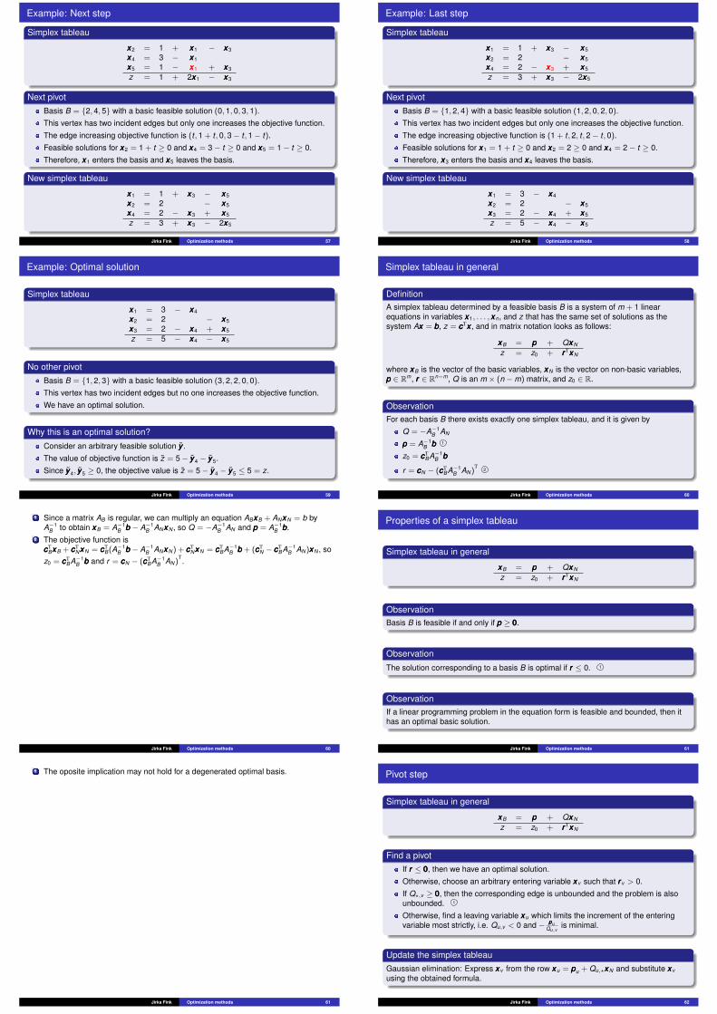
Example: Next step

Simplex tableau


xxx4 = 3 − xxx1


z = 1 + 2xxx1 − xxx3

Next pivotBasis B = {2, 4, 5} with a basic feasible solution (0, 1, 0, 3, 1).

This vertex has two incident edges but only one increases the objective function.

The edge increasing objective function is (t , 1 + t , 0, 3− t , 1− t).

Feasible solutions for xxx2 = 1 + t ≥ 0 and xxx4 = 3− t ≥ 0 and xxx5 = 1− t ≥ 0.

Therefore, xxx1 enters the basis and xxx5 leaves the basis.

New simplex tableau


xxx2 = 2 − xxx5


z = 3 + xxx3 − 2xxx5


Example: Last step

Simplex tableau


xxx2 = 2 − xxx5


z = 3 + xxx3 − 2xxx5

Next pivotBasis B = {1, 2, 4} with a basic feasible solution (1, 2, 0, 2, 0).

This vertex has two incident edges but only one increases the objective function.

The edge increasing objective function is (1 + t , 2, t , 2− t , 0).

Feasible solutions for xxx1 = 1 + t ≥ 0 and xxx2 = 2 ≥ 0 and xxx4 = 2− t ≥ 0.

Therefore, xxx3 enters the basis and xxx4 leaves the basis.

New simplex tableau

xxx1 = 3 − xxx4

xxx2 = 2 − xxx5


z = 5 − xxx4 − xxx5


Example: Optimal solution

Simplex tableau

xxx1 = 3 − xxx4

xxx2 = 2 − xxx5


z = 5 − xxx4 − xxx5

No other pivotBasis B = {1, 2, 3} with a basic feasible solution (3, 2, 2, 0, 0).

This vertex has two incident edges but no one increases the objective function.

We have an optimal solution.

Why this is an optimal solution?

Consider an arbitrary feasible solution yyy .

The value of objective function is z = 5− yyy4 − yyy5.

Since yyy4, yyy5 ≥ 0, the objective value is z = 5− yyy4 − yyy5 ≤ 5 = z.


Simplex tableau in general

DefinitionA simplex tableau determined by a feasible basis B is a system of m + 1 linearequations in variables xxx1, . . . ,xxxn, and z that has the same set of solutions as thesystem Axxx = bbb, z = cccTxxx , and in matrix notation looks as follows:

xxxB = ppp + QxxxN

z = z0 + rrr TxxxN

where xxxB is the vector of the basic variables, xxxN is the vector on non-basic variables,ppp ∈ Rm, rrr ∈ Rn−m, Q is an m × (n −m) matrix, and z0 ∈ R.

ObservationFor each basis B there exists exactly one simplex tableau, and it is given by

Q = −A−1B AN

ppp = A−1B bbb 1

z0 = cccTBA−1

B bbb

r = cccN − (cccTBA−1

B AN)T

2


1 Since a matrix AB is regular, we can multiply an equation ABxxxB + ANxxxN = b byA−1

B to obtain xxxB = A−1B bbb − A−1

B ANxxxN , so Q = −A−1B AN and ppp = A−1

B bbb.2 The objective function is

cccTBxxxB + cccT

NxxxN = cccTB(A−1

B bbb − A−1B ANxxxN) + cccT

NxxxN = cccTBA−1

B bbb + (cccTN − cccT

BA−1B AN)xxxN , so

z0 = cccTBA−1

B bbb and r = cccN − (cccTBA−1

B AN)T.


Properties of a simplex tableau


xxxB = ppp + QxxxN

z = z0 + rrr TxxxN

ObservationBasis B is feasible if and only if ppp ≥ 000.

Observation

The solution corresponding to a basis B is optimal if rrr ≤ 0. 1

ObservationIf a linear programming problem in the equation form is feasible and bounded, then ithas an optimal basic solution.


1 The oposite implication may not hold for a degenerated optimal basis.


Pivot step


xxxB = ppp + QxxxN

z = z0 + rrr TxxxN

Find a pivotIf rrr ≤ 000, then we have an optimal solution.

Otherwise, choose an arbitrary entering variable xxxv such that rrr v > 0.

If Q?,v ≥ 000, then the corresponding edge is unbounded and the problem is alsounbounded. 1

Otherwise, find a leaving variable xxxu which limits the increment of the enteringvariable most strictly, i.e. Qu,v < 0 and − pppu

Qu,vis minimal.

Update the simplex tableauGaussian elimination: Express xxxv from the row xxxu = pppu + Qu,?xxxN and substitute xxxv

using the obtained formula.


1 Consider the following edge: xxxv = t , remaining nonbasic variables are 0, andxxxB = p + Q?,v t . All solutions on this edge are feasible for t ≥ 0 since xxx ≥ 000. Forthe objective value, cccTxxx = z0 + rrr TxxxN = z0 + rrr v t →∞ as t →∞, so the objectivefunction is unbounded.


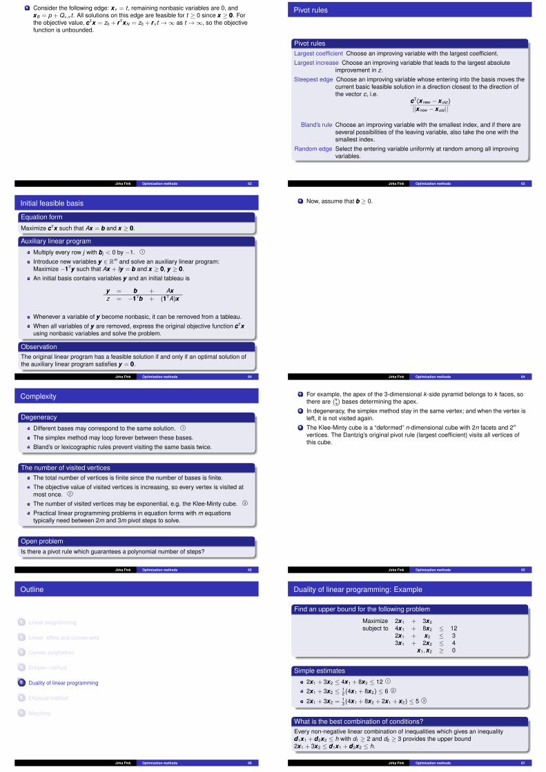
Pivot rules

Pivot rulesLargest coefficient Choose an improving variable with the largest coefficient.

Largest increase Choose an improving variable that leads to the largest absoluteimprovement in z.

Steepest edge Choose an improving variable whose entering into the basis moves thecurrent basic feasible solution in a direction closest to the direction ofthe vector c, i.e.

cccT(xxxnew − xxxold )

||xxxnew − xxxold ||

Bland’s rule Choose an improving variable with the smallest index, and if there areseveral possibilities of the leaving variable, also take the one with thesmallest index.

Random edge Select the entering variable uniformly at random among all improvingvariables.


Initial feasible basis

Equation form

Maximize cccTxxx such that Axxx = bbb and xxx ≥ 000.

Auxiliary linear program

Multiply every row j with bbbj < 0 by −1. 1

Introduce new variables yyy ∈ Rm and solve an auxiliary linear program:Maximize −111Tyyy such that Axxx + Iyyy = bbb and xxx ≥ 000, yyy ≥ 000.

An initial basis contains variables yyy and an initial tableau is

yyy = bbb + Axxxz = −111Tbbb + (111TA)xxx

Whenever a variable of yyy become nonbasic, it can be removed from a tableau.

When all variables of yyy are removed, express the original objective function cccTxxxusing nonbasic variables and solve the problem.

ObservationThe original linear program has a feasible solution if and only if an optimal solution ofthe auxiliary linear program satisfies yyy = 000.


1 Now, assume that bbb ≥ 0.


Complexity

Degeneracy

Different bases may correspond to the same solution. 1

The simplex method may loop forever between these bases.

Bland’s or lexicographic rules prevent visiting the same basis twice.

The number of visited verticesThe total number of vertices is finite since the number of bases is finite.

The objective value of visited vertices is increasing, so every vertex is visited atmost once. 2

The number of visited vertices may be exponential, e.g. the Klee-Minty cube. 3

Practical linear programming problems in equation forms with m equationstypically need between 2m and 3m pivot steps to solve.

Open problemIs there a pivot rule which guarantees a polynomial number of steps?


1 For example, the apex of the 3-dimensional k -side pyramid belongs to k faces, sothere are

(k3

)bases determining the apex.

2 In degeneracy, the simplex method stay in the same vertex; and when the vertex isleft, it is not visited again.

3 The Klee-Minty cube is a “deformed” n-dimensional cube with 2n facets and 2n

vertices. The Dantzig’s original pivot rule (largest coefficient) visits all vertices ofthis cube.


Outline



3 Convex polyhedron

4 Simplex method


6 Ellipsoid method

7 Matching


Duality of linear programming: Example

Find an upper bound for the following problem

Maximize 2xxx1 + 3xxx2

subject to 4xxx1 + 8xxx2 ≤ 122xxx1 + xxx2 ≤ 33xxx1 + 2xxx2 ≤ 4

xxx1,xxx2 ≥ 0

Simple estimates

2xxx1 + 3xxx2 ≤ 4xxx1 + 8xxx2 ≤ 12 1

2xxx1 + 3xxx2 ≤ 12 (4xxx1 + 8xxx2) ≤ 6 2

2xxx1 + 3xxx2 = 13 (4xxx1 + 8xxx2 + 2xxx1 + xxx2) ≤ 5 3

What is the best combination of conditions?Every non-negative linear combination of inequalities which gives an inequalityddd1xxx1 + ddd2xxx2 ≤ h with d1 ≥ 2 and d2 ≥ 3 provides the upper bound2xxx1 + 3xxx2 ≤ ddd1xxx1 + ddd2xxx2 ≤ h.


1 The first condition2 A half of the first condition3 A third of the sum of the first and the second conditions


Duality of linear programming: Example

Consider a non-negative combination yyy of inequalities

Maximize 2xxx1 + 3xxx2

subject to 4xxx1 + 8xxx2 ≤ 12 / · yyy12xxx1 + xxx2 ≤ 3 / · yyy23xxx1 + 2xxx2 ≤ 4 / · yyy3

xxx1,xxx2 ≥ 0

ObservationsEvery feasible solution xxx and non-negative combination yyy satisfies(4yyy1 + 2yyy2 + 3yyy3)xxx1 + (8yyy1 + yyy2 + 2yyy3)xxx2 ≤ 12yyy1 + 3yyy2 + 4yyy3.

If 4yyy1 + 2yyy2 + 3yyy3 ≥ 2 and 8yyy1 + yyy2 + 2yyy3 ≥ 3,then 12yyy1 + 2yyy2 + 4yyy3 is an upper for the objective function.

Dual program 1

Minimize 12yyy1 + 2yyy2 + 4yyy3subject to 4yyy1 + 2yyy2 + 3yyy3 ≥ 2

8yyy1 + yyy2 + 2yyy3 ≥ 3yyy1,yyy2,yyy3 ≥ 0


1 The primal optimal solution is xxxT = ( 12 ,

54 ) and the dual solution is yyyT = ( 5

16 , 0,14 ),

both with the same objective value 4.75.


Duality of linear programming: General

Primal linear program

Maximize cccTxxx subject to Axxx ≤ bbb and xxx ≥ 000

Dual linear program

Minimize bbbTyyy subject to ATyyy ≥ ccc and yyy ≥ 000

Weak duality theorem

For every primal feasible solution xxx and dual feasible solution yyy hold cccTxxx ≤ bbbTyyy .

CorollaryIf one program is unbounded, then the other one is infeasible.

Duality theoremExactly one of the following possibilities occurs

1 Neither primal nor dual has a feasible solution2 Primal is unbounded and dual is infeasible3 Primal is infeasible and dual is unbounded4 There are feasible solutions xxx and yyy such that cccTxxx = bbbTyyy


Dualization

Every linear programming problem has its dual, e.g.

Maximize cccTxxx subject to Axxx ≥ bbb and xxx ≥ 000 — Primal program

Maximize cccTxxx subject to −Axxx ≤ −bbb and xxx ≥ 000 — Equivalent formulation

Minimize −bbbTyyy subject to −ATyyy ≥ ccc and yyy ≥ 000 — Dual program

Minimize bbbTyyy subject to ATyyy ≥ ccc and yyy ≤ 000 — Simplified formulation

A dual of a dual problem is the (original) primal problem

Minimize bbbTyyy subject to ATyyy ≥ ccc and yyy ≥ 000 — Dual program

-Maximize −bbbTyyy subject to ATyyy ≥ ccc and yyy ≥ 000 — Equivalent formulation

-Minimize cccTxxx subject to Axxx ≥ −bbb and xxx ≤ 000 — Dual of the dual program

-Minimize −cccTxxx subject to −Axxx ≥ −bbb and xxx ≥ 000 — Simplified formulation

Maximize cccTxxx subject to Axxx ≤ bbb and xxx ≥ 000 — The original primal program


Dualization: General rules

Maximizing program Minimizing program

Variables xxx1, . . . ,xxxn yyy1, . . . ,yyym

Matrix A AT

Right-hand side bbb ccc

Objective function maxcccTxxx minbbbTyyy

Constraints i-th constraint has ≤ yyy i ≥ 0i-th constraint has ≥ yyy i ≤ 0i-th constraint has = yyy i ∈ R

xxx j ≥ 0 j-th constraint has ≥xxx j ≤ 0 j-th constraint has ≤xxx j ∈ R j-th constraint has =


Linear programming: Feasibility versus optimality

Feasibility versus optimalityFinding a feasible solution of a linear program is computationally as difficult as findingan optimal solution.

Using dualityThe optimal solutions of linear programs

Primal: Maximize cccTxxx subject to Axxx ≤ bbb and xxx ≥ 000

Dual: Minimize bbbTyyy subject to ATyyy ≥ ccc and yyy ≥ 000

are exactly feasible solutions satisfying

Axxx ≤ bbbATyyy ≥ ccccccTxxx ≥ bbbTyyyxxx ,yyy ≥ 000


Complementary slackness

TheoremFeasible solutions xxx and yyy of linear programs



are optimal if and only if

xxx i = 0 or ATi,?yyy = ccc i for every i = 1, . . . , n and

yyy j = 0 or Aj,?xxx = bbbj for every j = 1, . . . ,m.

Proof

cccTxxx =n∑

i=1

ccc ixxx i ≤n∑

i=1

(yyyTA?,i )xxx i = yyyTAxxx =m∑

j=1

yyy j (Aj,?xxx) ≤m∑

j=1

yyy jbbbj = bbbTyyy


Fourier–Motzkin elimination: Example

Goal: Find a feasible solution

2x − 5y + 4z ≤ 103x − 6y + 3z ≤ 95x + 10y − z ≤ 15−x + 5y − 2z ≤ −7−3x + 2y + 6z ≤ 12

Express the variable x in each condition

x ≤ 5 + 52 y − 2z

x ≤ 3 + 2y − zx ≤ 3 − 2y + 1

5 zx ≥ 7 + 5y − 2zx ≥ −4 + 2

3 y + 2z

Eliminate the variable xThe original system has a feasible solution if and only if there exist y and z satisfying

max{

7 + 5y − 2z,−4 +23

y + 2z}≤ min

{5 +

52

y − 2z, 3 + 2y − z, 3− 2y +15

z}


Fourier–Motzkin elimination: Example

Rewrite into a system of inequalitiesReal numbers y and z satisfymax

{7 + 5y − 2z,−4 + 2

3 y + 2z}≤ min

{5 + 5

2 y − 2z, 3 + 2y − z, 3− 2y + 15 z}

ifand only they satisfy

7 + 5y − 2z ≤ 5 + 52 y − 2z

7 + 5y − 2z ≤ 3 + 2y − z7 + 5y − 2z ≤ 3 − 2y + 1

5 z−4 + 2

3 y + 2z ≤ 5 + 52 y − 2z

−4 + 23 y + 2z ≤ 3 + 2y − z

−4 + 23 y + 2z ≤ 3 − 2y + 1

5 z

OverviewEliminate the variable y , find a feasible evaluation of z a and compute y a x .

In every step, we eliminate one variable; however, the number of conditions mayincrease quadratically.

If we start with m conditions, then after n eliminations the number of conditions isup to 4(m/4)2n

.


Fourier–Motzkin elimination: In general

ObservationLet Axxx ≤ bbb be a system with n ≥ 1 variables and m inequalities. There is a systemA′xxx ′ ≤ bbb′ with n − 1 variables and at most max

{m,m2/4

}inequalities, with the

following properties:1 Axxx ≤ bbb has a solution if and only if A′xxx ′ ≤ bbb′ has a solution, and2 each inequality of A′xxx ′ ≤ bbb′ is a positive linear combination of some inequalities

from Axxx ≤ bbb.

Proof1 WLOG: Ai,1 ∈ {−1, 0, 1} for all i = 1, . . . ,m2 Let C = {i ; Ai,1 = 1}, F = {i ; Ai,1 = −1} and L = {i ; Ai,1 = 0}3 Let A′xxx ′ ≤ bbb′ be the system of n − 1 variables and |C| · |F |+ |L| inequalities

j ∈ C, k ∈ F : (Aj,? + Ak,?)xxx ≤ bbbj + bbbk (1)l ∈ L : Al,?xxx ≤ bbbl (2)

4 Assuming A′xxx ′ ≤ bbb′ has a solution xxx ′, we find a solution xxx of Axxx ≤ bbb:(1) is equivalent to A′k,?xxx

′ − bbbk ≤ bbbj − A′j,?xxx′ for all j ∈ C, k ∈ F ,

which is equivalent to maxk∈F

{A′k,?xxx

′ − bbbk

}≤ minj∈C

{bbbj − A′j,?xxx

′}

Choose xxx1 between these bounds and xxx = (xxx1,xxx ′) satisfies Axxx ≤ bbb


Farkas lemma

DefinitionA cone generated by vectors aaa1, . . . ,aaan ∈ Rm is the set of all non-negativecombinations of aaa1, . . . ,aaan, i.e.

{∑ni=1 αiaaai ; α1, . . . , αn ≥ 0

}.

Proposition (Farkas lemma geometrically)

Let aaa1, . . . ,aaan,bbb ∈ Rm. Then exactly one of the following two possibilities occurs:1 The point bbb lies in the cone generated by aaa1, . . . ,aaan.2 There exists a hyperplane h =

{xxx ∈ Rm; yyyTxxx = 0

}containing 000 for some yyy ∈ Rm

separating aaa1, . . . ,aaan and bbb, i.e. yyyTaaai ≥ 0 for all i = 1, . . . , n and yyyTbbb < 0.

Proposition (Farkas lemma)

Let A ∈ Rm×n and bbb ∈ Rm. Then exactly one of the following two possibilities occurs:1 There exists a vector xxx ∈ Rn satisfying Axxx = bbb and xxx ≥ 000.2 There exists a vector yyy ∈ Rm satisfying yyyTA ≥ 000 and yyyTb < 000.


Farkas lemma

Proposition (Farkas lemma)

Let A ∈ Rm×n and bbb ∈ Rm. The following statements hold.1 The system Axxx = bbb has a non-negative solution xxx ∈ Rn if and only if every yyy ∈ Rm

with yyyTA ≥ 000T satisfies yyyTbbb ≥ 0.2 The system Axxx ≤ bbb has a non-negative solution xxx ∈ Rn if and only if every

non-negative yyy ∈ Rm with yyyTA ≥ 000T satisfies yyyTbbb ≥ 0.3 The system Axxx ≤ bbb has a solution xxx ∈ Rn if and only if every non-negative yyy ∈ Rm

with yyyTA = 000T satisfies yyyTbbb ≥ 0.

Overview of the proof of dualityFourier–Motzkin elimination

⇓Farkas lemma, 3rd version

⇓Farkas lemma, 2nd version

⇓Duality of linear programming

Observation (Exercise)Variants of Farkas lemma are equivalent.


Farkas lemma

Proposition (Farkas lemma, 3rd version)

Let A ∈ Rm×n and bbb ∈ Rm. Then, the system Axxx ≤ bbb has a solution xxx ∈ Rn if and only ifevery non-negative yyy ∈ Rm with yyyTA = 000T satisfies yyyTbbb ≥ 0.

Proof (overview)

⇒ If xxx satisfies Axxx ≤ bbb and yyy ≥ 000 satisfies yyyTA = 000T, then yyyTbbb ≥ yyyTAxxx ≥ 000Txxx = 000

⇐ If Axxx ≤ bbb has no solution, the find yyy ≥ 000 satisfying yyyTA = 000T and yyyTbbb < 0 by theinduction on n

n = 0 The system Axxx ≤ bbb equals to 000 ≤ bbb which is infeasible, so bi < 0 for some iChoose yyy = ei (the i-th unit vector)

n > 0 Using Fourier–Motzkin elimination we obtain an infeasible system A′xxx ′ ≤ bbb′

There exists a non-negative matrix M such that (000|A′) = MA and bbb′ = MbbbBy induction, there exists yyy ′ ≥ 0, yyy ′TA′ = 000T, yyy ′Tbbb′ < 0We verify that yyy = MTyyy ′ satisfies all requirements of the inductionyyy = MTyyy ′ ≥ 000yyyTA = (MTyyy ′)TA = yyy ′TMA = yyy ′T(000|A′) = 000T

yyyTbbb = (MTyyy ′)Tbbb = yyy ′TMbbb = yyy ′Tbbb′ < 000T


Proof of the duality of linear programming

Proposition (Farkas lemma, 2nd version)

Let A ∈ Rm×n and bbb ∈ Rm. The system Axxx ≤ bbb has a non-negative solution if and onlyif every non-negative yyy ∈ Rm with yyyTA ≥ 000T satisfies yyyTbbb ≥ 0.

Duality



If the primal problem has an optimal solution xxx?, then the dual problem has an optimalsolution yyy? and cccTxxx? = bbbTyyy?.

Proof of duality using Farkas lemma1 Let xxx? be an optimal solution of the primal problem and γ = cccTxxx?

2 ε > 0 iff Axxx ≤ bbb and xxx ≥ 000 and cccTxxx ≥ γ + ε is infeasible3 ε > 0 iff

( A−cccT

)xxx ≤

( bbb−γ−ε

)and xxx ≥ 000 is infeasible

4 ε > 0 iff uuu, z ≥ 0 and(uuu

z

)T( A−cccT

)≥ 000T and

(uuuz

)T( bbb−γ−ε

)< 0 is feasible

5 ε > 0 iff uuu, z ≥ 0 and ATuuu ≥ zccc and bbbTuuu < z(γ + ε) is feasible


Proof of the duality of linear programming

Duality



If the primal problem has an optimal solution xxx?, then the dual problem has an optimalsolution yyy? and cccTxxx? = bbbTyyy?.

Proof of duality using Farkas lemma (continue)1 Let xxx? be an optimal solution of the primal problem and γ = cccTxxx?

2 ε > 0 iff uuu, z ≥ 0 and ATuuu ≥ zccc and bbbTuuu < z(γ + ε) is feasible3 For ε > 0, there exists uuu′, z′ ≥ 0 with ATuuu′ ≥ z′ccc and bbbTuuu′ < z′(γ + ε)

4 For ε = 0 it holds that uuu′, z′ ≥ 0 and ATuuu′ ≥ z′ccc so bbbTuuu′ ≥ z′γ5 Since z′γ ≤ bbbTuuu′ < z′(γ + ε) and z′ ≥ 0 it follows that z′ > 06 Let vvv = 1

z′ uuu′

7 Since ATvvv ≥ ccc and vvv ≥ 000, the dual solution vvv is feasible8 Since the dual is feasible and bounded, there exists an optimal dual solution yyy?

9 Hence, bbbTyyy? < γ + ε for every ε > 0, and so bbbTyyy? ≤ γ10 From the weak duality theorem it follows that bbbTyyy? = cccTxxx?


Outline



3 Convex polyhedron

4 Simplex method


6 Ellipsoid method

7 Matching


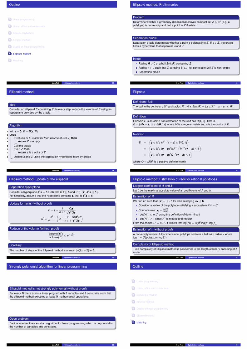
Ellipsoid method: Preliminaries

ProblemDetermine whether a given fully-dimensional convex compact set Z ⊆ Rn (e.g. apolytope) is non-empty and find a point in Z if exists.

Separation oracleSeparation oracle determines whether a point s belongs into Z . If s /∈ Z , the oraclefinds a hyperplane that separates s and Z .

InputsRadius R > 0 of a ball B(0,R) containing Z

Radius ε > 0 such that Z contains B(s, ε) for some point s if Z is non-empty

Separation oracle


Ellipsoid method

IdeaConsider an ellipsoid E containing Z . In every step, reduce the volume of E using anhyperplane provided by the oracle.

Algorithm

1 Init: s = 000, E = B(s,R)2 Loop3 if volume of E is smaller than volume of B(0, ε) then4 return Z is empty

5 Call the oracle6 if s ∈ Z then7 return s is a point of Z

8 Update s and Z using the separation hyperplane fount by oracle


Ellipsoid

Definition: BallThe ball in the centre sss ∈ Rn and radius R ≥ 0 is B(sss,R) = {xxx ∈ Rn; ||xxx − sss|| ≤ R}.

DefinitionEllipsoid E is an affine transformation of the unit ball B(000, 1). That is,E = {Mxxx + sss; xxx ∈ B(000, 1)} where M is a regular matrix and s is the centre of E .

Notation

E ={

yyy ∈ Rn; M−1(yyy − sss) ∈ B(000, 1)}

={

yyy ∈ Rn; (yyy − sss)T(M−1)TM−1(yyy − sss) ≤ 1

}=

{yyy ∈ Rn; (yyy − sss)TQ−1(yyy − sss) ≤ 1

}where Q = MMT is a positive definite matrix


Ellipsoid method: update of the ellipsoid

Separation hyperplane

Consider a hyperplane aaaTxxx = b such that aaaTsss ≥ b and Z ⊆{xxx ; aaaTxxx ≤ b

}.

For simplicity, assume that the hyperplane contains sss, that is aaaTsss = b.

Update formulas (without proof)

sss′ = sss − 1n + 1

Qaaa√aaaTQaaa

Q′ =n2

n2 − 1

(Q − 2

n + 1QaaaaaaTQaaaTQaaa

)

Reduce of the volume (without proof)

volume(E ′)volume(E)

≤ e−1

2n+2

Corollary

The number of steps of the Ellipsoid method is at most⌈n(2n + 2) ln R

ε

⌉.


Ellipsoid method: Estimation of radii for rational polytopes

Largest coefficient of A and bbbLet L be the maximal absolute value of all coefficients of A and b.

Estimation of RWe find R′ such that ||xxx ||∞ ≤ R′ for all xxx satisfying Axxx ≤ bbb:

Consider a vertex of the polytope satisfying a subsystem A′xxx = bbb′

Cramer’s rule: xxx i =det A′

idet A′

| det(A′i )| ≤ n!Ln using the definition of determinant

| det(A′)| ≥ 1 since A′ is integral and regular

From the choice R′ = n!Ln, it follows that log(R) = O(n2 log(n) log(L))

Estimation of ε (without proof)A non-empty rational fully-dimensional polytope contains a ball with radius ε wherelog 1

ε= O(poly(n,m, log L)).

Complexity of Ellipsoid methodTime complexity of Ellipsoid method is polynomial in the length of binary encoding of Aand bbb.


Strongly polynomial algorithm for linear programming

Ellipsoid method is not strongly polynomial (without proof)For every M there exists a linear program with 2 variables and 2 constrains such thatthe ellipsoid method executes at least M mathematical operations.

Open problemDecide whether there exist an algorithm for linear programming which is polynomial inthe number of variables and constrains.


Outline



3 Convex polyhedron

4 Simplex method


6 Ellipsoid method

7 Matching


Matching problems

Perfect matching problemInput: Graph (V ,E)

Output: Perfect matching M ⊆ E if it exists

Minimum weight perfect matching problem

Input: Graph (V ,E) and weights ccce ≥ 0 on edges e ∈ E 1

Output: Perfect matching M ⊆ E minimizing the weight∑

e∈M ccce

Overview1 Tools: Augmenting paths, Tutte-Berge formula, alternating trees2 Perfect matching in bipartite graphs without weights3 Minimum weight perfect matching in bipartite graphs4 Tool: Shrinking odd circuits5 Perfect matching in general graphs without weights6 Minimum weight perfect matching in general graphs7 Maximum weight matching


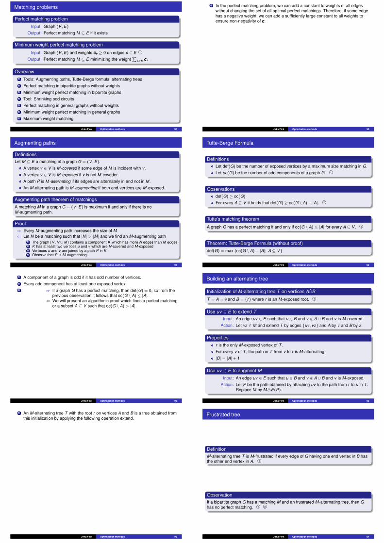
1 In the perfect matching problem, we can add a constant to weights of all edgeswithout changing the set of all optimal perfect matchings. Therefore, if some edgehas a negative weight, we can add a sufficiently large constant to all weights toensure non-negativity of ccc.


Augmenting paths

DefinitionsLet M ⊆ E a matching of a graph G = (V ,E).

A vertex v ∈ V is M-covered if some edge of M is incident with v .

A vertex v ∈ V is M-exposed if v is not M-coveder.

A path P is M-alternating if its edges are alternately in and not in M.

An M-alternating path is M-augmenting if both end-vertices are M-exposed.

Augmenting path theorem of matchingsA matching M in a graph G = (V ,E) is maximum if and only if there is noM-augmenting path.

Proof⇒ Every M-augmenting path increases the size of M⇐ Let N be a matching such that |N| > |M| and we find an M-augmenting path

1 The graph (V ,N ∪M) contains a component K which has more N edges than M edges2 K has at least two vertices u and v which are N-covered and M-exposed3 Verteces u and v are joined by a path P in K4 Observe that P is M-augmenting


Tutte-Berge Formula

DefinitionsLet def(G) be the number of exposed vertices by a maximum size matching in G.

Let oc(G) be the number of odd components of a graph G. 1

Observationsdef(G) ≥ oc(G)

For every A ⊆ V it holds that def(G) ≥ oc(G \ A)− |A|. 2

Tutte’s matching theorem

A graph G has a perfect matching if and only if oc(G \ A) ≤ |A| for every A ⊆ V . 3

Theorem: Tutte-Berge Formula (without proof)def(G) = max {oc(G \ A)− |A|; A ⊆ V}


1 A component of a graph is odd if it has odd number of vertices.2 Every odd component has at least one exposed vertex.3 ⇒ If a graph G has a perfect matching, then def(G) = 0, so from the

previous observation it follows that oc(G \ A) ≤ |A|.⇐ We will present an algorithmic proof which finds a perfect matching

or a subset A ⊆ V such that oc(G \ A) > |A|.


Building an alternating tree

Initialization of M-alternating tree T on vertices A∪B

T = A = ∅ and B = {r} where r is an M-exposed root. 1

Use uv ∈ E to extend TInput: An edge uv ∈ E such that u ∈ B and v /∈ A ∪ B and v is M-covered.

Action: Let vz ∈ M and extend T by edges {uv , vz} and A by v and B by z.

Propertiesr is the only M-exposed vertex of T .

For every v of T , the path in T from v to r is M-alternating.

|B| = |A|+ 1

Use uv ∈ E to augment M

Input: An edge uv ∈ E such that u ∈ B and v /∈ A ∪ B and v is M-exposed.

Action: Let P be the path obtained by attaching uv to the path from r to u in T .Replace M by M4E(P).


1 An M-alternating tree T with the root r on vertices A and B is a tree obtained fromthis initialization by applying the following operation extend.


Frustrated tree

DefinitionM-alternating tree T is M-frustrated if every edge of G having one end vertex in B hasthe other end vertex in A. 1

ObservationIf a bipartite graph G has a matching M and an frustrated M-alternating tree, then Ghas no perfect matching. 2 3


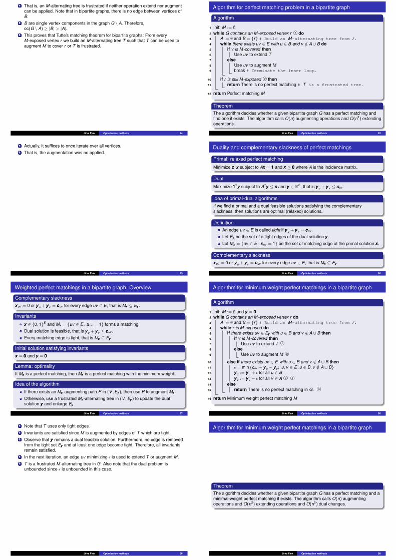
1 That is, an M-alternating tree is frustrated if neither operation extend nor augmentcan be applied. Note that in bipartite graphs, there is no edge between vertices ofB.

2 B are single vertex components in the graph G \ A. Therefore,oc(G \ A) ≥ |B| > |A|.

3 This proves that Tutte’s matching theorem for bipartite graphs: From everyM-exposed vertex r we build an M-alternating tree T such that T can be used toaugment M to cover r or T is frustrated.


Algorithm for perfect matching problem in a bipartite graph

Algorithm

1 Init: M := ∅2 while G contains an M-exposed vertex r 1 do3 A := ∅ and B = {r} # Build an M-alternating tree from r.4 while there exists uv ∈ E with u ∈ B and v /∈ A ∪ B do5 if v is M-covered then6 Use uv to extend T7 else8 Use uv to augment M9 break # Terminate the inner loop.

10 if r is still M-exposed 2 then11 return There is no perfect matching # T is a frustrated tree.

12 return Perfect matching M

TheoremThe algorithm decides whether a given bipartite graph G has a perfect matching andfind one if exists. The algorithm calls O(n) augmenting operations and O(n2) extendingoperations.


1 Actually, it suffices to once iterate over all vertices.2 That is, the augmentation was no applied.


Duality and complementary slackness of perfect matchings

Primal: relaxed perfect matching

Minimize cccTxxx subject to Axxx = 111 and xxx ≥ 000 where A is the incidence matrix.

Dual

Maximize 111Tyyy subject to ATyyy ≤ ccc and yyy ∈ RE , that is yyyu + yyy v ≤ cccuv .

Idea of primal-dual algorithmsIf we find a primal and a dual feasible solutions satisfying the complementaryslackness, then solutions are optimal (relaxed) solutions.

DefinitionAn edge uv ∈ E is called tight if yyyu + yyy v = cccuv .

Let Eyyy be the set of a tight edges of the dual solution yyy .

Let Mxxx = {uv ∈ E ; xxxuv = 1} be the set of matching edge of the primal solution xxx .

Complementary slacknessxxxuv = 0 or yyyu + yyy v = cccuv for every edge uv ∈ E , that is Mxxx ⊆ Eyyy .


Weighted perfect matchings in a bipartite graph: Overview

Complementary slacknessxxxuv = 0 or yyyu + yyy v = cccuv for every edge uv ∈ E , that is Mxxx ⊆ Eyyy .

Invariants

xxx ∈ {0, 1}E and Mxxx = {uv ∈ E ; xxxuv = 1} forms a matching.

Dual solution is feasible, that is yyyu + yyy v ≤ cccuv .

Every matching edge is tight, that is Mxxx ⊆ Eyyy .

Initial solution satisfying invariantsxxx = 000 and yyy = 000

Lemma: optimalityIf Mxxx is a perfect matching, then Mxxx is a perfect matching with the minimum weight.

Idea of the algorithm

If there exists an Mxxx -augmenting path P in (V ,Eyyy ), then use P to augment Mxxx .

Otherwise, use a frustrated Mxxx -alternating tree in (V ,Eyyy ) to update the dualsolution yyy and enlarge Eyyy .


Algorithm for minimum weight perfect matchings in a bipartite graph

Algorithm

1 Init: M := ∅ and yyy = 0002 while G contains an M-exposed vertex r do3 A := ∅ and B = {r} # Build an M-alternating tree from r.4 while r is M-exposed do5 if there exists uv ∈ Eyyy with u ∈ B and v /∈ A ∪ B then6 if v is M-covered then7 Use uv to extend T 1

8 else9 Use uv to augment M 2

10 else if there exists uv ∈ E with u ∈ B and v /∈ A ∪ B then11 ε = min {cuv − yyyu − yyy v ; u, v ∈ E , u ∈ B, v /∈ A ∪ B}12 yyyu := yyyu + ε for all u ∈ B13 yyy v := yyy v − ε for all v ∈ A 3 4

14 else15 return There is no perfect matching in G. 5

16 return Minimum weight perfect matching M


1 Note that T uses only tight edges.2 Invariants are satisfied since M is augmented by edges of T which are tight.3 Observe that yyy remains a dual feasible solution. Furthermore, no edge is removed

from the tight set Eyyy and at least one edge become tight. Therefore, all invariantsremain satisfied.

4 In the next iteration, an edge uv minimizing ε is used to extend T or augment M.5 T is a frustrated M-alternating tree in G. Also note that the dual problem is

unbounded since ε is unbounded in this case.


Algorithm for minimum weight perfect matchings in a bipartite graph

TheoremThe algorithm decides whether a given bipartite graph G has a perfect matching and aminimal-weight perfect matching if exists. The algorithm calls O(n) augmentingoperations and O(n2) extending operations and O(n2) dual changes.


Shrinking odd circuits

DefinitionLet C be an odd circuit in G. The graph G × C has vertices (V (G) \ V (C)) ∪ {c′}where c′ is a new vertex and edges 1

E(G) with both end-vertices in V (G) \ V (C) and

and uc′ for every edge uv with u /∈ V (C) and v ∈ V (C).

Edges E(C) are removed.

Proposition

Let C be an odd circuit of G and M ′ be a matching G × C. Then, there exists amatching M of G such that M ⊆ M ′ ∪ E(C) and the number of M ′-exposed nodes of Gis the same as the number of M ′-exposed nodes in G × C.

Corollarydef(G) ≤ def(G × C)

RemarkThere exists a graph G with odd circuit C such that def(G) < def(G × C).


1 Formally, E(G × C) = {uv ; uv ∈ E(G), u, v ∈ V (G) \ V (C)} ∪{uc′; ∃v ∈ V (C) : uv ∈ E(G), u ∈ V (G) \ V (C)}.


Perfect matching in general graphs

Use uv to shrink and update M ′ and T

Input: A matching M ′ of a graph G′, an M ′-alternating tree T , edge uv ∈ E ′

such that u, v ∈ B

Action: Let C be the circuit formed by uv together with the path in T from u to v .Replace

G′ by G′ × CM ′ by M ′ \ E(C)T by the tree having edge-set E(T ) \ E(C).

ObservationLet G′ be a graph obtained from G by a sequence of odd-circuit shrinkings. Let M ′ bematching of G′ and let T be an M ′ alternating tree of G′ such that all vertices of A areoriginal vertices of G. If T is frustrated, then G has no perfect matching.

Proof is based on Tutte’s matching theoremA graph G has a perfect matching if and only if oc(G \ A) ≤ |A| for every A ⊆ V .


Perfect matchings algorithm in a non-weighted graph

Algorithm

1 Init: M := ∅2 while G contains an M-exposed vertex r do3 M ′ = M, G′ = G and T = ({r} , ∅)4 while there exists uv ∈ E(G′) with u ∈ B and v /∈ A do5 if v ∈ B then6 Use uv to shrink and update M ′ and T7 else if v is M ′-covered then8 Use uv to extend T9 else

10 Use uv to augment M ′

11 Extend M ′ to a matching M of G12 break # Terminate the inner loop.

13 if r is still M-exposed then14 return There is no perfect matching



Perfect matchings algorithm in a non-weighted graph II

Algorithm

1 Init: M ′ := ∅, G′ = G2 while G′ contains an M ′-exposed vertex r do3 T = ({r} , ∅)4 while r is M ′-exposed do5 if there exists uv ∈ E(G′) with u ∈ B and v /∈ A then6 if v ∈ B then7 Use uv to shrink and update M ′ and T8 else if v is M ′-covered then9 Use uv to extend T

10 else11 Use uv to augment M ′

12 else if there exists a pseudonode u in A then13 Expand u into a circuit and update T , M ′ and G′

14 else15 return There is no perfect matching

16 Expand all pseudonodes and obtain M from M ′



Minimum-Weight perfect matchings in general graphs

ObservationLet M be a perfect matching of G and D be an odd set of vertices of G. Then thereexists at least one edge uv ∈ M between D and V \ D.

Linear programming for Minimum-Weight perfect matchings in general graphs

Minimize cccxxxsubject to δuxxx = 1 for all u ∈ V

δDxxx ≥ 1 for all D ∈ Cxxx ≥ 000

Where δD ∈ {0, 1}E is a vector such that δDuv = 1 if |uv ∩ D| = 1 and δw = δ{w} and C is

the set of all odd-size subsets of V .

Theorem

Let G be a graph and ccc ∈ RE . Then G has a perfect matching if and only if the LPproblem is feasible. Moreover, if G has a perfect matching, the minimum weight of aperfect matching is equal to the optimal value of the LP problem.


Minimum-Weight perfect matchings in general graphs: Duality

Primal

Minimize cccxxxsubject to δuxxx = 1 for all u ∈ V

δDxxx ≥ 1 for all D ∈ Cxxx ≥ 000

Dual

Maximize∑

v∈V yyy v +∑

D∈C zzzD

subject to yyyu + yyy v +∑

uv∈D∈C zzzD ≤ cccuv for all uv ∈ Ezzz ≥ 000

Notation: Reduced costcccuv := cccuv − yyyu − yyyv −

∑uv∈D∈C zzzD

An edge e is tight if ccce = 0 and let Ey be the set of tight edges.

Complementary slacknessxxxe > 0 implies e is tight for all e ∈ E

zzzD > 0 implies δDxxx = 1 for all D ∈ C


Minimum-Weight perfect matchings in general graphs: Change of y

Updates weights and dual solution when shrinking a circuit C

Replace ccc′uv by ccc′uv − yyy ′v for u ∈ C and v /∈ C and set yyy ′c′ = 0 for the new vertex c′.Note that the reduced cost is unchanged.

Expand c′ into circuit C

Set zzz′C = yyy ′c′Replace ccc′uv by ccc′uv + yyy ′v for u ∈ C and v /∈ C

Update M ′ and T

Change of yyy and zzz on a frustrated tree

Input: A graph G′ with weights ccc′, a feasible dual solution yyy ′, a matching M ′ oftight edges of G′ and an M ′-alternating tree T of tight edges of G′.

Action: ε1 = min{ccce′; e joins a vertex in B and a vertex not in T

}ε2 = min

{ccce′/2; e joins two vertices of B

}ε3 = min {yyy ′v ; v ∈ A and v is a pseudonode of G}ε = min {ε1, ε2, ε3}Replace yyy ′v by yyy ′v + ε for all v ∈ BReplace yyy ′v by yyy ′v − ε for all v ∈ A


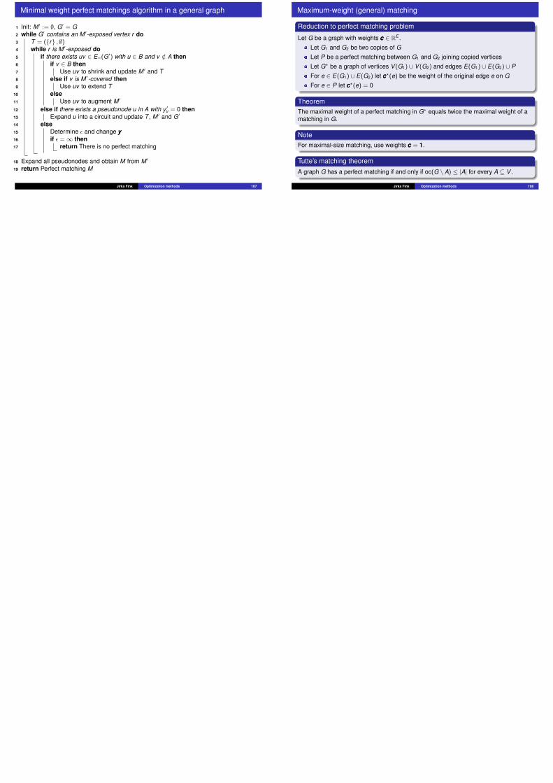
Minimal weight perfect matchings algorithm in a general graph

1 Init: M ′ := ∅, G′ = G2 while G′ contains an M ′-exposed vertex r do3 T = ({r} , ∅)4 while r is M ′-exposed do5 if there exists uv ∈ E=(G′) with u ∈ B and v /∈ A then6 if v ∈ B then7 Use uv to shrink and update M ′ and T8 else if v is M ′-covered then9 Use uv to extend T

10 else11 Use uv to augment M ′

12 else if there exists a pseudonode u in A with y ′u = 0 then13 Expand u into a circuit and update T , M ′ and G′

14 else15 Determine ε and change yyy16 if ε =∞ then17 return There is no perfect matching

18 Expand all pseudonodes and obtain M from M ′



Maximum-weight (general) matching

Reduction to perfect matching problem

Let G be a graph with weights ccc ∈ RE .

Let G1 and G2 be two copies of G

Let P be a perfect matching between G1 and G2 joining copied vertices

Let G? be a graph of vertices V (G1) ∪ V (G2) and edges E(G1) ∪ E(G2) ∪ P

For e ∈ E(G1) ∪ E(G2) let ccc?(e) be the weight of the original edge e on G

For e ∈ P let ccc?(e) = 0

TheoremThe maximal weight of a perfect matching in G? equals twice the maximal weight of amatching in G.

NoteFor maximal-size matching, use weights ccc = 111.

Tutte’s matching theoremA graph G has a perfect matching if and only if oc(G \ A) ≤ |A| for every A ⊆ V .


ktiml.mff.cuni.czfink/teaching/optimization...Optimization methods NOPT048 Jirka Fink œfink/ Department of Theoretical Computer Science and Mathematical Logic Faculty of …

Documents