Knowledge Presentation and Cognitive Psychology J.A.A. Stevens Maastricht, The Netherlands 4th November 2012

Welcome message from author
This document is posted to help you gain knowledge. Please leave a comment to let me know what you think about it! Share it to your friends and learn new things together.
Transcript

Knowledge Presentation and Cognitive Psychology
J.A.A. Stevens
Maastricht, The Netherlands4th November 2012

Table of Contents
Table of Contents i
1 Neuroanatomy 11.1 Terminology of the nervous system . . . . . . . . . . . . . . . . . . . . . . . . . . . . . . . 11.2 The Autonomic Nervous system . . . . . . . . . . . . . . . . . . . . . . . . . . . . . . . . . 31.3 The Cerebral Cortex . . . . . . . . . . . . . . . . . . . . . . . . . . . . . . . . . . . . . . . 5
1.3.1 The Occipital Lobe . . . . . . . . . . . . . . . . . . . . . . . . . . . . . . . . . . . . 61.3.2 The Parietal Lobe . . . . . . . . . . . . . . . . . . . . . . . . . . . . . . . . . . . . 61.3.3 The Temporal Lobe . . . . . . . . . . . . . . . . . . . . . . . . . . . . . . . . . . . 71.3.4 The Frontal Lobe . . . . . . . . . . . . . . . . . . . . . . . . . . . . . . . . . . . . . 8
2 Cognitive Neuroscience 92.1 The Cells of the Nervous System . . . . . . . . . . . . . . . . . . . . . . . . . . . . . . . . 9
2.1.1 Anatomy of Neurons and Glia . . . . . . . . . . . . . . . . . . . . . . . . . . . . . . 92.1.1.1 The Structures of an Animal Cell . . . . . . . . . . . . . . . . . . . . . . 102.1.1.2 The Structure of a Neuron . . . . . . . . . . . . . . . . . . . . . . . . . . 122.1.1.3 Variations among Neurons . . . . . . . . . . . . . . . . . . . . . . . . . . 142.1.1.4 Glia . . . . . . . . . . . . . . . . . . . . . . . . . . . . . . . . . . . . . . . 15
2.1.2 The Blood-Brain Barrier . . . . . . . . . . . . . . . . . . . . . . . . . . . . . . . . . 172.1.2.1 Why We Need a Blood-Brain Barrier . . . . . . . . . . . . . . . . . . . . 172.1.2.2 How the Blood-Brain Barrier works . . . . . . . . . . . . . . . . . . . . . 17
2.2 The Nerve Impulse . . . . . . . . . . . . . . . . . . . . . . . . . . . . . . . . . . . . . . . . 182.2.1 The Resting Potential of the Neuron . . . . . . . . . . . . . . . . . . . . . . . . . . 19
2.2.1.1 Forces Acting on Sodium and Potassium Ions . . . . . . . . . . . . . . . . 202.2.1.2 Why a Resting Potential? . . . . . . . . . . . . . . . . . . . . . . . . . . . 23
2.2.2 The Action Potential . . . . . . . . . . . . . . . . . . . . . . . . . . . . . . . . . . . 232.2.2.1 The Molecular Basis of the Action Potential . . . . . . . . . . . . . . . . 242.2.2.2 The All-or-None Law . . . . . . . . . . . . . . . . . . . . . . . . . . . . . 27
i

TABLE OF CONTENTS TABLE OF CONTENTS
2.2.2.3 The Refractory Period . . . . . . . . . . . . . . . . . . . . . . . . . . . . . 272.2.3 Propagation of the Action Potential . . . . . . . . . . . . . . . . . . . . . . . . . . 282.2.4 The Myelin Sheath and Saltatory Conduction . . . . . . . . . . . . . . . . . . . . . 30
2.3 The Synapse . . . . . . . . . . . . . . . . . . . . . . . . . . . . . . . . . . . . . . . . . . . 312.3.1 Neurotransmitter Release . . . . . . . . . . . . . . . . . . . . . . . . . . . . . . . . 322.3.2 Neurotransmitters Bind to Postsynaptic Receptor Sites . . . . . . . . . . . . . . . 342.3.3 Termination of the chemical signal . . . . . . . . . . . . . . . . . . . . . . . . . . . 362.3.4 Postsynaptic Potentials . . . . . . . . . . . . . . . . . . . . . . . . . . . . . . . . . 372.3.5 Neural Integration . . . . . . . . . . . . . . . . . . . . . . . . . . . . . . . . . . . . 39
ii

Chapter 1
Neuroanatomy
Before we can study the brain, we need a basic orientation in the brain. Just as you study a map when
you are lost in some faroff place, we need an understanding of the layout of the brain.
Although we can study the anatomy of the brain in very great detail, this is not the goal of this
coarse. You do need some basic terminology to understand how we denote regions and orient ourselves
in the brain. Likewise, you need to know at least how the cortex is divided into functional units. This
will all be described in the next sections. The interested student should not hesitate to gain a deeper
understanding of the anatomy of the brain, which by itself can already learn us a lot of how the brain
evolved.
Be advised that this chapter contains a lot of new terminology which you might not be familiar
with. However, by learning this terminology now, you will have an easier understanding of examples and
theories later in the course. The text and pictures in this chapter are based largely on Kalat, Biological
Psychology, 9th edition.
1.1 Terminology of the nervous system
Vertebrates have a central nervous system and a peripheral nervous system, which are of course connected
(see Figure 1.1). The central nervous system (CNS) is the brain and the spinal cord, each of which includes
1

Chapter 1. Neuroanatomy 1.1. Terminology of the nervous system
a great many substructures. The peripheral nervous system (PNS)the nerves outside the brain and spinal
cordhas two divisions: The somatic nervous system consists of the nerves that convey messages from the
sense organs to the CNS and from the CNS to the muscles. The autonomic nervous system controls the
heart, the intestines, and other organs.
Figure 1.1: Both the central nervous system and the peripheral nervous system have major subdivisions. The
closeup of the brain shows the right hemisphere as seen from the midline.
To follow a road map, you first must understand the terms north, south, east, and west. Because
the nervous system is a complex three-dimensional structure, we need more terms to describe it. As
Figure 1.2 indicates, dorsal means toward the back and ventral means toward the stomach. (One way
to remember these terms is that a ventriloquist is literally a “stomach talker.”) In a four-legged animal,
the top of the brain (with respect to gravity) is dorsal (on the same side as the animals back), and the
bottom of the brain is ventral (on the stomach side).
2

Chapter 1. Neuroanatomy 1.2. The Autonomic Nervous system
Figure 1.2: In four-legged animals, dorsal and ventral point in the same direction for the head as they do for the
rest of the body. However, humans upright posture has tilted the head, so the dorsal and ventral
directions of the head are not parallel to those of the spinal cord.
When humans evolved an upright posture, the position of our head changed relative to the spinal
cord. For convenience, we still apply the terms dorsal and ventral to the same parts of the human brain
as other vertebrate brains. Consequently, the dorsalventral axis of the human brain is at a right angle to
the dorsalventral axis of the spinal cord. If you picture a person in a crawling position with all four limbs
on the ground but nose pointing forward, the dorsal and ventral positions of the brain become parallel
to those of the spinal cord.
1.2 The Autonomic Nervous system
The autonomic nervous system consists of neurons that receive information from and send commands to
the heart, intestines, and other organs. It is comprised of two parts: the sympathetic and parasympathetic
nervous systems (Figure 1.3). The sympathetic nervous system, a network of nerves that prepare the
organs for vigorous activity, consists of two paired chains of ganglia lying just to the left and right of the
spinal cord in its central regions (the thoracic and lumbar areas) and connected by axons to the spinal cord.
3
Chapter 1. Neuroanatomy 1.2. The Autonomic Nervous system
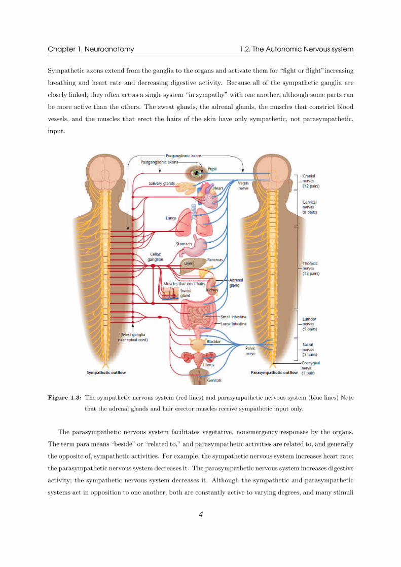
Sympathetic axons extend from the ganglia to the organs and activate them for “fight or flight”increasing
breathing and heart rate and decreasing digestive activity. Because all of the sympathetic ganglia are
closely linked, they often act as a single system “in sympathy” with one another, although some parts can
be more active than the others. The sweat glands, the adrenal glands, the muscles that constrict blood
vessels, and the muscles that erect the hairs of the skin have only sympathetic, not parasympathetic,
input.
Figure 1.3: The sympathetic nervous system (red lines) and parasympathetic nervous system (blue lines) Note
that the adrenal glands and hair erector muscles receive sympathetic input only.
The parasympathetic nervous system facilitates vegetative, nonemergency responses by the organs.
The term para means “beside” or “related to,” and parasympathetic activities are related to, and generally
the opposite of, sympathetic activities. For example, the sympathetic nervous system increases heart rate;
the parasympathetic nervous system decreases it. The parasympathetic nervous system increases digestive
activity; the sympathetic nervous system decreases it. Although the sympathetic and parasympathetic
systems act in opposition to one another, both are constantly active to varying degrees, and many stimuli
4

Chapter 1. Neuroanatomy 1.3. The Cerebral Cortex
arouse parts of both systems.
The parasympathetic nervous system is also known as the craniosacral system because it consists
of the cranial nerves and nerves from the sacral spinal cord (see Figure 1.3). Unlike the ganglia in
the sympathetic system, the parasympathetic ganglia are not arranged in a chain near the spinal cord.
Rather, long preganglionic axons extend from the spinal cord to parasympathetic ganglia close to each
internal organ; shorter postganglionic fibers then extend from the parasympathetic ganglia into the organs
themselves. Because the parasympathetic ganglia are not linked to one another, they act somewhat more
independently than the sympathetic ganglia do. Parasympathetic activity decreases heart rate, increases
digestive rate, and in general, promotes energy-conserving, nonemergency functions.
The parasympathetic nervous systems postganglionic axons release the neurotransmitter acetylcholine.
Most of the postganglionic synapses of the sympathetic nervous system use norepinephrine, although a
few, including those that control the sweat glands, use acetylcholine. Because the two systems use different
transmitters, certain drugs may excite or inhibit one system or the other. For example, over-thecounter
cold remedies exert most of their effects either by blocking parasympathetic activity or by increasing
sympathetic activity. This action is useful because the flow of sinus fluids is a parasympathetic response;
thus, drugs that block the parasympathetic system inhibit sinus flow. The common side effects of cold
remedies also stem from their sympathetic, antiparasympathetic activities: They inhibit salivation and
digestion and increase heart rate.
1.3 The Cerebral Cortex
The most prominent part of the mammalian brain is the cerebral cortex, consisting of the cellular layers
on the outer surface of the cerebral hemispheres. The cells of the cerebral cortex are gray matter; their
axons extending inward are white matter. The cortex is divides into four lobes that are named for the
skull bones that lie over them: occipital, parietal, temporal and frontal.
5

Chapter 1. Neuroanatomy 1.3. The Cerebral Cortex
Figure 1.4: (a) The four lobes: occipital, parietal, temporal, and frontal. (b) The primary sensory cortex for
vision, hearing, and body sensations; the primary motor cortex; and the olfactory bulb, a noncortical
area responsible for the sense of smell.
1.3.1 The Occipital Lobe
The occipital lobe, located at the posterior (caudal) end of the cortex (Figure 1.4), is the main target
for axons from the thalamic nuclei that receive visual input. The posterior pole of the occipital lobe is
known as the primary visual cortex, or striate cortex, because of its striped appearance in cross-section.
Destruction of any part of the striate cortex causes cortical blindness in the related part of the visual
field. For example, extensive damage to the striate cortex of the right hemisphere causes blindness in the
left visual field (the left side of the world from the viewers perspective). A person with cortical blindness
has normal eyes, normal pupillary reflexes, and some eye movements but no pattern perception and not
even visual imagery. People who suffer severe damage to the eyes become blind, but if they have an
intact occipital cortex and previous visual experience, they can still imagine visual scenes and can still
have visual dreams.
1.3.2 The Parietal Lobe
The parietal lobe lies between the occipital lobe and the central sulcus, which is one of the deepest grooves
in the surface of the cortex (see Figure 1.4). The area just posterior to the central sulcus, the postcentral
gyrus, or the primary somatosensory cortex, is the primary target for touch sensations and information
from muscle-stretch receptors and joint receptors. Brain surgeons sometimes use only local anesthesia
6
Chapter 1. Neuroanatomy 1.3. The Cerebral Cortex
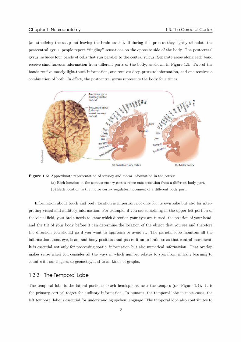
(anesthetizing the scalp but leaving the brain awake). If during this process they lightly stimulate the
postcentral gyrus, people report “tingling” sensations on the opposite side of the body. The postcentral
gyrus includes four bands of cells that run parallel to the central sulcus. Separate areas along each band
receive simultaneous information from different parts of the body, as shown in Figure 1.5. Two of the
bands receive mostly light-touch information, one receives deep-pressure information, and one receives a
combination of both. In effect, the postcentral gyrus represents the body four times.
Figure 1.5: Approximate representation of sensory and motor information in the cortex
(a) Each location in the somatosensory cortex represents sensation from a different body part.
(b) Each location in the motor cortex regulates movement of a different body part.
Information about touch and body location is important not only for its own sake but also for inter-
preting visual and auditory information. For example, if you see something in the upper left portion of
the visual field, your brain needs to know which direction your eyes are turned, the position of your head,
and the tilt of your body before it can determine the location of the object that you see and therefore
the direction you should go if you want to approach or avoid it. The parietal lobe monitors all the
information about eye, head, and body positions and passes it on to brain areas that control movement.
It is essential not only for processing spatial information but also numerical information. That overlap
makes sense when you consider all the ways in which number relates to spacefrom initially learning to
count with our fingers, to geometry, and to all kinds of graphs.
1.3.3 The Temporal Lobe
The temporal lobe is the lateral portion of each hemisphere, near the temples (see Figure 1.4). It is
the primary cortical target for auditory information. In humans, the temporal lobe in most cases, the
left temporal lobe is essential for understanding spoken language. The temporal lobe also contributes to
7

Chapter 1. Neuroanatomy 1.3. The Cerebral Cortex
some of the more complex aspects of vision, including perception of movement and recognition of faces.
A tumor in the temporal lobe may give rise to elaborate auditory or visual hallucinations, whereas a
tumor in the occipital lobe ordinarily evokes only simple sensations, such as flashes of light. In fact, when
psychiatric patients report hallucinations, brain scans detect extensive activity in the temporal lobes.
The temporal lobes also play a part in emotional and motivational behaviors. Temporal lobe damage
can lead to a set of behaviors known as the Klver-Bucy syndrome (named for the investigators who
first described it). Previously wild and aggressive monkeys fail to display normal fears and anxieties
after temporal lobe damage. They put almost anything they find into their mouths and attempt to pick
up snakes and lighted matches (which intact monkeys consistently avoid). Interpreting this behavior
is difficult. For example, a monkey might handle a snake because it is no longer afraid (an emotional
change) or because it no longer recognizes what a snake is (a cognitive change).
1.3.4 The Frontal Lobe
The frontal lobe, which contains the primary motor cortex and the prefrontal cortex, extends from the
central sulcus to the anterior limit of the brain (see Figure 1.4). The posterior portion of the frontal lobe
just anterior to the central sulcus, the precentral gyrus, is specialized for the control of fine movements,
such as moving one finger at a time. Separate areas are responsible for different parts of the body, mostly
on the contralateral (opposite) side but also with slight control of the ipsilateral (same) side. Figure 1.5
shows the traditional map of the precentral gyrus, also known as the primary motor cortex. However,
the map is only an approximation; for example, the arm area does indeed control arm movements, but
within that area, there is no one-to-one relationship between brain location and specific muscles.
The most anterior portion of the frontal lobe is the prefrontal cortex. In general, the larger a species
cerebral cortex, the higher the percentage of it is devoted to the prefrontal cortex. For example, it forms
a larger portion of the cortex in humans and all the great apes than in other species. It is not the primary
target for any single sensory system, but it receives information from all of them, in different parts of the
prefrontal cortex. The dendrites in the prefrontal cortex have up to 16 times as many dendritic spines as
neurons in other cortical areas. As a result, the prefrontal cortex can integrate an enormous amount of
information.
8

Chapter 2
Cognitive Neuroscience
Anervous system, composed of many individual cells, is in some regards like a society of people who work
together and communicate with one another or even like elements that form a chemical compound. In
each case, the combination has properties that are unlike those of its individual components. We begin
our study of the nervous system by examining single cells; later, we examine how cells act together.
2.1 The Cells of the Nervous System
Before you could build a house, you would first assemble bricks or other construction materials. Simil-
arly, before we can address the great philosophical questions such as the mindbrain relationship or the
great practical questions of abnormal behavior, we have to start with the building blocks of the nervous
systemthe cells.
2.1.1 Anatomy of Neurons and Glia
The nervous system consists of two kinds of cells: neurons and glia. Neurons receive information and
transmit it to other cells. Glia provide a number of functions that are difficult to summarize, and we
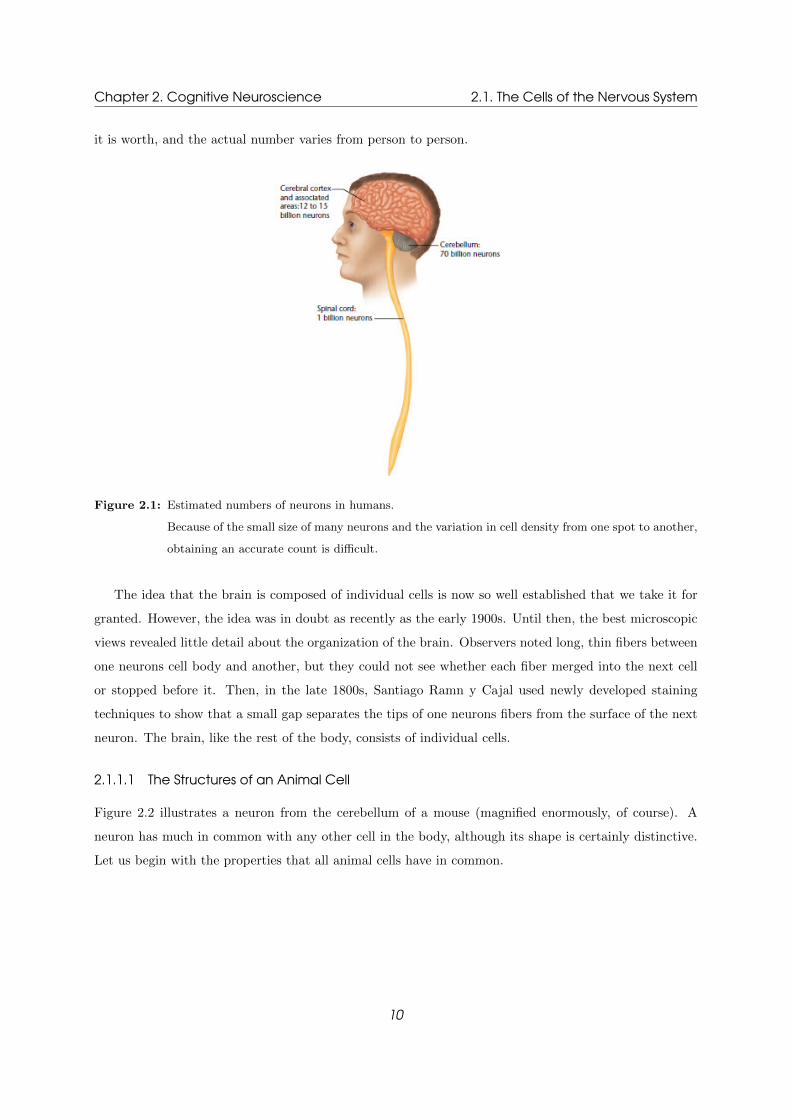
shall defer that discussion until later in the chapter. According to one estimate, the adult human brain
contains approximately 100 billion neurons (Figure 2.1). An accurate count would be more difficult than
9
Chapter 2. Cognitive Neuroscience 2.1. The Cells of the Nervous System
it is worth, and the actual number varies from person to person.
Figure 2.1: Estimated numbers of neurons in humans.
Because of the small size of many neurons and the variation in cell density from one spot to another,
obtaining an accurate count is difficult.
The idea that the brain is composed of individual cells is now so well established that we take it for
granted. However, the idea was in doubt as recently as the early 1900s. Until then, the best microscopic
views revealed little detail about the organization of the brain. Observers noted long, thin fibers between
one neurons cell body and another, but they could not see whether each fiber merged into the next cell
or stopped before it. Then, in the late 1800s, Santiago Ramn y Cajal used newly developed staining
techniques to show that a small gap separates the tips of one neurons fibers from the surface of the next
neuron. The brain, like the rest of the body, consists of individual cells.
2.1.1.1 The Structures of an Animal Cell
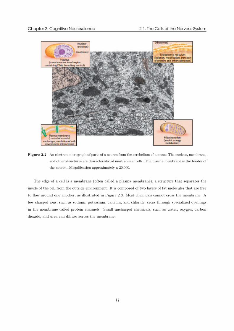
Figure 2.2 illustrates a neuron from the cerebellum of a mouse (magnified enormously, of course). A
neuron has much in common with any other cell in the body, although its shape is certainly distinctive.
Let us begin with the properties that all animal cells have in common.
10
Chapter 2. Cognitive Neuroscience 2.1. The Cells of the Nervous System
Figure 2.2: An electron micrograph of parts of a neuron from the cerebellum of a mouse The nucleus, membrane,
and other structures are characteristic of most animal cells. The plasma membrane is the border of
the neuron. Magnification approximately x 20,000.
The edge of a cell is a membrane (often called a plasma membrane), a structure that separates the
inside of the cell from the outside environment. It is composed of two layers of fat molecules that are free
to flow around one another, as illustrated in Figure 2.3. Most chemicals cannot cross the membrane. A
few charged ions, such as sodium, potassium, calcium, and chloride, cross through specialized openings
in the membrane called protein channels. Small uncharged chemicals, such as water, oxygen, carbon
dioxide, and urea can diffuse across the membrane.
11

Chapter 2. Cognitive Neuroscience 2.1. The Cells of the Nervous System
Figure 2.3: The membrane of a neuron
Embedded in the membrane are protein channels that permit certain ions to cross through the
membrane at a controlled rate.
Except for mammalian red blood cells, all animal cells have a nucleus, the structure that contains the
chromosomes. A mitochondrion (pl.: mitochondria) is the structure that performs metabolic activities,
providing the energy that the cell requires for all its other activities. Mitochondria require fuel and
oxygen to function. Ribosomes are the sites at which the cell synthesizes new protein molecules. Proteins
provide building materials for the cell and facilitate various chemical reactions. Some ribosomes float
freely within the cell; others are attached to the endoplasmic reticulum, a network of thin tubes that
transport newly synthesized proteins to other locations.
2.1.1.2 The Structure of a Neuron
A neuron contains a nucleus, a membrane, mitochondria, ribosomes, and the other structures typical of
animal cells. The distinctive feature of neurons is their shape.
Figure 2.4: The components of a vertebrate motor neuron
The cell body of a motor neuron is located in the spinal cord. The various parts are not drawn to
scale; in particular, a real axon is much longer in proportion to the soma.
12

Chapter 2. Cognitive Neuroscience 2.1. The Cells of the Nervous System
The larger neurons have these major components: dendrites, a soma (cell body), an axon, and pre-
synaptic terminals. (The tiniest neurons lack axons and some lack well-defined dendrites.) Contrast the
motor neuron in Figure 2.4 and the sensory neuron in Figure 2.5. A motor neuron has its soma in the
spinal cord. It receives excitation from other neurons through its dendrites and conducts impulses along
its axon to a muscle. A sensory neuron is specialized at one end to be highly sensitive to a particular
type of stimulation, such as touch information from the skin. Different kinds of sensory neurons have
different structures; the one shown in Figure 2.4 is a neuron conducting touch information from the skin
to the spinal cord. Tiny branches lead directly from the receptors into the axon, and the cells soma is
located on a little stalk off the main trunk.
Figure 2.5: A vertebrate sensory neuron
Note that the soma is located on a stalk off the main trunk of the axon.
Dendrites are branching fibers that get narrower near their ends. (The term dendrite comes from
a Greek root word meaning tree; a dendrite is shaped like a tree.) The dendrites surface is lined with
specialized synaptic receptors, at which the dendrite receives information from other neurons. The greater
the surface area of a dendrite, the more information it can receive. Some dendrites branch widely and
therefore have a large surface area. Some also contain dendritic spines, the short outgrowths that increase
the surface area available for synapses (Figure 2.7). The shape of dendrites varies enormously from one
neuron to another and can even vary from one time to another for a given neuron. The shape of the
dendrite has much to do with how the dendrite combines different kinds of input.
The cell body, or soma (Greek for “body”; pl.: somata), contains the nucleus, ribosomes, mitochondria,
and other structures found in most cells. Much of the metabolic work of the neuron occurs here. Cell
bodies of neurons range in diameter from 0.005 mm to 0.1 mm in mammals and up to a full millimeter
in certain invertebrates. Like the dendrites, the cell body is covered with synapses on its surface in many
neurons.
The axon is a thin fiber of constant diameter, in most cases longer than the dendrites. (The term axon
comes from a Greek word meaning “axis.”) The axon is the information sender of the neuron, conveying
an impulse toward either other neurons or a gland or muscle. Many vertebrate axons are covered with
13

Chapter 2. Cognitive Neuroscience 2.1. The Cells of the Nervous System
an insulating material called a myelin sheath with interruptions known as nodes of Ranvier. Invertebrate
axons do not have myelin sheaths. An axon has many branches, each of which swells at its tip, forming a
presynaptic terminal, also known as an end bulb or bouton (French for “button”). This is the point from
which the axon releases chemicals that cross through the junction between one neuron and the next.
Figure 2.6: Cell structures and axons
It all depends on the point of view. An axon from A to B is an efferent axon from A and an afferent
axon to B, just as a train from Washington to New York is exiting Washington and approaching
New York.
A neuron can have any number of dendrites, but no more than one axon, which may have branches.
Axons can range to a meter or more in length, as in the case of axons from your spinal cord to your feet.
In most cases, branches of the axon depart from its trunk far from the cell body, near the terminals.
Other terms associated with neurons are afferent, efferent, and intrinsic. An afferent axon brings
information into a structure; an efferent axon carries information away from a structure. Every sensory
neuron is an afferent to the rest of the nervous system; every motor neuron is an efferent from the nervous
system. Within the nervous system, a given neuron is an efferent from the standpoint of one structure
and an afferent from the standpoint of another. (You can remember that efferent starts with e as in exit;
afferent starts with a as in admission.) For example, an axon that is efferent from the thalamus may be
afferent to the cerebral cortex (Figure 2.6). If a cells dendrites and axon are entirely contained within a
single structure, the cell is an interneuron or intrinsic neuron of that structure. For example, an intrinsic
neuron of the thalamus has all its dendrites or axons within the thalamus; it communicates only with
other cells of the thalamus.
2.1.1.3 Variations among Neurons
Neurons vary enormously in size, shape, and function. The shape of a given neuron determines its
connections with other neurons and thereby determines its contribution to the nervous system. The wider
the branching, the more connections with other neurons. The function of a neuron is closely related to
its shape (Figure 2.7). For example, the dendrites of the Purkinje cell of the cerebellum (Figure 2.7a)
branch extremely widely within a single plane; this cell is capable of integrating an enormous amount of
14
Chapter 2. Cognitive Neuroscience 2.1. The Cells of the Nervous System
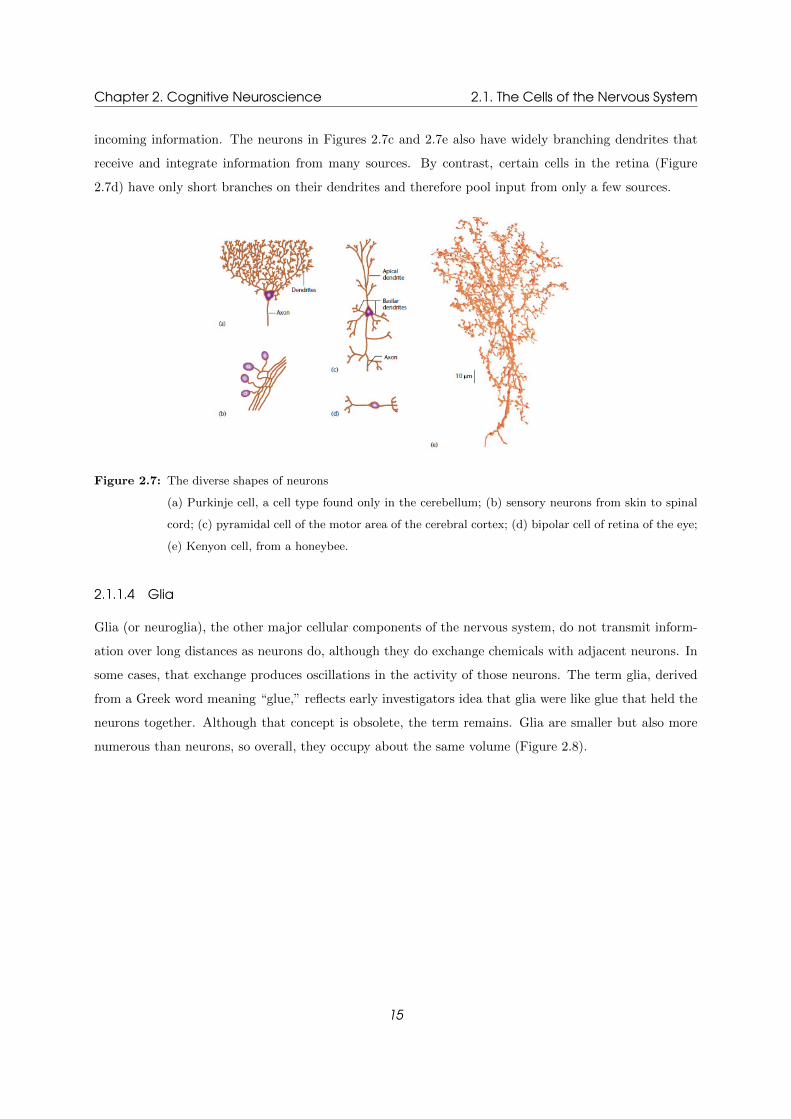
incoming information. The neurons in Figures 2.7c and 2.7e also have widely branching dendrites that
receive and integrate information from many sources. By contrast, certain cells in the retina (Figure
2.7d) have only short branches on their dendrites and therefore pool input from only a few sources.
Figure 2.7: The diverse shapes of neurons
(a) Purkinje cell, a cell type found only in the cerebellum; (b) sensory neurons from skin to spinal
cord; (c) pyramidal cell of the motor area of the cerebral cortex; (d) bipolar cell of retina of the eye;
(e) Kenyon cell, from a honeybee.
2.1.1.4 Glia
Glia (or neuroglia), the other major cellular components of the nervous system, do not transmit inform-
ation over long distances as neurons do, although they do exchange chemicals with adjacent neurons. In
some cases, that exchange produces oscillations in the activity of those neurons. The term glia, derived
from a Greek word meaning “glue,” reflects early investigators idea that glia were like glue that held the
neurons together. Although that concept is obsolete, the term remains. Glia are smaller but also more
numerous than neurons, so overall, they occupy about the same volume (Figure 2.8).
15

Chapter 2. Cognitive Neuroscience 2.1. The Cells of the Nervous System
Figure 2.8: Oligodendrocytes produce myelin sheaths that insulate certain vertebrate axons in the central
nervous system; Schwann cells have a similar function in the periphery. The oligodendrocyte is
shown here forming a segment of myelin sheath for two axons; in fact, each oligodendrocyte forms
such segments for 30 to 50 axons. Astrocytes pass chemicals back and forth between neurons and
blood and among neighboring neurons. Microglia proliferate in areas of brain damage and remove
toxic materials. Radial glia (not shown here) guide the migration of neurons during embryological
development. Glia have other functions as well.
Glia have many functions. One type of glia, the star-shaped astrocytes, wrap around the presynaptic
terminals of a group of functionally related axons. By taking up chemicals released by those axons and
later releasing them back to the axons, an astrocyte helps synchronize the activity of the axons, enabling
them to send messages in waves. Astrocytes also remove waste material created when neurons die and
help control the amount of blood flow to a given brain area.
Microglia, very small cells, also remove waste material as well as viruses, fungi, and other microorgan-
isms. In effect, they function like part of the immune system. Oligodendrocytes (OL-igo- DEN-druh-sites)
in the brain and spinal cord and Schwann cells in the periphery of the body are specialized types of glia
that build the myelin sheaths that surround and insulate certain vertebrate axons. Radial glia, a type of
astrocyte, guide the migration of neurons and the growth of their axons and dendrites during embryonic
development. Schwann cells perform a related function after damage to axons in the periphery, guiding
a regenerating axon to the appropriate target.
16
Chapter 2. Cognitive Neuroscience 2.1. The Cells of the Nervous System
2.1.2 The Blood-Brain Barrier
Although the brain, like any other organ, needs to receive nutrients from the blood, many chemicals
ranging from toxins to medicationscannot cross from the blood to the brain. The mechanism that keeps
most chemicals out of the vertebrate brain is known as the blood-brain barrier. Before we examine how
it works, lets consider why we need it.
2.1.2.1 Why We Need a Blood-Brain Barrier
From time to time, viruses and other harmful substances enter the body. When a virus enters a cell,
mechanisms within the cell extrude a virus particle through the membrane so that the immune system
can find it. When the immune system cells attack the virus, they also kill the cell that contains it. In
effect, a cell exposing a virus through its membrane says, “Look, immune system, Im infected with this
virus. Kill me and save the others.”
This plan works fine if the virus-infected cell is, say, a skin cell or a blood cell, which the body
replaces easily. However, with few exceptions, the vertebrate brain does not replace damaged neurons.
To minimize the risk of irreparable brain damage, the body literally builds a wall along the sides of the
brains blood vessels. This wall keeps out most viruses, bacteria, and harmful chemicals.
“What happens if a virus does enter the brain?” you might ask. After all, certain viruses do break
through the blood-brain barrier. The brain has ways to attack viruses or slow their reproduction but
doesnt kill them or the cells they inhabit. Consequently, a virus that enters your nervous system probably
remains with you for life. For example, herpes viruses (responsible for chicken pox, shingles, and genital
herpes) enter spinal cord cells. No matter how much the immune system attacks the herpes virus outside
the nervous system, virus particles remain in the spinal cord and can emerge decades later to reinfect
you.
A structure called the area postrema, which is not protected by the blood-brain barrier, monitors blood
chemicals that could not enter other brain areas. This structure is responsible for triggering nausea and
vomitingimportant responses to toxic chemicals. It is, of course, exposed to the risk of being damaged
itself.
2.1.2.2 How the Blood-Brain Barrier works
The blood-brain barrier (Figure 2.9) depends on the arrangement of endothelial cells that form the walls
of the capillaries. Outside the brain, such cells are separated by small gaps, but in the brain, they are
joined so tightly that virtually nothing passes between them. Chemicals therefore enter the brain only
by crossing the membrane itself.
17
Chapter 2. Cognitive Neuroscience 2.2. The Nerve Impulse
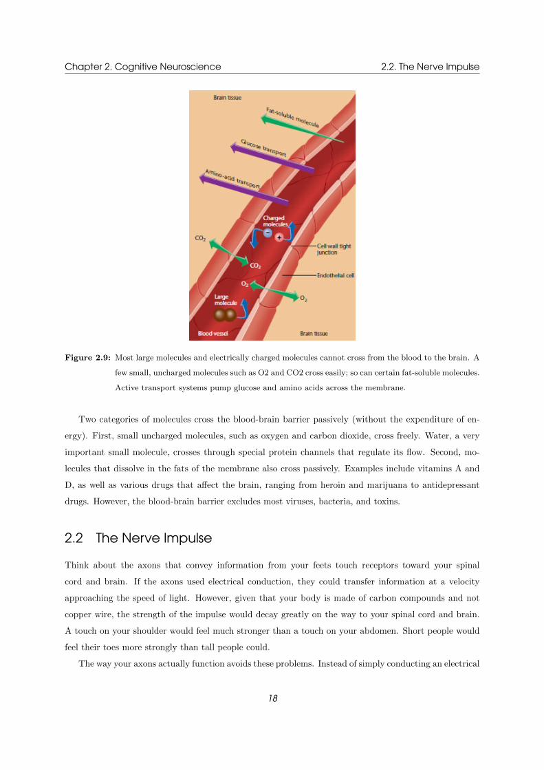
Figure 2.9: Most large molecules and electrically charged molecules cannot cross from the blood to the brain. A
few small, uncharged molecules such as O2 and CO2 cross easily; so can certain fat-soluble molecules.
Active transport systems pump glucose and amino acids across the membrane.
Two categories of molecules cross the blood-brain barrier passively (without the expenditure of en-
ergy). First, small uncharged molecules, such as oxygen and carbon dioxide, cross freely. Water, a very
important small molecule, crosses through special protein channels that regulate its flow. Second, mo-
lecules that dissolve in the fats of the membrane also cross passively. Examples include vitamins A and
D, as well as various drugs that affect the brain, ranging from heroin and marijuana to antidepressant
drugs. However, the blood-brain barrier excludes most viruses, bacteria, and toxins.
2.2 The Nerve Impulse
Think about the axons that convey information from your feets touch receptors toward your spinal
cord and brain. If the axons used electrical conduction, they could transfer information at a velocity
approaching the speed of light. However, given that your body is made of carbon compounds and not
copper wire, the strength of the impulse would decay greatly on the way to your spinal cord and brain.
A touch on your shoulder would feel much stronger than a touch on your abdomen. Short people would
feel their toes more strongly than tall people could.
The way your axons actually function avoids these problems. Instead of simply conducting an electrical
18

Chapter 2. Cognitive Neuroscience 2.2. The Nerve Impulse
impulse, the axon regenerates an impulse at each point. Imagine a long line of people holding hands.
The first person squeezes the second persons hand, who then squeezes the third persons hand, and so
forth. The impulse travels along the line without weakening because each person generates it anew.
Although the axons method of transmitting an impulse prevents a touch on your shoulder from feeling
stronger than one on your toes, it introduces a different problem: Because axons transmit information
at only moderate speeds (varying from less than 1 meter/ second to about 100 m/s), a touch on your
shoulder will reach your brain sooner than will a touch on your toes. If you get someone to touch you
simultaneously on your shoulder and your toe, you probably will not notice that your brain received one
stimulus before the other. In fact, if someone touches you on one hand and then the other, you wont be
sure which hand you felt first, unless the delay between touches exceeds 70 milliseconds (ms). Your brain
is not set up to register small differences in the time of arrival of touch messages. After all, why should
it be? You almost never need to know whether a touch on one part of your body occurred slightly before
or after a touch somewhere else.
In vision, however, your brain does need to know whether one stimulus began slightly before or after
another one. If two adjacent spots on your retinalets call them A and Bsend impulses at almost the same
time, an extremely small difference in timing indicates whether a flash of light moved from A to B or
from B to A. To detect movement as accurately as possible, your visual system compensates for the fact
that some parts of the retina are slightly closer to your brain than other parts are. Without some sort
of compensation, simultaneous flashes arriving at two spots on your retina would reach your brain at
different times, and you might perceive a flash of light moving from one spot to the other. What prevents
that illusion is the fact that axons from more distant parts of your retina transmit impulses slightly faster
than those closer to the brain!
In short, the properties of impulse conduction in an axon are well adapted to the exact needs for
information transfer in the nervous system. Lets now examine the mechanics of impulse transmission.
2.2.1 The Resting Potential of the Neuron
The membrane of a neuron maintains an electrical gradient, a difference in electrical charge between the
inside and outside of the cell. All parts of a neuron are covered by a membrane about 8 nanometers
(nm) thick (just less than 0.00001 mm), composed of two layers (an inner layer and an outer layer) of
phospholipid molecules (containing chains of fatty acids and a phosphate group). Embedded among the
phospholipids are cylindrical protein molecules (see Figure 2.3). The structure of the membrane provides
it with a good combination of flexibility and firmness and retards the flow of chemicals between the inside
and the outside of the cell.
In the absence of any outside disturbance, the membrane maintains an electrical polarization, meaning
a difference in electrical charge between two locations. Specifically, the neuron inside the membrane has
a slightly negative electrical potential with respect to the outside. This difference in voltage in a resting
19

Chapter 2. Cognitive Neuroscience 2.2. The Nerve Impulse
neuron is called the resting potential. The resting potential is mainly the result of negatively charged
proteins inside the cell.
Figure 2.10: Methods for recording activity of a neuron
(a) Diagram of the apparatus and a sample recording. (b) A microelectrode and stained neurons
magnified hundreds of times by a light microscope.
Researchers can measure the resting potential by inserting a very thin microelectrode into the cell
body,as Figure 2.10 shows. The diameter of the electrode must be as small as possible so that it can
enter the cell without causing damage. By far the most common electrode is a fine glass tube filled with
a concentrated salt solution and tapering to a tip diameter of 0.0005 mm or less. This electrode, inserted
into the neuron, is connected to recording equipment. A reference electrode placed somewhere outside
the cell completes the circuit. Connecting the electrodes to a voltmeter, we find that the neurons interior
has a negative potential relative to its exterior. The actual potential varies from one neuron to another;
a typical level is 70 millivolts (mV), but it can be either higher or lower than that.
2.2.1.1 Forces Acting on Sodium and Potassium Ions
If charged ions could flow freely across the membrane, the membrane would depolarize at once. However,
the membrane is selectively permeablethat is, some chemicals can pass through it more freely than others
can. (This selectivity is analogous to the blood-brain barrier, but it is not the same thing.) Most large
or electrically charged ions and molecules cannot cross the membrane at all. Oxygen, carbon dioxide,
urea, and water cross freely through channels that are always open. A few biologically important ions,
such as sodium, potassium, calcium, and chloride, cross through membrane channels (or gates) that are
sometimes open and sometimes closed. When the membrane is at rest, the sodium channels are closed,
preventing almost all sodium flow. These channels are shown in Figure 2.11.
20

Chapter 2. Cognitive Neuroscience 2.2. The Nerve Impulse
Figure 2.11: Ion channels in the membrane of a neuron
When a channel opens, it permits one kind of ion to cross the membrane. When it closes, it
prevents passage of that ion.
Certain kinds of stimulation can open the sodium channels. When the membrane is at rest, potassium
channels are nearly but not entirely closed, so potassium flows slowly.
Sodium ions are more than ten times more concentrated outside the membrane than inside because
of the sodium-potassium pump, a protein complex that repeatedly transports three sodium ions out of
the cell while drawing two potassium ions into it. The sodium-potassium pump is an active transport
requiring energy. Various poisons can stop it, as can an interruption of blood flow.
The sodium-potassium pump is effective only because of the selective permeability of the membrane,
which prevents the sodium ions that were pumped out of the neuron from leaking right back in again.
As it is, the sodium ions that are pumped out stay out. However, some of the potassium ions pumped
into the neuron do leak out, carrying a positive charge with them. That leakage increases the electrical
gradient across the membrane, as shown in Figure 2.12.
21
Chapter 2. Cognitive Neuroscience 2.2. The Nerve Impulse
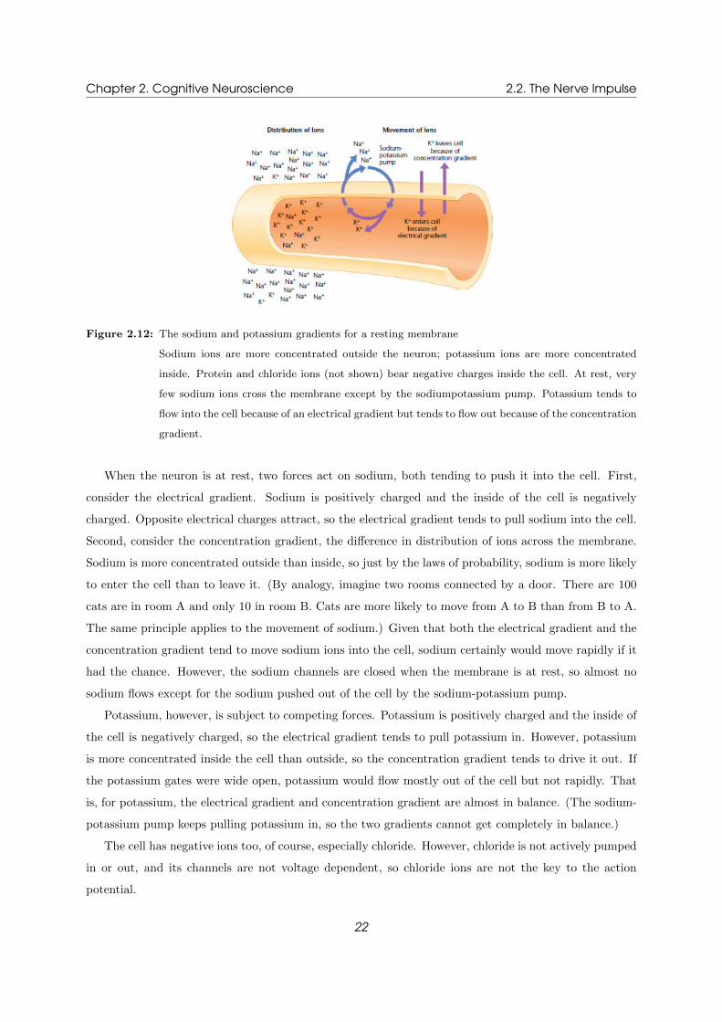
Figure 2.12: The sodium and potassium gradients for a resting membrane
Sodium ions are more concentrated outside the neuron; potassium ions are more concentrated
inside. Protein and chloride ions (not shown) bear negative charges inside the cell. At rest, very
few sodium ions cross the membrane except by the sodiumpotassium pump. Potassium tends to
flow into the cell because of an electrical gradient but tends to flow out because of the concentration
gradient.
When the neuron is at rest, two forces act on sodium, both tending to push it into the cell. First,
consider the electrical gradient. Sodium is positively charged and the inside of the cell is negatively
charged. Opposite electrical charges attract, so the electrical gradient tends to pull sodium into the cell.
Second, consider the concentration gradient, the difference in distribution of ions across the membrane.
Sodium is more concentrated outside than inside, so just by the laws of probability, sodium is more likely
to enter the cell than to leave it. (By analogy, imagine two rooms connected by a door. There are 100
cats are in room A and only 10 in room B. Cats are more likely to move from A to B than from B to A.
The same principle applies to the movement of sodium.) Given that both the electrical gradient and the
concentration gradient tend to move sodium ions into the cell, sodium certainly would move rapidly if it
had the chance. However, the sodium channels are closed when the membrane is at rest, so almost no
sodium flows except for the sodium pushed out of the cell by the sodium-potassium pump.
Potassium, however, is subject to competing forces. Potassium is positively charged and the inside of
the cell is negatively charged, so the electrical gradient tends to pull potassium in. However, potassium
is more concentrated inside the cell than outside, so the concentration gradient tends to drive it out. If
the potassium gates were wide open, potassium would flow mostly out of the cell but not rapidly. That
is, for potassium, the electrical gradient and concentration gradient are almost in balance. (The sodium-
potassium pump keeps pulling potassium in, so the two gradients cannot get completely in balance.)
The cell has negative ions too, of course, especially chloride. However, chloride is not actively pumped
in or out, and its channels are not voltage dependent, so chloride ions are not the key to the action
potential.
22

Chapter 2. Cognitive Neuroscience 2.2. The Nerve Impulse
2.2.1.2 Why a Resting Potential?
Presumably, evolution could have equipped us with neurons that were electrically neutral at rest. The
resting potential must provide enough benefit to justify the energy cost of the sodium-potassium pump.
The advantage is that the resting potential prepares the neuron to respond rapidly to a stimulus. As
we shall see in the next section, excitation of the neuron opens channels that let sodium enter the cell
explosively. Because the membrane did its work in advance by maintaining the concentration gradient
for sodium, the cell is prepared to respond strongly and rapidly to a stimulus.
The resting potential of a neuron can be compared to a poised bow and arrow: An archer who pulls
the bow in advance and then waits is ready to fire as soon as the appropriate moment comes. Evolution
has applied the same strategy to the neuron.
2.2.2 The Action Potential
The resting potential remains stable until the neuron is stimulated. Ordinarily, stimulation of the neuron
takes place at synapses. In the laboratory, it is also possible to stimulate a neuron by inserting an
electrode into it and applying current.
We can measure a neurons potential with a microelectrode, as shown in Figure 2.10b. When an axons
membrane is at rest, the recordings show a steady negative potential inside the axon. If we now use
an additional electrode to apply a negative charge, we can further increase the negative charge inside
the neuron. The change is called hyperpolarization, which means increased polarization. As soon as the
artificial stimulation ceases, the charge returns to its original resting level. The recording looks like this:
Now, let us apply a current for a slight depolarization of the neuronthat is, reduction of its polarization
toward zero. If we apply a small depolarizing current, we get a result like this:
With a slightly stronger depolarizing current, the potential rises slightly higher, but again, it returns
to the resting level as soon as the stimulation ceases:
23

Chapter 2. Cognitive Neuroscience 2.2. The Nerve Impulse
Now let us see what happens when we apply a still stronger current: Any stimulation beyond a certain
level, called the threshold of excitation, produces a sudden, massive depolarization of the membrane.
When the potential reaches the threshold, the membrane suddenly opens its sodium channels and permits
a rapid, massive flow of ions across the membrane. The potential then shoots up far beyond the strength
of the stimulus:
Any subthreshold stimulation produces a small response proportional to the amount of current. Any
stimulation beyond the threshold, regardless of how far beyond, produces the same response, like the one
just shown. That response, a rapid depolarization and slight reversal of the usual polarization, is referred
to as an action potential. The peak of the action potential, shown as +30 mV in this illustration, varies
from one axon to another, but it is nearly constant for a given axon.
2.2.2.1 The Molecular Basis of the Action Potential
Remember that both the electrical gradient and the concentration gradient tend to drive sodium ions into
the neuron. If sodium ions could flow freely across the membrane, they would enter rapidly. Ordinarily,
the membrane is almost impermeable to sodium, but during the action potential, its permeability increases
sharply.
The membrane proteins that control sodium entry are voltage-activated channels, membrane channels
whose permeability depends on the voltage difference across the membrane. At the resting potential,
the channels are closed. As the membrane becomes slightly depolarized, the sodium channels begin to
open and sodium flows more freely. If the depolarization is less than the threshold, sodium crosses the
membrane only slightly more than usual. When the potential across the membrane reaches threshold, the
sodium channels open wide. Sodium ions rush into the neuron explosively until the electrical potential
across the membrane passes beyond zero to a reversed polarity, as shown in the following diagram:
24

Chapter 2. Cognitive Neuroscience 2.2. The Nerve Impulse
Compared to the total number of sodium ions in and around the axon, only a tiny percentage cross
the membrane during an action potential. Even at the peak of the action potential, sodium ions continue
to be far more concentrated outside the neuron than inside. An action potential increases the sodium
concentration inside a neuron by far less than 1%. Because of the persisting concentration gradient,
sodium ions should still tend to diffuse into the cell. However, at the peak of the action potential, the
sodium gates quickly close and resist reopening for about the next millisecond.
After the peak of the action potential, what brings the membrane back to its original state of polariza-
tion? The answer is not the sodium-potassium pump, which is too slow for this purpose. After the action
potential is underway, the potassium channels open. Potassium ions flow out of the axon simply because
they are much more concentrated inside than outside and they are no longer held inside by a negative
charge. As they flow out of the axon, they carry with them a positive charge. Because the potassium
channels open wider than usual and remain open after the sodium channels close, enough potassium ions
leave to drive the membrane beyond the normal resting level to a temporary hyperpolarization. Figure
2.13 summarizes the movements of ions during an action potential.
25
Chapter 2. Cognitive Neuroscience 2.2. The Nerve Impulse
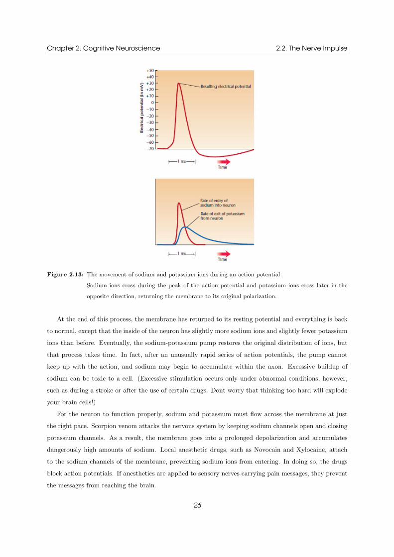
Figure 2.13: The movement of sodium and potassium ions during an action potential
Sodium ions cross during the peak of the action potential and potassium ions cross later in the
opposite direction, returning the membrane to its original polarization.
At the end of this process, the membrane has returned to its resting potential and everything is back
to normal, except that the inside of the neuron has slightly more sodium ions and slightly fewer potassium
ions than before. Eventually, the sodium-potassium pump restores the original distribution of ions, but
that process takes time. In fact, after an unusually rapid series of action potentials, the pump cannot
keep up with the action, and sodium may begin to accumulate within the axon. Excessive buildup of
sodium can be toxic to a cell. (Excessive stimulation occurs only under abnormal conditions, however,
such as during a stroke or after the use of certain drugs. Dont worry that thinking too hard will explode
your brain cells!)
For the neuron to function properly, sodium and potassium must flow across the membrane at just
the right pace. Scorpion venom attacks the nervous system by keeping sodium channels open and closing
potassium channels. As a result, the membrane goes into a prolonged depolarization and accumulates
dangerously high amounts of sodium. Local anesthetic drugs, such as Novocain and Xylocaine, attach
to the sodium channels of the membrane, preventing sodium ions from entering. In doing so, the drugs
block action potentials. If anesthetics are applied to sensory nerves carrying pain messages, they prevent
the messages from reaching the brain.
26

Chapter 2. Cognitive Neuroscience 2.2. The Nerve Impulse
2.2.2.2 The All-or-None Law
Action potentials occur only in axons and cell bodies. When the voltage across an axon membrane
reaches a certain level of depolarization (the threshold), voltageactivated sodium channels open wide to
let sodium enter rapidly, and the incoming sodium depolarizes the membrane still further. Dendrites can
be depolarized, but they dont have voltage-activated sodium channels, so opening the channels a little,
letting in a little sodium, doesnt cause them to open even more and let in still more sodium. Thus,
dendrites dont produce action potentials.
For a given neuron, all action potentials are approximately equal in amplitude (intensity) and velocity
under normal circumstances. This is the all-or-none law: The amplitude and velocity of an action potential
are independent of the intensity of the stimulus that initiated it. By analogy, imagine flushing a toilet:
You have to make a press of at least a certain strength (the threshold), but pressing even harder does
not make the toilet flush any faster or more vigorously.
The all-or-none law puts some constraints on how an axon can send a message. To signal the difference
between a weak stimulus and a strong stimulus, the axon cant send bigger or faster action potentials. All
it can change is the timing. By analogy, suppose you agree to exchange coded messages with someone
in another building who can see your window by occasionally flicking your lights on and off. The two of
you might agree, for example, to indicate some kind of danger by the frequency of flashes. (The more
flashes, the more danger.) You could also convey information by a rhythm.
Flash-flash . . . long pause . . . flash-flash
might mean something different from
Flash . . . pause . . . flash . . . pause . . . flash . . . pause . . . flash.
The nervous system uses both of these kinds of codes. Researchers have long known that a greater
frequency of action potentials per second indicates stronger stimulus. In some cases, a different rhythm
of response also carries information. For example, an axon might show one rhythm of responses for sweet
tastes and a different rhythm for bitter tastes.
2.2.2.3 The Refractory Period
While the electrical potential across the membrane is returning from its peak toward the resting point,
it is still above the threshold. Why doesnt the cell produce another action potential during this period?
Immediately after an action potential, the cell is in a refractory period during which it resists the pro-
duction of further action potentials. In the first part of this period, the absolute refractory period, the
membrane cannot produce an action potential, regardless of the stimulation. During the second part,
the relative refractory period, a stronger than usual stimulus is necessary to initiate an action potential.
The refractory period is based on two mechanisms: The sodium channels are closed, and potassium is
flowing out of the cell at a faster than usual rate.
27

Chapter 2. Cognitive Neuroscience 2.2. The Nerve Impulse
Most of the neurons that have been tested have an absolute refractory period of about 1 ms and a
relative refractory period of another 24 ms. (To return to the toilet analogy, there is a short time right
after you flush a toilet when you cannot make it flush againan absolute refractory period. Then follows
a period when it is possible but difficult to flush it againa relative refractory periodbefore it returns to
normal.)
2.2.3 Propagation of the Action Potential
Up to this point, we have dealt with the action potential at one location on the axon. Now let us consider
how it moves down the axon toward some other cell. Remember that it is important for axons to convey
impulses without any loss of strength over distance.
In a motor neuron, an action potential begins on the axon hillock, a swelling where the axon exits
the soma (see Figure 2.4). Each point along the membrane regenerates the action potential in much the
same way that it was generated initially. During the action potential, sodium ions enter a point on the
axon. Temporarily, that location is positively charged in comparison with neighboring areas along the
axon. The positive ions flow down the axon and across the membrane, as shown in Figure 2.14. Other
things being equal, the greater the diameter of the axon, the faster the ions flow (because of decreased
resistance). The positive charges now inside the membrane slightly depolarize the adjacent areas of the
membrane, causing the next area to reach its threshold and regenerate the action potential. In this
manner, the action potential travels like a wave along the axon.
28

Chapter 2. Cognitive Neuroscience 2.2. The Nerve Impulse
Figure 2.14: Current that enters an axon during the action potential flows down the axon, depolarizing adjacent
areas of the membrane. The current flows more easily through thicker axons. Behind the area of
sodium entry, potassium ions exit.
The term propagation of the action potential describes the transmission of an action potential down
an axon. The propagation of an animal species is the production of offspring; in a sense, the action
potential gives birth to a new action potential at each point along the axon. In this manner, the action
potential can be just as strong at the end of the axon as it was at the beginning. The action potential is
much slower than electrical conduction because it requires the diffusion of sodium ions at successive points
along the axon. Electrical conduction in a copper wire with free electrons travels at a rate approaching
the speed of light, 300 million meters per second (m/s). In an axon, transmission relies on the flow of
charged ions through a water medium. In thin axons, action potentials travel at a velocity of less than 1
m/s. Thicker axons and those covered with an insulating shield of myelin conduct with greater velocities.
Let us reexamine Figure 2.14 for a moment. What is to prevent the electrical charge from flowing
in the direction opposite that in which the action potential is traveling? Nothing. In fact, the electrical
charge does flow in both directions. In that case, what prevents an action potential near the center of an
axon from reinvading the areas that it has just passed? The answer is that the areas just passed are still
in their refractory period.
29

Chapter 2. Cognitive Neuroscience 2.2. The Nerve Impulse
2.2.4 The Myelin Sheath and Saltatory Conduction
The thinnest axons conduct impulses at less than 1 m/s. Increasing the diameters increases conduction
velocity but only up to about 10 m/s. At that speed, an impulse from a giraffes foot takes about half a
second to reach its brain. At the slower speeds of thinner unmyelinated axons, a giraffes brain could be
seconds out of date on what was happening to its feet. In some vertebrate axons, sheaths of myelin, an
insulating material composed of fats and proteins, increase speed up to about 100 m/s.
Consider the following analogy. Suppose it is my job to carry written messages over a distance of 3
kilometers (km) without using any mechanical device. Taking each message and running with it would
be reliable but slow, like the propagation of an action potential along an unmyelinated axon. I could try
tying each message to a ball and throwing it, but I cannot throw a ball even close to 3 km. The ideal
compromise is to station people at moderate distances along the 3 km and throw the messagebearing ball
from person to person until it reaches its destination.
The principle behind myelinated axons, those covered with a myelin sheath, is the same. Myelinated
axons, found only in vertebrates, are covered with a coating composed mostly of fats. The myelin sheath
is interrupted at intervals of approximately 1 mm by short unmyelinated sections of axon called nodes of
Ranvier (RAHN-vee-ay), as shown in Figure 2.15. Each node is only about 1 micrometer wide.
Figure 2.15: An axon surrounded by a myelin sheath and interrupted by nodes of Ranvier
The inset shows a cross-section through both the axon and the myelin sheath. Magnification
approximately x 30,000. The anatomy is distorted here to show several nodes; in fact, the distance
between nodes is generally about 100 times as large as the nodes themselves.
Suppose that an action potential is initiated at the axon hillock and propagated along the axon until
it reaches the first myelin segment. The action potential cannot regenerate along the membrane between
nodes because sodium channels are virtually absent between nodes. After an action potential occurs at a
node, sodium ions that enter the axon diffuse within the axon, repelling positive ions that were already
30

Chapter 2. Cognitive Neuroscience 2.3. The Synapse
present and thus pushing a chain of positive ions along the axon to the next node, where they regenerate
the action potential (Figure 2.16). This flow of ions is considerably faster than the regeneration of an
action potential at each point along the axon. The jumping of action potentials from node to node
is referred to as saltatory conduction, from the Latin word saltare, meaning to jump. (The same root
shows up in the word somersault.) In addition to providing very rapid conduction of impulses, saltatory
conduction has the benefit of conserving energy: Instead of admitting sodium ions at every point along
the axon and then having to pump them out via the sodium-potassium pump, a myelinated axon admits
sodium only at its nodes.
Some diseases, including multiple sclerosis, destroy myelin sheaths, thereby slowing action potentials
or stopping them altogether. An axon that has lost its myelin is not the same as one that has never had
myelin. A myelinated axon loses its sodium channels between the nodes. After the axon loses myelin,
it still lacks sodium channels in the areas previously covered with myelin, and most action potentials
die out between one node and the next. People with multiple sclerosis suffer a variety of impairments,
including poor muscle coordination.
Figure 2.16: Saltatory conduction in a myelinated axon
An action potential at the node triggers flow of current to the next node, where the membrane
regenerates the action potential.
2.3 The Synapse
The birth and propagation of the action potential within the presynaptic neuron makes up the first half
of our story of neural communication. The second half begins when the action potential reaches the axon
terminal and the message must cross the synaptic gap to the adjacent postsynaptic neuron. Figure 2.17
shows an electron micrograph of many axons forming synapses on a cell body.
31

Chapter 2. Cognitive Neuroscience 2.3. The Synapse
Figure 2.17: Neurons Communicate at the Synapse
This colored electron micrograph shows the axon terminals from many neurons forming synapses
on a cell body.
The human brain contains about 100 billion neurons, and the average neuron forms something on the
order of 1,000 synapses. Remarkably, these numbers suggest that the human brain has more synapses
than there are stars in our galaxy. In spite of these large numbers, synapses take one of only two forms. At
chemical synapses, neurons stimulate adjacent cells by sending chemical messengers, or neurotransmitters,
across the synaptic gap. At electrical synapses, neurons directly stimulate adjacent cells by sending ions
across the gap through channels that actually touch. Because the gap at an electrical synapse is so narrow
and the movement of ions is so rapid, the transmission is nearly instantaneous. We will not delve deeper
into the electrical synapse.
We can divide our discussion of the signaling at chemical synapses into two steps. The first step is
release of the neurotransmitter chemicals by the presynaptic cell. The second step is the reaction of the
postsynaptic cell to the neurotransmitters.
2.3.1 Neurotransmitter Release
In response to the arrival of an action potential at the terminal, a new type of voltage-dependent channel
will open. This time, voltage-dependent calcium (Ca 2+) channels will play the major role in the cellfs
activities. The amount of neurotransmitter released is a direct reflection of the amount of calcium that
enters the presynaptic neuron. A large influx of calcium triggers a large release of neurotransmitter
substance.
Calcium is a positively charged ion (Catextsuperscript2+) that is more abundant in the extracellular
fluid than in the intracellular fluid. Therefore, its situation is very similar to sodium, and it will move
under the same circumstances that cause sodium to move. Calcium channels are rather rare along the
length of the axon, but there are a large number located in the axon terminal membrane. Calcium channels
open in response to the arrival of the depolarizing action potential. Calcium does not move immediately,
however, because it is a positively charged ion and the intracellular fluid is positively charged during
32

Chapter 2. Cognitive Neuroscience 2.3. The Synapse
the action potential. As the action potential recedes in the axon terminal, however, calcium is attracted
by the relatively negative interior. Once calcium enters the presynaptic cell, it triggers the release of
neurotransmitter substance within about 0.2 msec.
Prior to release, molecules of neurotransmitter are stored in synaptic vesicles. These vesicles are
anchored by special proteins near release sites on the presynaptic membrane. The process by which these
vesicles release their contents is known as exocytosis, illustrated in Figure 2.18. Calcium entering the
cell appears to release the vesicles from their protein anchors, which allows them to migrate toward the
release sites. At the release site, calcium stimulates the fusion between the membrane of the vesicle and
the membrane of the axon terminal, forming a channel through which the neurotransmitter molecules
escape.
A long-standing assumption regarding exocytosis is that each released vesicle is fully emptied of
neurotransmitter. However, some researchers have suggested the possibility that there are instances of
partial release, which they have dubbed “kiss and run”. In kiss and run, vesicles are oly partially emptied
of neurotransmitter molecules before closing up again and returning to the interior of the axon terminal.
If vesicles did indeed have the ability to kiss and run, the process of neurotransmission would be much
faster than if they had to be filled from scratch after each use. In addition, kiss and run raises the
possibility that the vesicles themselves control the amount of neurotransmitter released to some extent.
The prevalence and significance of the full-release and kiss-and-run modes remains an active area of
research interest.
Following exocytosis, the neuron must engage in several housekeeping duties to prepare for the arrival
of the next action potential. Calcium pumps must act to return calcium to the extracellular fluid.
Otherwise, neurotransmitters would be released constantly rather than in response to the arrival of an
action potential. Because the vesicle membrane fuses with the presynaptic membrane, something must be
done to prevent a gradual thickening of the membrane that would interfere with neurotransmitter release.
The solution to this unwanted thickening is the recycling of the vesicle material. Excess membrane
material forms a pit, which is eventually pinched off to form a new vesicle.
Before we leave the presynaptic neuron, we need to consider one of the feedback loops the presynaptic
neuron uses to monitor its own activity. Embedded within the presynaptic membrane are special protein
structures known as autoreceptors. Autoreceptors bind some of the neurotransmitter molecules released
by the presynaptic neuron, providing feedback to the presynaptic neuron about its own level of activity.
This information may affect the rate of neurotransmitter synthesis and release
33

Chapter 2. Cognitive Neuroscience 2.3. The Synapse
Figure 2.18: Exocytosis Results in the Release of Neurotransmitters
Calcium is a positively charged ion (Ca2+) that is more abundant in the extracellular fluid than
in the intracellular fluid. Therefore, its situation is very similar to sodium, and it will move under
the same circumstances that cause sodium to move. Calcium channels are rather rare along the
length of the axon, but there are a large number located in the axon terminal membrane. Calcium
channels open in response to the arrival of the depolarizing action potential. Calcium does not move
immediately, however, because it is a positively charged ion and the intracellular fluid is positively
charged during the action potential. As the action potential recedes in the axon terminal, however,
calcium is attracted by the relatively negative interior. Once calcium enters the presynaptic cell,
it triggers the release of neurotransmitter substance within about 0.2 msec.
2.3.2 Neurotransmitters Bind to Postsynaptic Receptor Sites
The newly released molecules of neurotransmitter substance float across the synaptic gap. On the post-
synaptic side of the synapse, we find new types of proteins embedded in the postsynaptic cell membrane,
known as receptor sites. The receptor sites are characterized by recognition molecules that respond only
to certain types of neurotransmitter substance. Recognition molecules extend into the extracellular fluid
of the synaptic gap, where they come into contact with molecules of neurotransmitter. The molecules of
neurotransmitter function as keys that fit into the locks made by the recognition molecules.
Two major types of receptors are illustrated in Figure 2.19. Once the neurotransmitter molecules
have bound to receptor sites, ligand-gated ion channels will open either directly or indirectly. In the
direct case, known as an ionotropic receptor, the receptor site is located on the channel protein. As
soon as the receptor captures molecules of neurotransmitter, the ion channel opens. These one-step
receptors are capable of very fast reactions to neurotransmitters. In other cases, however, the receptor
34

Chapter 2. Cognitive Neuroscience 2.3. The Synapse
site does not have direct control over an ion channel. In these cases, known as metabotropic receptors,
a recognition site extends into the extracellular fluid, and a special protein called a G protein is located
on the receptor’s intracellular side. When molecules of neurotransmitter bind at the recognition site, the
G protein separates from the receptor complex and moves to a different part of the postsynaptic cell.
G proteins can open ion channels in the nearby membrane or activate additional chemical messengers
within the postsynaptic cell known as second messengers. (Neurotransmitters are the first messengers.)
Because of the multiple steps involved, the metabotropic receptors respond more slowly, in hundreds
of milliseconds to seconds, than the ionotropic receptors, which respond in milliseconds. In addition,
the effects of metabotropic activation can last much longer than those produced by the activation of
ionotropic receptors.
Figure 2.19: Ionotropic and Metabotropic Receptors
Ionotropic receptors, shown in (a), feature a recognition site for molecules of neurotransmitter
located on an ion channel. These one-step receptors provide a very fast response to the presence
of neurotransmitters. Metabotropic receptors, shown in (b), require additional steps. Neurotrans-
mitter molecules are recognized by the receptor, which in turn releases internal messengers known
as G proteins. G proteins initiate a wide variety of functions within the cell, including opening
adjacent ion channels and changing gene expression.
What is the advantage to an organism of evolving a slower, more complicated system? The answer is
35

Chapter 2. Cognitive Neuroscience 2.3. The Synapse
that the metabotropic receptor provides the possibility of a much greater variety of responses to the release
of neurotransmitter. The activation of metabotropic receptors can result not only in the opening of ion
channels, but also in a number of additional functions. Different types of metabotropic receptors influence
the amount of neurotransmitter released, help maintain the resting potential, and initiate changes in gene
expression. Unlike the ionotropic receptor, which affects a very small, local part of a cell, a metabotropic
receptor can have wideranging and multiple influences within a cell due to its ability to activate a variety
of second messengers.
2.3.3 Termination of the chemical signal
Before we can make a second telephone call, we need to hang up the phone to end the first call. If we want
to send a second message across a synapse, itfs necessary to have some way of ending the first message.
As shown in Figure 2.20, neurons have three ways of ending a chemical message. The particular
method used depends on the neurotransmitter involved. The first method is simple diffusion away from
the synapse. Like any other molecule, a neurotransmitter diffuses away from areas of high concentration
to areas of low concentration. The astrocytes surrounding the synapse influence the speed of neuro-
transmitter diffusion away from the synapse. In the second method for ending chemical transmission,
neurotransmitter molecules are deactivated in the synapse by enzymes in the synaptic gap. In the third
process, reuptake, the presynaptic membrane uses its own set of receptors known as transporters to re-
capture molecules of neurotransmitter substance and return them to the interior of the axon terminal. In
the terminal, the neurotransmitter can be repackaged in vesicles for subsequent release. Unlike the cases
in which enzymes deactivate neurotransmitters, reuptake spares the cell the extra step of reconstructing
the molecules out of component parts.
36

Chapter 2. Cognitive Neuroscience 2.3. The Synapse
Figure 2.20: Methods for Deactivating Neurotransmitters
Neurotransmitters released into the synaptic gap must be deactivated before additional signals
are sent by the presynaptic neuron. Deactivation may occur through (a) diffusion away from
the synapse, (b) through the action of special enzymes, or (c) through reuptake. Deactivating
enzymes break the neurotransmitter molecules into their components. The presynaptic neuron
collects these components and then synthesizes and packages more neurotransmitter substance. In
reuptake, presynaptic transporters recapture released neurotransmitter molecules and repackage
them in vesicles.
2.3.4 Postsynaptic Potentials
When molecules of neurotransmitter bind to postsynaptic receptors, they can produce one of two out-
comes, illustrated in Figure 2.21. The first possible outcome is a slight depolarization of the postsynaptic
membrane, known as an excitatory postsynaptic potential, or EPSP. EPSPs generally result from the
opening of ligand-gated rather than voltage-dependent sodium channels in the postsynaptic membrane.
The inward movement of positive sodium ions produces the slight depolarization of the EPSP. In addi-
tion to opening a different type of channel, EPSPs differ from action potentials in other ways. We have
described action potentials as being all-or-none. In contrast, EPSPs are known as graded potentials,
referring to their varying size and shape. Action potentials last about 1 msec, but EPSPs can last up to
5 to 10 msec.
37

Chapter 2. Cognitive Neuroscience 2.3. The Synapse
Figure 2.21: Neural Integration Combines Excitatory and Inhibitory Input
These graphs illustrate the effects of excitatory postsynaptic potentials (EPSPs) and inhibitory
postsynaptic potentials (IPSPs) alone and together on the overall response by the postsynaptic
neuron. In (a), the EPSP alone depolarizes the postsynaptic cell to threshold and initiates an
action potential. In (b), the IPSP alone hyperpolarizes the postsynaptic neuron. In (c), the EPSP
and IPSP essentially cancel each other out, and no action potential occurs.
The second possible outcome of the binding of neurotransmitter to a postsynaptic receptor is the
production of an inhibitory postsynaptic potential, or IPSP. The IPSP is a slight hyperpolarization of
the postsynaptic membrane, which reduces the likelihood that the postsynaptic cell will produce an action
potential. Like the EPSP, the IPSP is a graded potential that can last 5 to 10 msec. IPSPs are usually
produced by the opening of ligand-gated channels that allow for the inward movement of chloride (Cl-)
or the outward movement of potassium (K+). The movement of negatively charged chloride ions into
the postsynaptic cell would add to the cells negative charge. The loss of positively charged potassium
cells would also increase a cells negative charge. A comparison of the characteristics of action potentials,
EPSPs, and IPSPs may be found in Table 2.1.
38

Chapter 2. Cognitive Neuroscience 2.3. The Synapse
Action Potential EPSPs IPSPs
Role Signaling within neurons Signaling between neurons Signaling between neurons
Duration 1 to 2 msec 5 to 10 msec up to 100 msec 5 to 10 msec up to 100 msec
Size About 100mV Up to 20mV Up to 15mV
Character All-or-none Graded depolarization Graded hyperpolarization
Propagation Active Passive Passive
Channels involved Voltage-dependent sodium and
potassium channels
Ligand-gated sodium channels Ligand-gated potassium and
chloride channels
Table 2.1: A Comparison of the Characteristics of Action Potentials, EPSPs, and IPSPs
2.3.5 Neural Integration
The average neuron in the human brain receives input from about 1,000 other neurons. Some of that
input will be in the form of EPSPs, some in the form of IPSPs. The task faced by one of these neurons
is to decide which input merits the production of an action potential. You may have had the experience
of asking friends and family members for help with a moral dilemma. Some of your advisors give you
an excitatory “go for it” message, and others give you an inhibitory“dont even think about it” message.
After reviewing the input, it is your task, like the neurons, to consider all of the advice youve received
and decide whether to go forward. This decision-making process on the part of the neuron is known as
neural integration.
In vertebrates, cells receive their excitatory and inhibitory advice in different locations. The dendrites
and their spines are the major locations for excitatory input. In contrast, most of the inhibitory input
occurs at synapses on the cell body. Because the dendrites and cell body contain few voltage-dependent
channels, they do not typically produce action potentials. Instead, EPSPs from the dendrites and IPSPs
from the cell body spread passively but very rapidly until they reach the axon hillock.
The only time the cell will produce an action potential is when the area of the axon hillock is de-
polarized to threshold. This may occur as a result of spatial summation, in which inputs from all over
the cell converge at the axon hillock. The cell adds up all the excitatory inputs and subtracts all the
inhibitory inputs. If the end result at the axon hillock is about 5mV in favor of depolarization, the cell
will fire. Spatial summation is analogous to adding up all of your friends votes and following the will of
the majority.
Because EPSPs and IPSPs last longer than action potentials, they can build on one another at a very
active synapse, leading to temporal summation. Although it typically takes a lot of excitatory input to
produce an action potential in the postsynaptic cell, temporal summation provides a means for a single,
very active synapse to trigger the postsynaptic cell. One particularly persistent (and noisy) friend can
definitely influence our decisions.
39

Chapter 3
Sensation and Perception
The function of the visual system is to convert light energy into neural activity that has meaning for us.
In this chapter, we begin an exploration of how this conversion takes place with a general summary of
sensation and perception what it really means to experience the sensory information transmitted by our
environment. In an overview of the visual systems anatomy, we then consider the anatomical structure
of the eyes, the connections between the eyes and the brain, and the sections of the brain that process
visual information. Finally, we will briefly review some theories about how this information is integrated
in objetc recognition and encoded in the brain.
3.1 Anatomy of the visual system
Vision is our primary sensory experience. Far more of the human brain is dedicated to vision than
to any of our other senses. Understanding the organization of the visual system is therefore key to
understanding human brain function. To build this understanding, we begin by following the routes that
visual information takes to the brain and within it. This exercise is a bit like traveling a road to discover
where it goes. The first step is to consider what the visual system analyzesnamely, light.
40

Chapter 3. Sensation and Perception 3.1. Anatomy of the visual system
3.1.1 Light: the stimulus for vision
Simply put, light is electromagnetic energy that we see. This energy comes either directly from a source,
such as a lamp or the sun, that produces it or indirectly after having been reflected off one or more
objects. In either case, light energy travels from the outside world, through the pupil, and into the eye,
where it strikes a light-sensitive surface on the back of the eye called the retina. From this stimulation
of receptors on the retina, we start the process of creating a visual world.
Figure 3.1: The part of the electromagnetic spectrum visible to the human eye is restricted to a mere sliver of
wavelengths.
A useful way to represent light is as a continuously moving wave. Not all light waves are the same
length, however. Figure ?? shows that, within the rather narrow range of electromagnetic energy visible
to humans, the wavelength varies from about 400 nanometers (violet) to 700 nanometers (red). (A
nanometer, abbreviated nm, is one-billionth of a meter.)
The range of visible light is constrained not by the properties of light waves but rather by the properties
of our visual receptors. If our receptors could detect light in the ultraviolet or infrared range, we would
see additional colors. In fact, bees detect light in both the visible and the ultraviolet range and so have
a broader range of color perception than we do.
3.1.2 Structure of the Eye
How do the cells of the retina absorb light energy and initiate the processes leading to vision? To answer
this question, we first consider the structure of the eye as a whole so that you can understand how it is
designed to capture and focus light. Only then do we consider the photoreceptor cells.
41

Chapter 3. Sensation and Perception 3.1. Anatomy of the visual system
Figure 3.2: The cornea and lens of the eye, like the lens of a camera, focus light rays to project a backward,
inverted image on the receptive surfacenamely, the retina and film, respectively. The optic nerve
conveys information from the eye to the brain. The fovea is the region of best vision and is char-
acterized by the densest distribution of photoreceptor cells. The region in the eye where the blood
vessels enter and the axons of the ganglion cells leave, called the optic disc, has no receptors and
thus forms a blind spot. Note that there are few blood vessels around the fovea in the photograph
of the retina at far right.
The functionally distinct parts of the eye are shown in Figure ??. They include the sclera, the white
part that forms the eyeball; the cornea, the eyes clear outer covering;the iris, which opens and closes to
allow more or less light in; the lens, which focuses light; and the retina, where light energy initiates neural
activity. As light enters the eye, it is bent first by the cornea, travels through the hole in the iris called
the pupil, and is then bent again by the lens. The curvature of the cornea is fixed, and so the bending of
light waves there is fixed, whereas small muscles adjust the curvature of the lens.
The shape of the lens adjusts to bend the light to greater or lesser degrees. This ability allows near
and far images to be focused on the retina. When images are not properly focused, we require a corrective
lens. This corrective lens we usually use in the form of contacts or glasses.
42
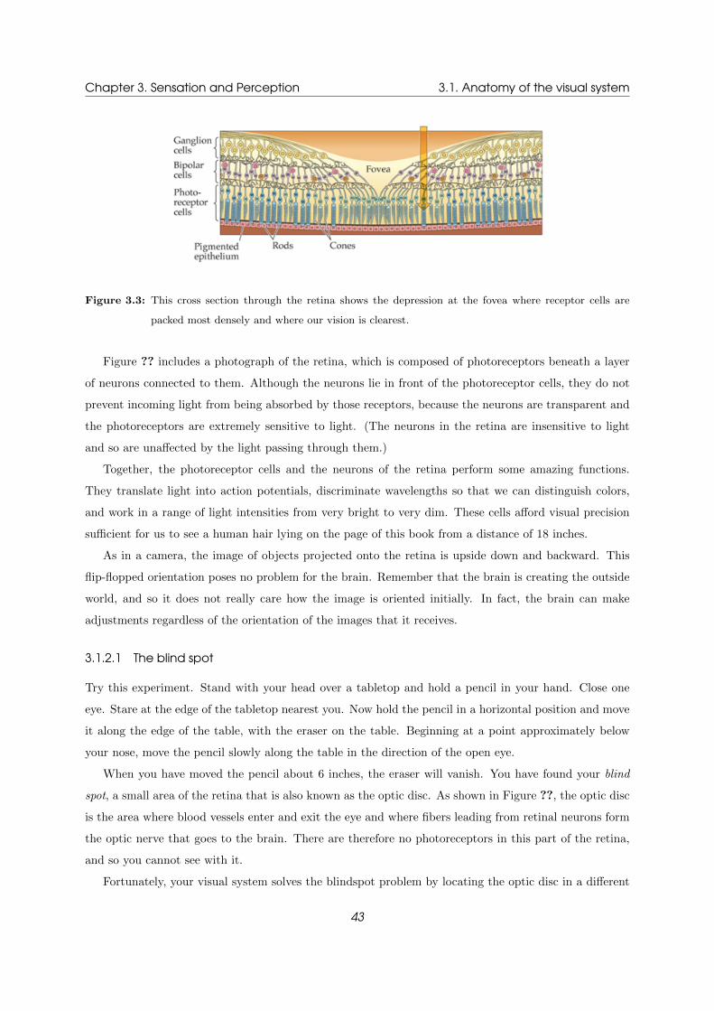
Chapter 3. Sensation and Perception 3.1. Anatomy of the visual system
Figure 3.3: This cross section through the retina shows the depression at the fovea where receptor cells are
packed most densely and where our vision is clearest.
Figure ?? includes a photograph of the retina, which is composed of photoreceptors beneath a layer
of neurons connected to them. Although the neurons lie in front of the photoreceptor cells, they do not
prevent incoming light from being absorbed by those receptors, because the neurons are transparent and
the photoreceptors are extremely sensitive to light. (The neurons in the retina are insensitive to light
and so are unaffected by the light passing through them.)
Together, the photoreceptor cells and the neurons of the retina perform some amazing functions.
They translate light into action potentials, discriminate wavelengths so that we can distinguish colors,
and work in a range of light intensities from very bright to very dim. These cells afford visual precision
sufficient for us to see a human hair lying on the page of this book from a distance of 18 inches.
As in a camera, the image of objects projected onto the retina is upside down and backward. This
flip-flopped orientation poses no problem for the brain. Remember that the brain is creating the outside
world, and so it does not really care how the image is oriented initially. In fact, the brain can make
adjustments regardless of the orientation of the images that it receives.
3.1.2.1 The blind spot
Try this experiment. Stand with your head over a tabletop and hold a pencil in your hand. Close one
eye. Stare at the edge of the tabletop nearest you. Now hold the pencil in a horizontal position and move
it along the edge of the table, with the eraser on the table. Beginning at a point approximately below
your nose, move the pencil slowly along the table in the direction of the open eye.
When you have moved the pencil about 6 inches, the eraser will vanish. You have found your blind
spot, a small area of the retina that is also known as the optic disc. As shown in Figure ??, the optic disc
is the area where blood vessels enter and exit the eye and where fibers leading from retinal neurons form
the optic nerve that goes to the brain. There are therefore no photoreceptors in this part of the retina,
and so you cannot see with it.
Fortunately, your visual system solves the blindspot problem by locating the optic disc in a different
43

Chapter 3. Sensation and Perception 3.1. Anatomy of the visual system
location in each of your eyes. The optic disc is lateral to the fovea in each eye, which means that it is
left of the fovea in the left eye and right of the fovea in the right eye. Because the visual world of the
two eyes overlaps, the blind spot of the left eye can be seen by the right eye and visa versa.
Thus, using both eyes together, you can see the whole visual world. People with blindness in one eye
have a greater problem, however, because the sightless eye cannot compensate for the blind spot in the
functioning eye. Still, the visual system compensates for the blind spot in several other ways, and so
people who are blind in one eye have no sense of a hole in their field of vision.
The optic disc that produces a blind spot is of particular importance in neurology. It allows neurolo-
gists to indirectly view the condition of the optic nerve that lies behind it while providing a window onto
events within the brain.
If there is an increase in intracranial pressure, such as occurs with a tumor or brain abscess (infection),
the optic disc swells, leading to a condition known as papilloedema (swollen disc). The swelling occurs in
part because, like all neural tissue, the optic nerve is surrounded by cerebrospinal fluid. Pressure inside
the cranium can displace this fluid around the optic nerve, causing swelling at the optic disc.
Another reason for papilloedema is inflammation of the optic nerve itself, a condition known as optic
neuritis. Whatever the cause, a person with a swollen optic disc usually loses vision owing to pressure on
the optic nerve. If the swelling is due to optic neuritis, probably the most common neurological visual
disorder, the prognosis for recovery is good.
3.1.2.2 The Fovea
When you focus on one letter on the beginning of this sentence, this letter will be clearly legible. Now, if
you try to read letters that are further away, near the end of the sentence, while holding your eyes still,
you will find this very difficult.
The lesson is that our vision is better in the center of the visual field than at the margins, or periphery.
This difference is partly due to the fact that photoreceptors are more densely packed at the center of the
retina, in a region known as the fovea. Figure ?? shows that the surface of the retina is depressed at the
fovea. This depression is formed because many of the fibers of the optic nerve skirt the fovea to facilitate
light access to its receptors.
3.1.3 Photoreceptors
The retinas photoreceptor cells convert light energy first into chemical energy and then into neural
activity. When light strikes a photoreceptor, it triggers a series of chemical reactions that lead to a
change in membrane potential. This change in turn leads to a change in the release of neurotransmitter
onto nearby neurons.
44

Chapter 3. Sensation and Perception 3.1. Anatomy of the visual system
Figure 3.4: Both rods and cones are tubelike structures, as the scanning electron micrograph at the far right
shows, but they differ, especially in the outer segment, which contains the light-absorbing visual
pigment. Functionally, rods are especially sensitive to broad-spectrum luminance, and cones are
sensitive to particular wavelengths of light.
Rods and cones, the two types of photoreceptors, differ in many ways. As you can see in Figure
??, they are structurally different. Rods are longer than cones and cylindrically shaped at one end,
whereas cones have a tapered end. Rods, which are more numerous than cones, are sensitive to low levels
of brightness (luminance), especially in dim light, and are used mainly for night vision. Cones do not
respond to dim light, but they are highly responsive in bright light. Cones mediate both color vision and
our ability to see fine detail.
Rods and cones are not evenly distributed over the retina. The fovea has only cones, but their density
drops dramatically at either side of the fovea. For this reason, our vision is not so sharp at the edges of
the visual field, as demonstrated earlier.
A final difference between rods and cones is in their light-absorbing pigments. Although both rods and
cones have pigments that absorb light, all rods have the same pigment, whereas cones have three different
pigment types. Any given cone has one of these three cone pigments. The four different pigments, one
in the rods and three in the cones, form the basis of our vision.
45

Chapter 3. Sensation and Perception 3.1. Anatomy of the visual system
Figure 3.5: Our actual perception of color corresponds to the summed activity of the three types of cones, each
type most sensitive to a narrow range of the spectrum. Note that rods, represented by the white
curve, also have a preference for a range of wavelengths centered on 496 nm, but the rods do not
contribute to our color perception; their activity is not summed with the cones in the color system.
The three types of cone pigments absorb light over a range of frequencies, but their maximum absorp-
tions are at about 419, 531, and 559 nm, respectively. The small range of wavelengths to which each cone
pigment is maximally responsive is shown in Figure ??. Cones that contain these pigments are called
“blue”, “green”, and “red”, respectively, loosely referring to colors in their range of peak sensitivity.
Note, however, that, if you were to look at lights with wavelengths of 419, 531, and 559 nm, they
would not appear blue, green, and red but rather violet, blue green, and yellow green, as you can see on
the background spectrum in Figure ??. Remember, though, that you are looking at the lights with all
three of your cone types and that each cone pigment is responsive to light across a range of frequencies,
not just to its frequency of maximum absorption. So the terms blue, green, and red cones are not that
far off the mark. Perhaps it would be more accurate to describe these three cone types as responsive to
short, middle, and long visible wavelengths, referring to the relative length of light waves at which their
sensitivities peak.
Not only does the presence of three different cone receptors contribute to our perception of color,
so does the relative number and distribution of cone types across the retina. The three cone types are
distributed more or less randomly across the retina, making our ability to perceive different colors fairly
constant across the visual field. Although there are approximately equal numbers of red and green cones,
there are fewer blue cones, which means that we are not as sensitive to wavelengths in the blue part of
the visible spectrum.
Other species that have color vision similar to that of humans also have three types of cones, with three
46

Chapter 3. Sensation and Perception 3.1. Anatomy of the visual system
color pigments. But, because of slight variations in these pigments, the exact frequencies of maximum
absorption differ among different species. For humans, the exact frequencies are not identical with the
numbers given earlier, which were an average across mammals. They are actually 426 and 530 nm for the
blue and green cones, respectively, and 552 or 557 nm for the red cone. There are two peak sensitivity
levels given for red because humans, as stated earlier, have two variants of the red cone. The difference
in these two red cones appears minuscule, but recall that it does make a functional difference in color
perception.
This functional difference between the two human variants of red cone becomes especially apparent
in some women. The gene for the red cone is carried on the X chromosome. Because males have only
one X chromosome, they have only one of these genes and so only one type of red cone. The situation
is more complicated for women. Although most women have only one type of red cone, some have both,
with the result that they are more sensitive than the rest of us to color differences at the red end of the
spectrum. Their color receptors create a world with a richer range of red experiences. However, these
women also have to contend with peculiar-seeming color coordination by others.
3.1.4 Retinal Neuron Types
Figure ?? shows that the photoreceptors in the retina are connected to two layers of retinal neurons.
In the procession from the rods and cones toward the brain, the first layer contains three types of cells:
bipolar cells, horizontal cells, and amacrine cells. Two cell types in the first neural layer are essentially
linkage cells. The horizontal cells link photoreceptors with bipolar cells, whereas the amacrine cells link
bipolar cells with cells of the second neural layer, the retinal ganglion cells. The axons of the ganglion
cells collect in a bundle at the optic disc and leave the eye to form the optic nerve.
Important to remember here is that there are extensive horizontal connections between cells, and that
neuronal signal produced by multiple receptors converge on one ganglion cell. This means that there is
a compression of inrormation even within eye.
47

Chapter 3. Sensation and Perception 3.1. Anatomy of the visual system
Figure 3.6: The enlargement of the retina at the right shows the positions of the four types of layer in the retina:
Rod and cone, bipolar, and ganglion cell layer. Notice that light must pass through both neuron
layers to reach the photoreceptors.
3.1.5 Visual Pathways
Imagine leaving your house and finding yourself on an unfamiliar road. Because the road is not on any
map, the only way to find out where it goes is to follow it. You soon discover that the road divides in
two, and so you must follow each branch sequentially to figure out its end point. Suppose you learn that
one branch goes to a city, whereas the other goes to a national park. By knowing the end point of each
branch, you can conclude something about their respective functionsthat one branch carries people to
work, whereas the other carries them to play, for example.
The same strategy can be used to follow the paths of the visual system. The retinal ganglion cells
form the optic nerve, which is the road into the brain. This road travels to several places, each with a
different function. By finding out where the branches go, we can begin to guess what the brain is doing
with the visual input and how the brain creates our visual world.
Let us begin with the optic nerves, one exiting from each eye. As you know, they are formed by the
axons of ganglion cells leavingthe retina. Just before entering the brain, the optic nerves partly cross,
forming the optic chiasm (from the Greek letter Ξ).
About half the fibers from each eye cross in such a way that the left half of each optic nerve goes to
the left side of the brain, whereas the right halves go to the brains right side, as diagrammed in Figure
??. The medial path of each retina, the nasal retina, crosses to the opposite side. The lateral path, the
temporal retina, goes straight back on the same side. Because the light that falls on the right half of the
48

Chapter 3. Sensation and Perception 3.1. Anatomy of the visual system
retina actually comes from the left side of thevisual field, information from the left visual field goes to
the brains right hemisphere, whereas information from the right visual field goes to the left hemisphere.
Thus, half of each retinas visual field is represented on each side of the brain.
Figure 3.7: This horizontal slice through the brain shows the visual pathway from each eye to the primary visual
cortex of each hemisphere. Information from the blue side of the visual field goes to the two left
halves of the retinas and ends up in the left hemisphere. Information from the red side of the visual
field hits the right halves of the retinas and travels to the right side of the brain.
Having entered the brain, the axons of the ganglion cells separate, forming two distinct pathways,
charted in Figure 8-12. All the axons of ganglion cells a form a pathway called the geniculostriate system.
This pathway goes from the retina to the lateral geniculate nucleus (LGN) of the thalamus and then to
layer IV of the primary visual cortex, which is in the occipital lobe.
The primary visual cortex has broad stripes across it in layer IV and so is known as striate cortex. The
term geniculostriate therefore means a bridge between the thalamus (geniculate) and the striate cortex.
From the striate cortex, the axon pathway now splits, with one route going to vision-related regions of
the parietal lobe and another route going to vision-related regions of the temporal lobe.
49

Chapter 3. Sensation and Perception 3.2. Location in the visual world
Figure 3.8: The optic nerve has two principal branches: (1) the geniculostriate system through the LGN in
the thalamus to the primary visual cortex and (2) the tectopulvinar system through the superior
colliculus of the tectum to the pulvinar region of the thalamus and thus to the temporal and parietal
lobes.
The second pathway leading from the eye is formed by the axons of the remaining ganglion cells. These
cells send their axons to the superior colliculus. The superior colliculus sends connections toa region of the
thalamus known as the pulvinar. This pathway is therefore known as the tectopulvinar system because
it goes from the eye through the tectum to the pulvinar. The pulvinar then sends connections to the
parietal and temporal lobe. This system is mainly responsible for very low-level automatic movement of
the eye, known as saccades.
To summarize, two principal pathways extend into the visual brainnamely, the geniculostriate and
tectopulvinar systems. Each pathway eventually travels either to the parietal or the temporal lobe. Our
next task is to determine the respective roles of the parietal lobe and the temporal lobe in creating our
visual world.
3.2 Location in the visual world
One aspect of visual information that we have not yet considered is location. As we move around, going
from place to place, we encounter objects in specific locations. Indeed, if we had no sense of location,
the world would be a bewildering mass of visual information. Our next task, then, is to look at how the
brain constructs a spatial map from this complex array of visual input.
The coding of location begins in the retina and is maintained throughout all the visual pathways. To
understand how this spatial coding is accomplished, you need to imagine your visual world as seen by
your two eyes. The visual field can be divided into two halves, the left and right visual fields, by drawing
a vertical line down the middle of the black cross. Now recall from Figure ?? that the left half of each
retina looks at the right side of the visual field, whereas the right half of each retina looks at the visual
fields left side. This means that input from the right visual field goes to the left hemisphere, whereas
input from the left visual field goes to the right hemisphere.
50

Chapter 3. Sensation and Perception 3.2. Location in the visual world
Therefore the brain can easily determine whether visual information is located to the left or right of
center. If input goes to the left hemisphere, the source must be in the right visual field; if input goes
to the right hemisphere, the source must be in the left visual field. This arrangement tells you nothing
about the precise location of an object in the left or right side of the visual field, however. To understand
how precise spatial localization is accomplished, we must return to the retinal ganglion cells.
3.2.1 Coding location in the retina
Look again at Figure ?? and you can see that each retinal ganglion cell receives input through bipolar
cells from several photoreceptors. In the 1950s, Stephen Kuffler, a pioneer in studying the physiology of
the visual system, made an important discovery about how photoreceptors and ganglion cells are linked.
By shining small spots of light on the receptors, he found that each ganglion cell responds to stimulation
on just a small circular patch of the retina. This patch became known as the ganglion cells receptive field.
A ganglion cells receptive field is therefore the region of the retina on which it is possible to influence
that cells firing. Stated differently, the receptive field represents the outer world as seen by a single cell.
Each ganglion cell sees only a small bit of the world, much as you would if you looked through a narrow
cardboard tube. The visual field is composed of thousands of such receptive fields.
Now let us consider how receptive fields enable the visual system to interpret the location of objects.
Imagine that the retina is flattened like a piece of paper. When a tiny light is shone on different parts
of the retina, different ganglion cells respond. For example, when a light is shone on the top-left corner
of the flattened retina, a particular ganglion cell responds because that light is in its receptive field.
Similarly, when a light is shone on the top-right corner, a different ganglion cell responds.
By using this information, we can identify the location of a light on the retina by knowing which
ganglion cell is activated.We can also interpret the location of the light in the outside world because we
know where the light must come from to hit a particular place on the retina. For example, light from
above hits the bottom of the retina after passing through the eyes lens, whereas light from below hits the
top of the retina. Information at the top of the visual field will stimulate ganglion cells on the bottom of
the retina, whereas information at the bottom of the field will stimulate ganglion cells on the top of the
retina.
3.2.2 Location in the LGN and V1
Now consider the connection from the ganglion cells to the lateral geniculate nucleus. In contrast with
the retina, the LGN is not a flat sheet; rather, it is a three-dimensional structure in the brain.We can
compare it to a stack of cards, with each card representing a layer of cells.
A retinal ganglion cell that responds to light in the top-left corner of the retina connects to the left
side of the first card. A retinal ganglion cell that responds to light in the bottom-right corner of the
51

Chapter 3. Sensation and Perception 3.3. Neural Activity
retina connects to the right side of the last card. In this way, the location of leftright and topbottom
information is maintained in the LGN.
Like the ganglion cells, each of the LGN cells has a receptive field, which is the region of the retina that
influences its activity. If two adjacent retinal ganglion cells synapse on a single LGN cell, the receptive
field of that LGN cell will be the sum of the two ganglion cells receptive fields. As a result, the receptive
fields of LGN cells can be bigger than those of retinal ganglion cells.
The LGN projection to the striate cortex (region V1) also maintains spatial information. As each LGN
cell, representing a particular place, projects to region V1, a topographic representation, or topographic
map, is produced in the cortex. As illustrated in Figure ??, this representation is essentially a map of
the visual world.
The central part of the visual field is represented at the back of the brain, whereas the periphery is
represented more anteriorly. The upper part of the visual field is represented at the bottom of region V1,
the lower part at the top of V1. The other regions of the visual cortex (such as V3, V4, and V5) also
have topographical maps similar to that of V1. Thus the V1 neurons must project to the other regions
in an orderly manner, just as the LGN neurons project to region V1 in an orderly way.
Within each visual cortical area, each neuron has a receptive field corresponding to the part of the
retina to which the neuron is connected. As a rule of thumb, the cells in the cortex have much larger
receptive fields than those of retinal ganglion cells. This increase in receptive-field size means that the
receptive field of a cortical neuron must be composed of the receptive fields of many retinal ganglion cells.
3.3 Neural Activity
The pathways of the visual system are made up of individual neurons. By studying how these cells behave
when their receptive fields are stimulated, we can begin to understand how the brain processes different
features of the visual world beyond just the locations of light. To illustrate, we examine how neurons
from the retina to the temporal cortex respond to shapes.
Imagine that we have placed a microelectrode near a neuron somewhere in the visual pathway from
retina to cortex and are using that electrode to record changes in the neurons firing rate. This neuron
occasionally fires spontaneously, producing action potentials with each discharge. Let us assume that the
neuron discharges, on the average, once every 0.08 second. Each action potential is brief, on the order of
1 millisecond.
52

Chapter 3. Sensation and Perception 3.3. Neural Activity
Figure 3.9: When visually responsive neurons encounter a particular stimulus in their visual fields, they may
show either excitation or inhibition. (A) At the baseline firing rate of a neuron, each action potential
is represented by a spike. In a 1-second time period, there were 12 spikes. (B) Excitation is indicated
by an increase in firing rate over baseline. (C) Inhibition is indicated by a decrease in firing rate
under baseline.
If we plot action potentials spanning a second, we see only spikes in the record because the action
potentials are so brief. Figure ??A is a single-cell recording in which there are 12 spikes in the span of
1 second. If the firing rate of this cell increases, we will see more spikes (Figure ??B). If the firing rate
decreases, we will see fewer spikes (Figure ??C). The increase in firing represents excitation of the cell,
whereas the decrease represents inhibition. Excitation and inhibition, as you know, are the principal
mechanisms of information transfer in the nervous system.
Now suppose we present a stimulus to the neuron by illuminating its receptive field in the retina,
perhaps by shining a light stimulus on a blank screen within the cells visual field. We might place
before the eye a straight line positioned at a 45a◦ngle. The cell could respond to this stimulus either
by increasing or decreasing its firing rate. In either case, we would conclude that the cell is creating
information about the line.
Note that the same cell could show excitation to one stimulus, inhibition to another stimulus, and
no reaction at all. For instance, the cell could be excited by lines oriented 45t◦o the left and inhibited
by lines oriented 45t◦o the right. Similarly, the cell could be excited by stimulation in one part of its
receptive field (such as the center) and inhibited by stimulation in another part (such as the periphery).
Finally,we might find that the cells response to a particular stimulus is selective. Such a cell would
be telling us about the importance of the stimulus to the animal. For instance, the cell might fire (be
53

Chapter 3. Sensation and Perception 3.3. Neural Activity
excited) when a stimulus is presented with food but not fire (be inhibited) when the same stimulus is
presented alone. In each case, the cell is selectively sensitive to characteristics in the visual world.
Now we are ready to move from this hypothetical example to what visual neurons actually do when
they process information about shape. Neurons at each level of the visual system have distinctly different
characteristics and functions. Our goal is not to look at each neuron type but rather to consider generally
how some typical neurons at each level differ from one another in their contributions to processing shape.
We focus on neurons in two areas: the ganglion-cell layer of the retina and the primary visual cortex.
3.3.1 Processing in retinal ganglion cells
Cells in the retina do not actually see shapes. Shapes are constructed by processes in the cortex from
the information that ganglion cells pass on about events in their receptive fields. Keep in mind that the
receptive fields of ganglion cells are very small dots. Each ganglion cell responds only to the presence or
absence of light in its receptive field, not to shape.
The receptive field of a ganglion cell has a concentric circle arrangement, as illustrated in Figure ??.
A spot of light falling in the central circle of the receptive field excites some of these cells, whereas a spot
of light falling in the surround (periphery) of the receptive field inhibits the cell. A spot of light falling
across the entire receptive field causes a weak increase in the cells rate of firing.
Figure 3.10: (A) In the receptive field of a retinal ganglion cell with an on-center and off-surround, a spot of
light placed on the center causes excitation in the neuron, whereas a spot of light in the surround
causes inhibition. When the light in the surround region is turned off, firing rate increases briefly
(called an offset response). A light shining in both the center and the surround would produce
a weak increase in firing in the cell. (B) In the receptive field of a retinal ganglion cell with an
off-center and on-surround, light in the center produces inhibition, whereas light on the surround
produces excitation, and light across the entire field produces weak inhibition.
This type of neuron is called an on-center cell. Other ganglion cells, called off-center cells, have
54

Chapter 3. Sensation and Perception 3.3. Neural Activity
the opposite arrangement, with light in the center of the receptive field causing inhibition, light in the
surround causing excitation, and light across the entire field producing weak inhibition (Figure ??B). The
onoff arrangement of ganglion-cell receptive fields makes these cells especially responsive to very small
spots of light.
This description of ganglion-cell receptive fields might mislead you into thinking that they form a
mosaic of discrete little circles on the retina that do not overlap. In fact, neighboring retinal ganglion
cells receive their inputs from an overlapping set of receptors. As a result, their receptive fields overlap.
In this way, a small spot of light shining on the retina is likely to produce activity in both on-center and
off-center ganglion cells.
How can on-center and off-center ganglion cells tell the brain anything about shape? The answer is
that a ganglion cell is able to tell the brain about the amount of light hitting a certain spot on the retina
compared with the average amount of light falling on the surrounding retinal region. This comparison is
known as luminance contrast.
Figure 3.11: Activity at the Margins
Responses of a hypothetical population of on-center ganglion cells whose receptive fields (AE) are
distributed across a lightdark edge. The activity of the cells along the edge is most affected relative
to those away from the edge.
The ganglion cells with receptive fields in the dark or light areas are least affected because they
experience either no stimulation or stimulation of both the excitatory and the inhibitory regions of their
receptive fields. The ganglioncells most affected by the stimulus are those lying along the edge. Ganglion
cell B is inhibited because the light falls mostly on its inhibitory surround, and ganglion cell D is excited
because its entire excitatory center is stimulated but only part of its inhibitory surround is.
Consequently, information transmitted from retinal ganglion cells to the visual areas in the brain does
not give equal weight to all regions of the visual field. Rather, it emphasizes regions containing differences
in luminance. Areas with differences in luminance are found along edges. So retinal ganglion cells are
really sending signals about edges, and edges are what form shapes.
55

Chapter 3. Sensation and Perception 3.3. Neural Activity
3.3.2 Processing in the primary visual cortex
Now consider cells in region V1, the primary visual cortex, that receive their visual inputs from LGN
cells, which in turn receive theirs from retinal ganglion cells. Because each V1 cell receives input from
multiple retinal ganglion cells, the receptive fields of the V1 neurons are much larger than those of retinal
neurons. Consequently, the V1 cells respond to stimuli more complex than simply “light on” or “light
off”. In particular, these cells are maximally excited by bars of light oriented in a particular direction
rather than by spots of light. These cells are therefore called orientation detectors.
Like the ganglion cells, some orientation detectors have an onoff arrangement in their receptive fields,
but the arrangement is rectangular rather than circular. Visual cortex cells with this property are known
as simple cells. Typical receptive fields for simple cells in the primary visual cortex are shown in Figure
??.
56

Chapter 3. Sensation and Perception 3.3. Neural Activity
Figure 3.12: Typical Receptive Fields for Simple Visual Cortex Cells Simple cells respond to a bar of light in a
particular orientation, such as horizontal (A) or oblique (B). The position of the bar in the visual
field is important, because the cell either responds (ON) or does not respond (OFF) to light in
adjacent regions of the visual field.
Simple cells are not the only kind of orientation detector in the primary visual cortex; several func-
tionally distinct types of neurons populate region V1. For instance, complex cells have receptive fields
that are maximally excited by bars of light moving in a particular direction through the visual field. A
hypercomplex cell, like a complex cell, is maximally responsive to moving bars but also has a strong
inhibitory area at one end of its receptive field. As illustrated in Figure ??, a bar of light landing on the
right side of the hypercomplex cells receptive field excites the cell, but, if the bar lands on the inhibitory
area to the left, the cells firing is inhibited.
57

Chapter 3. Sensation and Perception 3.3. Neural Activity
Figure 3.13: Receptive Field of a Hypercomplex Cell
A hypercomplex cell responds to a bar of light in a particular orientation (e.g., horizontal) anywhere
in the excitiatory (ON) part of its receptive field. If the bar extends into the inhibitory area (OFF),
no response occurs.
Note that each class of V1 neurons responds to bars of light in some way, yet this response results
from input originating in retinal ganglion cells that respond maximally not to bars but to spots of light.
How does this conversion from responding to spots to responding to bars take place? An example will
help explain the process.
A thin bar of light falls on the retinal photoreceptors, striking the receptive fields of perhaps dozens
of retinal ganglion cells. The input to a V1 neuron comes from a group of ganglion cells that happen to
be aligned in a row, as in Figure ??. That V1 neuron will be activated (or inhibited) only when a bar
of light hitting the retina strikes that particular row of ganglion cells. If the bar of light is at a slightly
different angle, only some of the retinal ganglion cells in the row will be activated, and so the V1 neuron
will be excited only weakly.
Figure ?? illustrates the connection between light striking the retina in a certain pattern and the
activation of a simple cell in the primary visual cortex, one that responds to a bar of light in a partic-
ular orientation. Using the same logic, we can also diagram the retinal receptive fields of complex or
58

Chapter 3. Sensation and Perception 3.4. Perception
hypercomplex V1 neurons.
Figure 3.14: A V1 cell responds to a row of ganglion cells in a particular orientation on the retina. The bar of
light strongly activates a row of ganglion cells, each connected through the LGN to a V1 neuron.
The activity of this V1 neuron is most affected by a bar of light at a 45 angle.
3.4 Perception
One of the things that makes many movies exciting is the amazing special effects, such as those in films
like The Lord of the Rings. The special effects in movies may amaze us, but you don’t have to go to a
movie to see amazing visual effects - you are experiencing them right now, as you read this book or when
you look up to perceive whatever is around you. Perception, the conscious experience that results from
stimulation of the senses, may not seem particularly special because all we have to do is look around,
listen, or touch something, and perception just “happens” with little effort or our part. However, the
mechanisms responsible for your ability to perceive are far more amazing than the technology used to
create even the most complicated special effects.
Because of the ease with which we perceive, many people don’t see the feats achieved by our senses
as complex or amazing. “After all,” the skeptic might say, “for vision, a picture of the environment is
focused on the back of my eye, and that picture provides all the information my brain needs to duplicate
the environment in my consciousness.” But the idea that perception is not that complex is exactly what
misled computer scientists in the 1950s and 1960s into proposing that it would take only about a decade
or so to create “perceiving machines” that could negotiate the environment with humanlike ease.
59

Chapter 3. Sensation and Perception 3.4. Perception
These predictions, made over 40 years ago, have yet to come true, even though a computer defeated
the world chess champion in 1997. From a computer’s point of view, perceiving a scene is more difficult
than playing world-championship chess. One of the goals of this section is to make you aware of the
processes that are responsible for creating our perceptions.
We first describe how the process of perception depends both on the incoming stimulation and know-
ledge we bring to the situation. Following this introduction, we will devote the rest of the section to
answering the question, “How do we perceive objects?”
One reason that we will be focusing on object perception is that perceiving objects is central to our
everyday experience. Consider, for example, what you would say if you were asked to look up and describe
what you are perceiving right now. Your answer would, of course, depend on where you are but it is
likely that a large part of your answer would include naming the objects that you see. (“I see a book.
There’s a chair against the wall. .. .”)
Another reason for focusing on object perception is that it enables us to achieve a more in-depth
understanding of the basic principles of perception than we could achieve by covering a number of different
types of perception more superficially. After describing a number of mechanisms of object perception,
we will consider the idea that perception is “intelligent.” We will see that behavioral and physiological
evidence supports this idea.
3.4.1 Top-down and bottom-up
Although perception seems to just “happen,” it is actually the end result of a complex process. We can
appreciate the complexity involved in seemingly simple behaviors by using the following example.
Roger is driving through an unfamiliar part of town. He is following directions, which indicate that
he should turn left on Washington Street. It is dark and the street is poorly lit, so it is difficult to read
the street signs. Suddenly, just before an intersection, he sees the sign for Washington Street and quickly
makes a left turn. However, after driving a block, he realizes he is on Washburn Avenue, not Washington
Street. He feels a little foolish because it isn’t that hard to tell the difference between Washington Street
and Washburn Avenue, but the sign really did look like it said Washington at the time.
We can understand what happened in this example by considering some of the events that occur
during the process of perception. The first event in the process of perception is reception of the stimulus.
Light from a streetlight is reflected from the sign into Roger’s eye. We can consider this step “data in”
since a pattern of light and dark enters Roger’s eye and creates a pattern on his retina.
Before Roger can see anything, this information on his retina has to be changed into electrical signals,
transmitted to his brain, and processed. During processing, various mechanisms work toward creating a
conscious perception of the sign. But just saying that “processing” results in conscious perception of the
sign does not tell the entire story, as we will see next.
Up to this point, saying that the“data comes in and is processed,” could be describing what happens
60

Chapter 3. Sensation and Perception 3.4. Perception
in a computer. In the case of human perception, the computer is the brain, which contains neurons and
synapses instead of solid-state circuitry. This analogy between the digital computer and the brain is
not totally inaccurate, but it leaves out something that is extremely important. Roger’s brain contains
not only neurons and synapses but also knowledge, and when the incoming data interacts with this
knowledge, the resulting response is different from what would happen if the brain were just a computer
that responded in an automatic way to whatever stimulus patterns it was receiving.
Before Roger even saw the sign, his brain contained knowledge about driving, street signs, how to
read a map, and how to read letters and words, among other things. In addition, the fact that he was
looking for Washington Street and was expecting it to be coming up soon played a large role in causing
him to mistakenly read Washington when the actual stimulus was Washburn. Thus, if Roger had not
been expecting to see Washington, he might have read the sign correctly. However when the incoming
data collided with his ex-pectation, Washburn turned into Washington.
Psychologists distinguish between the processing that is based on incoming data and the processing
that is based on existing knowledge by distinguishing between bottom-up processing and top-down pro-
cessing. Bottom-up processing (also called data-based processing) is processing that is based on incoming
data. This is always the starting point for perception because if there is no incoming data, there is no
perception. In our example, the incoming data is the pattern of light that enters Roger’s eye. Top-down
processing (also called knowledge-based processing) refers to processing that is based on knowledge.
Knowledge doesn’t have to be involved in perception but, as we will see, it usually is - sometimes without
our even being aware of its presence.
Roger’s experience in looking for a street sign on a dark night illustrates how these two types of
processing can interact. The following demonstration illustrates what happens when incoming data is
affected by knowledge that has been provided just moments earlier.
3.4.2 Feature detection
Our lack of awareness of the processes that create perception is particularly true at the very beginning
of the perceptual process, when the incoming data is being analyzed. Early in the process of object
perception objects are analyzed into smaller components called features. We will describe the feature
approach to object perception by first describing a simple model for recognizing letters, then describing
how physiological and behavioral evidence supports the idea that features are important in perception.
Finally, we will describe two theories of object perception that are based on the idea that objects are
analyzed into features early in the perceptual process.
61

Chapter 3. Sensation and Perception 3.4. Perception
Figure 3.15: A model for recognizing letters by analyzing their features. The stimulus, A activates three feature-
units. These feature-units cause strung activation of the A letter-unit and weaker activation of
units for letters such as the N and the 0, which lack some of A’s features. The A is identified by
the high level of activation of the A letter-unit
Figure ?? shows a simple model, which illustrates how the analysis of features can lead to the recogni-
tion of letters. We will describe how it works by considering the way the model responds to presentation
of the letter A. The first stage of this model, called the feature analysis stage, consists of a bank of feature
units, each of which responds to a specific feature. The A activates three of these units - one for “line
slanted to the right,” one for “line slanted to the left,” and one for “horizontal line.” Thus, in this stage,
the A is broken down into its individual features.
The second stage, called the letter-analysis stage, consists of a bank of letter units, each of which
represents a specific letter. Just six of these letter units are shown here, but in the complete model there
would be one unit for each letter in the alphabet. Notice that each letter unit receives inputs from the
feature units associated with that letter. Thus, when the letter A is presented, the A-unit receives inputs
from three feature units. Other letters that have features in common with the A also receive inputs from
feature units that are activated by the A.
The basic idea behind feature analysis is that activation of letter units provides the information needed
to determine which letter is present. All the visual system has to do is determine which unit is activated
most strongly. In our example, the units for A, N, and T are activated, but because the A receives inputs
from three feature units and the T and N receive inputs from only one, the A-unit is activated more
strongly, indicating that A was the letter that was presented.
The idea that objects are analyzed into features is especially appealing because it helps explain how
we can recognize all of the patterns in Figure ?? as being the letter K. Analyzing letters into features
makes it possible to identify many of these K ’s as being the same letter, even though they look different,
because underneath their differences, each K contains many of the same features.
62

Chapter 3. Sensation and Perception 3.4. Perception
Figure 3.16: Different kinds of K that share features.
The feature analysis model we have described is a simple one that would have trouble identifying
more unconventional looking letters and would also have problems telling the difference between letters
with similar features that are arranged differently, like L and T. To tell the difference between the L and
the T, a more complex model is required. Furthermore, a feature analysis model designed to consider
objects in addition to letters would have to be even more complex. Thus, the point of presenting the
model in Figure ?? is not to present a model that would actually work under real-world conditions, but
to illustrate the basic principle behind feature analysis - feature units are activated and these units send
signals to other, higher-order, units.
3.4.3 Evidence for Feature Analysis
The idea of feature-based perception is supported by both physiological and behavioral evidence.
The neural feature detectors are simple feature detectors that respond to oriented lines like the ones
in the model, and there are also more complex feature detectors that respond to combinations of these
simple features.
The feature approach has been studied behaviorally using a technique called visual search in which
participants are asked to find a target stimulus among a number of distractor stimuli. In one of the early
visual search experiments, Ulric Neisser asked participants to find a target letter among a number of
“distractor” letters. Neisser’s participants detected the Z more rapidly in the first list than in the second
one. The reason for this was that the first list only contained letters that had no features in common
with the Z, like the O, D, U,· · · .
Following Neisser’s lead, Ann Treisman also has used visual search to study feature analysis. However,
instead of just showing that letters can be detected faster if their features are different from the distractors,
she asked the question: “How does the speed that a target can be detected depend on how many
distractors are present?”
63
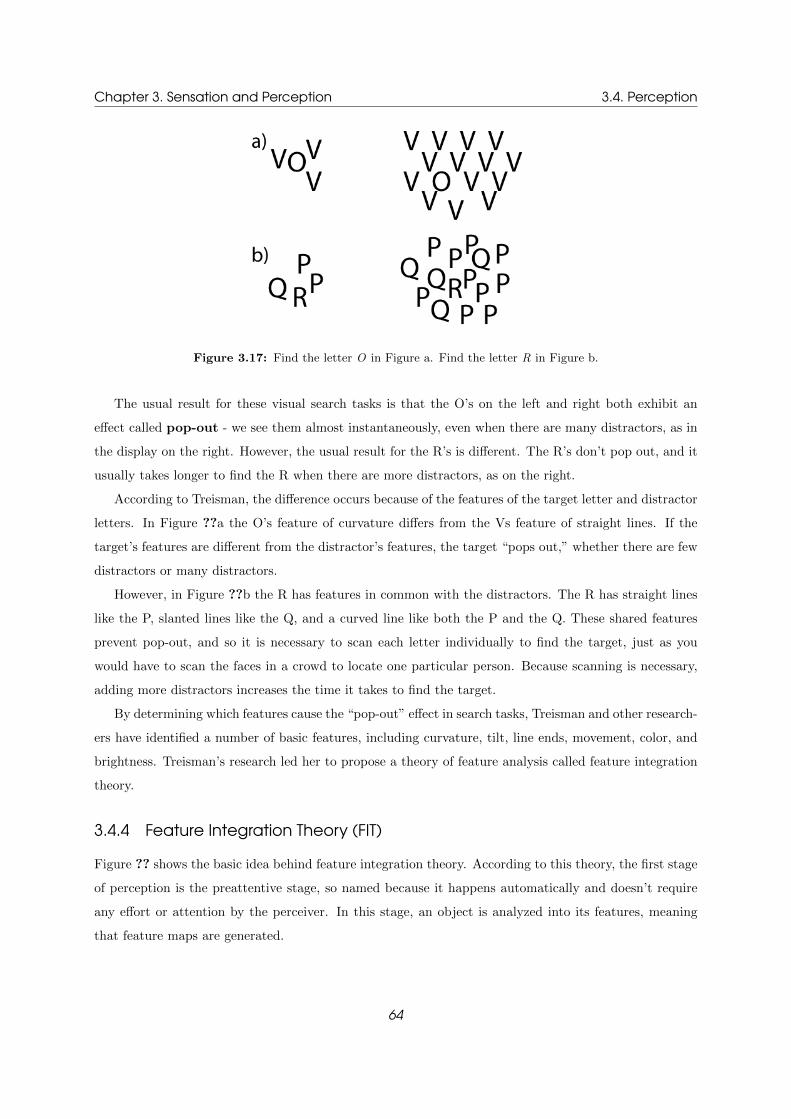
Chapter 3. Sensation and Perception 3.4. Perception
Figure 3.17: Find the letter O in Figure a. Find the letter R in Figure b.
The usual result for these visual search tasks is that the O’s on the left and right both exhibit an
effect called pop-out - we see them almost instantaneously, even when there are many distractors, as in
the display on the right. However, the usual result for the R’s is different. The R’s don’t pop out, and it
usually takes longer to find the R when there are more distractors, as on the right.
According to Treisman, the difference occurs because of the features of the target letter and distractor
letters. In Figure ??a the O’s feature of curvature differs from the Vs feature of straight lines. If the
target’s features are different from the distractor’s features, the target “pops out,” whether there are few
distractors or many distractors.
However, in Figure ??b the R has features in common with the distractors. The R has straight lines
like the P, slanted lines like the Q, and a curved line like both the P and the Q. These shared features
prevent pop-out, and so it is necessary to scan each letter individually to find the target, just as you
would have to scan the faces in a crowd to locate one particular person. Because scanning is necessary,
adding more distractors increases the time it takes to find the target.
By determining which features cause the “pop-out” effect in search tasks, Treisman and other research-
ers have identified a number of basic features, including curvature, tilt, line ends, movement, color, and
brightness. Treisman’s research led her to propose a theory of feature analysis called feature integration
theory.
3.4.4 Feature Integration Theory (FIT)
Figure ?? shows the basic idea behind feature integration theory. According to this theory, the first stage
of perception is the preattentive stage, so named because it happens automatically and doesn’t require
any effort or attention by the perceiver. In this stage, an object is analyzed into its features, meaning
that feature maps are generated.
64

Chapter 3. Sensation and Perception 3.4. Perception
Figure 3.18: A model of the FIT of Ann Treisman. Features are decomposed at the pre-attentive stage. In the
focused attention stage, features are recombined into objectes from the mastermap of locations.
The idea that an object is automatically broken into features seems counterintuitive because when
we look at an object, we see the whole object, not an object that has been divided into its individual
features. The reason we aren’t aware of this process of feature analysis is that it occurs early in the
perceptual process, before we have become conscious of the object. To provide some perceptual evidence
that objects are, in fact, analyzed into features, Treisman and H. Schmidt did an ingenious experiment
to show that early in the perceptual process features may exist independently of one another.
Treisman and Schmidt’s display consisted of four objects flanked by two black numbers. She flashed
this display onto a screen for one-fifth of a second, followed by a random-dot masking field designed to
eliminate any residual perception that may remain after the stimuli are turned off. Participants were told
to report the black numbers first and then to report what they saw at each of the four locations where
the shapes had been.
In 18 percent of the trials, participants reported seeing objects that were made up of a combination of
features from two different stimuli. For example, after being presented with the display, in which the small
triangle was red and the small circle was green, they might report seeing a small red circle and a small
green triangle. These combinations of features from different stimuli are called illusory conjunctions.
Illusory conjunctions can occur even if the stimuli differ greatly in shape and size. For example, a small
65

Chapter 3. Sensation and Perception 3.4. Perception
blue circle and a large green square might be seen as a large blue square and a small green circle.
According to Treisman, these illusory conjunctions occur because at the beginning of the perceptual
process each feature exists independently of the others. That is, features such as “redness,”, “curvature,”
or “tilted line” are not, at this early stage of processing, associated with a specific object. They are,
in Treisman’s words, “free floating” and can therefore be incorrectly combined in laboratory situations
when briefly flashed stimuli are followed by a masking field.
One way to think about these features is that they are components of an “alphabet” of vision. At the
very beginning of the process of perception these components of perception exist independently of one
another, just as the individual letter tiles in a game of Scrabble exist as individual units when the tiles
are scattered at the beginning of the game. However, just as the individual Scrabble tiles are combined
to form words, the individual features combine to form perceptions of whole objects. According to
Treisman’s model, these features are combined in the second stage, which is called the focused attention
stage. Once the features have been combined in this stage, we perceive the object.
During the focused attention stage, the observer’s attention plays an important role in combining the
features to create the perception of whole objects. To illustrate the importance of attention for combining
the features, Treisman repeated the illusory conjunction experiment, but she instructed her participants
to ignore the black numbers and to focus all of their attention on the four target items. This focusing of
attention eliminated illusory conjunctions so that all of the shapes were paired with their correct colors.
The feature analysis approach proposes that at the beginning of the process of perception, the stimulus
is analyzed into elementary features, which are then combined to create perception of the object. This
process involves mostly bottom-up processing because knowledge is not involved. In some situations
however, top-down processing can come into play. For example, when Treisman did an illusory conjunction
experiment and asked participants to identify the objects, the usual illusory conjunctions occurred, so
the orange triangle would, for example, sometimes be perceived to be black. However, when she told
participants that they were being shown a carrot, a lake, and a tire, illusory conjunctions were less likely
to occur, so subjects were more likely to perceive the triangular “carrot” as being orange. Thus, in this
situation, the participants’ knowledge of the usual colors of objects influenced their ability to correctly
combine the features of each object. Top-down processing comes into play even more in the focused
attention stage because the observer’s attention can be controlled by meaning, expectations, and what
the observer is looking for, as when Roger was watching for a particular street sign.
3.4.5 Recognition by Components Approach
In the recognition-by-components (RBC) approach to perception, the features are not lines, curves, or
colors, bui are three-dimensional volumes called geons. Figure ??1 shows a number of geons, which
are shapes such as cylinders, rectangular solids, and pyramids. Irving Biederman, who developed RBC
theory, has proposed that there are 36 different geons, and that this number of geons is enough to enable
66

Chapter 3. Sensation and Perception 3.4. Perception
us to construct a large proportion of the objects that exist in the environment. Figure ??b shows a few
objects that have been constructed from geons.
Figure 3.19: (a) Some geons; (b) Some objects created from the geons on the left. The numbers indicate which
geons are present.
An important property of geons is that they can be identified when viewed from different angles.
This property, which is called view invariance, occurs because geons contain view invariant properties -
properties such as the three parallel edges of the rectangular solid in Figure ?? that remain visible even
when the geon is viewed from many different angles.
You can test the view-invariant properties of a rectangular solid yourself by picking up a book and
moving it around so you are looking at it from many different viewpoints. As you do this, notice what
percentage of the time you are seeing the three parallel edges. Also notice that occasionally, as when you
look at the book end-on, you do not see all three edges. However, these situations occur only rarely, and
when they do occur it becomes more difficult to recognize the object.
Two other properties of geons are discriminability and resistance to visual noise. Discriminability
means that each geon can be distinguished from the others from almost all viewpoints. Resistance to
visual noise means that we can still perceive geons under “noisy” conditions.
The basic message of RBC theory is that if enough information is available to enable us to identify
an object’s basic geons, we will be able to identify the object. A strength of Biederman’s theory is that
it shows that we can recognize objects based on a relatively small number of basic shapes.
Both feature-integration theory (FIT) and recognition-by-components (RBC) theory are based on
the idea the idea of early analysis of objects into parts. These two theories explain different facets of
object perception. FIT theory is more concerned with very basic features like lines, curves, colors, and
with how attention is involved in combining them, whereas RBC theory is more about how we perceive
three-dimensional shapes. Thus, both theories explain how objects are analyzed into parts early in the
perceptual process.
3.4.6 David Marr’s Computation Theory
Marr once said that trying to understandperception by studying neurons alone was like trying to un-
derstand how a bird flies by studying only its feathers. Hence, it is not possible to understand why
67

Chapter 3. Sensation and Perception 3.4. Perception
retinal ganglion cells and lateral geniculate neurons have the receptive fields they do simply by studying
their anatomy and physiology. It is possible to understand how they behave by studying their connec-
tions and interactions, but to understand why receptive fields are the way they are, it is necessary to
know something about differential operators, band-pass channels, and the mathematics of the uncertainty
principle
A visual image is composed of a wide array of intensity, created by the way in which light is reflected
by the objects viewed by the observer. Early visual processing aims to create a description of these
objects by constructing a number of representations from the intensity values of the image. The resultant
description of these shapes of surfaces and objects, their orientations and distances away from the viewer,
is called the primal sketch.
This first stage makes local changes in light intensity explicit locating discontinuities in light intensity
because such edges often coincide with important boundaries in the visual scene. The resultant primal
sketch consists of a collection of statements about any edges and blobs present, where they are located and
orientated, and other information to define a crude first processing. From this rather messy interpretation,
such structures as boundaries and regions can be constructed using the application of grouping procedures.
This refined description is called the full primal sketch.
Although the full primal sketch seizes many of the contours and textures of an image, it is only one
aspect of early visual processing. Marrsaw the consequence of early visual processing as an observer-
orientated representation which he called the 21/2D sketch. This is produced by an analysis of motion,
depth and shading as well as a full analysis of the primal sketch.
The 21/2D sketch is necessary to guide any action undertaken. However, in order to recognise objects,
a third representational level is required to allow the observer to recognise what object a particular shape
corresponds to. This third level must be centred on the object rather than the observer and is what Marr
calls his 3D-model representation.
Marrs theory, therefore, involves a number of levels, each of which involves a symbolic representation
of the information carried in the retinal image each building further and further detail back into the
image so that final recognition and response is achieved.
Such a theory suggests that vision proceeds by explicit computation of symbolic descriptions of the
image, and that object recognition, for example, is reached when one of the reconstructed descriptions
matches a stored representation of a known object class. However, questions are still unanswered as to
how these stored concepts originally develop in the brain, since the visual centres of the embryonic brain
show only instinctive development patterns as with a computer before we load on any programs.
Marr did not regard his early processing model as solving the figure-ground or segmentation problems
of traditional visual perception theory. He saw the goal of early visual processing as not to recover the
actual object present in the scene, but rather the initial description of the surfaces present in the image.
There is clearly a relationship between the places in an image where light intensity and spectral
68

Chapter 3. Sensation and Perception 3.4. Perception
composition change, and the places in the surroundings where one surface ends and another begins.
There are, however, other reasons why these changes occur, for example, where a shadow is cast over a
surface. So when referring to edges, we must be careful to indicate if we are referring to features found
in the scene or the actual image of it. They are two entirely separate functions, and the unenviable task
of visual perception is to recreate a representation of the former from the latter.
There is also much to learn about how surfaces can be defined from such things as depth cues, but
recent work has suggested that luminance contours, texture, stereo and motion details are integrated to
produce a representation, as Marr suggested. Where there is ambiguity from one cue, another will supply
the missing information. The beauty of Marrs theory is that to describe an object, we do not need to
know or hypothesise what we are looking at in order to at least determine some aspects of it.
Marrs theory sees perception as involving the construction and manipulation of abstract symbolic
descriptions of the environment. Edge-detecting algorithms applied to the retinal image result in a
description which could be likened to a written description of which edge features are where in an image,
in much the same way as programming code on a computer describes the formation of an icon on the
display screen. In the brain, such a role is undertaken by neurons which are more or less active depending
upon the inputs they receive.
3.4.7 Gestalt Theory
What do you see in Figure ??? Take a moment and decide before reading further.If you have never seen
this picture before, you may just see a bunch of black splotches on a white background. However, if you
look closely you can see that the picture is a Dalmatian, with its nose to the ground. Once you have
seen this picture as a Dalmatian, it is hard to see it any other way. Your mind has achieved perceptual
organization-the organization of elements of the environment into objects-and has perceptually organized
the black areas into a Dalmatian. But what is behind this process? The first psychologists to study this
question were a group called the Gestalt psychologists, who were active in Europe beginning in the 1920s.
69

Chapter 3. Sensation and Perception 3.4. Perception
Figure 3.20: What is this? The process of grouping the elements of this scene together to form a perception of
an object is called perceptual organization.
Early in the 1900s, perception was explained by an approach called structuralism as the adding-up of
small elementary units called sensations. But the Gestalt psychologists took a different approach. They
considered the overall pattern. The Gestalt psychologists proposed “laws of perceptual organization” to
explain why certain perceptions are more likely than others.
The laws of perceptual organization are a series of rules that specify how we perceptually organize
parts into wholes. Let’s look at six of the Gestalt laws.
� Pragnanz Pragnanz, roughly translated from the German, means ”good figure.” The law of Prag-
nanz, the central law of Gestalt psychology, which is also called the law of good figure or the law
of simplicity, states: Every stimulus pattern is seen in such a way that the resulting structure is as
simple as possible. The familiar Olympic symbol in Figure ?? is an example of the law of simplicity
at work. We see this display as five circles and not as other, more complicated shapes such as the
ones in Figure ??.
Figure 3.21: Law of simplicity
� Similarity Most people perceive Figure ?? as either horizontal rows of circles, vertical columns of
circles, or both. But when we change some of the circles to squares, as in Figure ??, most people
perceive vertical columns of squares and circles. This perception illustrates the law of similarity:
Similar things appear to be grouped together. This law causes the circles to be grouped with other
70

Chapter 3. Sensation and Perception 3.4. Perception
circles and the squares to be grouped with other squares. Grouping can also occur because of
similarity of lightness in Figure ??, hue, size, or orientation.
Figure 3.22: Law of similarity
� Good Continuation We see the electric cord starting at A in Figure ?? as flowing smoothly to
B. It does not go to C or D because that path would involve making sharp turns and would violate
the law of good continuation: Points which, when connected, result in straight or smoothly curving
lines, are seen as belonging together, and the lines tend to be seen as following the smoothest path.
Because of the law of good continuation we see one cord going from the clock to B and another one
going from the lamp to D.
Figure 3.23: Law of good continuation
� Proximity or Nearness Figure ?? is the pattern from Figure ?? that can be seen as either
horizontal rows or vertical columns or both. By moving the circles closer together, as in Figure ??,
we increase the likelihood that the circles will be seen in horizontal rows. This illustrates the law
of proximity or nearness: Things that are near to each other appear to be grouped together.
Figure 3.24: Law of proximity
71

Chapter 3. Sensation and Perception 3.4. Perception
� Common Fate The law of common fate states: Things that are moving in the same direction
appear to be grouped together. Thus, when you see a flock of hundreds of birds all flying together,
you tend to see the flock as a unit, and if some birds start flying in another direction, this creates
a new unit.
� Familiarity According to the law of familiarity, things are more likely to form groups if the groups
appear familiar or meaningful.
The purpose of perception is to provide accurate information about the properties of the environment.
The Gestalt laws provide this information because they reflect things we know from long experience in
our environment and because we are using them unconsciously all the time. For example, the law of
good continuation reflects the fact that we know that many objects in the environment have straight
or smoothly curving contours so when we see smoothly curving contours, such as the electrical wires in
Figure ??, we correctly perceive the two wires.
Despite the fact that the Gestalt laws usually result in accurate perceptions of the environment,
sometimes they don’t. We can illustrate a situation in which the Gestalt laws might cause an incorrect
perception by imagining the following: As you are hiking in the woods, you stop cold in your tracks
because not too far ahead, you see what appears to be an animal lurking behind a tree. The Gestalt laws
of organization play a role in creating this perception. You see the two dark shapes to the left and right
of the tree as a single object because of the Gestalt law of similarity (since both shapes are dark, it is
likely that they are part of the same object). Also, good continuation links , these two parts into one,
since the line along the top of the object extends smoothly from one side of the tree to another. Finally,
the image resembles animals you’ve seen before. For all of these reasons, it is not surprising that you
perceive the two dark objects as part of one animal.
Since you fear that the animal might be dangerous, you take a different path and as your detour takes
you around the tree, you notice that the dark shapes aren’t an animal after all, but are two oddly shaped
tree stumps. So in this case, the Gestalt laws have misled you.
The fact that perception guided by the Gestalt laws results in accurate perceptions of the environment
most of the time, but not always, means that instead of calling the Gestalt principles laws, it is more
correct to call them heuristics. A heuristic is a “rule of thumb” that provides a best-guess solution to
a problem. Another way of solving a problem, an algorithm, is a procedure that is guaranteed to solve
a problem. An example of an algorithm is the procedures we learn for addition, subtraction, and long
division. If we apply these procedures correctly, we get a right answer every time. In contrast, a heuristic
may stumps, not result in a correct solution every time.
To illustrate the difference between a heuristic and an algorithm, let’s consider two different ways of
finding a cat that is hiding somewhere in the house. An algorithm for doing this would be to systematically
search every room in the house (being careful not to let the cat sneak past you!). If you do this, you will
72

Chapter 3. Sensation and Perception 3.4. Perception
eventually find the cat, although it may take a while. A heuristic for finding the cat would be to first look
in the places where the cat likes to hide. So you check under the bed and in the hall closet. This may
not always lead to finding the cat, but if it does, it has the advantage of being faster than the algorithm.
73
Chapter 4
Research Methods
The frontiers of scientific discovery are defined as much by the tools available for observation as by
conceptual innovation. In the 16th century the Earth was considered the center of the solar system.
Simple observation verified it The sun rose each morning in the east and slowly moved across the sky to
set in the west But the invention of the telescope in 1608 changed astronomers’ observational methods.
With this new tool, astronomers suddenly found galactic entities that they could track as these objects
moved across the night sky. These observations rapidly exposed geocentric theories as painfully wrong.
Indeed, within 5 years, Galileo spoke out for a heliocentric universe-a heretical claim that even the
powerful Roman Catholic Church could not suppress in the face of new technology.
Theoretical breakthroughs in all scientific domains can be linked to the advent of new methods for
observation. The invention of the bubble chamber allowed particle physicists to discover new and unex-
pected elementary particles such as mesons-discoveries that have totally transformed our understanding
of the microscopic structure of matter. Gene cloning and sequencing techniques provided the tools for
identifying new forms of proteins and for recognizing that these proteins formed previously unknown bio-
logical structures, such as the neurotransmitter receptor that binds with tetrahydrocannabinol (THC),
the psychoactive ingredient in marijuana. Research in this area is now devoted to searching for endo-
genous substances that utilize these receptors rather than following the more traditional view that THC
produces its effects by binding to receptors linked to known transmitters.
74

Chapter 4. Research Methods 4.1. The Cognitive Approach
The emergence of cognitive neuroscience has been similarly fueled by new methods, some of which util-
ize high-technology tools unavailable to scientists of previous generations. Positron emission tomography
(PET), for instance, has enabled scientists to measure, albeit indirectly, activity in the human brain while
people perform simple tasks such as reading or memory retrieval. Brain lesions can be localized with
amazing precision owing to methods such as magnetic resonance imaging (MRI). High-speed computers
allow investigators to construct elaborate models to simulate patterns of connections and processing.
Powerful electron microscopes bring previously un-seen neural elements into view.
The real power of these tools, however, is still constrained by the types of problems one chooses to
investigate. The dominant theory at any point in time defines the research paradigms and shapes the
questions to be explored. The telescope helped Galileo plot the position of the planets with respect to
the sun. But without an appreciation of the forces of gravity, he would have been at a loss to provide a
causal account of planetary revolution. In an analogous manner, the problems investigated with the new
tools of neuroscience are shaped by contemporary ideas of how the brain works in perception, othought,
and action. Put simply, if well-formulated questions are not asked, even the most powerful tools will not
provide a sensible answer.
In this chapter we investigate methods that form the core of cognitive cience research. We focus on
methods for studying brain-behavior relationships that are employed by cognitive psychologists, com-
puter modelers, neurophysiologists, and neurologists. Although each of the areas represented by these
professionals has blossomed in its own way, the interdisciplinary nature of cognitive neuroscience has de-
pended on the clever ways in which scientists have integrated paradigms across these areas. The chapter
concludes with examples of this integration.
4.1 The Cognitive Approach
Two key concepts underlie the cognitive approach. The first idea, that information processing depends
on internal representations, we usually take for granted. Consider the concept “ball”. If we met someone
from a planet composed of straight lines, we could try to convey what this concept means in many ways.
We could draw a picture of a sphere, we could provide a verbal definition indicating that such a three-
dimensional object is circular along any circumference, or we could write a mathematical definition. Each
instance is an alternative form of representing the “circular” concept. Whether one form of representation
is better than another depends on our visitor. To understand the picture, our visitor would need a visual
system and the ability to comprehend the spatial arrangement of a curved drawing. To understand
the mathematical definition, our visitor would have to comprehend geometric and algebraic relations.
Assuming our visitor had these capabilities, the task would help dictate which representational format was
most useful. For example, if we wanted to show that the ball rolls down a hill, a pictorial representation
is likely to be much more useful than an algebraic formula.
75
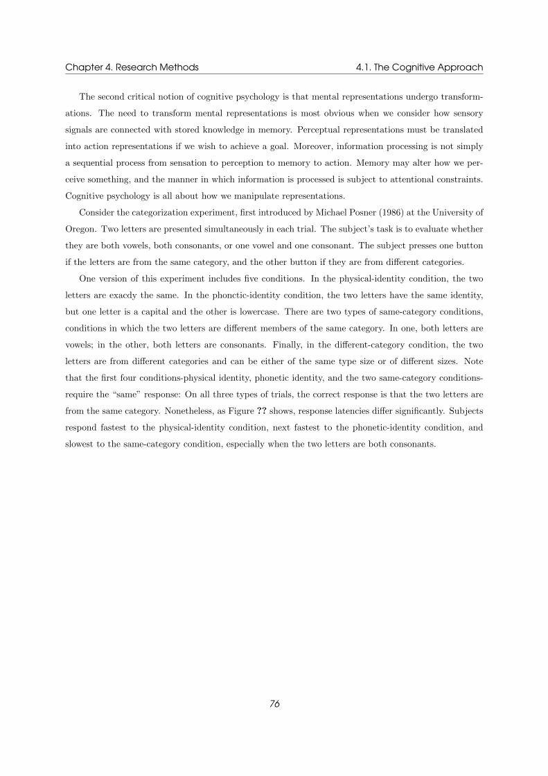
Chapter 4. Research Methods 4.1. The Cognitive Approach
The second critical notion of cognitive psychology is that mental representations undergo transform-
ations. The need to transform mental representations is most obvious when we consider how sensory
signals are connected with stored knowledge in memory. Perceptual representations must be translated
into action representations if we wish to achieve a goal. Moreover, information processing is not simply
a sequential process from sensation to perception to memory to action. Memory may alter how we per-
ceive something, and the manner in which information is processed is subject to attentional constraints.
Cognitive psychology is all about how we manipulate representations.
Consider the categorization experiment, first introduced by Michael Posner (1986) at the University of
Oregon. Two letters are presented simultaneously in each trial. The subject’s task is to evaluate whether
they are both vowels, both consonants, or one vowel and one consonant. The subject presses one button
if the letters are from the same category, and the other button if they are from different categories.
One version of this experiment includes five conditions. In the physical-identity condition, the two
letters are exacdy the same. In the phonctic-identity condition, the two letters have the same identity,
but one letter is a capital and the other is lowercase. There are two types of same-category conditions,
conditions in which the two letters are different members of the same category. In one, both letters are
vowels; in the other, both letters are consonants. Finally, in the different-category condition, the two
letters are from different categories and can be either of the same type size or of different sizes. Note
that the first four conditions-physical identity, phonetic identity, and the two same-category conditions-
require the “same” response: On all three types of trials, the correct response is that the two letters are
from the same category. Nonetheless, as Figure ?? shows, response latencies differ significantly. Subjects
respond fastest to the physical-identity condition, next fastest to the phonetic-identity condition, and
slowest to the same-category condition, especially when the two letters are both consonants.
76
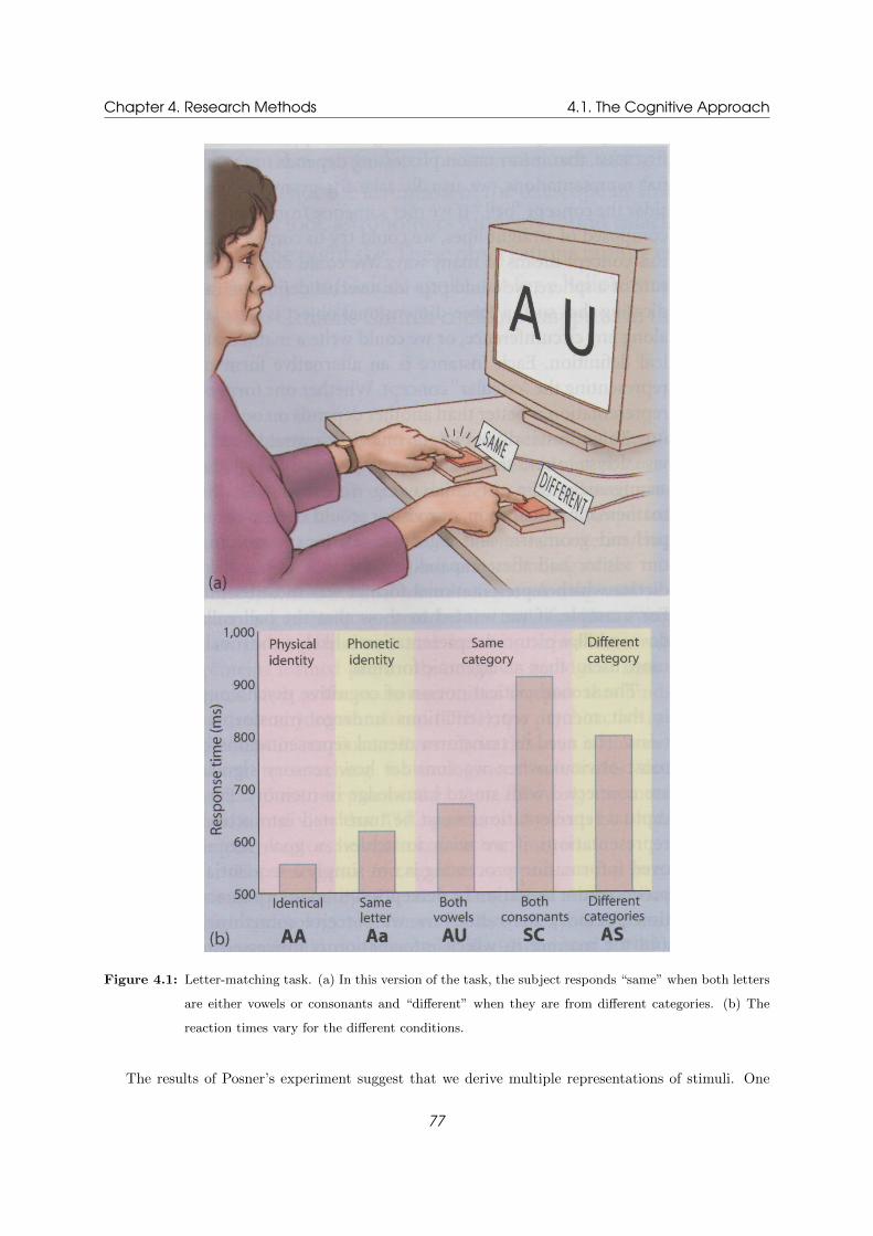
Chapter 4. Research Methods 4.1. The Cognitive Approach
Figure 4.1: Letter-matching task. (a) In this version of the task, the subject responds “same” when both letters
are either vowels or consonants and “different” when they are from different categories. (b) The
reaction times vary for the different conditions.
The results of Posner’s experiment suggest that we derive multiple representations of stimuli. One
77

Chapter 4. Research Methods 4.1. The Cognitive Approach
representation is based on the physical aspects of the stimulus. In this experiment, it is a visually derived
representation of the shape presented on the screen. A second representation corresponds to the letter’s
identity. This representation reflects the fact that many stimuli can correspond to the same letter. A
third level of abstraction represents the category to which a letter belongs. At this level, the letters
A and E activate our internal representation of the category “vowel.” Posner maintains that different
response latencies reflect the degrees of processing required to do the letter-matching task. By this logic,
we infer that physical representations are activated first, phonetic representations next, and category
representations last.
This experiment provides a powerful demonstration that, even with simple stimuli, the mind derives
multiple representations. Other manipulations with this task have explored how representations are
transformed from one form to another. In a follow-up study, Posner and his colleagues used a sequential
mode of presentation. Two letters were presented again, but a brief interval (referred to as the stimulus
onset asynchrony, the time between the two stimuli) separated the presentations for the letters. The
difference in response time to the physical-identity and phonetic-identity conditions was reduced as the
stimulus onset asynchrony became longer. Hence, the internal representation of the first letter is trans-
formed during the interval. The representation of the physical stimulus gives way to the more abstract
representation of the letter’s phonetic identity.
As you may have experienced personally, experiments such as these elicit as many questions as answers.
Why do subjects take longer to judge that two letters are consonants than they do to judge that two
letters are vowels? Would the same advantage for identical stimuli exist if the letters were spoken?
What about if one letter were visual and the other were auditory? Suppose that the task were to judge
whether two letters were physically identical. Would manipulating the stimulus onset asynchrony affect
reaction times in this version? Cognitive psychologists address these questions and then devise methods
for inferring the mind’s machinery from observable behaviors.
In the preceding example, the primary dependent variable was reaction time, the speed with which
subjects make their judgments. Reaction time experiments utilize the chronometric methodology. Chro-
nometric comes from the Greek words chronos (“time”) and metron (“measure”). The chronometric
study of the mind is essential for cognitive psychologists because mental events occur rapidly and effi-
ciently. If we consider only whether a person is correct or incorrect on a task, we miss subtle differences
in performance. Measuring reaction time permits a finer analysis of internal processes. In addition to
measuring processing time as a dependent variable, chronometric manipulations can be applied to inde-
pendent variables, as with the letter- matching experiment in which the stimulus onset asynchrony was
varied.
78

Chapter 4. Research Methods 4.1. The Cognitive Approach
4.1.1 Characterizing Mental Operations
Suppose you arrive at the grocery store and discover that you forgot to bring your shopping list. As you
wander up and down the aisles, you gaze upon the thousands of items lining the shelves, hoping that they
will help prompt your memory. Perhaps you cruise through the pet food section, but when you come to
the dairy section you hesitate: Was there a carton of eggs in the refrigerator? Was the milk supply low?
Were there any cheeses not covered by a 6-month rind of mold?
This memory retrieval task draws on a number of cognitive capabilities. A fundamental goal of
cognitive psychology is to identify the different mental operations that are required to perform tasks
such as these. Not only are cognitive psychologists interested in describing human performance - the
observable behavior of humans and other animals - but also they seek to identify the internal processing
that underlies this performance. A basic assumption of cognitive psychology is that tasks are composed of
a set of mental operations. Mental operations involve taking a representation as an input and performing
some sort of process on it, thus producing a new representation, or output. As such, mental operations
are processes that generate, elaborate on, or manipulate mental representations. Cognitive psychologists
design experiments to test hypotheses about mental operations.
Consider an experimental task introduced by Saul Sternberg (1975) when he was working at Bell
Laboratories. The task bears some similarity to the problem faced by an absentminded shopper, except
that in Stern-berg’s task, the difficulty is not so much in terms of forgetting items in memory, but rather
in comparing sensory information with representations that are active in memory. On each trial, the
subject is first presented with a set of letters to memorize. The memory set could consist of one, two, or
four letters. Then a single letter is presented, and the subject must decide if this letter was part of the
memorized set. The subject presses one button to indicate that the target was part of the memory set
(“yes” response) and a second button to indicate that the target was not part of the set (“no” response).
Once again the primary dependent variable is reaction time.
Sternberg postulated that, to respond on this task, the subject must engage in four primary mental
operations:
1. Encode. The subject must identify the visible target.
2. Compare. The subject must compare the mental representation of the target with the representa-
tions of the items in memory.
3. Decide. The subject must decide whether the target matches one of the memorized items.
4. Respond. The subject must respond appropriately for the decision made in Step 3.
Note that each of these operations is likely to be composed of additional operations. For example,
responding might be subdivided into processes involved in selecting the appropriate finger and processes
79
Chapter 4. Research Methods 4.1. The Cognitive Approach
involved in activating the muscles that make the finger move. Nonetheless, by postulating a set of mental
operations, we can devise experiments to explore how putative mental operations are carried out.
A basic question for Sternberg was how to characterize the efficiency of recognition memory. Assuming
that all items in the memory set are actively represented, the recognition process might work in one of
two different ways: A highly efficient system might compare a representation of the target with all of the
items in the memory set simultaneously. On the other hand, the recognition operation might be limited
in terms of how much information it can handle at any point in time. For example, it might require the
input to be compared successively to each item in memory.
Sternberg realized that the reaction time data could distinguish between these two alternatives. If the
comparison process can be simultaneous for all items - what is called a parallel process - then reaction
time should be independent of the number of items in the memory set. But if the comparison process
operates in a sequential, or serial, manner, then reaction time should slow down as the memory set
becomes larger, because more time is required to compare an item with a large memory list than with
a small memory list. Sternberg’s results convincingly supported the serial hypothesis. In fact, reaction
time increased in a constant, or linear, manner with set size, and the functions for the “yes” and “no”
trials were essentially identical.
The parallel, linear functions allowed Sternberg to make two inferences about the mental operations
associated with this task. First, the linear increase in reaction time as the set size increased implied
that the memory comparison operation took a fixed amount of internal processing time. In the initial
study, the slope of the function was approximately 40 ms per item, implying that it takes about 40 ms
for each successive comparison of the target to the items in the memory set. This does not mean that
this value represents a fixed property of memory comparison. It is likely to be affected by factors such
as task difficulty (e.g., whether the nontarget items in the memory set arc similar or dissimilar to the
target item) and experience. Nonetheless, the experiment demonstrates how mental operations can be
evaluated both qualitatively and quantitatively from simple behavioral tasks.
Second, the fact that the two functions were parallel implied that subjects compared all of the memory
items to the target before responding. If subjects had terminated the comparison as soon as a match
was found, then the slope of the “no” function should have been twice as steep as the slope of the “yes”
function. This follows because in “no” trials, all of the items have to be checked. With “yes” trials, on
average only half the items need to be checked before a match is found. The feet that the functions were
parallel implies that comparisons were carried out on all items in what is called an exhaustive search
(as opposed to a serial, self-terminating search). An exhaustive process seems illogical, though. Why
continue to compare the target to the memory set after a match has been detected? One possible answer
is that it is easier to store the result of each comparison for later evaluation than to monitor “online” the
results of successive comparisons.
80

Chapter 4. Research Methods 4.1. The Cognitive Approach
4.1.2 Constraints on information Processing
In the memory search experiment, information processing operates in a certain manner because the
memory comparison process is limited. The subjects cannot compare the target item to all of the items
in the memory set simultaneously. An important question is whether this limitation reflects properties
that are specific to memory or a more general processing constraint. Perhaps the amount of internal
processing that people can do at any one time is limited regardless of the task. An alternative explanation
is that processing limitations are task specific. Processing constraints are defined only by the particular
set of mental operations associated with a particular task. For example, although the comparison of a
probe item to the memory set might require a serial operation, encoding might occur in parallel such
that it would not matter whether the probe was presented by itself or among a noisy array of competing
stimuli.
Exploring the limitations in task performance is a central concern for cognitive psychologists. Consider
a simple color-naming task that was devised in the early 1930s by an aspiring doctoral student, J. R.
Stroop (1935; for a review, see MacLeod, 1991), and that has become one of the most widely employed
tasks in all of cognitive psychology. In this task, a list of words is presented and the subject is asked to
name the color of each stimulus as fast as possible. As Figure ?? illustrates, it is much easier to do this
task when the words match the colors.
Figure 4.2: Stroop task. Time yourself as you work through each column, naming the color of the ink in each
stimulus as fast as possible. Assuming that you do not squint to blur the words, it should be easy
to read the first and second columns but quite difficult to read the third.
81

Chapter 4. Research Methods 4.1. The Cognitive Approach
The Stroop effect powerfully demonstrates the multiplicity of mental representations. The stimuli in
this task appear to activate at least two separable representations. One representation corresponds to
the color of each stimulus; it is what allows the subject to perform the task. The second representation
corresponds to the color concept associated with the words. The fact that you are slower to name the
colors when the ink color and words are mismatched indicates that this representation is activated even
though it is irrelevant to the task. Indeed, the activation of a representation based on the words rather
than the colors of the words appears to be automatic. The Stroop effect persists even after thousands of
trials of practice, reflecting the fact that skilled readers have years of practice in analyzing letter strings
for their symbolic meaning. On the other hand, the interference from the words is markedly reduced if
the response requires a key press rather than a vocal response. Thus, the word-based representations
are closely linked to the vocal response system and have little effect when the responses are produced
manually.
Another method used to examine constraints on information processing involves dual tasks. For these
studies, performance on a primary task alone is compared to performance when that task is carried
out concurrently with a secondary task. The decrement in primary-task performance during the dual-
task situation helps elucidate the limits of cognition. Sophisticated use of dual-task methodology also
can identify the exact source of interference. For example, the Stroop effect is not reduced when the
color-naming task is performed simultaneously with a secondary task in which the subject must judge
the pitch of an auditory tone. However, if the auditory stimuli for the secondary task are a list of
words and the subject must monitor this list for a particular target, the Stroop effect is attenuated. It
appears that the verbal demands of the secondary task interfere with the automatic activation of the
word-based representations in the Stroop task, thus leaving the color-based representations relatively free
from interference.
The efficiency of our mental abilities and the way in which mental operations interact can change with
experience. The beginning driver has her hands rigidly locked to the steering wheel; within a few months,
though, she is unfazed to steer with her left hand while maintaining a conversation with a passenger and
using her right hand to scan for a good radio station. Even more impressive is the fact that, with extensive
practice, people can become proficient at simultaneously performing two tasks that were originally quite
incompatible.
Elizabeth Spelke and her colleagues at Cornell University studied how well college students read for
comprehension while taking dictation. Prior to any training, their subjects could read about 400 words
per minute when faced with difficult reading material such as modern short stories. As we would expect,
this rate fell to 280 words per minute when the subjects were required to simultaneously take dictation,
and their comprehension of the stories was also impaired. Remarkably, after 85 hours of training spread
over a 17-week period, the students’ proficiency in reading while taking dictation was essentially as good
as when reading alone. The results offer an elixir for all college students. Imagine finishing the reading
82

Chapter 4. Research Methods 4.2. Computer Modeling
for an upcoming psychology examination while taking notes during a history lecture!
4.2 Computer Modeling
The computer is a powerful metaphor for cognitive neuroscience. Both the brain and the computer
chip are impressive processing machines, capable of representing and transforming large amounts of
information. Although there are vast differences in how these machines process information, cognitive
scientists use computers to simulate cognitive processes. To simulate is to imitate, to reproduce behavior
in an alternative medium. The simulated cognitive processes are commonly referred to as artificial
intelligence - artificial in the sense that they are artifacts, human creations - and intelligent in that the
computers perform complex functions. Computer programs control robots on factory production lines,
assist physicians in making differential diagnoses or in detecting breast cancer, and create models of the
universe in the first nanoseconds after the big bang.
Many commercial computer applications are developed without reference to how brains think. More
relevant to our present concerns are the efforts of cognitive scientists to create models of cognition. In
these investigations, simulations are designed to mimic behavior and the cognitive processes that support
that behavior. The computer is given input and then must perform internal operations to create a
behavior. By observing the behavior, the researcher can assess how well it matches behavior produced
by a real mind. Of course, to get the computer to succeed, the modeler must specify how information is
represented and transformed within the program. To do this, concrete hypotheses regarding the “mental”
operations needed for the machine must be generated. As such, computer simulations provide a useful tool
for testing theories of cognition. Successes and failures of models give valuable insights to the strengths
and weaknesses of a theory.
4.2.1 Models Are Explicit
Computer models of cognition are useful because they can be analyzed in detail. In creating a simulation,
the researcher must be completely explicit; the way the computer represents and processes information
must be totally specified. This does not mean that a computer’s operation is always completely predictable
and that the outcome of a simulation is known in advance. Computer simulations can incorporate random
events or be on such a large scale that analytic tools do not reveal the solution. But the internal operations,
the way information is computed, must be determined. Computer simulations are especially helpful to
cognitive neuroscientists in recognizing problems that the brain must solve to produce coherent behavior.
Braitenberg gave elegant examples of how modeling brings insights to information processing. Imagine
observing the two creatures shown in Figure ?? as they move about a minimalist world consisting of a
single heat source such as a sun. From the outside, the creatures look identical: They both have two
sensors and four wheels. Despite this similarity, their behavior is distinct: One creature moves away from
83

Chapter 4. Research Methods 4.2. Computer Modeling
the sun, and the other homes in on it. Why the difference? As outsiders with no access to the internal
operations of these creatures, we might conjecture that they have had different experiences and so the
same input activates different representations. Perhaps one was burned at an early age and fears the sun,
and maybe the other likes the warmth.
Figure 4.3: Two very simple vehicles, each equipped with two sensors that excite motors on the rear wheels.
The wheel linked to the sensor closest to the sun will turn faster than the other wheel, thus causing
the vehicle to turn. Simply changing the wiring scheme from uncrossed to crossed radically alters
the behavior of the vehicles. The “coward” will always avoid the source, whereas the “aggressor”
will relentlessly pursue it
As their internal wiring reveals, however, the behavioral differences depend on how the creatures are
wired. The uncrossed connections make the creature on the left turn away from the sun; the crossed
connections force the creature on the right to orient toward it. Thus, the two creatures’ behavioral
differences arise from a slight variation in how sensory information is mapped onto motor processes.
These creatures are exceedingly simple and inflexible in their actions. At best, they offer only the
crudest model of how an invertebrate might move in response to a phototropic sensor. The point of
Braitenberg’s example is not to model a behavior; rather, it represents how a single computational
change from crossed to uncrossed wiring can yield a major behavioral change. When interpreting such
a behavioral difference, we might postulate extensive internal operations and representations. When we
look inside Braitenberg’s models, however, we see that there is no difference in how the two models
process information, but only a difference in their patterns of connectivity.
84

Chapter 4. Research Methods 4.2. Computer Modeling
4.2.2 Representations in Computer Models
Computer models differ widely in their representations. Symbolic models include, as we might expect,
units that represent symbolic entities. A model for object recognition might have units that represent
visual features like corners or volumetric shapes. An alternative architecture that figures prominently
in cognitive neuroscience is the neural network. In neural networks, processing is distributed over innu-
merable units whose input and output can represent specific features. For example, they may indicate
whether a stimulus contains a visual feature such as a vertical or a horizontal line. Of critical importance
in many of these models, however, is the fact that so-called hidden units are connected to input and
output units.
Hidden units provide intermediate processing steps between the input and output units. They enable
the model to extract the information that allows for the best mapping between the input and desired
output by changing the strength of connections between units. To do this, a modeler must specify a
learning rule, a quantitative description of how processing within the model changes. With most learning
rules, changes are large when the model performs poorly and small when the model performs well. Other
learning algorithms are even simpler. For example, whenever two neighboring nodes are simultaneously
active, the link between them is strengthened; if one is active when the other is silent, then the link
between them is weakened.
Models can be very powerful for solving complex problems. Simulations cover the gamut of cognitive
processes, including perception, memory, language, and motor control. One of the most appealing aspects
of neural networks is that the architecture resembles, at least superficially, the nervous system. In these
models, processing is distributed across many units, similar to the way that neural structures depend on
the activity of many neurons. The contribution of any unit may be small in relation to the system’s total
output, but complex behaviors can be generated by the aggregate action of all units. In addition, the
computations in these models are simulated to occur in parallel. The activation levels of the units in the
network can be updated in a relatively continuous and simultaneous manner.
Computational models can vary widely in the level of explanation they seek to provide. Some models
simulate behavior at the systems level, seeking to show how cognitive operations such as motion perception
or skilled movements can be generated from a network of interconnected processing units. In other cases,
the simulations operate at a cellular or even molecular level. For example, neural network models have
been used to investigate how the variation in transmitter uptake is a function of dendrite geometry. The
amount of detail that must be incorporated into the model will be dictated to a large extent by the type of
question being investigated. Many of these problems are difficult to evaluate without simulations, either
experimentally because the available experimental methods are insufficient or mathematically because
the solutions become too complicated given the many interactions of the processing elements.
An appealing aspect of neural network models, especially for people interested in cognitive neuros-
85

Chapter 4. Research Methods 4.2. Computer Modeling
cience, is that “lesion” techniques demonstrate how a model’s performance changes when its parts are
altered. Unlike strictly serial computer models that collapse if a circuit is broken, neural network models
degrade gracefully: The model may continue to perform appropriately after some units are removed,
because each unit plays only a small part in the processing. Artificial lesioning is thus a fascinating way
to test a model’s validity. At the first level, a model is constructed to see if it adequately simulates normal
behavior. Then “lesions” can be made to see if the breakdown in the model’s performance resembles the
behavioral deficits observed in neurological patients.
4.2.3 Models Lead to Testable Predictions
The contribution of computer modeling usually goes beyond the assessment of whether a model succeeds
in mimicking a cognitive process. Models can generate novel predictions that can be tested with real
brains. An example of the predictive power of computer modeling comes from the work of Szabolcs Kali of
the Hungarian Academy of Sciences and Peter Dayan at the University College London. Their computer
models were designed to ask questions about how people store and retrieve information in memory about
specific events - what is called episodic memory. Observations from the neurosciences suggest that the
formation of episodic memories depends critically on the hippocampus and adjacent areas of the medial
temporal lobe, whereas the storage of such memories involves the neocortex. Kali and Dayan used a
computer model to explore a specific question: How is access to stored memories maintained in a system
where the neocortical connections are ever changing? Does the maintenance of memories over time require
the reactivation of hippocampal-neocortical connections, or can neocortical representations remain stable
despite fluctuations and modifications over timet?
The model architecture was based on anatomical facts regarding patterns of connectivity between
the hippocampus and neocortex. The model was then trained on a set of patterns that represented
distinct episodic memories. For example, one might correspond to the first time you visited the Pacific
Ocean; another, to the lecture in which you first learned about the Stroop effect. Once the model had
mastered the memory set by showing that it could correctly recall a full episode when given only partial
information, it was tested on a consolidation task. Could old memories remain after the hippocampus was
disconnected from the cortex if cortical units continued to follow their initial learning rules? In essence,
this was a test of whether lesions to the hippocampus would disrupt long-term episodic memory. The
results indicated that episodic memory became quite impaired when the hippocampus and cortex were
disconnected. Thus, the model predicts that hippocampal reactivation is necessary for maintaining even
well-consolidated episodic memories. In the model, this maintenance process requires a mechanism that
keeps hippocampal and neocortical representations in register with one another, even as the neocortex
undergoes subtle changes associated with daily learning.
This modeling project was initiated because research on people with lesions of the hippocampus
had failed to provide a clear answer about the role of this structure in memory consolidation. The
86

Chapter 4. Research Methods 4.3. Experimental Techniques Used With Animals
model, based on known principles of neuroanatomy and neurophysiology, could be used to test specific
hypotheses concerning one type of memory, episodic memory, and to direct future research. Of course,
the goal here is not to make a model that has perfect memory consolidation. Rather, it is to ask how
human memory works. Thus, human experiments can be conducted to test predictions derived from the
model, as well as to generate new empirical observations that must be incorporated into future versions
of the computational model.
4.2.4 Limitations of Computer Models
Computer modeling is limited as a method for studying the operation of living nervous systems. For
one thing, models always require radical simplifications of the nervous system. Although the units in a
typical neural network model bear some similarity to neurons - for example, nonlinear activation rules
produce spikelike behavior - the models are limited in scope, usually consisting of just a few hundred or
so elements, and it is not always clear whether the elements correspond to single neurons or to ensembles
of neurons. Second, some requirements and problems arise in modeling work, particularly in learning,
and are at odds with what we know occurs in biological organisms. Many network models require an
“allknowing” teacher who “knows” the right answer and can be used to correct the behavior of the internal
elements. These models can also suffer catastrophic interference, the loss of old information when new
material is presented.
Third, most modeling efforts are restricted to relatively narrow problems, such as demonstrating how
the Stroop effect can be simulated by postulating separate word name and word color representations
under the control of a common attentional system. As such, they provide useful computational tests of the
viability of a particular hypothesis but arc typically less useful for generating new predictions. Moreover,
as some critics have argued, unlike experimental work that, by its nature, is cumulative, modeling research
tends to be conducted in isolation. There may be lots of ways to model a particular phenomenon, but
less effort has been devoted to devising critical tests that pit one theory against another.
These limitations are by no means insurmountable, and we should expect the contribution of computer
simulations to continue to grow in the cognitive neuro-sciences. Indeed, the trend in the field is for
modeling work to be more constrained by neuroscience, with researchers replacing generic processing units
with elements that embody the biophysics of the brain. In a reciprocal manner, computer simulations
provide a useful way to develop theory, which may then aid researchers in designing experiments and
interpreting results.
4.3 Experimental Techniques Used With Animals
The use of animals for experimental procedures has played a critical role in the medical and biological
sciences. Although many insights can be gleaned from careful observations of people with neurological
87

Chapter 4. Research Methods 4.3. Experimental Techniques Used With Animals
disorders, as we will sec throughout this book, such methods are, in essence, correlational. We can observe
how behavior is disturbed following a neurological insult, but it can be difficult to pinpoint the exact
cause of the disorder. For one thing, insults such as stroke or tumor tend to be quite large, with the
damage extending across many neural structures. Moreover, damage in one part of the brain may disturb
function in other parts of the brain that are spared. There is also increasing evidence that the brain is a
plastic device: Neural function is constantly being reshaped by our experiences, and such reorganization
can be quite remarkable following neurological damage.
The use of animals in scientific research allows researchers to adopt a more experimental approach.
Because neural function depends on electrochemical processes, neurophysiologists have developed tech-
niques that can be used to measure and manipulate neuronal activity. Some of these techniques measure
and record cell activity, in either passive or in active conditions. Others manipulate activity by creating
lesions through the destruction or temporary inactivation of targeted brain regions. Lesion studies in
animals face the same limitations associated with the study of human neurological dysfunction. However,
modern techniques allow the researcher to be highly selective in creating these lesions, and the effects of
the damage can be monitored carefully following the surgery.
4.3.1 Single-Cell Recording
The most important technological advance in neurophysiology - perhaps in all of neuroscience - was the
development of methods to record the activity of single neurons in laboratory animals. With this method,
the understanding of neural activity advanced a quantum leap. No longer did the neuroscientist have
to be content with describing nervous system action in terms of functional regions. Single-cell recording
enabled researchers to describe response characteristics of individual elements.
In single-cell recording, a thin electrode is inserted into an animal’s brain. If the electrode is in
the vicinity of a neuronal membrane, electrical changes can be measured. Although the surest way to
guarantee that the electrode records the activity of a single cell is to record intracellularly, this technique
is difficult, and penetrating the membrane frequently damages the cell. Thus, single-cell recording is
typically done extracellularly. With this method, the electrode is situated on the outside of the neuron.
The problem with this approach is that there is no guarantee that the changes in electrical potential
at the electrode tip reflect the activity of a single neuron. It is more likely that the tip will record the
activity of a small set of neurons. Computer algorithms are used to differentiate this pooled activity into
the contributions from individual neurons.
Neurons are constantly active, even in the absence of stimulation or movement. This baseline activity
varies widely from one brain area to another. For example, some cells within the basal ganglia have
spontaneous firing rates of over 100 spikes/s, whereas cells in another basal ganglia region have a baseline
rate of about 1 spike/s. These spontaneous firing levels fluctuate. The primary goal of single-cell recording
experiments is to determine experimental manipulations that produce a consistent change in the response
88

Chapter 4. Research Methods 4.3. Experimental Techniques Used With Animals
rate of an isolated cell. Does the cell increase its firing rate when the animal moves its arm? Is this change
specific to movements in a particular direction? Does the firing rate for that movement depend on the
outcome of the action (e.g., the food morsel to be reached)? As interesting, what makes the cell decrease
its response rate?
The neurophysiologist is interested in what causes change in the synaptic activity of a neuron. The
experimenter seeks to determine the response characteristics of individual neurons by correlating their
activity with a given stimulus pattern or behavior. The technique has been used in almost all regions of
the brain in a wide range of nonhuman species. For sensory neurons, the experimenter might manipulate
the type of stimulus presented to the animal. For motor neurons, recordings can be made as the animal
performs a task or moves about the cage. Some of the most recent advances in neurophysiology have
come about as researchers probe higher brain centers to examine changes in cellular activity related to
goals, emotions, and rewards.
In the typical neurophysiological experiment, recordings are obtained from a series of cells in a targeted
area of interest In this manner, a functional map can describe similarities and differences between neurons
in a specified cortical region. One area where the single-cell method has been used extensively is the study
of the visual system of primates. In a typical experiment the researcher targets the electrode to a cortical
area that contains cells thought to respond to visual stimulation. Once a cell has been identified, the
researcher tries to characterize its response properties.
A single cell is not responsive to all visual stimuli. A number of stimulus parameters might correlate
with the variation in the cell’s firing rate; examples include the shape of the stimulus, its color, and
whether or not it is moving. An important factor is the location of the stimulus. As Figure ?? shows, all
visually sensitive cells respond to stimuli in only a limited region of space. This region of space is referred
to as that cell’s receptive field. For example, some neurons respond when the stimulus is located in the
lower left portion of the visible field. For other neurons, the stimulus may have to be in the upper left.
89

Chapter 4. Research Methods 4.3. Experimental Techniques Used With Animals
Figure 4.4: Electrophysiological methods are used to identify the response characteristics of cells in the visual
cortex. (a) While the activity of a single cell is monitored, the monkey is required to maintain
fixation, and stimuli are presented at various positions in its field of view, (b) The vertical lines to
the right of each stimulus correspond to individual action potentials. The cell fires vigorously when
the stimulus is presented in the upper right quadrant, thus defining the upper right as the receptive
field for this cell.
The sizes of the receptive fields of visual cells vary; they are smallest in primary visual cortex and
become larger in association visual areas. Thus, a stimulus will cause a cell in primary visual cortex to
increase its firing rate only when it is positioned in a very restricted region of the visible world. If the
stimulus is moved outside this region of space, the cell will return to its spontaneous level of activity. In
contrast, displacing a stimulus over a large distance may produce a similar increase in the firing rate of
90

Chapter 4. Research Methods 4.3. Experimental Techniques Used With Animals
visually sensitive cells in the temporal lobe.
Neighboring cells have at least partially overlapping receptive fields. As a region of visually responsive
cells is traversed, there is an orderly relation between the receptive-field properties of these cells and
the external world. External space is represented in a continuous manner across the cortical surface:
Neighboring cells have receptive fields of neighboring regions of external space. As such, cells form a
topographic representation, an orderly mapping between an external dimension such as spatial location
and the neural representation of that dimension. In vision, topographic representations are referred to
as retinotopic.
The retina is composed of a continuous sheet of photoreceptors, neurons that respond to visible light
passing through the lens of the eye. Visual cells in subcortical and cortical areas maintain retinotopic
information. Thus, if light falls on one spot of the retina, cells with receptive fields spanning this area
are activated. If the light moves and falls on a different region of the retina, activity ceases in these cells
and begins in other cells whose receptive fields encompass the new region of stimulation. In this manner,
visual areas provide a representation of the location of the stimulus. Cell activity within a retinotopic
map correlates with (i.e., predicts) the location of the stimulus.
There are other types of topographic maps. In a similar sense, auditory areas in the subcortex and
cortex contain tonotopic maps, in which the physical dimension reflected in neural organization is the
sound frequency of a stimulus. With a tonotopic map, some cells are maximally activated by a 1000-
Hz tone, and others by a 5000-Hz tone. In addition, neighboring cells tend to be tuned to similar
frequencies. Thus, sound frequencies are reflected in cells that are activated upon the presentation of
a sound. Tonotopic maps are sometimes referred to as cochleotopic because the cochlea, the sensory
apparatus in the ear, contains hair cells tuned to distinct regions of the auditory spectrum.
When the single-cell method was first introduced, neuroscientists were optimistic that the mysteries
of brain function would be solved. All they needed was a catalog of contributions by different cells. Yet
it soon became clear that, with neurons, the aggregate behavior of cells might be more than just the sum
of its parts. The function of an area might be better understood by identification of the correlations in
the firing patterns of groups of neurons rather than by identification of the response properties of each
individual neuron. This idea has inspired single-cell physiologists to develop new techniques that allow
recordings to be made in many neurons simultaneously - what is called multiunit recording.
Bruce McNaughton at the University of Arizona studied how the rat hippocampus represents spatial
information by simultaneously recording from 150 cells! By looking at the pattern of activity over the
group of neurons, the researchers were able to show how the rat coded spatial and episodic information
differently. Today it is not uncommon to record from over 400 cells simultaneously. Multiunit recordings
from motor areas of the brain are now being used to allow animals to control artificial limbs, a dramatic
medical advance that may change the way rehabilitation programs are designed for paraplegics. For
example, multiunit recordings can be obtained while people think about actions they would like to
91
Chapter 4. Research Methods 4.3. Experimental Techniques Used With Animals
perform, and this information can be analyzed by computers to control robotic or artificial limbs.
4.3.2 Lesions
The brain is a complicated organ composed of many structures, including subcortical nuclei and distinct
cortical areas. It seems evident that any task a person performs requires the successful operation of many
brain components. A long-standing method of the neurophysiologist has been to study how behavior is
altered by selective removal of one or more of these parts. The logic of this approach is straightforward.
If a neural structure contributes to a task, then rendering the structure dysfunctional should impair the
performance of that task.
Humans obviously cannot be subjected to brain lesions as experimental procedures with the goal of
understanding brain function. Typically, human neuropsychology involves research with patients who
have suffered naturally occurring lesions. But animal researchers have not been constrained in this way.
They share a long tradition of studying brain function by comparing the effects of different brain lesions.
In one classic example, Nobel laureate Charles Sherrington employed the lesion method at the start of
the 20th century to investigate the importance of feed-back in limb movement in the dog. By severing
the nerve fibers carrying sensory information into the spinal cord, he observed that the animals stopped
walking.
Lesioning a neural structure will eliminate that structure’s contribution. But the lesion also might
force the animal to change its normal behavior and alter the function of intact structures. One cannot be
confident that the effect of a lesion eliminates the contribution of only a single structure. The function of
neural regions that are connected to the lesioned area might be altered, either because they are deprived
of their normal neural input or because their axons fail to make normal synaptic connections. The lesion
might also cause the animal to develop a compensatory strategy to minimize the consequences of the
lesion. For example, when monkeys are deprived of sensory feedback to one arm, they stop using the
limb. However, if the sensory feedback to the other arm is eliminated at a later date, the animals begin
to use both limbs. The monkeys prefer to use a limb that has normal sensation, but the second surgery
shows that they could indeed use the other limb.
With this methodology we should remember that a lesion may do more than eliminate the function
provided by the lesioned structure. Nonetheless, the method has been critical for neurophysiologists.
Over the years, lesioning techniques have been refined, allowing for much greater precision. Most lesions
were originally made by the aspiration of neural tissue. In aspiration experiments, a suction device is
used to remove the targeted structures. Another method was to apply electrical charges strong enough
to destroy tissue. One problem with this method is the difficulty of being selective. Any tissue within
range of the voltage generated by the electrode tip will be destroyed. For example, a researcher might
want to observe the effects of a lesion to a certain cortical area, but if the electrolytic lesion extends
into underlying white matter, these fibers also will be destroyed. Therefore, a distant structure might be
92
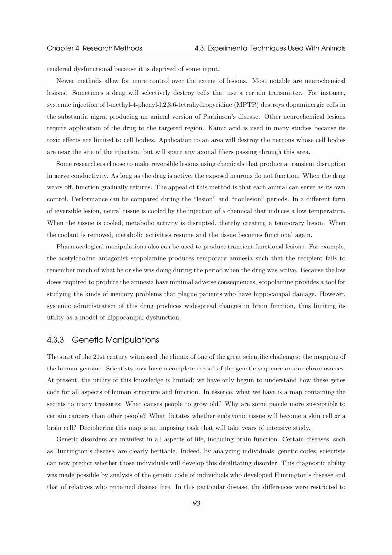
Chapter 4. Research Methods 4.3. Experimental Techniques Used With Animals
rendered dysfunctional because it is deprived of some input.
Newer methods allow for more control over the extent of lesions. Most notable are neurochemical
lesions. Sometimes a drug will selectively destroy cells that use a certain transmitter. For instance,
systemic injection of l-methyl-4-phenyl-l,2,3,6-tetrahydropyridine (MPTP) destroys dopaminergic cells in
the substantia nigra, producing an animal version of Parkinson’s disease. Other neurochemical lesions
require application of the drug to the targeted region. Kainic acid is used in many studies because its
toxic effects are limited to cell bodies. Application to an area will destroy the neurons whose cell bodies
are near the site of the injection, but will spare any axonal fibers passing through this area.
Some researchers choose to make reversible lesions using chemicals that produce a transient disruption
in nerve conductivity. As long as the drug is active, the exposed neurons do not function. When the drug
wears off, function gradually returns. The appeal of this method is that each animal can serve as its own
control. Performance can be compared during the “lesion” and “nonlesion” periods. In a different form
of reversible lesion, neural tissue is cooled by the injection of a chemical that induces a low temperature.
When the tissue is cooled, metabolic activity is disrupted, thereby creating a temporary lesion. When
the coolant is removed, metabolic activities resume and the tissue becomes functional again.
Pharmacological manipulations also can be used to produce transient functional lesions. For example,
the acetylcholine antagonist scopolamine produces temporary amnesia such that the recipient fails to
remember much of what he or she was doing during the period when the drug was active. Because the low
doses required to produce the amnesia have minimal adverse consequences, scopolamine provides a tool for
studying the kinds of memory problems that plague patients who have hippocampal damage. However,
systemic administration of this drug produces widespread changes in brain function, thus limiting its
utility as a model of hippocampal dysfunction.
4.3.3 Genetic Manipulations
The start of the 21st century witnessed the climax of one of the great scientific challenges: the mapping of
the human genome. Scientists now have a complete record of the genetic sequence on our chromosomes.
At present, the utility of this knowledge is limited; we have only begun to understand how these genes
code for all aspects of human structure and function. In essence, what we have is a map containing the
secrets to many treasures: What causes people to grow old? Why are some people more susceptible to
certain cancers than other people? What dictates whether embryonic tissue will become a skin cell or a
brain cell? Deciphering this map is an imposing task that will take years of intensive study.
Genetic disorders are manifest in all aspects of life, including brain function. Certain diseases, such
as Huntington’s disease, are clearly heritable. Indeed, by analyzing individuals’ genetic codes, scientists
can now predict whether those individuals will develop this debilitating disorder. This diagnostic ability
was made possible by analysis of the genetic code of individuals who developed Huntington’s disease and
that of relatives who remained disease free. In this particular disease, the differences were restricted to
93

Chapter 4. Research Methods 4.3. Experimental Techniques Used With Animals
a single chromosomal abnormality. This discovery is also expected to lead to new treatments that will
prevent the onset of Huntington’s. Scientists hope to devise techniques to alter the aberrant genes, either
by modifying them or by figuring out a way to prevent them from being expressed.
In a similar way, scientists have sought to understand other aspects of normal and abnormal brain
function through the study of genetics. Behavioral geneticists have long known that many aspects of
cognitive function are heritable. For example, controlling mating patterns on the basis of spatial-learning
performance allows the development of “maze-bright” and “maze-dull” strains of rats. Rats that are
quick to learn to navigate mazes are likely to have offspring with similar abilities, even if the offspring
are raised by rats that are slow to navigate the same mazes. Such correlations also are observed across a
range of human behaviors, including spatial reasoning, reading speed, and even preferences in watching
television. This should not be taken to mean that our intelligence or behavior is genetically determined.
Maze-bright rats perform quite poorly if raised in an impoverished environment. The truth surely reflects
complex interactions between the environment and genetics.
To understand the genetic component of this equation, neuroscientists are now working with many
species, seeking to identify the genetic mechanisms of both brain structure and function. Dramatic ad-
vances have been made in studies with the fruit fly and mouse, two species with reproductive propensities
that allow many generations to be spawned over a relatively short period of time. As with humans, the
genome sequence for these species has been mapped out. More important, the functional role of many
genes can be explored. A key methodology is to develop genetically altered animals, using what are
referred to as knockout procedures. The term knockout comes from the fact that specific genes have been
manipulated so that they are no longer present or expressed.
Scientists can then study the new species to explore the consequences of these changes. For example,
weaver mice are a knockout strain in which Purkinje cells, the prominent cell type in the cerebellum, fail
to develop. As the name implies, these mice exhibit coordination problems.
At an even more focal level, knockout procedures have been used to create strains that lack single
types of postsynaptic receptors in specific brain regions while leaving intact other types of receptors.
Susumu Tonegawa at the Massachusetts Institute of Technology (MIT) and his colleagues developed a
mouse strain in which they altered cells within a subregion of the hippocampus that typically contain
a receptor for N-methyl-D-aspartate, or NMDA. Knockout strains lacking the NMDA receptor in the
hippocampus exhibit poor learning on a variety of memory tasks, providing a novel approach for linking
memory with its molecular substrate. In a sense, this approach constitutes a lesion method, but at a
microscopic level.
4.3.4 The New Genomics
Neurogenetic research is not limited to identifying the role of each gene individually; it is widely re-
cognized that complex brain function and behavior arise from interactions between many genes and the
94

Chapter 4. Research Methods 4.4. Structural Imaging
environment. Using DNA arrays and knowledge gained from mapping of the human and mouse gen-
omes, scientists can now make quantitative parallel measurements of gene expression, observing how
these change over time or as a function of environmental factors. These methods, which have been used
to investigate gene changes in the developing brain and in the diseased brain, can shed light on normal
and abnormal development.
Gene expression can also be used to study the genes that underlie specific behaviors. For instance,
Michael Miles and his colleagues at the University of California, San Francisco studied the effects of alcohol
on gene expression, asking how specific genes might be related to variations in alcohol tolerance and
dependence. Similarly, Jorge Medina and his colleagues at the Universidad de Buenos Aires in Argentina
used genomic methods to investigate memory consolidation and found that orchestrated, differential
hippocampal gene expression is necessary for long-term memory consolidation.
Gene arrays and the new genomics provide great promise for detecting the polygenetic influences on
brain function and behavior.
4.4 Structural Imaging
Human pathology has long provided key insights into the relationship between brain and behavior. Ob-
servers of neurological dysfunction have certainly contributed much to our understanding of cognition
- long before the advent of cognitive neuroscience. Discoveries concerning the contralateral wiring of
sensory and motor systems were made by physicians in ancient societies attending to warriors with open
head injuries. Postmortem studies by early neurologists, such as Broca and Wernicke, were instrumental
in linking the left hemisphere with language functions. Many other disorders of cognition were described
in the first decades of the 20th century, paralleling the emergence of neurology as a specialty within
medicine.
Even so, there is now an upsurge in testing neurological patients to elucidate issues related to normal
and aberrant cognitive function. As with other subfields of cognitive ncuroscience, this enthusiasm has
been inspired partly by advances in the technologies for diagnosing neurological disorders. As important,
studies of patients with brain damage have benefited from the use of experimental tasks derived from
research with healthy people.
Examples of the merging of cognitive psychology and neurology are presented at the end of this
chapter; in this section we focus on the causes of neurological disorders and the tools that neurologists
use to localize neural pathology. We also take a brief look at treatments for ameliorating neurological
disorders.
We can best address basic research questions, such as those attempting to link cognitive processes
to neural structures, by selecting patients with a single neurological disturbance whose pathology is well
circumscribed. Patients who have suffered trauma or infections frequently have diffuse damage, rendering
95

Chapter 4. Research Methods 4.4. Structural Imaging
it difficult to associate the behavioral deficit with a structure. Nonetheless, extensive clinical and basic
research studies have focused on patients with degenerative disorders such as Alzheimer’s disease, both
to understand the disease processes and to characterize abnormal cognitive function.
Brain damage can result from vascular problems, tumors, degenerative disorders, and trauma. The
first charge of neurologists is to make the appropriate diagnosis. They need to follow appropriate pro-
cedures, especially if a disorder is life-threatening, and to work toward stabilizing the patient’s condition.
Although diagnosis frequently can be made on the basis of a clinical examination, almost all hospitals in
the Western world are equipped with tools that help neurologists visualize brain structure.
4.4.0.1 Computed tomography
Computed tomography (CT or CAT scanning), introduced commercially in 1983, has been an
extremely important medical tool for structural imaging of neurological damage in living people. This
method is an advanced version of the conventional X-ray study; whereas the conventional X-ray study
compresses three-dimensional objects into two dimensions, CT allows for the reconstruction of three-
dimensional space from the compressed two-dimensional images. Figure ?? depicts the method, showing
how X-ray beams are passed through the head and a two-dimensional image is generated by sophisticated
computer software.
Figure 4.5: Computed tomography provides an important tool for imaging neurological pathology, (a) The CT
process is based on the same principles as X-rays. An X-ray is projected through the head, and the
recorded image provides a measurement of the density of the intervening tissue. By projection of
the X-ray from multiple angles and with the use of computer algorithms,a three-dimensional image
based on tissue density is obtained, (b) In this transverse CT image, the dark regions along the
midline are the ventricles, the reservoirs of cerebrospinal fluid.
To undergo CT, a patient lies supine in a scanning machine. The machine has two main parts: an
X-ray source and a set of radiation detectors. The source and detectors are located on opposite sides of
the scanner. These sides can rotate, allowing the radiologist to project X-ray beams from all possible
directions. Starting at one position, an X-ray beam passes through the head. Some radiation in the
96

Chapter 4. Research Methods 4.4. Structural Imaging
X-ray is absorbed by intervening tissue. The remainder passes through and is picked up by the radiation
detectors located on the opposite side of the head. The X-ray source and detectors are then rotated and
a new beam is projected. This process is repeated until X-rays have been projected over 180 .◦ At this
point, recordings made by the detectors are fed into a computer that reconstructs the images.
The key principle underlying CT is that the density of biological material varies and the absorption
of X- ray radiation is correlated with tissue density. High-density material such as bone absorbs a lot of
radiation. Low-density material such as air or blood absorbs little radiation. The absorption capacity of
neural tissue lies between these extremes. Thus, the software for making CT scans actually provides an
image of the differential absorption of intervening tissue. The reconstructed images are usually contrast
reversed: High-density regions show up as light colored, and low-density regions are dark.
Figure ?? shows a CT scan of a healthy individual. Most of the cortex and white matter appear as
homogeneous gray areas. The typical spatial resolution for CT scanners is approximately 0.5 to 1.0 cm
in all directions. Each point on the image reflects an average density of that point and the surrounding
1.0 mm of tissue. Thus, it is not possible to discriminate two objects that are closer than approximately
5 mm. Since the cortex is only 4 mm thick, it is very difficult to see the boundary between white and
gray matter on a CT scan. The white and gray matter are also of very similar density, further limiting
the ability of this technique to distinguish them. But larger structures can be easily identified. The
surrounding skull and eye sockets appear white because of the high density of bone. The ventricles are
black owing to the cerebrospinal fluid’s low density.
4.4.0.2 Magnetic Resonance Imaging
Although CT machines are still widely used, many hospitals have now added a second important imaging
tool,the magnetic resonance imaging (MRI) scanner. In contrast to use of X-rays in CT, the MRI process
exploits the magnetic properties of organic tissue. The number of the protons and neutrons in their
nuclei makes certain atoms especially sensitized to magnetic forces. One such atom that is pervasive
in the brain, and indeed in all organic tissue, is hydrogen. The protons that form the nucleus of the
hydrogen atom are in constant motion, spinning about their principal axis. This motion creates a tiny
magnetic field. In their normal state, the orientation of these protons is randomly distributed, unaffected
by the weak magnetic field created by Earth’s gravity.
The MRI machine creates a powerful magnetic field, measured in tesla units. Whereas gravitational
forces on the Earth create a magnetic field of about 1/1000 tesla, the typical MRI scanner produces a
magnetic field that ranges from 0.5 to 1.5 teslas. When a person is placed within the magnetic field of
the MRI machine, a significant proportion of the protons become oriented in the direction parallel to the
magnetic force. Radio waves are then passed through the magnetized regions, and as the protons absorb
the energy in these waves, their orientation is perturbed in a predictable direction. When the radio
waves are turned off, the absorbed energy is dissipated and the protons rebound toward the orientation
97

Chapter 4. Research Methods 4.4. Structural Imaging
of the magnetic field. This synchronized rebound produces energy signals that are picked up by detectors
surrounding the head. By systematically measuring the signals throughout the three-dimensional volume
of the head, the MRI system can then construct an image reflecting the distribution of the protons and
other magnetic agents in the tissue.
Figure 4.6: Transverse,coronal, and sagittal images.Compar-ing the transverse slice in this figure with the CT
image in Figure ?? reveals the finer resolution offered by MRI. Both images are from about the
same level of the brain.
As ?? shows, MRI scans provide a much dearer image of the brain than is possible with CT scans.
This improvement reflects the feet that the density of protons is much greater in gray matter compared
to white matter. With MRI, it is easy to see the individual sulci and gyri of the cerebral cortex. A
sagittal section at the midline reveals the impressive size of the corpus callosum. The MRI scans can
resolve structures that ar less than 1 mm, allowing elegant views of small, subcortical structures such as
the mammillary bodies or superior colliculus.
4.4.0.3 Diffusion Tensor Imaging
MRI scanners are now also used to study the microscopic anatomical structure of the axon tracts that
form the white matter. This method is called diffusion tensor imaging (DTI; Figure ??). DTI is performed
with an MRI scanner, but unlike traditional MRI scans, DTI measures the density and, more important,
motion of the water contained in the axons. DTI utilizes the known diffusion characteristics of water to
determine the boundaries that restrict water movement throughout the brain. Free diffusion of water is
isotropic; that is, it occurs equally in all directions. However, diffusion of water in the brain is anisotropic,
or restricted, so it does not diffuse equally in all directions. The reason for this anisotropy is that the
98

Chapter 4. Research Methods 4.4. Structural Imaging
axon membranes restrict the diffusion of water; the probability of water moving in the direction of the
axon is thus greater than the probability of water moving perpendicular to the axon. The anisotropy is
greatest in axons because myelin creates a lipid boundary, limiting the flow of water to a much greater
extent than gray matter or cerebrospinal fluid does. In this way, the orientation of axon bundles within
the white matter can be imaged.
Figure 4.7: Example of the result of diffusion tension imaging. Bundles from corpus callosum and brain stem
are depicted.
MRI principles can be combined with what is known about the diffusion of water to determine the
diffusion anisotropy for each region within the MRI scan. These regions are referred to as voxels, a
term that captures the computer graphics idea of a pixel, but volumetrically. By introducing two large
pulses to the magnetic field, we can make MRI signals sensitive to the diffusion of water. The first pulse
determines the initial position of the protons carried by water. The second pulse, introduced after a short
delay, detects how far the protons have moved in space in the specific direction that is being measured.
It is standard to acquire DTI images in more than 30 directions.
The functional differences in diffusion anisotropy have been the subject of recent investigations. For
instance, fractional anisotropy (a measure of the degree of anisotropy in while matter) in the temporo-
parietal region of the left hemisphere is significantly correlated with reading scores in adults with and
without dyslexia. This correlation might reflect the differences in the strength of communication between
visual, auditory, and language-processing areas in the brain.
99
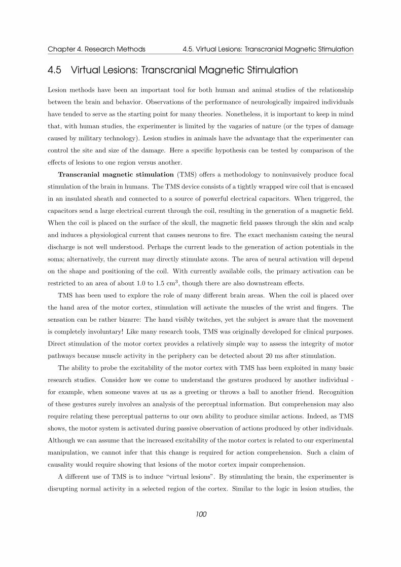
Chapter 4. Research Methods 4.5. Virtual Lesions: Transcranial Magnetic Stimulation
4.5 Virtual Lesions: Transcranial Magnetic Stimulation
Lesion methods have been an important tool for both human and animal studies of the relationship
between the brain and behavior. Observations of the performance of neurologically impaired individuals
have tended to serve as the starting point for many theories. Nonetheless, it is important to keep in mind
that, with human studies, the experimenter is limited by the vagaries of nature (or the types of damage
caused by military technology). Lesion studies in animals have the advantage that the experimenter can
control the site and size of the damage. Here a specific hypothesis can be tested by comparison of the
effects of lesions to one region versus another.
Transcranial magnetic stimulation (TMS) offers a methodology to noninvasively produce focal
stimulation of the brain in humans. The TMS device consists of a tightly wrapped wire coil that is encased
in an insulated sheath and connected to a source of powerful electrical capacitors. When triggered, the
capacitors send a large electrical current through the coil, resulting in the generation of a magnetic field.
When the coil is placed on the surface of the skull, the magnetic field passes through the skin and scalp
and induces a physiological current that causes neurons to fire. The exact mechanism causing the neural
discharge is not well understood. Perhaps the current leads to the generation of action potentials in the
soma; alternatively, the current may directly stimulate axons. The area of neural activation will depend
on the shape and positioning of the coil. With currently available coils, the primary activation can be
restricted to an area of about 1.0 to 1.5 cm3, though there are also downstream effects.
TMS has been used to explore the role of many different brain areas. When the coil is placed over
the hand area of the motor cortex, stimulation will activate the muscles of the wrist and fingers. The
sensation can be rather bizarre: The hand visibly twitches, yet the subject is aware that the movement
is completely involuntary! Like many research tools, TMS was originally developed for clinical purposes.
Direct stimulation of the motor cortex provides a relatively simple way to assess the integrity of motor
pathways because muscle activity in the periphery can be detected about 20 ms after stimulation.
The ability to probe the excitability of the motor cortex with TMS has been exploited in many basic
research studies. Consider how we come to understand the gestures produced by another individual -
for example, when someone waves at us as a greeting or throws a ball to another friend. Recognition
of these gestures surely involves an analysis of the perceptual information. But comprehension may also
require relating these perceptual patterns to our own ability to produce similar actions. Indeed, as TMS
shows, the motor system is activated during passive observation of actions produced by other individuals.
Although we can assume that the increased excitability of the motor cortex is related to our experimental
manipulation, we cannot infer that this change is required for action comprehension. Such a claim of
causality would require showing that lesions of the motor cortex impair comprehension.
A different use of TMS is to induce “virtual lesions”. By stimulating the brain, the experimenter is
disrupting normal activity in a selected region of the cortex. Similar to the logic in lesion studies, the
100

Chapter 4. Research Methods 4.6. Functional Methods
consequences of the stimulation on behavior are used to shed light on the normal function of the disrupted
tissue. What makes this method appealing is that the technique, when properly conducted, is safe and
noninvasive, producing only a relatively brief alteration in neural activity. Thus, performance can be
compared between stimulated and nonstimulated conditions in the same individual. This, of course, is
not possible with brain-injured patients.
The virtual-lesion approach has been successfully employed with stimulation of various brain sites,
even when the person is not aware of any effects from the stimulation. For example, stimulation over
visual cortex can interfere with a person’s ability to identify a letter. The synchronized discharge of the
underlying visual neurons interferes with their nor-mal operation. The timing between the onset of the
TMS pulse and the onset of the stimulus (e.g., presentation of a letter) can be manipulated to plot the
time course of processing. In the letter identification task, the person will err only if the stimulation
occurs between 70 and 170 ms after presentation of the letter. If the TMS is given before this interval,
the neurons have time to recover; if the TMS is given after this interval, the visual neurons have already
responded to the stimulus.
TMS has some notable limitations. As the previous example illustrated, the effects of TMS are
generally quite brief. The method tends to work best with tasks in which the stimulation is closely linked
to either stimulus events or movement. It remains to be seen if more complex tasks can be disrupted by
brief volleys of externally induced stimulation. The fact that stimulation activates a restricted area of the
cortex is both a plus and a minus. The experimenter can restrict stimulation to a specific area, especially
if the coordinates are based on MRI scans. But TMS will be of limited value in exploring the function of
cortical areas that are not on the superficial surface of the brain. Despite these limitations, TMS offers
the potential of providing the cognitive neuroscientist with a relatively safe method for momentarily
disrupting the activity of the human brain. Almost all other methods rely on correlational procedures,
either through the study of naturally occurring lesions or, as we will see in the next section, through the
observation of brain function with various neuroimaging tools.
TMS studies are best conducted in concert with other neuroscience methods. Much of the cutting-edge
research in this area combines data from structural and functional MRI (fMRl; see the next section) with
TMS. Collecting MRI and fMRI images on a subject before commencing the TMS study, and feeding the
data into specialized software programs, allows for real-time copositioning of the TMS stimulation area
and the underlying anatomical region (MRI) with known functional activation (fMRI) in an individual
subject.
4.6 Functional Methods
We already mentioned that patient research rests on the assumption that brain injury is an eliminative
process: The lesion is believed to disrupt certain mental operations while having little or no impact
101

Chapter 4. Research Methods 4.6. Functional Methods
on others. But the brain is massively interconnected, so damage in one area might have widespread
consequences. It is not always easy to analyze the function of a missing part by looking at the operation
of the remaining system. For example, allowing the spark plugs to decay or cutting the line distributing
the gas to the pistons will cause an automobile to stop running, but this does not mean that spark plugs
and distributors do the same thing; rather, their removal has similar functional consequences.
Concerns such as these point to the need for methods that measure activity in the normal brain.
Along this front have occurred remarkable technological break-throughs during the past 25 years. Indeed,
new tools and methods of analysis develop at such an astonishing pace that new journals and scientific
organizations have been created for rapid dissemination of this information. In the following section we
review some of the technologies that allow researchers to observe the electrical and metabolic activity of
the healthy human brain in vivo.
4.6.1 Electrical and magnetic signals
Neural activity is an electrochemical process. Although the electrical potential produced by a single
neuron is minute, when large populations of neurons are active together, they produce electrical potentials
large enough to be measured by electrodes placed on the scalp. These surface electrodes are much larger
than those used for single-cell recordings, they but involve the same principles: A change in voltage
corresponding to the difference in potential between the signal at a recording electrode and the signal
at a reference electrode is measured. This potential can be recorded at the scalp because the tissues of
the brain, skull, and scalp passively conduct the electrical currents produced by synaptic activity. The
record of the signals is referred to as an electroencephalogram.
Electroencephalography, or EEG, provides a continuous recording of overall brain activity and has
proved to have many important clinical applications. The reasons stem from the fact that predictable
EEG signatures are associated with different behavioral states. In deep sleep, for example, the EEG is
characterized by slow, high-amplitude oscillations, presumably resulting from rhythmic changes in the
activity states of large groups of neurons. In other phases of sleep and during various wakeful states, this
pattern changes, but in a predictable manner.
Because the normal EEG patterns are well established and consistent among individuals, EEG record-
ings can detect abnormalities in brain function. EEG provides valuable information in the assessment
and treatment of epilepsy. Of the many forms of epileptic seizures, generalized seizures have no known
locus of origin and appear bilaterally symmetrical in the EEG record. Focal seizures, in contrast, begin
in a restricted area and Spread throughout the brain. Focal seizures frequently provide the first hint of a
neurological abnormality. They can result from congenital abnormalities such as a vascular malformation
or can develop as a result of a focal infection, enlargement of a tumor, or residual damage from a stroke
or traumatic event. Surface EEG can only crudely localize focal seizures, because some electrodes detect
the onset earlier and with higher amplitude than other electrodes.
102

Chapter 4. Research Methods 4.6. Functional Methods
EEG is limited in providing insight to cognitive processes because the recording tends to reflect the
brain’s global electrical activity. A more powerful approach used by many cognitive neuroscientists focuses
on how brain activity is modulated in response to a particular task. The method requires extracting an
evoked response from the global EEG signal.
The logic of this approach is straightforward. EEG traces from a series of trials are averaged together
by being aligned according to an external event, such as the onset of a stimulus or response. This
alignment washes out variations in the brain’s electrical activity that are unrelated to the events of
interest. The evoked response or event-related potential (ERP), is a tiny signal embedded in the
ongoing EEG. By averaging the traces, investigators can extract this signal, which reflects neural activity
that is specifically related to sensory, motor, or cognitive events-hence the name event-related potential
(Figure ??). A significant feature of evoked responses is that they provide a precise temporal record of
underlying neural activity. The evoked response gives a picture of how neural activity changes over time
as information is being processed in the human brain.
Figure 4.8: The relatively small electrical responses to specific events can be observed only if the EEG traces
are averaged over a series of trials.The large background oscillations of the EEG trace make it
impossible to detect the evoked response to the sensory stimulus from a single trial. Averaging
across tens or hundreds of trials, however, removes the background EEG, leaving the event-related
potential (ERP). Note the difference in scale between the EEG and ERP waveforms.
ERPs have proved to be an important tool for both clinicians and researchers. Sensory evoked
responses offer a useful window for identifying the level of disturbance in patients with neurological
disorders. For example, the visual evoked potential can be useful in the diagnosis of multiple sclerosis,
a disorder that leads to demyelination. When demyelination occurs in the optic nerve, the early peaks
of the visual evoked response are delayed in their time of appearance. Similarly, in the auditory system,
tumors that compromise hearing by compressing or damaging auditory processing areas can be localized
by the use of auditory evoked potentials (AEPs) because characteristic peaks and troughs in the AEP
are known to arise from neuronal activity in anatomically defined areas of the ascending auditory system.
103

Chapter 4. Research Methods 4.6. Functional Methods
The earliest of these AEPs indexes activity in the auditory nerve, occurring within just a few milliseconds
of the sound. Within the first 20 to 30 ms, a series of responses indexes, in sequence, neural firing in
the brainstem, midbrain, thalamus, and cortex. These stereotyped responses allow the neurologist to
pinpoint the level at which the pathology has occurred. Thus, by looking at the sensory evoked responses
in patients with hearing problems, the clinician can determine if the problem is due to poor sensory
processing and, if so, at what level the deficit becomes apparent.
In this example we specified the neural structures associated with the early components of the ERP.
Note that these localization claims are based on indirect methods because the electrical recordings are
made on the surface of the scalp. For early components related to the transmission of signals along
the sensory pathways, the neural generators are inferred from the findings of other studies that used
direct recording techniques, as well as considerations of the time required for peripheral pathways to
transmit neural signals. This is not possible when we look at evoked responses generated by cortical
structures. The auditory cortex relays its message to many cortical areas; all contribute to the measured
evoked response. Thus, the problem of localization becomes much harder once we look at these latter
components of the ERP.
For this reason, ERPs are better suited to addressing questions about the time course of cognition
than to elucidating the brain structures that produce the electrical events. For example evoked responses
can tell us when attention affects how a stimulus is processed. ERPs also provide physiological indices
of when a person decides to respond, or when an error is detected.
Nonetheless, researchers have made significant progress in developing analytic tools to localize the
sources of ERPs recorded at the scalp. This localization problem has a long history; In the late 19th
century, the German physicist Hermann von Helmholtz showed that an electrical event located within
a spherical volume of homogeneously conducting material (approximated by the brain) produces one
unique pattern of electrical activity on the surface of the sphere. This is called the forward solution.
However, Helmholtz also demonstrated that, given a particular pattern of electrical charge on the surface
of the sphere, it is impossible to determine the distribution of charge within the sphere that caused it.
This is called the inverse problem. The problem arises because an infinite number of possible charge
distributions in the sphere could lead to the same pattern on the surface. ERP researchers unfortunately
face the inverse problem, given that all of their measurements are made at the scalp. The challenge is to
determine what areas of the brain must
To solve this problem, researchers have turned to sophisticated modeling techniques. They have been
able to do so by simplifying assumptions about the physics of the brain and head tissues, as well as the
electrical nature of the active neurons. Of critical importance is the assumption that neural generators
can be modeled as electrical dipoles, conductors with one positive end and one negative end.1. For
example, the excitatory postsynaptic potential generated at the synapse of a cortical pyramidal cell can
be viewed as a dipole.
104

Chapter 4. Research Methods 4.6. Functional Methods
Inverse dipole modeling is relatively straightforward. Using a high-speed computer, we create a model
of a spherical head and place a dipole somewhere within the sphere. We then calculate the forward solution
to determine the distribution of voltages that this dipole would create on the surface of the sphere. Finally,
we compare this predicted pattern to the data actually recorded. If the difference between the predicted
and obtained results is small, then the model is supported; if the difference is large, then the model is
rejected and we test another solution by shifting the location of the dipole. In this manner, the location
of the dipole is moved about inside the sphere until the best match between predicted and actual results
is obtained. In many cases, it is necessary to use more than one dipole to obtain a good match. But this
should not be surprising: It is likely that ERPs are the result of processing in multiple brain areas.
Unfortunately, as more dipoles are added it becomes harder to identify a unique solution; the inverse
problem returns. Various methods are employed to address this problem. Using anatomical MRI, in-
vestigators can study precise three-dimensional models of the head instead of generic spherical models.
Alternatively, results from anatomically based neuroimaging techniques can be used to constrain the
locations of the dipoles. In this way, the set of possible solutions can be made much smaller. A technique
related to the ERP method is magnetoencephalography, or MEG. In addition to the electrical events
associated with synaptic activity, active neurons produce small magnetic fields. Just as with EEG, MEG
traces can be averaged over a series of trials to obtain event-related fields (ERFs). MEG provides the
same temporal resolution as with ERPs and has an advantage in terms of localizing the source of the
signal. This advantage stems from the fact that, unlike electrical signals, magnetic fields are not distorted
as they pass through the brain, skull, and scalp. Inverse modeling techniques similar to those used in
EEG are necessary, but the solutions are more accurate.
Indeed, the reliability of spatial resolution with MEG has made it a useful tool in neurosurgery.
Suppose that an MRI scan reveals a large tumor near the central sulcus. Such tumors present a surgical
dilemma. If the tumor extends into the precentral sulcus, surgery might be avoided or delayed because
the procedure is likely to damage motor cortex and leave the person with partial paralysis. However, if the
tumor does not extend into the motor cortex, surgery is usually warranted. MEG provides a noninvasive
procedure to identify somatosensory cortex. From the ERFs produced following repeated stimulation of
the fingers, arm, and foot, inverse modeling techniques arc used to determine if the underlying neural
generators are anterior to the lesion. In the case the surgeon can proceed to excise the tumor without
fear of producing paralysis because inverse modeling shows that the tumor borders on the posterior part
of the postcentral sulcus, clearly sparing the motor cortex. There is, however, one disadvantage with
MEG compared to EEG, at least in its present form: MEG is able to detect current flow only if that flow
is oriented parallel to the surface of the skull. Most cortical MEG signals are produced by intracellular
current flowing within the apical dendrites of pyramidal neurons. For this reason, the neurons that can
be recorded with MEG tend to be located within sulci, where the long axis of each apical dendrite tends
to be oriented parallel to the skull surface.
105

Chapter 4. Research Methods 4.6. Functional Methods
4.6.2 Metabolic signals
The most exciting methodological advances for cognitive neuroscience have been provided by new imaging
techniques that identify anatomical correlates of cognitive processes. The two prominent methods are
positron emission tomography, commonly referred to as PET, and functional magnetic resonance
imaging, or fMRI. These methods detect changes in metabolism or blood flow in the brain while the
subject is engaged in cognitive tasks. As such, they enable researchers to identify brain regions that are
activated during these tasks, and to test hypotheses about functional anatomy.
Unlike EEG and MEG, PET and fMRI do not direcdy measure neural events. Rather, they measure
metabolic changes correlated with neural activity. Neurons are no different from other cells of the human
body. They require energy in the form of oxygen and glucose, both to sustain their cellular integrity
and to perform their specialized functions. As with all other parts of the body, oxygen and glucose are
distributed to the brain by the circulatory system. The brain is an extremely metabolically demanding
organ. As noted previously, the central nervous system uses approximately 20% of all the oxygen we
breathe. Yet the amount of blood supplied to the brain varies only a little between the time when the
brain is most active and when it is quiet (perhaps because what we regard as active and quiet in relation
to behavior does not correlate with active and quiet in the context of neural activity). Thus, the brain
must regulate itself. When a brain area is active, more oxygen and glucose are made available by increased
blood flow.
PET activation studies measure local variations in cerebral blood flow that are correlated with mental
activity (Figure ??). To do this, a tracer must be introduced into the bloodstream. For PET, radioactive
elements (isotopes) are used as tracers. Owing to their unstable state, these isotopes rapidly decay by
emitting a positron from their atomic nucleus. When a positron collides with an electron, two photons,
or gamma rays, are created. Not only do the two photons move at the speed of light, passing unimpeded
through all tissue, but also they move in opposite directions. The PET scanner - essentially a gamma
ray detector - can determine where the collision took place. Because these tracers are in the blood, a
reconstructed image can show the distribution of blood flow: Where there is more blood flow, there will
be more radiation.
The most common isotope used in cognitive studies is 15O, an unstable form of oxygen with a half-life
of 123 s. This isotope, in the form of water (H20), is injected in the bloodstream while a person is engaged
in a cognitive task. Although all areas of the body will absorb some radioactive oxygen, the fundamental
assumption of PET is that there will be increased blood flow to the brain regions that have heightened
neural activity. Thus, PET activation studies do not measure absolute metabolic activity, but rather
relative activity. In the typical PET experiment, the injection is administered at least twice: during a
control condition and during an experimental condition. The results are usually reported in terms of a
change in regional cerebral blood flow (rCBF) between the two conditions.
106

Chapter 4. Research Methods 4.6. Functional Methods
Consider, for example, a PET study designed to identify brain areas involved in visual perception:
In the experimental condition the subject views a circular checkerboard surrounding a small fixation
point (to keep subjects from moving their eyes); in the control condition, only the fixation point is
presented. With PET analysis, researchers subtract the radiation counts measured during the control
condition from those measured during the experimental condition. Areas that were more active when
the subject was viewing the checkerboard stimulus will have higher counts, reflecting increased blood
flow. This subtractive procedure ignores variations in absolute blood flow between the brain’s areas. The
difference image identifies areas that show changes in metabolic activity as a function of the experimental
manipulation.
Figure 4.9: Positron emission tomography, PET scanning allows metabolic activity to be measured in the human
brain. In the most common form of PET, water labeled with radioactive oxygen, 15O,is injected
into the subject. As positrons break off from this unstable isotope, they collide with electrons. A
by-product of this collision is the generation of two gamma rays,or photons, that move in opposite
directions.The PET scanner measures these photons and calculates their source. Regions of the
brain that are most active will increase their demand for oxygen.
PET scanners are capable of resolving metabolic activity to regions, or voxels, that are approximately
5 to 10 mm3 in volume. Although this size includes thousands of neurons, it is sufficient to identify
cortical and subcortical areas and can even show functional variation within a given cortical area. The
panels in Figure 4.34 show a shift in activation within the visual cortex as the stimulus moves from being
adjacent to the fixation point to more eccentric places.
As with PET, fMRI exploits the fact that local blood flow increases in active parts of the brain. The
procedure is essentially identical to the one used in traditional MRI: Radio waves make the protons in
hydrogen atoms oscillate, and a detector measures local energy fields that are emitted as the protons
return to the orientation of the external magnetic field. With fMRI, however, imaging is focused on
the magnetic properties of hemoglobin. Hemoglobin carries oxygen in the bloodstream, and when the
107

Chapter 4. Research Methods 4.6. Functional Methods
oxygen is absorbed the hemoglobin becomes deoxygenated. Deoxygenated hemoglobin is more sensitive,
or paramagnetic, than oxygenated hemoglobin. The fMRI detectors measure the ratio of oxygenated to
deoxygenated hemoglobin. This ratio is referred to as the blood oxygenation level-dependent, or BOLD,
effect
Intuitively, one would expect the proportion of deoxygenated tissue to be greater in active tissue,
given the intensive metabolic costs associated with neural function. However, fMRI results are generally
reported in terms of an increase in the ratio of oxygenated to deoxygenated hemoglobin. This change
occurs because, as a brain area becomes active, the amount of blood being directed to that area increases.
The neural tissue is unable to absorb all of the excess oxygen. The time course of this regulatory process
is what is measured in fMRI studies. Although neural events occur on a scale measured in milliseconds,
blood flow is modulated much more slowly, with the initial rise not evident for at least a couple of seconds
and peaking 6 to 10 seconds later. This delay suggests that, right after a neural region is engaged, there
should be a small drop in the ratio of oxygenated to deoxygenated hemoglobin. In fact, the newest
generation of MRI scanners, reaching strengths of 4 teslas and above, are able to detect the initial drop.
This decrease is small, representing no more than 1% of the total hemoglobin signal. The sub-sequent
increase in the oxygenated blood can produce a signal as large as 5%. Continual measurement of the
fMRI signal makes it possible to construct a map of changes in regional blood flow that are coupled with
local neuronal activity.
PET scanning provided a breakthrough for cognitive neuroscience, but fMRI has led to revolutionary
changes. Only about a decade after the first fMRI papers appeared (in the early 1990s), fMRl imaging
studies now fill the pages of neuroscience journals and proceedings of conferences. Functional MRI is
popular for various reasons. For one thing, compared to PET, fMRI is a more practical option for most
cognitive neuroscientists. MRI scanners are present in almost all hospitals in technologically advanced
countries, and with modest hardware modifications most of them can be used for functional imaging.
In contrast, PET scanners are available in only a handful of major medical facilities and require a large
technical staff to run the scanner and the cyclotron used to produce the radioactive tracers.
In addition, important methodological advantages favor fMRI over PET. Because fMRI does not
require the injection of radioactive tracers, the same individual can be tested repeatedly, either in a
single session or over multiple sessions. With these multiple observations it becomes possible to perform
a complete statistical analysis on the data from a single subject. This advantage is important, given the
individual differences in brain anatomy. With PET, computer algorithms must be used to average the
data and superimpose them on a “standardized” brain because each person can be given only a limited
number of injections. Even with the newest generation of high-resolution PET scanners, subjects can
receive only 12 to 16 injections.
Spatial resolution is superior with fMRI compared to PET. Current fMRI scanners are able to resolve
voxels of about 3 mm3. Moreover, the localization process is improved with fMRI because high-resolution
108

Chapter 4. Research Methods 4.6. Functional Methods
anatomical images can be obtained when the subject is in the scanner. With PET, not only is anatomical
precision compromised by averaging across individuals, but precise localization requires that structural
MRIs be obtained from the subjects. Error will be introduced in the alignment of anatomical markers
between the PET and MRI scans.
Functional MRI can also be used to improve temporal resolution. It takes time to collect sufficient
“counts” of radioactivity in order to create images of adequate quality with PET. The subject must be
engaged continually in a given experimental task for at least 40 s, and metabolic activity is averaged
over this interval. The signal changes in fMRI also require averaging over successive observations, and
many fMRI studies utilize a block design similar to that of PET in which activation is compared between
experimental and control scanning phases.
However, the BOLD effect in fMRI can be timelocked to specific events to allow a picture of the time
course of neural activity. This method is called event-related fMRI and follows the same logic as is used
in ERP studies. The BOLD signal can be measured in response to single events, such as the presentation
of a stimulus or the onset of a movement. Although metabolic changes to any single event are likely to
be hard to detect among background fluctuations in the brain’s hemodynamic response, a clear signal
can be obtained by averaging over repetitions of these events. Event-related fMRI allows for improved
experimental designs because the experimental and control trials can be presented in a random fashion.
With this method, the researcher can be more confident that the subjects are in a similar attentional
state during both types of trials, thus increasing the likelihood that the observed differences reflect the
hypothesized processing demands rather than more generic factors, such as a change in overall arousal.
A powerful advantage of event-related fMRI is that the experimenter can choose to combine the data
in many different ways after the scanning is completed. As an example, consider memory failure. Most
of us have experienced the frustration of being introduced to someone at a party and then being unable
to remember the person’s name just 2 minutes later. Is this because we failed to listen carefully during
the original introduction and thus the information never really entered memory? Or did the information
enter our memory stores but, after 2 minutes of distraction, we are unable to access the information?
The former would constitute a problem with memory encoding; the latter would reflect a problem with
memory retrieval. Distinguishing between these two possibilities has proved very difficult, as witnessed
by the thousands of articles on this topic that have appeared in cognitive psychology journals over the
past 100 years.
Anthony Wagner and his colleagues at Harvard University used event-related fMRl to take a fresh
look at the question of encoding versus retrieval. They obtained fMRI scans while the subjects : were
studying a list of words, with one word appearing every 2 s. About 20 minutes after the scanning session
. was completed, the subjects were given a recognition memory test. On average, the subjects correctly
recognized 88% of the words studied during the scanning session. The researchers then separated the
trials on the basis of whether a word had been remembered or forgotten. If the memory failure was due
109

Chapter 4. Research Methods 4.6. Functional Methods
to retrieval difficulties, no differences should be detected in the fMRI response to these two trials, since
the scans were obtained only while the subjects were reading the words. However, if the memory failure
was due to poor encoding, then one would expect to see a different fMRI pattern following presentation of
the words that were later remembered compared to those that were forgotten. The results clearly favored
the encoding-failure hypothesis. The BOLD signal recorded from two areas, the prefrontal cortex and
the hippocampus, was stronger following the presentation of words that were later remembered. These
two areas of the brain play a critical role in memory formation. This type of study would not be possible
with a block design method, because the signal is averaged over all of the events within each scanning
phase.
The limitations of imaging techniques such as PET and fMRI must be kept in mind. The data
sets from an imaging study are massive, and in many studies the contrast of experimental and control
conditions produces a large set of activations. This should not be surprising, given what we know about
the distributed nature of brain function; for example, asking someone to generate a verb associated with
a noun (experimental task) likely requires many more cognitive operations than just saying the noun
(control task).
The standard analytic procedure in imaging studies has been to generate maps of all the areas that
show greater activity in the experimental condition. However, even if we discover that the metabolic
activity in a particular area correlates with an experimental variation, we still need to make inferences
about the area’s functional contribution. Correlation does not imply causation. For example, an area
may be activated during a task but not play a critical role in the task’s performance. The area simply
might be “listening” to other brain areas that provide the critical computations. New analytic methods
are being developed that address these concerns. A starting point is to ask whether the activation changes
in one brain area are related to activation changes in another brain area- that is, to look at what is called
functional connectivity.
Using event-related designs, it is possible not only to measure changes in activity within brain regions,
but also to ask if the changes in one area are correlated with changes in another area. In this manner,
fMRI data can be used to describe networks associated with particular cognitive operations and the
relationships between nodes within those networks.
Interpretation of the results from imaging studies is frequently guided by other methodologies. For
example, single-cell recording studies of primates can be used to identify regions of interest in an fMRI
study of humans. Or imaging studies can be used to isolate a component operation that is thought to be
linked to a particular brain region because of the performance of patients with injuries to that area.
In turn, imaging studies can be used to generate hypotheses that are tested with alternative methodo-
logies. For example, in one experiment fMRI was used to identify neural areas that become activated when
people recognize objects through touch alone. Surprisingly, tactile object recognition led to pronounced
activation of the visual cortex, even though the subjects’ eyes were shut during the entire experiment.
110

Chapter 4. Research Methods 4.7. Summary
One possible reason for the pronounced activation is that the subjects identified the objects through
touch and then generated visual images of them. Alternatively, the subjects might have constructed
visual images during tactile exploration and then used the images to identify the objects.
A follow-up study with TMS was used to pit these hypotheses against one another. TMS stimulation
over the visual cortex impaired tactile object recognition. The disruption was observed only when the
TMS pulses were delivered 180 ms after the hand touched the object; no effects were seen with earlier
or later stimulation. Thus, the results indicate that the visual representations generated during tactile
exploration were essential for inferring object shape from touch. These studies demonstrate how the
combination of fMRI and TMS allows investigators to test causal accounts of neural function, as well
as to make inferences about the time course of processing. Obtaining converging evidence from various
methodologies enables us to make the strongest conclusions possible.
Another limitation of PET and fMRI is that both methods have poor temporal resolution in com-
parison to techniques such as single-cell recording or ERPs. PET is constrained by the decay rate of the
radioactive agent. Even the fastest isotopes, such as 15O, require measurements for 40 s to obtain stable
radiation counts. Although fMRI can operate much faster, the metabolic changes used to measure the
BOLD response occur over many seconds. Thus, PET and fMRI cannot give a temporal picture of the
“online” operation of mental operations. Researchers at the best-equipped centers frequently combine
the temporal resolution of evoked potentials with the spatial resolution of fMRI for a better picture of
the physiology and anatomy of cognition.
One of the most promising methodological developments in cognitive neuroscience is the combination
of imaging, behavioral, and genetic techniques into single studies. This approach is widely employed in
studies of psychiatric conditions known to have a genetic basis.
4.7 Summary
Two goals have guided the overview of cognitive neuroscience methods presented in this chapter: The
first was to provide a sense of the methodologies that come together to form an interdisciplinary field
such as cognitive neuroscience (Figure ??). The practitioners of the neurosciences, cognitive psychology,
and neurology differ not only in the tools they use but also in the questions they seek to answer. The
neurologist may request a CT scan of an aged boxer to find out if the patient’s confusional state is reflected
in atrophy of the frontal lobes. The neuroscientist may want a blood sample from the patient to search
for metabolic markers indicating a reduction in a transmitter system. The cognitive psychologist may
design a reaction time experiment to test whether a component of a decision-making model is selectively
impaired. Cognitive neuroscience endeavors to answer these questions by taking advantage of the insights
that each approach has to offer and using them together.
The second goal of this chapter was to introduce methods that we will encounter in subsequent
111

Chapter 4. Research Methods 4.7. Summary
chapters. These chapters focus on content domains such as perception, language, and memory, and on
how the tools are being applied to understand the brain and behavior. Each chapter draws on research
that uses the diverse methods of cognitive neuroscience. Often the convergence of results yielded by
different methodologies offers the most complete theories. A single method cannot bring about a complete
understanding of the complex processes of cognition.
Figure 4.10: Spatial and temporal resolution of the prominent methods used in cognitive neuroscience.Temporal
sensitivity, plotted on the x-axis, refers to the timescale over which a particular measurement is
obtained. It can range from the millisecond activity of single cells to the behavioral changes ob-
served over years in patients who have had strokes. Spatial sensitivity, plotted on they- axis, refers
to the localization capability of the methods. For example, real-time changes in the membrane
potential of isolated dendritic regions can be detected with the patch clamp method, providing
excellent temporal and spatial resolution. In contrast, naturally occurring lesions damage large
regions of the cortex and are detectable with MRI.
We have reviewed many methods, but the review is incomplete, in part because new methodologies
for investigating the relation of the brain and behavior spring to life each year. Neuroscientists are
continually refining techniques for measuring and manipulating neural processes at a finer and finer
level. Patch clamp techniques isolate restricted regions on the neuron, enabling studies of the membrane
changes that underlie the inflow of neurotransmitters. Laser surgery can be used to restrict lesions to
just a few neurons in simple organisms, providing a means to study specific neural interactions. The use
of genetic techniques such as knockout procedures has exploded in the past decade, promising to reveal
112

Chapter 4. Research Methods 4.7. Summary
the mechanisms involved in normal and pathological brain function.
Technological change is also the driving force in our understanding of the human mind. Our current
imaging tools are constantly being refined. Each year we witness the development of more sensitive
equipment to measure the electrophysiological signals of the brain or the metabolic correlates of neural
activity, and the mathematical tools for analyzing these data are constantly becoming more sophisticated.
In addition, entire new classes of imaging techniques are just beginning to gain prominence.
In recent years we have seen the development of optical imaging. With this type of imaging a short
pulse of near-infrared light is projected at the head. The light diffuses through the tissues and scatters
back. Sensors placed on the skull detect the photons of light as they exit the head. Brain areas that are
active scatter the light more than areas that are inactive, allowing the measurement of neural activity.
Noninvasive optical imaging offers excellent temporal resolution. Its spatial resolution is comparable
to that of current high-field MRI systems, although the technique at present is limited to measuring
structures near the cortical surface. Furthermore, the method is relatively inexpensive, and the tools
are transportable. Whereas an MRI system might cost $5 million and require its own building, optical-
imaging systems cost less than $100,000 and can be used at the bedside.
We began this chapter by pointing out that paradigmatic changes in science are often fueled by
technological developments. In a symbiotic way, the maturation of a scientific field such as cognitive
neuroscience provides a tremendous impetus for the development of new methods. The questions we ask
are constrained by the available tools, but new research tools are promoted by the questions that we ask.
It would be foolish to imagine that current methodologies will become the status quo for the field, which
makes it an exciting time to study brain and behavior.
113

Chapter 5
Memory and Attention
5.1 Selective Attention
Suppose you are at a dinner party. It is just your luck that you are sitting next to a salesman. He sells
110 brands of vacuum cleaners. He describes to you in excruciating detail the relative merits of each
brand. As you are listening to this blatherer, who happens to be on your right, you become aware of the
conversation of the two diners sitting on your left. Their exchange is much more interesting. It contains
juicy information you had not known about one of your acquaintances. You find yourself trying to keep
up the semblance of a conversation with the blabbermouth on your right. But you are also tuning in to
the dialogue on your left.
The preceding vignette describes a naturalistic experiment in selective attention. It was inspired
by the research of Colin Cherry (1953). Cherry referred to this phenomenon as the cocktail party
problem, the process of tracking one conversation in the face of the distraction of other conversations.
He observed that cocktail parties are often settings in which selective attention is salient. The preceding
is a good example.
Cherry did not actually hang out at numerous cocktail parties to study conversations. He studied
selective attention in a more carefully controlled experimental setting. He devised a task known as
shadowing. In shadowing, you listen to two different messages. You are required to repeat back only
114

Chapter 5. Memory and Attention 5.1. Selective Attention
one of the messages as soon as possible after you hear it. In other words, you are to follow one message
(think of a detective “shadowing” a suspect) but ignore the other. For some participants, he used
binaural presentation, presenting the same two messages or sometimes just one message to both ears
simultaneously. For other participants, he used dichotic presentation, presenting a different message to
each ear.
Cherry’s participants found it virtually impossible to track only one message during simultaneous bin-
aural presentation of two distinct messages. It is as though in attending to one thing, we divert attention
from another. His participants much more effectively shadowed distinct messages in dichotic-listening
tasks. In such tasks they generally shadowed messages fairly accurately. During dichotic listening, parti-
cipants also were able to notice physical, sensory changes in the unattended message, for example when
the message was changed to a tone or the voice changed from a male to a female speaker. However,
they did not notice semantic changes in the unattended message. They failed to notice even when the
unattended message shifted to English or German or was played backward.
Think of being at a cocktail party or in a noisy restaurant. Three factors help you to selectively attend
only to the message of the target speaker to whom you wish to listen. The first is distinctive sensory
characteristics of the target’s speech. Examples of such characteristics are high versus low pitch, pacing,
and rhythmicity. A second is sound intensity (loudness). And a third is location of the sound source.
Attending to the physical properties of the target speaker’s voice has its advantages. You can avoid being
distracted by the semantic content of messages from nontarget speakers in the area. Clearly, the sound
intensity of the target also helps. In addition, you probably intuitively can use a strategy for locating
sounds. This changes a binaural task into a dichotic one. You turn one ear toward and the other ear
away from the target speaker. Note that this method offers no greater total sound intensity. The reason
is that with one ear closer to the speaker, the other is farther away. The key advantage is the difference
in volume. It allows you to locate the source of the target
Models of selective attention can be of several different kinds. The models differ in two ways. First,
do they have a distinct “filter” for incoming information? Second, if they do, where in the processing of
information does the filter occur?
5.1.1 Broadbent’s Model
According to one of the earliest theories of attention, we filter information right after it is registered at
the sensory level. In Broadbent’s view, multiple channels of sensory input reach an attentional filter.
It permits only one channel of sensory information to proceed through the filter to reach the processes
of perception. We thereby assign meaning to our sensations. In addition to the target stimuli, stimuli
with distinctive sensory characteristics may pass through the attentional system. Examples would be
differences in pitch or in loudness. They thereby reach higher levels of processing, such as perception.
However, other stimuli will be filtered out at the sensory level. They may never pass through the
115

Chapter 5. Memory and Attention 5.1. Selective Attention
attentional filter to reach the level of perception. Broadbent’s theory was supported by Colin Cherry’s
findings that sensory information may be noticed by an unattended ear. Examples of such material
would be male versus female voices or tones versus words. But information requiring higher perceptual
processes is not noticed in an unattended ear. Examples would be German versus English words or even
words played backward instead of forward.
Figure 5.1: Broadbent’s model of attention. The filter is placed early in the model.
5.1.2 Treisman’s Attentuation Model
While a participant is shadowing a coherent message in one ear and ignoring a message in the other ear,
something interesting occurs. If the message in the attended ear suddenly is switched to the unattended
ear, participants will pick up the first few words of the old message in the new ear. This finding suggests
that context briefly will lead the participants to shadow a message that should be ignored.
Moreover, if the unattended message was identical to the attended one, all participants noticed it.
They noticed even if one of the messages was slightly out of temporal synchronization with the other.
Participants typically recognized the two messages to be the same when the shadowed message was as
much as 4.5 seconds ahead of the unattended one. They also recognized it if it was as far as 1.5 seconds
behind the unattended one. In other words, it is easier to recognize the unattended message when it
precedes, rather than follows, the attended one. Treisman also observed fluently bilingual participants.
Some of them noticed the identity of messages if the unattended message was a translated version of the
attended one.
Here, as noted, synonymous messages were recognized in the unattended ear. Her findings suggested
to Treisman that at least some information about unattended signals is being analyzed. Treisman also
interpreted her findings as indicating that some higher-level processing of the in-formation reaching the
supposedly unattended ear must be taking place. Otherwise, participants would not recognize the familiar
sounds to realize that they were salient. That is, the incoming information cannot be filtered out at the
level of sensation. If it were, we would never perceive the message to recognize its salience.
Based on these findings, Treisman proposed a theory of selective attention. It involves a different kind
of filtering mechanism. Recall that in Broadbent’s theory the filter acts to block stimuli other than the
target stimulus. In Treisman’s theory, however, the mechanism merely attenuates (weakens the strength
of) stimuli other than the target stimulus. For particularly potent stimuli, the effects of the attenuation
are not great enough to prevent the stimuli from penetrating the signal-weakening mechanism.
116

Chapter 5. Memory and Attention 5.1. Selective Attention
According to Treisman, selective attention involves three stages. In the first stage, we preattentively
analyze the physical properties of a stimulus. Examples would be loudness (sound intensity) and pitch
(related to the “frequency” of the sound waves. This preattentive process is conducted in parallel (sim-
ultaneously) on all incoming sensory stimuli. For stimuli that show the target properties, we pass the
signal on to the next stage. For stimuli that do not show these properties, we pass on only a weakened
version of the stimulus. In the second stage, we analyze whether a given stimulus has a pattern, such as
speech or music. For stimuli that show the target pattern, we pass the signal on to the next stage. For
stimuli that do not show the target pattern, we pass on only a weakened version of the stimulus. In the
third stage we focus attention on the stimuli that make it to this stage. We sequentially evaluate the
incoming messages. We assign appropriate meanings to the selected stimulus messages.
Figure 5.2: Treisman’s Attentuation Model. The filter modulates which information is padded through.
5.1.3 Deutsch and Deutsch’s Late Filter Model
Consider an alternative to Treisman’s attenuation theory. It simply moves the location of the signal-
blocking filter to follow, rather than precede, at least some of the perceptual processing needed for
recognition of meaning in the stimuli. In this view, the signal-blocking filter occurs later in the process.
It has its effects after sensory analysis. Thus, it occurs after some perceptual and conceptual analysis
of input have taken place. This later filtering would allow people to recognize information entering the
unattended ear. For example, they might recognize the sound of their own names or a translation of
attended input (for bilinguals). If the information does not perceptually strike some sort of chord, people
will throw it out at the filtering mechanism. If it does, however, as with the sound of an important name,
people will pay attention to it. Note that proponents of both the early and the late filtering mechanisms
propose that there is an attentional bottleneck through which only a single source of information can
pass. The two models differ only in terms of where they hypothesize the bottleneck to be positioned.
117

Chapter 5. Memory and Attention 5.1. Selective Attention
Figure 5.3: Deutsch and Deutsch’s Late Filter Model. The filter is placed at the end.
5.1.4 Divided Attention
Have you ever been driving with a friend and the two of you were engaged in an exciting conversation?
Or have made dinner while on the phone with a friend? Anytime you are engaged in two or more tasks
at the same time, your attention is divided between those tasks.
Early work in the area of divided attention had participants view a videotape in which the display of a
basketball game was superimposed on the display of a handslapping game. Participants could successfully
monitor one activity and ignore the other. However, they had great difficulty in monitoring both activities
at once, even if the basketball game was viewed by one eye and the hand-slapping game was watched
separately by the other eye.
Neisser and Becklen hypothesized that improvements in performance eventually would have occurred
as a result of practice. They also hypothesized that the performance of multiple tasks was based on skill
resulting from practice. They believed it not to be based on special cognitive mechanisms.
The following year, investigators used a dual-task paradigm to study divided attention during the
simultaneous performance of two activities: reading short stories and writing down dictated words. The
researchers would compare and contrast the response time (latency) and accuracy of performance in
each of the three conditions. Of course, higher latencies mean slower responses. As expected, initial
performance was quite poor for the two tasks when the tasks had to be performed at the same time.
However, Spelke and her colleagues had their participants practice to perform these two tasks 5 days a
week for many weeks (85 sessions in all). To the surprise of many, given enough practice, the participants
performance improved on both tasks. They showed improvements in their speed of reading and accuracy
of reading comprehension, as measured by comprehension tests. They also showed increases in their
recognition memory for words they had written during dictation. Eventually, participants performance
on both tasks reached the same levels that the participants previously had shown for each task alone.
When the dictated words were related in some way (e.g., they rhymed or formed a sentence), parti-
cipants first did not notice the relationship. After repeated practice, however, the participants started to
notice that the words were related to each other in various ways. They soon could perform both tasks
at the same time without a loss in performance. Spelke and her colleagues suggested that these findings
showed that controlled tasks can be automatized so that they consume fewer attentional resources. Fur-
thermore, two discrete controlled tasks may be automatized to function together as a unit. The tasks do
118

Chapter 5. Memory and Attention 5.1. Selective Attention
not, however, become fully automatic. For one thing, they continue to be intentional and conscious. For
another, they involve relatively high levels of cognitive processing.
An entirely different approach to studying divided attention has focused on extremely simple tasks
that require speedy responses. When people try to perform two overlapping speeded tasks, the responses
for one or both tasks are almost always slower. When a second task begins soon after the first task has
started, speed of performance usually suffers. The slowing resulting from simultaneous engagement in
speeded tasks, as mentioned earlier in the chapter, is the PRP (psychological refractory period) effect, also
called attentional blink. Findings from PRP studies indicate that people can accommodate fairly easily
perceptual processing of the physical properties of sensory stimuli while engaged in a second speeded
task. However, they cannot readily accomplish more than one cognitive task requiring them to choose
a response, retrieve information from memory, or engage in various other cognitive operations. When
both tasks require performance of any of these cognitive operations, one or both tasks will show the PRP
effect.
How well people can divide their attention also has to do with their intelligence. For example, suppose
that participants are asked to solve mathematical problems and simultaneously to listen for a tone and
press a button as soon as they hear it. We can expect that they both would solve the math problems
effectively and respond quickly to hearing the tone. According to Hunt and Lansman, more intelligent
people are better able to timeshare between two tasks and to perform both effectively.
In order to understand our ability to divide our attention, researchers have developed capacity models
of attention. These models help to explain how we can perform more than one attention-demanding task
at a time. They posit that people have a fixed amount of attention that they can choose to allocate
according to what the task requires. There are two different kinds: One kind of model suggests that
there is one single pool of attentional resources that can be divided freely, and the other model suggests
that there are multiple sources of attention. Figure ?? shows examples of the two kinds of models. In
panel (a), the system has a single pool of resources that can be divided up, say, among multiple tasks.
119

Chapter 5. Memory and Attention 5.2. Memory Models
Figure 5.4: Attentional resources may involve either a single pool or a multiplicity of modality-specific pools.
Although the attentional resources theory has been criticized for its imprecision, it seems to com-
plement filter theories in explaining some aspects of attention.
It now appears that such a model represents an oversimplification. People are much better at dividing
their attention when competing tasks are in different modalities. At least some attentional resources may
be specific to the modality (e.g., verbal or visual) in which a task is presented. For example, most people
easily can listen to music and concentrate on writing simultaneously. But it is harder to listen to the
news station and concentrate on writing at the same time. The reason is that both are verbal tasks. The
words from the news interfere with the words you are thinking about. Similarly, two visual tasks are
more likely to interfere with each other than are a visual task coupled with an auditory one. Panel (b)
of Figure ?? shows a model that allows for attentional resources to be specific to a given modality.
Attentional-resources theory has been criticized severely as overly broad and vague. Indeed, it may
not stand alone in explaining all aspects of attention, but it complements filter theories quite well. Filter
and bottleneck theories of attention seem to be more suitable metaphors for competing tasks that appear
to be attentionally incompatible, like selective-attention tasks or simple divided-attention tasks.
Consider the psychological refractory period (PRP) effect, for example. To obtain this effect, par-
ticipants are asked to respond to stimuli once they appear, and if a second stimulus follows a first one
immediately, the second response is delayed. For these kinds of tasks, it appears that processes requiring
attention must be handled
5.2 Memory Models
Who is the president of the United States? What is today’s date? What does your best friend look like,
and what does your friend’s voice sound like? What were some of your experiences when you first started
college? How do you tie your shoelaces?
How do you know the answers to the preceding questions, or to any questions for that matter? How
do you remember any of the information you use every waking hour of every day? Memory is the means
120

Chapter 5. Memory and Attention 5.2. Memory Models
by which we retain and draw on our past experiences to use that information in the present. As a process,
memory refers to the dynamic mechanisms associated with storing, retaining, and retrieving information
about past experience. Specifically, cognitive psychologists have identified three common operations of
memory: encoding, storage, and retrieval. Each operation represents a stage in memory processing. In
encoding, you transform sensory data into a form of mental representation. In storage, you keep encoded
information in memory. In retrieval, you pull out or use information stored in memory.
This section introduces some of the tasks used for studying memory. It then discusses the traditional
model of memory. This model includes the sensory, short-term, and long-term storage systems. Although
this model still influences current thinking about memory, we consider some interesting alternative per-
spectives before moving on to discuss exceptional memory and insights provided by neuropsychology.
5.2.1 Tasks used for measuring memory
In studying memory, researchers have devised various tasks that require participants to remember ar-
bitrary information (e.g., numerals) in different ways. Because this chapter includes many references to
these tasks, we begin this section with an advance organizer - a basis for organizing the information to
be given. In this way, you will know how memory is studied. The tasks involve recall versus recognition
memory and implicit versus explicit memory.
5.2.1.1 Recall versus recognition tasks
In recall, you produce a fact, a word, or other item from memory. Fill-in-the-blank tests require that
you recall items from memory. In recognition, you select or otherwise identify an item as being one that
you learned previously. Multiple-choice and true-false tests involve some degree of recognition. There are
three main types of recall tasks used in experiments. The first is serial recall, in which you recall items
in the exact order in which they were presented. The second is free recall, in which you recall items in
any order you choose. The third is cued recall, in which you are first shown items in pairs, but during
recall you are cued with only one member of each pair and are asked to recall each mate. Cued recall is
also called “paired-associates recall”. Psychologists also can measure relearning, which is the number of
trials it takes to learn once again items that were learned at some time in the past.
Recognition memory is usually much better than recall. For example, in one study, participants
could recognize close to 2,000 pictures in a recognition-memory task. It is difficult to imagine anyone
recalling 2,000 items of any kind they were just asked to memorize. As you will see later in the section
on exceptional memory, even with extensive training the best measured recall performance is around 80
items.
Different memory tasks indicate different levels of learning. Recall tasks generally elicit deeper levels
than recognition ones. Some psychologists refer to recognition-memory tasks as tapping receptive know-
121

Chapter 5. Memory and Attention 5.2. Memory Models
ledge. Recall memory tasks, in which you have to produce an answer, instead require expressive know-
ledge. Differences between receptive and expressive knowledge also are observed in areas other than that
of simple memory tasks (e.g., language, intelligence, and cognitive development).
5.2.1.2 Implicit versus explicit memory tasks
Memory theorists distinguish between explicit memory and implicit memory. Each the preceding tasks
involve explicit memory, in which participants engage in conscious recollection. For example, they might
recall or recognize words, facts, or pictures from a particular prior set of items. A related phenomenon is
implicit memory, in which we recollect something but are not consciously aware that we are trying to do
so. Every day you engage in many tasks that involve your unconscious recollection of information. Even
as you read this book, you unconsciously are remembering various things. They include the meanings
of particular words, some of the cognitive-psychological concepts you read about in earlier chapters, and
even how to read. These recollections are aided by implicit memory.
In the laboratory, people sometimes perform word-completion tasks, which involve implicit memory.
In a word-completion task, participants receive a word fragment, such as the first three letters of a word.
They then complete it with the first word that comes to mind. For example, suppose that you are asked
to supply the missing five letters to fill in these blanks to form a word: imp...... Because you recently
have seen the word implicit, you would be more likely to provide the five letters for the blanks than
would someone who had not recently been exposed to the word. You have been primed. Priming is the
facilitation in your ability to utilize missing information. In general, participants perform better when
they have seen the word on a recently presented list, although they have not been explicitly instructed
to remember words from that list.
5.2.2 The traditional model of memory
There are several different major models of memory. In the mid-1960s, based on the data available at the
time, researchers proposed a model of memory distinguishing two structures of memory first proposed by
William James (1890/1970): primary memory, which holds temporary information currently in use, and
secondary memory, which holds information permanently or at least for a very long time. Three years
later, Richard Atkinson and Richard Shiffrin (1968) proposed an alternative model that conceptualized
memory in terms of three memory stores: (1) a sensory store, capable of storing relatively limited
amounts of information for very brief periods; (2) a short-term store, capable of storing information
for somewhat longer periods but also of relatively limited capacity; and (3) a long-term store, of very
large capacity, capable of storing information for very long periods, perhaps even indefinitely.
The model differentiates among structures for holding information, termed stores, and the information
stored in the structures, termed memory. Today, however, cognitive psychologists commonly describe the
122

Chapter 5. Memory and Attention 5.2. Memory Models
three stores as sensory memory, short-term memory, and long-term memory. Also, Atkinson and Shiffrin
were not suggesting that the three stores are distinct physiological structures. Rather, the stores are
hypothetical constructs - concepts that are not themselves directly measurable or observable but that
serve as mental models for understanding how a psychological phenomenon works. Figure ?? shows a
simple information-processing model of these stores. As this figure shows, the Atkinson-Shiffrin model
emphasizes the passive receptacles in which memories are stored. But it also alludes to some control
processes that govern the transfer of information from one store to another.
Figure 5.5: The memory model of Atkinson and Shiffrin.
5.2.2.1 Sensory Store
The sensory store is the initial repository of much information that eventually enters the short- and
long-term stores. Strong evidence argues in favor of the existence of an iconic store. The iconic store is
a discrete visual sensory register that holds information for very short periods of time. Its name derives
from the fact that information is stored in the form of icons. These in turn are visual images that
represent something. Icons usually resemble whatever is being represented.
If you have ever “written” your name with a lighted sparkler (or stick of incense) against a dark
background, you have experienced the persistence of a visual memory. You briefly “see” your name,
although the sparkler leaves no physical trace. This visual persistence is an example of the type of
information held in the iconic store.
To summarize, visual information appears to enter our memory system through an iconic store. This
store holds visual information for very short periods. In the normal course of events, this information may
be transferred to another store. Or it may be erased. Erasure occurs if other information is superimposed
123
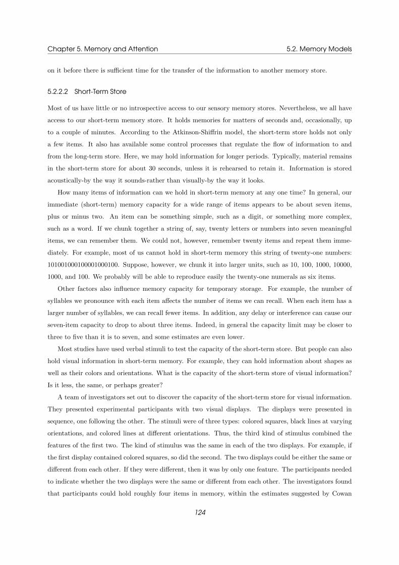
Chapter 5. Memory and Attention 5.2. Memory Models
on it before there is sufficient time for the transfer of the information to another memory store.
5.2.2.2 Short-Term Store
Most of us have little or no introspective access to our sensory memory stores. Nevertheless, we all have
access to our short-term memory store. It holds memories for matters of seconds and, occasionally, up
to a couple of minutes. According to the Atkinson-Shiffrin model, the short-term store holds not only
a few items. It also has available some control processes that regulate the flow of information to and
from the long-term store. Here, we may hold information for longer periods. Typically, material remains
in the short-term store for about 30 seconds, unless it is rehearsed to retain it. Information is stored
acoustically-by the way it sounds-rather than visually-by the way it looks.
How many items of information can we hold in short-term memory at any one time? In general, our
immediate (short-term) memory capacity for a wide range of items appears to be about seven items,
plus or minus two. An item can be something simple, such as a digit, or something more complex,
such as a word. If we chunk together a string of, say, twenty letters or numbers into seven meaningful
items, we can remember them. We could not, however, remember twenty items and repeat them imme-
diately. For example, most of us cannot hold in short-term memory this string of twenty-one numbers:
101001000100001000100. Suppose, however, we chunk it into larger units, such as 10, 100, 1000, 10000,
1000, and 100. We probably will be able to reproduce easily the twenty-one numerals as six items.
Other factors also influence memory capacity for temporary storage. For example, the number of
syllables we pronounce with each item affects the number of items we can recall. When each item has a
larger number of syllables, we can recall fewer items. In addition, any delay or interference can cause our
seven-item capacity to drop to about three items. Indeed, in general the capacity limit may be closer to
three to five than it is to seven, and some estimates are even lower.
Most studies have used verbal stimuli to test the capacity of the short-term store. But people can also
hold visual information in short-term memory. For example, they can hold information about shapes as
well as their colors and orientations. What is the capacity of the short-term store of visual information?
Is it less, the same, or perhaps greater?
A team of investigators set out to discover the capacity of the short-term store for visual information.
They presented experimental participants with two visual displays. The displays were presented in
sequence, one following the other. The stimuli were of three types: colored squares, black lines at varying
orientations, and colored lines at different orientations. Thus, the third kind of stimulus combined the
features of the first two. The kind of stimulus was the same in each of the two displays. For example, if
the first display contained colored squares, so did the second. The two displays could be either the same or
different from each other. If they were different, then it was by only one feature. The participants needed
to indicate whether the two displays were the same or different from each other. The investigators found
that participants could hold roughly four items in memory, within the estimates suggested by Cowan
124

Chapter 5. Memory and Attention 5.2. Memory Models
(2001). The results were the same whether just individual features were varied (i.e. colored squares;
black lines at varying orientation) or pairs of features (i.e. colored lines at different orientations). Thus,
storage seems to depend on numbers of objects rather than numbers of features.
This work contained a possible confound (i.e. other responsible factor that cannot be easily disen-
tangled from the supposed causal factor). In the stimuli with colored lines at different orientations, the
added feature was at the same spatial location as the original one. That is, color and orientation were
with respect to the same object in the same place in the display. A further study thus was done to
separate the effects of spatial location from number of objects. In this research, stimuli comprising boxes
and lines could he either at separate locations or at overlapping locations. The overlapping locations thus
separated the objects from the fixed locations. The research would thus enable one to determine whether
people can remember four objects, as suggested in the previous work, or four spatial locations. The
results were the same as in the earlier research. Participants still could remember four objects, regardless
of spatial locations. Thus, memory was for objects, not spatial locations.
5.2.2.3 Long-Term Store
We constantly use short-term memory throughout our daily activities. When most of us talk about
memory, however, we usually are talking about long-term memory. Here we keep memories that stay
with us over long periods, perhaps indefinitely. All of us rely heavily on our long-term memory. We hold
in it information we need to get us by in our day-to-day lives. Examples are what people’s names are,
where we keep things, how we schedule ourselves on different days, and so on. We also worry when we
fear that our long-term memory is not up to snuff.
How much information can we hold in long-term memory? How long does the information last? The
question of storage capacity can be disposed of quickly because the answer is simple. We do not know.
Nor do we know how we would find out. We can design experiments to tax the limits of short-term
memory. But we do not know how to test the limits of long-term memory and thereby find out its
capacity. Some theorists have suggested that the capacity of long-term memory is infinite, at least in
practical terms. It turns out that the question of how long information lasts in long-term memory is not
easily answerable. At present, we have no proof even that there is an absolute outer limit to how long
information can be stored.
What is stored in the brain? Wilder Penfield addressed this question while performing operations on
the brains of conscious patients afflicted with epilepsy. He used electrical stimulation of various parts of
the cerebral cortex to locate the origins of each patient’s problem. In fact, his work was instrumental in
plotting the motor and sensory areas of the cortex.
During the course of such stimulation, Penfield found that patients sometimes would appear to recall
memories from way back in their childhoods. These memories may not have been called to mind for
many, many years. (Note that the patients could be stimulated to recall episodes such as events from
125

Chapter 5. Memory and Attention 5.2. Memory Models
their childhood, not facts such as the names of U.S. presidents.) These data suggested to Penfield that
long-term memories may be permanent.
Some researchers have disputed Penfield’s interpretations. For example, they have noted the small
number of such reports in relation to the hundreds of patients on whom Penfield operated. In addition,
we cannot be certain that the patients actually were recalling these events. They may have been inventing
them. Other researchers, using empirical techniques on older participants, found contradictory evidence.
Some researchers tested participants’ memory for names and photographs of their high-school classmates.
Even after 25 years, there was little forgetting of some aspects of memory. Participants tended to recognize
names as belonging to classmates rather than to outsiders. Recognition memory for matching names to
graduation photos was quite high. As you might expect, recall of names showed a higher rate of forgetting.
The term permastore refers to the very longterm storage of information, such as knowledge of a foreign
language and of mathematics.
5.2.3 Levels-of-Processing
A radical departure from the three-stores model of memory is the levels-of-processing framework, which
postulates that memory does not comprise three or even any specific number of separate stores but rather
varies along a continuous dimension in terms of depth of encoding. In other words, there are theoretically
an infinite number of levels of processing (LOP) at which items can be encoded. There are no distinct
boundaries between one level and the next. The emphasis in this model is on processing as the key
to storage. The level at which information is stored will depend, in large part, on how it is encoded.
Moreover, the deeper the level of processing, the higher, in general, is the probability that an item may
be retrieved.
A set of experiments seemed to support the LOP view. Participants received a list of words. A
question preceded each word. Questions were varied to encourage three different levels of processing.
In progressive order of depth, they were physical, acoustic, and semantic. The results of the research
were clear. The deeper the level of processing encouraged by the question, the higher the level of recall
achieved. Words that were logically (e.g., taxonomically) connected (e.g., dog and animal) were recalled
more easily than were words that were concretely connected (e.g., dog and leg). At the same time,
concretely connected words were more easily recalled than were words that were unconnected.
126

Chapter 5. Memory and Attention 5.2. Memory Models
Figure 5.6: The levels of processing framework. Memories are rememberd better if they are processed deeper.
An even more powerful inducement to recall has been termed the self-reference effect. In the self-
reference effect, participants show very high levels of recall when asked to relate words meaningfully to
themselves, by determining whether the words describe them. Even the words that participants assess as
not describing themselves are recalled at high levels. This high recall is a result of considering whether the
words do or do not describe the participants. However, the highest levels of recall occur with words that
people consider self-descriptive. Similar self-reference effects have been found by many other researchers.
Some researchers suggest that the self-reference effect is distinctive, but others suggest that it is
explained easily in terms of the LOP framework or other ordinary armory processes. Specifically, each of
us has a very elaborate self-schema. This self-schema is an organized system of internal cues regarding
ourselves, our attributes, and our personal experiences. Thus, we can richly and elaborately encode’
information related to ourselves much more so than information about other topics. Also, we easily
can organize new information pertaining to ourselves. When other information is also readily organized,
we may recall nonself-referent information easily as well. Finally, when we generate our own cues, we
demonstrate much higher levels of recall than when someone else generates cues for us to use.
Despite much supporting evidence, the LOP framework as a whole has its critics. For one thing,
some researchers suggest that the particular levels may involve a circular definition. On this view, the
levels are defined as deeper because the information is retained better. But the information is viewed as
being retained better because the levels are deeper. In addition, some researchers noted some paradoxes
in retention. For example, under some circumstances, strategies that use rhymes have produced better
retention than those using just semantic rehearsal. For example, focusing on superficial sounds and nor
underlying meanings can result in better retention than focusing on repetition of underlying meanings.
Specifically, consider what happens when the context for retrieval involves attention to phonological
(acoustic) properties of words (e.g., rhymes). Here, performance is enhanced when the context for en-
coding involves rehearsal based on phonological properties, rather than on semantic properties of words.
127

Chapter 5. Memory and Attention 5.2. Memory Models
Nonetheless, consider what happened when semantic retrieval, based on semantic encoding, was com-
pared with acoustic (rhyme) retrieval, based on rhyme encoding. Performance was greater for semantic
retrieval than for acoustic retrieval.
In light of these criticisms and some contrary findings, the LOP model has been revised. The sequence
of the levels of encoding may not be as important as the match between the type of elaboration of the
encoding and the type of task required for retrieval. Furthermore, there appear to be two kinds of
strategies for elaborating the encoding. The first is within-item elaboration. It elaborates encoding of
the particular item (e.g., a word or other fact) in terms of its characteristics, including the various levels
of processing. The second kind of strategy is between-item elaboration. It elaborates encoding by relating
each item’s features (again, at various levels) to the features of items already in memory. Thus, suppose
you wanted to be sure to remember something in particular. You could elaborate it at various levels for
each of the two strategies.
5.2.4 An integrative model: Working Memory
The working-memory model is probably the most widely used and accepted today. Psychologists who use
it view short-term and long-term memory from a different perspective. The key feature of the alternative
view is the role of working memory. Working memory holds only the most recently activated portion
of long-term memory, and it moves these activated elements into and out of brief, temporary memory
storage. Since Richard Atkinson and Richard Shiffrin first proposed their three-stores model of memory
(which may be considered a traditional view of memory), various other models have been suggested.
Alan Baddeley has suggested an integrative model of memory. It synthesizes the working-memory
model with the LOP framework. Essentially, he views the LOP framework as an extension of, rather
than as a replacement for, the working-memory model.
Baddeley originally suggested that working memory comprises four elements. The first is a visuospatial
sketchpad, which briefly holds some visual images. The second is a phonological loop, which briefly holds
inner speech for verbal comprehension and for acoustic rehearsal. Two components of this loop are critical.
One is phonological storage, which holds information in memory. The other is subvocal rehearsal, which
is used to put the information into memory in the first place. Without this loop, acoustic information
decays after about 2 seconds. The third element is a central executive, which both coordinates attentional
activities and governs responses. The central executive is critical to working memory because it is the
gating mechanism that decides what information to process further and how to process it. It decides
what resources to allocate to memory and related tasks, and how to allocate them. It is also involved in
higher order reasoning and comprehension, and is central to human intelligence. The fourth element is a
number of other “subsidiary slave systems” that perform other cognitive or perceptual tasks. Recently,
another component has been added to working memory. This is the episodic buffer. The episodic buffer
is a limited-capacity system that is capable of binding information from the subsidiary systems and from
128

Chapter 5. Memory and Attention 5.2. Memory Models
long-term memory into a unitary episodic representation. This component integrates information from
different parts of working memory so that they make sense to us.
Figure 5.7: Baddeley’s working memory model. On the right are the associated regions in the brain.
Neuropsychological methods, and especially brain imaging, can be very helpful in understanding the
nature of memory. Support for a distinction between working memory and longterm memory comes
from neuropsychological research. Neuropsychological studies have shown abundant evidence of a brief
memory buffer. The buffer is used for remembering information temporarily. It is distinct from long-
term memory, which is used for remembering information for long periods. Furthermore, through some
promising new research using positron emission tomography (PET) techniques, investigators have found
evidence for distinct brain areas involved in the different aspects of working memory. The phonological
loop, maintaining speech-related information, appears to involve bilateral activation of the frontal and
parietal lobes. It is interesting that the visuospatial sketchpad appears to activate slightly different areas.
Which ones it activates depends on the length of the retention interval. Shorter intervals activate areas
of the occipital and right frontal lobes. Longer intervals activate areas of the parietal and left frontal
lobes. Finally, the central executive functions appear to involve activation mostly in the frontal lobes.
Whereas the three-stores view emphasizes the structural receptacles for stored information, the
working-memory model underscores the functions of working memory in governing the processes of
memory. These processes include encoding and integrating information. Examples are integrating acous-
tic and visual information through cross-modality, organizing information into meaningful chunks, and
linking new information to existing forms of knowledge representation in long-term memory. We can
conceptualize the differing emphases with contrasting metaphors. For example, we can compare the
three-stores view to a warehouse, in which information is passively stored. The sensory store serves as
the loading dock. The short-term store comprises the area surrounding the loading dock. Here, informa-
tion is stored temporarily until it is moved to or from the correct location in the warehouse. A metaphor
129

Chapter 5. Memory and Attention 5.2. Memory Models
for the working-memory model might be a multimedia production house. It continuously generates and
manipulates images and sounds. It also coordinates the integration of sights and sounds into meaning-
ful arrangements. Once images, sounds, and other information are stored, they still are available for
reformatting and reintegration in novel ways, as new demands and new information become available.
Different aspects of working memory are represented in the brain differently.
5.2.5 Multiple Memory Systems
The working-memory model is consistent with the notion that multiple systems may be involved in the
storage and retrieval of information. Recall that when Wilder Penfield electrically stimulated the brains
of his patients, the patients often asserted that they vividly recalled particular episodes and events.
They did not, however, recall semantic facts that were unrelated to any particular event. These findings
suggest that there may be at least two separate memory systems. One would be for organizing and storing
information with a distinctive time referent. It would address questions such as, “What did you eat for
lunch yesterday?” or “Who was the first person you saw this morning?” The second system would be for
information that has no particular time referent. It would address questions such as, “Who were the two
psychologists who first proposed the three-stores model of memory?” and “What is a mnemonist?”.
Based on such findings, Endel Tulving (1972) proposed a distinction between two kinds of memory.
Semantic memory stores general world knowledge. It is our memory for facts that are not unique to
us and that are not recalled in any particular temporal context. Episodic memory stores personally
experienced events or episodes. According to Tulving, we use episodic memory when we learn lists of
words or when we need to recall something that occurred to us at a particular time or in a particular
context. For example, suppose I needed to remember that I saw Harrison Hardimanowitz in the dentist’s
office yesterday. I would be drawing on an episodic memory. But if I needed to remember the name of
the person I now see in the waiting room (“Harrison Hardimanowitz”), I would be drawing on a semantic
memory. There is no particular time tag associated with the name of that individual as being Harrison.
But there is a time tag associated with my having seen him at the dentist’s office yesterday.
Tulving and others provide support for the distinction between semantic and episodic memory. It
is based on both cognitive research and neurological investigation. The neurological investigations have
involved electrical-stimulation studies, studies of patients with memory disorders, and cerebral blood flow
studies. For example, lesions in the frontal lobe appear to affect recollection regarding when a stimulus was
presented. But they do not affect recall or recognition memory that a particular stimulus was presented.
It is not clear that semantic and episodic memories are two distinct systems. Nevertheless, they sometimes
appear to function in different ways. Many cognitive psychologists question this distinction. They point
to blurry areas on the boundary between these two types of memory. They also note methodological
problems with some of the supportive evidence. Perhaps episodic memory is merely a specialized form
of semantic memory. The question is open.
130

Chapter 5. Memory and Attention 5.2. Memory Models
A third discrete memory system is procedural memory, or memory for procedural knowledge. The
cerebellum of the brain seems to be centrally involved in this type of memory. The neuropsychological
and cognitive evidence supporting a discrete procedural memory has been quite well documented. An
alternative taxonomy of memory is shown in Figure ?? below. It distinguishes declarative (explicit)
memory from various kinds of nondeclarative (implicit) memory. Nondeclarative memory comprises pro-
cedural memory, priming effects, simple classical conditioning, habituation, sensitization, and perceptual
aftereffects. In yet another view, there are five memory systems in all: episodic, semantic, perceptual
(i.e., recognizing things on the basis of their form and structure), procedural, and working.
Figure 5.8: Multiple Memory Systems model.
5.2.6 Amnesia
Several different syndromes are associated with memory loss. The most well known is amnesia. Amnesia
is severe loss of explicit memory. One type is retrograde amnesia, in which individuals lose their
purposeful memory for events prior to whatever trauma induces memory loss. Mild forms of retrograde
amnesia can occur fairly commonly when someone sustains a concussion. Usually, events immediately
prior to the concussive episode are not well remembered.
W. Ritchie Russell and P. W. Nathan (1946) reported a more severe case of retrograde amnesia. A
22-year-old greenkeeper was thrown from his motorcycle in August 1933. A week after the accident, the
young man was able to converse sensibly. He seemed to have recovered. However, it quickly became
apparent that he had suffered a severe loss of memory for events that had occurred prior to the trauma.
On questioning, he gave the date as February 1922. He believed himself to be a schoolboy. He had no
recollection of the intervening years. Over the next several weeks, his memory for past events gradually
returned. The return started with the least recent and proceeded toward more recent events. By 10
weeks after the accident, he had recovered his memory for most of the events of the previous years. He
finally was able to recall everything that had happened up to a few minutes prior to the accident. In
retrograde amnesia, the memories that return typically do so starting from the more distant past. They
then progressively return up to the time of the trauma, Often events right before the trauma are never
recalled.
One of the most famous cases of amnesia is the case of H. M.. H. M. underwent brain surgery to save
him from continual disruptions due to uncontrollable epilepsy. The operation took place on September 1,
131

Chapter 5. Memory and Attention 5.3. Memory Processes
1953. It was largely experimental. The results were highly unpredictable. At the time of the operation,
H. M. was 29 years old. He was above average in intelligence. After the operation, his recovery was
uneventful with one exception. He suffered severe anterograde amnesia, the inability to remember
events that occur after a traumatic event. However, he had good (although not perfect) recollection of
events that had occurred before his operation. H. M.’s memory has severely affected his life. On one
occasion, he remarked, “Every day is alone in itself, whatever enjoyment I’ve had, and whatever sorrow
I’ve had”. Apparently, H. M. lost his ability purposefully to recollect any new memories of the time
following his operation. As a result, he lived suspended in an eternal present.
5.3 Memory Processes
The procedure is actually quite simple. First you arrange items into different groups. Of
course one pile may be sufficient depending on how much there is to do. If you have to go
somewhere else due to lack of facilities that is the next step; otherwise, you are pretty well set.
It is important not to overdo things. That is, it is better to do too few things at once than
too many. In the short run this may not seem important but complications can easily arise.
A mistake can be expensive as well. At first, the whole procedure will seem complicated.
Soon, however, it will become just another facet of life. It is difficult to foresee any end to
the necessity for this task in the immediate future, but then, one can never tell. After the
procedure is completed one arranges the materials into different groups again. Then they can
be put into their appropriate places. Eventually they will be used once more and the whole
cycle will then have to be repeated. However, that is part of life.
John Bransford and Marcia Johnson asked their participants to read the preceding passage and to
recall the steps involved. To get an idea of how easy it was for their participants to do so, try to recall
those steps now yourself. Bransford and Johnson’s participants (and probably you too) had a great
deal of difficulty understanding this passage and recalling the steps involved. What makes this task so
difficult? What are the mental processes involved in this task?
As mentioned in the previous section, cognitive psychologists generally refer to the main processes of
memory as comprising three common operations: encoding, storage, and retrieval. Each one represents
a stage in memory processing. Encoding refers to how you transform a physical, sensory input into
a kind of representation that can be placed into memory. Storage refers to how you retain encoded
information in memory. Retrieval refers to how you gain access to information stored in memory. Our
emphasis in discussing these processes will be on recall of verbal and pictorial material. Remember,
however, that we have memories of other kinds of stimuli as well, such as odors.
Encoding, storage, and retrieval often are viewed as sequential stages. You first take in information.
Then you hold it for a while. Later you pull it out. However, the processes interact with each other and
132

Chapter 5. Memory and Attention 5.3. Memory Processes
are interdependent. For example, you may have found the text in the chapter-opening paragraph difficult
to encode, thereby also making it hard to store and to retrieve the information. However, a verbal label
can facilitate encoding and hence storage and retrieval. Most people do much better with the passage if
given its title, “Washing Clothes.” Try now to recall the steps described in the passage. The verbal label
helps us to encode, and therefore to remember, a pas-sage that otherwise seems incomprehensible.
5.3.1 Encoding and Transfer of Information
5.3.1.1 Short-term Storage
When you encode information for temporary storage and use, what kind of code do you use? Participants
were visually presented with several series of six letters at the rate of 0.75 seconds per letter. The letters
used in the various lists were B, C, F, M, N, P, S, T, V, and X. Immediately after the letters were
presented, participants had to write down each list of six letters in the order given. What kinds of errors
did participants make? Despite the fact that letters were presented visually, errors tended to be based
on acoustic confusability. In other words, instead of recalling the letters they were supposed to recall,
participants substituted letters that sounded like the correct letters. Thus, they were likely to confuse F
for S, B for V, P for B, and so on. Another group of participants simply listened to single letters in a
setting that had noise in the background. They then immediately reported each letter as they heard it.
Participants showed the same pattern of confusability in the listening task as in the visual memory task.
Thus, we seem to encode visually presented letters by how they sound, not by how they look.
The Conrad experiment shows the importance in short-term memory of an acoustic code rather than
a visual code. But the results do not rule out the possibility that there are other codes. One such code
would be a semantic code - one based on word meaning. One researcher argued that short-term memory
relies primarily on an acoustic rather than a semantic code. He compared recall performance for lists of
acoustically confusable words - such as map, cab, mad, man, and cap - with that for lists of acoustically
distinct words - such as cow, pit, day, rig, and bun. He found that performance was much worse for the
visual presentation of acoustically similar words.
He also compared performance for lists of semantically similar words - such as big, long, large, wide,
and broad - with performance for lists of semantically dissimilar words - such as old, foul, late, hot,
and strong. There was little difference in recall between the two lists. Suppose performance for the
semantically similar words had been much worse. It would have indicated that participants were confused
by the semantic similarities and hence were processing the words semantically. However, performance for
the semantically similar words was only slightly worse than that for the semantically dissimilar words.
Subsequent work investigating how information is encoded in short-term memory has shown clear
evidence of at least some semantic encoding in short-term memory. Thus, encoding in short-term memory
appears to be primarily acoustic. But there may be some secondary semantic encoding as well. In
133

Chapter 5. Memory and Attention 5.3. Memory Processes
addition, we sometimes temporarily encode information visually as well. But visual encoding appears to
be even more fleeting (about 1.5 seconds). It also is more vulnerable to decay than acoustic encoding.
Thus, initial encoding is primarily acoustic in nature. But other forms of encoding may be used under
some circumstances.
5.3.1.2 Long-Term Storage
As mentioned, information stored temporarily in working memory is encoded primarily in acoustic form.
Hence, when we make errors in retrieving words from short-term memory, the errors tend to reflect
confusions in sound. How is information encoded into a form that can be transferred into storage and
available for subsequent retrieval?
Most information stored in long-term memory seems to be primarily semantically encoded. In other
words, it is encoded by the meanings of words. Consider some relevant evidence.
Participants learned a list of 41 different words. Five minutes after learning took place, participants
were given a recognition test. Included in the recognition test were distracters. These are items that
appear to be legitimate choices but that are not correct alternatives. That is, they were not presented
previously. Nine of the distracters were semantically related to words on the list. Nine were not. The data
of interest were false alarms to the distracters. These are responses in which the participants indicated
that they had seen the distracters, although they had not. Participants falsely recognized an average of
1.83 of the synonyms but only an average of 1.05 of the unrelated words. This result indicated a greater
likelihood of semantic confusion.
Another way to show semantic encoding is to use sets of semantically related test words, rather than
distracters. Participants learn a list of 60 words that included 15 animals, 15 professions, 15 vegetables,
and 15 names of people. The words were presented in random order. Thus, members of the various
categories were intermixed thoroughly. After participants heard the words, they were asked to free-recall
the list in any order they wished. The investigator then analyzed the order of output of the recalled
words. Did participants recall successive words from the same category more frequently than would be
expected by chance? Indeed, successive recalls from the same category did occur much more often than
would be expected by chance occurrence. Participants were remembering words by clustering them into
categories.
Encoding of information in long-term memory is not exclusively semantic. There also is evidence
for visual encoding. Participants received 16 drawings of objects, including four items of clothing, four
animals, four vehicles, and four items of furniture. The investigator manipulated not only the semantic
category but also the visual category. The drawings differed in visual orientation. Four were angled to
the left, four angled to the right, four horizontal, and four vertical. Items were pre-sented in random
order. Participants were asked to recall them freely. The order of participants responses showed effects
of both semantic and visual categories. These results suggested that participants were encoding visual
134

Chapter 5. Memory and Attention 5.3. Memory Processes
as well as semantic information.
In addition to semantic and visual information, acoustic information can be encoded in long-term
memory. Thus, there is considerable flexibility in the way we store information that we retain for long
periods. Those who seek to know the single correct way to encode information are seeking an answer
to the wrong question. There is not one correct way. A more useful question involves ask-ing, “In what
ways do we encode information in long-term memory?” From a more psychological perspective, however,
the most useful question to ask is, “When do we encode in which ways?” In other words, under what
circumstances do we use one form of encoding, and under what circumstances do we use another? These
questions are the focus of present and future research.
5.3.1.3 Transfer from STM to LTM
Given the problems of decay and interference, how do we move information from short-term memory
to long-term memory? The means of moving information depend on whether the information involves
declarative or nondeclarative memory. Some forms of nondeclarative memory are highly volatile and decay
quickly. Examples are priming and habituation. Other declarative forms are maintained more readily,
particularly as a result of repeated practice (of procedures) or repeated conditioning (of responses).
Examples are procedural memory and simple classical conditioning.
For entrance into long-term declarative memory, various processes are involved. One method of ac-
complishing this goal is by deliberately attending to information to comprehend it. Another is by making
connections or associations between the new information and what we already know and understand. We
make connections by integrating the new data into our existing schemas of stored information. Consol-
idation is this process of integrating new information into stored information. In humans, the process
of consolidating declarative information into memory can continue for many years after the initial exper-
ience.
The disruption of consolidation has been studied effectively in amnesics. Studies have particularly
examined people who have suffered brief forms of amnesia as a consequence of electroconvulsive therapy.
For these amnesics, the source of the trauma is clear. Confounding variables can be minimized. A patient
history before the trauma can be obtained, and follow-up testing and supervision after the trauma are
more likely to be available. A range of studies suggests that during the process of consolidation, our
memory is susceptible to disruption and distortion.
To preserve or enhance the integrity of memories during consolidation, we may use various meta-
memory strategies. Metamemory strategies involve reflecting on our own memory processes with a view
to improving our memory. Such strategies are especially important when we are transferring new in-
formation to long-term memory by rehearsing it. Metamemory strategies are just one component of
metacognition, our ability to think about and control our own processes of thought and ways of enhan-
cing our thinking.
135
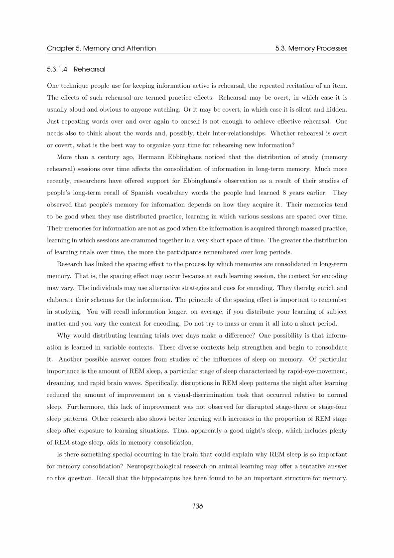
Chapter 5. Memory and Attention 5.3. Memory Processes
5.3.1.4 Rehearsal
One technique people use for keeping information active is rehearsal, the repeated recitation of an item.
The effects of such rehearsal are termed practice effects. Rehearsal may be overt, in which case it is
usually aloud and obvious to anyone watching. Or it may be covert, in which case it is silent and hidden.
Just repeating words over and over again to oneself is not enough to achieve effective rehearsal. One
needs also to think about the words and, possibly, their inter-relationships. Whether rehearsal is overt
or covert, what is the best way to organize your time for rehearsing new information?
More than a century ago, Hermann Ebbinghaus noticed that the distribution of study (memory
rehearsal) sessions over time affects the consolidation of information in long-term memory. Much more
recently, researchers have offered support for Ebbinghaus’s observation as a result of their studies of
people’s long-term recall of Spanish vocabulary words the people had learned 8 years earlier. They
observed that people’s memory for information depends on how they acquire it. Their memories tend
to be good when they use distributed practice, learning in which various sessions are spaced over time.
Their memories for information are not as good when the information is acquired through massed practice,
learning in which sessions are crammed together in a very short space of time. The greater the distribution
of learning trials over time, the more the participants remembered over long periods.
Research has linked the spacing effect to the process by which memories are consolidated in long-term
memory. That is, the spacing effect may occur because at each learning session, the context for encoding
may vary. The individuals may use alternative strategies and cues for encoding. They thereby enrich and
elaborate their schemas for the information. The principle of the spacing effect is important to remember
in studying. You will recall information longer, on average, if you distribute your learning of subject
matter and you vary the context for encoding. Do not try to mass or cram it all into a short period.
Why would distributing learning trials over days make a difference? One possibility is that inform-
ation is learned in variable contexts. These diverse contexts help strengthen and begin to consolidate
it. Another possible answer comes from studies of the influences of sleep on memory. Of particular
importance is the amount of REM sleep, a particular stage of sleep characterized by rapid-eye-movement,
dreaming, and rapid brain waves. Specifically, disruptions in REM sleep patterns the night after learning
reduced the amount of improvement on a visual-discrimination task that occurred relative to normal
sleep. Furthermore, this lack of improvement was not observed for disrupted stage-three or stage-four
sleep patterns. Other research also shows better learning with increases in the proportion of REM stage
sleep after exposure to learning situations. Thus, apparently a good night’s sleep, which includes plenty
of REM-stage sleep, aids in memory consolidation.
Is there something special occurring in the brain that could explain why REM sleep is so important
for memory consolidation? Neuropsychological research on animal learning may offer a tentative answer
to this question. Recall that the hippocampus has been found to be an important structure for memory.
136

Chapter 5. Memory and Attention 5.3. Memory Processes
In recording studies of rat hippocampal cells, researchers have found that cells of the hippocampus that
were activated during initial learning are reactivated during subsequent periods of sleep. It is as if they
are replaying the initial learning episode to achieve consolidation into long-term storage.
In a recent review, investigators have proposed that the hippocampus acts as a rapid learning system.
It temporarily maintains new experiences until they can be appropriately assimilated into the more
gradual neocortical representation system of the brain. Such a complementary system is necessary to allow
memory to represent more accurately the structure of the environment. McClelland and his colleagues
have used connectionist models of learning to show that integrating new experiences too rapidly leads
to disruptions in long-term memory systems. Thus, the benefits of distributed practice seem to occur
because we have a relatively rapid learning system in the hippocampus. It becomes activated during sleep.
Repeated exposure on subsequent days and repeated reactivation during subsequent periods of sleep help
learning. These rapidly learned memories become integrated into our more permanent long-term memory
system.
The spacing of practice sessions affects memory consolidation. However, the distribution of learning
trials within any given session does not seem to affect memory. According to the total-time hypothesis,
the amount of learning depends on the amount of time spent mindfully rehearsing the material. This
relation occurs more or less without regard to how that time is divided into trials in any one session. The
total-time hypothesis does not always hold, however. Moreover, the total-time hypothesis of rehearsal
has at least two apparent constraints. First, the full amount of time allotted for rehearsal actually must
be used for that purpose. Second, to achieve beneficial effects, the rehearsal should include various kinds
of elaboration or mnemonic devices that can enhance recall.
To move information into long-term memory, an individual most engage in elaborative rehearsal.
In elaborative rehearsal, the individual somehow elaborates the items to be remembered. Such rehearsal
makes the items either more meaningfully integrated into what the person already knows or more mean-
ingfully connected to one another and therefore more memorable. Consider, in contrast, maintenance
rehearsal. In maintenance rehearsal, the individual simply repetitiously rehearses the items to be re-
peated. Such rehearsal temporarily maintains information in short-term memory without transferring
the information to long-term memory. Without any kind of elaboration, the information cannot be
organized and transferred.
5.3.2 Forgetting and Memory Distortion
= Why do we so easily and so quickly forget phone numbers we have just looked up or the names of
people whom we have just met? Several theories have been proposed as to why we forget information
stored in working memory. The two most well-known theories are interference theory and decay theory.
Interference occurs when competing information causes us to forget something; decay occurs when simply
the passage of time causes us to forget.
137

Chapter 5. Memory and Attention 5.3. Memory Processes
5.3.2.1 Interference versus Decay Theory
Interference theory refers to the view that forgetting occurs because recall of certain words interferes with
recall of other words. Evidence for interference goes back many years. In one study, participants were
asked to recall trigrams (strings of three letters) at intervals of 3, 6, 9, 12, 15, or 18 seconds after the
presentation of the last letter. The investigator used only consonants, so that the trigrams would not be
easily pronounceable-for example, “K B E” Each participant was tested eight times at each of the six
delay intervals for a total of 48 trials. It was found that recall declined rapidly, because after the oral
presentation of each trigram, participants counted backward by threes from a three-digit number spoken
immediately after the trigram. The purpose of having the participants count backward was to prevent
them from rehearsing during the retention interval. This is the time between the presentation of the last
letter and the start of the recall phase of the experimental trial.
Clearly, the trigram is almost completely forgotten after just 18 seconds if participants are not allowed
to rehearse it. Moreover, such forgetting also occurs when words rather than letters are used as the stimuli
to be recalled. Thus, counting backward interfered with recall from short-term memory, supporting the
interference account of forgetting in short-term memory. At that time, it seemed surprising that counting
backward with numbers would interfere with the recall of letters. The previous view had been that verbal
information would interfere only with verbal (words) memory. Similarly, it was thought that quantitative
(numerical) information would interfere only with quantitative memory.
Although the foregoing discussion has construed interference as though it were a single construct,
at least two kinds of interference figure prominently in psychological theory and research: retroactive
interference and proactive interference. Retroactive interference (or retroactive inhibition) is caused by
activity occurring after we learn something but before we are asked to recall that thing. The interference
in the Brown-Peterson task appears to be retroactive, because counting backward by threes occurs after
learning of the trigram. It interferes with our ability to remember information we learned previously.
A second kind of interference is proactive interference (or proactive inhibition). Proactive interference
occurs when the interfering material occurs before, rather than after, learning of the to-be-remembered
material. Proactive as well as retroactive interference may play a role in short-term memory. Thus,
retroactive interference appears to be important but not the only factor.
If you are like most people, you will find that your recall of words is best for items at and near the
end of the list. Your recall will be second best for items near the beginning of the list, and poorest for
items in the middle of the list. A typical serial-position curve is shown in Figure ??.
138

Chapter 5. Memory and Attention 5.3. Memory Processes
Figure 5.9: A serial position curve
The recency effect refers to superior recall of words at and near the end of a list. The primacy effect
refers to superior recall of words at and near the beginning of a list. As Figure ?? shows, both the
recency effect and the primacy effect seem to influence recall. The serial-position curve makes sense in
terms of interference theory. Words at the end of the list are subject to proactive but not to retroactive
interference. Words at the beginning of the list are subject to retroactive but not to proactive interference.
And words in the middle of the list are subject to both types of interference. Hence, recall would be
expected to be poorest in the middle of the list. Indeed, it is poorest.
The amount of proactive interference generally climbs with increases in the length of time between
when the information is presented (and encoded) and when the information is retrieved. Also as you
might expect, proactive interference increases as the amount of prior - and potentially interfering - learning
increases. The effects of proactive interference appear to dominate under conditions in which recall is
delayed. But proactive and retroactive interference now are viewed as complementary phenomena. Yet
another theory for explaining how we forget information is decay theory.
Decay theory asserts that information is forgotten because of the gradual disappearance, rather than
displacement, of the memory trace. Thus, decay theory views the original piece of information as gradually
disappearing unless something is done to keep it intact. This view contrasts with interference theory, just
discussed, in which one or more pieces of information block recall of another.
Decay theory turns out to be exceedingly difficult to test. Why? First, under normal circumstances,
preventing participants from rehearsing is difficult. Through rehearsal, participants maintain the to-be-
remembered information in memory. Usually participants know that you are testing their memory. They
may try to rehearse the information or they may even inadvertently rehearse it to perform well during
139

Chapter 5. Memory and Attention 5.3. Memory Processes
testing. However, if you do prevent them from rehearsing, the possibility of interference arises. The task
you use to prevent rehearsal may interfere retroactively with the original memory.
For example, try not to think of white elephants as you read the next two pages. When instructed
not to think about them, you actually find it quite difficult not to. The difficulty persists even if you
try to follow the instructions. Unfortunately, as a test of decay theory, this experiment is itself a white
elephant, because preventing people from rehearsing is so difficult.
5.3.3 The Constructive Nature of Memory
An important lesson about memory is that memory retrieval is not just reconstructive, involving the use
of various strategies (e.g., searching for cues, drawing inferences) for retrieving the original memory traces
of our experiences and then rebuilding the original experiences as a basis for retrieval (see Kolodner, 1983,
for an artificial-intelligence model of reconstructive memory). Rather, in real-life situations, memory is
also constructive, in that prior experience affects how we recall things and what we actually recall from
memory. Recall the Bransford and Johnson (1972) study, cited at the opening of this section. In this
study participants could remember a passage about washing clothes quite well but only if they realized
that it was about washing clothes.
In a further demonstration of the constructive nature of memory, participants read an ambiguous
passage that could be interpreted meaningfully in two ways. Either it could be viewed as being either
about watching a peace march from the fortieth floor of a building or about a space trip to an inhabited
planet. Participants omitted different details, depending on what they thought the passage was about.
Consider, for example, a sentence mentioning that the atmosphere did not require the wearing of special
clothing. Participants were more likely to remember it when they thought the passage was about a
trip into outer space than when they thought it was about a peace march. Consider a comparable
demonstration in a different domain. Investigators showed participants 28 different droodles - nonsense
pictures that can be given various interpretations. Half of the participants in their experiment were
given an interpretation by which they could label what they saw. The other half did not receive an
interpretation prompting a label. Participants in the label group correctly reproduced almost 20% more
droodles than did participants in the control group.
5.3.3.1 Eyewitness Testimonies
A survey of U.S. prosecutors estimated that about 77,000 suspects are arrested each year after being
identified by eyewitnesses. Studies of more than 1,000 known wrongful convictions have pointed to errors
in eyewitness identification as being “the single largest factor leading to those false convictions”. What
proportion of eyewitness identifications are mistaken? The answer to that question varies widely (“from
as low as a few percent to greater than 90%”), but even the most conservative estimates of this proportion
140
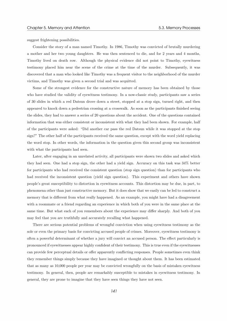
Chapter 5. Memory and Attention 5.3. Memory Processes
suggest frightening possibilities.
Consider the story of a man named Timothy. In 1986, Timothy was convicted of brutally murdering
a mother and her two young daughters. He was then sentenced to die, and for 2 years and 4 months,
Timothy lived on death row. Although the physical evidence did not point to Timothy, eyewitness
testimony placed him near the scene of the crime at the time of the murder. Subsequently, it was
discovered that a man who looked like Timothy was a frequent visitor to the neighborhood of the murder
victims, and Timothy was given a second trial and was acquitted.
Some of the strongest evidence for the constructive nature of memory has been obtained by those
who have studied the validity of eyewitness testimony. In a now-classic study, participants saw a series
of 30 slides in which a red Datsun drove down a street, stopped at a stop sign, turned right, and then
appeared to knock down a pedestrian crossing at a crosswalk. As soon as the participants finished seeing
the slides, they had to answer a series of 20 questions about the accident. One of the questions contained
information that was either consistent or inconsistent with what they had been shown. For example, half
of the participants were asked: “Did another car pass the red Datsun while it was stopped at the stop
sign?” The other half of the participants received the same question, except with the word yield replacing
the word stop. In other words, the information in the question given this second group was inconsistent
with what the participants had seen.
Later, after engaging in an unrelated activity, all participants were shown two slides and asked which
they had seen. One had a stop sign, the other had a yield sign. Accuracy on this task was 34% better
for participants who had received the consistent question (stop sign question) than for participants who
had received the inconsistent question (yield sign question). This experiment and others have shown
people’s great susceptibility to distortion in eyewitness accounts. This distortion may be due, in part, to
phenomena other than just constructive memory. But it does show that we easily can be led to construct a
memory that is different from what really happened. As an example, you might have had a disagreement
with a roommate or a friend regarding an experience in which both of you were in the same place at the
same time. But what each of you remembers about the experience may differ sharply. And both of you
may feel that you are truthfully and accurately recalling what happened.
There are serious potential problems of wrongful conviction when using eyewitness testimony as the
sole or even the primary basis for convicting accused people of crimes. Moreover, eyewitness testimony is
often a powerful determinant of whether a jury will convict an accused person. The effect particularly is
pronounced if eyewitnesses appear highly confident of their testimony. This is true even if the eyewitnesses
can provide few perceptual details or offer apparently conflicting responses. People sometimes even think
they remember things simply because they have imagined or thought about them. It has been estimated
that as many as 10,000 people per year may be convicted wrongfully on the basis of mistaken eyewitness
testimony. In general, then, people are remarkably susceptible to mistakes in eyewitness testimony. In
general, they are prone to imagine that they have seen things they have not seen.
141

Chapter 5. Memory and Attention 5.3. Memory Processes
Lineups can lead to faulty conclusions. Eyewitnesses assume that the perpetrator is in the lineup. This
is not always the case however. When the perpetrator of a staged crime was not in a lineup, participants
were susceptible to naming someone other than the perpetrator as the perpetrator. In this way, they can
recognize someone in the lineup as having committed the crime. The identities of the nonperpetrators in
the lineup also can affect judgments. In other words, whether a given person is identified as a perpetrator
can be influenced simply by who the others in the lineup are. So the choice of the “distracter” individuals
is important. Police may inadvertently affect the likelihood of whether identification occurs or not and
also whether a false identification is likely to occur.
Eyewitness identification is particularly weak when identifying people of a race other than the race of
the witness. Even infants seem to be influenced by postevent information when recalling an experience,
as shown through their behavior in operant-conditioning experiments.
Not everyone views eyewitness testimony with such skepticism. It is still not clear whether the
information about the original event actually is displaced by, or is simply competing with, the sub-
sequent misleading information. Some investigators have argued that psychologists need to know a great
deal more about the circumstances that impair eyewitness testimony before impugning such testimony
before a jury. At present, the verdict on eyewitness testimony is still not in. The same can be said for
repressed memories, considered in the next section.
5.3.3.2 Repressed Memories
Might you have been exposed to a traumatic event as a child but have been so traumatized by this
event that you now cannot remember it? Some psychotherapists have begun using hypnosis and related
techniques to elicit from people what are alleged to be repressed memories. Repressed memories are
memories that are alleged to have been pushed down into unconsciousness because of the distress they
cause. Such memories, according to the view of psychologists who believe in their existence, are very
inaccessible. But they can be dredged out.
Do repressed memories actually exist? Many psychologists strongly doubt their existence. Others are
at least highly skeptical. First, some therapists inadvertently may be planting ideas in their clients’ heads.
In this way, they may be creating false memories of events that never took place. Indeed, creating false
memories is relatively easy, even in people with no particular psychological problems. Such memories can
be implanted by using ordinary, nonemotional stimuli. Second, showing that implanted memories are
false is often extremely hard to do. Reported incidents often end up, as in the case of childhood sexual
abuse, merely pitting one person’s word against another. At the present time, no compelling evidence
points to the existence of such memories. But psychologists also have not reached the point where their
existence can be ruled out definitively. Therefore, no clear conclusion can be reached at this time.
142

Chapter 5. Memory and Attention 5.3. Memory Processes
5.3.4 Context Effects on Encoding and Retrieval
As studies of constructive memory show, our cognitive contexts for memory clearly influence our memory
processes of encoding, storing, and retrieving information. Studies of expertise also show how existing
schemas may provide a cognitive context for encoding, storing, and retrieving new information. Specific-
ally, experts generally have more elaborated schemas than do novices in regard to their areas of expertise.
These schemas provide a cognitive context in which the experts can operate. They relatively easily can
integrate and organize new information. They fill in gaps when provided with partial or even distorted
information and visualize concrete aspects of verbal information. They also can implement appropriate
metacognitive strategies for organizing and rehearsing new information. Clearly, expertise enhances our
confidence in our recollected memories.
Another factor that enhances our confidence in recall is the perceived clarity-the vividness and richness
of detail-of the experience and its context. When we are recalling a given experience, we often associate
the degree of perceptual detail and intensity with the degree to which we are accurately remembering the
experience. We feel greater confidence that our recollections are accurate when we perceive them with
greater richness of detail. Although this heuristic for reality monitoring is generally effective, there are
some situations in which factors other than accuracy of recall may lead to enhanced vividness and detail
of our recollections.
In particular, an oft-studied form of vivid memory is the flashbulb memory-a memory of an event so
powerful that the person remembers the event as vividly as if it were indelibly preserved on film. People
old enough to recall the assassination of President John Kennedy may have flashbulb memories of this
event. Some people also have flashbulb memories for the explosion of the space shuttle Challenger, the
destruction of the World Trade Center on 9/11, or momentous events in their personal lives. The emo-
tional intensity of an experience may enhance the likelihood that we will recall the particular experience
(over other experiences) ardently and perhaps accurately. A related view is that a memory is most likely
to become a flashbulb memory under three circumstances. These are that the memory trace is important
to the individual, is surprising, and has an emotional effect on the individual.
Some investigators suggest that flashbulb memories may be more vividly recalled because of their
emotional intensity. Other investigators, however, suggest that the vividness of recall may be the result
of the effects of rehearsal. The idea here is that we frequently retell, or at least silently contemplate, our
experiences of these momentous events. Perhaps our retelling also enhances the perceptual intensity of
our recall. Other findings suggest that flashbulb memories may be perceptually rich. On this view, they
may be recalled with relatively greater confidence in the accuracy of the memories but not actually he
any more reliable or accurate than any other recollected memory. Suppose flashbulb memories are indeed
more likely to be the subject of conversation or even silent reflection. Then perhaps, at each retelling of
the experience, we reorganize and construct our memories such that the accuracy of our recall actually
143

Chapter 5. Memory and Attention 5.3. Memory Processes
diminishes while the perceived vividness of recall increases over time. At present, researchers heatedly
debate whether studies of such memories as a special process are a flash in the pan or a flash of insight
into memory processes. The emotional intensity of a memorable event is not the only way in which
emotions, moods, and states of consciousness affect memory. Our moods and states of consciousness also
may provide a context for encoding that affects later retrieval of semantic memories. Thus, when we
encode semantic information during a particular mood or state of consciousness, we may more readily
retrieve that information when in the same state again something that is encoded when we are influenced
by alcohol or other drugs may be retrieved more readily while under those same influences again. On the
whole, however, the “main effect” of alcohol and many drugs is stronger than the interaction. In other
words, the depressing effect of alcohol and many drugs on memory is greater than the facilitating effect
of recalling something in the same drugged state as when one encoded it.
In regard to mood, some investigators have suggested a factor that may maintain depression. In
particular, the depressed person can more readily retrieve memories of previous sad experiences, which
may further the continuation of the depression. If psychologists or others can intervene to prevent
the continuation of this vicious cycle, the person may begin to feel happier. As a result, other happy
memories may be more easily retrieved, thus further relieving the depression, and so on. Perhaps the folk-
wisdom advice to “think happy thoughts” is not entirely unfounded. In fact, under laboratory conditions,
participants seem more accurately to recall items that have pleasant associations than they recall items
that have unpleasant associations.
Emotions, moods, states of consciousness, schemas, and other features of our internal context clearly
affect memory retrieval. In addition, even our external contexts may affect our ability to recall inform-
ation. We appear to be better able to recall information when we are in the same physical context as
the one in which we learned the material. In one experiment, 16 underwater divers were asked to learn
a list of 40 unrelated words. Learning occurred either while the divers were on shore or while they were
20 feet beneath the sea. Later, they were asked to recall the words when either in the same environment
as where they had learned them or in the other environment. Recall was better when it occurred in the
same place as did the learning.
All of the preceding context effects may he viewed as an interaction between the context for encoding
and the context for retrieval of encoded information. The results of various experiments on retrieval
suggest that how items are encoded has a strong effect both on how and on how well items are retrieved.
This relationship is called encoding specificity-what is recalled depends on what is encoded. Consider a
rather dramatic example of encoding specificity. We know that recognition memory is virtually always
better than recall. For example, generally recognizing a word that you have learned is easier than recalling
it. After all, in recognition you have only to say whether you have seen the word. In recall, you only
have to generate the word and then mentally confirm whether it appeared on the list.
In one experiment, Watkins and Tulving (1975) had participants learn a list of 24 paired associates,
144

Chapter 5. Memory and Attention 5.3. Memory Processes
such as ground-cold and crust-cake. Participants were instructed to learn to associate each response
(such as cold) with its stimulus word (such as ground). After participants had studied the word pairs,
they were given an irrelevant task. Then they were given a recognition test with distracters. Participants
were asked simply to circle the words they had seen previously. Participants recognized an average of
60% of the words from the list. Then, participants were provided with the 24 stimulus words. They were
asked to recall the responses. Their cued recall was 73%. Thus, recall was better than recognition. Why?
According to the encoding-specificity hypothesis, the stimulus was a better cue for the word than the
word itself. The reason was that the words had been learned as paired associates.
To summarize, retrieval interacts strongly with encoding. Suppose you are studying for a test and
want to recall well at the time of testing. Organize the information you are studying in a way that
appropriately matches the way in which you will be expected to recall it. Similarly, you will recall
information better if the level of processing for encoding matches the level of processing for retrieval .
145
Related Documents

![[XLS] · Web view1 1 1 2 3 1 1 2 2 1 1 1 1 1 1 2 1 1 1 1 1 1 2 1 1 1 1 2 2 3 5 1 1 1 1 34 1 1 1 1 1 1 1 1 1 1 240 2 1 1 1 1 1 2 1 3 1 1 2 1 2 5 1 1 1 1 8 1 1 2 1 1 1 1 2 2 1 1 1 1](https://static.cupdf.com/doc/110x72/5ad1d2817f8b9a05208bfb6d/xls-view1-1-1-2-3-1-1-2-2-1-1-1-1-1-1-2-1-1-1-1-1-1-2-1-1-1-1-2-2-3-5-1-1-1-1.jpg)


![CkvtIm¬...5 bqWnäv 1 apJh- pc- , kn²m´w, kµÀ`w]mTw 1 kzmKXw & apJhp- c X¯z§fpw aqey-§fpw tImgvknsâ hnim-e-amb Dt±i§Ä tImgvkv Askkvsaâv]mTw 2 Kpcp X¯zhpw ]c¼-- cbpw](https://static.cupdf.com/doc/110x72/5e98c35f4ffbeb387558379a/ckvtim-5-bqwnv-1-apjh-pc-knmw-kwmtw-1-kzmkxw-apjhp-.jpg)