Kording On Choice Of Sparse Prior 2003

On the choice of a sparse prior Konrad P. Körding, Christoph Kayser & Peter König

Institute of Neuroinformatics, University and ETH Zürich, Winterthurerstr. 190, 8057

Zürich, Switzerland, email: {koerding, kayser, peterk}@ini.phys.ethz.ch

Correspondence should be addressed to K.P.K ([email protected])

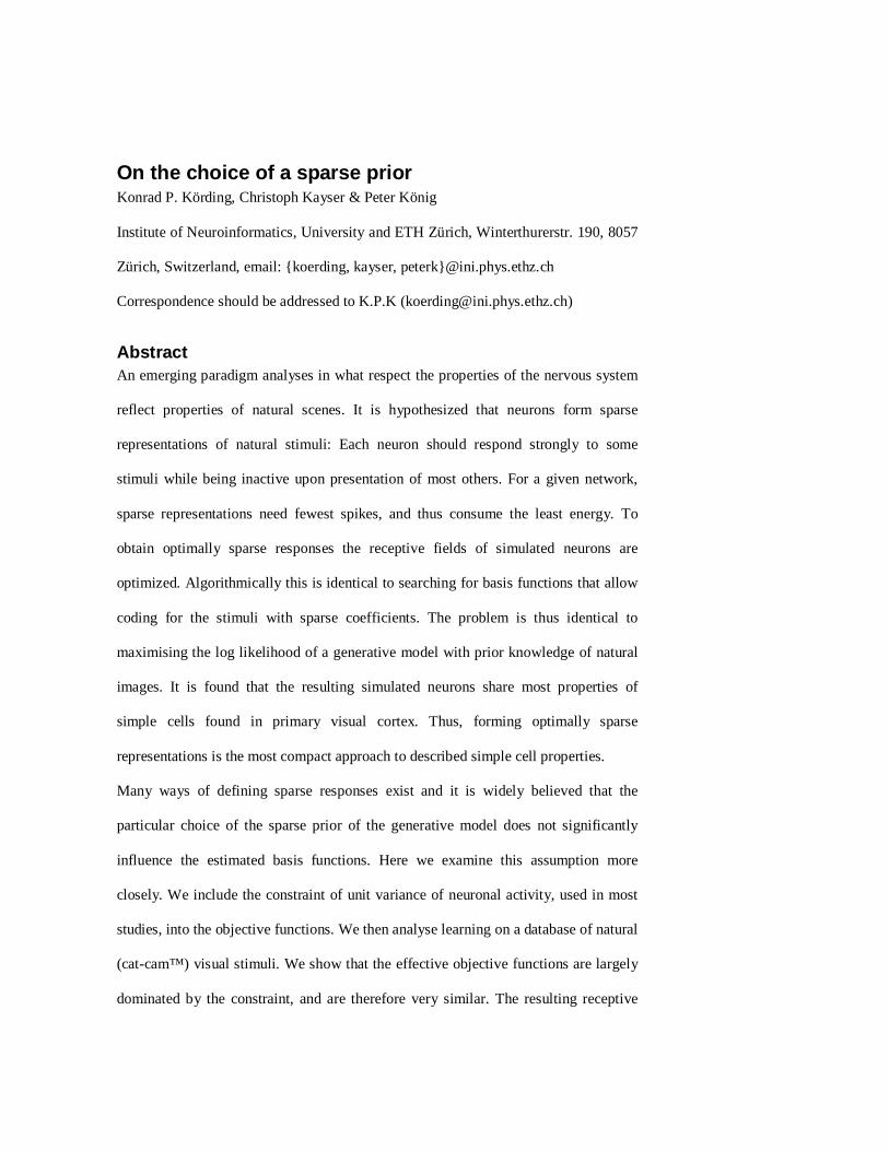
Abstract An emerging paradigm analyses in what respect the properties of the nervous system

reflect properties of natural scenes. It is hypothesized that neurons form sparse

representations of natural stimuli: Each neuron should respond strongly to some

stimuli while being inactive upon presentation of most others. For a given network,

sparse representations need fewest spikes, and thus consume the least energy. To

obtain optimally sparse responses the receptive fields of simulated neurons are

optimized. Algorithmically this is identical to searching for basis functions that allow

coding for the stimuli with sparse coefficients. The problem is thus identical to

maximising the log likelihood of a generative model with prior knowledge of natural

images. It is found that the resulting simulated neurons share most properties of

simple cells found in primary visual cortex. Thus, forming optimally sparse

representations is the most compact approach to described simple cell properties.

Many ways of defining sparse responses exist and it is widely believed that the

particular choice of the sparse prior of the generative model does not significantly

influence the estimated basis functions. Here we examine this assumption more

closely. We include the constraint of unit variance of neuronal activity, used in most

studies, into the objective functions. We then analyse learning on a database of natural

(cat-cam™) visual stimuli. We show that the effective objective functions are largely

dominated by the constraint, and are therefore very similar. The resulting receptive

fields show some similarities but also qualitative differences. Even in the region

where the objective functions are dissimilar, the distributions of coefficients are

similar and do not match the priors of the assumed generative model. In conclusion,

the specific choice of the sparse prior is relevant, as is the choice of additional

constraints, such as normalization of variance.

Introduction It is important to analyze in what respect properties of sensory systems are matched to

the properties of natural stimuli (Barlow 1961). Many recent studies analyse

simulated neurons learning from natural scenes and compare their properties to the

properties of real neurons in the visual system (Atick 1992; Dong and Atick 1995;

Fyfe and Baddeley 1995; Bell 1996; Olshausen and Field 1996; Bell and Sejnowski

1997; Olshausen and Field 1997; Blais, Intrator et al. 1998; van Hateren and

Ruderman 1998; Van Hateren and van der Schaaf 1998; Hyvärinen and Hoyer 2000;

Lewicki and Sejnowski 2000; Kayser, Einhäuser et al. 2001; Olshausen 2001;

Simoncelli and Olshausen 2001; Einhäuser, Kayser et al. 2002). Most of these studies

follow the independent component analysis (ICA) paradigm: An explicit generative

model is assumed where hidden, nongaussian generators are linearly combined to

yield the image I(t) from the natural stimuli.

( ) ( )( , , ) ,j jj

I x y t a t x yφ=∑ . (1)

The coefficients are assumed to occasionally be nonzero but about zero most of the

time. This assumption is formulated probabilistically as ( )ip aand referred to as a

sparse prior is assumed for the coefficients ( )ia t . The log likelihood of the image

given the model is very expensive to compute and is therefore typically approximated

by an objective function Ψ . This objective Ψ is subsequently maximized using

standard optimisation algorithms. Frequently used options are scaled gradient descent,

conjugate gradient descent and even faster methods like the fastICA (Hyvärinen

1999) method. The properties of the optimized neurons are subsequently compared to

properties of real neurons in the visual system. It is found that these simulated

neurons share selectivity to orientation, spatial frequency, localisation and motion

with simple cells found in primary visual cortex. A number of further studies even

directly addresses sparse coding in experiments and shows that the brain is indeed

encoding stimuli sparsely (Baddeley, Abbott et al. 1997; Vinje and Gallant 2000;

Willmore and Tolhurst 2001). Thus, sparse coding offers an approach that leads to

simulated neurons with properties which compare well to those of real neurons.

An important property of the ICA paradigm was demonstrated in a seminal

contribution by Hyvärinen and Oja (1998). Given a known and finite number of

independent non-gaussian sources the resulting basis functions do not significantly

depend on the chosen nonlinear objective. Applied to the problems considered here

this would predict, that the specific definition of sparseness does not have any

influence on the resulting basis functions.

However, do natural stimuli match the assumptions of this theorem? Firstly a finite

number of generators in the real world is not obvious, and their number is definitely

not known. Secondly, the generators in the real world are combined nonlinearly for

obtaining the image. Occlusions, deformations and so forth make the generative

process non-linear, making it intractable to directly invert it. Thirdly objects in natural

scenes are not independent of each other, the real world is highly ordered and shows a

high degree of dependence. The real world situation is therefore often different to the

situation addressed in the paper of Hyvärinen and Oja (1998).

Nevertheless it is widely believed that the choice of the sparse objective does not

significantly influence the estimated basis functions. Here we examine this

assumption more closely. There are two factors that influence the objective to be

optimised. The first part captures how well the assumed sparse prior on the

coefficients is met. The second part captures how well the neurons collectively code

for the image, i.e. how well the image can be reconstructed from their activities. Here

we investigate the form of the combined effective objective functions. Furthermore,

we analyse the distribution of activities (coefficient values) and in how far they match

the specific priors. Finally, we compare the form of the basis functions obtained when

optimizing different objectives.

Methods

Relation of generative models to objective function approaches Here we relate probabilistic generative models of natural stimuli to the optimisation

scheme used throughout this paper.

Let I be the image, φ a set of variables describing the model and a(t) a set of

statistical variables, called coefficients, describing each image in terms of the model.

The probability of the image given the data is calculated as:

( )( ¦ ) ( ¦ , )p I p I a p a daφ φ= ∫ (2)

This integration however is typically infeasible. Olshausen and Field (1997) used the

idea of maximizing an upper bound of this probability: If the probability of the image

given φ and a is highly peaked at some maximal value we can rewrite (2) and

obtain:

( )max max( ¦ ) ( ¦ , )p I p I a p aφ φ≈ (3)

The log-likelihood is thus:

( )max maxlog ( ¦ ) log ( ¦ , ) logp I p I a p aφ φ≈ + (4)

If we assume Gaussian noise on the image the first term is proportional to the squared

reconstruction error. The second term contains the (sparse) prior on the distribution of

the generative model.

Typically the log likelihood of the data given the model is maximized. This leads to

an optimisation problem on the following class of objective functions:

prob square error priorΨ = Ψ + Ψ (5)

The latter term represents the a priori information about the coefficients a, the first

term measures deviations from the models stimulus reconstruction.

The process sketched above can often be inverted. If Ψ consists of the standard errorΨ ,

and priorΨ and is sufficiently peaked then we simply obtain ( )( ) error ap a eΨ= .

The reconstruction error term Here we simplify the minimum square error term so that different approaches can be

compared in a unified framework.

The reconstruction error is defined as

2

error j i ijj i

I aφ Ψ = − −

∑ ∑ (6)

Assuming unit variance of the input this can be simplified to:

( )( ),0, , ,

1 2error i i i j ki kji j i j k

a a a a φ φΨ = − − +∑ ∑ (7)

Where ,0ia = iIφ is the feedforward activity. If we furthermore assume whitened input

i j ijI I δ= and linear activities then we can further simplify the last term:

,0 ,0 ,0, ,

1 2error i i i j i ji j i j

a a a a a aΨ = − + −∑ ∑ (8)

The system is defined in a purely feedforward way since it does not directly depend

on the input. In a linear system where each unit has unit variance this simplifies, after

omitting constant terms, to:

( )22

, ,

,error i j i ji j i j

a a CC a aΨ ≈ − =∑ ∑ (9)

Here CC denotes the coefficient of covariation. Thus, if the system is linear,

decorrelating the outputs is equivalent to minimizing the reconstruction error.

This formalism also captures methods that constrain the a to be uncorrelated which is

identical to making the sparseness term small compared to the error term or having a

noise free model (Olshausen and Field 1996). While most models effectively share

the same square errorΨ there is a wide divergence for the sparseness

objective ( ) ( )( )logprior a p aΨ = .

Stimuli Out of the videos described in (Kayser, Einhäuser et al. 2001) 40.000 30 by 30

patches are extracted from random positions and convolved with a Gaussian Kernel of

standard deviation 15 pixels to minimize orientation artefacts. They are whitened to

avoid effects of the second and lower order statistics that are prone to noise

influences. Only the principal components 2 through 100 are used for learning since

they contain more than 95% of the overall variance. Component 1 was removed since

it contained the mean brightness.

The weights of the simulated neurons are randomly initialised with a uniform

distribution in the whitened principal component space. For computational efficieny

they are orthonormalized before starting the optimisation..

Decorrelation As argued above, the considered models should allow the correct reconstruction of the

image and thus minimize the squares of the coefficients of covariation CC between

pairs of coefficients of different basis functions. The standard deviation can

furthermore be biased to be 1. All optimisations are therefore done with the following

objective function added.

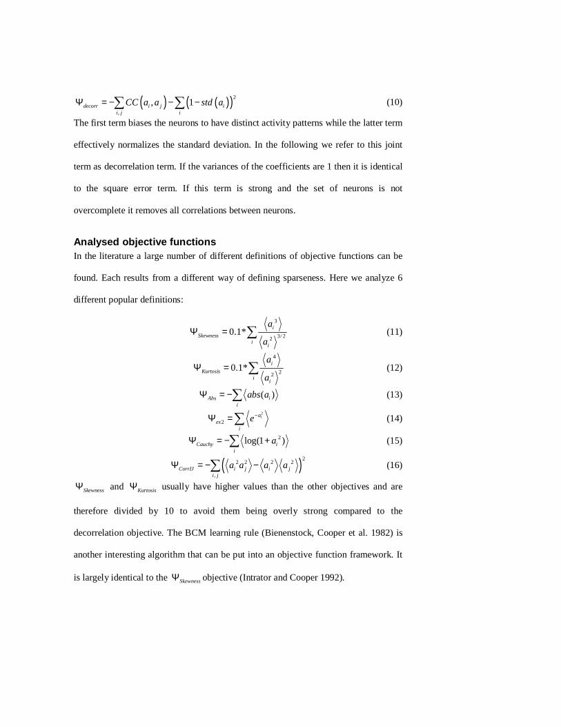
( ) ( )( )2

,

, 1decorr i j ii j i

CC a a std aΨ = − − −∑ ∑ (10)

The first term biases the neurons to have distinct activity patterns while the latter term

effectively normalizes the standard deviation. In the following we refer to this joint

term as decorrelation term. If the variances of the coefficients are 1 then it is identical

to the square error term. If this term is strong and the set of neurons is not

overcomplete it removes all correlations between neurons.

Analysed objective functions In the literature a large number of different definitions of objective functions can be

found. Each results from a different way of defining sparseness. Here we analyze 6

different popular definitions:

3

3/ 220.1*

i

Skewnessi

i

a

aΨ = ∑ (11)

4

220.1*

i

Kurtosisi

i

a

aΨ = ∑ (12)

( )Abs ii

abs aΨ = −∑ (13)

2

2ia

exi

e−Ψ =∑ (14)

2log(1 )Cauchy ii

aΨ = − +∑ (15)

( )22 2 2 2

,CorrIJ i j i j

i j

a a a aΨ = − −∑ (16)

SkewnessΨ and KurtosisΨ usually have higher values than the other objectives and are

therefore divided by 10 to avoid them being overly strong compared to the

decorrelation objective. The BCM learning rule (Bienenstock, Cooper et al. 1982) is

another interesting algorithm that can be put into an objective function framework. It

is largely identical to the SkewnessΨ objective (Intrator and Cooper 1992).

Optimization The optimisation algorithm uses the above objective functions and their derivatives

with respect to the weights. These derivatives are often complicated functions

containing a large number of terms. We found it very useful to verify these

numerically. The objective functions are maximised using 50 iterations of RPROP

(resilient backprop Riedmiller and Braun 1993) with 1.2η + = and .5η − = , starting at

a weightchange parameter of 0.01. We observe a significantly faster convergence of

the objective function compared to scaled gradient descent. It is interesting to note

that RPROP, where each synapse stores its weight and how fast it is supposed to

change, is a local learning algorithm that could be implemented by neural hardware.

Results

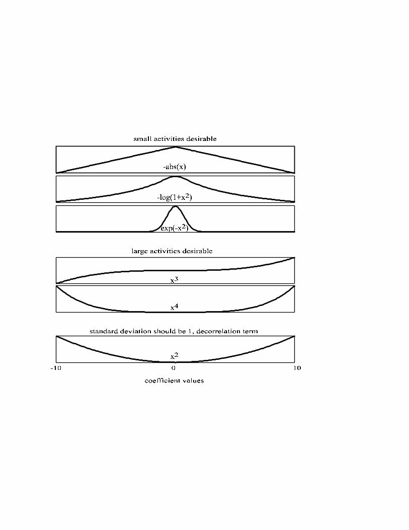
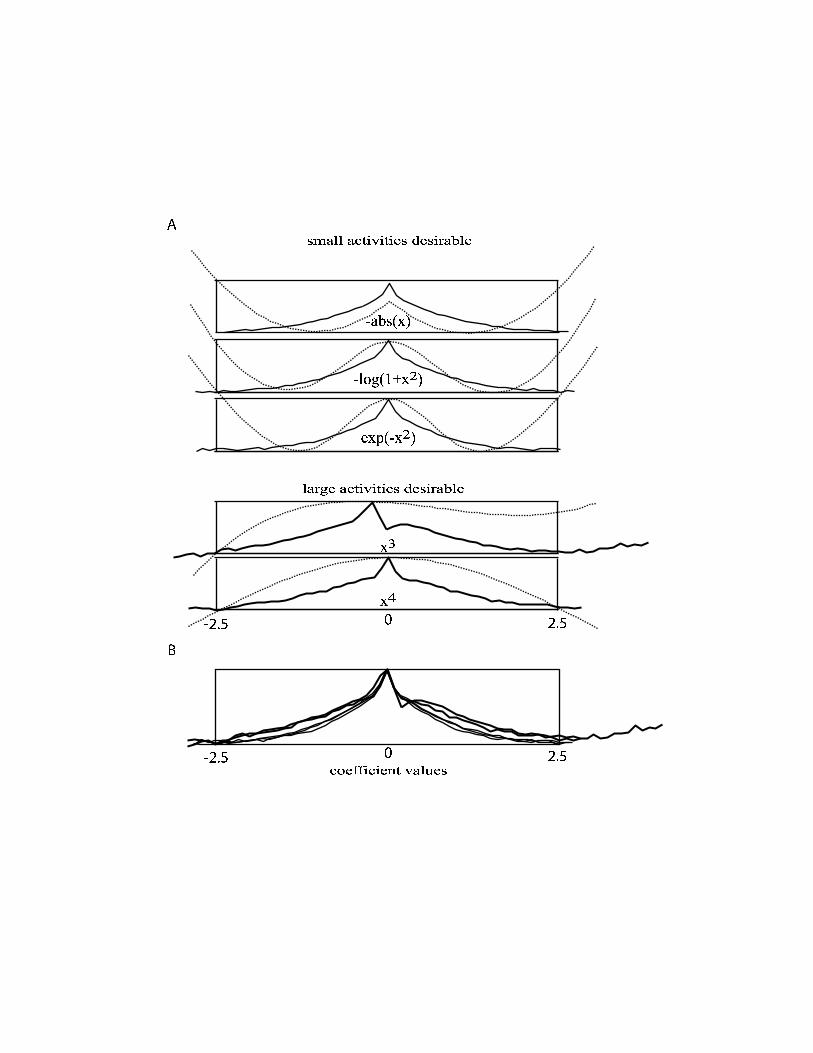
The effective priors Each of the analyzed objective functions is plotted in figure 1. They are divided into

two groups. AbsΨ , ( )2exp a−Ψ and CauchyΨ punish coefficients that differ from zero in a

graded manner. SkewnessΨ and KurtosisΨ to the contrary reward high coefficients. The

effective objective that is optimized by the system, however, consists of two terms.

The first term represents the sparseness objective as plotted in Figure 1. At first sight

it their wildly divergent properties could be expected to lead to differing basis

functions, and it is counterintuitive to assume that all these objectives lead to similar

basis functions. It however is necessary to take into account the term of the objective

function that biases the neurons to avoid correlations and to have unitary variance (see

methods). This term turns into a constraint when the neurons are directly required to

be uncorrelated. This term should therefore be including into the prior. Figure 2

shows the objective function measured after convergence. The decorrelation term

DecorrΨ has a strong influence on AbsΨ , the ( )2exp a−Ψ and the CauchyΨ objective

function. All these functions bias the coefficients to have small variance. The

decorrelation term ensures that the variance does not approach zero. The definition of

the decorrelation term results in a parabola shaped function that is added to the

original objective functions. The resulting objective functions are almost identical for

these three priors for higher coefficient values. After considering this effect they are

also very similar to KurtosisΨ and the values of SkewnessΨ for positive activities. All these

priors punish intermediate activities while preferring activities that are either small or

very large. The priors are very similar for high values and only differ for smaller

values.

The distribution of the coefficients We want to investigate in how far the optimisation process leads to a distribution of

coefficients which actually matches the log prior or the objective function. We

furthermore want to know if the different objective functions lead to different

distributions of coefficients.

Observing the histogram of the coefficients in response to the natural stimuli after

convergence reveals high peaks at zero for all objective functions. They are thus very

dissimilar to their priors. The coefficients a in response to different patches are not

independent from each other. If any of the basis functions is changed then all the

coefficients change. Since the number of coefficients is only a fraction of the number

of stimuli used, it is impossible for the distribution to perfectly follow the prior. We

will therefore consider the logarithm of the deviation of the distribution of coefficients

divided by the distribution of coefficients before learning:

( )( )

|log

|

i after learningi

reli start

i

p ad

p a

φ

φ=

∑∑

. (17)

We cannot directly measure p and thus instead use the number of observations

divided by the number of overall stimuli. Using the relative distribution instead of the

original distribution automatically corrects for the distribution of contrasts in the

natural scenes. It thus converts the highly peaked distribution of coefficients into a

rather flat function. Before learning the basis functions are random and the

distribution of the coefficients therefore is identical to the distribution of contrast in

natural scenes. By dividing by the distribution before learning we correct for these

effects. Similar behaviour could be achieved using nonlinear neurons that feature

lateral divisive inhibition as in (Schwartz and Simoncelli 2001). Figure 3 shows that

the relative distribution for large coefficients is well fit by the prior. It is interesting to

note that the prior for larger coefficients is the decorrelation term that is not directly

visible in most papers addressing sparse coding.

To analyze the differences between the different priors, we are interested in the range

of small coefficients where the specific type of the prior matters most. Figure 4a

shows that the relative distributions in this region cannot be fit by the prior. The peaks

of the functions have conserved shape and only the position of their maximal value is

determined by the objective function (Figure 4b). The distributions are largely

identical even for coefficient values where the objective functions are considerably

different.

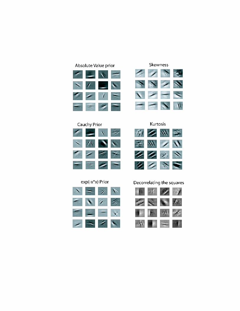
Comparison of basis functions The optimisation algorithm yields the basis functions that are the analogue of

receptive fields of real neurons (Figure 5). A number of important similarities and

differences can be observed. Some of the properties are identical for all the different

priors. All of them lead to receptive fields that are localised in orientation and spatial

frequency. This can be understood from the fact that all analyzed objective functions

reward high absolute values of the activity. High contrast regions are associated with

defined orientation (Einhäuser, Kayser et al. 2002) explaining why all learned

receptive fields are oriented. All of the considered objectives also lead to localisation

in space if the decorrelation term is strong enough.

However also a large number of important differences exist between the resulting

receptive fields: The differences between the functions punishing non-zero activities

is small, they mostly exhibit small variations in the smoothness and the size of the

receptive fields. This is not surprising knowing that their objectives only slightly

differ for small coefficients. KurtosisΨ is known to be prone to overfitting (Hyvärinen

and Oja 1997). Due to its sensitivity to outliers, maximising KurtosisΨ leads to basis

functions that can be expected to be specific to the real natural stimuli chosen in our

study. Using less natural stimuli such as pictures from man made objects would be

likely to significantly change the resulting receptive fields obtained from maximising

KurtosisΨ . While optimising the objective functions that punish non-zero coefficients

lead to small localised, Gabor-type receptive fields, optimising KurtosisΨ leads to more

elaborate filters. Optimising SkewnessΨ also leads to interesting basis functions. All of

the basis functions show black lines on bright background. This is a very common

feature in our dataset since many of the pictures show trees and branches in front of

the bright sky (observation from the raw data). We attribute the possibility of learning

from SkewnessΨ to these properties. It is an interesting violation of contrast reversal

invariance. It would seem that many statistics of natural scenes are conserved if the

contrast is reversed. If the statistics is invariant with respect to contrast reversal then

all distributions of the coefficients a need to be symmetric and SkewnessΨ would not be a

valid objective. The skewed receptive fields nevertheless share orientation and spatial

frequency selectivity with the other objectives.

The methods analyzed in this paper all belong to the class of independent component

analysis. They are however necessarily only an approximation to statistical

independence. We therefore compare the receptive fields with another prior that more

directly measures independence (Comon 1991). If the coefficients are independent

then the coefficients as well as their squares should also be uncorrelated. We thus

maximise CorrIJΨ that punishes correlations between the squares. After a much slower

convergence of 500 RPROP iterations the estimated basis functions are shown in

Figure 5. They are also localised in orientation and spatial frequency. Their properties

lie in between those obtained maximising KurtosisΨ and those obtained maximising the

objective functions that punish non-zero activities. All variants of ICA analyzed here

lead to basis functions that share some basic properties while having some individual

characteristics.

Discussion What general approach should be used in studying different systems of coding and

learning? Above we shortly described the relation of generative model and objective

function approaches. There are two obvious ways of comparing such learning

systems. 1) It is possible to interpret the system as performing optimal regression with

some a priori information. In this framework a generative model is fitted to the data.

2) It is possible to interpret that the system’s task is to learn to extract variables of

relevance from input data. In this interpretation the objective function is central since

it measures the quality or importance of the extracted variables.

Both formulations come with inherent weaknesses and strengths.

1) The generative models used for describing the data are always so simple, for

example linear, that they can not adequately describe the complexity of the real world.

When fitting a generative model to data it is furthermore often infeasible to directly

optimize the log likelihood of the data given the model. Instead it is typically

necessary to simplify a sparse prior to an objective function that can be optimised

efficiently (but see Olshausen and Millman 2000). This step can in fact lead to

objective functions that seem counterintuitive. The objective function used in the

model proposed by Hyvärinen and Hoyer (2000) for the emergence of complex cells

derives from a sparse prior. The resulting objective function however can be

interpreted as minimizing the average coefficient a and thus the number of spikes.

This is equivalent to minimising the overall number of spikes fired by the neuron and

thus their energy consumption. This property was not visible from analysing the prior.

The choice of a prior furthermore is often arbitrary and as shown in this paper often

far from the resulting distributions. The estimated generative model can however be a

strong tool for analysing, improving and generating pictures. Image processing tools

like super resolution (Hertzmann, Jacobs et al. 2001), denoising (Hyvärinen 1999) as

well as sampling pictures from the learned distribution (Dayan, Hinton et al. 1995) is

straightforward once such a model is learned.

2) When optimising an objective function the particular choice might often seem

arbitrary because it needs to be indirectly deduced from evolutionary or design

principles. Following these ideas the brains task is to extract relevant information

from the real world while minimising its energy consumption (Barlow 1961).

Objective functions can be interpreted as heuristics that measure the value of data and

the price of computation in this framework. The energy consumption might be

captured by a variant of the sparseness objective since each spike comes with an

associated energy consumption (Attwell and Laughlin 2001). The AbsΨ objective for

example punishes the average value of the coefficients that can be associated with the

number of spikes and thus the energy consumption. One simple heuristic for

measuring the usefulness of data might be temporal smoothness or stability (Földiak

1991; Kayser, Einhäuser et al. 2001). It derives from the observation that most

variables that are important and that we have names for change on a timescale that is

slow compared to for example the brightness changes of sensors of the retina. The

advantage of the objective function approach is that hypotheses for the objectives of

the system can sometimes directly be derived from evolutionary ideas while allowing

comparison of the results to the properties of the animal’s nervous system.

In the objective function approach also used in the present study, it is directly visible

that the decorrelation term strongly influence learning. It ensures the normalization of

the standard deviation of the coefficients. When designing systems of sparse learning

it is thus also important to also take into account the way the system is normalized.

Considering this normalisation makes it far easier to understand similarities and

differences between objective functions, such as the similarities between the results of

the Kurtosis and the Cauchy simulations.

Sparse coding and Independent component analysis are powerful methods that have

many technical applications in dealing with real world data (c.f. Hyvärinen 1999).

Their strength is that they do not merely depend on statistics of second order (as does

PCA) that can easily be created by uninteresting noise sources. Its most impressive

applications are blind deconvolution (Bell and Sejnowski 1995), blind source

separation (Karhunen, Cichocki et al. 1997), the processing of EEG (Makeig,

Westerfield et al. 1999; Vigario and Oja 2000) and fMRI (c.f. Quigley, Haughton et

al. 2002) data as well as denoising (Hyvärinen 1999). Using heuristics that derive

from the idea of data value might allow designing better objective functions for ICA.

It could lead to algorithms that can better replicate physiological data (Kayser,

Einhäuser et al. 2001) and potentially lead to outputs that are more useful as input to

pattern recognition systems.

Acknowledgements We like to thank Bruno Olshausen for inspiring discussions. We furthermore like to

thank the EU IST-2000-28127 and the BBW 01.0208-1, Collegium Helveticum

(KPK), the Center of Neuroscience Zürich (CK) and the SNF (PK, Grant Nr 31-

65415.01) for financial support.

Figure Captions Figure 1:

The sparseness objectives are shown as a function of the value of the coefficient. The

original forms of the objective functions as used in most papers are shown. For better

comparison all of them are scaled to the same interval.

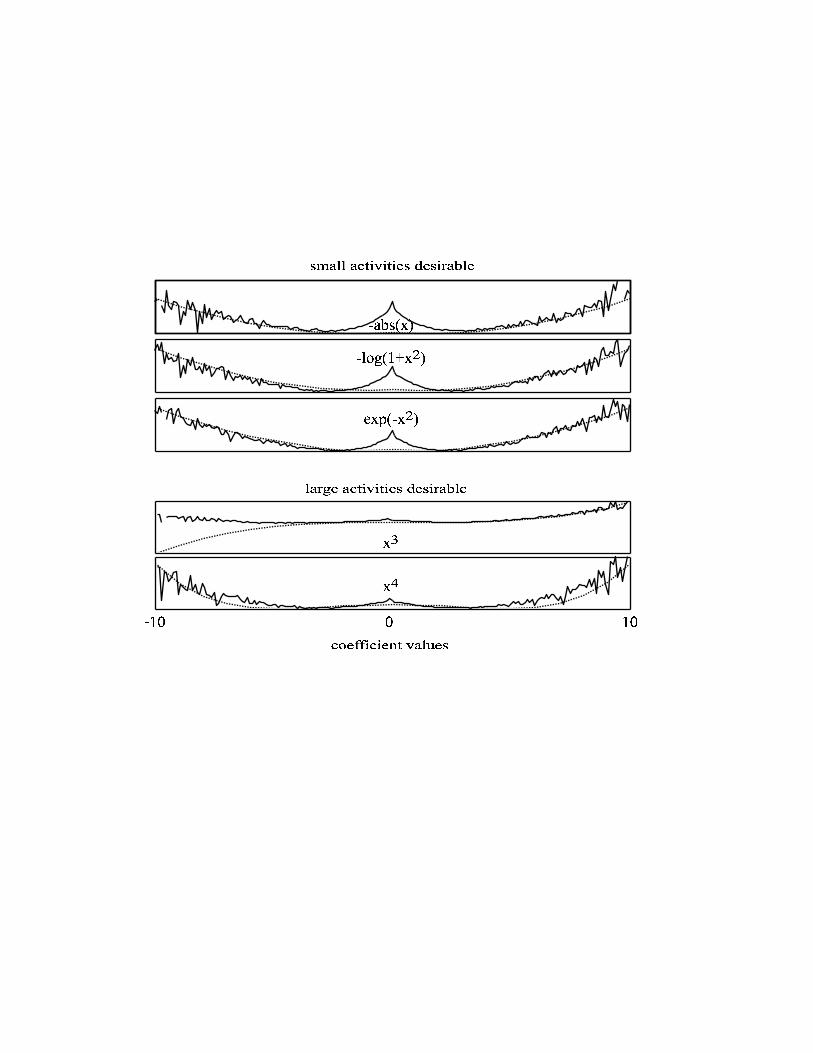
Figure 2:

The full objective functions, including the decorrelation term, are shown as a function

of the coefficient. The objective function was only evaluated after convergence of the

network, which is necessary since the decorrelation term is a function of the basis

functions. For better comparison all objectives were scaled to the same interval.

Figure 3:

The relative distribution of coefficients after convergence is shown as solid lines. The

objective functions are shown as dotted lines.

Figure 4:

A) The same graphs as in figure 3 are shown, zoomed into the range -2.5…2.5 to

depict the details for small coefficient values. The relative distribution of coefficients

after convergence is shown as solid lines. The objective functions are also shown as

dotted lines.

B) The relative distributions are shown, all aligned to their maximal value.

Figure 5:

Typical examples of the resulting basis functions are depicted, each derived from the

respective objective function .

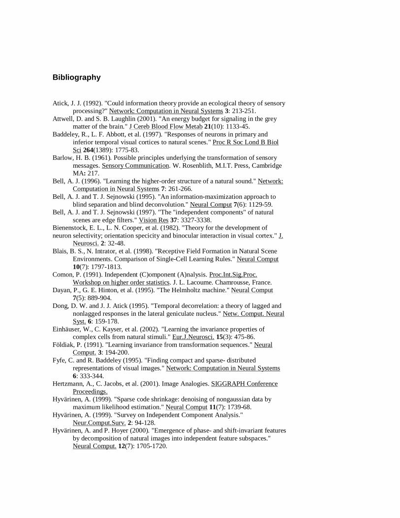
Bibliography Atick, J. J. (1992). "Could information theory provide an ecological theory of sensory

processing?" Network: Computation in Neural Systems 3: 213-251. Attwell, D. and S. B. Laughlin (2001). "An energy budget for signaling in the grey

matter of the brain." J Cereb Blood Flow Metab 21(10): 1133-45. Baddeley, R., L. F. Abbott, et al. (1997). "Responses of neurons in primary and

inferior temporal visual cortices to natural scenes." Proc R Soc Lond B Biol Sci 264(1389): 1775-83.

Barlow, H. B. (1961). Possible principles underlying the transformation of sensory messages. Sensory Communication. W. Rosenblith, M.I.T. Press, Cambridge MA: 217.

Bell, A. J. (1996). "Learning the higher-order structure of a natural sound." Network: Computation in Neural Systems 7: 261-266.

Bell, A. J. and T. J. Sejnowski (1995). "An information-maximization approach to blind separation and blind deconvolution." Neural Comput 7(6): 1129-59.

Bell, A. J. and T. J. Sejnowski (1997). "The "independent components" of natural scenes are edge filters." Vision Res 37: 3327-3338.

Bienenstock, E. L., L. N. Cooper, et al. (1982). "Theory for the development of neuron selectivity; orientation specicity and binocular interaction in visual cortex." J.

Neurosci. 2: 32-48. Blais, B. S., N. Intrator, et al. (1998). "Receptive Field Formation in Natural Scene

Environments. Comparison of Single-Cell Learning Rules." Neural Comput 10(7): 1797-1813.

Comon, P. (1991). Independent (C)omponent (A)nalysis. Proc.Int.Sig.Proc. Workshop on higher order statistics. J. L. Lacoume. Chamrousse, France.

Dayan, P., G. E. Hinton, et al. (1995). "The Helmholtz machine." Neural Comput 7(5): 889-904.

Dong, D. W. and J. J. Atick (1995). "Temporal decorrelation: a theory of lagged and nonlagged responses in the lateral geniculate nucleus." Netw. Comput. Neural Syst. 6: 159-178.

Einhäuser, W., C. Kayser, et al. (2002). "Learning the invariance properties of complex cells from natural stimuli." Eur.J.Neurosci. 15(3): 475-86.

Földiak, P. (1991). "Learning invariance from transformation sequences." Neural Comput. 3: 194-200.

Fyfe, C. and R. Baddeley (1995). "Finding compact and sparse- distributed representations of visual images." Network: Computation in Neural Systems 6: 333-344.

Hertzmann, A., C. Jacobs, et al. (2001). Image Analogies. SIGGRAPH Conference Proceedings.

Hyvärinen, A. (1999). "Sparse code shrinkage: denoising of nongaussian data by maximum likelihood estimation." Neural Comput 11(7): 1739-68.

Hyvärinen, A. (1999). "Survey on Independent Component Analysis." Neur.Comput.Surv. 2: 94-128.

Hyvärinen, A. and P. Hoyer (2000). "Emergence of phase- and shift-invariant features by decomposition of natural images into independent feature subspaces." Neural Comput. 12(7): 1705-1720.

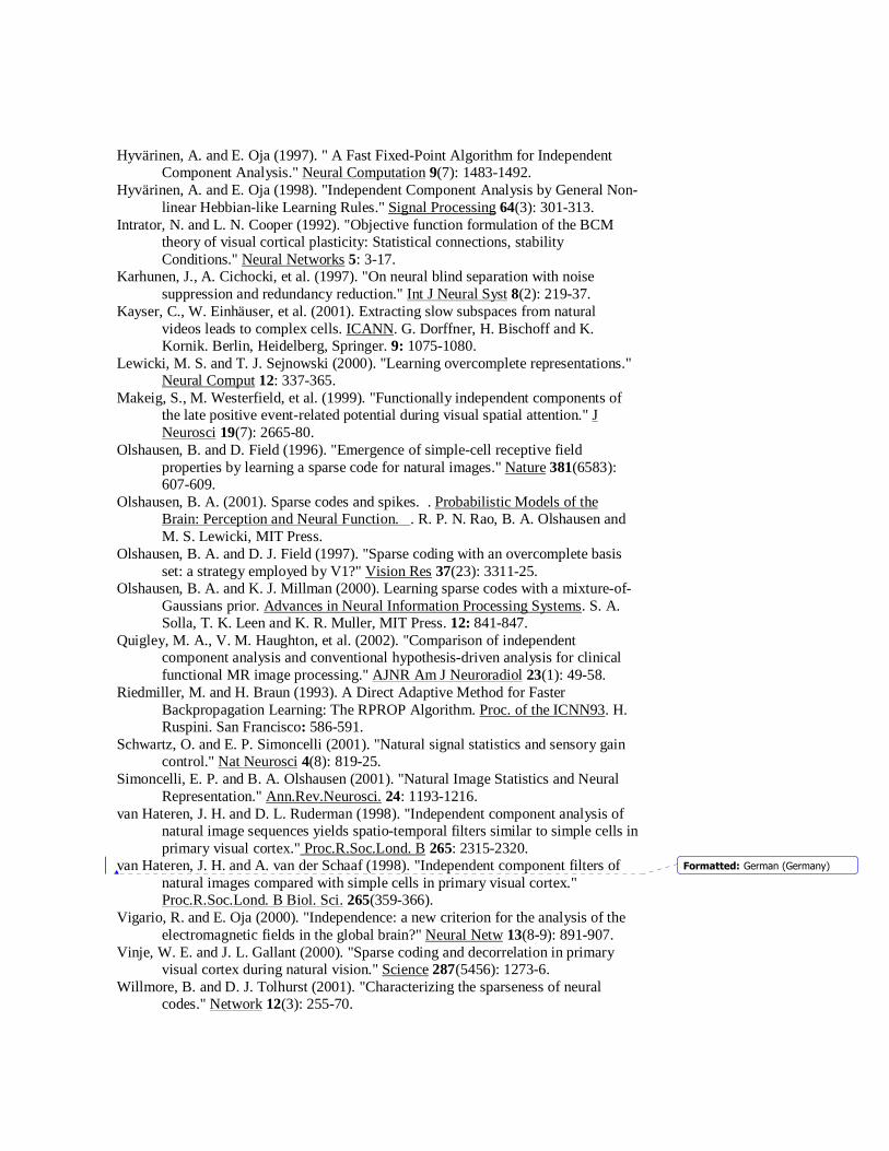
Hyvärinen, A. and E. Oja (1997). " A Fast Fixed-Point Algorithm for Independent Component Analysis." Neural Computation 9(7): 1483-1492.

Hyvärinen, A. and E. Oja (1998). "Independent Component Analysis by General Non-linear Hebbian-like Learning Rules." Signal Processing 64(3): 301-313.

Intrator, N. and L. N. Cooper (1992). "Objective function formulation of the BCM theory of visual cortical plasticity: Statistical connections, stability Conditions." Neural Networks 5: 3-17.

Karhunen, J., A. Cichocki, et al. (1997). "On neural blind separation with noise suppression and redundancy reduction." Int J Neural Syst 8(2): 219-37.

Kayser, C., W. Einhäuser, et al. (2001). Extracting slow subspaces from natural videos leads to complex cells. ICANN. G. Dorffner, H. Bischoff and K. Kornik. Berlin, Heidelberg, Springer. 9: 1075-1080.

Lewicki, M. S. and T. J. Sejnowski (2000). "Learning overcomplete representations." Neural Comput 12: 337-365.

Makeig, S., M. Westerfield, et al. (1999). "Functionally independent components of the late positive event-related potential during visual spatial attention." J Neurosci 19(7): 2665-80.

Olshausen, B. and D. Field (1996). "Emergence of simple-cell receptive field properties by learning a sparse code for natural images." Nature 381(6583): 607-609.

Olshausen, B. A. (2001). Sparse codes and spikes. . Probabilistic Models of the Brain: Perception and Neural Function. . R. P. N. Rao, B. A. Olshausen and M. S. Lewicki, MIT Press.

Olshausen, B. A. and D. J. Field (1997). "Sparse coding with an overcomplete basis set: a strategy employed by V1?" Vision Res 37(23): 3311-25.

Olshausen, B. A. and K. J. Millman (2000). Learning sparse codes with a mixture-of-Gaussians prior. Advances in Neural Information Processing Systems. S. A. Solla, T. K. Leen and K. R. Muller, MIT Press. 12: 841-847.

Quigley, M. A., V. M. Haughton, et al. (2002). "Comparison of independent component analysis and conventional hypothesis-driven analysis for clinical functional MR image processing." AJNR Am J Neuroradiol 23(1): 49-58.

Riedmiller, M. and H. Braun (1993). A Direct Adaptive Method for Faster Backpropagation Learning: The RPROP Algorithm. Proc. of the ICNN93. H. Ruspini. San Francisco: 586-591.

Schwartz, O. and E. P. Simoncelli (2001). "Natural signal statistics and sensory gain control." Nat Neurosci 4(8): 819-25.

Simoncelli, E. P. and B. A. Olshausen (2001). "Natural Image Statistics and Neural Representation." Ann.Rev.Neurosci. 24: 1193-1216.

van Hateren, J. H. and D. L. Ruderman (1998). "Independent component analysis of natural image sequences yields spatio-temporal filters similar to simple cells in primary visual cortex." Proc.R.Soc.Lond. B 265: 2315-2320.

van Hateren, J. H. and A. van der Schaaf (1998). "Independent component filters of natural images compared with simple cells in primary visual cortex." Proc.R.Soc.Lond. B Biol. Sci. 265(359-366).

Vigario, R. and E. Oja (2000). "Independence: a new criterion for the analysis of the electromagnetic fields in the global brain?" Neural Netw 13(8-9): 891-907.

Vinje, W. E. and J. L. Gallant (2000). "Sparse coding and decorrelation in primary visual cortex during natural vision." Science 287(5456): 1273-6.

Willmore, B. and D. J. Tolhurst (2001). "Characterizing the sparseness of neural codes." Network 12(3): 255-70.

Formatted: German (Germany)

� ����������� ��

������ �����

� ����� � �� ��

���

�����! �!

"$#&%('�'�%()+*�,.-/,.*�,10�"32�04"5,765%98�'10

:�;

'1%!6$<�0=%>)+*�,7-�,.*�,104"32�0�"5,?65%!8�'�0

"@*A%CB�2�%C6D2E2�0+-/,1%+*�,1F�BG"$H�F�I�'12J8�0LK(M�2N0>)>F�6O650P'1%+*�,1F�BQ*A0C6$#

)>FN0>RSRT,1)(,10!B/*�-�%P'7I�0�"

� ����������� ��������� �����

� ����� � �� ��

���

���! #"�"� #$&%�')(�'*%�',+��.-�+/�0'*10 32�",+

��4

", 5176�+8 9$&%�'*(�')%�',+/�:-;+��0'*1< 52�"�+

=<>&? ? >@?A#B�C9DEDGF,A@F,CIHKJ�L�M#N*O�C/P

�������������� ��� ��� ����������� ����������

�! �"$#&%('()+*&,.-

�0/(1+2�%�*&-

3 *�45%0��*&,.-

*76

*.8

���9�;:7�<�=9�� ��5 ��� ������7���� ������+���

>�?�@BA C ?&@BA

>�?�@BA C ?&@BA

D

E

FG7H=I!IKJ�F�J�H9L�M+N5OP�Q�HSR

����������� ������������� �����

� ���������� �!����

�#"$��%'&�"$()"$*+� � �����

,.- �+/102�+���

34��5� ������

6 �+�7���!� �+��8�!�029:�!���;��<2���� �+�