Knowledge discovery in metabolomics: An overview of MS data handling

Review

Knowledge discovery in metabolomics: Anoverview of MS data handling

While metabolomics attempts to comprehensively analyse the small molecules char-

acterising a biological system, MS has been promoted as the gold standard to study the

wide chemical diversity and range of concentrations of the metabolome. On the other

hand, extracting the relevant information from the overwhelming amount of data

generated by modern analytical platforms has become an important issue for knowledge

discovery in this research field. The appropriate treatment of such data is therefore of

crucial importance in order, for the data, to provide valuable information. The aim of this

review is to provide a broad overview of the methodologies developed to handle and

process MS metabolomic data, compare the samples and highlight the relevant metabo-

lites, starting from the raw data to the biomarker discovery. As data handling can be

further separated into data processing, data pre-treatment and data analysis, recent

advances in each of these steps are detailed separately.

Keywords: Data mining / Data processing / Metabolomics / MSDOI 10.1002/jssc.200900609

1 Metabolomics

1.1 Systems biology

Metabolomics (also known as metabonomics) is a recent

discipline that attempts to globally study metabolites and

their concentrations, interactions and dynamics within

complex samples [1]. It constitutes one of the tools of the

post-genomic era [2], which is concerned with the study of

the different functional levels of a biological system, i.e. the

transcriptome, the proteome and the metabolome [3, 4]. As

metabolites can be considered the downstream products of

cellular regulatory processes [5], metabolomics data can

precisely characterise cells, tissues, biofluids or whole

organisms by defining specific biochemical phenotypes that

are representative of physiological or developmental states.

The metabolome is the holistic quantitative set of low-

molecular-weight compounds (o1000 Da), including many

hundreds or thousands of molecules such as carbohydrates,

vitamins, lipids and amino or fatty acids. These metabolites

participate in the metabolic reactions necessary for normal

functions, the maintenance or growth of a cell [2]. Their

origin can be either endogenous such as the products of

biosynthesis and catabolism or exogenous such as nutrients

or pharmaceutical compounds degradation products [6, 7].

The chemical properties of the organic or inorganic

constituents of this set are greatly variable and this diversity

is a critical aspect to consider [8]. The variability in the

molecular weight, polarity or solubility and the wide

dynamic range of concentrations (from pmol to mmol)

constitute additional difficulties when analysing metabolites

while no amplification process is available.

1.2 Applications of metabolomics

Measuring metabolites changes could offer deeper insights

into biological mechanisms by describing the responses of

systems to environmental or genetic modifications. Meta-

bolomic analyses constitute a potent tool for the discovery of

biomarkers related to a physiological response and the

diagnosis of complex phenotypes. Numerous applications

have already been developed in a variety of research fields of

the post-genomic era, from medical science to agriculture.

Although early metabolic studies focused on pre-selec-

ted specific compounds, modern untargeted approaches

represent efficient tools for the early detection of diseases

[9–11]. The screening of drug candidates constitutes another

prominent application through the assessment of the effects

of metabolic modifications or toxicity [12, 13]. In addition,

metabolomics has recently received an increasing interest

from the nutrition research field [14]. Several applications

Julien BoccardJean-Luc VeutheySerge Rudaz

School of PharmaceuticalSciences, University of Geneva,University of Lausanne, Geneva,Switzerland

Received September 29, 2009Revised November 3, 2009Accepted November 3, 2009

Abbreviations: ANN, artificial neural networks; DIMS, directinfusion mass spectrometry; HCA, hierarchical clusteranalysis; PCA, principal component analysis; PLS,

projection to latent structures by means of partial leastsquares; SVM, support vector machine; UV, unit variance

Correspondence: Dr. Serge Rudaz, School of PharmaceuticalSciences – EPGL, University of Geneva, 20 Bd d’Yvoy, 1211Geneva 4, SwitzerlandE-mail: [email protected]: 141-22-379-68-08

& 2010 WILEY-VCH Verlag GmbH & Co. KGaA, Weinheim www.jss-journal.com

J. Sep. Sci. 2010, 33, 1–15 1

are foreseen, such as food composition analyses, quality and

authenticity assessments and the monitoring of the

physiological consequences of specific diets. Additionally,

metabolomics is expected to greatly benefit agriculture,

plant biochemistry, phytomedicine and natural product

approaches [4, 15]. Metabolome analysis represents a key

tool to uncover the roles of genes in functional genomics

[16]. Genotyping and phenotyping will certainly provide

precious information to link the sequence of a gene to its

function.

2 Analytical methods

2.1 General considerations

Due to the high chemical diversity of the metabolome,

complementary analytical techniques are required to

monitor it completely [17]. Moreover, sensitivity constitutes

a major concern, because there is no available method of

amplification as in the case of transcriptome analysis.

Multiple analytical platforms have already been applied to

metabolomic studies [18], such as direct infusion MS

(DIMS), hyphenated separation technique MS platforms,

i.e. GC [19–23], LC [24–26] or CE [27–30], as well as NMR [1,

31, 32], Fourier transform-infrared spectroscopy [33] or

accelerator MS [34]. The selection of the most appropriate

methodology can be considered as a compromise between

the chemical selectivity, sensitivity and speed of the different

techniques [35].

2.2 MS

MS is a well-established detection method employed in

many fields and is one of the essential instruments in

analytical laboratories. By measuring the m/z of elemental

or molecular species, it allows the simultaneous detection of

multiple analytes with high sensitivities. MS has

been demonstrated as a potent platform for metabolomics,

thanks to its ability to detect metabolites present at

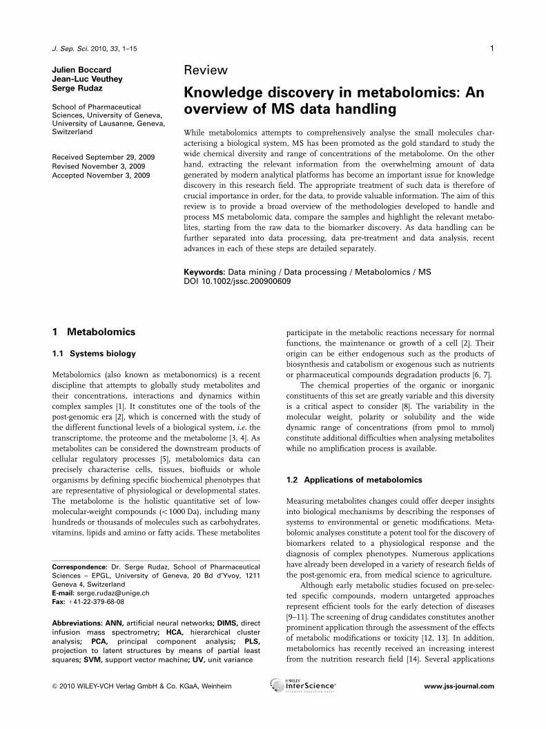
low levels (mM concentrations) [36, 37]. Atmospheric

pressure ionisation includes common soft ionisation

techniques that generally produce protonated molecules

[M1H]1 or deprotonated molecules [M�H]�. For metabo-

lomic purposes and due to the fact that some metabolites

can be observed exclusively in only one ionisation

mode, acquisition should be performed in both positive

and negative ion mode to maximise the metabolome

coverage (Fig. 1). The high mass accuracy of MS provides

structural information, as an exact molecular mass can be

indicative of the molecular formula or fragments of the

molecular structure [18]. The vast majority of recent

metabolomic studies have relied on this particular techni-

que [38].

2.3 Direct injection MS

DIMS is the most simple and direct approach to MS

technology. It provides high-throughput screening and is

mainly used for sample classification. Its use is rather

limited in terms of quantification and metabolite identifica-

tion due to signal suppression. In fact, the simultaneous

measurements of a large number of compounds may suffer

from matrix effects, such as ion suppression, especially

when DIMS analyses are performed on complex

samples [39]. A high mass accuracy is desirable and

fragmentation through tandem MS is usually employed as

it provides more information for the identification of

metabolites through the detection of both the parent

molecules and the fragments.

100

100

%

Time5.00 10.00 15.00 20.00 25.00 30.00 35.00 40.00

Figure 1. Complementarity of thepositive and the negative ionisationmodes.

J. Sep. Sci. 2010, 33, 1–152 J. Boccard et al.


2.4 Chromatography-MS

The hyphenation of MS with separative techniques such as

chromatography greatly increases the quality of the raw data

generated [18, 40]. The sequential introduction of

compounds into the mass spectrometer enables a higher

sensitivity and allows more metabolites to be detected but it

also involves an increase in the analysis time. Two main

separative methods are currently extensively used in

metabolomics, namely GC and LC.

2.4.1 GC-MS

GC-MS is well established and already employed [41–43].

The typical ionisation techniques are chemical ionisation,

which minimises fragmentation, and fragmentation

through electron impact [23]. GC-MS provides reproducible

and accurate measurements of volatile compounds and the

fragmentation pattern of these molecules [19, 21]. The

chemical derivatisation of semi-volatile compounds is

required to increase the volatility and produces ions that

can be separated in the GC column [44–46]. GC-MS was

historically the method-of-choice for the early development

of metabolomic studies [47, 48], and libraries have been

built to facilitate the identification of compounds [49].

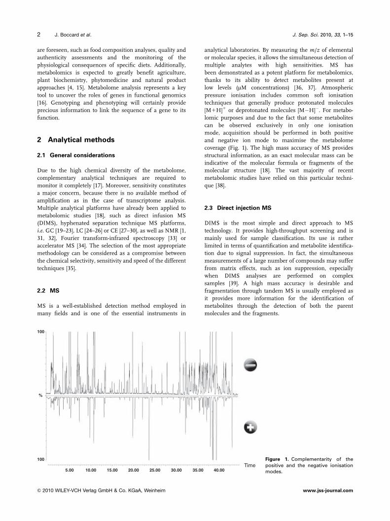
Recent developments include comprehensive GC�GC-MS,

which separated compounds with two columns of orthogo-

nal properties (Fig. 2) [50].

2.4.2 LC-MS

LC is able to handle a broader range of molecular weights

and has become increasingly popular for the analysis of

biological samples due to its high sensitivity [51, 52].

Another advantage of LC over GC resides in the large

diversity of separation mechanisms including normal phase

(silica), reverse phase (C18,C8,C4, phenyl), hydrophilic

interaction chromatography and ion exchange chromato-

graphy. The phase chemistry greatly influences the nature

of metabolites that can be investigated, and the assessment

of complete metabolomes is currently impossible using a

single chromatographic system [25, 53, 54]. The recent

introduction of capillary LC [55, 56] and ultra-high pressure

LC [57] offers great potential for metabolomic analyses on

complex samples by highly improving the chromatographic

performance. Columns packed with sub-2-mm particles can

lead either to the better separation of narrower chromato-

graphic peaks or to a faster analysis without the loss of

resolution, compared with conventional LC. The use of

elevated temperatures is another recent area of investigation

to improve the resolution of LC [58–60], whereas monolithic

columns constitute another alternative to improve the

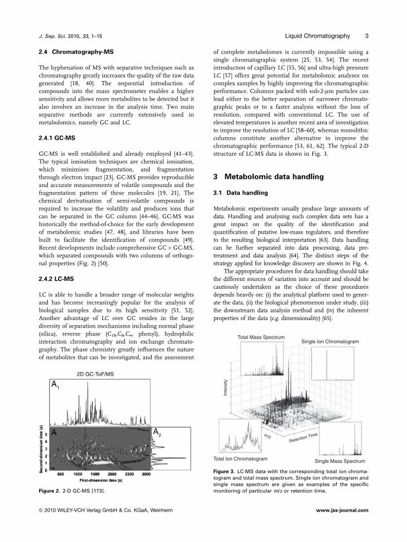
chromatographic performance [53, 61, 62]. The typical 2-D

structure of LC-MS data is shown in Fig. 3.

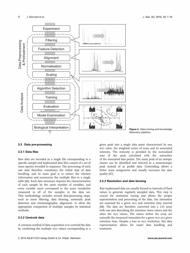
3 Metabolomic data handling

3.1 Data handling

Metabolomic experiments usually produce large amounts of

data. Handling and analysing such complex data sets has a

great impact on the quality of the identification and

quantification of putative low-mass regulators, and therefore

to the resulting biological interpretation [63]. Data handling

can be further separated into data processing, data pre-

treatment and data analysis [64]. The distinct steps of the

strategy applied for knowledge discovery are shown in Fig. 4.

The appropriate procedures for data handling should take

the different sources of variation into account and should be

cautiously undertaken as the choice of these procedures

depends heavily on: (i) the analytical platform used to gener-

ate the data, (ii) the biological phenomenon under study, (iii)

the downstream data analysis method and (iv) the inherent

properties of the data (e.g. dimensionality) [65].

Figure 2. 2-D GC-MS [173].

Total Ion Chromatogram Single Mass Spectrum

Single Ion ChromatogramTotal Mass Spectrum

Inte

nsity

Figure 3. LC-MS data with the corresponding total ion chroma-togram and total mass spectrum. Single ion chromatogram andsingle mass spectrum are given as examples of the specificmonitoring of particular m/z or retention time.

J. Sep. Sci. 2010, 33, 1–15 Liquid Chromatography 3


3.2 Data pre-processing

3.2.1 Data files

Raw data are recorded as a single file corresponding to a

specific sample and hyphenated data files consist of a set of

mass spectra recorded in sequence. The processing of such

raw data therefore constitutes the initial step of data

handling, and its main goal is to extract the relevant

information and summarise the multiple files in a single

table [66]. Such data summary requires the characterisation

of each sample by the same number of variables, and

every variable must correspond to the same metabolite

measured in all of the samples in the data set.

This methodology includes several data-processing steps,

such as noise filtering, data binning, automatic peak

detection and chromatographic alignment, to allow the

appropriate comparison of multiple samples by statistical

methods.

3.2.2 Centroid data

A common method of data acquisition is to centroid the data

by combining the multiple m/z values corresponding to a

given peak into a single data point characterised by one

m/z value, the weighted centre of mass and its associated

intensity. The intensity is provided by the normalised

area of the peak calculated with the intensities

of the associated data points. The main peak of an isotopic

cluster can be identified and selected as a monoisotopic

peak instead of as profile data. Centroiding allows a

better mass assignment and usually increases the data

quality [67].

3.2.3 Resolution and data binning

Raw hyphenated data are usually binned in intervals of fixed

values to generate regularly sampled data. This step is

crucial for resolution tuning and allows the proper

representation and processing of the data. Ion intensities

are summed for a given m/z and retention time interval

[68]. The data are therefore converted into a 2-D array

with one axis describing the retention times values and the

other the m/z values. The values within the array are

naturally the measured intensities for a given m/z at a given

retention time. Despite a loss in m/z resolution, this data

representation allows for easier data handling and

treatment.

Ctrl

Experiment

Filtering

Feature Detection

Alignment

NormalisationDat

a P

repr

oces

sing

& P

retre

atm

ent

Dat

a A

naly

sis

Training

Algorithm Selection

Evaluation

Model Examination

Biological Interpretation

Scaling

A

B

A B A B

A B A B

Figure 4. Data mining and knowledgediscovery pipeline.



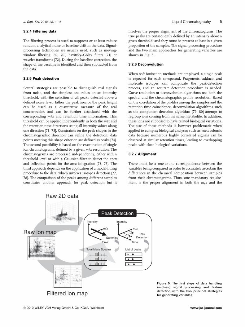
3.2.4 Filtering data

The filtering process is used to suppress or at least reduce

random analytical noise or baseline drift in the data. Signal-

processing techniques are usually used, such as moving-

window filtering [69, 70], Savitzky–Golay filters [71] or

wavelet transforms [72]. During the baseline correction, the

shape of the baseline is identified and then subtracted from

the data.

3.2.5 Peak detection

Several strategies are possible to distinguish real signals

from noise, and the simplest one relies on an intensity

threshold, with the selection of all peaks detected above a

defined noise level. Either the peak area or the peak height

can be used as a quantitative measure of the real

concentration and can be further associated with the

corresponding m/z and retention time information. This

threshold can be applied independently in both the m/z and

the retention time directions using all intensity values along

one direction [71, 73]. Constraints on the peak shapes in the

chromatographic direction can refine the detection; data

points meeting this shape criterion are defined as peaks [74].

The second possibility is based on the examination of single

ion chromatograms, defined by a given m/z resolution. The

chromatograms are processed independently, either with a

threshold level or with a Gaussian-filter to detect the apex

and inflection points for the area integration [75, 76]. The

third approach depends on the application of a model-fitting

procedure to the data, which involves isotopes detection [77,

78]. The comparison of the peaks among different samples

constitutes another approach for peak detection but it

involves the proper alignment of the chromatograms. The

true peaks are consequently defined by an intensity above a

given threshold, and they must be present at least in a given

proportion of the samples. The signal-processing procedure

and the two main approaches for generating variables are

shown in Fig. 5.

3.2.6 Deconvolution

When soft ionisation methods are employed, a single peak

is expected for each compound. Fragments, adducts and

molecule isotopes can complicate the peak-detection

process, and an accurate detection procedure is needed.

Curve resolution or deconvolution algorithms use both the

spectral and the chromatographic profile resolution. Based

on the correlation of the profiles among the samples and the

retention time coincidence, deconvolution algorithms such

as the component detection algorithm [79, 80] attempt to

regroup ions coming from the same metabolite. In addition,

these ions are supposed to have related biological variations.

The use of these methods is however problematic when

applied to complex biological analyses such as metabolomic

data because numerous highly correlated signals can be

observed at similar retention times, leading to overlapping

peaks with close biological variations.

3.2.7 Alignment

There must be a one-to-one correspondence between the

variables being compared in order to accurately ascertain the

differences in the chemical composition between samples

from their chromatograms. Thus, one mandatory require-

ment is the proper alignment in both the m/z and the

Raw 2D data

Raw ion map

Filtered ion map

Peak Detection

Intensity

m/z

Time

Total Mass Spectra

Summing

Time

Peak Detection

Intensity

m/z

List of peaks

Figure 5. The first steps of data handlinginvolving signal processing and featuredetection with the two principal strategiesfor generating variables.



retention time dimensions in order to combine results.

Shifts along the m/z axis are usually easily corrected using

calibration, but changes in retention times are more

problematic. Progress in chromatographic techniques has

reduced these shifts but variability in the retention time of a

given metabolite is frequently encountered [81]. These drifts

can be caused by multiple factors, including temperature

changes, pH, pump pressure fluctuations or column

clogging. An alignment algorithm usually requires a

reference chromatogram to correct these retention time

differences, and its choice has a great influence on the

results. Additionally, numerous issues need to be tackled

when performing such corrections. For instance, the

method must preserve the chemical selectivity between

samples of distinct compositions while minimising run-to-

run shifts [82]. Moreover, corresponding peaks are expected

to be shifted by less than the representative distance

between adjacent peaks. On the other hand, an alignment

algorithm must be fast enough to deal quickly with a large

amount of data to supply a high sample throughput.

Three approaches are commonly utilised to align chro-

matograms [83]. The simplest solution resides in summing

or binning data along the chromatographic dimension. No

loss of information is required and the errors are pushed

back towards the bin boundaries. Indeed peaks can be

occasionally allocated to neighbouring m/z bins alternatively

[75].

Secondly, an alignment without peak detection can be

performed by compressing or stretching the retention time

axis of all samples to a common reference. As it needs only a

minimal manual contribution, this approach is interesting

from an automation point of view [84]. The mapping of total

ion chromatograms is one of the most investigated align-

ment methods, and warping methods are well-known

alternatives for that purpose, allowing the stretching and

shrinking of segments of the chromatograms [85]. Numer-

ous warping methods are available [86–88], but two algo-

rithms were initially developed, namely correlation

optimised warping [89] and dynamic time warping [90].

Unfortunately, such iterative alignment procedures are

considerably time consuming when dealing with the large

data sets of long chromatograms.

Another way to match the corresponding peaks among

samples relies on the detection of independent signals using

curve resolution. Several algorithms are available such as

progressive clustering [91], GENTLE [92] or MEND [93]. The

correspondence between the detected peaks of different

samples can then be assigned by the use of a time and m/ztolerance to regroup similar peaks. Another solution is to

match components with high-spectral similarity in a given

time window.

3.2.8 Normalisation

Prior to analysis, data are often pre-treated to remove

systematic variations between samples [64]. Normalisation

is a critical step, because it aims to remove bias in the data

while preserving biological information. It is a difficult task

mainly due to the great chemical diversity of complex data,

leading to discrepancies in the extraction or ionisation

efficiencies. Statistical models represent simple methods to

estimate the scaling factors among samples, such as the

unit norm [94] or median intensities [71]. The addition of a

set of internal or external standards that reasonably cover

the retention time range constitutes another way to perform

normalisation in a practical manner [95–97].

3.2.9 Software packages

The need of powerful data-processing methods gave rise to

numerous commercial or free tools, implementing either

one specific part or combining several steps of the data-

processing pipeline. Most of the tools include standard

procedures of noise filtering, peak detection, alignment and

normalisation, while they output a data matrix containing

the peak intensities or areas for each detected ion among all

the samples.

Integrated platforms for hyphenated MS data pre-

processing and analysis include free packages such as

MZmine [74], MAthDAMP [98], metAlign [99], MSFacts

[100], XCMS [75] and MeltDB [101] or commercial solutions

as, for example, MS Resolver [102], MarkerLynx [103] or

Sieve based on the ChromAlign algorithm [104]. Moreover,

comparisons of performance have been published recently

[105, 106].

3.3 Metabolomic data pre-treatment

The data pre-treatment phase constitutes another crucial

step that can drastically change the pertinence and the

outcome of the data analysis. Centring aims to estimate the

model parameters with an observed bias. Mean centring

across the first mode is a classical pre-processing practice

prior to model fitting. It provides simpler models by

reducing the rank, increasing the fit to the data, removing

offsets and avoiding algorithmic problems [107]. The

fluctuations of the variables are centred around zero instead

of their mean value to focus on the variation between

samples. Scaling is used to adjust the importance allocated

to the elements of the data in fitting the model. Most scaling

methods adjust the weight of each variable with a scaling

factor that can be estimated by either a dispersion criterion

or a size measure. It may be obtained by calculating the

inverse of its standard deviation so that all variables have the

same chance to contribute to the model as they have an

equal unit variance (UV). This technique is called UV

scaling, or auto-scaling when prior mean centring is

performed [108]. Further analyses are then based on

correlations instead of covariances. UV scaling is often

suitable when no prior information is available but equal

weights are allocated to the baseline noise and proper

signals. Pareto scaling involves a similar procedure based on

the dispersion except that the square root of the standard



deviation is used as scaling factor [109]. It is an intermediate

situation as it gives a variance equal to the standard

deviation of each variable instead of UV. Large fold changes

have less influence than when raw data are used, but the

reasonable weight allocated to small values can avoid the

detrimental effects caused by a similar error increase. Other

methods such as variable stability scaling [110] or range

scaling [111] are available, but UV and Pareto scaling are the

prevailing methods applied in metabolomic MS-based

studies.

Furthermore, as many statistical procedures are based

on the assumption of normally distributed values, a trans-

formation can be desirable to address skewed data. Log or

power transformation are well-known functions generally

applied to correct heteroscedasticity [112]. The log function

is useful when the interactions between variables are not

only additive but also multiplicative and its use allows the fit

of linear models [113].

4 Data analysis

4.1 Modelling metabolomic data

Metabolomic experiments exploit computerised instru-

ments leading to the simultaneous detection of a great

number of variables, and the generation of large multi-

variate data sets [114]. From a statistical point of view,

metabolomic data sets constitute a great challenge, as

reliable and robust approaches are necessary to handle and

extract the relevant information from the vast amount of

data generated [115, 116]. The outputs of a metabolomic

data analysis may differ greatly depending on the purposes

of the investigation. Although very few highly reliable

metabolites can be sufficient for diagnostic purposes (as in

the case of disease evaluation), an extended set of

compounds may be desired when a biochemical network

is under examination. Alternatively, an overview of the

distribution of samples can be desirable to assess a data set

globally. The choice of the data analysis strategy depends

heavily on the questions that are asked. Changes in

metabolite levels may be drastic or subtle, and statistical

processing is required to determine the relevance of an

observed change. The choice of the most appropriate model

for a given data set constitutes an important issue. The

structural descriptions and the explicit knowledge that are

obtained by examining the model are more important than

the predictive ability of new samples in many applications.

The description of the underlying concept has therefore to

be both operational and intelligible. The methods are

expected to constitute high-throughput and potent auto-

mated tools to highlight trends and patterns among samples

or relevant biomarkers within large metabolomic data sets.

Metabolomic commercial solutions include built-in

statistical packages for data analysis. Common chemometric

tools [117, 118] such as principal component analysis (PCA)

[119] are generally proposed for display and exploratory

analysis purposes, whereas univariate statistical tests such

as the Student’s t-test are used to identify the relevant

variables. These methods are useful by providing an over-

view of the pre-processed data but are rather limited [120].

There is, therefore, a considerable opportunity to increase

the understanding of biological phenomena through the use

of data mining methods with respect to their strengths and

applicability.

4.2 Univariate hypothesis testing

Univariate significance tests such as the Student’s t-test, the

one-way analysis of variance or the non-parametric equiva-

lents can be used to identify statistical differences between

samples of distinct classes [121]. The predictive power of

each variable is assessed by finding statistically significant

differences between the mean intensity values of a given

signal, and the calculated p-value is a straightforward

indicator. Such procedures are easily understandable but

their use is rather limited when dealing with thousands of

highly correlated variables. False positives (type I error) are

likely to occur when performing multiple comparisons and

procedures such as the Bonferroni correction have been

introduced to address this issue [122]. The vast majority of

metabolomics-dedicated software provides statistical

hypothesis testing [99, 123, 124].

4.3 Exploratory analysis by unsupervised learning

Unsupervised methods attempt to analyse a set of observa-

tions without measuring or observing any related outcome.

As there is no specified class label or response, the data set

is considered as a collection of analogous objects. Unsu-

pervised learning uses procedures that attempt to find the

natural partitions of patterns to facilitate the understanding

of the relationship between the samples and to highlight the

variables that are responsible for these relationships. By

providing means for visualisation, unsupervised learning

aids in the discovery of unknown but meaningful categories

of samples or variables that naturally fall together. The

success of such approaches is frequently evaluated subjec-

tively by the interpretability and usefulness of the results

with respect to a given problem.

4.3.1 PCA

PCA can be considered as the starting point of multivariate

data analyses. PCA is an orthogonal transformation of

multivariate data first formulated by Pearson [125] mostly

used for exploratory analyses by extracting and displaying

systematic variations. PCA attempts to uncover hidden

internal structures by building principal components

describing the maximal variance of the data [119]. This

method represents a very useful tool for display purposes as

it provides a low-dimension projection of the data, i.e. a



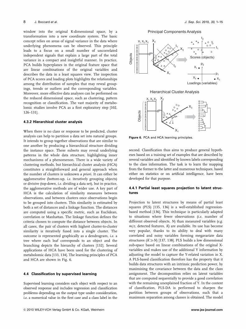
window into the original K-dimensional space, by a

transformation into a new coordinate system. The basic

concept relies on areas of signal variance in the data where

underlying phenomena can be observed. This principle

leads to a focus on a small number of uncorrelated

independent signals that explain a large part of the total

variance in a compact and insightful manner. In practice,

PCA builds hyperplanes in the original feature space that

are linear combinations of the original variables and

describes the data in a least squares view. The inspection

of PCA scores and loading plots highlights the relationships

among the distribution of samples that may reveal group-

ings, trends or outliers and the corresponding variables.

Moreover, more effective data analyses can be performed on

the reduced dimensional space, such as clustering, pattern

recognition or classification. The vast majority of metabo-

lomic studies involve PCA as a first exploratory step [102,

126–131].

4.3.2 Hierarchical cluster analysis

When there is no class or response to be predicted, cluster

analysis can help to partition a data set into natural groups.

It intends to group together observations that are similar to

one another by producing a hierarchical structure dividing

the instance space. These subsets may reveal underlying

patterns in the whole data structure, highlighting inner

mechanisms of a phenomenon. There is a wide variety of

clustering methods, but hierarchical cluster analysis (HCA)

constitutes a straightforward and general approach when

the number of clusters is unknown a priori. It can either be

agglomerative (bottom-up, i.e. iteratively grouping objects)

or divisive (top-down, i.e. dividing a data set), but in practice,

the agglomerative methods are of wider use. A key part of

HCA is the calculation of similarity measures between

observations, and between clusters once observations begin

to be grouped into clusters. This similarity is estimated by

both a set of distances and a linkage function. The distances

are computed using a specific metric, such as Euclidean,

correlation or Manhattan. The linkage function defines the

criteria chosen to compute the distance between objects. In

all cases, the pair of clusters with highest cluster-to-cluster

similarity is iteratively fused into a single cluster. The

outcome is represented graphically as a dendrogram, i.e. a

tree where each leaf corresponds to an object and the

branching depicts the hierarchy of clusters [132]. Several

applications of HCA have been used for the clustering of

metabolomic data [133, 134]. The learning principles of PCA

and HCA are shown in Fig. 6.

4.4 Classification by supervised learning

Supervised learning considers each object with respect to an

observed response and includes regression and classification

problems depending on the output type under consideration,

i.e. a numerical value in the first case and a class label in the

second. Classification thus aims to produce general hypoth-

eses based on a training set of examples that are described by

several variables and identified by known labels corresponding

to the class information. The task is to learn the mapping

from the former to the latter and numerous techniques, based

either on statistics or on artificial intelligence, have been

developed for that purpose.

4.4.1 Partial least squares projection to latent struc-

tures

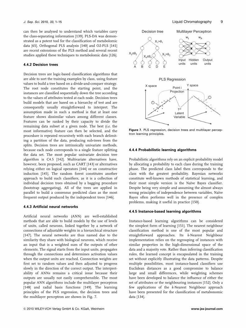
Projection to latent structures by means of partial least

squares (PLS) [135, 136] is a well-established regression-

based method [136]. This technique is particularly adapted

to situations where fewer observations (i.e. number of

different observed objects, N) than measured variables (e.g.m/z, detected features, K) are available. Its use has become

very popular, thanks to its ability to deal with many

correlated and noisy variables forming megavariate data

structures (K�N) [137, 138]. PLS builds a low dimensional

sub-space based on linear combinations of the original X-

variables and makes use of the additional Y information by

adjusting the model to capture the Y-related variation in X.

A PLS-based classification therefore has the property that it

builds data structures with an intrinsic prediction power, by

maximising the covariance between the data and the class

assignment. The decomposition relies on latent variables

that are computed sequentially to provide a good correlation

with the remaining unexplained fraction of Y. In the context

of classification, PLS-DA is performed to sharpen the

partition between groups of observations, such that a

maximum separation among classes is obtained. The model

Principal Components Analysis

Hierarchical Cluster Analysis

Obj

ects

X1 X2 X3

X1 X2 X3

X2

X1

X3

t1

t2

t2

t1

Scores (objects)

Loadings (variables)

p2

p1

X1

X3X2

Obj

ects

X2

X1

X3

Figure 6. PCA and HCA learning principles.



can then be analysed to understand which variables carry

the class-separating information [139]. PLS-DA was demon-

strated as a potent tool for the classification of metabolomic

data [65]. Orthogonal PLS analysis [140] and O2-PLS [141]

are recent extensions of the PLS method and several recent

studies applied these techniques to metabolomic data [126].

4.4.2 Decision trees

Decision trees are logic-based classification algorithms that

are able to sort the training examples by class, using feature

values to build a tree based on a divide-and-conquer strategy.

The root node constitutes the starting point, and the

instances are classified sequentially down the tree according

to the values of attributes tested at each node. Decision trees

build models that are based on a hierarchy of test and are

consequently usually straightforward to interpret. The

assumption made in such a method is that at least one

feature shows dissimilar values among different classes.

Features can be ranked by their capacity to divide the

remaining data subset at a given node. The best (i.e. the

most informative) feature can then be selected, and the

procedure is repeated recursively with each branch delimit-

ing a partition of the data, producing sub-trees from the

splits. Decision trees are intrinsically univariate methods,

because each node corresponds to a single feature splitting

the data set. The most popular univariate decision tree

algorithm is C4.5 [142]. Multivariate alternatives have,

however, been proposed, such as CART [143] or alternatives

relying either on logical operators [144] or on constructive

induction [145]. The random forest constitutes another

approach to build such classifiers, as it is a collection of

individual decision trees obtained by a bagging procedure

(bootstrap aggregating). All of the trees are applied in

parallel to build a consensus predicted class as the most

frequent output produced by the independent trees [146].

4.4.3 Artificial neural networks

Artificial neural networks (ANN) are well-established

methods that are able to build models by the use of levels

of units, called neurons, linked together by a network of

connections of adjustable weights in a hierarchical structure

[147]. The neural networks are thus named due to the

similarity they share with biological neurons, which receive

an input that is a weighted sum of the outputs of other

elements. The signal starts from the input units, propagates

through the connections and determines activation values

when the output units are reached. Connection weights are

first set to random values and then adjusted to progress

slowly in the direction of the correct output. The interpret-

ability of ANNs remains a critical issue because their

outputs are usually not easily comprehensible. The most

popular ANN algorithms include the multilayer perceptron

[148] and radial basis functions [149]. The learning

principles of the PLS regression, the decision trees and

the multilayer perceptron are shown in Fig. 7.

4.4.4 Probabilistic learning algorithms

Probabilistic algorithms rely on an explicit probability model

by allocating a probability to each class during the training

phase. The predicted class label then corresponds to the

class with the greatest probability. Bayesian networks

constitute well-known methods of statistical learning, and

their most simple version is the Naıve Bayes classifier.

Despite being very simple and assuming the almost always

wrong principles of independence between variables, Naıve

Bayes often performs well in the presence of complex

problems, making it useful in practice [150].

4.4.5 Instance-based learning algorithms

Instance-based learning algorithms can be considered

the simplest form of learning [151]. The nearest neighbour

classification method is one of the most popular and

straightforward approaches. Its k-Nearest Neighbour

implementation relies on the regrouping of instances with

similar properties in the high-dimensional space of the

data and a majority vote. Rather than inferring classification

rules, the learned concept is encapsulated in the training

set without explicitly illustrating the data patterns. Despite

multiple possibilities, most instance-based classifiers use

Euclidean distances as a good compromise to balance

large and small differences, while weighting schemes

have been developed to balance the influence of either the

set of attributes or the neighbouring instances [152]. Only a

few applications of the k-Nearest Neighbour approach

have been presented for the classification of metabonomic

data [134].

Multilayer PerceptronDecision tree

PLS Regression

X1>θ1

X3>θ3X2≤θ2

X4≤θ4Input units

Output units

Hidden units

wij wjk

X space Y spacePoint i

Projection

1st

LatentVariable

i

i

A B C D E

Figure 7. PLS regression, decision trees and multilayer percep-tron learning principles.



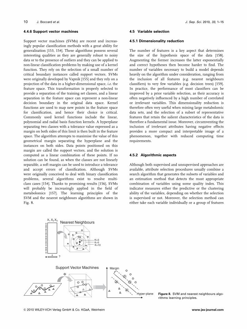
4.4.6 Support vector machines

Support vector machines (SVMs) are recent and increas-

ingly popular classification methods with a great ability for

generalisation [153, 154]. These algorithms possess several

interesting qualities as they are generally robust to noisy

data or to the presence of outliers and they can be applied to

non-linear classification problems by making use of a kernel

function. They rely on the selection of a small number of

critical boundary instances called support vectors. SVMs

were originally developed by Vapnik [155] and they rely on a

projection of the data in a higher-dimensional space, i.e. the

feature space. This transformation is properly selected to

provide a separation of the training set classes, and a linear

separation in the feature space can represent a non-linear

decision boundary in the original data space. Kernel

functions are used to map new points in the feature space

for classification, and hence their choice is critical.

Commonly used kernel functions include the linear,

polynomial and radial basis function kernels. A hyperplane

separating two classes with a tolerance value expressed as a

margin on both sides of this limit is then built in the feature

space. The algorithm attempts to maximise the value of this

geometrical margin separating the hyperplane and the

instances on both sides. Data points positioned on this

margin are called the support vectors, and the solution is

computed as a linear combination of these points. If no

solution can be found, as when the classes are not linearly

separable, a soft margin can be used to introduce a tolerance

and accept errors of classification. Although SVMs

were originally conceived to deal with binary classification

problems, several algorithms exist to resolve multi-

class cases [154]. Thanks to promising results [156], SVMs

will probably be increasingly applied in the field of

metabolomics [157]. The learning principles of the

SVM and the nearest neighbours algorithms are shown in

Fig. 8.

4.5 Variable selection

4.5.1 Dimensionality reduction

The number of features is a key aspect that determines

the size of the hypothesis space of the data [158].

Augmenting the former increases the latter exponentially

and correct hypotheses then become harder to find. The

number of variables necessary to build a model depends

heavily on the algorithm under consideration, ranging from

the inclusion of all features (e.g. nearest neighbours

classifiers) to very few variables (e.g. decision trees) [159].

In practice, the performance of most classifiers can be

improved by a prior variable selection, as their accuracy is

often negatively influenced by a high number of correlated

or irrelevant variables. This dimensionality reduction is

therefore often very useful when mining large metabolomic

data sets, and the selection of a subset of representative

features that retain the salient characteristics of the data is

therefore a fundamental issue. Moreover, circumventing the

inclusion of irrelevant attributes having negative effects

provides a more compact and interpretable image of a

phenomenon, together with reduced computing time

requirements.

4.5.2 Algorithmic aspects

Although both supervised and unsupervised approaches are

available, attribute selection procedures usually combine a

search algorithm that generates the subsets of variables and

an estimation method that detects the most appropriate

combination of variables using some quality index. This

indicator measures either the predictive or the clustering

ability of the variables, depending on whether the selection

is supervised or not. Moreover, the selection method can

either take each variable individually or a group of features

+

Nearest NeighboursX1 X2 X3

+ ?

? K=3K=5K=10

Support Vector Machines

Φ

Margin

Hyper-plane Figure 8. SVM and nearest neighbours algo-rithms learning principles.



into consideration. Due to its nature, individual feature

evaluation is unable to detect feature interactions. Moreover,

a totally uninformative variable can significantly enhance

the predictive ability in the context of other variables.

Two main approaches are usually proposed, the filter

and the wrapper methodologies [160]. The filter selection

relies generally on a pre-processing evaluation system that is

independent from the learning phase. A quality index can

be measured for individual or groups of attributes, and

although it can be derived from a classifier, it does not

directly rely on the prediction accuracy. Among several

methods, feature ranking represents a simple supervised

approach to filter the most valuable variables. Several

ranking criteria are available to find variables that discri-

minate between the observed classes, including the analysis

of variance [161] and Recursive Elimination of Features [162,

163]. On the other hand, algorithms that build linear models

provide rankings by comparing the coefficients of features,

such as orthogonal signal correction [164]. Other methods

use different indicators, such as the information gain [165]

based on entropy, to quantify the information content of a

variable. Such rankings imply, however, the determination

of a suitable number of features to select. Methods that

eliminate redundant variables by allocating a goodness

measure to subsets of the attributes are able to take the

inter-correlations into account [166]. The correlation issue

can be addressed either by selecting only one of the corre-

lated variables within a group, such as correlation-based

feature selection, or by building new features starting from

the original correlated variables (feature construction/

transformation).

On the other hand, wrapper selection relies on the

predictive accuracy of a learning algorithm as a quality index

of a features subset, e.g. SVM-based feature selection. As the

assortment giving raise to the best performance is kept,

the selection is an integrated part of the learning phase and

the number of features can be automatically determined.

The wrapper model is computationally very expensive when

dealing with a large number of features and the selection is

evidently oriented by the choice of the classifier used as a

black box [167]. Finally, by combining complementary filter

selection and learning algorithms relying on distinct learn-

ing principles, performance can be improved by the

strengths of both methods.

4.6 Algorithms comparison

Selecting a particular classification algorithm from the wide

variety of available methods constitutes a critical operation.

Despite numerous measures of performance, such as

sensitivity, specificity and the Kappa coefficient [168, 169],

the performance of a classifier is most often based on its

prediction accuracy, i.e. the percentage of correctly predicted

examples over the total number of predictions. However,

this single value is not sufficiently informative when dealing

with a limited number of observations, as this estimate will

be completely optimistic. Several schemes are available for

the robust evaluation of this accuracy to avoid overfitting,

but the most popular include the repeated cross-validation

and the prediction of an independent test set. By evaluating

the accuracies of multiple algorithms using cross-validation,

each experiment provides an independent error estimate

[170]. Moreover, distinct costs of misclassification errors can

be defined to avoid a given type of error, e.g. false positives

or negatives. These results are then used to determine

whether the average accuracy value of a particular algorithm

is significantly greater or lower than another by performing

a Student’s t-test for statistical comparison [171]. The sub-

sampling of the whole data set to generate subsets, however,

is in contradiction with the independency statement

required by hypothesis testing, and a test should not

depend on the partitioning of the data set. Several heuristic

solutions have been proposed to counteract this difficulty,

such as the corrected resampled t-test [172]. Repeated

random partitioning of ten folds is commonly used to

evaluate the prediction accuracies by examining their

replicability.

5 Concluding remarks

Deciphering complex biological systems and processes

requires detailed descriptions of the systems under study

as well as data mining techniques suitable to handle large

amounts of information. As continued data accumulation is

inevitable, finding automatically the valuable but hidden

information in metabolomic data of high dimensionality is

already a crucial issue. Data mining, therefore, has a central

role to play by making sense of data and inferring the

structures governing biological phenomena. Indeed, these

methods will have more and more opportunities to prove

their worth when dealing with massive data sets and may

lead to fruitful results by helping to decode complex

phenomena. However, the relevant answers will not come

from computer programs but from the people working with

the data and understanding its related characteristics and

issues.

On the other hand, an increasing number of metabo-

lomic studies rely on multiple analytical platforms

combining GC-, LC-, CE-MS or NMR data. Merging the

information from data of different natures and structures

and extracting the common traits will undoubtedly consti-

tute a key issue in the perspective of a more comprehensive

vision of metabolomics. In addition, the merging with data

from other Omic technologies, such as transcriptomics and

proteomics will probably offer a deeper insight into the

regulatory networks in systems biology and will definitely

represent another great challenge. Modelling all types

of regulatory events occurring within a cell in a holistic

manner is expected to provide a global view of the

system.

The authors have declared no conflict of interest.



6 References

[1] Nicholson, J. K., Lindon, J. C., Holmes, E., Xenobiotica1999, 29, 1181–1189.

[2] Sumner, L. W., Mendes, P., Dixon, R. A., Phytochem-istry 2003, 62, 817–836.

[3] Hollywood, K., Brison, D. R., Goodacre, R., Proteomics2006, 6, 4716–4723.

[4] Oksman-Caldentey, K. M., Saito, K., Curr. Opin.Biotechnol. 2005, 16, 174–179.

[5] Oresic, M., Clish, C. B., Davidov, E. J., Verheij, E.,Vogels, J., Havekes, L. M., Neumann, E., Adourian, A.,Naylor, S., van der Greef, J., Plasterer, T., Appl.Bioinformatics 2004, 3, 205–217.

[6] Keun, H. C., Pharmacol. Ther. 2006, 109, 92–106.

[7] Plumb, R. S., Dear, G. J., Mallett, D. N., Higton, D. M.,Pleasance, S., Biddlecombe, R. A., Xenobiotica 2001,31, 599–617.

[8] Forster, J., Famili, I., Fu, P., Pjzalsson, B. O., Nielsen, J.,Genome Res. 2003, 13, 244–253.

[9] Ackermann, B. L., Hale, J. E., Duffin, K. L., Curr. DrugMetab. 2006, 7, 525–539.

[10] van der Greef, J., Martin, S., Juhasz, P., Adourian, A.,Plasterer, T., Verheij, E. R., McBurney, R. N.,J. Proteome Res. 2007, 6, 1540–1559.

[11] Sreekumar, A., Poisson, L. M., Rajendiran, T. M., Khan,A. P., Cao, Q., Yu, J. D., Laxman, B., Mehra, R., Lonigro,R. J., Li, Y., Nyati, M. K., Ahsan, A., Kalyana-Sundaram,S., Han, B., Cao, X. H., Byun, J., Omenn, G. S., Ghosh,D., Pennathur, S., Alexander, D. C., Berger, A., Shuster,J. R., Wei, J. T., Varambally, S., Beecher, C., Chinnai-yan, A. M., Nature 2009, 457, 910–914.

[12] Lindon, J. C., Nicholson, J. K., Holmes, E., Antti, H.,Bollard, M. E., Keun, H., Beckonert, O., Ebbels, T. M.,Reilly, M. D., Robertson, D., Stevens, G. J., Luke, P.,Breau, A. P., Cantor, G. H., Bible, R. H., Niederhauser,U., Senn, H., Schlotterbeck, G., Sidelmann, U. G.,Laursen, S. M., Tymiak, A., Car, B. D., Lehman-McKeeman, L., Colet, J. M., Loukaci, A., Thomas, C.,Toxicol. Appl. Pharmacol. 2003, 187, 137–146.

[13] Dieterle, F., Schlotterbeck, G. T., Ross, A., Niederhauser,U., Senn, H., Chem. Res. Toxicol. 2006, 19, 1175–1181.

[14] Wishart, D. S., Trends Food Sci. Technol. 2008, 19,482–493.

[15] Weckwerth, W., Annu. Rev. Plant. Biol. 2003, 54,669–689.

[16] Fiehn, O., Plant Mol. Biol. 2002, 48, 155–171.

[17] Atherton, H. J., Bailey, N. J., Zhang, W., Taylor, J.,Major, H., Shockcor, J., Clarke, K., Griffin, J. L., Physiol.Genomics 2006, 27, 178–186.

[18] Dunn, W. B., Ellis, D., Trends Anal. Chem. 2005, 24,285–294.

[19] Jonsson, P., Gullberg, J., Nordstrom, A., Kusano, M.,Kowalczyk, M., Sjostrom, M., Moritz, T., Anal. Chem.2004, 76, 1738–1745.

[20] Sinha, A. E., Hope, J. L., Prazen, B. J., Nilsson, E. J.,Jack, R. M., Synovec, R. E., J. Chromatogr. A 2004,1058, 209–215.

[21] Veriotti, T., Sacks, R., Anal. Chem. 2001, 73, 4395–4402.

[22] Wagner, C., Sefkow, M., Kopka, J., Phytochemistry2003, 62, 887–900.

[23] Kopka, J., J. Biotechnol. 2006, 124, 312–322.

[24] Huhman, D. V., Sumner, L. W., Phytochemistry 2002,59, 347–360.

[25] Idborg, H., Zamani, L., Edlund, P. O., Schuppe-Koisti-nen, I., Jacobsson, S. P., J. Chromatogr. B 2005, 828,9–13.

[26] Wolfender, J. L., Terreaux, C., Hostettmann, K., Pharm.Biol. 2000, 38, 41–54.

[27] Ramautar, R., Demirci, A., de Jong, G. J., Trends Anal.Chem. 2006, 25, 455–466.

[28] Garcia-Perez, I., Vallejo, M., Garcia, A., Legido-Quigley,C., Barbas, C., J. Chromatogr. A 2008, 1204, 130–139.

[29] Soga, T., Ohashi, Y., Ueno, Y., Naraoka, H., Tomita, M.,Nishioka, T., J. Proteome Res. 2003, 2, 488–494.

[30] von Roepenack-Lahaye, E., Degenkolb, T., Zerjeski, M.,Franz, M., Roth, U., Wessjohann, L., Schmidt, J., Scheel,D., Clemens, S., Plant Physiol. 2004, 134, 548–559.

[31] Krishnan, P., Kruger, N. J., Ratcliffe, R. G., J. Exp. Bot.2005, 56, 255–265.

[32] Wolfender, J. L., Ndjoko, K., Hostettmann, K., Phyto-chem. Anal. 2001, 12, 2–22.

[33] Brown, S. C., Kruppa, G., Dasseux, J. L., Mass Spec-trom. Rev. 2005, 24, 223–231.

[34] Brown, K., Tompkins, E. M., White, I. N. H., MassSpectrom. Rev. 2006, 25, 127–145.

[35] Brown, M., Dunn, W. B., Ellis, D. I., Goodacre, R.,Handl, J., Knowles, J. D., O’Hagan, S., Spasic, I., Kell,D. B., Metabolomics 2005, 1, 39–51.

[36] van der Greef, J., van der Heijden, R., Verheij, E. R.,Adv. Mass Spectrom. 2004, 16, 145–165.

[37] Werner, E., Heilier, J. F., Ducruix, C., Ezan, E., Junot, C.,Tabet, J. C., J. Chromatogr. B 2008, 871, 143–163.

[38] Dunn, W. B., Phys. Biol. 2008, 5, 11001.

[39] Taylor, A. J., Linforth, R. S. T., Int. J. Spectrom. 2003,223, 179–191.

[40] van der Greef, J., Niessen, W. M. A., Int. J. MassSpectrom. Ion Process. 1992, 118, 857–873.

[41] Villas-Boas, S. G., Mas, S., Akesson, M., Smedsgaard,J., Nielsen, J., Mass Spectrom. Rev. 2005, 24,613–646.

[42] Robards, K., Haddad, P. R., Jackson, P. E., Principlesand Practice of Modern Chromatographic Methods,Academic Press, London 1996.

[43] Roessner, U., Wagner, C., Kopka, J., Trethewey, R. N.,Willmitzer, L., Plant J. 2000, 23, 131–142.

[44] Halket, J. M., Zaikin, V. G., Eur. J. Mass Spectrom.2003, 9, 1–21.

[45] Halket, J. M., Waterman, D., Przyborowska, A. M.,Patel, R. K. P., Fraser, P. D., Bramley, P. M., J. Exp. Bot.2005, 56, 219–243.

[46] Zaikin, V. G., Halket, J. M., Eur. J. Mass Spectrom.2003, 9, 421–434.

[47] Horning, E. C., Clin. Chem. 1968, 14, 777.

[48] Pauling, L., Robinson, A. B., Teranish, R., Cary, P., Proc.Natl. Acad. Sci. USA 1971, 68, 2374–2376.



[49] Schauer, N., Steinhauser, D., Strelkov, S., Schomburg,D., Allison, G., Moritz, T., Lundgren, K., Roessner-Tunali, U., Forbes, M. G., Willmitzer, L., Fernie, A. R.,Kopka, J., FEBS Lett. 2005, 579, 1332–1337.

[50] Beens, J., Brinkman, U. A. T., Analyst 2005, 130, 123–127.

[51] Idborg, H., Edlund, P. O., Jacobsson, S. P., RapidCommun. Mass. Spectrom. 2004, 18, 944–954.

[52] Niessen, W. M. A., J. Chromatogr. A 1999, 856,179–197.

[53] Tolstikov, V. V., Lommen, A., Nakanishi, K., Tanaka, N.,Fiehn, O., Anal. Chem. 2003, 75, 6737–6740.

[54] Wang, C., Kong, H. W., Guan, Y. F., Yang, J., Gu, J. R.,Yang, S. L., Xu, G. W., Anal. Chem. 2005, 77,4108–4116.

[55] Ding, J., Sorensen, C. M., Zhang, Q. B., Jiang, H. L.,Jaitly, N., Livesay, E. A., Shen, Y. F., Smith, R. D., Metz,T. O., Anal. Chem. 2007, 79, 6081–6093.

[56] Dear, G. J., Ayrton, J., Plumb, R., Fraser, I. J., RapidCommun. Mass. Spectrom. 1999, 13, 456–463.

[57] Swartz, M. E., J. Liquid Chromatogr. Rel. Technol.2005, 28, 1253–1263.

[58] Plumb, R. S., Rainville, P., Smith, B. W., Johnson, K. A.,Castro-Perez, J., Wilson, I. D., Nicholson, J. K., Anal.Chem. 2006, 78, 7278–7283.

[59] Stoll, D. R., Cohen, J. D., Carr, P. W., J. Chromatogr.A 2006, 1122, 123–137.

[60] Grata, E., Boccard, J., Guillarme, D., Glauser, G.,Carrupt, P. A., Farmer, E. E., Wolfender, J. L., Rudaz, S.,J. Chromatogr. B Analyt. Technol. Biomed. Life Sci.2008, 871, 261–270.

[61] Maruska, A., Kornysova, O., J. Chromatogr. A 2006,1112, 319–330.

[62] Pham-Tuan, H., Kaskavelis, L., Daykin, C. A., Janssen,H. G., J. Chromatogr. B 2003, 789, 283–301.

[63] Hendriks, M. M. W. B., Cruz-Juarez, L., De Bont, D.,Hall, R., Anal. Chim. Acta 2005, 545, 53–64.

[64] van den Berg, R. A., Hoefsloot, H. C. J., Westerhuis,J. A., Smilde, A. K., van der Werf, M. J., Biomed.Chromatogr. Genomics 2006, 7.

[65] Jonsson, P., Bruce, S. J., Moritz, T., Trygg, J., Sjoes-troem, M., Plumb, R., Granger, J., Maibaum, E.,Nicholson, J. K., Holmes, E., Antti, H., Analyst 2005,130, 701–707.

[66] Hilario, M., Kalousis, A., Pellegrini, C., Muller, M., MassSpectrom. Rev. 2006, 25, 409–449.

[67] Katajamaa, M., Oresic, M., J. Chromatogr. A 2007,1158, 318–328.

[68] Davis, R. A., Charlton, A. J., Godward, J., Jones, S. A.,Harrison, M., Wilson, J. C., Chemometric Intell. Lab.Syst. 2007, 85, 144–154.

[69] Fleming, C. M., Kowalski, B. R., Apffel, A., Hancock,W. S., J. Chromatogr. A 1999, 849, 71–85.

[70] Radulovic, D., Jelveh, S., Ryu, S., Hamilton, T. G., Foss,E., Mao, Y., Emili, A., Mol. Cell. Proteom. 2004, 3,984–997.

[71] Wang, W., Zhou, H., Lin, H., Roy, S., Shaler, T. A., Hill,L. R., Norton, S., Kumar, P., Anderle, M., Becker, C. H.,Anal. Chem. 2003, 75, 4818–4826.

[72] Li, X. J., Yi, E. C., Kemp, C. J., Zhang, H., Aebersold, R.,Mol. Cell. Proteom. 2005, 4, 1328–1340.

[73] Hastings, C. A., Norton, S. M., Roy, S., Rapid Commun.Mass. Spectrom. 2002, 16, 462–467.

[74] Katajamaa, Mi., Oresic, M., Biomed. Chromatogr.Bioinformatics 2005, 6, 179.

[75] Smith, C. A., Want, E. J., O’Maille, G., Abagyan, R.,Siuzdak, G., Anal. Chem. 2006, 78, 779–787.

[76] Eanes, R. C., Marcus, R. K., Spectrochim. Acta B. At.Spectrosc. 2000, 55B, 403–428.

[77] Hermansson, M., Uphoff, A., Kakela, R., Somerharju,P., Anal. Chem. 2005, 77, 2166–2175.

[78] Leptos, K. C., Sarracino, D. A., Jaffe, J. D., Krastins, B.,Church, G. M., Proteomics 2006, 6, 1770–1782.

[79] Windig, W., Phalp, J. M., Payne, A. W., Anal. Chem.1996, 68, 3602–3606.

[80] Windig, W., Smith, W. F., J. Chromatogr. A 2007, 1158,251–257.

[81] Gika, H. G., Macpherson, E., Theodoridis, G. A.,Wilson, I. D., J. Chromatogr. B 2008, 871, 299–305.

[82] Lange, E., Tautenhahn, R., Neumann, S., Gropl, C.,Biomed Chromatogr. Bioinformatics 2008, 9, 375.

[83] Nordstrom, A., O’Maille, G., Qin, C., Siuzdak, G., Anal.Chem. 2006, 78, 3289–3295.

[84] Johnson, K. J., Wright, B. W., Jarman, K. H., Synovec,R. E., J. Chromatogr. A 2003, 996, 141–155.

[85] Wang, C. P., Isenhour, T. L., Anal. Chem. 1987, 59,649–654.

[86] Bylund, D., Danielsson, R., Malmquist, G., Markides,K. E., J. Chromatogr. A 2002, 961, 237–244.

[87] Tomasi, G., van den Berg, F., Andersson, C.,J. Chemometrics 2004, 18, 231–241.

[88] Prince, J. T., Marcotte, E. M., Anal. Chem. 2006, 78,6140–6152.

[89] Nielsen, N. P. V., Carstensen, J. M., Smedsgaard, J.,J. Chromatogr. A 1998, 805, 17–35.

[90] Pravdova, V., Walczak, B., Massart, D. L., Anal. Chim.Acta 2002, 456, 77–92.

[91] De Souza, D. P., Saunders, E. C., McConville, M. J.,Likic, V. A., Bioinformatics 2006, 22, 1391–1396.

[92] Shen, H. L., Grung, B., Kvalheim, O. M., Eide, I., Anal.Chim. Acta 2001, 446, 313–328.

[93] Andreev, V. P., Rejtar, T., Chen, H. S., Moskovets, E. V.,Ivanov, A. R., Karger, B. L., Anal. Chem. 2003, 75,6314–6326.

[94] Scholz, M., Gatzek, S., Sterling, A., Fiehn, O., Selbig, J.,Bioinformatics 2004, 20, 2447–2454.

[95] Bijlsma, S., Bobeldijk, L., Verheij, E. R., Ramaker, R.,Kochhar, S., Macdonald, I. A., van Ommen, B., Smilde,A. K., Anal. Chem. 2006, 78, 567–574.

[96] Wu, L., Mashego, M. R., van Dam, J. C., Proell, A. M.,Vinke, J. L., Ras, C., van Winden, W. A., van Gulik,W. M., Heijnen, J. J., Anal. Biochem. 2005, 336,164–171.

[97] Birkemeyer, C., Luedemann, A., Wagner, C.,Erban, A., Kopka, J., Trends Biotechnol. 2005, 23,28–33.



[98] Baran, R., Kochi, H., Saito, N., Suematsu, M., Soga, T.,Nishioka, T., Robert, M., Tomita, M., Biomed Chro-matogr. Bioinformatics 2006, 7, 530.

[99] Vorst, O., De Vos, C. H. R., Lommen, A., Staps, R. V.,Visser, R. G. F., Bino, R. J., Hall, R. D., Metabolomics2005, 1, 169–180.

[100] Duran, A. L., Yang, J., Wang, L., Sumner, L. W.,Bioinformatics 2003, 19, 2283–2293.

[101] Neuweger, H., Albaum, S. P., Dondrup, M., Persicke,M., Watt, T., Niehaus, K., Stoye, J., Goesmann, A.,Bioinformatics 2008, 24, 2726–2732.

[102] Idborg-Bjorkman, H., Edlund, P. O., Kvalheim, O. M.,Schuppe-Koistinen, I., Jacobsson, S. P., Anal. Chem.2003, 75, 4784–4792.

[103] Lenz, E. M., Bright, J., Knight, R., Westwood, F. R.,Davies, D., Major, H., Wilson, I. D., Biomarkers 2005,10, 173–187.

[104] Sadygov, R. G., Maroto, F. M., Huhmer, A. F. R., Anal.Chem. 2006, 78, 8207–8217.

[105] Idborg, H., Zamani, L., Edlund, P. O., Schuppe-Koistinen,I., Jacobsson, S. P., J. Chromatogr. B 2005, 828, 14–20.

[106] Kind, T., Tolstikov, V., Fiehn, O., Weiss, R. H., Anal.Biochem. 2007, 363, 185–195.

[107] Bro, R., Smilde, A. K., J. Chemometrics 2003, 17, 16–33.

[108] Jackson, J. E., A User’s Guide to Principal Compo-nents, Wiley Interscience, New York 2004.

[109] Eriksson, L., Johansson, E., Kettaneh-Wold, N., Wold,S., Multi- and Megavariate Data Analysis: Principlesand Applications, Umetrics Academy, Umea, Sweden2002.

[110] Keun, H. C., Ebbels, T. M. D., Antti, H., Bollard, M. E.,Beckonert, O., Holmes, E., Lindon, J. C., Nicholson,J. K., Anal. Chim. Acta 2003, 490, 265–276.

[111] Smilde, A. K., van der Werf, M. J., Bijlsma, S., van derWerff-van der Vat, B., Jellema, R. H., Anal. Chem. 2005,77, 6729–6736.

[112] Kvalheim, O. M., Brakstad, F., Liang, Y. Z., Anal. Chem.1994, 66, 43–51.

[113] Sokal, R. R., Rohlf, F. J., Biometry: The Principles andPractice of Statistics in Biological Research, W. H.Freeman and Company, New York 1995.

[114] Weckwerth, W., Morgenthal, K., Drug Discov. Today2005, 10, 1551–1558.

[115] Broadhurst, D. I., Kell, D. B., Metabolomics 2006, 2,171–196.

[116] Holmes, E., Antti, H., Analyst 2002, 127, 1549–1557.

[117] Massart, D. L., Vandeginste, B. G. M., Buydens,L. M. C., De Jong, S., Lewi, P. J., Smeyers-Verbeke, J.(Eds.), Handbook of Chemometrics and Qualimetrics,Part A, Elsevier, Oxford, UK 1997.

[118] Eriksson, L., Antti, H., Gottfries, J., Holmes, E., Johans-son, E., Lindgren, F., Long, I., Lundstedt, T., Trygg, J.,Wold, S., Anal. Bioanal. Chem. 2004, 380, 419–429.

[119] Hotelling, H., J. Educat. Psychol. 1933, 24, 417–441.

[120] Trygg, J., Gullberg, J., Johansson, A. I., Jonsson, P.,Moritz, T., Biotechnol. Agri. Forestry 2006, 57, 117–128.

[121] Wiener, M. C., Sachs, J. R., Deyanova, E., Yates, N. A.,Anal. Chem. 2004, 76, 6085–6096.

[122] Shaffer, J. P., Ann. Rev. Psychol. 1995, 46, 561–584.

[123] Schauer, N., Zamir, D., Fernie, A. R., J. Exp. Bot. 2005,56, 297–307.

[124] Serkova, N. J., Jackman, M., Brown, J. L., Liu, T.,Hirose, R., Roberts, J. P., Maher, J. J., Niemann, C. U.,J. Hepatol. 2006, 44, 956–962.

[125] Pearson, K., Philos. Mag. 1901, 2, 559–572.

[126] Major, H. J., Williams, R., Wilson, A. J., Wilson, I. D.,Rapid Commun. Mass Spectrom. 2006, 20, 3295–3302.

[127] Pierce, K. M., Hope, J. L., Hoggard, J. C., Synovec,R. E., Talanta 2006, 70, 797–804.

[128] Bylund, D., Samskog, J., Markides, K. E., Jacobsson,S. P., J. Am. Soc. Mass Spectrom. 2003, 14, 236–240.

[129] Belton, P. S., Colquhoun, I. J., Kemsley, E. K., Delga-dillo, I., Roma, P., Dennis, M. J., Sharman, M., Holmes,E., Nicholson, J. K., Spraul, M., Food Chem. 1998, 61,207–213.

[130] Jansen, J. J., Hoefsloot, H. C. J., Boelens, H. F. M., vander Greef, J., Smilde, A. K., Bioinformatics 2004, 20,2438–2446.

[131] Chan, E. C. Y., Yap, S. L., Lau, A. J., Leow, P. C., Toh,D. F., Koh, H. L., Rapid Commun. Mass Spectrom.2007, 21, 519–528.

[132] Eisen, M. B., Spellman, P. T., Brown, P. O., Botstein, D.,Proc. Natl. Acad. Sci. USA 1998, 95, 14863–14868.

[133] Tikunov,Y., Lommen, A., De Vos, C. H. R., Verhoeven,H. A., Bino, R. J., Hall, R. D., Bovy, A. G., Plant Physiol.2005, 139, 1125–1137.

[134] Beckonert, O., Bollard, M. E., Ebbels, T. M. D., Keun,H. C., Antti, H., Holmes, E., Lindon, J. C., Nicholson, J.K., Anal. Chim. Acta 2003, 490, 3–15.

[135] Wold, S., Johansson, E., Cocchi, M., 3D QSAR in DrugDesign: Theory, Methods and Applications, EscomScience Publisher, Leiden 1993, pp. 523–550.

[136] Wold, S., Sjostrom, M., Eriksson, L., ChemometricIntell. Lab. Syst. 2001, 58, 109–130.

[137] Kettaneh-Wold, N., Chemometric Intell. Lab. Syst.1992, 14, 57–69.

[138] Wold, S., Ruhe, A., Wold, H., Dunn, W. J., Siam J., Sci.Stat. Comput. 1984, 5, 735–743.

[139] Daszykowski, M., Walczak, B., Massart, D. L., Chemo-metric Intell. Lab. Syst. 2003, 65, 97–112.

[140] Trygg, J., Wold, S., J. Chemometrics 2002, 16, 119–128.

[141] Trygg, J., Wold, S., J. Chemometrics 2003, 17, 53–64.

[142] Quinlan, J. R., J. Artif. Intell. Res. 1996, 4, 77–90.

[143] Breiman, L., Friedman, J. H., Olshen, R. A., Stone, C. J.,Classification and Regression Trees, Wadsworth &Brooks, Monterey, CA, USA 1984.

[144] Zheng, Z. J., Knowl-Based Syst. 1998, 10, 421–430.

[145] Gama, J., Adv. Intell. Data Anal. 1997, 1280, 187–198.

[146] Breiman, L., Mach. Learn. 2001, 45, 5–32.

[147] Gallant, S. I., IEEE Trans. Neural Netw. 1990, 1,179–191.

[148] Taylor, J., King, R. D., Altmann, T., Fiehn, O., Bioin-formatics 2002, 18, S241–S248.

[149] Poggio, T., Girosi, F., Proc. IEEE 1990, 78, 1481–1497.

[150] Hand, D. J., Yu, K. M., Int. Stat. Rev. 2001, 69, 385–398.



[151] Aha, D. W., Kibler, D., Albert, M. K., Mach. Learn. 1991,6, 37–66.

[152] Wettschereck, D., Aha, D. W., Mohri, T., Artif. Intell.Rev. 1997, 11, 273–314.

[153] Keerthi, S. S., Gilbert, E. G., Mach. Learn. 2002, 46,351–360.

[154] Platt, J., IEEE Intell. Syst. 1998, 13, 26–28.

[155] Vapnik, V. N., IEEE Trans. Neural Netw. 1999, 10, 988–999.

[156] Guyon, I., Weston, J., Barnhill, S., Vapnik, V., Mach.Learn. 2002, 46, 389–422.

[157] Mahadevan, S., Shah, S. L., Marrie, T. J., Slupsky,C. M., Anal. Chem. 2008, 80, 7562–7570.

[158] Mitchell, T. M., Machine Learning, McGraw Hill HigherEducation, New York 1997.

[159] Hall, M. A., Holmes, G., IEEE Trans. Knowl. Data En.2003, 15, 1437–1447.

[160] Guyon, I., Elisseeff, A., J. Mach. Learn. Res. 2003, 3,1157–1182.

[161] Fisher, R. A., Statistical Methods for Research Workers,Oliver and Boyd, Edinburgh, UK 1925.

[162] Robnik-Sikonja, M., Kononenko, I., Mach. Learn. 2003,53, 23–69.

[163] Kononenko, I., Simec, E., Robnik-Sikonja, M., Appl.Intell. 1997, 7, 39–55.

[164] Wold, S., Antti, H., Lindgren, F., Ohman, J., Chemo.Intell. Lab. Syst. 1998, 44, 175–185.

[165] Kullback, S., Ann. Math. Stat. 1952, 23, 88–102.

[166] Yu, L., Liu, H., J. Mach. Learn. Res. 2004, 5, 1205–1224.

[167] Kohavi, R., John, G. H., Artif. Intell. 1997, 97, 273–324.

[168] Cohen, J., Edu. Psychol. Meas. 1960, 20, 37–46.

[169] Fleiss, J. L., Psychol. Bull. 1971, 76, 378–382.

[170] Bousquet, O., Elisseeff, A., J. Mach. Learn. Res. 2002,2, 499–526.

[171] Dietterich, T. G., Neural Comput. 1998, 10,1895–1923.

[172] Nadeau, C., Bengio, Y., Mach. Learn. 2003, 52,239–281.

[173] Pierce, K. M., Hoggard, J. C., Mohler, R. E., Synovec, R.E., J. Chromatogr. A 2008, 1184, 341–352.



Knowledge discovery in metabolomics: An overview of MS data handling

Documents