Advanced Information and Knowledge Processing Series Editors Professor Lakhmi J ain [email protected]u Professor Xindong W u [email protected] Also in this series Gregoris Mentzas, Dimitris Apostolou, Andreas Abecker and Ron Young Knowledge Asset Management 1-85233-583-1 Michalis Vazirgiannis, Maria Halkidi and Dimitrios Gunopulos Uncertainty Handling and Quality Assessment in Data Mining 1-85233-655-2 Asunción Gómez-Pérez, Mariano Fernández-López and Oscar Corcho Ontological Engineering 1-85233-551-3 Arno Scharl (Ed.) Environmental Online Communication 1-85233-783-4 Shichao Zhang, Chengqi Zhang and Xindong Wu Knowledge Discovery in Multiple Databases 1-85233-703-6 Jason T.L. Wang, Mohammed J. Zaki, Hannu T.T. Toivonen and Dennis Shasha (Eds) Data Mining in Bioinformatics 1-85233-671-4 C.C. Ko, Ben M. Chen and Jianping Chen Creating Web-based Laboratories 1-85233-837-7 Manuel Graña, Richard Duro, Alicia d’Anjou and Paul P. Wang (Eds) Information Processing with Evolutionary Algorithms 1-85233-886-0 Colin Fyfe Hebbian Learning and Negative Feedback Networks 1-85233-883-0 Yun-Heh Chen-Burger and Dave Robertson Automating Business Modelling 1-85233-835-0

Welcome message from author
This document is posted to help you gain knowledge. Please leave a comment to let me know what you think about it! Share it to your friends and learn new things together.
Transcript

Advanced Information and Knowledge Processing
Series EditorsProfessor Lakhmi [email protected]
Professor Xindong [email protected]
Also in this series
Gregoris Mentzas, Dimitris Apostolou, Andreas Abecker and Ron YoungKnowledge Asset Management1-85233-583-1
Michalis Vazirgiannis, Maria Halkidi and Dimitrios GunopulosUncertainty Handling and Quality Assessment in Data Mining1-85233-655-2
Asunción Gómez-Pérez, Mariano Fernández-López and Oscar CorchoOntological Engineering1-85233-551-3
Arno Scharl (Ed.)Environmental Online Communication1-85233-783-4
Shichao Zhang, Chengqi Zhang and Xindong WuKnowledge Discovery in Multiple Databases1-85233-703-6
Jason T.L. Wang, Mohammed J. Zaki, Hannu T.T. Toivonen and Dennis Shasha (Eds)Data Mining in Bioinformatics1-85233-671-4
C.C. Ko, Ben M. Chen and Jianping ChenCreating Web-based Laboratories1-85233-837-7
Manuel Graña, Richard Duro, Alicia d’Anjou and Paul P. Wang (Eds)Information Processing with Evolutionary Algorithms1-85233-886-0
Colin FyfeHebbian Learning and Negative Feedback Networks1-85233-883-0
Yun-Heh Chen-Burger and Dave RobertsonAutomating Business Modelling1-85233-835-0

Dirk Husmeier, Richard Dybowski and Stephen Roberts (Eds)Probabilistic Modeling in Bioinformatics and Medical Informatics1-85233-778-8
Ajith Abraham, Lakhmi Jain and Robert Goldberg (Eds)Evolutionary Multiobjective Optimization1-85233-787-7
K.C. Tan, E.F.Khor and T.H. LeeMultiobjective Evolutionary Algorithms and Applications1-85233-836-9
Nikhil R. Pal and Lakhmi Jain (Eds)Advanced Techniques in Knowledge Discovery and Data Mining1-85233-867-9
Yannis Manolopoulos, Alexandros Nanopoulos, Apostolos N. Papadopoulos, Yannis TheodoridisR-trees: Theory and Applications1-85233-977-2
Miroslav Kárný (Ed.)Optimized Bayesian Dynamic Advising1-85233-928-4
Sifeng Liu and Yi LinGrey Information1-85233-955-0
Amit Konar and Lakhmi JainCognitive Engineering1-85233-975-6

Sanghamitra Bandyopadhyay, Ujjwal Maulik, Lawrence B. Holder and Diane J. Cook (Eds)
Advanced Methodsfor KnowledgeDiscovery from
g
Complex Datay
With 120 Figures
123

Sanghamitra Bandyopadhyay, PhDMachine Intelligence Unit, Indian Statistical Institute, Kolkata, India
Ujjwal Maulik, PhDDepartment of Computer Science & Engineering, Jadavpur University, Kolkata, India
Lawrence B. Holder, PhDDiane J. Cook, PhDDepartment of Computer Science & Engineering, University of Texas at Arlington, USA
British Library Cataloguing in Publication DataA catalogue record for this book is available from the British Library
Library of Congress Control Number: 2005923138
Apart from any fair dealing for the purposes of research or private study, or criticism or review, as permitted under the Copyright, Designs and Patents Act 1988, this publication may only be reproduced, stored or transmitted, in any form or by any means, with the prior permission in writing of the publishers, or in the case of reprographic reproduction in accordance with the terms of licences issuedby the Copyright Licensing Agency. Enquiries concerning reproduction outside those terms should besent to the publishers.
AI&KP ISSN 1610-3947
ISBN 1-85233-989-6Springer Science+Business Mediaspringeronline.com
© Dr Sanghamitra Bandyopadhyay 2005
The use of registered names, trademarks etc. in this publication does not imply, even in the absence of a specific statement, that such names are exempt from the relevant laws and regulations and thereforefifree for general use.
The publisher makes no representation, express or implied, with regard to the accuracy of the information contained in this book and cannot accept any legal responsibility or liability for any errors or omissions that may be made.
Typesetting: Electronic text files prepared by editorsfiPrinted in the United States of America34-543210 Printed on acid-free paper SPIN 11013006

To our parents, for their unflinching support, andto Utsav, for his unquestioning love.
S. Bandyopadhyay and U. Maulik
To our parents, for their constant love and support.L. Holder and D. Cook

Contents
Contributors . . . . . . . . . . . . . . . . . . . . . . . . . . . . . . . . . . . . . . . . . . . . . . . . . . . ix
Preface . . . . . . . . . . . . . . . . . . . . . . . . . . . . . . . . . . . . . . . . . . . . . . . . . . . . . . . . xv
Part I Foundations
1 Knowledge Discovery and Data MiningSanghamitra Bandyopadhyay, Ujjwal Maulik . . . . . . . . . . . . . . . . . . . . . . . . 3
2 Automatic Discovery of Class Hierarchies via Output SpaceDecompositionJoydeep Ghosh, Shailesh Kumar and Melba M. Crawford . . . . . . . . . . . . 43
3 Graph-based Mining of Complex DataDiane J. Cook, Lawrence B. Holder, Jeff Coble and Joseph Potts . . . . . . . 75
4 Predictive Graph Mining with Kernel MethodsThomas Gartner . . . . . . . . . . . . . . . . . . . . . . . . . . . . . . . . . . . . . . . . . . . . . . . . . 95
5 TreeMiner: An Efficient Algorithm for Mining EmbeddedOrdered Frequent TreesMohammed J. Zaki . . . . . . . . . . . . . . . . . . . . . . . . . . . . . . . . . . . . . . . . . . . . . . 123
6 Sequence Data MiningSunita Sarawagi . . . . . . . . . . . . . . . . . . . . . . . . . . . . . . . . . . . . . . . . . . . . . . . . . 153
7 Link-based ClassificationLise Getoor . . . . . . . . . . . . . . . . . . . . . . . . . . . . . . . . . . . . . . . . . . . . . . . . . . . . . 189

viii Contents
Part II Applications
8 Knowledge Discovery from Evolutionary TreesSen Zhang, Jason T. L. Wang . . . . . . . . . . . . . . . . . . . . . . . . . . . . . . . . . . . . . 211
9 Ontology-Assisted Mining of RDF DocumentsTao Jiang, Ah-Hwee Tan . . . . . . . . . . . . . . . . . . . . . . . . . . . . . . . . . . . . . . . . . . 231
10 Image Retrieval using Visual Features and RelevanceFeedbackSanjoy Kumar Saha, Amit Kumar Das and Bhabatosh Chanda . . . . . . . . . 253
11 Significant Feature Selection Using ComputationalIntelligent Techniques for Intrusion DetectionSrinivas Mukkamala and Andrew H. Sung . . . . . . . . . . . . . . . . . . . . . . . . . . . 285
12 On-board Mining of Data Streams in Sensor NetworksMohamed Medhat Gaber, Shonali Krishnaswamy and Arkady Zaslavsky . 307
13 Discovering an Evolutionary Classifier over a High-speedNonstatic StreamJiong Yang, Xifeng Yan, Jiawei Han and Wei Wang . . . . . . . . . . . . . . . . . 337
Index . . . . . . . . . . . . . . . . . . . . . . . . . . . . . . . . . . . . . . . . . . . . . . . . . . . . . . . . . . 365

Contributors
Sanghamitra BandyopadhyayMachine Intelligence UnitIndian Statistical InstituteKolkata, [email protected]
Bhabatosh ChandaElectronics and Communication Sciences UnitIndian Statistical InstituteKolkata, [email protected]
Jeff CobleDepartment of Computer Science and EngineeringUniversity of Texas at ArlingtonArlington, Texas [email protected]
Diane J. CookDepartment of Computer Science and EngineeringUniversity of Texas at ArlingtonArlington, Texas [email protected]
Melba M. CrawfordThe University of Texas at AustinAustin, Texas [email protected]

x Contributors
Amit K. DasComputer Science and Technology DepartmentBengal Engineering College (Deemed University)Kolkata, [email protected]
Mohamed M. GaberSchool of Computer Science and Software EngineeringMonash [email protected]
Thomas GartnerFraunhofer Institut Autonome Intelligente [email protected]
Lise GetoorDepartment of Computer Science and UMIACSUniversity of Maryland, College ParkMaryland, [email protected]
Joydeep GhoshThe University of Texas at AustinAustin, Texas [email protected]
Jiawei HanUniversity of Illinois at Urbana-ChampaignUrbana-Champaign, Illinois [email protected]
Lawrence B. HolderDepartment of Computer Science and EngineeringUniversity of Texas at ArlingtonArlington, Texas [email protected]

Contributors xi
Tao JiangSchool of Computer EngineeringNanyang Technological UniversityNanyang Avenue, [email protected]
Shonali KrishnaswamySchool of Computer Science and Software EngineeringMonash [email protected]
Shailesh KumarFair Isaac CorporationSan Diego, California [email protected]
Ujjwal MaulikDepartment of Computer Science and EngineeringJadavpur UniversityKolkata, [email protected]
Srinivas MukkamalaDepartment of Computer ScienceNew Mexico Tech, Socorro, [email protected]
Joseph PottsDepartment of Computer Science and EngineeringUniversity of Texas at ArlingtonArlington, Texas [email protected]

xii Contributors
Sanjoy K. SahaDepartment of Computer Science and EngineeringJadavpur UniversityKolkata, [email protected]
Sunita SarawagiDepartment of Information TechnologyIndian Institute of TechnologyMumbai, [email protected]
Andrew H. SungDepartment of Computer ScienceInstitute for Complex Additive Systems AnalysisNew Mexico Tech, Socorro, [email protected]
Ah-Hwee TanSchool of Computer EngineeringNanyang Technological UniversityNanyang Avenue, [email protected]
Jason T. L. WangDepartment of Computer ScienceNew Jersey Institute of TechnologyUniversity HeightsNewark, New Jersey [email protected]
Wei WangUniversity of North Carolina at Chapel HillChapel Hill, North Carolina [email protected]
Xifeng YanUniversity of Illinois, Urbana-ChampaignUrbana-Champaign, Illinois [email protected]

Contributors xiii
Jiong YangCase Western Reserve UniversityCleveland, Ohio [email protected]
Mohammed J. ZakiComputer Science DepartmentRensselaer Polytechnic InstituteTroy, New York [email protected]
Arkady ZaslavskySchool of Computer Science and Software EngineeringMonash [email protected]
Sen ZhangDepartment of Mathematics, Computer Science and Statistics,State University of New York, OneontaOneonta, New York [email protected]

Preface
The growth in the amount of data collected and generated has exploded inrecent times with the widespread automation of various day-to-day activities,advances in high-level scientific and engineering research and the developmentof efficient data collection tools. This has given rise to the need for automati-cally analyzing the data in order to extract knowledge from it, thereby makingthe data potentially more useful.
Knowledge discovery and data mining (KDD) is the process of identifyingvalid, novel, potentially useful and ultimately understandable patterns frommassive data repositories. It is a multi-disciplinary topic, drawing from sev-eral fields including expert systems, machine learning, intelligent databases,knowledge acquisition, case-based reasoning, pattern recognition and statis-tics.
Many data mining systems have typically evolved around well-organizeddatabase systems (e.g., relational databases) containing relevant information.But, more and more, one finds relevant information hidden in unstructuredtext and in other complex forms. Mining in the domains of the world-wideweb, bioinformatics, geoscientific data, and spatial and temporal applicationscomprise some illustrative examples in this regard. Discovery of knowledge,or potentially useful patterns, from such complex data often requires the ap-plication of advanced techniques that are better able to exploit the natureand representation of the data. Such advanced methods include, among oth-ers, graph-based and tree-based approaches to relational learning, sequencemining, link-based classification, Bayesian networks, hidden Markov models,neural networks, kernel-based methods, evolutionary algorithms, rough setsand fuzzy logic, and hybrid systems. Many of these methods are developed inthe following chapters.
In this book, we bring together research articles by active practitionersreporting recent advances in the field of knowledge discovery, where the in-formation is mined from complex data, such as unstructured text from theworld-wide web, databases naturally represented as graphs and trees, geoscien-tific data from satellites and visual images, multimedia data and bioinformaticdata. Characteristics of the methods and algorithms reported here include theuse of domain-specific knowledge for reducing the search space, dealing with

xvi Preface
uncertainty, imprecision and concept drift, efficient linear and/or sub-linearscalability, incremental approaches to knowledge discovery, and increased leveland intelligence of interactivity with human experts and decision makers. Thetechniques can be sequential, parallel or stream-based in nature.
The book has been divided into two main sections: foundations and appli-cations. The chapters in the foundations section present general methods formining complex data. In Chapter 1, Bandyopadhyay and Maulik present anoverview of the field of data mining and knowledge discovery. They discussthe main concepts of the field, the issues and challenges, and recent trendsin data mining, which provide the context for the subsequent chapters onmethods and applications.
In Chapter 2, Ghosh, Kumar and Crawford address the issue of high di-mensionality in both the attributes and class values of complex data. Theirapproach builds a binary hierarchical classifier by decomposing the set ofclasses into smaller partitions and performing a two-class learning problembetween each partition. The simpler two-class learning problem often allows areduction in the dimensionality of the attribute space. Their approach showsimprovement over other approaches to the multi-class learning problem andalso results in the discovery of knowledge in the form of the class hierarchy.
Cook, Holder, Coble and Potts describe techniques for mining complexdata represented as a graph in Chapter 3. Many forms of complex data in-volve entities, their attributes, and their relationships to other entities. Itis these relationships that make appropriate a graph representation of thedata. The chapter describes numerous techniques based on the core Subduemethodology that uses data compression as a metric for interestingness inmining knowledge from the graph data. These techniques include supervisedand unsupervised learning, clustering and graph grammar learning. They ad-dress efficiency issues by introducing an incremental approach to processingstreaming graph data. They also introduce a method for mining graphs inwhich relevant examples are embedded, possibly overlapping, in one largegraph. Numerous successes are documented in a number of domains.
In Chapter 4, Gartner also presents techniques for mining graph data,but these techniques are based on kernel methods which implicitly map thegraph data to a higher-dimensional, non-relational space where learning iseasier, thus avoiding the computational complexity of graph operations formatching and covering. While kernel methods have been applied to singlegraphs, Gartner introduces kernels that apply to sets of graphs and shows theireffectiveness on problems from the fields of relational reinforcement learningand molecular classification.
While graphs represent one of the most expressive forms of complex datarepresentations, some specializations of graphs (e.g., trees) still allow the rep-resentation of significant relational information, but with reduced computa-tional cost. In Chapter 5, Zaki presents a technique called TreeMiner forfinding all frequent subtrees in a forest of trees and compares this approachto a pattern-matching approach. Zaki shows results indicating a significant

Preface xvii
increase in speed over the pattern-matching approach and applies the newtechnique to the problem of mining usage patterns from real logs of websitebrowsing behavior.
Another specialized form in which complex data might be expressed is a se-quence. In Chapter 6, Sarawagi discusses several methods for mining sequencedata, i.e., data modeled as a sequence of discrete multi-attribute records. Shereviews state-of-the-art techniques in sequence mining and applies these to tworeal applications: address cleaning and information extraction from websites.
In Chapter 7, Getoor returns to the more general graph representation ofcomplex data, but includes probabilistic information about the distributionof links (or relationships) between entities. Getoor uses a structured logisticregression model to learn patterns based on both links and entity attributes.Results in the domains of web browsing and citation collections indicate thatthe use of link distribution information improves classification performance.
The remaining chapters constitute the applications section of the book.Significant successes have been achieved in a wide variety of domains, indi-cating the potential benefits of mining complex data, rather than applyingsimpler methods on simpler transformations of the data. Chapter 8 beginswith a contribution by Zhang and Wang describing techniques for miningevolutionary trees, that is, trees whose parent–child relationships representactual evolutionary relationships in the domain of interest. A good example,and one to which they apply their approach, is phylogenetic trees that describethe evolutionary pathways of species at the molecular level. Their algorithmefficiently discovers “cousin pairs,” which are two nodes sharing a commonancestor, in a single tree or a set of trees. They present numerous experimen-tal results showing the efficiency and effectiveness of their approach in bothsynthetic and real domains, namely, phylogenic trees.
In Chapter 9, Jiang and Tan apply a variant of the Apriori-based associ-ation rule-mining algorithm to the relational domain of Resource DescriptionFramework (RDF) documents. Their approach treats RDF relations as itemsin the traditional association-rule mining framework. Their approach alsotakes advantage of domain ontologies to provide generalizations of the RDFrelations. They apply their technique to a synthetically-generated collection ofRDF documents pertaining to terrorism and show that the method discoversa small set of association rules capturing the main associations known to bepresent in the domain.
Saha, Das and Chanda address the task of content-based image retrievalby mapping image data into complex data using features based on shape,texture and color in Chapter 10. They also develop an image retrieval sim-ilarity measure based on human perception and improve retrieval accuracyusing feedback to establish the relevance of the various features. The authorsempirically validate the superiority of their method over competing methodsof content-based image retrieval using two large image databases.
In Chapter 11, Mukkamala and Sung turn to the problem of intrusiondetection. They perform a comparative analysis of three advanced mining

xviii Preface
methods: support vector machines, multivariate adaptive regression splines,and linear genetic programs. Overall, they found that the three methods per-formed similarly on the intrusion detection problem. However, they also foundthat a significant increase in performance was possible using feature selection,where the above three mining methods were used to rank features by rele-vance. Their conclusions are empirically validated using the DARPA intrusiondetection benchmark database.
One scenario affecting the above methods for mining complex data is theincreasing likelihood that data will be collected via a continuous stream. InChapter 12, Gaber, Krishnaswamy and Zaslavsky present a theoretical frame-work for mining algorithms applied to this scenario based on a model of on-board, resource-constrained mining. They apply their model to the task ofon-board mining of data streams in sensor networks. In addition to this gen-eral framework they have also developed lightweight mining algorithms forclustering, classification and frequent itemset discovery. Their model and al-gorithms are empirically validated using synthetic streaming data and theresource-constrained environment of a common handheld computer.
Finally, in Chapter 13, Yang, Yan, Han and Wang also consider the taskof mining data streams. They specifically focus on the constraints that themining algorithm scan the data only once and adapt to evolving patternspresent in the data stream. They develop an evolutionary classifier based on anaive Bayesian classifier and employ a train-and-test method combined witha divergence measure to detect evolving characteristics of the data stream.They perform extensive empirical testing based on synthetic data to show theefficiency and effectiveness of their approach.
In summary, the chapters on the foundations and applications of miningcomplex data provide a representative selection of the available methods andtheir evaluation in real domains. While the field is rapidly evolving into newalgorithms and new types of complex data, these chapters clearly indicatethe importance and potential benefit of developing such algorithms to minecomplex data. The book may be used either in a graduate level course aspart of the subject of data mining, or as a reference book for research workersworking in different aspects of mining complex data.
We take this opportunity to thank all the authors for contributing chaptersrelated to their current research work that provide the state of the art inadvanced methods for mining complex data. We are grateful to Mr S. Santraof Machine Intelligence Unit, Indian Statistical Institute, Kolkata, India, forproviding technical assistance during the preparation of the final manuscript.Finally, a vote of thanks to Ms Catherine Drury of Springer Verlag LondonLtd. for her initiative and constant support.
January, 2005 Sanghamitra BandyopadhyayUjjwal Maulik
Lawrence B. HolderDiane J. Cook

Part I
Foundations

1
Knowledge Discovery and Data Mining
Sanghamitra Bandyopadhyay and Ujjwal Maulik
Summary. Knowledge discovery and data mining has recently emerged as an im-portant research direction for extracting useful information from vast repositories ofdata of various types. This chapter discusses some of the basic concepts and issuesinvolved in this process with special emphasis on different data mining tasks. Themajor challenges in data mining are mentioned. Finally, the recent trends in datamining are described and an extensive bibliography is provided.
1.1 Introduction
The sheer volume and variety of data that is routinely being collected as aconsequence of widespread automation is mind-boggling. With the advantageof being able to store and retain immense amounts of data in easily accessibleform comes the challenge of being able to integrate the data and make senseout of it. Needless to say, this raw data potentially stores a huge amount ofinformation, which, if utilized appropriately, can be converted into knowledge,and hence wealth for the human race. Data mining (DM) and knowledgediscovery (KD) are related research directions that have emerged in the recentpast for tackling the problem of making sense out of large, complex data sets.
Traditionally, manual methods were employed to turn data into knowl-edge. However, sifting through huge amounts of data manually and makingsense out of it is slow, expensive, subjective and prone to errors. Hence theneed to automate the process arose; thereby leading to research in the fieldsof data mining and knowledge discovery. Knowledge discovery from databases(KDD) evolved as a research direction that appears at the intersection of re-search in databases, machine learning, pattern recognition, statistics, artificialintelligence, reasoning with uncertainty, expert systems, information retrieval,signal processing, high performance computing and networking.
Data stored in massive repositories is no longer only numeric, but could begraphical, pictorial, symbolic, textual and linked. Typical examples of somesuch domains are the world-wide web, geoscientific data, VLSI chip layout
4 Sanghamitra Bandyopadhyay and Ujjwal Maulik
and routing, multimedia, and time series data as in financial markets. More-over, the data may be very high-dimensional as in the case of text/documentrepresentation. Data pertaining to the same object is often stored in differentforms. For example, biologists routinely sequence proteins and store them infiles in a symbolic form, as a string of amino acids. The same protein may alsobe stored in another file in the form of individual atoms along with their threedimensional co-ordinates. All these factors, by themselves or when taken to-gether, increase the complexity of the data, thereby making the developmentof advanced techniques for mining complex data imperative. A cross-sectionalview of some recent approaches employing advanced methods for knowledgediscovery from complex data is provided in the different chapters of this book.For the convenience of the reader, the present chapter is devoted to the de-scription of the basic concepts and principles of data mining and knowledgediscovery, and the research issues and challenges in this domain. Recent trendsin KDD are also mentioned.
1.2 Steps in the Process of Knowledge Discovery
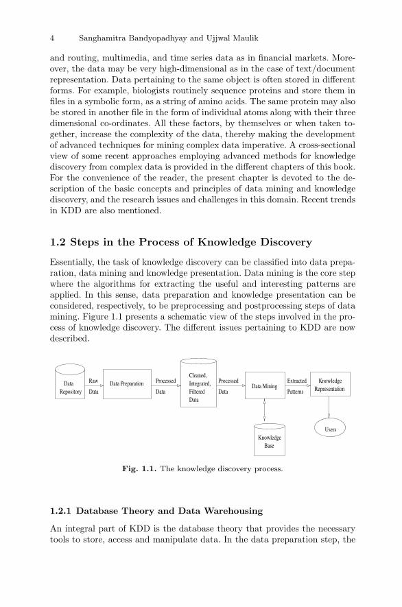
Essentially, the task of knowledge discovery can be classified into data prepa-ration, data mining and knowledge presentation. Data mining is the core stepwhere the algorithms for extracting the useful and interesting patterns areapplied. In this sense, data preparation and knowledge presentation can beconsidered, respectively, to be preprocessing and postprocessing steps of datamining. Figure 1.1 presents a schematic view of the steps involved in the pro-cess of knowledge discovery. The different issues pertaining to KDD are nowdescribed.
RepositoryData Data PreparationRaw
Data
Processed
Data
Cleaned,Integrated,FilteredData
Processed
DataData Mining
Extracted
Patterns RepresentationKnowledge
BaseKnowledge
Users
Fig. 1.1. The knowledge discovery process.
1.2.1 Database Theory and Data Warehousing
An integral part of KDD is the database theory that provides the necessarytools to store, access and manipulate data. In the data preparation step, the

1.2 Steps in the Process of Knowledge Discovery 5
data is first cleaned to reduce noisy, erroneous and missing data as far aspossible. The different sub tasks of the data preparation step are often per-formed iteratively by utilizing the knowledge gained in the earlier steps in thesubsequent phases. Once the data is cleaned, it may need to be integratedsince there could be multiple sources of the data. After integration, furtherredundancy removal may need to be carried out. The cleaned and integrateddata is stored in databases or data warehouses.
Data warehousing [40, 66] refers to the tasks of collecting and cleaningtransactional data to make them available for online analytical processing(OLAP). A data warehouse includes [66]:
• Cleaned and integrated data: This allows the miner to easily look acrossvistas of data without bothering about matters such as data standardiza-tion, key determination, tackling missing values and so on.
• Detailed and summarized data: Detailed data is necessary when the mineris interested in looking at the data in its most granular form and is nec-essary for extracting important patterns. Summary data is important fora miner to learn about the patterns in the data that have already beenextracted by someone else. Summarized data ensures that the miner canbuild on the work of others rather than building everything from scratch.
• Historical data: This helps the miner in analyzing past trends/seasonalvariations and gaining insights into the current data.
• Metadata: This is used by the miner to describe the context and the mean-ing of the data.
It is important to note that data mining can be performed without thepresence of a data warehouse, though data warehouses greatly improve theefficiency of data mining. Since databases often constitute the repository ofdata that has to be mined, it is important to study how the current databasemanagement system (DBMS) capabilities may be utilized and/or enhancedfor efficient mining [64].
As a first step, it is necessary to develop efficient algorithms for imple-menting machine learning tools on top of large databases and utilizing theexisting DBMS support. The implementation of classification algorithms suchas C4.5 or neural networks on top of a large database requires tighter couplingwith the database system and intelligent use of coupling techniques [53, 64].For example, clustering may require efficient implementation of the nearestneighbor algorithms on top of large databases.
In addition to developing algorithms that can work on top of existingDBMS, it is also necessary to develop new knowledge and data discoverymanagement systems (KDDMS) to manage KDD systems [64]. For this it isnecessary to define KDD objects that may be far more complex than databaseobjects (records or tuples), and queries that are more general than SQL andthat can operate on the complex objects. Here, KDD objects may be rules,classifiers or a clustering [64]. The KDD objects may be pre-generated (e.g.,as a set of rules) or may be generated at run time (e.g., a clustering of the

6 Sanghamitra Bandyopadhyay and Ujjwal Maulik
data objects). KDD queries may now involve predicates that can return aclassifier, rule or clustering as well as database objects such as records ortuples. Moreover, KDD queries should satisfy the concept of closure of a querylanguage as a basic design paradigm. This means that a KDD query may takeas argument another compatible type of KDD query. Also KDD queries shouldbe able to operate on both KDD objects and database objects. An exampleof such a KDD query may be [64]: “Generate a classifier trained on a userdefined training set generated though a database query with user definedattributes and user specified classification categories. Then find all records inthe database that are wrongly classified using that classifier and use that setas training data for another classifier.” Some attempts in this direction maybe found in [65, 120].
1.2.2 Data Mining
Data mining is formally defined as the process of discovering interesting, pre-viously unknown and potentially useful patterns from large amounts of data.Patterns discovered could be of different types such as associations, subgraphs,changes, anomalies and significant structures. It is to be noted that the termsinteresting and potentially useful are relative to the problem and the con-cerned user. A piece of information may be of immense value to one userand absolutely useless to another. Often data mining and knowledge discov-ery are treated as synonymous, while there exists another school of thoughtwhich considers data mining to be an integral step in the process of knowledgediscovery.
Data mining techniques mostly consist of three components [40]: a model,a preference criterion and a search algorithm. The most common model func-tions in current data mining techniques include classification, clustering, re-gression, sequence and link analysis and dependency modeling. Model rep-resentation determines both the flexibility of the model for representing theunderlying data and the interpretability of the model in human terms. Thisincludes decision trees and rules, linear and nonlinear models, example-basedtechniques such as NN-rule and case-based reasoning, probabilistic graphicaldependency models (e.g., Bayesian network) and relational attribute models.
The preference criterion is used to determine, depending on the under-lying data set, which model to use for mining, by associating some measureof goodness with the model functions. It tries to avoid overfitting of the un-derlying data or generating a model function with a large number of degreesof freedom. Finally, once the model and the preference criterion are selected,specification of the search algorithm is defined in terms of these along withthe given data.
1.2.3 Knowledge Presentation
Presentation of the information extracted in the data mining step in a formateasily understood by the user is an important issue in knowledge discovery.

1.3 Tasks in Data Mining 7
Since this module communicates between the users and the knowledge dis-covery step, it goes a long way in making the entire process more useful andeffective. Important components of the knowledge presentation step are datavisualization and knowledge representation techniques. Presenting the infor-mation in a hierarchical manner is often very useful for the user to focusattention on only the important and interesting concepts. This also enablesthe users to see the discovered patterns at multiple levels of abstraction. Somepossible ways of knowledge presentation include:
• rule and natural language generation,• tables and cross tabulations,• graphical representation in the form of bar chart, pie chart and curves,• data cube view representation, and• decision trees.
The following section describes some of the commonly used tasks in datamining.
1.3 Tasks in Data Mining
Data mining comprises the algorithms employed for extracting patterns fromthe data. In general, data mining tasks can be classified into two categories,descriptive and predictive [54]. The descriptive techniques provide a summaryof the data and characterize its general properties. The predictive techniqueslearn from the current data in order to make predictions about the behavior ofnew data sets. The commonly used tasks in data mining are described below.
1.3.1 Association Rule Mining
The root of the association rule mining problem lies in the market basket ortransaction data analysis. A lot of information is hidden in the thousands oftransactions taking place daily in supermarkets. A typical example is thatif a customer buys butter, bread is almost always purchased at the sametime. Association analysis is the discovery of rules showing attribute–valueassociations that occur frequently.
Let I = i1, i2, . . . , in be a set of n items and X be an itemset where X ⊂I. A k-itemset is a set of k items. Let T = (t1, X1), (t2, X2) . . . , (tm, Xm) bea set of m transactions, where ti and Xi, i = 1, 2, . . . , m, are the transactionidentifier and the associated itemset respectively. The cover of an itemset Xin T is defined as follows:
cover(X, T ) = ti|(ti, Xi) ∈ T, X ⊂ Xi. (1.1)
The support of an itemset X in T is
support(X, T ) = |cover(X, T )| (1.2)

8 Sanghamitra Bandyopadhyay and Ujjwal Maulik
and the frequency of an itemset is
frequency(X, T ) =support(X, T )
|T | . (1.3)
In other words, support of an itemset X is the number of transactions whereall the items in X appear in each transaction. The frequency of an itemsetrepresents the probability of its occurrence in a transaction in T . An itemset iscalled frequent if its support in T is greater than some threshold min sup. Thecollection of frequent itemsets with respect to a minimum support min supin T , denoted by F(T, min sup) is defined as
F(T, min sup) = X ⊂ I, support(X, T ) > min sup. (1.4)
The objective in association rule mining is to find all rules of the formX ⇒ Y , X
⋂Y = ∅ with probability c%, indicating that if itemset X occurs
in a transaction, the itemset Y also occurs with probability c%. X is calledthe antecedent of the rule and Y is called the consequent of the rule. Supportof a rule denotes the percentage of transactions in T that contains both Xand Y . This is taken to be the probability P (X
⋃Y ). An association rule is
called frequent if its support exceeds a minimum value min sup.The confidence of a rule X ⇒ Y in T denotes the percentage of the
transactions in T containing X that also contains Y . It is taken to be theconditional probability P (X|Y ). In other words,
confidence(X ⇒ Y, T ) =support(X
⋃Y, T )
support(X, T ). (1.5)
A rule is called confident if its confidence value exceeds a threshold min conf .The problem of association rule mining can therefore be formally stated asfollows: Find the set of all rules R of the form X ⇒ Y such that
R = X ⇒ Y |X, Y ⊂ I, X⋂
Y = ∅, X⋃Y = F(T, min sup),confidence(X ⇒ Y, T ) > min conf. (1.6)
Other than support and confidence measures, there are other measures ofinterestingness associated with association rules. Tan et al. [125] have pre-sented an overview of various measures proposed in statistics, machine learn-ing and data mining literature in this regard.
The association rule mining process, in general, consists of two steps:
1. Find all frequent itemsets,2. Generate strong association rules from the frequent itemsets.
Although this is the general framework adopted in most of the research inassociation rule mining [50, 60], there is another approach to immediatelygenerate a large subset of all association rules [132].

1.3 Tasks in Data Mining 9
The task of generating frequent itemsets is a challenging issue due to thehuge number of itemsets that must be considered. The number of itemsetsgrows exponentially with the number of items |I|. A commonly used algo-rithm for generating frequent itemsets is the Apriori algorithm [3, 4]. It isbased on the observation that if an itemset is frequent, then all its possiblesubsets are also frequent. Or, in other words, if even one subset of an item-set X is not frequent, then X cannot be frequent. Thus starting from all 1itemsets, and proceeding in a recursive fashion, if any itemset X is not fre-quent, then that branch of the tree is pruned, since any possible superset of Xcan never be frequent. Chapter 9 describes an approach based on the Apriorialgorithm for mining association rules from resource description frameworkdocuments, which is a data modeling language proposed by the World WideWeb Consortium (W3C) for describing and interchanging metadata aboutweb resources.
1.3.2 Classification
A typical pattern recognition system consists of three phases. These are dataacquisition, feature extraction and classification. In the data acquisition phase,depending on the environment within which the objects are to be classified,data are gathered using a set of sensors. These are then passed on to thefeature extraction phase, where the dimensionality of the data is reducedby measuring/retaining only some characteristic features or properties. In abroader perspective, this stage significantly influences the entire recognitionprocess. Finally, in the classification phase, the extracted features are passedon to the classifier that evaluates the incoming information and makes a fi-nal decision. This phase basically establishes a transformation between thefeatures and the classes.
The problem of classification is basically one of partitioning the featurespace into regions, one region for each category of input. Thus it attemptsto assign every data point in the entire feature space to one of the possible(say, k) classes. Classifiers are usually, but not always, designed with labeleddata, in which case these problems are sometimes referred to as supervisedclassification (where the parameters of a classifier function D are learned).Some common examples of the supervised pattern classification techniquesare the nearest neighbor (NN) rule, Bayes maximum likelihood classifier andperceptron rule [7, 8, 31, 36, 45, 46, 47, 52, 105, 127]. Figure 1.2 providesa block diagram showing the supervised classification process. Some of therelated classification techniques are described below.NN Rule [36, 46, 127]Let us consider a set of n pattern points of known classification x1,x2, . . . ,xn, where it is assumed that each pattern belongs to one of the classesC1, C2, . . . , Ck. The NN classification rule then assigns a pattern x of unknownclassification to the class of its nearest neighbor, where xi ∈ x1,x2, . . . ,xnis defined to be the nearest neighbor of x if

10 Sanghamitra Bandyopadhyay and Ujjwal Maulik
Training Set
Test Set
Learn the Classifier Produce Model
Unknown data Classify Data
ABSTRACTION PHASE
Model
GENERALIZATION PHASE
Fig. 1.2. The supervised classification process.
D(xi,x) = minlD(xl,x), l = 1, 2, . . . , n (1.7)
where D is any distance measure definable over the pattern space.Since the aforesaid scheme employs the class label of only the nearest
neighbor to x, this is known as the 1-NN rule. If k neighbors are consideredfor classification, then the scheme is termed as the k-NN rule. The k-NN ruleassigns a pattern x of unknown classification to class Ci if the majority of thek nearest neighbors belongs to class Ci. The details of the k-NN rule alongwith the probability of error is available in [36, 46, 127].
The k-NN rule suffers from two severe limitations. Firstly, all the n trainingpoints need to be stored for classification and, secondly, n distance compu-tations are required for computing the nearest neighbors. Some attempts atalleviating the problem may be found in [14].
Bayes Maximum Likelihood Classifier [7, 127]In most of the practical problems, the features are usually noisy and theclasses in the feature space are overlapping. In order to model such systems,the feature values x1, x2, . . . , xj , . . . , xN are considered as random values inthe probabilistic approach. The most commonly used classifier in such prob-abilistic systems is the Bayes maximum likelihood classifier, which is nowdescribed.
Let Pi denote the a priori probability and pi(x) denote the class condi-tional density corresponding to the class Ci (i = 1, 2, . . . , k). If the classifierdecides x to be from the class Ci, when it actually comes from Cl, it incursa loss equal to Lli. The expected loss (also called the conditional average lossor risk) incurred in assigning an observation x to the class Ci is given by

1.3 Tasks in Data Mining 11
ri(x) =k∑
l=1
Lli p(Cl/x), (1.8)
where p(Cl/x) represents the probability that x is from Cl. Using Bayes for-mula, Equation (1.8) can be written as,
ri(x) =1
p(x)
k∑l=1
Lli pl(x)Pl, (1.9)
where
p(x) =k∑
l=1
pl(x)Pl.
The pattern x is assigned to the class with the smallest expected loss. Theclassifier which minimizes the total expected loss is called the Bayes classifier.
Let us assume that the loss (Lli) is zero for correct decision and greaterthan zero but the same for all erroneous decisions. In such situations, theexpected loss, Equation (1.9), becomes
ri(x) = 1− Pipi(x)p(x)
. (1.10)
Since p(x) is not dependent upon the class, the Bayes decision rule is nothingbut the implementation of the decision functions
Di(x) = Pipi(x), i = 1, 2, . . . , k, (1.11)
where a pattern x is assigned to class Ci if Di(x) > Dl(x), ∀l = i. Thisdecision rule provides the minimum probability of error. It is to be noted thatif the a priori probabilities and the class conditional densities are estimatedfrom a given data set, and the Bayes decision rule is implemented using theseestimated values (which may be different from the actual values), then theresulting classifier is called the Bayes maximum likelihood classifier.
Assuming normal (Gaussian) distribution of patterns, with mean vectorµi and covariance matrix
∑i, the Gaussian density pi(x) may be written as
pi(x) = 1
(2π)N2 |∑
i|12
exp[ −12(x− µi)′∑
i−1(x− µi)], (1.12)
i = 1, 2, . . . , k.
Then, Di(x) becomes (taking log)
Di(x) = lnPi − 12 ln |∑i| −
12(x− µi)′∑
i−1(x− µi) (1.13)
i = 1, 2, . . . , k

12 Sanghamitra Bandyopadhyay and Ujjwal Maulik
Note that the decision functions in Equation (1.13) are hyperquadrics, sinceno terms higher than the second degree in the components of x appear in it.It can thus be stated that the Bayes maximum likelihood classifier for normaldistribution of patterns provides a second-order decision surface between eachpair of pattern classes. An important point to be mentioned here is that if thepattern classes are truly characterized by normal densities, then, on average,no other surface can yield better results. In fact, the Bayes classifier designedover known probability distribution functions, provides, on average, the bestperformance for data sets which are drawn according to the distribution. Insuch cases, no other classifier can provide better performance, on average, be-cause the Bayes classifier gives minimum probability of misclassification overall decision rules.
Decision TreesA decision tree is an acyclic graph, of which each internal node, branch andleaf node represents a test on a feature, an outcome of the test and classesor class distribution, respectively. It is easy to convert any decision tree intoclassification rules. Once the training data points are available, a decision treecan be constructed from them from top to bottom using a recursive divideand conquer algorithm. This process is also known as decision tree induction.A version of ID3 [112] , a well known decision-tree induction algorithm, isdescribed below.
Decision tree induction (training data points, features)
1. Create a node N.2. If all training data points belong to the same class (C) then return N as
a leaf node labelled with class C.3. If cardinality (features) is NULL then return N as a leaf node with the
class label of the majority of the points in the training data set.4. Select a feature (F) corresponding to the highest information gain label
node N with F.5. For each known value fi of F, partition the data points as si.6. Generate a branch from node N with the condition feature = fi.7. If si is empty then attach a leaf labeled with the most common class in
the data points.8. Else attach the node returned by Decision tree induction(si,(features-F)).
The information gain of a feature is measured in the following way. Letthe training data set (D) have n points with k distinct class labels. Moreover,let ni be the number of data points belonging to class Ci (for i = 1, 2, . . . , k).The expected information needed to classify the training data set is
I(n1, n2, . . . , nk) = −k∑
i=1
pi logb(pi) (1.14)

1.3 Tasks in Data Mining 13
where pi (= ni
n ) is the probability that a randomly selected data point belongsto class Ci. In case the information is encoded in binary the base b of the logfunction is set to 2. Let the feature space be d-dimensional, i.e., F has ddistance values f1, f2, . . . , fd, and this is used to partition the data pointsD into s subsets D1, D2, . . . , Ds. Moreover, let nij be the number of datapoints of class Ci in a subset Dj . The entropy or expected information basedon the partition by F is given by
E(A) =s∑
j=1
(n1j , n2j . . . nkj
n)I(n1j , n2j . . . nkj), (1.15)
where
I(n1j , n2j . . . nkj) = −j=k∑j=1
pij logb(pij). (1.16)
Here, pij is the probability that a data point in Di belongs to class Ci. Thecorresponding information gain by branching on F is given by
Gain(F ) = I(n1, n2, . . . , nk)− E(A). (1.17)
The ID3 algorithm finds out the feature corresponding to the highest informa-tion gain and chooses it as the test feature. Subsequently a node labelled withthis feature is created. For each value of the attribute, branches are generatedand accordingly the data points are partitioned.
Due to the presence of noise or outliers some of the branches of the deci-sion tree may reflect anomalies causing the overfitting of the data. In thesecircumstances tree-pruning techniques are used to remove the least reliablebranches, which allows better classification accuracy as well as convergence.
For classifying unknown data, the feature values of the data point aretested against the constructed decision tree. Consequently a path is tracedfrom the root to the leaf node that holds the class prediction for the test data.
Other Classification ApproachesSome other classification approaches are based on learning classification rules,Bayesian belief networks [68], neural networks [30, 56, 104], genetic algorithms[17, 18, 19, 20, 21, 100] and support vector machines [29]. In Chapter 2,a novel binary hierarchical classifier is built for tackling data that is high-dimensional in both the attributes and class values. Here, the set of classes isdecomposed into smaller partitions and a two-class learning problem betweeneach partition is performed. The simpler two-class learning problem oftenallows a reduction in the dimensionality of the attribute space.
1.3.3 Regression
Regression is a technique used to learn the relationship between one or moreindependent (or, predictor) variables and a dependent (or, criterion) variable.

14 Sanghamitra Bandyopadhyay and Ujjwal Maulik
The simplest form of regression is linear regression where the relationshipis modeled with a a straight line learned using the training data points asfollows.
Let us assume that for the input vector X (x1, x2, . . . , xn) (known as thepredictor variable), the value of the vector Y (known as the response variable)(y1, y2, . . . , yn) is known. A straight line through the vectors X,Y can bemodeled as Y = α + βX where α and β are the regression coefficients andslope of the line, computed as
β =∑n
i=1(xi − x∗)(yi − y∗)∑ni=1(xi − x∗)2
(1.18)
α = y∗ − βx∗ (1.19)
where x∗ and y∗ are the average of (x1, x2, . . . , xn) and (y1, y2, . . . , yn).An extension of linear regression which involves more than one predictor
variable is multiple regression. Here a response variable can be modeled as alinear function of a multidimensional feature vector. For example
Y = α + β1Xi + β2X2 + . . . + βnXn (1.20)
is a multiple regression model based on n predictor variables (X1, X2, . . . Xn).For evaluating α, β1 and β2, the least square method can be applied.
Data having nonlinear dependence may be modeled using polynomial re-gression. This is done by adding polynomial terms to the basic linear model.Transformation can be applied to the variable to convert the nonlinear modelinto a linear one. Subsequently it can be solved using the method of leastsquare. For example consider the following polynomial
Y = α + β1X + β2X2 + . . . + βnXn (1.21)
The above polynomial can be converted to the following linear form bydefining the new variables X1 = X, X2 = X2, . . . , Xn = Xn and can besolved using the method of least squares.
Y = α + β1X1 + β2X2 + . . . + βnXn (1.22)
1.3.4 Cluster Analysis
When the only data available are unlabelled, the classification problems aresometimes referred to as unsupervised classification. Clustering [6, 31, 55,67, 127] is an important unsupervised classification technique where a set ofpatterns, usually vectors in a multidimensional space, are grouped into clustersin such a way that patterns in the same cluster are similar in some sense andpatterns in different clusters are dissimilar in the same sense. For this it isnecessary to first define a measure of similarity which will establish a rulefor assigning patterns to a particular cluster. One such measure of similarity

1.3 Tasks in Data Mining 15
may be the Euclidean distance D between two patterns x and z defined byD = ‖x− z‖. The smaller the distance between x and z, the greater is thesimilarity between the two and vice versa.
Clustering in N -dimensional Euclidean space IRN is the process of par-titioning a given set of n points into a number, say K, of groups (or, clus-ters) based on some similarity/dissimilarity metric. Let the set of n pointsx1,x2, . . . ,xn be represented by the set S and the K clusters be repre-sented by C1, C2, . . . , CK . Then
Ci = ∅ for i = 1, . . . , K,Ci
⋂Cj = ∅ for i = 1, . . . , K, j = 1, . . . , K and i = j, and⋃K
i=1 Ci = S.
Clustering techniques may be hierarchical or non-hierarchical [6]. In hierar-chical clustering, the clusters are generated in a hierarchy, where every levelof the hierarchy provides a particular clustering of the data, ranging from asingle cluster (where all the points are put in the same cluster) to n clusters(where each point comprises a cluster). Among the non-hierarchical cluster-ing techniques, the K-means algorithm [127] has been one of the more widelyused ones; it consists of the following steps:
1. Choose K initial cluster centers z1, z2, . . . , zK randomly from the n pointsx1,x2, . . . ,xn.
2. Assign point xi, i = 1, 2, . . . , n to cluster Cj , j ∈ 1, 2, . . . , K iff
‖xi − zj‖ < ‖xi − zp‖, p = 1, 2, . . . , K, and j = p.
Ties are resolved arbitrarily.3. Compute new cluster centers z∗
1, z∗2, . . . , z
∗K as follows :
z∗i =
1ni
Σxj∈Cixj i = 1, 2, . . . , K,
where ni is the number of elements belonging to cluster Ci.4. If z∗
i = zi, i = 1, 2, . . . , K then terminate. Otherwise continue from Step2.
Note that if the process does not terminate at Step 4 normally, then it isexecuted for a maximum fixed number of iterations.
It has been shown in [119] that the K-means algorithm may converge tovalues that are not optimal. Also global solutions of large problems cannot befound within a reasonable amount of computation effort [122]. It is because ofthese factors that several approximate methods, including genetic algorithmsand simulated annealing [15, 16, 91], are developed to solve the underlyingoptimization problem. These methods have also been extended to the casewhere the number of clusters is variable [13, 92], and to fuzzy clustering [93].
The K-means algorithm is known to be sensitive to outliers, since suchpoints can significantly affect the computation of the centroid, and hence the

16 Sanghamitra Bandyopadhyay and Ujjwal Maulik
resultant partitioning. K-medoid attempts to alleviate this problem by us-ing the medoid, the most centrally located object, as the representative ofthe cluster. Partitioning around medoid (PAM) [75] was one of the earliestK-medoid algorithms introduced. PAM finds K clusters by first finding a rep-resentative object for each cluster, the medoid. The algorithm then repeatedlytries to make a better choice of medoids analyzing all possible pairs of objectssuch that one object is a medoid and the other is not. PAM is computation-ally quite inefficient for large data sets and large number of clusters. TheCLARA algorithm was proposed by the same authors [75] to tackle this prob-lem. CLARA is based on data sampling, where only a small portion of thereal data is chosen as a representative of the data and medoids are chosenfrom this sample using PAM. CLARA draws multiple samples and outputsthe best clustering from these samples. As expected, CLARA can deal withlarger data sets than PAM. However, if the best set of medoids is never chosenin any of the data samples, CLARA will never find the best clustering. Ng andHan [96] proposed the CLARANS algorithm which tries to mix both PAM andCLARA by searching only the subset of the data set. However, unlike CLARA,CLARANS does not confine itself to any sample at any given time, but drawsit randomly at each step of the algorithm. Based upon CLARANS, two spa-tial data mining algorithms, the spatial dominant approach, SD(CLARANS),and the nonspatial dominant approach, NSD(CLARANS), were developed. Inorder to make CLARANS applicable to large data sets, use of efficient spatialaccess methods, such as R*-tree, was proposed [39]. CLARANS had a limita-tion that it could provide good clustering only when the clusters were mostlyequisized and convex. DBSCAN [38], another popularly used density cluster-ing technique that was proposed by Ester et al., could handle nonconvex andnon-uniformly-sized clusters. Balanced Iterative Reducing and Clustering us-ing Hierarchies (BIRCH), proposed by Zhang et al. [138], is another algorithmfor clustering large data sets. It uses two concepts, the clustering feature andthe clustering feature tree, to summarize cluster representations which helpthe method achieve good speed and scalability in large databases. Discussionon several other clustering algorithms may be found in [54].
Deviation Detection
Deviation detection, an inseparably important part of KDD, deals with iden-tifying if and when the present data changes significantly from previouslymeasured or normative data. This is also known as the process of detectionof outliers. Outliers are those patterns that are distinctly different from thenormal, frequently occurring, patterns, based on some measurement. Such de-viations are generally infrequent or rare. Depending on the domain, deviationsmay be just some noisy observations that often mislead the standard classifi-cation or clustering algorithms, and hence should be eliminated. Alternatively,they may become more valuable than the average data set because they con-

1.3 Tasks in Data Mining 17
tain useful information on the abnormal behavior of the system, described bythe data set.
The wide range of applications of outlier detection include fraud detection,customized marketing, detection of criminal activity in e-commerce, networkintrusion detection, and weather prediction. The different approaches for out-lier detection can be broadly categorized into three types [54]:
• Statistical approach: Here, the data distribution or the probability modelof the data set is considered as the primary factor.
• Distance-based approach: The classical definition of an outlier in this con-text is: An object O in a data set T is a DB(p, D)-outlier if at least fractionp of the objects in T lies greater than distance D from O [77].
• Deviation-based approach: Deviation from the main characteristics of theobjects are basically considered here. Objects that “deviate” from thedescription are treated as outliers.
Some algorithms for outlier detection in data mining applications may befound in [2, 115].
1.3.5 Major Issues and Challenges in Data Mining
In this section major issues and challenges in data mining regarding underlyingdata types, mining techniques, user interaction and performance are described[54].
Issues Related to the Underlying Data Types
• Complex and high dimensional dataDatabases with very large number of records having high dimensionality(large numbers of attributes) are quite common. Moreover, these databasesmay contain complex data objects such as, hypertext and multimedia,graphical data, transaction data, and spatial and temporal data. Conse-quently mining these data may require exploring combinatorially explosivesearch space and may sometimes result in spurious patterns. Therefore, itis important that the algorithms developed for data mining tasks are veryefficient and can also exploit the advantages of techniques such as dimen-sionality reduction, sampling, approximation methods, incorporation ofdomain specific prior knowledge, etc. Moreover, it is essential to developdifferent techniques for mining different databases, given the diversity ofthe data types and the goals. Some such approaches are described in dif-ferent chapters of this book. For example,– hybridization of several computational intelligence techniques for fea-
ture selection from high-dimensional intrusion detection data is de-scribed in Chapter 11,

18 Sanghamitra Bandyopadhyay and Ujjwal Maulik
– complex data that is modeled as a sequence of discrete multi-attributerecords is tackled in Chapter 6, with two real applications, viz., addresscleaning and information extraction from websites,
– mining complex data represented as graphs forms the core of Chapters3, 4 and 7, and
– tree mining is dealt with in Chapters 5 and 8.• Missing, incomplete and noisy data
Sometime data stored in a database either may not have a few importantattributes or may have noisy values. These can result from operator error,actual system and measurement failure, or from a revision of the data col-lection process. These incomplete or noisy objects may confuse the miningprocess causing the model to overfit/underfit the data. As a result, the ac-curacy of the discovered patterns can be poor. Data cleaning techniques,more sophisticated statistical methods to identify hidden attributes andtheir dependencies, as well as techniques for identifying outliers are there-fore required.
• Handling changing data and knowledgeSituations where the data set is changing rapidly (e.g., time series dataor data obtained from sensors deployed in real-life situations) may makepreviously discovered patterns invalid. Moreover, the variables measuredin a given application database may be modified, deleted or augmentedwith time. Incremental learning techniques are required to handle thesetypes of data.
Issues Related to Data Mining Techniques
• Parallel and distributed algorithmsThe very large size of the underlying databases, the complex nature of thedata and their distribution motivated researchers to develop parallel anddistributed data mining algorithms.
• Problem characteristicsThough a number of data mining algorithms have been developed, thereis none that is equally applicable to a wide variety of data sets and canbe called the universally best data mining technique. For example, thereexist a number of classification algorithms such as decision-tree classi-fiers, nearest-neighbor classifiers, neural networks, etc. When the data ishigh-dimensional with a mixture of continuous and categorical attributes,decision-tree-based classifiers may be a good choice. However they maynot be suitable when the true decision boundaries are nonlinear multivari-ate functions. In such cases, neural networks and probabilistic models maybe a better choice. Thus, the particular data mining algorithm chosen iscritically dependent on the problem domain.
Issues Related to Extracted Knowledge
• Mining different types of knowledge

1.3 Tasks in Data Mining 19
Different users may be interested in different kinds of knowledge from thesame underlying database. Therefore, it is essential that the data miningmethod allows a wide range of data analysis and knowledge discovery taskssuch as data characterization, classification and clustering.
• Understandability of the discovered patternsIn most of the applications, it is important to represent the discovered pat-terns in more human understandable form such as natural language, visualrepresentation, graphical representation, rule structuring. This requires themining techniques to adopt more sophisticated knowledge representationtechniques such as rules, trees, tables, graphs, etc.
Issues Related to User Interaction and Prior Knowledge
• User interactionThe knowledge discovery process is interactive and iterative in nature assometimes it is difficult to estimate exactly what can be discovered froma database. User interaction helps the mining process to focus the searchpatterns, appropriately sampling and refining the data. This in turn resultsin better performance of the data mining algorithm in terms of discoveredknowledge as well as convergence.
• Incorporation of a priori knowledgeIncorporation of a priori domain-specific knowledge is important in allphases of a knowledge discovery process. This knowledge includes integrityconstraints, rules for deduction, probabilities over data and distribution,number of classes, etc. This a priori knowledge helps with better conver-gence of the data mining search as well as the quality of the discoveredpatterns.
Issues Related to Performance of the Data Mining Techniques
• ScalabilityData mining algorithms must be scalable in the size of the underlying data,meaning both the number of patterns and the number of attributes. Thesize of data sets to be mined is usually huge, and hence it is necessary eitherto design faster algorithms or to partition the data into several subsets,executing the algorithms on the smaller subsets, and possibly combiningthe results [111].
• Efficiency and accuracyEfficiency and accuracy of a data mining technique is a key issue. Datamining algorithms must be very efficient such that the time required toextract the knowledge from even a very large database is predictable andacceptable. Moreover, the accuracy of the mining system needs to be betterthan or as good as the acceptable range.

20 Sanghamitra Bandyopadhyay and Ujjwal Maulik
• Ability to deal with minority classesData mining techniques should have the capability to deal with minorityor low-probability classes whose occurrence in the data may be rare.
1.4 Recent Trends in Knowledge Discovery
Data mining is widely used in different application domains, where the data isnot necessarily restricted to conventional structured types, e.g., those found inrelational databases, transactional databases and data warehouses. Complexdata that are nowadays widely collected and routinely analyzed include:
• Spatial data – This type of data is often stored in Geographical Informa-tion Systems (GIS), where the spatial coordinates constitute an integralpart of the data. Some examples of spatial data are maps, preprocessedremote sensing and medical image data, and VLSI chip layout. Clusteringof geographical points into different regions characterized by the presenceof different types of land cover, such as lakes, mountains, forests, residen-tial and business areas, agricultural land, is an example of spatial datamining.
• Multimedia data – This type of data may contain text, image, graphics,video clips, music and voice. Summarizing an article, identifying the con-tent of an image using features such as shape, size, texture and color,summarizing the melody and style of a music, are some examples of mul-timedia data mining.
• Time series data – This consists of data that is temporally varying. Exam-ples of such data include financial/stock market data. Typical applicationsof mining time series data involve prediction of the time series at some fu-ture time point given its past history.
• Web data – The world-wide web is a vast repository of unstructured infor-mation distributed over wide geographical regions. Web data can typicallybe categorized into those that constitute the web content (e.g., text, im-ages, sound clips), those that define the web structure (e.g., hyperlinks,tags) and those that monitor the web usage (e.g., http logs, applicationserver logs). Accordingly, web mining can also be classified into web con-tent mining, web structure mining and web usage mining.
• Biological data – DNA, RNA and proteins are the most widely studiedmolecules in biology. A large number of databases store biological datain different forms, such as sequences (of nucleotides and amino acids),atomic coordinates and microarray data (that measure the levels of geneexpression). Finding homologous sequences, identifying the evolutionaryrelationship of proteins and clustering gene microarray data are some ex-amples of biological data mining.
In order to deal with different types of complex problem domains, spe-cialized algorithms have been developed that are best suited to the particular

1.4 Recent Trends in Knowledge Discovery 21
problem that they are designed for. In the following subsections, some suchcomplex domains and problem solving approaches, which are currently widelyused, are discussed.
1.4.1 Content-based Retrieval
Sometimes users of a data mining system are interested in one or more pat-terns that they want to retrieve from the underlying data. These tasks, com-monly known as content-based retrieval, are mostly used for text and imagedatabases. For example, searching the web uses a page ranking technique thatis based on link patterns for estimating the relative importance of differentpages with respect to the current search. In general, the different issues incontent-based retrieval are as follows:
• Identifying an appropriate set of features used to index an object in thedatabase;
• Storing the objects, along with their features, in the database;• Defining a measure of similarity between different objects;• Given a query and the similarity measure, performing an efficient search
in the database;• Incorporating user feedback and interaction in the retrieval process.
Text Retrieval
Text retrieval is also commonly referred to as information retrieval (IR).Content-based text retrieval techniques primarily exploit the semantic con-tent of the data as well as some distance metric between the documents andthe user queries. IR has gained importance with the advent of web-basedsearch engines which need to perform this task extensively. Though most ofthe users or text retrieval systems would want to retrieve documents closest inmeaning to their queries (i.e., on the basis of semantic content), practical IRsystems usually ignore this aspect in view of the difficulty of the problem (thisis an open and extremely difficult problem in natural language processing).Instead, the IR systems typically match terms occurring in the query and thestored documents. The content of a document is generally represented as aterm vector (which typically has very high dimensionality). A widely useddistance measure between two term vectors V1 and V2 is the cosine distance,which is defined as
Dc(V1, V2) =
∑Tj=1∑T
i=1 v1iv2j√∑Ti=1 v2
1i
∑Ti=1 v2
2i
, (1.23)
where Vk = vk1vk2 . . . vkT . This represents the inner product of the twoterm vectors after they are normalized to have unit length, and it reflects thesimilarity in the relative distribution of their term components.

22 Sanghamitra Bandyopadhyay and Ujjwal Maulik
The term vectors may have Boolean representation where 1 indicates thatthe corresponding term is present in the document and 0 indicates that it isnot. A significant drawback of the Boolean representation is that it cannotbe used to assign a relevance ranking to the retrieved documents. Anothercommonly used weighting scheme is the Term Frequency–Inverse DocumentFrequency (TF–IDF) scheme [24]. Using TF, each component of the term vec-tor is multiplied by the frequency of occurrence of the corresponding term. TheIDF weight for the ith component of the term vector is defined as log(N/ni),where ni is the number of documents that contain the ith term and N is thetotal number of documents. The composite TF–IDF weight is the product ofthe TF and IDF components for a particular term. The TF term gives moreimportance to frequently occurring terms in a document. However, if a termoccurs frequently in most of the documents in the document set then, in allprobability, the term is not really that important. This is taken care of by theIDF factor.
The above schemes are based strictly on the terms occurring in the docu-ments and are referred to as vector space representation. An alternative to thisstrategy is latent semantic indexing (LSI). In LSI, the dimensionality of theterm vector is reduced using principal component analysis (PCA) [31, 127].PCA is based on the notion that it may be beneficial to combine a set of
features in order to obtain a single composite feature that can capture mostof the variance in the data. In terms of text retrieval, this could identify thesimilar pattern of occurrences of terms in the documents, thereby capturingthe hidden semantics of the data. For example, the terms “data mining” and“knowledge discovery” have nothing in common when using the vector spacerepresentation, but could be combined into a single principal component termsince these two terms would most likely occur in a number of related docu-ments.
Image Retrieval
Image and video data are increasing day by day; as a result content-basedimage retrieval is becoming very important and appealing. Developing in-teractive mining systems for handling queries such as Generate the N mostsimilar images of the query image is a challenging task. Here image data doesnot necessarily mean images generated only by cameras but also images em-bedded in a text document as well as handwritten characters, paintings, maps,graphs, etc.
In the initial phase of an image retrieval process, the system needs to un-derstand and extract the necessary features of the query images. Extractingthe semantic contents of a query image is a challenging task and an activeresearch area in pattern recognition and computer vision. The features of animage are generally expressed in terms of color, texture, shape. These featuresof the query image are computed, stored and used during retrieval. For exam-ple, QBIC (Query By Image Content) is an interactive image mining system

1.4 Recent Trends in Knowledge Discovery 23
developed by the scientists in IBM. QBIC allows the user to search a largeimage database with content descriptors such as color (a three-dimensionalcolor feature vector and k-dimensional color histogram where the value of kis dependent on the application), texture (a three-dimensional texture vectorwith features that measure coarseness, contrast and directionality) as well asthe relative position and shape (twenty-dimensional features based on area,circularity, eccentricity, axis orientation and various moments) of the queryimage. Subsequent to the feature-extraction process, distance calculation andretrieval are carried out in multidimensional feature space. Chapter 10 dealswith the task of content-based image retrieval where features based on shape,texture and color are extracted from an image. A similarity measure basedon human perception and a relevance feedback mechanism are formulated forimproved retrieval accuracy.
Translations, rotations, nonlinear transformation and changes of illumi-nation (shadows, lighting, occlusion) are common distortions in images. Anychange in scale, viewing angle or illumination changes the features of the dis-torted version of the scene compared to the original version. Although thehuman visual system is able to handle these distortions easily, it is far morechallenging to design image retrieval techniques that are invariant under suchtransformation and distortion. This requires incorporation of translation anddistortion invariance into the feature space.
1.4.2 Web Mining
The web consists of a huge collection of widely distributed and inter-relatedfiles on one or more web servers. Web mining deals with the application ofdata mining techniques to the web for extracting interesting patterns anddiscovering knowledge. Web mining, though essentially an integral part ofdata mining, has emerged as an imporant and independent research directiondue to the typical characteristics, e.g., the diversity, size, dynamic and link-based nature, of the web. Some reviews on web mining are available in [79, 87].
As already mentioned, the information contained in the web can be broadlycategorized into:
• Web content – the component that consists of the stored facts, e.g., text,images, sound clips and structured records such as lists and tables,
• Web structure – the component that defines the connections within thecontent of the web, e.g., hyperlinks and tags, and
• Web usage – the components that describes the user’s interaction with theweb, e.g., http logs and application server logs.
Depending on which category of web data is being mined, web mining hasbeen classified as:
• Web content mining,• Web structure mining, or

24 Sanghamitra Bandyopadhyay and Ujjwal Maulik
• Web usage mining.
Web content mining (WCM) is the process of analyzing and extractinginformation from the contents of web documents. Research in this directioninvolves using techniques of other related fields, e.g., information retrieval,text mining, image mining, natural language processing.
In WCM, the data is preprocessed to extract text from HTML documents,eliminating the stop words, and identifying the relevant terms and computingsome measures such as the term frequency (TF) and document frequency(DF). The next issue in WCM involves adopting a strategy for representingthe documents in such a way that the retrieval process is facilitated. Herethe common information retrieval techniques are used. The documents aregenerally represented as a sparse vector of term weights; additional weightsare given to terms appearing in title or keywords. The common data miningtechniques applied on the resulting representation of the web content are:
• Classification, where the documents are assigned to one or more exisingcategories,
• Clustering, where the documents are grouped based on some similaritymeasure (the dot product between two document vectors being the morecommonly used measure of similarity), and
• Association, where association between the documents is identified.
Other issues in WCM include topic identification, tracking and drift analysis,concept hierarchy creation and computing the relevance of the web content.
In web structure mining (WSM) the structure of the web is analyzed inorder to identify important patterns and inter-relations. For example, WSMmay reveal information about the quality of a page, ranking, page classificationaccording to topic and related/similar pages.
Typically, the web may be viewed as a directed graph as shown in Fig-ure 1.3. Here the nodes represent the web pages, and the edges representthe hyperlinks. The hyperlinks contain important information which can beutilized for efficient information retrieval. For example, in Figure 1.3 the in-formation that several hyperlinks (edges) point to page A may indicate thatA is an authority [76] on some topic. Again, based on the structure of the webgraph, it may be possible to identify web communities [41]. A web commu-nity is described as a collection of web pages, such that each member of thecollection contains many more links to other members in the community thanoutside it.
The web pages are typically maintained on web servers, which are ac-cessed by different users in client–server transactions. The access patterns,user profiles and other data are maintained at the servers and/or the clients.Web usage mining (WUM) deals with mining such data in order to discovermeaningful patterns such as associations among the web pages and catego-rization of users. An example of discovered associations could be that 60%of users who accessed some site www.isical.ac.in/∼sanghami, also accessed

1.4 Recent Trends in Knowledge Discovery 25
A
Fig. 1.3. Example of a part of the web viewed as a directed graph
www.isical.ac.in/∼sanghami/pub pointer.htm. WUM can be effectively uti-lized in commercial applications, for designing new product promotions andevaluating existing ones, determining the value of clients and predicting userbehavior based on users’ profiles. It can also be used in reorganizing the webmore rationally.
Resource Description Framework (RDF) is becoming a popular encodinglanguage for describing and interchanging metadata of web resources. Chapter9 describes an Apriori-based algorithm for mining association rules from RDFdocuments. User behavior analysis, distributed web mining, web visualizationand web services [88, 89, 95, 124] are some of the recent research directionsin web mining. Semantic webs, where the stored documents have attachedsemantics, are also a recent development, and hence semantic web mining isalso a promising area.
1.4.3 Mining Biological Data
Over the past few decades, major advances in the field of molecular biol-ogy, coupled with advances in genomic technology, have led to an explosivegrowth in the biological information generated by the scientific community.Bioinformatics, viewed as the use of computational methods to make biolog-ical discoveries, has evolved as a major research direction in response to thisdeluge of information. The main purpose is to utilize computerized databasesto store, organize and index the data and to use specialized tools to viewand analyze the data. The ultimate goal of the field is to enable the discov-ery of new biological insights as well as to create a global perspective fromwhich unifying principles in biology can be derived. Sequence analysis, phy-logenetic/evolutionary trees, protein classification and analysis of microarraydata constitute some typical problems of bioinformatics where mining tech-niques are required for extracting meaningful patterns. A broad classificationof some (not all) bioinformatic tasks is provided in Figure 1.4. The mining

26 Sanghamitra Bandyopadhyay and Ujjwal Maulik
tasks often used for biological data include clustering, classification, predictionand frequent pattern identification [130]. Applications of some data miningtechniques in bioinformatics and their requirements are mentioned below.
Study of Genes Study of Proteins
GeneInteraction Analysis
StructureAnalysisSequence
AnalysisSequence StructureAnalysis
RNA
Trans-criptionSiteDocking
GeneRegula-toryNetwork
Gene Expression& Microarray
Align-ment
Classifi -cation
StructurePrediction
&Classific--ation
DNAStruct.Predic-tion
Phylo--geneticTrees
Align-ment
Bioinformatics
GeneMapping
Gene Finding& Structure
PredictionPromoter
Identification
Molecular Dock-ing & Design
Fig. 1.4. Broad classification of certain bioinformatic tasks.
The huge amount of biological data stored in repositories distributed allaround the globe is often noisy. Moreover, the same information may be storedin different formats. Therefore data preprocessing tasks such as cleaning andintegration is important in this domain [130]. Clustering and classification ofgene-expression profiles or microarray data is performed in order to identifythe genes that may be responsible for a particular trait [22]. Determining ormodeling the evolutionary history of a set of species from genomic DNA oramino acid sequences using phylogenetic trees is widely studied in bioinfor-matics [32]. Mining such trees to extract interesting information forms thebasis of study in Chapter 8. Classification of proteins and homology modelingare two important approaches for predicting the structure of proteins, andmay be useful in drug design [11, 28, 34]. Motif-based classification of pro-teins is also another important research direction [62]. A motif is a conservedelement of a protein sequence that usually correlates with a particular func-tion. Motifs are identified from a local multiple sequence alignment of proteinscorresponding to a region whose function or structure is known. Motif iden-tification from a number of protein sequences is another mining task that isimportant in bioinformatics.
Data analysis tools used earlier in bioinformatics were mainly based onstatistical techniques such as regression and estimation. Recently, computa-tional intelligence techniques such as genetic algorithms and neural networksare being widely used for solving certain bioinformatics problems with theneed to handle large data sets in biology in a robust and computationallyefficient manner [101, 116]. Some such techniques are discussed later in thischapter.

1.4 Recent Trends in Knowledge Discovery 27
1.4.4 Distributed Data Mining
Sometimes the data to be mined may not be available in a centralized node;rather, it is distributed among different sites with network connections. Dis-tributed data mining (DDM) algorithms are designed to analyse these dis-tributed data without necessarily downloading everything to a single site, dueto the following reasons:
• Network cost and trafficDownloading large volumes of data from different sites to a single noderequires higher bandwidth of the network system with the problem ofassociated traffic congestion.
• Privacy preservationSometimes, privacy may be a key consideration that precludes the transferof data from one site to another. For example, credit card companies maynot want to share their databases with other users, though they wouldwant to extract meaningful and potentially useful information from thedata.
In general, data may be distributed either homogeneously or heterogeneously.For a homogeneous (or heterogeneous) distributed system one can assume thewhole data set is horizontally (or vertically) fragmented and the fragmentedmodules are kept in different sites. An example of homogeneously distributeddata is a banking database where the different sites have the same attributesrelated to customer accounts but for different customers. An example of het-erogeneously distributed data is astronomy data in which different sites ob-serve the same region of the sky, but take readings corresponding to differentproperties, e.g., in different frequency bands.
In general the goal of DDM algorithms [69, 70, 73] is to analyze homo-geneously or heterogeneously distributed data efficiently using the networkand resources available in different sites. Several distributed algorithms havebeen developed in recent times. Principal component analysis is a useful tech-nique for feature extraction that has been used successfully to design DDMalgorithms [72]. In [35] a decision-tree-based classifier has been designed fromdistributed data. The idea of the K-means clustering algorithm has been ex-tended for clustering distributed data [12, 37, 129].
1.4.5 Mining in Sensor and Peer-to-Peer Networks
In recent times, data that are distributed among different sites that are dis-persed over a wide geographical area are becoming more and more common. Inparticular, sensor networks, consisting of a large number of small, inexpensivesensor devices, are gradually being deployed in many situations for monitoringthe environment. The nodes of a sensor network collect time-varying streamsof data, have limited computing capabilities, small memory storage, and low

28 Sanghamitra Bandyopadhyay and Ujjwal Maulik
communication and battery power capabilities. One of the modes of commu-nication among the nodes in a sensor network is of the peer-to-peer style. Hereeach node exchanges messages only with its direct neighbors. Mining in sucha scenario offers many challenges, including:
• limited communication bandwidth,• constraints on computing resources,• limited power supply,• the need for fault-tolerance, and• the asynchronous nature of the network.
Chapters 12 and 13 describe some mining techniques for data streams ina sensor network scenario where memory constraints, speed and the dynamicnature of the data are taken into consideration. In designing algorithms forsensor networks, it is imperative to keep in mind that power consumption hasto be minimized. Even gathering the distributed sensor data in a single sitecould be expensive in terms of battery power consumed. LEACH, LEACH-C,LEACH-F [58, 59], and PEGASIS [84] are some of the attempts towards mak-ing the data collection task energy efficient. The issue of the energy–qualitytrade-off has been studied in [121] along with a discussion on energy–qualityscalability of three categories of commonly used signal-processing algorithmsviz., filtering, frequency domain transforms and classification. In [114], Radi-vojac et al. develop an algorithm for intrusion detection in a supervised frame-work, where there are far more negative instances than positive (intrusions). Aneural-network-based classifier is trained at the base station using data wherethe smaller class is over-sampled and the larger class is under-sampled [25].An unsupervised approach to the outlier detection problem in sensor networksis presented in [103], where kernel density estimators are used to estimate thedistribution of the data generated by the sensors, and then the outliers aredetected depending on a distance-based criterion. Detecting regions of inter-esting environmental events (e.g., sensing which regions in the environmenthave a chemical concentration greater than a threshold) has been studied in[81] under the assumption that faults can occur in the equipment, thoughthey would be uncorrelated, while environmental conditions are spatially cor-related.
Clustering the nodes of the sensor networks is an important optimizationproblem. Nodes that are clustered together can easily communicate with eachother. Ghiasi et al. [48] have studied the theoretical aspects of this problemwith application to energy optimization. They illustrate an optimal algorithmfor clustering the sensor nodes such that each cluster (that is characterized bya master) is balanced and the total distance between the sensor nodes and themaster nodes is minimized. Some other approaches in this regard are availablein [26, 135].
Algorithms for clustering the data spread over a sensor network are likelyto play an important role in many sensor-network-based applications. Seg-mentation of data observed by the sensor nodes for situation awareness and

1.4 Recent Trends in Knowledge Discovery 29
detection of outliers for event detection are only two examples that may re-quire clustering algorithms. The distributed and resource-constrained natureof the sensor networks demands a fundamentally distributed algorithmic so-lution to the clustering problem. Therefore, distributed clustering algorithmsmay come in handy [71] when it comes to analyzing sensor network data ordata streams.
1.4.6 Mining Techniques Based on Soft Computing Approaches
Soft computing [137] is a consortium of methodologies that works synergis-tically and provides, in one form or another, flexible information processingcapability for handling real-life ambiguous situations. Its aim is to exploitthe tolerance for imprecision, uncertainty, approximate reasoning, and partialtruth in order to achieve tractability, robustness, and low-cost solutions. Theguiding principle is to devise methods of computation that lead to an accept-able solution at low cost, by seeking an approximate solution to an impreciselyor precisely formulated problem. In data mining, it is often impractical toexpect the optimal or exact solution. Moreover, in order for the mining algo-rithms to be useful, they must be able to provide good solutions reasonablyfast. As such, the requirements of a data mining algorithm are often found tobe the same as the guiding principle of soft computing, thereby making theapplication of soft computing in data mining natural and appropriate.
Some of the main components of soft computing include fuzzy logic, neuralnetworks and probabilistic reasoning, with the latter subsuming belief net-works, evolutionary computation and genetic algorithms, chaos theory andparts of learning theory [1]. Rough sets, wavelets, and other optimizationmethods such as tabu search, simulated annealing and ant colony optimiza-tion are also considered to be components of soft computing. In the followingsubsections, some of the major components in the soft computing paradigm,viz., fuzzy sets, genetic algorithms and neural networks, are discussed followedby a brief description of their applications in data mining.
Fuzzy Sets
Fuzzy set theory was developed in order to handle uncertainties, arising fromvague, incomplete, linguistic or overlapping patterns, in various problem-solving systems. This approach is developed based on the realization thatan object may belong to more than one class, with varying degrees of classmembership. Uncertainty can result from the incomplete or ambiguous in-put information, the imprecision in the problem definition, ill-defined and/oroverlapping boundaries among the classes or regions, and the indefinitenessin defining or extracting features and relations among them.
Fuzzy sets were introduced in 1965 by Lotfi A. Zadeh [136, 137], as away to represent vagueness in everyday life. We almost always speak in fuzzyterms, e.g., he is more or less tall, she is very beautiful. Hence, concepts of tall

30 Sanghamitra Bandyopadhyay and Ujjwal Maulik
and beautiful are fuzzy, and the gentleman and lady have membership valuesto these fuzzy concepts indicating their degree of belongingness. Since thistheory is a generalization of the classical set theory, it has greater flexibilityto capture various aspects of incompleteness, imprecision or imperfection ininformation about a situation. It has been applied successfully in computingwith words or the matching of linguistic terms for reasoning.
Fuzzy set theory has found a lot of applications in data mining [10, 107,134]. Examples of such applications may be found in clustering [82, 106, 128],association rules [9, 133], time series [27], and image retrieval [44, 94].
Evolutionary Computation
Evolutionary computation (EC) is a computing paradigm comprising problem-solving techniques that are based on the principles of biological evolution.The essential components of EC are a strategy for representing or encod-ing a solution to the problem under consideration, a criterion for evaluatingthe fitness or goodness of an encoded solution, and a set of biologically in-spired operators applied on the encoded solutions. Because of the robustnessand effectiveness of the techniques in the EC family, they have widespreadapplications in various engineering and scientific circles such as pattern recog-nition, image processing, VLSI design, and embedded and real-time systems.The commonly known techniques in EC are genetic algorithms (GAs) [51],evolutionary strategies [118] and genetic programming [80]. Of these, GAsappear to be the most well-known and widely used technique in this comput-ing paradigm.
GAs, which are efficient, adaptive and robust search and optimization pro-cesses, use biologically-inspired operators to guide the search in very large,complex and multimodal search spaces. In GAs, the genetic information ofeach individual or potential solution is encoded in structures called chromo-somes. They use some domain or problem-dependent knowledge for direct-ing the search into more promising areas; this is known as the fitness func-tion. Each individual or chromosome has an associated fitness function, whichindicates its degree of goodness with respect to the solution it represents.Various biologically-inspired operators such as selection, crossover and mu-tation are applied on the chromosomes to yield potentially better solutions.GAs represent a form of multi-point, stochastic search in complex landscapes.Applications of genetic algorithms and related techniques in data mining in-clude extraction of association rules [85], predictive rules [42, 43, 97], clus-tering [13, 15, 16, 91, 92, 93], program evolution [117, 126] and web mining[98, 99, 108, 109, 110].
Neural Networks
Neural networks can be formally defined as massively-parallel interconnectionsof simple (usually adaptive) processing elements that interact with objects of

1.4 Recent Trends in Knowledge Discovery 31
the real world in a manner similar to biological systems. Their origin canbe traced to the work of Hebb [57], where a local learning rule is proposed.The benefit of neural nets lies in the high computation rate provided by theirinherent massive parallelism. This allows real-time processing of huge data setswith proper hardware backing. All information is stored distributed amongthe various connection weights. The redundancy of interconnections producesa high degree of robustness resulting in a graceful degradation of performancein the case of noise or damage to a few nodes/links.
Neural network models have been studied for many years with the hopeof achieving human-like performance (artificially), particularly in the field ofpattern recognition, by capturing the key ingredients responsible for the re-markable capabilities of the human nervous system. Note that these modelsare extreme simplifications of the actual human nervous system. Some com-monly used neural networks are the multi-layer perceptron, Hopfield network,Kohonen’s self organizing maps and radial basis function network [56].
Neural networks have been widely used in searching for patterns in data[23] because they appear to bridge the gap between the generalization capabil-ity of human beings and the deterministic nature of computers. More impor-tant among these applications are rule generation and classification [86], clus-tering [5], data modeling [83], time series analysis [33, 49, 63] and visualization[78]. Neural networks may be used as a direct substitute for autocorrelation,multivariable regression, linear regression, trigonometric and other regressiontechniques [61, 123]. Apart from data mining tasks, neural networks havealso been used for data preprocessing, such as data cleaning and handlingmissing values. Various applications of supervised and unsupervised neuralnetworks to the analysis of the gene expression profiles produced using DNAmicroarrays has been studied in [90]. A hybridization of genetic algorithmsand perceptrons has been used in [74] for supervised classification in microar-ray data. Issues involved in the research on the use of neural networks for datamining include model selection, determination of an appropriate architectureand training algorithm, network pruning, convergence and training time, datarepresentation and tackling missing values. Hybridization of neural networkswith other soft computing tools such as fuzzy logic, genetic algorithms, roughsets and wavelets have proved to be effective for solving complex problems.
1.4.7 Case-Based Reasoning
Case-based reasoning (CBR) is a model of reasoning where the systems ex-pertise is embodied in a library of past cases (stored as a case base) alreadyexperienced by the system, rather than being encoded explicitly as rules, orimplicitly as decision boundaries. In CBR, a problem is solved by first match-ing it to problems encountered in the past and retrieving one or a small set ofsimilar cases. The retrieved cases are used to suggest a solution to the presentproblem, which is tested, and, if necessary, revised. The present problem andits solution is updated in the case base as a new case.

32 Sanghamitra Bandyopadhyay and Ujjwal Maulik
All case-based systems iterate in the following manner:
1. Retrieve the most similar case (or a small set of cases) by comparing thecurrent case to the cases in the case base.
2. Reuse the retrieved case (or cases) to formulate a mechanism for solvingthe current problem.
3. Revise and adapt the proposed solution if necessary.4. Update the case base by storing the current problem and the final solution
as part of a new case.
The major tasks in CBR are case representation and indexing, case retrieval,case adaptation, case learning and case-base maintenance [102]. The represen-tation of a case in a case base usually includes specification of the problem,relevant attributes of the environment that describe the circumstances of theproblem, and a description of the solution that was adopted when the casewas encountered. The cases stored in the case base should be stored in sucha way that future retrieval and comparison tasks are facilitated. The issue ofcase indexing refers to this. A good choice of indexing strategy is one thatreflects the important features of a case and the attributes that influence theoutcome of the case, and also describes the circumstances in which a case isexpected to be retrieved in the future.
Case retrieval refers to the process of finding the cases most similar to thecurrent query case. The important issues involved are the case base searchmechanism and the selection/match criteria. Several criteria, e.g., the numberof cases to be searched and the availability of domain knowledge, are used fordetermining a suitable retrieval technique. The most commonly used retrievalapproaches are the nearest neighbor and decision-tree-based methods.
Once a matching case is retrieved, case adaptation is used to transform thesolution for the retrieved case to one that is suitable for the current problem.Some common approaches of case adaptation are to use the retrieved solution,derive a consensus solution, or provide multiple solutions, if multiple cases areretrieved.
Case learning deals with the issue of adding any new information thatis gained while processing the current case into the case base, so that itsinformation content is increased. This will be beneficial when processing futurecases. One common learning method is to add the new problem, its solution,and the outcome to the case base. Case-base maintenance refers to the taskof pruning the case base so that redundant and noisy information is removed,while important information is retained. Some important considerations hereare the coverage and reachability [113]. While coverage refers to the set ofproblems that each could solve, reachability refers to the set of cases thatcould provide solutions to the current problem.
Case-based reasoning first appeared in commercial tools in the early 1990sand since then has been applied in a wide range of domains. These in-clude medical diagnosis, product/service help desk, financial/marketing as-sessments, decision-support systems and assisting human designers in archi-

References 33
tectural and industrial design. Details about CBR may be found in [131] andmore recently in [102].
1.5 Conclusions
This chapter presented the basic concepts and issues in KDD, and also dis-cussed the challenges that data mining researchers are facing. Such challengesarise due to different reasons, such as very high dimensional and extremelylarge data sets, unstructured and semi-structured data, temporal and spatialpatterns and heterogeneous data. Some important application domains wheredata mining techniques are heavily used have been elaborated. These includeweb mining, bioinformatics, and image and text mining. The recent trends inKDD have also been summarized, including brief descriptions of some commonmining tools. An extensive bibliography is provided.
Traditional data mining generally involved well-organized database sys-tems such as relational databases. With the advent of sophisticated technol-ogy, it is now possible to store and manipulate very large and complex data.The data complexity arises due to several reasons, e.g., high dimensionality,semi- and/or un-structured nature, and heterogeneity. Data related to theworld-wide web, the geoscientific domain, VLSI chip layout and routing, mul-timedia, financial markets, sensor networks, and genes and proteins constitutesome typical examples of complex data. In order to extract knowledge fromsuch complex data, it is necessary to develop advanced methods that canexploit the nature and representation of the data more efficiently. The fol-lowing chapters report the research work of active practitioners in this field,describing recent advances in the field of knowledge discovery from complexdata.
References
[1] The Berkeley Initiative in Soft Computing. URL:www-bisc.cs.berkeley.edu/
[2] Agrawal, C. C., and Philip S. Yu, 2001: Outlier detection for high di-mensional data. Proccedings of the SIGMOD Conference.
[3] Agrawal, R., T. Imielinski and A. N. Swami, 1993: Mining associa-tion rules between sets of items in large databases. Proceedings of the1993 ACM SIGMOD International Conference on Management of Data,P. Buneman and S. Jajodia, eds., Washington, D.C., 207–16.
[4] Agrawal, R., and R. Srikant, 1994: Fast algorithms for mining associa-tion rules. Proc. 20th Int. Conf. Very Large Data Bases, VLDB , J. B.Bocca, M. Jarke, and C. Zaniolo, eds., Morgan Kaufmann, 487–99.
[5] Alahakoon, D., S. K. Halgamuge, and B. Srinivasan, 2000: Dynamic selforganizing maps with controlled growth for knowledge discovery. IEEETransactions on Neural Networks , 11, 601–14.

34 Sanghamitra Bandyopadhyay and Ujjwal Maulik
[6] Anderberg, M. R., 1973: Cluster Analysis for Application. AcademicPress.
[7] Anderson, T. W., 1958: An Introduction to Multivariate Statistical Anal-ysis. Wiley, New York.
[8] Andrews, H. C., 1972: Mathematical Techniques in Pattern Recognition.Wiley Interscience, New York.
[9] Au, W. H. and K. Chan, 1998: An effective algorithm for discoveringfuzzy rules in relational databases. Proceedings of IEEE InternationalConference on Fuzzy Systems FUZZ IEEE , IEEE Press, Alaska, USA,1314–19.
[10] Baldwin, J. F., 1996: Knowledge from data using fuzzy methods. PatternRecognition Letters, 17, 593–600.
[11] Bandyopadhyay, S., 2005: An Efficient Technique for Superfamily Classi-fication of Amino Acid Sequences: Feature Extraction, Fuzzy Clusteringand Prototype Selection. Fuzzy Sets and Systems (accepted).
[12] Bandyopadhyay, S., C. Giannella, U. Maulik, H. Kargupta, K. Liu andS. Datta, 2005: Clustering distributed data streams in peer-to-peer en-vironments. Information Sciences (accepted).
[13] Bandyopadhyay, S., and U. Maulik, 2001: Non-parametric genetic clus-tering: Comparison of validity indices. IEEE Transactions on Systems,Man and Cybernetics Part-C , 31, 120–5.
[14] — 2002: Efficient prototype reordering in nearest neighbor classification.Pattern Recognition, 35, 2791–9.
[15] — 2002: An evolutionary technique based on k-means algorithm foroptimal clustering in rn. Information Sciences, 146, 221–37.
[16] Bandyopadhyay, S., U. Maulik and M. K. Pakhira, 2001: Clustering us-ing simulated annealing with probabilistic redistribution. InternationalJournal of Pattern Recognition and Artificial Intelligence, 15, 269–85.
[17] Bandyopadhyay, S., C. A. Murthy and S. K. Pal, 1995: Pattern classifi-cation using genetic algorithms. Pattern Recognition Letters , 16, 801–8.
[18] — 1998: Pattern classification using genetic algorithms: Determinationof H. Pattern Recognition Letters , 19, 1171–81.
[19] — 1999: Theoretical performance of genetic pattern classifier. J.Franklin Institute. 336, 387–422.
[20] Bandyopadhyay, S., and S. K. Pal, 1997: Pattern classification with ge-netic algorithms: Incorporation of chromosome differentiation. PatternRecognition Letters, 18, 119–31.
[21] Bandyopadhyay, S., S. K. Pal and U. Maulik, 1998: Incorporating chro-mosome differentiation in genetic algorithms. Information Science, 104,293–319.
[22] Ben-Dor, A., R. Shamir and Z. Yakhini, 1999: Clustering gene expressionpatterns. Journal of Computational Biology, 6, 281–97.
[23] Bigus, J. P., 1996: Data Mining With Neural Networks: Solving BusinessProblems from Application Development to Decision Support . McGraw-Hill.

References 35
[24] Chakrabarti, S., 2002: Mining the Web: Discovering Knowledge fromHypertext Data. Morgan Kaufmann.
[25] Chawla, N. V., K. W. Bowyer, L. O. Hall and W. P. Kegelmeyer, 2002:Smote: Synthetic minority over-sampling technique. Journal of ArtificialIntelligence Research, 16, 321–57.
[26] Chen, W., J. C. Hou and L. Sha, 2004: Dynamic clustering for acous-tic target tracking in wireless sensor networks. IEEE Transactions onMobile Computing, 3, 258–71.
[27] Chiang, D. A., L. R. Chow and Y. F. Wang, 2000: Mining time seriesdata by a fuzzy linguistic summary system. Fuzzy Sets and Systems,112, 419–32.
[28] Chiba, S., K. Sugawara, and T. Watanabe, 2001: Classification and func-tion estimation of protein by using data compression and genetic algo-rithms. Proc. Congress on Evolutionary Computation, 2, 839–44.
[29] Cristianini, N. and J. Shawe-Taylor, 2000: An Introduction to SupportVector Machines (and other kernel-based learning methods). CambridgeUniversity Press, UK.
[30] Dayhoff, J. E., 1990: Neural Network Architectures: An Introduction.Van Nostrand Reinhold, New York.
[31] Devijver, P. A. and J. Kittler, 1982: Pattern Recognition: A StatisticalApproach. Prentice-Hall, London.
[32] Dopazo, H., J. Santoyo and J. Dopazo, 2004: Phylogenomics and thenumber of characters required for obtaining an accurate phylogeny ofeukaryote model species. Bioinformatics, 20, Suppl 1, I116–I121.
[33] Dorffner, G., 1996: Neural networks for time series processing. NeuralNetwork World , 6, 447–68.
[34] Dorohonceanu, B. and C. G. Nevill-Manning, 2000: Accelerating pro-tein classification using suffix trees. Proceedings of the 8th InternationalConference on Intelligent Systems for Molecular Biology (ISMB), 128–33.
[35] Du, W. and Z. Zhan, 2002: Building decision tree classifier on privatedata. Proceedings of the IEEE International Conference on Data MiningWorkshop on Privacy, Security, and Data Mining, Australian ComputerSociety, 14, 1–8.
[36] Duda, R. O. and P. E. Hart, 1973: Pattern Classification and SceneAnalysis. John Wiley, New York.
[37] Eisenhardt, M., W. Muller and A. Henrich, 2003: Classifying Docu-ments by Distributed P2P Clustering. Proceedings of Informatik 2003,GI Lecture Notes in Informatics, Frankfurt, Germany.
[38] Ester, M., H.-P. Kriegel, J. Sander and X. Xu, 1996: Density-basedalgorithm for discovering clusters in large spatial databases. Proc. of theSecond International Conference on Data Mining KDD-96 , Portland,Oregon, 226–31.
[39] Ester, M., H.-P. Kriegel and X. Xu, 1995: Knowledge discovery in largespatial databases: Focusing techniques for efficient class identification.

36 Sanghamitra Bandyopadhyay and Ujjwal Maulik
Proc. 4th Int. Symp. on Large Spatial Databases (SSD’95), Portland,Maine, 67–82.
[40] Fayyad, U., G. Piatetsky-Shapiro and P. Smyth, 1996: The KDD processfor extracting useful knowledge from volumes of data. Communicationsof the ACM , 39, 27–34.
[41] Flake, G. W., S. Lawrence and C. L. Giles, 2000: Efficient identifica-tion of the web communities. Proceedings on the 6th ACM SIGKDDConference on Knowledge Discovery and Data Mining , 150–160.
[42] Flockhart, I. W., 1995: GA-MINER: Parallel data mining with hierar-chical genetic algorithms–final report. Technical Report EPCC-AIKMS-GA-MINER-REPORT 1.0, University of Edinburgh, UK.
[43] Flockhart, I. W. and N. J. Radcliffe, 1996: A genetic algorithm-based ap-proach to data mining. Proceedings of the Second International Confer-ence on Knowledge Discovery and Data Mining (KDD-96), E. Simoudis,J. W. Han and U. Fayyad, eds., AAAI Press, Portland, Oregon, USA,299–302.
[44] Frigui, H., 1999: Adaptive image retrieval using the fuzzy integral. Pro-ceedings of NAFIPS 99 , IEEE Press, New York, USA, 575–9.
[45] Fu, K. S., 1982: Syntactic Pattern Recognition and Applications . Aca-demic Press, London.
[46] Fukunaga, K., 1972: Introduction to Statistical Pattern Recognition.Academic Press, New York.
[47] Gelsema, E. S. and L. N. Kanal, eds., 1986: Pattern Recognition inPractice II . North Holland, Amsterdam.
[48] Ghiasi, S., A. Srivastava, X. Yang and M. Sarrafzadeh, 2002: Optimalenergy aware clustering in sensor networks. Sensors, 2, 258–69.
[49] Giles, C. L., S. Lawrence and A. C. Tsoi, 2001: Noisy time series pre-diction using a recurrent neural network and grammatical inference.Machine Learning , 44, 161–83.
[50] Goethals, B., 2002: Efficient Frequent Pattern Mining . Ph.D. thesis,University of Limburg, Belgium.
[51] Goldberg, D. E., 1989: Genetic Algorithms: Search, Optimization andMachine Learning . Addison-Wesley, New York.
[52] Gonzalez, R. C. and M. G. Thomason, 1978: Syntactic Pattern Recog-nition: An Introduction. Addison-Wesley, Reading, MA.
[53] Hammond, K., R. Burke, C. Martin and S. Lytinen, 1995: FAQ finer:A case-based approach to knowledge navigation. Working notes of theAAAI Spring Symposium: Information gathering from heterogeneous,distributed environments, AAAI Press, Stanford University, 69–73.
[54] Han, J. and M. Kamber, 2000: Data Mining: Concepts and Techniques.Morgan Kaufmann, San Francisco, USA.
[55] Hartigan, J. A., 1975: Clustering Algorithms. John Wiley.[56] Haykin, S., 1994: Neural Networks, A Comprehensive Foundation.
McMillan College Publishing Company, New York.

References 37
[57] Hebb, D. O., 1949: The Organization of Behavior . John Wiley, NewYork.
[58] Heinzelman, W., A. Chandrakasan and H. Balakrishnan, 2000: Energy-efficient communication protocol for wireless microsensor networks. Pro-ceedings of the Hawaii Conference on System Sciences.
[59] — 2002: An application-specific protocol architecture for wireless mi-crosensor networks. IEEE Transactions on Wireless Communications,1, 660–70.
[60] Hipp, J., U. Guntzer and G. Nakhaeizadeh, 2000: Algorithms for asso-ciation rule mining – a general survey and comparison. SIGKDD Explo-rations, 2, 58–64.
[61] Hoya, T. and A. Constantidines, 1998: A heuristic pattern correctionscheme for GRNNS and its application to speech recognition. Proceed-ings of the IEEE Signal Processing Society Workshop, 351–9.
[62] Hu, Y.-J., S. Sandmeyer, C. McLaughlin and D. Kibler, 2000: Combi-natorial motif analysis and hypothesis generation on a genomic scale.Bioinformatics, 16, 222–32.
[63] Husken, M. and P. Stagge, 2003: Recurrent neural networks for timeseries classification. Neurocomputing , 50(C).
[64] Imielinski, T. and H. Mannila, 1996: A database perspective on knowl-edge discovery. Communications of the ACM , 39, 58–64.
[65] Imielinski, T., A. Virmani and A. Abdulghani, 1996: A discovery boardapplication programming interface and query language for databasemining. Proceedings of KDD 96 , Portland, Oregon, 20–26.
[66] Inmon, W. H., 1996: The data warehouse and data mining. Communi-cations of the ACM , 39, 49–50.
[67] Jain, A. K. and R. C. Dubes, 1988: Algorithms for Clustering Data.Prentice-Hall, Englewood Cliffs, NJ.
[68] Jensen, F. V., 1996: An Introduction to Bayesian Networks . Springer-Verlag, New York, USA.
[69] Kargupta, H., S. Bandyopadhyay and B. H. Park, eds., 2005: SpecialIssue on Distributed and Mobile Data Mining, IEEE Transactions onSystems, Man, and Cybernetics Part B . IEEE.
[70] Kargupta, H. and P. Chan, eds., 2001: Advances in Distributed andParallel Knowledge Discovery . MIT Press.
[71] Kargupta. H, R. Bhargava, K. Liu, M. Powers, P. Blair and M. Klein,2004: VEDAS: A mobile distributed data stream mining system for real-time vehicle monitoring. Proceedings of the 2004 SIAM InternationalConference on Data Mining .
[72] Kargupta, H., W. Huang, S. Krishnamoorthy and E. Johnson, 2000:Distributed clustering using collective principal component analysis.Knowledge and Information Systems Journal , 3, 422–48.
[73] Kargupta, H., A. Joshi, K. Sivakumar and Y. Yesha, eds., 2004: DataMining: Next Generation Challenges and Future Directions. MIT/AAAIPress.

38 Sanghamitra Bandyopadhyay and Ujjwal Maulik
[74] Karzynski, M., A. Mateos, J. Herrero and J. Dopazo, 2003: Using agenetic algorithm and a perceptron for feature selection and supervisedclass learning in DNA microarray data. Artificial Intelligence Review ,20, 39–51.
[75] Kaufman, L. and P. J. Rousseeuw, 1990: Finding Groups in Data: Anintroduction to cluster analysis. John Wiley.
[76] Kleinberg, J. M., 1998: Authoritative sources in a hyperlinked envi-ronment. Proceedings of the ninth annual ACM-SIAM symposium ondiscrete algorithms.
[77] Knorr, E. M. and R. T. Ng, 1998: Algorithms for mining distance-basedoutliers in large datasets. Proceedings of the 24th International Confer-ence on Very Large Data Bases, VLDB, 392–403.
[78] Koenig, A., 2000: Interactive visualization and analysis of hierarchicalprojections for data mining. IEEE Transactions on Neural Networks ,11, 615–24.
[79] Kosala, R. and H. Blockeel, 2000: Web mining research: A survey.SIGKDD Explorations, 2, 1–15.
[80] Koza, J. R., 1992: Genetic Programming: On the programming of com-puters by means of natural selection. MIT Press, Cambridge, USA.
[81] Krishnamachari, B. and S. Iyengar, 2004: Distributed Bayesian algo-rithms for fault tolerant event region detection in wireless sensor net-works. IEEE Trans. Comp., 53, 241–50.
[82] Krishnapuram, R., A. Joshi, O. Nasraoui and L. Yi, 2001: Low complex-ity fuzzy relational clustering algorithms for web mining. IEEE Trans-actions on Fuzzy Systems, 9, 595–607.
[83] Lin, Y. and G. A. Cunningham III, 1995: A new approach to fuzzy-neural system modeling. IEEE Transactions on Fuzzy Systems, 3, 190–8.
[84] Lindsey, S., C. Raghavendra and K. M. Sivalingam, 2002: Data gath-ering algorithms in sensor networks using energy metrics. IEEE Trans-actions on Parallel and Distributed Systems, special issue on MobileComputing , 13, 924–35.
[85] Lopes, C., M. Pacheco, M. Vellasco and E. Passos, 1999: Rule-evolver:An evolutionary approach for data mining. Proceedings of RSFDGrC99 , Yamaguchi, Japan, 458–62.
[86] Lu, H. J., R. Setiono and H. Liu, 2003: Effective data mining using neu-ral networks. IEEE Transactions on Knowledge and Data Engineering ,15, 14–25.
[87] Madria, S. K., S. S. Bhowmick, W. K. Ng and E. P. Lim, 1999: Researchissues in web data mining. Proceedings of First International Conferenceon data warehousing and knowledge discovery DaWaK , M. K. Mohaniaand A. M. Tjoa, eds., Springer, volume 1676 of Lecture Notes in Com-puter Science, 303–12.

References 39
[88] Masand, B., M. Spiliopoulou, J. Srivastava and O. Zaiane, 2002: We-bkdd 2002: Web mining for usage patterns & profiles. SIGKDD Explor.Newsl., 4, 125–7, URL: doi.acm.org/10.1145/772862.772888.
[89] — eds., 2003: WEBKDD 2002 – Mining Web Data for Discovering Us-age Patterns and Profiles, Proceedings of 4th International Workshop,volume 2703 of Lecture Notes in Artificial Intelligence. Springer, Ed-monton, CA.
[90] Mateos, A., J. Herrero, J. Tamames and J. Dopazo, 2002: Supervisedneural networks for clustering conditions in DNA array data after reduc-ing noise by clustering gene expression profiles. Microarray data analysisII , Kluwer Academic Publishers, 91–103.
[91] Maulik, U. and S. Bandyopadhyay, 2000: Genetic algorithm-based clus-tering technique. Pattern Recognition, 33, 1455–65.
[92] — 2002: Performance evaluation of some clustering algorithms and va-lidity indices. IEEE Transactions on Pattern Analysis and Machine In-telligence, 24, 1650–4.
[93] — 2003: Fuzzy partitioning using a real-coded variable-length geneticalgorithm for pixel classification. IEEE Trans. Geoscience and RemoteSensing , 41, 1075– 81.
[94] Medasani, S. and R. Krishnapuram, 1999: A fuzzy approach to complexlinguistic query based image retrieval. Proceedings of NAFIPS 99 , IEEEPress, New York, USA, 590–4.
[95] Mohan, C., 2002: Dynamic e-business: Trends in web services. Invitedtalk at the 3rd VLDB Workshop on Technologies for E-Services (TES).
[96] Ng, R. and J. Han, 1994: Efficient and effective clustering method forspatial data mining. Proc. 1994 Int. Conf. Very Large Data Bases, San-tiago, Chile, 144–55.
[97] Noda, E., A. A. Freitas and H. S. Lopes, 1999: Discovering interestingprediction rules with a genetic algorithm. Proceedings of IEEE Congresson Evolutionary Computation CEC 99 , Washington D. C., USA, 1322–9.
[98] Oliver, A., N. Monmarche and G. Venturini, 2002: Interactive design ofwebsites with a genetic algorithm. Proceedings of the IADIS Interna-tional Conference WWW/Internet , Lisbon, Portugal, 355–62.
[99] Oliver, A., O. Regragui, N. Monmarche and G. Venturini, 2002: Geneticand interactive optimization of websites. Eleventh International WorldWide Web Conference, Honolulu, Hawaii.
[100] Pal, S. K., S. Bandyopadhyay and C. A. Murthy, 1998: Genetic algo-rithms for generation of class boundaries. IEEE Transactions on Sys-tems, Man and Cybernetics, Part B , 28, 816–28.
[101] Pal, S. K., S. Bandyopadhyay and S. S. Ray: Evolutionary computationin bioinformatics: A review. IEEE Transactions on Systems, Man andCybernetics, Part B (communicated).
[102] Pal, S. K. and S. C. K. Liu, 2004: Foundations of Soft Case-Based Rea-soning . Wiley Series on Intelligent Systems, USA.

40 Sanghamitra Bandyopadhyay and Ujjwal Maulik
[103] Palpanas, T., D. Papadopoulos, V. Kalogeraki and D. Gunopulos, De-cember, 2003: Distributed deviation detection in sensor networks. SIG-MOD Record , 32, 77–82.
[104] Pao, Y. H., 1989: Adaptive Pattern Recognition and Neural Networks .Addison-Wesley, New York.
[105] Pavilidis, T., 1977: Structural Pattern Recognition. Springer-Verlag,New York.
[106] Pedrycz, W., 1996: Conditional fuzzy c-means. Pattern Recognition Let-ters, 17, 625–32.
[107] — 1998: Fuzzy set technology in knowledge discovery. Fuzzy Sets andSystems, 98, 279–90.
[108] Picarougne, F., C. Fruchet, A. Oliver, N. Monmarche and G. Venturini,2002: Recherche d’information sur Internet par algorithme genetique.Actes des quatriemes journees nationales de la ROADEF , Paris, France,247–8.
[109] — 2002: Web searching considered as a genetic optimization problem.Local Search Two Day Workshop, London, UK.
[110] Picarougne, F., N. Monmarche, A. Oliver and G. Venturini, 2002: Webmining with a genetic algorithm. Eleventh International World WideWeb Conference, Honolulu, Hawaii.
[111] Provost, F. and V. Kolluri, 1999: A survey of methods for scaling upinductive algorithms. Data Mining and Knowledge Discovery , 2, 131–69.
[112] Quinlan, J. R. and R. L. Rivest, 1989: Inferring decision trees using theminimum description length principle. Information and Computation,80, 227–48.
[113] Racine, K. and Q. Yang, 1997: Maintaining unstructured case bases.Proceedings of the Second International Conference on Case-Based Rea-soning (ICCBR-97), Springer-Verlag, Berlin, 553–64.
[114] Radivojac, P., U. Korad, K. M. Sivalingam and Z. Obradovic, October,2003: Learning from class-imbalanced data in wireless sensor networks.58th IEEE Semiannual Conf. Vehicular Technology Conference (VTC),Orlando, FL, 5, 3030–4.
[115] Ramaswamy, S., R. Rastogi and K. Shim, 2000: Efficient algorithms formining outlier from large data sets. Proceedings of the ACM conferenceon Management of Data, 427–38.
[116] Ray, S. S., S. Bandyopadhyay, P. Mitra and S. K. Pal, 2005: Bioinfor-matics in neurocomputing framework, IEE Proceedings Circuits, Devicesand Systems (accepted).
[117] Raymer, M. L., W. F. Punch, E. D. Goodman and L. A. Kuhn, 1996:Genetic programming for improved data mining: An application to thebiochemistry of protein interactions. Proceedings of First Annual Con-ference on Genetic Programming , MIT Press, Stanford University, CA,USA, 375–80.
[118] Schwefel, H. P., 1981: Numerical Optimization of Computer Models.John Wiley, Chichester.

References 41
[119] Selim, S. Z. and M. A. Ismail, 1984: K-means type algorithms: A gen-eralized convergence theorem and characterization of local optimality.IEEE Transactions on Pattern Analysis and Machine Intelligence, 6,81–7.
[120] Shen, W. M., K. Ong, B. Mitbander and C. Zaniolo, 1996: Metaqueriesfor data mining. Advances in Knowledge Discovery and Data Mining ,U. M. Fayyad, G. Piatetsky-Shapiro, P. Smyth and R. Uthurusamy, eds.,AAAI Press, 375–98.
[121] Sinha, A., A. Wang and A. Chandrakasan, 2000: Algorithmic trans-forms for efficient energy scalable computation. Proc. of the Interna-tional Symposium on Low Power Electronics and Design (ISLPED).
[122] Spath, H., 1989: Cluster Analysis Algorithms. Ellis Horwood, Chich-ester, UK.
[123] Specht, D. F., 1991: A general regression neural network. IEEE Trans-actions on Neural Networks, 2, 568–76.
[124] Sperberg-McQueen, C. M., 2003: Web services and W3C.URL: w3c.dstc.edu.au/presentations/2003-08-21-web-services-interop/msm-ws.html
[125] Tan, P.-N., V. Kumar and J. Srivastava, 2002: Selecting the right in-terestingness measure for association patterns. Proceedings of the eighthACM SIGKDD international conference on Knowledge discovery anddata mining , ACM Press, New York, USA, 32–41.
[126] Teller, A. and M. Veloso, 1995: Program evolution for data mining. TheInternational Journal of Expert Systems, 8, 216–36.
[127] Tou, J. T. and R. C. Gonzalez, 1974: Pattern Recognition Principles.Addison-Wesley, Reading, MA.
[128] Turksen, I. B., 1998: Fuzzy data mining and expert system development.Proceedings of IEEE International Conference on Systems, Man, andCybernetics, IEEE Press, San Diego, CA, 2057–61.
[129] Vaidya, J., and C. Clifton, 2003: Privacy preserving K-means clusteringover vertically partitioned data. Proceedings of the ninth ACM SIGKDDInternational Conference on Knowledge Discovery and Data Mining ,ACM Press, New York, USA, 206–15.
[130] Wang, J. T. L., M. J. Zaki, H. Toivonen and D. E. Shasha, eds., 2005:Data Mining in Bioinformatics. Advanced Information and KnowledgeProcessing, Springer, USA.
[131] Watson, I., 1997: Applying Case-Based Reasoning: Techniques for En-terprise Systems. Morgan Kaufmann, San Francisco, USA.
[132] Webb, G. I., 2000: Efficient search for association rules. Proceedings ofthe Sixth ACM SIGKDD International Conference on Knowledge Dis-covery and Data Mining , The Association for Computing Machinery,99–107.
[133] Wei, Q. and G. Chen, 1999: Mining generalized association rules withfuzzy taxonomic structures. Proceedings of NAFIPS 99 , IEEE Press,New York, USA, 477–81.

42 Sanghamitra Bandyopadhyay and Ujjwal Maulik
[134] Yager, R. R., 1996: Database discovery using fuzzy sets. InternationalJournal of Intelligent Systems, 11, 691–712.
[135] Younis, O. and S. Fahmy, 2004 (to appear): Heed: A hybrid, energy-efficient, distributed clustering approach for ad-hoc sensor networks.IEEE Transactions on Mobile Computing , 3.
[136] Zadeh, L. A., 1965: Fuzzy sets. Information and Control , 8, 338–53.[137] — 1994: Fuzzy logic, neural networks and soft computing. Communica-
tions of the ACM , 37, 77–84.[138] Zhang, T., R. Ramakrishnan and M. Livny, 1996: Birch: an efficient
data clustering method for very large databases. Proceedings of the 1996ACM SIGMOD international conference on management of data, ACMPress, 103–114.

2
Automatic Discovery of Class Hierarchies viaOutput Space Decomposition
Joydeep Ghosh, Shailesh Kumar and Melba M. Crawford
Summary. Many complex pattern classification problems involve high-dimensionalinputs as well as a large number of classes. In this chapter, we present a modularlearning framework called the Binary Hierarchical Classifier (BHC) that takesa coarse-to-fine approach to dealing with a large number of output classes. BHC de-composes a C-class problem into a set of C−1 two-(meta)class problems, arrangedin a binary tree with C leaf nodes and C−1 internal nodes. Each internal nodeis comprised of a feature extractor and a classifier that discriminates between thetwo meta-classes represented by its two children. Both bottom-up and top-down ap-proaches for building such a BHC are presented in this chapter. The Bottom-upBinary Hierarchical Classifier (BU-BHC) is built by applying agglomerativeclustering to the set of C classes. The Top-down Binary Hierarchical Classi-fier (TD-BHC) is built by recursively partitioning a set of classes at any internalnode into two disjoint groups or meta-classes. The coupled problems of finding agood partition and of searching for a linear feature extractor that best discrimi-nates the two resulting meta-classes are solved simultaneously at each stage of therecursive algorithm. The hierarchical, multistage classification approach taken bythe BHC also helps with dealing with high-dimensional data, since simpler featurespaces are often adequate for solving the two-(meta)class problems. In addition,it leads to the discovery of useful domain knowledge such as class hierarchies orontologies, and results in more interpretable results.
2.1 Introduction
A classification problem involves identifying a set of objects, each representedin a suitable common input space, using one or more class labels taken froma pre-determined set of possible labels. Thus it may be described as a four-tuple: (I,Ω, PX×Ω ,X ), where I is the input space, in which the raw data isavailable (e.g. the image of a character), Ω is the output space, comprised ofall the class labels that can be assigned to an input pattern (e.g. the set of26 alphabetic characters in English), PX×Ω is the unknown joint probabilitydensity function over random variables X ∈ I and Ω ∈ Ω, and X ⊂ I ×Ω isthe training set sampled from the distribution PX×Ω . The goal is to determine

44 Joydeep Ghosh, Shailesh Kumar and Melba M. Crawford
the relationship between the input and output spaces, a full specification ofwhich is given by modeling the joint probability density function PX×Ω .
Complexity in real-world classification problems can arise from multiplecauses. First, the objects (and their representation) may themselves be com-plex, e.g. XML trees, protein sequences with 3-D folding geometry, variablelength sequences, etc. [18]. Second, the data may be very noisy, the classesmay have significant overlap and the optimal decision boundaries may behighly nonlinear. In this chapter we concentrate simultaneously on complex-ity due to high-dimensional inputs and a large number of class labels thatcan be potentially assigned to any input. Recognition of characters from theEnglish alphabet (C = 26 classes) based on a (say) 64× 64 binary input im-age and labeling of a piece of land into one of 10–12 land-cover types basedon 100+ dimensional hyperspectral signatures are two examples that exhibitsuch complex characteristics.
There are two main approaches to simplifying such problems:
• Feature extraction: A feature extraction process transforms the inputspace, I, into a lower-dimensional feature space, F , in which discrimina-tion among the classes Ω is high. It is particularly helpful given finitetraining data in a high-dimensional input space, as it can alleviate fun-damental problems arising from the curse of dimensionality [2, 15]. Bothdomain knowledge and statistical methods can be used for feature extrac-tion [4, 9, 12, 16, 27, 33]. Feature selection is a specific case of linearfeature extraction [33].
• Modular learning: Based on the divide-and-conquer precept that “learn-ing a large number of simple local concepts is both easier and more usefulthan learning a single complex global concept” [30], a variety of modularlearning architectures have been proposed by the pattern recognition andcomputational intelligence communities [28, 36, 47]. In particular, multi-classifier systems develop a set of M classifiers instead of one, and sub-sequently combine the individual solutions in a suitable way to addressthe overall problem. In several such architectures, each individual classi-fier addresses a simpler problem. For example, it may specialize in onlypart of the feature space as in the mixture of experts framework [26, 41].Alternatively, a simpler input space may effectively be created per clas-sifier by sampling/re-weighting (as in bagging and boosting), using onemodule for each data source [48]; different feature subsets for differentclasses (input decimation) [49], etc. Advantages of modular learning in-clude the ease and efficiency in learning, scalability, interpretability, andtransparency [1, 21, 36, 38, 42].
This chapter focuses on yet another type of modularity which is possiblefor multi-class problems, namely, the decomposition of a C-class problem intoa set of binary problems. Such decompositions have attracted much interestrecently because of the popularity of certain powerful binary classifiers, mostnotably the support vector machine (SVM), which was originally formulated

2.1 Introduction 45
for binary dichotomies [50]. Although several extensions of SVMs to multi-class problems have been subsequently suggested (see papers referred to in[25]), the results of [25] show that such direct approaches are inferior to de-composing the multiclass problem into several binary classification problems,each addressed by a binary SVM.
Over the years, several approaches to decomposing the output space havebeen proposed. The most popular approaches, described in more detail in Sec-tion 2.2, are: (i) solving C “one-versus-rest” two-class problems; (ii) examining(C2
)pairwise classifications; (iii) sequentially looking for or eliminating a sin-
gle class at a time and (iv) applying error correcting output codes [10]. Theseapproaches have been met with varying degrees of success. For the moment,we note that they typically do not take into account the natural affinitiesamong the classes, or simultaneously determine simpler feature spaces thatare tailored for specific output decompositions.
In this chapter, we propose an alternative approach to problem decom-position in output space that involves building a Binary HierarchicalClassifier (BHC) in which a C-class problem is addressed using a set ofM = C−1 two-(meta)class feature extractor/classifier modules. These mod-ules are arranged to form the C−1 internal nodes of a binary tree with Cleaf nodes, one for each class. At each internal node, the partitioning of theparent meta-class into two child meta-classes is done simultaneously with theidentification of an appropriately small but discriminating feature space forthe corresponding classification problem. This is unlike the commonly useddecision trees in which there may be several leaf nodes per class and the par-titionings are explicitly done only in the input space. Instead the BHC canbe considered as an example of a coarse-to-fine approach to multi-class prob-lems. In earlier pattern recognition literature, several multistage approaches,including hierarchical ones were considered in which classes were progressivelyeliminated for an unlabelled sample [8, 43]. One of the goals of this work isto motivate the reader to reconsider such approaches as they often providevaluable domain information as a side-effect.
In addition to reducing the number of binary classifiers from O(C2) inthe pairwise classifier framework to O(C), the BHC framework also generatesa class taxonomy that often provides useful domain knowledge. Indeed, thehierarchical problem decomposition viewpoint was motivated by the observa-tion that many real-world classification problems have inherent taxonomiesassociated with them. Examples of such hierarchically structured classes canbe found in domains as diverse as Biology, where all life forms are arranged ina multilevel taxonomy, and Internet portals such as Yahoo!, where all articlesare arranged in a hierarchical fashion for ease of navigation and organization.
In fact, the BHC was developed by us while attempting to produce ef-fective solutions to classification of land cover from remotely sensed hyper-spectral imagery. Land covers have natural hierarchies and inter-class affini-ties, which the BHC was able to automatically infer and exploit. Figure 2.1shows an example of a simple two-level hierarchy of various land-cover types

46 Joydeep Ghosh, Shailesh Kumar and Melba M. Crawford
ScrubWillow SwampCabbage Palm HammockCabbage Palm/Oak HammockSlash PineBroadleaf/Oak HammockHardwood Swamp
Graminoid MarshSpartin MarshCattail MarshSalt MarshMud flats
WATERLAND
Mid-infrared band
UPLANDS WETLANDS
NDVI
Fig. 2.1. A simple two-level hierarchy for a site with one WATER class and 12LAND classes divided into seven UPLANDS and five WETLANDS meta-classes.The land versus water distinction is made by the response in the mid-infrared bandwhile the distinction between uplands and wetlands is made using the NormalizedDifference Vegetation Index (NDVI).
in the Bolivar peninsula [7]. In this example, 13 original (base) classes arefirst decomposed into two groups, LAND and WATER. WATER and LAND“meta-classes” can be readily separated based on the pixel responses in themid-infrared frequency bands. WATER is one of the 13 base classes, while theLAND meta-class comprises 12 classes and is thus further partitioned intoUPLANDS and WETLANDS meta-classes comprised of seven and five baseclasses respectively. The distinction between the UPLANDS and WETLANDSis made using the Normalized Difference Vegetation Index (NDVI) [45]. In-stead of solving a 13-class problem, the hierarchy shown in Figure 2.1 canbe used to first solve a binary problem (separating WATER from LAND),and then solve another binary problem to separate UPLANDS from WET-LANDS. Note that both the feature space as well as the output space of thetwo problems are different. The seven-class problem of discriminating amongthe UPLANDS classes and the five-class problem of discriminating among theWETLANDS classes can be further addressed in appropriate feature spacesusing appropriate classifiers. Thus, a 13-class problem is decomposed using anexisting hierarchy into simpler classification problems in terms of their outputspaces.
Section 2.2 summarizes existing approaches to solving multi-class prob-lems through output space decomposition. The BHC framework is formally

2.2 Background: Solving Multi-Class Problems 47
defined in Section 2.3. The Bottom-up Binary Hierarchical Classifier(BU-BHC) algorithm for building the BHC using ideas from agglomerativeclustering [11] in a bottom-up fashion is described in Section 2.4. The Top-down Binary Hierarchical Classifier (TD-BHC) algorithm for buildingthe BHC using ideas from our GAMLS framework [30] in a top-down approachis described in Section 2.5. Section 2.6 discusses both hard and soft ways ofcombining the results from individual binary classifiers to solve the originalmulti-class problem, for both top-down and bottom-up approaches. An ex-perimental evaluation of the BHC framework over several large classificationtasks follows in Section 2.7, and several class hierarchies extracted from thedata are displayed in Section 2.8.
2.2 Background: Solving Multi-Class Problems
In this section we summarize and compare four main types of approachesthat have been developed over the years to address multi-class problems usingbinary classifiers.
2.2.1 One-versus-rest
The traditional approach to multiclass problems is to develop C classifiers,each focussed on distinguishing one particular class from the rest. Often thisis achieved by developing a discriminant function for each of the C classes.A new data point is assigned the class label corresponding to the discrimi-nant function that gives the highest value for that data point. For example,in Nilsson’s classic linear machine [37], the discriminant functions are linear,so the decision boundaries are constrained to be hyperplanes that intersect ata point. This is an example of the discriminant analysis family of algorithms,that includes Quadratic Discriminant Analysis [22, 34], Regularized Discrim-inant Analysis [13], and Kernel Discriminant Analysis [6, 20]. The essentialdifference among different discriminant analysis methods is the nature andbias of the discriminant function used.
2.2.2 Pairwise classification
Also known as round robin classification [17], these approaches learn one clas-sifier for each pair of classes (employing a total of
(C2
)classifiers in the process)
and then combine the outputs of these classifiers in a variety of ways to de-termine the final class label. This approach has been investigated by severalresearchers [14, 23, 39, 46]. Typically the binary classifiers are developed andexamined in parallel, a notable exception being the efficient DAG-structuredordering given in [39]. A straightforward way of finding the winning class isthrough a simple voting scheme used for example in [14], which evaluates

48 Joydeep Ghosh, Shailesh Kumar and Melba M. Crawford
pairwise classification for two versions of CART and for the nearest neighborrule. Alternatively, if the individual classifiers provide good estimates of thetwo-class posterior probabilities, then these estimates can be combined usingan iterative hill-climbing approach suggested by [23].
Our first attempts at output space decomposition [7, 31] involved applyinga pairwise classifier framework for land-cover prediction problems involvinghyperspectral data. Class-pair-specific feature extraction was used to obtainsuperior classification accuracies. It also provided important domain knowl-edge with regard to what features were more useful for discriminating specificpairs of classes. While such a modular-learning approach for decomposing aC-class problem is attractive for a number of reasons including focussed fea-ture extraction, interpretability of results and automatic discovery of domainknowledge, the fact that it requires O(C2) pairwise classifiers might makeit less attractive for problems involving a large number of classes. Further,the combiner that integrates the results of all the
(C2
)classifiers must resolve
the couplings among these outputs that might increase with the number ofclasses.
2.2.3 Error correcting output codes (ECOC)
Inspired by distributed output representations in biological systems, as wellas by robust data communication ideas, ECOC is one of the most innovativeand popular approaches to have emerged recently to deal with multi-classproblems [10]. A C-class problem is encoded as C binary problems. For eachbinary problem, one subset of the classes serves as the positive class (target= 1) while the rest form the negative class (target = 0). As a consequence,each original class is encoded into a C-dimensional binary vector. The C × Cbinary matrix is called the coding matrix. A given test input is labelled asbelonging to the class whose code is closest to the code formed by the outputsof the C classifiers in response to that input.
2.2.4 Sequential methods
These approaches impose an ordering among the classes, and the classifiersare developed in sequence rather than in parallel. For example, one can firstdiscriminate between class “1” and the rest. Then for data classified as “rest”,a second classifier is designed to separate class “2” from the other remainingclasses, and so on. Problem decomposition in the output space can also be ac-complished implicitly by having C classifiers, each trying to solve the completeC-class problem, but with each classifier using input features most correlatedwith only one of the classes. This idea was used in [49] for creating an en-semble of classifiers, each using different input decimations. This method notonly reduces the correlation among individual classifiers in an ensemble, butalso reduces the dimensionality of the input space for classification problems.Significant improvements in misclassification error together with reductions

2.3 The Binary Hierarchical Classifier Framework 49
in the number of features used were obtained on various public-domain datasets using this approach.
2.2.5 Comments and comparisons
A common characteristic of the approaches described above is that they donot take into account the underlying affinities among the individual classes(for example, how close or separated they are) while deciding on class se-lection/grouping for binary classification. Both one-versus-rest and pairwisemethods treat each class the same way while, in ECOC, design of the codematrix is based on the properties of this matrix rather than the classes theyrepresent. That is why it is helpful to have a strong base learner when ap-plying ECOC since some of the groupings may lead to complicated decisionboundaries. In contrast, the groupings in BHC are determined by the proper-ties of the class distributions. Not being agnostic to class affinities helps us indetermining natural groupings that facilitate both the discrimination processand the interpretation of results.
Three noteworthy studies have emerged recently that compare the threemajor approaches. Furnkranz [17] shows that the
(C2
)learning problems of
pairwise classification can be learned more efficiently than the C problems ofthe one-versus-rest technique. His analysis is independent of the base learn-ing algorithm. He also observes that both these approaches are more efficientthan ECOC. A large number of empirical results are shown using Ripperand C5.0 as base classifiers. The BHC uses only C−1 classifiers, similar toone-versus-rest, but since the class groupings are based on affinities, the bi-nary classifications are simpler in general. Hence BHCs do not compromisemuch on efficiency in the process of reducing the number of classifiers needed.Hsu and Lin [25] did a detailed study comparing one-versus-rest and pairwiseclassification, both using the SVM as base classifier, to two approaches fordirectly generalizing the SVM algorithm to multi-class problems. The pair-wise method performed best both in terms of accuracy and training time.One-versus-rest was second and both methods were better than the directgeneralizations of SVM. Finally, a recent intriguing study [44] shows that noone of these methods performs significantly better than any other as far as testerrors are concerned. The study is carefully done, but it is not clear whetherthe results are affected by the choice of SVMs with Gaussian kernels as thebase classifiers.
2.3 The Binary Hierarchical Classifier Framework
Definition 1 A binary hierarchical classifier for a C-class problem P(I,Ω,PX×Ω ,X ) is defined as an ensemble of C−1 two-(meta)class problems, ar-ranged as a binary tree T (Ω1), (Ω1 = Ω) recursively defined as follows:

50 Joydeep Ghosh, Shailesh Kumar and Melba M. Crawford
T (Ωn) =
[P(Fn, Ωn, PYn×Ωn
,Yn), T (Ω2n), T (Ω2n+1)]
if |Ωn| > 1Ωn if |Ωn| = 1,
(2.1)in which each internal node n (i.e. n : |Ωn| > 1) has an associated two-(meta)class problem:
P(Fn, Ωn, PYn×Ωn,Yn) (2.2)
where n is the index of a node in the tree. For each node n, Ωn is a set ofclasses in the associated meta-class. For each internal node n, 2n, 2n+1 areindices of the left and right children, Ωn = Ω2n,Ω2n+1, Fn is the featurespace for the binary problem, Yn are random variables in Fn, and Ωn arerandom variables in Ωn. Further, each internal node n is comprised of meta-class feature extractors ψn : I → Fn, such that discrimination between Ω2n
and Ω2n+1 is high in Fn, and meta-class classifiers φn for classes Ωn. Finally,a tree combiner Ξ integrates the outputs of all the internal node classifiersφn into a single output. The classifiers φn can be hard classifiers definedby the mapping φH
n : Fn → Ωn, or soft classifiers given by the mappingφS
n : Fn → Pn(Ωn = Ω2n|Yn). (Note that Pn(Ωn = Ω2n+1|yn(x)) is simply1− Pn(Ωn = Ω2n|yn(x)).)Correspondingly the combiner Ξ can be a hard combiner ΞH : Ωnn:|Ωn|>1 →Ω, where inputs to ΞH are the C−1 (meta)class labels and output is one ofthe C class labels in Ω, or a soft combiner ΞS : Pn(Ωn|Yn)n:|Ωn|>1 →P (ω|X)ω∈Ω, where inputs to ΞS are the meta-class posterior probabilitiesgenerated by the C−1 classifiers.
Figure 2.2 shows an example of a five-class BHC with four internal nodesand five leaf nodes. In general, the BHC tree T (Ω) contains C = |Ω| leaf nodesand C−1 internal nodes. Each internal node n has its own feature extractorand classifier that discriminates the two meta-classes Ω2n and Ω2n+1. The de-composition of the set of classes Ωn into two disjoint subsets Ω2n and Ω2n+1 isan NP problem with O(2|Ωn|) possible alternatives. Further, the feature spaceFn depends on the decomposition of Ωn. Hence the two coupled problems offinding the best possible decomposition of Ωn and the best feature space thatdiscriminates the two resulting meta-classes must be solved simultaneously.The bottom up and top-down approaches of building such binary hierarchicalclassifiers are described next.
2.4 Bottom-up BHC
The Bottom-up Binary Hierarchical classifier (BU-BHC) algorithmis analogous to hierarchical agglomerative clustering [11]. Instead of mergingdata points or clusters at each stage, ] classes or meta-classes are mergedin the BU-BHC algorithm. Starting from the set of C meta-classes ΠC =Ω(c)Cc=1, where Ω(c) = ωc, a sequence ΠC → ΠC−1 → . . . Π2 → Π1 with

2.4 Bottom-up BHC 51
3 5
1 4
2
Ω
Ω Ω
Ω
Ω Ω
Ω
1
3
4 7
1213
2
= 1,2,3,4,5
= 3,5 = 1,2,4
= 2
= 4= 1
= 3
= 1,4Ω6
Ω5= 5
1
2 3
6
φ3
FeatureExtractor
Classifier
3ψ
Leaf node
Fig. 2.2. An example of a Binary Hierarchical Classifier for a C = 5 classproblem with four internal nodes and five leaf nodes. Each internal node n comprisesa feature extractor ψn and a classifier φn. Each node n is associated with a set ofclasses Ωn. The left and right children of internal node n are indexed 2n and 2n+1,respectively.
an associated decreasing number of meta-classes is generated by merging twometa-classes Ωα and Ωβ in ΠK to obtain the set ΠK−1.
In order to decide which of the K meta-classes in ΠK are to be merged toobtain ΠK−1, a “distance” between every pair of meta-classes, ϑ(Ωα, Ωβ) isdefined as the separation between the two meta-classes in the most discrimina-tory feature space F(Ωα, Ωβ). Any suitable family of feature extractors can beused to quantify the distance between two meta-classes. In this chapter, sincewe are largely concerned with numeric data, two variants of the Fisher dis-criminant based linear feature extractors are proposed: Fisher(1), in which aone-dimensional projection of the D-dimensional input space is sought for thetwo-meta class problem, and Fisher(m), in which an m-dimensional featurespace where m = minD, |Ωα|+ |Ωβ | − 1 is sought.
2.4.1 Fisher(1) Feature Extraction
The dimensionality of the Fisher projection space for a C-class problem witha D-dimensional input space is minD, C−1. At each internal node in the

52 Joydeep Ghosh, Shailesh Kumar and Melba M. Crawford
BHC, a two-class problem is solved, and hence only a one-dimensional featurespace can be obtained for discriminating these two meta-classes. The distancefunction and the feature space obtained by the Fisher(1) feature extractorfor the two meta-classes Ωα and Ωβ are defined in this section.
Let µρ ∈ D×1, ρ ∈ α, β and Σρ ∈ D×D, ρ ∈ α, β be the meansand covariances of the two meta-classes and let P (Ωρ), ρ ∈ α, β be theirpriors. The statistics of meta-class Ωρ can be defined in terms of the estimatedmean vectors, µω ∈ D×1, ω ∈ Ωρ, covariance matrices, Σω ∈ D×D, ω ∈Ωρ and class priors P (ω), ω ∈ Ωρ as follows:
P (Ωρ) =∑
ω∈Ωρ
P (ω) =
∑ω∈Ωρ
|Xω|∑γ∈Ω |Xγ |
, ρ ∈ α, β, (2.3)
µρ =
∑ω∈Ωρ
∑x∈Xω
x∑ω∈Ωρ
|Xω|=
∑ω∈Ωρ
P (ω)µω∑ω∈Ωρ
P (ω), ρ ∈ α, β, (2.4)
Σρ =∑
ω∈Ωρ
∑x∈Xω
(x−µρ)(x−µρ)T
∑ω∈Ωρ
|Xω|
=∑
ω∈ΩρP (ω)[Σω+(µρ−µω)(µρ−µω)T ]∑
ω∈ΩρP (ω)
(2.5)
The Fisher discriminant depends on the D×D symmetric within class covari-ance matrix Wα,β given by:1
Wα,β = P (Ωα)Σα + P (Ωβ)Σβ , (2.6)
and the D ×D, rank 1, between class covariance matrix Bα,β given by:
Bα,β = P (Ωα)P (Ωβ)(µα − µβ)(µα − µβ)T . (2.7)
The corresponding one-dimensional Fisher projection is given by:
vαβ = arg maxv∈D×1
vT Bα,βvvT Wα,βv
∝W−1α,β
(µα − µβ
). (2.8)
Thus, the Fisher(1) feature extractor ψ(1)fisher(X|Ωα, Ωβ) = vT
αβx, wherex ∈ D×1 and y ∈ is a one-dimensional feature. The distance between thetwo meta-classes Ωα and Ωβ is the Fisher(1) discriminant along the Fisherprojection vαβ of Equation (2.8).
2.4.2 Fisher(m) Feature Extraction
The basic assumption in Fisher’s discriminant is that the two classes areunimodal. Even if this assumption is true for individual classes, it is not true
1Substituting estimated parameters for expected ones (e.g. P ≡ P , µ ≡ µ, andΣ ≡ Σ).

2.4 Bottom-up BHC 53
for meta-classes comprised of two or more classes. Moreover, as the numberof classes in the meta-classes Ωα and Ωβ increases, the dimensionality of thefeature space should also increase to compensate for the more complex decisionboundaries between the two meta-classes. In the Fisher(1) feature extractor,irrespective of the sizes of the two meta-classes (in terms of the number oforiginal classes), the Fisher projection is always one-dimensional because therank of the between-class covariance matrix Bα,β defined in Equation (2.7) is1.
To alleviate this problem, we replace Bα,β by a pairwise between-class co-variance matrix Bα,β that is defined in terms of the between-class covariancesBω,ω′ = P (ω)P (ω′)(µω − µω′)(µω − µω′)T , ∀(ω, ω′ ∈ Ωα ×Ωβ as follows:
Bα,β =∑
ω∈Ωα
∑ω′∈Ωβ
P (ω)P (ω′)(µω − µω′)(µω − µω′)T =∑
ω∈Ωα
∑ω′∈Ωβ
Bω,ω′ .
(2.9)The rank of Bα,β is mαβ = minD, |Ωα| + |Ωβ | − 1. The within-class co-variance matrix for Fisher(m) is the same as in Equation (2.6). The Fisherprojection matrix Vαβ ∈ D×mαβ for the Fisher(m) feature extractor isgiven by:
Vαβ = arg maxV∈D×mαβ
tr(
VT Wα,βV)−1 (
VT Bα,βV)
. (2.10)
The optimal solution is the first mαβ eigenvectors of(W−1
α,βBα,β
). Thus, the
Fisher(m) feature extractor ψ(m)fisher(X|Ωα, Ωβ) = VT
αβx, where y ∈ mαβ×1
is an mαβ-dimensional feature vector. The distance between the two meta-classes Ωα and Ωβ is the Fisher(m) discriminant along the projection Vαβ
of Equation (2.10).The dimensionality of the feature space using the Fisher(m) feature ex-
tractor depends on the size of the meta-classes that are merged. In terms ofthe notation of the BHC introduced in Definition 1, the dimensionality of thefeature space Fn at the internal node n is minD, |Ωn|−1. In particular, thedimensionality at the root node n = 1 is minD, |Ω1| − 1 = minD, C − 1.This is the same as the dimensionality of the Fisher projection of the origi-nal C-class problem, the key difference being that in BHC, a two meta-classproblem is solved in this space instead of the C-class problem. The tradeoffbetween the reduction in the number of classes from C to two and the in-crease in the complexity of the two meta-classes determines the utility of sucha feature space.
2.4.3 Merging the Meta-Classes
Let Ωα and Ωβ be the two closest (in terms of the Fisher projected dis-tances defined in Sections 2.4.1 and 2.4.2) classes that are merged to form themeta-class Ωαβ = merge(Ωα, Ωβ). The estimated mean vector µαβ ∈ D×1,

54 Joydeep Ghosh, Shailesh Kumar and Melba M. Crawford
covariance matrix ΣαβD×D, and prior probability P (Ωαβ) of the meta-classΩαβ are related to the means, covariances, and priors of the two merged meta-classes as follows:
P (Ωαβ) =∑
ω∈Ωαβ
P (ω) = P (Ωα) + P (Ωβ), (2.11)
µαβ =
∑ω∈Ωαβ
∑x∈Xω
x∑ω∈Ωαβ
|Xω|=
P (Ωα)µα + P (Ωβ)µβ
P (Ωα) + P (Ωβ), (2.12)
Σαβ =∑
ω∈Ωαβ
∑x∈Xω (x−µαβ)(x−µαβ)T
∑ω∈Ωαβ
|Xω|
=∑
ρ∈α,β P (Ωρ)[Σρ+(µρ−µαβ)(µρ−µαβ)T
]
P (Ωα)+P (Ωβ).
(2.13)
Once the mean and covariance of the new meta-class Ωαβ are obtained, itsdistance from the remaining classes Ωγ ∈ ΠK − Ωα, Ωβ is computed asfollows. The within-class covariance Wαβ,γ is given by:2,3
Wαβ,γ = P (Ωαβ)Σαβ + P (Ωγ)Σγ
= 12 [Wα,γ + Wβ,γ + Wα,β ] + Bα,β
P (Ωα)+P (Ωβ) .(2.14)
Similarly, the between-class covariance Bαβ,γ for the fisher(1) case is definedas:
Bαβ,γ = P (Ωαβ)P (Ωγ)(µαβ − µγ
) (µαβ − µγ
)TBαβ,γ
= Bα,γ + Bβ,γ − P (Ωγ)P (Ωα)+P (Ωβ)Bα,β .
(2.15)
Finally, the pairwise between-class covariance Bαβ,γ for fisher(m) case isdefined as:
Bαβ,γ =∑
ω∈Ωαβ
∑ω′∈Ωγ
P (ω)P (ω′) (µω − µω′) (µω − µω′)T = Bα,γ + Bβ,γ
(2.16)The recursive updates of Wαβ,γ , Bαβ,γ and Bαβ,γ can be used to efficiently
compute the distance ϑ(Ωαβ , Ωγ) and continue to build the tree bottom-upefficiently.
2.5 Top-down BHC
The bottom-up BHC algorithm is O(C2) as the distance between all pairsof classes must be computed at the very first stage. Each of the C−1 sub-sequent stages is O(C). For a large number of classes this might make the
2Substituting estimated parameters for expected ones (e.g. P ≡ P , µ ≡ µ, andΣ ≡ Σ).
3See [29] for details of simplifications.

2.5 Top-down BHC 55
BU-BHC algorithm less attractive. In this section, we propose an alternateapproach to building the BHC, i.e., the Top-down Binary Hierarchi-cal classifier (TD-BHC) algorithm. This algorithm is motivated by ourGAMLS framework [30]. In TD-BHC, starting from a single meta-class setΠ1 at the root node comprising of all the C classes, an increasing sequenceΠ1 → Π2 → . . . ΠC−1 → ΠC of meta-classes is obtained. At each stage,ΠK , one of the meta-classes is partitioned into two disjoint subsets leadingto ΠK+1. Using the notation introduced in Definition 1, the basic TD-BHCalgorithm, BuildTree(Ωn), can be written as follows:
1. Partition Ωn into two meta-classes (Ω2n,Ω2n+1)← PartitionNode(Ωn)2. Recurse on each child:• if |Ω2n| > 1 then BuildTree(Ω2n)• if |Ω2n+1| > 1 then BuildTree(Ω2n+1)
The purpose of the PartitionNode function is to find a partition of theset of classes Ωn into two disjoint subsets such that the discrimination betweenthe two meta-classes Ω2n and Ω2n+1 is high. The feature space that bestdiscriminates between the two meta-classes is also discovered simultaneously.Fisher(1) and Fisher(m) are two examples of such feature extractors. Thetwo problems of finding a partition, as well as the feature extractor thatmaximizes discrimination between the meta-classes obtained as a result ofthis partition, are coupled. These coupled problems are solved simultaneouslyusing association and specialization ideas of the GAMLS framework [30].
2.5.1 The PartitionNode Algorithm
When partitioning a set of classes into two meta-classes, initially each classis associated with both the meta-classes. The update of these associationsand meta-class parameters is performed alternately while gradually decreas-ing the temperature, until a hard partitioning is achieved. The complete Par-titionNode algorithm which forms the basis of the TD-BHC algorithm isdescribed in this section.
Let Ω = Ωn be some meta-class at internal node n with K = |Ωn| > 2classes that needs to be partitioned into two meta-classes, Ωα = Ω2n andΩβ = Ω2n+1. The “association” A = [aω,ρ] between class ω ∈ Ω and meta-class Ωρ, (ρ ∈ α, β) is interpreted as the posterior probability of ω belong-ing to Ωρ: P (Ωρ|ω). The completeness constraint of GAMLS [30] implies thatP (Ωα|ω) + P (Ωβ |ω) = 1, ∀ω ∈ Ω.
PartitionNode(Ω)
1. Initialize associations aω,α = P (Ωα|ω), ω ∈ Ω (aω,β = 1− aω,α):
P (Ωα|ω) =
1 for some ω = ω(1) ∈ Ω0.5 ∀ ω ∈ Ω − ω(1)
(2.17)

56 Joydeep Ghosh, Shailesh Kumar and Melba M. Crawford
The association of one of the classes ω(1) ∈ Ω with the meta-class Ωα
is fixed to 1, while all other classes are associated equally with both themeta-classes. This deterministic, non-symmetric and unbiased associationinitialization is possible only because PartitionNode seeks to divide Ωinto two meta-classes only and not more. As a result of this initialization,the TD-BHC algorithm always yields the same partition for a given dataset and learning parameters, irrespective of the choice of ω(1). The tem-perature parameter T is initialized to 1 in this chapter, and then decayedgeometrically, as indicated in Step 6 of the algorithm below. Although thepartition is not affected by the choice of the class ω(1), the class that is“farthest” (in terms of e.g. Bhattacharya distance) from the meta-class Ωshould be chosen for faster convergence.
2. Find the most discriminating feature space F(Ωα, Ωβ): For thecurrent set of “soft” meta-classes (Ωα, Ωβ) defined in terms of the associ-ations A, the feature extractor ψ(X|A) : I → F(Ωα, Ωβ) that maximallydiscriminates the two meta-classes is sought. This step depends on thethe feature extractor used. Section 2.5.3 describes how the Fisher(1) andFisher(m) feature extractors can be extended to soft meta-classes.
3. Compute the mean log-likelihoods of classes ω ∈ Ω in the featurespace F(Ωα, Ωβ):
L(ω|Ωρ) =1
Nω
∑x∈Xω
log p(ψ(x|A)|Ωρ), ρ ∈ α, β, ∀ ω ∈ Ω, (2.18)
where the pdf p(ψ(x|A)|Ωρ) can be modeled using any distribution func-tion. A single Gaussian per class is used in this chapter.
4. Update the meta-class posteriors by optimizing Gibb’s free en-ergy [30]:
aω,α = P (Ωα|ω) =exp(L(ω|Ωα)/T )
exp(L(ω|Ωα)/T ) + exp(L(ω|Ωβ)/T ). (2.19)
5. Repeat Steps 2 through 4 until the increase in Gibb’s free energy is in-significant.
6. If(
1|Ω|∑
ω∈ΩH(aω))
< θH (user-defined threshold) stop, otherwise:• Cool temperature: T ← TθT (θT < 1 is a user-defined cooling param-
eter).• Go to Step 2.
As the temperature cools sufficiently and the entropy decreases to nearzero (θH = 0.01 in our implementation), the associations or the posteriorprobabilities P (Ωα|ω), ω ∈ Ω become close to 0 or 1. The meta-class Ω =Ωn is then split as follows:
Ω2n = ω ∈ Ωn|aω,α = P (Ωα|ω) > P (Ωβ |ω) = aω,βΩ2n+1 = ω ∈ Ωn|aω,β = P (Ωβ |ω) > P (Ωα|ω) = aω,α . (2.20)

2.5 Top-down BHC 57
2.5.2 Soft Meta-Class Parameter Updates
For any set of associations A, the estimates of the meta-class mean vectorsµρ ∈ D×1, ρ ∈ α, β, the covariance matrices Σρ ∈ D×D, ρ ∈ α, β,and priors P (Ωρ), ρ ∈ α, β are updated using the mean vectors µω ∈D×1, ω ∈ Ω, covariance matrices Σω ∈ D×D, ω ∈ Ω, and class priorsP (ω), ω ∈ Ω, of the classes in Ω. Let Xω denote the training set compris-ing Nω = |Xω| examples of class ω. For any given associations or posteriorprobabilities A = aω,ρ = P (Ωρ|ω), ρ ∈ α, β, ω ∈ Ω, the estimate of themean is computed by µρ =
∑ω∈Ω P (ω|Ωρ)µω, ρ ∈ α, β. The corresponding
covariance is:
Σρ =∑
ω∈ΩP (ω|Ωρ)
Nω
[∑x∈Xω
(x− µρ)(x− µρ)T]
=∑
ω∈Ω P (ω|Ωρ)[Σω + (µω − µρ)(µω − µρ)T
], ρ ∈ α, β. (2.21)
Using Bayes theorem, P (ω|Ωρ) = P (ω)P (Ωρ|ω)P (Ωρ)
, where
P (Ωρ) =1
P (Ω)
∑ω∈Ω
P (Ωρ|ω)P (ω) : ρ ∈ α, β. (2.22)
2.5.3 Soft Fisher-Based Feature Extractor
The Fisher(1) feature extractor is computed exactly as described in Sec-tion 2.4.1. The only difference is that in the soft meta-classes case the meanand covariance of the two meta-classes are estimated as shown in the previoussection. Using these, the within-class covariance Wα,β and the between-classcovariance Bα,β are computed as in Equation (2.6) and Equation (2.7) re-spectively. The one-dimensional Fisher projection is given by Equation (2.8).The one-dimensional projection obtained byFisher(1) may not be sufficientfor discriminating meta-classes with a large number of classes. Thus, theFisher(m) feature extractor proposed in Section 2.4.2 is also extended tothe soft meta-classes case.
In the BU-BHC algorithm at any merge step, each class belongs to eitherof the two meta-classes while in the TD-BHC, at any stage of the Partition-Node algorithm, a class ω ∈ Ω partially belongs to both the meta-classes.To reflect this soft assignment of classes to the two meta-classes, the pair-wise between-class covariance matrix Bα,β used in Fisher(m) is modified asfollows:
Bα,β = 12
∑ω∈Ω
∑ω′∈Ω−ω |aω,α − aω′,α|P (ω)P (ω′)(µω − µω′)(µω − µω′)T
= 12
∑ω∈Ω
∑ω′∈Ω−ω |aω,α − aω′,α|Bω,ω′ ,
(2.23)where |aω,α − aω′,α| is large if the associations of ω and ω′ with the twometa-classes are different. Thus, the weight corresponding to the between-

58 Joydeep Ghosh, Shailesh Kumar and Melba M. Crawford
class covariance component is large only when the associations with the re-spective classes are different. In the limiting case, when the associations be-come hard i.e. 0 or 1, then Equation (2.23) reduces to Equation (2.9). Therank of the pairwise between-class covariance matrix is minD, |Ω| − 1 andhence the dimensionality of the feature space Fn at internal node n remainsminD, |Ωn| − 1 as it was in the BU-BHC algorithm. Either Fisher(1) orFisher(m) can be used as the feature extractors ψ(X|A) in Step 2 of thePartitionNode algorithm.
If the original class densities are Gaussian (G(x|µ, Σ)), the class densityfunctions in Step 3 of the PartitionNode algorithm in Equation (2.18) forFisher(1) is:
p(ψ(1)fisher(x|A)|Ωρ) = G
(vT
αβx|vTαβµρ,vT
αβΣρvαβ
), ρ ∈ α, β, (2.24)
where vαβ is defined in Equation (2.8). Similarly the class density functionsfor the Fisher(m) feature extractor can be defined as a multivariate (mαβ-dimensional) Gaussians,
p(ψ(m)fisher(x|A)|Ωρ) = G
(VT
αβx,VTα,βµρ,VT
αβΣρVαβ
), ρ ∈ α, β, (2.25)
where Vαβ is defined in Equation (2.10).
2.6 Combining in BHCs
As mentioned in Definition 1, either a hard or a soft classifier can be used ateach internal node in the BHC, leading to two types of combiners: hard andsoft. In this section both the hard and soft combining schemes are presented.The hard combiner ΞH essentially uses ideas from decision tree classifiers [3]to propagate a novel example to one of the leaf nodes based on the outputs ofall the internal nodes, while the soft combiner ΞS estimates the true posteriorsof the leaf-node classes from the posteriors of the internal node classifiers.
2.6.1 The Hard Combiner
A novel test example is classified by the hard combiner ΞH of BHC by pushingit from the root node to a leaf node. The output of the hard classifier atinternal node n, φH
n (ψn(x)), is a class label Ω2n or Ω2n+1. Depending on theoutput at node n, x is pushed either to the left child or the right child. Thebasic hard combiner is implemented as follows:
1. Initialize n = 1 (start at root node).2. while node n is an internal node, recursively push point x to the appro-
priate child:
n←
2n if φHn (ψn(x)) = Ω2n
2n + 1 if φHn (ψn(x)) = Ω2n+1
(2.26)
3. Assign the (unique) class label Ωn at the leaf node n to x.
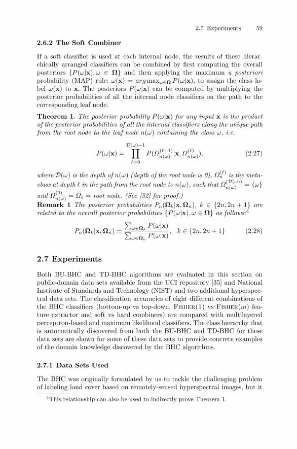
2.7 Experiments 59
2.6.2 The Soft Combiner
If a soft classifier is used at each internal node, the results of these hierar-chically arranged classifiers can be combined by first computing the overallposteriors P (ω|x), ω ∈ Ω and then applying the maximum a posterioriprobability (MAP) rule: ω(x) = arg maxω∈Ω P (ω|x), to assign the class la-bel ω(x) to x. The posteriors P (ω|x) can be computed by multiplying theposterior probabilities of all the internal node classifiers on the path to thecorresponding leaf node.
Theorem 1. The posterior probability P (ω|x) for any input x is the productof the posterior probabilities of all the internal classifiers along the unique pathfrom the root node to the leaf node n(ω) containing the class ω, i.e.
P (ω|x) =D(ω)−1∏
=0
P (Ω(+1)n(ω) |x, Ω
()n(ω)), (2.27)
where D(ω) is the depth of n(ω) (depth of the root node is 0), Ω()n is the meta-
class at depth in the path from the root node to n(ω), such that Ω(D(ω))n(ω) = ω
and Ω(0)n(ω) = Ω1 = root node. (See [32] for proof.)
Remark 1 The posterior probabilities Pn(Ωk|x,Ωn), k ∈ 2n, 2n + 1 arerelated to the overall posterior probabilities P (ω|x), ω ∈ Ω as follows:4
Pn(Ωk|x,Ωn) =
∑ω∈Ωk
P (ω|x)∑ω∈Ωn
P (ω|x), k ∈ 2n, 2n + 1 (2.28)
2.7 Experiments
Both BU-BHC and TD-BHC algorithms are evaluated in this section onpublic-domain data sets available from the UCI repository [35] and NationalInstitute of Standards and Technology (NIST) and two additional hyperspec-tral data sets. The classification accuracies of eight different combinations ofthe BHC classifiers (bottom-up vs top-down, Fisher(1) vs Fisher(m) fea-ture extractor and soft vs hard combiners) are compared with multilayeredperceptron-based and maximum likelihood classifiers. The class hierarchy thatis automatically discovered from both the BU-BHC and TD-BHC for thesedata sets are shown for some of these data sets to provide concrete examplesof the domain knowledge discovered by the BHC algorithms.
2.7.1 Data Sets Used
The BHC was originally formulated by us to tackle the challenging problemof labeling land cover based on remotely-sensed hyperspectral images, but it
4This relationship can also be used to indirectly prove Theorem 1.

60 Joydeep Ghosh, Shailesh Kumar and Melba M. Crawford
Table 2.1. The twelve classes in the AVIRIS/KSC hyperspectral data set
Num Class NameUpland Classes
1 Scrub2 Willow Swamp3 Cabbage palm hammock4 Cabbage oak hammock5 Slash pine6 Broad leaf/oak hammock7 Hardwood swamp
Wetland Classes8 Graminoid marsh9 Spartina marsh10 Cattail marsh11 Salt marsh12 Mud flats
clearly has broader applicability. Therefore in this section we shall evaluate iton five public-domain data sets in addition to two hyperspectral data sets. Thefour public-domain data sets obtained from the UCI repository [35] consist oftwo 26-class English letter recognition data sets (LETTER-I and LETTER-II)with classes A–Z, a 10-class DIGITS data set with classes 0–9 and a six-classSATIMAGE data set with the following classes: red soil, cotton crop, graysoil, damp gray soil, soil with vegetation stubble, and very damp gray soil.See [29] for more details about these data sets.
The two high-dimensional hyperspectral data sets are AVIRIS and HYMAP,both obtained from NASA. AVIRIS covers 12 classes or land-cover types, andwe used a 183-band subset of the 224 bands (excluding water absorptionbands) acquired by NASA’s Airborne Visible/Infrared Imaging Spectrome-ter (AVIRIS) sensor over Kennedy Space Center in Florida. The seven uplandand five wetland cover types identified for classification are listed in Table 2.1.Classes 3–7 are all trees. Class 4 is a mixture of Class 3 and oak hammock.Class 6 is a mixture of broad leaf trees (maples and laurels) and oak hammock.Class 7 is also a broad leaf tree. These classes have similar spectral signaturesand are very difficult to discriminate in multispectral, and even hyperspectral,data using traditional methods.
The HYMAP data set represents a nine-class land-cover prediction prob-lem, where the input is 126 bands across the reflective solar wavelength regionof 0.441–2.487 µm with contiguous spectral coverage (except in the atmo-spheric water vapor bands) and bandwidths between 15 and 20 nm. This dataset was obtained over Stover Point (South Texas) in September of 1999. Thevegetation here consists of common high estuarine marsh species includingSpartina spartinae, Borrichia frutescens, Monanthochloa littoralis, and Batis

2.7 Experiments 61
Table 2.2. The nine classes in the STOVER/HYMAP data set.
Num Class Name1 Water2 Spartina Spartinae3 Batis maritima4 Borrichia frutescens + Spartina spartinae + Monanthocloa littoralis5 Sand flats (bare soil)6 Pure Borrichia frutescens7 Trees8 Dense bushes9 Borrichia frutescens + Spartina spartinae
maritima. Adjacent to the resaca (which is a generic term that refers to anold river bed which has been cut off by the meandering of the river resultingin an ox-bow) is an almost impregnable layer of dense shrubs and trees. Thenine classes determined for Stover Point are listed in Table 2.2.
2.7.2 Classification Results
The eight versions of the BHC framework that are evaluated on the data setsdescribed in the previous section are generated by the following sets of choices:
• Building the tree: The BHC tree can be built either bottom-up or top-down. The biases of the BU-BHC and the TD-BHC algorithms are dif-ferent. The BU-BHC tries to find the most similar meta-classes from theavailable set and hence is more greedy at each step than the TD-BHC,which attempts to partition a meta-class into two subsets with a moreglobal perspective. As a result of the differences of these biases, differentBHC trees and therefore different classification accuracies can be obtained.
• Feature extractor used: Both the Fisher(1) and Fisher(m) featureextractors based on Fisher’s discriminant are investigated. While the treestructure for the two Fisher projections may be different, the discrimina-tion between classes at any internal node using Fisher(m) projections ishigher than the discrimination with Fisher(1) projection and thereforeFisher(m)-based BHC performs better in general than the correspondingBHC with Fisher(1) feature extractor.
• Nature of combiner: Both hard and soft combiners were investigated. Ingeneral, the soft combiner performs slightly better than the hard combiner,as is expected.
The classification accuracy averaged over 10 experiments on each data setis reported in Table 2.3. In each experiment, stratified sampling was used topartition the data set into training and test sets of equal size.5 Eight versions
510-fold cross validation is currently in vogue in some circles but is an overkillfor fairly large data sets.

62 Joydeep Ghosh, Shailesh Kumar and Melba M. Crawford
of the BHC classifiers were compared to two standard classifiers leading tothe following 10 classifiers for each data set:
• MLP: a finely-tuned multilayered perceptron-based classifier for each dataset;
• MLC: a maximum-likelihood classifier using a full covariance matrix wher-ever possible and using a diagonal covariance matrix if the full covariancematrix is ill-conditioned due to high input dimensionality;
• BU-BHC(1,H): BU-BHC with Fisher(1) and hard combiner;• BU-BHC(1,S): BU-BHC with Fisher(1) and soft combiner;• BU-BHC(m,H): BU-BHC with Fisher(m) and hard combiner;• BU-BHC(m,S): BU-BHC with Fisher(m) and soft combiner;• TD-BHC(1,H): TD-BHC with Fisher(1) and hard combiner;• TD-BHC(1,S): TD-BHC with Fisher(1) and soft combiner;• TD-BHC(m,H): TD-BHC with Fisher(m) and hard combiner;• TD-BHC(m,S): TD-BHC with Fisher(m) and soft combiner.
Table 2.3. Classification accuracies on public-domain data sets from the UCI repos-itory [35] (satimage, digits, letter-i) and NIST(letter-ii) and remote-sensingdata sets from the Center for Space Research, The University of Texas at Austin(hymap, aviris). The input dimensions and number of classes are also indicated foreach data set.
satimage digits letter-I letter-II hymap aviris
Dimensions 36 64 16 30 126 183Classes 6 10 26 26 9 12MLP 79.77 82.33 79.28 76.24 78.21 74.54MLC 77.14 74.85 82.73 79.48 82.73 72.66BU-BHC(1,H) 83.26 88.87 71.29 78.45 95.18 94.97BU-BHC(1,S) 84.48 89.00 72.81 79.93 95.62 95.31BU-BHC(m,H) 85.29 91.71 76.55 80.94 95.12 95.51BU-BHC(m,S) 85.35 91.95 78.41 81.11 95.43 95.83TD-BHC(1,H) 83.77 90.11 70.45 74.59 95.31 96.33TD-BHC(1,S) 84.02 90.24 72.71 75.83 95.95 97.09TD-BHC(m,H) 84.70 91.44 77.85 81.48 96.48 97.15TD-BHC(m,S) 84.95 91.61 79.13 81.99 96.64 97.93
The finely tuned MLP classifiers and the MLC classifiers are used as bench-marks for evaluating the BHC algorithms. Almost all the BHC versions per-formed significantly better than the MLP and MLC classifiers on all data setsexcept LETTER-I and LETTER-II. In general the TD-BHC was slightly bet-ter than the BU-BHC mainly because its global bias leads to less greedy treesthan the BU-BHC algorithm. Further, the Fisher(m) feature extractor con-sistently yields slightly better results than the Fisher(1) feature extractor,

2.8 Domain Knowledge Discovery 63
as expected. Finally, the soft combiner also performed sightly better than thehard combiner. This again is an expected result as the hard combiner losessome information as it thresholds the posteriors at each internal node.
2.7.3 Discussion of Results and Further Comparative Studies
From Table 2.3, we see that the BHC classifiers did not perform as well onthe LETTER-I data set. This turns out to be due to the presence of somebimodal classes in this data set, which is problematic for the simple Fisherdiscriminant. For such data sets it is preferable to use more powerful binaryclassifiers at the internal nodes of the BHC, i.e. use the BHC framework onlyto obtain the class hierarchy and then use other, more appropriate, feature-extractors/classifiers for the two-class problems at each internal node. Thisintuition is borne out in our recent work [40] where gaussian-kernel basedSVMs were used for the internal nodes, leading to statistically significant per-formance improvements for all the nine data sets considered. Also of interestis the comparison of this BHC-SVM architecture with an ECOC-based en-semble (using well-tuned SVMs as the base classifiers) given in this work. Theoutcome of this comparison is not obvious since two very different philoso-phies are being encountered. While the BHC groups the classes according totheir natural affinities in order to make each binary problem easier, it cannotexploit the powerful error correcting properties of an ECOC ensemble thatcan provide good results even when individual classifiers are weak. This em-pirical study showed that while is no clear advantage to either technique interms of classification accuracy, the BHCs typically achieve this performanceusing fewer classifiers. Note that each dichotomy in an ECOC setup can beaddressed using all the training data, while for the BHC the data available de-creases as one moves away from the root since only a subset of the classes areinvolved in lower-level dichotomies. Thus one may expect the ECOC approachto be less affected by a paucity of training data. However the experiments in[40] showed that BHC was competitive even for small sample sizes, indicat-ing that the reduction in data is compensated for by the simpler dichotomiesresulting from affinity-based grouping of classes.
All the results above assume equal penalty for each type of misclassifica-tion. In many real applications, classification into a nearby class is less costlythan being labeled as a distant class. For example, wet gray soil being clas-sified as damp gray soil is not as costly as being labeled as red, dry soil.If such asymmetric costs are considered, the coarse-to-fine approach of theBHC framework provides an additional advantage over all the other methodsconsidered.
2.8 Domain Knowledge Discovery
One of the important aspects of the BHC classifiers is the domain knowledgethat is discovered by the automatic BU-BHC and TD-BHC tree construction

64 Joydeep Ghosh, Shailesh Kumar and Melba M. Crawford
algorithms. The trees constructed by the BU-BHC(m) and TD-BHC(m) areshown in Figures 2.3 to 2.10 for the most common of the trees obtained in theten experiments for each data set. The numbers at the internal nodes of thebinary trees represent the mean training and test set classification accuraciesat that internal node over all the experiments for which this tree is obtained.
• IRIS: It is well known that Iris Versicolour and Virginica are “closer” toeach other than Iris Setosa. So, not surprisingly, the first split for both BU-BHC(m) and TD-BHC(m) algorithms invariably separates Setosa from theother two classes.
• SATIMAGE: Figures 2.3 and 2.4 show the BU-BHC(m) and TD-BHC(m)trees generated for the SATIMAGE data set. In the BU-BHC tree, theClasses 4 (damp gray soil) and 6 (very damp gray soil) merged first. Thiswas followed by Class 3 (gray soil) merging in the meta-class (4,6). Theright child of the root node contains the remaining three classes out ofwhich the vegetation classes i.e. Class 2 (cotton crop) and Class 5 (soilwith vegetation stubble) were grouped first. The tree formed in the TD-BHC is even more informative as it separates the four bare soil classes fromthe two vegetation classes at the root node and then separates the foursoil classes into red-soil (Class 1) and gray-soil (Classes 3, 4, and 6) meta-classes. The gray-soil meta-class is further partitioned into damp-gray-soil(Classes 4 and 6) and regular-gray-soil (Class 3). Thus reasonable class hi-erarchies are discovered by the BHC framework for the SATIMAGE dataset.
VeryDampGraySoil
GraySoil
DampGraySoil
CottonCrop
Soil withVegetation
Stubble
RedSoil
96.9 – 96.9
93.6 – 91.7 98.0 – 97.6
83.3 – 82.9 95.8 – 94.9
Fig. 2.3. BU-BHC(m) class hierarchy for the satimage data set.

2.8 Domain Knowledge Discovery 65
CottonCrop
Soil withVegetation
Stubble
RedSoil
VeryDampGraySoil
GraySoil
DampGraySoil
95.5 – 95.5
83.3 – 83.3
93.6 – 93.6
99.0 – 99.095.8 – 95.8
Fig. 2.4. TD-BHC(m) class hierarchy for the satimage data set.
• LETTER: The 26-class LETTER-I data set is only 16-dimensional. Al-though relatively lower dimensionality makes it an “easier” problem fromthe curse of dimensionality perspective, the fact that the number of classesis more than the dimensionality makes it a “harder” problem from theproblem decomposition perspective. As seen in Table 2.3, the performanceof BHC classifiers actually is poorer than other approaches, the reasonsfor which have already been discussed. Nevertheless, it is interesting to seethe trees obtained by the BHC algorithms for such a large (in terms ofoutput space) classification problem (Figures 2.5 and 2.6). Several inter-esting groups of characters are merged in the BU-BHC tree. For examplemeta-classes like M,W,N,U F,P, V,Y,T, S,Z,B,E, I,J, K,R,and G,Q,C are discovered. These conform well with the shapes of theletters. The TD-BHC tree is different from the BU-BHC tree but alsohas several interesting meta-classes like M,W,U,H,N, K,R, V,Y,T,F,P, S,Z, C,G,O, and B,D,E. Even for a small dimensional inputspace, as compared to the number of classes, the BHC algorithm was ableto discover a meaningful class hierarchy for this 26-class problem. How-ever, note that one could have obtained other reasonable hierarchies aswell, and it is difficult to quantify the quality of a specific hierarchy otherthan through its corresponding classification accuracy.
• LETTER-II: Since the output space is still the same, the BHC treesfor LETTER-II should be similar to the LETTER-I trees. In our experi-ments, similar interesting meta-classes such as M,W,N,U, F,P, V,T,S,Z,B,E, I,J and G,Q,C were discovered in the BU-BHC tree. The

66 Joydeep Ghosh, Shailesh Kumar and Melba M. Crawford
N U F P
V Y S Z B E I J K R D L
T A
X C
H O G Q
M W
92.4 – 92.4
97.3 – 97.2 87.9 – 87.5
95.0 – 94.3 95.3 – 94.9 93.4 – 93.4 87.8 – 86.1
Fig. 2.5. BU-BHC(m) class hierarchy for the letter-I data set.
N
U
F P
V Y S Z B
EI
JK R
D
L
T
A
X
C
H O
G
Q
WM
88.8 – 88.8
92.9 – 92.9
94.8 – 94.8 97.2 – 97.2
94.5 – 94.5
89.3 – 89.3 98.3 – 93.3
Fig. 2.6. TD-BHC(m) class hierarchy for the letter-I data set.
TD-BHC classifier for LETTER-II data set resulted in a few new groupingsas well, including O,Q, H,K,A,R and P,D.
• Hyperspectral data: Figures 2.7, 2.8, 2.9 and 2.10 show the bottom-upand top-down trees obtained for AVIRIS and HYMAP. By considering themeaning of the class labels it is evident that this domain provided the mostuseful knowledge. Invariably, when water was present, it was the first to

2.8 Domain Knowledge Discovery 67
be split off. Subsequent partitions would, for example, distinguish betweenmarshy wetlands and uplands, as in Figure 2.1. Note that the trees shownare representative results. While there are sometimes small variations inthe trees obtained by perturbing the data, invariably all the trees producehierarchies that are meaningful and reasonable to a domain expert [24].
10 12 11
8 9
1 6 2
5
3
4 7
99.4 – 98.4
99.3 – 99.1
100 – 94.7
100 – 99.9
99.1 – 99.1
99.6 – 98.9
99.4 – 88.3 100 – 94.3
99.7 – 88.9
100 – 91.5
90.3 – 87.5
Fig. 2.7. BU-BHC(m) class hierarchy for the AVIRIS data set.
98.8 – 98.8
99.7 – 99.7
99.3 – 99.3
99.4 – 99.4
99.8 – 99.8
99.2 – 99.2
100 – 100 99.4 – 99.4
99.9 – 99.9
98.5 – 98.5
11 12
10 8 9
2 7
4 5
3 1 6
96.0 – 96.0
Fig. 2.8. TD-BHC(m) class hierarchy for the AVIRIS data set.

68 Joydeep Ghosh, Shailesh Kumar and Melba M. Crawford
2 9 5
4 6
7 8 1 3
100 – 100
100 – 100
100 – 10099.4 – 98.4
99.4 – 99.4
99.9 – 99.889.3 – 87.6
98.8 – 98.4
Fig. 2.9. BU-BHC(m) class hierarchy for the HYMAP data set.
100 – 100
100 – 10098.6 – 98.6
99.9 – 99.9 99.6 – 99.6
99.9 – 99.9
99.4 – 99.4
89.3 – 89.3
7 8
6
5 4
2 9
1 3
Fig. 2.10. TD-BHC(m) class hierarchy for the HYMAP data set.

2.9 Conclusions 69
2.9 Conclusions
This chapter presented a general framework for certain difficult classificationproblems in which the complexity is primarily due to having several classesas well as high-dimensional inputs. The BHC methodology relies on progres-sively partitioning or grouping the set of classes based on their affinities withone another. The BHC, as originally conceived, uses a custom Fisher’s dis-criminant feature extraction for each partition, which is quite fast as it onlyinvolves summary class statistics. Moreover, as a result of the tree buildingalgorithms, a class taxonomy is automatically discovered from data, which of-ten leads to useful domain knowledge. This property was particularly helpfulin our analysis of hyperspectral data.
The hierarchical BHC approach is helpful only if some class affinities areactually present, i.e. it will not be appropriate if all the classes are essen-tially “equidistant” from one another. In practice, this is not very restrictivesince many applications involving multiple class labels, such as those basedon biological or text data, do have natural class affinities, quite often reflectedin class hierarchies or taxonomies. In fact it has been shown that exploitinga known hierarchy of text categories substantially improves text classifica-tion [5]. In contrast, the BHC attempts to induce a hierarchy directly fromthe data where no pre-existing hierarchy is available. Another recent approachwith a similar purpose is presented in [19] where Naive Bayes is first used toquickly generate a confusion matrix for a text corpus. The classes are thenclustered based on this matrix such that classes that are more confused withone another tend to be placed in the same group. Then SVMs are used ina “one-versus-all” framework within each group of classes to come up withthe final result. Thus this approach produces a two-level hierarchy of classes.On text benchmarks, this method was three to six times faster than using“one-vs-all” SVMs directly, while producing comparable or better classifica-tion results.
We note that one need not be restricted to our choices of a Fisher dis-criminant and a simple Bayesian classifier at each internal node of the class-partitioning tree. In Section 2.7.3, we summarized our related work on usingSVMs as the internal classifiers on a tree obtained via the Fisher discrimi-nant/Bayesian classifier combination. The feature extraction step itself canalso be customized for different domains such as image or protein sequenceclassification. In this context, recollect that the trees obtained for a givenproblem can vary somewhat depending on the specific training set or classi-fier design, indicative of the fact that that there are often multiple reasonableways of grouping the classes. The use of more powerful binary classifiers pro-vides an added advantage in that the overall results are more tolerant to thequality of the tree that is obtained.
The design space for selecting an appropriate feature extractor–classifiercombination is truly rich and needs to be explored further. A well-knowntrade-off exists between these two functions. For example, a complex feature

70 Joydeep Ghosh, Shailesh Kumar and Melba M. Crawford
extraction technique can compensate for a simple classifier. With this view-point, let us compare the top-down BHC with decision trees such as C5.0,CART and CHAID. One can view the action at each internal node of a de-cision tree as the selection of a specific value of exactly one variable (featureextraction stage), followed by a simple classifier that just performs a sim-ple comparison against this value. Thus the BHC node seems more complex.However, the demands on a single node in a decision tree are not that strong,since samples from the same class can be routed to different branches of thetree and still be identified correctly at later stages. In contrast, in the hardversion of BHC, all the examples of a given class have to be routed to thesame child at each internal node visited by them.
Acknowledgments: This research was supported in part by NSF grant IIS-0312471, the Texas Advanced Technology Research Program (CSRA-ATP-009), and a grant from Intel Corp. We thank members of CSR, and in partic-ular Jisoo Ham and Alex Henneguelle, for helpful comments.
References
[1] Ballard, D., 1987: Modular learning in neural networks. Proc. AAAI-87 ,279–84.
[2] Bellman, R. E., ed., 1961: Adaptive Control Processes. Princeton Univer-sity Press.
[3] Breiman, L., J. H. Friedman, R. Olshen and C. J. Stone, 1984: Clas-sification and Regression Trees. Wadsworth and Brooks, Pacific Grove,California.
[4] Brill, F. Z., D. E. Brown and W. N. Martin, 1992: Fast genetic selectionof features for neural network classifiers. IEEE Transactions on NeuralNetworks , 3, 324–28.
[5] Chakrabarti, S., B. Dom, R. Agrawal and P. Raghavan, 1998: Scalablefeature selection, classification and signature generation for organizinglarge text databases into hierarchical topic taxonomies. VLDB Journal ,7, 163–78.
[6] Chakravarthy, S., J. Ghosh, L. Deuser and S. Beck, 1991: Efficient train-ing procedures for adaptive kernel classifiers. Neural Networks for SignalProcessing , IEEE Press, 21–9.
[7] Crawford, M. M., S. Kumar, M. R. Ricard, J. C. Gibeaut and A. Neuensh-wander, 1999: Fusion of airborne polarimetric and interferometric SARfor classification of coastal environments. IEEE Transactions on Geo-science and Remote Sensing , 37, 1306–15.
[8] Dattatreya, G. R. and L. N. Kanal, 1985: Decision trees in pattern recog-nition. Progress in Pattern Recognition 2 , L. N. Kanal and A. Rosenfeld,eds., Elsevier Science, 189–239.

References 71
[9] Deco, G. and L. Parra, 1997: Nonlinear feature extraction by redundancyreduction in an unsupervised stochastic neural network. Neural Networks,10, 683–91.
[10] Dietterich, T. G. and G. Bakiri, 1995: Solving multiclass learning prob-lems via error-correcting output codes. Journal of Artificial IntelligenceResearch, 2, 263–86.
[11] Duda, R. and P. Hart, 1973: Pattern Classification and Scene Analysis.Addison-Wesley.
[12] Etemad, K. and R. Chellappa, 1998: Separability-based multiscale basisselection and feature extraction for signal and image classification. IEEETransactions on Image Processing , 7, 1453–65.
[13] Friedman, J., 1989: Regularized discriminant analysis. Journal of theAmerican Statistical Association, 84, 165–75.
[14] — 1996: Another approach to polychotomous classification. Technicalreport, Stanford University.
[15] — 1996: On bias, variance, 0/1 loss, and the curse-of-dimensionality.Technical report, Department of Statistics, Stanford University.
[16] Fukunaga, K., 1990: Introduction to Statistical Pattern Recognition (2ndEd.), Academic Press, NY.
[17] Furnkranz, J., 2002: Round robin classification. Jl. Machine LearningResearch, 2, 721–47.
[18] Ghosh, J., 2003: Scalable clustering. The Handbook of Data Mining ,N. Ye, ed., Lawrence Erlbaum Assoc., 247–77.
[19] Godbole, S., S. Sarawagi and S. Chakrabarti, 2002: Scaling multi-classsupport vector machines using inter-class confusion. Proceedings of the8th International Conference on Knowledge Discovery and Data Mining(KDD-02), 513–18.
[20] Hand, D., 1982: Kernel Discriminant Analysis. Research Studies Press,Chichester, UK.
[21] Happel, B. and J. Murre, 1994: Design and evolution of modular neuralnetwork architectures. Neural Networks, 7:6/7, 985–1004.
[22] Hastie, T. and R. Tibshirani, 1996: Discriminant adaptive nearest neight-bor classification. IEEE Transactions on Pattern Analysis and MachineIntelligence, PAMI-18, 607–16.
[23] — 1998: Classification by pairwise coupling. Advances in Neural Infor-mation Processing Systems, M. J. K. Michael, I. Jordan and S. A. Solla,eds., MIT Press, Cambridge, Massachusetts, 10, 507–13.
[24] Henneguelle, A., J. Ghosh and M. M. Crawford, 2003: Polyline featureextraction for land cover classification using hyperspectral data. Proc.IICAI-03 , 256–69.
[25] Hsu, C. W. and C. J. Lin, 2002: A comparison of methods for multiclasssupport vector machines. IEEE Transactions on Neural Networks , 13,415–25.
[26] Jordan, M. and R. Jacobs, 1994: Hierarchical mixture of experts and theEM algorithm. Neural Computation, 6, 181–214.

72 Joydeep Ghosh, Shailesh Kumar and Melba M. Crawford
[27] Khotanzad, A. and Y. Hong, 1990: Invariant image recognition by zernikemoments. IEEE Transactions on Pattern Analysis and Machine Intelli-gence, 12, 28–37.
[28] Kittler, J. and F. Roli, eds., 2001: Multiple Classifier Systems. LNCS Vol.1857, Springer.
[29] Kumar, S., 2000: Modular learning through output space decomposition.Ph.D. thesis, Dept. of ECE, Univ. of Texas at Austin, USA.
[30] Kumar, S. and J. Ghosh, 1999: GAMLS: A generalized framework forassociative modular learning systems (invited paper). Proceedings ofthe Applications and Science of Computational Intelligence II , Orlando,Florida, 24–34.
[31] Kumar, S., J. Ghosh and M. M. Crawford, 1999: A versatile frameworkfor labeling imagery with a large number of classes. Proceedings of theInternational Joint Conference on Neural Networks, Washington, D.C.
[32] — 2002: Hierarchical fusion of multiple classifiers for hyperspectral dataanalysis. Pattern Analysis and Applications, splecial issue on Fusion ofMultiple Classifiers, 5, 210–20.
[33] Mao, J. and A. K. Jain, 1995: Artificial neural networks for feature ex-traction and multivariate data projection. IEEE Transactions on NeuralNetworks , 6 (2), 296–317.
[34] McLachlan, G. J., 1992: Discriminant Analysis and Statistical PatternRecognition. John Wiley, New York.
[35] Merz, C. and P. Murphy, 1996: UCI repository of machine learningdatabases. URL: www.ics.uci.edu/∼mlearn/MLRepository.html.
[36] Murray-Smith, R. and T. A. Johansen, 1997: Multiple Model Approachesto Modelling and Control . Taylor and Francis, UK.
[37] Nilsson, N. J., 1965: Learning Machines: Foundations of TrainablePattern-Classifying Systems. McGraw Hill, NY.
[38] Petridis, V. and A. Kehagias, 1998: Predictive Modular Neural Networks:Applications to Time Series. Kluwer Academic Publishers, Boston.
[39] Platt, J. C., N. Cristianini and J. Shawe-Taylor, 2000: Large marginDAGs for multiclass classification. MIT Press, 12, 547–53.
[40] Rajan, S. and J. Ghosh, 2004: An empirical comparison of hierarchicalvs. two-level approaches to multiclass problems. Multiple Classifier Sys-tems, F. Roli, J. Kittler and T. Windeatt, eds., LNCS Vol. 3077, Springer,283–92.
[41] Ramamurti, V. and J. Ghosh, 1998: On the use of localized gating inmixtures of experts networks (invited paper), SPIE Conf. on Applicationsand Science of Computational Intelligence, SPIE Proc. Vol. 3390 , 24–35.
[42] — 1999: Structurally adaptive modular networks for nonstationary envi-ronments. IEEE Trans. on Neural Networks, 10, 152–60.
[43] Rasoul Safavian, S. and D. Landgrebe, 1991: A survey of decision treeclassifier methodology. IEEE Transactions on Systems, Man, and Cyber-netics, 21, 660–74.
References 73
[44] Rifkin, R. and A. Klautau, 2004: In defense of one-vs-all classification.Jl. Machine Learning Research, 5, 101–41.
[45] Sakurai-Amano, T., J. Iisaka and M. Takagi, 1997: Comparison of landcover indices of AVHRR data. International Geoscience and RemoteSensing Symposium, 916–18.
[46] Scholkopf, B., C. Burges and A. J. Smola, eds., 1998: Advances in KernelMethods: Support Vector Learning . MIT Press.
[47] Sharkey, A., 1999: Combining Artificial Neural Nets. Springer-Verlag.[48] Sharkey, A. J. C., N. E. Sharkey, and G. O. Chandroth, 1995: Neural
nets and diversity. Proceedings of the 14th International Conference onComputer Safety, Reliability and Security, Belgirate, Italy.
[49] Tumer, K. and N. C. Oza, 1999: Decimated input ensembles for improvedgeneralization. Proceedings of the International Joint Conference on Neu-ral Networks, Washington, D.C.
[50] Vapnik, V., 1995: The Nature of Statistical Learning Theory. Springer.

3
Graph-based Mining of Complex Data
Diane J. Cook, Lawrence B. Holder, Jeff Coble and Joseph Potts
Summary. We describe an approach to learning patterns in relational data rep-resented as a graph. The approach, implemented in the Subdue system, searchesfor patterns that maximally compress the input graph. Subdue can be used forsupervised learning, as well as unsupervised pattern discovery and clustering.
Mining graph-based data raises challenges not found in linear attribute–valuedata. However, additional requirements can further complicate the problem. In par-ticular, we describe how Subdue can incrementally process structured data thatarrives as streaming data. We also employ these techniques to learn structural con-cepts from examples embedded in a single large connected graph.
3.1 Introduction
Much of current data-mining research focuses on algorithms to discover setsof attributes that can discriminate data entities into classes, such as shop-ping or banking trends for a particular demographic group. In contrast, weare developing data-mining techniques to discover patterns consisting of com-plex relationships between entities. The field of relational data mining, ofwhich graph-based relational learning is a part, is a new area investigatingapproaches to mining relational information by finding associations involvingmultiple tables in a relational database.
Two main approaches have been developed for mining relational infor-mation: logic-based approaches and graph-based approaches. Logic-based ap-proaches fall under the area of inductive logic programming (ILP) [16]. ILPembodies a number of techniques for inducing a logical theory to describethe data, and many techniques have been adapted to relational data mining[6]. Graph-based approaches differ from logic-based approaches to relationalmining in several ways, the most obvious of which is the underlying represen-tation. Furthermore, logic-based approaches rely on the prior identificationof the predicate or predicates to be mined, while graph-based approaches aremore data-driven, identifying any portion of the graph that has high support.However, logic-based approaches allow the expression of more complicated

76 Diane J. Cook, Lawrence B. Holder, Jeff Coble and Joseph Potts
patterns involving, e.g., recursion, variables, and constraints among variables.These representational limitations of graphs can be overcome, but at a com-putational cost.
Our research is particularly applicable to domains in which the data isevent-driven, such as counter-terrorism intelligence analysis, and domainswhere distinguishing characteristics can be object attributes or relational at-tributes. This ability has also become a crucial challenge in many security-related domains. For example, the US House and Senate Intelligence Commit-tees’ report on their inquiry into the activities of the intelligence communitybefore and after the September 11, 2001 terrorist attacks revealed the necessityfor “connecting the dots” [18], that is, focusing on the relationships betweenentities in the data, rather than merely on an entity’s attributes. A natu-ral representation for this information is a graph, and the ability to discoverpreviously-unknown patterns in such information could lead to significant im-provement in our ability to identify potential threats. Similarly, identifyingcharacteristic patterns in spatial or temporal data can be a critical compo-nent in acquiring a foundational understanding of important research in manyof the basic sciences.
Problems of such complexity often present additional challenges, such asthe need to assimilate incremental data updates and the need to learn modelsfrom data embedded in a single input graph. In this article we review tech-niques for graph-based data mining and focus on a method for graph-basedrelational learning implemented in the Subdue system. We describe meth-ods of enhancing the algorithm to handle challenges associated with complexdata, such as incremental discovery of streaming structural data and learningmodels from embedded instances in supervised graphs.
3.2 Related Work
Graph-based data mining (GDM) is the task of finding novel, useful, andunderstandable graph-theoretic patterns in a graph representation of data.Several approaches to GDM exist, based on the task of identifying frequentlyoccurring subgraphs in graph transactions, i.e., those subgraphs meeting aminimum level of support. Kuramochi and Karypis [15] developed the FSGsystem for finding all frequent subgraphs in large graph databases. FSG startsby finding all frequent single and double edge subgraphs. Then, in each itera-tion, it generates candidate subgraphs by expanding the subgraphs found inthe previous iteration by one edge. In each iteration the algorithm checks howmany times the candidate subgraph occurs within an entire graph. The candi-dates whose frequency is below a user-defined level are pruned. The algorithmreturns all subgraphs occurring more frequently than the given level.
Yan and Han [19] introduced gSpan, which combines depth-first searchand lexicographic ordering to find frequent subgraphs. Their algorithm startsfrom all frequent one-edge graphs. The labels on these edges, together with

3.3 Graph-based Relational Learning in Subdue 77
labels on incident vertices, define a code for every such graph. Expansion ofthese one-edge graphs maps them to longer codes. The codes are stored in atree structure such that if α = (a0, a1, ..., am) and β = (a0, a1, ..., am, b), theβ code is a child of the α code. Since every graph can map to many codes, thecodes in the tree structure are not unique. If there are two codes in the codetree that map to the same graph and one is smaller than the other, the branchwith the smaller code is pruned during the depth-first search traversal of thecode tree. Only the minimum code uniquely defines the graph. Code orderingand pruning reduces the cost of matching frequent subgraphs in gSpan.
Inokuchi et al. [12] developed the Apriori-based Graph Mining (AGM)system, which uses an approach similar to Agrawal and Srikant’s [2] Apriorialgorithm for discovering frequent itemsets. AGM searches the space of fre-quent subgraphs in a bottom-up fashion, beginning with a single vertex, andthen continually expanding by a single vertex and one or more edges. AGMalso employs a canonical coding of graphs in order to support fast subgraphmatching. AGM returns association rules satisfying user-specified levels ofsupport and confidence.
We distinguish graph-based relational learning (GBRL) from graph-baseddata mining in that GBRL focuses on identifying novel, but not necessarilythe most frequent, patterns in a graph representation of data [10]. Only a fewGBRL approaches have been developed to date. Subdue [4] and GBI [20] takea greedy approach to finding subgraphs, maximizing an information theoreticmeasure. Subdue searches the space of subgraphs by extending candidate sub-graphs by one edge. Each candidate is evaluated using a minimum descriptionlength metric [17], which measures how well the subgraph compresses the in-put graph if each instance of the subgraph were replaced by a single vertex.GBI continually compresses the input graph by identifying frequent triplesof vertices, some of which may represent previously-compressed portions ofthe input graph. Candidate triples are evaluated using a measure similar toinformation gain. Kernel-based methods have also been used for supervisedGBRL [14].
3.3 Graph-based Relational Learning in Subdue
The Subdue graph-based relational learning system1 [4, 5] encompasses severalapproaches to graph-based learning, including discovery, clustering and super-vised learning, which will be described in this section. Subdue uses a labeledgraph G = (V,E,L) as both input and output, where V = v1, v2, . . . , vn isa set of vertices, E = (vi, vj)|vi, vj ∈ V is a set of edges, and L is a set of la-bels that can appear on vertices and edges. The graph G can contain directededges, undirected edges, self-edges (i.e., (vi, vi) ∈ E), and multi-edges (i.e.,
1Subdue source code, sample data sets and publications are available atailab.uta.edu/subdue.

78 Diane J. Cook, Lawrence B. Holder, Jeff Coble and Joseph Potts
more than one edge between vertices vi and vj). The input graph need not beconnected, but the learned patterns must be connected subgraphs (called sub-structures) of the input graph. The input to Subdue can consist of one largegraph or several individual graph transactions and, in the case of supervisedlearning, the individual graphs are classified as positive or negative examples.
3.3.1 Substructure Discovery
Subdue searches for a substructure that best compresses the input graph.Subdue uses a variant of beam search for its main search algorithm. A sub-structure in Subdue consists of a subgraph definition and all its occurrencesthroughout the graph. The initial state of the search is the set of substructuresconsisting of all uniquely labeled vertices. The only operator of the search isthe ExtendSubstructure operator. As its name suggests, it extends a substruc-ture in all possible ways by a single edge and a vertex, or by only a singleedge if both vertices are already in the subgraph.
The search progresses by applying the ExtendSubstructure operator to eachsubstructure in the current state. The resulting state, however, does not con-tain all the substructures generated by the ExtendSubstructure operator. Thesubstructures are kept on a queue and are ordered based on their descriptionlength (sometimes referred to as value) as calculated using the MDL principledescribed below.
The search terminates upon reaching a user-specified limit on the numberof substructures extended, or upon exhaustion of the search space. Once thesearch terminates and Subdue returns the list of best substructures found, thegraph can be compressed using the best substructure. The compression pro-cedure replaces all instances of the substructure in the input graph by singlevertices, which represent the substructure definition. Incoming and outgoingedges to and from the replaced instances will point to, or originate in thenew vertex that represents the instance. The Subdue algorithm can be in-voked again on this compressed graph. This procedure can be repeated auser-specified number of times, and is referred to as an iteration.
Subdue’s search is guided by the minimum description length (MDL) [17]principle, which seeks to minimize the description length of the entire dataset. The evaluation heuristic based on the MDL principle assumes that thebest substructure is the one that minimizes the description length of the inputgraph when compressed by the substructure [4]. The description length of thesubstructure S given the input graph G is calculated as DL(S) + DL(G|S),where DL(S) is the description length of the substructure, and DL(G|S) isthe description length of the input graph compressed by the substructure. De-scription length DL() is calculated as the number of bits in a minimal encodingof the graph. Subdue seeks a substructure S that maximizes compression ascalculated in Equation (3.1).
Compression =DL(S) + DL(G|S)
DL(G)(3.1)
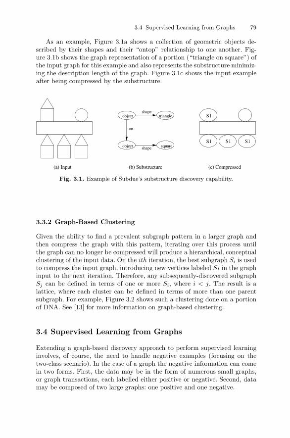
3.4 Supervised Learning from Graphs 79
As an example, Figure 3.1a shows a collection of geometric objects de-scribed by their shapes and their “ontop” relationship to one another. Fig-ure 3.1b shows the graph representation of a portion (“triangle on square”) ofthe input graph for this example and also represents the substructure minimiz-ing the description length of the graph. Figure 3.1c shows the input exampleafter being compressed by the substructure.
S1
S1 S1 S1
object
object
triangle
square
on
shape
shape
(a) Input (b) Substructure (c) Compressed
Fig. 3.1. Example of Subdue’s substructure discovery capability.
3.3.2 Graph-Based Clustering
Given the ability to find a prevalent subgraph pattern in a larger graph andthen compress the graph with this pattern, iterating over this process untilthe graph can no longer be compressed will produce a hierarchical, conceptualclustering of the input data. On the ith iteration, the best subgraph Si is usedto compress the input graph, introducing new vertices labeled Si in the graphinput to the next iteration. Therefore, any subsequently-discovered subgraphSj can be defined in terms of one or more Si, where i < j. The result is alattice, where each cluster can be defined in terms of more than one parentsubgraph. For example, Figure 3.2 shows such a clustering done on a portionof DNA. See [13] for more information on graph-based clustering.
3.4 Supervised Learning from Graphs
Extending a graph-based discovery approach to perform supervised learninginvolves, of course, the need to handle negative examples (focusing on thetwo-class scenario). In the case of a graph the negative information can comein two forms. First, the data may be in the form of numerous small graphs,or graph transactions, each labelled either positive or negative. Second, datamay be composed of two large graphs: one positive and one negative.

80 Diane J. Cook, Lawrence B. Holder, Jeff Coble and Joseph Potts
OCH2
O
N
N
NN
N
H
H
H
O
N
O CH3
O
OOCH2
O
NO
PO OH
O
O
PO OH
OCH2
O
O
PO OH
CH2
O
P OHO
H
H
O
CH3
O
CH2
ONO
NN
NN
N
P OHO
O
O
CH2
O
N H
NN O
H
P OHO
O
O
NN
OCH3
H
H N
NN
N
H
N
adenine
guanine
thymine adenine
cytosine
thymine
C N C C
O
P OHO
O
CH2
O
P OHO
N
C
C
C
C
C N C
C
C
O
O
C C
O
DNA
Fig. 3.2. Example of Subdue’s clustering (bottom) on a portion of DNA (top).

3.5 Incremental Discovery from Streaming Data 81
The first scenario is closest to the standard supervised learning problem inthat we have a set of clearly defined examples. Figure 3.3a depicts a simple setof positive and negative examples. Let G+ represent the set of positive graphs,and G− represent the set of negative graphs. Then, one approach to supervisedlearning is to find a subgraph that appears often in the positive graphs, but notin the negative graphs. This amounts to replacing the information-theoreticmeasure with an error-based measure. For example, we would find a subgraphS that minimizes
|g ∈ G+|S ⊆ g|+ |g ∈ G−|S ⊆ g||G+|+ |G−| ,
where S ⊆ g means S is isomorphic to a subgraph of g. The first term of thenumerator is the number of false negatives and the second term is the numberof false positives.
This approach will lead the search toward a small subgraph that discrim-inates well, e.g., the subgraph in Figure 3.3b. However, such a subgraph doesnot necessarily compress well, nor represent a characteristic description of thetarget concept. We can bias the search toward a more characteristic descrip-tion by using the information-theoretic measure to look for a subgraph thatcompresses the positive examples, but not the negative examples. If I(G) rep-resents the description length (in bits) of the graph G, and I(G|S) representsthe description length of graph G compressed by subgraph S, then we can lookfor an S that minimizes I(G+|S) + I(S) + I(G−) − I(G−|S), where the lasttwo terms represent the portion of the negative graph incorrectly compressedby the subgraph. This approach will lead the search toward a larger subgraphthat characterizes the positive examples, but not the negative examples, e.g.,the subgraph in Figure 3.3c.
Finally, this process can be iterated in a set-covering approach to learna disjunctive hypothesis. If using the error measure, then any positive ex-ample containing the learned subgraph would be removed from subsequentiterations. If using the information-theoretic measure, then instances of thelearned subgraph in both the positive and negative examples (even multipleinstances per example) are compressed to a single vertex. See [9] for moreinformation on graph-based supervised learning.
3.5 Incremental Discovery from Streaming Data
Many challenging problems require processing and assimilation of periodicincrements of new data, which provides new information in addition to thatwhich was previously processed. We introduce our first enhancement of Sub-due, called Incremental-Subdue (I-Subdue), which summarizes discoveriesfrom previous data increments so that the globally-best patterns can be com-puted by examining only the new data increment.
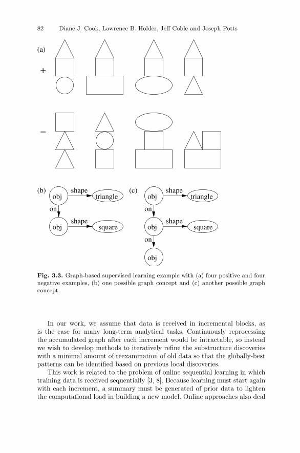
82 Diane J. Cook, Lawrence B. Holder, Jeff Coble and Joseph Potts
(a)
+
−
(b) (c)shape
shape
on
shape
shape
on
on
square
triangleobj
obj square
triangleobj
obj
obj
Fig. 3.3. Graph-based supervised learning example with (a) four positive and fournegative examples, (b) one possible graph concept and (c) another possible graphconcept.
In our work, we assume that data is received in incremental blocks, asis the case for many long-term analytical tasks. Continuously reprocessingthe accumulated graph after each increment would be intractable, so insteadwe wish to develop methods to iteratively refine the substructure discoverieswith a minimal amount of reexamination of old data so that the globally-bestpatterns can be identified based on previous local discoveries.
This work is related to the problem of online sequential learning in whichtraining data is received sequentially [3, 8]. Because learning must start againwith each increment, a summary must be generated of prior data to lightenthe computational load in building a new model. Online approaches also deal

3.5 Incremental Discovery from Streaming Data 83
with this incremental mining problem, but restrict the problem to itemset dataand assume the data arrives in complete and independent units [1, 7, 11].
Fig. 3.4. Incremental data can be viewed as a unique extension to the accumulatedgraph.
In our approach, we view each new data increment as a distinct datastructure. Figure 3.4 illustrates one conceptual approach to mining sequentialdata, where each new increment received at time step ti is considered indepen-dently of earlier data increments so that the accumulation of these structuresis viewed as one large, but disconnected, graph. The original Subdue algo-rithm would still work equally well if we applied it to the accumulated graphafter each new data increment is received. The obstacle is the computationalburden required for repeated full batch processing.
The concept depicted in Figure 3.4 can be intuitively applied to real prob-lems. For example, a software agent deployed to assist an intelligence analystwould gradually build up a body of data as new information streams in overtime. This streaming data could be viewed as independent increments fromwhich common structures are to be derived. Although the data itself maybe generated in very small increments, we would expect to accumulate someminimum amount before we mine it. Duplicating nodes and edges in the accu-mulated graph serves the purpose of giving more weight to frequently-repeatedpatterns.

84 Diane J. Cook, Lawrence B. Holder, Jeff Coble and Joseph Potts
3.5.1 Sequential Discovery
Storing all accumulated data and continuing to periodically repeat the entirestructure discovery process is intractable both from a computational perspec-tive and for data storage purposes. Instead, we wish to devise a method bywhich we can discover structures from the most recent data increment andsimultaneously refine our knowledge of the globally-best substructures dis-covered so far. However, we can often encounter a situation where sequentialapplications of Subdue to individual data increments will yield a series oflocally-best substructures that are not the globally-best substructures, thatwould be found if the data were evaluated as one aggregate block.
Figure 3.5 illustrates an example where Subdue is applied sequentially toeach data increment as it is received. At each increment, Subdue discoversthe best substructure for the respective data increment, which turns out to beonly a local best. However, if we aggregate the same data, as depicted in Fig-ure 3.6, and then apply the baseline Subdue algorithm we get a different bestsubstructure, which in fact is globally best. This is illustrated in Figure 3.7.Although our simple example could easily be aggregated at each time step,realistically large data sets would be too unwieldy for this approach.
In general, sequential discovery and action brings with it a set of uniquechallenges, which are generally driven by the underlying system that is gen-erating the data. One problem that is almost always a concern is how to re-evaluate the accumulated data at each time step in the light of newly-addeddata. There is a tradeoff between the amount of data that can be stored andre-evaluated, and the quality of the result. A summarization technique is of-ten employed to capture salient metrics about the data. The richness of thissummarization is a tradeoff between the speed of the incremental evaluationand the range of new substructures that can be considered.
3.5.2 Summarization Metrics
We need to develop a summarization metric that can be maintained from eachincremental application of Subdue and will allow us to derive the globally-bestsubstructure without reapplying Subdue when new data arrives. To accom-plish this goal, we rely on a few artifacts of Subdue’s discovery algorithm.First, Subdue maintains a list of the n best substructures discovered from anydata set, where n is configurable by the user.
Second, we modify the Compression measure used by Subdue, as shownin Equation (3.2).
Compressm(Si) =DL(Si) +
∑mj=1 DL(Gj |Si)∑m
j=1 DL(Gj)(3.2)
I-Subdue calculates compression achieved by a particular substructure, Si,through the current data increment m. The DL(Si) term is the description

3.5 Incremental Discovery from Streaming Data 85
Fig. 3.5. Three data increments received serially and processed individually bySubdue. The best substructure is shown for each local increment.

86 Diane J. Cook, Lawrence B. Holder, Jeff Coble and Joseph Potts
Fig. 3.6. Accumulated graph for Subdue batch processing.
length of the substructure, Si, under consideration. The term∑m
j=1 DL(Gj |Si)represents the description length of the accumulated graph after it is com-pressed by substructure Si. Finally, the term
∑mj=1 DL(Gj) represents the full
description length of the accumulated graph. I-Subdue then can re-evaluatesubstructures using Equation (3.3) (an inverse of Equation (3.2)), choosingthe one with the lowest value as globally best.
argmax(i)
[DL(Si) +
∑mj=1 DL(Gj |Si)∑m
j=1 DL(Gj)
](3.3)
The process of computing the global substructure value takes place inaddition to the normal operation of Subdue on the isolated data increment. Weonly need to store the requisite description-length metrics after each iterationfor use in our global computation.
As an illustration of our approach, consider the results from the exampledepicted in Figure 3.6. The top n = 3 substructures from each iteration areshown in Figure 3.8. Table 3.1 lists the values returned by Subdue from thelocal top n substructures discovered in each increment. The second best sub-structures in increments 2 and 3 (S22, S32) are the same as the second bestsubstructure in increment 1 (S12), which is why the column corresponding

3.5 Incremental Discovery from Streaming Data 87
Fig. 3.7. Result from applying Subdue to the three aggregated data increments.
Fig. 3.8. The top n=3 substructures from each local increment.

88 Diane J. Cook, Lawrence B. Holder, Jeff Coble and Joseph Potts
Table 3.1. Substructure values computed independently for each iteration.
Substructures from Substructures from Substructures fromIncrement Increment #1 Increment #2 Increment #3
S11 S12 S13 S21 S23 S31 S33
1 1.2182 1.04808 0.98152 1.04808 1.21882 0.9815113 1.03804 1.15126 0.966017
Table 3.2. Using I-Subdue to calculate the global value of each substructure.
Substructures from Substructures from Substructures fromIncrement Increment #1 Increment #2 Increment #3
S11 S12 S13 S21 S23 S31 S33 DL(Gj)1 1.2182 1.04808 0.9815 1172 1.0983 1.1235 0.9906 1.0986 0.9906 1173 1.0636 1.1474 0.9937 1.0638 0.9937 1.0455 0.9884 116
DL(Si) 15 15 25.7549 15 25.7549 15 26.5098
to S12 has a value for each iteration. The values in Table 3.1 are the resultof the compression evaluation metric from Equation (3.1). The locally-bestsubstructures illustrated in Figure 3.5 have the highest values overall.
Table 3.2 depicts our application of I-Subdue to the increments from Fig-ure 3.5. After each increment is received, we apply Equation (3.3) to selectthe globally-best substructure. The values in Table 3.2 are the inverse ofthe compression metric from Equation (3.2). As an example, the calcula-tion of the compression metric for substructure S12 after iteration 3 wouldbe DL(S12)+DL(G1|S12)+DL(G2|S12)+DL(G3|S12)
DL(G1)+DL(G2)+DL(G3). Consequently the value of S12
would be (117 + 117 + 116) / (15 + 96.63 + 96.63 + 96.74) = 1.1474.For this computation, we rely on the metrics computed by Subdue when it
evaluates substructures in a graph, namely the description length of the dis-covered substructure, the description length of the graph compressed by thesubstructure, and the description length of the graph. By storing these valuesafter each increment is processed, we can retrieve the globally-best substruc-ture using Equation (3.3). In circumstances where a specific substructure isnot present in a particular data increment, such as S31 in iteration 2, thenDL(G2|S31) = DL(G2) and the substructure’s value would be calculated as(117 + 117 + 116) / (15 + 117 + 117 + 85.76) = 1.0455.
3.5.3 Experimental Evaluation
To illustrate the relative value of I-Subdue with respect to performance inprocessing incremental data, we have conducted experiments with a synthetic

3.5 Incremental Discovery from Streaming Data 89
data generator. This data generator takes as input a library of data labels,configuration parameters governing the size of random graph patterns andone or more specific substructures to be embedded within the random data.Connectivity can also be controlled.
I-Subdue vs Subdue Run-Time
0
20
40
60
80
10 20 30 40 50
Number of Increments
Tim
e in
Sec
onds
I-Subdue
Subdue
11000 vertices,
7183 edges
8800 vertices,
6049 edges
6600 vertices,
4409 edges
4400 vertices,
2859 edges
2200 vertices,
1499 edges
11000 vertices,
7183 edges
8800 vertices,
6049 edges
6600 vertices,
4409 edges
4400 vertices,
2859 edges
2200 vertices,
1499 edges
A
CB
D
A
CB
D
Fig. 3.9. Comparison of I-Subdue with Subdue on 10–50 increments, each with 220new vertices and 0 or 1 outgoing edges.
For the first experiment, illustrated in Figure 3.9, we compare the per-formance of I-Subdue to Subdue at benchmarks ranging from 10 to 50 in-crements. Each increment introduced 220 new vertices, within which five in-stances of the four-vertex substructure pictured in Figure 3.9 were embedded.The quality of the result, in terms of the number of discovered instances, wasthe same.
The results from the second graph are depicted in Figure 3.10. For thisexperiment, we increased the increment size to 1020 vertices. Each degreevalue between 1 and 4 was shown with 25% probability, which means that onaverage there are about twice as many edges as vertices. This more denselyconnected graph begins to illustrate the significance of the run-time differencebetween I-Subdue and Subdue. Again, five instances of the four-vertex sub-structure shown in Figure 3.10 were embedded within each increment. Thediscovery results were the same for both I-Subdue and Subdue with the onlyqualitative difference being in the run time.
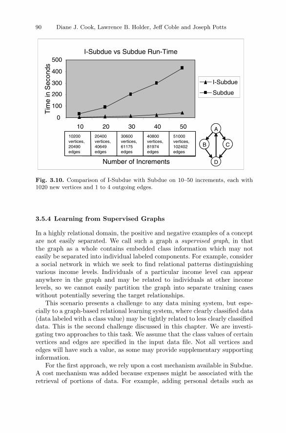
90 Diane J. Cook, Lawrence B. Holder, Jeff Coble and Joseph Potts
I-Subdue vs Subdue Run-Time
0
100
200
300
400
500
10 20 30 40 50
Number of Increments
Tim
e in
Sec
onds
I-Subdue
Subdue
51000 vertices, 102402 edges
40800 vertices, 81974 edges
30600 vertices, 61175 edges
20400 vertices, 40649 edges
10200 vertices, 20490 edges
51000 vertices, 102402 edges
40800 vertices, 81974 edges
30600 vertices, 61175 edges
20400 vertices, 40649 edges
10200 vertices, 20490 edges
A
CB
D
A
CB
D
Fig. 3.10. Comparison of I-Subdue with Subdue on 10–50 increments, each with1020 new vertices and 1 to 4 outgoing edges.
3.5.4 Learning from Supervised Graphs
In a highly relational domain, the positive and negative examples of a conceptare not easily separated. We call such a graph a supervised graph, in thatthe graph as a whole contains embedded class information which may noteasily be separated into individual labeled components. For example, considera social network in which we seek to find relational patterns distinguishingvarious income levels. Individuals of a particular income level can appearanywhere in the graph and may be related to individuals at other incomelevels, so we cannot easily partition the graph into separate training caseswithout potentially severing the target relationships.
This scenario presents a challenge to any data mining system, but espe-cially to a graph-based relational learning system, where clearly classified data(data labeled with a class value) may be tightly related to less clearly classifieddata. This is the second challenge discussed in this chapter. We are investi-gating two approaches to this task. We assume that the class values of certainvertices and edges are specified in the input data file. Not all vertices andedges will have such a value, as some may provide supplementary supportinginformation.
For the first approach, we rely upon a cost mechanism available in Subdue.A cost mechanism was added because expenses might be associated with theretrieval of portions of data. For example, adding personal details such as
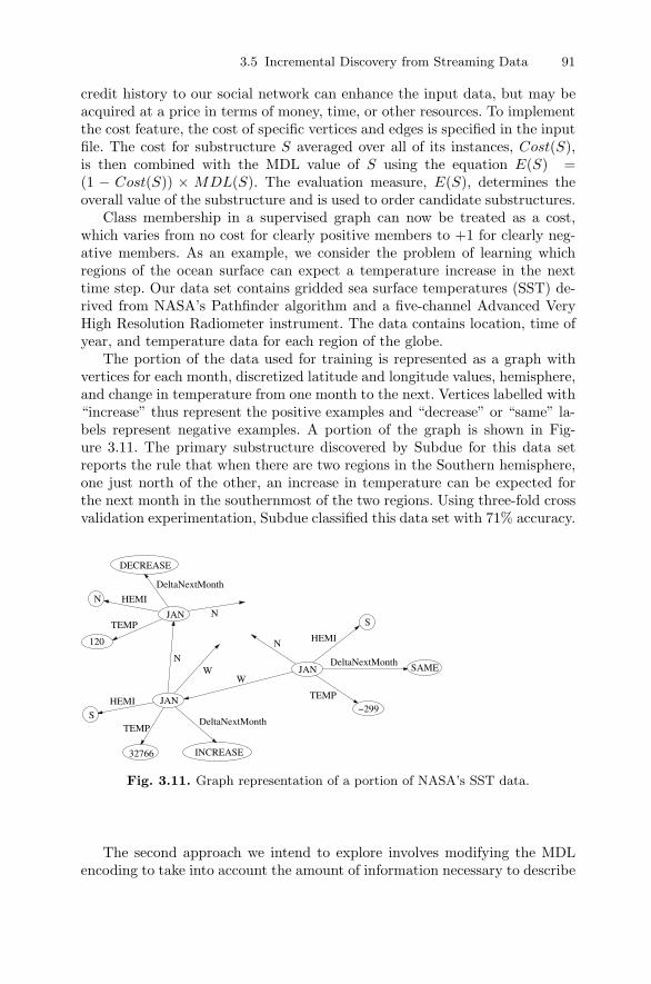
3.5 Incremental Discovery from Streaming Data 91
credit history to our social network can enhance the input data, but may beacquired at a price in terms of money, time, or other resources. To implementthe cost feature, the cost of specific vertices and edges is specified in the inputfile. The cost for substructure S averaged over all of its instances, Cost(S),is then combined with the MDL value of S using the equation E(S) =(1 − Cost(S)) × MDL(S). The evaluation measure, E(S), determines theoverall value of the substructure and is used to order candidate substructures.
Class membership in a supervised graph can now be treated as a cost,which varies from no cost for clearly positive members to +1 for clearly neg-ative members. As an example, we consider the problem of learning whichregions of the ocean surface can expect a temperature increase in the nexttime step. Our data set contains gridded sea surface temperatures (SST) de-rived from NASA’s Pathfinder algorithm and a five-channel Advanced VeryHigh Resolution Radiometer instrument. The data contains location, time ofyear, and temperature data for each region of the globe.
The portion of the data used for training is represented as a graph withvertices for each month, discretized latitude and longitude values, hemisphere,and change in temperature from one month to the next. Vertices labelled with“increase” thus represent the positive examples and “decrease” or “same” la-bels represent negative examples. A portion of the graph is shown in Fig-ure 3.11. The primary substructure discovered by Subdue for this data setreports the rule that when there are two regions in the Southern hemisphere,one just north of the other, an increase in temperature can be expected forthe next month in the southernmost of the two regions. Using three-fold crossvalidation experimentation, Subdue classified this data set with 71% accuracy.
DECREASE
JAN
N
120
DeltaNextMonth
HEMI
TEMPN
JAN
S
32766 INCREASE
HEMI
TEMPDeltaNextMonth
JAN SAME
−299
S
DeltaNextMonth
HEMI
TEMP
NW
W
N
Fig. 3.11. Graph representation of a portion of NASA’s SST data.
The second approach we intend to explore involves modifying the MDLencoding to take into account the amount of information necessary to describe
92 Diane J. Cook, Lawrence B. Holder, Jeff Coble and Joseph Potts
the class membership of the compressed graph. Substructures would now bediscovered that not only compress the raw data of the graph but also expressclass membership for vertices and edges within the graph.
3.6 Conclusions
There are several future directions for our graph-based relational learningresearch that will improve our ability to handle such challenging data as de-scribed in this chapter. The incremental discovery technique described in thischapter did not address data that is connected across increment boundaries.However, many domains will include event correlations that transcend mul-tiple data iterations. For example, a terrorist suspect introduced in one dataincrement may be correlated to events that are introduced in later incre-ments. As each data increment is received it may contain new edges thatextend from vertices in the new data increment to vertices received in pre-vious increments. We are investigating techniques of growing substructuresacross increment boundaries. We are also considering methods of detectingchanges in the strengths of substructures across increment boundaries, thatcould represent concept shift or drift.
The handling of supervised graphs is an important direction for miningstructural data. To extend our current work, we would like to handle embed-ded instances without a single representative instance node (the “increase”and “decrease” nodes in our NASA example) and instances that may possiblyoverlap.
Finally, improved scalability of graph operations is necessary to learn pat-terns, evaluate their accuracy on test cases and, ultimately, to use the patternsto find matches in future intelligence data. The graph and subgraph isomor-phism operations are a significant bottleneck to these capabilities. We needto develop faster and approximate versions of these operations to improve thescalability of graph-based relational learning.
Acknowledgments: This research is sponsored by the Air Force ResearchLaboratory (AFRL) under contract F30602-01-2-0570. The views and conclu-sions contained in this document are those of the authors and should not beinterpreted as necessarily representing the official policies, either expressed orimplied, of AFRL or the United States Government.
References
[1] Agrawal, R. and G. Psaila, 1995: Active data mining. Proceedings of theConference on Knowledge Discovery in Databases and Data Mining .
[2] Agrawal, R. and R. Srikant, 1994: Fast algorithms for mining associationrules. Proceedings of the Twentieth Conference on Very Large Databases,487–99.

References 93
[3] Blum, A., 1996: On-line algorithms in machine learning. Proceedings ofthe workshop on on-line algorithms.
[4] Cook, D. J. and L. B. Holder, 1994: Substructure discovery using mini-mum description length and background knowledge. Journal of ArtificialIntelligence Research, 1, 231–55.
[5] — 2000: Graph-based data mining. IEEE Intelligent Systems, 15, 32–41.[6] Dzeroski, S. and N. Lavrac, eds., 2001: Relational Data Mining . Springer.[7] Fang, H., W. Fan, P. Yu and J. Han, 2003: Mining concept-drifting
data streams using ensemble classifiers. Proceedings of the Conferenceon Knowledge Discovery and Data Mining .
[8] Friedman, N. and M. Goldszmidt, 1997: Sequential update of Bayesiannetwork structure. Proceedings of the Conference on Uncertainty in Ar-tificial Intelligence.
[9] Gonzalez, J., L. Holder and D. Cook, 2002: Graph-based relational con-cept learning. Proceedings of the Nineteenth International Conference onMachine Learning .
[10] Holder, L. B. and D. J. Cook, 2003: Graph-based relational learning:Current and future directions. ACM SIGKDD Explorations, 5, 90–93.
[11] Hulten, G., L. Spencer and P. Domingos, 2001: Mining time-changingdata streams. Proceedings of the Conference on Knowledge Discovery andData Mining .
[12] Inokuchi, A., T. Washio and H. Motoda, 2003: Complete mining of fre-quent patterns from graphs: Mining graph data. Machine Learning , 50,321–54.
[13] Jonyer, I., D. Cook and L. Holder, 2001: Graph-based hierarchical con-ceptual clustering. Journal of Machine Learning Research, 2, 19–43.
[14] Kashima, H. and A. Inokuchi, 2002: Kernels for graph classification. Pro-ceedings of the International Workshop on Active Mining .
[15] Kuramochi, M. and G. Karypis, 2001: Frequent subgraph discovery. Pro-ceedings of the First IEEE Conference on Data Mining .
[16] Muggleton, S., ed., 1992: Inductive Logic Programming . Academic Press,San Diego, CA, USA.
[17] Rissanen, J., 1989: Stochastic Complexity in Statistical Inquiry. WorldScientific, Singapore.
[18] US Senate, 2002: Joint inquiry into intelligence community activities be-fore and after the terrorist attacks of September 11, 2001. S. Rept.107-351.
[19] Yan, X. and J. Han, 2002: gSpan: Graph-based substructure pattern min-ing. Proceedings of the International Conference on Data Mining.
[20] Yoshida, K., H. Motoda and N. Indurkhya, 1994: Graph-based inductionas a unified learning framework. Journal of Applied Intelligence, 4, 297–328.

4
Predictive Graph Mining with Kernel Methods
Thomas Gartner
Summary. Graphs are a major tool for modeling objects with complex data struc-tures. Devising learning algorithms that are able to handle graph representationsis thus a core issue in knowledge discovery with complex data. While a significantamount of recent research has been devoted to inducing functions on the vertices ofthe graph, we concentrate on the task of inducing a function on the set of graphs.Application areas of such learning algorithms range from computer vision to biologyand beyond. Here, we present a number of results on extending kernel methods tocomplex data, in general, and graph representations, in particular. With the verygood performance of kernel methods on data that can easily be embedded in a Eu-clidean space, kernel methods have the potential to overcome some of the majorweaknesses of previous approaches to learning from complex data. In order to applykernel methods to graph data, we propose two different kernel functions and comparethem on a relational reinforcement learning problem and a molecule classificationproblem.
4.1 Introduction
Graphs are an important tool for modeling complex data in a systematic way.Technically, different types of graphs can be used to model the objects. Con-ceptually, different aspects of the objects can be modeled by graphs: (i) Eachobject is a vertex in a graph modeling the relation between the objects, and(ii) each object is modeled by a graph. While a significant amount of recentresearch is devoted to case i, here we are concerned with case ii. An importantexample for this case is the prediction of biological activity of molecules giventheir chemical structure graph.
Suppose we know of a function that estimates the effectiveness of chemicalcompounds against a particular illness. This function would be very helpful indeveloping new drugs. One possibility for obtaining such a function is to usein-depth chemical knowledge. A different – and for us more interesting – pos-sibility is to try to learn from chemical compounds with known effectiveness

96 Thomas Gartner
against that illness. We will call these compounds “training instances”. Super-vised machine learning tries to to find a function that generalizes over thesetraining instances, i.e., a function that is able to estimate the effectiveness ofother chemical compounds against this disease. We will call this function the“hypothesis” and the set of all functions considered as possible hypotheses,the “hypothesis space”.
Though chemical compounds are three-dimensional structures, the three-dimensional shape is often determined by the chemical structure graph. Thatis, the representation of a molecule by a set of atoms, a set of bonds con-necting pairs of atoms, and a mapping from atoms to element-types (carbon,hydrogen, ...) as well as from bonds to bond-types (single, double, aromatic,...). Standard machine learning algorithms can not be applied to such a rep-resentation.
Predictive graph mining is interested in supervised machine learning prob-lems with graph-based representations. This is an emerging research topic atthe heart of knowledge discovery from complex data. In contrast with othergraph mining approaches it is not primarily concerned with finding interestingor frequent patterns in a graph database but only with supervised machinelearning, i.e., with inducing a function on the set of all graphs that approxi-mates well some unknown functional or conditional dependence. In the abovementioned application this would be effectiveness against an illness dependingon the chemical structure of a compound.
Kernel methods are a class of learning algorithms that can be applied toany learning problem as long as a positive-definite kernel function has beendefined on the set of instances. The hypothesis space of kernel methods isthe linear hull (i.e., the set of linear combinations) of positive-definite kernelfunctions “centered” at some training instances. Kernel methods have showngood predictive performance on many learning problems, such as text classi-fication. In order to apply kernel methods to instances represented by graphs,we need to define meaningful and efficiently computable positive-definite ker-nel functions on graphs.
In this article we describe two different kernels for labeled graphs togetherwith applications to relational reinforcement learning and molecule classifica-tion. The first graph kernel is based on comparing the label sequences corre-sponding to walks occurring in each graph. Although these walks may haveinfinite length, for undirected graphs, such as molecules, this kernel functioncan be computed in polynomial time by using properties of the direct productgraph and computing the limit of a power series. In the molecule classifica-tion domain that we will look at, however, exact computation of this kernelfunction is infeasible and we need to resort to approximations. This motivatesthe search for other graph kernels that can be computed more efficiently onthis domain. We thus propose a graph kernel based on the decomposition ofeach graph into a set of simple cycles and into the set of connected compo-nents of the graph induced by the set of bridges in the graph. Each of thesecycles and trees is transformed into a pattern and the cyclic-pattern kernel

4.2 Learning with Kernels and Distances 97
for graphs is the cardinality of the intersection of two pattern sets. Althoughcyclic-pattern kernels can not be computed in polynomial time, empirical re-sults on a molecule classification problem show that, while walk-based graphkernels exhibit higher predictive performance, cyclic-pattern kernels can becomputed much faster. Both kernels perform better than, or at least as goodas, previously proposed predictive graph mining approaches over different sub-problems and parameter settings.
Section 4.2 introduces kernel methods, kernels for structured instancesspaces, and discusses the relation between kernels and distances for structuredinstances. Section 4.3 begins with the introduction of general set kernels andconceptually describes kernels for other data structures afterwards. Section4.4 describes walk-based graph kernels and cyclic-pattern kernels for graphs.Two applications of predictive graph mining are shown in Section 4.5, beforeSection 4.6 concludes.
4.2 Learning with Kernels and Distances
In this section we first define what is meant by a positive-definite kernel func-tion and briefly introduce the basics of kernel methods. We illustrate theimportance of choosing the “right” kernel function on a simple example. Af-ter that, we summarise different definitions of kernel functions for instancesrepresented by vertices in a graph. Last but not least, we discuss the relationbetween well known distance functions for complex data and kernel functions.
4.2.1 Kernel Methods
Kernel methods [41] are a popular class of algorithms within the machine-learning and data-mining communities. Being theoretically well founded instatistical learning theory, they have shown good empirical results in manyapplications. One particular aspect of kernel methods such as the support vec-tor machine is the formation of hypotheses by linear combination of positive-definite kernel functions “centered” at individual training instances. By the re-striction to positive-definite kernel functions, the regularized risk minimizationproblem (we will define this problem once we have defined positive-definitefunctions) becomes convex and every locally optimal solution is globally op-timal.
Kernel FunctionsKernel methods can be applied to different kinds of (structured) data by usingany positive-definite kernel function defined on the data.
A symmetric function k : X×X → R on a set X is called a positive-definitekernel on that set if, for all n ∈ Z
+, x1, . . . , xn ∈ X , and c1, . . . , cn ∈ R, itfollows that

98 Thomas Gartner ∑i,j∈1,...,n
ci cj k(xi, xj) ≥ 0.
Kernel MachinesThe usual supervised learning model [44] considers a set X of individuals anda set Y of labels, such that the relation between individuals and labels is afixed but unknown probability measure on the set X ×Y. The common themein many different kernel methods such as support vector machines, Gaussianprocesses, or regularized least squares regression is to find a hypothesis func-tion that minimizes not just the empirical risk (the training error) but alsothe regularized risk . This gives rise to the optimization problem
minf(·)∈H
C
n
n∑i=1
V (yi, f(xi)) + ‖f(·)‖2H
where C is a parameter, (xi, yi)ni=1 is a set of individuals with known label(the training set), H is a set of functions forming a Hilbert space (the hypoth-esis space) and V is a function that takes on small values whenever f(xi) is agood guess for yi and large values whenever it is a bad guess (the loss func-tion). The representer theorem shows that under rather general conditions onV , solutions of the above optimization problem have the form
f(·) =n∑
i=1
cik(xi, ·). (4.1)
Different kernel methods arise from using different loss functions.
Regularized Least SquaresChoosing the square loss function, i.e., V (yi, f(xi)) = (yi−f(xi))2, we obtainthe optimization problem of the algorithm [39, 40]:
minf(·)∈H
C
n
n∑i=1
(yi − f(xi))2 + ‖f(·)‖2H
Plugging in our knowledge about the form of solutions and taking the direc-tional derivative with respect to the parameter vector c of Equation (4.1), wecan find the analytic solution to the optimization problem as:
c =(K +
n
CI)−1
y
where I denotes the identity matrix of appropriate size.
Support Vector MachinesSupport vector machines [2, 41] are a kernel method that can be applied tobinary-supervised classification problems. They are derived from the above

4.2 Learning with Kernels and Distances 99
optimization problem by choosing the so-called hinge loss V (y, f(x)) =max0, 1−yf(x). The motivation for support vector machines often given inthe literature is that the solution can be interpreted as a hyperplane that sep-arates both classes (if it exists) and is maximally distant from the convex hullsof both classes. A different motivation is the computational attractiveness ofsparse solutions of Equation (4.1) used for classification.
For support vector machines the problem of minimizing the regularizedrisk can be transformed into the so-called “primal” optimization problem ofsoft-margin support vector machines:
minc∈Rn
Cn
n∑i=1
ξi + cKc
subject to: yi
∑j
cjk(xi, xj) ≥ 1− ξi i = 1, . . . n
ξi ≥ 0 i = 1, . . . n.
Gaussian ProcessesGaussian processes [35] are an incrementally learnable Bayesian regressionalgorithm. Rather than parameterizing some set of possible target functionsand specifying a prior over these parameters, Gaussian processes directly puta (Gaussian) prior over the function space. A Gaussian process is defined bya mean function and a covariance function, implicitly specifying the prior.The choice of covariance functions is thereby only limited to positive-definitekernels. It can be seen that the mean prediction of a Gaussian process corre-sponds to the prediction found by a regularized least squares algorithm. Thislinks the regularization parameter C with the variance of the Gaussian noisedistribution assumed in Gaussian processes.
IllustrationTo illustrate the importance of choosing the “right” kernel function, we nextillustrate the hypothesis found by a Gaussian process with different kernelfunctions.
In Figure 4.1 the training examples are pairs of real numbers x ∈ X = R2
illustrated by black discs and circles in the figure. The (unknown) tar-get function is an XOR-type function, the target variable y takes values−1 for the black discs and +1 for the black circles. The probability ofa test example being of class +1 is illustrated by the color of the corre-sponding pixel in the figure. The different kernels used are the linear ker-nel k(x, x′) = 〈x, x′〉, the polynomial kernel k(x, x′) = (〈x, x′〉 + l)p, thesigmoid kernel k(x, x′) = tanh(γ 〈x, x′〉), and the Gaussian kernel functionk(x, x′) = exp
[−‖x− x′‖2/σ2
].
Figure 4.2 illustrates the impact of choosing the parameter of a Gaussiankernel function on the regularization of the solution found by a Gaussianprocess. Training examples are single real numbers and the target value is

100 Thomas Gartner
(a) (b)
(c) (d)
Fig. 4.1. Impact of different kernel functions on the solution found by Gaussianprocesses. Kernel functions are (a) linear kernel, (b) polynomial kernel of degree 2,(c) sigmoid kernel and (d) Gaussian kernel.
also a real number. The unknown target function is a sinusoid function shownby a thin line in the figure. Training examples perturbed by random noise aredepicted by black circles. The color of each pixel illustrates the likeliness of atarget value given a test example, with the most likely value colored white.

4.2 Learning with Kernels and Distances 101
Fig. 4.2. Impact of the bandwidth of a Gaussian kernel function on the regulariza-tion of the solution found by Gaussian processes. The bandwidth is decreasing fromleft to right, top to bottom.
4.2.2 Kernels for Structured Instance Spaces
To model the structure of instance spaces, undirected graphs or hypergraphsare often used. While the use of hypergraphs is less common in the literature,it appears more systematic and intuitive.
A hypergraph is described by a set of vertices V – the instances – and a setof edges E , where each edge corresponds to a set of vertices. Each edge of thehypergraph can be interpreted as some property that all vertices of the edgehave in common. For documents, for example, the edges could correspond towords or citations that they have in common; in a metric space the hyperedgecould include all vertices with distance less than a given threshold from somepoint.

102 Thomas Gartner
For a hypergraph with n vertices and m edges, we define the n×m matrixB by Bij = 1 if and only if vi ∈ ej and Bij = 0, otherwise. Let then the n×nmatrix D be defined by Dii =
∑j
[BB
]ij
=∑
j
[BB
]ji
. The matricesBB and L = D −BB are positive-definite by construction. The matrix Lis known as the graph Laplacian. Often also the normalized Laplacian is used.
Conceptually, kernel matrices are then defined as the limits of matrixpower series of the form
K =∞∑
i=0
λi
(BB
)ior K =
∞∑i=0
λi (−L)i
with parameters λi. These power series can be interpreted as measuring thenumber of walks of different lengths between given vertices.
Limits of such power series can be computed by means of an eigenvaluedecomposition of −L or BB, and a “recomposition” with modified eigen-values. The modification of the eigenvalues is usually such that the order ofeigenvalues is kept, while all eigenvalues are forced to become positive.
Examples for such kernel functions are the diffusion kernel [29]
K =∞∑
i=0
βi
i!(−L)i ,
the von Neumann kernel [25]
K =∞∑
i=1
γi−1 (BB)i
,
and the regularized Laplacian kernel [42]
K =∞∑
i=1
γi(−L)i .
For exponential power series such as the diffusion kernel, the limit canbe computed by exponentiating the eigenvalues, while for geometrical powerseries, the limit can be computed by the formula 1/(1 − γe), where e is aneigenvalue of BB or −L, respectively. A general framework and analysis ofthese kernels is given in [42].
4.2.3 Kernels versus Distances for Structured Instances
Previous approaches to predictive graph mining mostly used decision trees[20] or distance-based algorithms. Due to the close relation between kernelsand distances1 we thus investigate how distances on structured instances aredefined.
1Every inner product space is a metric space.

4.2 Learning with Kernels and Distances 103
In the literature, distances are often defined using the minima and/or max-ima over a set of distances, e.g., all distances described in [12] between pointsets, the string edit distance [13] between sequences, or the subgraph dis-tance [3, 36] between graphs. It is thus interesting to investigate whether ingeneral kernel functions can be defined as the minimum and/or maximum ofa set of kernels. In this section we investigate whether certain uses of minimaand/or maxima give rise to positive-definite kernels and discuss minima- andmaxima-based kernels on instances represented by sets.
Minimal and Maximal FunctionsWe begin our discussion with two very simple uses of minima and maxima.
The function minx, x′ defined on non-negative real numbers is positive-definite: Let θx(·) be the function such that θx(z) = 1 if z ∈ [0;x] and θx(z) = 0otherwise. Then,
minx, x′ =∫
R
θx(·) ∗ θx′(·)dµ
coincides with the usual (L2) inner product between the functions θx(·) andθx′(·). Thus it is positive-definite.
The function maxx, x′ defined on non-negative real numbers is notpositive-definite. Setting x = 0, x′ = 1 we obtain the indefinite matrix(
0 11 1
).
We show next, that – in general – functions built from positive-definitekernels using the min or max function are not positive-definite.
The function mini ki(x, x′) where each ki is a positive-definite kernel, is notnecessarily positive-definite: Setting x = 1;x′ = 2; k1(x, x′) = xx′; k2(x, x′) =(3− x)(3− x′) gives rise to the indefinite matrix(
1 22 1
).
The function maxi ki(x, x′) where again each ki is a positive-definite kernel,is not necessarily positive-definite: If this function was positive-definite thenthe component wise maximum of two positive-definite matrices would also bepositive-definite. Consider the matrices
A =
⎛⎝1 1 0
1 1 00 0 1
⎞⎠ ; B =
⎛⎝1 0 0
0 1 10 1 1
⎞⎠ .
Here, A has the eigenvectors (1, 1, 0); (0, 0, 1); (1,−1, 0) with correspond-ing eigenvalues 2, 1, 0 ≥ 0, showing that both matrices are positive-definite.The component wise maximum of A and B

104 Thomas Gartner
D =
⎛⎝1 1 0
1 1 10 1 1
⎞⎠
is, however, indefinite: (1, 0, 0)D(1, 0, 0) = 1 > 0 and (1,−1, 1)D(1,−1, 1) =−1 < 0.
Minimal and Maximal Functions on SetsWe now proceed with two simple cases in which positive-definiteness holds forkernels on sets using minima or maxima functions.
The function minx∈X,x′∈X′ x∗x′ defined on sets of non-negative real num-bers X, X ′ ⊂ R
+ is positive-definite as
minx∈X,x′∈X′
x ∗ x′ =(
minx∈X
x
)∗(
minx′∈X′
x′)
.
The function maxx∈X,x′∈X′ x∗x′ defined on sets of non-negative real num-bers X, X ′ ⊂ R
+ is positive-definite as
maxx∈X,x′∈X′
x ∗ x′ =(
maxx∈X
x
)∗(
maxx′∈X′
x′)
.
Now we turn to the more general functions minx∈X,x′∈X′ k(x, x′) andmaxx∈X,x′∈X′ k(x, x′). These are strongly related to the functions mini ki(x, x′)and maxi ki(x, x′) considered above. To see this let X = xi; X ′ = x′
j andkij(X, X ′) = k(xi, x
′j). Then
minx∈X,x′∈X′
k(x, x′) = minij
kij(X, X ′)
andmax
x∈X,x′∈X′k(x, x′) = max
ijkij(X, X ′) .
Though this indicates that minx∈X,x′∈X′ k(x, x′) and maxx∈X,x′∈X′ k(x, x′)are not positive-definite, it does not prove it yet. Thus we continue with twocounter-examples. For minx∈X,x′∈X′ k(x, x′) with X =
(1, 2), (2, 1), (2, 0),
X ′ =(2, 1), and using k(x, x′) = 〈x, x′〉 we obtain the indefinite matrix(
2 44 5
).
Similarly, for maxx∈X,x′∈X′ k(x, x′) with x1 =(1, 0), x2 =
(1, 0), (0, 1),
x3 =(0, 1), and again k(x, x′) = 〈x, x′〉 we obtain the matrix
D =
⎛⎝1 1 0
1 1 10 1 1
⎞⎠

4.3 Sets and Beyond 105
which is again indefinite.The observations made above indicate that kernels for complex data can
not be made up such that they directly correspond to the previously defineddistances for complex data. This motivates the search for alternative kernelfunctions such as the ones described below.
4.3 Sets and Beyond
An integral part of many kernels for complex data is the decomposition ofan object into a set of its parts and the intersection of two sets of parts.The kernel on two objects is then defined as a measure of the intersection ofthe two corresponding sets of parts. In this section we first summarise somebasics about kernels on sets. Then we give a brief overview of different kernelfunctions for complex data.
The general case of interest for set kernels is when the instances Xi areelements of a semi-ring of sets S and there is a measure µ with S as itsdomain of definition.
A natural choice of a kernel on such data is the intersection kernel definedas
k∩(Xi, Xj) = µ(Xi ∩Xj);Xi, Xi ∈ S . (4.2)
It is known [28] that for any X1, . . . Xn belonging to S there is a finite systemof pairwise disjoint sets A = A1, . . . Am ⊆ S such that every Xi is a unionof some Al. Let Bi ⊆ A be such that Xi =
⋃B∈Bi
B. Furthermore let thecharacteristic function ΓX : A → 0; 1 be defined as ΓX(A) = 1⇔A ⊆ Xand ΓX(A) = 0 otherwise. With these definitions we can write
µ(Xi ∩Xj) =∑
B∈Bi∩Bj
µ(B) =∑A∈A
ΓXi(A)ΓXj (A)µ(A) .
The intersection kernel is then positive-definite on X1, . . . Xn as∑ij
cicjµ(Xi ∩Xj) =∑ij
cicj
∑A∈A
ΓXi(A)ΓXj
(A)µ(A)
=∑A∈A
(∑i
ciΓXi(A)
)2
µ(A)
≥0 .
Note that in the simplest case (finite sets with µ(·) being the set cardinal-ity) the intersection kernel coincides with the inner product of the bitvectorrepresentations of the sets.
In the case that the sets Xi are finite or countable sets of elements onwhich a kernel has been defined, it is often beneficial to use set kernels otherthan the intersection kernel. For example the crossproduct kernel

106 Thomas Gartner
k×(Xi, Xj) =∑
xi∈Xi,xj∈Xj
k(xi, xj) . (4.3)
The crossproduct kernel with the right kernel set to the matching kernel (de-fined as kδ(xi, xj) = 1⇔ xi = xj and 0 otherwise) coincides with the inter-section kernel.
In the remainder of this section we are more interested in the case that S isa Borel algebra with unit X , and µ is countably additive with µ(X ) <∞. Wecan then extend the definition of the characteristic functions to X =
⋃C∈S C
such that ΓX(x) = 1⇔ x ∈ X and ΓX(x) = 0 otherwise. We can then writethe intersection kernel as
k∩(Xi, Xj) = µ(X ∩X ′) =∫
XΓXi
(x) ∗ ΓXj(x)dµ (4.4)
this shows the relation of the intersection kernel to the usual (L2) inner prod-uct between the characteristic functions ΓX(·), ΓX′(·) of the sets.
Similarly, for the crossproduct kernel in Equation (4.3) we obtain in thissetting the integral equation∫
X×X′k(x, x′)dµdµ =
∫X×X
ΓX(x) ∗ k(x, x′) ∗ ΓX′(x′)dµdµ
with any positive-definite kernel k defined on the elements.Note, that with the matching kernel kδ we recover the intersection kernel
from Equation (4.4) albeit with different measure.In the remainder of this section we describe kernels for complex data that
have been defined in the literature. For a more complete survey of kernels forstructured data we recommend [16].
4.3.1 Convolution Kernels
The best known kernel for representation spaces that are not mere attribute-value tuples is the convolution kernel proposed by Haussler [22]. The basic ideaof convolution kernels is that the semantics of composite objects can often becaptured by a relation R between the object and its parts. The kernel on theobject is then made up from kernels defined on different parts.
Let x, x′ ∈ X be the objects and x,x′ ∈ X1 × · · · × XD be tuples of partsof these objects. Given the relation R : (X1× · · ·×XD)×X we can define thedecomposition R−1 as R−1(x) = x : R(x, x). Then the convolution kernelis defined as
kconv(x, x′) =∑
x∈R−1(x),x′∈R−1(x′)
D∏d=1
kd(xd, x′d) .
The term “convolution kernel” refers to a class of kernels that can beformulated in the above way. The advantage of convolution kernels is that

4.3 Sets and Beyond 107
they are very general and can be applied in many different problems. How-ever, because of that generality, they require a significant amount of work toadapt them to a specific problem, which makes choosing R in “real-world”applications a non-trivial task.
4.3.2 String Kernels
The idea of most string kernels [34, 47] defined in the literature is to basethe similarity of two strings on the number of common subsequences. Thesesubsequences need not occur contiguously in the strings but the more gapsin the occurrence of the subsequence, the less weight is given to it in thekernel function. For example, the string “cat” would be decomposed in thesubsequences “c”, “a”, “t”, “ca”, “at”, “ct”, and “cat”. These subsequencesalso occur in the string “cart”, albeit with different length of the occurrence.Usually the length of the occurrence of the substring is used as a penalty.With an exponentially decaying penalty, the weight of every occurrencein “cat”/“cart” becomes: “c”:(λ1λ1), “a”:(λ1λ1), “t”:(λ1λ1), “ca”:(λ2λ2),“at”:(λ2λ3), “ct”:(λ3λ4), “cat”:(λ3λ4) and the kernel of “cat” and “cart” be-comes k(“cat”, “cart”) = 2λ7 + λ5 + λ4 + 3λ2. Using a divide and conquerapproach, computation of this kernel can be reduced to O(n|s||t|) [34]. In [45]and [32] other string kernels are proposed and it is shown how these can becomputed efficiently by using suffix and mismatch trees, respectively.
4.3.3 Tree Kernels
A kernel function that can be applied in many natural language processingtasks is described in [4]. The instances of the learning task are consideredto be labeled ordered directed trees. The key idea for capturing structuralinformation about the trees in the kernel function is to consider all subtreesoccurring in a parse tree. Here, a subtree is defined as a connected subgraphof a tree such that either all children or no child of a vertex is in the subgraph.The children of a vertex are the vertices that can be reached from the vertexby traversing one directed edge. The kernel function is the inner product inthe space which describes the number of occurrences of all possible subtrees.
Recently, [45] proposed the application of string kernels to trees by repre-senting each tree by the sequence of labels generated by a depth-first traversalof the trees, written in preorder notation. To ensure that trees only differing inthe order of their children are represented in the same way, the children of eachvertex are ordered according to the lexical order of their string representation.
4.3.4 Kernels for Higher-Order Terms
In [19], a framework has been been proposed that allows for the application ofkernel methods to different kinds of structured data. This approach is based

108 Thomas Gartner
on the idea of having a powerful representation that allows for modeling thesemantics of an object by means of the syntax of the representation. Theunderlying principle is that of representing individuals as (closed) terms in atyped higher-order logic [33]. The biggest difference to terms of a first-orderlogic is the use of types and the presence of abstractions that allow explicitmodeling of sets, multisets, and so on.
The typed syntax is important for pruning search spaces and for modelingas closely as possible the semantics of the data in a human- and machine-readable form. The individuals-as-terms representation is a natural general-ization of the attribute-value representation and collects all information aboutan individual in a single term.
Basic terms represent the individuals that are the subject of learning andfall into one of three categories: basic structures that represent individuals thatare lists, trees, and so on; basic abstractions that represent sets, multisets, andso on; and basic tuples that represent tuples. Basic abstractions are almostconstant mappings β → γ that can be regarded as lookup tables, where allbasic terms of type β in the table are mapped to some basic term of type γand all basic terms not in the table are mapped to one particular basic term,the default term of type γ.
Applications of this kernel are spatial clustering of demographic data,multi-instance learning for drug-activity prediction and predicting the struc-ture of molecules from their NMR spectra.
Multi-instance learning problems [8] occur whenever example objects, in-dividuals, can only be described by a set of which any single element could beresponsible for the classification of the set. Here, it can be shown that witha particular abstraction kernel, the number of iterations needed by a kernelperceptron to converge to a consistent hypothesis is bound by a polynomialin the number of elements in the sets.
4.4 Graphs, Graphs, Graphs ...
The obvious approach to defining kernels on objects that have a natural rep-resentation as a graph is to decompose each graph into a set of subgraphs andmeasure the intersection of two decompositions. With such a graph kernel,one could decide whether a graph has a Hamiltonian path or not [18]. Asthis problem is known to be NP-hard, it is strongly believed that the obviousgraph kernel can not be computed in polynomial time. This holds even if thedecomposition is restricted to paths only.
In the literature different approaches are described to overcome this prob-lem. Graepel [21] restricted the decomposition to paths up to a given size,and Deshpande et al. [6] only considers the set of connected graphs that oc-cur frequently as subgraphs in the graph database. The approach taken thereto compute the decomposition of each graph is an iterative one [31]. The al-gorithm starts with a frequent set of subgraphs with one or two edges only.

4.4 Graphs, Graphs, Graphs ... 109
Then, in each step, from the set of frequent subgraphs of size l, a set of can-didate graphs of size l + 1 is generated by joining those graphs of size l thathave a subgraph of size l− 1 in common. Of the candidate graphs only thosesatisfying a frequency threshold are retained for the next step. The iterationstops when the set of frequent subgraphs of size l is empty.
Conceptually, the graph kernels presented in [15, 18, 26, 27] are based ona measure of the walks in two graphs that have some or all labels in common.In [15] walks with equal initial and terminal label are counted, in [26, 27] theprobability of random walks with equal label sequences is computed, and in[18] walks with equal label sequences, possibly containing gaps, are counted.In [18] computation of these – possibly infinite – walks is made possible inpolynomial time by using the direct product graph and computing the limitof matrix power series involving its adjacency matrix. The work on rationalgraph kernels [5] generalizes these graph kernels by applying a general trans-ducer between weighted automata instead of forming the direct product graph.However, only walks up to a given length are considered in the kernel com-putation. More recently, Horvath et al. [23] suggested that the computationalintractability of detecting all cycles in a graph can be overcome in practicalapplications by observing that “difficult structures” occur only infrequentlyin real-world databases. As a consequence of this assertion, Horvath et al.[23] use a cycle-detection algorithm to decompose all graphs in a moleculedatabase into all simple cycles occurring.
In the remainder of this section we will describe walk- and cycle-basedgraph kernels in more detail.
4.4.1 Walk-Based Graph Kernels
A labeled directed graph G is described by a finite set of vertices V, a finiteset of edges E , and a function . The set of edges is a subset of the Cartesianproduct of the set of vertices with itself (E ⊆ V×V) such that that (νi, νj) ∈ Eif and only if there is an edge from νi to νj in graph G. The function mapseach edge and/or vertex to a label. The adjacency matrix of the graph is a|V| × |V| matrix E where the Eij = 1 if and only if (νi, νj) ∈ E and Eij = 0otherwise.
We concentrate now on one type of kernel introduced in [18], measuring thenumber of walks with common label sequence in two graphs. There, efficientcomputation of these – possibly infinite – walks is made possible by using thedirect product graph and computing the limit of matrix power series involvingits adjacency matrix.
The two graphs generating the product graph are called the factor graphs.The vertex set of the direct product of two graphs is a subset of the Cartesianproduct of the vertex sets of the factor graphs. The direct product graph hasa vertex if and only if the labels of the corresponding vertices in the factorgraphs are the same. There is an edge between two vertices in the productgraph if and only if there is an edge between the corresponding vertices in

110 Thomas Gartner
both factor graphs and both edges have the same label. For unlabeled graphs,the adjacency matrix of the direct product graph corresponds to the tensorproduct of the adjacency matrices of its factors.
With a sequence of weights λ0, λ1, . . . (λi ∈ R; λi ≥ 0 for all i ∈ N) thedirect product kernel is defined as
k×(G1, G2) =|V×|∑i,j=1
[ ∞∑n=0
λnEn×
]ij
if the limit exists.For symmetric E×, limits of such power series can be computed by means
of an eigenvalue decomposition of E, and a “recomposition” with modifiedeigenvalues. The modification of the eigenvalues is usually such that the orderof eigenvalues is kept.
To illustrate these kernels, consider a simple graph with four vertices la-beled “c”, “a”, “r”, and “t”, respectively. We also have four edges in thisgraph: one from the vertex labeled “c” to the vertex labeled “a”, one from“a” to “r”, one from “r” to “t”, and one from “a” to “t”. The non-zero fea-tures in the label sequence feature space are φc = φa = φr = φt =
√λ0,
φca = φar = φat = φrt =√
λ1, φcar = φcat = φart = λ2, and φcart =√
λ3.The λi are user defined weights and the square-roots appear only to makethe computation of the kernel more elegant. The above kernel function corre-sponds to the inner product between such feature vectors (of possibly infinitedimension).
4.4.2 Cyclic-Pattern Kernels
A labeled undirected graph can be seen as a labeled directed graph where theexistence of an edge between two vertices implies the existence of an edge inthe other direction and both edges are mapped to the same label. Each edgeof an undirected graph is usually represented by a subset of the vertex setwith cardinality two. A path in an undirected graph is a sequence v1, . . . vn ofdistinct vertices vi ∈ V where vi, vi+1 ∈ E . A simple cycle in an undirectedgraph is a path, where also v1, vn ∈ E . A bridge is an edge not part of anysimple cycle; the graph made up by all bridges is a forest, i.e., a set of trees.
We describe now the kernel proposed in [23] for molecule classification.The key idea is to decompose every undirected graph into the set of cyclicand tree patterns in the graph. A cyclic pattern is a unique representation ofthe label sequence corresponding to a simple cycle in the graph. A tree patternin the graph is a unique representation of the label sequence corresponding toa tree in the forest made up by all bridges. The cyclic-pattern kernel betweentwo graphs is defined by the cardinality of the intersection of the pattern setsassociated with each graph.
Consider a graph with vertices 1, . . . 6 and labels (in the order of vertices)“c”, “a”, “r”, “t”, “e”, and “s”. Let the edges be the set

4.5 Applications of Predictive Graph-Mining 111
1, 2, 2, 3, 3, 4, 2, 4, 1, 5, 1, 6.
This graph has one simple cycle and the lexicographically smallest represen-tation of the labels along this cycle is the string “art”. The bridges of thegraph are 1, 2, 1, 5, 1, 6 and the bridges form a forest consisting of asingle tree. The lexicographically smallest representation of the labels of thistree (in pre-order notation) is the string “aces”.
If the cyclic-pattern kernel between any two graphs could be computedin polynomial time, the Hamiltonian cycle problem could also be solved inpolynomial time. Furthermore, the set of simple cycles in a graph can not becomputed in polynomial time – even worse, the number of simple cycles ina graph can be exponential in the number of vertices of the graph. Considera graph consisting of two paths v0, . . . vn and u0, . . . un with additional edgesvi, ui : 0 ≤ i ≤ n ∪ vi, ui−2 : 2 ≤ i ≤ n where the number of pathsfrom v0 to un is lower bound by 2n. It follows directly that the number ofsimple cycles in the graph with the additional edge un, v0 is also lowerbound by 2n.
The only remaining hope for a practically feasible algorithm is that thenumber of simple cycles in each graph can be bound by a small polynomial.Read and Tarjan [38] proposed an algorithm with polynomial delay complex-ity, i.e., the number of steps that the algorithm needs between finding onesimple cycle and finding the next simple cycle is polynomial. This algorithmcan be used to enumerate all cyclic patterns. Note that this does not implythat the number of steps the algorithm needs between two cyclic patterns ispolynomial.
In the next section we will compare walk- and cycle-based graph kernels inthe context of drug design and prediction of properties of molecules. It is illus-trated there that indeed for the application considered, only a few moleculesexist that have a large number of simple cycles. Before that we describe anapplication of walk-based graph kernels in a relational reinforcement learningsetting.
4.5 Applications of Predictive Graph-Mining
In this section we describe two applications of graph kernels. The first appli-cation is a relational reinforcement learning task in the blocks world. The sec-ond application is a molecule classification task on a relatively large database(> 40, 000 instances) of molecules classified according to their ability to pro-tect human cells from the HIV virus.
4.5.1 Relational Reinforcement Learning
Reinforcement learning [43], in a nutshell, is about controlling an autonomousagent in an environment about which he has no prior knowledge. The only

112 Thomas Gartner
information the agent can get about the environment is its current state andwhether it received a reward. The goal of reinforcement learning is to maximizethis reward. One particular form of reinforcement learning is Q-learning [46].It tries to learn a map from state-action-pairs to real numbers (Q-values)reflecting the quality of that action in that state.
Relational reinforcement learning [10, 11] (RRL) is a Q-learning techniquethat can be applied whenever the state-action space can not easily be repre-sented by tuples of constants but has an inherently relational representationinstead. In this case, explicitly representing the mapping from state-action-pairs to Q-values is usually not feasible.
The RRL-system learns through exploration of the state-space in a waythat is very similar to normal Q-learning algorithms. It starts with runningan episode2 just like table-based Q-learning, but uses the encountered states,chosen actions and the received rewards to generate a set of examples thatcan then be used to build a Q-function generalization. These examples use astructural representation of states and actions.
To build this generalized Q-function, RRL applies an incremental rela-tional regression engine that can exploit the structural representation of theconstructed example set. The resulting Q-function is then used to decide whichactions to take in the following episodes. Every new episode can be seen as anew experience and is thus used to updated the Q-function generalization.
A rather simple example of relational reinforcement learning takes placein the blocks world. The aim there is to learn how to put blocks that are inan arbitrary configuration into a given configuration.
v5
v4
v1
v2
v
v3
0
4
1
2 3
on
block, a/2
on
on
onon
onaction
clear
block, a/1
block
block
floor
Fig. 4.3. Simple example of a blocks world state and action (left) and its represen-tation as a graph (right).
2An “episode” is a sequence of states and actions from an initial state to aterminal state. In each state, the current Q-function is used to decide which actionto take.

4.5 Applications of Predictive Graph-Mining 113
In this section we describe an application of Gaussian processes to learnthe mapping from relational state-action spaces to Q-values in the blocksworld. One advantage of using Gaussian processes in RRL is that rather thanpredicting a single Q-value, they actually return a probability distributionover Q-values. In order to employ Gaussian processes in a relational reinforce-ment learning setting, we use graph kernels as the covariance function betweenstate-action pairs. For that we needed to extend the above described graphkernels to graphs that may have multiple edges between the same vertices.The details of this extension are described in [17].
State and Action RepresentationA blocks world consists of a constant number of identical blocks. Each blockis put either on the floor or on another block. On top of each block is ei-ther another block or the top of the block is clear. Figure 4.3 illustrates a(state, action)-pair in a blocks world with four blocks in two stacks. The rightside of Figure 4.3 shows the graph representation of this blocks world. Thevertices of the graph correspond either to a block, the floor, or “clear”. Thisis reflected in the labels of the vertices. Each edge labeled “on” (solid arrows)denotes that the block corresponding to its initial vertex is on top of the blockcorresponding to its terminal vertex. The edge labeled “action” (dashed ar-row) denotes the action of putting the block corresponding to its initial vertexon top of the block corresponding to its terminal vertex; in the example “putblock 4 on block 3”. The labels “a/1” and “a/2” denote the initial and ter-minal vertex of the action, respectively. Every blocks world state–action paircan be represented by a directed graph in this way.
Blocks World KernelIn finite state–action spaces, Q-learning is guaranteed to converge if the map-ping between state–action pairs and Q-values is represented explicitly. Oneadvantage of Gaussian processes is that for particular choices of the covari-ance function, the representation is explicit.
A frequently used kernel function for instances that can be represented byvectors is the Gaussian radial basis function kernel (RBF). Given the band-width parameter σ the RBF kernel is defined as: krbf(x, x′) = exp(−||x −x′||2/σ2). For small enough σ the RBF kernel behaves like the matching ker-nel. In other words, the parameter σ can be used to regulate the amount ofgeneralization performed in the Gaussian process algorithm: For very smallσ all instances are very different and the Q-function is represented explicitly;for large enough σ all examples are considered very similar and the resultingfunction is very smooth.
In order to have a similar way to regulate the amount of generalization inthe blocks world setting, we do not use the above proposed walk-based graphkernel directly, but use a Gaussian modifier with it. Let k be the graph kernelwith exponential weights, then the kernel used in the blocks world is given by

114 Thomas Gartner
k∗(x, x′) = exp[−(k(x, x)− 2k(x, x′) + k(x′, x′))/σ2].
EvaluationWe evaluated RRL with Gaussian processes and walk-based graph kernels onthree different goals: stacking all blocks, unstacking all blocks and putting twospecific blocks on top of each other. The RRL-system was trained in worldswhere the number of blocks varied between three and five, and given “guided”traces [9] in a world with 10 blocks. The Q-function and the related policywere tested at regular intervals on 100 randomly generated starting states inworlds where the number of blocks varied from 3 to 10 blocks.
In our empirical evaluation, RRL with Gaussian processes and walk-basedgraph kernels proved competitive or better than the previous implementa-tions of RRL. However, this is not the only advantage of using graph kernelsand Gaussian processes in RRL. The biggest advantages are the elegance andpotential of our approach. Very good results could be achieved without sophis-ticated instance selection or averaging strategies. The generalization abilitycan be tuned by a single parameter. Probabilistic predictions can be used toguide exploration of the state–action space.
4.5.2 Molecule Classification
One of the most interesting application areas for predictive graph miningalgorithms is the classification of molecules.
We used the HIV data set of chemical compounds to evaluate the predictivepower of walk- and cycle-based graph kernels. The HIV database is maintainedby the US National Cancer Institute (NCI) [37] and describes information ofthe compounds’ capability to inhibit the HIV virus. This database has beenused frequently in the empirical evaluation of graph-mining approaches (forexample [1, 7, 30]). However, the only approaches to predictive graph miningon this data set are described in [6, 7]. There, a support vector machinewas used with the frequent subgraph kernel mentioned at the beginning ofSection 4.4.
Figure 4.4 shows the number of molecules with a given number of simplecycles. This illustrates that in the HIV domain the assumption made in thedevelopment of cyclic-pattern kernels holds.
Data setIn the NCI HIV database, each compound is described by its chemical struc-ture and classified into one of three categories: confirmed inactive (CI), mod-erately active (CM), or active (CA). A compound is inactive if a test showedless than 50% protection of human CEM cells. All other compounds werere-tested. Compounds showing less than 50% protection (in the second test)are also classified inactive. The other compounds are classified active, if they

4.5 Applications of Predictive Graph-Mining 115
Fig. 4.4. Log-log plot of the number of molecules (y) versus the number of simplecycles (x).
provided 100% protection in both tests, and moderately active, otherwise.The NCI HIV data set we used3 contains 42, 689 molecules, 423 of which areactive, 1081 are moderately active, and 41, 185 are inactive.
Vertex coloringThough the number of molecules and thus atoms in this data set is ratherlarge, the number of vertex labels is limited by the number of elements oc-curring in natural compounds. For that, it is reasonable to not just use theelement of the atom as its label. Instead, we use the pair consisting of theatom’s element and the multiset of all neighbouring elements as the label. Inthe HIV data set, this increases the number of different labels from 62 to 1391.
More sophisticated vertex coloring algorithms are used in isomorphismtests. There, one would like two vertices to be colored differently iff they donot lie on the same orbit of the automorphism group [14]. As no efficient algo-rithm for the ideal case is known, one often resorts to colorings such that twodifferently colored vertices can not lie on the same orbit. One possibility thereis to apply the above simple vertex coloring recursively. This is guaranteed toconverge to a “stable coloring”.
Implementation IssuesThe size of this data set, in particular the size of the graphs in this data set,hinders the computation of walk-based graph kernels by means of eigen decom-positions on the product graphs. The largest graph contains 214 atoms (notcounting hydrogen atoms). If all had the same label, the product graph would
3http://cactus.nci.nih.gov/ncidb/download.html
116 Thomas Gartner
have 45, 796 vertices. As different elements occur in this molecule, the prod-uct graph has fewer vertices. However, it turns out that the largest productgraph (without the vertex coloring step) still has 34, 645 vertices. The vertexcoloring above changes the number of vertices with the same label, thus theproduct graph is reduced to 12, 293 vertices. For each kernel computation,either eigendecomposition or inversion of the adjacency matrix of a productgraph has to be performed. With cubic time complexity, such operations onmatrices of this size are not feasible.
The only chance to compute graph kernels in this application is to approx-imate them. There are two choices. First we consider counting the number ofwalks in the product graph up to a certain depth. In our experiments it turnedout that counting walks with 13 or fewer vertices is still feasible. An alter-native is to explicitly construct the image of each graph in feature space. Inthe original data set 62 different labels occur and after the vertex coloring1391 different labels occur. The size of the feature space of label sequences oflength 13 is then 6213 > 1023 for the original data set and 139113 > 1040 withthe vertex coloring. We would also have to take into account walks with fewerthan 13 vertices but at the same time not all walks will occur in at least onegraph. The size of this feature space hinders explicit computation. We thusresorted to counting walks with 13 or fewer vertices in the product graph.
Experimental MethodologyWe compare our approach to the results presented in [6] and [7]. The clas-sification problems considered there were: (1) distinguish CA from CM, (2)distinguish CA and CM from CI, and (3) distinguish CA from CI. For eachproblem, the area under the ROC curve (AUC), averaged over a five-foldcrossvalidation, is given for different misclassification cost settings.
In order to choose the parameters of the walk-based graph kernel weproceeded as follows. We split the smallest problem (1) into 10% for pa-rameter tuning and 90% for evaluation. First we tried different parametersfor the exponential weight (10−3, 10−2, 10−1, 1, 10) in a single nearest neigh-bor algorithm (leading to an average AUC of 0.660, 0.660, 0.674, 0.759, 0.338)and decided to use 1 from now. Next we needed to choose the complexity(regularization) parameter of the SVM. Here we tried different parameters(10−3, 10−2, 10−1 leading to an average AUC of 0.694, 0.716, 0.708) and foundthe parameter 10−2 to work best. Evaluating with an SVM and these param-eters on the remaining 90% of the data, we achieved an average AUC of 0.820and standard deviation of 0.024.
For cyclic-pattern kernels, only the complexity constant of the supportvector machine has to be chosen. Here, the heuristic as implemented in SVM-light [24] is used. Also, we did not use any vertex coloring with cyclic patternkernels.

4.5 Applications of Predictive Graph-Mining 117
Table 4.1. Area under the ROC curve for different costs and problems (•: significantloss against walk-based kernels at 10% / ••: significant loss against walk-based ker-nels at 1% / : significant loss against cyclic-pattern kernels at 10% / : significantloss against cyclic-pattern kernels at 1%).
walk-based cyclic-patternproblem cost kernels kernels FSG FSG∗
CA vs CM 1.0 0.818(±0.024) 0.813(±0.014) 0.774 •• 0.810CA vs CM 2.5 0.825(±0.032) 0.827(±0.013) 0.782 • 0.792 •
CA vs CM+CI 1.0 0.926(±0.015) 0.908(±0.024) • — —CA vs CM+CI 100.0 0.928(±0.013) 0.921(±0.026) — —CA+CM vs CI 1.0 0.815(±0.015) 0.775(±0.017) •• 0.742 •• 0.765 ••CA+CM vs CI 35.0 0.799(±0.011) 0.801(±0.017) 0.778 •• 0.794
CA vs CI 1.0 0.942(±0.015) 0.919(±0.011) • 0.868 •• 0.839 ••CA vs CI 100.0 0.944(±0.015) 0.929(±0.01) • 0.914 •• 0.908 ••
Results of Experimental EvaluationTo compare our results to those achieved in previous work, we fixed theseparameters and reran the experiments on the full data of all three problems.Table 4.1 summarises these results and the results reported in [6]. In [7] theauthors of [6] describe improved results (FSG∗). There, the authors reportresults obtained with an optimized threshold on the frequency of patterns.4
Clearly, the graph kernels proposed here outperform FSG and FSG∗ over allproblems and misclassification cost settings
To evaluate the significance of our results we proceeded as follows: Aswe did not know the variance of the area under the ROC curve for FSG,we assumed the same variance as obtained with graph kernels. Thus, to testthe hypothesis that graph kernels significantly outperform FSG, we used apooled sample variance equal to the variance exhibited by graph kernels. AsFSG and graph kernels were applied in a five-fold crossvalidation, the esti-mated standard error of the average difference is the pooled sample variance
multiplied by√
25 . The test statistic is then the average difference divided
by its estimated standard error. This statistic follows a t distribution. Thenull hypothesis — graph kernels perform no better than FSG — can be re-jected at the significance level α if the test statistic is greater than t8(α), thecorresponding percentile of the t distribution.
Table 4.1 shows the detailed results of this comparison. Walk-based graphkernels always perform better or at least not significantly worse than anyother kernel. Cyclic-pattern kernels are sometimes outperformed by walk-based graph kernels but can be computed much more efficiently. For example,in the classification problem where we tried to distinguish active compounds
4In [7], including a description of the three-dimensional shape of each moleculeis also considered. We do not compare our results to those obtained using the three-dimensional information. We are also considering including three-dimensional infor-mation in our future work and expect similar improvements.

118 Thomas Gartner
from moderately active compounds and inactive compounds, five-fold cross-validation with walk-based graph kernels finished in about eight hours, whilechanging to cyclic-pattern kernels reduced the run time to about 20 minutes.
4.6 Concluding Remarks
In this article we described a kernel based approach to predictive graph-mining. In contrast to other graph mining problems, predictive graph min-ing is concerned with the predictive performance of classifiers rather thaninterestingness or frequency of patterns. In contrast to other predictive learn-ing approaches, predictive graph mining is concerned with learning problemswhere each example has a natural graph-based representation.
We described different kernel functions on objects with complex data struc-tures and made clear why these approaches can not easily be extended tohandle graphs – the obvious way to do this would result in a kernel functionthat, if it could be computed in polynomial time, would allow us to solve theHamiltonian path problem in polynomial time. We then described walk-basedgraph kernels and cyclic-pattern kernels for graphs in more detail.
Walk-based graph kernels circumvent the computational problems by re-sorting to a measure of the common walks in graphs rather than commonpaths. Using a few computational tricks, walk-based graph kernels can becomputed in polynomial time.
Cyclic pattern kernels explicitly compute the set of cyclic and tree pat-terns of each graph. Although computing this set is, in general, computa-tionally hard, for graph databases where the number of simple cycles in eachgraph is small, cyclic pattern kernels can be computed efficiently. This is,for example, the case in a database with more than 40, 000 molecules, usedin the empirical evaluation in this paper. There, using cyclic-pattern kernelsinstead of walk-based kernels leads to a small decrease in predictive perfor-mance but to a large improvement of the run time of support vector machines.
Acknowledgements: This research was supported in part by the DFGproject (WR 40/2-1) Hybride Methoden und Systemarchitekturen fur hetero-gene Informationsraume. Part of this work resulted from collaborations withKurt Driessens, Peter Flach, Tamas Horvath, Jan Ramon and Stefan Wrobel.
References
[1] Borgelt, C. and M. R. Berthold, 2002: Mining molecular fragments: Find-ing relevant substructures of molecules. Proc. of the 2002 IEEE Interna-tional Conference on Data Mining , IEEE Computer Society.
References 119
[2] Boser, B. E., I. M. Guyon and V. N. Vapnik, 1992: A training algorithmfor optimal margin classifiers. Proceedings of the 5th Annual ACM Work-shop on Computational Learning Theory , D. Haussler, ed., ACM Press,144–52.
[3] Bunke, H. and G. Allerman, 1983: Inexact graph matching for structuralpattern recognition. Pattern Recognition Letters , 4.
[4] Collins, M. and N. Duffy, 2002: Convolution kernels for natural language.Advances in Neural Information Processing Systems , T. G. Dietterich,S. Becker and Z. Ghahramani, eds., MIT Press, 14.
[5] Cortes, C., P. Haffner and M. Mohri, 2003: Positive definite rationalkernels. Proceedings of the 16th Annual Conference on ComputationalLearning Theory and the 7th Kernel Workshop.
[6] Deshpande, M., M. Kuramochi and G. Karypis, 2002: Automated ap-proaches for classifying structures. Proceedings of the 2nd ACM SIGKDDWorkshop on Data Mining in Bioinformatics.
[7] — 2003: Frequent sub-structure based approaches for classifying chemicalcompounds. Proc. of the 2003 IEEE International Conference on DataMining , IEEE Computer Society.
[8] Dietterich, T. G., R. H. Lathrop and T. Lozano-Perez, 1997: Solving themultiple instance problem with axis-parallel rectangles. Artificial Intelli-gence, 89, 31–71.
[9] Driessens, K. and S. Dzeroski, 2002: Integrating experimentationand guidance in relational reinforcement learning. Proceedings of the19th International Conference on Machine Learning , C. Sammut andA. Hoffmann, eds., Morgan Kaufmann, 115–22.URL: www.cs.kuleuven.ac.be/cgi-bin-dtai/publ info.pl?id=38637
[10] Driessens, K., J. Ramon and H. Blockeel, 2001: Speeding up relationalreinforcement learning through the use of an incremental first order de-cision tree learner. Proceedings of the 13th European Conference on Ma-chine Learning , L. De Raedt and P. Flach, eds., Springer-Verlag, LectureNotes in Artificial Intelligence, 2167, 97–108.
[11] Dzeroski, S., L. De Raedt and H. Blockeel, 1998: Relational reinforcementlearning. Proceedings of the 15th International Conference on MachineLearning , Morgan Kaufmann, 136–43.
[12] Eiter, T. and H. Mannila, 1997: Distance measures for point sets andtheir computation. Acta Informatica, 34.
[13] Fischer, R. and M. Fischer, 1974: The string-to-string correction problem.Journal of the Association for Computing Machinery, 21.
[14] Furer, M., 1995: Graph isomorphism testing without numerics for graphsof bounded eigenvalue multiplicity. Proceedings of the 6th Annual ACM-SIAM Symposium on Discrete Algorithms.
[15] Gartner, T., 2002: Exponential and geometric kernels for graphs. NIPSWorkshop on Unreal Data: Principles of Modeling Nonvectorial Data.
[16] — 2003: A survey of kernels for structured data. SIGKDD Explorations.

120 Thomas Gartner
[17] Gartner, T., K. Driessens and J. Ramon, 2003: Graph kernels and Gaus-sian processes for relational reinforcement learning. Proceedings of the13th International Conference on Inductive Logic Programming .
[18] Gartner, T., P. A. Flach and S. Wrobel, 2003: On graph kernels: Hardnessresults and efficient alternatives. Proceedings of the 16th Annual Confer-ence on Computational Learning Theory and the 7th Kernel Workshop.
[19] Gartner, T., J. W. Lloyd and P. A. Flach, 2004: Kernels for structureddata. Machine Learning .
[20] Geibel, P. and F. Wysotzki, 1996: Relational learning with decision trees.Proceedings of the 12th European Conference on Artificial Intelligence,W. Wahlster, ed., John Wiley, 428–32.
[21] Graepel, T., 2002: PAC-Bayesian Pattern Classification with Kernels.Ph.D. thesis, TU Berlin.
[22] Haussler, D., 1999: Convolution kernels on discrete structures. Techni-cal report, Department of Computer Science, University of California atSanta Cruz.
[23] Horvath, T., T. Gartner and S. Wrobel, 2004: Cyclic pattern kernels forpredictive graph mining. Proceedings of the International Conference onKnowledge Discovery and Data Mining .
[24] Joachims, T., 1999: Making large-scale SVM learning practical. Advancesin Kernel Methods: Support Vector Learning , B. Scholkopf, C. J. C.Burges and A. J. Smola, eds., MIT Press.
[25] Kandola, J., J. Shawe-Taylor and N. Christianini, 2003: Learning se-mantic similarity. Advances in Neural Information Processing Systems ,S. Becker, S. Thrun and K. Obermayer, eds., MIT Press, 15.
[26] Kashima, H., and A. Inokuchi, 2002: Kernels for graph classification.ICDM Workshop on Active Mining.
[27] Kashima, H., K. Tsuda and A. Inokuchi, 2003: Marginalized kernels be-tween labeled graphs. Proceedings of the 20th International Conferenceon Machine Learning .
[28] Kolmogorov, A. N., and S. V. Fomin, 1960: Elements of the Theoryof Functions and Functional Analysis: Measure, Lebesgue Integrals, andHilbert Space, Academic Press, NY, USA, 2.
[29] Kondor, R. I. and J. Lafferty, 2002: Diffusion kernels on graphs and otherdiscrete input spaces. Proceedings of the 19th International Conferenceon Machine Learning , C. Sammut and A. Hoffmann, eds., Morgan Kauf-mann, 315–22.
[30] Kramer, S., L. De Raedt and C. Helma, 2001: Molecular feature min-ing in HIV data. Proceedings of the 7th ACM SIGKDD InternationalConference on Knowledge Discovery and Data Mining , F. Provost andR. Srikant, eds., 136–43.
[31] Kuramochi, M. and G. Karypis, 2001: Frequent subgraph discovery. Pro-ceedings of the IEEE International Conference on Data Mining.
[32] Leslie, C., E. Eskin, J. Weston and W. Noble, 2003: Mismatch stringkernels for SVM protein classification. Advances in Neural Information

References 121
Processing Systems, S. Becker, S. Thrun and K. Obermayer, eds., MITPress, 15.
[33] Lloyd, J., 2003: Logic for Learning . Springer-Verlag.[34] Lodhi, H., J. Shawe-Taylor, N. Christianini and C. Watkins, 2001: Text
classification using string kernels. Advances in Neural Information Pro-cessing Systems, T. Leen, T. Dietterich and V. Tresp, eds., MIT Press,13.
[35] MacKay, D. J. C., 1997: Introduction to Gaussian processes, available athttp://wol.ra.phy.cam.ac.uk/mackay.
[36] Messmer, B., 1995: Graph Matching Algorithms and Applications. Ph.D.thesis, University of Bern.
[37] NCI HIV database. URL: http://cactus.nci.nih.gov/.[38] Read, R. C. and R. E. Tarjan, 1975: Bounds on backtrack algorithms for
listing cycles, paths, and spanning trees. Networks , 5, 237–52.[39] Rifkin, R. M., 2002: Everything Old is New Again: A fresh look at his-
torical approaches to machine learning . Ph.D. thesis, MIT.[40] Saunders, C., A. Gammerman and V. Vovk, 1998: Ridge regression learn-
ing algorithm in dual variables. Proceedings of the 15th InternationalConference on Machine Learning , Morgan Kaufmann.
[41] Scholkopf, B. and A. J. Smola, 2002: Learning with Kernels. MIT Press.[42] Smola, A. J. and R. Kondor, 2003: Kernels and regularization on graphs.
Proceedings of the 16th Annual Conference on Computational LearningTheory and the 7th Kernel Workshop.
[43] Sutton, R. and A. Barto, 1998: Reinforcement Learning: an introduction.MIT Press, Cambridge, MA.
[44] Vapnik, V., 1995: The Nature of Statistical Learning Theory. Springer-Verlag.
[45] Vishwanathan, S. and A. Smola, 2003: Fast kernels for string andtree matching. Advances in Neural Information Processing Systems,S. Becker, S. Thrun and K. Obermayer, eds., MIT Press, 15.
[46] Watkins, C., 1989: Learning from Delayed Rewards. Ph.D. thesis, King’sCollege, Cambridge.
[47] — 1999: Kernels from matching operations. Technical report, Departmentof Computer Science, Royal Holloway, University of London.

5
TreeMiner: An Efficient Algorithm for MiningEmbedded Ordered Frequent Trees
Mohammed J. Zaki
Summary. Mining frequent trees is very useful in domains like bioinformatics,web mining, mining semi-structured data, and so on. We formulate the problem ofmining (embedded) subtrees in a forest of rooted, labeled, and ordered trees. Wepresent TreeMiner, a novel algorithm to discover all frequent subtrees in a forest,using a new data structure called a scope-list. We contrast TreeMiner with apattern-matching tree-mining algorithm (PatternMatcher). We conduct detailedexperiments to test the performance and scalability of these methods. We find thatTreeMiner outperforms the pattern matching approach by a factor of 4 to 20,and has good scale-up properties. We also present an application of tree mining toanalyze real web logs for usage patterns.
5.1 Introduction
Frequent structure mining (FSM) refers to an important class of exploratorymining tasks, namely those dealing with extracting patterns in massivedatabases representing complex interactions between entities. FSM not onlyencompasses mining techniques like associations [3] and sequences [4], but italso generalizes to more complex patterns like frequent trees and graphs [17,20]. Such patterns typically arise in applications like bioinformatics, web min-ing, mining semi-structured documents, and so on. As one increases the com-plexity of the structures to be discovered, one extracts more informative pat-terns; we are specifically interested in mining tree-like patterns.
As a motivating example for tree mining, consider the web usage min-ing [13] problem. Given a database of web access logs at a popular site, onecan perform several mining tasks. The simplest is to ignore all link informa-tion from the logs, and to mine only the frequent sets of pages accessed byusers. The next step can be to form for each user the sequence of links theyfollowed and to mine the most frequent user access paths. It is also possible tolook at the entire forward accesses of a user, and to mine the most frequentlyaccessed subtrees at that site. In recent years, XML has become a popular wayof storing many data sets because the semi-structured nature of XML allows
124 Mohammed J. Zaki
the modeling of a wide variety of databases as XML documents. XML datathus forms an important data mining domain, and it is valuable to developtechniques that can extract patterns from such data. Tree-structured XMLdocuments are the most widely occurring in real applications. Given a setof such XML documents, one would like to discover the commonly occurringsubtrees that appear in the collection.
Tree patterns also arise in Bioinformatics. For example, researchers havecollected vast amounts of RNA structures, which are essentially trees. To getinformation about a newly sequenced RNA, they compare it with known RNAstructures, looking for common topological patterns, which provide importantclues to the function of the RNA [28].
In this paper we introduce TreeMiner, an efficient algorithm for theproblem of mining frequent subtrees in a forest (the database). The key con-tributions of our work are as follows:
• We introduce the problem of mining embedded subtrees in a collection ofrooted, ordered, and labeled trees.
• We use the notion of a scope for a node in a tree. We show how any treecan be represented as a list of its node scopes, in a novel vertical formatcalled a scope-list.
• We develop a framework for non-redundant candidate subtree generation,i.e., we propose a systematic search of the possibly frequent subtrees, suchthat no pattern is generated more than once.
• We show how one can efficiently compute the frequency of a candidatetree by joining the scope-lists of its subtrees.
• Our formulation allows one to discover all subtrees in a forest, as well asall subtrees in a single large tree. Furthermore, simple modifications alsoallow us to mine unlabeled subtrees, unordered subtrees and also frequentsub-forests (i.e., disconnected subtrees).
We contrast TreeMiner with a base tree-mining algorithm based onpattern matching, PatternMatcher. Our experiments on several syntheticdata sets and one real data set show that TreeMiner outperforms Pattern-Matcher by a factor of 4 to 20. Both algorithms exhibit linear scale up withincreasing number of trees in the database. We also present an applicationstudy of tree mining in web usage mining. The input data is in the form ofXML documents that represent user sessions extracted from raw web logs.We show that the mined tree patterns do indeed capture more interestingrelationships than frequent sets or sequences.
5.2 Problem Statement
A tree is an acyclic connected graph and a forest is an acyclic graph. A forestis thus a collection of trees, where each tree is a connected component of theforest. A rooted tree is a tree in which one of the vertices is distinguished from

5.2 Problem Statement 125
others and called the root. We refer to a vertex of a rooted tree as a node ofthe tree. An ordered tree is a rooted tree in which the children of each nodeare ordered, i.e., if a node has k children, then we can designate them as thefirst child, second child, and so on up to the kth child. A labeled tree is a treewhere each node of the tree is associated with a label. In this paper, all treeswe consider are ordered, labeled, and rooted trees. We choose to focus onlabeled rooted trees, since those are the types of data sets that are most com-mon in a data mining setting, i.e., data sets represent relationships betweenitems or attributes that are named, and there is a top root element (e.g., themain web page on a site). In fact, if we treat each node as having the samelabel, we can mine all ordered, unlabeled subtrees as well!
Ancestors and DescendantsConsider a node x in a rooted tree T with root r. Any node y on the uniquepath from r to x is called an ancestor of x, and is denoted as y ≤l x, where l isthe length of the path from y to x. If y is an ancestor of x, then x is a descen-dant of y. (Every node is both an ancestor and descendant of itself.) If y ≤1 x(i.e., y is an immediate ancestor), then y is called the parent of x and x thechild of y. We say that nodes x and y are siblings if they have the same par-ent and we say they are embedded siblings if they have some common ancestor.
Node Numbers and LabelsWe denote a tree as T = (N, B), where N is the set of labeled nodes, andB the set of branches. The size of T , denoted |T |, is the number of nodesin T . Each node has a well-defined number, i, according to its position in adepth-first (or pre-order) traversal of the tree. We use the notation ni to referto the ith node according to the numbering scheme (i = 0 . . . |T | − 1). Thelabel (also referred to as an item) of each node is taken from a set of labelsL = 0, 1, 2, 3, ..., m−1, and we allow different nodes to have the same label,i.e., the label of node number i is given by a function, l : N → L, whichmaps ni to some label l(ni) = y ∈ L. Each node in T is thus identified by itsnumber and its label. Each branch, b = (nx, ny) ∈ B, is an ordered pair ofnodes, where nx is the parent of ny.
SubtreesWe say that a tree S = (Ns, Bs) is an embedded subtree of T = (N, B), denotedas S T , provided Ns ⊆ N , and b = (nx, ny) ∈ Bs if and only if ny ≤l nx,i.e., nx is an ancestor of ny in T . In other words, we require that a branchappears in S if and only if the two vertices are on the same path from theroot to a leaf in T . If S T , we also say that T contains S. A (sub)treeof size k is also called a k-(sub)tree. Note that in the traditional definitionof an induced subtree , for each branch b = (nx, ny) ∈ Bs, nx must be aparent of ny in T . Embedded subtrees are thus a generalization of inducedsubtrees; they allow not only direct parent–child branches, but also ancestor–descendant branches. As such embedded subtrees are able to extract patterns

126 Mohammed J. Zaki
“hidden” (or embedded) deep within large trees which might be missed bythe traditional definition.
B
CA
B C
C
B B
A
A
B
CA CA
Embedded Subtree
T3T2T1
Fig. 5.1. Embedded subtree
As an example, consider Figure 5.1, which shows three trees. Let’s assumewe want to mine subtrees that are common to all three trees (i.e., 100% fre-quency). If we mine induced trees only, then there are no frequent trees ofsize more than one. On the other hand, if we mine embedded subtrees, thenthe tree shown in the box is a frequent pattern appearing in all three trees; itis obtained by skipping the “middle” node in each tree. This example showswhy embedded trees are of interest. Henceforth, a reference to subtree shouldbe taken to mean an embedded subtree, unless indicated otherwise. Also notethat, by definition, a subtree must be connected. A disconnected pattern isa sub-forest of T . Our main focus is on mining subtrees, although a simplemodification of our enumeration scheme also produces sub-forests.
ScopeLet T (nl) refer to the subtree rooted at node nl and let nr be the right-mostleaf node in T (nl). The scope of node nl is given as the interval [l, r], i.e., thelower bound is the position (l) of node nl, and the upper bound is the position(r) of node nr. The concept of scope will play an important part in countingsubtree frequency.
Tree Mining ProblemLet D denote a database of trees (i.e., a forest), and let subtree S T forsome T ∈ D. Each occurrence of S can be identified by its match label, whichis given as the set of matching positions (in T ) for nodes in S. More formally,let t1, t2, . . . , tn be the nodes in T , with |T | = n, and let s1, s2, . . . , sm bethe nodes in S, with |S| = m. Then S has a match label ti1 , ti2 , . . . tim, ifand only if: 1) l(sk) = l(tik
) for all k = 1, . . . m, and 2) branch b(sj , sk) in Siff tij
is an ancestor of tikin T . Condition 1 indicates that all node labels in
S have a match in T , while Condition 2 indicates that the tree topology ofthe matching nodes in T is the same as S. A match label is unique for eachoccurrence of S in T .
Let δT (S) denote the number of occurrences of the subtree S in a tree T .Let dT (S) = 1 if δT (S) > 0 and dT (S) = 0 if δT (S) = 0. The support of asubtree S in the database is defined as σ(S) =
∑T∈D dT (S), i.e., the number

5.2 Problem Statement 127
of trees in D that contain at least one occurrence of S. The weighted supportof S is defined as σw(S) =
∑T∈D δT (S), i.e., the total number of occurrences
of S over all trees in D. Typically, support is given as a percentage of the totalnumber of trees in D. A subtree S is frequent if its support is more than orequal to a user-specified minimum support (minsup) value. We denote by Fk
the set of all frequent subtrees of size k. Given a user specified minsup valueour goal is to efficiently enumerate all frequent subtrees in D. In some domainsone might be interested in using weighted support, instead of support. Both ofthem are supported by our mining approach, but we focus mainly on support.
S1
1
1 2
S2
2 2 1 2
0
1 2
3
1
0
2
2
T (a tree in D)
S3
2
1
3
1
0
support = 1
T’s String Encoding: 0 1 3 1 −1 2 −1 −1 2 −1 −1 2 −1
not a subtree; a sub−forestweighted support = 2
string = 1 1 −1 2 −1
support = 1weighted support = 1
string = 0 1 −1 2 −1 2 −1 2 −1
n4, s = [4, 4]
n5, s = [5, 5]
n6, s = [6, 6]
n2, s = [2, 4]
n3, s =[3, 3]
n1, s = [1, 5]
n0, s = [0, 6]
match label = 03456match labels = 134, 135
Fig. 5.2. An example tree with subtrees.
Example 1. Consider Figure 5.2, which shows an example tree T with nodelabels drawn from the set L = 0, 1, 2, 3. The figure shows for each node, itslabel (circled), its number according to depth-first numbering, and its scope.For example, the root occurs at position n = 0, its label l(n0) = 0, and sincethe right-most leaf under the root occurs at position 6, the scope of the rootis s = [0, 6]. Tree S1 is a subtree of T ; it has a support of 1, but its weightedsupport is 2, since node n2 in S1 occurs at positions 4 and 5 in T , both ofwhich support S1, i.e., there are two match labels for S1, namely 134 and 135(we omit set notation for convenience). S2 is also a valid subtree. S3 is not a(sub)tree since it is disconnected; it is a sub-forest.

128 Mohammed J. Zaki
5.3 Generating Candidate Trees
There are two main steps for enumerating frequent subtrees in D. First, weneed a systematic way of generating candidate subtrees whose frequenciesare to be computed. The candidate set should be non-redundant, i.e., eachsubtree should be generated at most once. Second, we need efficient ways ofcounting the number of occurrences of each candidate in the database D, andto determine which candidates pass the minsup threshold. The latter step isdata-structure dependent and will be treated later. Here we are concernedwith the problem of non-redundant pattern generation. We describe belowour tree representation and candidate generation procedure.
Representing Trees as StringsStandard ways of representing a labeled tree are via an adjacency matrix oradjacency list. For a tree with n nodes and m branches (note, m = n− 1 fortrees), adjacency matrix representation requires n + fn = n(f + 1) space (fis the maximum fanout; n is for storing labels and fn for storing adjacencyinformation), while adjacency lists require 2n + 2m = 4n− 2 space (2n is forstoring labels and header pointers for adjacency lists and 2m is for storinglabel and next pointer per list node). Since f can possibly be large, we expectadjacency lists to be more space-efficient. If we directly store a labeled treenode as a (label, child pointer, sibling pointer) triplet, we would require 3nspace.
For efficient subtree counting and manipulation we adopt a string rep-resentation of a tree. We use the following procedure to generate the stringencoding, denoted T , of a tree T . Initially we set T = ∅. We then performa depth-first preorder search starting at the root, adding the current node’slabel x to T . Whenever we backtrack from a child to its parent we add aunique symbol −1 to the string (we assume that −1 ∈ L). This format (seeFigure 5.2) allows us to conveniently represent trees with an arbitrary numberof children for each node. Since each branch must be traversed in both forwardand backward directions, the space usage to store a tree as a string is exactly2m + 1 = 2n− 1. Thus our string encoding is more space-efficient than otherrepresentations. Moreover, it is simpler to manipulate strings rather than ad-jacency lists or trees for pattern counting. We use the notation l(T ) to referto the label sequence of T , which consists of the node labels of T in depth-first ordering (without backtrack symbol −1), i.e., label sequence ignores treetopology.
Example 2. In Figure 5.2, we show the string encodings for the tree T as wellas each of its subtrees. For example, subtree S1 is encoded by the string1 1 −1 2 −1. That is, we start at the root of S1 and add 1 to the string. Thenext node in preorder traversal is labeled 1, which is added to the encoding.We then backtrack to the root (adding −1) and follow down to the next node,adding 2 to the encoding. Finally we backtrack to the root adding −1 to thestring. Note that the label sequence of S1 is given as 112.

5.3 Generating Candidate Trees 129
5.3.1 Candidate Subtree Generation
We use the anti-monotone property of frequent patterns for efficient candidategeneration, namely that the frequency of a super-pattern is less than or equalto the frequency of a sub-pattern. Thus, we consider only a known frequentpattern for extension. Past experience also suggests that an extension by asingle item at a time is likely to be more efficient. Thus we use informationfrom frequent k-subtrees to generate candidate (k + 1)-subtrees.
Equivalence ClassesWe say that two k-subtrees X, Y are in the same prefix equivalence class iffthey share a common prefix up to the (k − 1)th node. Formally, let X ,Y bethe string encodings of two trees, and let function p(X , i) return the prefix upto the ith node. X, Y are in the same class iff p(X , k− 1) = p(Y, k− 1). Thusany two members of an equivalence class differ only in the position of the lastnode.
Equivalence Class 3
4
2 1
Prefix String: 3 4 2 −1 1
x
x
x x
n0
n1
n2 n3 (x, 1) // attached to n1: 3 4 2 −1 1 −1 x −1 −1
(x, 3) // attached to n3: 3 4 2 −1 1 x −1 −1 −1
(x, 0) // attached to n0: 3 4 2 −1 1 −1 −1 x −1
Element List: (label, attached to position)
Class Prefix
Fig. 5.3. Prefix equivalence class.
Example 3. Consider Figure 5.3, which shows a class template for subtrees ofsize 5 with the same prefix subtree P of size 4, with string encoding P =3 4 2 −1 1. Here x denotes an arbitrary label from L. The valid positionswhere the last node with label x may be attached to the prefix are n0, n1 andn3, since in each of these cases the subtree obtained by adding x to P hasthe same prefix. Note that a node attached to position n2 cannot be a validmember of class P, since it would yield a different prefix, given as 3 4 2 x.
The figure also shows the actual format we use to store an equivalenceclass; it consists of the class prefix string, and a list of elements. Each elementis given as a (x, p) pair, where x is the label of the last node, and p specifiesthe depth-first position of the node in P to which x is attached. For example(x, 1) refers to the case where x is attached to node n1 at position 1. The figureshows the encoding of the subtrees corresponding to each class element. Note
130 Mohammed J. Zaki
how each of them shares the same prefix up to the (k − 1)th node. Thesesubtrees are shown only for illustration purposes; we only store the elementlist in a class.
Let P be a prefix subtree of size k − 1; we use the notation [P ]k−1 to referto its class (we omit the subscript when there is no ambiguity). If (x, i) is anelement of the class, we write it as (x, i) ∈ [P ]. Each (x, i) pair correspondsto a subtree of size k, sharing P as the prefix, with the last node labeled x,attached to node ni in P . We use the notation Px to refer to the new prefixsubtree formed by adding (x, i) to P .
Lemma 1. Let P be a class prefix subtree and let nr be the right-most leaf nodein P , whose scope is given as [r, r]. Let (x, i) ∈ [P ]. Then the set of valid nodepositions in P to which x can be attached is given by i : ni has scope [i, r],where ni is the ith node in P .
This lemma states that a valid element x may be attached to only those nodesthat lie on the path from the root to the right-most leaf nr in P . It is easyto see that if x is attached to any other position the resulting prefix would bedifferent, since x would then be before nr in depth-first numbering.
Candidate GenerationGiven an equivalence class of k-subtrees, how do we obtain candidate (k +1)-subtrees? First, we assume (without loss of generality) that the elements (x, p)in each class are kept sorted by node label as the primary key and positionas the secondary key. Given a sorted element list, the candidate generationprocedure we describe below outputs a new class list that respects that order,without explicit sorting. The main idea is to consider each ordered pair ofelements in the class for extension, including self extension. There can be upto two candidates from each pair of elements to be joined. The next theoremformalizes this notion.
Theorem 1 (Class Extension). Let P be a prefix class with encoding P,and let (x, i) and (y, j) denote any two elements in the class. Let Px denotethe class representing extensions of element (x, i). Define a join operator ⊗on the two elements, denoted (x, i)⊗(y, j), as follows:case I – (i = j):
(a) If P = ∅, add (y, j) and (y, ni) to class [Px], where ni is the depth-firstnumber for node (x, i) in tree Px.
(b) If P = ∅, add (y, j + 1) to [Px].
case II – (i > j): add (y, j) to class [Px].case III – (i < j): no new candidate is possible in this case.
Then all possible (k + 1)-subtrees with the prefix P of size k − 1 will be enu-merated by applying the join operator to each ordered pair of elements (x, i)and (y, j).

5.3 Generating Candidate Trees 131
1
2 4
1
2 4 4
1
2 4
4
1
2
3
3
1
2
3 3
1
2
3
Equivalence ClassPrefix: 1 2
Element List: (3,1) (4,0)
Prefix: 1 2 3Element List: (3,1) (3,2) (4,0)
Prefix: 1 2 −1 4Element List: (4,0) (4,1)
1
2
3
4
+ +
Fig. 5.4. Candidate generation
Example 4. Consider Figure 5.4, showing the prefix class P = (1 2), whichcontains two elements, (3, 1) and (4, 0). The first step is to perform a self join(3, 1)⊗(3, 1). By case I(a) this produces candidate elements (3, 1) and (3, 2)for the new class P3 = (1 2 3). That is, a self join on (3, 1) produces twopossible candidate subtrees, one where the last node is a sibling of (3, 1) andanother where it is a child of (3, 1). The left-most two subtrees in the figureillustrate these cases.
When we join (3, 1)⊗(4, 0) case II applies, i.e., the second element is joinedto some ancestor of the first one, thus i > j. The only possible candidateelement is (4, 0), since 4 remains attached to node n0 even after the join (seethe third subtree in the left-most class in Figure 5.4). We thus add (4, 0) toclass [P3]. We now move to the class on the right with prefix P4 = (1 2 −1 4).When we try to join (4, 0)⊗(3, 1), case III applies, and no new candidate isgenerated. Actually, if we do merge these two subtrees, we obtain the newsubtree 1 2 3 − 1 − 1 4, which has a different prefix, and was already addedto the class [P3]. Finally we perform a self-join (4, 0)⊗(4, 0) adding elements(4, 0) and (4, 2) to the class [P4] shown on the right hand side.
Case I(b) applies only when we join single items to produce candidate 2-subtrees, i.e., we are given a prefix class [∅] = (xi,−1), i = 1, . . . , m, whereeach xi is a label, and −1 indicates that it is not attached to any node. If wejoin (xi,−1)⊗(xj ,−1), since we want only (connected) 2-subtrees, we insertthe element (xj , 0) into the class of xi. This corresponds to the case where xj
is a child of xi. If we want to generate sub-forests as well, all we have to dois to insert (xj ,−1) in the class of xi. In this case xj would be a sibling of

132 Mohammed J. Zaki
xi, but since they are not connected, they would be roots of two trees in asub-forest. If we allow such class elements then one can show that the classextension theorem would produce all possible candidate sub-forests. However,in this paper we will focus only on subtrees.
Corollary 1 (Automatic Ordering). Let [P ]k−1 be a prefix class with ele-ments sorted according to the total ordering < given as follows: (x, i) < (y, j)if and only if x < y or (x = y and i < j). Then the class extension methodgenerates candidate classes [P ]k with sorted elements.
Corollary 2 (Correctness). The class extension method correctly generatesall possible candidate subtrees and each candidate is generated at most once.
5.4 TreeMiner Algorithm
TreeMiner performs depth-first search (DFS) for frequent subtrees, usinga novel tree representation called a scope-list for fast support counting, asdiscussed below.
1 2 3
2
2 4
n0, [0,5]
n1, [1,3]
n2, [2,2] n3, [3, 3]
n4, [4, 4] n5, [5,5]
1
2 3
4
2
1
3 5n1, [1,2]
n2, [2,2]
n3, [3,7]
n4, [4,7]
n5, [5,5]
n6, [6,7]
n7, [7,7]
n0, [0,7]
Tree T2D in Horizontal Format : (tid, string encoding)
(T0, 1 2 −1 3 4 −1 −1)
(T1, 2 1 2 −1 4 −1 −1 2 −1 3 −1)
(T2, 1 3 2 −1 5 1 2 −1 3 4 −1 −1 −1 −1)
D in Vertical Format: (tid, scope) pairs
Tree T1
Database D of 3 Trees
1 2 3 4 5
0, [0, 3]1, [1, 3]2, [0, 7]2, [4, 7]
0, [1, 1]1, [0, 5]1, [2, 2]1, [4, 4]2, [2, 2]2, [5, 5]
0, [2, 3]1, [5, 5]2, [1, 2]2, [6, 7]
0, [3, 3]1, [3, 3]2, [7, 7]
2, [3, 7]
Tree T0
1
2 3
4
n0, [0,3]
n1, [1,1]n2, [2,3]
n3, [3,3]
Fig. 5.5. Scope-lists.
5.4.1 Scope-List Representation
Let X be a k-subtree of a tree T . Let xk refer to the last node of X. Weuse the notation L(X) to refer to the scope-list of X. Each element of thescope-list is a triple (t, m, s), where t is a tree id (tid) in which X occurs, m is

5.4 TreeMiner Algorithm 133
a match label of the (k − 1) length prefix of X, and s is the scope of the lastitem xk. Recall that the prefix match label gives the positions of nodes in Tthat match the prefix. Since a given prefix can occur multiple times in a tree,X can be associated with multiple match labels as well as multiple scopes.The initial scope-lists are created for single items (i.e., labels) i that occurin a tree T . Since a single item has an empty prefix, we don’t have to storethe prefix match label m for single items. We will show later how to computepattern frequency via joins on scope-lists.
Example 5. Figure 5.5 shows a database of three trees, along with the hori-zontal format for each tree and the vertical scope-list format for each item.Consider item 1; since it occurs at node position 0 with scope [0, 3] in tree T0,we add (0, [0, 3]) to its scope list L(1). Item 1 also occurs in T1 at position n1with scope [1, 3], so we add (1, [1, 3]) to L(1). Finally, item 1 occurs with scope[0, 7] and [4, 7] in tree T2, so we add (2, [0, 7]) and (2, [4, 7]) to its scope-list.In a similar manner, the scope-lists for other items are created.
5.4.2 Frequent Subtree Enumeration
Figure 5.6 shows the high-level structure of TreeMiner. The main steps in-clude the computation of the frequent items and 2-subtrees, and the enumera-tion of all other frequent subtrees via DFS search within each class [P ]1 ∈ F2.We will now describe each step in more detail.
TreeMiner (D, minsup):F1 = frequent 1-subtrees ;F2 = classes [P ]1 of frequent 2-subtrees ;for all [P ]1 ∈ E do Enumerate-Frequent-Subtrees([P ]1);
Enumerate-Frequent-Subtrees([P ]):for each element (x, i) ∈ [P ] do
[Px] = ∅;for each element (y, j) ∈ [P ] do
R = (x, i)⊗(y, j);L(R) = L(x) ∩⊗ L(y);if for any R ∈ R, R is frequent then
[Px] = [Px] ∪ R;Enumerate-Frequent-Subtrees([Px]);
Fig. 5.6. TreeMiner algorithm.
Computing F1 and F2: TreeMiner assumes that the initial database is inthe horizontal string-encoded format. To compute F1, for each item i ∈ T , thestring encoding of tree T , we increment i’s count in a one-dimensional array.This step also computes other database statistics such as the number of trees,maximum number of labels, and so on. All labels in F1 belong to the class

134 Mohammed J. Zaki
with empty prefix, given as [P ]0 = [∅] = (i,−1), i ∈ F1, and the position−1 indicates that i is not attached to any node. Total time for this step isO(n) per tree, where n = |T |.
By Theorem 1 each candidate class [P ]1 = [i] (with i ∈ F1) consists ofelements of the form (j, 0), where j ≥ i. For efficient F2 counting we computethe supports of each candidate by using a two-dimensional integer array of sizeF1 × F1, where cnt[i][j] gives the count of candidate subtrees with encoding(i j −1). Total time for this step is O(n2) per tree. While computing F2 wealso create the vertical scope-list representation for each frequent item i ∈ F1.
Computing Fk(k ≥ 3): Figure 5.6 shows the pseudo-code for the depth-firstsearch for frequent subtrees (Enumerate-Frequent-Subtrees). The inputto the procedure is a set of elements of a class [P ], along with their scope-lists. Frequent subtrees are generated by joining the scope-lists of all pairs ofelements (including self-joins). Before joining the scope-lists, a pruning stepcan be inserted to ensure that subtrees of the resulting tree are frequent.If this is true, then we can go ahead with the scope-list join, otherwise wecan avoid the join. For convenience, we use the set R to denote the up totwo possible candidate subtrees that may result from (x, i)⊗(y, j), accordingto the class extension theorem, and we use L(R) to denote their respectivescope-lists. The subtrees found to be frequent at the current level form theelements of classes for the next level. This recursive process is repeated untilall frequent subtrees have been enumerated. If [P ] has n elements, the totalcost is given as O(ln2), where l is the cost of a scope-list join (given later). Interms of memory management it is easy to see that we need memory to storeclasses along a path in the DFS search. At the very least we need to storeintermediate scope-lists for two classes, i.e., the current class [P ] and a newcandidate class [Px]. Thus the memory footprint of TreeMiner is not large.
5.4.3 Scope-List Joins (L(x) ∩⊗ L(y))
Scope-list join for any two subtrees in a class [P ] is based on interval algebraon their scope lists. Let sx = [lx, ux] be a scope for node x, and sy = [ly, uy]a scope for y. We say that sx is strictly less than sy, denoted sx < sy, if andonly if ux < ly, i.e., the interval sx has no overlap with sy, and it occursbefore sy. We say that sx contains sy, denoted sx ⊃ sy, if and only if lx ≤ lyand ux ≥ uy, i.e., the interval sy is a proper subset of sx. The use of scopesallows us to compute in constant time whether y is a descendant of x or yis a embedded sibling of x. Recall from the candidate extension Theorem 1that when we join elements (x, i)⊗(y, j) there can be at most two possibleoutcomes, i.e., we either add (y, j + 1) or (y, j) to the class [Px].
In-Scope TestThe first candidate (y, j + 1) is added to [Px] only when i = j, and thus refersto the candidate subtree with y as a child of node x. In other words, (y, j + 1)

5.4 TreeMiner Algorithm 135
represents the subtree with encoding (Px y). To check if this subtree occursin an input tree T with tid t, we search for triples (ty, sy, my) ∈ L(y) and(tx, sx, mx) ∈ L(x), such that:
• ty = tx = t, i.e., the triples both occur in the same tree, with tid t.• my = mx = m, i.e., x and y are both extensions of the same prefix
occurrence, with match label m.• sy ⊂ sx, i.e., y lies within the scope of x.
If the three conditions are satisfied, we have found an instance where y is adescendant of x in some input tree T . We next extend the match label my
of the old prefix P , to get the match label for the new prefix Px (given asmy ∪ lx), and add the triple (ty, sy, my ∪ lx) to the scope-list of (y, j + 1) in[Px]. We refer to this case as an in-scope test.
Out-Scope TestThe second candidate (y, j) represents the case when y is a embedded siblingof x, i.e., both x and y are descendants of some node at position j in the prefixP , and the scope of x is strictly less than the scope of y. The element (y, j),when added to [Px] represents the pattern (Px −1 ... −1 y) with the numberof -1’s depending on the path length from j to x. To check if (y, j) occurs insome tree T with tid t, we need to check for triples (ty, sy, my) ∈ L(y) and(tx, sx, mx) ∈ L(x), such that:
• ty = tx = t, i.e., the triples both occur in the same tree, with tid t.• my = mx = m, i.e., x and y are both extensions of the same prefix
occurrence, with match label m.• sx < sy, i.e., x comes before y in depth-first ordering and their scopes do
not overlap.
If these conditions are satisfied, we add the triple (ty, sy, my ∪ lx) to thescope-list of (y, j) in [Px]. We refer to this case as an out-scope test. Note thatif we just check whether sx and sy are disjoint (with identical tids and prefixmatch labels), i.e., either sx < sy or sx > sy, then the support can be countedfor unordered subtrees!
Computation TimeEach application of in-scope or out-scope test takes O(1) time. Let a and bbe the distinct (t, m) pairs in L(x, i) and L(y, j), respectively. Let α denotethe average number of scopes with a match label. Then the time to performscope-list joins is given as O(α2(a + b)), which reduces to O(a + b) if α is asmall constant.
Example 6. Figure 5.7 shows an example of how scope-list joins work, usingthe database D from Figure 5.5, with minsup = 100%, i.e., we want to minesubtrees that occur in all three trees in D. The initial class with empty pre-fix consists of four frequent items (1, 2, 3 and 4), with their scope-lists. All

136 Mohammed J. Zaki
1
2
1
2
1 2 3 4
0, [0, 3]1, [1, 3]2, [0, 7]2, [4, 7]
0, [1, 1]1, [0, 5]1, [2, 2]1, [4, 4]2, [2, 2]2, [5, 5]
0, [2, 3]1, [5, 5]2, [1, 2]2, [6, 7]
0, [3, 3]1, [3, 3]2, [7, 7]
1
4
0, 0, [1, 1]1, 1, [2, 2]2, 0, [2, 2]2, 0, [5, 5]2, 4, [5, 5]
0, 0, [3, 3]1, 1, [3, 3]2, 0, [7, 7]2, 4, [7, 7]
4
0, 01, [3, 3]1, 12, [3, 3]2, 02, [7, 7]2, 05, [7, 7]2, 45, [7, 7]
Elements = (1,−1), (2,−1), (3,−1), (4,−1)Prefix =
Elements = (2,0), (4,0)Prefix = 1
Infrequent Elements(1,0) : 1 1 −1(3,0) : 1 3 −1
(5,−1): 5Infrequent Elements
Prefix = 12Elements = (4,0)
Infrequent Elements(2,0) : 1 2 −1 2
(4,1) : 1 2 4 −1 −1(2,1) : 1 2 2 −1 −1
Fig. 5.7. Scope-list joins: minsup = 100%.
pairs of elements are considered for extension, including self-join. Consider theextensions from item 1, which produces the new class [1] with two frequentsubtrees: (1 2 − 1) and (1 4 − 1). The infrequent subtrees are listed at thebottom of the class.
While computing the new scope-list for the subtree (1 2 −1) from L(1)∩⊗L(2), we have to perform only in-scope tests, since we want to find thoseoccurrences of 2 that are within some scope of 1 (i.e., under a subtree rooted at1). Let si denote a scope for item i. For tree T0 we find that s2 = [1, 1] ⊂ s1 =[0, 3]. Thus we add the triple (0, 0, [1, 1]) to the new scope-list. In like manner,we test the other occurrences of 2 under 1 in trees T1 and T2. Note that forT2 there are three instances of the candidate pattern: s2 = [2, 2] ⊂ s1 = [0, 7],s2 = [5, 5] ⊂ s1 = [0, 7], and s2 = [5, 5] ⊂ s1 = [4, 7]. If a new scope-list occursin at least minsup tids, the pattern is considered frequent.
Consider the result of extending class [1]. The only frequent pattern is(1 2 −1 4 −1), whose scope-list is obtained from L(2, 0)∩⊗L(4, 0), by appli-cation of the out-scope test. We need to test for disjoint scopes, with s2 < s4,which have the same match label. For example we find that s2 = [1, 1] ands4 = [3, 3] satisfy these condition. Thus we add the triple (0, 01, [1, 1]) toL(4, 0) in class [1 2]. Notice that the new prefix match label (01) is obtainedby adding to the old prefix match label (0) to the position where 2 occurs (1).The final scope list for the new candidate has three distinct tids, and is thusfrequent. There are no more frequent patterns at minsup= 100%.
Reducing Space RequirementsGenerally speaking the most important elements of the in-scope and out-scopetests are to make sure that sy ⊂ sx and sx < sy, respectively. Whenever thetest is true we add (t, sy, my ∪ lx) to the candidate’s scope-list. However,the match labels are only useful for resolving the prefix context when an itemoccurs more than once in a tree. Using this observation it is possible to reducethe space requirements for the scope-lists. We add lx to the match label my if

5.5 PatternMatcher Algorithm 137
and only if x occurs more than once in a subtree with tid t. Thus, if most itemsoccur only once in the same tree, this optimization drastically cuts down thematch label size, since the only match labels kept refer to items with morethan one occurrence. In the special case that all items in a tree are distinct,the match label is always empty and each element of a scope-list reduces to a(tid, scope) pair.
Example 7. Consider the scope-list of (4, 0) in class [12] in Figure 5.7. Since 4occurs only once in T0 and T1 we can omit the match label from the first twoentries altogether, i.e., the triple (0, 01, [3, 3]) becomes a pair (0, [3, 3]), andthe triple (1, 12, [3, 3]) becomes (1, [3, 3]).
Opportunistic Candidate PruningWe mentioned above that before generating a candidate k-subtree, S, we per-form a pruning test to check if its (k − 1)-subtrees are frequent. While thisis easily done in a BFS pattern search method like PatternMatcher (seenext section), in a DFS search we may not have all the information availablefor pruning, since some classes at level (k − 1) would not have been countedyet. TreeMiner uses an opportunistic pruning scheme whereby it first de-termines if a (k− 1)-subtree would already have been counted. If it had beencounted but is not found in Fk−1, we can safely prune S. How do we know if asubtree was counted? For this we need to impose an ordering on the candidategeneration, so that we can efficiently perform the subtree pruning test. Fortu-nately, our candidate extension method has the automatic ordering property(see Corollary 1). Thus we know the exact order in which patterns will beenumerated. To apply the pruning test for a candidate S, we generate eachsubtree X, and test if X < S according to the candidate ordering property.If yes, we can apply the pruning test; if not, we test the next subtree. If S isnot pruned, we perform a scope-list join to get its exact frequency.
5.5 PatternMatcher Algorithm
PatternMatcher serves as a base pattern matching algorithm againstwhich to compare TreeMiner. PatternMatcher employs a breadth-firstiterative search for frequent subtrees. Its high-level structure, as shown inFigure 5.8, is similar to Apriori [3]. However, there are significant differencesin how we count the number of subtree matches against an input tree T . Forinstance, we make use of equivalence classes throughout and we use a prefix-tree data structure to index them, as opposed to hash-trees. The details ofpattern matching are also completely different. PatternMatcher assumesthat each tree T in D is stored in its string encoding (horizontal) format (seeFigure 5.5). F1 and F2 are computed as in TreeMiner. Due to lack of spacewe describe only the main features of PatternMatcher; see [37] for details.

138 Mohammed J. Zaki
PatternMatcher (D, minsup):1. F1 = frequent 1-subtrees ;2. F2 = classes of frequent 2-subtrees ;3. for (k = 3; Fk−1 = ∅; k = k + 1) do4. Ck = classes [P ]k−1 of candidate k-subtrees ;5. for all trees T in D do6. Increment count of all S T , S ∈ [P ]k−1
7. Ck = classes of frequent k-subtrees ;8. Fk = hash table of frequent subtrees in Ck;9. Set of all frequent subtrees =
⋃k Fk;
Fig. 5.8. PatternMatcher algorithm.
Pattern PruningBefore adding each candidate k-subtree to a class in Ck we make sure that allits (k − 1)-subtrees are also frequent. To perform this step efficiently, duringcreation of Fk−1 (line 8), we add each individual frequent subtree into a hashtable. Thus it takes O(1) time to check each subtree of a candidate, and sincethere can be k subtrees of length k − 1, it takes O(k) time to perform thepruning check for each candidate.
Prefix Tree Data StructureOnce a new candidate set has been generated, for each tree in D we need tofind matching candidates efficiently. We use a prefix tree data structure toindex the candidates (Ck) to facilitate fast support counting. Furthermore,instead of adding individual subtrees to the prefix tree, we index an entireclass using the class prefix. Thus if the prefix does not match the input treeT , then none of the class elements would match either. This allows us torapidly focus on the candidates that are likely to be contained in T . Let [P ]be a class in Ck. An internal node of the prefix tree at depth d refers to the dthnode in P ’s label sequence. An internal node at depth d points to a leaf nodeor an internal node at depth d + 1. A leaf node of the prefix tree consists of alist of classes with the same label sequence, thus a leaf can contain multipleclasses. For example, classes with prefix encodings (1 2 −1 4 3), (1 2 4 3),(1 2 4 −1 −1 3), etc., all have the same label sequence 1243, and thus belongto the same leaf.
Storing equivalence classes in the prefix tree as opposed to individual pat-terns results in considerable efficiency improvements while pattern matching.For a tree T , we can ignore all classes [P ]k−1 where P T . Only when theprefix has a match in T do we look at individual elements. Support countingconsists of three main steps: finding a leaf containing classes that may po-tentially match T , checking if a given class prefix P exactly matches T , andchecking which elements of [P ] are contained in T .

5.5 PatternMatcher Algorithm 139
Finding Potential Matching Leaf NodesLet l(T ) be the label sequence for a tree T in the database. To locate matchingleaf nodes, we traverse the prefix tree from the root, following child pointersbased on the different items in l(T ), until we reach a leaf. This identifies classeswhose prefixes have the same label sequence as a subsequence of l(T ). Thisprocess focuses the search to some leaf nodes of Ck, but the subtree topologyfor the leaf classes may be completely different. We now have to perform anexact prefix match. In the worst case there may be
(nk
)≈ nk subsequences of
l(T ) that lead to different leaf nodes. However, in practice it is much smaller,since only a small fraction of the leaf nodes match the label sequences, espe-cially as the pattern length increases. The time to traverse from the root toa leaf is O(k log m), where m is the average number of distinct labels at aninternal node. Total cost of this step is thus O(knk log m).
Prefix MatchingMatching the prefix P of a class in a leaf against the tree T is the main step insupport counting. Let X[i] denote the ith node of subtree X, and let X[i, . . . , j]denote the nodes from positions i to j, with j ≥ i. We use a recursive routineto test prefix matching. At the rth recursive call we maintain the invariantthat all nodes in P [0, 1, ..., r] have been matched by nodes in T [i0, i1, ..., ir],i.e., prefix node P [0] matches T [i0], P [1] matches T [i1], and so on, and finallyP [r] matches T [ir]. Note that while nodes in P are traversed consecutively,the matching nodes in T can be far apart. We thus have to maintain a stackof node scopes, consisting of the scope of all nodes from the root i0 to thecurrent right-most leaf ir in T . If ir occurs at depth d, then the scope stackhas size d + 1.
Assume that we have matched all nodes up to the rth node in P . If thenext node P [r + 1] to be matched is the child of P [r], we likewise search forP [r + 1] under the subtree rooted at T [ir]. If a match is found at positionir+1 in T , we push ir+1 onto the scope stack. On the other hand, if the nextnode P [r + 1] is outside the scope of P [r], and is instead attached to positionl (where 0 ≤ l < r), then we pop from the scope stack all nodes ik, wherel < k ≤ r, and search for P [r + 1] under the subtree rooted at T [il]. Thisprocess is repeated until all nodes in P have been matched. This step takesO(kn) time in the worst case. If each item occurs once it takes O(k +n) time.
Element MatchingIf P T , we search for a match in T for each element (x, k) ∈ [P ], bysearching for x starting at the subtree T [ik−1]. (x, k) is either a descendantor an embedded sibling of P [k − 1]. Either check takes O(1) time. If a matchis found the support of the element (x, k) is incremented by one. If we areinterested in support (at least one occurrence in T ), the count is incrementedonly once per tree; if we are interested in weighted support (all occurrencesin T ), we continue the recursive process until all matches have been found.

140 Mohammed J. Zaki
5.6 Experimental Results
All experiments were performed on a 500MHz Pentium PC with 512MB mem-ory running RedHat Linux 6.0. Timings are based on total wall-clock time,and include preprocessing costs (such as creating scope-lists for TreeMiner).
Synthetic Data SetsWe wrote a synthetic data generation program mimicking website browsingbehavior. The program first constructs a master website browsing tree, W,based on parameters supplied by the user. These parameters include the max-imum fanout F of a node, the maximum depth D of the tree, the total numberof nodes M in the tree, and the number of node labels N . We allow multiplenodes in the master tree to have the same label. The master tree is generatedusing the following recursive process. At a given node in the treeW, we decidehow many children to generate. The number of children is sampled uniformlyat random from the range 0 to F . Before processing child nodes, we assignrandom probabilities to each branch, including an option of backtracking tothe node’s parent. The sum of all the probabilities for a given node is 1. Theprobability associated with a branch b = (x, y), indicates how likely is a visi-tor at x to follow the link to y. As long as tree depth is less than or equal tomaximum depth D this process continues recursively.
Once the master tree has been created we create as many subtrees ofW asspecified by the parameter T . To generate a subtree we repeat the followingrecursive process starting at the root: generate a random number between 0and 1 to decide which child to follow or to backtrack. If a branch has alreadybeen visited, we select one of the other unvisited branches or backtrack. Weused the following default values for the parameters: the number of labelsN = 100, the number of nodes in the master tree M = 10, 000, the maximumdepth D = 10, the maximum fanout F = 10 and total number of subtreesT = 100, 000. We use three synthetic data sets: D10 data set had all the de-fault values, F5 had all values set to default except for fanout F = 5, and forT1M we set T = 1, 000, 000, with remaining default values.
CSLOGS Data SetThis data set consists of web log files collected over one month at the CS de-partment. The logs touched 13,361 unique web pages within our department’sweb site. After processing the raw logs we obtained 59,691 user browsing sub-trees of the CS department website. The average string encoding length for auser-subtree was 23.3.
Figure 5.9 shows the distribution of the frequent subtrees by length forthe different data sets used in our experiments; all of them exhibit a symmet-ric distribution. For the lowest minimum support used, the longest frequentsubtrees in F5 and in T1M had 12 and 11 nodes, respectively. For cslogs andD10 data sets the longest subtrees had 18 and 19 nodes.

5.6 Experimental Results 141
0
200
400
600
800
1000
1200
1400
1600
0 2 4 6 8 10 12 14 16
Nu
mb
er
of
Fre
qu
en
t T
ree
s
Length
F5 (0.05%)T1M (0.05%)
0
20000
40000
60000
80000
100000
120000
140000
160000
0 5 10 15 20
Nu
mb
er
of
Fre
qu
en
t T
ree
s
Length
D10 (0.075%)cslogs (0.3%)
Fig. 5.9. Distribution of frequent trees by length.
Performance ComparisonFigure 5.10 shows the performance of PatternMatcher versus Tree-Miner. On the real cslogs data set, we find that TreeMiner is about twiceas fast as PatternMatcher until support 0.5%. At 0.25% support Tree-Miner outperforms PatternMatcher a factor of by more than 20! Thereason is that cslogs had a maximum pattern length of 7 at 0.5% support.The level-wise pattern matching used in PatternMatcher is able to easilyhandle such short patterns. However, at 0.25% support the maximum pat-tern length suddenly jumped to 19, and PatternMatcher is unable to dealefficiently with such long patterns. Exactly the same thing happens for D10as well. For supports lower than 0.5% TreeMiner outperforms Pattern-Matcher by a wide margin. At the lowest support the difference is a fac-tor of 15. Both T1M and F5 have relatively short frequent subtrees. Heretoo TreeMiner outperforms PatternMatcher but, for the lowest supportshown, the difference is only a factor of four. These experiments clearly indi-cate the superiority of the scope-list-based method over the pattern-matchingmethod, especially as patterns become long.
Scaleup ComparisonFigure 5.11 shows how the algorithms scale with increasing number of treesin the database D, from 10,000 to 1 million trees. At a given level of support,we find a linear increase in the running time with increasing number of trans-actions for both algorithms, though TreeMiner continues to be four timesas fast as PatternMatcher.
Effect of PruningIn Figure 5.12 we evaluated the effect of candidate pruning on the performanceof PatternMatcher and TreeMiner. We find that PatternMatcher(denoted PM in the graph) always benefits from pruning, since the fewerthe number of candidates, the lesser the cost of support counting via pat-tern matching. On the other hand TreeMiner (labeled TM in the graph)

142 Mohammed J. Zaki
0.1
1
10
100
1000
10000
5 2.5 1 0.75 0.5 0.25
Tota
l T
ime (
sec)
[log-s
cale
]
Minimum Support (%)
cslogs
PatternMatcherTreeMiner
0
20
40
60
80
100
120
140
1 0.5 0.1 0.075 0.05
To
tal T
ime
(se
c)
Minimum Support (%)
T1M
PatternMatcherTreeMiner
0
1000
2000
3000
4000
5000
6000
7000
1 0.5 0.1 0.075
Tota
l T
ime (
sec)
Minimum Support (%)
D10
PatternMatcherTreeMiner
0
5
10
15
20
25
1 0.5 0.1 0.075 0.05
To
tal T
ime
(se
c)
Minimum Support (%)
F5
PatternMatcherTreeMiner
Fig. 5.10. Performance comparison
0
20
40
60
80
100
120
140
10 100 250 500 1000
To
tal T
ime
(se
c)
Number of Trees (in 1000’s)
minsup (0.05%)
PatternMatcherTreeMiner
Fig. 5.11. Scaleup.
1
10
100
1000
10000
1 0.5 0.1
To
tal T
ime
(se
c)
Minimum Support (%)
D10
PM-NoPruningPM-Pruning
TM-NoPruningTM-Pruning
Fig. 5.12. Pruning.
does not always benefit from its opportunistic pruning scheme. While prun-ing tends to benefit it at higher supports, for lower supports its performanceactually degrades by using candidate pruning. TreeMiner with pruning at0.1% support on D10 is twice as slow as TreeMiner with no pruning. Thereare two main reasons for this. First, to perform pruning, we need to storeFk in a hash table, and we need to pay the cost of generating the (k − 1)

5.7 Application: Web/XML Mining 143
subtrees of each new k-pattern. This adds significant overhead, especially forlower supports when there are many frequent patterns. Second, the verticalrepresentation is extremely efficient; it is actually faster to perform scope-listjoins than to perform a pruning test.
Table 5.1. Full vs opportunistic pruning.
minsup No Pruning Full Pruning Opportunistic1% 14595 2775 35050.5% 70250 10673 137360.1% 3555612 481234 536496
Table 5.1 shows the number of candidates generated on the D10 dataset with no pruning, with full pruning (in PatternMatcher), and withopportunistic pruning (in TreeMiner). Both full pruning and opportunisticpruning are extremely effective in reducing the number of candidate patterns,and opportunistic pruning is almost as good as full pruning (within a factorof 1.3). Full pruning cuts down the number of candidates by a factor of 5 to7! Pruning is thus essential for pattern-matching methods, and may benefitscope-list methods in some cases (for high support).
5.7 Application: Web/XML Mining
To demonstrate the usefulness of mining complex patterns, we present belowa detailed application study on mining usage patterns in web logs. Miningdata that has been collected from web server log files, is not only useful forstudying customer choices, but also helps to better organize web pages. Thisis accomplished by knowing which web pages are most frequently accessed bythe web surfers.
We use LOGML [25], a publicly available XML application, to describe logreports of web servers. LOGML provides an XML vocabulary to structurallyexpress the contents of the log file information in a compact manner. LOGMLdocuments have three parts: a web graph induced by the source–target pagepairs in the raw logs, a summary of statistics (such as top hosts, domains, key-words, number of bytes accessed, etc.), and a list of user-sessions (subgraphsof the web graph) extracted from the logs.
There are two inputs to our web mining system: the website to be analyzedand raw log files spanning many days, or extended periods of time. The websiteis used to populate a web graph with the help of a web crawler. The raw logsare processed by the LOGML generator and turned into a LOGML documentthat contains all the information we need to perform various mining tasks.We use the web graph to obtain the page URLs and their node identifiers.
For enabling web mining we make use of user sessions within the LOGMLdocument. User sessions are expressed as subgraphs of the web graph and

144 Mohammed J. Zaki
contain a complete history of the user clicks. Each user session has a sessionid (IP or host name) and a list of edges (uedges) giving source and targetnode pairs and the time (utime) when a link is traversed. An example usersession is shown below:
<userSession name="ppp0-69.ank2.isbank.net.tr" ...><uedge source="5938" target="16470" utime="7:53:46"/><uedge source="16470" target="24754" utime="7:56:13"/><uedge source="16470" target="24755" utime="7:56:36"/><uedge source="24755" target="47387" utime="7:57:14"/><uedge source="24755" target="47397" utime="7:57:28"/><uedge source="16470" target="24756" utime="7:58:30"/>
Itemset MiningTo discover frequent sets of pages accessed we ignore all link information andnote down the unique nodes visited in a user session. The user session aboveproduces a user “transaction” containing the user name, and the node set,as follows: (ppp0-69.ank2.isbank.net.tr, 5938 16470 24754 24755 47387 4739724756).
After creating transactions for all user sessions we obtain a database thatis ready to be used for frequent set mining. We applied an association miningalgorithm to a real LOGML document from the CS website (one day’s logs).There were 200 user sessions with an average of 56 distinct nodes in eachsession. An example frequent set found is shown below. The pattern refers toa popular Turkish poetry site maintained by one of our department members.The user appears to be interested in the poet Akgun Akova.
Let Path=http://www.cs.rpi.edu/∼name/poetryFREQUENCY=16, NODE IDS = 16395 38699 38700 38698 5938
Path/poems/akgun akova/index.htmlPath/poems/akgun akova/picture.htmlPath/poems/akgun akova/biyografi.htmlPath/poems/akgun akova/contents.htmlPath/sair listesi.html
Sequence MiningIf our task is to perform sequence mining, we look for the longest forwardlinks [7] in a user session, and generate a new sequence each time a back edgeis traversed. We applied sequence mining to the LOGML document fromthe CS website. From the 200 user sessions, we obtain 8208 maximal forwardsequences, with an average sequence size of 2.8. An example frequent sequence(shown below) indicates in what sequence the user accessed some of the pagesrelated to Akgun Akova. The starting page sair listesi contains a list ofpoets.
Let Path=http://www.cs.rpi.edu/∼name/poetryFREQUENCY = 20, NODE IDS = 5938 -> 16395 -> 38698
Path/sair listesi.html ->

5.8 Related Work 145
Path/poems/akgun akova/index.html ->Path/poems/akgun akova/contents.html
Tree MiningFor frequent tree mining, we can easily extract the forward edges from theuser session (avoiding cycles or multiple parents) to obtain the subtree corre-sponding to each user. For our example user-session we get the tree: (ppp0-69.ank2.isbank.net.tr, 5938 16470 24754 -1 24755 47387 -1 47397 -1 -1 24756-1 -1).
We applied the TreeMiner algorithm to the CS logs. From the 200 usersessions, we obtain 1009 subtrees (a single user session can lead to multipletrees if there are multiple roots in the user graph), with an average recordlength of 84.3 (including the back edges, -1). An example frequent subtreefound is shown below. Notice how the subtree encompasses all the partialinformation of the sequence and the unordered information of the itemsetrelating to Akgun Akova. The mined subtree is clearly more informative,highlighting the usefulness of mining complex patterns.
Let Path=http://www.cs.rpi.edu/˜name/poetryLet Akova = Path/poems/akgun_akovaFREQUENCY=59, NODES = 5938 16395 38699 -1 38698 -1 38700
Path/sair_listesi.html|
Path/poems/akgun_akova/index.html/ | \
Akova/picture.html Akova/contents.html Akova/biyografi.html
We also ran detailed experiments on log files collected over one monthat the CS department, which touched a total of 27,343 web pages. Afterprocessing, the LOGML database had 34,838 user graphs. We do not havespace to show the results here (we refer the reader to [25] for details), but theseresults lead to interesting observations that support the mining of complexpatterns from web logs. For example, itemset mining discovers many longpatterns. Sequence mining takes a longer time but the patterns are moreuseful, since they contain path information. Tree mining, though it takes moretime than sequence mining, produces very informative patterns beyond thoseobtained from item-set and sequence mining.
5.8 Related Work
Tree mining, being an instance of frequent structure mining, has an obviousrelationship to association [3] and sequence [4] mining. Frequent tree miningis also related to tree isomorphism [27] and tree pattern matching [11]. Givena pattern tree P and a target tree T , with |P | ≤ |T |, the subtree isomorphismproblem is to decide whether P is isomorphic to any subtree of T , i.e., there

146 Mohammed J. Zaki
is a one-to-one mapping from P to a subtree of T , that preserves the nodeadjacency relations. In tree pattern-matching, the pattern and target treesare labeled and ordered. We say that P matches T at node v if there existsa one-to-one mapping from nodes of P to nodes of T such that: a) the rootof P maps to v, b) if x maps to y, then x and y have the same labels, andc) if x maps to y and x is not a leaf, then the ith child of x maps to theith child of y. Both subtree isomorphism and pattern matching deal withinduced subtrees, while we mine embedded subtrees. Further we are interestedin enumerating all common subtrees in a collection of trees. The tree inclusionproblem was studied in [19], i.e., given labeled trees P and T , can P beobtained from T by deleting nodes? This problem is equivalent to checking ifP is embedded in T . The paper presents a dynamic programming algorithm forsolving ordered tree inclusion, which could potentially be substituted for thepattern matching step in PatternMatcher. However, PatternMatcherutilizes prefix information for fast subtree checking, and its three-step patternmatching is very efficient over a sequence of such operations.
Recently tree mining has attracted a lot of attention. We developedTreeMiner [37, 38] to mine labeled, embedded and ordered subtrees. Thenotions of scope-lists and rightmost extension were introduced in that work.TreeMiner was also used in building a structural classifier for XML data [39].Asai et al. [5] presented FreqT, an Apriori-like algorithm for mining labeledordered trees; they independently proposed the rightmost candidate genera-tion scheme. Wang and Liu [32] developed an algorithm to mine frequentlyoccurring subtrees in XML documents. Their algorithm is also reminiscentof the level-wise Apriori [3] approach, and they mine induced subtrees only.There are several other recent algorithms that mine different types of tree pat-terns, including FreeTreeMiner [9] which mines induced, unordered, free trees(i.e., there is no distinct root); FreeTreeMiner for graphs [26] for extractingfree trees in a graph database; and PathJoin [33], uFreqt [23], uNot [6], andHybridTreeMiner [10] which mine induced, unordered trees. TreeFinder [30]uses an Inductive Logic Programming approach to mine unordered, embed-ded subtrees, but it is not a complete method, i.e, it can miss many frequentsubtrees, especially as support is lowered or when the different trees in thedatabase have common node labels. SingleTreeMining [29] is another algo-rithm for mining rooted, unordered trees, with application to phylogenetictree pattern mining. Recently, XSpanner [31], a pattern-growth-based methodhas been proposed for mining embedded ordered subtrees. They report thatXSpanner outperforms TreeMiner, however, note that TreeMiner minesall embeddings, whereas XSpanner counts only the distinct trees.
There has been active work in indexing and querying XML documents [2,15, 22, 40], which are mainly tree (or graph) structured. To efficiently answerancestor–descendant queries, various node numbering schemes similar to ourshave been proposed [1, 22, 40]. Other work has looked at path query evaluationthat uses local knowledge within data graphs based on path constraints [2] orgraph schemas [15]. The major difference between these works and ours is that

5.9 Conclusions 147
instead of answering user-specified queries based on regular path expressions,we are interested in finding all frequent tree patterns among the documents.A related problem of accurately estimating the number of matches of a smallnode-labeled tree in a large labeled tree, in the context of querying XML data,was presented in [8]. They compute a summary data structure and then givefrequency estimates based on this summary, rather than using the databasefor exact answers. In contrast, we are interested in the exact frequency ofsubtrees. Furthermore, their work deals with traditional (induced) subtrees,while we mine embedded subtrees.
There has also been recent work in mining frequent graph patterns. TheAGM algorithm [18] discovers induced (possibly disconnected) subgraphs.The FSG algorithm [21] improves upon AGM and mines only the connectedsubgraphs. Both methods follow an Apriori-style level-wise approach. Recentmethods to mining graphs using a depth-first tree based extension have beenproposed in [34, 35]. Another method uses a candidate generation approachbased on Canonical Adjacency Matrices [16]. The GASTON method [24]adopts an interesting step-wise approach using a combination of path, freetree and finally graph mining to discover all frequent subgraphs. There areimportant differences in graph mining and tree mining. Our trees are rootedand thus have a unique ordering of the nodes based on depth-first traversal.In contrast, graphs do not have a root and allow cycles. For mining graphs themethods above first apply an expensive canonization step to transform graphsinto a uniform representation. This step is unnecessary for tree mining. Graphmining algorithms are likely to be overly general (thus not efficient) for treemining. Our approach utilizes the tree structure for efficient enumeration.
The work by Dehaspe et al. [14] describes a level-wise Inductive LogicProgramming technique to mine frequent substructures (subgraphs) describ-ing the carcinogenesis of chemical compounds. They reported that miningbeyond six predicates was infeasible due to the complexity of the subgraphpatterns. The SUBDUE system [12] also discovers graph patterns using theMinimum Description Length principle. An approach termed Graph-Based In-duction (GBI), which uses beam search for mining subgraphs, was proposedin [36]. However, both SUBDUE and GBI may miss some significant pat-terns, since they perform a heuristic search. We perform a complete (but notexhaustive) search, which guarantees that all patterns are found. In contrastto these approaches, we are interested in developing efficient algorithms fortree patterns.
5.9 Conclusions
In this paper we introduced the notion of mining embedded subtrees in a(forest) database of trees. Among our novel contributions is the procedure forsystematic candidate subtree generation, i.e., no subtree is generated morethan once. We utilize a string encoding of the tree that is space-efficient to

148 Mohammed J. Zaki
store the horizontal data set, and we use the notion of a node’s scope to developa novel vertical representation of a tree, called a scope-list. Our formalizationof the problem is flexible enough to handle several variations. For instance,if we assume the label on each node to be the same, our approach mines allunlabeled trees. A simple change in the candidate tree extension procedureallows us to discover sub-forests (disconnected patterns). Our formulation canfind frequent trees in a forest of many trees or all the frequent subtrees in asingle large tree. Finally, it is relatively easy to extend our techniques to findunordered trees (by modifying the out-scope test) or to use the traditionaldefinition of a subtree. To summarize, this paper proposes a framework fortree mining which can easily encompass most variants of the problem thatmay arise in different domains.
We introduced a novel algorithm, TreeMiner, for tree mining. TreeM-iner uses depth-first search; it also uses the novel scope-list vertical represen-tation of trees to quickly compute the candidate tree frequencies via scope-listjoins based on interval algebra. We compared its performance against a basealgorithm, PatternMatcher. Experiments on real and synthetic data con-firmed that TreeMiner outperforms PatternMatcher by a factor of 4 to20, and scales linearly in the number of trees in the forest. We studied anapplication of TreeMiner in web usage mining.
For future work we plan to extend our tree mining framework to incorpo-rate user-specified constraints. Given that tree mining, though able to extractinformative patterns, is an expensive task, performing general unconstrainedmining can be too expensive and is also likely to produce many patterns thatmay not be relevant to a given user. Incorporating constraints is one way tofocus the search and to allow interactivity. We also plan to develop efficientalgorithms to mine maximal frequent subtrees from dense data sets whichmay have very large subtrees. Finally, we plan to apply our tree mining tech-niques to other compelling applications, such as finding common tree patternsin RNA structures within bioinformatics, as well as the extraction of struc-ture from XML documents and their use in classification, clustering, and so on.
Acknowledgments: This work was supported in part by NSF Career AwardIIS-0092978, DOE Career Award DE-FG02-02ER25538 and NSF grants CCF-0432098 and EIA-0103708.
References
[1] Abiteboul, S., H. Kaplan and T. Milo, 2001: Compact labeling schemesfor ancestor queries. ACM Symp. on Discrete Algorithms.
[2] Abiteboul, S., and V. Vianu, 1997: Regular path expressions with con-straints. ACM Int’l Conf. on Principles of Database Systems.
[3] Agrawal, R., H. Mannila, R. Srikant, H. Toivonen and A. I. Verkamo,1996: Fast discovery of association rules. Advances in Knowledge Discov-

References 149
ery and Data Mining , U. Fayyad et al., eds., AAAI Press, Menlo Park,CA, 307–28.
[4] Agrawal, R., and R. Srikant, 1995: Mining sequential patterns. 11th Intl.Conf. on Data Engineering .
[5] Asai, T., K. Abe, S. Kawasoe, H. Arimura, H. Satamoto and S. Arikawa,2002: Efficient substructure discovery from large semi-structured data.2nd SIAM Int’l Conference on Data Mining .
[6] Asai, T., H. Arimura, T. Uno and S. Nakano, 2003: Discovering frequentsubstructures in large unordered trees. 6th Int’l Conf. on Discovery Sci-ence.
[7] Chen, M., J. Park and P. Yu, 1996: Data mining for path traversalpatterns in a web environment. International Conference on DistributedComputing Systems.
[8] Chen, Z., H. Jagadish, F. Korn, N. Koudas, S. Muthukrishnan, R. Ng andD. Srivastava, 2001: Counting twig matches in a tree. 17th Intl. Conf. onData Engineering .
[9] Chi, Y., Y. Yang and R. R. Muntz, 2003: Indexing and mining free trees.3rd IEEE International Conference on Data Mining .
[10] — 2004: Hybridtreeminer: An efficient algorihtm for mining frequentrooted trees and free trees using canonical forms. 16th International Con-ference on Scientific and Statistical Database Management .
[11] Cole, R., R. Hariharan and P. Indyk, 1999: Tree pattern matching andsubset matching in deterministic o(n log3 n)-time. 10th Symposium onDiscrete Algorithms.
[12] Cook, D., and L. Holder, 1994: Substructure discovery using minimaldescription length and background knowledge. Journal of Artificial Intel-ligence Research, 1, 231–55.
[13] Cooley, R., B. Mobasher and J. Srivastava, 1997: Web mining: Informationand pattern discovery on the world wide web. 8th IEEE Intl. Conf. onTools with AI .
[14] Dehaspe, L., H. Toivonen and R. King, 1998: Finding frequent substruc-tures in chemical compounds. 4th Intl. Conf. Knowledge Discovery andData Mining .
[15] Fernandez, M., and D. Suciu, 1998: Optimizing regular path expressionsusing graph schemas. IEEE Int’l Conf. on Data Engineering .
[16] Huan, J., W. Wang and J. Prins, 2003: Efficient mining of frequent sub-graphs in the presence of isomorphism. IEEE Int’l Conf. on Data Mining .
[17] Inokuchi, A., T. Washio and H. Motoda, 2000: An Apriori-based algo-rithm for mining frequent substructures from graph data. 4th EuropeanConference on Principles of Knowledge Discovery and Data Mining .
[18] — 2003: Complete mining of frequent patterns from graphs: Mining graphdata. Machine Learning , 50, 321–54.
[19] Kilpelainen, P., and H. Mannila, 1995: Ordered and unordered tree inclu-sion. SIAM J. of Computing , 24, 340–56.

150 Mohammed J. Zaki
[20] Kuramochi, M., and G. Karypis, 2001: Frequent subgraph discovery. 1stIEEE Int’l Conf. on Data Mining .
[21] — 2004: An efficient algorithm for discovering frequent subgraphs. IEEETransactions on Knowledge and Data Engineering , 16, 1038–51.
[22] Li, Q., and B. Moon, 2001: Indexing and querying XML data for regularpath expressions. 27th Int’l Conf. on Very Large Databases.
[23] Nijssen, S., and J. N. Kok, 2003: Efficient discovery of frequent unorderedtrees. 1st Int’l Workshop on Mining Graphs, Trees and Sequences.
[24] — 2004: A quickstart in frequent structure mining can make a difference.ACM SIGKDD Int’l Conf. on KDD .
[25] Punin, J., M. Krishnamoorthy and M. J. Zaki, 2001: LOGML: Logmarkup language for web usage mining. ACM SIGKDD Workshop onMining Log Data Across All Customer TouchPoints.
[26] Ruckert, U., and S. Kramer, 2004: Frequent free tree discovery in graphdata. Special Track on Data Mining, ACM Symposium on Applied Com-puting .
[27] Shamir, R., and D. Tsur, 1999: Faster subtree isomorphism. Journal ofAlgorithms, 33, 267–80.
[28] Shapiro, B., and K. Zhang, 1990: Comparing multiple RNA secondarystructures using tree comparisons. Computer Applications in Biosciences,6(4), 309–18.
[29] Shasha, D., J. Wang and S. Zhang, 2004: Unordered tree mining withapplications to phylogeny. International Conference on Data Engineering .
[30] Termier, A., M.-C. Rousset and M. Sebag, 2002: Treefinder: a first steptowards XML data mining. IEEE Int’l Conf. on Data Mining .
[31] Wang, C., M. Hong, J. Pei, H. Zhou, W. Wang and B. Shi, 2004: Efficientpattern-growth methods for frequent tree pattern mining. Pacific-AsiaConference on KDD .
[32] Wang, K., and H. Liu, 1998: Discovering typical structures of documents:A road map approach. ACM SIGIR Conference on Information Retrieval .
[33] Xiao, Y., J.-F. Yao, Z. Li and M. H. Dunham, 2003: Efficient data miningfor maximal frequent subtrees. International Conference on Data Mining .
[34] Yan, X., and J. Han, 2002: gSpan: Graph-based substructure patternmining. IEEE Int’l Conf. on Data Mining .
[35] — 2003: Closegraph: Mining closed frequent graph patterns. ACMSIGKDD Int. Conf. on Knowledge Discovery and Data Mining .
[36] Yoshida, K., and H. Motoda, 1995: CLIP: Concept learning from inferencepatterns. Artificial Intelligence, 75, 63–92.
[37] Zaki, M. J., 2001: Efficiently mining trees in a forest. Technical Report01-7, Computer Science Dept., Rensselaer Polytechnic Institute.
[38] — 2002: Efficiently mining frequent trees in a forest. 8th ACM SIGKDDInt’l Conf. Knowledge Discovery and Data Mining.
[39] Zaki, M. J. and C. Aggarwal, 2003: Xrules: An effective structural classi-fier for XML data. 9th ACM SIGKDD Int’l Conf. Knowledge Discoveryand Data Mining .

References 151
[40] Zhang, C., J. Naughton, D. DeWitt, Q. Luo and G. Lohman, 2001: Onsupporting containment queries in relational database managment sys-tems. ACM Int’l Conf. on Management of Data.

6
Sequence Data Mining
Sunita Sarawagi
Summary. Many interesting real-life mining applications rely on modeling data assequences of discrete multi-attribute records. Existing literature on sequence miningis partitioned on application-specific boundaries. In this article we distill the basicoperations and techniques that are common to these applications. These includeconventional mining operations, such as classification and clustering, and sequencespecific operations, such as tagging and segmentation. We review state-of-the-arttechniques for sequential labeling and show how these apply in two real-life appli-cations arising in address cleaning and information extraction from websites.
6.1 Introduction
Sequences are fundamental to modeling the three primary media of humancommunication: speech, handwriting and language. They are the primarydata types in several sensor and monitoring applications. Mining models fornetwork-intrusion detection view data as sequences of TCP/IP packets. Textinformation-extraction systems model the input text as a sequence of wordsand delimiters. Customer data-mining applications profile buying habits ofcustomers as a sequence of items purchased. In computational biology, DNA,RNA and protein data are all best modeled as sequences.
A sequence is an ordered set of pairs (t1 x1) . . . (tn xn) where ti denotes anordered attribute like time (ti−1 ≤ ti) and xi is an element value. The length nof sequences in a database is typically variable. Often the first attribute is notexplicitly specified and the order of the elements is implicit in the position ofthe element. Thus, a sequence x can be written as x1 . . . xn. The elements of asequence are allowed to be of many different types. When xi is a real number,we get a time series. Examples of such sequences abound – stock prices overtime, temperature measurements obtained from a monitoring instrument in aplant or day to day carbon monoxide levels in the atmosphere. When si is ofdiscrete or symbolic type we have a categorical sequence. Examples of suchsequences are protein sequences where each element is an amino acid that cantake one of 20 possible values, or a gene sequence where each element can

154 Sunita Sarawagi
take one of four possible values, or a program trace consisting of a sequence ofsystem calls [18]. In the general case, the element could be any multi-attributerecord.
We will study the basic operations used for analyzing sequence data. Theseinclude conventional mining operations like classification (Section 6.2) andclustering (Section 6.3) and sequence specific operations like tagging (Sec-tion 6.4) and segmentation (Section 6.6). In Section 6.5 we present two ap-plications of sequence tagging. These operators bring out interesting issuesin feature engineering, probabilistic modeling and distance function design.Lack of space prevents us from covering a few other popular sequence min-ing primitives including frequent subsequence discovery, periodicity detection,and trend analysis.
We will use bold-faced symbols to denote vectors or sequences and non-bold-faced symbols to denote scalars.
6.2 Sequence Classification
Given a set of classes C and a number of example sequences in each class,the goal during classification is to train a model so that for an unseen se-quence we can predict to which class it belongs. This arises in several real-lifeapplications:
• Given a set of protein families, find the family of a new protein.• Given a sequence of packets, label a session as intrusion or normal.• Given several utterances of a set of words, classify a new utterance to the
right word.• Given a set of acoustic and seismic signals generated from sensors below
a road surface, recognize the category of the moving vehicle as truck, caror scooter.
Classification is an extensively researched topic in data mining and ma-chine learning. The main hurdle to leveraging the existing classification meth-ods is that these assume record data with a fixed number of attributes. Incontrast, sequences are of variable length with a special notion of order thatseems important to capture. To see how the wide variety of existing methodsof classification can be made to handle sequence data, it is best to categorizethem into the following three types: generative classifiers, boundary-basedclassifiers and distance/kernel-based classifiers.
6.2.1 Boundary-based Classifiers
Many popular classification methods like decision trees, neural networks, andlinear discriminants like Fisher’s fall in this class. These differ a lot in whatkind of model they produce and how they train such models but they allrequire the data to have a fixed set of attributes so that each data instance

6.2 Sequence Classification 155
can be treated as a point in a multidimensional space. The training processpartitions the space into regions for each class. When predicting the class labelof an instance x, we use the defined region boundaries to find the region towhich x belongs and predict the associated class.
A number of methods have been applied for embedding sequences in afixed-dimensional space in the context of various applications.
The simplest of these ignore the order of attributes and aggregate the ele-ments over the sequence. For example, in text-classification tasks a documentthat is logically a sequence of words is commonly cast as a vector where eachword is a dimension and its coordinate value is the aggregated count or theTF-IDF score of the word in the document [9].
Another set of techniques are the sliding window techniques where for afixed parameter, called the window size k, we create dimensions correspondingto k-grams of elements. Thus, if the domain size of elements is m, the numberof possible coordinates is mk. The a-th coordinate is the number of timesthe k-gram a appears in the sequence. In Figure 6.1 we present an exampleof these alternatives. The first table shows the coordinate representation ofthe sequence on the left with the simplest method of assuming no order. Thesecond table shows the coordinates corresponding to a size 3 sliding windowmethod. The sliding window approach has been applied to classify sequencesof system calls as intrusions or not [29, 48].
The main shortcoming of the sliding window method is that it creates anextremely sparse embedded space. A clever idea to get around this problemis proposed in [30] where the a-th coordinate is the number of k-grams in thesequence with at most b mismatches where b < k is another parameter. Thethird table of Figure 6.1 shows an example of this method with mismatchscore b = 1. Accordingly, the coordinate value of the first 3-gram “ioe” is 2since in the sequence we have two 3-grams “ioe” and “ime” within a distanceof one of this coordinate. Methods based on k-grams have been applied toclassify system call sequences as intrusion or not [29].
The next option is to respect the global order in determining a fixed setof properties of the sequence. For categorical elements, an example of suchorder-sensitive derived features is the number of symbol changes or the aver-age length of segments with the same element. For real-valued elements, ex-amples are properties like Fourier coefficients, Wavelet coefficients, and Auto-regressive coefficients. In an example application, Deng et al. [14] show howthe parameters of the Auto Regression Moving Average (ARMA) model canhelp distinguish between sober and drunk drivers. The experiments reportedin [14] showed that sober drivers have large values of the second and thirdcoefficients, indicating steadiness. In contrast, drunk drivers exhibit close tozero values of the second and third coefficients, indicating erratic behavior. Inthe area of sensor networks, a common application of time series classificationis target recognition. For example, [31] deploys Fast Fourier Transform-basedcoefficients and Autoregressive coefficients on seismic and acoustic sensor out-puts to discriminate between tracked and wheeled vehicles on a road.
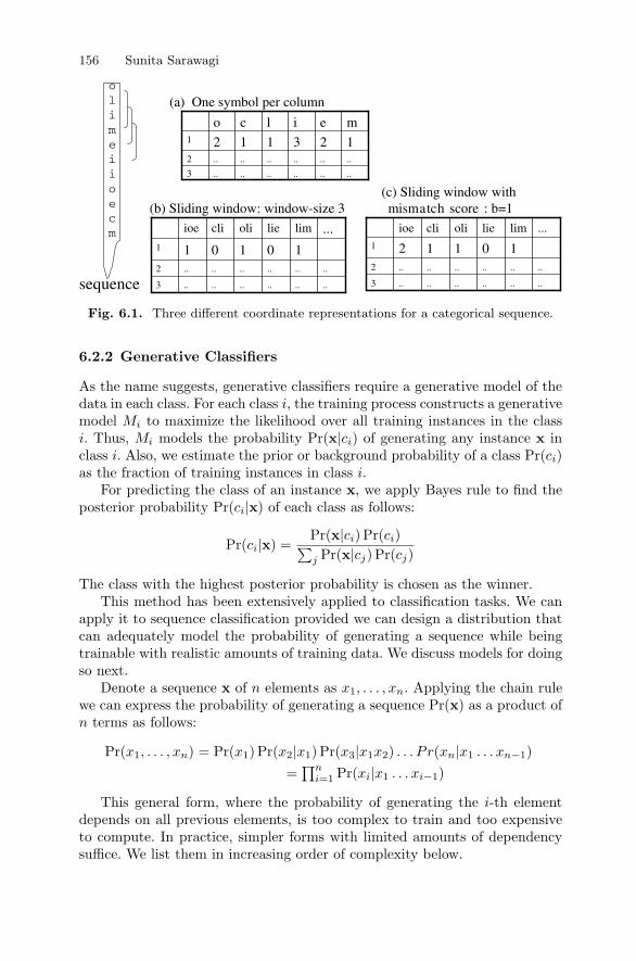
156 Sunita Sarawagi
............3
............2
1231121
meilco
olimeiioecm
(a) One symbol per column
(b) Sliding window: window-size 3
............3
............2
101011
...limlieolicliioe
............3
............2
101121
...limlieolicliioe
(c) Sliding window with mismatch score : b=1
sequence
Fig. 6.1. Three different coordinate representations for a categorical sequence.
6.2.2 Generative Classifiers
As the name suggests, generative classifiers require a generative model of thedata in each class. For each class i, the training process constructs a generativemodel Mi to maximize the likelihood over all training instances in the classi. Thus, Mi models the probability Pr(x|ci) of generating any instance x inclass i. Also, we estimate the prior or background probability of a class Pr(ci)as the fraction of training instances in class i.
For predicting the class of an instance x, we apply Bayes rule to find theposterior probability Pr(ci|x) of each class as follows:
Pr(ci|x) =Pr(x|ci) Pr(ci)∑j Pr(x|cj) Pr(cj)
The class with the highest posterior probability is chosen as the winner.This method has been extensively applied to classification tasks. We can
apply it to sequence classification provided we can design a distribution thatcan adequately model the probability of generating a sequence while beingtrainable with realistic amounts of training data. We discuss models for doingso next.
Denote a sequence x of n elements as x1, . . . , xn. Applying the chain rulewe can express the probability of generating a sequence Pr(x) as a product ofn terms as follows:
Pr(x1, . . . , xn) = Pr(x1) Pr(x2|x1) Pr(x3|x1x2) . . . P r(xn|x1 . . . xn−1)=∏n
i=1 Pr(xi|x1 . . . xi−1)
This general form, where the probability of generating the i-th elementdepends on all previous elements, is too complex to train and too expensiveto compute. In practice, simpler forms with limited amounts of dependencysuffice. We list them in increasing order of complexity below.

6.2 Sequence Classification 157
For ease of explanation we will assume sequences with m categorical el-ements v1 . . . vm. We will illustrate each model with an example sequencecomprising of one of two possible elements “A” and “C”, thus m = 2. As-sume the training set T is a collection of N sequences x1 . . .xN . An examplesequence “AACA” will be used to explain the computation of the probabilityof generating a sequence from each model.
The Independent ModelThe simplest is the independent model where we assume that the probabilitydistribution of an element at position i is independent of all elements beforeit, i.e., Pr(xi|x1 . . . xi−1) = Pr(xi). If xi is categorical with m possible valuesin the domain v1 . . . vm, then Pr(xi) can be modeled as a multinomial dis-tribution with m possible parameters of the form p(vj) and
∑nj=1 p(vj) = 1.
The number of parameters to train are then m− 1. Given a set T of trainingsequences, the parameter p(vj) can be easily estimated as the fraction of se-quence positions over T where the element value is equal to vj . For example, asequence that is generated by the outcomes of an m-faced die rolled n times,is modeled perfectly by this independent model.
Figure 6.2(a) shows an example trained independent model with two pos-sible elements. In this example, the probability of a sequence AACA is calcu-lated as Pr(AACA) = Pr(A)3 Pr(C) = 0.13 × 0.9.
Pr(A) = 0.1Pr(C) = 0.9
CA
0.9
0.4
0.1 0.6
start0.5 0.5
ACAA
C 0.9
A 0.1
CCCA
0.8
A 0.7A 0.4
C 0.6
start0.5
CCAC
C 0.7
C 0.9
A 0.1
A
A 0.3
start
0.2 0.5(a) Independent
(b) Order(1) Markov (c) Order(2) Markov (d) Variable memory
e
A C
AC CC
0.3, 0.7
0.28, 0.72
0.25, 0.75
0.1, 0.9 0.4, 0.6
(e) Probabilistics uffix trees
Fig. 6.2. Models of increasing complexity for a sequence data set with two cate-gorical elements “A” and “C”.
First-order Markov ModelIn a first-order Markov model, the probability of generating the i-th ele-ment is assumed to depend on the element immediately preceding it. Thus,Pr(xi|x1 . . . xi−1) = Pr(xi|xi−1). This gives rise to m2 parameters of the formPr(vj |vk) plus m parameters that denote the probability of starting a sequencewith each of the m possible values denoted by πj .

158 Sunita Sarawagi
Figure 6.2(b) shows an example trained Markov model with two possibleelements. In this example, the probability of a sequence AACA is calculatedas Pr(AACA) = Pr(A) Pr(A|A) Pr(C|A) Pr(A|C) = 0.5× 0.1× 0.9× 0.4.
During training the maximum likelihood value of the parameter Pr(vj |vk)is estimated as the ratio of vkvj occurrences in T over the number of vk oc-currences. The value of πj is the fraction of sequences in T that start withvalue vj .
Higher-order Markov ModelIn general the probability of generating an element at position i could de-pend on a fixed length of symbols before it. Thus, Pr(xi|x1 . . . xi−1) =Pr(xi|xi− . . . xi−1). The number of parameters in the model then becomesm+1 for the conditional probabilities and m for the starting probabilities.
Figure 6.2c shows an example Markov model with two possible elementsand = 2. In this example, the probability of a sequence AACA is calculatedas Pr(AACA) = Pr(AA) Pr(C|AA) Pr(A|AC) = 0.5× 0.9× 0.7.
During training the maximum likelihood value of the parameter
Pr(vj |vk. . . vk1)
is estimated as the ratio of vk. . . vk1vj occurrences in T over the number of
vk. . . vk1 occurrences. For each l-gram vk
. . . vk1 , the value of the startingprobability is the fraction of sequences in T that start with that l-gram.
Variable-Memory Markov ModelThe number of parameters in higher-order Markov models increases expo-nentially in the order of the model. In many cases, it may not be neces-sary to model large memories uniformly for all elements. This motivated theneed for variable-memory models where each element value vj is assumedto have a variable number of elements on which it depends. An impor-tant special class of variable-memory models is a Probabilistic Suffix Au-tomata (PSA) introduced in [41]. A PSA is a Markov model where eachstate comprises symbol sequences of length no more than (the maximummemory length) and the state labels are such that no label is a suffix ofanother. Figure 6.2d shows an example PSA for maximum memory = 2.The probability of a sequence AACA here is calculated as Pr(AACA) =Pr(A) Pr(A|A) Pr(C|A) Pr(A|AC) = 0.5× 0.3× 0.7× 0.1.
The training process for these models is not as for straightforward as theprevious models because we need to simultaneously discover a subset of statesthat capture all significant dependencies in the model. A closely related struc-ture to PSA that enables efficient discovery of such states is the probabilisticsuffix tree (PST). A PST is a suffix tree with emission probabilities of obser-vation attached with each tree node. In Figure 6.2e we show the PST thatis roughly equivalent to the PSA to its left. The j-th emission probabilityattached to each node denotes the probability of generating vj provided the

6.2 Sequence Classification 159
label of the node is the largest match that can be achieved with the suffix ofthe sequence immediately before vj . The probability of an example sequencePr(AACA) is evaluated as 0.28× 0.3× 0.7× 0.1. The first 0.28 is for the first“A” in “AACA” obtained from the root node with an empty history. Thesecond 0.3 denotes the probability of generating “A” from the node labeled“A”. The third “0.7” denotes the probability of generating a “C” from thesame node. The fourth multiplicand “0.1” is the probability of generating “A”from the node labeled “AC”. The “AC”-labeled node has the largest suffixmatch with the part of the sequence before the last “A”. This example, showsthat calculating the probability of generating a sequence is more expensivewith a PST than with a PSA. However, PSTs are amenable to more efficienttraining. Linear time algorithms exist for constructing such PSTs from train-ing data in one single pass [2]. Simple procedures exist to convert a PST tothe equivalent PSA after the training [41].
PSTs/PSAs have been generalized to even sparser Markov models and ap-plied to protein classification in [17] and for classifying sequences of systemcalls as intrusions or not [18].
Hidden Markov ModelIn the previous models, the probability distribution of an element in the se-quence depended just on symbols before some distance but on no other factor.Often in real-life it is necessary to allow for more general distributions wherean element’s distribution also depends on some external cause. Consider theexample of the dice sequence captured by an independent model. Suppose in-stead of rolling a single die to generate the sequence, we probabilistically pickany one of a set of s dice each with a different probability distribution androll that for a while before switching to another. Then, none of the modelspresented earlier can capture this distribution. However a set of s indepen-dent distributions with some probability of switching between them modelsthis perfectly. Such distributions are generalized elegantly by hidden Markovhodels (HMMs). In HMMs, states do not correspond to observed sequenceelements hence the name “hidden”. The basic HMM model consists of:
• a set of s states,• a dictionary of m output symbols,• an s× s transition matrix A where the ijth element aij is the probability
of making a transition from state i to state j,• an s×m emission matrix B where entry bjk = bj(vk) denotes the proba-
bility of emitting the k-th element vk in state j and• an s-vector π where the j-th entry denotes the probability of starting in
state j.
HMMs have been extensively used for modeling various kinds of sequencedata. HMMs are popularly used for word recognition in speech processing [39].[48] reports much higher classification accuracy with HMMs when used fordetecting intrusions compared to previous k-grams approach. A lot of work

160 Sunita Sarawagi
S2
S4
S1
0.9
0.5
0.50.8
0.2
0.1
S3
A
C
0.6
0.4
A
C
0.3
0.7
A
C
0.5
0.5
A
C
0.9
0.1
Fig. 6.3. A hidden Markov model with four states, transition and emission prob-abilities as shown and starting probability π = [1 0 0 0].
has been done on building specialized hidden Markov models for capturingthe distribution of protein sequences within a family [16].
The probability of generating a sequence
The probability of generating a sequence x = x1, x2, . . . , xn from a trainedHMM model is not as straightforward to find as in the previous models wherea sequence could be generated only from a single path through the states ofthe model. In the case of an HMM, a sequence in general could have beengenerated from an exponential number of paths. For example, for AACA andthe HMM in Figure 6.3 each element of the sequence can be generated fromany of the four states giving rise to 44 possible state sequences over whichthe sum has to be computed. Thus, the total probability of generating AACAfrom the HMM in Figure 6.3 is given by
Pr(AACA) =∑
ijkl Pr(AACA, SiSjSkSl)=∑
ijkl Pr(Si) Pr(A|Si) Pr(Sj |Si)..Pr(A|Sl).
Given a state sequence S1S2S4S4, the probability of generating AACAthrough this sequence is
Pr(AACA, S1S2S4S4) = 1× 0.9× 0.9× 0.6× 0.5× 0.7× 0.2× 0.3.
We can exploit the Markov property of the model to design an efficient dy-namic programming algorithm to avoid enumerating the exponential numberof paths. Let α(i, q) be the value of
∑q′∈qi:q
Pr(x1..i,q′) where qi:q denotesall state sequences from 1 to i with the i-th state q and x1..i denotes the partof the sequence from 1 to i, that is x1 . . . xi. α() can be expressed recursivelyas
α(i, q) =∑
q′∈S α(i− 1, q′)aq′qbq(xi) if i > 1πqbq(xi) if i = 1
The value of Pr(x) can then be written as Pr(x) =∑
q α(|x|, q).The running time of this algorithm is O(ns) where n is the sequence length
and s is the number of states.

6.2 Sequence Classification 161
Training an HMM
The parameters of the HMM comprising of the number of states s, the setof symbols in the dictionary m, the edge transition matrix A, the emissionprobability matrix B, and starting probability π are learnt from training data.The training of an HMM has two phases. In the first phase we choose thestructure of the HMM, that is, the number of states s and the edges amongststates. This is often decided manually based on domain knowledge. A numberof algorithms have also been proposed for learning the structure automaticallyfrom the training data [42, 45]. We will not go into a discussion of thesealgorithms. In the second phase we learn the probabilities, assuming a fixedstructure of the HMM.
Learning transition and emission probabilities
The goal of the training process is to learn the model parameters Θ =(A, B, π) such that the probability of the HMM generating the training se-quences x1 . . .xN is maximized. We write the training objective function as
argmaxΘL(Θ) = argmaxΘ
N∏=1
Pr(x|Θ). (6.1)
Since a given sequence can take multiple paths, direct estimates of themaximum likelihood parameters is not possible. An expectation maximization(EM) algorithm is used to estimate these parameters. For HMMs the EMalgorithm is popularly called the Baum-Welch algorithm. It starts with initialguesses of the parameter values and then makes multiple passes over thetraining sequence to iteratively refine the estimates. In each pass, first inthe E-step the previous values of parameters are used to assign the expectedprobability of each transition and each emission for each training sequence.Then, in the M -step the maximum-likelihood values of the parameters arerecalculated by a straight aggregation of the weighted assignments of the E-step. Exact formulas can be found elsewhere [38, 39]. The above algorithm isguaranteed to converge to the locally optimum value of the likelihood of thetraining data.
6.2.3 Kernel-based Classifiers
Kernel-based classification is a powerful classification technique that includeswell-known classifiers like Support Vector Machines, Radial Basis functions,and Nearest Neighbor classifiers.
Kernel classifiers require a function K(xi,xj) that intuitively defines thesimilarity between two instances and satisfies two properties: K is symmetrici.e., K(xi,xj) = K(xj ,xi), and, K is positive definite, i.e., the kernel matrixdefined on training instance pairs is positive definite [7]. Each class c is as-sociated with a set of weight values wc
i over each training sequence xi and a

162 Sunita Sarawagi
bias term bc. These parameters are learnt during training via classifier-specificmethods [7]. The predicted class of a sequence x is found by computing foreach class c, f(x, c) =
∑i wc
i K(xi,x) + bc and choosing the class with thehighest value of f(x, c).
We can exploit kernel classifiers like SVMs for sequence classification, pro-vided we can design appropriate kernel functions that take as input two datapoints and output a real value that roughly denotes their similarity. For near-est neighbor classifiers it is not necessary for the function to satisfy the abovetwo kernel properties but the basic structure of the similarity functions is of-ten shared. We now discuss examples of similarity/kernel functions proposedfor sequence data.
A common approach is to first embed the sequence in a fixed dimen-sional space using methods discussed in Section 6.2.1 and then computesimilarity using well-known functions like Euclidean, or any of the otherLp norms, or a dot-product. For time series data, [31] deploys a degreethree polynomial over a fixed number of Fourier coefficients computed asK(x,x′) = (FFT (x).FFT (x′)+1)3. The mismatch coefficients for categoricaldata described in Section 6.2.1 were used in [30] with a dot-product kernelfunction to perform protein classification using SVMs.
Another interesting technique is to define a fixed set of dimensions fromintermediate computations of a structural generative model and then super-impose a suitable distance function on these dimensions. Fisher’s kernel isan example of such a kernel [23] which has been applied to the task of pro-tein family classification. A lot of work has been done on building specializedhidden Markov models for capturing the distribution of protein sequenceswithin a family [16]. The Fisher’s kernel provides a mechanism of exploit-ing these models for building kernels to be used in powerful discriminativeclassifiers like SVMs. First we train the parameters Θp of an HMM using allpositive example sequences in a family. Now, for any given sequence x theFisher’s co-ordinate is derived from the HMM as the derivative of the gen-erative probability Pr(x|Θp) with respect to each parameter of the model.Thus x is expressed as a vector ∇Θ Pr(x|Θ) of size equal to the number ofparameters of the HMM. This intuitively captures the influence of each of themodel parameters on the sequence x and thus captures the key characteristicsof the sequence as far as the classification problem is concerned. Now, givenany two sequences x and x′ the distance between them can be measured usingeither a scaled Euclidean or a general scaled similarity computation based ona co-variance matrix. [23] deployed such a distance computation on a Gaus-sian kernel and obtained accuracies that are significantly higher than withapplying the Bayes rule on generative models as discussed in Section 6.2.2.
Finally, a number of sequence-specific similarity measures have also beenproposed. For real-valued elements these include measures such as the Dy-namic Time Warping method [39] and for categorical data these include mea-sures such as the edit distance, the more general Levenstein distance [3], andsequence alignment distances like BLAST and PSI-BLAST protein data.

6.3 Sequence Clustering 163
6.3 Sequence Clustering
Given a set of sequences, during clustering the goal is to create groups suchthat similar sequences are in the same group and sequences in different groupsare dissimilar. Like classification, clustering is also an extensively researchedtopic with several formulations and algorithms. With the goal of mapping theproblem of clustering sequences to clustering normal record data, we partitionthe clustering algorithms into three main types.
6.3.1 Distance-based Clustering
This is the most popular clustering method and includes the famous K-means and K-medoid clustering algorithms and the various hierarchical al-gorithms [21]. The primary requirement for these algorithms is to be able todesign a similarity measure over a pair of sequences. We have already discussedsequence similarity measures in Section 6.2.3.
6.3.2 Model-based Algorithms
Model-based clustering assumes that data is generated from a mixture ofK underlying distributions in which each distribution represents a groupor a cluster. Each group k is associated with a mixing parameter called τk
(∑K
k=1 τk = 1) in addition to the parameters Θk of the distribution functionof that group. The goal during clustering is to recover the K sets of parame-ters of the distributions and the mixing value τk such that the probability ofgenerating the data is maximized. This clustering method is better known interms of the expectation maximization (EM) algorithm used to discover theseclusters.
The only primitive needed to adapt the algorithms of model-based cluster-ing to sequence data is designing a suitable generative model. We have alreadypresented sequence-specific generative models in Section 6.2.2 and these applydirectly to sequence data clustering.
6.3.3 Density-based Algorithms
In density-based clustering [21], the goal is to define clusters such that regionsof high point density in a multidimensional space are grouped together into aconnected region. The primary requirement to be able to deploy these algo-rithms is to be able to embed the variable-length sequence data into a fixeddimensional space. Techniques for creating such embeddings are discussed inSection 6.2.1.

164 Sunita Sarawagi
6.4 Sequence Tagging
The sequence tagging problem is defined as follows: We are given a set oftags L and several training examples of sequences showing the breakup ofthe sequence into the set of tags. During training we learn to assign tagsto elements of the sequence so that given a sequence x = x1 . . . xn we canclassify each of its elements into one of L tags giving rise to a tag sequencey = y1 . . . yn. Tagging is often referred as sequential labeling.
This operation has several applications. Information extraction or NamedEntity Recognition (NER) is a tagging problem. Well-studied cases of NERare identifying personal names and company names in newswire text (e.g., [5]),identifying gene and protein names in biomedical publications (e.g., [6, 22]),identifying titles and authors in on-line publications (e.g., [28, 35]), breakingan address record into tag labels like Road, City name, etc.[4]. In continu-ous speech recognition, the tagging problem arises in trying to identify theboundary of individual words from continuous speech. In bio-informatics, theproblem of identifying coding regions from gene sequences is a tagging prob-lem. Figure 6.4 shows a sequence of nine words forming an address recordtagged using six label elements.
A number of solutions have been proposed for the tagging problem par-ticularly in the context of information extraction.
Housenumber Building Road City Zip
4089 Whispering Pines Nobel Drive San Diego CA 92122
State
Fig. 6.4. An example showing the tagging of a sequence of nine words with sixlabels.
6.4.1 Reduce to Per-element Tagging
As for whole sequence classification, one set of methods for the sequence tag-ging problems is based on reduction to existing classification methods. Thesimplest approach is to independently assign for each element xi of a sequencex a label yi using features derived from the element xi. This ignores the con-text in which xi is placed. The context can be captured by taking a windowof w elements around xi. Thus, for getting predictions for xi we would useas input features derived from the record (xi−w . . . xi−1xixi+1 . . . xi+w). Anyexisting classifier like SVM or decision trees can be applied on such fixed-dimensional record data to get a predicted value for yi. However, in severalapplications the tags assigned to adjacent elements of a sequence depend oneach other and assigning independent labels may not be a good idea. A pop-ular method of capturing such dependency is to assign tags to the sequence

6.4 Sequence Tagging 165
elements in a fixed left to right or right to left order. The predicted labelsof the previous h positions are added as features in addition to the usual xcontext features. During training, the features corresponding to each positionconsist of the x-window features and the true labels of the previous h posi-tions. This method has been applied for named-entity recognition by [46] andfor English pronunciation prediction by [15]. In Section 6.4.3 we will considerextensions where instead of using a fixed prediction from the previous labels,we could exploit multiple predictions each attached with a probability valueto assign a globally optimum assignment.
6.4.2 Probabilistic Generative Models
A more unified approach is to build a joint global probability distributionrelating the x and y sequences with varying amounts of memory/dependencyinformation as discussed in Section 6.2.2. Hidden Markov models provide aready solution where each state is associated with a label from the set L andthe distribution of the elements xi is modeled via the emission probabilitiesattached with a dictionary. Each state of the HMM is marked with exactlyone of the L elements, although more than one state could be marked withthe same element. The training data consists of a sequence of element-symbolpairs. This imposes the restriction that for each pair 〈e, x〉 the symbol x canonly be emitted from a state marked with element e.
In Section 6.5.1 we present an application where HMMs are used for textsegmentation.
After training such a model, predicting the y sequence for a given x se-quence reduces to the problem of finding the best path through the model,such that the ith symbol xi is emitted by the ith state in the path. The labelassociated with this state is the predicted label of xi. Given s states and asequence of length n, there can be O(ns) possible paths that the sequence cango through. This exponential complexity is cut down to O(ns2) by the famousdynamic programming-based Viterbi Algorithm [39].
The Viterbi algorithm for HMMs
Given a sequence x = x1, x2, . . . , xn of length n, we want to find out the mostprobable state sequence y = y1 . . . yn such that Pr(x,y) is maximized.
Let δ(i, y) be the value of maxy′∈yi:y Pr(x1..i,y′) where yi:y denotes allstate sequences from 1 to i with the i-th state y and x1..i denotes the part ofthe sequence from 1 to i, that is x1 . . . xi. δ() can be expressed recursively as
δ(i, y) =
maxy′∈L δ(i− 1, y′)ay′yby(xi) if i > 1πyby(xi) if i = 1
The value of the highest probability path corresponds to maxy δ(|x|, y).

166 Sunita Sarawagi
6.4.3 Probabilistic Conditional Models
A major shortcoming of generative models like HMMs is that they maximizethe joint probability of sequence x and labels y. This does not necessarilymaximize accuracy. During testing, x is already known and we are only in-teresting in finding the best y corresponding to this x. Hence, a number ofmodels have been proposed to directly capture the distribution of Pr(y|x)through discriminative methods. There are two categories of models in thisspace.
Local ModelsA common variant is to define the conditional distribution of y given x as
P (y|x) =n∏
i=1
P (yi|yi−1, xi)
This is the formalism used in maximum-entropy taggers [40] and it hasbeen variously called a maximum- entropy Markov model (MEMM) [34] anda conditional Markov model (CMM) [24].
Given training data in the form of pairs (x,y), the “local” conditionaldistribution P (yi|yi−1, xi) can be learned from derived triples (yi, yi−1, xi), forexample by using maximum- entropy methods. For maximum-entropy taggersthe value of P (yi|yi−1, xi) is expressed as an exponential function of the form:
P (yi|yi−1, xi) =1
Z(xi)eW.f(yi,xi,yi−1) (6.2)
where f(yi, xi, yi−1) is the set of local features at position xi, current label yi
and previous label yi−1. The normalization term Z(xi) =∑
y′ eW.f(y′,xi,yi−1).Inferencing in these models is discussed along with the global models of
the next section.
Global Conditional Models: Conditional Random FieldsConditionally-structured models like the CMM have been improved recentlyby algorithms that learn a single global conditional model for P (y|x)[26]. ACRF models Pr(y|x) a Markov random field, with nodes corresponding to el-ements of the structured object y and potential functions that are conditionalon (features of) x. For sequential learning tasks, NP chunking [43] and POStagging [26] the Markov field is a chain, and y is a linear sequence of labelsfrom a fixed set Y and the label at position i depends only on its previouslabel. For instance, in the NER application, x might be a sequence of words,and y might be a sequence in I, O|x|, where yi = I indicates “word xi isinside a name” and yi = O indicates the opposite.
Assume a vector f of local feature functions f = 〈f1, . . . , fK〉, each ofwhich maps a pair (x,y) and a position i in the vector x to a measurementfk(i,x,y) ∈ R. Let f(i,x,y) be the vector of these measurements, and let

6.4 Sequence Tagging 167
F(x,y) =|x|∑i
f(i,x,y). (6.3)
For the case of NER, the components of f might include the measurementf13(i,x,y) = [[xi is capitalized]]·[[yi = I]], where the indicator function [[c]] = 1if c if true and zero otherwise; this implies that F 13(x,y) would be the numberof capitalized words xi paired with the label I.
For sequence learning, any feature fk(i,x,y) is local in the sense that thefeature at a position i will depend only on the previous labels. With a slightabuse of notation, we claim that a local feature fk(i,x,y) can be expressedas fk(yi, yi−1,x, i). Some subset of these features can be simplified further todepend only on the current state and are independent of the previous state.We will refer to these as state features and denote them by fk(yi,x, i) whenwe want to make the distinction explicit. The term transition features refersto the remaining features that are not independent of the previous state.
A conditional random field (CRF) [26, 43] is an estimator of the form
Pr(y|x,W) =1
Z(x)eW·F(x,y) (6.4)
where W is a weight vector over the components of F, and the normalizingterm Z(x) =
∑y′ eW·F(x,y′).
The only difference between the CRF equation above and the maximum-entropy (Maxent) Equation (6.2) is in the normalization term. The normal-ization for Maxent models is local to each position i causing all positions tohave the same normalized weight equal to 1. Thus, even if there is a particularxi which is not too sure about discriminating between two possible labels itwill still have to contribute a weight of 0.5 at least to the objective function(assuming |L| = 2). This leads to a problem, termed label bias in [26]. A CRFthrough global optimization and normalization can more effectively suppressthe weight of such weak predictors and avoid the label bias.
An efficient inference algorithm
The inference problem for a CRF and the Maxent classifier of Equation (6.2) isidentical and is defined as follows: given W and x, find the best label sequence,argmaxy Pr(y|x,W), where Pr(y|x,W) is defined by Equation (6.4).
argmaxy Pr(y|x,W) = argmaxyW · F(x,y)
= argmaxyW ·∑
j
f(yj , yj−1,x, j)
An efficient inference algorithm is possible because all features are assumedto be local. Let yi:l denote the set of all partial labels starting from 1 (the firstindex of the sequence) to i, such that the i-th label is y. Let δ(i, y) denote

168 Sunita Sarawagi
the largest value of W · F(x,y′) for any y′ ∈ yi:l. The following recursivecalculation implements the usual Viterbi algorithm:
δ(i, y) =
maxy′ δ(i− 1, y′) + W · f(y, y′,x, i) if i > 00 if i = 0 (6.5)
The best label then corresponds to the path traced by maxy δ(|x|, y).
Training algorithm
Learning is performed by setting parameters to maximize the likelihood of atraining set T = (x,y)N=1 expressed as
L(W) =∑
log Pr(y|x,W) =∑
(W · F(x,y)− log ZW(x))
We wish to find a W that maximizes L(W). The above equation is convex,and can thus be maximized by gradient ascent, or one of many related methodslike a limited-memory quasi-Newton method [32, 33]. The gradient of L(W)is the following:
∇L(W) =∑
F(x,y)−∑
y′ F(y′,x)eW·F(x,y′)
ZW(x)
=∑
F(x,y)− EPr(y′|W)F(x,y′)
The first set of terms is easy to compute. However, we must use theMarkov property of F and a dynamic programming step to compute thenormalizer, ZW(x), and the expected value of the features under the cur-rent weight vector, EPr(y′|W)F(x,y′). We thus define α(i, y) as the value of∑
y′∈yi:yeW·F(y′,x) where again yi:y denotes all label sequences from 1 to i
with i-th position labeled y. For i > 0, this can be expressed recursively as
α(i, y) =∑y′∈L
α(i− 1, y′)eW·f(y,y′,x,i)
with the base cases defined as α(0, y) = 1. The value of ZW(x) can then bewritten as ZW(x) =
∑y α(|x|, y).
A similar approach can be used to compute the expectation∑y′
F(x,y′)eW·F(x,y′).
For the k-th component of F, let ηk(i, y) be the value of the sum∑y′∈yi:y
F k(y′,x)eW·F(x,y′),

6.4 Sequence Tagging 169
restricted to the part of the label ending at position i. The following recursioncan then be used to compute ηk(i, y):
ηk(i, y) =∑y′∈L
(ηk(i− 1, y′) + α(i− 1, y′)fk(y, y′,x, i))eW·f(y,y′,x,i)
Finally we let EPr(y′|W)Fk(y′,x) = 1
ZW(x)
∑y ηk(|x|, y).
As in the forward-backward algorithm for chain CRFs [43], space require-ments here can be reduced from K|L| + |L|n to K + |L|n, where K is thenumber of features, by pre-computing an appropriate set of β values.
6.4.4 Perceptron-based Models
Another interesting mechanism for sequence tagging, is based on an extensionof the perceptron model for discriminative classification [12]. The structureof the model is similar to the global CRF model involving the feature vectorF(x,y) defined as in Equation (6.3) and corresponding weight parametersW. Inferencing is done by picking the y corresponding to which WF(x,y)is maximum. The predicted label sequence can be efficiently found using thesame Viterbi procedure as for CRFs. The goal during training is to learn thevalue of W so as to minimize the error between the correct labels and thepredicted Viterbi labels. This “best” W is found by repeatedly updating W toimprove the quality of the Viterbi decoding on a particular example (xt,yt).Specifically, Collin’s algorithm starts with W0 = 0. After the t-th examplext,yt, the Viterbi sequence yt is computed, and Wt is replaced with
Wt+1 = Wt + F(xt,yt)− F(xt, yt)
= Wt +M∑i=1
f(i,xt,yt)− f(i,xt, yt) (6.6)
After training, one takes as the final learned weight vector W the averagevalue of Wt over all time steps t.
This simple perceptron-like training algorithm has been shown to performsurprisingly well for sequence learning tasks in [12].
6.4.5 Boundary-based Models
Boundary-based models learn to identify start and end boundaries of eachlabel by building two classifiers for accepting its two boundaries along withthe classifiers that identify the content part of the tag. Such an approach isuseful in applications like NER where we need to identify a multi-word entityname (like person or company) from a long word sequence where most ofthe words are not part of the entity. Although any classifier could be used toidentify the boundaries, the rule-based method has been most popular [8, 44].Rapier [8] is one such rule-learning approach where a bottom-up algorithm isused to learn the pattern marking the beginning, the ending and the contentpart of each entity type.

170 Sunita Sarawagi
6.5 Applications of Sequence Tagging
In this section we present two applications of the sequence-tagging operation.The first is an example of text segmentation where noisy text strings likeaddresses are segmented based on a fixed set of labels using hidden Markovmodels [4]. The second is an example of learning paths leading to informativepages in a website using conditional random fields [47].
6.5.1 Address Segmentation using Hidden Markov Models
Large customer-oriented organizations like banks, telephone companies, anduniversities store millions of addresses. In the original form, these addresseshave little explicit structure. Often for the same person, there are differentaddress records stored in different databases. During warehouse construction,it is necessary to put all these addresses in a standard canonical format wherethe different structured fields like names of street, city and state comprisingan address are identified and duplicates removed. An address record brokeninto its structured fields not only enables better querying, it also provides amore robust way of doing deduplication and householding — a process thatidentifies all addresses belonging to the same household.
Existing commercial approaches rely on hand-coded rule-based methodscoupled with a database of cities, states and zipcodes. This solution is notpractical and general because postal addresses in different parts of the worldhave drastically different structures. In some countries, zip codes are five-digitnumbers whereas in others they are allowed to have letters. The problem ismore challenging in older countries like India because most street names donot follow a uniform building numbering scheme, the reliance on ad hoc de-scriptive landmarks is common, city names keep changing, state abbreviationsare not standardized, spelling mistakes are rampant and zip codes optional.Further each region has evolved its own style of writing addresses that dif-fers significantly from those of the other regions. Consider for instance thefollowing two valid addresses from two different Indian cities:7D-Brijdham 16-B Bangur Nagar Goregaon (West) Bombay 400 09013 Shopping Center Kota (Raj) 324 007The first address consists of seven elements: house number: ‘‘7D’’, buildingname: ‘‘Brijdham’’, building number: ‘‘16-B’’, colony name: ‘‘BangurNagar’’, area: ‘‘Goregaon (West)’’, city: ‘‘Bombay’’ and zip code: ‘‘400090’’. The second address consists of the following five elements: house num-ber: ‘‘13’’, Colony name: ‘‘Shopping center’’, city: ‘‘Kota’’, State:‘‘(Raj)’’ and zip code: ‘‘324 007’’. In the first address, “West” was en-closed in parentheses and depicted direction while in the second the string“Raj” within parentheses is the name of a geographical State. This elementis missing in the first address. In the second address building name, colonyname and area elements are missing.

6.5 Applications of Sequence Tagging 171
We propose an automated method for elementizing addresses based onhidden Markov models. An HMM combines information about multiple dif-ferent aspects of the record in segmenting it. One source is the characteristicwords in each elements, for example the word “street” appears in road-names.A second source is the limited partial ordering between its element. Often thefirst element is a house number, then a possible building name and so onand the last few elements are zipcode and state name. A third source is thetypical number of words in each element. For example, state names usuallyhave one or two words whereas road names are longer. Finally, the HMM si-multaneously extracts each element from the address to optimize some globalobjective function. This is in contrast to existing rule learners used in tradi-tional information tasks [1, 13, 25, 36, 37] that treat each element in isolation.
Structure of the HMM for Address ElementizationAn easy way to exploit HMMs for address segmentation is to associate a statefor each label or tag as described in Section 6.4.2. In Figure 6.5 we show anexample HMM for address segmentation. The number of states s is 10 and theedge labels depict the state transition probabilities (A Matrix). For example,the probability of an address beginning with House Number is 0.92 and that ofseeing a City after Road is 0.22. The dictionary and the emission probabilitiesare not shown for compactness. The dictionary would comprise of words thatappeared in the training sequences.
0.400.67
0.05
0.75
0.13
0.21Building Name0.47
State
0.50
Zipcode
House No. Road
Start
City
End
0.92
0.12 0.35
0.22
0.10 0.28
0.20
0.08
0.35
0.10
0.25
0.12
0.05
0.35
Area
0.3
0.320.2
0.38
0.33
0.2
0.15
Landmark 0.45
Fig. 6.5. Structure of an HMM used for tagging addresses.
However, the above model does not provide a sufficiently detailed model ofthe text within each tag. We therefore associate each tag with another innerHMM embedded within the outer HMM that captures inter-tag transitions.We found a parallel-path HMM as shown in Figure 6.6 to provide the bestaccuracy while requiring little or no tuning over different tag types. In thefigure, the start and end states are dummy nodes to mark the two end pointsof a tag. They do not output any token. All records of length one will pass

172 Sunita Sarawagi
through the first path, length two will go through the second path and so on.The last path captures all records with four or more tokens. Different elementswould have different numbers of such parallel paths depending on the elementlengths observed during training.
Start End
Fig. 6.6. A four-length parallel path structure.
Estimating Parameters during TrainingDuring training, we get examples of addresses where structured elements havebeen identified. Each training token maps to exactly one state of the HMMeven with the above multi-state nested structure for each tag. Therefore, wecan deploy straight maximum likelihood estimates for the transition and emis-sion probabilities.
An important issue in practice is dealing with zero probability estimatesarising when the training data is insufficient. The traditional smoothingmethod is Laplace smoothing [27] according to an unseen symbol k, state jwill be assigned probability 1
Tj+m where Tj is the number of training symbolsin state j and m is the number of distinct symbols. We found this smooth-ing method unsuitable in our case. An element like “road name”, that dur-ing training has seen more distinct words than an element like “country”,is expected to also encounter unseen symbols more frequently during test-ing. Laplace smoothing does not capture this intuition. We use a methodcalled absolute discounting. In this method we subtract a small value, say εfrom the probability of all known mj distinct words seen in state j. We thendistribute the accumulated probability equally amongst all unknown values.Thus, the probability of an unknown symbol is mjε
m−mj. The choice of ε de-
pends on whether the unknown symbol is unseen over all states of the HMMor just a subset of the sets. We want ε to be lower in the second case, whichwe arbitrarily fix to be a factor of 1000 lower. The value of ε is then chosenempirically.
We experimented with a number of more principled methods of smoothingincluding cross-validation but we found them not to perform as well as theabove ad hoc method.

6.5 Applications of Sequence Tagging 173
Experimental Evaluation
We report evaluation results on the following three real-life address data sets:
• US address: The US address data set consisted of 740 addresses down-loaded from an Internet directory.1 The addresses were segmented into sixelements: House No, Box No. Road Name, City, State, Zip.
• Student address: This data set consisted of 2388 home addresses of stu-dents in the author’s university. These addresses were partitioned into 16elements based on the postal format of the country. The addresses in thisset do not have the kind of regularity found in US addresses.
• Company address: This data set consisted of 769 addresses of customersof a major national bank in a large Asian metropolis. The address wassegmented into six elements: Care Of, House Name, Road Name, Area,City, Zipcode.
For the experiments all the data instances were first manually segmented intotheir constituent elements. In each set, one-third of the data set was usedfor training and the remaining two-thirds used for testing as summarized inTable 6.1.
Table 6.1. Data sets used for the experiments.
Data set Number of Number of Number ofelements (E) training test instances
instancesUS address 6 250 490Student address 16 650 1738Company address 6 250 519
All tokens were converted to lower case. Each word, digit and delimiter inthe address formed a separate token to the HMM. Each record was prepro-cessed where all numbers were represented by a special symbol “digit” and alldelimiters where represented with a special “delimit” symbol.
We obtained accuracy of 99%, 88.9% and 83.7% on the US, Student andCompany data sets respectively. The Asian addresses have a much highercomplexity compared to the US addresses. The company data set had loweraccuracy because of several errors in the segmentation of data that was handedto us.
We compare the performance of the proposed nested HMM with the fol-lowing three automated approaches.
1www.superpages.com

174 Sunita Sarawagi
Naive HMM
This is the HMM model with just one state per element. The purpose here isto evaluate the benefit of the nested HMM model.
Independent HMM
In this approach, for each element we train a separate HMM to extract just itspart from a text record, independent of all other elements. Each independentHMM has a prefix and suffix state to absorb the text before and after itsown segment. Otherwise the structure of the HMM is similar to what weused in the inner HMMs. Unlike the nested-model there is no outer HMMto capture the dependency amongst elements. The independent HMMs learnthe relative location in the address where their element appears through theself-loop transition probabilities of the prefix and suffix states. This is similarto the approach used in [19] for extracting location and timings from talkannouncements.
The main idea here is to evaluate the benefit of simultaneously tagging allthe elements of a record exploiting the sequential relationship amongst theelements using the outer HMM.
Rule learner
We compare HMM-based approaches with a rule learner, Rapier [8], a bottom-up inductive learning system for finding information extraction rules to markthe beginning, content and end of an entity. Like the independent HMM ap-proach it also extracts each tag in isolation from the rest.
Student Data Company Data US Data0
20
40
60
80
100
Acc
urac
y Naive HMM
Independent HMM
Rapier
DATAMOLD
Fig. 6.7. Comparison of four different methods of text segmentation
Figure 6.7 shows a comparison of the accuracy of the four methods naiveHMM, independent HMM, rule learner and nested HMM. We can make thefollowing observations:

6.5 Applications of Sequence Tagging 175
• The independent HMM approach is significantly worse than the nestedmodel because of the loss of valuable sequence information. For example,in the former case there is no restriction that tags cannot overlap – thusthe same part of the address could be tagged as being part of two differentelements. With a single HMM the different tags corroborate each other’sfinding to pick the segmentation that is globally optimal.
• Naive HMM gives 3% to 10% lower accuracy than the nested HMM. Thisshows the benefit of a detailed HMM for learning the finer structure ofeach element.
• The accuracy of Rapier is considerably lower. Rapier leaves many tokensuntagged by not assigning them to any of the elements. Thus it has lowrecall. However, the precision of Rapier was found to be competitive toour method – 89.2%, 88%, and 98.3% for Student, Company and US datasets respectively. The overall accuracy is acceptable only for US addresseswhere the address format is regular enough to be amenable to rule-basedprocessing. For the complicated sixteen-element Student data set such rule-based processing could not successfully tag all elements.
6.5.2 Learning Paths in Websites using Conditional RandomFields
Another interesting application of sequential tagging models is in learning thesequence of links that lead to a specific goal page on a large website. Oftenwebsites within a domain are structurally similar to each other. Humans aregood at navigating these websites to reach specific information within largedomain-specific websites. Our goal is to learn the navigation path by observingthe user’s clicks on as few example websites as possible. Next, when presentedwith a list of new websites, we use the learnt model to automatically crawlthe desired pages using as few redundant page fetches as possible.
We present a scenario where such a capability would be useful. Citationportals, such as Citeseer, need to gather publications on a particular disciplinefrom home pages of faculty starting from lists of universities easily obtainedfrom web directories such as Dmoz. This requires following a path startingfrom the root page of the university, to the home pages of departments rele-vant to the discipline, from there visiting the home pages of faculty members,and then searching for links such as “Papers”, “Publications”, or “ResearchInterests” that lead to the publications page, if it exists. Several universitiesfollow this template website, although there is lot of variation in the exactwords used on pages and around links and the placement of links. We expectsuch a learning-based approach to capture the main structure in a few exam-ples so as to automatically gather all faculty publications from any given listof universities without fetching too many superflous pages.
There are two phases to this task: first is the training phase, where theuser teaches the system by clicking through pages and labeling a subset witha dynamically defined set of classes, one of them being the goal class. The

176 Sunita Sarawagi
classes assigned on intermittent pages along the path can be thought of as“milestones” that capture the structural similarity across websites. At the endof this process, we have a set of classes L, and a set of training paths where asubset of the pages in the path are labeled with a class from L. All unlabeledpages before a labeled page are represented with a special prefix state for thatlabel. The system trains a model using the example paths, modeling each classin L as a milestone state. The second phase is the foraging phase where thegiven list of websites is automatically navigated to find all goal pages.
The ratio of relevant pages visited to the total number of pages visitedduring the execution is called the harvest rate. The objective function is tomaximize the harvest rate.
We treat this as a sequence-tagging problem where the path is a sequenceof pages ending in a goal page. We first train a CRF to recognize such paths.We then superimpose ideas from reinforcement learning to prioritize the or-der in which pages should be fetched to reach the goal page. This providesan elegant and unified mechanism of modeling the path learning and foragingproblem. Also, as we will see in the experimental results section, it providesvery high accuracy.
Model TrainingDuring training, we are given examples of several paths of labeled pages wheresome of the paths end in goal pages and others end with a special “fail” label.We can treat each path as a sequence of pages denoted by the vector x andtheir corresponding labels denoted by y. Each xi is a web page representedsuitably in terms of features derived from the words in the page, its URL, andanchor text in the link pointing to xi.
A number of design decisions about the label space and feature space needto be made in constructing a CRF to recognize characteristics of valid paths.One option is to assign a state to each possible label in the set L which consistsof the milestone labels and two special labels “goal” and “fail”. An exampleof such a model for the publications scenario is given in Figure 6.8(a) whereeach circle represents a label.
State features are defined on the words or other properties comprisinga page. For example, state features derived from words are of the formfk(i,x, yi) = [[xi is “computer” and yi = faculty]]. The URL of a page alsoyields valuable features. For example, a “tilda” in the URL is strongly associ-ated with a personal home page and a link name with the word “contact” isstrongly associated with an address page. We tokenize each URL on delimitersand add a feature corresponding to each feature.
Transition features capture the soft precedence order amongst labels. Oneset of transition features is of the form:fk(i,x, yi, yi−1) = [[yi is “faculty” and yi−1 is “department”]]. They are inde-pendent of xi and are called edge features since they capture dependencyamongst adjacent labels. In this model, transition features are also derivedfrom the words in and around the anchor text surrounding the link leading to

6.5 Applications of Sequence Tagging 177
Faculty/StaffInformation
FacultyList Home page
Faculty(Goal state)Publication
Courses
DepartmentHome page
ResearchGrp. List
Research Grp.Home page
(Events, etc.)Fail state (News,
(a) One state per label with links as transitions
Faculty/StaffInformation
(Goal state)Publication
Courses
DepartmentHome page
ResearchGrp. List
(Events, etc.)Fail state (News,
FacultyList Home page
Faculty
ResearchGrp. Page
(b) A state for each label and each link
Fig. 6.8. State transition diagram for the Publications domain.
the next state. Thus, a transition feature could be of the form fk(i,x, yi, yi−1)= [[xi is an anchor word “advisor”, yi is “faculty”, and yi−1 is “student”]].
A second option is to model each given label as a dual-state — one forthe characteristics of the page itself (page-states) and the other for theinformation around links that lead to such a page (link-states). Hence, everypath alternates between a page-state and a link-state.
In Figure 6.8(b), we show the state space corresponding to this optionfor the publications domain. There are two advantages of this labeling. First,it reduces the sparcity of parameters by making the anchor word featuresbe independent of the label of the source page. In practice, it is often foundthat the anchor text pointing to the same page are highly similar and this iscaptured by allowing multiple source labels to point to the same link stateof label. Second for the foraging phase, it allows one to easily reason about

178 Sunita Sarawagi
intermediate probability of a path prefix where only the link is known and thepage leading to it has not been fetched.
In this model, the state features of the page states are the same as in theprevious model and the state features of the link states are derived from theanchor text. Thus, the anchor-text transition features of the previous model,become state features of the link state. Thus the only transition features inthis model are the edge features that capture the precedence order betweenlabels.
Path ForagingGiven the trained sequential model M and a list of starting pages of websites,our goal is to find all paths from the list that lead to the “goal” state in Mwhile fetching as few unrelated pages.
The key issue in solving this is to be able to score from a prefix of a pathalready fetched, all the set of outgoing links with a value that is inversely pro-portional to the expected work involved in reaching the goal pages. Considera path prefix of the form P1L2P3 . . . Li where Li−1 is a link to page Pi inthe path. We need to find for link Li a score value that would indicate thedesirability of fetching the page pointed to by Li. This score is computed intwo parts. First, we estimate for each state y, the proximity of the state tothe goal state. We call this the reward associated with the state. Then wecompute for the link Li the probability of its being in state y.
Reward of a state
We apply techniques from reinforcement learning to compute the reward scorethat captures the probability of a partially-observed sequence to end up in agoal state of the CRF model M . Reinforcement learning is a machine learningparadigm that helps in choosing the optimal action at each state to reachthe goal states. The goal states are associated with rewards that start todepreciate as the goal states get farther from the current state. The actionsare chosen so as to maximize the cumulative discounted reward. We estimatethis probability based on the training data by learning a reward function R foreach state. For each position i of a given sequence x we estimate the expectedproximity to the goal state from a state y Rx
i (y) recursively as follows:
Rxi (y) =
∑y′ eW·f(y′,y,x,i+1)Rx
i+1(y′) 1 ≤ i < n
[[y == goal]] i = n(6.7)
When i = n, the reward is 1 for the goal state and 0 for every other label.Otherwise the values are computed recursively from the proximity of the nextstate and the probability of transition to the next state from the current state.
We then compute a weighted sum of these positioned reward values toget position-independent reward values. The weights are controlled via γ, adiscount factor that captures the desirability of preferring states that are closerto the goal state as follows:

6.5 Applications of Sequence Tagging 179
Rx =
n∑k=1
γk ·Rxn−k
n∑k=1
γk
(6.8)
where n is the length of the sequence.The final reward value of a state is computed by averaging over all training
sequences x1 . . .xN as
R =∑N
=1 Rx
N. (6.9)
Probability of being in a state
Consider a path prefix of the form P1L2P3 . . . Li where Li−1 is a link to pagePi in the path. We need to find for link Li the probability of its being inany one of the link states. We provide a method for computing this. Let αi(y)denote the total weight of ending in state y after i states. We thus define αi(y)as the value of
∑y′∈yi:y
eW·F(y′,x) where yi:y denotes all label sequences from1 to i with i-th position labeled y. For i > 0, this can be expressed recursivelyas
αi(y) =∑y′∈Y
αi−1(y′)eW·f(y,y′,x,i) (6.10)
with the base cases defined as α0(y) = 1.The probability of Li being in the link state y is then αi(y)∑
y′∈YL αi(y′) where
YL denotes the link states.
Score of a link
Finally, the score of a link Li, after i steps, is calculated as the sum of theproduct of reaching a state y and the static reward at state y.
Score(Li) =∑
y
αi(y)∑y′∈YL αi(y′)
R(y) (6.11)
If a link appears in multiple paths, we sum over its score from each path.Thus, at any give snapshot of the crawl we have a set of unfetched links
whose scores we compute and maintain in a priority queue. We pick the linkwith the highest score to fetch next. The links in the newly fetched page areadded to the queue. We stop when no more unfetched links have a score abovea threshold value.
Experimental ResultsWe present a summary of experiments over two applications — a task of fetch-ing publication pages starting from university pages and a task of reaching

180 Sunita Sarawagi
company contact addresses starting from a root company web page. The re-sults are compared with generic focused crawlers [10] that are not designed toexploit the commonality of the structure of groups such as university websites.More details of the experiment can be found in [47].
Publications data set
The data sets were built manually by navigating sample websites and en-listing the sequence of web pages from the entry page to a goal page. Se-quences that led to irrelevant pages were identified as negative examples. ThePublications model was trained on 44 sequences (of which 28 were positivepaths) from seven university domains and computer science departments ofUS universities chosen randomly from an online list.2
We show the percentage of relevant pages as a function of pages fetched fortwo different websites where we applied the above trained model for findingpublications:
• www.cs.cmu.edu/, henceforth referred to as the CMU domain.• www.cs.utexas.edu/, henceforth referred to as the UTX domain.
Performance is measured in terms of harvest rates. The harvest rate isdefined as the ratio of relevant pages (goal pages, in our case) found to thetotal number of pages visited.
Figure 6.9 shows a comparison of how our model performs against thesimplified model of the accelerated focused crawler (AFC). We observe thatthe performance of our model is significantly better than the AFC model. Therelevant pages fetched by the CRF model increases rapidly at the beginningbefore stabilizing at over 60%, when the Crawler model barely reaches 40%.
Address data set
The Address data set was trained on 32 sequences out of which 17 sequenceswere positive. There was a single milestone state “About-us” in addition tothe start, goal and fail states.
The foraging experimentation on the address data set differs slightly fromthe one on the Publications data set. In the Publications data set, we havemultiple goal pages with a website. During the foraging experiment, the modelaims at reaching as many goal pages as possible quickly. In effect, the modeltries to reach a hub — i.e. a page that links many desired pages directly suchthat the outlink probability from the page to goal state is maximum.
In the Address data set, there is only one (or a countable few) goal pages.Hence, following an approach similar to that of the Publications data setwould lead to declining harvest rates once the address page is fetched. Hencewe modify the foraging run to stop when a goal page is reached. We proceed
2www.clas.ufl.edu/CLAS/american-universities.html

6.5 Applications of Sequence Tagging 181
0
20
40
60
80
100
120
0 500 1000 1500 2000 2500 3000 3500 4000 4500 5000
%ag
e of
rel
evan
t pag
es
No. of pages fetched
Comparison of Harvest Rates with Focused Crawler
CMU: PathLearnerCMU: Crawler
(a) For CMU domain
0
20
40
60
80
100
120
0 500 1000 1500 2000 2500 3000 3500 4000 4500 5000
%ag
e of
rel
evan
t pag
es
No. of pages fetched
Comparison of Harvest Rates with Focused Crawler
UTX: PathLearnerUTX: Crawler
(b) For UTX domain
Fig. 6.9. Comparison with simplified accelerated focused crawler. The graphslabeled PathLearner show the performance of our model.

182 Sunita Sarawagi
with the crawling only when we have a link with a higher score of reachingthe goal state than the current page score.
The experiment was run on 108 domains of company addresses taken ran-domly from the list of companies available at www.hoovers.com. We calculatethe average number of pages required to reach the goal page from the companyhome page.
The average length of path from home page to goal page was observed tobe 3.426, with the median and mode value being 2. This agrees with the usualpractice of having a “Contact Us” link on the company home page that leadsin one link access to the contact address.
Summary
This study showed that conditional random fields provide an elegant, unifiedand high-performance method of solving the information foraging task fromlarge domain-specific websites. The proposed model performs significantly bet-ter than a generic focused crawler and is easy to train and deploy.
6.6 Sequence Segmentation
In sequence segmentation we need to break up a sequence along boundarieswhere the sequence appears to be transitioning to a different distribution.This is unlike the tagging problem above in that there is no fixed labeled setto be assigned to each tag. The basic premise behind this operation is thatthe given sequence was generated from multiple models one after another andthe goal during segmentation is to identify the point of switching from onemodel to the next.
The segmentation operation has applications in bioinformatics and in ex-ploratory mining to detect shifts in measures like the buying rate of a prod-uct. For example, [20] discusses a bioinformatics application where a DNA se-quence needs to be segmented to detect viral or microbial inserts. [11] discussesan application in market basket analysis where 0/1 buying patterns of prod-ucts over time are segmented to detect surprising changes in co-occurrencepatterns of groups of products.
We first consider a simpler formulation of the segmentation problem whereour goal is to recover the segments of a sequence under the simplifying as-sumption that the segments are independent of each other. This problem hasbeen studied by a number of researchers and for a variety of scoring functions,dynamic programming can be used to find the segments in time proportionalto O(n2k) where n is the length of the segment and k is the number of seg-ments.
In the previous formulation each segment is assumed to be independentof every other, requiring a user to fit as many model parameters as the num-ber of segments. [20] addresses a more general formulation called the (k, h)

6.7 Conclusions 183
segmentation problem where a fixed number h of models is to be used forsegmenting into k parts an n-element sequence (k > h). Unfortunately, thisnew formulation is NP-hard for the general case. A number of approximationalgorithms are proposed in [20]. We present one of these here. The first step isto get a (k, k) segmentation that is solvable using the dynamic programmingalgorithm of independent segments. The second step is to solve (n, h) to get hmodels: that is to find the best h models to describe the n unordered sequenceelements. Finally, assign each of the k segments of the first step to the best ofthe h models found in the second step. The second step can be replaced witha variant where for each of the k segments we find the best fit model, clusterthese k models into h groups and choose a representative of the h clusters asthe h chosen model.
6.7 Conclusions
In this article we reviewed various techniques for analyzing sequence data. Wefirst studied two conventional mining operations, classification and clustering,that work on whole sequences. We were able to exploit the wealth of existingformalisms and algorithms developed for fixed attribute record data by defin-ing three primitive operations on sequence data. The first primitive was to mapvariable length sequences to a fixed-dimensional space using a wealth of tech-niques ranging from aggregation after collapsing order, k-grams, to capturinglimited order and mismatching scores on k-grams. The second primitive wasdefining generative models for sequences where we considered models startingfrom simple independent models to variable- length Markov models to thepopular hidden Markov models. The third primitive was designing kernels orsimilarity functions between sequence pairs where amongst standard sequencesimilarity functions we discussed the interesting Fisher’s kernels that allow apowerful integration of generative and discriminative models such as SVMs.
We studied two sequence specific operations, tagging and segmentation,that operate on parts of the sequence and can be thought of as the equiva-lent of classification and clustering respectively for whole sequences. Sequencetagging is an extremely useful operation that has seen extensive applicationsin the field of information extraction. We explored generative approaches likehidden Markov models and conditional approaches like conditional randomfields (CRFs) for sequence tagging.
The field of sequence mining is still being actively explored, spurred byemerging applications in information extraction, bio-informatics and sensornetworks. We can hope to witness more exciting research in the techniquesand application of sequence mining in the coming years.

184 Sunita Sarawagi
References
[1] Aldelberg, B., 1998: Nodose: A tool for semi-automatically extractingstructured and semistructured data from text documents. SIGMOD .
[2] Apostolico, A., and G. Bejerano, 2000: Optimal amnesic probabilistic au-tomata or how to learn and classify proteins in linear time and space.Proceedings of RECOMB2000 .
[3] Bilenko, M., R. Mooney, W. Cohen, P. Ravikumar and S. Fienberg,2003: Adaptive name-matching in information integration. IEEE Intel-ligent Systems.
[4] Borkar, V. R., K. Deshmukh and S. Sarawagi, 2001: Automatic text seg-mentation for extracting structured records. Proc. ACM SIGMOD Inter-national Conf. on Management of Data, Santa Barbara, USA.
[5] Borthwick, A., J. Sterling, E. Agichtein and R. Grishman, 1998: Exploit-ing diverse knowledge sources via maximum entropy in named entityrecognition. Sixth Workshop on Very Large Corpora, New Brunswick,New Jersey. Association for Computational Linguistics.
[6] Bunescu, R., R. Ge, R. J. Mooney, E. Marcotte and A. K. Ramani, 2002:Extracting gene and protein names from biomedical abstracts, unpub-lished Technical Note. Available fromURL: www.cs.utexas.edu/users/ml/publication/ie.html.
[7] Burges, C. J. C., 1998: A tutorial on support vector machines for patternrecognition. Data Mining and Knowledge Discovery , 2, 121–67.
[8] Califf, M. E., and R. J. Mooney, 1999: Relational learning of pattern-match rules for information extraction. Proceedings of the Sixteenth Na-tional Conference on Artificial Intelligence (AAAI-99), 328–34.
[9] Chakrabarti, S., 2002: Mining the Web: Discovering Knowledge from Hy-pertext Data. Morgan Kauffman.URL: www.cse.iitb.ac.in/∼ soumen/mining-the-web/
[10] Chakrabarti, S., K. Punera and M. Subramanyam, 2002: Accelerated fo-cused crawling through online relevance feedback. WWW, Hawaii , ACM.
[11] Chakrabarti, S., S. Sarawagi and B. Dom, 1998: Mining surprising tem-poral patterns. Proc. of the Twentyfourth Int’l Conf. on Very LargeDatabases (VLDB), New York, USA.
[12] Collins, M., 2002: Discriminative training methods for hidden Markovmodels: Theory and experiments with perceptron algorithms. EmpiricalMethods in Natural Language Processing (EMNLP).
[13] Crespo, A., J. Jannink, E. Neuhold, M. Rys and R. Studer, 2002: A surveyof semi-automatic extraction and transformation.URL: www-db.stanford.edu/∼ crespo/publications/.
[14] Deng, K., A. Moore and M. Nechyba, 1997: Learning to recognize timeseries: Combining ARMA models with memory-based learning. IEEE Int.Symp. on Computational Intelligence in Robotics and Automation, 1,246–50.

References 185
[15] Dietterich, T., 2002: Machine learning for sequential data: A review.Structural, Syntactic, and Statistical Pattern Recognition; Lecture Notesin Computer Science, T. Caelli, ed., Springer-Verlag, 2396, 15–30.
[16] Durbin, R., S. Eddy, A. Krogh and G. Mitchison, 1998: Biological sequenceanalysis: probabilistic models of proteins and nucleic acids. CambridgeUniversity Press.
[17] Eskin, E., W. N. Grundy and Y. Singer, 2000: Protein family classificationusing sparse Markov transducers. Proceedings of the Eighth InternationalConference on Intelligent Systems for Molecular Biology (ISMB-2000).San Diego, CA.
[18] Eskin, E., W. Lee and S. J. Stolfo, 2001: Modeling system calls for intru-sion detection with dynamic window sizes. Proceedings of DISCEX II .
[19] Freitag, D., and A. McCallum, 1999: Information extraction using HMMsand shrinkage. Papers from the AAAI-99 Workshop on Machine Learningfor Information Extraction, 31–6.
[20] Gionis, A., and H. Mannila, 2003: Finding recurrent sources in sequences.In Proceedings of the 7th annual conference on Computational MolecularBiology. Berlin, Germany.
[21] Han, J., and M. Kamber, 2000: Data Mining: Concepts and Techniques.Morgan Kaufmann.
[22] Humphreys, K., G. Demetriou and R. Gaizauskas, 2000: Two applica-tions of information extraction to biological science journal articles: En-zyme interactions and protein structures. Proceedings of the 2000 PacificSymposium on Biocomputing (PSB-2000), 502–13.
[23] Jaakkola, T., M. Diekhans and D. Haussler, 1999: Using the Fisher kernelmethod to detect remote protein homologies. ISMB , 149–58.
[24] Klein, D., and C. D. Manning, 2002: Conditional structure versus con-ditional estimation in NLP models. Workshop on Empirical Methods inNatural Language Processing (EMNLP).
[25] Kushmerick, N., D. Weld and R. Doorenbos, 1997: Wrapper induction forinformation extraction. Proceedings of IJCAI .
[26] Lafferty, J., A. McCallum and F. Pereira, 2001: Conditional random fields:Probabilistic models for segmenting and labeling sequence data. Proceed-ings of the International Conference on Machine Learning (ICML-2001),Williams, MA.
[27] Laplace, P.-S., 1995: Philosophical Essays on Probabilities. Springer-Verlag, New York, translated by A. I. Dale from the 5th French editionof 1825.
[28] Lawrence, S., C. L. Giles and K. Bollacker, 1999: Digital libraries andautonomous citation indexing. IEEE Computer , 32, 67–71.
[29] Lee, W., and S. Stolfo, 1998: Data mining approaches for intrusion detec-tion. Proceedings of the Seventh USENIX Security Symposium (SECU-RITY ’98), San Antonio, TX .

186 Sunita Sarawagi
[30] Leslie, C., E. Eskin, J. Weston, and W. S. Noble, 2004: Mismatch stringkernels for discriminative protein classification. Bioinformatics, 20, 467–76.
[31] Li, D., K. Wong, Y. H. Hu and A. Sayeed., 2002: Detection, classifica-tion and tracking of targets in distributed sensor networks. IEEE SignalProcessing Magazine, 19.
[32] Liu, D. C., and J. Nocedal, 1989: On the limited memory BFGS methodfor large-scale optimization. Mathematic Programming , 45, 503–28.
[33] Malouf, R., 2002: A comparison of algorithms for maximum entropy pa-rameter estimation. Proceedings of The Sixth Conference on Natural Lan-guage Learning (CoNLL-2002), 49–55.
[34] McCallum, A., D. Freitag and F. Pereira, 2000: Maximum entropy Markovmodels for information extraction and segmentation. Proceedings of theInternational Conference on Machine Learning (ICML-2000), Palo Alto,CA, 591–8.
[35] McCallum, A. K., K. Nigam, J. Rennie, and K. Seymore, 2000: Automat-ing the construction of Internet portals with machine learning. Informa-tion Retrieval Journal , 3, 127–63.
[36] Muslea, I., 1999: Extraction patterns for information extraction tasks: Asurvey. The AAAI-99 Workshop on Machine Learning for InformationExtraction.
[37] Muslea, I., S. Minton and C. A. Knoblock, 1999: A hierarchical approachto wrapper induction. Proceedings of the Third International Conferenceon Autonomous Agents, Seattle, WA.
[38] Rabiner, L., 1989: A tutorial on Hidden Markov Models and selectedapplications in speech recognition. Proceedings of the IEEE, 77(2).
[39] Rabiner, L., and B.-H. Juang, 1993: Fundamentals of Speech Recognition,Prentice-Hall, Chapter 6.
[40] Ratnaparkhi, A., 1999: Learning to parse natural language with maximumentropy models. Machine Learning , 34.
[41] Ron, D., Y. Singer and N. Tishby, 1996: The power of amnesia: learningprobabilistic automata with variable memory length. Machine Learning ,25, 117–49.
[42] Seymore, K., A. McCallum and R. Rosenfeld, 1999: Learning HiddenMarkov Model structure for information extraction. Papers from theAAAI-99 Workshop on Machine Learning for Information Extraction,37–42.
[43] Sha, F., and F. Pereira, 2003: Shallow parsing with conditional randomfields. InProceedings of HLT-NAACL.
[44] Soderland, S., 1999: Learning information extraction rules for semi-structured and free text. Machine Learning , 34.
[45] Stolcke, A., 1994: Bayesian Learning of Probabilistic Language Models.Ph.D. thesis, UC Berkeley.

References 187
[46] Takeuchi, K., and N. Collier, 2002: Use of support vector machines inextended named entity recognition. The 6th Conference on Natural Lan-guage Learning (CoNLL).
[47] Vydiswaran, V., and S. Sarawagi, 2005: Learning to extract informationfrom large websites using sequential models. COMAD .
[48] Warrender, C., S. Forrest and B. Pearlmutter, 1999: Detecting intrusionsusing system calls: Alternative data models. IEEE Symposium on Securityand Privacy .

7
Link-based Classification
Lise Getoor
Summary. A key challenge for machine learning is the problem of mining richlystructured data sets, where the objects are linked in some way due to either anexplicit or implicit relationship that exists between the objects. Links among theobjects demonstrate certain patterns, which can be helpful for many machine learn-ing tasks and are usually hard to capture with traditional statistical models. Re-cently there has been a surge of interest in this area, fuelled largely by interest inweb and hypertext mining, but also by interest in mining social networks, biblio-graphic citation data, epidemiological data and other domains best described usinga linked or graph structure. In this chapter we propose a framework for modelinglink distributions, a link-based model that supports discriminative models describingboth the link distributions and the attributes of linked objects. We use a structuredlogistic regression model, capturing both content and links. We systematically eval-uate several variants of our link-based model on a range of data sets including bothweb and citation collections. In all cases, the use of the link distribution improvesclassification performance.
7.1 Introduction
Traditional data mining tasks such as association rule mining, market basketanalysis and cluster analysis commonly attempt to find patterns in a data setcharacterized by a collection of independent instances of a single relation. Thisis consistent with the classical statistical inference problem of trying to identifya model given a random sample from a common underlying distribution.
A key challenge for machine learning is to tackle the problem of miningmore richly structured data sets, for example multi-relational data sets inwhich there are record linkages. In this case, the instances in the data set arelinked in some way, either by an explicit link, such as a URL, or a constructedlink, such as join between tables stored in a database. Naively applying tradi-tional statistical inference procedures, which assume that instances are inde-pendent, can lead to inappropriate conclusions [15]. Care must be taken thatpotential correlations due to links are handled appropriately. Clearly, this is

190 Lise Getoor
information that should be exploited to improve the predictive accuracy ofthe learned models.
Link mining is a newly emerging research area that is at the intersectionof the work in link analysis [10, 16], hypertext and web mining [3], relationallearning and inductive logic programming [9] and graph mining [5]. Link min-ing is potentially useful in a wide range of application areas including bio-informatics, bibliographic citations, financial analysis, national security, andthe Internet. Link mining includes tasks such as predicting the strength oflinks, predicting the existence of links, and clustering objects based on similarlink patterns.
The link mining task that we focus on in this chapter is link-based clas-sification. Link-based classification is the problem of labeling, or classifying,objects in a graph, based in part on properties of the objects, and based inpart on the properties of neighboring objects. Examples of link-based classifi-cation include web-page classification based both on content of the web pageand also on the categories of linked web pages, and document classificationbased both on the content of a document and also the properties of cited,citing and co-cited documents.
Three elements fundamental to link-based classification are:
• link-based feature construction – how do we represent and make useof properties of the neighborhood of an object to help with prediction?
• collective classification – the classifications of linked objects are usu-ally correlated, in other words the classification of an object depends onthe classification of neighboring objects. This means we cannot optimizeeach classification independently, rather we must find a globally optimalclassification.
• use of labeled and unlabeled data – The use of labeled and unlabeleddata is especially important to link-based classification. A principled ap-proach to collective classification easily supports the use of labeled andunlabeled data.
In this chapter we examine each of these elements and propose a statisticalframework for modeling link distributions and study its properties in detail.Rather than an ad hoc collection of methods, the proposed framework extendsclassical statistical approaches to more complex and richly structured domainsthan commonly studied.
The framework we propose stems from our earlier work on link uncertaintyin probabilistic relational models [12]. However in this work, we do not con-struct explicit models for link existence. Instead we model link distributions,which describe the neighborhood of links around an object, and can capturethe correlations among links. With these link distributions, we propose algo-rithms for link-based classification. In order to capture the joint distributionsof the links, we use a logistic regression model for both the content and thelinks. A key challenge is structuring the model appropriately; simply throwingboth links and content attributes into a “flat” logistic regression model does

7.2 Background 191
not perform as well as a structured logistic regression model that combines onelogistic regression model built over content with a separate logistic regressionmodel built over links.
Having learned a model, the next challenge is classification using thelearned model. A learned link-based model specifies a distribution over linkand content attributes and, unlike traditional statistical models, these at-tributes may be correlated. Intuitively, for linked objects, updating the cat-egory of one object can influence our inference about the categories of itslinked neighbors. This requires a more complex classification algorithm. Iter-ative classification and inference algorithms have been proposed for hypertextcategorization [4, 28] and for relational learning [17, 25, 31, 32]. Here, wealso use an iterative classification algorithm. One novel aspect is that un-like approaches that make assumptions about the influence of the neighbor’scategories (such as that linked objects have similar categories), we explicitlylearn how the link distribution affects the category. We also examine a rangeof ordering strategies for the inference and evaluate their impact on overallclassification accuracy.
7.2 Background
There has been a growing interest in learning from structured data. By struc-tured data, we simply mean data best described by a graph where the nodesin the graph are objects and the edges/hyper-edges in the graph are links orrelations between objects. Tasks include hypertext classification, segmenta-tion, information extraction, searching and information retrieval, discovery ofauthorities and link discovery. Domains include the world-wide web, biblio-graphic citations, criminology, bio-informatics to name just a few. Learningtasks range from predictive tasks, such as classification, to descriptive tasks,such as the discovery of frequently occurring sub-patterns.
Here, we describe some of the most closely related work to ours, howeverbecause of the surge of interest in recent years, and the wide range of venueswhere research is reported (including the International World Wide Web Con-ference (WWW), the Conference on Neural Information Processing (NIPS),the International Conference on Machine Learning (ICML), the InternationalACM conference on Information Retrieval (SIGIR), the International Confer-ence of Management of Data (SIGMOD) and the International Conference onVery Large Databases (VLDB)), our list is sure to be incomplete.
Probably the most famous example of exploiting link structure is the useof links to improve information retrieval results. Both the well-known pagerank [29] and hubs and authority scores [19] are based on the link-structureof the web. These algorithms work using in-links and out-links of the webpages to evaluated the importance or relevance of a web-page. Other work,such Dean and Henzinger [8] propose an algorithm based on co-citation to find

192 Lise Getoor
related web pages. Our work is not directly related to this class of link-basedalgorithms.
One line of work more closely related to link-based classification is thework on hypertext and web page classification. This work has its roots in theinformation retrieval community. A hypertext collection has a rich structurebeyond that of a collection of text documents. In addition to words, hyper-text has both incoming and outgoing links. Traditional bag-of-words modelsdiscard this rich structure of hypertext and do not make full use of the linkstructure of hypertext.
Beyond making use of links, another important aspect of link-based classi-fication is the use of unlabeled data. In supervised learning, it is expensive andlabor-intensive to construct a large, labeled set of examples. However in manydomains it is relatively inexpensive to collect unlabeled examples. Recentlyseveral algorithms have been developed to learn a model from both labeledand unlabeled examples [1, 27, 34]. Successful applications in a number of ar-eas, especially text classification, have been reported. Interestingly, a numberof results show that while careful use of unlabeled data is helpful, it is notalways the case that more unlabeled data improves performance [26].
Blum and Mitchell [2] propose a co-training algorithm to make use of un-labeled data to boost the performance of a learning algorithm. They assumethat the data can be described by two separate feature sets which are notcompletely correlated, and each of which is predictive enough for a weak pre-dictor. The co-training procedure works to augment the labeled sample withdata from unlabeled data using these two weak predictors. Their experimentsshow positive results on the use of unlabeled examples to improve the per-formance of the learned model. In [24], the author states that many naturallearning problems fit the problem class where the features describing the ex-amples are redundantly sufficient for classifying the examples. In this case, theunlabeled data can significantly improve learning accuracy. There are manyproblems falling into this category: web page classification; semantic classifi-cation of noun phrases; learning to select word sense and object recognitionin multimedia data.
Nigam et al. [27] introduce an EM algorithm for learning a naive Bayesclassifier from labeled and unlabeled examples. The algorithm first trains aclassifier based on labeled documents and then probabilistically classifies theunlabeled documents. Then both labeled and unlabeled documents participatein the learning procedure. This process repeats until it converges. The ideas ofusing co-training and EM algorithms for learning from labeled and unlabeleddata are fully investigated in [13].
Joachims et al. [18] proposes a transductive support vector machine(TSVM) for text classification. A TSVM takes into account a particular testset and tries to optimize the classification accuracy for that particular testset. This also is an important means of using labeled and unlabeled examplesfor learning.

7.2 Background 193
In other recent work on link mining [12, 25, 31], models are learned fromfully labeled training examples and evaluated on a disjoint test set. In somecases, the separation occurs naturally, for example in the WebKB data set[6]. This data set describes the web pages at four different universities, andone can naturally split the data into a collection of training schools and a testschool, and there are no links from the test school web pages to the trainingschool pages. But in other cases, the data sets are either manipulated toextract disconnected components, or the links between the training and testsets are simply ignored. One major disadvantage of this approach is that itdiscards links between labeled and unlabeled data which may be very helpfulfor making predictions or may artificially create skewed training and test sets.
Chakrabarti et al. [4] proposed an iterative relaxation labeling algorithmto classify a patent database and a small web collection. They examine us-ing text, neighboring text and neighbor class labels for classification in arather realistic setting wherein some portion of the neighbor class labels areknown. In the start of their iteration, a bootstrap mechanism is introducedto classify unlabeled documents. After that, classes from labeled and unla-beled documents participate in the relaxation labeling iteration. They showedthat naively incorporating words from neighboring pages reduces performance,while incorporating category information, such has hierarchical category pre-fixes, improves performance.
Oh et al. [28] also suggest an incremental categorization method, where theclassified documents can take part in the categorization of other documents inthe neighborhood. In contrast to the approach used in Chakrabarti et al., theydo not introduce a bootstrap stage to classify all unlabeled documents. In-stead they incrementally classify documents and take into account the classesof unlabeled documents as they become available in the categorization process.They report similar results on a collection of encyclopedia articles: merely in-corporating words from neighboring documents was not helpful, while makinguse of the predicted class of neighboring documents was helpful.
Popescul et al. [30] study the use of inductive logic programming (ILP) tocombine text and link features for classification. In contrast to Chakrabartiet al. and Oh et al., where class labels are used as features, they incorporatethe unique document IDs of the neighborhood as features. Their results alsodemonstrate that the combination of text and link features often improvesperformance.
These results indicate that simply assuming that link documents are on thesame topic and incorporating the features of linked neighbors is not generallyeffective. One approach is to identify certain types of hypertext regularitiessuch as encyclopedic regularity (linked objects typically have the same class)and co-citation regularity (linked objects do not share the same class, butobjects that are cited by the same object tend to have the same class). Yang etal. [33] compare several well-known categorization learning algorithms: naiveBayes [22], kNN [7], and FOIL on three data sets. They find that adding wordsfrom linked neighbors is sometimes helpful for categorization and sometimes

194 Lise Getoor
harmful. They define five hypertext regularities for hypertext categorization.Their experiments indicate that application of this knowledge to classifierdesign is crucial for real-world categorization. However, the issue of discoveringthe regularity is still an open issue.
Here, we propose a probabilistic method that can learn a variety of dif-ferent regularities among the categories of linked objects using labeled andunlabeled examples. Our method differs from the previous work in severalways. First, instead of assuming a naive Bayes model [4] for the class labelsin the neighborhood, we adopt a logistic regression model to capture the con-ditional probability of the class labels given the object attributes and linkdescriptions. In this way our method is able to learn a variety of differentregularities and is not limited to a self-reinforcing encyclopedic regularity. Weexamine a number of different types of links and methods for representingthe link neighborhood of an object. We propose an algorithm to make pre-dictions using both labeled and unlabeled data. Our approach makes use ofthe description of unlabeled data and all of the links between unlabeled andlabeled data in an iterative algorithm for finding the collective labeling whichmaximizes the posterior probability for the class labels of all of the unlabeleddata given the observed labeled data and links.
7.3 Link-based Models
Here we propose a general notion of a link-based model that supports richprobabilistic models based on the distribution of links and based on attributesof linked objects.
7.3.1 Definitions
The generic link-based data we consider is essentially a directed graph, inwhich the nodes are objects and edges are links between objects.
• O – The collection of objects, O = X1, . . . , XN where Xi is an object,or node in the graph. O is the set of nodes in the graph.
• L – The collections of links between objects. Li→j is a link between objectXi and object Xj . L is the set of edges in the graph.
• G(O,L) – The directed graph defined over O by L.
Our model supports classification of objects based both on features of theobject and on properties of its links. The object classifications are a finite setof categories c1, . . . , ck where c(X) is the category c of object X. We willconsider the neighbors of an object Xi via the following relations:
• In(Xi) – the set of incoming neighbors of object Xi, Xj | Lj→i ∈ L.• Out(Xi) – the set of outgoing neighbors of object Xi, Xj | Li→j ∈ L.

7.3 Link-based Models 195
• Co-In(Xi) – The set of objects co-cited with object Xi, Xj | Xj = Xi
and there is a third object Xk that links to both Xi and Xj. We can thinkof these as the co-citation in-links (Co-In), because there is an object Xk
with in-links to both Xi and Xj .• Co-Out(Xi) – The set of objects co-cited by object Xi, Xj | Xj = Xi
and there is a third object Xk to which both Xi and Xj link. We canthink of these as the co-citation out-links (Co-Out), because both Xi andXj have out links to some object Xk.
7.3.2 Object Features
The attributes of an object provide a basic description of the object. Tra-ditional classification algorithms are based on object attributes. In a linked-based approach, it may also make sense to use attributes of linked objects.Furthermore, if the links themselves have attributes, these may also be used.1
However, in this paper, we simply use object attributes, and we use the no-tation OA(X) for the attributes of object X. As an example, in the scientificliterature domain, the object features might consist of a variety of text in-formation such as title, abstract, authorship and content. In the domains weexamined, the objects are text documents and the object features we use areword occurrences.
7.3.3 Link Features
To capture the link patterns, we introduce the notion of link features as away of capturing the salient characteristics of the objects’ links. We examinea variety of simple mechanisms for doing this. All are based on statistics com-puted from the linked objects rather than the identity of the linked objects.Describing only the limited collection of statistics computed from the linkscan be significantly more compact than storing the link incidence matrix. Inaddition, these models can accommodate the introduction of new objects, andthus are applicable in a wider range of situations.
We examine several ways of constructing link features. All are constructedfrom the collection of the categories of the linked objects. We use LD(X) todenote the link description.
The simplest statistic to compute is a single feature, the mode, from eachset of linked objects from the in-links, out-links and both in and out co-citationlinks. We call this the mode-link model.
We can use the frequency of the categories of the linked objects; we referto this as the count-link model. In this case, while we have lost the information
1Essentially this is a propositionalization [11, 20] of the aspects of the neighbor-hood of an object in the graph. This is a technique that has been proposed in theinductive logic programming community and is applicable here.

196 Lise Getoor
B
A
?
A
C
BB
B
A
A
A
In Links:
•mode: A
•binary: (1,1,1)
•count: (3,1,1)
Co-In Links:
•mode: A
•binary: (1,0,0)
•count: (2,0,0)
Out Links:
•mode: B
•binary: (1,1,0)
•count: (1,2,0)
Co-Out Links:
•mode: B
•binary: (1,1,0)
•count: (2,1,0)
BB
Fig. 7.1. Assuming there are three possible categories for objects, A, B and C, thefigure shows examples of the mode, binary and count link features constructed forthe object labeled with ?.
about the individual entity to which the object is connected, we maintain thefrequencies of the different categories.
A middle ground between these two is a simple binary feature vector; foreach category, if a link to an object of that category occurs at least once,the corresponding feature is 1; the feature is 0 if there are no links to thiscategory. In this case, we use the term binary-link model. Figure 7.1 showsexamples of the three types of link features computed for an object for eachcategory of links (In links, Out links, Co-In links and Co-Out links).
7.4 Predictive Model for Object Classification
Clearly we may make use of the object and link features in a variety of modelssuch as naive Bayes classifiers, SVMs and logistic regression models. For thedomains that we have examined, logistic regression models have outperformednaive Bayes models, so these are the models we have focused on.
For our predictive model, we used a regularized logistic regression model.Given a training set of labeled data (xi, ci), where i = 1, 2, . . . , n and ci ∈−1,+1, to compute the conditional probability P (c | w, x) is to find theoptimal w for the discriminative function, which is equivalent to the followingregularized logistic regression formulation [35]:
w = arginfw1n
n∑i=1
ln(1 + exp(−wT xici)) + λw2
where we use a zero-mean independent Gaussian prior for the parameter w:P (w) = exp(λw2).
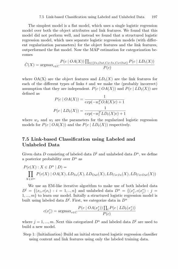
7.5 Link-based Classification using Labeled and Unlabeled Data 197
The simplest model is a flat model, which uses a single logistic regressionmodel over both the object attributes and link features. We found that thismodel did not perform well, and instead we found that a structured logisticregression model, which uses separate logistic regression models (with differ-ent regularization parameters) for the object features and the link features,outperformed the flat model. Now the MAP estimation for categorization be-comes
C(X) = argmaxc∈C
P (c | OA(X))∏
t∈In,Out,Co-In,Co-Out P (c | LDt(X))
P (c)
where OA(X) are the object features and LDt(X) are the link features foreach of the different types of links t and we make the (probably incorrect)assumption that they are independent. P (c | OA(X)) and P (c | LDt(X)) aredefined as
P (c | OA(X)) =1
exp(−wTo OA(X)c) + 1
P (c | LDt(X)) =1
exp(−wTl LDt(X)c) + 1
where wo and wl are the parameters for the regularized logistic regressionmodels for P (c | OA(X)) and the P (c | LDt(X)) respectively.
7.5 Link-based Classification using Labeled andUnlabeled Data
Given data D consisting of labeled data Dl and unlabeled data Du, we definea posterior probability over Du as
P (c(X) : X ∈ Du | D) =∏X∈Du
P (c(X) | OA(X), LDIn(X), LDOut(X), LDCo-In(X), LDCo-Out(X))
We use an EM-like iterative algorithm to make use of both labeled dataDl = (xi, c(xi) : i = 1, .., n and unlabeled data Du = (x∗
j , c(x∗j ) : j =
1, ..., m to learn our model. Initally a structured logistic regression model isbuilt using labeled data Dl. First, we categorize data in Du
c(x∗j ) = argmaxc∈C
P (c | OA(x∗j ))∏
t P (c | LDt(x∗j ))
P (c)
where j = 1, ..., m. Next this categorized Du and labeled data Dl are used tobuild a new model.
Step 1: (Initialization) Build an initial structured logistic regression classifierusing content and link features using only the labeled training data.

198 Lise Getoor
Step 2: (Iteration) Loop while the posterior probability over the unlabeledtest data increases:1. Classify unlabeled data using the current model.2. Recompute the link features of each object. Re-estimate the parame-
ters of the logistic regression models.
In our above iterative algorithm, after we categorize the unlabeled data,the link descriptions for all labeled and unlabeled data will change due to thelinks between labeled and unlabeled data. The first step is to recompute thelink descriptions for all data based on the results from the current estimatesand the link graph over labeled and unlabeled data.
In the iterative step there are many possible orderings for objects. Oneapproach is based simply on the number of links; Oh et al. [28] report nosignificant improvement using this method. Neville and Jensen [25] proposean iterative classification algorithm where the ordering is based on the infer-ence posterior probability of the categories. They report an improvement inclassification accuracy. We explore several alternate orderings based on theestimated link statistics. We propose a range of link-based adaptive strategieswhich we call Link Diversity. Link diversity measures the number of differentcategories to which an object is linked. The idea is that, in some domains atleast, we may be more confident of categorizations of objects with low link –diversity in essence, the object’s neighbors are all in agreement. So we maywish to make these assignments first, and then move on to the rest of thepages. In our experiments, we evaluate the effectiveness of different orderingschemes based on link diversity.
7.6 Results
We evaluated our link-based classification algorithm on two variants of theCora data set [23], a data set that we constructed from CiteSeer entries [14]and WebKB [6].
The first Cora data set, CoraI, contains 4187 machine learning papers,each categorized into one of seven possible topics. We consider only the 3181papers that are cited or cite other papers. There are 6185 citations in the dataset. After stemming and removing stop words and rare words, the dictionarycontains 1400 words.
The second Cora data set, CoraII,2 contains 30,000 papers, each catego-rized into one of ten possible topics: information retrieval, databases, artifi-cial intelligence, encryption and compression, operating systems, networking,hardware and architecture, data structure algorithms and theory, program-ming and human–computer interaction. We consider only the 3352 documentsthat are cited or cite other papers. There are 8594 citations in the data set.
2www.cs.umass.edu/∼mccallum/code-data.html

7.6 Results 199
After stemming and removing stop words and rare words, the dictionary con-tains 3174 words.
The CiteSeer data set has 3312 papers from six categories: Agents, Artifi-cial Intelligence, Database, Human Computer Interaction, Machine Learningand Information Retrieval. There are 7522 citations in the data set. Afterstemming and removing stop words and rare words, the dictionary for Cite-Seer contains 3703 words.
The WebKB data set contains web pages from four computer science de-partments, categorized into topics such as faculty, student, project, courseand a catch-all category, other. In our experiments we discard pages in the“other” category, which generates a data set with 700 pages. After stemmingand removing stop words, the dictionary contains 2338 words. For WebKB,we train on three schools, plus 2/3 of the fourth school, and test on the last1/3.
On Cora and CiteSeer, for each experiment, we take one split as a testset, and the remaining two splits are used to train our model: one for trainingand the other for a validation set used to find the appropriate regularizationparameter λ. Common values of λ were 10−4 or 10−5. On WebKB, we learnedmodels for a variety of λ; here we show the best result.
In our experiments, we compared a baseline classifier (Content) with ourlink-based classifiers (Mode, Binary, Count). We compared the classifiers:
• Content: Uses only object attributes.• Mode: Combines a logistic regression classifier over the object attributes
with separate logistic regression classifiers over the mode of the In Links,Out Links, Co-In Links, and Co-Out Links.
• Binary: Combines a logistic regression classifier over the object attributeswith a separate logistic regression classifier over the binary link statisticsfor all of the links.
• Count-Link: Combines a logistic regression classifier over the object at-tributes with a separate logistic regression classifier over the counts linkstatistics for all of the links.
7.6.1 Link Model Comparison
Table 7.1 shows details of our results using four different metrics (accuracy,precision, recall and F1 measure)3 on the four data sets. Figure 7.2 shows asummary of the results for the F1 measure.
3A true positive is a document that is correctly labeled. Let TP be the numberof true positives, FP be the number of false positive, TN be the number of truenegatives, FP be the number of false negatives. Accuracy is the percentage of cor-rectly labeled documents, TP+TN
TP+FP+TN+FN. Precision, recall and the F1 measure are
macro-averaged over each of the categories. Precision is the percentage of documentsthat are predicted to be of a category, that actually are of that category TP
TP+FP.
Recall is the percentage of documents that are predicted to be of a category, out ofall the documents of the category TP
TP+FN. The F1 measure is 2PR
R+P.

200 Lise Getoor
Table 7.1. Results with Content, Mode, Binary and Count models on CoraI,CoraII, CiteSeer and WebKB. Statistically significant results (at or above 90% con-fidence level) for each row are shown in bold.
CoraIContent Mode Binary Count
avg accuracy 68.14 82.35 77.53 83.14avg precision 67.47 81.01 77.35 81.74avg recall 63.08 80.08 76.34 81.20avg F1 measure 64.17 80.0 75.69 81.14
CoraIIContent Mode Binary Count
avg accuracy 67.55 83.03 81.46 83.66avg precision 65.87 78.62 74.54 80.62avg recall 47.51 75.27 75.69 76.15avg F1 measure 52.11 76.52 74.62 77.77
CiteSeerContent Mode Binary Count
avg accuracy 60.59 71.01 69.83 71.52avg precision 55.48 64.61 62.6 65.22avg recall 55.33 60.09 60.3 61.22avg F1 measure 53.08 60.68 60.28 61.87
WebKBContent Mode Binary Count
avg accuracy 87.45 88.52 78.91 87.93avg precision 78.67 77.27 70.48 77.71avg recall 72.82 73.43 71.32 73.33avg F1 measure 71.77 73.03 66.41 72.83
Different Link Models
0
20
40
60
80
100
CoraI Cora II CiteSeer WebKB
Aver
age
F1 M
easu
re (%
)
Content Only
Mode
Binary
Count
Fig. 7.2. Average F1 measure for different models (Content, Mode, Binary andCount) on four data sets (CoraI, CoraII, CiteSeer and WebKB).
In this set of experiments, all of the links (In Links, Out Links, Co-InLinks, Co-Out Links) are used and we use a fixed ordering for the iterativeclassification algorithm.

7.6 Results 201
For all four data sets, the link-based models outperform the content onlymodels. For three of the four data sets, the difference is statistically significantat the 99% significance level. For three of the four data sets, count outper-forms mode at the 90% significance level or higher, for both accuracy and F1measure. Both mode and count outperform binary; the difference is mostdramatic for CoraI and WebKB.
Clearly, the mode, binary and count link-based models are using infor-mation from the description of the link neighborhood of an object to improveclassification performance. Mode and count seem to make the best use ofthe information; one explanation is that while binary contains more informa-tion in terms of which categories of links exist, it loses the information aboutwhich link category is most frequent. In many domains one might think thatmode should be enough information, particulary bibliographic domains. So itis somewhat surprising that the count model is the best for our three citationdata sets.
Our results on WebKB were less reliable. Small changes to the ways thatwe structured the classifiers resulted in different outcomes. Overall, we feltthere were problems because the link distributions were quite different amongthe different schools. Also, after removing the other pages, the data set israther small.
7.6.2 Effect of Link Types
Different Link Types
0
20
40
60
80
100
CoraI Cora II CiteSeer WebKB
Av
era
ge
F1 M
ea
su
re (
%)
Content Links In Links & ContentOut Links & ContentCo-In Links & ContentCo-Out Links & ContentLinks & Content
Fig. 7.3. Average F1 measure for Count on four data sets (CoraI, CoraII, CiteSeerand WebKB) for varying content and links (Content, Links, In Links & Content,Out Links & Content, Co-In Links & Content, Co-Out links & Content and Links& Content).
Next we examined the individual effect of the different categories of links:In Links, Out Links, Co-In Links and Co-Out links. Using the countmodel, we included in the comparision Content, with a model which used

202 Lise Getoor
all the links, but no content (Links),4 and Link & Content (which gaveus the best results in the previous section). Figure 7.3 shows the average F1accuracy for the four of the data sets using different link types.
Clearly using all of the links performs best. Individually, the Out Linksand Co-In Links seem to add the most information, although again, theresults for WebKB are less definitive.
More interesting is the difference in results when using only Links versusLinks & Content. For CoraI and Citeseer, Links only performs reasonablywell, while for the other two cases, CoraII and WebKB, it performs horribly.Recall that the content helps give us an initial starting point for the iterativeclassification algorithm. Our theory is that, for some data sets, especiallythose with fewer links, getting a good initial starting point is very important.In others, there is enough information in the links to overcome a bad startingpoint for the iterative classification algorithm. This is an area that requiresfurther investigation.
7.6.3 Prediction with Links Between Training and Test Sets
Next we were interested in investigating the issue of exploiting the links be-tween test and training data for predictions. In other work, Neville and Jensen[25], Getoor et al. [12] and Taskar et al. [31] used link distributions for cate-gorization; the experimental data set are split into training set and test set,and any links across training and test sets are ignored.
In reality, in domains such as web and scientific literature, document col-lections are constantly expanding. There are new papers published and newweb sites created. New objects and edges are being added to the existinggraph. A more realistic evaluation, such as that done in Chakrabarti et al. [4],exploits the links between test and training.
In an effort to understand this phenomenon more fully, we examined theeffect of ignoring links between training and test sets. Here we compared amethod which discards all link information across training set and test set,which is denoted as “Test Links Only”, with a more realistic method whichkeeps all the links between test and training sets which is denoted as “Com-plete Links”. The results are shown in Table 7.2. With “Test Links Only”, inour iterative classification process, the link descriptions of test data are con-structed based only on the link graph over test data, while with “CompleteLinks” link descriptions of test data are formulated over the link graph usingboth training and test data. These results demonstrate that the complete linkstructure is informative and can be used to improve overall performance.
7.6.4 Link-based Classification using Labeled and Unlabeled Data
In the previous section we experimented with making use of labeled datafrom the training set during testing. Next we explore the more general setting
4This model was inspired by results in [21].
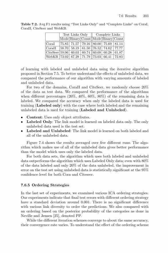
7.6 Results 203
Table 7.2. Avg F1 results using “Test Links Only” and “Complete Links” on CoraI,CoraII, CiteSeer and WebKB.
Test Links Only Complete LinksMode Binary Count Mode Binary Count
CoraI 75.85 71.57 79.16 80.00 75.69 81.14CoraII 58.70 58.19 61.50 76.52 74.62 77.77CiteSeer 59.06 60.03 60.74 60.68 60.28 61.87WebKB 73.02 67.29 71.79 73.03 66.41 72.83
of learning with labeled and unlabeled data using the iterative algorithmproposed in Section 7.5. To better understand the effects of unlabeled data, wecompared the performance of our algorithm with varying amounts of labeledand unlabeled data.
For two of the domains, CoraII and CiteSeer, we randomly choose 20%of the data as test data. We compared the performance of the algorithmswhen different percentages (20%, 40%, 60%, 80%) of the remaining data islabeled. We compared the accuracy when only the labeled data is used fortraining (Labeled only) with the case where both labeled and the remainingunlabeled data is used for training (Labeled and Unlabeled).
• Content: Uses only object attributes.• Labeled Only: The link model is learned on labeled data only. The only
unlabeled data used is the test set.• Labeled and Unlabeled: The link model is learned on both labeled and
all of the unlabeled data.
Figure 7.4 shows the results averaged over five different runs. The algo-rithm which makes use of all of the unlabeled data gives better performancethan the model which uses only the labeled data.
For both data sets, the algorithm which uses both labeled and unlabeleddata outperforms the algorithm which uses Labeled Only data; even with 80%of the data labeled and only 20% of the data unlabeled, the improvement inerror on the test set using unlabeled data is statistically significant at the 95%confidence level for both Cora and Citeseer.
7.6.5 Ordering Strategies
In the last set of experiments, we examined various ICA ordering strategies.Our experiments indicate that final test errors with different ordering strategyhave a standard deviation around 0.001. There is no significant differencewith various link diversity to order the predictions. We also compared withan ordering based on the posterior probability of the categories as done inNeville and Jensen [25], denoted PP.
While the different iteration schemes converge to about the same accuracy,their convergence rate varies. To understand the effect of the ordering scheme

204 Lise Getoor
CoraII
60
65
70
75
80
85
20 40 60 80
% Data Labeled
Acc
urac
y
Labeled &Unlabeled
Labeled Only
Content
CiteSeer
60
65
70
75
80
85
20 40 60 80
% Data Labeled
Acc
urac
y
Labeled &Unlabeled
Labeled Only
Content
(a) (b)
Fig. 7.4. (a) Results varying the amount of labeled and unlabeled data used fortraining on CoraII (b) and on CiteSeer. The results are averages of five runs.
CoraII
6567697173757779818385
30 120
210
300
390
480
570
660
750
840
930
1020
1110
1200
1290
1380
1470
#of updates
accu
racy Random
INC-OUTDEC-OUTPP
Fig. 7.5. The convergence rates of different iteration methods on the CoraII dataset.
at a finer level of detail, Figure 7.5 shows an example of the accuracy ofthe different iteration schemes for the CoraII data set (to make the graphreadable, we show only ordering by increasing diversity of out links (INC-Out)and decreasing diversity of out-links (DEC-Out); the results for in links, co-inlinks and co-out links are similar). Our experiments indicate that orderingby increasing link diversity converges faster than ordering by decreasing linkdiversity, and the RAND ordering converges the most quickly at the start.

References 205
7.7 Conclusions
Many real-world data sets have rich structures, where the objects are linkedin some way. Link mining targets data-mining tasks on this richly-structureddata. One major task of link mining is to model and exploit the link distribu-tions among objects. Here we focus on using the link structure to help improveclassification accuracy.
In this chapter we have proposed a simple framework for modeling linkdistributions, based on link statistics. We have seen that for the domains weexamined, a combined logistic classifier built over the object attributes andlink statistics outperforms a simple content-only classifier. We found the ef-fect of different link types is significant. More surprisingly, the mode of thelink statistics is not always enough to capture the dependence. Avoiding theassumption of homogeneity of labels and modeling the distribution of the linkcategories at a finer grain is useful.
Acknowledgments: I’d like to thank Prithviraj Sen and Qing Lu for theirwork on the implementation of the link-based classification system. This studywas supported by NSF Grant 0308030 and the Advanced Research and De-velopment Activity (ARDA) under Award Number NMA401-02-1-2018. Theviews, opinions, and findings contained in this report are those of the authorand should not be construed as an official Department of Defense position,policy, or decision unless so designated by other official documentation.
References
[1] Blum, A., and S. Chawla, 2001: Learning from labeled and unlabeleddata using graph mincuts. Proc. 18th International Conf. on MachineLearning. Morgan Kaufmann, San Francisco, CA, 19–26.
[2] Blum, A. and T. Mitchell, 1998: Combining labeled and unlabeled datawith co-training. COLT: Proceedings of the Workshop on ComputationalLearning Theory. Morgan Kaufmann.
[3] Chakrabarti, S., 2002: Mining the Web. Morgan Kaufman.[4] Chakrabarti, S., B. Dom and P. Indyk, 1998: Enhanced hypertext cate-
gorization using hyperlinks. Proc of SIGMOD-98 .[5] Cook, D., and L. Holder, 2000: Graph-based data mining. IEEE Intelli-
gent Systems, 15, 32–41.[6] Craven, M., D. DiPasquo, D. Freitag, A. McCallum, T. Mitchell,
K. Nigam and S. Slattery, 1998: Learning to extract symbolic knowledgefrom the world wide web. Proc. of AAAI-98 .
[7] Dasarathy, B. V., 1991: Nearest neighbor norms: NN pattern classificationtechniques. IEEE Computer Society Press, Los Alamitos, CA.
[8] Dean, J., and M. Henzinger, 1999: Finding related pages in the WorldWide Web. Computer Networks, 31, 1467–79.
206 Lise Getoor
[9] Dzeroski, S., and N. Lavrac, eds., 2001: Relational Data Mining . Kluwer,Berlin.
[10] Feldman, R., 2002: Link analysis: Current state of the art. Tutorial at theKDD-02 .
[11] Flach, P., and N. Lavrac, 2000: The role of feature construction in induc-tive rule learning. Proc. of the ICML2000 workshop on Attribute-Valueand Relational Learning: crossing the boundaries.
[12] Getoor, L., N. Friedman, D. Koller and B. Taskar, 2002: Learning prob-abilistic models with link uncertainty. Journal of Machine Learning Re-search.
[13] Ghani, R., 2001: Combining labeled and unlabeled data for text clas-sification with a large number of categories. Proceedings of the IEEEInternational Conference on Data Mining , N. Cercone, T. Y. Lin andX. Wu, eds., IEEE Computer Society, San Jose, US, 597–8.
[14] Giles, C., K. Bollacker, and S. Lawrence, 1998: CiteSeer: An automaticcitation indexing system. ACM Digital Libraries 98 .
[15] Jensen, D., 1999: Statistical challenges to inductive inference in linkeddata. Seventh International Workshop on Artificial Intelligence andStatistics.
[16] Jensen, D., and H. Goldberg, 1998: AAAI Fall Symposium on AI andLink Analysis. AAAI Press.
[17] Jensen, D, J. Neville. and B. Gallagher, 2004: Why collective inferenceimproves relational classification. Proceedings of the 10th ACM SIGKDDInternational Conference on Knowledge Discovery and Data Mining .
[18] Joachims, T., 1999: Transductive inference for text classification usingsupport vector machines. Proceedings of ICML-99, 16th InternationalConference on Machine Learning , I. Bratko and S. Dzeroski, eds., MorganKaufmann, San Francisco, US, 200–9.
[19] Kleinberg, J., 1999: Authoritative sources in a hyperlinked environment.Journal of the ACM , 46, 604–32.
[20] Kramer, S., N. Lavrac and P. Flach, 2001: Propositionalization ap-proaches to relational data mining. Relational Data Mining , S. Dzeroskiand N. Lavrac, eds., Kluwer, 262–91.
[21] Macskassy, S., and F. Provost, 2003: A simple relational classifier. KDDWorkshop on Multi-Relational Data Mining.
[22] McCallum, A., and K. Nigam, 1998: A comparison of event models fornaive Bayes text classification. AAAI-98 Workshop on Learning for TextCategorization.
[23] McCallum, A., K. Nigam, J. Rennie and K. Seymore, 2000: Automatingthe construction of Internet portals with machine learning. InformationRetrieval , 3, 127–63.
[24] Mitchell, T., 1999: The role of unlabeled data in supervised learning.Proceedings of the Sixth International Colloquium on Cognitive Science.

References 207
[25] Neville, J., and D. Jensen, 2000: Iterative classification in relational data.Proc. AAAI-2000 Workshop on Learning Statistical Models from Rela-tional Data, AAAI Press.
[26] Nigam, K., 2001: Using Unlabeled Data to Improve Text Classification.Ph.D. thesis, Carnegie Mellon University.
[27] Nigam, K., A. McCallum, S. Thrun, and T. Mitchell, 2000: Text classifica-tion from labeled and unlabeled documents using EM. Machine Learning ,39, 103–34.
[28] Oh, H., S. Myaeng, and M. Lee, 2000: A practical hypertext categorizationmethod using links and incrementally available class information. Proc.of SIGIR-00 .
[29] Page, L., S. Brin, R. Motwani and T. Winograd, 1998: The page rankcitation ranking: Bringing order to the web. Technical report, StanfordUniversity.
[30] Popescul, A., L. Ungar, S. Lawrence and D. Pennock, 2002: Towardsstructural logistic regression: Combining relational and statistical learn-ing. KDD Workshop on Multi-Relational Data Mining .
[31] Taskar, B., P. Abbeel and D. Koller, 2002: Discriminative probabilisticmodels for relational data. Proc. of UAI-02 , Edmonton, Canada, 485–92.
[32] Taskar, B., E. Segal and D. Koller, 2001: Probabilistic classification andclustering in relational data. Proc. of IJCAI-01 .
[33] Yang, Y., S. Slattery and R. Ghani, 2002: A study of approaches to hy-pertext categorization. Journal of Intelligent Information Systems, 18,219–41.
[34] Zhang, T., and F. J. Oles, 2000: A probability analysis on the value ofunlabeled data for classification problems. Proc. 17th International Conf.on Machine Learning , Morgan Kaufmann, San Francisco, CA, 1191–8.
[35] — 2001: Text categorization based on regularized linear classificationmethods. IEEE Transactions on Pattern Analysis and Machine Intelli-gence, 5–31.

Part II
Applications

8
Knowledge Discovery from Evolutionary Trees
Sen Zhang and Jason T. L. Wang
Summary. In this chapter we present new techniques for discovering knowledgefrom evolutionary trees. An evolutionary tree is a rooted unordered labeled tree inwhich there is a root and the order among siblings is unimportant. The knowledge tobe discovered from these trees refers to “cousin pairs” in the trees. A cousin pair isa pair of nodes sharing the same parent, the same grandparent, or the same great-grandparent, etc. Given a tree T , our algorithm finds all interesting cousin pairsof T in O(|T |2) time where |T | is the number of nodes in T . We also extend thisalgorithm to find interesting cousin pairs in multiple trees. Experimental resultson synthetic data and real trees demonstrate the scalability and effectiveness ofthe proposed algorithms. To show the usefulness of these techniques, we discuss anapplication of the cousin pairs to evaluate the consensus of equally parsimonioustrees and compare them with the widely used clusters in the trees. We also reportthe implementation status of the system built based on the proposed algorithms,which is fully operational and available on the world-wide web.
8.1 Introduction
Data mining, or knowledge discovery from data, refers to the process of ex-tracting interesting, non-trivial, implicit, previously unknown and potentiallyuseful information or patterns from data [13]. In life sciences, this processcould refer to detecting patterns in evolutionary trees, extracting clusteringrules for gene expressions, summarizing classification rules for proteins, infer-ring associations between metabolic pathways and predicting genes in genomicDNA sequences [25, 26, 28, 29], among others. This chapter presents knowl-edge discovery algorithms for extracting patterns from evolutionary trees.
Scientists model the evolutionary history of a set of taxa (organisms orspecies) that have a common ancestor using rooted unordered labeled trees,also known as phylogenetic trees (phylogenies) or evolutionary trees [20]. Theinternal nodes within a particular tree represent older organisms from whichtheir child nodes descend. The children represent divergences in the genetic

212 Sen Zhang and Jason T. L. Wang
composition in the parent organism. Since these divergences cause new or-ganisms to evolve, these organisms are shown as children of the previous or-ganism. Evolutionary trees are usually constructed from molecular data [20].They can provide guidance in aligning multiple molecular sequences [24] andin analyzing genome sequences [6].
The patterns we want to find from evolutionary trees contain “cousinpairs.” For example, consider the three hypothetical evolutionary trees inFigure 8.1. In the figure, a and y are cousins with distance 0 in T1; e and fare cousins with distance 0.5 in T2; b and f are cousins with distance 1 in allthe three trees.
b
11
3TT
ddce
c
5
4
5
2 3
1
dya
764
3
bbf f
1
x
T2
98
6 5 6
32
g
a
p
10f
d cc
7
a
2
11
4
Fig. 8.1. Three trees T1, T2 and T3. Each node in a tree may or may not havea label, and is associated with a unique identification number (represented by theinteger outside the node).
The measure “distance” represents kinship of two nodes; two cousins withdistance 0 are siblings, sharing the same parent node. Cousins of distance1 share the same grandparent. Cousins of distance 0.5 represent aunt–niecerelationships. Our algorithms can find cousin pairs of varying distances in asingle tree or multiple trees. The cousin pairs in the trees represent evolution-ary relationships between species that share a common ancestor. Finding thecousin pairs helps one to better understand the evolutionary history of thespecies [22], and to produce better results in multiple sequence alignment [24].
The rest of the chapter is organized as follows. Section 8.2 introducesnotation and terminology. Section 8.3 presents algorithms for finding frequentcousin pairs in trees. Section 8.4 reports experimental results on both syntheticdata and real trees, showing the scalability and effectiveness of the proposedapproach. Section 8.5 reports implementation efforts and discusses severalapplications where we use cousin pairs to define new similarity measures fortrees and to evaluate the quality of consensuses of equally parsimonious trees.

8.2 Preliminaries 213
Section 8.6 compares our work with existing methods. Section 8.7 concludesthe chapter and points out some future work.
8.2 Preliminaries
We model evolutionary trees by rooted unordered labeled trees. Let Σ be afinite set of labels. A rooted unordered labeled tree of size k > 0 on Σ is aquadruple T = (V, N, L, E), where
• V is the set of nodes of T in which a node r(T ) ∈ V is designated as theroot of T and |V | = k;
• N : V → 1 . . . , k is a numbering function that assigns a unique identifi-cation number N(v) to each node v ∈ V ;
• L : V ′ → Σ, V ′ ⊆ V , is a labeling function that assigns a label L(v) toeach node v ∈ V ′; the nodes in V − V ′ do not have a label;
• E ⊂ N(V )×N(V ) contains all parent–child pairs in T .
For example, refer to the trees in Figure 8.1. The node numbered 6 in T1does not have a label. The nodes numbered 2, 3 in T3 have the same label dand the nodes numbered 5, 6 in T3 have the same label c. We now introducea series of definitions that will be used in our algorithms.
Cousin DistanceGiven two labeled nodes u, v of tree T where neither node is the parent ofthe other, we represent the least common ancestor, w, of u and v as lca(u, v),and represent the height of u, v respectively, in the subtree rooted at w asH(u, w), H(v, w) respectively. We define the cousin distance of u and v, de-noted c dist(u, v), as shown in Equation (8.1).
c dist(u, v) =
H(u, w)− 1 if H(u, w) = H(v, w)maxH(u, w), H(v, w) − 1.5 if |H(u, w)−H(v, w)| = 1
(8.1)The cousin distance c dist(u, v) is undefined if |H(u, w) − H(v, w)| is
greater than 1, or one of the nodes u, v is unlabeled. (The cutoff of 1 is aheuristic choice that works well for phylogeny. In general there could be nocutoff, or the cutoff could be much greater.)
Our cousin distance definition is inspired by genealogy [12]. Node u is afirst cousin of v, or c dist(u, v) = 1, if u and v share the same grandparent. Inother words, v is a child of u’s aunts or vice versa. Node u is a second cousinof v, or c dist(u, v) = 2, if u and v have the same great-grandparent, but notthe same grandparent. For two nodes u, v that are siblings, i.e. they share thesame parent, c dist(u, v) = 0.
We use the number “0.5” to represent the “once removed” relationship.When the word “removed” is used to describe a relationship between two

214 Sen Zhang and Jason T. L. Wang
nodes, it indicates that the two nodes are from different generations. Thewords “once removed” mean that there is a difference of one generation. Forany two labeled nodes u and v, if u is v’s parent’s first cousin, then u isv’s first cousin once removed [12], and c dist(u, v) = 1.5. “Twice removed”means that there is a two-generation difference. Our cousin distance definitionrequires |H(u, w)−H(v, w)| ≤ 1 and excludes the twice removed relationship.As mentioned above, this is a heuristic rather than a fundamental restriction.
For example, consider again T1 in Figure 8.1. There is a one-generationdifference between the aunt–niece pair y, x and c dist(y, x) = 0.5. Node b isnode f ’s first cousin and c dist(b, f) = 1. Node d is node g’s first cousinonce removed, and c dist(d, g) = 1.5. Node f is node g’s second cousin,and c dist(f, g) = 2. Node f is node p’s second cousin once removed, andc dist(f, p) = 2.5.
Notice that parent–child relationships are not included in our work be-cause the internal nodes of evolutionary trees usually have no labels. (Eachleaf in these trees has a label, which is a taxon name.) So, we do not treatparent–child pairs at all. This heuristic works well in phylogenetic applica-tions, but could be generalized. We proposed one such generalization usingthe UpDown distance [27]. Another approach would be to use one upper limitparameter for inter-generational (vertical) distance and another upper limitparameter for horizontal distance.
Cousin Pair ItemLet u, v be cousins in tree T . A cousin pair item of T is a quadruple(L(u), L(v), c dist(u, v), occur(u, v)) where L(u) and L(v) are labels of u, v,respectively, c dist(u, v) is the cousin distance of u, v and occur(u, v) > 0 isthe number of occurrences of the cousin pair in T with the specified cousindistance. Table 8.1 lists all the cousin pair items of tree T3 in Figure 8.1.Consider, for example, the cousin pair item (d, c, 0.5, 2) in the second rowof Table 8.1. Nodes 2 and 6, and nodes 3 and 5 are an aunt–niece pairs withcousin distance 0.5. When taking into account labels of these nodes, we seethat the cousin pair (d, c) with distance 0.5 occurs 2 times totally in tree T3,and hence (d, c, 0.5, 2) is a valid cousin pair item in T3.
Table 8.1. Cousin pair items of T3 in Figure 8.1.
Cousin Distance Cousin Pair Items0 (b, c, 0, 1), (c, f, 0, 1), (d, d, 0, 1)
0.5 (d, b, 0.5, 1), (d, c, 0.5, 2), (d, f, 0.5, 1)1 (b, f, 1, 1), (b, c, 1, 1), (c, c, 1, 1), (c, f, 1, 1)
We may also consider the total number of occurrences of the cousins u andv regardless of their distance, for which case we use λ in place of c dist(u, v) in

8.3 Tree-Mining Algorithms 215
the cousin pair item. For example, in Table 8.1, T3 has (b, c, 0, 1) and (b, c, 1, 1),and hence we obtain (b, c, λ, 2). Here, the cousin pair (b, c) occurs once withdistance 0 and occurs once with distance 1. Therefore, when ignoring thedistance, the total number of occurrences of (b, c) is 2. Likewise we can ig-nore the number of occurrences of a cousin pair (u, v) by using λ in place ofoccur(u, v) in the cousin pair item. For example, in Table 8.1, T3 has (b, c, 0, λ)and (b, c, 1, λ). We may ignore both the cousin distance and the number of oc-currences and focus on the cousin labels only. For example, T3 has (b, c, λ, λ),which simply indicates that b, c are cousins in T3.
Frequent Cousin PairLet S = T1, T2, . . . , Tn be a set of n trees and let d be a given distance value.We define δu,v,i to be 1 if Ti has the cousin pair item (L(u), L(v), d, occur(u, v)),occur(u, v) > 0; otherwise δu,v,i is 0. We define the support of the cousin pair(u, v) with respect to the distance value d as Σ1≤i≤nδu,v,i. Thus the sup-port value represents the number of trees in the set S that contain at leastone occurrence of the cousin pair (u, v) having the specified distance valued. A cousin pair is frequent if its support value is greater than or equal to auser-specified threshold, minsup.
For example, consider Figure 8.1 again. T1 has the cousin pair item(c, f, 1, 1), T2 has the cousin pair item (c, f, 0.5, 1) and T3 has the cousinpair item (c, f, 1, 1) and (c, f, 0, 1). The support of (c, f) w.r.t. distance 1 is2 because both T1 and T3 have this cousin pair with the specified distance.One can also ignore cousin distances when finding frequent cousin pairs. Forexample, the support of (c, f) is 3 when the cousin distances are ignored.
Given a set S of evolutionary trees, our approach offers the user severalalternative kinds of frequent cousin pairs in these trees. For example, thealgorithm can find, in a tree T of S, all cousin pairs in T whose distancesare less than or equal to maxdist and whose occurrence numbers are greaterthan or equal to minoccur, where maxdist and minoccur are user-specifiedparameters. The algorithm can also find all frequent cousin pairs in S whosedistance values are at most maxdist and whose support values are at leastminsup for a user-specified minsup value. In the following section, we willdescribe the techniques used in finding these frequent cousin pairs in a singletree or in multiple trees.
8.3 Tree-Mining Algorithms
Given a tree T and a node u of T , let children set(u) contain all children ofu. Our algorithm preprocesses T to obtain children set(u) for every node uin T . We also preprocess T to be able to locate a list of all ancestors of anynode u in O(1) time using a conventional hash table.
Now, given a user-specified value maxdist, we consider all valid distancevalues 0, 0.5, 1, 1.5, . . ., maxdist. For each valid distance value d, we define

216 Sen Zhang and Jason T. L. Wang
my level(d) and mycousin level(d) as follows:
my level(d) = 1 + d (8.2)mycousin level(d) = my level(d) + R (8.3)
where
R = 2× (d− d) (8.4)
Let m = my level(d) and n = mycousin level(d). Intuitively, given a nodeu and the distance value d, beginning with u, we can go m levels up to reach anancestor w of u. Then, from w, we can go n levels down to reach a descendant vof w. Referring to the cousin distance definition in Equation (8.1), c dist(u, v)must be equal to the distance value d. Furthermore, all the siblings of u mustalso be cousins of the siblings of v with the same distance value d. Thesenodes are identified by their unique identification numbers. To obtain cousinpair items having the form (L(u), L(v), c dist(u, v), occur(u, v)), we check thenode labels of u, v and add up the occurrence numbers for cousin pairs whosecorresponding node labels are the same and whose cousin distances are thesame. Figure 8.2 summarizes the algorithm.
Notice that within the loop (Steps 3 to 10) of the algorithm in Figure 8.2,we find cousin pairs with cousin distance d where d is incremented from 0to maxdist. In Step 8 where a cousin pair with the current distance value dis formed, we check, through node identification numbers, to make sure thiscousin pair is not identical to any cousin pair with less distance found in aprevious iteration in the loop. This guarantees that only cousin pairs withexact distance d are formed in the current iteration in the loop.
Lemma 1. Algorithm Single Tree Mining correctly finds all cousin pair itemsof T where the cousin pairs have a distance less than or equal to maxdist andan occurrence number greater than or equal to minoccur.Proof. The correctness of the algorithm follows directly from two observa-tions: (i) every cousin pair with distance d where 0 ≤ d ≤ maxdist is foundby the algorithm; (ii) because Step 9 eliminates duplicate cousin pairs fromconsideration, no cousin pair with the same identification numbers is countedtwice.
Lemma 2. The time complexity of algorithm Single Tree Mining is O(|T |2).Proof. The algorithm visits each children set of T . For each visited node, ittakes at most O(|T |) time to go up and down to locate its cousins. Thus, thetime spent in finding all cousin pairs identified by their unique identificationnumbers is O(|T |2). There are at most O(|T |2) such cousin pairs. Through thetable lookup, we get their node labels and add up the occurrence numbers ofcousin pairs whose distances and corresponding node labels are the same inO(|T |2) time.

8.4 Experiments and Results 217
Procedure: Single Tree MiningInput: A tree T and a maximum distance value allowed, maxdist, and a minimum
occurrence number allowed, minoccur.Output: All cousin pair items of T where the cousin pairs have a distance less
than or equal to maxdist and an occurrence number greater than orequal to minoccur.
1. for each node p where children set(p) = ∅ do2. begin3. for each valid distance value d ≤ maxdist do4. begin5. let u be a node in children set(p);6. calculate m = my level(d) and n = mycousin level(d) as defined
in Equations (8.2), (8.3);7. beginning with u, go m levels up to reach an ancestor w and
then from w, go n levels down to reach a descendant v of w;8. combine all siblings of u and all siblings of v to form cousin pairs
with the distance value d;9. if a specific pair of nodes with the distance d has been found
previously, don’t double-count them;10. end;11. end;12. add up the occurrence numbers of cousin pairs whose corresponding node
labels are the same and whose cousin distances are the same to getqualified cousin pair items of T .
Fig. 8.2. Algorithm for finding frequent cousin pair items in a single tree.
To find all frequent cousin pairs in a set of trees T1, . . . , Tk whose dis-tance is at most maxdist and whose support is at least minsup for a user-specified minsup value, we first find all cousin pair items in each of the treesthat satisfy the distance requirement. Then we locate all frequent cousin pairsby counting the number of trees in which a qualified cousin pair item occurs.This procedure will be referred to as Multiple Tree Mining and its time com-plexity is clearly O(kn2) where n = max|T1|, . . . , |Tk|.
8.4 Experiments and Results
We conducted a series of experiments to evaluate the performance of the pro-posed tree-mining algorithms, on both synthetic data and real trees, run underthe Solaris operating system on a SUN Ultra 60 workstation. The syntheticdata was produced by a C++ program based on the algorithm developed in[15]. This program is able to generate a large number of random trees fromthe whole tree space. The real trees were obtained from TreeBASE, availableat www.treebase.org [21].

218 Sen Zhang and Jason T. L. Wang
Table 8.2 summarizes the parameters of our algorithms and their defaultvalues used in the experiments. The value of 4 was used for minimum supportbecause the evolutionary trees in TreeBASE differ substantially and using thissupport value allowed us to find interesting patterns in the trees. Table 8.3lists the parameters and their default values related to the synthetic trees.The fanout of a tree is the number of children of each node in the tree. Thealphabet size is the total number of distinct node labels these synthetic treeshave.
Table 8.2. Parameters and their default values used in the algorithms.
Name Meaning Valueminoccur minimum occurrence number of an interesting cousin pair 1
in a treemaxdist maximum distance allowed for an interesting cousin pair 1.5minsup minimum number of trees in the database that contain 4
an interesting cousin pair
Table 8.3. Parameters and their default values related to synthetic trees.
Name Meaning Valuetree size number of nodes in a tree 200
database size number of trees in the database 1000fanout number of children of each node in a tree 5
alphabet size size of the node label alphabet 200
Figure 8.3 shows how changing the fanout of synthetic trees affects therunning time of the algorithm Single Tree Mining. 1000 trees were tested andthe average was plotted. The other parameter values are as shown in Table 8.2and Table 8.3. Given a fixed tree size value, a large fanout value will result ina small number of children sets, which will consequently reduce the times ofexecuting the outer for-loop of the algorithm, see Step 1 in Figure 8.2. There-fore, one may expect that the running time of Single Tree Mining drops asfanout increases. To our surprise, however, Figure 8.3 shows that the runningtime of Single Tree Mining increases as a tree becomes bushy, i.e. its fanoutbecomes large. This happens mainly because for bushy trees, each node hasmany siblings and hence more qualified cousin pairs could be generated, seeStep 8 in Figure 8.2. As a result, it takes more time in the postprocessingstage to aggregate those cousin pairs, see Step 12 in Figure 8.2.
Figure 8.4 shows the running times of Single Tree Mining with differentmaxdist values for varying node numbers of trees. 1000 synthetic trees were

8.4 Experiments and Results 219
0
0.05
0.1
0.15
0.2
0.25
0.3
0.35
0 10 20 30 40 50 60Fanout
Tim
e (s
ec.)
Fig. 8.3. Effect of fanout.
0
0.05
0.1
0.15
0.2
0.25
0.3
0 250 500 750 1000 1250
Tree size
Tim
e (s
ec.)
maxdist=2 maxdist=1.5
maxdist=1 maxdist=0.5
Fig. 8.4. Effect of maxdist and tree size.
tested and the average was plotted. The other parameter values are as shownin Table 8.2 and Table 8.3. It can be seen from the figure that as maxdistincreases, the running time becomes large, because more time will be spentin the inner for-loop of the algorithm for generating cousin pairs, Steps 3to 10 in Figure 8.2. We also observed that a lot of time needs to be spent inaggregating qualified cousin pairs in the postprocessing stage of the algorithm,Step 12 in Figure 8.2. This extra time, though not explicitly described by theasymptotic time complexity O(|T |2) in Lemma 2, is reflected by the graphsin Figure 8.4.

220 Sen Zhang and Jason T. L. Wang
The running times of Multiple Tree Mining when applied to 1 million syn-thetic trees and 1,500 evolutionary trees obtained from TreeBASE are shownin Figures 8.5 and 8.6, respectively. Each evolutionary tree has between 50and 200 nodes and each node has between two and nine children (most in-ternal nodes have two children). The size of the node label alphabet for theevolutionary trees is 18,870. The other parameter values are as shown in Ta-ble 8.2 and Table 8.3. We see from Figure 8.6 that Multiple Tree Mining canfind all frequent cousin pair items in the 1,500 evolutionary trees in less than150 seconds. The algorithm scales up well – its running time increases linearlywith increasing number of trees (Figure 8.5).
0
50
100
150
200
250
0 250 500 750 1000
Number of trees (in 1000s)
Tim
e (1
000
sec.
)
Fig. 8.5. Effect of database size for synthetic trees.
0
50
100
150
200
250
0 250 500 750 1000 1250 1500
Number of trees
Tim
e (s
ec.)
Fig. 8.6. Effect of database size for evolutionary trees.

8.5 Implementation and Applications 221
8.5 Implementation and Applications
8.5.1 Evolutionary Tree Miner
Fig. 8.7. Interface of the proposed evolutionary tree miner.
We have implemented the proposed algorithms into a system, called evo-lutionary tree miner, that runs on a collection of phylogenies obtained fromTreeBASE. Figure 8.7 shows the interface of the evolutionary tree miner. Theuser can input a set of tree IDs as described in TreeBASE and specify ap-propriate parameter values through the interface shown in the left windowof the system. The data mining result is shown in the right window of thesystem. Each discovered cousin pair has the format (label1, label2, c dist, oc-currence): k, where k is the number of input trees in which the cousin pairoccurs. For example, (Scutellaria californica, Scutellaria siphocampyloides, 0,1): 5 indicates that Scutellaria californica and Scutellaria siphocampyloides isa cousin pair of distance 0 that occurs in five input trees, with the occurrencenumber in each tree being one. The cousin pairs in the output list shownin the right window are sorted and displayed based on cousin distances andsupport values. By clicking on a tree ID (e.g. Tree873), the user can see a

222 Sen Zhang and Jason T. L. Wang
graphical display of the tree via a pop-up window, as shown in Figure 8.8.In this figure, the found cousin pair (Scutellaria californica and Scutellariasiphocampyloides) is highlighted with a pair of bullets.
Fig. 8.8. A discovered cousin pair highlighted with bullets.
8.5.2 New Similarity Measures for Trees
We develop new similarity measures for comparing evolutionary trees basedon the cousin pairs found in the trees. Specifically, let T1 and T2 be two trees.Let cpi(T1) contain all the cousin pair items of T1 and let cpi(T2) contain allthe cousin pair items generated from T2. We define the similarity of T1 andT2, denoted t sim(T1, T2), as
t sim(T1, T2) =|cpi(T1) ∩ cpi(T2)||cpi(T1) ∪ cpi(T2)|
(8.5)
Depending on whether the cousin distance and the number of occurrences of acousin pair in a tree are considered, we have four different types of cousin pairitems in the tree. Consequently we obtain four different tree similarity mea-sures. We represent them by t simnull(T1, T2) (considering neither the cousin

8.5 Implementation and Applications 223
distance nor the occurrence number in each tree), t simcdist(T1, T2) (consid-ering the cousin distance only in each tree), t simocc(T1, T2) (considering theoccurrence number only in each tree), and t simocc cdist(T1, T2) (consideringboth the cousin distance and the occurrence number in each tree), respectively.
For example, referring to the trees T2 and T3 in Figure 8.1, we havet simnull (T2, T3) = 4
12 = 0.33, t simcdist(T2, T3) = 216 = 0.125, t simocc(T2,
T3) = 412 = 0.33, t simocc cdist(T2, T3) = 2
16 = 0.125. The intersection andunion of two sets of cousin pair items take into account the occurrence num-bers in them. For example, suppose cpi(T1) = (a, b, m, occur1) and cpi(T2) =(a, b, m, occur2). Then cpi(T1) ∩ cpi(T2) = (a, b, m,min(occur1, occur2))and cpi(T1)∪cpi(T2) = (a, b, m,max(occur1, occur2)). These similarity mea-sures can be used to find kernel trees in a set of phylogenies [22].
8.5.3 Evaluating the Quality of Consensus Trees
One important topic in phylogeny is to automatically infer or reconstructevolutionary trees from a set of molecular sequences or species. The mostcommonly used method for tree reconstruction is based on the maximumparsimony principle [11]. This method often generates multiple trees ratherthan a single tree for the input sequences or species. When the number ofequally parsimonious trees is too large to suggest an informative evolutionhypothesis, a consensus tree is sought to summarize the set of parsimonioustrees. Sometimes the set is divided into several clusters and a consensus treefor each cluster is derived [23].
There are five most popular methods for generating consensus trees:Adams [1], strict [8], majority [17], semi-strict [2], and Nelson [18]. We de-velop a method to evaluate the quality of these consensus trees based on asimilarity measure defined in the previous subsection.
Specifically, let C be a consensus tree and let S be the set of originalparsimonious trees from which the consensus tree C is generated. Let T be atree in S. We define the similarity score, based on cousins, between C and T ,denoted δcus(C, T ), as
δcus(C, T ) = t simcdist(C, T ) (8.6)
where the similarity measure t simcdist is as defined in the previous subsec-tion.
The average similarity score, based on cousins, of the consensus tree Cwith respect to the set S, denoted ∆cus(C, S), is
∆cus(C, S) =∑
T ∈S δcus(C,T )|S| (8.7)
where |S| is the total number of trees in the set S. The higher the averagesimilarity score ∆cus(C, S) is, the better consensus tree C is.
Figure 8.9 compares average similarity scores of the consensus trees gener-ated by the five methods mentioned above for varying number of parsimonious

224 Sen Zhang and Jason T. L. Wang
trees. The parameter values used by our algorithms for finding the cousinpairs are as shown in Table 8.2. The parsimonious trees were generated bythe PHYLIP tool [10] using the first 500 nucleotides extracted from six genesrepresenting paternally, maternally, and biparentally inherited regions of thegenome among 16 species of Mus [16]. There are 33 trees in total. We randomlychoose 10, 15, 20, 25, 30 or 33 trees for each test. In each test, five differentindividual runs of the algorithms are performed and the average is plotted. Itcan be seen from Figure 8.9 that the majority consensus method and Nelsonconsensus method are better than the other three consensus methods – theyyield consensus trees with higher average similarity scores.
0
0.1
0.2
0.3
0.4
0.5
0.6
0.7
0.8
0.9
1
5 10 15 20 25 30 35
Number of trees
Ave
rage
sim
ilari
ty sc
ore
base
d on
co
usin
s
Majority Nelson
Adams Strict
Semi
Fig. 8.9. Comparing the quality of consensus trees using cousin pairs.
In addition to cousin patterns, we have also considered another type ofpatterns, namely clusters, for evaluating the quality of consensus trees. Givenan evolutionary tree T and a non-leaf node n of T , the cluster in T withrespect to n is defined to be the set of all leaves in the subtree rooted at n[19]. The cluster set of T , denoted cluster set(T ), is the set of clusters withrespect to all non-leaf nodes in T . For example, consider T3 in Figure 8.1. Thecluster set of T3 is 4, 5,6, 7, 4, 5, 6, 7 where each integer representsa node identification number in T3.
Now, let C be a consensus tree and let S be the set of original parsimonioustrees from which the consensus tree C is generated. Let T be a tree in S.We define the similarity score, based on clusters, between C and T , denotedδclu(C, T ), as
δclu(C, T ) =|cluster set(C) ∩ cluster set(T )||cluster set(C) ∪ cluster set(T )| (8.8)
The average similarity score, based on clusters, of the consensus tree C withrespect to the set S, denoted ∆clu(C, S), is

8.5 Implementation and Applications 225
∆clu(C, S) =∑
T∈S δclu(C, T )|S| (8.9)
For example, let us assume the cluster set of tree C, cluster set(C), is a,b, c,d, e. Assume the cluster set of tree T , cluster set(T ), is a, b,a,b, c, a, b, c, d. Since only a, b, c appears in both sets, δclu(C, T ) is
δclu(C, T ) =|cluster set(C) ∩ cluster set(T )||cluster set(C) ∪ cluster set(T )|
= 1/4= 0.25
0
0.1
0.2
0.3
0.4
0.5
0.6
0.7
0.8
0.9
1
5 10 15 20 25 30 35Number of trees
Aver
age s
imila
rity
scor
e bas
ed o
n cl
uste
rs
Majority NelsonAdams StrictSemi
Fig. 8.10. Comparing the quality of consensus trees using clusters.
Figure 8.10 shows the experimental results in which clusters are used toevaluate the quality of consensus trees. The data used here are the same as thedata for cousin pairs. In comparing the graphs in Figure 8.9 and Figure 8.10,we observe that majority consensus and Nelson consensus trees are the bestconsensus trees, yielding the highest average similarity scores between theconsensus trees and the original parsimonious trees. A close look at the datareveals why this happens. All the original parsimonious trees are fully resolved;i.e. the resolution rate [23] of these trees is 100%. This means every nodein an original parsimonious tree has two children, i.e. the tree is a binarytree. Furthermore the average depth of these trees is eight. When considering10 out of 33 parsimonious trees, the average resolution rate and the depthof the obtained majority consensus trees are 73% and 7 respectively. Theaverage resolution rate and the depth of the obtained Nelson consensus treesare 66% and 7 respectively. The average resolution rate and the depth ofAdams consensus trees are 60% and 6 respectively. The average resolution rate

226 Sen Zhang and Jason T. L. Wang
and the depth of the strict consensus trees are only 33% and 4 respectively.This shows that the majority consensus trees and Nelson consensus trees areclosest to the original parsimonious trees. On average, the majority consensustrees differ from the Nelson consensus trees by only two clusters and five cousinpairs. These small differences indicate that these two kinds of consensus treesare close to each other. Similar results were observed for the other input data.
Notice that, in Figure 8.10 where clusters are used, the average similar-ity scores for strict consensus trees decrease monotonously as the number ofequally parsimonious trees increases. This happens because when the numberof equally parsimonious trees is large, the number of common clusters sharedby all the parsimonious trees becomes small. Thus, the obtained strict con-sensus trees become less resolved; i.e., they are shallow and bushy. As a result,the similarity scores between the strict consensus trees and each fully resolvedparsimonious tree become small.
Notice also that, in both Figure 8.9 and Figure 8.10, the average similarityscores of semi-strict consensus trees and strict consensus trees are almost thesame. This happens because the parsimonious trees used in the experimentsare all generated by the PHYLIP tool, which produces fully resolved binarytrees. It is well known that a semi-strict consensus tree and a strict consensustree are exactly the same when the original equally parsimonious trees arebinary trees [2].
8.6 Related Work
In this section, we compare the proposed cousin-finding method and similaritymeasures with existing approaches. Computational biologists have developedseveral metrics for analyzing phylogenetic trees. The best known tree metricsinclude the quartet metric, triplet metric, partition metric, nearest neighborinterchange (NNI) metric and maximum agreement subtree metric. All ofthese metrics have been implemented in Page’s COMPONENT toolbox [19].
The quartet metric, designed mainly for unrooted trees, is to check whethertwo given trees have similar “quartets”, which are obtained based on adja-cency relationships among all possible subsets of four leaves (species or taxa).The similarity between the two trees is then computed as the proportion ofquartets that are shared in the two trees. A naive algorithm for calculatingthe quartet metric between two trees has the time complexity of O(n4) wheren is the number of nodes in the trees. Douchette [9] proposed an efficientalgorithm with the time complexity of O(n3), which is implemented in COM-PONENT. More recently, Bryant et al. [5] proposed a method to compute thequartet metric between two trees in time O(n2). Brodal et al. [3] presentedan algorithm that runs in time O(n log n) with the constraint that the treeshave to be fully resolved. When using COMPONENT to calculate the quartetmetric for rooted trees, these trees are treated as unrooted trees.

8.6 Related Work 227
The triplet metric is similar to the quartet metric except that we enumeratetriplets (three leaves) as opposed to quartets (four leaves). In other words, thetriplet metric counts the number of subtrees with three taxa that are differentin two trees. This metric is useful for rooted trees while the quartet metric isuseful for unrooted trees. The algorithm for calculating the triplet metric oftwo trees runs in time O(n2).
The partition metric treats each phylogenetic tree as an unrooted tree andanalyzes the partitions of species resulting from removing one edge at a timefrom the tree. By removing one edge from a tree, we are able to partitionthat tree. The distance between two trees is defined as the number of edgesfor which there is no equivalent (in the sense of creating the same partitions)edge in the other tree. The algorithm implemented in COMPONENT forcomputing the partition metric runs in time O(n).
An agreement subtree between two trees T1 and T2 is a substructure of T1and T2 on which the two trees are the same. Commonly such a subtree willhave fewer leaves than either T1 or T2. A maximum agreement subtree (MAS)between T1 and T2 is an agreement subtree of T1 and T2. Furthermore thereis no other agreement subtree of T1 and T2 that has more leaves (species ortaxa) than MAS. The MAS metric is defined as the number of leaves removedfrom T1 and T2 to obtain an MAS of T1 and T2. In COMPONENT, programshave been written to find the MAS for two (rooted or unrooted) fully resolvedbinary trees.
Given two unrooted, unordered trees with the same set of labeled leaves,the NNI metric is defined to be the number of NNI operations needed to trans-form one tree to the other. DasGupta et al. [7] showed that calculating theNNI metric is NP-hard, for both labeled and unlabeled unrooted trees. Brownand Day [4] developed approximation algorithms, which were implemented inCOMPONENT. The time complexities of the algorithms are O(nlogn) andO(n2logn), respectively, for rooted trees and unrooted trees, respectively.
Another widely used metric for trees is the edit distance, defined throughthree edit operations, change node label, insert a node and delete a node, ontrees. Finding the edit distance between two unordered trees is NP-hard, andhence a constrained edit distance, known as the degree-2 edit distance, wasdeveloped [30]. In contrast to the above tree metrics, the similarity measuresbetween two trees proposed in this chapter are defined in terms of the cousinpairs found in the two trees. The definition of cousin pairs is different fromthe definitions for quartets, triplets, partitions, maximum agreement subtrees,NNI operations and edit operations, and consequently the proposed similaritymeasures are different from the existing tree metrics. These measures providecomplementary information when applied to real-world data.

228 Sen Zhang and Jason T. L. Wang
8.7 Conclusion
We presented new algorithms for finding and extracting frequent cousin pairswith varying distances from a single evolutionary tree or multiple evolu-tionary trees. A system built based on these algorithms can be accessed athttp://aria.njit.edu/mediadb/cousin/main.html. The proposed singletree mining method, described in Section 8.3, is a quadratic-time algorithm.We suspect the best-case time complexity for finding all frequent cousin pairsin a tree is also quadratic. We have also presented some applications of theproposed techniques, including the development of new similarity measuresfor evolutionary trees and new methods to evaluate the quality of consensustrees through a quantitative measure. Future work includes (i) extending theproposed techniques to trees whose edges have weights, and (ii) finding differ-ent types of patterns in the trees and using them in phylogenetic data cluster-ing as well as other applications (e.g. the analysis of metabolic pathways [14]).
Acknowledgments: We thank Professor Dennis Shasha for providing thesoftware used in the chapter and for helpful comments while preparing thischapter. We also thank Professor William Piel for useful discussions on Tree-BASE. The anonymous reviewers provided very useful suggestions that helpedto improve the quality and presentation of this work.
References
[1] Adams, E. N., 1972: Consensus techniques and the comparison of taxo-nomic trees. Systematic Zoology, 21, 390–97.
[2] Bremer, K., 1990: Combinable component consensus. Cladistics, 6, 369–72.
[3] Brodal, G. S., R. Fagerberg and C. N. S. Pedersen, 2003: Computing thequartet distance between evolutionary trees in time O(n log n). Algorith-mica, 38(2), 377–95.
[4] Brown, E. K., and W. H. E. Day, 1984: A computationally efficient ap-proximation to the nearest neighbor interchange metric. Journal of Clas-sification, 1, 93–124.
[5] Bryant, D., J. Tsang, P. E. Kearney and M. Li, 2000: Computing thequartet distance between evolutionary trees. In Proceedings of the 11thAnnual ACM-SIAM Symposium on Discrete Algorithms, 285–6.
[6] Bustamante, C. D., R. Nielsen and D. L. Hartl, 2002: Maximum likeli-hood method for analyzing pseudogene evolution: Implications for silentsite evolution in humans and rodents. Molecular Biology and Evolu-tion, 19(1), 110–17.
[7] DasGupta, B., X. He, T. Jiang, M. Li, J. Tromp and L. Zhang, 1997: Ondistances between phylogenetic trees. In Proceedings of the 8th AnnualACM-SIAM Symposium on Discrete Algorithms, 427–36.

References 229
[8] Day W. H. E., 1985: Optimal algorithms for comparing trees with labeledleaves. Journal of Classification, 1, 7–28.
[9] Douchette, C. R., 1985: An efficient algorithm to compute quartet dis-similarity measures. Unpublished BSc (Hons) dissertation, Memorial Uni-versity of Newfoundland.
[10] Felsenstein, J., 1989: PHYLIP: Phylogeny inference package (version3.2). Cladistics, 5, 164–6.
[11] Fitch, W., 1971: Toward the defining the course of evolution: Minimumchange for a specific tree topology. Systematic Zoology, 20, 406–16.
[12] Genealogy.com, What is a first cousin, twice removed? Available at URL:www.genealogy.com/16 cousn.html.
[13] Han, J., and M. Kamber, 2000: Data Mining: Concepts and Techniques.Morgan Kaufmann, San Francisco, California.
[14] Heymans, M., and A. K. Singh, 2003: Deriving phylogenetic trees from thesimilarity analysis of metabolic pathways. In Proceedings of the 11th Inter-national Conference on Intelligent Systems for Molecular Biology, 138–46.
[15] Holmes, S., and P. Diaconis, 2002: Random walks on trees and matchings.Electronic Journal of Probability, 7.
[16] Lundrigan, B. L., S. Jansa and P. K. Tucker, 2002: Phylogenetic relation-ships in the genus mus, based on paternally, maternally, and biparentallyinherited characters. Systematic Biology, 51, 23–53.
[17] Margush, T., and F. R. McMorris, 1981: Consensus n-trees. Bull. Math.Biol., 43, 239–44.
[18] Nelson, G., 1979: Cladistic analysis and synthesis: Principles and defini-tions, with a historical note on Adanson’s Famille des Plantes (1763–4).Systematic Zoology, 28, 1–21.
[19] Page, R. D. M., 1989: COMPONENT user’s manual (release 1.5). Uni-versity of Auckland, Auckland.
[20] Pearson, W. R., G. Robins and T. Zhang, 1999: Generalized neighbor-joining: More reliable phylogenetic tree reconstruction. Molecular Biologyand Evolution, 16(6), 806–16.
[21] Sanderson, M. J., M. J. Donoghue, W. H. Piel and T. Erikson, 1994: Tree-base: A prototype database of phylogenetic analyses and an interac-tive tool for browsing the phylogeny of life. American Journal ofBotany, 81(6), 183.
[22] Shasha, D., J. T. L. Wang, and S. Zhang, 2004: Unordered tree miningwith applications to phylogeny. In Proceedings of the 20th InternationalConference on Data Engineering, 708–19.
[23] Stockham, C., L. Wang and T. Warnow, 2002: Statistically based post-processing of phylogenetic analysis by clustering. In Proceedings of the10th International Conference on Intelligent Systems for Molecular Biol-ogy, 285–93.
[24] Tao, J., E. L. Lawler and L. Wang, 1994: Aligning sequences via anevolutionary tree: Complexity and approximation. In Proceedings of the26th Annual ACM Symposium on Theory of Computing, 760–9.

230 Sen Zhang and Jason T. L. Wang
[25] Wang, J. T. L., T. G. Marr, D. Shasha, B. A. Shapiro, G. W. Chirn andT. Y. Lee, 1996: Complementary classification approaches for proteinsequences. Protein Engineering, 9(5), 381–6.
[26] Wang, J. T. L., S. Rozen, B. A. Shapiro, D. Shasha, Z. Wang and M.Yin, 1999: New techniques for DNA sequence classification. Journal ofComputational Biology, 6(2), 209–218.
[27] Wang, J. T. L., H. Shan, D. Shasha and W. H. Piel, 2003: Tree–Rank: A similarity measure for nearest neighbor searching in phyloge-netic databases. In Proceedings of the 15th International Conference onScientific and Statistical Database Management, 171–80.
[28] Wang, J. T. L, B. A. Shapiro and D. Shasha, eds., 1999: Pattern Discov-ery in Biomolecular Data: Tools, Techniques and Applications. OxfordUniversity Press, New York, New York.
[29] Wang, J. T. L., C. H. Wu and P. P. Wang, eds., 2003: ComputationalBiology and Genome Informatics. World Scientific, Singapore.
[30] Zhang, K., J. T. L. Wang and D. Shasha, 1996: On the editing distancebetween undirected acyclic graphs. International Journal of Foundationsof Computer Science, 7(1), 43–58.

9
Ontology-Assisted Mining of RDF Documents
Tao Jiang and Ah-Hwee Tan
Summary. Resource description framework (RDF) is becoming a popular encodinglanguage for describing and interchanging metadata of web resources. In this paper,we propose an Apriori-based algorithm for mining association rules (AR) from RDFdocuments. We treat relations (RDF statements) as items in traditional AR miningto mine associations among relations. The algorithm further makes use of a domainontology to provide generalization of relations. To obtain compact rule sets, wepresent a generalized pruning method for removing uninteresting rules. We illustratea potential usage of AR mining on RDF documents for detecting patterns of terroristactivities. Experiments conducted based on a synthetic set of terrorist events haveshown that the proposed methods were able to derive a reasonably small set ofassociation rules capturing the key underlying associations.
9.1 Introduction
Resource description framework (RDF) [19, 20] is a data modeling languageproposed by the World Wide Web Consortium (W3C) for describing andinterchanging metadata about web resources. The basic element of RDF isstatements, each consisting of a subject, an attribute (or predicate), and anobject. A sample RDF statement based on the XML syntax is depicted inFigure 9.1. At the semantic level, an RDF statement could be interpretedas “the subject has an attribute whose value is given by the object” or “thesubject has a relation with the object”. For example, the statement in Fig-ure 9.1 represents the relation: “Samudra participates in a car bombing event”.For simplicity, we use a triplet of the form <subject, predicate, object> toexpress an RDF statement. The components in the triplets are typically de-scribed using an ontology [15], which provides the set of commonly approvedvocabularies for concepts of a specific domain. In general, the ontology alsodefines the taxonomic relations between concepts in the form of a concepthierarchy.
Due to the continual popularity of the semantic web, in a foreseeable futurethere will be a sizeable amount of RDF-based content available on the web.

232 Tao Jiang and Ah-Hwee Tan
<rdf:Description about="http://localhost:8080/TerroristOntoEx.rdfs#Samudra ">
<TerroristOntoEx: participate
rdf:resource = "http://localhost:8080/TerroristOntoEx.rdfs#CarBombing"/>
</rdf:Description>
Fig. 9.1. A sample RDF statement based on the XML syntax. “Samudra” denotesthe subject, “participate” denotes the attribute (predicate), and “CarBombing” de-notes the object.
A new challenge thus arises as to how we can efficiently manage and tap theinformation represented in RDF documents.
In this paper, we propose a method, known as Apriori-based RDF Asso-ciation Rule Mining (ARARM), for discovering association rules from RDFdocuments. The method is based on the Apriori algorithm [2], whose sim-plistic underlying principles enable it to be adapted for a new data model.Our work is motivated by the fact that humans could learn useful patternsfrom a set of similar events or evidences. As an event is typically decomposedinto a set of relations, we treat a relation as an item to discover associationsamong relations. For example, many terrorist attack events may include thescenario that the terrorists carried out a robbery before the terrorist attacks.Though the robberies may be carried out by different terrorist groups andmay have different types of targets, we can still derive useful rules from thoseevents, such as “<Terrorist, participate, TerroristAttack>→ <Terrorist, rob,CommercialEntity>”.
The flow of the proposed knowledge discovery process is summarized inFigure 9.2. First, the raw information content of a domain is encoded usingthe vocabularies defined in the domain ontology to produce a set of RDFdocuments. The RDF documents, each containing a set of relations, are usedas the input of the association rule mining process. For RDF association rulemining, RDF documents and RDF statements correspond to transactions anditems in the traditional AR mining context respectively. Using the ontology,the ARARM algorithm is used to discover generalized associations betweenrelations in RDF documents. To derive compact rule sets, we further presenta generalized pruning method for removing uninteresting rules.
The rest of this chapter is organized as follows. Section 9.2 provides areview of the related work. Section 9.3 discusses the key issues of miningassociation rules from RDF documents. Section 9.4 formulates the problemstatement for RDF association rule mining. Section 9.5 presents the proposedARARM algorithm. An illustration of how the ARARM algorithm works isprovided in Section 9.6. Section 9.7 discusses the rule redundancy issue andpresents a new algorithm for pruning uninteresting rules. Section 9.8 reportsour experimental results by evaluating the proposed algorithms on an RDF

9.2 Related Work 233
Speech Data
(audio)
Video Data
Web Page
(Hypermedia)
RDF
Encoding RDF
Document RDF
Document RDF
Document
<C1, R1, C2>
<C2, R2, C3>
…
AR Mining <C1, R1, C2>
<C2, R2, C3>
support:30%,
confidence:66%
…
C1
C2
C3
R1
Ontology
Fig. 9.2. The flow of the proposed RDF association rule mining process.
document set in the Terrorist domain. Section 9.9 concludes and highlightsthe future work.
9.2 Related Work
Association rule (AR) mining [1] is one of the most important tasks in thefield of data mining. It was originally designed for well-structured data intransaction and relational databases. The formalism of typical AR miningwas presented by Agrawal and Srikant [2]. Many efficient algorithms, such asApriori [2], Close [16], and FP-growth [10], have been developed. A generalsurvey of AR mining algorithms was given in [12]. Among those algorithms,Apriori is the most popular one because of its simplicity.
In addition to typical association mining, variants of the Apriori algo-rithm for mining generalized association rules have been proposed by Srikantand Agrawal [17] to find associations between items located in any level of ataxonomy (is-a concept hierarchy). For example, a supermarket may want tofind not only specific associations, such as “users who buy the Brand A milkusually tend to buy the Brand B bread”, but also generalized associations,such as “users who buy milk tend to buy bread”. For generalized rule min-ing, several optimization strategies have been proposed to speed up supportcounting. An innovative rule pruning method based on taxonomic informationwas also provided. Han and Fu [9] addressed a similar problem and presented

234 Tao Jiang and Ah-Hwee Tan
an approach to generate frequent itemsets in a top-down manner using anApriori-based algorithm.
In recent years, AR mining has also been used in the field of text mining.Some basic differences between text mining and data mining were describedin [8]. Whereas data mining handles relational or tabular data with relativelylow dimensions, text mining generally deals with unstructured text docu-ments with high feature dimensions. A framework of text mining techniqueswas presented in [18]. According to [13], text mining involves two kinds oftasks, namely deductive text mining (DTM) and inductive text mining (ITM).Deductive text mining (or information extraction) involves the extraction ofuseful information using predefined patterns from a set of text. Inductive textmining, on the other hand, detects interesting patterns or rules from textdata. In [5], an AR mining algorithm, known as the Close algorithm, wasproposed to extract explicit formal concepts and implicit association rulesbetween concepts with the use of a taxonomy. However, the method was de-signed to discover statistical relations between concepts. It therefore can notbe used to extract semantic relations among concepts from unstructured textdata.
Recently, some interesting work on mining semi-structured XML data hasbeen reported [3, 4, 6, 7, 14]. A general discussion of the potential issues inapplying data mining to XML was presented in [4]. XML is a data markuplanguage that provides users with a syntax specification to freely define el-ements, to describe their data and to facilitate data exchange on the web.However, the flexibility has resulted in a heterogeneous problem for knowl-edge discovery on XML. Specifically, XML documents that describe similardata content may have very different structures and element definitions. In[14], this problem was discussed and a method for determining the similaritybetween XML documents was proposed. In contrast to relational and trans-action databases, XML data have a tree structure. Therefore, the context forknowledge discovery in XML documents should be redefined. Two approachesfor mining association rules from XML documents have been introduced [3, 7].In general, both approaches aimed to find similar nested element structuresamong the branches of the XML Document Object Model (DOM) trees [21].At the semantic level, the detected association rules represent the correlationamong attributes (nested elements) of a certain kind of elements. In [6], anapproach was presented that used association rule mining methods for detect-ing patterns among RDF queries. The detected association rules were thenused to improve the performance of RDF storage and query engines. How-ever, the method was designed for mining association rules among subjectsand attributes, but not among RDF statements.

9.4 Problem Statement 235
9.3 Mining Association Rules from RDF
RDF/RDFS data consist of a set of RDF statements in the form of triplets.The RDF triplets form a directed graph (RDF Graph) with labels (attributesor predicates) on its edges. For the purpose of data exchange, RDF/RDFSuses an XML-based syntax. Mining association rules from RDF/RDFS datapresents a number of unique challenges, described as follows.
First, each RDF statement is composed of a subject, an attribute (orpredicate), and an object, that are described using the vocabularies from apredefined domain ontology. Suppose the ontology includes 100 concepts andan average of three predicates between each pair of concepts, the number ofpossible RDF statements is already 30,000. In real applications, the numberof concepts defined in domain ontology could far exceed 100. Therefore, thenumber of distinct statements may be so large that each single RDF statementonly appears a very small number of times, far below the typical minimumsupport threshold. This motivates our approach in mining generalized associ-ation rules.
Second, RDF statements with the same attributes can be generalized, ifboth their subjects and objects share common super-concepts. Recursivelygeneralizing a set of statements creates a relation lattice. The informationin the relation lattices can be used to improve the performance of itemsetcandidate generation and frequency counting (see Section 9.5).
Third, in contrast to items in relational databases, statements in RDFdocuments may be semantically related. Intuitively, semantically related state-ments should be statistically correlated as well. This motivates us to define anew interestingness measure for pruning uninteresting rules.
Furthermore, RDF statements express a rich set of explicit semantic re-lations between concepts. This makes the association rules discovered fromRDF documents more understandable for humans.
9.4 Problem Statement
The problem formulation of association rule mining on RDF documents isgiven as follows. As we are interested in mining the associations among RDFstatements, i.e., relations, we will use the term “relationset” instead of “item-set” in our description.
Let O = <E , S , H> be an ontology, in which E=e1,e2,. . . ,em is a set ofliterals called entities; S=s1,s2,. . . ,sn is a set of literals called predicates (orattributes); and H is a tree whose nodes are entities. An edge in H representsan is-a relationship between two entities. If there is an edge from e1 to e2, wesay e1 is a parent of e2, denoted by e1 > e2; and e2 is a child of e1, denoted bye2 < e1. We call e+ an ancestor of e, if there is a path from e+ to e in H ,denoted by e+ >> e. If e >> e1, e >> e2. . . .e>> ek, we call e a commonancestor of e1,e2,. . . ,ek, denoted by e >> e1,e2,. . . ,ek. For a set of entities

236 Tao Jiang and Ah-Hwee Tan
e1, e2, . . . e k, if e′ ∈ e | e >> e1, e2, . . . e k and not exists e′′ ∈ e | e >>e1, e2, . . . e k such that e′ >> e′′, e′ is called the least common ancestorof e1, e2, . . . e k, denoted by e′ = lca(e1, e2, . . . e k).
Thing
TerroristTerrorist
Activity
Samudra Omar
Financial
Crime
Terrorist
Attack
Bank
Robbery
Card
Cheating Bombing Kidnapping
Fig. 9.3. A simple concept hierarchy for the Terrorist domain ontology.
Table 9.1. A sample RDF knowledge base SD in the terrorist domain.
Transaction Relation1 <Samudra, raiseFundBy, BankRobbery >
< Samudra, participate, Bombing>
2 <Omar, raiseFundBy, CardCheating><Omar, participate, Kidnapping>
3 <Omar, participate, Bombing>
Typically, there is a top-most entity in the ontology, called thing , whichis the ancestor of all other entities in E . Thus, E and H define a concepthierarchy. A sample concept hierarchy for the Terrorist domain is shown inFigure 9.3. The ontology O defines a set of vocabularies for describing knowl-edge in a specific domain.
Let D be a set of transactions, called a knowledge base . Each trans-action T is a set of relations (RDF statements), where each relation r isa triplet in the form of <x, s, y>, in which x, y∈E , and s∈S . We call x thesubject of the relation r, denoted by sub(r)=x; we call s the predicate of

9.5 The ARARM Algorithm 237
the relation r, denoted by pred(r)=s; we call y the object of the relation r,denoted by obj(r) = y.
A sample knowledge base SD in the terrorist domain is shown in Table 9.1.There are three transactions in the knowledge base, each of which contains aset of relations describing a terrorist event.
A set of relations R = r1, r2, . . ., rd (where ri =< xi, si, yi > for i =1, . . ., d) is called an abstract relation of r1, r2, . . ., rd in D , if and only if s1 =s2 = . . . = sd and there exist e′ and e′′ ∈ E , such that e′=lcax1, x2, . . ., xd,e′′ = lcay1, y2, . . ., yd, e′ = thing , and e′′ = thing , and not exist r′ =<x′, s′, y′ > in transactions of D where r′ /∈ R, s′ = s1 = ... = sd, e
′ >> x′ ande′′ >> y′. We also define the subject of R as sub(R) = e′ = lcax1, x2, . . ., xd;the predicate of R as pred(R) = s′, where s′ = s1 = s2. . . = sd; and the objectof R as obj(R) = e′′ = lcay1, y2, . . ., yd. For simplicity, we use the triplet< e′, s′, e′′ >, similar to that for denoting relations, to represent abstractrelations. We call an abstract relation R a sub-relation of an abstract relationR′, if R ⊂ R′ hold. An abstract relation R is the most abstract relation ,if and only if there does not exist another abstract relation R′ in D whereR⊂ R′.
We say a transaction T supports a relation r if r ∈ T . We say a trans-action T supports an abstract relation R if R∩T = ∅. We assume that eachtransaction T has an id, denoted by tid. We use r.tids = tid1, tid2,. . ., tidnto denote the set of ids of the transactions in D that support the relation r.We define the support of r, denoted by support(r) = |r.tids|. Similarly, foran abstract relation R, we define R.tids = ∪r.tids, for all r ∈ R. We furtherdefine the support of R, denoted by support(R) = |R.tids|. In this paper,we use A, B, or C to represent a set of abstract relations R1, R2. . .Rn,named relationset . We define the support of a relationset A, denoted bysupport(A) = | ∩ Ri.tids|, i = 1, 2, . . .n. We call a relationset A a fre-quent relationset , if support(A) is greater than a user-defined minimumsupport (minSup). An association rule in D is of the form A→B, whereA, B, and A∪B are frequent relationsets and its confidence , denoted byconfidence(A→B) = support(A∪B)/support(A), is greater than a user-definedminimum confidence (minConf).
9.5 The ARARM Algorithm
Following the method presented in [2], our Apriori-based approach for miningassociation rules can be decomposed into the following steps.
1. Find all 1-frequent relationsets. Each 1-frequent relationset contains onlyone abstract relation R, which may contain one or more relations r1. . . rn
(n≥1).2. Repeatedly generate k-frequent (k ≥2) relationsets based on k−1-frequent
relationsets, until no new frequent relationsets could be generated.3. Generate association rules and prune uninteresting rules.

238 Tao Jiang and Ah-Hwee Tan
9.5.1 Generation of 1-Frequent Relationsets
For generating 1-frequent relationsets, we use a top-down strategy. We firstfind all the most abstract relations by scanning the RDF knowledge base Dand merging similar relations that have common abstract relations. Next, werepeatedly split the frequent abstract relations into their sub-relations untilall abstract relations are not frequent. We then keep all the frequent abstractrelations as the 1-frequent relationsets. The procedure of identifying mostabstract relations is summarized in Figure 9.4.
Algorithm 1: Find Most Abstract Relations
Input: A set of transactions DOutput: A set of most abstract relations
(1) Rlist:=
(2) for each transaction T D do
(3) for each relation r in T do
(4) if (exist an abstract relation R in Rlist AND
(5) (r R OR (pred(r) == pred(R) AND lca(sub(R), sub(r)) != thing AND
(6) lca(obj(R), obj(r)) != thing)))(7) R := r R //For the set of transactions D’ scanned, R is an abstract relation.
(8) R.r.tids := R.r.tids T.tid //In R, R.r.tids represents the set of ids of the
transactions that have been scanned and support r. If r doesn’t exist in R before, R.r.tids represents .
(9) else
(10) R’ :=r //if r could not be merged into an existing abstract relation, create a
new abstract relation R’ for r.
(11) R’.r.tids := T.tid
(12) Rlist :=R’ Rlist
(13) Output Rlist
Fig. 9.4. The algorithm for identifying most abstract relations.
Through the algorithm defined in Figure 9.4, we obtain a set of most ab-stract relations (Rlist). Each abstract relation and its sub-relations form arelation lattice. An example of a relation lattice is shown in Figure 9.5. In thislattice, <Terrorist, participate, TerroristAttack> is the most abstract relationsubsuming the eight relations at the bottom levels. The middle-level nodes inthe lattice represent sub-abstract-relations. For example, <Samudra, partici-pate, Bombing> represents a sub-abstract-relation composed of two relations,namely <Samudra, participate, CarBombing> and <Samudra, participate,SuicideBombing>.
The algorithm for finding all 1-frequent relationsets is given in Figure 9.6.For each most abstract relation R in Rlist, if R is frequent, we add R into 1-frequent relationsets L1 and we traverse the relation lattice whose top vertexis R to find all 1-frequent sub-relations of R (Figure 9.6a).
Figures 9.6b and 9.6c define the procedures of searching the abstract rela-tion lattice. First, we recursively search the right children of the top relationto find 1-frequent relationsets and add them into L1. Then, we look at each

9.5 The ARARM Algorithm 239
<Terrorist, participate, TerroristAttack>
<Terrorist, participate, Bombing>
<Terrorist, participate, Kidnapping> <Samudra, participate, TerroristAttack >
<Omar, participate, TerroristAttack >
< Samudra, participate, Bombing>
< Omar, participate, Bombing >
<Samudra, participate, Kidnapping >
<Omar, participate, Kidnapping >
< Samudra, participate, CarBombing>
< Omar, participate, CarBombing >
< Samudra, participate, SuicideBombing>
< Omar, participate, SuicideBombing >
<Samudra, participate, Kidnapping1 >
<Omar, participate, Kidnapping1 >
<Samudra, participate, Kidnapping2 >
<Omar, participate, Kidnapping2 >
< Terrorist, participate, CarBombing>
< Terrorist, participate, SuicideBombing>
< Terrorist, participate, Kidnapping1 >
< Terrorist, participate, Kidnapping2 >
1
2
3
4
5
Fig. 9.5. The flow of searching in a sample relation lattice.
left child of the top abstract relation. If it is frequent, we add it into L1 and re-cursively search the sub-lattice using this left child as the new top relation. InFigure 9.5, the dashed arrows and the order numbers of the arrows illustratethe process of searching the lattice for 1-frequent relationsets.
Here, we define the notions of right/left children, right/left sibling, andleft/right parent of an abstract relation in a relation lattice. In Figure 9.5,<Terrorist, participate, Bombing> and <Terrorist, participate, Kidnapping>are sub-relations of <Terrorist, participate, TerroristAttack>. They are de-rived from their parent by drilling down its object based on the domainconcept hierarchy. We call them the right children of <Terrorist, partici-pate, TerroristAttack> and call <Terrorist, participate, TerroristAttack> theleft parent of <Terrorist,participate, Bombing> and <Terrorist, participate,Kidnapping>. Similarly, if some sub-relations are derived from their parentby drilling down its subject, we call them the left children of their parentand call their parent the right parent of these sub-relations. If there existsan abstract relation that has a left child A and a right child B, A is called aleft sibling of B and B is called a right sibling of A.
Lemma 1. (Abstract Relation Lattice) Given an abstract relation R =<x, s, y> with a right parent Rrp = <x+, s, y> (or left parent Rlp = <x,s, y+>), if support(Rrp) < minSup (or support(Rlp) < minSup), it can bederived that support(R) < minSup.

240 Tao Jiang and Ah-Hwee Tan
Algorithm 2: Find 1-frequent relationsets
Input: A set of transactions DOutput: A set of 1-frequent relationsets
(1) marList := getMostAbsRelations(D)
(2) for each most abstract relation R in marList do
(3) if (support(R) minSup)
(4) L1 := R L1
(5) L1’:=searchAbsRelationLattice(R, NULL); //NULL means that most abstract relations
don’t have right siblings.
(6) L1 := L1 L1’
(7) Output L1
(a)
Procedure searchAbsRelationLattice
Input: Abstract relation R; hash table that stores right siblings of R, rSiblings
Output: 1-frequent relationsets in the relation lattice of R (excluding R)
(1) L1’:=
(2) L1’ :=searchRightChildren(R, rSiblings)
(3) for each left children Rlc of R do //get left child by drilling down the subject of R
(4) if support(Rlc) minSup
(5) L1’ := Rlc L1’
(6) Rlc.rightParent := R
(7) R.leftChildren.insert(Rlc)
(8) L1’’:=searchAbsRelationLattice(Rlc, R.rightChildren)
(9) L1’ := L1’ L1’’
(10) Output L1’
(b)
Procedure searchRightChildren
Input: Abstract relation R; hash table that stores right siblings of R, rSiblings
Output: 1-frequent relationsets among the right descendants of R
(1) L1R:=
(2) for each right children Rrc of R do
(3) rParent := getRParent(Rrc, rSiblings) //get the right parent of Rrc by finding the right
sibling of R that has the same object with Rrc.
(4) if support(rParent) < minSup
(5) continue; //Optimization 1.
(6) if support(Rrc) minSup
(7) if rParent != NULL
(8) rParent.leftChildren.insert(Rrc);
(9) Rrc.rightParent := rParent
(10) R.rightChildren.insert(Rrc)
(11) Rrc.leftParent := R
(12) L1R := Rrc L1
R
(13) L1R’:=searchRightChildren(Rrc,
rParent.rightChildren)
(14) L1R := L1
R L1R’
(15) Output L1R
(c)
Fig. 9.6. The algorithm for generating 1-frequent relationsets.

9.5 The ARARM Algorithm 241
Proof. We only need to prove support(R) ≤ support(Rrp) (and support(R)≤ support(Rlp)). Since R is a sub-relation of Rrp (or Rlp), for each relationr∈R, r∈Rrp(or r∈Rlp) holds. Therefore, ∪r.tids (r∈R) is a subset of ∪r′.tids(r′ ∈Rrp or r′ ∈Rlp). Then the cardinality of ∪r.tids is smaller than or equalsto the cardinality of ∪r′.tids, i.e. support(R) ≤ support(Rrp) (support(R) ≤support(Rlp)).
According to Lemma 1, once we find that the left parent or right parentof an abstract relation is not frequent, we do not need to calculate the sup-port of this abstract relation and can simply prune it away. This forms ourOptimization Strategy 1.
9.5.2 Generation of k-Frequent Relationsets
Observation 1. Given two abstract relations R1 and R2, if R1∩R2 = ∅and |R1| ≥ |R2|, either R2 is a sub-abstract-relation of R1 (i.e. R1∩R2=R2), or R1 and R2 have a common sub-abstract-relation R3 in the rela-tion lattice (i.e. R1∩R2=R3). For example, in Figure 9.5, two abstract re-lations <Samudra, participate, TerroristAttack> and <Terrorist, participate,Kidnapping> have a common sub-abstract-relation <Samudra, participate,Kidnapping> = <Samudra, participate, Kidnapping1>, <Samudra, partic-ipate, Kidnapping2>.
Lemma 2. Given a k-relationset A=R1,R2, . . . ,Rk, if there are two ab-stract relations Ri and Rj (1≤i, j≤k and i =j), such that |Ri| ≥ |Rj | andRi∩Rj = ∅, there exists a k−1-relationset B with support(B) = support(A).
Proof. According to Observation 1, there exists an abstract relation R′,where either R′=Rj or R′ is a common sub-abstract-relation of Ri and Rj
(Ri∩Rj=R′). Therefore, there exists a k−1-relationset B = A∪R′ <minus>Ri, Rj and support(B) = support(A).
According to Lemma 2, a k-relationset that includes two intersecting ab-stract relations is redundant and should be discarded. This is the basis of ourOptimization Strategy 2.
Observation 2. Given two 2-frequent relationsets A=R1, R2 and B=R1,R2+, where R1, R2, and R2+ are frequent abstract relations and R2+ is anancestor of R2, if the support of the relationset R1, R2 equals the supportof the relationset R1, R2+, the relationset B is redundant because A andB are supported by the same set of transactions. As R1, R2 provides amore precise semantics than R1, R2+, the latter is redundant and shouldbe discarded. This is Optimization Strategy 3.
The procedure of generating k-frequent relationsets Lk is described in Fig-ure 9.7. To generate Lk, we need to first generate k-candidate relationsetsbased on k− 1-frequent relationsets. We search the k− 1-frequent relationset

242 Tao Jiang and Ah-Hwee Tan
Algorithm 3: Find k-frequent relationsets
Input: 1-frequent relationset list L1
Output: k-frequent relationsets(k 2)
(1) k:=2
(2) L:=
(3) while |L k-1| k do
(4) Ck:= generateCandidate(L k-1)
(5) for each candidate relationset A Ck do
(6) if support(A) minSup
(7) Lk =A U Lk
(8) prune(Lk) //Optimization 3
(9) L := L Lk
(10) k := k+1
(11) Output L
Fig. 9.7. The algorithm for identifying k-frequent relationsets.
pair (A, B), where A, B ∈ Lk−1, A=R1,R2,. . . ,Rk−1, B=R′1,R
′2,. . . ,R
′k−1,
Ri= R′i (i=1,2,. . . , k−2), and Rk−1∩R’k−1 = ∅ (Optimization Strategy 2 ). For
each such pair of k-1-frequent relationsets (A, B), we generate a k-candidaterelationset A∪B=R1,R2,. . . ,Rk−1,R′
k−1. We use Ck to denote the entireset of k-candidate relationsets. We further generate Lk by pruning the k-candidate relationsets whose supports are below minSup. In Lk, some redun-dant k-frequent relationsets also need to be removed according to OptimizationStrategy 3.
9.5.3 Generation of Association Rules
For each frequent relationset A, the algorithm finds each possible sub-relationset B and calculates the confidence of the association rule B → A< minus > B, where A < minus > B denotes the set of relations in A but notin B. If confidence(B→A<minus>B) is larger than minConf, B→A<minus>Bis generated as a rule.
9.6 Illustration
In this section, we illustrate our ARARM algorithm by mining associationsfrom the sample knowledge base SD depicted in Table 9.1. Suppose that theminimum support is 2 and the minimum confidence is 66%. The relations(RDF statements) in the knowledge base are constructed using the ontologyas shown in Figure 9.3. The predicate set is defined as S = raiseFundBy,participate.
First, we aggregate all relations in SD (as described in Figure 9.4) andobtain two most-abstract relations (Table 9.2). Because the supports of thosetwo abstract relations are all greater than or equal to minimum support of 2,they will be used in the next step to generate 1-frequent relationsets.

9.6 Illustration 243
Table 9.2. The most-abstract relations obtained from the knowledge base SD .
Most-Abstract Relations Support<Terrorist, raiseFundBy, FinancialCrime> 2<Terrorist, participate, TerroristAttack> 3
(a)
(b)
<Terrorist, participate, TerroristAttack> , support 3
<Terrorist, participate,
Bombing>, support 2
<Terrorist, participate,
Kidnapping>, support 1
<Samudra, participate,
TerroristAttack >, support 1
<Omar, participate,
TerroristAttack >, support 2
< Samudra, participate, Bombing>, support 1
< Omar, participate, Bombing >, support 1
<Samudra, participate, Kidnapping >, support 0
<Omar, participate, Kidnapping >, support 1
<Terrorist, raiseFundBy, FinancialCrime> , support 2
<Terrorist, raiseFundBy,
BankRobbery>, support 1
<Terrorist, raiseFundBy,
CardCheating>, support 1
<Samudra, raiseFundBy,
FinancialCrime>, support 1
<Omar, raiseFundBy,
FinancialCrime >, support 1
< Samudra, raiseFundBy, BankRobbery>, support 1
< Omar, raiseFundBy, BankRobbery >, support 0
<Samudra, raiseFundBy, CardCheating >, support 0
<Omar, raiseFundBy, CardCheating >, support 1
Fig. 9.8. The relation lattices of the two most-abstract relations.
Next, we search the relation lattices to find 1-frequent relationsets. Therelation lattices of the two most-abstract relations are shown in Figure 9.8.

244 Tao Jiang and Ah-Hwee Tan
In Figure 9.8a, because all of the relations in the second level are be-low the minimum support, the relations at the bottom of the lattice willnot be considered. In Figure 9.8b, because the relations <Omar, participate,TerroristAttack> and <Terrorist, participate, Bombing> are frequent, theirchild relation <Omar, participate, Bombing> at the bottom of the lattice willstill be considered. Other relations will be directly pruned because either thesupport of their left parent or right parent is below the minimum support.
Table 9.3. The 1-frequent relationsets identified from the sample knowledge baseSD .
1-Frequent Relationsets Support
<Terrorist, raiseFundBy, FinancialCrime> 2 1,2<Terrorist, participate, TerroristAttack> 3 1,2,3<Omar, participate, TerroristAttack > 2 2,3<Terrorist, participate, Bombing> 2 1,3
Table 9.4. The k-frequent relationsets (k ≥2) identified from the sample knowledgebase SD .
k-Frequent Relationsets Support
<Terrorist, raiseFundBy, FinancialCrime>,<Terrorist, participate, TerroristAttack>
21,2
Table 9.5. The association rules discovered from the sample knowledge base SD .
Association rules Support/Confidence
<Terrorist, raiseFundBy, FinancialCrime>→<Terrorist, participate, TerroristAttack>
2/66.6%
<Terrorist, participate, TerroristAttack>→<Terrorist, raiseFundBy, FinancialCrime>
2/100%
After traversing the relation lattices, we obtain the 1-frequent relationsetsas shown in Table 9.3. Using the k-frequent relationset generation algorithm,

9.7 Pruning Uninteresting Rules 245
we obtain the k-frequent relationsets (k ≥ 2), depicted in Table 9.4. Theassociation rule generation algorithm then derives the two association rulesas shown in Table 9.5.
9.7 Pruning Uninteresting Rules
Association rule mining algorithms typically produce a large number of rules.Therefore, efficient methods for detecting and pruning uninteresting rules areusually needed. A general survey on rule interestingness measures was pre-sented in [11]. In [13], a set of commonly used properties for defining theinterestingness of the associations were introduced. The issues of pruning re-dundant rules with the use of a concept hierarchy were discussed in [9] and[17]. Srikant and Agrawal presented a method for calculating the expectedsupport and confidence of a rule according to its “ancestors” in a concepthierarchy. A rule is considered as “redundant” if its support and confidencecan be estimated from those of its “ancestors”. The method however assumesthat the items appearing in an association are independent.
For mining association rules among the relations in RDF documents, theproblem of measuring interestingness becomes more complex on two accounts.First, generalization and specialization of RDF relations are more compli-cated. For example, a relation may have two direct parents in the relationlattice. Second, the relations may be semantically related. For example, therelations <Samudra, raiseFundBy, BankRobbery> and <Samudra, partici-pate, Bombing> refer to the same subject Samudra. They are thus more likelyto appear together than two unrelated relations. To improve upon Srikant’smethod [17], we develop a generalized solution for calculating the expectedsupport and confidence of a rule based on its ancestors.
We call a relationset A+ an ancestor of relationset A if A+ and A havethe same number of relations and A+ can be derived from A by replacing oneor more concepts in A with their ancestors in a concept hierarchy. Given anassociation rule A→B, we call the association rules A+→B, A+→B+, andA→B+, the ancestors of A→B. We call A+→B+ a close ancestor of A→B,if there does not exist a rule A′ → B′ such that A′ → B′ is an ancestor ofA→B and A+→B+ is an ancestor of A′ → B′. A similar definition applies toboth A+→B and A→B+.
For calculating the expected support and confidence of an association rulebased on its close ancestors’ support and confidence, the contribution of theconcept replacement could be estimated according to the three cases describedbelow.
• Concept replacement in both the left- and right-hand sides. For example,an association rule AR1: <a, rel1, b> → <c, rel2, a> could be derivedfrom an association rule AR2: <a+, rel1, b>→ <c, rel2, a+> by replacingconcept “a+” with its sub-concept “a”. This kind of concept replacement

246 Tao Jiang and Ah-Hwee Tan
only influences the support of the association rule. The expected supportand confidence of AR1 is given by
supportE(AR1) = support(AR2) · P (a|a+) (9.1)
andconfidenceE(AR1) = confidence(AR2) (9.2)
where P(a|a+) is the conditional probability of a, given a+.• Concept replacement in the left-hand side only. For example, an associ-
ation rule AR1: <a, rel1, b> → <c, rel2, d> could be generated froman association rule AR2: <a+, rel1, b> → <c, rel2, d> by replacing theconcept “a+” with its sub concept “a”. This kind of concept replacementinfluences only the support of the association rule. We can calculate thesupport and confidence of AR1 by using Eqns. (9.1) and (9.2).
• Concept replacement in the right-hand side only. For example, an associ-ation rule AR1: <c, rel1, d> → <a, rel2, b> could be generated from anassociation rule AR2: <c, rel1, d> → <a+, rel2, b> by replacing concept“a+” with its sub concept “a”. This kind of concept replacement influ-ences both the support and the confidence of the association rule. We cancalculate the expected support and confidence of AR1 by
supportE(AR1) = support(AR2) · P (a|a+) (9.3)
andconfidenceE(AR1) = confidence(AR2) · P (a|a+) (9.4)
respectively.
Note that the above three cases may be combined to calculate the overallexpected support and confidence of an association rule. The conditional prob-ability P(a|a+) can be estimated by the ratio of the number of the leaf sub-concepts of “a” and the number of the leaf sub-concepts of “a+” in the domainconcept hierarchy. For example, in Figure 9.3, the number of the leaf sub-concepts of “Financial Crime” is two and the number of the leaf sub-conceptsof “Terrorist Activity” is four. The conditional probability P(Financial Crime|Terrorist Activity) is thus estimated as 0.5.
Following the idea of Srikant and Agrawal [17], we define the interesting-ness of a rule as follows. Given a set of rules S and a minimum interest factorF , a rule A→B is interesting , if there is no ancestor of A→B in S or boththe support and confidence of A→B are at least F times the expected supportand confidence of its close ancestors respectively. We name the above inter-estingness measure expectation measure with semantic relationships (EMSR).EMSR may be used in conjunction with other pruning methods, such as thosedescribed in [13].

9.8 Experiments 247
9.8 Experiments
Experiments were conducted to evaluate the performance of the proposedassociation rule mining and pruning algorithms both quantitatively and qual-itatively. Our experiments were performed on an IBM T40 (1.5GHz PentiumMobile CPU, 512MB RAM) running Windows XP. The RDF storage systemwas Sesame (release 1.0RC1) running on MySQL database (release 4.0.17).The ARARM algorithm was implemented using Java (JDK 1.4.2).
(1) Every event includes an RDF relation <Terrorist, participate, TerroristActivity>.
(2) 90% of the events, which include an RDF relation <Terrorist, participate, Bombing>
also include an RDF relation <Terrorist, participate, Robbery>.
(3) 85% of the events include an RDF relation <Terrorist, takeVehicle, Vehicle>.
(4) For any event containing an RDF relation <Terrorist, participate, SuicideBombing >,
if it also includes (probability of 85%) <Terrorist, takeVehicle, Vehicle>, there is a
probability of 80% that <Terrorist, takeVehicle, Vehicle> is in specialized form
<Terrorist, takeVehicle, Truck>.
(5) 85% of the events include an RDF relation <Terrorist, useWeapon, Weapon>.
(6) For any event containing <Terrorist, participate, Bombing>, if it also includes
(probability of 85%) <Terrorist, useWeapon, Weapon>, there is a probability of 100%
that <Terrorist, useWeapon, Weapon> is in specialized form <Terrorist, useWeapon,
Bomb>, and there is a probability of 70% that <Terrorist, useWeapon, Weapon> is in
specialized form <Terrorist, useWeapon, PlasticBomb>.
(7) For any event containing an RDF relation <Terrorist, participate, Kidnapping >, if it
also includes (probability of 85%) <Terrorist, useWeapon, Weapon>, there is a
probability of 100% that <Terrorist, useWeapon, Weapon> is in specialized form
<Terrorist, useWeapon, NormalWeapon>, and there is a probability of 90% that
<Terrorist, useWeapon, Weapon> is in specialized form <Terrorist, useWeapon,
AK-47>.
Fig. 9.9. The seven domain axioms for generating the terrorist events.
Due to a lack of large RDF document sets, we created a synthetic dataset, which contained a large number of RDF statements related to the ter-rorist domain. The data set has enabled us to conduct empirically extensiveexperiments of the various algorithms. The ontology for encoding terroristevents contained a total of 44 concepts (including classes and instances) andfour predicates (attributes). Among the four predicates, three were used fordescribing the relationships between concepts in the terrorist events and onewas used to provide additional information, such as the start time of terroristevents. To perform empirical evaluation, 1000 RDF documents were gener-ated using a set of domain axioms (Figure 9.9). The maximum number ofRDF statements in a single RDF document was four. We then performed as-

248 Tao Jiang and Ah-Hwee Tan
sociation rule mining according to the ARARM algorithm and evaluated if theextracted rules captured the underlying associations specified by the domainaxioms. With a 5% minimum support and a 50% minimum confidence, theARARM algorithm generated 76 1-frequent and 524 k-frequent (k ≥2) rela-tionsets, based on which 1061 association rules were extracted. With a 10%minimum support and a 60% minimum confidence, the algorithm produced 421-frequent relationsets, 261 k-frequent relationsets, and 516 association rules.
We observed that although the events were generated based on onlyseven domain axioms, a much larger number of rules were extracted. Forexample, axiom 2 may cause the association rule “<Terrorist, participate,Bombing> → <Terrorist, participate, Robbery>” to be generated. Axiom 2may also result in the association rule “<Terrorist, participate, Robbery> →<Terrorist, participate, Bombing>”, as <Terrorist, participate, Bombing>tended to co-occur with <Terrorist, participate, Robbery>. In addition, ax-ioms can be combined to generate new rules. For example, axioms 1, 3, and5 can combine to generate association rules, such as “<Terrorist, partici-pate, TerroristActivity> → <Terrorist, takeVehicle, Vehicle>, <Terrorist,useWeapon, Weapon>”. As the association rule sets generated using theARARM algorithm may still be quite large, pruning methods were furtherapplied to derive more compact rule sets.
We experimented with a revised version of Srikant’s interestingness mea-sure method [17] and the EMSR method for pruning the rules. The exper-imental results are summarized in Table 9.6 and Table 9.7. We further ex-perimented with two simple statistical interestingness measure methods [13]described below:
• Statistical correlations measure (SC): Given a rule R1→R2, where R1 andR2 are relationsets, if the conjunctive probability P(R1,R2) = P(R1)·P(R2),R1 and R2 are correlated and the rule R1→R2 is considered as interesting.
• Conditional independency measure (CI): Given two rules R1→R2 and R1,R3→R2 where R1, R2 and R3 are relationsets, if the conditional prob-ability P(R2|R1) = P(R2|R1,R3), we say R2 and R3 are conditionallyindependent and the rule R1, R3→R2 is considered as redundant and un-interesting.
Table 9.6. The experimental results using Srikant’s method.
minSup/minConf
Number of rulesbefore pruning
Number of rulesafter applying
Srikant’s method
Number of rules aftercombining with
SC and CI
5%/50% 1061 297 14810%/60% 516 162 72

9.9 Conclusions 249
Table 9.7. The experimental results using the EMSR interestingness measuremethod.
minSup/minConf
Number of rulesbefore pruning
Number of rulesafter applying
EMSR
Number of rules aftercombining with
SC and CI
5%/50% 1061 277 9110%/60% 516 177 46
When pruning association rules, we first applied Srikant’s and the EMSRmethods on the rule sets produced by the ARARM algorithm and derivedassociation rule sets considered as interesting for each strategy. Then we com-bined Srikant’s method and the EMSR method individually with the SC andCI interestingness measures to derive even smaller rule sets.
We observed that there was no significant difference between the numbersof rules obtained using the EMSR method and Srikant’s method. However, bycombining with other pruning methods, the resultant rule sets of EMSR wereabout 40% smaller than those produced by Srikant’s method. The reason wasthat the rule sets produced by Srikant’s method contained more rules similarto those produced using the SC and CI measures. In other words, Srikant’smethod failed to remove those uninteresting rules that could not be detectedby the SC and CI measures.
For evaluating the quality of the rule sets produced by the EMSR method,we analyzed the association rule set obtained using a 5% minimum supportand a 50% minimum confidence. We found that the heuristics of all seven ax-ioms were represented in the rules discovered. In addition, most of the associa-tion rules can be traced to one or more of the domain axioms. A representativeset of the association rules is shown in Table 9.8.
9.9 Conclusions
We have presented an Apriori-based algorithm for discovering associationrules from RDF documents. We have also described how uninteresting rulescan be detected and pruned in the RDF AR mining context.
Our experiments so far have made use of a synthetic data set, createdbased on a set of predefined domain axioms. The data set has allowed us toevaluate the performance of our algorithms in a quantitative manner. We arein the process of building a real Terrorist data set by annotating web pages.
Our ARARM algorithm assumes that all the RDF relations of interestcould fit into the main memory. In fact, the maximum memory usage of ouralgorithm is proportional to the number of relations. When the number of

250 Tao Jiang and Ah-Hwee Tan
Table 9.8. Sample association rules obtained by ARARM and EMSR.
Examples of associationrules discovered
Explanation Domainaxioms
<Terrorist, participate, Kidnapping>→<Terrorist, useWeapon, AK-47>support:0.166; confidence:0.817
The rule reflects theheuristics of a do-main axiom directly.
7
<Terrorist, useWeapon, AK-47>→<Terrorist, participate, Kidnapping>support:0.166; confidence:0.790
The rule reflectsthe heuristics ofa domain axiomindirectly.
7
<Terrorist, participate, Kidnapping>→<Terrorist, useWeapon, Gun>support:0.168; confidence:0.827
The rule is a general-ized form of a domainaxiom.
7
<Terrorist, useWeapon, PlasticBomb>→<Terrorist, participate, Robbery>support:0.251; confidence:0.916
The rule reflects theinteraction of two ormore domain axioms.
2, 6
<terroristA, participate,TerroristActivity>→ <terroristA, useWeapon,Weapon>support:0.051; confidence:0.809
The rule is gener-ated due to spuriousevents. The supportfor this type of rule isusually very low.
relations is extremely large, an optimization strategy should be developed tomaintain the efficiency of the AR mining process.
For simplicity, we assume that the subjects and objects of the RDF state-ments in the document sets are in the form of RDF Unified Resource Identifier(URI), each referring to a term defined in a domain ontology. According tothe RDF/RDFS specification [19, 20], an RDF statement could also includeRDF literals and blank nodes. We will address these issues in our future work.
References
[1] Agrawal, R., T. Imielinski and A. Swami, 1993: Mining association rulesbetween sets of items in large databases. Proceedings of the ACM SIG-MOD International Conference on Management of Data, 207–16.
[2] Agrawal, R., and R. Srikant, 1994: Fast algorithms for mining associa-tion rules. Proceedings of the 20th International Conference in Very LargeDatabases, 487–99.
[3] Braga, D., A. Campi, S. Ceri, M. Klemettinen and P.L. Lanzi, 2003:Discovering interesting information in XML data with association rules.Proceedings of ACM Symposium on Applied Computing, 450–4.

References 251
[4] Buchner, A. G., M. Baumgarten, M. D. Mulvenna, R. Bohm and S. S.Anand, 2000: Data mining and XML: Current and future issues. Proceed-ings of International Conference on Web Information Systems Engineer-ing 2000 IEEE, II, 131–5.
[5] Cherif Latiri, Ch. and S. Ben Yahia, 2001: Generating implicit associ-ation rules from textual data. Proceedings of ACS/IEEE InternationalConference on Computer Systems and Applications, 137–43.
[6] Ding, L., K. Wilkinson, C. Sayer and H. Kuno, 2003: Application-specificschema design for storing large RDF datasets. First International Work-shop on Practical and Scalable Semantic Systems.
[7] Ding, Q., K. Ricords and J. Lumpkin, 2003: Deriving general associ-ation rules from XML data. Proceedings of International Conferenceon Software Engineering, Artificial Intelligence, Networking, and Par-allel/Distributed Computing, 348–52.
[8] Dorre, J., P. Gerstl and R. Seiffert, 1999: Text mining: Finding nuggets inmountains of textual data. Proceedings of ACM SIGKDD InternationalConference on Knowledge Discovery and Data Mining, 398-401.
[9] Han, J., and Y. Fu, 1995: Discovery of multi-level association rules fromlarge databases. Proceedings of the 21st International Conference in VeryLarge Databases, 420–31.
[10] Han, J., J. Pei and Y. Yin, 2000: Mining frequent patterns without can-didate generation. Proceedings of the 2000 ACM-SIGMOD InternationalConference on Management of Data, 1–12.
[11] Hilderman, R., J., and H. J. Hamilton, 1999: Knowledge discovery and in-terestingness measures: A survey. Technical Report CS 99-04, Departmentof Computer Science, University of Regina.
[12] Hipp, J., U. Guntzer and G. Nakaeizadeh, 2000: Algorithms for asso-ciation rule mining: A general survey and comparison. ACM SIGKDDExplorations, 2(1), 58–64.
[13] Kodratoff, Y., 2001: Rating the interest of rules induced from data andwithin texts. Proceedings of Database and Expert Systems Applications12th International Conference, 265–9.
[14] Lee, J.-W., K. Lee and W. Kim, 2001: Preparations for semantics-basedXML mining. Proceedings of 1st IEEE International Conference on DataMining, 345–52.
[15] Maedche, A., and V. Zacharias, 2002: Clustering ontology-based meta-data in the semantic web. Proceedings of the 6th European Conference onPrinciples and Practice of Knowledge Discovery in Databases, 342–60.
[16] Pasquier, N., Y. Bastide, R. Taouil and L. Lakhal, 1998: Pruning closeditemset lattices for association rules. Proceedings of the BDA French Con-ference on Advanced Databases, 177–96.
[17] Srikant, R., and R. Agrawal, 1995: Mining generalized association rules.Proceedings of the 21st International Conference in Very Large Databases,407–19.

252 Tao Jiang and Ah-Hwee Tan
[18] Tan, A.-H., 1999: Text mining: The state of the art and the challenges.Proceedings of the Pacific Asia Conference on Knowledge Discovery andData Mining PAKDD’99 workshop on Knowledge Discovery from Ad-vanced Databases, 65–70.
[19] W3C, RDF Specification. URL: www.w3.org/RDF/.[20] W3C, RDF Schema Specification. URL: www.w3.org/TR/rdf-schema/.[21] XML DOM Tutorial. URL: www.w3schools.com/dom/default.asp.

10
Image Retrieval using Visual Features andRelevance Feedback
Sanjoy Kumar Saha, Amit Kumar Das and Bhabatosh Chanda
Summary. The present paper describes the design and implementation of a novelCBIR system using a set of complex data that comes from completely different kindsof low-level visual features such as shape, texture and color. In the proposed system,a petal projection technique is used to extract the shape information of an object. Torepresent the texture of an image, a co-occurrence matrix of a texture pattern over a2× 2 block is proposed. A fuzzy index of color is suggested to measure the closenessof the image color to six major colors. Finally, a human-perception-based similaritymeasure is employed to retrieve images and its performance is established throughrigorous experimentation. Performance of the system is enhanced through a novelrelevance feedback scheme as evident from the experimental results. Performance ofthe system is compared with that of the others.
10.1 Introduction
Image search and retrieval has been a field of very active research since the1970s and this field has observed an exponential growth in recent years as aresult of unparalleled increase in the volume of digital images. This has ledto the development and flourishing of Content-based Image Retrieval (CBIR)systems [12, 18, 34]. There are, in general, two fundamental modules in a
CBIR system, visual feature extraction and retrieval engine. An image maybe considered as the integrated representation of a large volume of complexinformation. Spatial and spectral distribution of image data or pixel values to-gether carry some complex visual information. Thus visual feature extractionis crucial to any CBIR scheme, since it annotates the image automaticallyusing its contents. Secondly, these visual features may be completely differentfrom one another suggesting complex relations among them inherent in theimage. So the retrieval engine handles all such complex data and retrievesthe images using some sort of similarity measure. Quality of retrieval can beimproved deploying the relevance feedback scheme. Proper indexing improvesefficiency of the system considerably.

254 Sanjoy Kumar Saha, Amit Kumar Das and Bhabatosh Chanda
Visual features may be classified into two broad categories: high-level fea-tures and low-level features. High-level features mostly involve semantics ofthe region(s) as well as that of the entire image. On the other hand, low-level features are more elementary and general and are computed from pixelvalues. In this work, we confine ourselves to extraction of low-level featuresonly. Shape, texture and color are three main independent groups of low-levelfeatures that are used in CBIR systems.
Most of the CBIR systems measure shape features either by geometricmoments or by Fourier descriptor [4, 38] methods. Hu [14] suggested sevenmoment invariants by combining raw geometric moments. Teh and Chin [53]studied various types of moments and their capabilities for characterizing vi-sual patterns. Fourier descriptor methods use as shape features the coefficientsobtained by Fourier transformation of object boundaries [35]. Other methodsproposed for shape matching include features like area, perimeter, convex-ity, aspect ratio, circularity and elongatedness [4, 38]. Elastic deformation oftemplates [3], comparison of directional histograms of edges [17], skeletal rep-resentation [20] and polygonal approximation [42] of shapes are also used.
Texture is another feature that has been extensively explored by variousresearch groups. Texture features are measured using either a signal processingor statistical model [28] or a human perception model [52]. In [13], Haralick etal. proposed the co-occurrence matrix representation of texture features. Manyresearchers have used wavelets [2, 27] and their variants to extract appropriatetexture features. Gabor Filters [9] and fractal dimensions [19] are also used asa measure of the texture property.
Another widely used visual feature for CBIR is color. The main advantageof this feature is its invariance to size, position, orientation and arrangementsof the objects. On the other hand, the disadvantage is its immense varia-tion within a single image. In CBIR systems, a color histogram is most com-monly used for representing color features. Various color similarity measuresbased on histogram intersection have been reported [50, 51]. Other than colorhistogram, color layout vectors [24], color correlograms [16], color coherencevectors [7], color sets [47] and color moments [22, 56] are also commonly used.
The retrieval engine is responsible for finding the set of similar images fromthe database against a query on the basis of certain similarity measures on thefeature set. It is evident from the literature that various distance/similaritymeasures have been adopted by CBIR systems. Mukherjee et al. [31] haveused template matching for shape-based retrieval. A number of systems [29,33, 49] have used Euclidean distance (weighted or unweighted) for matching.Other schemes include the Minkowski metric [9], self-organizing maps [22],proportional transportation distance [55], the CSS matching algorithm [30],etc. For matching multivalued features such as a color histogram or texturematrix, a variety of distance measures are deployed by different systems. Theyinclude schemes like quadratic form distance [33], Jaccard’s co-efficient [23], L1distance [2, 7, 21], histogram intersection [11], etc. The details on combining

10.2 Computation of Features 255
the distance of various types of features is not available. But, it is clear thatEuclidean distance is the most widely used similarity measure.
The quality of retrieved images can be improved through a relevance feed-back mechanism. As the importance of the features varies for different queriesand applications, to achieve better performance, different emphases have to begiven to different features and the concept of relevance feedback (RF) comesinto the picture. Relevance feedback, originally developed in [54], is a learn-ing mechanism to improve the effectiveness of information retrieval systems.For a given query, the CBIR system retrieves a set of images according to apredefined similarity measure. Then, the user provides feedback by markingthe retrieved images as relevant to the query or not. Based on the feedback,the system takes action and retrieves a new set. The classical RF schemes canbe classified into two categories: query point movement (query refinement)and re-weighting (similarity measure refinement) [37, 41]. The query pointmovement method tries to improve the estimate of the ideal query point bymoving it towards the relevant examples and away from bad ones. Rocchio’sformula [37] is frequently used to improve the estimation iteratively. In [15],a composite query is created based on relevant and irrelevant images. Varioussystems like WebSEEk [46], Quicklook [5], iPURE [1] and Drawsearch [44]have adopted the query refinement principle. In the re-weighting method, theweight of the feature that helps in retrieving the relevant images is enhancedand the importance of the feature that hinders this process is reduced. Ruiet al. [39] and Squire et al. [48] have proposed weight adjustment techniquesbased on the variance of the feature values. Systems like ImageRover [45] andRETIN [9] use a re-weighting technique.
Here in this paper we have given emphasis to the extraction of shape,texture and color features which together form a complex data set as theybear diverse kinds of information. A human-perception-based similarity mea-sure and a novel relevance feedback scheme are designed and implemented toachieve the goal. This paper is organised as follows. Section 10.2 deals withthe computation of features. Section 10.3 describes a new similarity measurebased on human perception. A relevance feedback scheme based on the Mann-Whitney test has been elaborated in Section 10.4. Results and discussions aregiven in Section 10.5 followed by the concluding remarks in Section 10.6.
10.2 Computation of Features
The images we usually deal with may be classified into two groups: one consistsof photos of our friends, relatives, leaders, monuments, articles of interest, etc.and the other group consists of landscape, outdoor scenery, pictures of crowds,etc. Our present system works on the images of the first group where imagesconsist of only one dominant object, and other objects are less emphasized inthe shot. We apply a fast and automatic segmentation method to extract the

256 Sanjoy Kumar Saha, Amit Kumar Das and Bhabatosh Chanda
∆θ
R
Fig. 10.1. Petal projection.
desired object [40]. All the visual features are then computed on the segmentedregion of interest.
10.2.1 Shape Features
Fourier descriptors and moment invariants are the two widely used shapefeatures. In the case of Fourier descriptors, data is transformed to a completelydifferent domain where co-coefficients may not have direct correlation withthe shape perception except whether the boundary is smooth or rough, etc.They do not, in general, straightaway indicate properties like symmetry orconcavity. This is also true for higher-order moments. Moreover, moments ofdifferent order vary so widely that it becomes difficult to balance their effectson distance measures. These observations have led us to look for differentshape descriptors.
It is known that projection signatures retain the shape information, whichis confirmed by the existence of image reconstruction algorithms from pro-jection data [38]. Horizontal and vertical projection of image gray levels arealready used in image retrieval [36]. In this work we propose petal projectionwhich explicitly reveals the symmetricity, circularity, concavity and aspect ra-tio.
Petal ProjectionAfter segmentation the object is divided into a number of petals where apetal is an angular strip originating from the center of gravity as shown inFigure 10.1. The area of the object lying within a petal is taken as the pro-jection along it. Thus, Sθi
, the projection on the ith petal can be representedas:
Sθi =∫ θi+θ
θi
∫ R
r=0f(r, θ)drdθ (10.1)
where, f(r, θ) represents the segmented object, R is greater than or equal tothe radius of the minimum bounding circle, θ = θi+1 − θi is the angularwidth of the petal and the ith petal lies within the angle θi to θi + θ.

10.2 Computation of Features 257
In order to make the projection size invariant we consider the normalisedvalues of Sθi
so that∑
i Sθibecomes 1. Thus, an n-dimensional vector
(Sθ0 , Sθ1 , . . . Sθn−1) is obtained by taking the projection on n petals (notethat n should be even). As the projections are taken from the center ofgravity, the dimension of the vector can be reduced to n/2 and it becomes(sθ0 , sθ1 , . . . sθn/2−1), where sθi
= (Sθi+ Sθi+180)/2.
The vector thus obtained is scale and translation invariant. To make itrotation invariant, a cyclic shift on the data set is applied. Through successivecyclic shifts n/2 different cases are obtained. For each case, a plot of sθi
versus i is made (conceptually). The set of discrete points in each plot isapproximated by a straight line using the least square regression technique.To make it flip invariant, projection data are considered in reverse order too.The case for which the slope of the line takes maximum value is considered andthe corresponding data set forms the actual n/2 dimensional petal projectionvector. Along with the vector, the slope and error which indicate bulging andsmoothness of boundary, respectively are also used as two features. Now, usingthe petal projection, symmetricity, circularity, aspect ratio and concavity canbe measured based on Sθm
= maxSθi as follows.
Linear symmetricity: It can be measured from the projection vector(Sθ0 , Sθ1 , . . . Sθn−1) and expressed as:
Symmetry =1n
n/2∑k=1
| Sθ(m+n−k) mod n− Sθ(m+k−1) mod n
| (10.2)
For a perfectly symmetric object, the value is zero and it gives a positive valuefor an asymmetric one.Circularity: It can be expressed as:
Circularity =1n
n/2−1∑i=0
| sθm− sθi
| (10.3)
For a perfectly circular object it gives zero and a positive value otherwise.Aspect ratio: In order to compute the aspect ratio, sθm is obtained first.Then pθi
, the projection of sθialong the direction orthogonal to θm is com-
puted for all sθiother than sθm
. Finally, the aspect ratio can be representedas:
Asp.Ratio =sθm
maxpθi (10.4)
Concavity: Consider the the triangle BOA as shown in Figure 10.2. SupposeOC of length r is the angular bisector of ∠BOA. The point c is said to be aconcave point with respect to AB if
r <ra.rb
(ra + rb)2cos2α
Hence, Ci, the concavity due to the ith petal zone can be obtained as

258 Sanjoy Kumar Saha, Amit Kumar Das and Bhabatosh Chanda
ar
br
αα
B
AO
C(x, y)
r
Fig. 10.2. Concavity measure.
Ci =
⎧⎨⎩
0; if sθi≥ sθi+1×sθi−1
(sθi+1+sθi−1 )×2cos2θsθi+1×sθi−1
(sθi+1+sθi−1 )×2cos2θ − sθi; otherwise
Thus
Concavity =n/2−1∑
i=0
Ci (10.5)
can act as the measure for concavity.
Supplementary FeaturesPetal-projection-based measures of shape features are very effective when ∆θis sufficiently small. However, since the mathematical formulation for measur-ing the shape features available in the literature, including the proposed ones,are based on intuition and heuristics, it is observed that more features usuallyimproves performance of the system particularly for a wide variety of images.For this reason, similar types of shape features may also be computed in adifferent manner as described next. These supplementary features improve theperformance by about 2 to 3% and do not call for much extra computation.
Three different measures for circularity, Ci, (see Figure 10.3a) are definedand computed as follows:
C1 = (object area)/(π D2/4)
C2 =Length of the object boundary
πD + length of the object boundary
C3 = (2×minri)/D
where D is the diameter of the smallest circle enclosing the object and ri issame as Sθi
for very small ∆θ. D can be determined by taking projections ofris along θm.
To compute the aspect ratio the principal axis (PA) and the axis orthogo-nal to it (OA) are obtained first [38] using ri. Two different aspect ratio, ARi
features (see Figure 10.3b) are computed as
AR1 = OA length/PA length
AR2 = Median ofOLi/median ofPLi

10.2 Computation of Features 259
D
r
rr3
45
Dr1 r
2
(a)
PA
OA
PA
OA
dl
dr
dr
dl
1
1
2
2
PA
OA
Lines parallel to PA
Lines parallel to OA
dudu
1
dbdb
21
2
(b)
Fig. 10.3. Computing (a) circularity and (b) aspect ratio.
where the length of the lines parallel to PA (or OA) forms PLi (OLi).Symmetricity (see Figure 10.3b) about various axes are measured in the
following way.
Symmetricity about PA =1n
n∑i=1
dui − dbi
dui + dbi
where n denotes the number of pixels on PA. Similarly;
Symmetricity about OA =1m
m∑i=1
dli − dri
dli + dri
where m denotes the number of pixels on OA. Note that dui and dbi are thelengths of line segments parallel to OA drawn on either side of PA from theith pixel on PA. dli and dri can be defined in a similar way. Here again, dui
(or dbi) and dli (dri) may be obtained by taking projections of Sθialong OA
and PA respectively for very small ∆θ. However, we have implemented it bypixel counting along the lines.
The convex hull of the object is obtained first and then the concavityfeatures (Coni) are computed as follows:

260 Sanjoy Kumar Saha, Amit Kumar Das and Bhabatosh Chanda
Con1 =Object area
Area of the convex hull
Con2 =Perimeter of the convex hull
Perimeter of the object
10.2.2 Texture Feature
By the term ”texture” we mean, in general, roughness or coarseness of theobject surface. Texture is an innate property of virtually all object surfaces,including fabric, bark, water ripple, brick, skin, etc. In satellite images tex-ture of a region can distinguish among grassland, beach, water body, urbanarea, etc. In an intensity image, texture puts its signature as the variationin intensity from pixel to pixel. Usually a small patch is required to feel ormeasure a local texture value. The smallest region for such a purpose could bea 2× 2 block. Based on this idea, we propose a texture co-occurrence matrixfor texture representation.
Texture Co-occurrence MatrixComputation of the texture co-occurrence matrix is carried on with the in-tensity of image. As mentioned above, an image is divided into blocks of size2× 2 pixels. Then the gray-level pattern of the block is converted to a binarypattern by thresholding at the average value of the intensities. This operationis same as the method of obtaining the binary pattern in the case of blocktruncation coding [8]. The 2×2 binary pattern obtained this way provides anidea of distribution of high and low intensities or, in other words, the kind oflocal texture within the block.
By arranging this pattern in raster order, a binary string is formed. It isconsidered as the gray code and the corresponding decimal equivalent is itstexture value. Thus, by virtue of the gray code, blocks with similar textureare expected to have closer values.
Gray Code 1100 0101 1010 1001 1001
8 126 14 14Texture value
20 22
8 7
1 1
0 0
9
11
19
20
0 1
0 1
18
1
20 7
6 23
1 0
0 1
7
6 8
8
1 0
0 1
17 11
1 0
0
9Block
BinaryPattern
Intensity
(a) (b) (c) (d) (e)
Fig. 10.4. Blocks and texture values.
Some examples of blocks and corresponding texture values are shown inFigure 10.4. Thus we get 15 such texture values since a block of all 1s does

10.2 Computation of Features 261
Fig. 10.5. An image and corresponding texture image.
not occur. A problem of this approach is that a smooth intensity block (seeFigure 10.4e) and a coarse textured block (see Figure 10.4d) may producesame binary pattern and, hence, the same texture value. To surmount thisproblem we define a smooth block as having an intensity variance less thana small threshold. In our experiment, the threshold is 0.0025 of the averageintensity variance computed over all the blocks. All such smooth blocks havetexture value 0. Thus we get the scaled (both in space and value) image whoseheight and width are half of that of the original image and the pixel valuesrange from 0 to 15 except 10 (all 1 combination). This new image may beconsidered as the image representing the texture of the original image (seeFigure 10.5).
Finally, considering left-to-right and top-to-bottom directions, the co-occurence matrix of size 15 × 15 is computed from this texture image. Tomake this matrix translation invariant the 2 × 2 block frames are shifted byone pixel horizontally and vertically. For each case, the co-occurence matrix iscomputed. To make the measure flip invariant, co-occurence matrices are alsocomputed for the mirrored image. Thus, we have sixteen such matrices. Then,we take the element-wise average of all the matrices and normalize them toobtain the final one. In the case of landscape, this is computed over the wholeimage; while in the case of an image containing dominant object(s) the texturefeature is computed over the segmented region(s) of interest only.
The texture co-occurrence matrix provides the detailed description of theimage texture, but handling of such multivalued features is always difficult,particularly in the context of indexing and comparison cost. Hence, to obtainmore perceivable features, statistical measures like entropy, energy and tex-ture moments [13] are computed based on this matrix. We have consideredmoments up to order 4 as the higher orders are not perceivable. The use ofgray code has enabled us to measure homogeneity and variation in texture.
10.2.3 Color Feature
It is quite common to use a 3-D color histogram of an image as its colorfeature. However, one important issue is to decide about the color space to

262 Sanjoy Kumar Saha, Amit Kumar Das and Bhabatosh Chanda
use. Lim and Lu [25] have suggested that among various color models, theHSV (Hue, Saturation, Value) model is most effective for CBIR applicationsand is less sensitive to quantization. Hence, in our system, the color featureis computed based on the HSV model. As, H controls the luminance, it hasmore impact on the perception of color and we have used a fuzzy index ofcolor based on hue histogram to improve the performance of the system.
Color is represented using the HSV model. A hue histogram is formed. Thehue histogram thus obtained can not be used directly to search for similarimages. As an example, a red image and an almost red image (with similarcontents) are visually similar but their hue histogram may differ. Hence, tocompute the color features the hue histogram is first smoothed with a Gaussiankernel and normalized. Then, for each of the six major colors (red, yellow,green, blue, cyan and magenta), an index of fuzziness is computed as follows.
30012060 180 240−60(or 300)
0(or 360)
Ideal distributionActual distribution
HUE
Fig. 10.6. Computation of Bhattacharya distance.
It is assumed that in the ideal case for an image with one dominant colorof hue h, the hue histogram would follow the Gaussian distribution p(i) withmean h and standard deviation, say, σ. In our experiment we have chosen σ =20 so that 99% of the population falls within h−60 to h+60. Figure 10.6 showsthe ideal distribution for h = 120 and actual hue distribution of an image.The Bhattacharya distance [10], dh, between the actual distribution pa(i) andthis ideal one p(i) indicates the closeness of the image color to hue h, wheredh =
∑i
√p(i)pa(i). Therefore, dh gives a measure of similarity between two
distributions. Finally, an S-function [26] maps dh to fuzzy membership F (h)where
F (h) =1
1 + e−θ(dh−0.5)
For h = 0, 60, 120, . . . membership values corresponding to red, yellow, greenetc. are obtained. In our experiment θ is taken as 15.
10.3 Human-Perception-Based Similarity Measure
In the previous section we have suggested some formulae to compute visualfeatures from pixel values. The collection of features (often referred to as the

10.3 Human-Perception-Based Similarity Measure 263
feature vector) thus formed conveys, to some extent, the visual appearance ofthe image in quantitative terms. Image retrieval engines compare the featurevector of the query image with those of the database images and presentsto the users the images of highest similarity (i.e., least distance) in order asthe retrieved images. However, it must be noted that this collection is highlycomplex as its elements carry different kinds of information, shape, textureand color, which are mutually independent. Hence, they should be handleddifferently as suited to their nature. In other words, if there are n featuresaltogether, one should not consider the collection as a point in n-dimensionalspace and apply a single distance measure to find similarity between two suchcollections. For example, in the set of shape features, circularity indicatesa particular appearance of the object. If the object in the query image iscircular, then objects present in the retrieved images must be circular. If thoseobjects are not circular the images are rejected; it does not matter whetherthe objects of those rejected images are triangular or oblong or somethingelse. Simply speaking, two images are considered to be similar in terms ofcircularity, if their circularity feature exceeds a predefined threshold. It maybe observed that almost every shape feature presented in this work, as well asin the literature, usually carries some information about the appearance of theobject independently. On the other hand, texture features as mentioned in theprevious section together represent the type of texture of the object surface,and none of them can represent the coarseness or periodicity independently.Hence, a distance function comprising all the texture features can be usedto determine the similarity between two images. Color features like redness,greenness etc. convey, in some sense, the amount of a particular color and itsassociated color present in the image. However, they are not as independentas the shape features (circularity, convexity etc.). Secondly, these features arerepresented in terms of a fuzzy index which are compared (a logical operation)to find similarity between two images. Thus, it is understandable that thoughthese features together annotate an image, they are not in the same scale ofunit nor they are evenly interpretable. Moreover, it is very difficult to findout the correlations hidden among the various features, color and texturefeatures especially. On the other hand, there are strong implications in theretrieval of similar images against a query. As the similarity (distance) measureestablishes the association between the query image and the correspondingretrieved images based on these features only, it becomes the major issue.
The early work shows that most of the schemes deal with Euclidean dis-tance, which has a number of disadvantages. One pertinent question is how tocombine the distance of multiple features. Berman and Shapiro [2] proposedthe following operations to deal with the problem:
Addition : distance =∑
i
di (10.6)
where di is the Euclidean distance of the ith features of the images beingcompared. This operation may declare visually similar images as dissimilar due

264 Sanjoy Kumar Saha, Amit Kumar Das and Bhabatosh Chanda
to the mismatch of only a few features. The effect will be further pronouncedif the mismatched features are sensitive enough even for a minor dissimilarity.The situation may be improved by using
Weighted Sum : distance =∑
i
cidi (10.7)
where ci is the weight for the Euclidean distance of ith feature. The problemwith this measure is that selection of the proper weight is again a difficultproposition. One plausible solution could be taking ci as some sort of recip-rocal of the variance of the ith feature. An alternative measure could be
Max : distance = Max(d1, d2, . . . , dn) (10.8)
It indicates that similar images will have all their features lying within a range.It suffers from similar problems as the addition method. On the other hand,the following measure
Min : distance = Min(d1, d2, . . . , dn) (10.9)
helps in finding images which have at least one feature within a specifiedthreshold. The effect of all other features are thereby ignored and the measurebecomes heavily biased. Hence, it is clear that for high-dimensional data, Eu-clidean distance-based neighbor searching can not do justice to the problem.This observation motivates us to develop a new distance-measuring scheme.
A careful investigation of a large group of perceptually similar imagesreveals that similarity between two images is not usually judged by all possibleattributes. Which means visually similar images may be dissimilar in termsof some features as shown in Figures 10.7, 10.8 and 10.9.
(a) (b) (c)
Fig. 10.7. Figure shows similar images: (a) and (b) are symmetric but differ incircularity; whereas (b) and (c) are similar in circularity but differ in symmetricity.

10.3 Human-Perception-Based Similarity Measure 265
Fig. 10.8. Figures show similar textured objects with different shapes.
Fig. 10.9. Figures show similar shapes with different textures.
It leads us to propose that if k out of n features of two images match thenthey are considered similar. A low value of k will make the measurement tooliberal and a high value may make the decision very conservative. Dependingon the composition of the database, the value of k can be tuned.
Distance or range-based search basically looks into a region for similar im-ages. In the case of Euclidean distance as defined in Equation (10.6) the regionis a hypersphere. Weighted Euclidean distance as given by Equation (10.7)results in a hyperellipsoid. Equation (10.8) suggests a hypercube. While inrange, the search region is hypercuboid. Our proposed similarity measure,i.e., matching k features out of n features leads to a star-shaped region. Fig-ure 10.10 shows some examples of such regions. When k = n we arrive atthe region defined by Equation (10.8), and that defined by Equation (10.9) ifk = 1. Hence, our similarity measure is much more generalized and flexible.
Now, the question is how to measure whether a feature of two imagesmatches or not. If the Euclidean distance of features is considered, then sen-sitivity of the different features poses a problem. The same distance corre-sponding to a different set of features may not reflect the same quantity of

266 Sanjoy Kumar Saha, Amit Kumar Das and Bhabatosh Chanda
Feature 1
Feature 2Feature 3
Feature 2
Feature 1
Feature 1
Feature 2Feature 3
(a) (b) (c)
Fig. 10.10. Search regions for (a) 1 out of 2; (b) 2 out of 3; (c) 1 out of 3.
dissimilarity. Secondly, in the beginning of the section we mentioned that thecollection of the features is of complex nature as they carry different kinds ofinformation and are to be treated differently, appropriate to their characteris-tics. To cope with this problem, we propose the following scheme to map realfeature values to character-based tag. The mapping algorithm is as follows:
Assume n is the number of features, N is the number of images in thedatabase and D is the number of divisions into which each feature range willbe divided.
for i = 1 to n dobeginDivide the entire range of i-th feature values into D divisions.Sort the i-th feature values in ascending order.For all the feature values belonging to the topmost division, set the i-th
feature tag = “A”, for the feature values belonging to next division thecorresponding value is “B” and so on.
end
The divisions may be imposed based on absolute values, percentiles orsome other criterion. Thus the n dimensional feature vector is converted intoa tag consisting of n characters. For example, if n = 8 and D = 10, then a tagmay look like ADGACBIH. The same division thresholds are used to generatea tag for the query image.
When we perform a query on the database on the basis of Euclidean dis-tance, nearest neighbors are searched in the hypercube/hypersphere domain.Basically, for each feature, images within a value range participate. Whencharacters representing the feature values are compared to check their prox-imity in our scheme, it also deals with a range. The differences are that thereis no floating point operation and that the sensitivity factor of different fea-tures are also reduced as their ordered grades are considered instead of their

10.4 Relevance Feedback Scheme 267
absolute values. To avoid the boundary problem, at the time of comparingneighboring groups may be considered by setting a tolerance range t. As thetags represent the ordered grades based on the actual numerical values, thesecan be used to implement range search, comparison of linguistic terms, andthresholded comparison straightaway.
Thus in the proposed scheme, similarity between two images is measuredby matching corresponding features or subsets of features based on the criteriasuitable to them rather than using a single distance measure considering allthe features. A counter, initially set to zero, is increased if a feature is matchedand similarity is declared by comparing the count with k. The retrieved imagesmay be ordered based on this count for top-order retrieval.
10.4 Relevance Feedback Scheme
In the previous section, the difficulty in finding the correlation among thefeatures has been mentioned. To cope with this problem, the concept of rel-evance feedback can be used. Once a set of images is retrieved, they may bemarked as relevant or irrelevant. This information can be used for discoveringthe relations and for refining the association of the features with the queryas well as the retrieved images. Accordingly, the similarity measure can berefined for better performance.
In the proposed relevance feedback (RF) scheme, the distance (similarity)measure is refined by updating the emphasis of the useful features. The termuseful feature means features capable of discriminating relevant and irrelevantimages within the retrieved set. The most crucial issue is to identify the usefulfeatures. Once, it is done then the question arises how to adjust the emphasis.
10.4.1 Identification of Useful Features
A close study of past work indicates that a re-weighting technique is widelyused for relevance feedback. But most of the systems address how to updatethe weight without identifying the good features. In this paper, we present anRF scheme that first identifies the useful features following a non-parametricstatistical approach and then updates their weights.
Useful features are identified using the Mann-Whitney test. In a two-sample situation where two samples are taken from different populations, theMann-Whitney test is used to determine whether the null hypothesis that thetwo populations are identical can be rejected or not.
Let, X1, X2, . . . , Xn be random samples of size n from population-1 andY1, Y2, . . . , Ym be random samples of size m from population-2. The Mann-Whitney test determines whether X and Y come from the same population ornot. It proceeds as follows [6]. X and Y are combined to form a single orderedsample set and ranks 1 to n+m are assigned to the observations from smallestto largest. In case of a tie (i.e. if the sample values are equal), the average of

268 Sanjoy Kumar Saha, Amit Kumar Das and Bhabatosh Chanda
the ranks that would have been assigned in the case of no ties, are assigned.Based on the ranks, a test statistic is generated to check the null hypothesis.If the value of the test statistic falls within the critical region then the nullhypothesis is rejected. Otherwise, it is accepted.
In CBIR systems, a set of images are retrieved according to a similaritymeasure. Then feedback is taken from the user to identify the relevant andirrelevant outcomes. For the time being, let us consider only the jth featureand Xi = dist(Qj , fij), where Qj is the jth feature of the query image and fij
is the jth feature of the ith relevant image retrieved by the process. Similarly,Yi = dist(Qj , f
′ij) where f ′
ij is the jth feature of ith irrelevant image. Thus,Xi and Yi form the different random samples. Then, the Mann-Whitney testis applied to judge the discriminating power of the jth feature. Let F (x) andG(x) be the distribution functions corresponding to X and Y respectively. Thenull hypothesis, H0, and alternate hypothesis, H1, may be stated as follows:H0: The jth feature cannot discriminate X and Y (X and Y come from samepopulation) i.e.,
F (x) = G(x) for all x.H1: The jth feature can discriminate X and Y (X and Y come from differentpopulation) i.e.,
F (x) = G(x) for some x.It becomes a two-tailed test Because, H0 is rejected for any of the two cases:F (x) < G(x) and F (x) > G(x).
It can be understood that a useful feature can separate the two sets andX may be followed by Y or Y may be followed by X in the combined orderedlist. Thus, if H0 is rejected then the jth feature is taken to be a useful feature.The steps are as follows:
1. Combine X and Y to form a single sample of size N , where N = n + m.2. Arrange them in ascending order3. Assign a rank starting from 1. If required, resolve ties.4. Compute the test statistic, T , as follows.
T =∑n
i=1 R(Xi)− n× N + 12√
nmN(N − 1)
∑Ni=1 R2
i −nm(N + 1)2
4(N − 1)
where R(Xi) denotes the rank assigned to Xi and∑
R2i denotes the sum
of the squares of the ranks of all X and Y .5. If the value of T falls within the critical region then H0 is rejected and
the jth feature is considered useful otherwise it is not.
The critical region depends on the level of significance α which denotes themaximum probability of rejecting a true H0. If T is less than its α/2 quantileor greater than its 1 − α/2 quantile then H0 is rejected. In our experiment,the distribution of T is assumed to be normal and α is taken as 0.1. If theconcerned feature discriminates and places the relevant images at the begin-ning of the combined ordered list, then T will fall within the lower critical

10.4 Relevance Feedback Scheme 269
region. On the other hand, if the concerned feature discriminates and placesthe relevant images at the end of the same list then T will fall within theupper critical region.
It may be noted that, the proposed work proceeds only if the retrieved setcontains both relevant and irrelevant images. Otherwise, samples from twodifferent populations will not be available and no feedback mechanism can beadopted.
10.4.2 Adjustment of the Emphasis of Features
Adjustment of the emphasis of features is closely related with the dis-tance/similarity measure adopted by the system. In the current work we haveadopted a human-perception-based similarity measure. However, for easy un-derstanding we first present an emphasis adjustment scheme for Euclideandistance. Subsequently we will transfer the idea to the perception-based sim-ilarity measure.
Euclidean distance is a widely used metric for CBIR systems. If an imageis described by M features, the distance between two images can be expressedas∑M
j=1 wjdj where dj denotes the Euclidean distance between them withrespect to the jth feature and wj is the weight assigned to the feature.
d1
d 2
w1 w2= w2w
1 >
Fig. 10.11. Variation of search space with the weights of the features.
In the proposed scheme, wj is adjusted only if the jth feature is useful.To explain the strategy for adjustment of the weights of the features, let usconsider a system that relies on two features only, say, f1 and f2. The differencein feature values between the query image and the database image are d1 andd2. With w1 = w2, the search space corresponding to Euclidean distance isa circle (as shown in Figure 10.11 by the solid line). Now suppose f1 is auseful feature such that the test statistic of d1 lies in the lower critical region.That means f1 can discriminate between relevant and irrelevant images andthe d1 of a relevant image is, in general, less than the d1 of an irrelevant

270 Sanjoy Kumar Saha, Amit Kumar Das and Bhabatosh Chanda
image. By making w1 > w2, the search space is changed to an ellipse (asshown in Figure 10.11 by the dashed line) and thereby discarding irrelevantimages as much as possible from the retrieved set. Similarly, if f1 is a usefulfeature and the test statistic of d1 lies in the upper critical region then the d1of relevant images are, in general, greater than ithe d1 of irrelevant images.Hence, by making w1 < w2, more relevant images can be included in theretrieved set. Thus by increasing the weight of the useful feature with thelower test statistic, we try to exclude the irrelevant images from the retrievedset. On the other hand, by decreasing the weight of the useful feature withthe higher test statistic, we try to include the relevant images in the retrievedset.
Once images are retrieved, feedback is taken from the user and usefulfeatures are identified. Finally, weight adjustment is done according to thefollowing steps:
1. Initialize all wj to 1.2. For each jth useful feature where the test statistic falls within the lower
critical region, set wj as follows:
wj = wj + σ2x
where σ2x is the variance of X.
3. For each jth useful feature where the test statistic falls within the uppercritical region, set wj as follows:
if wj > σ2x then wj = wj − σ2
x
where σ2x is the variance of X.
4. Repeat steps 2 and 3 for successive iterations.
In the case of the human-perception-based similarity measure, features areidentified following the same technique. But the adjustment of emphasis of afeature is addressed in a slightly different manner. In this method, whether ornot an image would be retrieved is decided by the count of matched featureswith the query image. Hence, updating the emphasis of a feature must havea direct impact on feature matching, so that irrelevant images are excludedand relevant ones are included by deploying the user feedback. It can beachieved by changing the match tolerance or threshold for the useful features.The basic principle is similar to the Euclidean distance-based search. Whensimilar images lie in the close vicinity of the query image in terms of theuseful features i.e. the test statistic falls within the lower critical region, inthat case tolerance is reduced to restrict the inclusion of irrelevant images.The situation is reversed for useful features with the test statistic falling in theupper critical region. In that case, the similar images are lying in the distantbuckets. Thus, to increase the possibility of inclusion of similar images, thematch tolerance is increased. The steps are as follows:
1. Initialize the tolerance for all features to t.
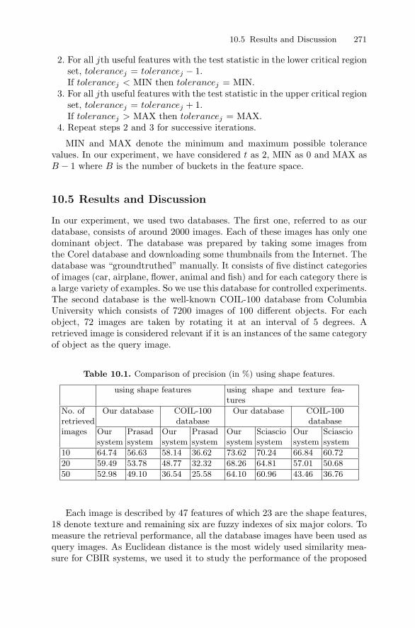
10.5 Results and Discussion 271
2. For all jth useful features with the test statistic in the lower critical regionset, tolerancej = tolerancej − 1.If tolerancej < MIN then tolerancej = MIN.
3. For all jth useful features with the test statistic in the upper critical regionset, tolerancej = tolerancej + 1.If tolerancej > MAX then tolerancej = MAX.
4. Repeat steps 2 and 3 for successive iterations.
MIN and MAX denote the minimum and maximum possible tolerancevalues. In our experiment, we have considered t as 2, MIN as 0 and MAX asB − 1 where B is the number of buckets in the feature space.
10.5 Results and Discussion
In our experiment, we used two databases. The first one, referred to as ourdatabase, consists of around 2000 images. Each of these images has only onedominant object. The database was prepared by taking some images fromthe Corel database and downloading some thumbnails from the Internet. Thedatabase was “groundtruthed” manually. It consists of five distinct categoriesof images (car, airplane, flower, animal and fish) and for each category there isa large variety of examples. So we use this database for controlled experiments.The second database is the well-known COIL-100 database from ColumbiaUniversity which consists of 7200 images of 100 different objects. For eachobject, 72 images are taken by rotating it at an interval of 5 degrees. Aretrieved image is considered relevant if it is an instances of the same categoryof object as the query image.
Table 10.1. Comparison of precision (in %) using shape features.
using shape features using shape and texture fea-tures
No. of Our database COIL-100 Our database COIL-100retrieved database databaseimages Our Prasad Our Prasad Our Sciascio Our Sciascio
system system system system system system system system10 64.74 56.63 58.14 36.62 73.62 70.24 66.84 60.7220 59.49 53.78 48.77 32.32 68.26 64.81 57.01 50.6850 52.98 49.10 36.54 25.58 64.10 60.96 43.46 36.76
Each image is described by 47 features of which 23 are the shape features,18 denote texture and remaining six are fuzzy indexes of six major colors. Tomeasure the retrieval performance, all the database images have been used asquery images. As Euclidean distance is the most widely used similarity mea-sure for CBIR systems, we used it to study the performance of the proposed

272 Sanjoy Kumar Saha, Amit Kumar Das and Bhabatosh Chanda
(a)
(b)
Fig. 10.12. Recall–precision graphs for our database (a) using shape features and(b) using shape and texture features.
features. Finally, we carried out our experiment using the perception-basedsimilarity measure. An exhaustive search was made on the entire database.To compare the performance of the proposed shape features, we implementedthe shape feature proposed by Prasad et al. [36]. We also implemented theHough-transform based features, proposed by Sciascio and Celentano, [43],which take care of shape and texture. In the experiment using our database,the recall–precision graphs in Figure 10.12 and Table 10.1 show that the per-formance of the proposed features is better. The same result is also establishedwhen the experiments are carried out on the COIL-100 database. It is evidentin the recall–precision graphs in Figure 10.13 and in Table 10.1. Table 10.2and the recall–precision graphs of Figure 10.14 show the performance of the

10.5 Results and Discussion 273
proposed system for various types of features using the two databases. Somesample results are shown in Figures 10.15 and 10.16 for our database and theCOIL-100 database respectively.
(a)
(b)
Fig. 10.13. Recall–precision graphs for the COIL-100 database (a) using shapefeatures and (b) using shape and texture features.
In order to check the capability of the proposed human-perception-basedsimilarity measure, the experiment is carried on using both the databases. Inorder to deal with our database, each feature space is divided into 10 bucketsand k is taken as 35. For the COIL-100 database, the corresponding valuesare 20 and 30 respectively. In both the cases, t, the tolerance for matching thecharacter tag is taken as 2. In the case of retrieval using the perception-based-

274 Sanjoy Kumar Saha, Amit Kumar Das and Bhabatosh Chanda
(a)
(b)
Fig. 10.14. Recall–precision graphs for (a) our database and (b) the COIL-100database.
Table 10.2. Precision (in %) of the proposed system.
Our database COIL-100 databaseNo. of Only Shape Shape & Shape, Only Shape Shape & Shape,
retrieved Petal Petal & Texture Texture & Texture Texture &images suppl. Color Color
10 61.89 64.74 73.62 76.16 58.14 66.84 82.4620 57.25 59.49 68.26 70.87 48.77 57.01 73.5950 51.03 52.98 64.10 66.05 36.54 43.46 58.54

10.6 Conclusions 275
similarity measure, as it is quite likely that similar images may spread overmultiple divisions of a feature space, achievement of high recall is quite diffi-cult. Hence, performance is studied based on top order retrievals. Moreover,Muller et al. [32] have mentioned that, from the perspective of a user, toporder retrievals are of major interest. Table 10.3 shows that retrieval precisionis higher in the case of the human-perception-based similarity measure and itproves the retrieval capability of the proposed similarity measure.
The proposed relevance feedback scheme is also applied to improve theretrieval performance. It has been checked for both the databases and usingboth Euclidean distance and the proposed human-perception-based measure.Tables 10.4 and 10.5 along with the recall–precision graphs in Figures 10.17and 10.18 reflect the improvement achieved through the proposed scheme forthe measures.
Table 10.3. Precision (in %) of retrieval using different similarity measures.
Our database COIL-100 databaseNumber of re-trieved images
Euclideandistancebased
Proposedsimilaritymeasure
Euclideandistancebased
Proposedsimilaritymeasure
10 76.16 81.10 82.46 88.5220 70.87 76.39 73.59 79.2530 68.05 73.15 67.31 72.25
Table 10.4. Precision (in %) using relevance feedback for our database.
Euclidean distance Proposed similarity measureNo. of No No
retrieved relevance Relevance feedback relevance Relevance feedbackimages feedback Iter1 Iter2 Iter3 feedback Iter1 Iter2 Iter3
10 76.16 77.91 79.61 81.40 81.10 87.39 89.32 91.1720 70.87 74.50 76.03 78.48 76.39 82.39 84.85 86.6330 68.05 69.89 71.38 72.63 73.15 78.61 81.34 83.20
10.6 Conclusions
In this paper we have established the capability of petal projection and othertypes of shape features for content-based retrieval. The use of the textureco-occurrence matrix and fuzzy indexes of color based on a hue histogram

276 Sanjoy Kumar Saha, Amit Kumar Das and Bhabatosh Chanda
Fig. 10.15. Retrieval results (using our database): first image of each row is thequery image and the others are the top five images matched.

10.6 Conclusions 277
Fig. 10.16. Retrieval results (using the COIL-100 database): first image of eachrow is the query image and the others are the top five images matched.

278 Sanjoy Kumar Saha, Amit Kumar Das and Bhabatosh Chanda
Fig. 10.17. Recall–precision graphs for different classes; they are (in raster order)Airplane, Car, Fish and Overall database.
Table 10.5. Precision (in %) using relevance feedback for COIL-100 database.
Euclidean distance Proposed similarity measureNo. of No relevance Relevance No relevance Relevance
retrieved feedback feedback feedback feedbackimages (after iteration 3) (after iteration 3)
10 82.46 84.74 88.52 91.0720 73.59 76.47 79.25 83.9130 67.31 70.40 72.25 79.57
further improves the performance. Comparison with similar systems was alsomade, as a benchmark. A new measure of similarity based on human percep-tion was presented and its capability has been established. To improve theretrieval performance, a novel feedback mechanism was described and experi-ment shows that the enhancement is substantial. Hence, our proposed retrievalscheme in conjunction with the proposed relevance feedback strategy are ableto discover knowledge about the image content by assigning various emphasesto the annotating features.

References 279
Fig. 10.18. Recall–precision graphs for different objects from the COIL-100database; they are (in raster order) objects 17, 28, 43 and 52.
A proper multidimensional indexing scheme may be adopted in future forfaster response times.
Acknowledgments: In this work, we have used databases available withCorel DRAW software from Corel Corporation and the COIL-100 databasefrom Columbia University.
References
[1] Aggarwal, G., P. Dubey, S. Ghosal, A. Kulshreshtha and A. Sarkar, July2000: IPURE: Perceptual and user-friendly retrieval of images. Proceed-ings of IEEE Conference on Multimedia and Exposition (ICME 2000),New York, USA, volume 2, 693–6.
[2] Berman, A. P., and L. G. Shapiro, 1999: A flexible image database systemfor content-based retrieval. Computer Vision and Image Understanding ,75, 175–95.

280 Sanjoy Kumar Saha, Amit Kumar Das and Bhabatosh Chanda
[3] Bimbo, A. D., P. Pala and S. Santini, 1996: Image retrieval by elasticmatching of shapes and image patterns. Proceedings of Multimedia’96 ,215–18.
[4] Chanda, B., and D. D. Majumdar, 2000: Digital Image Processing andAnalysis. Prentice Halla, New Delhi, India.
[5] Ciocca, G., I. Gagliardi and R. Schettini, 2001: Quicklook2: An integratedmultimedia system. International Journal of Visual Languages and Com-puting, Special issue on Querying Multiple Data Sources Vol 12 (SCI5417), 81–103.
[6] Conover, W. J., 1999: Practical nonparametric statistics, 3rd edition. JohnWiley and Sons, New York.
[7] Cox, I. J., M. L. Miller, T. P. Minka, T. Papathomas and P. N. Yiani-los, 2000: The Bayesian image retrieval system, pichunter: Theory, imple-mentation and psychophysical experiments. IEEE Transactions on ImageProcessing , 9(1), 20–37.
[8] Delp, E. J., and O. R. Mitchell, 1979: Image compression using blocktruncation coding. IEEE Trans. on Comm., 27, 1335–42.
[9] Fournier, J., M. Cord and S. Philipp-Foliguet, 2001: RETIN: A content-based image indexing and retrieval system. Pattern Analysis and Appli-cations, 4, 153–73.
[10] Fukunaga, K., 1972: Introduction to Statistical Pattern Recognition. Aca-demic Press, NY, USA.
[11] Gevers, T., and A. Smeulders, 2000: Pictoseek: Combining color and shapeinvariant features for shape retrieval. IEEE Transactions on Image Pro-cessing , 9(1), 102–19.
[12] Gudivada, V. N., and V. V. Raghavan, 1995: Content-based image re-trieval systems. IEEE Computer , 28(9), 18–22.
[13] Haralick, R. M., K. Shanmugam and I. Dinstein, 1973: Texture featuresfor image classification. IEEE Trans. on SMC , 3(11), 610–22.
[14] Hu, M. K., 1962: Visual pattern recognition by moment invariants. IRETrans. on Info. Theory, IT-8, 179–87.
[15] Huang, J., S. R. Kumar, and M. Mitra, 1997: Combining supervised learn-ing with color correlogram for content-based retrieval. 5th ACM Intl. Mul-timedia Confernce, 325–34.
[16] Huang, J., S. R. Kumar, M. Mitra, W. J. Zhu and R. Zabih, 1997: Imageindexing using color correlogram. IEEE Conference on Computer Visionand Pattern Recognition, 762–8.
[17] Jain, A. K., and A. Vailaya, 1998: Shape-based retrieval: A case studywith trademark image database. Pattern Recognition, 31(9), 1369–90.
[18] Jain, R., ed., 1997: Special issue on visual information management.Comm. ACM .
[19] Kaplan, L. M., 1998: Fast texture database retrieval using extended frac-tal features. SPIE 3312 , SRIVD VI, 162–73.

References 281
[20] Kimia, B., J. Chan, D. Bertrand, S. Coe, Z. Roadhouse and H. Tek, 1997:A shock-based approach for indexing of image databases using shape.SPIE 3229 , MSAS II, 288–302.
[21] Ko, B., J. Peng and H. Byun, 2001: Region-based image retrieval usingprobabilistic feature relevance learning. Pattern Analysis and Applica-tions, 4, 174–84.
[22] Laaksonen, J., M. Koskela, S. Laakso and E. Oja, 2000: Picsom: content-based image retrieval with self-organizing maps. PRL, 21, 1199–1207.
[23] Lai, T.-S., January 2000: CHROMA: a Photographic Image Retrieval Sys-tem. Ph.D. thesis, School of Computing, Engineering and Technology,University of Sunderland, UK.
[24] Li, Z. N., D. R. Zaiane and Z. Tauber, 1999: Illumination invariance andobject model in content-based image and video retrieval. Journal of VisualCommunication and Image Representation, 10(3), 219–44.
[25] Lim, S. and G. Lu, 2003: Effectiveness and efficiency of six colour spacesfor content based image retrieval. CBMI 2003 , France, 215–21.
[26] Lin, C., and C. S. G. Lee, 1996: Neural Fuzzy Systems. Prentice-Hall, NJ.[27] Ma, W. Y., and B. S. Manjunath, 1995: A comparison of wavelet trans-
form features for texture image annotation. IEEE Intl. Conf. on ImageProcessing , 256–9.
[28] Manjunath, B. S., and W. Y. Ma, 1996: Texture features for browsingand retrieval of image data. IEEE Trans. on PAMI , 18, 837–42.
[29] Mills, T. J., D. Pye, D. Sinclair and K. R. Wood, 2000: Shoebox: A digitalphoto management system. technical report 2000.10.
[30] Mokhtarian, F., S. Abbasi and J. Kittler, August 1996: Efficient androbust retrieval by shape content through curvature scale space. ImageDatabase and Multi-Media Search, Proceedings of the First InternationalWorkshop IDB-MMS’96 , Amsterdam, The Netherlands. Amsterdam Uni-versity Press, 35–42.
[31] Mukherjee, S., K. Hirata and Y. Hara, 1999: A world wide web imageretrieval engine. The WWW journal , 2(3), 115–32.
[32] Muller, H., W. Muller, S. Marchand-Mallet, T. Pun and D. M. Squire,2001: Automated benchmarking in content-based image retrieval. ICME2001 , Tokyo, Japan, 22–5.
[33] Niblack, W., 1993: The QBIC project: Querying images by content usingcolor, texture and shape. SPIE , SRIVD.
[34] Pentland, A., and R. Picard, 1996: Introduction to special section on thedigital libraries: Representation and retrieval. IEEE Trans. on PAMI , 18,769–70.
[35] Persoon, E., and K. S. Fu, 1977: Shape discrimination using Fourier de-scriptors. IEEE Trans. on SMC , 7, 170–9.
[36] Prasad, B. G., S. K. Gupta and K. K. Biswas, 2001: Color and shape indexfor region-based image retrieval. IWVF4 , volume LNCS 2059, 716–25.

282 Sanjoy Kumar Saha, Amit Kumar Das and Bhabatosh Chanda
[37] Rocchio, J. J., 1971: Relevance feedback in information retrieval. TheSMART Retrieval System: Experiments in Automatic Document Process-ing, G. Salton, ed., Prentice Hall, 313–23.
[38] Rosenfeld, A., and A. C. Kak, 1982: Digital Picture Processing , volume II.Academic Press, N.Y.
[39] Rui, Y., T. S. Haung, S. Mehrotra and M. Ortega, 1998: Relevance feed-back: A power tool in interactive cotent-based image retrieval. IEEE Tran.on Circuits and Systems for Video Technology, Special issue on interactiveMultimedia Systems for the Internet , 8(5), 644–55.
[40] Saha, S. K., A. K. Das and B. Chanda, 2003: Graytone image retrievalusing shape feature based on petal projection. ICAPR 2003 , India, 252–6.
[41] Salton, G., and M. J. McGill, 1983: Introduction to Modern InformationRetrieval for Image and Video Databases. McGraw-Hill.
[42] Schettini, R., 1994: Multicolored object recognition and location. PRL,15, 1089–97.
[43] Sciascio, E. D., and A. Celentano, 1997: Similarity evaluation in imageretrieval using simple features. SPIE , 3022, 467–77.
[44] Sciascio, E. D., G. Mingolla and M. Mongiello, 1999: Content-based im-age retrieval over the web using query by sketch and relevance feedback.Visual Information and Information Systems, Proceedings of the Third In-ternational Conference VISUAL ’99 , Amsterdam, The Netherlands, June1999, Lecture Notes in Computer Science 1614, Springer, 123–30.
[45] Sclaroff, S., L. Taycher and M. L. Cascia, 1997: ImageRover: A content-based image browser for the world wide web. IEEE Workshop on content-based Access of Image and Video Libraries, San Juan, Puerto Rico, 2–9.
[46] Smith, J. R., February 1997: Integrated Spatial and Feature ImageSystems: Retrieval, Compression and Analysis. Ph.D. thesis, GraduateSchool of Arts and Sciences, Columbia University.
[47] Smith, J. R., and S. F. Chang, 1995: Tools and techniques for color imageretrieval. SPIE 2420 , SRIVD III.
[48] Squire, D. M., W. Muller, H. Muller and T. Pun, 2000: Content-basedquery of image databases: inspirations from text retrieval. PRL, 21, 1193–98.
[49] Srihari, R., Z. Zhang, and A. Rao, 2000: Intelligent indexing and semanticretrieval of multimodal documents. Information Retrieval, 2(2), 245–75.
[50] Stricker, M., and M. Orengo, 1995: Similarity of color images. SPIE ,SRIVD, 381–92.
[51] Swain, M., and D. Ballard, 1991: Color indexing. International Journalof Computer Vision, 7(1), 11–32.
[52] Tamura, H., S. Mori and T. Yamawaki, 1978: Texture features correspond-ing to visual perception. IEEE Trans. on SMC , 8(6), 460–73.
[53] Teh, C., and R. T. Chin, 1988: On image analysis by the methods ofmoments. IEEE Trans. on PAMI , 10, 496–13.
[54] Turtle, H. R., and W. B. Croft, 1982: A comparison of text retrievalmodels. The Computer Journal , 35(3), 279–90.

References 283
[55] Vleugels, J., and R. C. Veltkamp, 2002: Efficient image retrieval throughvantage objects. Pattern Recognition, 35(1), 69–80.
[56] Yu, H., M. Li, H. Jiang Zhang and J. Feng, 2002: Color texture momentsfor content-based image retrieval. IEEE Int. Conf. on Image Proc., NewYork, USA.

11
Significant Feature Selection UsingComputational Intelligent Techniques forIntrusion Detection
Srinivas Mukkamala and Andrew H. Sung
Summary. Due to increasing incidence of cyber attacks and heightened concerns forcyber terrorism, implementing effective intrusion detection and prevention systems(IDPSs) is an essential task for protecting cyber security as well as physical securitybecause of the great dependence on networked computers for the operational controlof various infrastructures.
Building effective intrusion detection systems (IDSs), unfortunately, has re-mained an elusive goal owing to the great technical challenges involved; and com-putational techniques are increasingly being utilized in attempts to overcome thedifficulties. This chapter presents a comparative study of using support vector ma-chines (SVMs), multivariate adaptive regression splines (MARSs) and linear geneticprograms (LGPs) for intrusion detection. We investigate and compare the perfor-mance of IDSs based on the mentioned techniques, with respect to a well-known setof intrusion evaluation data.
We also address the related issue of ranking the importance of input features,which itself is a problem of great interest. Since elimination of the insignificantand/or useless inputs leads to a simplified problem and possibly faster and moreaccurate detection, feature selection is very important in intrusion detection. Ex-periments on current real-world problems of intrusion detection have been carriedout to assess the effectiveness of this criterion. Results show that using significantfeatures gives the most remarkable performance and performs consistently well overthe intrusion detection data sets we used.
11.1 Introduction
Feature selection and ranking is an important issue in intrusion detection.Of the large number of features that can be monitored for intrusion detectionpurposes, which are truly useful, which are less significant, and which may beuseless? The question is relevant because the elimination of useless features(audit trail reduction) enhances the accuracy of detection while speeding upthe computation, thus improving the overall performance of an IDS. In caseswhere there are no useless features, by concentrating on the most important

286 Srinivas Mukkamala and Andrew H. Sung
ones we may well improve the time performance of an IDS without affectingthe accuracy of detection in statistically significant ways.
The feature selection and ranking problem for intrusion detection is similarin nature to various engineering problems that are characterized by:
• Having a large number of input variables x = (x1, x2,. . . , xn) of vary-ing degrees of importance to the output y; i.e., some elements of x areessential, some are less important, some of them may not be mutuallyindependent, and some may be useless or irrelevant (in determining thevalue of y);
• Lacking an analytical model that provides the basis for a mathematicalformula that precisely describes the input–output relationship, y = F (x);
• Having available a finite set of experimental data, based on which a model(e.g. a neural network) can be built for simulation and prediction purposes;
• Excess features that can reduce classifier accuracy;• Excess features that can be costly to collect;• Excess features that can reduce classifier operating speed independent of
data collection;• Excess features that can be costly to store.
Feature selection is typically viewed as a search for the feature subset resultingin the best classifier error rate. Usually, the best error rate is equated withthe smallest magnitude, since we hope that the error rate is a measurementof future classifier performance. The procedure is to use operators which mapfrom a feature subset to other feature subsets, analyze these subsets, andselect one of these to continue searching from. However, we immediately seehow difficult a problem this is; there are an exponential number of featuresets to search through. Although for small numbers of features this searchis tractable, it does not scale. Many search algorithms sacrifice a “complete”search and explore only a fraction of the space in order to find a “good”feature set. Techniques include sequential search and best-first search with alimited “queue” of states to expand to limit the search time.
Feature selection is designed to select important features and producebetter classifiers. However, the very process of feature selection can introducebias into the feature sets searched. Each time a new feature set is examined, wemust build a classifier and analyze it using the same data set. The more oftenthis data set is used, the more our results will be biased towards classifierswhich perform well on this data. Recent work has shown that we can createoperators which search the space more efficiently, thereby using the data lessoften and creating better, unbiased feature sets which perform better on futuredata.
Through a variety of experiments and analysis of different computationalintelligent techniques, it is found that, with appropriately chosen populationsize, program size, crossover rate and mutation rate, LGPs outperform othertechniques in terms of detection accuracy at the expense of time. SVMs out-

11.2 Support Vector Machines 287
perform MARSs and artificial neural networks (ANNs) in three critical aspectsof intrusion detection: accuracy, training time, and testing time [9].
A brief introduction to SVMs and SVM-specific feature selection is given inSection 11.2. Section 11.3 introduces LGPs and LGP-specific feature selection.In Section 11.4 we introduce MARSs and MARS-specific feature selection. Anexperimental data set used for evaluation is presented in Section 11.5. Sec-tion 11.6 describes the significant feature identification problem for intrusiondetection systems, a brief overview of significant features as identified by dif-ferent ranking algorithms and the performance of classifiers using all featuresand significant features. Conclusions of our work are given in Section 11.7.
11.2 Support Vector Machines
The support vector machine (SVM) approach transforms data into a featurespace F that usually has a huge dimension. It is interesting to note that SVMgeneralization depends on the geometrical characteristics of the training data,not on the dimensions of the input space [5, 6]. Training an SVM leads to aquadratic optimization problem with bound constraints and one linear equal-ity constraint. Vapnik shows how training an SVM for the pattern recognitionproblem leads to the following quadratic optimization problem [14].
Minimize
W (α) = −l∑
i=1
αi +12
l∑i=1
l∑j=1
yiyjαiαjk(xi, xj) (11.1)
subject tol∑
i=1yiαi
∀i : 0 ≤ αi ≤ C(11.2)
where l is the number of training examples, α is a vector of l variables andeach component αicorresponds to a training example (xi, yi). The solution ofEquation (11.1) is the vector α∗ for which Equation (11.1) is minimized andEquation (11.2) is fulfilled.
In the first phase of the SVM, called the learning phase, the decisionfunction is inferred from a set of objects. For these objects the classificationis known a priori. The objects of the family of interest are called, for easeof notation, the positive objects and the objects from outside the family, thenegative objects.
In the second phase, called the testing phase, the decision function is ap-plied to arbitrary objects in order to determine, or more accurately predict,whether they belong to the family under study, or not.

288 Srinivas Mukkamala and Andrew H. Sung
Linear case SVMThe objects are represented by vectors in Rn where each coefficient representsa feature of the object: weight, size, etc. An example of a linear case SVM isbriefly shown in Figure 11.1.
margin
+
+
+
+
+
+
++
*
*
**
**
**
*
*
H
Hb
Hr+
+
Fig. 11.1. Linear case SVM.
The positive examples form a cloud of points, say the points labelled “+”(referred to as a set Xb), while the negative examples form another cloud ofpoints, say, the points labelled “*” (referred to as Xr). The aim is to find ahyper-plane H separating the two clouds of points in some optimal way.
Definition of Margin and Maximal MarginLet H be a separating hyper-plane, Hb a separating hyper-plane parallel to Hand passing through the points in Xb that are closest to H, Hr a separatinghyper-plane parallel to H and passing through the points in Xr that are closestto H.
The margin, γ, is the distance between two parallel separating hyper-planes Hb and Hr (as shown in Figure 11.1). Vapnik’s theory of risk mini-mization shows that hyper-planes for which γ is maximum have better gener-alization potential than others, and so the problem of a linear SVM is to finda separating hyper-plane with maximum margin.
There are many ways to represent mathematically such an optimizationproblem. We have two concerns here. The first is to find a formulation thatcan be handled by standard optimization techniques (quadratic programmingin our case). The second concern is of major significance from an applicationpoint of view: is it indeed possible to find a formulation that will allow us toconstruct nonlinear separating surfaces while remaining in the previous com-putational framework of linear separation?
Quadratic Programming:A constrained optimization problem consists of two parts: a function to op-timize and a set of constraints to be satisfied by the variables. Constraintsatisfaction is typically a hard combinatorial problem; while, for an appro-priate choice of function, optimization is a comparatively easier analytical

11.2 Support Vector Machines 289
problem. Hence, we choose the design of formulations where the constraintsare simple linear constraints and we use duality to move expressions from theset of constraints to the function we seek to optimize. In the maximum margincase, we want to maximize a distance. In order to express distances of pointsto a hyper-plane W ∗ X + b = 0, we require that ||W||2= 1. Equivalently wecan divide the expression by ||W||2.
However either formulation gives us a nonlinear constraint, which doesnot lead to efficient computation. We will therefore formulate the problem tomove the nonlinear constraint into the function to optimize.
Let W * X + b = 0 be the equation of a separating hyperplane, situatedhalfway between the two sets, so that for some t>0 we have all the points inXb on one side and all the points in Xr on the other:
(W * Xr+ b)/||W||2 >= t/||W||2
and
(W * Xb + b)/||W||2 <= -t/||W||2,
and there exist points in Xb and Xr for which the inequalities are replacedby equalities. Consequently we have the margin:
γ = g2t/||W ||2
Assume the maximum margin is reached for W= W0, b = b0, t = t0. DividingW0 and b0 by t0 shows that the maximal margin is reached for hyper-planessuch that γ =2/||W||2.
Without loss of generality we may therefore assume that t = 1. The prob-lem of maximizing γ is replaced by the problem of minimizing the norm ofW,
12∗ < W, W > (11.3)
under the linear constraints:
Yi ∗ (W ∗Xi + b) ≥ 1 for any I (11.4)
where Xi, is a data point and Yi is the label of the data point, equal to 1 or–1 depending on whether the point is a positive or a negative example.
We now have a typical quadratic programming problem and we will changethis formulation with nonlinear separability in mind.
Nonlinear SeparationIt can be shown that if you have fewer points than the dimension, then anytwo sets are separable. It is therefore tempting, when the two sets are notlinearly separable, to map the problem into a higher dimension where it willbecome separable. There is however a price to pay as quadratic programmingproblems are quite sensitive to high dimensions. SVM handles this problem
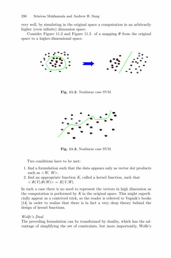
290 Srinivas Mukkamala and Andrew H. Sung
very well, by simulating in the original space a computation in an arbitrarilyhigher (even infinite) dimension space.
Consider Figure 11.2 and Figure 11.3 of a mapping Φ from the originalspace to a higher-dimensional space.
Fig. 11.2. Nonlinear case SVM.
Fig. 11.3. Nonlinear case SVM.
Two conditions have to be met:
1. find a formulation such that the data appears only as vector dot productssuch as <W, W>.
2. find an appropriate function K, called a kernel function, such that< Φ(V),Φ(W)> = K(V,W).
In such a case there is no need to represent the vectors in high dimension asthe computation is performed by K in the original space. This might superfi-cially appear as a contrived trick, so the reader is referred to Vapnik’s books[14] in order to realize that there is in fact a very deep theory behind thedesign of kernel functions.
Wolfe’s DualThe preceding formulation can be transformed by duality, which has the ad-vantage of simplifying the set of constraints, but more importantly, Wolfe’s

11.2 Support Vector Machines 291
dual gives us a formulation where the data appears only as vector dot prod-ucts. As a consequence we can handle nonlinear separation.
Minimizing 1/2*||W||2 under the constraint of Equation (11.4) is equivalentto maximizing the dual Lagrangian obtained by computing variables from thestationary conditions and replacing them by the values so obtained in theprimal Lagrangian. Details can be found in [3].
Yi ∗ (W ∗Xi + b) ≥ 1 for any I (11.5)
The primal Lagrangian is:
L =12(W ∗W )−
∑αi ∗ (Yi ∗ (W ∗Xi + b)− 1), (11.6)
where the αi is the Lagrange multiplier and Yi is the label of the correspondingdata point under the constraint:
αi ≥ 0 for any i (11.7)
The stationary conditions are:
∂L/∂b =∑
αi ∗ Yi = 0 (11.8)
∂L/∂w = W −∑
αi ∗ Yi ∗Xi = 0. (11.9)
Substituting the value of w from Equation (11.8) in the primal Lagrangian(Equation (11.5)) gives us the Wolfe Dual Lagrangian:
W (a) =∑
αi −12∗∑
αi ∗ αjYi ∗ Yj ∗ (Xi ∗Xj) (11.10)
This must be maximized subject to the constraints of Equations (11.7) and(11.8). It is then straightforward to implement nonlinearity by simply replac-ing the vector products by kernel functions.
Support VectorsIt is clear that the maximum margin is not defined by all points to be sep-arated, but by only a subset of points called support vectors. Indeed fromEquation (11.9) we know that W =
∑Yi* αi *Xi, and the data points Xi
whose coefficients αi= 0 are irrelevant to W, are therefore irrelevant to thedefinition of the separating surface; the others are the support vectors.
Over-fitting and Soft Margin Trade OffFigure 11.4 shows an example where, by choosing a kernel of sufficient degreewe can find a surface complex enough to separate the two clouds of points.When there is noise we can make this surface extremely complex in orderto fit the data. This phenomenon is called over-fitting, as perhaps some ofthese noisy points should be in fact ignored, leading to a simpler surface of

292 Srinivas Mukkamala and Andrew H. Sung
Fig. 11.4. Over-fitting an SVM.
Fig. 11.5. Soft margin trade-off in an SVM.
separation. In Figure 11.5 we have a trade-off: a simple linear separation ratherthan a complex one at the cost of a training error, which could in fact be noiseor erroneous data.
So there exists a trade-off between the degree of the kernel function andthe extent to which training errors are allowed. This has a very importantconsequence as the algorithm we described will not work when the sets arenot separable. Therefore to have the algorithm work we must increase thenonlinearity, and therefore the complexity of the surface, and therefore therisk of grossly over-fitting.
The problem is solved by relaxing the conditions in such a way that acertain degree of misclassification is allowed, leading to simpler solutions atthe cost of some erroneous, or potentially erroneous, predictions.
We refer the reader to [3] for the description of the techniques involved.The user has to define the value of a parameter that controls the extent ofmisclassification allowed. This value is heavily dependent on the data at hand.
11.2.1 SVM-specific Feature Ranking Method
It is of great interest and use to find exactly which features underline thenature of connections of various classes. This is precisely the goal of datavisualization in data mining. The problem is that the high-dimensionality ofdata makes it hard for human experts to gather any knowledge. If we knewthe key features, we could greatly reduce the dimensionality of the data and

11.2 Support Vector Machines 293
thus help human experts become more efficient and productive in learningabout network intrusions.
The information about which features play key roles and which are moreneutral is “hidden” in the SVM decision function. Equation (11.11) is theformulation of the decision function in the case of using linear kernels.
F (X) =< W, X > +b (11.11)
The point X is predicted to be in class A or “positive class” if F(X) ispositive, and class B or “negative class” if F(X) is negative. We can rewriteEquation (11.11) to expand the dot product of W and X.
F (X) = ΣWiXi + b (11.12)
One can see that the value of F(X) depends on the contribution of eachfactor, WiXi. Since Xi can take only b ≥ g0, the sign of Wi indicates whetherthe contribution is towards positive classification or negative classification.The absolute size of Wi measures the strength of this contribution. In otherwords if Wi is a large positive value, then the ith feature is a key factor of“positive class” or class A. Similarly if Wi is a large negative value then theith feature is a key factor of the “negative class” or class B. Consequently theWi, that are close to zero, either positive or negative, carry little weight. Thefeature, which corresponds to this Wi, is said to be a garbage feature andremoving it has very little effect on the classification.
Having retrieved this information directly from the SVM’s decision func-tion, we rank the Wi, from largest positive to largest negative. This essentiallyprovides the soft partitioning of the features into the key features of class A,neutral features, and key features of class B. We say soft partitioning, as itdepends on either a threshold on the value of Wi that will define the parti-tions or the proportions of the features that we want to allocate to each ofthe partitions. Both the threshold and the value of proportions can be set bythe human expert.
Support Vector Decision Function RankingThe input ranking is done as follows: First the original data set is used forthe training of the classifier. Then the classifier’s decision function is used torank the importance of the features. The procedure is:
1. Calculate the weights from the support vector decision function.2. Rank the importance of the features by the absolute values of the weights.
11.2.2 Performance-Based Ranking
We first describe a general (i.e., independent of the modeling tools being used),performance-based input ranking (PBR) methodology [12]: One input featureis deleted from the data at a time; the resultant data set is then used for

294 Srinivas Mukkamala and Andrew H. Sung
the training and testing of the classifier. Then the classifier’s performance iscompared to that of the original classifier (based on all features) in terms ofrelevant performance criteria. Finally, the importance of the feature is rankedaccording to a set of rules based on the performance comparison.
The procedure is summarized as follows:
1. Compose the training set and the testing set.2. For each feature do the following:• delete the feature from the (training and testing) data;• use the resultant data set to train the classifier;• analyze the performance of the classifier using the test set, in terms of
the selected performance criteria;• rank the importance of the feature according to the rules.
11.3 Linear Genetic Programming
Linear Genetic Programming (LGP) is a variant of the Genetic Programming(GP) technique that acts on linear genomes [1]. The linear genetic program-ming technique used for our current experiment is based on machine code levelmanipulation and evaluation of programs. Its main characteristics, in compar-ison to tree-based GP, are that the evolvable units are not the expressions ofa functional programming language (like LISP), instead the programs of animperative language (like C) are evolved. In the automatic induction of ma-chine code by genetic programming, individuals are manipulated directly asbinary code in memory and executed directly without passing an interpreterduring fitness calculation. The LGP tournament selection procedure puts thelowest selection pressure on the individuals by allowing only two individualsto participate in a tournament. A copy of the winner replaces the loser ofeach tournament. The crossover points only occur between instructions. In-side instructions the mutation operation randomly replaces the instructionidentifier. In LGP the maximum size of the program is usually restricted toprevent programs without bounds.
In genetic programming, an intron is defined as part of a program thathas no influence on the fitness calculation of outputs for all possible inputs.
Ranking Algorithm using Evolutionary AlgorithmsThe performance of each of the selected input feature subsets is measured byinvoking a fitness function with the correspondingly reduced feature space andtraining set and evaluating the intrusion detection accuracy. Once the requirednumber of iterations is completed, the evolved high-ranking programs areanalyzed for the number of times each input appears in a way that contributesto the fitness of the programs that contain them. The best feature subset foundis then output as the recommended set of features to be used in the actualinput for the classifier.

11.4 Multivariative Adaptive Regression Splines 295
Fig. 11.6. LGP intron elimination and fitness evaluation.
In the feature selection problem the main interest is in the representationof the space of all possible subsets of the given input feature set. Each featurein the candidate feature set is considered as a binary gene and each individualconsists of a fixed-length binary string representing some subset of the givenfeature set. An individual of length d corresponds to a d-dimensional binaryfeature vector Y, where each bit represents the elimination or inclusion of theassociated feature. Then, yi = 0 represents elimination and yi = 1 indicatesinclusion of the ith feature. Fitness F of an individual program p is calculatedas the mean square error (MSE ) between the predicted output (Opred
ij ) andthe desired output (Odes
ij ) for all n training samples and m outputs [2].
F (p) =1
n ·m
n∑i=1
m∑j=1
(Opredij −Odes
ij )2 +w
nCE = MSE + w ·MCE (11.13)
Classification Error (CE ) is computed as the number of misclassifications.Mean Classification Error (MCE ) is added to the fitness function while itscontribution is multiplied by an absolute value of weight (w).
11.4 Multivariative Adaptive Regression Splines
Splines can be considered as an innovative mathematical process for compli-cated curve drawings and function approximation. To develop a spline theX-axis is broken into a convenient number of regions. The boundary betweenregions is also known as a knot. With a sufficiently large number of knotsvirtually any shape can be well approximated. While it is easy to draw a

296 Srinivas Mukkamala and Andrew H. Sung
spline in two-dimensions by keying on knot locations (approximating usinglinear, quadratic or cubic polynomial etc.), manipulating the mathematics inhigher dimensions is best accomplished using basis functions. The multivaria-tive adaptive regression splines (MARS) model is a regression model usingbasis functions as predictors in place of the original data. The basis func-tion transform makes it possible to selectively blank out certain regions ofa variable by making them zero, and allows the MARS model to focus onspecific sub-regions of the data. It excels at finding optimal variable transfor-mations and interactions, and the complex data structure that often hides inhigh-dimensional data [4, 13].
Fig. 11.7. MARS data estimation using splines and knots (actual data on the right).
Given the number of records in most data sets, it is infeasible to approxi-mate the function y = f(x) by summarizing y in each distinct region of x. Forsome variables, two regions may not be enough to track the specifics of thefunction. If the relationship of y to some x is different in three or four regions,for example, the number of regions requiring examination is even larger than34 billion with only 35 variables. Given that the number of regions cannotbe specified a priori, specifying too few regions in advance can have seriousimplications for the final model. A solution is needed that accomplishes thefollowing two criteria:
• judicious selection of which regions to look at and their boundaries;• judicious determination of how many intervals are needed for each variable.
Given these two criteria, a successful method will essentially need to be adap-tive to the characteristics of the data. Such a solution will probably ignore

11.5 The Experimental Data 297
quite a few variables (affecting variable selection) and will take into accountonly a few variables at a time (also reducing the number of regions). Even ifthe method selects 30 variables for the model, it will not look at all 30 simul-taneously. Such simplification is accomplished by a decision tree at a singlenode, only ancestor splits being considered; thus, at a depth of six levels inthe tree, only six variables are used to define the node.
Ranking Algorithm using MARSGeneralized cross-validation is an estimate of the actual cross-validation whichinvolves more computationally intensive goodness of fit measures. Along withthe MARS procedure, a generalized cross-validation (GCV) procedure is usedto determine the significant input features. Non-contributing input variablesare thereby eliminated.
GCV =1N
N∑i=1
[yi − f(xi)2
1− k/N] (11.14)
where N is the number of records and x and y are independent and dependentvariables respectively. k is the effective number of degrees of freedom wherebythe GCV adds penalty for adding more input variables to the model. The con-tribution of the input variables may be ranked using the GCV with/withoutan input feature [13].
11.5 The Experimental Data
A subset of the DARPA intrusion detection data set is used for off-line anal-ysis. In the DARPA intrusion detection evaluation program, an environmentwas set up to acquire raw TCP/IP dump data for a network by simulatinga typical US Air Force LAN. The LAN was operated like a real environ-ment, but blasted with multiple attacks [7, 15]. For each TCP/IP connection,41 various quantitative and qualitative features were extracted [8]. The 41features extracted fall into three categories: “intrinsic” features that describethe individual TCP/IP connections can be obtained from network audit trails;“content-based” features that describe the payload of the network packet canbe obtained from the data portion of the network packet; “traffic-based” fea-tures that are computed using a specific window (connection time or numberof connections). Attack types fall into four main categories:
• Probing: surveillance and other probing• DoS: denial of service• U2Su: unauthorized access to local super user (root) privilege• R2U: unauthorized access from a remote machine
As DoS and probing attacks involve several connections in a short time frame,whereas R2U and U2Su attacks are embedded in the data portions of the

298 Srinivas Mukkamala and Andrew H. Sung
connection and often involve just a single connection, “traffic-based” featuresplay an important role in deciding whether a particular network activity isengaged in probing or not.
11.5.1 Probing
Probing is a class of attacks where an attacker scans a network to gatherinformation or find known vulnerabilities. An attacker with a map of machinesand services that are available on a network can use the information to lookfor exploits. There are different types of probes (see Table 11.1): some of themabuse the computer’s legitimate features; some of them use social engineeringtechniques. This class of attacks is the most commonly known and requiresvery little technical expertise.
Table 11.1. Probe attacks.
Attack Type Service Mechanism Effect of the attackIpsweep Icmp Abuse of feature Identifies active machinesMscan Many Abuse of feature Looks for known vulnerabilitiesNmap Many Abuse of feature Identifies active ports on a machineSaint Many Abuse of feature Looks for known vulnerabilitiesSatan Many Abuse of feature Looks for known vulnerabilities
11.5.2 Denial of Service Attacks
Denial of service (DoS) is a class of attacks where an attacker makes somecomputing or memory resource too busy or too full to handle legitimate re-quests, thus denying legitimate users access to a machine. There are differentways to launch DoS attacks: by abusing the computer’s legitimate features;by targeting implementation bugs; or by exploiting the system’s misconfigura-tions. DoS attacks are classified based on the services that an attacker rendersunavailable to legitimate users (Table 11.2).
11.5.3 User to Super user Attacks
User to super user (U2Su) exploits are a class of attacks where an attackerstarts out with access to a normal user account on the system and is able toexploit a vulnerability to gain root access to the system. The most commonexploits in this class of attacks are buffer overflows, which are caused byprogramming mistakes and environment assumptions (see Table 11.3).

11.6 Significant Feature Selection for Intrusion Detection 299
Table 11.2. Denial of service attacks.
Attack Type Service Mechanism Effect of the attackApache2 http Abuse Crashes httpdBack http Abuse/Bug Slows down server responseLand http Bug Freezes the machineMail bomb Abuse AnnoyanceSYN Flood TCP Abuse Denies service on one or more
portsPing of Death Icmp Bug NoneProcess table TCP Abuse Denies new processesSmurf Icmp Abuse Slows down the networkSyslogd Syslog Bug Kills the SyslogdTeardrop Bug Reboots the machineUdpstrom Echo/Chargen Abuse Slows down the network
Table 11.3. User to super user attacks.
Attack Type Service Mechanism Effect of the attackEject User session Buffer overflow Gains root shellFfbconfig User session Buffer overflow Gains root shellFdformat User session Buffer overflow Gains root shellLoadmodule User session Poor environment sanitation Gains root shellPerl User session Poor environment sanitation Gains root shellPs User session Poor temp file management Gains root shellXterm User session Buffer overflow Gains root shell
11.5.4 Remote to User Attacks
A remote to user (R2U) attack is a class of attacks where an attacker sendspackets to a machine over a network, then exploits machine’s vulnerability toillegally gain local access as a user. There are different types of R2U attacks;the most common attack in this class is done using social engineering (seeTable 11.4).
11.6 Significant Feature Selection for Intrusion Detection
Feature selection and ranking is an important issue in intrusion detection[10, 11]. Of the large number of features that can be monitored for intrusiondetection purposes, which are truly useful, which are less significant, andwhich may be useless? The question is relevant because the elimination ofuseless features (audit trail reduction) enhances the accuracy of detectionwhile speeding up the computation, thus improving the overall performanceof an IDS. In cases where there are no useless features, by concentrating on

300 Srinivas Mukkamala and Andrew H. Sung
Table 11.4. Remote to user attacks.
Attack Type Service Mechanism Effect of the attackDictionary telnet, rlogin,
pop, ftp, imapAbuse feature Gains user access
Ftp-write ftp Misconfiguration Gains user accessGuest telnet, rlogin Misconfiguration Gains user accessImap imap Bug Gains root accessNamed dns Bug Gains root accessPhf http Bug Executes commands as
http userSendmail smtp Bug Executes commands as rootXlock smtp Misconfiguration Spoof user to obtain pass-
wordXnsoop smtp Misconfiguration Monitor key stokes re-
motely
the most important ones we may well improve the time performance of an IDSwithout affecting the accuracy of detection in statistically significant ways.
The feature ranking and selection problem for intrusion detection is similarin nature to various engineering problems that are characterized by:
• Having a large number of input variables x = (x1, x2,. . . , xn) of vary-ing degrees of importance to the output y; i.e., some elements of x areessential, some are less important, some of them may not be mutuallyindependent, and some may be useless or irrelevant (in determining thevalue of y);
• Lacking an analytical model that provides the basis for a mathematicalformula that precisely describes the input–output relationship, y = F (x);
• Having available a finite set of experimental data, based on which a model(e.g. a neural network) can be built for simulation and prediction purposes.
Due to the lack of an analytical model, one can only seek to determine therelative importance of the input variables through empirical methods. A com-plete analysis would require examination of all possibilities, e.g., taking twovariables at a time to analyze their dependence or correlation, then takingthree at a time, etc. This, however, is both infeasible (requiring 2n experi-ments!) and not infallible (since the available data may be of poor quality insampling the whole input space). Features are ranked based on their influencetowards the final classification. Description of the most important features asranked by three feature-ranking algorithms (SVDF, LGP, and MARS) is givenin Tables 11.5, 11.6, and 11.7. The (training and testing) data set contains11,982 randomly generated points from the five classes, with the amount ofdata from each class proportional to its size, except that the smallest classis completely included. The normal data belongs to class 1, probe belongs toclass 2, denial of service belongs to class 3, user to super user belongs to class

11.6 Significant Feature Selection for Intrusion Detection 301
Table 11.5. Most important feature descriptions as ranked by SVDF.
Data class Feature descriptionNormal • destination bytes: number of bytes received by the source host
from the destination host• dst host count: number of connections from the same host to
the destination host during a specified time window• logged in: binary decision (1 successfully logged in, 0 failed login)• dst host same srv rate: % of connections to same service ports
from a destination host• flag: normal or error status of the connection
Probe • source bytes: number of bytes sent from the host system to thedestination system
• dst host srv count: number of connections from the same hostwith same service to the destination host during a specified timewindow
• count: number of connections made to the same host system ina given interval of time
• protocol type: type of protocol used to connect (e.g. tcp, udp,icmp, etc.)
• srv count: number of connections to the same service as thecurrent connection during a specified time window
DoS • count: number of connections made to the same host system ina given interval of time
• srv count: number of connections to the same service as thecurrent connection during a specified time window
• dst host srv serror rate: % of connections to the same servicethat have SYN errors from a destination host
• serror rate: % of connections that have SYN errors• dst host same src port rate: % of connections to same service
ports from a destination hostU2Su • source bytes: number of bytes sent from the host system to the
destination system• duration: length of the connection• protocol type: type of protocol used to connect (e.g. tcp, udp,
icmp, etc.)• logged in: binary decision (1 successfully logged in, 0 failed login)• flag: normal or error status of the connection
R2U • dst host count: no of connections from the same host to thedestination host during a specified time window
• service: type of service used to connect (e.g. finger, ftp, telnet,ssh, etc.)
• duration: length of the connection• count: number of connections made to the same host system in
a given interval of time• srv count: number of connections to the same service as the
current connection during a specified time window

302 Srinivas Mukkamala and Andrew H. Sung
Table 11.6. Most important feature descriptions as ranked by LGP.
Data class Feature descriptionNormal • hot: number of “hot” indicators
• source bytes: number of bytes sent from the host system to thedestination system
• destination bytes: number of bytes received by the source hostfrom the destination host
• num compromised: number of compromised conditions• dst host rerror rate: % of connections that have REJ errors from
a destination hostProbe • dst host diff srv rate: % of connections to different services from
a destination host• rerror rate: % of connections that have REJ errors• srv diff host rate: % of connections that have the same service
to different hosts• logged in: binary decision (1 successfully logged in, 0 failed login)• service: type of service used to connect (e.g. finger, ftp, telnet,
ssh, etc.)DoS • count: number of connections made to the same host system in
a given interval of time• num compromised: number of compromised conditions• wrong fragments: number of wrong fragments• land: binary decision (1 if connection is from/to the same
host/port; 0 otherwise)• logged in: binary decision (1 successfully logged in, 0 failed login)
U2Su • root shell: binary decision (1 if root shell is obtained; 0 other-wise)
• dst host srv serror rate: % of connections to the same servicethat have SYN errors from a destination host
• num file creations: number of file creations• serror rate: % of connections that have SYN errors• dst host same src port rate: % of connections to same service
ports from a destination hostR2U • guest login: binary decision (1 if the login is guest, 0 otherwise)
• num file access: number of operations on access control files• destination bytes: number of bytes received by the source host
from the destination host• num failed logins: number of failed login attempts• logged in: binary decision (1 successfully logged in, 0 failed login)

11.6 Significant Feature Selection for Intrusion Detection 303
Table 11.7. Most important feature descriptions as ranked by MARS.
Data class Feature descriptionNormal • destination bytes: number of bytes received by the source host
from the destination host• source bytes: number of bytes sent from the host system to the
destination system• service: type of service used to connect (e.g. finger, ftp, telnet,
ssh, etc.)• logged in: binary decision (1 successfully logged in, 0 failed login)• hot: number of “hot” indicators
Probe • dst host diff srv rate: % of connections to different services froma destination host
• dst host srv count: : number of connections from the same hostwith same service to the destination host during a specified timewindow
• source bytes: number of bytes sent from the host system to thedestination system
• dst host same srv rate: % of connections to same service portsfrom a destination host
• srv count: number of connections to the same service as thecurrent connection during a specified time window
DoS • count: number of connections made to the same host system ina given interval of time
• srv count: number of connections to the same service as thecurrent connection during a specified time window
• dst host srv diff host rate: % of connections to the same servicefrom different hosts to a destination host
• source bytes: number of bytes sent from the host system to thedestination system
• destination bytes: number of bytes received by the source hostfrom the destination host
U2Su • dst host srv count: number of connections from the same hostwith the same service to the destination host during a specifiedtime window
• count: number of connections made to the same host system ina given interval of time
• duration: length of the connection• srv count: number of connections to the same service as the
current connection during a specified time window• dst host count: number of connections from the same host to
the destination host during a specified time windowR2U • srv count: number of connections to the same service as the
current connection during a specified time window• count: number of connections made to the same host system in
a given interval of time• service: type of service used to connect (e.g. finger, ftp, telnet,
ssh, etc.)• dst host srv count: number of connections from the same host
with same service to the destination host during a specified timewindow
• logged in: binary decision (1 successfully logged in, 0 failed login)

304 Srinivas Mukkamala and Andrew H. Sung
4, remote to user belongs to class 5. Attack data is a collection of 22 differ-ent types of attack instances that belong to the four classes probe, denial ofservice, user to super user, and remote to local. A different randomly selectedset of 6890 points of the total data set (11,982) is used for testing differentintelligent techniques. Classifier performance using all 41 features and the sixmost important features as inputs to the classifier is given in Tables 11.8 and11.9, respectively. SVM performance using performance-based feature rankingand SVDF are reported in Table 11.10.
Table 11.8. Performance of classifiers using all 41 features.
Class LGP Accuracy (%) MARS Accuracy (%) SVM Accuracy (%)Normal 99.89 96.08 99.55Probe 99.85 92.32 99.70DOS 99.91 94.73 99.25U2Su 99.80 99.71 99.87R2U 99.84 99.48 99.78
Table 11.9. Performance of classifiers using six most important features.
Class LGP Accuracy (%) MARS Accuracy (%) SVM Accuracy (%)Normal 99.77 94.34 99.23Probe 99.87 90.79 99.16DOS 99.14 95.47 99.16U2Su 99.83 99.71 99.87R2U 99.84 99.48 99.78
Table 11.10. Performance of SVM using important features.
Class No of FeaturesIdentified
TrainingTime (sec)
TestingTime (sec)
Accuracy (%)
PBR SVDF PBR SVDF PBR SVDF PBR SVDFNormal 25 20 9.36 4.58 1.07 0.78 99.59 99.55Probe 7 11 37.71 40.56 1.87 1.20 99.38 99.36DOS 19 11 22.79 18.93 1.84 1.00 99.22 99.16U2Su 8 10 2.56 1.46 0.85 0.70 99.87 99.87R2U 6 6 8.76 6.79 0.73 0.72 99.78 99.72

References 305
11.7 Conclusions
Three different significant feature identification techniques along with a com-parative study of feature selection metrics for intrusion detection systems arepresented. Another contribution of this work is a novel significant featureselection algorithm (independent of the modeling tools being used) that con-siders the performance of a classifier to identify significant features. One inputfeature is deleted from the data at a time; the resultant data set is then usedfor the training and testing of the classifier. Then the classifier’s performanceis compared to that of the original classifier (based on all features) in terms ofrelevant performance criteria. Finally, the importance of the feature is rankedaccording to a set of rules based on the performance comparison.
Regarding feature ranking, we observe that
• The three feature-ranking methods produce largely consistent results. Ex-cept for the class 1 (Normal) and class 4 (U2Su) data, the features rankedas important by the three methods heavily overlap.
• The most important features for the two classes of Normal and DoS heavilyoverlap.
• U2Su and R2U are the two smallest classes representing the most seriousattacks. Each has a small number of important features and a large numberof insignificant features.
• Using the important features for each class gives the most remarkable per-formance: the testing time decreases in each class, the accuracy increasesslightly for Normal, decreases slightly for Probe and DoS, and remains thesame for the two most serious attack classes.
• Performance-based and SVDF feature ranking methods produce largelyconsistent results: except for the class 1 (Normal) and class 4 (U2Su) data,the features ranked as important by the two methods heavily overlap.
Acknowledgments: Support for this research was received from ICASA (In-stitute for Complex Additive Systems Analysis, a division of New MexicoTech), and DoD and NSF IASP capacity building grant. We would also liketo acknowledge many insightful suggestions from Dr. Jean-Louis Lassez andDr. Ajith Abraham that helped clarify our ideas and contributed to our work.
References
[1] Banzhaf, W., P. Nordin, E. R. Keller and F. D. Francone, 1998: Geneticprogramming: An introduction – on the automatic evolution of computerprograms and its applications. Morgan Kaufmann.
[2] Brameier, M., and W. Banzhaf, 2001: A comparison of linear geneticprogramming and neural networks in medical data mining. IEEE Trans-actions on Evolutionary Computation, 5 (1), 17–26.

306 Srinivas Mukkamala and Andrew H. Sung
[3] Cristianini, N., and S. J. Taylor, 2000: An introduction to support vectormachines. Cambridge University Press.
[4] Friedman, J. H., 1991: Multivariate adaptive regression splines. Annals ofStatistics, 19, 1–141.
[5] Joachims, T., 2000: Making large-scale SVM learning practical. LS8-Report, University of Dortmund.
[6] — 2000: SVMlight is an implementation of support vector machines(SVMs) in C. Collaborative Research Center on Complexity Reductionin Multivariate Data (SFB475), University of Dortmund.
[7] Kendall, K., 1998: A database of computer attacks for the evaluation ofintrusion detection systems. Master’s Thesis, Massachusetts Institute ofTechnology.
[8] Lee, W., and S. Stolfo, 2000: A framework for constructing features andmodels for intrusion detection systems.ACM Transactions on Informationand System Security, 3, 227–61.
[9] Mukkamala, S., and A. H. Sung, 2003: A comparative study of techniquesfor intrusion detection. Proceedings of 15th IEEE International Confer-ence on Tools with Artificial Intelligence, IEEE Computer Society Press,570–579.
[10] — 2003: Feature selection for intrusion detection using neural networksand support vector machines. Journal of the Transportation ResearchBoard of the National Academics, Transportation Research Record, No1822, 33–9.
[11] — 2003: Identifying significant features for network forensic analysis us-ing artificial intelligence techniques. International Journal on Digital Ev-idence, IJDE, 1.
[12] Sung, A. H., 1998: Ranking importance of input parameters of neuralnetworks. Journal of Expert Systems with Applications, 15, 405–41.
[13] Steinberg, D., P. L. Colla and K. Martin, 1999: MARS user guide. SalfordSystems, San Diego.
[14] Vapnik, V. N., 1995: The nature of statistical learning theory. Springer.[15] Webster, S. E., 1998: The development and analysis of intrusion detection
algorithms. Master’s Thesis, Massachusetts Institute of Technology.

12
On-board Mining of Data Streams in SensorNetworks
Mohamed Medhat Gaber, Shonali Krishnaswamy and Arkady Zaslavsky
Summary. Data streams are generated in large quantities and at rapid rates fromsensor networks that typically monitor environmental conditions, traffic conditionsand weather conditions among others. A significant challenge in sensor networks isthe analysis of the vast amounts of data that are rapidly generated and transmittedthrough sensing. Given that wired communication is infeasible in the environmen-tal situations outlined earlier, the current method for communicating this data foranalysis is through satellite channels. Satellite communication is exorbitantly ex-pensive. In order to address this issue, we propose a strategy for on-board miningof data streams in a resource-constrained environment. We have developed a novelapproach that dynamically adapts the data-stream mining process on the basis ofavailable memory resources. This adaptation is algorithm-independent and enablesdata-stream mining algorithms to cope with high data rates in the light of finitecomputational resources. We have also developed lightweight data-stream miningalgorithms that incorporate our adaptive mining approach for resource constrainedenvironments.
12.1 Introduction
In its early stages, data-mining research was focused on the development ofefficient algorithms for model building and pattern extraction from large cen-tralized databases. The advance in distributed computing technologies had itseffect on data mining research and led to the second generation of data miningtechnology – distributed data mining (DDM) [46]. There are primarily twomodels proposed in the literature for distributed data mining: collect the datato a central site to be analyzed (which is infeasible for large data sets) andmine data locally and merge the results centrally. The latter model addressesthe issue of communication overhead associated with data transfer, however,brings with it the new challenge of knowledge integration [38]. On yet anotherstrand of development, parallel data mining techniques have been proposedand developed to overcome the problem of length execution times of complexmachine learning algorithms [53].

308 Mohamed Medhat Gaber, Shonali Krishnaswamy and Arkady Zaslavsky
Recently, we have witnessed a new wave in data mining research, that ofmining streams of data. The emergence of sensor networks and disseminationof mobile devices along with the increase of computational power in such de-vices have opened up new vistas, opportunities and challenges for data mining.The data generated from sensors and other small devices are continuous andrapid and there is a real-need to analyze these data in real-time. Examples ofsuch data streams include:
• the NASA Earth Observation System (EOS) and other NASA satellitesthat generate around 1.5 TB/day [14],
• the pair of Landsat 7 and Terra spacecraft which generates 350 GB of dataper day [46],
• oil drills that can transmit data about their current drilling conditions at1 Mb/second [42], and
• NetFlow from AT&T that generates a total of 100 GB/day of data [14].
The transfer of such vast amounts of data streams for analysis from sensornetworks is dependent on satellite communication, which is exorbitantly ex-pensive. A potential and intuitive solution to this problem is to develop newtechniques that are capable of coping with the high data rate of streams anddeliver mining results in real-time with application-oriented acceptable accu-racy [24]. Such predictive or analytical models of streamed data can be usedto reduce the transmission of raw data from sensor networks since they arecompact and representative. The analysis of data in such ubiquitous environ-ments has been termed ubiquitous data mining(UDM) [20, 32]. The researchin the field has two main directions: the development of lightweight analysisalgorithms that are capable of coping with rapid and continuous data streamsand the application of such algorithms for real-time decision making [34, 35].
The applications of UDM can vary from critical astronomical and geophys-ical applications to real-time decision support in business applications. Thereare several potential scenarios for such applications:
• Analyzing biosensor measurements around a city for security reasons isone of the emerging applications [13].
• Analysis of simulation results and on-board sensors in science has potentialin changing the mission plan or the experimental settings in real time.
• Web log and web click-streams analysis is an important application in thebusiness domain. Such analysis of web data can lead to real time intrusiondetection.
• The analysis of data streams generated from the marketplace, such as stockmarket information [35], is another important application.
One-pass algorithms have been proposed as the typical approach to dealingwith the new challenges introduced by the resource constraints of wirelessenvironments. We have developed lightweight one-pass algorithms: LWC forclustering, LWClass for classification and LWF for counting frequent items.

12.2 Data Streams: An Overview 309
These algorithms have proved their efficiency [20, 21, 28]. However, we realizedthat one-pass algorithms don’t address the problem of resource constraintswith regard to high data rates of incoming streams.
Algorithm output granularity (AOG) introduces the first resource-awaredata analysis approach that can cope with fluctuating data rates accordingto available memory and processing speed. AOG was first introduced in [20,28]. Holistic perspective and integration of our lightweight algorithms withthe resource-aware AOG approach is discussed. Experimental validation thatdemonstrates the feasibility and applicability of our proposed approach ispresented in this chapter.
This chapter is organized as follows. In Section 12.2, an overview of the fieldof data-stream processing is presented. Data-stream mining is discussed in Sec-tion 12.3. Section 12.4 presents our AOG approach in addressing the problem.Our lightweight algorithms that use AOG are discussed in Section 12.5. Theexperimental results of using the AOG approach are shown and discussed inSection 12.5.3. Finally, open issues and challenges in the field conclude ourchapter.
12.2 Data Streams: An Overview
A data stream is a flow of rapid data items that challenges the computingsystem’s abilities to transmit, process, and store these massive amounts ofincoming elements. Data streams have three models:
• time series: data items come in ascending order without increments ordecrements;
• cash-register model: data items increment temporally;• turnstile model: data items increment and decrement temporally.
The complexity of stream processing increases with the increase in model com-plexity [41]. Most data-stream applications deal with the cash-register model.Figure 12.1 shows the general processing model for mining data streams.
Fig. 12.1. Mining data stream process model.
Stream-processing systems [26] deal with stream storage, mining andquerying over data streams. Storage and querying [54] on data streams have

310 Mohamed Medhat Gaber, Shonali Krishnaswamy and Arkady Zaslavsky
been addressed in research recently. STREAM [5], Aurora [1] and Tele-graphCQ [37] are representative work for such prototypes and systems. STan-ford stREam datA Manager (STREAM) [5] is a data-stream management sys-tem that handles multiple continuous data streams and supports long-runningcontinuous queries. The intermediate results of a continuous query are storedin a Scratch Store. The results of a query could be a data stream transferredto the user or it could be a relation that could be stored for re-processing.Aurora [1] is a data work-flow system under construction. It directs the inputdata stream using pre-defined operators to the applications. The system canalso maintain historical storage for ad hoc queries. The Telegraph project is asuite of novel technologies developed for continuous adaptive query process-ing implementation. TelegraphCQ [37] is the next generation of that system,which can deal with continuous data stream queries.
Querying over data streams faces the problem of the unbounded memoryrequirement and the high data rate [39]. Thus, the computation time per dataelement should be less than the data rate. Also, it is very hard, due to un-bounded memory requirements, to have an exact result. Approximating queryresults have been addressed recently. One of the techniques used in solvingthis problem is the sliding window, in which the query result is computedover a recent time interval. Batch processing, sampling, and synopsis datastructures are other techniques for data reduction [6, 24].
12.3 Mining Data Streams
Mining data streams is the process of extracting application-oriented accept-able accuracy models and patterns from a continuous, rapid, possibly non-ended flow of data items. The state of the art of this recent field of study isgiven in this section. Data-stream mining techniques address three researchproblems:
• Unbounded memory requirements due to the continuous feature of theincoming data elements.
• Mining algorithms require several passes and this is not applicable becauseof the high data rate feature of the data stream.
• Data streams generated from sensors and other wireless data sources arevery challenging to transfer to a central server to be analyzed.
12.3.1 Techniques
There are different algorithms proposed to tackle the high speed nature ofmining data streams using different techniques. In this section, we review thestate of the art of mining data streams.
Guha et al. [29, 30] have studied clustering data streams using the K-median technique. Their algorithm makes a single pass over the data and uses

12.3 Mining Data Streams 311
little space. It requires O(nk) time and O(nε) space where k is the number ofcenters, n is the number of points and ε <1. The algorithm is not implemented,but the analysis of space and time requirements of it are studied analytically.They proved that any k-median algorithm that achieves a constant factorapproximation can not achieve a better run time than O(nk). The algorithmstarts by clustering a calculated size sample according to the available memoryinto 2k, and then at a second level, the algorithm clusters the above pointsfor a number of samples into 2k and this process is repeated to a number oflevels, and finally it clusters the 2k clusters to k clusters.
Babcock et al. [8] have used an exponential histogram (EH) data structureto enhance the Guha et al. algorithm. They use the same algorithm describedabove, however they try to address the problem of merging clusters when thetwo sets of cluster centers to be merged are far apart by marinating the EHdata structure. They have studied their proposed algorithm analytically.
Charikar et al. [12] have proposed a k-median algorithm that overcomesthe problem of increasing approximation factors in the Guha et al. algorithmby increasing the number of levels used to result in the final solution of thedivide and conquer algorithm. This technique has been studied analytically.
Domingos et al. [16, 17, 33] have proposed a general method for scaling upmachine-learning algorithms. This method depends on determining an upperbound for the learner’s loss as a function in a number of examples in eachstep of the algorithm. They have applied this method to K-means clustering(VFKM) and decision tree classification (VFDT) techniques. These algorithmshave been implemented and tested on synthetic data sets as well as real webdata. VFDT is a decision-tree learning system based on Hoeffding trees. Itsplits the tree using the current best attribute taking into consideration thatthe number of examples used satisfies a statistical result which is “Hoeffd-ing bound”. The algorithm also deactivates the least promising leaves anddrops the non-potential attributes. VFKM uses the same concept to deter-mine the number of examples needed in each step of the K-means algorithm.The VFKM runs as a sequence of K-means executions with each run usingmore examples than the previous one until a calculated statistical bound issatisfied.
O’Callaghan et al. [43] have proposed STREAM and LOCALSEARCH al-gorithms for high quality data-stream clustering. The STREAM algorithmstarts by determining the size of the sample and then applies the LO-CALSEARCH algorithm if the sample size is larger than a pre-specified equa-tion result. This process is repeated for each data chunk. Finally, the LO-CALSEARCH algorithm is applied to the cluster centers generated in theprevious iterations.
Aggarwal et al. [2] have proposed a framework for clustering data steams,called the CluStream algorithm. The proposed technique divides the clus-tering process into two components. The online component stores summarystatistics about the data streams and the offline one performs clustering onthe summarized data according to a number of user preferences such as the

312 Mohamed Medhat Gaber, Shonali Krishnaswamy and Arkady Zaslavsky
time frame and the number of clusters. A number of experiments on real datasets have been conducted to prove the accuracy and efficiency of the proposedalgorithm. Aggarwal et al. [3] have recently proposed HPStream, a projectedclustering for high dimensional data streams. HPStream has outperformedCluStream in recent results. The idea of micro-clusters introduced in CluS-tream has also been adopted in On-Demand classification in [4] and it showsa high accuracy.
Keogh et al. [36] have proved empirically that most cited clustering time-series data-stream algorithms proposed so far in the literature come out withmeaningless results in subsequence clustering. They have proposed a solutionapproach using a k-motif to choose the subsequences that the algorithm canwork on.
Ganti et al. [19] have described an algorithm for model maintenance un-der insertion and deletion of blocks of data records. This algorithm can beapplied to any incremental data mining model. They have also described ageneric framework for change detection between two data sets in terms ofthe data mining results they induce. They formalize the above two techniquesinto two general algorithms: GEMM and Focus. The algorithms are not imple-mented, but are applied analytically to decision tree models and the frequentitemset model. The GEMM algorithm accepts a class of models and an incre-mental model maintenance algorithm for the unrestricted window option, andoutputs a model maintenance algorithm for both window-independent andwindow-dependent block selection sequences. The FOCUS framework usesthe difference between data mining models as the deviation in data sets.
Papadimitriou et al. [45] have proposed AWSOM (Arbitrary WindowStream mOdeling Method) for interesting patterns discovery from sensors.They developed a one-pass algorithm to incrementally update the patterns.Their method requires only O(log N) memory where N is the length of thesequence. They conducted experiments on real and synthetic data sets. Theyuse wavelet coefficients for compact information representation and correlationstructure detection, and then apply a linear regression model in the waveletdomain.
Giannella et al. [25] have proposed and implemented a frequent itemsetsmining algorithm over data streams. They proposed to use tilted windows tocalculate the frequent patterns for the most recent transactions based on thefact that people are more interested in the most recent transactions. Theyuse an incremental algorithm to maintain the FP-stream, which is a tree datastructure, to represent the frequent itemsets. They conducted a number ofexperiments to prove the algorithm’s efficiency. Manku and Motwani [40] haveproposed and implemented approximate frequency counts in data streams.The implemented algorithm uses all the previous historical data to calculatethe frequent patterns incrementally.
Wang et al. [52] have proposed a general framework for mining concept-drifting data streams. They observed that data-stream mining algorithmsdon’t take notice of concept drifting in the evolving data. They proposed

12.3 Mining Data Streams 313
using weighted classifier ensembles to mine data streams. The expiration ofold data in their model depends on the data’s distribution. They use syntheticand real life data streams to test their algorithm and compare between thesingle classifier and classifier ensembles. The proposed algorithm combinesmultiple classifiers weighted by their expected prediction accuracy. Also theselection of a number of classifiers instead of using all is an option in theproposed framework without losing accuracy.
Ordonez [44] has proposed several improvements to the K-means algo-rithm to cluster binary data streams. He proposed an incremental K-meansalgorithm. The experiments were conducted on real data sets as well as syn-thetic data sets. They demonstrated that the proposed algorithm outperformsthe scalable K-means in most of the cases. The proposed algorithm is a one-pass algorithm in O(Tkn) complexity, where T is the average transactionsize, n is number of transactions and k is number of centers. The use of bi-nary data simplifies the manipulation of categorical data and eliminates theneed for data normalization. The main idea behind the proposed algorithmis that it updates the centers and cluster weights after reading a batch oftransactions which equals square root of the number of transactions ratherthan updating them one by one.
Datar et al. [15] have proposed a sketch-based technique to identify therelaxed period and the average trend in a time-series data stream. The pro-posed methods are tested experimentally showing an acceptable accuracy forthe approximation methods compared to the optimal solution. The main ideabehind the proposed methods is the use of sketches as a dimensionality reduc-tion technique. Table 12.1 shows a summary of mining data stream techniques.
12.3.2 Systems and Applications
Recently systems and applications that deal with data streams have beendeveloped. These systems include:
• Burl et al. [10] have developed Diamond Eye for NASA and JPL. Theyaim by this project to enable remote systems as well as scientists to extractpatterns from spatial objects in real-time image streams. The success ofthis project will enable “a new era of exploration using highly autonomousspacecraft, rovers, and sensors” [3].
• Kargupta et al. [35, 46] have developed the first UDM system: MobiMine.It is a client/server PDA-based distributed data mining application forfinancial data. They develop the system prototype using a single datasource and multiple mobile clients; however the system is designed to han-dle multiple data sources. The server functionalities in the proposed systemare data collection from different financial web sites; storage; selection ofactive stocks using common statistics; and applying online data miningtechniques to the stock data. The client functionalities are portfolio man-agement using a mobile micro database to store portfolio data and user’s

314 Mohamed Medhat Gaber, Shonali Krishnaswamy and Arkady Zaslavsky
Table 12.1. Summary of mining data stream techniques.
Algorithm Mining Task Technique ImplementationVFKM K-means Sampling and reducing the
number of passes at eachstep of the algorithm
Implemented andtested.
VFDT Decision trees Sampling and reducing thenumber of passes at eachstep of the algorithm
Implemented andtested.
ApproximateFrequentCounts
Frequent item-sets
Incremental pruning and up-date of itemsets with eachblock of transactions
Implemented andtested.
FP-Stream Frequent item-sets
Incremental pruning and up-date of itemsets with eachblock of transactions andtime-sensitive patterns ex-tension
Implemented andtested.
Concept-Drifting Clas-sification
Classification Ensemble classifiers Implemented andtested.
AWSOM Prediction Incremental wavelets Implemented andtested. (This algo-rithm is designedto run on a sensorbut the implemen-tation is not on asensor).
ApproximateK-median
K-median Sampling and reducing thenumber of passes at eachstep of the algorithm
Analytical Study.
GEMM Applied todecision tressand frequentitemsets
Sampling Analytical study.
CDM Decision trees,Bayesian netsand clustering
Fourier spectrum representa-tion of the results to save thelimited bandwidth
Implemented andtested.
ClusStream Clustering Online summarization andoffline clustering
Implemented andtested.
STREAM,LOCALSEARCH
Clustering Sampling and incrementallearning
Implemented andtested againstother techniques.
12.3 Mining Data Streams 315
preference information, and construction of the WatchList and this is thefirst point of interaction between the client and the server. The server com-putes the most active stocks in the market, and the client in turn selects asubset of this list to construct the personalized WatchList according to anoptimization module. The second point of interaction between the clientand the server is that the server performs online data mining and repre-sents the results as a Fourier spectrum and then sends this to the client,and the client in turn displays the results on the screen. Kargupta and hiscolleagues believe that a PDA may not be the right place to perform dataanalysis.
• Kargupta et al. [34] have developed a Vehicle Data Stream Mining System(VEDAS ). It is a ubiquitous data-mining system that allows continuousmonitoring and pattern extraction from data streams generated on boarda moving vehicle. The mining component is located at the PDA. VEDASuses online incremental clustering for modeling of driving behavior androad safety.
• Tanner et al.[48] have developed an environment for on-board processing(EVE ). The system mines data streams continuously generated from mea-surements of different on-board sensors. Only interesting patterns are sentto the ground stations for further analysis, preserving the limited band-width.
• Srivastava and Stroeve [47] work in a NASA project for onboard detectionof geophysical processes, such as snow, ice and clouds. They use kernelclustering methods for data compression to preserve limited bandwidthwhen sending image streams to the ground centers. The kernel methodshave been chosen due to their low computational complexity.
• Cai et al. [11] are developing an integrated mining and querying system.The system can classify, cluster, count frequency and query over datastreams. Mining alarming incidents of data streams (MAIDS ) is currentlyunder development and recently they had a prototype presentation.
The above systems and techniques use different strategies to overcome thethree main problems discussed earlier. The following is an abstraction of thesestrategies [27]:
• Input data rate adaptation: This approach uses sampling, filtering,aggregation, and load shedding on the incoming data elements. Samplingis the process of statistically selecting the elements of the incoming streamthat will be analyzed. Filtering is the semantics sampling in which thedata element is checked for its importance, for example to be analyzed ornot. Aggregation is the representation of number of element in one aggre-gated elements using some statistical measure such as the average. Loadshedding, which has been proposed in the context of querying data streams[7, 49, 50, 51] rather than mining data streams, is the process of eliminatinga batch of subsequent elements from being analyzed rather than checking

316 Mohamed Medhat Gaber, Shonali Krishnaswamy and Arkady Zaslavsky
each element that is used in the sampling technique. Figure 12.2 illustratesthe idea of data rate adaptation from the input side using sampling.
Fig. 12.2. Data rate adaptation using sampling.
• Knowledge abstraction level: This approach uses the higher knowl-edge level to categorize the incoming elements into a limited number ofcategories and replace each incoming element with the matching categoryaccording to a specified measure or a look-up table. This producs fewerresults, conserving the limited memory. Moreover, it requires fewer pro-cessing CPU cycles.
• Approximation algorithms: In this approach, one-pass mining algo-rithms are designed to approximate the mining results according to someacceptable error margin. Approximation algorithms have been studied ex-tensively in addressing hard problems in computer algorithms.
The above strategies have attempted to solve the research problems raisedfrom mining streams of information; however the issue of resource-awarenesswith regard to high data rates has not been addressed. We have proposedalgorithm output granularity (AOG) as a novel strategy to solve this problem.The details and formalization of the approach is given in the next section.
12.4 Algorithm Output Granularity
AOG uses data rate adaptation from the output side. Figure 12.3 [20] showsour strategy. We use the algorithm output granularity to preserve the limitedmemory size according to the incoming data rate and the remaining time to

12.4 Algorithm Output Granularity 317
Fig. 12.3. The algorithm output granularity approach.
mine the incoming stream without incremental integration; this represents asufficient time for model stability given that the more frequent the knowledgeintegration, the less the algorithm accuracy. The algorithm threshold is acontrolling distance-based parameter that is able to change the algorithmoutput rate according to data rate, available memory, algorithm output ratehistory and remaining time for mining without integration.
The algorithm output granularity approach is based on the following ax-ioms:
• The algorithm rate (AR) is a function of the data rate (DR), i.e., AR =f(DR).
• The time needed to fill the available memory by the algorithm results(TM) is a function of (AR), i.e., TM = f(AR).
• The algorithm accuracy (AC) is a function of (TM), i.e., AC = f(TM).
AOG is a three-stage, resource-aware, distance-based data-streams miningapproach. The process of mining data streams using AOG starts with a miningphase. In this step, a threshold distance measure is determined. The algorithmcan have only one look at each data element. Using a distance threshold inclustering has been introduced in BIRCH [32] for mining large data sets. Inthe mining stage, there are three variations in using this threshold accordingto the mining technique:
• Clustering: the threshold is used to specify the minimum distance betweenthe cluster center and the data element;

318 Mohamed Medhat Gaber, Shonali Krishnaswamy and Arkady Zaslavsky
• Classification: In addition to using the threshold in specifying the distance,the class label is checked. If the class label of the stored items and the newitem that is similar (within the accepted distance) are the same, the weightof the stored item is increased along with the weighted average of the otherattributes, otherwise the weight is decreased and the new item is ignored;
• Frequent patterns: the threshold is used to determine the number of coun-ters for the heavy hitters.The second stage in the AOG mining approach is the adaptation phase.In this phase, the threshold value is adjusted to cope with the data rateof the incoming stream, the available memory, and time constraints tofill the available memory with generated knowledge. This stage gives theuniqueness of our approach in adjusting the output rate according to theavailable resources of the computing device. The last stage in the AOGapproach is the knowledge integration phase. This stage represents themerging of generated results when the memory is full. This integrationallows the continuity of the mining process. Figure 12.4 [28] shows theAOG mining process.
Fig. 12.4. The AOG mining approach.
12.4.1 Concept and Terminology of AOG
Algorithm ThresholdThe algorithm threshold is a controlling parameter built into the algorithmlogic that encourages or discourages the creation of new outputs according tothree factors that vary over temporal scale:
• Available memory.• Remaining time to fill the available memory.• Data stream rate.

12.4 Algorithm Output Granularity 319
The algorithm threshold is the maximum acceptable distance between thegroup means and the data element of the stream. The higher the threshold,the lower the output size produced. The algorithm threshold can use Eu-clidean or Manhattan distance functions and a normalization process wouldbe done online in the case of a multidimensional data stream.
Threshold Lower BoundThe threshold lower bound is the minimum acceptable distance (similaritymeasure) that can be used. As a matter of fact, the lower the threshold thehigher the algorithm accuracy. If the distance measure is very small, it has twomajor drawbacks. It is meaningless in some applications, such as astronomicalonce, to set the distance measure to a very small value. The distance betweensome of data elements in such applications is relatively high. And the smallerthe threshold, the greater the run time for the model use.
Threshold Upper BoundThe threshold upper bound is the maximum acceptable similarity measurethat can be accepted to produce meaningful results. If the distance measureis high, the model building is faster; however it has the limitation of needingto produce meaningful results; that is, it should not group data elements thatare totally different in the same class or cluster.
Output GranularityThe output granularity is the amount of generated results that are acceptableaccording to a pre-specified accuracy measure. This amount should be resi-dent in memory before doing any incremental integration.
Time ThresholdThe time threshold is the required time to generate the results before any in-cremental integration. This time might be specified by the user or calculatedadaptively based on the history of running the algorithm.
Time FrameThe time frame is the time between each two consecutive data rate measure-ments. This time varies from one application to another and from one miningtechnique to another.
12.4.2 The Process of Mining Data Stream
i. Determine the frequency of adaptation and mining.ii. According to the data rate, calculate the algorithm output rate and the
algorithm threshold.iii. Mine the incoming stream using the calculated algorithm threshold.iv. Adjust the threshold after a time frame to adapt with the change in the
data rate using linear regression.

320 Mohamed Medhat Gaber, Shonali Krishnaswamy and Arkady Zaslavsky
v. Repeat steps 3 and 4 till the algorithm lasts the time interval threshold.vi. Perform knowledge integration of the results
The algorithm output granularity in mining data streams has primitiveparameters, and operations that operate on these parameters. AOG algebrais concerned with defining these parameters and operations. The develop-ment of AOG-based mining techniques should be guided by these primitivesdepending on empirical studies. That means defining the timing settings ofthese parameters to get the required results. Thus the settings of these pa-rameters depend on the application and technique used. For example, we canuse certain settings for a clustering technique when we use it in astronomi-cal applications that require higher accuracy; however we can change thesesettings in business applications that require less accuracy. Figure 12.5 andFigure 12.6 show the conceptual framework of AOG.
AOG parameters:
• TFi: The time frame i• Di: Input data stream during the time frame i• I(Di): Average data rate of the input stream Di• O(Di): Average output rate resulting from mining the stream Di
AOG operations:
• α(Di) Mining process of the Di stream• β([I(D1), O(D1)],. . . ,[I(Di), O(Di)]) Adaptation process of the algo-
rithm threshold at the end of time frame i• Ω (Oi, ...,Ox) Knowledge integration process done on the output i to
the output x
AOG settings:
• D(TF) Time duration of each time frame• D(Ω) Time duration between each two consecutive knowledge integration
processes
Fig. 12.5. AOG-based mining.

12.4 Algorithm Output Granularity 321
Fig. 12.6. AOG-based mining (detailed).
12.4.3 Mathematical Formalization
The following is a mathematical formalization of AOG-based data-stream min-ing. Table 12.2 shows the symbols used in the mathematical formulation.
Table 12.2. AOG symbols.
Symbol MeaningAAO Atomic algorithm output size. The size of smallest the el-
ement produced from the mining algorithm. For example,in clustering, the AAO represents the size of storing thecluster center and the weight of the cluster.
D Duration of the time frame.Mi Remaining memory size by the end of time frame i (Mi=
Mi−1 – (AAO x O(TF i))).TF i Time frame i by which the threshold is adjusted to cope
with the data rate.N(TF i) Number of data elements that arrived during the time
frame i.O(TF i) Number of outputs produced during the time frame i.ARi The average algorithm rate during TFi (O(TF i)/D).DRi The average data rate during TFi(N(TF i)/D).ti Remaining time from the time interval threshold needed
by the algorithm to fill the main memory (Ti = Ti−1 –D).
thi Threshold value during the time frame i.

322 Mohamed Medhat Gaber, Shonali Krishnaswamy and Arkady Zaslavsky
The main idea behind our approach is to change the threshold value thatin turn changes the algorithm rate according to three factors:
• History of data rate to algorithm rate ratio• Remaining time• Remaining memory
The target is to keep the balance between the algorithm rate and the datarate from one side and the remaining time and remaining memory from theother side.
[(ARi+1/DRi+1)/(ARi/DRi)] = [(Mi/ARi)/ti] (12.1)
ARi+1 = (Mi/ti).(DRi+1/DRi) (12.2)
Using the ARi+1 in the following equation to determine the new thresholdvalue:
thi+1 = [(ARi+1/DRi+1).thi]/(ARi/DRi) (12.3)
After a time frame we can use linear regression to estimate the threshold usingthe values obtained from the AR and th.
th = a.AR + b, b = Σ(th.AR)/ΣAR2, a = (Σth/ΣN)− (bΣth/N) (12.4)
Linear regression is used because of the fluctuating distribution of theincoming data elements. Data stream distribution is an effective factor indetermining the algorithm output rate.
12.5 AOG-based Mining Techniques
In this section, we show the application of the algorithm output granularityto clustering, classification and frequent items.
12.5.1 Lightweight Clustering (LWC)
LWC is a one-pass similarity-based algorithm. The main idea behind the algo-rithm is to incrementally add new data elements to existing clusters accordingto an adaptive threshold value. If the distance between the new data pointand all existing cluster centers is greater than the current threshold value,then create a new cluster. Figure 12.7 shows the algorithm.

12.5 AOG-based Mining Techniques 323
1. x = 1, c = 1, M = number of memory blocksavailable
2. Receive data item DI[x]3. Center[c] = DI[x]4. M = M - 15. Repeat6. x = x + 17. Receive DI[x]8. For i = 1 to c9. Measure the distance between Center[i]
and DI[x]10. If distance > dist (the threshold)11. Then12. c = c + 113. If (M <> 0)14. Then15. Center[c] = DI[x]16. Else17. Merge DI[]18. Else19. For j = 1 to c20. Compare between Center[j] and DI[x] to
find shortest distance21. Increase weight for Center[j] by the
shortest distance22. Center[j] = (Center[j] * weight + DI[x]) /
(weight + 1)24. Until Done.
Fig. 12.7. Lightweight clustering algorithm.
12.5.2 Lightweight Classification (LWClass)
LWClass starts with determining the number of instances according to theavailable space in the main memory. Once a new classified data element ar-rives, the algorithm searches for the nearest instance already stored in themain memory according to a pre-specified distance threshold. The thresholdhere represents the similarity measure acceptable by the algorithm to considertwo or more elements as one element according to the element’s attribute val-ues. If the algorithm finds this element, it checks the class label. If the classlabel is the same, it increases the weight for this instance by one, otherwise itdecrements the weight by one. If the weight becomes zero, this element will bereleased from the memory. Given that CL is the class label vector, Figure 12.8shows the LWClass algorithm.

324 Mohamed Medhat Gaber, Shonali Krishnaswamy and Arkady Zaslavsky
1. x = 1, c = 1, M = number of memory blocks available2. Receive data item DI[x]3. Center[c] = DI[x]4. M = M - 15. Repeat6. x = x + 17. Receive DI[x]8. For i = 1 to c9. Measure the distance between Center[i] and DI[x]10. If distance > dist (The threshold)11. Then12. c = c + 113. If (M <> 0)14. Then15. Center[c] = DI[x]16. Else17. Merge DI[]18. Else19. For j = 1 to c20. Compare between Center[j] and DI[x] to find
shortest distance21. If CL[j] = CL[x]22. Then23. Increase weight for Center[j] with shortest
distance24. Center[j] = (Center[j] * weight + DI[x]) /
(weight + 1)25. Else26. Increase weight for Center[j] with shortest
distance27.Until Done
Fig. 12.8. Lightweight classification algorithm.
12.5.3 Lightweight Frequent Items (LWF)
LWF starts by setting the number of frequent items that will be calculatedaccording to the available memory. This number changes over time to copewith the high data rate. The algorithm receives the data elements one byone, tries to find a counter for any new item and increases the item for theregistered items. If all the counters are occupied, any new item will be ignoredand the counters will be decreased by one till the algorithm reaches sometime threshold. A number of the least frequent items will be ignored and theircounters will be re-set to zero. If the new item is similar to one of the itemsin memory, the counter will be increased by one. The main parameters thatcan affect the algorithm accuracy are time threshold, number of calculatedfrequent items and number of items that will be ignored. Their counters will

12.6 Experimental Results 325
be re-set after some time threshold. Figure 12.9 shows the algorithm outlinefor the LWF algorithm.
1. Set the number of top frequent items to k2. Set the counter for each k3. Repeat4. Receive the item5. If the item is new and one of the k counters are 06. Then7. Put this item and increase the counter by 18. Else9. If the item is already in one of the k counters10. Then11. Increase the counter by 112. Else13. If the item is new and all the counters are full14. Then15. Check the time16. If time > Threshold Time17. Then18. Re-set number of least n of k counters to 019. Put the new item and increase the counter by 120. Else21. Ignore the item22. Decrease all the counters by 123. Until Done
Fig. 12.9. Lightweight frequent item algorithm.
12.6 Experimental Results
The experiments have been developed on an iPAQ with 64 MB of RAM and astrongARM processor, running Microsoft Windows CE version 3.0.9348. Thedata sets used are synthetic data with low dimensionality generated randomlywith uniform distribution. Different domains were used in the experiments.The program was developed using Microsoft embedded Visual C++ 3.0. Weran several experiments using AOG with LWC, LWClass and LWF. The aimof these experiments was to measure the accuracy of the generated resultswith and without adding the AOG in addition to measuring the AOG costoverhead. Figure 12.10 and Figure 12.11 show that the AOG overhead is sta-ble with the increase in data set size which indicates the applicability of thisapproach in such a resource-constrained environment. Figure 12.12 shows thefeasibility of AOG using the concept of the number of generated knowledge

326 Mohamed Medhat Gaber, Shonali Krishnaswamy and Arkady Zaslavsky
structures. The number of generated clusters is comparable with and withoutAOG. Thus using AOG adds resource awareness to mining data-stream algo-rithms while maintaining a high degree of accuracy. The accuracy is measuredas the number of created knowledge structures.
Fig. 12.10. LWC with AOG overhead.
Fig. 12.11. LWClass with AOG overhead.

12.7 RA-UDM 327
Fig. 12.12. Number of knowledge structures created with and without AOG.
12.7 RA-UDM
Having developed the theoretical model and experimental validation, we arenow implementing a resource-aware UDM system (RA-UDM) [22, 27]. In thissection, we describe the architecture, design and operation of each compo-nent of this system. The system architecture of our approach is shown inFigure 12.13 [27]. The detailed discussion about each component is given inthe following.
Resource-aware ComponentLocal resource information is a resource monitoring component which isable to inform the system by the number of running processes in a mobile de-vice, battery consumption status, available memory and scheduled resources.Context-aware middleware is a component that can monitor the environ-mental measurements such as the effective bandwidth. It can use reasoningtechniques to reason about the context attributes of the mobile device.Resource measurements is a component that can receive the informationfrom the above two modules and formulate this information to be used by thesolution optimizer.Solution optimizer is a component determines the data mining task scenarioaccording to the available information about the local and context informa-tion. The module can choose from different scenarios to achieve the UDMprocess in a cost-efficient way. The following is a formalization of this task.Table 12.3 shows the symbols used.

328 Mohamed Medhat Gaber, Shonali Krishnaswamy and Arkady Zaslavsky
Fig. 12.13. RA-UDM system architecture.
In the UDM process, we have three main strategies:
• Fully distributed data mining, in which the DM processes are done locally:
Cost(UDM) = Σni=1DMi + Σm
j=1DMj + Σz∈1,2,...,n+m−1KIz +Σt∈1,2,...,n+m−1(Kt/bandt) + (KFinal/bandFinal) +
Σe∈1,2,...,n+m(age/bande) (12.5)
• Central data mining, in which the DM process is done centrally:
Cost(UDM) = Σn+mi=1 (Di/bandi) + DM + KI + (KFinal/bandFinal)
(12.6)• Partially distributed data mining, in which the DM processes are done
locally at some sites to which the other sites transfer their data:
Cost(UDM) = Σci=1Di + Σn+m−c
j=1 DMj + Σz∈1,2,...,n+m−c−1KIz +Σt∈1,2,...,n+m−c−1(Kt/bandt) + (KFinal/bandFinal) +
Σe∈1,2,...,n+m−c(age/bande) (12.7)

12.8 Conclusions 329
Table 12.3. Solution optimizer symbols.
Symbol MeaningDM The time needed for the data mining
process centrallyDMi The time needed for the data process
at site i
n Number of stationary data sourcesm Number of mobile data sourcesKI The time needed for knowledge inte-
gration process at the central siteKIz The time needed for KI at site z
bandt The effective bandwidth between twodevices
Kt The generated knowledge at site t
age The mobile agent e transferred to aspecific data source
Mobile Lightweight Data Analysis AgentLightweight data-mining agent is a component that incorporates our AOGmethodology in mining data streams. The module has the ability to continuethe process at another device in case of a sudden lack of computational re-sources. This is done by using mobile agents to perform this process.Incremental learning and knowledge integration: is a component thatcan merge the results when the device runs out of memory. It also has theability to integrate knowledge that has been sent from other mobile devices.Data stream generator Most mobile devices have the ability to generatedata streams. Sensors are a typical example. Handheld devices can generatedata streams about the user context.High performance data-mining computing facility is component thatruns a grid computing facility. This is the manager for the whole process andcan inform the mobile device of the solution if the solution optimizer can’tachieve the required information to make a decision.
12.8 Conclusions
Mining data streams is in its infancy. The last two years have witnessed in-creasing attention this area of research because of the increase in sensor net-works that generate vast amounts of data streams and the increase of com-putational power of small devices. In this chapter, we have presented ourcontribution to the field represented in three mining techniques and a generalstrategy that adds resource-awareness which is a highly demanded feature inpervasive and ubiquitous environments. AOG has proved its applicability andefficiency.

330 Mohamed Medhat Gaber, Shonali Krishnaswamy and Arkady Zaslavsky
The following open issues need to be addressed to realize the full potentialof this exciting field [18, 23]:
• Handling the continuous flow of data streams: Data items in data streamsare characterized by continuity. That dictates the design of non-stoppingmanagement and analysis techniques that can cope with the continuous,rapid data elements.
• Minimizing energy consumption of the mobile device [9]: The analysiscomponent in the UDM is local to the mobile device site. Mobile devicesface the problem of battery life-time.
• Unbounded memory requirements: Due to the continuous flow of datastreams, sensors or handheld devices have the problem of lack of sufficientmemory size to run traditional data-mining techniques.
• Transferring data mining results over a wireless network with limited band-width: The wireless environment is characterized by unreliable connectionsand limited bandwidth. If the number of mobile devices involved in a UDMprocess is high, the process of sending the results back to a central sitebecomes a challenging process.
• Data mining results visualization on the small screen of mobile device: Theuser interface on a handheld device for visualizing data-mining results isa challenging issue. The visualization of data mining results on a desk-top is still a challenging process. Novel visualization techniques that areconcerned with the size of image should be investigated.
• Modeling changes of mining results over time: Due to the continuity of datastreams, some researchers have pointed out that capturing the change ofmining results is more important in this area than the mining results. Theresearch issue is how to model this change in the results.
• Interactive mining environment to satisfy user requirements: The usershould be able to change the process settings in real time. The problem ishow the mining technique can use the generated results to integrate withthe new results after the change in the settings.
• Integration between data-stream management systems and ubiquitousdata-stream mining approaches: There is a separation between the researchin querying and management of data streams and mining data streams.The integration between the two is an important research issue that shouldbe addressed by the research community. The process of management andanalysis of data streams is highly correlated.
• The relationship between the proposed techniques and the needs of real-world applications: The needs of real-time analysis of data streams is af-fected by the application needs. Most of the proposed techniques don’tpay attention to real-world applications: they attempt to achieve the min-ing task with low computational and space complexity regardless of theapplicability of such techniques. One of the interesting studies in this areais by Keogh et al.[36] who have proved that the results of the most citedclustering techniques in times series are meaningless.

References 331
• Data pre-processing in the stream-mining process: One of the importantissues in data mining is data pre-processing. In data streams, data pre-processing is a challenging process, because the global view over the dataset is missed. The need for real-time lightweight data pre-processing is anurgent need that should be addressed in order to come out with meaningfulresults.
• The technological issue of mining data streams: The real-time aspect ofUDM raises some issues about the technologies that should be used. Toolsthat can be used for offline business applications are not sufficient to de-velop real-time applications.
• The formalization of real-time accuracy evaluation: There is a need toformalize the accuracy evaluation, so the user can know the degree ofreliability of the extracted knowledge.
• The data-stream computing formalization: The mining of data streamscould be formalized within a theory of data stream computation [31].This formalization will facilitate the design and development of algorithmsbased on a concrete mathematical foundation.
References
[1] Abadi, D., D. Carney, U. Cetintemel, M. Cherniack, C. Convey, C. Er-win, E. Galvez, M. Hatoun, J. Hwang, A. Maskey, A. Rasin, A. Singer,M. Stonebraker, N. Tatbul, Y. Xing, R. Yan and S. Zdonik, 2003: Aurora:A data stream management system (demonstration). Proceedings of theACM SIGMOD International Conference on Management of Data.
[2] Aggarwal, C., J. Han, J. Wang and P. S. Yu, 2003: A framework forclustering evolving data streams. Proceedings of 2003 International Con-ference on Very Large Databases.
[3] — 2004: A framework for projected clustering of high dimensionaldata streams. Proceedings of International Conference on Very LargeDatabases.
[4] — 2004: On demand classification of data streams. Proceedings of Inter-national Conference on Knowledge Discovery and Data Mining.
[5] Arasu, A., B. Babcock, S. Babu, M. Datar, K. Ito, I. Nishizawa, J. Rosen-stein and J. Widom, 2003: STREAM: The Stanford stream data man-ager demonstration description – short overview of system status andplans. Proceedings of the ACM International Conference on Managementof Data.
[6] Babcock, B., S. Babu, M. Datar, R. Motwani and J. Widom, 2002: Modelsand issues in data stream systems. Proceedings of the 21 st Symposium onPrinciples of Database Systems.
[7] Babcock, B., M. Datar and R. Motwani 2003: Load shedding techniquesfor data stream systems (short paper). Proceedings of the Workshop onManagement and Processing of Data Streams.

332 Mohamed Medhat Gaber, Shonali Krishnaswamy and Arkady Zaslavsky
[8] Babcock, B., M. Datar, R. Motwani and L. O’Callaghan, 2003: Maintain-ing variance and k-medians over data stream windows. Proceedings of the22nd Symposium on Principles of Database Systems.
[9] Bhargava, R., H. Kargupta and M. Powers, 2003: Energy consumptionin data analysis for on-board and distributed applications. Proceedings ofthe International Conference on Machine Learning workshop on MachineLearning Technologies for Autonomous Space Applications.
[10] Burl, M., C. Fowlkes, J. Roden, A. Stechert and S. Mukhtar, 1999: Dia-mond Eye: A distributed architecture for image data mining. Proceedingsof SPIE Conference on Data Mining and Knowledge Discovery: Theory,Tools, and Technology.
[11] Cai, Y. D., D. Clutter, G. Pape, J. Han, M. Welge and L. Auvil, 2004:MAIDS: Mining alarming incidents from data streams (system demon-stration). Proceedings of ACM-SIGMOD International Conference onManagement of Data.
[12] Charikar, M., L. O’Callaghan and R. Panigrahy, 2003: Better streamingalgorithms for clustering problems. Proceedings of 35th ACM Symposiumon Theory of Computing.
[13] Cormode, G., and S. Muthukrishnan, 2003: Radial histograms for spatialstreams, Technical Report DIMACS TR 2003-11.
[14] Coughlan, J., 2004: Accelerating scientific discovery at NASA. Proceedingsof Fourth SIAM International Conference on Data Mining.
[15] Datar, M., A. Gionis, P. Indyk and R. Motwani: Maintaining streamstatistics over sliding windows (extended abstract). Proceedings of 13thAnnual ACM-SIAM Symposium on Discrete Algorithms.
[16] Domingos, P., and G. Hulten, 2000: Mining high-speed data streams. Pro-ceedings of the Association for Computing Machinery Sixth InternationalConference on Knowledge Discovery and Data Mining ,71–80.
[17] — 2001: A general method for scaling up machine learning algorithms andits application to clustering. Proceedings of the Eighteenth InternationalConference on Machine Learning, 106–13.
[18] Dong, G., J. Han, L. Lakshmanan, J. Pei, H. Wang and P. S. Yu, 2003:Online mining of changes from data streams: Research problems and pre-liminary results. Proceedings of the ACM SIGMOD Workshop on Man-agement and Processing of Data Streams. In cooperation with the ACM-SIGMOD International Conference on Management of Data.
[19] Ganti, V., J. Gehrke and R. Ramakrishnan, 2002: Mining data streamsunder block evolution. SIGKDD Explorations, 3(2), 1–10.
[20] Gaber, M. M., S. Krishnaswamy and A. Zaslavsky, 2003: Adaptive miningtechniques for data streams using algorithm output granularity. Proceed-ings of the Australasian Data Mining Workshop, Held in conjunction withthe Congress on Evolutionary Computation.
[21] — 2004: Cost-efficient mining techniques for data streams. Proceedingsof the Australasian Workshop on Data Mining and Web Intelligence(DMWI2004), CRPIT, 32. Purvis, M., Ed. ACS.

References 333
[22] — 2004: A wireless data stream mining model. Proceedings of the ThirdInternational Workshop on Wireless Information Systems, Held in con-junction with the Sixth International Conference on Enterprise Informa-tion Systems ICEIS Press.
[23] — 2004: Ubiquitous data stream mining, Current Research and FutureDirections Workshop Proceedings held in conjunction with the EighthPacific-Asia Conference on Knowledge Discovery and Data Mining.
[24] Garofalakis, M., J. Gehrke and R. Rastogi, 2002: Querying and miningdata streams: you only get one look (a tutorial). Proceedings of the ACMSIGMOD international conference on Management of data.
[25] Giannella, C., J. Han, J. Pei, X. Yan and P. S. Yu, 2003: Mining frequentpatterns in data streams at multiple time granularities. H. Kargupta, A.Joshi, K. Sivakumar and Y. Yesha (eds.), Next Generation Data Mining,AAAI/MIT.
[26] Golab L., and M. Ozsu, 2003: Issues in data stream management. SIG-MOD Record, Number 2, 32, 5–14.
[27] Gaber, M. M., A. Zaslavsky and S. Krishnaswamy, 2004: A cost-efficientmodel for ubiquitous data stream mining. Proceedings of the Tenth In-ternational Conference on Information Processing and Management ofUncertainty in Knowledge-Based Systems.
[28] — 2004: Resource-aware knowledge discovery in data streams. Proceed-ings of First International Workshop on Knowledge Discovery in DataStreams, to be held in conjunction with the 15 thEuropean Conference onMachine Learning and the 8 thEuropean Conference on the Principals andPractice of Knowledge Discovery in Databases.
[29] Guha, S., N. Mishra, R. Motwani and L. O’Callaghan, 2000: Clusteringdata streams. Proceedings of the IEEE Annual Symposium on Founda-tions of Computer Science.
[30] Guha, S., A. Meyerson, N. Mishra, R. Motwani and L. O’Callaghan, 2003:Clustering data streams: Theory and practice. TKDE special issue onclustering, 15.
[31] Henzinger, M., P. Raghavan and S. Rajagopalan, 1998: Computing ondata streams. Technical Note 1998-011, Digital Systems Research Center.
[32] Hsu, J., 2002: Data mining trends and developments: The key data miningtechnologies and applications for the 21st century. Proceedings of the 19 th
Annual Information Systems Education Conference.[33] Hulten, G., L. Spencer and P. Domingos, 2001: Mining time-changing
data streams. Proceedings of the seventh ACM SIGKDD internationalconference on Knowledge discovery and data mining, 97–106.
[34] Kargupta, H., R. Bhargava, K. Liu, M. Powers, P. Blair, S. Bushra,J. Dull, K. Sarkar, M. Klein, M. Vasa and D. Handy, 2004: VEDAS:A mobile and distributed data stream mining system for real-time vehi-cle monitoring. Proceedings of SIAM International Conference on DataMining.

334 Mohamed Medhat Gaber, Shonali Krishnaswamy and Arkady Zaslavsky
[35] Kargupta, H., B. Park, S. Pittie, L. Liu, D. Kushraj and K. Sarkar, 2002:MobiMine: Monitoring the stock market from a PDA. ACM SIGKDDExplorations, 3, 2, 37–46.
[36] Keogh, E., J. Lin and W. Truppel, 2003: Clustering of time series sub-sequences is meaningless: implications for past and future research. Pro-ceedings of the 3rd IEEE International Conference on Data Mining.
[37] Krishnamurthy, S., S. Chandrasekaran, O. Cooper, A. Deshpande,M. Franklin, J. Hellerstein, W. Hong, S. Madden, V. Raman, F. Reissand M. Shah, 2003: TelegraphCQ: An architectural status report. IEEEData Engineering Bulletin, 26(1).
[38] Krishnaswamy, S., S. W. Loke and A. Zaslavsky, 2000: Cost models forheterogeneous distributed data mining. Proceedings of the 12 th Interna-tional Conference on Software Engineering and Knowledge Engineering,31–8.
[39] Koudas, N., and D. Srivastava, 2003: Data stream query processing: Atutorial. Presented at International Conference on Very Large Databases.
[40] Manku, G. S., and R. Motwani, 2002: Approximate frequency counts overdata streams. Proceedings of the 28th International Conference on VeryLarge Databases.
[41] Muthukrishnan, S., 2003: Data streams: algorithms and applications. Pro-ceedings of the fourteenth annual ACM-SIAM symposium on discrete al-gorithms.
[42] Muthukrishnan, S., 2003: Seminar on processing massive data sets. Avail-able at URL: athos.rutgers.edu/%7Emuthu/stream- seminar.html.
[43] O’Callaghan, L., N. Mishra, A. Meyerson, S. Guha and R. Motwani,2002: Streaming-data algorithms for high-quality clustering. Proceedingsof IEEE International Conference on Data Engineering.
[44] Ordonez, C., 2003: Clustering binary data streams with k-means. Proceed-ings of ACM SIGMOD Workshop on Research Issues on Data Mining andKnowledge Discovery (DMKD), 10–17.
[45] Papadimitriou, S., C. Faloutsos and A. Brockwell, 2003: Adaptive, hands-off stream mining. Proceedings of 29 th International Conference on VeryLarge Databases.
[46] Park, B., and H. Kargupta, 2002: Distributed data mining: Algorithms,systems, and applications. Data Mining Handbook, Nong Ye (ed.).
[47] Srivastava, A., and J. Stroeve, 2003: Onboard detection of snow, ice,clouds and other geophysical processes using kernel methods. Proceed-ings of the International Conference on Machine Learning workshop onMachine Learning Technologies for Autonomous Space Applications.
[48] Tanner, S., M. Alshayeb, E. Criswell, M. Iyer, A. McDowell, M. McEniryand K. Regner, 2002: EVE: On-board process planning and execution.Proceedings of Earth Science Technology Conference.
[49] Tatbul, N., U. Cetintemel, S. Zdonik, M. Cherniack and M. Stonebraker,2003: Load shedding in a data stream manager. Proceedings of the 29 th
International Conference on Very Large Data Bases.

References 335
[50] — 2003 Load shedding on data streams, Proceedings of the Workshop onManagement and Processing of Data Streams.
[51] Viglas, S. D., and F. Jeffrey, 2002: Rate based query optimization forstreaming information sources. Proceedings of the ACM SIGMOD Inter-national Conference on Management of Data.
[52] Wang, H., W. Fan, P. Yu and J. Han, 2003: Mining concept-drifting datastreams using ensemble classifiers. Proceedings of 9th ACM InternationalConference on Knowledge Discovery and Data Mining.
[53] Zaki, M., V. Stonebraker and D. Skillicorn, eds., 2001: Parallel and dis-tributed data mining. CD-ROM Workshop Proceedings, IEEE ComputerSociety Press.
[54] Zhu, Y., and D. Shasha, 2002: StatStream: Statistical monitoring of thou-sands of data streams in real time. Proceedings of the 28 thInternationalConference on Very Large Databases, 358–69.

13
Discovering an Evolutionary Classifier over aHigh-speed Nonstatic Stream
Jiong Yang, Xifeng Yan, Jiawei Han and Wei Wang
Summary. With the emergence of large-volume and high-speed streaming data,mining data streams has become a focus of increasing interest. The major new chal-lenges in streaming data mining are as follows: since streams may flow in and outindefinitely and at fast speed, it is usually expected that a stream-mining processcan only scan a data stream once; and since the characteristics of the data mayevolve over time, it is desirable to incorporate the evolving features of data streams.This paper investigates the issues of developing a high-speed classification methodfor streaming data with concept drifts. Among several popular classification tech-niques, the naıve Bayesian classifier is chosen due to its low construction cost, ease ofincremental maintenance, and high accuracy. An efficient algorithm, called EvoClass(Evolutionary Classifier), is devised. EvoClass builds an incremental, evolutionaryBayesian classifier on streaming data. A train-and-test method is employed to dis-cover the changes in the characteristics of the data and the need for constructionof a new classifier. In addition, divergence is utilized to quantify the changes in theclassifier and inform the user what aspects of the data characteristics have evolved.Finally, an intensive empirical study has been performed that demonstrates theeffectiveness and efficiency of the EvoClass method.
13.1 Introduction
Data mining has been an active research area in the past decade. With theemergence of sensor nets, the world-wide web, and other on-line data-intensiveapplications, mining streaming data has become an urgent problem. Recently,a lot of research has been performed on data-stream mining, including clus-tering [12, 20], aggregate computation [5, 11], classifier construction [3, 15],and frequent counts computation [18]. However, a lot of issues still need tobe explored to ensure that high-speed, nonstatic streams can be mined inreal-time and at a reasonable cost.
Let’s examine some application areas that pose a demand for real-timeclassification of nonstatic streaming data:

338 Jiong Yang, Xifeng Yan, Jiawei Han and Wei Wang
• Online shopping. At different times, shoppers may have different shoppingpatterns. For instance, some shoppers may be interested in buying a t-shirtand shorts while other shoppers would be interested in leather jackets andsweaters. In addition, new items may appear at any time. As a result, theclassifier may evolve over time. Thus, it is necessary to devise an adaptiveclassifier.
• Target marketing. In business advertisement campaigns, mailing out coupons(or credit card pre-approval applications) is an expensive operation due tohandling costs and mailing fees. If a coupon recipient does not use thecoupon, the overhead is wasted. It is essential to identify the set of cus-tomers who will use the coupons for further purchases. To identify thesecustomers, a classifier can be built based on the customer’s shopping his-tory to determine to whom a coupon should be sent. This classifier willhave to evolve over time due to the change of economic environment, fash-ion, etc. As a result, it is important to find the best classifier for the currenttrend.
• Sensor nets. A sensor net continuously collects information from nearbysites and sends signals. The stream of sensor data can be used to detectthe malfunction of sensors, outliers, congestions, and so on. For instance,based on the data from traffic sensors in a major city, a model has to beconstructed dynamically based on the current traffic and weather situation,such as accidents, traffic jams, storms, special events, and so on.
The above examples show that there is a need to dynamically constructclassifiers based on the history and current information of streaming data,which poses the following challenges:
• The classifier construction process should be fast and dynamic becausethe data may arrive at a high rate, with dramatic changes. For example,thousands of packets can be collected from sensor nets every second, andmillions of customers may make purchases every day.
• The classifier should also evolve over time since the label of each recordmay change from time to time. As a result, how to keep trace of this typeof evolution and how to discover the cause that leads to the evolution isan important and difficult problem.
• The classifier should not only be suitable for peer prediction, but also forfuture prediction. In some applications, the behaviors of one peer is not agood indication of another, but rather the behavior in the past is a betterindication for the future. For instance, the price of stocks may not followthe same trend, but the previous fluctuation of the stock price may be agood indication of future stock price.
Let’s first examine what kinds of classifiers may be good candidates forbuilding fast, adaptive, and evolving classifiers in the data-stream environ-ment. Classification is one of the most popularly studied fields in data mining,machine learning and statistics [13, 14, 19, 21]. There have been many well-studied classifiers, such as decision trees, Bayesian networks, naıve Bayesian

13.1 Introduction 339
classifiers, support vector machines, neural networks, and so on. In many stud-ies, researchers have found that each classifier has advantages for certain typesof data sets. Among these classifiers, some, such as neural networks and sup-port vector machines, are obviously not good candidates for single-scan, veryfast model reconstruction while handling the huge amount of data streams.
In the previous studies on classification of streaming data, decision treeshave been popularly used as the first choice for their simplicity and easyexplanation, such as [3, 13, 15]. However, it is difficult to dynamically anddrastically change decision trees due to the costly reconstruction once theyhave been built. In many real applications, dynamic changes in stream datacould be normal, such as in stock market analysis, traffic or weather modeling,and so on. In addition, a large amount of raw data is needed to build a decisiontree. According to the model proposed in [15], it has to keep them in memoryor on disk since they may be used later for updating the statistics whenold records leave the window and for reconstructing parts of the tree. If theconcept drifts very often, the related data needs to be scanned multiple timesso that the decision tree can be kept updated. This is usually unaffordablefor streaming data. Also, after detecting the drift in the model, it may takea long time to accumulate sufficient data to build an accurate decision tree[15]. Any drift taking place during that period either cannot be caught or willmake the tree unstable. In addition, the method presented in this paper onlyworks for peer prediction, but not for future prediction.
Based on the above analysis, we do not use the decision tree model, in-stead we choose the naıve Bayesian classifier scheme because it is easy toconstruct and adapt. The naıve Bayesian classifier, in essence, maintains a setof probability distributions P (ai|v) where ai and v are the attribute value andthe class label, respectively. To classify a record with several attribute values,it is assumed that the conditional probability distributions of these valuesare independent of each other. Thus, one can simply multiply the conditionalprobabilities together and label the record with the class label of the greatestprobability. Despite its simplicity, the accuracy of the naıve Bayesian classifieris comparable to other classifiers such as decision trees [4, 19].
The characteristics of the stream may change at any moment. Table 13.1illustrates an example of a credit card pre-approval database, constructed bya target marketing department in a credit card company. Suppose it is usedto trace the customers to whom the company sent credit card pre-approvalpackages and the applications received from the customers. In the first portionof the stream, client 1578 is sent a pre-approval package. However, in thesecond portion of the stream, client 7887 has similar attribute values, but isnot delivered such a package due to a change in the economic situation.
The above example shows that it is critical to detect the changes in theclassifier and construct a new classifier in a timely manner to reflect thechanges in the data. Furthermore, it is nice to know which attribute is dom-inant for such a change. Notice that almost all the classifiers require a goodamount of data to build. If the data for constructing a classifier is insufficient,

340 Jiong Yang, Xifeng Yan, Jiawei Han and Wei Wang
Table 13.1. Example of credit card pre-approval database.
Client ID Age Salary Credit Year ApprovalHistory
1578 30–34 25k–30k Good 2000 Yes1329 40–44 30k–35k Bad 2000 Yes2345 35–39 30k–35k Good 2000 Yes3111 25–29 25k–30k Bad 2000 No... ... ... ... ... ...7887 30-34 30k-35k Good 2002 No
the accuracy of the classifier may degrade significantly. On the other hand, itis impractical to keep all the data in memory especially when the arrival rateof the data is high, e.g., in network monitoring. As a result, we have to keeponly a small amount of summarized data. The naıve Bayesian classifier canwork for this scenario nicely, where the summarized data structure is just theoccurrence frequency of each attribute value for every given class label.
Since the change of underlying processes may occur at any time, the streamcan be partitioned into disjoint windows. Each window contains a portion ofthe stream. The summarized data (occurrence frequency) of each window iscomputed and stored. When the stream is very long, even the summarizeddata may not be able to fit in the main memory. With a larger window size,the memory can store the summarized data for a larger portion of the stream.However, this can make the summarized data too coarse. During the processof constructing a new classifier, we may not be able to recover much usefulinformation from the coarse summarized data. To overcome this difficulty, atilted window [2] is employed for summarizing the data. In the tilted windowscheme, the most recent window contains the finest frequency counts. Thewindow size increases exponentially for older data. This design is based on theobservation that more recent data is usually more important. With this tiltedwindow scheme, the summarized counts for a large portion of the stream can fitin memory. During the construction of the classifier, more recent informationcan be obtained, and the classifier can be updated accordingly.
Based on the above observation, an evolutionary stream data classificationmethod is developed in this study, with the following contributions:
• The proposal of a model for the construction of an evolutionary classifier(e.g., naıve Bayesian) over streaming data.
• A novel two-fold algorithm, EvoClass, is developed with the following fea-tures:– A test-and-update technique is employed to detect the changes of con-
ditional probability distributions of the naıve Bayesian.– The naıve Bayesian is adaptive to new data by continuous refinement.– A tilted window is utilized to partition the data so that more detailed
information is maintained for more recent data.
13.2 Related Work 341
– Variational divergence and Kullback-Leibler divergence are used to dis-cover the dominant attributes that contribute to the classifier changes.
– The algorithm can also be adapted to future prediction in addition tothe peer prediction.
• An extensive performance study has been conducted on the proposedmethod using synthetic data, which shows the correctness and high ef-ficiency of the EvoClass algorithm.
The remainder of the paper is organized as follows. Related work is pre-sented in Section 13.2. We briefly describe the problem of streaming-dataclassification in Section 13.3. We formulate the EvoClass approach in Sec-tion 13.4 and report the experimental results in Section 13.5. Related work andcomparison between EvoClass and decision-tree-based algorithms are given inSection 13.6. We also discuss other issues related to EvoClass in that section.Finally, we draw our conclusion in Section 13.7.
13.2 Related Work
Querying and mining streaming data has raised great interest in the databasecommunity. An overview of the current state of the art of stream data man-agement systems, stream query processing, and stream data mining can befound in [1, 9]. Here, we briefly introduce the major work on streaming dataclassification.
Building classifiers on streaming data has been studied in [3, 15], withdecision trees as the classification approach. In [3], it is assumed that thedata is generated by a static Markov process. As a result, each portion of thestream can be viewed as a sample of the same underlying process, which maynot handle well dynamically evolving data. A new decision-tree constructionalgorithm, VFDT is proposed. The first portion (window) of the stream datais used to determine the root node. The second portion (window) of the streamdata is used to build the the second node of the tree, and so on. The windowsize is determined by the desired accuracy. The higher the accuracy desired,the more data in a window. According to [3], this method can achieve a higherdegree of accuracy and it outperforms some other decision-tree constructionmethods, such as C4.5.
The algorithm proposed in [15], CVFDT, relaxed the assumption of staticclassification modeling in VFDT. It allows concept drift, which means theunderlying classification model may change over time. CVFDT keeps its un-derlying model consistent with the ongoing data. When the concept in thestreaming data changes, CVFDT can adaptively change the decision tree bygrowing alternative subtrees in questionable portions of the old tree. Whenthe accuracy of the alternative subtree outperforms the old subtree, the oldone will be replaced with the new one. CVFDT achieves better performancethan VFDT because of its fitness to changing data. However, because of the

342 Jiong Yang, Xifeng Yan, Jiawei Han and Wei Wang
inherent properties of constructing decision tree, CVFDT has the followingdifficulties in processing highly variant streaming data:
• CVFDT needs to store the records of the current window in memory oron disk. These records are prepared for reconstruction of the tree whenconcept drift takes place. When the window size is large, or when theconcept drifts frequently, it often needs multiple scans over the records inorder to partially rebuild the tree.
• In CVFDT, the window on which the decision tree is built is fixed, whichmeans that the decision tree covers all the records in the window. If there isa concept drift in the middle of the window, it cannot discard the first partof the records in the window. Thus it may not reflect the newest concepttrend accurately. The window size cannot be reduced further since thereis a lower bound of necessary records to build a tree.
• The entire decision tree may become bushy over time due to the mainte-nance of a large number of alternative subtrees.
• If the alternative subtrees do not lead to replacements for old ones, thecomputation time spent on these subtrees is wasted.
EvoClass avoids the above problems using a tilted window scenario andnaıve Bayesian classifier. Since naıve Bayesian needs only the summary in-formation of records, EvoClass does not need to store data records, it is atruly one-scan algorithm. EvoClass can refine the minimum window size tosmall granularity without much loss of efficiency. Thus EvoClass can catchhigh frequency significant concept drifts. Furthermore, the additive propertyof the naıve Bayesian classifier makes the merging of two probability distribu-tions simple and robust. Finally, the cost per record for EvoClass is O(|V ||A|),which is much cheaper than that for CVFDT, O(dNt|V |
∑∀j |Aj |) [15] (where
d is the maximum depth of the decision tree and Nt is the number of alternatetrees; the notation is introduced in the next section).
13.3 Problem Definition and Analysis
We assume that a data stream consists of a sequence of data records, r1, r2, . . . ,rn, where n could be an arbitrarily large integer. Each record consists of aset of attributes and a class label. Let A = A1, A2, . . . , Am be a set ofattributes. A data record, r = 〈a1, a2, . . . , am, v〉, where aj is the value ofattribute Aj , and v is the class label of r.
Streaming Data ClassificationThe problem is to build a classifier based on streaming data in order to predictthe class label of unknown, coming records. In this paper, we focus on theproblem that the underlying process behind the streaming data may not bestatic, i.e., it may change over time. We call such changes concept drifts. It is

13.3 Problem Definition and Analysis 343
challenging to build an adaptive classifier over streaming data, as well as torepresent how the concepts drift.
We assume that the values in each attribute are categorical values. In thecase that an attribute has real values, we first discretize the data into bins viaeither equal-width or equal-depth binning techniques [17], which will not beelaborated here.
Comparing with other classification methods, the naıve Bayesian classifi-cation approach is an affordable solution for data stream classification due tothe following characteristics:
• The construction cost and memory consumption are relatively low.• It is easy to update the naıve Bayesian classifier with new data.• Its accuracy is comparable to other classifiers, e.g., Bayesian network and
decision trees [19].
We first introduce the concept of the naıve Bayesian classification. LetV = v1, v2, . . . , vk be the set of target class labels. As we know, the conditionalprobability distribution, P (vi|a1, a2, . . . , an), can be used to predict the classlabel of records where aj is the value of the j-th attribute. By applying theBayes theory, we can obtain the following formula.
P (vi|a1, . . . , an) =P (a1, . . . , an|vi)× P (vi)
P (a1, a2, . . . , an)∝ P (a1, a2, . . . , an|vi)× P (vi) (13.1)∝ P (a1|vi)× · · · × P (an|vi)× P (vi) (13.2)
For a given record 〈a1, a2, . . . , an〉, we compute the probability for all vi. Theclass label of this record is that vj (for some j where 1 ≤ j ≤ k) which yieldsthe maximum probability in Equation (13.1). The number of conditional prob-abilities that need to be stored is |A1| × |A2| × · · · × |Am| × |V | where |Ai| isthe number of distinct values in the ith attribute. If there are 10 attributesand 100 distinct values for each attribute and 10 class labels, there will be10010 × 10 conditional probabilities to be computed which is prohibitivelyexpensive. On the other hand, the naıve Bayesian classifier assumes the inde-pendence of each variable, i.e., P (ai, aj |v) = P (ai|v) × P (aj |v). In this case,Equation (13.1) can be simplified to Equation (13.2). Then we need only track∑
∀i |Ai| × |V | probabilities. In the previous example, we only need to track10,000 probabilities, a manageable task. The set of conditional probabilitiesthat can be learned from the data seen so far is, P (ai|v) = P (ai,v)
P (v) , whereP (ai, v) is the joint probability distribution of attribute value ai and classlabel v, and P (v) is the probability distribution of the class label.
Classifier EvolutionThe problem is to catch the concept drifts and identify them. For discovery ofthe evolution of a classifier, one needs to keep trace of the changes of the data

344 Jiong Yang, Xifeng Yan, Jiawei Han and Wei Wang
or conditions closely related to the classifier [8]. The naıve Bayesian classifiercaptures the probability distributions of attribute values and class labels, andthus becomes a good candidate for the task. It is important to capture andmeasure the difference between two probability distributions. There exist somemethods which assess the difference between two probability distributions,among which the variational distance and the Kullback-Leibler divergence arethe most popular ones [16].
• Variational Distance: Given two probability distributions, P1 and P2,of the variable σ, the variational distance is defined as V (P1, P2) =∑
σ∈Ω |P1(σ)− P2(σ)|.• Kullback-Leibler Divergence: The Kullback-Leibler divergence is one of the
well-known divergence measures rooted in information theory. There aretwo popular versions of the Kullback-Leibler Divergence. The asymmetricmeasure (sometimes referred as the I-directed divergence) is defined as
I(P1, P2) =∑σ∈Ω
P1(σ) logP1(σ)P2(σ)
.
Since the I-divergence does not satisfy the metric properties, its sym-metrized measure, J-divergence, is often used to serve as a distance mea-sure.
J(P1, P2) = I(P1, P2) + I(P2, P1)
=∑σ∈Ω
(P1(σ)− P2(σ)) logP1(σ)P2(σ)
(13.3)
In this paper, we also adopt the J-divergence to measure the differ-ence between two probability distributions. One limitation to applyingthe Kullback-Leibler divergence is that the measure is undefined if eitherP1(σ) = 0 or P2(σ) = 0. To resolve this issue, a smoothing process can beperformed on the probability distributions. Probabilities with zero valuewill be assigned to a small but positive probability after the smoothing pro-cess. A simple way to implement the smoothing probability is to slightlydecrease the value of each non-zero empirical probability and uniformlydistribute the small amount of probability to the zero probability virtu-ally. The decrement of each non-zero probability is done in proportion toits value.
13.4 Approach of EvoClass
As discussed before, a naıve Bayesian classifier is essentially a set of prob-ability distributions induced from data. The probability P (ai, v) and P (v)are crucial to the accuracy of a classifier. In this section, we are to present anovel approach that dynamically estimates the probability distributions over

13.4 Approach of EvoClass 345
the stream data, which may evolve over time. We first present a high leveloverview of our approach and then give the detailed description of each com-ponent in the algorithm.
13.4.1 Overview
As mentioned previously, the naıve Bayesian classifier is chosen for its efficientconstruction, incremental update, and high accuracy. Since data may arrive ata high rate and the set of overall data stream can be very large, it is expectedthat the computer system cannot store the complete set of data in the mainmemory, especially for sensor nets. As a result, only part of the raw data andsome summarized data may be stored. Most of the raw data is only processedonce and discarded. Thus, one needs to know the count of the number ofrecords in which the value ai and the class label v occurred together.
The stream is partitioned into a set of disjoint windows, each of whichconsists of a portion of the stream. The coming data is continuously usedto test the classifier to see whether the classifier is still sufficiently accurate.Once the data in a window is full, the counts of the occurrences of all distinctai ∩ v are computed. After computing the counts, the raw data of the streamcan be discarded. These counts are used to train the classifier, i.e., to updatethe probability distributions.
There are two cases to be considered. First, if the accuracy of the classifierdegrades significantly, one needs to discard the old classifier and build a newone. In many occasions, the changes in the classifier are also interesting to theusers because based on the changes, they may know what occurred in the data.Therefore, the major changes in the classifier will be reported. The procedureis depicted in Figure 13.1. Second, when the probability distribution does notchange for a long time, there may be a significant amount of informationaccumulated on the counts. In this case, some of the windows will need to becombined to reduce the amount of information.
In the following subsections, we will present the details of each step.
13.4.2 Window Size
The size of the window is a critical factor that may influence the classificationquality. The probability distribution is updated when the accumulated datahas filled a window. When the window size is small, the evidence in a windowmay be also small, and the induced probability distribution could be inac-curate, which may lead to a low-quality naıve Bayesian classifier. However,when the window size is too large, it will be slow in detecting the change ofprobability distribution, and the classifier may not be able to reflect the truestate of the current stream.
The summary information of a window includes the number of occurrencesof each distinct pair of aj ∩ v, the number of occurrences of each v, and thenumber of records in the window. There are in total |V |×∑∀j |Aj | counts (for

346 Jiong Yang, Xifeng Yan, Jiawei Han and Wei Wang
Accumulate datauntil window is full
Update the classifier
Test theclassifier
Condense windows
Rebuild a classifier anddiscard invalid
windows
good
not good
Initialize a new window
Report thechanges
Fig. 13.1. Flowchart of EvoClass.
all distinct v∩aj) where |V | and |Aj | are respectively the number of class labelsand the number of distinct values for attribute Aj . As a result, the numberof counts for summarizing a window is |V | ×∑∀j |Aj | + |V | + 1. First, letus assume that each count can be represented by an integer which consumesfour bytes. Then the total number of windows (summary information), Nw,that can fit in the allocated memory is M
4×(|V |×∑∀j |Aj |+|V |+1) where M is the
size of the allocated memory. Now the problem becomes how to partition thestream into Nw windows.
First, we want to know the minimum window size, wmin. Let us assumethat each record has |A| attributes. There are overall |V | ×∑1≤j≤|A| |Aj |counts that need to be tracked for the purpose of computing conditional prob-abilities. Each record can update |A| counts. The minimum window size is set
to q× |V |×∑1≤j≤|A| |Aj ||A| , where q is a small number. In Section 13.5, we exper-
iment with various wmin. We found that with large wmin, the accuracy is lowand the delay of evolution detection may be large. This is because the changeof the data characteristics may take place at any time but the constructionof a new classifier is done only at the end of a window. On the other hand,although a smaller wmin can improve the accuracy, the average response timeis prolonged. After a window is full, we need to update the classifier. Since thecost of classifier update is the same regardless of window size, the per recordcost of classifier updating can be large with a small wmin. In Section 13.5, wewill discuss how to decide wmin empirically.
To approximate the exponential window growth, we use the following al-gorithm. When the summary information can fit in the allocated memory,

13.4 Approach of EvoClass 347
we keep the size of each window as wmin. Once the memory is full, somewindows may have to be merged, and the newly freed space can be utilizedfor the summary data of a new window. We choose to merge the consecutivewindows with the smallest growth ratio i.e., wi and wi−1 where |wi−1|
|wi| is thesmallest ratio. The rationale behind this choice is that we want the growth ofthe window size to be as smooth as possible. If there exists a tie, we choose theoldest windows to merge because recent windows contain more updated infor-mation than older ones. Figure 13.2 shows the process of window merging. Atthe beginning, there are four windows, each of which contains a record. Forillustration, we assume the memory can only store the summary data for fourwindows (in Figure 13.2a). When a new window of data arrives, some windowshave to be merged. Since the ratio between any two consecutive windows isthe same, the earliest two windows are merged (as shown in Figure 13.2b). Asa result, the size ratios between windows 3 and 4 and windows 2 and 3 is 1while the size ratio between windows 1 and 2 is 2. Thus, windows 2 and 3 aremerged when the new data is put in window 4 as illustrated in Figure 13.2c.
Window 4 Window 3 Window 2 Window 1
Window 4 Window 3 Window 2 Window 1
Window 4 Window 3 Window 2 Window 1
(a)
(c )
(b)
Fig. 13.2. Merging windows.
After the merge of two existing windows, some space is freed to store thenew data. Once wmin new records have been obtained, the counts for thenew window of data are calculated. For instance, assuming that the windowconsists of the first four records in Table 13.1, Table 13.2 shows the summarycounts after processing the window of data. This structure is similar to AVC-Set (Attribute–Value–ClassLabel) in [7].

348 Jiong Yang, Xifeng Yan, Jiawei Han and Wei Wang
Table 13.2. Counts after processing first four records in Table 13.1.
Pre-ApprovalAttribute ValueYes No
25–29 0 130–34 1 0
Age 35–39 1 040–44 1 045–49 0 020k–25k 0 025k–30k 1 130k–35k 1 1
Salary 35k–40k 0 040k–45k 0 045k–50k 0 0
Credit History Good 2 0Bad 1 1
13.4.3 Classifier Updating
The classifier is updated once the current window is full and there is nosignificant error increasing (see Section 13.4.4). Let’s assume that we havea naıve Bayesian classifier, i.e., a set of probability distribution P (ai|v) andP (v) and a set of new counts c(ai ∩ v) and c(v) where c(ai ∩ v) and c(v)are the number of records having Ai = ai with class label v and the numberof records having class label v in the new window, respectively. If there is noprior knowledge about the probability distribution, we can assume the uniformprior distribution which yields the largest entropy, i.e., uncertainty. Based onthe current window, we can obtain the probability distribution within thewindow Pcur(ai|v) = c(ai∩v)
c(v) . For example, based on the data in Table 13.2,Pcur(25k–30k|yes) = 1
2 = 0.5. Next we need to merge the current and the priorprobability distributions. Let’s assume that the overall number of records inthe current window is w, and the number of records for building the classifierbefore this window is s. The updated probability distribution is
Pnew(v) =µPpast(v) + Pcur(v)
µ + 1
Pnew(ai|v) =µPpast(v)Ppast(ai|v) + Pcur(ai|v)Pcur(v)
µPpast(v) + Pcur(v)
where µ = sw if the importance of the current and past records are equal. µ
can be used to control the weight of the windows. For example, in the fadingmodel, i.e., the recent data can reflect the trend much better than the pastdata, µ can be less than s
w , even equal to 0.

13.4 Approach of EvoClass 349
13.4.4 Detect Changes
Due to noise and randomness, it is very difficult to tell whether a set ofprobability distribution has changed. In this paper, we adopt a train-and-testtechnique as follows. In each window, the training records are also used totest the model after their final class labels are known. If the accuracy of theclassifier decreases significantly, e.g., by an amount of γ, then we may considerthe data has changed, and a new classifier is needed. The main challenge iswhat the value of γ should take. If γ is too large, we may miss the conceptchange. However, since there may exist noise in the data set, the accuracymay vary from one test data set to another. On the other hand, if γ is toosmall, the system may over-react to the noise in the data set. Therefore, wewant to set γ to the value that enables one to separate noise from the realchanges of the underlying data.
We assume that whether a record is correctly classified by our classifieris a random variable X. X = 1 if the class label is correct, 0 otherwise. Theaccuracy of a classifier with a test data set is equal to the expected valueof X in the test data set. Let accuracy0 be the maximum accuracy of theclassifier on recent test data sets, and ξ be the true mean (accuracy of ourclassifier). According to the Hoeffding bound [14, 15], the true mean ξ is atleast accuracy0 − ε with 1 − δ confidence, where ε can be computed by thefollowing formula:
ε = R
√ln(1/δ)
2N(13.4)
where N is the number of records in the test data set, 1− δ is the confidencelevel, and R is the range of X which is 1 in this case.
Let accuracy1 be the accuracy of the classifier on the current test dataset. Based on the Hoeffding bound, with 1 − δ confidence, accuracy1 is atleast ξ − ε. Therefore, with 1− δ confidence, we can conclude that accuracy1is at least accuracy0 − 2ε. When accuracy1 falls below accuracy0 − 2ε, wemay consider that the concept has changed and it is time to construct a newclassifier.
There is one drawback of this approach. When the change of the underlyingprocess is gradual, it may lead to a situation in which accuracy of the classifiermay also degrade gradually. For instance, if the accuracy of the classifier forwindow i, i−1, i−2, i−3 is 0.65, 0.7, 0.75, 0.8, respectively, and the threshold2ε is 0.06, then our scheme would not detect the gradual change. To overcomethis problem, we compare the accuracy of the classifier for this window withthe best accuracy yielded by the current classifier. In the same example, let usassume that 0.8 is the best accuracy achieved by the current classifier. Thenwe can detect the change at window i− 1.

350 Jiong Yang, Xifeng Yan, Jiawei Han and Wei Wang
13.4.5 Under-representing
There is one major drawback of the Bayesian classifier: underestimation. Forexample, if the joint probability of aj and v is 10−6 and there exist 100,000records, then it is very likely that there exists no record having aj with classlabel v. Thus, it is natural to assign P (aj |v) = 0. As a result, v will notbe assigned to any record with attribute Aj = aj because the probability iszero. It can lead to a significant misclassification. This problem may becomesevere especially when the number of attributes and distinct attribute valuesis large. A smoothing technique is applied to remove zero probabilities. Let
P (ai|v) be the probability value before smoothing and P ′(ai|v) =P (ai|v)+ ω
|Ai|1+ω
be the probability after smoothing, where ω is a small constant, e.g., 10−10.
13.4.6 Change Representation
As mentioned before, the naıve Bayesian classifier can be viewed as a set ofjoint probability distributions, P (ai, v). There exist several methods to qualifythe difference between two probability distributions, e.g., mutual information,divergence, and so on. In this paper, the divergence is employed for this pur-pose because it is one of the most popular measures. However, from the di-vergence, one may know only that there exists a probability change, but nothow the probability changes. As a result, we compute the Kullback-Leiblerdivergence for each individual conditional probability distribution. In otherwords, for each given class label v, we calculate the divergence of P (ai|v).The divergence of P (v) is also computed to catch the class label distribu-tion changes. In reality, the majority of the probability distributions does notchange significantly during a short period. Only a small number of probabil-ities in P (ai|v) distribution may change dramatically, which finally leads tothe change of the classifier and the record labels. It is meaningful to let theusers know where the probability changes significantly. For instance, if theprobability distribution for one particular class label changes largely, the usermay conjecture that something related to this class label and its attributeshas taken place and can investigate it further.
Because there are thousands of probabilities in P (ai|v), it is unaffordableto ask the user to check the divergences one by one. Thus we propose to presentonly the top-k probabilities which have the greatest divergence for a small kchosen by an expert or a user. Our experiments show that it can usually catchmore than half of the major causes that contribute to the classifier changes.
13.4.7 Estimation of Processing Cost
By putting together all the techniques discussed so far, we present a generalview of the cost for each step depicted in Figure 13.1. The total processingtime can be partitioned roughly into four parts: accumulating records, testing

13.5 Experimental Results 351
the classifier, updating the classifier, and rebuilding a new classifier. Assumethe minimum window size is wmin, the number of testing records in eachwindow is T , and the number of windows in record is Nw. We have,
• Accumulating records: The cost to count each record (updating c(ai ∩ v)and c(v)) is O(|A|).
• Testing the classifier: The cost is O(T |V ||A|) per window.• Updating the classifier: The cost to merge two windows is O(|V |∑∀j |Aj |).
The cost to update the current probability distribution is O(|V |∑∀j |Aj |).• Rebuilding a new classifier: Since each time we have to scan the history
windows and build a best naıve Bayesian classifier based on the testingrecords, the cost is O(Nw|V |
∑∀j |Aj |+ NwT |V ||A|).
We set wmin = q|V | ∑
∀j |Aj ||A| and T = σwmin, where usually q > 1 and
σ < 1. Based on the above analysis, we can calculate the lower bound andthe upper bound of the amortized cost for processing one single record. Tocalculate the lower bound cost, one extreme case is that the concept does notchange at all over time. Then it will not rebuild any classifiers except theinitial one. Therefore, the lower bound for the total cost per record is
O
(|A|+
2|V |∑∀j |Aj |wmin
)∼ O(|A|).
For the upper bound, the worst case is that the concept changes dramaticallyin each window. The cost is
O
(|A|+
2|V |∑∀j |Aj |+ Nw|V |∑
∀j |Aj |+ NwT |V ||A|wmin
)
which can be simplified to O(|V ||A|) if q is larger than Nw, and σNw is asmall constant. Therefore, the amortized upper bound of processing cost foreach record is O(|V ||A|), which is equal to the cost of classifying one record.
13.5 Experimental Results
We conducted an empirical study to examine the performance of EvoClass,which is implemented using C++ with the standard template library. The ex-periments were conducted on an Intel Pentium III PC (1.13GHz) with 384MBmain memory, running Windows XP Professional. The result demonstratedthe characteristics of EvoClass in terms of accuracy, response time, sensitivity,and scalability for varying concept drift level and frequency.
13.5.1 Synthetic Data Generation
We experimented on several synthetic data sets embedded with changing con-cept over time. The data sets are produced by a synthetic data generator

352 Jiong Yang, Xifeng Yan, Jiawei Han and Wei Wang
using a rotating hyperplane. The general description of the generator can befound in [15]. Here, we briefly introduce the concept behind this generator. Ad-dimensional hyperplane can be viewed as a set of points which satisfy
d∑i=1
wiai = w0 (13.5)
where ai is the coordinate of the ith dimension. We can treat the vector〈a1, a2, ..., ad〉 as a data record, where ai is the value of attribute Ai. The classlabel v of the record can be determined by the following rule: if
∑di=1 wiai >
w0, it is assigned the positive label; otherwise (i.e.,∑d
i=1 wiai w0), it isassigned the negative label. By randomly assigning the value of ai in a record,an infinite number of data records can be generated in this way. One canregard wi as the weight of Ai. The larger wi is, the more dominant is theattribute Ai. Therefore, through rotating the hyperplane to some degree bychanging the magnitude of wi, the possible distribution of the class labelvs 〈a1, a2, . . . , ad〉 changes, which is equal to saying the underlying conceptdrifts. This also means that some records are relabelled according to the newconcept. In our experiments, we set w0 to 0.1d and restrict the value of vi in[0.0, 1.0]. We increase the value of wi with +0.01d or −0.01d gradually. Afterit reaches either 0.1d or 0.0, it then changes in the opposite direction.
While generating the synthetic data, we also inject noise into the data.With the probability pnoise, the data is arbitrarily assigned to the class labels.pnoise is randomly selected from [0, Pnoise,max] each time the concept drifts.We do not use a fixed probability of noise injection such as that performed in[15] since we want to test the robustness and sensitivity of our algorithm. Theconcept drift from small changes of wi cannot be detected since the drift andthe noise are not distinguishable. The average probability of noise is aroundPnoise,max/2 for the synthetic data set. Because there are only two class labelsin the data set, so with 50% probability (assume Ppositive = Pnegative = 0.5),the injected noise produces wrong class labels. Therefore, the error causedby the noise is around Pnoise,max/4 on average. This is a background errorthat cannot be removed for any kind of classification algorithm. We denotepne = Pnoise,max/4. In Table 13.3, we collect the parameters used in thesynthetic data sets and our experiments.
13.5.2 Accuracy
The first two experiments show how quickly our algorithm can respond to theunderlying concept changes by checking the classifier error of EvoClass aftera concept drift.
We assume that the Bayesian classifier has an error rate pb which meanswithout the injection of any noise and concept drift, given a synthetic dataset described above, the Bayesian classifier can achieve the accuracy of 1−pb.Suppose the noise does not affect pb significantly if the noise is not very large

13.5 Experimental Results 353
Table 13.3. Parameters for the synthetic data set.
Symbol Meaning|A| Number of attributesC CardinalityN Number of recordsNw Number of windowswmin Minimum window size (records)fc Concept drift frequency (per records)pnoise,max Max noise rate
(which is justified in Section 13.5.3), we can achieve the average error rateperror = pb + pne. We denote the new error rate p′
error for the classifier webuild after the concept changes. We want to see how fast our algorithm cancatch it. Drift level [15], pde, is the error rate if we still use the old conceptCold (before one drift) to label the new data (after that drift). It is expectedthat p′
error should evolve from perror + pde to some value close to perror. Theproblem is how fast this procedure takes place.
In this experiment, we set |A| = 30, C = 8, N = 4, 800, 000, Nw = 32,wmin = 12, 000, fc = 400, 000, and pnoise,max = 5%. Figure 13.3a shows threekinds of errors: the error from concept drift (the percentage of records thatchange their labels at each concept drift point), the error from our EvoClassalgorithm without any concept drift, and the error from our EvoClass algo-rithm with concept drift. It illustrates that the EvoClass algorithm can startof respond to the concept drift very quickly. The very start of Figure 13.3ashows that when a huge drift happens (> 10% records change their labels),EvoClass can respond with a spike and quickly adapt to the new concept.For the small concept drifts taking place in the middle of the figure, EvoClassstruggles to absorb the drift. It takes much longer because it is more difficultto separate the concept drift from noise in the middle of a stream. Further-more, since the ε-error tolerance (by Equation (13.4)) in this experiment is0.034, it makes EvoClass oscillate around its average classifier error.
Figure 13.3b depicts the result of another experiment where fc is set to20, 000. It means the concept drifts in 20 times faster than in the first experi-ment. Again the curves show that the change of classifier error rate can followthe concept drift.
Next we want to test the model described in Section 13.3, which representsthe set of attributes causing the concept drift. Here we use Kullback-Leiblerdivergence to rank the top-k greatest changes (Equation (13.3)) discovered inthe distribution of P (ai|v). We vary the value of w1, w2, . . . , wk simultaneouslyfor each concept drift. Then the average recall and precision are calculated.Figure 13.4 shows the recall and precision from the top-k divergence list whenk is between 1 and 5. The overall recall and precision are around 50–60%. It

354 Jiong Yang, Xifeng Yan, Jiawei Han and Wei Wang
0 0.5 1 1.5 2 2.5 3 3.5 4 4.5 50
0.02
0.04
0.06
0.08
0.1
0.12
0.14
0.16
0.18
0.2
Number of Records Over Time( x1M)
Err
or
concept driftclassifier error w/o concept drift classifier error w/o concept drift (smoothed)classifier error with concept drift
(a)
0 0.5 1 1.5 2 2.5 3 3.5 4 4.5 50
0.05
0.1
0.15
0.2
0.25
0.3
0.35
Number of Records Over Time( x1M)
Err
or
concept driftclassifier error w/o concept drift classifier error w/o concept drift (smoothed)classifier error with concept drift
(b)
Fig. 13.3. Accuracy over time when the concept drifts over a)400,000 records andb) 20,000 records.
demonstrates EvoClass not only helps build an evolutionary classifier adaptto the concept drift but also discovers which attributes lead to the drift.
13.5.3 Sensitivity
Sensitivity is used to measure how the fluctuation of noise level may influencethe quality of a classifier. Sensitivity is involved with the percentage of noise inthe data set, the concept drift frequency, and the minimum window size. Weuse the same experimental setting mentioned previously. Figure 13.5a shows

13.5 Experimental Results 355
1 2 3 4 50
0.1
0.2
0.3
0.4
0.5
0.6
0.7
0.8
0.9
1
Number of Changing Attributes
Rec
all /
Pre
cisi
on
RecallPrecision
Fig. 13.4. Recall and precision vs number of changing attributes.
the relationship between the noise rate and the classifier error rate. The errorrate of the classifier increases proportionally to the percentage changes of thenoise. The dotted line shows pne caused by the average noise rate. The formulaperror = pb + pne holds very well based on the result in Figure 13.5a. Thatmeans that the performance of our EvoClass algorithm will not degrade evenwhen lots of noise presents in the data set.
We next conduct an experiment to see the influence of the concept driftfrequency in the classifier error rate. We set the minimum window size wmin
to 10k and then vary the concept drift frequency fc from 200 to 100k. Fig-ure 13.5b shows that the classifier cannot update its underlying structure tofit the new concept if fc is below 10k. This is because our minimum processingunit is 10k, and the classifier cannot catch up with the changing frequencybelow that minimum processing unit.
In Figure 13.5c, we vary the minimum window size from 100 to 40k and fixthe concept drift frequency to 20k. It shows that when the minimum windowsize is below 10k, the error rate will be in the range [popt, 1.1popt], where popt
is the best error rate achieved in this series of experiments. When the conceptdoes not drift very frequently, the minimum window size can be selected freelyin a very large range and EvoClass can still achieve a nearly optimal result.When wmin is close to 100, the error rate increases steadily because of over-fitting. Figure 13.5c also shows the processing time for a varying minimumwindow size: generally it will take a longer time to complete the task if wechoose a smaller minimum window size.
We then check the performance of EvoClass when the total availablenumber of windows, Nw, varies. We have the following experiment settings:|A| = 30, C = 32, N = 480, 000, wmin = 400, and fc = 400. We intentionallychange w0 to 0.001 and pnoise,max to 0.10 such that in a long period, the con-

356 Jiong Yang, Xifeng Yan, Jiawei Han and Wei Wang
0 0.05 0.1 0.15 0.2 0.250
0.05
0.1
0.15
0.2
0.25
Average Noise Rate
Err
or
classifier error caused by noise (estimated)classifier error (total)
(a)
0 10 20 30 40 50 60 70 80 90 1000.05
0.1
0.15
0.2
0.25
0.3
0.35
0.4
Concept Drift Frequency (x1K)
Err
or
classifier error (window size = 12000)
(b)
102
103
104
105
0.090.1
0.110.120.130.140.15
Window Size
Err
or
5060708090100110
Pro
cess
ing
Tim
e (s
ec)
classifier error total runtime
(c)
Fig. 13.5. Sensitivity: noise, concept drift frequency, window size
cept drift cannot be detected from noise. With the increase of cardinality (ornumber of attributes), one window is not enough to build an accurate clas-sifier. The increment of minimum window size does not work because of thesmall concept drift frequency. The tilt window scenario performs well in thiscase. The result is depicted in Figure 13.6. As we can see, only maintainingone window will result in a significant increase of errors when compared with

13.5 Experimental Results 357
0 5 10 15 20 25 30 350
0.1
0.2
Number of Windows
Err
or
0 5 10 15 20 25 30 359.8
10
10.2
Pro
cess
ing
Tim
e (s
ec)
classifier error total runtime
Fig. 13.6. Accuracy and run time vs number of windows.
maintaining several windows. In terms of processing time, a large number ofwindows does not affect the performance too much. In fact, the time spentupdating the classifier is dominant when compared with that for completelyrebuilding the classifier in this case. The former is unavoidable for all thesituations where different numbers of windows are used.
13.5.4 Scalability
Finally, the scalability of our EvoClass algorithm is tested in our experiments.The scalability is measured in two aspects in terms of processing time andaccuracy: when the number of attributes increases, and when the cardinalityfor each attribute increases.
First, we fix the cardinality of each attribute to 8, and vary the numberof attributes from 10 to 200. Figure 13.7a shows that both the total process-ing time and the classifier construction time increase linearly as the numberof attributes increases. The reason is obvious: naıve Bayesian classification,the processing time is proportional to the number of attributes as shown inEquation (13.2). Figure 13.7a also tells us that the average classifier error ratedecreases from 15% to 9%. To some extent, this is because the independenceassumption in naıve Bayesian classification becomes more realistic when thenumber of attributes increases.
Second, we fix the number of dimensions to 30 and vary the cardinalityfrom 3 to 50. The minimum window size is 10, 000. The result is depicted inFigure 13.7b. It shows that the processing time is basically unrelated to thecardinality. However, the cardinality affects the accuracy a little bit. In thecase of C = 3, the error rate increases mainly because the discretization is toocoarse. In this case, many cells cross the hyperplane defined in Equation (13.5),thus they cannot be labelled accurately.

358 Jiong Yang, Xifeng Yan, Jiawei Han and Wei Wang
10 30 50 100 2000
50
100
150
200
250
300
Pro
cess
ing
Tim
e (s
ec)
Number of Attributes
classifier construction timetotal run timeclassifier error
0 50 100 150 200 2500.05
0.1
0.15
0.20
0.25
Err
or
(a)
0
20
40
60
80
Pro
cess
ing
Tim
e (s
ec)
Cardinality
classifier construction timetotal run timeclassifier error
0.11
0.115
0.12
0.125
0.13
Err
or
3 5 10 20 50
(b)
Fig. 13.7. Accuracy and run time as the system scales.
13.5.5 Path Length Measurement
Figure 13.7a also illustrates the computational time in different parts of theEvoClass algorithm. We roughly divide the processing time into two parts:classifier construction time, which includes classifier initialization, change de-tection, testing, and classifier updating; and the classification time, whichincludes the time to predict the class label of each record when it arrives. Theexperiments show that the first part occupies 1/6 to 1/2 of the total process-ing time. This ratio can be further reduced if the concept changes slow downor the minimum window size is enlarged. We collect the data that shows thenumber of records that can be processed each second. For a 200-attribute dataset, the processing speed is around 20,000 records per second. For 10-attributedata set, it can achieve processing of 100,000 records per second. Since ourimplementation is based on C++/STL, we believe that it can be further im-proved using a C implementation and a more compact data structure.

13.6 Discussion 359
13.6 Discussion
We first discuss why we chose the naive Bayesian classifier as the base classi-fier for streaming data and then consider other issues for improvements andextensions of EvoClass.
13.6.1 Classifier Selection
There have been numerous studies on classification methods in the statistics,machine learning and data-mining communities. Several types of popular clas-sifiers, including decision trees, neural networks, naıve Bayesian classifiers andsupport vector machines [6, 19], have been constructed and popularly used inpractice. Here we first examine a few classification methods and see why wehave selected the naıve Bayesian method for classification of stream data.
The decision tree is a widely studied classifier, where each node in a de-cision tree specifies a test of some attribute of the instance, and each branchdescending from that node corresponds to one of the possible values of thisattribute. An instance is classified by starting at the root node of the tree,testing the attribute specified by this node, then moving down the tree branchcorresponding to the value of the attribute in the given examples. This pro-cess is then repeated for the subtree rooted at the new node. The time toconstruct a decision tree is usually high and requires multiple scans of thedata. The recent decision tree construction algorithms (for large databases),such as BOAT [10], proposed a two-scan algorithm. It first uses a subset ofdata to construct an initial decision tree, then makes a scan over the wholedatabase to build the final tree. BOAT can also be extended to a dynamicenvironment where the classifier may change over time. However, BOAT hassimilar problems to CVFDT [15].
A neural network is another popular method to learn real-valued, discrete-valued, and vector-valued target functions. A neural network is usually con-structed by iteratively scanning the data, which is slow and is not suitable forthe streaming data environment. The same problem exists for support vectormachines and several other classification methods. Thus among several ma-jor classification methods, we have selected the naıve Bayesian classificationmethod as the major candidate for extension to classification of streamingdata.
13.6.2 Other Related Issues
In this subsection, we are going to discuss a few related issues, including choos-ing the window size, handling high frequent data streams, window weighting,and alternative classifiers.

360 Jiong Yang, Xifeng Yan, Jiawei Han and Wei Wang
Window Size
In the previous section, we mentioned that a window has a minimum size,q × |V |×∑
1≤j≤|A| |Aj ||A| . When the cardinality of attributes is large, the mini-
mum number of records in a window can also be quite large. Certainly, wecan arbitrarily reduce the minimum size, in the extreme to 1. A smaller win-dow size means updating the classifier more frequently, which degrades theperformance a lot. A user can determine the window size based on the trade-off between processing speed and data arriving rate. Once the size of theminimum window is fixed, it may need to wait until a window is full beforeEvoClass can process the data. This may lead to longer delay in detecting theevolution of the classifier. To solve this problem, we test the classifier at thesame time as data accumulating. Let accuracy1 be the best accuracy of theclassifier for all previous windows. A change will be detected if the accuracyfalls below accuracy1 − 2ε. This means that we will detect a change if morethan wmin × (1 + 2ε− accuracy1) records are mislabeled in the current win-dow. Thus, we can keep track of the number of misclassified records. If thenumber of records exceeds this threshold, a change is detected and we willimmediately build a new classifier. Under this scheme, the new classifier canbe done much earlier.
High Frequent Data Stream
When the data arrival rate is extremely high, it is possible that our algorithmmay not be able to process the data in time. In turn, more data have tobe buffered. Over time, the system would become unstable. To solve thisproblem, we propose to use a sampling method. Let’s assume that the timefor processing a window of data is wmin, and wnew new records arrive inthat time. If wnew ≤ wmin, it means that we are able to process the newdata. Otherwise, we only can process a fraction of the new data. As a result,among the new wnew records, we use a random sample to pick wmin records,each having the probability wmin
wnewof being chosen. The unchosen records are
discarded because it is important to process the new data as soon as possibleso that one can detect the changes as early as possible.
Window Weighting
In this paper, µ is the parameter that controls the weight that a new windowcarries. This value can easily be adjusted to fit the needs of different users. µwill be set to a smaller value if a user believe that the current data is a betterindicator of the classifier. In the extreme case, we can set µ = 0 when a useronly wants a classifier that is solely built on the current window. On the otherhand, if the user thinks that each record contributes equally to the classifier,we should set µ = s
w where s and w are the number of records in previouswindows and the current window, respectively.

13.7 Conclusions 361
Alternative Classifiers
In this paper, we presented an algorithm for building a naıve Bayesian classifierfor streaming data. However, the framework we proposed is not restricted tothis specific classification algorithm, instead, it can be generalized to otherclassifiers, e.g., decision trees. To construct a decision tree on the evolvingstream data, the new arrival window of data can be used first to test theaccuracy of the decision tree. If the accuracy of the decision tree does notdegrade significantly, then the new data will be used to refine the decisiontree, e.g., building more leaf nodes. On the other hand, if the accuracy ofthe decision tree degrades significantly with respect to the current window ofdata, then it may signal the characteristics have changed and a new decisiontree needs to be constructed. The new decision tree can be constructed in thesame manner as the Bayesian classifier proposed in this paper. We trace backthe previous windows of data, for a new set of windows, and a new decisiontree is built. Among these new decision trees, the most accurate one (withrespect to the current window of data) is chosen as the current decision tree.
13.7 Conclusions
We have investigated the major issues in classifying large-volume, high-speedand dynamically evolving streaming data, and proposed a novel approach,EvoClass, which integrates the naıve Bayesian classification method with ti-tled window, boosting, and several other optimization techniques, and achieveshigh accuracy, high adaptivity, and low construction cost.
Compared with other classification methods, the EvoClass approach offersseveral distinct features:
• It is highly scalable and dynamically adaptive, since it does not need tobuffer streaming data in memory, and it integrates the newly arrivingsummary information smoothly with the existing summary, which makes itespecially valuable for dynamic model re-construction for streaming data.
• The introduction of tilted windows facilitates the effective maintenance forflexible weight/fading adjustment of historical information.
• The usage of Kullback-Leibler divergence provides us with the power tocatch the important factors that are likely lead to concept drifts.
EvoClass represents a new methodology for effective classification of dy-namic, fast-growing, and large volume data streams. It works well with lowdimensional data. However, classification of high-dimensional streaming data(such as web documents, e-mails, etc.) is an interesting topic for future re-search.

362 Jiong Yang, Xifeng Yan, Jiawei Han and Wei Wang
References
[1] Babcock, B., S. Babu, M. Datar, R. Motwani and J. Widom, 2002: Modelsand issues in data stream systems. In Proceedings of ACM Symp. onPrinciples of Database Systems, 1–16.
[2] Chen, Y., G. Dong, J. Han, B. W. Wah and J. Wang, 2002: Multidimen-sional regression analysis of time-series data streams. In Proceedings ofInternational Conference on Very Large Databases.
[3] Domingos, P., and G. Hulten, 2000: Mining high-speed data streams. Pro-ceedings of ACM Conference on Knowledge Discovery and Data Mining,71–80.
[4] Domingos, P., and M. J. Pazzani, 1997: On the optimality of the simplebayesian classifier under zero-one loss. Machine Learning, 29, no. 2–3,103–30.
[5] Dobra, A., M. N. Garofalakis, J. Gehrke and R. Rastogi, 2002: Process-ing complex aggregate queries over data streams. In Proceedings of ACMConference on Management of Data, 61–72.
[6] Duda, R., P. E. Hart and D. G. Stork, 2000: Pattern Classification. Wi-leyInterscience.
[7] Gehrke, J., R. Ramakrishnan and V. Ganti. RainForest: A framework forfast decision tree construction of large datasets, 1998: In Proceedings ofInternational Conference on Very Large Databases, 416–27.
[8] Ganti, V., J. Gehrke, R. Ramakrishnan and W. Loh, 1999: A frameworkfor measuring changes in data characteristics. In Proceedings of ACMSymp. Principles of Database Systems, 126–37.
[9] Garofalakis, M., J. Gehrke and R. Rastogi, 2002: Querying and miningdata streams: you only get one look. Tutorial in Proc. 2002 ACM Con-ference on Management of Data.
[10] Gehrke, J., V. Ganti, R. Ramakrishnan and W. Loh, 1999: BOAT: opti-mistic decision tree construction. Proceedings of Conference on Manage-ment of Data, 169–80.
[11] Gehrke, J., F. Korn and D. Srivastava, 2001: On computing correlatedaggregates over continuous data streams. In Proceedings of ACM Confer-ence on Management of Data, 13–24.
[12] Guha, S., N. Mishra, R. Motwani and L. O’Callaghan, 2000: Clusteringdata streams. In Proc. IEEE Symposium on Foundations of ComputerScience, 359–66.
[13] Han, J., and M. Kamber, 2000: Data Mining Concepts and Techniques.Morgan Kaufmann.
[14] Hastie, T., R. Tibshirani and J. Friedman, 2001: The Elements of Statis-tical Learning: Data Mining, Inference, and Prediction. Springer-Verlag.
[15] Hulton, G., L. Spencer and P. Domingos, 2001: Mining time-changingdata streams. Proceedings of ACM Conference on Knowledge Discoveryin Databases, 97–106.

References 363
[16] Lin, J., 1991: Divergence measures based on the Shannon entropy. IEEETran. on Information Theory, 37, 1, 145–51.
[17] Liu, H., F. Hussain, C.L. Tan and M. Dash, 2002: Discretization: Anenabling technique. Data Mining and Knowledge Discovery, 6, 393–423.
[18] Manku, G., and R. Motwani, 2002: Approximate frequency counts overdata streams. In Proc. 2002 Int. Conf. on Very Large Databases.
[19] Mitchell, T., 1997: Machine Learning. McGraw-Hill.[20] O’Callaghan, L., N. Mishra, A. Meyerson, S. Guha and R. Motwani, 2002:
High-performance clustering of streams and large data sets. In Proceedingsof IEEE International Conference on Data Engineering.
[21] Witten, I., and E. Frank, 2001: Data Mining: Practical Machine LearningTools and Techniques with Java Implementations. Morgan Kaufmann.

Index
Apriori, 9, 233, 237Apriori-based RDF association rule
mining (ARARM), 232Apriori-based graph mining, 77K -means algorithm, 15K -medoid, 15k -NN rule, 10TreeMiner algorithm, 132
adjacency matrix, 109agglomerative clustering, 43algorithm output granularity, 309, 320aspect ratio, 257, 258association rule mining, 7, 233
Bayes Maximum Likelihood Classifier,10, 11
beam search, 78Binary Hierarchical Classifier, 43, 45binary-link model, 196bioinformatics, 25biological data mining, 25BIRCH, 15
candidate subtree generation, 129case, 31
adaptation, 32learning, 32retrieval, 32reuse, 32update, 32
case-based reasoning,CBR, 31CBIR, 22, 253
low-level features, 254
circularity, 257, 258CLARA, 15CLARANS, 15classification, 9, 196
hypertext, 192link-based, 190supervised, 9unsupervised, 14web page, 192
clustering, 14, 77hierarchical, 15nonhierarchical, 15
co-training, 192collective classification, 190color feature, 261complex data, 17compressed graph, 78, 79compression metric, 88concavity, 259conceptual clustering, 79Conditional Random Fields, 166content-based image retrieval, 22, 253count-link model, 195cousin distance, 213cousin pair, 211, 214coverage, 32CRF, 166CVFDT, 359
databiological, 20cleaned and integrated, 5historical, 5missing, 18

366 Index
multimedia, 20noisy, 18preparation, 4spatial, 20summarized, 5time series, 20unlabeled, 197warehousing, 5web, 20
data acquisition, 9data mining, 3, 4, 6, 82, 90, 211
accuracy, 19efficiency, 19minority class, 20model selection, 6preference criterion, 6recent trends, 20scalability, 19search algorithm, 6tasks, 7
data stream, 27, 307, 309data-mining, 75database theory, 4DBSCAN, 15DDM, 27, 307decision tree, 12, 339deductive text mining, 234denial of service, 298depth-first search, 76, 77deviation detection, 16distance, 21
cosine, 21measure, 21
distributed data mining, 27, 307distributed systems
heterogeneous, 27homogeneous, 27
DNA molecule, 79document classification, 190
EM algorithm, 192, 197embedded subtree, 124, 125equivalence class, 129event-driven, 76EvoClass, 344evolutionary computation, 30evolutionary tree, 211evolutionary tree miner, 221
feature extraction, 9feature ranking, 285, 286, 292, 299feature selection, 285, 286, 295, 299Fisher’s kernel, 162forest, 124frequent cousin pair, 212, 215frequent itemset mining, 144frequent sequence mining, 144frequent structure mining, 123frequent subtree enumeration, 133frequent tree mining, 123, 145fuzzy index of color, 262fuzzy set, 29
GA, 30Gaussian processes, 99generalized association rule, 233genetic algorithm (GA), 30GIS, 20graph, 77
bridge, 110direct product, 109directed, 24factor, 109labeled directed, 109labeled undirected, 110Laplacian, 102mining, 190
graph-based approaches, 75graph-based data mining, 76, 77graph-based relational learning, 77
hidden Markov model, 159hubs and authorities, 191hypergraph, 101hyperlink, 24hypertext, 192
ID3, 12IDF, 22IDS, 285image
content descriptor, 22distortion, 23feature, 22retrieval, 22semantic content, 22
incremental discovery, 76incremental Subdue, 81induced subtree, 125

Index 367
inductive logic programming, 190, 193inductive text mining, 234information gain, 12information retrieval (IR), 21information-theoretic measure, 81intrusion detection, 285itemset
cover, 8frequent, 8support, 8
iterative classification, 191
KDD, 3KDDMS, 5kernel
convolution, 106crossproduct, 105cyclic pattern, 110diffusion, 102direct product, 110functions, 97Gaussian, 99intersection, 105linear, 99polynomial, 99positive-definite, 97regularized Laplacian, 102sigmoid, 99von Neumann, 102
kernel methods, 97kernel-based methods, 77knowledge discovery from databases, 3knowledge incorporation, 19knowledge presentation, 6Kullback-Leibler divergence, 344
latent semantic indexing, 22lattice, 79learning paths in websites, 175linear genetic programming (LGP), 294linear regression, 14link
analysis, 190diversity, 198mining, 190uncertainty, 190
link-basedclassification, 190, 197models, 194
logic-based approaches, 75logistic regression, 190LOGML, 143loss, 98
hinge, 99square, 98
LSI, 22LWC, 322LWClass, 323LWF, 324
Mann-Whitney test, 267MARS, 295, 297maximum entropy taggers, 166metadata, 5minimum description length, 78mining data stream, 310mode-link model, 195modular learning, 43motif, 26multi-relational data, 189
naive Bayes classifier, 192, 339naive Bayes model, 194Named Entity Recognition, 164nearest neighbor rule, 9neural network, 30, 359Nilsson’s classic linear machine, 47NN rule, 9normal distribution, 11
online analytical processing,OLAP, 5ontology, 231ordering strategies, 203outlier detection, 16
page rank, 191PAM, 15pattern, 211
cyclic, 110tree, 110
pattern recognition, 9PCA, 22peer to peer network, 27perception based similarity measure,
262, 265performance-based ranking, 293petal projection, 256phylogenetic tree, 211predictive graph mining, 96

368 Index
prefix equivalence class, 129principal component analysis, 22privacy preservation, 27probabilistic relational models, 190probing, 298
QBIC, 22
RA-UDM, 327random graph patterns, 89RDF statement, 235reachability, 32regression, 13regularized least squares, 98regularized risk, 98reinforcement learning, 111relational data mining, 75relational learning, 75relational reinforcement learning, 112relevance feedback, 267remote to user, 299representer theorem, 98resource description framework (RDF),
231retrieval
content-based, 21image, 22text, 21TF–IDF, 22
rooted, ordered, labeled trees, 124, 125rule, 8
confidence, 8frequency, 8interestingness measure, 8
scope-list, 132join, 134
semantic web, 25sensor network, 27sequence, 153sequence clustering, 163sequence segmentation, 182sequence tagging, 164sequential discovery, 84simple cycle, 110soft computing, 29spatial data, 76streaming data classification, 342sub-forest, 126
Subdue, 77substructure discovery, 78summarization metric, 84supervised graph, 90, 91supervised learning, 77, 79support vector machine, 44, 98, 192,
196, 287, 289support vectors, 291SVM, 44, 98, 192, 196, 287, 289symmetricity, 257, 259
temporal data, 76term vector, 21, 22text segmentation, 170texture co-occurrence matrix, 260TF, 22transductive support vector machine,
192tree, 124
ancestor, 125descendent, 125embedded sibling, 125immediate ancestor, 125labeled, 125number, 125ordered, 125rooted, 124scope, 126sibling, 125size, 125
tree encoding, 128tree mining, 126
unlabeled data, 190unordered labeled tree, 211user interaction, 19user to super user, 298
variable-memory Markov models, 158vector space representation, 22vertex coloring, 115Viterbi algorithm, 165
webauthority, 24community, 24content, 20structure, 20usage, 20world-wide, 20

Index 369
web mining, 23, 143, 191content, 24structure, 24usage, 24
WebKB, 193
webpage classification, 190weighted support, 127
XML, 123, 234XML mining, 143
Related Documents