KNOWLEDGE DISCOVERY AND DATA MINING IN BIOMEDICINE THESIS FOR HABILITATION (venia docendi) in Biomedical Engineering by Christian Baumgartner, PhD University for Health Sciences, Medical Informatics and Technology, Hall in Tyrol Hall, November 2005

Welcome message from author
This document is posted to help you gain knowledge. Please leave a comment to let me know what you think about it! Share it to your friends and learn new things together.
Transcript

KNOWLEDGE DISCOVERY ANDDATA MINING IN BIOMEDICINE
THESIS FOR HABILITATION(venia docendi)
in
Biomedical Engineering
by
Christian Baumgartner, PhD
University for Health Sciences, Medical Informaticsand Technology, Hall in Tyrol
Hall, November 2005


i
CONTENTS
FOREWORD iiiINTRODUCTION 1
1 KNOWLEDGE DISCOVERY AND DATA MINING 3
OBJECTIVES 5
SUPERVISED DATA MINING 5Feature selection 5Classification algorithms 7Performance of classification and validation 12
UNSUPERVISED DATA MINING 13Feature and subspace selection 13Cluster analysis 16
(SEMI)SUPERVISED CLUSTERING 18
GENETIC ALGORITHMS 18
STATISTICS AND HYPOTHESIS TESTING 18
REFERENCES 20
2 DATA MINING IN METABOLOMICS: FROM METABOLITEPROFILING TO DIAGNOSIS IN INBORN ERRORS OFMETABOLISM 23
METABOLITE PROFILING 24
METABOLIC DISORDERS AND MS RESEARCH DATA 24
BIOMARKER IDENTIFICATION AND PRIORITIZATION 26Biomarker identification using BMI 26Biomarker prioritization and biochemical interpretation 29Benchmark feature selection algorithms 31
METABOLIC PROFILE RETRIEVAL 33
DISEASE CLASSIFICATION 34
SCREENING MODELS 35Experimental study design 35Screening models built on identified metabolite subsets 37Models built on flags representing metabolite interactions 39
CONCLUSION 40
REFERENCES 40

ii
3 GENOTYPE-PHENOTYPE CORRELATION, DIAGNOSISAND THERAPY MONITORING IN HUMANS WITH FBN1MUTATIONS 43
THE FBN1 GENE AND THE FIBRILLIN-1 PROTEIN 44
MOLECULAR GENETIC ANALYSIS 45
THE CLINICAL PHENOTYPE 45The Gent diagnostic criteria 45Aortic abnormality 47
THE GENOTYPE-PHENOTYPE DATA MODEL 50The genotype data model 50The phenotype data model 51
SIMILARITY QUERY PROCESSING 53Phenotype score calculation 53Similarity requests on specified mutation classes 55Similarity requests for explicit mutations on DB 56
PHENOTYPE CLASSIFICATION 58Phenotype classes on accumulated symptoms 58Phenotype classes on the Gent diagnostic criteria 60Patterns of aortic wall changes 61
DIAGNOSTIC MARKERS AND THERAPY MONITORING 63Predictive models on aortic parameters 63Therapy monitoring 63
CONCLUSION 65
REFERENCES 66
4 TISSUE CLASSIFICATION IN STROKE PATIENTS USING CLUSTER ANALYSIS OF CT-PERFUSION MAPS 69
BASIC PRINCIPLES OF BRAIN PHYSIOLOGY 69CT perfusion 69CBF, CBV and transit times 69
PATHOPHYSIOLOGY 70
CT EXAMINATION PROTOCOL 71
CLUSTER ANALYSIS AND IMAGE PROCESSING 72Clustering techniques 72Image pre- and post-processing 73
CLINICAL EXAMPLE 74
TISSUE CLASSIFICATION 75
CONCLUSION 79
REFERENCES 79
SUMMARY 81CURRICULUM VITAE 83APPENDIX - ATTACHED PUBLICATIONS 87

iii
FOREWORD
Knowledge discovery and data mining in biomedicine represent a newgrowing scientific area that uses computational approaches to extract newknowledge out of large and complex data sets to draw valid conclusionsand answer scientifically hot questions. In particular, progress in pre-clinical and clinical research methods as well as in information technologyand computational sciences during the last decade has pushed research inbiomedicine ahead. Encouraged by this rapid progress, I have focused myresearch interests on clinical bioinformatics, a realm that bridges thespectrum of genomic, biomolecular and clinical research by challengingcomputational solutions.
This thesis tries to provide an overview of my research activities inthis area during the past three years at UMIT. I had the chance to developnew data mining and bioinformatics approaches that help to improvediagnostics in complex clinical situations. This is a first step to apersonalized medicine, a vision that stands a chance to become true in thenear future.
All this does not go without that I wish to express my gratitude to severalpersons who encouraged me to write this thesis:
I wish to thank Professor Dr. Bernhard Tilg, rector of UMIT, director of theInstitute for Biomedical Engineering, for providing me with the opportunityto complete this thesis in his institute.
Especially, I would like to dedicate this thesis to my wife Dr. DanielaBaumgartner and my sons David Benedict and Elias Gabriel, whose patientlove enabled me to achieve this goal.
Christian Baumgartner
November, 2005Hall in Tyrol

iv
“World”, David Benedict, 17 months (Nov.10th, 2003)
1
INTRODUCTION
In the past ten years, data mining grew as a direct consequence of theavailability of large reservoirs of data. Data collection in digital form wasalready underway by the 1960s, allowing for retrospective data analysisvia computers. Relational databases arose in the 1980s along withStructured Query Languages (SQL), allowing for dynamic, on-demandanalysis of data. The 1990s saw an explosion in growth of data. Datawarehouses were beginning to be used for storage of data. Data miningthus arose as a response to challenges faced by the database communityin dealing with massive amounts of data, application of statistical analysisto data and application of search techniques from artificial intelligence tothese problems. Data are any facts, numbers, images or text that can beprocessed by a computer. The patterns, associations, or relationshipsamong all this data can provide information. Information can then beconverted into knowledge about historical patterns and future trends.
Thus, data mining, a key task of the knowledge discovery process, isplaying a central role in biomedical research. Advances in modern high-throughput experimental techniques as well as in data handling,management and analysis facilitate the discovery of unknown causalmechanisms in the cell, organ and the whole organism in a morecomprehensive way. Mass spectrometry, for instance, has become animportant tool to measure a large amount of compounds (metabolites andproteins) in body fluids or tissue, which permits an insight into theabnormal biochemical and biological mechanisms of the organism.Therefore, measuring and mining the biochemical state of diseased peopleis very relevant to the understanding of how diseases manifest or drugsact, which improves healthcare, disease prevention and healthmaintenance. Genetic information, for example, gathered by mutationscanning, DNA sequence or gene expression analysis, and clinical datacomplete the full spectrum of biological (genetic, proteomic, metabolomic)and medical information, a knowledge base that incorporates clinicalbioinformatics. Clinical bioinformatics is thus an important contribution tothe knowledge discovery process because it provides algorithms,processes and systems to allow individualized healthcare using relevantsources of medical information and bioinformatics.
In this thesis, which is organized in four chapters, I intended tocover basic data mining concepts, new developments and trends (chapter1), and report on their application to specific biomedical research projectsin the realm of metabolomics, clinical genomics, and medical imageprocessing (chapter 2–4). In detail, in chapter one, I would like to give the

2
reader an overview on data mining principles and techniques popular inbiomedical research extended by new on-going developments. Theprovided topics give an insight into the most crucial data mining methodsin this area, though this review has to remain incomplete. In chapter two,I will address new algorithms and processes for biomarker discovery,disease classification and screening on MS high throughput screening dataof inborn errors of metabolism. In chapter three, bioinformatics overlapswith medical informatics. The chapter covers a bioinformatics frameworkto correlate data on FBN1 mutation analysis with the correspondingclinical phenotypes of Marfan syndrome and other fibrillinopathies, anddescribes data mining strategies for clinical decision making andmonitoring of medical treatment. Finally, chapter four deals with a newapproach to classify cerebral tissue on CT perfusion maps in patients withacute stroke. Papers relevant for the thesis are attached in the appendix.

DATA MINING METHODS
3
KNOWLEDGE DISCOVERY AND DATA MINING
Knowledge Discovery in Databases (KDD) is the nontrivial process ofidentifying valid, novel, potentially useful and ultimately understandablepatterns in data. Data Mining (DM) is a step in the KDD process consistingof particular data mining algorithms that, under some acceptablecomputationally efficiency limitations, produce a particular enumeration ofpatterns (definition by Fayyad et al., 1996a, 1996b).
The term KDD thus refers to the broad process of finding knowledgein data, and emphasizes the "high-level" application of particular datamining methods. It does this by using mining methods (algorithms) toextract (identify) what is deemed knowledge, according to thespecifications of measures and thresholds, using a database along withany required preprocessing, subsampling, and transformations of thatdatabase. Note that the terms knowledge discovery and data mining aredistinct. So this field is of interest to researchers in machine learning,pattern recognition, databases, statistics, artificial intelligence, knowledgeacquisition for expert systems and data visualization, and requires aninterdisciplinary view of research, in particular in a biomedical setting.
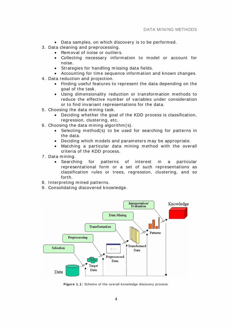
The overall process of finding and interpreting patterns from data involvesthe repeated application of the following steps (see also Figure 1.1):
1. Developing an understanding of• the application domain• the relevant prior knowledge• the goals of the end-user
2. Data cleaning and preprocessing.• Selecting a data set.• Focusing on a subset of variables.
DATA MINING METHODS
4
• Data samples, on which discovery is to be performed.3. Data cleaning and preprocessing.
• Removal of noise or outliers.• Collecting necessary information to model or account for
noise.• Strategies for handling missing data fields.• Accounting for time sequence information and known changes.
4. Data reduction and projection.• Finding useful features to represent the data depending on the
goal of the task.• Using dimensionality reduction or transformation methods to
reduce the effective number of variables under considerationor to find invariant representations for the data.
5. Choosing the data mining task.• Deciding whether the goal of the KDD process is classification,
regression, clustering, etc.6. Choosing the data mining algorithm(s).
• Selecting method(s) to be used for searching for patterns inthe data.
• Deciding which models and parameters may be appropriate.• Matching a particular data mining method with the overall
criteria of the KDD process.7. Data mining.
• Searching for patterns of interest in a particularrepresentational form or a set of such representations asclassification rules or trees, regression, clustering, and soforth.
8. Interpreting mined patterns.9. Consolidating discovered knowledge.
Figure 1.1: Scheme of the overall knowledge discovery process.
DATA MINING METHODS
5
In this chapter, I would like to cover data mining basics, algorithmsand strategies, particularly with respect to biomedical applications. I dothis by giving the reader a better understanding to the difference betweensupervised and unsupervised learning, and by addressing further relatedtopics such as (semi)supervised clustering, genetic approaches andsupplemental statistics.
OBJECTIVES
Depending on the feedback, data mining algorithms can be distinguishedbetween the following forms of learning: supervised, unsupervised andreinforcement learning. The latter form, in which the algorithm has tolearn a policy that maps inputs to actions resulting in the bestperformance, is not further elaborated in this chapter, so that I mainlyfocus on aspects of supervised and unsupervised data mining.
In supervised learning or class prediction, knowledge of a particulardomain is used to help make distinctions of interest. In biomedicine,analyses tend to involve selecting the features of most correlatedphenotypic distinctions (e.g. biomolecular and clinical markers). Thesefeatures are then used as the input to a classification algorithm that usesknown sample labeling to build a model, so that future unknown samples(individuals) can be classified. For example, a model could be built toidentify on which metabolic disorder a patient is suffering from, basedupon a subset of metabolites that distinguish the different diseases ofinterest. Supervised learning classifiers can be very accurate, for example,in biomolecular classification, especially if a large number of high qualitysamples are used to train the model.
In unsupervised learning or clustering, the goal of the analyses is touncover trends, correlations, or patterns, and no assumptions are madeabout the structure of data. In this context, data mining algorithms areused to find clusters or relevant subspaces based on multiple scenarios,such as how close a set of biological samples or clinical data are to eachother using a correlation, distance or similarity function. For example, ifdata is collected about various mutations in an affected human gene thatare expressed in a various phenotypic description, unsupervised datamining algorithms can cluster people into meaningful groups based on thesimilarity of their aggregate phenotypic expressions.
SUPERVISED DATA MINING
Feature selection
Success of data mining algorithms on a given task is affected by factorssuch if information is irrelevant or redundant, or the data is noisy andunreliable. Thus, feature selection is the process of identifying andremoving as much of irrelevant or redundant information as possible. Onepopular categorization of feature selection techniques has coined theterms “filter” and “wrapper” to describe the nature of metric used to
DATA MINING METHODS
6
evaluate the worth of features (Kohavi and John, 1998; Liu and Motoda,1998; Hall and Holmes, 2003; Liu et al., 2004).
Wrappers evaluate feature subsets by using accuracy estimates providedby a machine learning algorithm. In general, forward selection search isused to produce a list of features, ranked according to their overallcontribution to the accuracy of the attribute subset with respect to thetarget learning algorithm. Here, it starts with an empty set, evaluateseach attribute to find the best single attributes and then tries to find thebest pair/group of three etc. attributes, until no single attribute additionimproves the evaluation of the subset. Wrappers generally give betterresults than filters because of the interaction between search and learningscheme’s inductive bias. But improved performance comes at the cost ofcomputational expense due to invoking the learning algorithm for everyattribute subset considered during the search (Figure 1.2).
Figure 1.2: The “wrapper” approach for feature selection.
Filters use general characteristics of the data to evaluate attributes andoperate independently of any learning algorithm by producing a rankedlist of feature candidates. In the following, three major feature selectiontechniques with a ranking of identified attributes are presented:
Information gain (IG) is a measure how well the given feature Aseparates the remaining training data by expecting a reduction of entropyE, a measure of the impurity in the data (Mitchell, 1997).
∑ ⋅−=∈Cc
cc
SS
lnSS
)S(E (1)
∑ ⋅−=∈ )A(Vv
vv )S(E
S
S)S(E)A,S(IG (2)
S represents the data collection, |S| its cardinality, C is the classcollection, Sc the subset of S containing items belonging to class c, V(A) is
DATA MINING METHODS
7
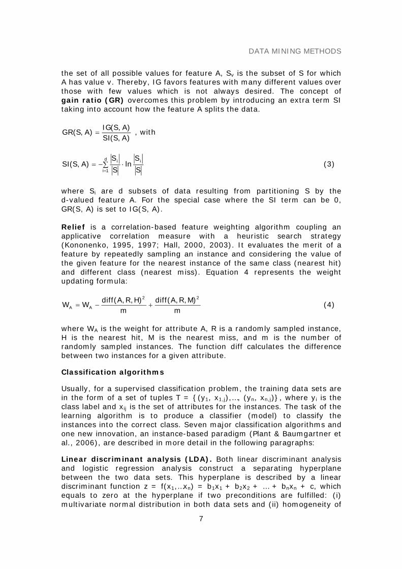
the set of all possible values for feature A, Sv is the subset of S for whichA has value v. Thereby, IG favors features with many different values overthose with few values which is not always desired. The concept ofgain ratio (GR) overcomes this problem by introducing an extra term SItaking into account how the feature A splits the data.
)A,S(SI)A,S(IG
)A,S(GR = , with
∑ ⋅−==
d
1i
ii
S
Sln
S
S)A,S(SI (3)
where Si are d subsets of data resulting from partitioning S by thed-valued feature A. For the special case where the SI term can be 0,GR(S, A) is set to IG(S, A).
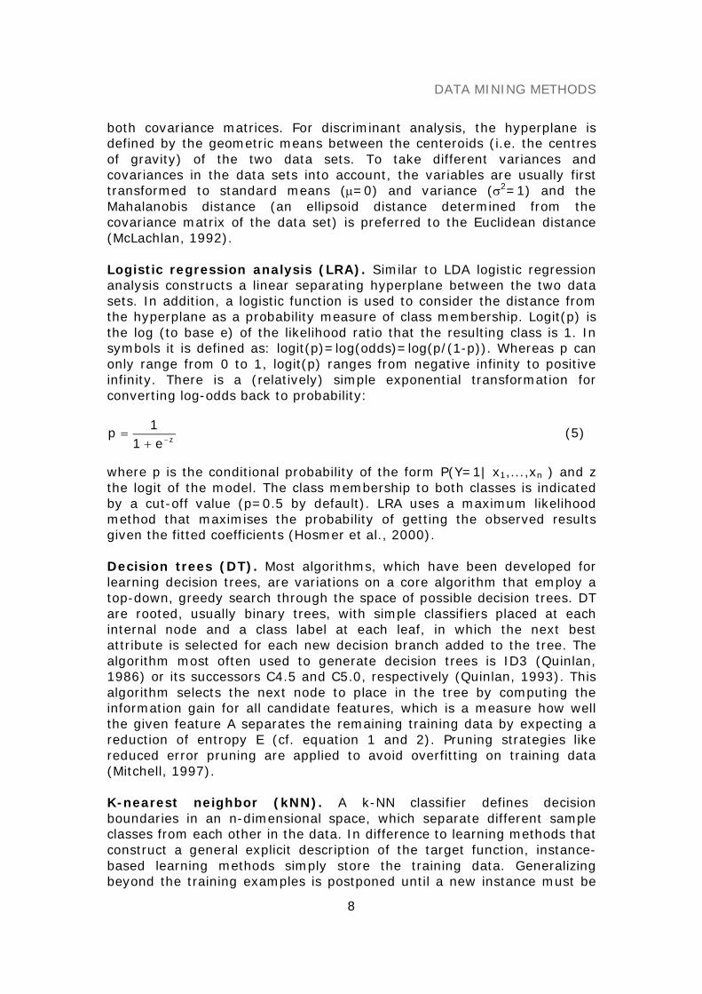
Relief is a correlation-based feature weighting algorithm coupling anapplicative correlation measure with a heuristic search strategy(Kononenko, 1995, 1997; Hall, 2000, 2003). It evaluates the merit of afeature by repeatedly sampling an instance and considering the value ofthe given feature for the nearest instance of the same class (nearest hit)and different class (nearest miss). Equation 4 represents the weightupdating formula:
m)M,R,A(diff
m)H,R,A(diff
WW22
AA +−= (4)
where WA is the weight for attribute A, R is a randomly sampled instance,H is the nearest hit, M is the nearest miss, and m is the number ofrandomly sampled instances. The function diff calculates the differencebetween two instances for a given attribute.
Classification algorithms
Usually, for a supervised classification problem, the training data sets arein the form of a set of tuples T = {(y1, x1,j),…, (yn, xn,j)}, where yi is theclass label and xij is the set of attributes for the instances. The task of thelearning algorithm is to produce a classifier (model) to classify theinstances into the correct class. Seven major classification algorithms andone new innovation, an instance-based paradigm (Plant & Baumgartner etal., 2006), are described in more detail in the following paragraphs:
Linear discriminant analysis (LDA). Both linear discriminant analysisand logistic regression analysis construct a separating hyperplanebetween the two data sets. This hyperplane is described by a lineardiscriminant function z = f(x1,…xn) = b1x1 + b2x2 + … + bnxn + c, whichequals to zero at the hyperplane if two preconditions are fulfilled: (i)multivariate normal distribution in both data sets and (ii) homogeneity of
DATA MINING METHODS
8
both covariance matrices. For discriminant analysis, the hyperplane isdefined by the geometric means between the centeroids (i.e. the centresof gravity) of the two data sets. To take different variances andcovariances in the data sets into account, the variables are usually firsttransformed to standard means (μ=0) and variance (σ2=1) and theMahalanobis distance (an ellipsoid distance determined from thecovariance matrix of the data set) is preferred to the Euclidean distance(McLachlan, 1992).
Logistic regression analysis (LRA). Similar to LDA logistic regressionanalysis constructs a linear separating hyperplane between the two datasets. In addition, a logistic function is used to consider the distance fromthe hyperplane as a probability measure of class membership. Logit(p) isthe log (to base e) of the likelihood ratio that the resulting class is 1. Insymbols it is defined as: logit(p)=log(odds)=log(p/(1-p)). Whereas p canonly range from 0 to 1, logit(p) ranges from negative infinity to positiveinfinity. There is a (relatively) simple exponential transformation forconverting log-odds back to probability:
ze11
p−+
= (5)
where p is the conditional probability of the form P(Y=1| x1,...,xn ) and zthe logit of the model. The class membership to both classes is indicatedby a cut-off value (p=0.5 by default). LRA uses a maximum likelihoodmethod that maximises the probability of getting the observed resultsgiven the fitted coefficients (Hosmer et al., 2000).
Decision trees (DT). Most algorithms, which have been developed forlearning decision trees, are variations on a core algorithm that employ atop-down, greedy search through the space of possible decision trees. DTare rooted, usually binary trees, with simple classifiers placed at eachinternal node and a class label at each leaf, in which the next bestattribute is selected for each new decision branch added to the tree. Thealgorithm most often used to generate decision trees is ID3 (Quinlan,1986) or its successors C4.5 and C5.0, respectively (Quinlan, 1993). Thisalgorithm selects the next node to place in the tree by computing theinformation gain for all candidate features, which is a measure how wellthe given feature A separates the remaining training data by expecting areduction of entropy E (cf. equation 1 and 2). Pruning strategies likereduced error pruning are applied to avoid overfitting on training data(Mitchell, 1997).
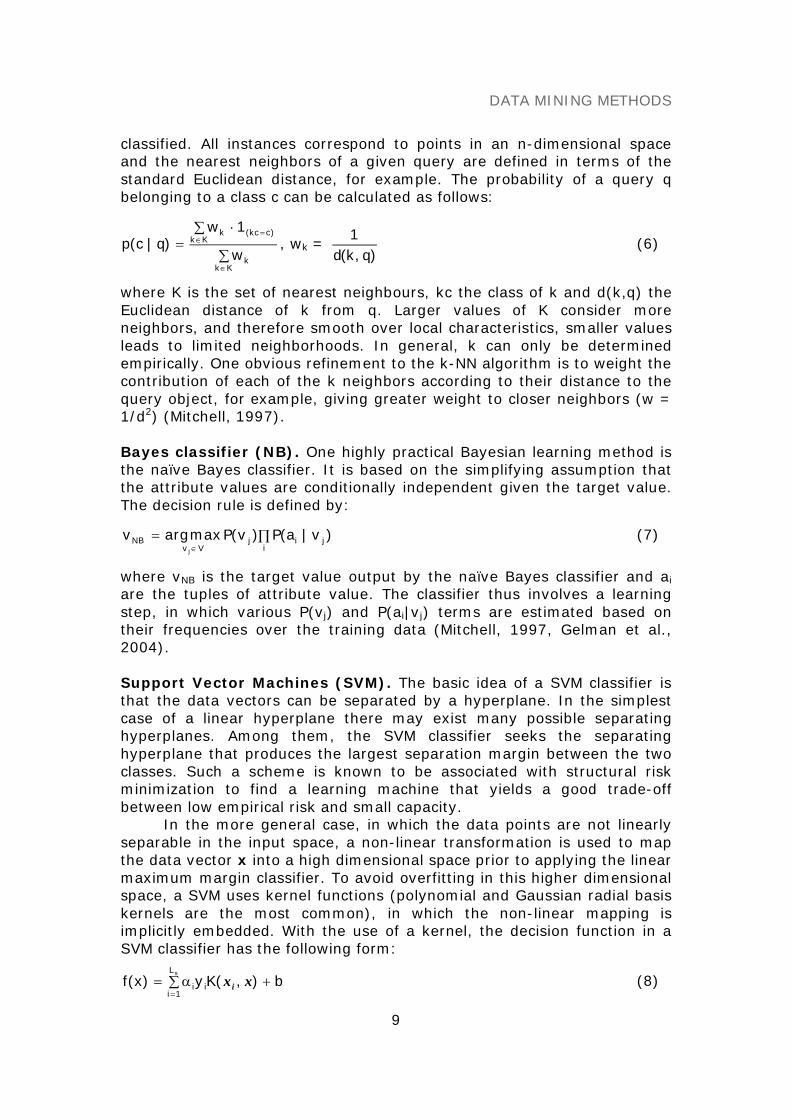
K-nearest neighbor (kNN). A k-NN classifier defines decisionboundaries in an n-dimensional space, which separate different sampleclasses from each other in the data. In difference to learning methods thatconstruct a general explicit description of the target function, instance-based learning methods simply store the training data. Generalizingbeyond the training examples is postponed until a new instance must be
DATA MINING METHODS
9
classified. All instances correspond to points in an n-dimensional spaceand the nearest neighbors of a given query are defined in terms of thestandard Euclidean distance, for example. The probability of a query qbelonging to a class c can be calculated as follows:
∑
∑ ⋅=
∈
∈=
Kkk
Kk)ckc(k
w
1w)q|c(p , wk =
)q,k(d1
(6)
where K is the set of nearest neighbours, kc the class of k and d(k,q) theEuclidean distance of k from q. Larger values of K consider moreneighbors, and therefore smooth over local characteristics, smaller valuesleads to limited neighborhoods. In general, k can only be determinedempirically. One obvious refinement to the k-NN algorithm is to weight thecontribution of each of the k neighbors according to their distance to thequery object, for example, giving greater weight to closer neighbors (w =1/d2) (Mitchell, 1997).
Bayes classifier (NB). One highly practical Bayesian learning method isthe naïve Bayes classifier. It is based on the simplifying assumption thatthe attribute values are conditionally independent given the target value.The decision rule is defined by:
∏=∈ i
jijVv
NB )v|a(P)v(Pmaxargvj
(7)
where vNB is the target value output by the naïve Bayes classifier and ai
are the tuples of attribute value. The classifier thus involves a learningstep, in which various P(vj) and P(ai|vj) terms are estimated based ontheir frequencies over the training data (Mitchell, 1997, Gelman et al.,2004).
Support Vector Machines (SVM). The basic idea of a SVM classifier isthat the data vectors can be separated by a hyperplane. In the simplestcase of a linear hyperplane there may exist many possible separatinghyperplanes. Among them, the SVM classifier seeks the separatinghyperplane that produces the largest separation margin between the twoclasses. Such a scheme is known to be associated with structural riskminimization to find a learning machine that yields a good trade-offbetween low empirical risk and small capacity.
In the more general case, in which the data points are not linearlyseparable in the input space, a non-linear transformation is used to mapthe data vector x into a high dimensional space prior to applying the linearmaximum margin classifier. To avoid overfitting in this higher dimensionalspace, a SVM uses kernel functions (polynomial and Gaussian radial basiskernels are the most common), in which the non-linear mapping isimplicitly embedded. With the use of a kernel, the decision function in aSVM classifier has the following form:
∑ +α==
sL
1iii b),(Ky)x(f xxi (8)
DATA MINING METHODS
10
where K (·,·) is the kernel function, xi are the so-called support vectorsdetermined from training data, LS is the number of support vectors, yi isthe class indicator associated with each xi, and αi the Lagrangemultipliers. In addition, for a given kernel it is necessary to specify thecost factor c, a positive regularization parameter that controls the trade-off between complexity of the machine and the allowed classification error(Cortes et al., 1995; Vapnik, 1998; Cristianini and Shawe-Taylor, 2000;Shawe-Taylor and Cristianini, 2004).
Artificial neural networks (ANN). An artificial neural network is aninformation processing paradigm that is inspired by the biological nervoussystems, such as the brain. Each artificial neuron has a certain number ofinputs, each of which has a weight assigned to them. The weights simplyare an indication of how 'important' the incoming signal for that input is.The net value of the neuron is then calculated - the net is simply theweighted sum, the sum of all the inputs multiplied by their specific weight.Each neuron has its own unique threshold value, and if the net is greaterthan the threshold, the neuron fires (or outputs a 1), otherwise it staysquiet (outputs a 0). The output is then fed into all the neurons it isconnected to. The network consists of several layers of neurons, the input,hidden and output layers. An input layer takes the input and distributes itto the hidden layers, which do all the necessary computation and outputthe results to the output layer. The standard algorithm, which is used forclassification, is a multi-layered ANN trained using back-propagation andthe delta rule. This algorithm attempts to minimize the squared errorbetween the network output values and the target value for these outputs(Bishop, 1995; Mitchell, 1997; Raudys, 2001).
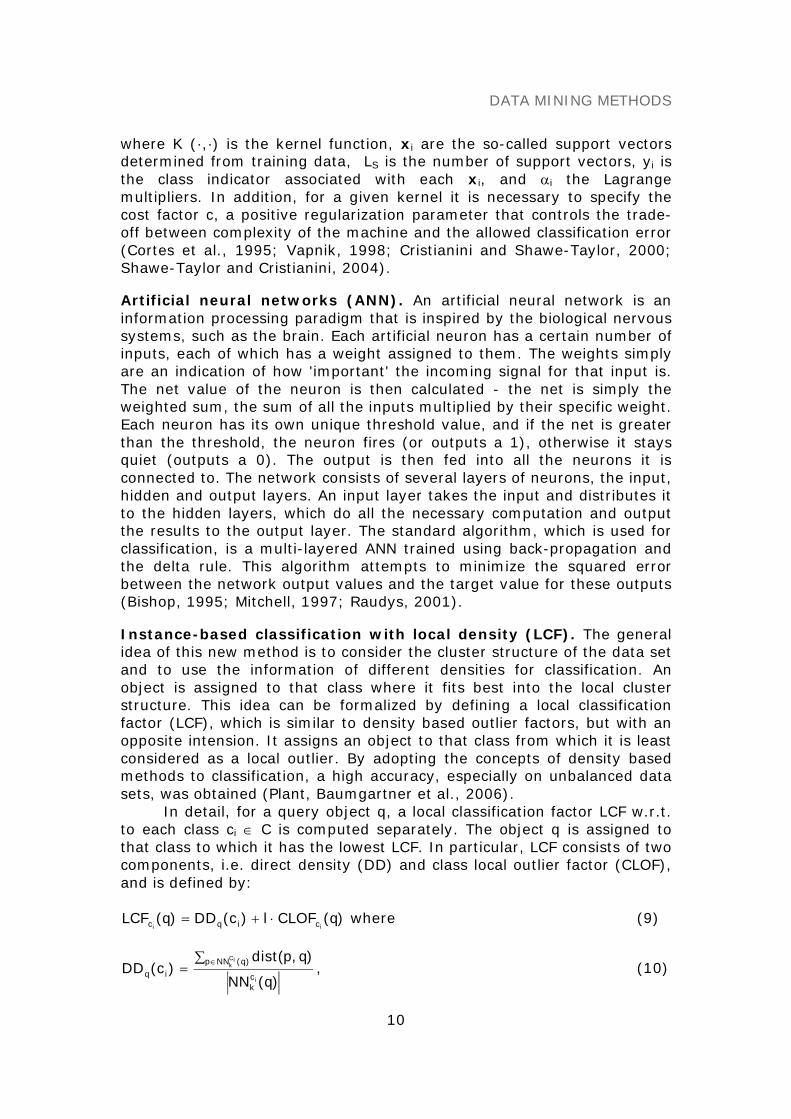
Instance-based classification with local density (LCF). The generalidea of this new method is to consider the cluster structure of the data setand to use the information of different densities for classification. Anobject is assigned to that class where it fits best into the local clusterstructure. This idea can be formalized by defining a local classificationfactor (LCF), which is similar to density based outlier factors, but with anopposite intension. It assigns an object to that class from which it is leastconsidered as a local outlier. By adopting the concepts of density basedmethods to classification, a high accuracy, especially on unbalanced datasets, was obtained (Plant, Baumgartner et al., 2006).
In detail, for a query object q, a local classification factor LCF w.r.t.to each class ci ∈ C is computed separately. The object q is assigned tothat class to which it has the lowest LCF. In particular, LCF consists of twocomponents, i.e. direct density (DD) and class local outlier factor (CLOF),and is defined by:
)q(CLOFl)c(DD)q(LCFii ciqc ⋅+= where (9)
)q(NN
)q,p(dist)c(DD
i
iCk
ck
)q(NNpiq
∑= ∈ , (10)

DATA MINING METHODS
11
)c(ID
)c(DD)q(CLOF
iq
iqci
= with)q(NN
)c(DD)c(ID
i
iCk
ck
)q(NNp ipiq
∑= ∈
. (11)
DD was introduced to capture the density of class ci ∈ C in the regionsurrounding the object q and is computed by the mean value of thedistances to the k nearest neighbors of q, belonging to class ci (equation10). Indirect density (ID) of the class ci is defined as the density of theregion surrounding the object q, excluding q itself. The class local outlierfactor (CLOF) thus describes the degree to which an object q is an outlierto the local cluster structure w.r.t. class ci (equation 11).
50
55
60
65
70
75
80
85
90
95
15 20 25 30 35 40 45attribute A1
attri
bute
A2
Class 1Class 2
50
55
60
65
70
75
80
85
90
95
15 20 25 30 35 40 45attribute A1
attri
bute
A2
Class 1Class 2Wrong
(a) Two-dimensional synthetic data. (b) Result with direct density only.
50
55
60
65
70
75
80
85
90
95
15 20 25 30 35 40 45attribute A1
attri
bute
A2
Class 1Class 2Wrong
50
55
60
65
70
75
80
85
90
95
15 20 25 30 35 40 45attribute A1
attri
bute
A2
Class 1Class 2Wrong
(c) Result with class local outlier factor only. (d) Result with LCF for l=6, k=5.
Figure 1.3 a-d: Concept of instance-based classification with local density demonstrated onsynthetic experimental data [Plant, Baumgartner et al., Bioinformatics, 2006].
DATA MINING METHODS
12
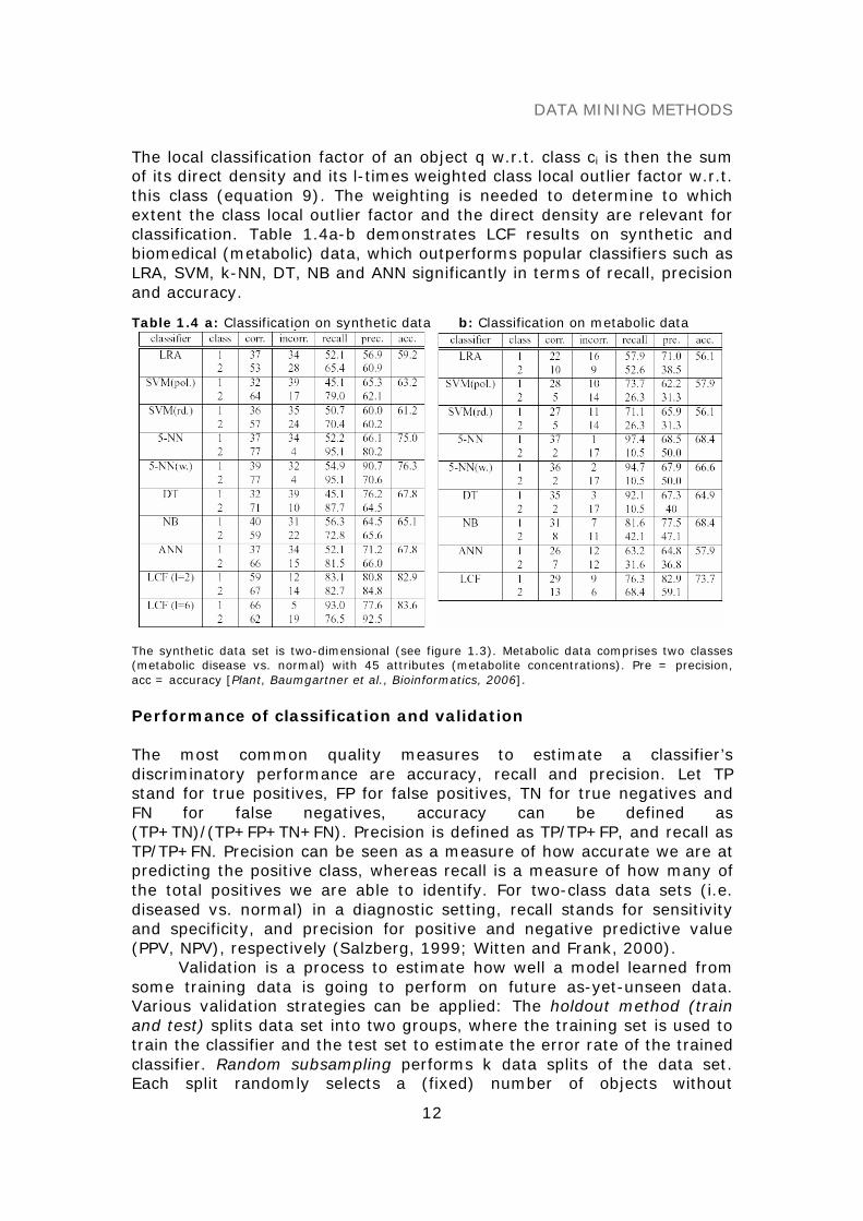
The local classification factor of an object q w.r.t. class ci is then the sumof its direct density and its l-times weighted class local outlier factor w.r.t.this class (equation 9). The weighting is needed to determine to whichextent the class local outlier factor and the direct density are relevant forclassification. Table 1.4a-b demonstrates LCF results on synthetic andbiomedical (metabolic) data, which outperforms popular classifiers such asLRA, SVM, k-NN, DT, NB and ANN significantly in terms of recall, precisionand accuracy.
Table 1.4 a: Classification on synthetic data b: Classification on metabolic data
The synthetic data set is two-dimensional (see figure 1.3). Metabolic data comprises two classes(metabolic disease vs. normal) with 45 attributes (metabolite concentrations). Pre = precision,acc = accuracy [Plant, Baumgartner et al., Bioinformatics, 2006].
Performance of classification and validation
The most common quality measures to estimate a classifier’sdiscriminatory performance are accuracy, recall and precision. Let TPstand for true positives, FP for false positives, TN for true negatives andFN for false negatives, accuracy can be defined as(TP+TN)/(TP+FP+TN+FN). Precision is defined as TP/TP+FP, and recall asTP/TP+FN. Precision can be seen as a measure of how accurate we are atpredicting the positive class, whereas recall is a measure of how many ofthe total positives we are able to identify. For two-class data sets (i.e.diseased vs. normal) in a diagnostic setting, recall stands for sensitivityand specificity, and precision for positive and negative predictive value(PPV, NPV), respectively (Salzberg, 1999; Witten and Frank, 2000).
Validation is a process to estimate how well a model learned fromsome training data is going to perform on future as-yet-unseen data.Various validation strategies can be applied: The holdout method (trainand test) splits data set into two groups, where the training set is used totrain the classifier and the test set to estimate the error rate of the trainedclassifier. Random subsampling performs k data splits of the data set.Each split randomly selects a (fixed) number of objects without
DATA MINING METHODS
13
replacement. For each data split, the classifier is retrained from scratchwith the training objects and the error rate Ei is determined with the testobjects. The true error estimate is obtained as the average of the separateerror rates Ei. K-fold cross validation creates a k-fold partition of the dataset. Here, for each of k experiments k-1 folds are used for training andthe remaining one for testing. The advantage of k-fold cross validation isthat all the objects in the data set are eventually used for both trainingand testing. As before, the true error is estimated as the average errorrate. Leave-one-out is the degenerate case of k-fold cross validation,where k is chosen as the total number of objects. N experiments areperformed for a data set with N objects. For each experiment, N-1examples are used for training and the remaining example for testing(Witten and Frank, 2000).
UNSUPERVISED DATA MINING
Feature and subspace selection
The objective in unsupervised feature selection, which does not make useof a class attribute, is to search for a subset of features that best coversnatural grouping (clusters) from data according to some criterion. To findthe subset of features that maximizes the performance criterion is difficultbecause the number of clusters is unknown beforehand.
In the following, two feature/subspace selection methods including anew algorithm developed by Baumgartner et al., 2004 are described,which utilize the structure of clusters in lower dimensional spaces toidentify relevant features. Beforehand a very popular method, principalcomponent analysis (PCA), is presented that does not search forsubspaces explicitly, but reduces data dimensionality by transforming anumber of correlated attributes into a number of uncorrelated attributesto identify new meaningful underlying features.
Principal component analysis (PCA). PCA is a mathematical procedurethat transforms a number of (possibly) correlated variables into a(smaller) number of uncorrelated variables called principal components.
The objective is to reduce the dimensionality (number of variables)of the data set, but retain most of the original variability in the data.Transformed attributes are formed by first computing the covariancematrix of the original attributes and then extracting its eigenvectors. Theeigenvectors (principal components) define a linear transformation fromthe original attribute space to a new space, in which attributes areuncorrelated. Eigenvectors can be ranked according to the amount ofvariation in the original data that they account for. Thus, principalcomponents are those linear combinations of the original variables, whichmaximize the variance of the linear combination and which have zerocovariance (and hence zero correlation) with the previous principalcomponents. Typically, the first few transformed attributes account formost of the variation in the data and are retained, whereas the remainder

DATA MINING METHODS
14
are discard. PCA is extremely useful when attributes are expected to belinearly (or even monotonically) related to each other, a situation, whichhowever is not generally encountered in biomedical data.
Ranking interesting subspaces (RIS). RIS selects all interestingsubspaces of arbitrary size and shape in high dimensional data using adensity-based clustering notation (Ester et al., 1996). The quality of asubspace S, measuring the interestingness of S, is defined by
]Sdim[
]Sdim[
attrRangenVol
n
]S[count)S(QUALITY
⋅⋅
=ε
(12)
on which the identified subspaces are finally ranked. Count[S] denotes thesum of all objects lying in the ε-neighborhood of all core objects in S.Because naturally with each dimension the number of expected objects inthe ε-neighborhood of an object decreases, this naïve quality value favorslower dimensional subspaces over higher dimensional ones. A scalingcoefficient that takes the dimensionality of the subspace into account isintroduced, which determines the ratio between the count[S] value andthe count[S] value under the assumption that all data objects areuniformly distributed in S. For that purpose, the volume of ad-dimensional ε-neighborhood, denoted by dVolε and the number of
objects lying in dVolε assuming uniform distribution, was computed.A downward pruning step to eliminate redundant subspaces is
provided: If there exists a (k+1) dimensional subspace S with higherquality than the k dimensional subspace T (S ⊃ T), T is deleted (Kailing etal., 2003).
Selecting subspaces relevant for clustering (SURFING). SURFING isa feature selection method for clustering that does not rely on a globaldensity parameter. This approach explores all subspaces exhibiting aninteresting hierarchical clustering structure and ranks them according to aquality criterion. The algorithm is more or less parameterless, i.e. it doesnot require the user to specify parameters that are hard to anticipate suchas the number of clusters, the (average) dimensionality of subspaceclusters, or a global density threshold (Baumgartner et al., 2004).
A quality criterion measuring the interestingness of a subspacew.r.t. to its hierarchical clustering structure was introduced, whichidentifies relevant subspaces built on the k-nearest neighbour distances(k-NN distances) of the objects. The k-NN distance of an object o in asubspace S, denoted by )o(nnDistS
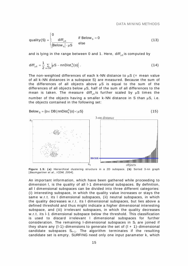
k , is the distance between o and itsk-nearest neighbor. It indicates how densely the data space is populatedaround o in S. Figure 1.5a-b illustrates these considerations, using asample 2D subspace S = {a1, a2} and k = 3. The quality measure isdefined as follows:
DATA MINING METHODS
15
⎪⎩
⎪⎨
⎧
μ⋅= μ
SBelow
diff0
)S(quality
S
Selse
0Belowif S =(13)
and is lying in the range between 0 and 1. Here, Sdiffμ is computed by
∑ −μ=∈
μDBo
SkS )o(nnDistS
21
diff . (14)
The non-weighted differences of each k-NN distance to μS (= mean valueof all k-NN distances in a subspace S) are measured. Because the sum ofthe differences of all objects above μS is equal to the sum of thedifferences of all objects below μS, half of the sum of all differences to themean is taken. The measure Sdiffμ is further scaled by μS times the
number of the objects having a smaller k-NN distance in S than μS, i.e.the objects contained in the following set:
}S)o(nnDist|DBo{Below SkS μ<∈= (15)
Figure 1.5: (a) Hierarchical clustering structure in a 2D subspace. (b) Sorted 3-nn graph[Baumgartner et al., ICDM, 2004].
An important information, which have been gathered while proceeding todimension l, is the quality of all l-1 dimensional subspaces. By definition,all l dimensional subspaces can be divided into three different categories:(i) interesting subspace, in which the quality value increases or stays thesame w.r.t. its l dimensional subspaces, (ii) neutral subspaces, in whichthe quality decreases w.r.t. its l dimensional subspaces, but lies above adefined threshold and thus might indicate a higher dimensional interestingsubspace, and (iii) irrelevant subspaces, in which the quality decreasesw.r.t. its l-1 dimensional subspace below the threshold. This classificationis used to discard irrelevant l dimensional subspaces for furtherconsideration. The remaining l-dimensional subspaces in Sl are joined ifthey share any (l-1)-dimensions to generate the set of (l + 1)-dimensionalcandidate subspaces Sl+1. The algorithm terminates if the resultingcandidate set is empty. SURFING need only one input parameter k, which
DATA MINING METHODS
16
must somehow correspond to the minimum cluster size that is theminimal number of objects regarded as a cluster.
Cluster analysis
Clustering algorithms are useful tools for the task of class identification. Ingeneral, there are three basic types of clustering algorithms: partitioning,hierarchical and density-based algorithms (Kaufman and Rousseeuw,1990; Everitt, 1993; Ester et al., 1996).
Partitioning algorithms construct a partition of a database D of nobjects into a set of k clusters. k is an input parameter for thesealgorithms. The partitioning algorithm typically starts with an initialpartition of D and then uses an iterative strategy to optimize an objectivefunction. Here, each cluster is represented by the gravity center of thecluster (k-means) or by one of the objects of the cluster located near toits center (k-medoid). Therefore partitioning algorithms base on a two-step procedure:
(1) Determination of k representatives minimizing theobjective function.
(2) Assignment of each object to the cluster with itsrepresentative closest to the considered object.
The second step implied that a partition is equivalent to a voronoi diagramand each cluster is contained in one of the voronoi cells. Thus, the shapeof all clusters found by these algorithms is convex, what is veryrestrictive. Further partitioning algorithms such as CLARANS (Clusteringlarge applications based on randomized search), which is an improvedk-medoid method, were described (Ng and Han, 1994). CLARANS is moreeffective and more efficient compared to former algorithms like PAM. Itassumes that all objects to be clustered can reside in the main memory atthe same time, which however does not hold for large databases.
The EM algorithm, which is also assigned to the group of partitioningalgorithms, is a generic tool for solving maximum likelihood problems bymodeling the probability density of the data (typically Gaussian datadistribution) (McLachlan and Krishnan, 1997).
Hierarchical algorithms create a hierarchical decomposition of adatabase D, which is represented by a dendrogram, a tree that iterativelysplits D into smaller subsets until each subset consists of only one object.In such a hierarchy, each node of the tree represents a cluster. The treecan either be created from the leaves up to the root (agglomerative) orfrom the root down to the leaves (divisive) by merging or dividing clustersat each step. When hierarchical clustering algorithm merges two clustersto generate a new bigger cluster, it should calculate the distancesbetween the new cluster and remaining clusters. Exemplarily the followinglinkage approaches can be processed. Here, let Cn be a new cluster, amerge of Ci and Cj. Let Ck be a remaining cluster. Dist is the distancebetween two clusters, for example, between Ci and Ck (Hubert, 1974):

DATA MINING METHODS
17
(i) Single linkage
D(Cn,Ck) = Min[D(Ci,Ck), D(Cj,Ck)] (16)
(ii) Complete linkage approach
D(Cn,Ck) = Max[D(Ci,Ck), D(Cj,Ck)] (17)
(iii) Average linkage (Unweighted Pair Group Method with ArithmeticMean, UPGMA)
)C,C(DistCC
C)C,C(Dist
CC
C)C,C(Dist kj
ji
jki
ji
ikn +
++
= (18)
Hierarchical clustering algorithms, which do not need a predeterminednumber of clusters as input parameters, are very popular in biomedicalapplications because they enable the user to determine the naturalgrouping with interactive visual feedback (dendrogram and color mosaic).
Density-based algorithms rely on the simple assumption that theobjects within a cluster have a typical density which is considerably higherthan outside the cluster. Furthermore, the density within areas of noise islower than the density in any of the clusters. The key idea of thealgorithm DBSCAN, developed by Ester et al., 1996, is that for each objectof a cluster the neighborhood of a given radius ε has to contain at least aminimum number of objects MinPts, that means that the density in theneighborhood has to exceed some threshold
Nε(p) = {q ∈ D | dist(p, q) ≤ ε}. (19)
The shape of the neighborhood is determined by the choice of a distancefunction (e.g. Euclidean distance) for two objects p and q, denoted bydist(p, q). For instance, when using the Manhattan distance in a 2D space,the shape of the neighborhood is rectangular. For the formal definitionsfor this clustering notion w.r.t. the terms directly density-reachable,density-reachable, density-connected, cluster and noise see Ester at al.,1996. Here, a density based cluster is defined as a set of density-connected objects, which is maximal w.r.t. density-reachability, and noiseis the set of objects not contained in any cluster.
OPTICS, a further innovation based on a density-based notion, doesnot produce a clustering of a data set explicitly, but instead creates anaugmented ordering of the database representing its density-basedclustering structure. The cluster ordering of a data set can be representedand understood graphically by a so-called reachability plot. This plotshows the hierarchical clustering structure of data plotting the reachabilitydistance values for each object in the clustering order (Ankerst et al.,1999).
DATA MINING METHODS
18
(SEMI)SUPERVISED CLUSTERING
Traditional clustering algorithms determine clusters by maximizing theintra-cluster similarity and minimizing inter-cluster similarity withoutconsidering class labels. A technique that uses additional information inform of class labels assigned to all or part of the objects to find class pureclusters is called supervised or semi-supervised clustering, respectively.Algorithms such as MPC-k-Means, COP-k-Means, and SPAM have recentlybeen published (Wagstaff et al., 2001; Bilenko et al., 2004; Eick et al.,2004). Most of them extend well-known clustering methods by enforcingtwo types of constraints: mustlinks between objects of the same class andcannot-links between objects of different classes. It is noteworthy thatthese new approaches seem to be an interesting innovation w.r.t. toclassification because they utilize partitioning, hierarchical or density-based clustering notions for assigning objects.
GENETIC ALGORITHMS
Genetic algorithms provide a learning method motivated by an analogy tobiological evolution that generate successor hypotheses by repeatedlymutating and recombining parts of the best currently hypotheses. Thesearch for an appropriate hypothesis begins with a population (collection)of initial hypotheses. At each step, the hypotheses in the currentpopulation are evaluated relative to a given measure of fitness, with themost fit hypotheses selected probabilistically as seeds for producing thenext generation. Thus, this process forms a generate-and-test beam-search of hypotheses, in which variants of the best current hypotheses aremost likely to be considered next. Hypotheses are typically described bybit strings, but also by symbolic expressions or genetic programming, inwhich hypotheses are described by computer programs.
STATISTICS AND HYPOTHESIS TESTING
A basic familiarity with concepts from statistics is important tounderstanding how to evaluate hypotheses and learning algorithms. Keynotations from statistics and sampling theory are briefly summarized inthe following:
A random variable can be viewed as the name of an experiment with aprobabilistic outcome. Its value is the outcome of the experiment.
A probability distribution for a random variable Y specifies the probabilityP(Y=yi) that Y will take on the value yi, for each possible value yi.
The expected value, or mean, of a random variable Y is∑ == i ii ).yY(Py]Y[E The symbol μY is commonly used to represent E[Y].

DATA MINING METHODS
19
The variance of a random variable is Var(Y) = E[(Y - μY)2]. The variancecharacterizes the width or dispersion of the distribution about its mean.
The standard deviation of Y is )Y(Var . The symbol σY is often used torepresent the standard deviation of Y.
The Binomial distribution give the probability of observing r heads in aseries of n independent coin tosses if the probability of heads in a singletoss is p.
The Normal distribution is a bell-shaped probability distribution thatcovers many natural phenomena.
The Central Limit Theorem is a theorem stating that the sum of a largenumber of independent, identically distributed random variablesapproximately follows a Normal distribution.
An estimator is a random variable Y used to estimate some parameter p ofan underlying population.
The estimation bias of Y as an estimator for p is the quantity (E[Y] – p).An unbiased estimator is one for which the bias is zero.
An N% confidence interval estimate for parameter p is an interval thatincludes p with probability N%.
Statistical theory provides a basis for estimating the true error (errorD(h))of a hypothesis h, based on its observed error (errorS(h)) over a sample Sof data. For example, the problem of estimating confidence intervals isapproached by identifying the parameter to be estimated (e.g. errorD(h))and an estimator (e.g. errorS(h)) for this quantity. Confidence intervalscan then be calculated by determining the interval that contains thedesired probability mass under this distribution. Possible causes ofestimation error are the estimation bias and the variance in the estimate.
Comparing the relative effectiveness of two learning methods is anestimation problem that is relatively easy when data and time isunlimited, but more difficult when these resources are limited. A possibleapproach is to run learning methods on different subsets of the availabledata, testing the learned hypotheses on the remaining data, thenaveraging the results of these experiments (Dietterich, 1996) (see alsoparagraph “Performance of classification and validation”). Much literatureexists on the topic of statistical methods for estimating mean and testingsignificance of hypothesis, where more detailed information can be founde.g. in DeGroot, 1986 or Casella and Berger, 1990.

DATA MINING METHODS
20
REFERENCES
Ankerst M, Breunig MM, Kriegel HP, Sander J. (1999) OPTICS: Ordering points to identifythe clustering structure. Proc. ACM SIGMOD Int. Conf. on Management of Data(SIGMOD’99), Philadelphia, PA, pp. 49-60.
Baumgartner C, Kailing K, Kriegel HP, Kröger P, Plant C. (2004) Subspace selection forclustering high-dimensional data. Proc. 4th IEEE Int. Conf. on Data Mining (ICDM’04),Brighton, UK, pp. 11-18.
Bilenko M, Basu S, Mooney RJ (2004). Integrating constraints and metric learning insemi-supervised clustering. Proc. 21th Int. Conf. on Machine Learning (ICML ’04),Banff, Alberta, Canada, pp. 81-92.
Bishop CM. (1995) Neural networks for pattern recognition, Oxford university press,Oxford.
Casella G, Berger RL. (1990) Statistical inference. Pacific Grove, CA, Wadsworth andBooks/Cole.
Cristianini N, Shawe-Taylor J. (2000) An introduction to support vector machines andother kernel-based learning methods, Cambridge University Press, Cambridge, UK.
DeGroot MH. (1986) Probability and statistics. (2nd ed.) Reading, MA, Addison Wesley.Cortes C, Vapnik V. (1995) Support vector networks. Mach Learn, 20, 273-297.Dietterich TG. (1996) Proper statistical tests for comparing supervised classification
learning algorithms (Technical report). Department of Computer Science, OregonState University Corvallis, OR.
Eick C, Zeidat N, Zhao Z. (2004) Supervised clustering - algorithms and benefits. Proc.Int. Conf. on Tools with Artificial Intelligence (ICTAI’04), Boca Raton, Florida, pp. 774-776.
Ester M, Kriegel HP, Sander J, Xu X. (1996) A density-based algorithm for discoveringclusters in large spatial databases with noise. Proc. 2nd Int. Conf. on KnowledgeDiscovery and Data Mining (KDD’96), AAAI Press, Menlo Park, CA, pp. 226-231.
Everitt BS. (1993) Cluster Analysis, London, Edward Arnold.Fayyad UM, Piatetsky-Shapiro G, Smyth P. (1996a) Advances in knowledge discovery and
data mining, chapter: From data mining to knowledge discovery: An overview, AAAIPress, Menlo Park, CA, pp. 1-30.
Fayyad UM, Piatetsky-Shapiro G, Smyth P. (1996b) Knowledge discovery and datamining: Towards a unifying framework. In: Simoudis E, Han JW, Fayyad UM (Hrsg.),Proc. 2nd Int. Conf. on Knowledge Discovery and Data Mining, AAAI Press, pp. 82-88.
Gelman A, Carlin JB, Stern HS, Rubin DB. (2004) Baysean data analysis, 2nd edn.Chapman & Hall/CRC Press.
Hall MA. (2000) Correlation-based feature selection for discrete and numeric classmachine learning. Proc. 17th Int. Conf. on Machine Learning, (ICML’00), pp. 359-366.
Hall MA, Holmes G. (2003) Benchmarking attribute selection techniques for discrete classdata mining. IEEE T on Knowl Data En, 15, 1437-1447.
Hubert L. (1974) Approximate evaluation techniques for the single-link and complete-linkhierarchical clustering procedures. J Am Stat Assoc, 69, 698-704.
Hosmer DW, Lemeshow S. (2000) Applied logistic regression, 2nd edition, Wiley, NewYork.
Kaufman L, Rousseeuw PJ. (1990) Finding groups in data: An introduction to clusteranalysis. John Wiley & Sons.

DATA MINING METHODS
21
Kailing K, Kriegel HP, Kröger P, Wanka S. (2003) Ranking interesting subspaces forclustering high dimensional data. Proc. 7th European Conf. on Principles and Practiceof Knowledge Discovery in Databases (PKDD’03). In: Lecture Notes in ArtificialIntelligence (LNAI), Vol. 2838, pp. 241-252.
Kohavi R, John GH. (1998) The wrapper approach, In: Feature selection for knowledgediscovery and data mining, H. Liu & H. Motoda (Ed.), Kluwer, pp. 33-50.
Kononenko, I. (1995) On biases in estimating multi-valued attributes. Proc. IJCAI’95,Montreal, Canada, pp. 1034–1040.
Kononenko I, Simec E, Robnik-Sikonja M. (1997) Overcoming the myopia of inductivelearning algorithms with RELIEFF, Appl Intell, 7, 39–55.
Liu H, Motoda H (1998) Feature selection for knowledge discovery and data mining,Kluwer Academic, Boston, MA.
Liu H, Motoda H, Yua L (2004) A selective sampling approach to active feature selection.Artif Intell, 159, 49–74.
McLachlan GJ. (1992) Discriminant analysis and statistical pattern recognition. Wiley,New York.McLachlan GJ, Krishnan T. (1997) The EM algorithm and extensions. Wiley, New York.Mitchell TM. (1997) Machine learning, McGraw-Hill Boston, MA.Ng RT, Han J. (1994) Efficient and effective clustering methods for spatial data mining.
Proc. 20th Int. Conf. on Very Large Data Bases (VLDB’94), Santiago, Chile, pp. 144-155.
Quinlan RJ. (1986) Induction of decision trees, Mach Learn, 1, 81-106.Quinlan RJ. (1993) C4.5: Program for machine learning, Morgan Kaufmann, San Mateo,
CA.Raudys S. (2001) Statistical and neural classifiers, Springer-Verlag, London. Shawe-Taylor J, Cristianini N. (2004) Kernel methods for pattern analysis. Cambridge
University Press, Cambridge, UK. Plant C, Böhm C, Tilg, Baumgartner C. (2006) Enhancing instance-based classification
with local density: A new algorithm for classifying unbalanced biomedical data.Bioinformatics, in press.
Salzberg S. (1999) On comparing classifiers: A critique of current research and methods.Data Min Knowl Disc, 1, 1-12.
Vapnik V. (1998) Statistical Learning Theory, Wiley, New York.Wagstaff K, Cardie C, Rogers S, Schroedel S. (2001) Constrained k-Means clustering with
background knowledge. Proc. 18th Int. Conf. on Machine Learning (ICML´01), pp.577–584.
Witten IH, Frank E. (2000) Data Mining - Practical machine learning tools and techniqueswith java implementations. Morgan Kaufmann, San Francisco.

DATA MINING METHODS
22
“Faces”, Elias Gabriel, 15 months (Aug. 2nd, 2005)

DATA MINING IN METABOLOMICS
23
DATA MINING IN METABOLOMICS:FROM METABOLITE PROFILING TO DIAGNOSIS
IN INBORN ERRORS OF METABOLISM
Recent advances in modern high throughput technologies such astandem mass spectrometry (MS/MS) have made it possible to separateand identify small molecules based on their masses from samples of abiofluid like blood or urine. By using appropriate internal standards, theconcentration of a molecule in fluid can be measured with great precisionbecause the accuracy and sensitivity of the instrumentation are so high(Chace et al., 1999; Charrow et al., 2000; Neville et al., 2003; Gamacheet al., 2004; Dunn et al., 2005). MS/MS provides high-throughput data forthe discovery of diagnostic markers, which is very relevant to theunderstanding of how metabolic disorders manifest. In particular,abnormal concentrations of metabolites may indicate erroneous metabolicreactions and may reflect the actual functional state of a patient. Sobiomarkers are important tools for disease screening and early diagnosis(Roschinger et al., 2003; Wilcken et al., 2003; Strauss, 2004; German etal., 2004; Lee et al., 2005; Gao et al., 2005).
Newborn screening programs for severe metabolic disorders, whichhinder an infant’s normal physical or mental development, are well-established (Liebl et al., 2002a, 2002b; Roschinger et al., 2003; Maier etal., 2005). These primarily monogenic diseases are due to the change of asingle gene, resulting in an enzyme or other protein not being produced orhaving altered functionality. Otherwise not apparent at this early age,inborn errors of metabolism can be addressed by effective therapies.Screening simultaneously for more than 20 inherited metabolic disordersby analyzing more than 50 metabolites, the experimental data is quicklybecoming too voluminous and unmanageable to catalog by hand. Thus,powerful statistical bioinformatics and data mining tools are needed todiscover novel biomarkers in MS high-throughput data on which screeningmodels of high diagnostic power can be developed (Lilien et al., 2003,Purohit et al., 2003, Baumgartner et al., 2004a, 2004b, 2005, 2006).
fχ: ℜg → {classes}
0
0.05
0.1
0.15
0.2
0.25
0.3
0.35
P H EX LE
G LUV A L
G LY
P YR G L TAL A
O R NM E T
A R G C ITT Y R
S E R
A R GS U C
Amino acidsR
elie
f
PKU
fχ: ℜg → {classes}fχ: ℜg → {classes}
0
0.05
0.1
0.15
0.2
0.25
0.3
0.35
P H EX LE
G LUV A L
G LY
P YR G L TAL A
O R NM E T
A R G C ITT Y R
S E R
A R GS U C
Amino acidsR
elie
f
PKU
0
0.05
0.1
0.15
0.2
0.25
0.3
0.35
P H EX LE
G LUV A L
G LY
P YR G L TAL A
O R NM E T
A R G C ITT Y R
S E R
A R GS U C
Amino acidsR
elie
f
PKU
0
0.05
0.1
0.15
0.2
0.25
0.3
0.35
P H EX LE
G LUV A L
G LY
P YR G L TAL A
O R NM E T
A R G C ITT Y R
S E R
A R GS U C
Amino acidsR
elie
f
PKU

DATA MINING IN METABOLOMICS
24
In this chapter, I would like to outline a two-step procedure to thebiomarker discovery process on MS high-throughput data of inborn errorsof metabolism. This includes (1) the identification of potential markercandidates from the disease-specific metabolite profiles and (2) theprioritization of selected candidates according to literature knowledge todisease metabolism. It further covers the efficiency of data mining anddatabase retrieval methods to classify subjects and describes the generalprocess of developing screening models for diagnosis and diseaseprevention taking both single and interacting metabolites for the model-building process into account.
METABOLITE PROFILING
Metabolite profiling technologies comprise advanced analytical and dataprocessing tools. By coupling two mass spectrometers, usually separatedby a reaction chamber or collision cell, the modern tandem massspectrometry allows simultaneous analysis of multi-compounds in a high-throughput process (Millington et al., 1984). Characteristic patterns offragments and relative peak intensities in the resulting spectrum allowqualitative as well as quantitative determination of chemical compounds.MS/MS has been used for several years to identify and measure carnitineester concentrations in blood and urine of children suspected of havinginborn errors of metabolism. Indeed, acylcarnitine analysis is a superiordiagnostic test for disorders of fatty acid oxidation because abnormallevels of related metabolites are detected before the patient is acutely ill(Millington et al. 1992). More recently, MS/MS has been used in pilotprograms to screen newborns for these conditions and for disorders ofamino- and organic-acid metabolism as well (Liebl et al., 2002a, 2002b;Wilcken et al., 2003). Targeted MS/MS analysis thus permits very rapid,sensitive and, with internal standards, accurate quantitative measurementof a wide set of the human metabolome by calculating concentrates onmetabolites (μmol/L) from the raw MS spectra.
METABOLIC DISORDERS AND MS RESEARCH DATA
Table 2.1 summarizes a brief description of the examined disordersregarding their enzyme defects, established diagnostic markers, and theirnatural history, which is needed later to prioritize and confirm markercandidates according to the established biochemical knowledge (Claytonet al., 1998; Hoffmann and Zschocke, 1999; ACMG/ASHG, 2000; Blau etal., 2001; Rinaldo et al., 2002; Dezateux, 2003; Donlon et al., 2004).
Experiments were performed on two-class (diseased vs. normal)data sets extracted from a provided MS research database. The data setcomprises data from seven inborn errors of metabolism, that is, oneamino acid disorder, phenylketonuria (PKU), four organic acid disorders,glutaric academia type I (GA-I), 3-methylcrotonylglycinemia deficiency (3-MCCD), methlymalonic acidemia (MMA), propionic acidemia(PA), two fatty acid oxidation disorders, medium-chain acyl CoAdehydrogenase deficiency (MCADD), 3-OH long-chain acyl CoA

DATA MINING IN METABOLOMICS
25
dehydrogenase deficiency (LCHADD), and a group of 5100 healthycontrols. The database (DB) is organized in the form of a set of tuplesTDB = {(cj, m) | cj∈ C, m ∈ M}, where cj is the class label of the collectionC of investigated disorders and controls, and M = {m | m1, … , mn } is thegiven set of metabolite concentrations in μmol/L. Here, M consists of 29acyl-carnitines (i.e. C0, C2, C3, C4, C5, C6, C8, C10, C12, C14, C16, C18,C5:1, C10:1, C14:1, C16:1, C18:1, C10:2, C14:2, C18:2, C5OH, C14OH,C16OH, C16:1OH, C18:1OH, C4DC, C5DC, C6DC, C12DC) and 14 aminoacids (i.e. ALA, ARG, ARGSUC, CIT, GLU, GLY, MET, ORN, PHE, PYRGLT,SER, TYR, VAL, and XLE), in all 43 metabolites. In Table 2.2 full names ofmetabolites are given.
Table 2.1: Brief overview of investigated metabolic disorders
Inborn errors of metabolism Enzyme defect/ affectedpathway
Diagnosticmetabolites
Symptoms if untreated
Phenylketonuria(PKU)
Phenylalaninehydroxylase or impairedsynthesis of biopterincofactor
PHE ↑TYR ↓
Microcephaly, mental retardation,autistic-like behavior, seizures
Glutaric acidemia, Type I(GA-I)
Glutaryl CoAdehydrogenase
C5DC ↑ Macrocephaly at birth, neurologicalproblems, episodes of acidosis/ketosis, vomiting
3-Methylcrotonylglycinemia deficiency (3-MCCD)
3-methylcrotonyl CoAcarboxylase
C5OH ↑ Metabolic acidosis andhypoglycemia,some asymptomatic
Methlymalonic acidemia(MMA)
Methlymalonyl CoAmutase or synthesis ofcobalamin (B12) cofactor
C3 ↑C4DC↑
Life threatening/fatal ketoacidosis,hyper-ammonemia, latersymptoms: failure to thrive, mentalretardation
Propionic acidemia(PA)
Propionyl CoAcarboxylase α or βsubunit or biotin cofactor
C3 ↑ Feeding difficulties, lethargy,vomiting and life threateningacidosis
Medium-chain acyl CoAdehydrogenase deficiency(MCADD)
Medium chain acyl CoAdehydrogenase
C8 ↑C6 ↑C10↑C10:1 ↑
Fasting intolerance, hypoglycemia,hyperammonemia, acuteencephalopathy, cardiomyopathy
3-OH long-chain acyl CoAdehydrogenase deficiency(LCHADD)
Long chain acyl CoAdehydrogenase or mitochondrial trifunctionalprotein
C16OH ↑C18OH ↑C18:1OH ↑
Hypoglycemia, lethargy, vomiting,coma, seizures, hepatic disease,cardiomyopathy
Arrows ↑ and ↓ indicate abnormally enhanced and diminished metabolite concentrations. Boldmetabolites denote the established primary diagnostic markers. For further information seeACMG/ASHG, 2000, www.ncbi.nlm.nih.gov/entrez/query.fcgi?db=OMIM, www.geneclinics.org,www.slh.wisc.edu/newborn/guide/panel.php [Baumgartner et al., J Biomol Screen, 2006].
Table 2.2: Overview of metabolites measured by MS/MS
Amino acids (symbols) Acyl-carnitines (symbols) Acyl-carnitines (symbols)Alanine (Ala) Free carnitine (C0) Hexadecenoyl-carnitine (C16:1)Arginine (Arg) Acetyl-carnitine (C2) Octadecenoyl-carnitine (C18:1)Argininosuccinate (Argsuc) Propionyl-carnitine (C3) Decenoyl-carnitine (C10:2)Citrulline (Cit) Butyryl-carnitine (C4) Tetradecadienoyl-carnitine (C14:2)Glutamate (Glu) Isovaleryl-carnitine (C5) Octadecadienoyl-carnitine (C18:2)Glycine (Gly) Hexanoyl-carnitine (C6) Hydroxy-isovaleryl-carnitine (C5-OH)Methionine (Met) Octanyl-carnitine (C8) Hydroxytetradecadienoyl-carnitine (C14-OH)Ornitine (Orn) Decanoyl-carnitine (C10) Hydroxypalmitoyl-carnitine (C16-OH)Phenylalanine (Phe) Dodecanoyl-carnitine (C12) Hydroxypalmitoleyl-carnitine (C16:1-OH)Pyroglutamate (Pyrglt) Myristoyl-carnitine (C14) Hydroxyoleyl-carnitine (C18:1-OH)Serine (Ser) Hexadecanoyl-carnitine (C16) Dicarboxyl-butyryl-carnitine (C4-DC)Tyrosine (Tyr) Octadecanoyl-carnitine (C18) Glutaryl-carnitine (C5-DC)Valine (Val) Tiglyl-carnitine (C5:1) Methylglutaryl-carnitine (C6-DC)Leucine+Isoleucine (Xle) Decenoyl-carnitine (C10:1) Methylmalonyl-carnitine (C12-DC)
Myristoleyl-carnitine (C14:1)
Fourteen amino acids and 29 acyl-carnitines [Baumgartner et al., J Biomed Inform, 2005].

DATA MINING IN METABOLOMICS
26
BIOMARKER IDENTIFICATION AND PRIORITIZATION
Generally, feature subset selection is the process of identifying andremoving as much irrelevant and redundant information as possible. Thisreduces the dimensionality of data and may allow learning algorithms tooperate faster and more efficiently. In metabolic data, biomarkers arethose extracted key features that allow a well-done classification.Ultimately, qualified and validated biomarkers can be used for diseasescreening and therapeutic monitoring (Baumgartner et al., 2004a, 2004b,2005, 2006).
Biomarker identification using BMI
A new supervised feature selection algorithm, the biomarker identifier(BMI), was developed to identify disease state metabolites from quantifiedtwo-class (diseased vs. normal) MS data sets. BMI returns a ranked list ofmarker candidates qualified by a suitable score measure (Baumgartner etal., 2006).
The basic idea of the paradigm BMI was to make use of a two-stepdata processing procedure to discern the discriminatory attributesbetween two classes of interest, i.e. the full set of MS traces of eachmetabolite profile from diseased patients against another set from normalpeople (Duda et al., 2001). Both steps include the following:
(1) Identification of marker candidates and deletion of irrelevantmetabolites from a given metabolite collection M. For that task, threemeasures describing erroneous metabolic reactions at the level ofconcentration changes in fluid were taken into account to develop aquality (score) measure for the selection of potential markers candidates.It defines:
(a) The discriminatory performance of each metabolite m ∈ Mdetermined by a machine learning paradigm.
(b) The extent of discriminatory space between normal anddisease state concentration values.
(c) The variance of measured abnormal metabolite concentrationsat the state of disease.
(2) Ranking of the selected metabolites. A list of marker candidatesranked by the size of calculated score values is returned.
The following definitions are required: Let DS be a two-class MS data setorganized as a set of tuples TDS = {(cj, m) | cj∈ C, j =[1,2], m ∈ M},where c1 is the class label of a metabolic disorder, c2 of the control class,and M is the given set of metabolite concentrations.
Logistic regression analysis (LRA) was applied to determine thediscriminatory performance of each metabolite m ∈ M. A performancemeasure TP* was introduced, which is calculated by the product of thetrue positive (TP) rates of class c1 and c2:
TP* = TPc1 ⋅ TPc2 (1)

DATA MINING IN METABOLOMICS
27
In addition, the discriminatory threshold ts separating both classes wasdetermined from the LRA logit coefficients a0 and a1, and is denoted by
1
0s a
at = . (2)
This parameter is needed later (see paragraph “Metabolite profileretrieval”). The range of discriminatory space between normal and diseasestate concentrations of m is estimated by the parameter Δdiff, whichapproximates the mean distance between both data distributions underthe assumption that both cohorts are normal distributed:
⎪⎩
⎪⎨⎧
Δ−
≥ΔΔ=Δ
else1
1ifdiff with
2
1
c
c
x
x=Δ , (3)
whereicx is the mean metabolite concentration in class ci. Δ ≥ 1 denotes a
concentration enhancement, Δ < 1 a decrease of concentration in fluid.The score value si ∈ S qualifying a processed metabolite mi ∈ M is thusdefined by
CV*TPs diff
iΔ⋅
⋅λ= (4)
where λ (λ is set to 10 by default) is a scaling factor and CV defined asσ/ x is the coefficient of variation at the state of disease. S denotes thecollectivity of identified marker candidates represented by their scorevalues. Finally, a ranked list of marker candidates, mi ⊆ M, is returned byBMI. Irrelevant metabolites, mj ⊆ M (mi ∪ mj = M), are discarded using acut-off score value |s| < 5 by default. The algorithm boxed below is brieflysketched in pseudo-code:
Input: Two-class dataset DS organized as set of tuples Tc1 and Tc2Tc1:= c1, m1, m2,…, mn; Tc2:= c2, m1, m2,…, mn; S = {}
Output: Ranked list of marker candidates S:= s1, s2,…, smList of discriminatory thresholds TS:= ts1, ts2,…, tsm
Algorithm: BMI (Dataset DS, RankedList S, ThresholdList TS)for i from 1 to n domi := DS.get(i);
TP*i := Discriminatory performance of mi determined by thelearning method;
tsi := Discriminatory threshold of mi determined by thelearning method;
Δdiffi := Extent of discriminatory space of mi;CVi := Coefficient of variation of class c1;
si = 10 ⋅ (TP*i ⋅ Δdiffi) / CVi;if |si| ≥ 5 then
S[i] = si;TS[i] = tsi;
else delete (si, tsi);
sort (S, TS);write (S, TS);

DATA MINING IN METABOLOMICS
28
Figure 2.3 exemplifies all analytical steps for calculating score value sC8,i.e. octanyl-carnitine (C8), the primary diagnostic marker for MCADD.Values of discriminatory parameters ts and TP*, extent of discriminatoryspace Δdiff and coefficient of variation CV are shown explicitly. Morespecifically, the discriminatory threshold of C8 was computed more than15 standard deviations above the controls’ mean (ts = 0.62 μmol/L), itsdiscriminatory performance was close to 1.0 (TP* = 0.96). Furthermore,the higher variance of measured concentrations in MCADD group lead to atwice as large CV value (0.78) compared to the control class (CV = 0.36).A 62-fold elevation of mean C8 concentration at the state of disease (Δdiff
= 61.9) returned a strongly elevated score value sC8 of 914, the largestone identified within this study.
Figure 2.3: Measured concentrations of octanyl-carnitine (C8) in healthy controls and MCADDpatients. All analytical steps for calculating score value sC8 with BMI are depicted in detail.Histograms emphasize the different data distributions during health and disease [Baumgartner etal., J Biomol Screen, 2006].
To quantify the information content of a disease-specific score set S, themeasure Ds was introduced:
∑=∈Ss
2D ss (5)
In addition, the information content of an individual metabolic expression*sD can be expressed similar to equation 5, but the parameter Δdiff defined
in equation 3 must be replaced by
⎪⎩
⎪⎨⎧
Δ−
≥ΔΔ=Δ
else1
1if*diff with
2cxm
=Δ , (6)
DATA MINING IN METABOLOMICS
29
where m denotes the measured metabolite concentrations of a singlesubject. This measure is very helpful to assess gradual expressions ofaffected individuals (e.g. strong or mild form) compared to the over-allpicture of a disease and bring them into agreement with the patient’stherapeutic management. Figure 2.4 depicts the information content ofthe full MCADD marker score set ( 939sMCADD = ), supplemented by two
examples of a strong ( 2008*sMCADD = ) and a mild ( 467*sMCADD = ) profile.
Figure 2.4: Ranked list of identified metabolites for MCADD returned by the biomarker identifier(BMI). The information content of MCADD’s class score set and two examples of a strong and mildexpression are denoted explicitly. Positive score values indicate an abnormal increase, negativescores a decrease of metabolite concentrations in fluid. [Baumgartner et al., J Biomol Screen,2006].
Biomarker prioritization and biochemical interpretation
Table 2.5a summarizes and Figure 2.5b visualizes the identified markersubsets of examined inborn errors. Interpreting the computed scorevalues, it is conspicuous that each disorder is characterized by at least onehallmark metabolite, which outperform the others significantly. These keymetabolites showing scores uniformly above 100 corresponded exactlywith the established primary diagnostic markers as described in theliterature (see also Table 2.1). So, metabolites with score values |s| ≥ 100were prioritized as primary markers, score values between 20 ≤ |s| < 100as secondary, and score values |s| < 20 as tertiary markers.

DATA MINING IN METABOLOMICS
30
Table 2.5a: Identified marker candidates using BMI
Disorder
C3
C5
C6
C8
C10
C14
C16
C18
C5:1
C10:1
C16:1
C18:1
PKU 7 10 -74 10 -39 -8GA-I 8 -61 93-MCC 12 -61 9 14 -16 -13MMA 153 11 19 45 -9 54PA 261 -27 16MCADD 16 914 90 -8 -42 -8 173 -10 -30LCHADD 13 -53 -5
Disorder
C18:2
C5O
H
C14O
H
C16O
H
C18:1
OH
C4D
C
C5D
C
C12D
C
ARG
GLU
PHE
DsPKU 27 -9 104 127 219 288GA-I 34 514 62 52 5253-MCC 110 130 162 245MMA 23 11 46 74 60 202PA 25 7 19 20 266MCADD 51 56 939LCHADD 8 152 66 31 29 180
Metabolites with score values |s| < 5 were deleted by BMI. A positive score value indicates anabnormal increase, a negative score a decrease of metabolite concentration in fluid. Ds denotes the
information content of a given score set S w.r.t. disorder D. [Baumgartner et al., J Biomol Screen,2006].
Figure 2.5b: Visualization of the abnormal metabolite profiles of seven inborn errors ofmetabolism. Identified key metabolites are assessed by the BMI score measure.

DATA MINING IN METABOLOMICS
31
Categorized marker subsets are presented in Table 2.6. The prioritizationinto secondary and tertiary markers appears to be useful to distinguishbetween further promising marker candidates, of which the latter groupmay be closer associated with secondary effects of metabolism. A forthcategory was required to be introduced because several markercandidates, that is, decanoyl-carnitine (C10), hexadecanoyl-carnitine(C16), decenoyl-carnitine (C10:1), arginine (ARG) and glutamate (GLU),appeared together in nearly all seven study disorders representing thegroup of not disease-specific markers. Interestingly, C18:1 - by ourclassification defined as secondary marker - appeared before C6 in theranking, a further established (secondary) diagnostic metabolite inMCADD. Because C10:1, which is metabolized by four β-oxidation cyclesof oleyl-carnitine (C18:1), is a product of a metabolic reaction in the fattyacid metabolism, C18:1 is qualified to become a novel secondary marker.
However, all identified primary and some secondary prioritizedmetabolites were able to be confirmed by literature association to diseasebiochemistry. So far, some additional metabolites were found, whichrequire further validation steps by generating testable hypothesesregarding their biochemical role in health and disease. These most notablehallmark secondary candidates are C16:1 and C4DC for PKU, C4DC forGA-I and C18:1 for MCADD. A validation of the not disease-specificmarker candidates (fourth category) seems to be delicate because someof which are prioritized as secondary or even primary markers accordingto the proposed categorization. In particular, the highly scored aminoacids ARG and GLU cannot be confirmed by the diseases’ primarymetabolic reactions. However, this last step of biomarker discovery isinevitable and emphasizes, for example, the development of bioassays orpre-clinical models to confirm the bioanalytical measurements to initiatefuture marker validation.
Table 2.6: Prioritization of metabolic marker candidates
Disorder Primarymarkers
|score| ≥ 100
Secondarymarkers
20 ≤ |score| < 100
Tertiarymarkers
5 ≤ |score| < 20
Not disease-specificmarkers
PKU PHE C16:1, C4DC C5, C12DC, C18:1GA-I C5DC C4DC3-MCC C5OH C5:1, C16:1, C18:1MMA C3 C4DC C5, C8, C18:2, C5OHPA C3 C18:2, C5OHMCADD C8 C18:1 C6, C14, C18, C16:1LCHADD C16OH C18:1OH C18:1, C14OH
C10C16
C10:1ARGGLU
Four classes are defined: primary, secondary, tertiary and not disease-specific marker candidates[Baumgartner et al., J Biomol Screen, 2006].
Benchmark feature selection algorithms
To assess the quality of attribute selection, BMI was benchmarked withtwo established filter-based feature selection techniques producing anattribute ranking equally to the new algorithm: (1) Information gain (IG),which computes how well a given feature separates data by expecting a

DATA MINING IN METABOLOMICS
32
reduction of entropy, and (2) Relief, which is an exponent of a correlation-based selection method coupling an applicative correlation measure with aheuristic search strategy (Baumgartner et al., 2004b).
Information gain returned a quite similar metabolite rankingcompared to BMI, whereas Relief’s ranking differed significantly from bothmethods BMI and IG (Figure 2.7). Although IG and Relief produced aranked list of attributes, they lacked the ability to differ clearly betweenprimary and secondary/tertiary markers as BMI did. In particular,MCADD’s diagnostic key metabolite C8 did not stand out significantly fromthe others in both approaches. Relief even ranked C8 after C16 and C18:1- both metabolites showed slightly decreased concentration values - whichdoes not clearly reflect C8’s high discriminatory performance, its superiorconcentration enhancement and moderate coefficient of variation at thestate of disease.
Thus, the biomarker identifier (BMI) was developed to betteraddress the issue of biochemical alteration of metabolites in fluid, so thatentropy-based or correlation-based approaches are second choice becausethey do not optimally reflect the characteristics of given MS datastructures at disease state.
Figure 2.7: Ranked lists of metabolites are shown using the filter paradigms Information gain(IG) and Relief. The first 11 metabolites are depicted to be comparable with BMI. Black barsindicate the established diagnostic metabolites in MCADD (see Table 2.1) [Baumgartner et al.,J Biomol Screen, 2006].

DATA MINING IN METABOLOMICS
33
METABOLITE PROFILE RETRIEVAL
Similarity query processing on a large screening DB enables the user tosearch and classify subjects highly related to a requested metaboliteprofile. For matching MS profiles, a square distance measure based onBMI score-weights was introduced. The following definitions are required:
Let DB* be a MS screening database in the form of a set ofunclassified tuples TDB* = {m | m∈ M}. Furthermore let QD = {(s, ts) | s ∈ S, ts∈ TS} be the query model of an abnormal metabolite profile givenby the score set S and its corresponding set of discriminatory thresholdsTS as determined by the biomarker identifier BMI. For matching TDB* withthe query model QD, the following similarity measure Dr is computed:
∑ δ⋅==
N
1i
2iiD )s(r with
⎪⎩
⎪⎨
⎧<<
>≥
=δ
else0
0sfortmelseif
0sfortmif1
isi
isi
i . (7)
Here, the decision function δ identifies those metabolites in TDB* (δ = 1),whose concentration values exceed or fall below the discriminatorythreshold ts and replaces them by the corresponding scores s ∈ QD.Because maximal metabolic similarity fits to a maximal value of Dr , thebest ranked hits according to maximal value of Dr are returned as thequery result.
Figure 2.8 illustrates the first 100 hits of a MMA query on the givenresearch DB (545 data of 7 inborn errors of metabolism and 5100 healthycontrols) graphically. Two requests using query models based on the fullBMI marker set and, respectively, the disease-specific subset wereperformed and classification accuracy of delivered hits was determined.The first 41 hits (left to arrow 1 in the figure) represented a veryhomogenous group of MMA cases if the similarity measure MMAr wascomputed based on the disease-specific markers. This groupdemonstrated a TP-rate of 74% including a small number of wronglyassigned PA cases (9.8%). A slight drop-off of similarity measure MMAr inturn indicated the beginning of a second, homogenous group of 42 PA plus4 MMA cases. The TP-rate for PA was 84%. So, two groups of relatedmetabolite profiles could be separately delivered from one requestshowing a high degree of homogeneity with high classification accuracy.Otherwise, a request based on all extracted metabolites returned onemixed cohort of MMA and PA cases with a continuous decay of MMArmeasure approaching arrow 2. This result is surprising and can beexplained by strongly differing Dr values of both marker sets, MMAr = 202vs. PAr = 266 for the full set, and MMAr = 262 vs. PAr = 163 for the disease-specific set, respectively. However, a two times higher difference of the Drmeasure in the latter set lead thus to a better separation of both cohorts.DB requests for the remaining disorders were unproblematic because thequery model QD differed significantly from each other.

DATA MINING IN METABOLOMICS
34
Figure 2.8: MMA similarity request on a research DB. The first 100 hits returned are displayed.Squares ( ) indicate cases using the full BMI marker set for the request, circles ( ) the disease-specific BMI marker set (primary+secondary+tertiary markers). Filled squares/circles representMMA cases, empty ones PA cases. Hits left to arrow 2 show solely MMA and PA cases, hits right toarrow 2 entries of the remaining DB (≤ 51.4 for and ≤ 129.1 for ) [Baumgartner et al., J BiomolScreen, 2006].
DISEASE CLASSIFICATION
The performance of identified marker candidates is determined on theirability to classify subjects. Classifiers are built from MS data with knownclasses that comprise a training set in the form of a set of tuples TR = {(cj, m) | cj∈ C, m ∈ M}. Classifiers can then be applied to a test setconsisting of a set of tuples TS = {m | m ∈ M} to predict the class foreach subject.
Five machine learning paradigms, i.e. logistic regression analysis(LRA), k-NN, naïve Bayes, support vector machines (SVM) and artificalneural networks (ANN) according to their discriminatory power werecompared to assess their applicability for disease screening anddiagnostics (Table 2.9, Baumgartner et al., 2006). Classifiers werebasically applied to two-class data sets testing classification accuracy of(1) primary markers alone; (2) primary, secondary and tertiary markersexcluding not disease-specific ones; and (3) the full BMI marker set. Twoclasses of interest were designed: (a) disorder vs. controls and (b)disorder vs. controls, including the remaining study diseases w.r.t. a realscreening population. These experiments clearly indicated increasingclassification accuracy when considering the order of primary →primary+secondary+tertiary → all markers as classifiers’ inputs and littledifferences in accuracy when comparing data sets (a) and (b). However,

DATA MINING IN METABOLOMICS
35
two exceptions in experimental data (i.e. MMA and PA) appeared. MMAand PA belong to the group of organic acid disorders and are characterizedby the identical primary diagnostic marker propionyl-carnitine (C3). Table2.9 points out this situation considering as example MMA.
Table 2.9: Classification accuracy of five machine learning paradigms tested on MMA
MMA Primary Primary+secondary+tertiary All markersDataset (a) Sens. PPV Acc. Sens. PPV Acc. Sens. PPV Acc.LRA 80 97.6 99.79 84 91.4 99.77 90 95.7 99.861-NN 80 90.0 99.93 82 91.1 99.75 92 97.9 99.905-NN 80 97.6 99.79 84 97.7 99.82 88 97.8 99.86Naïve Bayes 86 68.3 99.48 92 52.9 99.13 96 68.6 99.53SVM (linear) 66 100 99.67 80 97.6 99.79 92 97.9 99.90SVM (pol 2d) 55 100 99.51 80 97.6 99.79 90 97.8 99.88SVM (RBF) 46 100 99.48 68 97.1 99.67 88 97.8 99.86ANN 82 97.6 99.81 82 93.2 99.77 98 98.0 99.96
Dataset (b)LRA 19 50.0 99.11 40 66.7 99.29 50 71.4 99.401-NN 34 40.5 98.97 74 78.7 99.59 64 78.0 99.525-NN 40 54.1 99.17 68 68.0 99.65 58 93.5 99.59Naïve Bayes 64 45.7 99.01 80 22.9 97.43 90 13.5 94.81SVM (linear) 2 50.0 99.11 14 77.8 99.20 48 80.0 99.43SVM (pol 2d) 8 100 99.19 40 87.0 99.42 52 86.7 99.50SVM (RBK) 0 100 99.11 10 83.3 99.19 14 70.0 99.19ANN 20 52.6 99.13 74 88.1 99.68 78 88.6 99.72
Classifiers were separately tested on the disease’s primary, primary, secondary and tertiarymarkers, and the full marker set as identified by the biomarker identifier (BMI). Part (a) showsclassification accuracy when testing classifiers on a two-class data set of MMA cases vs. healthycontrols, and part (b) depicts findings examined on the data set of MMA cases vs. controls,including the remaining study disorders. Classification results are given in percent (%). Specificitiesfor all experiments were uniformly ≥ 99.6%. We tested logistic regression analysis (LRA),unweighted 1-NN and 5-NN with an Euclidian distance function, naïve Bayes, standard SVM (linear)and SVM with polynomial (degree 2) and Gaussian radial basis (RBF) kernels using a cost factor of100, and a three-layer (input-hidden-output) ANN using delta rule and back-propagation, 500epochs to train trough and a learning rate of 0.3. Sens. is sensitivity, PPV is positive predictivevalue, and Acc. is accuracy [Baumgartner et al., J Biomol Screen, 2006].
These results revealed that sensitivity of all tested classifiers droppeddramatically, particularly if classification models were solely built on theprimary markers (e.g. LRA: 80% (a) ↓ 19% (b), SVM (linear): 66% (a) ↓2% (b) or ANN: 82% (a) ↓ 20% (b)). Testing the full marker set,classification accuracy could be further enhanced, but accuracy did notachieve values of data set (a). Analyzing the behavior of classifiers onMMA data in more detail, ANN yielded the best classification accuracyw.r.t. both data sets. Although both classes are strongly unbalanced insize, LRA, SVM and k-NN showed promising results as well. Nevertheless,little differences in accuracy were observed, which primarily arise from thestrengths and weaknesses of the target learning algorithm, along with thecharacteristics of the analyzed data. Naïve Bayes, which classifies asubject based on the probability of each class given the subject’s featurevariables, returned the most unbalanced classification results indicated bya too large fraction of false negative cases. This minimizes PPV on fullmarker set dramatically (68.6% data set (a), 13.5% data set (b)), whichis undesirable for disease screening.

DATA MINING IN METABOLOMICS
36
SCREENING MODELS
For the clinical routine, the predictive performance and generalizationpower of candidate biomarkers is utilized to build classification models fordisease screening. Typically high sensitivity and specificity is required torule out other diseases and to reduce subsequent diagnostic procedures,which cause additional efforts and costs (Thomason et al., 1998; Pandoret al., 2004). Additionally, the models have to consider and adjust for thereal incidence rate of a disease to calculate false-positive rates, assumingthat the prevalence of the disease was artificially controlled in the study.
Experimental study design
The general scheme for constructing a screening model on MS high-throughput data is illustrated in Figure 2.10 (Baumgartner et al., 2004b).
Figure 2.10: General process of data analysis for constructing a screening model on high-throughput MS/MS data. Starting from the newborn screening database (NBS DB), severalintermediate data mining steps result in a screening model with optimised sensitivity andspecificity. The symbol χ represents tuples of the database. xi is the set of metaboliteconcentrations, yi is the class membership variable and fχ indicates the target function (model)[Baumgartner et al., Bioinformatics, 2004].
DATA MINING IN METABOLOMICS
37
Starting from a pre-classified, clinically validated newborn screening(NBS) database, two-class (diseased vs. normal) data sets of all availablediseased cases (due to the disorders’ low prevalence) and a representativegroup of randomly sampled controls (>1000) were built. The first stepaimed at the identification of potential marker candidates from the diseasespecific metabolite profiles by using a supervised feature selectionapproach. Here, the so-called filter approach was applied that returns aranked list of marker candidates extracted from the full metabolite set.Secondly, classification models were trained and cross-validated on thebest ranked metabolite subsets because the disorder classes were toosmall to be split into representative train and test sets (cf. holdoutmethod). In the following, the best sensitive classifiers were furtherprocessed because the specific power of the screening model remains stillunanswered at this experimental stage. So, finally the most sensitivemodels were re-evaluated on a larger control database (100,000 normals)to estimate the classifiers’ real specific power. It is noteworthy thatidentified subsets using wrappers do not ultimately correspond to the bestranked filter outcome what in turn disqualify wrappers for astraightforward approach to identify a complete list of biomarkercandidates. Consequently important subsets are lost, that are ultimatelyneeded if the whole range of affected pathways is reviewed forbiochemical interpretation and further validation.
Screening models built on identified metabolite subsets
Models, which may prove feasible for clinical routine, have to ensure easyinterpretation without loosing predictive power. Within this context, fromsix investigated machine learning paradigms, LRA, k-NN and SVM gavepromising classification results on identified metabolite subsets(Baumgartner et al., 2004b). LRA classifiers that are directly interpretableby a target decision function were finally trained to build screening modelsfor classic MCADD and classic PKU showing highest sensitivities (Sn)≥95.2% (see Table 2.11a-b). In order to enhance classification accuracy,all pair-wise combinations of the six top-ranked metabolites returned fromtwo different filter-based feature selection methods (gain ratio and relief)were computed. But subsets of more than two metabolites did not furtherimprove classification accuracy in both examined disorders. Table 2.11summarizes the most sensitive and specific screening models (PKU: Sn =95.4-100%, MCADD: Sn = 95.2-96.8%). The total number of falselynegative classified newborns did not exceed the values of 0-4.6% for PKUand 3.2-4.8% for MCADD.
More specifically, the PKU models contained PHE as the primarydiagnostic marker, which is consistent with its role in erroneousmetabolism (Chace et al. 1993; Rashed et al., 1995). Models includingPHE alone or combined with ARG or ARGSUC yielded the highest PPV of70.7-71.9%, i.e. 16-17 FP cases (0.00017%) out of 100,000 controls. Theclassifier that included the established diagnostic markers PHE and TYRshowed maximum Sn (100%), but its PPV dropped off significantly

DATA MINING IN METABOLOMICS
38
(16.2%). Nevertheless, the role of ARG, GLU, ARGSUC, VAL or XLE needsto be cross-checked with intermediary pathways to better understandtheir contribution to PKU metabolism.
Table 2.11a-b: Screening models based on LRA for classic PKU and classic MCADD
Metabolites(PKU)
Sn
(%)FN
(# of cases)Sp
(%)FP
(# of cases)PPV(%)
NPV(%)
Acc(%)
Logit of modelsz=a0+a1m1+ …+ anmn
PHE, TYR 100 0 99.775 222 16.23 100 99.775 − 211.2566+ 2.1318⋅PHE− 0.6224⋅TYR
PHE, XLE 100 0 99.793 204 17.41 100 99.793 − 61.2577+ 1.8037⋅PHE− 1.4518⋅XLE
PHE, VAL 97.67 1 99.895 103 28.96 99.999 99.894 − 11.8046+ 0.2248⋅PHE− 0.1210⋅VAL
PHE, ARG 95.35 2 99.983 17 70.69 99.998 99.981 − 9.827+ 0.0462⋅PHE− 0.0035⋅ARG
PHE,ARGSUC
95.35 2 99.984 16 71.93 99.998 99.982 − 10.167+ 0.0457⋅PHE− 0.340⋅ARGSUC
PHE 95.35 2 99.984 16 71.93 99.998 99.982 − 10.1482+ 0.0455⋅PHE
Metabolites(MCADD)
Sn
(%)FN
(# of cases)Sp
(%)FP
(# of cases)PPV(%)
NPV(%)
Acc(%)
Logit of modelsz=a0+a1m1+ …+ anmn
C8, C18:1 96.83 2 99.992 8 88.41 99.998 99.990 − 5.4917+ 5.7436⋅C8− 2.1833⋅C18:1
C8 95.24 3 99.992 8 88.24 99.997 99.989 − 7.5362+ 5.7931⋅C8
C8, C12DC 95.24 3 99.990 10 85.71 99.997 99.987 − 4.8647+ 5.149⋅C8− 40.4661⋅C12DC
C8, C10 95.24 3 99.989 11 84.51 99.997 99.986 − 7.6114+ 4.6649⋅C8+ 3.3668⋅C10
C8, C10:1 95.24 3 99.950 50 54.55 99.997 99.947 − 8.7572+ 4.2517⋅C8+ 10.888⋅C10:1
Screening models for (a) classic PKU (n=43) and (b) classic MCADD (n=63). Sensitivity (Sn),specificity (Sp), positive predictive value (PPV), negative predictive value (NPV), accuracy (Acc),number (#) of false negatives (FN), number (#) of false positives (FP) and the logits (z) of the LRAmodels are shown. The specificity of the models was re-evaluated on a representative controldatabase of 98,400 cases [Baumgartner et al., Bioinformatics, 2004].
MCADD models showed slightly decreased Sn values (95.2-96.8%), butspecificities (Sp) and PPV were higher compared to the PKU models. Themost sensitive model (Sn = 96.8%) considering the subset of octanyl-carnitine (C8) and octadecenoyl-carnitine (C18:1) yielded an excellent Sp
of 99.992% and a PPV of 88.4%. In other words, only a marginal fractionof 8 FP cases (0.00008% of all controls) is wrongly classified as classicMCADD. Considering the established diagnostic markers C8 and C10:1,PPV of the model decreased to 54.6%. Therefore, combinations like C8 +C18:1 or C8 + C12DC are meaningful subsets for disease screening withhigh diagnostic power. C8, which showed the highest discriminatoryperformance as well, is the predominant, but not specific marker forMCADD, so that C8 alone can be used to pre-screen the family of C8affected fatty oxidation disturbances.
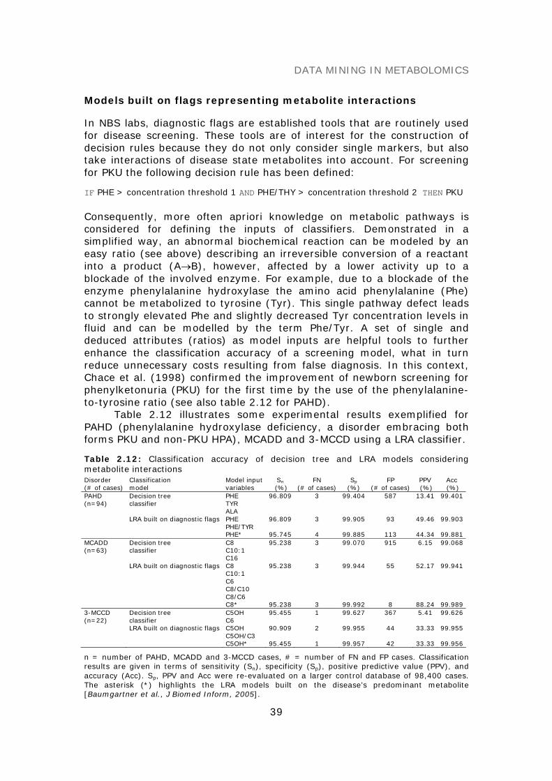
DATA MINING IN METABOLOMICS
39
Models built on flags representing metabolite interactions
In NBS labs, diagnostic flags are established tools that are routinely usedfor disease screening. These tools are of interest for the construction ofdecision rules because they do not only consider single markers, but alsotake interactions of disease state metabolites into account. For screeningfor PKU the following decision rule has been defined:
IF PHE > concentration threshold 1 AND PHE/THY > concentration threshold 2 THEN PKU
Consequently, more often apriori knowledge on metabolic pathways isconsidered for defining the inputs of classifiers. Demonstrated in asimplified way, an abnormal biochemical reaction can be modeled by aneasy ratio (see above) describing an irreversible conversion of a reactantinto a product (A→B), however, affected by a lower activity up to ablockade of the involved enzyme. For example, due to a blockade of theenzyme phenylalanine hydroxylase the amino acid phenylalanine (Phe)cannot be metabolized to tyrosine (Tyr). This single pathway defect leadsto strongly elevated Phe and slightly decreased Tyr concentration levels influid and can be modelled by the term Phe/Tyr. A set of single anddeduced attributes (ratios) as model inputs are helpful tools to furtherenhance the classification accuracy of a screening model, what in turnreduce unnecessary costs resulting from false diagnosis. In this context,Chace et al. (1998) confirmed the improvement of newborn screening forphenylketonuria (PKU) for the first time by the use of the phenylalanine-to-tyrosine ratio (see also table 2.12 for PAHD).
Table 2.12 illustrates some experimental results exemplified forPAHD (phenylalanine hydroxylase deficiency, a disorder embracing bothforms PKU and non-PKU HPA), MCADD and 3-MCCD using a LRA classifier.
Table 2.12: Classification accuracy of decision tree and LRA models consideringmetabolite interactionsDisorder(# of cases)
Classificationmodel
Model inputvariables
Sn
(%)FN
(# of cases)Sp
(%)FP
(# of cases)PPV(%)
Acc(%)
PAHD(n=94)
Decision treeclassifier
PHETYRALA
96.809 3 99.404 587 13.41 99.401
LRA built on diagnostic flags PHEPHE/TYR
96.809 3 99.905 93 49.46 99.903
PHE* 95.745 4 99.885 113 44.34 99.881MCADD(n=63)
Decision treeclassifier
C8C10:1C16
95.238 3 99.070 915 6.15 99.068
LRA built on diagnostic flags C8C10:1C6C8/C10C8/C6
95.238 3 99.944 55 52.17 99.941
C8* 95.238 3 99.992 8 88.24 99.9893-MCCD(n=22)
Decision treeclassifier
C5OHC6
95.455 1 99.627 367 5.41 99.626
LRA built on diagnostic flags C5OHC5OH/C3
90.909 2 99.955 44 33.33 99.955
C5OH* 95.455 1 99.957 42 33.33 99.956
n = number of PAHD, MCADD and 3-MCCD cases, # = number of FN and FP cases. Classificationresults are given in terms of sensitivity (Sn), specificity (Sp), positive predictive value (PPV), andaccuracy (Acc). Sp, PPV and Acc were re-evaluated on a larger control database of 98,400 cases.The asterisk (*) highlights the LRA models built on the disease’s predominant metabolite[Baumgartner et al., J Biomed Inform, 2005].
DATA MINING IN METABOLOMICS
40
These findings were compared with a decision tree classifier, whichhowever came off badly. Nevertheless, the main interest here was abenchmark of screening models built on single and interactingmetabolites, respectively. For MCADD experimental results werecomparable (cf. Table 2.11b and Table 2.12) because data sets andexperimental design stayed the same. Surprisingly, screening models builton the diagnostic established flags, i.e C6, C8, C10:1, C8/C10 and C8/C6,showed a decreased PPV compared to those considering solely singlemetabolites as identified by the machine learning approach (52.2% vs.>84%). Definitely, the subset of C8 and C18:1 yielded highestclassification accuracy and is thus best qualified for disease screening. Inparticular, C18:1 seems to be a putative diagnostic marker for MCADDand requires further validation. This example emphasizes the necessity ofpowerful data mining tools for biomarker identification on MS highthroughput data to advance novel biomolecular knowledge.
CONCLUSION
Computational innovations in metabolomics have great potential for thedevelopment of automated diagnostics, taking both machine learning anda-priori knowledge on disease metabolism into account. After reviewing acertain population of healthy and diseased patients, the proposedprocedure can identify abnormal metabolite profiles that have significantvariance from a normal profile and thus can become diagnostic of a givendisease. By huge advances in high-throughput technologies in the lastpast years, a wide set of the human metabolome is already generable, sothat not previously discovered markers can be identified from MS datausing appropriate data mining techniques. These findings can enlarge theknown marker spectrum of a disease significantly, which in turn furtherenhances the sensitivity of diagnostic testing. Therefore, measuring andmining the biochemical state of diseased people as well as drugmonitoring of patients with a known disease is very relevant to theunderstanding of how diseases manifest and drugs act. Powerfulbioinformatics and data mining methods such as BMI are helpful tools thatcontribute to the challenging biomarker discovery process.
REFERENCES
American College of Medical Genetics/American Society of Human Genetics Test andTechnology Transfer Committee Working Group (ACMG/ASHG). (2000) Tandem massspectrometry in newborn screening. Genet Med, 2, 267-269.
Baumgartner C, Baumgartner D, Böhm C. (2004a) Classification on high dimensionalmetabolic data: Phenylketonuria as an example. Proc. 2nd Int. Conf. on BiomedicalEngineering (BioMED 2004), Innsbruck, Austria, pp. 357-360.
Baumgartner C, Böhm C, Baumgartner D, Marini G, Weinberger K, Olgemöller B, LieblB, Roscher AA. (2004b) Supervised machine learning techniques for the classificationof metabolic disorders in newborns. Bioinformatics, 20, 2985-2996.

DATA MINING IN METABOLOMICS
41
Baumgartner C, Böhm C, Baumgartner D. (2005) Modelling of classification rules onmetabolic patterns including machine learning and expert knowledge. J BiomedInform, 38, 89-98.
Baumgartner C, Baumgartner D. (2006) Biomarker discovery, disease classification andsimilarity query processing on high-throughput MS/MS data of inborn errors ofmetabolism. J Biomol Screen, 11, 90-99.
Blau N, Thony B, Cotton RGH, Hyland K. (2001) Disorders of tetrahydrobiopterin andrelated biogenic amines. In: Scriver CR, Kaufman S, Eisensmith E, Woo SLC,Vogelstein B, Childs B (eds) The metabolic and molecular bases of inherited disease, 8ed. McGraw Hill, New York, Ch. 78.
Chace DH, Millington DS, Terada N, Kahler SG, Roe CR, Hofman LF. (1993) Rapiddiagnosis of phenylketonuria by quantitative analysis for phenylalanine and tyrosine inneonatal blood spots by tandem mass spectrometry. Clin Chem, 39, 66 –71.
Chace DH, Sherwin JE, Hillman SL, Lorey F, Cunningham GC. (1998) Use ofphenylalanine-to-tyrosine ratio determined by tandem mass spectrometry to improvenewborn screening for phenylketonuria of early discharge specimens collected in thefirst 24 hours. Clin Chem, 44, 2405-2409.
Chace DH, DiPerna JC, Naylor EW. (1999) Laboratory integration and utilization oftandem mass spectrometry in neonatal screening: A model for clinical massspectrometry in the next millennium. Acta Paediatr (Suppl), 88, 45-47.
Charrow J, Goodman SI, McCabe ER, Rinaldo P. (2000) Tandem mass spectrometry innewborn screening. Genet Med, 2, 267-269.
Clayton PT, Doig M, Ghafari S, Meaney C, Taylor C, Leonard JV, Morris M, Johnson AW.(1998) Screening for medium chain acyl-CoA dehydrogenase deficiency usingelectrospray ionisation tandem mass spectrometry. Arch Dis Child, 79, 109-115.
Dezateux C. (2003) Newborn screening for medium chain acyl-CoA dehydrogenasedeficiency: Evaluating the effects on outcome. Eur J Pediatr, 162 Suppl 1:S25-28.
Donlon J, Levy H, Scriver CR. (2004) Hyperphenylalaninemia: phenylalanine hydroxylasedeficiency. In: Scriver CR, Beaudet AL, Sly SW, Valle D (eds) Childs B, Kinzler KW,Vogelstein B (assoc eds) The metabolic and molecular bases of inherited disease,Online. McGraw-Hill, New York.
Duda RO, Hart PE, Stork GG. (2001) Pattern classification. John Wiley & Son Inc, NewYork.
Dunn WB, Bailey NJ, Johnson HE. (2005) Measuring the metabolome: Current analyticaltechnologies. Analyst, 130, 606-625.
Gamache PH, Meyer DF, Granger MC, Acworth IN. (2004) Metabolomic applications ofelectrochemistry/mass spectrometry. J Am Soc Mass Spectrom, 15, 1717-1726.
Gao J, Garulacan LA, Storm SM, Opiteck GJ, Dubaquie Y, Hefta SA, Dambach DM, DongreAR. (2005) Biomarker discovery in biological fluids. Methods, 35, 291-302.
German JB, Bauman DE, Burrin DG, Failla ML, Freake HC, King JC, Klein S, Milner JA,Pelto GH, Rasmussen KM, Zeisel SH. (2004) Metabolomics in the opening decade ofthe 21st century: Building the roads to individualized health. J Nutr, 134, 2729-2732.
Hoffmann GF, Zschocke J. (1999) Glutaric aciduria type I: From clinical, biochemical andmolecular diversity to successful therapy. J Inherit Metab Dis, 22, 381-391.
Lee JW, Weiner RS, Sailstad JM, Bowsher RR, Knuth DW, O'brien PJ, Fourcroy JL, Dixit R,Pandite L, Pietrusko RG, Soares HD, Quarmby V, Vesterqvist OL, Potter DM, Witliff JL,Fritche HA, O'leary T, Perlee L, Kadam S, Wagner JA. (2005) Method validation andmeasurement of biomarkers in nonclinical and clinical samples in drug development:A conference report. Pharm Res, 22, 499-511.

DATA MINING IN METABOLOMICS
42
Liebl B, Nennstiel-Ratzel U, von Kries R, Fingerhut R, Olgemoller B, Zapf A, Roscher AA.(2002a) Very high compliance in an expanded MS-MS-based newborn screeningprogram despite written parental consent. Prev Med, 34, 127-131.
Liebl B, Nennstiel-Ratzel U, von Kries R, Fingerhut R, Olgemoller B, Zapf A, Roscher AA.(2002b) Expanded newborn screening in Bavaria: Tracking to achieve requestedrepeat testing. Prev Med, 34, 132-137.
Lilien RH, Farid H, Donald BR. (2003) Probabilistic disease classification of expression-dependent proteomic data from mass spectrometry of human serum. J Comput Biol,10, 925-946.
Maier EM, Liebl B, Roschinger W, Nennstiel-Ratzel U, Fingerhut R, Olgemoller B, Busch U,Krone N, von Kries R, Roscher AA. (2005) Population spectrum of ACADM genotypescorrelated to biochemical phenotypes in newborn screening for medium-chain acyl-CoA dehydrogenase deficiency. Hum Mutat, 25, 443-452.
Millington DS, Roe CR, Maltby DA. (1984) Application of high resolution fast atombombardment and constant B/E ratio linked scanning to the identification and analysisof acylcarnitines in metabolic disease. Biomed Mass Spectrom, 11, 236-241.
Millington DS, Terada N, Kodo K, Chace DH. (1992) A review: Carnitine and acylcarnitineanalysis in the diagnosis of metabolic diseases: Advantages of tandem massspectrometry. In: Matsumoto I, editor. Advances in chemical diagnosis and treatmentof metabolic disorders, Vol 1. New York, John Wiley & Sons, pp. 59-71.
Neville P, Tan PY, Mann G, Wolfinger R. (2003) Generalizable mass spectrometry miningused to identify disease state biomarkers from blood serum. Proteomics, 3, 1710-1715.
Pandor A, Eastham J, Beverley C, Chilcott J, Paisley S. (2004) Clinical effectiveness andcost-effectiveness of neonatal screening for inborn errors of metabolism using tandemmass spectrometry: A systematic review. Health Technol Assess, 8:iii ,1-121.
Purohit PV, Rocke DM. (2003) Discriminant models for high-throughput proteomics massspectrometer data. Proteomics, 3, 1699-1703.
Rashed MS, Ozand PT, Bucknall MP, Little D. (1995) Diagnosis of inborn errors ofmetabolism from blood spots by acylcarnitines and amino acids profiling usingautomated electrospray tandem mass spectrometry. Pediatr Res, 38, 324-331.
Rinaldo P, Matern D, Bennett MJ. (2002) Fatty acid oxidation disorders. Annu RevPhysiol, 64, 477-502.
Roschinger W, Olgemoller B, Fingerhut R, Liebl B, Roscher AA. (2003) Advances inanalytical mass spectrometry to improve screening for inherited metabolic diseases.Eur J Pediatr, 162 Suppl 1, S67-76.
Strauss AW. (2004) Tandem mass spectrometry in discovery of disorders of themetabolome. Clin Invest, 113, 354-356.
Thomason MJ, Lord J, Bain MD, Chalmers RA, Littlejohns P, Addison GM, Wilcox AH,Seymour CA. (1998) A systematic review of evidence for the appropriateness ofneonatal screening programmes for inborn errors of metabolism. J Public Health Med,20, 331-343.
Wilcken B, Wiley V, Hammond J, Carpenter K. (2003) Screening newborns for inbornerrors of metabolism by tandem mass spectrometry. N Engl J Med, 348, 2304-2312.
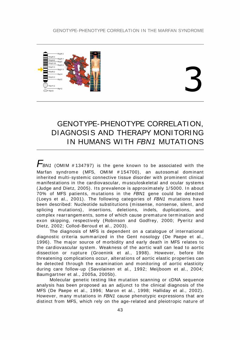
GENOTYPE-PHENOTYPE CORRELATION IN THE MARFAN SYNDROME
43
GENOTYPE-PHENOTYPE CORRELATION,DIAGNOSIS AND THERAPY MONITORING
IN HUMANS WITH FBN1 MUTATIONS
FBN1 (OMIM #134797) is the gene known to be associated with theMarfan syndrome (MFS, OMIM #154700), an autosomal dominantinherited multi-systemic connective tissue disorder with prominent clinicalmanifestations in the cardiovascular, musculoskeletal and ocular systems(Judge and Dietz, 2005). Its prevalence is approximately 1/5000. In about70% of MFS patients, mutations in the FBN1 gene could be detected(Loeys et al., 2001). The following categories of FBN1 mutations havebeen described: Nucleotide substitutions (missense, nonsense, silent, andsplicing mutations), insertions, deletions, indels, duplications, andcomplex rearrangements, some of which cause premature termination andexon skipping, respectively (Robinson and Godfrey, 2000; Pyeritz andDietz, 2002; Collod-Beroud et al., 2003).
The diagnosis of MFS is dependent on a catalogue of internationaldiagnostic criteria summarized in the Gent nosology (De Paepe et al.,1996). The major source of morbidity and early death in MFS relates tothe cardiovascular system. Weakness of the aortic wall can lead to aorticdissection or rupture (Groenink et al., 1998). However, before lifethreatening complications occur, alterations of aortic elastic properties canbe detected through the examination and monitoring of aortic elasticityduring care follow-up (Savolainen et al., 1992; Meijboom et al., 2004;Baumgartner et al., 2005a, 2005b).
Molecular genetic testing like mutation scanning or cDNA sequenceanalysis has been proposed as an adjunct to the clinical diagnosis of theMFS (De Paepe et al., 1996; Maron et al., 1998; Halliday et al., 2002).However, many mutations in FBN1 cause phenotypic expressions that aredistinct from MFS, which rely on the age-related and pleiotropic nature of
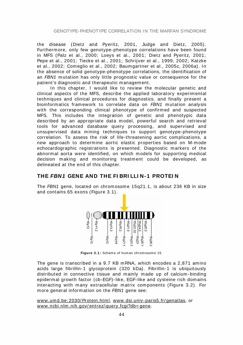
GENOTYPE-PHENOTYPE CORRELATION IN THE MARFAN SYNDROME
44
the disease (Dietz and Pyeritz, 2001, Judge and Dietz, 2005).Furthermore, only few genotype-phenotype correlations have been foundin MFS (Palz et al., 2000; Loeys et al., 2001; Dietz and Pyeritz, 2001;Pepe et al., 2001; Tiecke et al., 2001; Schrijver et al., 1999, 2002; Katzkeet al., 2002; Comeglio et al., 2002; Baumgartner et al., 2005c, 2006a). Inthe absence of solid genotype-phenotype correlations, the identification ofan FBN1 mutation has only little prognostic value or consequence for thepatient’s diagnostic and therapeutic management.
In this chapter, I would like to review the molecular genetic andclinical aspects of the MFS, describe the applied laboratory experimentaltechniques and clinical procedures for diagnostics, and finally present abioinformatics framework to correlate data on FBN1 mutation analysiswith the corresponding clinical phenotype of confirmed and suspectedMFS. This includes the integration of genetic and phenotypic datadescribed by an appropriate data model, powerful search and retrievaltools for advanced database query processing, and supervised andunsupervised data mining techniques to support genotype-phenotypecorrelation. To assess the risk of life-threatening aortic complications, anew approach to determine aortic elastic properties based on M-modeechocardographic registrations is presented. Diagnostic markers of theabnormal aorta were identified, on which models for supporting medicaldecision making and monitoring treatment could be developed, asdelineated at the end of this chapter.
THE FBN1 GENE AND THE FIBRILLIN-1 PROTEIN
The FBN1 gene, located on chromosome 15q21.1, is about 236 KB in sizeand contains 65 exons (Figure 3.1).
Figure 3.1: Scheme of human chromosome 15.
The gene is transcribed in a 9.7 KB mRNA, which encodes a 2,871 aminoacids large fibrillin-1 glycoprotein (320 kDa). Fibrillin-1 is ubiquitouslydistributed in connective tissue and mainly made up of calcium-bindingepidermal growth factor (cb-EGF)-like, EGF-like and cysteine rich domainsinteracting with many extracellular matrix components (Figure 3.2). Formore general information on the FBN1 gene see:
www.umd.be:2030/Protein.html, www.dsi.univ-paris5.fr/genatlas, orwww.ncbi.nlm.nih.gov/entrez/query.fcgi?db=gene.
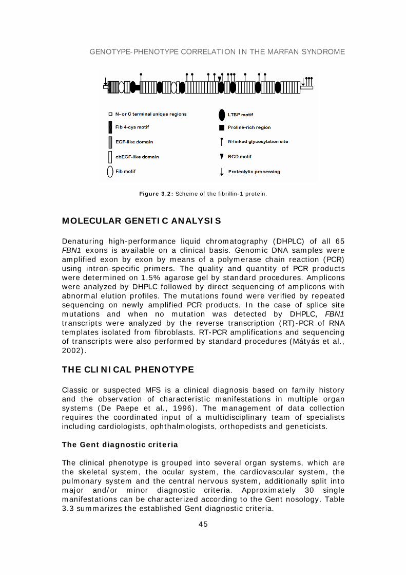
GENOTYPE-PHENOTYPE CORRELATION IN THE MARFAN SYNDROME
45
Figure 3.2: Scheme of the fibrillin-1 protein.
MOLECULAR GENETIC ANALYSIS
Denaturing high-performance liquid chromatography (DHPLC) of all 65FBN1 exons is available on a clinical basis. Genomic DNA samples wereamplified exon by exon by means of a polymerase chain reaction (PCR)using intron-specific primers. The quality and quantity of PCR productswere determined on 1.5% agarose gel by standard procedures. Ampliconswere analyzed by DHPLC followed by direct sequencing of amplicons withabnormal elution profiles. The mutations found were verified by repeatedsequencing on newly amplified PCR products. In the case of splice sitemutations and when no mutation was detected by DHPLC, FBN1transcripts were analyzed by the reverse transcription (RT)-PCR of RNAtemplates isolated from fibroblasts. RT-PCR amplifications and sequencingof transcripts were also performed by standard procedures (Mátyás et al.,2002).
THE CLINICAL PHENOTYPE
Classic or suspected MFS is a clinical diagnosis based on family historyand the observation of characteristic manifestations in multiple organsystems (De Paepe et al., 1996). The management of data collectionrequires the coordinated input of a multidisciplinary team of specialistsincluding cardiologists, ophthalmologists, orthopedists and geneticists.
The Gent diagnostic criteria
The clinical phenotype is grouped into several organ systems, which arethe skeletal system, the ocular system, the cardiovascular system, thepulmonary system and the central nervous system, additionally split intomajor and/or minor diagnostic criteria. Approximately 30 singlemanifestations can be characterized according to the Gent nosology. Table3.3 summarizes the established Gent diagnostic criteria.

GENOTYPE-PHENOTYPE CORRELATION IN THE MARFAN SYNDROME
46
Table 3.3: Clinical symptoms and family/genetic history according to the Gent nosology
Skeletal system (major criteria):1. pectus excavatum requiring surgery or pectus carinatum,2. reduced upper to lower segment ratio or arm span to height ratio greater than 1.05,3. - wrist sign (requiring that the thumb overlaps the terminal phalanx of the 5th digit when
grasping the contralateral wrist)- thumb sign (when the hand is clenched, the entire nail of the thumb projects beyond theulnar border of the hand),
4. scoliosis of >20° or spondylolisthesis,5. reduced extension at the elbows (<170°),6. medial displacement of the medial malleolus causing pes planus,7. protrusio acetabuli of any degree (ascertained on radiographs).
Skeletal system (minor criteria):1. pectus excavatum of moderate severity,2. joint hypermobility,3. highly arched palate with crowding of teeth,4. facial appearance (dolichocephaly, malar hypoplasia, enophthalmos, retrognathia,
downslanting palpebral fissures).
Ocular system (major criterion):1. ectopia lentis.
Ocular system (minor criteria):1. abnormally flat cornea (as measured by keratometry),2. increased axial length of globe (as measured by ultrasound),3. hypoplastic iris or hypoplastic ciliary muscle causing increased myosis.
Cardiovascular system (major criteria):1. dilatation of the ascending aorta with or without aortic regurgitation and involving at least
the sinuses of Valsalva, 2. dissection of the ascending aorta.
Cardiovascular system (minor criteria):1. mitral valve prolapse with or without mitral valve regurgitation,2. dilatation of the main pulmonary artery, in the absence of valvular or peripheral
pulmonary stenosis or any other obvious cause, below the age of 40 years,3. calcification of the mitral annulus below the age of 40 years,4. dilatation or dissection of the descending thoracic or abdominal aorta below the age of 50
years.
Pulmonary system (minor criteria):1. spontaneous pneumothorax,2. apical blebs (ascertained by chest radiography).
Skin and integument (minor criteria):1. striae atrophicae (stretch marks) not associated with marked weight changes, pregnancy
or repetitive stress,2. recurrent inguinal or incisional herniae.
Dura (major criterion):1. lumbosacral dural ectasia (ascertained by CT or MRI).
Family/genetic history (major criteria):1. having a parent, child or sibling who meets these diagnostic criteria independently,2. presence of a mutation in FBN1 known to cause the Marfan syndrome,3. presence of a haplotype around FBN1, inherited by descent, known to be associated with
unequivocally diagnosed Marfan syndrome in the family.
Gent nosology for the Marfan syndrome [De Paepe et al., Am J Med Genet, 1996; summarizedagain in: Baumgartner et al., Methods Inf Med, 2005].
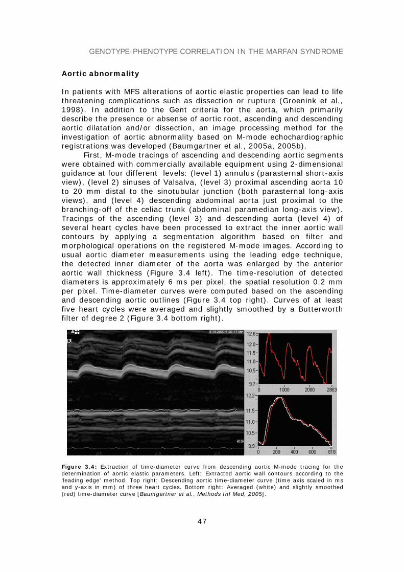
GENOTYPE-PHENOTYPE CORRELATION IN THE MARFAN SYNDROME
47
Aortic abnormality
In patients with MFS alterations of aortic elastic properties can lead to lifethreatening complications such as dissection or rupture (Groenink et al.,1998). In addition to the Gent criteria for the aorta, which primarilydescribe the presence or absense of aortic root, ascending and descendingaortic dilatation and/or dissection, an image processing method for theinvestigation of aortic abnormality based on M-mode echochardiographicregistrations was developed (Baumgartner et al., 2005a, 2005b).
First, M-mode tracings of ascending and descending aortic segmentswere obtained with commercially available equipment using 2-dimensionalguidance at four different levels: (level 1) annulus (parasternal short-axisview), (level 2) sinuses of Valsalva, (level 3) proximal ascending aorta 10to 20 mm distal to the sinotubular junction (both parasternal long-axisviews), and (level 4) descending abdominal aorta just proximal to thebranching-off of the celiac trunk (abdominal paramedian long-axis view).Tracings of the ascending (level 3) and descending aorta (level 4) ofseveral heart cycles have been processed to extract the inner aortic wallcontours by applying a segmentation algorithm based on filter andmorphological operations on the registered M-mode images. According tousual aortic diameter measurements using the leading edge technique,the detected inner diameter of the aorta was enlarged by the anterioraortic wall thickness (Figure 3.4 left). The time-resolution of detecteddiameters is approximately 6 ms per pixel, the spatial resolution 0.2 mmper pixel. Time-diameter curves were computed based on the ascendingand descending aortic outlines (Figure 3.4 top right). Curves of at leastfive heart cycles were averaged and slightly smoothed by a Butterworthfilter of degree 2 (Figure 3.4 bottom right).
Figure 3.4: Extraction of time-diameter curve from descending aortic M-mode tracing for thedetermination of aortic elastic parameters. Left: Extracted aortic wall contours according to the‘leading edge’ method. Top right: Descending aortic time-diameter curve (time axis scaled in msand y-axis in mm) of three heart cycles. Bottom right: Averaged (white) and slightly smoothed(red) time-diameter curve [Baumgartner et al., Methods Inf Med, 2005].

GENOTYPE-PHENOTYPE CORRELATION IN THE MARFAN SYNDROME
48
In some M-mode tracings, minor manual corrections of aortic wallcontours had to be carried out; however, the interobserver reproducibilitydid not exceed 5%. Blood pressure measurements were taken at the rightarm oscillometrically (Dinamap) immediately before M-mode registration.The following aortic root (RootAo), ascending (AscAo) and descending(DescAo) aortic parameters were calculated from M-mode time-diametercurves and blood pressure registrations. Aortic dilatation was determinedusing standard nomograms:
Normalized diastolic RootAo, AscAo and DescAo diameters (referenced topatient’s body surface area, BSA):
Dd’ = Dd /BSA [mm/m2] (1)
AscAo and DescAo maximum systolic diameter increase:
Increase = (Ds-Dd)/Dd [%] (2)
AscAo and DescAo distensibility:
7
dsd
ds 013331PPA
AAlityDistensibi ⋅
⋅−⋅−
=)(
[kPa-1⋅10-3] (3)
AscAo and DescAo stiffness index (SI):
( )dsd
ds
DDDPPln
SI)/(
/−
= dimensionless (4)
AscAo and DescAo maximum systolic area increase (MSAI):
( )( )max
d 1001A/)t(Adtd
MSAI ⋅−= [%/100ms] (5)
Magnitude of a vector loop by combining AscAo and DescAo diameterchanges:
Magnitude(t) =
( )( ) ( )( )2DescAod2AscAod 0011D/)t(D0011D/)t(D ⋅−+⋅−= [%] (6)
Phase of the vector loop
( )( ) ⎟⎟
⎠
⎞⎜⎜⎝
⎛−−
=AscAod
DescAod
1D)t(D1D)t(D
arctan)t(Phase//
[degree, °] (7)
Dd and Ds are the diastolic (minimum) and systolic (maximum) aorticdiameters, Ad and As are the diastolic and systolic cross-sectional (CS)aortic areas, Pd and Ps are the diastolic and systolic blood pressures inmmHg, D(t) is the aortic time-diameter curve and A(t) is the aortic time-area curve over the heart cycle. CS area A is estimated by (D/2)2⋅π.
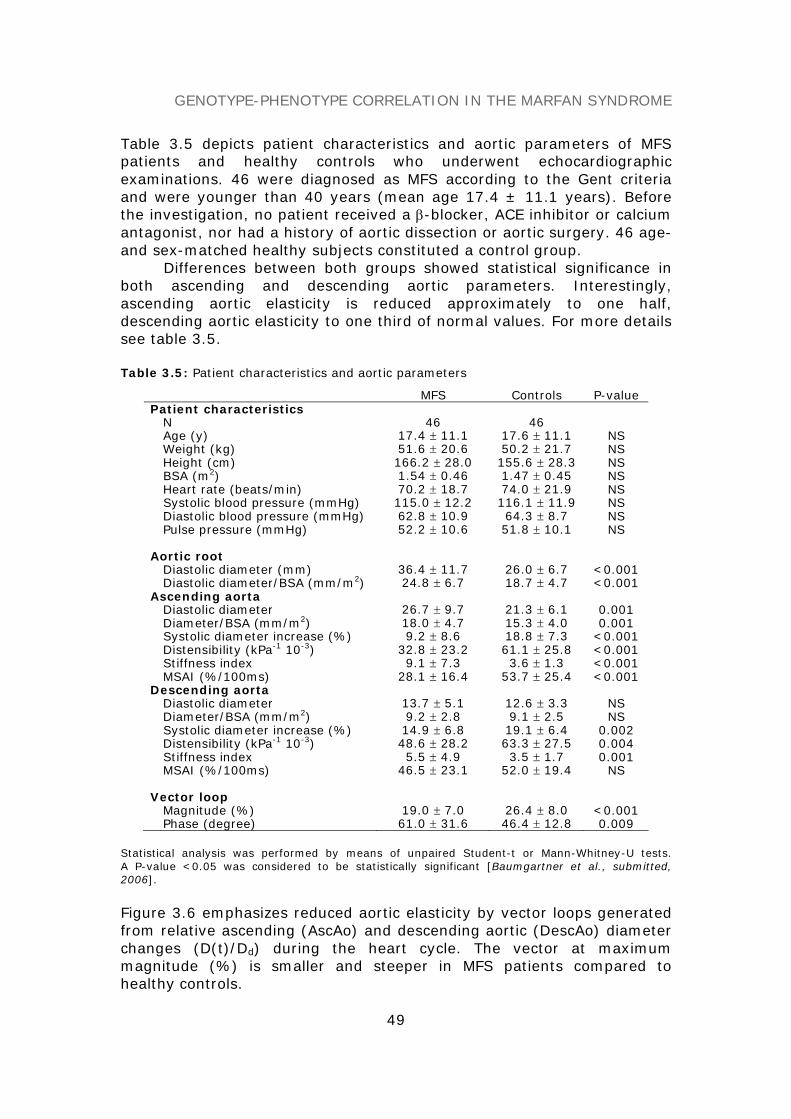
GENOTYPE-PHENOTYPE CORRELATION IN THE MARFAN SYNDROME
49
Table 3.5 depicts patient characteristics and aortic parameters of MFSpatients and healthy controls who underwent echocardiographicexaminations. 46 were diagnosed as MFS according to the Gent criteriaand were younger than 40 years (mean age 17.4 ± 11.1 years). Beforethe investigation, no patient received a β-blocker, ACE inhibitor or calciumantagonist, nor had a history of aortic dissection or aortic surgery. 46 age-and sex-matched healthy subjects constituted a control group.
Differences between both groups showed statistical significance inboth ascending and descending aortic parameters. Interestingly,ascending aortic elasticity is reduced approximately to one half,descending aortic elasticity to one third of normal values. For more detailssee table 3.5.
Table 3.5: Patient characteristics and aortic parameters
MFS Controls P-valuePatient characteristics
N 46 46Age (y) 17.4 ± 11.1 17.6 ± 11.1 NSWeight (kg) 51.6 ± 20.6 50.2 ± 21.7 NSHeight (cm) 166.2 ± 28.0 155.6 ± 28.3 NSBSA (m2) 1.54 ± 0.46 1.47 ± 0.45 NSHeart rate (beats/min) 70.2 ± 18.7 74.0 ± 21.9 NSSystolic blood pressure (mmHg) 115.0 ± 12.2 116.1 ± 11.9 NSDiastolic blood pressure (mmHg) 62.8 ± 10.9 64.3 ± 8.7 NSPulse pressure (mmHg) 52.2 ± 10.6 51.8 ± 10.1 NS
Aortic rootDiastolic diameter (mm) 36.4 ± 11.7 26.0 ± 6.7 <0.001Diastolic diameter/BSA (mm/m2) 24.8 ± 6.7 18.7 ± 4.7 <0.001
Ascending aortaDiastolic diameter 26.7 ± 9.7 21.3 ± 6.1 0.001Diameter/BSA (mm/m2) 18.0 ± 4.7 15.3 ± 4.0 0.001Systolic diameter increase (%) 9.2 ± 8.6 18.8 ± 7.3 <0.001Distensibility (kPa-1 10-3) 32.8 ± 23.2 61.1 ± 25.8 <0.001Stiffness index 9.1 ± 7.3 3.6 ± 1.3 <0.001MSAI (%/100ms) 28.1 ± 16.4 53.7 ± 25.4 <0.001
Descending aortaDiastolic diameter 13.7 ± 5.1 12.6 ± 3.3 NSDiameter/BSA (mm/m2) 9.2 ± 2.8 9.1 ± 2.5 NSSystolic diameter increase (%) 14.9 ± 6.8 19.1 ± 6.4 0.002Distensibility (kPa-1 10-3) 48.6 ± 28.2 63.3 ± 27.5 0.004Stiffness index 5.5 ± 4.9 3.5 ± 1.7 0.001MSAI (%/100ms) 46.5 ± 23.1 52.0 ± 19.4 NS
Vector loopMagnitude (%) 19.0 ± 7.0 26.4 ± 8.0 <0.001Phase (degree) 61.0 ± 31.6 46.4 ± 12.8 0.009
Statistical analysis was performed by means of unpaired Student-t or Mann-Whitney-U tests.A P-value <0.05 was considered to be statistically significant [Baumgartner et al., submitted,2006].
Figure 3.6 emphasizes reduced aortic elasticity by vector loops generatedfrom relative ascending (AscAo) and descending aortic (DescAo) diameterchanges (D(t)/Dd) during the heart cycle. The vector at maximummagnitude (%) is smaller and steeper in MFS patients compared tohealthy controls.

GENOTYPE-PHENOTYPE CORRELATION IN THE MARFAN SYNDROME
50
Figure 3.6: Vector loops represent relative ascending (AscAo) and descending aortic (DescAo)diameter changes (D(t)/Dd) during the heart cycle. The 95% confidence interval at 0, 200, 400 and600 ms is denoted by thin lines. The loop of the Marfan (MFS) patients is smaller and a littlesteeper than that of the control group. This shows the reduction of aortic elasticity predominantlypresent in the AscAo of MFS patients. The two arrows indicate the vectors’ maximum magnitude ofthe MFS and the control group. Loops are not closed because of varying cycle length of individuals.Beyond 600 ms cycle length data were not included [Baumgartner et al., J Thorac Cardiovasc Surg,2005].
THE GENOTYPE-PHENOTYPE DATA MODEL
A web-based FBN1/MFS information system, implemented as three tierarchitecture with presentation, business and data layer, was provided tocollect, manage and analyze genotypic and phenotypic data. To integratecomplex and heterogeneous data, a relational data model was designed,which enables the user to query the database at different levels ofmutational and clinical information for reviewing datasets of interest andmining correlations.
The genotype data model
An international nomenclature system has been suggested for thedescription of mutations and polymorphisms in DNA and proteinsequences (Den Dunnen and Antonarakis, 2001). Based on theserecommendations, a genotype database scheme, which describessequence variations at both cDNA and protein levels systematically, wasdesigned. Figure 3.7a depicts the genotype data model represented by a

GENOTYPE-PHENOTYPE CORRELATION IN THE MARFAN SYNDROME
51
simplified UML class diagram. The top compartment contains the name ofthe class (=DB relation), the bottom compartment the list of attributesdeclared in SQL data types. Associations between relations are modeledby 0..1 relationships.
The description of nucleotide changes at the cDNA level wasmodeled by introducing class attributes according to the internationalmutation nomenclature. In order to categorize mutations, different sub-types of nucleotide changes like substitutions, which were furthercategorized into transversions and transitions, deletions, insertions,duplications, inversions and, respectively, more complex arrangementswere defined. Consequence of mutations at the protein level weredescribed and modeled in a similar way. The genotype general descriptionclass represents the combination of mutation types at the DNA level andtheir consequences at the protein level, the affected exons/introns andprotein domains. Based on this scheme, three different mutations with theexplicit attribute values are exemplified in Table 3.8.
The phenotype data model
The phenotype data model was designed according to the multi-systemicpicture of the disease (Gent nosology). Figure 3.7b depicts the UML classdiagram of the clinical phenotype in more detail:
Each affected organ system, i.e. the skeletal, cardiovascular (CVS),ocular, pulmonary, skin and integument, and dura system, was modeledfrom a more general view to emphasize the system involvement and theaccumulated number of diagnosed criteria. To be more specific, eachorgan system was further separated into sub-systems, which contain thesingle manifestations. A general patient information class providesadditional information according to the patient’s ethnics, sex, age, MFStype (e.g. classical, suspected) and family history.
Table 3.8: Three examples of FBN1 mutations described by the genotype data model(Part 1)
Sub/Mis Sub/Stop Del/FsNucleotide Changes–DNA Levelname ‘3410G>C’ ‘6339T>G’ ‘1206del1’wt codon ‘CGC’ ‘TAT’ ‘CCT’mutant codon ‘CCC’ ‘TAG’ ‘CCC’nucleotide position 3410 6339 1206event ‘G>C’ ‘T>G’ ‘FS+PTC’exon coding region affected 1 1 1intron 5’ part affected 0 0 0intron 3’ part affected 0 0 0gene flanking or UTR region affected 0 0 0
Substitution - DNAtransversion 1 1transition 0 0
Deletion - DNAsingle nucleotide deletion 1several nucleotide deletion 0deleted unit ‘T’deleted length 1
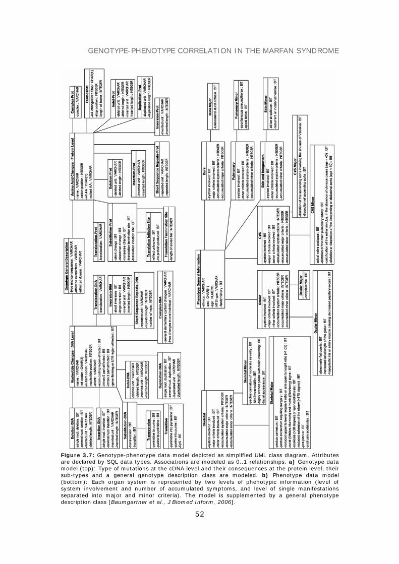
GENOTYPE-PHENOTYPE CORRELATION IN THE MARFAN SYNDROME
52
Figure 3.7: Genotype-phenotype data model depicted as simplified UML class diagram. Attributesare declared by SQL data types. Associations are modeled as 0..1 relationships. a) Genotype datamodel (top): Type of mutations at the cDNA level and their consequences at the protein level, theirsub-types and a general genotype description class are modeled. b) Phenotype data model(bottom): Each organ system is represented by two levels of phenotypic information (level ofsystem involvement and number of accumulated symptoms, and level of single manifestationsseparated into major and minor criteria). The model is supplemented by a general phenotypedescription class [Baumgartner et al., J Biomed Inform, 2006].

GENOTYPE-PHENOTYPE CORRELATION IN THE MARFAN SYNDROME
53
Table 3.8: Three examples of FBN1 mutations described by the genotype data model(Part 2)
Sub/Mis Sub/Stop Del/FsAmino Acid Changes–Protein Levelname ‘R1137P’ ‘Y2113X’ ‘P404HfsX44’codon position 1137 2113 404wt AA ‘R’ ‘Y’ ‘P’mutant AA ‘P’ ‘X’ ‘H’
Substitution - Protsilent change 0 0missense change 1 0nonsense change 0 1translation termination site 0 0translation initiation site 0 0
FrameshiftAA changed into Stop ‘V’stop position 447length of new reading frame 44
Genotype General Descriptiontype and consequence ‘Sub/Mis’ ‘Sub/Stop’ ‘Del/Fs’affected exon/intron ‘e27’ ‘e51’ ‘e10’affected domain ‘cb-EGF 17’ ‘LTBP 6’ ‘Pro-rich’
Nucleotide changes at the cDNA level, amino acid (AA) changes at the protein level specified bytheir subtypes, and a general genotype description are exemplified for a substitution/missensemutation (Sub/Mis), a substitution/nonsense mutation (Sub/Stop) and a deletion causing FS + PTC(Del/Fs). Attribute values are given in SQL data types. The Deletion-Prot class is not exemplifiedbecause it is only relevant for deleted units of at least one AA [Baumgartner et al., J BiomedInform, 2006].
SIMILARITY QUERY PROCESSING
A query model based on log-likelihood weights for each of the Gentcriteria was introduced to request the database for mutations of relatedphenotype. In the following the log-likelihood weights are defined byphenotype scores.
Phenotype score calculation
Let DB be a genotype-phenotype database organized in the form of a setof tuples T = {(cj, o) | cj ∈ C, o ∈ DB && o =[0,1]}, where cj is a specifiedmutation class and o is the set of clinical manifestations binary coded. Therelative entropy of two probability distributions P and Q is computed as
∑−==
N
1i i
i2i qp
logp)Q,P(H (8)
where pi is the frequency of a symptom within class cj, whereas qi isdefined as the frequency of the symptom in DB, excluding all tuples ofclass cj. A score value si of a single symptom with respect to (w.r.t.) classcj is thus given as
i
i2ii q
plogps ⋅λ= (9)

GENOTYPE-PHENOTYPE CORRELATION IN THE MARFAN SYNDROME
54
where λ is a scaling factor (λ was set to 100). The score value si can beinterpreted as a measure of the distance between pi and qi. If pi equals qi,then si is 0. If pi is 0, si is undefined. In order to consider a symptom thatis not present in class cj through a corresponding score value, si can be setto 0 under the assumption that pi → 0. Consequently, positive si valuesindicate the symptoms’ frequencies w.r.t. class ci above qi (frequencies inDB - ci), negative values below them.
A matrix M of score sets can be generated, where cj ∈ C representspecified mutation classes at the same level of mutational information, forexample, Sub/Mis, Sub/Stop, Del/Fs, Ins/Fs, etc.:
M = {(cj, s) | cj ∈ C, s ∈ S && s ∈ R} (10)
s is the set of score values of a clinical phenotype w.r.t. mutation class cj
and S is the collectivity of score sets in M. To assess phenotypicsimilarity/dissimilarity between a specified mutation class cj ∈ M and arequested MFS phenotype the parameter sc, a measure for the informationcontent of a given score set, is calculated. It is defined:
∑==
N
1iic ss (11)
The larger sc, the smaller the phenotypic similarity between a mutationclass cj and the requested phenotype.
Table 3.9 summarizes the calculated frequencies of MFS manifestations ona database of 163 patient entries. Mutation classes at four different levelsof mutational information, i.e. (i) type, (ii) type and consequence, (iii)type, consequence and location/mutational event, and (iv) the explicitmutation, were defined.
Table 3.9: Frequencies of clinical symptoms at different levels of mutational information
Information level Mutation class EL AADIL AADIS MVP PC PES ASR WTS SC PE JH HAP SA HE n AgeDatabase All entries 60 72 11 56 35 5 46 64 51 21 76 66 58 20 163 24(15)Type (DNA) Substitutions 66 69 11 51 34 4 42 61 50 22 72 64 52 20 119 24(16)
Non-substitutions 41 80 11 68 39 7 57 73 55 18 86 70 75 20 44 26(15)Type (DNA) and Sub/Mis 82 65 8 49 31 5 36 58 47 26 67 58 45 23 78 23(15)consequence (Prot) Sub/Stop 22 81 22 70 56 4 59 78 67 15 89 85 78 19 27 30(15)
Del/Fs 35 94 6 71 42 3 58 84 52 16 84 77 77 16 31 27(16)Type, consequence Sub/Mis/e1-e23 93 67 3 43 23 3 27 50 37 20 47 47 47 17 30 28(16)and location/event Sub/Mis/e24-e68 75 65 10 52 35 6 42 63 54 29 79 65 44 27 48 20(14)
Sub/Mis/Transition 82 62 8 48 26 8 34 54 46 26 68 56 44 30 50 25(17)Sub/Mis/Transversion 82 71 7 50 39 0 39 64 50 25 64 61 46 11 28 19(11)
Explicit mutation 507del1; Y170TfsX20 17 100 0 100 83 0 83 100 0 0 50 100 100 0 6 20(12)7801C>T; Q2601X 75 100 0 100 75 0 100 100 0 25 100 100 100 0 4 23(13)
Frequencies of symptoms are given in percent (%). Ocular system: EL = ectopia lentis;cardiovascular system: AADIL = dilation of ascending aorta, AADIS = dissection of ascendingaorta, MVP = Mitral valve prolapse; skeletal system: PC = pectus carinatum, PES = pectusexcavatum requiring surgery, ASR = arm span ratio, WTS = wrist or thumb sign, SC = scoliosis, PE= moderate pectus excavatum, JH = joint hypermobility, HAP = highly arched palate with crowdingof teeth; skin system: SA = striae atrophicae and HE = herniae. Non-substitutions are representedby Del, Ins, Dup and Indel mutations. Age is given as mean (SD) years. e is exon; n is number oftuples per mutation class [Baumgartner et al., J Biomed Inform, 2006].

GENOTYPE-PHENOTYPE CORRELATION IN THE MARFAN SYNDROME
55
By way of example, three classes of mutations, i.e. Sub/Mis, Sub/Stopand Del/Fs, were specified at the level of type and consequence ofmutations. Within these classes, ectopia lentis (EL) manifested in 82% ofmissense mutations (score 89), but only in 22% of nonsense mutations(score -35). Interestingly, in deletions causing FS + PTC we observed asimilarly decreased frequency of EL of 35% (score = -31). Nonsensemutations showed the second highest proportion of aortic dilatation(AADIL = 81%, score = 18) and the highest risks for aortic dissection(AADIS = 22%, score = 30), and thus lead to the most severe phenotypicexpressions in the CVS with a higher risk of life-threatening complications.The highest accumulated absolute score sc was also calculated for thismutation class (362), which emphasizes its low degree of phenotypicsimilarity w.r.t. DB. Explicit mutations, however, yielded the largest sc
values (s507del1 = 601, s7801C>T = 621) arising from maximum homogeneityof several manifestations. Moreover, both mutations point out a closephenotypic similarity because phenotypic expressions are almost equal.
Similarity requests on specified mutation classes
In order to assign a query phenotype O = { o | (o1, …, oN), o ∈ [0,1]} ofunknown mutation to a specified mutation class cj ∈ M, a matchingparadigm that operates on matrix M by processing similarity requests foreach class cj ∈ M was developed. A two-step procedure must beprocessed:
1. Balancing of the score matrix M w.r.t all specified mutation classesc ∈ M. The absolute score values sc of classes c ∈ M can significantlydiffer in size, which can lead to a preferred assignment of the querytuple O to that class cj, which is represented by the highest measuresc within M. Therefore, each score set s ∈ S has to be corrected tothe mean absolute score cs , which is calculated as the mean valueof all sc ∈ M, in order to balance matrix M. Therefore, M* is the
cs -balanced matrix of M with s*∈ M*.2. Assignment of the query phenotype O, weighted by the balanced
score sets s*∈ M* to a mutation class cj ∈ M*. The decision rule isdefined as follows:
( ) ⎟⎟⎠
⎞⎜⎜⎝
⎛∑ ⋅==∈
N
1i
2
i*i
*McosmaxargC for
⎩⎨⎧
=absentissymptomif0presentissymptomif1
oi (12)
Here, the query model built on a square distance measure assigns therequested MFS phenotype O to that mutation class cj ∈ M*, whosedistance is maximal.
Scoring matrices were generated based on data subsets returned from DBqueries, utilizing the underlying data model. Table 3.10 shows scorematrices at different levels of mutational information.

GENOTYPE-PHENOTYPE CORRELATION IN THE MARFAN SYNDROME
56
Table 3.10: Score matrices M and classification accuracy of matching
Matrix Mutation class EL AADIL AADIS MVP PC PES ASR WTS SC PE JH HAP SA HE sc Rec. Prec. Acc.M1 Substitutions 46 -14 -1 -21 -7 -3 -18 -16 -7 6 -19 -9 -27 0 194 67.2 80.8 65.0
Non-substitutions -29 16 1 28 8 5 25 19 8 -5 22 10 39 0 215 59.1 40M2 Sub/Mis 89 -16 -7 -17 -10 1 -22 -15 -9 16 -23 -20 -29 9 284 82.1 79 64.7
Sub/Stop -35 18 30 29 47 -2 27 27 32 -9 24 40 40 -3 362 18.5 50Del/Fs -31 46 -6 31 14 -2 25 42 1 -7 15 23 41 -6 291 61.3 42.2
M3 Sub/Mis/e1-e23 79 -9 -6 -19 -16 -2 -24 -21 -21 -1 -39 -27 -18 -6 288 66.7 32.8 34.6Sub/Mis/e24-e68 37 -14 -1 -7 1 3 -8 -3 7 22 7 -2 -24 17 154 14.6 41.2
M4 Sub/Mis/Transition 60 -18 -5 -15 -15 9 -20 -18 -10 13 -16 -18 -24 27 268 0.04 100 38.5Sub/Mis/Transversion 48 -1 -5 -9 8 0 -11 1 -2 8 -19 -8 -18 -11 148 100 36.8
M5 507del1; Y170TfsX20 -31 50 0 89 111 0 75 68 0 0 -31 64 82 0 601 - - -7801C>T; Q2601X 26 49 0 87 86 0 116 67 0 7 41 63 81 0 621 - - -
Score matrices M1 – M5 correspond to the symptom’s frequencies at different levels of mutationalinformation as shown in Table 3.9 (e.g. M1 = Type (DNA)). Score values are dimensionless. sc isthe accumulated absolute score w.r.t. a mutation class. Classification accuracy (Rec. = recall,Prec. = precision and Acc. = accuracy) is given in percent (%). Balanced matrices (M1* – M4*) arenot explicitly shown [Baumgartner et al., J Biomed Inform, 2006].
Based on score matrices M and the accumulated absolute score measuresc, four cs -balanced matrices, M1* - M4*, were generated. Similarityrequests w.r.t. score matrix M1* lead to a recall rate of 67%(substitutions) vs. 59% (non-substitutions) with an overall classificationaccuracy of 65%. Three mutation classes (missense, nonsense mutations,and deletions causing FS + PTC) could be generated at the level of typeand consequence (M2*). 82% of Sub/Mis mutations and 61% of Del/Fswere correctly assigned, whereas the majority of nonsense mutationswere wrongly classified to the Del/Fs class. Comparing score sets ofSub/Stop and Del/Fs, both groups yielded partly similar score values,which cause the incorrect assignment. Location and type of mutationalevents were considered for class specification in M3* and M4*. Recallvalues of 0.04% and 14.6%, respectively, demonstrated that one of bothclasses was wrongly assigned. Marginal differences between thephenotypic expressions emphasize this result.
Similarity requests for explicit mutations
For searching mutations of related phenotypic expression in DB, asimilarity request at the level of explicit mutations can be processed ifscore sets of single mutations can be generated. From the clinicalsituation it is known that more than 20 to 25 subjects per mutation arenot available because of the multiplicity of mutations. Therefore, at least5-10 tuples per mutation are provided for the scoring task. An explicitmutation ms, of which a score set s can be generated, can formally bewritten as:
ms = {s | s ∈ S && s ∈ R } (13)
Let DB be a genotype-phenotype database at the level of single mutationsgiven in the form of a set of tuples T = {(mj, o) | mj ∈ MU, o ∈ DB &&o ∈ [0,1]}, where mj is an explicit mutation and o is the set of clinicalmanifestations. MU is the collectivity of all different mutations represented

GENOTYPE-PHENOTYPE CORRELATION IN THE MARFAN SYNDROME
57
in DB. For a DB request the query model of mutation ms uses the definedsimilarity measure:
( )∑ ⋅==
N
1i
2
iim oss (14)
Here, s ∈ S represents the score set of mutation ms as denoted inequation 13. The best ranked hits T according to maximal value of ms arereturned as the query result.
A similarity request for the mutation 507del1;Y170TfsX20 was performed,of which a score set was generable (see Table 3.10, M5). The returnedquery result is shown in Table 3.11. The best 20 hits (~12% of DB)assessed by the similarity measure ms are displayed. 80% of them areSub/Stop or Del/Fs mutations, one is a deletion-splice site mutation (Del-Splice/?), and 15% are Sub/Mis mutations. No substitution-splice sitemutations were returned. Among the first 10 hits solely Sub/Stop orDel/Fs mutations were displayed. The 507del1 mutation, on which thequery score set was generated, was displayed four times.
Table 3.11: Similarity request for mutation 507del1;Y170TfsX20 on DB (best 20 hits).
No. NucleotideChanges
AAChanges
Type/Consequence
Exon/Intron
Domain Age(y) ms Rank
1 7801 C>T Q2601X Sub/Stop 62 cb-EGF 45 43 213 12 7801 C>T Q2601X Sub/Stop 62 cb-EGF 45 16 213 13 2581 C>T R861X Sub/Stop 21 hybrid 49 213 14 6423 del1 L2104fsX? Del/Fs 52 LTBP 6 45 213 15 507 del1 Y170fsX20 Del/Fs 5 EGF 3 43 211 26 507 del1 Y170fsX20 Del/Fs 5 EGF 3 14 211 27 7801 C>T Q2601X Sub/Stop 62 cb-EGF 45 18 211 28 4567 C>T R1521X Sub/Stop 36 cb-EGF 26 49 211 29 507 del1 Y170fsX20 Del/Fs 5 EGF 3 10 208 310 507 del1 Y170fsX20 Del/Fs 5 EGF 3 18 208 311 5065+3_5065+7del5 ? Del-Splice/? IVS40 intronic 16 207 412 461 G>C C154S Sub/Mis 5 EGF 3 14 202 513 6661 T>C C2221R Sub/Mis 54 cb-EGF 38 27 200 614 507 del1 Y170fsX20 Del/Fs 5 EGF 3 20 197 715 8080 C>T R2694X Sub/Stop 64 C-term 22 197 716 5826 C>A C1942X Sub/Stop 47 cb-EGF 33 18 197 717 5826 C>A C1942X Sub/Stop 47 cb-EGF 33 22 197 718 3302 A>G Y1101C Sub/Mis 26 cb-EGF 16 17 197 719 3464 del17 R1192fsX? Del/Fs 28 cb-EGF 18 6 197 720 1206 del1 P404fsX44 Del/Fs 10 Pro-rich 7 195 8
The symbol ? denotes data not available (length of frameshift, AA change or consequence at theprotein level) [Baumgartner et al., J Biomed Inform, 2006].
This retrieval method facilitates the search of mutations of relatedphenotypes on DB, as exemplified for the mutation 507del1;Y170TfsX20.Here, the similarity measure ms is a useful parameter to assess phenotypicsimilarity of people carrying the same or related mutations as it may be ofinterest for the examination of the syndrome’s intra- and inter-familialphenotypic heterogeneity.

GENOTYPE-PHENOTYPE CORRELATION IN THE MARFAN SYNDROME
58
PHENOTYPE CLASSIFICATION
Phenotype classes identified on accumulated symptoms
A further score measure, which describes the similarity between apatient’s phenotypic expression and defined phenotype classes at the levelof accumulated major and minor criteria, was introduced. The followingdefinitions are required:
1. μsystem : Mean value of diagnosed symptoms in an organ system(major and minor criteria separated),
2. σsystem : Standard deviation of symptoms in an organ system (majorand minor criteria separated),
3. systemeksystemσ= : Factor quantifying phenotypic purity of an organ
system within a clustered phenotype class (k ≥ 1).
Table 3.12 depicts four phenotype classes identified from cluster analysison a data set of 100 patients. Statistical measures μsystem, σsystem andksystem are shown in the table in more detail.
Table 3.12: Statistical analysis of four phenotype classes
SkeletonMajor(0-7)
SkeletonMinor(0-4)
OcularMajor(0,1)
CVSMajor(0-2)
CVSMinor(0-2)
SkinMinor(0-2)
Phenotype I (n=46)
μ 2.74 2.04 1.00 1.00 0.72 0.59σ 1.29 1.09 0.00 0.00 0.58 0.62k 3.63 2.99 1.00 1.00 1.79 1.85Subtype Ia (n=23)
μ 2.52 1.65 1.00 1.00 0.43 0.04σ 1.08 1.07 0.00 0.00 0.51 0.21k 2.95 2.92 1.00 1.00 1.66 1.23Subtype Ib (n=23)
μ 2.96 2.43 1.00 1.00 1.00 1.13σ 1.46 0.99 0.00 0.00 0.52 0.34k 4.31 2.70 1.00 1.00 1.69 1.41Phenotype II (n=31)
μ 2.42 2.06 0.00 1.00 0.68 0.71σ 1.39 1.36 0.00 0.00 0.70 0.59k 3.99 3.91 1.00 1.00 2.02 1.80Phenotype III (n=16)
μ 1.69 1.56 1.00 0.00 0.31 0.69σ 1.35 1.21 0.00 0.00 0.48 0.60k 3.87 3.35 1.00 1.00 1.61 1.83Phenotype IV (n=7)
μ 1.71 2.29 0.00 0.00 0.43 0.29σ 1.11 1.11 0.00 0.00 0.53 0.49k 3.04 3.04 1.00 1.00 1.71 1.63
Mean value (μ), standard deviation (σ) and purity factor k of investigated organ systems are shownfor four phenotype classes I, Ia, Ib, II, III, and IV identified by hierarchical cluster analysis. Ocularmajor (ectopia lentis) and CVS major criterion (aortic root dilatation) showed maximum puritywithin each clustered phenotype class (k=1) [Baumgartner et al., Methods Inf Med, 2005].
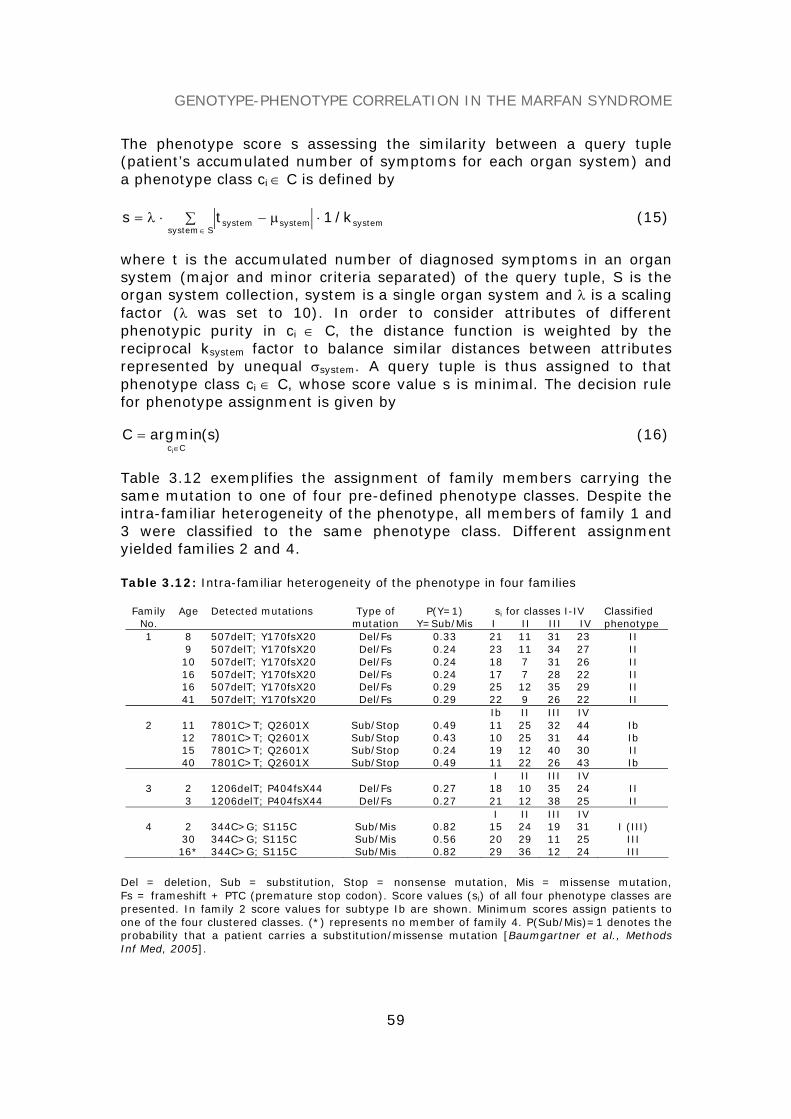
GENOTYPE-PHENOTYPE CORRELATION IN THE MARFAN SYNDROME
59
The phenotype score s assessing the similarity between a query tuple(patient’s accumulated number of symptoms for each organ system) anda phenotype class ci ∈ C is defined by
systemsystemsystemSsystem
k/1ts ⋅μ−∑⋅λ=∈
(15)
where t is the accumulated number of diagnosed symptoms in an organsystem (major and minor criteria separated) of the query tuple, S is theorgan system collection, system is a single organ system and λ is a scalingfactor (λ was set to 10). In order to consider attributes of differentphenotypic purity in ci ∈ C, the distance function is weighted by thereciprocal ksystem factor to balance similar distances between attributesrepresented by unequal σsystem. A query tuple is thus assigned to thatphenotype class ci ∈ C, whose score value s is minimal. The decision rulefor phenotype assignment is given by
)s(minargCCci∈
= (16)
Table 3.12 exemplifies the assignment of family members carrying thesame mutation to one of four pre-defined phenotype classes. Despite theintra-familiar heterogeneity of the phenotype, all members of family 1 and3 were classified to the same phenotype class. Different assignmentyielded families 2 and 4.
Table 3.12: Intra-familiar heterogeneity of the phenotype in four families
FamilyNo.
Age Detected mutations Type ofmutation
P(Y=1)Y=Sub/Mis
si for classes I-IVI II III IV
Classifiedphenotype
1 8 507delT; Y170fsX20 Del/Fs 0.33 21 11 31 23 II9 507delT; Y170fsX20 Del/Fs 0.24 23 11 34 27 II10 507delT; Y170fsX20 Del/Fs 0.24 18 7 31 26 II16 507delT; Y170fsX20 Del/Fs 0.24 17 7 28 22 II16 507delT; Y170fsX20 Del/Fs 0.29 25 12 35 29 II41 507delT; Y170fsX20 Del/Fs 0.29 22 9 26 22 II
Ib II III IV2 11 7801C>T; Q2601X Sub/Stop 0.49 11 25 32 44 Ib
12 7801C>T; Q2601X Sub/Stop 0.43 10 25 31 44 Ib15 7801C>T; Q2601X Sub/Stop 0.24 19 12 40 30 II40 7801C>T; Q2601X Sub/Stop 0.49 11 22 26 43 Ib
I II III IV3 2 1206delT; P404fsX44 Del/Fs 0.27 18 10 35 24 II
3 1206delT; P404fsX44 Del/Fs 0.27 21 12 38 25 III II III IV
4 2 344C>G; S115C Sub/Mis 0.82 15 24 19 31 I (III)30 344C>G; S115C Sub/Mis 0.56 20 29 11 25 III16* 344C>G; S115C Sub/Mis 0.82 29 36 12 24 III
Del = deletion, Sub = substitution, Stop = nonsense mutation, Mis = missense mutation,Fs = frameshift + PTC (premature stop codon). Score values (si) of all four phenotype classes arepresented. In family 2 score values for subtype Ib are shown. Minimum scores assign patients toone of the four clustered classes. (*) represents no member of family 4. P(Sub/Mis)=1 denotes theprobability that a patient carries a substitution/missense mutation [Baumgartner et al., MethodsInf Med, 2005].

GENOTYPE-PHENOTYPE CORRELATION IN THE MARFAN SYNDROME
60
Phenotype classes identified on the Gent diagnostic criteria
Cluster analysis is a useful tool to subgroup data. Here, hierarchicalcluster analysis on a set of clinical manifestations was performed. Figure3.13 demonstrated clusters identified on patients carrying either Sub/Mis,Sub/Stop or Del/Fs mutations.
Figure 3.13: Hierarchical cluster analysis of MFS Gent criteria. The complete linkage method wasapplied to calculate the distances. Left of the colour mosaic the type and consequence of mutationsare shown. The hierarchical tree is depicted to the right of the mosaic. The clustered manifestationsare given at the top; the scale measure of the linkage distance is shown on the bottom. Sub/Mis =missense mutation, Sub/Stop = nonsense mutation, Del/Fs = deletion/FS + PTC. For abbreviationsto clinical manifestations see legend in Table 3.9 [Baumgartner et al., J Biomed Inform, 2006].
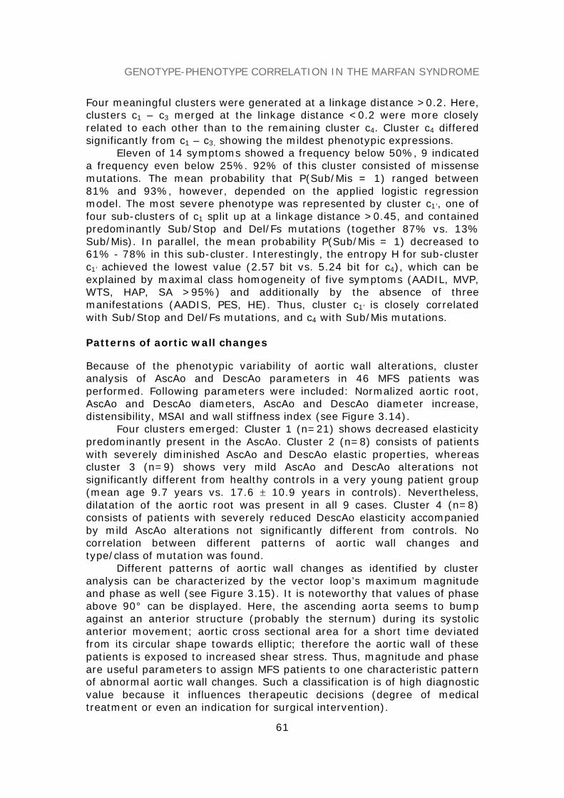
GENOTYPE-PHENOTYPE CORRELATION IN THE MARFAN SYNDROME
61
Four meaningful clusters were generated at a linkage distance >0.2. Here,clusters c1 – c3 merged at the linkage distance <0.2 were more closelyrelated to each other than to the remaining cluster c4. Cluster c4 differedsignificantly from c1 – c3, showing the mildest phenotypic expressions.
Eleven of 14 symptoms showed a frequency below 50%, 9 indicateda frequency even below 25%. 92% of this cluster consisted of missensemutations. The mean probability that P(Sub/Mis = 1) ranged between81% and 93%, however, depended on the applied logistic regressionmodel. The most severe phenotype was represented by cluster c1’, one offour sub-clusters of c1 split up at a linkage distance >0.45, and containedpredominantly Sub/Stop and Del/Fs mutations (together 87% vs. 13%Sub/Mis). In parallel, the mean probability P(Sub/Mis = 1) decreased to61% - 78% in this sub-cluster. Interestingly, the entropy H for sub-clusterc1’ achieved the lowest value (2.57 bit vs. 5.24 bit for c4), which can beexplained by maximal class homogeneity of five symptoms (AADIL, MVP,WTS, HAP, SA >95%) and additionally by the absence of threemanifestations (AADIS, PES, HE). Thus, cluster c1’ is closely correlatedwith Sub/Stop and Del/Fs mutations, and c4 with Sub/Mis mutations.
Patterns of aortic wall changes
Because of the phenotypic variability of aortic wall alterations, clusteranalysis of AscAo and DescAo parameters in 46 MFS patients wasperformed. Following parameters were included: Normalized aortic root,AscAo and DescAo diameters, AscAo and DescAo diameter increase,distensibility, MSAI and wall stiffness index (see Figure 3.14).
Four clusters emerged: Cluster 1 (n=21) shows decreased elasticitypredominantly present in the AscAo. Cluster 2 (n=8) consists of patientswith severely diminished AscAo and DescAo elastic properties, whereascluster 3 (n=9) shows very mild AscAo and DescAo alterations notsignificantly different from healthy controls in a very young patient group(mean age 9.7 years vs. 17.6 ± 10.9 years in controls). Nevertheless,dilatation of the aortic root was present in all 9 cases. Cluster 4 (n=8)consists of patients with severely reduced DescAo elasticity accompaniedby mild AscAo alterations not significantly different from controls. Nocorrelation between different patterns of aortic wall changes andtype/class of mutation was found.
Different patterns of aortic wall changes as identified by clusteranalysis can be characterized by the vector loop’s maximum magnitudeand phase as well (see Figure 3.15). It is noteworthy that values of phaseabove 90° can be displayed. Here, the ascending aorta seems to bumpagainst an anterior structure (probably the sternum) during its systolicanterior movement; aortic cross sectional area for a short time deviatedfrom its circular shape towards elliptic; therefore the aortic wall of thesepatients is exposed to increased shear stress. Thus, magnitude and phaseare useful parameters to assign MFS patients to one characteristic patternof abnormal aortic wall changes. Such a classification is of high diagnosticvalue because it influences therapeutic decisions (degree of medicaltreatment or even an indication for surgical intervention).
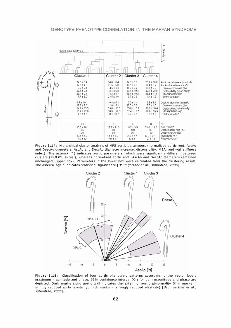
GENOTYPE-PHENOTYPE CORRELATION IN THE MARFAN SYNDROME
62
Figure 3.14: Hierarchical cluster analysis of MFS aortic parameters (normalized aortic root, AscAoand DescAo diameters, AscAo and DescAo diameter increase, distensibility, MSAI and wall stiffnessindex). The asterisk (*) indicates aortic parameters, which were significantly different betweenclusters (P<0.05, H-test), whereas normalized aortic root, AscAo and DescAo diameters remainedunchanged (upper box). Parameters in the lower box were calculated from the clustering result.The asterisk again indicates statistical significance [Baumgartner et al., submitted, 2006].
Figure 3.15: Classification of four aortic phenotypic patterns according to the vector loop’smaximum magnitude and phase. 95% confidence interval (CI) for both magnitude and phase aredepicted. Dark marks along aortic wall indicates the extent of aortic abnormality (thin marks =slightly reduced aortic elasticity, thick marks = strongly reduced elasticity) [Baumgartner et al.,submitted, 2006].

GENOTYPE-PHENOTYPE CORRELATION IN THE MARFAN SYNDROME
63
DIAGNOSTIC MARKERS AND THERAPY MONITORING
Predictive models on aortic parameters
In order to find aortic parameters, which distinguish best MFS patientsfrom healthy controls, parameters were evaluated by logistic regressionanalysis. Significant parameters were identified using the wrapperapproach for attribute selection. This method selects key markers from agiven parameter set, on which finally a classification model of minimizederror rate is built.
A multiple logistic regression model trained on 46 patients and 46matched controls including four key parameters, i.e. normalized aorticroot and AscAo diameters, AscAo and DescAo distensibility, discriminatedbest between both groups showing the highest sensitivity (85.1%),specificity (87.2%), and overall accuracy of 86.2%. The model wasvalidated by 5-fold cross-validation. The mean probability P for thepresence of MFS, P(MFS=1), was 81.6 ± 24% for the MFS group and18.4 ± 22.6% for the control group. Model coefficients, significance ofparameters and odds ratios are displayed in Table 3.16.
Table 3.16: Logistic regression analysis on aortic parameters
Parameters in the model Regressioncoefficients
Standarderror
Significance Oddsratios
Normalized root diameter(mm/m2)
0.842 0.201 <0.001 2.321
Normalized AscAo diameter(mm/m2)
-0.727 0.215 0.001 0.483
AscAo distensibility (kPa-1⋅10-3) -0.098 0.027 <0.001 0.907DescAo distensibility (kPa-1⋅10-3) -0.033 0.015 0.028 0.968Intercept 0.352 1.795 0.844 1.422
A probability measure in the form of P(MFS = 1) = 1/[1+exp(-z)], where z = a0 + a1x1 + a2x2 +anxn is the logit of the model, determines the class membership. P(MFS=1) means that MFS ispresent if P ≥ 0.5 or MFS is absent if P < 0.5 [Baumgartner et al., submitted, 2006].
This diagnostic model can predict MFS more reliably than a cardiologicalinvestigation including only aortic diameter measurements yielding asensitivity of 85.1% in our and 61-84% in published patient populations(Bruno et al., 1984; Roman et al., 1993; Peters et al., 2001).
Therapy monitoring
Data of 30 patients before, and 39 ± 16 months later during β-blockertreatment with 0.79 ± 0.46 mg/kg of atenolol were analyzed. Usually, thelast follow-up investigation was considered. In patients who had an aorticreplacement operation for severe aortic dilatation (n= 5) the lastpreoperative investigation was considered. Mean age at follow-up was19.9 ± 11.0 years. Heart rate decreased from 70 ± 22 bpm to 57 ± 11 bpmduring β-blocker treatment (P<0.001), diastolic blood pressure decreasedslightly from 63 to 60 mmHg (P=0.036), whereas systolic blood pressureand pulse pressure remained unchanged. Absolute diameters of the aortic

GENOTYPE-PHENOTYPE CORRELATION IN THE MARFAN SYNDROME
64
root increased from 34.8 ± 8.9 to 36.2 ± 8.4 mm; P=0.001 and of theAscAo from 25.9 ± 8.4 to 26.8 ± 7.5 mm; P=0.048, normalized diametersdecreased. DescAo absolute diameter increased significantly from12.7 ± 3.6 to 14.3 ± 3.5 mm, P<0.001, nevertheless, normalized DescAodiameters remained unchanged. AscAo and DescAo elastic parameterstended to improve, but differences were not statistically significant.Because a heterogenous response to β-blocker treatment is well known(Haouzi et al., 1997), data were sorted according to (A) diameter of theaortic root and (B) AscAo distensibility (see Figure 3.17).
Table 3.17: Aortic abnormality in response to β-blocker treatment
P is the probability that aortic abnormality is present based upon the model presented inTable 3.16 [Baumgartner et al., submitted, 2006].
The multiple logistic regression model´s interpretation can be modifiedinsofar, that the probability P, that MFS is present is changed to P, thataortic abnormality is present. In 70% of MFS patients P (aorticabnormality) decreased from 78% to 56% (-22%) and so indicatedimprovement of elasticity; in the remaining 30% patients P (aorticabnormality) increased from 75% to 94% (+18%) as a sign ofdeterioration. Mean β-blocker dosages of the two groups (0.78 ± 0.49mg/kg, and 0.82 ± 0.36 mg/kg) did not differ significantly. P (aortic

GENOTYPE-PHENOTYPE CORRELATION IN THE MARFAN SYNDROME
65
abnormality) sank in all patients having aortic root diameters between 20and 30 mm (see Figure 3.17a, left), in 62% with diameters between 30and 40 mm (middle), and in 60% with diameters between 40 and 52 mm(right). The three subgroups were statistically different from each otherregarding absolute and normalized diameters of the aortic root, AscAo,and DescAo, DescAo distensibility and stiffness index as well aspercentage of AscAo dilatation (14%, 31%, and 80% in the subgroups). Ifdata was sorted according to AscAo distensibility (Figure 3.17b), theprobability P of aortic abnormality dropped also in 100% of patients withan AscAo distensibility between 45 and 83 kPa-1· 10-3, in 75% of patientswith a distensibility between 30 and 45 kPa-1·10-3, and in 40% with adistensibility between 0 and 30 kPa-1·10-3. β-blocker dose of subgroups didnot differ significantly from each other (H-Test). Not surprisingly, theyoungest patients were to be found in the groups with the lowestdiameters and the greatest distensibility. Within the four characteristicaortic wall patterns only cluster 1 yielded a positive therapeutic responsewith a significant decrease of P(aortic abnormality).
CONCLUSION
As mentioned before, a few accepted genotype-phenotype correlations inthe MFS have been reported, for example, with a hot spot for neonatalMFS in exons 24-32 or a clustering of mutations causing milder forms inexons 59-65. More common occurrence of large-joint hypermobility (JH),less common ectopia lentis (EL) and retinal detachment are associatedwith premature termination codon (PTC) mutations, whereas, for example,missense mutations show a high frequency of EL (Sarfarazi et al., 1992;Palz et al., 2000; Loeys et al., 2001; Dietz and Pyeritz, 2001; Pepe et al.,2001; Tiecke et al., 2001; Schrijver et al., 1999, 2002; Katzke et al.,2002; Comeglio et al., 2002; Baumgartner et al., 2005c, 2006a). Some ofthe aforementioned correlations could be confirmed, some novel oneswere identified, although limitations concerning the incomplete descriptionof symptoms and the limited size of the provided data exist. Briefly,maximum phenotypic dissimilarity was found between missense mutationsand the groups of nonsense mutations and deletions causing FS + PTC.Key manifestations, which are relevant for best discriminating Sub/Misand Sub/Stop + Del/Fs class, are EL and several skeletal (major andminor) criteria, but not manifestations of the CVS and skin system.Comparing missense and nonsense mutations - independent of thelocation of the mutation in the gene - AADIS appears to be an additionaldiagnostic marker predominantly observed in patients carrying a nonsensemutation. More severe manifestations in the CVS lead to a higher risk oflife-threatening aortic dissection or rupture, which require immediatetherapeutic intervention. The most severe phenotypic expressions weresolely found in patients carrying a Sub/Stop or Del/Fs mutation, whereasthe mildest MFS phenotype appeared in Sub/Mis mutations. As thesefindings demonstrate, defined correlations are helpful tools to anticipateclinical consequences of specific mutations or mutation classes.

GENOTYPE-PHENOTYPE CORRELATION IN THE MARFAN SYNDROME
66
The determination of decreased aortic elastic properties in patientswith MFS by a standardized semi-automated image segmentationtechnique facilitates the estimation of ascending and descending aorticdistensibility, stiffness index and maximum systolic area increase withhigh reproducibility. It so gives way to high quality follow-upinvestigations of aortic elastic properties in patients with suspected orconfirmed MFS. Further successful application of this methodology hasbeen proven, for example, in systemic vascular diseases of the prestenoticarteries before and early after successful coarctation repair (Vogt et al.,2005) and in patients with Takayasu arteritis (Baumgartner et al., 2006b).Four characteristic patterns of ascending and descending aortic wallchanges could be identified in the MFS and so may show the region at riskfor severe aortic complications. Probabilistic models can be used asdiagnostic and prognostic tool with high accuracy, which are helpful toassess aortic abnormality during the follow-up, prove the efficiency ofmedical treatment, and so may serve as additional criteria to indicateelective surgical intervention.
REFERENCES
Baumgartner C, Mátyás G, Steinmann B, Eberle M, Stein JI, Baumgartner D. (2006a) A bioinformatics framework for genotype-phenotype correlation in humans withMarfan syndrome caused by FBN1 gene mutations. J Biomed Inform, 39, 171-183.
Baumgartner D*, Baumgartner C*, Schermer E, Engl G, Schweigmann U, Stein IJ.(2006b) Different patterns of aortic wall elasticity in patients with Marfan syndrome: A noninvasive follow-up study, submitted.
Baumgartner C, Mátyás G, Steinmann B, Baumgartner D. (2005a) Marfan syndrome:A diagnostic challenge caused by phenotypic and genetic heterogeneity. Methods InfMed, 44, 487-497.
Baumgartner D, Baumgartner C, Mátyás G, Steinmann B, Löffler J, Schermer E,Schweigmann U, Baldissera I, Frischhut B, Hess J, Hammerer I. (2005b) Diagnosticpower of aortic elastic properties in young patients with Marfan syndrome. J ThoracCardiovasc Surg, 129, 730-739.
Baumgartner C, Baumgartner D, Eberle M, Plant C, Mátyás G, Steinmann B. Genotype-phenotype correlation in patients with fibrillin-1 gene mutations. (2005c) Proc. 3rd Int.Conf. on Biomedical Engineering (BioMED2005), Innsbruck, Austria, pp. 561-566.
Baumgartner D*, Sailer-Höck M*, Baumgartner C, Trieb T, Maurer H, Schirmer M,Zimmerhackl LB, Stein JI. (2005d) Reduced aortic elastic properties in a child withTakayasu arteritis: Case report and literaure review. Eur J Pediatr, 164, 685-690.
Bruno L, Tredici S, Mangiavacchi M, Colombo V, Mazzotta GF, Sirtori CR. (1984) Cardiac,skeletal, and ocular abnormalities in patients with Marfan´s syndrome and in theirrelatives: Comparison with the cardiac abnormalities in patients with kyphoscoliosis.Br Heart J, 51, 220-230.
Collod-Beroud G, Le Bourdelles S, Ades L, Ala-Kokko L, Booms P, Boxer M, Child A,Comeglio P, De Paepe A, Hyland JC, Holman K, Kaitila I, Loeys B, Matyas G, NuytinckL, Peltonen L, Rantamaki T, Robinson P, Steinmann B, Junien C, Beroud C, Boileau C.(2003) Update of the UMD-FBN1 mutation database and creation of an FBN1polymorphism database. Hum Mutat, 22, 199-208.
GENOTYPE-PHENOTYPE CORRELATION IN THE MARFAN SYNDROME
67
Comeglio P, Evans AL, Brice G, Cooling RJ, Child AH. (2002) Identification of FBN1 genemutations in patients with ectopia lentis and marfanoid habitus. Br J Ophthalmol, 86,1359-1362.
Den Dunnen JT, Antonarakis SE. (2001) Nomenclature for the description of sequencevariations (www.hgvs.org/mutnomen). Hum Mutat, 109, 121-124.
De Paepe A, Devereux RB, Dietz HC, Hennekam RCM, Pyeritz RE. (1996) Reviseddiagnostic criteria for the Marfan syndrome. Am J Med Genet, 62, 417-426.
Dietz HC, Pyeritz RE. (2001) Marfan syndrome and related disorders. In: Scriver CR,Beaudet AL, Sly WS, Valle D. (eds) The metabolic and molecular bases of inheriteddisease, 8 ed. McGraw-Hill, New York, pp. 5287-5311.
Groenink M, Rozendaal L, Naeff MSJ, Hennekam RCM, Hart AAM, van der Wall EE, MulderBJ. (1998) Marfan syndrome in children and adolescents: Predictive and prognosticvalue of aortic root growth for screening for aortic complications. Heart, 80, 163-169.
Halliday DJ, Hutchinson S, Lonie L, Hurst JA, Firth H, Handford PA, Wordsworth P. (2002)Twelve novel FBN1 mutations in Marfan syndrome and Marfan related phenotypes testthe feasibility of FBN1 mutation testing in clinical practice. J Med Genet, 39, 589-593.
Haouzi A, Berglund H, Pelikan PCD, Maurer G, Siegel RJ. (1997) Heterogeneous aorticresponse to acute β-adrenergic blockade in Marfan syndrome. Am Heart J, 133, 60-63.
Judge DP, Dietz HC. (2005) Marfan's syndrome. Lancet, 3, 366, 1965-1976.Katzke S, Booms P, Tiecke F, Palz M, Pletschacher A, Turkmen S, Neumann LM, Pregla R,
Leitner C, Schramm C, Lorenz P, Hagemeier C, Fuchs J, Skovby F, Rosenberg T,Robinson PN. (2002) TGGE screening of the entire FBN1 coding sequence in 126individuals with Marfan syndrome and related fibrillinopathies. Hum Mutat, 20, 197-208.
Loeys B, Nuytinck L, Delvaux I, De Bie S, De Paepe A. (2001) Genotype and phenotypeanalysis of 171 patients referred for molecular study of the fibrillin-1 gene FBN1because of suspected Marfan syndrome. Arch Intern Med, 161, 2447-2454.
Mátyás G, De Paepe A, Halliday D, Boileau C, Pals G, Steinmann B. (2002) Evaluationand application of denaturing HPLC for mutation detection in Marfan syndrome:Identification of 20 novel mutations and two novel polymorphisms in the FBN1 gene.Hum Mutat, 19, 443-456.
Maron BJ, Moller JH, Seidman CE, Vincent GM, Dietz HC, Moss AJ, Towbin JA,Sondheimer HM, Pyeritz RE, McGee G, Epstein AE. (1998) Impact of laboratorymolecular diagnosis on contemporary diagnostic criteria for genetically transmittedcardiovascular diseases: Hypertrophic cardiomyopathy, long-QT syndrome, and Marfansyndrome. A statement for healthcare professionals from the Councils on ClinicalCardiology, Cardiovascular Disease in the Young, and Basic Science, American HeartAssociation. Circulation, 98, 1460-1471.
Meijboom LJ, Nollen GJ, Mulder BJM. (2004) Prevention of cardiovascular complications inthe Marfan syndrome. Vasc Dis Prev, 1, 79-86.
Palz M, Tiecke F, Booms P, Goldner B, Rosenberg T, Fuchs J, Skovby F, Schumacher H,Kaufmann UC, von Kodolitsch Y, Nienaber CA, Leitner C, Katzke S, Vetter B,Hagemeier C, Robinson PN. (2000) Clustering of mutations associated with mildMarfan-like phenotypes in the 3-prime region of FBN1 suggests a potential genotype-phenotype correlation. Am J Med Genet, 91, 212-221.
Pepe G, Giusti B, Evangelisti L, Porcini MC, Brunelli T, Giurlani L, Attanasio M, Fattori R,Bagni C, Comeglio P, Abbate R, Genuini GF. (2001) Fibrillin-1 (FBN1) gene frameshiftmutations in Marfan patients: Genotype-phenotype correlation. Clin Genet, 59, 444-450.
GENOTYPE-PHENOTYPE CORRELATION IN THE MARFAN SYNDROME
68
Peters KF, Kong F, Horne R, Francomano CA, Biesecker BB. (2001) Living with Marfansyndrome I. Perceptions of the condition. Clin Genet, 60, 273-282.
Pyeritz RE, Dietz HC. (2002) Marfan syndrome and other microfibrillar disorders. In:Royce PM, Steinmann B. editors. Connective tissue and its heritable disorders:molecular. genetic and medical aspects. 2nd ed. New York: Wiley-Liss, pp. 585-626.
Robinson PN, Godfrey M. (2000) The molecular genetics of Marfan syndrome and relatedmicrofibrillopathies. J Med Genet, 37, 9-25.
Roman MJ, Rosen SE, Kramer-Fox R, Devereux RB. (1993) Prognostic significance of thepattern of aortic root dilation in the Marfan syndrome. J Am Coll Cardiol, 22, 1470-1476.
Sarfarazi M, Tsipouras P, Del Mastro R, Kilpatrick M, Farndon P, Boxer M, Bridges A,Boileau C, Junien C, Hayward C. (1992) A linkage map of 10 loci flanking the Marfansyndrome locus on 15q: Results of an International Consortium study. J Med Genet,29, 75-80.
Savolainen A, Keto P, Hekali P, Nisula L, Kaitila I, Vitasalo M, Poutanen VP,Standertskjold-Nordenstam CG, Kupari M. (1992) Aortic distensibility in children withthe Marfan syndrome. Am J Cardiol, 70, 691-693.
Schrijver I, Liu W, Brenn T, Furthmayr H, Francke U. (1999) Cysteine substitutions inepidermal growth factor-like domains of fibrillin-1: Distinct effects on biochemical andclinical phenotypes. Am J Hum Genet, 65, 1007-1020.
Schrijver I, Liu W, Odom R, Brenn T, Oefner P, Furthmayr H, Francke U. (2002)Premature termination mutations in FBN1: Distinct effects on differential allelicexpression and on protein and clinical phenotypes. Am J Hum Genet, 71, 223-237.
Tiecke F, Katzke S, Booms P, Robinson PN, Neumann L, Godfrey M, Mathews KR,Scheuner M, Hinkel GK, Brenner RE, Hovels-Gurich HH, Hagemeier C, Fuchs J, SkovbyF, Rosenberg T. (2001) Classic, atypically severe and neonatal Marfan syndrome:Twelve mutations and genotype-phenotype correlations in FBN1 exons 24-40. Eur JHum Genet, 9, 13-21.
Vogt M*, Kühn A*, Baumgartner D, Baumgartner C, Busch R, Kostolny M, Hess J.(2005) Impaired elastic properties of the ascending aorta in newborns before andearly after successful coarctation repair. Proof of a systemic vascular disease of theprestenotic arteries? Circulation, 111, 3269-3273.

TISSUE CLASSIFICATION IN AKUTE STROKE
69
TISSUE CLASSIFICATION IN STROKEPATIENTS USING CLUSTER ANALYSIS
OF CT-PERFUSION MAPS
Stroke constitutes the third most frequent cause of death and disabilityin industrialized countries. Examination of cerebral perfusion usingcomputed tomography (CT) has become an accepted tool to assessfunctional properties of ischemic brain tissues (König et al., 2000a;Wintermark et al., 2001a, 2002; Keith et al., 2002; Miles, 2003; Bohner etal., 2003). Under normal conditions, the mean global cerebral blood flow(CBF) is about 50 ml/100g/min. CBF in gray matter (40-60 ml/100g/min)is twice to three times higher compared to white matter (20-25ml/100g/min) and decreases in older people. Regional CBF values lowerthan 20 or 15 ml/100g/min can be observed in cerebral ischemic events.Below 15 ml/100g/min, irreversible damage occurs.
The combined interpretation of CBF, CBV and TTP maps via visualanalysis is most commonly used in the clinical situation. Manual extractionof defined cerebral regions may help to estimate the degree ofhemodynamic alteration, but relies on a tedious and observer-dependentprocess of segmentation.
In this chapter, I delineate a new approach to classify cerebraltissue by means of functional cluster analysis of CT perfusion maps(Baumgartner et al., 2005). It aims to facilitate a computer-assistedextraction of normal and apparently ischemic cerebral parenchyma inacute stroke by clustering hemodynamic alterations of CBF, CBV and TTPinto a single map. Absolute functional values of each identified cerebralcluster can be used as an additional tool, which helps the physician tospeed-up the diagnostic decision making process. A clinical exampledemonstrates how to utilize this new approach.

TISSUE CLASSIFICATION IN AKUTE STROKE
70
BASIC PRINCIPLES OF BRAIN PHYSIOLOGY
CT perfusion
CBF, CBV and transit time maps were calculated using commercialsoftware (Syngo® Siemens, Erlangen, Germany). This software uses theso-called “maximal slope model” for determining absolute values of CBFand was initially developed for microspheres assuming that the indicator iscompletely extracted in the capillary network at first pass (König et al.,2000b; Wintermark et al., 2001). This model can also be applied to CTperfusion studies as follows:
)t(Cofheightimalmax)t(Qofslopeimalmax
CBFa
= (1)
where Q(t) designates the amount of indicator in a local vascular networkand Ca(t) is the arterial concentration of indicator at time t.
CBF, CBV and transit times
Basically, dynamic CT can be used for measurements of CBF, CBV andblood transit time through the cerebral tissue after injection of aniodinated contrast medium into a large vein, in particular in an antecubitalposition (Cenic et al., 1999; Nabavi et al., 1999a, 1999b; Wintermark etal., 2001a; Bohner et al., 2003).The theoretical basis is the indicator-dilution principle, which relates CBF,CBV and mean transit time (MTT) values in the simple relationship (Meierand Zierler, 1954; Zierler, 1965):
MTTCBV
CBF = (2)
Mean transit time (MTT) relates to the time it takes for blood to cross thelocal capillary network. The calculation of a CBV map necessitatesknowledge of a time-concentration curve in a vascular region of interest(ROI), for example, at the center of the superior sagittal venous sinus,devoid of a partial averaging effect:
ROIvasculartheincurvetheunderareaROIlparenchymaaincurvetheunderarea
KCBV ⋅= (3)
where K is a proportionality constant considering the ratio of peripheralhematocrit and tissue hematocrit. Finally, the combination of CBV andMTT at each pixel gives a CBF value, as indicated by equation 2.
To be valid, the “maximal slope model” requires a very short injectiontime accompanied by a high injection rate of the intravenous contrast
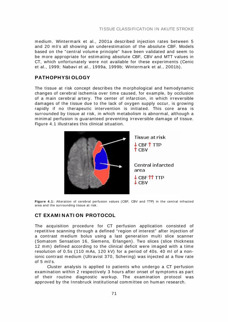
TISSUE CLASSIFICATION IN AKUTE STROKE
71
medium. Wintermark et al., 2001a described injection rates between 5and 20 ml/s all showing an underestimation of the absolute CBF. Modelsbased on the “central volume principle” have been validated and seem tobe more appropriate for estimating absolute CBF, CBV and MTT values inCT, which unfortunately were not available for these experiments (Cenicet al., 1999; Nabavi et al., 1999a, 1999b; Wintermark et al., 2001b).
PATHOPHYSIOLOGY
The tissue at risk concept describes the morphological and hemodynamicchanges of cerebral ischemia over time caused, for example, by occlusionof a main cerebral artery. The center of infarction, in which irreversibledamages of the tissue due to the lack of oxygen supply occur, is growingrapidly if no therapeutic intervention is initiated. This core area issurrounded by tissue at risk, in which metabolism is abnormal, although aminimal perfusion is guaranteed preventing irreversible damage of tissue.Figure 4.1 illustrates this clinical situation.
Figure 4.1: Alteration of cerebral perfusion values (CBF, CBV and TTP) in the central infractedarea and the surrounding tissue at risk.
CT EXAMINATION PROTOCOL
The acquisition procedure for CT perfusion application consisted ofrepetitive scanning through a defined “region of interest” after injection ofa contrast medium bolus using a last generation multi slice scanner(Somatom Sensation 16, Siemens, Erlangen). Two slices (slice thickness12 mm) defined according to the clinical deficit were imaged with a timeresolution of 0.5s (110 mAs, 120 kV) for a period of 40s. 40 ml of a non-ionic contrast medium (Ultravist 370, Schering) was injected at a flow rateof 5 ml/s.
Cluster analysis is applied to patients who undergo a CT perfusionexamination within 2 respectively 3 hours after onset of symptoms as partof their routine diagnostic workup. The examination protocol wasapproved by the Innsbruck institutional committee on human research.
TISSUE CLASSIFICATION IN AKUTE STROKE
72
CLUSTER ANALYSIS AND IMAGE PROCESSING
Clustering techniques
For cluster analysis, (i) CBF (ml/100g/min) as calculated from themaximal slope model, (ii) CBV (ml/100g) using equation 3, and (iii) TTP(time-to-peak), which is the time (seconds) it takes from injection of acontrast bolus to the maximum level of attenuation recorded in a ROI wasconsidered. The calculation of the MTT map is not provided in the Syngopackage.
Clustering algorithms are used for the task of tissue classification bygrouping “functional” pixels of CBF, CBV and TTP maps into meaningfulsubclasses. The similarity among pixels of the form fPixel =f(CBF,CBV,TTP) within the transformed 3-dimensional Euclidian spaceS(CBF, CBV, TTP) is calculated by means of a distance function, that is theEuclidian distance (ED):
( )∑ −==
n
1i
2ii yx)y,x(ED (4)
where xi = xCBF, xCBV, xTTP and yi = yCBF, yCBV, yTTP are two processed pixelsin the transformed space. Finally, the identified clusters are retransformedfrom feature space back into image space by visualizing the clusters in asingle map. Thereby, pixels of the same cluster, which may representnormal, abnormal (ischemic) cerebral tissue or large vessels, arecharacterized by maximum similarity in hemodynamic behavior; pixels ofdifferent clusters indicate maximum dissimilarity (Kaufman andRousseeuw, 1990; Everitt et al., 2001). For tissue classification twodifferent clustering techniques, k-means and a density-based (DBSCAN)algorithm were applied, and their clustering characteristics compared(Ester et al., 1996; Theiler and Gisler, 1997; Everitt et al., 2001).
K-means, a partitioning paradigm, constructs a partition of thedatabase of N pixels (= 3⋅n⋅m, three maps of image size n⋅m, n=numberof pixels in rows, m=number of pixels in columns) into a set of k clusters.Each cluster is represented by the gravity center and all pixels must beassigned to a cluster. The algorithm is briefly sketched as follows:
(i) Initialization (arbitrary assignment of the ith pixel to the i modulo kth class).(ii) Start loop until termination condition is met:
Each pixel in the image is assigned to a class such that the distance (= Euclidean distance, which is the square root of the componentwise squareof the difference between the pixel and the class, see equation 4) from thispixel to the center of that class is minimized. Means of each class arerecalculated on the pixels that belong to that class.
(iii) End loop.
Theoretically, k-means should terminate when no more pixels changeclasses. This relies on the fact that both steps of k-means (assign pixels tonearest centers, move centers to cluster centroids) reduce variance.Running to completion (no pixels changing classes) may require a large

TISSUE CLASSIFICATION IN AKUTE STROKE
73
number of iterations. So the algorithm is terminated after maximal 50iterations. For the application of k-means on perfusion maps, the userneeds to know the “natural” number of clusters (k = expected number ofcerebral structures) in the image data, which is the only input parameterof the paradigm. The limited spatial resolution of the functional mapsprovided enables primarily the classification of normal parenchyma (grayand white matter), abnormal ischemic parenchyma and large vessels.Therefore, a k-value of 3 for the segmentation of gray and white matteras well as large vessels in normal brain perfusion or reversible ischemia(e.g. TIA) was suggested, a k-value >3, if additionally ischemicparenchyma was visualized in perfusion maps.
The key idea of density-based clustering is that for each pixel of acluster the neighborhood of a given radius ε has to contain at least aminimum number of pixels MinPts. The algorithm DBSCAN (density basedspatial clustering of applications with noise), which discovers clusters andnoise in a database, is based on the fact that a cluster is equivalent to theset of all pixels, which are density-reachable from an arbitrary core pixelin the cluster. To find a cluster, DBSCAN starts with an arbitrary pixel inthe database and checks the ε-neighborhood of each pixel in thedatabase. If the ε-neighborhood Nε(p) of a pixel p has more than MinPtspixels, a new cluster C containing the pixels in Nε(p) is created. Then, theε-neighborhood of all pixels q in C, which have not yet been processed ischecked. If Nε(q) contains more than MinPts pixels, the neighbors of q,which are not already contained in C, are added to the cluster and theirε-neighborhood is checked in the next step. This procedure is repeateduntil no new point can be added to the current cluster C. DBSCAN usesMinPts and ε-neighborhood as global input parameters, specifying thelowest density not considered to be noise. MinPts is recommended to be>3. For this application MinPts >50 and an ε-neighborhood >0.8 havebeen proven to be useful settings.
Image pre- and post-processing
For cluster analysis, input image data was generated routinely in a 12-bitgrayscale format (Monochrome2) from Siemens Syngo software. Syngoalready segments cerebral tissue so that the processed matrix size can bereduced from originally 512x512 to approximately 300x350 (depending onthe patient’s head size and the imaged topographic level). This reductionis helpful in shortening the runtime of the cluster algorithms becausepixels outside the skull contain no information that could changeclustering outcome. The segmented areas of the ventricle system andbackground pixels were set to zero by default. The pre-segmented mapscontained the absolute CBF, CBV and TTP values, however, added to anoffset of 210 (=1024) counts, which had to be subtracted before thealgorithm was started. These offset-corrected maps were then normalizedto μ=0 and σ2=1 (z-transformation), which is an essential condition forcalculating the Euclidian distance function (equation 4) in a meaningfulway.

TISSUE CLASSIFICATION IN AKUTE STROKE
74
Functional maps were also available in RGB format, which are preferablyused for clinical decision making (see figure 4.3), but were not appropriatefor cluster analysis. After each analytic run, all clusters identified wereretransformed from feature space into a single 8-bit grayscale image(TIFF), visualizing the clustered cerebral regions and displaying CBF, CBVand TTP values of each cluster detected. Currently, the developedsoftware (Borland C++) runs on a PC (Pentium IV, 500 MB RAM, 2 GHz)computing cluster results <120 s when applying k-means and <60s whenusing DBSCAN supported by an index structure (R*-tree) (Ester et al.,1995).
Image pre/post-processing and cluster analysis is performed using asoftware tool developed at our research institution (Figure 4.2). It is easyto handle, so that cluster analysis can be performed by physicians or CTtechnologists during clinical routine.
Figure 4.2: Software tool developed for cluster analysis. The red arrow shows the central area ofinfarction (white) using DBSCAN cluster algorithm. Right to the cluster picture, the mean CBF, CBVand TTP values of the cluster are displayed (CBF = 12.8 ml/100g/min, CBV = 3.7 ml/100g,TTP = 26.4s).
CLINICAL EXAMPLE
Cluster analysis was applied to CBF, CBV and TTP maps of a patient whohad undergone a CT perfusion examination within 2 respectively 3 hoursafter onset of symptoms as part of their routine diagnostic workup. Theinvestigated patient (male, 40 years) showed a left-sided hemiparesis. CT

TISSUE CLASSIFICATION IN AKUTE STROKE
75
angiography revealed an occlusion of the right middle cerebral artery(MCA). On CT perfusion maps there was marked prolongation of TTP overthe right MCA territory. Decrease of CBF and CBV was less prominent(Figure 4.3, first line). He received thrombolytic therapy (rTPA 47.7 mgi.v.). Follow-up examination after 24 hours showed normalized perfusionparameters and recanalization of the MCA, the neurologic deficit resolved(Figure 4.3, second line).
Figure 4.3: Cerebral blood flow (CBF), cerebral blood volume (CBV) and time-to-peak (TTP) mapsof a 40-year-old male patient (patient 2) at acute stroke (left-sided hemiparesis, occlusion of theright MCA, first line) and 24h after thrombolytic therapy (second line) [Baumgartner et al., J DigitImaging, 2005].
TISSUE CLASSIFICATION
K-means clusters, identified by scanning CBF, CBV and TTP maps, aresummarized in Figure 4.4 (k=2 to k=5). Mean (SD) cluster values of CBF,CBV and TTP are shown in Table 4.5. Choosing k = 1, the mean globalCBF, CBV and TTP values were determined. The high standard deviationsof accumulated CBF and CBV can be explained by the large differences ofthese parameters in white and gray matter, large vessels and infarctedtissue, respectively. TTP yielded more homogenous values.
The patient revealed a diminished mean global CBF of 29.5ml/100g/min (k=1) compared to the 24h follow-up examination (47.9ml/100g/min, P<0.001, Table 4.5). Similar results were obtained withCBV and TTP (P<0.001). Increasing the value of k, clustering yielded moreclusters with altered hemodynamic patterns (Figure 4.4). A k-value of 2identified the apparent territory of the occluded right MCA with a decreasein CBF (15.9 ml/100g/min vs. 32.2 ml/100g/min in normal brain tissue of

TISSUE CLASSIFICATION IN AKUTE STROKE
76
cluster c2, P<0.001), CBV (3.3 ml/100g vs. 5.6 ml/100g in normal braintissue, P<0.001) and prolonged TTP (17 s vs. 9.8 s in normal brain tissue,P<0.001). Increasing k up to 3, areas of high blood flow (predominatelylarge vessels) were separated. At k = 4, arterial and venous vessels maybe distinguished (arterial TTP = 9.6 s, venous TTP = 11.9 s, P<0.001). Ata k-value of 5, two low-perfused areas, c1 (ischemic parenchyma) and c2(normal or slightly affected tissue), were clustered, showing the same CBFof approximately 15 ml/100g/min (P=0.387), but different CBV and TTPvalues (P<0.001).
Comparing cluster results from admission to the 24-hours follow-upexamination after therapy, improvement in global CBF, CBV andnormalization of TTP were observed (Table 4.5). On follow-up, cluster c1(ischemic area at the initial examination) had disappeared according tothe recanalization of the MCA. At the k-value of 3, cluster c1* (whitematter) and cluster c2* (gray matter) showed normalized values(P<0.001) as well as symmetric cluster patterns for both hemispheres(maps not shown).
Figure 4.4: Clusters identified applying k-means at acute stroke are depicted for k = 2, 3, 4 and 5(clusters c2 – c5). Cluster analysis 24h after thrombolytic therapy with k = 3 showed symmetriccluster patterns for both hemispheres (maps not shown, absolute CBF, CBV and TTP values seetable 4.5) [Baumgartner et al., J Digit Imaging, 2005].
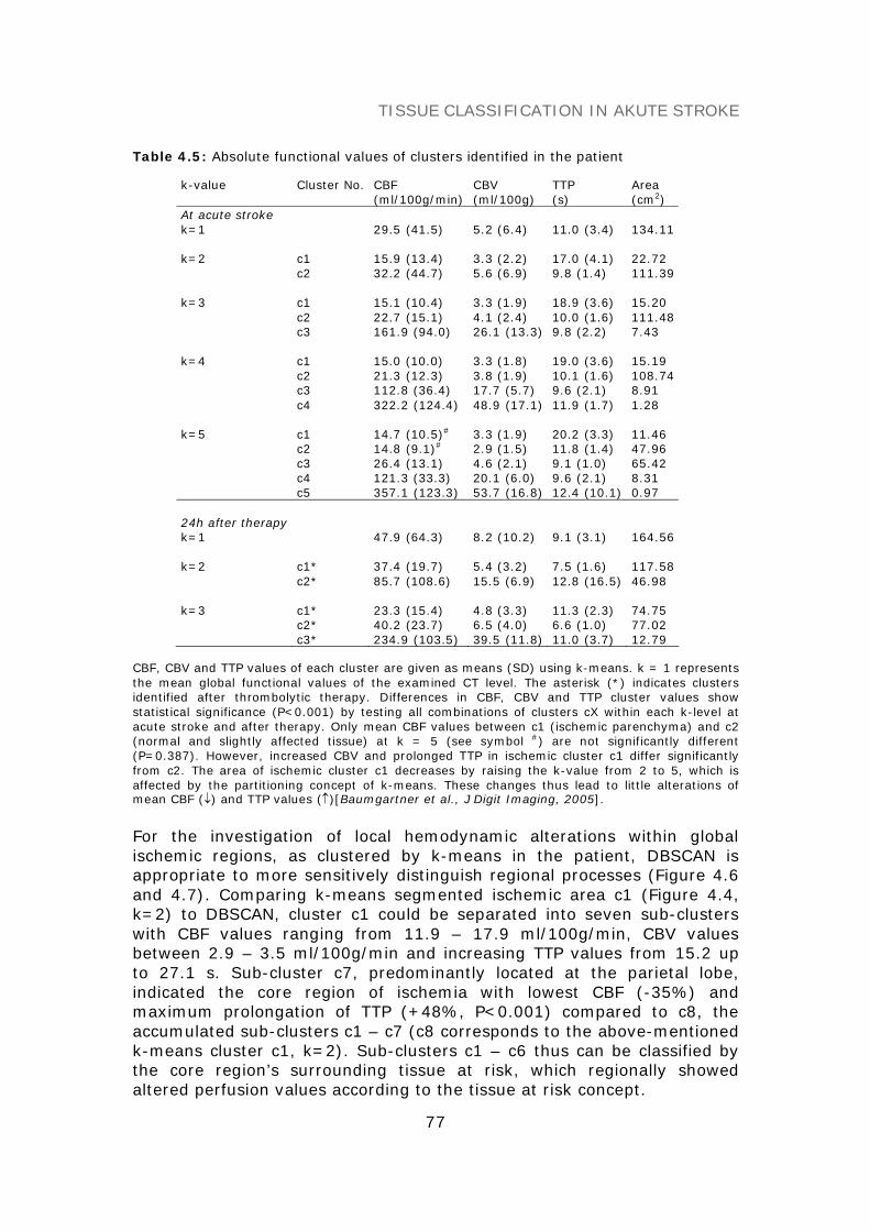
TISSUE CLASSIFICATION IN AKUTE STROKE
77
Table 4.5: Absolute functional values of clusters identified in the patient
k-value Cluster No. CBF CBV TTP Area(ml/100g/min) (ml/100g) (s) (cm2)
At acute strokek=1 29.5 (41.5) 5.2 (6.4) 11.0 (3.4) 134.11
k=2 c1c2
15.9 (13.4)32.2 (44.7)
3.3 (2.2)5.6 (6.9)
17.0 (4.1)9.8 (1.4)
22.72111.39
k=3 c1c2c3
15.1 (10.4)22.7 (15.1)161.9 (94.0)
3.3 (1.9)4.1 (2.4)26.1 (13.3)
18.9 (3.6)10.0 (1.6)9.8 (2.2)
15.20111.487.43
k=4 c1c2c3c4
15.0 (10.0)21.3 (12.3)112.8 (36.4)322.2 (124.4)
3.3 (1.8)3.8 (1.9)17.7 (5.7)48.9 (17.1)
19.0 (3.6)10.1 (1.6)9.6 (2.1)11.9 (1.7)
15.19108.748.911.28
k=5 c1c2c3c4c5
14.7 (10.5)#
14.8 (9.1)#
26.4 (13.1)121.3 (33.3)357.1 (123.3)
3.3 (1.9)2.9 (1.5)4.6 (2.1)20.1 (6.0)53.7 (16.8)
20.2 (3.3)11.8 (1.4)9.1 (1.0)9.6 (2.1)12.4 (10.1)
11.4647.9665.428.310.97
24h after therapyk=1 47.9 (64.3) 8.2 (10.2) 9.1 (3.1) 164.56
k=2 c1*c2*
37.4 (19.7)85.7 (108.6)
5.4 (3.2)15.5 (6.9)
7.5 (1.6)12.8 (16.5)
117.5846.98
k=3 c1*c2*c3*
23.3 (15.4)40.2 (23.7)234.9 (103.5)
4.8 (3.3)6.5 (4.0)39.5 (11.8)
11.3 (2.3)6.6 (1.0)11.0 (3.7)
74.7577.0212.79
CBF, CBV and TTP values of each cluster are given as means (SD) using k-means. k = 1 representsthe mean global functional values of the examined CT level. The asterisk (*) indicates clustersidentified after thrombolytic therapy. Differences in CBF, CBV and TTP cluster values showstatistical significance (P<0.001) by testing all combinations of clusters cX within each k-level atacute stroke and after therapy. Only mean CBF values between c1 (ischemic parenchyma) and c2(normal and slightly affected tissue) at k = 5 (see symbol #) are not significantly different(P=0.387). However, increased CBV and prolonged TTP in ischemic cluster c1 differ significantlyfrom c2. The area of ischemic cluster c1 decreases by raising the k-value from 2 to 5, which isaffected by the partitioning concept of k-means. These changes thus lead to little alterations ofmean CBF (↓) and TTP values (↑)[Baumgartner et al., J Digit Imaging, 2005].
For the investigation of local hemodynamic alterations within globalischemic regions, as clustered by k-means in the patient, DBSCAN isappropriate to more sensitively distinguish regional processes (Figure 4.6and 4.7). Comparing k-means segmented ischemic area c1 (Figure 4.4,k=2) to DBSCAN, cluster c1 could be separated into seven sub-clusterswith CBF values ranging from 11.9 – 17.9 ml/100g/min, CBV valuesbetween 2.9 – 3.5 ml/100g/min and increasing TTP values from 15.2 upto 27.1 s. Sub-cluster c7, predominantly located at the parietal lobe,indicated the core region of ischemia with lowest CBF (-35%) andmaximum prolongation of TTP (+48%, P<0.001) compared to c8, theaccumulated sub-clusters c1 – c7 (c8 corresponds to the above-mentionedk-means cluster c1, k=2). Sub-clusters c1 – c6 thus can be classified bythe core region’s surrounding tissue at risk, which regionally showedaltered perfusion values according to the tissue at risk concept.

TISSUE CLASSIFICATION IN AKUTE STROKE
78
Figure 4.6: Sub-clusters identified (c1 – c7) in the global ischemic region using density-basedclustering are shown. Sub-clusters c1-c7 are ordered by increasing TTP. Sub-cluster c8 representsthe accumulated cluster of all 7 sub-clusters [Baumgartner et al., J Digit Imaging, 2005].
Figure 4.7: CBF, CBV and TTP values of sub-clusters c1 – c7 and accumulated cluster c8 aredisplayed as means (SD) [Baumgartner et al., J Digit Imaging, 2005].
TISSUE CLASSIFICATION IN AKUTE STROKE
79
CONCLUSION
Diagnostic interpretation of CT perfusion integrates the informationderived from CBF, CBV and TTP maps, and shows limitations whenperforming visual analysis. The degree of hemodynamic alterations canbetter be analyzed quantitatively using manual segmentation of definedbrain areas on single CBF, CBV and TTP maps, which can be done withinminutes, but is observer-dependent. Functional cluster analysis of CBF,CBV and TTP maps facilitates the identification and classification ofanatomic regions with inherent hemodynamic properties. Each calculatedcluster represents tissue with related functional parameters by combiningall three parameters into a single map, where CBF, CBV and TTP values ofeach voxel are simultaneously accessible. The identified clusters areautomatically computed in a few analytical runs and reflect functionalinteractions of the measured parameters.
TTP maps seem to represent the most sensitive parameter for theestimation of endangered brain tissue following vessel occlusion. Thisobservation corresponds well with the result of cluster analysis in theexample patient who had suffered a completed stroke. The “k=2” clustermap of this patient segmented an area that is comparable to the TTP map.In the clinical situation, the extension of abnormal values on TTP mapsindicates the maximum amount of tissue that may be salvaged by arecanalization therapy. The extension of abnormal CBF indicates the tissuethat is reached by collateral flow and may still be amenable to benefitfrom recanalization. CBV shows the center of ischemia with completecessation of perfusion that is likely to progress to infarction. Thecorrelation of CBF and CBV with cluster maps of k > 2 or with identifiedsub-clusters c1-c7 using DBSCAN and its impact on decision making forrecanalization therapy remains to be investigated in larger patientsamples to correlate functional clusters with pathophysiology andhistological characteristics of the identified tissues, as well as to validatedifferent clusters with clinical outcome.
REFERENCES
Baumgartner C, Gautsch K, Böhm C, Felber S. (2005) Functional cluster analysis of CTperfusion maps: A new tool for diagnosis of acute stroke ? J Digit Imaging, 18, 219-226.
Bohner G, Forschler A, Hamm B, Lehmann R, Klingebiel R. (2003) Quantitative perfusionimaging by multi-slice CT in stroke patients. Rofo Fortschr Geb Rontgenstr NeuenBildgeb Verfahr, 175, 806-813.
Cenic A, Nabavi DG, Craen RA, Gelb AW, Lee TY. (1999) Dynamic CT measurement ofcerebral blood flow: A validation study. Am J Neuroradiol, 20, 63-73.
Ester M, Kriegel HP, Xu X. (1995) Knowledge discovery in large spatial databases:Focusing techniques for efficient class identification, Lec. Notes in Computer Science,Proc. 4th Intern. Symp. on Large Spatial Databases, Springer, Vol. 591, pp. 67-82.

TISSUE CLASSIFICATION IN AKUTE STROKE
80
Ester M, Kriegel HP, Sander J, Xu X. (1996) A density based algorithm for discoveringclusters in large spatial databases with noise. Proc. 2nd Int. Conf. on KnowledgeDiscovery and Data Mining (KDD’96). AAAI Press, Menlo Park, CA. pp. 226-231.
Everitt BS, Landau S, Leese M. (2001) Cluster analysis. 4th edn. Oxford University Press,New York.
Kaufman L, Rousseeuw PJ. (1990) Finding groups in data: An introduction to clusteranalysis. John Wiley & Sons.
Keith CJ, Griffiths M, Petersen B, Anderson RJ, Miles KA. (2002) Computed tomographyperfusion imaging in acute stroke. Australas Radiol, 46, 221-230.
König M, Banach-Planchamp R, Kraus M, Klotz E, Falk A, Gehlen W, Heuser L. (2000a) CTperfusion imaging in acute ischemic cerebral infarct: Comparison of cerebral perfusionmaps and conventional CT findings. Rofo Fortschr Geb Rontgenstr Neuen BildgebVerfahr, 172, 219-226.
König M, Klotz E, Heuser L. (2000b) Cerebral perfusion CT: Theoretical aspects,methodical implementation and clinical experience in the diagnosis of ischemiccerebral infarction. Rofo Fortschr Geb Rontgenstr Neuen Bildgeb Verfahr, 172, 210-218.
Meier P, Zierler KL. (1954) On the theory of the indicator-dilution method formeasurement of blood flow and volume. J Appl Pysiol, 12, 731-744.
Miles KA. (2003) Acute cerebral stroke imaging and brain perfusion with the use of high-concentration contrast media. Eur Radiol, 13;Suppl 5, 117-120.
Nabavi DG, Cenic A, Craen RA, Gelb AW, Bennett JD, Kozak R, Lee TY. (1999a) CTassessment of cerebral perfusion: Experimental validation and initial clinicalexperience. Radiology, 213, 141-149.
Nabavi DG, Cenic A, Dool J, Smith RM, Espinosa F, Craen RA, Gelb AW, Lee TY. (1999b)Quantitative assessment of cerebral hemodynamics using CT: Stability, accuracy, andprecision studies in dogs. J Comput Assist Tomogr, 23, 506-515.
Theiler J, Gisler G. (1997) A contiguity-enhanced k-means clustering algorithm forunsupervised multispectral image segmentation, Proc SPIE’97 Vol 3159, pp. 108-118.
Wintermark M, Maeder P, Thiran JP, Schnyder P, Meuli R. (2001a) Quantitativeassessment of regional cerebral blood flows by perfusion CT studies at low injectionrates: A critical review of the underlying theoretical models. Eur Radiol, 11, 1220-1230.
Wintermark M, Thiran JP, Maeder P, Schnyder P, Meuli R. (2001b) Simultaneousmeasurement of regional cerebral blood flow by perfusion CT and stable xenon CT:A validation study. Am J Neuroradiol, 22, 905-914.
Wintermark M, Reichhart M, Thiran JP, Maeder P, Chalaron M, Schnyder P, BogousslavskyJ, Meuli R. (2002) Prognostic accuracy of cerebral blood flow measurement byperfusion computed tomography, at the time of emergency room admission, in acutestroke patients. Ann Neurol, 51, 417-432.
Zierler KL. (1965) Equations for measuring blood flow by external monitoring ofradioisotopes. Circulation, 16, 309-321.

81
SUMMARY (ENGLISH)
Data mining in biomedicine represents a new growing scientific area thatuses computational approaches to extract new knowledge out of large andcomplex data sets. Mined patterns, associations, or relationships amongall this data can provide information, which can then be converted intobiomedical knowledge about historical patterns and future trends.
In particular, advances in preclinical and clinical research methodsas well as in information technology and computational sciences facilitatethe discovery of unknown causal mechanisms in the cell, organ and thewhole organism in a more comprehensive way. Mass spectrometry, forinstance, has become an important tool to measure a large amount ofcompounds in body fluids, which permits an insight into the abnormalbiochemical and biological mechanisms of the organism. Genotypic andphenotypic data complete the full spectrum of biological (genetic,proteomic, metabolomic) and clinical information, a knowledge base thatincorporates clinical bioinformatics. Clinical bioinformatics is thus animportant contribution to the knowledge discovery process because itprovides algorithms, processes and systems to allow individualizedhealthcare using relevant sources of medical information andbioinformatics.
The main focus of this thesis is to review basic data miningconcepts, new developments and trends, and to report on their applicationto specific biomedical research projects in the realm of metabolomics,clinical genomics, and medical image processing. This includes (i) newstrategies and methods for biomarker discovery and disease screening onMS high throughput newborn screening data of metabolic disorders, (ii) abioinformatics framework to correlate data on FBN1 mutation analysiswith the corresponding clinical phenotypes of Marfan syndrome or otherfibrillinopathies extended by new concepts for clinical decision making andmonitoring of medical treatment, and (iii) a new approach to classifycerebral tissue on CT perfusion maps in patients with acute stroke.
In summary, clinical bioinformatics provides infrastructure,processes and data mining approaches that contribute to the challengingknowledge discovery process, which supports diagnostics and therapy as afirst step to personalized medicine.
KEY WORDSKnowledge discovery, data mining, algorithms, data models, similarityquery processing, image processing, analytical techniques, biomarkerdiscovery, metabolic disorders, clinical genetics, Marfan syndrome, CTperfusion, stroke.

82
SUMMARY (GERMAN)
Data Mining in der Biomedizin stellt ein junges, aufstrebendesForschungsgebiet dar, welches sich mit der Entwicklung innovativer,computerunterstützter Verfahren zur Extraktion neuen Wissens ausgroßen und komplexen Datenmengen beschäftigt. Die in diesen Datenentdeckten Muster, Assoziationen oder Beziehungen beinhaltenneuwertige Informationen, die in weiterer Folge in biomedizinischesWissen übersetzt und mit historischen Mustern und neuen Trendsabgestimmt werden müssen.
Insbesondere die rasanten Forschritte im Bereich der präklinischenund klinischen Forschungsmethoden sowie im Bereich derInformationstechnologie und Computerwissenschaften ermöglichen derWissenschaft heute, unbekannte kausale Zusammenhänge auf zellulärerEbene, auf Organebene bzw. im gesamten Organismus systematisch zuuntersuchen. Moderne bioanalytische Hochdurchsatzverfahren, wie zB. dieMassenspektrometrie, erlauben eine Analyse sämtlicherStoffwechselparameter aus geringen Blutmengen und ermöglichen somiteinen Einblick in die abnormalen biologischen und biochemischenMechanismen des Organismus. Die gesamtheitliche Sichtweise vongenetischer (Genomics, Transcriptomics), molekularbiologischer(Proteomics, Metabolomics) und klinischer Information erlaubt den Aufbauumfassender Wissensbasen, die mit Hilfe innovativer Methoden undVerfahren der Bioinformatik untersucht und mit dem Ziel, neuediagnostische und therapeutische Ansätze zu entwickeln, analysiertwerden.
Ziel meiner Habilitationsschrift ist es, einen umfassenden Überblicküber grundlegende Data Mining Konzepte, sowie neue Entwicklungen undTrends in diesem Bereich zu geben sowie am Beispiel dreier spezifischerbiomedizinischer Forschungsprojekte aus den Bereichen Metabolomics,klinischer Genetik und medizinischer Bildverarbeitung eineanwendungsorientierte Sichtweise dieser Thematik zu vermitteln. Diesbeinhaltet (i) neue Methoden und Verfahren für die Biomarker Suche undKlassifikation am Beispiel von MS Hochdurchsatzdaten von Neugeborenenmit angeborenen Stoffwechselkrankheiten, (ii) einen BioinformatikFramework zur Genotyp-Phänotyp Korrelation bei Patienten mit MarfanSyndrom und anderen Fibrillinopathien mit nachgewiesenen FBN1-Genmutationen, und (iii) ein neues Verfahren zur Gewebsklassifikation beiSchlaganfallpatienten auf Basis von cerebralen CT-Perfusionsbildern.
Zusammenfassend stellt die klinische Bioinformatik Prozesse undMethoden zur Untersuchung klinischer Fragestellungen zur Verfügung, umneues Wissen für Diagnostik und Therapie aus den Daten zu gewinnen undso dem Ziel einer individualisierten Medizin näher zu kommen.

83
CURRICULUM VITAE
Christian Baumgartner, Univ.-Ass. Dipl.-Ing. Dr.techn.
Personal data
Date of birth: June 13th, 1968Place of birth: Feldbach/Styria,Nationality: AustrianMartial status: Married with Daniela Baumgartner, MD
Two children: David Benedict, Elias Gabriel
Education
1978 – 1986 High school (“Gymnasium”) in Fürstenfeld1986 – 1994 Diploma study in Electrical and Biomedical Engineering,
Graz University of Technology, 1994 Master degree(“Dipl.-Ing.”)
1992 – 1994 Organ studies at University of Music and Performing Artsin Graz
1996 – 1998 PhD program at Graz University of Technology/ GrazMedical University, 1998 Doctor degree in BiomedicalEngineering (“Dr.techn.”) Title of thesis: “Measurementof cerebral perfusion using electron-beam computedtomography”
1995 – 1998 Study of Sacred Music at the Conservatory of Graz, 1998B-Diploma (organ, conducting)
1997 – 1998 Medical studies, Graz Medical University
Career history
1996 – 1998 Research assistant at the General Department ofRadiology, Graz Medical University
1999 – 2002 R&D systems engineer at Tecan Austria GmbH Salzburg,(Business area Genomics, Confocal fluorescence laserscanning systems for DNA micro array analysis)
2002 – 2003 Research and teaching assistant at the University forHealth Sciences, Medical Informatics and Technology(UMIT)
2004 – present Head of the Research Group for Clinical Bioinformatics,Institute for Biomedical Engineering, UMIT

84
Courses
LecturesData mining in biomedicine (6 ECTS)Algorithms in bioinformatics (3 ECTS)
SeminarsBasics in Java programming (1 ECTS)Algorithms and data structures 2 (1 ECTS)Databases and information systems (1 ECTS)
Special activities
Reviews for journalsMethods of Information in MedicineArtificial Intelligence in MedicineEuropean Radiology
Reviews for conferences2nd Int. Conf. on Biomedical Engineering (BioMed’04)3rd Int. Conf. on Biomedical Engineering (BioMed’05)
Program committee4th Int. Workshop on Biological Data Management (BIDM’06)
Grants
• FFG (HITT, UMIT), Data mining in biomedical data, applicant andproject leader, 2003 – 2005
• GEN-AU, Bioinformatics integration network II, Component: Datamining in proteomics, applicant and project leader, 2006 – 2008
Publications (Σ IFSCI 2004 = 39.5)
Journal papers 14Conference proceedings 10Abstracts 14
1997 – 1999 (Σ IF = 2.930)
Journal papers
Rienmüller R, Baumgartner C, Kern R, Harb S, Aigner R, Fueger G, Weihs W. (1997)Quantitative Bestimmung der linksventrikulären Myokardperfusion mittels EBCT.Herz, 22, 63-71. PMID: 9206706
Rienmüller R, Kern R, Baumgartner C, Hackel B. (1997) Electron-Beam-Computertomographie (EBCT) des Herzen. Radiologe, 37, 410-416. PMID: 9312784
Krause W, Gröll R, Kern R, Baumgartner C, Rienmüller R. (1999) Application ofpharmacokinetics to electron-beam tomography of the abdomen. Academic Radiol, 6,487-495. PMID: 10480045

85
Conference Proceedings
Baumgartner C, Rienmüller R, Harb S, Kern R, Hutten H. (1996) Myokardiale Zeit-CT-Werte Diagramme nach Kontrastmittelapplikation mittels Elektronenstrahl-Computertomographie. Biomed Techn (Berlin), 41(Suppl), 158-159.
Baumgartner C, Rienmüller R, Melisch B, Kern R, Graif E, Hutten H. (1997) Measurementof cerebral blood flow using electron beam computed tomography. Biomed Techn(Berlin), 42(Suppl), 35-36.
Baumgartner C, Rienmüller R, Melisch B, Graif E, Kern R, Hutten H. (1998) Determiningcerebral circulation with electron beam computerized tomography. Biomed Techn(Berlin), 43(Suppl), 48-49.
2004 (Σ IF = 5.742)
Journal papers
Baumgartner C, Böhm C, Baumgartner D, Marini G, Weinberger K, Olgemöller B, Liebl B,Roscher AA. (2004) Supervised machine learning techniques for the classification ofmetabolic disorders in newborns. Bioinformatics, 20, 2985-2996. PMID: 15180934
Conference Proceedings
Baumgartner C, Baumgartner D, Böhm C. (2004) Classification on high dimensionalmetabolic data: Phenylketonuria as an example. Proc. 2nd Int. Conf. on BiomedicalEngineering (BioMED 2004), Innsbruck, Austria, pp. 357-360.
Baumgartner C, Baumgartner D, Mátyás G, Steinmann B. (2004) Das Marfan-Syndrom:Eine diagnostische Herausforderung bedingt durch phänotypische und genetische Vielfalt(German). Tagungsband der 49. Jahrestagung der Deutschen Gesellschaft fürMedizinische Informatik, Biometrie und Epidemiologie (GMDS 2004), Innsbruck, Austria,pp. 237-239.
Baumgartner C, Kailing K, Kriegel H-P, Kröger P, Plant C. (2004) Subspace selection forclustering high-dimensional data. Proc. 4th IEEE Int. Conf. on Data Mining (ICDM 2004),Brighton, UK, pp. 11-18.
2005 (Σ IF = 21.644)
Journal papers
Baumgartner C, Böhm C, Baumgartner D. (2005) Modelling of classification rules onmetabolic patterns including machine learning and expert knowledge. J Biomed Inform,38, 89-98. PMID: 15796999
Baumgartner D, Baumgartner C, Mátyás G, Steinmann B, Löffler J, Schermer E,Schweigmann U, Baldissera I, Frischhut B, Hess J, Hammerer I. (2005) Diagnostic powerof aortic elastic properties in young patients with Marfan-syndrome. J Thorac CardiovascSurg, 129, 730-739. PMID: 15821637
Vogt M*, Kühn A*, Baumgartner D, Baumgartner C, Busch R, Kostolny M, Hess J. (2005)Impaired elastic properties of the ascending aorta in newborns before and early aftersuccessful coarctation repair: Proof of a systemic vascular disease of the prestenoticarteries? Circulation, 111, 3269-3273. PMID: 15956120
Baumgartner C, Mátyás G, Steinmann B, Baumgartner D. (2005) Marfan syndrome:A diagnostic challenge caused by phenotypic and genetic heterogeneity. Methods InfMed, 44, 487-497. PMID: 16342915
Baumgartner C, Gautsch K, Böhm C, Felber S. (2005) Functional cluster analysis of CTperfusion maps: A new tool for diagnosis of acute stroke? J Digit Imaging, 18, 219-226.PMID: 15827821

86
Baumgartner D*, Sailer-Höck M*, Baumgartner C, Trieb T, Maurer H, Schirmer M,Zimmerhackl LB, Stein JI. (2005) Reduced aortic elastic properties in a child withTakayasu arteritis: case report and literature review. Eur J Pediatr, 164, 685-690.PMID: 16044277
Conference Proceedings
Baumgartner C, Baumgartner D, Eberle M, Plant C, Mátyás G, Steinmann B. (2005)Genotype-phenotype correlation in patients with fibrillin-1 gene mutations. Proc. 3nd Int.Conf. on Biomedical Engineering (BioMED 2005), Innsbruck, Austria, pp. 561-566.
Baumgartner C, Baumgartner D, Eberle M, Mátyás G, Steinmann B.(2005) Aufbau einerBioinformatik-Plattform für Mutationen im FBN1-Gen zur Genotyp-Phänotyp Korrelationbeim Marfan-Syndrom (German). Tagungsband der 50. Jahrestagung der DeutschenGesellschaft für Medizinische Informatik, Biometrie und Epidemiologie (GMDS 2005),Freiburg, Germany, pp. 19-21.
Breit M, Visvanathan M, Pfeifer B, Baumgartner C, Tilg B. (2005) Computer simulation ininflammatory diseases: Analysis of the TNFα mediated NF-κB signal transductionpathway. Proc. Ann. Meeting Austrian Society for Biomedical Engineering, Hall in Tyrol,pp. 57-58.
Baumgartner C. (2005) Data Mining in der Diagnostik von Stoffwechselstörungen: DerWeg vom metabolischen Profil zum Screening-Modell (German). Proc. Ann. MeetingAustrian Society for Biomedical Engineering, Hall in Tyrol, pp. 59-60.
2006 (Σ IF = 9.18)
Journal papers
Baumgartner C, Mátyás G, Steinmann B, Eberle M, Stein JI, Baumgartner D. (2006) A bioinformatics framework for genotype-phenotype correlation in humans with Marfansyndrome caused by FBN1 gene mutations. J Biomed Inform, 39, 171-183.PMID: 16061422
Baumgartner C, Baumgartner D. (2006) Biomarker discovery, disease classification andsimilarity query processing on high-throughput MS/MS data of inborn errors ofmetabolism. J Biomol Screen, 11, 90-99. PMID: 16314408
Plant C, Böhm C, Tilg B, Baumgartner C. (2006) Enhancing instance-based classificationwith local density: A new algorithm for classifying unbalanced biomedical data,Bioinformatics, in press. PMID: 16443633
Baumgartner C, Böhm C, Baumgartner D, Marini G, Weinberger K, Olgemöller B, Liebl B,Roscher AA. (2006) Supervised machine learning techniques for the classification ofmetabolic disorders in newborns. To appear in: Haux R, Kulikowski C (eds.) IMIAYearbook of Medical Informatics.
Submitted
Baumgartner D*, Baumgartner C*, Schermer E, Engl G, Schweigmann U, Stein IJ.(2006) Different patterns of aortic wall elasticity in patients with Marfan syndrome:A noninvasive follow-up study, submitted.

87
APPENDIX
Attached publications (Σ IFSCI 2004 = 36.5)
Chapter 1
Baumgartner C, Kailing K, Kriegel H-P, Kröger P, Plant C. (2004) Subspace selection for clusteringhigh-dimensional data. Proc. 4th IEEE Int. Conf. on Data Mining (ICDM 2004), Brighton, UK,pp. 11-18. [AR <1/10]
Plant C, Böhm C, Tilg B, Baumgartner C. (2006) Enhancing instance-based classification with localdensity: A new algorithm for classifying unbalanced biomedical data, Bioinformatics, in press.[IF 5.742]
Chapter 2
Baumgartner C, Baumgartner D. (2006) Biomarker discovery, disease classification and similarityquery processing on high-throughput MS/MS data of inborn errors of metabolism. J BiomolScreen, 11, 90-99. [IF 2.427]
Baumgartner C, Böhm C, Baumgartner D. (2005) Modelling of classification rules on metabolicpatterns including machine learning and expert knowledge. J Biomed Inform, 38, 89-98.[IF 1.013]
Baumgartner C, Böhm C, Baumgartner D, Marini G, Weinberger K, Olgemöller B, Liebl B, RoscherAA. (2004) Supervised machine learning techniques for the classification of metabolic disorders innewborns. Bioinformatics, 20, 2985-2996. [IF 5.742]
Chapter 3
Baumgartner C, Mátyás G, Steinmann B, Eberle M, Stein JI, Baumgartner D. (2006)A bioinformatics framework for genotype-phenotype correlation in humans with Marfan syndromecaused by FBN1 gene mutations. J Biomed Inform, 39, 171-183. [IF 1.013]
Baumgartner C, Mátyás G, Steinmann B, Baumgartner D. (2005) Marfan syndrome: A diagnosticchallenge caused by phenotypic and genetic heterogeneity. Methods Inf Med, 44, 487-497.[IF 1.338]
Baumgartner D, Baumgartner C, Mátyás G, Steinmann B, Löffler J, Schermer E, Schweigmann U,Baldissera I, Frischhut B, Hess J, Hammerer I. (2005) Diagnostic power of aortic elastic propertiesin young patients with Marfan-syndrome. J Thorac Cardiovasc Surg, 129, 730-739. [IF 3.263]
Vogt M*, Kühn A*, Baumgartner D, Baumgartner C, Busch R, Kostolny M, Hess J. (2005) Impairedelastic properties of the ascending aorta in newborns before and early after successful coarctationrepair: Proof of a systemic vascular disease of the prestenotic arteries? Circulation, 111, 3269-3273. [IF 12.563]
Baumgartner D*, Sailer-Höck M*, Baumgartner C, Trieb T, Maurer H, Schirmer M, Zimmerhackl LB,Stein JI. (2005) Reduced aortic elastic properties in a child with Takayasu arteritis: case report andliterature review. Eur J Pediatr, 164, 685-690. [IF 1.369]
Chapter 4
Baumgartner C, Gautsch K, Böhm C, Felber S. (2005) Functional cluster analysis of CT perfusionmaps: A new tool for diagnosis of acute stroke? J Digit Imaging, 18, 219-226. [IF 2.098]

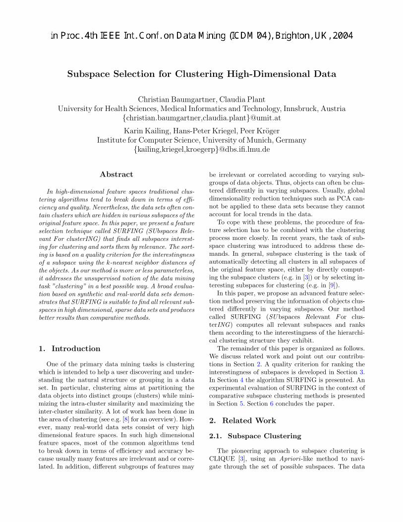
Subspace Selection for Clustering High-Dimensional Data
Christian Baumgartner, Claudia PlantUniversity for Health Sciences, Medical Informatics and Technology, Innsbruck, Austria
{christian.baumgartner,claudia.plant}@umit.at
Karin Kailing, Hans-Peter Kriegel, Peer KrogerInstitute for Computer Science, University of Munich, Germany
{kailing,kriegel,kroegerp}@dbs.ifi.lmu.de
Abstract
In high-dimensional feature spaces traditional clus-tering algorithms tend to break down in terms of effi-ciency and quality. Nevertheless, the data sets often con-tain clusters which are hidden in various subspaces of theoriginal feature space. In this paper, we present a featureselection technique called SURFING (SUbspaces Rele-vant For clusterING) that finds all subspaces interest-ing for clustering and sorts them by relevance. The sort-ing is based on a quality criterion for the interestingnessof a subspace using the k-nearest neighbor distances ofthe objects. As our method is more or less parameterless,it addresses the unsupervised notion of the data miningtask ”clustering” in a best possible way. A broad evalua-tion based on synthetic and real-world data sets demon-strates that SURFING is suitable to find all relevant sub-spaces in high dimensional, sparse data sets and producesbetter results than comparative methods.
1. Introduction
One of the primary data mining tasks is clusteringwhich is intended to help a user discovering and under-standing the natural structure or grouping in a dataset. In particular, clustering aims at partitioning thedata objects into distinct groups (clusters) while mini-mizing the intra-cluster similarity and maximizing theinter-cluster similarity. A lot of work has been done inthe area of clustering (see e.g. [8] for an overview). How-ever, many real-world data sets consist of very highdimensional feature spaces. In such high dimensionalfeature spaces, most of the common algorithms tendto break down in terms of efficiency and accuracy be-cause usually many features are irrelevant and or corre-lated. In addition, different subgroups of features may
be irrelevant or correlated according to varying sub-groups of data objects. Thus, objects can often be clus-tered differently in varying subspaces. Usually, globaldimensionality reduction techniques such as PCA can-not be applied to these data sets because they cannotaccount for local trends in the data.
To cope with these problems, the procedure of fea-ture selection has to be combined with the clusteringprocess more closely. In recent years, the task of sub-space clustering was introduced to address these de-mands. In general, subspace clustering is the task ofautomatically detecting all clusters in all subspaces ofthe original feature space, either by directly comput-ing the subspace clusters (e.g. in [3]) or by selecting in-teresting subspaces for clustering (e.g. in [9]).
In this paper, we propose an advanced feature selec-tion method preserving the information of objects clus-tered differently in varying subspaces. Our methodcalled SURFING (SUbspaces Relevant For clus-terING) computes all relevant subspaces and ranksthem according to the interestingness of the hierarchi-cal clustering structure they exhibit.
The remainder of this paper is organized as follows.We discuss related work and point out our contribu-tions in Section 2. A quality criterion for ranking theinterestingness of subspaces is developed in Section 3.In Section 4 the algorithm SURFING is presented. Anexperimental evaluation of SURFING in the context ofcomparative subspace clustering methods is presentedin Section 5. Section 6 concludes the paper.
2. Related Work
2.1. Subspace Clustering
The pioneering approach to subspace clustering isCLIQUE [3], using an Apriori -like method to navi-gate through the set of possible subspaces. The data
kroegerp
in Proc. 4th IEEE Int. Conf. on Data Mining (ICDM'04), Brighton, UK, 2004

space is partitioned by an axis-parallel grid into equi-sized units of width ξ. Only units whose densities ex-ceed a threshold τ are retained. A cluster is defined asa maximal set of connected dense units. The perfor-mance of CLIQUE heavily depends on the positioningof the grid. Objects that naturally belong to a clus-ter may be missed or objects that are naturally noisemay be assigned to a cluster due to an unfavorable gridposition.
Another recent approach called DOC [10] proposesa mathematical formulation for the notion of an opti-mal projected cluster, regarding the density of pointsin subspaces. DOC is not grid-based but as the den-sity of subspaces is measured using hypercubes of fixedwidth w, it has similar problems like CLIQUE.
In [2] the method PROCLUS to compute projectedclusters is presented. However, PROCLUS misses outthe information of objects clustered differently in vary-ing subspaces. The same holds for ORCLUS [1].
2.2. Feature Selection for Clustering
In [9] a method called RIS is proposed that ranksthe subspaces according to their clustering structure.The ranking is based on a quality criterion using thedensity-based clustering notion of DBSCAN [7]. AnApriori -like navigation through the set of possible sub-spaces in a bottom-up way is performed to find all in-teresting subspaces. Aggregated information is accu-mulated for each subspace to rank its interestingness.
In [6] a quality criterion for subspaces based on theentropy of point-to-point distances is introduced. How-ever, there is no algorithm presented to compute theinteresting subspaces. The authors propose to use aforward search strategy which most likely will miss in-teresting subspaces, or an exhaustive search strategywhich is obviously not efficient in higher dimensions.
2.3. Our Contributions
Recent density-based approaches to subspace clus-tering or subspace selection methods (RIS) use a globaldensity threshold for the definition of clusters due to ef-ficiency reasons. However, the application of a globaldensity threshold to subspaces of different dimension-ality and to all clusters in one subspace is rather un-acceptable. The data space naturally increases expo-nentially with each dimension added to a subspace andclusters in the same subspace may exceed different den-sity parameters or exhibit a nested hierarchical clus-tering structure. Therefore, for subspace clustering, itwould be highly desirable to adapt the density thresh-old to the dimensionality of the subspaces or even bet-
ter to rely on a hierarchical clustering notion that isindependent from a globally fixed threshold.
In this paper, we introduce SURFING, a feature se-lection method for clustering which does not rely ona global density parameter. Our approach explores allsubspaces exhibiting an interesting hierarchical clus-tering structure and ranks them according to a qual-ity criterion. SURFING is more or less parameterless,i.e. it does not require the user to specify parametersthat are hard to anticipate such as the number of clus-ters, the (average) dimensionality of subspace clusters,or a global density threshold. Thus, our algorithm ad-dresses the unsupervised notion of the data mining task“clustering” in a best possible way.
3. Subspaces Relevant for Clustering
Let DB be a set of N feature vectors with dimen-sionality d, i.e. DB ⊆ Rd. Let A = {a1, . . . , ad} be theset of all attributes ai of DB. Any subset S ⊂ A, iscalled a subspace. T is a superspace of S if S ⊂ T . Theprojection of an object o onto a subspace S ⊆ A is de-noted by oS . We assume that d : DB ×DB → R is ametric distance function.
3.1. General Idea
The main idea of SURFING is to measure the “in-terestingness” of a subspace w.r.t. to its hierarchicalclustering structure, independent from its dimension-ality. Like most previous approaches to subspace clus-tering, we base our measurement on a density-basedclustering notion. Since we do not want to rely on aglobal density parameter, we developed a quality crite-rion for relevant subspaces built on the k-nearest neigh-bor distances (k-nn-distances) of the objects in DB.
For a user-specified k ∈ N (k ≤ N) and a subspaceS ⊆ A let NNS
k (o) be the set of k-nearest neighbors ofan object o ∈ DB in a subspace S. The k-nn-distanceof o in a subspace S, denoted by nn-DistSk (o), is the dis-tance between o and its k-nearest neighbor, formally:
nn-DistSk (o) = max{d(oS , pS) | p ∈ NNSk (o)}.
The k-nn-distance of an object o indicates howdensely the data space is populated around o in S.The smaller the value of nn-DistSk (o), the more densethe objects are packed around o, and vice versa. If asubspace contains a recognizable hierarchical cluster-ing structure, i.e. clusters with different densities andnoise objects, the k-nn-distances of objects should dif-fer significantly. On the other hand, if all points are uni-formly distributed, the k-nn-distances can be assumed

3-nn distance
objectsa1
a2
mean
(a) Hierarchical clustering structure in a 2D subspace(left); ac-cording sorted 3-nn graph (right)
3-nn distance
a1 objects
meana2
(b) Uniform distribution in a 2D subspace (left); accordingsorted 3-nn graph (right)
Figure 1: Usefulness of the k-nn distance to rate the interestingness of subspaces.
to be almost equal. Figure 1 illustrates these consider-ations using a sample 2D subspace S = {a1, a2} andk = 3. Consequently, we are interested in subspaceswhere the k-nn-distances of the objects differ signifi-cantly from each other, because the hierarchical clus-tering structure in such subspaces will be considerablyclearer than in subspaces where the k-nn-distances arerather similar to each other.
3.2. A Quality Criterion for Subspaces
As mentioned above we want to measure how muchthe k-nn-distances in S differ from each other. Toachieve comparability between subspaces of differentdimensionality, we scale all k-nn-distances in a sub-space S into the range [0, 1]. Thus, we assume thatnn-DistSk (o) ∈ [0, 1] for all o ∈ DB throughout the restof the paper.
Two well-known statistical measures for our purposeare the mean value µS of all k-nn-distances in subspaceS and the variance. However, the variance is not appro-priate for our purpose because it measures the squareddifferences of each k-nn-distance to µS and thus, highdifferences are weighted stronger than low differences.For our quality criterion we want to measure the non-weighted differences of each k-nn-distance to µS . Sincethe sum of the differences of all objects above µS isequal to the sum of the differences of all objects be-low µS , we only take half of the sum of all differencesto the mean value, denoted by diffµS
, which can becomputed by
diffµS=
12
∑o∈DB
|µS − nn-DistSk (o)|.
In fact, diffµSis already a good measure for rating
the interestingness of a subspace. We can further scalethis value by µS times the number of objects having
a smaller k-nn-distance in S than µS , i.e. the objectscontained in the following set:
BelowS := {o ∈ DB |nn-DistSk (o) < µS}.
Obviously, if BelowS is empty, the subspace con-tains uniformly distributed noise.
Definition 1 (quality of a subspace) Let S ⊆ A.The quality of S, denoted by quality(S), is defined as fol-lows:
quality(S) =
{0 if BelowS = ∅
diffµS
|BelowS |·µSelse.
The quality values are in the range between 0 and 1.A subspace where all objects are uniformly distributed(e.g. as depicted in Figure 1(b)) has a quality value ofapproximately 0, indicating a less interesting clusteringstructure. On the other hand, the clearer the hierarchi-cal clustering structure in a subspace S is, the higheris the value of quality(S). For example, the sample 2Dsubspace in which the data is highly structured as de-picted in Figure 1(a) will have a significantly higherquality value. Let us note that in the synthetic casewhere all objects in BelowS have a k-nn-distance of 0and all other objects have a k-nn-distance of 2 ·µS , thequality value quality(S) is 1.
In almost all cases, we can detect the relevant sub-spaces with this quality criterion, but there are two ar-tificial cases rarely found in natural data sets whichnevertheless cannot be ignored.
First, there might be a subspace containing someclusters, each of the same density, and without noise(e.g. data set A in Figure 2). If the number of data ob-jects in the clusters exceeds k, such subspaces cannot bedistinguished from subspaces containing uniformly dis-tributed data objects spread over the whole attributerange (e.g. data set B in Figure 2) because in both
data set A data set B
% of inserted points quality(A) quality(B)0 0.13 0.15
0.1 0.15 0.150.2 0.19 0.150.5 0.31 0.151 0.38 0.155 0.57 0.1510 0.57 0.15
Figure 2: Benefit of inserted points.
cases, the k-nn-distances of the objects will marginallydiffer from the mean value.
Second, subspaces containing data of one Gaussiandistribution spread over the whole attribute range arenot really interesting. However, the k-nn-distances ofthe objects will scatter significantly around the meanvalue. Thus, such subspaces cannot be distinguishedfrom subspaces containing two or more Gaussian clus-ters without noise.
To overcome these two artificial cases, we can tem-porarily insert some randomly generated points beforecomputing the quality value of a subspace. In cases ofuniform or Gaussian distribution over the whole at-tribute range, the insertion of a few randomly gener-ated additional objects does not significantly affect thequality value. The k-nn-distances of these objects aresimilar to the k-nn-distances of all the other data ob-jects. However, if there are dense and empty areas in asubspace, the insertion of some additional points verylikely increases the quality value, because these addi-tional objects have large k-nn-distances compared tothose of the other objects. The table in Figure 2 showsthe quality value of the 2D data set A depicted inFigure 2 w.r.t. the percentage of temporarily insertedrandom objects. Data set B in Figure 2 has no visi-ble cluster structure and therefore the temporarily in-serted points do not affect the quality value. For ex-ample, 0.2 % additionally inserted points means thatfor n = 5, 000 10 random objects have been temporar-ily inserted before calculating the quality value.
Thus, inserting randomly generated points is aproper strategy to distinguish (good) subspaces con-taining several uniformly distributed clusters of equaldensity or several Gaussian clusters without noise from(bad) subspaces containing only one uniform or Gaus-sian distribution. In fact, it empirically turned out that1% of additional points is sufficient to achieve the de-sired results. Let us note that this strategy is onlyrequired, if the subspaces contain a clear cluster-ing structure without noise. In most real-world datasets the subspaces do not show a clear cluster struc-ture and often have much more than 10% noise. Inaddition, the number of noise objects is usually grow-ing with increasing dimensionality. In such data sets,temporarily inserting additional points is not re-quired. Since our quality criterion is very sensible toareas of different density, it is suitable to detect rel-evant subspaces in data sets with high percentagesof noise, e. g. in gene expression data sets or in syn-thetic data sets containing up to 90% noise.
4. Algorithm
The pseudocode of the algorithm SURFING is givenin Figure 3. Since lower dimensional subspaces are morelikely to contain an interesting clustering, SURFINGgenerates all relevant subspaces in a bottom-up way,i.e. it starts with all 1-dimensional subspaces S1 anddiscards as many irrelevant subspaces as early as pos-sible. Therefore, we need a criterion to decide whetherit is interesting to generate and examine a certain sub-space or not. Our above described quality measure canonly be used to decide about the interestingness of analready given subspace. An important information wehave gathered while proceeding to dimension l is thequality of all (l − 1)-dimensional subspaces. We canuse this information to compute a quality thresholdwhich enables us to rate all l-dimensional candidatesubspaces Sl. We use the lowest quality value of any(l − 1)-dimensional subspace as threshold. If the qual-ity values of the (l − 1)-dimensional subspaces do notdiffer enough (it empirically turned out that a differ-ence of at least 1/3 is a reasonable reference difference),we take half of the best quality value instead. Using thisquality threshold, we can divide all l-dimensional sub-spaces into three different categories:Interesting subspace: the quality value increases orstays the same w.r.t. its (l− 1)-dimensional subspaces.Neutral subspaces: the quality decreases w.r.t. its(l−1)-dimensional subspaces, but lies above the thresh-old and thus might indicate a higher dimensional inter-esting subspace.Irrelevant subspaces: the quality decreases w.r.t its

(l − 1)-dimensional subspace below the threshold.We use this classification to discard all irrelevant l-dimensional subspaces from further consideration. Weknow that these subspaces are not interesting itself and,as our quality value is comparable over different di-mensions, we further know that no superspace of sucha subspace will obtain a high quality value comparedto interesting subspaces of dimensionality l. Even ifthrough adding a “good” dimension, the quality valuewould slightly increase it will not be getting better thanalready existing ones.
However, before we discard an irrelevant subspace Sof dimensionality l, we have to test whether its cluster-ing structure exhibits one of the artificial cases men-tioned in the previous section. For that purpose, if thequality of S is lower than the quality of a subspace con-taining an l-dimensional Gaussian distribution, we in-sert 1% random points and recompute the quality of S.Otherwise, the clustering structure of S cannot get bet-ter through the insertion of additional points. In case ofa clean cluster structure without noise in S, the qualityvalue improves significantly after the insertion. At leastit will be better than the quality of the l-dimensionalGaussian distribution, and, in this case, S is not dis-carded.
If, due to the threshold, there are only irrelevant l-dimensional subspaces, we don’t use the threshold, butkeep all l-dimensional subspaces. In this case, the in-formation we have so far, is not enough to decide aboutthe interestingness.
Finally, the remaining l-dimensional subspaces in Sl
are joined if they share any (l−1)-dimensions to gener-ate the set of (l + 1)-dimensional candidate subspacesSl+1. SURFING terminates if the resulting candidateset is empty.
SURFING needs only one input parameter k, thechoice of which is rather simple. If k is too small, thek-nn-distances are not meaningful, since objects withindense regions might have similar k-nn-distance valuesas objects in sparse regions. If k is too high, the samephenomenon may occur. Obviously, k must somehowcorrespond to the minimum cluster size, i.e. the mini-mal number of objects regarded as a cluster.
5. Evaluation
We tested SURFING on several synthetic and real-world data sets and evaluated its accuracy in compar-ison to CLIQUE, RIS and the subspace selection pro-posed in [6] (in the following called Entropy). All ex-periments were run on a PC with a 2.79 GHz CPU and504 MB RAM. We combined SURFING, RIS and En-tropy with the hierarchical clustering algorithm OP-
algorithm SURFING(Database DB, Integer k)
// 1-dimensional subspaces
S1 := {{a1}, . . . , {ad}};compute quality of all subspaces S ∈ S1;Sl := S ∈ S1 with lowest quality;Sh := S ∈ S1 with highest quality;if quality(Sl) > 2
3· quality(Sh) then
τ := quality(Sh)2
;else
τ := quality(Sl);S1 = S1 − {Sl};
end if
// k-dimensional-subspaces
k := 2;create S2 from S1;while not Sk = ∅ do
compute quality of all subspaces S in Sk;Interesting := {S ∈ Sk|quality(S) ↑};Neutral := {S ∈ Sk|quality(s) ↓ ∧ quality(S) > τ};Irrelevant := {S ∈ Sk|quality(S) ≤ τ};Sl := S ∈ Sk with lowest quality;Sh := S ∈ Sk − Interesting with highest quality;if quality(Sl) > 2
3· quality(Sh) then
τ := quality(Sh)2
;else
τ := quality(sl);end ifif not all subspaces irrelevant thenSk := Sk − Irrelevant;
end ifcreate Sk+1 from Sk;k := k + 1;
end whileend
Figure 3: Algorithm SURFING.
TICS [4] to compute the hierarchical clustering struc-ture in the detected subspaces.Synthetic Data. The synthetic data sets were gener-ated by a self-implemented data generator. It permitsto specify the number and dimensionality of subspaceclusters, dimensionality of the feature space and den-sity parameters for the whole data set as well as for eachcluster. In a subspace that contains a cluster, the aver-age density within that cluster is much larger than thedensity of noise. In addition, it is ensured that noneof the synthetically generated data sets can be clus-tered in the full dimensional space.Gene Expression Data. We tested SURFING on areal-world gene expression data set studying the yeastmitotic cell cycle [11]. We used only the data set of theCDC15 mutant and eliminated those genes from ourtest data set having missing attribute values. The re-

Table 1: Results on synthetic data sets.data d cluster N # subspaces timeset dim. m % (s)
02 10 4 4936 107 10.45 351
03 10 4 18999 52 5.08 2069
04 10 4 27704 52 5.08 4401
05 15 2 4045 119 0.36 194
06 15 5 3802 391 1.19 807
07 15 3,5,7 4325 285 0.87 715
08 15 5 4057 197 0.60 391
09 15 7 3967 1046 3.19 3031
10 15 12 3907 4124 12.59 15321
11 10 5 3700 231 22.56 442
12 20 5 3700 572 0.05 1130
13 30 5 3700 1077 0.0001 2049
14 40 5 3700 1682 1.5·10−7 3145
15 50 5 3700 2387 2.1·10−10 4255
16 15 4,6,7,10 2671 912 2.8 4479
sulting data set contains around 4000 genes measuredat 24 different time slots. The task is to find function-ally related genes using cluster analysis.Metabolome Data. In addition we tested SURFINGon high-dimensional metabolic data provided from thenewborn screening program in Bavaria, Germany. Ourexperimental data sets were generated from moderntandem mass spectrometry. In particular we focused ona dimensionality of 14 metabolites in order to mine sin-gle and promising combinations of key markers in theabnormal metabolism of phenylketonuria (PKU), a se-vere amino acid disorder. The resulting database con-tains 319 cases designated as PKU and 1322 controlindividuals expressed as 14 amino acids and interme-diate metabolic products.The task is to extract a sub-set of metabolites that correspond well to the abnor-mal metabolism of PKU.
5.1. Efficiency
The runtimes of SURFING applied to the syntheticdata sets are summarized in Table 1. In all experiments,we set k = 10.
For each subspace, SURFING needs O(N2) time tocompute for each of the N points in DB the k-nn-distance, since there is no index structure which couldsupport the partial k-nn-queries in arbitrary subspacesin logarithmic time. If SURFING analyzes m differentsubspaces the overall runtime complexity is O(m ·N2).Of course in the worst case m can be 2d, but in prac-tice we are only examining a very small percentage ofall possible subspaces. Indeed, our experiments show,that the heuristic generation of subspace candidates
used by SURFING ensures a small value for m (cf. Ta-ble 1). For most complex data sets, SURFING com-putes less than 5% of the total number of possible sub-spaces. In most cases, this ratio is even significantlyless than 1%. For data set 10 in Table 1 where thecluster is hidden in a 12-dimensional subspace of a 15-dimensional feature space, SURFING only computes12.5% of the possible subspaces. Finally, for both thereal world data sets, SURFING computes even signif-icantly less than 0.1% of the possible subspaces (notshown in Table 1). The worst ever observed percentagewas around 20%. This empirically demonstrates thatSURFING is a highly efficient solution for the com-plex subspace selection problem.
5.2. Effectivity
Results on Synthetic Data. We applied SURF-ING to several synthetic data sets (cf. Table 1).In all but one case, SURFING detected the cor-rect subspaces containing the relevant clusters andranked them first. Even for data set 16, SURF-ING was able to detect 4 out of 5 subspacescontaining clusters, although the clustering struc-ture of the subspaces containing clusters was ratherweak, e.g. one of the 4-dimensional subspaces con-tained a cluster with only 20 objects having an av-erage k-nn-distance of 2.5 (the average k-nn-distancefor all objects in all dimensions was 15.0). SURF-ING only missed a 10-dimensional subspace whichcontained a cluster with 17 objects having an aver-age k-nn-distance of 9.0.Results on Gene Expression Data. We testedSURFING on the gene expression data set and re-trieved a hierarchical clustering by applying OPTICS[4] to the top-ranked subspaces. We found many bi-ologically interesting and significant clusters in sev-eral subspaces. The functional relationships of thegenes in the resulting clusters were validated us-ing the public Saccharomyces Genome Database1.Some excerpts from sample clusters in varying sub-spaces found by SURFING applied to the geneexpression data are depicted in Table 2. Clus-ter 1 contains several cell cycle genes. In addition,the two gene products are part of a common pro-tein complex. Cluster 2 contains the gene STE12, animportant regulatory factor for the mitotic cell cy-cle [11] and the genes CDC27 and EMP47 which aremost likely co-expressed with STE12. Cluster 3 con-sists of the genes CDC25 (starting point for mitosis),MYO3 and NUD1 (known for an active role dur-
1 http://www.yeastgenome.org/

Table 2: Results on gene expression data.Gene Name Function
Cluster 1 (subspace 90, 110, 130, 190)
RPC40 builds complex with CDC60
CDC60 tRNA synthetase
FRS1 tRNA synthetase
DOM34 protein synthesis, mitotic cell cycle
CKA1 mitotic cell cycle control
MIP6 RNA binding activity, mitotic cell cycle
Cluster 2 (subspace 90, 110, 130, 190)
STE12 transcription factor (cell cycle)
CDC27 possible STE12-site
EMP47 possible STE12-site
XBP1 transcription factor
Cluster 3 (subspace 90, 110, 130, 190)
CDC25 starting control factor for mitosis
MYO3 control/regulation factor for mitosis
NUD1 control/regulation factor for mitosis
Cluster 4 (subspace 190, 270, 290)
RPT6 protein catabolism; complex with RPN10
RPN10 protein catabolism; complex with RPT6
UBC1 protein catabolism; part of 26S protease
UBC4 protein catabolism; part of 26S protease
Cluster 5 (subspace 70, 90, 110, 130)
SOF1 part of small ribosomal subunit
NAN1 part of small ribosomal subunit
RPS1A structural constituent of ribosome
MIP6 RNA binding activity, mitotic cell cycle
Cluster 6 (subspace 70, 90, 110, 130)
RIB1 participate in riboflavin biosynthesis
RIB4 participate in riboflavin biosynthesis
RIB5 participate in riboflavin biosynthesis
ing mitosis) and various other transcription factorsrequired during the cell cycle. Cluster 4 contains sev-eral genes related to the protein catabolism. Clus-ter 5 contains several structural parts of the ribo-somes and related genes. Let us note, that MPI6 isclustered differently in varying subspaces (cf. Clus-ter 1 and Cluster 5). Cluster 6 contains the genes thatcode for proteins participating in a common path-way.Results on Metabolome Data. Applying SURF-ING to metabolic data, we identified 13 subspaces con-sidering quality values > 0.8. In detail, we extracted5 one-dimensional spaces (the metabolites ArgSuc,Phe, Glu, Cit and Arg), 6 two-dimensional spaces(e.g. Phe-ArgSuc, Phe-Glu) and 3 three-dimensionalspaces (e.g. Phe-Glu-ArgSuc). Alterations of our bestranked single metabolites correspond well to the ab-normal metabolism of PKU [5]. We compared SURF-ING findings with results using PCA. Only compo-
Table 3: Comparative tests on synthetic data.data # clusters/ correct clusters/subspaces found byset subspaces CLIQUE RIS E SURFING
06 2 1 2 0 2
07 3 1 2 0 2
08 3 1 3 0 3
16 5 0 3 0 4
nents with eigen value > 1 were extracted. Varimaxrotation was applied. PCA findings showed 4 com-ponents (eigen values of components 1-4 are 4.039,2.612, 1.137 and 1.033) that retain 63% of total varia-tion. However, SURFING’s best ranked single metabo-lites ArgSuc, Glu, Cit and Arg are not highly loaded(> 0.6) on one of four extracted components. More-over, combinations of promising metabolites (higherdimensional subspaces) are not able to be consid-ered in PCA. Particularly in abnormal metabolism,not only alterations of single metabolites but more in-teractions of several markers are often involved.As our results demonstrate, SURFING is more us-able on metabolic data taking higher dimensional sub-spaces into account.Influence of Parameter k. We re-ran ourexperiments on the synthetic data sets withk = 3, 5, 10, 15, 20. We observed that if k = 3, SURF-ING did find the correct subspaces but did not rankthe subspaces first (i.e. subspaces with a less clear hi-erarchical clustering structure got a higher qual-ity value). In the range of 5 ≤ k ≤ 20, SURF-ING produced similar results for all synthetic datasets. This indicates that SURFING is quite ro-bust against the choice of k within this range.Comparison with CLIQUE. The results ofCLIQUE applied to the synthetic data sets con-firmed the suggestions that its accuracy heavily de-pends on the choice of the input parameters which isa nontrivial task. In some cases, CLIQUE failed to de-tect the subspace clusters hidden in the data but com-puted some dubious clusters. In addition, CLIQUEis not able to detect clusters of different density. Ap-plied to our data sets which exhibit several clus-ters with varying density (e.g. data set 16), CLIQUEwas not able to detect all clusters correctly butcould only detect (parts of) one cluster (cf. Ta-ble 3) — even though we used a broad parametersetting. A similar result can be reported when we ap-plied CLIQUE to the gene expression data set.CLIQUE was not able to obtain any useful clus-ters for a broad range of parameter settings. In sum-mary, SURFING does not only outperform CLIQUE

by means of quality, but also saves the user from find-ing a suitable parameter setting.Comparison with RIS. Using RIS causes simi-lar problems as observed when using CLIQUE. Thequality of the results computed by RIS also de-pends, with slightly less impact, on the input pa-rameters. Like CLIQUE, in some cases RIS failedto detect the correct subspaces due to the utiliza-tion of a global density parameter (cf. Table 3). Forexample, applied to data set 16, RIS was able to com-pute the lower dimensional subspaces, but couldnot detect the higher dimensional one. The ap-plication of RIS to the gene expression data setis described in [9]. SURFING confirmed these re-sults but found several other interesting subspaceswith important clusters, e.g. clusters 5 and 6 in sub-space 70, 90, 110, 130 (cf. Figure 2). Applying RISto the metabolome data set the best ranked sub-space contains 12 attributes which represent nearlythe full feature space and are biologically not in-terpretable. The application of RIS to all data sets,was limited by the choice of the right parameter set-ting. Again, SURFING does not only outperform RISby means of quality, but also saves the user from find-ing a suitable parameter setting.Comparison with Entropy. Using the quality cri-terion Entropy (E) in conjunction with the proposedforward search algorithm in [6], none of the correct sub-spaces were found. In all cases, the subspace selectionmethod stops at a dimensionality of 2. Possibly, an ex-haustive search examining all possible subspaces couldproduce better results. However, this approach obvi-ously yields unacceptable run times. Applied to themetabolome data, the biologically relevant 1D sub-spaces are ranked low.
6. Conclusion
In this paper, we introduced a new method to sub-space clustering called SURFING which is more or lessparameterless and — in contrast to most recent ap-proaches — does not rely on a global density thresh-old. SURFING ranks subspaces of high dimensionaldata according to their interestingness for clustering.We empirically showed that the only input parame-ter of SURFING is stable in a broad range of settingsand that SURFING does not favor subspaces of a cer-tain dimensionality. A comparative experimental eval-uation shows that SURFING is an efficient and accu-rate solution to the complex subspace clustering prob-lem. It outperforms recent subspace clustering meth-ods in terms of effectivity.
Acknowledgment
Parts of this work is supported by the German Min-istry for Education, Science, Research and Technology(BMBF) (grant no. 031U112F) and by the AustrianIndustrial Research Promotion Fund FFF (grand no.HITT-10 UMIT).
References
[1] C.Aggarwal andP.Yu. ”FindingGeneralizedProjectedClusters in High Dimensional Space”. In Proc. ACMSIGMOD Int. Conf. on Management of Data (SIG-MOD’00), 2000.
[2] C. C. Aggarwal and C. Procopiuc. ”Fast Algorithmsfor Projected Clustering”. In Proc. ACM SIGMOD Int.Conf. on Management of Data (SIGMOD’99), 1999.
[3] R. Agrawal, J. Gehrke, D. Gunopulos, and P. Raghavan.”Automatic Subspace Clustering of High DimensionalData for Data Mining Applications”. In Proc. ACMSIGMOD Int. Conf. on Management of Data (SIG-MOD’98), 1998.
[4] M.Ankerst,M.M.Breunig,H.-P.Kriegel, andJ.Sander.”OPTICS: Ordering Points to Identify the ClusteringStructure”. In Proc. ACM SIGMOD Int. Conf. on Man-agement of Data (SIGMOD’99), 1999.
[5] C. Baumgartner, C. Bohm, D. Baumgartner, G. Marini,K. Weinberger, B. Olgemoller, B. Liebl, and A. A.Roscher. ”Supervised machine learning techniques forthe classification of metabolic disorders in newborns”.Bioinformatics, 2004. in press.
[6] M.Dash,K.Choi,P. Scheuermann, andH.Liu. ”FeatureSelection for Clustering – A Filter Solution”. In Proc.IEEE Int. Conf. on Data Mining (ICDM’02), 2002.
[7] M. Ester, H.-P. Kriegel, J. Sander, and X. Xu. ”ADensity-Based Algorithm for Discovering Clusters inLarge Spatial Databases with Noise”. In Proc. 2ndInt. Conf. on Knowledge Discovery and Data Mining(KDD’96), 1996.
[8] J. Han and M. Kamber. Data Mining: Concepts andTechniques. Academic Press, 2001.
[9] K. Kailing, H.-P. Kriegel, P. Kroger, and S. Wanka.”Ranking Interesting Subspaces for Clustering High Di-mensional Data”. In Proc. 7th European Conf. on Prin-ciples andPractice ofKnowledgeDiscovery inDatabases(PKDD’03), 2003.
[10] C. M. Procopiuc, M. Jones, P. K. Agarwal, and T. M.Murali. ”A Monte Carlo Algorithm for Fast ProjectiveClustering”. InProc.ACMSIGMODInt.Conf. onMan-agement of Data (SIGMOD’02), 2002.
[11] P. Spellman, G. Sherlock, M. Zhang, V. Iyer, K. An-ders, M. Eisen, P. Brown, D. Botstein, and B. Futcher.”Comprehensive Identification of Cell Cycle-RegulatedGenes of the Yeast Saccharomyces Cerevisiae by Mi-croarray Hybridization.”. Molecular Biolology of theCell, 9:3273–3297, 1998.

Vol. 00 no. 0 2006, pages 1–8 doi:10.1093/bioinformatics/btl027
© The Author 2006. Published by Oxford University Press. All rights reserved. For Permissions, please email: [email protected] 1
BIOINFORMATICS ORIGINAL PAPER
Data and text mining
Enhancing instance-based classification with local density: a new algorithm for classifying unbalanced biomedical data Claudia Plant1, Christian Böhm2, Bernhard Tilg1 and Christian Baumgartner1,* 1Research Group for Clinical Bioinformatics, Institute for Biomedical Engineering, University for Health Sciences, Medical Informatics and Technology, Hall in Tyrol, Austria and 2Institute for Computer Science, University of Munich, Germany
Received on September 29, 2005; revised on January 3, 2006; accepted on January 25, 2006
Advance Access publication . . .
Associate Editor: Alfonso Valencia
ABSTRACT Motivation: Classification is an important data mining task in bio-medicine. In particular, classification on biomedical data often claims the separation of pathological and healthy samples with highest discriminatory performance for diagnostic issues. Even more impor-tant than the overall accuracy is the balance of a classifier, particu-larly if data sets of unbalanced class size are examined. Results: We present a novel instance based classification tech-nique which takes both information of different local density of data objects and local cluster structures into account. Our method, which adopts the basic ideas of density based outlier detection, determines the local point density in the neighborhood of an object to be classi-fied and of all clusters in the corresponding region. A data object is assigned to that class where it fits best into the local cluster struc-ture. The experimental evaluation on biomedical data demonstrates that our approach outperforms most popular classification methods. Availability: The algorithm LCF is available for testing under: http://biomed.umit.at/upload/lcfx.zip Contact: [email protected] 1 INTRODUCTION Efficient and effective classification is a core problem in biomedical data mining. Some of the existing classification methods produce explicit rules, e. g. decision trees, linear discriminant analysis, logistic regression analysis and sup-port vector machines, etc. Other classification methods such as the k-nearest neighbor classifier are called instance based because no explicit model is produced (Mitchell, 1997; Baumgartner et al., 2004). Many biological data sets consist of a complex cluster structure. Even class-pure subsets of the data objects may be composed of different clusters. In this case, the classes are not easily separable by planes, polynomial functions or combinations thereof and rule-based classifiers tend to break down in terms of accuracy. Often, the simple instance-based k-nearest neighbor (k-NN) classifier performs better, but only if the point density is relatively uniform in all classes. Unbalanced data sets exhib-iting a high variation in the number of data items per class
*To whom correspondence should be addressed.
tend to have regions of different density. Data objects situ-ated in boundary regions between high and low density are always classified into the class of the region of higher den-sity. For unsupervised data mining tasks, density based clus-tering methods have become very successful owing to their robustness and efficiency (Ester et al., 1996; Ankerst et al., 1999). Recently, density based methods for outlier detection have appeared, such as LOF or LOCI (Breuning et al., 2000; Papadimitriou et al., 2003). In contrast to distance based methods local and global outliers can be discovered. In the density based notion outliers are determined by taking the density of the surrounding region into account.
The general idea of our paper is to consider the cluster structure of the data set and to use the information of differ-ent densities for classification. A data object is assigned to that class where it fits best into the local cluster structure. This idea can be formalized by defining a local classifica-tion factor (LCF) which is similar to the density based out-lier factors, but with an opposite intention. It assigns a data object to that class from which it is least considered as a local outlier. By adopting the concepts of density based methods to classification, we obtain a high accuracy espe-cially on unbalanced data sets.
2 SYSTEM AND METHODS
2.1 Classification methods Model-generating classification methods first learn a model from the train-ing set which is then used to assign class labels to the unlabeled objects. Logistic regression analysis (LRA) e. g. constructs a linear separating hy-perplane between classes (Hosmer et al., 2000). Decision Trees (DT) are usually rooted, binary trees with simple classifiers at each internal node recursively splitting the feature space (Quinlan, 1986, 1993). The Naive Bayes classifier (NB) is an approximation to an ideal Bayesian classifier which would classify an object based on the probability of each class given the object’s feature variables. Naive Bayes assumes Gaussian distributed data (Langley et al., 1992; Gelman et al., 2004). Inspired by the biological nervous system, Artificial Neural Networks (ANN) can deal with arbitrary data distributions. Consisting of several layers of neurons, an input layer takes the input and distributes it to the hidden layers - which do all the necessary computations - and outputs the result to the output layer (Bishop,

C. Plant et al.
2
1995; Mitchell, 1997). More efficient and less sensitive to the number of training examples than ANN, the Support Vector Machine (SVM) is one of the most successful learning algorithms. Using kernel functions data ob-jects are transformed to a higher dimensional space where a separating maximum margin hyperplane can efficiently be determined by solving a constrained dynamic optimization problem (Cortes et al., 1995; Vapnic, 1998; Platt et al., 2000; Cristianini et al., 2000).
Requiring no preprocessing, instance-based classifiers can very effi-ciently be applied to all types of data. The k-NN classifier simply assigns to an object the most frequent class label among its k nearest neighbors. On complex, high dimensional and unbalanced data sets, the simple instance based k-NN classifier sometimes outperforms other more sophisticated methods in terms of accuracy, as shown e.g. in Horton et al., 1997 for predicting protein cellular localization sites. Several extensions to k-NN have recently been proposed, such as using locally weighted Euclidian distance to determine neighborhoods that better reflect the local class dis-tribution (Hastie et al., 1996; Paredes et al., 2000). Xie et al., 2002 pro-posed an instance based Bayesian classifier using different distance neighborhoods for classification. In this paper, we show that ideas from density based outlier detection can enhance instance based classification.
2.2 Density based outlier detection Methods based on a density based clustering notion have been successfully applied to outlier detection since they can cope with data sets exhibiting both sparse and dense regions. The local outlier factor LOF (Breuning et al., 2000) determines to which extent an object is an outlier with respect to (w. r. t.) its neighborhood. The neighborhood is here defined by the k-nearest neighbors of an object. The density based outlier factor LOCI (Pa-padimitriou et al., 2003) specifies the local neighborhood using range que-ries.
To the best of our knowledge, the classification problem has not been addressed before from the viewpoint of density based clustering or outlier detection. We found our approach on the density based clustering notion by defining a local classification factor assigning an object to the class of that cluster where the point fits best into according to the data density. The extensive experimental evaluation shows that the aspect of local density can significantly improve instance-based classification.
3 ALGORITHM
3.1 Using information of local density in data For a data object q we compute a local classification factor LCF w. r. t. each class ci ∈ C separately. We assign the object q to the class w. r. t. which it has the lowest LCF. In particular, the LCF consists of two parts: • Direct Density (DD) • Class Local Outlier Factor (CLOF). The LCF is a weighted sum of these two aspects. Roughly speaking we assign an object q to class ci if there is a high density of objects of class ci in the region surrounding q. In addition, we claim that q is not an outlier w. r. t. the objects of class ci in this region. In the following sections we ex-plain these two parts in more detail. We introduce the concept of direct density and define a simple and accurate outlier factor which is especially useful for classification. For illustration we use a two dimensional synthetic data set visualized in Figure 1a.
3.2 Direct density Taking a global look at our demonstration data set, the first impression probably is that class 2 is of much higher density than class 1. But since there may be regions of extremely different density among one class, we can not globally specify the density of a class. However, we can locally examine the density of each class in the region of the object to be classi-fied. For each class ci the region surrounding the object q can be described by the set of the k-nearest neighbors of q of class ci.
DEFINITION 1. Class k-nearest neighbors of an object q. For any positive integer k, the set of class k-nearest neighbors of an object q w. r. t. class ci ∈ C, denoted as ic
kNN , contains the objects of class ci for which the fol-lowing condition holds: If |ci| < k: }cp|DBp{)q(NN i
ck
i ∈∈= otherwise )q(NN ick is a subset of
k elements in database (DB) for which
ick co),q(NN)p( i ∈∀∈∀ \ )q,o(dist)q,p(dist:)q(NN ic
k < .
If a class contains less than k elements, the set )q(NN ick contains all ob-
jects of this class. If there are more objects, )q(NN ick contains the class
internal nearest neighbors. To capture the density of class ci ∈ C in the region surrounding the object q, we compute the mean value of the dis-tances to the k nearest neighbors of q belonging to class ci. DEFINITION 2: Direct density (DD) of class ci w.r.t. q
)q(NN
)q,p(dist)c(DD
i
iCk
ck
)q(NNpiq
∑ ∈=
We can use direct density alone for classification by assigning an object q to that class where DDq(ci) is minimal. The concept of direct density has several advantages to k-NN: Objects of rare classes get the chance to be correctly classified. We have no majority voting. Moreover, for the deci-sion to which class an object should be assigned to we get a continuous value by computing the direct density measure. So it is very unlikely to have a standoff situation. The result on our demonstration data set using direct density only is depicted in Figure 1b. (As described in section Ex-periments in more detail, we used k = 5 and 10-fold cross validation). Many objects of the sparser class 1 are wrongly classified. Intuitively they fit better in the cluster structure of their own class, so it should be possible to classify them correctly.
3.3 Class local outlier factor In addition to the direct density, we now examine to which extent an object q is an outlier considering the local cluster structure of each class ci sepa-rately. We define a density based class local outlier factor (CLOF), similar to LOF (Breuning et al., 2000), but more suitable for classification. The idea that being an outlier is not a binary property is very useful for classifi-cation. Nevertheless, we can not directly apply the LOF because it is based on the reachability distances of the data objects to reduce statistical fluctua-tions of the distances among objects significantly close to each other. Ow-ing to this, the LOF of objects in the k-distance neighborhood of an object q is always similar to the LOF of q. This may be useful to discover meaning-ful outliers. However, for classification of an object q placed at the border between one or more classes we want to see even minor differences in the degree to which q is an outlier w. r. t. these classes. Instead of the reach-ability distance we use the distances to the k-nearest neighbors, again com-puted class-wise separated. In addition to the direct density as defined in 2.2, we need for the class local outlier factor a measure for the indirect density of the class ci, i. e. for the density of the region surrounding the object q excluding q itself. DEFINITION 3: Indirect density of class ci w. r .t. q
)q(NN
)c(DD)c(ID
i
iCk
ck
)q(NNp ipiq
∑ ∈=
Similar to the direct density, the indirect density measure can be 0, if there are at least k duplicates of class ci in DB. For simplicity, we here assume that there are no duplicates. To deal with duplicates, we can base definition 1 on the k distinct class nearest neighbors of the object in class ci, with the additional assumption that there are at least k such objects. For the class local outlier factor of an object q w. r. t. class ci we consider the ratio of the direct and the indirect density of a class ci w. r. t. q.
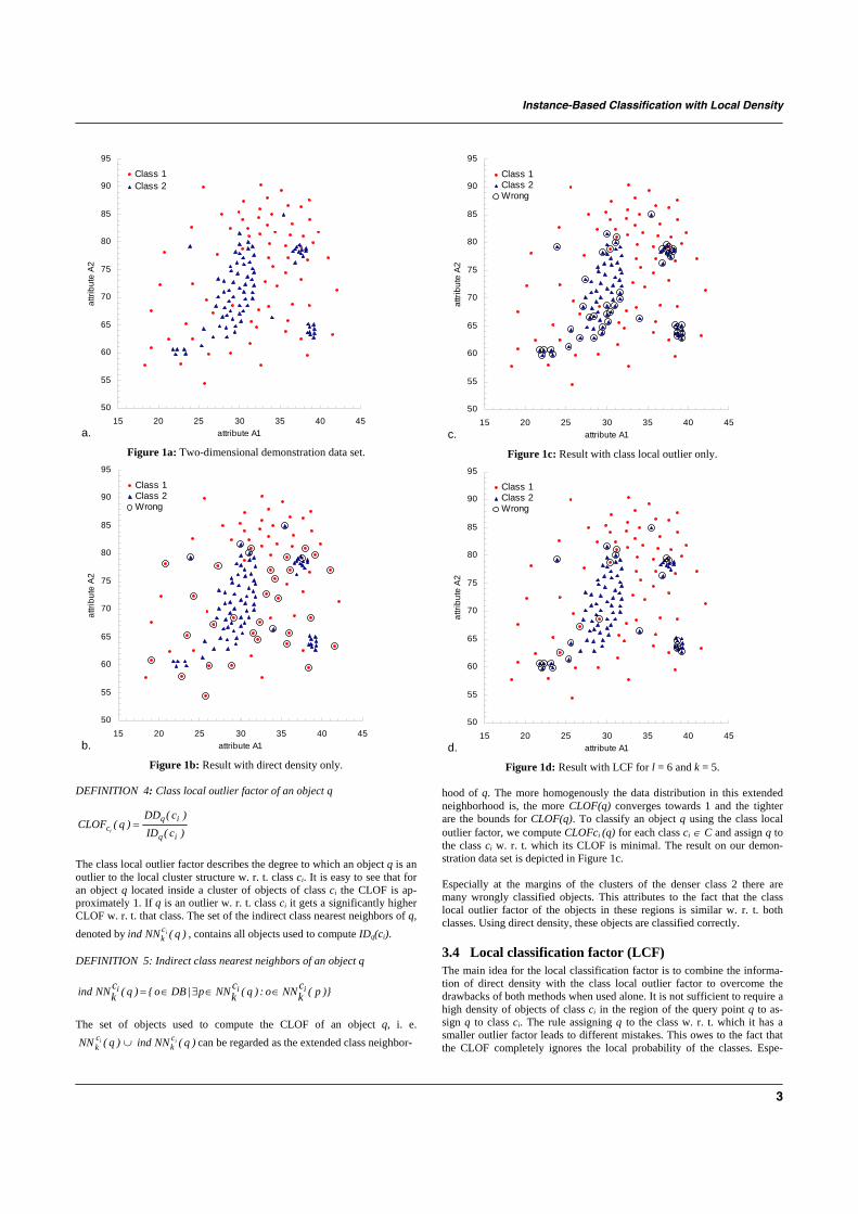
Instance-Based Classification with Local Density
3
a.
50
55
60
65
70
75
80
85
90
95
15 20 25 30 35 40 45attribute A1
attri
bute
A2
Class 1Class 2
Figure 1a: Two-dimensional demonstration data set.
b.
50
55
60
65
70
75
80
85
90
95
15 20 25 30 35 40 45attribute A1
attri
bute
A2
Class 1Class 2Wrong
Figure 1b: Result with direct density only.
DEFINITION 4: Class local outlier factor of an object q
)c(ID)c(DD
)q(CLOFiq
iqci
= The class local outlier factor describes the degree to which an object q is an outlier to the local cluster structure w. r. t. class ci. It is easy to see that for an object q located inside a cluster of objects of class ci the CLOF is ap-proximately 1. If q is an outlier w. r. t. class ci it gets a significantly higher CLOF w. r. t. that class. The set of the indirect class nearest neighbors of q, denoted by )q(NNind ic
k , contains all objects used to compute IDq(ci). DEFINITION 5: Indirect class nearest neighbors of an object q
)}p(ckNNo:)q(c
kNNp|DBo{)q(ckNNind iii ∈∈∃∈=
The set of objects used to compute the CLOF of an object q, i. e.
)q(NN ick ∪ )q(NNind ic
k can be regarded as the extended class neighbor-
c.
50
55
60
65
70
75
80
85
90
95
15 20 25 30 35 40 45attribute A1
attri
bute
A2
Class 1Class 2Wrong
Figure 1c: Result with class local outlier only.
d.
50
55
60
65
70
75
80
85
90
95
15 20 25 30 35 40 45attribute A1
attri
bute
A2
Class 1Class 2Wrong
Figure 1d: Result with LCF for l = 6 and k = 5.
hood of q. The more homogenously the data distribution in this extended neighborhood is, the more CLOF(q) converges towards 1 and the tighter are the bounds for CLOF(q). To classify an object q using the class local outlier factor, we compute CLOFci (q) for each class ci ∈ C and assign q to the class ci w. r. t. which its CLOF is minimal. The result on our demon-stration data set is depicted in Figure 1c. Especially at the margins of the clusters of the denser class 2 there are many wrongly classified objects. This attributes to the fact that the class local outlier factor of the objects in these regions is similar w. r. t. both classes. Using direct density, these objects are classified correctly.
3.4 Local classification factor (LCF) The main idea for the local classification factor is to combine the informa-tion of direct density with the class local outlier factor to overcome the drawbacks of both methods when used alone. It is not sufficient to require a high density of objects of class ci in the region of the query point q to as-sign q to class ci. The rule assigning q to the class w. r. t. which it has a smaller outlier factor leads to different mistakes. This owes to the fact that the CLOF completely ignores the local probability of the classes. Espe-
C. Plant et al.
4
cially if the CLOF of an object o is similar w. r. t. all classes we should assign the object to the most frequent class in its direct neighborhood. DEFINITION 6: Local classification factor of an object q LCFci (q) := DDq(ci) + l · CLOFci (q) The local classification factor of an object q w. r. t. class ci is the sum of its direct density and its l-times weighted class local outlier factor w. r. t. this class. We use a weighting factor l to determine to which extent the class local outlier factor and the direct density are relevant for classification. To classify an object q, we compute the LCF w. r. t. each class ci for q and assign q to the class w. r. t. which its LCF is minimal.
In Figure 1d the final result on the demonstration data set is de-picted. Owing to combination of both aspects, most classification errors disappear. In the following we explain why we combine the two aspects in this way and give hints on a proper parameter choice.
3.5 Parameter choice for k and l The parameter k determines the size of the region considered for comput-ing the LCF. If k is chosen too small the local density cannot be appropri-ately characterized. k corresponds to the minimum cluster size, i. e. to the minimum number of objects of a class that should be regarded as a cluster. For our experiments, we used the training data sets to determine an appro-priate value for k. In general, we defined k according to the recommenda-tions for the k-NN classifier (range: k = 3…15). Larger values of k consider more neighbors, and therefore smooth over local characteristics, smaller values lead to limited neighborhoods.
The parameter l determines to which degree the outlier factor of an object q w. r. t. the classes ci ∈ C is relevant for its classification. A higher value for l leads to more correctly classified objects in the sparser classes, to the expense of incorrectly classified objects in the denser classes. Margin objects of the denser class often have a higher class local outlier factor w. r. t. their own class than w. r. t. the sparser class. These objects are typically misclassified if the CLOF gets too much weight. Depending on the con-crete application domain, l can be determined either to maximize the over-all accuracy or to optimize recall and precision of a certain class. Particu-larly in biomedical data, high precision and recall on sparse classes is es-sential, since they often represent abnormal observations. Figure 2 shows accuracy and recall on the synthetic data set for k = 5 and l = 1...15, similar characteristics can be observed considering precision. However, it is diffi-cult to provide a general recommendation for parameter l because, as afore-mentioned, it depends on the given local data densities w.r.t. to the classes ci ∈ C. On examined biomedical data, higher dimensional data sets tend to larger l-values (metabolic data, l = 35…55), whereas lower-dimensional data sets show l-values close to 1 (e.g. synthetic l = 2, yeast l = 0.1, E. coli l = 0.1) to be balanced in terms of recall or precision.
50
55
60
65
70
75
80
85
90
95
100
1 2 3 4 5 6 7 8 9 10 11 12 13 14 15Parameter l
%
accuracyrecall class 1recall class 2
Figure 2: Influence of parameter l on classification accuracy of synthetic data (data see Figure 1).
4 EXPERIMENTS
4.1 Biomedical data LCF was tested and evaluated on one synthetic (cf. Figure 1a) and six real biomedical data sets as summarized in Table 1. Metabolic data was provided by a project partner (see acknowledgement). Five data sets (yeast, E. coli, liver, iris and diabetes) come from the UCI Machine Learning Re-pository (Blake and Merz, 1998). The table shows the di-mensionality of data, the number of classes and objects and the number of objects per class. Detailed biological informa-tion and experimental results are described and discussed for each data set separately throughout this section. Table 1: Synthetic and biomedical data sets.
Name Classes Dimensionality Objects Objects/Class Synthetic 2 2 152 71:81 Metabolic 2 45 57 38:19 Yeast* 10 8 1448 463:429:244:163:
51:44:35:30:20:5 E. coli* 8 7 336 143:2:35:77:5:20:
20:5 Liver* 2 5 345 145:200 Iris plant* 3 4 150 50:50:50 Diabetes* 2 8 768 500:268 Biological data sets marked by * come from the UCI Machine Learning Repository.
4.2 Benchmark classifiers, validation and parameter settings We compared LCF with six popular classification methods obtained from the publicly available WEKA data mining software (www.cs.waikato.ac.nz/ml/weka). For validation we used 10-fold cross validation. All classifiers were pa-rameterized to optimize accuracy. For SVM we used both polynomial (of degree 2) and radial kernels, the cost factor c was appropriately chosen using the training data set. We used the C4.5 decision tree algorithm with reduced error pruning. For ANN, we designed a single layer of hidden units with (number of attributes + number of classes)/2 hid-den units, 500 epochs to train through and a learning rate of 0.3. For LRA and NB no advanced settings can be per-formed. We applied both weighted (1/distance) and un-weighted k-NN with an Euclidian distance function and an appropriate value for k determined of the training data sets. For LCF we also used Euclidian distance and determined k and l of the training data sets.
4.3 Synthetic data For demonstration issues, a two-dimensional synthetic data set with various classes of local densities into account (Fig-ure 1a). Here, class 2 is split up into three partitions that are separated from each other by objects belonging to the less dense class 1. This data structure was generated by using a data generator developed in-house. Table 2 summarizes classification accuracy, precision, recall in percent (%) and the number of correctly and incorrectly classified instances.

Instance-Based Classification with Local Density
5
For LCF the parameter k was set to 5, l was set to 2 and 6 respectively (cf. Figure 2). LCF outperforms the other meth-ods in terms of accuracy and balance of correctly classified instances between both classes for l = 2 (82.9 %). LRA and SVM (polynomial, radial kernels) drop off in accuracy (59.2% - 63.2%) not being able to handle such complex data structures. DT, NB and ANN yielded higher accuracy (65.1% - 67.8%), but also lack on the balance of correctly assigned objects within the two classes. k-NN, however, was able to further increase accuracy, but also classifies in-stances of the sparser class 1 predominantly to those of the denser class 2. Weighting only slightly attenuates this ten-dency.
Table 2: Classification results on synthetic data.
Classifier Class Corr. Incorr. Recall Precision Accuracy LRA 1
2 37 53
34 28
52.1 65.4
56.9 60.9
59.2
SVM (poly)
1 2
32 64
39 17
45.1 79.0
65.3 62.1
63.2
SVM (radial)
1 2
36 57
35 24
50.7 70.4
60.0 60.2
61.2
5-NN 1 2
37 77
34 4
52.2 95.1
66.1 80.2
75.0
5-NN (weighted)
1 2
39 77
32 4
54.9 95.1
90.7 70.6
76.3
DT 1 2
32 71
39 10
45.1 87.7
76.2 64.5
67.8
NB 1 2
40 59
31 22
56.3 72.8
64.5 65.6
65.1
ANN 1 2
37 66
34 15
52.1 81.5
71.2 66.0
67.8
LCF (l=2)
1 2
59 67
12 14
83.1 82.7
80.8 84.8
82.9
LCF (l=6)
1 2
65 62
6 19
91.5 76.5
77.4 91.2
83.6
Corr. = correctly classified, Incorr. = incorrectly classified instances.
4.4 Metabolic data Classification in metabolomics has great potential for the development of automated diagnostics. After reviewing a certain population of healthy and diseased patients, abnor-mal metabolic profiles that are significantly different from a normal profile can be identified from data and thus can be-come diagnostic of a given disease (Baumgartner et al., 2004, 2005). The provided metabolic data, which was gen-erated by modern tandem mass spectrometry (MS/MS) technology, contains concentration values of 45 metabolites (12 amino acids and 33 sugars (saccharides)) grouped into patients suffering from a multigenic metabolic disorder and healthy controls. Further information on data is strictly con-fidential. However, an anonymized test set is publicly avail-able under http://biomed.umit.at/upload/lcfx.zip (2005). Table 3 summarizes our experiments by setting parameter k again to 5 and parameter l to 35 for LCF. Ow-ing to the small size of this data set (57 instances) it is fa-vorable to use a small k. It can be expected that metabolic data exhibits regions of various densities caused by a higher variation of metabolite concentration levels at the state of disease vs. normal (Baumgartner et al., 2006). The borders between healthy and pathological instances are blurred in
this high dimensional data set containing overlapping clus-ters of both classes. Best accuracy was obtained for value of l = 35. Of all investigated classifiers LCF showed highest classification accuracy of 73.7% and a superior recall value of 68.4% for class 2, i.e. the abnormal metabolic profiles of diseased people. LCF results are highest balanced in terms of recall and precision, and are comparable to LRA yielding correctly classified cases above 50% in both classes. How-ever, LRA lacks on accuracy of only 56.1%. SVM and ANN constitute similar accuracy values like LRA, but assign up to 80% of pathological cases to healthy subjects (false nega-tive cases). The k-NN classifier demonstrates the best accu-racy values within all benchmark classifiers, but breaks down in recall dramatically. The use of weighted k-NN does not help here. For diagnostic issues it is of highest impor-tance to classify instances of smaller and sparser classes correctly, particularly if this class is represented by patho-logical cases. Thus, balance of correctly classified objects between classes and high accuracy is essential for classify-ing diseased vs. normal metabolite profiles so that LCF is an interesting tool to be used for diagnostics. Figure 3 demonstrates classification accuracy of LCF as 3D plot by setting parameter k = 1, 3, 5, 7, 10 and l = 5, 15, 25, 35, 45, 55. Best accuracy was achieved for k = 5 and l-values between 35 and 55. Table 3: Classification results on metabolic data.
Classifier Class Corr. Incorr. Recall Precision Accuracy LRA 1
2 22 10
16 9
57.9 52.6
71.0 38.5
56.1
SVM (poly)
1 2
28 5
10 14
73.7 26.3
62.2 31.3
57.9
SVM (radial)
1 2
27 5
11 14
71.1 26.3
65.9 31.3
56.1
5-NN 1 2
37 2
1 17
97.4 10.5
68.5 50
68.4
5-NN (weighted)
1 2
36 2
2 17
94.7 10.5
67.9 50
66.6
DT 1 2
35 2
3 17
92.1 10.5
67.3 40
64.9
NB 1 2
31 8
7 11
81.6 42.1
77.5 47.1
68.4
ANN 1 2
26 7
12 12
63.2 31.6
64.8 36.8
57.9
LCF (l=35)
1 2
29 13
9 6
76.3 68.4
82.9 59.1
73.7
4.5 Yeast data The yeast data set contains 1484 protein sequences labeled according to ten classes (Horton and Nakai, 1996, 1997). Table 4 depicts classification results w. r. t. the three largest classes (1. cytoplasm, 2. nucleus and 3. mitochondria). The classes membrane protein (no N-terminal signal, uncleaved and cleaved signal, classes 4-6), extracellular, vacuole, per-oxisome and endoplasmic reticulum (classes 7-10) consist of 5 up to 163 instances and are not shown in detail. Pa-rameter settings for LCF were k = 12 and l = 0.1. Compar-ing all classifiers, most of the errors are due to confusing cytoplasmic proteins with nuclear proteins and vice versa.

C. Plant et al.
6
515
2535
4555
1
3
5
71060
65
70
75
Acc
urac
y
lk
Figure 3: Parameterization of LCF on unbalanced metabolic data. Classifi-cation accuracy depending on different k- and l-values is displayed. This reflects a fundamental difficulty in identifying nuclear proteins. One reason is the fact that unlike other localization signals the nuclear localization signal does not appear to be limited to one portion of a protein’s primary sequence. In some cases a protein without a nuclear localization signal may be transported to the nucleus as part of a protein com-plex if another subunit of the complex contains a nuclear localization signal (Zhao et al., 1988; Garcia-Bustos et al., 1991). In spite of this, LCF demonstrates the best balanced result for the first three classes w. r. t. recall (62.2%;59.7%;60%) and precision (56.4%;57.4%;63.8%), and an overall accuracy of 60.3%. Table 4: Classification results on yeast data.
Classifier Class Corr. Incorr. Recall Precision Accuracy LRA 1
2 3
324 198 139
139 231 105
70.0 46.2 57
51.3 61.7 62.1
58.6
SVM (poly)
1 2 3
320 217 128
141 212 116
69.1 50.6 52.5
51.7 60.4 66.0
59.3
SVM (radial)
1 2 3
362 162 139
101 267 105
37.1 37.8 57.0
49.5 64.8 67.1
58.9
21-NN 1 2 3
327 210 139
136 219 105
70.6 49.0 57.0
52.7 59.0 65.6
59.2
21-NN (weighted)
1 2 3
331 235 141
132 194 103
71.5 54.8 57.8
55.8 62.0 66.5
61.9
DT 1 2 3
294 223 116
169 206 128
63.5 52.0 47.5
52.1 57.8 64.1
57.8
NB 1 2 3
324 171 148
139 258 96
70.0 39.9 60.7
51.5 63.3 62.2
57.6
ANN 1 2 3
301 230 135
162 199 109
65.0 53.6 55.3
54.1 58.4 65.2
59.4
LCF (l=0.1)
1 2 3
288 256 139
175 173 105
62.2 59.7 60.0
56.4 57.4 63.8
60.3
Table 5: Confusion matrix for yeast data with LCF.
Class 1 2 3 4 5 6 7 8 9 10 1 288 132 33 6 1 0 2 0 1 0 2 131 256 27 11 3 0 1 0 0 0 3 57 24 139 10 6 2 3 0 3 0 4 13 17 7 125 1 0 0 0 0 0 5 5 6 4 3 19 8 6 0 0 0 6 0 0 1 0 3 34 6 0 0 0 7 5 0 3 0 2 5 20 0 0 0 8 10 7 2 6 2 0 3 0 0 0 9 2 4 2 0 0 0 2 0 10 0 10 0 0 0 0 1 0 0 0 0 4 LCF seems to be the best choice to identify nuclear proteins, however accompanied by a slight decrease of recall in class 1. In Table 5 the confusion matrix of LCF is shown in more detail. For the other classes not considered in Table 4 classi-fication accuracy corresponds well to the results reported in Horton and Nakai, 1997. With the exception of the ANN, DT and the weighted 21-NN classifier all other paradigms constitute a recall rate below 50% for nuclear proteins clas-sification. For the k-NN classifier we used an optimized k value for this special data set (Horton and Nakai, 1997). Here, weighting leads to an increase of overall accuracy (61.9%) and also of recall of class 2 (54.8%). However, the recall value of LCF is not reached. With l optimized for correctly identifying nuclear proteins (l = 0.5) we even ob-tain 66.0 % recall in class 2, but overall accuracy decreases to 56.8 % mainly because of incorrectly classified instances of the biggest class 1.
4.6 E. coli data set Similar to the yeast data set, E. coli data describes 7 protein location sites distributed to 8 classes, i.e. cytoplasm (143), inner membrane without signal sequence (77), periplasm (52), inner membrane, uncleavable signal sequence (35), outer membrane (20), outer membrane lipoprotein (5), inner membrane lipoprotein (2), and inner membrane, cleavable signal sequence (2) (Horton and Nakai, 1996, 1997). Table 6 shows the confusion matrix for the E. coli data set. Pa-rameters for LCF were set to k = 10 and l = 0.1 Table 7 de-picts precision and recall for the classes 2 and 4, the accu-racy on these classes and the overall accuracy. All examined classifiers show most classification errors due to mixing up inner membrane proteins without a signal sequence (class 2) and inner membrane proteins with an uncleavable signal sequence (class 4). The accuracy on these classes (denoted by C) is approximately 10 percent less than the overall accuracy (denoted by O). Class 2 and 4 which are unbalanced (c.f. 77 vs. 35 data) are very similar, both representing inner membrane proteins. Horton and Na-kai, 1997 explained the difficulty to separate both classes with the fact that the labelling of some of the training exam-ples includes some uncertainty; that means some training instances are probably wrongly labeled. However, LCF per-forms best w. r. t. balancedness in these classes and is slightly better in terms of overall accuracy. Performance on the other classes corresponds well to the results described in
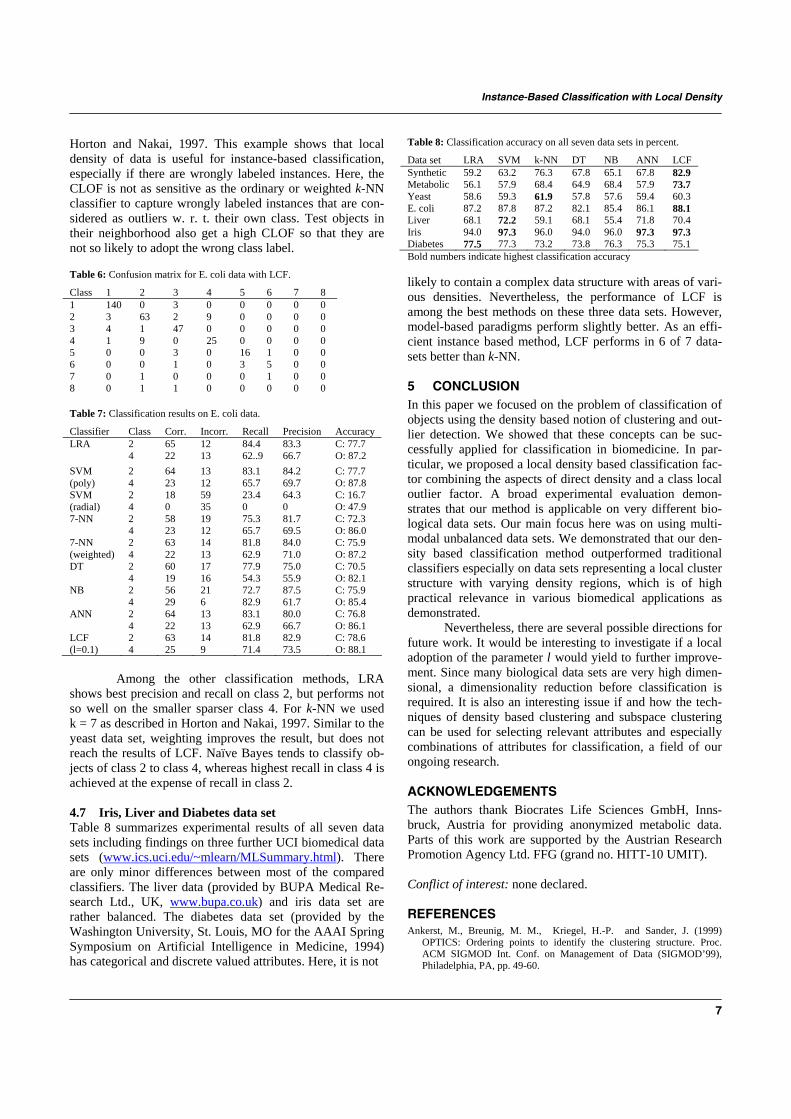
Instance-Based Classification with Local Density
7
Horton and Nakai, 1997. This example shows that local density of data is useful for instance-based classification, especially if there are wrongly labeled instances. Here, the CLOF is not as sensitive as the ordinary or weighted k-NN classifier to capture wrongly labeled instances that are con-sidered as outliers w. r. t. their own class. Test objects in their neighborhood also get a high CLOF so that they are not so likely to adopt the wrong class label. Table 6: Confusion matrix for E. coli data with LCF.
Class 1 2 3 4 5 6 7 8 1 140 0 3 0 0 0 0 0 2 3 63 2 9 0 0 0 0 3 4 1 47 0 0 0 0 0 4 1 9 0 25 0 0 0 0 5 0 0 3 0 16 1 0 0 6 0 0 1 0 3 5 0 0 7 0 1 0 0 0 1 0 0 8 0 1 1 0 0 0 0 0 Table 7: Classification results on E. coli data.
Classifier Class Corr. Incorr. Recall Precision Accuracy LRA 2
4 65 22
12 13
84.4 62..9
83.3 66.7
C: 77.7 O: 87.2
SVM (poly)
2 4
64 23
13 12
83.1 65.7
84.2 69.7
C: 77.7 O: 87.8
SVM (radial)
2 4
18 0
59 35
23.4 0
64.3 0
C: 16.7 O: 47.9
7-NN 2 4
58 23
19 12
75.3 65.7
81.7 69.5
C: 72.3 O: 86.0
7-NN (weighted)
2 4
63 22
14 13
81.8 62.9
84.0 71.0
C: 75.9 O: 87.2
DT 2 4
60 19
17 16
77.9 54.3
75.0 55.9
C: 70.5 O: 82.1
NB 2 4
56 29
21 6
72.7 82.9
87.5 61.7
C: 75.9 O: 85.4
ANN 2 4
64 22
13 13
83.1 62.9
80.0 66.7
C: 76.8 O: 86.1
LCF (l=0.1)
2 4
63 25
14 9
81.8 71.4
82.9 73.5
C: 78.6 O: 88.1
Among the other classification methods, LRA shows best precision and recall on class 2, but performs not so well on the smaller sparser class 4. For k-NN we used k = 7 as described in Horton and Nakai, 1997. Similar to the yeast data set, weighting improves the result, but does not reach the results of LCF. Naïve Bayes tends to classify ob-jects of class 2 to class 4, whereas highest recall in class 4 is achieved at the expense of recall in class 2. 4.7 Iris, Liver and Diabetes data set Table 8 summarizes experimental results of all seven data sets including findings on three further UCI biomedical data sets (www.ics.uci.edu/~mlearn/MLSummary.html). There are only minor differences between most of the compared classifiers. The liver data (provided by BUPA Medical Re-search Ltd., UK, www.bupa.co.uk) and iris data set are rather balanced. The diabetes data set (provided by the Washington University, St. Louis, MO for the AAAI Spring Symposium on Artificial Intelligence in Medicine, 1994) has categorical and discrete valued attributes. Here, it is not
Table 8: Classification accuracy on all seven data sets in percent.
Data set LRA SVM k-NN DT NB ANN LCF Synthetic 59.2 63.2 76.3 67.8 65.1 67.8 82.9 Metabolic 56.1 57.9 68.4 64.9 68.4 57.9 73.7 Yeast 58.6 59.3 61.9 57.8 57.6 59.4 60.3 E. coli 87.2 87.8 87.2 82.1 85.4 86.1 88.1 Liver 68.1 72.2 59.1 68.1 55.4 71.8 70.4 Iris 94.0 97.3 96.0 94.0 96.0 97.3 97.3 Diabetes 77.5 77.3 73.2 73.8 76.3 75.3 75.1 Bold numbers indicate highest classification accuracy likely to contain a complex data structure with areas of vari-ous densities. Nevertheless, the performance of LCF is among the best methods on these three data sets. However, model-based paradigms perform slightly better. As an effi-cient instance based method, LCF performs in 6 of 7 data-sets better than k-NN.
5 CONCLUSION In this paper we focused on the problem of classification of objects using the density based notion of clustering and out-lier detection. We showed that these concepts can be suc-cessfully applied for classification in biomedicine. In par-ticular, we proposed a local density based classification fac-tor combining the aspects of direct density and a class local outlier factor. A broad experimental evaluation demon-strates that our method is applicable on very different bio-logical data sets. Our main focus here was on using multi-modal unbalanced data sets. We demonstrated that our den-sity based classification method outperformed traditional classifiers especially on data sets representing a local cluster structure with varying density regions, which is of high practical relevance in various biomedical applications as demonstrated.
Nevertheless, there are several possible directions for future work. It would be interesting to investigate if a local adoption of the parameter l would yield to further improve-ment. Since many biological data sets are very high dimen-sional, a dimensionality reduction before classification is required. It is also an interesting issue if and how the tech-niques of density based clustering and subspace clustering can be used for selecting relevant attributes and especially combinations of attributes for classification, a field of our ongoing research.
ACKNOWLEDGEMENTS The authors thank Biocrates Life Sciences GmbH, Inns-bruck, Austria for providing anonymized metabolic data. Parts of this work are supported by the Austrian Research Promotion Agency Ltd. FFG (grand no. HITT-10 UMIT). Conflict of interest: none declared.
REFERENCES Ankerst, M., Breunig, M. M., Kriegel, H.-P. and Sander, J. (1999)
OPTICS: Ordering points to identify the clustering structure. Proc. ACM SIGMOD Int. Conf. on Management of Data (SIGMOD’99), Philadelphia, PA, pp. 49-60.
C. Plant et al.
8
Baumgartner, C., Böhm, C., Baumgartner, D., Marini, G., Weinberger, K., Olgemöller, B., Liebl, B. and Roscher, A.A. (2004) Supervised machine learning techniques for the classification of metabolic disorders in new-borns. Bioinformatics, 20, 2985–2996.
Baumgartner, C. and Baumgartner, D. (2006) Biomarker discovery, disease classification and similarity query processing on high-throughput MS/MS data of inborn errors of metabolism. J. Biomol. Screen., in press.
Bishop, C. M. (1995) Neural networks for pattern recognition. Oxford University Press, Oxford, UK.
Blake, C. L. and Merz, C. J. (1998) UCI Repository of machine learning databases,
http://www.ics.uci.edu/~mlearn/MLSummary.html. University of Califor-nia, Irvine, Dept. of Information and Computer Sciences.
Breuning, M. M., Kriegel, H.-P., Ng, R. T. and Sander, J. (2000) LOF: Identifying density-based local outliers. Proc. ACM Int. Conf. on Man-agement of Data (SIGMOD’00, Dallas, TX, pp. 93-104.
Cristianini, N. and Shawe-Taylor, J. (2000) An introduction to support vector machines and other kernel-based learning methods, Cambridge University Press, Cambridge, UK.
Cortes, C. and Vapnic, V. (1995) Support vector networks. Mach. Learn., 20, 273–297.
Ester, M., Kriegel, H.-P., Sander, J. and Xu, X. (1996) A density-based algorithm for discovering clusters in large spatial databases with noise. Proc. 2nd Int. Conf. on Knowledge Discovery and Data Mining (KDD’96). Portland, OR, pp. 226-231.
Gelman, A., Carlin, J.B., Stern, H.S. and Rubin, D.B. (2004) Bayesian data analysis, 2nd edn. Chapman & Hall/CRC Press, Boca Raton. FL.
Garcia-Bustos, J., Heitman, J. and Hall, M. (1991) Nuclear protein localiza-tion. Biochim. Biophys. Acta, 1071, 83–101.
Hastie, T. and Tibshirani, R. (1996) Discriminant adaptive nearest neighbor classification. IEEE Trans. Pattern Anal. Mach. Intell., 18, 607–616.
Horton, P., Nakai, K. (1996) A probabilistic classification system for pre-dicting the cellular localization sites of proteins. Proc. Int. Conf. Intell. Syst. Mol. Biol., 4, 109-15.
Horton, P. and Nakai, K. (1997) Better prediction of protein cellular local-ization sites with the k nearest neighbors classifier. Proc. 5th Interna-tional Conference on Intelligent Systems for Molecular Biology, Halkidiki, Greece, AAAI Press, pp. 147–152.
Hosmer, D. W. and Lemeshow, S. (2000). Applied logistic regression. Wiley. New York.
Langley, P., Iba, W. and Thompson, K. (1992) An analysis of Bayesian classifers. Proc. 10th National Conference on Artificial Intelligence, San Jose, CA, pp. 223–228.
Mitchell, T. M. (1997) Machine Learning. McGraw-Hill Boston, MA. Papadimitriou, S., Kitagawa, H., Gibbons, P. B. and Faloutsos, C. (2003)
LOCI: Fast outlier detection using the local correlation integral . Proc. of the 19th International Conference on Data Engineering (ICDE´03), Bangalore, India, pp. 315–327.
Paredes, R. and Vidal, E. (2000). A class-dependent weighted dissimilarity measure for nearest neighbor classification problems. Pattern Recogni-tion Letters, 21, 1027–1036.
Platt, J., Cristianini, N. and Shawe-Taylor, J. (2000) Large margin DAGs for multiclass classification. Proc. of Neural Information Processing Systems (NIPS'99), Denver, pp. 547-553.
Quinlan, R.J. (1986) Induction of decision trees, Mach. Learn., 1, 81-106. Quinlan, R.J. (1993) C4.5: Program for Machine Learning, Morgan Kauf-
mann, San Mateo, CA. Vapnic, V. (1998). Statistical Learning Theory. Wiley. New York. Xie, Z., Hsu, W., Liu, Z., and Lee, M.-L. (2002) SNNB: A selective
neighborhood based naive bayes for lazy learning. Proc. 6th Pacific-Asia Conference on Knowledge Discovery (PAKDD’02), Taipei, Tai-wan, pp. 104–114.
Zhao, L.J. and Padmanabhan, R. (1988) Nuclear transport of adenovirus DNA polymerase is facilitated by interaction with preterminal protein. Cell, 55, 1005–1015.

10.1177/1087057105280518ARTICLEBaumgartner and BaumgartnerBiomarker Discovery and Classification on MS/MS Data
Biomarker Discovery, Disease Classification, andSimilarity Query Processing on High-Throughput
MS/MS Data of Inborn Errors of Metabolism
CHRISTIAN BAUMGARTNER1 and DANIELA BAUMGARTNER1,2
In newborn errors of metabolism, biomarkers are urgently needed for disease screening, diagnosis, and monitoring of thera-peutic interventions. This article describes a 2-step approach to discover metabolic markers, which involves (1) the identifica-tion of marker candidates and (2) the prioritization of them based on expert knowledge of disease metabolism. For step 1, theauthors developed a new algorithm, the biomarker identifier (BMI), to identify markers from quantified diseased versus nor-mal tandem mass spectrometry data sets. BMI produces a ranked list of marker candidates and discards irrelevant metabolitesbased on a quality measure, taking into account the discriminatory performance, discriminatory space, and variance of metab-olites’ concentrations at the state of disease. To determine the ability of identified markers to classify subjects, the authorscompared the discriminatory performance of several machine-learning paradigms and described a retrieval technique thatsearches and classifies abnormal metabolic profiles from a screening database. Seven inborn errors of metabolism—phenylketonuria (PKU), glutaric acidemia type I (GA-I), 3-methylcrotonylglycinemia deficiency (3-MCCD), methylmalonicacidemia (MMA), propionic acidemia (PA), medium-chain acyl CoA dehydrogenase deficiency (MCADD), and 3-OH long-chain acyl CoA dehydrogenase deficiency (LCHADD)—were investigated. All primarily prioritized marker candidatescould be confirmed by literature. Some novel secondary candidates were identified (i.e., C16:1 and C4DC for PKU, C4DC forGA-I, and C18:1 for MCADD), which require further validation to confirm their biochemical role during health and disease.(Journal of Biomolecular Screening 2005:1-000)
Key words: biomarker discovery, disease classification, similarity query processing, tandem mass spectrometry, metabolicdisorders
INTRODUCTION
RECENT ADVANCES IN MODERN SCREENING TECHNOLOGIES
such as tandem mass spectrometry (MS/MS) have made itpossible to separate and identify small molecules based on theirmasses from samples of a biofluid such as blood serum or urine.By using appropriate internal standards, the concentration of amolecule in fluid can be measured with great precision because theaccuracy and sensitivity of the instrumentation are high.1-4 MS/MS
provides high-throughput data for the discovery of diagnosticmarkers, which is very relevant to the understanding of how meta-bolic disorders manifest. In particular, abnormal concentrations ofmetabolites may indicate erroneous metabolic reactions and mayreflect the actual functional state of a patient. So biomarkers areimportant tools for disease screening and early diagnosis.5-11
In this work, we delineated a 2-step approach to biomarker dis-covery, which involves (1) the identification of markers and (2) theprioritization of identified subsets of marker candidates. For step 1,we developed a new algorithm, the biomarker identifier (BMI), toidentify disease state metabolites from quantified 2-class (diseasedvs. normal) MS data sets. BMI returns a ranked list of marker can-didates qualified by a suitable score measure. In step 2, markercandidates were prioritized based on literature knowledge of dis-ease metabolism. Because biomarkers are those features that allowa well-done classification, we compared various classifiers to esti-mate their prognostic and diagnostic power. High-throughput MS/MS data, as generated in newborn screening programs, for exam-ple, are too voluminous and complex to catalog by hand, so theymust be stored and managed in modern database systems. A query
© 2005 The Society for Biomolecular Screening www.sbsonline.org 1
1Research Group for Clinical Bioinformatics,* Institute for BiomedicalEngineering, University for Health Sciences, Medical Informatics and Technol-ogy, A-6060 Hall i. T., Austria.2Department of Pediatrics, Innsbruck Medical University, A-6020 Innsbruck,Austria.*Research group has been renamed as the Research Group for ClinicalBioinformatics (formerly Research Group for Biomedical Data Mining).
Received May 9, 2005, and in revised form Jun 23, 2005. Accepted for publicationJul 18, 2005.
Journal of Biomolecular Screening X(X); 2005DOI: 10.1177/1087057105280518
J Biomol Screen OnlineFirst, published on November 28, 2005 as doi:10.1177/1087057105280518
Copyright 2005 by Society for Biomolecular Sciences.
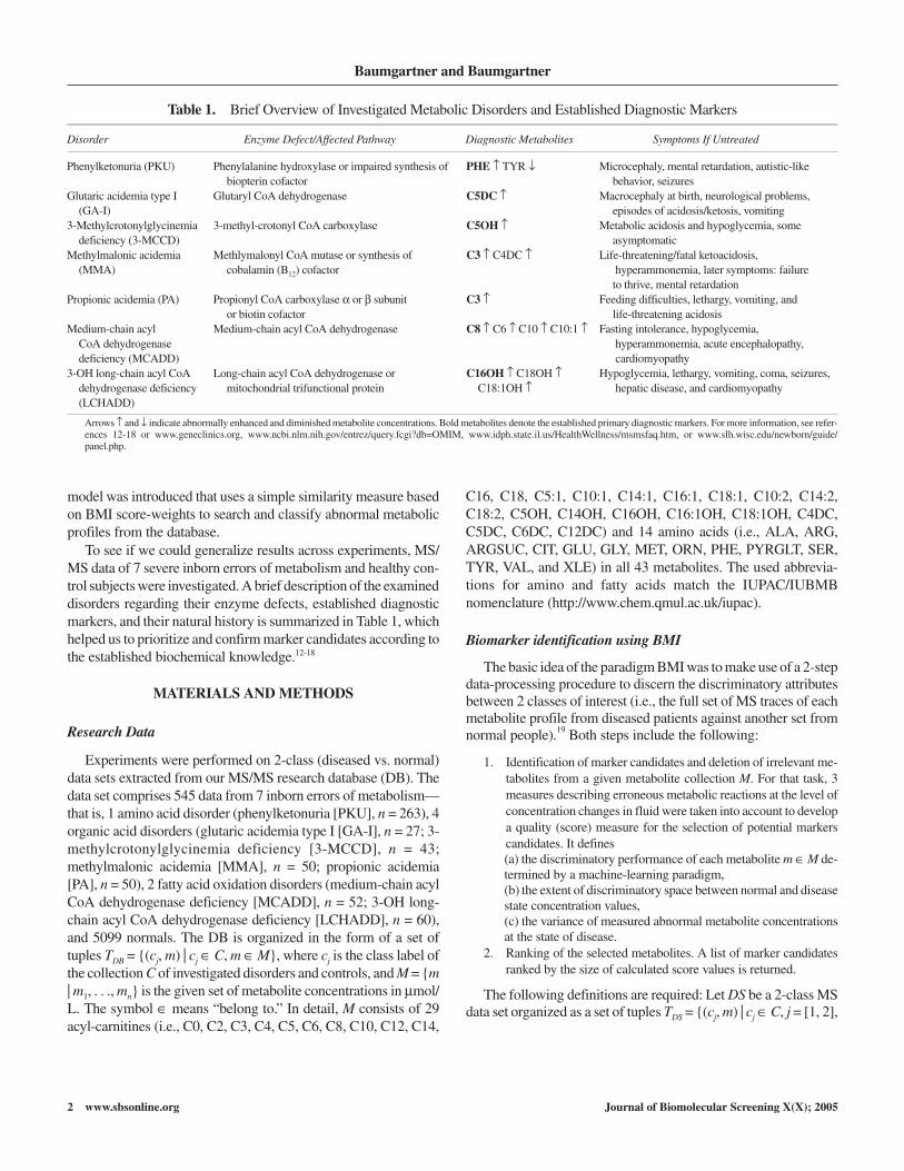
model was introduced that uses a simple similarity measure basedon BMI score-weights to search and classify abnormal metabolicprofiles from the database.
To see if we could generalize results across experiments, MS/MS data of 7 severe inborn errors of metabolism and healthy con-trol subjects were investigated. A brief description of the examineddisorders regarding their enzyme defects, established diagnosticmarkers, and their natural history is summarized in Table 1, whichhelped us to prioritize and confirm marker candidates according tothe established biochemical knowledge.12-18
MATERIALS AND METHODS
Research Data
Experiments were performed on 2-class (diseased vs. normal)data sets extracted from our MS/MS research database (DB). Thedata set comprises 545 data from 7 inborn errors of metabolism—that is, 1 amino acid disorder (phenylketonuria [PKU], n = 263), 4organic acid disorders (glutaric acidemia type I [GA-I], n = 27; 3-methylcrotonylglycinemia deficiency [3-MCCD], n = 43;methylmalonic acidemia [MMA], n = 50; propionic acidemia[PA], n = 50), 2 fatty acid oxidation disorders (medium-chain acylCoA dehydrogenase deficiency [MCADD], n = 52; 3-OH long-chain acyl CoA dehydrogenase deficiency [LCHADD], n = 60),and 5099 normals. The DB is organized in the form of a set oftuples TDB = {(cj, m) | cj ∈ C, m ∈ M}, where cj is the class label ofthe collection C of investigated disorders and controls, and M = {m| m1, . . ., mn} is the given set of metabolite concentrations in µmol/L. The symbol ∈ means “belong to.” In detail, M consists of 29acyl-carnitines (i.e., C0, C2, C3, C4, C5, C6, C8, C10, C12, C14,
C16, C18, C5:1, C10:1, C14:1, C16:1, C18:1, C10:2, C14:2,C18:2, C5OH, C14OH, C16OH, C16:1OH, C18:1OH, C4DC,C5DC, C6DC, C12DC) and 14 amino acids (i.e., ALA, ARG,ARGSUC, CIT, GLU, GLY, MET, ORN, PHE, PYRGLT, SER,TYR, VAL, and XLE) in all 43 metabolites. The used abbrevia-tions for amino and fatty acids match the IUPAC/IUBMBnomenclature (http://www.chem.qmul.ac.uk/iupac).
Biomarker identification using BMI
The basic idea of the paradigm BMI was to make use of a 2-stepdata-processing procedure to discern the discriminatory attributesbetween 2 classes of interest (i.e., the full set of MS traces of eachmetabolite profile from diseased patients against another set fromnormal people).19 Both steps include the following:
1. Identification of marker candidates and deletion of irrelevant me-tabolites from a given metabolite collection M. For that task, 3measures describing erroneous metabolic reactions at the level ofconcentration changes in fluid were taken into account to developa quality (score) measure for the selection of potential markerscandidates. It defines(a) the discriminatory performance of each metabolite m ∈ M de-termined by a machine-learning paradigm,(b) the extent of discriminatory space between normal and diseasestate concentration values,(c) the variance of measured abnormal metabolite concentrationsat the state of disease.
2. Ranking of the selected metabolites. A list of marker candidatesranked by the size of calculated score values is returned.
The following definitions are required: Let DS be a 2-class MSdata set organized as a set of tuples TDS = {(cj, m) | cj ∈ C, j = [1, 2],
Baumgartner and Baumgartner
2 www.sbsonline.org Journal of Biomolecular Screening X(X); 2005
Table 1. Brief Overview of Investigated Metabolic Disorders and Established Diagnostic Markers
Disorder Enzyme Defect/Affected Pathway Diagnostic Metabolites Symptoms If Untreated
Phenylketonuria (PKU) Phenylalanine hydroxylase or impaired synthesis of PHE ↑ TYR ↓ Microcephaly, mental retardation, autistic-likebiopterin cofactor behavior, seizures
Glutaric acidemia type I Glutaryl CoA dehydrogenase C5DC ↑ Macrocephaly at birth, neurological problems,(GA-I) episodes of acidosis/ketosis, vomiting
3-Methylcrotonylglycinemia 3-methyl-crotonyl CoA carboxylase C5OH ↑ Metabolic acidosis and hypoglycemia, somedeficiency (3-MCCD) asymptomatic
Methylmalonic acidemia Methlymalonyl CoA mutase or synthesis of C3 ↑ C4DC ↑ Life-threatening/fatal ketoacidosis,(MMA) cobalamin (B12) cofactor hyperammonemia, later symptoms: failure
to thrive, mental retardationPropionic acidemia (PA) Propionyl CoA carboxylase α or β subunit C3 ↑ Feeding difficulties, lethargy, vomiting, and
or biotin cofactor life-threatening acidosisMedium-chain acyl Medium-chain acyl CoA dehydrogenase C8 ↑ C6 ↑ C10 ↑ C10:1 ↑ Fasting intolerance, hypoglycemia,
CoA dehydrogenase hyperammonemia, acute encephalopathy,deficiency (MCADD) cardiomyopathy
3-OH long-chain acyl CoA Long-chain acyl CoA dehydrogenase or C16OH ↑ C18OH ↑ Hypoglycemia, lethargy, vomiting, coma, seizures,dehydrogenase deficiency mitochondrial trifunctional protein C18:1OH ↑ hepatic disease, and cardiomyopathy(LCHADD)
Arrows ↑ and ↓ indicate abnormally enhanced and diminished metabolite concentrations. Bold metabolites denote the established primary diagnostic markers. For more information, see refer-ences 12-18 or www.geneclinics.org, www.ncbi.nlm.nih.gov/entrez/query.fcgi?db=OMIM, www.idph.state.il.us/HealthWellness/msmsfaq.htm, or www.slh.wisc.edu/newborn/guide/panel.php.

m ∈ M}, where c1 is the class label of a metabolic disorder, c2 is thecontrol class, and M is the given set of metabolite concentrations.
We used logistic regression analysis (LRA) to determine thediscriminatory performance of each metabolite m ∈ M.20 LRA, alearning method that constructs a separating hyperplane betweenthe 2 data sets, assigns class membership by a probability measurein the form of P(y = 1) = 1/[1 + exp(–z)], where z = a0 + a1x is thelogit of the classification model. Here, x is the input variable, themetabolite concentration, and a0, a1 are the logit coefficients thathave to be learned by the method. The discriminatory threshold ts
between both classes can be explicitly calculated from the coeffi-cients a0 and a1 and is defined in equation (1):
ta
as = 0
1
.(1)
This concentration threshold separating both classes corre-sponds with a probability of P(y = 1) = 0.5, the measure that deter-mines class membership. Thus, a P-value ≥ 0.5 or < 0.5 clearly as-signs a test subject. We do need the parameter ts later for matchingmetabolic profiles (see Similarity Query Processing).
The discriminatory performance of each metabolite m was cal-culated as product of the true positive (TP) rates of class c1 and c2:
TP* = TPc1 • TPc2. (2)
To emphasize the small prevalence of inborn errors in a realscreening population, a ~100-fold larger group of normals com-pared to disorder class was examined. This unbalance of class sizeis necessary to avoid an overestimation of TP rates in the controlclass.21 Because TPc2 rates (specificities) ≥ 99.6% were computedin all study experiments, the performance measure TP* is predom-inantly determined by the value of the TPc1 rate (sensitivity) de-scribing the fraction of correctly classified diseased subjects. TP*
is thus more sensitive than overall classification accuracy (= cor-rectly classified subjects in both classes/all subjects), which doesnot reflect the unbalancedness of classes.
The range of discriminatory space between normal and diseasestate concentrations of m is estimated by the parameter ∆diff, whichapproximates the mean distance between both data distributions:
∆∆ ∆
∆∆diff
c
c
if
elsex
x=
≥
− =⎧⎨⎪
⎩⎪
11 1
2
with ,(3)
where x c iis the mean metabolite concentration in class ci. ∆ ≥ 1
denotes a concentration enhancement, ∆ < 1 a decrease of concen-tration in fluid.
The score value si ∈ S qualifying a processed metabolite mi ∈ Mis thus defined as
sTP
CVi
diff= ••
λ* ∆
,(4)
where λ is a scaling factor, and CV defined as σ/x is the coefficientof variation at the state of disease. We set λ = 10 by default becausethen score values range between 1 and ~1000, which is of practicaladvantage. x is the mean value and σ the standard deviation of con-centration values calculated from disorder class c1. S denotes thecollectivity of identified marker candidates represented by theirscore values.
Finally, a ranked list of marker candidates, mi ⊆ M, is returnedby BMI. Irrelevant metabolites, mj ⊆ M (mi ∪ mj = M), are dis-carded from M using a cutoff score value |s| < 5 by default.
The algorithm boxed above is briefly sketched as pseudo-codehelpful for software implementation.
To quantify the information content of a disease-specific scoreset S, the measure �sD was introduced:
Biomarker Discovery and Classification on MS/MS Data
Journal of Biomolecular Screening X(X); 2005 www.sbsonline.org 3
Input Two-class data set DS organized as a set of tuples Tc1 and Tc2
Tc1 := c1, m1, m2, . . ., mn; Tc2 := c2, m1, m2, . . ., mn; S = { }Output: Ranked list of marker candidates S := s1, s2, . . ., sm
List of discriminatory thresholds TS := ts1, ts2, . . ., tsm
Algorithm: BMI (Data set DS, Ranked list S, Threshold list TS)for i from 1 to n domi := DS.get(i)
TPi* := Discriminatory performance of mi determined by the learning method;
tsi := Discriminatory threshold of mi determined by the learning method;∆diffi := Extent of discriminatory space of mi;CVi := Coefficient of variation of class C1;
si = 10 • (TPi* • ∆diffi) / CVi;
if |si | ≥ 5 thenS[i] = si;TS[i] = tsi;
else delete (si, tsi);sort (S, TS);write (S, TS);
(The calculation of TS is optional)
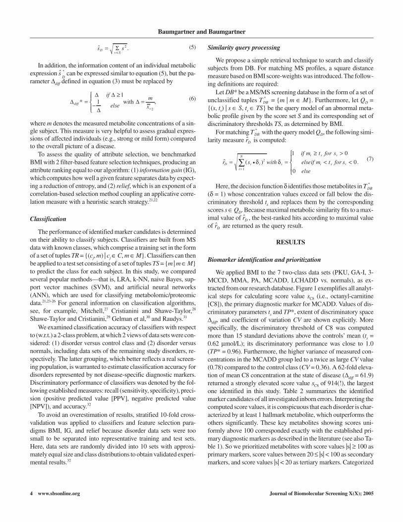
�s sDs S
=∈Σ 2 . (5)
In addition, the information content of an individual metabolicexpression � *s
Dcan be expressed similar to equation (5), but the pa-
rameter ∆diff defined in equation (3) must be replaced by
∆∆ ∆
∆∆diff
c
if
elsem
x* =
≥
−
⎧⎨⎪
⎩⎪=
11
2
with , (6)
where m denotes the measured metabolite concentrations of a sin-gle subject. This measure is very helpful to assess gradual expres-sions of affected individuals (e.g., strong or mild form) comparedto the overall picture of a disease.
To assess the quality of attribute selection, we benchmarkedBMI with 2 filter-based feature selection techniques, producing anattribute ranking equal to our algorithm: (1) information gain (IG),which computes how well a given feature separates data by expect-ing a reduction of entropy, and (2) relief, which is an exponent of acorrelation-based selection method coupling an applicative corre-lation measure with a heuristic search strategy.21,22
Classification
The performance of identified marker candidates is determinedon their ability to classify subjects. Classifiers are built from MSdata with known classes, which comprise a training set in the formof a set of tuples TR = {(cj, m) | cj ∈ C, m ∈ M}. Classifiers can thenbe applied to a test set consisting of a set of tuples TS = {m | m ∈ M}to predict the class for each subject. In this study, we comparedseveral popular methods—that is, LRA, k-NN, naive Bayes, sup-port vector machines (SVM), and artificial neural networks(ANN), which are used for classifying metabolomic/proteomicdata.21,23-26 For general information on classification algorithms,see, for example, Mitchell,27 Cristianini and Shawe-Taylor,28
Shawe-Taylor and Cristianini,29 Gelman et al,30 and Raudys.31
We examined classification accuracy of classifiers with respectto (w.r.t.) a 2-class problem, at which 2 views of data sets were con-sidered: (1) disorder versus control class and (2) disorder versusnormals, including data sets of the remaining study disorders, re-spectively. The latter grouping, which better reflects a real screen-ing population, is warranted to estimate classification accuracy fordisorders represented by not disease-specific diagnostic markers.Discriminatory performance of classifiers was denoted by the fol-lowing established measures: recall (sensitivity, specificity), preci-sion (positive predicted value [PPV], negative predicted value[NPV]), and accuracy.32
To avoid an overestimation of results, stratified 10-fold cross-validation was applied to classifiers and feature selection para-digms BMI, IG, and relief because disorder data sets were toosmall to be separated into representative training and test sets.Here, data sets are randomly divided into 10 sets with approxi-mately equal size and class distributions to obtain validated experi-mental results.32
Similarity query processing
We propose a simple retrieval technique to search and classifysubjects from DB. For matching MS profiles, a square distancemeasure based on BMI score-weights was introduced. The follow-ing definitions are required:
Let DB* be a MS/MS screening database in the form of a set ofunclassified tuples TDB
* = {m | m ∈ M}. Furthermore, let QD ={(s, ts) | s ∈ S, ts ∈ TS} be the query model of an abnormal meta-bolic profile given by the score set S and its corresponding set ofdiscriminatory thresholds TS, as determined by BMI.
For matching TDB* with the query model QD, the following simi-
larity measure �rD is computed:
� ( )r s with
if m t for s
elseif m tD i i
i
N
i
i s i
i s= =≥ >
<•=∑ δ δ2
1
1 0
for s
elsei <
⎧⎨⎪
⎩⎪0
0
. (7)
Here, the decision function δ identifies those metabolites in TDB*
(δ = 1) whose concentration values exceed or fall below the dis-criminatory threshold ts and replaces them by the correspondingscores s ∈ QD. Because maximal metabolic similarity fits to a max-imal value of �rD , the best-ranked hits according to maximal valueof �rD are returned as the query result.
RESULTS
Biomarker identification and prioritization
We applied BMI to the 7 two-class data sets (PKU, GA-I, 3-MCCD, MMA, PA, MCADD, LCHADD vs. normals), as ex-tracted from our research database. Figure 1 exemplifies all analyt-ical steps for calculating score value sC8 (i.e., octanyl-carnitine[C8]), the primary diagnostic marker for MCADD. Values of dis-criminatory parameters ts and TP*, extent of discriminatory space∆diff, and coefficient of variation CV are shown explicitly. Morespecifically, the discriminatory threshold of C8 was computedmore than 15 standard deviations above the controls’ mean (ts =0.62 µmol/L); its discriminatory performance was close to 1.0(TP* = 0.96). Furthermore, the higher variance of measured con-centrations in the MCADD group led to a twice as large CV value(0.78) compared to the control class (CV = 0.36). A 62-fold eleva-tion of mean C8 concentration at the state of disease (∆diff = 61.9)returned a strongly elevated score value sC8 of 914(!), the largestone identified in this study. Table 2 summarizes the identifiedmarker candidates of all investigated inborn errors. Interpreting thecomputed score values, it is conspicuous that each disorder is char-acterized by at least 1 hallmark metabolite, which outperforms theothers significantly. These key metabolites showing scores uni-formly above 100 corresponded exactly with the established pri-mary diagnostic markers as described in the literature (see also Ta-ble 1). So we prioritized metabolites with score values |s| ≥ 100 asprimary markers, score values between 20 ≤ |s| < 100 as secondarymarkers, and score values |s| < 20 as tertiary markers. Categorized
Baumgartner and Baumgartner
4 www.sbsonline.org Journal of Biomolecular Screening X(X); 2005

marker subsets are presented in Table 3. The prioritization into sec-ondary and tertiary markers appears to be useful to distinguish be-tween further promising marker candidates, of which the lattergroup may be more closely associated with secondary effects ofmetabolism. A fourth category was required to be introduced be-cause several marker candidates—that is, decanoyl-carnitine(C10), hexadecanoyl-carnitine (C16), decenoyl-carnitine (C10:1),arginine (ARG), and glutamate (GLU)—appeared together innearly all 7 study disorders representing the group of not disease-specific markers. For more details, see Tables 2 and 3. By way ofexample, Figure 2 displays the ranked list of selected metabolitesfor MCADD, a fatty acid oxidation defect, which leads to an accu-mulation of short- and medium-chain fatty acids and, in turn, to adecrease of cell energy metabolism. Indeed, the first 3 candi-dates—C8, C10:1, and C10—fit well to the biochemical knowl-edge, followed by a group of not disease-specific metabolites. In-terestingly, C18:1—by our classification, defined as a secondarymarker—appeared before C6 in ranking, a further established(secondary) diagnostic metabolite. Because C10:1, which is me-tabolized by 4 β-oxidation cycles of oleyl-carnitine (C18:1), is aproduct of a metabolic reaction in the fatty acid metabolism, C18:1is qualified to become a novel secondary marker. In addition, Fig-ure 2 depicts the information content of the full MCADD markerscore set (�sMCADD = 939) supplemented by 2 examples of a strong (�*sMCADD = 2008) and a mild (�*sMCADD = 467) expression. This mea-sure may be helpful to assess individual metabolic expressions and
to bring them into agreement with the patients’ therapeuticmanagement.
We benchmarked BMI with 2 popular feature subset selectionmethods. Figure 3 demonstrates these findings, again exemplifiedfor MCADD. IG returned a quite similar metabolite ranking com-
Biomarker Discovery and Classification on MS/MS Data
Journal of Biomolecular Screening X(X); 2005 www.sbsonline.org 5
Table 2. Identified Marker Candidates Using the Biomarker Identifier (BMI)
Disorder C3 C5 C6 C8 C10 C14 C16 C18 C5:1 C10:1 C16:1 C18:1 C18:2 C5OH C14OH C16OH C18:1OH C4DC C5DC C12DC ARG GLU PHE �sD
PKU 7 10 –74 10 –39 –8 27 –9 104 127 219 288GA-I 8 –61 9 34 514 62 52 5253-MCCD 12 –61 9 14 –16 –13 110 130 162 245MMA 153 11 19 45 –9 54 23 11 46 74 60 202PA 261 –27 16 25 7 19 20 266MCADD 16 914 90 –8 –42 –8 173 –10 –30 51 56 939LCHADD 13 –53 –5 8 152 66 31 29 180
�sD denotes the information content of a given score set S with respect to disorder D. Metabolites with score values |s| < 5 were deleted by BMI. A positive score value indicates an abnormal in-crease, and a negative score indicates a decrease of metabolite concentration in fluid. For definitions of abbreviations, see Table 1.
Table 3. Prioritization of Metabolic Marker Candidates
Primary Markers Secondary Markers Tertiary Markers Not Disease-
Disorder |Score| 100 20 |Score| < 100 5 |Score| < 20 Specific Markers
PKU PHE C16:1, C4DC C5, C12DC, C18:1GA-I C5DC C4DC C103-MCCD C5OH C5:1, C16:1, C18:1 C16MMA C3 C4DC C5, C8, C18:2, C5OH C10:1PA C3 C18:2, C5OH ARGMCADD C8 C18:1 C6, C14, C18, C16:1 GLULCHADD C16OH C18:1OH C18:1, C14OH
For definitions of abbreviations, see Table 1.
FIG. 1. Measured concentrations of octanyl-carnitine (C8) in healthycontrols and MCADD patients. All analytical steps for calculating scorevalue sC8 with the biomarker identifier (BMI) are depicted in detail. Histo-grams emphasize the different data distributions during health and disease.

pared to BMI, whereas relief’s ranking differed significantly fromboth methods BMI and IG. Although IG and relief produced aranked list of attributes, they lacked the ability to differ clearly be-tween primary and secondary/tertiary markers as BMI did. In par-ticular, MCADD’s diagnostic key marker C8 did not stand out sig-nificantly from the others in both approaches. For instance, C8’sIG was only 6.8% above that of C10:1, whereas C8’s BMI scoreoutperformed C10:1 more than 5 times (+528%). Relief evenranked C8 after C16 and C18:1—both metabolites showed slightlydecreased concentration values—which does not clearly reflectC8’s high discriminatory performance, its superior concentrationenhancement, and moderate coefficient of variation at the state ofdisease.
Disease classification
The performance of metabolic markers is determined on theirability to classify subjects. So we compared 5 machine-learningparadigms (i.e., LRA, k-NN, naive Bayes, SVM, and ANN) ac-cording to their discriminatory power and tried to assess their ap-plicability for disease screening and diagnostics. In this study, clas-sifiers were basically applied to 2-class data sets testingclassification accuracy of (1) primary markers alone; (2) primary,secondary, and tertiary markers, excluding not disease-specificones; and (3) the full BMI marker set. We designed both classes ofinterest as aforementioned: (a) disorder versus controls and (b) dis-order versus controls, including the remaining study diseases. Ourexperiments clearly indicated increasing classification accuracy
when considering the order of primary → primary + secondary +tertiary → all markers as classifiers’ inputs and little differences inaccuracy when comparing data sets (a) and (b). However, 2 excep-tions in experimental data (i.e., MMA and PA) appeared. MMAand PA belong to the group of organic acid disorders and are char-acterized by the identical primary diagnostic marker propionyl-carnitine (C3). Table 4 points out this situation, considering as ex-ample MMA. Our results revealed that sensitivity of all tested clas-sifiers dropped dramatically, particularly if classification modelswere solely built on the primary markers—for example, LRA:80% (a) ↓ 19% (b), SVM (linear): 66% (a) ↓ 2% (b), or ANN: 82%(a) ↓ 20% (b). Testing the full marker set, classification accuracycould be further enhanced, but accuracy did not achieve values ofdata set (a). Analyzing the behavior of classifiers on MMA data inmore detail, ANN yielded the best classification accuracy w.r.t.both data sets. Although both classes are strongly unbalanced insize, LRA, SVM, and k-NN showed promising results as well.Nevertheless, little differences in accuracy were observed, whichprimarily arise from the strengths and weaknesses of the targetlearning algorithm, along with the characteristics of the analyzeddata. Naive Bayes, which classifies a subject based on the proba-bility of each class given the subject’s feature variables, returnedthe most unbalanced classification results, indicated by a too-largefraction of false-negative cases. This minimizes PPV on the fullmarker set dramatically (68.6% data set (a), 13.5% data set (b)),which is undesirable for disease screening.
Baumgartner and Baumgartner
6 www.sbsonline.org Journal of Biomolecular Screening X(X); 2005
FIG. 2. Ranked list of identified metabolites for medium-chain acylCoA dehydrogenase deficiency (MCADD) returned by the biomarkeridentifier (BMI). The information content of MCADD’s class score set(�sMCADD) and 2 examples of a strong and mild expression (�*sMCADD) are de-noted explicitly. Positive score values indicate an abnormal increase, andnegative scores indicate a decrease of metabolite concentrations in fluid.
FIG. 3. Ranked lists of metabolites are shown using the following filterparadigms: information gain (IG) and relief. The first 11 metabolites aredepicted to be comparable with the biomarker identifier (BMI). Black barsindicate the established diagnostic metabolites in MCADD (see Table 1).

Abnormal metabolic profile retrieval
Similarity query processing on a large screening DB enablesthe user to search and classify subjects highly related to a requestedmetabolic profile. Figure 4 illustrates the first 100 hits of a MMAquery on our research DB graphically. We performed 2 requestsusing query models based on the full BMI marker set and, respec-tively, the disease-specific subset and determined classification ac-curacy of delivered hits. Surprisingly, the first 41 hits (left to arrow1 in the figure) represented a very homogeneous group of MMAcases if the similarity measure �rMMA was computed based on thedisease-specific markers. This group demonstrated a TP rate of74%, which was close to that of the best classifier (ANN, 78%),and contained only a small number of wrongly assigned PA cases(9.8%). A slight drop-off of similarity measure �rMMA in turn indi-cated the beginning of a second, homogeneous group of 42 PA plus4 MMA cases. The TP rate for PA was 84%. So, 2 groups of relatedmetabolic profiles could be separately delivered from 1 requestshowing a high degree of homogeneity with high classification ac-curacy. Otherwise, a request based on all marker candidates re-turned 1 mixed cohort of MMA and PA cases, with a continuousdecay of �rMMA measure approaching arrow 2. This result is surpris-ing and can be explained by strongly differing �rD values of bothmarker sets: �rMMA = 202 versus �rPA = 266 for the full set and �rMMA =262 versus �rPA = 163 for the disease-specific set, respectively. A 2times higher difference of the �rD measure in the latter set led, thus,to a better separation of both cohorts. DB requests for the remain-
ing disorders were unproblematic because the query model QD dif-fered significantly from each other.
Biomarker Discovery and Classification on MS/MS Data
Journal of Biomolecular Screening X(X); 2005 www.sbsonline.org 7
Table 4. Classification Accuracy of 5 Machine-Learning Paradigms Tested on MMA Data
Primary Primary + Secondary + Tertiary All Markers
MMA Sensitivity PPV Accuracy Sensitivity PPV Accuracy Sensitivity PPV Accuracy
Dataset (a)LRA 80 97.6 99.79 84 91.4 99.77 90 95.7 99.861-NN 80 90.0 99.93 82 91.1 99.75 92 97.9 99.905-NN 80 97.6 99.79 84 97.7 99.82 88 97.8 99.86Naïve Bayes 86 68.3 99.48 92 52.9 99.13 96 68.6 99.53SVM (linear) 66 100 99.67 80 97.6 99.79 92 97.9 99.90SVM (poly 2d) 55 100 99.51 80 97.6 99.79 90 97.8 99.88SVM (RBF) 46 100 99.48 68 97.1 99.67 88 97.8 99.86ANN 82 97.6 99.81 82 93.2 99.77 98 98.0 99.96
Dataset (b)LRA 19 50.0 99.11 40 66.7 99.29 50 71.4 99.401-NN 34 40.5 98.97 74 78.7 99.59 64 78.0 99.525-NN 40 54.1 99.17 68 68.0 99.65 58 93.5 99.59Naive Bayes 64 45.7 99.01 80 22.9 97.43 90 13.5 94.81SVM (linear) 2 50.0 99.11 14 77.8 99.20 48 80.0 99.43SVM (poly 2d) 8 100 99.19 40 87.0 99.42 52 86.7 99.50SVM (RBK) 0 100 99.11 10 83.3 99.19 14 70.0 99.19ANN 20 52.6 99.13 74 88.1 99.68 78 88.6 99.72
Classifiers were separately tested on the disease’s primary, secondary, and tertiary markers, as well as the full marker set as identified by biomarker identifier (BMI). Part (a) shows classificationaccuracy when testing classifiers on a 2-class data set of methylmalonic acidemia (MMA) cases versus healthy controls, and part (b) depicts findings examined on the data set of MMA cases ver-sus controls, including the remaining study disorders. Classification results are given in percentages. Specificities for all experiments were uniformly ≥ 99.6%. We tested logistic regression anal-ysis (LRA), unweighted 1-NN and 5-NN with an Euclidean distance function, naive Bayes, standard SVM (linear) and SVM with polynomial (degree 2) and Gaussian radial basis (RBF) kernelsusing a cost factor of 100, and a 3-layer (input-hidden-output) ANN using delta rule and back-propagation, 500 epochs to train trough, and a learning rate of 0.3. NN = nearest neighbor; ANN =artificial neural network; SVM = support vector machines; PPV = positive predictive value.
FIG. 4. Methylmalonic acidemia (MMA) similarity request on tan-dem mass spectrometry (MS/MS) research database (DB). The first 100hits returned are displayed. Squares indicate cases using the full biomarkeridentifier (BMI) marker set for the request, and circles indicate thedisease-specific BMI marker set (primary + secondary + tertiary markers).Filled squares/circles represent MMA cases, empty ones PA cases. �rMMA
denotes the similarity measure as computed (y-axis). Hits left of arrow 2show solely MMA and propionic acidemia (PA) cases, and hits right of ar-row 2 show entries of the remaining DB.

DISCUSSION
Recent publications on disease classification using data gener-ated by mass spectrometry have mainly focused on identifying bi-ological markers in biofluids to distinguish between disease andnormal samples.21,23-26,33 In particular, at the state of disease, a novelmarker may be an indicator for an abnormal metabolic reaction,which is relevant to the understanding of the biochemical cause be-hind it. Methods used to identify biomarkers in metabolic/proteomic data include, for example, T-statistics, filter-based fea-ture selection paradigms, classification methods such as decisiontrees, genetic algorithms, or artificial neural networks.8-10,21,34,35
In this work, we developed BMI, a new supervised featureselection paradigm applied to high-dimensional, quantifieddiseased-versus-normal MS data sets. BMI combines 3 aspectsthat are relevant for abnormal metabolic reactions at the level ofconcentration changes in fluid: discriminatory performance, ex-tent of discriminatory space, and variance of concentration valuesat disease state. Based on these measures, BMI computes a qualitycriterion that selects the most relevant and discards all irrelevantmetabolites from a given metabolite set. The cutoff for deletion(|s| < 5) is suggested because scores below 5 are characterized byinsignificant TP* values < 0.15 and slight ∆diff measures < 2.5, re-spectively. However, the cutoff parameter is adjustable, which en-ables the user to select or separate the 3 proposed marker catego-ries. We used LRA for BMI’s classification step because it returnsthe class discriminatory threshold as calculated from the model’slogit explicitly. This parameter is essential to formulate the match-ing rule for numerical data to perform similarity requests of meta-bolic profiles on DB. However, machine-learning paradigms suchas k-NN or neural networks enable a well-done classification, sothey can alternatively be used for BMI’s classification step, butthey lack an easy description of the threshold in terms of the origi-nal attributes. Poor classification results on the 1-dimensional datarevealed SVM and naive Bayes indicated by highly unbalanced TPrates (cf. Table 4). We benchmarked BMI with 2 established filter-based feature selection paradigms, and BMI scored absolutelywell. As aforementioned, IG returned a ranking result similar toBMI but did not allow a convincing prioritization, particularly be-tween primary and secondary marker candidates. Relief came offworse because its heuristic takes into account the usefulness of at-tributes for class prediction along with the level of intercorrelationamong them. BMI was developed to better address the issue of bio-chemical alteration of metabolites in fluid, so that entropy-based orcorrelation-based approaches are second choice because they donot optimally reflect the characteristics of given MS data structuresat disease state.
We prioritized marker candidates according to the proposedscheme of primary, secondary, and tertiary markers. All identifiedprimary and some secondary markers were able to be confirmedby literature association to disease biochemistry (cf. Table 1 andreferences 12-18). So far, some additional marker candidates were
found that, however, require further validation steps by generatingtestable hypotheses regarding their biochemical role in health anddisease. The most notable hallmark secondary candidates areC16:1 and C4DC for PKU, C4DC for GA-I, and C18:1 forMCADD. For the latter, C18:1, a biochemical explanation wasalready mentioned in the Results section. A validation of the notdisease-specific marker candidates (fourth category) seems to bedelicate because some are prioritized as secondary or even primarymarkers according to our categorization. In particular, the highlyscored amino acids ARG and GLU cannot be confirmed by thediseases’ primary metabolic reactions. However, this last step ofbiomarker discovery is inevitable and emphasizes, for example,the development of bioassays or preclinical models to confirm thebioanalytical measurements to initiate future marker validation.9,10
To assess the diagnostic power of identified marker candidates, wetested several classifiers. Our experimental results for MMA indi-cated sensitivities between 88% and 98%, PPV ranged between68.6% and 98%, depending on the applied classifier and markersubset. All other diseases achieved comparable classification re-sults compared to MMA; the best overall classification accuracyyielded a 3-layer neural network. In newborn screening, diseaseclassification is targeted to achieve sensitivities close to 100% andPPV significantly above 50% to reduce subsequent diagnostic pro-cedures, which cause additional efforts and costs.36,37 Because ourresearch data comprise newborn screening data of not standard-ized date of sampling—the influence of nutrition or early treat-ments was not clearly assessable—the classifiers’accuracy is defi-nitely underestimated as expected in this context. Our results mayreflect the constitution of provided research data, but they certainlydo not obscure the novelty of our methodological approach toidentify metabolic markers. Alternatively to the popular machine-learning approach for disease classification, we presented a re-trieval technique that combines the tasks of biomarker identifica-tion and similarity query processing to classify abnormal meta-bolic profiles directly from DB requests. We introduced asimilarity measure based on BMI score weights, which is the baseto match MS data with high accuracy.
The presented methodology has great potential for the develop-ment of automated diagnostics, taking neither a priori nor expertknowledge into account. After reviewing a certain population ofhealthy and diseased patients, the proposed procedure can identifymarker candidates that have significant variance from a normalprofile and thus can become diagnostic of a given disease. By hugeadvances in high-throughput technologies in the past years, a wideset of the human metabolome is already generable so that not pre-viously discovered markers can be identified from MS data usingappropriate data-mining techniques.38 These findings can enlargethe known marker spectrum of a disease significantly, which inturn further enhances the sensitivity of diagnostic testing. There-fore, measuring and mining the biochemical state of diseased peo-ple as well as drug monitoring of patients with a known disease arevery relevant to understanding how diseases manifest and drugs
Baumgartner and Baumgartner
8 www.sbsonline.org Journal of Biomolecular Screening X(X); 2005
act. Powerful bioinformatics and data-mining methods such asBMI are helpful tools that contribute to the challenging biomarkerdiscovery process.
In conclusion, we delineated a new approach to discoverbiomarkers consisting of identification and prioritization ofmarker candidates, as well as disease classification that contributesto a better understanding of biochemical roles of metabolites dur-ing health and disease. Our experimental results confirmed allknown markers of several disturbances of newborn metabolismand revealed a number of marker candidates, which have the po-tential to become novel diagnostic markers urgently needed fordisease screening and early diagnostics.
ACKNOWLEDGMENT
We thank Dr. A. A. Roscher from the University of Munich,Germany, for providing anonymized newborn screening researchdata. The study was supported by the Austrian Industrial FundsFFF (HITT-10 UMIT).
REFERENCES
1. Chace DH, DiPerna JC, Naylor EW: Laboratory integration and utilization oftandem mass spectrometry in neonatal screening: a model for clinical massspectrometry in the next millennium. Acta Paediatr (Suppl) 1999;88:45-47.
2. Charrow J, Goodman SI, McCabe ER, Rinaldo P: Tandem mass spectrometryin newborn screening. Genet Med 2000;2:267-269.
3. Gamache PH, Meyer DF, Granger MC, Acworth IN: Metabolomic applica-tions of electrochemistry/mass spectrometry. J Am Soc Mass Spectrom2004;15:1717-1726.
4. Dunn WB, Bailey NJ, Johnson HE: Measuring the metabolome: current ana-lytical technologies. Analyst 2005;130:606-625.
5. Roschinger W, Olgemoller B, Fingerhut R, Liebl B, Roscher AA: Advancesin analytical mass spectrometry to improve screening for inherited metabolicdiseases. Eur J Pediatr 2003;162(Suppl 1):S67-S76.
6. Wilcken B, Wiley V, Hammond J, Carpenter K: Screening newborns for in-born errors of metabolism by tandem mass spectrometry. N Engl J Med2003;348:2304-2312.
7. Strauss AW: Tandem mass spectrometry in discovery of disorders of themetabolome. Clin Invest 2004;113:354-356.
8. Neville P, Tan PY, Mann G, Wolfinger R: Generalizable mass spectrometrymining used to identify disease state biomarkers from blood serum.Proteomics 2003;3:1710-1715.
9. Lee JW, Weiner RS, Sailstad JM, Bowsher RR, Knuth DW, O’Brien PJ, et al:Method validation and measurement of biomarkers in nonclinical and clinicalsamples in drug development: a conference report. Pharm Res 2005;22:499-511.
10. Gao J, Garulacan LA, Storm SM, Opiteck GJ, Dubaquie Y, Hefta SA, et al:Biomarker discovery in biological fluids. Methods 2005;35:291-302.
11. German JB, Bauman DE, Burrin DG, Failla ML, Freake HC, King JC, et al:Metabolomics in the opening decade of the 21st century: building the roads toindividualized health. J Nutr 2004;134:2729-2732.
12. American College of Medical Genetics/American Society of Human Genet-ics Test and Technology Transfer Committee Working Group: Tandem massspectrometry in newborn screening. Genet Med 2000;2:267-269.
13. Blau N, Thony B, Cotton RGH, Hyland K: Disorders of tetrahydrobiopterinand related biogenic amines. In Scriver CR, Kaufman S, Eisensmith E, WooSLC, Vogelstein B, Childs B (eds): The Metabolic and Molecular Bases of In-herited Disease. 8th ed. New York: McGraw-Hill, 2001.
14. Donlon J, Levy H, Scriver CR: Hyperphenylalaninemia: phenylalanine hy-droxylase deficiency. In Scriver CR, Beaudet AL, Sly SW, Valle D (eds): The
Metabolic and Molecular Bases of Inherited Disease [Online]. New York:McGraw-Hill, 2004.
15. Hoffmann GF, Zschocke J: Glutaric aciduria type I: from clinical, biochemi-cal and molecular diversity to successful therapy. J Inherit Metab Dis1999;22:381-391.
16. Clayton PT, Doig M, Ghafari S, Meaney C, Taylor C, Leonard JV, et al:Screening for medium chain acyl-CoA dehydrogenase deficiency usingelectrospray ionisation tandem mass spectrometry. Arch Dis Child1998;79:109-115.
17. Dezateux C: Newborn screening for medium chain acyl-CoA dehydrogenasedeficiency: evaluating the effects on outcome. Eur J Pediatr 2003;162(Suppl1):S25-S28.
18. Rinaldo P, Matern D, Bennett MJ: Fatty acid oxidation disorders. Annu RevPhysiol 2002;64:477-502.
19. Duda RO, Hart PE, Stork GG: Pattern Classification. New York: John Wiley,2001.
20. Hosmer DW, Lemeshow S: Applied Logistic Regression. 2nd ed. New York:John Wiley, 2000.
21. Baumgartner C, Böhm C, Baumgartner D, Marini G, Weinberger K,Olgemöller B, et al: Supervised machine learning techniques for the classifi-cation of metabolic disorders in newborns. Bioinformatics 2004;20:2985-2996.
22. Hall MA, Holmes G: Benchmarking attribute selection techniques for dis-crete class data mining. IEEE Trans Knowledge Data Eng 2003;15:1437-1447.
23. Purohit PV, Rocke DM: Discriminant models for high-throughput proteomicsmass spectrometer data. Proteomics 2003;3:1699-1703.
24. Vlahou A, Schorge JO, Gregory BW, Coleman RL: Diagnosis of ovarian can-cer using decision tree classification of mass spectral data. J BiomedBiotechnol 2003;5:308-314.
25. Ball G, Mian S, Holding F, Allibone RO, Lowe J, Ali S, et al: An integratedapproach utilizing artificial neural networks and seldi mass spectrometry forthe classification of human tumors and rapid identification of potentialbiomarkers. Bioinformatics 2002;18:395-404.
26. Baumgartner C, Böhm C, Baumgartner D: Modelling of classification ruleson metabolic patterns including machine learning and expert knowledge. JBiomed Inform 2005;38:89-98.
27. Mitchell TM: Machine Learning. Boston: McGraw-Hill, 1997.
28. Cristianini N, Shawe-Taylor J: An Introduction to Support Vector Machinesand Other Kernel-Based Learning Methods. Cambridge, UK: CambridgeUniversity Press, 2000.
29. Shawe-Taylor J, Cristianini N: Kernel Methods for Pattern Analysis. Cam-bridge, UK: Cambridge University Press, 2004.
30. Gelman A, Carlin JB, Stern HS, Rubin DB: Bayesian Data Analysis 2nd ed.London: Chapman & Hall/CRC Press, 2004.
Biomarker Discovery and Classification on MS/MS Data
Journal of Biomolecular Screening X(X); 2005 www.sbsonline.org 9

31. Raudys S: Statistical and Neural Classifiers. London: Springer-Verlag, 2001.
32. Witten IH, Frank E: Data Mining: Practical Machine Learning Tools and
Techniques with Java Implementations. San Francisco: Morgan Kaufmann,2000.
33. Lilien RH, Farid H, Donald BR: Probabilistic disease classification of expres-sion-dependent proteomic data from mass spectrometry of human serum. JComput Biol 2003;10:925-946.
34. Baggerly KA, Morris JS, Coombes KR: Reproducibility of SELDI-TOF pro-tein patterns in serum: comparing datasets from different experiments.Bioinformatics 2004;20:777-785.
35. Yu JS, Ongarello S, Fiedler R, Chen XW, Toffolo G, Cobelli C, Trajanoski Z:Ovarian cancer identification based on dimensionality reduction for high-throughput mass spectrometry data. Bioinformatics 2005;21:2200-2209.
36. Thomason MJ, Lord J, Bain MD, Chalmers RA, Littlejohns P, Addison GM,et al: A systematic review of evidence for the appropriateness of neonatalscreening programmes for inborn errors of metabolism. J Public Health Med1998;20:331-343.
37. Pandor A, Eastham J, Beverley C, Chilcott J, Paisley S: Clinical effectivenessand cost-effectiveness of neonatal screening for inborn errors of metabolismusing tandem mass spectrometry: a systematic review. Health Technol Assess2004;8:iii,1-121.
38. Beecher C: The human metabolome. In Harrigan GG, Goodacre R (eds): Met-abolic Profiling: Its Role in Biomarker Discovery and Gene Function Analy-sis. Berlin: Kluwer Academic, 2003.
Address reprint requests to:Dr. Christian Baumgartner
Research Group for Clinical BioinformaticsInstitute for Biomedical Engineering
University for Health Sciences, Medical Informatics and TechnologyEduard Wallnöfer Zentrum 1A-6060 Hall in Tyrol, Austria
E-mail: [email protected]
Baumgartner and Baumgartner
10 www.sbsonline.org Journal of Biomolecular Screening X(X); 2005

www.elsevier.com/locate/yjbin
Journal of Biomedical Informatics 38 (2005) 89–98
Modelling of classification rules on metabolic patternsincluding machine learning and expert knowledge
Christian Baumgartnera,*, Christian Bohmb, Daniela Baumgartnerc
a Research Group for Biomedical Data Mining, Institute for Information Systems, University for Health Sciences,
Medical Informatics and Technology, Innrain 98, A-6020 Innsbruck, Austriab Institute for Computer Science, University of Munich, Oettingenstrasse 67, D-80538 Munich, Germanyc Department of Pediatrics, Innsbruck Medical University, Anichstrasse 35, A-6020 Innsbruck, Austria
Received 8 March 2004
Available online 11 November 2004
Abstract
Machine learning has a great potential to mine potential markers from high-dimensional metabolic data without any a priori
knowledge. Exemplarily, we investigated metabolic patterns of three severe metabolic disorders, PAHD, MCADD, and 3-MCCD,
on which we constructed classification models for disease screening and diagnosis using a decision tree paradigm and logistic regres-
sion analysis (LRA). For the LRA model-building process we assessed the relevance of established diagnostic flags, which have been
developed from the biochemical knowledge of newborn metabolism, and compared the models� error rates with those of the decision
tree classifier. Both approaches yielded comparable classification accuracy in terms of sensitivity (>95.2%), while the LRA models
built on flags showed significantly enhanced specificity. The number of false positive cases did not exceed 0.001%.
� 2004 Elsevier Inc. All rights reserved.
Keywords: Machine learning; Classification rules; Metabolic patterns; Expert knowledge; Metabolic disorders
1. Introduction
Newborn screening permits the detection of meta-
bolic disorders in newborns during the first few days
of life prior to the manifestation of symptoms [1–3].
Due to recent innovations and refinements of the screen-
ing methodology using modern tandem mass spectrom-
etry (MS/MS) more than 20 inherited metabolic
disorders can be detected simultaneously from a single
blood spot by quantifying concentrations of up to 50metabolites [4,5]. Machine learning techniques offer an
obvious and promising approach to examine high-di-
mensional metabolic data, where manual analysis is te-
dious and time-consuming due to the great number
and complexity. The investigation of novel metabolic
1532-0464/$ - see front matter � 2004 Elsevier Inc. All rights reserved.
doi:10.1016/j.jbi.2004.08.009
* Corresponding author. Fax: +43 50 8648 673827.
E-mail address: [email protected] (C. Baumgartner).
patterns, the construction of classification models with
high diagnostic prediction and the discovery of newclues for unknown causal relations lead to a better
understanding of mined data in metabolic networks
and constitutes a significant contribution to preventive
medicine [6].
Our goal was to investigate high-dimensional meta-
bolic data with respect to three severe inborn errors of
metabolism to construct classification models for disease
screening and diagnosis. In particular, we focused on(i) phenylalanine hydroxylase deficiency (PAHD), an
amino acid disorder, which includes cases of classic
phenylketonuria (PKU, OMIM No. 261600 [7]) and
hyperphenylalaninemia (non-PKU HPA, OMIM No.
264070) [8,9], (ii) medium-chain acyl-CoA dehydroge-
nase deficiency (MCADD, OMIM No. 201450), a fatty
acid oxidation defect [10], and (iii) 3-methylcrotonyl
CoA carboxylase deficiency (3-MCCD, OMIM No.210200), an organic acid disorder [11,12].

90 C. Baumgartner et al. / Journal of Biomedical Informatics 38 (2005) 89–98
For the model-building process we applied two di-
rectly interpretable classification algorithms, i.e., the
C4.5 decision tree paradigm and binary logistic regres-
sion analysis (LRA), to a metabolome training dataset.
Decision trees optimize classification accuracy by reduc-
ing the full feature dimensionality to a relevant featuresubset according to the algorithms� internal feature
selection strategy. The aim is to assess the relevance of
metabolic knowledge for the model-building process
by comparing C4.5s feature subset with established
diagnostic flags which have been developed from the
current biochemical knowledge of abnormalities in new-
born metabolism. For this task we built LRA models on
these flags and benchmarked their error rates with thoseof the decision tree classifier which does not require any
a priori knowledge for tree construction.
2. Metabolic data
Metabolites analyzed by modern MS/MS employing
appropriate internal standards can be quantified veryrapidly, sensitively and accurately requiring only mini-
mal sample preparation [1]. For MS/MS analysis a sin-
gle blood sample, which has been taken within few
days after the newborn�s birth, is sufficient. This screen-
ing methodology creates a high-dimensional metabolic
dataset of each newborn including concentration values
of more than 40 metabolites (14 amino acids and 29
fatty acids, see Table 1).Our experimental datasets were anonymously pro-
vided from the newborn screening program of the State
of Bavaria, Germany, between 1999 and 2002. For our
train-and-test design cycle we focused on one represen-
tative disorder of the amino acid, one of the fatty acid
oxidation, and one of the organic acid metabolism, each
of them showing a relatively high incidence in-between
Table 1
Overview of metabolites measured from MS/MS analysis
Amino acids (symbols) Fatty acids (symbols)
Alanine (Ala) Free carnitine (C0)
Arginine (Arg) Acetyl-carnitine (C2)
Argininosuccinate (Argsuc) Propionyl-carnitine (C3)
Citrulline (Cit) Butyryl-carnitine (C4)
Glutamate (Glu) Isovaleryl-carnitine (C5)
Glycine (Gly) Hexanoyl-carnitine (C6)
Methionine (Met) Octanyl-carnitine (C8)
Ornitine (Orn) Decanoyl-carnitine (C10)
Phenylalanine (Phe) Dodecanoyl-carnitine (C12
Pyroglutamate (Pyrglt) Myristoyl-carnitine (C14)
Serine (Ser) Hexadecanoyl-carnitine (C
Tyrosine (Tyr) Octadecanoyl-carnitine (C1
Valine (Val) Tiglyl-carnitine (C5:1)
Leucine + Isoleucine (Xle) Decenoyl-carnitine (C10:1)
Myristoleyl-carnitine (C14:
Fourteen amino acids and 29 fatty acids are analyzed from a single blood s
their group of disorders (PAHD, n = 94 cases including
43 cases of classic PKU and 51 cases of non-PKU HPA,
classic MCADD, n = 63 cases, and 3-MCCD, n = 22
cases). Unfortunately, the number of cases of further
screened metabolic disorders was too small (n < 5 cases)
for useful examination.Based on the given number of PAHD, MCADD, and
3-MCCD cases we sampled a statistically representative
control group from the newborn screening (NBS) data-
base (�600,000 entries, end of year 2002) using a rate of
�1:15–50 (disorder to controls). The PAHD sub-data-
base thus contains all 94 cases designated as confirmed
PAHD and 1241 randomly sampled controls, i.e., each
500th case from NBS controls. The MCADD and3-MCCD sub-databases consist of all 63 and 22 cases
designated as classic MCADD and 3-MCCD, and again
1241 controls. In our study population ‘‘controls’’ repre-
sent individuals without verified cases of known meta-
bolic disorders.
A much larger randomly sampled control database of
98,411 cases, i.e., one sixth of the NBS control database,
serves to estimate the real specific power of our con-structed models. Table 2 gives a short clinical overview
of the investigated disorders (enzyme defects, symptoms,
proposed treatments, and diagnostic tests) [7,13–15].
3. Process of data analysis
3.1. Overview of data mining steps
The data analysis process constructing classification
models on high-dimensional metabolic data is illustrated
in Fig. 1. We constructed classification models using
C4.5 decision tree paradigm and LRA. Both models
were trained and 10-fold-cross validated according to a
two-class problem on a training dataset containing n
Fatty acids (symbols)
Hexadecenoyl-carnitine (C16:1)
Octadecenoyl-carnitine (C18:1)
Decenoyl-carnitine (C10:2)
Tetradecadienoyl-carnitine (C14:2)
Octadecadienoyl-carnitine (C18:2)
Hydroxy-isovaleryl-carnitine (C5-OH)
Hydroxytetradecadienoyl-carnitine (C14-OH)
Hydroxypalmitoyl-carnitine (C16-OH)
) Hydroxypalmitoleyl-carnitine (C16:1-OH)
Hydroxyoleyl-carnitine (C18:1-OH)
16) Dicarboxyl-butyryl-carnitine (C4-DC)
8) Glutaryl-carnitine (C5-DC)
Methylglutaryl-carnitine (C6-DC)
Methylmalonyl-carnitine (C12-DC)
1)
pot using MS/MS. The concentrations are given in lmol/L.
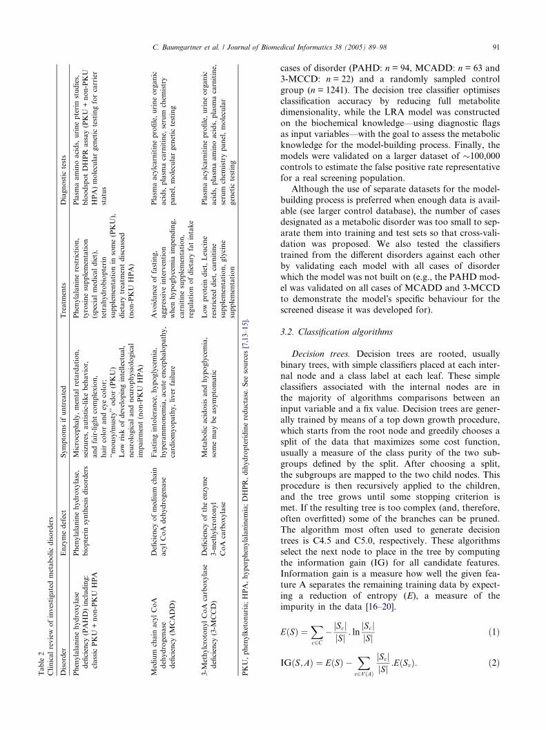
Table
2
Clinicalreview
ofinvestigatedmetabolicdisorders
Disorder
Enzymedefect
Symptomsifuntreated
Treatm
ents
Diagnostic
tests
Phenylalaninehydroxylase
deficiency
(PAHD)including:
classic
PKU
+non-PKU
HPA
Phenylalaninehydroxylase,
biopterinsynthesisdisorders
Microcephaly,mentalretardation,
seizures,autistic-likebehavior,
andfair-lightcomplexion,
haircolorandeyecolor;
‘‘mousy/m
usty’’odor(PKU)
Low
risk
ofdevelopingintellectual,
neurologicalandneurophysiological
impairment(non-PKU
HPA)
Phenylalaninerestriction,
tyrosinesupplementation
(specialmedicaldiet),
tetrahydrobiopterin
supplementationin
some(PKU),
dietary
treatm
entdiscussed
(non-PKU
HPA)
Plasm
aaminoacids,urinepterinstudies,
bloodspotDHPR
assay(PKU
+non-PKU
HPA)moleculargenetic
testingforcarrier
status
Medium
chain
acylCoA
dehydrogenase
deficiency
(MCADD)
Deficiency
ofmedium
chain
acylCoA
dehydrogenase
Fastingintolerance,hypoglycemia,
hyperammonem
ia,acute
encephalopathy,
cardiomyopathy,liver
failure
Avoidance
offasting,
aggressiveintervention
when
hypoglycemia
impending,
carnitinesupplementation,
regulationofdietary
fatintake
Plasm
aacylcarnitineprofile,urineorganic
acids,plasm
acarnitine,
serum
chem
istry
panel,moleculargenetic
testing
3-M
ethylcrotonylCoA
carboxylase
deficiency
(3-M
CCD)
Deficiency
oftheenzyme
3-m
ethylcrotonyl
CoA
carboxylase
Metabolicacidosisandhypoglycemia,
somemaybeasymptomatic
Low
protein
diet,Leucine
restricted
diet,carnitine
supplementation,glycine
supplementation
Plasm
aacylcarnitineprofile,urineorganic
acids,plasm
aaminoacids,plasm
acarnitine,
serum
chem
istrypanel,molecular
genetic
testing
PKU,phenylketonuria;HPA,hyperphenylalaninem
ia;DHPR,dihydropteridinereductase.See
sources
[7,13–15].
C. Baumgartner et al. / Journal of Biomedical Informatics 38 (2005) 89–98 91
cases of disorder (PAHD: n = 94, MCADD: n = 63 and
3-MCCD: n = 22) and a randomly sampled control
group (n = 1241). The decision tree classifier optimises
classification accuracy by reducing full metabolite
dimensionality, while the LRA model was constructed
on the biochemical knowledge—using diagnostic flagsas input variables—with the goal to assess the metabolic
knowledge for the model-building process. Finally, the
models were validated on a larger dataset of �100,000controls to estimate the false positive rate representative
for a real screening population.
Although the use of separate datasets for the model-
building process is preferred when enough data is avail-
able (see larger control database), the number of casesdesignated as a metabolic disorder was too small to sep-
arate them into training and test sets so that cross-vali-
dation was proposed. We also tested the classifiers
trained from the different disorders against each other
by validating each model with all cases of disorder
which the model was not built on (e.g., the PAHD mod-
el was validated on all cases of MCADD and 3-MCCD
to demonstrate the model�s specific behaviour for thescreened disease it was developed for).
3.2. Classification algorithms
Decision trees. Decision trees are rooted, usually
binary trees, with simple classifiers placed at each inter-
nal node and a class label at each leaf. These simple
classifiers associated with the internal nodes are inthe majority of algorithms comparisons between an
input variable and a fix value. Decision trees are gener-
ally trained by means of a top down growth procedure,
which starts from the root node and greedily chooses a
split of the data that maximizes some cost function,
usually a measure of the class purity of the two sub-
groups defined by the split. After choosing a split,
the subgroups are mapped to the two child nodes. Thisprocedure is then recursively applied to the children,
and the tree grows until some stopping criterion is
met. If the resulting tree is too complex (and, therefore,
often overfitted) some of the branches can be pruned.
The algorithm most often used to generate decision
trees is C4.5 and C5.0, respectively. These algorithms
select the next node to place in the tree by computing
the information gain (IG) for all candidate features.Information gain is a measure how well the given fea-
ture A separates the remaining training data by expect-
ing a reduction of entropy (E), a measure of the
impurity in the data [16–20].
EðSÞ ¼X
c2C� jScjjSj : ln
jScjjSj ð1Þ
IGðS;AÞ ¼ EðSÞ �X
v2V ðAÞ
jSvjjSj :EðSvÞ: ð2Þ

Fig. 1. Experimental design of model-building on high-dimensional metabolic data. Several intermediate data mining steps are performed resulting
in a classification model with high diagnostic prediction.
92 C. Baumgartner et al. / Journal of Biomedical Informatics 38 (2005) 89–98
S represents the data collection, jSj its cardinality, C isthe class collection, Sc the subset of S containing items
belonging to class c, V (A) is the set of all possible values
for feature A, Sv is the subset of S for which A has value
v. For our experiments we used C4.5 for tree construc-
tion with pruning option.
Logistic regression analysis. We constructed classifi-
cation models on diagnostic flags using logistic regres-
sion analysis, which is widely used in medicalapplications. LRA constructs a linear separating hyper-
plane between two datasets (cases of disorder and
controls) which have to be distinguished by the classifi-
ers. This hyperplane is mathematically described by a
linear discriminant function z = f (x1, . . . ,xn) = b1x1 +
b2x2 + � � � + bnxn + c. Here, x1, . . . ,xn are the input vari-ables. The coefficients b1, . . . ,bn and the constant c have
to be learned by the method.The distance from the hyperplane is considered as
probability measure of class membership based on a
so-called logistic function p = 1/(1 + e�z), where p is
the conditional probability of the form P (z = 1jx1, . . .,xn) and z the logit (discriminant function) of the model.
The class membership is indicated by a cut-off value
(p = 0.5 by default, p < 0.5 classifies controls and
p P 0.5 cases of disorder). LRA uses a maximum likeli-hood method which maximizes the probability of getting
the observed results given the fitted coefficients [21].
3.3. Diagnostic flags
In NBS labs diagnostic flags are routinely used to
pre-screen newborns that are highly suspicious for the
screened disorders. The procedure how these flags havebeen modelled is briefly sketched by an example.
In the abnormal PAHD metabolism the essential
amino acid Phe can not be metabolized to Tyr due to
a blockade of the enzyme phenylalanine hydroxylase.
Therefore, Phe shows strongly elevated concentration
levels accompanied by slightly decreased Tyr concentra-
tions. The diagnostic flags for PAHD contain the key
marker Phe showing the most significant concentrationchanges and additionally the ratio of Phe/Tyr represent-
ing the block of the enzyme phenylalanine hydroxylase.
For our experiments we used flags, which were devel-
oped by biochemical and medical experts of the Bavar-
ian newborn screening program, as summarized in
Table 3. NBS centres worldwide use such decision rules
with slight modifications for disease screening [22,23].
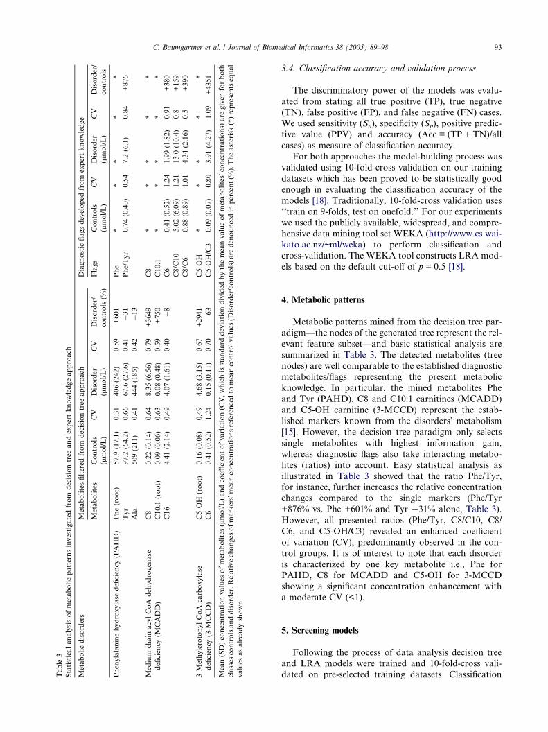
Table
3
Statisticalanalysisofmetabolicpatternsinvestigatedfrom
decisiontree
andexpertknowledgeapproach
Metabolicdisorders
Metabolitesfiltered
from
decisiontree
approach
Diagnostic
flagsdeveloped
from
expertknowledge
Metabolites
Controls
(lmol/L)
CV
Disorder
(lmol/L)
CV
Disorder/
controls(%
)
Flags
Controls
(lmol/L)
CV
Disorder
(lmol/L)
CV
Disorder/
controls
Phenylalaninehydroxylase
deficiency
(PAHD)
Phe(root)
57.9
(17.1)
0.31
406(242)
0.59
+601
Phe
**
**
*
Tyr
97.2
(64.2)
0.66
67.6
(27.6)
0.41
�31
Phe/Tyr
0.74(0.40)
0.54
7.2
(6.1)
0.84
+876
Ala
509(211)
0.41
444(185)
0.42
�13
Medium
chain
acylCoA
dehydrogenase
deficiency
(MCADD)
C8
0.22(0.14)
0.64
8.35(6.56)
0.79
+3649
C8
**
**
*
C10:1
(root)
0.09(0.06)
0.63
0.08(0.48)
0.59
+750
C10:1
**
**
*
C16
4.41(2.14)
0.49
4.07(1.61)
0.40
�8
C6
0.41(0.52)
1.24
1.99(1.82)
0.91
+380
C8/C10
5.02(6.09)
1.21
13.0
(10.4)
0.8
+159
C8/C6
0.88(0.89)
1.01
4.34(2.16)
0.5
+390
3-M
ethylcrotonylCoA
carboxylase
deficiency
(3-M
CCD)
C5-O
H(root)
0.16(0.08)
0.49
4.68(3.15)
0.67
+2941
C5-O
H*
**
**
C6
0.41(0.52)
1.24
0.15(0.11)
0.70
�63
C5-O
H/C3
0.09(0.07)
0.80
3.91(4.27)
1.09
+4351
Mean(SD)concentrationvalues
ofmetabolites(lmol/L)andcoeffi
cientofvariation(C
V,whichisstandard
deviationdivided
bythemeanvalueofmetabolites�concentrations)
are
given
forboth
classes
controlsanddisorder.Relativechanges
ofmarkers�meanconcentrationsreferencedto
meancontrolvalues
(Disorder/controls)are
denouncedin
percent(%
).Theasterisk(*)representsequal
values
asalreadyshown.
C. Baumgartner et al. / Journal of Biomedical Informatics 38 (2005) 89–98 93
3.4. Classification accuracy and validation process
The discriminatory power of the models was evalu-
ated from stating all true positive (TP), true negative
(TN), false positive (FP), and false negative (FN) cases.
We used sensitivity (Sn), specificity (Sp), positive predic-tive value (PPV) and accuracy (Acc = (TP + TN)/all
cases) as measure of classification accuracy.
For both approaches the model-building process was
validated using 10-fold-cross validation on our training
datasets which has been proved to be statistically good
enough in evaluating the classification accuracy of the
models [18]. Traditionally, 10-fold-cross validation uses
‘‘train on 9-folds, test on onefold.’’ For our experimentswe used the publicly available, widespread, and compre-
hensive data mining tool set WEKA (http://www.cs.wai-
kato.ac.nz/~ml/weka) to perform classification and
cross-validation. The WEKA tool constructs LRA mod-
els based on the default cut-off of p = 0.5 [18].
4. Metabolic patterns
Metabolic patterns mined from the decision tree par-
adigm—the nodes of the generated tree represent the rel-
evant feature subset—and basic statistical analysis are
summarized in Table 3. The detected metabolites (tree
nodes) are well comparable to the established diagnostic
metabolites/flags representing the present metabolic
knowledge. In particular, the mined metabolites Pheand Tyr (PAHD), C8 and C10:1 carnitines (MCADD)
and C5-OH carnitine (3-MCCD) represent the estab-
lished markers known from the disorders� metabolism
[15]. However, the decision tree paradigm only selects
single metabolites with highest information gain,
whereas diagnostic flags also take interacting metabo-
lites (ratios) into account. Easy statistical analysis as
illustrated in Table 3 showed that the ratio Phe/Tyr,for instance, further increases the relative concentration
changes compared to the single markers (Phe/Tyr
+876% vs. Phe +601% and Tyr �31% alone, Table 3).
However, all presented ratios (Phe/Tyr, C8/C10, C8/
C6, and C5-OH/C3) revealed an enhanced coefficient
of variation (CV), predominantly observed in the con-
trol groups. It is of interest to note that each disorder
is characterized by one key metabolite i.e., Phe forPAHD, C8 for MCADD and C5-OH for 3-MCCD
showing a significant concentration enhancement with
a moderate CV (<1).
5. Screening models
Following the process of data analysis decision treeand LRA models were trained and 10-fold-cross vali-
dated on pre-selected training datasets. Classification

Table 4a
Classification accuracy of decision tree and LRA models trained and cross-validated on a small training set
Disorder (No. of cases) Classification model Model input
variables
Sn (%) FN (No.
of cases)
Sp
(%)
FP (No.
of cases)
Acc (%) Tree structure of C4.5 classifier/logit
of LRA models z = a0 + a1 m1+ � � �+ an mn
Standard error
of coefficients
RMS
error
PAHD (n = 94) Decision tree classifier Phe 96.809 3 99.758 3 99.551 Phe < = 115.58: control 0.0678
Tyr Phe > 115.58
Ala j Ty r < = 95.92: PAHD
j Tyr > 95.92
j j Ala < = 686.13: PAHD
j j Ala > 686.13: control
LRA built on diagnostic flags Phe 96.809 3 99.758 3 99.551 �14.776 2.622 0.0598
Phe/Tyr +0.0738 Æ Phe 0.015
+2.2157 Æ Phe/Tyr 0.519
Phe* 93.617 6 99.678 4 99.251 �11.8681 1.429 0.0687
+0.081 Æ Phe 0.011
MCADD (n = 63) Decision tree classifier C8 95.238 3 99.517 6 99.310 C10:1 <= 0.37 0.0813
C10:1 j C8 <= 0.46: control
C16 j C8 > 0.46
j j C16 <= 3.16: MCADD
j j C16 > 3.16
j j j C8 <= 1.48: control
j j j C8 > 1.48: MCADD
C10:1 > 0.37: MCADD
LRA built on diagnostic flags C8 95.238 3 99.678 4 99.463 �8.5391 2.394 0.0658
C10:1 +7.1856 Æ C8 2.865
C6 +11.0392 Æ C10:1 4.092
C8/C10 �1.6439 Æ C6 2.893
C8/C6 �0.1836 Æ C8/C10 0.060
�0.1774 Æ C8/C10 1.837
C8* 95.238 3 99.839 2 99.617 �7.5362 0.746 0.0595
+5.7931 Æ C8 0.764
3-MCCD (n = 22) Decision tree classifier C5-OH 95.455 1 99.839 3 99.683 C5–OH <= 0.41: Control 0.0563
C6 C5–OH > 0.41
j C6 <= 0.37: 3-MCCD
j C6 > 0.37: control
LRA built on diagnostic flags C5-OH 90.909 2 99.919 1 99.762 �722.52 3935.91 0.0486
C5-OH/C3 +1054.41 Æ C5-OH 5719.10
�248.09 Æ C5-OH/C3 1348.61
C5-OH* 95.455 1 99.919 1 99.942 �47.349 48.291 0.0404
+63.205 Æ C5-OH 65.095
n, number of PAHD, MCADD and 3-MCCD cases, No, number of FN and FP cases. Classification results are given in terms of sensitivity (Sn), specificity (Sp) and accuracy (Acc). The generated
C4.5 tree structures as well as the logit z of the LRA models and the standard error of their coefficients are given. For both algorithms the root mean squared (RMS) error, which is a measure of
success of numeric prediction, is shown. The asterisk (*) highlights those LRA models built on the disease�s predominant metabolite (see Table 3, Disorder/controls). Tenfold-cross validation was
applied to validate both classifiers.
94
C.Baumgartn
eret
al./JournalofBiomedica
lInform
atics
38(2005)89–98

C. Baumgartner et al. / Journal of Biomedical Informatics 38 (2005) 89–98 95
accuracy in terms of sensitivity (Sn), specificity (Sp) and
accuracy (Acc) is given in Table 4a. In addition to the
parameters Sn, Sp and PPV we also denounce the gener-
ated tree structure as well as the logit of the LRA model
and its standard error of the coefficients, and for both
approaches the root mean squared (RMS) error, ameasure of success of numeric prediction. Both the
decision tree and LRA model for PAHD showed equal
classification accuracy (Sn = 96.809%, Sp = 99.758%,
and Acc = 99.551%). The MCADD models� error rateswere comparable to the PAHD ones. Only the decision
tree model yielded a slightly reduced specificity. The
3-MCCD models achieved the highest classification
accuracy showing only small alterations in sensitivityand specificity.
However, to estimate specificity and positive predic-
tive value (PPV) representative for a real screening pop-
ulation we validated our models on a larger control
database of approximately 100,000 cases. All validation
results based on a real screening population are summa-
rized in Table 4b. As expected, the specificity of both
models decreased, while the number of false positivecases of the decision tree models was 6–16th fold re-
duced compared to that of the LRA/flag approach.
For instance, considering Phe, and Phe/Tyr as LRA
model input variables, the most specific PAHD model
was established showing a Sp of 99.905% and a PPV
of 49.5%, respectively. In other words, only a fraction
of 93 FP cases (i.e., 0.0009% out of 98,411 controls)
Table 4b
Classification accuracy of decision tree and LRA models validated on a larg
Disorder (No. of cases) Classification model Model input
variables
PAHD (n = 94) Decision tree classifier Phe
Tyr
Ala
LRA built on diagnostic flags Phe
Phe/Tyr
Phe*
MCADD (n = 63) Decision tree classifier C8
C10:1
C16
LRA built on diagnostic flags C8
C10:1
C6
C8/C10
C8/C6
C8*
3-MCCD (n = 22) Decision tree classifier C5-OH
C6
LRA built on diagnostic flags C5-OH
C5-OH/C3
C5-OH*
n, number of PAHD, MCADD, and 3-MCCD cases, No. number of FN an
specificity (Sp), positive predictive value (PPV), and accuracy (Acc). Sp, PPV a
estimate specificities of a representative screening population. Sn remain unch
built on the disease�s predominant metabolite (see Table 3, Disorder/control
was wrongly classified. Testing the PAHD model with
all MCADD and 3-MCCD cases no additional false
negative cases were observed, because abnormal PAHD
metabolism only alters amino acid, but not fatty acid
concentrations. In analogy, no false negative cases were
observed when checking the MCADD or 3-MCCDmodels with all PAHD/3-MCCD or PAHD/MCADD
cases, respectively.
For MCADD our results yielded a different picture.
Constructing a model on the diagnostic flags (model in-
puts are three single metabolites and two ratios) the
number of FP cases could be reduced from 915 to 55
false positive cases compared to the decision tree clas-
sifier. The best classification accuracy (Sn = 95.2%,Sp = 99.992%, PPV = 88.2%) was obtained by building
the model solely on the predominant marker C8 carni-
tine which basically can be explained by the dramatic
concentration changes of C8 caused by the erroneous
fatty acid metabolism of MCADD (cf. increase of
mean concentration level of +3649%, Table 3). The
flags C6, C10:1, C8/C10, and C8/C6 yielded a promis-
ing impact (mean concentration changes 159–750%)and moderate CV in the MCADD class (<0.92), but
they were not able to further increase specificity. How-
ever, the false positive rates for MCADD between dif-
ferent screening programs most likely vary because of
differences in acylcarnitine analysis and profiling. C8,
the predominant, but not specific marker for MCADD,
which is elevated in several other disorders (e.g.,
er control database
Sn (%) FN (No.
of cases)
Sp (%) FP (No.
of cases)
PPV (%) Acc (%)
96.809 3 99.404 587 13.41 99.401
96.809 3 99.905 93 49.46 99.903
95.745 4 99.885 113 44.34 99.881
95.238 3 99.070 915 6.15 99.068
95.238 3 99.944 55 52.17 99.941
95.238 3 99.992 8 88.24 99.989
95.455 1 99.627 367 5.41 99.626
90.909 2 99.955 44 33.33 99.955
95.455 1 99.957 42 33.33 99.956
d FP cases. Classification results are given in terms of sensitivity (Sn),
nd Acc were re-evaluated on a larger database of �100,000 controls to
anged (see results Table 4a). The asterisk (*) highlights the LRA models
s).

96 C. Baumgartner et al. / Journal of Biomedical Informatics 38 (2005) 89–98
medium/short chain 3-OH acyl CoA dehydrogenase
deficiency), can be used to pre-screen several fatty oxi-
dation disorders. Both presented models including
additional markers to C8 are specific for MCADD
which is important when physicians consider differen-
tial diagnostic aspects.The classification models for 3-MCCD differed signif-
icantly from that of PAHD and MCADD as both ap-
proaches showed the lowest classification error rates.
The LRA model built on the predominant marker C5-
OH, however, yielded the best classification accuracy.
The ratio C5-OH/C3 seems to be redundant.
6. Procedure to optimize sensitivity
In newborn screening the declared aim is to optimise
sensitivity to 100% and to increase specificity as far as
possible. This assignment is of high importance as ethi-
cal arguments and cost effectiveness related to an erro-
neous diagnosis are concerned. However, the presented
models showing high specificity do not always have opti-mal Sn of 100%. Exemplarily, Fig. 2 illustrates a proce-
dure to optimize sensitivity of our most specific PAHD
model (constructed on Phe and Phe/Tyr) by changing
the default cut-off level from p = 0.5 stepwise to
p = 0.25, 0.15, 0.1, and 0.01. By reducing the cut-off
value to p = 0.15, all PAHD cases can be correctly
Fig. 2. Procedure to optimize sensitivity of the LRA model for PAHD
constructed on the input variables Phe and Phe/Tyr: costs to optimize
sensitivity by reduction of specificity are illustrated. The changes of
sensitivity (%), specificity (%) and absolute number of FP cases (n) are
given for cut-off values of p = 0.5, 0.25, 0.15, 0.1, and 0.01. The arrow
indicates 100% sensitivity and a lower specificity of 99.818% (n = 179
FP cases) at p = 0.15 compared to p = 0.5 by default showing a
sensitivity of 96.809% and a specificity of 99.905% (n = 93 FP cases).
The cut-off optimization was performed on full training data (not
validated).
classified (Sn = 100%, arrow in Fig. 2), while the num-
ber of FP cases increases from 93 to 179. Therefore, Sp
demounted from 99.905 to 99.818%. However, this
procedure to optimize sensitivity of the regression
model was performed only on the full training dataset,
thus giving too optimistic results in general. For cross-or leave-one-out validation, which is recommended, if
training sets are small, the entire model-building pro-
cess including optimisation of the cut-off value, and
classification has to be repeated in each cross-valida-
tion training subset. Currently, the validation proce-
dure is in progress, these results have to be presented
later.
7. Discussion
To satisfy the ever growing need for effective screen-
ing and diagnostic tests MS/MS provides a very high
throughput and has the potential to be highly accurate.
The complexity of analysed high-dimensional metabolic
data using MS/MS requires machine learning and datamining techniques to support the classification of disease
and the identification of potentially useful diagnostic
markers. In turn, the identification of key metabolites
could shed light on the nature of the disorder.
However, there are many data mining techniques for
the processing and general learning of high-dimensional
data in proteomics/metabolomics. Current research
focuses on the detection of regions of interest in ma-trix-assisted desorption/ionization-time of flight mass
spectra to mine differences in the protein pattern
between healthy and diseased persons using established
supervised and unsupervised methods [24,25]. Our
experiments were not directly applied to the protein
mass spectra, but were performed on data by the con-
version of raw mass spectra into clinically meaningful
results (amino acid and fatty acid concentrations) [1].We investigated two different approaches to build clas-
sification models on provided newborn screening data
with high diagnostic prediction. Machine learning offers
the advantage that markers are found without any other
a priori assumptions or conditions, and our results cor-
respond well to the established biochemical knowledge
[8–12]. In our approach we used the decision tree para-
digm to identify potentially useful metabolites (nodes oftree) by computing the information gain for all candi-
date features. However, filter based selection techniques
like information gain or correlation-based filters also
yield promising results, but solely select single attributes
as subsets [26,27]. Building LRA models on single
metabolites and ratios, which reflect the interaction
of single metabolites in newborn metabolism (cf.
PAHD: Phe ›\ Tyr fl) Phe/Tyr), the number of falsepositive cases could be diminished significantly (up to
6–16 times) compared to the decision tree classifier.

C. Baumgartner et al. / Journal of Biomedical Informatics 38 (2005) 89–98 97
Therefore, knowledge on abnormal newborn metabo-
lism modelled as ratios of interacting attributes thus
provides an important contribution to enhance a mod-
el�s specific power, while sensitivities in both approaches
remain unchanged.
However, no classification model in both approachesachieved 100% sensitivity. In this context we briefly
sketched a procedure showing the best trade-off between
optimal sensitivity and specificity that can be accepted
by adjusting the cut-off value in LRA. As mentioned be-
fore, further validation studies are warranted.
In addition to the decision tree classifier we used
LRA, which shows highest discriminatory performance
as we could demonstrate in prior experiments compar-ing various classification algorithms on metabolic data
[27]. Some of them are well accepted in current proteo-
mic research as other authors described [28]. However,
both paradigms can be classified as directly interpretable
techniques, which represent their data relations in an
explicit way like a probabilistic model (LRA) or a tree
structure, and so they find more acceptance in a clinical
ambience.
8. Conclusion
Data mining in MS/MS data enables us to identify
disease state metabolites without any a priori knowl-
edge. The consideration of biochemical knowledge for
the model-building process by combining interactingdisease state metabolites revealed a further increase of
the classifiers� discriminatory performance and lead to
a significant increase of the specific power of our screen-
ing models. Our models achieved sensitivity values
>95.2%. The number of FP cases in all three disorders
did not exceed 0.001%.
The presented approach, which considers mining
techniques and expert knowledge for the model-buildingprocess, permits the construction of classification rules
with high diagnostic prediction.
Acknowledgments
We thank Dr. A.A. Roscher from Dr. von Hauner
Children�s Hospital, University of Munich, Germanyfor providing anonymous newborn screening data. This
study was generously supported by the Austrian Indus-
trial Research Promotion Fund FFF (Grant No. HITT-
10 UMIT).
References
[1] Chace DH, DiPerna JC, Naylor EW. Laboratory integration and
utilization of tandem mass spectrometry in neonatal screening: a
model for clinical mass spectrometry in the next millennium. Acta
Paediatr (Suppl) 1999;88:45–7.
[2] Liebl B, Nennstiel-Ratzel U, von Kries R, Fingerhut R, Olgmoller
B, Zapf A, et al. Expanded newborn screening in Bavaria:
tracking to achieve requested repeat testing. Prev Med
2002;34:132–7.
[3] Liebl B, Nennstiel-Ratzel U, Roscher AA, von Kries R. Data
required for the evaluation of newborn screening programmes.
Eur J Pediatr 2003;162(Suppl. 1):57–61.
[4] Millington DS, Terada N, Kodo K, Chace DH. A review:
carnitine and acylcarnitine analysis in the diagnosis of metabolic
diseases: advantages of tandem mass spectrometry. In: Matsum-
oto I, editor. Advances in chemical diagnosis and treatment of
metabolic disorders, vol 1. New York: John Wiley; 1992. p.
59–71.
[5] Rashed MS, Ozand PT, Bucknall MP, Little D. Diagnosis of
inborn errors of metabolism from blood spots by acylcarnitines
and amino acids profiling using automated electrospray tandem
mass spectrometry. Pediatr Res 1995;38:324–31.
[6] Mendes P. Emerging bioinformatics for the metabolome. Brief
Bioinform 2002;3:134–45.
[7] National Center for Biotechnology Information. Online Mende-
lian Inheritance in Man (OMIM), Available from: http://
www3.ncbi.nlm.nih.gov/Omim.
[8] Adler C, Ghisla S, Rebrin I, Heizmann CW, Blau N, Curtius
HC. Suspected pterin-4a-carbinolamine dehydratase deficiency:
hyperphenylalaninemia due to inhibition of phenylalanine
hydroxylase by tetrahydro-7-biopterin. J Inherit Metab Dis
1992;15:405–8.
[9] Chace DH, Millington DS, Terada N, Kahler SG, Roe CR,
Hofman LF. Rapid diagnosis of phenylketonuria by quantitative
analysis for phenylalanine and tyrosine in neonatal blood spots by
tandem mass spectrometry. Clin Chem 1993;39:66–71.
[10] Van Hove JL, Zhang W, Kahler SG, Roe CR, Chen YT, Tereda
N, et al. Medium-chain acyl-CoA dehydrogenase (MCAD)
deficiency: diagnosis by acylcarnitine analysis in blood. Am J
Hum Genet 1993;52:958–66.
[11] Bannwart C, Wermuth B, Baumgartner R, Suormala T,
Wiesmann UN. Isolated biotin-resistant deficiency of 3-meth-
ylcrotonyl-CoA carboxylase presenting as a clinically severe
form in a newborn with fatal outcome. J Inherit Metab Dis
1992;15:863–8.
[12] Blau N, Thony B, Cotton RGH, Hyland K. Disorders of
tetrahydrobiopterin and related biogenic amines. In: Scriver
CR, Kaufman S, Eisensmith E, Woo SLC, Vogelstein B, Childs
B, editors. The metabolic and molecular bases of inherited
disease. 8th ed. New York: McGraw Hill; 2001. chapter 78.
[13] Children�s Health System and University of Washington, Gene-
Tests. A medical genetics information resource, Available from:
http://www.geneclines.org.
[14] California Department of Health Services, Newborn Screening
Program MS/MS Research Project, Available from: http://
www.dhs.ca.gov/pcfh/gdb/html/PDE/MSMSMainPage.htm.
[15] American College of Medical Genetics/American Society of
Human Genetics Test and Technology Transfer Committee
Working Group. Tandem mass spectrometry in newborn screen-
ing. Genet Med 2000;2:267–9.
[16] Mitchell TM. Machine learning. Boston, MA: McGraw-Hill;
1997.
[17] Langley P. Selection of relevant features in machine learning. In:
Proceedings of the AAAI fall symposium on relevance. New
york: AAAI Press; 1994. p. 140–4.
[18] Witten IH, Frank E. Data mining—practical machine learning
tools and techniques with java implementations. San Fran-
cisco: Morgan Kaufmann; 2000.
[19] Quinlan RJ. Induction of decision trees. Machine learning
1986;1:81–106.

98 C. Baumgartner et al. / Journal of Biomedical Informatics 38 (2005) 89–98
[20] Quinlan RJ. C4.5: program for machine learning. San Mateo,
CA: Morgan Kaufmann; 1993.
[21] Hosmer DW, Lemeshow S. Applied logistic regression. 2nd
ed. New York: Wiley; 2000.
[22] Health professionals guide to newborn screening. Wisconsin state
laboratory of hygiene.Available from:www.slh.wisc.edu/newborn/
guide.
[23] Chace DH, Sherwin JE, Hillman SL, Lorey F, Cunningham GC.
Use of phenylalanine-to-tyrosine ratio determined by tandem
mass spectrometry to improve newborn screening for phenylke-
tonuria of early discharge specimens collected in the first 24 hours.
Clin Chem 1998;44:2405–9.
[24] Lee KR, Lin X, Park DC, Eslava S. Megavariate data analysis of
mass spectrometric proteomics data using latent variable projec-
tion method. Proteomics 2003;3:1680–6.
[25] Neville P, Tan PY, Mann G, Wolfinger R. Generalizable mass
spectrometry mining used to identify disease state biomarkers
from blood serum. Proteomics 2003;3:1710–5.
[26] Baumgartner C, Baumgartner D, Bohm C, Classification on high
dimensional metabolic data: Phenylketonuria as an example. In:
Proceedings of the Second International Conference on Biomed-
ical Engineering (BioMED 2004), Innsbruck, Austria, ACTA
Press; 2004, p. 357-60.
[27] Baumgartner C, Bohm C, Baumgartner D, Marini G, Weinberger
K, Olgemoller B, et al. Supervised machine learning techniques
for the classification of metabolic disorders in newborns. Bioin-
formatics 2004 [in press].
[28] Purohit PV, RockeDM.Discriminant models for high-throughput
proteomics mass spectrometer data. Proteomics 2003;3:1699–
1703.

BIOINFORMATICS Vol. 20 no. 17 2004, pages 2985–2996doi:10.1093/bioinformatics/bth343
Supervised machine learning techniquesfor the classification of metabolic disordersin newborns
C. Baumgartner1,∗, C. Böhm2, D. Baumgartner3, G. Marini4,K. Weinberger4, B. Olgemöller5, B. Liebl6 and A. A. Roscher7
1Research Group for Biomedical Data Mining, University for Health Sciences, MedicalInformatics and Technology, Innrain 98, A-6020 Innsbruck, Austria, 2Institute forComputer Science, University of Munich, Oettingenstrasse 67, D-80538 Munich,Germany, 3Department of Pediatrics, Innsbruck Medical University, Anichstrasse 35,A-6020 Innsbruck, Austria, 4Biocrates Life Sciences Biotechnology GmbH, Innrain 66,A-6020 Innsbruck, Austria, 5Laboratory Becker, Olgemöller & Colleagues,Führichstrasse 70, D-81671 Munich, Germany, 6Public Health Newborn ScreeningCenter of the State of Bavaria, Landesuntersuchungsamt Südbayern, D-85762Oberschleissheim, Germany and 7Department of Biomedical Genetics and MolecularBiology, Dr von Hauner Children’s Hospital, University of Munich, Lindwurmstrasse 4,D-80337 Munich, Germany
Received on February 23, 2004; revised and accepted on May 13, 2004
Advance Access publication June 4, 2004
ABSTRACTMotivation: During the Bavarian newborn screening pro-gramme all newborns have been tested for about 20 inheritedmetabolic disorders. Owing to the amount and complexityof the generated experimental data, machine learning tech-niques provide a promising approach to investigate novelpatterns in high-dimensional metabolic data which form thesource for constructing classification rules with high discrimin-atory power.Results: Six machine learning techniques have been investig-ated for their classification accuracy focusing on two metabolicdisorders, phenylketo nuria (PKU) and medium-chain acyl-CoA dehydrogenase deficiency (MCADD). Logistic regressionanalysis led to superior classification rules (sensitivity >96.8%,specificity >99.98%) compared to all investigated algorithms.Including novel constellations of metabolites into the models,the positive predictive value could be strongly increased (PKU71.9% versus 16.2%, MCADD 88.4% versus 54.6% comparedto the established diagnostic markers). Our results clearlyprove that the mined data confirm the known and indicatesome novel metabolic patterns which may contribute to a betterunderstanding of newborn metabolism.Availability: WEKA machine learning package: www.cs.waikato.ac.nz/∼ml/weka and statistical software packageADE-4: http://pbil.univ-lyon1.fr/ADE-4Contact: [email protected]
∗To whom correspondence should be addressed.
INTRODUCTIONBackgroundNewborn screening programmes for severe metabolicdisorders, which hinder an infant’s normal physical or men-tal development, are well established (Lieblet al., 2002b,2003). Otherwise not apparent at this early age, these meta-bolic disorders can be addressed by effective therapies. Newand refined screening methodologies based on tandem massspectrometry of metabolites have been developed for routinedeployment (Millingtonet al., 1984). The functional endpointof metabolic cycles, which offer a precise snapshot of the cur-rent metabolic state, can be detected in a single analysis of asmall blood sample that is collected during the first few daysof life. Screening simultaneously for more than 20 inheritedmetabolic disorders by quantifying the concentrations of upto 50 metabolites (Millingtonet al., 1992; Chaceet al., 1999),the amount and complexity of the experimental data is quicklybecoming unmanageable to be evaluated manually. Therefore,machine learning techniques have been suggested to discoverand mine novel data in metabolic networks and to constructscreening models for metabolic disorders in newborns withhigh predictive power (Mendes, 2002; Nevilleet al., 2003;Purohitet al., 2003; Baumgartneret al., 2004).
Task definitionFocusing on two representative inborn errors of metabolism—phenylketonuria (PKU), an amino acid disorder, and medium-chain acyl-CoA dehydrogenase deficiency (MCADD), a
Bioinformatics vol. 20 issue 17 © Oxford University Press 2004; all rights reserved. 2985

C.Baumgartner et al.
fatty acid oxidation defect—six well-established supervisedmachine learning techniques were evaluated to determinethe ‘best’ screening model according to the followingcriteria:
• discriminatory performance of the learning algorithmbased on pre-classified, selected and clinically valid-ated sub-databases of PKU and MCADD newborns, andcontrols,
• diagnostic prediction of constructed classifiers withrespect to optimizing sensitivity and minimizing the num-ber of false positive results considering a larger databaseof approximately 100 000 controls.
In particular, we compared the classification capabilities ofthree directly interpretable decision rules (discriminant ana-lysis, logistic regression analysis and decision trees), whichrepresent the data relations in an explicit way, e.g. in aformula or in a tree-like structure, and three not directly inter-pretable techniques (k-nearest neighbours, artificial neuralnetworks and support vector machines), which cannot easilybe described in terms of the original variables or attributes.Two feature-selection methods were applied which aim atremoving irrelevant and redundant metabolites while retainingor improving the discriminatory power of our classificationmodels.
SYSTEMS AND METHODSTandem mass spectrometry (MS/MS)A mass spectrometer separates ions based on theirmass/charge (m/z) ratios. Characteristic patterns of fragmentsand relative peak intensities in the resulting spectrum allowqualitative as well as quantitative determination of chemicalcompounds. By coupling two mass spectrometers, usuallyseparated by a reaction chamber or collision cell, the mod-ern tandem mass spectrometry (MS/MS) allows simultaneousanalysis of multicompounds in a high-throughput process(Millington et al., 1984). MS/MS has been used for severalyears to identify and measure carnitine ester concentrationsin blood and urine of children suspected of having inbornerrors of metabolism. Indeed, acylcarnitine analysis is asuperior diagnostic test for disorders of fatty acid oxidationbecause abnormal levels of related metabolites are detectedbefore the patient is acutely ill (Millingtonet al., 1992).More recently, MS/MS has been used in pilot programmesto screen newborns for these conditions and for disordersof amino acid and organic acid metabolism as well (Lieblet al., 2002a,b, 2003). MS/MS thus permits very rapid,sensitive and, with internal standards, accurate quantitativemeasurement of many different types of metabolites by con-version of raw mass spectra into clinically meaningful results(concentrations).
Disease characteristics, metabolism andepidemiological aspects of investigated disordersPhenylketonuria (PKU, OMIM #261600 http://www3.ncbi.nlm.nih.gov/Omim) is an amino acid disorder which is causedprimarily by a deficiency of phenylalanine hydroxylase activ-ity with blocked hydroxylation of phenylalanine to tyrosineor impaired synthesis or recycling of the biopterin (BN4)cofactor. Phenylalanine hydroxylase deficiency produces aspectrum of disorders, including classic PKU, non-PKUhyperphenylalaninemia and variant PKU (Chaceet al., 1993;Rashedet al., 1995; Guldberget al., 1998). Untreated childrenwith persistent severe PKU show impaired brain develop-ment. Signs and symptoms, include microcephaly, epilepsy,mental retardation and behaviour problems. Since the appear-ance of universal newborn screening, symptomatic classicPKU is infrequently seen. Its predicted incidence in screenedpopulations of less than one in a million live births reflectsthose children not detected by newborn screening. Prevalenceof phenylalanine hydroxylase deficiency in various popu-lations shows different values: Turks (1:2600), Caucasians(1:10 000), Japanese (1:143 000). In our experiments wefocused on cases of classic PKU. The estimated incidenceof classic PKU calculated from Bavarian newborn screening(NBS) data is approximately 1:14 000.
Medium-chain acyl-CoA dehydrogenase deficieny(MCADD, OMIM #201450, http://www3.ncbi.nlm.nih.gov/Omim) is a fatty acid oxidation defect which leads to anaccumulation of fatty acids and a decrease in cell energymetabolism. Fatty acids that accumulate due to the erro-neous metabolism of MCADD are C6-carnitine, C8-carnitine,C10-carnitine as well as C10:1, which is metabolized byfour β-oxidation cycles of oleylcarnitine (C18:1) (Van Hoveet al., 1993; Rashedet al., 1995; Blauet al., 2001; Rinaldoet al., 2002). Patients with MCADD (clinically two formsof MCADD can be distinguished, i.e. ‘classic’ and ‘mild’MCADD) appear normal at birth and usually present between3 and 24 months of age in response to intercurrent andcommon infections. Instances of metabolic stress can leadto vomiting and lethargy, which may quickly process tocoma and death. MCADD is a disease that is prevalent inCaucasians, especially those of Northern European descent.The overall frequency of the disorder has been estimated torange from 1:4900 to 1:17 000 (variations related to the eth-nic background of populations). Based on NBS programmesworldwide, the incidence has been defined in Northern Ger-many (1:4900), USA (1:15 700) and in Australia (1:25 000).In our experiments we only investigated the classic formof MCADD. The estimated incidence of classic MCADDcalculated from Bavarian (Southern Germany) NBS data isapproximately 1:10 000.
For the screening of inborn errors of metabolism physiciansgenerally use decision rules or flags, which are based on so-called primary diagnostic metabolites. In 2000, the American
2986

Machine learning in metabolic disorders
College of Medical Genetics/American Society of HumanGenetics Test and Technology Transfer Committee Work-ing Group (ACMG/ASHG) published a guideline where theseprimary metabolites/markers are summarized. According tothis document phenylalanine (Phe) and tyrosine (Tyr) are men-tioned as established primary markers for PKU, C8-carnitineand C10:1-carnitine for MCADD. We have used the proposedmarkers as reference for discussion of our found metabolites.
Examined newborn screening dataOur experimental datasets were anonymously provided fromthe newborn screening programme in Bavaria, Germany(Public Health Newborn Screening Center of the State ofBavaria, Oberschleissheim) between 1999 and 2002. A singleblood sample, which has been taken within a few days afternewborn’s birth, undergoes MS/MS analysis, the measuredmetabolic datasets have been saved in a database (file basedDB, stage 2002).
For an objective train-and-test design cycle we focused onone representative disorder of the amino acid and one of thefatty acid oxidation metabolism, each of them showing a rel-atively high incidence in-between their group of disorders(classic PKU,n = 43 cases and classic MCADD,n = 63cases). The number of cases of further screened metabolic dis-orders was unfortunately too small for a useful examination(e.g. 3-OH long-chain acyl-CoA dehydrogenase deficiency,LCHADD, n = 2; short-chain acyl-CoA dehydrogenasedeficiency, SCADD,n = 1; very long-chain acyl-CoA dehyd-rogenase deficiency, VLCADD,n = 5; propionic acidemia,PA, n = 6; and methylmalonic acidemia, MMA,n = 5).Based on the limited number of PKU and MCADD cases,we created a statistically representative control group fromthe NBS database (∼600 000 entries, end of the year 2002)using a rate of∼1:25 (disorder to controls). Therefore, thePKU sub-database (train-and-test database) contains all 43cases designated as confirmed classic PKU and a small num-ber of randomly sampled controls (1241 cases i.e. each500th case from NBS controls, which represent all new-borns without verified cases of known metabolic disorders),the MCADD sub-database contains all 63 cases newbornsof classic MCADD and again 1241 controls. A much largerrandomly sampled control group of 98 411 cases, represent-ing one-sixth of the NBS control database, serves to obtainreliable estimates of the false positive rates.
Experimental design of the classification analysisThe general scheme for constructing a screening model (clas-sifier) of high-dimensional metabolic data is illustrated inFigure 1. Starting from the NBS database, we first selec-ted two sub-databases containing all available PKU andMCADD cases and a representative small number of ran-domized controls for training and cross (X)-validation. Thus,computational efficiency could be ensured without loosingthe models’ classification accuracy on reduced data during
training phase. However, aim of the classification task is toachieve highest discriminatory performance by minimizingthe number of false negative and false positive cases. Featuresubselection algorithms led to a reduced number of metabol-ites relevant for the calculated classifier. Finally, the mostsensitive models were re-evaluated by applying them on alarger database of∼100 000 controls in order to estimate arepresentative value for specificity.
Supervised machine learning techniquesUsually, for a supervised classification problem, thetraining datasets are in the form of a set of tuples{(y1,x1,j ), . . . , (yn,xn,j )} whereyi is the class label andxij isthe set of attributes (metabolites) for the instances. The taskof the learning algorithm is to produce a classifier (model) toclassify the instances into the correct class. The used classi-fication and feature selection algorithms are described shortlyin the section ‘algorithms’.
ALGORITHMSClassification algorithmsDiscriminant analysis (DA) Both discriminant analysis andlogistic regression analysis construct a separating hyperplanebetween the two datasets. This hyperplane is described bya linear discriminant functionz = f (x1, . . . ,xn) = b1x1 +b2x2 + · · · + bnxn + c which equals to zero at the hyper-plane if two preconditions are fulfilled: (i) multivariate normaldistribution in both datasets and (ii) homogeneity of both cov-ariance matrices. For discriminant analysis, the hyperplane isdefined by the geometric means between the centeroids (i.e.the centres of gravity) of the two datasets. To take differ-ent variances and covariances in the datasets into account,the variables are usually first transformed to standard means(µ = 0) and variance (σ 2 = 1) and the Mahalanobis dis-tance (an ellipsoid distance determined from the covariancematrix of the dataset) is preferred to the Euclidean distance.(McLachlan, 1992).
Logistic regression analysis (LRA) Similar to DA logisticregression analysis constructs a linear separating hyper-plane between the two datasets which have to be dis-tinguished by the classifier. In addition, a logisticfunctionp
p = 1
1 + e−z(1)
is used to consider the distance from the hyperplane as aprobability measure of class membership, wherep is the con-ditional probability of the formP(z = 1|x1, . . . ,xn) andz thelogit of the model. The class membership to both classes isindicated by a cut-off value (P = 0.5 by default). LRA uses amaximum-likelihood method which maximizes the probabil-ity of getting the observed results given the fitted coefficients(Hosmeret al., 2000).
2987
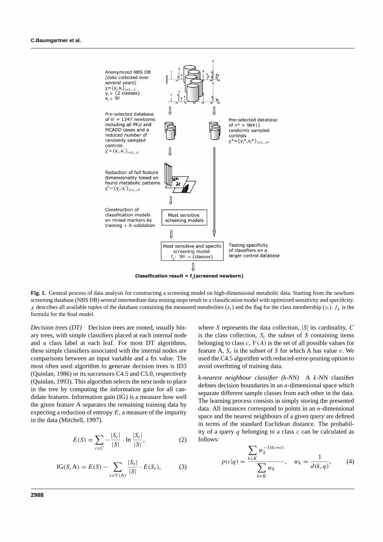
C.Baumgartner et al.
Fig. 1. General process of data analysis for constructing a screening model on high-dimensional metabolic data. Starting from the newbornscreening database (NBS DB) several intermediate data mining steps result in a classification model with optimized sensitivity and specificity.χ describes all available tuples of the database containing the measured metabolites (xi) and the flag for the class membership (yi). fχ is theformula for the final model.
Decision trees (DT) Decision trees are rooted, usually bin-ary trees, with simple classifiers placed at each internal nodeand a class label at each leaf. For most DT algorithms,these simple classifiers associated with the internal nodes arecomparisons between an input variable and a fix value. Themost often used algorithm to generate decision trees is ID3(Quinlan, 1986) or its successors C4.5 and C5.0, respectively(Quinlan, 1993). This algorithm selects the next node to placein the tree by computing the information gain for all can-didate features. Information gain (IG) is a measure how wellthe given feature A separates the remaining training data byexpecting a reduction of entropyE, a measure of the impurityin the data (Mitchell, 1997).
E(S) =∑
c∈C
−|Sc||S| · ln
|Sc||S| , (2)
IG(S, A) = E(S) −∑
v∈V (A)
|Sv||S| · E(Sv), (3)
whereS represents the data collection, |S| its cardinality,Cis the class collection,Sc the subset ofS containing itemsbelonging to classc, V (A) is the set of all possible values forfeature A,Sv is the subset ofS for which A has valuev. Weused the C4.5 algorithm with reduced-error-pruning option toavoid overfitting of training data.
k-nearest neighbour classifier (k-NN) A k-NN classifierdefines decision boundaries in ann-dimensional space whichseparate different sample classes from each other in the data.The learning process consists in simply storing the presenteddata. All instances correspond to points in ann-dimensionalspace and the nearest neighbours of a given query are definedin terms of the standard Euclidean distance. The probabil-ity of a queryq belonging to a classc can be calculated asfollows:
p(c|q) =
∑
k∈K
w−1(kc=c)k
∑
k∈K
wk
, wk = 1
d(k,q), (4)
2988

Machine learning in metabolic disorders
whereK is the set of nearest neighbours,kc the class ofk andd(k,q) the Euclidean distance ofk from q. Larger values ofK consider more neighbours, and therefore smooth over localcharacteristics, smaller values leads to limited neighbour-hoods (Mitchell, 1997). In general,K can only be determinedempirically. For our data representation we proposedK valuesof 1, 3 and 5.
Artificial neural networks (ANN) An ANN is an informationprocessing paradigm that is inspired by the biological nervoussystems, such as the brain. The network consists of severallayers of neurons, which are the input, hidden and outputlayers. An input layer takes the input and distributes it to thehidden layers which do all the necessary computation andoutput the results to the output layer.
The standard algorithm which we used is a multilayeredANN trained using backpropagation and the delta rule. Thisalgorithm attempts to minimize the squared error betweenthe network output values and the target value for these out-puts (Bishop, 1995; Mitchell, 1997). The ANN was designedusing a single layer of hidden units with (number of attrib-utes+ number of classes)/2 hidden units. Note that too manyor too few hidden units can lead to over- or underestima-tion of training data. We chose 500 epochs to train throughand a learning rate of 0.3, the amount the weights to beupdated.
Support vector machines (SVM) The basic idea of an SVMclassifier is that the data vectors can be separated by a hyper-plane. In the simplest case of a linear hyperplane theremay exist many possible separating hyperplanes. Amongthem, the SVM classifier seeks the separating hyperplanethat produces the largest separation margin between the twoclasses. Such a scheme is known to be associated withstructural risk minimization to find a learning machine thatyields a good trade-off between low empirical risk and smallcapacity.
In the more general case in which the data points are notlinearly separable in the input space, a non-linear transforma-tion is used to map the data vectorx into a high-dimensionalspace prior to applying the linear maximum-margin classi-fier. To avoid over-fitting in this higher dimensional space,an SVM uses kernel functions (polynomial and Gaussianradial basis kernels are the most common) in which the non-linear mapping is implicitly embedded. With the use of akernel, the decision function in a SVM classifier has thefollowing form:
f (x) =Ls∑
i=1
αiyiK(xi ,x) + b, (5)
where K(·,·) is the kernel function,xi are the so-calledsupport vectors determined from training data,LS is thenumber of support vectors,yi is the class indicator asso-ciated with eachxi , and αi , the Lagrange multipliers. In
addition, for a given kernel it is necessary to specify thecost factorc, a positive regularization parameter that con-trols the trade-off between complexity of the machine andthe allowed classification error (Corteset al., 1995; Vapnik,1998). We used the SVM with its simplest case of a lin-ear hyperplane and with polynomial kernels of degree 2and 3. The cost factorc was set to 100 for all three SVMsettings.
Feature selection algorithmsFeature subset selection is the process of identifying andremoving as much irrelevant and redundant information aspossible. This reduces the dimensionality of the data andmay allow learning algorithms to operate faster and moreefficiently (Mitchell, 1997).
We propose the filter approach using gain ratio and relief, arepresentative of correlation-based selection techniques coup-ling an applicative correlation measure with a heuristic searchstrategy: As described previously the effectiveness of a fea-ture in classifying the training data can be quantified using thegiven entropyE [Equation (2)]. Using Equation (3) (inform-ation gain, IG) the expected reduction of entropy caused bypartitioning the data according to feature A can be measured.Thereby, IG favours features with many different values overthose with few values which is not always desired. The conceptof gain ratio (GR) overcomes this problem by introducing anextra term SI taking into account how the feature A splits thedata.
GR(S, A) = IG(S, A)
SI(S, A), with
SI(S, A) = −d∑
i=1
|Si ||S| · ln
|Si ||S| , (6)
whereSi ared subsets of data resulting from partitioningS
by thed-valued feature A. For the special case where the SIterm can be 0, GR(S, A) is set to IG(S, A).
Relief is a feature weighting algorithm that is sensitive tofeature interactions. It evaluates the merit of a feature byrepeatedly sampling an instance and considering the valueof the given feature for the nearest instance of the same class(nearest hit) and different class (nearest miss). Equation (7)represents the weight updating formula:
WA = WA − diff(A,R,H)2
m+ diff(A,R,M)2
m(7)
whereWA is the weight for attributeA, R is a randomlysampled instance,H is the nearest hit,M is the nearestmiss andm is the number of randomly sampled instances.The function diff calculates the difference between twoinstances for a given attribute (Kira and Rendell, 1992; Konon-enko, 1995). The number of nearest neighbours was selectedto be 10.
2989

C.Baumgartner et al.
Evaluation of classifier’s accuracy and validationWe evaluated the discriminatory power of the investigatedtechniques constructing a classification (confusion or contin-gency) table for our two class problem stating true positives(TPs), true negatives (TNs), false positives (FPs) and falsenegatives (FNs). The most frequently used evaluation meas-ure in classification is accuracy (Acc) which describes theproportion of correctly classified instances: Acc= (TP +TN)/(TP + FP + TN + FN). Measures which considermore precisely the influence of the class size are sensitiv-ity (Sn) or recall, specificity (Sp), positive predictive value(PPV) or precision and negative predictive value (NPV).Sn = TP/(TP+ FN) measures the fraction of actual positiveinstances that are correctly classified; whileSp = TN/(TN +FP) measures the fraction of actual negative examples thatare correctly classified. The PPV (or the reliability of pos-itive predictions) is computed by PPV= TP/(TP + FP),the NPV is defined as NPV= TN/(TN + FN) (Salzberg,1999).
Five classification algorithms (DT, LRA, kNN, ANN andSVM) and the feature selection techniques gain ratio and reliefused in this study were obtained from the WEKA machinelearning package (http://www.cs.waikato.ac.nz/∼ml/weka).WEKA is a publicly available, widespread and comprehensivetool set which guarantees high comparability of our results.DA and statistical analysis were performed with the soft-ware package ADE-4 (http://pbil.univ-lyon1.fr/ADE-4). Thepackages were used to investigate the models’ discriminatorypower on full and reduced data dimensionality. An establishedmethodology to evaluate the robustness of the classifier isto perform a cross-validation on the classifier. 10-fold cross-validation has been proved to be statistically good enough inevaluating the classification accuracy of the models (Wittenet al., 2000).
EXPERIMENTSDescriptive statistics of metabolic dataTable 1 summarizes all metabolites measured by mass spec-trometry: 14 amino acid representing the spectrum of meta-bolites involved in investigated amino acid disorders and 29fatty acids (acylcarnitines) involved in the metabolism offatty acid oxidation defects. The mean concentrations andrespective SD of all metabolites are given inµmol/l. Dif-ferences of metabolite concentrations between disorder andcontrol group were performed with unpaired significancetesting.
Comparison of classification methods examined onthe full metabolite dimensionalityIn order to investigate the discriminatory performance ina high-dimensional feature space, we first examined all
Table 1. Metabolites of a single blood spot from MS/MS analysis
Amino acids PKU ControlsAlanine (Ala) 421.8± 129.8 508.9± 210.7Arginine (Arg) 333.0± 447.5 90.9± 49.7Argininosuccinate
(Argsuc)1.17± 2.23 0.01± 0.02
Citrulline (Cit)∗ 24.7± 21.7 28.7± 39.9Glutamate (Glu) 3498± 2485 235.9± 74.0Glycine (Gly) 331.2± 140.0 624.2± 315.9Methionine (Met) 23.5± 7.9 29.2± 12.9Ornitine (Orn)∗ 80.4± 54.7 85.2± 60.7Phenylalanine (Phe) 588.0± 240.4 57.9± 17.9Pyroglutamate (Pyrglt) 32.1± 18.1 51.8± 31.6Serine (Ser) 689.8± 362.2 400.6± 358.2Tyrosine (Tyr) 58.1± 24.2 97.2± 64.2Valine (Val)∗ 183.4± 71.8 170.6± 61.3Leucine+ Isoleucine (Xle) 193.1± 91.7 264.5± 107.7
Fatty acids MCADD ControlsFree carnitine (C0) 26.416± 11.138 29.416± 12.087Acetyl-carnitine (C2) 14.361± 7.245 6.661± 3.066Propionyl-carnitine (C3) 3.209± 1.396 2.326± 1.205Butyryl-carnitine (C4)∗ 0.524± 0.396 0.522± 0.309Isovaleryl-carnitine (C5) 0.195± 0.122 0.160± 0.105Hexanoyl-carnitine (C6) 1.990± 1.821 0.415± 0.516Octanyl-carnitine (C8) 8.346± 6.558 0.223± 0.142Decanoyl-carnitine (C10) 0.764± 0.501 0.079± 0.067Dodecanoyl-carnitine
(C12)∗0.166± 0.104 0.209± 0.206
Myristoyl-carnitine (C14)∗ 0.207± 0.104 0.198± 0.106Hexadecanoyl-carnitine
(C16)∗4.066± 1.615 4.413± 2.144
Octadecanoyl-carnitine(C18)∗
0.954± 0.378 0.928± 0.394
Tiglyl-carnitine (C5:1) 0.031± 0.027 0.052± 0.067Decenoyl-carnitine (C10:1) 0.805± 0.478 0.095± 0.059Myristoleyl-carnitine
(C14:1)0.096± 0.048 0.122± 0.094
Hexadecenoyl-carnitine(C16:1)
0.158± 0.078 0.185± 0.104
Octadecenoyl-carnitine(C18:1)
0.743± 0.276 1.030± 0.401
Decenoyl-carnitine(C10:2)∗
0.045± 0.029 0.051± 0.045
Tetradecadienoyl-carnitine(C14:2)
0.032± 0.019 0.055± 0.046
Octadecadienoyl-carnitine(C18:2)
0.108± 0.068 0.161± 0.115
Hydroxy-isovaleryl-carnitine(C5-OH)∗
0.168± 0.101 0.159± 0.078
Hydroxytetradecadienoyl-carnitine(C14-OH)
0.016± 0.010 0.028± 0.024
Hydroxypalmitoyl-carnitine(C16-OH)∗
0.021± 0.013 0.023± 0.016
Hydroxypalmitoleyl-carnitine(C16:1-OH)∗
0.036± 0.021 0.043± 0.038
2990

Machine learning in metabolic disorders
Table 1. Continued.
Fatty acids MCADD ControlsHydroxyoleyl-carnitine
(C18:1-OH)∗0.013± 0.010 0.016± 0.013
Dicarboxyl-butyryl-carnitine (C4-DC)∗
0.137± 0.054 0.151± 0.077
Glutaryl-carnitine (C5-DC) 0.092± 0.056 0.047± 0.031Methylglutaryl-carnitine
(C6-DC)0.072± 0.049 0.046± 0.040
Methylmalonyl-carnitine(C12-DC)
0.036± 0.036 0.096± 0.064
Concentrations (mean± SD) of amino acids and fatty acids are denounced inµmol/lfor PKU, MCADD and control group. Controls represent a randomized fraction of 1241cases. The asterisks indicate no significant (P > 0.05) differences between both classescompared by means of an unpaired significance test.
presented supervised machine learning algorithms on selec-ted sub-databases considering full amino acid dimension-ality (PKU sub-database) and full fatty acid dimensional-ity (MCADD sub-database), respectively. Overview of fullamino and fatty acid dimensionality (Table 1). The effective-ness of the classifiers is summarized in Table 2.
These results revealed that most of the classifiers (withoutDA andk-NN) applied on the PKU database performed wellin terms of classification accuracy (Sn ≥ 95.3%,Sp ≥ 99.8%,Acc≥ 99.7%). Except the DT learner, all classifiers indicatedan optimal specificity of 100%. Thereby, not directly inter-pretable algorithms such as ANN and SVM-2 yielded a minoradvantage in sensitivity compared to the other ones (Table 2).Running our experiments on the MCADD sub-database, allsix algorithms showed reduced classification accuracy (cf.Sn
and Acc compared to the PKU results, Table 2). This tendencymay arise from the induced classifiers being able to character-ize the negative samples as our training set contains twice asmuch higher feature dimensionality compared to the PKU data(29:14 metabolites). In general, the DA andk-NN learnersdemonstrated decreased classification accuracy for both PKUand MCADD datasets. LRA, ANN, DT, SVM-1 (linear hyper-plane) and SVM-2 (polynomial kernel, degree 2) led to betterdiscrimination and, accordingly, classification accuracy indic-ated by highSn (≥95.3%) and highSp (≥99.8%) in PKUdata, and minor reducedSn (≥92.1%) but also superiorSp
of ≥99.6% in MCADD data.
Feature selection and metabolic patternsFeature extraction methods identify redundant metaboliteswhich can be removed leading to simplified classificationmodels. We applied two filter techniques, gain ratio and relief,in order to identify most significant metabolites. Figure 2aand b summarizes the ranked metabolic patterns resultingfrom both techniques. Black bars indicate the establisheddiagnostic markers.
According to the sequence in-between the amino acidgroup obtained by the gain ratio filter (Fig. 2a), Glu, Argsuc
Table 2. Discriminatory performance of all six machine learning algorithmsapplied to full metabolite dimensionality
Classifier Sn(%) Sp(%) Acc(%)
PKUDA 90.7 100 99.7LRA 95.3 100 99.8DT 95.3 99.8 99.71-NN 93.0 100 99.83-NN 90.7 100 99.75-NN 90.7 100 99.7ANN 97.7 100 99.9SVM-1 95.3 100 99.8SVM-2 97.7 100 99.9SVM-3 95.3 100 99.8
MCADDDA 88.9 100 99.5LRA 93.7 98.8 98.5DT 92.1 99.8 99.41-NN 88.9 99.4 98.93-NN 84.1 100 99.25-NN 82.5 100 99.2ANN 92.1 99.7 99.3SVM-1 93.7 99.6 99.3SVM-2 93.7 99.8 99.5SVM-3 93.7 99.8 99.5
Directly interpretable (DA, LRA and DT) and not directly interpretable classifiers run-ning on 14 amino acids (PKU data) and on 29 fatty acids (MCADD data). 1-NN, 3-NNand 5-NN represent thek-NN classifiers with ak-value of 1, 3 and 5. SVMs with a linearhyperplane are denounced as SVM-1, SVMs with polynomial kernels of degree 2 and 3are abbreviated by the symbols SVM-2 and SVM-3.
and Arg showed a high impact in the PKU data in addi-tion to Phe. However, these results correspond just partlywith the abnormal PKU metabolism, as solely Phe and Tyrare used as conventional diagnostic metabolites for screen-ing for PKU. Little differences were observed in the reliefranking where again Phe, which shows a highly accumu-lated concentration, was top-placed followed by the acidsXle, Glu, Val and Gly. The diagnostic marker Tyr, whichis significantly diminished in PKU metabolism (cf. Table 1),ranked at an irrelevant position in both filter approaches. Inaddition to Phe, Arg and Glu yielded strongly increased con-centration levels, but accompanied by high variances (cf.descriptive results) in the PKU data. However, they showno significant concentration changes in the control group.These observations cannot be directly explained by the defi-ciency of phenylalanine hydroxylase activity, but seem tobe an interesting secondary effect of metabolism which cur-rently is in discussion with our clinical and biochemicalexperts.
For MCADD data the ranked gain ratio results figured outa strong dominance of octanyl-carnitine (C8), followed byC10:1, which corresponds well to the established diagnosticmarkers. It is also of interest to note that the result of the reliefalgorithm yielded similar ranking results in the order of thefirst six fatty acids. In addition to C8 and C10:1 also C10 and
2991
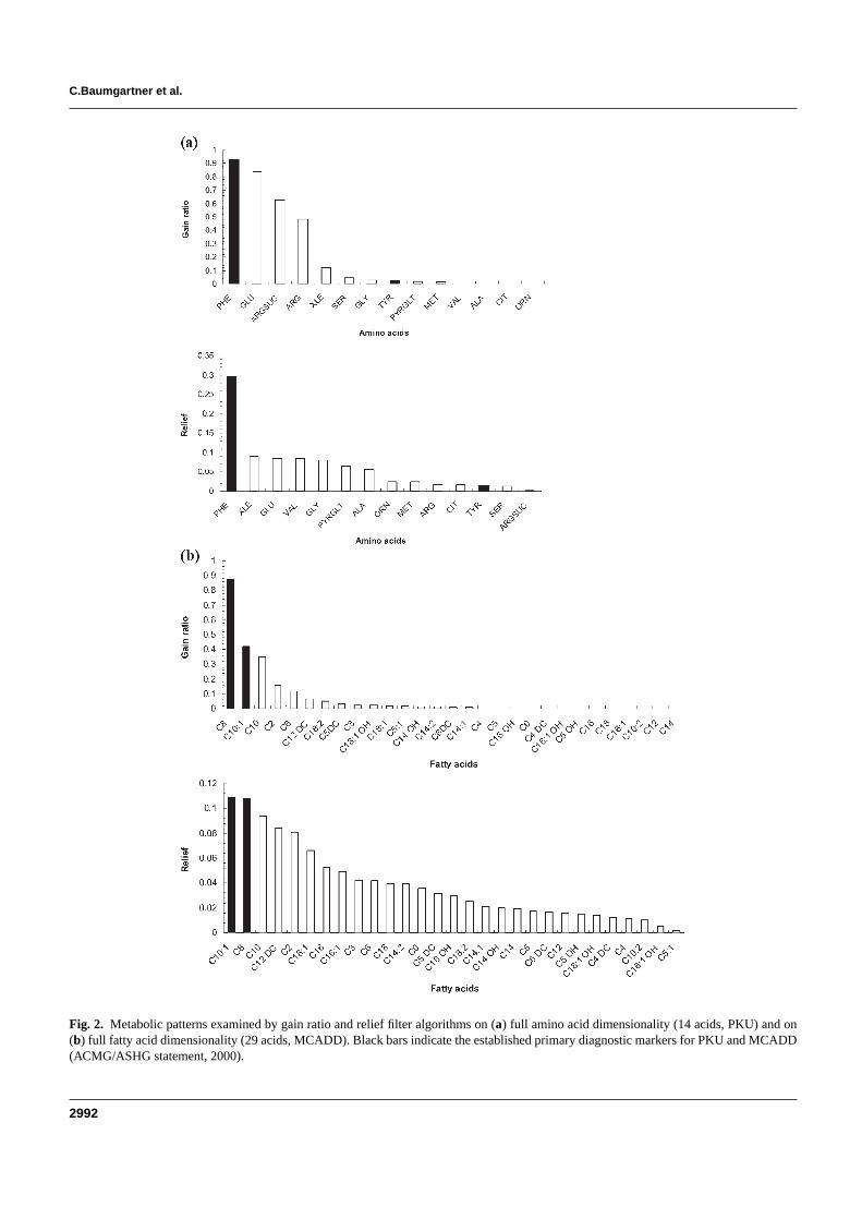
C.Baumgartner et al.
Fig. 2. Metabolic patterns examined by gain ratio and relief filter algorithms on (a) full amino acid dimensionality (14 acids, PKU) and on(b) full fatty acid dimensionality (29 acids, MCADD). Black bars indicate the established primary diagnostic markers for PKU and MCADD(ACMG/ASHG statement, 2000).
2992

Machine learning in metabolic disorders
C2 (medium and short-chain fatty acids) with elevated andC12DC and C18:1 (long-chain fatty acids) with diminishedconcentration levels correspond quite well with the abnormalMCADD metabolism.
Comparison of classifiers examined on reducedmetabolite dimensionalityWe applied five of six machine learning algorithms (DTlearner was not examined on the reduced feature spectrumdue to its internal feature selection strategy) to the estab-lished diagnostic markers (ACMG/ASHG statement, 2000),which served as a reference for employing a low-dimensionalmetabolite space. Table 3 summarizes the classification accur-acy for PKU’s and MCADD’s primary diagnostic metabolitesPhe and Tyr, and C8 and C10:1, respectively. Despite thesmall nuances on differences in classification accuracy withinthe examined algorithms on full and reduced feature dimen-sionality LRA is top-ranked for MCADD (Sn = 95.2%)and together with ANN andk-NN learners also best rankedfor PKU (Sn = 97.7%). In contrast, DA and SVMs withpolynomial kernels show considerably decreasedSn valuescompared to full metabolite dimensionality. However, theminor alterations of classification accuracy in both disordersare caused simply by the obvious statistically significant dif-ferences between the groups of disorder and controls (cf.descriptive results).
Screening models for classic PKU and classicMCADDModels which may prove feasible for clinical routine have toensure easy interpretation without loosing predictive power.Within this context, from all the six investigated machinelearning paradigms, LRA, 1-NN, 3-NN, ANN and SVM-1gave promising classification results on reduced metabolitedimensionality. For the screening of classic MCADD and clas-sic PKU, we trained the LRA model—a paradigm widely usedin medical applications—on both metabolic sub-databasesshowing highestSn of ≥ 95.2% (cf. Table 3). In order tofurther optimize the model’s discriminatory performance, wecomputed the six top-ranked metabolites as investigated fromfeature selection methods and examined their possible pair-wise combinations. Including combinations of more than twometabolites did not further improve the classification accur-acy. Table 4 summarizes the most sensitive screening models(PKU: Sn = 95.4–100%, MCADD:Sn = 95.2–96.8%).The total number of falsely negative classified newborns didnot exceed 0–4.6% for PKU and 3.2–4.8% for MCADD.Promising models predominantly include two metabolites, butdiffer partly from the clinically applied diagnostic metabol-ites. Following the process of analysis depicted in Figure 1,our most sensitive models were consecutively re-evaluatedon a larger control database of 98 411 cases. As expec-ted this procedure decreased specificities of the constructedmodels significantly. However, the models’ real classification
Table 3. Discriminatory performance of all six machine learning algorithmsapplied to the established diagnostic markers
Classifier Sn(%) Sp(%) Acc(%)
PKUDA 93 100 99.8LRA 97.7 99.9 99.8(DT) (95.3) (99.8) (99.7)1-NN 97.7 99.9 99.83-NN 97.7 100 99.95-NN 95.3 100 99.8ANN 97.7 100 99.9SVM-1 95.3 100 99.8SVM-2 93 100 99.8SVM-3 76.7 100 99.2
MCADDDA 71.4 100 98.6LRA 95.2 99.8 99.6(DT) (92.1) (99.8) (99.4)1-NN 93.7 99.8 99.53-NN 93.7 99.8 99.55-NN 92.1 99.8 99.5ANN 92.1 99.8 99.4SVM-1 93.7 99.9 99.6SVM-2 84.1 99.9 99.2SVM-3 60.3 100 98.1
Directly interpretable (DA, LRA and DT) and not directly interpretable (k-NN, ANN,SVM) classifiers are including the primary diagnostic markers. Phe and Tyr for PKUand C8 and C10:1 for MCADD. The DT learner was not examined on pre-selectedmetabolites due to its internal feature extraction strategy. Therefore, the results are notdirectly comparable with the other classifiers and are depicted in parentheses.
accuracy in terms of the false positive rate and the positivepredictive value can now easily be extrapolated consideringthe disorder’s estimated incidences.
All derived screening models for PKU contain Phe as thepredominant metabolite which is consistent with its role inerroneous metabolism (Chaceet al., 1993; Rashedet al.,1995). Models including Phe alone or combined with Argor Argsuc yielded the highest PPV of 70.7–71.9%, i.e. 16–17 FP cases (0.00017%) out of 98 411 controls. The latterconstellations, however, cannot be directly explained by thePKU metabolism. The classifier which includes the estab-lished diagnostic markers Phe and Tyr show maximumSn
(100%), but its PPV drops off significantly (16.2%). However,combinations of Phe and further meaningful metabolites donot change classification accuracy significantly, Phe remainsthe key marker for PKU. Nevertheless, the role of Arg, Glu,Argsuc, Val or Xle in alternative pathways needs to be cross-checked in order to understand their individual influence onPKU metabolism.
MCADD models led toSn values (95.2–96.8%) slightlydecreased but still superior to the established clinical mark-ers;Sp and PPV showed higher values compared to the PKUmodels. The most sensitive model (Sn = 96.8%) combin-ing octanyl-carnitine (C8) and octadecenoyl-carnitine (C18:1)yields an excellentSp of 99.992% and a PPV of 88.4%.
2993

C.Baumgartner et al.
Table 4. Screening models based on LRA for classic PKU and classic MCADD
Metabolites Sn (%) FN (# of cases) Sp (%) FP (# of cases) PPV (%) NPV (%) Acc (%) Logit of modelsz = a0 + a1m1 + · · · + anmn
PKUPhe, Tyr 100 0 99.775 222 16.23 100 99.775 −211.2566+ 2.1318·Phe− 0.6224·TyrPhe, Xle 100 0 99.793 204 17.41 100 99.793−61.2577+ 1.8037·Phe− 1.4518·XlePhe, Val 97.67 1 99.895 103 28.966 99.999 99.894−11.8046+ 0.2248·Phe− 0.1210·ValPhe, Arg 95.35 2 99.983 17 70.69 99.998 99.981−9.827+ 0.0462·Phe− 0.0035·ArgPhe, Argsuc 95.35 2 99.984 16 71.93 99.998 99.982−10.167+ 0.0457·Phe− 0.340·ArgsucPhe 95.35 2 99.984 16 71.93 99.998 99.982−10.1482+ 0.0455·Phe
MCADDC8, C18:1 96.83 2 99.992 8 88.41 99.998 99.990−5.4917+ 5.7436·C8− 2.1833·C18:1C8 95.24 3 99.992 8 88.24 99.997 99.989 −7.5362+ 5.7931·C8C8, C12DC 95.24 3 99.990 10 85.71 99.997 99.987−4.8647+ 5.149·C8− 40.4661·C12DCC8, C10 95.24 3 99.989 11 84.51 99.997 99.986−7.6114+ 4.6649·C8+ 3.3668·C10C8, C10:1 95.24 3 99.950 50 54.55 99.997 99.947−8.7572+ 4.2517·C8+ 10.888·C10:1
Screening models for classic PKU and classic MCADD. Sensitivity (Sn), specificity (Sp), positive predictive value (PPV), negative predictive value (NPV), accuracy (Acc), number(#) of false negatives (FN), number (#) of false positives (FP) and the logits (z) of the LRA models are denounced. The specificity of the models was re-evaluated on a randomlyselected control database of 98 411 cases.
In other words only a marginal fraction of eight FP cases(0.00008% of all controls) is wrongly classified as classicMCADD patients. Considering the established diagnosticmarkers C8 and C10:1 in the model, PPV decreases to 54.6%,so that decision rules based on alternative combinations of C8+ C18:1 and C8+ C12DC or C8 alone seem to be the bettermarkers to enhance discriminatory performance and thus tooptimize classification accuracy.
In addition, the derived classification models allow to calcu-late a conditional probability value of the formP(disorder=1|metabolite1, . . . , metaboliten). The logits of constructedLRA models (z = a0 + a1m1 + · · · + anmn) are presented inTable 4 (final column).
DISCUSSIONMachine learning techniques have great potential to increaseour knowledge in functional metabolomics, an area which isstill in the early stages of comprehensive investigation. Focus-ing on inborn errors of metabolism from newborn screeningdata the metabolic patterns of a wide spectrum of amino andfatty acid concentrations were examined in order to enhancediagnostics in an early stage of disorder.
Therefore, we investigated six different machine learningtechniques for their suitability to construct classification mod-els for two severe metabolic disorders, PKU and MCADD. Toincrease the classifier’s effectiveness, we reduced full meta-bolite dimensionality by two feature selection algorithms,gain ratio and relief, the latter one with its central hypo-thesis that good feature sets contain features that are highlycorrelated with the class, yet uncorrelated with each other.Experiments showed that correlation-based feature selectionquickly removes irrelevant, redundant and noisy features,and identifies relevant attributes as long as their relevance
does not strongly depend on other features (Hall, 1999).In most cases, classification accuracy using reduced feature(metabolite) dimensionality equaled or increased accuracyusing the entire metabolite spectrum as our experimentsconfirm.
The highest discriminatory performance was achieved bythe LRA model, a directly interpretable technique, whichproved readily applicable in the daily screening procedure.The resulting discriminant function can easily be cross-checked with already acquired patient data. Furthermore, theformulas can be used as a starting point for the detection of pre-viously unknown causal dependencies in metabolic pathways.
For both disorders the computed sensitivity of the best LRAmodels ranged>96.8%, the specificity exceeded 99.98%.By including novel constellations of metabolites into ourmodels—as examined by the feature extraction procedures—specificity and PPV could be increased compared to theestablished screening metabolites. In case of PKU the PPV,which was determined on a larger sampled control database of98 411 cases, improved up to 71.9% using solely Phe, and upto 70.7% by combining Phe and Arg. The PPV deterioratedto just 16.2% when considering Phe and Tyr, both of thembeing the metabolites predominantly altered in the abnormalPKU metabolism. Note that for the classification task solelysingle metabolite concentrations have been considered asmodel input variables. However, modelling a ratio of Phe/Tyr,which represent abnormal changes of Phe (↑) and Tyr (↓)due to the blocked hydroxylation of Phe to Tyr, the PPVcan significantly be increased as already shown elsewhere(Chaceet al., 1998).
For MCADD, the model’s PPV increased significantlycompared to the PPV of 54.6% for the established screeningmetabolites C8 and C10:1 resulting in PPV values of 88.4%
2994
Machine learning in metabolic disorders
for C8 and C18:1, 88.2% for solely C8 and 85.7% for com-bining C8 and C12DC, respectively. The false positive rate forMCADD most likely varies between screening programmesbecause of differences in acylcarnitine analysis and profil-ing. Programmes that screen for MCADD but not for otherfatty oxidation disorders often limit their analysis to C8, thepredominant, but not specific marker for MCADD which iselevated in several other disorders (e.g. medium/short chain 3-OH acyl-CoA dehydrogenase deficiency or glutaric acidemiatype II). Consideration of the disorders included in the differ-ential diagnosis should minimize the false positive rate. Ourpresented models including novel combinations such as C8+C18:1 and C8+ C12DC give additional information withrespect to the aforementioned differential diagnostic chal-lenges. However, the experimental confirmation is essentialand is part of our ongoing investigations.
For the routine clinical screening LRA models proved par-ticularly feasible because of their highly significant prognosticaccuracy. The models permit to calculate the probability forthe occurrence of the disorder by classifying the tested new-borns according to a default cut-off level ofP = 0.5. Byemploying sharper cut-offs (e.g. 0.25≤ P ≤ 0.75, i.e.between the first and third quartile), this approach can beextended to a prognostic ‘alarm system’ allowing a moreeffective response to cases of metabolic disorders detectedduring the screening procedure. Subsequent diagnostic clari-fication has only to focus on this ‘third’ class of newbornsin the interval [0.25, 0.75] which is highly suspicious forthe screened disorders. However, the presented models show-ing high specificity do not always have optimalSn of 100%.A feasible procedure for optimizing sensitivity is to changethe default cut-off level ofP = 0.5. The costs for elevatingsensitivity by decreasing the default cut-off are subject of ourcurrent work. Preliminary results indicate that classificationmodels showing optimized sensitivity of 100% have to accepta 2–3-fold increase in FP cases.
To sum it up, the top three machine learning techniques,LRA (as discussed above), SVM and ANN, delivered resultsof high predictive power when running on full as well as onreduced feature dimensionality. Although SVMs can effect-ively construct nonlinear decision boundaries by mappingtraining data into a higher-dimensional feature space (SVM-2, SVM-3), these polynomial SVMs did not perform better inlow-dimensional feature spaces compared to the known lin-ear techniques like LRA. Interestingly, SVM operating with alinear separating hyperplane (SVM-1) performed better thanthe polynomial ones. They led to results similar to the LRAclassifier, an observation already described by other authors(Dreiseitlet al., 2001). The C4.5 DT classifier, which selectsfeatures internally based on the information gain, showedgood discriminatory performance, leading to the sameSn
(95.3%) as LRA on PKU data (tree root= Phe, no childnodes) and slightly decreasedSn (−1.6%) on MCADD data(tree root C10:1, two child nodes C8 and C16). The third
directly interpretable method, DA, operates on a separatinglinear hyperplane similar to LRA. As expected, the DA clas-sifier discriminated worse in both, full and reduced featurespectrum, since an important precondition, the homogeneityof both covariance matrices, was not fulfilled (confer e.g.the data distribution of Phe in the PKU and control groups;Table 1). Out of the group of not directly interpretable tech-niques the ANN classifier performed best. Despite lackingdirect interpretation of the knowledge representation, its abil-ity to calculate non-linear decision boundaries emphasizes itsdiagnostic potential. The results of thek-NN algorithms (forall appliedk-values) were comparable with those running onestablished diagnostic metabolites, but significantly inferior(2–10% points) to those running on the entire dimensional-ity of PKU and MCADD databases. However,k-values largerthan 5 generally led to a decrease in the classification accuracydue to smoothing effects of local data characteristics.
In conclusion, our results show that the use of machinelearning paradigms, in particular the LRA model, is suit-able to construct classifiers on high-dimensional metabolicdata. Moreover, we could demonstrate that the screeningmodels high predictive power could be achieved by reduc-ing the dimensionality of the parameter space using only 1–2representative metabolites for PKU and MCADD. The minedresults confirm some known patterns among the metabolitesand reveal a number of novel patterns which may contributetowards a better understanding of newborn metabolism, andconstitutes a significant contribution to the early recognitionand therapy of metabolic diseases.
ACKNOWLEDGEMENTSThis study was generously supported by the Austrian Indus-trial Research Promotion Fund FFF (Grand No. HITT-10UMIT).
REFERENCESAmerican College of Medical Genetics/American Society of Human
Genetics Test and Technology Transfer Committee WorkingGroup (2000) Tandem mass spectrometry in newborn screening.Genet. Med., 2, 267–269.
Baumgartner,C., Baumgartner,D. and Böhm, C. (2004) Classifica-tion on high dimensional metabolic data: phenylketonuria as anexample.IASTED Proceedings of 2nd International Conferenceon Biomedical Engineering (BioMED 2004), Innsbruck, Austria,pp. 357–360.
Bishop,C.M. (1995)Neural Networks for Pattern Recognition.Oxford University Press, Oxford.
Blau,N., Thony,B., Cotton,R.G.H. and Hyland,K. (2001)Disorders of tetrahydrobiopterin and related biogenic amines.In Scriver,C.R., Kaufman,S., Eisensmith,E., Woo,S.L.C.,Vogelstein,B. and Childs,B. (eds),The Metabolic and MolecularBases of Inherited Disease, 8th edn. McGraw Hill, New York,pp. 1725–1776.
2995

C.Baumgartner et al.
Chace,D.H., Millington,D.S., Terada,N., Kahler,S.G., Roe,C.R.and Hofman,L.F. (1993) Rapid diagnosis of phenylketonuria byquantitative analysis for phenylalanine and tyrosine in neonatalblood spots by tandem mass spectrometry.Clin. Chem., 39,66–71.
Chace,D.H., Sherwin,J.E., Hillman,S.L., Lorey,F. and Cunning-ham,G.C. (1998) Use of phenylalanine-to-tyrosine ratio determ-ined by tandem mass spectrometry to improve newborn screeningfor phenylketonuria of early discharge specimens collected in thefirst 24 hours.Clin. Chem., 44, 2405–2409.
Chace,D.H., DiPerna,J.C. and Naylor,E.W. (1999) Laboratory integ-ration and utilization of tandem mass spectrometry in neonatalscreening: a model for clinical mass spectrometry in the nextmillennium.Acta Paediatr. Suppl., 88, 45–47.
Cortes,C. and Vapnik,V. (1995) Support vector networks.Mach.Learning, 20, 273–297.
Dreiseitl,S., Ohno-Machado,L., Kittler,H., Vinterbo,S., Billhardt,H.and Binder,M. (2001) A comparison of machine learning methodsfor the diagnosis of pigmented skin lesions.J. Biomed. Inform.,34, 28–36.
Guldberg,P., Rey,F., Zschocke,J., Romano,V., Francois,B.,Michiels,L., Ullrich,K., Hoffmann,G.F., Burgard,P., Schmidt,H.et al. (1998) A European multicenter study of phenylalan-ine hydroxylase deficiency: classification of 105 mutations anda general system for genotype-based prediction of metabolicphenotype.Am. J. Hum. Genet., 63, 71–79
Hall,M.A. (1999) Correlation-based feature selection for machinelearning. PhD Thesis. University of Waikato, New Zealand.
Hosmer,D.W. and Lemeshow,S. (2000)Applied Logistic Regression,2nd edn. Wiley, New York.
Kira,K. and Rendell,L.A. (1992) A practical approach tofeature selection. InMachine Learning: Proceedings ofthe Ninth International Conference, Aberdeen, Scotland,pp. 249–256.
Kononenko,I. (1995) On biases in estimating multi-valued attributes.In IJCAI’95, Montreal, Canada, pp. 1034–1040.
Liebl,B., Nennstiel-Ratzel,U., von Kries,R., Fingerhut,R., Olge-moller,B., Zapf,A. and Roscher,A.A. (2002a) Very high com-pliance in an expanded MS-MS-based newborn screeningprogram despite written parental consent.Prev. Med., 34,127–131.
Liebl,B., Nennstiel-Ratzel,U., von Kries,R., Fingerhut,R., Olge-moller,B., Zapf,A. and Roscher,A.A. (2002b) Expanded newbornscreening in Bavaria: tracking to achieve requested repeat testing.Prev. Med., 34, 132–137.
Liebl,B., Nennstiel-Ratzel,U., Roscher,A.A. and von Kries,R. (2003)Data required for the evaluation of newborn screening pro-grammes.Eur. J. Pediatr., 162(Suppl. 1), 57–61.
McLachlan,G.J. (1992)Discriminant Analysis and Statistical Pat-tern Recognition. Wiley, New York.
Mendes,P. (2002) Emerging bioinformatics for the metabolome.Brief. Bioinform., 3, 134–145.
Millington,D.S., Roe,C.R. and Maltby,D.A. (1984) Applicationof high resolution fast atom bombardment and constant B/Eratio linked scanning to the identification and analysis of acyl-carnitines in metabolic disease.Biomed. Mass Spectrom., 11,236–241.
Millington,D.S., Terada,N., Kodo,K. and Chace,D.H. (1992) Areview: carnitine and acylcarnitine analysis in the diagnosis ofmetabolic diseases: advantages of tandem mass spectrometry. InMatsumoto,I. (ed).Advances in Chemical Diagnosis and Treat-ment of Metabolic Disorders. John Wiley & Sons, New York, Vol1, pp. 59–71.
Mitchell,T.M. (1997) Machine Learning. McGraw-Hill, Boston,MA.
National Center for Biotechnology Information. Online MendelianInheritance in Man (OMIM), http://www3.ncbi.nlm.nih.gov/Omin
Neville,P., Tan,P.Y., Mann,G. and Wolfinger,R. (2003) Generaliz-able mass spectrometry mining used to identify disease statebiomarkers from blood serum.Proteomics, 3, 1710–1715.
Purohit,P.V. and Rocke,D.M. (2003) Discriminant models for high-throughput proteomics mass spectrometer data.Proteomics, 3,1699–1703.
Quinlan,R.J. (1986) Induction of decision trees.Mach. Learning, 1,81–106.
Quinlan,R.J. (1993)C4.5: Program for Machine Learning. MorganKaufmann, San Mateo, CA.
Rashed,M.S., Ozand,P.T., Bucknall,M.P. and Little,D. (1995)Diagnosis of inborn errors of metabolism from blood spotsby acylcarnitines and amino acids profiling using automatedelectrospray tandem mass spectrometry.Pediatr. Res., 38,324–331.
Rinaldo,P., Matern,D. and Bennett,M.J. (2002) Fatty acid oxidationdisorders.Annu. Rev. Physiol., 64, 477–502.
Salzberg,S. (1999) On comparing classifiers: a critique of currentresearch and methods.Data Min. Knowl. Disc., 1, 1–12.
Van Hove,J.L., Zhang,W., Kahler,S.G., Roe,C.R., Chen,Y.T.,Terada,N., Chace,D.H., Iafolla,A.K., Ding,J.H., and Mil-lington,D.S. (1993) Medium-chain acyl-CoA dehydrogenase(MCAD) deficiency: diagnosis by acylcarnitine analysis in blood.Am. J. Hum. Genet., 52, 958–966.
Vapnik,V. (1998)Statistical Learning Theory. Wiley, New York.Witten,I.H. and Frank,E. (2000)Data Mining—Practical Machine
Learning Tools and Techniques with Java Implementations.Morgan Kaufmann, San Francisco, CA.
2996
ARTICLE IN PRESS
www.elsevier.com/locate/yjbin
Journal of Biomedical Informatics xxx (2005) xxx–xxx
A bioinformatics framework for genotype–phenotype correlationin humans with Marfan syndrome caused by FBN1 gene mutations
Christian Baumgartner a,*, Gabor Matyas b,c, Beat Steinmann b, Martin Eberle a,Jorg I. Stein d, Daniela Baumgartner a,d
a Research Group for Clinical Bioinformatics, University for Health Sciences, Medical Informatics and Technology, A-6060 Hall in Tyrol, Austriab Division of Metabolism and Molecular Pediatrics, University Children�s Hospital, CH-8032 Zurich, Switzerland
c Division of Medical Molecular Genetics and Gene Diagnostics, Institute of Medical Genetics, University of Zurich,
CH-8603 Schwerzenbach, Switzerlandd Clinical Division of Pediatric Cardiology, Innsbruck Medical University, A-6020 Innsbruck, Austria
Received 20 April 2005
Abstract
Mutations in the human FBN1 gene are known to be associated with the Marfan syndrome, an autosomal dominant inher-ited multi-systemic connective tissue disorder. However, in the absence of solid genotype–phenotype correlations, the identifi-cation of an FBN1 mutation has only little prognostic value. We propose a bioinformatics framework for the mutatedFBN1 gene which comprises the collection, management, and analysis of mutation data identified by molecular genetic analysis(DHPLC) and data of the clinical phenotype. To query our database at different levels of information, a relational data model,describing mutational events at the cDNA and protein levels, and the disease�s phenotypic expression from two alternativeviews, was implemented. For database similarity requests, a query model which uses a distance measure based on log-likelihoodweights for each clinical manifestation, was introduced. A data mining strategy for discovering diagnostic markers, classificationand clustering of phenotypic expressions was provided which enabled us to confirm some known and to identify some newgenotype–phenotype correlations.� 2005 Elsevier Inc. All rights reserved.
Keywords: FBN1 gene; Marfan syndrome; Similarity query processing; Data mining; Genotype–phenotype correlation
1. Introduction
FBN1 (OMIM #134797) is the gene known to beassociated with the Marfan syndrome (MFS, OMIM#154700), an autosomal dominant inherited multi-sys-temic connective tissue disorder with prominent clinicalmanifestations in the cardiovascular, musculoskeletal,and ocular systems (OMIM: www.ncbi.nlm.nih.gov/en-trez/query.fcgi?db=OMIM). Its prevalence is 1/5000.In about 70% of MFS patients, mutations in the
1532-0464/$ - see front matter � 2005 Elsevier Inc. All rights reserved.
doi:10.1016/j.jbi.2005.06.001
* Corresponding author. Fax: +43 50 8648 673827.E-mail address: [email protected] (C. Baumgartner).
FBN1 gene could be detected [1]. The following catego-ries of FBN1 mutations have been described: nucleotidesubstitutions (missense, nonsense, silent, and splicingmutations), insertions, deletions, indels, duplications,and complex rearrangements, some of which cause pre-mature termination and exon skipping, respectively [2–4].
The diagnosis of MFS is dependent on a catalogue ofinternational diagnostic criteria summarized in the Gentnosology [5]. The major source of morbidity and earlydeath in MFS relates to the cardiovascular system.Weakness of the aortic wall can lead to aortic dissectionor rupture [6]. However, before life threatening compli-cations occur, alterations of aortic elastic properties can

2 C. Baumgartner et al. / Journal of Biomedical Informatics xxx (2005) xxx–xxx
ARTICLE IN PRESS
be detected through the examination and monitoring ofaortic elasticity during care follow-up [7–10].
Molecular genetic testing like mutation scanning orcDNA sequence analysis has been proposed as an ad-junct to the clinical diagnosis of the MFS [5,11,12].However, many mutations of FBN1 cause phenotypicexpressions that are distinct from MFS, which rely onthe age-related and pleiotropic nature of the disease[13]. Furthermore, only few genotype–phenotype corre-lations have been found in MFS [1,13–17]. In the ab-sence of solid genotype–phenotype correlations, theidentification of an FBN1 mutation has only little prog-nostic value or consequence for the patient�s diagnosticand therapeutic management.
In this work, we developed a bioinformatics frame-work to support genotype–phenotype correlationsusing a suite of statistical methods, algorithms anddatabase applications: Core component is an FBN1
information system which collects, manages and ana-lyzes genetic information as gained from moleculargenetic testing and clinical data according to a stan-dardized catalogue of diagnostic criteria. To querythe database (DB) at different levels of genetic and phe-notypic information, a relational data model was devel-oped which models mutational events at the cDNAand protein levels, and MFS phenotypic expressionfrom two alternative views. A query model was intro-duced which uses a distance measure based on log-like-lihood weights for each clinical manifestation to querythe DB for mutations of related phenotypic expres-sions. A straightforward data mining strategy for theidentification of diagnostic markers, classification andcluster analysis of phenotypic expressions was providedto perform genotype–phenotype investigations. Initialexperiments confirmed some known correlations andidentified some novel ones when using the proposedframework.
2. Methods
2.1. Genotyping and phenotyping
2.1.1. FBN1 gene and fibrillin-1 protein
The FBN1 gene, located on chromosome 15q21.1, isabout 236 kb in size and contains 65 exons. The geneis transcribed in a 9.7 kb mRNA which encodes a2871 amino acids large fibrillin-1 glycoprotein(320 kDa). Fibrillin-1 is ubiquitously distributed in con-nective tissue and mainly made up of calcium-bindingepidermal growth factor (cb-EGF)-like, EGF-like, andcysteine rich domains interacting with many extracellu-lar matrix components. For general information onthe FBN1 gene see: www.ncbi.nlm.nih.gov/entrez/que-ry.fcgi?db=gene, www.dsi.univ-paris5.fr/genatlas orwww.umd.be:2030/Protein.html.
2.1.2. Mutation analysis of the FBN1 gene
Denaturing high-performance liquid chromatogra-phy (DHPLC) of all 65 FBN1 exons is available on aclinical basis. Genomic DNA samples were amplifiedexon by exon by means of a polymerase chain reaction(PCR) using intron-specific primers. Quality and quanti-ty of PCR products were determined on 1.5% agarosegel by standard procedures. Amplicons were analyzedby DHPLC followed by direct sequencing of ampliconswith abnormal elution profiles. The mutations foundwere verified by repeated sequencing on newly amplifiedPCR products. In the case of splice site mutations andwhen no mutation was detected by DHPLC, FBN1 tran-scripts were analyzed by the reverse transcription (RT)-PCR of RNA templates isolated from fibroblasts. RT-PCR amplifications and sequencing of transcripts werealso performed by standard procedures [18].
2.1.3. The clinical phenotype
Classic or suspected MFS is a clinical diagnosis basedon family history and the observation of characteristicmanifestations in multiple organ systems [5]. The man-agement of data collection requires the coordinated in-put of a multidisciplinary team of specialists includingcardiologists, ophthalmologists, orthopedists, andgeneticists. Within our Innsbruck/Zurich FBN1-net-work, anonymized clinical, and genetic data (mutationscanning is performed by the Zurich group, UniversityChildren�s Hospital Zurich, Switzerland) are broughttogether at the Innsbruck Marfan Clinical Center, Clin-ical Division of Pediatric Cardiology, Innsbruck Medi-cal University, ready for entering into the database.
2.2. The database
For our experiments, genetic and phenotypic data hasbeen collected from different sources. The data wereanonymously provided by the University Children�sHospital of Zurich, Switzerland and Innsbruck MedicalUniversity, Austria [9], and extended by data recentlypublished [17,19–22].
Our current research DB contains 163 entries with 127different mutations (mean patients� age 24.3 ± 15.4years). The different numbers of entries and mutationsarise from entries of 22 families (between two and six fam-ily members) carrying the same mutation. One hundredand nineteen entries are substitutions (Sub), 44 are dis-tributed amongst deletions (Del), insertions (Ins), dupli-cations (Dup), and indel mutations (Indel). The groupof substitutions can be split into 78 missense (Mis), 27nonsense (Stop), and 14 splice site mutations (Splice).Out of the pool of non-substitutions (Del, Ins, Dup, andIndel) 31 entries are deletions causing frameshift (FS)and premature termination codon (PTC).
We investigated 14 Gent criteria which were consis-tently described in the publications presenting clinical

C. Baumgartner et al. / Journal of Biomedical Informatics xxx (2005) xxx–xxx 3
ARTICLE IN PRESS
data: ocular system: 1. ectopia lentis (EL); cardiovascularsystem: 2. dilation of ascending aorta (AADIL), 3. dis-section of ascending aorta (AADIS), 4. mitral valve pro-lapse (MVP); skeletal system: 5. pectus carinatum (PC),6. pectus excavatum requiring surgery (PES), 7. armspan ratio (ASR), 8. wrist or thumb sign (WTS), 9. sco-liosis (SC), 10. moderate pectus excavatum (PE), 11.joint hypermobility (JH), 12. highly arched palate withcrowding of teeth (HAP); skin system: 13. striae atrophi-cae (SA) and 14. herniae (HE). For a more detaileddescription see Fig. 1B.
2.3. FBN1 information system
The information system, which is embedded in aJ2EE three tier architecture consisting of client, applica-tion and data tier, provides cross-DBMS (databasemanagement system) connectivity to a relational DBMSusing a modern server environment and JDBC technol-ogy. A genotype–phenotype data model was designed
Fig. 1. Genotype–phenotype data model depicted as simplified UML classmodelled as 0..1 relationships. (A) Genotype data model (top): type of mutatisub-types, and a general genotype description class are modeled. (B) Phenotyof phenotypic information (level of system involvement and number of accmajor and minor criteria). The model is supplemented by a general phenoty
and implemented to query the database at different lev-els of genetic and phenotypic information (see next sec-tion). Modules for data collection, administration, andanalysis are provided as web-based services, which arestill under construction.
2.4. Genotype–phenotype data model
An international nomenclature system has been sug-gested for the description of mutations and polymor-phisms in DNA and protein sequences [23]. Based onthese recommendations, we designed a genotype data
model which describes sequence variations at bothcDNA and protein levels, systematically. Fig. 1A depictsthe genotype data model represented by a simplifiedUML class diagram. The top compartment containsthe name of the class (= DB relation), the bottom com-partment the list of attributes declared as SQL datatypes. Associations between relations are modeled by0..1 relationships.
diagram. Attributes are declared as SQL data types. Associations areons at the cDNA level and their consequences at the protein level, theirpe data model (bottom): each organ system is represented by two levelsumulated symptoms, and level of single manifestations separated intope description class.

4 C. Baumgartner et al. / Journal of Biomedical Informatics xxx (2005) xxx–xxx
ARTICLE IN PRESS
The description of nucleotide changes at the cDNA le-vel wasmodeled by introducing class attributes accordingto the international mutation nomenclature. To definemutations, different sub-types of nucleotide changes wereconsidered. The consequence of mutations at the proteinlevel are described and modeled in a similar way. Thegenotype general description class represents the combi-nation of mutation types at the DNA level and their con-sequence at the protein level, the affected exons/intronsand protein domains. For representation issues three dif-ferent mutations are exemplified in Table 1.
The phenotype data model was designed accordingto the multi-systemic picture of the disease (Gent
Table 1Three examples of FBN1 mutations described by the genotype data model
Sub/Mis
Nucleotide changes—DNA level
Name �3410G > C�wt codon �CGC�Mutant codon �CCC�Nucleotide position 3410
Event �G > C�Exon coding region affected 1
Intron 5 0 part affected 0
Intron 3 0 part affected 0
Gene flanking or UTR region affected 0
Substitution—DNA
Transversion 1
Transition 0
Deletion—DNA
Single nucleotide deletionSeveral nucleotide deletionDeleted unitDeleted length
Amino acid changes—protein level
Name �R1137P�Codon position 1137wt AA �R�mutant AA �P�
Substitution—Prot
Silent change 0
Missense change 1
Nonsense change 0
Translation termination site 0
Translation initiation site 0
Frameshift
AA changed into StopStop positionLength of new reading frame
Genotype general description
Type and consequence �Sub/Mis�Affected exon/intron �e27�Affected domain �cb-EGF 17�
Nucleotide changes at the cDNA level, amino acid (AA) changes at the proteare exemplified for a substitution/missense mutation (Sub/Mis), a substitutionFs). Attribute values are given in SQL data types. The Deletion-Prot class is nAA.
nosology). Fig. 1B depicts the UML class diagramof the clinical phenotype in more detail: Each affectedorgan system, i.e., the skeletal, cardiovascular (CVS),ocular, pulmonary, skin and integument, and durasystem, was modeled from a more general view toemphasize the system involvement and the accumulat-ed number of diagnosed criteria. To be more specific,each organ system was further separated into sub-sys-tems which contain the single manifestations. A gen-eral patient information class provides additionalinformation according to the patient�s ethnics, sex,age, MFS type (e.g., classical, suspected), and familyhistory.
Sub/Stop Del/Fs
�6339T > G� �1206del1��TAT� �CCT��TAG� �CCC�6339 1206
�T > G� �FS+PTC�1 1
0 0
0 0
0 0
1
0
1
0
�T�1
�Y2113X� �P404HfsX44�2113 404�Y� �P��X� �H�
0
0
1
0
0
�V�447
44
�Sub/Stop� �Del/Fs��e51� �e10��LTBP 6� �Pro-rich�
in level specified by their subtypes, and a general genotype description/nonsense mutation (Sub/Stop) and a deletion causing FS + PTC (Del/ot exemplified because it is only relevant for deleted units of at least one
C. Baumgartner et al. / Journal of Biomedical Informatics xxx (2005) xxx–xxx 5
ARTICLE IN PRESS
2.5. Similarity query processing
We introduce a query model based on log-likelihoodweights for each of the Gent criteria to query the DB formutations of related phenotypes. In the following thelog-likelihood weights are defined as phenotype scores.
2.5.1. Phenotype score calculation
Let DB be a genotype–phenotype database organizedin the form of a set of tuples
T ¼ fðcj; oÞjcj 2 C; o 2 DB && o ¼ ½0; 1�g; ð1Þ
where cj is a specified mutation class and o is the set ofclinical manifestations (0/1). The symbol 2 means ‘‘be-long to,’’ && is ‘‘and.’’ It is important to note thatmutation classes can be specified at different levels ofmutational information: (i) at the level of mutation type(DNA level), e.g., a substitution, (ii) at the level of muta-tion type and consequence (DNA and protein level),e.g., substitution/missense, or (iii) at the level of muta-tion type and consequence, and location of mutationalevent(s) in the gene or the affected protein domain(s),e.g., substitution/missense/exons 3–5 or EGF domain.However, if enough tuples of an explicit mutation areavailable, a score set at this highest level of mutationalinformation is generable. We propose at least 25 tuplesper class/type of mutations to generate representativescore sets.
The entropy of a phenotype probability distributionP = (p1, . . . ,pN) is defined as
HðP Þ ¼ Eð�log2PÞ ¼ �XN
i¼1pilog2pi; ð2Þ
where pj is the frequency (probability) of a symptomwithin the class cj. H(P) is the entropy of the Gent phe-notype with respect to (w.r.t.) a class cj in bit. N is thetotal number of considered symptoms.
The relative entropy of two probability distributionsP and Q is computed as
HðP ;QÞ ¼ �XN
i¼1pilog2
piqi; ð3Þ
where pi is again the frequency of a symptom withinclass cj while qi is defined as the frequency of the symp-tom in DB, excluding all tuples of class cj.
A score value si of a single symptom w.r.t. class cj isthus given as
si ¼ k � pilog2piqi; ð4Þ
where k is a scaling factor (we set k = 100). The scorevalue si can be interpreted as a measure of the distancebetween pi and qi. If pi equals qi then si is 0. If pi is 0,si is undefined. To consider a symptom that is not pres-ent in class cj through a corresponding score value, si can
be set to 0 under the assumption that pi fi 0. Conse-quently, positive si values indicate the symptoms� fre-quencies w.r.t. class ci above qi (frequencies inDB � ci), negative values below them.
A matrix M of score sets can be generated, wherecj 2 C represent specified mutation classes at the samelevel of mutational information, e.g., Sub/Mis, Sub/Stop, Del/Fs, Ins/Fs, etc:
M ¼ fðcj; sÞjcj 2 C; s 2 S && s 2 Rg; ð5Þ
where s is the set of score values of a clinical phenotypew.r.t. mutation class cj and S is the collectivity of scoresets in M. The symbol R represents the set of all realnumbers.
To assess phenotypic similarity/dissimilarity betweena specified mutation class cj 2M and a requested MFSphenotype we calculate the parameter sc, a measurefor the information content of a given score set. It isdefined:
sc ¼XN
i¼1jsij. ð6Þ
The larger sc, the smaller the phenotypic similarity be-tween a mutation class cj and the requested phenotype.
2.5.2. Similarity requests on specified mutation classes
To assign a query phenotype O = {o|(o1, . . . ,oN),o 2 (0,1)} of unknown mutation to a specified mutationclass cj 2M, we present a matching paradigm that oper-ates on matrix M by processing similarity requests foreach class cj 2M. Two steps must be processed for thistask:
1. Balancing of the score matrix M w.r.t. all specifiedmutation classes c 2M. The absolute score valuessc of classes c 2M can significantly differ in sizewhich can lead to a preferred assignment of thequery tuple O to that class cj which is representedby the highest measure sc within M. Therefore,each score set s 2 S has to be corrected to themean absolute score �sc, which is calculated as themean value of all sc 2M, to balance matrix M.Therefore, M* is the �sc-balanced matrix of M withs* 2M*.
2. Assignment of the query phenotype O weighted bythe balanced score sets s* 2M* to a mutation classcj 2M*. The decision rule is defined as follows:
C¼ argmaxc2M�
ffiffiffiffiffiffiffiffiffiffiffiffiffiffiffiffiffiffiffiffiffiffiffiXN
i¼1ðs�i �oiÞ
2
vuut0@
1Afor oi¼
1 if symptom is present;
0 if symptom is absent.
�
ð7Þ
Here, the query model built on a square distance mea-sure assigns the MFS query phenotype O to that muta-tion class cj 2M*, whose distance is maximal.
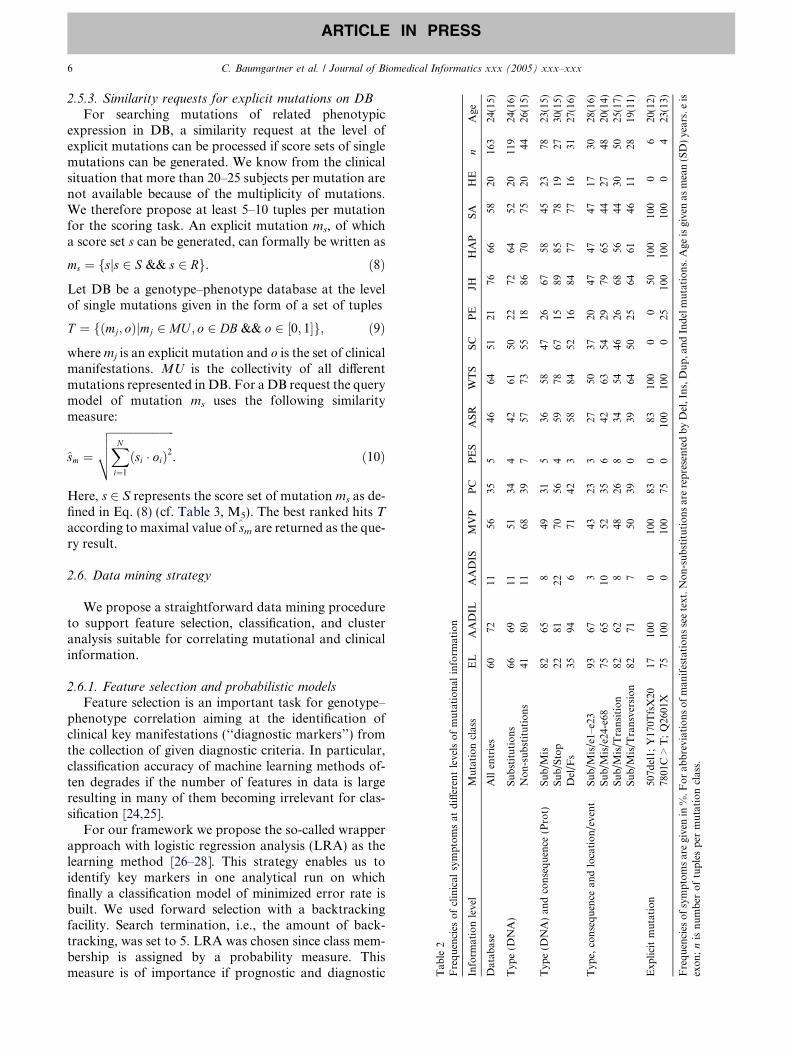
Tab
le2
Frequencies
ofclinical
symptomsat
differentlevelsofmutational
inform
ation
Inform
ationlevel
Mutationclass
EL
AADIL
AADIS
MVP
PC
PES
ASR
WTS
SC
PE
JHHAP
SA
HE
nAge
Datab
ase
Allentries
6072
1156
355
4664
5121
7666
5820
163
24(15)
Typ
e(D
NA)
Substitutions
6669
1151
344
4261
5022
7264
5220
119
24(16)
Non-substitutions
4180
1168
397
5773
5518
8670
7520
4426
(15)
Typ
e(D
NA)an
dconsequence
(Prot)
Sub/M
is82
658
4931
536
5847
2667
5845
2378
23(15)
Sub/Stop
2281
2270
564
5978
6715
8985
7819
2730
(15)
Del/F
s35
946
7142
358
8452
1684
7777
1631
27(16)
Typ
e,consequence
andlocation/event
Sub/M
is/e1–
e23
9367
343
233
2750
3720
4747
4717
3028
(16)
Sub/M
is/e24
-e68
7565
1052
356
4263
5429
7965
4427
4820
(14)
Sub/M
is/T
ransition
8262
848
268
3454
4626
6856
4430
5025
(17)
Sub/M
is/T
ransversion
8271
750
390
3964
5025
6461
4611
2819(11)
Exp
licitmutation
507d
el1;
Y170T
fsX20
17100
0100
830
83100
00
50100
100
06
20(12)
7801C>T;Q26
01X
7510
00
100
750
100
100
025
100
100
100
04
23(13)
Frequencies
ofsymptomsaregivenin
%.F
orab
breviationsofman
ifestationsseetext.N
on-substitutionsarerepresentedbyDel,Ins,Dup,a
ndIndelmutations.Age
isgivenas
mean(SD)years.eis
exon;nisnumber
oftuplesper
mutationclass.
6 C. Baumgartner et al. / Journal of Biomedical Informatics xxx (2005) xxx–xxx
ARTICLE IN PRESS
2.5.3. Similarity requests for explicit mutations on DB
For searching mutations of related phenotypicexpression in DB, a similarity request at the level ofexplicit mutations can be processed if score sets of singlemutations can be generated. We know from the clinicalsituation that more than 20–25 subjects per mutation arenot available because of the multiplicity of mutations.We therefore propose at least 5–10 tuples per mutationfor the scoring task. An explicit mutation ms, of whicha score set s can be generated, can formally be written as
ms ¼ fsjs 2 S && s 2 Rg. ð8Þ
Let DB be a genotype–phenotype database at the levelof single mutations given in the form of a set of tuples
T ¼ fðmj; oÞjmj 2 MU ; o 2 DB && o 2 ½0; 1�g; ð9Þ
wheremj is an explicit mutation and o is the set of clinicalmanifestations. MU is the collectivity of all differentmutations represented in DB. For aDB request the querymodel of mutation ms uses the following similaritymeasure:
sm ¼
ffiffiffiffiffiffiffiffiffiffiffiffiffiffiffiffiffiffiffiffiffiffiffiXN
i¼1ðsi � oiÞ2
vuut . ð10Þ
Here, s 2 S represents the score set of mutation ms as de-fined in Eq. (8) (cf. Table 3, M5). The best ranked hits Taccording to maximal value of sm are returned as the que-ry result.
2.6. Data mining strategy
We propose a straightforward data mining procedureto support feature selection, classification, and clusteranalysis suitable for correlating mutational and clinicalinformation.
2.6.1. Feature selection and probabilistic models
Feature selection is an important task for genotype–phenotype correlation aiming at the identification ofclinical key manifestations (‘‘diagnostic markers’’) fromthe collection of given diagnostic criteria. In particular,classification accuracy of machine learning methods of-ten degrades if the number of features in data is largeresulting in many of them becoming irrelevant for clas-sification [24,25].
For our framework we propose the so-called wrapperapproach with logistic regression analysis (LRA) as thelearning method [26–28]. This strategy enables us toidentify key markers in one analytical run on whichfinally a classification model of minimized error rate isbuilt. We used forward selection with a backtrackingfacility. Search termination, i.e., the amount of back-tracking, was set to 5. LRA was chosen since class mem-bership is assigned by a probability measure. Thismeasure is of importance if prognostic and diagnostic

Tab
le3
Score
matricesM
andclassificationaccuracy
ofmatching
Matrix
Mutationclass
EL
AADIL
AADIS
MVP
PC
PES
ASR
WTS
SC
PE
JHHAP
SA
HE
s cRec.
Prec.
Acc.
M1
Substitutions
46�14
�1
�21
�7
�3
�18
�16
�7
6�19
�9
�27
019
467
.280
.865
.0Non-substitutions
�29
161
288
525
198
�5
2210
390
215
59.1
40
M2
Sub/M
is89
�16
�7
�17
�10
1�22
�15
�9
16�23
�20
�29
928
482
.179
64.7
Sub/Stop
�35
1830
2947
�2
2727
32�9
2440
40�3
362
18.5
50Del/F
s�31
46�6
3114
�2
2542
1�7
1523
41�6
291
61.3
42.2
M3
Sub/M
is/e1–
e23
79�9
�6
�19
�16
�2
�24
�21
�21
�1
�39
�27
�18
�6
288
66.7
32.8
34.6
Sub/M
is/e24
–e68
37�14
�1
�7
13
�8
�3
722
7�2
�24
1715
414
.641
.2
M4
Sub/M
is/T
ransition
60�18
�5
�15
�15
9�20
�18
�10
13�16
�18
�24
2726
80.04
100
38.5
Sub/M
is/T
ransversion
48�1
�5
�9
80
�11
1�2
8�19
�8
�18
�11
148
100
36.8
M5
507d
el1;
Y17
0TfsX20
�31
500
8911
10
7568
00
�31
6482
060
1—
——
7801C>T;Q26
01X
2649
087
860
116
670
741
6381
062
1—
——
Score
matricesM
1–M
5correspondto
thedifferentlevelsofmutational
inform
ationas
shownin
Tab
le2(e.g.,M
1=
Typ
e(D
NA)).Score
values
aredim
ensionless.s
cistheaccumulatedab
solute
score
w.r.t.amutationclass.Classificationaccuracy
(Rec.=
recall,Prec.=
precision,an
dAcc.=
accuracy)isgivenin
%.Balan
cedmatricesðM� 1–M� 4Þarenotexplicitlyshown.
C. Baumgartner et al. / Journal of Biomedical Informatics xxx (2005) xxx–xxx 7
ARTICLE IN PRESS
questions in a clinical context arise. The probability forclass membership is given as P (Y = 1) = 1/[1 +exp(�z)], where z represents the logit of the model.Basically, LRA was designed for a two-class problem.For multiple hypotheses testing, the classification prob-lem can be reduced to a two-class problem by testing allpossible pair-wise combinations or by using a multino-mial logistic regression approach.
For the train and validation cycle we used leave-oneout cross validation of the overall data analysis pro-cess to avoid underestimation of error rates due tothe small number of cases per class. Generally, trainand test or stratified 10-fold cross validation is suggest-ed if the datasets are larger. The models� classificationaccuracy was assessed by determining the establishedquality measures: accuracy, recall (TP rate), and preci-
sion [29].
2.6.2. Cluster analysis
Hierarchical cluster analysis was applied to divideMFS phenotypes into meaningful subgroups. It permitsthe user to interactively change a given cluster hierarchywith visual feedback [30]. We used the complete linkageapproach, i.e., D (Cn,Ck) = Max[D (Ci,Ck),D (Cj,Ck)],to calculate the distances. No attribute-wise normali-zation was required because of the dichotomous charac-ter of phenotypic data (symptom present/absent),and Manhattan distance was chosen as the distancefunction. To determine a proper number of clusters,the linkage distance (scaled between 0 and 1) must bechanged.
For assessment of cluster results we evaluated theproportions of the different mutation classes and deter-mined the frequency of manifestations in each cluster.Additionally, we calculated the entropy H of each clus-ter according to Eq. (2) to estimate the homogeneity/in-homogeneity of manifestations in the cluster.
3. Results
3.1. Frequency and scoring matrices
Mutation classes were specified at different levels ofmutational information. Scoring matrices were generat-ed based on data subsets returned from DB queries uti-lizing the underlying data model. Table 2 summarizesthe frequencies of investigated symptoms w.r.t. specifiedclasses. Table 3 shows the corresponding score sets.
By way of example, three classes of mutations, i.e.,Sub/Mis, Sub/Stop, and Del/Fs, could be specified atthe level of type and consequence of mutations. Withinthese classes, ectopia lentis (EL) manifested in 82% ofmissense mutations (score 89), but only in 22% of non-sense mutations (score �35). Interestingly, in deletionscausing FS + PTCwe observed a similarly decreased fre-
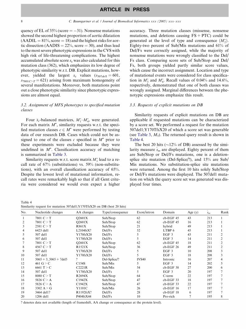
8 C. Baumgartner et al. / Journal of Biomedical Informatics xxx (2005) xxx–xxx
ARTICLE IN PRESS
quency of EL of 35% (score = �31). Nonsense mutationsshowed the second highest proportion of aortic dilatation(AADIL = 81%, score = 18) and the highest risks for aor-tic dissection (AADIS = 22%, score = 30), and thus leadto themost severe phenotypic expressions in theCVSwithhigh risk of life-threatening complications. The highestaccumulated absolute score sc was also calculated for thismutation class (362), which emphasizes its low degree ofphenotypic similarity w.r.t. DB. Explicit mutations, how-ever, yielded the largest sc values (s507del1 = 601,s7801C>T = 621) arising from maximum homogeneity ofseveral manifestations. Moreover, both mutations pointout a close phenotypic similarity since phenotypic expres-sions are almost equal.
3.2. Assignment of MFS phenotypes to specified mutation
classes
Four �sc-balanced matrices, M�1–M�4, were generated.
For each matrix M*, similarity requests w.r.t. the speci-fied mutation classes c 2M* were performed by testingdata of our research DB. Cases which could not be as-signed to one of the classes c specified in M* prior tothese experiments were excluded because they wereundefined in M*. Classification accuracy of matchingis summarized in Table 3.
Similarity requests w.r.t. score matrixM�1 lead to a re-call rate of 67% (substitutions) vs. 59% (non-substitu-tions), with an overall classification accuracy of 65%.Despite the lowest level of mutational information, re-call rates were remarkably high so that if all Gent crite-ria were considered we would even expect a higher
Table 4Similarity request for mutation 507del1;Y170TfsX20 on DB (best 20 hits)
No. Nucleotide changes AA changes Type/consequence
1 7801 C > T Q2601X Sub/Stop2 7801 C > T Q2601X Sub/Stop3 2581 C > T R861X Sub/Stop4 6423 del1 L2104fsX? Del/Fs5 507 del1 Y170fsX20 Del/Fs6 507 del1 Y170fsX20 Del/Fs7 7801 C > T Q2601X Sub/Stop8 4567 C > T R1521X Sub/Stop9 507 del1 Y170fsX20 Del/Fs10 507 del1 Y170fsX20 Del/Fs11 5065 + 3_5065 + 7del5 ? Del-Splice/?12 461 G > C C154S Sub/Mis13 6661 T > C C2221R Sub/Mis14 507 del1 Y170fsX20 Del/Fs15 8080 C > T R2694X Sub/Stop16 5826 C > A C1942X Sub/Stop17 5826 C > A C1942X Sub/Stop18 3302 A > G Y1101C Sub/Mis19 3464 del17 R1192fsX? Del/Fs20 1206 del1 P404fsX44 Del/Fs
? denotes data not available (length of frameshift, AA change or consequen
accuracy. Three mutation classes (missense, nonsensemutations, and deletions causing FS + PTC) could begenerated at the level of type and consequence ðM�2Þ.Eighty-two percent of Sub/Mis mutations and 61% ofDel/Fs were correctly assigned, while the majority ofnonsense mutations were wrongly classified to the Del/Fs class. Comparing score sets of Sub/Stop and Del/Fs, both groups yielded partly similar score values,which cause the incorrect assignment. Location and typeof mutational events were considered for class specifica-tion in M�3 and M�4. Recall values of 0.04% and 14.6%,respectively, demonstrated that one of both classes waswrongly assigned. Marginal differences between the phe-notypic expressions emphasize this result.
3.3. Requests of explicit mutations on DB
Similarity requests of explicit mutations on DB areapplicable if requested mutations can be characterizedby a score set. We performed a request for the mutation507del1;Y170TfsX20 of which a score set was generable(see Table 3, M5). The returned query result is shown inTable 4.
The best 20 hits (�12% of DB) assessed by the simi-larity measure sm are displayed. Eighty percent of themare Sub/Stop or Del/Fs mutations, one is a deletion-splice site mutation (Del-Splice/?), and 15% are Sub/Mis mutations. No substitution-splice site mutationswere returned. Among the first 10 hits solely Sub/Stopor Del/Fs mutations were displayed. The 507del1 muta-tion on which the query score set was generated was dis-played four times.
Exon/intron Domain Age (y) sm Rank
62 cb-EGF 45 43 213 162 cb-EGF 45 16 213 121 hybrid 49 213 152 LTBP 6 45 213 15 EGF 3 43 211 25 EGF 3 14 211 262 cb-EGF 45 18 211 236 cb-EGF 26 49 211 25 EGF 3 10 208 35 EGF 3 18 208 3IVS40 Intronic 16 207 45 EGF 3 14 202 554 cb-EGF 38 27 200 65 EGF 3 20 197 764 C-term 22 197 747 cb-EGF 33 18 197 747 cb-EGF 33 22 197 726 cb-EGF 16 17 197 728 cb-EGF 18 6 197 710 Pro-rich 7 195 8
ce at the protein level).

Fig. 2. Hierarchical cluster analysis of MFS clinical manifestations. Left of the mosaic the type and consequence of mutations are shown. Thehierarchical tree is depicted to the right of the mosaic. The clustered manifestations are given at the top; the scale measure of the linkage distance isshown on the bottom. Sub/Mis = missense mutation, Sub/Stop = nonsense mutation, Del/Fs = deletion/FS + PTC.
C. Baumgartner et al. / Journal of Biomedical Informatics xxx (2005) xxx–xxx 9
ARTICLE IN PRESS

Tab
le5
Evaluationofidentified
clustersusinghierarchical
cluster
analysis
Cluster
EL
AADIL
AADIS
MVP
PC
PES
ASR
WTS
SC
PE
JHHAP
SA
HE
nH
Sub/M
isSub/Stop
Del/F
sP(Sub/M
is=
1)
m1
m2
m3
c 10
3910
00
9665
070
9617
2287
100
960
232.57
1339
4861
(18)
64(34)
78(27)
c 159
806
8245
658
9464
2792
8580
2166
4.45
4327
3072
(19)
77(20)
81(22)
c 267
675
6771
043
2462
2471
525
1021
4.82
7614
1077
(23)
88(12)
94(11)
c 338
8825
2138
433
2546
879
7592
2524
5.43
4621
3362
(28)
80(19)
87(21)
c 480
568
240
424
7616
1228
2820
2025
5.24
924
482
(17)
81(16)
93(12)
Frequencies
ofman
ifestationsan
dthefractionofSub/M
is,Sub/Stop,an
dDel/F
smutationsin
clustersaregivenin
%.Probab
ilitiesthat
missense
mutationsin
clustersarepresentP(Sub/M
is=
1)aredepictedas
mean(SD)%.Model
1(m
1)discrim
inates
Sub/M
isfrom
Sub/Stopan
dDel/F
s,model
2(m
2)Sub/M
isfrom
Del/F
s,an
dmodel
3(m
3)Sub/M
isfrom
Sub/Stopmutations.nisthe
number
ofclustered
casesan
dH
theentropyofacluster
inbit.Clustersc 1–c
4aregenerated
atalinkag
edistance
>0.2,
sub-cluster
c 10issplitupat
alinkag
edistance
>0.45
(Fig.2).
10 C. Baumgartner et al. / Journal of Biomedical Informatics xxx (2005) xxx–xxx
ARTICLE IN PRESS
3.4. Diagnostic markers and probabilistic models
We focused on the investigation of the Sub/Mis, Sub/Stop, and Del/Fs mutation classes. Here, key manifesta-tions could be identified on which LRA models of min-imal classification error rates were built.
Superior classification accuracy was achieved whenseparating missense mutations from stop and/or dele-tions/FS + PTC mutations (both models 80%). Highestdiscriminatory performance yielded the Sub/Mis vs.Sub/Stop model (accuracy = 87%), however, withunbalanced recall rates of 92% (Sub/Mis) and 70%(Sub/Stop), respectively. Ectopia lentis (EL) representsthe hallmark manifestation in all three classes. In addi-tion to EL ascending aortic dilatation (AADIL) andone skeletal major symptom (WTS) distinguished be-tween Sub/Mis and Sub/Stop mutations, ascending aor-tic dissection (AADIS) and several skeletalmanifestations (PC, ASR, WTS, PE, and JH) distin-guished between Sub/Mis and Del/Fs mutations, andthus were identified as the predominant diagnosticmarkers. Merging Sub/Stop and Del/Fs class, and test-ing it against the Sub/Mis class, EL, PC, ASR, PE,and HAP were the discriminatory markers. EL, AADILand AADIS were the markers discriminating betweenSub/Stop and Del/Fs mutations best. However, classifi-cation accuracy of the latter model was relatively low(64%, recall 87% and 37%). Mitral valve prolapse(MVP) and both skin minor criteria (HE, SA) never ap-peared in the selected subsets and do not seem to havediagnostic value when distinguishing between Sub/Mis,Sub/Stop, and Del/Fs mutations.
3.5. Cluster analysis
Hierarchical cluster analysis was performed on the setof clinical manifestations. Again, we focused on subjectscarrying a Sub/Mis, Sub/Stop or Del/Fs mutation(Fig. 2). Table 5 summarizes the evaluation of identifiedclusters.
Four meaningful clusters were generated at a linkagedistance >0.2. Here, clusters c1–c3, merged at the linkagedistance <0.2 were more closely related to each otherthan to the remaining cluster c4. Cluster c4 differed sig-nificantly from c1 to c3, showing the mildest phenotypicexpressions. Here, 11 of 14 symptoms showed a frequen-cy below 50%, nine indicated a frequency even below25%. Ninety-two percent of this cluster consisted of mis-sense mutations. The mean probability that P (Sub/Mis = 1) ranged between 81 and 93%, however depend-ed on the applied LRA model. The most severe pheno-type was represented by cluster c10 , one of four sub-clusters of c1 split up at a linkage distance >0.45, andcontained predominantly Sub/Stop and Del/Fs muta-tions (together 87% vs. 13% Sub/Mis). In parallel, themean probability P (Sub/Mis = 1) decreased to 61–78%

C. Baumgartner et al. / Journal of Biomedical Informatics xxx (2005) xxx–xxx 11
ARTICLE IN PRESS
in this sub-cluster. Interestingly, the entropy H for sub-cluster c10 achieved the lowest value (2.57 bit vs. 5.24 bitfor c4) which can be explained by maximal class homo-geneity of five symptoms (AADIL, MVP, WTS, HAP,and SA > 95%) and additionally the absence of threemanifestations (AADIS, PES, and HE). Thus, clusterc10 is closely correlated with Sub/Stop and Del/Fs muta-tions, and c4 with Sub/Mis mutations.
4. Discussion
Genotype–phenotype correlation in humans withFBN1 gene mutations is a challenging bioinformaticstask. In particular, the age-related and pleiotropic nat-ure of the MFS as well as its intra- and inter-familialheterogeneity seem to make this task unmanageable[10,17,19]. The lack of a publicly available FBN1 re-source providing a maximum degree of genetic and phe-notypic information, and the absence of an informaticsframework for data management, analysis, and repre-sentation are mainly responsible for the moderate pro-gress of defining genotype–phenotype correlation.
Indeed, the two public FBN1 mutation DBs, HGMD(Human gene mutation database, http://archive.uwcm.ac.uk/uwcm/mg/search/127115.html) and UMD (Uni-versal mutation database, www.umd.be:2030/gene.htmland www.umd.necker.fr), are not sufficient to systemati-cally link genetic and clinical information; while HGMDfocuses on the collection, description, and literature anno-tation of published FBN1 mutations, UMD includessome more phenotypic information. UMD is currentlythe only publicly available FBN1 genotype–phenotypedatabase that provides data at DNA, protein, and clinicallevels similar to our resource [4]. The clinical information,however, contains merely the involvement (+/�) of theaffected organ systems, and therefore UMD is uselessfor extended genotype–phenotype investigations.
In this article, we propose a bioinformatics frame-work for FBN1 genotype–phenotype correlation, whichwill be publicly available via a web portal. A centralcomponent of the information system is a relationalDBMS for storing and managing mutation data, clinicaldata according to the Gent nosology and, in future,additional aortic elastic parameters to better monitoraortic abnormality [9,10]. The underlying databasescheme represents a biological model of a multi-systemicinherited disease, which describes mutations and theirpolymorphisms in DNA and protein sequences, andthe disease�s variability in phenotypic expression com-prehensively. Thus, our methodology is well generaliz-able to other monogenic diseases causing phenotypicpleiotropy; only an adaptation of the phenotype datamodel is needed. Depending on the amount of muta-tions, the number of involved organ systems and diag-nostic key features, and the number of required cases
to perform genotype–phenotype correlations vary. Ifdata analysis is performed at mutation type and conse-quence (cDNA and protein) level, a number of casescomparable to our study is essential. Considerably moredata are required, if data are analyzed at the level oflocation of mutational events in the gene or the affectedprotein domains, so that the web portal will help to col-lect sufficient data worldwide to perform genotype–phe-notype investigations at this level in future.
For advanced DB requests the proposed data modelpermits queries for the wide spectrum of mutation types,subtypes and their mutational events which are requiredfor the generation of the score sets at different levels. Weintroduced log-likelihood weights as similarity measuresto match phenotypes, similar to the well-known PAM orBLOSUM matrices, which were developed for proteinsequence alignment. Thus this simple retrieval techniquepermits the search of mutations of related phenotypeson DB, as exemplified for 507del1;Y170TfsX20, whichmay be helpful, e.g., to estimate the degree of intra-and inter-familial heterogeneity of the syndrome.
Relevant diagnostic markers were identified using awrapper-based feature selection approach. This strategyis preferred to the filter method, since computationallimitations caused by the size of DB (>600 publishedFBN1 mutations) and the dimensionality of investigateddata (n < 30) may not arise [26,27]. In particular, LRAmodels fulfill the requirement of clinical experts to havea quantitative (probability), not only a qualitative mea-sure for patient classification. Hierarchical cluster anal-ysis was proposed for sub-grouping phenotype data.Due to the high variability within the MFS phenotype,mutation classes of enhanced phenotypic homogeneityare surprising (cf. c10 and c4), since clusters with highclass homogeneity are indicators for a very close geno-type–phenotype relationship. The proposed data miningstrategy, which takes both a supervised and non-super-vised view of data analysis into account, properlyaddresses prognostic and diagnostic questions for thecorrelation task. Nevertheless, the evaluation and fur-ther development of data mining procedures are in pro-gress, so that in the future new meaningful approachescan readily be incorporated in the framework.
A few accepted genotype–phenotype correlations inthe MFS have been reported, e.g., with a hot spot forneonatal MFS in exons 24–32 or a clustering of muta-tions causing milder forms in exons 59–65. More com-mon occurrence of large-joint hypermobility (JH), lesscommon ectopia lentis (EL), and retinal detachmentare associated with premature termination codon(PTC) mutations, while, e.g., missense mutations showa high frequency of EL [1,13–17,31]. Using the proposedbioinformatics framework, some of the aforementionedcorrelations could be confirmed. A few novel ones wereidentified, although some limitations concerning theincomplete description of symptoms in the literature
12 C. Baumgartner et al. / Journal of Biomedical Informatics xxx (2005) xxx–xxx
ARTICLE IN PRESS
and the limited size of our current research DB exist.Maximum phenotypic dissimilarity was found betweenmissense mutations and the groups of nonsense muta-tions and deletions causing FS + PTC. The latter bothclasses indicate similar phenotypic expressions (cf. Ta-bles 2 and 3). This can be explained by related mutation-al events causing termination of fibrillin-1 synthesis. Keymanifestations, which are relevant for best discriminat-ing between Sub/Mis and Sub/Stop + Del/Fs classes,are EL and several skeletal (major and minor) criteria,but not manifestations of the CVS and the skin system.Comparing missense and nonsense mutations—indepen-dent of the location of the mutational event—AADISappears to be an additional key marker predominantlyobserved in patients carrying a nonsense mutation.More severe manifestations in the CVS lead to a higherrisk of life-threatening aortic dissection or rupture whichrequire immediate therapeutic intervention. The mostsevere phenotypic expressions were solely found in pa-tients carrying a Sub/Stop or Del/Fs mutation, whilethe mildest MFS phenotype appeared in Sub/Mis muta-tions. No difference was found if, e.g., point mutationsat different gene locations (exons 1–24 vs. exons 25–68) or with different mutational events (transitions vs.transversions) were compared.
In summary, our proposed bioinformatics frameworkfor FBN1 genotype–phenotype correlation provides apipeline for data management and analysis which canhelp to better link genetic and clinical information.Using this framework some well-known genotype–phe-notype correlations could be confirmed and other novelcorrelations were identified, which emphasize the powerof the methodology to address these important ques-tions with respect to diagnosis and therapy of MFS.
Acknowledgments
This study was supported by the Austrian IndustrialFunds FFF (HITT-10 UMIT) and the Wolfermann-Nageli-Stiftung Zurich, Switzerland.
References
[1] Loeys B, Nuytinck L, Delvaux I, De Bie S, De Paepe A. Genotypeand phenotype analysis of 171 patients referred for molecularstudy of the fibrillin-1 gene FBN1 because of suspected Marfansyndrome. Arch Intern Med 2001;161:2447–54.
[2] Robinson PN, Godfrey M. The molecular genetics of Marfansyndrome and related microfibrillopathies. J Med Genet2000;37:9–25.
[3] Pyeritz RE, Dietz HC. Marfan syndrome and other microfibrillardisorders. In: Royce PM, Steinmann B, editors. Connective tissueand its heritable disorders: molecular, genetic and medicalaspects. 2nd ed. New York: Wiley-Liss; 2002. p. 585–626.
[4] Collod-Beroud G, Le Bourdelles S, Ades L, Ala-Kokko L, BoomsP, Boxer M, et al. Update of the UMD-FBN1 mutation database
and creation of an FBN1 polymorphism database. Hum Mutat2003;22:199–208.
[5] De Paepe A, Devereux RB, Dietz HC, Hennekam RCM, PyeritzRE. Revised diagnostic criteria for the Marfan syndrome. Am JMed Genet 1996;62:417–26.
[6] Groenink M, Rozendaal L, Naeff MSJ, Hennekam RCM,Hart AAM, van der Wall EE, et al. Marfan syndrome inchildren and adolescents: predictive and prognostic value ofaortic root growth for screening for aortic complications.Heart 1998;80:163–9.
[7] Savolainen A, Keto P, Hekali P, Nisula L, Kaitila I, Vitasalo M,et al. Aortic distensibility in children with the Marfan syndrome.Am J Cardiol 1992;70:691–3.
[8] Meijboom LJ, Nollen GJ, Mulder BJM. Prevention of cardio-vascular complications in the Marfan syndrome. Vasc Dis Prev2004;1:79–86.
[9] Baumgartner D, Baumgartner C, Matyas G, Steinmann B, LofflerJ, Schermer E, Schweigmann U, Baldissera I, Frischhut B, Hess J,Hammerer I. Diagnostic power of aortic elastic properties inyoung patients with Marfan syndrome. J Thorac Cardiovasc Surg2005;129:730–9.
[10] Baumgartner C, Matyas G, Steinmann B, Baumgartner D.Marfan syndrome: a diagnostic challenge caused by phenotypicand genetic heterogeneity. Methods Inf Med, 2005 (in press).
[11] Maron BJ, Moller JH, Seidman CE, Vincent GM, Dietz HC,Moss AJ, et al. Impact of laboratory molecular diagnosis oncontemporary diagnostic criteria for genetically transmittedcardiovascular diseases: hypertrophic cardiomyopathy, long-QTsyndrome, and Marfan syndrome. A statement for healthcareprofessionals from the Councils on Clinical Cardiology, Cardio-vascular Disease in the Young, and Basic Science, AmericanHeart Association. Circulation 1998;98:1460–71.
[12] Halliday DJ, Hutchinson S, Lonie L, Hurst JA, Firth H,Handford PA, et al. Twelve novel FBN1 mutations in Marfansyndrome and Marfan related phenotypes test the feasibility ofFBN1 mutation testing in clinical practice. J Med Genet2002;39:589–93.
[13] Dietz HC, Pyeritz RE. Marfan syndrome and related disorders.In: Scriver CR, Beaudet AL, Sly WS, Valle D, editors. Themetabolic and molecular bases of inherited disease. 8th ed. NewYork: McGraw-Hill; 2001. p. 5287–311.
[14] Palz M, Tiecke F, Booms P, Goldner B, Rosenberg T, Fuchs J,et al. Clustering of mutations associated with mild Marfan-likephenotypes in the 3-prime region of FBN1 suggests a potentialgenotype–phenotype correlation. Am J Med Genet2000;91:212–21.
[15] PepeG,Giusti B,Evangelisti L, PorciniMC,Brunelli T,GiurlaniL,et al. Fibrillin-1 (FBN1) gene frameshift mutations in Marfanpatients: genotype–phenotype correlation. Clin Genet2001;59:444–50.
[16] Tiecke F, Katzke S, Booms P, Robinson PN, Neumann L,Godfrey M, et al. Classic, atypically severe and neonatal Marfansyndrome: twelve mutations and genotype–phenotype correla-tions in FBN1 exons 24-40. Eur J Hum Genet 2001;9:13–21.
[17] Schrijver I, Liu W, Odom R, Brenn T, Oefner P, Furthmayr H,et al. Premature termination mutations in FBN1: distinct effectson differential allelic expression and on protein and clinicalphenotypes. Am J Hum Genet 2002;71:223–37.
[18] Matyas G, De Paepe A, Halliday D, Boileau C, Pals G,Steinmann B. Evaluation and application of denaturing HPLCfor mutation detection in Marfan syndrome: identification of 20novel mutations and two novel polymorphisms in the FBN1 gene.Hum Mutat 2002;19:443–56.
[19] Schrijver I, Liu W, Brenn T, Furthmayr H, Francke U. Cysteinesubstitutions in epidermal growth factor-like domains of fibrillin-1: distinct effects on biochemical and clinical phenotypes. Am JHum Genet 1999;65:1007–20.

C. Baumgartner et al. / Journal of Biomedical Informatics xxx (2005) xxx–xxx 13
ARTICLE IN PRESS
[20] Katzke S, Booms P, Tiecke F, Palz M, Pletschacher A, TurkmenS, et al. TGGE screening of the entire FBN1 coding sequence in126 individuals with Marfan syndrome and related fibrillinopa-thies. Hum Mutat 2002;20:197–208.
[21] Comeglio P, Evans AL, Brice G, Cooling RJ, Child AH.Identification of FBN1 gene mutations in patients with ectopialentis and marfanoid habitus. Br J Ophthalmol 2002;86:1359–62.
[22] Biggin A, Holman K, Brett M, Bennetts B, Ades L. Detection ofthirty novel FBN1 mutations in patients with Marfan syndromeor a related fibrillinopathy. Hum Mutat 2004;23:99.
[23] Den Dunnen JT, Antonarakis SE. Nomenclature for the descrip-tion of sequence variations (www.hgvs.org/mutnomen). HumMutat, 2001;109: 121–4.
[24] Blum AL, Langley P. Selection of relevant features and examplesin machine learning. Artif. Intell. 1997;97:245–71.
[25] Baumgartner C, Bohm C, Baumgartner D, Marini G, WeinbergerK, Olgemoller B, et al. Supervised machine learning techniques
for the classification of metabolic disorders in newborns. Bioin-formatics 2004;20:2985–96.
[26] Kohavi R, John GH. The wrapper approach. In: Liu H, MotodaH, editors. Feature selection for knowledge discovery and datamining. NY: Kluwer; 1998. p. 33–50.
[27] Hall MA, Holmes G. Benchmarking attribute selection techniquesfor discrete class data mining. IEEE Trans Knowl Data Eng2003;15:1437–47.
[28] Hosmer DW, Lemeshow S. Applied logistic regression. 2nded. New York: Wiley; 2000.
[29] Witten H, Frank E. Data mining—practical machine learningtools and techniques with java implementations. San Francis-co: Morgan Kaufmann; 2000.
[30] Everitt BS. Cluster analysis. London: Edward Arnold; 1993.[31] Sarfarazi M, Tsipouras P, Del Mastro R, Kilpatrick M, Farndon
P, Boxer M, et al. A linkage map of 10 loci flanking the Marfansyndrome locus on 15q: results of an International Consortiumstudy. J Med Genet 1992;29:75–80.


Marfan SyndromeA Diagnostic Challenge Caused by Phenotypic and Genetic Heterogeneity
C. Baumgartner1*, G. Mátyás2, 3, B. Steinmann2, D. Baumgartner4
1Research Group for Biomedical Data Mining, University for Health Sciences, Medical Informatics andTechnology, Hall i. T., Austria2Division of Metabolism and Molecular Pediatrics, University Children´s Hospital, Zurich, Switzerland3Institute of Medical Genetics, University of Zurich, Schwerzenbach, Switzerland4Clinical Division of Pediatric Cardiology, Innsbruck Medical University, Innsbruck, Austria
SummaryObjectives: Marfan syndrome (MFS) is an autosomaldominant inherited connective tissue disorder causedby mutations in the fibrillin-1 (FBN1) gene withvariable clinical manifestations in the cardiovascular,musculoskeletal and ocular systems.Methods: Data of molecular genetic analysis and acatalogue of clinical manifestations including aorticelastic parameters were mined in order to (i) assessaortic abnormality before and during medical treat-ment, and to (ii) identify novel correlations betweenthe genotype and phenotype of the disease using hier-archical cluster analysis and logistic regression analysis.A score measure describing the similarity betweena patient’s clinical symptoms and a characteristicphenotype class was introduced.Results: A probabilistic model for monitoring the loss ofaortic elasticity was built on merely aortic parametersof 34 patients with classic MFS and 43 control subjectsshowing a sensitivity of 82% and a specificity of 96%.The clinical phenotypes of 100 individuals with classi-cal or suspected MFS were clustered yielding four differ-ent phenotypic expressions. The highest correlation wasfound between FBN1 missense mutations, which mani-fested as ectopia lentis, skeletal major and skin minorcriteria, and two out of four clustered phenotypes. Theprobability of the presence of a missense mutationin both phenotype classes is approximately 70%.Conclusions: Monitoring of aortic elastic propertiesduring medical treatment may serve as additional cri-terion to indicate elective surgical interventions. Geno-type-phenotype correlation may contribute to anticipatethe clinical consequences of specific FBN1 mutationsmore comprehensively and may be helpful to identifyMFS patients at risk at an early stage of disease.
KeywordsMarfan syndrome, fibrillin-1 (FBN1), aortic elasticity,phenotype-genotype correlation, data mining
Methods Inf Med 2005; 44: 487–97
Introduction
Marfan syndrome (MFS, OMIM #154700)is an autosomal dominant inherited con-nective tissue disorder with prominent clini-cal manifestations in the cardiovascular,musculoskeletal and ocular systems. Thedisease’s prevalence is approximately1/5000 [1]. At present more than 600 differ-ent mutations in the gene encoding fibril-lin-1 (FBN1, OMIM #134797) are known,and mutations could be detected in at least80% of MFS patients [2, 3].
The diagnosis of MFS is dependent on acatalogue set of clinical diagnostic criteriaaccording to the ‘Gent nosology’[4]. Milderand more severe clinical symptoms groupedas minor and major criteria, which affect atleast two organ systems (major criteria), andthe involvement of a third system (minorcriteria) are required for classic MFS.Weakness of the aortic wall accounts for80% of known causes of death of patientswith MFS [5]. Before life-threatening com-plications like dissection or rupture occur,alterations of aortic elastic properties due todefective fibrillin-1 can be detected throughthe examination and monitoring of aorticelasticity during follow-up care [6-9]. Inaddition, molecular genetic analysis maybe helpful to anticipate the clinical con-sequences of specific FBN1 mutationsthrough the analysis of detailed clinical in-formation and mutation data. For instancepatients with an identified FBN1 mutationwere more likely to have ectopia lentis andcardiovascular complications than thosewithout an identifiable mutation [10].
Since 2000 data from molecular geneticanalysis, clinical manifestations according
to the Gent nosology and data of aortic elas-ticity have been collected at the InnsbruckMarfan Clinical Center, Innsbruck MedicalUniversity, Austria. The aim of our studywas a detailed analysis of clinical in-formation and mutation data in order toi. investigate aortic elasticity, assess its ab-
normality and determine the course ofaortic elasticity during treatment, and
ii. to explore novel correlations betweenFBN1 mutations and the clinical pheno-type, which may be helpful to anticipatethe clinical consequences of specificmutations in patients with classical orsuspected MFS more comprehensively.
To monitor changes of aortic elastic proper-ties, a software tool was developed to pro-cess M-mode echocardiographic tracings ofthe ascending and descending aorta. We ap-plied probabilistic models and hierarchicalcluster analysis for the data analysis task, inparticular the latter one for phenotype clas-sification. A score value was introduced toquantify phenotypic similarity of patients’clinical symptoms and characteristic pheno-type classes.
MethodsThe Innsbruck Marfan ProjectThe organization chart of the InnsbruckMarfan project and close collaborationswith the Innsbruck Medical University,Austria (Clinical Divisions of Pediatric Car-diology, Ophthalmology and Orthopedics,and the Institute of Medical Biology andHuman Genetics), the University for Health
487
© 2005 Schattauer GmbH
Methods Inf Med 4/2005

Sciences, Medical Informatics and Tech-nology – UMIT, Hall in the Tyrol, Austria(Research Group for Biomedical Data Min-ing) and University of Zurich, Switzerland(University Children’s Hospital, Divisionof Metabolism and Molecular Pediatrics),is illustrated in Figure 1. The informationprocess is organized into three layers rep-resenting patient administration (1), clinicalinvestigation (2), and biomedical dataprocessing which supports the developmentof new strategies for diagnosis and thera-py (3).
Layer 1 organizes the patients’ admis-sion, administration and coordination of theexamination procedure. Clinical investi-gations were performed in layer 2. Data ofthe clinical phenotype was collected in adatabase located at the MFS clinical center,Clinical Division of Pediatric Cardiology,Innsbruck Medical University, and com-pleted by genetic data after molecular gen-etic analysis at the University Children’sHospital Zurich. Owing to the complexityof the medical picture and the large amountof clinical and genetic information, it is achallenge for biomedical informatics tomine novel medical knowledge because itinfluences diagnostic and clinical decisions(layer 3). Phenotyping and genotyping
(layer 2), and the data analysis task (layer 3)are described in the following paragraphs inmore detail.
PhenotypingThe Gent Nosology
The diagnosis of classic MFS is dependenton a set of international diagnostic criteriaaccording to the Gent nosology [4]. Basi-cally, it is necessary to distinguish betweentwo different cases:1. the index case, if the family/genetic his-
tory is not contributory (major criteria inat least two different organ systems, andinvolvement of a third organ system) or ifa mutation known to cause MFS is de-tected (one major criterion in an organsystem and involvement of a secondorgan system),
2. a relative of an index case (presence of amajor criterion in the family history andone major criterion in an organ systemand involvement of a second organ sys-tem).
Table 1 summarizes the Gent criteriagrouped by the affected organ systems and
further separated into major and/or minorcriteria [4]. Data from the pulmonary sys-tem (minor criteria), the ocular system(minor criteria), the dura (major criterion)and two minor criteria of the CVS system(no. 2 and 3) were partly not available so thisadditional clinical information was not con-sidered for data analysis.
Aortic Parameters
Alterations of aortic elastic properties canlead to life-threatening complications suchas dissection or rupture. In addition to theGent nosology for the cardiovascular sys-tem, which predominantly focuses on thepresence of aortic root, ascending and de-scending aortic dilatation and/or dissection,we assessed altered aortic elasticity accord-ing to an approach as we previously de-scribed in [9]. Based on M-mode echo-cardiographic tracings at the ascending anddescending aorta, we developed a softwaretool which enables us to calculate aorticelastic parameters of each aortic segmentautomatically.
First, M-mode tracings of both aorticsegments were obtained with commerciallyavailable equipment (System Five, GEVingmed Ultrasound, Horten, Norway)using 2-dimensional guidance at four differ-ent levels: (level 1) annulus (parasternalshort-axis view), (level 2) sinuses of Val-salva, (level 3) proximal ascending aorta10-20 mm distal to the sinotubular junction(both parasternal long-axis views), and(level 4) descending abdominal aorta justproximal to the branching-off of the celiactrunk (abdominal paramedian long-axisview). Tracings of the ascending (level 3)and descending aorta (level 4) of severalheart cycles have been processed to extractthe inner aortic wall contours by applying asegmentation algorithm using filter andmorphological operations on the registeredM-mode images. According to usual aorticdiameter measurements using the leadingedge technique the detected inner diameterof the aorta was enlarged by the anterior aor-tic wall thickness (Fig. 2 left). The time-res-olution of detected diameters is approxi-mately 6 ms per pixel, the spatial resolution0.2 mm per pixel. Time-diameter curveswere computed based on the ascending and
Methods Inf Med 4/2005
488
Baumgartner et al.
Fig. 1 The Innsbruck approach: An interdisciplinary and international MFS diagnostic framework

descending aortic outlines (Fig. 2 top right).Curves of at least five heart cycles wereaveraged and slightly smoothed by a Butter-worth filter of degree 2 (Fig. 2 bottomright).
In some M-mode tracings minor manualcorrections of aortic wall contours had to becarried out; however, the interobserver re-producibility did not exceed 5%. Bloodpressure measurements were taken at theright arm oscillometrically (Dinamap) im-mediately before M-mode registration. Thefollowing aortic root (RootAo), ascending(AscAo) and descending (DescAo) aorticparameters were calculated from M-modetime-diameter curves and blood pressureregistrations. Aortic dilatation was deter-mined using standard nomograms [9]:
Normalized diastolic RootAo, AscAoand DescAo diameters (referenced to pa-tient’s body surface area, BSA):
Dd’ = Dd /BSA [mm/m2] (1)
AscAo and DescAo maximum systolicdiameter increase:Increase = (Ds – Dd)/Dd [%] (2)
AscAo and DescAo distensibility:Distensibility =
(3)
AscAo and DescAo stiffness index (SI):
(4)
AscAo and DescAo maximum systolic areaincrease (MSAI):
[%/100ms] (5)
Magnitude of a vector loop by combiningAscAo and DescAo diameter changes:Magnitude(t) =
[%] (6)
Phase of the vector loop
[degree, °] (7)
Dd and Ds are the diastolic (minimum) andsystolic (maximum) aortic diameters, Ad
and As are the diastolic and systolic cross-sectional aortic areas, Pd and Ps are the dia-stolic and systolic blood pressures inmmHg, D(t) is the aortic time-diametercurve and A(t) is the aortic time-area curveover the heart cycle.
489
Marfan Syndrome – Diagnosis and Therapy Monitoring
Methods Inf Med 4/2005
Skeletal system (major criteria):1. pectus excavatum requiring surgery or pectus carinatum,2. reduced upper to lower segment ratio or arm span to height ratio greater than 1.05,3. – wrist sign (requiring that the thumb overlaps the terminal phalanx of the 5th digit
when grasping the contralateral wrist)–thumb sign (when the hand is clenched, the entire nail of the thumb projects beyond theulnar border of the hand),
4. scoliosis of > 20° or spondylolisthesis,5. reduced extension at the elbows (<170°),6. medial displacement of the medial malleolus causing pes planus,7. protrusio acetabuli of any degree (ascertained on radiographs).Skeletal system (minor criteria):1. pectus excavatum of moderate severity,2. joint hypermobility,3. highly arched palate with crowding of teeth,4. facial appearance (dolichocephaly, malar hypoplasia, enophthalmos, retrognathia,
downslanting palpebral fissures).
Ocular system (major criterion):1. ectopia lentis.Ocular system (minor criteria)*:1. abnormally flat cornea (as measured by keratometry),2. increased axial length of globe (as measured by ultrasound),3. hypoplastic iris or hypoplastic ciliary muscle causing increased myosis.
Cardiovascular system (major criteria):1. dilatation of the ascending aorta with or without aortic regurgitation and involving at least
the sinuses of Valsalva,2. dissection of the ascending aorta.Cardiovascular system (minor criteria):1. mitral valve prolapse with or without mitral valve regurgitation,2. dilatation of the main pulmonary artery, in the absence of valvular or peripheral
pulmonary stenosis or any other obvious cause, below the age of 40 years*,3. calcification of the mitral annulus below the age of 40 years*,4. dilatation or dissection of the descending thoracic or abdominal aorta below the age of
50 years.
Pulmonary system (minor criteria)*:1. spontaneous pneumothorax,2. apical blebs (ascertained by chest radiography).
Skin and integument (minor criteria):1. striae atrophicae (stretch marks) not associated with marked weight changes, pregnancy
or repetitive stress,2. recurrent inguinal or incisional herniae.
Dura (major criterion)*:1. lumbosacral dural ectasia (ascertained by CT or MRI).
Family/genetic history (major criteria)*:1. having a parent, child or sibling who meets these diagnostic criteria independently,2. presence of a mutation in FBN1 known to cause the Marfan syndrome,3. presence of a haplotype around FBN1, inherited by descent, known to be associated with
unequivocally diagnosed Marfan syndrome in the family.
* represent organ systems or single symptoms including family/genetic history which were not considered for clusteranalysis.
Table 1Clinical symptoms andfamily/genetic history ac-cording to the Gent nosol-ogy
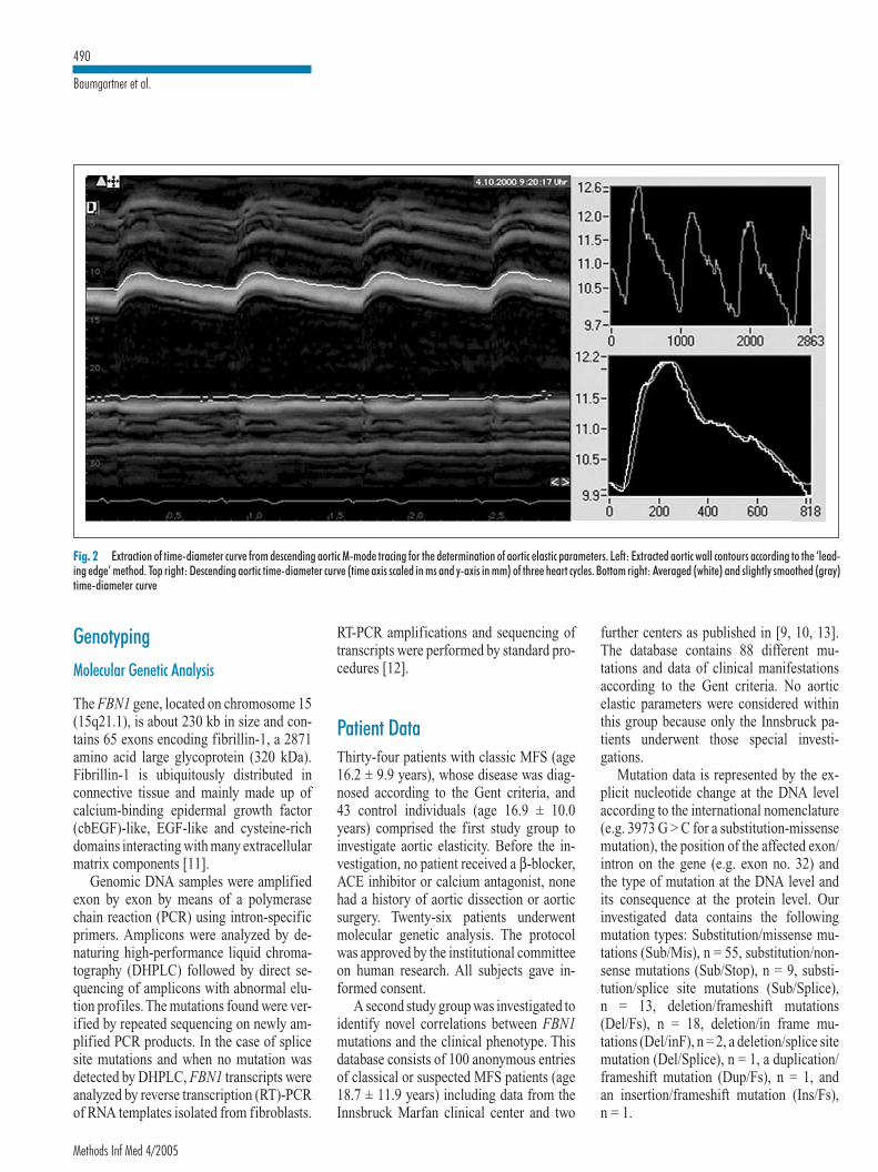
GenotypingMolecular Genetic Analysis
The FBN1 gene, located on chromosome 15(15q21.1), is about 230 kb in size and con-tains 65 exons encoding fibrillin-1, a 2871amino acid large glycoprotein (320 kDa).Fibrillin-1 is ubiquitously distributed inconnective tissue and mainly made up ofcalcium-binding epidermal growth factor(cbEGF)-like, EGF-like and cysteine-richdomains interacting with many extracellularmatrix components [11].
Genomic DNA samples were amplifiedexon by exon by means of a polymerasechain reaction (PCR) using intron-specificprimers. Amplicons were analyzed by de-naturing high-performance liquid chroma-tography (DHPLC) followed by direct se-quencing of amplicons with abnormal elu-tion profiles. The mutations found were ver-ified by repeated sequencing on newly am-plified PCR products. In the case of splicesite mutations and when no mutation wasdetected by DHPLC, FBN1 transcripts wereanalyzed by reverse transcription (RT)-PCRof RNA templates isolated from fibroblasts.
RT-PCR amplifications and sequencing oftranscripts were performed by standard pro-cedures [12].
Patient DataThirty-four patients with classic MFS (age16.2 ± 9.9 years), whose disease was diag-nosed according to the Gent criteria, and43 control individuals (age 16.9 ± 10.0years) comprised the first study group toinvestigate aortic elasticity. Before the in-vestigation, no patient received a β-blocker,ACE inhibitor or calcium antagonist, nonehad a history of aortic dissection or aorticsurgery. Twenty-six patients underwentmolecular genetic analysis. The protocolwas approved by the institutional committeeon human research. All subjects gave in-formed consent.
A second study group was investigated toidentify novel correlations between FBN1mutations and the clinical phenotype. Thisdatabase consists of 100 anonymous entriesof classical or suspected MFS patients (age18.7 ± 11.9 years) including data from theInnsbruck Marfan clinical center and two
further centers as published in [9, 10, 13].The database contains 88 different mu-tations and data of clinical manifestationsaccording to the Gent criteria. No aorticelastic parameters were considered withinthis group because only the Innsbruck pa-tients underwent those special investi-gations.
Mutation data is represented by the ex-plicit nucleotide change at the DNA levelaccording to the international nomenclature(e.g. 3973 G > C for a substitution-missensemutation), the position of the affected exon/intron on the gene (e.g. exon no. 32) andthe type of mutation at the DNA level andits consequence at the protein level. Ourinvestigated data contains the followingmutation types: Substitution/missense mu-tations (Sub/Mis), n = 55, substitution/non-sense mutations (Sub/Stop), n = 9, substi-tution/splice site mutations (Sub/Splice),n = 13, deletion/frameshift mutations(Del/Fs), n = 18, deletion/in frame mu-tations (Del/inF), n = 2, a deletion/splice sitemutation (Del/Splice), n = 1, a duplication/frameshift mutation (Dup/Fs), n = 1, andan insertion/frameshift mutation (Ins/Fs),n = 1.
Fig. 2 Extraction of time-diameter curve from descending aortic M-mode tracing for the determination of aortic elastic parameters. Left: Extracted aortic wall contours according to the ‘lead-ing edge’ method. Top right: Descending aortic time-diameter curve (time axis scaled in ms and y-axis in mm) of three heart cycles. Bottom right: Averaged (white) and slightly smoothed (gray)time-diameter curve
Methods Inf Med 4/2005
490
Baumgartner et al.

Phenotype data was available as the ac-cumulated number of symptoms of eachorgan system separated into major and/or minor criteria. According to the Gentcriteria, the skeletal system, for instance,comprises a maximum of seven majorsymptoms. The following example demon-strates one tuple of the dataset which is or-ganized as follows: {Nucleotide change:=6794 G > A, type and consequence of mu-tation:= Sub/Mis, position of affectedexon:= 55; skeletal (major):= 4, skeletal(minor):= 3, ocular (major):= 1; CVS(major):=1, CVS (minor):= 1, skin(minor):= 1}.
Data AnalysisFor the data analysis task we introducedprobabilistic models for class predictionand applied hierarchical cluster analysis todivide phenotypic expressions into mean-ingful subgroups. More specifically, to clas-sify patients with MFS and to monitor theiralteration of aortic elasticity during medicaltherapy we built a probabilistic model onsolely aortic parameters using logistic re-gression analysis (LRA). For the genotype-phenotype correlation task we again pro-pose LRA models which serve as a predictorfor the presence of a specific FBN1 mu-tation dependent on the relevant phenotypicpattern. A new score measure was intro-duced for phenotype class assignment.
Logistic Regression Analysis and ParameterSelection
Logistic regression analysis (LRA) con-structs a linear separation hyperplane be-tween two class datasets (e.g. MFS patientsvs. control individuals or classes of Sub/Mismutations vs. Del/Fs mutations). The hyper-plane is described by a discriminant func-tion, i.e. z = b1x1 + b2x2 + … + bnxn + c,which represents the logit of the model.x1, …, xn are the input variables (i.e. the ac-cumulated number of symptoms of theorgan system), b1, …, bn and constant c rep-resent the coefficients which have to betrained by the paradigm. Class membership(class 0 or 1) is indicated by a probabilitymeasure of the form p (y = 1) = 1 – p (y = 0)
= 1/(1 + exp (– z)) using a cut-off p value of0.5 by default [14]. For multiple hypothesistesting (e.g. Sub/Mis vs. Sub/Stop vs. Sub/Splice, etc.) we reduced the multiple classproblem to a two-class problem byalternative testing of each selected classagainst the remaining tuples of the given da-tabase DB as we carried out in our experi-ments (e.g. Sub/Mis vs. DB – Sub/Mis).However, classification algorithms likek-NN, decision trees or artificial neural net-works are well applicable for multiple clas-sification problems, but lack a direct inter-pretation of the decision rule with respect toprognostic questions.
Parameter selection – we used a forwardselection strategy with a backtracking fa-cility (search termination = 5) – was per-formed to search through the space of pa-rameter subsets to identify the optimal one.First, it starts with the empty set of features.It evaluates all the one-feature subsets, andselects the one with the best performancemeasure. It then evaluates all the two-fea-ture subsets that include the feature alreadyselected from the first step, and selects thebest one. This process continues until ex-tending the size of the current subset leadsto a lower performance measure. Thereby,each subset of features is directly evaluatedby the learning algorithm, i.e. LRA, that wasused in order to progressively generate newand better subsets. For each search step theclassification error of the LRA model, i.e.the proportion of incorrectly classified sub-jects divided by the total number of subjectsof both classes, is determined as a perform-ance parameter. This genetic approach iden-tifying the relevant parameter sub-space ac-cording to the paradigm’s error rate in oneanalytical run was thus favored over the so-called filter approach which delivers aquantitative value of each investigated at-tribute. Here, the user has the final task ofidentifying the relevant parameter sub-space through continued testing of classi-fier’s accuracy with the aim to optimize itstep by step.
For the model-building process we usedstratified 10-fold-cross validation which ispreferred when datasets are small. Therebythe given dataset is split into ten folds usingnine folds for training and one fold for test-ing [15].
Hierarchical Cluster Analysis
Multidimensional data sets are common inmany research areas by using cluster analy-sis to find meaningful groups in data. Someclustering algorithms, such as k-means,require users to specify the number ofclusters as an input, but users rarely knowthe right number beforehand. Hierarchicalclustering algorithms, which do not need apredetermined number of clusters as inputparameters, enable the user to determine thenatural grouping with interactive visualfeedback (dendrogram and color mosaic).To determine a proper number of clusters,the minimum similarity threshold (between0 and 1) needs to be changed [16, 17].
When hierarchical clustering algorithmmerges two clusters to generate a newbigger cluster, it should calculate the dis-tances between the new cluster and remain-ing clusters. We used the average linkageapproach (Unweighted Pair Group Methodwith Arithmetic Mean, UPGMA). Let Cn bea new cluster, a merge of Ci and Cj. Let Ck bea remaining cluster. Dist is the distance be-tween two clusters, e.g. between Ci and Ck:
(8)
A column-by-column (attribute-wise) nor-malization by rescaling from 0.0 to 1.0 wasperformed. Euclidean distance was thuschosen as the distance (similarity) measure.Cluster analysis was applied to accumulatedsymptoms of (1) skeletal major, (2) skeletalminor, (3) CVS major, (4) CVS minor, (5)ocular major and (6) skin minor criteria.
Phenotype Score
Based on the clustered phenotype classeswe introduced a quantitative measure whichdescribes the similarity between a patient’sphenotype and a phenotype class by a scorevalue. To characterize the symptomaticsimilarity within a characteristic phenotypeclass the following definitions are required:1. µsystem: mean value of diagnosed symp-
toms in an organ system (major andminor criteria separated),
491
Marfan Syndrome – Diagnosis and Therapy Monitoring
Methods Inf Med 4/2005
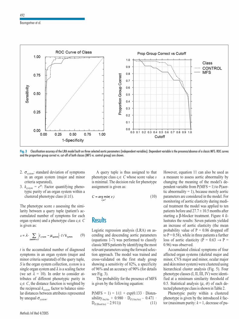
2. σsystem: standard deviation of symptomsin an organ system (major and minorcriteria separated),
3. ksystem = eσ: Factor quantifying pheno-typic purity of an organ system within aclustered phenotype class (k ≥1).
The phenotype score s assessing the simi-larity between a query tuple (patient’s ac-cumulated number of symptoms for eachorgan system) and a phenotype class ci∈ Cis given as:
(9)
t is the accumulated number of diagnosedsymptoms in an organ system (major andminor criteria separated) of the query tuple,S is the organ system collection, system is asingle organ system and λ is a scaling factor(we set λ = 10). In order to consider at-tributes of different phenotypic purity inci∈ C, the distance function is weighted bythe reciprocal ksystem factor to balance simi-lar distances between attributes representedby unequal σsystem.
A query tuple is thus assigned to thatphenotype class ci∈ C whose score value sis minimal. The decision rule for phenotypeassignment is given as:
(10)
ResultsLogistic regression analysis (LRA) on as-cending and descending aortic parameters(equations 1-7) was performed to classifyclassic MFS patients by identifying the mostrelevant parameters using the forward selec-tion approach. The model was trained andcross-validated on the first study groupshowing a sensitivity of 82%, a specificityof 96% and an accuracy of 90% (for detailssee Fig. 3).
The probability for the presence of MFSis given by the following equation:
P(MFS = 1) = 1/(1 + exp(0.133 · Disten-sibilityAscAo + 0.980 · Dd’(AscAo) – 0.471 ·Dd’(RootAo) – 2.911)) (11)
However, equation 11 can also be used asa measure to assess aortic abnormality bychanging the meaning of the model’s de-pendent variable from P(MFS = 1) to P(aor-tic abnormality = 1), because merely aorticparameters are considered in the model. Formonitoring of aortic elasticity during medi-cal treatment the model was applied to tenpatients before and 27.7 ± 10.5 months afterstarting a β-blocker treatment. Figure 4 il-lustrates the results: Seven patients yieldedan increase of aortic elasticity (the meanprobability value of P = 0.86 dropped offto P = 0.58), while in three patients a furtherloss of aortic elasticity (P = 0.63 → P =0.96) was observed.
Accumulated clinical symptoms of fouraffected organ systems (skeletal major andminor, CVS major and minor, ocular majorand skin minor system) were clustered usinghierarchical cluster analysis (Fig. 5). Fourphenotype classes (I, II, III, IV) were identi-fied at a minimum similarity threshold of0.5. Statistical analysis (µ, σ) of each de-tected phenotype class is shown inTable 2.
Phenotypic purity within a clusteredphenotype is given by the introduced k fac-tor (maximum purity: k = 1, decrease of pu-
Fig. 3 Classification accuracy of the LRA model built on three selected aortic parameters (independent variables). Dependent variable is the presence/absence of a classic MFS. ROC curvesand the proportion group correct vs. cut-off of both classes (MFS vs. control group) are shown.
Methods Inf Med 4/2005
492
Baumgartner et al.

rity: k > 1). Maximum dissimilarity betweenthe four clustered phenotype classes how-ever is primarily caused by the alternatingpresence of the ocular major criterion (ecto-pia lentis) and the CVS major criterion (aor-tic root dilatation) in the different clusters.Moreover, both dichotomous attributesshowed maximum purity (k = 1) within eachphenotype class. In detail, types I (Ia + Ib)and III are characterized by the prevalenceof ectopia lentis, types I and II by an aorticroot dilatation, while type IV manifestsneither with ectopia lentis nor with aorticroot dilatation. However, the coincidence ofboth major symptoms ectopia lentis and aor-tic root dilatation in type I corresponds wellwith a more severe, the absence of bothsymptoms (type IV) with a milder clinicalpicture of the MFS phenotype. In contrast,skeletal major and minor criteria, CVSminor and skin minor criteria yielded alower purity in all four clustered phenotypeclasses expressed by a k factor >1, but <4.Individuals with the mildest clinical mani-festations of skeletal and CVS symptomsare represented in phenotype class III whilephenotype class I indicates the most severemanifestations in the same organ systems.Type IV however represents the mildestMFS phenotype without ocular manifes-tation, with marginal CVS and skin, andmoderate skeletal symptoms.
Again, LRA was performed to discrimi-nate FBN1 missense mutations from allother types of mutations in DB by selectingthe most relevant organ systems as modelparameters. The model was trained andcross-validated on 55 cases with a Sub/Mismutation and 45 cases representing thegroup of remaining mutations in DB, i.e.Sub/Stop, Sub/Splice, Del/Fs, Dup/Fs, Ins/Fs, Del/inF and Del/Splice mutations. Themodel revealed a sensitivity of 58%, a spe-cificity of 78% and an accuracy of 69%.Theprobability for the presence of a Sub/Mismutation – independent of the position inthe gene – is thus given by equation 12:
P(Sub/Mis = 1) = 1/(1 + exp(– 1.708 · ocular(major) + 0.275 · skeletal (major) +0.471 ·skin (minor) – 0.133)) (12)
Ocular major, skeletal major and skin minorcriteria are the selected attributes when
using forward selection and can be inter-preted as the predominant clinical pheno-type of MFS patients carrying an FBN1point mutation.
Correlating the presence of Sub/Mis mu-tations with the clustered phenotype classesI-IV, highest correlation was found withphenotype classes I and III (Fig. 5). Bothphenotypes yielded a mean probability of~ 0.7 for the presence of a point mutationwhich corresponds well with the observedfrequency of Sub/Mis cases (72% for type Iand 63% for type III) within the two classes.At a minimum similarity threshold of 0.646phenotype class I splits into two sub-classes: Class Ia indicates a further increaseof P(Sub/Mis) to 0.75 accompanied by anenhanced frequency of 87%. According tothe skin criteria Ia differs from Ib by show-ing nearly no skin minor criteria. Only phe-notype IV showed a discrepancy betweenthe frequency of missense mutations (72%)and the probability value (0.38) which canbe explained by the small number of clus-tered cases (n = 7). On the other hand pheno-type class II, which constituted more severemanifestations of all investigated systems,but without the presence of an ectopia lentis,contains a fraction of 45% of Del/Fs mu-tations and represents 78% of all investi-gated Del/Fs mutations. No correlation be-tween the position and the nature of a FBN1mutation, and the severity of the phenotype
was found when comparing e.g. intron withexon mutations, or mutations on exons 1-23with those on exons 33-68.
Phenotype-genotype correlation withinfour families is summarized in Table 3. Theminimum score value, which was calculatedfor phenotype classes I-IV in families 1, 3,4, and for classes Ib, II- IV in family 2, as-signed all members of family 1 (father withthree children and two nieces) to phenotypeclass II. The probability for a Sub/Mis mu-tation within family 1 was lower than 34%which corresponds well with the probabilitythat a Sub/Mis mutation is detected in thisclass. Family 2 (mother and her threechildren) yielded equal class membership inthree of four cases. Both members of family3 (two sisters) were assigned to type II, andfamily 4 (mother and daughter) to the simi-lar phenotype classes I and III. The subjectassigned by the symbol * is not related tofamily 4, but corresponds well with the phe-notype of the adult in family 4.
DiscussionThe Innsbruck Marfan project, which wasstarted in 2000, has been enlarged to an in-terdisciplinary and international diagnosticframework with the aim to contribute to-wards a better understanding of the complex
Fig. 4Probability values (mean(95% CI)) for the loss ofaortic elasticity before and~27 month after startinga β-blocker treatment.Seven of ten patientsshow an increase of aorticelasticity (P for aortic ab-normality drops from 0.86to 0.58) and three afurther decrease, respect-ively. Dose (mean (SD)) ofthe β-blocker Atenolol isgiven in mg/kg bodyweight (BW). CI = con-fidence interval and SD= standard deviation
493
Marfan Syndrome – Diagnosis and Therapy Monitoring
Methods Inf Med 4/2005

Fig. 5Hierarchical cluster analy-sis of four affected organsystems (two of them,skeletal and CVS, are or-ganized into major andminor criteria, ocular sys-tem solely into major cri-terion and skin systemonly in minor criteria) in100 patients with classicalor suspected MFS. FourMFS phenotype classes (I,II, III, and IV) were clus-tered at a minimum simi-larity threshold of 0.5, ata threshold of 0.646 classI is split into both sub-classes Ia and Ib. The nu-cleotide change of anFBN1 mutation is depictedleft of the mosaic. Theprobability for the pres-ence of a missense mu-tation P(Sub/Mis = 1),given in mean (95% CI),and the observed frequen-cy of missense mutationsfor each clustered pheno-type is shown right of thedendrogram. CI = con-fidence interval
Methods Inf Med 4/2005
494
Baumgartner et al.

nature of the disease and to an early diag-nosis and therapy. Main efforts are the in-vestigation and assessment of aortic elasticproperties before life-threatening compli-cations like aortic dissection and ruptureoccur, as well as the anticipation of clinicalmanifestations caused by specific FBN1mutations.
Weakness of the aortic wall can lead tolife-threatening complications due to de-fective fibrillin-1 which can be detectedby examinations and monitoring of aorticdiameter changes and alterations of elasticparameters [5-8]. Aortic diameters andcross-sectional areas, which underlie the de-termination of aortic elastic parameters, stillrely on a tedious and observer-dependentprocess of manual outlining. We providea new, noninvasive, semiautomated M-mode echocardiographic image-segmen-tation technique showing reduced aorticelastic properties in patients with MFS withhigh accuracy [9]. Aortic root dilatation, aGent major criterion, was reported in62-84% of adults and 43-76% of children,AscAo dilatation in 54% of adults and 42%of children [18-21]. Aortic root growth aswell as the reduction of aortic elasticity cal-culated as decrease of distensibility or in-crease of stiffness index is of prognosticvalue for the progression of aortic dilatationand the occurrence of aortic complications[22]. We presented a cross-validated prob-abilistic model for the prediction of MFSbased solely on aortic parameters which canbe used as an additional diagnostic tool torecognize and classify MFS. The selectedaortic parameters, i.e. aortic root diameter,ascending aortic diameter and distensibility,lead to a high classification accuracy of90%. In addition, the model can be appliedto monitor the alteration of aortic elasticityas our clinical experiences demonstrated.Follow-up investigations using the modelcan prove the efficiency of medical treat-ment (e.g. β-blocking agents, cf. Fig. 4) andmay be of help in the timing of elective aor-tic surgery, in particular prosthetic aorticroot replacement.
Genotype-phenotype correlation in heri-table multi-systemic diseases like the MFSis a big challenge because it influences diag-nostic and therapeutic decisions [20]. More-over, the age-related nature of some clinical
manifestations and the variable phenotypicexpressions both within and betweenfamilies with MFS, and the diversity ofdetected mutations underline the complexnature of the disease. For instance, the so-called neonatal region in the FBN1 genecomprises one of the few generally acceptedgenotype-phenotype correlations showing asignificant clustering of mutations in exons24-32 [23]. Further efforts in data analysisare warranted to understand the complexstructure of cause (mutation) and effect
(clinical manifestation) more comprehen-sively [24, 25]. Missense mutations, whichare caused by the substitution of solely onebase pair of the gene sequence (point mu-tation), are the most common type of re-ported mutations – 55% in our data. In thisstudy we focused on genotype-phenotypecorrelation of missense mutations and es-tablished a probabilistic model to predict thetype of mutation – independent of thelocation of the mutation on the gene – atthe level of accumulated symptoms in four
SkeletonMajor (0-7)
Phenotype I(n = 46)
µ 2.74
σ 1.29
k 3.63
Subtype Ia(n = 23)
µ 2.52
σ 1.08k 2.95
SkeletonMinor (0-4)
2.04
1.09
2.99
1.65
1.07
2.92
OcularMajor (0, 1)
1.00
0.00
1.00
1.00
0.00
1.00
Subtype Ib(n = 23)
µσk
Phenotype II(n = 31)
µσk
Phenotype III(n = 16)
µσk
Phenotype IV(n = 7)
µσk
Mean value (µ), standard deviation (σ) and purity factor k of investigated organ systems are shown for clustered phenotype classes I, Ia, Ib, II, III, and IV. Four clus-ters (I, II, III, and IV) were identified at a minimum similarity threshold of 0.5. At a threshold of 0.646 phenotype class I was split into subtypes Ia and Ib (cf. dendro-gram, Fig. 5). Ocular major (ectopia lentis) and CVS major criterion (aortic root dilatation) showed maximum purity within each clustered phenotype class (k= 1).
2.96
1.46
4.31
2.42
1.39
3.99
1.69
1.35
3.87
1.71
1.11
3.04
2.43
0.99
2.70
2.06
1.36
3.91
1.56
1.21
3.35
2.29
1.11
3.04
1.00
0.00
1.00
0.00
0.00
1.00
1.00
0.00
1.00
0.00
0.00
1.00
CVSMajor (0-2)
1.00
0.00
1.00
1.00
0.00
1.00
1.00
0.00
1.00
1.00
0.00
1.00
0.00
0.00
1.00
0.00
0.00
1.00
CVSMinor (0-2)
0.72
0.58
1.79
0.43
0.51
1.66
1.00
0.52
1.69
0.68
0.70
2.02
0.31
0.48
1.61
0.43
0.53
1.71
SkinMinor (0-2)
0.59
0.62
1.85
0.04
0.21
1.23
1.13
0.34
1.41
0.71
0.59
1.80
0.69
0.60
1.83
0.29
0.49
1.63
Table 2 Statistical analysis of clustered phenotypes
495
Marfan Syndrome – Diagnosis and Therapy Monitoring
Methods Inf Med 4/2005
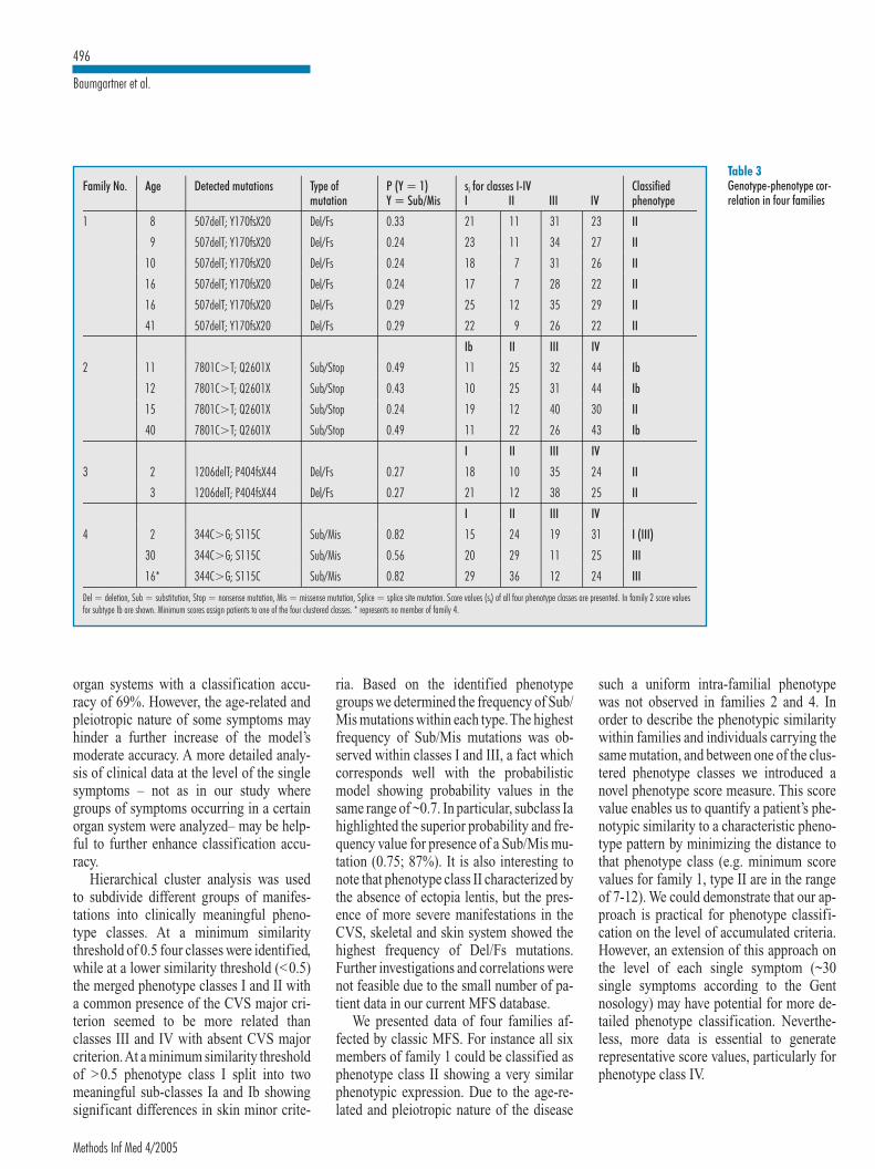
1 8
9
10
16
16
41
2 11
507delT; Y170fsX20
507delT; Y170fsX20
507delT; Y170fsX20
507delT; Y170fsX20
507delT; Y170fsX20
507delT; Y170fsX20
7801C>T; Q2601X
mutation
Del/Fs
Del/Fs
Del/Fs
Del/Fs
Del/Fs
Del/Fs
Sub/Stop
3
4
Del = deletion, Sub = substitution, Stop = nonsense mutation, Mis = missense mutation, Splice = splice site mutation. Score values (si) of all four phenotype classes are presented. In family 2 score valuesfor subtype Ib are shown. Minimum scores assign patients to one of the four clustered classes. * represents no member of family 4.
12
15
40
2
3
2
30
16*
7801C>T; Q2601X
7801C>T; Q2601X
7801C>T; Q2601X
1206delT; P404fsX44
1206delT; P404fsX44
344C>G; S115C
344C>G; S115C
344C>G; S115C
Sub/Stop
Sub/Stop
Sub/Stop
Del/Fs
Del/Fs
Sub/Mis
Sub/Mis
Sub/Mis
Y = Sub/Mis
0.33
0.24
0.24
0.24
0.29
0.29
0.49
0.43
0.24
0.49
0.27
0.27
0.82
0.56
0.82
I
21
23
18
17
25
22
Ib
11
10
19
11
I
18
21
I
15
20
29
II
11
11
7
7
12
9
II
25
25
12
22
II
10
12
II
24
29
36
III
31
34
31
28
35
26
III
32
31
40
26
III
35
38
III
19
11
12
IV
23
27
26
22
29
22
IV
44
44
30
43
IV
24
25
IV
31
25
24
phenotype
II
II
II
II
II
II
Ib
Ib
II
Ib
II
II
I (III)
III
III
Family No. Age Detected mutations Type of P (Y = 1) si for classes I-IV ClassifiedTable 3Genotype-phenotype cor-relation in four families
organ systems with a classification accu-racy of 69%. However, the age-related andpleiotropic nature of some symptoms mayhinder a further increase of the model’smoderate accuracy. A more detailed analy-sis of clinical data at the level of the singlesymptoms – not as in our study wheregroups of symptoms occurring in a certainorgan system were analyzed– may be help-ful to further enhance classification accu-racy.
Hierarchical cluster analysis was usedto subdivide different groups of manifes-tations into clinically meaningful pheno-type classes. At a minimum similaritythreshold of 0.5 four classes were identified,while at a lower similarity threshold (<0.5)the merged phenotype classes I and II witha common presence of the CVS major cri-terion seemed to be more related thanclasses III and IV with absent CVS majorcriterion.At a minimum similarity thresholdof >0.5 phenotype class I split into twomeaningful sub-classes Ia and Ib showingsignificant differences in skin minor crite-
ria. Based on the identified phenotypegroups we determined the frequency of Sub/Mis mutations within each type.The highestfrequency of Sub/Mis mutations was ob-served within classes I and III, a fact whichcorresponds well with the probabilisticmodel showing probability values in thesame range of ~0.7. In particular, subclass Iahighlighted the superior probability and fre-quency value for presence of a Sub/Mis mu-tation (0.75; 87%). It is also interesting tonote that phenotype class II characterized bythe absence of ectopia lentis, but the pres-ence of more severe manifestations in theCVS, skeletal and skin system showed thehighest frequency of Del/Fs mutations.Further investigations and correlations werenot feasible due to the small number of pa-tient data in our current MFS database.
We presented data of four families af-fected by classic MFS. For instance all sixmembers of family 1 could be classified asphenotype class II showing a very similarphenotypic expression. Due to the age-re-lated and pleiotropic nature of the disease
such a uniform intra-familial phenotypewas not observed in families 2 and 4. Inorder to describe the phenotypic similaritywithin families and individuals carrying thesame mutation, and between one of the clus-tered phenotype classes we introduced anovel phenotype score measure. This scorevalue enables us to quantify a patient’s phe-notypic similarity to a characteristic pheno-type pattern by minimizing the distance tothat phenotype class (e.g. minimum scorevalues for family 1, type II are in the rangeof 7-12). We could demonstrate that our ap-proach is practical for phenotype classifi-cation on the level of accumulated criteria.However, an extension of this approach onthe level of each single symptom (~30single symptoms according to the Gentnosology) may have potential for more de-tailed phenotype classification. Neverthe-less, more data is essential to generaterepresentative score values, particularly forphenotype class IV.
Methods Inf Med 4/2005
496
Baumgartner et al.
References1. Pyeritz RE, Dietz HC. Marfan syndrome and
other microfibrillar disorders. In: Royce PM,Steinmann B, editors. Connective tissue and itsheritable disorders: molecular. genetic and medi-cal aspects. 2nd ed. New York: Wiley-Liss; 2002.pp 585-626.
2. Nijbroek G, Sood S, McIntosh I, Francomano CA,Bull E, Pereira L, Ramirez F, Pyeritz RE, DietzHC. Fifteen novel FBN1 mutations causing Mar-fan syndrome detected by heteroduplex analysisof genomic amplicons. Am J Hum Genet 1995; 5:8-21.
3. Collod-Beroud G, Le Bourdelles S, Ades L, Ala-Kokko L, Booms P, Boxer M, Child A, Comeglio
Correspondence to:Dr. Christian BaumgartnerResearch Group for Biomedical Data MiningUniversity for Health Sciences, Medical Informatics andTechnology – UMITEduard-Wallnöfer-Zentrum 16060 Hall i. T.AustriaE-mail: [email protected]
Conclusions
Data on MFS phenotype, aortic elasticityusing M-mode echocardiography and mol-ecular genetic analysis were mined to assessaortic abnormality during medical treat-ment, and to identify novel correlations be-tween type of mutation and clinical mani-festation. A probabilistic model for moni-toring the efficiency of β-blocker treatment,which may be of help in the timing of elec-tive aortic surgery, was established. Highestcorrelation between FBN1 missense mu-tations and phenotype classes I and III,which manifested as ectopia lentis, skeletalmajor and skin minor criteria, was found.Moreover, 78% of all deletion/frameshiftmutations were assigned to phenotype classII with absent ectopia lentis, but presence ofmore severe manifestations in the CVS,skeletal and skin system. Our analysis ofclinical phenotype and mutation data maycontribute to anticipate the clinical con-sequences of specific FBN1 mutations, andmay be helpful to identify at-risk patientsearly. Loss of aortic elasticity can be moni-tored during medical treatment, and mayserve as an indicator for the necessity ofelective surgical intervention.
AcknowledgementsThis study was generously supported by the AustrianIndustrial Research Promotion Fund FFF (grantnumber HITT-10 UMIT) and the Wolfermann-Nägeli-Stiftung Zurich.
P, De Paepe A, Hyland JC, Holman K, Kaitila I,Loeys B, Matyas G, Nuytinck L, Peltonen L, Ran-tamaki T, Robinson P, Steinmann B, Junien C, Be-roud C, Boileau C. Update of the UMD-FBN1mutation database and creation of an FBN1polymorphism database. Hum Mutat 2003; 22:199-208.
4. De Paepe A, Devereux RB, Dietz HC, HennekamRCM, Pyeritz RE. Revised diagnostic criteria forthe Marfan syndrome. Am J Med Genet 1996; 62:417-26.
5. Murdoch JL, Walker BA, Halpern BL, Kuzma JW,McKusick VA. Life expectancy and causes ofdeath in the Marfan syndrome. N Engl J Med1972; 286: 804-8.
6. Stefanadis C, Stratos C, Boudoulas H, KourouklisC, Toutouzas P. Distensibility of the ascendingaorta: comparison of invasive and non-invasivetechniques in healthy men and in men withcoro-nary artery disease. Eur Heart J 1990; 11: 990-6.
7. Hirata K, Triposkiadis F, Sparks E, Bowen J, Woo-ley CF, Boudoulas H. The Marfan syndrome: ab-normal aortic elastic properties. J Am Coll Car-diol 1991; 18: 57-63.
8. Savolainen A, Keto P, Hekali P, Nisula L, Kaitila I,Vitasalo M, Poutanen VP, Standertskjold-Norden-stam CG, Kupari M. Aortic distensibility inchildren with the Marfan syndrome. Am J Cardiol1992; 70: 691-3.
9. Baumgartner D, Baumgartner C, Matyas G, Stein-mann B, Löffler J, Schermer E, Schweigmann U,Baldissera I, Frischhut B, Hess J, Hammerer I.Diagnostic power of aortic elastic properties inyoung patients with Marfan syndrome. J ThoracCardiovasc Surg 2005; 129: 730-9.
10. Biggin A, Holman K, Brett M, Bennetts B, AdesL. Detection of thirty novel FBN1 mutations inpatients with Marfan syndrome or a related fibril-linopathy. Hum Mutat 2004; 23: 99.
11. Pereira L, D’Alessio M, Ramirez F, Lynch JR,Sykes B, PangilinanT, Bonadio J. Genomic organ-ization of the sequence coding for fibrillin. Thedefective gene product in Marfan syndrome. HumMol Genet 1993; 2: 961-8.
12. Mátyás G, De Paepe A, Halliday D, Boileau C,Pals G, Steinmann B. Evaluation and applicationof denaturing HPLC for mutation detection inMarfan syndrome: identification of 20 novel mu-tations and two novel polymorphisms in the FBN1gene. Hum Mutat 2002; 19: 443-56.
13. Katzke S, Booms P,Tiecke F, Palz M, PletschacherA, Turkmen S, Neumann LM, Pregla R, Leitner C,Schramm C, Lorenz P, Hagemeier C, Fuchs J,Skovby F, Rosenberg T, Robinson PN. TGGEscreening of the entire FBN1 coding sequencein 126 individuals with marfan syndrome andrelated fibrillinopathies. Hum Mutat 2002; 20:197-208.
14. Hosmer DW, Lemeshow S. Applied logistic re-gression. 2nd edition. New York: Wiley; 2000.
15. Witten IH, Frank E. Data Mining – Practical ma-chine learning tools and techniques with java im-plementations, San Francisco: Morgan Kauf-mann; 2000.
16. Kaufman L, Rousseeuw PJ. Finding groups indata: an introduction to cluster analysis. JohnWiley & Sons, 1990.
17. Everitt BS. Cluster Analysis. London: Edward Ar-nold; 1993.
18. Peters KF, Kong F, Horne R, Francomano CA,Biesecker BB. Living with Marfan syndrome I.Perceptions of the condition. Clin Genet 2001; 60:273-82.
19. Roman MJ, Rosen SE, Kramer-Fox R, DevereuxRB. Prognostic significance of the pattern of aor-tic root dilation in the Marfan syndrome. J AmColl Cardiol 1993; 22: 1470-6.
20. Loeys B, Nuytinck L, Delvaux I, De Bie S, DePaepe A. Genotype and phenotype analysis of 171patients referred for molecular study of the fibril-lin-1 gene FBN1 because of suspected Marfansyndrome. Arch Intern Med 2001; 161: 2447-54.
21. Lipscomb KJ, Clayton-Smith J, Harris R. Evolv-ing phenotype of Marfan’s syndrome. Arch DisChild 1997; 76: 41-6.
22. Groenink M, Rozendaal L, Naeff MSJ, HennekamRCM, Hart AAM, van der Wall EE, Mulder BJ.Marfan syndrome in children and adolescents:predictive and prognostic value of aortic rootgrowth for screening for aortic complications.Heart 1998; 80: 163-9.
23. Tiecke F, Katzke S, Booms P, Robinson PN,Neumann L, Godfrey M, Mathews KR, ScheunerM, Hinkel GK, Brenner RE, Hovels-Gurich HH,Hagemeier C, Fuchs J, Skovby F, Rosenberg T.Classic, atypically severe and neonatal Marfansyndrome: twelve mutations and genotype-phe-notype correlations in FBN1 exons 24-40. Eur JHum Genet 2001; 9: 13-21.
24. Pepe G, Giusti B, Evangelisti L, Porcini MC, Bru-nelli T, Giurlani L, Attanasio M, Fattori R, BagniC, Comeglio P, Abbate R, Genuini GF. Fibrillin-1(FBN1) gene frameshift mutations in Marfan pa-tients: genotype-phenotype correlation. ClinGenet 2001; 59: 444-50.
25. Robinson PN, Booms P, Katzke S, Ladewig M,Neumann L, Palz M, Pregla R, Tiecke F, Rosen-berg T. Mutations of FBN1 and genotype-pheno-type correlations in Marfan syndrome and relatedfibrillinopathies. Hum Mutat 2002; 20: 153-61.
497
Marfan Syndrome – Diagnosis and Therapy Monitoring
Methods Inf Med 4/2005

Surgery forCongenital Heart
DiseaseDiagnostic power of aortic elasticproperties in young patients withMarfan syndromeDaniela Baumgartner, MD,a Christian Baumgartner, PhD,b
Gabor Mátyás, PhD,c,d Beat Steinmann, MD,c Judith Löffler-Ragg, MD,e
Elisabeth Schermer, MD,a Ulrich Schweigmann, MD,a Ivo Baldissera, MD,f
Bernhard Frischhut, MD,g John Hess, MD, PhD,h and Ignaz Hammerer, MDa
From the Department of Pediatric Cardiol-ogy, Innsbruck Medical University, Inns-bruck, Austria,a Research Group for Bio-medical Data Mining, Institute forInformation Systems, University for HealthSciences, Medical Informatics and Tech-nology, Innsbruck, Austria,b Division ofMetabolism and Molecular Pediatrics, Uni-versity Children’s Hospital, Zurich, Swit-zerland,c Institute of Medical Genetics,University of Zurich, Schwerzenbach,Switzerland,d Institute of Medical Biologyand Human Genetics, Innsbruck MedicalUniversity, Innsbruck, Austria,e Depart-ment of Ophthalmology, Innsbruck Medi-cal University, Innsbruck, Austria,f Depart-ment of Orthopedics, Innsbruck MedicalUniversity, Innsbruck, Austria,g and De-partment of Pediatric Cardiology and Con-genital Heart Disease, German Heart Cen-ter, Munich, Germany.h
Supported by the Austrian Industrial Re-search Promotion Fund (grant HITT-10UMIT), Wolfermann-Nägeli-Stiftung (Zu-rich, Switzerland), and the Swiss NationalScience Foundation (grant 3200-059 445/2).
Received for publication March 4, 2004;revisions received June 21, 2004; acceptedfor publication July 8, 2004.
Address for reprints: Daniela Baumgartner,MD, Department of Pediatric Cardiology,Innsbruck Medical University, Anichstr 35,A-6020 Innsbruck, Austria (E-mail: [email protected])
J Thorac Cardiovasc Surg 2005;129:730–9
0022-5223/$30.00
Copyright © 2005 by The American Asso-ciation for Thoracic Surgery
doi:10.1016/j.jtcvs.2004.07.019
730 The Journal of Thoracic and Cardio
Background: In patients with Marfansyndrome, progressive aortic dilationimplicates a still-unpredictable risk oflife-threatening aortic dissection andrupture. We sought to quantify aorticwall dysfunction noninvasively, deter-mine the diagnostic power of variousaortic parameters, and establish a diagnostic model for the early detection of aortic abnor-malities associated with Marfan syndrome.
Methods: In 19 patients with Marfan syndrome (age, 17.7 � 9.5 years) and 19 age-and sex-matched healthy control subjects, computerized ascending and abdominal aorticwall contour analysis with continuous determination of aortic diameters was performed outof transthoracic M-mode echocardiographic tracings. After simultaneous oscillometric bloodpressure measurement, aortic elastic properties were determined automatically.
Results: The following ascending aortic elastic parameters showed statistically signif-icant differences between the Marfan group and the control group: (1) decreased aorticdistensibility (P � .001), (2) increased wall stiffness index (P � .01), (3) decreasedsystolic diameter increase (P � .01), and (4) decreased maximum systolic area increase(P � .001). The diagnostic power of all investigated parameters was tested by singlelogistic regression models. A multiple logistic regression model including solely aorticparameters yielded a sensitivity of 95% and a specificity of 100%.
Conclusions: In young patients with Marfan syndrome, a computerized image-analyz-ing technique revealed decreased aortic elastic properties expressed by parametersshowing high diagnostic power. A multiple logistic regression model including merelyaortic parameters can serve as useful predictor for Marfan syndrome.
Marfan syndrome (MFS; Online Mendelian Inheritance in Man#154700) is an autosomal dominant connective tissue disor-der caused by mutations in the gene encoding fibrillin-1(FBN1), with highly variable clinical manifestations in themusculoskeletal, ocular, and cardiovascular systems.1,2 Dila-tation of the aortic root predisposes the subject to aortic
Ambras Castle, Innsbruck. Top left to bottom right: D.Baumgartner, C. Baumgartner, Mátyás, Steinmann,Löffler-Ragg, Schermer, Schweigmann, Baldissera,
Frischhut, Hess, Hammerer
dissection and rupture or severe regurgit
vascular Surgery ● April 2005
ation and heart failure.3 Diseases of the

Baumgartner et al Surgery for Congenital Heart Disease
CHD
aorta account for 80% of known causes of death.3 Beforelife-threatening complications, alterations of aortic elasticproperties due to defective FBN1 can be characterized bythe terms of elasticity or compliance, distensibility, stiffnessindex, and pulse wave velocity.4-7
The aim of this study was to investigate aortic elasticityand assess its abnormality in patients with MFS by means ofa standardized, semiautomated, and noninvasive method.This technique is appropriate for determining the course ofaortic elasticity during follow-up investigations. All aorticparameters were implemented in single logistic regressionmodels to test their diagnostic power. To further increasesensitivity and specificity, we searched for a multiple logis-tic regression model able to serve as an appropriate diag-nostic marker for MFS. To localize aortic elastic dysfunc-tion, we suggest visualization of ascending (AscAo) anddescending aortic (DescAo) diameter changes by a vectorloop.
MethodsPatients and Control SubjectsForty-seven people with suspected MFS were investigated at theDepartments of Pediatric Cardiology, Ophthalmology, and Ortho-pedics and at the Institute of Medical Biology and Human Genet-ics, Innsbruck Medical University, according to a standardizedprotocol. Nineteen of these, whose diseases were diagnosed asMFS according to the Ghent criteria8 and who were younger than40 years, comprised the study group (3 males and 16 females;mean age, 17.7 � 9.5 years). Clinical characteristics are shown inTables 1 and 2. Physical features were documented according tothe consensus of 2 physicians (D.B. and J.L.-R.). Before theinvestigation, no patient received a �-blocker, angiotensin-con-verting enzyme inhibitor, or calcium antagonist or had a history ofaortic dissection or aortic surgery. Nineteen age- and sex-matchedhealthy subjects constituted the control group. Two of them werehealthy relatives of patients with MFS. A group of 35 peopletotally different from the study population, including 16 patientswith MFS and 19 healthy controls, served as validation group forthe logistic regression analysis. The mean age of this group was14.2 � 8.0 years and ranged from 0 to 36 years. The studycomplied with the Declaration of Helsinki. The protocol wasapproved by the institutional committee on human research. Allsubjects gave informed consent.
Molecular Genetic AnalysisMutation analysis of the FBN1 gene was performed in all 19 MFSpatients as described.9 In brief, genomic DNA samples wereamplified exon by exon by means of polymerase chain reaction(PCR) by using intron-specific primers. All 65 amplicons wereanalyzed by denaturing high-performance liquid chromatographyfollowed by direct sequencing of amplicons with abnormal elutionprofiles. The mutations found were verified by repeated sequenc-ing on newly amplified PCR products. In the case of splice sitemutations and when no mutation was detected by denaturing
high-performance liquid chromatography, FBN1 transcripts wereThe Journal of Thoraci
analyzed by reverse transcription-PCR of RNA templates isolatedfrom fibroblasts.
Echocardiographic EvaluationAll echocardiographic examinations were performed by 1 investi-gator (D.B.) in the left decubitus position with commerciallyavailable equipment (System Five; GE Vingmed Ultrasound,Horten, Norway). M-mode tracings of the aorta were obtainedaccording to published criteria10 by using 2-dimensional guidanceat 4 different levels: level 1, annulus (parasternal short-axis view);level 2, sinuses of Valsalva; level 3, proximal AscAo 10 to 20 mmdistal to the sinotubular junction (both parasternal long-axisviews); and level 4, descending abdominal aorta just proximal tothe branching off of the celiac trunk (abdominal paramedian long-axis view). Attention was paid to setting the line of sight exactlyperpendicular to the long axis of the aorta in views showing thelargest aortic diameters. Sharp endothelial lines were used asadditional indicators for the line of sight to cut the central line ofthe aorta. Aortic dilatation was determined with standard nomo-grams.10
For automated and standardized calculation of aortic diameters,we developed suitable software. First, M-mode tracings of theAscAo (level 3) and DescAo (level 4) of at least 5 heart cycleswere loaded into the program. To find the inner aortic wall con-tours, an image-processing algorithm ran on the M-mode images.Out of the determined aortic edge map, AscAo and DescAooutlines were calculated throughout the heart cycles (Figure 1,left). In some images with a suboptimal signal-to-noise ratio,minor manual corrections of aortic wall contours had to be per-formed. Interobserver reproducibility, calculated as the standarddeviation of the differences between measurements and expressedas the percentage of the mean of the measurements, was deter-mined after re-evaluation of randomly selected images by a secondinvestigator blinded to the initial results. According to the usualaortic diameter measurements with the leading edge technique,10
the automatically detected inner diameter of the aorta was enlargedby the anterior aortic wall thickness. Time-diameter curves of 5heart cycles were generated, based on the aortic wall contours.They showed a time resolution of approximately 6 ms per pixeland a spatial resolution of 0.2 mm per pixel. The curves wereaveraged and slightly smoothed by a digital low-pass filter (But-terworth; degree 2) to eliminate the digitalization noise (Figure 1,right). Out of time-diameter curves and averaged threefold bloodpressure measurements, which were taken at the right arm oscil-lometrically (Dinamap; GE Healthcare, Slough, United Kingdom)immediately before M-mode registration, aortic elastic parameterswere estimated automatically.
Calculation of Aortic ParametersIn addition to established aortic elastic parameters such as aorticdistensibility and wall stiffness index,6,11 we developed maximumsystolic area increase (MSAI), a parameter that is advantageousbecause of its easy determination. Aortic integral ratio and vec-toraortography indicate the region of reduced aortic elasticity. Theparameters were defined as follows.
Systolic diameter increase was calculated as
c and Cardiovascular Surgery ● Volume 129, Number 4 731

Surgery for Congenital Heart Disease Baumgartner et al
CHD
(Ds � Dd) ⁄ Dd (%), (1)
where Ds is systolic (maximum) and Dd is end-diastolic (mini-mum) aortic diameter. Cross-sectional (CS) aortic distensibilityand stiffness index were estimated as previously described6,11:
Distensibilty �As � Ad
Ad · (Ps � Pd) · 1333· 107(kPa�1 · 10�3) (2)
Stiffness index �In(Ps ⁄ Pd)
(Ds � Dd) ⁄ Dd(dimensionless), (3)
TABLE 1. Aortic parameters and FBN1 gene mutations in
Patient No.Age(y) Sex BSA (m2) Mutation
Aorticdiast
diametedilate
1* 2 F 0.59 344C�G; S115C§ 202 2 F 0.63 1206delT; frameshift
� PTC21
3† 9 F 1.20 508delT; frameshift �PTC
27
4† 10 F 1.21 508delT; frameshift �PTC
28
5‡ 11 F 1.51 7801C�T; Q2601X 316‡ 12 F 1.78 7801C�T; Q2601X 377 12 F 1.40 1453C�T; R485C 278‡ 15 F 1.95 7801C�T; Q2601X 339† 16 F 1.63 508delT; frameshift �
PTC32
10 16 M 1.81 No FBN1 mutationdetected
34
11 17 M 1.87 IVS14�2A�G� 3612 18 F 1.87 IVS45 � 3insCC¶ 4413 18 M 1.87 3194delAAAG;
frameshift � PTC42
14 22 F 1.63 4337delATA;D1446_I1447delinsV
50
15 23 F 1.81 651G�A; W217X 3616 25 F 1.88 6794G�A; C2265Y 3617 30 F 1.76 2638G�A; G880S 5118* 30 F 1.85 344C�G; S115C§ 3219‡ 40 F 2.02 7801C�T; Q2601X 42
PatientsMean 17.7 1.56 34.7 n
SD 9.5 0.43 8.5Controls
Mean 17.6 1.44 24.6SD 9.9 0.39 4.6
P value NS NS �.001
BSA, Body surface area; AscAo, ascending aortic; DescAo, descendingsignificant, �, Dilated; �, not dilated.*, †, and ‡ indicate the members of family 1, 2 and 3.§Patients 1 and 18 carry a published mutation.29
�Cryptic splice site in intron 14 and insertion of 18 bp in frame.¶Deletion of exon 45 in frame.
where As is systolic and Ad is end-diastolic area and Ps is systolic
732 The Journal of Thoracic and Cardiovascular Surgery ● Apri
and Pd is diastolic blood pressure (mm Hg). Area A was deter-mined as (D/2)2 · �.
MSAI was defined as the maximum systolic slope of thearea-time curve A(t) normalized to Ad:
MSAI �d
dt��A(t) ⁄ Ad � 1� · 100�max (%/100 ms) (4)
Integrals of the AscAo and DescAo area-time curves normalized tothe corresponding end-diastolic area—defined as aortic integralratios—show in which aortic segment elasticity is reduced more
tients with Marfan syndrome
,
AscAodiastolic
diameter (mm,dilated�)
DescAodiastolicdiameter
(mm)
Systolicblood
pressure(mm Hg)
Pulsepressure(mm Hg)
Distensibility(kPa�1 · 10�3)
AscAo DescAo
14.4 � 5.2 90 38 39 7915.4 � 7.7 106 60 21 36
18.5 � 12.1 111 58 70 56
20.1 � 12.3 96 57 24 40
21.2 � 12.7 118 47 43 4422.8 � 11.5 122 46 61 7224.1 � 12.2 116 55 38 3428.2 � 11.8 116 55 22 4826.5 � 12.1 117 48 35 73
23.1 � 10.9 116 54 21 76
25.8 � 17.4 117 61 20 3541.5 � 14.4 113 48 0 3731.9 � 15.0 137 62 0 48
34.2 � 14.1 111 33 0 31
24.8 � 14.6 130 50 30 927.3 � 17.3 120 64 67 1442.6 � 17.4 116 47 27 4128.7 � 12.7 129 46 0 3527.7 � 15.5 131 57 25 13
7 26.2 n � 8 13.0 116 52 29 437.5 42% 3.1 11 8 21 21
0 20.6 n � 1 12.0 116 49 62 654.0 5% 2.6 8 9 24 30.007 NS NS NS �0.001 0.013
ic; PTC, premature termination codon; SD, standard deviation; NS, not
19 paroot
olicr (mmd�)
��
�
�
�����
�
���
�
�����
� 189%
n �
aort
severely.
l 2005

,
ed dia
Baumgartner et al Surgery for Congenital Heart Disease
CHD
Aortic integral ratio �
�HC
�A(t) ⁄ Ad�AscAodt
�HC
�A(t) ⁄ Ad�DescAodt, (5)
where A(t) the is aortic area-time curve and HC is the heart cycle.The vectoraortography visualizes the vector loop of the relative
AscAo and DescAo diameter changes during the heart cycle. Therotating vector can be characterized by its magnitude and phase:
Magnitude(t)
� ��(D(t) ⁄ Dd � 1) · 100�AscAo2 � �(D(t) ⁄ Dd � 1) · 100�DescAo
2 (%)(6)
Phase(t) � arctan��D(t) ⁄ Dd � 1�DescAo
�D(t) ⁄ Dd � 1�AscAo (degree), (7)
where D(t) is the aortic diameter-time curve.
StatisticsData are expressed as mean � SD and, in Figure 2, A as mean � 95%confidence interval. Quantitative variables were compared by meansof unpaired Student t tests and Mann-Whitney U tests, respectively.The relation between continuous variables was tested by linear re-gression analysis. Single and multiple logistic regression models were
TABLE 2. Cardiovascular parameters in patients with Mar
Parameters
Heart rate (beats/min)Systolic blood pressure (mm Hg) 1Diastolic blood pressure (mm Hg)Pulse pressure (mm Hg)Bulbus aortae
Diastolic diameter (mm) 3Normalized diastolic diameter (mm/m2) 2
Ascending aortaDiastolic diameter (mm) 2Normalized diastolic diameter (mm/m2) 1Systolic diameter increase (%)Distensibility (kPa�1 · 10�3)Stiffness indexMaximum systolic area increase (%/100 ms)
Descending aortaDiastolic diameter (mm) 1Normalized diastolic diameter (mm/m2)Systolic diameter increase (%) 1Distensibility (kPa�1 · 10�3)Stiffness indexMaximum systolic area increase (%/100 ms)
VectoraortographyMagnitude (%) 1Phase (degree)Aortic integral ratio
Values are shown as mean � SD; NS, Not significant (P � .05); normaliz
developed to estimate the diagnostic power of the aortic parameters.
The Journal of Thoraci
The conditional probability for the presence of MFS is denoted by theequation P�MFS � 1� � 1⁄�1 � exp� � z�� where z indicates the logitof the model. The effect of each model parameter is given by its oddsratio. All statistical analyses were performed with the software pack-age SPSS 11.0 (SPSS Inc, Chicago, Ill).
ResultsClinical CharacteristicsClinical characteristics of the Marfan patients and controlpersons were compared in Tables 1 and 2. Age, sex, weight,height, body-surface area, and heart rate did not differbetween Marfan patients and control persons. Four patients(21%) presented with mild aortic regurgitation (1�), 16(84%) presented with mitral valve prolapse, and 16 (84%)presented with mitral regurgitation (7 with 1�, 8 with 2�,and 1 with 3�) as defined by Doppler echocardiography.Seventeen patients (90%) showed skeletal symptoms ofMFS; in 6 (32%) of them the skeleton was involved, and 11(58%) fulfilled the major skeletal criteria according to theGhent nosology.8 Ectopia lentis was present in 10 patients(53%), and 11 patients (58%) had a family history of MFS.Results of FBN1 gene mutation analysis are presented in
yndrome (MFS) and in control subjectsS19)
Control subjects(n � 19) P value
19 73 � 14 NS11 116 � 8 NS12 68 � 10 NS8 49 � 9 NS
8.5 24.6 � 4.6 �.0015.1 18.0 � 4.0 .002
7.5 20.6 � 4.0 .0074.1 15.2 � 3.4 NS10.6 18.0 � 6.1 .00121 62 � 24 �.0012.6 3.4 � 1.4 �.00119 55 � 21 �.001
3.1 12.0 � 2.6 NS1.6 8.8 � 2.2 NS5.9 18.6 � 6.1 .01421 65 � 30 .0133.9 3.2 � 1.0 .00917 54 � 21 .044
6.2 25.4 � 7.2 .00241 47 � 11 NS2.1 1.1 � 0.5 NS
stolic diameter means diastolic diameter divided by body surface area.
fan sMF
(n �
71 �16 �65 �52 �
4.7 �2.9 �
6.2 �7.0 �7.5 �29 �6.2 �28 �
3.0 �8.4 �3.6 �43 �5.8 �41 �
8.2 �66 �1.1 �
Table 1.
c and Cardiovascular Surgery ● Volume 129, Number 4 733

desc
Surgery for Congenital Heart Disease Baumgartner et al
CHD
Aortic Dimensions and Calculation of ElasticParametersEchocardiographic aortic findings of the Marfan group andthe control group are shown in Tables 1 and 2. Diastolicaortic root (P � .001) and diastolic AscAo diameter (P �.007) were significantly increased in the MFS group,whereas the difference of DescAo diameters betweengroups did not reach statistical significance. All 4 investi-gated elastic parameters demonstrated reduced aortic elasticproperties in MFS patients (Table 2 and Figure 2): AscAosystolic diameter increase (42% of control group), CS dis-tensibility (47%), and MSAI (51%) were significantly di-minished in the Marfan group. The stiffness index, as beinginversely related to distensibility, was markedly increased(182% of control group). Four MFS patients (patients 12-14
Figure 1. Semiautomated aortic wall contour analysisand descending (bottom left) aorta of patient 5. Arrowstime-diameter curves of the ascending (top right) and
and 18; Table 1) revealed an AscAo diameter decrease
734 The Journal of Thoracic and Cardiovascular Surgery ● Apri
during systole; in these cases, CS distensibility and MSAIwere set to 0, and stiffness index could not be calculated.Note that both patients without aortic root dilatation (pa-tients 7 and 18; Table 1) showed a decreased AscAo dis-tensibility and a reduced DescAo distensibility of �1 SD. Inthe DescAo of MFS patients, we observed less systolicdiameter increase, CS distensibility, and MSAI; the stiffnessindex was markedly greater than in the control group. Thedifferences were smaller than in the AscAo (Table 2). In 3of 5 adult MFS patients, in whom elective prosthetic aorticroot replacement was indicated at or 1 year after the initialinvestigation (patients 12, 14, and 17 out of the study group[Table 1] and 2 patients out of the validation group), AscAodistensibility and MSAI were 0. Because of systolic diam-eter decrease, aortic stiffness index could not be calculated.
te lines) in M-mode images of the ascending (top left)cate the beginning and end of 1 heart cycle. Averagedending (bottom right) aorta are shown.
(whiindi
In the remaining 2 of the 5 operated patients, AscAo dis-
l 2005

vectobers
Baumgartner et al Surgery for Congenital Heart Disease
CHD
tensibility was strongly decreased (12 and 27 kPa�1 · 10�3).However, 1 MFS patient (patient 18) showed an AscAo 0
Figure 2. Vectoraortography. A, Vector loops representdiameter changes (D(t)/Dd) during the heart cycle. The 9by thin lines. The loop of the Marfan (MFS) patients isThis shows the reduction of aortic elasticity predominathe vectors’ maximum magnitude in the MFS and the colengths of individuals. Beyond 600 ms cycle length, da4 subgroups according to the aortic integral ratio. Thecontrol group are shown. *, †, and ‡ indicate the mem
distensibility without aortic root dilatation.
The Journal of Thoraci
AscAo and DescAo CS distensibility were greater inyoung patients and control persons (age, 2-12 years; n � 7)
ive ascending (AscAo) and descending (DescAo) aorticonfidence interval at 0, 200, 400, and 600 ms is denotedller and a little steeper than that of the control group.present in the AscAo of MFS patients. Arrows indicategroups. Loops are not closed because of varying cycleere not included. B, The MFS group was divided intors of the total MFS group, the MFS subgroups, and theof family 1, 2, and 3 (Table 1).
relat5% csmantlyntrolta w
than in older ones (age, 15-19 years; n � 6; and age, 20-42
c and Cardiovascular Surgery ● Volume 129, Number 4 735

Surgery for Congenital Heart Disease Baumgartner et al
CHD
years; n � 6), although no strong linear correlation betweenage and distensibility could be found (r � 0.8). In MFSpatients, the differences between age groups were less pro-nounced than in controls.
CS distensibility and MSAI values of the AscAo and Des-cAo of Marfan patients and control persons correlated signif-icantly (MSAI � 0.68 � CS distensibility � 10.54; r � 0.86;P � .01).
Interobserver reproducibility, which was determined in 6consecutive patients, was 2.6% and 3.3% for AscAo andDescAo diastolic diameter measurements and was 3.8% and4.6% for AscAo and DescAo distensibility. Reproducibilityof further aortic elastic parameters showed comparable val-ues.
Aortic Integral RatioMean values of the AscAo/DescAo integral ratio were sim-ilar between Marfan patients and control persons, but in theMFS group, the standard deviation was markedly increased(1.1 � 2.1 in the MFS vs 1.1 � 0.5 in the control group;Table 2). This ratio showed the variable extent of regionalaortic elasticity alterations in the Marfan patients and, con-versely, a tight relationship of AscAo and DescAo integralsin healthy control subjects.
VectoraortographyThe vector loops characterizing the relative aortic diameterchanges during the heart cycle differed significantly be-tween the MFS and the control group (Figure 2, A and Table2). The maximum magnitude of the vector (Figure 2, A) wassignificantly reduced in the MFS group, and the vector’sphase at maximum magnitude (ie, the angle below thevector) showed no significant difference between groups (P� .061). Because of the high standard deviation of the phaseand aortic integral ratio in the MFS group, we split theMarfan patients into 4 subgroups to distinguish amongdifferent elasticity patterns (Figure 2, B). In the first sub-group, the AscAo diameter decreased during early systole,so that phase was strongly increased (mean, 131°). In sub-group 2, phase was also increased, but AscAo diameterincreased during systole. Subgroup 3 (aortic integral ratio,0.6-1.6; ie, mean value � 1 SD of control group) showed amean phase (54°) roughly comparable to the control groupbecause of similar reduction of AscAo and DescAo pulsatilediameter changes. In subgroup 4, phase was strongly re-duced (mean 10°) because of decreased pulsatile diameterchanges predominantly in the DescAo.
Single and Multiple Logistic Regression AnalysisAll presented aortic parameters were tested separately fortheir diagnostic power by single logistic regression analysis(Table 3). AscAo distensibility and systolic diameter in-
crease demonstrated the highest sensitivity (84%); the dia-736 The Journal of Thoracic and Cardiovascular Surgery ● Apri
stolic diameter of the bulbus aortae normalized to body-surface area showed the highest specificity (84%).
To increase the diagnostic power of the classificationmodels, we searched for the multiple logistic regressionmodel z displaying the highest sensitivity (94.7%) and spec-ificity (100%). The logit of the regression model is given bythe following equation:
�z � 4.379 � 2.293 · normalized BA diastolic diameter
� 2.449 · normalized AscAo diastolic diameter
� 0.247 · AscAo distensibility�(P � .030; P � .028; P � .035; odds ratios: 9.901, 0.086,and 0.781; Table 3)
Subsequently, our best model z was tested on the inde-pendent validation group and showed a sensitivity of 100%and a specificity of 94.7%. Validation of the single logisticregression models also yielded comparable results to thoseestablished in the study population.
DiscussionOur new noninvasive semiautomated M-mode echocardio-graphic image-segmentation technique showed reduced aor-tic elastic properties in children and young adults with MFS,with high accuracy and objectivity. In most published stud-ies, aortic diameters and CS areas, which underlie the cal-culation of aortic elastic properties, still rely on a slow,tedious, and observer-dependent process of manual outlin-ing, which has to be performed by expert physicians.
In adults with MFS, automated border detection has beenused to measure aortic diameters out of transesophagealaortic images.12 We used 2-dimensional guided transtho-racic M-mode echocardiographic aortic diameter measure-ments, which showed good correlation with 2-dimensionalechocardiographically obtained values.10 Two-dimensionalguidance is indispensable for correct diameter measure-ments out of M-mode echocardiographic images, especiallyfor displaying the largest aortic diameter and for finding anaxis strictly perpendicular to the long axis of the aorta.10 Incontrast to continuous aortic measurements out of 2-dimensional echocardiographic or magnetic resonance im-aging sequences, M-mode echocardiography enables us tomeasure aortic diameters over 5 heart cycles with twofold tofivefold higher time resolution out of merely 1 to 2 images.In children and young adults, images of high quality can beobtained in most cases. However, accurate image acquisi-tion with a high signal-to-noise ratio is essential for appro-priate computerized contour finding.
Aortic root dilatation, a major criterion of MFS,8 wasshown to be present in 89% of our patients and was reportedin 61.5% to 84% of adults1,13-16 and in 42.5% to 76% ofchildren aged 0.25 to 18 years.15,17 AscAo dilatation waspresent in 42% of our patients and has been reported in 54%
of adults15 and in 45% of children (age, 0.5-18 years).15l 2005

ity aody s
Baumgartner et al Surgery for Congenital Heart Disease
CHD
Because aortic dilatation evolves during childhood and ad-olescence, serial evaluations of aortic dimensions may benecessary to clearly demonstrate the presence and progres-sion of aortic dilatation.18 Because aortic root growth is ofprognostic value for the occurrence of aortic complica-tions,18 objective diameter measurements will enhance theaccuracy of results.
The representation of time-diameter curves gives us anoptical impression of aortic diameter changes during theheart cycle (Figure 1, right). The vectoraortography—acompaction of time-diameter relations of 2 aortic segmentsin 1 diagram—and the aortic integral ratio allow us todistinguish different patterns of aortic stiffening within theMFS group (Figure 2). In 4 patients with considerable aorticroot dilatation, the AscAo anteroposterior diameter de-creased during systole, which—to our knowledge—hasnever been described before (patients 12-14 and 18; meanend-diastolic aortic root diameter, 42.0 � 7.5 mm vs 34.9 �8.6 mm in the total MFS group; mean end-diastolic AscAodiameter, 34.0 � 5.4 mm vs 26.2 � 7.5 mm in the totalMFS group; Figure 2, B, subgroup 1). As we observed byechocardiography in a few patients with excellent quality ofAscAo 2-dimensional images, the AscAo seemed to bumpagainst an anterior structure (probably the sternum) during
TABLE 3. Predictive power of single and multiple logistic
Cardiovascular parameters
Single logistic modelsBulbus aortae (BA)
Normalized diastolic diameter (mm/m2)Ascending aorta (AscAo)
Normalized diastolic diameter (mm/m2)Systolic diameter increase (%)Distensibility (kPa�1 · 10�3)Stiffness indexMaximum systolic area increase (MSAI) (%/100 ms)
Descending aorta (DescAo)Normalized diastolic diameter (mm/m2)Systolic diameter increase (%)Distensibility (kPa�1 · 10�3)Stiffness indexMaximum systolic area increase (MSAI) (%/100 ms)
VectoraortographyMagnitude (%)Phase (degree)Aortic integral ratio
Multiple logistic model (best model)Normalized BA diastolic diameter; normalized AscAo diastolic
AscAo distensibility
The diagnostic performance of the models is indicated by their sensitivparameter(s). AscAo and DesAo diastolic diameters were normalized to b
its systolic anterior movement; the aortic CS area for a short
The Journal of Thoraci
time deviated from its circular shape toward an ellipticshape. Therefore, the aortic wall of these patients is exposedto increased shear stress. AscAo distensibility and MSAIwere set to 0, and AscAo stiffness index could not becalculated. Patients with predominant loss of DescAo elas-ticity (subgroup 4) may resemble those who are at risk foraneurysm or dissection of the DescAo.19,20 Our techniquecan thus serve as a valuable noninvasive tool for assessingthe descending abdominal aorta.
Simultaneous diameter and blood pressure registration isessential for exact calculation of elastic parameters. Simul-taneous diameter and pressure registration at the same aorticsite is impossible if elastic parameters are determined non-invasively. However, close correlation of invasive and non-invasive determination of AscAo distensibility has beendemonstrated.5 Nevertheless, aortic valve competence andnormal left ventricular systolic function are basic require-ments for the interpretation of calculated aortic elastic pa-rameters.
Several authors have shown decreased aortic distensibil-ity and increased aortic stiffness index in patients withMFS.6,7,12,21-25 Data obtained in children are rare.6,21 Ourresults, which show a 50% reduced AscAo and a 30%reduced DescAo distensibility in the MFS group, compare
ession models
Sensitivity (%) Specificity (%)P value of
parameter(s)
63.2 84.2 .013
47.4 68.4 NS84.2 68.4 .00684.2 68.4 .00273.3 78.8 .00668.4 68.4 .003
52.6 47.4 NS63.2 68.4 .02773.7 57.9 .02268.4 73.7 .02152.6 57.9 NS
73.7 63.2 .00763.2 68.4 NS73.7 47.4 NS
eter; 94.7 100 .030; .028; .035
nd specificity. The P value describes the significance of each model’surface area (mm/m2).
regr
diam
well to published data on children6 and young adults7,22
c and Cardiovascular Surgery ● Volume 129, Number 4 737

Surgery for Congenital Heart Disease Baumgartner et al
CHD
with MFS. Smaller values of mean aortic distensibility werereported in older patients,24-27 and greater values were re-ported in younger children.21 Our data confirm this depen-dence of aortic distensibility on age. It is interesting to notethat the patients with normal diameters of the bulbus and theAscAo also showed aortic dysfunction in terms of decreasedAscAo and DescAo distensibility. Therefore, assessment ofaortic dysfunction is of additional diagnostic value com-pared with AscAo diameter measurements. The necessity of�-blocker therapy should be discussed in those patients.MSAI is a further elastic parameter that is easy to deter-mine, because blood pressure measurement is not required.In our series, MSAI correlated very closely with aorticdistensibility. Follow-up investigations with the presentedelastic parameters could prove the efficiency of medicaltreatment with, eg, �-blocking agents and may be of help inthe timing of elective aortic surgery, especially in childrenand adolescents not presenting with excessively dilatedaortic diameters that are unquestionably an indication forelective prosthetic aortic root replacement. In our opinion,an AscAo 0 distensibility can be regarded as additionalargument for elective aortic surgery. More detailed clinicaldescription was thought to be necessary to allow a geno-type/phenotype correlation between patients described byother groups28; our results in this relatively small MFSgroup, however, did not reveal a dependence of aorticdistensibility on the type of FBN1 mutation (data notshown). Objective data on aortic elastic properties, togetherwith the results of FBN1 gene mutation analysis of a greaterpatient population, will perhaps show certain relationships.Because FBN1 mutation analysis is still too expensive andtime-consuming to be used as screening tool, our logisticregression models based on the results of only aortic pa-rameters are an alternative approach to recognize and clas-sify MFS. In patients with suspected MFS without aorticdilatation, they can serve as useful additional diagnostictools to decide whether these patients should be geneticallytested. Our best multiple logistic regression model showedhigher sensitivity (94.7%) and specificity (100%) than thebest single logistic regression models (sensitivity and spec-ificity of 68%-84%). This validated multiple logistic regres-sion model can predict MFS more reliably than a cardio-logic investigation including only aortic diametermeasurements (yielding a sensitivity of 89% in our popu-lation and 61%-84% in published patient populations).1,13-16
It helps to decide about the necessity of time-consumingfollow-up investigations, especially in patients with lowsuspicion of MFS and normal aortic elasticity, but does notreplace ophthalmologic and orthopedic investigations, be-cause some rare patients with MFS show no aortic involve-ment.14,17 Patients with Ehlers-Danlos syndrome type IV30
and thoracic aortic aneurysm2 may show reduced aortic
738 The Journal of Thoracic and Cardiovascular Surgery ● Apri
elastic properties, too, and therefore may be investigatedwith similar logistic regression models.
ConclusionsIn summary, we determined decreased aortic elastic prop-erties in young patients with MFS by a standardized semi-automated image-segmentation technique that enables us toestimate AscAo and DescAo distensibility, stiffness index,and MSAI with high reproducibility. It also gives way tohigh-quality follow-up investigations of aortic elastic prop-erties in patients with suspected or confirmed MFS. Vec-toraortography illustrates and the aortic integral ratio quan-tifies the relationship of AscAo and DescAo elasticity andso may show the region at risk for severe aortic complica-tions. Our multiple logistic regression model enables us tocalculate the probability for the presence of MFS on thebasis of the results of solely aortic parameters (distensibil-ity, normalized diastolic diameters of aortic bulbus, andAscAo) and so can be used as a diagnostic tool with highpredictive power. Follow-up investigations in a larger pa-tient population will prove the efficiency of medical treat-ment and may determine the value of this method for theprediction of aortic dissection and rupture, so these elasticparameters may serve as additional criteria to indicate elec-tive surgical intervention.
We thank Dr Peter Oefner (Stanford University) for the initialmutational analysis of patient 13 by denaturing high-performanceliquid chromatography, Dr Barbara Utermann (Innsbruck MedicalUniversity) for genetic counseling of several patients, MelanieMaudrich for laboratory assistance, and Karin Kirchner and SilviaAchenrainer for secretarial assistance.
References
1. Pyeritz RE, McKusick VA. The Marfan syndrome: diagnosis andmanagement. N Engl J Med. 1979;300:772-7.
2. Pyeritz RE, Dietz HC. Marfan syndrome and other microfibrillardisorders. In: Royce PM, Steinmann B, editors. Connective tissue andits heritable disorders: molecular, genetic and medical aspects. 2nd ed.New York: Wiley-Liss; 2002. p. 585-626.
3. Murdoch JL, Walker BA, Halpern BL, Kuzma JW, McKusick VA.Life expectancy and causes of death in the Marfan syndrome. N EnglJ Med. 1972;286:804-8.
4. Yin FCP, Brin KP, Ting CT, Pyeritz RE. Arterial hemodynamicindexes in Marfan’s syndrome. Circulation. 1989;79:854-62.
5. Stefanadis C, Stratos C, Boudoulas H, Kourouklis C, Toutouzas P.Distensibility of the ascending aorta: comparison of invasive andnon-invasive techniques in healthy men and in men with coronaryartery disease. Eur Heart J. 1990;11:990-6.
6. Savolainen A, Keto P, Hekali P, Nisula L, Kaitila I, Vitasalo M, et al.Aortic distensibility in children with the Marfan syndrome. Am JCardiol. 1992;70:691-3.
7. Hirata K, Triposkiadis F, Sparks E, Bowen J, Wooley CF, BoudoulasH. The Marfan syndrome: abnormal aortic elastic properties. J Am CollCardiol. 1991;18:57-63.
8. De Paepe A, Devereux RB, Dietz HC, Hennekam RCM, Pyeritz RE.Revised diagnostic criteria for the Marfan syndrome. Am J Med Genet.1996;62:417-26.
9. Mátyás G, De Paepe A, Halliday D, Boileau C, Pals G, SteinmannB. Evaluation and application of denaturing HPLC for mutation
l 2005

Baumgartner et al Surgery for Congenital Heart Disease
CHD
detection in Marfan syndrome: identification of 20 novel mutationsand two novel polymorphisms in the FBN1 gene. Hum Mutat.2002;19:443-56.
10. Roman MJ, Devereux RB, Kramer-Fox R, O’Loughlin J. Two-dimen-sional echocardiographic aortic root dimensions in normal childrenand adults. Am J Cardiol. 1989;64:507-12.
11. Kawasaki T, Sasayama S, Yagi SI, Asakawa T, Hirai T. Non-invasiveassessment of the age related changes in stiffness of major branches ofthe human arteries. Cardiovasc Res. 1987;21:678-87.
12. Franke A, Mühler EG, Klues HG, Peters K, Lepper W, von Bernuth G,et al. Detection of abnormal aortic elastic properties in asymptomaticpatients with Marfan syndrome by combined transoesophageal echo-cardiography and acoustic quantification. Heart. 1996;75:307-11.
13. Peters KF, Kong F, Horne R, Francomano CA, Biesecker BB. Livingwith Marfan syndrome I. Perceptions of the condition. Clin Genet.2001;60:273-82.
14. Bruno L, Tredici S, Mangiavacchi M, Colombo V, Mazzotta GF,Sirtori CR. Cardiac, skeletal, and ocular abnormalities in patients withMarfan’s syndrome and in their relatives: comparison with the cardiacabnormalities in patients with kyphoscoliosis. Br Heart J. 1984;51:220-30.
15. Roman MJ, Rosen SE, Kramer-Fox R, Devereux RB. Prognosticsignificance of the pattern of aortic root dilation in the Marfan syn-drome. J Am Coll Cardiol. 1993;22:1470-6.
16. Loeys B, Nuytinck L, Delvaux I, De Bie S, De Paepe A. Genotype andphenotype analysis of 171 patients referred for molecular study of thefibrillin-1 gene FBN1 because of suspected Marfan syndrome. ArchIntern Med. 2001;161:2447-54.
17. Lipscomb KJ, Clayton-Smith J, Harris R. Evolving phenotype ofMarfan’s syndrome. Arch Dis Child. 1997;76:41-6.
18. Groenink M, Rozendaal L, Naeff MSJ, Hennekam RCM, Hart AAM,van der Wall EE, et al. Marfan syndrome in children and adolescents:predictive and prognostic value of aortic root growth for screening foraortic complications. Heart. 1998;80:163-9.
19. Finkbohner R, Johnston D, Crawford S, Coselli J, Milewicz DM.Marfan syndrome: long-term survival and complications after aortic
aneurysm repair. Circulation. 1995;91:728-33.The Journal of Thoraci
20. Gott VL, Cameron DE, Alejo DE, Greene PS, Shake JG, Caparrelli DJ,et al. Aortic root replacement in 271 Marfan patients: a 24-yearexperience. Ann Thorac Surg. 2002;73:438-43.
21. Reed CM, Fox ME, Alpert BS. Aortic biomechanical properties inpediatric patients with the Marfan syndrome, and the effects of ateno-lol. Am J Cardiol. 1993;71:606-8.
22. Jeremy RW, Huang H, Hwa J, McCarron H, Hughes CF, Richards JG.Relation between age, arterial distensibility, and aortic dilatation in theMarfan syndrome. Am J Cardiol. 1994;74:369-73.
23. Adams JN, Brooks M, Redpath TW, Smith FW, Dean J, Gray J, et al.Aortic distensibility and stiffness index measured by magnetic reso-nance imaging in patients with Marfan’s syndrome. Br Heart J. 1995;73:265-9.
24. Haouzi A, Berglund H, Pelikan PCD, Maurer G, Siegel RJ. Hetero-geneous aortic response to acute �-adrenergic blockade in Marfansyndrome. Am Heart J. 1997;133:60-3.
25. Rios AS, Silber EN, Bavishi N, Varga P, Burton BK, Clark WA, et al.Effect of long-term �-blockade on aortic root compliance in patientswith Marfan syndrome. Am Heart J. 1999;137:1057-61.
26. Groenink M, de Roos A, Mulder BJM, Spaan JAE, van der Wall EE.Changes in aortic distensibility and pulse wave velocity assessed withmagnetic resonance imaging following beta-blocker therapy in theMarfan syndrome. Am J Cardiol. 1998;82:203-8.
27. Jondeau G, Boutouyrie P, Lacolley P, Laloux B, Dubourg O, Bour-darias JP, et al. Central pulse pressure is a major determinant ofascending aorta dilation in Marfan syndrome. Circulation. 1999;99:2677-81.
28. Pepe G, Giusti B, Evangelisti L, Porciani MC, Brunelli T, Giurlani L,et al. Fibrillin-1 (FBN1) gene frameshift mutations in Marfan patients:genotype-phenotype correlation. Clin Genet. 2001;59:444-50.
29. Katzke S, Booms P, Tiecke F, Palz M, Pletschacher A, Türkmen S, etal. TGGE screening of the entire FBN1 coding sequence in 126individuals with Marfan syndrome and related fibrillinopathies. HumMutat. 2002;20:197-208.
30. Steinmann B, Royce PM, Superti-Furga A. The Ehlers-Danlos syn-drome. In: Royce PM, Steinmann B, editors. Connective tissue and itsheritable disorders: molecular, genetic and medical aspects. 2nd ed.
New York: Wiley-Liss; 2002. p. 431-523.c and Cardiovascular Surgery ● Volume 129, Number 4 739

Impaired Elastic Properties of the Ascending Aorta in NewbornsBefore and Early After Successful Coarctation Repair
Proof of a Systemic Vascular Disease of the Prestenotic Arteries?
Manfred Vogt, MD*; Andreas Kühn, MD*; Daniela Baumgartner, MD;Christian Baumgartner, PhD; Raymonde Busch, MS; Martin Kostolny, MD; John Hess, MD
Background—Despite successful surgical correction, morbidity of patients with coarctation of the aorta is increased. It iswell known that these patients have impaired elastic properties of the prestenotic arteries. To find out whether theseabnormalities are primarily present or develop later, we studied 17 newborns before and early after surgical repair.
Methods and Results—Aortic wall stiffness index and distensibility were calculated using ascending and abdominal aorticdiameters determined by M-mode echocardiography and noninvasive estimation of aortic pulse pressure in the right armand leg. Seventeen patients with aortic coarctation (mean age, 20�26 days) were compared with 17 normal neonates(mean age, 13�7 days) preoperatively and postoperatively (10�6 days after surgery). Ascending aortic distensibility inpatients was significantly reduced preoperatively (79�58 versus 105�36; P�0.03) and postoperatively (65�24 versus105�36; P�0.005). Preoperative and postoperative ascending aortic stiffness index was higher in patients (preopera-tive, 5.2�4.4 versus 2.7�0.9; P�0.04; postoperative, 4.0�1.6 versus 2.7�0.9; P�0.005). Elastic properties of thedescending aorta did not differ preoperatively or postoperatively compared with those in normal subjects.
Conclusions—Elastic properties of the prestenotic aorta of patients with coarctation seem to be impaired primarily, evenin neonates, and remain unchanged early after successful operation. Surgical correction does not resolve inbornpathology of the prestenotic aortic vascular bed. (Circulation. 2005;111:3269-3273.)
Key Words: coarctation � elasticity � pediatrics � ultrasonics
Patients with coarctation of the aorta have a significantlyincreased cardiovascular morbidity and reduced life ex-
pectancy even after successful surgical correction at a youngage.1,2 Arterial hypertension, coronary heart disease, andheart failure affect mid- and long-term outcomes of thisdisease. Since 1976, altered vascular reactivity in rest andunder maximal exercise in the upper extremities of patientsafter successful repair of coarctation was recognized bymeans of 133Xe clearance,3 whereas lower extremities showednormal flow reaction. More collagen and fewer smoothmuscle cells in the precoarctation aorta could be demon-strated histologically in fresh aortic tissue of resected coarc-tation walls of 20 patients compared with postcoarctationtissue, postulating a more rigid aortic wall in the precoarcta-tion region.4
Noninvasive assessment of the elastic properties of periph-eral conduit arteries is possible through measurement offlow-mediated dilatation and analysis of pulse-wave veloci-
ty.5–9 Recently, distensibility and wall stiffness of the aorticwall has also been measured by means of transthoracic,10–12
transesophageal,13 or intravascular echocardiography.14 Ex-aminations in patients with coarctation of the aorta showedreduced elasticity of the vascular system in the prestenoticregion even after successful surgical correction.5–14 Earlysurgical correction (�4 months) seems to be associated withbetter preserved elastic properties of conduit arteries in theupper part of the body.5
The fact that early surgery can prevent long-term alter-ations of arterial stiffness in conduit arteries might beexplained by 2 theories: Either vascular stiffness in newbornswith coarctation is not impaired primarily and changeshappen later in life, or elastic properties in newborns areaffected primarily but can improve and become normal ifsurgery is done early. Until now, no data have been availablein the literature on elastic properties of newborns withcoarctation before and early after surgery.
Received December 15, 2004; revision received February 10, 2005; accepted March 3, 2005.From the Department of Pediatric Cardiology and Congenital Heart Disease (M.V., A.K., J.H.) and the Department of Cardiovascular Surgery (M.K.),
Deutsches Herzzentrum München, Technische Universität, Munich, Germany; Clinical Division of Pediatric Cardiology (D.B.), Clinical Department ofPediatrics, Innsbruck Medical University, Innsbruck, Austria; Research Group for Biomedical Data Mining (C.B.), University for Health Sciences,Medical Informatics and Technology, Hall, Austria; Institut für Medizinische Statistik und Epidemiologie (R.B.), Klinikum rechts der Isar, TechnischeUniversität, Munich, Germany.
*Drs Vogt and Kühn contributed equally to this work.Correspondence to Dr Andreas Kühn, Department of Pediatric Cardiology and Congenital Heart Disease, Deutsches Herzzentrum München, Lazarettstr
36, 80636 München, Germany. E-mail [email protected]© 2005 American Heart Association, Inc.
Circulation is available at http://www.circulationaha.org DOI: 10.1161/CIRCULATIONAHA.104.529792
3269
Pediatric Cardiology

To answer the question of whether aortic elastic propertiesin newborns are primarily affected or not, we examined 17newborn patients with aortic coarctation (mean age, 20�26days) before and early after surgery (mean, 10�6 days) andcompared their aortic stiffness data with those obtained in 17healthy newborns matched in age, weight, and gender.
MethodsStudy PopulationClinical characteristics of the study population are shown in Table 1.Seventeen neonates who presented with coarctation of the aorta atour institution between November 2001 and April 2004 wereprospectively included in the study. Patients had a mean age of20�26 days at the preoperative examination. The postoperativeexamination was performed 10�6 days after surgical correction,with a mean age of 33�26 days.
Seventeen healthy children matched for age, weight, and genderserved as a control group. All children underwent clinical examina-tion by a pediatric cardiologist and a complete echocardiographicexamination. None had any abnormalities of the heart or greatvessels. None of them had a patent ductus arteriosus. All had atricuspid aortic valve.
Before the operation, 10 patients received continuous infusion ofprostaglandin E to restore or to maintain patency of the arterial duct.One patient received sotalol for supraventricular tachycardia. Sixpatients took no medication.
After the operation, 7 patients took no medication, whereas 10were on a diuretic therapy with furosemide and spironolactone. Onepatient received an additional antihypertensive therapy with pro-panolol because of systolic blood pressure values above the 97thpercentile. In the patient with supraventricular tachycardia, treatmentwith sotalol was continued after the operation.
Study ProtocolAll subjects underwent a complete transthoracic echocardiographicexamination using a General Electric Vingmed System V echomachine with 5- and 7.5-MHz multifrequency probes. In patients, thefirst examination served to establish the diagnosis preoperatively; thesecond examination was performed postoperatively just beforedischarge. Healthy control subjects were examined on 1 occasionfollowing the same protocol. Two-dimensional guided M-modemeasurements of the left ventricle were performed according torecommendations of the American Society of Echocardiography15 todetermine fractional shortening and left ventricular end-diastolic and-systolic diameters.
Anatomy and function of the mitral and aortic valve were assessedby 2D echocardiography, color flow mapping, and pulsed-wave and
continuous-wave Doppler recordings. Morphology of the aortic archwas evaluated by 2D echocardiography and color-flow Doppler.Systolic peak flow velocities in the descending aorta were deter-mined by the use of continuous-wave Doppler from a suprasternal orhigh right parasternal axis, and the presence or absence of a“diastolic tail” was noted. M-mode tracings of the ascending andabdominal aortic wall motion were recorded simultaneously with anECG in the left decubitus position at 2 different levels: level 1,proximal ascending aorta 5 mm superior to the sinotubular junction(parasternal long-axis view, the Figure), and level 2, descendingabdominal aorta just proximal to the branching off of the celiac trunk(abdominal paramedian long-axis view). Attention was paid tosetting the cursor line exactly perpendicular to the long axis of theaorta in views showing the largest aortic diameters. Sharp endothe-lial lines were used as additional indicators for the cursor line to cutthe central line of the aorta. All images were digitally stored as rawdata with the EchoPAC System, version 6.4.1 (General ElectricVingmed).
Throughout the echocardiographic examination, supine systolicand diastolic blood pressures were measured 3 times in the right armand in the right leg by an automatic oscillometric device (DinamapPRO 300, Critikon Inc) according to the recommendations of theAmerican Heart Association.16 Right arm blood pressure was ob-tained during examination of the ascending aorta; blood pressure inthe right leg was obtained during scanning of the abdominal aorta.For further calculations, the mean of the 3 measurements was taken.The difference between systolic and diastolic blood pressures wastaken as an estimation of the aortic pulse pressure. Accuracy andreproducibility of this method have been demonstrated previously.17
Length and weight were recorded for each subject. Currentmedication was noted from the patients’ charts. Written informedconsent was obtained for all patients, and all data were handledaccording to the 1975 Declaration of Helsinki.
Determination of Aortic Elastic PropertiesA software tool for automated and standardized calculation of aorticdiameters was developed (C.B. and D.B.) as described elsewhere.18
In brief, M-mode tracings of the ascending (level 1) and descending(level 2) aortas of �5 heart cycles were uploaded. To detect the inneraortic wall contours, an image-processing algorithm ran on theimages. From the computed aortic edge map, ascending and descend-ing aortic outlines were calculated throughout the heart cycles.According to the usual aortic diameter measurements with theleading edge technique, the automatically detected inner diameter ofthe aorta was enlarged by the anterior aortic wall thickness.19
TABLE 1. Clinical Characteristics of the Study Population
Patients(n�17)
Control Subjects(n�17) P
Gender, M/F 11/6 11/6
Age, d
Preoperative examination 20�26 13�7 0.93
At operation 24�26
Postoperative examination 33�26
Weight, kg
Preoperative examination 3.6�0.9 3.3�0.4 0.56
Postoperative examination 3.7�0.9
Length, cm
Preoperative examination 52�4 52�2 0.74
Postoperative examination 52�4
Values are mean�SD.
Position of M-mode trace in parasternal long-axis view throughascending aorta, 5 mm above sinotubular junction and verticalto aortic wall. LV indicates left ventricle; LA, left atrium; and Ao,aorta.
3270 Circulation June 21, 2005

Time-diameter curves of 5 heart cycles were generated, averaged,and slightly smoothed to eliminate digitalization noise. Out of thesecurves and averaged 3-fold blood pressure measurements, aorticelastic parameters such as cross-sectional distensibility and wallstiffness index were estimated automatically as previously de-scribed20–22:
Distensibility�(As�Ad)/[Ad · (Ps�Pd) · 1333] · 107 (10�3 kPa�1).
Stiffness index�[ln(Ps/Pd)]/[(Ds�Dd)/Dd] (dimensionless).
In these equations, As is systolic area, Ad is end-diastolic area, Ps
is systolic blood pressure, and Pd is diastolic blood pressure (bothin mm Hg). Area A was determined as (D/2)2 · �.
Statistical AnalysisData are presented as mean�SD and, if stated, as median and range.Data analysis was performed with the SPSS 11.0 statistical package.Paired continuous variables were compared by use of the Wilcoxontest; for unpaired variables, the Mann-Whitney test was adminis-tered. A value of P�0.05 was considered to be statisticallysignificant.
ResultsStudy PopulationThere were no significant differences with regard to age atexamination, weight, length, and gender between patients andcontrol subjects (Table 1). Resting blood pressure in the rightarm and heart rate did not differ significantly betweenpatients and control subjects preoperatively, whereas postop-erative systolic blood pressure in the right arm was signifi-cantly higher in patients (Table 2). Blood pressure in the rightleg was significantly lower before the operation, whereasthere was no difference postoperatively compared with that incontrol subjects.
Mean left ventricular end-diastolic diameter did not differbetween patients and control subjects preoperatively or post-operatively. Fractional shortening of the left ventricle washigher in patients after surgery compared with control sub-jects. Seven of the 17 patients had bicuspid aortic valves.None of them had a hypoplastic ascending aorta (Table 3).
There was no evidence of residual obstruction at thecoarctation site after surgery, defined as the systolic bloodpressure gradient from the right arm to right leg �20 mm Hg(8�13 mm Hg) and continuous-wave Doppler peak velocity
at the coarctation site �3.5 m/s (2�0.5 m/s). In addition,none of the patients showed a diastolic tail at continuous-wave Doppler examination.
Aortic Elastic PropertiesCross-sectional distensibility of the ascending aorta wassignificantly reduced in the patient group both before andafter the operation compared with control subjects. Wallstiffness index correspondingly was increased in patients inboth situations. No significant changes concerning the as-cending aorta occurred within the patient group before orafter the operation (Table 4).
Distensibility and wall stiffness index of the descendingaorta did not differ between patients and control subjectsbefore or after the operation. In the patient group, wall
TABLE 2. Blood Pressure and Left Ventricular Function in Patients andControl Subjects
Patients (n�17)Control Subjects
(n�17) P * P † P ‡Preoperative Postoperative
Heart rate, bpm 142�14 133�15 141�18 0.96 0.14 0.2
Blood pressure, mm Hg
Right arm, systolic 91�22 93�13 82�13 0.2 0.02 0.96
Right arm, diastolic 52�14 56�10 50�9 0.5 0.09 0.55
Right leg, systolic 62�14 85�15 81�12 �0.005 0.7 �0.005
Right leg, diastolic 39�10 52�13 46�8 0.01 0.1 0.03
Echocardiography
LVEDd, mm 20�7 20�4 18�12 0.14 0.17 0.5
FS, % 33�9 40�5 36�5 0.13 0.03 0.02
LVEDd indicates left ventricular end diastolic diameter. Values are mean�SD.*Preoperative vs control; †postoperative vs control; ‡preoperative vs postoperative.
TABLE 3. Diastolic and Systolic Diameters of the AscendingAorta in Patients Preoperatively
Patient BSADiastolic Diameter,
mmSystolic Diameter,
mm
1 0.20 5.9 7.7
2 0.34 11.6 14.2
3 0.22 9.7 10.2
4 0.22 6.9 8.8
5 0.26 10.8 12.9
6 0.21 8.3 10.1
7 0.21 9.3 9.9
8 0.21 6.9 7.2
9 0.22 10.9 12.2
10 0.20 10.9 12.5
11 0.19 7.4 7.8
12 0.22 9.8 11.3
13 0.24 8.5 10.6
14 0.27 10.4 11.9
15 0.22 9 9.8
16 0.22 7.9 9.1
17 0.20 6.4 7.9
BSA indicates body surface area.
Vogt et al Aortic Distensibility in Neonates With Coarctation 3271

stiffness index was significantly lower after the operationcompared with preoperatively; differences in distensibilitywere not statistically significant.
The subgroup of the 7 patients with bicuspid aortic valvedid not differ from the 10 patients with tricuspid aortic valvesin terms of distensibility and stiffness index in the ascendingaorta preoperatively (Table 5).
DiscussionOur data show that the aortic elastic properties of theascending aorta are primarily impaired in newborns withcoarctation and remain unchanged after successful operation.This gives more evidence to the assumption that coarctationis not only a localized mechanical problem of the aorticisthmus but also a systemic vascular disease of the precoarc-tational arteries.
It is well known that in addition to the intrinsic gene-regulated processes of vascular development, normal bloodflow is required for adequate intrauterine growth. There areincreasing insights into the genetic regulation of these intra-uterine angiogenic and vasculogenic pathways and theirdisorders.23 It may be speculated that a primary genetic defectaccounts for both the development of coarctation and thedisturbances in the elastic properties that we found in theascending aorta in these patients. On the other hand, it ispossible that impaired intrauterine flow conditions in coarc-tation patients secondarily lead to altered gene expression andregulation and consequently to disturbed endothelial functionin fetal and early postnatal life.
Since the late 1970s, it has been known that, in thecoarctation syndrome, functional abnormalities in the vascu-lar bed of the upper body exist even after successful surgicalcorrection.3 Meanwhile, similar findings were demonstratedwith different diagnostic methods such as nuclear perfusion
scanning,3 measurement of vascular resistance,24 2D echocar-diography,10–14 and measurement of flow-mediated dilatationor analysis of pulse-wave velocity.5–9 However, almost allprevious studies investigated patients substantially later aftersurgical correction without any preoperative data.
In addition to the functional data on elastic properties,histological findings support the assumption of a systemicvascular disease of the prestenotic arteries. Volumetric anal-ysis of prestenotic aortic tissue showed significantly morecollagen and less smooth muscle mass compared with thepoststenotic aorta.4 Very few data exist on the morphology ofthe aortic wall in neonates with coarctation. The data avail-able on a few patients (2 patients �24 hours postpartum and8 patients �6 weeks of age) suggest that medial abnormali-ties within the stenotic aortic segment in terms of cysticmedial necrosis are present at or shortly after birth.25,26 Thesefindings support the theory that, in patients with coarctation,morphological changes in the aortic wall develop in utero.Our data confirm the functional abnormalities early after birthas well. The mechanism responsible for these morphologicaland functional abnormalities remains unclear.
Other authors have shown the influence of the timing of thesurgical correction on the preservation of vascular function incoarctation patients. de Divitiis et al5 demonstrated a benefitof early repair (median age at operation, 4 months) on theelastic properties of brachioradial arteries, although reducedreactivity to vasodilatation persists. In contrast to theirfindings, in a much older population (mean age, 19 years), wefound impaired elastic properties even in neonates early aftersurgery (mean age at operation, 24 days). Surgical correctiondid not influence elastic properties in the short term. Becausewe do not yet have any data on mean or long-term outcomein our population, the question of whether elastic propertiescan be restored later in life is still unanswered.
Recent studies on adults with coarctation repair haveproved that age and bicuspid aortic valve are the main riskfactors for wall complications in the long-term follow-upperiod.27 Analysis of the subgroup of patients with bicuspidaortic valves in our series showed no difference comparedwith patients with tricuspid aortic valves. A longer longitu-dinal follow-up of a larger group of patients could determinewhether having a bicuspid aortic valve is an independent riskfactor.
TABLE 4. Comparison of Aortic Distensibility and Wall Stiffness Index Between PatientsPreoperatively and Postoperatively and Normal Control Subjects
Patients (n�17)Control Subjects
(n�17) P * P † P ‡Preoperative Postoperative
Ascending aorta
Distensibility, 10�3 kPa�1 79�58 65�24 105�36 0.03 �0.005 0.57
Stiffness index 5.2�4.4 4.0�1.6 2.7�0.9 0.04 �0.005 0.72
Descending aorta
Distensibility, 10�3 kPa�1 53�45 66�40 57�41 0.44 0.22 0.23
Stiffness index 9.7�8.4 4.6�2.1 6.0�2.6 0.33 0.14 0.03
Values are mean�SD.*Preoperative vs control; †postoperative vs control; ‡preoperative vs postoperative.
TABLE 5. Comparison of Elastic Properties of the AscendingAorta: Patients With Bicuspid Versus Patients With TricuspidAortic Valves Preoperatively
Bicuspid Valve(n�7)
Tricuspid Valve(n�10) P
Distensibility, 10�3 kPa�1 83�65 (62) 76�57 (59) 1.0
Stiffness index 4.9�3.0 (3.8) 5.4�5.4 (3.9) 0.74
Values are mean�SD. Numbers in parentheses are medians.
3272 Circulation June 21, 2005

In our series, we used M-mode tracings of the ascendingand descending aortas, together with noninvasive bloodpressure measurement, to calculate wall stiffness index anddistensibility of the prestenotic and poststenotic aortic walls.The advantage of this method is that it can be performedeasily at any age with low costs using a standard echomachine and a routine echo modality with no side effects.Because the method is standardized, it may also be used forthe individual long-term follow-up of aortic wall elasticity inpatients as it has been described earlier in patients withMarfan syndrome.28
ConclusionsNeonates with coarctation of the aorta have impaired elasticproperties before and early after successful operation in theascending aorta, whereas the descending aorta seems not tobe affected.
References1. Cohen M, Fuster V, Steele PM, Driscoll D, McGoon DC. Coarctation of
the aorta: long-term follow-up and prediction of outcome after surgicalcorrection. Circulation. 1989;80:840–845.
2. Clarkson PM, Nicholson MR, Barratt-Boyes BG, Neutze JM, WhitlockRM. Results after repair of coarctation of the aorta beyond infancy: a 10to 28 years follow-up with particular reference to late systemic hyper-tension. Am J Cardiol. 1983;81:1541–1548.
3. Samanek M, Goetzova J, Fiserova J, Skovranek J. Differences in muscleblood flow in upper and lower extremities of patients after correction ofcoarctation of the aorta. Circulation. 1976;54:377–381.
4. Sehested J, Baandrup U, Mikkelsen E. Different reactivity and structureof the prestenotic and poststenotic aorta in human coarctation: impli-cations for baroreceptor function. Circulation. 1982;65:1060–1065.
5. de Divitiis M, Pilla C, Kattenhorn M, Zadinello M, Donald A, Leeson P,Wallace S, Redington A, Deanfield JE. Vascular dysfunction after repairof coarctation of the aorta: impact of early surgery. Circulation. 2001;104(suppl I):I-165–I-170.
6. Gardiner HM, Celermajer DS, Sorensen KE, Georgakopoulos D,Robinson J, Thomas O, Deanfield JE. Arterial reactivity is significantlyimpaired in normotensive young adults after successful repair of aorticcoarctation in childhood. Circulation. 1994;89:1745–1750.
7. de Divitiis M, Pilla C, Kattenhorn M, Donald A, Zadinello M, Wallace S,Redington A, Deanfield J. Ambulatory blood pressure, left ventricularmass, and conduit artery function late after successful repair of coarc-tation of the aorta. J Am Coll Cardiol. 2003;41:2259–2265.
8. Guenthard J, Wyler F. Exercise-induced hypertension in the arms due toimpaired arterial reactivity after successful coarctation resection.Am J Cardiol. 1995;75:814–817.
9. Aggoun Y, Sidi D, Bonnet D. Arterial dysfunction after treatment ofcoarctation of the aorta. Arch Mal Coeur Vaiss. 2001;94:785–789.
10. Ong CM, Canter CE, Gutierrez FR, Sekarski DR, Goldring DR. Increasedstiffness and persistent narrowing of the aorta after successful repair ofcoarctation of the aorta: relationship to left ventricular mass and bloodpressure at rest and with exercise. Am Heart J. 1992;123:1594–1600.
11. Wessel A, von Samson-Himmelstjerna MC, Ruschewski W, Bursch JH.Effects of age in the correction of isthmus stenosis on postoperativestiffness of the aorta. Z Kardiol. 1995;84:237–242.
12. Motz R, Waltner-Romen M, Geiger R, Wessel A. Blood pressure dif-ference between upper arm and thigh, and aortic stiffness in healthysubjects and in patients after coarcectomy [in German]. Klin Padiatr.2001;213:290–294.
13. Brili S, Dernellis J, Aggeli C, Pitsavos C, Hatzos C, Stefanadis C,Toutouzas P. Aortic elastic properties in patients with repaired coarctationof aorta. Am J Cardiol. 1998;82:1140–1143.
14. Xu J, Shiota T, Omoto R, Zhou X, Kyo S, Ishii M, Rice MJ, SahnDJ. Intravascular ultrasound assessment of regional aortic wall stiffness,distensibility, and compliance in patients with coarctation of the aorta. AmHeart J. 1997;134:93–98.
15. DJ Sahn, DeMaria A, Kisslo J, Weyman A. Recommendations regardingquantitation in M-mode echocardiography: results of a survey of echo-cardiographic measurements. Circulation. 1978;58:1072–1083.
16. National High Blood Pressure Education Program Working Group onHypertension Control in Children and Adolescences. Update on the 1987task force report on high blood pressure in children and adolescence: aworking group report from the National High Blood Pressure EducationProgram. Pediatrics. 1996;98:649–658.
17. Borow KM, Newburger JW. Noninvasive estimation of central aorticpressure using the oscillometric method for analyzing systemic arterypulsatile blood flow: comparative study of indirect systolic, diastolic, andmean brachial artery pressure with simultaneous direct ascending aorticpressure measurements. Am Heart J. 1982;103:879–886.
18. Baumgartner D, Baumgartner C, Matyas G, Steinmann B, Löffler-Ragg J,Schermer E, Schweigmann U, Baldissera I, Frischhut B, Hess J,Hammerer I. Diagnostic power of aortic elastic properties in youngpatients with Marfan syndrome. J Thorac Cardiov Surg. 2005;129:730–739.
19. Roman MJ, Devereux RB, Kramer-Fox R, O’Loughlin J. Two-dimensional echocardiographic aortic root dimensions in normal childrenand adults. Am J Cardiol. 1989;64:507–512.
20. Savolainen A, Keto P, Hekali P, Nisula L, Kaitila I, Viitasalo M,Poutanen VP, Standertskjold-Nordenstam CG, Kupari M. Aortic disten-sibility in children with the Marfan syndrome. Am J Cardiol. 1992;70:691–693.
21. Kawasaki T, Sasayama S, Yagi SI, Asakawa T, Hirai T. Non-invasiveassessment of the age related changes in stiffness of major branches of thehuman arteries. Cardiovasc Res. 1987;21:678–687.
22. Stefanadis C, Stratos C, Boudoulas H, Kourouklis C, Toutouzas P. Dis-tensibility of the ascending aorta: comparison of invasive and non-invasive techniques in healthy men and in men with coronary arterydisease. Eur Heart J. 1990;11:990–996.
23. Towbin JA, Belmont J. Molecular determinants of left and right outflowtract obstruction. Am J Med Genet. 2000;97:297–303.
24. Gidding SS, Rocchini AP, Moorehead C, Schork MA, Rosenthal A.Increased forearm vascular reactivity in patients with hypertension afterrepair of coarctation. Circulation. 1985;71:495–499.
25. Niwa K, Perloff JK, Bhuta SM, Laks H, Drinkwater DC, Child JS, MinerPD. Structural abnormalities of great arterial walls in congenital heartdisease: light and electron microscopic analyses. Circulation. 2001;103:393–400.
26. Isner JM, Donaldson RF, Fulton D, Bhan I, Payne DD, Cleveland RJ.Cystic medial necrosis in coarctation of the aorta: a potential factorcontributing to adverse consequences observed after percutaneousballoon angioplasty of coarctation sites. Circulation. 1987;75:689–695.
27. Oliver JM, Gallego P, Gonzalez A, Aroca A, Bret M, Mesa JM. Riskfactors for aortic complications in adults with coarctation of the aorta.J Am Coll Cardiol. 2004;19:44:1641–1647.
28. Baumgartner D, Baumgartner C, Schweigmann U, Schermer E,Hammerer I, Geiger R. Aortic elastic properties in patients with Marfansyndrome (MFS): new diagnostic markers? Cardiol Young. 2004;14(suppl 2):13. Abstract.
Vogt et al Aortic Distensibility in Neonates With Coarctation 3273

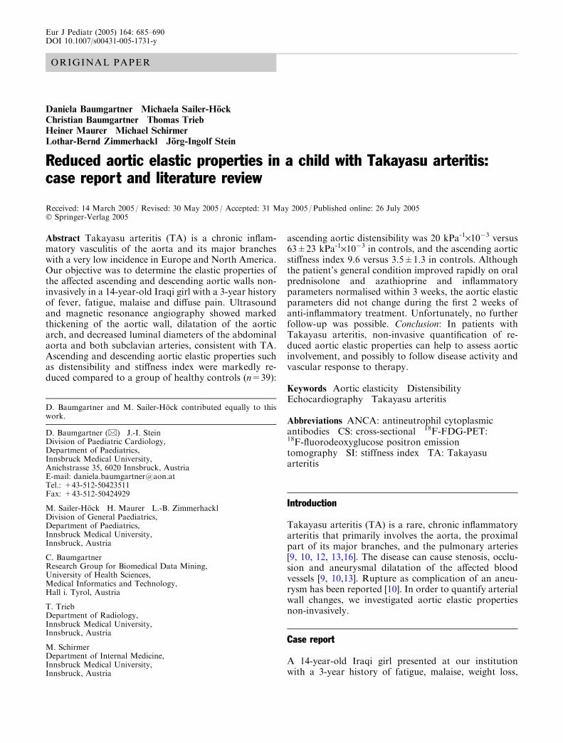
ORIGINAL PAPER
Daniela Baumgartner Æ Michaela Sailer-Hock
Christian Baumgartner Æ Thomas Trieb
Heiner Maurer Æ Michael Schirmer
Lothar-Bernd Zimmerhackl Æ Jorg-Ingolf Stein
Reduced aortic elastic properties in a child with Takayasu arteritis:case report and literature review
Received: 14 March 2005 / Revised: 30 May 2005 / Accepted: 31 May 2005 / Published online: 26 July 2005� Springer-Verlag 2005
Abstract Takayasu arteritis (TA) is a chronic inflam-matory vasculitis of the aorta and its major brancheswith a very low incidence in Europe and North America.Our objective was to determine the elastic properties ofthe affected ascending and descending aortic walls non-invasively in a 14-year-old Iraqi girl with a 3-year historyof fever, fatigue, malaise and diffuse pain. Ultrasoundand magnetic resonance angiography showed markedthickening of the aortic wall, dilatation of the aorticarch, and decreased luminal diameters of the abdominalaorta and both subclavian arteries, consistent with TA.Ascending and descending aortic elastic properties suchas distensibility and stiffness index were markedly re-duced compared to a group of healthy controls (n=39):
ascending aortic distensibility was 20 kPa-1·10�3 versus63±23 kPa-1·10�3 in controls, and the ascending aorticstiffness index 9.6 versus 3.5±1.3 in controls. Althoughthe patient’s general condition improved rapidly on oralprednisolone and azathioprine and inflammatoryparameters normalised within 3 weeks, the aortic elasticparameters did not change during the first 2 weeks ofanti-inflammatory treatment. Unfortunately, no furtherfollow-up was possible. Conclusion: In patients withTakayasu arteritis, non-invasive quantification of re-duced aortic elastic properties can help to assess aorticinvolvement, and possibly to follow disease activity andvascular response to therapy.
Keywords Aortic elasticity Æ Distensibility ÆEchocardiography Æ Takayasu arteritis
Abbreviations ANCA: antineutrophil cytoplasmicantibodies Æ CS: cross-sectional Æ 18F-FDG-PET:18F-fluorodeoxyglucose positron emissiontomography Æ SI: stiffness index Æ TA: Takayasuarteritis
Introduction
Takayasu arteritis (TA) is a rare, chronic inflammatoryarteritis that primarily involves the aorta, the proximalpart of its major branches, and the pulmonary arteries[9, 10, 12, 13,16]. The disease can cause stenosis, occlu-sion and aneurysmal dilatation of the affected bloodvessels [9, 10,13]. Rupture as complication of an aneu-rysm has been reported [10]. In order to quantify arterialwall changes, we investigated aortic elastic propertiesnon-invasively.
Case report
A 14-year-old Iraqi girl presented at our institutionwith a 3-year history of fatigue, malaise, weight loss,
D. Baumgartner and M. Sailer-Hock contributed equally to thiswork.
D. Baumgartner (&) Æ J.-I. SteinDivision of Paediatric Cardiology,Department of Paediatrics,Innsbruck Medical University,Anichstrasse 35, 6020 Innsbruck, AustriaE-mail: [email protected].: +43-512-50423511Fax: +43-512-50424929
M. Sailer-Hock Æ H. Maurer Æ L.-B. ZimmerhacklDivision of General Paediatrics,Department of Paediatrics,Innsbruck Medical University,Innsbruck, Austria
C. BaumgartnerResearch Group for Biomedical Data Mining,University of Health Sciences,Medical Informatics and Technology,Hall i. Tyrol, Austria
T. TriebDepartment of Radiology,Innsbruck Medical University,Innsbruck, Austria
M. SchirmerDepartment of Internal Medicine,Innsbruck Medical University,Innsbruck, Austria
Eur J Pediatr (2005) 164: 685–690DOI 10.1007/s00431-005-1731-y
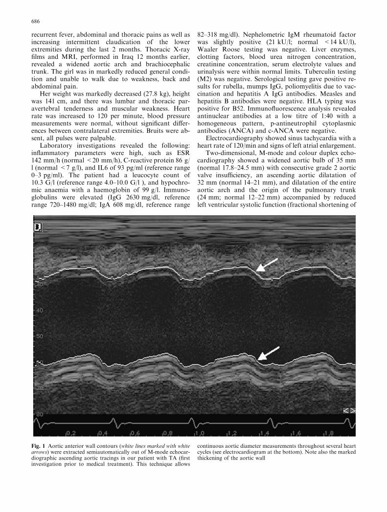
recurrent fever, abdominal and thoracic pains as well asincreasing intermittent claudication of the lowerextremities during the last 2 months. Thoracic X-rayfilms and MRI, performed in Iraq 12 months earlier,revealed a widened aortic arch and brachiocephalictrunk. The girl was in markedly reduced general condi-tion and unable to walk due to weakness, back andabdominal pain.
Her weight was markedly decreased (27.8 kg), heightwas 141 cm, and there was lumbar and thoracic par-avertebral tenderness and muscular weakness. Heartrate was increased to 120 per minute, blood pressuremeasurements were normal, without significant differ-ences between contralateral extremities. Bruits were ab-sent, all pulses were palpable.
Laboratory investigations revealed the following:inflammatory parameters were high, such as ESR142 mm/h (normal <20 mm/h), C-reactive protein 86 g/l (normal <7 g/l), and IL6 of 93 pg/ml (reference range0–3 pg/ml). The patient had a leucocyte count of10.3 G/l (reference range 4.0–10.0 G/l ), and hypochro-mic anaemia with a haemoglobin of 99 g/l. Immuno-globulins were elevated (IgG 2630 mg/dl, referencerange 720–1480 mg/dl; IgA 608 mg/dl, reference range
82–318 mg/dl). Nephelometric IgM rheumatoid factorwas slightly positive (21 kU/l; normal <14 kU/l),Waaler Roose testing was negative. Liver enzymes,clotting factors, blood urea nitrogen concentration,creatinine concentration, serum electrolyte values andurinalysis were within normal limits. Tuberculin testing(M2) was negative. Serological testing gave positive re-sults for rubella, mumps IgG, poliomyelitis due to vac-cination and hepatitis A IgG antibodies. Measles andhepatitis B antibodies were negative. HLA typing waspositive for B52. Immunofluorescence analysis revealedantinuclear antibodies at a low titre of 1:40 with ahomogeneous pattern, p-antineutrophil cytoplasmicantibodies (ANCA) and c-ANCA were negative.
Electrocardiography showed sinus tachycardia with aheart rate of 120/min and signs of left atrial enlargement.
Two-dimensional, M-mode and colour duplex echo-cardiography showed a widened aortic bulb of 35 mm(normal 17.8–24.5 mm) with consecutive grade 2 aorticvalve insufficiency, an ascending aortic dilatation of32 mm (normal 14–21 mm), and dilatation of the entireaortic arch and the origin of the pulmonary trunk(24 mm; normal 12–22 mm) accompanied by reducedleft ventricular systolic function (fractional shortening of
Fig. 1 Aortic anterior wall contours (white lines marked with whitearrows) were extracted semiautomatically out of M-mode echocar-diographic ascending aortic tracings in our patient with TA (firstinvestigation prior to medical treatment). This technique allows
continuous aortic diameter measurements throughout several heartcycles (see electrocardiogram at the bottom). Note also the markedthickening of the aortic wall
686

28%; normal 30%–45%) and circular pericardial effu-sion of 5 mm [15].
Aortic elastic properties were determined non-inva-sively as previously described based on M-mode echo-cardiographic images of the ascending aorta 1–2 cmdistally to the sinotubular junction and of the descend-ing aorta slightly proximal to the branching-off of thecoeliac trunk [2]. Using a special autocontour findingsoftware, aortic wall contours of at least five heart cycleswere segmented followed by automated diameter cal-
culation (Fig. 1 and Fig. 2). Blood pressure was mea-sured oscillometrically immediately before diameterregistration. From diameter and blood pressuremeasurements, the following elastic parameters werecalculated automatically as described in [2]:
Distensibility ¼ As � Ad
AdðPs � PdÞ1333� 107 kPa�1 � 10�3
� �,
Stiffness Index ¼ ln Ps=Pdð ÞðDs � DdÞ=Dd
dimensionless½ �,
where As is systolic, Ad is enddiastolic area, Ps is systolicand Pd is diastolic blood pressure in mmHg. Area A wasdetermined as (D/2)2p.
Results were compared to those obtained in a controlgroup comprising of 39 healthy individuals aged14.7±7.4 years (mean ± SD), who were admitted to ourpaediatric cardiology outpatient department because ofheart murmurs or thoracic pains or were members of ourmedical staff. Disease of the heart and the aorta wasexcluded by a complete echocardiographic examinationand blood pressure registration in all of them. In ourpatient cross sectional (CS) distensibility of the ascend-ing and descending aorta was markedly reduced com-pared to healthy controls while ascending anddescending aortic wall stiffness index b (SI) was stronglyincreased (Table 1).
Two-dimensional ultrasound, MRI and MR angiog-raphy confirmed the echocardiographic findings of tho-racic aortic dilatation and intimal thickening (maximum5 mm) along the entire aorta and its branches (carotidarteries bilaterally, brachiocephalic trunk, left sub-clavian artery, mesenteric arteries, renal arteries bilat-erally). There was marked luminal narrowing of theinfrarenal descending aorta (Fig. 3).
Based on these findings the diagnosis of type V TAwas established according to the criteria of the AmericanCollege of Rheumatology [1].
We started treatment with prednisolone (2 mg/kg/day) and azathioprine (2 mg/kg/day) simultaneouslyaccompanied by ranitidine (5 mg/kg body weight) daily.We slowly tapered prednisolone from day 15 on to0.6 mg/kg per day 6 weeks after initiation. Medicaltreatment was accompanied by physiotherapy andoccupational therapy.
The patient responded promptly to the anti-inflam-matory treatment and was free of pain within a few days.Inflammatory parameters returned to normal within 2weeks. Left ventricular function as well as electrocardio-graphic changes normalised. Pericardial effusion resolvedand aortic valve regurgitation decreased to grade 1.Ultrasound and MRI showed a decrease in aortic wallthickening. M-mode echocardiographically assessedaortic elastic properties 2 weeks after initiation of immu-nosuppressive treatment remained unchanged (Table 1).Unfortunately, follow-up was not possible because thegirl came to our institution via a charity organisation andtherefore had to return to Iraq after 6 weeks.
Fig. 2 The ascending aortic time-diameter curve (averaged over 5heart cycles and slightly smoothed) of (a) our patient at the firstinvestigation prior to medical treatment shows a diminishedsystolic diameter increase of 2.3 mm (=7.1%) compared to (b)6.0 mm (31.9%) in an age- and sex-matched healthy control person
687

Discussion
Reduced arterial elastic properties have been describedin the proximal descending aorta [21], the commoncarotid and the femoral arteries [14] of only a few adultpatients with TA. To the best of our knowledge, this isthe first report of decreased ascending and descendingaortic elastic properties in a child affected by TA. Usingour non-invasive technique, we were able to show athree-fold reduction of ascending and a five-fold reduc-tion of descending aortic elasticity in our patient(Table 1).
In the past, conventional angiography was proposedas the gold standard for the assessment of arterialvasculature [10,11]. Within the last few years, MRI,MR-angiography, 2-dimensional and colour duplexultrasound, CT and 18F-fluorodeoxyglucose positronemission tomography (18F-FDG-PET) proved to bepotentially useful for evaluation of TA [3, 8, 11, 14,17,22]. MR- and CT-angiography provide a generalisedarterial survey of affected vessels. MRI and 2D ultra-sound provide information on arterial wall anatomy andthus can be used to detect new vascular lesions in theearly ‘‘prepulseless’’ stage of the disease, when intimalthickening and mild stenoses are the dominant charac-teristics [3, 4, 8, 11,22]. Both techniques allow us torecognise the progress of stenoses, the presence of vas-cular occlusions, aneurysms and dissections, whileavoiding the risks of arterial puncture, iodinated con-trast load, and radiation exposure. Contrast enhance-ment in T1-weighted MR images represents earlyvascular inflammation, while 18F-FDG-PET scanninggives information about hypermetabolism within in-flamed arterial walls before arterial stenosis andischaemia occur. Therefore, these methods make itpossible to determine disease activity [8].
Ultrasound plays a crucial role in the evaluation ofpatients with TA because of its diagnostic validity andwide availability, although a comprehensive examina-tion of the arterial system is time-consuming, and
imaging of peripheral arterial segments is limited.However, with our semi-automated image segmentationtechnique, which has been established in patients withMarfan syndrome and healthy control persons, andwhich has recently been applied to newborns with aorticcoarctation, ascending and descending aortic luminaldiameters can be determined exactly because of the veryhigh spatial resolution of 2D-gated M-mode echocar-diographic images [2,24]. The investigation does notrequire sedation, is objective and reproducible, can beperformed without any side-effects or pain within20 min, and is therefore apt for high quality follow-upinvestigations especially in smaller children. It is note-worthy that children can be affected by TA at a veryyoung age [5, 18,19], and about 25% of patients with TAare younger than 20 years [1].
Aortic elastic parameters can be calculated auto-matically using diameter and oscillometric blood pres-sure registrations with high accuracy [2] because of theclose correlation between invasive and non-invasivetechniques to determine ascending aortic distensibility[20]. Decreased arterial distensibility and increased SIwere shown to be accompanied by increased wallthickness [14], so the visualization of segments withthickened arterial walls can guide to ‘‘hot spots’’, wherefunctional arterial assessment by elasticity measure-ments should be performed during follow-up.
If follow-up investigations show marked differencesin CS distensibility or SI, we speculate that TA isprobably still active. This is of special interest, becausethen surgical or interventional therapy is contraindi-cated [11]. Therefore, these therapy options should beconsidered before progressive vascular lesions cause se-vere problems like end-organ damage that can occurdespite treatment with anti-inflammatory drugs [7,19].Of course, our method can also be applied to more distalarteries such as the carotids, the mesenteric and femoralarteries. Nevertheless, elasticity measurements in distalvessels have to be excluded from further analysis if ste-noses are present proximal to them [14]. As parts of the
Table 1 Ascending anddescending aortic parameters inthe patient with TA and inhealthy controls
Parameter Patient Control group( n =39)
Firstinvestigation
Secondinvestigation
Age (years) 14.2 14.2 14.7±7.4Systolic blood pressure (mmHg) 109 107 116±12Diastolic blood pressure (mmHg) 55 60 64±9Heart rate (bpm) 122 105 76±26Ascending aortaEnddiastolic diameter (mm) 32.3 36.6 20.5±5.7Systolic diameter increase (%) 7.1 6.7 19.2±6.7CS distensibility (kPa-1·10-3) 20 22 63±23Wall SI 9.6 8.6 3.4±1.2Descending aortaEnddiastolic diameter (mm) 13.4. 17.0 11.9±2.9Systolic diameter increase (%) 4.2 3.8 20.5±5.8CS distensibility (kPa-1·10-3) 12 12 68±26Wall SI 16.3 15.1 3.1±0.9
688

aorta are involved in most patients with TA, evaluationof aortic elasticity is appropriate for screening of vas-cular involvement and can be used to determine thebenefit of therapy.
Glucocorticoid treatment is unequivocally recom-mended in active disease as soon as TA is diagnosed[11]. Immunosuppressive therapy in general has afavourable effect on the general symptoms of inflam-mation in patients with TA, a fact which we observedin our patient within 2 weeks after initiation of treat-ment. The effect of additional immunosuppressiveagents such as azathioprine, methotrexate, cyclosporineA, and tumour necrosis factor alpha antagonists ap-pears promising, but has not been proven in rando-mised trials [6]. Our therapeutic regimen adding
azathioprine to prednisolone from the very beginningcan be questioned; however, our patient had to returnhome within 6 weeks, therefore we had to choose atherapy providing a long-lasting effect. Also, as wewere concerned about contraception in this girl, wepreferred azathioprine to methotrexate.
Anti-inflammatory drug dosage may be adjustedindividually depending on disease activity shown by anincrease or decrease of aortic elastic parameters. Nev-ertheless, in contrast to the clinical improvement, vas-cular lesions seem not to respond as fast to medicaltreatment, as has been shown in an angiographic study[23]. In our patient we also experienced the fact thataortic elastic properties remained unchanged for 2weeks. So we urgently need a marker for vascular
Fig. 3 a Maximum intensity projection of contrast-enhancedmagnetic resonance angiography (flip angle 25�, TR/TE 3.25/1.34 ms, 1.2 mm slice thickness) shows decreased luminal diameterof the abdominal aorta (arrow) and both subclavian arteries (dottedarrows). b Oblique sagittal turbo spin echo T2 weighted dark blood
image (TR/TE 982/74 ms, 5 mm slice thickness) shows mildhyperintensity and marked thickening of the aortic wall (arrows).c Post-contrast transverse turbo spin echo T1 weighted dark bloodimage (TR/TE 514/7.1 ms, 8 mm slice thickness, section level isindicated in b) shows marked thickening of the aortic wall
689

response to therapy. Of course, long-term evaluation ofelastic properties is warranted.
Apart from immunosuppressive treatment, diltiazemhas improved aortic elastic properties in an adult withTA [21]. There is no clear evidence which patients benefitfrom diltiazem and should be treated with a calciumchannel blocker. In children and adolescents, diltiazemcannot be recommended as appropriate pharmacologi-cal studies are lacking.
In conclusion, our method is a non-invasive, time-sparing, objective, reproducible, and easily available toolto quantify the loss of aortic elasticity in young patientswith TA.
References
1. Arend WP, Michel BA, Bloch DA, Hunder GG, Calabrese LH,Edworthy SM, Fauci AS, Leavitt RY, Lie JT, Lightfoot RW,Masi AT, McShane DJ, Mills JA, Stevens MB, Wallace SL,Zvaifler NJ (1990) The American College of Rheumatology1990 criteria for classification of Takayasu’s arteritis. ArthritisRheum 33: 1129–1134
2. Baumgartner D, Baumgartner C, Matyas G, Steinmann B,Loffler J, Schermer E, Schweigmann U, Baldissera I, FrischhutB, Hess J, Hammerer I (2005) Diagnostic power of aortic elasticproperties in young patients with Marfan syndrome. J ThoracCardiovasc Surg 129: 730–739
3. Choe YH, Kim DK, Koh EM, Do YS, Lee WR (1999)Takayasu arteritis: diagnosis with MR imaging and MR angi-ography in acute and chronic active stages. J Magn ResonImaging 10: 751–757
4. Choe YH, Han BK, Koh EM, Kim DK, Do YS, Lee WR(2000) Takayasu’s arteritis: assessment of disease activity withcontrast-enhanced MR imaging. Am J Roentgenol 175: 505–511
5. Hahn D, Thomson PD, Kala U, Beale PG, Levin SE (1998) Areview of Takayasu’s arteritis in children in Gauteng, SouthAfrica. Pediatr Nephrol 12: 668–675
6. Hoffman GS, Leavitt RY, Kerr GS, Rottem M, Sneller MC,Fauci AS (1994) Treatment of glucocorticoid-resistant ofrelapsing Takayasu arteritis with methotrexate. ArthritisRheum 37: 578–582
7. Kart-Kaseoglu H, Yucel AE, Tasdelen A, Bovyat F (2004)Delayed diagnosis of Takayasu’s arteritis: total abdominalaorta occlusion treated with axillo-bifemoral bypass. J Rheu-matol 31: 393–395
8. Kissin EY, Merkel PA (2003) Diagnostic imaging in Takayasuarteritis. Curr Opin Rheumatol 16: 31–37
9. Lande A, Berkman YM (1976) Aortitis: pathological, clinicaland arteriographic review. Radiol Clin North Am 14: 219–240
10. Matsumura K, Hirano T, Takeda K, Matsuda A, Nakagawa T,Yamagushi N, Yuasa H, Kusakawa M, Nakano T (1991)Incidence of aneurysms in Takayasu’s arteritis. Angiology 42:308–315
11. Mohan N, Kerr G (1999) Takayasu’s arteritis. Curr TreatOptions Cardiovasc Med 1: 35–41
12. Nakao K, Ikeda M, Kimata S, Nutani H, Miyahara M, IshimiZ, Hashiba K, Takeda Y, Ozawa T, Matsushita S, KuramochiM (1967) Takayasu’s arteritis: clinical report of eighty-fourcases and immunological studies of seven cases. Circulation 35:1141–1155
13. Nasu T (1975) Takayasu’s trunk arteritis in Japan: a statisticalobservation of 76 autopsy cases. Pathol Microbiol 43: 140–146
14. Raninen RO, Kupari MM, Hekali PE (2002) Carotid andfemoral artery stiffness in Takayasu’s arteritis. Scand J Rheu-matol 31: 85–88
15. Roman MJ, Devereux RB, Kramer-Fox R, O’Loughlin J(1989) Two-dimensional echocardiographic aortic root dimen-sions in normal children and adults. Am J Cardiol 64: 507–512
16. Ross RS, McKusick VA (1953) Aortic arch syndromes:diminished or absent pulses in arteries arising from arch ofaorta. Arch Intern Med 92: 701–740
17. Schmidt WA, Nerenheim A, Seipelt E, Poehls C, Gromnica-Ihle E (2002) Diagnosis of early Takayasu arteritis withsonography. Rheumatology 41: 496–502
18. Shetty AK, Stopa AR, Gedalia A (1998) Low-dose metho-trexate as a steroid-sparing agent in a child with Takayasu’sarteritis. Clin Exp Rheumatol 16: 335–336
19. Sparks SR, Chock A, Seslar S, Bergan JJ, Owens EL (2000)Surgical treatment of Takayasu’s arteritis: case report and lit-erature review. Ann Vasc Surg 14: 125–129
20. Stefanadis C, Stratos C, Boudoulas H, Kourouklis C,Toutouzas P (1990) Distensibility of the ascending aorta:comparison of invasive and non-invasive techniques in healthymen and in men with coronary artery disease. Eur Heart J 11:990–996
21. Stefanadis C, Dernellis J, Toutouzas P (1998) Aortic elasticproperties in Takayasu arteritis. Int J Cardiol 67: 273–274
22. Tso E, Flamm SD, White RD, Schvartzman PR, Mascha E,Hoffman GS (2002) Takayasu arteritis- utility and limitationsof magnetic resonance imaging in diagnosis and treatment.Arthritis Rheum 46: 1634–1642
23. Valsakumar AK, Valappil UC, Jorapur V, Garg N, NityanandS, Sinha N (2003) Role of immunosuppressive therapy onclinical, immunological, and angiographic outcome in activeTakayasu’s arteritis. J Rheumatol 30: 1793–1798
24. Vogt M, Kuhn A, Baumgartner D, Baumgartner C, Busch R,Kostolny M, Hess J (2005) Impaired elastic properties of theascending aorta in newborns before and early after successfulcoarctation repair: proof of a systemic vascular disease of theprestenotic arteries? Circulation 111: 3269–3273
690

Functional Cluster Analysis of CT Perfusion Maps: A New Toolfor Diagnosis of Acute Stroke?
Christian Baumgartner, Ph.D.,1 Kurt Gautsch, M.D.,2 Christian Bohm, Ph.D.,3 and Stephan Felber, M.D.2
CT perfusion imaging constitutes an important contribu-tion to the early diagnosis of acute stroke. Cerebralblood flow (CBF), cerebral blood volume (CBV) and time-to-peak (TTP) maps are used to estimate the severity ofcerebral damage after acute ischemia. We introducefunctional cluster analysis as a new tool to evaluate CTperfusion in order to identify normal brain, ischemictissue and large vessels. CBF, CBV and TTP mapsrepresent the basis for cluster analysis applying apartitioning (k-means) and density-based (density-basedspatial clustering of applications with noise, DBSCAN)paradigm. In patients with transient ischemic attack andstroke, cluster analysis identified brain areas withdistinct hemodynamic properties (gray and white mat-ter) and segmented territorial ischemia. CBF, CBV andTTP values of each detected cluster were displayed. Ourpreliminary results indicate that functional cluster anal-ysis of CT perfusion maps may become a helpful tool forthe interpretation of perfusion maps and provide a rapidmeans for the segmentation of ischemic tissue.
KEY WORDS: Computed tomography, perfusion imag-ing, brain infarction, cluster analysis
INTRODUCTION
Stroke constitutes the third most frequent cause
of death and disability in industrialized
countries. Examination of cerebral perfusion using
computed tomography (CT) has become an
accepted tool to assess functional properties of
ischemic brain tissues.1Y6 Under normal condi-
tions, the mean global cerebral blood flow (CBF)
is about 50 ml/100 g/min. CBF in gray matter
(40Y60 ml/100 g/min) is twice to three times
higher compared to white matter (20Y25 ml/100
g/min) and decreases in older people. Regional
CBF values lower than 20 or 15 ml/100 g/min
can be observed in cerebral ischemic events. Below
15 ml/100 g/min, irreversible damage occurs.
The combined interpretation of CBF, cerebral
blood volume (CBV) and time-to-peak (TTP) maps
via visual analysis is most commonly used in the
clinical situation. Manual extraction of defined
cerebral regions may help to estimate the degree
of hemodynamic alteration but relies on a tedious
and observer-dependent process of segmentation.
Our purpose was to employ functional cluster
analysis to facilitate a computer-assisted extraction
of abnormal brain perfusion in acute stroke. We
applied a partitioning (k-means) and a density-
based (density-based spatial clustering of applica-
tions with noise, DBSCAN) clustering algorithm to
CBF, CBV and TTP maps in order to (i) identify
and segment clusters of normal and apparently
ischemic parenchyma by combining hemodynamic
alterations of all three parameters into a single map
1From the Research Group for Biomedical Data Mining,
Institute for Information Systems, University for Health
Sciences, Medical Informatics and Technology, Eduard
Wallnofer Zentrum 1, A-6060 Hall in Tirol, Austria.2From the Department for Radiology II, Innsbruck Medical
University, Anichstrasse 35, A-6020 Innsbruck, Austria.3From the Institute for Computer Science, University of
Munich, Oettingenstrasse 67, D-80538 Munich, Germany.
Correspondence to: Christian Baumgartner, Ph.D., Re-
search Group for Biomedical Data Mining, Institute for
Information Systems, University for Health Sciences, Medical
Informatics and Technology, Eduard Wallnofer Zentrum 1,
A-6060 Hall in Tirol, Austria; tel: +43-50-86483827; fax:
+43-50-8648673827; e-mail: [email protected]
Copyright * 2005 by SCAR (Society for Computer
Applications in Radiology)
Online publication 26 January 2005
doi: 10.1007/s10278-004-1048-9
Journal of Digital Imaging, Vol 18, No 3 (September), 2005: pp 219Y226 219

and to (ii) estimate absolute values of each detec-
ted cerebral cluster area.7,8
METHODS
CT Examination Protocol
The acquisition procedure for CT perfusion application
consisted of repetitive scanning through a defined Bregion of
interest^ (ROI) after injection of a contrast medium bolus using
a last generation multi slice scanner (Somatom Sensation 16,
Siemens, Erlangen, Germany). Two slices (slice thickness
12 mm) defined according to the clinical deficit were imaged
with a time resolution of 0.5 s (110 mAs, 120 kV) for a period
of 40 s. 40 ml of a non-ionic contrast medium (Ultravist
370 Schering, Berlin, Germany) was injected at a flow rate of
5 ml/s.
CT Perfusion
CBF, CBV and transit time maps were calculated using
commercial software (Syngo\, Siemens). This software uses
the so-called maximal slope model for determining absolute
values of CBF and was initially developed for microspheres
assuming that the indicator is completely extracted in the
capillary network at first pass.5,9 This model can also be
applied to CT perfusion studies as follows:
CBF ¼ maximal slope of QðtÞmaximal height of CaðtÞ
ð1Þ
where Q(t) designates the amount of indicator in a local
vascular network and Ca(t) is the arterial concentration of
indicator at time t.
CBF, CBV and Transit Times
Basically, dynamic CT can be used for measurements of
CBF, CBV and blood transit time through the cerebral tissue
after injection of an iodinated contrast medium into a large
vein, in particular, in an antecubital position.2,5,10Y12
The theoretical basis is the indicator-dilution principle13,14
which relates CBF, CBV and mean transit time (MTT) values
in the simple relationship:
CBF ¼ CBV
MTTð2Þ
Mean transit time (MTT) relates to the time it takes for blood
to cross the local capillary network. The calculation of a CBV
map necessitates knowledge of a timeYconcentration curve in a
vascular region of interest (ROI), e.g., at the center of the
superior sagittal venous sinus, devoid of a partial averaging
effect:
CBV ¼ Karea under the curve in a parenchymal ROI
area under the curve in the vascular ROIð3Þ
where K is a proportionality constant considering the ratio of
peripheral hematocrit and tissue hematocrit. Finally, the
combination of CBV and MTT at each pixel gives a CBF
value, as indicated by Equation 2.
Clustering Techniques
For cluster analysis, we considered (i) CBF (ml/100 g/min)
as calculated from the maximal slope model, (ii) CBV (ml/
100 g) using Equation 3, and (iii) TTP (time-to-peak) which
is the time (seconds) it takes from injection of a contrast
bolus to the maximum level of attenuation recorded in a ROI.
The calculation of the MTT map is not provided in the Syngo
package.
Clustering algorithms are used for the task of class
identification, i.e., the grouping of Bfunctional^ pixels into
meaningful subclasses scanning CBF, CBV and TTP maps.
The similarity among pixels of the form f Pixel = f (CBF,
CBV, TTP) within the transformed three-dimensional feature
space S(CBF, CBV, TTP) is calculated by means of a distance
function, i.e., the Euclidian distance (ED):
EDðx; yÞ ¼ffiffiffiffiffiffiffiffiffiffiffiffiffiffiffiffiffiffiffiffiffiffiffiffiffiffiffiXn
i ¼ 1
xi � yið Þ2s
ð4Þ
where xi = xCBF, xCBV, xTTP and yi = yCBF, yCBV, yTTP are two
pixels in the n = 3 dimensional feature space. Finally, the
identified clusters are retransformed from feature space back
into image space by visualizing the clusters in a single map.
Thereby, pixels of the same cluster, which may represent
normal, abnormal (ischemic) cerebral tissue or large vessels,
are characterized by maximum similarity in hemodynamic
behavior; pixels of different clusters indicate maximum
dissimilarity.7,8
For the classification of cerebral tissue, we applied
two different clustering techniques, k-means and a density-
based (DBSCAN) algorithm, and compared their clustering
characteristics.
k-Means
k-Means, a partitioning paradigm, constructs a partition of
the database of N pixels (= 3nm, three maps of image size nm;
n = number of pixels in rows; m = number of pixels in
columns) into a set of k clusters. Each cluster is represented
by the gravity center and all pixels must be assigned to a
cluster.8,15 The algorithm is briefly sketched as follows:
(i) Initialization (arbitrary assignment of the ith pixel to the i
modulo k th class).
(ii) Start loop until termination condition is met:
Each pixel in the image is assigned to a class such that the
distance (= Euclidean distance, which is the square root of
the componentwise square of the difference between the
pixel and the class, see Eq 4) from this pixel to the center
of that class is minimized.
Means of each class are recalculated on the pixels that
belong to that class.
(iii) End loop.
Theoretically, k-means should terminate when no more pixels
change classes. This relies on the fact that both steps of
k-means (assign pixels to nearest centers, move centers to cluster
centroids) reduce variance. Running to completion (no pixels
220 BAUMGARTNER ET AL.

changing classes) may require a large number of iterations, so
we terminated after 50 iterations.
For the application of k-means on perfusion maps, the user
needs to know the Bnatural^ number of clusters (k = expected
number of cerebral structures) in the image data which is the
only input parameter of the paradigm. The limited spatial
resolution of the functional maps provided enables primarily
the classification of normal parenchyma (gray and white
matter), abnormal ischemic parenchyma and large vessels.
Therefore, we suggested a k-value of 3 for the segmentation of
gray and white matter as well as large vessels in normal brain
perfusion or reversible ischemia (e.g., TIA), a k-value 9 3, if
additionally, ischemic parenchyma was visualized in perfusion
maps.
DBSCAN
The key idea of density-based clustering is that for each
pixel of a cluster the neighborhood of a given radius EE has to
contain at least a minimum number of pixels MinPts. The
algorithm DBSCAN (density-based spatial clustering of appli-
cations with noise), which discovers clusters and noise in a
database, is based on the fact that a cluster is equivalent to the
set of all pixels which are density-reachable from an arbitrary
core pixel in the cluster.16
To find a cluster, DBSCAN starts with an arbitrary pixel in
the database and checks the EE-neighborhood of each pixel in
the database. If the EE-neighborhood NEE (p) of a pixel p has more
than MinPts pixels, a new cluster C containing the pixels in
NEE ( p) is created. Then, the EE-neighborhood of all pixels q in C
which have not yet been processed is checked. If NEE(q)
contains more than MinPts pixels, the neighbors of q which
are not already contained in C are added to the cluster and their
EE-neighborhood is checked in the next step. This procedure is
repeated until no new point can be added to the current cluster
C. DBSCAN uses MinPts and EE-neighborhood as global input
parameters specifying the lowest density not considered to be
noise. MinPts is recommended to be 93.16 We used MinPts =
5. An EE-neighborhood of 0.1 was determined empirically from
prior experiments.
Image Pre- and Post-Processing
Our calculations were performed on a software tool which
has been developed at our institutions implementing k-means
and DBSCAN. It is easy to handle so that cluster analysis can
be performed by physicians or CT technologists during clinical
routine.
For cluster analysis, input image data was generated
routinely in a 12-bit grayscale format (Monochrome2) from
Siemens Syngo software. Syngo already segments cerebral
tissue so that the processed matrix size can be reduced from
originally 512 � 512 to approximately 300 � 350 (depending
on the patient’s head size and the imaged topographic level).
This reduction is helpful in shortening the runtime of the
cluster algorithms, because pixels outside the skull contain no
information that could change clustering outcome. The seg-
mented areas of the ventricle system and background pixels
were set to zero by default. However, the pre-segmented maps
contained the absolute CBF, CBV and TTP values added to an
offset of 210 (= 1024) counts, which had to be subtracted before
the algorithm was started. These offset-corrected maps were
then normalized to m = 0 and s2 = 1, which is an essential
condition for calculating the Euclidian distance function (Eq 4)
in a meaningful way.
Functional maps were also available in RGB format, which
were preferably used for clinical decision making (see Figs 1
and 2a), but were not appropriate for cluster analysis. After
each analytic run, all clusters identified were retransformed
from feature space into a single 8-bit grayscale image (TIFF),
visualizing the clustered cerebral regions and displaying CBF,
CBV and TTP values of each cluster detected. Currently, our
software runs on a PC (Pentium IV, 500 MB RAM, 2 GHz)
computing cluster results G10 min when applying k-means
and G2 min when using DBSCAN supported by an index
structure.
Quality of Clustering
Between-cluster and within-cluster variance measurements
for each k-level were performed using F-tests. In this test, the
ratio of two variances was calculated. If the two variances were
not significantly different (P 9 0.05), their ratio would be close
to 1. This measure constitutes a way to test whether the use
of k + 1 clusters instead of k clusters adds any significant
information. Student’s t-tests were considered to compare the
mean CBF, CBV or TTP values between clusters. A P-value
less than 0.05 indicated two significantly different means.
Fig 1. Cerebral blood flow (CBF), cerebral blood volume (CBV)and time-to-peak (TTP) maps of a 66-year-old male patient(patient 1) with aphasia and moderate hemiparesis. Clustersidentified applying k-means (k = 3) are shown. Clusters c1 andc2 represent gray and white matter, cluster c3 depicts a largevenous vessel.
CLUSTER ANALYSIS OF CT PERFUSION MAPS 221
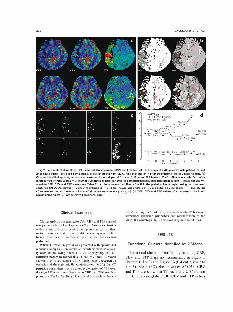
Clinical Examples
Cluster analysis was applied to CBF, CBV and TTP maps of
two patients who had undergone a CT perfusion examination
within 2 and 3 h after onset of symptoms as part of their
routine diagnostic workup. Patient data was anonymized before
transfer to an external workstation where cluster analysis was
performed.
Patient 1 (male, 66 years) was presented with aphasia and
moderate hemiparesis on admission, which resolved complete-
ly over the following hours. CT, CT angiography and CT
perfusion maps were normal (Fig 1). Patient 2 (male, 40 years)
showed a left-sided hemiparesis. CT angiography revealed an
occlusion of the right middle cerebral artery (MCA). On CT
perfusion maps, there was a marked prolongation of TTP over
the right MCA territory. Decrease in CBF and CBV was less
prominent (Fig 2a, first line). He received thrombolytic therapy
(rTPA 47.7 mg, i.v.). Follow-up examination after 24 h showed
normalized perfusion parameters and recanalization of the
MCA, the neurologic deficit resolved (Fig 2a, second line).
RESULTS
Functional Clusters Identified by k-Means
Functional clusters identified by scanning CBF,
CBV and TTP maps are summarized in Figure 1
(Patient 1, k = 3) and Figure 2b (Patient 2, k = 2 to
k = 5). Mean (SD) cluster values of CBF, CBV
and TTP are shown in Tables 1 and 2. Choosing
k = 1, the mean global CBF, CBV and TTP values
Fig 2. (a) Cerebral blood flow (CBF), cerebral blood volume (CBV) and time-to-peak (TTP) maps of a 40-year-old male patient (patient2) at acute stroke (left-sided hemiparesis, occlusion of the right MCA, first line) and 24 h after thrombolytic therapy (second line). (b)
Clusters identified applying k-means at acute stroke are depicted for k = 2, 3, 4 and 5 (clusters c2Yc5). Cluster analysis 24 h afterthrombolytic therapy with k = 3 showed symmetric cluster patterns for both hemispheres, as illustrated in patient 1 (maps not shown,absolute CBF, CBV and TTP values see Table 2). (c) Sub-clusters identified (c1Yc7) in the global ischemic region using density-basedclustering (DBSCAN, MinPts = 5 and EE-neighborhood = 0.1) are shown. Sub-clusters c1Yc7 are ordered by increasing TTP. Sub-clusterc8 represents the accumulated cluster of all seven sub-clusters c8 ¼
P7
i ¼ 1ci
� �. (d) CBF, CBV and TTP values of sub-clusters c1Yc7 and
accumulated cluster c8 are displayed as means (SD).
222 BAUMGARTNER ET AL.
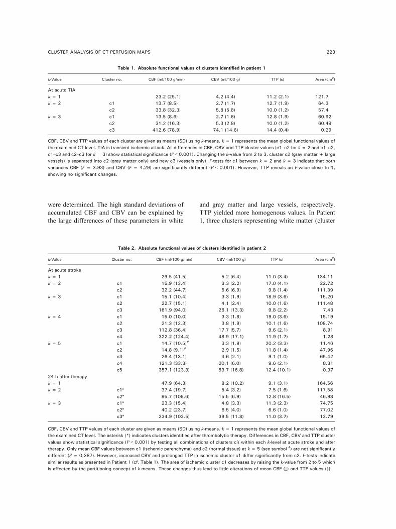
were determined. The high standard deviations of
accumulated CBF and CBV can be explained by
the large differences of these parameters in white
and gray matter and large vessels, respectively.
TTP yielded more homogenous values. In Patient
1, three clusters representing white matter (cluster
Table 1. Absolute functional values of clusters identified in patient 1
k-Value Cluster no. CBF (ml/100 g/min) CBV (ml/100 g) TTP (s) Area (cm2)
At acute TIA
k = 1 23.2 (25.1) 4.2 (4.4) 11.2 (2.1) 121.7
k = 2 c1 13.7 (8.5) 2.7 (1.7) 12.7 (1.9) 64.3
c2 33.8 (32.3) 5.8 (5.8) 10.0 (1.2) 57.4
k = 3 c1 13.5 (8.6) 2.7 (1.8) 12.8 (1.9) 60.92
c2 31.2 (16.3) 5.3 (2.8) 10.0 (1.2) 60.49
c3 412.6 (78.9) 74.1 (14.6) 14.4 (0.4) 0.29
CBF, CBV and TTP values of each cluster are given as means (SD) using k-means. k = 1 represents the mean global functional values of
the examined CT level. TIA is transient ischemic attack. All differences in CBF, CBV and TTP cluster values (c1Yc2 for k = 2 and c1Yc2,
c1Yc3 and c2Yc3 for k = 3) show statistical significance (P G 0.001). Changing the k-value from 2 to 3, cluster c2 (gray matter + large
vessels) is separated into c2 (gray matter only) and new c3 (vessels only). F-tests for c1 between k = 2 and k = 3 indicate that both
variances CBF (F = 3.93) and CBV (F = 4.29) are significantly different (P G 0.001). However, TTP reveals an F-value close to 1,
showing no significant changes.
Table 2. Absolute functional values of clusters identified in patient 2
k-Value Cluster no. CBF (ml/100 g/min) CBV (ml/100 g) TTP (s) Area (cm2)
At acute stroke
k = 1 29.5 (41.5) 5.2 (6.4) 11.0 (3.4) 134.11
k = 2 c1 15.9 (13.4) 3.3 (2.2) 17.0 (4.1) 22.72
c2 32.2 (44.7) 5.6 (6.9) 9.8 (1.4) 111.39
k = 3 c1 15.1 (10.4) 3.3 (1.9) 18.9 (3.6) 15.20
c2 22.7 (15.1) 4.1 (2.4) 10.0 (1.6) 111.48
c3 161.9 (94.0) 26.1 (13.3) 9.8 (2.2) 7.43
k = 4 c1 15.0 (10.0) 3.3 (1.8) 19.0 (3.6) 15.19
c2 21.3 (12.3) 3.8 (1.9) 10.1 (1.6) 108.74
c3 112.8 (36.4) 17.7 (5.7) 9.6 (2.1) 8.91
c4 322.2 (124.4) 48.9 (17.1) 11.9 (1.7) 1.28
k = 5 c1 14.7 (10.5)# 3.3 (1.9) 20.2 (3.3) 11.46
c2 14.8 (9.1)# 2.9 (1.5) 11.8 (1.4) 47.96
c3 26.4 (13.1) 4.6 (2.1) 9.1 (1.0) 65.42
c4 121.3 (33.3) 20.1 (6.0) 9.6 (2.1) 8.31
c5 357.1 (123.3) 53.7 (16.8) 12.4 (10.1) 0.97
24 h after therapy
k = 1 47.9 (64.3) 8.2 (10.2) 9.1 (3.1) 164.56
k = 2 c1* 37.4 (19.7) 5.4 (3.2) 7.5 (1.6) 117.58
c2* 85.7 (108.6) 15.5 (6.9) 12.8 (16.5) 46.98
k = 3 c1* 23.3 (15.4) 4.8 (3.3) 11.3 (2.3) 74.75
c2* 40.2 (23.7) 6.5 (4.0) 6.6 (1.0) 77.02
c3* 234.9 (103.5) 39.5 (11.8) 11.0 (3.7) 12.79
CBF, CBV and TTP values of each cluster are given as means (SD) using k-means. k = 1 represents the mean global functional values of
the examined CT level. The asterisk (*) indicates clusters identified after thrombolytic therapy. Differences in CBF, CBV and TTP cluster
values show statistical significance (P G 0.001) by testing all combinations of clusters cX within each k-level at acute stroke and after
therapy. Only mean CBF values between c1 (ischemic parenchyma) and c2 (normal tissue) at k = 5 (see symbol #) are not significantly
different (P = 0.387). However, increased CBV and prolonged TTP in ischemic cluster c1 differ significantly from c2. F-tests indicate
similar results as presented in Patient 1 (cf. Table 1). The area of ischemic cluster c1 decreases by raising the k-value from 2 to 5 which
is affected by the partitioning concept of k-means. These changes thus lead to little alterations of mean CBF (,) and TTP values (j).
CLUSTER ANALYSIS OF CT PERFUSION MAPS 223

c1: CBF = 13.5 ml/100 g/min, CBV = 2.7 ml/100 g,
TTP = 12.8 s), gray matter (cluster c2: CBF =
31.2 ml/100 g/min, CBV = 5.3 ml/100 g, TTP =
10.0 s) and large vessels (cluster c3, see Fig 1
bottom right and Table 1) were identified at a
k-level of 3. Mean CBF, CBV and TTP values
between white and gray matter and vessels differed
significantly (P G 0.001).
Patient 2 revealed a diminished mean global
CBF of 29.5 ml/100 g/min (k = 1) compared to the
24 h follow-up examination (47.9 ml/100 g/min,
P G 0.001, Table 2). Similar results were obtained
with CBV and TTP (P G 0.001). By increasing
the value of k, clustering yielded more clusters
with altered hemodynamic patterns (Fig 2b). A
k-value of 2 identified the apparent territory of
the occluded right MCA with a decrease in CBF
(15.9 ml/100 g/min vs. 32.2 ml/100 g/min in
normal brain tissue of cluster c2, P G 0.001), CBV
(3.3 ml/100 g vs. 5.6 ml/100 g in normal brain
tissue, P G 0.001) and prolonged TTP (17 vs. 9.8 s
in normal brain tissue, P G 0.001). Increasing k up
to 3, the areas of high blood flow (predominately
large vessels) were separated. At k = 4, arterial
and venous vessels may be distinguished (arterial
TTP = 9.6 s, venous TTP = 11.9 s, P G 0.001). At a
k-value of 5, two low-perfused areas, c1 (ischemic
parenchyma) and c2 (normal tissue), were clus-
tered, showing the same CBF of approximately 15
ml/100 g/min (P = 0.387) but different CBV and
TTP values (P G 0.001).
Comparing cluster results from admission to
the 24-h follow-up examination after therapy, im-
provement in global CBF, CBV and normalization
of TTP were observed (Table 2). On follow-up,
cluster c1 (ischemic area at the initial examina-
tion) had disappeared according to the recanali-
zation of the MCA. At a k-value of 3, cluster c1*
(white matter) and cluster c2* (gray matter)
showed normalized values (P G 0.001) as well as
symmetric cluster patterns for both hemispheres
(maps not shown).
Functional Clusters Identified by DBSCAN
For the investigation of local hemodynamic
alterations within global ischemic regions, as
clustered by k-means in Patient 2, DBSCAN is
appropriate to more sensitively distinguish region-
al processes (Fig 2cYd). Comparing k-means
segmented ischemic area c1 (Fig 2b, k = 2) to
DBSCAN, cluster c1 could be separated into seven
sub-clusters with CBF values ranging from 11.9
to 17.9 ml/100 g/min, CBV values between 2.9
and 3.5 ml/100 g/min and increasing TTP values
from 15.2 up to 27.1 s. Sub-cluster c7, predom-
inantly located at the parietal lobe, indicated
the core region of ischemia with lowest CBF
(j35%) and maximum prolongation of TTP
(+48%, P G 0.001) compared to c8, the accumu-
lated sub-clusters c1Yc7 (c8 corresponds to the
above-mentioned k-means cluster c1, k = 2).
DISCUSSION
Diagnostic interpretation of CT perfusion inte-
grates the information derived from CBF, CBV
and TTP maps and shows limitations when
performing visual analysis. The degree of hemo-
dynamic alterations can better be analyzed quan-
titatively using manual segmentation of defined
brain areas on single CBF, CBV and TTP maps,
which can be done within minutes but is observer-
dependent.
Functional cluster analysis of CBF, CBV and
TTP maps facilitates the identification and seg-
mentation of anatomic regions with inherent
hemodynamic properties. Each calculated cluster
represents tissue with related functional parame-
ters by combining all three parameters into a
single map, where CBF, CBV and TTP values of
each voxel are simultaneously accessible. The
detected clusters are automatically computed in a
few analytical runs and reflect functional inter-
actions of the measured parameters in terms of
similarity operations in the three-dimensional
feature space.
In normals, the segmentation of gray and white
matter, as well as areas of large vessels can be
obtained with the algorithm k-means, choosing a
k-value of 3 by default (cf. Fig 1). k-Means clus-
ters all pixels independent of the number of iden-
tified clusters and—in contrary to DBSCAN—
requires the favored number of clusters as input
parameter (cf. Figs 1 and 2b). However, the
Bnatural^ number of clusters is limited by k $ 5
since the quality of provided functional maps en-
ables primarily the classification of normal paren-
chyma (gray and white matter), abnormal infarcted
parenchyma and large (arterial and venous) ves-
sels. Therefore, a further increase in k is not likely
224 BAUMGARTNER ET AL.
to yield meaningful results, as the number of
cerebral tissues and structures with functional
varying data is less than the specified number of
clusters. k-Means also reveals a decrease in the
cluster area (cf. ischemic cluster c1 of Patient 2,
Table 2) after incrementing the k-value which is
affected by the partitioning concept of k-means
and has to be accepted.
Density-based cluster analysis using the para-
digm DBSCAN is more sensitive to local he-
modynamic alterations within global ischemic
regions and provides an additional means to grade
between ischemic core (sub-cluster c7) and adja-
cent ischemic tissue (sub-clusters c1Yc6), as
shown in Patient 2 (Fig 2cYd). DBSCAN detects
a finite number of clusters and—compared to
k-means—noise pixels which, however, are gener-
ated according to the settings of the given input
parameters, MinPts and EE-neighborhood. As al-
ready mentioned, MinPts and EE-neighborhood
were determined empirically for this specific case
to identify hemodynamic alterations within the
global ischemic cluster. However, more patients
are needed to optimize parameter settings for both
algorithms—these experiments are presently on-
going—and to compare cluster findings to the
clinical situation.
Both algorithms showed small SDs for TTP
cluster values and larger SDs for CBF and CBV
values. This observation might be caused by the
high dissimilarity between the examined function-
al parameters (TTP vs. CBF and CBV) and a
correlation of CBF and CBV (cf. Eq 2), which can
be easily verified using, e.g., principal component
analysis. A decorrelation of the features is jus-
tified, e.g., in normal brain perfusion or reversible
ischemia clustering solely CBF (or CBV) and TTP
maps. However, ischemia is a complex pathophys-
iological condition, where CBF and CBV become
important when distinguishing reversible and irre-
versible changes. In our approach we thus con-
sidered all three feature maps for cluster analysis
in which correlation of CBF and CBV does not
affect final clustering results significantly, as prior
experiments showed.
TTP maps seem to represent the most sensitive
parameter for the estimation of endangered brain
tissue following vessel occlusion. This observa-
tion corresponds well with the result of cluster
analysis in our patient who had suffered a completed
stroke. The Bk = 2^ cluster map of this patient
segmented an area that is comparable to the TTP
map. In the clinical situation, the extension of ab-
normal values on TTP maps indicates the maxi-
mum amount of tissue that may be salvaged by a
recanalization therapy. The extension of abnormal
CBF indicates the tissue that is reached by col-
lateral flow and may still be amenable to benefit
from recanalization. CBV shows the center of
ischemia with complete cessation of perfusion that
is likely to progress to infarction. The correlation
of CBF and CBV with cluster maps of k 9 2 or
with identified sub-clusters c1Yc7 using DBSCAN
and its impact on decision making for recanaliza-
tion therapy remains to be investigated in larger
patient samples.
Appropriate models to quantify CBF, CBV and
TTP (or MTT) are needed to differentiate various
stages of cerebral ischemia. For our investiga-
tions we used Siemens Syngo perfusion software
which creates perfusion maps based on the max-
imal slope model.5,9 To be valid, this model re-
quires a very short injection time accompanied
by a high injection rate of the intravenous contrast
medium. Wintermark et al.5 described injection
rates between 5 and 20 ml/s, all showing an un-
derestimation of the absolute CBF. Models based
on the central volume principle have been
validated and seem to be more appropriate for
estimating absolute CBF, CBV and MTT values
in CT.10Y12,17 However, cluster analysis, which
runs on the normalized data space (m = 0, s2 = 1)
of CBF, CBV and TTP maps, is thus unaffected
by the underlying perfusion model. Absolute
cluster values, of course, reflect the accuracy of
the model to measure cerebral perfusion, which
may limit the clinical interpretation of functional
values.
CONCLUSION
Our preliminary results show that functional
cluster analysis of CT perfusion maps is a pro-
mising means for the identification of acute ce-
rebral ischemia. It facilitates the segmentation of
tissue at risk as well as the estimation of areas
with different severity of ischemia and collaterali-
zation within the endangered brain parenchyma.
Further studies are now warranted to investigate
the correlation between functional clusters and
pathophysiology and histological characteristics
CLUSTER ANALYSIS OF CT PERFUSION MAPS 225
of the identified tissues, as well as to correlate
different clusters with clinical outcome.
ACKNOWLEDGMENTS
We thank Mr. Mattias Bair for the software implementation.
This study was supported by the Austrian Industrial Research
Promotion Fund FFF (Grant no. HITT-10 UMIT).
REFERENCES
1. Miles KA: Acute cerebral stroke imaging and brain
perfusion with the use of high-concentration contrast media.
Eur Radiol 13(Suppl 5):117Y120, 2003
2. Bohner G, Forschler A, Hamm B, Lehmann R, Klingebiel
R: Quantitative perfusion imaging by multi-slice CT in stroke
patients. Rofo, Fortschr Geb Rontgenstrahlen Neuen Bildgeb
Verfahr 175:806Y813, 2003
3. Wintermark M, Reichhart M, Thiran JP, Maeder P,
Chalaron M, Schnyder P, Bogousslavsky J, Meuli R: Prognos-
tic accuracy of cerebral blood flow measurement by perfusion
computed tomography, at the time of emergency room
admission, in acute stroke patients. Ann Neurol 51:417Y432,
2002
4. Keith CJ, Griffiths M, Petersen B, Anderson RJ, Miles
KA: Computed tomography perfusion imaging in acute stroke.
Australas Radiol 46:221Y230, 2002
5. Wintermark M, Maeder P, Thiran JP, Schnyder P, Meuli
R: Quantitative assessment of regional cerebral blood flows by
perfusion CT studies at low injection rates: a critical review of
the underlying theoretical models. Eur Radiol 11:1220Y1230,
2001
6. Konig M, Banach-Planchamp R, Kraus M, Klotz E, Falk
A, Gehlen W, Heuser L: CT perfusion imaging in acute
ischemic cerebral infarct: comparison of cerebral perfusion
maps and conventional CT findings. Rofo, Fortschr Geb
Rontgenstrahlen Neuen Bildgeb Verfahr 172:219Y226, 2000
7. Kaufman L, Rousseeuw PJ: Finding Groups in Data: An
Introduction to Cluster Analysis. New York: John Wiley &
Sons, 1990
8. Everitt BS, Landau S, Leese M: Cluster Analysis, 4th
edition. New York: Oxford University Press, 2001
9. Konig M, Klotz E, Heuser L: Cerebral perfusion CT:
theoretical aspects, methodical implementation and clinical
experience in the diagnosis of ischemic cerebral infarction.
Rofo, Fortschr Geb Rontgenstrahlen Neuen Bildgeb Verfahr
172:210Y218, 2000
10. Cenic A, Nabavi DG, Craen RA, Gelb AW, Lee TY:
Dynamic CT measurement of cerebral blood flow: a validation
study. Am J Neuroradiol 20:63Y73, 1999
11. Nabavi DG, Cenic A, Craen RA, Gelb AW, Bennett JD,
Kozak R, Lee TY: CT assessment of cerebral perfusion:
experimental validation and initial clinical experience. Radiol-
ogy 213:141Y149, 1999
12. Nabavi DG, Cenic A, Dool J, Smith RM, Espinosa F,
Craen RA, Gelb AW, Lee TY: Quantitative assessment of
cerebral hemodynamics using CT: stability, accuracy, and pre-
cision studies in dogs. J Comput Assist Tomogr 23:506Y515,
1999
13. Meier P, Zierler KL: On the theory of the indicator-
dilution method for measurement of blood flow and volume.
J Appl Physiol 12:731Y744, 1954
14. Zierler KL: Equations for measuring blood flow by external
monitoring of radioisotopes. Circulation 16:309Y321, 1965
15. Theiler J, Gisler G: A contiguity-enhanced k-means
clustering algorithm for unsupervised multispectral image
segmentation. Proc SPIE 3159:108Y118, 1997
16. Ester M, Kriegel HP, Sander J, Xu X: A density based
algorithm for discovering clusters in large spatial databases
with noise. Proceedings of the 2nd International Conference on
Knowledge Discovery and Data Mining (KDD’96). Menlo
Park, CA: AAAI Press, 1996, pp 226Y231
17. Wintermark M, Thiran JP, Maeder P, Schnyder P, Meuli
R: Simultaneous measurement of regional cerebral blood flow
by perfusion CT and stable xenon CT: a validation study. Am J
Neuroradiol 22:905Y914, 2001
226 BAUMGARTNER ET AL.
Related Documents


![Knowledge Discovery and Data Mining 1 [0.1cm] (Data Mining ...€¦ · Lehrstuhl fur Datenbanksysteme und Data Mining Prof. Dr. Thomas Seidl Knowledge Discovery and Data Mining 1](https://static.cupdf.com/doc/110x72/5e8e618919f71a49e0297f52/knowledge-discovery-and-data-mining-1-01cm-data-mining-lehrstuhl-fur-datenbanksysteme.jpg)


![Knowledge Discovery - Data Mining Methodologies – CRISP · Knowledge Discovery [Data Mining] Knowledge Discovery in Data is the non-trivial process of identifying valid novel potentially](https://static.cupdf.com/doc/110x72/61218f60b7d6e94a816fea8c/knowledge-discovery-data-mining-methodologies-a-crisp-knowledge-discovery-data.jpg)
